1

Measurement in Health and Disease

Measurement Error

Martin Bland

Professor of Health StatisticsUniversity of York

http://martinbland.co.uk/

Accuracy and precisionIn this lecture: measurements which are numerical variables (blood pressure, forced expiratory volume).

We shall look at how good a measurement is:

• from the clinical point of view --- giving us informationabout the individual subject or patient.

• from the research point of view --- how good amethod is at telling us something about thepopulation.

Error‘error’ -- Latin root meaning ‘to wander’.

In statistics: error means the variation of observations or estimates about some central value.

Example: several measurements of FEV on a subject.

Will not all be the same, because the subject cannot blow in exactly the same way each time.

This variation is called error.

Not the same as a mistake, and does not imply any fault on the part of the observer.

A measurement mistake might be if we transpose digits in recording the FEV, writing 9.4 litres instead of 4.9.

2

Precision and accuracyA measurement is precise if repeated observations of the same quantity are close together.

It is accurate if observations are close to the true value of the quantity.

A measurement can be precise without being accurate, but cannot be accurate without being precise.

In this lecture I shall be concerned with precision.

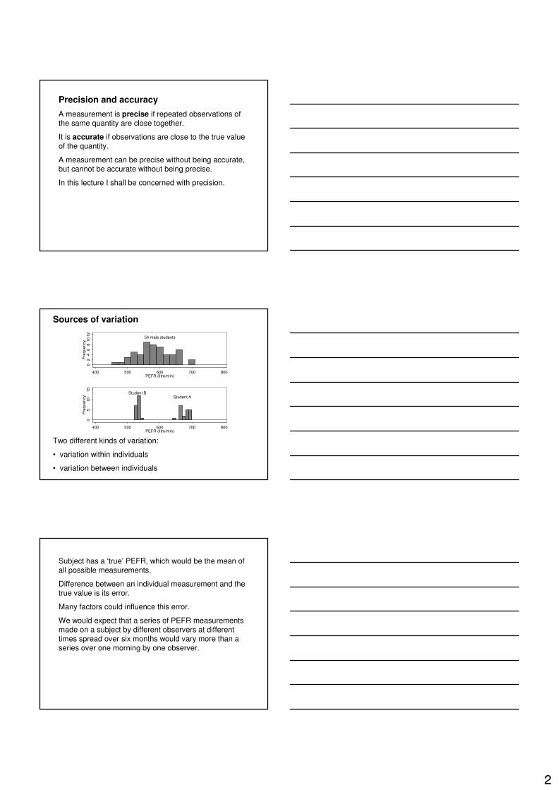
Sources of variation

54 male students

02

46

810

12Fr

eque

ncy

400 500 600 700 800PEFR (litre/min)

Student AStudent B

05

1015

Freq

uenc

y

400 500 600 700 800PEFR (litre/min)

Two different kinds of variation:

• variation within individuals

• variation between individuals

Subject has a ‘true’ PEFR, which would be the mean of all possible measurements.

Difference between an individual measurement and the true value is its error.

Many factors could influence this error.

We would expect that a series of PEFR measurements made on a subject by different observers at different times spread over six months would vary more than a series over one morning by one observer.

3

We might be interested in different types of variability for different purposes.

Monitoring short term changes in blood pressure in a single patient requires one type of error, interpreting random blood pressure in a screening clinic another.

In the first case, we are detecting shifts in mean blood pressure over a short period of time.

In the second case, we are determining from one or two measurements whether the subject's mean blood pressure is above some cut-off point such as 90mm Hg diastolic.

Need to define what we mean by measurement error rather carefully.

The British Standards Institution (1979) considered this question for laboratory measurements, and made the distinction between repeatability, incorporating variability between measurements made by the same operator in the same laboratory, and reproducibility, incorporating variability between measurements made by different operators working in different laboratories.

Repeatability and measurement errorEstimating the variation between repeated measurements for the same subject.

How far from the true value is a single measurement likely to be?

Simplest if we assume that the error is the same for everybody, irrespective of the value of the quantity being measured.

This will not always be the case, and the error may depend on the magnitude of the quantity, for example being proportional to it.

4

The within-subject standard deviation, sw

Measurement error assumed to be the same for everyone.

A simple model; may be that some subjects will show more individual variation than others.

If the measurement error varies from subject to subject, independently of magnitude so that it cannot be predicted, then we have to estimate its average value. We estimate the within-subject variability as if it were the same for all subjects.

Repeated PEFR (litre/min) measurements for two male medical students

Student A Student B685 695 660 660 690 530 535 530 535 525690 665 665 685 680 530 520 530 525 520675 660 660 670 690 525 535 520 535 535685 645 660 690 680 530 525 530 540 530

Student AStudent B

05

1015

Freq

uenc

y

400 500 600 700 800PEFR (litre/min)

Repeated PEFR (litre/min) measurements for two male medical students

Student A Student B685 695 660 660 690 530 535 530 535 525690 665 665 685 680 530 520 530 525 520675 660 660 670 690 525 535 520 535 535685 645 660 690 680 530 525 530 540 530

s1 = 14.3178 s2 = 5.6835

Combined estimate averaged over the two students:

m1 and m2 are the numbers of measurements for subjects 1 and 2. Taking the square root gives sw= 10.9 litres/min.

6509.118)120()120(

5.6835)120(14.3178)120()1()1()1()1( 22

21

222

2112 =

−+−×−+×−=

−+−−+−=

mmsmsm

sw

5

In this way we obtain the standard deviation, sw, of repeated measurements from the same subject, called the within-subject standard deviation.

As for any standard deviation, we expect that about two thirds of observations will fall within one standard deviation of the mean, the subject's true value, and about 95% within two standard deviations.

If errors follow a Normal distribution, then we can formalise this by saying that we expect 68% of observations to lie within one standard deviation of the true value and 95% within 1.96 standard deviations.

More than two subjects:

)1()1()1()1()1()1()1()1(

321

2233

222

2112

−+⋅⋅⋅+−+−+−−+⋅⋅⋅+−+−+−=

n

nnw mmmm

smsmsmsms

where n is the number of subjects.

In practice: one-way analysis of variance.

Concept of the within-subject standard deviation is important, not the mechanics of it.

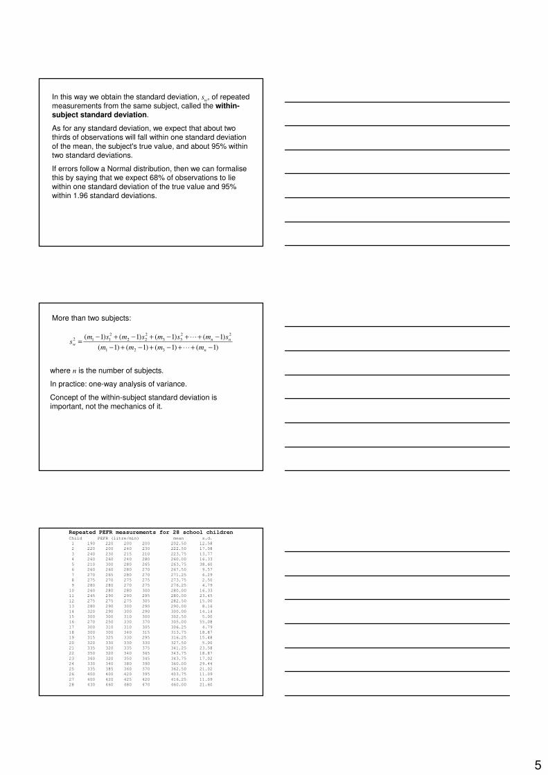
Repeated PEFR measurements for 28 school childrenChild PEFR (litre/min) mean s.d.1 190 220 200 200 202.50 12.58 2 220 200 240 230 222.50 17.08 3 240 230 215 210 223.75 13.77 4 260 260 240 280 260.00 16.33 5 210 300 280 265 263.75 38.60 6 260 260 280 270 267.50 9.57 7 270 265 280 270 271.25 6.29 8 275 270 275 275 273.75 2.50 9 280 280 270 275 276.25 4.79

10 260 280 280 300 280.00 16.33 11 245 290 290 295 280.00 23.45 12 275 275 275 305 282.50 15.00 13 280 290 300 290 290.00 8.16 14 320 290 300 290 300.00 14.14 15 300 300 310 300 302.50 5.00 16 270 250 330 370 305.00 55.08 17 300 310 310 305 306.25 4.79 18 300 300 340 315 313.75 18.87 19 315 325 330 295 316.25 15.48 20 320 330 330 330 327.50 5.00 21 335 320 335 375 341.25 23.58 22 350 320 340 365 343.75 18.87 23 360 320 350 345 343.75 17.02 24 330 340 380 390 360.00 29.44 25 335 385 360 370 362.50 21.02 26 400 400 420 395 403.75 11.09 27 400 420 425 420 416.25 11.09 28 430 460 480 470 460.00 21.60

6

PEFR for 28 schoolchildren

Common within-subject standard deviation:

sw = 19.6 litre/min.

This large variability in PEFR is well known and so individual PEFR readings are seldom used. In this study the variable used for analysis was the mean of the last three readings.

Analysis of varianceCalculate a sum of squares for the repeated observations each subject. This is the sum of squares about the subject mean. Add them together to get the sum of squares within subjects. Hence we get an estimate of the variance within the subjects.

Calculate a sum of squares and hence a variance for the subject means.

Analysis of varianceSource | Sum of Degrees of Mean F P

| squares freedom Square ratio---------+-----------------------------------------------Subject | 365604.24 27 13540.90 35.14 0.0000Residual | 32368.75 84 385.34 ---------+-----------------------------------------------Total | 397972.99 111 3585.342

The sum of squares add up.

The degrees of freedom add up.

We had 28 subjects, 4 observations on each.

27 = 28 – 1, 84 = 28 × (4 – 1), 111 = 28 × 4 – 1.

13540.90 = 365604.24/27, 385.34 = 32368.75/84.

35.14 = 13540.90/385.34.

7

Analysis of varianceSource | Sum of Degrees of Mean F P

| squares freedom Square ratio---------+-----------------------------------------------Subject | 365604.24 27 13540.90 35.14 0.0000Residual | 32368.75 84 385.34 ---------+-----------------------------------------------Total | 397972.99 111 3585.342

We do not need the P value, we know the subjects are different.

We need the mean squares.

The residual mean square is also called the within subjects mean square.

It is the variance within the subject = the within-subject standard deviation squared: √385.34 = 19.63 = sw.

Analysis of varianceSource | Sum of Degrees of Mean F P

| squares freedom Square ratio---------+-----------------------------------------------Subject | 365604.24 27 13540.90 35.14 0.0000Residual | 32368.75 84 385.34 ---------+-----------------------------------------------Total | 397972.99 111 3585.342

The subject mean square is also called the between subjects mean square.

From it we can estimate the standard deviation and variance between the subjects.

13540.90 = 4sb2 + sw

2 � sb = 57.35.

This is the standard deviation of the subjects true PEFR (i.e. average of many measurements).

Reporting the measurement errorThe within-subject standard deviation can be presented and used in several ways.

We can report sw as it stands.

We can report the maximum difference which is likely to occur between the observation and the true mean, which is 1.96sw.

For the children's PEFR data (Table 2) this is 1.96sw = 1.96×19.63 = 38.5 litre/min. For 95% of measurements, the subject's true mean PEFR will be within 38.5 litre/min of that observed.

8

Reporting the measurement errorThe British Standards Institution (1979) recommended the repeatability coefficient, r, the maximum difference likely to occur between two successive measurements. This defined as

ww ssr 83.222 ==

To correspond to a probability of 95%,

would be better, but the difference is numerically unimportant.

ww ssr 77.2296.1 ==

Reporting the measurement error

ww ssr 83.222 ==

For the children's PEFR we have repeatability

litre/min. This tells us that two measurements on the same subject are unlikely to be more than 55.6 litres/min apart.

55.6 19.63 2.83 83.2 =×== wsr

Reporting the measurement errorCoefficient of variation (CV or cv): ratio of the standard deviation to the mean.

Not really appropriate to use the coefficient of variation when the error is independent of the mean, although such usage is widespread.

For the PEFR data, for example, we would have

064.00.307/63.19/ === xscv w

The CV is usually quoted as a percentage: 6.4%.

9

Reporting the measurement errorCoefficient of variation (CV or cv): ratio of the standard deviation to the mean.

The implication is that the error is proportional to the magnitude of the measurement.

This is often the case, but then the calculation of swassuming a constant error, as described above, is incorrect.

We discuss the appropriate circumstances for the use of the coefficient of variation and its calculation later.

Assumptions in the calculation of the within-subject standard deviationTwo assumptions are required for the calculation of sw:

• measurement error does not depend on the magnitude ofthe measurement,

Essential if we are to have one estimate of standard deviation. If measurement error depends on the magnitude of the measurement, any estimate sw will be correct at only one particular point on the scale.

• measurement errors for each subject follow a Normaldistribution.

Not necessary for the calculation of sw, and about 95% of observations will be within 2sw of the subject mean whether the errors follow a Normal distribution or not.

Graphical checkse.g. histogram of differences from subject mean:

010

2030

4050

Freq

uenc

y

-80 -60 -40 -20 0 20 40 60 80PEFR minus subject mean (litre/min)

10

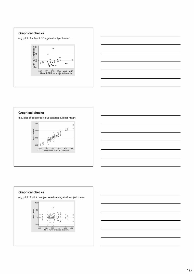
Graphical checkse.g. plot of subject SD against subject mean:

020

4060

SD

of P

EF

R fo

r sub

ject

200 250 300 350 400 450Mean PEFR for subject (litre/min)

Graphical checkse.g. plot of observed value against subject mean:

200

300

400

500

PE

FR

(litr

e/m

in)

200 250 300 350 400 450Mean PEFR for subject (litre/min)

Graphical checkse.g. plot of within subject residuals against subject mean:

-50

0

50

100

PE

FR

- m

ean

200 250 300 350 400 450Mean PEFR for subject (litre/min)

11

Pairs of measurements of FEV1 (litres) a few weeks apart, from 164 Scottish schoolchildren (D. Strachan, personal communication)

1st 2nd 1st 2nd 1st 2nd 1st 2nd 1st 2nd 1st 2nd 0.92 0.94 1.35 1.40 1.45 1.48 1.55 1.56 1.64 1.72 1.80 1.761.04 1.72 1.35 1.40 1.46 1.47 1.55 1.60 1.65 1.43 1.80 1.791.05 1.18 1.35 1.59 1.46 1.49 1.56 1.60 1.65 1.60 1.80 1.821.08 1.28 1.36 1.25 1.47 1.19 1.57 1.57 1.65 2.05 1.80 1.82 1.10 1.11 1.36 1.32 1.47 1.44 1.57 1.60 1.66 1.64 1.82 1.881.17 1.24 1.37 1.39 1.47 1.53 1.58 1.36 1.67 1.50 1.85 1.731.19 1.25 1.37 1.52 1.47 1.65 1.58 1.49 1.67 1.63 1.85 1.811.19 1.26 1.38 1.16 1.48 1.35 1.58 1.60 1.69 1.67 1.85 1.891.19 1.37 1.38 1.29 1.48 1.48 1.58 1.60 1.69 1.69 1.86 1.90 1.20 1.24 1.38 1.37 1.49 1.47 1.58 1.65 1.69 1.79 1.87 1.881.21 1.19 1.38 1.39 1.49 1.51 1.58 1.67 1.70 1.82 1.88 1.821.22 1.26 1.38 1.40 1.49 1.60 1.59 1.41 1.72 1.69 1.89 1.901.22 1.38 1.38 1.43 1.50 1.45 1.59 1.60 1.72 1.73 1.89 2.00 1.23 1.28 1.39 1.44 1.50 1.47 1.59 1.71 1.72 1.74 1.92 2.001.23 1.54 1.40 1.38 1.50 1.58 1.60 1.58 1.73 1.73 1.92 2.10 1.27 1.31 1.40 1.42 1.51 1.51 1.60 1.63 1.74 1.71 1.94 1.43 1.28 1.27 1.40 1.57 1.51 1.54 1.60 1.66 1.74 1.79 1.94 2.101.28 1.29 1.42 1.45 1.51 1.73 1.60 1.68 1.74 1.80 1.95 2.271.28 1.38 1.42 1.46 1.52 1.53 1.60 1.75 1.75 1.61 1.97 2.03 1.29 1.23 1.42 1.83 1.53 1.46 1.61 1.44 1.75 1.84 2.10 2.201.29 1.28 1.43 1.38 1.53 1.48 1.61 1.53 1.75 1.87 2.10 2.211.32 1.37 1.43 1.38 1.53 1.48 1.61 1.55 1.76 1.62 2.11 2.131.33 1.32 1.43 1.41 1.53 1.51 1.61 1.61 1.76 1.82 2.15 2.07 1.33 1.35 1.43 1.51 1.53 1.56 1.61 1.61 1.77 1.78 2.21 2.02 1.33 1.42 1.43 1.54 1.53 2.01 1.62 1.57 1.77 1.85 1.34 1.39 1.43 1.65 1.54 1.56 1.62 1.68 1.78 1.72 1.34 1.44 1.45 1.29 1.54 1.57 1.63 1.70 1.78 1.76 1.35 1.40 1.45 1.42 1.55 0.69 1.64 1.61 1.80 1.72

.51

1.5

22.

5S

econ

d F

EV

(lit

re)

.5 1 1.5 2 2.5First FEV (litre)

0.2

.4.6

.81

Abs

olut

e di

ffere

nce

(litre

)

.5 1 1.5 2 2.5Mean FEV (litre)

When we have only two observations per subject, the within-subject standard deviation is equal to the absolute value of the difference divided by �2.

We can plot the absolute difference against the subject mean to show the relationship between mean and standard deviation.

Data which go off the scaleMany assays have some limit below which no measurement can be made, and the result is recorded as below the limit of detection.

12

Duplicate salivary cotinine measurements for a group of Scottishschoolchildren, ordered by magnitude (D. Strachan, personal communication)

1st 2nd 1st 2nd 1st 2nd 1st 2nd 1st 2nd 1st 2nd ND ND 0.2 0.2 0.4 0.1 0.6 0.8 1.2 1.8 3.2 4.5 ND ND 0.2 0.3 0.4 0.1 0.6 1.0 1.3 0.3 3.3 4.5 ND ND 0.2 0.3 0.4 0.1 0.7 0.1 1.4 0.7 3.5 3.4 ND ND 0.2 0.3 0.4 0.1 0.7 0.2 1.5 0.6 3.5 4.9 ND 0.1 0.2 0.5 0.4 0.2 0.7 0.3 1.6 0.8 3.6 0.2 ND 0.1 0.2 0.6 0.4 0.2 0.7 0.3 1.6 1.3 3.7 2.6 ND 0.1 0.3 ND 0.4 0.3 0.7 0.8 1.7 4.7 3.8 3.6 ND 0.2 0.3 ND 0.4 0.3 0.7 0.9 1.8 0.9 3.9 5.5 ND 0.2 0.3 ND 0.4 0.3 0.7 1.4 1.8 1.9 4.0 3.1 ND 0.2 0.3 ND 0.4 0.3 0.8 0.4 1.8 2.1 4.1 3.4 ND 0.2 0.3 ND 0.4 0.3 0.8 0.5 1.8 2.3 4.1 3.7 ND 0.6 0.3 ND 0.4 0.4 0.8 0.8 1.9 1.2 4.1 5.0 0.1 ND 0.3 0.1 0.4 0.4 0.8 0.9 1.9 1.5 4.4 1.7 0.1 0.1 0.3 0.1 0.4 0.4 0.8 1.8 1.9 2.8 4.7 4.5 0.1 0.1 0.3 0.1 0.4 1.1 0.9 0.2 2.0 1.4 4.8 4.3 0.1 0.2 0.3 0.2 0.4 1.4 0.9 0.2 2.0 3.1 4.9 1.4 0.1 0.2 0.3 0.2 0.5 0.1 0.9 0.3 2.0 3.4 4.9 3.9 0.1 0.4 0.3 0.3 0.5 0.1 0.9 0.7 2.1 2.9 6.5 5.4 0.1 0.5 0.3 0.3 0.5 0.3 0.9 0.7 2.3 4.1 7.0 4.0 0.2 ND 0.3 0.3 0.5 0.3 0.9 3.3 2.7 1.4 7.6 4.7 0.2 ND 0.3 0.4 0.5 0.3 1.0 0.2 2.7 2.4 7.8 3.6 0.2 ND 0.3 0.4 0.5 0.4 1.0 1.6 2.7 4.0 9.3 5.4 0.2 0.1 0.3 0.4 0.5 1.0 1.1 0.4 2.8 2.2 9.9 7.2 0.2 0.1 0.3 0.4 0.6 ND 1.1 0.9 2.8 3.9 0.2 0.1 0.3 0.5 0.6 0.3 1.1 1.0 2.8 6.8 ND = Not Detectable0.2 0.1 0.3 0.6 0.6 0.5 1.2 0.8 3.1 1.6 0.2 0.1 0.4 ND 0.6 0.6 1.2 0.9 3.2 2.9 0.2 0.2 0.4 ND 0.6 0.8 1.2 1.5 3.2 3.0

Data which go off the scaleMany assays have some limit below which no measurement can be made, and the result is recorded as below the limit of detection.

When such data are used as outcome or predictor variables in regression analyses, the undetectable observations can be set to an arbitrary low value, such as half the lowest possible detectable value. Provided there are not many such observations, the presence of these arbitrary values will not influence the analysis much.

Data which go off the scaleAn arbitrary low value will not work for the estimation of measurement error, because serious bias may be introduced.

In particular, individuals for whom both measurements are recorded as not detectable will have differences of zero, which will not occur in the higher parts of the scale and violate the assumption that the measurement error is uniform throughout the scale of measurement.

13

Data which go off the scaleProvided the measurement error is uniform, we can simply omit observations which are below the detectable range. Variables which have ‘not detectable’ observations are unlikely to meet this assumption, however, but usually have error increasing as the quantity being measured increases, as does salivary cotinine.

We can usually deal with this relationship between error and subject mean by transformation.

Repeatability dependent on the magnitude of the variableWhen the within-subject standard deviation is related to the magnitude of the measurement, we cannot estimate sw as described above, because it is not constant.

02

46

810

Sec

ond

cotin

ine

(mm

ol/li

tre)

0 2 4 6 8 10First cotinine (mmol/litre)

01

23

45

Abs

olut

e di

ffere

nce

(mm

ol/li

tre)

0 2 4 6 8 10Mean salivary cotinine (mmol/litre)

The simplest alternative model to consider is that the standard deviation is proportional to the mean.

We then estimate the ratio of subject standard deviation to subject mean, the within-subject coefficient of variation (details omitted).

If the standard deviation is proportional to the mean, CV should be a constant.

For the cotinine example, the coefficient of variation is 67%.

From it, we can estimate the standard deviation of repeated measurements at any point within the range of measurement, by multiplying by the mean at that point.

14

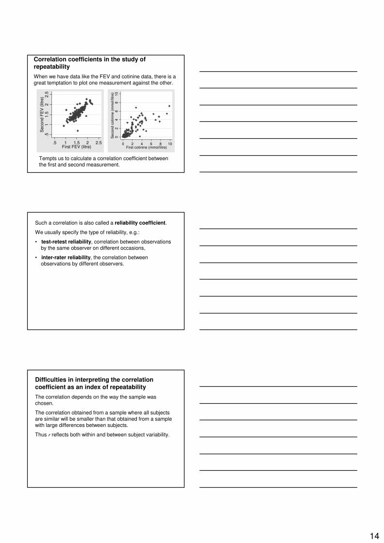
Correlation coefficients in the study of repeatabilityWhen we have data like the FEV and cotinine data, there is a great temptation to plot one measurement against the other.

.51

1.5

22.

5S

econ

d F

EV

(lit

re)

.5 1 1.5 2 2.5First FEV (litre)

02

46

810

Sec

ond

cotin

ine

(mm

ol/li

tre)

0 2 4 6 8 10First cotinine (mmol/litre)

Tempts us to calculate a correlation coefficient between the first and second measurement.

Such a correlation is also called a reliability coefficient.

We usually specify the type of reliability, e.g.:

• test-retest reliability, correlation between observationsby the same observer on different occasions,

• inter-rater reliability, the correlation betweenobservations by different observers.

Difficulties in interpreting the correlation coefficient as an index of repeatabilityThe correlation depends on the way the sample was chosen.

The correlation obtained from a sample where all subjects are similar will be smaller than that obtained from a sample with large differences between subjects.

Thus r reflects both within and between subject variability.

15

Example: the FEV data.

Correlation between repeated measurements is r = 0.82.

Split the FEV sample into two sub-samples at 1.5 litres.

First sub-sample, r = 0.54, second sub-sample, r = 0.73.

Within-subject standard deviation: whole sample sw = 0.10 litre, first sub-sample sw = 0.09 litre, second sub-sample, sw = 0.11 litre.

.51

1.5

22.

5S

econ

d F

EV

(lit

re)

.5 1 1.5 2 2.5First FEV (litre)

Second FEV (litre) Second FEV (litre)

The correlation coefficient is dependent on the way the sample is chosen.

It only has meaning for the population from which the study subjects can be regarded as a random sample.

If we select subjects to give a wide range of the measurement, for example, this will inflate the correlation coefficient.

Advantages of the correlation coefficient We can use it to test the null hypothesis that the first and second measurements are independent, i.e. that there is no repeatability at all. Thus it is useful in investigating the validity of measurement methods.

Enables us to compare the repeatability of different measurements collected on the same subjects.

Useful for piloting a number of scales to which best discriminates between individuals.

The scale with the highest correlation between repeated measurements IN THE SAME POPULATION would discriminate best between subjects.

It would carry the most information.

16

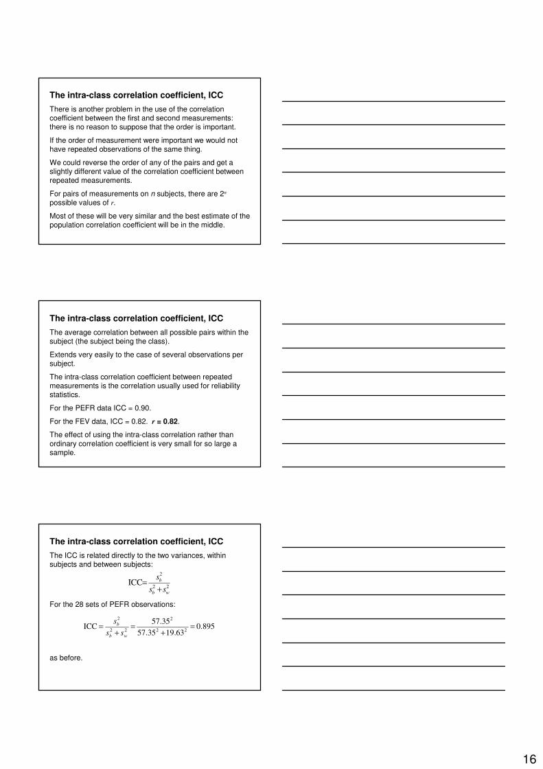
The intra-class correlation coefficient, ICCThere is another problem in the use of the correlation coefficient between the first and second measurements: there is no reason to suppose that the order is important.

If the order of measurement were important we would not have repeated observations of the same thing.

We could reverse the order of any of the pairs and get a slightly different value of the correlation coefficient between repeated measurements.

For pairs of measurements on n subjects, there are 2n

possible values of r.

Most of these will be very similar and the best estimate of the population correlation coefficient will be in the middle.

The intra-class correlation coefficient, ICCThe average correlation between all possible pairs within the subject (the subject being the class).

Extends very easily to the case of several observations per subject.

The intra-class correlation coefficient between repeated measurements is the correlation usually used for reliability statistics.

For the PEFR data ICC = 0.90.

For the FEV data, ICC = 0.82. r = 0.82.

The effect of using the intra-class correlation rather than ordinary correlation coefficient is very small for so large a sample.

The intra-class correlation coefficient, ICCThe ICC is related directly to the two variances, within subjects and between subjects:

For the 28 sets of PEFR observations:

as before.

22

2

ICCwb

b

sss+

=

895.063.1935.57

35.57ICC 22

2

22

2

=+

=+

=wb

b

sss

17

The intra-class correlation coefficient, ICCICC = 1.00 when sw

2 = 0, for each subject all measurements are identical.

The correlation will be zero when there is no more difference between the subjects than would be expected by chance if the subjects were identical, i.e. if sb

2 = 0.

Thus the intra-class correlation coefficient, like the ordinary correlation coefficient, depends on the range of the subject means.