Lidar based emissions measurement at the whole facility scale: Method and error analysis

Gail E. Bingham1, Christian C. Marchant1, Vladimir V. Zavyalov1,Douglas J. Ahlstrom1, Kori D. Moore1, Derek S. Jones1, Thomas D.

Wilkerson1, Larry E. Hipps2, Randal S. Martin2, Jerry L. Hatfield3, John H. Prueger3, Richard L. Pfeiffer3

1Space Dynamics Laboratory, 1695 North Research Parkway, North Logan, UT 84341. Tel: 435-797-4320 Fax: 435-797-4599 gail.bingham@sdl.usu.edu

2Utah State University, Logan, UT 84322 3Agricultural Research Service, National Soil Tilth Laboratory, 2110 University Blvd., Ames,

IA 50011-4420, jerry.hatfield@ars.usda.gov

Abstract. Particulate emissions from agricultural sources vary from dust created by operations and animal movement to the fine secondary particulates generated from ammonia and other emitted gases. The development of reliable facility emission data using point sampling methods designed to characterize regional, well-mixed aerosols are challenged by changing wind directions, disrupted flow fields caused by structures, varied surface temperatures, and the episodic nature of the sources found at these facilities. We describe a three-wavelength lidar-based method, which, when added to a standard point sampler array, provides unambiguous measurement and characterization of the particulate emissions from agricultural production operations in near real time. Point-sampled data are used to provide the aerosol characterization needed for the particle concentration and size fraction calibration, while the lidar provides 3D mapping of particulate concentrations entering, around, and leaving the facility. Differences between downwind and upwind measurements provide an integrated aerosol concentration profile, which, when multiplied by the wind speed profile, produces the facility source flux. This approach assumes only conservation of mass, eliminating reliance on boundary layer theory. We describe the method, examine measurement error, and demonstrate the approach using data collected over a range of agricultural operations, including a swine grow-finish operation, an almond harvest, and a cotton gin emission study.

Keywords: aerosol characterization, agriculture emission measurement, system error, flux measurement

1 INTRODUCTION

The movement of urban populations into agricultural production areas, combined with the increasing size of these facilities to capture economies of scale and meet global food needs, has elevated the issue of agricultural production emissions to national attention. Accurate measurement of specific operations and whole facility aerosol emissions, especially those that contain large percentages of organic matter, are technically challenging. Currently, regulations of Concentrated Agricultural Feeding Operations (CAFO) and other particulate emission sources are based on multiple point-sampled measurements taken near these facilities and combined with models to account for wind and time variation [1]. The combination makes it difficult to determine the effectiveness of specific conservation and management practices.

The accuracy and cost of emission and management practice studies could be reduced if it were possible to directly measure the flux of emissions from a facility and its components in

Journal of Applied Remote Sensing, Vol. 3, 033510 (20 February 2009)

© 2009 Society of Photo-Optical Instrumentation Engineers [DOI: 10.1117/1.3097919]Received 4 Aug 2008; accepted 17 Feb 2009; published 20 Feb 2009 [CCC: 19313195/2009/$25.00]Journal of Applied Remote Sensing, Vol. 3, 033510 (2009) Page 1

Downloaded From: http://remotesensing.spiedigitallibrary.org/ on 08/19/2014 Terms of Use: http://spiedl.org/terms

near real time. While the concept behind the measurement of a physical flux is intuitively simple—the mass transport of material from a defined surface in a defined time—in environmental applications, actual measurement is difficult. Taken in its simplest form, mass flux can be defined as the mean amount of material moving through a defined area per unit time. In a pipe or closed container, flux can be measured as accurately as desired, by defining the accuracy of the sensors and the velocity of movement. Extensive work has been conducted over the past century to develop methods that extend this concept to uncontained fluxes, such as momentum, water vapor, heat, and carbon dioxide from natural and managed surfaces [2].

While initial studies were limited to mean measurements and derived diffusion coefficients by the slow response of available sensors, the general availability of robust, fast-response sensors have made eddy correlation flux measurement the method of choice for flux determination in the atmospheric boundary layer [3][4]. Emission measurements from agricultural sources, however, challenge the assumptions and costs associated with this method. The uniform flow disruptions of scattered, variable-sized and roofed buildings, surface treatments, and mobile sources, combined with unconfined wind vectors make mean determination difficult. In this paper, we discuss the potential of using remote sensing to surround a facility or operation with the equivalent of a vast number of rapid response sensors to map the emission plume and track its movement. Toward this approach, we utilize a multi-wavelength lidar calibrated using standard point sensors. The combination allows us to build real time and averaged particulate mass concentration fields, which are combined with the mean wind field to produce the flux measurement.

Aerosol sounding techniques for the retrieval of physical aerosol parameters from multi-wavelength lidar measurements have been reported since the 1980s and have made major progress in the past five years [5][6][7][8][9][10]. Unambiguous and stable retrieval of aerosol physical parameters using lidar can require up to twelve empirically derived quantities, which are not easily derived optically [11]. The instrumentation required to provide both multi-wavelength elastic scatter lidar and Raman information is expensive, complicated to operate, and often immobile. To date, a significant database of atmospheric aerosol characteristics has been obtained using a combination of satellite and ground-based observations [12][13]. Using this database, several researchers have shown that the physical properties of assumed aerosols can be successfully retrieved based on measurements of backscatter coefficients at only three wavelengths [6][14][15]. However, since agricultural aerosols may differ from the database, direct characterization must be part of the measurement.

The Aglite lidar is a robust, agile, and easily operated system that displays emitted particulate distributions in a few seconds under most meteorological and diurnal conditions. The system uses three wavelengths combined with information derived from an array of point sensors to distinguish between different types and sizes of particulate emissions. The resulting combination of point samplers and scanning lidar provides near real time measurements of facility operations, which can be used to evaluate emission fluxes and operational approaches to minimize them.

2 MEASUREMENTS AND METHODS

The lidar system is developed around a monostatic laser transmitter and 28-cm receiver telescope (Fig. 1). The laser is a three-wavelength, 6W, Nd:YAG laser, emitting at 1.064 (3W), 0.532 (2W) and 0.355 (1W) m with a 10 kHz repetition rate [16]. Backscattered energy at the visible and UV wavelengths is detected using photon-counting photo-multiplier tubes, while the IR reflection is detected using an APD photon Counting Module. The minimum system range gate is 6 m; however, the range resolution for this data is ~12 m, limited by the laser pulse width. A measurement integration time of 1 second was used for all

Journal of Applied Remote Sensing, Vol. 3, 033510 (2009) Page 2

Downloaded From: http://remotesensing.spiedigitallibrary.org/ on 08/19/2014 Terms of Use: http://spiedl.org/terms

data presented in this paper. The lidar is vertically orientated, with a turning mirror turret to direct the beam -10 to + 45 vertically and 140 horizontally from the top of a small trailer. Lidar scan rates from 0.1 – 1 /s are used to develop the 3D map of the source(s), dependent on range and concentration of the aerosol [16].

Fig. 1. The three wavelength Aglite lidar at dusk, scanning a harvested wheat field.

The lidar equation (1) describes the lidar return signal as a function of range z for wavelength :

zzz

zz

zAcLPzP020 2exp

2. (1)

The term P (z) is the measured reflected power for distance z and is measured in photon counts. P0 is the output power of the lidar, L is the lidar coefficient, which represents system efficiency, c is the speed of light, is the pulse width of the lidar, A (z) is the effective area function, which includes the geometric form factor (GFF), (z) is the atmospheric backscatter coefficient, and (z) is the atmospheric extinction coefficient. The backscatter and extinction coefficients are functions of temperature, pressure, humidity, and the background and emitted aerosols.

Expected signal-to-noise ratios (SNR) calculated by Marchant [16] using synthetic data for the Aglite lidar at 20 and 100 percent emitted power and 1 s, full range resolution are shown in Fig. 2. These plots were made using system calibration constants measured in the field. Standard temperature and pressure and zero percent humidity were assumed. The background aerosol was assumed to have the same properties as the continental average aerosol from the OPAC aerosol database [12]. In these plots, SNR is defined as the ratio of the mean aerosol backscatter amplitude over the standard-deviation of the aerosol backscatter. Because the noise is not correlated, SNR can be increased by both time and range averaging [15].

Journal of Applied Remote Sensing, Vol. 3, 033510 (2009) Page 3

Downloaded From: http://remotesensing.spiedigitallibrary.org/ on 08/19/2014 Terms of Use: http://spiedl.org/terms

Fig. 2. Aerosol backscatter 1s SNR for the Aglite lidar, corrected for molecular backscatter, as a function of range for 20% and full power levels and two PM10 background loadings. Chart color

represents laser wavelength (red – IR, green – visible, blue – UV).

2.1 Aerosol Information

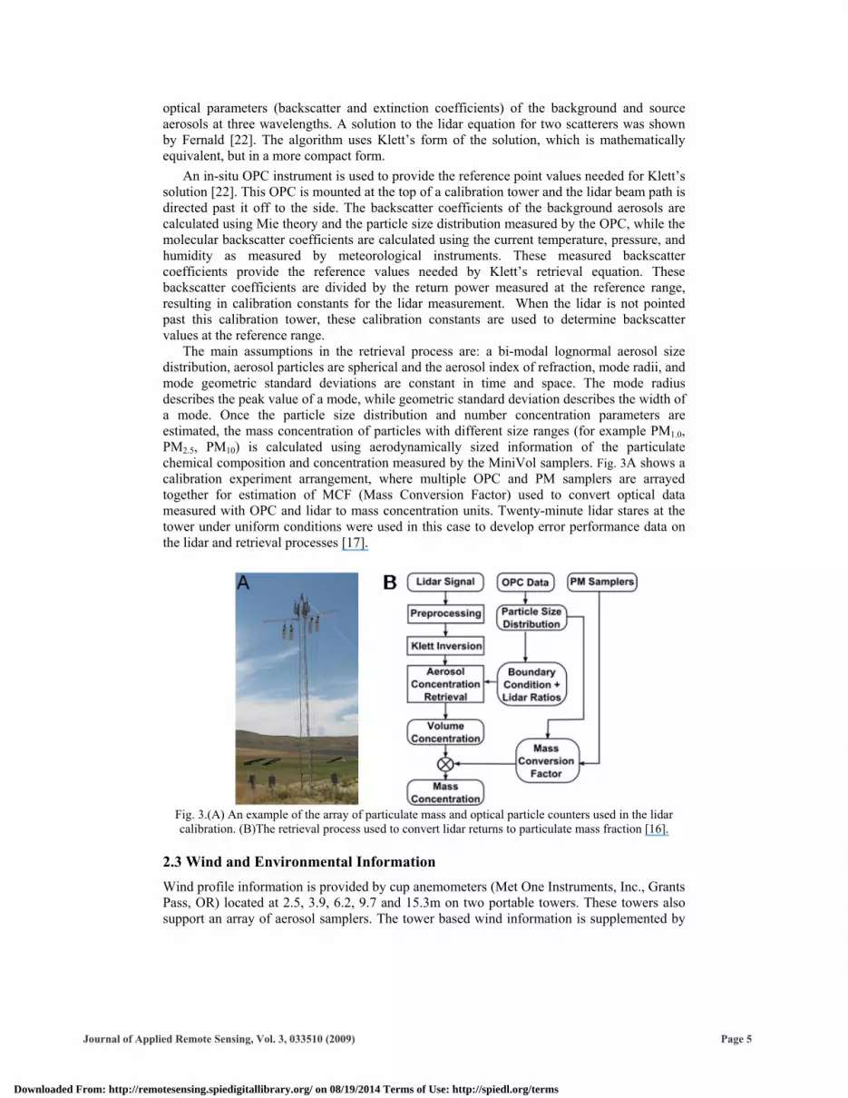
The solution of (1) requires knowledge of the optical parameters of the both the background and source aerosols, which need to be measured at one or more reference points upwind (background) and downwind (background plus source) of the facility. In our approach [17], both optical and aerodynamic mass faction sensors are utilized to develop these parameters (see Fig. 3B). Aerodynamic mass fraction samples are collected using MiniVols (Airmetrics, Eugene, OR.), which are portable, self-contained, filter-based impactor particulate samplers. Chow (2006) demonstrated that PM2.5 and PM10 concentrations measured by MiniVols in California’s San Joaquin Valley did not differ statistically from the concentrations measured by the collocated Federal Reference Method (FRM) samplers [18].

We have also conducted extensive calibration and intercalibration comparisons of the MiniVols against FRM samplers located at an air quality sampling site in Logan, Utah, operated by the Utah Division of Air Quality. In-situ particle size profiles are collected in parallel with the MiniVol samplers using Aerosol Profilers, Model 9722 (Met One Instruments, Inc., Grants Pass, OR.) This Optical Particle Counter (OPC) uses a laser to count and size particles at a sampling rate of l/min with a sheath flow of 2 l/min. The counts are grouped into eight user-specified size bins from 0.3 to >10 µm (0.3-0.5, 0.5-0.6, 0.6-1.0, 1.0-2.0, 2.0-2.5, 2.5-5.0, 5.0-10.0, and 10µm in our studies). The OPCs can be read out at a range of times from 2 – 60 s per sample.

2.2 Lidar Retrieval Calibration

The details of our lidar calibration and aerosol retrieval process are discussed in detail by Marchant [19] and Zavyalov [11]. The lidar return power from range z for a single scatter is shown in (1). In the case of two distinct classes of scatters, (z) and (z) represent the total backscatter and extinction from the sum of a background scattering component plus an emission source scattering component. The background scattering component represents homogeneous scatterers, including both background aerosol scattering and molecular scattering, which is expected to be constant over the relatively short ranges near the ground where Aglite is used. These contributions of aerosol scatterers to these coefficients are derived from aerosol sampler data, while the contributions due to molecular scattering are calculated using data from portable met-stations. The algorithm used to retrieve aerosol physical parameters from a raw Aglite lidar signal shown schematically in Fig. 3B involves four major steps [11][21], which account for the geometrical form factor of the telescope receiving optics and scattered sunlight background radiation. The routine then calculates the

A B

Background = 10 µg/m3 Background = 50 µg/m3

A B

Background = 10 µg/m3 Background = 50 µg/m3

Journal of Applied Remote Sensing, Vol. 3, 033510 (2009) Page 4

Downloaded From: http://remotesensing.spiedigitallibrary.org/ on 08/19/2014 Terms of Use: http://spiedl.org/terms

optical parameters (backscatter and extinction coefficients) of the background and source aerosols at three wavelengths. A solution to the lidar equation for two scatterers was shown by Fernald [22]. The algorithm uses Klett’s form of the solution, which is mathematically equivalent, but in a more compact form.

An in-situ OPC instrument is used to provide the reference point values needed for Klett’s solution [22]. This OPC is mounted at the top of a calibration tower and the lidar beam path is directed past it off to the side. The backscatter coefficients of the background aerosols are calculated using Mie theory and the particle size distribution measured by the OPC, while the molecular backscatter coefficients are calculated using the current temperature, pressure, and humidity as measured by meteorological instruments. These measured backscatter coefficients provide the reference values needed by Klett’s retrieval equation. These backscatter coefficients are divided by the return power measured at the reference range, resulting in calibration constants for the lidar measurement. When the lidar is not pointed past this calibration tower, these calibration constants are used to determine backscatter values at the reference range.

The main assumptions in the retrieval process are: a bi-modal lognormal aerosol size distribution, aerosol particles are spherical and the aerosol index of refraction, mode radii, and mode geometric standard deviations are constant in time and space. The mode radius describes the peak value of a mode, while geometric standard deviation describes the width of a mode. Once the particle size distribution and number concentration parameters are estimated, the mass concentration of particles with different size ranges (for example PM1.0,PM2.5, PM10) is calculated using aerodynamically sized information of the particulate chemical composition and concentration measured by the MiniVol samplers. Fig. 3A shows a calibration experiment arrangement, where multiple OPC and PM samplers are arrayed together for estimation of MCF (Mass Conversion Factor) used to convert optical data measured with OPC and lidar to mass concentration units. Twenty-minute lidar stares at the tower under uniform conditions were used in this case to develop error performance data on the lidar and retrieval processes [17].

Fig. 3.(A) An example of the array of particulate mass and optical particle counters used in the lidar calibration. (B)The retrieval process used to convert lidar returns to particulate mass fraction [16].

2.3 Wind and Environmental Information

Wind profile information is provided by cup anemometers (Met One Instruments, Inc., Grants Pass, OR) located at 2.5, 3.9, 6.2, 9.7 and 15.3m on two portable towers. These towers also support an array of aerosol samplers. The tower based wind information is supplemented by

Journal of Applied Remote Sensing, Vol. 3, 033510 (2009) Page 5

Downloaded From: http://remotesensing.spiedigitallibrary.org/ on 08/19/2014 Terms of Use: http://spiedl.org/terms

tethered balloon profiles collected at 5 min. intervals to observe boundary layer structure. The wind, humidity, temperature and OPC data are transmitted to the lidar- and data-processing trailers for storage and experiment management.

2.4 Flux Measurement Method

The lidar’s capability to accurately sample 3D aerosol concentrations entering and leaving an operation in near real time (1-3 minutes) makes it possible to measure facility emissions with approximately twice that time resolution. Fig. 4A shows the concept behind our approach, where the facility is treated as one would calculate the source strength in a bioreactor. In this approach, the source strength is determined using the mean flow rate through the reactor and the difference in reactive species concentration entering and leaving the vessel. The scanning lidar samples the mass concentration fields entering and leaving the facility, while standard anemometers provide the mean wind speed profile. This same simple relationship applies to defining a box large enough that no source material escapes through the top or side.

In applying this method, the downwind face of the box has to be far enough from the facility that the anemometers provide an accurate wind speed profile. Fig. 4B shows an example of our lidar-derived concentration data. The location-concentration plot pattern from scanning up one side, across the top, and down the other resembles a common staple used to clip papers together and is referred to as a “staple scan.” The data from the top of the box are monitored such that no source particulate transport passes through the top. The data for the left side panel of the staple provide the background concentration entering the box, while those on the right provide the background plus facility concentration leaving the box. The short-term flux is calculated by multiplying the area integrated mass concentration difference by the wind speed during the scan.

Flux In Flux Out

Lidar Scan

Wind Direction

A B

Flux In Flux Out

Lidar Scan

Wind Direction

Flux In Flux Out

Lidar Scan

Wind Direction

A B

Fig. 4. (A)Conceptual illustration of the scheme for using lidar to generate time-resolved local area particulate fluxes. (B) An example of a “staple” lidar scan over the facility showing aerosol

concentrations on the three sides of the box. The flux equation in the integral form for calculating emission is:

hrUD drdhChrChrvF

,

,, (2)

where is the average wind speed component, the direction of which defines the long axis of the box, CD – C forms the mass concentration difference upwind and downwind, integrated over the range (width) and height of the exit plume. In our routine, F is conceptually calculated as:

Journal of Applied Remote Sensing, Vol. 3, 033510 (2009) Page 6

Downloaded From: http://remotesensing.spiedigitallibrary.org/ on 08/19/2014 Terms of Use: http://spiedl.org/terms

R

Ri

H

HjUDijij hrCCvF

0 0

(3)

where R0 and R are the near and far along beam edges of the box and H0 and H form the top and bottom of the box. (In many cases, H0 is set above eye level and concentration is extrapolated to the ground to avoid illuminating personnel and animals.) The r h term is the individual area element for which each flux component is calculated by each step in the double summation.

3 FLUX MEASUREMENT ERROR ESTIMATION

Since the flux measurement (f) is a function of several variables, nxxxf ,,, 21 , and the uncertainty of each variable, xi, is known, the uncertainty of f can be calculated. If the variables are assumed to be independent, the flux error can be expressed as the square-root of the sum of the squares of the uncertainty induced by each individual variable (Met One Instruments, Inc., Grants Pass, OR). That is,

2

1

n

ii

i

xxff , (4)

which for our flux calculations breaks out as:

i jijU

UDij

Dijij

ij

ACCFC

CFv

vFF 2

222

2 , (5)

or

iji j

UijDijijijUDij ACvCvvCCF2/1

222 (6)

where is the wind speed in the direction perpendicular to the lidar scan (cos corrected). Components that are crosswise to the box do not contribute to the flux error because the box is defined large enough that none of the source material leaves through the sides or top. Specific terms in our error analysis include , the concentration terms, and the mass conversion factor (MCF), which is included in Equation (6) as a constant in the concentration calculation. Additional understanding of the flux error estimate can be seen from additional rearrangement. Substituting averaged parameters over the inferred area from Eq. 2 to Eq. 5, a simplified equation can be obtained:

,

2 2 22 22 2 2

2 20 0) )

2( (

D UD U

D U D U

CC Cv vF A A

C CF v C A v C A(6a)

Typically the mass concentration errors are the same from the downwind and upwind sides. In this case, the right hand side approximation is valid. As shown by Zavyalov [17] the

Journal of Applied Remote Sensing, Vol. 3, 033510 (2009) Page 7

Downloaded From: http://remotesensing.spiedigitallibrary.org/ on 08/19/2014 Terms of Use: http://spiedl.org/terms

errors are now shown in fractional form. In this form, two things become obvious that are not as easily seen in the earlier form. First, the center term includes a 2, which enters in because the flux requires both upwind and downwind calculations. The second is the relationship between the values of CD and CU. When the two terms are of similar size, their difference in the denominator quickly dominates over the other terms.

Wind speed and direction errors are dominated by sampling issues and not by the instrument calibration as we are estimating the wind field for a parameter averaged over a 200-300 m area at a particular time. For this error calculation, we estimate the wind errors using the standard deviation of the direction and velocity over a 20-min. sampling period. For our field campaigns described in this analysis, these errors are typically 10-15% of the wind value. We set our wind dataloggers to collect 1-min. averages and standard deviations to provide a quality control value for the flux data.

Short term error calculations after Marchant [16] for the Aglite system and the Zavyalov [17] particulate volume concentration retrieval calibration as applied in the flux calculation are shown in Table 1. To understand the flux error, we consider that the sides of the flux box include data collected over about one minute and ranging from 600 to 1000 m. In the flux calculation, the range and scan data are rolled into the single flux number. Flux error analysis data were collected during a calibration stare past the OPC-MiniVol array with the beam horizontal to the ground and an upwind scan taken after the stare. The upper section shows the SNR ( Cv/Cv) for a (1-sec) stare without OPC noise, while the lower section shows the measured system (lidar plus OPC) volume concentration SNR for the lidar measurement during the 1-min scan time typically used for flux measurements, as in [18].

Table 1 data were collected in system performance experiments under stable aerosol conditions with continental aerosol. For these measurements, the system was operating at ~5% power, and OPC measured particulate background concentrations were 9.0, 25.4, and 50.2 g/m3 (MCF=1).

Table 1. Aglite lidar 1- and 60-second aerosol signal to noise ratios (SNR) measured at 5% power under uniform conditions at the ranges normally used in flux measurements [16][17].

Lidar SNR (Average/standard deviation) during a horizontal stare Range PM 600 m 700 m 800 m 900 m 1000 m PM2.5 9.0 69 66 63 60 57 PM10 25.4 6.3 6.0 5.7 5.4 5.2 TSP 50.2 4.4 4.2 4.0 3.8 3.7 Concentration Calibration SNR (Lidar and OPC) during a 60 sec stare PM2.5 9.0 239 229 218 208 197 PM10 25.4 22 21 20 19 18 TSP 50.2 15 15 14 13 13

These values can be compared with the overall SNR calculated for the system in Fig. 2,where SNR is given in terms of backscatter. The SNR for increasing particle diameter decreases as the particle size to wavelength ratio increases.

A flux calculation example, with the error estimates and magnitude data demonstrating the primary terms of (6), and the resultant hourly average flux or emission strength estimate obtained using the Aglite system are shown in Table 2. These data are typical values from our system precision experiments, and are designed to show the experienced precision.

Journal of Applied Remote Sensing, Vol. 3, 033510 (2009) Page 8

Downloaded From: http://remotesensing.spiedigitallibrary.org/ on 08/19/2014 Terms of Use: http://spiedl.org/terms

Table 2. Example Aglite lidar system derived aerosol average emission flux component measurement error and estimated flux error determined for uniform conditions.

PMBin

Wind Dir ( )

CD-CU (µg/m3) @ MCF = 1 MCF CD-CU

(µg/m3)Wind (m/s)

Area(m2)

Mass Flux (g/s)

PM2.5 330 9.2 0.70 0.002 3.04 0.3 2.19 0.21 4.7 0.69 1000 0.01 0.005

PM10 330 9.2 21.0 0.58 2.10 0.3 44.10 0.64 4.7 0.69 1000 0.21 0.043

TSP 330 9.2 57.4 2.24 1.88 0.3 107.91 17.7 4.7 0.69 1000 5.07 0.11

4 FLUX MEASUREMENT EXAMPLES AND RESULTS

In this section, we show three examples where the Aglite system is applied to agricultural system analysis, and we compare those examples with traditional sampler/model results. Each example illustrates the system’s effectiveness for long- and short-term measurements and shows lessons learned as the system has evolved.

4.1 Swine Finishing Facility Measurements

The Aglite measurement system was applied to an Iowa swine feeding emissions experiment August 24 – September 8, 2005. The swine farm data provided a uniform, fixed, nearly constant flux demonstration (except for periods when road dust plumes from a nearby county road occurred). The fairly steady wind and steady operations during this experiment provided ideal conditions for demonstrating the flux calculation method. The facility consisted of three separate parallel barns, each housing around 1250 pigs, with 1.4-m tall screen-vented windows running along nearly the length of the north and south sides of the barns. The areas of the facility not used for barns, feed-bin footprints, or access roads were covered with maintained grass. Cultivated fields surrounded the facility with corn to the north, south and west and soybeans to the east. The barns were located ~650 m from the lidar. A 20-meter tower was sited between two of the barns to support the aerosol and micrometeorological instruments (three heights). A particulate diagnostic trailer was located 50 m in the general downwind direction from the barns. Other instrument support towers were located around the facility.

Example single scans of the upwind (CU, PM10 only) and downwind (CD) staple face show the mass concentration values for PM10, PM2.5 between 400 and 900 m from the lidar (Fig. 5). The figure shows the typical structure observable in a uniform background and typical plume profile. Each vertical scan was collected in approximately 1.25 minutes.

The vertical profile of horizontal mass concentration difference of the downwind minus upwind layers can be easily obtained from these data (Fig. 5C). Single scan differences, of course, do not account for accumulation or depletion in the measurement box due to wind speed variation during a scan, for input background variation, or for storage in or flushing of the box due to the existing large scale wind eddy structure (i.e. we do not attempt to measure the same air mass at the upwind and downwind scans). Negative features can be observed in the individual profiles. Several scans are required to achieve a meaningful mean estimate of the facility emission. For calculation efficiency, we calculate flux through the downwind surface first and then the upwind flux, differencing the flux rather than concentration. Choosing an area that fully includes the source plume but not a lot of extra area eliminates the need to spend resources calculating for pixels that difference to zero. The CD and CU area average measurements provide aerosol mass concentration ( g/m3), which, when multiplied by the wind speed (m/s), provides the area average flux (FD &FU, g/m2s). Differencing (FD-

Journal of Applied Remote Sensing, Vol. 3, 033510 (2009) Page 9

Downloaded From: http://remotesensing.spiedigitallibrary.org/ on 08/19/2014 Terms of Use: http://spiedl.org/terms

FU) and integrating over the plume area provides the facility emission estimate (FS, g/s) for that staple.

Fig. 5. Single upwind (A) and downwind (B) PM10 scans of the swine facility airmass showing the distribution of the background and facility leaving plume concentrations ( g/m3), the horizontally

averaged PM10 concentrations and their difference (C), and the PM10 particulate flux ( g/m2s)distribution (D) calculated when the difference is multiplied by the wind speed profile.

Table 3 shows emission summary data collected by various methods during the Iowa measurement sequence. Martin provides the emissions calculated from the sampler data and modeled facility flux during this experiment [23]. Emission rates were also estimated from lidar-measured fluxes dividing total day fluxes by the number of pigs inside of the flux box. This site has a gravel road on the upwind (south) side that had traffic at a rate of 1-2 cars per hour. The road dust could not be separated in the impactor particulate sampler data, but was identifiable and could be processed separately in the OPC and lidar data (see PM-concentrations “without dust” in Table 3). The modeled PM sampler data are similar to PM10and PM2.5 emission rate values from the lidar. The PM and OPC data were collected over an 8-day period, while the lidar data were calculated hourly. This was an early deployment of the Aglite system, and consistent flux measurement scans were collected only for a two-hour period for each particulate class. Considering the large difference in the sample periods and that fugitive dust was not excluded from the filter data, we conclude that these data show the Aglite system’s capability to characterize a stationary facility with fairly uniform emissions in a relatively short period of time. While the magnitude of the PM2.5 emission rate shows excellent agreement, the lidar PM10 emission rate was roughly half what was indicated by the long term filter data. The PM2.5 emission was relatively constant over the entire sampling period, while significant structure was observed in the PM10 data dominated by road dust and feeding operations. Since the filter data incorporated emissions from both road and facility

A B

C D

Journal of Applied Remote Sensing, Vol. 3, 033510 (2009) Page 10

Downloaded From: http://remotesensing.spiedigitallibrary.org/ on 08/19/2014 Terms of Use: http://spiedl.org/terms

operations, this difference is consistent with the lower level of road traffic that occurred during the lidar flux measurement period.

Table 3. Comparison of the ambient (background) and facility mass concentration and emission rate(g/pig-day) data measured by filters (23 hour base), OPC (24 hour base) and the lidar (2 hour base).

PM samplers OPC data Lidar data CM - g/m3

EM - g/pig/day Ambient (CU)

Plume (CD)

Ambient (CU)

Plume (CD)

Ambient (CU)

Plume (CD)

CM-PM10 (with dust) Without dust,

38.7±5.4 49.4±8.3 34.4±24 28.6±7.8

42.2±28 38.7±7.8

37.1±18 30.2±2.5

52.8±21 46.4±6.5

CM-PM2.5 (with dust) Without dust,

13.3±3.2 14.7±3.3 14.3±9.0 13.7±4.7

17.2±9.7 16.7±6.6

11.2±7.2 9.5±0.8

12.8±6.5 11.6±1.4

EM- PM10

EM – PM 2.5

0.83 0.440.09 0.03

0.42 0.13 0.09 0.04

4.2 Cotton Gin Measurements

Measurements at a working cotton gin facility were made from December 11-14, 2006. For this deployment, 13 MiniVol impactors (total) were distributed in clusters with PM1, PM2.5,PM10 and TSP heads, and 5 MetOne OPCs were used for particulate characterization. Facility emission rates were not calculated from inverse modeling using measured PM concentrations as explained by Martin [22] due to the facility layout (emissions mainly coming from the elevated cyclone outlets). The lidar was located 800 m SW of the gin, with reference towers directly north and east of the lidar. A wind profile tower supporting the five levels of anemometers and temperature sensors, a wind direction and rain gauge, and two levels of OPC and MiniVol clusters was located near the gin. A second, similarly instrumented tower located south of the gin was used to provide ambient conditions. The season presented a nighttime fog challenge, which limited lidar operation to daylight hours, and occasional gin operation interruptions were observed as the operators performed maintenance and mechanical adjustments. The site provided a diurnally rotating wind condition that made emission aerosol measurements more challenging.

Lidar operations showed two continuous plumes in scans above the facility, one from gin stack effluents not captured by the cyclones, and a smaller plume originating at the seed pile, which we assume resulted from the wind picking up aerosols from the falling seed stream. Other activities, such as vehicle movement and dumping and transferring the cyclone trash, were intermittent sources captured by the lidar. Fig. 6 shows sequential lidar measurements taken during two days of fairly uniform conditions. Of the 111 scans, 62 were taken on December 12th and the remainder on December 14th. These data show relatively consistent gin operation, with both days punctuated by downwind concentration spikes associated with non-continuous activities on the site. There is an increase in fine particulates the second day, with nearly equal PM2.5 and PM10 flux. . The top chart shows the wind speed value used in the flux calculation, with the two middle strips showing the volume concentration of CU and CD in

m3/cm3. While this is a somewhat unusual unit, it is the last step before converting to mass/m3, and is equivalent to g /m3 if the volume to mass conversion factor (MCF) is 1 (the particulates had the density of water). The net flux, in the bottom panel, is the product of the CD-CU difference multiplied by the MCF and the wind speed. The MCF values are presented

Journal of Applied Remote Sensing, Vol. 3, 033510 (2009) Page 11

Downloaded From: http://remotesensing.spiedigitallibrary.org/ on 08/19/2014 Terms of Use: http://spiedl.org/terms

in Table 4. An error in the MCF calculation [17], could explain the increase in PM2.5 value approximately doubling on the second day.

Fig. 6. Wind speed, upwind and downwind volume concentrations, and mass flux calculated using the Aglite data collected on December 12 & 14, 2006. December 14th data begin at point 62.

At the time these data were collected, it was assumed that the upwind aerosol concentrations were uniform and would be sampled at a significantly lower rate that the downwind values. This experiment and the Almond experiment discussed in the following section show that uniform upwind conditions cannot be assumed and that even distant upwind activity can add pulses of upwind particulates. Measurement variability for the combined period and for each of the individual days is shown in Table 4. Table 4 also shows the MCF values used to convert from volume concentration (measured optically by the OPCs and lidar) to mass concentration (utilized in regulations and measured by the MiniVol samplers). While it is expected that the facility plume and background may have a significant difference in aerosol characteristics, identical upwind and downwind MCF values have been used in this analysis. Because of the long sampling time required to attain a measurable mass on the filter, not knowing how much time the plume is actually impinging on a downwind sampler can cause a significant error when the aerosols have different characteristics. We have acquired a cascade impactor and an aerodynamic particle sizer to resolve this problem, but for this analysis we chose to average the readings from all of the samplers.

Journal of Applied Remote Sensing, Vol. 3, 033510 (2009) Page 12

Downloaded From: http://remotesensing.spiedigitallibrary.org/ on 08/19/2014 Terms of Use: http://spiedl.org/terms

Table 4. Cotton gin aerosol mass concentration, mass conversion factors, and flux statistics for Fig. 6, The concentrations and flux means are shown with 95% confidence intervals.

While emission rates for the facility were not calculated using inverse modeling, an air dispersion model was run using emission rates reported in the facility’s 2005 air permit assuming 22 hour per day gin operations for four months of the year combined with the meteorological data collected during the field deployment. The model used was the Industrial Source Complex Short-Term Model, version 3 (ISCST3), the dispersion model previously recommended by the U.S. EPA for use in regulatory applications [24]. As of November 2006, the U.S. EPA recommends the use of AERMOD for regulatory applications [Appendix W of 40 CFR 51, U.S. EPA (November 9, 2005)], but the more complex meteorological inputs for this model were not collected during this field study.

The ISCST3 model assumes steady-state conditions, continuous emissions, and conservation of mass. ISCST3 assumes a Gaussian distribution of pollutants based on time-averaged meteorological data. It also uses stability classes to address pollution dispersion due to atmospheric mixing. Stability classes are typically determined by a combination of vertical temperature lapse rates and incoming solar radiation or methods using vertical or horizontal wind variance. For reference, lidar-based concentrations are compared with the concentrations modeled by ISCST3. Fig. 7 compares the lidar-derived PM2.5 aerosol concentrations (Table 4) averaged for ~6 hours with the model estimates for the same period. Because the source and wind speed were relatively constant for the impactor sampling period, a relatively good comparison of the gin emissions was obtained with both the lidar and the U.S. EPA dispersion model. The concentration offset between the two is due to the omission of the background concentration from the model field.

Fig. 7. A comparison of lidar and ISCST3 model derived PM2.5 concentrations for a cotton gin under variable wind conditions. The model does not include the background aerosol. The white circles are the

wind and sampler tower locations.

Whole Period First Day Second Day Concentration ( g/m3)Flux (g/s) PM2.5 PM10 TSP PM2.5 PM10 TSP PM2.5 PM10 TSP

CU –ave 40.2 1.28 42.4 3.1 52.2 7.1 38.4 1.9 43.0 6.2 46.1 11.9 41.7 1.2 41.8 2.7 57.1 7.9

CU - 2.92 7.06 16.27 2.89 9.52 18.18 2.07 4.63 13.36

CD -ave 45.1 0.7 48.3 3.5 79.5 7.1 44.7 0.7 72.6 3.5 105.9 7.1 44.1 0.7 46.1 1.5 72.7 4.6 CD - 2.95 13.78 28.11 2.95 13.78 28.11 2.51 5.34 16.58

MCF 3.04 2.10 1.88 2.69 1.63 1.59

F -ave 4.5 0.5 7.1 0.6 11.7 1.0 2.7 0.3 7.2 0.8 12.6 1.5 6.8 0.7 7.0 0.8 10.7 1.3

F - 2.82 3.06 5.52 1.24 3.34 6.04 2.57 2.70 4.65

Journal of Applied Remote Sensing, Vol. 3, 033510 (2009) Page 13

Downloaded From: http://remotesensing.spiedigitallibrary.org/ on 08/19/2014 Terms of Use: http://spiedl.org/terms

4.3 Almond Harvesting Measurement

The Aglite system was applied to a mobile source emitter in an almond harvest at the Nickels Soils Laboratory Research Farm near Woodland, CA. from September 26 to October 11, 2006. This experiment compared lidar-based measurements to sampler-based model results, for a mobile source, tree-obstructed harvest. This orchard was a working orchard in an almond-producing area surrounded by orchards under a variety of management schemes. The orchard has two varieties in rows orientated north/south with a tree height of about 7 m. The soil surface condition was bare ground with a slight crust, and the trees were irrigated by drip system. For this deployment, 20 MiniVol samplers (total) distributed in clusters with PM1,PM2.5, PM10, and TSP heads were used along with 10 MetOne OPCs.

Fig. 8 shows wind speed, volume-based concentrations, and flux data for 138 scans collected over a four-hour period of orchard-sweeping operations. The operation was a “mock” or “simulated sweeping” activity that was conducted the day after the nut pickup was completed. While measurements were made during actual sweeping and pickup, these data were unusable because the light and variable winds on those days caused plume-mixing with surrounding field operations. The same equipment and procedures were used for the “mock” sweep as for the actual sweeping operation.

The top plot in Fig. 8 is the wind speed observed for each scan, showing a fairly consistent northerly wind between 2-6 m/s, averaging 4 m/s. At sample 60, the sweeping method was changed. In the first 59 samples, the sweeper fan operated, but it did not operate with the higher-scan numbers. Since the source is mobile, the plume from the upwind side is filtered by the trees, and some areas of the orchard contributed more emission than others (see Fig. 9). As expected for this mechanical operation, the PM fractions show significantly higher concentrations of larger particulates, with little contribution from PM2.5 for the operation (with and without the fan). The upwind concentration during the measurement period was relatively smooth with some variations in TSP during the operation. The downwind concentrations were much more variable, and the higher concentrations were associated with the sweeper locations near the downwind end of the orchard, especially during turns at the downwind end of the rows. We attribute the area emission differences—without validation data—to local differences in the soil surface being swept and to reduced orchard filtering. The data show a significant difference in TSP emissions with and without the fan. The PM10 data remained relatively constant throughout the entire operation, and the TSP emission increased significantly when the fan operated. Fan-generated dust was heaviest during end-of-row turns, where vehicle traffic disturbed the surface. Some operation variability occurred because the operator stopped occasionally for short periods that were not coordinated with the lidar scan sequence. Both location in the orchard (surface effect) and distance into the orchard affected the concentrations, especially for larger particles.

As with the cotton gin data shown previously, the two middle strips in Fig. 8 show the volume concentration of CU and CD in m3/cm3. Volume concentration is shown to avoid confusion caused by uncertainty in the MCF. The net flux, in the bottom panel, is the CD-CUdifference multiplied by the MCF and the wind speed. The MCF values are presented in Table 5. As Zavyalov pointed out [17], the MCF determination was the largest measurement error in our system during these operations. Table 5 shows specific values for the operation. As with the cotton data, two things are noticeable. First, as particle size increases, the particulate density (MCF) decreases, and the error associated with the largest particulates increases significantly. This correlation was discussed by Zavyalov [17] and is expected with this optical system. Because the particle sizes are larger than the lidar and OPC wavelengths being used for the measurement, accuracy decreases as particle size increases.

Journal of Applied Remote Sensing, Vol. 3, 033510 (2009) Page 14

Downloaded From: http://remotesensing.spiedigitallibrary.org/ on 08/19/2014 Terms of Use: http://spiedl.org/terms

Fig. 8. Wind speed, upwind and downwind concentrations, and flux for 138 scans during a four hour period of mock almond sweeping operations on October 11, 2006.

Table 5. Mock almond sweeping aerosol upwind and downwind mass concentration and mass flux statistics associated with Fig. 8, showing the values for the entire operation, sweeping without the fan (<

#60) and with the fan operating (> #59). Averages are shown with 95% confidence intervals.

Comparison of the lidar-based concentrations with the output of the ISCST3 model is shown in Fig. 9. Final emission rates were determined with inverse modeling techniques using observed aerosol concentrations at five 2m height sampling sites and one 9m height sampling site along the downwind side of the orchard. The area emission estimates (Fig. 9) were obtained using hourly average wind speeds and directions taken at 5m and an average source emission rate of 5.53 g m-2 s-1 to achieve a “best fit” to the measured sampler profile. Sampler to model concentration ratio for the operation averaged 1.00, with a variation ranging from 0.46 to 1.57 (Table 6). The data confirm the significant variation in surface

Whole Operation With Fan Without Fan CU,D = ( g/m3)Flux = (g/s)

PM2.5 PM10 TSP PM2.5 PM10 TSP PM 2.5

PM 10 TSP

CU -Ave 9.5 0.4 28. 6 3.5 33.1 6.7 9.2 0.4 25.0 4.0 26.2 7.5 9.8 0.5 31.3 5.1 38.2 9.7 CU- 1.063 10.376 19.509 0.786 7.660 14.399 1.172 11.446 21.524 CD -Ave 10.0 0.3 33.1 2.8 41.6 5.2 10.4 0.5 37.7 4.9 50.4 9.3 9.7 0.3 29.6 2.9 34.9 5.5 CD - 1.71 16.69 31.39 2.02 19.53 36.67 1.34 13.24 24.92 MCF 8.369 2.739 1.263 F-Ave 1.7 0.1 5.7 0.6 7.1 1.0 2.0 0.15 6.8 0.8 8.7 1.5 1.5 0.2 4.8 0.8 5.9 1.2 F- 0.68 3.50 5.91 0.57 3.34 5.99 0.69 3.41 5.60

Journal of Applied Remote Sensing, Vol. 3, 033510 (2009) Page 15

Downloaded From: http://remotesensing.spiedigitallibrary.org/ on 08/19/2014 Terms of Use: http://spiedl.org/terms

emission that the lidar observed. Period average concentrations measured by the samplers varied from 15.3 to 49.5 g/m3 (Table 6), while observed individual lidar scan plume concentrations (averaged over the active plume) ranged from 15 to 106 g/m3.

36

32

28

24

20

16

12

8

4

0

D7 D8 D9 D10 D11

36

32

28

24

20

16

12

8

4

0

D7 D8 D9 D10 D11

36

32

28

24

20

16

12

8

4

0

D7 D8 D9 D10 D11

36

32

28

24

20

16

12

8

4

0

36

32

28

24

20

16

12

8

4

0

D7 D8 D9 D10 D11

Fig. 9. Modeled PM10 aerosol concentrations ( g/m3) for the four-hour October 11, 2006 almond sweeping exercise, based on the five aerosol sampling stations (D72-D11) on the downwind side of the

orchard using the ISCST3 model with an average emission rate of 5.53 g m-2 s-1.

Table 6. Model and particulate sampler measurements for the total sweeping period shown in Fig. 8, showing the area variability not picked up by the model.

Sampler Location

Measured Concentration

Modeled Concentration

Meas./Model

g m-3 g m-3 Ave. = 1.00 D7 (2m) 49.50 31.44 1.574 D8 (2m) 20.49 32.65 0.628 D8 (9m) 20.66 12.20 1.693 D9 (2m) 24.35 32.28 0.754 D10 (2m) 29.31 32.93 0.890 D11 (2m) 15.31 33.18 0.461

Some discussion is warranted about the potential for sampling error due to the relatively slow vertical scans used in the above analysis. Eddy covariance flux measurement frequencies in the 20Hz range are often specified. However, eddy covariance sampling volumes are very small and the eddy frequency correspondingly high. In our case, the sampling volume is typically one- to two-hundred meters long and is being used to derive an estimate of the mean concentration crossing the plane of the scan, not the variation. In addition, we are sampling at a maximum rate of 10 Hz. The difference is that the beam is being vertically scanned, not held at a single height. These differences in sampling suggest that the scales involved should be carefully analyzed. The scan rate must be considered for sources where the emission stability is not understood.

For the applications presented here, we make the following observations: First, we are measuring relatively continuous processes, with emission variation time periods longer than a single staple scan. While turbulent transfer-driven emission puffs observed at a point may not be captured, emissions from the operation are effectively sampled. The comparisons we show against the ISCST3 model appear to validate the approach. Second, this system is ideal for mobile source operations, such as a plowing or harvesting operation. Since the lidar data allows the flux box to move with the source, each staple may be rotated and adjusted when

Journal of Applied Remote Sensing, Vol. 3, 033510 (2009) Page 16

Downloaded From: http://remotesensing.spiedigitallibrary.org/ on 08/19/2014 Terms of Use: http://spiedl.org/terms

position and general wind direction change. This contrasts against static sampling systems where the plume moves on and off the sampler at random.

If transport from the process is interrupted by a sudden wind shift or a pause in the operation, that transmission period can be easily identified and deleted from the sample sequence. The Aglite data processing system monitors these factors, and these periods are excluded by the quality control process. Unlike a fixed sampler where the plume wanders on and off, the lidar measures the entire plume with each scan.

The data presented here demonstrate how the Aglite system effectively measures emissions under a wide range of conditions. The swine production facility was a stable, consistent source—except for the road traffic. The strong peaks in the lidar data from the road dust allowed the affected scans to be eliminated [16]. The flux data reported in this paper includes these spikes, because they could not be eliminated from the filter data that is shown for comparison. The cotton gin data provided a different challenge, with significantly different aerosol types between the background and facility emissions. The almond data set shows the Aglite’s capability to track a mobile source and determine the difference in the equipment’s operation method in a short period of time. Aglite not only followed the mobile system, it quantified the difference. Variations resulting from local surface conditions were also quantified.

5 CONCLUSIONS

We have demonstrated a process for measuring near real time whole facility and agricultural operation particulate fluxes. The three wavelength lidar allows aerosol emissions to be determined and calibrated using characteristics from fixed-point measurements. Aerosol concentration and distribution entering and leaving the facility are differenced and multiplied by the mean wind speed to develop the mass flux. The 3D concentration image, collected by the lidar, allows the plume profile to be identified and tracked so that a virtual box can be built around the facility plume. This paper has shown the details of the flux calculation process and has provided a detailed error analysis. The examples given have shown that under relatively constant wind conditions, fluxes with errors in the 10-25% range can be developed with sampling periods in the 30-minute to 1-hour time frame for both fixed and mobile sources. System performance at a CAFO, a mobile harvester, and a fixed product processing plant are used as examples. While the Aglite system is flexible and agile, under light and variable wind conditions, it does not allow flux measurement, as the internal mixing and random transport of materials from the source do not allow accurate measurements by any means during such conditions. Also, when emissions from upwind fields or facilities provide a significantly variable aerosol input, longer sample periods are required to achieve the same flux accuracy.

While not the purpose of this paper, these examples show that to be of value for either regulatory, conservation practice or improved method development efforts the flux and fast response emission measurements must be combined with accurate and insightful data and understanding of the processes being evaluated. When these are combined, significant advances in agricultural emission mitigation should be possible.

Acknowledgments

The development of the Aglite system was performed under USDA Agreement number 58-3625-4-121 with Dr. Jerry Hatfield, the Director of the National Soil Tilth Laboratory in Ames, Iowa, providing valuable direction to the Aglite development team. Any opinions, findings, conclusions, or recommendations expressed in this publication are those of the authors and do not necessarily reflect the view of the USDA.

Journal of Applied Remote Sensing, Vol. 3, 033510 (2009) Page 17

Downloaded From: http://remotesensing.spiedigitallibrary.org/ on 08/19/2014 Terms of Use: http://spiedl.org/terms

6 References

[1] S. J. Hoff, K. C. Hornbuckle, P. S. Thorne, D. S. Bundy, and P. T. O'Shaughnessy, “Emissions and community exposures from CAFOs,” in Iowa Concentrated Animal Feeding Operations Air Quality Study, pp. 45-85, Iowa State University and The University of Iowa Study Group (2002).

[2] C. A. Friehe, “Fine-scale measurements of velocity, temperature and humidity in the atmospheric boundary layer,” in Probing the Atmospheric Boundary Layer, D. Lenschow, Ed., Amer. Met. Soc. (1986).

[3] W. E. Eichinger, H. E. Holder, R. Knight, J. Nichols, D. I. Cooper, L. E. Hipps, W. P. Kusta, and J. H. Prueger, “Lidar measurement of boundary layer evolution to determine sensible heat fluxes,” J. Hydromet. 6(6), 840-53 (2005) [doi:10.1175/JHM461.1].

[4] J. L. Chávez, C. M. U. Neale, L. E. Hipps, J. H. Prueger, and W. P. Kustas, “Comparing aircraft-based remotely sensed energy balance fluxes with eddy covariance tower data using heat flux source area functions,” J. Hydromet. 6(6), 923-40 (2005) [doi:10.1175/JHM467.1]

[5] J. Heintzenberg, H. Muller, H. Quenzel, and E. Thomalla, “Information content of optical data with respect to aerosol properties: numerical studies with a randomized minimization-search-technique inversion algorithm,” Appl. Opt. 20(8), 1308-15 (1981) [doi:10.1364/AO.20.001308].

[6] K. Rajeev and K. Parameswaran, “Iterative method for the inversion of multiwavelength lidar signals to determine aerosol size distribution,” Appl. Opt.37(21), 4690–4700 (1998) [doi:10.1364/AO.37.004690].

[7] D. Müller, U. Wandinger, and A. Ansmann, “Microphysical particle parameters from extinction and backscatter lidar data by inversion with regularization: theory,” Appl. Opt. 38(12), 2346–57 (1999) [doi:10.1364/AO.38.002346].

[8] C. Böckmann, “Hybrid regularization method for the ill-posed inversion of multiwavelength lidar data in the retrieval of aerosol size distributions,” Appl. Opt.40(9), 1329–1342 (2001) [doi:10.1364/AO.40.001329].

[9] I. Veselovskii, A. Kolgotin, V. Griaznov, D. Muller, K. Franke, and D. N. Whiteman,“Inversion of multiwavelength Raman lidar data for retrieval of bimodal aerosol size distribution,” Appl. Opt. 43(5), 1180-1195 (2004) [doi:10.1364/AO.43.001180].

[10] D. Althausen, D. Müller, A. Ansmann, U. Wandinger, H. Hube, E. Clauder, and S. Zörner, “Scanning 6-wavelength 11-channel aerosol lidar,” J. Atmos. Oceanic Technol. 17(11), 1469–1482 (2000) [doi:10.1175/1520-0426(2000)017<1469:SWCAL>2.0.CO;2].

[11] V. V. Zavyalov, C. Marchant, G. E. Bingham, T. D. Wilkerson, J. Swasey, C. Rogers, D. Ahlstrom, and P. Timothy, “Retrieval of physical properties of particulate emission from animal feeding operations using three wavelength elastic lidar measurements,” Proc. SPIE 6299, 62990S (2006) [doi:10.1117/12.680967].

[12] M. Hess, P. Koepke, and I. Schult, “Optical properties of aerosols and clouds: the software package OPAC,” Bull. Am. Meteorol. Soc. 79(5), 831-844 (1998)[doi:10.1175/1520-0477(1998)079<0831:OPOAAC>2.0.CO;2].

[13] O. Dubovik, B. Holben, T. F. Eck, A. Smirnov, Y. J. Kaufman, M. D. King, D. Kino, D. Tanre, and I. Slutsker, “Variability of absorption and optical properties of key aerosol types observed in worldwide locations,” J. Atm. Sci. 59(3), 590-608 (2002) [doi:10.1175/1520-0469(2002)059<0590:VOAAOP>2.0.CO;2].

[14] Y. Sasano and E. V. Browell, “Light scattering characteristics of various aerosol types derived from multiple wavelength lidar observations,” Appl. Opt. 28, 1670-1679 (1989).

Journal of Applied Remote Sensing, Vol. 3, 033510 (2009) Page 18

Downloaded From: http://remotesensing.spiedigitallibrary.org/ on 08/19/2014 Terms of Use: http://spiedl.org/terms

[15] M. Del Guasta, M. Morandi, L. Stefanutti, B. Stein, and J. P. Wolf, “Derivation of Mount Pinatubo stratospheric aerosol mean size distribution by means of a multiwavelength lidar,” Appl. Opt. 33, 5690–5697 (1994).

[16] C. C. Marchant, T. D. Wilkerson, G. E. Bingham, V. V. Zavyalov, J. M. Andersen, C. B. Wright, S. S. Cornelsen, R. S. Martin, P. J. Silva, J. L. Hatfield. “Aglite lidar: a portable elastic lidar system for investigating aerosol and wind motions at or around agricultural production facilities,” J. Applied Remote Sensing, under review (2009).

[17] V. V. Zavyalov, C. C. Marchant, G. E. Bingham, T. D. Wilkerson, J. L. Hatfield, R. S. Martin, P. J. Silva, K. D. Moore, J. Swasey, D. J. Ahlstrom, T. L. Jones. “Aglite lidar: calibration and retrievals of well characterized aerosols from agricultural operations using a three-wavelength elastic lidar,” J. Appl. Rem. Sens., under review (2009).

[18] J. C. Chow, J. G. Watson, D. H. Lowenthal, L.-W A. Chen, R. J. Tropp, K. Park, and K. A. Magliano, “PM2.5 and PM10 mass measurements in California’s San Joaquin Valley,” Aerosol Sci. and Tech. 40(10), 796–810 (2006) [doi:10.1080/02786820600623711].

[19] C. C. Marchant, “Algorithm development of the Aglite-lidar instrument ,” MS Thesis, Utah State University <http://digitalcommons.usu.edu/etd/107/> (2007).

[20] F. G. Fernald, B. M. Herman, and J. A. Reagan, “Determination of aerosol height distributions by lidar,” J. of Applied Meteor. 11(3), 482-489 (1972) [doi:10.1175/1520-0450(1972)011<0482:DOAHDB>2.0.CO;2].

[21] J. D. Klett, “Lidar inversion with variable backscatter/extinction ratio,” Appl. Opt.24, 1638-1683 (1985).

[22] R. S. Martin, K. D. Moore, and V. S. Doshi, “Determination of particle (PM10 and PM2.5) and gas-phase ammonia (NH3) emissions from a deep-pit swine operation using arrayed field measurements and inverse Gaussian plume modeling,” J. of Atmos. Chem., under review (2009).

[23] P. R. Bevington, Data Reduction and Error analysis for the Physical Sciences,McGraw-Hill, NY (1969).

[24] EPA, “Appendix W of 40 CFR Part 51,” U. S. EPA (1998).

About the Authors Gail Bingham, Vladimir Zavyalov, and Thomas Wilkerson are senior scientists, Christopher Marchant, Douglas Ahlstrom and Derek Jones are graduate students, and Kori Moore is an environmental engineer at Utah State University’s Space Dynamics Laboratory, 1695 North Research Parkway, North Logan, UT 84341. Larry Hipps and Randal Martin are professors at Utah State University, Logan. Jerry Hatfield, John Prueger and Richard Pfeiffer are scientists at the Agricultural Research Service, National Soil Tilth Laboratory, 2110 University Blvd., Ames, IA 50011.

Journal of Applied Remote Sensing, Vol. 3, 033510 (2009) Page 19

Downloaded From: http://remotesensing.spiedigitallibrary.org/ on 08/19/2014 Terms of Use: http://spiedl.org/terms