LiSBOA (LiDAR Statistical Barnes Objective Analysis) for ...

Atmos. Meas. Tech., 14, 2065–2093, 2021https://doi.org/10.5194/amt-14-2065-2021© Author(s) 2021. This work is distributed underthe Creative Commons Attribution 4.0 License.

LiSBOA (LiDAR Statistical Barnes Objective Analysis) for optimaldesign of lidar scans and retrieval of wind statistics – Part 1:Theoretical frameworkStefano Letizia, Lu Zhan, and Giacomo Valerio IungoWind Fluids and Experiments (WindFluX) Laboratory, Mechanical Engineering Department, The University of Texas atDallas, 800 W Campbell Road, Richardson, TX 75080, USA

Correspondence: Giacomo Valerio Iungo ([email protected])

Received: 11 June 2020 – Discussion started: 31 August 2020Revised: 20 January 2021 – Accepted: 22 January 2021 – Published: 16 March 2021

Abstract. A LiDAR Statistical Barnes Objective Analysis(LiSBOA) for the optimal design of lidar scans and retrievalof the velocity statistical moments is proposed. LiSBOA rep-resents an adaptation of the classical Barnes scheme for thestatistical analysis of unstructured experimental data in N -dimensional space, and it is a suitable technique for the eval-uation over a structured Cartesian grid of the statistics ofscalar fields sampled through scanning lidars. LiSBOA isvalidated and characterized via a Monte Carlo approach ap-plied to a synthetic velocity field. This revisited theoreticalframework for the Barnes objective analysis enables the for-mulation of guidelines for the optimal design of lidar ex-periments and efficient application of LiSBOA for the post-processing of lidar measurements. The optimal design of li-dar scans is formulated as a two-cost-function optimizationproblem, including the minimization of the percentage of themeasurement volume not sampled with adequate spatial res-olution and the minimization of the error on the mean ofthe velocity field. The optimal design of the lidar scans alsoguides the selection of the smoothing parameter and the to-tal number of iterations to use for the Barnes scheme. LiS-BOA is assessed against a numerical data set generated us-ing the virtual lidar technique applied to the data obtainedfrom a large eddy simulation (LES). The optimal samplingparameters for a scanning Doppler pulsed wind lidar are re-trieved through LiSBOA, and then the estimated statistics arecompared with those of the original LES data set, showing amaximum error of about 4 % for both mean velocity and tur-bulence intensity.

1 Introduction

Reliable measurements of the wind velocity vector field areessential for understanding the complex nature of atmo-spheric turbulence and providing valuable data sets for thevalidation of theoretical and numerical models. However,field measurements of wind speed are typically characterizedby large uncertainties due to the generally unknown and un-controllable boundary conditions (Braham, 1979), the broadrange of timescales and length scales (Cushman-Roisin andBeckers, 1990a), and the complexity of the physics involved(Stull, 1988). Furthermore, the large measurement volume,which typically extends throughout the height of the atmo-spheric boundary layer, imposes on the experimentalists theselection of the sampling parameters as a trade-off betweenspatial and temporal resolutions.

Wind speed has been traditionally measured through localsensors, such as mechanical, sonic, and hot-wire anemome-ters (Liu et al., 2019; Kunkel and Marusic, 2006). Besidestheir simplicity, mechanical anemometers are affected by er-rors due to the flow distortion of the supporting structures,drawbacks under harsh weather conditions (Mortensen,1994), and overspeeding (Busch and Kristensen, 1976). Fur-thermore, their relatively slow response results in a limitedrange of the measurable time–length scales, which makesthem unsuitable, for instance, for measuring the turbulentflow around urban areas (Pardyjak and Stoll, 2017). Sonicanemometers can measure the three velocity components,with frequencies up to 100 Hz (Cuerva and Sanz-Andrés,2000), in a probing volume of the order of 10−4 m3, yetmeasurements might be still affected by the wakes generated

Published by Copernicus Publications on behalf of the European Geosciences Union.

2066 S. Letizia et al.: LiSBOA (LiDAR Statistical Barnes Objective Analysis) – Part 1

by the supporting structures, such as met towers and struts,and they are sensitive to temperature variations (Mortensen,1994). Hot-wire anemometers, although they provide a fullcharacterization of the energy spectrum, require a compli-cated calibration (Kunkel and Marusic, 2006) and are ex-tremely fragile (Wheeler and Ganji, 2010a). Furthermore,traditional, single-point sensors are unable to provide an ade-quate characterization of the spatial gradients of the wind ve-locity vector, which is particularly significant in the verticaldirection (Cushman-Roisin and Beckers, 1990b). To over-come this issue, several anemometers arranged in arrays, andsupported by meteorological masts, have been deployed inseveral field campaigns (Haugen et al., 1971; Bradley, 1983;Taylor and Teunissen, 1987; Emeis et al., 1995; Pahlow et al.,2001; Berg et al., 2011; Kunkel and Marusic, 2006).

In the last few decades, remote sensing instruments havebeen increasingly utilized to probe the atmospheric bound-ary layer (Debnath et al., 2017a, b), and nowadays they rep-resent a more cost-effective and flexible alternative to mete-orological towers (Newsom et al., 2017). In particular, in therealm of remote sensing anemometry, Doppler wind light de-tection and ranging (lidar) systems underwent a rapid devel-opment due to the significant advancement in eye-safe lasertechnology (Emeis, 2010). Wind lidars have been heavilyemployed in wind energy (Bingöl et al., 2010; Aitken andLundquist, 2014; Trujillo et al., 2011; Iungo et al., 2013b;Machefaux et al., 2016; Garcia et al., 2017; El-Asha et al.,2017; Bromm et al., 2018; Zhan et al., 2019, 2020), airportmonitoring (Köpp et al., 2005; Tang et al., 2011; Holzäpfelet al., 2016; Thobois et al., 2019), micro-meteorology (Gal-Chen et al., 1992; Banakh et al., 1999; Banta et al., 2006;Mann et al., 2010; Muñoz-Esparza et al., 2012; Rajewskiet al., 2013; Schween et al., 2014), urban wind research(Davies et al., 2007; Newsom et al., 2008; Xia et al., 2008;Kongara et al., 2012; Huang et al., 2017; Halios and Barlow,2018), and studies of terrain-induced effects (Bingöl, 2009;Krishnamurthy et al., 2013; Kim et al., 2016; Pauscher et al.,2016; Risan et al., 2018; Fernando et al., 2019; Bell et al.,2020).

Besides the mentioned capabilities, lidars present someimportant limitations, such as reduced range in adverseweather conditions (precipitation, heavy rain, fog, lowclouds, or low aerosol concentration; Liu et al., 2019; Mannet al., 2018) and a limited spatiotemporal resolution of thisinstrument, namely about 20 m in the radial direction andabout 10 Hz in sampling frequency. These technical speci-fications, associated with the nonstationary wind conditionstypically encountered for field experiments, pose major chal-lenges in the application of wind lidars for the statistical anal-ysis of turbulent atmospheric flows.

In the realm of wind energy, early lidar measurementswere limited to the qualitative analysis of snapshots of theline-of-sight (LOS) velocity, i.e., the velocity component par-allel to the laser beam (Käsler et al., 2010; Clive et al.,2011). Fitting of the wake velocity deficit was also success-

fully exploited for the extraction of quantitative informationabout wake evolution from lidar measurements (Aitken andLundquist, 2014; Wang and Barthelmie, 2015; Kumer et al.,2015; Trujillo et al., 2016; Bodini et al., 2017). To charac-terize velocity fields with higher statistical significance, thetime averages of several lidar scans were calculated for pe-riods with reasonably steady inflow conditions (Iungo andPorté-Agel, 2014; Machefaux et al., 2015; Van Dooren et al.,2016). In the case of data collected under different wind andatmospheric conditions, clustering and bin-averaging of li-dar data were carried out (Machefaux et al., 2016; Garciaet al., 2017; Bromm et al., 2018; Zhan et al., 2019, 2020).Finally, more advanced techniques for first-order statisticalanalysis, such as variational methods (Xia et al., 2008; New-som and Banta, 2004), optimal interpolation (Xu and Gong,2002; Kongara et al., 2012), least squares methods (Newsomet al., 2008), and Navier–Stokes solvers (Astrup et al., 2017;Sekar et al., 2018), were applied for the reconstruction of thevelocity vector field from dual Doppler measurements.

Besides the mean field, the calculation of higher-orderstatistics from lidar data to investigate atmospheric turbu-lence is still an open problem. In this regard, Eberhardet al. (1989) re-adapted the postprocessing of the veloc-ity azimuth display (VAD) scans (Lhermitte, 1969; Wilson,1970; Kropfli, 1986) to estimate all the components of theReynolds stress tensor by assuming horizontal homogene-ity of the mean flow within the scanning volume, whichcan be a limiting constraint for measurements in complexterrains (Frisch, 1991; Bingöl, 2009). Range height indica-tor (RHI) scans were used to detect second-order statistics(Bonin et al., 2017), spectra, skewness, dissipation rate ofthe velocity field, and even heat flux (Gal-Chen et al., 1992).Recently, in the context of wind radar technology, but read-ily applicable to lidars as well, a promising method for theestimation of the instantaneous turbulence intensity (i.e., theratio between standard deviation and mean of streamwise ve-locity), based on the Taylor hypothesis of frozen turbulence,was proposed by Duncan et al. (2019). More advanced tech-niques exploit additional information of turbulence carriedby the spectrum of the backscattered lidar signal (Smalikho,1995). However, this approach requires the availability of li-dar raw data, which is not generally available for commer-cial lidars. For a review on turbulence statistical analysesthrough lidar measurements, the reader can refer to Satheand Mann (2013). Another typical scanning strategy to ob-tain high-frequency lidar data consists of performing scanswith fixed elevation and azimuthal angles of the laser beamwhile maximizing the sampling frequency (Mayor et al.,1997; O’Connor et al., 2010; Vakkari et al., 2015; Frehlichand Cornman, 2002; Debnath et al., 2017b; Choukulkar et al.,2017; Lundquist et al., 2017).

For remote sensing instruments, data are typically col-lected based on a spherical coordinate system, and then in-terpolated over a Cartesian reference frame oriented with thex axis in the mean wind direction. This interpolation can be a

Atmos. Meas. Tech., 14, 2065–2093, 2021 https://doi.org/10.5194/amt-14-2065-2021

S. Letizia et al.: LiSBOA (LiDAR Statistical Barnes Objective Analysis) – Part 1 2067

source of error (Fuertes Carbajo and Porté-Agel, 2018), espe-cially if a linear interpolation method is used (Garcia et al.,2017; Carbajo Fuertes et al., 2018; Beck and Kühn, 2017;Astrup et al., 2017). Delaunay triangulation has also beenwidely adopted for coordinate transformation (Clive et al.,2011; Trujillo et al., 2011, 2016; Iungo and Porté-Agel, 2014;Machefaux et al., 2015), yet the accuracy has not been quan-tified in the case of nonuniformly distributed data. It is rea-sonable to weight the influence of the experimental points ontheir statistics according to the distance from the respectivegrid centroid, such as using uniform (Newsom et al., 2008),hyperbolic (Van Dooren et al., 2016), or Gaussian weights(Newsom et al., 2014; Wang and Barthelmie, 2015; Zhanet al., 2019). The use of distance-based Gaussian weights forthe interpolation of scattered data over a Cartesian grid is atthe base of the Barnes objective analysis (or Barnes scheme;Barnes, 1964), which has been systematically used in meteo-rology but only sporadically used for lidar data. It representsan iterative statistical ensemble procedure to reconstruct ascalar field arbitrarily sampled in space and is low-pass fil-tered with a cut-off wavelength that is a function of the pa-rameters of the scheme.

The scope of this work is to define a methodology to post-process scattered data of a turbulent velocity field measuredthrough a scanning Doppler wind lidar (or eventually otherremote sensing instruments) to calculate mean, standard de-viation and even higher-order statistical moments on a Carte-sian grid. The proposed methodology, referred to as the Li-DAR Statistical Barnes Objective Analysis (LiSBOA), rep-resents an adaptation of the classic Barnes scheme to N -dimensional domains, enabling applications for nonisotropicscalar fields through a coordinate transformation. A majorpoint of novelty of LiSBOA is the estimation of wind ve-locity variance (and, eventually, higher-order statistics) fromthe residual field of the mean, which also provides adequatefiltering of dispersive stresses due to data variability not con-nected with the turbulent motion. A criterion for the rejec-tion of statistical data affected by aliasing, due to the under-sampling of the spatial wavelengths under investigation, isformulated. LiSBOA is assessed against a synthetic scalarfield to validate its theoretical response and the formulatederror metric. Detailed guidelines for the optimal design ofa lidar experiment and the effective reconstruction of thewind statistics are provided. The effectiveness of the pro-posed scheme in the identification of the optimal scanningparameters and retrieval of turbulence statistics is quantifiedusing virtual lidar data.

It will be shown in the following that the revisited Barnesscheme offers several advantages compared to the above-cited techniques for lidar data analysis: (i) it allows one to ex-plicitly select the cut-off wavenumber to filter out small-scalevariability, while retaining relevant modes in the flow field;(ii) the distance-based weighting function provides smootherfields than linear interpolation or window average, while stillbeing simpler and computationally inexpensive compared

to more sophisticated techniques (e.g., optimal interpolationand variational methods); and (iii) it provides guidance forthe optimal design of lidar scans to investigate specific wave-lengths in the flow. On the other hand, the procedure requiresestimates of input parameters for the flow under investigationand the lidar system used. In case these parameters cannot beobtained from existing literature or preliminary tests, a sen-sitivity study on the variability in the LiSBOA results to theinput parameters can be carried out.

The remainder of the paper is organized as follows: inSect. 2, the extension of the Barnes scheme theory to N -dimensional domains and higher-order statistical momentsis presented. In Sect. 3, the theoretical response function ofLiSBOA is validated against a synthetic case, while guide-lines for proper use of the proposed algorithm and optimalscan design are provided in Sect. 4. In Sect. 5, the accuracyof LiSBOA is tested, using the virtual lidar technique. Chal-lenges in the application of the methodology to field experi-mental data are then discussed in Sect. 6. Finally, concludingremarks are provided in Sect. 7.

2 The Barnes objective analysis – fundamentals andextension to statistical N -dimensional analysis

The Barnes scheme was originally conceived as an iterativealgorithm aiming to interpolate a set of sparse data over aCartesian grid (Barnes, 1964), and it was inspired by the suc-cessive correction scheme by Cressman (1959). The first iter-ation of the algorithm calculates a weighted space-averagedfield, g0, over a Cartesian grid from the sampled scalar field,f . The mean field is iteratively modified by adding contri-butions to recover features characterized by shorter wave-lengths, which are inevitably damped by the initial averagingprocess. In this work, we adopt the most classical form of theBarnes scheme as follows:g0i =

∑j

wijfj

gmi =∑j

wij (fj −φ(gm−1)j )+ g

m−1i ∀ m ∈ N+,

(1)

where gmi is the average field at the ith grid node with coor-dinates ri (bold symbols indicate vectorial quantities) for themth iteration, fj is the scalar field sampled at the locationrj , and φ represents the linear interpolation operator fromthe Cartesian grid to the sample location. The weights for thesample acquired at the location rj and for the calculation ofthe statistics of f at the grid node, with coordinates ri , wij ,are defined as follows:

wij =e−|ri−rj |

2

2σ2∑j

e−|ri−rj |

2

2σ2

, (2)

where σ is referred to as the smoothing parameter, and |.|indicates Euclidean norm. For practical reasons, the summa-

https://doi.org/10.5194/amt-14-2065-2021 Atmos. Meas. Tech., 14, 2065–2093, 2021


tions over j are performed over the neighboring points in-cluded in a ball with a finite radius Rmax (also called the ra-dius of influence) and centered at the ith grid point. In thiswork, following Barnes (1964), we select Rmax = 3σ , whichencompasses 99.7 % and 97 % of the volume of the weight-ing function in 2D and 3D, respectively.

In the literature, there is a lack of consensus regardingthe selection of the total number of iterations (Barnes, 1964;Achtemeier, 1989; Smith and Leslie, 1984; Seaman, 1989)and the smoothing parameter (Barnes, 1994a; Caracena,1987; Pauley and Wu, 1990). A reduction of the smoothingparameter, σ , as a function of the iteration, m, was originallyproposed by Barnes (1973); however, this approach turnedout to be detrimental in terms of noise suppression (Barnes,1994c).

In the frequency domain, the Barnes objective analysis istractable as a low-pass filter applied to a scalar field, f , witha response as a function of the spatial wavelength, dependingon the smoothing parameter, σ , and the number of iterations,m. This feature has been exploited in meteorology to separatesmall-scale from mesoscale motions (Doswell, 1977; Mad-dox, 1980; Gomis and Alonso, 1990). The spectral behaviorof the Barnes scheme has been traditionally characterized bycalculating the so-called continuous response at the mth iter-ation, Dm(k), with k being the wavenumber vector. Dm(k)is defined as the ratio between the amplitude of the Fouriermode eik·x (with i=

√−1) for the reconstructed field, gm, to

its amplitude in the input field, f , in the limit of a continuousdistribution of samples and an infinite domain. The analyti-cal expression for the continuous response was provided byBarnes (1964) and Pauley and Wu (1990) for 1D and 2D do-mains, respectively, while, in the context of LiSBOA, it isextended to N dimensions to enhance its applicability. Fur-thermore, besides the spatial variability of f , the temporalcoordinate, t , is introduced to determine the response of thestatistical moments of f .

We consider a continuous scalar field, f (x, t), which is de-fined over anN -dimensional domain, x. It is further assumedthat the field f is ergodic in time. In practice, ergodic datacan be obtained by selecting samples collected for a temporalwindow exhibiting stationary boundary conditions or, moregenerally, through a cluster analysis of discontinuous data(Machefaux et al., 2016; Bromm et al., 2018; Iungo et al.,2018; Zhan et al., 2019, 2020). By adopting the approachproposed by Pauley and Wu (1990), and by taking advantageof the isotropy of the Gaussian weights (Eq. 2), we can definethe LiSBOA operator at the 0th iteration as follows:

g0(x)=1

(√

2πσ)N

∫RN

1t2− t1

t2∫t1

f (ξ , t)dt

e− |x−ξ |22σ2 dξ , (3)

where t1 and t2 are initial and final time. The term within thesquare brackets represents the mean of f over the consideredsampling interval [t1, t2], which is indicated as f . Moreover,to reconstruct a generic qth central statistical moment of the

scalar field, f , it is sufficient to apply the LiSBOA opera-tor of Eq. (3) to the fluctuations over f to the qth power asfollows:

µqf (x) =

1

(√

2πσ)N

·

∫RN

1t2− t1

t2∫t1

[f (ξ , t)− f (ξ , t)

]qdt

· e−|x−ξ |2

2σ2 dξ . (4)

For practical applications, the mean field f is generally notknown, but it can be approximated by the LiSBOA output,gm, interpolated at the sample location through the operatorφ. By comparing Eq. (4) with Eq. (3), it is understandablethat the response function of any central moment with an or-der higher than one is equal to that of the 0th iteration re-sponse of the mean, g0. Indeed, Eq. (3) can be interpreted asthe 0th iteration of the LiSBOA spatial operator (see Eq. 3)applied to the fluctuation field to the qth power.

By leveraging the convolution theorem, it is possible tocalculate the response function of the mean of the 0th itera-tion of LiSBOA in the frequency domain (see Appendix Afor more details). This result, combined with the recursiveformula of Barnes (1964) for the response at the generic it-eration, m, provides the spectral response of LiSBOA for themean as follows:

Dm =

D0(k)= e−

σ22 |k|

2= e−σ2π2

2

[∑Np=1

11n2p

],

for m= 0;D0∑m

p=0(1−D0)p,

for m ∈ N+,

(5)

where 1n is the half-wavelength vector associated with k.Equation (5) states that, for a given wavenumber (i.e., halfwavelength), the respective amplitude of the interpolatedscalar field, gm, is equal to that of the original scalar fielddamped with a function of the smoothing parameter, σ , andthe number of iterations, m. This implies that the parame-ters σ and m should be selected properly to avoid significantdamping for wavelengths of interest or dominating the spatialvariability of the scalar field under investigation.

For real applications, the actual LiSBOA response func-tion can depart from the abovementioned theoretical re-sponse (Eq. 5) for the following reasons:

– the convolution integral in Eq. (3) is calculated over aball of finite radius Rmax;

– f is sampled over a discrete domain and, thus, intro-duces related limitations, such as the risk of aliasing(Pauley and Wu, 1990);

– the distribution of the sampling points is usually irreg-ular and nonuniform, leading to larger errors where a



lower sample density is present (Smith et al., 1986;Smith and Leslie, 1984; Buzzi et al., 1991; Barnes,1994a) or in proximity to the domain boundaries(Achtemeier, 1986);

– an error is introduced by the back-interpolation func-tion, φ, from the Cartesian grid, ri , to the location ofthe samples, rj (Eq. 1) (Pauley and Wu, 1990).

Before proceeding with further analysis, it is necessaryto address the applicability of LiSBOA to anisotropic andmulti-chromatic scalar fields. Generally, the application ofLiSBOA with an isotropic weighting function is not recom-mended in the case of severe anisotropy of the field and/orthe data distribution. At the early stages of objective analy-sis techniques, the use of an anisotropic weighting functionwas proved to be beneficial for increasing accuracy whilehighlighting patterns elongated along a specific direction,based on empirical (Endlich and Mancuso, 1968) and the-oretical arguments (Sasaki, 1971). Furthermore, the adop-tion of a directional smoothing parameter, σp, where p isa generic direction, allows maximizing the utilization of thedata retrieved through inherently anisotropic measurements,such as the line-of-sight fields detected by remote sensing in-struments (Askelson et al., 2000; Trapp and Doswell, 2000).With this in mind, we propose a linear scaling of the physicalcoordinates before the application of LiSBOA to recover apseudo-isotropic velocity field. The scaling reads as follows:

xp =xp − x

∗p

1n0,p, (6)

where x∗ is the origin of the scaled reference frame, and1n0,p is the scaling factor for the pth direction. Hereinafter,· refers to the scaled frame of reference. From a physicalstandpoint, the scaling is equivalent to the adoption of ananisotropic weighting function, while the rescaling approachis preferred to ensure generality with respect to the mathe-matical formulation outlined in this section.

The scaling factor, 1n0, is an important parameter in thepresent framework and is referred to as the fundamental halfwavelength, while the associated Fourier mode is denotedas the fundamental mode. The selection of the fundamen-tal half wavelength should be guided by a priori knowledgeof the dominant length scales of the flow in various direc-tions. Modes exhibiting degrees of anisotropy different tothat of the selected fundamental mode will not be isotropic inthe scaled mapping, which leads to the following two conse-quences: first, their response will not be optimal, in the sensethat the shortest directional wavelength can produce exces-sive damping of the specific mode (Askelson et al., 2000);second, the shape preservation of such nonspherical featuresin the field reconstructed through LiSBOA is not ensured(Trapp and Doswell, 2000).

Regarding the reconstruction of the flow statistics throughLiSBOA, two categories of error can be identified. The first

is the statistical error due to the finite number of samples ofthe scalar field, f , available in time. This error is strictly con-nected with the local turbulence statistics, the sampling rate,and the duration of the experiment. The second error cate-gory is the spatial sampling error, which is due to the dis-crete sampling of f in the spatial domain x. The Petersen–Middleton theorem (Petersen and Middleton, 1962) statesthat the reconstruction of a continuous and band-limited sig-nal from its samples is possible if, and only if, the spacingof the sampling points is small enough to ensure nonover-lapping of the spectrum of the signal with the replicas dis-tributed over the so-called reciprocal lattice (or grid). Thelatter is defined as the Fourier transform of the specific sam-pling lattice. The 1D version of this theorem is the well-known Shannon–Nyquist theorem (Shannon, 1984). An ap-plication of this theorem to nonuniform distributed samples,like those measured by remote sensing instruments, is unfea-sible due to the lack of periodicity of the sampling points.To circumvent this issue, we adopted the approach suggestedby Koch et al. (1983), who defined the random data spacing,1d , as the equivalent distance that a certain number of sam-ples enclosed in a certain region, Nexp, would have if theywere uniformly distributed over a structured Cartesian grid.The generalized form of the random data spacing reads asfollows:

1d(ri)=V

1N

Nexp(ri)1N − 1

, (7)

where V is the volume of the hyper sphere, with radiusRmax = 3σ centered at the specific grid point, andNexp repre-sents the number of not colocated sample locations includedwithin the hyper sphere. Then, the Petersen–Middleton the-orem for the reconstruction of the generic Fourier mode ofhalf-wavelength 1n can be translated as the following con-straint:

1d(ri) < 1np, p = 1,2, . . .,N. (8)

Violation of the inequality (Eq. 8) will lead to local aliasing,with the energy content of the undersampled wavelengths be-ing added to the low-frequency part of the spectrum.

3 LiSBOA assessment through Monte Carlosimulations

The spectral response of LiSBOA is studied through theMonte Carlo method. The goal of the present section istwofold, namely validating the analytical response of meanand variance (Eq. 5) and characterizing the sampling errorof LiSBOA as a function of the random data spacing. Forthese aims, a synthetic 3D scalar field is generated, while itstemporal variability is reproduced locally by randomly sam-pling a normal probability density function. Specifically, the



synthetic scalar field is as follows:

f =[1+ sin

( π1n

x)

sin( π1n

y)

sin( π1n

z)]

+

[1+ sin

( π1n

x)

sin( π1n

y)

sin( π1n

z)]0.5ℵ(0,1), (9)

where ℵ is a generator of random numbers with a normalprobability density function with mean value of zero andstandard deviation equal to one. The constant of one in thetwo terms on the right-hand side (RHS) of Eq. (9) does not af-fect LiSBOA response and is introduced to obtain both meanand variance of f equal to the following function:

f = 1+ sin( π1n

x)

sin( π1n

y)

sin( π1n

z). (10)

It is noteworthy that f−1 is a monochromatic isotropic func-tion.

An experimental sampling process is mimicked by eval-uating the scalar field f through randomly and uniformlydistributed samples collected at the locations rj . The latterare distributed within a cube spanning the range ±10σ inthe three Cartesian directions. The total number of samplingpoints considered for each realization,Ns, is varied from 500up to 20 000 to explore the effects of the sample density onthe error. The sampling process is repeated L times for eachgiven distribution of Ns points to capture the variability inthe field introduced by the operator ℵ. The whole procedurecan be considered as an idealized lidar experiment, where ascan including Ns sampling points is performed L times toprobe an ergodic turbulent velocity field.

Since the response is only a function of 1n/σ and m

(Eq. 5), for the spectral characterization of LiSBOA, theparameter 1n/σ is varied among the following values:[1,2,3,4,5]. An implementation of LiSBOA algorithm fordiscrete samples is then applied to reconstruct the mean, gm,and variance, vm, of the scalar field, f , over a Cartesian struc-tured grid, ri , with a resolution of 0.25. Figure 1 depicts anexample of the reconstruction of the mean scalar field, gm,and its variance, vm, from the Monte Carlo synthetic dataset.

For the error quantification, the 95th percentile of the abso-lute error calculated at each grid point ri (AE95 hereinafter)is adopted as follows:

AE95(1n/σ,m,Ns,L)

=

percentile95〈|(g

m− 1)−Dm(f − 1)|〉ri ,

for the mean;

percentile95〈|(vm− 1)−D0(f − 1)|〉ri ,

for the variance.

(11)

The AE95 quantifies the discrepancy between the outcome ofLiSBOA and the analytical input damped by the theoreticalresponse evaluated over the Cartesian grid. As highlighted inEq. (11), the expected value of AE95 is a function of the half

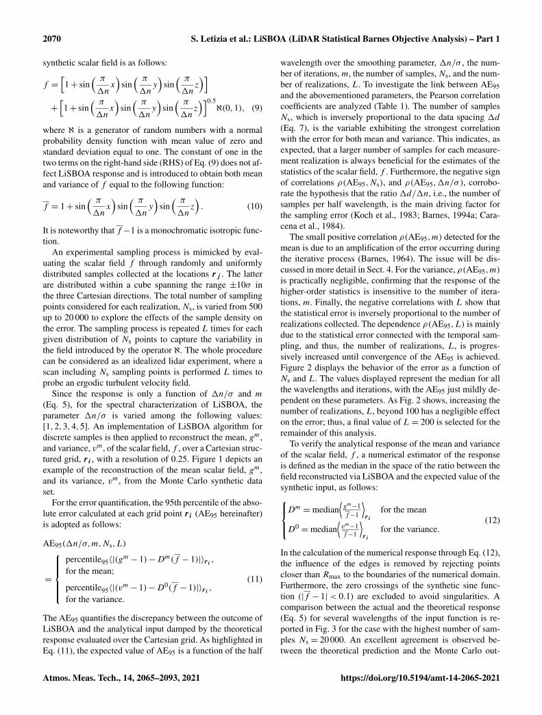
wavelength over the smoothing parameter, 1n/σ , the num-ber of iterations,m, the number of samples,Ns, and the num-ber of realizations, L. To investigate the link between AE95and the abovementioned parameters, the Pearson correlationcoefficients are analyzed (Table 1). The number of samplesNs, which is inversely proportional to the data spacing 1d(Eq. 7), is the variable exhibiting the strongest correlationwith the error for both mean and variance. This indicates, asexpected, that a larger number of samples for each measure-ment realization is always beneficial for the estimates of thestatistics of the scalar field, f . Furthermore, the negative signof correlations ρ(AE95,Ns), and ρ(AE95,1n/σ), corrobo-rate the hypothesis that the ratio 1d/1n, i.e., the number ofsamples per half wavelength, is the main driving factor forthe sampling error (Koch et al., 1983; Barnes, 1994a; Cara-cena et al., 1984).

The small positive correlation ρ(AE95,m) detected for themean is due to an amplification of the error occurring duringthe iterative process (Barnes, 1964). The issue will be dis-cussed in more detail in Sect. 4. For the variance, ρ(AE95,m)

is practically negligible, confirming that the response of thehigher-order statistics is insensitive to the number of itera-tions, m. Finally, the negative correlations with L show thatthe statistical error is inversely proportional to the number ofrealizations collected. The dependence ρ(AE95,L) is mainlydue to the statistical error connected with the temporal sam-pling, and thus, the number of realizations, L, is progres-sively increased until convergence of the AE95 is achieved.Figure 2 displays the behavior of the error as a function ofNs and L. The values displayed represent the median for allthe wavelengths and iterations, with the AE95 just mildly de-pendent on these parameters. As Fig. 2 shows, increasing thenumber of realizations, L, beyond 100 has a negligible effecton the error; thus, a final value of L= 200 is selected for theremainder of this analysis.

To verify the analytical response of the mean and varianceof the scalar field, f , a numerical estimator of the responseis defined as the median in the space of the ratio between thefield reconstructed via LiSBOA and the expected value of thesynthetic input, as follows:Dm =median

⟨gm−1f−1

⟩ri

for the mean

D0=median

⟨vm−1f−1

⟩ri

for the variance.(12)

In the calculation of the numerical response through Eq. (12),the influence of the edges is removed by rejecting pointscloser than Rmax to the boundaries of the numerical domain.Furthermore, the zero crossings of the synthetic sine func-tion (|f − 1|< 0.1) are excluded to avoid singularities. Acomparison between the actual and the theoretical response(Eq. 5) for several wavelengths of the input function is re-ported in Fig. 3 for the case with the highest number of sam-ples Ns = 20000. An excellent agreement is observed be-tween the theoretical prediction and the Monte Carlo out-



Figure 1. Visualization of LiSBOA applied to a Monte Carlo simulation of the synthetic field in Eq. (9) for the case with Ns = 20000,L= 200, 1n/σ = 4, and m= 5. (a) Samples, (b) 3D reconstructed mean field, gm, and (c) 3D reconstructed variance, vm.

Table 1. Pearson correlation coefficient between the AE95 of the mean and variance and the parameters 1n/σ , m, Ns, and L. The values inparenthesis represent the 95 % confidence bounds.

1n/σ m Ns L

AE95 of mean −0.259 (−0.303, −0.210) 0.257 (0.211, 0.301) −0.709 (−0.732, −0.684) −0.171 (−0.217, −0.124)AE95 of variance −0.069 (−0.117, −0.021) −0.03 (−0.078, 0.019) −0.694 (−0.718, −0.668) −0.206 (−0.251, −0.159)

come, which indicates that, in the limit of negligible statisti-cal error (large L) and adequate sampling (largeNs and near-uniform distributed samples), the response approaches thepredictions obtained from the developed theoretical frame-work.

The trend of the response of the mean (Fig. 3a) sug-gests that, for a given wavelength, the same response canbe achieved for an infinite number of combinations σ −m,and specifically, a larger σ requires a larger number of itera-tions, m, to achieve a certain response, Dm. It is noteworthythat, for a smaller number of iterations, m, the slope of theresponse function is lower. This feature can be beneficial forpractical applications for which the LiSBOA response willhave small changes for small variations of 1n. However, alower slope of the response function can be disadvantageousfor short wavelength noise suppression. Figure 3b confirmsthat the response of the variance and, similarly for higher-order statistics, is not a function of the total number of itera-tions, m, and is equal to the response of the mean for the 0thiteration, D0.

Finally, the link between error and the random data spac-ing, 1d, is investigated. In Fig. 4, the discrepancy with re-spect to theory quantified by the AE95 is plotted versus therandom data spacing normalized by the half wavelength fora fixed total number of iterations m= 5. The values dis-played on the x axis represent the median over all grid points,ri . This analysis reveals a strong correlation between thenormalized random data spacing and the error. This anal-ysis corroborates that, in the limit of negligible statisticalerror (i.e., a high number of realizations, L), uncertainty ismainly driven by the local data density normalized by thewavelength, which is related to the Petersen–Middleton cri-

terion. Indeed, the cases satisfying the Petersen–Middletonconstraint (Eq. 8) are those exhibiting an AE95 smaller than∼ 40% of the amplitude of the harmonic function f for boththe mean and variance. However, if a smaller error is needed,it will be necessary to reduce the maximum threshold valuefor 1d/1n.

4 Guidelines for an efficient application of LiSBOA towind lidar data

An efficient application of LiSBOA to lidar data relies onthe appropriate selection of the parameters of the algorithm,namely the fundamental half wavelengths, 1n0, the smooth-ing parameter, σ , the number of iterations, m, and the spa-tial discretization of the Cartesian grid, dx. Furthermore,the data collection strategy must be designed to ensure ad-equate sampling of the spatial wavelengths of interest so thatthe Petersen–Middleton constraint (Eq. 8) is satisfied. In thissection, we show that the underpinning theory of LiSBOA,along with an estimate of the properties of the flow underinvestigation, can guide the optimal design of a lidar exper-iment and evaluation of the statistics for a turbulent ergodicflow. The whole procedure can be divided into three phases,namely characterization of the flow, design of the experi-ment, and reconstruction of the statistics from the collecteddata set.

First, the integral quantities of the flow under investigationrequired for the application of LiSBOA need to be estimated,such as extension of the spatial domain of interest, character-istic length scales, integral timescale, τ , characteristic tempo-ral variance of the velocity, u′2, and expected total samplingtime, T , which depends on the typical duration of stationary



Figure 2. Median of the AE95 for all the tested half wavelengths, 1n/σ , and the number of iterations, m. (a) AE95 of the mean field, gm,and (b) AE95 of the variance field, vm. The error bars span the interquartile range.

Figure 3. Validation of the 3D theoretical response of LiSBOA for the case Ns = 20000−L= 200. (a) Mean and (b) variance. The circlesare the numerical output of the Monte Carlo simulation (Eq. 12), while the continuous lines represent Eq. (5).

boundary conditions over the domain. These estimates canbe based on previous studies available in the literature, nu-merical simulations, or preliminary measurements.

Then, it is necessary to define the fundamental half wave-lengths, 1n0, which are required for the coordinate scaling(Eq. 6). Imposing the fundamental half wavelengths equalto (or even smaller than) the estimated characteristic lengthscales of the smallest spatial features of interest in the flow isadvisable. This ensures isotropy of the mode associated withthe fundamental half wavelength (and all the modes char-acterized by the same degree of anisotropy) and guides theselection of the main input parameters of the LiSBOA algo-rithm, i.e., smoothing parameter, σ , and number of iterations,m. Indeed, 1n0 can be considered as the cut-off half wave-length of the spatial low-pass filter represented by the LiS-BOA operator. To this end, it is necessary to select σ and mto obtain a response of the mean associated with the funda-mental mode, Dm(1n0), as close as possible to one. Afterthe coordinate scaling (Eq. 6), the response of the fundamen-tal mode is universal, and it is reported in Fig. 5. For instance,if we select a response equal to 0.95, then all the points lyingon the isocontour defined by the equality Dm(1n0)= 0.95

give, in theory, the same response for the mean of the scalarfield f . This implies that an infinite number of combinationsσ −m allow us to obtain a response of the mean equal to theselected value. However, with increasing σ , the response atthe 0th iteration, D0(1n0), reduces, which indicates a lowerresponse for higher-order statistics. For the LiSBOA applica-tion, the following aspects should be also considered:

– the smaller σ , the smaller the radius of influence of LiS-BOA, Rmax, and, thus, the lower the number of samplesaveraged per grid node, Nexp, and the greater the statis-tical uncertainty;

– an excessively large m can lead to overfitting of the ex-perimental data and noise amplification (Barnes, 1964);

– the higher m, the higher the slope of the response func-tion (see Fig. 3), which improves the damping of high-frequency noise, but it produces a larger variation in theresponse of the mean with different spatial wavelengths;and



Figure 4. AE95 as a function of the random data spacing (Eq. 7) for the case with m= 5, N = 20000, and L= 200. (a) Error on the meanand (b) error on the variance. The full symbols refer to points not affected by the presence of the finite boundaries of the domain, while theempty symbols are taken within a distance of less than Rmax from the boundaries.

– the radius of influence Rmax (and therefore σ ) can affectthe data spacing 1d in case of nonuniform data distri-bution.

A few handy combinations of smoothing parameters and to-tal iterations for Dm(1n0)= 0.95 are provided in Table 2.As mentioned above, all these σ−m pairs allow us to achieveroughly the same response for the mean, while the responsefor the higher-order statistics reduces with an increasingnumber of iterations, m.

As a final remark about the selection of 1n0, we shouldconsider that, if the fundamental half wavelength is too largecompared to the dominant modes in the flow, small-scale spa-tial oscillations of f will be smoothed out during the calcu-lation of the mean, with the consequence of underestimatedgradients and incorrect estimates of the high-order statisticsdue to the dispersive stresses (Arenas et al., 2019). On theother hand, the selection of an overly small 1n0 would re-quire an excessively fine data spacing to satisfy the Petersen–Middleton constraint (Eq. 8), which may lead to an overlylong sampling time, or it may even exceed the sampling ca-pabilities of the lidar.

The optimal lidar scanning strategy aimed to characterizeatmospheric turbulent flows implies finding a trade-off be-tween a sufficiently fine data spacing, which is quantifiedthrough 1d in the present work (Eq. 7), and an adequatenumber of time realizations, L, to reduce the temporal sta-tistical uncertainty. Considering a total sampling period, T ,for which statistical stationarity can be assumed, and a pulsedlidar that scans Nr points evenly spaced along the lidar laserbeam, with a range gate 1r and accumulation time τa, thetotal number of collected velocity samples is then equal toNs =Nr · T/τa. The angular resolution of the lidar scanninghead in azimuth (1θ for plan position indicators, PPIs), el-evation (1β, for RHIs), or both axes (for volumetric scans)can be selected to modify the angular spacing between con-secutive lines of sight (i.e., the data spacing) and the total

sampling period for a single scan, τs (i.e., the number of re-alizations, L).

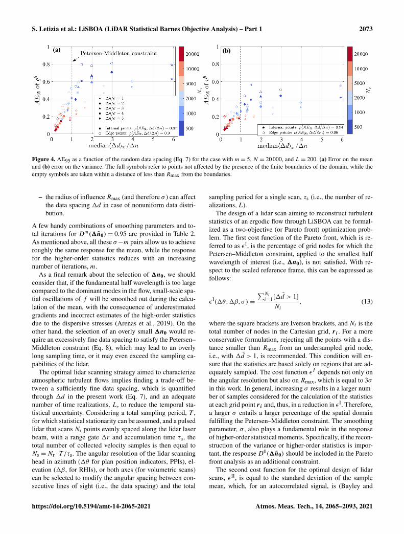
The design of a lidar scan aiming to reconstruct turbulentstatistics of an ergodic flow through LiSBOA can be formal-ized as a two-objective (or Pareto front) optimization prob-lem. The first cost function of the Pareto front, which is re-ferred to as εI, is the percentage of grid nodes for which thePetersen–Middleton constraint, applied to the smallest halfwavelength of interest (i.e., 1n0), is not satisfied. With re-spect to the scaled reference frame, this can be expressed asfollows:

εI(1θ,1β,σ)=

∑Nii=1[1d > 1]

Ni, (13)

where the square brackets are Iverson brackets, and Ni is thetotal number of nodes in the Cartesian grid, ri . For a moreconservative formulation, rejecting all the points with a dis-tance smaller than Rmax from an undersampled grid node,i.e., with 1d > 1, is recommended. This condition will en-sure that the statistics are based solely on regions that are ad-equately sampled. The cost function εI depends not only onthe angular resolution but also on Rmax, which is equal to 3σin this work. In general, increasing σ results in a larger num-ber of samples considered for the calculation of the statisticsat each grid point ri and, thus, in a reduction in εI. Therefore,a larger σ entails a larger percentage of the spatial domainfulfilling the Petersen–Middleton constraint. The smoothingparameter, σ , also plays a fundamental role in the responseof higher-order statistical moments. Specifically, if the recon-struction of the variance or higher-order statistics is impor-tant, the response D0(1n0) should be included in the Paretofront analysis as an additional constraint.

The second cost function for the optimal design of lidarscans, εII, is equal to the standard deviation of the samplemean, which, for an autocorrelated signal, is (Bayley and



Figure 5. Response of the fundamental mode in the scaled coordinates as a function of the number of iterations and the smoothing parameter.(a) 2D LiSBOA and (b) 3D LiSBOA. The white crosses indicate the pairs σ −m provided in Table 2.

Table 2. Selected combinations of σ and m for achieving a ∼ 95 % recovery of the mean of the selected fundamental half wavelength andassociated response of the higher-order moments (HOM).

N = 2 N = 3

σ m Dm (mean) D0 HOM σ m Dm (mean) D0 (HOM)

1/3 6 0.942 0.334 1/4 5 0.952 0.3971/4 3 0.955 0.540 1/6 2 0.961 0.6631/6 1 0.942 0.76 1/8 1 0.957 0.7931/13 0 0.943 0.943 1/17 0 0.950 0.950

Hammersley, 1946) as follows:

εII(1θ,1β)=

√u′2

√√√√ 1L+

2L2

L−1∑p=1

(L−p)ρp

∼

√u′2

√√√√ 1L+

2L2

L−1∑p=1

(L−p) e−τsτp, (14)

where ρp is the autocorrelation function at lag p, τ is the in-tegral timescale, and the approximation is based on Georgeet al. (1978). The velocity variance, u′2, and the autocorrela-tion, ρp, are functions of space; however, to a good degree ofapproximation, they can be replaced by a representative valueand be considered as being uniform in space. Figure 6 showsthe standard deviation of the sample mean normalized by thestandard deviation of the velocity as a function of the numberof realizations, L, and for different integral timescales, τ . Itis noteworthy that the standard deviation of the sample meanrepresents the uncertainty of the time average of each mea-surement point, rj , while the final uncertainty of the meanfield at the grid nodes ri is generally reduced due to thespatial averaging process intrinsic to LiSBOA. It is notewor-thy that the estimates of the statistical error obtained throughLiSBOA do not consider other sources of error, such as ac-curacy of the instruments and spatial averaging due to thelidar measuring process (Rye and Hardesty, 1993; O’Connor

et al., 2010; Puccioni and Iungo, 2020). Eventually, othererror estimates can be coupled with the sampling error es-timated through LiSBOA for a more comprehensive erroranalysis (Wheeler and Ganji, 2010b). Furthermore, LiSBOAallows the calculation of velocity statistics, including contri-butions of eddies with different sizes, which span from thelargest eddy advected within the total sampling time to thesmallest eddy detectable for a given accumulation time (Puc-cioni and Iungo, 2020). Therefore, a careful preprocessing ofthe lidar data should eventually be performed to remove con-tributions due to nonturbulent mesoscale eddies (Högströmet al., 2002; Metzger et al., 2007; O’Connor et al., 2010).

The whole procedure for the design of a lidar scan and re-trieval of the statistics is reported in the flow chart of Fig. 7.Summarizing, from a preliminary analysis of the velocityfield under investigation, we estimate the maximum totalsampling time, T , the characteristic integral timescale, τ , thecharacteristic velocity variance, u′2, and the fundamental halfwavelengths, 1n0. This information, together with the set-tings of the lidar (namely the accumulation time, τa, the num-ber of points per beam, Nr, and the gate length, 1r), allowthe generation of the Pareto front as a function of 1θ and/or1β and for different values of σ . Based on the specific goalsof the lidar campaign in terms of the coverage of the selecteddomain (i.e., εI ), the statistical significance of the data (i.e.,εII) and, eventually, the response of the higher-order statisti-



Figure 6. Standard deviation of the sample mean normalized by thestandard deviation of velocity as a function of the number of real-izations, L, and for different values of the ratio between the integraltimescale and the sampling time, τ/τs.

cal moments (i.e.,D0(1n0)), the LiSBOA user should selectthe optimal angular resolution, 1θ and/or 1β, and the set ofallowable σ values. Due to the abovementioned nonideal ef-fects on LiSBOA, the selection of σ is finalized during thepostprocessing phase when the lidar data set is available andthe statistics can be calculated for different pairs of σ −mvalues. For the resolution of the Cartesian grid, Koch et al.(1983) suggested that it should be chosen as a fraction ofthe data spacing, which, in turn, is linked to the fundamentalhalf wavelength. The same author suggested a grid spacingincluded in the range dx ∈ [1n0/3,1n0/2]. In this work,we have used dx =1n0/4, which ensures a good grid reso-lution with acceptable computational costs.

By following the steps outlined in the present section,the mean, variance, or even higher-order statistical momentsof the velocity field can be accurately reconstructed for thewavelengths of interest. It is worth mentioning that the LiS-BOA of wind lidar data should always be combined with arobust quality control process of the raw measurements. In-deed, the space–time averaging operated by LiSBOA makesthe data analysis sensitive to the presence of data outliers,which need to be identified and rejected beforehand to pre-vent contamination of the final statistics. The interestedreader is referred to Manninen et al. (2016), Beck and Kühn(2017), and Vakkari et al. (2019) for more information onquality control of lidar data. On a final note, for applicationsof LiSBOA, the uncontrollable environmental conditions andthe uncertainty in the flow characteristics needed, as the in-put of LiSBOA may pose some challenges, will be discussedmore in detail in Sect. 6.

5 LiSBOA validation against virtual lidar data

The LiSBOA algorithm is applied to a synthetic data set gen-erated through the virtual lidar technique to assess accuracyin the calculation of statistics for a wind turbine wake probedthrough a scanning lidar installed on the turbine nacelle.For this purpose, a simulator of a scanning Doppler pulsedwind lidar is implemented to extract the line-of-sight veloc-ity from a numerical velocity field produced through high-fidelity large eddy simulations (LES). Due to their simplic-ity and low computational costs, lidar simulators have beenwidely used for the assessment of postprocessing algorithmsof lidar data and scan design procedures (Mann et al., 2010;Stawiarski et al., 2015; Lundquist et al., 2015; Mirocha et al.,2015).

As a case study, we use the LES data set of the flow pastof a single turbine with the same characteristics of the 5-MWNREL (National Renewable Energy Laboratory) referencewind turbine (Jonkman et al., 2009). The rotor is three bladedand has a diameter D = 126 m. The tip-to-speed ratio of theturbine is set to its optimal value of 7.5. A uniform incom-ing wind with a free stream velocity of U∞ = 10 ms−1 andturbulence intensity of 3.6 % is considered. The rotor is simu-lated through an actuator disk with rotation, while the drag ofthe nacelle is taken into account using an immersed bound-ary method (Ciri et al., 2017). More details on the LES solvercan be found in Santoni et al. (2015). The computationaldomain has dimensions (Lx ×Ly ×Lz = 12D× 6D× 6D)in the streamwise, spanwise, and vertical directions, respec-tively, and it is discretized with 960× 256× 300 uniformlyspaced grid points, respectively, resulting in a spacing ofdx = 0.0125D, dy = 0.025D and dz= 0.0202D. A radiativecondition is imposed at the outlet (Orlanski, 1976), while pe-riodicity is applied in the spanwise direction. For the sake ofgenerality, a uniform incoming wind is generated by impos-ing free-slip conditions at the top and bottom of the numeri-cal domain. Ergodic velocity vector fields are available for atotal time of T = 750 s.

For the estimation of the flow characteristics necessary forthe scan design, the azimuthally averaged mean and stan-dard deviation of streamwise velocity, as well as the integraltimescale are considered (Fig. 8). The use of cylindrical co-ordinates is justified by the axisymmetry of the statistics ofthe wake velocity field generated by a turbine operating in auniform velocity field (Iungo et al., 2013a; Viola et al., 2014;Ashton et al., 2016).

The streamwise LES velocity field shows the presence ofa higher-velocity jet surrounding the nacelle, while u/U∞exhibits a clear minimum placed at y/D ∼ 0.25 (Fig. 8a).These flow features are consistent with the double Gaussianvelocity profile typically observed in the near-wake region(Aitken and Lundquist, 2014). In Fig. 8b, the standard de-viation of the streamwise velocity has high values in thevery near wake (x/D < 1) in the proximity of the rotor axis,which is most probably connected with the vorticity struc-



Figure 7. Schematic of the LiSBOA procedure for the optimal design of lidar scans and reconstruction of the statistics for a turbulent ergodicflow.

Figure 8. Azimuthally averaged statistics of the LES streamwise velocity field. (a) Mean value, (b) standard deviation, and (c) integraltimescale.

tures generated in proximity of the rotor hub and their dy-namics (Iungo et al., 2013a; Viola et al., 2014; Ashton et al.,2016). Similarly, enhanced values of the velocity standarddeviation occur at the wake boundary (r/D ≈ 0.5), which areconnected with the formation and dynamics of the helicoidaltip vortices (Ivanell et al., 2010; Debnath et al., 2017c). A

peak of√u′2/U∞ is observed around (x/D ≈ 3), which can

be considered as being the formation length of the tip vor-tices. The integral timescale is evaluated by integrating thesample biased autocorrelation function of the time series ofu up to the first zero crossing (Zieba and Ramza, 2011). Theintegral timescale is generally smaller within the wake thanfor the typical values observed in the free stream, which isconsistent with the smaller dimensions of the wake vortic-



ity structures compared to the larger energy-containing struc-tures present in the incoming turbulent wind.

To reconstruct the mentioned flow features, the funda-mental half wavelengths in the spanwise and vertical direc-tions selected for this application of LiSBOA are 1n0,y =

1n0,z = 0.5D, which allows the retrieval of spatial featuresof the velocity field as small as the rotor blade in the cross-stream direction, which are typically observed in the nearwake (Aitken and Lundquist, 2014; Santoni et al., 2017). Fur-thermore, considering the streamwise elongation of the iso-contours of the flow statistics shown in Fig. 8a, a conserva-tive value of the fundamental half wavelength in the x direc-tion 1n0,x = 2.5D is selected. This information could alsohave been inferred from previous studies (e.g., Chamorro andPorté-Agel, 2010; Abkar and Porté-Agel, 2013; Zhan et al.,2019).

The availability of the LES data set allows the testing ofthe relevance of the selected 1n0 by evaluating the 3D en-ergy spectrum of u/U∞ and u′2/U2

∞ in the physical andscaled reference frames (Eq. 6). The spectra are azimuthallyaveraged by exploiting the axisymmetry of the wake. Thespectra in the physical reference frame (Fig. 9a and b) re-veal the clear signature of a streamwise elongation of theenergy-containing scales for both velocity mean and vari-ance, with the energy being spread over a larger range offrequencies in the radial direction compared to the stream-wise direction. After the scaling (Fig. 9c and d), the spec-tra become more isotropic in the spectral domain, namelythe energy is distributed equally along the kx and kr axes.In Fig. 9c, the blue dashed line represents the intersectionwith the kx–kr plane of the spherical isosurface that, in thewavenumber space, is characterized by Dm(1n0)= 0.95.All the modes contained within that sphere are reconstructedwith a response Dm > 0.95, while higher-frequency featureslying outside will be damped. Numerical integration of the3D energy spectrum shows that 94 % of the total spatial vari-ance of the mean is contained within that sphere, which en-sures that the energy-containing modes in the mean flow areadequately reconstructed with the selected parameters.

The analysis of the flow statistics reported in Fig. 8 en-ables estimates of flow parameters needed as input for LiS-BOA. For instance, the wake region is characterized by√〈u′2〉/U∞ ≈ 0.1 and τU∞/D ≈ 0.4 (τ ≈ 5 s).A main limitation of lidars is represented by the spatiotem-

poral averaging of the velocity field, which is connected withthe acquisition process. Three different types of smoothingmechanisms can occur during the lidar sampling. The firstis the averaging along the laser beam direction within eachrange gate, which has commonly been modeled through theconvolution of the actual velocity field with a weightingfunction within the measurement volume (Smalikho, 1995;Frehlich, 1997; Sathe et al., 2011). The second process isthe time averaging associated with the sampling period re-quired to achieve a backscattered signal with adequate inten-

sity (O’Connor et al., 2010; Sathe et al., 2011), while the lastone is the transverse averaging (azimuth-wise or elevation-wise averaging) occurring in case of a scanning lidar operat-ing in continuous mode (Stawiarski et al., 2013). These fil-tering processes lead to a significant underestimation of theturbulence intensity (Sathe et al., 2011), an overestimation ofintegral length scales (Stawiarski et al., 2015), and a dampingof energy spectra for increasing wavenumbers (Risan et al.,2018; Puccioni and Iungo, 2020).

A total of three versions of a lidar simulator are imple-mented for this work. The simplest one is referred to as ideallidar, which samples the LES velocity field at the experi-mental points through a nearest-neighbor interpolation. Thismethod minimizes the turbulence damping while retainingthe geometry of the scan and the projection of the wind veloc-ity vector onto the laser beam direction. The second versionof the lidar simulator reproduces a step-stare lidar, i.e., thelidar scans for the entire duration of the accumulation timeat a fixed direction of the lidar laser beam. A total of twofiltering processes take place for this configuration, namelybeam-wise convolution and time averaging. To model thebeam-wise average, the retrieval process of the Doppler li-dar is reproduced using a spatial convolution (Mann et al.,2010) as follows:

uLOS(x, t)=

∞∫−∞

φ(s)n ·u(x+ns, t)ds, (15)

where n is the lidar laser beam direction, u is the instanta-neous velocity vector, and the dot indicates scalar product.A triangular weighting function φ(s) was proposed by Mannet al. (2010) as follows:

φ(s)=

{1r/2−|s|1r2/4 if |s|<1r/2

0 otherwise,(16)

where 1r is the gate length. The former expression is valid,assuming matching time windowing, i.e., gate length equal tothe pulse width, and the velocity value is retrieved based onthe first momentum of the backscattering spectrum. Despiteits simplicity, Eq. (16) has shown to estimate realistic tur-bulence attenuation due to the beam-wise averaging processof a pulsed Doppler wind lidar (Mann et al., 2009). Further-more, time averaging occurs due to the accumulation timenecessary for the lidar to acquire a velocity signal with suf-ficient intensity and, thus, signal-to-noise-ratio. This processis modeled through a window average within the acquisitioninterval of each beam. For the sampling of the LES veloc-ity field in space and time, a nearest-neighbor interpolationmethod is used.

The third version of the lidar simulator mimics a pulsed li-dar operating in continuous mode and performing PPI scans,where, in addition to the beam-wise convolution and time av-eraging, azimuth-wise averaging occurs due to the variationin the lidar azimuth angle of the scanning head during the



Figure 9. Azimuthally averaged energy spectra of the LES velocity fields. (a) Mean streamwise velocity on the physical domain, (b) varianceof streamwise velocity on the physical domain, (c) mean streamwise velocity on the scaled domain, and (d) variance of streamwise velocityon the scaled domain. The blue dashed line indicates wavenumbers reconstructed with response equal to Dm(1n0)= 0.95.

scan. The latter is taken into account by adding an azimuthalaveraging to the time average, among all data points includedwithin the following angular sector:{|θ − θp|<1θ/2

|β −βp|< sin−1(1z2rp

),

(17)

where r is the radial distance from the emitter, while θ and βare the associated azimuth and elevation angles, respectively.The subscript p refers to the pth lidar data point. Followingthe suggestions by Stawiarski et al. (2013), the out-of-planethickness, 1z, is considered equal to the length of the diago-nal of a cell of the computational grid.

It is noteworthy that the accuracy estimated through thepresent analysis only includes error due to the sampling intime and space and data retrieval. Other error sources, suchas the accuracy of the instrument (Rye and Hardesty, 1993;O’Connor et al., 2010), are not included and should be cou-pled to the LiSBOA estimates for a more general error quan-tification (Wheeler and Ganji, 2010b).

Figure 10a shows a snapshot of the streamwise velocityfield over the horizontal plane at hub height obtained fromthe LES. The respective data of the radial velocity obtainedfrom the three versions of the lidar simulator, by consid-ering a scanning pulsed wind lidar deployed at the turbinelocation and at hub height, highlight the increased spatialsmoothing of the radial velocity field by adding the various

averaging processes connected with the lidar measuring pro-cess, namely beam-wise, temporal, and azimuthal averaging(Fig. 10).

The application of LiSBOA requires the provision of tech-nical specifications of the lidar, specifically accumulationtime, τa, number of gates, Nr, and gate length, 1r . For thiswork, these parameters are selected based on the typical set-tings of the WindCube 200S and StreamLine XR lidars (El-Asha et al., 2017; Zhan et al., 2019, 2020), namely τa = 0.5 s,Nr = 39, and1r = 25 m. Furthermore, to probe the wake re-gion, a volumetric scan, including several PPI scans, withazimuth and elevation angles uniformly spanning the range±10◦, with a constant angular resolution in both azimuth andelevation being selected, is conducted, while the virtual lidaris placed at the turbine hub.

With the information provided about the flow under in-vestigation and the lidar system, it is possible to draw thePareto front for the optimization of the lidar scan as a func-tion of different combinations of angular resolutions of thelidar scanning head, 1θ and 1β, and the smoothing param-eter of LiSBOA, σ , as shown in Fig. 11 for the case underinvestigation.

For the optimization of the lidar scan, the lidar angularresolution, 1θ , is evenly varied for a total number of sevencases, from 0.75 to 4◦, whereas three values of the ratio1β/1θ , namely 0.5, 1, and 2, are tested separately. Thefour values of σ recommended in Table 2, to achieve a re-



Figure 10. Snapshot at the hub height horizontal plane of the wake generated by the 5-MW NREL reference wind turbine. (a) LES streamwisevelocity. (b) Ideal virtual lidar with angular resolution 1θ = 2.5◦, zero elevation, accumulation time τa = 0.5 s, and gate length 1r = 25 m.(c) Step-stare virtual lidar (same settings). (d) Continuous mode virtual lidar (same settings).

Figure 11. Pareto front for the design of the optimal lidar scan for the LES data set for different 1θ/1β combinations. (a) 1β/1θ = 0.5.(b) 1β/1θ = 1. (c) 1β/1θ = 2. The circle indicates the selected optimal configurations.

sponse of the mean Dm(1n0)= 0.95, are considered here.In Fig. 11, markers indicate the different σ and, thus, the re-sponse of high-order statistical moments, D0(1n0). Chang-ing the ratio 1β/1θ affects the optimal 1θ (circled in blackin Fig. 11); however, it has a negligible effect on the mag-nitude of the optimal εI and εII. For the rest of the dis-cussion, we select the setup 1β/1θ = 1, as suggested byFuertes Carbajo and Porté-Agel (2018). The Pareto frontfor 1β/1θ = 1 (Fig. 11b) shows that increasing 1θ from0.75 up to 2.5◦ drastically reduces the uncertainty on themean (εII) by roughly 70 % but does not significantly af-fect data loss consequent to the enforcement of the Petersen–Middleton constraint (εI). For larger angular resolutions, thestatistical significance improves just marginally but at thecost of a relevant data loss. For 1θ ≥ 2◦, in particular, εI

becomes extremely sensitive to σ , with the most severe dataloss occurring for small σ (i.e., small Rmax). The Pareto frontalso shows that, to achieve a higher response for the higher-order statistics, D0(1n0) generally entails an increased data

loss and/or statistical uncertainty of the mean. This analysissuggests that the optimal lidar scan for the reconstruction ofthe mean velocity field should be performed with 1θ = 2.5◦

and σ = 1/4 or 1/6.Virtual lidar simulations are performed for all the values

of angular resolution utilized in the Pareto front reportedin Fig. 11. The streamwise component is estimated fromthe line-of-sight velocity through an equivalent velocity ap-proach (Zhan et al., 2019). The latter states that, for smallelevation angles (i.e., β� 1) and under the assumption ofnegligible vertical velocity compared to the horizontal com-ponent (i.e., |w| �

√u2+ v2) and uniform wind direction,

θw, a proxy for the streamwise velocity can be calculated asfollows:

u∼uLOS

cos(θ − θw)cosβ. (18)

The mean velocity and turbulence intensity are reconstructedthrough LiSBOA. The maximum error is quantified through



Figure 12. Error analysis of LiSBOA applied to virtual radial velocity fields: (a, d) ideal lidar; (b, e) step-stare lidar; (c, f) continuous lidar;(a, b, c) mean streamwise velocity; (d, e, f) streamwise turbulence intensity. The optimal configurations are highlighted in yellow.

the 95th percentile of the absolute error, AE95, using as ref-erence the LES statistics interpolated on the LiSBOA grid.

Figure 12 reports the AE95 for the flow statistics for all thevirtual experiments. The error for the mean field (Fig. 12a–c) is mostly governed by the angular resolution, with ahigher error occurring for slower scans. This is a clear con-sequence of the increased statistical uncertainty due to thelimited number of scan repetitions, L, that are achievable forsmall 1θ values and a fixed total sampling period, T , whileAE95 stabilizes for 1θ ≥ 2.5◦. The trend of the AE95 foru/U∞, with the pair-smoothing-parameter number of itera-tions, σ −m, is less significant since the theoretical responseof the fundamental mode is ideally equal for all four cases.Conversely, the error on the turbulence intensity (Fig. 12d–f)shows low sensitivity to the angular resolution but a steep in-crease for small σ values, which is due to the reduction in theradius of influence, Rmax, and the number of points averagedper grid node.

From a more technical standpoint, the error on the meanvelocity field, u/U∞, appears to be relatively insensitive tothe type of lidar scan, with the spatial and temporal filteringoperated by the step-stare and continuous lidar even beingbeneficial in some cases. In contrast, the error on the turbu-lence intensity exhibits a more consistent and opposite trend,with the continuous lidar showing the most severe turbulencedamping. This feature has been extensively documented inprevious studies, see e.g., Sathe et al. (2011).

This error analysis confirms that the optimal configu-rations selected through the Pareto front (i.e., 1θ = 2.5◦,σ = 1/4−m= 5, and σ = 1/6−m= 2) are arguably opti-mal in terms of accuracy (AE95 of u/U∞ = 3.3 %–4.1 % and

3.9 %–4.4 % and AE95 of√u′2/u= 3.2 %–4.7 % and 3.3 %–

4.5 %, respectively) and data loss (εI = 33 % and 37 %, re-spectively).

The 3D fields of mean velocity and turbulence intensitycalculated over T = 750 s through the first optimal configu-ration, (i.e., 1θ = 2.5◦, σ = 1/4, and m= 5), are renderedin Figs. 13 and 14, respectively. Furthermore, in Fig. 15, az-imuthally averaged profiles at three downstream locations arealso provided for a more insightful comparison. The meanvelocity field is reconstructed fairly well, regardless of thetype of lidar scan, due to the careful choice of the funda-mental half wavelength, 1n0, for this specific flow. On theother hand, the reconstructed turbulence intensity is highlyaffected by the lidar processing, which leads to visible damp-ing of the velocity variance for the step stare and even morefor the continuous mode. The ideal lidar scan, whose acqui-sition is inherently devoid of any space–time averaging, al-lows the retrieval of the correct level of turbulence intensityfor locations for x ≥ 4D, while in the near wake it strugglesto recover the thin turbulent ring observed in the wake shearlayer. Indeed, such a short wavelength feature has a small re-sponse for the chosen settings of LiSBOA, particularly 1n0and σ (see Fig. 3b). On the other hand, any attempt to in-



Figure 13. Mean streamwise velocity for 1θ = 2.5◦, σ = 1/4, m= 5. (a) LES, (b) ideal lidar, (c) step-stare lidar, and (d) continuous modelidar. The shaded area corresponds to the points rejected after the application of the Petersen–Middleton constraint.

Figure 14. As in Fig. 13 but for streamwise turbulence intensity.

crease the response of the higher-order moments, for instanceby reducing the fundamental half wavelengths or decreasingthe smoothing and the number of iterations, would result inhigher data loss and fewer experimental points per grid node.

Finally, Figs. 16 and 17 show u/U∞ and√u′2/u over sev-

eral cross-flow planes and for all the combinations of σ −mtested for the ideal lidar and the optimal angular resolution.For the mean velocity, the most noticeable effect is the in-

creasingly severe data loss as a consequence of the reductionin σ , which indicates σ = 1/4−m= 5 as being the most ef-fective setting. The turbulence intensity exhibits, in additionto the data loss, a moderate increase in the maximum valuefor smaller σ , which is due to the higher response of thehigher-order statistics (see Table 2). However, this effect isnegligible in the far wake, where the radial diffusion of theinitially sharp turbulent shear layer results in a shift of the en-



Figure 15. Azimuthally averaged profiles of mean streamwise velocity and turbulence intensity for three downstream locations. (a) x/D =2.25, (b) x/D = 4.125, and (c) x/D = 6. The dashed lines correspond to regions rejected after the application of the Petersen–Middletonconstraint.

Figure 16. Mean streamwise velocity fields obtained through the ideal lidar simulator with 1θ = 2.5◦ over cross-flow planes at threedownstream locations and four combinations of σ −m, compared with the corresponding LES data.

ergy content towards scales with larger 1n, which are fairlywell recovered – even for σ = 1/4.

6 Notes on LiSBOA applications

LiSBOA can be applied to lidar data sets that are statisticallyhomogeneous as a function time, t . This statistical propertycan be ensured with two approaches. The first approach con-sists of considering lidar data collected continuously in time,with a given sampling frequency, for a period where en-vironmental parameters, such as wind speed and direction,Obukhov length, and bulk Richardson number for the atmo-spheric stability regime, are constrained within prefixed in-tervals (e.g., Banta et al., 2006; Iungo et al., 2013b; Kumer

et al., 2015; Puccioni and Iungo, 2020). For instance, the sta-tistical stationarity of a generic flow signal, α, can be verifiedthrough the nonstationary index (IST; Liu et al., 2017) as fol-lows:

IST=|α′α′m−α′α′|

α′α′, (19)

where · represents time averaging and α′α′m is the meanvalue of the variance calculated over consecutive nonover-lapping subperiods. The IST values should be lower than aselected threshold, depending on the specific flow parameterconsidered (Foken et al., 2004). A second approach to en-sure statistical homogeneity of the lidar data set consists ofperforming a cluster analysis based on environmental param-eters, such as those mentioned above. This can be a fruitful



Figure 17. Same as Fig. 16 but for streamwise turbulence intensity.

alternative when the application of the first approach leadsto too short periods with statistical stationarity and, thus,with low accuracy in the calculation of the turbulent statis-tics. With the clustering approach, larger data sets can beachieved for each cluster, enabling an enhanced statisticalconvergence (see, e.g., applications of clustering analysis tolidar measurements of wind turbine wakes; Machefaux et al.,2016; Bromm et al., 2018; Iungo et al., 2018; Zhan et al.,2019, 2020).

The results of LiSBOA for the optimal design of wind lidarscans are affected by the selection of the input parameters,such as the total sampling time, T , the integral timescale, τ ,the velocity variance, u′2, and the fundamental half wave-length,1n0. In this section, we will discuss the sensitivity ofLiSBOA to these input parameters by considering, as a ref-erence case, the volumetric scan performed with the virtuallidar technique on the LES data set analyzed in Sect. 5. Therespective results are summarized in Fig. 18.

The total sampling time, T , directly affects the objectivefunction εII through parameter L, which represents the num-ber of realizations. In Fig. 18a–d, different Pareto fronts aregenerated for the case under investigation, by varying T from3 min to 1 h. The various Pareto fronts exhibit similar trendsfor the various values of T and generally higher values of εII,so lower statistical accuracy, for smaller T . For all the cases,the optimal configuration is still that selected in Sect. 5,namely 1θ = 2.5◦–σ = 1/4.

For this sensitivity study, the characteristic integraltimescale, τ , has been varied between 0 s (completely ran-dom uncorrelated data) up to 35 s, with the upper value be-ing based on the largest integral length scale in the atmo-spheric boundary layer (ABL), according to (ESDU, 1975),and considering an advection velocity of 8 ms−1. The respec-

tive Pareto fronts reported in Fig. 18e–h show that the opti-mal lidar scan is weakly affected by variations of τ , whichis an advantageous feature of LiSBOA for applications inwhich this parameter cannot be estimated from previous in-vestigations or the literature.

Regarding the characteristic velocity variance, u′2, it isa multiplicative parameter for the objective function εII

(Eq. 14). Therefore, even though it affects the accuracy ofthe statistics retrieved, it does not alter the selection of theoptimal scanning parameters.

The choice of the fundamental half wavelength, 1n0, de-serves special attention since it affects both the optimal scandesign and retrieval of data statistics. The fundamental halfwavelength can be considered as being the cut-off wave-length of the spatial low-pass filtering operated by LiSBOA(Sect. 4). The selection of1n0 depends mostly on the lengthof the smallest spatial feature of interest in the flow under in-vestigation, so the Pareto front is likely to be rather sensitiveto changes in1n0. As mentioned in Sect. 4, if the fundamen-tal half wavelengths are too large compared to the predomi-nant spatial modes, the turbulence statistics may be contam-inated by over-smoothing and dispersive stresses, whereasoverly small 1n0 may require angular and radial resolu-tions that are too small, a longer sampling period, and, thus,a smaller number of repetitions for a given T . Figure 18i–l shows the Pareto fronts calculated at different 1n0,x . Thepreviously selected optimal setup (1θ = 2.5◦−σ = 1/4) stillbelongs to the optimality frontier. Finally, Fig. 18p–m dis-plays the effect of varying 1n0,y on the Pareto front. Unlikethe other cases, the shape of the front is very sensitive to1n0,y , with a significant increase in data loss, εI, consequentto refinements of the angular resolution,1θ . The Pareto frontcorrectly indicates that finer angular resolutions are needed to



Figure 18. Pareto fronts for the design of the volumetric scan for different inputs. (a–d) Sensitivity to total sampling time T . (e–h) Sensitivityto integral timescale, τ . (i–l) Sensitivity to streawmise fundamental half wavelength, 1n0,x . (m–p) Sensitivity to spanwise fundamental halfwavelength, 1n0,y . The parameters not indicated at the top of the figures are kept equal to the optimal design case identified in Sect. 5.

adequately sample a velocity field characterized by smallerwavelengths.

For the sake of completeness, the influence of the differ-ent fundamental half wavelengths on the statistics is assessedby calculating the AE95 between LiSBOA and LES for thestatistics reconstructed using several combinations of 1n0,xand 1n0,y (Fig. 19). Larger values of 1n0,x and 1n0,y pro-duce detrimental effects on the accuracy for both mean veloc-ity and turbulence intensity due to the over-smoothing of themean velocity and turbulence intensity field and dispersivestresses for the turbulence intensity only. On the other hand,excessively small values of 1n0,y exhibit a slight increase inerror as a consequence of the smaller number of samples pergrid node. Nonetheless, the most relevant effect, in this case,is represented by the high data loss, as already identified inthe Pareto front (e.g., Fig. 18m, n). It is worth noting howthe choice of 1n0 = [2.5,0.5,0.5]D in Sect. 5, which waspurely based on physical considerations about the expectedrelevant modes in the near wake, turned out to be the opti-mal configuration in terms of the overall error of u/U∞ and√u′2/u.We acknowledge that the technical specifications required

by LiSBOA (namely τa, Nr, and 1r) are dependent on thespecific lidar system used, the contingent atmospheric condi-tions, and the best practices followed by the user. Since theseparameters are greatly case dependent, they will not be dis-cussed further in this context. In general, the selection of theaccumulation time and gate length is a trade-off between the

need to achieve a target maximum range, while keeping asufficiently fine radial resolution and a sufficient intensity ofthe backscattered lidar signal. In the case of uncertain envi-ronmental conditions, checking, before the deployment, theinfluence of selected combinations of τa, Nr, and 1r on thePareto front is recommended.

For the sake of completeness, LiSBOA is compared withother widely used techniques for statistical postprocessing ofwind lidar data, specifically the Delaunay triangulation (see,e.g., Clive et al., 2011; Trujillo et al., 2011, 2016; Iungo andPorté-Agel, 2014; Machefaux et al., 2015), linear interpola-tion in spherical coordinates (see, e.g., Mohr and Vaughan,1979; Fuertes Carbajo and Porté-Agel, 2018), and windowaveraging (see, e.g., Newsom et al., 2008). Figure 20 showsthe mean velocity and turbulence intensity fields retrievedfrom the considered LES data set through the various tech-niques for a step-stare virtual lidar scan. The various meth-ods use the same grid as for LiSBOA (see Sect. 5). The voidsin the 3D rendering correspond to regions outside of the datadistribution for the Delaunay triangulation and linear interpo-lation (i.e., extrapolation cannot be performed) or bins havinga standard error on the mean higher than 15 % of the incom-ing wind speed for the window average (for an analogy withLiSBOA, see Fig. 4). A qualitative comparison of the resultsreported in Fig. 20 with those for LiSBOA in Figs. 13c and14c reveals that LiSBOA is the method enabling the largestspatial coverage for the retrieved statistics for the same li-dar scan. From the parameter εI , which is reported in Ta-



Figure 19. AE95 of the statistics reconstructed from virtual lidar data for different streamwise and spanwise fundamental half wavelengths,for the setup 1θ = 2.5◦− σ = 1/4. (a) Mean streamwise velocity. (b) Streamwise turbulence intensity.

Figure 20. Statistics retrieved from a step-stare virtual lidar scan of the LES data set by means of different techniques. (a, d) Delaunaytriangulation. (b, e) Linear interpolation. (c, f) Window averaging. (a, b, c) Mean streamwise velocity. (d, e, f) Streamwise turbulenceintensity.

ble 3 for the various methods, it is noted that LiSBOA is themethod with the lowest data rejection rate (εI = 33 %), whilethe largest is for the window average (εI = 66 %).

Overall, all the methods, except for the window average,have similar accuracy in the retrieval of the mean velocity(see the mean absolute percentage error, MAPE, in Table 3),yet LiSBOA is the method with the lowest error. Further-more, LiSBOA is the only method not showing artifacts forthe retrieval of turbulence intensity over space, such as en-hanced turbulence intensity and unexpected peaks, as the sig-nificantly lower error on turbulence intensity confirms. Thisresult is in agreement with Trapp and Doswell (2000), wherethe effectiveness of the Barnes scheme in the suppression ofshort-wavelength noise compared to linear interpolation wasalready noted. Finally, the computational time, using MAT-LAB on a quad-core i7 laptop, is negligible and comparable

Table 3. Comparison between LiSBOA and other techniques for theretrieval of mean velocity and turbulence intensity from the LESdata set through a virtual lidar scan.

MAPE of MAPE of εI Time

u/U∞

√u′2/u

LiSBOA 1.2 % 1.3 % 33 % 1.79 sDelaunay triangulation 1.3 % 1.7 % 53 % 0.65 sLinear interpolation 1.3 % 1.6 % 55 % 0.01 sWindow average 2 % 1.5 % 66 % 1.55 s

for all the algorithms considered (∼ 1–2 s), with only the lin-ear interpolation being considerably faster (Table 3).

On a final note, it is noteworthy that LiSBOA is currentlyformulated for a single scalar field, namely a velocity com-ponent (radial or equivalent horizontal). However, in princi-



ple, this procedure can be extended to vector fields, such asfully 3D velocity fields. Furthermore, other constraints canbe added for the optimal scanning design, such as imposing adivergence-free velocity field for incompressible flows. Also,some modifications could extend the application of LiSBOAto other remote sensing instruments, such as sodars and scan-ning radars.

7 Conclusions

A revisited Barnes objective analysis for sparse, nonuniformdistributed, and stationary lidar data has been formulated tocalculate mean, variance, and higher-order statistics of thewind velocity field over a structured N -dimensional Carte-sian grid. This LiDAR Statistical Barnes Objective Analysis(LiSBOA) provides a theoretical framework to quantify theresponse in the reconstruction of the velocity statistics as afunction of the spatial wavelengths of the velocity field un-der the investigation and quantification of the sampling error.

LiSBOA has been validated against volumetric synthetic3D data generated through Monte Carlo simulations. The re-sults of this test have shown that the sampling error for amonochromatic scalar field is mainly driven by the data spac-ing being normalized by the half wavelength.

The LiSBOA framework provides guidelines for the op-timal design of scans performed with a scanning Dopplerpulsed wind lidar and the calculation of wind velocity statis-tics. The optimization problem consists of providing back-ground information about the turbulent flow under investiga-tion, such as total sampling time, expected velocity variance,and integral length scales, technical specifications of the li-dar, such as range gate and accumulation time, and spatialwavelengths of interest for the velocity field. The formulatedoptimization problem has two cost functions, namely the per-centage of grid nodes not satisfying the Petersen–Middletonconstraint for the smallest half wavelength of interest (i.e.,lacking adequate spatial resolution to avoid aliasing in thestatistics), and the standard deviation of the sample mean.The outputs of the optimization problem are the lidar angu-lar resolution and, for a given response of the mean field, theallowable smoothing parameters and number of iterations touse for LiSBOA.

LiSBOA has been validated using a data set obtainedthrough the virtual lidar technique, namely by numericallysampling the turbulent velocity field behind the rotor of a5 MW turbine obtained from a large eddy simulation (LES).The 3D mean streamwise velocity and turbulence intensityfields have shown a maximum error with respect to the LESdata set of about 4 % of the undisturbed wind speed for themean streamwise velocity and 4 % of the streamwise tur-bulence intensity in absolute terms. Wake features, such asthe high-velocity stream in the hub region and the turbulentshear layer at the wake boundary, have been accurately re-constructed.

In the companion paper (Letizia et al., 2021), LiSBOA isused to reconstruct the turbulence statistics of utility-scaleturbine wakes probed with scanning pulsed Doppler lidars.That study also illustrates the detailed preconditioning ap-plied to the raw lidar data to extract statistically stationaryand normalized radial velocity data and showcases the po-tential of LiSBOA for wind energy research.



Appendix A: Derivation of the analytical responsefunction of LiSBOA

The first iteration of LiSBOA produces a weighted average inspace of the scalar field, f , with the weights being Gaussianfunctions centered at the specific grid nodes, x. In the limit ofa continuous function defined over an infinite domain, Eq. (3)represents the convolution between the scalar field, f , andthe Gaussian weights, w. Therefore, the response function ofLiSBOA can be expressed in the spectral domain as follows(Pauley and Wu, 1990):

D0=

F[g0]

F[f ]= F[w], (A1)

where the operator F indicates the Fourier transform (FT).The FT of the weighting function in Eq. (A1) can be conve-niently recast as the product of N 1D FT as follows:

F[w] =N∏p=1

∞∫−∞

1√

2πσe−x2p

2σ2 · e−ikpxp dxp, (A2)

where kp is the directional wavenumber and i=√−1.

Hence, by leveraging the closed form FT of the Gaussianfunction (Greenberg, 1998) as follows:

F

[1

√2πσ

e−x2

2σ2

]= e

−k2σ22 , (A3)

we obtain the desired results, i.e., the following:

D0(k)= e−σ22 |k|

2. (A4)

Appendix B: List of symbols

x, y, z Streamwise, spanwise, andvertical Cartesian coordinates

t Nonspatial coordinate or timeu, v, w Streamwise, spanwise, and vertical

velocity componentsuLOS Radial or line-of-sight wind speedL Number of realizations and/or scansθ Azimuth angleβ Elevation angle1θ Azimuth angle resolution1β Elevation angle resolutionτa Accumulation time1r Gate lengthNr Number of range gates along the laser beamT Total sampling timeσ Smoothing parameterm Number of iterationsRmax Radius of influence1n Half-wavelength vector1n0 Fundamental half-wavelength vector1d Random data spacingdx Resolution vector in Cartesian coordinatesDm Response at the mth iterationri position in the N -dimensional space of

the ith grid node of the Cartesian gridrj Position in the N -dimensional space

of the j th sampleεI Cost function I (data loss)εII Cost function II (standard deviation

of the sample mean)Ni Total number of nodes of the Cartesian gridτ Integral timescale. Spatial variable in the scaled frame

of reference



Code availability. The LiSBOA algorithm has been implementedin a publicly available code which can be downloaded at https://github.com/UTD-WindFluX/LiSBOA (last access: 4 March 2021,Letizia and Iungo, 2021).

Author contributions. SL and GVI developed LiSBOA and pre-pared the paper. The lidar data were generated as part of a teameffort, which included contributions from all three authors. SL im-plemented LiSBOA in a MATLAB code under the supervision ofGVI.

Competing interests. The authors declare that they have no conflictof interest.

Disclaimer. Any opinions, findings, and conclusions or recommen-dations expressed in this material are those of the authors and do notnecessarily reflect the views of the sponsors.

Acknowledgements. This research has been funded by the NationalScience Foundation CBET Fluid Dynamics (grant no. 1705837).This material is based upon work supported by the National Sci-ence Foundation (grant no. IIP-1362022; Collaborative Research– I/UCRC for Wind Energy, Science, Technology, and Research)and from the WindSTAR I/UCRC Members of Aquanis, Inc., EDPRenewables, Bachmann Electronic Corp., GE Energy, Huntsman,Hexion, Leeward Asset Management, LLC, Pattern Energy, EPRI,LM Wind, Texas Wind Tower, and TPI Composites. The Texas Ad-vanced Computing Center is acknowledged for providing computa-tional resources. The authors thank Stefano Leonardi and UmbertoCiri for sharing the LES data set.

Financial support. This research has been supported by the Na-tional Science Foundation, Directorate for Engineering (grant nos.1705837 and IIP-1362022).

Review statement. This paper was edited by Ulla Wandinger andreviewed by two anonymous referees.

References

Abkar, M. and Porté-Agel, F.: The effect of free-atmospherestratification on boundary-layer flow and power outputfrom very large wind farms, Energies, 6, 2338–2361,https://doi.org/10.3390/en6052338, 2013.

Achtemeier, G. L.: The Impact of Data Boundaries upon a Succes-sive Corrections Objective Analysis of Limited-Area Datasets,Mon. Weather Rev., 114, 40–49, https://doi.org/10.1175/1520-0493(1986)114<0040:TIODBU>2.0.CO;2, 1986.

Achtemeier, G. L.: Modification of a Successive CorrectionsObjective Analysis for Improved Derivative Calculations,

Mon. Weather Rev., 117, 78–86, https://doi.org/10.1175/1520-0493(1989)117<0078:MOASCO>2.0.CO;2, 1989.

Aitken, M. L. and Lundquist, J. K.: Utility-Scale Wind Tur-bine Wake Characterization Using Nacelle-Based Long-RangeScanning Lidar, J. Atmos. Ocean. Tech., 31, 1529–1539,https://doi.org/10.1175/JTECH-D-13-00218.1, 2014.

Arenas, I., García, E., Fu, M. K., Orlandi, P., Hultmark, M.,and Leonardi, S.: Comparison between super-hydrophobic,liquid infused and rough surfaces: a direct numeri-cal simulation study, J. Fluid Mech., 869, 500–525,https://doi.org/10.1017/jfm.2019.222, 2019.

Ashton, R., Iungo, G. V., Viola, F., Gallaire, F., and Ca-marri, S.: Hub vortex instability within wind turbinewakes : Effects of wind turbulence, loading conditions andblade aerodynamics, Physical Review Fluids, 1, 073 603,https://doi.org/10.1103/PhysRevFluids.1.073603, 2016.

Askelson, M. A., Aubagnac, J. P., and Straka, J. M.:An Adaptation of the Barnes Filter Applied to theObjective Analysis of Radar Data, Mon. WeatherRev., 128, 3050–3082, https://doi.org/10.1175/1520-0493(2000)128<3050:AAOTBF>2.0.CO;2, 2000.

Astrup, P., Mikkelsen, T. K., and van Dooren, M. F.: Wind fielddetermination from multiple Spinner-Lidar line-of-sight mea-surements using linearized CFD, DTU Wind Energy E. 0102,DTU, Department of Wind Energy Frederiksborgvej 399 DK-4000 Roskilde Denmark, 2017.

Banakh, V. A., Smalikho, I. N., Köpp, F., and Werner, C.: Mea-surements of Turbulent Energy Dissipation Rate with a CWDoppler Lidar in the Atmospheric Boundary Layer, J. Atmos.Ocean. Tech., 16, 1044–1061, https://doi.org/10.1175/1520-0426(1999)016<1044:MOTEDR>2.0.CO;2, 1999.

Banta, R. M., Pichugina, Y. L., and Brewer, W. A.: TurbulentVelocity-Variance Profiles in the Stable Boundary Layer Gen-erated by a Nocturnal Low-Level Jet, J. Atmos. Sci., 63, 2700–2719, https://doi.org/10.1175/JAS3776.1, 2006.

Barnes, S.: Application of Barnes Objective Analysis scheme.Part III: tuning for minimum error., J. Atmos. Ocean.Tech., 11, 1449–1458, https://doi.org/10.1175/1520-0426(1994)011<1459:AOTBOA>2.0.CO;2, 1994c.

Barnes, S. L.: A Technique for Maximizing Detailsin Numerical Weather Map Analysis, J. Appl. Me-teorol., 3, 396–409, https://doi.org/10.1175/1520-0450(1964)003<0396:ATFMDI>2.0.CO;2, 1964.

Barnes, S. L.: Mesoscale Objective Map Analysis Using WeightedTime-Series Observations, NOAA Technical Memorandum ERLNSSL-62, National Severe Storms Laboratory Norman, OK,USA, 1973.

Barnes, S. L.: Applications of the Barnes Objective Anal-ysis Scheme. Part I: Effects of Undersampling, WavePosition and Station Randomness, J. Atmos. Ocean.Tech., 11, 1433–1448, https://doi.org/10.1175/1520-0426(1994)011<1433:AOTBOA>2.0.CO;2, 1994a.

Bayley, V. G. and Hammersley, J. M.: The ”Effective” Numberof Independent Observations in an Autocorrelated Time Series,Supplement to the Journal of Royal Statistical Society, 8, 184–197, 1946.

Beck, H. and Kühn, M.: Dynamic Data Filtering of Long-RangeDoppler LiDAR Wind Speed Measurements, Remote Sens.-Basel, 9, 561, 2017.


https://github.com/UTD-WindFluX/LiSBOA


https://doi.org/10.3390/en6052338

https://doi.org/10.1175/1520-0493(1986)114<0040:TIODBU>2.0.CO;2

https://doi.org/10.1175/1520-0493(1986)114<0040:TIODBU>2.0.CO;2

https://doi.org/10.1175/1520-0493(1989)117<0078:MOASCO>2.0.CO;2

https://doi.org/10.1175/1520-0493(1989)117<0078:MOASCO>2.0.CO;2

https://doi.org/10.1175/JTECH-D-13-00218.1

https://doi.org/10.1017/jfm.2019.222

https://doi.org/10.1103/PhysRevFluids.1.073603

https://doi.org/10.1175/1520-0493(2000)128<3050:AAOTBF>2.0.CO;2

https://doi.org/10.1175/1520-0493(2000)128<3050:AAOTBF>2.0.CO;2

https://doi.org/10.1175/1520-0426(1999)016<1044:MOTEDR>2.0.CO;2

https://doi.org/10.1175/1520-0426(1999)016<1044:MOTEDR>2.0.CO;2

https://doi.org/10.1175/JAS3776.1

https://doi.org/10.1175/1520-0426(1994)011<1459:AOTBOA>2.0.CO;2


https://doi.org/10.1175/1520-0450(1964)003<0396:ATFMDI>2.0.CO;2

https://doi.org/10.1175/1520-0450(1964)003<0396:ATFMDI>2.0.CO;2




Bell, T. M., Klein, P., Wildmann, N., and Menke, R.: Analysis offlow in complex terrain using multi-Doppler lidar retrievals, At-mos. Meas. Tech., 13, 1357–1371, https://doi.org/10.5194/amt-13-1357-2020, 2020.

Berg, J., Mann, J., Bechmann, A., Courtney, M. S., and Jørgensen,H. E.: The Bolund Experiment. Part I : Flow Over a Steep,Three-dimensional Hill, Bound.-Lay. Meteorol., 20, 219–243,https://doi.org/10.1007/s10546-011-9636-y, 2011.

Bingöl, F.: Complex terrain and wind lidars, DTU PhD Thesis Risø-PhD-52, Technical Univeristy of Denmark, DTU Vindenergi NilsKoppels Allé Bygning 403 2800 Kgs. Lyngby, 2009.

Bingöl, F., Mann, J., and Larsen, G. C.: Light detection and rangingmeasurements of wake dynamics. Part I: one-dimensional scan-ning, Wind Energy, 13, 51–61, https://doi.org/10.1002/we.352,2010.

Bodini, N., Zardi, D., and Lundquist, J. K.: Three-dimensional structure of wind turbine wakes as measuredby scanning lidar, Atmos. Meas. Tech., 10, 2881–2896,https://doi.org/10.5194/amt-10-2881-2017, 2017.

Bonin, T. A., Choukulkar, A., Brewer, W. A., Sandberg, S. P., We-ickmann, A. M., Pichugina, Y. L., Banta, R. M., Oncley, S. P., andWolfe, D. E.: Evaluation of turbulence measurement techniquesfrom a single Doppler lidar, Atmos. Meas. Tech., 10, 3021–3039,https://doi.org/10.5194/amt-10-3021-2017, 2017.

Bradley, E. F.: The influence of thermal stability and angle of inci-dence on the acceleration of wind up a slope, J. Wind Eng. Ind.Aerod., 15, 231–242, 1983.

Braham, R. R.: Field Experimentation in Weather Modification,J. Am. Stat. Assoc., 74, 57–68, http://www.jstor.org/stable/2286722 (last access: 3 March 2021), 1979.

Bromm, M., Rott, A., Beck, H., Vollmer, L., Steinfeld, G., andKühn, M.: Field investigation on the influence of yaw misalign-ment on the propagation of wind turbine wakes, Wind Energy,21, 1011–1028, https://doi.org/10.1002/we.2210, 2018.

Busch, N. E. and Kristensen, L.: Cup Anemometer Overspeeding, J.Appl. Meteorol., 15, 1328–1332, https://doi.org/10.1175/1520-0450(1976)015<1328:cao>2.0.co;2, 1976.

Buzzi, A., D Gomis, D., A., P. M., and Alonso, S.: AMethod to Reduce the Adverse Impact that InhomogeneousStation Distributions Have on Spatial Interpolation, Mon.Weather Rev., 119, 2465–2491, https://doi.org/10.1175/1520-0493(1991)119<2465:AMTRTA>2.0.CO;2, 1991.

Caracena, F.: Analytic Approximation of DiscreteField Samples with Weighted Sums and the Grid-less Computation of Field Derivatives, J. Atmos.Sci., 44, 3753–3768, https://doi.org/10.1175/1520-0469(1987)044<3753:AAODFS>2.0.CO;2, 1987.

Caracena, F., Barnes, S. L., and Doswell III, C.: Weighting functionparameters for objective interpolation of meteorological data,in: Preprints, 10th Conf. on Weather Forecasting and Analysis,Clearwater Beach, FL, 25–29 June 1984, 109–116, 1984.

Carbajo Fuertes, F., Markfort, C. D., and Porté-Agel, F.: Wind Tur-bine Wake Characterization with Nacelle-Mounted Wind Lidarsfor Analytical Wake Model Validation, Remote Sens.-Basel, 10,668, https://doi.org/10.3390/rs10050668, 2018.

Chamorro, L. P. and Porté-Agel, F.: Effects of Thermal Sta-bility and Incoming Boundary-Layer Flow Characteristics onWind-Turbine Wakes: A Wind-Tunnel Study, Bound.-Lay. Me-

teor., 136, 515–533, https://doi.org/10.1007/s10546-010-9512-1,2010.

Choukulkar, A., Brewer, W. A., Sandberg, S. P., Weickmann, A.,Bonin, T. A., Hardesty, R. M., Lundquist, J. K., Delgado, R.,Iungo, G. V., Ashton, R., Debnath, M., Bianco, L., Wilczak, J.M., Oncley, S., and Wolfe, D.: Evaluation of single and mul-tiple Doppler lidar techniques to measure complex flow duringthe XPIA field campaign, Atmos. Meas. Tech., 10, 247–264,https://doi.org/10.5194/amt-10-247-2017, 2017.

Ciri, U., Rotea, M., Santoni, C., and Leonardi, S.: Large-eddysimulations with extremum-seeking control for individual windturbine power optimization, Wind Energy, 20, 1617–1634,https://doi.org/10.1002/we.2112, 2017.

Clive, P. J. M., Dinwoodie, I., and Quail, F.: Direct measurement ofwind turbine wakes using remote sensing, Proc. EWEA, 2011.

Cressman, G. P.: An Operational Objective Analysis System,Mon. Weather Rev., 87, 367–374, https://doi.org/10.1175/1520-0493(1959)087<0367:AOOAS>2.0.CO;2, 1959.

Cuerva, A. and Sanz-Andrés, A.: On sonic anemometer mea-surement theory, J. Wind Eng. Ind. Aerod., 88, 25–55,https://doi.org/10.1016/S0167-6105(00)00023-4, 2000.

Cushman-Roisin, B. and Beckers, J. M.: Introduction, in: Intro-duction to Geophysical Fluid Dynamics, Academic Press, 7–11,1990a.

Cushman-Roisin, B. and Beckers, J. M.: Stratification effects, in:Introduction to Geophysical Fluid Dynamics, p. 319, AcademicPress, 1990b.

Davies, F., Middleton, D. R., and Bozier, K. E.: Urbanair pollution modelling and measurements of bound-ary layer height, Atmos. Environ., 41, 4040–4049,https://doi.org/10.1016/j.atmosenv.2007.01.015, 2007.

Debnath, M., Iungo, G. V., Ashton, R., Brewer, W. A., Choukulkar,A., Delgado, R., Lundquist, J. K., Shaw, W. J., Wilczak, J.M., and Wolfe, D.: Vertical profiles of the 3-D wind ve-locity retrieved from multiple wind lidars performing triplerange-height-indicator scans, Atmos. Meas. Tech., 10, 431–444,https://doi.org/10.5194/amt-10-431-2017, 2017a.

Debnath, M., Iungo, G. V., Brewer, W. A., Choukulkar, A.,Delgado, R., Gunter, S., Lundquist, J. K., Schroeder, J. L.,Wilczak, J. M., and Wolfe, D.: Assessment of virtual towersperformed with scanning wind lidars and Ka-band radars dur-ing the XPIA experiment, Atmos. Meas. Tech., 10, 1215–1227,https://doi.org/10.5194/amt-10-1215-2017, 2017b.

Debnath, M., Santoni, C., Leonardi, S., and Iungo, G. V.: Towardsreduced order modelling for predicting the dynamics of coher-ent vorticity structures within wind turbine wakes, Philos. T. R.Soc. A., 375, 20160108, https://doi.org/10.1098/rsta.2016.0108,2017c.

Doswell, C. A.: Obtaining Meteorologically Signifi-cant Surface Divergence Fields Through the Filter-ing Property of Objective Analysis, Mon. WeatherRev., 105, 885–892, https://doi.org/10.1175/1520-0493(1977)105<0885:OMSSDF>2.0.CO;2, 1977.

Duncan, Jr., J. B., Hirth, B. D., and Schroeder, J. L.: Enhancedestimation of boundary layer advective properties to improvespace-to-time conversion processes for wind energy applications,Wind Energy, 22, 1203–1218, https://doi.org/10.1002/we.2350,https://doi.org/10.1002/we.2350, 2019.


https://doi.org/10.5194/amt-13-1357-2020

https://doi.org/10.5194/amt-13-1357-2020

https://doi.org/10.1007/s10546-011-9636-y

https://doi.org/10.1002/we.352

https://doi.org/10.5194/amt-10-2881-2017

https://doi.org/10.5194/amt-10-3021-2017

http://www.jstor.org/stable/2286722

http://www.jstor.org/stable/2286722


https://doi.org/10.1175/1520-0450(1976)015<1328:cao>2.0.co;2

https://doi.org/10.1175/1520-0450(1976)015<1328:cao>2.0.co;2

https://doi.org/10.1175/1520-0493(1991)119<2465:AMTRTA>2.0.CO;2

https://doi.org/10.1175/1520-0493(1991)119<2465:AMTRTA>2.0.CO;2

https://doi.org/10.1175/1520-0469(1987)044<3753:AAODFS>2.0.CO;2

https://doi.org/10.1175/1520-0469(1987)044<3753:AAODFS>2.0.CO;2

https://doi.org/10.3390/rs10050668

https://doi.org/10.1007/s10546-010-9512-1

https://doi.org/10.5194/amt-10-247-2017


https://doi.org/10.1175/1520-0493(1959)087<0367:AOOAS>2.0.CO;2

https://doi.org/10.1175/1520-0493(1959)087<0367:AOOAS>2.0.CO;2

https://doi.org/10.1016/S0167-6105(00)00023-4

https://doi.org/10.1016/j.atmosenv.2007.01.015

https://doi.org/10.5194/amt-10-431-2017

https://doi.org/10.5194/amt-10-1215-2017

https://doi.org/10.1098/rsta.2016.0108

https://doi.org/10.1175/1520-0493(1977)105<0885:OMSSDF>2.0.CO;2

https://doi.org/10.1175/1520-0493(1977)105<0885:OMSSDF>2.0.CO;2




Eberhard, W. L., Cupp, R. E., and Healy, K. R.: Doppler LidarMeasurement of Profiles of Turbulence and Momentum Flux, J.Atmos. Ocean. Tech., 6, 809–819, https://doi.org/10.1175/1520-0426(1989)006<0809:DLMOPO>2.0.CO;2, 1989.

El-Asha, S., Zhan, L., and Iungo, G. V.: Quantification of powerlosses due to wind turbine wake interactions through SCADA,meteorological and wind LiDAR data, Wind Energy, 20, 1823–1839, https://doi.org/10.1002/we.2123, 2017.

Emeis, S.: Surface-Based Remote Sensing of the AtmosphericBoundary Layer, Springer, Berlin/Heidelberg, 2010.

Emeis, S., Frank, H. R., and Fiedler, F.: Modification of air flowover an escarpment – Results from the Hjardemal experiment,Bound.-Lay. Meteorol., 74, 131–161, 1995.

Endlich, R. M. and Mancuso, R. L.: Objective analysis ofenvironmental conditions associated with severe thunder-storms and tornadoes, Mon. Weather Rev., 96, 342–350,https://doi.org/10.1126/science.27.693.594, 1968.

ESDU: Characteristics of atmospheric turbulence near the ground.Part III: Variations in space and time for strong winds (neutral at-mosphere), Engineering Sciences Data Unit, Regent Street, Lon-don, England, 1975.

Fernando, H. J. S., Mann, J., Palma, J. M. L. M., Lundquist,J. K., Barthelmie, R. J., Belo-Pereira, M., Brown, W., Chow,F. K., and Gerz, T., e. a.: Peering into microscale detailsof mountain winds, Bull. Am. Meteorol. Soc., 100, 799–820,https://doi.org/10.1175/BAMS-D-17-0227.1, 2019.

Foken, T., Göockede, M., Mauder, M., Mahrt, L., B., A., and W.,M.: Post-Field Data Quality Control, in: Handbook of Microm-eteorology, Atmospheric and Oceanographic Sciences Library,vol. 29, Springer, Dordrecht, 2004.

Frehlich, R.: Effects of Wind Turbulence on Coher-ent Doppler Lidar Performance, J. Atmos. Ocean.Tech., 14, 54–75, https://doi.org/10.1175/1520-0426(1997)014<0054:EOWTOC>2.0.CO;2, 1997.

Frehlich, R. and Cornman, L.: Estimating Spatial Velocity Statisticswith Coherent Doppler Lidar, J. Atmos. Ocean. Tech., 19, 355–366, https://doi.org/10.1175/1520-0426-19.3.355, 2002.

Frisch, A. S.: On the measurement of second moments of tur-bulent wind velocity with a single Doppler radar over non-homogeneous terrain, Bound.-Lay. Meteorol., 54, 29–39, 1991.

Fuertes Carbajo, F. and Porté-Agel, F.: Using a Virtual Lidar Ap-proach to Assess the Accuracy of the Volumetric Reconstruc-tion of a Wind Turbine Wake, Remote Sens.-Basel, 10, 721,https://doi.org/10.3390/rs10050721, 2018.

Gal-Chen, T., Xu, M., and Eberhard, W. L.: Estimations of atmo-spheric boundary layer fluxes and other turbulence parametersfrom Doppler lidar data, J. Geophys. Res.-Atmos., 97, 18409–18423, https://doi.org/10.1029/91JD03174, 1992.

Garcia, E. T., Aubrun, S., Boquet, M., Royer, P., Coupiac, O., andGirard, N.: Wake meandering and its relationship with the in-coming wind characteristics: a statistical approach applied tolong-term on-field observations, J. Phys. Conf. Ser., 854, 012045,https://doi.org/10.1088/1742-6596/854/1/012045, 2017.

George, W. K., Beuther, P. D., and Lumley, J. L.: Processing of ran-dom signals, Proceedings of the Dynamic Flow Conference 1978on Dynamic Measurements in Unsteady Flows, Springer, Dor-drecht, 1978.

Gomis, D. and Alonso, S.: Diagnosis of a CyclogeneticEvent in the Western Mediterranean Using an Objec-

tive Technique for Scale Separation, Mon. WeatherRev., 118, 723–736, https://doi.org/10.1175/1520-0493(1990)118<0723:DOACEI>2.0.CO;2, 1990.

Greenberg, M.: Advanced Engineering Mathematics, 2nd edn.,Prentice Hall, Upper Saddle River, NJ, 1998.

Halios, C. H. and Barlow, J. F.: Observations of the Morning Devel-opment of the Urban Boundary Layer Over London, UK, TakenDuring the ACTUAL Project, Bound.-Lay. Meteorol., 166, 395–422, https://doi.org/10.1007/s10546-017-0300-z, 2018.

Haugen, D. A., Kaimal, J. C., and Bradley, E. F.: An experi-mental study of Reynolds stress and heat flux in the atmo-spheric surface layer, Q. J. Roy. Meteorol. Soc., 97, 168–180,https://doi.org/10.1002/qj.49709741204, 1971.

Högström, U., Hunt, J. C. R., and Smedman, A. S.: Theory andmeasurements for turbulence spectra and variances in the atmo-spheric neutral surface layer, Bound.-Lay. Meteor., 103, 101–124, https://doi.org/10.1023/A:1014579828712, 2002.

Holzäpfel, F., Stephan, A., Heel, T., and Körner, S.: En-hanced wake vortex decay in ground proximity triggeredby plate lines, Aircr. Eng. Aerosp. Technol., 88, 206–214,https://doi.org/10.1108/AEAT-02-2015-0045, 2016.

Huang, M., Gao, Z., Miao, S., Chen, F., LeMone, M. A.,Li, J., Hu, F., and Wang, L.: Estimate of Boundary-LayerDepth Over Beijing, China, Using Doppler Lidar DataDuring SURF-2015, Bound.-Lay. Meteorol., 162, 503–522,https://doi.org/10.1007/s10546-016-0205-2, 2017.

Iungo, G. V. and Porté-Agel, F.: Volumetric Lidar Scanning ofWind Turbine Wakes under Convective and Neutral AtmosphericStability Regimes, J. Atmos. Ocean. Tech., 31, 2035–2048,https://doi.org/10.1175/JTECH-D-13-00252.1, 2014.

Iungo, G. V., Viola, F., Camarri, S., Porté-Agel, F., and Gallaire,F.: Linear stability analysis of wind turbine wakes performedon wind tunnel measurements, J. Fluid Mech., 737, 499–526,https://doi.org/10.1017/jfm.2013.569, 2013a.

Iungo, G. V., Wu, Y., and Porté-Agel, F.: Field Measurements ofWind Turbine Wakes with Lidars, J. Atmos. Ocean. Tech., 30,274–287, https://doi.org/10.1175/JTECH-D-12-00051.1, 2013b.

Iungo, G. V., Letizia, S., and Zhan, L.: Quantification of the axialinduction exerted by utility-scale wind turbines by coupling Li-DAR measurements and RANS simulations, J. Phys. Conf. Ser.,1037, https://doi.org/10.1088/1742-6596/1037/7/072023, 2018.

Ivanell, S., Mikkelsen, R., Sørensen, J. N., and Henningson, D.: Sta-bility analysis of the tip vortices of a wind turbine, Wind Energy,13, 705–715, https://doi.org/10.1002/we.391, 2010.

Jonkman, J., Butterfield, S., Musial, W., and Scott, G.: Definition ofa 5-MW Reference Wind Turbine for Offshore System Develop-ment, Technical report NREL/TP-500-38060, NREL, 1617 ColeBoulevard, Golden, CO, USA, 2009.

Käsler, Y., S., R., Simmet, R., and Kühn, M.: Wake Measurementsof a Multi-MW Wind Turbine with Coherent Long-Range PulsedDoppler Wind Lidar, J. Atmos. Ocean. Tech., 27, 1529–1532,https://doi.org/10.1175/2010JTECHA1483.1, 2010.

Kim, D., Kim, T., Oh, G., Huh, J., and Ko, K.: A com-parison of ground-based LiDAR and met mast wind mea-surements for wind resource assessment over various ter-rain conditions, J. Wind Eng. Ind. Aerod., 158, 109–121,https://doi.org/10.1016/j.jweia.2016.09.011, 2016.

Koch, S. E., Des Jardins, M., and Kocin, P. J.: An Inter-active Barnes objective Map Analysis Scheme for Use


https://doi.org/10.1175/1520-0426(1989)006<0809:DLMOPO>2.0.CO;2

https://doi.org/10.1175/1520-0426(1989)006<0809:DLMOPO>2.0.CO;2


https://doi.org/10.1126/science.27.693.594

https://doi.org/10.1175/BAMS-D-17-0227.1

https://doi.org/10.1175/1520-0426(1997)014<0054:EOWTOC>2.0.CO;2

https://doi.org/10.1175/1520-0426(1997)014<0054:EOWTOC>2.0.CO;2

https://doi.org/10.1175/1520-0426-19.3.355

https://doi.org/10.3390/rs10050721

https://doi.org/10.1029/91JD03174

https://doi.org/10.1088/1742-6596/854/1/012045

https://doi.org/10.1175/1520-0493(1990)118<0723:DOACEI>2.0.CO;2

https://doi.org/10.1175/1520-0493(1990)118<0723:DOACEI>2.0.CO;2

https://doi.org/10.1007/s10546-017-0300-z

https://doi.org/10.1002/qj.49709741204

https://doi.org/10.1023/A:1014579828712

https://doi.org/10.1108/AEAT-02-2015-0045

https://doi.org/10.1007/s10546-016-0205-2


https://doi.org/10.1017/jfm.2013.569


https://doi.org/10.1088/1742-6596/1037/7/072023


https://doi.org/10.1175/2010JTECHA1483.1

https://doi.org/10.1016/j.jweia.2016.09.011


with Satellite and Conventional Data, J. Clim. Appl.Meteorol., 22, 1487–1503, https://doi.org/10.1175/1520-0450(1983)022<1487:AIBOMA>2.0.CO;2, 1983.

Kongara, S., Calhoun, R., Choukulkar, A., and Boldi, M. O.: Ve-locity retrieval for coherent Doppler lidar, Int. J. Remote Sens.,33, 3596–3613, https://doi.org/10.1080/01431161.2011.631948,2012.

Köpp, F., Rahm, S., Smalikho, I., Dolfi, A., Cariou, J. P., Harris,M., and Young, R. I.: Comparison of wake-vortex parametersmeasured by pulsed and continuous-wave lidars, J. Aircr., 42,916–923, https://doi.org/10.2514/1.8177, 2005.

Krishnamurthy, R., Choukulkar, A., Calhoun, R., Fine, J.,Oliver, A., and Barr, K. S.: Coherent Doppler lidar forwind farm characterization, Wind Energy, 16, 189–206,https://doi.org/10.1002/we.539, 2013.

Kropfli, R. A.: Single Doppler Radar Measurements of Tur-bulence Profiles in the Convective Boundary Layer, J. At-mos. Ocean. Tech., 3, 305–314, https://doi.org/10.1175/1520-0426(1986)003<0305:SDRMOT>2.0.CO;2, 1986.

Kumer, V. M., Reudera, J., Svardalc, B., Sætrec, C., and Eecen,P.: Characterisation of Single Wind Turbine Wakes with Staticand Scanning WINTWEX-W LiDAR Data, Energy Procedia,80, 245–254, https://doi.org/10.1016/j.egypro.2015.11.428, 12thDeep Sea Offshore Wind R and D Conference, EERA DeepWind2015, Trondheim, Norway, 2–5 February 2015.

Kunkel, G. J. and Marusic, I.: Study of the near-wall-turbulentregion of the high-Reynolds-number boundary layer us-ing an atmospheric flow, J. Fluid Mech., 548, 375–402,https://doi.org/10.1017/S0022112005007780, 2006.

Letizia, S. and Iungo, G. V.: LiSBOA, GitHub, available at: https://github.com/UTD-WindFluX/LiSBOA, last access: 4 March2021.

Letizia, S., Zhan, L., and Iungo, G. V.: LiSBOA (LiDAR Statisti-cal Barnes Objective Analysis) for optimal design of lidar scansand retrieval of wind statistics – Part 2: Applications to lidar mea-surements of wind turbine wakes, Atmos. Meas. Tech., 14, 2095–2113, https://doi.org/10.5194/amt-14-2095-2021, 2021.

Lhermitte, R. M.: Note on the Observation of Small-Scale Atmo-spheric Turbulence by Doppler Radar Techniques, Radio Sci., 4,1241–1246, https://doi.org/10.1029/RS004i012p01241, 1969.

Liu, H. Y., , Bo, T. L., and Liang, Y. R.: The variation oflarge-scale structure inclination angles in high Reynolds num-ber atmospheric surface layers, Phys. Fluids, 29, 035104,https://doi.org/10.1063/1.4978803, 2017.

Liu, Z., Barlow, J. F., Chan, P. W., Fung, J. C. H., Li, Y., Ren, C.,Mak, H. W. L., and Ng, E.: A review of progress and applicationsof pulsed Doppler Wind LiDARs, Remote Sens.-Basel, 11, 1–47,https://doi.org/10.3390/rs11212522, 2019.

Lundquist, J. K., Churchfield, M. J., Lee, S., and Clifton, A.:Quantifying error of lidar and sodar Doppler beam swing-ing measurements of wind turbine wakes using computa-tional fluid dynamics, Atmos. Meas. Tech., 8, 907–920,https://doi.org/10.5194/amt-8-907-2015, 2015.

Lundquist, J. K., Wilczak, J. M., Ashton, R., Bianco, L., Brewer,W. A., Choukulkar, A., Clifton, A., Debnath, M., Delgado, R.,Friedrich, K., Gunter, S., Hamidi, A., Iungo, G. V., Kaushik, A.,Kosovic, B., Langan, P., Lass, A., Lavin, E., Lee, J. C. Y., McCaf-frey, K. L., Newsom, R. K., Noone, D. C., Oncley, S. P., Quelet,P. T., Sandberg, S. P., Schroeder, J. L., Shaw, W. J., Sparling,

L., Martin, C. S., Pe, A. S., Strobach, E., Tay, K., Vanderwende,B. J., Weickmann, A., Wolfe, D., and Worsnop, R.: Assessingstate-of-The-Art capabilities for probing the atmospheric bound-ary layer the XPIA field campaign, Bull. Am. Meteorol. Soc., 98,289–314, https://doi.org/10.1175/BAMS-D-15-00151.1, 2017.

Machefaux, E., Larsen, G. C., Troldborg, N., Hansen, K. S.,Angelou, N., Mikkelsen, T., and Mann, J.: Investigationof wake interaction using full-scale lidar measurementsand large eddy simulation, Wind Energy, 19, 1535–1551,https://doi.org/10.1002/we.1936, 2015.

Machefaux, E., Larsen, G. C., Koblitz, T., Troldborg, N., Kelly,M. C., Chougule, A., Hansen, K. S., and Rodrigo, J. S.: Anexperimental and numerical study of the atmospheric stabilityimpact on wind turbine wakes, Wind Energy, 19, 1785–1805,https://doi.org/10.1002/we.1950, 2016.

Maddox, R. A.: An Objective Technique for Separating Macroscaleand Mesoscale Features in Meteorological Data, Mon.Weather Rev., 108, 1108–1121, https://doi.org/10.1175/1520-0493(1980)108<1108:AOTFSM>2.0.CO;2, 1980.

Mann, J., Cariou, J. P., Courtney, M., Parmentier, R., Mikkelsen,T., Wagner, R., Lindelöw, P., Sjöholm, M., and Enevoldsen,K.: Comparison of 3D turbulence measurements using threestaring wind lidars and a sonic anemometer, Meteorol. Z.,https://doi.org/10.1127/0941-2948/2009/0370, 2009.

Mann, J., Peña, A., Bingöl, F., Wagner, R., and Courtney, M. S.:Lidar Scanning of Momentum Flux in and above the Atmo-spheric Surface Layer, J. Atmos. Ocean. Tech., 27, 959–976,https://doi.org/10.1175/2010JTECHA1389.1, 2010.

Mann, J., Menke, R., Vasiljevic, N., Berg, J., and Troldborg,N.: Challenges in using scanning lidars to estimate wind re-sources in complex terrain, J. Phys. Conf. Ser., 1037, 0–8,https://doi.org/10.1088/1742-6596/1037/7/072017, 2018.

Manninen, A. J., O’Connor, E. J., Vakkari, V., and Petäjä, T.: A gen-eralised background correction algorithm for a Halo Doppler li-dar and its application to data from Finland, Atmos. Meas. Tech.,9, 817–827, https://doi.org/10.5194/amt-9-817-2016, 2016.

Mayor, S. D., Lenschow, D. H., Schwiesow, R. L., Mann,J., Frush, C. L., and Simon, M. K.: Validation of NCAR10.6-µm CO2 Doppler Lidar Radial Velocity Measure-ments and Comparison with a 915-MHz Profiler, J. Atmos.Ocean. Tech., 14, 1110–1126, https://doi.org/10.1175/1520-0426(1997)014<1110:VONMCD>2.0.CO;2, 1997.

Metzger, M., McKeon, B. J., and Holmes, H.: The near-neutral atmospheric surface layer: turbulence and non-stationarity, Phil. Trans. R. Soc. A, 365, 859–876,https://doi.org/10.1098/rsta.2006.1946, 2007.

Mirocha, J. D., Rajewski, D. A., Marjanovic, N., Lundquist, J. K.,Kosovic, B., Draxl, C., and Churchfield, M. J.: Investigating windturbine impacts on near-wake flow using profiling lidar data andlarge-eddy simulations with an actuator disk model, J. Renew.Sustain. Ener., 7, 1–21, https://doi.org/10.1063/1.4928873, 2015.

Mohr, C. and Vaughan, R.: An Economical Procedure for CartesianInterpolation and Display of Reflectivity Factor Data in Three-Dimensional Space, J. Appl. Meteorol., 18, 661–670, 1979.

Mortensen, N. G.: Wind measurements for wind energy applica-tions – a review, Proceedings of the 16th British Wind EnergyAssociation Conference, Stirling, Scotland, 15–17 June 1994,353–360, 1994.


https://doi.org/10.1175/1520-0450(1983)022<1487:AIBOMA>2.0.CO;2

https://doi.org/10.1175/1520-0450(1983)022<1487:AIBOMA>2.0.CO;2

https://doi.org/10.1080/01431161.2011.631948

https://doi.org/10.2514/1.8177


https://doi.org/10.1175/1520-0426(1986)003<0305:SDRMOT>2.0.CO;2

https://doi.org/10.1175/1520-0426(1986)003<0305:SDRMOT>2.0.CO;2

https://doi.org/10.1016/j.egypro.2015.11.428

https://doi.org/10.1017/S0022112005007780



https://doi.org/10.5194/amt-14-2095-2021

https://doi.org/10.1029/RS004i012p01241

https://doi.org/10.1063/1.4978803

https://doi.org/10.3390/rs11212522

https://doi.org/10.5194/amt-8-907-2015




https://doi.org/10.1175/1520-0493(1980)108<1108:AOTFSM>2.0.CO;2

https://doi.org/10.1175/1520-0493(1980)108<1108:AOTFSM>2.0.CO;2

https://doi.org/10.1127/0941-2948/2009/0370


https://doi.org/10.1088/1742-6596/1037/7/072017

https://doi.org/10.5194/amt-9-817-2016

https://doi.org/10.1175/1520-0426(1997)014<1110:VONMCD>2.0.CO;2

https://doi.org/10.1175/1520-0426(1997)014<1110:VONMCD>2.0.CO;2

https://doi.org/10.1098/rsta.2006.1946

https://doi.org/10.1063/1.4928873


Muñoz-Esparza, D., Cañadillas, B., Neumann, T., and VanBeeck, J.: Turbulent fluxes, stability and shear in the off-shore environment: Mesoscale modelling and field obser-vations at FINO1, J. Renew. Sustain. Ener., 4, 063136,https://doi.org/10.1063/1.4769201, 2012.

Newsom, R., Berg, L., Shaw, W. J., and Fischer, M. L.: Turbine-scale wind field measurements using dual-Doppler lidar, WindEnergy, 18, 219–235, https://doi.org/10.1002/we.1691, 2014.

Newsom, R. K. and Banta, R. M.: Assimilating CoherentDoppler Lidar Measurements into a Model of the At-mospheric Boundary Layer. Part I: Algorithm Develop-ment and Sensitivity to Measurement Error, J. Atmos.Ocean. Tech., 21, 1328–1345, https://doi.org/10.1175/1520-0426(2004)021<1328:ACDLMI>2.0.CO;2, 2004.

Newsom, R. K., Calhoun, R., Ligon, D., and Allwine, J.: Lin-early Organized Turbulence Structures Observed Over a Subur-ban Area by Dual-Doppler Lidar, Bound.-Lay. Meteorol., 127,111–130, https://doi.org/10.1007/s10546-007-9243-0, 2008.

Newsom, R. K., Brewer, W. A., Wilczak, J. M., Wolfe, D. E.,Oncley, S. P., and Lundquist, J. K.: Validating precision esti-mates in horizontal wind measurements from a Doppler lidar, At-mos. Meas. Tech., 10, 1229–1240, https://doi.org/10.5194/amt-10-1229-2017, 2017.

O’Connor, E. J., Illingworth, A. J., Brooks, I. M., West-brook, C. D., Hogan, R. J., Davies, F., and Brooks,B. J.: A Method for Estimating the Turbulent Kinetic En-ergy Dissipation Rate from a Vertically Pointing DopplerLidar and Independent Evaluation from Balloon-Borne InSitu Measurements, J. Atmos. Ocean. Tech., 27, 1652–1664,https://doi.org/10.1175/2010JTECHA1455.1, 2010.

Orlanski, I.: A simple boundary condition for unboundedhyperbolic flows, J. Comput. Phys., 21, 251–269,https://doi.org/10.1016/0021-9991(76)90023-1, 1976.

Pardyjak, E. R. and Stoll, R.: Improving measurement technol-ogy for the design of sustainable cities, Meas. Sci. Technol., 28,092001, https://doi.org/10.1088/1361-6501/aa7c77, 2017.

Pahlow, M., Parlange, M. B., and Porté-Agel, F.: On Monin–Obukhov similarity in the stable atmospheric boundary layer,Bound.-Lay. Meteorol., 99, 225–248, https://doi.org/10.1023/A,2001.

Pauley, P. M. and Wu, X.: The Theoretical, Discrete and Ac-tual Response of the Barnes Objective Analysis Schemefor One- and Two-Dimensional Fields, Mon. WeatherRev., 118, 1145–1164, https://doi.org/10.1175/1520-0493(1990)118<1145:TTDAAR>2.0.CO;2, 1990.

Pauscher, L., Vasiljevic, N., Callies, D., Lea, G., Mann, J., Klaas,T., Hieronimus, J., Gottschall, J., Schwesig, A., Kühn, M., andCourtney, M.: An inter-comparison study of multi- and DBS lidarmeasurements in complex terrain, Remote Sens.-Basel, 8, 782,https://doi.org/10.3390/rs8090782, 2016.

Petersen, D. P. and Middleton, D.: Sampling and reconstructionof wave-number-limited functions in N-dimensional Euclideanspaces, Inf. Control., 5, 279–323, https://doi.org/10.1016/S0019-9958(62)90633-2, 1962.

Puccioni, M. and Iungo, G. V.: Spectral correction of turbu-lent energy damping on wind LiDAR measurements due torange-gate averaging, Atmos. Meas. Tech. Discuss. [preprint],https://doi.org/10.5194/amt-2020-27, in review, 2020.

Rajewski, D. A., Takle, E. S., Lundquist, J. K., Oncley, S., Prueger,J. H., Horst, T. W., Rhodes, M. E., Pfeiffer, R., Hatfield, J. L.,Spoth, K. K., and Doorenbos, R. K.: Crop wind energy exper-iment (CWEX): Observations of surface-layer, boundary layerand mesoscale interactions with a wind farm, Bull. Am. Me-teorol. Soc., 94, 655–672, https://doi.org/10.1175/BAMS-D-11-00240.1, 2013.

Risan, A., Lund, J. A., Chang, C. Y., and Sætran, L.: Wind in Com-plex Terrain - Lidar Measurements for Evaluation of CFD Simu-lations, Remote Sens.-Basel, 10, 59, 2018.

Rye, B. and Hardesty, M.: Discrete Spectral Peak Estimation in In-coherent Backscatter Heterodyne Lidar. I: Spectral Accumula-tion and the Cramer-Rao Lower Bound, IEEE T. Geosci. Remote,31, 16–27, https://doi.org/10.1109/36.210440, 1993.

Santoni, C., Ciri, U., Rotea, M., and Leonardi, S.: Development ofa high fidelity CFD code for wind farm control, Proceedings ofthe American Control Conference, 1–3 July 2015, 1715–1720,https://doi.org/10.1109/ACC.2015.7170980, 2015.

Santoni, C., Carrasquillo, K., Arenas-Navarro, I., and Leonardi, S.:Effect of tower and nacelle on the flow past a wind turbine, WindEnergy, 20, 1927–1939, https://doi.org/10.1002/we.2130, 2017.

Sasaki, Y.: A theoretical interpretation of anisotropically weightedsmoothing on the basis of numerical variational analysis, Mon.Weather Rev., 99, 698–707, 1971.

Sathe, A. and Mann, J.: A review of turbulence measurements usingground-based wind lidars, Atmos. Meas. Tech., 6, 3147–3167,https://doi.org/10.5194/amt-6-3147-2013, 2013.

Sathe, A., Mann, J., Gottschall, J., and Courtney, M. S.: Can WindLidars Measure Turbulence?, J. Atmos. Ocean. Tech., 28, 853–868, https://doi.org/10.1175/JTECH-D-10-05004.1, 2011.

Schween, J. H., Hirsikko, A., Löhnert, U., and Crewell, S.: Mixing-layer height retrieval with ceilometer and Doppler lidar: fromcase studies to long-term assessment, Atmos. Meas. Tech., 7,3685–3704, https://doi.org/10.5194/amt-7-3685-2014, 2014.

Seaman, R. S.: Tuning the Barnes Objective Analysis Pa-rameters by Statistical Interpolation Theory, J. Atmos.Ocean. Tech., 6, 993–1000, https://doi.org/10.1175/1520-0426(1989)006<0993:TTBOAP>2.0.CO;2, 1989.

Sekar, A. P. K., van Dooren, M. F., Mikkelsen, T., Sjöholm,M., Astrup, P., and Kühn, M.: Evaluation of the LIN-COM wind field reconstruction method with simulations andfull-scale measurements, J. Phys. Conf. Ser., 1037, 052 008,https://doi.org/10.1088/1742-6596/1037/5/052008, 2018.

Shannon, C. E.: Communication in the Presence ofNoise, Proceedings of the IEEE, 72, 1192–1201,https://doi.org/10.1109/PROC.1984.12998, 1984.

Smalikho, I. N.: On measurement of dissipation rate of the turbu-lent energy with a CW lidar, Atmos. Ocean. Optics, 8, 788–793,1995.

Smith, D. R. and Leslie, F. W.: Error Determination of a Suc-cessive Correction Type Objective Analysis Scheme, J. At-mos. Ocean. Tech., 1, 120–130, https://doi.org/10.1175/1520-0426(1984)001<0120:EDOASC>2.0.CO;2, 1984.

Smith, D. R., Pumphry, M. E., and Snow, J. T.: A Compar-ison of Errors in objectively Analyzed Fields for Uni-form and Nonuniform Station Distributions, J. Atmos.Ocean. Tech., 3, 84–97, https://doi.org/10.1175/1520-0426(1986)003<0084:ACOEIO>2.0.CO;2, 1986.


https://doi.org/10.1063/1.4769201


https://doi.org/10.1175/1520-0426(2004)021<1328:ACDLMI>2.0.CO;2

https://doi.org/10.1175/1520-0426(2004)021<1328:ACDLMI>2.0.CO;2

https://doi.org/10.1007/s10546-007-9243-0

https://doi.org/10.5194/amt-10-1229-2017

https://doi.org/10.5194/amt-10-1229-2017


https://doi.org/10.1016/0021-9991(76)90023-1

https://doi.org/10.1088/1361-6501/aa7c77

https://doi.org/10.1023/A

https://doi.org/10.1175/1520-0493(1990)118<1145:TTDAAR>2.0.CO;2

https://doi.org/10.1175/1520-0493(1990)118<1145:TTDAAR>2.0.CO;2

https://doi.org/10.3390/rs8090782

https://doi.org/10.1016/S0019-9958(62)90633-2

https://doi.org/10.1016/S0019-9958(62)90633-2

https://doi.org/10.5194/amt-2020-27



https://doi.org/10.1109/36.210440

https://doi.org/10.1109/ACC.2015.7170980


https://doi.org/10.5194/amt-6-3147-2013


https://doi.org/10.5194/amt-7-3685-2014

https://doi.org/10.1175/1520-0426(1989)006<0993:TTBOAP>2.0.CO;2

https://doi.org/10.1175/1520-0426(1989)006<0993:TTBOAP>2.0.CO;2

https://doi.org/10.1088/1742-6596/1037/5/052008

https://doi.org/10.1109/PROC.1984.12998

https://doi.org/10.1175/1520-0426(1984)001<0120:EDOASC>2.0.CO;2

https://doi.org/10.1175/1520-0426(1984)001<0120:EDOASC>2.0.CO;2

https://doi.org/10.1175/1520-0426(1986)003<0084:ACOEIO>2.0.CO;2

https://doi.org/10.1175/1520-0426(1986)003<0084:ACOEIO>2.0.CO;2


Stawiarski, C., Traumner, K., Knigge, C., and Calhoun, R.: Scopesand challenges of dual-Doppler lidar wind measurements-an error analysis, J. Atmos. Ocean. Tech., 30, 2044–2062,https://doi.org/10.1175/JTECH-D-12-00244.1, 2013.

Stawiarski, C., Träumner, K., Kottmeier, C., Knigge, C., andRaasch, S.: Assessment of Surface-Layer Coherent Struc-ture Detection in Dual-Doppler Lidar Data Based on Vir-tual Measurements, Bound.-Lay. Meteorol., 156, 371–393,https://doi.org/10.1007/s10546-015-0039-3, 2015.

Stull, R. B.: Preface, in: An introduction to Boundary Layer Meteo-rology, p. xi, Kluwer Academic Publisher, P.O. 80x 17. 3300 AADordredt, the Netherlands, 1988.

Tang, W., Chan, P. W., and Haller, G.: Lagrangian coherent struc-ture analysis of terminal winds detected by lidar. Part I: Tur-bulence structures, J. Appl. Meteorol. Clim., 50, 325–338,https://doi.org/10.1175/2010JAMC2508.1, 2011.

Taylor, P. A. and Teunissen, H. W.: The Askervin hill project:overview and background data, Bound.-Lay. Meteorol., 39, 15–39, 1987.

Thobois, L., Cariou, J. P., and Gultepe, I.: Review of Lidar-BasedApplications for Aviation Weather, Pure Appl. Geophys., 176,1959–1976, https://doi.org/10.1007/s00024-018-2058-8, 2019.

Trapp, R. J. and Doswell, C. A.: Radar data objective analysis, J. At-mos. Ocean. Tech., 17, 105–120, https://doi.org/10.1175/1520-0426(2000)017<0105:RDOA>2.0.CO;2, 2000.

Trujillo, J. J., F., B., Larsen, G. C., Mann, J., and Kühn, M.:Light detection and ranging measurements of wake dynamics.Part II: two-dimensional scanning, Wind Energy, 14, 61–75,https://doi.org/10.1002/we.402, 2011.

Trujillo, J. J., Seifert, J. K., Würth, I., Schlipf, D., and Kühn,M.: Full-field assessment of wind turbine near-wake deviationin relation to yaw misalignment, Wind Energ. Sci., 1, 41–53,https://doi.org/10.5194/wes-1-41-2016, 2016.

Vakkari, V., O’Connor, E. J., Nisantzi, A., Mamouri, R. E., and Had-jimitsis, D. G.: Low-level mixing height detection in coastal lo-cations with a scanning Doppler lidar, Atmos. Meas. Tech., 8,1875–1885, https://doi.org/10.5194/amt-8-1875-2015, 2015.

Vakkari, V., Manninen, A. J., O’Connor, E. J., Schween, J. H.,van Zyl, P. G., and Marinou, E.: A novel post-processing algo-rithm for Halo Doppler lidars, Atmos. Meas. Tech., 12, 839–852,https://doi.org/10.5194/amt-12-839-2019, 2019.

Van Dooren, M. F., Trabucchi, D., and Kühn, M.: A Methodologyfor the Reconstruction of 2D Horizontal Wind Fields of WindTurbine Wakes Based on Dual-Doppler Lidar Measurements,Remote Sens.-Basel, 8, 809, https://doi.org/10.3390/rs8100809,2016.

Viola, F., Iungo, G. V., Camarri, S., Porté-Agel, F., and Gal-laire, F.: Prediction of the hub vortex instability in a windturbine wake: Stability analysis with eddy-viscosity modelscalibrated on wind tunnel data, J. Fluid Mech., 750, R1,https://doi.org/10.1017/jfm.2014.263, 2014.

Wang, H. and Barthelmie, R. J.: Wind turbine wake detection witha single Doppler wind lidar, J. Phys. Conf. Ser., 625, 012017,https://doi.org/10.1088/1742-6596/625/1/012017, 2015.

Wheeler, A. J. and Ganji, A. R.: Measuring Fluid Flow Rate, FluidVelocity, Fluid Level and Combustion Pollutants, in: Introduc-tion to engineering experimentation, Pearson Higher Education,1 Lake St., Upper Saddle River, New Jersey, 07458., 2010a.

Wheeler, A. J. and Ganji, A. R.: Experimental Uncertainty Analysis,in: Introduction to Engineering Experimentation, Pearson HigherEducation, 1 Lake St., Upper Saddle River, New Jersey, 07458.,2010b.

Wilson, D. A.: Doppler Radar Studies of Boundary Layer, WindProfiles and Turbulence in Snow Conditions, Proc. 14th Confer-ence on Radar Meteorology, Tucson, USA, p. 191–196, 1970.

Xia, Q., Lin, C. L., Calhoun, R., and Newsom, R. K.: Re-trieval of Urban Boundary Layer Structures from Doppler Li-dar Data. Part I: Accuracy Assessment, J. Atmos. Sci., 65, 3–20,https://doi.org/10.1175/2007JAS2328.1, 2008.

Xu, Q. and Gong, J.: Background error covariance functions forDoppler radial-wind analysis, Q. J. Roy. Meteorol. Soc., 129,1703–1720, https://doi.org/10.1256/qj.02.129, 2002.

Zhan, L., Letizia, S., and Iungo, G. V.: LiDAR measurements foran onshore wind farm: Wake variability for different incomingwind speeds and atmospheric stability regimes, Wind Energy, 23,1–27, https://doi.org/10.1002/we.2430, 2019.

Zhan, L., Letizia, S., and Iungo, G. V.: Wind LiDAR Measure-ments of Wind Turbine Wakes Evolving over Flat and Com-plex Terrains: Ensemble Statistics of the Velocity Field, J.Phys. Conf. Ser., 1452, 012077, https://doi.org/10.1088/1742-6596/1452/1/012077, 2020.

Zieba, A. and Ramza, P.: Standard deviation of the mean of autocor-related observations estimated with the use of the autocorrelationfunction estimated from the data, Metrol. Meas. Syst., XVIII,529–542, https://doi.org/10.1017/cbo9780511921247.018, 2011.



https://doi.org/10.1007/s10546-015-0039-3

https://doi.org/10.1175/2010JAMC2508.1

https://doi.org/10.1007/s00024-018-2058-8

https://doi.org/10.1175/1520-0426(2000)017<0105:RDOA>2.0.CO;2

https://doi.org/10.1175/1520-0426(2000)017<0105:RDOA>2.0.CO;2


https://doi.org/10.5194/wes-1-41-2016

https://doi.org/10.5194/amt-8-1875-2015

https://doi.org/10.5194/amt-12-839-2019

https://doi.org/10.3390/rs8100809

https://doi.org/10.1017/jfm.2014.263

https://doi.org/10.1088/1742-6596/625/1/012017

https://doi.org/10.1175/2007JAS2328.1

https://doi.org/10.1256/qj.02.129


https://doi.org/10.1088/1742-6596/1452/1/012077

https://doi.org/10.1088/1742-6596/1452/1/012077

https://doi.org/10.1017/cbo9780511921247.018

LiSBOA (LiDAR Statistical Barnes Objective Analysis) for ...

Documents

Transcript of LiSBOA (LiDAR Statistical Barnes Objective Analysis) for ...