Systematic Implementation of Implicit Regularization for MultiLoop Feynman Diagrams

arX

iv:1

008.

1377

v3 [

hep-

th]

19

Apr

201

1

Systematic Implementation of Implicit Regularization for Multi-Loop

Feynman Diagrams

A. L. Cherchiglia(a),∗ Marcos Sampaio(a),† and M. C. Nemes(a)‡

(a) Federal University of Minas Gerais - Physics Department - ICExP.O. BOX 702, 30.161-970, Belo Horizonte MG - Brazil

(Dated: January 22, 2014)

Implicit Regularization (IReg) is a candidate to become an invariant framework in momentumspace to perform Feynman diagram calculations to arbitrary loop order. In this work we present asystematic implementation of our method that automatically displays the terms to be subtractedby Bogoliubov’s recursion formula. Therefore, we achieve a twofold objective: we show that theIReg program respects unitarity, locality and Lorentz invariance and we show that our method isconsistent since we are able to display the divergent content of a multi-loop amplitude in a welldefined set of basic divergent integrals in one loop momentum only which is the essence of IReg.Moreover, we conjecture that momentum routing invariance in the loops, which has been shownto be connected with gauge symmetry, is a fundamental symmetry of any Feynman diagram in arenormalizable quantum field theory.

PACS numbers: 11.10.Gh, 11.15.Bt, 11.30.Qc

I. INTRODUCTION

A consistent renormalization program in QFTappeared after the work of Bogoliubov, Parasiuk,Hepp and Zimmerman (BPHZ) [1]-[7] in whicha prescription to extract recursively the diver-gences of a multi-loop Feynman graph comply-ing with unitarity, locality and Lorentz invariancewas presented. The BPHZ program generalizedthe Dyson’s subtraction to general overlapping di-agrams to arbitrary loop order leading to the con-cept of renormalizable quantum field theory. Suchprogram systematizes, according to the topology ofthe graph, the subtraction necessary to render thecorresponding amplitude finite through the forestformula. The proof of finitude provided by the lat-ter is by construction regularization independent.However, for concrete predictions such as scatter-ing amplitudes in collision processes of elementaryparticles, the method of Dimensional Regulariza-tion (DReg) and minimal subtraction [8], [9] com-bined with Zimmerman’s forest formula has provento be an efficient and successful calculational toolparticularly for gauge theories. The forest for-mula can be casted into a counterterm languageby means of Bogoliubov’s recursion formula [10],complying with locality, Lorentz invariance, uni-tarity and causality.

∗ [email protected]† [email protected]‡ [email protected]

To calculate S-matrix elements in a symmetrypreserving fashion in a quantum field theoreticalmodel sensitive to dimensional continuation on thespace-time, the problem is more subtle. The con-struction of an invariant regularization frameworkis aesthetically more appealing but this is not themain motivation. Although in one hand impos-ing constraint equations derived from Ward iden-tities order by order in perturbation theory oblit-erates the need of an invariant regularization, onthe other hand it renders the calculation more in-volved from the calculational viewpoint. Besides,if quantum symmetry breakings occur in pertur-bation theory, an invariant scheme is essential tojudge it as physical or spurious. Supersymmetricgauge theories are conspicuous examples of modelsin which regularization and renormalization playa fundamental role especially as new accurate ex-perimental evidence, viz. electroweak precision ob-servables [11]-[14], demands consistent theoreticalcalculations higher than one loop order to under-stand physics beyond the Standard Model.

Therefore, the construction of an invariant reg-ularization is justified and, in order to be as reli-able as DReg (wherever DReg can be applied), itmust be shown to comply with locality, Lorentz in-variance, unitarity and causality. Recently, an in-variant regularization framework (IReg) has beendeveloped and shown to be consistent and symme-try preserving in several instances [15]-[31]. Theessence of the method is to write the divergencesin terms of loop integrals in one internal momen-tum which do not need to be explicitly evaluated.Moreover it acts in the physical dimension of the

http://arxiv.org/abs/1008.1377v3

mailto:[email protected]



2

theory and gauge invariance is controlled by reg-ularization dependent surface terms which whenset to zero define a constrained version of IReg(CIReg) and deliver gauge invariant amplitudesautomatically. Therefore it is in principle appli-cable to all physical relevant quantum field theo-ries, supersymmetric gauge theories included. Anon trivial question is whether we can generalizethis program to arbitrary loop order in consonancewith locality, unitarity and Lorentz invariance, es-pecially when overlapping divergences occur. Thisis the main subject of this work in which we usethe simplest renormalizable field theoretical modelto show how to implement IReg in such a way thatit displays all the terms to be subtracted by Bo-goliubov’s recursion formula automatically. All theother physical theories can be treated within thesame strategy after space time and internal algebraare performed. Another result of this contributionis to show that if the surface terms are not setto zero they will contaminate the renormalizationgroup coefficients. Thus, we are forced to adoptCIReg which is equivalent to demand momentumrouting invariance in the loops. This feature leadsus to conjecture that momentum routing invari-ance is a fundamental symmetry of any Feynmandiagram.

II. THE RULES OF IMPLICIT

REGULARIZATION

We restrict ourselves to massless theories andpower counting infrared safe integrals. The first re-striction is justified because, as we show in SectionIV, to implement a mass independent renormal-ization scheme in IReg we need only the masslessbasic divergent integrals that we present below.When infrared divergences do appear, a dual ver-sion of IReg operating in coordinate space displaysinfrared divergences as basic divergent integrals aswell, in a way that infrared and ultraviolet degreesof freedom are clearly distinguished [32]-[35].Given the amplitude of a n-loop Feynman graph

with L external legs, the basic strategy of IReg isto free all divergences of external momenta and ex-press them in terms of basic divergent integrals inone loop momentum only. To achieve this purpose,we need to perform (n − 1) integrations, but theorder in which they are performed is not clear apriori. In the next section we present a systematicway to choose the order of integration which, asa byproduct, displays the counterterms to be sub-tracted by Bogoliubov’s recursion formula. Con-

sidering that we made this choice, we can redefinethe internal momenta in such a way that the inte-gral in kl is the l-th we are going to deal with andit is typically of the form

Iν1...νm =

∫

kl

Aν1...νm(kl, qi)∏

i[(kl − qi)2 − µ2]lnl−1

(

−k2l − µ2

λ2

)

,

(1)

where l = 1 · · ·n. In the above equation, qi isan element (or combination of elements) of the set{p1, . . . , pL, kl+1, . . . , kn},

∫

kl≡∫

ddkl/(2π)d and

µ2 is an infrared regulator.Since the original integral is infrared safe, the

limit µ2 → 0 is well-defined and must be takenin the end of the calculation. The logarithmicaldependence appears because this is the character-istic behaviour of the finite part of massless ampli-tudes [36]. λ is an arbitrary non-vanishing param-eter with dimension of mass which parametrizesthe freedom one has to subtract the divergences(renormalization group scale). It appears at oneloop level and survives to higher orders through aregularization independent mathematical identity(eq. 8) as we show in the end of this section. Thefunction Aν1...νm(kl, qi) may contain constants andall possible combinations of kl and qi compatiblewith the Lorentz structure. Care must be exer-cised when it contains a term like (kl−qi)

2. In thiscase, we must cancel it against one of the denom-inators because, as we are dealing with divergentintegrals, symmetric integration is a forbidden op-eration [20], [37].

Now, we apply the rules of IReg. Assuming thata regulator Λ is implicit in the integral, we can usethe following mathematical identity in the denom-inators:

1

(kl − qi)2 − µ2=

n(kl)

i−1

∑

j=0

(−1)j(q2i − 2qi · kl)j

(k2l − µ2)j+1

+(−1)n

(kl)

i (q2i − 2qi · kl)n(kl)

i

(k2l − µ2)n(kl)

i [(kl − qi)2 − µ2]. (2)

The values of n(kl)i are chosen such that all di-

vergent integrals have a denominator free of qi.After the use of (2), the divergent integrals can

be casted as a combination of

I(l)log(µ

2) ≡

Λ∫

kl

1

(k2l − µ2)d/2lnl−1

(

−k2l − µ2

λ2

)

, (3)

3

and

I(l)ν1···νrlog (µ2) ≡

Λ∫

kl

kν1l · · · kνrl(k2l − µ2)β

lnl−1

(

−k2l − µ2

λ2

)

.

(4)

In the above formula, the subscript log meansthat we are dealing with a logarithmic divergentintegral (r = 2β − d). It is important to note thatonly this type of divergence appears because linearand quadratic divergent integrals vanish for mass-less theories [29], [38].Although we have already reduced the diver-

gences to basic divergent integrals free of externalmomenta, we can show that the integrals definedabove are related. For example, in a case in whichr = 2 we have

I(l)µνlog (µ2) =

l∑

j=1

(

2

d

)j(l − 1)!

(l − j)!

{

gµν

2I(l−j+1)log (µ2)

−gµρ

2

∫

k

∂

∂kρ

[

kν

(k2 − µ2)d/2lnl−j

(

−k2− µ2

λ2

)

]}

,

(5)

or equivalently, for short

I(l)µνlog (µ2)− gµν

l∑

j=1

aj I(l−j+1)log (µ2) = Υl g

µν ,

aj ≡1

2

(

2

d

)j(l − 1)!

(l − j)!. (6)

In the previous equation, Υl is a surface termwhich is arbitrary and in general regularization de-pendent. It was shown in [15]-[20] that setting allsurfaces terms to zero defines a constrained versionof IReg (CIReg) and corresponds to invoking mo-mentum routing invariance in the loops of a Feyn-man graph. This in turn is related to gauge invari-ance and it was shown that adopting CIReg is asufficient condition to ensure gauge symmetry [31].One may verify that Dimensional Regularization(DReg) evaluates the surface terms to zero whatdemonstrates that CIReg and DReg are compati-ble. In theories with less symmetry content such asscalar field theories one could ask whether momen-tum routing invariance plays any relevant role. Weshall answer this question by calculating the firsttwo coefficients of the φ3

6 theory β function whichare universal. We verify that the arbitrarity intro-duced by the surface terms cannot be hidden in the

redefinition of a renormalization scheme. This fea-ture leads us to conjecture that momentum routinginvariance is a fundamental symmetry of Feynmandiagrams.

At this point we notice that the divergences canbe written in terms of one object namely

I(l)log(µ

2) ≡

Λ∫

kl

1

(k2l − µ2)d/2lnl−1

(

−k2l − µ2

λ2

)

. (7)

However, the above integral is ultraviolet andinfrared divergent as µ2 → 0. To separate thesedivergences and define a genuine ultraviolet diver-gent object we use the scale relation below [39]

I(l)log(µ

2) = I(l)log(λ

2)−bdllnl(

µ2

λ2

)

+

bd

A∑

k=1

(

A

k

) l−1∑

j=1

(−1)k

kj(l − 1)!

(l − j)!lnl−j

(

µ2

λ2

)

,

(8)

λ2 6= 0, A ≡(d− 2)

2, bd ≡

i

(4π)d/2(−1)d/2

Γ(d/2). (9)

Since we are dealing with infrared safe modelsthe infrared divergence must disappear in the am-plitude as a whole. This in fact occurs because, aswe use identity (2), the finite part of the amplitudewill also have a logarithmical dependence in µ2 andit is just the one expected to cancel the infrared di-vergence coming from the use of the scale relation.As mentioned before, we note that λ parametrizesthe freedom we have to subtract the divergencesand becomes a natural candidate for a renormal-ization group scale.

We repeat the above procedure until we are leftwith only one integral in the internal momentumand, consequently, we are able to express all diver-

gences in terms of I(n)log (λ

2). One of the purposesof the next sections is to show, for a general n-loopFeynman graph, how this program can be imple-mented in a systematic way which is compatiblewith Bogoliubov’s recursion formula.

III. SYSTEMATIC IMPLEMENTATION

OF BOGOLIUBOV’S RECURSION

FORMULA IN IREG

In this section we develop an algorithm that im-plements IReg to multi-loop Feynman graphs. Itis constructed in such a way that it displays theterms to be subtracted by Bogoliubov’s recursion

4

formula and thus fulfilling unitarity, locality andLorentz invariance.In order to implement IReg in a systematic way

to a n-loop Feynman graph we adapt identity (2),which was initially conceived for one-loop order, toarbitrary order since it does not furnish us a nat-ural sequence in which the integrals must be per-formed. Therefore, our first task is to rewrite it insuch a way that it evinces the divergent behaviourof the amplitude as the internal momenta go to in-finity in all possible ways. Restricting qi in (2) tobe external momenta and expanding (p2i − 2pi · k)j

with the familiar binomial formula yields,

1

(k − pi)2 − µ2=

2(n(k)i

−1)∑

l=0

f(k, pi)l + f (k, pi), (10)

where we defined,

f(k, pi)l ≡

⌊l/2⌋∑

j=0

Θ(B)

(

l − j

j

)

(−p2i )j(2pi · k)l−2j

(k2 − µ2)l+1−j,

(11)

f (k, pi) ≡(−1)n

(k)i (p2i − 2pi · k)n

(k)i

(k2 − µ2)n(k)i [(k − pi)2 − µ2]

, (12)

Θ(x) ≡

{

0 if x ≤ 01 if x > 0

,

B ≡ n(k)i + j − l, ⌊x⌋ ≡ max{n ∈ Z|n ≤ x}.

The terms f(k, pi)l are constructed in such a way

that they behave like k−(l+2) as k → ∞ and we

choose the values of n(k)i in order to assure the

UV finitude of f (k, pi). The above identity is thekeystone of our procedure which, when applied toa given Feynman graph, can be summarized in thefollowing steps:

A. Identify the propagators which depend on theexternal momenta of the graph and apply iden-tity (10);

B. Find out the minimum value of n(ki)j needed

to assure the finitude of the terms that containf (ki, pj) as ki → ∞ in all possible ways;

C. Repeat the above step for all propagators iden-tified in step A;

D. Identify the divergent terms and classify themaccording to all possible ways that the internalmomenta approach infinity;

E. Use the rules of IReg (in the way presented inSection II) in the terms identified in step D ac-cording to their classification;

F. Set aside the divergent terms that contain

I(l)log(λ

2) and apply the procedure again on theones that do not.

After step F, we have only two kind of terms: the

ones in which I(l)log(λ

2) multiplies an integral and

the ones in which I(l)log(λ

2) multiplies only constants

and/or polynomials in the external momenta. Thefirst are just the terms cancelled by Bogoliubov’srecursion formula while the latter are the typicaldivergence of the graph, i.e. after subtraction ofsubdivergences. In other words, our prescriptionimplements IReg in a way that displays automati-cally the terms cancelled by Bogoliubov’s recursionformula.

We illustrate its applicability with some exam-ples. Since we are concerned only with the struc-ture of the divergences, we work with the simplestrenormalizable quantum field theory: massless φ3

6.In this theory, only graphs up to three external legsare divergent [10]. The graphs with one externalleg have only quadratic divergences and these al-ways vanish for massless theories [29]. Therefore,the graphs we deal with have only two or three ex-ternal legs and correspond to the renormalizationof the propagator and the vertex functions respec-tively.

In all the examples we present we choose a par-ticular momentum routing in order to simplify ourcalculation. However, we could have chosen a dif-ferent set of internal momenta and, if we have doneso, we would obtain the same divergent structureexpressed as basic divergent integrals. In otherwords, our prescription is not limited to a specificchoice of momentum routing in the internal linesof a Feynman graph.

A. One- and two-loop self-energy and vertex

diagrams

We begin with the one-loop correction for thepropagator whose graph is

p p

FIG. 1. Graph P (1)

5

The amplitude depicted by fig. 1 reads

Ξ(1)≡g2

2

∫

k

1

(k2 − µ2)

1

[(k − p)2 − µ2],

∫

k

≡

∫

d6k

(2π)6.

(13)

Notice that we have introduced an infrared reg-ulator in the denominators. We use identity (10)in the denominator that contains the external mo-mentum to obtain

Ξ(1)

g2=

1

2

∫

k

1

(k2 − µ2)

2(n(k)−1)∑

l=0

f(k, p)l + f (k, p)

.

(14)

We must choose n(k) in order to guarantee thefinitude of the term that contains f (k, p). Bypower counting we find that n(k) > 2 and thuswe choose n(k) = 3. Having found the value of n(k)

we can extract the divergent terms. As f(k, p)l goes

like k−(l+2) we find by power counting that theyare given by:

1. Quadratic divergence

∫

k

f(k, p)0

(k2 − µ2)=

∫

k

1

(k2 − µ2)2, (15)

2. Linear divergence

∫

k

f(k, p)1

(k2 − µ2)=

∫

k

2p · k

(k2 − µ2)3, (16)

3. Logarithmic divergence

∫

k

f(k, p)2

(k2 − µ2)=

∫

k

1

(k2 − µ2)3

[

(2p · k)2

(k2 − µ2)− p2

]

. (17)

The quadratic and linear divergences vanish inthe limit µ2 → 0. The logarithmic one containstwo terms which can be identified with Iµνlog(µ

2)

and Ilog(µ2) respectively. We use identity (6) to

express all divergences in terms of Ilog(µ2) and

therefore the amplitude is given by

Ξ(1)

g2= −

p2

6Ilog(µ

2) + 2p2Υ1 + finite, (18)

where Υ1 is an arbitrary constant steaming from asurface term. The explicit expression for the finite

part of (18) reads

1

2

∫

k

f(k, p)3 + f

(k, p)4 + f (k, p)

(k2 − µ2)=

1

2

∫

k

1

(k2 − µ2)4

[

−4p2(p · k) + p4 −(p2 − 2p · k)3

(k − p)2 − µ2

]

=

=p2b66

ln

(

−p2

µ2

)

−4p2b69

+O(µ2). (19)

Using the scale relation (eq. 8) and taking thelimit µ2 → 0 we finally obtain

Ξ(1)=−g2p2

6

[

Ilog(λ2)− b6 ln

(

−p2

λ2

)

+8b63

−12Υ1

]

.

(20)

In a similar way we obtain the amplitude of theone-loop correction for the vertex function:

p1 p2

= −g3

[

Ilog(λ2)− b6 ln(−

p21λ2 ) + 2b6 − h(p1, p2)

]

FIG. 2. Graph V (1)

In the amplitude depicted by V (1), h(p1, p2) is afunction of p1 and p2 which vanishes if p2 = 0.

Although the previous examples are too simpleto display the terms to be subtracted by Bogoli-ubov’s recursion formula (the one-loop graphs donot contain subdivergences), we presented themhere to familiarize the reader with the rules of IRegand identity (10). We proceed now to the two-loopcorrections for the propagator and the vertex func-tions. The graphs needed in the renormalization ofthe propagator are:

pk1 k2 p p k2

k1

p

FIG. 3. Graphs P(2)A and P

(2)B respectively

The amplitude corresponding to P(2)A is given by

Ξ(2)A

ig4=

1

2

∫

k1k2

∆(k1)∆(k1 − p)∆(k1 − k2)×

∆(k2)∆(k2 − p), (21)

6

where we defined

∆(ki) ≡1

k2i − µ2. (22)

We begin by applying identity (10) in the prop-agators that depend on the external momenta toobtain

∫

k1k2

∆(k1)∆(k1 − k2)∆(k2)×

2(n(k1)−1)∑

l=0

f(k1, p)l +f (k1, p)

2(n(k2)−1)∑

m=0

f (k2, p)m +f (k2, p)

.

(23)

Our next task is to determine the values of n(ki).They are chosen in order to assure the finitude ofthe terms that contain f (ki, p) as ki → ∞ in allpossible ways. We consider first n(k1). The termsthat contain f (k1, p) are

∫

k1k2

∆(k1)∆(k1 − k2)∆(k2)f(k1, p)×

2(n(k2)−1)∑

m=0

f (k2, p)m + f (k2, p)

=

∫

k1k2

∆(k1)∆(k1 − k2)∆(k2)f(k1, p)∆(k2 − p). (24)

We want to guarantee that the above integral isfinite as k1 → ∞. There are two cases:

1. Finitude as k1 → ∞ and k2 fixed: n(k1) > 0,

2. Finitude as k1 → ∞ and k2 → ∞: n(k1) >2,

which leads us to conclude that n(k1) should be atleast 3. In a similar fashion, we obtain n(k2) = 3.Having found the values of n(ki), we proceed to

identify the divergent terms contained in (23) ask1 and/or k2 go to infinity. There are three pos-sibilities. We start with the case k1 → ∞ and k2fixed where the divergence terms are of the type

∫

k1k2

∆(k1)∆(k2)∆(k1 − k2)f(k1, p)l ×

[

4∑

m=0

f (k2, p)m + f (k2, p)

]

. (25)

As f(k1, p)l goes like k

−(l+2)1 , we find by power

counting that the divergent terms in this case aregiven by

AΞ1 ≡

∫

k1k2

∆(k1)∆(k2)∆(k1 − k2)f(k1, p)0 ×

[

4∑

m=0

f (k2, p)m + f (k2, p)

]

=

=

∫

k1k2

∆2(k1)∆(k1 − k2)∆(k2)∆(k2 − p). (26)

We consider now the case where k2 → ∞ and k1is fixed. Repeating the previous reasoning, we findthat the divergent terms are

AΞ2 ≡

∫

k1k2

∆(k1)∆(k2)∆(k1 − k2)f(k2, p)0 ×

[

4∑

l=0

f(k1, p)l + f (k1, p)

]

=

=

∫

k1k2

∆2(k2)∆(k1 − k2)∆(k1)∆(k1 − p). (27)

Finally we consider k1 → ∞ and k2 → ∞ si-multaneously. The choice of n(ki) = 3 (i = 1, 2)assures us that the divergent terms must be of thetype∫

k1k2

∆(k1)∆(k2)∆(k1 − k2)f(k1, p)l f (k2, p)

m . (28)

By power counting, we obtain that l and m areconstrained by l + m ≤ 2. The cases l = 0 andm = 0, 1, 2 are contained in AΞ

1 (eq. 26) while thecasesm = 0 and l = 0, 1, 2 are contained in AΞ

2 (eq.27). We are therefore left with the case l = m = 1which reads

AΞ3 ≡

∫

k1k2

∆(k2)∆(k1 − k2)∆(k1)f(k1, p)1 f

(k2, p)1 =

=

∫

k1k2

∆3(k1)∆(k1 − k2)∆3(k2)(2p · k1)(2p · k2).

(29)

Summarizing, the divergent terms are:

1. Divergences as k1 → ∞ and k2 is fixed

AΞ1 =

∫

k1k2

∆2(k1)∆(k1 − k2)∆(k2)∆(k2 − p), (30)

7

2. Divergences as k2 → ∞ and k1 is fixed

AΞ2 =

∫

k1k2

∆2(k2)∆(k1 − k2)∆(k1)∆(k1 − p), (31)

3. Divergences as k1 → ∞ and k2 → ∞ simul-taneously

AΞ3 =

∫

k1k2

∆3(k1)∆(k1 − k2)∆3(k2)(2p · k1)(2p · k2).

(32)

Therefore, the divergent content of Ξ(2)A is given

by AΞ1 +AΞ

2 +AΞ3 −AΞ

4 . The last term correspondsto the case (l = m = 0)

AΞ4 ≡

∫

k1k2

∆(k2)∆(k1 − k2)∆(k1)f(k1, p)0 f

(k2, p)0 =

=

∫

k1k2

∆2(k2)∆(k1 − k2)∆2(k1) (33)

and must be subtracted because it is counted twice.The above classification of the divergent terms

in different cases (the term AΞ4 can be thought of

as the intersection between the cases k1 → ∞ andk2 fixed, k2 → ∞ and k1 fixed) furnishes us anatural order in which the integrals must be per-formed and allow us to implement IReg to multi-loop Feynman graphs in a systematic way. Moreimportantly, as a byproduct it also displays theterms to be subtracted by Bogoliubov’s recursionformula as we shall verify. Roughly speaking, foreach of the cases we have studied characterizingthe divergent behaviour in all possible ways thatthe internal momenta go to infinity we may read-ily apply the formalism developed in Section II todefine basic divergent integrals. For this purposewe use identity (2) to each case taking kl to be theinternal momentum that we pick to go to infinity.In our example, k1(2) in AΞ

1(2) and k1 and k2 in

AΞ3(4).

Examining AΞ1 and AΞ

2 , we notice that both havethe same structure and the integral in which we aregoing to use the rules of IReg is given by

∫

ki

∆2(ki)∆(ki − kj), i, j = 1, 2 and i 6= j (34)

This is the same amplitude of graph V1 (fig 2) ifwe identify p1 → kj and set p2 = 0. Thus we can

readily write

AΞi = AΞ

i + αΞi , i, j = 1, 2 and i 6= j

AΞi ≡

∫

kj

∆(kj)∆(kj − p)[

Ilog(λ2)]

,

αΞi ≡ b6

∫

kj

∆(kj)∆(kj − p) ln

(

−k2j − µ2

e2λ2

)−1

. (35)

We turn to AΞ3 . Since the integral in k1 is finite,

we evaluate it by Feynman parametrization. Weinsert the result in the integral in k2 and use therules of IReg to obtain

αΞ3 ≡ AΞ

3 = b6p2

[

Ilog(λ2)

3+ 2Υ1

]

. (36)

Similarly

AΞ4 =

∫

k2

∆2(k2)

[

Ilog(λ2)− b6ln

(

−k22 −µ2

λ2

)

+ 2b6

]

= 0 (37)

in the limit µ2 → 0.We will show that the terms AΞ

i (i = 1, 2) arejust the ones which must be subtracted by Bogoli-ubov’s recursion formula. Let us set them asidefor the time being and evaluate the rest (αΞ

i ). Us-ing identity (10) in the propagator that depend onthe external momentum, we identify the divergentterms. In the limit µ2 → 0, the only one thatcontributes is

αΞi ≡

∫

kj

∆(kj)f(kj , p)2

[

−b6 ln

(

−k2j − µ2

λ2

)

+ 2b6

]

(38)

which can be expressed by

αΞi = b6p

2

[

I(2)log(λ

2)

3−

8

9Ilog(λ

2) + 8Υ1 − 4Υ2

]

.

(39)

Hence, the divergent content of Ξ(2)A plus surface

terms is given by

Ξ(2)∞A

ig4≡

1

2

(

αΞ1 + αΞ

2 + αΞ3 + AΞ

1 + AΞ2

)

. (40)

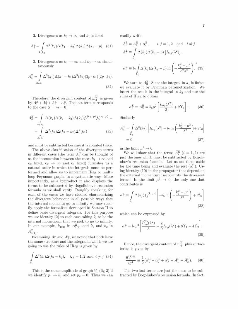
The two last terms are just the ones to be sub-tracted by Bogoliubov’s recursion formula. In fact,

8

in order to subtract the subdivergences of this par-ticular graph we must add the following countert-erms

pk2

p pk1

p

= (−1)× Divergence of

FIG. 4. Counterterms for P(2)A

whose amplitudes are, respectively

ig4

2

∫

k2

∆(k2)∆(k2 − p)[

−Ilog(λ2)]

=ig4

2

(

−AΞ1

)

,

(41)

ig4

2

∫

k1

∆(k1)∆(k1 − p)[

−Ilog(λ2)]

=ig4

2

(

−AΞ2

)

.

(42)

Notice that we are adopting a “MS” scheme that,in IReg, corresponds to the subtraction of basicdivergent integrals [18].

Therefore, subtracting the subdivergences yields

Ξ(2)A

ig4≡

b6p2

6

[

2I(2)log(λ

2)−13

3Ilog(λ

2)+

+ 54Υ1 − 24Υ2 + finite

]

. (43)

We turn now to the two loop nested graph (P(2)B )

whose amplitude is

Ξ(2)B

ig4=

1

2

∫

k1k2

∆2(k1)∆(k1 − p)∆(k2)∆(k1 − k2).

(44)

We use identity (10) in the propagator that de-pend on the external momentum and find that thechoice n(k1) = 3 guarantees the finitude of theterms that contain f (k1, p) as k1 → ∞ in all pos-sible ways. We proceed to identify the divergentterms. The case k1 → ∞ and k2 fixed does notcontain any divergent term while the case k2 → ∞

and k1 fixed does. They are given by

∫

k1k2

∆2(k1)∆(k1 − k2)∆(k2)

[

4∑

l=0

f(k1, p)l +f (k1, p)

]

=

∫

k1k2

∆2(k1)∆(k1 − k2)∆(k2)∆(k1 − p). (45)

For definiteness call the above integral BΞ1 . This

is the only one which we have to deal with (the di-vergent terms from the case k1 → ∞ and k2 → ∞simultaneously are contained in the above inte-gral). One may notice that it is just the originalamplitude of the graph but now we have a naturalorder to implement IReg. We use its rules in theintegral in k2 to obtain

BΞ1 = BΞ

1 + βΞ1 ,

BΞ1 ≡

∫

k1

∆(k1)∆(k1 − p)

[

−Ilog3

(λ2)

]

,

βΞ1 ≡

∫

k1

∆(k1)∆(k1 − p)

[

b63ln

(

−k21 − µ2

λ2

)

]

+

+

∫

k1

∆(k1)∆(k1 − p)

[

4Υ1 −8b69

]

. (46)

We apply the procedure again in βΞ1 to find the

following divergent terms

βΞ1 ≡

∫

k1

∆(k1)

[

2∑

l=0

f(k2, p)l

]

[

b63ln

(

−k21 − µ2

λ2

)]

+

+

∫

k1

∆(k1)

[

2∑

l=0

f(k2, p)l

]

(

4Υ1 −8b69

)

=−p2

3

{

b63I(2)log(λ

2)−10b69

Ilog(λ2)− 4b6Υ2

+ 4Υ1

[

Ilog(λ2) +

2b63

− 3Υ1

]}

. (47)

Notice that an arbitrary valued surface termappears multiplied by a divergence expressed byIlog(λ

2). Should we have adopted CIReg whichsets Υl = 0 as required by momentum routing in-variance (and gauge symmetry) it would not haveappeared. We shall keep all surface terms untilthe end to see whether they play any role in the

9

physics of a less symmetrical theory such as scalarfield theories.Therefore, the divergent content of Ξ

(2)B plus sur-

face terms is given by

Ξ(2)∞B

ig4≡

1

2

(

βΞ1 + BΞ

1

)

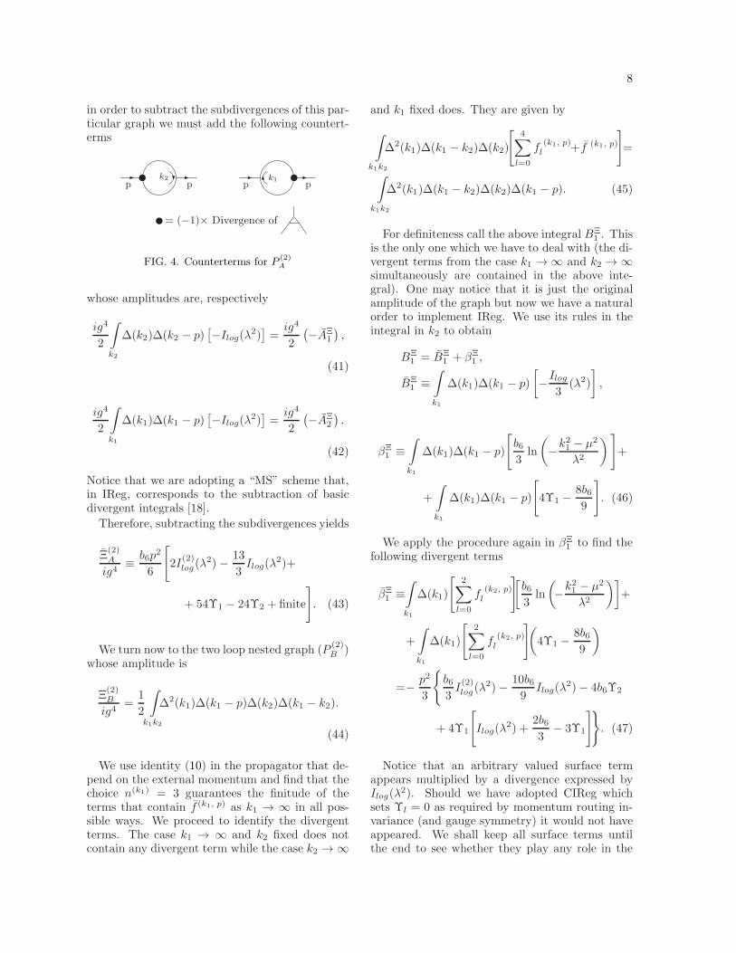
. (48)

Again, the last term is just the one which issubtracted by Bogoliubov’s recursion formula sincethe counterterm we must add is

p

k1

p= ig4

2

∫

k1

∆(k1)∆(k1 − p)[

13Ilog(λ

2)]

= (−1)× Divergence ofk1 k1

FIG. 5. Counterterm for P(2)B

After we add the counterterm we obtain

Ξ(2)B

ig4≡

b6p2

6

{

−I(2)log (λ

2)

3+

10

9Ilog(λ

2) + 4Υ2

}

+

+p2

6

{

− 4Υ1

[

Ilog(λ2) +

2b63

− 3Υ1

]

+ finite

}

.

(49)

Notice that the term proportional to 4Υ1Ilog(λ2)

is not subtracted as a subdivergence since we areadopting a “MS” scheme in IReg. In the next sec-tion we discuss what would happen if we had in-cluded the surface term in the counterterm.At this point, we can write down the renormal-

ization of the propagator at two loop order

Ξ(2) ≡ Ξ(2)A + Ξ

(2)B

= ig4p2

6

{

5b63

I(2)log(λ

2)−29b69

Ilog(λ2)− 20Υ2+

− 2Υ1

[

2Ilog(λ2)−

77b63

+ 6Υ1

]

+ finite

}

.

(50)

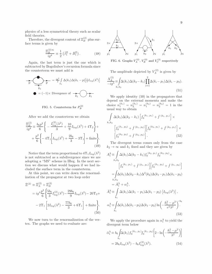
We now turn to the renormalization of the ver-tex. The graphs we need to evaluate are:

p1

k1

k2

p2

3×

p1

k1 k2

p2

3×

p1 k2

k1

p2

FIG. 6. Graphs V(2)A , V

(2)B and V

(2)C respectively

The amplitude depicted by V(2)A is given by

Λ(2)A

−ig5≡

∫

k1k2

∆(k1)∆(k2− k1)

2∏

i=1

∆(ki− p1)∆(ki − p2).

(51)

We apply identity (10) in the propagators thatdepend on the external momenta and make the

choice n(k1)1 = n

(k1)2 = n

(k2)1 = n

(k2)2 = 1 in the

usual way to obtain∫

k1k2

∆(k1)∆(k2 − k1)[

f(k1, p1)0 + f (k1, p1)

]

×

[

f(k1, p2)0 + f (k1, p2)

][

f(k2, p1)0 + f (k2, p1)

]

×[

f(k2, p2)0 + f (k2, p2)

]

. (52)

The divergent terms comes only from the casek2 → ∞ and k1 fixed and they are given by

AΛ1 ≡

∫

k1k2

∆(k1)∆(k2 − k1)f(k2, p1)0 f

(k2, p2)0 ×

[

f(k1, p1)0 + f (k1, p1)

][

f(k1, p2)0 + f (k1, p2)

]

=

∫

k1k2

∆(k1)∆(k2−k1)∆2(k2)∆(k1−p1)∆(k1−p2)

= AΛ1 + αΛ

1 ,

AΛ1 ≡

∫

k1

∆(k1)∆(k1 − p1)∆(k1 − p2)[

Ilog(λ2)]

,

αΛ1 ≡

∫

k1

∆(k1)∆(k1−p1)∆(k1−p2) ln

(

−k21 − µ2

e2λ2

)−b6

.

(53)

We apply the procedure again in αΛ1 to yield the

divergent term below

αΛ1 ≡ b6

∫

k1

∆(k1)f(k1, p1)0 f

(k1, p2)0

[

2−ln

(

−k21 −µ2

λ2

)]

= 2b6Ilog(λ2)− b6I

(2)log(λ

2). (54)

10

Hence, the divergent content of Λ(2)A is given by

Λ(2)∞A ≡ −ig5

[

αΛ1 + AΛ

1

]

(55)

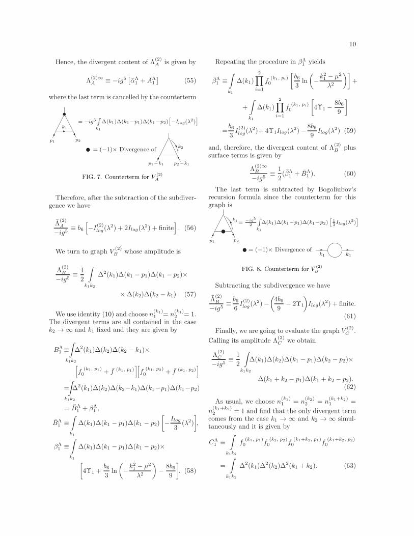
where the last term is cancelled by the counterterm

p1

k1

p2

= −ig5∫

k1

∆(k1)∆(k1−p1)∆(k1−p2)[

−Ilog(λ2)]


p1−k1

k2

p2−k1

FIG. 7. Counterterm for V(2)A

Therefore, after the subtraction of the subdiver-gence we have

Λ(2)A

−ig5≡ b6

[

−I(2)log(λ

2) + 2Ilog(λ2) + finite

]

. (56)

We turn to graph V(2)B whose amplitude is

Λ(2)B

−ig5≡

1

2

∫

k1k2

∆2(k1)∆(k1 − p1)∆(k1 − p2)×

×∆(k2)∆(k2 − k1). (57)

We use identity (10) and choose n(k1)1 = n

(k1)2 = 1.

The divergent terms are all contained in the casek2 → ∞ and k1 fixed and they are given by

BΛ1 ≡

∫

k1k2

∆2(k1)∆(k2)∆(k2 − k1)×

[

f(k1, p1)0 + f (k1, p1)

][

f(k1, p2)0 + f (k1, p2)

]

=

∫

k1k2

∆2(k1)∆(k2)∆(k2−k1)∆(k1−p1)∆(k1−p2)

= BΛ1 + βΛ

1 ,

BΛ1 ≡

∫

k1

∆(k1)∆(k1 − p1)∆(k1 − p2)

[

−Ilog3

(λ2)

]

,

βΛ1 ≡

∫

k1

∆(k1)∆(k1 − p1)∆(k1 − p2)×

[

4Υ1 +b63ln

(

−k21 − µ2

λ2

)

−8b69

]

. (58)

Repeating the procedure in βΛ1 yields

βΛ1 ≡

∫

k1

∆(k1)

2∏

i=1

f(k1, pi)0

[

b63ln

(

−k21 − µ2

λ2

)]

+

+

∫

k1

∆(k1)

2∏

i=1

f(k1, pi)0

[

4Υ1 −8b69

]

=b63I(2)log(λ

2)+ 4Υ1Ilog(λ2)−

8b69

Ilog(λ2) (59)

and, therefore, the divergent content of Λ(2)B plus

surface terms is given by

Λ(2)∞B

−ig5≡

1

2(βΛ

1 + BΛ1 ). (60)

The last term is subtracted by Bogoliubov’srecursion formula since the counterterm for thisgraph is

= −ig5

2

∫

k1

∆(k1)∆(k1−p1)∆(k1−p2)[

13Ilog(λ

2)]


p1

k1

p2

k1 k1

FIG. 8. Counterterm for V(2)B

Subtracting the subdivergence we have

Λ(2)B

−ig5≡b66I(2)log(λ

2)−

(

4b69

− 2Υ1

)

Ilog(λ2) + finite.

(61)

Finally, we are going to evaluate the graph V(2)C .

Calling its amplitude Λ(2)C we obtain

Λ(2)C

−ig5≡

1

2

∫

k1k2

∆(k1)∆(k2)∆(k1 − p1)∆(k2 − p2)×

∆(k1 + k2 − p1)∆(k1 + k2 − p2).(62)

As usual, we choose n(k1)1 = n

(k2)2 = n

(k1+k2)1 =

n(k1+k2)2 = 1 and find that the only divergent term

comes from the case k1 → ∞ and k2 → ∞ simul-taneously and it is given by

CΛ1 ≡

∫

k1k2

f(k1, p1)0 f

(k2, p2)0 f

(k1+k2, p1)0 f

(k1+k2, p2)0

=

∫

k1k2

∆2(k1)∆2(k2)∆

2(k1 + k2). (63)

11

After the integration over k2 and the use of therules of IReg we have

Λ(2)C ≡ Λ

(2)C = −ig5b6

[

Ilog(λ2) + finite

]

. (64)

Collecting all the results we find that the renor-malization of the vertex at two loop order is givenby

Λ(2) ≡Λ(2)A + Λ

(2)B + Λ

(2)C

=ig5[

5b62

I(2)log(λ

2)−

(

17b63

+ 6Υ1

)

Ilog(λ2)

]

+

+ ig5 × (finite) . (65)

Although our procedure found success in all theexamples already presented, one may wonder howgeneral it is. To answer this question, we apply itto diagrams with more than two-loops.

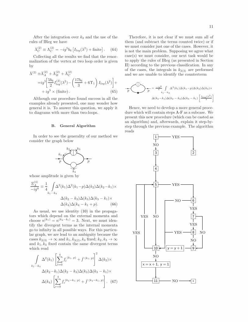
B. General Algorithm

In order to see the generality of our method weconsider the graph below

k2 k3

k1

k4

p p

whose amplitude is given by

Ξ(4)A

−ig8≡

1

4

∫

k1···k4

∆2(k1)∆2(k1−p)∆(k2)∆(k2−k1)×

∆(k2 − k3)∆(k3)∆(k3 − k1)×

∆(k4)∆(k4 − k1 + p). (66)

As usual, we use identity (10) in the propaga-tors which depend on the external momenta andchoose n(k1) = n(k4−k1) = 3. Next, we must iden-tify the divergent terms as the internal momentago to infinity in all possible ways. For this particu-lar graph, we are lead to an ambiguity because thecases k2(3) → ∞ and k1, k3(2), k4 fixed; k2, k3 → ∞and k1, k4 fixed contain the same divergent termswhich read

∫

k1···k4

∆2(k1)

[

4∑

l=0

f(k1, p)l + f (k1, p)

]2

∆(k2)×

∆(k2−k1)∆(k2 − k3)∆(k3)∆(k3 − k1)×

∆(k4)

[

4∑

r=0

f (k4−k1, p)r + f (k4−k1, p)

]

. (67)

Therefore, it is not clear if we must sum all ofthem (and subtract the terms counted twice) or ifwe must consider just one of the cases. However, itis not the main problem. Supposing we agree whatcase(s) we must consider, our next task would beto apply the rules of IReg (as presented in SectionII) according to the previous classification. In anyof the cases, the integrals in k2(3) are performedand we are unable to identify the counterterm

p p= −ig8

4

∫

k1···k3

∆2(k1)∆(k1−p)∆(k2)∆(k3)×

∆(k2−k1)∆(k2 − k3)∆(k3 − k1)

[

Ilog(λ2)

3

]

Hence, we need to develop a more general proce-dure which will contain steps A-F as a subcase. Wepresent this new procedure (which can be casted asan algorithm) and, afterwards, explain it step-by-step through the previous example. The algorithmreads

1

3 2

4

5

6

7

8

10 9

x = x+ 1, y = 1

11 ∗

NO

YES

NO

YES

NO

YES

YES

NO

YES NO

y = y + 1

NO

YES

YES

NO

12

1. Let Se be the set of subgraphs Gi that shareone external leg with the whole graph G. LetSe be the complementary set. Is Se an emptyset?

2. Apply the procedure stated before (stepsA→F) to the amplitude.

3. Identify the propagators which depend onthe external momenta and do not belong to asubgraph contained in Se. Use identity (10)in such propagators and find out the values

of n(ki)j in the usual way.

4. Set x = 0 and y = 1. Group all internal mo-

menta in the set K(y=1)x=0 and define its com-

plement (which is an empty set) by K(y=1)x=0 .

5. Is there a subgraph Gi whose internal mo-

menta are precisely the ones grouped in K(y)x ?

6. Are there divergent terms as all internal mo-

menta contained in K(y)x go to infinity and all

elements of K(y)x are kept fixed?

7. Have all the divergent terms identified in step6 been stored?

8. Is K(y)x a subset of a already stored K

(j)i (i =

0, 1, · · · , x− 1)?

9. Store the terms identified in step 6 as well as

K(y)x (if K

(y)x is a subset of a already stored

K(j)i , erase the result corresponding to the

latter).

10. Choose a new combination of x numbers ofinternal momenta and group them in the set

K(y)x . Is it possible?

11. Choose x numbers of internal momenta andgroup them in the set K

(y)x . Is it possible?

When the algorithm gets to asterisk (∗) , wewrite down all the results stored. Each one isclassified according to a particular set of internalmomenta that go to infinity. If this set has twoor more elements, we identify the subgraph thatcontains them and run the algorithm on it. Onthe other hand, if the set has only one elementwe use the rules of IReg (as presented in SectionII). At this point, we set aside the terms that

contain I(l)log(λ

2) and apply the algorithm on theothers. Eventually, we obtain two kind of terms:

the ones in which I(l)log(λ

2) multiplies an integral

(that correspond to the terms cancelled by Bogoli-ubov’s recursion formula) and the ones in which

I(l)log(λ

2) multiplies only constants and/or polyno-

mials in the external momenta (that correspond tothe typical divergence of the graph).

As stated, we are going to clarify the methodwith the previous example. In the following, wepresent the result we obtain after each one of thesteps.

• Step 1 : answer is NO

k4

k1−p k1−p

k2 k3

k1 k1

k3 − k1 k3

k2

k2 k2 − k1

Se = {, ,

, }k3

p pSe = { }

• Step 3

n(k1) = 3, ∆(k1 − p) =

[

4∑

l=0

f(k1, p)l + f (k1, p)

]

.

• Step 4

K(1)0 = {k1 · · · k4}, K

(1)0 = ∅

• Step 5 : answer is YES

The internal momenta k1 · · · k4 (which are con-

tained in K(y=1)x=0 ) belong to a subgraph of the set

Se.


The divergent terms are

∫

k1···k4

∆2(k1)

l+l′≤2∑

l, l′= 0

f(k1, p)l f

(k1, p)l′

∆(k2)×

∆(k2−k1)∆(k2 − k3)∆(k3)∆(k3 − k1)×

∆(k4)∆(k4 − k1 + p). (68)

13


• Step 9

We store the divergent terms given by (68) as

well as K(y=1)x=0 = {k1 · · · k4}.



We choose k1 and obtain

K(y=1)x=1 = {k2 · · · k4}, K

(y=1)x=1 = {k1}


None subgraph contains {k2 · · · k4} as its inter-nal momenta.



K(y=1)x=1 = {k1, k3, k4}, K

(y=1)x=1 = {k2}


None subgraph contains {k1, k3, k4} as its inter-nal momenta..



K(y=1)x=1 = {k1, k2, k4}, K

(y=1)x=1 = {k3}


None subgraph contains {k1, k2, k4} as its inter-nal momenta.



K(y=1)x=1 = {k1 · · · k3}, K

(y=1)x=1 = {k4}


None subgraph contains {k1 · · · k3} as its inter-nal momenta.



We choose k1, k2 and obtain

K(y=1)x=2 = {k3, k4}, K

(y=1)x=2 = {k1, k2}


None subgraph contains {k3, k4} as its internalmomenta.



K(y=1)x=2 = {k2, k4}, K

(y=1)x=2 = {k1, k3}





K(y=1)x=2 = {k2, k3}, K

(y=1)x=2 = {k1, k4}


The second subgraph of Se has {k2, k3} as itsinternal momenta.



∫

k1···k4

∆2(k1)

[

4∑

l=0

f(k1, p)l + f (k1, p)

]2

∆(k2)×

∆(k2−k1)∆(k2 − k3)∆(k3)∆(k3 − k1)×

∆(k4)∆(k4 − k1 + p). (69)


One may notice that (69) possesses more termsthan (68).

• Step 9

Since K(y=1)x=2 is a subset of K

(y=1)x=0 , we erase the

result corresponding to the latter. Therefore, we

14

store only the divergent terms given by (69) as well

as K(y=1)x=2 = {k2, k3}.



K(y=2)x=2 = {k1, k4}, K

(y=1)x=2 = {k2, k3}





K(y=2)x=2 = {k1, k3}, K

(y=1)x=2 = {k2, k4}





K(y=2)x=2 = {k1, k2}, K

(y=2)x=2 = {k3, k4}





We choose k1, k2, k3 and obtain

K(y=1)x=3 = {k4}, K

(y=1)x=3 = {k1, k2, k3}


The first subgraph of Se has {k4} as its internalmomentum.



∫

k1···k4

∆2(k1)

[

4∑

l=0

f(k1, p)l + f (k1, p)

]2

∆(k2)×

∆(k2−k1)∆(k2 − k3)∆(k3)∆(k3 − k1)×

∆(k4)∆(k4 − k1 + p). (70)


One may notice that (70) contains the sameterms of (69).


Since we erased the result corresponding to

K(y=1)x=0 , we notice that K

(y=1)x=3 is not a subset of

a previously stored K(y=j)x=i .

• Step 9

We store the divergent terms given by (70) as

well as K(y=1)x=3 = {k4}.



K(y=2)x=3 = {k3}, K

(y=2)x=3 = {k1, k2, k4}


The fourth subgraph of Se has {k3} as its inter-nal momentum.



∫

k1···k4

∆2(k1)

[

4∑

l=0

f(k1, p)l + f (k1, p)

]2

∆(k2)×

∆(k2−k1)∆(k2 − k3)∆(k3)∆(k3 − k1)×

∆(k4)∆(k4 − k1 + p). (71)


One may notice that (71) contains the sameterms of (69) and (70).


15

One may notice that K(y=2)x=3 is a subset of K

(y=1)x=2 .



K(y=2)x=3 = {k2}, K

(y=2)x=3 = {k1, k3, k4}


The third subgraph of Se has {k2} as its internalmomentum.



∫

k1···k4

∆2(k1)

[

4∑

l=0

f(k1, p)l + f (k1, p)

]2

∆(k2)×

∆(k2−k1)∆(k2 − k3)∆(k3)∆(k3 − k1)×

∆(k4)∆(k4 − k1 + p). (72)


One may notice that (72) contains the sameterms of (69) and (70).


One may notice that K(y=2)x=3 is a subset of K

(y=1)x=2 .



K(y=2)x=3 = {k1}, K

(y=2)x=3 = {k2, k3, k4}


None subgraph has {k1} as its internal momen-tum.



We choose k1, k2, k3, k4 and obtain

K(y=1)x=4 = ∅, K

(y=1)x=4 = {k1, k2, k3, k4}




At this point, we write down the results stored:

1. K(y=1)x=2 = {k2, k3} and eq. (69)

A(4)1 ≡

∫

k1···k4

∆2(k1)∆2(k1 − p)∆(k4)∆(k4 − k1 + p)×

×∆(k2)∆(k2−k1)∆(k2−k3)∆(k3)∆(k3−k1),

2. K(y=1)x=3 = {k4} and eq. (70)

A(4)2 ≡

∫

k1···k4

∆2(k1)∆2(k1 − p)∆(k4)∆(k4 − k1 + p)×

×∆(k2)∆(k2−k1)∆(k2−k3)∆(k3)∆(k3−k1),

3. Term counted twice (intersection betweenthe cases (1) and (2))

A(4)3 ≡

∫

k1···k4

∆2(k1)∆2(k1 − p)∆(k4)∆(k4 − k1 + p)×

×∆(k2)∆(k2−k1)∆(k2−k3)∆(k3)∆(k3−k1),

The term A(4)1 is divergent as two momenta

(k2, k3) go to infinity. Therefore, we identify thesubgraph that contains these momenta and applythe algorithm on it. The result can be written us-ing a graphic notation as below [40]

ig4

2

∫

k2k3

∆(k2)∆(k2−k1)∆(k2−k3)∆(k3)∆(k3−k1)

= ig4

{

k21b66

[

2I(2)log(λ

2)−13

3Ilog(λ

2) + finite

]

+

+

3∑

i=2

∫

ki

∆(ki)∆(ki−k1)

[

Ilog(λ2)

2

]

}

≡− + F −

1−

1

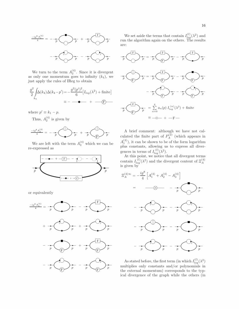
Therefore, A(4)1 can be re-expressed as

16

−p p

+F

p p

−1

p p−

1

p p

−ig8A(4)1

4=

We turn to the term A(4)2 . Since it is divergent

as only one momentum goes to infinity (k4), wejust apply the rules of IReg to obtain

g2

2

∫

k4

∆(k4)∆(k4−p′)=−g2(p′)2

6

[

Ilog(λ2) + finite

]

≡ − + F

where p′ ≡ k1 − p.

Thus, A(4)2 is given by

−p p

+F

p p

−ig8A(4)2

4=

We are left with the term A(4)3 which we can be

re-expressed as

p p

− + −

1−

1F

- + F

or equivalently

−ig8A(4)3

4= −

F

p p

−

Fp p

p p

+1

p p+

1

p p

+

F

Fp p

−1

Fp p

−1

Fp p

We set aside the terms that contain I(l)log(λ

2) andrun the algorithm again on the others. The resultsare:

F

p p= −

F

Fp p

F

p p

Fp p

= −

− −

F

Fp p

Fp p

1

Fp p

1

Fp p

F

Fp p

=4∑

n=0

an(p) I(n)log (λ2) + finite

≡ ⊗ + F

A brief comment: although we have not cal-

culated the finite part of P(2)A (which appears in

A(4)1 ), it can be shown to be of the form logarithm

plus constants, allowing us to express all diver-

gences in terms of I(l)log (λ

2).At this point, we notice that all divergent terms

contain I(l)log (λ

2) and the divergent content of Ξ(4)A

is given by

Ξ(4)∞A = −

ig8

4

[

A(4)1 +A

(4)2 −A

(4)3

]

= −p p

−p p

−p p

−1

p p−

1

p p

⊗

−1

p p−

1

p p

As stated before, the first term (in which I(l)log(λ

2)

multiplies only constants and/or polynomials inthe external momentum) corresponds to the typ-ical divergence of the graph while the others (in

17

which I(l)log(λ

2) multiplies an integral) correspondto the terms to be subtracted by Bogoliubov’s re-cursion formula.

C. N-loop vertex and self-energy diagrams of

the ladder type

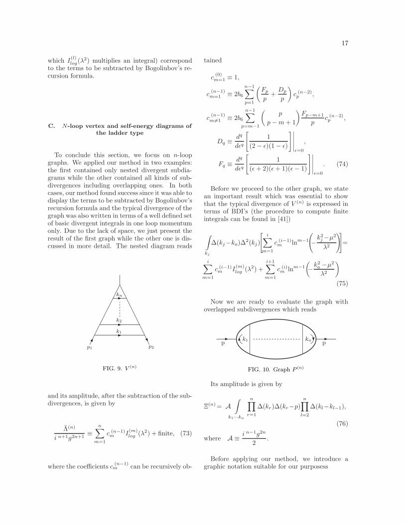
To conclude this section, we focus on n-loopgraphs. We applied our method in two examples:the first contained only nested divergent subdia-grams while the other contained all kinds of sub-divergences including overlapping ones. In bothcases, our method found success since it was able todisplay the terms to be subtracted by Bogoliubov’srecursion formula and the typical divergence of thegraph was also written in terms of a well defined setof basic divergent integrals in one loop momentumonly. Due to the lack of space, we just present theresult of the first graph while the other one is dis-cussed in more detail. The nested diagram reads

p1

k1

k2

p2

kn

FIG. 9. V (n)

and its amplitude, after the subtraction of the sub-divergences, is given by

Λ(n)

i n+1g2n+1≡

n∑

m=1

c (n−1)m I

(m)log (λ2) + finite, (73)

where the coefficients c(n−1)m can be recursively ob-

tained

c(0)m=1 ≡ 1,

c(n−1)m=1 ≡ 2b6

n−1∑

p=1

(

Fp

p+

Dp

p

)

c (n−2)p ,

c(n−1)m 6=1 ≡ 2b6

n−1∑

p=m−1

(

p

p−m+ 1

)

Fp−m+1

pc (n−2)p ,

Dq ≡dq

dǫq

[

1

(2 − ǫ)(1− ǫ)

]∣

∣

∣

∣

∣

ǫ=0

,

Fq ≡dq

dǫq

[

1

(ǫ + 2)(ǫ+ 1)(ǫ− 1)

]∣

∣

∣

∣

∣

ǫ=0

. (74)

Before we proceed to the other graph, we statean important result which was essential to showthat the typical divergence of V (n) is expressed interms of BDI’s (the procedure to compute finiteintegrals can be found in [41])

∫

kj

∆(kj−ka)∆2(kj)

[

i∑

m=1

c (i−1)m lnm−1

(

−k2j−µ2

λ2

)]

=

i∑

m=1

c (i−1)m I

(m)log (λ2) +

i+1∑

m=1

c (i)m lnm−1

(

−k2a −µ2

λ2

)

(75)

Now we are ready to evaluate the graph withoverlapped subdivergences which reads

pk1 kn p

FIG. 10. Graph P (n)

Its amplitude is given by

Ξ(n)= A

∫

k1···kn

n∏

r=1

∆(kr)∆(kr−p)

n∏

l=2

∆(kl−kl−1),

(76)

where A ≡i n−1g2n

2.

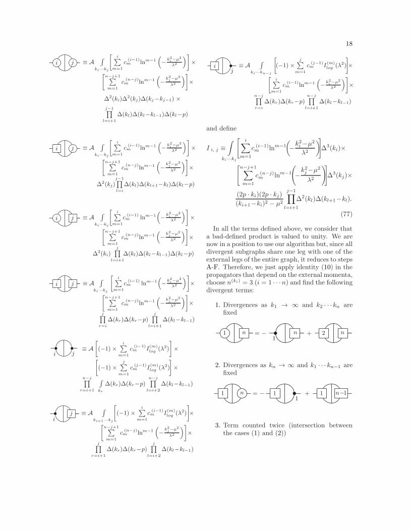
Before applying our method, we introduce agraphic notation suitable for our purposess

18

i j ≡ A∫

ki···kj

[

i∑

m=1

c(i−1)m lnm−1

(

−k2i−µ2

λ2

)

]

×

[

n−j+1∑

m=1

c(n−j)m lnm−1

(

−k2j−µ2

λ2

)

]

×

∆2(ki)∆2(kj)∆(kj−kj−1) ×

j−1∏

l=i+1

∆(kl)∆(kl−kl−1)∆(kl−p)

i j ≡ A∫

ki···kj

[

i∑

m=1

c(i−1)m lnm−1

(

−k2i−µ2

λ2

)

]

×

[

n−j+1∑

m=1

c(n−j)m lnm−1

(

−k2j−µ2

λ2

)

]

×

∆2(kj)j−1∏

l=i

∆(kl)∆(kl+1−kl)∆(kl−p)

i j ≡ A∫

ki···kj

[

i∑

m=1

c(i−1)m lnm−1

(

−k2i−µ2

λ2

)

]

×

[

n−j+1∑

m=1

c(n−j)m lnm−1

(

−k2j−µ2

λ2

)

]

×

∆2(ki)j∏

l=i+1

∆(kl)∆(kl−kl−1)∆(kl−p)

i j ≡ A∫

ki···kj

[

i∑

m=1

c(i−1)m lnm−1

(

−k2i−µ2

λ2

)

]

×

[

n−j+1∑

m=1

c(n−j)m lnm−1

(

−k2j−µ2

λ2

)

]

×

j∏

r=i

∆(kr)∆(kr−p)j∏

l=i+1

∆(kl−kl−1)

i j≡ A

[

(−1)×i∑

m=1

c(i−1)m I

(m)log (λ2)

]

×

[

(−1)×j∑

m=1

c(j−1)m I

(m)log (λ2)

]

×

n−j∏

r=i+1

∫

kr

∆(kr)∆(kr−p)n−j∏

l=i+2

∆(kl−kl−1)

ij ≡ A

∫

ki+1···kj

[

(−1)×i∑

m=1

c(i−1)m I

(m)log (λ2)

]

×

[

n−j+1∑

m=1

c(n−j)m lnm−1

(

−k2j−µ2

λ2

)

]

×

j∏

r=i+1

∆(kr)∆(kr−p)j∏

l=i+2

∆(kl−kl−1)

ij

≡ A∫

ki···kn−j

[

(−1)×j∑

m=1

c(j−1)m I

(m)log (λ2)

]

×

[

i∑

m=1

c(i−1)m lnm−1

(

−k2i−µ2

λ2

)

]

×

n−j∏

r=i

∆(kr)∆(kr−p)n−j∏

l=i+1

∆(kl−kl−1)

and define

I i, j ≡

∫

ki···kj

[

i∑

m=1

c (i−1)m lnm−1

(

−k2i −µ2

λ2

)

]

∆3(ki)×

[

n−j+1∑

m=1

c (n−j)m lnm−1

(

−k2j−µ2

λ2

)]

∆3(kj)×

(2p · ki)(2p · kj)

(ki+1−ki)2 − µ2

j−1∏

l=i+1

∆2(kl)∆(kl+1−kl).

(77)

In all the terms defined above, we consider thata bad-defined product is valued to unity. We arenow in a position to use our algorithm but, since alldivergent subgraphs share one leg with one of theexternal legs of the entire graph, it reduces to stepsA-F. Therefore, we just apply identity (10) in thepropagators that depend on the external momenta,choose n(ki) = 3 (i = 1 · · ·n) and find the followingdivergent terms:

1. Divergences as k1 → ∞ and k2 · · · kn arefixed

1 n1

n 2 n= − +

2. Divergences as kn → ∞ and k1 · · · kn−1 arefixed

1 n 11

1 n−1= − +


19

1 n1

n−1 21

1 12 n−1

= − −

+ +

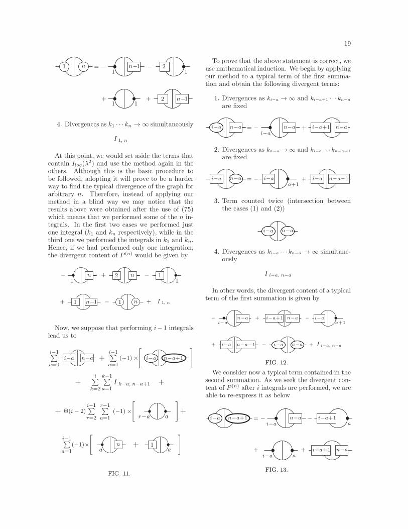
4. Divergences as k1 · · · kn → ∞ simultaneously

I 1, n

At this point, we would set aside the terms thatcontain Ilog(λ

2) and use the method again in theothers. Although this is the basic procedure tobe followed, adopting it will prove to be a harderway to find the typical divergence of the graph forarbitrary n. Therefore, instead of applying ourmethod in a blind way we may notice that theresults above were obtained after the use of (75)which means that we performed some of the n in-tegrals. In the first two cases we performed justone integral (k1 and kn respectively), while in thethird one we performed the integrals in k1 and kn.Hence, if we had performed only one integration,the divergent content of P (n) would be given by

−1

n + 2 n − 11

+ 1 n−1 − 1 n + I 1, n

Now, we suppose that performing i− 1 integralslead us to

i−1∑

a=0i−a n−a +

i−1∑

a=1(−1)×

[ ]

i−a n−a+1

+i∑

k=2

k−1∑

a=1I k−a, n−a+1 +

i−1∑

r=2

r−1∑

a=1+ Θ(i− 2) (−1)×

[ ]

+r−a a

i−1∑

a=1(−1)×

[ ]

an + 1

a

FIG. 11.

To prove that the above statement is correct, weuse mathematical induction. We begin by applyingour method to a typical term of the first summa-tion and obtain the following divergent terms:

1. Divergences as ki−a → ∞ and ki−a+1 · · · kn−a

are fixed

i−a n−a

i−a

n−a i−a+1 n−a= − +

2. Divergences as kn−a → ∞ and ki−a · · · kn−a−1

are fixed

i−a n−a i−aa+1

i−a n−a−1= − +


i−a n−a

4. Divergences as ki−a · · · kn−a → ∞ simultane-ously

I i−a, n−a

In other words, the divergent content of a typicalterm of the first summation is given by

−i−a

n−a + i−a+1 n−a − i−aa+1

+ i−a n−a−1 − i−a n−a + I i−a, n−a

FIG. 12.

We consider now a typical term contained in thesecond summation. As we seek the divergent con-tent of P (n) after i integrals are performed, we areable to re-express it as below

i−a n−a+1i−a

n−a i−a+1a

= − −

i−a ai−a+1 n−a+ +

FIG. 13.

20

Inserting the results of (fig 12) and (fig 13) at(fig 11) we obtain

i∑

a=0

i+1−a n−a +i∑

a=1(−1)×

[ ]

i+1−a n−a+1

+i+1∑

k=2

k−1∑

a=1I k−a, n−a+1 +

i∑

r=2

r−1∑

a=1+ Θ(i− 1) (−1)×

[ ]

+r−a a

i∑

a=1(−1)×

[ ]

an + 1

a

One may notice that the result above is justthe one we supposed (fig 11) if we set i → i + 1.Therefore, by mathematical induction, we proveour statement and we will be able to identify thetypical divergence of the graph. Performing n− 1integrals lead us to

n−1∑

a=0

n−a n−a +n−1∑

a=1(−1)×

[ ]

i−a n−a+1

+n∑

k=2

k−1∑

a=1I k−a, n−a+1 +

n−1∑

r=2

r−1∑

a=1+ Θ(n− 2) (−1)×

[ ]

+r−a a

n−1∑

a=1(−1)×

[ ]

an + 1

a

We apply our method in the first summation andfind that the divergent terms coming from it aregiven by

p2n−1∑

a=0

n−a∑

m=1

a+1∑

m′=1

c (n−a−1)m c

(a)m′

[

−I

(M−1)log (λ2)

3+

2 Θ(M − 2)

M−1∑

k=2

(

1

3

)k(M − 2)!

(M − 1− k)!I

(M−k)log (λ2)

]

,

M ≡ m+m′. (78)

In the second summation all the terms containonly quadratic divergences and, therefore, they

give a null contribution. The third summation canbe evaluated and the result is

p2n∑

k=2

k−1∑

a=1

k−1∑

m=1

a∑

m′=1

c (k−2)m d

(n−a−k+2)m′ ×

2

m+m′−1∑

l=1

(

1

3

)l(m+m′ − 2)!

(m+m′ − 1− l)!I

(m+m′−l)log (λ2)

,

d (0)q ≡ c

(n−j)k ,

d (i)q ≡ 2b6

n−j+1∑

k=q

d(i−1)k

(

k − 1

k − q

)

Gk−q,

Gq ≡dq

d(ǫa)q

[

1

[4− (ǫa)2][1− (ǫa)2]

]

∣

∣

∣

∣

∣

ǫ=0

. (79)

The others terms are just the ones that are sub-tracted by Bogoliubov’s recursion formula sincethe counterterms for the graph we are dealing withcan be re-expressed as

r−akr−a+1 kn−a

a=

r−a a

aka+1 kn =

an

k1 kn−aa

= 1a

= (−1)× Divergence ofa

a loops

Therefore, the typical divergence of P (n) (afterthe subtraction of subdivergences) is given by thesum of (78) with (79).

One may notice that our method once again dis-played the terms to be subtracted by Bogoliubov’srecursion formula and allowed us to express thetypical divergence of the graph in terms of welldefined BDI’s. Therefore, we claim that the pro-cedure we developed here (which is summarized in

21

the algorithm) is the systematization of IReg tomulti-loop Feynman graphs. Although the resultswe already obtained are restricted to massless the-ories, we can develop a similar procedure to treatmassive ones as shown in the next section.

IV. MASSIVE THEORIES

We generalize identity (10) to massive theoriesand implement a mass independent regularizationscheme. The procedure we develop here allows usto write the divergences of any theory (massive ornot) in terms of the set of basic divergent integralswe have already presented and, therefore, justifiesour restriction to massless theories in the previoussections.The identity we are going to use is

1

(k−pi)2−m2−µ2=

2(n(k)i

−1)∑

l=0

h(k, pi)l + h (k, pi), (80)

where we defined,

h(k, pi)l ≡

⌊l/2⌋∑

j=0

Θ(n(k)i + j − l)

(

l − j

j

)

×

×(−p2i +m2)j(2pi · k)l−2j

(k2 − µ2)l+1−j

(81)

h (k, pi) ≡(−1)n

(k)i (p2i −m2 − 2pi · k)n

(k)i

(k2−µ2)n(k)i [(k−pi)2−m2−µ2]

. (82)

Notice that, if we set m2 → 0, we recover iden-tity (10). The procedure to be followed is similar

to the one of the massless theory since h(k, pi)l was

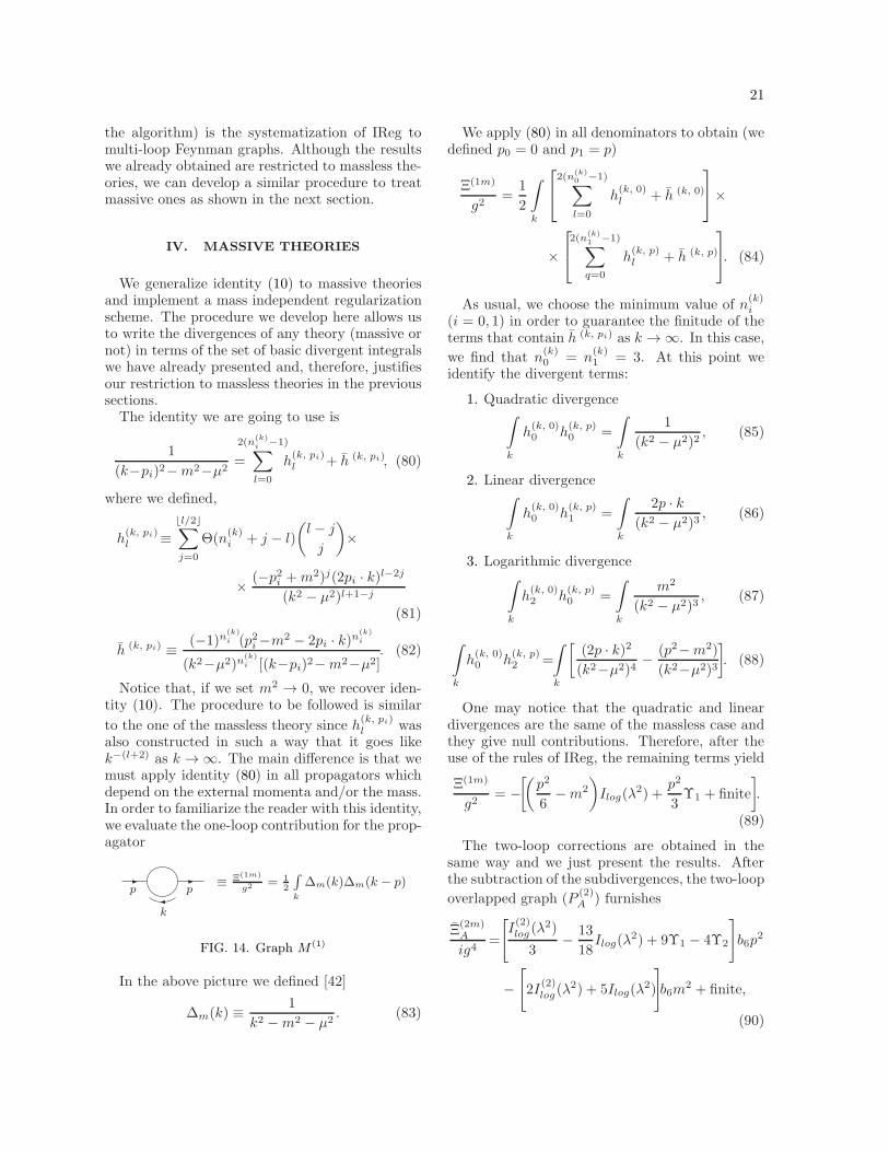
also constructed in such a way that it goes likek−(l+2) as k → ∞. The main difference is that wemust apply identity (80) in all propagators whichdepend on the external momenta and/or the mass.In order to familiarize the reader with this identity,we evaluate the one-loop contribution for the prop-agator

p

k

p≡ Ξ(1m)

g2= 1

2

∫

k

∆m(k)∆m(k − p)

FIG. 14. Graph M (1)

In the above picture we defined [42]

∆m(k) ≡1

k2 −m2 − µ2. (83)

We apply (80) in all denominators to obtain (wedefined p0 = 0 and p1 = p)

Ξ(1m)

g2=

1

2

∫

k

2(n(k)0 −1)∑

l=0

h(k, 0)l + h (k, 0)

×

×

2(n(k)1 −1)∑

q=0

h(k, p)l + h (k, p)

. (84)

As usual, we choose the minimum value of n(k)i

(i = 0, 1) in order to guarantee the finitude of theterms that contain h (k, pi) as k → ∞. In this case,

we find that n(k)0 = n

(k)1 = 3. At this point we

identify the divergent terms:

1. Quadratic divergence∫

k

h(k, 0)0 h

(k, p)0 =

∫

k

1

(k2 − µ2)2, (85)

2. Linear divergence∫

k

h(k, 0)0 h

(k, p)1 =

∫

k

2p · k

(k2 − µ2)3, (86)

3. Logarithmic divergence∫

k

h(k, 0)2 h

(k, p)0 =

∫

k

m2

(k2 − µ2)3, (87)

∫

k

h(k, 0)0 h

(k, p)2 =

∫

k

[

(2p · k)2

(k2−µ2)4−

(p2−m2)

(k2−µ2)3

]

. (88)

One may notice that the quadratic and lineardivergences are the same of the massless case andthey give null contributions. Therefore, after theuse of the rules of IReg, the remaining terms yield

Ξ(1m)

g2= −

[(

p2

6−m2

)

Ilog(λ2) +

p2

3Υ1 + finite

]

.

(89)

The two-loop corrections are obtained in thesame way and we just present the results. Afterthe subtraction of the subdivergences, the two-loop

overlapped graph (P(2)A ) furnishes

Ξ(2m)A

ig4=

[

I(2)log(λ

2)

3−

13

18Ilog(λ

2) + 9Υ1 − 4Υ2

]

b6p2

−

[

2I(2)log(λ

2) + 5Ilog(λ2)

]

b6m2 + finite,

(90)

22

while for the two-loop nested graph (P(2)B ) we ob-

tain

Ξ(2m)B

ig4=

{(

−b6p

2

18−

b6m2

2

)

I(2)log(λ

2)+

+

[(

5b627

−2Υ1

3

)

p2+

(

2b63

+6Υ1

)

m2

]

Ilog(λ2)

+

(

2b6Υ2

3−

4b6Υ1

9+ 2(Υ1)

2

)

p2 + finite

}

.

(91)

Therefore, the renormalization of the propagatorat two-loop order is given by

Ξ(2m)

ig4=

(

5b6p2

18−

5b6m2

2

)

I(2)log(λ

2)−

−

[(

29b654

+2Υ1

3

)

p2−

(

17b63

+6Υ1

)

m2

]

Ilog(λ2)

−

(

10b6Υ2

3−

77b6Υ1

9− 2(Υ1)

2

)

p2 + finite.

(92)

To conclude, we calculate the renormalizationgroup functions. As usual, we make the definitions

φo ≡ Z12

φ φ, mo ≡ Z12mm, go ≡ Zgg, (93)

which allows us to divide the bare lagrangian intwo parts: the renormalized lagrangian and thecounterterms. Explicitly,

L =1

2

[

(∂µφ)2 −m2φ2

]

+g

3!φ3+

+1

2

[

A(∂µφ)2 −Bm2φ2

]

+g

3!Cφ3,

A ≡ Zφ − 1, B ≡ ZφZm − 1, C ≡ ZgZ32

φ − 1.

(94)

We also define the renormalization group func-tions by

γ ≡λ

2

∂ lnZφ

∂λ, β ≡ λ

∂g

∂λ= −gλ

∂ lnZg

∂λ, (95)

γm ≡ −2

mλ∂m

∂λ= λ

∂ lnZm

∂λ. (96)

Supposing that A, B and C have a expansion inthe coupling constant g as below

A = A1g2 +A2g

4 +O(g6), (97)

B = B1g2 +B2g

4 +O(g6), (98)

C = C1g2 + C2g

4 +O(g6), (99)

we obtain

lnZφ =A1g2 +

(

A2 −A2

1

2

)

g4 +O(g6), (100)

lnZm =(B1 −A1) g2+

(

B2 −A2 +A2

1

2−

B21

2

)

g4+O(g6), (101)

lnZg =

(

C1 −3A1

2

)

g2+

(

C2 −3A2

2+3A2

1

4−C2

1

2

)

g4+O(g6). (102)

Since γ, γm and β can also be written as

γ = γ1g2 + γ2g

4 +O(g6), (103)

γm = γ(1)m g2 + γ(2)

m g4 +O(g6), (104)

β = β1g3 + β2g

5 +O(g6), (105)

we deduce the relations below

γ1 =λ

2

∂A1

∂λ, (106)

γ2 = β1A1 +λ

2

∂

∂λ

(

A2 −A2

1

2

)

, (107)

γ(1)m = λ

∂

∂λ(B1 −A1), (108)

γ(2)m = 2 (B1 −A1)β1 + λ

∂D

∂λ, (109)

β1 = −λ∂

∂λ

(

C1 −3A1

2

)

, (110)

β2 = −2

(

C1 −3A1

2

)

β1 − λ∂E

∂λ, (111)

D ≡

(

B2 −A2 +A2

1

2−

B21

2

)

, (112)

E ≡

(

C2 −3A2

2+

3A21

4−

C21

2

)

. (113)

Because we chose a “MS” scheme in IReg, thecoefficients Ai, Bi and Ci are given by (equations

23

(89), (92), (65) and fig. 2)

A1 = −i

6Ilog(λ

2), (114)

A2 = −5b618

I(2)log(λ

2) +

(

29b654

+2Υ1

3

)

Ilog(λ2), (115)

B1 = −iIlog(λ2), (116)

B2 = −5b62

I(2)log(λ

2) +

(

17b63

+ 6Υ1

)

Ilog(λ2), (117)

C1 = −iIlog(λ2), (118)

C2 = −5b62

I(2)log(λ

2) +

(

17b63

+ 6Υ1

)

Ilog(λ2). (119)

Since we have the relations

λ∂Ilog(λ

2)

∂λ= 2λ2 ∂Ilog(λ

2)

∂λ2= −2b6, (120)

λ∂I

(2)log(λ

2)

∂λ= −2Ilog(λ

2)− 3b6, (121)

we finally obtain

γ =g2

12(4π)3+

13g4

432(4π)6+

ig4

3(4π)3Υ1 +O(g6),

(122)

γm=5g2

6(4π)3+

97g4

108(4π)6+

16ig4

3(4π)3Υ1 +O(g6),

(123)

β = −3g3

4(4π)3−

125g5

144(4π)6−

5ig5

(4π)3Υ1+O(g6).

(124)

One may notice the appearance of arbitrary sur-face terms in the renormalization group functions.At first glance, this feature may be a result of thedefinition of the “MS” scheme in IReg which cor-responds to the subtraction of basic divergent in-tegrals only. However, if we use a different schemein which we subtract basic divergent integrals andsurface terms we obtain the same result above forthe first two coefficients of the β function.As pointed out earlier, surface terms are related

to gauge and supersymmetry in such a mannerthat setting them to zero guarantees the invari-ance of the amplitude regarding these symmetries.In our present case we are not dealing with gaugeor supersymmetric theories but with a scalar one.Therefore, it is natural to ask if the surface termswill play any role and the answer is that they in-troduce an arbitrariness in the first two coefficients

of the β function which are known to be univer-sal. Hence, we must set them to zero even in ascalar theory. This in turn corresponds to assuremomentum routing invariance in the loops of anarbitrary Feynman diagram [17] and allow us to toconjecture that momentum routing invariance is afundamental symmetry of Feynman graphs.

It is also important to note that when anoma-lies come into play, they may express themselves,from the perturbative viewpoint, as an explicit de-pendence in momentum routing as pointed out byJackiw [43]. In such case, to exhibit democraticallythe anomaly among the Ward identities, surfaceterms should be left arbitrary [24].

V. CONCLUDING REMARKS

We have shown that IReg being a strong candi-date for a symmetry preserving invariant regular-ization is consistent to locality, Lorentz invariance,unitarity and causality. This was achieved throughan algorithm that implements IReg to multi-loopFeynman graphs in such a way that the terms tobe subtracted by Bogoliubov’s recursion formulaare displayed automatically. We have also demon-strated that CIReg (which corresponds to settingthe surface terms to zero and is the sufficient condi-tion to deliver gauge and supersymmetric invariantGreen’ s functions) should be adopted in theorieswith less symmetry content as well. We learn fromthis that momentum routing invariance is a funda-mental symmetry of any Feynman diagram and allregularization procedures should comply with it atthe expense of bringing arbitrary non physical pa-rameters into the amplitude. In our example thisis manifest in the two-loop coefficient of the β func-tion. It is important to notice that IReg is a n-loopinvariant program that displays the divergences asbasic divergent integrals. If one evaluate the BDI’sor surface terms using a specific regularization (di-mensional, Pauli-Villars, etc) then it becomes ap-parent that any regularization which attributes anon zero value to surface terms could crash withmomentum routing invariance and thus assign anon physical value to the universal coefficients ofthe β function. An exceptional case correspondsto anomalies in perturbation theory which mani-fests themselves as a breaking of momentum rout-ing invariance [43]. Then, for instance, in order todemocratically display the anomaly between thevector and axial sectors of the AVV triangle (ABJanomaly) surface terms must be let arbitrary asphysical free parameters.

24

ACKNOWLEDGEMENTS

This work was supported by CNPQ.

[1] N. N. Bogoliubov and O. S. Parasiuk, Acta Math.97 (1957) 227.

[2] O. S. Parasiuk, Ukrain. Mat. Zh. 12 (1960), 287.[3] N. N. Bogoliubov and O. V. Shirkov, “Introduction

to the Theory of Quantized Fields”, 4th ed., Wiley,New York (1980).

[4] K. Hepp, Commun. Math. Phys. 2 (1966) 301.[5] K. Hepp, “La Theorie de la Renormalisation”,

Lect. Notes in Physics 2 Springer (1969).[6] W. Zimmermann, Commun. Math. Phys. 11

(1968) 1.[7] W. Zimmermann, Commun. Math. Phys. 15

(1969) 208.[8] C. G. Bollini and J. J. Giambiagi, Nuovo Cimento

B 12 (1972) 20.[9] G. ’t Hooft and M. J. G. Veltman, Nucl. Phys. B

44 (1972) 189.[10] T. Muta, “Foundations of QCD”, World Scientific,

Singapore (1987).[11] S. Heinemeyer, W. Hollik, D. Stockinger, A. M.

Weber and G. Weiglein, J. High Energy Phys.0608 (2006) 052.

[12] J. R. Ellis, S. Heinemeyer, K. A. Olive, A. M. We-ber and G. Weiglein, J. High Energy Phys. 0708(2007) 083.

[13] S. Heinemeyer, X. Miao, S. Su and G. Weiglein,J. High Energy Phys. 0808 (2008) 087.

[14] A. Falkowski and M. Perez-Victoria, J. High En-ergy Phys. 0912 (2009) 061.

[15] O. A. Battistel, A. L. Mota and M. C. Nemes,Mod. Phys. Lett. A 13 (1998) 1597.

[16] A. P. Baeta Scarpelli, M. Sampaio, B. Hiller andM. C. Nemes, Phys. Rev. D 64 (2001) 046013.

[17] A. P. Baeta Scarpelli, M. Sampaio and M. C.Nemes, Phys. Rev. D 63 (2001) 046004.

[18] M. Sampaio, A. P. Baeta Scarpelli, B. Hiller, A.Brizola, M. C. Nemes and S. Gobira, Phys. Rev.D 65 (2002) 125023.

[19] M. D. Sampaio, A. P. Baeta Scarpelli, J. E. Ottoniand M. C. Nemes, Int. J. Theor. Phys. 45 (2006)436.

[20] C. R. Pontes, A. P. Baeta Scarpelli, M. Sampaio,J. L. Acebal and M. C. Nemes, Eur. Phys. J. C53 (2008) 121.

[21] O. A. Battistel and M. C. Nemes, Phys. Rev. D59 (1999) 055010.

[22] O. A. Battistel, PhD thesis, Federal University ofMinas Gerais (2000).

[23] D. E. Carneiro, A. P. Baeta Scarpelli, M. Sam-paio and M. C. Nemes, J. High Energy Phys. 0312

(2003) 044.[24] L. A.M. Souza, M. Sampaio and M. C. Nemes,

Phys. Lett. B 632 (2006) 717.[25] J. E. Ottoni, A. P. Baeta Scarpelli, M. Sampaio

and M. C. Nemes, Phys. Lett. B 642 (2006) 253.[26] E.W. Dias, B. Hiller, A. L. Mota, M. C. Nemes,

M. Sampaio and A. A. Osipov, Mod. Phys. Lett.A 21 (2006) 339.

[27] B. Hiller, A. L. Mota, M. C. Nemes, A. A. Osipovand M. Sampaio, Nucl. Phys. A 769 (2006) 53.

[28] O. A. Battistel and G. Dallabona, Eur. Phys. J.C 45 (2006) 721.

[29] C. R. Pontes, M. C. Nemes, A. P. Baeta Scarpelliand M. Sampaio, J. Phys. G 34, 2215 (2007).

[30] A. P. B. Scarpelli, M. Sampaio, M. C. Nemes andB. Hiller, Eur. Phys. J. C 56 (2008) 571.

[31] E. W. Dias, A. P. Baeta Scarpelli, L. C. T. Brito,M. Sampaio and M. C. Nemes, Eur. Phys. J. C55 (2008) 667.

[32] K. G. Chetyrkin, F. V. Tkachov, Phys. Lett. B114 (1982) 340.

[33] K. G. Chetyrkin, V. A. Smirnov, Phys. Lett. B144 (1984) 419.

[34] H. G. Fargnoli, A. P. Baeta Scarpelli, L. C. T.Brito, B. Hiller, M. Sampaio, M. C. Nemes andA. A. Osipov, Mod. Phys. Lett. A 26 (2011) 289;

[35] H. G. Fargnoli, A. P. Baeta Scarpelli, B. Hiller, M.Sampaio, M. C. Nemes, arXiv:1009.2976 [hep-th],submitted .

[36] B. Delamotte, Am. J. Phys. 72 (2004) 170.[37] M. Perez-Victoria, J. High Energy Phys. 0104

(2001) 032.[38] However, in the physical situations where the

scaling behaviour expressed by quadratic diver-gences becomes important (viz. the gap equationin gauged Nambu-Jona-Lasino model), IReg canbe effectively implemented as well [21].

[39] In this equation, we are assuming an even numberof dimensions. We can deduce a similar expressionfor odd dimensions.

[40] In the remaining of this section we adopt CIReg.[41] E. W. Dias, A. P. Baeta Scarpelli, L. C. T. Brito

and H. G. Fargnoli, Braz. J. Phys. 40 (2010) 2[42] Notice the introduction of the infrared regulator.

It is here to allow the application of identity (80).[43] S. B. Treiman, E. Witten, R. Jackiw and B. Zu-

mino, “Current Algebra and Anomalies”, Singa-pore, Singapore: World Scientific (1985).

http://arxiv.org/abs/1009.2976

Systematic Implementation of Implicit Regularization for MultiLoop Feynman Diagrams

Documents

Transcript of Systematic Implementation of Implicit Regularization for MultiLoop Feynman Diagrams