Feynman Diagrams for Beginners - Annamalai University

Feynman Diagrams for Beginners∗

Krešimir Kumericki†

Department of Physics, Faculty of Science, University of Zagreb, Croatia

Abstract

We give a short introduction to Feynman diagrams, with many exer-cises. Text is targeted at students who had little or no prior exposure toquantum field theory. We present condensed description of single-particleDirac equation, free quantum fields and construction of Feynman amplitudeusing Feynman diagrams. As an example, we give a detailed calculation ofcross-section for annihilation of electron and positron into a muon pair. Wealso show how such calculations are done with the aid of computer.

Contents1 Natural units 2

2 Single-particle Dirac equation 42.1 The Dirac equation . . . . . . . . . . . . . . . . . . . . . . . . . 42.2 The adjoint Dirac equation and the Dirac current . . . . . . . . . 62.3 Free-particle solutions of the Dirac equation . . . . . . . . . . . . 6

3 Free quantum fields 93.1 Spin 0: scalar field . . . . . . . . . . . . . . . . . . . . . . . . . 103.2 Spin 1/2: the Dirac field . . . . . . . . . . . . . . . . . . . . . . . 103.3 Spin 1: vector field . . . . . . . . . . . . . . . . . . . . . . . . . 10

4 Golden rules for decays and scatterings 11

5 Feynman diagrams 13∗Notes for the exercises at the Adriatic School on Particle Physics and Physics Informatics, 11

– 21 Sep 2001, Split, Croatia†[email protected]

1

arX

iv:1

602.

0418

2v1

[ph

ysic

s.ed

-ph]

8 F

eb 2

016

2 1 Natural units

6 Example: e+e− → µ+µ− in QED 166.1 Summing over polarizations . . . . . . . . . . . . . . . . . . . . 176.2 Casimir trick . . . . . . . . . . . . . . . . . . . . . . . . . . . . 186.3 Traces and contraction identities of γ matrices . . . . . . . . . . . 186.4 Kinematics in the center-of-mass frame . . . . . . . . . . . . . . 206.5 Integration over two-particle phase space . . . . . . . . . . . . . . 206.6 Summary of steps . . . . . . . . . . . . . . . . . . . . . . . . . . 226.7 Mandelstam variables . . . . . . . . . . . . . . . . . . . . . . . . 22

Appendix: Doing Feynman diagrams on a computer 22

1 Natural unitsTo describe kinematics of some physical system or event we are free to chooseunits of measure of the three basic kinematical physical quantities: length (L),mass (M) and time (T). Equivalently, we may choose any three linearly indepen-dent combinations of these quantities. The choice of L, T and M is usually made(e.g. in SI system of units) because they are most convenient for description ofour immediate experience. However, elementary particles experience a differentworld, one governed by the laws of relativistic quantum mechanics.

Natural units in relativistic quantum mechanics are chosen in such a way thatfundamental constants of this theory, c and ~, are both equal to one. [c] = LT−1,[~] = ML−2T−1, and to completely fix our system of units we specify the unit ofenergy (ML2T−2):

1 GeV = 1.6 · 10−10 kg m2 s−2 ,

approximately equal to the mass of the proton. What we do in practice is:

• we ignore ~ and c in formulae and only restore them at the end (if at all)

• we measure everything in GeV, GeV−1, GeV2, . . .

Example: Thomson cross section

Total cross section for scattering of classical electromagnetic radiation by a freeelectron (Thomson scattering) is, in natural units,

σT =8πα2

3m2e

. (1)

To restore ~ and c we insert them in the above equation with general powers α andβ, which we determine by requiring that cross section has the dimension of area

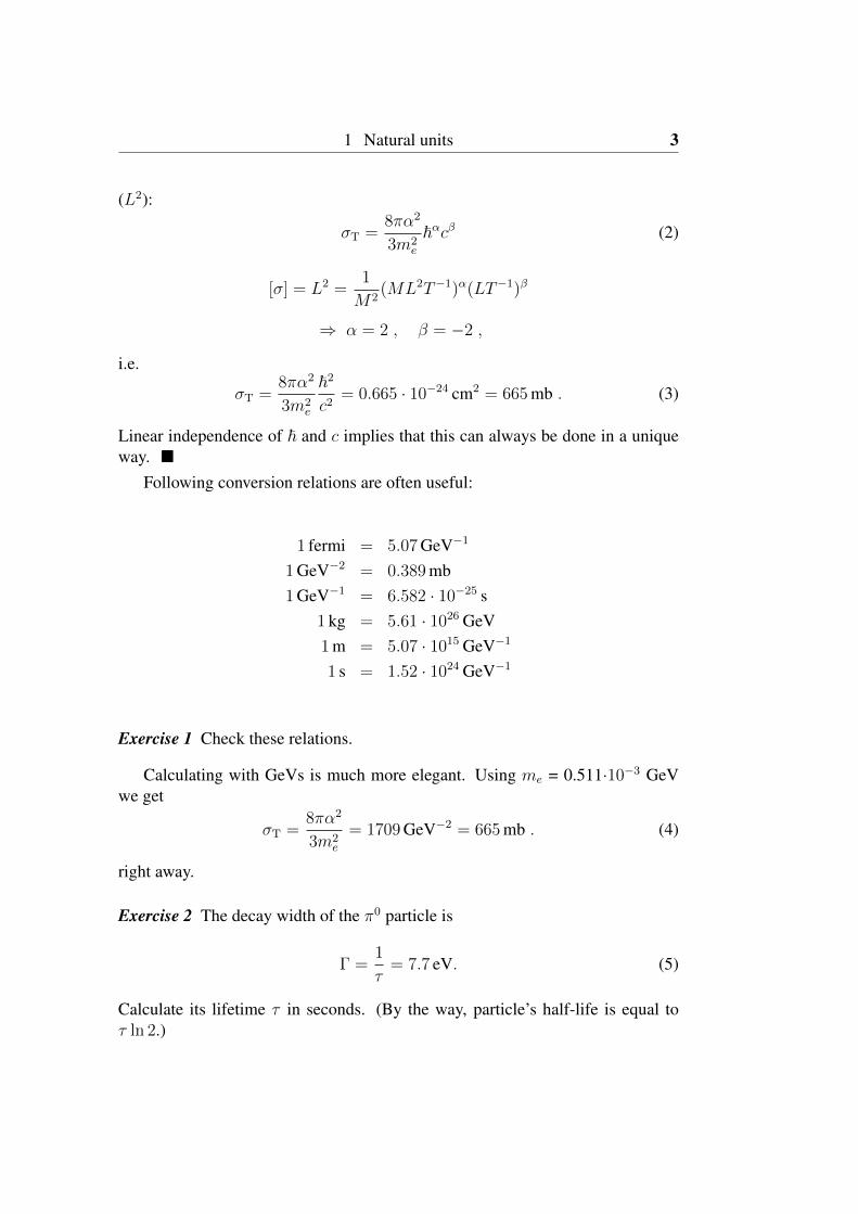
1 Natural units 3

(L2):

σT =8πα2

3m2e

~αcβ (2)

[σ] = L2 =1

M2(ML2T−1)α(LT−1)β

⇒ α = 2 , β = −2 ,

i.e.

σT =8πα2

3m2e

~2

c2= 0.665 · 10−24 cm2 = 665 mb . (3)

Linear independence of ~ and c implies that this can always be done in a uniqueway.

Following conversion relations are often useful:

1 fermi = 5.07 GeV−1

1 GeV−2 = 0.389 mb1 GeV−1 = 6.582 · 10−25 s

1 kg = 5.61 · 1026 GeV1 m = 5.07 · 1015 GeV−1

1 s = 1.52 · 1024 GeV−1

Exercise 1 Check these relations.

Calculating with GeVs is much more elegant. Using me = 0.511·10−3 GeVwe get

σT =8πα2

3m2e

= 1709 GeV−2 = 665 mb . (4)

right away.

Exercise 2 The decay width of the π0 particle is

Γ =1

τ= 7.7 eV. (5)

Calculate its lifetime τ in seconds. (By the way, particle’s half-life is equal toτ ln 2.)

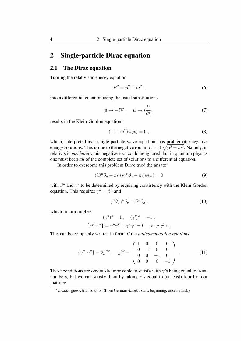
4 2 Single-particle Dirac equation

2 Single-particle Dirac equation

2.1 The Dirac equationTurning the relativistic energy equation

E2 = p2 +m2 . (6)

into a differential equation using the usual substitutions

p→ −i∇ , E → i∂

∂t, (7)

results in the Klein-Gordon equation:

( +m2)ψ(x) = 0 , (8)

which, interpreted as a single-particle wave equation, has problematic negativeenergy solutions. This is due to the negative root inE = ±

√p2 +m2. Namely, in

relativistic mechanics this negative root could be ignored, but in quantum physicsone must keep all of the complete set of solutions to a differential equation.

In order to overcome this problem Dirac tried the ansatz∗

(iβµ∂µ +m)(iγν∂ν −m)ψ(x) = 0 (9)

with βµ and γν to be determined by requiring consistency with the Klein-Gordonequation. This requires γµ = βµ and

γµ∂µγν∂ν = ∂µ∂µ , (10)

which in turn implies(γ0)2 = 1 , (γi)2 = −1 ,

γµ, γν ≡ γµγν + γνγµ = 0 for µ 6= ν .

This can be compactly written in form of the anticommutation relations

γµ, γν = 2gµν , gµν =

1 0 0 00 −1 0 00 0 −1 00 0 0 −1

. (11)

These conditions are obviously impossible to satisfy with γ’s being equal to usualnumbers, but we can satisfy them by taking γ’s equal to (at least) four-by-fourmatrices.∗ ansatz: guess, trial solution (from German Ansatz: start, beginning, onset, attack)

2 Single-particle Dirac equation 5

Now, to satisfy (9) it is enough that one of the two factors in that equation iszero, and by convention we require this from the second one. Thus we obtain theDirac equation:

(iγµ∂µ −m)ψ(x) = 0 . (12)

ψ(x) now has four components and is called the Dirac spinor.One of the most frequently used representations for γ matrices is the original

Dirac representation

γ0 =

(1 00 −1

)γi =

(0 σi

−σi 0

), (13)

where σi are the Pauli matrices:

σ1 =

(0 11 0

)σ2 =

(0 −ii 0

)σ3 =

(1 00 −1

). (14)

This representation is very convenient for the non-relativistic approximation, sincethen the dominant energy terms (iγ0∂0 − . . .−m)ψ(0) turn out to be diagonal.

Two other often used representations are

• the Weyl (or chiral) representation — convenient in the ultra-relativisticregime (where E m)

• the Majorana representation — makes the Dirac equation real; convenientfor Majorana fermions for which antiparticles are equal to particles

(Question: Why can we choose at most one γ matrix to be diagonal?)

Properties of the Pauli matrices:

σi†

= σi (15)

σi∗ = (iσ2)σi(iσ2) (16)

[σi, σj] = 2iεijkσk (17)

σi, σj = 2δij (18)

σiσj = δij + iεijkσk (19)

where εijk is the totally antisymmetric Levi-Civita tensor (ε123 = ε231 = ε312 = 1,ε213 = ε321 = ε132 = −1, and all other components are zero).

Exercise 3 Prove that (σ · a)2 = a2 for any three-vector a.


Exercise 4 Using properties of the Pauli matrices, prove that γ matrices in theDirac representation satisfy γi, γj = 2gij = −2δij , in accordance with theanticommutation relations. (Other components of the anticommutation relations,(γ0)2 = 1, γ0, γi = 0, are trivial to prove.)

Exercise 5 Show that in the Dirac representation γ0γµγ0 = γµ† .

Exercise 6 Determine the Dirac Hamiltonian by writing the Dirac equation in theform i∂ψ/∂t = Hψ. Show that the hermiticity of the Dirac Hamiltonian impliesthat the relation from the previous exercise is valid regardless of the representa-tion.

The Feynman slash notation, /a ≡ aµγµ, is often used.

2.2 The adjoint Dirac equation and the Dirac currentFor constructing the Dirac current we need the equation for ψ(x)†. By taking theHermitian adjoint of the Dirac equation we get

ψ†γ0(i←∂/ +m) = 0 ,

and we define the adjoint spinor ψ ≡ ψ†γ0 to get the adjoint Dirac equation

ψ(x)(i←∂/ +m) = 0 .

ψ is introduced not only to get aesthetically pleasing equations but also becauseit can be shown that, unlike ψ†, it transforms covariantly under the Lorentz trans-formations.

Exercise 7 Check that the current jµ = ψγµψ is conserved, i.e. that it satisfiesthe continuity relation ∂µjµ = 0.

Components of this relativistic four-current are jµ = (ρ, j). Note that ρ =j0 = ψγ0ψ = ψ†ψ > 0, i.e. that probability is positive definite, as it must be.

2.3 Free-particle solutions of the Dirac equationSince we are preparing ourselves for the perturbation theory calculations, we needto consider only free-particle solutions. For solutions in various potentials, see theliterature.

The fact that Dirac spinors satisfy the Klein-Gordon equation suggests theansatz

ψ(x) = u(p)e−ipx , (20)

2 Single-particle Dirac equation 7

which after inclusion in the Dirac equation gives the momentum space Dirac equa-tion

(/p−m)u(p) = 0 . (21)

This has two positive-energy solutions

u(p, σ) = N

χ(σ)

σ · pE +m

χ(σ)

, σ = 1, 2 , (22)

where

χ(1) =

(10

), χ(2) =

(01

), (23)

and two negative-energy solutions which are then interpreted as positive-energyantiparticle solutions

v(p, σ) = −N

σ · pE +m

(iσ2)χ(σ)

(iσ2)χ(σ)

, σ = 1, 2, E > 0 . (24)

N is the normalization constant to be determined later. Spinors above agree withthose of [1]. The momentum-space Dirac equation for antiparticle solutions is

(/p+m)v(p, σ) = 0 . (25)

It can be shown that the two solutions, one with σ = 1 and another with σ = 2,correspond to the two spin states of the spin-1/2 particle.

Exercise 8 Determine momentum-space Dirac equations for u(p, σ) and v(p, σ).

Normalization

In non-relativistic single-particle quantum mechanics normalization of a wave-function is straightforward. Probability that the particle is somewhere in space isequal to one, and this translates into the normalization condition

∫ψ∗ψ dV = 1.

On the other hand, we will eventually use spinors (22) and (24) in many-particlequantum field theory so their normalization is not unique. We will choose nor-malization convention where we have 2E particles in the unit volume:∫

unit volume

ρ dV =

∫unit volume

ψ†ψ dV = 2E (26)

This choice is relativistically covariant because the Lorentz contraction of the vol-ume element is compensated by the energy change. There are other normalizationconventions with other advantages.


Exercise 9 Determine the normalization constant N conforming to this choice.

Completeness

Exercise 10 Using the explicit expressions (22) and (24) show that∑σ=1,2

u(p, σ)u(p, σ) = /p+m , (27)∑σ=1,2

v(p, σ)v(p, σ) = /p−m . (28)

These relations are often needed in calculations of Feynman diagrams with unpo-larized fermions. See later sections.

Parity and bilinear covariants

The parity transformation:

• P : x→ −x, t→ t

• P : ψ → γ0ψ

Exercise 11 Check that the current jµ = ψγµψ transforms as a vector under par-ity i.e. that j0 → j0 and j → −j.

Any fermion current will be of the form ψΓψ, where Γ is some four-by-fourmatrix. For construction of interaction Lagrangian we want to use only thosecurrents that have definite Lorentz transformation properties. To this end we firstdefine two new matrices:

γ5 ≡ iγ0γ1γ2γ3Dirac rep.

=

(0 11 0

), γ5, γµ = 0 , (29)

σµν ≡ i

2[γµ, γν ] , σµν = −σνµ . (30)

Now ψΓψ will transform covariantly if Γ is one of the matrices given in thefollowing table. Transformation properties of ψΓψ, the number of different γ

3 Free quantum fields 9

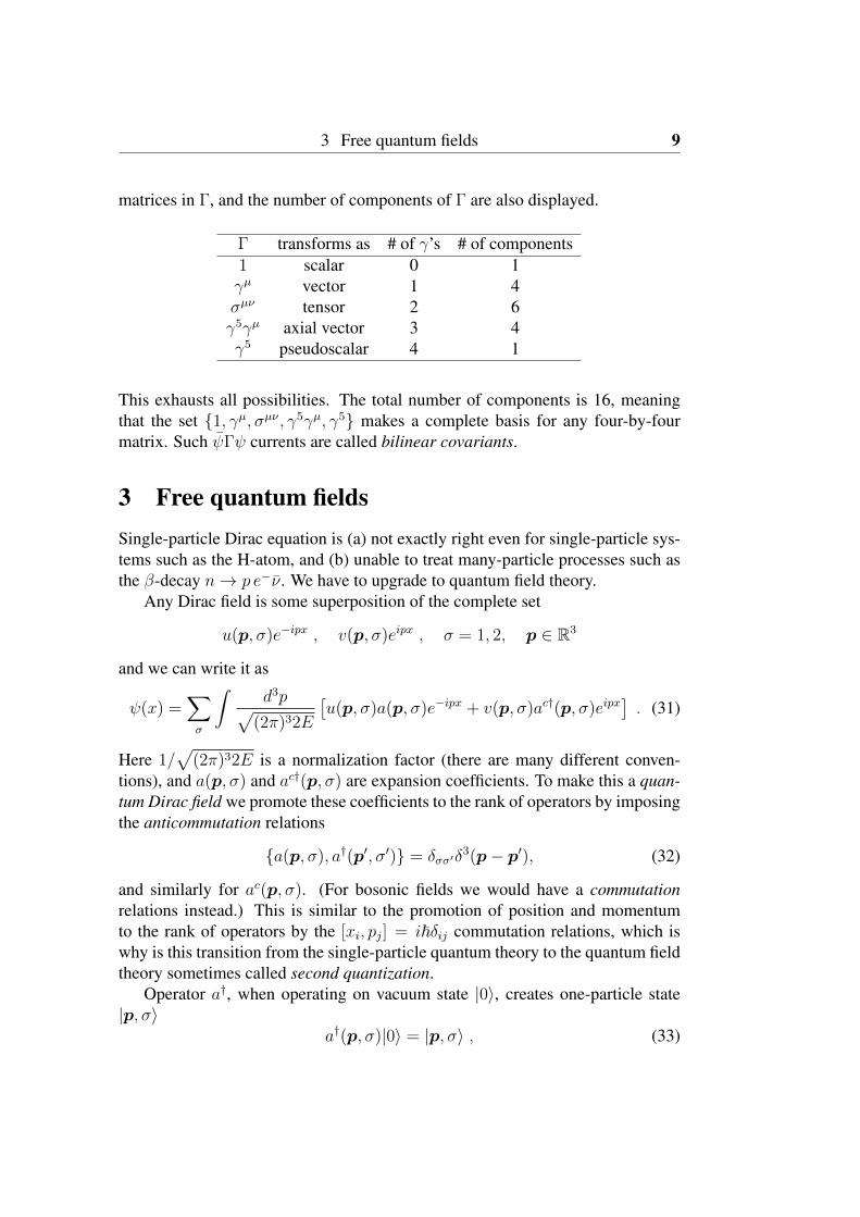
matrices in Γ, and the number of components of Γ are also displayed.

Γ transforms as # of γ’s # of components1 scalar 0 1γµ vector 1 4σµν tensor 2 6γ5γµ axial vector 3 4γ5 pseudoscalar 4 1

This exhausts all possibilities. The total number of components is 16, meaningthat the set 1, γµ, σµν , γ5γµ, γ5 makes a complete basis for any four-by-fourmatrix. Such ψΓψ currents are called bilinear covariants.

3 Free quantum fieldsSingle-particle Dirac equation is (a) not exactly right even for single-particle sys-tems such as the H-atom, and (b) unable to treat many-particle processes such asthe β-decay n→ p e−ν. We have to upgrade to quantum field theory.

Any Dirac field is some superposition of the complete set

u(p, σ)e−ipx , v(p, σ)eipx , σ = 1, 2, p ∈ R3

and we can write it as

ψ(x) =∑σ

∫d3p√

(2π)32E

[u(p, σ)a(p, σ)e−ipx + v(p, σ)ac†(p, σ)eipx

]. (31)

Here 1/√

(2π)32E is a normalization factor (there are many different conven-tions), and a(p, σ) and ac†(p, σ) are expansion coefficients. To make this a quan-tum Dirac field we promote these coefficients to the rank of operators by imposingthe anticommutation relations

a(p, σ), a†(p′, σ′) = δσσ′δ3(p− p′), (32)

and similarly for ac(p, σ). (For bosonic fields we would have a commutationrelations instead.) This is similar to the promotion of position and momentumto the rank of operators by the [xi, pj] = i~δij commutation relations, which iswhy is this transition from the single-particle quantum theory to the quantum fieldtheory sometimes called second quantization.

Operator a†, when operating on vacuum state |0〉, creates one-particle state|p, σ〉

a†(p, σ)|0〉 = |p, σ〉 , (33)

10 3 Free quantum fields

and this is the reason that it is named a creation operator. Similarly, a is an anni-hilation operator

a(p, σ)|p, σ〉 = |0〉 , (34)

and ac† and ac are creation and annihilation operators for antiparticle states (c inac stands for “conjugated”).

Processes in particle physics are mostly calculated in the framework of thetheory of such fields — quantum field theory. This theory can be described atvarious levels of rigor but in any case is complicated enough to be beyond thescope of these notes.

However, predictions of quantum field theory pertaining to the elementaryparticle interactions can often be calculated using a relatively simple “recipe” —Feynman diagrams.

Before we turn to describing the method of Feynman diagrams, let us justspecify other quantum fields that take part in the elementary particle physics inter-actions. All these are free fields, and interactions are treated as their perturbations.Each particle type (electron, photon, Higgs boson, ...) has its own quantum field.

3.1 Spin 0: scalar fieldE.g. Higgs boson, pions, ...

φ(x) =

∫d3p√

(2π)32E

[a(p)e−ipx + ac†(p)eipx

](35)

3.2 Spin 1/2: the Dirac fieldE.g. quarks, leptons

We have already specified the Dirac spin-1/2 field. There are other types: Weyland Majorana spin-1/2 fields but they are beyond our scope.

3.3 Spin 1: vector fieldEither

• massive (e.g. W,Z weak bosons) or

• massless (e.g. photon)

Aµ(x) =∑λ

∫d3p√

(2π)32E

[εµ(p, λ)a(p, λ)e−ipx + εµ∗(p, λ)a†(p, λ)eipx

](36)

4 Golden rules for decays and scatterings 11

εµ(p, λ) is a polarization vector. For massive particles it obeys

pµεµ(p, λ) = 0 (37)

automatically, whereas in the massless case this condition can be imposed thanksto gauge invariance (Lorentz gauge condition). This means that there are onlythree independent polarizations of a massive vector particle: λ = 1, 2, 3 or λ =+,−, 0. In massless case gauge symmetry can be further exploited to eliminateone more polarization state leaving us with only two: λ = 1, 2 or λ = +,−.

Normalization of polarization vectors is such that

ε∗(p, λ) · ε(p, λ) = −1 . (38)

E.g. for a massive particle moving along the z-axis (p = (E, 0, 0, |p|)) we cantake

ε(p,±) = ∓ 1√2

01±i0

, ε(p, 0) =1

m

|p|00E

(39)

Exercise 12 Calculate ∑λ

εµ∗(p, λ)εν(p, λ)

Hint: Write it in the most general form (Agµν + Bpµpν) and then determine Aand B.

The obtained result obviously cannot be simply extrapolated to the masslesscase via the limit m → 0. Gauge symmetry makes massless polarization sumsomewhat more complicated but for the purpose of the simple Feynman diagramcalculations it is permissible to use just the following relation∑

λ

εµ∗(p, λ)εν(p, λ) = −gµν .

4 Golden rules for decays and scatteringsPrincipal experimental observables of particle physics are

• scattering cross section σ(1 + 2→ 1′ + 2′ + · · ·+ n′)

• decay width Γ(1→ 1′ + 2′ + · · ·+ n′)

12 4 Golden rules for decays and scatterings

On the other hand, theory is defined in terms of Lagrangian density of quantumfields, e.g.

L =1

2∂µφ∂

µφ− 1

2m2φ2 − g

4!φ4 .

How to calculate σ’s and Γ’s from L?To calculate rate of transition from the state |α〉 to the state |β〉 in the pres-

ence of the interaction potential VI in non-relativistic quantum theory we have theFermi’s Golden Rule(

α→ β

transition rate

)=

2π

~|〈β|VI |α〉|2 ×

(density of finalquantum states

). (40)

This is in the lowest order perturbation theory. For higher orders we have termswith products of more interaction potential matrix elements 〈|VI |〉.

In quantum field theory there is a counterpart to these matrix elements — theS-matrix:

〈β|VI |α〉+ (higher-order terms) −→ 〈β|S|α〉 . (41)

On one side, S-matrix elements can be perturbatively calculated (knowing theinteraction Lagrangian/Hamiltonian) with the help of the Dyson series

S = 1− i∫d4x1H(x1) +

(−i)2

2!

∫d4x1 d

4x2 TH(x1)H(x2)+ · · · , (42)

and on another, we have “golden rules” that associate these matrix elements withcross-sections and decay widths.

It is convenient to express these golden rules in terms of the Feynman invariantamplitudeM which is obtained by stripping some kinematical factors off the S-matrix:

〈β|S|α〉 = δβα − i(2π)4δ4(pβ − pα)Mβα

∏i=α,β

1√(2π)3 2Ei

. (43)

Now we have two rules:

• Partial decay rate of 1→ 1′ + 2′ + · · ·+ n′

dΓ =1

2E1

|Mβα|2 (2π)4δ4(p1 − p′1 − · · · − p′n)n∏i=1

d3p′i(2π)3 2E ′i

, (44)

• Differential cross section for a scattering 1 + 2→ 1′ + 2′ + · · ·+ n′

dσ =1

uα

1

2E1

1

2E2

|Mβα|2 (2π)4δ4(p1 + p2− p′1− · · · − p′n)n∏i=1

d3p′i(2π)3 2E ′i

,

(45)

5 Feynman diagrams 13

where uα is the relative velocity of particles 1 and 2:

uα =

√(p1 · p2)2 −m2

1m22

E1E2

, (46)

and |M|2 is the Feynman invariant amplitude averaged over unmeasured particlespins (see Section 6.1). The dimension ofM, in units of energy, is

• for decays [M] = 3− n

• for scattering of two particles [M] = 2− n

where n is the number of produced particles.

So calculation of some observable quantity consists of two stages:

1. Determination of |M|2. For this we use the method of Feynman diagramsto be introduced in the next section.

2. Integration over the Lorentz invariant phase space

dLips = (2π)4δ4(p1 + p2 − p′1 − · · · − p′n)n∏i=1

d3p′i(2π)3 2E ′i

.

5 Feynman diagrams

Example: φ4-theory

L =1

2∂µφ∂

µφ− 1

2m2φ2 − g

4!φ4

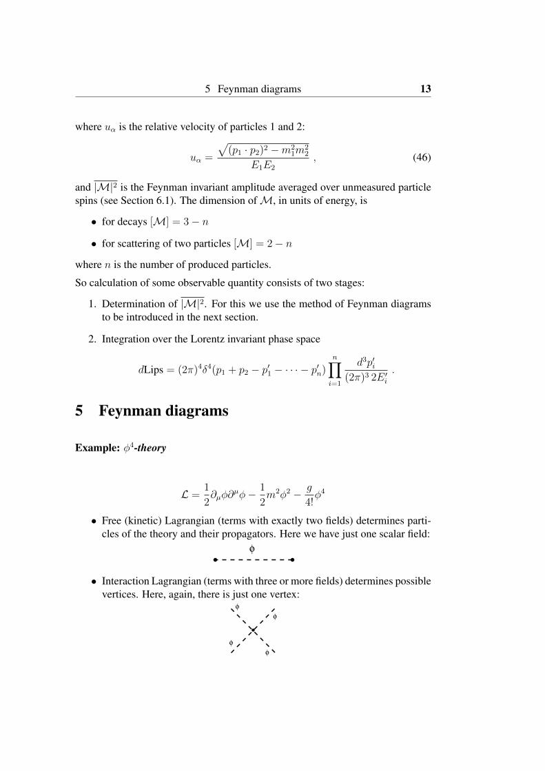
• Free (kinetic) Lagrangian (terms with exactly two fields) determines parti-cles of the theory and their propagators. Here we have just one scalar field:

φ

• Interaction Lagrangian (terms with three or more fields) determines possiblevertices. Here, again, there is just one vertex:

φ

φ

φ

φ

14 5 Feynman diagrams

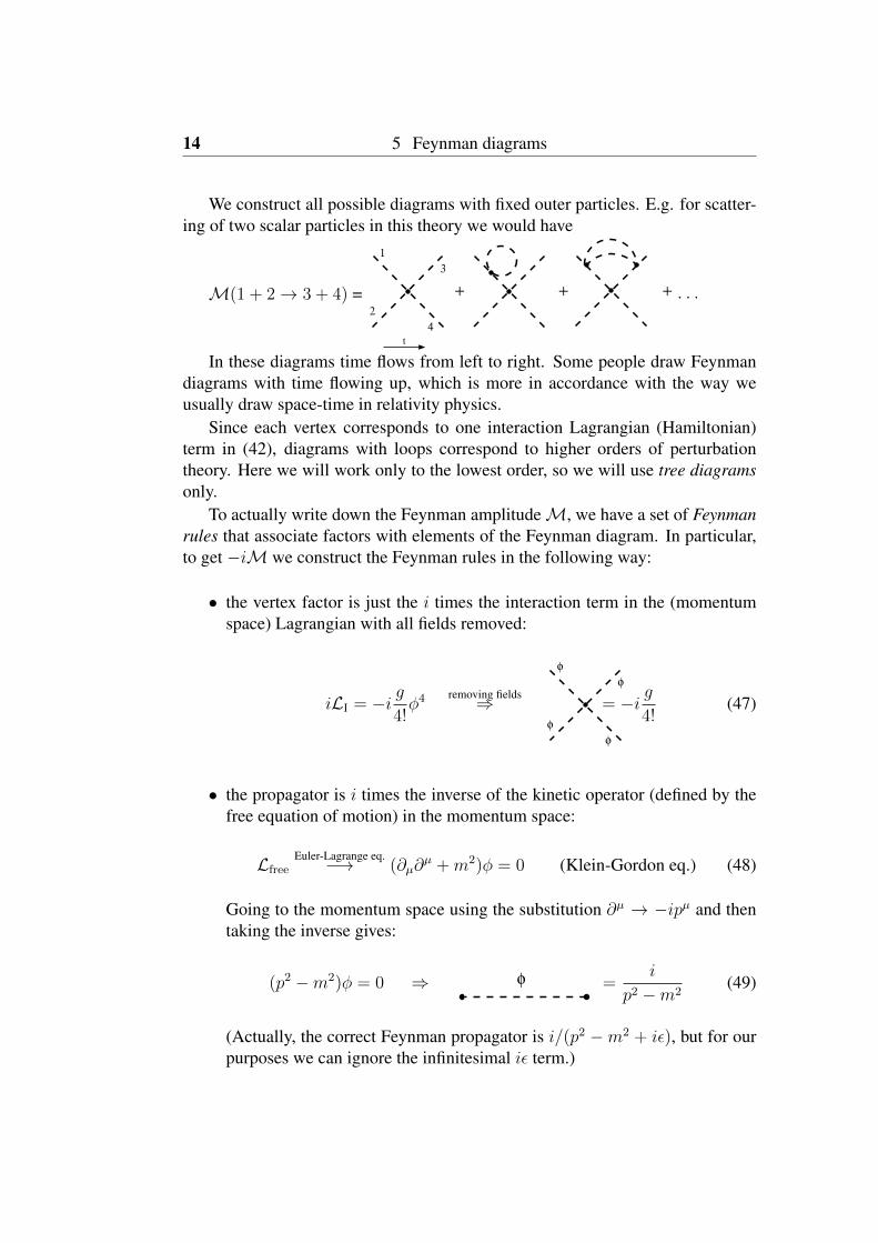
We construct all possible diagrams with fixed outer particles. E.g. for scatter-ing of two scalar particles in this theory we would have

M(1 + 2→ 3 + 4) = + + + . . .

1

2

3

4t

In these diagrams time flows from left to right. Some people draw Feynmandiagrams with time flowing up, which is more in accordance with the way weusually draw space-time in relativity physics.

Since each vertex corresponds to one interaction Lagrangian (Hamiltonian)term in (42), diagrams with loops correspond to higher orders of perturbationtheory. Here we will work only to the lowest order, so we will use tree diagramsonly.

To actually write down the Feynman amplitudeM, we have a set of Feynmanrules that associate factors with elements of the Feynman diagram. In particular,to get −iM we construct the Feynman rules in the following way:

• the vertex factor is just the i times the interaction term in the (momentumspace) Lagrangian with all fields removed:

iLI = −i g4!φ4 removing fields⇒

φ

φ

φ

φ

= −i g4!

(47)

• the propagator is i times the inverse of the kinetic operator (defined by thefree equation of motion) in the momentum space:

LfreeEuler-Lagrange eq.−→ (∂µ∂

µ +m2)φ = 0 (Klein-Gordon eq.) (48)

Going to the momentum space using the substitution ∂µ → −ipµ and thentaking the inverse gives:

(p2 −m2)φ = 0 ⇒ φ =i

p2 −m2(49)

(Actually, the correct Feynman propagator is i/(p2 −m2 + iε), but for ourpurposes we can ignore the infinitesimal iε term.)

5 Feynman diagrams 15

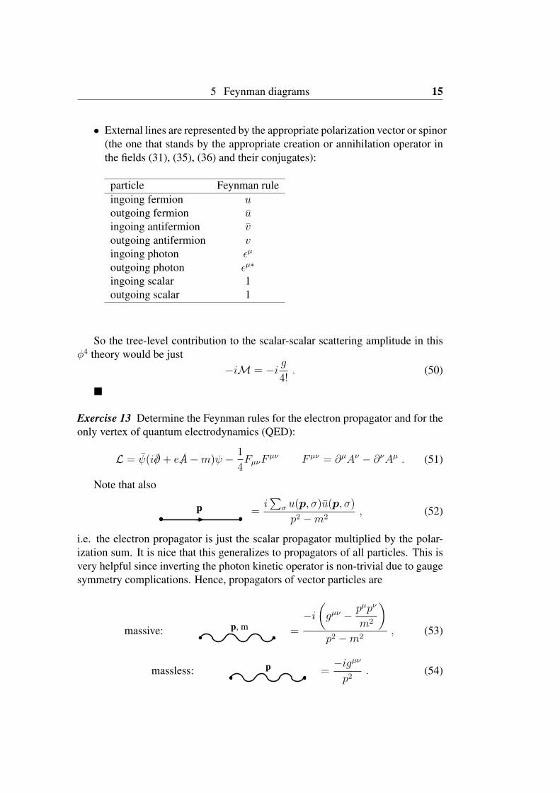
• External lines are represented by the appropriate polarization vector or spinor(the one that stands by the appropriate creation or annihilation operator inthe fields (31), (35), (36) and their conjugates):

particle Feynman ruleingoing fermion uoutgoing fermion uingoing antifermion voutgoing antifermion vingoing photon εµ

outgoing photon εµ∗

ingoing scalar 1outgoing scalar 1

So the tree-level contribution to the scalar-scalar scattering amplitude in thisφ4 theory would be just

−iM = −i g4!. (50)

Exercise 13 Determine the Feynman rules for the electron propagator and for theonly vertex of quantum electrodynamics (QED):

L = ψ(i/∂ + e/A−m)ψ − 1

4FµνF

µν F µν = ∂µAν − ∂νAµ . (51)

Note that also

p =i∑

σ u(p, σ)u(p, σ)

p2 −m2, (52)

i.e. the electron propagator is just the scalar propagator multiplied by the polar-ization sum. It is nice that this generalizes to propagators of all particles. This isvery helpful since inverting the photon kinetic operator is non-trivial due to gaugesymmetry complications. Hence, propagators of vector particles are

massive: p, m =

−i(gµν − pµpν

m2

)p2 −m2

, (53)

massless: p =−igµν

p2. (54)

16 6 Example: e+e− → µ+µ− in QED

This is in principle almost all we need to know to be able to calculate theFeynman amplitude of any given process. Note that propagators and external-linepolarization vectors are determined only by the particle type (its spin and mass)so that the corresponding rules above are not restricted only to the φ4 theory andQED, but will apply to all theories of scalars, spin-1 vector bosons and Diracfermions (such as the standard model). The only additional information we needare the vertex factors.

“Almost” in the preceding paragraph alludes to the fact that in general Feyn-man diagram calculation there are several additional subtleties:

• In loop diagrams some internal momenta are undetermined and we haveto integrate over those. Also, there is an additional factor (-1) for eachclosed fermion loop. Since we will consider tree-level diagrams only, wecan ignore this.

• There are some combinatoric numerical factors when identical fields comeinto a single vertex.

• Sometimes there is a relative (-) sign between diagrams.

• There is a symmetry factor if there are identical particles in the final state.

For explanation of these, reader is advised to look in some quantum field the-ory textbook.

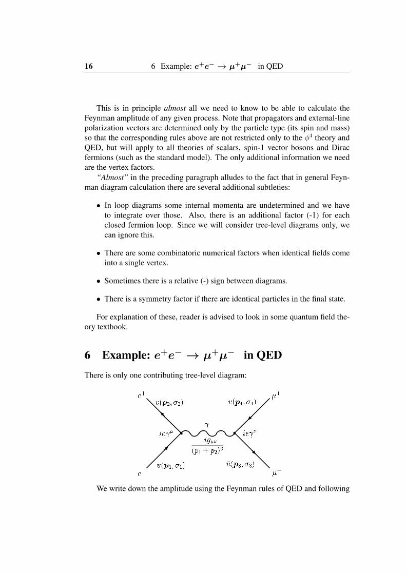
6 Example: e+e− → µ+µ− in QEDThere is only one contributing tree-level diagram:

!#"%$'&)( *+&-,

./02143561)7

89#:%;=<?> @<A

BDC4EF GDH4IKJ

LNM

OQP R#S

TVU

We write down the amplitude using the Feynman rules of QED and following

6 Example: e+e− → µ+µ− in QED 17

fermion lines backwards. Order of lines themselves is unimportant.

−iM = [u(p3, σ3)(ieγν)v(p4, σ4)]

−igµν(p1 + p2)2

[v(p2, σ2)(ieγµ)u(p1, σ1)] ,

(55)or, introducing abbreviation u1 ≡ u(p1, σ1),

M =e2

(p1 + p2)2[u3γµv4][v2γ

µu1] . (56)

Exercise 14 Draw Feynman diagram(s) and write down the amplitude for Comp-ton scattering γe− → γe−.

6.1 Summing over polarizations

If we knew momenta and polarizations of all external particles, we could calculateM explicitly. However, experiments are often done with unpolarized particles sowe have to sum over the polarizations (spins) of the final particles and averageover the polarizations (spins) of the initial ones:

|M|2 → |M|2 =1

2

1

2

∑σ1σ2︸︷︷︸

avg. over initial pol.

sum over final pol.︷︸︸︷∑σ3σ4

|M|2 . (57)

Factors 1/2 are due to the fact that each initial fermion has two polarization(spin) states.(Question: Why we sum probabilities and not amplitudes?)

In the calculation of |M|2 =M∗M, the following identity is needed

[uγµv]∗ = [u†γ0γµv]† = v†γµ†γ0u = [vγµu] . (58)

Thus,

|M|2 =e4

4(p1 + p2)4

∑σ1,2,3,4

[v4γµu3][u1γµv2][u3γνv4][v2γ

νu1] . (59)


6.2 Casimir trickSums over polarizations are easily performed using the following trick. First wewrite

∑[u1γ

µv2][v2γνu1] with explicit spinor indices α, β, γ, δ = 1, 2, 3, 4:∑

σ1σ2

u1αγµαβv2β v2γγ

νγδu1δ . (60)

We can now move u1δ to the front (u1δ is just a number, element of u1 vector, soit commutes with everything), and then use the completeness relations (27) and(28), ∑

σ1

u1δ u1α = (/p1 +m1)δα ,∑σ2

v2β v2γ = (/p2 −m2)βγ ,

which turn sum (60) into

(/p1 +m1)δα γµαβ (/p2 −m2)βγ γ

νγδ = Tr[(/p1 +m1)γ

µ(/p2 −m2)γν ] . (61)

This means that

|M|2 =e4

4(p1 + p2)4Tr[(/p1 +m1)γ

µ(/p2 −m2)γν ] Tr[(/p4 −m4)γµ(/p3 +m3)γν ] .

(62)Thus we got rid off all the spinors and we are left only with traces of γ matri-

ces. These can be evaluated using the relations from the following section.

6.3 Traces and contraction identities of γ matricesAll are consequence of the anticommutation relations γµ, γν = 2gµν , γµ, γ5 =0, (γ5)2 = 1, and of nothing else!

Trace identities

1. Trace of an odd number of γ’s vanishes:

Tr(γµ1γµ2 · · · γµ2n+1) = Tr(γµ1γµ2 · · · γµ2n+1

1︷︸︸︷γ5γ5)

(moving γ5 over each γµi ) = −Tr(γ5γµ1γµ2 · · · γµ2n+1γ5)

(cyclic property of trace) = −Tr(γµ1γµ2 · · · γµ2n+1γ5γ5)

= −Tr(γµ1γµ2 · · · γµ2n+1)

= 0


2. Tr 1 = 4

3.Trγµγν = Tr(2gµν − γνγµ)

(2.)= 8gµν − Trγνγµ = 8gµν − Trγµγν

⇒ 2Trγµγν = 8gµν ⇒ Trγµγν = 4gµν

This also implies:Tr/a/b = 4a · b

4. Exercise 15 Calculate Tr(γµγνγργσ). Hint: Move γσ all the way to theleft, using the anticommutation relations. Then use 3.

Homework: Prove that Tr(γµ1γµ2 · · · γµ2n) has (2n− 1)!! terms.

5. Tr(γ5γµ1γµ2 · · · γµ2n+1) = 0. This follows from 1. and from the fact that γ5

consists of even number of γ’s.

6. Trγ5 = Tr(γ0γ0γ5) = −Tr(γ0γ5γ0) = −Trγ5 = 0

7. Tr(γ5γµγν) = 0. (Same trick as above, with γα 6= µ, ν instead of γ0.)

8. Tr(γ5γµγνγργσ) = −4iεµνρσ, with ε0123 = 1. Careful: convention withε0123 = −1 is also in use.

Contraction identities

1.γµγµ =

1

2gµν (γµγν + γνγµ)︸︷︷︸

2gµν

= gµνgµν = 4

2.γµ γαγµ︸︷︷︸−γµγα+2gαµ

= −4γα + 2γα = −2γα

3. Exercise 16 Contract γµγαγβγµ.

4. γµγαγβγγγµ = −2γγγβγα

Exercise 17 Calculate traces in |M|2:

Tr[(/p1 +m1)γµ(/p2 −m2)γ

ν ] = ?Tr[(/p4 −m4)γµ(/p3 +m3)γν ] = ?

Exercise 18 Calculate |M|2


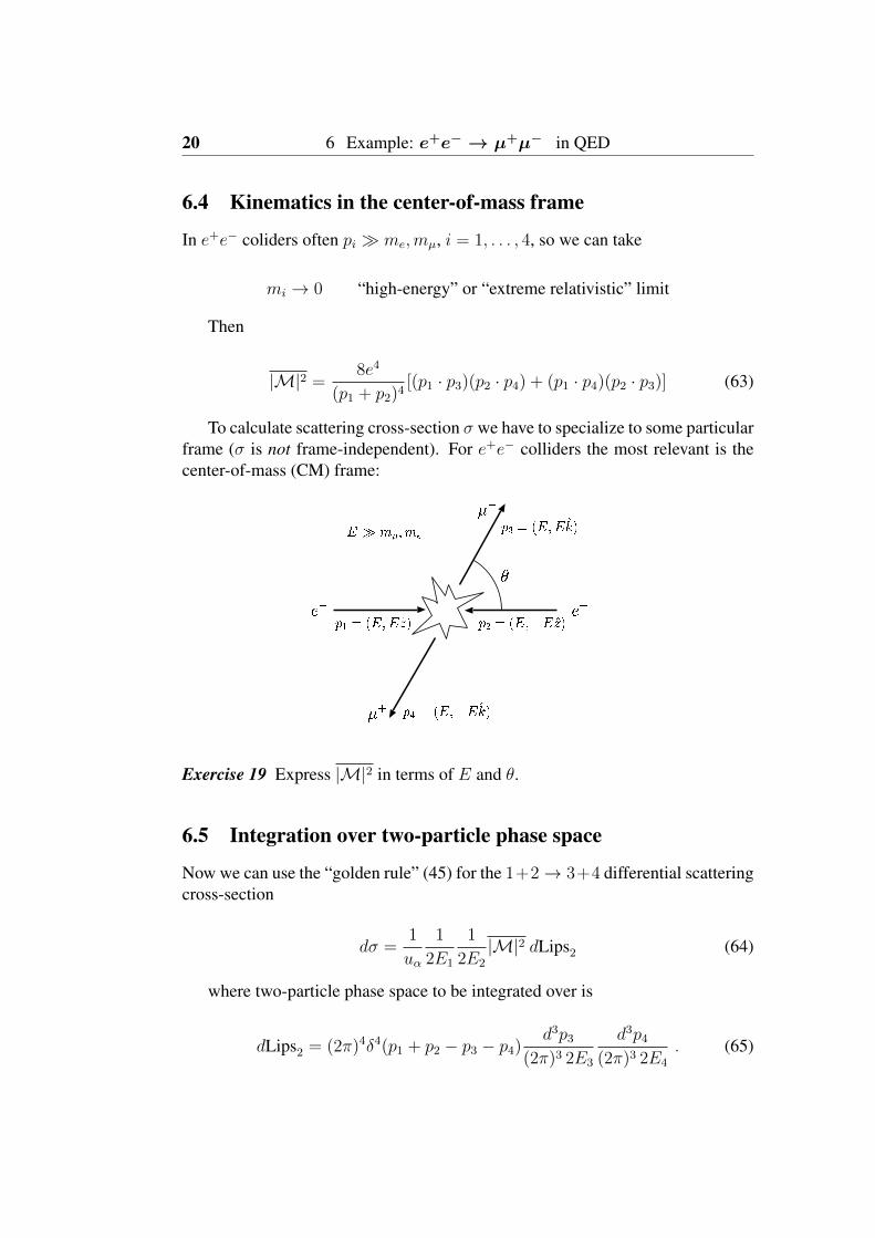
6.4 Kinematics in the center-of-mass frame

In e+e− coliders often pi me,mµ, i = 1, . . . , 4, so we can take

mi → 0 “high-energy” or “extreme relativistic” limit

Then

|M|2 =8e4

(p1 + p2)4[(p1 · p3)(p2 · p4) + (p1 · p4)(p2 · p3)] (63)

To calculate scattering cross-section σ we have to specialize to some particularframe (σ is not frame-independent). For e+e− colliders the most relevant is thecenter-of-mass (CM) frame:

!"#%$&"'(*)

+,.-0/12143576

89;:<=>%?&=A@BDC

E

FHGJILKMNILO

Exercise 19 Express |M|2 in terms of E and θ.

6.5 Integration over two-particle phase space

Now we can use the “golden rule” (45) for the 1+2→ 3+4 differential scatteringcross-section

dσ =1

uα

1

2E1

1

2E2

|M|2 dLips2 (64)

where two-particle phase space to be integrated over is

dLips2 = (2π)4δ4(p1 + p2 − p3 − p4)d3p3

(2π)3 2E3

d3p4(2π)3 2E4

. (65)


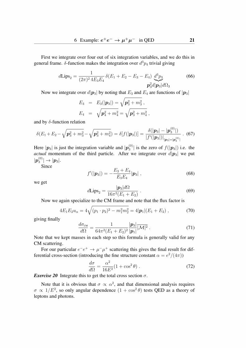
First we integrate over four out of six integration variables, and we do this ingeneral frame. δ-function makes the integration over d3p4 trivial giving

dLips2 =1

(2π)2 4E3E4

δ(E1 + E2 − E3 − E4) d3p3︸︷︷︸

p23d|p3|dΩ3

(66)

Now we integrate over d|p3| by noting that E3 and E4 are functions of |p3|

E3 = E3(|p3|) =√p23 +m2

3 ,

E4 =√p24 +m2

4 =√p23 +m2

4 ,

and by δ-function relation

δ(E1 +E2−√p23 +m2

3−√p23 +m2

4) = δ[f(|p3|)] =δ(|p3| − |p(0)3 |)|f ′(|p3|)||p3|=|p(0)

3 |. (67)

Here |p3| is just the integration variable and |p(0)3 | is the zero of f(|p3|) i.e. theactual momentum of the third particle. After we integrate over d|p3| we put|p(0)3 | → |p3|.

Sincef ′(|p3|) = −E3 + E4

E3E4

|p3| , (68)

we get

dLips2 =|p3|dΩ

16π2(E1 + E2). (69)

Now we again specialize to the CM frame and note that the flux factor is

4E1E2uα = 4√

(p1 · p2)2 −m21m

22 = 4|p1|(E1 + E2) , (70)

giving finallydσCM

dΩ=

1

64π2(E1 + E2)2|p3||p1||M|2 . (71)

Note that we kept masses in each step so this formula is generally valid for anyCM scattering.

For our particular e−e+ → µ−µ+ scattering this gives the final result for dif-ferential cross-section (introducing the fine structure constant α = e2/(4π))

dσ

dΩ=

α2

16E2(1 + cos2 θ) . (72)

Exercise 20 Integrate this to get the total cross section σ.

Note that it is obvious that σ ∝ α2, and that dimensional analysis requiresσ ∝ 1/E2, so only angular dependence (1 + cos2 θ) tests QED as a theory ofleptons and photons.


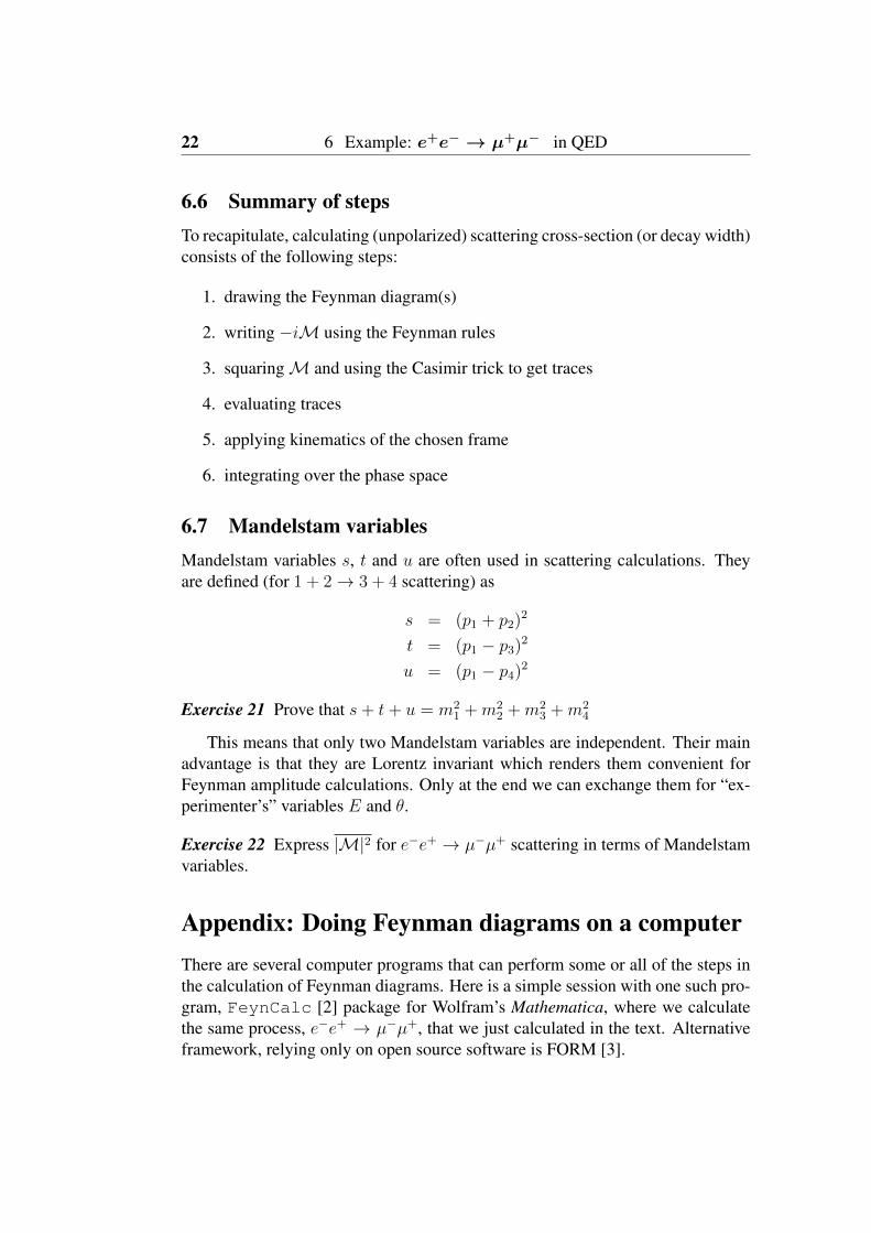
6.6 Summary of stepsTo recapitulate, calculating (unpolarized) scattering cross-section (or decay width)consists of the following steps:

1. drawing the Feynman diagram(s)

2. writing −iM using the Feynman rules

3. squaringM and using the Casimir trick to get traces

4. evaluating traces

5. applying kinematics of the chosen frame

6. integrating over the phase space

6.7 Mandelstam variablesMandelstam variables s, t and u are often used in scattering calculations. Theyare defined (for 1 + 2→ 3 + 4 scattering) as

s = (p1 + p2)2

t = (p1 − p3)2

u = (p1 − p4)2

Exercise 21 Prove that s+ t+ u = m21 +m2

2 +m23 +m2

4

This means that only two Mandelstam variables are independent. Their mainadvantage is that they are Lorentz invariant which renders them convenient forFeynman amplitude calculations. Only at the end we can exchange them for “ex-perimenter’s” variables E and θ.

Exercise 22 Express |M|2 for e−e+ → µ−µ+ scattering in terms of Mandelstamvariables.

Appendix: Doing Feynman diagrams on a computerThere are several computer programs that can perform some or all of the steps inthe calculation of Feynman diagrams. Here is a simple session with one such pro-gram, FeynCalc [2] package for Wolfram’s Mathematica, where we calculatethe same process, e−e+ → µ−µ+, that we just calculated in the text. Alternativeframework, relying only on open source software is FORM [3].

REFERENCES 23

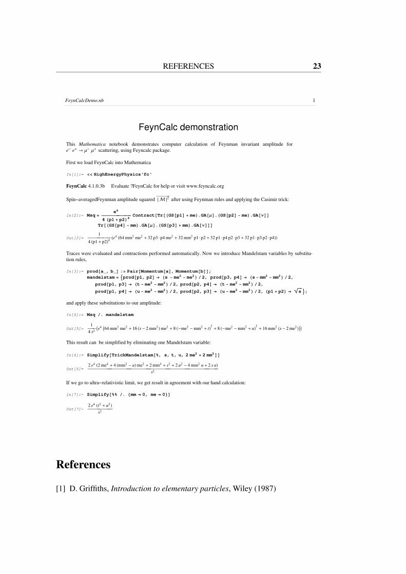
FeynCalc demonstration

This Mathematica notebook demonstrates computer calculation of Feynman invariant amplitude fore- e+ ® Μ- Μ+ scattering, using Feyncalc package.

First we load FeynCalc into Mathematica

In[1]:= << HighEnergyPhysics‘fc‘

FeynCalc 4.1.0.3b Evaluate ?FeynCalc for help or visit www.feyncalc.org

Spin−averaged Feynman amplitude squared È M È2 after using Feynman rules and applying the Casimir trick:

In[2]:= Msq =e4

4 Hp1 + p2L4

Contract@Tr@HGS@p1D + meL.GA@ΜD.HGS@p2D - meL.GA@ΝDD

Tr@HGS@p4D - mmL.GA@ΜD.HGS@p3D + mmL.GA@ΝDDDOut[2]=

14 Hp1 + p2L4

He4 H64 mm2 me2 + 32 p3 × p4 me2 + 32 mm2 p1 × p2 + 32 p1 × p4 p2 × p3 + 32 p1 × p3 p2 × p4LLTraces were evaluated and contractions performed automatically. Now we introduce Mandelstam variables by substitu-tion rules,

In[3]:= prod@a_, b_D := Pair@Momentum@aD, Momentum@bDD;mandelstam = 9prod@p1, p2D ® Hs - me2 - me2L 2, prod@p3, p4D ® Hs - mm2 - mm2L 2,

prod@p1, p3D ® Ht - me2 - mm2L 2, prod@p2, p4D ® Ht - me2 - mm2L 2,prod@p1, p4D ® Hu - me2 - mm2L 2, prod@p2, p3D ® Hu - me2 - mm2L 2, Hp1 + p2L ®

!!!!s =;

and apply these substitutions to our amplitude:

In[5]:= Msq . mandelstam

Out[5]=1

4 s2

Ie4 I64 mm2 me2 + 16 Hs - 2 mm2 L me2 + 8 H-me2 - mm2 + tL2+ 8 H-me2 - mm2 + uL2

+ 16 mm2 Hs - 2 me2 LMMThis result can be simplified by eliminating one Mandelstam variable:

In[6]:= Simplify@TrickMandelstam@%, s, t, u, 2 me2 + 2 mm2DDOut[6]=

2 e4 H2 me4 + 4 Hmm2 - uL me2 + 2 mm4 + s2 + 2 u2 - 4 mm2 u + 2 s uL

s2

If we go to ultra−relativistic limit, we get result in agreement with our hand calculation:

In[7]:= Simplify@%% . 8mm ® 0, me ® 0<DOut[7]=

2 e4 Ht2 + u2 L

s2

FeynCalcDemo.nb 1

References

[1] D. Griffiths, Introduction to elementary particles, Wiley (1987)

24 REFERENCES

[2] V. Shtabovenko, R. Mertig and F. Orellana, New Developments in FeynCalc9.0, arXiv:1601.01167 [hep-ph].

[3] J. A. M. Vermaseren, New features of FORM, math-ph/0010025.

Quantization of the Free Electromagnetic Field:Photons and Operators

G. M. [email protected], http://www.phys.ksu.edu/personal/wysin

Department of Physics, Kansas State University, Manhattan, KS 66506-2601

August, 2011, Vicosa, Brazil

Summary

The main ideas and equations for quantized free electromagnetic fields are developed

and summarized here, based on the quantization procedure for coordinates (components

of the vector potential A) and their canonically conjugate momenta (components of the

electric field E). Expressions for A, E and magnetic field B are given in terms of the

creation and annihilation operators for the fields. Some ideas are proposed for the inter-

pretation of photons at different polarizations: linear and circular. Absorption, emission

and stimulated emission are also discussed.

1 Electromagnetic Fields and Quantum Mechanics

Here electromagnetic fields are considered to be quantum objects. It’s an interesting subject, and thebasis for consideration of interactions of particles with EM fields (light). Quantum theory for lightis especially important at low light levels, where the number of light quanta (or photons) is small,and the fields cannot be considered to be continuous (opposite of the classical limit, of course!).

Here I follow the traditinal approach of quantization, which is to identify the coordinates andtheir conjugate momenta. Once that is done, the task is straightforward. Starting from the classicalmechanics for Maxwell’s equations, the fundamental coordinates and their momenta in the QM sys-tem must have a commutator defined analogous to [x, px] = ih as in any simple QM system. Thisgives the correct scale to the quantum fluctuations in the fields and any other dervied quantities.The creation and annihilation operators will have a unit commutator, [a, a†] = 1, but they haveto be connected to the fields correctly. I try to show how these relations work. Getting the cor-rect normalization on everything is important when interactions of the EM fields with matter areconsidered.

It is shown that the quantized fields are nothing more than a system of decoupled harmonicoscillators, at a collection of different wavevectors and wave-polarizations. The knowledge of how toquantize simple harmonic oscillators greatly simplifies the EM field problem. In the end, we get tosee how the basic quanta of the EM fields, which are called photons, are created and annihilated indiscrete processes of emission and absorption by atoms or matter in general. I also want to discussdifferent aspects of the photons, such as their polarization, transition rules, and conservation laws.

Later in related notes I’ll talk about how this relates to describing two other topics of interest:quantum description of the dielectric response of materials (dielectric function ε(ω)), and, effectsinvolving circularly polarized light incident on a material in the presence of a DC magnetic field(Faraday effect). I want to describe especially the quantum theory for the Faraday effect, which isthe rotation of the polarization of linearly polarized light when it passes through a medium in aDC magnetic field parallel to the light rays. That is connected to the dielectric function, hence theinterest in these related topics.

1.1 Maxwell’s equations and Lagrangian and Hamiltonian Densities

A Lagrangian density for the free EM field is

L =18π

[E2 −B2

](1)

1

[It’s integral over time and space will give the classical action for a situation with electromagneticfields.] This may not be too obvious, but I take it as an excercise for the reader in classical mechanics,because here we want to get to the quantum problem. Maxwell’s equations in free space, writtenfor the electric (E) and magnetic (B) fields in CGS units, are

∇ ·B = 0, ∇×E +1c

∂B∂t

= 0, ∇ ·E = 0, ∇×B− 1c

∂E∂t

= 0 (2)

The zero divegence of B and Faraday’s Law (1st and 2nd eqns) allow the introduction of vector andscalar potentials, A and Φ, respectively, that give the fields,

B = ∇×A, E = −∇Φ− 1c

∂A∂t

(3)

I consider a problem far from sources. If sources were present, they would appear in the last twoequations in (2), so these same potentials could still apply. The potentials are not unique and havea gauge symmetry. They can be shifted using some guage transformation (f) without changing theelectric and magnetic fields:

A′ = A +∇f, Φ′ = Φ− 1c

∂f

∂t(4)

The Euler-Lagrange variation of the Lagrangian w.r.t the coordinates q = (Φ, Ax, Ay, Az) givesback Maxwell’s equations. Recall Euler-Lagrange equation and try it as a practice problem inclassical mechanics.

To approach quantization, the canonical momenta pi need to be identified. But there is no timederivative of Φ in L, so there is no pΦ and Φ should be eliminated as a coordinate, in some sense.There are time derivatives of A, hence their canonical momenta are found as

pi =∂L∂Ai

=1

4πc

(∂Φ∂xi

+1c

∂Ai

∂t

)= − 1

4πcEi, i = 1, 2, 3 (5)

The transformation to the Hamiltonian energy density is the Legendre transform,

H =∑

i

piqi − L = p · ∂A∂t

− L = 2πc2p 2 +18π

(∇×A)2 − cp · ∇Φ (6)

When integrated over all space, the last term gives nothing, because ∇ · E = 0, and the first twoterms give a well known result for the effective energy density, in terms of the EM fields,

H =18π

(E2 + B2

)(7)

We might keep the actual Hamiltonian in terms of the coordinates A and their conjugate momentap, leading to the classical EM energy,

H =∫d3r

[2πc2p 2 +

18π

(∇×A)2]

(8)

Now it is usual to apply the Coulomb gauge, where Φ = 0 and ∇ ·A = 0. For one, this insureshaving just three coordinates and their momenta, so the mechanics is consistent. Also that isconsistent with the fields needing three coordinates because they are three-dimensional fields. (Wedon’t need six coordinates, because E and B are not independent. In a vague sense, the magneticand electric fields have some mutual conjugate relationship.) We can use either the Lagrangian orHamiltonian equations of motion to see the dynamics. For instance, by the Hamiltonian method,we have

qi =δHδpi

, pi = −δHδqi

(9)

Recall that the variation of a density like this means

δHδf

≡ ∂H∂f

−∑

i

∂

∂xi

∂H

∂(

∂f∂xi

) − ∂

∂t

∂H

∂(

∂f∂t

) (10)

2

The variation for example w.r.t coordinate qi = Ax gives the results

∂Ax

∂t= 4πc2px,

∂px

∂t=

14π∇2Ax (11)

By combining these, we see that all the components of the vector potential (and the conjugatemomentum, which is proportional to E) satisfy a wave equation, as could be expected!

∇2A− 1c2∂2A∂t2

= 0 (12)

Wave motion is essentially oscillatory, hence the strong connection of this problem to the harmonicoscillator solutions.

The above wave equation has plane wave solutions eik·r−ωkt at angular frequency ωk and wavevector k that have a linear dispersion relation, ωk = ck. For the total field in some volume V , we cantry a Fourier expansion over a collection of these modes, supposing periodic boundary conditions.

A(r, t) =1√V

∑k

Ak(t) eik·r (13)

Each coefficient Ak(t) is an amplitude for a wave at the stated wave vector. The different modesare orthogonal (or independent), due to the normalization condition∫

d3r eik·r e−ik′·r = V δkk′ (14)

The gauge assumption ∇ · k = 0 then is the same as k ·Ak = 0, which shows that the waves aretransverse. For any k, there are two transverse directions, and hence, two independent polarizationsdirections, identified by unit vectors ekα, α = 1, 2. Thus the total amplitude looks like

Ak = εk1Ak1 + εk2Ak2 =∑α

εkαAkα (15)

Yet, from the wave equation, both polarizations are found to oscillate identically, except perhapsnot in phase,

Ak(t) = Ak e−iωkt (16)

Now the amplitudes Ak are generally complex, whereas, we want to have the actual field beingquantized to be real. This can be accomplished by combining these waves appropriately with theircomplex conjugates. For example, the simple waves A = cos kx = (eikx +e−ikx)/2 and A = sin kx =(eikx−e−ikx)/2i are sums of ”positive” and ”negative” wavevectors with particular amplitudes. Tryto write A in (13) in a different way that exhibits the positive and negative wavevectors together,

A(r, t) =1

2√V

∑k

[Ak(t) eik·r + A−k(t) e−ik·r] (17)

[The sum over k here includes wave vectors in all directions. Then both k and −k are includedtwice. It is divided by 2 to avoid double counting.] In order for this to be real, a little considerationshows that the 2nd term must be the c.c. of the first term,

A−k = Ak∗ (18)

A wave needs to identified by both Ak and its complex conjugate (or equivalently, two real constants).So the vector potential is written in Fourier space as

A(r, t) =1

2√V

∑k

[Ak(t) eik·r + A∗

k(t) e−ik·r] (19)

Note that the c.c. reverses the sign on the frequency also, so the first term oscillates at positivefrequency and the second at negative frequency. But curiously, both together give a real wave

3

traveling along the direction of k. Based on this expression, the fields are easily determined byapplying (3), with ∇ → ±ik,

E(r, t) =i

2c√V

∑k

ωk

[Ak(t) eik·r −A ∗

k (t) e−ik·r] (20)

B(r, t) =i

2√V

∑k

k×[Ak(t) eik·r −A ∗

k (t) e−ik·r] (21)

Now look at the total energy, i.e., evaluate the Hamiltonian. It should be easy because of theorthogonality of the plane waves, assumed normalized in a box of volume V . We also know thatk is perpendicular to A (transverse waves!) which simplifies the magnetic energy. Still, some careis needed in squaring the fields and integrating. There are direct terms (btwn k and itself) andindirect terms (btwn k and −k).∫

d3r |E|2 =1

4c2V

∑k

∑k′

ωkωk′

∫d3r

[Ake

ik·r −A∗ke−ik·r] [

A∗k′e−ik′·r −Ak′eik′·r

](22)

Upon integration over the volume, the orthogonality relation will give 2 terms with k′ = k and 2terms with k′ = −k, for 4 equivalent terms in all. The same happens for the calculation of themagnetic energy. Also one can’t forget that Ak is the same as A∗

−k. These become

18π

∫d3r |E|2 =

18π

∑k

ω2k

c2|Ak(t)|2 (23)

18π

∫d3r |B|2 =

18π

∑k

k2|Ak(t)|2 (24)

Of course, k2 in the expression for magnetic energy is the same as ω2k/c

2 in that for electric energy.Then it is obvious that the magnetic and electric energies are equal. The net total energy is simple,

H =18π

∫d3r

(|E|2 + |B|2

)=

18π

∑k

k2|Ak|2 =14π

∑kα

k2|Akα|2 (25)

The last form recalls that each wave vector is associated with two independent polarizations. Theyare orthogonal, so there are no cross terms between them from squaring.

The Hamiltonian shows that the modes don’t interfere with each other, imagine how it is possiblethat EM fields in vacuum can be completely linear! But this is good because now we just need toquantize the modes as if they are a collection of independent harmonic oscillators. To do that,need to transform the expression into the language of the coordinates and conjugate momenta. Itwould be good to see H expressed through squared coordinate (potential energy term) and squaredmomentem (kinetic energy term).

The electric field is proportional to the canonical momentum, E = −4πcp. So really, the electricfield energy term already looks like a sum of squared momenta. Similarly, the magnetic field isdetermined by the curl of the vector potential, which is the basic coordinate here. So we have somerelations,

p(r, t) = − 14πc

E =−i

8πc2√V

∑k

ωk

[Ak(t) eik·r −A ∗

k (t) e−ik·r] (26)

This suggests the introduction of the momenta at each wavevector, i.e., analogous with the Fourierexpansion for the vector potential (i.e., the generalized coordinates),

p(r, t) =1

2√V

∑k

[pk(t) eik·r + p∗k(t) e−ik·r] (27)

Then we can make the important identifications,

pk(t) =−iωk

4πc2Ak(t) (28)

4

Even more simply, just write the electric field (and its energy) in terms of the momenta now.

E(r, t) = −4πcp(r, t) =−2πc√V

∑k

[pk(t)eik·r + p∗k(t)e−ik·r] (29)

When squared, the electric energy involves four equivalent terms, and there results

18π

∫d3r |E|2 =

16π2c2

8π

∑k

pk · p∗k = 2πc2∑k

pk · p∗k (30)

Also rewrite the magnetic energy. The generalized coordinates are the components of A, i.e., let’swrite

qk = Ak (31)

Consider the magnetic field written this way,

B(r, t) =i

2√V

∑k

k×[qk(t) eik·r − q∗k(t) e−ik·r] (32)

and the associated energy is written,

18π

∫d3r |B|2 =

44× 8π

∑k

k2qk · q∗k =1

8πc2∑k

ω2kqk · q∗k (33)

This gives the total canonical Hamiltonian, expressed in the Fourier modes, as

H = 2πc2∑k

pk · p∗k +1

8πc2∑k

ω2kqk · q∗k (34)

Check that it works for the classical problem. To apply correctly, one has to keep in mind thatat each mode k, there are the two amplitudes, qk and q∗k. In addition, it is important to rememberthat the sum goes over all positive and negative k, and that q−k is the same as q∗k.

Curiously, look what happens if you think that the Hamiltonian has only real coordinates, andwrite incorrectly

Hoo =∑k

[2πc2p2

k +ω2

k

8πc2q2k

](35)

The Hamilton equations of motion become

pk =δHoo

δqk=

ω2k

4πc2qk, qk = −δHoo

δpk= −4πc2 pk (36)

Combining these actually leads to the correct frequency of oscillation, but only by luck!

pk =ω2

k

4πc2qk = −ω2

k pk, qk = −4πc2 pk = −ω2k qk (37)

These are oscillating at frequency ωk.Now do the math (more) correctly. Variation of Hamiltonian (34) w.r.t. qk and q∗k are different

things. On the other hand, qk and q∗−k are the same, so don’t forget to account for that. It meansthat a term at negative wave vector is just like the one at positive wave vector: q−kq∗−k = q∗kqk.This doubles the interaction. The variations found are

pk =δH

δqk=

ω2k

4πc2q∗k, qk = − δH

δpk= −4πc2 p∗k (38)

p∗k =δH

δq∗k=

ω2k

4πc2qk, q∗k = − δH

δp∗k= −4πc2 pk (39)

Now we can see that the correct frequency results, all oscillate at ωk. For example,

pk =ω2

k

4πc2q∗k = −ω2

kpk qk = −4πc2 p∗k = −ω2kqk (40)

There are tricky steps in how to do the algebra correctly. Once worked through, we find that thebasic modes oscillate at the frequency required by the light wave dispersion relation, ωk = ck.

5

1.2 Quantization of modes: Simple harmonic oscillator example

Next the quantization of each mode needs to be accomplished. But since each mode analogous to aharmonic oscillator, as we’ll show, the quantization is not too difficult. We already can see that themodes are independent. So proceed essentially on the individual modes, at a given wave vector andpolarization. But I won‘t for now be writing any polarization indices, for simplicity.

Recall the quantization of a simple harmonic oscillator. The Hamiltonian can be re-expressed insome rescaled operators:

H =p2

2m+mω2

2q2 =

hω

2(P 2 +Q2

); Q =

√mω

hq, P =

1√mhω

p (41)

Then if the original commutator is [x, p] = ih, we have a unit commutator here,

[Q,P ] =√mω

h

1√mhω

[x, p] = i (42)

The Hamiltonian can be expressed in a symmetrized form as follows:

H =hω

212

[(Q+ iP )(Q− iP ) + (Q− iP )(Q+ iP )] (43)

This suggest defining the annihilation and creation operators

a =1√2(Q+ iP ), a† =

1√2(Q− iP ) (44)

Their commutation relation is then conveniently unity,

[a, a†] = (1√2)2[Q+ iP,Q− iP ] =

12−i[Q,P ] + i[P,Q] = 1 (45)

The coordinate and momentum are expressed

Q =1√2(a+ a†), P =

1i√

2(a− a†). (46)

The Hamiltonian becomesH =

hω

2(aa† + a†a) = hω(a†a+

12) (47)

where the last step used the commutation relation in the form, aa† = a†a+1. The operator n = a†ais the number operator that counts the quanta of excitation. The number operator can be easilyshown to have the following commutation relations:

[n, a] = [a†a, a] = [a†, a]a = −a, [n, a†] = [a†a, a†] = a†[a, a†] = +a, (48)

These show that a† creates or adds one quantum of excitation to the system, while a destroys orremoves one quantum. The Hamiltonian famously shows how the system has a zero-point energy ofhω/2 and each quantum of excitation adds an additional hω of energy.

The eigenstates of the number operator n = a†a are also eigenstates of H. And while a anda† lower and raise the number of quanta present, the eigenstates of the Hamiltonian are not theireigenstates. But later we need some matrix elements, hence it is good to summarize here exactlythe operations of a or a† on the number eigenstates, |n〉, which are assumed to be unit normalized.

If a state |n〉 is a normalized eigenstate of n, with eigenvalue n, then we must have

a†|n〉 = cn|n+ 1〉, 〈n|a = c∗n〈n+ 1| (49)

where cn is a normalization constant. Putting these together, and using the commutation relation,gives

1 = 〈n|aa†|n〉 = |cn|2〈n+ 1|n+ 1〉 =⇒ |cn|2 = 〈n|aa†|n〉 = 〈n|a†a+ 1|n〉 = n+ 1 (50)

6

In the same fashion, consider the action of the lowering operator,

a|n〉 = dn|n− 1〉, 〈n|a† = d∗n〈n− 1| (51)

1 = 〈n|a†a|n〉 = |dn|2〈n− 1|n− 1〉 =⇒ |dn|2 = 〈n|a†a|n〉 = n (52)

Therefore when these operators act, they change the normalization slightly, and we can write

a†|n〉 =√n+ 1 |n+ 1〉, a|n〉 =

√n |n− 1〉. (53)

Indeed, the first of these can be iterated on the ground state |0〉 that has no quanta, to produce anyexcited state:

|n〉 =1√n!

(a†)n|0〉 (54)

Based on these relations, then it is easy to see the basic matrix elements,

〈n+ 1|a†|n〉 =√n+ 1, 〈n− 1|a|n〉 =

√n. (55)

An easy way to remember these, is that the factor in the square root is always the larger of thenumber of quanta in either initial or final states. These will be applied later.

1.3 Fundamental commutation relations for the EM modes

Now how to relate what we know to the EM field Hamiltonian, Eqn. (34)? The main difference thereis the presence of operators together with their complex conjugates in the classical Hamiltonian. Howto decide their fundamental commutators? That is based on the fundamental commutation relationin real space (for one component only):

[Ai(r, t), pi(r′, t)] = ih δ(r− r′). (56)

The fields are expressed as in Eqns. (19) and (27). Using these expressions to evaluate the LHS of(56),

[Ai(r, t), pi(r′, t)] =1

4V

∑k

∑k′

[Ake

ik·r + A∗ke−ik·r,pk′eik′·r′

+ p∗k′e−ik′·r′]

(57)

In a finite volume, however, the following is a representation of a delta function:

δ(r− r′) =1V

∑k

eik·(r−r′) (58)

Although not a proof, we can see that (56) and (57) match if the mode operators have the followingcommutation relations (for each component):

[Ak,p∗k′ ] = ihδk,k′ , [A∗k,pk′ ] = ihδk,k′ , [Ak,pk′ ] = ihδk,−k′ , [A∗

k,p∗k′ ] = ihδk,−k′ . (59)

These together with the delta function representation, give the result for the RHS of (57),

[Ai(r, t), pi(r′, t)] =1

4V

∑±k

ih[2eik·(r−r′) + 2ei−k·(r−r′)

]= ih δ(r− r′). (60)

Thus the basic commutators of the modes are those in (59). Now we can apply them to quantizethe EM fields.

7

1.4 The quantization of the EM fields

At some point, one should keep in mind that these canonical coordinates are effectively scalars, oncethe polarization is accounted for:

qk =∑α

εkqkα, pk =∑α

εkpkα. (61)

The polarizations are decoupled, so mostly its effects can be ignored. But then the Hamiltonian(34) really has two terms at each wavevector, one for each polarization. For simplicity I will notbe writing the polarization index, but just write scalar qk and pk for each mode’s coordinate andmomentum. For any scalar coordinate and its momentum, we postulate from (59)

[qk, p†k′ ] = ihδk,k′ , [q†k, pk′ ] = ihδk,k′ , [qk, pk′ ] = ihδk,−k′ , [q†k, p

†k′ ] = ihδk,−k′ , (62)

Note that the first two look to be inconsistent if you think of the adjoint operation as just complexconjugate. But they are correct. Noting that (AB†)† = BA†, we have

[A,B†]† = BA† −A†B = [B,A†] = −[A†, B] (63)

Then applied to the problem with A = qk and B = pk′

[q†k, pk′ ] = −[qk, p†k′ ]† = −(ihδk,k′)† = ihδk,k′ (64)

So although the relations look unsual, they are correct.Let’s look at some algebra that hopefully leads to creation and annihilation operators. First, get

some coordinates and momenta with unit normalized commutators. Suppose that a given mode kαhas a Hamiltonian from (34). Consider first one term at one wave vector: [Even though, classically,the terms at k and −k in the sum give equal contributions] Consider making a transformation toQk and Pk,

H+kα = 2πc2p†kpk +ω2

k

8πc2q†kqk =

hωk

2

(P †kPk +Q†kQk

)(65)

Here because it is a quantum problem, we suppose that the terms from k and −k modes really arenot the same. Thus there is a similar term for the negative wave vector:

H−kα = 2πc2p†−kp−k +ω2

k

8πc2q†−kq−k =

hωk

2

(P †−kP−k +Q†−kQ−k

)(66)

The right hand sides are the same as the energies for SHO’s in the normalized coordinates andmomenta. However, we have relations like q†−k = qk, and q−k = q†k, and we suppose they shouldapply to the new rescaled coordinates and momenta. So this latter relation also takes the form

H−kα = 2πc2pkp†k +

ω2k

8πc2qkq

†k =

hωk

2

(PkP

†k +QkQ

†k

)(67)

In the quantum problem, the order in which conjugate operators act is important and should notbe modified. So H+kα and H−kα are not the same. To match the sides, try the identifications

Pk =

√4πc2

hωkpk, Qk =

√ωk

4πc2hqk (68)

The basic commutator that results between them is now unit normalized,

[Qk, P†k] =

√ωk

4πc2h

√4πc2

hωk[qk, p

†k] =

1hih = i (69)

It is obvious one can also show[Q†k, Pk] = i (70)

8

Now we can re-express the energy in the sense of operators like what was done for the SHO,although it is more complicated here because of the two directions for the wavevectors. Note thefollowing algebra that results if we try that, for complex operators:

F1 =12

[(Qk + iPk)(Q†k − iP †k) + (Q†k − iP †k)(Qk + iPk)

]= Q†kQk + P †kPk +

i

2

[PkQ

†k +Q†kPk − P †kQk −QkP

†k

](71)

That has extra terms that we do not want. To get rid of them, consider also the contribution fromthe opposite wave vector. We use the same form, but with −k, and employing Q−k = Q†k, P−k = P †k.

F2 =12

[(Q−k + iP−k)(Q†−k − iP †−k) + (Q†−k − iP †−k)(Q−k + iP−k)

]=

12

[(Q†k + iP †k)(Qk − iPk) + (Qk − iPk)(Q†k + iP †k)

]= Q∗kQk + P ∗kPk −

i

2

[PkQ

†k +Q†kPk − P †kQk −QkP

†k

](72)

So the combination of the two expressions eliminates the imaginary part, leaving only the part wewant in the Hamiltonian. Therefore, algebraically speaking we can write:

H+kα =hωk

212(F1 + F2) (73)

Based on these expressions, introduce creation and annihilation operators, for both the positive andnegative wave vectors:

ak =1√2(Qk + iPk), a†k =

1√2(Q†k − iP †k). (74)

a−k =1√2(Q†k + iP †k), a†−k =

1√2(Qk − iPk). (75)

By their definitions, they must have unit real commutators, e.g.,

[ak, a†k] =

1√

22 [Qk + iPk, Q

†k − iP †k] =

12

−i[Qk, P

†k] + i[Pk, Q

†k]

= 1 (76)

On the other hand, a commutator between different modes (or with different polarizations at onewave vector) gives zero. The individual term in the Hamiltonian sum is

H+kα =hωk

212

[aka

†k + a†kak + a−ka

†−k + a†−ka−k

](77)

So the total field Hamiltonian is the sum

H =∑k

hωk

2

[a†kak + 1/2 + a†−ka−k + 1/2

](78)

The sum is over all wave vectors, and the positive and negative terms give the same total, so

H =∑kα

hωk

(a†kαakα +

12

)=

∑kα

(nkα +

12

)(79)

The number operator is implicitly defined here:

nkα = a†kαakα (80)

Then each mode specified by a wave vector and a polarization contributes hω(a†kαakα + 1/2) tothe Hamiltonian. Every mode is equivalent, mathematically, to a simple harmonic oscillator. What

9

could be more simple? Really, it is hard to believe, when you think about it. The modes arecompletely independent, at this level, they do not interfere. There is just a linear superposition oftheir EM fields. To get those fields, summarize a few more relationships.

The fields associated with the creation and annihilation operators are found via solving theirdefinitions,

Qk =1√2(ak + a†−k), Pk =

1i√

2(ak − a†−k), (81)

Then with

Akα = Akαεkα, Akα = qkα =

√4πc2hωk

Qkα, (82)

applied into (19), the quantized fields are determined,

A(r, t) =1

2√V

∑k

εkα

√

4πc2hωk

(akα + a†−kα)√

2eik·r +

√4πc2hωk

(a−kα + a†kα)√2

e−ik·r

(83)

Swapping some terms between the positive and negative wave vector sums, this is the same as

A(r, t) =

√2πc2hV

∑k

εkα√ωk

[akαe

ik·r + a†kαe−ik·r

](84)

Then the vector potential determines both the electric and magnetic fields by (20) and (21), whichgive

E(r, t) = i

√2πhV

∑k

ωkεkα√ωk

[akαe

ik·r − a†kαe−ik·r

](85)

B(r, t) = i

√2πhV

∑k

ck× εkα√ωk

[akαe


](86)

Indeed, after all this work, the fields have a certain simplicity. Their amplitude depends on Planck’sconstant. Thus there must be quantum fluctuations determined by it.

The above do not show the explicit time dependence. However, that is implicit in the cre-ation/annihilation operators. Based on the Hamiltonian, their equations of motion are simple:

ihakα = [akα,H] = hωk[ak, a†kαakα] = hωk[akα, a

†kα]akα = +hωkakα (87)

iha†kα = [a†kα,H] = hωk[a†kα, a†kαakα] = hωka

†kα[a†kαakα] = −hωka

†kα (88)

And then they oscillate at opposite frequencies:

akα = −iωkakα =⇒ akα(t) = akα(0)e−iωkt (89)

a†kα = +iωka†kα =⇒ a†kα(t) = a†kα(0)e+iωkt (90)

1.5 Quantized field properties: momentum, angular momentum

The fields not only carry energy, but it is directed, so they carry linear momentum and even angularmomentum. The linear momentum is

G =∫d3r

E×B4πc

=i2

4πchc

V

∑kα

∑k′α′

[εkα × (k′ × εk′α′)]×∫d3r (akαe

ik·r − a†kαe−ik·r)(ak′α′eik′·r − a†k′α′e

−ik′·r) (91)

10

The orthognality relation only gives nonzero terms where k′ = k and k′ = −k, and there results

G =hc

4π

∑kα

∑k′α′

[εkα×(k′× εk′α′)]

(akαa†k′α′ + a†kαak′α′)δk,k′ − (akαak′α′ + a†kαa

†k′α′)δk,−k′

(92)

The orthogonality of the polarization vectors with each other and with k forces that vector crossproduct to be just kδα,α′ . Only the direct terms give a nonzero result:

G =hc

4π

∑kα

k(akαa†kα + a†kαakα) =

∑kα

hck a†kαakα (93)

There is no zero point term, because of the cancellation between a term at +k and one at −k. Theneach mode carries a linear momentum of hck.

Consider the angular momentum. The contribution from the fields is

J =1

4πc

∫d3r [r× (E×B)] (94)

But there is the identity,[r× (E×B)] = E(r ·B)− (r ·E)B. (95)

Furthermore, for any mode, the wave vector is perpendicular to both E and B. So this definition ofangular momentum seems to give zero for the total component along the direction of propagation.Even if it more properly symmetrized for the QM problem, it still gives zero.

That shows that the concept of angular momentum in an EM field is tricky. Possibly, assuminga plane wave is too restrictive, and instead one should not make any particular assumption on thenature of the fields, to start with. One can do a more careful analysis, that shows the angularmomentum is composed from an orbital part and a spin part.

Consider the following vector algebra for the ith component of the argument in the angularmomentum integral (essentially, the angular momentum density). Here the Levi-Civita symbol isused for the cross products, and the magnetic field is expressed via the vector potential. Repeatedindeces are summer over.

[r× (E×B)]i = εijk xj(E×B)k = εijk xj εklmElBm

= εijk xj εklmEl (εmnp∂nAp)= εijk xj El(δknδlp − δkpδln)∂nAp

= εijk xj [El∂kAl − El∂lAk] (96)

Now when this is integrated over all space, the last term can be integrated by parts, dropping anyvanishing surface terms at infinity. Further, far from any sources, the electric field is divergenceless,so ~∇ ·E = ∂lEl = 0. So now the expression becomes

[r× (E×B)]i = εijk [xjEl∂kAl + ∂l(xjEl)Ak] = εijk [xjEl∂kAl + δljElAk]= εijk [xjEl∂kAl + EjAk] = El(εijk xj∂k)Al + εijk EjAk (97)

This is an interesting expression. The first term contains effectively the orbital angular momentumoperator acting between E and A. The second term is their cross product. Then the total angularmomentum integrated over space is

J =1

4πc

∫d3r El(r×∇)Al + E×A (98)

Both terms can be written as operators acting between the fields, adding h in appropriate places:

[r× (E×B)]i =i

hEl(−ih εijk xj∂k)Al + Ej(−ih εijk )Ak (99)

11

The first term in (99) contains the orbital angular momentum operator, Li = (r× p)i, acting onidentical components of E and A; it is a diagonal operator. The second contains what is a spin-1operator, for which one can write its ith component,

(Si)jk = −ih εijk, (S)jk = (Sixi)jk = −ih xiεijk. (100)

Then the total angular momentum is expressed as a sum of these two parts, each being matrixelements of an operator,

J =i

4πhc

∫d3r Ej [(r× p)δjk + (S)jk]Ak (101)

Well, really (Si)jk comes from the cross product operator, however, it can be seen to be a quantumspin operator, that couples different components of E and A. This operator is defined here by itsmatrices, one for each component i, where j and k are the column and row

(Si)jk

(i = x, y, z) = −ihεijk = −ih

0 0 00 0 10 −1 0

,−ih

0 0 −10 0 01 0 0

,−ih

0 1 0−1 0 00 0 0

.

(102)Check some properties to be convinced that this is really a spin-1 operator. Consider a commu-tator between two of these, using the properties of the Levi-Civita symbol. Start from the matrixmultiplications, giving the lnth element of the matrix products:

[(Si)(Sj)]ln = (Si)lm(Sj)mn = (−ih)2εilm εjmn = (−ih)2(δinδlj − δijδln) (103)

[(Sj)(Si)]ln = (Sj)lm(Si)mn = (−ih)2εjlm εimn = (−ih)2(δjnδli − δjiδln) (104)

The difference cancels the last terms,

[(Si)(Sj)− (Sj)(Si)]ln = (−ih)2(δinδlj − δjnδli) (105)

Then the difference of deltas can be put back into a product of ε’s.

[(Si)(Sj)− (Sj)(Si)]ln = (−ih)2(−εijk)εlnk = ihεijk[−ihεkln] = ihεijk(Sk)ln. (106)

Therefore these matrices do have the commutation relations for an angular momentum,

[(Si), (Sj)] = ih εijk (Sk). (107)

Also, look at the matrix of ~S2, within the space that the operators act:

(~S2)ln = (Si)lm(Si)mn = (−ih)2εilmεimn = (−ih)2(δlmδmn − δlnδmm) (108)

The expression is summed over m = x, y, z, both the terms are diagonal. But δlmδmn = δln, whileδmm = 3. Then this square is the diagonal matrix:

(~S2)ln = (−ih)2(δln − 3δln) = 2h2δln. (109)

This clearly has s(s+ 1) = 2 with s = 1, so indeed it corresponds to spin-1.It may seem curious, that none of the matrices are diagonal. But this just means that the

Cartesian axes, to which these correspond, are not the good quantization axes. For example, findthe eigenvectors of the operator (Sx). The eigenvalue problem is

(Sx − λI)(u) =

−λ 0 00 −λ −ih0 ih −λ

ux

uy

uz

= 0. (110)

The eigenvalues are obviously λ = 0,±h. The sx = 0 eigenvector is trivial, u = (1, 0, 0), andseems to have little physical importance. The sx = +h eigenvector is u = 1√

2(0, 1, i) and the

12

sx = −h eigenvector is u = 1√2(0, 1,−i). If the vector potential were expressed in these as a

basis, the spin angular momentum components along x are specified. But this basis is not the pureCartesian components. It requires linear combinations of Cartesian components out of phase by±90. These combinations are states of circular polarization, which are the ”good” states of spinangular momentum. Thus, none of these three matrices is diagonal when expressed in Cartesiancomponents. More on the spin angular momentum and EM-wave polarization is discussed in thenext section.

Note, if one had seeked the eigenvectors of the matrix (Sz), one finds they are u = (0, 0, 1) forsz = 0, and u = (1, i, 0) for sz = +h, and u = (1,−i, 0) for sz = −h. These last two correspondto states where the A and E fields are rotating around the z-axis. It is typical to consider wavespropagating along z, hence, we see these vectors appear again when polarization is discussed for thiswave vector direction.

Thus the second part of the angular momentum involves just the cross product of E and A,which is considered the intrinsic spin angular momentum in the EM fields. It can seen to be thesame as the canonical angular momentum in the fields, although it is hard to say in general whythis is true. If one uses a definition like (coordinate × conjugate momentum), integrated over space,where the coordinate is the vector potential, and its conjugate momentum is −E/4πc, one gets

S =∫d3r A× −E

4πc=−14πc

∫d3r (A×E) (111)

Except for the ordering, it is the same as S obtained above. Assume the ordering doesn’t matter(both are fields depending on position), and continue to evaluate it,

S =−14πc

ihc

V

∑kα

∑k′α′

εkα × εk′α′

∫d3r

[akαe

ik·r + a†kαe−ik·r

] [ak′α′eik′·r − a†k′α′e

−ik′·r]

(112)

The integrations are the usual orthogonality relations, which give terms where k′ = k and termswhere k′ = −k. Only the first set gives nonzero results, due to the cross products of the polarizationvectors (Take them oppositely directed for the −k mode compared to the k mode. Further, we lookfor a quantity whose expectation value is nonzero.) So there remains only the terms

S =ih

4π

∑kαα′

εkα × εkα′(akαa†kα′ − a†kαakα′) (113)

Here the two polarizations must be different to give a nonzero result. We suppose they are orientedin such a way that

εk1 × εk2 = k (114)

so that this cross product is along the propagation direction. Then there are two equal terms andthe net is

S =∑k

ihk (ak1a†k2 − a†k1ak2) (115)

As shown with the eigenvalues of the S matrices, the basic unit of spin angular momentum is h, andit has a component only along (or opposite to) the propagation direction.

1.6 Orbital angular momentum

Mostly in atomic processes, the spin angular momentum is absorbed or emitted when photons areabsorbed or emitted by atoms. Not much is usually mentioned about the orbital angular momentumin the EM fields. Consider here what L is for the quantized EM field, using the expression,

L =1

4πc

∫d3r El(r×∇)Al. (116)

13

If the ∇ operation is applied to the fields in (84), it pulls out ik for each mode. One then has

(r×∇)Al =

√2πc2hV

∑k

xl · εkα√ωk

r× (ik)[akαe


](117)

Now combine with the same component of the electric field,

El(r×∇)Al = i

√2πhV

∑k′α′

ωk′ xl · εk′α′√ωk′

[ak′α′eik′·r − a†k′α′e

−ik′·r]

×√

2πc2hV

∑kα

xl · εkα√ωk

r× (ik)[akαe


](118)

The orbital angular momentum then is

L =ih

4πV

∑k,k′,αα′

√ωk′

ωkεk′α′ · εkα

∫d3r r

[ak′α′eik′·r − a†k′α′e

−ik′·r] [akαe


]× (ik)(119)

The basic integral to evaluate here is not exactly a normalization integral:

Ix =∫d3r xeik′·reik·r = −i ∂

∂kx

∫d3r eik′·reik·r = −i ∂

∂kxV δk,k′ (120)

It would seem to be zero, although singular in some sense. For now I’ll consider that the orbitalangular momentum should be zero.

One thing that can be said with more certainty is the component of L along the propagationdirection, k, for some mode in the sum. As [r × (ik)] · k = 0, for a particular mode, there is noorbital angular momentum component in the direction of propagation.

1.7 Polarization

It is better to express the spin angular momentum S in terms of circular polarization components.In the expressions for E, the cartesian polarization vectors could be re-expressed in terms of rotatingbasis vectors. For example, consider a wave moving in the z direction, with ε1 = x and ε2 = y. Thenif you look at, for example,

(x+ iy)e−iωt = (x cosωt+ y sinωt) + i(−x sinωt+ y cosωt) (121)

At t = 0, the real part is along x and the imaginary part is along y. At time progresses, both the realand imaginary parts rotate counterclockwise when viewed in the usual xy-plane. I am supposingthis multiplying the positive wave, akeik·r. Then both of these rotate in the positive helicity sense,where the angular momentum is in the same direction as the wave propagation. The following waverotates in the opposite sense, clockwise or negative helicity:

(x− iy)e−iωt = (x cosωt− y sinωt) + i(−x sinωt− y cosωt) (122)

These suggest inventing polarization basis vectors for these two helicities (the wave vector index issuppressed),

εL = ε+ =1√2(ε1 + iε2), εR = ε− =

1√2(ε1 − iε2) (123)

I use L and R for left and right in place of positive and negative. The inverse relations are

ε1 =1√2(εL + εR), ε2 =

1i√

2(εL − εR) (124)

Then we see that in the expression for the electric field, there appears a combination∑

α εkαakα, or

ε1ak1 + ε2ak2 =1√2(εL + εR)ak1 +

1i√

2(εL− εR)ak2 =

1√2(ak1− iak2)εL +

1√2(ak1 + iak2)εR (125)

14

This shows the two new alternative (circularly polarized) annihilation operators,

akL ≡1√2(ak1 − iak2), akR ≡ 1√

2(ak1 + iak2). (126)

Their inverse relations are

ak1 =1√2(akL + akR), ak2 =

i√2(akL − akR). (127)

Then a sum can be over either linear or circular basis:∑α

εkαakα = ε1ak1 + ε2ak2 = εLakL + εRakR (128)

Additionally there are the corresponding creation operators,

a†kL ≡1√2(a†k1 + ia†k2), a†kR ≡ 1√

2(a†k1 − ia†k2). (129)

Their inverse relations are

a†k1 =1√2(a†kL + a†kR), a†k2 =

−i√2(a†kL − a†kR). (130)

The expressions for the fields really don’t depend on which basis is used. However, the ones statedearlier do need to be modified to be more general, since now the basis vectors can be complex. Tobe totally consistent for the creation terms, we need to satisfy the conjugate relation∑

α

ε†kαa†kα = ε†1a

†k1 + ε†2a

†k2 = ε†La

†kL + ε†Ra

†kR (131)

It means that the correct expressions for the fields in the case of complex basis vectors must be

A(r, t) =

√2πc2hV

∑k

1√ωk

[εkαakαe

ik·r + ε†kαa†kαe

−ik·r]

(132)

E(r, t) = i

√2πhV

∑k

√ωk

[εkαakαe

ik·r − ε†kαa†kαe

−ik·r]

(133)

B(r, t) = i

√2πhV

∑k

ck×√ωk

[εkαakαe

ik·r − ε†kαa†kαe

−ik·r]

(134)

The combinations of operators with their conjugates shows that these totals are hermitian.Now the expression for the spin angular mometum can be expressed using the circular compo-

nents,

S =∑k

ihk

[1√2(akL + akR)

−i√2(a†kL − a†kR)− 1√

2(a†kL + a†kR)

i√2(akL − akR)

](135)

The different polarizations commute, and the only nonzero commutation relations for the circularpolarization creation and annihilation operators are

[akL, a†kL] = 1, [akR, a

†kR] = 1. (136)

So all that survives after using the commutation relations is

S =∑k

hk[a†kLakL − a†kRakR

](137)

15

This apparently involves number operators for each circular polarization. The left states contribute+hk and the right states contribute −hk to the total angular momentum. So in a sense, one canconsider that photons carry an intrinsic angular momentum of magnitude h. Then they can beconsidered as particles with spin-1. The numbers operators in this expression count the number ofphotons in each helicity or circular polarization state.

The creation operators generate quanta of the EM field, in some sense. There are the linearpolarization operators and the circular ones. We might think of the circular state as a linear com-bination of two linear states, and vice versa. Does a photon have an intrinsic angular momentum?Perhaps it is not a reasonable question. Depending on what is measured, you may only see eitherthe linear components or only the circular components. The basis you would use is determined byhow the experiment is performed, i.e., by what states your experiment projects out. However, somephoton-atom interactions, for example, may be most sensitive to the circular components. Thenthat type of experiment would view the photons as having circular polarization and as being spin-1particles.

2 Interactions of EM fields with matter

EM fields are always coupled to charged particles. Here coupling of the quantized EM field tononrelativistic charges is considered. It is expected that this is a situation where a perturbationapproach can be applied. It means, we think the eigenstates of some material problem are known,and we want to see the perturbations due to the application of light. Or, it could be we want to seethe emission of light that is expected, either spontaneously due to fluctuations in the EM field, orstimulated by the EM field. This is a brief summary of how to go about these calculations.

The usual prescription to include interactions is to modify the four-momentum of the particle ofcharge q, according to the effects of the field it experiences,

p −→ p− q

cA, E −→ E − qA0 (138)

where A is the vector potential and A0 is the scalar potential φ. The energy operator is the usualE = ih ∂

∂t and the momentum operator is the usual p = −ih∇. The original problem in the absenceof the fields is a Schrodinger problem HΨ = EΨ,[

p2

2m+ V (r)

]Ψ(r, t) = ih

∂

∂tΨ(r, t) (139)

When the EM fields are now turned on, this changes to[1

2m

(p− q

cA

)2

+ V (r) + qA0

]Ψ(r, t) = ih

∂

∂tΨ(r, t) (140)

Then the effective Hamiltonian for the perturbed problem is just

H =1

2m

(p− q

cA

)2

+ V (r) + qA0 (141)

The simplest case is to consider a single particle or charge as it interacts with the field. In addition,there is supposed to be the Hamiltonian for the free EM fields themselves, as we quantized in theprevious section. So the total effective Hamiltonian for particle in the field is

H =p2

2m+ V (r)− q

2mc(A · p + p ·A) +

q2A2

2mc2+ qA0 +Hphotons (142)

The first two terms are the free particle, the next three terms are the interaction with the EM fields,and the last term is the free photon Hamiltonian, whose eigenstates are states with certain numbersof photons are given wavevectors and polarizations.

Although not necessary, we can continue to use the radiation gauge, where∇ ·A = 0 and A0 = 0,as we used for the free photons. This implies p ·A = A · p. Then there are only two interaction

16

terms, one that is linear in A and one that is quadratic in A. The linear terms will involve individualphoton creation and annihilation terms, corresponding to single-photon processes that can be ana-lyzed in first order perturbation theory. The quadratic terms correspond to two-photon processeseven in first order PT, and probably to get those correct would actually require second order PT.However, they should be smaller. Thus the leading perturbation is due to only the single-photonterm,

H1 = − q

mcA · p +

q2A2

2mc2≈ − q

mcA · p (143)

Note that the A operator is due to the EM field (creation/annihilation) while the p operator isassociated with the charged particle momentum only. These would act on composite bra or ketsinvolving both the EM field state and the particle state.

In a basic process where the final state has one less photon than the initial state, a photon wasabsorbed by the matter. On the other hand, if the final state has one more photon than the initialstate, a photon was emitted by the matter.

In absorption, the absorbed photon could come from any direction dΩ. In emission, the emittedphoton can go out in any direction dΩ. In either case, some density of states is involved in thecalculation of the rate for the process, consistent with conservation of energy and other variables.

2.1 First order perturbations: single photon events

The amplitude for a transition between some initial and final states is given by a matrix element,which goes into Fermi’s Golden Rule to get the transition rate:

wI→F =2πh|〈ΨF |H1|ΨI〉|2 ρ (144)

where ρ is some density of states for the photon involved. The interaction can be written using thequantized EM field A,

H1 =−qmc

√2πc2hV

∑k

1√ωk

[εkαakαe


−ik·r]· p (145)

So we need matrix elements of this, between states with given numbers of photons, and initial andfinal states of the matter. Especially, the quantum process of light emission or absorption requiresuse of the basic matrix elements of the creation/annhilation operators.

The states are products of a state for the particle and a state for the fields. So we write ingeneral,

|Ψ〉 = |ψ〉| (n)〉 (146)

where ψ refers to the particle state, and (n) is a shorthand notation for the occupation numbersof all of the photon modes. In absorption or emission, we suppose that only one of the photonmodes changes its occupation number, because we are dealing with single-photon processes. Thenthe general matrix element for the process is

〈ΨF |H1|ΨI〉 =−qm

√h

V

∑kα

1√ωk

〈(n)f |akαe

−iωkt|(n)i〉〈ψf |eik·rεkα · p|ψi〉

+ 〈(n)f |a†kαeiωkt|(n)i〉〈ψf |e−ik·rεkα · p|ψi〉

(147)

In first order time-dependent perturbation theory, if an effective potential that is acting is V (t) =Voe

−iωt+V †o e+iωt, the transition amplitude according to the Born approximation is a matrix element,

〈f |U(t, 0)|i〉 =−ih

∫ t

0

dτ eiωfiτ 〈f |V (τ)|i〉, ωfi ≡(Ef − Ei)

h(148)

That’s the same form we have for this problem. The frequency here depends on the differencein energy of the initial and final states of the matter, which is being perturbed by the radiation.

17

Now when combined with the frequency of the radiation field (for one particular mode), the timeintegrations needed are simple, one for absorption or destruction of a photon, and one for emissionor creation of a photon,∫ t

0

dτ eiωfiτe−iωkτ =ei(ωfi−ωk)t − 1i(ωfi − ωk)

, for absorption (149)

∫ t

0

dτ eiωfiτe+iωkτ =ei(ωfi+ωk)t − 1i(ωfi + ωk)

, for emission (150)

These expressions tend to get large where the denominators go to zero. Since this occurs at differentplaces, we can consider absorption and emission separately.

For Absorption: The squared matrix element is the probability to find the system in the desiredfinal state after a time t has passed. When we let t → ∞, and divide by the time, it gives thetransition rate. This is one thing, for example, that can be calculated. In the problem of findingthe dielectric function of a material, however, we will want to find some different quantities. Thuslet’s just summarize this briefly.

For simplicitly, supposed there is only one wavelength of light present in the radiation field, theone that is exactly tuned to be absorbed! The radiation matrix element that is needed is

〈(n)f |akα|(n)i〉 =√nkα (151)

This is an extreme approximation, because the light should really have some spectral distribution.This can be corrected later. Then the probability for absorbing this one mode is the squared matrixelement (squared transition amplitude),

|〈f |U |i〉|2 =2πq2nkα

m2V hωk

∣∣〈ψf |eik·rεkα · p|ψi〉∣∣2 [

sin (ωfi−ωk)2 t

(ωfi−ωk)2

]2

(absorption) (152)

In the limit of large time, the last factor acts like a delta functon in its argument in the sine. Sothis result is particularly peaked at the resonance, ωk = ωfi, which just displays the conservation ofenergy in the absorption process.

Now consider a certain spectrum of radiation, but all travelling in one direction (a beam). Thesum over wave vector can be considered in this situation as an integral over only the magnitude ofk, or equivalently, over the frequency ωk. The beam is characterized by the intensity of its light atdifferent frequencies, i.e., its spectrum, which could be very narrow or very wide. Let a functionIα(ω) describe the intensity of light per unit frequency interval. Then Iα(ω)dω is the energy pertime per area in the beam, for modes of frequency ω and polarization α. Also, intensity in waves istheir energy density times their speed. For a collection of N monochromatic photons, the intensitycould be written

I =N

Vhωc, =⇒ N = V

I

hωc(153)

Here we have a sum and not exactly monochromatic light. If we change a sum over modes into acontinuous integral, we usually do the replacement,∑

k

−→ V

(2π)3

∫d3k (154)

But that would apply to photons travelling in all possible directions. If we instead just sum up thephotons, each of energy hω travelling at the speed c along the chosen beam direction, the numberof photons (in volume V in the beam) will be described by∑

k

nkα −→ V

∫dω

Iα(ω)hωc

(155)

18

The absorption transition rate involves the limit,

w = limt→∞

1t

∑kα

|〈f |U |i〉|2 (156)

For the matter in a beam of radiation, this leads to

w = limt→∞

1tV

∫dω

Iα(ω)hωc

2πq2

m2V hω

∣∣〈ψf |eik·rεkα · p|ψi〉∣∣2 [

sin (ωfi−ω)2 t

(ωfi−ω)2

]2

(157)

When the limit is taken, the last function on the end produces a delta function enforcing ω = ωfi.Using x = (ωfi−ω)

2 t, the weight is found to be

1t

∫ +∞

−∞dω

[sin (ωfi−ω)

2 t(ωfi−ω)

2

]2

=∫ +∞

−∞dx 2

(sinxx

)2

= 2π (158)

Therefore the transition rate for absorption of one polarization from the beam can be expressed

w =1c

(2πqmhωfi

)2

Iα(ωfi)∣∣〈ψf |eik·rεkα · p|ψi〉

∣∣2 (absorption) (159)

Emission: The radiation matrix element squared now is nkα + 1. The first term correspondsto stimulated emission, caused by radiation already present, and the second is the spontaneiousemission. The calculation of the stimulated rate follows the same algebra as for absorption. Onewill arrive at the rate in a beam to be

w =1c

(2πqmhωif

)2

Iα(ωif )∣∣〈ψf |e−ik·rεkα · p|ψi〉

∣∣2 (stimulated emission) (160)

So this is really now much different from the absorption expression. Physically, however, it iscompletely different, especialy, in that the rocess will produce a new photon that is coherent withthe present photons. This leads to masers, lasers, etc. The produced photon is just a copy of one ofthe original ones, and is also travelling in the same direction.

For now I don’t discuss spontaneous emission, although it is a very interesting subject!

3 Electric polarization and dielectrics

Here I want to consider the basic theory for induced electric dipoles in matter, and how that leadsto the electric permitivity ε(ω). In optical systems, it is clear that the response of a medium tothe radiation fields, i.e., photons, induces electric dipoles, and those in turn could react back on theradiation. The theory is related to that just discussed for using time-dependent perturbation theoryapplied to absorption and emission of photons.

An optical medium has a dielectric response due primarily to its electrons of charge q = −e, andtheir dipole moments induced by applied fields. I will consider this as a quantum problem, becauseI will include the effects of both the electric and magnetic fields, especially, what happens when aDC magnetic field is applied (Faraday effect).

Start from the simplest problem, the Drude model, where the optical medium is composed justfrom a gas of free (noninteracting) electrons, moving between fixed nuclei. Classically the problemis quite simple: the electric field in the radiation field at frequency ω displaces the electrons fromtheir original positions, at the frequency of the radiation. Then it is easy to find the induced dipolesand do the necessary electrodynamics to get ε(ω). The only possible difficulty: the gas oscillates asa whole, leading to plasma oscillations. But we aren’t really considering this kind of collective mode,only the averaged response of individual charges. An individual charge follows Newton’s Law, in thenet field surrounding it, E = E0e

−iωt,

mr = qE0e−iωt, =⇒ r(t) =

−qE0

mω2e−iωt =

−qmω2

E (161)

19

The charge oscillates at the same frequency as the radiation, and its displacements of amplitude−qE0/mω

2 about its original position are proportional to the strength of the radiation. The charge’sinduced electric dipole moment is d = qr. If there are N charges in a volume V , or a volume densityof n = N/V , then the net dipole moment per unit volume is the electric polarization,

P = nd = nqr = − nq2

mω2E (162)

The total electric displacement can then be found (CGS units) to get the dielectric function,

D = εE = E + 4πP =(

1− 4πnq2

mω2

)E =⇒ ε(ω) = 1− 4π

nq2

mω2(163)

One can see the large oscillations and response will occur if ε→ 0, which takes place at the plasmafrequency,

ωp =

√4πnq2

m(164)

Then it is usual to write the dielectric function for this simplest case as

ε(ω) = 1− 4πnq2

mω2= 1−

ω2p

ω2(165)

Note that to convert the results to SI units, just recall that the charge must be re-scaled by therelation

q2CGS →q2SI

4πε0; ωp =

√nq2

mε0(SI units) (166)

where ε0 = 8.854 pF/m is the permitivity of vacuum. Furthermore, one can consider partiallybound electrons with damped motion–it is a slight modification of the above and removes the infinitedivergence at the plasma frequency.

What about the QM problem for the Drude model? The free electrons can be assumed to be ineigenstates of momentum, i.e, their unperturbed Hamiltonian only has kinetic energy:

He =p2

2m(167)

Take the eigenstates as normalized plane waves:

ψk(r) =1√Veik·r (168)

First I’ll consider a zero temperature problem. Just consider the effects on an individual electronand its interaction with the quantized radiation fields in the Coulomb gauge. Take the interactiondue to single-photon processes, as discussed in the previous section:

H1 = − q

mcA · p (169)

The perturbation should cause the electron to make transitions between the plane wave states. Let’ssee what happens. We know the expression for the radiation vector potential, so

H1 =−qm

√h

V

∑k

1√ωk

[εkαakαe


−ik·r]· p (170)

Now we don’t necessarily need to know transition rates for this problem, we only want to know theexpectation value of the electric dipole moment operator, d = qr. Unfortunately, we see right away,that for whatever state of the electron we might pick, this expectation will be zero, because of thephoton operators. If the photon number does not change, the photon matrix elements will give zero.

20

Thus I suspect we need to look at this problem with second order perturbation theory. Further, weneed to be cleaer about what is the actual state of the photons being considered. However, thatcould be fairly simple, say, a state with n identical photons (a very large number) at the frequencyfor which we need to know ε(ω). Even for this state, first order PT will not give an induced dipolemoment.

It’s possible that states of the time-dependent Hamiltonian, He + H1 can be solved without aperturbation approach. Try that first.

21

Physics 195Course Notes

Second Quantization030304 F. Porter

1 Introduction

This note is an introduction to the topic of “second quantization”, and henceto quantum “field theory”. In the Electromagnetic Interactions note, we havealready been exposed to these ideas in our quantization of the electromagneticfield in terms of photons. We develop the concepts more generally here, forboth bosons and fermions. One of the uses of this new formalism is that itprovides a powerful structure for dealing with the symmetries of the statesand operators for systems with many identical particles.

2 Creation and Annihilation Operators

We begin with the idea that emerged in our quantization of the electro-magnetic field, and introduce operators that add or remove particles from asystem, similar to the changing of excitation quanta of a harmonic oscillator.

To follow an explicit example, suppose that we have a potential well,V (x), with single particle eigenstates φ0(x), φ1(x), . . . Suppose we have ann (identical) boson system, where all n bosons are in the lowest, φ0, level.Denote this state by |n〉. We assume that |n〉 is normalized: 〈n|n〉 = 1. Sincethe particles are bosons, we can have n = 0, 1, 2, . . ., where |0〉 is the statewith no particles (referred to as the “vacuum”).

Now define “annihilation” (or “destruction”) operators according to:

b0|n〉 =√n|n− 1〉 (1)

b†0|n〉 =√n+ 1|n+ 1〉. (2)

Note that these operators subtract or add a particle to the system, in the stateφ0. They have been defined so that their algebraic properties are identicalto the raising/owering operators of the harmonic oscillator. For example,consider the commutator:

[b0, b†0]|n〉 = (b0b

†0 − b†0b0)|n〉 (3)

= [(n+ 1)− (n)] |n〉 (4)

= |n〉. (5)1

Thus [b0, b†0] = 1. With these operators, we may write the n-particle state in

terms of the vacuum state by:

|n〉 = (b†0)n

√n!

|0〉. (6)

As in the case of the harmonic oscillator, b†0 is the hermitian conjugateof b0. To see this, consider the following: We have b†0|n〉 =

√n + 1|n + 1〉.

Thus,〈n+ 1|b†0|n〉 =

√n + 1, (7)

and hence, 〈n+ 1|b†0 =√n + 1〈n|, or

〈n|b†0 =√n〈n− 1|. (8)

Likewise, b0 acts as a creation operator when acting to the left:

〈n|b0 =√n+ 1〈n+ 1|. (9)

We may write the n-particle state in terms of the vacuum state by:

|n〉 = (b†0)n

√n!

|0〉. (10)

Finally, we have the “number of particles” operator: B0 ≡ b†0b0, with

B0|n〉 = n|n〉. (11)

Now suppose that the particles are fermions, and define fermion annihi-lation and creation operators:

f0|1〉 = |0〉, f0|0〉 = 0; (12)

f †0 |1〉 = 0, f †

0 |0〉 = |1〉. (13)

In the |0〉, |1〉 basis, these operators are the 2× 2 matrices:

f0 =(0 10 0

), f †

0 =(0 01 0

). (14)

With this explicit representation, we see that they are hermitian conjugateto each other. By construction, we cannot put two fermions in the same statewith these operators.

2

The algebraic properties of the fermion operators are different from thoseof the boson operators. The commutator, in the |0〉, |1〉 basis, is

[f0, f†0 ] =

(1 00 −1

)= I. (15)

Consider the anticommutator:

f0, f†0|1〉 = (f0f

†0 + f †

0f0)|1〉 = |1〉, (16)

f0, f†0|0〉 = |0〉 (17)

That is, f0, f†0 = 1. Also,

f0, f0 = 0, (18)

f †0 , f

†0 = 0. (19)

The number of particles operator is F0 = f †0f0.

Now return to bosons, and consider two levels, φ0 and φ1. Let |n0, n1〉 bethe state with n0 bosons in φ0 and n1 bosons in φ1. As before, define,

b0|n0, n1〉 =√n0|n0 − 1, n1〉 (20)

b†0|n0, n1〉 =√n0 + 1|n0 + 1, n1〉, (21)

and also,

b1|n0, n1〉 =√n1|n0, n1 − 1〉 (22)

b†1|n0, n1〉 =√n1 + 1|n0, n1 + 1〉. (23)

In addition to the earlier commutation relations, we have that the anni-hilation and creation operators for different levels commute with each other:

[b0, b1] = 0; [b†0, b1] = 0 (24)[b0, b

†1

]= 0; [b†0, b

†1] = 0 (25)

We can construct an arbitrary state from the vacuum by:

|n0, n1〉 = (b†0)n0

√n0!

(b†1)n1

√n1!

|0, 0〉 (26)

The total number operator is now

B = B0 +B1 = b†0b0 + b†1b1, (27)

3

so thatB|n0, n1〉 = (n0 + n1)|n0, n1〉. (28)

In the case of fermions, we now have four possible states: |0, 0〉, |1, 0〉, |0, 1〉,and |1, 1〉. We define:

f †0 |0, 0〉 = |1, 0〉; f †

0 |1, 0〉 = 0, (29)

f0|1, 0〉 = |0, 0〉; f0|0, 0〉 = 0, (30)

f0|0, 1〉 = 0; f †0 |1, 1〉 = 0, (31)

f †1 |0, 0〉 = |0, 1〉; f1|0, 0〉 = f1|1, 0〉 = 0, (32)

f †1 |1, 0〉 = |1, 1〉; f1|0, 1〉 = |0, 0〉, (33)

f †1 |0, 1〉 = f †

1 |1, 1〉 = 0; f1|1, 1〉 = |1, 0〉. (34)

But we must be careful in writing down the remaining actions, of f0, f†0 on

the states with n1 = 1. These actions are constrained by consistency withthe exclusion principle. We must get a sign change if we interchange thetwo fermions in a state. Thus, consider using the f and f † operators to“interchange” the two fermions in the |1, 1〉 state: First, take the fermionaway from φ1,

|1, 1〉 → |1, 0〉 = f1|1, 1〉. (35)

Then “move” the other fermion from φ0 to φ1,

|1, 0〉 → |0, 1〉 = f †1f0|1, 0〉. (36)

Finally, restore the other one to φ0,

|0, 1〉 → f †0 |0, 1〉 = f †

0f†1f0f1|1, 1〉 (37)

We require the result to be a sign change, i.e.,

f †0 |0, 1〉 = −|1, 1〉. (38)

Since f0 is the hermitian conjugate of f †0 , we also have f0|1, 1〉 = −|0, 1〉.

We therefore have the anticommutation relations:

f0, f†0 = f1, f

†1 = 1. (39)

All other anticommutators are zero, including f0, f1 = f0, f†1 = 0, fol-

lowing from the antisymmetry of fermion states under interchange.

4

We may generalize these results to spaces with an arbitrary number ofsingle particle states. Thus, let |n0, n1, . . .〉 be a vector in such a space. Forthe case of bosons, we have, in general:

[bi, b†j ] = δij, (40)

[bi, bj ] = [b†i , b†j] = 0, (41)

|n0, n1, . . .〉 = · · · (b†1)

n1

√n1!

(b†0)n0

√n0!

|0〉, (42)

where |0〉 represents the vacuum state, with all ni = 0. Note that theseare the same as the photon annihilation and creation operators A†, A, thatwe defined in the Electromagnetic Interactions note, except for the

√2π/ω

factor.For the fermion case, we have the generalization:

fi, f†j = δij , (43)

fi, fj = f †i , f

†j = 0, (44)

|n0, n1, . . .〉 = · · · (f †1)

n1(f †0)

n0|0〉. (45)

The number operators are similar in both cases:

B =∑

Bi =∑

i

b†ibi, (46)

F =∑

Fi =∑

i

f †i fi, (47)

and [Bi, Bj] = [Fi, Fj] = 0.

3 Field Operators

Consider now plane wave states in a box (rectangular volume V , sides Li, i =1, 2, 3), with periodic boundary conditions:

φk(x) =eik·x√V, (48)

where ki = 2πnj/Li, nj = 0,±1,±2, . . .. The creation operator a†ks (a iseither b or f , for bosons or fermions, respectively), adds a particle with

5

momentum k and spin projection s; the annilation operator aks removesone. Note that φk(x) is the amplitude at x to find a particle added by a†ks.

Now consider the operator:

ψ†s(x) ≡

∑k

e−ik·x√Va†ks. (49)

This operator adds a particle in a superpositon of momentum states withamplitude e−ik·x√

V, so that the amplitude for finding the particle at x′ added by

ψ†s(x) is a coherent sum of amplitudes eik·x′

/√V , with coefficients e−ik·x/

√V .

That is, the amplitude at x′ is

∑k

e−ik·x√V

eik·x′

√V

= δ(3)(x − x′) (50)

[by Fourier series expansion of δ(3)(x − x′):

g(x′) =1

V

∑k

eik·x′∫

Vd3(x′′)e−ik·x′′

g(x′′), (51)

with g(x′) = δ(3)(x − x′)].The operator ψ†

s(x) thus adds a particle at x – it creates a particle atpoint x (with spin projection s). Likewise, the operator

ψs(x) ≡∑k

eik·x√Vaks (52)

removes a particle at x. The operators ψ†s(x) and ψs(x) are called “field op-

erators”. They have commutation relations following from the commutationrelations for the a and a† operators:

ψs(x)ψs′(x′)± ψs′(x

′)ψs(x) = 0 (53)

ψ†s(x)ψ

†s′(x

′)± ψ†s′(x

′)ψ†s(x) = 0, (54)

where the upper sign is for fermions, and the lower sign is for bosons. Forbosons, adding (or removing) a particle at x commutes with adding one atx′. For fermions, adding (or removing) a particle at x anticommutes with

6

adding one at x′. Also,

ψs(x)ψ†s′(x

′)± ψ†s′(x

′)ψs(x) =∑k,k′

eik·xeik′·x′

V

fks, f

†k′s′

[bks, b†k′s′]

(55)

=∑k,k′

eik·xeik′·x′

Vδkk′δss′ (56)

=∑k

eik·(x−x′

Vδss′ (57)

= δ(x − x′)δss′. (58)

Thus, adding particles commutes (bosons) or anticommutes (fermions) withremoving them, unless it is at the same point and spin projection. If it isat the same point (and spin projection) we may consider the case with noparticle originally there – the ψ†ψ term gives zero, but the ψψ† term doesnot, since it creates a particle which it then removes.

If we suppress the spin indices, we construct a state with n particles atx1,x2,x3, . . . ,xn by:

|x1,x2,x3, . . . ,xn〉 = 1√n!ψ†(xn) . . . ψ

†(x1)|0〉. (59)

Note that such states form a useful basis for systems of many identical par-ticles, since, by the commutation relations of the ψ†’s, they have the desiredsymmetry under interchanges of xi’s.

1 For example, for fermions,

ψ†(x2)ψ†(x1) = −ψ†(x1)ψ

†(x2) (60)

gives|x2,x1,x3, . . . ,xn〉 = −|x1,x2,x3, . . . ,xn〉. (61)

Note also that we can add another particle, and automatically maintain thedesired symmetry:

ψ†(x)|x1,x2,x3, . . . ,xn〉 =√n+ 1|x1,x2,x3, . . . ,xn,x〉. (62)

1These Hilbert spaces of multiple, variable numbers of particles, are known as Fockspaces.

7

Now let us evaluate:

ψ(x)|x1,x2,x3, . . . ,xn〉 =1√n!ψ(x)ψ†(xn) . . . ψ

†(x1)|0〉

=1√n!

[δ(3)(x − xn)± ψ†(xn)ψ(x)

]ψ†(xn−1) . . . ψ

†(x1)|0〉

=1√n!

[δ(3)(x − xn)|x1,x2, . . . ,xn−1〉

±δ(3)(x − xn−1)|x1,x2, . . . ,xn−2,xn〉+ . . .+

(±)n−1δ(3)(x − x1)|x2,x2, . . . ,xn〉], (63)

where the upper sign is for bosons and the lower for fermions. This quantityis non-zero if and only if x = xj (and the corresponding suppressed spinprojections are also the same). If this is the case, the n − 1 particle statewhich remains after performing the operation has the correct symmetry.

Note that

〈x1,x2, . . . ,xn| =1√n!

[ψ†(xn)ψ

†(xn−1) . . . ψ†(x1)|0〉

]†

= 〈0|ψ(x1) . . . ψ(xn)1√n!. (64)

Thus, by iterating the above repeated commutation process we calculate:

〈x′1,x

′2, . . . ,x

′n|x1,x2, . . . ,xn〉 = δnn′

∑P

(±)PP [δ(x1 − x′1)δ(x2 − x′

2) . . . δ(xn − x′n)] ,

(65)where

∑P is a sum over all permutations, P , of x′

1,x′2, . . . ,x

′n and the (−)P

factor for fermions inserts a minus sign for odd permutations.Suppose we wish to create an n particle state φ(x1,x2, . . . ,xn) which has

the desired symmetry, even if φ itself does not. The desired state is:

|Φ〉 =∫d3(x1) . . . d

3(xn)φ(x1,x2, . . . ,xn)|x1,x2, . . . ,xn〉. (66)

We can calculate the amplitude for observing the particles at x1,x2, . . . ,xn

by:

〈x′1,x

′2, . . . ,x

′n|Φ〉 =

∫d3(x1) . . . d

3(xn)φ(x1,x2, . . . ,xn)〈x′1,x

′2, . . . ,x

′n|x1,x2, . . . ,xn〉

=1

n!

∑P

(±)PPφ(x′1,x

′2, . . . ,x

′n). (67)

8

That is, 〈x′1,x

′2, . . . ,x

′n|Φ〉 is properly symmetrized. If φ is already properly

symmetrized, then all n! terms in∑

P are equal and 〈x′1,x

′2, . . . ,x

′n|Φ〉 =

φ(x′1,x

′2, . . . ,x

′n). If φ is normalized to one, and symmetrized, we have:

〈Φ|Φ〉 =∫d3(x1) . . . d

3(xn)φ∗(x1,x2, . . . ,xn)〈x1,x2, . . . ,xn|∫

d3(x′1) . . . d

3(x′n)φ(x

′1,x

′2, . . . ,x

′n)|x′

1,x′2, . . . ,x

′n〉

=∫d3(x1) . . . d

3(xn)∫d3(x′

1) . . . d3(x′

n)

φ∗(x1,x2, . . . ,xn)φ(x′1,x

′2, . . . ,x

′n)

1

n!

∑P

(±)PP [δ(x1 − x′1)δ(x2 − x′

2) . . . δ(xn − x′n)]

=∫d3(x1) . . . d

3(xn)|φ(x1,x2, . . . ,xn)|2 (68)

= 1. (69)

We may write the state |Φ〉 in terms of an expansion in the amplitudes〈x1,x2, . . . ,xn|Φ〉 for observing the particles at x1,x2, . . . ,xn:

|Φ〉 =∫d3(x1) . . . d

3(xn)|x1,x2, . . . ,xn〉〈x1,x2, . . . ,xn|Φ〉. (70)

That is, we have the identity operator on symmetrized n particle states:

In =∫d3(x1) . . . d

3(xn)|x1,x2, . . . ,xn〉〈x1,x2, . . . ,xn|. (71)

If |Φ〉 is an n particle state, then

In′|Φ〉 = δnn′ |Φ〉. (72)

Summing the n particle identity operators gives the identity on the sym-metrized states of any number of particles: I =

∑∞n=0 In, where I0 = |0〉〈0|.

4 Exercises

1. Consider a two-level fermion system. With respect to basis |0, 0〉, |0, 1〉, |1, 0〉, |1, 1〉,construct the explisict 4×4 matrices representing the creation and an-nihilation operators f0, f1, f

†0 , f

†1 . Check that the desired anticommu-

tation relations are satisfied. Form the explicit matrix representationof the total number operator.

9

2. You showed in Exercise 1 of the Electromagnetic Interactions coursenote that under a gauge transformation:

A(x, t) → A′(x, t) = A(x, t) +∇χ(x, t) (73)

Φ(x, t) → Φ′(x, t) = Φ(x, t)− ∂tχ(x, t), (74)

that the wave function (the solution to the Schrodinger equation) hasthe corresponding transformation:

ψ′(x, t) = eiqχ(x,t)ψ(x, t). (75)

Generalize this result to the case of an N particle system.

10

SECOND QUANTIZATION

Lecture notes with course Quantum Theory

Dr. P.J.H. DenteneerFall 2008

2

SECOND QUANTIZATION

§1. Introduction and history 3§2. The N -boson system 4§3. The many-boson system 5§4. Identical spin-0 particles 8§5. The N -fermion system 13§6. The many-fermion system 14§7. Identical spin-1

2particles 17

§8. Bose-Einstein and Fermi-Dirac distributions 19

Second Quantization

1. Introduction and history

Second quantization is the standard formulation of quantum many-particle theory. It isimportant for use both in Quantum Field Theory (because a quantized field is a qm op-erator with many degrees of freedom) and in (Quantum) Condensed Matter Theory (sincematter involves many particles).

Identical (= indistinguishable) particles−→ state of two particles must either be symmetricor anti-symmetric under exchange of the particles.

|a⊗ b〉B =1√2

(|a1 ⊗ b2〉+ |a2 ⊗ b1〉) bosons; symmetric (1a)

|a⊗ b〉F =1√2

(|a1 ⊗ b2〉 − |a2 ⊗ b1〉) fermions; anti− symmetric (1b)

Motivation: why do we need the “second quantization formalism”?

(a) for practical reasons: computing matrix elements between N -particle symmetrizedwave functions involves (N !)2 terms (integrals); see the symmetrized states below.

(b) it will be extremely useful to have a formalism that can handle a non-fixed particlenumber N , as in the grand-canonical ensemble in Statistical Physics; especially ifyou want to describe processes in which particles are created and annihilated (asin typical high-energy physics accelerator experiments). So: both for CondensedMatter and High-Energy Physics this formalism is crucial!

(c) To describe interactions the formalism to be introduced will be vastly superior tothe wave-function- and Hilbert-space-descriptions.

Some historical remarks

1927: Dirac - Field theory of the electromagnetic field using creation and annihilationoperators.1927: Jordan & Klein and 1928: Jordan & Wigner - Note that Dirac’s description is alsouseful for many-particle systems in which particles may interact (!).1932: Fock - Invented Fock spaceFor more history see an article in Physics Today, Oct.’99, about Pascual Jordan (1902-1980; who never received a Nobel prize; Dirac received his in 1933, Wigner in 1963).

3

4

The spin-statistics theorem: Particles of integer spin (0, h, 2h, . . .) are bosons, particles ofhalf-integer spin (h/2, 3h/2, 5h/2, . . .) are fermions.The proof of this theorem needs the relativistic theory of quantized field and is beyond thescope of this course. Also: the proof is very complicated, which is unfortunate for such afundamental, important result of theoretical physics.

2. The N-boson system

One-boson Hilbert space E1

complete set of physical properties k; quantum numbers k;basis: |k〉.

N bosons: product space: EN = E (1)1 ⊗ E

(2)1 ⊗ · · · ⊗ E

(N)1

basis states: |k(1)1 k

(2)2 . . . k

(N)N 〉

(Note: all ki can take on all values in k-spectrum)

Subspace of fully symmetrized states: E (s)N

|k1 . . . kN〉 ≡ S|k(1)1 k

(2)2 . . . k

(N)N 〉 =

1

N !

∑P

|k(1)P1k

(2)P2 . . . k

(N)PN 〉 (2)

S is the symmetrization operator, working on a general N -particle state.The set of symmetrized states is complete:

completeness∑

k1...kN

|k1 . . . kN〉〈k1 . . . kN | = 1 in E (s)N , (3)

but not normalized(!):

〈k1 . . . kN |k′1 . . . k′N〉 =1

N !

∑P

δ(kP1, k′1)δ(kP2, k

′2) . . . δ(kPN , k

′N) (4)

Notation: In formula (3) and in the following sums over k should be read as integralsover k in case the spectrum of k is continuous. Even though a sum is written the for-mulae should be understood as covering both the cases of discrete and continuous spectra.

Remark: The symmetrized states are not orthonormal because the RHS (right-hand side)of (4) will in general be smaller than 1, i.e. the basis vectors are shorter than 1.

k-spectrum: a, b, c, . . .occupation numbers: na, nb, nc, . . . with

∑k nk = N

Notation for state in occupation number representation: na, nb, nc, . . . ;N ≡ nk;N

Orthonormalized, complete set of states:

∣∣∣nk;N〉 ≡ |na, nb, . . . ;N〉 =

(N !∏k nk!

)12

|k1 . . . kN〉 (5)

5

NB: This only works for a discrete spectrum! (for obvious reasons). One can showorthonormality and completeness for these states:

orthonormality 〈nk;N|n′k;N〉 =∏k

δnkn′k

(6)

completeness∑nk;N

∣∣∣nk;N〉〈nk;N∣∣∣ = 1 in E (s)N , (7)

For ease of notation and because it works for both discrete and continuous spectra, wewill work with the (non-orthonormal) symmetrized basis |k1 . . . kN〉 in the following.Physical properties for the N -boson system:one-body operator:

FN =∑i

f (i) , (8)

where f (i) is a one-particle operator, e.g. p2/2m.two-body operator:

GN = 12

∑i 6=j

g(i,j) , (9)

with g(i,j) = g(j,i) a two-particle operator, e.g. V(|~ri − ~rj|

).

In the k-representation in E (s)N the operators FN and GN take the form:

FN = N∑k1k′

1

∑k2...kN

|k1k2 . . . kN〉f(k1, k′1)〈k′1k2 . . . kN | (10)

with f(k1, k′1) ≡ 〈k1|f (1)|k′1〉. Similarly:

GN =N(N − 1)

2

∑k1k′

1k2k′2

∑k3...kN

|k1k2k3 . . . kN〉g(k1, k2; k′1, k′2)〈k′1k′2k3 . . . kN | (11)

with g(k1, k2; k′1, k′2) ≡ 〈k(1)

1 k(2)2 |g(1,2)|k′(1)

1 k′(2)2 〉.

Note that because of the use of symmetrized states and the symmetric form of the oper-ators FN and GN , these operators can be expressed in terms of matrix elements of one-and two-body operators between one- and two-particle states, respectively.

In this section, we have been concerned with the complication of the requirement ofsymmetrization, in the next section we will tackle the unifying description for an arbitrarynumber of particles, which is the actual purpose of the formalism.

3. The many-boson system

a. ”The big picture”

a1. Fock space

E = E0 ⊕ E1 ⊕ E (s)2 ⊕ E

(s)3 ⊕ · · · (12)

The space E0 consists of only one state: the vacuum state: |0〉.A linear operator A on E is represented as a very big matrix, which can be subdividedinto (N,N ′)-blocks, with N,N ′ the corresponding fixed-particle-number subspaces of E .

6

a2. Creation- and annihilation-operators

Creation- and annihilation-operators a†(k) and a(k) will be introduced. These will havenon-zero matrix elements only in (N,N ′) blocks which differ by one in particle number.

a3. Many-body operators O

All many-body operators can be expressed in the fundamental operators, the creation-and annihilation-operators.Example: The Bose-Hubbard model (or: boson Hubbard model)

HBH = −∑〈i,j〉

tij(b†i bj + b†j bi

)+U

2

∑i

ni(ni − 1) (13)

where ni = b†i bi is the number operator, counting the number of bosons on site i of alattice. There will be an interaction energy U if there are two bosons on a site. The firstterm is a hopping term for bosons hopping between neighboring sites j and i.

b. ”Details” (getting specific)

b1. Creation- and annihilation-operators

Definition of creation operator:

a†(k)|0〉 = |k〉 (14a)

a†(k)|k1 . . . kN〉 =√N + 1 |kk1 . . . kN〉 (14b)

Therefore:

|k1 . . . kN〉 =1√N !a†(k1) . . . a†(kN)|0〉 (15)

Matrix for a†(k): From this definition for a†(k) one can derive the matrix elements of

a†(k) in Fock space: (take N ′ = N − 1)

〈k1 . . . kN |a†(k)|k′1 . . . k′N−1〉 =√N〈k1 . . . kN |kk′1 . . . k′N−1〉

=

√N

N !

∑P

δ(kP1, k)δ(kP2, k′1) . . . δ(kPN , k

′N−1)

=

√N

N !(N − 1)!

δ(k1, k)〈k2 . . . kN |k′1 . . . k′N−1〉+ δ(k2, k)〈k1k3 . . . kN |k′1 . . . k′N−1〉+ · · ·

=1√N

N∑i=1

δ(ki, k)〈k1 . . . ki−1ki+1 . . . kN |k′1 . . . k

′N−1〉 (16)

In the first two steps we have used equations (14b) and (4), respectively. In the thirdstep, we split the sum over permutations (N ! terms) into N sums with (N − 1)! termseach, in which the first sum is over all permutations with P1 = 1, the second sum over allpermutations with P1 = 2, etc. In the second term, P2 to PN then take values 1, 3, . . . N .In the last step, the expression is written more compactly.

7

Matrix for a(k): Now the matrix elements of a(k) are easily derived by making use of:

〈ω′|a|ω〉 = 〈ω|a†|ω′〉?. For the (N,N ′ = N + 1) block we find:

〈k′1 . . . k′N−1|a(k)|k1 . . . kN〉 = 〈k1 . . . kN |a†(k)|k′1 . . . k′N−1〉? =

= 〈k′1 . . . k′N−1|

1√N

N∑i=1

δ(ki, k)|k1 . . . ki−1ki+1 . . . kN〉, (17)

from which it follows how a(k) operates in Fock space :

a(k)|0〉 = 0 (18a)

a(k)|k1 . . . kN〉 =1√N

N∑i=1

δ(k, ki)|k1 . . . ki−1ki+1 . . . kN〉 (18b)

Note that (18b) is more complicated than the lowering operator for the simple harmonicoscillator, a|n〉 =

√n|n− 1〉, because there is more choice in what to lower/annihilate. If

all ki equal k, one recovers a similar result as for the simple harmonic oscillator.

It is important to note that (14a) implies:

〈k| = 〈0|a(k) (19)

(therefore the annihilation operator working to the left acts as a creation operator; thesenames are therefore just a convention!)

b2. Commutation relations

From the results in section b1. the fundamental algebraic relations, i.e. the commutationrelations, between the a†(k) and a(k) follow directly (work this out for yourself!):[

a†(k), a†(`)]

= 0 (20a)

[a(k), a(`)] = 0 (20b)[a(k), a†(`)

]= δ(k, `) 1 (20c)

NB1: The commutation relation (20c) only takes on this elegant form because of thefactor

√N + 1 in the definition of a†(k), (14b).

NB2: The commutation relations (20) are now just as we saw them for phonons andindependent harmonic oscillators before.

NB3: The commutation relations are a consequence of symmetry! Note that the samein a certain sense is true for the canonical commutation relation [X,P ] = hi1 (seeCh. 8 of Le Bellac).

8

b3. Many-body operators F and G in Fock space

F =∞∑N=1

FN =∞∑N=1

∑i

f (i) (21)

Now use:|k1〉〈k′1| = a†(k1)|0〉〈0|a(k′1) (22)

and:N |k1k2 . . . kN〉〈k′1k2 . . . kN | = a†(k1)|k2 . . . kN〉〈k2 . . . kN |a(k′1) (23)

Using formula (10), F is found to be:

F =∑k1,k′

1

a†(k1)f(k1, k′1)

|0〉〈0|+∑k2

|k2〉〈k2|+ · · ·

a(k′1) (24)

The expression between the large brackets [,] is precisely the identity in E , because of the

completeness of the basis of symmetrized states in E (s)N . The final result for the general

form of a many-body operator constructed from one-particle operators in the secondquantization formalism therefore is:

F =∑k1,k′

1

a†(k1)f(k1, k′1)a(k′1) (25)

Using more ink and formula (11), but completely analogously (peeling off two k’s) onederives the general form for the many-body operator constructed from two-particle oper-ators:

G = 12

∑k1,k2,k′

1,k′2

a†(k1)a†(k2)g(k1, k2; k′1, k′2)a(k′2)a(k′1) (26)

4. Identical spin-0 particles

Application of the preceding: form of operators in Second Quantization for identical par-ticles with mass m and spin 0 (bosons!).

Discrete ~k-representation

In E1: ~k-basis:|~k〉

discrete ⇔ periodicity volume V = L3

~k = 2πL~n with nx, ny, nz integer numbers.

The creation- and annihilation-operators are written as: a†~k and a~k

a. What is the form of many-body operators F?

General procedure: (i) determine matrix elements

f(~k,~k′) = 〈~k|f (1)|~k′〉 (27)

9

(ii) Using (i):

F =∑~k,~k′

a†~kf(~k,~k′)a~k′ (28)

Examples

1. f = |~k〉〈~k| −→ f(~k′, ~k′′) = 〈~k′|~k〉〈~k|~k′′〉 = δ~k′,~kδ~k,~k′′ −→

F =∑~k′,~k′′

a†~k′ δ~k′,~k δ~k,~k′′ a~k′′ = a†~k a~k ≡ n~k (29)

operator: number of particles with wave vector ~k

2. f = 1 −→ (Use 1. and 1 =∑~k |~k〉〈~k|)

F =∑~k

n~k ≡ N (30)

operator: total particle number

3. f = ~p2

2m−→ f(~k,~k′) = h2

2m

(k2x + k2

y + k2z

)δ~k,~k′

F = · · · =∑~k

εk n~k ≡ H(0) (31)

where εk ≡ h2k2/2m.operator: kinetic energy of many-boson system

4. (Non-diagonal in ~k-representation) external potential u(~r)

To compute the necessary (~k,~k′) matrix element it is convenient to switch to the~r-representation (insert two complete sets of states):

〈~k|u(~r)|~k′〉 =∫Vd~r∫Vd~r ′ 〈~k |~r〉〈~r |u(~r)|~r ′〉〈~r ′ |~k′〉

with:

〈~r |~k〉 =1√Vei~k·~r (?)

and use that ∫Vd~r |~r 〉〈~r | = 1

Defining the Fourier components, c.q. transform, as follows:

u~q =1√V

∫Vd~r e−i~q·~r u(~r) (32a)

(as a result:

u(~r) =1√V

∑~q

u~q ei~q·~r (32b) ),

10

one finds (this is one of the problems in Problem Session 6):

F −→ U =1√V

∑~k,~k′

a†~k u~k−~k′ a~k′ =∑~q

u~q√V

∑~k′

a†~k′+~qa~k′ (33)

operator: potential energy of many-boson system

NB: The Fourier component that appears in the potential energy is the one correspond-ing to the difference wave vector ~k − ~k′ of the two wave vectors of the creation- andannihilation-operators: interaction happens with conservation of momentum.

b. Intermezzo: Change of representation and continuous ~k-representation

(i) The basic formula for a change of representation is:

a†(q) =∑k

a†(k) 〈k|q〉 (I.1)

It’s Hermitian conjugate is:

a(q) =∑k

〈q|k〉 a(k) (I.2)

Note that we only need the scalar product 〈k|q〉 of one-particle basis states to switchrepresentation, even for a description of many-body systems.

The above can be shown very elegantly in Dirac notation, as follows. For the q-representationwe have:

a†(q)|0〉 = |q〉 (I.3a)

a†(q)|q1 . . . qN〉 =√N + 1|qq1 . . . qN〉 (I.3b)

For one particle we have:

|q〉 =∑k

|k〉〈k|q〉 (I.4)

Then, symmetrizing state

|q(1)1 . . . q

(N)N 〉 =

∑k1...kN

|k(1)1 . . . k

(N)N 〉〈k1|q1〉 · · · 〈kN |qN〉

gives:|q1 . . . qN〉 =

∑k1...kN

|k1 . . . kN〉〈k1|q1〉 · · · 〈kN |qN〉 (I.5)

Now the expression of a†(q) in terms of the a†(k), formula (I.1), follows from:

a†(q)|q1 . . . qN〉 =√N + 1|qq1 . . . qN〉 =

=√N + 1

∑kk1...kN

|kk1 . . . kN〉〈k|q〉〈k1|q1〉 · · · 〈kN |qN〉

11

=∑

kk1...kN

a†(k)|k1 . . . kN〉〈k|q〉〈k1|q1〉 · · · 〈kN |qN〉

=∑k

a†(k)〈k|q〉

∑k1...kN

|k1 . . . kN〉〈k1|q1〉 · · · 〈kN |qN〉

Because the expression between the big brackets is according to (I.5) precisely |q1 . . . qN〉and this holds for a general state |q1 . . . qN〉 in Fock space, we have proven the change-of-representation formula (I.1).

(ii) continuous ~k-representation: to change from the discrete ~k-representation to the

continuous ~k-representation one just needs to rescale the state vectors:

|~k〉continuous =(L

2π

)3/2

|~k〉discrete =

√V

(2π)3/2|~k〉discrete (I.6)

This rescaling arises because in the continuum limit, L −→∞, sums over discrete ~k turninto integrals over continuous ~k as follows:

1

L3

∑~k

· · · −→∫ d~k

(2π)3· · · (I.7)

(see also section 9.6.2 in Le Bellac). As a result we have:

〈~r |~k〉discrete =1√Vei~k·~r and 〈~r |~k〉continuous =

1

(2π)3/2ei~k·~r (I.8)

(This explains the seeming discrepancy between (?) above and (9.21)-(9.22) in Le Bellac).

The completeness relations in the two ~k-representations then read as we are used to:

∑~k

|~k〉d d〈~k| = 1 and∫d~k |~k〉c c〈~k| = 1 (I.9)

(d: discrete, c: continuous).

c. Quantum fields: the ~r-representation

Instead of the discrete (or: continuous) ~k-representation, one can also present the wholeformalism in the (continuous) ~r-representation; it is customary to then call the corre-sponding creation- and annihilation-operators ψ†(~r) and ψ(~r). These operators are whatwe called quantized fields before (Ch.11 of Le Bellac). It is important not to confuse theseoperators with wave functions!

According to (I.2) and (I.8) we have:

ψ(~r) =∑~k

ei~k·~r√Va~k (34a)

12

a~k =1√V

∫Vd~r e−i

~k·~r ψ(~r) (34b)

All many-body operators can be expressed in terms of the ψ†(~r) and ψ(~r). This can bedone in two ways; (i) starting from a definition of ψ†(~r) and ψ(~r) in the ~r-representation

(just as we did for the discrete ~k-representation above), or: (ii) starting from the expres-

sions in the discrete ~k-representation and using the “Fourier transform” (34a) and (34b).Some examples of the results are:

N =∫d~r ψ†(~r) ψ(~r) (35)

P =∫d~r ψ†(~r)

h

i

∂

∂~rψ(~r) operator: total momentum (36)

H(0) =∫d~r ψ†(~r)

(− h2

2m∆

)ψ(~r) (37)

where ∆ is the Laplace operator (=(~∇)2

).

Commutation relations: the following commutation relations can be straightforwardlyderived from those for the a†~k and a~k:

[ψ(~r), ψ(~r ′)

]= 0 ,

[ψ†(~r), ψ†(~r ′)

]= 0 ,

[ψ(~r), ψ†(~r ′)

]= δ(~r − ~r ′) 1 (38)

Since the commutation relations are preserved in the change of representation (34), thischange of representation is called a canonical transformation.It is now straightforward to show:

[H(0), ψ(~r)

]=

h2

2m∆ψ(~r) (39)

Dynamics of a†~k and a~k: This is derived in a similar way as in section 11.3.2 of LB (Quan-

tization of a scalar field in 1D). For a free many-boson system:

d

dta~k(t) =

i

h

[H(0), a~k(t)

]=i

h

∑~k′

εk′

[n~k′ , a~k(t)

]= −iεk

ha~k(t) −→ a~k(t) = a~k e

−iωkt (40a)

where ωk ≡ εk/h (the commutator is evaluated in one of the problems). Analogously:

a†~k(t) = a†~k eiωkt (40b)

Having obtained the above results one can understand how the name “second quanti-zation” came about. Let us recall the time-dependent Schrodinger equation for a freeparticle:

ih∂

∂tψ(~r, t) = − h2

2m∆ψ(~r, t) (41)

13

The general solution is a linear combination of plane waves (as substitution will quicklyconfirm):

ψ(~r, t) =∑~k

a~kei(

~k·~r−ωkt)

√V

(42)

with hωk = εk = h2k2/2m and the a~k are Fouriercoefficients (i.e. numbers!).

For the operators ψ(~r, t) (Heisenberg picture) we have, in case of free bosons (using theresult (39)):

ih∂

∂tψ(~r, t) = −

[H(0), ψ(~r, t)

]= − h2

2m∆ψ(~r, t) (43)

Combining (34a) and (40a), we find as a solution:

ψ(~r, t) =∑~k

ei~k·~r√Va~k(t) =

∑~k

a~kei(

~k·~r−ωkt)

√V

(44)

Comparing (43) and (44) with (41) and (42), we see that we get the quantum theoryof many particles from the quantum theory of one particle by replacing the Fourier-coefficients a~k, a

∗~k

by (annihilation-, creation-) operators a~k, a†~k! This procedure is similar

as in the case of quantizing the classical electromagnetic field (Fourier-coefficients becomeoperators; see also the other examples in Ch.11 LB). This purely formal resemblance ofquantization procedures has led to the unfortunate name of “second quantization”, whichaccording to some should be banished, but because of it’s widespread use probably neverwill. It is important to stress that there is no such thing as quantizing twice: there is onlyone Quantum Theory!

5. The N-fermion system

One-fermion Hilbert space E1

complete set of physical properties k; quantum numbers k; basis: |k〉.

Now what k stands for will at least include a spin quantum number σ: e.g. k stands for:~kσ or ~rσN fermions: product space: EN = E (1)

1 ⊗ E(2)1 ⊗ · · · ⊗ E

(N)1

basis states: |k(1)1 k

(2)2 . . . k

(N)N 〉

(Note: all ki can take on all values in k-spectrum)

Subspace of fully anti-symmetrized states: E (a)N

|k1 . . . kN〉 ≡ A|k(1)1 k

(2)2 . . . k

(N)N 〉 =

1

N !

∑P

sign(P )|k(1)P1k

(2)P2 . . . k

(N)PN 〉 (45)

Here the anti-symmetrization operator A is defined as:

A ≡ 1

N !

∑P

sign(P ) UP (46)

14

where UP is the permutation operator and sign(P ) denotes the sign of the permutation:sign(P ) = +1 or -1, depending on whether the permutation consists of an even or oddnumber of pair exchanges, respectively (any permutation of N entities can be seen as aproduct of a number of pair exchanges).

As for the N -boson system, the set of anti-symmetrized states |k1 . . . kN〉 is overcompleteand non-orthonormal:

〈k1 . . . kN |k′1 . . . k′N〉 =1

N !

∑P

sign(P )δ(kP1, k′1)δ(kP2, k

′2) . . . δ(kPN , k

′N) (47)

Note the extra factor sign(P ) compared to the bosonic case; this factor will make it evenharder to reach 1, even if k1 = k′1, etc.; cf. formula (4).

Operators FN and GN are the same as for bosons, formulae (10) and (11).

Occupation-number representation:

∣∣∣nk;N〉 ≡ |na, nb, . . . ;N〉 ≡ √N ! |k1 . . . kN〉 (48)

The above formula is the analogon of formula (5) for bosons, where we have taken thePauli Exclusion Principle into account, which demands that the state vector changes signif two particles are interchanged; therefore nk cannot be larger than 1: nk = 0 or nk = 1.For fermions the order is important (to determine the overall sign of the state vector); wewill typically assume: k1 < k2 < k3 < · · · < kN . In case k is shorthand for more quantumnumbers, one has to agree on a more general convention to order the one-particle states,but this can always be done.

6. The many-fermion system

a. Fock space

E = E0 ⊕ E1 ⊕ E (a)2 ⊕ E

(a)3 ⊕ · · · (49)

Again the space E0 consists of only one state: the vacuum state: |0〉.

b. Creation- and annihilation operators

Definition of creation operator:

a†(k)|0〉 = |k〉 (50a)

a†(k)|k1 . . . kN〉 =√N + 1 |kk1 . . . kN〉 (50b)

Using

〈γ|a†(k)|δ〉∗ = 〈δ|a(k)|γ〉 (51)

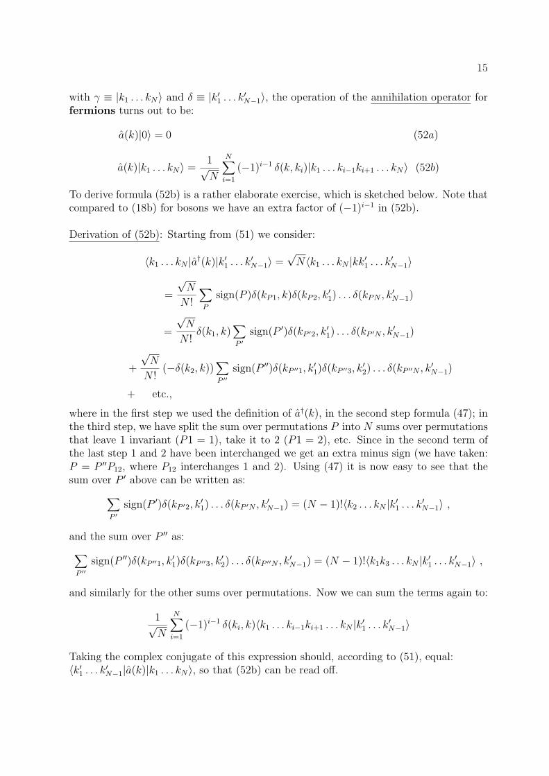
15

with γ ≡ |k1 . . . kN〉 and δ ≡ |k′1 . . . k′N−1〉, the operation of the annihilation operator forfermions turns out to be:

a(k)|0〉 = 0 (52a)

a(k)|k1 . . . kN〉 =1√N

N∑i=1

(−1)i−1 δ(k, ki)|k1 . . . ki−1ki+1 . . . kN〉 (52b)

To derive formula (52b) is a rather elaborate exercise, which is sketched below. Note thatcompared to (18b) for bosons we have an extra factor of (−1)i−1 in (52b).

Derivation of (52b): Starting from (51) we consider:

〈k1 . . . kN |a†(k)|k′1 . . . k′N−1〉 =√N〈k1 . . . kN |kk′1 . . . k′N−1〉

=

√N

N !

∑P

sign(P )δ(kP1, k)δ(kP2, k′1) . . . δ(kPN , k

′N−1)

=

√N

N !δ(k1, k)

∑P ′

sign(P ′)δ(kP ′2, k′1) . . . δ(kP ′N , k

′N−1)

+

√N

N !(−δ(k2, k))

∑P ′′

sign(P ′′)δ(kP ′′1, k′1)δ(kP ′′3, k

′2) . . . δ(kP ′′N , k

′N−1)

+ etc.,

where in the first step we used the definition of a†(k), in the second step formula (47); inthe third step, we have split the sum over permutations P into N sums over permutationsthat leave 1 invariant (P1 = 1), take it to 2 (P1 = 2), etc. Since in the second term ofthe last step 1 and 2 have been interchanged we get an extra minus sign (we have taken:P = P ′′P12, where P12 interchanges 1 and 2). Using (47) it is now easy to see that thesum over P ′ above can be written as:∑

P ′sign(P ′)δ(kP ′2, k

′1) . . . δ(kP ′N , k

′N−1) = (N − 1)!〈k2 . . . kN |k′1 . . . k′N−1〉 ,

and the sum over P ′′ as:∑P ′′

sign(P ′′)δ(kP ′′1, k′1)δ(kP ′′3, k

′2) . . . δ(kP ′′N , k

′N−1) = (N − 1)!〈k1k3 . . . kN |k′1 . . . k′N−1〉 ,

and similarly for the other sums over permutations. Now we can sum the terms again to:

1√N

N∑i=1

(−1)i−1 δ(ki, k)〈k1 . . . ki−1ki+1 . . . kN |k′1 . . . k′N−1〉

Taking the complex conjugate of this expression should, according to (51), equal:〈k′1 . . . k′N−1|a(k)|k1 . . . kN〉, so that (52b) can be read off.

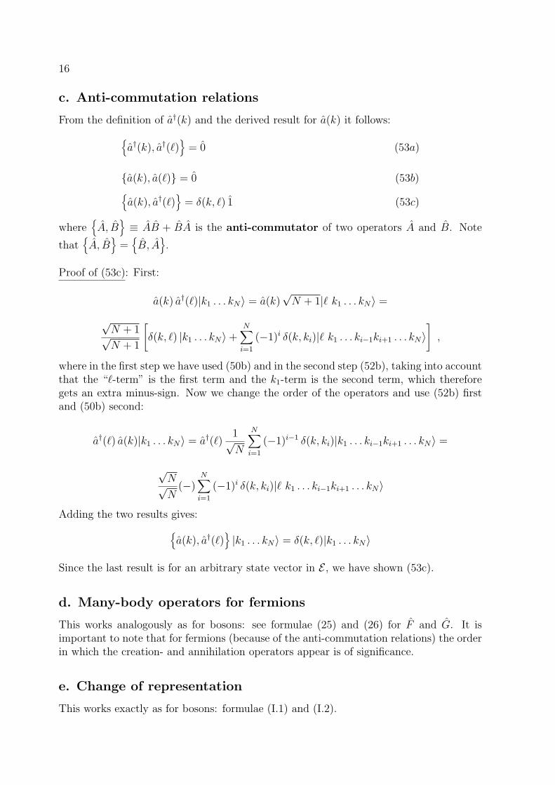
16

c. Anti-commutation relations

From the definition of a†(k) and the derived result for a(k) it follows:a†(k), a†(`)

= 0 (53a)

a(k), a(`) = 0 (53b)a(k), a†(`)

= δ(k, `) 1 (53c)

whereA, B

≡ AB + BA is the anti-commutator of two operators A and B. Note

thatA, B

=B, A

.

Proof of (53c): First:

a(k) a†(`)|k1 . . . kN〉 = a(k)√N + 1|` k1 . . . kN〉 =

√N + 1√N + 1

[δ(k, `) |k1 . . . kN〉+

N∑i=1

(−1)i δ(k, ki)|` k1 . . . ki−1ki+1 . . . kN〉],

where in the first step we have used (50b) and in the second step (52b), taking into accountthat the “`-term” is the first term and the k1-term is the second term, which thereforegets an extra minus-sign. Now we change the order of the operators and use (52b) firstand (50b) second:

a†(`) a(k)|k1 . . . kN〉 = a†(`)1√N

N∑i=1

(−1)i−1 δ(k, ki)|k1 . . . ki−1ki+1 . . . kN〉 =

√N√N

(−)N∑i=1

(−1)i δ(k, ki)|` k1 . . . ki−1ki+1 . . . kN〉

Adding the two results gives:a(k), a†(`)

|k1 . . . kN〉 = δ(k, `)|k1 . . . kN〉

Since the last result is for an arbitrary state vector in E , we have shown (53c).

d. Many-body operators for fermions

This works analogously as for bosons: see formulae (25) and (26) for F and G. It isimportant to note that for fermions (because of the anti-commutation relations) the orderin which the creation- and annihilation operators appear is of significance.

e. Change of representation

This works exactly as for bosons: formulae (I.1) and (I.2).

17

7. Identical spin-12 particles

Application of the preceding: form of operators in Second Quantization for identical par-ticles with mass m and spin 1

2(fermions!).

The one-fermion theory is often called “Schrodinger-Pauli theory”. It’s Hilbert space isagain called E1.

Basis in discrete ~k-representation in E1:|~kσ〉

~k = 2π

L~n with nx, ny, nz integer numbers; σ = +1 or -1 (spin 1

2).

In (continuous) ~r-representation: |~rσ〉

The connection between the ~kσ- and ~rσ-representations is (cf. (I.8)):

〈~rσ |~kσ′〉 =1√Vei~k·~r δσ,σ′ (54)

a. The ~kσ-representation

The form of operators for many-fermion systems is derived quite analogously to that forthe bosonic case; one has to drag along an extra spin index σ, compared to the spin 0 case.

Many-body operators

n~kσ = a†~kσ a~kσ (55)

n~k =∑σ

n~kσ (56)

N =∑~kσ

n~kσ total particle number (57)

H(0) =∑~kσ

εkn~kσ =∑~kσ

εk a†~kσa~kσ with εk =

h2k2

2m(58)

We need to use our knowledge of the Hilbert space for spin-12

objects to find many-bodyoperators that involve spin in a less trivial manner.

General procedure [cf. (27)-(28)]: (i) determine matrix elements

f~kσ,~k′σ′ = 〈~kσ|f (1)|~k′σ′〉 (59)

(ii) Using (i):

F =∑~kσ

∑~k′σ′

a†~kσf~kσ,~k′σ′ a~k′σ′ (60)

For instance, the operator Σx, x-component of spin of the many-fermion system (in unitsof h/2), is derived from the (one-particle) operator σx as follows (using the appropriatePauli matrix):

〈~kσ|σx|~k′σ′〉 = δ~k,~k′ [δσ,1 δσ′,−1 + δσ,−1 δσ′,1] −→

18

Σx =∑~k

[a†~k,1 a~k,−1

+ a†~k,−1a~k,1

](61a)

The other components of spin are (check for yourself):

Σy =∑~k

[−i a†~k,1 a~k,−1

+ i a†~k,−1a~k,1

](61b)

Σz =∑~k

[a†~k,1 a~k,1 − a

†~k,−1

a~k,−1

]=∑~k

(n~k,1 − n~k,−1

)(61c)

It is important to note that not all commutators have to be replaced by anti-commutatorsin going from bosons to fermions. For instance, the dynamics of operators (Heisenbergpicture) is still governed by the Heisenberg equations and these contain commutators.As an example we compute the time-dependence of the annihilation operator (in the~kσ-representation):

d

dt

(a~kσ(t)

)=i

h

[H(0), a~kσ(t)

]=i

h

∑~k′σ′

εk′

[a†~k′σ′ a~k′σ′ , a~kσ

](t) (62)

To compute the commutator we use the general operator formula:[AB, C

]= A

B, C

−A, C

B (63)

(which is easily proved by writing out the (anti-)commutators). Using the anti-commutationrelations we then find: [

a†~k′σ′ a~k′σ′ , a~kσ

]= a†~k′σ′ · 0 − δ~k,~k′ δσ,σ′ a~k′σ′

Substituting in (62), we have:

d

dt

(a~kσ(t)

)= −iεk

ha~kσ(t) −→ a~kσ(t) = a~kσ e

−iωkt , (64)

where ωk = εk/h. Note that this is the same result as for bosons in (40), but that thecalculation is quite different!

b. The ~rσ-representation

The change of representation is now easily made using formulae (I.2) and (54):

a~kσ −→ ψ(~rσ)

Mostly it is just a matter of replacing∫d~r . . . by

∑σ

∫d~r . . ., but for spin operators there

are some differences.

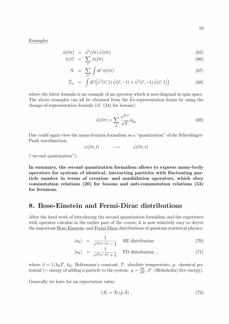
19

Examples

n(~rσ) = ψ†(~rσ) ψ(~rσ) (65)

n(~r) =∑σ

n(~rσ) (66)

N =∑σ

∫d~r n(~rσ) (67)

Σx =∫d~r(ψ†(~r, 1) ψ(~r,−1) + ψ†(~r,−1) ψ(~r, 1)

)(68)

where the latter formula is an example of an operator which is non-diagonal in spin space.The above examples can all be obtained from the ~kσ-representation forms by using thechange-of-representation formula (cf. (34) for bosons):

ψ(~rσ) =∑~k

ei~k·~r√Va~kσ (69)

One could again view the many-fermion formalism as a “quantization” of the Schrodinger-Pauli wavefunction;

ψ(~rσ, t) −→ ψ(~rσ, t)

(“second quantization”).

In summary, the second quantization formalism allows to express many-bodyoperators for systems of identical, interacting particles with fluctuating par-ticle number in terms of creation- and annihilation operators, which obeycommutation relations (20) for bosons and anti-commutation relations (53)for fermions.

8. Bose-Einstein and Fermi-Dirac distributions

After the hard work of introducing the second quantization formalism and the experiencewith operator calculus in the earlier part of the course, it is now relatively easy to derivethe important Bose-Einstein- and Fermi-Dirac distributions of quantum statistical physics.

〈nk〉 =1

eβ(εk−µ) − 1BE distribution (70)

〈nk〉 =1

eβ(εk−µ) + 1FD distribution , (71)

where β = 1/kBT , kB: Boltzmann’s constant, T : absolute temperature, µ: chemical po-tential (= energy of adding a particle to the system: µ = ∂F

∂N, F : (Helmholtz) free energy).

Generally we have for an expectation value:

〈A〉 = Tr (ρ A) , (72)

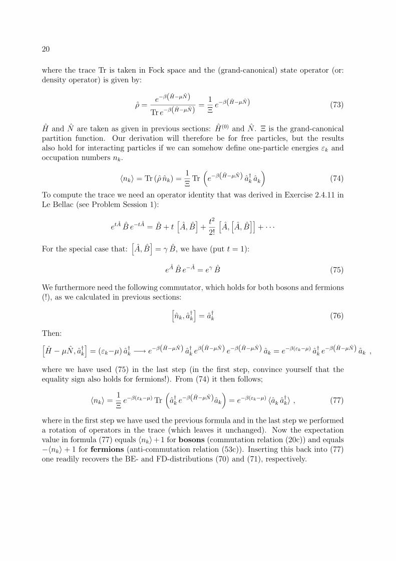
20

where the trace Tr is taken in Fock space and the (grand-canonical) state operator (or:density operator) is given by:

ρ =e−β(H−µN)

Tr e−β(H−µN)=

1

Ξe−β(H−µN) (73)

H and N are taken as given in previous sections: H(0) and N . Ξ is the grand-canonicalpartition function. Our derivation will therefore be for free particles, but the resultsalso hold for interacting particles if we can somehow define one-particle energies εk andoccupation numbers nk.

〈nk〉 = Tr (ρ nk) =1

ΞTr

(e−β(H−µN) a†k ak

)(74)

To compute the trace we need an operator identity that was derived in Exercise 2.4.11 inLe Bellac (see Problem Session 1):

etA B e−tA = B + t[A, B

]+t2

2!

[A,[A, B

]]+ · · ·

For the special case that:[A, B

]= γ B, we have (put t = 1):

eA B e−A = eγ B (75)

We furthermore need the following commutator, which holds for both bosons and fermions(!), as we calculated in previous sections:[

nk, a†k

]= a†k (76)

Then:[H − µN, a†k

]= (εk−µ) a†k −→ e−β(H−µN) a†k e

β(H−µN) e−β(H−µN) ak = e−β(εk−µ) a†k e−β(H−µN) ak ,

where we have used (75) in the last step (in the first step, convince yourself that theequality sign also holds for fermions!). From (74) it then follows;

〈nk〉 =1

Ξe−β(εk−µ) Tr

(a†k e

−β(H−µN)ak

)= e−β(εk−µ) 〈ak a

†k〉 , (77)

where in the first step we have used the previous formula and in the last step we performeda rotation of operators in the trace (which leaves it unchanged). Now the expectationvalue in formula (77) equals 〈nk〉+ 1 for bosons (commutation relation (20c)) and equals−〈nk〉+ 1 for fermions (anti-commutation relation (53c)). Inserting this back into (77)one readily recovers the BE- and FD-distributions (70) and (71), respectively.

Feynman Diagrams for Beginners - Annamalai University

Documents

Transcript of Feynman Diagrams for Beginners - Annamalai University