arX

iv:0

904.

0214

v3 [

hep-

th]

31

Mar

201

0

DESY 10–027 ISSN 0418-9833

March 2010

Differential reduction of generalized hypergeometric

functions from Feynman diagrams: One-variable case

Vladimir V. Bytev∗, Mikhail Yu. Kalmykov,∗ Bernd A. Kniehl

II. Institut fur Theoretische Physik, Universitat Hamburg,

Luruper Chaussee 149, 22761 Hamburg, Germany

Abstract

The differential-reduction algorithm, which allows one to express generalizedhypergeometric functions with parameters of arbitrary values in terms of such func-tions with parameters whose values differ from the original ones by integers, isdiscussed in the context of evaluating Feynman diagrams. Where this is possible,we compare our results with those obtained using standard techniques. It is shownthat the criterion of reducibility of multiloop Feynman integrals can be reformu-lated in terms of the criterion of reducibility of hypergeometric functions. Therelation between the numbers of master integrals obtained by differential reductionand integration by parts is discussed.

PACS numbers: 02.30.Gp, 02.30.Lt, 11.15.Bt, 12.38.BxKeywords: Generalized hypergeometric functions; Differential reduction; Laurentexpansion; Multiloop calculations

∗On leave of absence from Joint Institute for Nuclear Research,141980 Dubna (Moscow Region),Russia.

1

1 Introduction

It is commonly accepted that any multiloop and/or multileg Feynman diagram incovariant gauge within dimensional regularization [1] may be treated as a generalizedhypergeometric function1 [3]. Starting from its α representation, any Feynmandiagram may be written in the form of a Mellin-Barnes integral [4,5],

Φ(n) ∼∫ +i∞

−i∞

∏

a,b,c

Γ(∑m

i=1Aaizi +Ba)

Γ(∑r

j=1Cbjzj +Db)dzcY

zc−1 , (1)

where Ya are algebraic functions of external kinematic invariants and A,B,C,D aresome matrices depending in a linear way on the dimension of space-time n, whichis an arbitrary complex number, and the powers of the propagators.

By the application of Cauchy’s theorem,2 this integral can be rewritten as alinear combination of multiple series,3

Φ(n, ~x) ∼∞∑

k1,··· ,kr+m=0

∏

a,b

Γ(∑m

i=1 Aaiki + Ba)

Γ(∑r

j=1 Cbjkj + Db)xk11 · · · xkr+m

r+m . (2)

For real diagrams, some of the variables xk may be complex number. We call thistype of variable a “hidden variable” and the corresponding index of summation a“hidden index of summation.” In all existing examples, the representation of Eq. (2)belongs to a Horn-type hypergeometric series [8] if the hidden index of summationis considered as an independent variable.

For the reader’s convenience, we recall that the multiple series∑∞

~m=0 C(~m)~x~m iscalled Horn-type hypergeometric if, for each i = 1, . . . , r, the ratio C(~m+ ~ei)/C(~m)is a rational function in the index of summation (m1, · · · ,mr) [8,9]. The coefficientsof such a series have the general form

C(~m) =r∏

i=1

λmi

i R(~m)

∏Nj=1 Γ(µj(~m) + γj)

∏Mk=1 Γ(νk(~m) + δk)

, (3)

where N,M ≥ 0, λj , δj , γj are arbitrary complex numbers, µj , νk : Zr → Z arearbitrary integer-valued linear maps, and R is an arbitrary rational function [8,10].

However, to our knowledge, the proof that any Feynman diagram can be de-scribed by a Horn-type series does not exist. There is another way to proof thisstatement. The classical α representation of a Feynman diagram is a particular caseof the generalized Euler integral representation of the Gel’fand-Kapranov-Zelevinskisystem [8] that is related to the Horn-type series representation. We call the Feyn-man diagram representation of Eq. (1) or the equivalent representation of Eq. (2) ahypergeometric representation [8].

For Horn-type hypergeometric functions, there are so-called step-up (step-down)operators H+

λ (H−λ ) [9,11]. These are differential operators which, upon application

1This statement is also valid for phase-space integrals (see, e.g., Ref. [2]).2This is true if all arguments of the Γ functions are different. Otherwise, an additional regularization

for each propagator (or the introduction of extra masses) is necessary. See, e.g., Ref. [6].3One of the first examples of this type of representation for a Feynman diagram was given in Ref. [7].

2

to a hypergeometric function Sλ, shift the value of one its upper (lower) param-eters by unity, as H+

λ Sλ = Sλ+1 (H−λ Sλ = Sλ−1). Takayama [12] proposed an

algorithm that allows one to construct inverse differential operators, the step-down(step-up) operators B−

λ (B+λ ), starting from direct operators and systems of dif-

ferential equations for hypergeometric functions. These operators satisfy the re-lations B−

λ Sλ+1 → Sλ (B+λ Sλ → Sλ+1). Takayama pointed out [12] that inverse

operators are uniquely defined for any hypergeometric function with an irreduciblemonodromy group, which implies that the parameters and the differences betweenupper and lower parameters are not integer. By the action of such differential op-erators on a hypergeometric function, the value of any parameter can be shiftedby an arbitrary integer. We call this procedure of applying differential operatorsto shift the parameters by integers differential reduction.4 An important step ofTakayama’s algorithm is the construction of a differential Grobner basis for thesystem of differential equations for hypergeometric functions.5

It is quite surprising that the technique for the reduction of Feynman diagramsadvocated here, namely to split a given Feynman diagram into a linear combinationof Horn-type hypergeometric functions with rational coefficients and to subsequentlyapply differential reduction, has never been elaborated and that its interrelation withthe well-known integration-by-parts (IBP) technique [15] has never been discussed.

The aim of this paper is to demonstrate how the differential-reduction algorithmmay be successfully applied to evaluate Feynman diagrams. For simplicity, we con-sider here only the particular case of Horn-type multiple hypergeometric functions,i.e. the functions p+1Fp, and some Feynman diagrams with arbitrary powers ofpropagators, which are expressible in terms of these functions.

The structure of this paper is as follows. In Section 2, we discuss the differential-reduction algorithm for generalized hypergeometric functions p+1Fp. This is a cru-cial step towards proving theorems on the construction of all-order ε expansionspresented in Refs. [16–19]. Section 3 illustrates the application of differential re-duction to several Feynman diagrams of phenomenological interest. In Section 4,we discuss how the counting of master integrals in the differential-reduction ap-proach is related to that in the IBP technique. The results of our analysis arebriefly summarized in Section 5. In Appendix A, we describe interrelations betweena set of basis functions generated by the differential-reduction algorithm and a setof hypergeometric functions whose higher-order ε expansions were constructed inRef. [20].

4There are various publications on contiguous relations for hypergeometric functions, i.e. algebraicrelations between hypergeometric functions of several variables with shifted values of parameters, startingfrom the classical paper by Gauss [13]. To our knowledge, a closed algorithm for the algebraic reductionof Horn-type hypergeometric functions of several variables, i.e. an algorithm for solving these algebraicrelations, does not exist.

5The idea of using the differential-Grobner-basis technique directly for the reduction of off-shell Feyn-man diagrams, without spitting them into linear combinations of hypergeometric functions, was proposedby Tarasov [14].

3

2 Differential-reduction algorithm for the gen-

eralized hypergeometric function p+1Fp

2.1 Notation

Let us consider the generalized hypergeometric function pFq(a; b; z), defined by aseries about z = 0 as

pFq(~a;~b; z) ≡ pFq

(

~a~b

z

)

=∞∑

k=0

zk

k!

∏pi=1(ai)k

∏qj=1(bj)k

, (4)

where (a)k = Γ(a+ k)/Γ(a) is the Pochhammer symbol. The sets ~a = (a1, · · · , ap)and~b = (b1, · · · , bq) are called the upper and lower parameters of the hypergeometricfunction, respectively. In terms of the differential operator θ,

θ = zd

dz, (5)

the differential equation for the hypergeometric function pFq can be written as

[

z

p∏

i=1

(θ + ai)− θ

q∏

i=1

(θ + bi − 1)

]

pFq(~a;~b; z) = 0. (6)

Hypergeometric functions which differ by ±1 in the value of one of their parametersare called contiguous, and linear relations between contiguous functions and theirderivatives are called contiguous relations.6 In particular, the following differentialidentities between contiguous functions are universal [11]:

pFq(a1 + 1,~a;~b; z) = B+a1pFq(a1,~a;~b; z) =

1

a1(θ + a1) pFq(a1,~a;~b; z) ,

pFq(~a; b1 − 1,~b; z) = H−b1p

Fq(~a; b1,~b; z) =1

b1 − 1(θ + b1 − 1) pFq(~a; b1,~b; z) , (7)

which directly follow from the series representation of Eq. (4). The operators B+a1

(H−b1) are the step-up (step-down) operators for upper (lower) parameters of hyper-

geometric functions.

2.2 Non-exceptional values of parameters

In Ref. [12], it was shown that, for given step-up (step-down) operators, inversestep-down (step-up) operators, which are uniquely defined modulo Eq. (6), can beconstructed. This type of operators were explicitly constructed for the hypergeo-metric function p+1Fp by Takayama in Ref. [22]. For completeness, we reproduce

6A full set of contiguous relations for an arbitrary hypergeometric function pFq was considered byRainville [21]. For pFq, there are 2(p+ q) contiguous functions.

4

his result here:

p+1Fp(ai − 1,~a;~b; z) = B−aip+1Fp(ai,~a;~b; z) ,

B−ai = −ai

ci

ti(θ)− z∏

j 6=i

(θ + aj)

ai→ai−1

,

ci = −ai

p∏

j=1

(bj − 1− ai) ,

ti(x) =x∏p

j=1(x+ bj − 1)− ci

x+ ai, (8)

p+1Fp(~a; bi + 1,~b; z) = H+bi p+1Fp(~a; b1,~b; z) ,

H+ai =

bi − 1

di

θ

z

∏

j 6=i

(θ + bj − 1)− si(θ)

bi→bi+1

,

di =

p+1∏

j=1

(1 + aj − bi) ,

si(x) =

∏p+1j=1(x+ aj)− di

x+ bi − 1, (9)

where |a→a+1 means substitution of a by a + 1. The functions ti(x) and si(x) arepolynomials in x, so that Eqs. (8) and (9) are polynomials in the derivative θ. Let

us introduce the symmetric polynomial P(p)j ({rk}) as follows:

p∏

k=1

(z + rk) =

p∑

j=0

P(p)p−j({rk})zj =

p∑

j=0

P(p)j ({rk})zp−j , (10)

so that

P(p)0 ({rk}) = 1 ,

P(p)j ({rk}) =

p∑

i1,··· ,ir=1

∏

i1<···<ij

ri1 · · · rij , j = 1, · · · , p . (11)

For example, we have P(p)1 ({rk}) =

∑pj=1 rj and P

(p)p ({rk}) =

∏pj=1 rj . Then, we

may write

ti(x) =

p∑

j=0

P(p)p−j({br − 1})x

j+1 − (−ai)j+1

x+ ai=

p∑

j=0

P(p)p−j({br − 1})

j∑

k=0

xj−k(−ai)k . (12)

A similar consideration is valid also for the last relation in Eq. (9):

si(x) =

p+1∑

j=0

P(p+1)p+1−j({ar})

xj − (1− bi)j

x− (1− bi)=

p∑

j=0

P(p+1)p−j ({ar})

j∑

k=0

xj−k(1− bi)k .(13)

5

The differential reduction has the form of a product of several differential step-upand step-down operators, H±

bkand B±

ak, respectively:7

F (~a+ ~m;~b+ ~n; z) =(

H±{a}

)

∑i mi

(

B±{b}

)

∑j nj

F (~a;~b; z) , (14)

so that the maximal power of θ in this expression is equal to r ≡ ∑

imi +∑

j nj.In a symbolic form, this may be written as

R(ai, bj , z)F (~a+ ~m;~b+ ~n; z) = [S1(ai, bj , z)θr + · · ·+ Sr+1(ai, bj , z)]F (~a;~b; z) ,(15)

whereR and {Sj} are some polynomials. Since the hypergeometric function p+1Fp(~a;~b; z)satisfies the following differential equation of order p+ 1 [see Eq. (6)]:

(1− z)θp+1p+1Fp(~a;~b; z)

=

{

p∑

r=1

[

zP(p+1)p+1−r({aj})− P

(p)p+1−r({bj − 1})

]

θr + z

p+1∏

k=1

ak

}

p+1Fp(~a;~b; z) , (16)

it is possible to express all terms containing higher powers of the operator θ, θk withk ≥ p+1, as a linear combination of rational functions of z depending parametricallyon a and b multiplied by lower powers of θ, θj with j ≤ p. In this way, any function

p+1Fp(~a+ ~m;~b+~k; z), where ~m and ~k are sets of integers, is expressible in terms ofthe basic function and its first p derivatives as

S(ai, bj , z)p+1Fp(~a+ ~m;~b+ ~k; z) ={

R1(ai, bj , z)θp +R2(ai, bj , z)θ

p−1

+ · · ·+Rp(ai, bj , z)θ +Rp+1(ai, bj , z)} p+1Fp(~a;~b; z) , (17)

where S and Ri are polynomials in the parameters {ai} and {bj} and the argumentz.

From Eq. (8) it follows that, if one of the upper parameters aj is equal to unity,then the application of the step-down operator B−

aj to the hypergeometric function

p+1Fp produces unity, B−1 p+1Fp(1,~a;~b; z) = 1. Taking into account the explicit form

of the step-down operator B−1 ,

B−1 =

1∏p

k=1(bk − 1)

p∏

j=1

(bj − 1) +

p∑

j=1

P(p)p−j({bk − 1})θj − z

p∏

j=1

(θ + aj)

, (18)

we obtain the differential identity

p∏

j=1

(bj − 1)− z

p∏

j=1

aj + (1− z)θp

p+1Fp(1,~a;~b; z)

+

p−1∑

j=1

[

P(p)p−j({bk − 1}) − zP

(p)p−j({ak})

]

θj

p+1Fp(1,~a;~b; z) =

p∏

k=1

(bk − 1) .(19)

7Due to the relation θ pFq(~a;~b; z) = z∏p

i=1 ai/(∏q

j=1 bj)pFq(~a + 1;~b + 1; z), not all step-up oper-

ators are independent. In fact, (∏p

j=1 H+bj)(∏p+1

k=1 B+ak)F (~a;~b; z) = (

∏p+1k=1 B

+ak)(∏p

j=1 H+bj)F (~a;~b; z) =

∏p

j=1 bj/(∏p+1

k=1 ak)(d/dz)F (~a;~b; z).

6

The case where two or more upper parameters are equal to unity, e.g. a1 = a2 = 1,does not generate any new identities. As a consequence, if there is a subset ~l ofpositive integers in the set of upper parameters, the reduction procedure has themodified form:

P (ai, bj , z)p+1Fp(~l,~a+ ~m;~b+ ~k; z) = R1(ai, bj , z) +{

R2(ai, bj , z)θp−1

+ · · · + Rp(ai, bj , z)θ + Rp+1(ai, bj, z)}

p+1Fp(~1,~a;~b; z) . (20)

Let us write explicit expressions for the inverse operators for several hypergeo-metric functions. For the Gauss hypergeometric function 2F1, we have:

2F1

(

a1 − 1, a2b1

z

)

=1

b1 − a1[(1− z)θ + b1 − a1 − a2z] 2F1

(

a1, a2b1

z

)

, (21)

2F1

(

a1, a2b1 + 1

z

)

=b1

(b1 − a1)(b1 − a2)

[

(1− z)d

dz+ b1 − a1 − a2

]

2F1

(

a1, a2b1

z

)

.

For the hypergeometric function 3F2, the inverse differential operators read:

3F2

(

a1 − 1, a2, a3b1, b2

z

)

(b1 − a1)(b2 − a1)

={

(1− z)θ2 + [(b1 + b2 − 1− a1)− z(a2 + a3)] θ + (b1 − a1)(b2 − a1)− za2a3}

× 3F2

(

a1, a2, a3b1, b2

z

)

,

3F2

(

a1, a2, a3b1 + 1, b2

z

)

(a1 − b1)(a2 − b1)(a3 − b1)

= b1

{

1− z

zθ2 +

[

b2 − 1

z− (a1 + a2 + a3 − b1)

]

θ

− 1

b1[a1a2a3 − (a1 − b1)(a2 − b1)(a3 − b1)]

}

3F2

(

a1, a2, a3b1, b2

z

)

. (22)

7

For the hypergeometric function 4F3, the differential operators read:

4F3

(

a1 − 1, a2, a3, a4b1, b2, b3

z

)

(b1 − a1)(b2 − a1)(b3 − a1)

={

(1− z)θ3 + [(b1 + b2 + b3 − 2− a1)− z(a2 + a3 + a4)] θ2

+

b1b2 + b1b3 + b2b3 + a21 + (a1 + 1)

1−3∑

j=1

bj

− z(a2a3 + a2a4 + a3a4)

θ

+(b1 − a1)(b2 − a1)(b3 − a1)− za2a3a4} 4F3

(

a1, a2, a3, a4b1, b2, b3

z

)

,

4F3

(

a1, a2, a3, a4b1 + 1, b2, b3

z

)

(a1 − b1)(a2 − b1)(a3 − b1)(a4 − b1)

= b1

{

1− z

zθ3 +

[

b2 + b3 − 2

z− (a1 + a2 + a3 + a4 − b1)

]

θ2

+

(b2 − 1)(b3 − 1)

z− (a1a2 + a1a3 + a1a4 + a2a3 + a2a4 + a3a4) + b1

4∑

j=1

aj − b1

θ

− 1

b1[a1a2a3a4 − (a1 − b1)(a2 − b1)(a3 − b1)(a4 − b1)]

}

4F3

(

a1, a2, a3, a4b1, b2, b3

z

)

. (23)

2.3 Differential-reduction algorithms for special values

of parameters

A special consideration is necessary when bi = ai + 1. In this case, the expressionsin Eqs. (8) and (9) are equal to zero. Let us start with the case when all ai aredifferent. In this case, the following relation should be applied (see Eq. (15) inChapter 5 of Ref. [21], Chapter 7.2 in Ref. [23], and Ref. [24]):

(a− b) pFq

(

a, b, · · ·a+ 1, b+ 1, · · · z

)

= a p−1Fq−1

(

b, · · ·b+ 1, · · · z

)

− b p−1Fq−1

(

a, · · ·a+ 1, · · · z

)

. (24)

Repeating this procedure several times, we are able to split any original hypergeo-metric function with several parameters having unit difference into a set of hyper-geometric functions with only one kind of parameters having unit difference (for theparticular cases, see Eqs. (7.2.3.21)–(7.2.3.23) in Ref. [23]):

pFq

(

{a1}r1 , {a2}r2 , · · · , {am}rm , c1, · · · , ck{1 + a1}r1 , {1 + a2}r2 , · · · , {1 + am}rm , b1, · · · , bl

z

)

→m∑

i=1

p−R+riFq−R+ri

(

{aj}ri , c1, · · · , ck{1 + aj}ri , b1, · · · , bl

z

)

, (25)

where {aj}ri denotes rj repetitions of aj in the argument list,

R =

m∑

j=1

rj , ci 6= ai , bi 6= 1 + ai , cj 6= 1 + bj . (26)

8

For a special set of parameters, Eqs. (7.2.3.21) and (7.2.3.23) in Ref. [23] are useful:

pFq

(

{a}p−2, ρ, σ{b}q−2, ρ+ n, σ + 1

z

)

=(ρ)n

(ρ− σ)np−1Fq−1

(

{a}p−2, σ{b}q−2, σ + 1

z

)

− (ρ)nσ

(ρ− σ)nΣnk=1

(ρ− σ − 1)k(ρ)k

p−1Fq−1

(

{a}p−2, ρ{b}q−2, ρ+ k

z

)

, (27)

pFq

(

{a}p−n, σ1, · · · , σn{b}q−n, σ1 +m1, · · · , σn +mn

z

)

=

n∏

j=1

(σj)mj

(mj − 1)!Σnk=1Σ

m1−1j1=0 · · ·Σmn−1

jn=0

1

σk + jk

×n∏

l=1

(1−ml)jljl!

n∏

i=1;i 6=k

1

σi + ji − σk − jkp−n+1Fq−n+1

(

{a}p−n, σk + jk{b}q−n, σk + jk + 1

z

)

. (28)

In Eq. (28), mn are integers, all σi are different, and, if σi − σk = N with N =1, 2, · · · , then mk < N .

Let us return to the last expression in Eq. (25) and rewrite it as

p+1Fp

(

{a+m}r, a1 + k1, · · · , ap+1−r + kp+1−r

{1 + a+m}q, b1 + l1, · · · , bp−q + lp−qz

)

, (29)

where m, {kr}, and {lj} are integers and a, {ak}, and {bj} are parameters of thebasis function. Using the reduction procedure described in Sec. 2.2, we may convertthis function as

p+1Fp

(

{a+m}r, {aj + kj}p+1−r

{1 + a+m}q, {bk + lk}p−qz

)

→ p+1Fp

(

{a+m}r, {aj +m}p+1−r

{1 + a+m}q, {bk +m}p−qz

)

, (30)

and then apply the differential relation (see Eq. (7.2.3.47) in Ref. [23])8

pFq

(

{ai +m}p{bk +m}q

z

)

=

∏qk=1{(bk)m}

∏pj=1{(aj)m}

(

d

dz

)m

pFq

(

{ai}p{bk}q

z

)

, (31)

where the derivative d/(dz) could be rewritten in terms of θ, with the help of

(

d

dz

)m

=

(

1

z

)m

θ(θ − 1) · · · (θ −m+ 1) . (32)

If m ≥ p, Eq. (31) can be converted to a differential identity of order p− 1. Puttingeverything together, we obtain

P (ak, bj , z)p+1Fp

(

{a+m}r, {aj + kj}p+1−r

{1 + a+m}q, {bk + lk}p−qz

)

= [Q1(ak, bj , z)θp + · · ·+Qp+1(ak, bj , z)] p+1Fp

(

{a}r, a1, · · · , ap−r

{1 + a}q, b1, · · · , bp−q−1z

)

. (33)

8Another useful relation is Eq. (7.2.3.50) in Ref. [23]:

(

d

dz

)n [

zσ+n−1pFq

(

{ai}p−1, σ{bk}q−1

z

)]

= (σ)nzσ−1

pFq

(

{ai}p−1, σ + n{bk}q z

)

.

9

We remark that Eq. (33) can be further simplified by using Eq. (7), which can bewritten as

θkp+1Fp

(

A,~a

1 +A,~bz

)

= (−A)kp+1Fp

(

A,~a

1 +A,~bz

)

−k−1∑

j=0

(−A)k−jθjpFp−1

(

~a~b

z

)

. (34)

Recursive application of this expression allows us to reduce higher powers of deriva-tives in Eq. (33) as(

θ

A

)q

p+1Fp

( {A}r,~a{1 +A}r,~b

z

)

=

q∑

j=0

(−1)(j+q)

(

q

j

)

p+1−jFp−j

( {A}r−j ,~a

{1 +A}r−j ,~bz

)

, (35)

where q ≤ r.For a particular set of parameters, a further simplification of Eq. (33) can be

achieved. For example, for a = 1, we have

pFq

(

1, {ai}p−1

2, {bk}q−1z

)

=1

z

∏q−1l=1 (bl − 1)

∏p−1j=1(aj − 1)

[

p−1Fq−1

(

{ai − 1}p−1

{bk − 1}q−1z

)

− 1

]

, (36)

where aj, bk 6= 1.Further useful relations for particular values of parameters of the basis function

were derived in Ref. [24], namely

p+1Fp

(

{a}p, b{1 + a}p

z

)

= −(−a)p

Γ(p)

∫ 1

0dt

ta−1

(1− zt)blnp−1 t , (37)

and, for b = 1,

p+1Fp

(

1, a, · · · , aa+ 1, · · · , a+ 1

z

)

= apΦ(z, p, a) , (38)

where Φ(z, p, a) is the Lerch function defined as [9]

Φ(z, p, a) =

∞∑

k=0

zk

(a+ k)p=

1

Γ(p)

∫ ∞

0

e−(a−1)t

et − ztp−1dt , (39)

so thatLin (z) = zΦ(z, n, 1) . (40)

2.4 Criteria of reducibility of hypergeometric functions

In this section, we formulate the criteria of reducibility of the hypergeometric func-tion pFq(~a;~b; z), i.e. we state under which conditions the hypergeometric function

pFq(~a;~b; z) and its derivatives are expressible in terms of hypergeometric functionsof lower order and/or with lower derivatives.

We call the result derived by Karlsson [25] the first criterion of reducibility ofthe hypergeometric function pFq(~a;~b; z) to hypergeometric functions of lower order,

pFq

(

b1 +m1, · · · , bn +mn, an+1, · · · , apb1, · · · , bn, bn+1, · · · , bq

z

)

=

m1∑

j1=0

· · ·mn∑

jn=0

A(j1, · · · jn)zJnp−nFq−n

(

an+1 + Jn, · · · ap + Jnbn+1 + Jn, · · · , bq + Jn

z

)

, (41)

10

where mj are positive integers, Jn = j1 + · · ·+ jn, and

A(j1, · · · jn) =(

m1

j1

)

· · ·(

mn

jn

)

(b2 +m2)J1(b3 +m3)J2 · · · (bn +mn)Jn−1(an+1)Jn · · · (ap)Jn

(b1)J1(b2)J2 · · · (bn)Jn(bn+1)Jn · · · (bq)Jn.

(42)

In particular, we have

pFq

(

b1 +m1, a2, · · · , apb1, b2, · · · bq

z

)

=

m1∑

j=0

zj(

m1

j

)

(a2)j · · · (ap)j(b1)j · · · (bq)j p−1Fq−1

(

a2 + j, · · · ap + jb2 + j, · · · bq + j

z

)

.

(43)

In words, the first criterion of reducibility of the hypergeometric function reads:Criterion IThe hypergeometric function pFq(~a;~b; z) which has pairs of parameterssatisfying ai = bi + mi with mi being positive integers is expressible interms of functions of lower order according to Eq. (41).

Equations (24) and (25) yield the second criterion of reducibility of the hyperge-ometric function pFq(~a;~b; z) to functions of lower order. In its explicit form, it wasderived in Ref. [24] (see Eqs. (18)–(20) in Ref. [24]). Assuming that (i) {a1, · · · an}are different and (ii) if ar − ai = N with N = 1, 2, . . ., then mi < N , we have (seealso Eqs. (7.2.3.21) and (7.2.3.23) in Ref. [23])

pFq

(

a1, · · · an, an+1 · · · apa1 + 1 +m1, · · · , an + 1 +mn, bn+1, · · · , bq

z

) n∏

r=1

1

(ar)mr+1

=n∑

i=1

mi∑

j=0

(−mi)jj!(ai + j)mi!

n∏

r=1,r 6=i

1

(ar − ai − j)mr+1

×p−n+1Fq−n+1

(

ai + j, an+1, · · · , apai + 1 + j, bn+1, · · · , bq

z

)

, (44)

so that we may formulate it as:Criterion IIThe hypergeometric function pFq(~a;~b; z) which has two or more pairs ofparameters satisfying bi = ai +mi +1 with mi being positive integers isexpressible in terms of functions of lower order if additional conditionson the parameters ai (see Eq. (44)) are satisfied.

Equations (34) and (35) are considered as the third criterion of reducibility:Criterion IIIThe result of the differential reduction of a hypergeometric function ofthe type p+1Fp( ~A+ ~m,~a+~k;~1+ ~A+ ~m,~b+~l; z), where ~m, ~k, and ~l are sets

of integers, is expressible in terms of the function p+1Fp( ~A,~a;~1+ ~A,~b; z)and hypergeometric functions of lower order and their derivatives.

Equation (19) constitutes the fourth criterion of reducibility:Criterion IVIf one of the upper parameters of a hypergeometric function is an integer,

11

the result of the differential reduction of this hypergeometric functionhas one less derivative and is described by Eq. (20).

Criteria I–IV of reducibility of hypergeometric functions are much simpler thanthe ordinary criterion of reducibility of Feynman diagrams [26].

2.5 All-order ε expansions of hypergeometric functions

Recently, several theorems on the structure of the coefficients of all-order ε ex-pansions of hypergeometric functions about integer and/or rational values of theirparameters have been proven [16–19,27–30]. For a recent review, see Ref. [30].

In this paper, we mainly consider hypergeometric functions of the type of Eq. (109).There still does not exist a rigorous mathematical proof regarding the structure ofthe coefficients of the all-order ε expansions of hypergeometric functions of thistype beyond the Gauss hypergeometric functions 2F1 [16,19]. Through functions ofweight 4, the coefficients of the ε expansions were constructed in Ref. [20,31], asdiscussed in details in Appendix A), which is sufficient for next-to-next-to-leading-order (two-loop) calculations. Recently, more coefficients of the ε expansions of theClausen functions 3F2 have been evaluated in Ref. [32].

2.6 Reduction at z = 1 and construction of ε expansion

The value z = 1 is a particular case of a “hidden” variable. It is evident thatthe application of Eq. (6) to the r.h.s. of Eq. (17) gives rise to the generation offactors 1/(1 − z)k, so that the direct limit z → 1 cannot be taken. Let us recallthat the hypergeometric series defined by Eq. (4) converges [9] for |z| = 1, whenRe∑p

j=1 bj − Re∑p+1

j=1 aj > 0, so that, if the l.h.s. of Eq. (17) converges, the r.h.s.of the equation does also exist.

The main idea is to convert the original hypergeometric function p+1Fp(~a;~b; z) toa function of argument 1−z. However, beyond type 2F1, the analytical continuation

of the hypergeometric function p+1Fp( ~A; ~B; z)∣

∣

∣

z→1−zis not expressible in terms of

functions of the same type, but has a more complicated structure [33]. Nevertheless,we can perform the analytical continuation z → 1 − z of the coefficients of the εexpansions of hypergeometric functions entering the r.h.s. of Eq. (17). It was shownin Ref. [34] that, under the transformation z → 1−z, hyperlogarithms are expressibleagain in terms of hyperlogarithms. In this way, if the coefficients of the ε expansionare expressible in terms of hyperlogarithms, there is an opportunity to find the limitz → 1− z of the differential reduction, but only in fixed orders of the ε expansionsand only for such values of parameters of the hypergeometric functions for whichthe analytical structures of the coefficients are known.

An alternative approach to evaluate hypergeometric functions at z = 1 wasdiscussed in Refs. [22,27].

12

3 Application to Feynman diagrams

As an illustration of the differential-reduction algorithm, let us consider the dia-grams shown in Figs. 1 and 2.9 In general, Feynman diagrams suffer from irreduciblenumerators. Using the Davydychev-Tarasov algorithm [37], any tensor integral maybe represented in terms of scalar integrals with shifted space-time dimensions andarbitrary (positive) powers of propagators. In our analysis of the structures of thecoefficients of the ε expansions, we distinguish between two cases corresponding toeven value n = 2m − 2ε and odd value n = 2m − 1 − 2ε of space-time dimension,where m is an integer.

����

����

����

����

��

����

����

����

����

����

����

������������������������������������������������������������������������������

������������������������������������������������������������������������������

��������������������������������������������������������������������������������������������������������������������

������������������������������������������������������������������������

�������������������������������������������������������������������������������������������

�������������������������������������������������������������������������������������������

��������������������������������������������������������������������������������������������������������������������

������������������������������������������������������������������������

������������������������������������������������������������������������������

������������������������������������������������������������������������������

��������������������������������������������������������������������������������������������������������������������

������������������������������������������������������������������������

������������������������������������������������������������������������������

������������������������������������������������������������������������������

��������������������������������������������������������������������������������������������������������������������

������������������������������������������������������������������������

0

C3

0

m

Q

0

13

2

0 0

C 4

0 m

m

Q

21 3

m

Q

C 2

m

0 01 3 2

m

Q

0

C 1

0021 3

00

m

Figure 1: One-loop vertex diagrams expressible in terms of generalized hypergeometric

functions. Bold and thin lines correspond to massive and massless propagators, respec-

tively.

Since all diagrams shown in Fig. 2 contain massless subloops, we present forcompleteness the result for the q-loop massless sunset-type propagator with q + 1massless lines. It is given by

J0(p2, σ1, σ2, · · · , σq+1) =

∫

dn(k1k2 · · · kq)[k21 ]

σ1 [k22 ]σ2 · · · [k2q ]σq [(k1 + k2 + · · ·+ kq + p)2]σq+1

=

{

q+1∏

k=1

Γ(n2 − σk)

Γ(σk)

}

[

i1−nπn/2]q

Γ(

σ − n2 q)

Γ(

n2 (q + 1)− σ

) (p2)n2q−σ ,(45)

9A few examples of the differential-reduction algorithm applied to the reduction of Feynman diagramswere presented in Refs. [35,36].

13

F2

m

q−r

M

r

Eq

120

M

m

M

Eq

1220

zr

M

M

m m

q−2

m

q

1220

mq−2

B1220q

P^2

m

P^2

m

J22q

MM

m m

m

M

M

z r

1220q

q−1

r=0

r=0

σ

σ

αα

β

1

2

1 2

q

M M

0

0

V J

Figure 2: Diagrams considered in the paper. Bold and thin lines correspond to massive

and massless propagators, respectively.

where

σ =s∑

k=1

σk, (46)

with s = q + 1. Some of the massless lines can be dressed by insertions of masslesschains. In this case, the respective σk can be represented as σk = rk −Rk

n2 , where

rk and Rk and integers.

3.1 One-loop vertex: particular cases

We wish to remind the reader that any one-loop vertex diagram with arbitrarymasses, external momenta, and powers of propagators can be reduced by recurrencerelations, derived with the help of the integration-by-parts technique [15], to a ver-tex master integral plus propagator master integrals and bubble integrals (with allpowers of propagators being equal to unity), or, in the case of zero Gram and/or

14

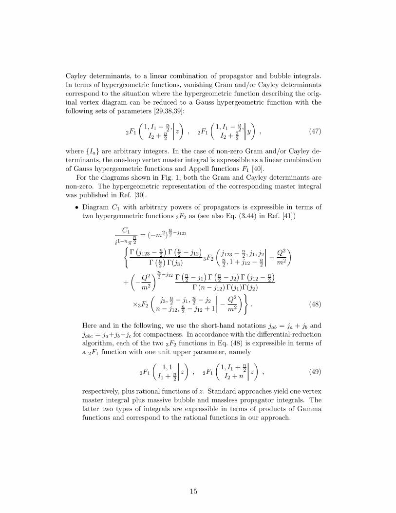
Cayley determinants, to a linear combination of propagator and bubble integrals.In terms of hypergeometric functions, vanishing Gram and/or Cayley determinantscorrespond to the situation where the hypergeometric function describing the orig-inal vertex diagram can be reduced to a Gauss hypergeometric function with thefollowing sets of parameters [29,38,39]:

2F1

(

1, I1 − n2 ,

I2 +n2

z

)

, 2F1

(

1, I1 − n2 ,

I2 +32

y

)

, (47)

where {Ia} are arbitrary integers. In the case of non-zero Gram and/or Cayley de-terminants, the one-loop vertex master integral is expressible as a linear combinationof Gauss hypergeometric functions and Appell functions F1 [40].

For the diagrams shown in Fig. 1, both the Gram and Cayley determinants arenon-zero. The hypergeometric representation of the corresponding master integralwas published in Ref. [30].

• Diagram C1 with arbitrary powers of propagators is expressible in terms oftwo hypergeometric functions 3F2 as (see also Eq. (3.44) in Ref. [41])

C1

i1−nπn2

= (−m2)n2−j123

{

Γ(

j123 − n2

)

Γ(

n2 − j12

)

Γ(

n2

)

Γ(j3)3F2

(

j123 − n2 , j1, j2

n2 , 1 + j12 − n

2

− Q2

m2

)

+

(

−Q2

m2

)

n2−j12 Γ

(

n2 − j1

)

Γ(

n2 − j2

)

Γ(

j12 − n2

)

Γ (n− j12) Γ(j1)Γ(j2)

×3F2

(

j3,n2 − j1,

n2 − j2

n− j12,n2 − j12 + 1

− Q2

m2

)

}

. (48)

Here and in the following, we use the short-hand notations jab = ja + jb andjabc = ja+jb+jc for compactness. In accordance with the differential-reductionalgorithm, each of the two 3F2 functions in Eq. (48) is expressible in terms ofa 2F1 function with one unit upper parameter, namely

2F1

(

1, 1I1 +

n2

z

)

, 2F1

(

1, I1 +n2

I2 + nz

)

, (49)

respectively, plus rational functions of z. Standard approaches yield one vertexmaster integral plus massive bubble and massless propagator integrals. Thelatter two types of integrals are expressible in terms of products of Gammafunctions and correspond to the rational functions in our approach.

15

• For diagram C2 with arbitrary powers of propagators, the result is

C2

i1−nπn2

= (−m2)n2−j123

{

Γ(

j123− n2

)

Γ(

n2−j12

)

Γ (n−j13−2j2)

Γ (n−j123) Γ(

n2−j2

)

Γ(j3)3F2

(

j123− n2 , j1, j2

1+j12− n2 , 1+j13+2j2−n

Q2

m2

)

+

(

−Q2

m2

)

n2−j12 Γ

(

n2 − j1

)

Γ(

j12 − n2

)

Γ(

n2 − j23

)

Γ (n− j123) Γ(j1)Γ(j2)

×3F2

(

j3,n2 − j2,

n2 − j1

n2 − j12 + 1, 1 + j23 − n

2

Q2

m2

)

}

. (50)

Similarly to the previous case, each of the two 3F2 functions in Eq. (50) isexpressible in terms of a 2F1 function with one unit upper parameter, namely

2F1

(

1, 1I1 − n

z

)

, 2F1

(

1, I1 +n2 ,

I2 − n2

z

)

, (51)

respectively, plus rational functions. Standard approaches yield one vertexmaster integral plus massive bubble and massless propagator integrals.

• Diagram C3 with arbitrary powers of propagators is expressible in terms ofone 4F3 function as

C3

i1−nπn2

= (−m2)n2−j123

Γ(

j123 − n2

)

Γ(

n2 − j3

)

Γ (j12) Γ(

n2

) 4F3

(

j123 − n2 , j1, j2,

n2 − j3

n2 ,

j122 , j12+1

2

Q2

4m2

)

.

(52)

In accordance with the differential-reduction algorithm, this function may bewritten in terms of a 3F2 function with one unit upper parameter and its firstderivative,

{1, θ} × 3F2

(

1, I1 − n2 ,

n2 − 1 + I2

n2 + I2,

12 + I3

z

)

, (53)

and a rational function. Standard approaches yield one vertex and one prop-agator master integral plus massive bubble integrals.

• Diagram C4 with arbitrary powers of propagators is expressible in terms ofone 3F2 function as

C4

i1−nπn2

= (−m2)n2−j123

Γ(

j123 − n2

)

Γ(

n2 − j1

)

Γ (j23) Γ(

n2

) 3F2

(

j123 − n2 , j1, j2

n2 , j23

Q2

m2

)

. (54)

In accordance with the differential-reduction algorithm, this function may bewritten in terms of a 3F2 function with one unit upper parameter and its firstderivative,

{1, θ} × 3F2

(

1, I1, I2 − n2

I1 + 1, n2 + I2z

)

, (55)

and a rational function. Standard approaches yield one vertex and one prop-agator master integral plus massive bubble integrals.

16

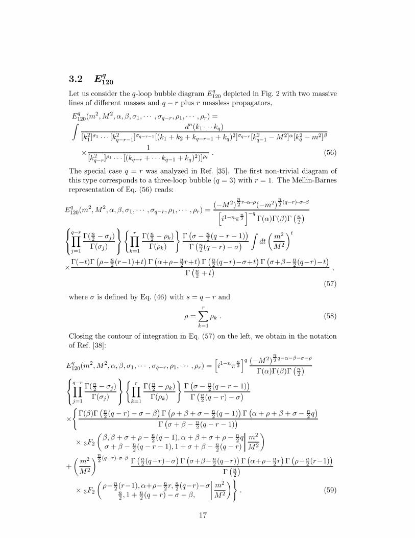
3.2 Eq120

Let us consider the q-loop bubble diagram Eq120 depicted in Fig. 2 with two massive

lines of different masses and q − r plus r massless propagators,

Eq120(m

2,M2, α, β, σ1, · · · , σq−r, ρ1, · · · , ρr) =∫

dn(k1 · · · kq)[k21 ]

σ1 · · · [k2q−r−1]σq−r−1 [(k1 + k2 + kq−r−1 + kq)2]σq−r [k2q−1 −M2]α[k2q −m2]β

× 1

[k2q−r]ρ1 · · · [(kq−r + · · · kq−1 + kq)2)]ρr

. (56)

The special case q = r was analyzed in Ref. [35]. The first non-trivial diagram ofthis type corresponds to a three-loop bubble (q = 3) with r = 1. The Mellin-Barnesrepresentation of Eq. (56) reads:

Eq120(m

2,M2, α, β, σ1, · · · , σq−r, ρ1, · · · , ρr) =(−M2)

n2 r−α−ρ(−m2)

n2 (q−r)−σ−β

[

i1−nπn2

]−qΓ(α)Γ(β)Γ

(

n2

)

q−r∏

j=1

Γ(n2 − σj)

Γ(σj)

{

r∏

k=1

Γ(n2 − ρk)

Γ(ρk)

}

Γ(

σ − n2 (q − r − 1)

)

Γ(

n2 (q − r)− σ

)

∫

dt

(

m2

M2

)t

×Γ(−t)Γ(

ρ− n2 (r−1)+t

)

Γ(

α+ρ− n2 r+t

)

Γ(

n2 (q−r)−σ+t

)

Γ(

σ+β− n2 (q−r)−t

)

Γ(

n2 + t

) ,

(57)

where σ is defined by Eq. (46) with s = q − r and

ρ =r∑

k=1

ρk . (58)

Closing the contour of integration in Eq. (57) on the left, we obtain in the notationof Ref. [38]:

Eq120(m

2,M2, α, β, σ1, · · · , σq−r, ρ1, · · · , ρr) =[

i1−nπn2

]q (−M2)n2 q−α−β−σ−ρ

Γ(α)Γ(β)Γ(

n2

)

q−r∏

j=1

Γ(n2 − σj)

Γ(σj)

{

r∏

k=1

Γ(n2 − ρk)

Γ(ρk)

}

Γ(

σ − n2 (q − r − 1)

)

Γ(

n2 (q − r)− σ

)

×{

Γ(β)Γ(

n2 (q − r)− σ − β

)

Γ(

ρ+ β + σ − n2 (q − 1)

)

Γ(

α+ ρ+ β + σ − n2 q)

Γ(

σ + β − n2 (q − r − 1)

)

× 3F2

(

β, β + σ + ρ− n2 (q − 1), α + β + σ + ρ− n

2 qσ + β − n

2 (q − r − 1), 1 + σ + β − n2 (q − r)

m2

M2

)

+

(

m2

M2

)

n2 (q−r)−σ−β Γ

(

n2 (q−r)−σ

)

Γ(

σ+β− n2 (q−r)

)

Γ(

α+ρ− n2 r)

Γ(

ρ− n2 (r−1)

)

Γ(

n2

)

× 3F2

(

ρ− n2 (r−1), α+ρ− n

2 r,n2 (q−r)−σ

n2 , 1 +

n2 (q − r)− σ − β,

m2

M2

)

}

. (59)

17

Let us discuss the differential reduction of the two hypergeometric functions inEq. (59) assuming that β, σj (σ ≥ 2), and ρk are integers. We distinguish betweentwo cases: r = 1 (q ≥ 3) and r ≥ 2 (q ≥ 4). For r = 1, both hypergeometricfunctions in Eq. (59) are reducible to 2F1 functions with one unit upper parameter,namely

2F1

(

1, I1 − n2 q

I2 − n2 (q − 2)

z

)

, 2F1

(

1, I1 − n2 ,

I2 +n2

z

)

, (60)

respectively. Standard approaches yield one three-loop bubble master integral andintegrals expressible in terms of Gamma functions. For r ≥ 2, the first hypergeomet-ric function is expressible in terms of a 3F2 function with one unit upper parameter,and the second one is reducible to a 2F1 function with both upper parameters con-taining non-zero ε parts, namely

(1, θ)×3F2

(

1, I1− n2 (q−1), I2− n

2 qI3− n

2 (q−r−1), I4− n2 (q−r)

z

)

, (1, θ)×2F1

(

I1− n2 (r−1), I2− n

2 rI3+

n2

z

)

,

(61)respectively. For q = 3 and r = 1, we present the explicit form of the master integral,with the powers of propagator being all equal to unity, in dimension n = 4− 2ε. Itreads:

E3120(m

2,M2, 1, 1, 1, 1, 1) =[

iπ2−ε]3

(M2)1−3εΓ2(1− ε)Γ (1 + 2ε) Γ (1 + ε)

2ε3(1− 2ε)(1 − ε)2×

{

(1−ε)

3(1−3ε)

Γ(1+3ε)

Γ(1+ε)2F1

(

1,−1+3ε1+ε

m2

M2

)

+

(

m2

M2

)1−2εΓ(1+ε)

Γ(1−ε)2F1

(

1, ε2−ε

m2

M2

)

}

.

(62)

The two Gauss hypergeometric functions in Eq. (62) can be reduced to the basisfunctions considered in Refs. [16,20,35] by the following relations:

(1− 2ε) 2F1

(

1, ε2− ε

z

)

= 1− ε− ε(1 − z) 2F1

(

1, 1 + ε2− ε

z

)

,

(1− 2ε) 2F1

(

1,−1 + 3ε1 + ε

z

)

= 1− 2ε− z(1− 3ε)

+3ε(1− 3ε)z(1 − z)

1 + ε2F1

(

1, 1 + 3ε2 + ε

z

)

. (63)

18

For illustration, we present here the first few coefficients of the ε expansion ofEq. (62):

E3120(m

2,M2, 1, 1, 1, 1, 1)

[iπ2−ε]3 Γ3(1 + ε)= (M2)1−3ε

(

1 + 2z

6ε3+

3 + z [5− 3 ln z)]

3ε2

+1

ε

{

25 + 34z

6− (1− z) [Li2 (z) + ln(z) ln(1− z)] + z ln z(ln z − 5) + ζ2

}

+(1− z) [2S1,2(z) + 2 (Li2 (z)− ζ2) ln(1− z) + Li2 (z) ln z]

+(1− z) {ln(1− z) ln z [ln z + ln(1− z)]− 5 [Li2 (z) + ln(z) ln(1− z)]}

+45 + 49z

3− 17z ln z + 5z ln2 z + 2 (3− z ln z) ζ2 −

5− 2z

3ζ3 −

2

3z ln3 z

+ε(1− z)

{

Li2 (z) [2 ln(1− z) (5− ln(1− z)− ln z)− ln z(ln z − 5)− 4ζ2 − 17]

+Li3 (z) ln z − Li4 (z) + 2S1,2(z) [5− 2 ln(1− z)− ln z]− 4S1,3(z)

+2 ln(1 − z)ζ2 [ln(1− z)− 5− ln z] + 4 ln(1− z)ζ3

+ ln z ln(1− z) [ln(1− z) + ln z]

[

5− 2

3(ln(1− z) + ln z)

]

+ ln z ln(1− z)

[

1

3ln z ln(1− z)− 17

]

}

+ε

{

z ln z

(

1

3ln2 z(ln z − 10) + 17 ln z + 2ζ2(ln z − 5) + 2ζ3 − 49

)

+301

6+ 43z + 25ζ2 −

10

3(3− z)ζ3 +

1

2ζ4(23 − 14z)

}

+O(ε)

)

, (64)

where

z =m2

M2. (65)

To check Eq. (64), we evaluate the first few coefficients of the ε expansion of theoriginal diagram in the large-mass limit [42] using the program packages developedin Refs. [43,44] to find agreement.

3.3 Jq22

Let us consider the q-loop sunset diagram Jq22 in Fig. 2 with two massive lines of

the same mass m and q − 2 massless subloops, which is one of the most frequentlystudied Feynman diagrams. It is defined as

Jq22(m

2, p2, α1, α2, σ1, · · · , σq−1) =∫

dn(k1 · · · kq)[k21 ]

σ1 · · · [k2q−1]σq−1 [k2q −m2]α1 [(k1 + k2 + · · ·+ kq + p)2 −m2]α2

. (66)

19

The Mellin-Barnes representation of Eq. (66) reads:10

Jq22(m

2, p2, α1, α2, σ1, · · · , σq−1) =(−m2)

n2−α1,2(p2)

n2 (q−1)−σ

[

i1−nπn/2]−q

Γ(α1)Γ(α2)

{

q−1∏

k=1

Γ(n2 − σk)

Γ(σk)

}

×∫

dt

(

− p2

m2

)t Γ(α1 + t)Γ(α2 + t)Γ(α1,2 − n2 + t)Γ(n2 + t)Γ(σ − n

2 (q − 1)− t)

Γ(α1,2 + 2t)Γ(n2 q − σ + t), (67)

where σ is defined by Eq. (46) with s = q − 1 and

α1,2 = α1 + α2 . (68)

Closing the contour of integration in Eq. (67) on the left, we obtain in the notationof Ref. [38]:

Jq22(m

2, p2, α1, α2, σ1, · · · , σq−1) =[

i1−nπn/2]q (−m2)

n2 q−α1,2−σ

Γ(α1)Γ(α2)

{

q−1∏

k=1

Γ(n2 − σk)

Γ(σk)

}

× Γ(

α1 + σ − n2 (q − 1)

)

Γ(

α2 + σ − n2 (q − 1)

)

Γ(

σ − n2 (q − 2)

)

Γ(

α1,2 + σ − n2 q)

Γ (α1,2 + 2σ − n(q − 1)) Γ(

n2

)

× 4F3

(

α1 + σ − n2 (q − 1), α2 + σ − n

2 (q − 1), σ − n2 (q − 2), α1,2 + σ − n

2 qn2 ,

12(α1,2 − n(q − 1)) + σ, 12 (1 + α1,2 − n(q − 1)) + σ,

p2

4m2

)

.

(69)

For q = 1 (see Footnote 10), the 4F3 function in Eq. (69) is reduced to a 3F2 function,in agreement with Ref. [38]. In the two-loop case (q = 2), the hypergeometricrepresentation of this diagram was derived in Refs. [45,46].

Let us analyze the reduction of the hypergeometric function in Eq. (69) assumingthat all parameters, α1, α2, and σk, are integer. For q = 1 (σk = 0), we obtain a

3F2 function with integer differences between upper and lower parameters, which,according to Criterion 1, is reducible to a 2F1 function with one integer upperparameter, so that we have a basis hypergeometric function plus a rational function.(For the one-loop propagator, there are one master integral and bubble integrals.)For q = 2, we get a 4F3 function with integer parameter differences and one integerupper parameter, so that it is reducible to a 3F2 function with one integer upperparameter and its first derivative,

(1, θ)× 3F2

(

1, I1 − n2 , I2 − n

I3 +n2 , I4 +

12 − n

2

z

)

, (70)

plus a rational function. In this case, there are two nontrivial master integrals ofthe same topology and bubble integrals, in accordance with the results of Ref. [47].For q ≥ 3, we have a 4F3 function with integer differences of parameters, which,according to Criterion 1, is reducible to a 3F2 function and its first two derivatives,

(1, θ, θ2)× 3F2

(

I1 − n2 (q − 1), I2 − n

2 (q − 2), I3 − n2 q

n2 , I4 +

12 − n

2 (q − 1)z

)

. (71)

10In the one-loop case (q = 1), the factor{

∏q−1k=1

Γ(n2−σk)

Γ(σk)

}

is equal to unity, and the representation of

Eq. (67) agrees with the one in Ref. [38].

20

3.4 Eq1220 and B

q1220

Let us consider the q-loop bubble diagram Eq1220 in Fig. 2 with two massive lines of

different masses and s plus r massless propagators,

Eq1220(m

2,M2, α1, α2, β, σ1, · · · , σs, ρ1, · · · , ρr) =∫

dn(k1 · · · kq)[k21 ]

σ1 · · · [k2s ]σs [k2s+1 −M2]α1 [(k1 + k2 + · · ·+ ks+1 + kq)2 −M2]α2

× 1

[k2s+2]ρ1 · · · [k2q−1]

ρr−1 [(ks+2 + · · · kq−1 + kq)2)]ρr(k2q −m2)β, (72)

where, by construction, s ≥ 0 and r ≥ 2 and, as a consequence, q = s + r + 1 ≥ 3.The Mellin-Barnes representation of Eq. (72) reads:

Eq1220(m

2,M2, α1, α2, β, σ1, · · · , σs, ρ1, · · · , ρr) =(−M2)

n2−α1,2(−m2)

n2 (q−1)−σ−β−ρ

Γ(α1)Γ(α2)Γ(β)Γ(

n2

)

×[

i1−nπn2

]q

s∏

j=1

Γ(n2 − σj)

Γ(σj)

{

r∏

k=1

Γ(n2 − ρk)

Γ(ρk)

}

Γ(

ρ− n2 (r − 1)

)

Γ(

n2 r − ρ

)

×∫

dt

(

m2

M2

)t Γ(α1 + t)Γ(α2 + t)Γ(α1,2 − n2 + t)Γ(n2 + t)

Γ(α1,2 + 2t)

× Γ(

σ − n2 s− t

)

Γ(

σ + β + ρ− n2 (q − 1)− t

)

Γ(

n2 (q − 1)− σ − ρ+ t

)

Γ(

n2 (s+ 1)− σ + t

) , (73)

where σ, ρ, and α1,2 are defined in Eqs. (46), (58), and (68), respectively.Diagram Bq

1220 in Fig. 2 emerges from Eq1220 with r = 1 and s = q − 2 in the

smooth limit ρ = ρ1 → 0. Then, Eq. (73) simplifies due toΓ(n2 (q−1)−σ−ρ+s)Γ(n2 (s+1)−σ+s)

= 1 .

Closing the contour of integration in Eq. (73) on the left, we obtain in the

21

notation of Ref. [38]:

Eq1220(m

2,M2, α1, α2, β, σ1, · · · , σz, ρ1, · · · , ρr) =[

i1−nπn2

]q (−M2)n2 q−α1,2−σ−β−ρ

Γ(α1)Γ(α2)Γ(β)Γ(

n2

)

s∏

j=1

Γ(n2 − σj)

Γ(σj)

{

r∏

k=1

Γ(n2 − ρk)

Γ(ρk)

}

Γ(

ρ− n2 (r − 1)

)

Γ(

n2 r − ρ

)

×{

(

m2

M2

)

n2 r−β−ρ Γ

(

σ − n2 (s− 1)

)

Γ(

n2 r − ρ

)

Γ(

ρ+ β − n2 r)

Γ(

n2

)

Γ (α1,2 + 2σ − ns)

×Γ(

a1,σ − n2 s)

Γ(

a2,σ − n2s)

Γ(

a1,2,σ − n2 (s+ 1)

)

5F4

(

a1,σ − n2 s, a2,σ − n

2s, a1,2,σ − n2 (s+ 1), σ − n

2 (s− 1), n2 r − ρn2 ,

α1,2−ns2 + σ,

α1,2+1−ns2 + σ, n2 r − ρ+ 1− β

m2

4M2

)

+Γ(β)Γ

(

n2 r − aβ,ρ

)

Γ(

aσ,β,ρ − n2 (q − 2)

)

Γ (α1,2 + 2σ + 2β + 2ρ− n(q − 1)) Γ(

aβ,ρ − n2 (r − 1)

)

×Γ(

a1,σ,β,ρ − n2 (q − 1)

)

Γ(

a2,σ,β,ρ − n2 (q − 1)

)

Γ(

a1,2,σ,β,ρ − n2 q)

5F4

(

a1,σ,β,ρ− n2 (q−1), a2,σ,β,ρ− n

2 (q−1), a1,2,σ,β,ρ− n2 q, aσ,β,ρ− n

2 (q−2), β

1+aβ,ρ− n2 r, aσ,β,ρ+

α1,2−n(q−1)2 , aσ,β,ρ+

α1,2+1−n(q−1)2 , aβ,ρ− n

2 (r−1)

m2

4M2

)}

,

(74)

where we have introduced the short-hand notations

ai,σ = α1 + σ , aβ,ρ = β + ρ ,

a1,2,σ = α1 + α2 + σ , aσ,β,ρ = σ + β + ρ ,

a1,2,σ,β = α1 + α2 + σ + β , ai,σ,β,ρ = αi + σ + β + ρ ,

a1,2,σ,β,ρ = α1 + α2 + σ + β + ρ , i = 1, 2 . (75)

Let us analyze the result of the differential reduction of the two hypergeometricfunctions in Eq. (74) assuming that all parameters, α1, α2, β, σk, ρj , are integer. Wedistinguish between the three cases: s = 0, s = 1, and s ≥ 2. For s = 0 (σk = 0,r = q−1), both hypergeometric functions in Eq. (74) are reducible to 2F1 functionswith one unit upper parameter,

2F1

(

1, I1 − n2

I2 +12

z

)

, 2F1

(

1, I1 − n2 q,

12 + I2 − n

2 (q − 1)z

)

. (76)

Standard approaches yield one master integral. For s = 1 (r = q − 2), each of thetwo hypergeometric functions is reducible to a 3F2 function with one unit upperparameter,

(1, θ)×3F2

(

1, I1−n, I2− n2

I3+n2 , I4+

12− n

2

z

)

, (1, θ)×3F2

(

1, I1− n2 (q−1), I2− n

2 qI3− n

2 (q−3), I4+12− n

2 (q−1)z

)

.

(77)For s ≥ 2, the first hypergeometric function is reducible to a 3F2 function and itsfirst two derivatives, while the second one is expressible in terms of a 4F3 function

22

and its first two derivatives, namely

(1, θ, θ2)× 3F2

(

I1 − n2 s, I2 − n

2 (s + 1), I3 − n2 (s− 1)

I4 +n2 , I5 +

12 − n

2 sz

)

,

(1, θ, θ2)× 4F3

(

1, I1 − n2 q, I2 − n

2 (q − 1), I3 − n2 (q − 2)

12 + I4 − n

2 (q − 1), I5 − n2 r, I6 − n

2 (r − 1)z

)

, (78)

respectively. Notice that, according to Criterion 4, a third derivative does notappear because one of the upper parameters is integer.

We now present an explicit result for the three-loop case in which there is nomassless propagator inside the massive loop, q = 3, s = 0, σk = σ = 0, r = 2, andn = 4−2ε. In this case, there is one master integral with α1 = α2 = β = ρ1 = ρ2 = 1(α1,2 = ρ = 2),

E31220(m

2,M2, 1, 1, 1, 1, 1) =[

iπ2−ε]3

(M2)1−3ε

Γ(1− ε)Γ2(1 + ε)Γ(1 + 2ε)

2ε3(1− ε)(1 − 2ε)

{

(

m2

M2

)1−2ε

2F1

(

1, ε32

m2

4M2

)

+2

3(1− 3ε)

Γ(1 + 2ε)Γ(1 + 3ε)

Γ(1 + 4ε)Γ (1 + ε)2F1

(

1,−1 + 3ε12 + 2ε

m2

4M2

)

}

. (79)

To reduce the Gauss hypergeometric functions in Eq. (79) to sets of functions studiedin Refs. [16,20,35], we apply the following relations:

(1− 2ε) 2F1

(

1, ε32

z

)

= 1− 2ε(1− z) 2F1

(

1, 1 + ε32

z

)

,

2F1

(

1,−1 + 3ε12 + 2ε

z

)

= 1− 2z(1− 3ε)

1− 2ε+

12ε(1 − 3ε)z(1 − z)

(1− 2ε)(1 + 4ε)2F1

(

1, 1 + 3ε32 + 2ε

z

)

. (80)

The first few coefficients of the ε expansion of Eq. (79) are given by

E31220(m

2,M2, 1, 1, 1, 1, 1)

Γ3(1 + ε) [iπ2−ε]3= (M2)1−3ε

(

(1 + z)

3ε3+

6 + z(5 − 3 ln z)

3ε2

+1

3ε

{

25 + z(17 − 15 ln z + 3 ln2 z + 3ζ2)}

+2(4− z)

ε

(1− y)

(1 + y)

[

Li2 (1− y) +1

4ln2 y +

1

2ln z ln y

]

+1

3(90 + 49z) +

1

3ζ3(8− 7z)− z

[

17 ln z − 5 ln2 z +2

3ln3 z

]

+ ζ2z(5 − 2 ln z)

+1− y

1 + y(4− z)

{

4S1,2(y) + 2S1,2(

y2)

− 4S1,2(−y)− 6Li3 (y)− 2Li3 (−y)

+Li2 (−y) [4 ln(1− y)− 2 ln z] + Li2 (1− y) [10− 8 ln(1− y)− 4 ln(1 + y)]

+ ln(1− y)[

2ζ2 − 4 ln y ln(1− y)− 3 ln2 y]

+ ln2 y

[

5

2− ln(1 + y) +

2

3ln y

]

−ζ2(ln z − 4 ln y)− ζ3 + ln z ln y

[

5 +1

2ln y − 2 ln(1 + y)− ln z

]

}

+O(ε)

)

, (81)

23

where z is defined in Eq. (65) and the variable y is defined as

y =1−

√

zz−4

1 +√

zz−4

, z = −(1− y)2

y, 4− z =

(1 + y)2

y. (82)

The O(ε) term is too long to be presented here, but is available from Ref. [48]. Wemention here only that, in accordance with the expansion of the Gauss hypergeo-metric function constructed in Refs. [20,35], this term is expressible just in terms ofNielsen polylogarithms. To check Eq. (81), we evaluate the first few coefficients ofthe ε expansion of the original diagram in the large-mass limit [42] using the pro-gram packages developed in Refs. [43,44] to find agreement. In order to constructthe series expansion about 1− y, which serves as the small parameter of the large-mass expansion, we employ the trick described in Ref. [49]. In fact, the variable1− y can be written as a series in the small parameter z as

1− y = i√z

[√

1− z

4− i

√

z

4

]

= i√z

[

1− i

√z

2− z

8

∞∑

k=0

(2k)!

(k!)21

k + 1

( z

16

)k]

. (83)

For completeness, we also present the explicit result for diagram Bq1220 in Fig. 2:11

Bq1220(m

2,M2, α1, α2, β, σ1, · · · , σq−2)

=(−M2)

n2 q−α1,2−σ−βΓ

(

n2 − β

)

Γ(α1)Γ(α2)Γ(β)Γ(

n2

)

[

i1−nπn2

]−q

{

q−2∏

k=1

Γ(n2 − σk)

Γ(σk)

}

×{

Γ(

a1,σ,β − n2 (q − 1)

)

Γ(

a2,σ,β − n2 (q − 1)

)

Γ(

a1,2,β,σ − n2 q)

Γ(

aσ,β − n2 (q − 2)

)

Γ (α1,2 + 2β + 2σ − n(q − 1))

4F3

(

a1,β,σ − n2 (q − 1), a2,β,σ − n

2 (q − 1), α1,2 + β + σ − n2 q, aσ,β − n

2 (q − 2)12(α1,2 − n(q − 1)) + σ + β, 12(α1,2 + 1− n(q − 1)) + σ + β, 1 + β − n

2

m2

4M2

)

+

(

m2

M2

)

n2−β Γ

(

a1,σ − n2 (q − 2)

)

Γ(

a2,σ − n2 (q − 2)

)

Γ(

a1,2,σ − n2 (q − 1)

)

Γ(

n2 − β

)

Γ (α1,2 + 2σ − n(q − 2))

×Γ(

σ − n2 (q − 3)

)

Γ(

β − n2

)

4F3

(

a1,σ − n2 (q − 2), a2,σ − n

2 (q − 2), a1,2,σ − n2 (q − 1), σ − n

2 (q − 3)12 (α1,2 − n(q − 2)) + σ, 12 (α1,2 + 1− n(q − 2)) + σ, 1− β + n

2

m2

4M2

)

}

,(84)

where q ≥ 2. For q = 2, the hypergeometric representation was derived in Ref. [51].12

The result of the differential reduction of the hypergeometric functions in Eq. (84)assuming that all parameters, α1, α2, β, and σk, are integer may be derived forq = 2, q = 3, and q ≥ 4 by directly substituting r = 1 and s = q − 2 in Eqs. (76)–(78), respectively. We only point out here that, for q = 3, the second hypergeometric

11For the four-loop case (q = 4) with equal masses m = M , the Mellin-Barnes representation of thisdiagram was published in Ref. [50]. In order to recover the result of Ref. [50] from Eq. (73), it is sufficientto redefine the variable of integration t to be t = N/2− α12 − s.

12In this case, we have σ = 0 and{

∏q−2k=1

Γ(n2−σk)

Γ(σk)

}

= 1.

24

function in Eq. (77) is reducible to a 2F1 function and its first derivative, so thatthe differential reduction yields

(1, θ)× 2F1

(

I1 − n, I2 − 3n2

12 + I3 − n

z

)

, (1, θ)× 3F2

(

1, I1 − n, I2 − n2

12 + I3 − n

2 , I4 +n2

z

)

, (85)

and that, for q ≥ 4, the second hypergeometric function in Eq. (78) is reducible toa 3F2 function and its first two derivatives, so that the differential reduction yields

(1, θ, θ2)× 3F2

(

I1 − n2 q, I2 − n

2 (q − 1), I3 − n2 (q − 2)

12 + I4 − n

2 (q − 1), I5 − n2

z

)

,

(1, θ, θ2)× 3F2

(

I1 − n2 (q − 2), I2 − n

2 (q − 1), I3 − n2 (q − 3)

I4 +n2 , I5 +

12 − n

2 (q − 2)z

)

. (86)

It is interesting to note that, in the single-scale case m = M [52], there is onlyone master integral [43]. This is because the hypergeometric functions 3F2 and

2F1 with special values of parameters and argument z = 1/4 are expressible asproducts of Gamma functions. For details, see Eqs. (4.36) and (4.42) in Ref. [29]. Adiagrammatic interpretation of similar identities was presented in Ref. [53]. On theother hand, this is a manifestation of the existence of functional relations betweenFeynman diagrams [54].

We now present the explicit result for the three-loop case q = 3, n = 4− 2ε. Inthis case, the first master integral corresponds to α1 = α2 = β = σ1 = 1, while wechoose α1 = β = σ1 = 1 and α2 = 2 for the second one,

B31220(m

2,M2, 1, 1, 1, 1) = (M2)2−3ε Γ3(1 + ε)(iπ2−ε)3

ε3(1− ε)2(1− 2ε)

×{

2(1 − ε)(1− 4ε)Γ2 (1 + 2ε) Γ (1 + 3ε) Γ(1− ε)

3(1− 3ε)(2 − 3ε)Γ(1 + 4ε)Γ2(1 + ε)2F1

(

−1 + 2ε,−2 + 3ε−1

2 + 2ε

m2

4M2

)

+

(

m2

M2

)1−ε

3F2

(

1, ε,−1 + 2ε2− ε, 12 + ε

m2

4M2

)

}

,

B31220(m

2,M2, 1, 2, 1, 1) = (M2)1−3εΓ3(1 + ε)(iπ2−ε)3

2ε3(1− ε)2

×{

2(1 − ε)(1− 4ε)Γ2 (1 + 2ε) Γ (1 + 3ε) Γ(1− ε)

3(1− 2ε)(1 − 3ε)Γ(1 + 4ε)Γ2(1 + ε)2F1

(

−1 + 2ε,−1 + 3ε−1

2 + 2ε

m2

4M2

)

+

(

m2

M2

)1−ε

3F2

(

1, ε, 2ε2− ε, 12 + ε

m2

4M2

)

}

. (87)

In order to express all hypergeometric functions entering Eq. (87) in terms of func-tions which were analyzed in Ref. [20] (see Appendix A for details), we apply the

25

following set of relations:

(1− 4ε) 2F1

(

−1 + 2ε,−2 + 3ε−1

2 + 2εz

)

= −24z(1 − z)(1 + 2z)ε2

(1 + 4ε)2F1

(

1 + 2ε, 1 + 3ε32 + 2ε

z

)

+[

1− 4ε− 4z + 8εz2 + 14εz]

2F1

(

2ε, 3ε12 + 2ε

z

)

,

(1− 4ε) 2F1

(

−1 + 2ε,−1 + 3ε−1

2 + 2εz

)

= −24z(1 − z)ε2

1 + 4ε2F1

(

1 + 2ε, 1 + 3ε32 + 2ε

z

)

+ [1− 4ε− 2z + 10zε)] 2F1

(

2ε, 3ε12 + fε

z

)

,

2z(1 − 2ε)(1 − 3ε)

1− ε3F2

(

1, ε, 2ε2− ε, 12 + ε

z

)

= 1− 2ε

+ [2ε(1 − 4z)− (1− 2z)] 3F2

(

1, ε, 2ε1− ε, 12 + ε

z

)

+8z(1 − z)ε2

(1− ε)(1 + 2ε)3F2

(

2, 1 + ε, 1 + 2ε2− ε, 32 + ε

z

)

,

z(1− 3ε)(2 − 3ε) 3F2

(

1, ε,−1 + 2ε2− ε, 12 + ε

z

)

=1

2(1− ε)(1− 2ε+ 2zε)

+4ε2z(1 − z)(1 + 2z)

(1 + 2ε)3F2

(

2, 1 + ε, 1 + 2ε2− ε, 32 + ε

z

)

−(1− ε)

2

[

1− 4z − 2ε(1 − 8z − 2z2)]

3F2

(

1, ε, 2ε1− ε, 12 + ε

z

)

. (88)

Here, the following relation was used:

z(b− a2)(b− a3)(1 + b− a3)(f − a3) 3F2

(

1, a2, a3 − 1b+ 1, f

z

)

= −b(1− a3)(1 − z) [a3 − f + (a2 − b)z] θ 3F2

(

1, a2, a3b, f

z

)

+b(1− a3)

{

a2(a2 − b)z2 + (a3 − f)(1− f)− b(1 + a2 + 2a3 − b)z

−[

f(2a2 + a3 − 2b) + a2(a2 − 1)− (a2 + a3)2]

z

}

3F2

(

1, a2, a3b, f

z

)

−b(f − 1) [(1− a3)(f − a3)− (b− 1)(b− a2)z] . (89)

26

The first coefficients of the ε expansions of Eq. (87) read:

B31220(m

2,M2, 1, 1, 1, 1)

Γ3(1 + ε)(iπ2−ε)3=(

M2)2−3ε

(

1 + 2z

3ε3+

1

ε2

{

7

6+

8

3z − 1

12z2 − z ln z

}

+1

ε

{

25

12+

20

3z − 5

8z2 +

1

4z ln z [z + 2 ln z − 16]

}

+8

3ζ3(1− z)− 5

24+

35

3z − 145

48z2 − 1

6z ln3 z +

(16− z)

8z ln2 z − (80− 15z)

8z ln z

−4(1− z) [S1,2(1− y) + ln yLi2 (1− y)]− (1− z) ln2 y

[

ln z +2

3ln y

]

−(8 + 2z − z2)(1 − y)

(1 + y)

[

Li2 (1− y) +1

2ln z ln y +

1

4ln2 y

]

+O(ε)

)

,

B31220(m

2,M2, 1, 2, 1, 1)

Γ3(1 + ε)(iπ2−ε)3=(

M2)1−3ε

(

1 + z

3ε3+

1

6ε2{4 + 5z − 3z ln z}

+1

3ε{1 + 4z} − 1

4εz ln z {4− ln z} − 10

3+

5

6z − 1

2z ln z

[

1− ln z +1

6ln2 z

]

+(4− z)(1− y)

(1 + y)

[

2Li2 (1− y) +1

2ln2 y + ln z ln y

]

+2(z − 2)

[

S1,2(1− y) + ln yLi2 (1− y) +1

6ln3 y +

1

4ln z ln2 y − 2

3ζ3

]

+O(ε)

)

, (90)

where y and z are defined in Eqs. (82) and (65), respectively. The O(ε) term is toolong to be presented here, but is available from Ref. [48]. To check Eq. (90), weevaluate the first few coefficients of the ε expansion of the original diagram in thelarge-mass limit [42] using the program packages developed in Refs. [43,44] to findagreement.

3.5 Vq1220 and J

q1220

Let us consider the q-loop on-shell propagator diagram V q1220 in Fig. 2 with s plus r

massless propagators,

V q1220(m

2,M2, α1, α2, β, σ1, · · · , σs, ρ1, · · · , ρr)

=

∫

dn(k1 · · · kq)[k21 ]

σ1 · · · [k2s ]σs [k2s+1 −M2]α1 [(k1 + k2 + · · ·+ ks+1 + kq)2 −M2]α2

× 1

[k2s+2]ρ1 · · · [k2q−1]

ρr−1 [(ks+2 + · · · + kq−1 + kq)2)]ρr ((kq − p)2 −m2)β

∣

∣

∣

∣

∣

p2=m2

, (91)

27

where q = s+ r + 1. The Mellin-Barnes representation of Eq. (91) reads:

V q1220(m

2,M2, α1, α2, β, σ1, · · · , σs, ρ1, · · · , ρr) =(−M2)

n2−α1,2(−m2)

n2 (q−1)−σ−β−ρ

Γ(α1)Γ(α2)Γ(β)

×[

i1−nπn2

]q

s∏

j=1

Γ(n2 − σj)

Γ(σj)

{

r∏

k=1

Γ(n2 − ρk)

Γ(ρk)

}

Γ(

ρ− n2 (r − 1)

)

Γ(

n2 r − ρ

)

×∫

dt

(

m2

M2

)t Γ(α1 + t)Γ(α2 + t)Γ(α1,2 − n2 + t)Γ(n2 + t)

Γ(α1,2 + 2t)

× Γ(

σ − n2 s− t

)

Γ(

σ + β + ρ− n2 (q − 1)− t

)

Γ (n(q − 1)− 2σ − β − 2ρ+ 2t)

Γ(

n2 (s + 1)− σ + t

)

Γ(

n2 q − σ − β − ρ+ t

) , (92)

where σ, ρ, and α1,2 are defined in Eqs. (46), (58), and (68), respectively.Diagram Jq

1220 in Fig. 2 emerges from V q1220 with r = 1 and s = q−2 in the smooth

limit ρ = ρ1 → 0. For the special case q = 3, the Mellin-Barnes representation hasrecently been presented in Ref. [55].

Closing the contour of integration in Eq. (92) on the left, we obtain:

V q1220(m

2,M2, α1, α2, β, σ1, · · · , σs, ρ1, · · · , ρr) =

(

i1−nπn2

)q(−M2)

n2 q−α1,2,σ,β,ρ

Γ(α1)Γ(α2)Γ(β)Γ(

n2

)

×

s∏

j=1

Γ(n2 − σj)

Γ(σj)

{

r∏

k=1

Γ(n2 − ρk)

Γ(ρk)

}

Γ(

ρ− n2 (r − 1)

)

Γ(

n2 r − ρ

)

×{

(

m2

M2

)

n2 r−aβ,ρ Γ

(

σ − n2 (s− 1)

)

Γ (nr − 2ρ− β) Γ(

ρ+ β − n2 r)

Γ (α1,2 + 2σ − ns) Γ(

n2 (r + 1)− ρ− β

)

× Γ(

a1,σ − n2 s)

Γ(

a2,σ − n2 s)

Γ(

a1,2,σ − n2 (s+ 1)

)

× 6F5

(

a1,σ− n2 s, a2,σ− n

2 s, a1,2,σ− n2 (s+1), σ− n

2 (s−1), nr−β2 −ρ, nr−β+12 −ρn2 ,

α1,2−ns2 +σ,

α1,2+1−ns2 +σ, n2 (r+1)−β−ρ, n2 r−β−ρ+1

m2

M2

)

+Γ(

n2 r − aβ,ρ

)

Γ(

aσ,β,ρ − n2 (q − 2)

)

Γ(β)

Γ (α1,2 + 2σ + 2β + 2ρ− n(q − 1)) Γ(

aβ,ρ − n2 (r − 1)

)

× Γ(

a1,σ,β,ρ − n2 (q − 1)

)

Γ(

a2,σ,β,ρ − n2 (q − 1)

)

Γ(

a1,2,σ,β,ρ − n2 q)

× 6F5

(

a1,σ,β,ρ− n2 (q−1), a2,σ,β,ρ− n

2 (q−1), a1,2,σ,β,ρ− n2 q, aσ,β,ρ− n

2 (q−2), β2 ,β+12

n2 , 1+aβ,ρ− n

2 r,α1,2−n(q−1)

2 +aσ,β,ρ,α1,2+1−n(q−1)

2 +aσ,β,ρ, aβ,ρ− n2 (r−1)

m2

M2

)}

,

(93)

where a1,σ, a2,σ, aβ,ρ, a1,2,σ, aσ,β,ρ, a1,σ,β,ρ, and a2,σ,β,ρ are defined in Eq. (75). In thespecial case in which there is no massless propagator inside the massive loop, s = 0

(r = q − 1, σ = 0,∏q−2

k=1

Γ(n2−σk)

Γ(σk)= 1), the 6F5 functions in Eq. (93) are reduced to

5F4 functions. For q = 2, s = 0, and r = 1, the hypergeometric representation wasgiven in Ref. [56].

Let us analyze the result of the differential reduction of the hypergeometricfunctions in Eq. (93) assuming that all parameters, α1, α2, β, σk, and ρk, are

28

integer. For r 6= 0, we distinguish between the three cases s = 0, s = 1, and s ≥ 2.For s = 0 (r = q−1, σ = 0), each of the two hypergeometric functions in Eq. (93) isreducible to a 3F2 function with one unit upper parameter and its first derivative,

(1, θ)× 3F2

(

1, I1 − n2 , I2 +

12 + n

2 (q − 1)I3 +

12 , I4 +

n2 q

z

)

,

(1, θ)× 3F2

(

1, I1 +12 , I2 − n

2 qI3 +

n2 ,

12 + I4 − n

2 (q − 1)z

)

. (94)

For s = 1 (r = q − 2), each of the two hypergeometric functions in Eq. (93) isreducible to a 4F3 function with one unit upper parameter and its first two deriva-tives,

(1, θ, θ2)× 4F3

(

1, I1 − n, I2 − n2 , I3 +

12 +

n2 (q − 2)

I4 +n2 , I5 +

12 − n

2 , I6 +n2 (q − 1)

z

)

,

(1, θ, θ2)× 4F3

(

1, I1 +12 , I2 − n

2 q, I3 − n2 (q − 1)

I4 +n2 ,

12 + I5 − n

2 (q − 1), I6 − n2 (q − 3)

z

)

. (95)

For s ≥ 2, one of the hypergeometric functions in Eq. (93) is reducible to a 4F3

function with all upper parameters having non-zero ε parts, whereas the second oneis expressible in terms of a 5F4 function with one unit upper parameter,

(1, θ, θ2, θ3)× 4F3

(

I1 − n2 (s− 1), I2 − n

2 s, I3 − n2 (s+ 1), I4 +

12 +

n2 r

I5 +n2 , I6 +

12 − n

2 s, I7 +n2 (r + 1)

z

)

,

(1, θ, θ2, θ3)× 5F4

(

1, I1 +12 , I2 − n

2 q, I3 − n2 (q − 1), I4 − n

2 (q − 2)I5 +

n2 ,

12 + I6 − n

2 (q − 1), I7 − n2 r, I8 − n

2 (r − 1)z

)

. (96)

For completeness, we also present an explicit result for diagram Jq1220 in Fig. 2:

Jq1220(m

2,M2, α1, α2, β, σ1, · · · , σq−2)

=

[

i1−nπn2

]qΓ(

β − n2

)

(−M2)n2q−α1,2,σ,β

Γ(α1)Γ(α2)Γ(β)Γ(

n2

)

{

q−2∏

k=1

Γ(n2 − σk)

Γ(σk)

}

×{

(

m2

M2

)

n2−β Γ

(

σ− n2 (q−3)

)

Γ(

a1,σ− n2 (q−2)

)

Γ(

a2,σ− n2 (q−2)

)

Γ(

a1,2,σ− n2 (q−1)

)

Γ (α1,2 + 2σ − n(q − 2))

× 6F5

(

a1,σ− n2 (q−2), a2,σ− n

2 (q−2), a1,2,σ− n2 (q−1), σ− n

2 (q−3), n−β2 , n−β+12n2 , n−β, n2+1−β,

α1,2−n(q−2)2 +σ,

α1,2+1−n(q−2)2 +σ

m2

M2

)

+Γ(

n2−β

)

Γ(

aσ,β− n2 (q−2)

)

Γ(

a1,σ,β− n2 (q−1)

)

Γ(

a2,σ,β− n2 (q−1)

)

Γ(

α1,2,σ,β− n2 q)

Γ(

β− n2

)

Γ (α1,2+2σ+2β−n(q−1))

× 6F5

(

a1,σ,β− n2 (q−1), a2,σ,β− n

2 (q−1), a1,2,σ,β− n2 q, aσ,β− n

2 (q−2), β2 ,β+12

n2 , β, 1+β− n

2 ,α1,2−n(q−1)

2 +σ+β,α1,2+1−n(q−1)

2 +σ+β

m2

M2

)}

.

(97)

In this case, the result of the differential reduction assuming that all parameters,α1, α2, β, and σk, are integer can be derived for q = 2, q = 3, and q ≥ 4 by directly

29

substituting r = 1 and s = q − 2 in Eqs. (94)–(96), respectively. We only point outhere that, for q = 3, the second hypergeometric function in Eq. (95) is reducible toa 3F2 function and its first two derivatives, so that the differential reduction yields

(1, θ, θ2)× 4F3

(

1, I1 − n, I2 − n2 , I3 +

12 +

n2

I4 +n2 , I5 +

12 − n

2 , I6 + nz

)

,

(1, θ, θ2)× 3F2

(

I1 +12 , I2 − n, I3 − 3n

2I4 +

n2 ,

12 + I5 − n

z

)

, (98)

and that, for q ≥ 4, the 5F4 hypergeometric functions in Eq. (96) is reducible to a

4F3 function with all upper parameters having non-zero ε parts:

(1, θ, θ2, θ3)× 4F3

(

I1 − n2 (q − 3), I2 − n

2 (q − 2), I3 − n2 (q − 1), I4 +

12 + n

2I5 +

n2 , I6 +

12 − n

2 (q − 2), I7 + nz

)

,

(1, θ, θ2, θ3)× 4F3

(

I1 +12 , I2 − n

2 q, I3 − n2 (q − 1), I4 − n

2 (q − 2)I5 +

n2 ,

12 + I6 − n

2 (q − 1), I7 − n2

z

)

. (99)

In particular, for q = 2, in accordance with Ref. [57], there are two nontrivial masterintegrals plus bubble integrals. For q = 3, in accordance with Ref. [55], there arethree nontrivial master integrals plus bubble integrals.

3.6 Two-loop vertex

Let us consider the diagram F2 shown in Fig. 2

F2(M2, p2, α1, α2, σ1, σ2, ) =

∫

dn(k1k2)

[(k1 − p1)2]σ1 [(k1 − p2)2]σ2 [k21]β [k22 −M2]α1 [(k1 − k2)2 −M2]α2

∣

∣

∣

∣

p21=p2

2=0

=[

i1−nπn2

]2 (−M2)n2−α12(p2)

n2−σ12−β

Γ(α1)Γ(α2)Γ(σ1)Γ(σ2)

×∫

dt

(

− p2

M2

)t Γ(−t)Γ(α1+t)Γ(α2+t)Γ(α12− n2+t)

Γ (α12 + 2t)

Γ(

n2−σ1−β+t

)

Γ(

n2−σ2−β+t

)

Γ(

σ12+β− n2−t

)

Γ(n− σ12 − β + t). (100)

30

where σ is defined in Eq. (46) with s = 2 and α12 in Eq. (68). Closing the contourof integration on the left we obtain in the notation of Ref. [38]:

F2(M2, p2, α1, α2, σ1, σ2, ) =

[

i1−nπn2

]2 (−M2)n2−α12(p2)

n2−σ12−βΓ

(

n2−σ12−β

)

Γ(α1)Γ(α2)

×{

Γ(α1)Γ(α2)Γ(

n2−σ1−β

)

Γ(

n2−σ2−β

)

Γ(

σ12+β− n2

)

Γ(

α12− n2

)

Γ(σ1)Γ(σ2)Γ(α12)Γ (n−σ12−β) Γ(

n2−σ12−β

)

× 5F4

(

α1, α2, α12− n2 ,

n2−σ1−β, n2−σ2−β

n−σ12−β, 1+ n2−σ12−β, α12

2 , α12+12

− p2

4M2

)

+

(

− p2

M2

)β+σ12−n2 Γ

(

α1+σ12+β− n2

)

Γ(

α2+σ12+β− n2

)

Γ (σ12+α12+β−n)

Γ(α12+2σ12+2β−n)Γ(

n2

)

× 5F4

(

σ1, σ2, α1+σ12+β− n2 , α2+σ12+β− n

2 , α12+σ12+β−nn2 , 1+σ12+β− n

2 , σ12+β+ α12−n2 , σ12+β+ α12+1−n

2

− p2

4M2

)

}

.(101)

By differential reduction, the two hypergeometric functions in Eq. (101) may bereduced to

(1, θ)× 3F2

(

1, I1− n2 ,

n2+I2

n+I3,12+I4

− p2

4M2

)

, (1, θ)× 3F2

(

1, 1, I1−nI2+

n2 , I3+

12− n

2

− p2

4M2

)

,(102)

respectively, where {Ia} is a set of integers. In accordance with Ref. [20], the first fewcoefficients of the ε expansion of this diagram are expressible in terms of Remiddi-Vermaseren functions, i.e. multiple polylogarithms of the square roots of unity, ofargument

y =1−

√

zz+4

1 +√

zz+4

, (103)

where z = p2/M2 (see also the discussion in Ref. [58]). The on-shell value z = 1 cor-responds to Remiddi-Vermaseren functions of argument (3−

√5)/2 = [(

√5−1)/2]2,

in agreement with results of Ref. [59]. It is interesting to note that these constantsare generated not only in Higgs-boson decay [59], but also in orthopositronium decay[60].

4 Master integrals in differential reduction and

IBP technique

In this section, we compare the differential-reduction and IPB techniques with re-spect to the numbers of master integrals which they produce. For this purpose,we return to the Feynman diagrams depicted in Figs. 1 and 2. They all have thefollowing hypergeometric structure:

Φ(n,~j; z) =

k∑

a=1

zlaCla(n,~j)p+1Fp( ~Aa; ~Ba;κz) , (104)

31

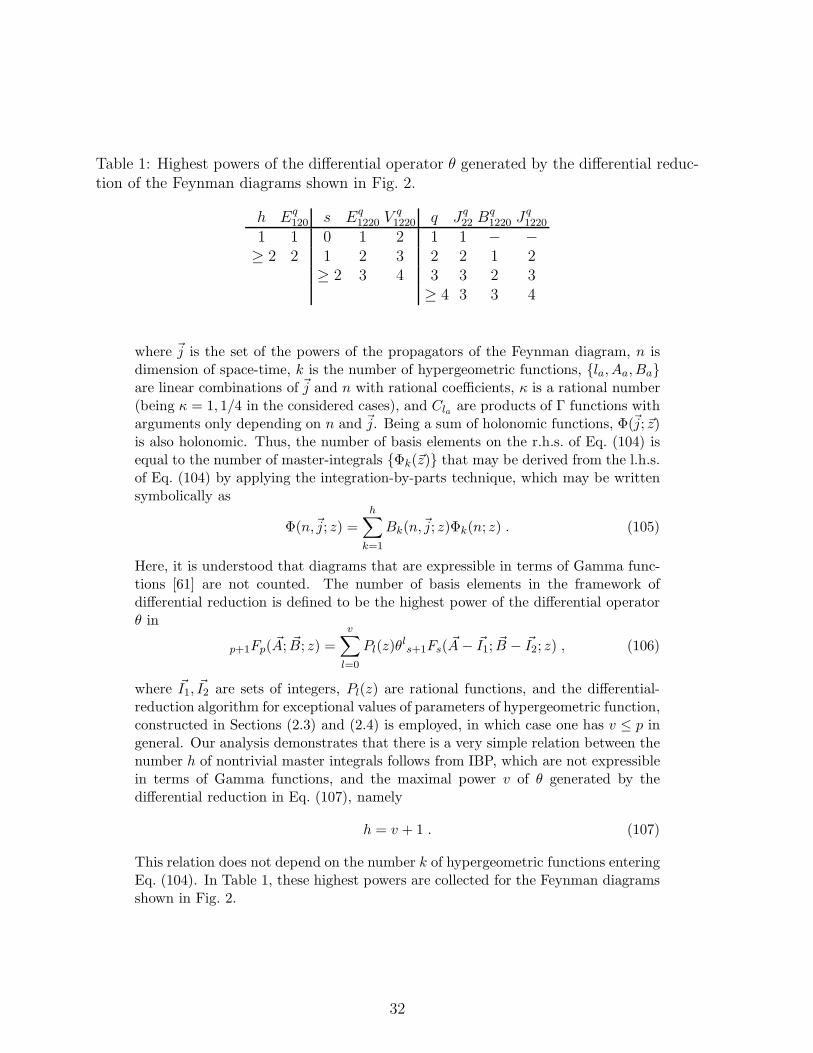
Table 1: Highest powers of the differential operator θ generated by the differential reduc-

tion of the Feynman diagrams shown in Fig. 2.

h Eq120 s E

q1220 V

q1220 q J

q22 B

q1220 J

q1220

1 1 0 1 2 1 1 − −≥ 2 2 1 2 3 2 2 1 2

≥ 2 3 4 3 3 2 3

≥ 4 3 3 4

where ~j is the set of the powers of the propagators of the Feynman diagram, n isdimension of space-time, k is the number of hypergeometric functions, {la, Aa, Ba}are linear combinations of ~j and n with rational coefficients, κ is a rational number(being κ = 1, 1/4 in the considered cases), and Cla are products of Γ functions witharguments only depending on n and ~j. Being a sum of holonomic functions, Φ(~j; ~z)is also holonomic. Thus, the number of basis elements on the r.h.s. of Eq. (104) isequal to the number of master-integrals {Φk(~z)} that may be derived from the l.h.s.of Eq. (104) by applying the integration-by-parts technique, which may be writtensymbolically as

Φ(n,~j; z) =h∑

k=1

Bk(n,~j; z)Φk(n; z) . (105)

Here, it is understood that diagrams that are expressible in terms of Gamma func-tions [61] are not counted. The number of basis elements in the framework ofdifferential reduction is defined to be the highest power of the differential operatorθ in

p+1Fp( ~A; ~B; z) =

v∑

l=0

Pl(z)θls+1Fs( ~A− ~I1; ~B − ~I2; z) , (106)

where ~I1, ~I2 are sets of integers, Pl(z) are rational functions, and the differential-reduction algorithm for exceptional values of parameters of hypergeometric function,constructed in Sections (2.3) and (2.4) is employed, in which case one has v ≤ p ingeneral. Our analysis demonstrates that there is a very simple relation between thenumber h of nontrivial master integrals follows from IBP, which are not expressiblein terms of Gamma functions, and the maximal power v of θ generated by thedifferential reduction in Eq. (107), namely

h = v + 1 . (107)

This relation does not depend on the number k of hypergeometric functions enteringEq. (104). In Table 1, these highest powers are collected for the Feynman diagramsshown in Fig. 2.

32

5 Discussion and conclusion

The idea that any Feynman diagram can be associated with a generalized Horn-type hypergeometric function or a linear combination of such functions was born atthe end of the 60s [7] and was applied during the last twenty years [38,46,62]. TheMellin-Barnes representation (1) of a Feynman diagram is universal. Under certainconditions, it can be converted to a linear combination of Horn-type hypergeometricfunctions (2). The latter possess very interesting properties. In fact, the systems ofdifferential equations which they satisfy are sufficient for (i) the differential reductionof the original functions to restricted sets of basis functions, whose number followsdirectly from the system of differential equations; (ii) the construction of the all-order ε expansions of the basis hypergeometric functions in form of iterated integrals[16–19]. To our knowledge, the first property has never been discussed in the contextof a reduction procedure of Feynman diagrams.

The aim of the present paper was to show how the differential-reduction al-gorithm can be applied to reduce Feynman diagrams without having to exploitthe integration-by-parts technique [15] or its dimensional generalization [37]. Inour analysis, we considered a phenomenologically interesting class of Feynman di-agrams, namely those shown in Figs. 1 and 2, which are expressible in terms ofgeneralized hypergeometric functions p+1Fp of one variable and cannot be treatedwith currently available program packages.

As first steps in our analysis, Takayama’s differential-reduction algorithm [22]was extended to the case of exceptional values of parameters in Section 2.3, andthe basis of differential reduction was written explicitly in Section 2.4. In partic-ular, this algorithm allowed us to complete the proofs of the theorems regardingthe construction of all-order ε expansions of hypergeometric functions presented inRefs. [16–19]. For non-exceptional values of parameters, this algorithm is imple-mented in the Mathematica based program HYPERDIRE to be described in a in aseparate communication [63].

The differential-reduction formalism via the construction of step-up and step-down operators can be applied to the reduction of any Feynman diagram. Itsadvantages reside in the simplicity and universality of the construction of this typeof operators, the full control over the analytical structure of the Feynman diagramsvia the hypergeometric representations, the simplicity of the criterion of reducibilityof hypergeometric functions to simpler functions, and the existence of a few, recentlydeveloped algorithms [16–20,27] for analytically constructing the coefficients of theε expansions of hypergeometric functions.

The main criteria of reducibility of hypergeometric functions, namely integerdifference between upper and lower parameters and integer value of one of theupper parameters, are also valid for Horn-type hypergeometric functions of morethan one variables. Moreover, the first type of reduction can be applied directly toMellin-Barnes representations of Feynman diagrams.

This approach becomes incomplete when some of the variables of a Horn-typehypergeometric function belong to its surface of singularities; for hypergeometricfunctions of one variable, this corresponds to z = 1. In this case, the extended Orealgebra technique [64], the telescoping approach [65], or the Laporta algorithm [66]

33

can be employed to obtain exact analytical results. In addition to these algorithms,there is another approach based on the analytical structure of the coefficients of theε expansions of hypergeometric functions: instead of looking for exact recurrencerelations, the limit z → 1 can be taken for the coefficients of the Laurent expansions.In particular, this procedure can be applied to any hypergeometric function whose εexpansion has coefficients that are expressible in terms of multiple polylogarithms.This algorithm may be applied to evaluate Feynman diagrams, if just the first fewcoefficients of their ε expansions are required.

As an illustration of the usefulness of our differential-reduction procedure, weconsidered a few examples, namely the Feynman diagrams shown in Figs. 1 and2 with arbitrary powers of propagators and space-time dimension, and explainedhow to express them in terms of hypergeometric functions and to construct their εexpansions to higher orders.

An interesting observation we made here is that, up to products of one-loopbubbles, the number of master integrals constructed through the integration-by-parts technique is equal to the highest power of the differential operator θ generatedby the differential reduction of hypergeometric functions plus one, independently ofthe number of hypergeometric functions occuring in the expressions for the Feynmandiagrams.

Acknowledgments.We are grateful to A. Isaev, A. Davydychev, V. Spiridonov, O. Tarasov, O. Veretin,B. Ward, and S. Yost for useful discussions, to G. Sandukovskaya for carefullyreading this manuscript, and to A. Scheplyakov for his contribution at an earlystage of this work. M.Y.K. is grateful to the members of Physics Department ofBaylor University for their hospitality when this project was started. This researchwas supported in part by BMBF Grant No. 05 HT6GUA, by DFG Grants No.KN 365/3–1 and KN 365/3–2, by HGF Grant No. HA 101, and by Russian Academyof Science Grant No. MK–1607.2008.2.

A Sets of basis functions for the Laurent ex-

pansions of hypergeometric functions

A.1 All parameters are integer

Using the algorithm described in Ref. [18], the derivatives of a basis hypergeomet-

ric function with integer parameters may be expressed in terms of the ρ(p−a)p+k (z)

functions defined in that reference, as13

θjpFp−1(~aε; 1 +~bε; z) = δj0 + εp

(

p∏

r=1

ar

)

∞∑

k=0

εkρ(p−1−j)p+k (z) , j = 0, · · · , p− 1 .

(108)

13In Eq. (2.11a) of Ref. [18], the last parameter should have the value p− 2 rather than p− 1.

34

The iterative solution of the ρ(p−1−j)p+k (z) functions is given by Eqs. (2.13a)–(2.13b)

in Ref. [18], and their explicit forms in terms of generalized polylogarithms arecollected in Section 3 therein.

A.2 One lower parameter is half-integer

In Refs. [20,29], the ε expansions of the functions

P+1FP

(

{1 + aiε}K , {2 + diε}P−K+1

32 + fε, {1 + ejε}R, {2 + ciε}P−R−1 z

)

, (109)

with K − R ≥ 2, were constructed up to functions of weight 4 and, in the case ofz = 1/4, up to weight 5.14 For these parameters, after some trivial factorization, thecoefficients of the ε expansions contain functions of only one definite weight. In thissection, we present explicit relations between the basis functions of the differentialreduction, defined by Eq. (17), and the functions of Eq. (109). One of the auxiliaryrelations intensively used in the following reads:

pFp−1

(

a1, a2, · · · , apb1, b2, · · · , bp−1

z

)

= 1 + z

∏pj=1 aj

∏p−1k=1 bk

p+1Fp

(

1, 1 + a1, 1 + a2, · · · , 1 + ap2, 1 + b1, 1 + b2, · · · , 1 + bp−1

z

)

. (110)

A.2.1 2F1

A detailed discussion of the 2F1 function was presented in Refs. [16,19,35].

A.2.2 3F2

For the hypergeometric function

3F2

(

I1 + a1ε, I2 + a2ε, I3 + a3εI4 +

12 + fε, I5 + c1ε

z

)

, (111)

where {Ik} are arbitrary integers and all ai 6= 0, the basis of the differential reductionis

{1, θ, θ2} × 3F2

(

a1ε, a2ε, a3ε12 + fε, 1 + c1ε

z

)

. (112)

For P = 2, there are four functions of the type of Eq. (109):

4F3

(

1 + a1ε, 1 + a2ε, 1 + a3ε, 132 + fε, 2 + c1ε, 2

z

)

, 3F2

(

1 + a1ε, 1 + a2ε, 1 + a3ε32 + fε, 2 + c1ε

z

)

,

3F2

(

1 + a1ε, 1 + a2ε, 2 + a3ε32 + fε, 2 + c1ε

z

)

, 3F2

(

1 + a1ε, 1 + a2ε, 1 + a3ε32 + fε, 1 + c1ε

z

)

.(113)

14The series representations of these hypergeometric functions are proportional to∑

∞

j=0zj

jK−R−1 .

35

The functions of Eqs. (112) and (113) are related as

3F2

(

a1ε, a2ε, a3ε12 + fε, 1 + c1ε

z

)

= 1 +2a1a2a3ε

3

(1 + 2fε)(1 + c1ε)4F3

(

1 + a1ε, 1 + a2ε, 1 + a3ε, 132 + fε, 2 + c1ε, 2

z

)

,

θ 3F2

(

a1ε, a2ε, a3ε12 + fε, 1 + c1ε

z

)

= 2za1a2a3ε

3

(1 + 2fε)(1 + c1ε)3F2

(

1 + a1ε, 1 + a2ε, 1 + a3ε32 + fε, 2 + c1ε

z

)

.

(114)

The second derivative in Eq. (112) may be obtained from any of the followingrelations:

3F2

(

1 + a1, 1 + a2, 1 + a31 + f, c1

z

)

=1

z

fθ(θ + c1 − 1)

a1a2a33F2

(

a1, a2, a3f, c1

z

)

,

3F2

(

1 + a1, 1 + a2, 2 + a31 + f, 1 + c1

z

)

=1

z

c1fθ(θ + a3)

a1a2a3(1 + a3)3F2

(

a1, a2, a3f, c1

z

)

, (115)

where

ai → aiε, f → 1

2+ fε, c1 → 1 + c1ε, (116)

are to be substituted. In particular, it can be expressed as a linear combination ofthe second, third, and fourth functions in Eq. (113) as

(γ1 + γ2)

z

fc1a1a2a3

θ2 3F2

(

a1, a2, a3c1, f

z

)

= γ1c1 3F2

(

1 + a1, 1 + a2, 1 + a3c1, 1 + f

z

)

+ γ2(1 + a3) 3F2

(

1 + a1, 1 + a2, 2 + a31 + c1, 1 + f

z

)

− [γ1(c1 − 1) + γ2a3] 3F2

(

1 + a1, 1 + a2, 1 + a31 + c1, 1 + f

z

)

, (117)

where γ1 and γ2 are arbitrary numbers. Putting γ2 = −γ1, we obtain a linearrelation between the hypergeometric functions on the r.h.s. of Eq. (117). We checkedthat the ε expansions of the hypergeometric functions constructed in Ref. [20] andcollected in Ref. [48] satisfy this relation.

In the case a1 = 1, the basis of the differential reduction is

{1, θ} × 3F2

(

1, 1 + a2ε, 1 + a3ε32 + fε, 2 + c1ε

z

)

. (118)

The first derivative in Eq. (118) can be obtained from any of the two functions

3F2

(

1, 1 + a2ε, 1 + a3ε32 + fε, 1 + c1ε

z

)

, 3F2

(

1, 1 + a2ε, 2 + a3ε32 + fε, 2 + c1ε

z

)

, (119)

by the single application of the step-up and step-down operators defined in Eq. (7).The result is

(γ1 + γ2)θ 3F2

(

1, 1 + a2ε, 1 + a3ε32 + fε, 2 + c1ε

z

)

=

γ1(1 + a3ε) 3F2

(

1, 1 + a2ε, 2 + a3ε32 + fε, 2 + c1ε

z

)

+ γ2(1 + c1ε) 3F2

(

1, 1 + a2ε, 1 + a3ε32 + fε, 1 + c1ε

z

)

− [γ1(1 + a3ε) + γ2(1 + c1ε)] 3F2

(

1, 1 + a2ε, 1 + a3ε32 + fε, 2 + c1ε

z

)

, (120)

36

where γ1 and γ2 are arbitrary numbers.

A.2.3 4F3

Similarly, for the hypergeometric function

4F3

(

I1 + a1ε, I2 + a2ε, I3 + a3ε, I4 + a4εI5 +

12 + fε, I6 + c1ε, I7 + c2ε

z

)

, (121)

where {Ik} are arbitrary integers and all ai 6= 0, the basis of the differential reductionis

{1, θ, θ2, θ3} × 4F3

(

a1ε, a2ε, a3ε, a4ε12 + fε, 1 + c1ε, 1 + c2ε

z

)

. (122)

There are seven functions of the type of Eq. (109), namely

5F4

(

1 + a1ε, 1 + a2ε, 1 + a3ε, 1 + a4ε, 132 + fε, 2 + c1ε, 2 + c2ε, 2

z

)

. 4F3

(

1 + a1ε, 1 + a2ε, 1 + a3ε, 1 + a4ε32 + fε, 2 + c1ε, 2 + c2ε

z

)

,

4F3

(

1 + a1ε, 1 + a2ε, 1 + a3ε, 2 + a4ε32 + fε, 2 + c1ε, 2 + c2ε

z

)

, 4F3

(

1 + a1ε, 1 + a2ε, 1 + a3ε, 1 + a4ε32 + fε, 2 + c1ε, 1 + c2ε

z

)

,

4F3

(

1 + a1ε, 1 + a2ε, 2 + a3ε, 2 + a4ε32 + fε, 2 + c1ε, 2 + c2ε

z

)

, 4F3

(

1 + a1ε, 1 + a2ε, 1 + a3ε, 2 + a4ε32 + fε, 1 + c1ε, 1 + c2ε

z

)

,

4F3

(

1 + a1ε, 1 + a2ε, 1 + a3ε, 1 + a4ε32 + fε, 1 + c1ε, 1 + c2ε

z

)

. (123)

The two bases defined by Eqs. (122) and (123) are related as

4F3

(

a1ε, a2ε, a3ε, a4ε12 + fε, 1 + c1ε, 1 + c2ε

z

)

=

1 +2a1a2a3a4ε

4

(1 + 2fε)(1 + c1ε)(1 + c2ε)5F4

(

1 + a1ε, 1 + a2ε, 1 + a3ε, 1 + a4ε, 132 + fε, 2 + c1ε, 2 + c2ε, 2

z

)

,

θ 4F3

(

a1ε, a2ε, a3ε, a4ε12 + fε, 1 + c1ε, 1 + c2ε

z

)

= 2za1a2a3a4ε

4

(1 + 2fε)(1 + c1ε)(1 + c2ε)4F3

(

1 + a1ε, 1 + a2ε, 1 + a3ε, 1 + a4ε32 + fε, 2 + c1ε, 2 + c2ε

z

)

.(124)

The second derivative in Eq. (122) may be obtained from any of the followingrelations:

4F3

(

1 + a1, 1 + a2, 1 + a3, 1 + a41 + f, 1 + c1, c2

z

)

=f

z

c1θ(θ + c2 − 1)

a1a2a3a44F3

(

a1, a2, a3, a4f, c1, c2

z

)

,

4F3

(

1 + a1, 1 + a2, 1 + a3, 2 + a41 + f, 1 + c1, 1 + c2

z

)

=f

z

c1c2θ(θ + a4)

a1a2a3a4(1 + a4)4F3

(

a1, a2, a3, a4f, c1, c2

z

)

,

(125)

37

with the substitutions of Eq. (116). In particular, it can be expressed it as a linearcombination of the second, third, and fourth hypergeometric functions in Eq. (123)as

(γ1 + γ2)

z

fc1c2a1a2a3a4

θ2 4F3

(

a1, a2, a3, a4f, c1, c2

z

)

= γ1c2 4F3

(

1 + a1, 1 + a2, 1 + a3, 1 + a41 + f, 1 + c1, c2

z

)

− [a4γ2 + (c2 − 1)γ1] 4F3

(

1 + a1, 1 + a2, 1 + a3, 1 + a41 + f, 1 + c1, 1 + c2

z

)

+γ2(1 + a4) 4F3

(

1 + a1, 1 + a2, 1 + a3, 2 + a41 + f, 1 + c1, 1 + c2

z

)

, (126)

where γ1 and γ2 are arbitrary numbers. Putting γ2 = −γ1, we obtain a linearrelation between the hypergeometric functions on the r.h.s. of Eq. (126). We checkedthat the ε expansions of the hypergeometric functions constructed in Ref. [20] satisfythis relation. The third derivative in Eq. (122) may be obtained from any of thefollowing relations:

4F3

(

1 + a1, 1 + a2, 1 + a3, 1 + a41 + f, c1, c2

z

)

=f

z

θ(θ + c1 − 1)(θ + c2 − 1)

a1a2a3a44F3

(

a1, a2, a3, a4f, c1, c2

z

)

,

4F3

(

1 + a1, 1 + a2, 2 + a3, 2 + a41 + f, 1 + c1, 1 + c2

z

)

=f

z

c1c2θ(θ + a3)(θ + a4)

a1a2a3a4(1 + a3)(1 + a4)4F3

(

a1, a2, a3, a4f, c1, c2

z

)

,

4F3

(

1 + a1, 1 + a2, 1 + a3, 2 + a41 + f, 1 + c1, c2

z

)

=f

z

c1θ(θ + a4)(θ + c2 − 1)

a1a2a3a4(1 + a4)4F3

(

a1, a2, a3, a4f, c1, c2

z

)

,

(127)

38

with the substitutions of Eq. (116). As a consequence of Eq. (127), the followinglinear relations between hypergeometric functions are valid:

c1 4F3

(

1 + a1, 1 + a2, 1 + a3, 1 + a41 + f, c1, c2

z

)

− (1 + a4) 4F3

(

1 + a1, 1 + a2, 1 + a3, 2 + a41 + f, 1 + c1, c2

z

)

= (c1 − a4 − 1) 4F3

(

1 + a1, 1 + a2, 1 + a3, 1 + a41 + f, 1 + c1, c2

z

)

,

c2 4F3

(

1 + a1, 1 + a2, 1 + a3, 2 + a41 + f, 1 + c1, c2

z

)

− (1 + a3) 4F3

(

1 + a1, 1 + a2, 2 + a3, 2 + a41 + f, 1 + c1, 1 + c2

z

)

= (c2 − a3 − 1) 4F3

(

1 + a1, 1 + a2, 1 + a3, 2 + a41 + f, 1 + c1, 1 + c2

z

)

,

(β1 + β2)

{

c1c2 4F3

(

1 + a1, 1 + a2, 1 + a3, 1 + a41 + f, c1, c2

z

)

−(1 + a3)(1 + a4) 4F3

(

1 + a1, 1 + a2, 2 + a3, 2 + a41 + f, 1 + c1, 1 + c2

z

)

}

+(c2 − a4 − 1) [β1(c2 − a3 − 1)− β2(c1 − a4 − 1)] 4F3

(

1 + a1, 1 + a2, 1 + a3, 1 + a41 + f, 1 + c1, 1 + c2

z

)

−β1(c1 + c2 − 2− a3 − a4)c2 4F3

(

1 + a1, 1 + a2, 1 + a3, 1 + a41 + f, 1 + c1, c2

z

)

−β2(c1 + c2 − 2− a3 − a4)(1 + a4) 4F3

(

1 + a1, 1 + a2, 1 + a3, 2 + a41 + f, 1 + c1, 1 + c2

z

)

= 0 , (128)

where β1 and β2 are arbitrary numbers. We checked that the ε expansions of thehypergeometric functions 4F3 constructed in Ref. [20] and collected in Ref. [48]satisfy all these relations.

In the case a1 = 1, the basis of the differential reduction is

{1, θ, θ2} × 4F3

(

1, 1 + a2ε, 1 + a3ε, 1 + a4ε32 + fε, 2 + c1ε, 2 + c2ε

z

)

. (129)

The first derivative in Eq. (129) can be related to any of the two functions,

4F3

(

1, 1 + a2ε, 1 + a3ε, 2 + a4ε32 + fε, 2 + c1ε, 2 + c2ε

z

)

, 4F3

(

1, 1 + a2ε, 1 + a3ε, 1 + a4ε32 + fε, 2 + c1ε, 1 + c2ε

z

)

,

(130)

by single application of the operators B(+)a4 or H

(−)c2 given in Eq. (7). The second

derivative in Eq. (129) is related to any of the following hypergeometric functions:

4F3

(

1 + a1ε, 1 + a2ε, 1 + a3ε, 1 + a4ε32 + fε, 1 + c1ε, 1 + c2ε

z

)

, 4F3

(

1 + a1ε, 1 + a2ε, 2 + a3ε, 2 + a4ε32 + fε, 2 + c1ε, 2 + c2ε

z

)

,

4F3

(

1 + a1ε, 1 + a2ε, 1 + a3ε, 2 + a4ε32 + fε, 2 + c1ε, 1 + c2ε

z

)

, (131)

which are generated from the basis function of Eq. (129) via application ofH(−)b2

H(−)b3

,

B(+)a3 B

(+)a4 , or H

(−)b3

B(+)a4 .

39

A.2.4 5F4

Similarly, for the hypergeometric function

5F4

(

I1 + a1ε, I2 + a2ε, I3 + a3ε, I4 + a4ε, I5 + a5εI6 +

12 + fε, I7 + c1ε, I8 + c2ε, I9 + c3ε

z

)

, (132)

where {Ik} are arbitrary integers and all ai 6= 0, the basis of the differential reductionis

{1, θ, θ2, θ3, θ4} × 4F3

(

a1ε, a2ε, a3ε, a4ε, a5ε12 + fε, 1 + c1ε, 1 + c2ε, 1 + c3ε

z

)

. (133)

In this case, there are eleven functions of the type of Eq. (109). The two basesdefined by Eqs. (133) and (109) are related as

5F4

(

a1ε, a2ε, a3ε, a4ε, a5ε12 + fε, 1 + c1ε, 1 + c2ε, 1 + c3ε

z

)

= 1 +

2ε5(

∏5i=1 ai

)

(1 + 2fε)[

∏3k=1(1 + ckε)

] 6F5

(

1 + a1ε, 1 + a2ε, 1 + a3ε, 1 + a4ε, 1 + a5ε, 132 + fε, 2 + c1ε, 2 + c2ε, 2 + c3ε, 2

z

)

,

θ 5F4

(

a1ε, a2ε, a3ε, a4ε, a5ε12 + fε, 1 + c1ε, 1 + c2ε, 1 + c3ε

z

)

=2z(

∏5i=1 ai

)

ε5

(1 + 2fε)[

∏3k=1(1 + ckε)

] 5F4

(

1 + a1ε, 1 + a2ε, 1 + a3ε, 1 + a4ε, 1 + a5ε32 + fε, 2 + c1ε, 2 + c2, 2 + c3εε

z

)

.(134)

The second derivative in Eq. (133) may be obtained as

(γ1 + γ2)

z

f(

∏3k=1 ck

)

(

∏5j=1 aj

) θ2 5F4

(

a1, a2, a3, a4, a5f, c1, c2, c3

z

)

= γ1c3 5F4

(

1 + a1, 1 + a2, 1 + a3, 1 + a4, 1 + a51 + f, 1 + c1, 1 + c2, c3

z

)

+ γ2(1 + a5) 5F4

(

1 + a1, 1 + a2, 1 + a3, 1 + a4, 2 + a51 + fε, 1 + c1, 1 + c2, 1 + c3

z

)

− [γ1(c3 − 1) + γ2a5] 5F4

(

1 + a1, 1 + a2, 1 + a3, 1 + a4, 1 + a51 + fε, 1 + c1, 1 + c2, 1 + c3

z

)

, (135)

with the substitutions of Eq. (116), where γ1 and γ2 are arbitrary numbers. Puttingγ2 = −γ1, we obtain a linear relation between the hypergeometric functions on ther.h.s. of Eq. (135). We checked that the ε expansions of the hypergeometric functionsconstructed in Ref. [20] satisfy this relation. The third derivative in Eq. (133) is

40

related to one of the following functions or their linear combination:

5F4

(

1 + a1, 1 + a2, 1 + a3, 2 + a4, 2 + a51 + f, 1 + c1, 1 + c2, 1 + c3

z

)

=f

z

(

∏3k=1 ck

)

θ(θ + a4)(θ + a5)(

∏5j=1 aj

)

(1 + a4)(1 + a5)F (z) ,

5F4

(

1 + a1, 1 + a2, 1 + a3, 1 + a4, 2 + a51 + f, 1 + c1, 1 + c2, c3

z

)

=f

z

(

∏2k=1 ck

)

θ(θ + c3 − 1)(θ + a5)(

∏5j=1 aj

)

(1 + a5)F (z) ,

5F4

(

1 + a1, 1 + a2, 1 + a3, 1 + a4, 1 + a51 + f, 1 + c1, c2, c3

z

)

=f

z

c1θ(θ + c2 − 1)(θ + c3 − 1)(

∏5j=1 aj

) F (z) , (136)

where

F (z) ≡ 5F4

(

a1, a2, a3, a4, a5f, c1, c2, c3

z

)

, (137)

As a consequence of Eq. (136), the following linear relations between hypergeometricfunctions hold:

(1 + a4 − c3) 5F4

(

1 + a1, 1 + a2, 1 + a3, 1 + a4, 2 + a51 + f, 1 + c1, 1 + c2, 1 + c3

z

)

= (1 + a4) 5F4

(

1 + a1, 1 + a2, 1 + a3, 2 + a4, 2 + a51 + f, 1 + c1, 1 + c2, 1 + c3

z

)

− c3 5F4

(

1 + a1, 1 + a2, 1 + a3, 1 + a4, 2 + a51 + f, 1 + c1, 1 + c2, c3

z

)

,

(1 + a5 − c2) 5F4

(

1 + a1, 1 + a2, 1 + a3, 1 + a4, 1 + a51 + f, 1 + c1, 1 + c2, c3

z

)

= (1 + a5) 5F4

(

1 + a1, 1 + a2, 1 + a3, 1 + a4, 2 + a51 + f, 1 + c1, 1 + c2, c3

z

)

− c2 5F4

(

1 + a1, 1 + a2, 1 + a3, 1 + a4, 1 + a51 + f, 1 + c1, c2, c3

z

)

,

(a5 − c3 + 1) [β1 (c3 − a4 − 1)− β2 (c2 − a5 − 1)] 5F4

(

1 + a1, 1 + a2, 1 + a3, 1 + a4, 1 + a51 + f, 1 + c1, 1 + c2, 1 + c3

z

)

= (β1 + β2)c2c3 5F4

(

1 + a1, 1 + a2, 1 + a3, 1 + a4, 1 + a51 + f, 1 + c1, c2, c3

z

)

− (β1 + β2)(1 + a4)(1 + a5) 5F4

(

1 + a1, 1 + a2, 1 + a3, 2 + a4, 2 + a51 + f, 1 + c1, 1 + c2, 1 + c3

z

)

+ β1c3 (a4 + a5 − c2 − c3 + 2) 5F4

(

1 + a1, 1 + a2, 1 + a3, 1 + a4, 1 + a51 + f, 1 + c1, 1 + c2, c3

z

)

+ β2(1 + a5) (a4 + a5 − c2 − c3 + 2) 5F4

(

1 + a1, 1 + a2, 1 + a3, 1 + a4, 2 + a51 + f, 1 + c1, 1 + c2, 1 + c3

z

)

. (138)

41

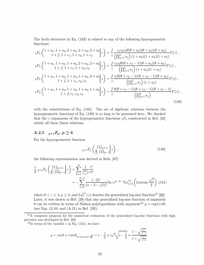
The forth derivative in Eq. (133) is related to any of the following hypergeometricfunctions:

5F4

(

1 + a1, 1 + a2, 2 + a3, 2 + a4, 2 + a51 + f, 1 + c1, 1 + c2, 1 + c3

z

)

=f

z

c1c2c3θ(θ + a3)(θ + a4)(θ + a5)(

∏5j=1 aj

)

(1 + a3)(1 + a4)(1 + a5)F (z) ,

5F4

(

1 + a1, 1 + a2, 1 + a3, 2 + a4, 2 + a51 + f, 1 + c1, 1 + c2, c3

z

)

=f

z

c1c2θ(θ + c3 − 1)(θ + a4)(θ + a5)(

∏5j=1 aj

)

(1 + a4)(1 + a5)F (z) ,

5F4

(

1 + a1, 1 + a2, 1 + a3, 1 + a4, 2 + a51 + f, 1 + c1, c2, c3

z

)

=f

z

c1θ(θ + c2 − 1)(θ + c3 − 1)(θ + a5)(

∏5j=1 aj

)

(1 + a5)F (z) ,

5F4

(

1 + a1, 1 + a2, 1 + a3, 1 + a4, 1 + a51 + f, c1, c2, c3

z

)

=f

z

θ(θ + c1 − 1)(θ + c2 − 1)(θ + c3 − 1)(

∏5j=1 aj

) F (z) ,

(139)

with the substitutions of Eq. (116). The set of algebraic relations between thehypergeometric functions of Eq. (139) is to long to be presented here. We checkedthat the ε expansions of the hypergeometric functions 5F4 constructed in Ref. [20]satisfy all these linear relations.

A.2.5 p+1Fp, p ≥ 6

For the hypergeometric function

p+1Fp

(

{1}p+1,32 , {2}p−1

z

)

, (140)

the following representation was derived in Refs. [67]:

z

2p+1Fp

(

{1}p+1,32 , {2}p−1

z

)

=∞∑

k=1

1(2nn

)

zn

np

= −p−2∑

j=0

(−2)j

(a− 2− j)!j!(ln z)a−2−jLs

(1)j+2

(

2 arcsin

√z

2

)

,(141)

where 0 ≤ z ≤ 4, p ≥ 2, and Ls(j)a (z) denotes the generalized log-sine function15 [69].

Later, it was shown in Ref. [29] that any generalized log-sine function of argumentθ can be written in terms of Nielsen polylogarithms with argument16 y = exp(±iθ)(see Eqs. (2.18) and (A.21) in Ref. [29]).

15A computer program for the numerical evaluation of the generalized log-sine functions with highprecision was developed in Ref. [68].

16In terms of the variable z in Eq. (141), we have

y = cos θ ± i sin θ|θ=2arcsin

√

z

2

= 1− z

2± i

√z

√

1− z

4≡

1−√

zz−4

1 +√

zz−4

.

42

References

[1] G. ’t Hooft, M. Veltman, Nucl. Phys. B 44 (1972) 189.

[2] C. Anastasiou, K. Melnikov, Nucl. Phys. B 646 (2002) 220.

[3] T. Regge, Battelle Rencontres: 1967 Lectures in Mathematics and Physics,C.M. DeWitt, J.A. Wheeler (Eds.), W.A. Benjamin, New York, 1968, pp. 433-458.

[4] C. de Calan, A.P.C. Malbouisson, Annales Poincare Phys. Theor. 32 (1980) 91;C. de Calan, F. David, V. Rivasseau, Commun. Math. Phys. 78 (1981) 531;C. de Calan, A.P.C. Malbouisson, Commun. Math. Phys. 90 (1983) 413.

[5] V.A. Smirnov, Feynman integral calculus, Springer, Berlin, 2006.

[6] V. Del Duca, C. Duhr, E. W. N. Glover, V. A. Smirnov, JHEP 1001 (2010)042.

[7] D.S. Kershaw, Phys. Rev. D 8 (1973) 2708;A.C.T. Wu, Phys. Rev. D 9 (1974) 370;K. Mano, Phys. Rev. D 11 (1975) 452.

[8] I.M. Gel’fand, M.I. Graev, V.S. Retakh, Russian Math. Surveys 47 (1992) 1.

[9] A. Erdelyi (Ed.), Higher Transcendental Functions, McGraw-Hill, New York,1953.

[10] O. Ore, J. Math. Pure Appl. 9 (1930) 311;M. Sato, Nagoya Math. J. 120 (1990) 1.

[11] M.Yu. Kalmykov, V.V. Bytev, B.A. Kniehl, B.F.L. Ward, S.A. Yost,PoS(ACAT08)125, arXiv:0901.4716.

[12] N. Takayama, Japan J. Appl. Math. 6 (1989) 147.

[13] C.F. Gauss, Gesammelte Werke, vol. 3, Teubner, Leipzig, 1823, pp. 1866–1929.

[14] O.V. Tarasov, Acta Phys. Polon. B 29 (1998) 2655;O.V. Tarasov, Nucl. Instrum. Meth. A 534 (2004) 293.

[15] F.V. Tkachov, Phys. Lett. B 100 (1981) 65;K.G. Chetyrkin, F.V. Tkachov, Nucl. Phys. B 192 (1981) 159.

[16] M.Yu. Kalmykov, B.F.L. Ward, S. Yost, JHEP 0702 (2007) 040.

[17] M.Yu. Kalmykov, B.F.L. Ward, S. Yost, JHEP 0710 (2007) 048;S.A. Yost, M.Yu. Kalmykov, B.F.L. Ward, arXiv:0808.2605.

[18] M.Yu. Kalmykov, B.F.L. Ward, S. Yost, JHEP 0711 (2007) 009.

[19] M.Yu. Kalmykov, B.A. Kniehl, Nucl. Phys. B 809 (2009) 365.

[20] A.I. Davydychev, M.Yu. Kalmykov, Nucl. Phys. B 699 (2004) 3.

[21] E.D. Rainville, Bull. Amer. Math. Soc. 51 (1945) 714.

[22] N. Takayama, J. Symbolic Comput. 20 (1995) 637.

[23] A.P. Prudnikov, Yu.A. Brychkov, O.I. Marichev, Integrals and Series, Vol. 3:More Special Functions, Gordon and Breach, New York, 1990.

43

[24] J.E. Gottschalk, E.N. Maslen, J. Phys. A 21 (1988) 1983.

[25] P.W. Karlsson, J. Math. Phys. 12 (1971) 270.

[26] P.A. Baikov, Phys. Lett. B 474 (2000) 385;P.A. Baikov, Phys. Lett. B 634 (2006) 325.

[27] S. Moch, P. Uwer, S. Weinzierl, J. Math. Phys. 43 (2002) 3363;S. Weinzierl, J. Math. Phys. 45 (2004) 2656.

[28] A.I. Davydychev, Phys. Rev. D 61 (2000) 087701;A.I. Davydychev, M.Yu. Kalmykov, Nucl. Phys. B (Proc. Suppl.) 89 (2000)283.

[29] A.I. Davydychev, M.Yu. Kalmykov, Nucl. Phys. B 605 (2001) 266.

[30] M.Yu. Kalmykov, B.A. Kniehl, B.F.L. Ward, S.A. Yost, arXiv:0810.3238.

[31] M.Yu. Kalmykov, Nucl. Phys. B (Proc. Suppl.) 135 (2004) 280.

[32] T. Huber, D. Maıtre, Comput. Phys. Commun. 178 (2008) 755.

[33] N.E. Norlund, Acta Math. 94 (1955) 289.

[34] I.A. Lappo-Danilevsky, Memoires sur la theorie des systemes des equationsdifferentielles lineaires, Chelsea, New York, 1953;A.B. Goncharov, Math. Res. Lett. 4 (1997) 617;A.B. Goncharov, Math. Res. Lett. 5 (1998) 497;E. Remiddi, J.A.M. Vermaseren, Int. J. Mod. Phys. A 15 (2000) 725;J. Vollinga, S. Weinzierl, Comput. Phys. Commun. 167 (2005) 177.

[35] M.Yu. Kalmykov, JHEP 0604 (2006) 056.

[36] V.V. Bytev, M. Kalmykov, B.A. Kniehl, B.F.L. Ward, S.A. Yost, in Proceedingsof the International Linear Collider Workshop (LCWS08 and ILC08), Chicago,USA, 16–20 November 2008, edited by T. Speer, F. Carminati, D. Peret-Gallix,R. Brun (Proceedings of Science, Trieste, 2009), arXiv:0902.1352 [hep-th].

[37] A.I. Davydychev, Phys. Lett. B 263 (1991) 107;O.V. Tarasov, Phys. Rev. D 54 (1996) 6479.

[38] E.E. Boos, A.I. Davydychev, Theor. Math. Phys. 89 (1991) 1052.

[39] F.A. Berends, A.I. Davydychev, V.A. Smirnov, J.B. Tausk, Nucl. Phys. B 439(1995) 536.

[40] O.V. Tarasov, Nucl. Phys. B (Proc. Suppl.) 89 (2000) 237;A.I. Davydychev, Nucl. Instrum. Meth. A 559 (2006) 293.

[41] C. Anastasiou, E.W.N. Glover, C. Oleari, Nucl. Phys. B 572 (2000) 307.

[42] V.A. Smirnov, Commun. Math. Phys. 134 (1990) 109;F.V. Tkachov, Int. J. Mod. Phys. A 8 (1993) 2047;G.B. Pivovarov, F.V. Tkachov, Int. J. Mod. Phys. A 8 (1993) 2241.

[43] L.V. Avdeev, Comput. Phys. Commun. 98 (1996) 15.

[44] F. Jegerlehner, M.Yu. Kalmykov, O. Veretin, Nucl. Phys. B 641 (2002) 285.

44

[45] A.I. Davydychev, Loop calculations in QCD with massivequarks, presentation at Internetional Conference on Rela-tivistic Nuclear Dynamics, Vladivostok, Russia, 1991, URL:http://wwwthep.physik.uni-mainz.de/ davyd/preprints/vladiv.pdf.

[46] D.J. Broadhurst, J. Fleischer, O.V. Tarasov, Z. Phys. C 60 (1993) 287.

[47] O.V. Tarasov, Nucl. Phys. B 502 (1997) 455.

[48] M.Yu. Kalmykov, http://theor.jinr.ru/ kalmykov/hypergeom/hyper.html

[49] F. Jegerlehner, M.Yu. Kalmykov, O. Veretin, Nucl. Phys. B 658 (2003) 49;Nucl. Phys. B (Proc. Suppl.) 116 (2003) 382.

[50] J. Gluza, K. Kajda, T. Riemann, Comput. Phys. Commun. 177 (2007) 879;T. Huber, Nucl. Phys. B (Proc. Suppl.) 183 (2008) 238.

[51] A.I. Davydychev, J.B. Tausk, Nucl. Phys. B 397 (1993) 123.

[52] D.J. Broadhurst, Eur. Phys. J. C 8 (1999) 311;J. Fleischer, M.Yu. Kalmykov, Phys. Lett. B 470 (1999) 168.

[53] M. Czakon, M. Awramik, A. Freitas, Nucl. Phys. B (Proc. Suppl.) 157 (2006)58.

[54] O.V. Tarasov, Phys. Lett. B 670 (2008) 67;B.A. Kniehl, O.V. Tarasov, Nucl. Phys. B 820 (2009) 178.

[55] S. Bekavac, A.G. Grozin, D. Seidel, V.A. Smirnov, Nucl. Phys. B 819 (2009)183.

[56] A.I. Davydychev, A.G. Grozin, Phys. Rev. D 59 (1999) 054023.

[57] N. Gray, D.J. Broadhurst, W. Grafe, K. Schilcher, Z. Phys. C 48 (1990) 673;A. Onishchenko, O. Veretin, Phys. Atom. Nucl. 68 (2005) 1405.

[58] G. Passarino, S. Uccirati, Nucl. Phys. B 747 (2006) 113 [arXiv:hep-ph/0603121];S. Actis, G. Passarino, C. Sturm, S. Uccirati, Nucl. Phys. B 811 (2009) 182[arXiv:0809.3667].

[59] A. Frink, B.A. Kniehl, D. Kreimer, K. Riesselmann, Phys. Rev. D 54 (1996)4548.

[60] B.A. Kniehl, A.V. Kotikov, O.L. Veretin, Phys. Rev. Lett. 101 (2008) 193401[arXiv:0806.4927]; Phys. Rev. A 80 (2009) 052501.

[61] A.A. Vladimirov, Theor. Math. Phys. 43 (1980) 417 [Teor. Mat. Fiz. 43 (1980)210].

[62] A.I. Davydychev, J. Math. Phys. 32 (1991) 1052; ibid 33 (1992) 358;D.J. Broadhurst, N. Gray, K. Schilcher, Z. Phys. C 52 (1991) 111;D.J. Broadhurst, Z. Phys. C 54 (1992) 599;F.A. Berends, M. Buza, M. Bohm, R. Scharf, Z. Phys. C 63 (1994) 227.

[63] V.V. Bytev, M.Yu. Kalmykov, B.A. Kniehl, in preparation.

45

[64] M. Bronstein, M. Petkovsek, Theoret. Comput. Sci. 157 (1996) 3;F. Chyzak, B. Salvy, J. Symbolic Comput. 26 (1998) 187;F. Chyzak, Grobner Bases, Symbolic Summation and Symbolic Integration,p.32–60, London Math. Soc. Lecture Note Ser. 251, Cambridge UniversityPress, Cambridge, 1998.

[65] M. Petkovsek, H.S. Wilf, D. Zeilberger, A=B, A.K. Peters, Natick, USA (1996);P. Paule, Contiguous relations and creative telescoping, Technical Report,RISC, Austria, 2001.

[66] S. Laporta, Int. J. Mod. Phys. A 15 (2000) 5087.

[67] M.Yu. Kalmykov, O. Veretin, Phys. Lett. B 483 (2000) 315;J.M. Borwein, D.J. Broadhurst, J. Kamnitzer, Exper. Math. 10 (2001) 25.

[68] M.Y. Kalmykov, A. Sheplyakov, Comput. Phys. Commun. 172 (2005) 45.

[69] L. Lewin, Polylogarithms and Associated Functions, North-Holland, Amster-dam, 1981.

46