ORDINARY MATTER IN NONLINEAR AFFINE GAUGE THEORIES

OF GRAVITATION

by

A. Lpez–Pinto, A. Tiemblo and R. Tresguerres

IMAFF, Consejo Superior de Investigaciones Cientficas,

Serrano 123, Madrid 28006, Spain

ABSTRACT

We present a general framework to include ordinary fermionic matter in the

metric–affine gauge theories of gravity. It is based on a nonlinear gauge realization of

the affine group, with the Lorentz group as the classification subgroup of the matter

and gravitational fields.

1. Introduction

Several generalizations of the gauge theory of gravitation originally proposed by

Utiyama, Sciama and Kibble(1) were developped in recent times(2). The metric–affine

gauge theories (MAGT’s) propugnated by Hehl et al.(3) are particularly interesting,

since they provide a dynamical foundation of the geometrical theory equiped with the

most general connection, namely with the general linear connection Γαβ . The affine

group is the transformation group of the geometry, thus being the main candidate to

describe things in the absence of matter. According to Ne’eman and Sijacki(4), the

adoption of the affine group as the dynamical group in a gauge theory of gravitation

could solve certain renormalizability and unitarity problems in Quantum Gravity,

with the help of the additional degrees of freedom contained in the linear connection.

A main difficulty for the common acceptance of the MAGT’s of gravitation is the

problem of including fermionic matter in this general framework, since no finite linear

half–integer representations of the affine group exist. To avoid this difficulty, infinite

dimensional representations were suggested by Ne’eman and Sijacki(4). They demon-

strated that the groups SL(n,R) admite half–integer representations, calledmanifields,

suitable to describe fermionic matter, and they proposed such a group as the clas-

sification group for hadrons, which allows to study the corresponding phaenomeno-

logical matter Lagrangians. Since this does not solve the problem of explaining the

1

coupling of the affine gravitational interactions to fundamental Dirac particles, the

same authors(4) proposed a mechanism to introduce leptonic matter in the context

of affine theories. They considered a nonlinear realization, as we shall do, with the

Poincar subgroup as the isotropy group of the vacuum state. But they did not sat-

isfactorily clarify the role played by the metric tensor. They did not pay attention

to the Minkowski metric (invariant under nonlinear transformations), as dicussed by

us in section 4. Instead, they identified the Goldstone field playing the role of the

nonlinear symmetry realizer, i.e. an object related to our rαβ , see (4.6), with the

(non–orthogonal) metric tensor. Thus, their treatment closely corresponds to the de-

generate case studied by us in section 5, where a metric tensor is defined in terms of

rαβ , see (5.3,7). As we will mention below, the degenerate case is an alternative to

the non–degenerate approach we are going to develope, as far as fields in the adjoint

representation are considered. But the interpretation of the action of the genera-

tors of the symmetric GL(4 , R) transformations on spinor fields, see (5.14), remains

problematic.

Nevertheless, the nonlinear realizations of symmetry groups(5) are in fact the

natural framework to include ordinary Dirac matter in the affine scheme, and when

treated suitably, they allow to work with an invariant Minkowskian metric tensor

in a pure connection formalism. The nonlinear coset realization, initially proposed

to treat internal symmetries, was soon extended to spacetime symmetries. In fact,

several attempts were made to apply the nonlinear realizations to gravity(6). In 1965,

Ogievetskii and Polubarinov(7) found out a nonlinear spinorial transformation law,

which strongly suggested to explore the possibility of a nonlinear realization of the

affine group. Borisov and Ogievetski(8) considered this possibility with the Lorentz

group as the classification subgroup. However, they only took into account the global

case, in conjunction with a simultaneous nonlinear realization of the conformal group,

since they were interested in reproducing local diffeomorphisms from the closure of

the algebras of both groups. Closely following Borisov and Ogievetskii, Hamamoto(8)

studied the nonlinear realization of the special affine group. Analogously to the for-

mer, he only considered the global case, which does not require to include new degrees

of freedom Ω in the nonlinear connection, see eqs.(3.4,5) below, in order to cancel the

inhomogeneous contributions due to the dependence of the group elements g on the

coset parametres ξ, see (3.2). Thus, his approach leads to a non–local theory in which

the nonlinear connections reduce to Goldstone fields. He did not construct a gauge

theory with independent connections.

2. The affine and the Lorentz groups: geometry and matter

Einstein’s aim was to construct a theory which guaranteed the undistiguishabil-

ity of the states of movement of arbitrary observers. From the geometrical point of

view, the most general spacetime transformations are those of the affine group. The

affine tensor spaces(9) involve the vector basis eα := eαi∂i , representing a coordinate–

independent local frame, and its dual 1–form basis ϑβ called the coframe, defined by

2

the requirement that the interior product of both bases is eα⌋ϑβ = δβα. In the gauge

theories of the affine group, the coframe plays the role of a nonlinear translational

connection, invariant under translations, see below. In addition, a linear connection

Γαβ , necessary in view of the local covariance, is in order. The group transforma-

tions act on the anholonomic indices. In particular, the general linear group acts on

the frame attached to the observer, rotating, shearing and dilatating it. Accordingly,

the linear connections may be splitted up into an antisymmetric, a symmetric trace-

less and a trace contribution. In principle, these are, in the absence of matter, the

dynamical degrees of freedom involved.

However, the inclusion of matter drastically modifies the situation. The role of

the Lorentz group as the classification group of the elementary particles oblies us

to consider it as the effective dynamical group. In so far, we described a pure affine

geometry without a metric. The metrization takes place when we impose the condition

that the speed of light remains a constant in every local reference frame. This means

that we have to introduce an invariant Minkowski metric, so that the Lorentz group

becomes the only admissible transformation group to act on the frames.

Matter fields must be placed on the linear representations of the Lorentz group.

Nevertheless, this does not mean that we have to renounce to the original affine

symmetry. One can realize the affine group nonlinearly in such a way that the Lorentz

group plays the role of the classification subgroup, without imposing constraints which

reduce the number of degrees of freedom of the original general linear connection. In

fact, this is the most natural way to match geometry and matter, preserving the

simultaneous validity of the spacetime groups characteristic for each one.

There is no an a priori reason to suppose that a given physical symmetry must be

realized linearly in nature. Indeed, studying the general formulation of nonlinear re-

alizations of spacetime symmetry groups, the linear realizations manifest themselves

as a very special case. Let us mention some arguments in favour of the nonlinear

realization of the affine group. In the first place, this group does not posses natural

invariants, as required to define the action of the theory. The conventional approach

to overcome this difficulty consists in distinguishing two kinds of representations de-

scribing co- and contravariant objects, transforming with Λ and Λ−1 respectively,

where Λ is a general linear transformation. This duplication of the representation

space is related with the inclusion of a metric tensor in the MAGT’s, with ten addi-

tional, dynamically (i.e. gauge–theoretically) not justified degrees of freedom, playing

a role similar as in the geometrical approach. Invariants are then obtained saturating

indices with the usual rules. The dynamical role played by the metric tensor in the

MAGT’s is obscure. An essential feature of the gauge theories of internal groups

is that the interactions are mediated exclusively by connections, playing the role of

gauge fields. Nevertheless, as far as gravity is concerned, a metric tensor is included

by hand, involving dynamical degrees of freedom of unknown origin.

We claim that a more natural solution to get invariants is to project the action

of the whole affine group into a subgroup which admits such invariants. In particular,

due also to the dynamical reasons mentioned above, we choose the Lorentz group,

3

which has the Minkowski metric as a natural invariant. Thus, as a consecuence of the

nonlinear realization, it becomes possible to construct invariants without increasing

the number of degrees of freedom of the theory, since the Minkowski metric is a

constant tensor. We will show below that the metric tensor of the MAGT’s can be

obtained from our approach as a degenerate case, by rearranging the hidden degrees

of freedom contained in the nonlinear realization, in such a way that the general linear

group becomes the classification subgroup.

The problem of the interpretion of the dynamical role played by the metric tensor

is closely related to that of the correct treatment of the coframes. At this respect,

a further argument to consider nonlinear realizations of spacetime symmetry groups

is their success in explaining the link between the translational connections and the

coframes. This problem(10) is solved by means of a nonlinear realization of the trans-

lations. The coframes turn out to be nonlinear translational connections, with the

right tensorial transformation properties(6)(11).

In spite of the geometrical interpretation of the dynamical objects, in particular of

the translational connections, one has to be careful in distinguishing the true dynamics

from the misleading manipulations allowed by the geometrical formalism, since this

may lead to the misunderstandings of the physical meaning of both, the coframes

and the metric tensor. Let us consider an ilustrative example. As we have pointed

out, in a gauge theory the interactions are given by the connections. In our nonlinear

approach, the coframes depend on the translational connection(T )

Γα in the form ϑα :=(T )

Γα+Dξα , see Ref.(11) and below. Thus, the coframe cannot be brought into the value

ϑα = δαi d xi in the whole space, unless in the absence of interactions. Nevertheless, in

practice one often makes this choice in order to work with holonomic frames (defined

by the condition dϑα = 0 ). This is not rigourous dynamically, but geometrically it

makes sense, since it is equivalent to redefine the metric tensor. Indeed, being the

coframes 1–forms, we can write them down as ϑα = eαid xi . Thus, one only has to

define the holonomic metric tensor gij := oαβ eαi e

βj , in order to realize the invariant

line element alternatively in the anholonomic and holonomic forms respectively as

oαβϑα ⊗ ϑβ = gij d x

i ⊗ d xj , where d xi in the r.h.s. plays the role of an holonomic

coframe as discussed above. This coframe does not posses the meaning of a gauge

field any more, since the dynamical information contained in the original coframes

with gauge theoretical meaning has been transfered to the metric tensor.

A systematic approach to the nonlinear realization of groups is given by the so

called coset realizations(5), that we are going to discuss in the following section.

3. Coset realizations of symmetry groups

Let G = g be a Lie group including a subgroup H = h whose linear repre-

sentations ρ(h) are known, acting on functions ψ belonging to a representation space

of H. The elements of the quotient space G/H are equivalence classes of the form

4

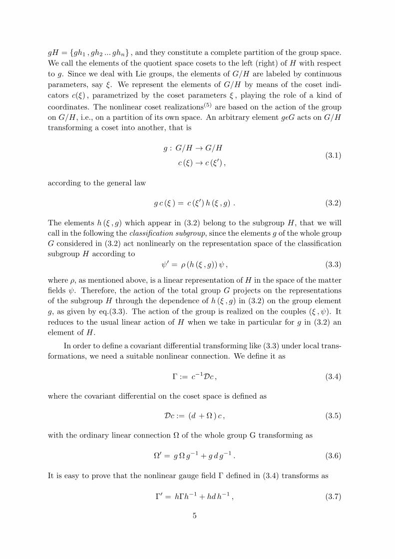
gH = gh1 , gh2 ... ghn , and they constitute a complete partition of the group space.

We call the elements of the quotient space cosets to the left (right) of H with respect

to g. Since we deal with Lie groups, the elements of G/H are labeled by continuous

parameters, say ξ. We represent the elements of G/H by means of the coset indi-

cators c(ξ) , parametrized by the coset parameters ξ , playing the role of a kind of

coordinates. The nonlinear coset realizations(5) are based on the action of the group

on G/H, i.e., on a partition of its own space. An arbitrary element gϵG acts on G/H

transforming a coset into another, that is

g : G/H → G/H

c (ξ) → c (ξ′) ,(3.1)

according to the general law

g c (ξ ) = c (ξ′)h (ξ , g) . (3.2)

The elements h (ξ , g) which appear in (3.2) belong to the subgroup H, that we will

call in the following the classification subgroup, since the elements g of the whole group

G considered in (3.2) act nonlinearly on the representation space of the classification

subgroup H according to

ψ′ = ρ (h (ξ , g))ψ , (3.3)

where ρ, as mentioned above, is a linear representation of H in the space of the matter

fields ψ. Therefore, the action of the total group G projects on the representations

of the subgroup H through the dependence of h (ξ , g) in (3.2) on the group element

g, as given by eq.(3.3). The action of the group is realized on the couples (ξ , ψ). It

reduces to the usual linear action of H when we take in particular for g in (3.2) an

element of H.

In order to define a covariant differential transforming like (3.3) under local trans-

formations, we need a suitable nonlinear connection. We define it as

Γ := c−1Dc , (3.4)

where the covariant differential on the coset space is defined as

Dc := (d +Ω) c , (3.5)

with the ordinary linear connection Ω of the whole group G transforming as

Ω′ = gΩ g−1 + g d g−1 . (3.6)

It is easy to prove that the nonlinear gauge field Γ defined in (3.4) transforms as

Γ′ = hΓh−1 + hdh−1 , (3.7)

5

thus allowing to define the nonlinear covariant differential operator

D := d + Γ . (3.8)

One can read out from (3.7) that only the components of Γ related to the generators

of H behave as true connections, transforming inhomogeneously, whereas the compo-

nents of Γ over the generators associated with the cosets c transform as tensors with

respect to the subgroup H notwithstanding their nature of connections.

4. Nonlinear gauge approach to the affine group

As we have discussed above, ordinary matter fields such as Dirac fields can only

be included in an affine theory if the affine group is realized nonlinearly, with the

Lorentz group as the classification subgroup. Thus, let us consider the affine group

A(4 , R) = GL(4 , R) ⊃× R4 in 4 dimensions, defined as the semidirect product of the

translations and the general linear transformations, with the generators Λαβ of the

linear transformations splitted up into the Lorentz generators Lαβ , plus the remaining

generators Sαβ of the symmetric linear transformations, as Λα

β = Lαβ + Sα

β . In

addition, we have the generators Pα of the translations. The commutation relations

read[Lαβ , Lµν ] = −i

(oα[µLν]β − oβ[µLν]α

),

[Lαβ , Sµν ] = i(oα(µSν)β − oβ(µSν)α

),

[Sαβ , Sµν ] = i(oα(µLν)β + oβ(µLν)α

),

[Lαβ , Pµ] = i oµ[αPβ] ,

[Sαβ , Pµ] = i oµ(αPβ) ,

[Pα , Pβ ] = 0 .

(4.1)

In order to realize the group action on the coset space A(4 , R)/SO(1 , 3), we make

use of the general formula (3.2) which defines the nonlinear group action, choosing in

particular for the cosets the parametrization

c := e−i ξαPαei hµνSµν , (4.2)

where ξα and hµν are the coset parameters. The group elements of the whole affine

group A(4 , R) are parametrized as

g = ei ϵαPαei α

µνSµνei βµνLµν , (4.3)

and those of the classification Lorentz subgroup are taken to be

h := ei uµνLµν . (4.4)

Other parametrizations are possible, leading to equivalent results.

6

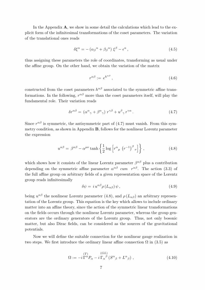
In the Appendix A, we show in some detail the calculations which lead to the ex-

plicit form of the infinitesimal transformations of the coset parameters. The variation

of the translational ones reads

δξα = − (αβα + ββ

α) ξβ − ϵα , (4.5)

thus assigning these parameters the role of coordinates, transforming as usual under

the affine group. On the other hand, we obtain the variation of the matrix

rαβ := ehαβ

, (4.6)

constructed from the coset parameters hαβ associated to the symmetric affine trans-

formations. In the following, rαβ more than the coset parameters itself, will play the

fundamental role. Their variation reads

δrαβ = (ααγ + βα

γ) rγβ + uβγ r

γα . (4.7)

Since rαβ is symmetric, the antisymmetric part of (4.7) must vanish. From this sym-

metry condition, as shown in AppendixB, follows for the nonlinear Lorentz parameter

the expression

uαβ = βαβ − αµν tanh

1

2log[rαµ

(r−1)β

ν

], (4.8)

which shows how it consists of the linear Lorentz parameter βαβ plus a contribution

depending on the symmetric affine parameter ααβ cum rαβ . The action (3.3) of

the full affine group on arbitrary fields of a given representation space of the Lorentz

group reads infinitesimally

δψ = i uαβρ (Lαβ)ψ , (4.9)

being uαβ the nonlinear Lorentz parameter (4.8), and ρ (Lαβ) an arbitrary represen-

tation of the Lorentz group. This equation is the key which allows to include ordinary

matter into an affine theory, since the action of the symmetric linear transformations

on the fields occurs through the nonlinear Lorentz parameter, whereas the group gen-

erators are the ordinary generators of the Lorentz group. Thus, not only bosonic

matter, but also Dirac fields, can be considered as the sources of the gravitational

potentials.

Now we will define the suitable connection for the nonlinear gauge realization in

two steps. We first introduce the ordinary linear affine connection Ω in (3.5) as

Ω := −i(T )

ΓαPα − i(GL)

Γαβ (Sα

β + Lαβ) , (4.10)

7

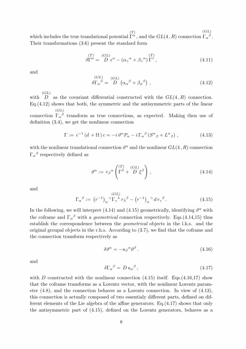
which includes the true translational potential(T )

Γα , and the GL(4 , R) connection(GL)

Γαβ .

Their transformations (3.6) present the standard form

δ(T )

Γα =(GL)

D ϵα − (αγα + βγ

α)(T )

Γγ , (4.11)

and

δ(GL)

Γαβ =

(GL)

D(αα

β + βαβ), (4.12)

with(GL)

D as the covariant differential constructed with the GL(4 , R) connection.

Eq.(4.12) shows that both, the symmetric and the antisymmetric parts of the linear

connection(GL)

Γαβ transform as true connections, as expected. Making then use of

definition (3.4), we get the nonlinear connection

Γ := c−1 (d +Ω) c = −i ϑαPα − iΓαβ (Sα

β + Lαβ) , (4.13)

with the nonlinear translational connection ϑα and the nonlinear GL(4 , R) connection

Γαβ respectively defined as

ϑα := rβα

((T )

Γβ +(GL)

D ξβ

), (4.14)

and

Γαβ :=

(r−1)α

γ(GL)

Γγλ rλ

β −(r−1)α

γ d rγβ . (4.15)

In the following, we will interpret (4.14) and (4.15) geometrically, identifying ϑα with

the coframe and Γαβ with a geometrical connection respectively. Eqs.(4.14,15) thus

establish the correspondence between the geometrical objects in the l.h.s. and the

original groupal objects in the r.h.s. According to (3.7), we find that the coframe and

the connection transform respectively as

δϑα = −uβαϑβ . (4.16)

and

δΓαβ = Duα

β , (4.17)

with D constructed with the nonlinear connection (4.15) itself. Eqs.(4.16,17) show

that the coframe transforms as a Lorentz vector, with the nonlinear Lorentz param-

eter (4.8), and the connection behaves as a Lorentz connection. In view of (4.13),

this connection is actually composed of two essentialy different parts, defined on dif-

ferent elements of the Lie algebra of the affine generators. Eq.(4.17) shows that only

the antisymmetric part of (4.15), defined on the Lorentz generators, behaves as a

8

true connection with respect to the Lorentz subgroup, whereas the symmetric part

is tensorial, transforming without any inhomogeneous contribution, since uαβ is an-

tisymmetric. The geometrical meaning of the nonlinear connection associated to the

symmetric affine generators will become clearer in terms of the Minkowski metric, as

we are going to show.

Since the nonlinear realization we are studying consists in a projection of the

action of the whole affine group on its Lorentz subgroup, i.e. on the pseudoorthogonal

group which, by definition, leaves invariant the symmetric tensor

oαβ := diag(+ − −− ) , (4.18)

this tensor appears automatically in the theory as a consequence of the nonlinear

treatment, being a natural invariant of the Lorentz group. We interpret it geometri-

cally in the common way as the Minkowskian metric tensor. No degrees of freedom

are related to it. Its inverse reads

oαβ := diag(+ − −− ) , (4.19)

and, as mentioned above, both are Lorentz invariant:

δoαβ = 0 , δoαβ = 0 . (4.20)

Defining the nonmetricity Qαβ as usual(3), i.e. as minus the covariant differential

of the metric tensor, we find that it is proportional to the symmetric part of the

nonlinear GL(4 , R) connection, namely

Qαβ := −Doαβ = 2Γ(αβ) . (4.21)

Thus, the geometrical meaning of the nonlinear connection associated to the sym-

metric affine generators becomes apparent as the nonmetricity, which behaves as a

Lorentz tensor. In order to show that, the transformation law (4.17) can be splitted

up into two parts, corresponding to the Lorentz connection(Lor)

Γαβ := Γ[αβ], and to the

nonmetricity respectively. We get

δ(Lor)

Γαβ =

(Lor)

D uαβ , (4.22)

and

δQαβ = 2u (αγQβ)γ . (4.23)

The tensorial character of the symmetric part of the connection is a result of the

nonlinear realization of the symmetric affine transformations, but it is also evident

from the definition (4.21) of the nonmetricity, since doαβ = 0.

9

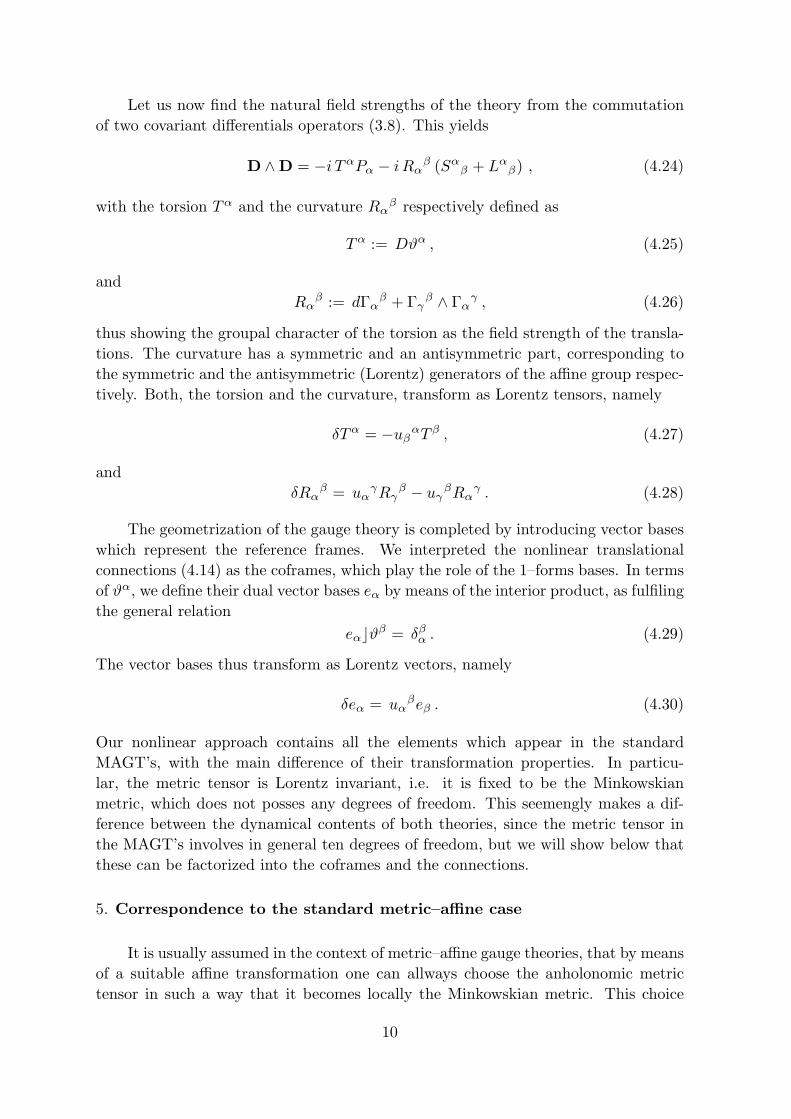
Let us now find the natural field strengths of the theory from the commutation

of two covariant differentials operators (3.8). This yields

D ∧D = −i TαPα − i Rαβ (Sα

β + Lαβ) , (4.24)

with the torsion Tα and the curvature Rαβ respectively defined as

Tα := Dϑα , (4.25)

and

Rαβ := dΓα

β + Γγβ ∧ Γα

γ , (4.26)

thus showing the groupal character of the torsion as the field strength of the transla-

tions. The curvature has a symmetric and an antisymmetric part, corresponding to

the symmetric and the antisymmetric (Lorentz) generators of the affine group respec-

tively. Both, the torsion and the curvature, transform as Lorentz tensors, namely

δTα = −uβαT β , (4.27)

and

δRαβ = uα

γRγβ − uγ

βRαγ . (4.28)

The geometrization of the gauge theory is completed by introducing vector bases

which represent the reference frames. We interpreted the nonlinear translational

connections (4.14) as the coframes, which play the role of the 1–forms bases. In terms

of ϑα, we define their dual vector bases eα by means of the interior product, as fulfiling

the general relation

eα⌋ϑβ = δβα . (4.29)

The vector bases thus transform as Lorentz vectors, namely

δeα = uαβeβ . (4.30)

Our nonlinear approach contains all the elements which appear in the standard

MAGT’s, with the main difference of their transformation properties. In particu-

lar, the metric tensor is Lorentz invariant, i.e. it is fixed to be the Minkowskian

metric, which does not posses any degrees of freedom. This seemengly makes a dif-

ference between the dynamical contents of both theories, since the metric tensor in

the MAGT’s involves in general ten degrees of freedom, but we will show below that

these can be factorized into the coframes and the connections.

5. Correspondence to the standard metric–affine case

It is usually assumed in the context of metric–affine gauge theories, that by means

of a suitable affine transformation one can allways choose the anholonomic metric

tensor in such a way that it becomes locally the Minkowskian metric. This choice

10

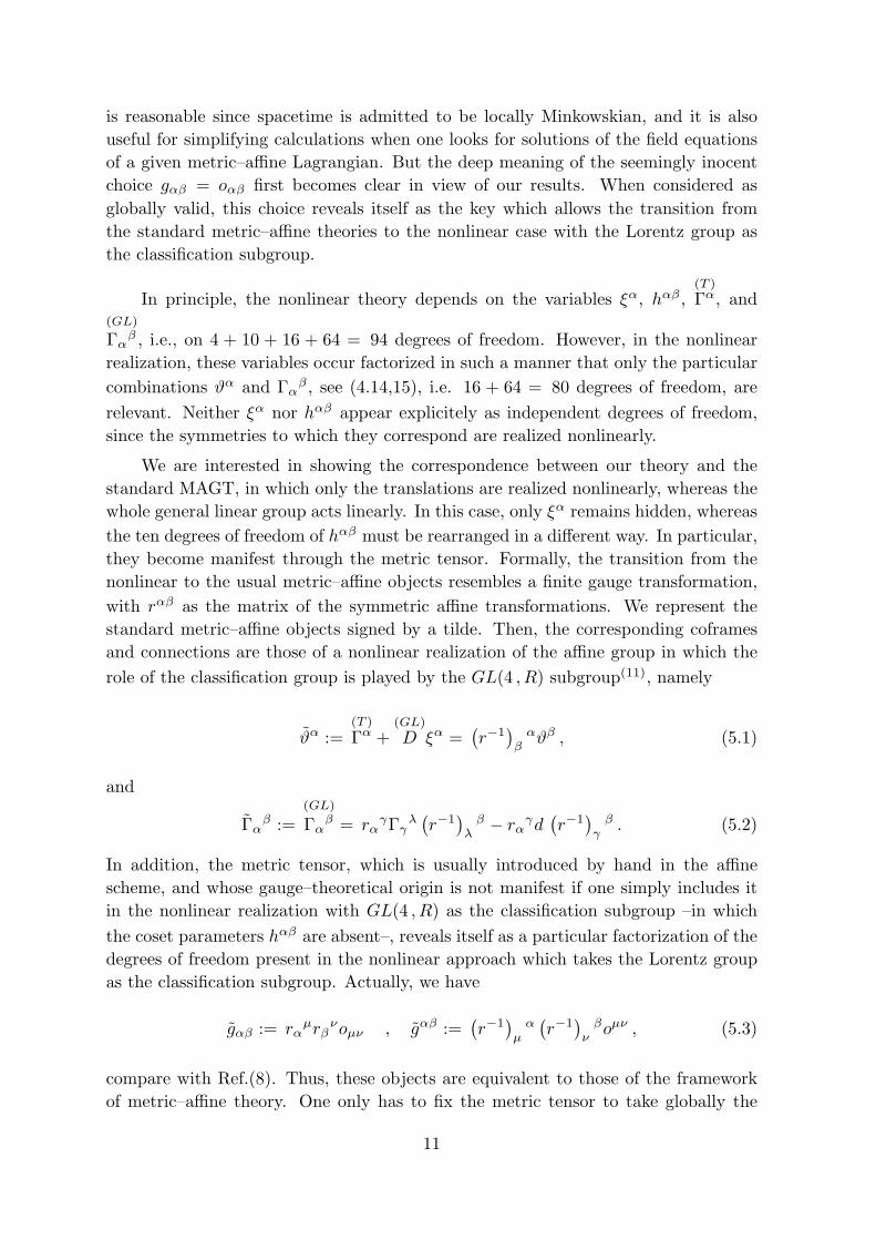
is reasonable since spacetime is admitted to be locally Minkowskian, and it is also

useful for simplifying calculations when one looks for solutions of the field equations

of a given metric–affine Lagrangian. But the deep meaning of the seemingly inocent

choice gαβ = oαβ first becomes clear in view of our results. When considered as

globally valid, this choice reveals itself as the key which allows the transition from

the standard metric–affine theories to the nonlinear case with the Lorentz group as

the classification subgroup.

In principle, the nonlinear theory depends on the variables ξα, hαβ ,(T )

Γα, and(GL)

Γαβ , i.e., on 4 + 10 + 16 + 64 = 94 degrees of freedom. However, in the nonlinear

realization, these variables occur factorized in such a manner that only the particular

combinations ϑα and Γαβ , see (4.14,15), i.e. 16 + 64 = 80 degrees of freedom, are

relevant. Neither ξα nor hαβ appear explicitely as independent degrees of freedom,

since the symmetries to which they correspond are realized nonlinearly.

We are interested in showing the correspondence between our theory and the

standard MAGT, in which only the translations are realized nonlinearly, whereas the

whole general linear group acts linearly. In this case, only ξα remains hidden, whereas

the ten degrees of freedom of hαβ must be rearranged in a different way. In particular,

they become manifest through the metric tensor. Formally, the transition from the

nonlinear to the usual metric–affine objects resembles a finite gauge transformation,

with rαβ as the matrix of the symmetric affine transformations. We represent the

standard metric–affine objects signed by a tilde. Then, the corresponding coframes

and connections are those of a nonlinear realization of the affine group in which the

role of the classification group is played by the GL(4 , R) subgroup(11), namely

ϑα :=(T )

Γα +(GL)

D ξα =(r−1)β

αϑβ , (5.1)

and

Γαβ :=

(GL)

Γαβ = rα

γΓγλ(r−1)λβ − rα

γd(r−1)γβ . (5.2)

In addition, the metric tensor, which is usually introduced by hand in the affine

scheme, and whose gauge–theoretical origin is not manifest if one simply includes it

in the nonlinear realization with GL(4 , R) as the classification subgroup –in which

the coset parameters hαβ are absent–, reveals itself as a particular factorization of the

degrees of freedom present in the nonlinear approach which takes the Lorentz group

as the classification subgroup. Actually, we have

gαβ := rαµrβ

νoµν , gαβ :=(r−1)µ

α(r−1)νβoµν , (5.3)

compare with Ref.(8). Thus, these objects are equivalent to those of the framework

of metric–affine theory. One only has to fix the metric tensor to take globally the

11

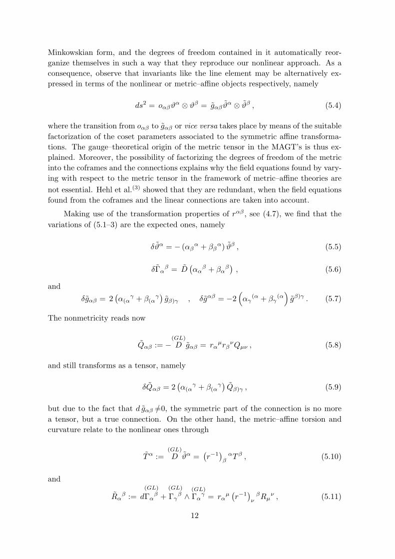
Minkowskian form, and the degrees of freedom contained in it automatically reor-

ganize themselves in such a way that they reproduce our nonlinear approach. As a

consequence, observe that invariants like the line element may be alternatively ex-

pressed in terms of the nonlinear or metric–affine objects respectively, namely

ds2 = oαβϑα ⊗ ϑβ = gαβϑ

α ⊗ ϑβ , (5.4)

where the transition from oαβ to gαβ or vice versa takes place by means of the suitable

factorization of the coset parameters associated to the symmetric affine transforma-

tions. The gauge–theoretical origin of the metric tensor in the MAGT’s is thus ex-

plained. Moreover, the possibility of factorizing the degrees of freedom of the metric

into the coframes and the connections explains why the field equations found by vary-

ing with respect to the metric tensor in the framework of metric–affine theories are

not essential. Hehl et al.(3) showed that they are redundant, when the field equations

found from the coframes and the linear connections are taken into account.

Making use of the transformation properties of rαβ , see (4.7), we find that the

variations of (5.1–3) are the expected ones, namely

δϑα = − (αβα + ββ

α) ϑβ , (5.5)

δΓαβ = D

(αα

β + βαβ), (5.6)

and

δgαβ = 2(α(α

γ + β(αγ)gβ)γ , δgαβ = −2

(αγ

(α + βγ(α)gβ)γ . (5.7)

The nonmetricity reads now

Qαβ := −(GL)

D gαβ = rαµrβ

νQµν , (5.8)

and still transforms as a tensor, namely

δQαβ = 2(α(α

γ + β(αγ)Qβ)γ , (5.9)

but due to the fact that d gαβ =/0, the symmetric part of the connection is no more

a tensor, but a true connection. On the other hand, the metric–affine torsion and

curvature relate to the nonlinear ones through

Tα :=(GL)

D ϑα =(r−1)β

αT β , (5.10)

and

Rαβ := d

(GL)

Γαβ +

(GL)

Γγβ ∧

(GL)

Γαγ = rα

µ(r−1)νβRµ

ν , (5.11)

12

and their variations read

δTα = − (αβα + ββ

α) T β , (5.12)

and

δRαβ = (αα

γ + βαγ) Rγ

β −(αγ

β + βγβ)Rα

γ . (5.13)

The general law relating the variations of the fields ψ of our theory, see (4.9), and of

those of the MAGT, can be written in an abstract way as

δ(ei h

µνSµνψ)= i

(ααβSαβ + βαβLαβ

) (ei h

µνSµνψ), (5.14)

which does not present any problems as far as the regular representations are con-

cerned. How to interpret (5.14) in the case of fields ψ in a half–integer representation

remains an open question. The same comment holds for the relation between the

abstract differential operators, namely

Dψ = e−i hµνSµν D(ei h

µνSµνψ). (5.15)

In short, the standard MAGT’s result from a particular factorization of the ten de-

grees of freedom of the nonlinear theory, which manifest themselves as the degrees of

freedom of the metric tensor.

6. Conclusions

The standard MAGT is a nonlinear realization of the affine group in which only

the translations are treated nonlinearly –the nonlinear connections of the translations

being identified with the coframes–, whereas the general linear group plays the role

of the classification subgroup. In addition, a metric tensor involving ten degrees of

freedom is included. We have proven that this theory, metric tensor included, can be

obtained from a more fundamental approach to gravity as a degenerate case, where

ordinary fermionic matter is absent.

In fact, the choice of the Lorentz group as the classification subgroup, in a non-

linear realization, leads to a theory in which ordinary Dirac fields can be included.

The essential difference between our approach and the standard metric–affine theories

consists in the transformation properties of the physical fields, which behave as repre-

sentations of the Lorentz group, and in that the symmetric part of the connection is

strictly proportional to the nonmetricity, transforming as a tensor. Nothing has to be

changed in the standard metric–affine formalism but the choice of the metric, and of

course the interpretation. The metric tensor is taken as the Minkowski metric. Since

it is invariant under Lorentz transformations, it is globally fixed once and forever, so

that space and time are everywhere well defined as distinguished quantities. Being a

constant tensor, the metric has not a dynamical meaning any more. The geometry is

13

determined by the interactions, and in the absence of gravity, the geometrical back-

ground simplifies to a flat spacetime. But the effect of gravitation is, strictly speaking,

affine more than metric. The whole information about the gravitational interactions

is contained in the connections, as in the gauge theories of internal groups.

Let us finally point out that, having the Lorentz group natural invariants, this

is also the case for the affine group when realized nonlinearly with the Lorentz group

as the classification subgroup. In the context of MAGT’s of gravitation, McCrea(12)

calculated the irreducible decomposition of the curvature, the torsion and the non-

metricity with respect to the Lorentz group. The utility of his work to construct

all possible invariants becomes evident in view of the nonlinear realization presented

here, since it enables us to work with an affine geometrical formalism whose objects

are defined on representation spaces of the Lorentz group.

APPENDIX

A.– Let us show how the expressions (4.5) and (4.7) were deduced (cfr. Ref.(8)). We

apply the general formula (3.2) defining the nonlinear action, namely

g c (ξ ) = c (ξ′)h (ξ , g) , (A.1)

with the particular choices

g = ei ϵαPαei α

µνSµνei βµνLµν , c := e−i ξαPαei h

µνSµν , h := ei uµνLµν ,

(A.2)

as given in (4.2–4). The equation we have to solve then reads

ei ϵαPαei α

µνSµνei βµνLµνe−i ξαPαei h

µνSµν = e−i ξ′αPαei h

′µνSµνei uµνLµν . (A.3)

We consider an affine transformation with infinitesimal group parameters ϵα, αµν

and βµν . Thus, the transformed coset parameters in the r.h.s. of (A.3) reduce to

ξ′α = ξα + δξα and h

′µν = hµν + δhµν , and uµν is also infinitesimal. Consequently,

eq.(A.3) reduces to

ei ξαPα(1 + i ϵαPα+i α

µνSµν + i βµνLµν

)e−i ξαPα

= (1− i δξαPα) ei (hµν+δhµν)Sµν

(1 + i uµνLµν

)e−i hµνSµν .

(A.4)

In order to simplify the calculations, we make use of the generators of the whole linear

transformations Λαβ := Lα

β + Sαβ , in terms of which, the commutation relations

(4.1) reduce to

[Λαβ ,Λ

µν ] = i

(δανΛ

µβ − δµβΛ

αν

),

[Λαβ , Pµ] = i δαµPβ ,

[Pα , Pβ ] = 0 .

(A.5)

14

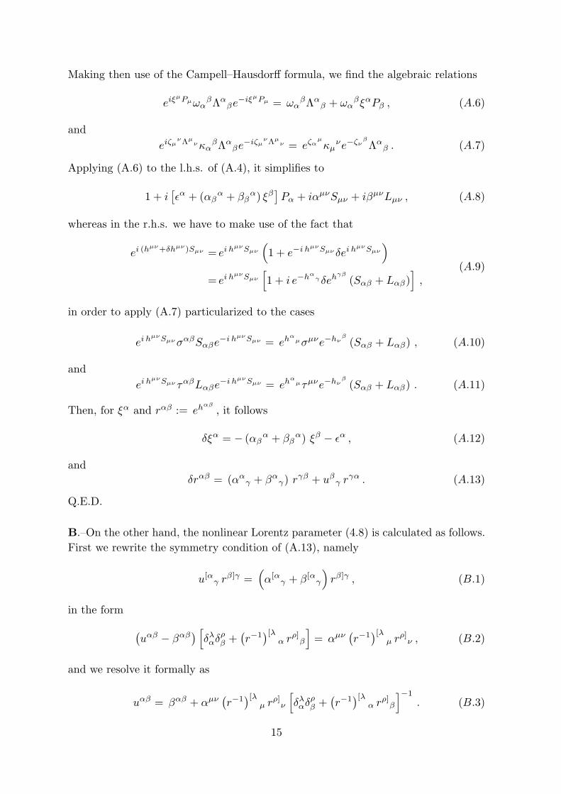
Making then use of the Campell–Hausdorff formula, we find the algebraic relations

eiξµPµωα

βΛαβe

−iξµPµ = ωαβΛα

β + ωαβξαPβ , (A.6)

and

eiζµνΛµ

νκαβΛα

βe−iζµ

νΛµν = eζα

µ

κµνe−ζν

β

Λαβ . (A.7)

Applying (A.6) to the l.h.s. of (A.4), it simplifies to

1 + i[ϵα + (αβ

α + ββα) ξβ

]Pα + iαµνSµν + iβµνLµν , (A.8)

whereas in the r.h.s. we have to make use of the fact that

ei (hµν+δhµν)Sµν = ei h

µνSµν

(1 + e−i hµνSµν δei h

µνSµν

)= ei h

µνSµν

[1 + i e−hα

γ δehγβ

(Sαβ + Lαβ)],

(A.9)

in order to apply (A.7) particularized to the cases

ei hµνSµνσαβSαβe

−i hµνSµν = ehα

µσµνe−hνβ

(Sαβ + Lαβ) , (A.10)

and

ei hµνSµν ταβLαβe

−i hµνSµν = ehα

µτµνe−hνβ

(Sαβ + Lαβ) . (A.11)

Then, for ξα and rαβ := ehαβ

, it follows

δξα = − (αβα + ββ

α) ξβ − ϵα , (A.12)

and

δrαβ = (ααγ + βα

γ) rγβ + uβγ r

γα . (A.13)

Q.E.D.

B.–On the other hand, the nonlinear Lorentz parameter (4.8) is calculated as follows.

First we rewrite the symmetry condition of (A.13), namely

u[αγ rβ]γ =

(α[α

γ + β[αγ

)rβ]γ , (B.1)

in the form (uαβ − βαβ

) [δλαδ

ρβ +

(r−1)[λ

α rρ]β

]= αµν

(r−1)[λ

µ rρ]ν , (B.2)

and we resolve it formally as

uαβ = βαβ + αµν(r−1)[λ

µ rρ]ν

[δλαδ

ρβ +

(r−1)[λ

α rρ]β

]−1

. (B.3)

15

Making then use of the fact that

(r−1)[λ

µ rρ]ν =

1

2

[e(h

ρν−hλ

µ) − e−(hρµ−hλ

ν)], (B.4)

we recognize that

uαβ =βαβ − αµν

sinh

(hλµ − hρν

) [δλαδ

ρβ + cosh

(hλα − hρβ

)]−1

=βαβ − αµν tanh

(hαµ − hβν

2

)=βαβ − αµν tanh

1

2log[rαµ

(r−1)β

ν

].

(B.5)

Q.E.D.

Acknowledgement

We are very grateful to Dr. Jaime Julve for helpful discussions.

16

REFERENCES

[1] R. Utiyama, Phys. Rev. 101 (1956) 1597

T. W. B. Kibble, J. Math. Phys. 2 (1961) 212

D. W. Sciama, Rev. Mod. Phys. 36 (1964) 463 and 1103

[2] A. Trautman, in Differential Geometry, Symposia Mathematica Vol. 12 (Aca-

demic Press, London, 1973), p. 139

A. G. Agnese and P. Calvini, Phys. Rev. D 12 (1975) 3800 and 3804

F. W. Hehl, P. von der Heyde, G. D. Kerlick and J. M. Nester, Rev. Mod. Phys.

48 (1976) 393

P. von der Heyde, Phys. Lett. 58 A (1976) 141

E.A. Ivanov and J. Niederle, Phys. Rev. D25 (1982) 976 and 988

D. Ivanenko and G.A. Sardanashvily, Phys. Rep. 94 (1983) 1

E. A. Lord, J. Math. Phys. 27 (1986) 2415 and 3051

[3] F. W. Hehl, J. D. McCrea, E. W. Mielke, and Y. Ne’eman Found. Phys. 19

(1989) 1075

R. D. Hecht and F. W. Hehl, Proc. 9th Italian Conf. G.R. and Grav. Phys.,

Capri (Napoli). R. Cianci et al.(eds.) (World Scientific, Singapore, 1991) p. 246

F.W. Hehl, J.D. McCrea, E.W. Mielke, and Y. Ne’eman, Physics Reports, to be

published.

[4] Y. Ne’eman and Dj. Sijacki, Proc. Natl. Acad. Sci. USA 76 (1979) 561

Y. Ne’eman and Dj. Sijacki, Ann. Phys. (N.Y.) 120 (1979) 292

Dj. Sijacki, Group and Gauge Structure of Affine Theories in Frontiers in Particle

Physics ’83 (World Scientific Pub. 1984)

Y. Ne’eman and Dj. Sijacki, Phys. Lett. B200 (1988) 489

Y. Ne’eman and Dj. Sijacki, Phys. Rev. D 37 (1988) 3267

[5] S. Coleman, J. Wess and B. Zumino, Phys. Rev. 117 (1969) 2239

C.G. Callan, S. Coleman, J. Wess and B. Zumino, Phys. Rev. 117 (1969) 2247

E. W. Mielke, Fortschr. Phys. 25 (1977) 401, and references therein

S. Coleman, Aspects of Symmetry. Cambridge University Press, Cambridge

(1985)

[6] A. Salam and J. Strathdee, Phys. Rev. 184 (1969) 1750 and 1760

C.J. Isham, A. Salam and J. Strathdee, Ann. of Phys. 62 (1971) 98

17

L.N. Chang and F. Mansouri, Phys. Lett. 78 B (1979) 274, and Phys. Rev. D

17 (1978) 3168

K.S. Stelle and P.C. West, Phys. Rev. D 21 (1980) 1466

E.A. Lord, Gen. Rel. Grav. 19 (1987) 983, and J. Math. Phys. 29 (1988) 258

[7] A.B. Borisov and I.V. Polubarinov, Zh. ksp. Theor. Fiz. 48 (1965) 1625, and

V. Ogievetsky and I. Polubarinov, Ann. Phys. (NY) 35 (1965) 167

[8] A.B. Borisov and V.I. Ogievetskii, Theor. Mat. Fiz. 21 (1974) 329

S. Hamamoto, Prog. Theor. Phys. 60 (1978) 1910

[9] E. Cartan, Sur les varits connexion affine et la thorie de la relativit gnralise,

Ouvres completes, Editions du C.N.R.S. (1984), Partie III. 1, pgs. 659 and 921

[10] K. Hayashi and T. Nakano, Prog. Theor. Phys 38 (1967) 491

K. Hayashi and T. Shirafuji, Prog. Theor. Phys 64 (1980) 866 and 80 (1988)

711

J. Hennig and J. Nitsch, Gen. Rel. Grav. 13 (1981) 947

H.R. Pagels, Phys. Rev. D 29 (1984) 1690

T. Kawai, Gen. Rel. Grav. 18 (1986) 995

G. Grignani and G. Nardelli, Phys. Rev. D 45 (1992) 2719

E. W. Mielke, J.D. McCrea, Y. Ne’eman and F.W. Hehl Phys. Rev. D 48 (1993)

673, and references therein

[11] J. Julve, A. Lpez–Pinto, A. Tiemblo and R. Tresguerres, Nonlinear gauge real-

izations of spacetime symmetries including translations, (1994), to be published

[12] J. D. McCrea, Class. Quantum Grav. 9 (1992) 553

18