Bedrock river erosion through dipping layered rocks - Earth ...
31
Earth Surf. Dynam., 9, 723–753, 2021 https://doi.org/10.5194/esurf-9-723-2021 © Author(s) 2021. This work is distributed under the Creative Commons Attribution 4.0 License. Bedrock river erosion through dipping layered rocks: quantifying erodibility through kinematic wave speed Nate A. Mitchell and Brian J. Yanites Department of Earth and Atmospheric Sciences, Indiana University, Bloomington, Indiana, USA Correspondence: Nate A. Mitchell ([email protected]) Received: 29 January 2021 – Discussion started: 24 February 2021 Revised: 27 May 2021 – Accepted: 14 June 2021 – Published: 21 July 2021 Abstract. Landscape morphology reflects drivers such as tectonics and climate but is also modulated by under- lying rock properties. While geomorphologists may attempt to quantify the influence of rock strength through direct comparisons of landscape morphology and rock strength metrics, recent work has shown that the con- tact migration resulting from the presence of mixed lithologies may hinder such an approach. Indeed, this work counterintuitively suggests that channel slopes within weaker units can sometimes be higher than channel slopes within stronger units. Here, we expand upon previous work with 1-D stream power numerical models in which we have created a system for quantifying contact migration over time. Although previous studies have devel- oped theories for bedrock rivers incising through layered stratigraphy, we can now scrutinize these theories with contact migration rates measured in our models. Our results show that previously developed theory is generally robust and that contact migration rates reflect the pattern of kinematic wave speed across the profile. Further- more, we have developed and tested a new approach for estimating kinematic wave speeds. This approach utilizes channel steepness, a known base-level fall rate, and contact dips. Importantly, we demonstrate how this new ap- proach can be combined with previous work to estimate erodibility values. We demonstrate this approach by accurately estimating the erodibility values used in our numerical models. After this demonstration, we use our approach to estimate erodibility values for a stream near Hanksville, UT. Because we show in our numerical models that one can estimate the erodibility of the unit with lower steepness, the erodibilities we estimate for this stream in Utah are likely representative of mudstone and/or siltstone. The methods we have developed can be applied to streams with temporally constant base-level fall, opening new avenues of research within the field of geomorphology. 1 Introduction Geomorphologists seek to extract geologic and climatic in- formation from landscape morphology, and the conceptual framework of the stream power model (Howard and Kerby, 1983; Whipple and Tucker, 1999) has driven many such en- deavors (Whipple et al., 2013). Indeed, as a representation of bedrock river incision, the stream power model has been used in many applications, including (1) identifying unrec- ognized earthquake risks (Kirby et al., 2003), (2) constrain- ing the timing and extent of normal fault activity (Whittaker et al., 2008; Boulton and Whittaker, 2009; Gallen and Weg- mann, 2017), (3) distinguishing between potential drivers of transient incision (Carretier et al., 2006; Gallen et al., 2013; Miller et al., 2013; Yanites et al., 2017), and (4) searching for spatial patterns in rock strength (Allen et al., 2013; Bursztyn et al., 2015). This last application is our focus here; to what extent can river morphology be used to detect spatial patterns in rock strength? While such a question seems straightfor- ward to address (e.g., comparing morphologies in different rock types), the mere presence of different rock strengths in- troduces complicating factors. For example, contact migra- tion perturbs the spatial distribution of erosion rates, causing dramatic variations in slope along a bedrock river (Forte et al., 2016; Perne et al., 2017; Darling et al., 2020). Surpris- ingly, these perturbations can even cause streams to counter- intuitively have steeper reaches in weaker rocks (Perne et al., Published by Copernicus Publications on behalf of the European Geosciences Union.
-
Upload
khangminh22 -
Category
Documents
-
view
1 -
download
0
Transcript of Bedrock river erosion through dipping layered rocks - Earth ...
Earth Surf. Dynam., 9, 723–753, 2021https://doi.org/10.5194/esurf-9-723-2021© Author(s) 2021. This work is distributed underthe Creative Commons Attribution 4.0 License.
Bedrock river erosion through dipping layered rocks:quantifying erodibility through kinematic wave speed
Nate A. Mitchell and Brian J. YanitesDepartment of Earth and Atmospheric Sciences, Indiana University, Bloomington, Indiana, USA
Correspondence: Nate A. Mitchell ([email protected])
Received: 29 January 2021 – Discussion started: 24 February 2021Revised: 27 May 2021 – Accepted: 14 June 2021 – Published: 21 July 2021
Abstract. Landscape morphology reflects drivers such as tectonics and climate but is also modulated by under-lying rock properties. While geomorphologists may attempt to quantify the influence of rock strength throughdirect comparisons of landscape morphology and rock strength metrics, recent work has shown that the con-tact migration resulting from the presence of mixed lithologies may hinder such an approach. Indeed, this workcounterintuitively suggests that channel slopes within weaker units can sometimes be higher than channel slopeswithin stronger units. Here, we expand upon previous work with 1-D stream power numerical models in whichwe have created a system for quantifying contact migration over time. Although previous studies have devel-oped theories for bedrock rivers incising through layered stratigraphy, we can now scrutinize these theories withcontact migration rates measured in our models. Our results show that previously developed theory is generallyrobust and that contact migration rates reflect the pattern of kinematic wave speed across the profile. Further-more, we have developed and tested a new approach for estimating kinematic wave speeds. This approach utilizeschannel steepness, a known base-level fall rate, and contact dips. Importantly, we demonstrate how this new ap-proach can be combined with previous work to estimate erodibility values. We demonstrate this approach byaccurately estimating the erodibility values used in our numerical models. After this demonstration, we use ourapproach to estimate erodibility values for a stream near Hanksville, UT. Because we show in our numericalmodels that one can estimate the erodibility of the unit with lower steepness, the erodibilities we estimate forthis stream in Utah are likely representative of mudstone and/or siltstone. The methods we have developed canbe applied to streams with temporally constant base-level fall, opening new avenues of research within the fieldof geomorphology.
1 Introduction
Geomorphologists seek to extract geologic and climatic in-formation from landscape morphology, and the conceptualframework of the stream power model (Howard and Kerby,1983; Whipple and Tucker, 1999) has driven many such en-deavors (Whipple et al., 2013). Indeed, as a representationof bedrock river incision, the stream power model has beenused in many applications, including (1) identifying unrec-ognized earthquake risks (Kirby et al., 2003), (2) constrain-ing the timing and extent of normal fault activity (Whittakeret al., 2008; Boulton and Whittaker, 2009; Gallen and Weg-mann, 2017), (3) distinguishing between potential drivers oftransient incision (Carretier et al., 2006; Gallen et al., 2013;
Miller et al., 2013; Yanites et al., 2017), and (4) searching forspatial patterns in rock strength (Allen et al., 2013; Bursztynet al., 2015). This last application is our focus here; to whatextent can river morphology be used to detect spatial patternsin rock strength? While such a question seems straightfor-ward to address (e.g., comparing morphologies in differentrock types), the mere presence of different rock strengths in-troduces complicating factors. For example, contact migra-tion perturbs the spatial distribution of erosion rates, causingdramatic variations in slope along a bedrock river (Forte etal., 2016; Perne et al., 2017; Darling et al., 2020). Surpris-ingly, these perturbations can even cause streams to counter-intuitively have steeper reaches in weaker rocks (Perne et al.,
Published by Copernicus Publications on behalf of the European Geosciences Union.
724 N. A. Mitchell and B. J. Yanites: Bedrock river erosion through dipping layered rocks
2017). Predicting how contrasts in rock strength are reflectedin topography, and specifically river profiles, is therefore nec-essary to advance our understanding of both (1) the drivers oflandscape evolution and (2) how we can use landscape mor-phology to extract information about geology and climate.
1.1 Motivations
Forte et al. (2016) demonstrated how rock strength perturba-tions can cause long-lasting landscape transience, even withconstant tectonic and climatic forcing. The spatiotemporaldistribution of erosion rates can strongly vary with rock type,with one rock type eroding well above the rock-uplift rateand another well below it. These findings have far-reachingimplications for landscape evolution and methodological ap-proaches to quantifying rates. For example, the exposure of anew lithology could trigger an increase in erosion rates, andthis increase could be mistakenly attributed to a change in ex-ternal forcing such as climate. Variations in erosion rate dueto mixed rock types can influence detrital zircon geochronol-ogy, detrital thermochronology, and detrital cosmogenic nu-clide analysis (Carretier et al., 2015; Forte et al., 2016; Dar-ling et al., 2020). Spatial contrasts in rock strength can alsoinfluence detrital geochronology (Lavarini et al., 2018), sospatial variations in both rock strength and erosion rate wouldfurther complicate the interpretation of grain age distribu-tions. Furthermore, the presence of a dipping contact separat-ing lithologies with different strengths can significantly influ-ence knickpoint migration following changes in rock-upliftrates (Wolpert and Forte, 2021), highlighting the influence ofrock properties on the transient adjustment of landscapes.
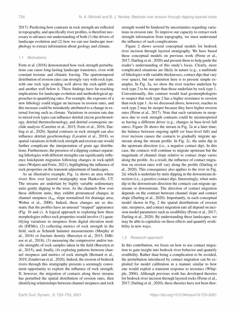
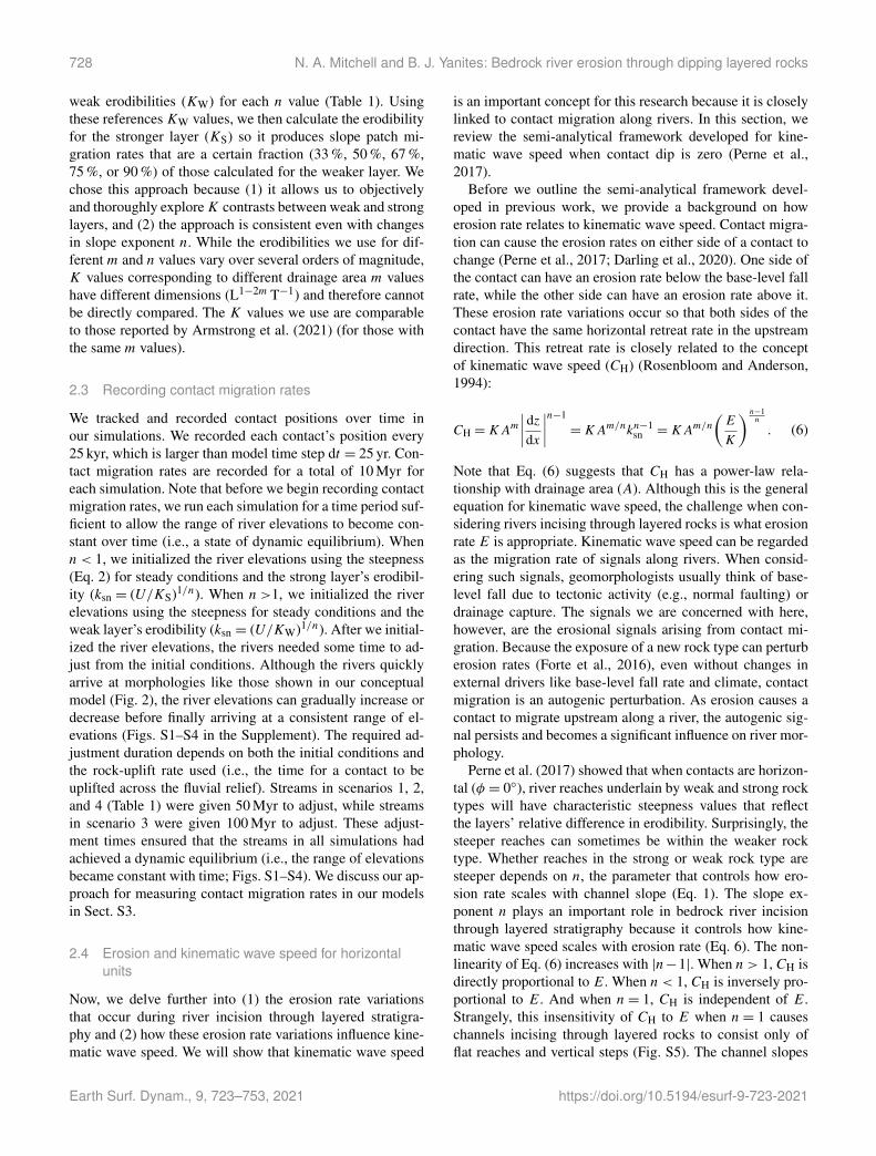
As an illustrative example, Fig. 1a shows an area whererivers flow over layered stratigraphy near Hanksville, UT.The streams are underlain by highly variable sedimentaryunits gently dipping to the west. As the channels flow overthese different units, they exhibit pronounced changes inchannel steepness (ksn, slope normalized for drainage area;Wobus et al., 2006). Indeed, these changes are so dra-matic that the profiles have an unusual “stepped” appearance(Fig. 1b and c). A logical approach to exploring how thesemorphologies reflect rock properties would involve (1) quan-tifying variations in steepness from digital elevation mod-els (DEMs), (2) collecting metrics of rock strength in thefield, such as Schmidt hammer measurements (Murphy etal., 2016) or fracture density (Bursztyn et al., 2015; DiBi-ase et al., 2018), (3) measuring the compressive and/or ten-sile strengths of rock samples taken in the field (Bursztyn etal., 2015), and, finally, (4) exploring patterns between chan-nel steepness and metrics of rock strength (Bernard et al.,2019; Zondervan et al., 2020). Indeed, the erosion of bedrockrivers through this stratigraphy presents a seemingly conve-nient opportunity to explore the influence of rock strength.If, however, the migration of contacts along these streamshas perturbed the spatial distribution of erosion rates, thenidentifying relationships between channel steepness and rock
strength would be hindered by uncertainties regarding varia-tions in erosion rate. To improve our capacity to extract rockstrength information from topography, we must understandthe influence of such complications.
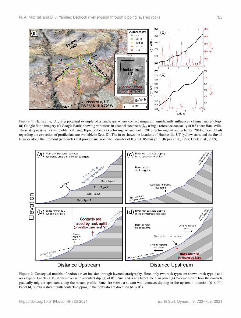
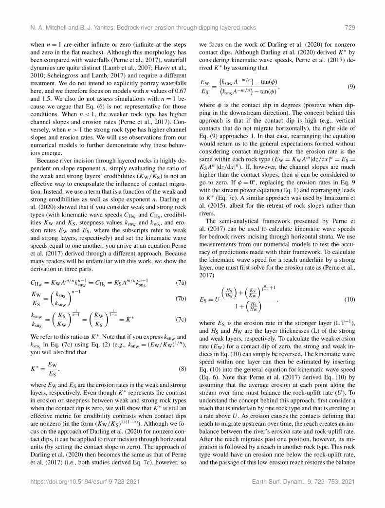
Figure 2 shows several conceptual models for bedrockriver incision through layered stratigraphy. We have basedthese conceptual models on previous work (Perne et al.,2017; Darling et al., 2020) and present them to help guide thereader’s understanding of this study’s focus. Clearly, morecomplicated situations are likely in nature (e.g., a multitudeof lithologies with variable thicknesses, contact dips that varyover space), but our intention here is to present simple ex-amples. In Fig. 2a, we show the river reaches underlain byrock type 2 to be steeper than those underlain by rock type 1.Conventionally, this contrast would lead geomorphologiststo suspect that rock type 2 has a higher resistance to erosionthan rock type 1. As we discussed above, however, reaches inrock type 2 may be steeper because they have higher erosionrates (Perne et al., 2017). Note that such variations in steep-ness due to rock strength contrasts could be misinterpretedas having a different driver (e.g., changes in base-level fallrates). Figure 2b shows the stream in Fig. 2a at a later time;the balance between ongoing uplift (or base-level fall) andriver incision causes the contacts to gradually migrate up-stream along the stream profile. In Fig. 2c, the units dip inthe upstream direction (i.e., a negative contact dip). In thiscase, the contacts will continue to migrate upstream but themagnitude of channel slope relative to contact slope variesalong the profile. As a result, the influence of contact migra-tion on erosion rates will vary along the profile (Darling etal., 2020). This consequence also applies to the river in Fig.2d, which is underlain by units dipping in the downstream di-rection (i.e., a positive contact dip). Interestingly, when unitsdip in the downstream direction the contacts can migrate up-stream or downstream. The direction of contact migrationdepends on the contrast between channel slope and contactslope (Darling et al., 2020). Importantly, in each conceptualmodel shown in Fig. 2 the spatial distributions of erosionrate, steepness, and contact migration rate all depend on inci-sion model parameters such as erodibility (Perne et al., 2017;Darling et al., 2020). By understanding these landscapes, wemay be able to capitalize on these effects and quantify erodi-bility in new ways.
1.2 Research approach
In this contribution, we focus on how to use contact migra-tion to gain insight into bedrock river behavior and quantifyerodibility. Rather than being a complication to be avoided,the perturbation introduced by contact migration can be ex-ploited for model calibration in a manner similar to howone would exploit a transient response to tectonics (Whip-ple, 2004). Although previous work has developed theoriesfor bedrock river incision through layered rocks (Perne et al.,2017; Darling et al., 2020), these theories have not been thor-
Earth Surf. Dynam., 9, 723–753, 2021 https://doi.org/10.5194/esurf-9-723-2021
N. A. Mitchell and B. J. Yanites: Bedrock river erosion through dipping layered rocks 725
Figure 1. Hanksville, UT, is a potential example of a landscape where contact migration significantly influences channel morphology.(a) Google Earth imagery (© Google Earth) showing variations in channel steepness (ksn using a reference concavity of 0.5) near Hanksville.These steepness values were obtained using TopoToolbox v2 (Schwanghart and Kuhn, 2010; Schwanghart and Scherler, 2014); more detailsregarding the extraction of profile data are available in Sect. S1. The inset shows the locations of Hanksville, UT (yellow star), and the fluvialterraces along the Fremont (red circle) that provide incision rate estimates of 0.3 to 0.85 mm yr−1 (Repka et al., 1997; Cook et al., 2009).
Figure 2. Conceptual models of bedrock river incision through layered stratigraphy. Here, only two rock types are shown: rock type 1 androck type 2. Panels (a, b) show a river with a contact dip (φ) of 0◦. Panel (b) is at a later time than panel (a) to demonstrate how the contactsgradually migrate upstream along the stream profile. Panel (c) shows a stream with contacts dipping in the upstream direction (φ < 0◦).Panel (d) shows a stream with contacts dipping in the downstream direction (φ > 0◦).
https://doi.org/10.5194/esurf-9-723-2021 Earth Surf. Dynam., 9, 723–753, 2021
726 N. A. Mitchell and B. J. Yanites: Bedrock river erosion through dipping layered rocks
oughly compared with observations from numerical models.Here, we use numerical models with which we can mea-sure contact migration over time to pursue the following re-search questions: (1) does the theory developed by Perne etal. (2017) for river incision through horizontal strata accu-rately reflect observations from numerical models? (2) Doesthe theory developed by Darling et al. (2020) for river in-cision through nonhorizontal strata accurately reflect obser-vations from numerical models? (3) What is the potentialfor using these theoretical frameworks to estimate incisionmodel parameters like erodibility for real bedrock rivers?By developing a new method for estimating kinematic wavespeed, we will show that morphologic metrics like steepnessand contact dip can be used to estimate bedrock erodibility,even where contact dips are nonzero. The dynamics of land-scapes with layered rocks are increasingly shown to be quiterich (Glade et al., 2017; Ward, 2019; Sheehan and Ward,2020a, b), and these landscapes offer valuable opportuni-ties to compare expectations shaped by model results withthe unflinching testimony of the field. Our intention hereis to (1) further elucidate what we should expect from thecommon form of the stream power model and (2) provide aframework for quantifying rock strength from bedrock rivermorphology. After developing this framework through theuse of numerical models, we demonstrate its application onTank Wash, one of the streams near Hanksville, UT (Fig. 1).
2 Methods
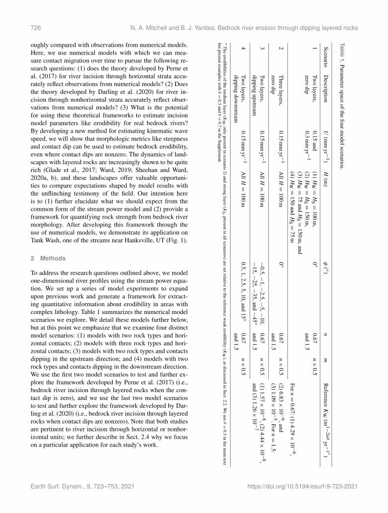
To address the research questions outlined above, we modelone-dimensional river profiles using the stream power equa-tion. We set up a series of model experiments to expandupon previous work and generate a framework for extract-ing quantitative information about erodibility in areas withcomplex lithology. Table 1 summarizes the numerical modelscenarios we explore. We detail these models further below,but at this point we emphasize that we examine four distinctmodel scenarios: (1) models with two rock types and hori-zontal contacts; (2) models with three rock types and hori-zontal contacts; (3) models with two rock types and contactsdipping in the upstream direction; and (4) models with tworock types and contacts dipping in the downstream direction.We use the first two model scenarios to test and further ex-plore the framework developed by Perne et al. (2017) (i.e.,bedrock river incision through layered rocks when the con-tact dip is zero), and we use the last two model scenariosto test and further explore the framework developed by Dar-ling et al. (2020) (i.e., bedrock river incision through layeredrocks when contact dips are nonzero). Note that both studiesare pertinent to river incision through horizontal or nonhor-izontal units; we further describe in Sect. 2.4 why we focuson a particular application for each study’s work.
Table1.Param
eterspaceofthe
fourmodelscenarios.
ScenarioD
escriptionU
(mm
yr−
1)H
(m)
φ(◦)
nm
Reference
KW
(m1−
2nθ
yr−
1∗)
1Tw
olayers,
0.15and
(1)H
W=H
S=
100m
,0◦
0.67n×
0.5
zerodip
0.3m
myr−
1(2)
HW=H
S=
150m
,and
1.5(3)
HW=
75and
HS=
150m
,and(4)
HW=
150and
HS=
75m
Forn=
0.67:(1)4
.29×
10−
6,
2T
hreelayers,
0.15m
myr−
1A
llH=
100m
0◦
0.67n×
0.5
(2)6.83×
10−
6,andzero
dipand
1.5(3)1
.09×
10−
5.Forn=
1.5:
3Tw
olayers,
0.15m
myr−
1A
llH=
100m
−0.5,−
1,−
2.5,−
5,−
10,0.67
n×
0.5
(1)1.57×
10−
8,(2)4.44×
10−
8,dipping
upstream−
15,−
25,−
35,and−
45◦
and1.5
and(3)1
.26×
10−
7
4Tw
olayers,
0.15m
myr−
1A
llH=
100m
0.5,1,2.5,5,10,and15◦
0.67n×
0.5
dippingdow
nstreamand
1.5
∗T
heerodibilities
ofthem
ediumlayer(K
M,only
presentinscenario
2)andstrong
layer(KS ,presentin
allscenarios)aresetrelative
tothe
referencew
eakerodibility
(KW
),asdiscussed
inSect.2.2.W
euse
θ=
0.5
inthe
main
textbutpresentexam
plesw
ithθ=
0.3
andθ=
0.7
inthe
Supplement.
Earth Surf. Dynam., 9, 723–753, 2021 https://doi.org/10.5194/esurf-9-723-2021
N. A. Mitchell and B. J. Yanites: Bedrock river erosion through dipping layered rocks 727
2.1 Bedrock river erosion and morphology
In this section, we present the basics of bedrock river erosionand the morphologic metrics we use to study it. We use afirst-order upwind finite-difference scheme to represent thestream power model (Howard and Kerby, 1983; Whipple andTucker, 1999):
δz
δt= U −E = U −KAm
∣∣∣∣ δzδx∣∣∣∣n, (1)
where z is elevation (L), t is time (T), U is rock-upliftrate L T−1), E is erosion rate (L T−1), K is erodibil-ity (L1−2m T−1), A is drainage area (L2), x is distance up-stream (L), and bothm and n are exponents. These exponentsreflect erosion physics and the scaling of both channel widthand discharge with drainage area (Whipple and Tucker, 1999;Lague, 2014). The ratio of m/n has been shown to influenceriver concavity (θ ) at steady state and uniform rock-uplift anderodibility (Tucker and Whipple, 2002). We use m/n= 0.5,which falls within the expected range of m/n values (Whip-ple and Tucker, 1999) and is consistent with many other stud-ies (Farías et al., 2008; Gasparini and Whipple, 2014; Hanet al., 2014; Mitchell and Yanites, 2019). We present sim-ulations using m/n values of 0.3, 0.5, and 0.7 in the Sup-plement, however. Because slope exponent n strongly influ-ences bedrock river dynamics (Tucker and Whipple, 2002),we evaluate n values of 0.67 and 1.5. Although n is often as-sumed to equal 1 (Farías et al., 2008; Fox et al., 2014; Gorenet al., 2014; Ma et al., 2020), we explain in Sect. 2.4 why wedo not evaluate models with n= 1.
For an equilibrated stream (dz/d = 0) with uniform prop-erties, channel steepness ksn is related to the ratio of rock-uplift rates to erodibility (Hack, 1973; Flint, 1974; Duvall etal., 2004; Wobus et al., 2006):
ksn =
∣∣∣∣ dzdx
∣∣∣∣Am/n = (UK)1/n
. (2)
Equation (2) has shaped the focus of many studies in tec-tonic geomorphology (Wobus et al., 2006). Although thisframework is powerful, the streams we examine here havespatially variable properties (i.e.,K = f (x)). This distinctionwill cause variations in channel slope and steepness that arenot captured by Eq. (2), and we seek to further understandthese variations in slope and channel steepness.
We use Hack’s law (Hack, 1957) to set each river’sdrainage area:
A(x)= C(`− x)h, (3)
where x is distance upstream from the stream’s outlet, ` isthe length of the drainage basin (taken as 20.6 km), C is acoefficient (L2−h), and h is an exponent. We use C and h val-ues of 1 m0.2 and 1.8, respectively. All streams are 20 kmlong, so using `= 20.6 km makes the rivers have a maximumdrainage area of about 58 km2. This ` value also causes the
critical drainage area (0.1 km2) to occur where x = 20 km.We use a distance between stream nodes of dx = 5 m.
We present the resulting stream profiles as χ plots herebecause χ–z space removes the influence of drainage area onchannel slope (Perron and Royden, 2013; Mudd et al., 2014):
χ =
x∫xb
(A0
A(x)
)m/ndx, (4)
where χ is transformed distance upstream (L), xb is the po-sition of base level (x = 0 m), and A0 is a reference drainagearea (here, taken as 1 km2).
An effective method for comparing channel slopes andcontact dip φ is to use the slope of the contact in χ space,which we refer to as φχ :
φχ =dzcontact
dχ, (5)
where zcontact is contact elevation (L) and χ is that of thestream node directly above the contact position in question.Admittedly, comparing contact elevations with χ may beinitially confusing, as χ is related to river elevations ratherthan contact elevations. Utilizing the apparent contact dip inχ space is advantageous, however, because it encapsulatesthe influence of both drainage area and contact dip in realspace. If one decides to utilize only drainage area or contactdip, then the influence of the excluded metric would not bepresent in one’s analyses. Note that we will present φχ asdimensionless values (i.e., the change in elevation over thechange in transformed river distance), while we present con-tact dip φ in degrees.
2.2 Defining the range of erodibility values
The contrast in erodibility (K) values between weak andstrong layers is one of the most important controls onbedrock river incision through layered stratigraphy, and wetherefore explore this parameter space thoroughly. Select-ing K values for different simulations is not a simple mat-ter, however. The way erodibility influences river dynamicsdepends on the exponents m and n, so the effects of a 2-fold difference in K on both stream morphology and ero-sion dynamics is not the same for n= 0.67 and n= 1.5.Furthermore, comparing K values is context-dependent. Forexample, K values could be selected to either (1) providea similar range of channel elevations (Beeson and McCoy,2020) or (2) allow similar timescales for transient adjustment(Mitchell and Yanites, 2019). Oftentimes, one cannot fulfillmultiple such requirements when selecting erodibilities andone must choose a specific approach. Because we examinedifferent n values here, we set the range of erodibility byconsidering slope patch migration rates (Royden and Perron,2013).
For the sake of concision, we summarize our approach forsetting erodibility values in Sect. S2. We use three reference
https://doi.org/10.5194/esurf-9-723-2021 Earth Surf. Dynam., 9, 723–753, 2021
728 N. A. Mitchell and B. J. Yanites: Bedrock river erosion through dipping layered rocks
weak erodibilities (KW) for each n value (Table 1). Usingthese referencesKW values, we then calculate the erodibilityfor the stronger layer (KS) so it produces slope patch mi-gration rates that are a certain fraction (33 %, 50 %, 67 %,75 %, or 90 %) of those calculated for the weaker layer. Wechose this approach because (1) it allows us to objectivelyand thoroughly exploreK contrasts between weak and stronglayers, and (2) the approach is consistent even with changesin slope exponent n. While the erodibilities we use for dif-ferent m and n values vary over several orders of magnitude,K values corresponding to different drainage area m valueshave different dimensions (L1−2m T−1) and therefore cannotbe directly compared. The K values we use are comparableto those reported by Armstrong et al. (2021) (for those withthe same m values).
2.3 Recording contact migration rates
We tracked and recorded contact positions over time inour simulations. We recorded each contact’s position every25 kyr, which is larger than model time step dt = 25 yr. Con-tact migration rates are recorded for a total of 10 Myr foreach simulation. Note that before we begin recording contactmigration rates, we run each simulation for a time period suf-ficient to allow the range of river elevations to become con-stant over time (i.e., a state of dynamic equilibrium). Whenn < 1, we initialized the river elevations using the steepness(Eq. 2) for steady conditions and the strong layer’s erodibil-ity (ksn = (U/KS)1/n). When n >1, we initialized the riverelevations using the steepness for steady conditions and theweak layer’s erodibility (ksn = (U/KW)1/n). After we initial-ized the river elevations, the rivers needed some time to ad-just from the initial conditions. Although the rivers quicklyarrive at morphologies like those shown in our conceptualmodel (Fig. 2), the river elevations can gradually increase ordecrease before finally arriving at a consistent range of el-evations (Figs. S1–S4 in the Supplement). The required ad-justment duration depends on both the initial conditions andthe rock-uplift rate used (i.e., the time for a contact to beuplifted across the fluvial relief). Streams in scenarios 1, 2,and 4 (Table 1) were given 50 Myr to adjust, while streamsin scenario 3 were given 100 Myr to adjust. These adjust-ment times ensured that the streams in all simulations hadachieved a dynamic equilibrium (i.e., the range of elevationsbecame constant with time; Figs. S1–S4). We discuss our ap-proach for measuring contact migration rates in our modelsin Sect. S3.
2.4 Erosion and kinematic wave speed for horizontalunits
Now, we delve further into (1) the erosion rate variationsthat occur during river incision through layered stratigra-phy and (2) how these erosion rate variations influence kine-matic wave speed. We will show that kinematic wave speed
is an important concept for this research because it is closelylinked to contact migration along rivers. In this section, wereview the semi-analytical framework developed for kine-matic wave speed when contact dip is zero (Perne et al.,2017).
Before we outline the semi-analytical framework devel-oped in previous work, we provide a background on howerosion rate relates to kinematic wave speed. Contact migra-tion can cause the erosion rates on either side of a contact tochange (Perne et al., 2017; Darling et al., 2020). One side ofthe contact can have an erosion rate below the base-level fallrate, while the other side can have an erosion rate above it.These erosion rate variations occur so that both sides of thecontact have the same horizontal retreat rate in the upstreamdirection. This retreat rate is closely related to the conceptof kinematic wave speed (CH) (Rosenbloom and Anderson,1994):
CH =KAm
∣∣∣∣ dzdx
∣∣∣∣n−1
=KAm/nkn−1sn =KA
m/n
(E
K
) n−1n
. (6)
Note that Eq. (6) suggests that CH has a power-law rela-tionship with drainage area (A). Although this is the generalequation for kinematic wave speed, the challenge when con-sidering rivers incising through layered rocks is what erosionrate E is appropriate. Kinematic wave speed can be regardedas the migration rate of signals along rivers. When consid-ering such signals, geomorphologists usually think of base-level fall due to tectonic activity (e.g., normal faulting) ordrainage capture. The signals we are concerned with here,however, are the erosional signals arising from contact mi-gration. Because the exposure of a new rock type can perturberosion rates (Forte et al., 2016), even without changes inexternal drivers like base-level fall rate and climate, contactmigration is an autogenic perturbation. As erosion causes acontact to migrate upstream along a river, the autogenic sig-nal persists and becomes a significant influence on river mor-phology.
Perne et al. (2017) showed that when contacts are horizon-tal (φ = 0◦), river reaches underlain by weak and strong rocktypes will have characteristic steepness values that reflectthe layers’ relative difference in erodibility. Surprisingly, thesteeper reaches can sometimes be within the weaker rocktype. Whether reaches in the strong or weak rock type aresteeper depends on n, the parameter that controls how ero-sion rate scales with channel slope (Eq. 1). The slope ex-ponent n plays an important role in bedrock river incisionthrough layered stratigraphy because it controls how kine-matic wave speed scales with erosion rate (Eq. 6). The non-linearity of Eq. (6) increases with |n−1|. When n > 1, CH isdirectly proportional to E. When n < 1, CH is inversely pro-portional to E. And when n= 1, CH is independent of E.Strangely, this insensitivity of CH to E when n= 1 causeschannels incising through layered rocks to consist only offlat reaches and vertical steps (Fig. S5). The channel slopes
Earth Surf. Dynam., 9, 723–753, 2021 https://doi.org/10.5194/esurf-9-723-2021
N. A. Mitchell and B. J. Yanites: Bedrock river erosion through dipping layered rocks 729
when n= 1 are either infinite or zero (infinite at the stepsand zero in the flat reaches). Although this morphology hasbeen compared with waterfalls (Perne et al., 2017), waterfalldynamics are quite distinct (Lamb et al., 2007; Haviv et al.,2010; Scheingross and Lamb, 2017) and require a differenttreatment. We do not intend to explicitly portray waterfallshere, and we therefore focus on models with n values of 0.67and 1.5. We also do not assess simulations with n= 1 be-cause we argue that Eq. (6) is not representative for thoseconditions. When n < 1, the weaker rock type has higherchannel slopes and erosion rates (Perne et al., 2017). Con-versely, when n > 1 the strong rock type has higher channelslopes and erosion rates. We will use observations from ournumerical models to further demonstrate why these behav-iors emerge.
Because river incision through layered rocks in highly de-pendent on slope exponent n, simply evaluating the ratio ofthe weak and strong layers’ erodibilities (KW/KS) is not aneffective way to encapsulate the influence of contact migra-tion. Instead, we use a term that is a function of the weak andstrong erodibilities as well as slope exponent n. Darling etal. (2020) showed that if you consider weak and strong rocktypes (with kinematic wave speeds CHW and CHS , erodibil-ities KW and KS, steepness values ksnW and ksnS , and ero-sion rates EW and ES, where the subscripts refer to weakand strong layers, respectively) and set the kinematic wavespeeds equal to one another, you arrive at an equation Perneet al. (2017) derived through a different approach. Becausemany readers will be unfamiliar with this work, we show thederivation in three parts.
CHW =KWAm/nkn−1
snW= CHS =KSA
m/nkn−1snS
(7a)
KW
KS=
(ksnS
ksnW
)n−1
(7b)
ksnW
ksnS
=
(KS
KW
) 1n−1=
(KW
KS
) 11−n=K∗ (7c)
We refer to this ratio asK∗. Note that if you express ksnW andksnS in Eq. (7c) using Eq. (2) (e.g., ksnW = (EW/KW)1/n),you will also find that
K∗ =EW
ES, (8)
whereEW andES are the erosion rates in the weak and stronglayers, respectively. Even though K∗ represents the contrastin erosion or steepness between weak and strong rock typeswhen the contact dip is zero, we will show that K∗ is still aneffective metric for erodibility contrasts when contact dipsare nonzero (in the form (KW/KS)1/(1−n)). Although we fo-cus on the approach of Darling et al. (2020) for nonzero con-tact dips, it can be applied to river incision through horizontalunits (by setting the contact slope to zero). The approach ofDarling et al. (2020) then becomes the same as that of Perneet al. (2017) (i.e., both studies derived Eq. 7c), however, so
we focus on the work of Darling et al. (2020) for nonzerocontact dips. Although Darling et al. (2020) derived K∗ byconsidering kinematic wave speeds, Perne et al. (2017) de-rived K∗ by assuming that
EW
ES=
(ksnWA
−m/n)− tan(φ)(
ksnSA−m/n
)− tan(φ)
, (9)
where φ is the contact dip in degrees (positive when dip-ping in the downstream direction). The concept behind thisapproach is that if the contact dip is high (e.g., verticalcontacts that do not migrate horizontally), the right side ofEq. (9) approaches 1. In that case, rearranging the equationwould return us to the general expectations formed withoutconsidering contact migration: that the erosion rate is thesame within each rock type (EW =KWA
m|dz/dx|n = ES =
KSAm|dz/dx|n). If, however, the channel slopes are much
higher than the contact slopes, then φ can be considered togo to zero. If φ = 0◦, replacing the erosion rates in Eq. 9with the stream power equation (Eq. 1) and rearranging leadsto K∗ (Eq. 7c). A similar approach was used by Imaizumi etal. (2015), albeit for the retreat of rock slopes rather thanrivers.
The semi-analytical framework presented by Perne etal. (2017) can be used to calculate kinematic wave speedsfor bedrock rivers incising through horizontal strata. We usemeasurements from our numerical models to test the accu-racy of predictions made with their framework. To calculatethe kinematic wave speed for a reach underlain by a stronglayer, one must first solve for the erosion rate as (Perne et al.,2017)
ES = U
(HSHW
)+
(KSKW
) n1−n+1
1+(HSHW
) , (10)
where ES is the erosion rate in the stronger layer (L T−1),and HS and HW are the layer thicknesses (L) of the strongand weak layers, respectively. To calculate the weak erosionrate (EW) for a contact dip of zero, the strong and weak in-dices in Eq. (10) can simply be reversed. The kinematic wavespeed within one layer can then be estimated by insertingEq. (10) into the general equation for kinematic wave speed(Eq. 6). Note that Perne et al. (2017) derived Eq. (10) byassuming that the average erosion at each point along thestream over time must balance the rock-uplift rate (U ). Tounderstand the concept behind this approach, first consider areach that is underlain by one rock type and that is eroding ata rate above U . As erosion causes the contacts defining thatreach to migrate upstream over time, the reach creates an im-balance between the river’s erosion rate and rock-uplift rate.After the reach migrates past one position, however, its mi-gration is followed by a reach in another rock type. This rocktype would have an erosion rate below the rock-uplift rate,and the passage of this low-erosion reach restores the balance
https://doi.org/10.5194/esurf-9-723-2021 Earth Surf. Dynam., 9, 723–753, 2021
730 N. A. Mitchell and B. J. Yanites: Bedrock river erosion through dipping layered rocks
over time between rock uplift and erosion. Perne et al. (2017)based this perspective on observations from their numeri-cal models; despite oscillations in channel slope as contactsmigrate upstream, the rivers reached a dynamic equilibriumsuch that the range of elevations was constant over time. Thisdynamic equilibrium suggests that erosion and rock uplift dobalance each other over a sufficient time interval (i.e., thetime for reaches in both rock types to migrate past a posi-tion). Given the assumptions involved in the derivation ofEq. (10), however, we will use measurements from our nu-merical models to test its accuracy.
To test if Eqs. (7)–(10) are accurate across differentm/n values, we also assess six additional simulations: twowith m/n= 0.3, two with m/n= 0.5, and two with m/n=0.7. For each m/n value, the two simulations use n valuesof either 0.67 or 1.5. Because each simulation uses differ-ent m values, these simulations require a different approachfor setting erodibility values. We discuss this approach inSect. S4.
2.5 Erosion and kinematic wave speed for nonhorizontalunits
When units have nonzero dips, the dynamics between erosionrate and kinematic wave speed change entirely (Darling etal., 2020). To evaluate how bedrock river erosion rates varywith contact dip, we fit multilinear regressions to our modelresults in the form
EW
U= f
(K∗, ln(|φχ |)
), (11)
where EW/U is the average erosion rate of the weak unitnormalized by rock-uplift rate, K∗ is a metric for the erodi-bility contrasts between weak and strong layers (Eq. 7c), andφχ is the contact dip in χ space (Eq. 5). The purpose of thisapproach is to demonstrate how erosion rates change withdrainage area, contact dip (both of which influence φχ ), andcontrasts in rock strength. We take the average EW /U andln(|φχ |) values within 10 drainage area bins spaced loga-rithmically from the highest to lowest drainage areas. Uti-lizing the logarithm of |φχ | is effective because this drainagearea proxy aids in portraying the power-law relationships sur-rounding drainage area in the stream power model (Eq. 1).Excluding the influence of contact dip by using drainage areainstead of ln(|φχ |) would, for example, provide only scat-ter rather than the three-dimensional relationships we willdemonstrate between EW /U , K∗, and ln(|φχ |). For theseanalyses, we only use erosion rates from the final model timestep (rather than values over the entire 10 Myr duration).
Now, we present the framework for kinematic wave speedsalong bedrock rivers incising through nonhorizontal strata.Darling et al. (2020) used geometric considerations to solve
for the kinematic wave speed as
CH =KWA
m∣∣∣ dz
dx
∣∣∣n∣∣∣ dzdx
∣∣∣− tan(φ)=
AmU((UKW
)1/nA−m/n
)− tan(φ)
, (12)
where the weak layer is assumed to erode at rock-upliftrate U . Note that Eq. (12) suggests that when φ < 0◦ (dip-ping upstream), CH will be lower (i.e., the denominatorwill increase). When φ > 0◦ (dipping downstream), CH willbe higher (i.e., the denominator will decrease). AlthoughCH usually increases as a power-law function of drainagearea (Eq. 6), Eq. (12) also suggests that nonzero contact dipswill cause a departure from the power-law relationships typi-cally expected (i.e., in a log–log plot of CH vs. drainage area,the data will no longer follow a linear trend). While Perneet al. (2017) showed that the erosion rate of the weak layerchanges when contact dip is zero, Darling et al. (2020) as-sumed that the weak layer erodes at the base-level fall rate.Darling et al. (2020) focused on scenarios with n > 1; be-cause the strong layer is the less steep layer when n < 1, wewill use the parameters of the strong layer (KS) in Eq. (12)when n < 1.
In addition to Eq. (12), we present an alternative methodto estimate kinematic wave speed from channel steepness.We have essentially modified the approach of Darling etal. (2020) to utilize observed channel steepness. The ap-proach remains applicable whether the contact dip is zero ornonzero, and although it utilizes a base-level rate (U ) it is notbased on assumptions regarding the erosion rate within eachlayer. Kinematic wave speed CH for a reach underlain by onerock type can be estimated as
CH =
(Uknsn
)Am(ksnA
−m/n)n(
ksnA−m/n)n− tan(φ)
=U(
ksnA−m/n)n− tan(φ)
, (13)
where ksn is the average steepness observed for the reachspanning the layer in question. We estimate the K value inEq. (13) as U/knsn; this approach assumes the reach is equi-librated to U and previous work (Forte et al., 2016; Perne etal., 2017; Darling et al., 2020) suggests that this assumptioncan be incorrect. The advantage of this approach, however,lies in taking the average of Eq. (13) estimates from mul-tiple rock types. For example, the Eq. (13) CH estimates forone rock type will be too high, while the CH estimates for theother rock type will be too low. By taking the average of bothestimates, the deviations in erosion rate balance each otherout and provide an accurate estimate of CH. Importantly,this approach can then be combined with that of Darling etal. (2020) (Eq. 12). By utilizing Eqs. (12) and (13) together,one can compare CH estimates based only on quantifiablemetrics (U , ksn, and φ in Eq. 13) and CH estimates calculatedusing a specified erodibility (Eq. 12). We will show that thiscombination can allow the estimation of erodibility for realstreams, like those near Hanksville, UT (Fig. 1). We describe
Earth Surf. Dynam., 9, 723–753, 2021 https://doi.org/10.5194/esurf-9-723-2021
N. A. Mitchell and B. J. Yanites: Bedrock river erosion through dipping layered rocks 731
this combination further below, after we provide more detailsregarding the application of Eq. (13).
To estimate CH with Eq. (13), we utilize the followingprocedure: (1) create bins defined by drainage area values,with 10 bins spaced logarithmically from the lowest to thehighest drainage areas; (2) for each drainage area bin, takethe average steepness (ksn) within each rock type; (3) usingthe average steepness for each rock type, calculate CH withEq. (13); and (4) take the average of the CH estimates fromboth rock types in each drainage area bin. Note that this ap-proach requires an independent estimate of rock-uplift rateU(or base-level fall rate) and contact dip φ. Due to the datalimitations for real streams, we will compare contact migra-tion rates measured in our models with Eq. (13) CH estimatesthat use only ksn values from the final model time step ofeach simulation. We show Eq. (13) estimates using the en-tire 10 Myr of recorded ksn values for each simulation in theSupplement, however. Equation (12) does not use ksn valuesrecorded over time. Note that we bin results by drainage areamainly for visual clarity in our figures. To test the influenceof our binning approach, we present a figure in the Supple-ment in which we use 20 drainage area bins instead of 10.
To further examine the influence of different m/n values,we also assess six additional simulations with a contact dip φof −2.5, n values of 0.67 or 1.5, and m/n values of 0.3, 0.5,or 0.7. The approach for setting erodibility values in thesesimulations is discussed in Sect. S4. Although we examinea wider range of contact dips in our main simulations (Ta-ble 1), these additional simulations are meant to be a limitedselection of examples that demonstrate the influence of dif-ferent m/n values on bedrock river incision through layeredrocks.
Now, we describe how we combine the framework devel-oped by Darling et al. (2020) (Eq. 12) with our approach(Eq. 13) in the evaluation of our numerical models. Notethat we perform this comparison to test how well it can re-cover erodibility values from river morphology in a numer-ical model; establishing this accuracy is important becausewe apply similar analyses to Tank Wash near Hanksville, UT(Fig. 1). We describe our analysis of Tank Wash in Sect. 2.6below. To test the effectiveness of this approach in the nu-merical models, we compare the average Eq. (13) CH esti-mate within each drainage area bin with Eq. (12) CH valuescalculated using the enforced contact dip (φ) and slope expo-nent (n) as well as a wide range of erodibilities (K , 200 val-ues spaced logarithmically from 10−9 to 10−4 m1−2nθ yr−1,where θ = 0.5). We compare the two sets of kinematic wavespeed estimates with the X2 misfit function (Jeffery et al.,2013):
X2=
1N − ν− 1
N∑i
(simi − obsitolerance
)2
, (14)
where N is the number of observations being compared (upto 10 for average values in the 10 drainage area bins), ν is the
number of free variables (ν = 1 here, as we only vary K inEq. 12), simi and obsi are the CH estimates from Eqs. (12)and (13) in each drainage area bin, respectively, and “toler-ance” is taken as 1 m yr−1. Note that we take the obsi val-ues as the average CH estimates made with Eq. (13); wemade this decision because (1) CH values from Eq. (13) arebased on measured steepness, (2) we thoroughly compare ourEq. (13) estimates with contact migration rates measured inour models, and (3) measured contact migration rates wouldnot be available for a real stream. Although tolerance canbe set in such a way that simulations with X2 values undersome threshold are defined as acceptable, we do not use X2
in that manner here. Instead, we show the X2 values for allEq. (12) estimates (using 200 K values spaced logarithmi-cally from 10−9 to 10−4 m1−2nθ yr−1) and focus on the Kwith the lowest X2 as the best-fit K (i.e., this would be thebest estimate for the stream’s erodibility). Varying the tol-erance would scale the magnitudes of all X2 values, but itwould not alter whichK value corresponds to the lowest X2.We compare the best-fitK values in each simulation with thesimulation’s weak and strong erodibilities (KW and KS).
Although we use this approach to search for the K valuethat produces the best agreement between the Eq. (12)and (13) estimates of CH (the Eq. 12 estimates use a rangeof K and the Eq. 13 estimates use measured ksn), we donot perform such a search for the slope exponent n value.In each simulation, we calculate Eq. (12) and (13) estimatesof CH using the n value enforced in each simulation. Usingthe correct m and n values is crucial for estimating the ap-propriate magnitude and dimensions of erodibility, but ourintention here is only to show how accurately K can be es-timated. Using the incorrect n to estimate the K used in asimulation would involve comparing erodibilities with differ-ent dimensions (if m/n remains constant). As we discussedin Sect. 2.2, comparing K values is context-dependent. Wecould compare the fluvial relief values expected for differ-ent K , or we could compare slope patch migration rates.Attempting to fully explore such considerations, however,would negatively impact the focus and brevity of this study.Furthermore, we perform these analyses on our numericalmodels to inform our analysis of Tank Wash (Sect. 2.6), andour analysis of Tank Wash includes the consideration of mul-tiple n values.
2.6 Analysis of Tank Wash
We explore the behavior of these rivers in numerical mod-els to develop a framework for quantifying erodibility frombedrock river morphology. After presenting our numericalmodel results, we apply the developed framework to TankWash near Hanksville, UT (Fig. 1). We use Google Earth im-agery and the nearby 1 : 62k geologic map of the San RafaelDesert Quadrangle (which includes the same units; Doellinget al., 2015) to infer the map-view positions of contacts nearTank Wash. We then infer the contact locations along Tank
https://doi.org/10.5194/esurf-9-723-2021 Earth Surf. Dynam., 9, 723–753, 2021
732 N. A. Mitchell and B. J. Yanites: Bedrock river erosion through dipping layered rocks
Wash’s longitudinal profile by considering both the inferredmap-view contacts and changes in the stream’s steepness(Fig. 1b). Channel profile data are taken from 10 m digi-tal elevation models (DEMs) provided by the United StatesGeological Survey. We extracted profile data using Topo-Toolbox v2 (Schwanghart and Kuhn, 2010; Schwanghart andScherler, 2014); more details regarding the extraction andprocessing of profile data are available in Sect. S1 in the Sup-plement. There are no contact dip measurements available inthe vicinity of Tank Wash, but based on regional geology, thecontact dips are likely relatively low. For example, Ahmed etal. (2014) reported a dip of 3◦ to the west in an area just northof Tank Wash. We evaluate contact dips of−1 and−5◦ (dip-ping in the upstream direction) because the geologic maps(Doelling et al., 2015) and imagery available in the area sug-gest that contact dips are likely relatively low. Furthermore,our results will demonstrate the effect of contact dip on theseanalyses in a manner that enables extrapolation (e.g., consid-ering if the dip was −3 or −10◦). Although this approach isfar from ideal, our intention here is only to demonstrate howone could apply the developed framework to real streams.Any accurate analyses would require detailed field surveys,and such endeavors could be the focus of future work.
After identifying the potential contacts, we (1) divide TankWash’s profile into reaches separated by the inferred con-tact locations and (2) use the average steepness of each reachto estimate kinematic wave speed (CH) values according toEq. (13). These CH estimates are made twice for each reach:once at the minimum drainage area and once at the maxi-mum. We then take the average of all CH values within fivedrainage area bins spaced logarithmically from the lowest tohighest drainage areas. To explore what erodibilities couldyield similar results (given the assumed contact dips evalu-ated), we compare the average CH estimates from our ap-proach (Eq. 13) with a range of predictions from the Darlinget al. (2020) portrayal of kinematic wave speed (Eq. 12). Weperform this comparison with theX2 misfit function (Eq. 14).We evaluate a large range of K for Tank Wash (200 val-ues spaced logarithmically from 10−8 to 10−2 m1−2nθ yr−1,where θ = 0.5). Because Eq. (12) requires an estimated rock-uplift rate (i.e., base-level fall rate), we use the range of in-cision rates from the cosmogenic dating of fluvial terracesalong the nearby Fremont River (0.3 to 0.85 mm yr−1; Repkaet al., 1997; Cook et al., 2009; red circle in Fig. 1a). Inci-sion rates from terraces are not necessarily representative ofbase-level fall rates, but there are no other constraints in thearea. Importantly, our results will enable us to consider howthe estimated erodibility would scale with the assumed base-level fall rate (i.e., considering how the erodibility wouldchange if the incision rate was only 0.15 mm yr−1 insteadof 0.3 mm yr−1). For this analysis of Tank Wash, we eval-uate n values of 0.67 and 1.5 and assume that m/n= 0.5.Although a wide range of n values are possible, our inten-tion is to focus on a limited number of examples for whichn is less than or greater than 1. Similarly, the example simu-
lations that use different m/n values (Sect. S4) will allow usto consider the influence of varying m/n.
3 Results
3.1 Scenario 1: two rock types with φ= 0◦
In this section, we present the results for scenario 1 of ournumerical models (Table 1). These simulations use two rocktypes (weak and strong) with contact dips of 0◦. We use theresults for scenario 1 to (1) further explain the dynamics ofbedrock river incision through flat-lying strata and (2) testand further explore the semi-analytical framework developedby Perne et al. (2017).
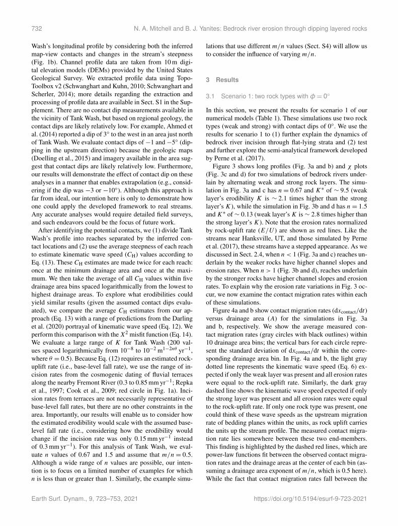
Figure 3 shows long profiles (Fig. 3a and b) and χ plots(Fig. 3c and d) for two simulations of bedrock rivers under-lain by alternating weak and strong rock layers. The simu-lation in Fig. 3a and c has n= 0.67 and K∗ of ∼ 9.5 (weaklayer’s erodibility K is ∼ 2.1 times higher than the stronglayer’s K), while the simulation in Fig. 3b and d has n= 1.5andK∗ of∼ 0.13 (weak layer’sK is∼ 2.8 times higher thanthe strong layer’s K). Note that the erosion rates normalizedby rock-uplift rate (E/U ) are shown as red lines. Like thestreams near Hanksville, UT, and those simulated by Perneet al. (2017), these streams have a stepped appearance. As wediscussed in Sect. 2.4, when n < 1 (Fig. 3a and c) reaches un-derlain by the weaker rocks have higher channel slopes anderosion rates. When n > 1 (Fig. 3b and d), reaches underlainby the stronger rocks have higher channel slopes and erosionrates. To explain why the erosion rate variations in Fig. 3 oc-cur, we now examine the contact migration rates within eachof these simulations.
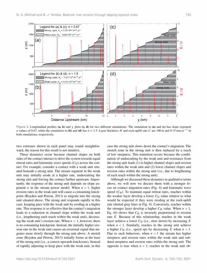
Figure 4a and b show contact migration rates (dxcontact/dt)versus drainage area (A) for the simulations in Fig. 3aand b, respectively. We show the average measured con-tact migration rates (gray circles with black outlines) within10 drainage area bins; the vertical bars for each circle repre-sent the standard deviation of dxcontact/dt within the corre-sponding drainage area bin. In Fig. 4a and b, the light graydotted line represents the kinematic wave speed (Eq. 6) ex-pected if only the weak layer was present and all erosion rateswere equal to the rock-uplift rate. Similarly, the dark graydashed line shows the kinematic wave speed expected if onlythe strong layer was present and all erosion rates were equalto the rock-uplift rate. If only one rock type was present, onecould think of these wave speeds as the upstream migrationrate of bedding planes within the units, as rock uplift carriesthe units up the stream profile. The measured contact migra-tion rate lies somewhere between these two end-members.This finding is highlighted by the dashed red lines, which arepower-law functions fit between the observed contact migra-tion rates and the drainage areas at the center of each bin (as-suming a drainage area exponent of m/n, which is 0.5 here).While the fact that contact migration rates fall between the
Earth Surf. Dynam., 9, 723–753, 2021 https://doi.org/10.5194/esurf-9-723-2021
N. A. Mitchell and B. J. Yanites: Bedrock river erosion through dipping layered rocks 733
Figure 3. Longitudinal profiles (a, b) and χ plots (c, d) for two different simulations. The simulation in (a) and (c) has slope exponentn values of 0.67, while the simulation in (b) and (d) has n= 1.5. Layer thickness H and rock-uplift rate U are 100 m and 0.15 mm yr−1 inboth simulations, respectively.
two extremes shown in each panel may sound straightfor-ward, the reason for this result is not intuitive.
These dynamics occur because channel slopes on bothsides of the contact interact to drive the system towards equalretreat rates and kinematic wave speeds (CH) across the con-tact. For example, consider a contact with a weak unit situ-ated beneath a strong unit. The stream segment in the weakunit may initially erode at a higher rate, undercutting thestrong unit and forcing the contact further upstream. Impor-tantly, the response of the strong unit depends on slope ex-ponent n in the stream power model. When n > 1, highererosion rates in the weak unit will cause a consuming knick-point (Royden and Perron, 2013) to migrate into the strongunit situated above. The strong unit responds rapidly in thiscase, keeping pace with the weak unit by eroding at a higherrate. This response is so effective that the contact’s migrationleads to a reduction in channel slope within the weak unit(i.e., lengthening each reach within the weak unit), decreas-ing the weak unit’s erosion rate. When n < 1, however, thereis no consuming knickpoint. Instead, the initially higher ero-sion rate in the weak unit causes an erosional signal that mi-grates more slowly through the strong unit above. A stretchzone (Royden and Perron, 2013) initially forms at the baseof the strong unit (i.e., a convex-upwards knickzone). Insteadof rapidly adjusting to keep pace with the weak unit, in this
case the strong unit slows down the contact’s migration. Thestretch zone in the strong unit is then replaced by a reachof low steepness. This transition occurs because the combi-nation of undercutting by the weak unit and resistance fromthe strong unit leads (1) to higher channel slopes and erosionrates within the weak unit and (2) lower channel slopes anderosion rates within the strong unit (i.e., due to lengtheningof each reach within the strong unit).
Although we discussed these dynamics in qualitative termsabove, we will now we discuss them with a stronger fo-cus on contact migration rates (Fig. 4) and kinematic wavespeed (CH). To maintain equal retreat rates, reaches withinthe weaker layer develop a lower CH value relative to whatwould be expected if they were eroding at the rock-upliftrate (dotted gray lines in Fig. 4). Conversely, reaches withinthe stronger layer develop a higher CH value. When n < 1,Eq. (6) shows that CH is inversely proportional to erosionrate E. Because of this relationship, reaches in the weaklayer achieve a lower CH (i.e., slow down) by increasing Ewhen n < 1. Similarly, reaches in the strong unit achievea higher CH (i.e., speed up) by decreasing E when n < 1.Due to such behaviors, when n < 1 the stream has highersteepness and erosion rates within the weak unit and sub-dued steepness and erosion rates within the strong unit. Theopposite is true when n > 1; reaches in the weak unit ob-
https://doi.org/10.5194/esurf-9-723-2021 Earth Surf. Dynam., 9, 723–753, 2021
734 N. A. Mitchell and B. J. Yanites: Bedrock river erosion through dipping layered rocks
Figure 4. Contact migration rates (dxcontact/dt) vs. drainage area (A) for (a) the simulation shown in Fig. 3a and c and (b) the simulationshown in Fig. 3b and d.
tain a lower CH value (i.e., slow down) by decreasing E, andreaches in the strong unit obtain a higherCH value (i.e., speedup) by increasing E.
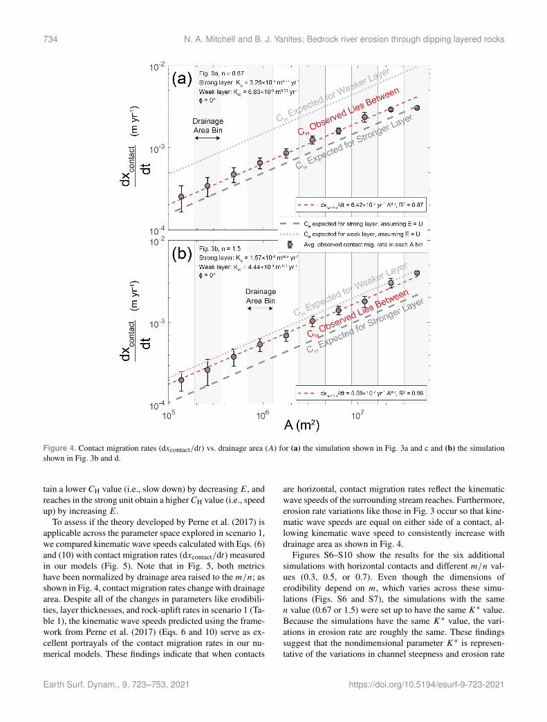
To assess if the theory developed by Perne et al. (2017) isapplicable across the parameter space explored in scenario 1,we compared kinematic wave speeds calculated with Eqs. (6)and (10) with contact migration rates (dxcontact/dt) measuredin our models (Fig. 5). Note that in Fig. 5, both metricshave been normalized by drainage area raised to the m/n; asshown in Fig. 4, contact migration rates change with drainagearea. Despite all of the changes in parameters like erodibili-ties, layer thicknesses, and rock-uplift rates in scenario 1 (Ta-ble 1), the kinematic wave speeds predicted using the frame-work from Perne et al. (2017) (Eqs. 6 and 10) serve as ex-cellent portrayals of the contact migration rates in our nu-merical models. These findings indicate that when contacts
are horizontal, contact migration rates reflect the kinematicwave speeds of the surrounding stream reaches. Furthermore,erosion rate variations like those in Fig. 3 occur so that kine-matic wave speeds are equal on either side of a contact, al-lowing kinematic wave speed to consistently increase withdrainage area as shown in Fig. 4.
Figures S6–S10 show the results for the six additionalsimulations with horizontal contacts and different m/n val-ues (0.3, 0.5, or 0.7). Even though the dimensions oferodibility depend on m, which varies across these simu-lations (Figs. S6 and S7), the simulations with the samen value (0.67 or 1.5) were set up to have the same K∗ value.Because the simulations have the same K∗ value, the vari-ations in erosion rate are roughly the same. These findingssuggest that the nondimensional parameter K∗ is represen-tative of the variations in channel steepness and erosion rate
Earth Surf. Dynam., 9, 723–753, 2021 https://doi.org/10.5194/esurf-9-723-2021
N. A. Mitchell and B. J. Yanites: Bedrock river erosion through dipping layered rocks 735
Figure 5. Estimated kinematic wave speeds (CH) and measuredcontact migration rates (dxcontact/dt) for all simulations in sce-nario 1 (Table 1). The low-U scenarios have U = 0.15 mm yr−1,while the high-U scenarios have U = 0.3 mm yr−1. Symbol sizerepresents the reference weak erodibility used (KW; Table 1).
caused by rock strength contrasts (Eqs. 7c, 8, and 10) evenwhen drainage area exponentm varies. Furthermore, the con-tact migration rates measured in these additional simulationsare still well represented by the kinematic wave speeds cal-culated with the framework of Perne et al. (2017) (Fig. S10).
3.2 Scenario 2: three rock types with φ= 0◦
In this section, we examine the results for scenario 2 (Ta-ble 1). Like scenario 1, scenario 2 only considers horizon-tal contacts (contact dip φ = 0◦). Unlike scenario 1, how-ever, scenario 2 utilizes three rock types (weak, medium, andstrong). Our intention is to test if the equations presented byPerne et al. (2017) still hold when there are more than tworock types because real streams usually incise through stratathat are far more complicated than those considered in sce-nario 1.
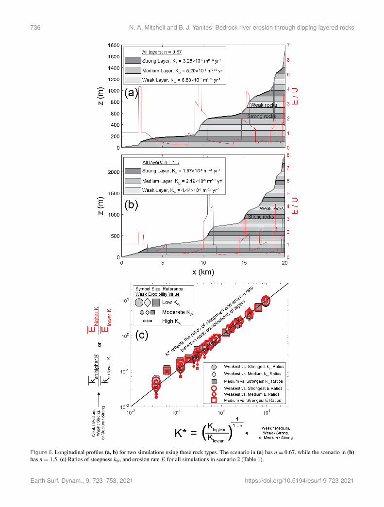
Figure 6a and b show long profiles with three rock typesof equal thickness (100 m) and n values of 0.67 (Fig. 6a) and1.5 (Fig. 6b). Figure 6c shows ratios of the average steep-ness values (ksn) and erosion rates (E) within different rocktypes (e.g., ksn of weak layer / ksn of strong layer) for all sim-ulations in scenario 2. The purpose of Fig. 6c is to test ifEqs. (7c) and (8) (Perne et al., 2017) are still accurate whenthere are three rock types instead of two. Because the steep-ness and erosion ratios in Fig. 6c follow a 1 : 1 relationshipwith K∗, these results are consistent with Eqs. (7c) and (8).
These results suggest that the theory developed by Perne etal. (2017) for bedrock river incision through horizontal stratastill applies when there are more than two rock types. Whenthere is an additional rock type (e.g., more than three litholo-gies), the channel slopes and erosion rates within the addi-
tional rock type will adjust to allow for a consistent trend inkinematic wave speed across the profile. Here, the mediumlayer is the additional rock type relative to the simulations inscenario 1. For example, Fig. S11 shows the contact migra-tion rates for the simulations in Fig. 6a and b; despite differ-ing erodibilities, contact migration rates and CH increase as apower-law function of drainage area. The fact that steepnessratios and erosion rate ratios are both well represented byK∗
(Fig. 6c) follows from Eqs. (7c) and (8), which were derivedby setting the kinematic wave speeds within two rock typesequal to each other.
3.3 Scenarios 3 and 4
3.3.1 General morphologic results of nonzero contactdips
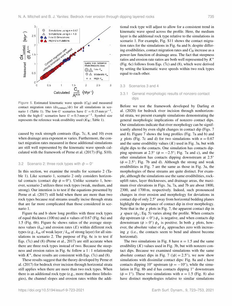
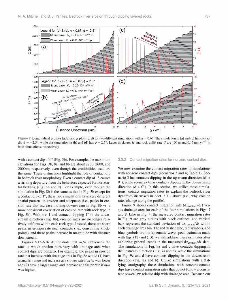
Before we test the framework developed by Darling etal. (2020) for bedrock river incision through nonhorizon-tal strata, we present example simulations demonstrating thegeneral morphologic implications of nonzero contact dips.Our simulations indicate that river morphology can be signif-icantly altered by even slight changes in contact dip (Figs. 7and 8). Figure 7 shows the long profiles (Fig. 7a and b) andχ plots (Fig. 7c and d) for two simulations with n= 0.67and the same erodibility values (K) used in Fig. 3a, but withslight dips to the contacts. One simulation has contacts dip-ping upstream at 2.5◦ (φ =−2.5◦; Fig. 7a and c), and theother simulation has contacts dipping downstream at 2.5◦
(φ = 2.5◦; Fig. 7b and d). Although the strong and weakerodibilities in Fig. 7 are the same as those in Fig. 3a, themorphologies of these streams are quite distinct. For exam-ple, although the simulations use the same erodibilities, rock-uplift rates, layer thicknesses, and drainage areas, the maxi-mum river elevations in Figs. 3a, 7a, and 7b are about 1800,2300, and 1700 m, respectively. Indeed, such pronouncedchanges in river erosion and morphology for deviations incontact dip of only 2.5◦ away from horizontal bedding planeshighlight the importance of contact dip in river morphology.Note that in the χ plots in Fig. 7, the apparent contact dip inχ space (φχ ; Eq. 5) varies along the profile. When contactsdip upstream (φ < 0◦) φχ is negative, and when contacts dipdownstream (φ > 0◦) φχ is positive. In both χ plots, how-ever, the absolute value of φχ approaches zero with increas-ing χ (i.e., the contacts seem to bend and almost becomehorizontal).
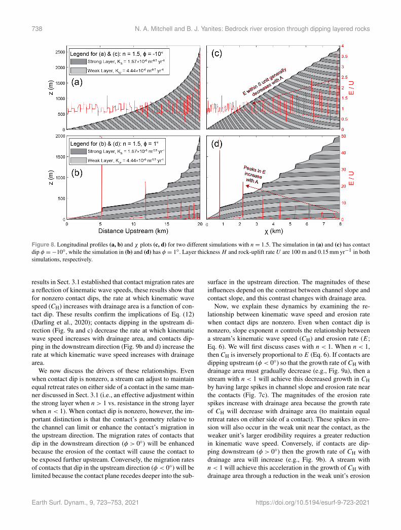
The two simulations in Fig. 8 have n= 1.5 and the sameerodibility (K) values used in Fig. 3b, but with nonzero con-tact dips. Because we examined simulations with the sameabsolute contact dips in Fig. 7 (|φ| = 2.5◦), we now showsimulations with dissimilar contact dips: Fig. 8a and c havecontacts dipping 10◦ upstream (φ =−10◦), while the simu-lation in Fig. 8b and d has contacts dipping 1◦ downstream(φ = 1◦). These two simulations with n= 1.5 (Fig. 8) alsohave distinct morphologies relative to similar simulations
https://doi.org/10.5194/esurf-9-723-2021 Earth Surf. Dynam., 9, 723–753, 2021
736 N. A. Mitchell and B. J. Yanites: Bedrock river erosion through dipping layered rocks
Figure 6. Longitudinal profiles (a, b) for two simulations using three rock types. The scenario in (a) has n= 0.67, while the scenario in (b)has n= 1.5. (c) Ratios of steepness ksn and erosion rate E for all simulations in scenario 2 (Table 1).
Earth Surf. Dynam., 9, 723–753, 2021 https://doi.org/10.5194/esurf-9-723-2021
N. A. Mitchell and B. J. Yanites: Bedrock river erosion through dipping layered rocks 737
Figure 7. Longitudinal profiles (a, b) and χ plots (c, d) for two different simulations with n= 0.67. The simulation in (a) and (c) has contactdip φ =−2.5◦, while the simulation in (b) and (d) has φ = 2.5◦. Layer thickness H and rock-uplift rate U are 100 m and 0.15 mm yr−1 inboth simulations, respectively.
with a contact dip of 0◦ (Fig. 3b). For example, the maximumelevations for Figs. 3b, 8a, and 8b are about 2200, 2600, and2000 m, respectively, even though the erodibilities used arethe same. These distinctions highlight the role of contact dipin bedrock river morphology. Even a contact dip of 1◦ causesa striking departure from the behaviors expected for horizon-tal bedding (Fig. 8b and d). For example, even though thesimulation in Fig. 8b is the same as that in Fig. 3b except fora contact dip of 1◦, these two simulations have very differentspatial patterns in erosion and steepness (i.e., peaks in ero-sion rate that increase moving downstream in Fig. 8b vs. amore consistent covariation of erosion rate with rock type inFig. 3b). With n > 1 and contacts dipping 1◦ in the down-stream direction (Fig. 8b), erosion rates are no longer rela-tively uniform within each rock type. Instead, there are sharppeaks in erosion rate near contacts (i.e., consuming knick-points), and these peaks increase in magnitude with distancedownstream.
Figures S12–S16 demonstrate that m/n influences therates at which erosion rates vary with drainage area whencontact dips are nonzero. For example, the peaks in erosionrate that increase with drainage area in Fig. 8c would (1) havea smaller range and increase at a slower rate ifm/nwas lowerand (2) have a larger range and increase at a faster rate ifm/nwas higher.
3.3.2 Contact migration rates for nonzero contact dips
We now examine the contact migration rates in simulationswith nonzero contact dips (scenarios 3 and 4; Table 1). Sce-nario 3 has contacts dipping in the upstream direction (φ <0◦), while scenario 4 has contacts dipping in the downstreamdirection (φ > 0◦). In this section, we utilize these simula-tions’ contact migration rates to explain the bedrock riverdynamics discussed in Sect. 3.3.1 above (i.e., why erosionrates change along the profile).
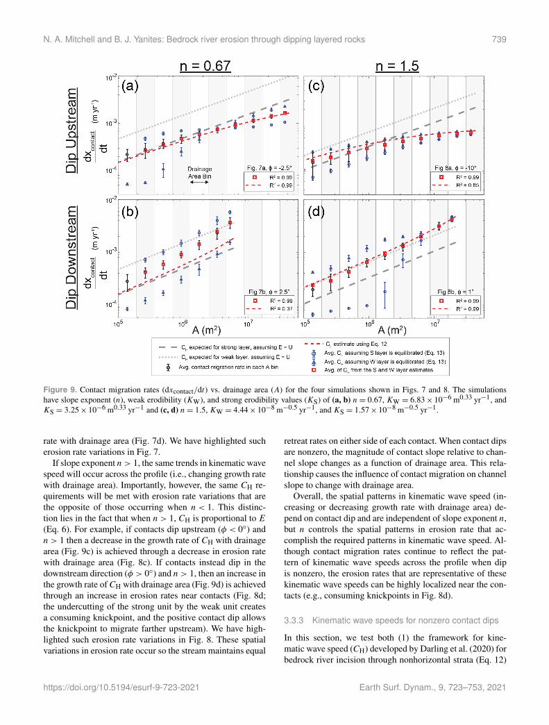
Figure 9 shows contact migration rate (dxcontact/dt) ver-sus drainage area for each of the four simulations in Figs. 7and 8. Like in Fig. 4, the measured contact migration ratesin Fig. 9 are gray circles with black outlines, and verticalbars represent the standard deviation of dxcontact/dt withineach drainage area bin. The red dashed line, red symbols, andblue symbols are the kinematic wave speed estimates madewith Eqs. (12) and (13); we will address these estimates afterexploring general trends in the measured dxcontact/dt data.The simulations in Fig. 9a and c have contacts dipping inthe upstream direction (Fig. 7a and b), while the simulationsin Fig. 9c and d have contacts dipping in the downstreamdirection (Fig. 8a and b). Unlike simulations with a flat-lying stratigraphy, these simulations with nonzero contactdips have contact migration rates that do not follow a consis-tent power-law relationship with drainage area. Because our
https://doi.org/10.5194/esurf-9-723-2021 Earth Surf. Dynam., 9, 723–753, 2021
738 N. A. Mitchell and B. J. Yanites: Bedrock river erosion through dipping layered rocks
Figure 8. Longitudinal profiles (a, b) and χ plots (c, d) for two different simulations with n= 1.5. The simulation in (a) and (c) has contactdip φ =−10◦, while the simulation in (b) and (d) has φ = 1◦. Layer thicknessH and rock-uplift rate U are 100 m and 0.15 mm yr−1 in bothsimulations, respectively.
results in Sect. 3.1 established that contact migration rates area reflection of kinematic wave speeds, these results show thatfor nonzero contact dips, the rate at which kinematic wavespeed (CH) increases with drainage area is a function of con-tact dip. These results confirm the implications of Eq. (12)(Darling et al., 2020); contacts dipping in the upstream di-rection (Fig. 9a and c) decrease the rate at which kinematicwave speed increases with drainage area, and contacts dip-ping in the downstream direction (Fig. 9b and d) increase therate at which kinematic wave speed increases with drainagearea.
We now discuss the drivers of these relationships. Evenwhen contact dip is nonzero, a stream can adjust to maintainequal retreat rates on either side of a contact in the same man-ner discussed in Sect. 3.1 (i.e., an effective adjustment withinthe strong layer when n > 1 vs. resistance in the strong layerwhen n < 1). When contact dip is nonzero, however, the im-portant distinction is that the contact’s geometry relative tothe channel can limit or enhance the contact’s migration inthe upstream direction. The migration rates of contacts thatdip in the downstream direction (φ > 0◦) will be enhancedbecause the erosion of the contact will cause the contact tobe exposed further upstream. Conversely, the migration ratesof contacts that dip in the upstream direction (φ < 0◦) will belimited because the contact plane recedes deeper into the sub-
surface in the upstream direction. The magnitudes of theseinfluences depend on the contrast between channel slope andcontact slope, and this contrast changes with drainage area.
Now, we explain these dynamics by examining the re-lationship between kinematic wave speed and erosion ratewhen contact dips are nonzero. Even when contact dip isnonzero, slope exponent n controls the relationship betweena stream’s kinematic wave speed (CH) and erosion rate (E;Eq. 6). We will first discuss cases with n < 1. When n < 1,then CH is inversely proportional to E (Eq. 6). If contacts aredipping upstream (φ < 0◦) so that the growth rate of CH withdrainage area must gradually decrease (e.g., Fig. 9a), then astream with n < 1 will achieve this decreased growth in CHby having large spikes in channel slope and erosion rate nearthe contacts (Fig. 7c). The magnitudes of the erosion ratespikes increase with drainage area because the growth rateof CH will decrease with drainage area (to maintain equalretreat rates on either side of a contact). These spikes in ero-sion will also occur in the weak unit near the contact, as theweaker unit’s larger erodibility requires a greater reductionin kinematic wave speed. Conversely, if contacts are dip-ping downstream (φ > 0◦) then the growth rate of CH withdrainage area will increase (e.g., Fig. 9b). A stream withn < 1 will achieve this acceleration in the growth of CH withdrainage area through a reduction in the weak unit’s erosion
Earth Surf. Dynam., 9, 723–753, 2021 https://doi.org/10.5194/esurf-9-723-2021
N. A. Mitchell and B. J. Yanites: Bedrock river erosion through dipping layered rocks 739
Figure 9. Contact migration rates (dxcontact/dt) vs. drainage area (A) for the four simulations shown in Figs. 7 and 8. The simulationshave slope exponent (n), weak erodibility (KW), and strong erodibility values (KS) of (a, b) n= 0.67, KW = 6.83× 10⁻⁶ m0.33 yr−1, andKS = 3.25× 10⁻⁶ m0.33 yr−1 and (c, d) n= 1.5, KW = 4.44× 10⁻⁸ m−0.5 yr−1, and KS = 1.57× 10⁻⁸ m−0.5 yr−1.
rate with drainage area (Fig. 7d). We have highlighted sucherosion rate variations in Fig. 7.
If slope exponent n > 1, the same trends in kinematic wavespeed will occur across the profile (i.e., changing growth ratewith drainage area). Importantly, however, the same CH re-quirements will be met with erosion rate variations that arethe opposite of those occurring when n < 1. This distinc-tion lies in the fact that when n > 1, CH is proportional to E(Eq. 6). For example, if contacts dip upstream (φ < 0◦) andn > 1 then a decrease in the growth rate of CH with drainagearea (Fig. 9c) is achieved through a decrease in erosion ratewith drainage area (Fig. 8c). If contacts instead dip in thedownstream direction (φ > 0◦) and n > 1, then an increase inthe growth rate ofCH with drainage area (Fig. 9d) is achievedthrough an increase in erosion rates near contacts (Fig. 8d;the undercutting of the strong unit by the weak unit createsa consuming knickpoint, and the positive contact dip allowsthe knickpoint to migrate farther upstream). We have high-lighted such erosion rate variations in Fig. 8. These spatialvariations in erosion rate occur so the stream maintains equal
retreat rates on either side of each contact. When contact dipsare nonzero, the magnitude of contact slope relative to chan-nel slope changes as a function of drainage area. This rela-tionship causes the influence of contact migration on channelslope to change with drainage area.
Overall, the spatial patterns in kinematic wave speed (in-creasing or decreasing growth rate with drainage area) de-pend on contact dip and are independent of slope exponent n,but n controls the spatial patterns in erosion rate that ac-complish the required patterns in kinematic wave speed. Al-though contact migration rates continue to reflect the pat-tern of kinematic wave speeds across the profile when dipis nonzero, the erosion rates that are representative of thesekinematic wave speeds can be highly localized near the con-tacts (e.g., consuming knickpoints in Fig. 8d).
3.3.3 Kinematic wave speeds for nonzero contact dips
In this section, we test both (1) the framework for kine-matic wave speed (CH) developed by Darling et al. (2020) forbedrock river incision through nonhorizontal strata (Eq. 12)
https://doi.org/10.5194/esurf-9-723-2021 Earth Surf. Dynam., 9, 723–753, 2021
740 N. A. Mitchell and B. J. Yanites: Bedrock river erosion through dipping layered rocks
and (2) our approach for estimating kinematic wave speedwith channel steepness values (Eq. 13). We test these ap-proaches by comparing contact migration rates measured inour models with CH estimates made with Eqs. (12) and (13)for all simulations in scenarios 3 and 4 (Table 1).
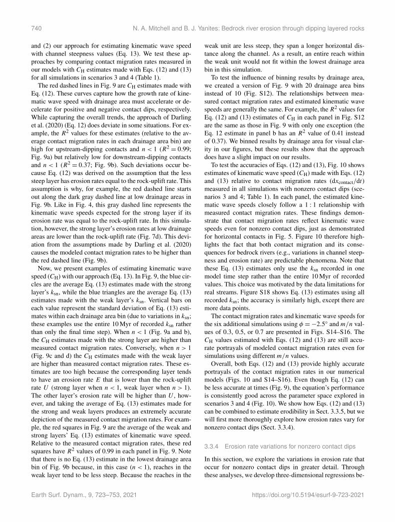
The red dashed lines in Fig. 9 are CH estimates made withEq. (12). These curves capture how the growth rate of kine-matic wave speed with drainage area must accelerate or de-celerate for positive and negative contact dips, respectively.While capturing the overall trends, the approach of Darlinget al. (2020) (Eq. 12) does deviate in some situations. For ex-ample, the R2 values for these estimates (relative to the av-erage contact migration rates in each drainage area bin) arehigh for upstream-dipping contacts and n < 1 (R2
= 0.99;Fig. 9a) but relatively low for downstream-dipping contactsand n < 1 (R2
= 0.37; Fig. 9b). Such deviations occur be-cause Eq. (12) was derived on the assumption that the lesssteep layer has erosion rates equal to the rock-uplift rate. Thisassumption is why, for example, the red dashed line startsout along the dark gray dashed line at low drainage areas inFig. 9b. Like in Fig. 4, this gray dashed line represents thekinematic wave speeds expected for the strong layer if itserosion rate was equal to the rock-uplift rate. In this simula-tion, however, the strong layer’s erosion rates at low drainageareas are lower than the rock-uplift rate (Fig. 7d). This devi-ation from the assumptions made by Darling et al. (2020)causes the modeled contact migration rates to be higher thanthe red dashed line (Fig. 9b).
Now, we present examples of estimating kinematic wavespeed (CH) with our approach (Eq. 13). In Fig. 9, the blue cir-cles are the average Eq. (13) estimates made with the stronglayer’s ksn, while the blue triangles are the average Eq. (13)estimates made with the weak layer’s ksn. Vertical bars oneach value represent the standard deviation of Eq. (13) esti-mates within each drainage area bin (due to variations in ksn;these examples use the entire 10 Myr of recorded ksn ratherthan only the final time step). When n < 1 (Fig. 9a and b),the CH estimates made with the strong layer are higher thanmeasured contact migration rates. Conversely, when n > 1(Fig. 9c and d) the CH estimates made with the weak layerare higher than measured contact migration rates. These es-timates are too high because the corresponding layer tendsto have an erosion rate E that is lower than the rock-upliftrate U (strong layer when n < 1, weak layer when n > 1).The other layer’s erosion rate will be higher than U , how-ever, and taking the average of Eq. (13) estimates made forthe strong and weak layers produces an extremely accuratedepiction of the measured contact migration rates. For exam-ple, the red squares in Fig. 9 are the average of the weak andstrong layers’ Eq. (13) estimates of kinematic wave speed.Relative to the measured contact migration rates, these redsquares have R2 values of 0.99 in each panel in Fig. 9. Notethat there is no Eq. (13) estimate in the lowest drainage areabin of Fig. 9b because, in this case (n < 1), reaches in theweak layer tend to be less steep. Because the reaches in the
weak unit are less steep, they span a longer horizontal dis-tance along the channel. As a result, an entire reach withinthe weak unit would not fit within the lowest drainage areabin in this simulation.
To test the influence of binning results by drainage area,we created a version of Fig. 9 with 20 drainage area binsinstead of 10 (Fig. S12). The relationships between mea-sured contact migration rates and estimated kinematic wavespeeds are generally the same. For example, theR2 values forEq. (12) and (13) estimates of CH in each panel in Fig. S12are the same as those in Fig. 9 with only one exception (theEq. 12 estimate in panel b has an R2 value of 0.41 insteadof 0.37). We binned results by drainage area for visual clar-ity in our figures, but these results show that the approachdoes have a slight impact on our results.
To test the accuracies of Eqs. (12) and (13), Fig. 10 showsestimates of kinematic wave speed (CH) made with Eqs. (12)and (13) relative to contact migration rates (dxcontact/dt)measured in all simulations with nonzero contact dips (sce-narios 3 and 4; Table 1). In each panel, the estimated kine-matic wave speeds closely follow a 1 : 1 relationship withmeasured contact migration rates. These findings demon-strate that contact migration rates reflect kinematic wavespeeds even for nonzero contact dips, just as demonstratedfor horizontal contacts in Fig. 5. Figure 10 therefore high-lights the fact that both contact migration and its conse-quences for bedrock rivers (e.g., variations in channel steep-ness and erosion rate) are predictable phenomena. Note thatthese Eq. (13) estimates only use the ksn recorded in onemodel time step rather than the entire 10 Myr of recordedvalues. This choice was motivated by the data limitations forreal streams. Figure S18 shows Eq. (13) estimates using allrecorded ksn; the accuracy is similarly high, except there aremore data points.
The contact migration rates and kinematic wave speeds forthe six additional simulations using φ =−2.5◦ andm/n val-ues of 0.3, 0.5, or 0.7 are presented in Figs. S14–S16. TheCH values estimated with Eqs. (12) and (13) are still accu-rate portrayals of modeled contact migration rates even forsimulations using different m/n values.
Overall, both Eqs. (12) and (13) provide highly accurateportrayals of the contact migration rates in our numericalmodels (Figs. 10 and S14–S16). Even though Eq. (12) canbe less accurate at times (Fig. 9), the equation’s performanceis consistently good across the parameter space explored inscenarios 3 and 4 (Fig. 10). We show how Eqs. (12) and (13)can be combined to estimate erodibility in Sect. 3.3.5, but wewill first more thoroughly explore how erosion rates vary fornonzero contact dips (Sect. 3.3.4).
3.3.4 Erosion rate variations for nonzero contact dips
In this section, we explore the variations in erosion rate thatoccur for nonzero contact dips in greater detail. Throughthese analyses, we develop three-dimensional regressions be-
Earth Surf. Dynam., 9, 723–753, 2021 https://doi.org/10.5194/esurf-9-723-2021
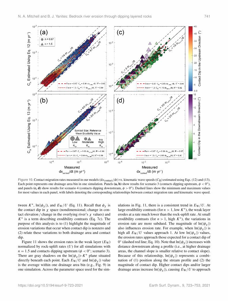
N. A. Mitchell and B. J. Yanites: Bedrock river erosion through dipping layered rocks 741
Figure 10. Contact migration rates measured in our models (dxcontact/dt) vs. kinematic wave speeds (CH) estimated using Eqs. (12) and (13).Each point represents one drainage area bin in one simulation. Panels (a, b) show results for scenario 3 (contacts dipping upstream, φ < 0◦),and panels (c, d) show results for scenario 4 (contacts dipping downstream, φ > 0◦). Dashed lines show the minimum and maximum valuesfor most values in each panel, with labels denoting the corresponding relationships between contact migration rate and kinematic wave speed.
tween K∗, ln(|φχ |), and EW/U (Eq. 11). Recall that φχ isthe contact dip in χ space (nondimensional; change in con-tact elevation / change in the overlying river’s χ values) andK∗ is a term describing erodibility contrasts (Eq. 7c). Thepurpose of this analysis is to (1) highlight the magnitude oferosion variations that occur when contact dip is nonzero and(2) relate these variations to both drainage area and contactdip.
Figure 11 shows the erosion rates in the weak layer (EW)normalized by rock-uplift rates (U ) for all simulations withn= 1.5 and contacts dipping upstream (φ < 0◦; scenario 3).There are gray shadows on the ln(|φχ |)–K∗ plane situateddirectly beneath each point. Each EW/U and ln(|φχ |) valueis the average within one drainage area bin (e.g., Fig. 9) inone simulation. Across the parameter space used for the sim-
ulations in Fig. 11, there is a consistent trend in EW/U . Atlarge erodibility contrasts (for n > 1, lowK∗), the weak layererodes at a rate much lower than the rock-uplift rate. At smallerodibility contrasts (for n > 1, high K∗), the variations inerosion rate are more subdued. The magnitude of ln(|φχ |)also influences erosion rate. For example, when ln(|φχ |) ishigh all EW/U values approach 1. At low ln(|φχ |) values,the erosion rates approach those expected for a contact dip of0◦ (dashed red line; Eq. 10). Note that ln(|φχ |) increases withdistance downstream along a profile (i.e., at higher drainageareas, the channel slope is smaller relative to contact slope).Because of this relationship, ln(|φχ |) represents a combi-nation of (1) position along the stream profile and (2) themagnitude of contact dip. Higher contact dips and/or largerdrainage areas increase ln(|φχ |), causing EW/U to approach
https://doi.org/10.5194/esurf-9-723-2021 Earth Surf. Dynam., 9, 723–753, 2021
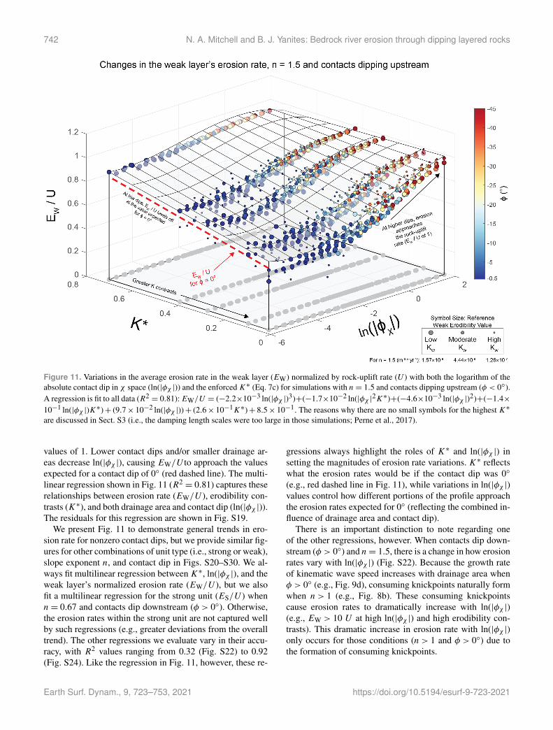
742 N. A. Mitchell and B. J. Yanites: Bedrock river erosion through dipping layered rocks
Figure 11. Variations in the average erosion rate in the weak layer (EW) normalized by rock-uplift rate (U ) with both the logarithm of theabsolute contact dip in χ space (ln(|φχ |)) and the enforcedK∗ (Eq. 7c) for simulations with n= 1.5 and contacts dipping upstream (φ < 0◦).A regression is fit to all data (R2
= 0.81):EW/U = (−2.2×10⁻³ ln(|φχ |)3)+(−1.7×10⁻² ln(|φχ |2K∗)+(−4.6×10⁻³ ln(|φχ |)2)+(−1.4×10⁻¹ ln(|φχ |)K∗)+ (9.7× 10⁻² ln(|φχ |))+ (2.6× 10⁻¹K∗)+ 8.5× 10⁻¹. The reasons why there are no small symbols for the highest K∗
are discussed in Sect. S3 (i.e., the damping length scales were too large in those simulations; Perne et al., 2017).
values of 1. Lower contact dips and/or smaller drainage ar-eas decrease ln(|φχ |), causing EW/U to approach the valuesexpected for a contact dip of 0◦ (red dashed line). The multi-linear regression shown in Fig. 11 (R2
= 0.81) captures theserelationships between erosion rate (EW/U ), erodibility con-trasts (K∗), and both drainage area and contact dip (ln(|φχ |)).The residuals for this regression are shown in Fig. S19.
We present Fig. 11 to demonstrate general trends in ero-sion rate for nonzero contact dips, but we provide similar fig-ures for other combinations of unit type (i.e., strong or weak),slope exponent n, and contact dip in Figs. S20–S30. We al-ways fit multilinear regression betweenK∗, ln(|φχ |), and theweak layer’s normalized erosion rate (EW/U ), but we alsofit a multilinear regression for the strong unit (ES/U ) whenn= 0.67 and contacts dip downstream (φ > 0◦). Otherwise,the erosion rates within the strong unit are not captured wellby such regressions (e.g., greater deviations from the overalltrend). The other regressions we evaluate vary in their accu-racy, with R2 values ranging from 0.32 (Fig. S22) to 0.92(Fig. S24). Like the regression in Fig. 11, however, these re-
gressions always highlight the roles of K∗ and ln(|φχ |) insetting the magnitudes of erosion rate variations. K∗ reflectswhat the erosion rates would be if the contact dip was 0◦
(e.g., red dashed line in Fig. 11), while variations in ln(|φχ |)values control how different portions of the profile approachthe erosion rates expected for 0◦ (reflecting the combined in-fluence of drainage area and contact dip).
There is an important distinction to note regarding oneof the other regressions, however. When contacts dip down-stream (φ > 0◦) and n= 1.5, there is a change in how erosionrates vary with ln(|φχ |) (Fig. S22). Because the growth rateof kinematic wave speed increases with drainage area whenφ > 0◦ (e.g., Fig. 9d), consuming knickpoints naturally formwhen n > 1 (e.g., Fig. 8b). These consuming knickpointscause erosion rates to dramatically increase with ln(|φχ |)(e.g., EW > 10 U at high ln(|φχ |) and high erodibility con-trasts). This dramatic increase in erosion rate with ln(|φχ |)only occurs for those conditions (n > 1 and φ > 0◦) due tothe formation of consuming knickpoints.
Earth Surf. Dynam., 9, 723–753, 2021 https://doi.org/10.5194/esurf-9-723-2021
N. A. Mitchell and B. J. Yanites: Bedrock river erosion through dipping layered rocks 743
To summarize the results for this section, when contactdips are nonzero the erosion rates within each unit change asa function of contact dip, drainage area (which both set φχ ),and erodibility contrasts (K∗). Assuming that the erosion rateis equal to the base-level fall rate (Eq. 12) will cause one tooverestimate kinematic wave speed (CH) when n > 1 (e.g.,Fig. 9c) and underestimate CH when n < 1 (e.g., Fig. 9b).Note that our intention is not to assign theoretical signifi-cance to these three-dimensional regressions, but only to usethem to highlight how contact dip, drainage area, and erodi-bility contrasts influence the erosion rates for nonzero contactdips.
3.3.5 Estimating erodibility in our numerical modelsusing nonzero contact dips
In this section, we evaluate how accurately the erodibil-ity (K) in our numerical models can be estimated using chan-nel steepness (ksn) without a priori information on erodi-bility. We demonstrated that Eqs. (12) and (13) are gener-ally accurate within numerical models (Fig. 10), but now wedemonstrate how the two equations can be combined to es-timate erodibility. The purpose of this analysis is to providecontext for our analysis of Tank Wash near Hanksville, UT(Sect. 3.4). We will attempt to quantify erodibility using thechannel steepness observed along Tank Wash, so our inten-tion here is to test how accurately one can estimate erodibilityin numerical models for which the true erodibility values areknown.
Figures 12 and 13 summarize how the K values we usein our numerical models can be estimated by combiningEqs. (12) and (13). Figure 12 focuses on weak erodibil-ities (KW) used in our numerical models, while Fig. 13focuses on the strong erodibilities (KS). Figures 12a–band 13a–b show the X2 values calculated between (1) theCH estimates made with Eq. (12) for a range of erodibil-ities and (2) the CH estimates made with Eq. (13) for theksn recorded in each simulation’s final time step. We chose touse only one time step of recorded ksn values due to the datalimitations for real rivers, but Figs. S31 and S32 are versionsof Figs. 12 and 13 that use all ksn recorded over the 10 Myrfor each simulation. The x axes of Figs. 12a–b and 13a–brepresent the entire range of K values assessed normalizedby the actual weak or strong erodibility used in that simula-tion (KW in Fig. 12, KS in Fig. 13). Each line represents onesimulation (blue for simulations with φ < 0◦, red for sim-ulations with φ > 0◦). Each of these lines has a minimumX2 value, and invariably this minimum occurs near an as-sessed K / enforced K value of 1.
Figures 12c–d and 13c–d are histograms showing the dis-tributions of the best-fit K (those with the minimum X2 val-ues) relative to the actual weak and strong erodibilities(KW in Fig. 12, KS in Fig. 13). The x axes for these his-tograms (best-fit K / enforced K) use bin sizes of 0.1. Thebest-fit K is almost always between KW and KS (there are
some exceptions with (best-fit K/KW)> 1 in Fig. 12d). Thebest-fitK can be much larger thanKS when n > 1 (Fig. 13d)because the strong layer tends to have larger deviations inerosion rate relative to the rock-uplift rate under those con-ditions (Figs. S26 and S28). Conversely, the rock type thattends to have lower steepness (weak layer when n > 1, stronglayer when n < 1) tends to have smaller deviations in ero-sion rate relative to the steep layer (Figs. 11 and S19–S30).As a result, the best-fit K values in Figs. 12 and 13 are moreconsistently close to the K for the layer that tends to havelower steepness. These results suggest that an erodibility es-timated using this approach is more likely to be representa-tive of the rock type with lower steepness (weak layer whenn > 1, strong layer when n < 1). Figures 12 and 13 highlightthe potential to estimate erodibility using observed channelsteepness (ksn), known contact dips (φ), and a known base-level fall rate (U ).
3.4 Analysis of Tank Wash
In this section, we apply the methods developed in this study(Sect. 3.3.5) to Tank Wash (Fig. 14). Figure 14a shows in-ferred contacts labeled with purple lines. The units clearlydip to the west–southwest here, which is generally in theupstream direction for Tank Wash. Using the (1) potentialcontacts identified using Google Earth and a nearby geo-logic map (Doelling et al., 2015) as well as (2) changes insteepness along Tank Wash, we then estimated the contactlocations along the stream’s longitudinal profile (Fig. 14b).Tank Wash flows across a wide range of lithologies, includ-ing sandstone, mudstone, shale, and siltstone, and these unitslikely offer different levels of resistance to fluvial erosion.In Fig. 14b, these contacts are projected into the subsurfaceusing an assumed contact dip (φ) of −1◦ (note the verticalexaggeration). Each of the potential contacts we identifiedoccur at a change in channel steepness; there are three loca-tions where steepness changes, but we could not confidentlyinfer a change in lithology. We highlight those three loca-tions in Fig. 14a and b. Those steepness changes could indi-cate, for example, changes in rock strength within one unit.It is important to note, however, that our models suggest thatchanges in steepness can occur both at contacts and somedistance away from contacts (e.g., Figs. 7a and 8b).
Figure 15a is a slope–area plot, with the inferred con-tact locations shown as vertical dashed lines and the av-erage steepness values of the reaches between each con-tact shown as dotted lines. We used these average steep-ness values to estimate kinematic wave speeds (CH) usingEq. (13) (Fig. 15b and c). For the two U values assessed(0.3 and 0.85 mm yr−1), the patterns in the data are the samebut CH magnitudes are scaled by the assumed U . We esti-mated two kinematic wave speeds for each stream reach de-fined by the inferred contacts: one CH at the lowest drainagearea of the reach and one at the highest. In Fig. 15b and c,each pair of CH estimates is connected by a dashed line. If
https://doi.org/10.5194/esurf-9-723-2021 Earth Surf. Dynam., 9, 723–753, 2021
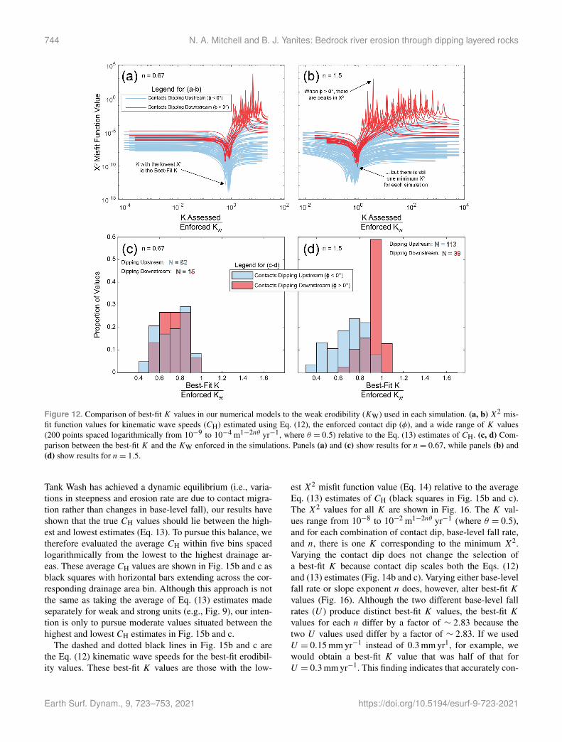
744 N. A. Mitchell and B. J. Yanites: Bedrock river erosion through dipping layered rocks
Figure 12. Comparison of best-fit K values in our numerical models to the weak erodibility (KW) used in each simulation. (a, b) X2 mis-fit function values for kinematic wave speeds (CH) estimated using Eq. (12), the enforced contact dip (φ), and a wide range of K values(200 points spaced logarithmically from 10−9 to 10−4 m1−2nθ yr−1, where θ = 0.5) relative to the Eq. (13) estimates of CH. (c, d) Com-parison between the best-fit K and the KW enforced in the simulations. Panels (a) and (c) show results for n= 0.67, while panels (b) and(d) show results for n= 1.5.
Tank Wash has achieved a dynamic equilibrium (i.e., varia-tions in steepness and erosion rate are due to contact migra-tion rather than changes in base-level fall), our results haveshown that the true CH values should lie between the high-est and lowest estimates (Eq. 13). To pursue this balance, wetherefore evaluated the average CH within five bins spacedlogarithmically from the lowest to the highest drainage ar-eas. These average CH values are shown in Fig. 15b and c asblack squares with horizontal bars extending across the cor-responding drainage area bin. Although this approach is notthe same as taking the average of Eq. (13) estimates madeseparately for weak and strong units (e.g., Fig. 9), our inten-tion is only to pursue moderate values situated between thehighest and lowest CH estimates in Fig. 15b and c.
The dashed and dotted black lines in Fig. 15b and c arethe Eq. (12) kinematic wave speeds for the best-fit erodibil-ity values. These best-fit K values are those with the low-
est X2 misfit function value (Eq. 14) relative to the averageEq. (13) estimates of CH (black squares in Fig. 15b and c).The X2 values for all K are shown in Fig. 16. The K val-ues range from 10−8 to 10−2 m1−2nθ yr−1 (where θ = 0.5),and for each combination of contact dip, base-level fall rate,and n, there is one K corresponding to the minimum X2.Varying the contact dip does not change the selection ofa best-fit K because contact dip scales both the Eqs. (12)and (13) estimates (Fig. 14b and c). Varying either base-levelfall rate or slope exponent n does, however, alter best-fit Kvalues (Fig. 16). Although the two different base-level fallrates (U ) produce distinct best-fit K values, the best-fit Kvalues for each n differ by a factor of ∼ 2.83 because thetwo U values used differ by a factor of ∼ 2.83. If we usedU = 0.15 mm yr−1 instead of 0.3 mm yr1, for example, wewould obtain a best-fit K value that was half of that forU = 0.3 mm yr−1. This finding indicates that accurately con-
Earth Surf. Dynam., 9, 723–753, 2021 https://doi.org/10.5194/esurf-9-723-2021
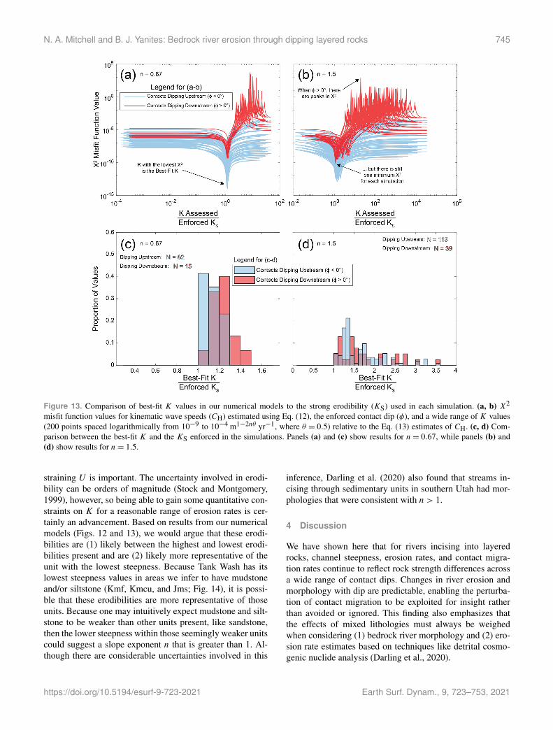
N. A. Mitchell and B. J. Yanites: Bedrock river erosion through dipping layered rocks 745
Figure 13. Comparison of best-fit K values in our numerical models to the strong erodibility (KS) used in each simulation. (a, b) X2
misfit function values for kinematic wave speeds (CH) estimated using Eq. (12), the enforced contact dip (φ), and a wide range of K values(200 points spaced logarithmically from 10−9 to 10−4 m1−2nθ yr−1, where θ = 0.5) relative to the Eq. (13) estimates of CH. (c, d) Com-parison between the best-fit K and the KS enforced in the simulations. Panels (a) and (c) show results for n= 0.67, while panels (b) and(d) show results for n= 1.5.
straining U is important. The uncertainty involved in erodi-bility can be orders of magnitude (Stock and Montgomery,1999), however, so being able to gain some quantitative con-straints on K for a reasonable range of erosion rates is cer-tainly an advancement. Based on results from our numericalmodels (Figs. 12 and 13), we would argue that these erodi-bilities are (1) likely between the highest and lowest erodi-bilities present and are (2) likely more representative of theunit with the lowest steepness. Because Tank Wash has itslowest steepness values in areas we infer to have mudstoneand/or siltstone (Kmf, Kmcu, and Jms; Fig. 14), it is possi-ble that these erodibilities are more representative of thoseunits. Because one may intuitively expect mudstone and silt-stone to be weaker than other units present, like sandstone,then the lower steepness within those seemingly weaker unitscould suggest a slope exponent n that is greater than 1. Al-though there are considerable uncertainties involved in this
inference, Darling et al. (2020) also found that streams in-cising through sedimentary units in southern Utah had mor-phologies that were consistent with n > 1.
4 Discussion
We have shown here that for rivers incising into layeredrocks, channel steepness, erosion rates, and contact migra-tion rates continue to reflect rock strength differences acrossa wide range of contact dips. Changes in river erosion andmorphology with dip are predictable, enabling the perturba-tion of contact migration to be exploited for insight ratherthan avoided or ignored. This finding also emphasizes thatthe effects of mixed lithologies must always be weighedwhen considering (1) bedrock river morphology and (2) ero-sion rate estimates based on techniques like detrital cosmo-genic nuclide analysis (Darling et al., 2020).
https://doi.org/10.5194/esurf-9-723-2021 Earth Surf. Dynam., 9, 723–753, 2021
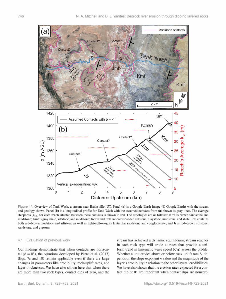
746 N. A. Mitchell and B. J. Yanites: Bedrock river erosion through dipping layered rocks
Figure 14. Overview of Tank Wash, a stream near Hanksville, UT. Panel (a) is a Google Earth image (© Google Earth) with the streamand geology shown. Panel (b) is a longitudinal profile for Tank Wash with the assumed contacts from (a) shown as gray lines. The averagesteepness (ksn) for each reach situated between these contacts is shown in red. The lithologies are as follows: Kmf is brown sandstone andmudstone; Kmt is gray shale, siltstone, and mudstone; Kcmu and Jmb are color-banded siltstone, claystone, mudstone, and shale; Jms containsboth red–brown mudstone and siltstone as well as light-yellow–gray lenticular sandstone and conglomerate; and Js is red–brown siltstone,sandstone, and gypsum.
4.1 Evaluation of previous work
Our findings demonstrate that when contacts are horizon-tal (φ = 0◦), the equations developed by Perne et al. (2017)(Eqs. 7c and 10) remain applicable even if there are largechanges in parameters like erodibility, rock-uplift rates, andlayer thicknesses. We have also shown here that when thereare more than two rock types, contact dips of zero, and the
stream has achieved a dynamic equilibrium, stream reachesin each rock type will erode at rates that provide a uni-form trend in kinematic wave speed (CH) across the profile.Whether a unit erodes above or below rock-uplift rate U de-pends on the slope exponent n value and the magnitude of thelayer’s erodibility in relation to the other layers’ erodibilities.We have also shown that the erosion rates expected for a con-tact dip of 0◦ are important when contact dips are nonzero;
Earth Surf. Dynam., 9, 723–753, 2021 https://doi.org/10.5194/esurf-9-723-2021
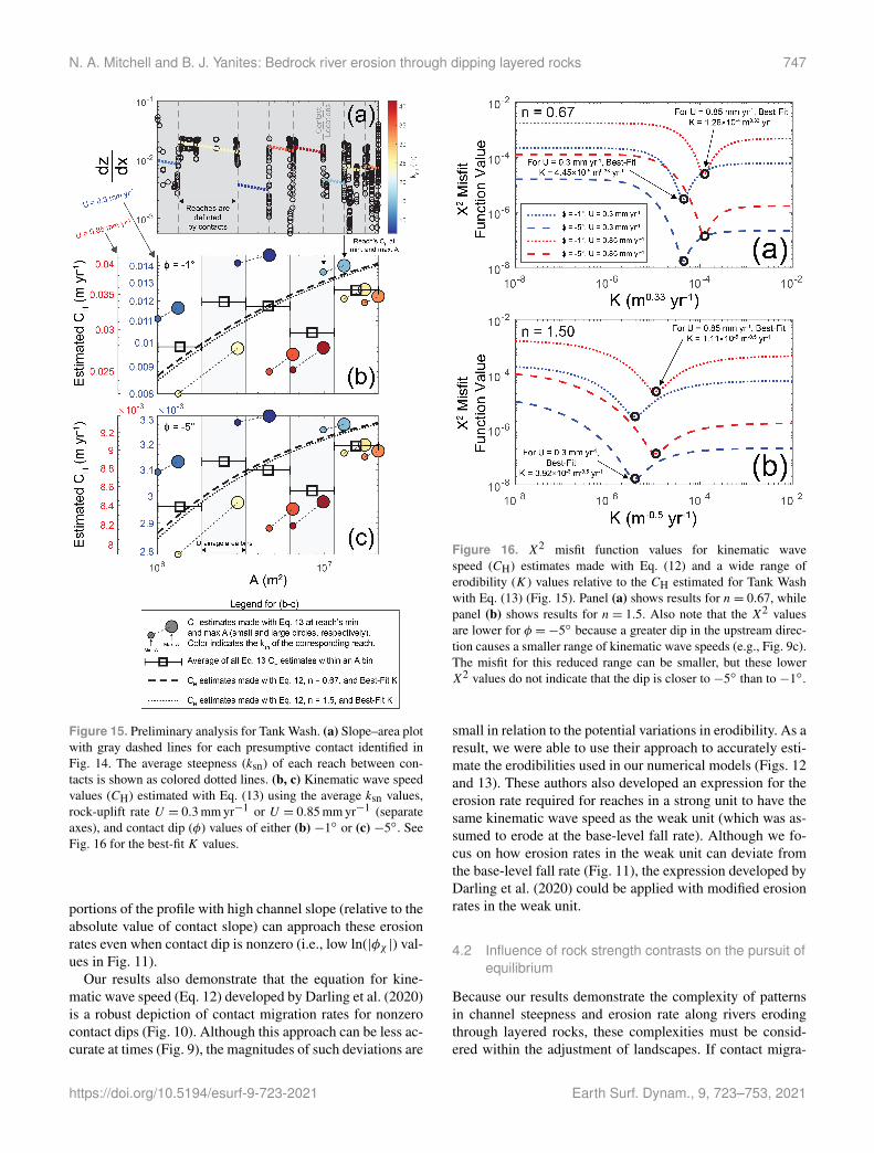
N. A. Mitchell and B. J. Yanites: Bedrock river erosion through dipping layered rocks 747
Figure 15. Preliminary analysis for Tank Wash. (a) Slope–area plotwith gray dashed lines for each presumptive contact identified inFig. 14. The average steepness (ksn) of each reach between con-tacts is shown as colored dotted lines. (b, c) Kinematic wave speedvalues (CH) estimated with Eq. (13) using the average ksn values,rock-uplift rate U = 0.3 mm yr−1 or U = 0.85 mm yr−1 (separateaxes), and contact dip (φ) values of either (b) −1◦ or (c) −5◦. SeeFig. 16 for the best-fit K values.
portions of the profile with high channel slope (relative to theabsolute value of contact slope) can approach these erosionrates even when contact dip is nonzero (i.e., low ln(|φχ |) val-ues in Fig. 11).
Our results also demonstrate that the equation for kine-matic wave speed (Eq. 12) developed by Darling et al. (2020)is a robust depiction of contact migration rates for nonzerocontact dips (Fig. 10). Although this approach can be less ac-curate at times (Fig. 9), the magnitudes of such deviations are
Figure 16. X2 misfit function values for kinematic wavespeed (CH) estimates made with Eq. (12) and a wide range oferodibility (K) values relative to the CH estimated for Tank Washwith Eq. (13) (Fig. 15). Panel (a) shows results for n= 0.67, whilepanel (b) shows results for n= 1.5. Also note that the X2 valuesare lower for φ =−5◦ because a greater dip in the upstream direc-tion causes a smaller range of kinematic wave speeds (e.g., Fig. 9c).The misfit for this reduced range can be smaller, but these lowerX2 values do not indicate that the dip is closer to −5◦ than to −1◦.
small in relation to the potential variations in erodibility. As aresult, we were able to use their approach to accurately esti-mate the erodibilities used in our numerical models (Figs. 12and 13). These authors also developed an expression for theerosion rate required for reaches in a strong unit to have thesame kinematic wave speed as the weak unit (which was as-sumed to erode at the base-level fall rate). Although we fo-cus on how erosion rates in the weak unit can deviate fromthe base-level fall rate (Fig. 11), the expression developed byDarling et al. (2020) could be applied with modified erosionrates in the weak unit.
4.2 Influence of rock strength contrasts on the pursuit ofequilibrium
Because our results demonstrate the complexity of patternsin channel steepness and erosion rate along rivers erodingthrough layered rocks, these complexities must be consid-ered within the adjustment of landscapes. If contact migra-
https://doi.org/10.5194/esurf-9-723-2021 Earth Surf. Dynam., 9, 723–753, 2021
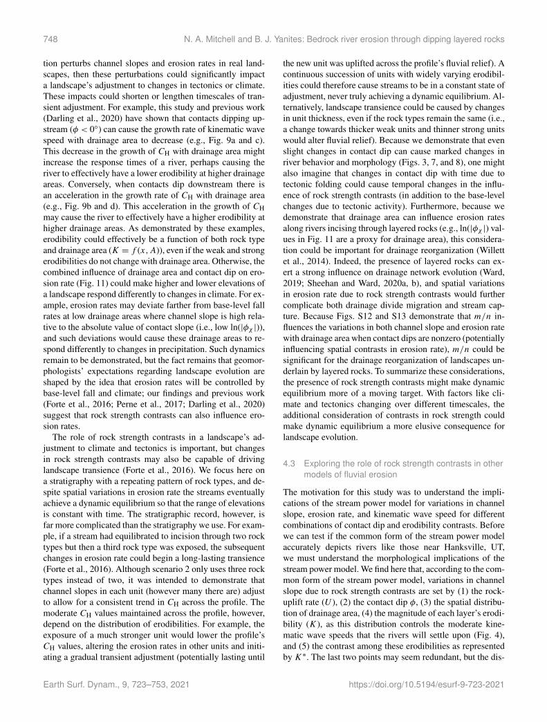
748 N. A. Mitchell and B. J. Yanites: Bedrock river erosion through dipping layered rocks
tion perturbs channel slopes and erosion rates in real land-scapes, then these perturbations could significantly impacta landscape’s adjustment to changes in tectonics or climate.These impacts could shorten or lengthen timescales of tran-sient adjustment. For example, this study and previous work(Darling et al., 2020) have shown that contacts dipping up-stream (φ < 0◦) can cause the growth rate of kinematic wavespeed with drainage area to decrease (e.g., Fig. 9a and c).This decrease in the growth of CH with drainage area mightincrease the response times of a river, perhaps causing theriver to effectively have a lower erodibility at higher drainageareas. Conversely, when contacts dip downstream there isan acceleration in the growth rate of CH with drainage area(e.g., Fig. 9b and d). This acceleration in the growth of CHmay cause the river to effectively have a higher erodibility athigher drainage areas. As demonstrated by these examples,erodibility could effectively be a function of both rock typeand drainage area (K = f (x,A)), even if the weak and strongerodibilities do not change with drainage area. Otherwise, thecombined influence of drainage area and contact dip on ero-sion rate (Fig. 11) could make higher and lower elevations ofa landscape respond differently to changes in climate. For ex-ample, erosion rates may deviate farther from base-level fallrates at low drainage areas where channel slope is high rela-tive to the absolute value of contact slope (i.e., low ln(|φχ |)),and such deviations would cause these drainage areas to re-spond differently to changes in precipitation. Such dynamicsremain to be demonstrated, but the fact remains that geomor-phologists’ expectations regarding landscape evolution areshaped by the idea that erosion rates will be controlled bybase-level fall and climate; our findings and previous work(Forte et al., 2016; Perne et al., 2017; Darling et al., 2020)suggest that rock strength contrasts can also influence ero-sion rates.
The role of rock strength contrasts in a landscape’s ad-justment to climate and tectonics is important, but changesin rock strength contrasts may also be capable of drivinglandscape transience (Forte et al., 2016). We focus here ona stratigraphy with a repeating pattern of rock types, and de-spite spatial variations in erosion rate the streams eventuallyachieve a dynamic equilibrium so that the range of elevationsis constant with time. The stratigraphic record, however, isfar more complicated than the stratigraphy we use. For exam-ple, if a stream had equilibrated to incision through two rocktypes but then a third rock type was exposed, the subsequentchanges in erosion rate could begin a long-lasting transience(Forte et al., 2016). Although scenario 2 only uses three rocktypes instead of two, it was intended to demonstrate thatchannel slopes in each unit (however many there are) adjustto allow for a consistent trend in CH across the profile. Themoderate CH values maintained across the profile, however,depend on the distribution of erodibilities. For example, theexposure of a much stronger unit would lower the profile’sCH values, altering the erosion rates in other units and initi-ating a gradual transient adjustment (potentially lasting until
the new unit was uplifted across the profile’s fluvial relief). Acontinuous succession of units with widely varying erodibil-ities could therefore cause streams to be in a constant state ofadjustment, never truly achieving a dynamic equilibrium. Al-ternatively, landscape transience could be caused by changesin unit thickness, even if the rock types remain the same (i.e.,a change towards thicker weak units and thinner strong unitswould alter fluvial relief). Because we demonstrate that evenslight changes in contact dip can cause marked changes inriver behavior and morphology (Figs. 3, 7, and 8), one mightalso imagine that changes in contact dip with time due totectonic folding could cause temporal changes in the influ-ence of rock strength contrasts (in addition to the base-levelchanges due to tectonic activity). Furthermore, because wedemonstrate that drainage area can influence erosion ratesalong rivers incising through layered rocks (e.g., ln(|φχ |) val-ues in Fig. 11 are a proxy for drainage area), this considera-tion could be important for drainage reorganization (Willettet al., 2014). Indeed, the presence of layered rocks can ex-ert a strong influence on drainage network evolution (Ward,2019; Sheehan and Ward, 2020a, b), and spatial variationsin erosion rate due to rock strength contrasts would furthercomplicate both drainage divide migration and stream cap-ture. Because Figs. S12 and S13 demonstrate that m/n in-fluences the variations in both channel slope and erosion ratewith drainage area when contact dips are nonzero (potentiallyinfluencing spatial contrasts in erosion rate), m/n could besignificant for the drainage reorganization of landscapes un-derlain by layered rocks. To summarize these considerations,the presence of rock strength contrasts might make dynamicequilibrium more of a moving target. With factors like cli-mate and tectonics changing over different timescales, theadditional consideration of contrasts in rock strength couldmake dynamic equilibrium a more elusive consequence forlandscape evolution.
4.3 Exploring the role of rock strength contrasts in othermodels of fluvial erosion
The motivation for this study was to understand the impli-cations of the stream power model for variations in channelslope, erosion rate, and kinematic wave speed for differentcombinations of contact dip and erodibility contrasts. Beforewe can test if the common form of the stream power modelaccurately depicts rivers like those near Hanksville, UT,we must understand the morphological implications of thestream power model. We find here that, according to the com-mon form of the stream power model, variations in channelslope due to rock strength contrasts are set by (1) the rock-uplift rate (U ), (2) the contact dip φ, (3) the spatial distribu-tion of drainage area, (4) the magnitude of each layer’s erodi-bility (K), as this distribution controls the moderate kine-matic wave speeds that the rivers will settle upon (Fig. 4),and (5) the contrast among these erodibilities as representedby K∗. The last two points may seem redundant, but the dis-
Earth Surf. Dynam., 9, 723–753, 2021 https://doi.org/10.5194/esurf-9-723-2021
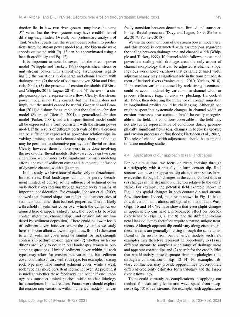
N. A. Mitchell and B. J. Yanites: Bedrock river erosion through dipping layered rocks 749
tinction lies in how two river systems may have the sameK∗ value, but the river systems may have erodibilities ofdiffering magnitudes. Overall, our preliminary analysis ofTank Wash suggests that the stream does conform to predic-tions from the stream power model (e.g., the kinematic wavespeeds estimated with Eq. 13 can be approximated using abest-fit erodibility and Eq. 12).
It is important to note, however, that the stream powermodel (Whipple and Tucker, 1999) depicts shear stress orunit stream power with simplifying assumptions regard-ing (1) the variations in discharge and channel width withdrainage area, (2) the role of sediment cover (Sklar and Diet-rich, 2004), (3) the presence of erosion thresholds (DiBiaseand Whipple, 2011; Lague, 2014), and (4) the use of a sin-gle geomorphically representative flow. Clearly, the streampower model is not fully correct, but that failing does notimply that the model cannot be useful. Gasparini and Bran-don (2011) did show, for example, that the saltation–abrasionmodel (Sklar and Dietrich, 2004), a generalized abrasionmodel (Parker, 2004), and a transport-limited model couldall be expressed in a form consistent with the stream powermodel. If the results of different portrayals of fluvial erosioncan be sufficiently expressed as power-law relationships in-volving drainage area and channel slope, then our findingsmay be pertinent to alternative portrayals of fluvial erosion.Clearly, however, there is more work to be done involvingthe use of other fluvial models. Below, we focus on two con-siderations we consider to be significant for such modelingefforts: the role of sediment cover and the potential influenceof dynamic channel width adjustment.
In this study, we have focused exclusively on detachment-limited rives. Real landscapes will not be purely detach-ment limited, of course, so the influence of sediment coveron bedrock rivers incising through layered rocks remains animportant consideration. For example, Johnson et al. (2009)showed that channel slopes can reflect the characteristics ofsediment load rather than bedrock properties. There is likelya threshold in sediment cover over which the dynamics ex-amined here disappear entirely (i.e., the feedbacks betweencontact migration, channel slope, and erosion rate are hin-dered by sediment deposition). There could be lower levelsof sediment cover, however, where the dynamics we studyhere still occur albeit at lower magnitudes. Both (1) the extentto which sediment cover must be limited for rock strengthcontrasts to perturb erosion rates and (2) whether such con-ditions are likely to occur in real landscapes remain as out-standing questions. Limited sediment cover within all rocktypes may allow for erosion rate variations, but sedimentcover could also covary with rock type. For example, a strongrock type may have limited sediment cover, while a weakrock type has more persistent sediment cover. At present, itis unclear whether these feedbacks can occur if one lithol-ogy has transport-limited reaches, while another lithologyhas detachment-limited reaches. Future work should explorethe erosion rate variations within numerical models that can
freely transition between detachment-limited and transport-limited fluvial processes (Davy and Lague, 2009; Shobe etal., 2017; Yanites, 2018).
We use the common form of the stream power model here,and this model is constructed with assumptions regardingthe scaling between drainage area and channel width (Whip-ple and Tucker, 1999). If channel width follows an assumedpower-law scaling with drainage area, the only aspect ofchannel morphology that can be adjusted is channel slope.Previous work, however, shows that dynamic channel widthadjustment may play a significant role in the transient adjust-ment of bedrock rivers (Yanites et al., 2010; Yanites, 2018).If the erosion variations caused by rock strength contrastscould be accommodated by variations in channel width orprocess efficiency (e.g., abrasion vs. plucking; Hancock etal., 1998), then detecting the influence of contact migrationin longitudinal profiles could be challenging. Although onemight suspect that systematic changes in channel width orerosion processes near contacts should be easily recogniz-able in the field, the conditions observable in the field maynot always be representative of conditions during geomor-phically significant flows (e.g, changes in bedrock exposureand erosion processes during floods; Hartshorn et al., 2002).The role of channel width adjustments should be examinedin future modeling studies.
4.4 Application of our approach to real landscapes
For our simulations, we focus on rivers incising througha stratigraphy with a spatially uniform contact dip. Realstreams can have the apparent dip change over space, how-ever, either through (1) changes in the actual contact dips or(2) changes in the streamflow direction relative to the units’strike. For example, the potential field example shown inFig. 1 has spatial changes in both contact dip and stream-flow directions. Indeed, the stream shown in Fig. 1c has aflow direction that is almost orthogonal to that of Tank Wash(Figs. 1b and 14). We have shown that even slight changesin apparent dip can have a pronounced effect on bedrockriver behavior (Figs. 3, 7, and 8), and the different streamsnear Hanksville may therefore require separate, unique treat-ments. Although apparent dip could vary along each stream,these streams are generally incising through the same units.Based on the results from our numerical models, such fieldexamples may therefore represent an opportunity to (1) usedifferent streams to sample a wide range of drainage areasand apparent contact dips and (2) search for the erodibilitiesthat would satisfy these disparate river morphologies (i.e.,through a combination of Eqs. 12–14). For example, trib-utary confluences may provide opportunities to corroboratedifferent erodibility estimates for a tributary and the largerriver it flows into.
There could certainly be complications in applying ourmethod for estimating kinematic wave speed from steep-ness (Eq. 13) to real streams. For example, such applications
https://doi.org/10.5194/esurf-9-723-2021 Earth Surf. Dynam., 9, 723–753, 2021
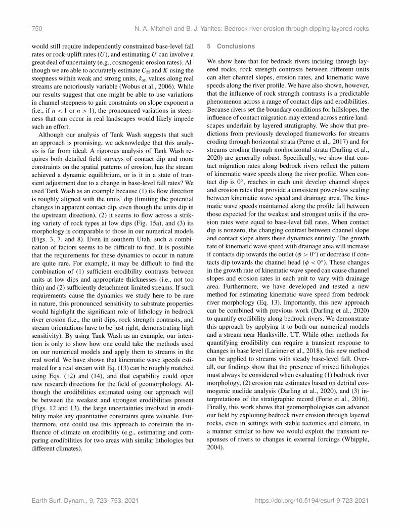
750 N. A. Mitchell and B. J. Yanites: Bedrock river erosion through dipping layered rocks
would still require independently constrained base-level fallrates or rock-uplift rates (U ), and estimating U can involve agreat deal of uncertainty (e.g., cosmogenic erosion rates). Al-though we are able to accurately estimateCH andK using thesteepness within weak and strong units, ksn values along realstreams are notoriously variable (Wobus et al., 2006). Whileour results suggest that one might be able to use variationsin channel steepness to gain constraints on slope exponent n(i.e., if n < 1 or n > 1), the pronounced variations in steep-ness that can occur in real landscapes would likely impedesuch an effort.
Although our analysis of Tank Wash suggests that suchan approach is promising, we acknowledge that this analy-sis is far from ideal. A rigorous analysis of Tank Wash re-quires both detailed field surveys of contact dip and moreconstraints on the spatial patterns of erosion; has the streamachieved a dynamic equilibrium, or is it in a state of tran-sient adjustment due to a change in base-level fall rates? Weused Tank Wash as an example because (1) its flow directionis roughly aligned with the units’ dip (limiting the potentialchanges in apparent contact dip, even though the units dip inthe upstream direction), (2) it seems to flow across a strik-ing variety of rock types at low dips (Fig. 15a), and (3) itsmorphology is comparable to those in our numerical models(Figs. 3, 7, and 8). Even in southern Utah, such a combi-nation of factors seems to be difficult to find. It is possiblethat the requirements for these dynamics to occur in natureare quite rare. For example, it may be difficult to find thecombination of (1) sufficient erodibility contrasts betweenunits at low dips and appropriate thicknesses (i.e., not toothin) and (2) sufficiently detachment-limited streams. If suchrequirements cause the dynamics we study here to be rarein nature, this pronounced sensitivity to substrate propertieswould highlight the significant role of lithology in bedrockriver erosion (i.e., the unit dips, rock strength contrasts, andstream orientations have to be just right, demonstrating highsensitivity). By using Tank Wash as an example, our inten-tion is only to show how one could take the methods usedon our numerical models and apply them to streams in thereal world. We have shown that kinematic wave speeds esti-mated for a real stream with Eq. (13) can be roughly matchedusing Eqs. (12) and (14), and that capability could opennew research directions for the field of geomorphology. Al-though the erodibilities estimated using our approach willbe between the weakest and strongest erodibilities present(Figs. 12 and 13), the large uncertainties involved in erodi-bility make any quantitative constraints quite valuable. Fur-thermore, one could use this approach to constrain the in-fluence of climate on erodibility (e.g., estimating and com-paring erodibilities for two areas with similar lithologies butdifferent climates).
5 Conclusions
We show here that for bedrock rivers incising through lay-ered rocks, rock strength contrasts between different unitscan alter channel slopes, erosion rates, and kinematic wavespeeds along the river profile. We have also shown, however,that the influence of rock strength contrasts is a predictablephenomenon across a range of contact dips and erodibilities.Because rivers set the boundary conditions for hillslopes, theinfluence of contact migration may extend across entire land-scapes underlain by layered stratigraphy. We show that pre-dictions from previously developed frameworks for streamseroding through horizontal strata (Perne et al., 2017) and forstreams eroding through nonhorizontal strata (Darling et al.,2020) are generally robust. Specifically, we show that con-tact migration rates along bedrock rivers reflect the patternof kinematic wave speeds along the river profile. When con-tact dip is 0◦, reaches in each unit develop channel slopesand erosion rates that provide a consistent power-law scalingbetween kinematic wave speed and drainage area. The kine-matic wave speeds maintained along the profile fall betweenthose expected for the weakest and strongest units if the ero-sion rates were equal to base-level fall rates. When contactdip is nonzero, the changing contrast between channel slopeand contact slope alters these dynamics entirely. The growthrate of kinematic wave speed with drainage area will increaseif contacts dip towards the outlet (φ > 0◦) or decrease if con-tacts dip towards the channel head (φ < 0◦). These changesin the growth rate of kinematic wave speed can cause channelslopes and erosion rates in each unit to vary with drainagearea. Furthermore, we have developed and tested a newmethod for estimating kinematic wave speed from bedrockriver morphology (Eq. 13). Importantly, this new approachcan be combined with previous work (Darling et al., 2020)to quantify erodibility along bedrock rivers. We demonstratethis approach by applying it to both our numerical modelsand a stream near Hanksville, UT. While other methods forquantifying erodibility can require a transient response tochanges in base level (Larimer et al., 2018), this new methodcan be applied to streams with steady base-level fall. Over-all, our findings show that the presence of mixed lithologiesmust always be considered when evaluating (1) bedrock rivermorphology, (2) erosion rate estimates based on detrital cos-mogenic nuclide analysis (Darling et al., 2020), and (3) in-terpretations of the stratigraphic record (Forte et al., 2016).Finally, this work shows that geomorphologists can advanceour field by exploiting bedrock river erosion through layeredrocks, even in settings with stable tectonics and climate, ina manner similar to how we would exploit the transient re-sponses of rivers to changes in external forcings (Whipple,2004).
Earth Surf. Dynam., 9, 723–753, 2021 https://doi.org/10.5194/esurf-9-723-2021
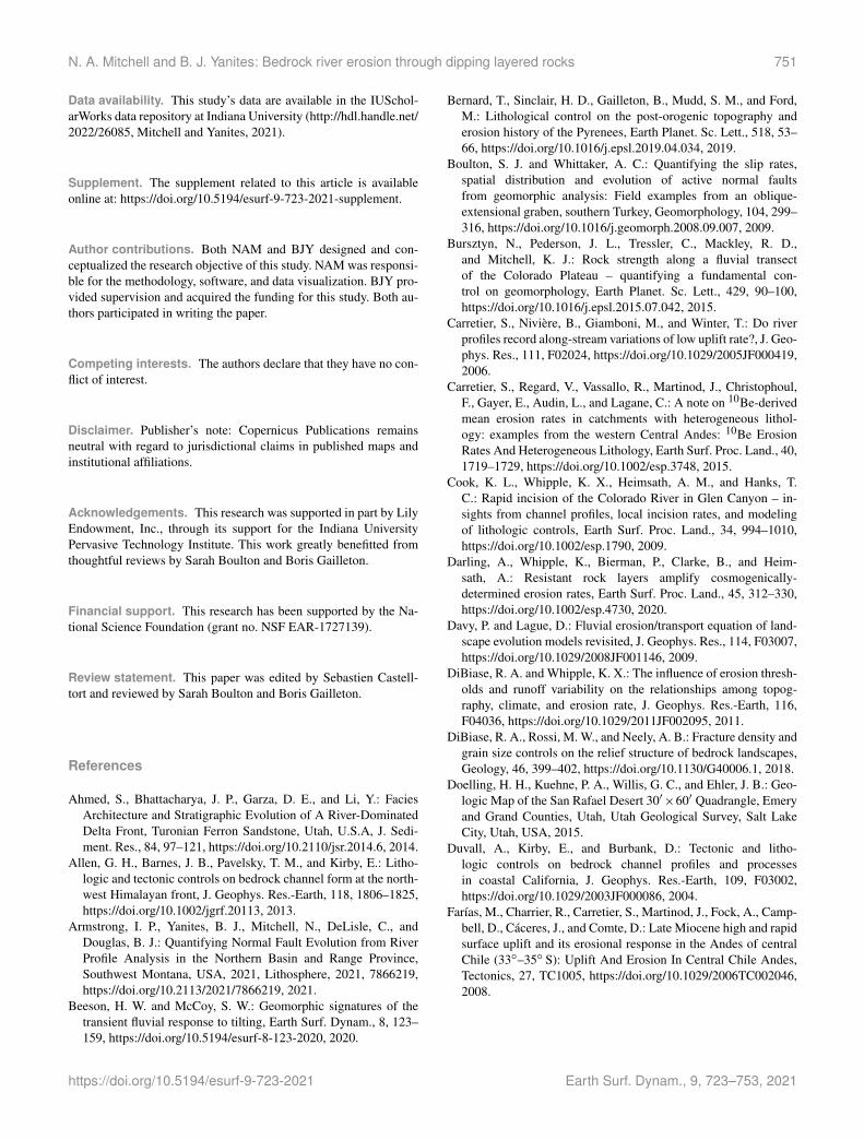
N. A. Mitchell and B. J. Yanites: Bedrock river erosion through dipping layered rocks 751
Data availability. This study’s data are available in the IUSchol-arWorks data repository at Indiana University (http://hdl.handle.net/2022/26085, Mitchell and Yanites, 2021).
Supplement. The supplement related to this article is availableonline at: https://doi.org/10.5194/esurf-9-723-2021-supplement.
Author contributions. Both NAM and BJY designed and con-ceptualized the research objective of this study. NAM was responsi-ble for the methodology, software, and data visualization. BJY pro-vided supervision and acquired the funding for this study. Both au-thors participated in writing the paper.
Competing interests. The authors declare that they have no con-flict of interest.
Disclaimer. Publisher’s note: Copernicus Publications remainsneutral with regard to jurisdictional claims in published maps andinstitutional affiliations.
Acknowledgements. This research was supported in part by LilyEndowment, Inc., through its support for the Indiana UniversityPervasive Technology Institute. This work greatly benefitted fromthoughtful reviews by Sarah Boulton and Boris Gailleton.
Financial support. This research has been supported by the Na-tional Science Foundation (grant no. NSF EAR-1727139).
Review statement. This paper was edited by Sebastien Castell-tort and reviewed by Sarah Boulton and Boris Gailleton.
References
Ahmed, S., Bhattacharya, J. P., Garza, D. E., and Li, Y.: FaciesArchitecture and Stratigraphic Evolution of A River-DominatedDelta Front, Turonian Ferron Sandstone, Utah, U.S.A, J. Sedi-ment. Res., 84, 97–121, https://doi.org/10.2110/jsr.2014.6, 2014.
Allen, G. H., Barnes, J. B., Pavelsky, T. M., and Kirby, E.: Litho-logic and tectonic controls on bedrock channel form at the north-west Himalayan front, J. Geophys. Res.-Earth, 118, 1806–1825,https://doi.org/10.1002/jgrf.20113, 2013.
Armstrong, I. P., Yanites, B. J., Mitchell, N., DeLisle, C., andDouglas, B. J.: Quantifying Normal Fault Evolution from RiverProfile Analysis in the Northern Basin and Range Province,Southwest Montana, USA, 2021, Lithosphere, 2021, 7866219,https://doi.org/10.2113/2021/7866219, 2021.
Beeson, H. W. and McCoy, S. W.: Geomorphic signatures of thetransient fluvial response to tilting, Earth Surf. Dynam., 8, 123–159, https://doi.org/10.5194/esurf-8-123-2020, 2020.
Bernard, T., Sinclair, H. D., Gailleton, B., Mudd, S. M., and Ford,M.: Lithological control on the post-orogenic topography anderosion history of the Pyrenees, Earth Planet. Sc. Lett., 518, 53–66, https://doi.org/10.1016/j.epsl.2019.04.034, 2019.
Boulton, S. J. and Whittaker, A. C.: Quantifying the slip rates,spatial distribution and evolution of active normal faultsfrom geomorphic analysis: Field examples from an oblique-extensional graben, southern Turkey, Geomorphology, 104, 299–316, https://doi.org/10.1016/j.geomorph.2008.09.007, 2009.
Bursztyn, N., Pederson, J. L., Tressler, C., Mackley, R. D.,and Mitchell, K. J.: Rock strength along a fluvial transectof the Colorado Plateau – quantifying a fundamental con-trol on geomorphology, Earth Planet. Sc. Lett., 429, 90–100,https://doi.org/10.1016/j.epsl.2015.07.042, 2015.
Carretier, S., Nivière, B., Giamboni, M., and Winter, T.: Do riverprofiles record along-stream variations of low uplift rate?, J. Geo-phys. Res., 111, F02024, https://doi.org/10.1029/2005JF000419,2006.
Carretier, S., Regard, V., Vassallo, R., Martinod, J., Christophoul,F., Gayer, E., Audin, L., and Lagane, C.: A note on 10Be-derivedmean erosion rates in catchments with heterogeneous lithol-ogy: examples from the western Central Andes: 10Be ErosionRates And Heterogeneous Lithology, Earth Surf. Proc. Land., 40,1719–1729, https://doi.org/10.1002/esp.3748, 2015.
Cook, K. L., Whipple, K. X., Heimsath, A. M., and Hanks, T.C.: Rapid incision of the Colorado River in Glen Canyon – in-sights from channel profiles, local incision rates, and modelingof lithologic controls, Earth Surf. Proc. Land., 34, 994–1010,https://doi.org/10.1002/esp.1790, 2009.
Darling, A., Whipple, K., Bierman, P., Clarke, B., and Heim-sath, A.: Resistant rock layers amplify cosmogenically-determined erosion rates, Earth Surf. Proc. Land., 45, 312–330,https://doi.org/10.1002/esp.4730, 2020.
Davy, P. and Lague, D.: Fluvial erosion/transport equation of land-scape evolution models revisited, J. Geophys. Res., 114, F03007,https://doi.org/10.1029/2008JF001146, 2009.
DiBiase, R. A. and Whipple, K. X.: The influence of erosion thresh-olds and runoff variability on the relationships among topog-raphy, climate, and erosion rate, J. Geophys. Res.-Earth, 116,F04036, https://doi.org/10.1029/2011JF002095, 2011.
DiBiase, R. A., Rossi, M. W., and Neely, A. B.: Fracture density andgrain size controls on the relief structure of bedrock landscapes,Geology, 46, 399–402, https://doi.org/10.1130/G40006.1, 2018.
Doelling, H. H., Kuehne, P. A., Willis, G. C., and Ehler, J. B.: Geo-logic Map of the San Rafael Desert 30′×60′ Quadrangle, Emeryand Grand Counties, Utah, Utah Geological Survey, Salt LakeCity, Utah, USA, 2015.
Duvall, A., Kirby, E., and Burbank, D.: Tectonic and litho-logic controls on bedrock channel profiles and processesin coastal California, J. Geophys. Res.-Earth, 109, F03002,https://doi.org/10.1029/2003JF000086, 2004.
Farías, M., Charrier, R., Carretier, S., Martinod, J., Fock, A., Camp-bell, D., Cáceres, J., and Comte, D.: Late Miocene high and rapidsurface uplift and its erosional response in the Andes of centralChile (33◦–35◦ S): Uplift And Erosion In Central Chile Andes,Tectonics, 27, TC1005, https://doi.org/10.1029/2006TC002046,2008.
https://doi.org/10.5194/esurf-9-723-2021 Earth Surf. Dynam., 9, 723–753, 2021
752 N. A. Mitchell and B. J. Yanites: Bedrock river erosion through dipping layered rocks
Flint, J. J.: Stream gradient as a function of order, mag-nitude, and discharge, Water Resour. Res., 10, 969–973,https://doi.org/10.1029/WR010i005p00969, 1974.
Forte, A. M., Yanites, B. J., and Whipple, K. X.: Complexities oflandscape evolution during incision through layered stratigra-phy with contrasts in rock strength, Earth Surf. Proc. Land., 41,1736–1757, https://doi.org/10.1002/esp.3947, 2016.
Fox, M., Goren, L., May, D. A., and Willett, S. D.: In-version of fluvial channels for paleorock uplift ratesin Taiwan, J. Geophys. Res.-Earth, 119, 1853–1875,https://doi.org/10.1002/2014JF003196, 2014.
Gallen, S. F. and Wegmann, K. W.: River profile response to normalfault growth and linkage: an example from the Hellenic forearcof south-central Crete, Greece, Earth Surf. Dynam., 5, 161–186,https://doi.org/10.5194/esurf-5-161-2017, 2017.
Gallen, S. F., Wegmann, K. W., and Bohnenstieh, D. R.: Miocenerejuvenation of topographic relief in the southern Appalachians,GSA Today, 23, 4–10, https://doi.org/10.1130/GSATG163A.1,2013.
Gasparini, N. M. and Brandon, M. T.: A generalized power law ap-proximation for fluvial incision of bedrock channels, J. Geophys.Res.-Earth, 116, F02020, https://doi.org/10.1029/2009JF001655,2011.
Gasparini, N. M. and Whipple, K. X.: Diagnosing climaticand tectonic controls on topography: Eastern flank ofthe northern Bolivian Andes, Lithosphere, 6, 230–250,https://doi.org/10.1130/L322.1, 2014.
Glade, R. C., Anderson, R. S., and Tucker, G. E.: Block-controlled hillslope form and persistence of topog-raphy in rocky landscapes, Geology, 45, 311–314,https://doi.org/10.1130/G38665.1, 2017.
Goren, L., Fox, M., and Willett, S. D.: Tectonics from fluvial to-pography using formal linear inversion: Theory and applicationsto the Inyo Mountains, California, J. Geophys. Res.-Earth, 119,1651–1681, https://doi.org/10.1002/2014JF003079, 2014.
Hack, J. T.: Studies of longitudinal stream profiles in Virginia andMaryland, Geological Survey Professional Paper 294-B, UnitedStates Government Printing Office, Washington D.C., USA, 45–94, 1957.
Hack, J. T.: Stream-profile analysis and stream-gradient index, J.Res. US Geol. Surv., 1, 421–429, 1973.
Han, J., Gasparini, N. M., Johnson, J. P. L., and Murphy, B. P.: Mod-eling the influence of rainfall gradients on discharge, bedrockerodibility, and river profile evolution, with application to theBig Island, Hawai’i, J. Geophys. Res.-Earth, 119, 1418–1440,https://doi.org/10.1002/2013JF002961, 2014.
Hancock, G. S., Anderson, R. S., and Whipple, K. X.: Be-yond power: Bedrock river incision process and form, Geo-phys. Monograph Series-American Geophys. Union, 107, 35–60, https://doi-org.proxyiub.uits.iu.edu/10.1029/GM107p0035,1998.
Hartshorn, K., Hovius, N., Dade, W. B., and Slinger-land, R. L.: Climate-Driven Bedrock Incision in anActive Mountain Belt, Science, 297, 2036–2038,https://doi.org/10.1126/science.1075078, 2002.
Haviv, I., Enzel, Y., Whipple, K. X., Zilberman, E., Mat-mon, A., Stone, J., and Fifield, K. L.: Evolution of verti-cal knickpoints (waterfalls) with resistant caprock: Insights
from numerical modeling, J. Geophys. Res., 115, F03028,https://doi.org/10.1029/2008JF001187, 2010.
Howard, A. D. and Kerby, G.: Channel changes in badlands, Geol.Soc. Am. Bull., 94, 739–752, https://doi.org/10.1130/0016-7606(1983)94<739:CCIB>2.0.CO;2, 1983.
Imaizumi, F., Nishii, R., Murakami, W., and Daimaru,H.: Parallel retreat of rock slopes underlain by al-ternation of strata, Geomorphology, 238, 27–36,https://doi.org/10.1016/j.geomorph.2015.02.030, 2015.
Jeffery, M. L., Ehlers, T. A., Yanites, B. J., and Poulsen, C. J.:Quantifying the role of paleoclimate and Andean Plateau up-lift on river incision, J. Geophys. Res.-Earth, 118, 852–871,https://doi.org/10.1002/jgrf.20055, 2013.
Johnson, J. P. L., Whipple, K. X., Sklar, L. S., and Hanks, T.C.: Transport slopes, sediment cover, and bedrock channel inci-sion in the Henry Mountains, Utah, J. Geophys. Res.-Earth, 114,F02014, https://doi.org/10.1029/2007JF000862, 2009.
Kirby, E., Whipple, K. X., Tang, W., and Chen, Z.: Dis-tribution of active rock uplift along the eastern marginof the Tibetan Plateau: Inferences from bedrock channellongitudinal profiles, J. Geophys. Res.-Solid, 108, 2217,https://doi.org/10.1029/2001JB000861, 2003.
Lague, D.: The stream power river incision model: evidence,theory and beyond, Earth Surf. Proc. Land., 39, 38–61,https://doi.org/10.1002/esp.3462, 2014.
Lamb, M. P., Howard, A. D., Dietrich, W. E., and Perron, J. T.:Formation of amphitheater-headed valleys by waterfall erosionafter large-scale slumping on Hawai’i, Geol. Soc. Am. Bull., 119,805–822, https://doi.org/10.1130/B25986.1, 2007.
Larimer, J. E., Yanites, B. J., Phillips, W., and Mittelstaedt, E.: LateMiocene rejuvenation of central Idaho landscape evolution: Acase for surface processes driven by plume–lithosphere interac-tion, Lithosphere, 10, 14, https://doi.org/10.1130/L746.1, 2018.
Lavarini, C., Attal, M., da Costa Filho, C. A., and Kirstein,L. A.: Does Pebble Abrasion Influence Detrital Age Pop-ulation Statistics? A Numerical Investigation of Natu-ral Data Sets, J. Geophys. Res.-Earth, 123, 2577–2601,https://doi.org/10.1029/2018JF004610, 2018.
Ma, Z., Zhang, H., Wang, Y., Tao, Y., and Li, X.: Inversion ofDadu River Bedrock Channels for the Late Cenozoic Uplift His-tory of the Eastern Tibetan Plateau, Geophys. Res. Lett., 47,e2019GL086882, https://doi.org/10.1029/2019GL086882, 2020.
Miller, S. R., Sak, P. B., Kirby, E., and Bierman, P. R.:Neogene rejuvenation of central Appalachian topography:Evidence for differential rock uplift from stream profilesand erosion rates, Earth Planet. Sc. Lett., 369–370, 1–12,https://doi.org/10.1016/j.epsl.2013.04.007, 2013.
Mitchell, N. A. and Yanites, B. J.: Spatially Variable In-crease in Rock Uplift in the Northern U.S. CordilleraRecorded in the Distribution of River Knickpoints and In-cision Depths, J. Geophys. Res.-Earth, 124, 1238–1260,https://doi.org/10.1029/2018JF004880, 2019.
Mitchell, N. and Yanites, B.: Bedrock river erosion through dippinglayered rocks: quantifying erodibility through kinematic wavespeed, IUScholarWorks [dataset], available at: http://hdl.handle.net/2022/26085, last access: 9 July 2021.
Mudd, S. M., Attal, M., Milodowski, D. T., Grieve, S. W. D., andValters, D. A.: A statistical framework to quantify spatial vari-ation in channel gradients using the integral method of chan-
Earth Surf. Dynam., 9, 723–753, 2021 https://doi.org/10.5194/esurf-9-723-2021
N. A. Mitchell and B. J. Yanites: Bedrock river erosion through dipping layered rocks 753
nel profile analysis, J. Geophys. Res.-Earth, 119, 2013JF002981,https://doi.org/10.1002/2013JF002981, 2014.
Murphy, B. P., Johnson, J. P. L., Gasparini, N. M., and Sklar,L. S.: Chemical weathering as a mechanism for the cli-matic control of bedrock river incision, Nature, 532, 223–227,https://doi.org/10.1038/nature17449, 2016.
Parker, G.: Somewhat less random notes on bedrock inci-sion, University of Minnesota Twin Cities, available at:http://hydrolab.illinois.edu/people/parkerg/_private/Reports/IR118BedrockIncisionNotes.pdf (last access: 9 July 2021),2004.
Perne, M., Covington, M. D., Thaler, E. A., and Myre, J. M.:Steady state, erosional continuity, and the topography of land-scapes developed in layered rocks, Earth Surf. Dynam., 5, 85–100, https://doi.org/10.5194/esurf-5-85-2017, 2017.
Perron, J. T. and Royden, L.: An integral approach to bedrockriver profile analysis, Earth Surf. Proc. Land., 38, 570–576,https://doi.org/10.1002/esp.3302, 2013.
Repka, J. L., Anderson, R. S., and Finkel, R. C.: Cosmo-genic dating of fluvial terraces, Fremont River, Utah, EarthPlanet. Sc. Lett., 152, 59–73, https://doi.org/10.1016/S0012-821X(97)00149-0, 1997.
Rosenbloom, N. A. and Anderson, R. S.: Hillslope andchannel evolution in a marine terraced landscape, SantaCruz, California, J. Geophys. Res., 99, 14013–14029,https://doi.org/10.1029/94JB00048, 1994.
Royden, L. and Perron, T.: Solutions of the stream powerequation and application to the evolution of river lon-gitudinal profiles, J. Geophys. Res.-Earth, 118, 497–518,https://doi.org/10.1002/jgrf.20031, 2013.
Scheingross, J. S. and Lamb, M. P.: A Mechanistic Modelof Waterfall Plunge Pool Erosion into Bedrock: WaterfallPlunge Pool Erosion, J. Geophys. Res.-Earth, 122, 2079–2104,https://doi.org/10.1002/2017JF004195, 2017.
Schwanghart, W. and Kuhn, N. J.: TopoToolbox: A set of Matlabfunctions for topographic analysis, Environ. Model. Softw., 25,770–781, https://doi.org/10.1016/j.envsoft.2009.12.002, 2010.
Schwanghart, W. and Scherler, D.: Short Communication: Topo-Toolbox 2 – MATLAB-based software for topographic analysisand modeling in Earth surface sciences, Earth Surf. Dynam., 2,1–7, https://doi.org/10.5194/esurf-2-1-2014, 2014.
Sheehan, C. E. and Ward, D. J.: An Autogenic Cycle of FluvialTransience in Dipping, Layered Rocks, Geophys. Res. Lett.,10, e2020GL090246, https://doi.org/10.1029/2020GL090246,2020a.
Sheehan, C. E. and Ward, D. J.: Migrating Trans-verse Escarpments in Strike Valleys on the ColoradoPlateau, J. Geophys. Res.-Earth, 125, e2019JF005260,https://doi.org/10.1029/2019JF005260, 2020b.
Shobe, C. M., Tucker, G. E., and Barnhart, K. R.: The SPACE 1.0model: a Landlab component for 2-D calculation of sedimenttransport, bedrock erosion, and landscape evolution, Geosci.Model Dev., 10, 4577–4604, https://doi.org/10.5194/gmd-10-4577-2017, 2017.
Sklar, L. S. and Dietrich, W. E.: A mechanistic model for river inci-sion into bedrock by saltating bed load, Water Resour. Res., 40,W06301, https://doi.org/10.1029/2003WR002496, 2004.
Stock, J. D. and Montgomery, D. R.: Geologic constraints onbedrock river incision using the stream power law, J. Geophys.Res., 104, 4983–4993, https://doi.org/10.1029/98JB02139, 1999.
Tucker, G. E. and Whipple, K. X.: Topographic outcomes pre-dicted by stream erosion models: Sensitivity analysis and inter-model comparison, J. Geophys. Res., 107, ETG 1-1–ETG 1-16,https://doi.org/10.1029/2001JB000162, 2002.
Ward, D. J.: Dip, layer spacing, and incision rate con-trols on the formatio of strike valleys, cuestas, and cliff-bands in heterogeneous stratigraphy, Lithosphere, 11, 697–707,https://doi.org/10.1130/L1056.1, 2019.
Whipple, K. X.: Bedrock Rivers and the Geomorphology of Ac-tive Orogens, Annu. Rev. Earth Planet, Sci., 32, 151–185,https://doi.org/10.1146/annurev.earth.32.101802.120356, 2004.
Whipple, K. X. and Tucker, G. E.: Dynamics of the stream-power river incision model: Implications for height lim-its of mountain ranges, landscape response timescales,and research needs, J. Geophys. Res., 104, 17661–17674,https://doi.org/10.1029/1999JB900120, 1999.
Whipple, K. X., DiBiase, R. A., and Crosby, B. T.: 9.28 BedrockRivers, in: Treatise on Geomorphology, edited by:Shroder, J. F., Academic Press, San Diego, 550–573,https://doi.org/10.1016/B978-0-12-374739-6.00254-2, 2013.
Whittaker, A. C., Attal, M., Cowie, P. A., Tucker, G. E., andRoberts, G.: Decoding temporal and spatial patterns of fault up-lift using transient river long profiles, Geomorphology, 100, 506–526, https://doi.org/10.1016/j.geomorph.2008.01.018, 2008.
Willett, S. D., McCoy, S. W., Perron, J. T., Goren, L., and Chen,C.-Y.: Dynamic Reorganization of River Basins, Science, 343,1248765, https://doi.org/10.1126/science.1248765, 2014.
Wobus, C., Whipple, K. X., Kirby, E., Snyder, N., Johnson, J., Spy-ropolou, K., Crosby, B., and Sheehan, D.: Tectonics from topog-raphy: Procedures, promise, and pitfalls, Geolog. Soc. AmericaSpec. Pap., 398, 55–74, https://doi.org/10.1130/2006.2398(04),2006.
Wolpert, J. A. and Forte, A. M.: Response of Transient RockUplift and Base Level Knickpoints to Erosional EfficiencyContrasts in Bedrock Streams, Earth Surf. Proc. Land.,https://doi.org/10.1002/esp.5146, online first, 2021.
Yanites, B. J.: The Dynamics of Channel Slope, Width,and Sediment in Actively Eroding Bedrock RiverSystems, J. Geophys. Res.-Earth, 123, 1504–1527,https://doi.org/10.1029/2017JF004405, 2018.
Yanites, B. J., Tucker, G. E., Mueller, K. J., Chen, Y.-G., Wilcox, T.,Huang, S.-Y., and Shi, K.-W.: Incision and channel morphologyacross active structures along the Peikang River, central Taiwan:Implications for the importance of channel width, GSA Bull.,122, 1192–1208, https://doi.org/10.1130/B30035.1, 2010.
Yanites, B. J., Becker, J. K., Madritsch, H., Schnellmann, M.,and Ehlers, T. A.: Lithologic effects on landscape responseto base level changes: a modeling study in the context ofthe eastern Jura Mountains, Switzerland: Lithologic effect onlandscape evolution, J. Geophys. Res.-Earth, 122, 2196–2222,https://doi.org/10.1002/2016JF004101, 2017.
Zondervan, J. R., Stokes, M., Boulton, S. J., Telfer, M. W., andMather, A. E.: Rock strength and structural controls on flu-vial erodibility: Implications for drainage divide mobility in acollisional mountain belt, Earth Planet. Sc. Lett., 538, 116221,https://doi.org/10.1016/j.epsl.2020.116221, 2020.
https://doi.org/10.5194/esurf-9-723-2021 Earth Surf. Dynam., 9, 723–753, 2021