lable at ScienceDirect

Environmental Modelling & Software 53 (2014) 1e18

Contents lists avai

Environmental Modelling & Software

journal homepage: www.elsevier .com/locate/envsoft

Stochastic reconstruction of paleovalley bedrock morphology fromsparse datasets

J.C. Castilla-Rho a,c,d,*, G. Mariethoz a,c,d, B.F.J. Kelly b,c,d, M.S. Andersen a,c,d

a School of Civil and Environmental Engineering, University of New South Wales, Sydney, NSW 2052, Australiab School Biological, Earth and Environmental Sciences, University of New South Wales, Sydney, NSW 2052, AustraliacConnected Waters Initiative Research Centre, University of New South Wales, Sydney, NSW 2052, AustraliadAffiliated with the National Centre for Groundwater Research and Training (NCGRT), Australia

a r t i c l e i n f o

Article history:Received 19 March 2013Received in revised form25 August 2013Accepted 29 October 2013Available online

Keywords:Geological uncertaintyStochastic hydrogeologyGeological analogGeostatisticsSpatial interpolation

* Corresponding author. School of Civil and Environsity of New South Wales, Kensington Campus, SyTel.: þ61 (0) 478074291.

E-mail addresses: j.castilla@unsw.edu.au (J.C. Castilunsw.edu.au (G. Mariethoz), bryce.kelly@unsw.edu.aunsw.edu.au (M.S. Andersen).

1364-8152/$ e see front matter � 2013 Elsevier Ltd.http://dx.doi.org/10.1016/j.envsoft.2013.10.025

a b s t r a c t

Stochastic groundwater models enable the characterization of geological uncertainty. Often the majorsource of uncertainty is not related to aquifer heterogeneity, but to the general shape of the aquifer. Thisis especially the case in paleovalley-type alluvial aquifers where the bedrock surface limits the extent ofeasily extractable groundwater. Determining the shape of a bedrock surface is not straightforward,because it is typically non-stationary and defined by few data points that are generally far apart. Thispaper presents a new workflow for the stochastic reconstruction of bedrock surfaces using limiteddatasets that are typically available for aquifer characterization. The method is based on a lateralpropagation of basement cross-sections interpreted from geophysical surveys, and conditions thereconstructed surface to existing well-log data and digital elevation model. To alleviate the typicallimitations of sparse data, we use an analog approach to incorporate prior geological knowledge. We testthe methodology on a synthetic example and a dataset from an alluvial aquifer in Northern Chile. Resultsof these case studies show that the algorithm is capable of enforcing the general notion of structuralcontinuity, with the aquifer shape being conceptualized as an elongated, continuous and connectedvalley-shaped body. Our method captures the large-scale topographic features of fluvial incision intobedrock and the uncertainty in the positioning of the surface. Small-scale spatial variability is incor-porated using Sequential Gaussian Simulation informed by geological analogs. Being stochastic, themethodology allows characterization of the uncertainty associated with positioning of the bedrocksurface, by generating an ensemble of models via a Monte-Carlo analysis. This makes it possible toquantify the uncertainty associated with estimating the aquifer volume. We also discuss how thismethodology may be used to better quantify the influence of uncertainty associated with defining theaquifer geometry on water resource assessment and management.

� 2013 Elsevier Ltd. All rights reserved.

Software availability

Name of software: stochastic paleovalley interpolation V 1.0Availability and cost: freeware downloadable from: https://github.

com/juancastilla/Paleovalley-Modelling.git includingdocumentation and demo datasets. The program isavailable as a set of Matlab functions and scripts. SGEMS

mental Engineering, Univer-dney, NSW 2052, Australia.

la-Rho), gregoire.mariethoz@u (B.F.J. Kelly), m.andersen@

All rights reserved.

and mgstat are open-source software and can bedownloaded at no cost from the developers’ website.

Developers: Juan Carlos Castilla-Rho, Gregoire MariethozContact address: School of Civil and Environmental Engineering,

University of New South Wales, Kensington Campus,Sydney, NSW 2052, Australia

Phone: þ61 (0) 478074291Email: j.castilla@unsw.edu.auHardware required: 32- or 64-bit PC with Windows or Mac OS. We

recommend a high-speed processor and at least 4 GB ofRAM.

Software required: Matlab R2012b, mGstat geostatistical toolbox(http://mgstat.sourceforge.net), SGEMS geostatisticalmodelling software (http://sgems.sourceforge.net)

J.C. Castilla-Rho et al. / Environmental Modelling & Software 53 (2014) 1e182

1. Introduction

The lack of spatial information is a prevalent issue for scientistsand practitioners needing to assemble 3D models of geologicalregions. While carefully designed studies should rely on dense datacollection campaigns, in practice economic and technical con-straints often result in poor control of the quality and spatialarrangement of the data. Hydrogeology is particularly affected bythis problem, as information mainly originates from localized datathat sample a very small portion of the geological region of interest.In addition, subsurface morphology is usually heterogeneous,anisotropic and non-stationary. Furthermore, geoscientists canproduce a range of interpretations from a single dataset, henceintroducing knowledge bias and interpretational uncertainties(Bond et al., 2007). For all these reasons, geological uncertainty isoften large, and significant research efforts are aimed at quantifyingand capturing it for 3D structural, volumetric, facies and flowmodeling applications.

Alluvial aquifers or basins are often modeled as a fillingsequence overlying a bedrock surface (Hoyos et al., 2012; Jairethet al., 2010; Whiteley, 2005). Their conceptualization is thereforecontrolled by the shape and geomorphology of the underlyingstructure, typically defined by a paleovalley bedrock surface. Theaquifer then constitutes the permeable units of the unconsolidatedsediments that overlie low permeability consolidated deposits orbedrock. However, the inherent limitations of geological datasetscan make the task of characterizing bedrock surfaces challenging.This has significant implications for defining the transmissivitydistribution in the aquifer or even for simpler characterizationsuch as estimating the total volume of porous material in thereservoir.

Geostatistics is a widely used framework for making predictionsat unmeasured locations from limited and sparsely arranged data.Geosciences and water resources rely heavily on geostatistics forspatial interpolation, with frequent use of kriging in its variousforms (Li and Heap, 2011). A limitation of kriging is that it relies onassumptions of stationarity and smoothness, and limited repre-sentation of anisotropy (such as zonal anisotropy). Althoughtraditional geostatistical methods can include data sources such asdigital elevation models (DEMs), wells and geophysics, it is oftenfound that representing complex geometries of geological systemsis difficult (Neuweiler and Vogel, 2007; Zinn and Harvey, 2003).These issues are general and arise when working on structureshaving characteristics of non-stationary and meandering geome-tries, such as 3D groundwater models demanding realistic bedrocksurfaces. Some of the approaches that have been proposed tomodel geological complexity include multiple-point statistics(Guardiano and Srivastava, 1993; Hu and Chugunova, 2008;Mariethoz and Kelly, 2011), object-based methods (Haldorsenand Chang, 1986) or complex forms of indicator simulation suchas the pluriGaussian method (Le Loc’h et al., 1994; Mariethoz et al.,2008). Although these methods are appropriate for 3D griddedfacies models, they are not always applicable to modelinggeological surfaces, which are continuous and strongly non-stationary.

The literature on spatial interpolation of topographic datasets inmeandering, non-stationary valley-shaped landscapes presents aseries of solutions and customizations to improve the performanceof simple interpolators when applied to such data (Nordfjord et al.,2005). One successful approach has been to transform the datasetsto a channel-oriented coordinate system prior to interpolation(Legleiter and Kyriakidis, 2008; Merwade, 2009; Merwade et al.,2006, 2005). This coordinate conversion, however, is more appro-priate for dense datasets and requires accurate definition of thechannel centerline, often a time-intensive task (Goff and Nordfjord,

2004). Unfortunately, in hydrogeology the data is frequently toosparse for this method to be successful. Another general principleoften used to improve topographic reconstructions is the conceptof separating trend from the data using empirical functions. Thisidea has been the focus of recent studies related to river bathym-etry modeling (Legleiter and Kyriakidis, 2008; Merwade, 2009),allowing subsequent application of isotropic interpolation. Thesemethods still present challenges, particularly in addressing non-stationarity (Merwade, 2009) and their suitability to site-specificdata. Even though some studies derive generic trend functionsusing modern analogs (Allan James, 1996), their applicability todifferent settings should be dealt with caution. For instance, themorphological differences between fluvial and glacial environ-ments may invalidate the applicability of a method derived for aspecific environment (Anderson et al., 2006; Graf, 1970; Li et al.,2001). Therefore, a general methodology is needed to fullyextract trends from available data, avoiding loss of informationtypically occurring during curve-fitting procedures. Also relevantto this work, is the use of random fields through SequentialGaussian Simulation (SGS). Gringarten et al. (2005) use thisapproach to simultaneously confer realistic geological features totopographic models, while conditioning to well-log data. As a by-product of this workflow, several possible realizations are ob-tained which can be used to convey quantitative measures ofuncertainty.

In recent years, many authors have demonstrated that aquiferconceptualization is responsible for a significant proportion of theuncertainty in groundwater model predictions (Bond et al., 2007;Bredehoeft, 2005; Neuman, 2004; Poeter, 2007; Rojas et al., 2010;Zeng et al., 2013). To date however, the specific problem of gener-ating 3D reconstructions of paleovalley geomorphologywith sparsedata has received little attention. The goal of this paper is to modeluncertainty related to the alluvium/bedrock interface caused bylimited subsurface information, which is often an important sourceof predictive uncertainty (Poeter, 2007; Refsgaard et al., 2012). Inthis regard, multi-realization methodologies have a proven track-record in the quantification of uncertainty due to data limitationand other factors (Refsgaard et al., 2012; Troldborg et al., 2007). Thislast point highlights the need for specialized geostatistical algo-rithms capable of generating multiple realizations of alluviume

bedrock interfaces.In this paper, we address the challenge of integrating, in an

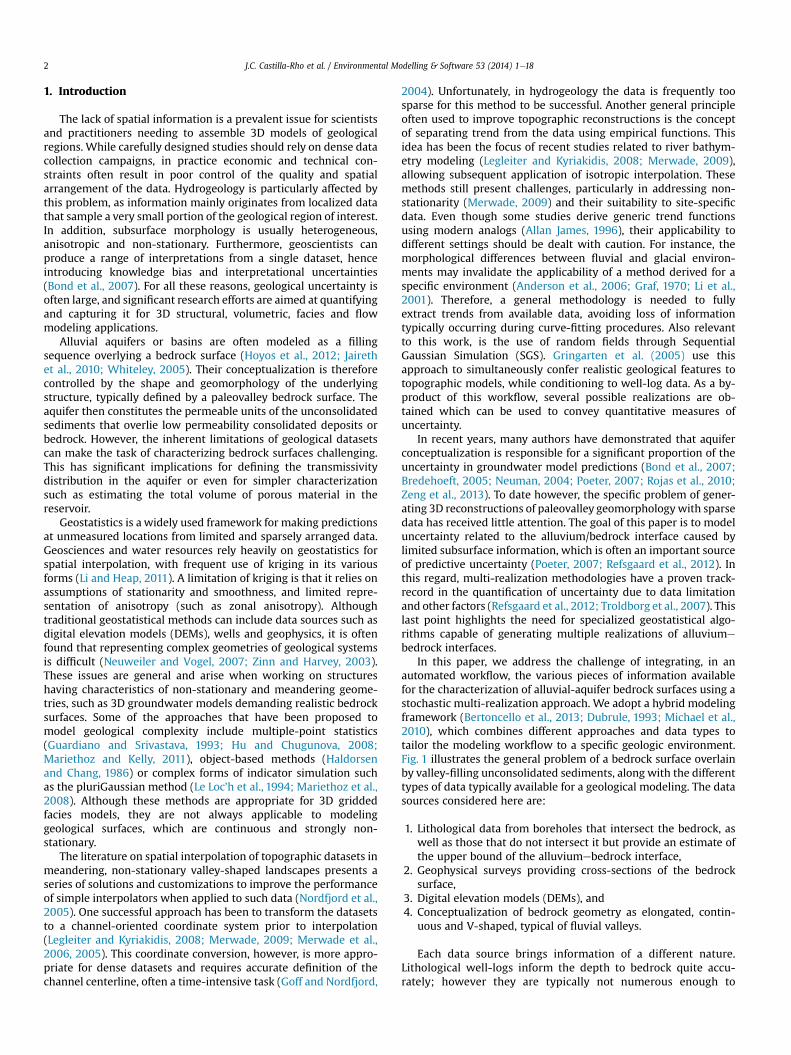
automated workflow, the various pieces of information availablefor the characterization of alluvial-aquifer bedrock surfaces using astochastic multi-realization approach. We adopt a hybrid modelingframework (Bertoncello et al., 2013; Dubrule, 1993; Michael et al.,2010), which combines different approaches and data types totailor the modeling workflow to a specific geologic environment.Fig. 1 illustrates the general problem of a bedrock surface overlainby valley-filling unconsolidated sediments, along with the differenttypes of data typically available for a geological modeling. The datasources considered here are:

1. Lithological data from boreholes that intersect the bedrock, aswell as those that do not intersect it but provide an estimate ofthe upper bound of the alluviumebedrock interface,

2. Geophysical surveys providing cross-sections of the bedrocksurface,

3. Digital elevation models (DEMs), and4. Conceptualization of bedrock geometry as elongated, contin-

uous and V-shaped, typical of fluvial valleys.

Each data source brings information of a different nature.Lithological well-logs inform the depth to bedrock quite accu-rately; however they are typically not numerous enough to

Fig. 1. Illustration of different types of input data typically needed for mapping buried bedrock surfaces.

J.C. Castilla-Rho et al. / Environmental Modelling & Software 53 (2014) 1e18 3

reliably infer the spatial variability and non-stationarity (or todetermine horizontal variograms). Geophysical surveys, such aselectrical resistivity or gravimetric profiles, are a useful source ofinformation since they delineate the bedrock depth and non-stationarity along certain cross-sections. Surface geophysicshowever suffers non-uniqueness and is prone to interpretationalerrors, which may be an important source of uncertainty (Kirsch,2008). Furthermore, these cross-sections may be relatively farapart and often do not cover the entire domain. This is whereassumptions have to be made about the continuity of themorphological features between observed profiles. Such as-sumptions need to be guided by established geomorphologicalconcepts about the structure of paleovalleys to realisticallycombine well and geophysical data.

Most of these morphological concepts can be represented bygeological analogs obtained from bedrock outcrops, experimentalsimulations, or observations from the present landscape. Geologicalanalogs have been widely used in geological modeling (Alexander,1993; Caers and Zhang, 2004; Enge et al., 2007; Friedmann et al.,2003; Grammer et al., 2004; Jones et al., 2008; Liu et al., 2004;Pringle et al., 2006; Tye, 2004), although they have not beenapplied to the specific problem of reconstructing paleovalley sur-faces. Our method extends the use of the analog approach for thispurpose, including typical characteristics of fluvial incision intobedrock such as profile convexities, knickpoints and irregular scourpatterns (Gardner, 1983; Phillips and Lutz, 2008; Seidl and Dietrich,1993; Shepherd and Schumm, 1974; Stock and Montgomery, 1999;Whittaker et al., 2007).

This study develops a methodology that is demonstrated onincised fluvial valleys, but with minor modifications the method isgenerally applicable for generating surfaces of glacial valleysthrough to ocean trenches. The paper outlines the overall workflowof our paleovalley bedrock interpolation technique, investigatinghow it addresses the challenge of integrating data of different na-ture, scale and resolution. Two examples are presented. The first is asynthetic meandering channel generated using a generic sinewave.In this example, the methodology is validated through an uncer-tainty characterization exercise, where we assess the potential tocapture large-scale morphological variability. The second exampleuses lithological well-logs and gravity survey data from the Azapavalley aquifer in Northern Chile, representing a typical case oflimited field data. This second application also demonstrates theincorporation of small-scale spatial variability using geologicalanalogs.

Our methodology is intended to complement available methodsand improve uncertainty characterization in groundwatermodeling. The methodology may be used to better evaluate theeffects of uncertainty and data limitation on water resource as-sessments, because it addresses an important and often overlookedcomponent of a hydrogeological conceptual model: the bedrockealluvium interface. This method is sufficiently simple and economicto be applied in resource-limited projects.

2. Methodology

The core of our approach is to pair each point of the unknown bedrock surface tolocations on geophysical cross-sections located on either side of it. The pairing ischosen such that a simple interpolation method enables smooth propagation of thegeophysical profiles, while ensuring continuity of the overall paleovalley shape.Pairing is accomplished by first determining the channel axis, or centerline, and thenpropagating locally observed features along the channel axis.

The approach is subdivided into three main steps:

1. Construct one or more trend surfaces consistent with known bedrock data.These trend models aim to capture the large-scale (first-order) topographicuncertainty of the paleovalley;

2. Generate a series of stochastic, equally likely error surfaces corresponding todepartures from the trend surface. The stochastic component is based ongeological analogs, and is used to impair natural variability to the bedrock sur-face. The error surface also confers geological realism and local conditioning toknown bedrock elevations (typically well-log data). Its aim is to capture thesmall-scale (second-order) morphological uncertainty; and

3. Combine the trend surfaces and stochastic models to create a final ensemble ofconditional model realizations.

These steps are developed in the following sections.

2.1. Trend surfaces

2.1.1. Input dataInput data consists of geological information stored in a Cartesian coordinate

system. Firstly, we focus on the aquifer boundary (x,y,z) data, depicting the limitbetween the alluvial aquifer and outcropping bedrock. These data can be obtainedfrom several sources such as aerial photographs, digital elevation models (DEMs),geological maps or existing GIS databases. Secondly, our methodology takes intoconsideration cross-sections, which delineate 2D slices of the bedrock at eachgeophysical transect. The latter are also incorporated as (x,y,z) points and can beinferred from either gravimetric, seismic, electromagnetic and resistivity surveys, ora combination of them. Fig. 1 summarizes the typical forms of input data. We as-sume, as is often the case, that considerable spacing exists between transects. It isthese sparser data arrangements that are challenging for conventional interpolation.

2.1.2. Finding the channel centerlineIn hydrological studies such as modeling of river bathymetry, where the

topography is accessible and data density is often large, it is generally possible todetermine the thalweg and use it as a centerline (see Merwade et al., 2006).

J.C. Castilla-Rho et al. / Environmental Modelling & Software 53 (2014) 1e184

However, in the case of subsurface topography the location of the minimumelevation line (analogous to the thalweg in hydrology) is unknown. To address thisproblem, we trace the channel centerline along the length of the aquifer byemploying the skeletonization algorithm used in mathematical morphology (Goldand Snoeyink, 2001; Gonzalez et al., 2009; Haunert and Sester, 2007; Niblacket al., 1992; Serra and Soille, 1994). A similar approach has been used in thecontext of river modeling (Bangmei et al., 2010).

The skeletonization method obtains the medial axis of a convex region bysequential thinning of a geometrical shape until the resulting figure is one pixelthick, while preserving the connectivity properties of the original shape, as shown inFig. 2aec. This algorithm often produces unwanted features protruding from theextracted centerline, known as spurs or parasitic components (Bangmei et al., 2010;Gonzalez et al., 2009), which are easily removed during a post-processing step. Sincethe skeletonization and spur removal sequence produce a unique result, the channelcenterline can be obtained automatically and unambiguously (Fig. 2d). Defining thepaleochannel centerline in this manner is a key component in the proposed method,because it allows generating a customized interpolation grid that follows the sin-uosity and meandering nature of the fluvial depositional system.

The skeletonization algorithm is capable of producing a centerline from any typeof irregular shape depicting the general outline of the region of interest. In itssimplest form, this outline would correspond to outcropping bedrock at the outeredges of the paleovalley. Alternatively, in the absence of outcrops, a suitable outlinemay be obtained from the interpretation of geophysical surveys, geological maps oraerial photographs.

2.1.3. Uniform grid space discretizationTo implement customized grids within our interpolationworkflow, we combine

the centerline extraction routine with the concept of interim cross-sections (Goffand Nordfjord, 2004; Merwade et al., 2008). This facilitates the automatic defini-tion of a uniform grid conforming to the specific paleochannel geometry beingstudied. Interim cross-sections are created between surveyed transects, that areequally spaced and orthogonally oriented with respect to the centerline (Fig. 3a,b).The number of interim sections to be created depends on several factors includingpaleochannel sinuosity, distance between surveyed cross-sections, desired along-channel resolution and shape of the aquifer boundary. In the context of river ba-thymetry, Merwade et al. (2008) comment on the maximum number of interimcross-sections that can be created in this manner, to avoid two adjacent cross-sections intersecting.

At this point, all interim cross-sections are discretized in a fixed number ofinterpolation nodes (Fig. 3a,b). This number, representing the level of discretization,depends on the desired across-channel model resolution. The lateral resolutionshould be at least equivalent to that of the surveyed cross section data. However, alarger number of nodes are recommended, as it does not dramatically increasecomputation times due to the simplicity of the final interpolation step describedbelow. Given that the channel width can vary along its profile and that the numberof nodes is fixed, the spacing between two neighboring nodes within interim sec-tions may vary along the channel. The (x,y) location of each of these nodes is storedin two separate M by N rectangular matrices, where M defines the number ofinterpolation nodes and N is the number of interim cross-sections, respectively(Fig. 3b). A matrix of the same dimensions (Z) is used to separately store theelevation data.

2.1.4. Locating the trajectory of channel minimum elevationOnce the uniform interpolation grid has been defined, we consider the problem

of maintaining coherent paleovalley morphology within the model. This can be

Fig. 2. Examples of the use of the skeletonization method from mathematical morpholoapplication on a meandering channel for centerline delineation.

understood as conserving the typical elongated U or V shape of the bedrock whileallowing for non-stationarity (i.e. a general longitudinal trend in the slope of thevalley bottom elevation and the meandering nature of the valley). For this purpose,we identify a valley minimum elevation on the known cross-sections and propagateit through the matrix representation of the bedrock surface Z (see Fig. 3c,d).

If the discretization of the interpolation grid Z is different from the resolution ofthe transect data, the data are interpolated using cubic splines or linear interpola-tion. This information is stored in the first and last columns of Z (columns 0 and N).The row positions of the z values corresponding to the minimum channel elevationare identified on these first and last columns. Then, a linear interpolation of theseindexes is performed, generating a vector of row index locations for each interimcross-section. The resulting vector corresponds to the expected location of the valleybottom along the model space. A graphical representation of this procedure ispresented in Fig. 3d.

2.1.5. Non-uniform grid adaptation for pairing of cross-section data pointsAfter completing the task of estimating the paleovalley minimum elevation axis,

the model space is discretized into a non-uniform grid in preparation for interpo-lating the remaining bedrock surface. Previous steps have located the nodal positionof the valleyminimum for each interim cross-section, but often the number of nodeson each side of the minimum will not be equal (see Fig. 3c,d) due to the generallyasymmetrical shape of paleovalleys. In the previous step, the uniform grid wasestablished exclusively to locate the points defining the valley minimum. Now, thetotal number of interpolation nodes on any interim cross-section is halved andplaced on each side of the valley minimum (Fig. 3f). This new non-uniform inter-polation grid maintains the number and location of interim cross-sections definedearlier, but the number and location of nodal points is redefined. The above gridadaptation is performed automatically, and illustrated in Fig. 3c,d (before redis-cretization) and Fig. 3e,f (after rediscretization).

Maintaining equal number of paired interim cross-section nodes across themodel is a key feature in the algorithm for several reasons. First, this allows pairingeach node with others located either upstream or downstream. The concept ofhaving a paired non-uniform interpolation grid is analogous to a fictitious longitu-dinal cross-section that travels from one (known) surveyed transect, which thenmorphs downstream and finally matches a downstream surveyed transect. Thiscorresponds to an explicit assumption of valley continuity as an elongated U or Vshape guided by geophysical cross-section data. Second, pairing allows significantreduction in computational resources, as simple linear interpolation proceduresbecome sufficient once the non-uniform grid is created. Third, a paired grid spaceallows storing and manipulating the data in rectangular matrices (Fig. 3f), withoutthe channel-oriented coordinate transformation proposed by several authors (Goffand Nordfjord, 2004; Legleiter and Kyriakidis, 2008; Merwade, 2009).

2.1.6. Simple spatial interpolation using channel distanceAs a result of discretizing the model grid in a paired manner, spatial interpola-

tion of bedrock elevation proceeds by propagating surveyed data along this grid inthe upstream and downstream directions. By propagating morphological data alongthe channel direction, we are able to enforce our main morphological assumptions,such as connectivity of the deepest portions of the bedrock surface for a fluvialvalley, the general elongation of the system and a V-shape or U-shape cross-section(depending on the measured cross-sections).

Meandering geometries such as paleochannels often have non-convexity: a lineconnecting two points in the paleovalleymay lie outside the paleovalley boundaries.Therefore, Euclidean distance is not an appropriate distance metric for interpolation.To solve this problem, we incorporate the concept of water distance as defined in

gy. (a)e(c) Schematic representation of skeleton extraction from binary images; (d)

Fig. 3. Illustration of the algorithm. (a), (b) Uniform discretization based on the extracted centre line, location of survey data, interim cross-sections and its matrix representation;(c), (d) locating the line of steepest descent within the uniform grid; (e), (f) grid adaptation by pairing nodes between interim cross-sections and notation used to calculate channeldistances.

J.C. Castilla-Rho et al. / Environmental Modelling & Software 53 (2014) 1e18 5

(Rathbun, 1998), but apply it in a slightly different manner. We define the notion ofchannel distance as the length of the path connecting two cross sections, which hasthe following characteristics: (1) is fully contained within the alluvial-aquiferboundaries, and (2) follows the natural sinuosity of the paleovalley.

Incorporating the concept of channel distance is simplified by using the matrixformulation presented in Fig. 3. Fig. 3e shows a synthetic channel segment with aseries of interim cross-sections, surveyed transects and interpolation nodes. For ameandering system, the channel distance between two paired nodes depends onthe relative location within the cross-section. For instance, channel distance AeA0

(inside of bend) is much shorter than distances BeB0 (channel centerline) and CeC0

(outside of bend). These distances are estimated by summing all individual linearsegments located between two paired nodes, as shown in Fig. 3e,f. Channel dis-tances DU (distance to upstream surveyed transect) and DD (distance to downstreamsurveyed transect) are then given by:

DUðm;nÞ ¼Xn

k¼2

Ddðm;k�1Þ�ðm;kÞ (1)

DDðm;nÞ ¼XN�1

k¼n

Ddðm;kÞ�ðm;kþ1Þ (2)

wherem is the node index, n is the cross-section index and N is the total number ofcross-sections (including the two surveyed transects). The final spatial interpolationis obtained by creating matrices containing DU(m,n) and DD(m,n) values for each node.The elevation at an interim node is computed as a weighted average of the corre-sponding (paired) upstream and downstream survey nodes, using channel distancesDU and DD.

J.C. Castilla-Rho et al. / Environmental Modelling & Software 53 (2014) 1e186

zðm;nÞ ¼ zðm;1ÞDUðm;nÞ þ zðm;NÞDDðm;nÞDUðm;nÞ þ DDðm;nÞ

(3)

where z(m,n) is the topographical elevation at any given node. Outside surfacenodes for each interim cross-section (i.e. next to the land surface channelboundary) adopt the known elevation of the bedrockealluvium boundary.Treating surface boundary nodes in this manner offers a simple way of integratingthe paleovalley bedrock model with contiguous DEM topographic data. Ulti-mately, a matrix of interpolated z values is obtained which defines the shape of thepaleovalley bedrock surface.

One common problem related to the acquisition of geophysical datasets is theoccurrence of natural or anthropogenic obstacles that prevent the ideal locationof sampling points. As a consequence, geophysical transects are rarely orientatedperpendicular to the valley axis. In these circumstances, interim cross sectionsare extended past the surveyed transects, elevations are interpolated using Eq.(3), and finally the nodes outside the region of interest are clipped from themodel.

2.2. Bedrock stochastic deviations

We use stochastic topographic simulations superimposed on the bedrocktrend surfaces, in order to reproduce the small-scale variability of subsurfacetopography and to characterize the related (second-order) geological uncertainty.These stochastic realizations have a zero mean, and add autocorrelated noise ontop of the trend without changing its overall shape. Multiple plausible represen-tations of the bedrock shape are calculated to quantify this second-order source ofuncertainty. In this study we use Sequential Gaussian Simulation as a perturbationmethod, although any continuous geostatistical simulation method would besuitable. SGS uses a parametric model (the variogram) that describes the small-scale variability of the bedrock topography. Our implementation employsSGEMS (Remy et al., 2009) with the mGSTAT interface (Hansen, 2004) to generatemultiple realizations of conditional topographic variability for the paleovalleysurface. In the particular case of SGS, small-scale topographic variability (i.e. theerror surface) is assumed to have a Gaussian distribution with parameters ob-tained from the kriging mean and variance. In our method, variograms are thechosen tool used to transfer the analog information into the bedrock surfacepredictions. They allow us to confer a realistic variability valley profile, resemblingthe typical characteristics of river incision into bedrock, such as a longitudinalprofile presenting irregularly-spaced scour highs and lows (Shepherd andSchumm, 1974). SGS however requires valid assumptions about the variogrammodel to be employed, which ultimately depends on site-specific geological fea-tures. One option is to utilize the topographic variations observed in local bedrockoutcrops. This strategy, along with alternative approaches, is discussed later in thispaper, when applying the methodology to the reconstruction of a real paleovalleybedrock surface in Chile.

Since SGS is a conditional method, it is used to impose further constraints onthe generated bedrock surface, such as elevations at points where the bedrocklocation is known from lithological well-logs and known elevations along theground-surface/paleovalley boundary (e.g. local outcropping). SGS-simulateddeviations from the trend are conditioned to the difference between a knownbedrock elevation and the elevation of the trend surface at the surveyed location,resulting in modeled bedrock elevations corresponding to the measured values.Since the interpolated trend is already conditional to intersections of the bedrockwith the surface topography, the boundaries of the domain are conditioned to avalue of zero.

In addition to conditioning using lithological well-logs, in certain cases it may bedesirable to introduce conditioning to the paleovalley minimum elevation of the 2Dtrend surface. For example, the modeler can impose different types of erosion pat-terns along the longitudinal profile of the valley, corresponding to distinct as-sumptions about the incision process. These assumptions may be related to differentconceptualizations about the sediment and rock strength controls or climate re-gimes during the development of the valley; for examples see Finnegan et al. (2005),Gardner (1983), Shepherd and Schumm (1974), Sklar (2007). By using this approachmany of the features found in modern and experimental analogs of bedrock incisionmay be incorporated into themodels. Most importantly, the approach offers ameansof exploring the smaller scale morphological uncertainties in the estimation of thepaleovalley shape.

Although in this study we focus on alluvium-filled incised bedrock valleys,simple customizations of this step allow for application to other types of paleo-channels, such as glaciated valleys. Glacial valleys, in contrast to fluvial V-shapedvalleys, are characterized by U-shaped troughs and a smoother longitudinal profilewith a larger-scale erosional footprint (Anderson et al., 2006; MacGregor et al.,2000). Therefore, for other morphologies the modeler may choose variogramswith a higher range and smaller variability to impair general smoothness of theglacial incision signature along the valley (Anderson et al., 2006).

The final step is to superimpose the trend and stochastic components of themodel; SGS realizations are combined with one or many trend surfaces, producingmultiple equally likely realizations of the bedrock surface. Fig. 4 presents a completeflowchart of our algorithm, describing the sequence of steps leading to a set ofstochastic realizations of the paleovalley topography.

3. A synthetic example

3.1. Input datasets

For the synthetic example, we consider a simple sine wavechannel and four synthetic generic surveyed cross-sections(Fig. 5a,b). Cross-section six (CS6) is included in the analysis toshow the effect of a stronger variation in channel depth.

3.2. Trend surfaces

The sequence of steps leading to a trendmodel is summarized inFig. 5cel, starting from extraction of channel centerline throughskeletonization and spur removal (Fig. 5cee); creation of interimcross-sections with subsequent location of bedrock minimumelevation (Fig. 5f) and final interpolation (Fig. 5g) to obtain a trendsurface.

A visual comparison of 2D trend surfaces for different pairs ofsurveyed cross-sections (Fig. 5gel) demonstrates that the methodis capable of producing non-stationary trend models of the paleo-valley. The trend model varies depending on which cross-sectionsare considered. The lateral position of the deepest point of thebedrock surface is different for each case, because it changes po-sition between surveyed transects. Overall, the reconstructedchannel corresponds to our earlier definition of channel continuity:consistent, elongated bodies maintaining longitudinal coherence ofthe channel morphology.

A trend surface with stronger elevation gradient is presented inFig. 5h, showing the ability to reproduce both linear (bed slope) andnon-linear (cross-section shape) trends. The resolution of the trendmodel can be customized according to specific modeling needs, asboth the number of interim cross-sections and transverse inter-polation nodes are parameters defined by the user. From our tests,interpolations considering higher model resolution only generatemarginal increases in computation time. Finally, we present themodularity of this approach when three trend models are stitchedtogether producing consistent fits (Fig. 5kel). This demonstrateshow trend surfaces can be constantly updated as new field data iscollected, and easily incorporated into existing models. In addition,comparison of Fig. 5g and l illustrates how the final trend surfaceimproves as more survey cross-sections are considered and com-bined through the stitching process.

The need to define the trajectory of the channel minimum ispresented in Fig. 6a, which shows a surface that has not beenconstrained to have the deepest values connected along a line ofsteepest descent. Here, the trend surface is a smooth transitionbetween the two survey profiles, with a flat section in the middle.In contrast, Fig. 6b shows that the inclusion of the minimum valleytrajectory by the process of grid adaptation and node pairing en-sures that the model conforms to the general morphological un-derstanding of the system. This demonstrates the importance ofincorporating the geomorphological knowledge of the overallshape associated with a buried paleovalley system. Moreover, it ispossible to consider alternative interpretations of the geophysicaldata to obtain alternative trend models, for example using aBayesian approach. Combinations of different paleovalley axis tra-jectories with several geophysical interpretations will produce aneven larger ensemble of trend models, with greater variability.

3.3. Adding the stochastic component

Generating the stochastic component of the valley can beapproached in several ways, depending on how the variabilitysurfaces are conditioned to hard data. Before generating stochasticdata, DEM elevation data needs to be imposed to the surface

Fig. 4. Flowchart representation of the algorithm developed for the stochastic construction of paleovalley bedrock surfaces from DEMs, geophysics and well-log data.

J.C. Castilla-Rho et al. / Environmental Modelling & Software 53 (2014) 1e18 7

expression of the aquifer boundaries as conditioning data, whichfor most locations can be obtained from raster satellite imagery.Fig. 5m shows the result of combining the trend surface of Fig. 5hwith a SGS model of small-scale variability, and the characteristicfluvial incision signature consisting of scour lows that is impaired(Shepherd and Schumm, 1974). Here, it is important to note thatalthough the SGS surface is stationary, along the longitudinal axis ofthe valley the resulting scour highs and lows are irregularly-spaced.Alternatively, the SGS realizations can be locally conditioned todepict different types of incision processes. Fig. 5n shows onerealization with a smoother incision footprint (compared toFig. 5m) along its longitudinal profile, obtained by constraining theSGS surface along the paleovalley bottom axis.

Fig. 5m,n shows only one of the many possible stochastic re-alizations that can be obtained. For the models presented inFig. 5m,n, an arbitrary set of Gaussian model parameters whereused, however in a real study the variogram parameters can beinferred from the topographic variability of outcropping bedrock or

any other type of geological analog (more details and discussion inSection 4.3). Finally, the SGS noise surface can be conditioned tobedrock depth data fromwells, as presented in Section 4, where themethodology is applied to the reconstruction of a real paleovalleyin Chile.

3.4. Characterization of large-scale uncertainties

Although SGS allows impairing small-scale (second-order)variability, it does not account for large uncertainties (first-order) inthe trend itself. An uncertainty analysis was done based onmultiplesynthetic paleovalley realizations to assess large-scale topographicuncertainties for varying sampling densities. This analysis canalso provide some insights on how to select future samplinglocations.

To compare the uncertainty results with a reference we con-structed a synthetic paleochannel reproducing some essentialcharacteristics of fluvial bedrock incisions such as: (1) knickpoints;

Fig. 5. Stepwise reconstruction of a synthetic paleovalley. (a), (b) Synthetic cross-sections; (c) paleochannel converted into binary image; (d) centerline extracted by skeletonization,with spurs; (e) centerline after spur removal; (f) interim cross-sections and linear approximation of maximum depth of the paleovalley; (g)e(l) trend surfaces for differentcombinations of synthetic cross-sections; (m) final reconstruction after addition of SGS noise to the trend surface, conditioned only to DEM elevations at the aquifer boundary; (n)final reconstruction after addition of SGS noise to the trend surface, conditioned to DEM elevations at the aquifer boundary and maximum depth of paleovalley from the trendsurface. Note in (m) the characteristic signature of bedrock incision, comprised of scour highs and lows. (h) is the trend surface for plots (m) and (n).

J.C. Castilla-Rho et al. / Environmental Modelling & Software 53 (2014) 1e188

(2) irregularly-spaced bedrock scour highs and lows; (3) longitu-dinal profile convexities; and (4) non-stationary longitudinal andtransverse incision, as shown in Fig. 7 (Gardner, 1983; Phillips andLutz, 2008; Seidl and Dietrich, 1993; Shepherd and Schumm, 1974;Stock andMontgomery,1999;Whittaker et al., 2007). Although thisis a specific test example, it represents a typical and challenginggeological scenario that is likely to be encountered in the field.

The uncertainty in capturing the longitudinal profile and inci-sion morphology of the paleovalley was assessed, as illustrated inFig. 8. These plots show the rapid convergence of the methodology,and its capacity to capture the large-scale topographic uncertaintywith relatively few surveys (s > 4). Fig. 8 also shows that an accu-rate estimation of the aquifer volume does not necessarily corre-spond to an accurate prediction of the longitudinal profile.

Using the fully known reference bedrock surface describedabove, we evaluated the effect of sparser survey datasets on thetopographic uncertainty. Fifty random realizations were generatedfor a relatively dense sampling strategy, and an equal number ofrandom realizations for progressively thinned versions of thisdataset, with the final case consisting of a single cross-section. Eachof the fifty realizations within a specific sampling density repre-sents a random spatial arrangement of a fixed number s of surveylocations. Fig. 9 presents three of those realizations, obtained for asparse (s ¼ 1), two intermediate (s ¼ 4 and s ¼ 10) and one dense(s ¼ 25) sampling strategy. By analyzing the ensemble of re-alizations, it was possible to characterize the uncertainties associ-ated with cross-section density and cross-section spatialconfiguration.

Fig. 6. Visual comparison of employing an adaptive grid with paired nodes. (a) Nopairing; (b) paired nodes around the line of steepest descent. Note how this achievesand elongated, V-shape valley and enforces continuity.

J.C. Castilla-Rho et al. / Environmental Modelling & Software 53 (2014) 1e18 9

The top part of Fig. 9 shows a selection of three random re-alizations for each sampling density. Although for a single survey(s ¼ 1) the realizations are highly variable, a slight increase insampling locations (s ¼ 4) manages to capture the main features ofthe real topography, particularly the location of the knickpoint. Fors¼ 10 the knickpoint is fully constrained by the realizations, and fors ¼ 25 the variability between realizations is marginal and local-ized. A closer inspection of Fig. 8 reveals that the most accuraterealizations within each ensemble (#50 in Fig. 8) have one commonfeature: they sample the main non-stationarities of the paleovalley,the knickpoint’s lip and foot. In this regard, selecting sampling lo-cations using prior geological knowledge depicting the possiblelocation of knickpoints along the profile, has the potential to reducefield costs.

Fig. 7. Synthetic test paleovalley surface, including the main features o

The bottom part of Fig. 9 shows the spatial patterns of topo-graphic uncertainty for each sampling ensemble, visualized by theensemble mean and standard deviation summary statistics. On onehand, the ensemble means reinforces that this method constrainsthe realizations to the reference topography after a relatively smallnumber of surveys (s ¼ 4). The ensemble standard deviationsprovide insights about the spatial structure of uncertainty. Theseplots show that for a sparse data arrangement, the uncertainty islargest in the central part of the model and around the deepestportion of the paleovalley. It is interesting to note that for s ¼ 1, thearea of largest variability extends beyond the location of theknickpoint. In fact, for s ¼ 1 the largest uncertainty is not theknickpoint foot, but the bottom of the valley at the central meander(location A, Fig. 9). This is simply because a single survey cannotreproduce the knickpoint feature using our methodology.Increasing the sampling to s ¼ 4 clearly reveals three distinctsources of uncertainty: the knickpoint (location B, Fig. 9); theincision scour signature along the longitudinal profile (location C,Fig. 9); and portions of the valley with sharp transverse topography(location D, Fig. 9). Further increasing the number of surveys showsthat the topographic variability due to the knickpoint (B) is reducedby s ¼ 10 and eliminated by s ¼ 25, however the remaining un-certainties (C and D) remain almost unchanged. Overall, this showsthat by increasing the number of surveys it is possible to capturethe large-scale topographic trend, but not the small-scalemorphological uncertainties. Uncertainties (E) and (D) in Fig. 9are due to the discretization of the model and the quality of thegeophysical prospecting method, respectively. While (E) can betargeted by increasing the number of interpolation cross-sections,(D) will require higher transverse survey resolutions. Finally, thesmall-scale topographic uncertainties such as (C) are the target ofthe SGS step of our methodology, which is developed in Section 4.

An important and often highly uncertain parameter ingroundwater resource estimates is the total aquifer volume. Non-

f fluvial bedrock incision including knickpoint and scour features.

Fig. 8. Ensemble longitudinal profiles for four sampling strategies: s ¼ 1, s ¼ 4, s ¼ 10 and s ¼ 12. Note the rapid convergence to the reference longitudinal profile for s > 4.

J.C. Castilla-Rho et al. / Environmental Modelling & Software 53 (2014) 1e1810

stationarities such as knickpoints can make it challenging to esti-mate this aquifer volume. The ensemble volumes for a range ofsampling densities are shown in Fig. 10. For sparse sampling, theensembles present a strong bias to underestimate the volume,however this bias mostly disappears after s ¼ 5. The real aquifervolume is captured in some cases by even the sparser samplingdensities, but this may not correspond to the real longitudinalprofile. Therefore, pinpointing possible knickpoints in the paleo-valley with the help of prior geological knowledge, can potentiallyallow accurate estimations of volume with only a few surveys. In

Fig. 9. Three sample realizations and ensemble statistics for the characterization of large-ssparse (s ¼ 1), intermediate (s ¼ 4,10) and dense (s ¼ 25). The bottom part of the figure showfifty realizations.

fact, the four realizations labeled with #50 in Fig. 9 have approxi-mately the same volume, as they plot close to the red dashed line inFig. 10. The ensemble ranges of Fig. 10 also help understanding thereduction of statistical uncertainty that occurs with conductingnew surveys or drilling new wells. This figure may serve as anillustration of uncertainty reduction with further surveying. Forexample, for the given case (based on Fig. 10), it can be argued thatfuture prospecting should lie in the range s ¼ 5e15, because itremoves the underestimation bias whereas further samplingbeyond s ¼ 15 yields little gains in terms of reducing uncertainty.

cale topographic uncertainties. Columns depict different sampling densities includings the ensemble mean and standard deviation for each sampling ensemble, consisting of

Fig. 10. Ensemble aquifer volume estimation for different sampling densities. The reddashed line represents the volume of the reference surface of Fig. 7. (For interpretationof the references to color in this figure legend, the reader is referred to the web versionof this article.)

J.C. Castilla-Rho et al. / Environmental Modelling & Software 53 (2014) 1e18 11

4. Application to the San Jose River aquifer paleovalley

4.1. Study area and input data

The applied case study area is the San Jose River aquifer, a110 km long fluvial system draining the Azapa valley in NorthernChile (Fig. 11). The coastal area on Northern Chile (18�Se30�S) ispart of the Atacama Desert, recognized as the driest in the world(Houston and Hartley, 2003; Schulz et al., 2012). The Azapa valley ischaracterized by extreme aridity, with annual rainfall less than1 mm in most of the basin (Clarke, 2006). Other localities in thisregion, such as Iquique and Antofagasta have mean annual rainfallbelow 0.6 mm (Houston and Hartley, 2003) and certain rainfallmonitoring stations have never recorded rainfall. For this reason,groundwater exploitation has been developed in Atacama duringthe last century to sustain domestic and agricultural activitiesparticularly in the Azapa valley. Groundwater abstractions from thisaquifer greatly exceed the long-term sustainable diversion limit.Unfortunately, existing groundwater models that have beendeveloped to predict future conditions of the San Jose River aquiferare based on limited hydrogeological knowledge, and thereforehave considerable geological uncertainty. The Azapa valley wasformed by the down cutting of the San Jose River in rocks of theLiparitic (Miocene) and Porphyritic (Jurassic-early Cretaceous)Formations. Later in the Pleistocene, the San Jose River began to fillthe valley, a process that is ongoing today (Taylor, 1949).

Input datasets for this study consist of (x,y,z) points in Cartesiancoordinates. Pairs (x,y) correspond to geographical locations ac-cording to the UTM WGS84 datum and (z) is the height above sealevel. Elevations are assigned using 3 arc second (30 m resolution)ASTER Global Elevation Data from NASA’s Earth Observing SystemData and Information System (EOSDIS).

For the San Jose River aquifer several sources of spatial data areavailable: vertical cross-sections depicting the subsurface bound-ary between the alluvial fill and the bedrock derived from gravitysurveys (Fig. 11bef); lithological well-logs indicating depth to

bedrock; and the ground surface perimeter of the alluvium, rep-resented by the contact between the alluvium and the bedrocksurface (Fig. 11a). Cross-section data for this study was obtainedfrom the public archives of the Chilean General Directorate ofWater (DGA). In addition, seven lithological well-logs (Taylor, 1949)depicting depth to bedrock are considered (Fig. 11g). The alluvium/bedrock boundaries where digitized and georeferenced using theopen-source GIS package QGIS 1.8 and aerial images.

4.2. Bedrock reconstruction

A total of five geophysical cross-sections were interpolated andintegrated with well-log data to create the subsurface paleovalleymodel for the San Jose River aquifer. The interpolation sequence forthe whole basin is presented in Fig. 12aee. Fig. 12aed shows thesteps leading to the reconstruction of the trend model for thispaleovalley. As discussed earlier, the algorithm extracts a channelcenterline and then uses it to create a customized grid, defined by apreselected number of interim cross-sections and interpolationnodes. Pairs of geophysical transects are propagated across interimcross-sections, creating a 2D interpolated trend surface (Fig. 12d).

Superimposing correlated topographical noise creates the finalpaleovalley model. Steps depicted in Fig. 12d,e illustrate the addi-tion of SGS correlated noise to the trend surface, without condi-tioning to well-log data (an example including conditioning ispresented below). The SGS step can be repeated to obtain anensemble of equally likely bedrock surfaces, reflecting geologicaluncertainty (one such realization is shown in Fig. 12f).

Considering that the distance between each pair of geophysicalcross-sections is on average 10 km, which is challenging for mostconventional methods, the final reconstruction of the San Jose Riveraquifer paleovalley satisfies the main desired features:

(1) a continuous V-shaped elongated surface,(2) connectivity of the longitudinal profile in the downstream

direction,(3) adequate handling of sinuosity and variable orientations,(4) along/across-channel coherence of morphological features,(5) conditioning to hard-data,(6) a realistic geometry within the limits of the sparse data, and(7) the final reconstruction is non-stationary.

For the reconstruction presented in Fig. 12, we employed a totalof 700 interim cross-sections and 7� 105 interpolation nodes (1000per interim cross-section). Considering a total reach of 35 km andaverage width of 900 m, the paleovalley reconstruction mesh has aresolution of approximately 50m in the along valley profile and 1min the across-valley direction. From a user perspective, the methodrequires very few parameters and is economical in terms ofcomputation since only linear (or spline) interpolations are per-formed. The only parameters that are needed correspond to thenumber of interpolation nodes and interim cross-sections.Although this step can be automated, it provides an opportunityfor the practitioner to adjust the model’s resolution in terms of thesize of the interpolation domain and available CPU resources.

Since the Azapa valley presents a relatively straight path alongits profile, in this specific example we make very simple assump-tions about the location of the valley bottom. Here, the deepest partof the valley is located by linear interpolation (see Fig. 3d).Although herewe do not explicitly introduce a geological analog forthe location of the deepest part of the valley, our methodologyenforces the general notion that erosion is concentrated on theoutside of a bend (Shepherd and Schumm, 1974). This is preciselywhat is shown in Fig. 12b, between transects T1 and T2. In theremaining parts of the model, the deepest part of the valley is

Fig. 11. Study area and data in Azapa valley, northern Chile. (a)e(e) Vertical transects of basement depth obtained from Gravimetry studies; (f) Lithological well-log data providingdepth to bedrock (Taylor, 1949). Horizontal axes in (a)e(e) represent distance from northern boundary of the paleochannel.

J.C. Castilla-Rho et al. / Environmental Modelling & Software 53 (2014) 1e1812

locally constrained by the position indicated on the survey tran-sects. Despite the simple assumption described above, any type ofsoft geological knowledge can be included. Similarly, variations onthe step described in Section 2.1.4 will allow the modeler to ‘steer’the valley in a desired direction.

4.3. Characterization of small-scale uncertainties

An important step in this methodology is the selection of anappropriate variogram model to guide the SGS process. This step isaimed at characterizing the small-scale component of topographicuncertainty, such as the erosion signature along the longitudinalprofile. In most situations no data are available to infer the base-ment surface spatial variability, however this can be solved byadopting an analog approach, which we demonstrate below.

To demonstrate the analog approach, we selected an area thatcharacterizes the expected texture of the paleovalley: a6.5 � 2.5 km polygon of denuded bedrock is chosen and used toinfer statistics for a representative model of topographic variability(Fig. 13). This polygon is located at Quebrada Las Lloysas, an outcropof the Liparitic Formation which forms the bedrock for most of thelower south slopes of the valley (Taylor,1949). It may be argued thatthe choice of this particular analog is not optimal, as the sur-rounding outcropping rock may not convey accurate informationabout the valley floor variability. We point out that local bedrockoutcrops are only one of many possible ways to supplement thepaleovalley reconstruction with a geological analog. Other appro-priate options for analogs are modern landscapes undergoingcomparable erosional processes, outcrops from different locationsand results from experimental simulations. Where a modern

Fig. 12. Stepwise reconstruction of the Azapa paleovalley. (a) Extracted centerline using a binary image of the channel and skeletonization; (b) adaptive grid and approximation ofthe paleovalley bottom; (c)e(d) propagation of geophysical transect data through the grid to obtain a trend surface; (e) generation of a SGS noise surface conditioned to the DEMelevations, well-log data and local topographic variability; (f) final model of the Azapa valley after superimposing trend þ SGS surfaces.

J.C. Castilla-Rho et al. / Environmental Modelling & Software 53 (2014) 1e18 13

analog is not available, geologists may derive synthetic variogramsbased on their conceptual understanding of the system. Refer toAlexander (1993) for a detailed discussion about the appropriateselection and implementation of geological analogs.

We borrow the variogram characteristics of the analog andimpose them on the bedrock surface predictions. Variograms allowconferring a realistic variability valley profile, resembling the

typical morphological characteristics of bedrock incision (e.g.irregularly-spaced scour lows), as shown in Fig. 5m. Within theselected sampling site, we extracted the DEM elevations (Fig. 13a),then estimated a topographic trend using a moving average algo-rithm (Fig. 13b), and finally subtract the trend from the DEM ele-vations to obtain a residual surface (Fig. 13c). The moving averageprocedure allows separating the large-scale geological trend from

Fig. 13. Illustration of using a surface sampling area to capture topographic variability at the study site. (a) DEM elevations; (b) resulting surface after applying a moving averagesmoothing filter; (c) residual surface; (d) directional variograms of residual surface.

J.C. Castilla-Rho et al. / Environmental Modelling & Software 53 (2014) 1e1814

Fig. 14. Visual comparison of the interpolation process conditioned with different levels of conditioning to hard data, between transects T2 and T3. (a) Plan view of trend surfaceand well locations; (b) 3D view of trend surface and well locations. First column is for conditioning only to DEM elevations at the aquifer boundaries, (c)e(f)e(i). Second columnshows conditioning for DEM elevations and paleovalley bottom (d)e(g)e(j). Third column adds conditioning to wells data (e)e(h)e(k).

Table 1Well-log data available for conditioning the SGS surface. Conditioning elevations arecomputed as the difference between the lithological well-log and trend at thelocation. Well notations have been maintained from (Taylor, 1949).

Well Basement elevationfrom well log [m]

Basement elevationfrom trend surface [m]

Conditioning elevationfor SGS surface [m]

(1) (2) (1) � (2)

LR4 241 260 �19LR1 234 239 �5LR2 234 232 2LR3 232 264 32A2 200 165 35A3 214 182 32A1 215 217 �2

J.C. Castilla-Rho et al. / Environmental Modelling & Software 53 (2014) 1e1816

the small-scale spatial variability. This surface represents theroughness and texture that we would like the models to convey.The residual surface is inspected in several orientations, by calcu-lating experimental variograms along four directions, as shown inFig. 13d. Although there is evidence of weak anisotropy, we havedecided to assume isotropy because we only aim at representingsmall-scale spatial variability. For sparse datasets with large con-ceptual uncertainty, and difficulty in choosing analogs, finelymodeling this slight anisotropy would mean overparameterizingour model, therefore a single Gaussian structure is fitted to the data(Sill ¼ 68, Nugget ¼ 0, Range ¼ 250). Although employing a singlevariogram across the whole paleovalley carries an assumptionabout stationarity, this is compensated by the fact that trend sur-faces created prior to this step are non-stationary and hence thefinal models will maintain this characteristic. In the presence ofzonal variability, a number of variograms could be derived andapplied along different reaches of the valley.

The SGS step also includes conditioning to hard geologic data, astep that introduces flexibility and additional modeling capabil-ities to the reconstruction process. Fig. 14 presents the super-position of correlated SGS noise conditioned to bedrock depthinformation extracted from lithological well-log data in an areabetween geophysical transects T2 and T3 (Fig. 14a,b). Two north-south geological cross-sections have been inferred from wellsdrilled for crop irrigation in the Azapa valley (Taylor, 1949),showing the Liparitic bedrock surface under the Pleistocene andrecent alluvial fill. Table 1 summarizes the available conditioningdata from these wells, elevations to the bedrock contact interfaceand the departure of the actual depths from the trend surface. Itshould be noted that the SGS implementation requires condi-tioning data to be expressed as trend departures and not absoluteelevations above sea level. These lithological well-logs offer moreprecise, but discrete (and sparse) information of the bedrocksurface, when compared to geophysical data that tends to becontinuous. Integrating the two data sources occurs when thetrend surface, derived using geophysical surveys, is adjusted tothe well-log data using conditional SGS. Special care needs to betaken here, as geophysics is often tied to well-log data for cali-bration and guiding of the inversion processes. To avoid re-dundancies, well-log data used for the SGS step needs to beindependent of the geophysical data. We took this into consider-ation for the Azapa valley reconstruction.

Fig. 14a,b shows two views of the trend surface obtained fromgeophysical transects, and the location of conditioning wells.Fig. 14cee presents the trend departure surfaces created using SGS.Fig. 14c is conditioned to the DEM only whereas Fig. 14d is condi-tioned to the DEM and the valley bottom. Fig. 14d demonstrateshow the incision signature can be controlled by constraining thetrend departure surface along the deepest portion of the paleo-valley. The small-scale variability surfaces shown in Fig. 14cee areadequate for a fluvial valley undergoing a filling process, becausethey convey the characteristic longitudinal profile scour pattern ofthese systems. Fig. 14e further adds conditioning to well-log data. Itis important to note how the SGS variability surface of Fig. 14ehonors the conditioning data given in Table 1. Very little variabilityneeds to be introduced in some locations (wells LR4, LR5 and A1),indicating that the trendmodel is capable of capturing here the realdepth to bedrock. In other locations, such as wells A2, A3 and LR3this correspondence is not equally satisfactory and the SGS surfacepresents larger departures. Fig. 14feh presents the superposition ofthe previous SGS perturbation surfaces to the trend model ofFig. 14a. These figures illustrate the effects that different combi-nations of geological data and prior knowledge have on the finalpaleovalley. Fig. 14iek presents a 3D view of the resultinggeomodels.

5. Discussion and conclusions

In this study we have introduced a stochastic, data-drivenworkflow for constructing paleovalley bedrock surfaces by inte-grating geophysical, DEM and lithological well-log data with softgeological knowledge. The technique was validated on a syntheticsine wave channel, and then applied to an alluvial aquifer in theAzapa valley in Northern Chile. Geophysical transects, althoughoften far apart, contain valuable information about the bedrockdepth and non-stationarity, which can be translated to a generaltrend model of the paleovalley. Lithological well-log data providediscrete but accurate bedrock depths, hence it is more suitable forinforming the local topography and for guiding a stochastic con-ditioning process, such as SGS. Finally, DEM raster images can beused to infer small-scale bedrock variability and to integrate thefinal model with the surrounding topography. This study illustratesthat the inclusion of conceptual geological knowledge in theworkflow improves howwe combine sparse data at multiple scalesand resolution. Although subjective and conceptual, geologicalanalogs convey important information about erosional processesthat shaped the landscape. This information would be difficult tocapture from an individual lithological well-log, the DEM, orgeophysical data.

In contrast to hard data, soft knowledge often comes in a moreabstract form, as general concepts about sediment transport, geo-morphology and erosion. These represent the type of informationthat is commonly available to guide the construction of geologicalsurfaces. The differing nature of each data source and their intrinsiclimitations pose a challenging and ubiquitous problem for hydro-geologists using existing interpolation tools. To solve these issues,we have developed and tested a methodology that adapts andcombines established methods from previous research in riverbathymetry modeling, structural geology, geostatistics and math-ematical morphology. Our approach extends previous work in thefield by automating the channel centerline extraction and thesubsequent generation of a customized interpolated domain.Additionally, implementing the concept of node pairing enforcesthe continuity and connectivity of valley shaped structures, whichcan be challenging for conventional interpolation methods. Thisapproach has important effects on the modeling workflow, since itallows storing, manipulating and integrating the different datasetsusing ordinary matrices and very simple interpolation methods.

Multi-realization methods have a proven track record in thecharacterization of geological uncertainty (Refsgaard et al., 2012;Troldborg et al., 2007). Our implementation highlights the valueof this approach for the specific problem of predicting the geometryof the alluvium/bedrock interfaces. These simulation-type work-flows have been strongly advocated in recent work on structuralmodel uncertainty, as they sample a greater subset of the plausiblespace of geological models (Bond et al., 2007; Bredehoeft, 2005;

J.C. Castilla-Rho et al. / Environmental Modelling & Software 53 (2014) 1e18 17

Neuman, 2004; Poeter, 2007; Rojas et al., 2010; Zeng et al., 2013).The result is capturing a greater portion of the uncertainty associ-ated with our limited geological understanding of the system.Overall, the uncertainty characterization exercise presented in thispaper shows that a methodology of this kind is likely to capture thelarge-scale and small-scale morphological uncertainty of fluvialincision into bedrock at a relatively low cost. For the specific case ofthe Azapa valley, our data suggests that with the current samplingdensity (s ¼ 4) the total aquifer volume is most likely under-estimated. Taking the information of Fig. 10 as a reference, werecommend additional prospecting up to s ¼ 10e15, preferentiallyat narrow portions of the valley and meanders, where the mainnon-stationarities of paleovalleys are likely to be located (Gardner,1983; Phillips and Lutz, 2008; Seidl and Dietrich, 1993; Shepherdand Schumm, 1974; Stock and Montgomery, 1999; Whittakeret al., 2007). This increases the chances of capturing the mainfeatures of the paleovalley, and also represents a balance betweenthe cost of future surveys and the need to reduce topographicuncertainty.

Uncertainty in the geophysical transects and lithological well-log data can be addressed in the same multi-realization frame-work. For instance, several trend surfaces based on alternativeinversion models for the geophysical data can be combined withmany variable surfaces generated by SGS realizations. In doing so, itis possible to obtain an ensemble of realizations with a wider rangeof variability, accounting also for the measurement uncertainty.

In summary, our work highlights the value of soft geologicalknowledge when hard data is limited, and how this knowledge canbe integrated and uncertainty characterized using an originalworkflow. Although our methodology attempts to get a betterhandle on uncertainties introduced by the lack and different natureof geological data, there is simply no substitute for a good dataset.Despite this methodology being specific to basic valley-shapedstructures, the general workflow has the potential to be adaptedto more complex geological surfaces. The approach presented hereis customizable and general in scope; hence we anticipate appli-cability to a broad range of valley-shaped morphologies in glacialvalleys, river valleys or ocean trenches. The Matlab implementationof this algorithm can be accessed through the supplementary filesattached to the electronic version of this article. Future work willfocus on modeling structures of increased complexity that arecommon in hydrogeological studies, such as networks ofconverging and superimposed paleovalleys, knickpoints and trib-utary junctions.

Acknowledgments

The authors would like to thank and the Chilean GeneralDirectorate of Water (DGA) for the datasets employed in this study.Funding for the research was provided by the National Centre forGroundwater Research and Training, supported by the AustralianResearch Council and the National Water Commission. We wouldalso like to thank Gonzalo Diaz for his invaluable support in thecoding and conception of this research.

References

Alexander, J., 1993. A discussion on the use of analogues for reservoir geology. In:Geological Society, London, Special Publications, vol. 69, pp. 175e194.

Allan James, L., 1996. Polynomial and power functions for glacial valley cross-section morphology. Earth Surf. Process. Landforms 21, 413e432.

Anderson, R.S., Molnar, P., Kessler, M.A., 2006. Features of glacial valley profilessimply explained. J. Geophys. Res. 111, F01004.

Bangmei, G., Tao, W., Rong, Z., 2010. Research on Extracting Skeleton Line of Poly-gon. IEEE, pp. 514e517.

Bertoncello, A., Sun, T., Li, H., Mariethoz, G., Caers, J., 2013. Conditioning surface-based geological models to well and thickness data. Math. Geosci., 1e21.

Bond, C.E., Gibbs, A.D., Shipton, Z.K., Jones, S., 2007. What do you think this is?Conceptual uncertainty in geoscience interpretation. Math. Geol. 17, 4.

Bredehoeft, J., 2005. The conceptualization model problemdsurprise. Hydrogeol. J.13, 37e46.

Caers, J., Zhang, T., 2004. Multiple-point geostatistics: a quantitative vehicle forintegrating geologic analogs into multiple reservoir models. AAPG Mem. 80,383e394.

Clarke, J.D.A., 2006. Antiquity of aridity in the Chilean Atacama Desert. Geo-morphology 73, 101e114.

Dubrule, O., 1993. Introducing more geology in stochastic reservoir modelling. In:Soares, A. (Ed.), Quantitative Geology and Geostatistics, Geostatistics Tróia’92.Springer, Netherlands, pp. 351e369.

Enge, H.D., Buckley, S.J., Rotevatn, A., Howell, J.A., 2007. From outcrop to reservoirsimulation model: workflow and procedures. Geosphere 3, 469e490.

Finnegan, N.J., Roe, G., Montgomery, D.R., Hallet, B., 2005. Controls on the channelwidth of rivers: implications for modeling fluvial incision of bedrock. Geology33, 229.

Friedmann, F., Chawathe, A., Larue, D.K., 2003. Assessing uncertainty in channelizedreservoirs using experimental designs. SPE Reserv. Eval. Eng. 6, 264e274.

Gardner, T.M., 1983. Experimental study of knickpoint and longitudinal profileevolution in cohesive, homogeneous material. Geol. Soc. Am. Bull. 94,664e672.

Goff, J.A., Nordfjord, S., 2004. Interpolation of fluvial morphology using channel-oriented coordinate transformation: a case study from the New Jersey Shelf.Math. Geol. 36, 643e658.

Gold, C., Snoeyink, J., 2001. A one-step crust and skeleton extraction algorithm.Surv. Geophys. 30, 144e163.

Gonzalez, R.C., Woods, R.E., Eddins, S.L., 2009. Digital Image Processing UsingMATLAB, second ed. Gatesmark Publishing.

Graf, W.L., 1970. The geomorphology of the glacial valley cross section. Arctic Alp.Res. 2, 303e312.

Grammer, G.M., Harris, P.M.M., Eberli, G.P., 2004. Integration of outcrop and modernanalogs in reservoir modeling: overview with examples from the Bahamas.

Gringarten, E., Mallet, J.-L., Alapetite, J., Leflon, B., 2005. Stochastic modeling offluvial reservoir: the YACS approach. In: Presented at the SPE Annual TechnicalConference and Exhibition, pp. 9e12.

Guardiano, F.B., Srivastava, R.M., 1993. Multivariate Geostatistics: Beyond BivariateMoments, pp. 133e144.

Haldorsen, H.H., Chang, D.M., 1986. Notes on stochastic shales: from outcrop tosimulation model. In: Reservoir Characterization, pp. 445e485.

Hansen, T., 2004. mgstat: a Geostatistical Matlab Toolbox. Online web resource.URL: http://mgstat.sourceforge.net.

Haunert, J.-H., Sester, M., 2007. Area collapse and road centerlines based on straightskeletons. Math. Geol. 12, 169e191.

Houston, J., Hartley, A.J., 2003. The central Andean west-slope rainshadow and itspotential contribution to the origin of hyper-aridity in the Atacama Desert. Int. J.Climatol. 23, 1453e1464.

Hoyos, A. de, Viennot, P., Ledoux, E., Matray, J.-M., Rocher, M., Certes, C., 2012. In-fluence of thermohaline effects on groundwater modelling e application to theParis sedimentary Basin. J. Hydrol. 464e465, 12e26.

Hu, L.Y., Chugunova, T., 2008. Multiple-point geostatistics for modeling subsurfaceheterogeneity: a comprehensive review. Water Resour. Res. 44, W11413.

Jaireth, S., Clarke, J., Cross, A., 2010. Exploring for sandstone-hosted uraniumdeposits in paleovalleys and paleochannels. Geosci. Aust. Ausgeo News 97,1e5.

Jones, R.R., Mccaffrey, K.J., Imber, J., Wightman, R., Smith, S.A., Holdsworth, R.E.,Clegg, P., De Paola, N., Healy, D., Wilson, R.W., 2008. Calibration and validationof reservoir models: the importance of high resolution, quantitative outcropanalogues. In: Geological Society, London, Special Publications, vol. 309,pp. 87e98.

Kirsch, R., 2008. Groundwater Geophysics: A Tool for Hydrogeology, 2nd ed.Springer.

Le Loc’h, G., Beucher, H., Galli, A., Doligez, B., 1994. Improvement in the truncatedGaussian method: combining several Gaussian functions.

Legleiter, C.J., Kyriakidis, P.C., 2008. Spatial prediction of river channel topographyby kriging. Earth Surf. Process. Landforms 33, 841e867.

Li, J., Heap, A.D., 2011. A review of comparative studies of spatial interpolationmethods in environmental sciences: performance and impact factors. Ecol.Inform. 6, 228e241.

Li, Y., Liu, G., Cui, Z., 2001. Glacial valley cross-profile morphology, Tian ShanMountains, China. Geomorphology 38, 153e166.

Liu, Y., Harding, A., Abriel, W., Strebelle, S., 2004. Multiple-point simulation inte-grating wells, three-dimensional seismic data, and geology. AAPG Bull. 88, 905e921.

MacGregor, K.R., Anderson, R.S., Anderson, S.P., Waddington, E.D., 2000. Numericalsimulations of glacial-valley longitudinal profile evolution. Geology 28, 1031e1034.

Mariethoz, G., Kelly, B.F., 2011. Modeling complex geological structures withelementary training images and transform-invariant distances. Water Resour.Res. 47, W07527.

Mariethoz, G., Renard, P., Cornaton, F., Jaquet, O., 2008. Truncated plurigaussiansimulations to characterize aquifer heterogeneity. Earth Surf. Process. Land-forms 47, 13e24.

Merwade, V.M., 2009. Effect of spatial trends on interpolation of river bathymetry.J. Hydrol. 371, 169e181.

J.C. Castilla-Rho et al. / Environmental Modelling & Software 53 (2014) 1e1818

Merwade, V.M., Cook, A., Coonrod, J., 2008. GIS techniques for creating river terrainmodels for hydrodynamic modeling and flood inundation mapping. Environ.Model. Softw. 23, 1300e1311.

Merwade, V.M., Maidment, D.R., Goff, J.A., 2006. Anisotropic considerations whileinterpolating river channel bathymetry. J. Hydrol. 331, 731e741.

Merwade, V.M., Maidment, D.R., Hodges, B.R., 2005. Geospatial representation ofriver channels. J. Hydrol. Eng 10, 243e251.

Michael, H.A., Li, H., Boucher, A., Sun, T., Caers, J., Gorelick, S.M., 2010. Combininggeologic-process models and geostatistics for conditional simulation of 3-Dsubsurface heterogeneity. Water Resour. Res. 46, W05527.

Neuman, S.P., 2004. Stochastic groundwater models in practice. Stoch. Environ. Res.Risk Assess. 18, 268e270.

Neuweiler, I., Vogel, H.-J., 2007. Upscaling for unsaturated flow for non-Gaussianheterogeneous porous media. Water Resour. Res. 43.

Niblack, C.W., Gibbons, P.B., Capson, D.W., 1992. Generating skeletons and center-lines from the distance transform. Comput. Geosci. 54, 420e437.

Nordfjord, S., Goff, J.A., Austin, J.A., Sommerfield, C.K., 2005. Seismic geomorphologyof buried channel systems on the New Jersey outer shelf: assessing past envi-ronmental conditions. Mar. Geol. 214, 339e364.

Phillips, J.D., Lutz, J.D., 2008. Profile convexities in bedrock and alluvial streams.Geomorphology 102, 554e566.

Poeter, E., 2007. All models are wrong, how do we know which are useful? GroundWater 45, 390e391.

Pringle, J.K., Howell, J.A., Hodgetts, D., Westerman, A.R., Hodgson, D.M., 2006. Vir-tual outcrop models of petroleum reservoir analogues: a review of the currentstate-of-the-art. First Break 24.

Rathbun, S.L., 1998. Spatial modelling in irregularly shaped regions: kriging estu-aries. Environmetrics 9, 109e129.

Refsgaard, J.C., Christensen, S., Sonnenborg, T.O., Seifert, D., Højberg, A.L.,Troldborg, L., 2012. Review of strategies for handling geological uncertainty ingroundwater flow and transport modeling. Adv. Water Resour. 36, 36e50.

Remy, N., Boucher, A., Jianbing, W.U., 2009. Applied geostatistics with SGeMS: auser’s guide. Lead. Edge 28.

Rojas, R., Kahunde, S., Peeters, L., Batelaan, O., Feyen, L., Dassargues, A., 2010.Application of a multimodel approach to account for conceptual modeland scenario uncertainties in groundwater modelling. Comput. Geosci.394, 416e435.

Schulz, N., Boisier, J.P., Aceituno, P., 2012. Climate change along the arid coast ofnorthern Chile. Int. J. Climatol. 32, 1803e1814.

Seidl, M.A., Dietrich, W.E., 1993. The problem of channel erosion into bedrock. Ca-tena Suppl. 23, 101.

Serra, J.P., Soille, P., 1994. Mathematical Morphology and its Applications to ImageProcessing. Kluwer Academic Pub.

Shepherd, R.G., Schumm, S.A., 1974. Experimental study of river incision. Geol. Soc.Am. Bull. 85, 257e268.

Sklar, E., 2007. NetLogo, a multi-agent simulation environment. Artif. Life 13, 303e311.Stock, J.D., Montgomery, D.R., 1999. Geologic constraints on bedrock river incision

using the stream power law. J. Geophys. Res. 104, 4983.Taylor, G.C., 1949. Geology and ground water of the Azapa valley, Province of Tar-

apaca, Chile. Econ. Geol. Bull. Soc. Econ. Geol. 44, 40e62.Troldborg, L., Refsgaard, J.C., Jensen, K.H., Engesgaard, P., 2007. The importance of

alternative conceptual models for simulation of concentrations in a multi-aquifer system. Hydrogeol. J. 15, 843e860.

Tye, R.S., 2004. Geomorphology: an approach to determining subsurface reservoirdimensions. AAPG Bull. 88, 1123e1147.

Whiteley, R.J., 2005. Gravity mapping and seismic imaging of paleochannels onlarge tunnel routes in Sydney, Australia. Geotechn. Eng. Geophys. 2, 549e558.

Whittaker, A.C., Cowie, P.A., Attal, M., Tucker, G.E., Roberts, G.P., 2007. Bedrockchannel adjustment to tectonic forcing: Implications for predicting river inci-sion rates. Geology 35, 103.

Zeng, X., Wang, D., Wu, J., 2013. Reliability analysis of the groundwater conceptualmodel. Hum. Ecol. Risk Assess. Int. J. 19, 515e525.

Zinn, B., Harvey, C.F., 2003. When good statistical models of aquifer heterogeneitygo bad: a comparison of flow, dispersion, and mass transfer in connected andmultivariate Gaussian hydraulic conductivity fields. Water Resour. Res. 39,WR001146.