Shaowei Lin (SUTD)

11 Nov 2016

Brain Lab

Cat Videos 2012 Experiment by Google, Stanford (Andrew Ng)

3 days, 1000 machines, 16,000 cores, 9-layered neural network,

1 billion connections, 10 million YouTube thumbnails

Le, Quoc V. "Building high-level features using large scale unsupervised learning.” IEEE ICASSP, 2013.

MIT Tech Review, “10 Breakthrough Technologies 2013.” http://www.technologyreview.com/featuredstory/513696/deep-learning/

Speech Translation EN Speech => EN Text => CH Text => CH Speech

Mastering Computer Games

Outline1. Deep Learning

2. Regularization

3. Probability Flow

What is Deep Learning? Biologically-inspired multilayer neural networks

Unsupervised learning (data without labels)

Hinton, Geoffrey E., and Ruslan R. Salakhutdinov. "Reducing the dimensionality of data with neural networks." Science 313.5786 (2006): 504-507.

What is Deep Learning?Example. Face recognition (Facebook)

Deeper layers learn higher-order features

Lee, Honglak, et al. "Convolutional deep belief networks for scalable unsupervised learning of hierarchical representations." Proceedings of the 26th Annual

International Conference on Machine Learning. ACM, 2009.

LISA lab, “Deep Learning Tutorials.” (http://www.deeplearning.net/tutorial/) accessed 2014.

Edges Eyes, Noses, Mouths Faces

Energy-based Learning Discrete model with states 𝑥 ∈ 𝒳

Parameters 𝑤 and probabilities 𝑝(𝑥|𝑤)

Boltzmann Machine

Graph with 𝑛 binary nodes (neurons)

𝒳 = 0, 1 𝑛, 𝒳 = 2𝑛

Each neuron 𝑖 has a bias 𝑏𝑖 Each edge (𝑖, 𝑗) has a weight 𝑊𝑖𝑗

Energy-based Learning Probabilities defined in terms of energy 𝑓(𝑥|𝑤)

Energy wells represent

likely states of the model

Boltzmann Machine

𝑓 𝑥 𝑤 = −σedge 𝑖,𝑗 𝑊𝑖𝑗𝑥𝑖𝑥𝑗−σnode 𝑖 𝑏𝑖𝑥𝑖

Markov Chain Monte Carlo Partition function 𝑍(𝑤) often difficult to compute,

but it is easy to sample from model distributions

using MCMC techniques such as Gibbs sampling

A Markov chain is a sequence 𝑋0, 𝑋1, 𝑋2, … ∈ 𝒳 of

random variables such that

𝑝 𝑋𝑡+1|𝑋1, 𝑋2, … , 𝑋𝑡 = 𝑝 𝑋𝑡+1|𝑋𝑡 .

Consider the matrix 𝑇 of transition probabilities

𝑇𝑦𝑥 = 𝑝 𝑋𝑡+1 = 𝑦|𝑋𝑡 = 𝑥 .

Markov Chain Monte Carlo Let the vector 𝜋𝑡 ∈ ℝ|𝒳| be the distribution of 𝑋𝑡 Then, we have 𝜋𝑡+1 = 𝑇𝜋𝑡 since

𝜋𝑡+1,𝑦 = 𝑝 𝑋𝑡+1 = 𝑦

= σ𝑥 𝑝 𝑋𝑡+1 = 𝑦 𝑋𝑡 = 𝑥 𝑝(𝑋𝑡 = 𝑥)

= σ𝑥 𝑇𝑦𝑥𝜋𝑡,𝑥

By induction, 𝜋𝑡 = 𝑇𝑡𝜋0.

Markov Chain Monte Carlo By choosing 𝑇 carefully, we can get 𝜋𝑡 → 𝑝 ⋅ 𝑤 .

This means that we can use the Markov chain to

sample from 𝑝 ⋅ 𝑤 , provided

𝑡 is sufficiently large, and

the number of steps between samples is also large.

𝜋0 𝜋1 𝜋2 𝜋∞…𝑇 𝑇 𝑇 𝑇

𝑝(𝑥|𝑤)=

Gibbs Sampling Suppose each state 𝑥 is a vector 𝑥1, … , 𝑥𝑛 .

Let 𝑥−𝑖 denote the vector with the entry 𝑥𝑖 deleted.

Consider the Markov chain where 𝑇𝑦𝑥 is nonzero

only if the vectors 𝑦 and 𝑥 differ by one entry, say 𝑥𝑖.

𝑇𝑦𝑥 =1

𝑛𝑝 𝑦𝑖 𝑥−𝑖 =

1

𝑛

𝑝 𝑦𝑖 , 𝑥−𝑖σ𝑧 𝑝 𝑧, 𝑥−𝑖

=1

𝑛

exp −𝑓 𝑦𝑖 , 𝑥−𝑖

σ𝑧 exp −𝑓 𝑧, 𝑥−𝑖

If the 𝑥𝑖 are binary, then 𝑇𝑦𝑥 =1

𝑛sig 𝑏𝑖 +σ𝑗≠𝑖𝑊𝑖𝑗𝑥𝑗 .

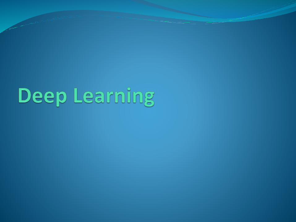
Restricted Boltzmann Machines

M. A. Cueto, J. Morton, B. Sturmfels. "Geometry of the restricted Boltzmann machine". Algebraic Methods in Statistics and Probability (AMS) 516 (2010)

M. Aoyagi. "Stochastic complexity and generalization error of a restricted Boltzmann machine in Bayesian estimation." JLMR 11 (2010): 1243-1272.

Contrastive Divergence MLE minimizes

Gradient

CD relaxes it to

This relaxation works well in experiments. It seems to regularize the model to prevent overfitting.

Hinton, Geoffrey E. "Training products of experts by minimizing contrastive divergence." Neural computation 14.8 (2002): 1771-1800.

Sparse Autoencoders Real-valued neurons (Andrew Ng)

Mean-field approximation of RBM

Given data vectors 𝑦1, 𝑦2, … , 𝑦𝑁, let

𝑥𝑖(0)

= 𝑦𝑖

𝑥𝑖(1)

= sig( 𝐴 0 𝑥𝑖0+ 𝑏(0) )

𝑥𝑖(2)

= sig( 𝐴 1 𝑥𝑖1+ 𝑏 1 )

Minimize over all weights 𝐴(0), 𝑏(0), 𝐴(1), 𝑏(1)

σ𝑖 𝑥𝑖2− 𝑥𝑖

02+ 𝛽 𝑥𝑖

1

1

+ 𝜆 𝐴 02

2+ 𝜆 𝐴 1

2

2

Sparsity Penalty

Weight Decay

A. Ng, J. Ngiam, C.Y. Foo, Y. Mai, and C. Suen. “Unsupervised feature learning and deep learning tutorial.” (http://ufldl.stanford.edu/wiki/index.php) 2011.

Andrew Ng. “Deep Learning, Self-Taught Learning and Unsupervised Feature Learning,” (http://www.youtube.com/watch?v=n1ViNeWhC24) 2012.

Deep Issues Slow hyperparameter search (uses cross-validation)

σ𝑖 𝑥𝑖2− 𝑥𝑖

02+ 𝛽 𝑥𝑖

1

1

+ 𝜆 𝐴 02

2+ 𝜆 𝐴 1

2

2

Sparsity Penalty

Weight Decay

Deep Issues Costly to train massive neural networks

e.g. cat video experiment (2012): 9 layers + 10m images + 16k cores => 3 days of training

“What we’re missing is the ability to parallelize the training of the network, mostly because the communication is the killer.”

“A lot of people are trying to solve this problem at Baidu, Facebook, Google, Microsoft and elsewhere […] it is both a hardware and software issue.”

“Eventually a lot of the deep learning task will be done on the device, which will keep pushing the need for on-board neural network accelerators

that operate at very low power and can be trained and used quickly.”

http://www.theplatform.net/2015/05/11/deep-learning-pioneer-pushing-gpu-neural-network-limits/

Parameters

Data Set 1 Data Set 3Data Set 2

Yann LeCun, NYU

Why does deep learning work?It’s not really about the RBMs…

Greedy layer-wise initialization of neuron weights

can be any of the following:

Contrastive divergence

Sparse autoencoder

Sparse coding

K-means clustering

Random data vectors

Coates, Adam, and Andrew Y. Ng. "The importance of encoding versus training with sparse coding and vector quantization.” ICML 2011.

Coates, Adam, and Andrew Y. Ng. "Learning feature representations with k-means." Neural Networks: Tricks of the Trade. Springer 2012. 561-580.

Why does deep learning work?… but it has something to do with regularization.

Compressed Sensing

If input is sparse in some known basis, then it can be

reconstructed from almost any random projections.

Hillar, Christopher, and Friedrich T. Sommer. "When can dictionary learning uniquely recover sparse data from subsamples?.” arXiv:1106.3616 (2011).

Candès, Emmanuel J.; Romberg, Justin K.; Tao, Terence (2006). "Stable signal recovery from incomplete and inaccurate measurements". CPAM 59 (8): 1207.

Donoho, D.L. (2006). "Compressed sensing". IEEE Transactions on Information Theory 52 (4): 1289.

Data is often near low-dim manifold in high-dim space

Why Regularization?

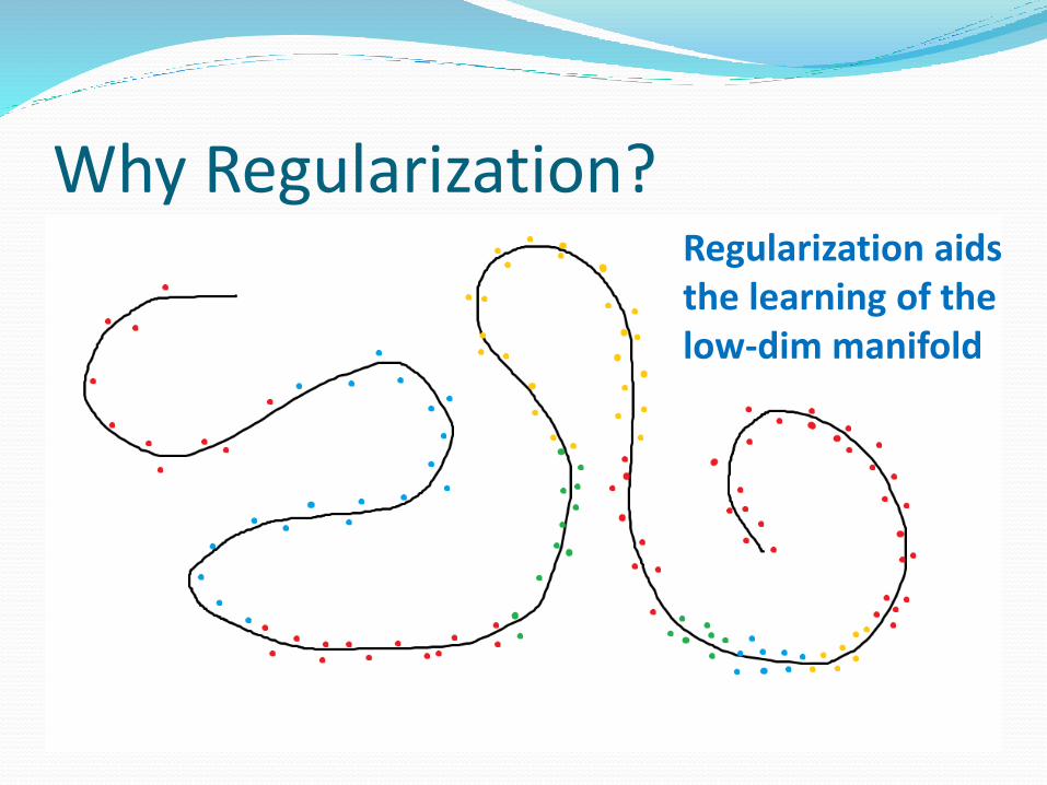
Why Regularization?Regularization aids the learning of the low-dim manifold

Why Regularization?Fewer labeled points needed for classification

Why Regularization?

http://colah.github.io/posts/2014-03-NN-Manifolds-Topology/

Why Regularization?

Structure preserved after randomprojections

Through the Lens of ComputationModel = Family of Distributions

Statistical learning often focuses only on deriving optimal parameters or posterior distributions

Computational considerations are put off till later

Model = Family of Distributions + Computations

What if models are defined and optimized with the computations to be performed in mind?

Study models whose goal is to approximate data distributions and generate samples using MCMC.

Through the Lens of ComputationModel = Family of Distributions

1. Define the model

2. Define the objective

3. Optimize

Model = Family of Distributions + Computations

1. Define the model

2. Define the computation

3. Define an objective that depends on computation

4. Optimize

Minimum Probability Flow

New look at learning

Tweaking 𝑤 so that the 𝜋𝑖 are “close” to the data

Use Kullback-Leibler (KL) distance for closeness

Different kinds of learning

min KL(𝜋0 || 𝜋∞) ~ Maximum likelihood

min KL(𝜋0 || 𝜋∞) – KL(𝜋1 || 𝜋∞) ~ Contrastive divergence

min KL(𝜋0 || 𝜋𝜀) ~ Minimum probability flow

𝜋0 𝜋1 𝜋2 𝜋∞…𝑇 𝑇 𝑇 𝑇

𝑝(𝑥|𝑤)=

Minimum Probability Flow

Think of 𝜋𝑡 as a flow in continuous time with transition

rate matrix Γ, i.e. T = exp Γ and 𝜋𝑡 = exp Γ𝑡 𝜋0.

In MPF, we assume that Γ has the form

where 𝑥, 𝑦 are states, and 𝑔𝑥𝑦 the connectivity matrix

𝜋0 𝜋1 𝜋2 𝜋∞…𝑇 𝑇 𝑇 𝑇

𝑝(𝑥|𝑤)=

Minimum Probability Flow

In MPF, we minimize the objective function

[Sohl-Dickstein, Battaglino, DeWeese 2011]

Minimize total flow out of data points

Sohl-Dickstein, Jascha, Peter B. Battaglino, and Michael R. DeWeese. "New method for parameter estimation in probabilistic models: minimum probability flow."

Physical review letters 107.22 (2011): 220601.

𝜋0 𝜋1 𝜋2 𝜋∞…𝑇 𝑇 𝑇 𝑇

𝑝(𝑥|𝑤)=

Minimum Probability Flow

No sampling is required (compare with CD) and

edge updates depend only on state of the endpoints!

where

Joint work with Chris Hillar (UC Berkeley)

Sohl-Dickstein, Jascha, Peter B. Battaglino, and Michael R. DeWeese. "New method for parameter estimation in probabilistic models: minimum probability flow."

Physical review letters 107.22 (2011): 220601.

𝜋0 𝜋1 𝜋2 𝜋∞…𝑇 𝑇 𝑇 𝑇

𝑝(𝑥|𝑤)=

Natural Images Apply MPF to complete Boltzmann Machine

(no hidden layer) to 8x8 patches from natural images

Natural Images Weight matrix learnt strong correlations between

nodes corresponding to neighboring pixels

Massive Neural Networks Minimum probability flow

Greedily minimizing computation time needed for

MCMC to converge near empirical distribution

Will allow us to train much bigger neural networks,

through model-parallelism, on multiple GPUs

Deep probability flow

Currently conducting experiments with a version of

MPF that contains hidden variables

Learning algorithm derived using Variational Bayes

http://people.sutd.edu.sg/~shaowei_lin/