Sparse Data Aggregation in Sensor Networks

Jie GaoComputer Science

DepartmentSUNY Stony Brook

Stony Brook, NY 11794jgao@cs.sunysb.edu

Leonidas GuibasNikola Milosavljevic

Computer ScienceDepartment

Stanford UniversityStanford, CA 94305

guibas@cs.stanford.edunikolam@cs.stanford.edu

John HershbergerMentor Graphics

8005 S.W. Boeckman RoadWilsonville, OR 97070

john hershberger@mentor.com

AbstractWe study the problem of aggregating data from a sparse set ofnodes in a wireless sensor network. This is a common situationwhen a sensor network is deployed to detect relatively rare events.In such situations, each node that should participate in the aggre-gation knows this fact based on its own sensor readings, but thereis no global knowledge in the network of where all these interest-ing nodes are located. Instead of blindly querying all nodes in thenetwork, we show how the interesting nodes can autonomously dis-cover each other in a distributed fashion and form an ad hoc aggre-gation structure that can be used to compute cumulants, moments,or other statistical summaries. Key to our approach is the capabilityfor two nodes that wish to communicate at roughly the same timeto discover each other at a cost that is proportional to their networkdistance. We show how to build nearly optimal aggregation struc-tures that can further deal with network volatility and compensatefor the loss or duplication of data by exploiting probabilistic tech-niques.

Categories and Subject DescriptorsC.2.2 [Computer-Communication Networks]: Network proto-cols—Routing protocols; F.2.2 [Analysis of Algorithms and Prob-lem Complexity]: Nonnumerical Algorithms and Problems—Ge-ometrical problems and computations

General TermsAlgorithms, Design, Theory

KeywordsAggregation, Sensor Networks

1. INTRODUCTION AND RATIONALEInformation aggregation is a common operation in sensor net-

works. Traditionally, information sampled at the sensor nodes needs

Permission to make digital or hard copies of all or part of this work forpersonal or classroom use is granted without fee provided that copies arenot made or distributed for profit or commercial advantage and that copiesbear this notice and the full citation on the first page. To copy otherwise, torepublish, to post on servers or to redistribute to lists, requires prior specificpermission and/or a fee.IPSN’07, April 25-27, 2007, Cambridge, Massachusetts, USA.Copyright 2007 ACM 978-1-59593-638-7/07/0004 ...$5.00.

Figure 1. An example of sparse aggregation trees in a 1, 024-node(32 × 32) grid network. The heavier solid lines represent the treeedges. Nodes marked by crosses are not in the tree, but have beeninvolved in the tree formation phase (by relaying probe and recallmessages).

to be conveyed to a central base station for further processing, anal-ysis, and visualization by the network users. Information aggrega-tion in this context can refer to the computation of statistical meansand moments, as well as other cumulative quantities that summa-rize the data obtained by the network. Such accumulation is impor-tant for data analysis and for obtaining a deeper understanding ofthe signal landscapes observed by the network. In certain contexts,when atomic sensor readings might reveal inappropriate informa-tion about a location or an individual, aggregation is also essentialfor alleviating privacy concerns.

An important topic addressed by the wireless sensor networkscommunity over the last several years has been in-network aggre-gation. The notion is that cumulants, moments, or summaries canbe computed directly in the network by sensor nodes endowed withcomputational power, thus avoiding the expensive transmission ofall sensor data to a (possibly distant) base station. It is well knownthat, for nearly all node technologies, data transmission over wire-less links costs hundreds to thousands of times more energy thanperforming local computation on the same data. In the setting ofuntethered, energy-constrained sensor nodes monitoring a physicalenvironment, it thus becomes quite significant, for energy conser-

vation and network lifetime considerations, to be able to trade localcomputation for communication as much as possible. There hasbeen a lot of interesting prior work on the in-network aggregationproblem, some of which is briefly surveyed in Section 2 below.

Most of the extant work assumes that the goal of the aggregationis to accumulate data from all the network nodes. This is certainlythe case in scientific applications, where scientists are aiming to ob-tain as detailed information as they can about the observed physicalphenomenon. In fact, physical scientists are often unhappy aboutin-network aggregation, as they want to have access to the raw sen-sor data, whenever possible. To some extent these concerns can bealleviated by providing tools for filtered aggregation, where only aselect subset of nodes participate in the aggregation, according tothe values of some of their sensors, their geographic location, etc.Even in these settings, however, all the nodes see all the queries—they simply decide whether to participate in the aggregation or not.

In this paper we are interested in exploring a new part of the ag-gregation problem space, by focusing on situations where only arelatively small subset of the nodes have useful data to report, orwant to participate in an aggregation. This is appropriate, for ex-ample, in settings where nodes perform some local processing first,to map raw sensor data into event detections, and where events ofinterest are relatively rare. Many applications of sensor networksfit this model, as sensor networks are often deployed to monitorand protect the health or safety of a system/space/environment, andanomalous events are, by their nature, infrequent. For example, ifwe have a sensor network monitoring a city, natural catastrophessuch as flooding, the spread of disease, earthquake damage, etc.,may affect a relatively small portion of the city at any one time. Thecausative factors of these disasters may depend on combinations ofexternal forces (e.g., rain, ground movement) and local conditions(e.g., building construction, health habits), making their locationshard to predict. What is common in such situations is that the sen-sor nodes observing the event of interest know that it has occurred,but there is no centralized knowledge in the network about whereall these event detections are.

In such situations existing aggregation methods are quite sub-optimal. One can poll and query the network for these events, butsuch queries will also have to be routed to the many nodes that havenothing to report, wasting large amounts of energy. Clearly, forrare events, frequent polling is inefficient. A purely event-drivenapproach, where each node with a detection independently trans-mits a record of the event to a base station, may also not be op-timal. In the settings we have in mind multiple detections mayoccur within a relatively short time period and it can be advanta-geous to aggregate in-network for all the reasons given earlier, aswell as for avoiding the creation of hot-spots and single points offailure around the base station. In other settings, where for exam-ple rescue workers are embedded and operating in the same spaceas the network, there may be no single fixed information sink. In-stead the detections should be reported to the nearest network users,with minimal latency. Similar challenges arise in settings where wewish to track intermittently observable targets moving through asensor network. Traditionally, leader nodes aggregate informationand perform hand offs as the target moves. But when the detectingnodes are all disconnected, this no longer works. How should thesenodes locally discover each other and pool their data to estimate thetarget tracks?

Our goal in this paper is to aggregate data in-network from asmall set of nodes that is possibly disconnected, but all of whichhave data to aggregate within a relatively short period. Each nodeknows locally whether it wants to be aggregated or not, but noglobal information about the location of this set is available in the

network. We call this the sparse aggregation problem. We focuson the problem of counting the number of nodes in the sparse de-tection set, or of summing a set of values, one from each of thesenodes, as the canonical aggregation problems. Many other varia-tions are possible. For brevity, we refer from now on to the nodesin the aggregation set as the hot nodes.

We present a class of solutions to the sparse aggregation problemwith several attractive properties:

• Our protocols are entirely distributed and need no prior in-formation about whether hot nodes exist or where they arelocated; nevertheless, they can exploit such information, ifavailable.

• We bring the hot nodes into a connected aggregation struc-ture, such as a tree, whose total cost is within a small factorof what would be possible if we had a full network map andperfect knowledge of where the hot nodes are located.

• We exploit probabilistic techniques in data aggregation, tomake our protocols robust to network volatility and the in-corporation of duplicate data, at the expense of a small prob-ability of modest errors.

An interesting aspect of our work is the way that the data processingand information aggregation can be interleaved with the routing,hot node discovery, and tree-formation aspects of our protocols—to the benefit of both. This paper provides a first theoretical analysisand simulation validation of this sparse aggregation framework.

2. PREVIOUS WORKWe are not aware of previous work that specifically addresses

the sparse aggregation problem. However, there is a vast amountof extant work on general in-network aggregation that we cannothope to fully survey here. Thus we focus on what is most relevantto our approach.

Early work on in-network aggregation, e.g., TinyDB [11], usesa tree-like structure to disseminate queries and collect results backto the sink. Queries are pushed down the network to construct aspanning tree. Aggregate values are routed up the tree with partialdata aggregated, compressed and pruned at internal tree nodes toreduce communication cost. Various algorithmic techniques havebeen proposed to allow efficient aggregation without increasing themessage size [3, 4, 17].

A serious problem with tree structures is that they are fragile un-der transmission failures, which are common in sensor networks.With in-network aggregation, packet loss can be fatal—as it maylead to the loss of the values from an entire subtree. To improverouting robustness, multi-path routing schemes can be adopted. Butthis may lead to duplicate packets arriving at the base station andsubsequently cause double counting. To deal with this problem,methods such as synopsis diffusion [3, 12, 13] were proposed todecouple aggregation from message routing by designing aggrega-tion schemes that are insensitive to message duplication and arrivalorders, a property named order and duplicate insensitive (ODI).Many of these techniques intuitively implement an aggregation op-eration by MAX/MIN or boolean operations on bit arrays, whichare by nature insensitive to duplicate data. The aggregation meth-ods we use in this paper exploit similar tools.

Non-tree based methods, such as sweeps, have also been pro-posed [18].

3. NETWORK SETUP AND AN OVERVIEWOur approach to the sparse aggregation problem is based on and

inspired by a number of tools that we briefly mention here, thendevelop further in later sections.

Suppose that sensor nodes are uniformly deployed inside a reg-ular region with sufficient density for connectivity and coverage.The boundary of the field is known. Furthermore, nodes on theboundary have connections to an external high-speed network. Basedon their own sensor measurements, certain sensors in the field de-cide that they are ‘hot’ (i.e., they believe they have detected some-thing of interest). Our goal is to count the number of hot nodes inthe network, or more generally to compute efficiently certain ag-gregate statistics about the set of hot nodes. These statistics mayinvolve the number of nodes, the locations of the nodes (if known),or other secondary physical measurements that convey more infor-mation about the phenomenon being observed. We assume that theset of hot nodes is relatively small compared to the whole network.There is no assumption that the hot nodes are ‘clustered’ in anyway, though this may turn out to be the case in practice, as physi-cal phenomena exhibit spatial coherence. We would like to collectthese statistics at periodic intervals.

To accomplish this goal without explicitly interrogating all nodes,we make a few assumptions that we believe to be reasonable. Sincewe want the data collection to be initiated by the hot nodes them-selves, we need to assume a common temporal framework for thenodes, with a shared clock that lets a node know when to initiatedata collection. We do not require perfect (and unrealistic) clocksynchronization among the nodes—instead we assume that clockdrift between a pair of nodes is proportional to the distance be-tween those nodes in the network. This can be accomplished by alow-overhead time synchronization protocol, simply by guarantee-ing that each node has a bounded drift with respect to each of its1-hop neighbors. In the case of target tracking, nodes detect eventsand participate in the aggregation protocol when a target passes by.As long as the target keeps moving with a minimum speed, detec-tion time differences at two nodes will also be bounded by someconstant times the relative distance of the nodes or the target pathlength.

Distance-sensitive neighbor discovery. Key to our approach is aprobe protocol that can be initiated independently by a node andinvolves emitting a few packets out of the node that follow certainpaths in the network while leaving a trail behind, until the probesare terminated. The key property of the probe protocol is that iftwo nodes, say u and v, at network distance d (with no knowledgeof each other) initiate probes at the same time, then a packet fromone of the nodes will encounter a trail left by a packet from theother node after O(d) steps. We call this crucial property distancesensitivity. At that encounter event

• if the probe packets carry data from the two nodes, the datacan be aggregated, and

• a path between the two nodes has been established whoselength is O(d) as well.

The same holds if the two nodes initiate probes within a time-lagof O(d) of each other. Furthermore, at this point it is possible toinitiate another recall protocol whose function is to terminate theprobe packets of one of the two nodes, say u. This can be doneso that when all the packets of u have been stopped by the recallprotocol, the total work performed by both the probe and recallprotocols on both nodes u and v is still O(d).

In the simplest scenario, when we use the probe and recall pro-tocols, we will think of u and v as ‘competing’ in a tournament.

When an encounter event occurs, the winner of the tournament isdecided based on the data carried or left behind by the probe pack-ets. The losing node then has his probes terminated by invoking therecall protocol, while the probes of the winner continue to propa-gate. Probe packets that are not recalled will eventually reach theboundary of the network, where they stop. Their data is aggregatedin an appropriate base station, using the high-speed network avail-able for the boundary nodes.

We will use the above communication pattern in several varia-tions in what follows. Effectively, our intersecting probes providea lightweight rendez-vous mechanism, allowing nodes within dis-tance d to discover each other’s existence at a cost of O(d), and notthe Ω(d2) that a traditional broadcast in a planar network requires.

Tree formation. To form an aggregation tree, we let each nodechoose a random number from some distribution, named the weightof this node. The weights of the hot nodes determine how the ag-gregation tree is formed. The weights can also be exploited in thespecific aggregation to be performed, as will be explained later.

At the right time, according to their local clocks, hot nodes ini-tiate probes carrying their weights. When two probes encountereach other, the packet with lower weight wins and initiates a recallprotocol for the packets of the node with the larger weight. Probemessages that are not recalled will eventually reach the networkboundary. Thus a spanning forest of the hot nodes all connected tothe network boundary is formed which can be used for subsequentdata aggregation.

What is the total cost of the tree formation? Note that each nodeu will have its probes recalled by a node v of smaller weight, towhom it loses in some encounter event during the tournament1.This happens at a total cost proportional to the distance d fromu to v. Thus each losing node spends effort that is proportional toits distance to the node that defeats it. We show in Section 5 thatthis simple property is enough to guarantee that the overall effortspent in the aggregation for nodes other than the one of minimumweight is O(T log n), where T is the cost of a minimum spanningtree connecting the hot nodes.

Our distributed construction of the aggregation tree was moti-vated by the nearest neighbor trees by Khan, Kumar, and Panduran-gan [8], which are built by giving desired nodes (the hot nodes inour context) certain priorities and then connecting, in a distributedmanner, each node to its nearest node of higher priority. We notethat in the aggregation tree (or forest) formed by our protocol, anode is not necessarily connected to its nearest neighbor of higherpriority. But our tree still has a small total weight. The overall costof the algorithm is O(T log n + K), where K is the time neededfor the probes of the minimum weight node to reach the sensor fieldboundary.

Aggregation. After the aggregation tree or forest is formed, dataaggregation can be conducted by having the data flow up the treeand aggregated in the standard way. An interesting aspect of ourprotocol is that we can actually integrate data aggregation with thetree formation process so that they both happen simultaneously.Recall that in the tree formation procedure we use random prior-ities to determine which probe message should proceed. Theserandom priorities can be used to implement data aggregation, byusing probabilistic counting techniques. Essentially the formationof the tree achieves the computation of the minimum of some ran-dom numbers chosen by the hot nodes, with which one can derivean approximation to the final aggregation value. Note that since1We assign the nodes on the boundary weight −∞ so that probesthat reach the boundary (and thus deliver their data to the sink) arerecalled.

we are aggregating by computing mins, the framework is robustto packet duplication, multiple encounter events between packetsfrom the same two nodes, etc.

4. FORMATION OF A SPARSEAGGREGATION TREE

This section generalizes and fleshes out the details of the meth-ods in Section 3. Note that an unknown sink (or sinks) seekingthe results of the aggregation can easily be integrated into this treediscovery/formation scheme. Thus the the aggregated data can bedelivered to any desired location or locations in the network.

4.1 Double RulingsTo achieve the distance-sensitivity property for neighbor discov-

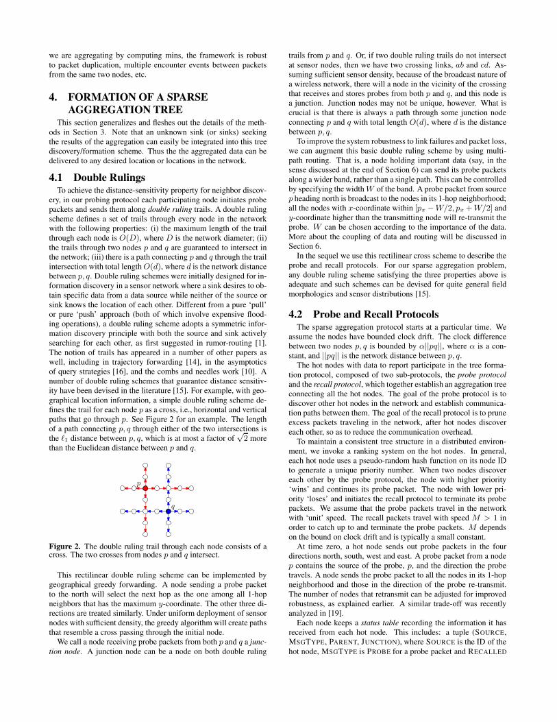
ery, in our probing protocol each participating node initiates probepackets and sends them along double ruling trails. A double rulingscheme defines a set of trails through every node in the networkwith the following properties: (i) the maximum length of the trailthrough each node is O(D), where D is the network diameter; (ii)the trails through two nodes p and q are guaranteed to intersect inthe network; (iii) there is a path connecting p and q through the trailintersection with total length O(d), where d is the network distancebetween p, q. Double ruling schemes were initially designed for in-formation discovery in a sensor network where a sink desires to ob-tain specific data from a data source while neither of the source orsink knows the location of each other. Different from a pure ‘pull’or pure ‘push’ approach (both of which involve expensive flood-ing operations), a double ruling scheme adopts a symmetric infor-mation discovery principle with both the source and sink activelysearching for each other, as first suggested in rumor-routing [1].The notion of trails has appeared in a number of other papers aswell, including in trajectory forwarding [14], in the asymptoticsof query strategies [16], and the combs and needles work [10]. Anumber of double ruling schemes that guarantee distance sensitiv-ity have been devised in the literature [15]. For example, with geo-graphical location information, a simple double ruling scheme de-fines the trail for each node p as a cross, i.e., horizontal and verticalpaths that go through p. See Figure 2 for an example. The lengthof a path connecting p, q through either of the two intersections isthe `1 distance between p, q, which is at most a factor of

√2 more

than the Euclidean distance between p and q.

p

q

Figure 2. The double ruling trail through each node consists of across. The two crosses from nodes p and q intersect.

This rectilinear double ruling scheme can be implemented bygeographical greedy forwarding. A node sending a probe packetto the north will select the next hop as the one among all 1-hopneighbors that has the maximum y-coordinate. The other three di-rections are treated similarly. Under uniform deployment of sensornodes with sufficient density, the greedy algorithm will create pathsthat resemble a cross passing through the initial node.

We call a node receiving probe packets from both p and q a junc-tion node. A junction node can be a node on both double ruling

trails from p and q. Or, if two double ruling trails do not intersectat sensor nodes, then we have two crossing links, ab and cd. As-suming sufficient sensor density, because of the broadcast nature ofa wireless network, there will a node in the vicinity of the crossingthat receives and stores probes from both p and q, and this node isa junction. Junction nodes may not be unique, however. What iscrucial is that there is always a path through some junction nodeconnecting p and q with total length O(d), where d is the distancebetween p, q.

To improve the system robustness to link failures and packet loss,we can augment this basic double ruling scheme by using multi-path routing. That is, a node holding important data (say, in thesense discussed at the end of Section 6) can send its probe packetsalong a wider band, rather than a single path. This can be controlledby specifying the width W of the band. A probe packet from sourcep heading north is broadcast to the nodes in its 1-hop neighborhood;all the nodes with x-coordinate within [px −W/2, px + W/2] andy-coordinate higher than the transmitting node will re-transmit theprobe. W can be chosen according to the importance of the data.More about the coupling of data and routing will be discussed inSection 6.

In the sequel we use this rectilinear cross scheme to describe theprobe and recall protocols. For our sparse aggregation problem,any double ruling scheme satisfying the three properties above isadequate and such schemes can be devised for quite general fieldmorphologies and sensor distributions [15].

4.2 Probe and Recall ProtocolsThe sparse aggregation protocol starts at a particular time. We

assume the nodes have bounded clock drift. The clock differencebetween two nodes p, q is bounded by α||pq||, where α is a con-stant, and ||pq|| is the network distance between p, q.

The hot nodes with data to report participate in the tree forma-tion protocol, composed of two sub-protocols, the probe protocoland the recall protocol, which together establish an aggregation treeconnecting all the hot nodes. The goal of the probe protocol is todiscover other hot nodes in the network and establish communica-tion paths between them. The goal of the recall protocol is to pruneexcess packets traveling in the network, after hot nodes discovereach other, so as to reduce the communication overhead.

To maintain a consistent tree structure in a distributed environ-ment, we invoke a ranking system on the hot nodes. In general,each hot node uses a pseudo-random hash function on its node IDto generate a unique priority number. When two nodes discovereach other by the probe protocol, the node with higher priority‘wins’ and continues its probe packet. The node with lower pri-ority ‘loses’ and initiates the recall protocol to terminate its probepackets. We assume that the probe packets travel in the networkwith ‘unit’ speed. The recall packets travel with speed M > 1 inorder to catch up to and terminate the probe packets. M dependson the bound on clock drift and is typically a small constant.

At time zero, a hot node sends out probe packets in the fourdirections north, south, west and east. A probe packet from a nodep contains the source of the probe, p, and the direction the probetravels. A node sends the probe packet to all the nodes in its 1-hopneighborhood and those in the direction of the probe re-transmit.The number of nodes that retransmit can be adjusted for improvedrobustness, as explained earlier. A similar trade-off was recentlyanalyzed in [19].

Each node keeps a status table recording the information it hasreceived from each hot node. This includes: a tuple (SOURCE,MSGTYPE, PARENT, JUNCTION), where SOURCE is the ID of thehot node, MSGTYPE is PROBE for a probe packet and RECALLED

for a recall packet, PARENT and JUNCTION are the parent and junc-tion node in the aggregation tree, to be defined later.

When a node w receives a probe packet from p, it first checkswhether it has already received any packet from p; if so, this packetis ignored. Otherwise w records the probe packet. In addition, ifw has received messages from other hot nodes, w checks if it isa junction node and if any probes need to be recalled. If w hasreceived a message from a node q with priority higher than p, thenthe probe message from p will be recalled. Node q is a candidateto be the parent of p in the aggregation tree. If p’s priority is higherthan all the other hot nodes whose status entries have MSGTYPE =PROBE at node w, then those probes will be recalled. They areassigned p as a potential parent. The probe packet for p will bere-transmitted.

The recall protocol is initiated when a hot node p ‘loses’ to an-other hot node q at a junction node w. Node q is a possible parentof p. The recall packet contains the IDs of p (the child), q (the par-ent), and w (the junction node). A recall packet travels at speed M ,faster than the speed of the probe packets. A recall packet has nodirection associated with it but uses flood-fill to travel through thetrails of the probe packets. When a node x receives (or initiates) arecall message, it first checks the status for node p in its local table.If x has received a message from p before and the current statusis PROBE, then x will change the status of p to RECALLED. Therecall message will be broadcast to all the 1-hop neighbors of x. Ifx has no message from p, or the status is RECALLED, x does notsend the recall message further.

When node p itself receives a recall packet for p, it sets its parentto be the parent-candidate q in the packet and remembers the junc-tion node w where the trails of p and q met. Thus the parent of pin the aggregation tree is determined by the first recall packet thatreaches p.

The boundary of the sensor region is incorporated into the proto-col by initializing every boundary node as a junction whose prob-ing node (the base station b) has the highest priority. When a probepacket for hot node p reaches a boundary node w, p loses to b, andw initiates the recall protocol for p with potential parent b and junc-tion node w. Finding boundaries in networks has been addressedby a number of authors [5, 6, 9, 20].

The status tables in the nodes record the trails of probe and recallpackets, and also provide a way to suppress redundant retransmis-sions. Due to the broadcast nature of wireless communication, apacket may be received by multiple nodes. In the probe and recallprotocol, multiple nodes may realize they are junction nodes andthus initiate the recall procedure. However, once a node has re-ceived a recall packet and updated its status, it will not respond toany further recall packets other nodes may have generated.

4.3 Forming an Aggregation TreeAs described in the preceding subsection, the aggregation tree

is a logical structure recorded in the hot nodes themselves: eachnode p knows its parent q in the tree. The parent may either beanother hot node or the boundary of the sensor region. Thus the‘tree’ is actually a forest of trees, with the number of trees in theforest dependent on the distance from the region of hot nodes to theboundary. Nevertheless, we will continue to use the word ‘tree’ todescribe the structure—it is still an aggregation tree, but the chil-dren of the base station are joined to it by high-performance links.

Our simulations, described in Section 7, use the simple parent-child representation of the aggregation tree. The earlier figure 1shows an example of the tree we obtained. One can see that onlya small fraction of the nodes are involved in the tree formation.Although our simulations use the simple tree representation, there

are several variants on the tree structure that pay greater attentionto the physical embedding of the tree in the sensor network, withvarying impacts on communication cost and reliability.

Using the logical representation of the aggregation tree, aggre-gation happens at the hot nodes themselves. The children of a nodep send their results to p, p aggregates them, and then p sends theresulting summary on to its parent. There are several choices forhow each node p sends data to its parent q.

• Send a packet from p along p’s trail to the junction node w,then along q’s trail to q. This has the advantage that the probeand recall protocol has already demonstrated the existence ofthis path—no path discovery is required.

• Use some network-specific point-to-point routing mechanism,such as geographic routing [7], to send a packet from p to q,bypassing the junction w entirely. This reduces the load onthe trail nodes, but forces the packet to discover its own path.

• If p’s results are known to be particularly important and theirsuccessful delivery is crucial, the preceding two possibilitiescan be combined, or either can be complemented by trans-mitting in a band around the basic path, with the width ofthe band dependent on the importance of the message, as de-scribed in Section 4.1.

Routing along the trails of the logical aggregation tree may causesome inefficiency in the routing. Packets may be sent in one direc-tion along p’s trails from its children, only to have the summarypacket from p traverse the same trail in the opposite direction onthe way to its parent. We can avoid this redundancy (possibly sav-ing a constant factor in communication costs) by exploiting the em-bedding of the aggregation tree. We add a third phase to the probeand recall protocol, in which a node p notifies all the nodes in itstrails of its parent q and junction node w. This allows all the nodesin p’s trails to direct the trail edges toward w. Node w becomes aproxy for p in the aggregation tree. Instead of sending data to p foraggregation, all p’s children (represented by their proxy nodes onp’s trail) send data along p’s trail to w, where aggregation occursbefore w sends a summary packet toward the junction represent-ing p’s parent. Node p also sends its own individual data to w foraggregation. Two variants of this approach are possible:

• Each proxy for a child of p sends its data along p’s trail in-dependently to w. A constant fraction of p’s trail may betraversed for each child.

• The child proxies along p’s trails may be used as intermedi-ate aggregation points, combining data from the child withdata flowing along p’s trail from nodes farther from w alongthe trail. This reduces the number of messages that must besent—each trail segment is traversed just once—but makesthe aggregation tree more vulnerable to deadlock because ofsingle-node failures.

A final modification enhances robustness by replacing the aggre-gation tree with a DAG. To do this, we modify the recall protocolso that all recall messages for a node p propagate back to p. Thisincreases the amount of communication in the recall phase of theprotocol, but has the advantage that p is informed of all its candi-date parents, not just the one whose recall packet reaches it first.Node p can choose multiple parents among the candidates, perhapsup to four, one for each cardinal direction. When p performs itsaggregation (here we assume the simple tree structure, with aggre-gation performed at hot nodes rather than proxies), it sends the re-sulting data to all its parents, thereby increasing the likelihood thatthe data will reach the base station. Of course this requires that weuse an ODI (order and duplicate insensitive) scheme.

5. QUALITY OF THE SPARSEAGGREGATION TREE

In this section we discuss the performance of the protocols inthe previous section and characterize the aggregation tree that theybuild. The asymptotic bounds we present apply to all the tree vari-ants discussed in Section 4.3, with the caveat that multiplying thewidth of important communication paths to increase reliability hasa corresponding multiplicative cost in communication resources.

As noted in Section 4.2, the clock skew between any two nodesu and v is bounded by α||uv||, where ||uv|| is the network distancebetween u and v. The speed of probe packets is 1 and the speed ofrecall packets is M > 1. We denote the set of hot nodes by S.

For any hot node p, let trail(p) be the set of nodes in p’s trails.Because of the uniform distribution of sensor nodes, |trail (p)| isproportional to the distance between p and the farthest node intrail(p). Furthermore, |trail(p)| is proportional to the total numberof packets in the probe and recall protocol attributable to p.

When a probe meets the trail of another node’s probe, at leastone of the two will be recalled, if neither has already been recalled.This observation leads to the following lemma (proof omitted):

Lemma 5.1. Let u and v be two hot nodes. Then

min(|trail(u)|, |trail(v)|) ≤ C · ||uv||for some constant C.

Let E be the set of nearest-neighbor edges: for each hot node u,E contains the edge from u to its nearest hot node, denoted nn(u).

Lemma 5.2. E contains a partial matching2 of size Θ(|S|).

It is well-known that the minimum spanning tree of S, denotedMST (S), contains all the edges of E. (If MST (S) does not con-tain e = (v, nn(v)) for some node v ∈ S, adding e to MST (S)creates a cycle, and the tree weight can be decreased by retaininge and removing the other cycle edge incident to v.) The weightof MST (S), i.e., its total length, is |MST (S)|. The length of anindividual edge e = (p, q) is len(e) = ||pq||.

Theorem 5.3. Let K be the maximum, over all v ∈ S, of the short-est axis-aligned distance from v to the boundary of the sensor re-gion. Then

X

v∈S

|trail(v)| = O(K + |MST (S)| · log |S|).

PROOF. For any subset X ⊆ S, define f(X) =P

v∈X |trail(v)|.We want to estimate f(S).

For a given X ⊆ S, let E be the set of nearest-neighbor edgesdefined with respect to X , and let EM be a maximal-cardinalitymatching in E. Because every edge of EM belongs to MST (X),

X

e∈EM

len(e) ≤ |MST (X)|.

Also note that |MST (X)| ≤ |TSP(X)| ≤ |TSP(S)| ≤ 2|MST (S)|,where TSP(·) is the minimum-length traveling salesman tour of apoint set.

By Lemma 5.1, every edge e ∈ EM is incident to a node v suchthat |trail(v)| ≤ C · len(e). Let the set of these nodes be XM . Wehave

f(XM ) =X

v∈XM

|trail (v)| ≤ C · |MST (X)|.

2A partial matching is a set of edges such that each node is anendpoint of at most one edge.

Create a new set X ′ = X \ XM ; by Lemma 5.2, |X ′| ≤ β|X|,for some constant β < 1. Assembling the pieces, we have

f(X) = f(XM ) + f(X ′) ≤ C · |MST (X)| + f(X ′)

≤ 2C · |MST (S)| + f(X ′).

The base case for |X| = 1 is f(X) = O(K). By induction on|X|, we have f(X) ≤ 2C · |MST (S)| · log1/α |X| + O(K).

Because the aggregation tree built in Section 4.3 uses a subset ofthe nodes in all the trails, the theorem has the following immediateconsequence:

Theorem 5.4. The aggregation tree constructed by our protocolhas total length O(|MST (S)| · log |S| + K), where K is as de-fined in Theorem 5.3.

The maximum degree of the aggregation tree is also importantfor its performance. Nodes with high degree must perform muchmore aggregation work than the average (which is just constant).In the following theorem we bound the maximum degree of our ag-gregation tree. The proof is omitted from this version of the paper.

Theorem 5.5. Let A be the aspect ratio of S, i.e., the ratio betweenthe maximum and minimum distances between elements of S. Ifthe clock skew parameter α is less than 1, then the maximum degreeof any node in the aggregation tree of Section 4.3 is O(log A).

6. AGGREGATIONMany possible aggregation strategies are possible, within the

framework discussed above. If the network has solid connectiv-ity and point-to-point routing already in place, then a logical ag-gregation tree is all that is needed and aggregation can happen inthe traditional way, after tree formation. If the network is volatile,however, then a DAG-based approach with multi-path connectiv-ity is preferable, together with an ODI aggregation scheme. Notealso that our tree discovery protocol naturally leads to a multiply-connected structure, as for each pair of nodes the multiple probepaths establish multiple routes between the nodes.

Of special interest is the fact that our protocols allow fine inter-leaving between tree formation and aggregation. Specifically, therandom priority needed by the tree formation process can be usedto implement a probabilistic aggregation scheme. In this way ag-gregation is already completed, as soon as the tree is formed.

Specifically, we can make use of certain properties of the classi-cal exponential distribution. A random variable x chosen from anexponential distribution with parameter λ, λ > 0, has a probabilitydensity function f(x; λ) given by

f(x; λ) =

λe−λx , if x ≥ 00 , if x < 0

The cumulative distribution function F (x;λ) is given by

F (x;λ) =

1 − e−λx , if x ≥ 00 , if x < 0

The distribution has mean 1/λ and variance 1/λ2. The followingtwo properties of the exponential distribution are crucial for us.

Theorem 6.1. If x1 and x2 are independent random variables withparameters λ1 and λ1 respectively, then

Prob(x1 < x2) =λ1

λ1 + λ2.

Theorem 6.2. If x1, x2, . . . , xn are independent exponential ran-dom variables, where xi has parameter λi, then

min(x1, x2, . . . , xn)

is an exponential random variable with parameterPn

i=1 λi.

A consequence of these properties is that if x1, x2, . . . , xn areindependent exponential random variables chosen from exponen-tial distributions with parameters λ1, λ2, . . . , λn respectively, thentheir minimum is a random variable with mean 1/

Pni=1 λi. This

effectively allows us to replace a data summation by a data mini-mization operation which, as mentioned, is insensitive to data du-plication and thus is advantageous in a volatile network setting.

This use, to our knowledge, was first pointed out by E. Cohen [2],in the context of solving counting problems on large graphs. In ouradaptation of the Cohen framework, each network node i holdingdata value fi independently selects a random number drawn froman exponential distribution with density function fie

−fix. If µ isthe minimum number chosen by any hot node, then 1/µ is an un-biased estimator of the sum of F = f1 + f2 + · · · + fn. Sum-ming values at the hot nodes is a surprisingly powerful aggregationprimitive. If node locations are known, this primitive can be usedto compute arbitrary moments of the hot node position distribution,conveying a picture of where the exceptional events are being de-tected. Alternatively, summation can be used to compute momentsof the values sensed by the nodes, covariances between node loca-tions and values, etc.

For the primitive of summing values, we can use the randomnumber chosen from the exponential distribution described aboveas the weights in the tree formation protocol. Recall that duringtree formation, a number of packets may reach the field boundary,from where these weights can be transmitted to the base stationand the minimum weight can be retained. No packet can stop thepackets of the hot node whose weight is globally minimal—andtherefore these packets will reach the boundary and the base sta-tion. Thus as the tree is formed, the base station can immediatelyderive an approximation to the aggregated value. For applicationsin which a quick and dirty approximation suffices, our job is doneat the moment when the tree is formed. For better accuracy, we canrepeat this experiment a number of times. Cohen shows that, for agiven parameter ε, if we repeat this experiment O( 1

ε2 log n) times,where n is the number of nodes involved, average the minimumweights obtained in each experiment, and then take the inverse ofthat, this quantity lies, with high probability, within relative errorε of F . With O( 1

ε2 ) experiments, the expected relative error is atmost ε. We report on some simulations validating these bounds inSection 7.

In summary, by integrating data aggregation with node discoveryand tree formation, the simple distributed probe protocol performstwo important tasks at once: it connects the hot nodes into an aggre-gation tree that is nearly optimal in terms of communication cost,while at the same time performing the min-based aggregation thatcan translate into an estimate of the final aggregation.

The robustness of aggregation deserves further exploration. Notethat this type of probabilistic counting has built-in robustness todata loss, as well as duplicate insensitivity. Some of the simulationsreported below quantify how many exponential variates are neces-sary to obtain a given degree of accuracy. For example, if the small-est variate in the counting problem is lost, but the second smallestmakes it, our final count will be off by only 1 in expectation—while in regular aggregation a single lost subtree count can causeunbounded error. If other variates are lost, they have no impact onthe count. The counting problem also allows this self-determined

yet globally consistent notion of data importance, which when cou-pled with multi-path routing can guarantee further robustness. Al-though this does not directly extend to the completely general caseof summation of hot node values, in most scenarios prior knowl-edge of the range of node values, past measurements, etc., can beused to develop a notion of the significance of data locally, withoutrequiring additional extensive communication.

7. SIMULATIONS AND EXPERIMENTSIn this section we evaluate by means of simulation the perfor-

mance of our sparse aggregation scheme in a number of settings.

7.1 Communication CostsThe main metric we consider is the communication cost of a sin-

gle aggregation task. If aggregation is initiated by a base station,then we include the costs of both the query phase and the data col-lection phase. In our protocol there is no query phase. Our aggrega-tion cost is defined to be the cost of forming an aggregation tree, asthe basic logical structure described in subsection 4.2, and the costof sending partial aggregates along child-parent paths if data ag-gregation/delivery has not been accomplished (if data aggregationis combined with tree formation as in Section 6 this cost is 0).

We assume that the cost of sending a message is proportionalto the Euclidean distance between the sender and the receiver, ajustified assumption in the case of dense deployment. Althoughnot completely realistic, we believe that this assumption does notinfluence the overall outcomes of our comparisons, but only theabsolute costs, which we are less interested in.

We compare our algorithm to two general aggregation paradigms,commonly known as ‘push’- and ‘pull’-style aggregation, ratherthan any specific method proposed in the literature. Almost all ex-isting methods that we are aware of (see Section 2) belong to oneof these categories. In Figures 3 and 4, the vertical axis is the ratioof the cost of our scheme vs. the cost of the corresponding ‘push’or ‘pull’ scheme—thus the smaller the better.

‘Pull’-based method: The base station queries all nodes, and onlythe hot nodes reply. The query cost is essentially the cost of flood-ing the entire network. We consider two variations for the datacollection cost. In the first data collection, the hot nodes reply bysending the data upstream along the spanning tree constructed inthe flooding phase. Data can be aggregated at internal nodes of thetree. We also consider the case when each hot node replies inde-pendently along its shortest path to the base station, disregardingany message trails it may encounter along the way. This methodinvokes higher communication cost, but requires no coordinationand scheduling of partial aggregates, which makes it much easier toimplement. Since the hot nodes are scattered at unpredictable loca-tions, scheduling for in-network aggregation of irregularly spacedparticipants is non-trivial. Our two performance metrics are thesum of the fixed query cost and that of the two reply costs, as de-scribed above. Note that we discount the costs of both reply meth-ods significantly by disregarding the non-trivial amount of workrequired to discover the shortest paths and the cost of coordinationand scheduling for in-network aggregation, respectively. Anotherserious overhead that we did not account for in the ‘pull’-methodis that the user/sink needs to know when to ‘pull’. As interestingevents happen irregularly and unexpectedly, a ‘pull’ approach inpractice may waste a lot of communication by querying when thedata is not yet be available. Our comparison is unrealistically favor-able to this approach, as we simply ignore the cost of the unfruitfulpolling queries that a practical ‘pull’-method would definitely in-clude.

0

0.2

0.4

0.6

0.8

1

0 0.05 0.1 0.15 0.2 0.25 0.3

cost

(fra

ctio

n)

hot nodes (fraction)

separation <= 0.10.1 < separation <= 0.20.2 < separation <= 0.50.5 < separation <= 1.0

separation > 1.0 0

0.2

0.4

0.6

0.8

1

1.2

1.4

0 0.02 0.04 0.06 0.08 0.1 0.12 0.14

cost

(fra

ctio

n)

hot nodes (fraction)

separation <= 0.10.1 < separation <= 0.20.2 < separation <= 0.50.5 < separation <= 1.0

separation > 1.0 0

0.5

1

1.5

2

2.5

3

0 0.05 0.1 0.15 0.2 0.25 0.3

cost

(fra

ctio

n)

hot nodes (fraction)

separation <= 0.10.1 < separation <= 0.20.2 < separation <= 0.50.5 < separation <= 1.0

separation > 1.0

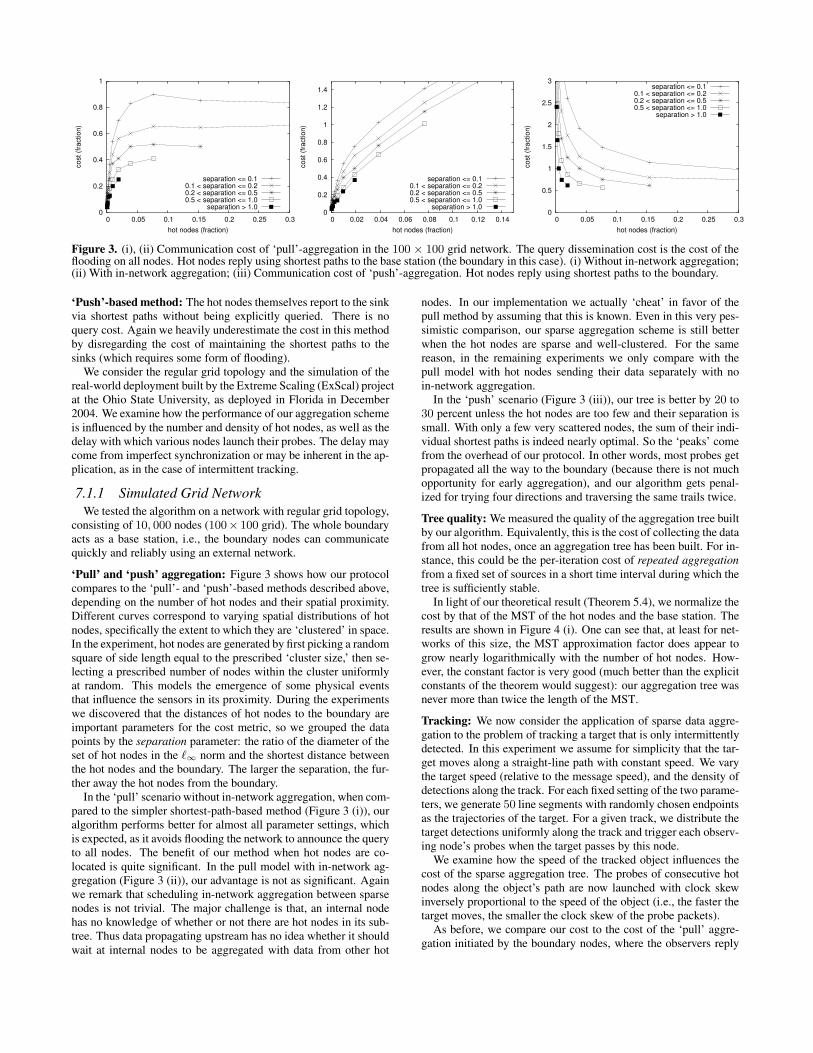
Figure 3. (i), (ii) Communication cost of ‘pull’-aggregation in the 100 × 100 grid network. The query dissemination cost is the cost of theflooding on all nodes. Hot nodes reply using shortest paths to the base station (the boundary in this case). (i) Without in-network aggregation;(ii) With in-network aggregation; (iii) Communication cost of ‘push’-aggregation. Hot nodes reply using shortest paths to the boundary.

‘Push’-based method: The hot nodes themselves report to the sinkvia shortest paths without being explicitly queried. There is noquery cost. Again we heavily underestimate the cost in this methodby disregarding the cost of maintaining the shortest paths to thesinks (which requires some form of flooding).

We consider the regular grid topology and the simulation of thereal-world deployment built by the Extreme Scaling (ExScal) projectat the Ohio State University, as deployed in Florida in December2004. We examine how the performance of our aggregation schemeis influenced by the number and density of hot nodes, as well as thedelay with which various nodes launch their probes. The delay maycome from imperfect synchronization or may be inherent in the ap-plication, as in the case of intermittent tracking.

7.1.1 Simulated Grid NetworkWe tested the algorithm on a network with regular grid topology,

consisting of 10, 000 nodes (100× 100 grid). The whole boundaryacts as a base station, i.e., the boundary nodes can communicatequickly and reliably using an external network.

‘Pull’ and ‘push’ aggregation: Figure 3 shows how our protocolcompares to the ‘pull’- and ‘push’-based methods described above,depending on the number of hot nodes and their spatial proximity.Different curves correspond to varying spatial distributions of hotnodes, specifically the extent to which they are ‘clustered’ in space.In the experiment, hot nodes are generated by first picking a randomsquare of side length equal to the prescribed ‘cluster size,’ then se-lecting a prescribed number of nodes within the cluster uniformlyat random. This models the emergence of some physical eventsthat influence the sensors in its proximity. During the experimentswe discovered that the distances of hot nodes to the boundary areimportant parameters for the cost metric, so we grouped the datapoints by the separation parameter: the ratio of the diameter of theset of hot nodes in the `∞ norm and the shortest distance betweenthe hot nodes and the boundary. The larger the separation, the fur-ther away the hot nodes from the boundary.

In the ‘pull’ scenario without in-network aggregation, when com-pared to the simpler shortest-path-based method (Figure 3 (i)), ouralgorithm performs better for almost all parameter settings, whichis expected, as it avoids flooding the network to announce the queryto all nodes. The benefit of our method when hot nodes are co-located is quite significant. In the pull model with in-network ag-gregation (Figure 3 (ii)), our advantage is not as significant. Againwe remark that scheduling in-network aggregation between sparsenodes is not trivial. The major challenge is that, an internal nodehas no knowledge of whether or not there are hot nodes in its sub-tree. Thus data propagating upstream has no idea whether it shouldwait at internal nodes to be aggregated with data from other hot

nodes. In our implementation we actually ‘cheat’ in favor of thepull method by assuming that this is known. Even in this very pes-simistic comparison, our sparse aggregation scheme is still betterwhen the hot nodes are sparse and well-clustered. For the samereason, in the remaining experiments we only compare with thepull model with hot nodes sending their data separately with noin-network aggregation.

In the ‘push’ scenario (Figure 3 (iii)), our tree is better by 20 to30 percent unless the hot nodes are too few and their separation issmall. With only a few very scattered nodes, the sum of their indi-vidual shortest paths is indeed nearly optimal. So the ‘peaks’ comefrom the overhead of our protocol. In other words, most probes getpropagated all the way to the boundary (because there is not muchopportunity for early aggregation), and our algorithm gets penal-ized for trying four directions and traversing the same trails twice.

Tree quality: We measured the quality of the aggregation tree builtby our algorithm. Equivalently, this is the cost of collecting the datafrom all hot nodes, once an aggregation tree has been built. For in-stance, this could be the per-iteration cost of repeated aggregationfrom a fixed set of sources in a short time interval during which thetree is sufficiently stable.

In light of our theoretical result (Theorem 5.4), we normalize thecost by that of the MST of the hot nodes and the base station. Theresults are shown in Figure 4 (i). One can see that, at least for net-works of this size, the MST approximation factor does appear togrow nearly logarithmically with the number of hot nodes. How-ever, the constant factor is very good (much better than the explicitconstants of the theorem would suggest): our aggregation tree wasnever more than twice the length of the MST.

Tracking: We now consider the application of sparse data aggre-gation to the problem of tracking a target that is only intermittentlydetected. In this experiment we assume for simplicity that the tar-get moves along a straight-line path with constant speed. We varythe target speed (relative to the message speed), and the density ofdetections along the track. For each fixed setting of the two parame-ters, we generate 50 line segments with randomly chosen endpointsas the trajectories of the target. For a given track, we distribute thetarget detections uniformly along the track and trigger each observ-ing node’s probes when the target passes by this node.

We examine how the speed of the tracked object influences thecost of the sparse aggregation tree. The probes of consecutive hotnodes along the object’s path are now launched with clock skewinversely proportional to the speed of the object (i.e., the faster thetarget moves, the smaller the clock skew of the probe packets).

As before, we compare our cost to the cost of the ‘pull’ aggre-gation initiated by the boundary nodes, where the observers reply

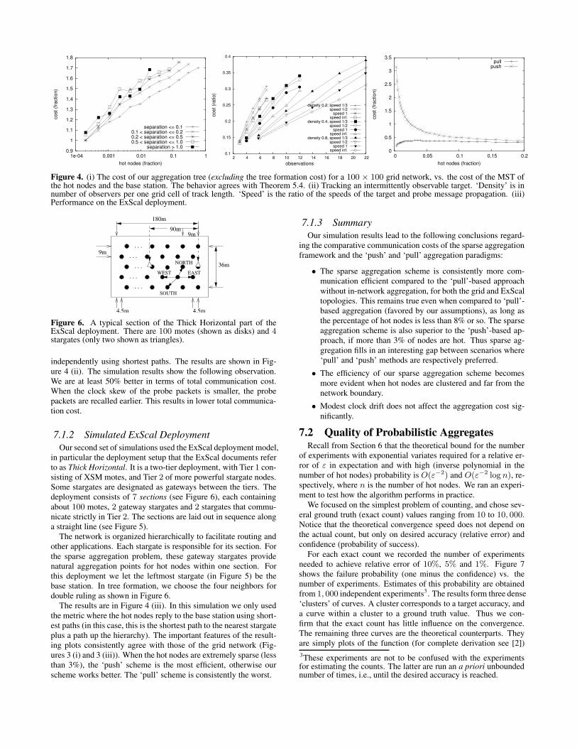
0.9

1

1.1

1.2

1.3

1.4

1.5

1.6

1.7

1.8

1e-04 0.001 0.01 0.1 1

cost

(fra

ctio

n)

hot nodes (fraction)

separation <= 0.10.1 < separation <= 0.20.2 < separation <= 0.50.5 < separation <= 1.0

separation > 1.0 0.1

0.15

0.2

0.25

0.3

0.35

0.4

2 4 6 8 10 12 14 16 18 20 22

cost

(rat

io)

observations

density 0.2, speed 1/3speed 1/2

speed 1speed inf.

density 0.4, speed 1/3speed 1/2

speed 1speed inf.

density 0.8, speed 1/3speed 1/2

speed 1speed inf. 0

0.5

1

1.5

2

2.5

3

3.5

0 0.05 0.1 0.15 0.2

cost

(fra

ctio

n)

hot nodes (fraction)

pullpush

Figure 4. (i) The cost of our aggregation tree (excluding the tree formation cost) for a 100 × 100 grid network, vs. the cost of the MST ofthe hot nodes and the base station. The behavior agrees with Theorem 5.4. (ii) Tracking an intermittently observable target. ‘Density’ is innumber of observers per one grid cell of track length. ‘Speed’ is the ratio of the speeds of the target and probe message propagation. (iii)Performance on the ExScal deployment.

WEST EAST

180m

9m

4.5m4.5m

36m

90m9m

SOUTH

NORTH

· · ·

· · ·

· · ·

· · ·

· · ·

Figure 6. A typical section of the Thick Horizontal part of theExScal deployment. There are 100 motes (shown as disks) and 4stargates (only two shown as triangles).

independently using shortest paths. The results are shown in Fig-ure 4 (ii). The simulation results show the following observation.We are at least 50% better in terms of total communication cost.When the clock skew of the probe packets is smaller, the probepackets are recalled earlier. This results in lower total communica-tion cost.

7.1.2 Simulated ExScal DeploymentOur second set of simulations used the ExScal deployment model,

in particular the deployment setup that the ExScal documents referto as Thick Horizontal. It is a two-tier deployment, with Tier 1 con-sisting of XSM motes, and Tier 2 of more powerful stargate nodes.Some stargates are designated as gateways between the tiers. Thedeployment consists of 7 sections (see Figure 6), each containingabout 100 motes, 2 gateway stargates and 2 stargates that commu-nicate strictly in Tier 2. The sections are laid out in sequence alonga straight line (see Figure 5).

The network is organized hierarchically to facilitate routing andother applications. Each stargate is responsible for its section. Forthe sparse aggregation problem, these gateway stargates providenatural aggregation points for hot nodes within one section. Forthis deployment we let the leftmost stargate (in Figure 5) be thebase station. In tree formation, we choose the four neighbors fordouble ruling as shown in Figure 6.

The results are in Figure 4 (iii). In this simulation we only usedthe metric where the hot nodes reply to the base station using short-est paths (in this case, this is the shortest path to the nearest stargateplus a path up the hierarchy). The important features of the result-ing plots consistently agree with those of the grid network (Fig-ures 3 (i) and 3 (iii)). When the hot nodes are extremely sparse (lessthan 3%), the ‘push’ scheme is the most efficient, otherwise ourscheme works better. The ‘pull’ scheme is consistently the worst.

7.1.3 SummaryOur simulation results lead to the following conclusions regard-

ing the comparative communication costs of the sparse aggregationframework and the ‘push’ and ‘pull’ aggregation paradigms:

• The sparse aggregation scheme is consistently more com-munication efficient compared to the ‘pull’-based approachwithout in-network aggregation, for both the grid and ExScaltopologies. This remains true even when compared to ‘pull’-based aggregation (favored by our assumptions), as long asthe percentage of hot nodes is less than 8% or so. The sparseaggregation scheme is also superior to the ‘push’-based ap-proach, if more than 3% of nodes are hot. Thus sparse ag-gregation fills in an interesting gap between scenarios where‘pull’ and ‘push’ methods are respectively preferred.

• The efficiency of our sparse aggregation scheme becomesmore evident when hot nodes are clustered and far from thenetwork boundary.

• Modest clock drift does not affect the aggregation cost sig-nificantly.

7.2 Quality of Probabilistic AggregatesRecall from Section 6 that the theoretical bound for the number

of experiments with exponential variates required for a relative er-ror of ε in expectation and with high (inverse polynomial in thenumber of hot nodes) probability is O(ε−2) and O(ε−2 log n), re-spectively, where n is the number of hot nodes. We ran an experi-ment to test how the algorithm performs in practice.

We focused on the simplest problem of counting, and chose sev-eral ground truth (exact count) values ranging from 10 to 10, 000.Notice that the theoretical convergence speed does not depend onthe actual count, but only on desired accuracy (relative error) andconfidence (probability of success).

For each exact count we recorded the number of experimentsneeded to achieve relative error of 10%, 5% and 1%. Figure 7shows the failure probability (one minus the confidence) vs. thenumber of experiments. Estimates of this probability are obtainedfrom 1, 000 independent experiments3. The results form three dense‘clusters’ of curves. A cluster corresponds to a target accuracy, anda curve within a cluster to a ground truth value. Thus we con-firm that the exact count has little influence on the convergence.The remaining three curves are the theoretical counterparts. Theyare simply plots of the function (for complete derivation see [2])3These experiments are not to be confused with the experimentsfor estimating the counts. The latter are run an a priori unboundednumber of times, i.e., until the desired accuracy is reached.

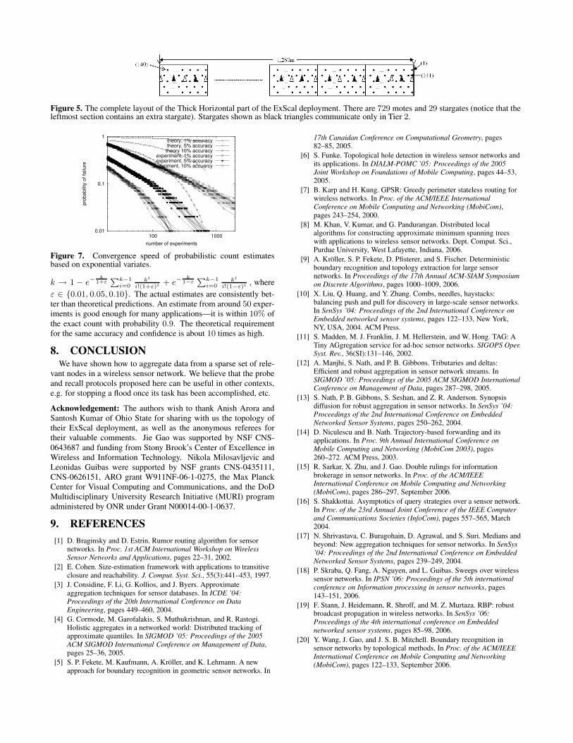
Figure 5. The complete layout of the Thick Horizontal part of the ExScal deployment. There are 729 motes and 29 stargates (notice that theleftmost section contains an extra stargate). Stargates shown as black triangles communicate only in Tier 2.

0.01

0.1

1

100 1000

prob

abilit

y of

failu

re

number of experiments

theory, 1% accuracytheory, 5% accuracy

theory 10% accuracyexperiment, 1% accuracyexperiment, 5% accuracy

experiment, 10% accuarcy

Figure 7. Convergence speed of probabilistic count estimatesbased on exponential variates.

k → 1 − e−k

1+ε

Pk−1i=0

ki

i!(1+ε)i + e−k

1−ε

Pk−1i=0

ki

i!(1−ε)i , whereε ∈ 0.01, 0.05, 0.10. The actual estimates are consistently bet-ter than theoretical predictions. An estimate from around 50 exper-iments is good enough for many applications—it is within 10% ofthe exact count with probability 0.9. The theoretical requirementfor the same accuracy and confidence is about 10 times as high.

8. CONCLUSIONWe have shown how to aggregate data from a sparse set of rele-

vant nodes in a wireless sensor network. We believe that the probeand recall protocols proposed here can be useful in other contexts,e.g. for stopping a flood once its task has been accomplished, etc.

Acknowledgement: The authors wish to thank Anish Arora andSantosh Kumar of Ohio State for sharing with us the topology oftheir ExScal deployment, as well as the anonymous referees fortheir valuable comments. Jie Gao was supported by NSF CNS-0643687 and funding from Stony Brook’s Center of Excellence inWireless and Information Technology. Nikola Milosavljevic andLeonidas Guibas were supported by NSF grants CNS-0435111,CNS-0626151, ARO grant W911NF-06-1-0275, the Max PlanckCenter for Visual Computing and Communications, and the DoDMultidisciplinary University Research Initiative (MURI) programadministered by ONR under Grant N00014-00-1-0637.

9. REFERENCES[1] D. Braginsky and D. Estrin. Rumor routing algorithm for sensor

networks. In Proc. 1st ACM International Workshop on WirelessSensor Networks and Applications, pages 22–31, 2002.

[2] E. Cohen. Size-estimation framework with applications to transitiveclosure and reachability. J. Comput. Syst. Sci., 55(3):441–453, 1997.

[3] J. Considine, F. Li, G. Kollios, and J. Byers. Approximateaggregation techniques for sensor databases. In ICDE ’04:Proceedings of the 20th International Conference on DataEngineering, pages 449–460, 2004.

[4] G. Cormode, M. Garofalakis, S. Muthukrishnan, and R. Rastogi.Holistic aggregates in a networked world: Distributed tracking ofapproximate quantiles. In SIGMOD ’05: Proceedings of the 2005ACM SIGMOD International Conference on Management of Data,pages 25–36, 2005.

[5] S. P. Fekete, M. Kaufmann, A. Kroller, and K. Lehmann. A newapproach for boundary recognition in geometric sensor networks. In

17th Canaidan Conference on Computational Geometry, pages82–85, 2005.

[6] S. Funke. Topological hole detection in wireless sensor networks andits applications. In DIALM-POMC ’05: Proceedings of the 2005Joint Workshop on Foundations of Mobile Computing, pages 44–53,2005.

[7] B. Karp and H. Kung. GPSR: Greedy perimeter stateless routing forwireless networks. In Proc. of the ACM/IEEE InternationalConference on Mobile Computing and Networking (MobiCom),pages 243–254, 2000.

[8] M. Khan, V. Kumar, and G. Pandurangan. Distributed localalgorithms for constructing approximate minimum spanning treeswith applications to wireless sensor networks. Dept. Comput. Sci.,Purdue University, West Lafayette, Indiana, 2006.

[9] A. Kroller, S. P. Fekete, D. Pfisterer, and S. Fischer. Deterministicboundary recognition and topology extraction for large sensornetworks. In Proceedings of the 17th Annual ACM-SIAM Symposiumon Discrete Algorithms, pages 1000–1009, 2006.

[10] X. Liu, Q. Huang, and Y. Zhang. Combs, needles, haystacks:balancing push and pull for discovery in large-scale sensor networks.In SenSys ’04: Proceedings of the 2nd International Conference onEmbedded networked sensor systems, pages 122–133, New York,NY, USA, 2004. ACM Press.

[11] S. Madden, M. J. Franklin, J. M. Hellerstein, and W. Hong. TAG: ATiny AGgregation service for ad-hoc sensor networks. SIGOPS Oper.Syst. Rev., 36(SI):131–146, 2002.

[12] A. Manjhi, S. Nath, and P. B. Gibbons. Tributaries and deltas:Efficient and robust aggregation in sensor network streams. InSIGMOD ’05: Proceedings of the 2005 ACM SIGMOD InternationalConference on Management of Data, pages 287–298, 2005.

[13] S. Nath, P. B. Gibbons, S. Seshan, and Z. R. Anderson. Synopsisdiffusion for robust aggregation in sensor networks. In SenSys ’04:Proceedings of the 2nd International Conference on EmbeddedNetworked Sensor Systems, pages 250–262, 2004.

[14] D. Niculescu and B. Nath. Trajectory-based forwarding and itsapplications. In Proc. 9th Annual International Conference onMobile Computing and Networking (MobiCom 2003), pages260–272. ACM Press, 2003.

[15] R. Sarkar, X. Zhu, and J. Gao. Double rulings for informationbrokerage in sensor networks. In Proc. of the ACM/IEEEInternational Conference on Mobile Computing and Networking(MobiCom), pages 286–297, September 2006.

[16] S. Shakkottai. Asymptotics of query strategies over a sensor network.In Proc. of the 23rd Annual Joint Conference of the IEEE Computerand Communications Societies (InfoCom), pages 557–565, March2004.

[17] N. Shrivastava, C. Buragohain, D. Agrawal, and S. Suri. Medians andbeyond: New aggregation techniques for sensor networks. In SenSys’04: Proceedings of the 2nd International Conference on EmbeddedNetworked Sensor Systems, pages 239–249, 2004.

[18] P. Skraba, Q. Fang, A. Nguyen, and L. Guibas. Sweeps over wirelesssensor networks. In IPSN ’06: Proceedings of the 5th internationalconference on Information processing in sensor networks, pages143–151, 2006.

[19] F. Stann, J. Heidemann, R. Shroff, and M. Z. Murtaza. RBP: robustbroadcast propagation in wireless networks. In SenSys ’06:Proceedings of the 4th international conference on Embeddednetworked sensor systems, pages 85–98, 2006.

[20] Y. Wang, J. Gao, and J. S. B. Mitchell. Boundary recognition insensor networks by topological methods. In Proc. of the ACM/IEEEInternational Conference on Mobile Computing and Networking(MobiCom), pages 122–133, September 2006.