Theoretical Foundations of Deep Learning

via Sparse Representations

Vardan Papyan, Yaniv Romano, Jeremias Sulam and Michael Elad

Abstract

Modeling data is the way we – scientists – believe that information should be explained and

handled. Indeed, models play a central role in practically every task in signal and image processing

and machine learning. Sparse representation theory (Sparseland, in our language) puts forward an

emerging, highly effective, and universal model. Its core idea is the description of data as a linear

combination of few atoms taken from a dictionary of such fundamental elements.

Our prime objective in this paper is to review a recently introduced [1] model-based explanation

of deep learning, which relies on sparse modeling of data. We start by presenting the general story

of Sparseland, describing its key achievements. We then turn to describe the Convolutional-Sparse-

Coding (CSC) model and present a multi-layered (ML-CSC) extension of it, both being special

cases of the general sparsity-inspired model. We show how ML-CSC leads to a solid and systematic

theoretical justification of the architectures used in deep learning, along with a novel ability of

analyzing the performance of the resulting machines. As such, this work offers a unique and first

of its kind theoretical view for a field that has been, until recently, considered as purely heuristic.

1 Introduction

The field of sparse and redundant representations has made a major leap in the past two decades.

Starting with a series of infant ideas and few mathematical observations, it grew to become a mature

and highly influential discipline. In its core, this field, broadly referred to as “Sparseland”, puts

forward a universal mathematical model for describing the inherent low-dimensionality that may exist

in natural data sources. This model suggests a description of signals as linear combinations of few

columns, called atoms, from a given redundant matrix, termed dictionary. In other words, these signals

1

admit sparse representations with respect to their corresponding dictionary of prototype signals.

The Sparseland model gradually became central in signal and image processing and machine learning

applications, leading to state-of-the-art results in a wide variety of tasks and across many different

domains. A partial explanation for the great appeal that this model has had is based on the theoretical

foundations that accompany its construction, providing a solid support for many of the developed

algorithms arising in this field. Indeed, in the broad scientific arena of data processing, Sparseland is

quite unique due to the synergy that exists between theory, algorithms, and applications.

This paper embarks from the story of Sparseland in order to discuss two recent special cases of it

– convolutional sparse coding and its multi-layered version. As we shall see, these descendant models

pave a clear and surprising highway between sparse modeling and deep learning architectures. This

paper’s main goal is to present a novel theory for explaining deep (convolutional) neural networks and

their origins, all through the language of sparse representations.

Clearly, our work is not the only one nor the first to theoretically explain deep learning. Indeed,

various such attempts have already appeared in the literature (e.g., [2, 3, 4, 5, 6, 7, 8, 9, 10, 11, 12, 13]).

Broadly speaking, this knowledge stands on three pillars – the architectures used, the algorithms and

optimization aspects involved, and the data these all serve. A comprehensive theory should cover all

three but this seems to be a tough challenge. The existing works typically cover one or two of these

pillars, such as in the following examples:

• Architecture: The work by Giryes et. al. [9], showed that the used architectures tend to

preserve distances, and explained the relevance of this property for classification. The work

reported in [7, 8] analyzed the capacity of these architectures to cover specific family of functions.

• Algorithms: Vidal’s work [5] explained why local minima are not to be feared as they may

coincide with the objective’s global minimum. Chaudhari and Soatto proved [6] that the stochas-

tic gradient descent (SGD) algorithm induces an implicit regularization that is related to the

information-bottleneck objective [3].

• Data: Bruna and Mallat [4] motivated the architectures by the data invariances that should be

taken care of. Baraniuk’s team [2] developed a probabilistic generative model for the data that

in turn justifies the architectures used.

2

In this context we should note that our work covers the data by modeling it, and the architectures as

emerging from the model. Our work is close in spirit to [2] but also markedly different.

A central idea that will accompany us in this article refers to the fact that Sparseland and its above-

mentioned descendants are all generative models. By this we mean that they offer a description of the

signals of interest by proposing a synthesis procedure for their creation. We argue that such generative

models facilitate a systematic pathway for algorithm design, while also enabling a theoretical analysis

of their performance. Indeed, we will see throughout this paper how these two benefits go hand in

hand. By relying on the generative model, we will analyze certain feed-forward convolutional neural

networks (CNN), identify key theoretical weaknesses in them, and then tackle these by proposing new

architectures. Surprisingly, this journey will lead us to some of the well-known feed-forward CNN used

today.

Standing at the horizon of this work is our desire to present the Multi-Layered Convolutional Sparse

Modeling idea, as it will be the grounds on which we derive all the above claimed results. Thus, we will

take this as our running title and build the paper, section by section, focusing each time on another

word in it. We shall start by explaining better what we mean by the term “Modeling”, and then move

to describe “Sparse Modeling”, essentially conveying the story of Sparseland. Then we will shift to

“Convolutional Sparse Modeling”, presenting this model along with a recent and novel analysis of it

that relies on local sparsity. We will conclude by presenting the “Multi-Layered Convolutional Sparse

Modeling”, tying this to the realm of deep learning, just as promised.

Before we start our journey, a few comments are in order:

1. Quoting Ron Kimmel (The Computer Science Department at the Technion - Israel), this grand

task of attaching a theory to deep learning behaves like a magic mirror, in which every researcher

sees himself. This explains the so diverse explanations that have been accumulated, relying on

information theory [3], passing through wavelets and invariances [4], proposing a sparse modeling

point of view [1], and going all the way to Partial Differential Equations [10]. Indeed, it was

David Donoho (Department of Statistics at Stanford university) who strengthened this vivid

description by mentioning that this magical mirror is taken straight from Cinderella’s story, as

it is not just showing to each researcher his/her reflection, but also accompanies this with warm

compliments, assuring that their view is truly the best.

3

2. This paper focuses mostly on the theoretical sides of the models we shall discuss, but without

delving into the proofs for the theorems we will state. This implies two things: (i) Less emphasis

will be put on applications and experiments; and (ii) the content of this paper is somewhat

involved due to the delicate theoretical statements brought, so be patient.

3. This paper echoes a keynote talk given by Michael Elad in the International Conference on Image

Processing (ICIP) 2017 in Beijing, as we follow closely this lecture, both in style and content.

The recent part of the results presented (on CSC and ML-CSC) can be found in [14, 1], but the

description of the path from Sparseland to deep learning as posed here differs substantially.

2 Modeling

2.1 Our Data is Structured

Engineers and researchers rarely stop to wonder about our core ability to process signals – we simply

take it for granted. Why is it that we can denoise signals? Why can we compress them, or recover

them from various degradations, or find anomalies in them, or even recognize their content? The

algorithms that tackle these and many other tasks – including separation, segmentation, identifica-

tion, interpolation, extrapolation, clustering, prediction, synthesis, and many more – all rely on one

fundamental property that only meaningful data sources obey: they are all structured.

Each source of information we encounter in our everyday lives exhibits an inner structure that is

unique to it, and which can be characterized in various ways. We may allude to redundancy in the

data, assume it satisfies a self-similarity property, suggest it is compressible due to low-entropy, or

even mention the possibility of embedding it into a low-dimensional manifold. No matter what the

assumption is, the bottom line is the same – the data we operate on is structured. This is true for

images of various kinds, video sequences, audio signals, 3D objects given as meshes or point-clouds,

financial time series, data on graphs as is the case in social or traffic networks, text files such as

emails and other documents, and more. In fact, we could go as far as stating that if a given data

is unstructured (e.g., being i.i.d. random noise), it would be of no interest to us, since processing it

would be virtually futile.

So, coming back to our earlier question, the reason we can process data is the above-mentioned

4

structure, which facilitates this ability in all its manifestations. Indeed, the fields of signal and image

processing and machine learning are mostly about identifying the structure that exists in a given

information source, and then exploiting it to achieve the processing goals. This brings us to discuss

models and the central role they play in data processing.

2.2 Identifying Structure via Models

An appealing approach for identifying structure in a given information source is imposing a (para-

metric) model on it, explicitly stating a series of mathematical properties that the data is believed to

satisfy. Such constraints lead to a dimensionality reduction that is so characteristic of models and

their modus-operandi. We should note, however, that models are not the only avenue for identifying

structure – the alternative being a non-parametric approach that simply describes the data distribu-

tion by accumulating many of its instances. We will not dwell on this option in this paper, as our

focus is on models and their role in data processing.

Consider the following example, brought to clarify our discussion. Assume that we are given a

measurement vector y ∈ Rn, and all that is known to us is that it is built from an ideal signal of

some sort, x ∈ Rn, contaminated by white additive Gaussian noise of zero mean and unit variance,

i.e., y = x + e where e ∼ N (0, I). Could we propose a method to clean the signal y from the noise?

The answer is negative! Characterizing the noise alone cannot suffice for handling the denoising task,

as there are infinitely many possible ways to separate y into a signal and a noise vector, where the

estimated noise matches its desired statistical properties.

Now, suppose that we are given additional information on the unknown x, believed to belong to

the family of piece-wise constant (PWC) signals, with the tendency to have as few jumps as possible.

In other words, we are given a model for the underlying structure. Could we leverage this extra

information in order to denoise y? The answer is positive – we can seek the simplest PWC signal that

is closest to y in such a way that the error matches the expected noise energy. This can be formulated

mathematically in some way or another, leading to an optimization problem whose solution is the

denoised result. What have we done here? We imposed a model on our unknown, forcing the result

to be likely under the believed structure, thus enabling the denoising operation. The same thought

process underlies the solution of almost any task in signal and image processing and machine learning,

either explicitly or implicitly.

5

As yet another example for a model in image processing and its impact, consider the JPEG com-

pression algorithm [15]. We are well-aware of the impressive ability of this method to compress images

by factor of ten to twenty with hardly any noticeable artifacts. What are the origins of this success?

The answer is two-fold: the inner-structure that exists in images, and the model that JPEG harnesses

to exploit it. Images are redundant, as we already claimed, allowing for the core possibility of such

compression to take place. However, the structure alone cannot suffice to get the actual compression,

as a model is needed in order to capture this redundancy. In the case of JPEG, the model exposes

this structure through the belief that small image patches (of size 8 × 8 pixels) taken from natural

images tend to concentrate their energy in the lower frequency part of the spectrum once operated

upon by the Discrete Cosine Transform (DCT). Thus, few transform coefficients can be kept while the

rest can be discarded, leading to the desired compression result. One should nevertheless wonder, will

this algorithm perform just as well on other signal sources? The answer is not necessarily positive,

suggesting that every information source should be fitted with a proper model.

2.3 The Evolution of Models

A careful survey of the literature in image processing reveals an evolution of models that have been

proposed and adopted over the years. We will not provide here an exhaustive list of all of these

models, but we do mention a few central ideas such as Markov Random Fields for describing the

relation between neighboring pixels [16], Laplacian smoothness of various sorts [17], Total Variation

[18] as an edge-preserving regularization, wavelets’ sparsity [19, 20], and Gaussian-Mixture Models

[21, 22]. With the introduction of better models, performance improved in a wide front of applications

in image processing.

Consider, for example, the classic problem of image denoising, on which thousands of papers have

been written. Our ability to remove noise from images has advanced immensely over the years1.

Performance in denoising has improved steadily over time, and this improvement was enabled mostly

by the introduction of better and more effective models for natural images. The same progress applies

to image deblurring, inpainting, super-resolution, compression, and many other tasks.

In our initial description of the role of models, we stated that these are expressing what the data

1Indeed, the progress made has reached the point where this problem is regarded by many in our field as nearly

solved[23, 24].

6

“... is believed to satisfy”, eluding to the fact that models cannot be proven to be correct, just as a

formula in physics cannot be claimed to describe our world perfectly. Rather, models can be compared

and contrasted, or simply tested empirically to see whether they fit reality sufficiently well. This is

perhaps the place to disclose that models are almost always wrong, as they tend to explain reality

in a simple manner at the cost of its oversimplification. Does this mean that models are necessarily

useless? Not at all. While they do carry an error in them, if this deviation is small enough2, then such

models are priceless and extremely useful for our processing needs.

For a model to succeed in its mission of treating signals, it must be a good compromise between

simplicity, reliability, and flexibility. Simplicity is crucial since this implies that algorithms harnessing

this model are relatively easy and pleasant to work with. However, simplicity is not sufficient. We

could suggest, for example, a model that simply assumes that the signal of interest is zero. This is the

simplest model imaginable, and yet it is also useless. So, next to simplicity, comes the second force

of reliability – we must offer a model that does justice to the data served, capturing its true essence.

The third virtue is flexibility, implying that the model can be tuned to better fit the data source, thus

erring less. Every model is torn between these three forces, and we are constantly seeking simple,

reliable, and flexible models that improve over their predecessors.

2.4 Models – Summary

Models are central for enabling the processing of structured data sources. In image processing, models

take a leading part in addressing many tasks, such as denoising, deblurring, and all the other inverse

problems, compression, anomaly detection, sampling, recognition, separation, and more. We hope

that this perspective on data sources and their inner-structure clarifies the picture, putting decades

of research activity in the fields of signal and image processing and machine learning in a proper

perspective.

In the endless quest for a model that explains reality, one that has been of central importance in the

past two decades is Sparseland. This model slowly and consistently carved its path to the lead, fueled

2How small is “small enough”? This is a tough question that has not been addressed in the literature. Here we will

simply be satisfied with the assumption that this error should be substantially smaller compared to the estimation error

the model leads to. Note that, often times, the acceptable relative error is dictated by the application or problem that

one is trying to solve by employing the model.

7

by both great empirical success and impressive accompanying theory that added a much needed color

to it. We turn now to present this model. We remind the reader that this is yet another station in

our road towards providing a potential explanation of deep learning using sparsity-inspired models.

3 Sparse Modeling

3.1 On the Origin of Sparsity-Based Modeling

Simplicity as a driving force for explaining natural phenomena has a central role in sciences. While

Occam’s razor is perhaps the earliest of this manifestation (though in a philosophical or religious

context), a more recent and relevant quote from Wrinch and Jeffrey (1921) [25] reads: “The existence

of simple laws is, then, apparently, to be regarded as a quality of nature; and accordingly we may infer

that it is justifiable to prefer a simple law to a more complex one that fits our observations slightly

better.”

When it comes to the description of data, sparsity is an ultimate expression of simplicity, which

explains the great attraction it has. While it is hard to pinpoint the exact appearance of the concept of

sparsity in characterizing data priors, it is quite clear that this idea became widely recognized with the

arrival of the wavelet revolution that took place during the late eighties and early nineties of the 20th

century. The key observation was that this particular transformation, when applied to many different

signals or images, produced representations that were naturally sparse. This, in turn, was leveraged in

various ways, both empirically and theoretically. Almost in parallel, approximation theorists started

discussing the dichotomy between linear and non-linear approximation, emphasizing further the role of

sparsity in signal analysis. These are the prime origins of the field of Sparseland, which borrowed the

core idea that signal representations should be redundant and sparse, while putting aside many other

features of wavelets, such as (bi-) orthogonality, multi-scale analysis, frame theory interpretation, and

more.

Early signs of Sparseland appeared already in the early and mid-nineties, with the seminal papers

on greedy (Zhang and Mallat, [26]) and relaxation-based (Chen, Donoho and Saunders, [27]) pursuit

algorithms, and even the introduction of the concept of dictionary-learning by Olshausen and Field

[28]. However, it is our opinion that this field was truly born only few years later, in 2000, with the

publication of the paper by Donoho and Huo [29], which was the first to show that the Basis Pursuit

8

(BP) is provably exact under some conditions. This work dared and defined a new language, setting

the stage for thousands of follow-up papers. Sparseland started with a massive theoretical effort, which

slowly expanded and diffused to practical algorithms and applications, leading in many cases to state-

of-the-art results in a wide variety of disciplines. The knowledge in this field as it stands today relies

heavily on numerical optimization and linear algebra, and parts of it have a definite machine-learning

flavor.

3.2 Introduction to Sparseland

So, what is this model? and how can it capture structure in a data source? Let us demonstrate this

for 8 × 8 image patches, in the spirit of the description of the JPEG algorithm mentioned earlier.

Assume that we are given a family of patches extracted from natural images. The Sparseland model

starts by preparing a dictionary – a set of atom-patches of the same size, 8 × 8 pixels. For example,

consider a dictionary containing 256 such atoms. Then, the model assumption is that every incoming

patch could be described as a linear combination of only few atoms from the dictionary. The word

‘few’ here is crucial, as every patch could be easily described as a linear combination of 64 linearly

independent atoms, a fact that leads to no structure whatsoever.

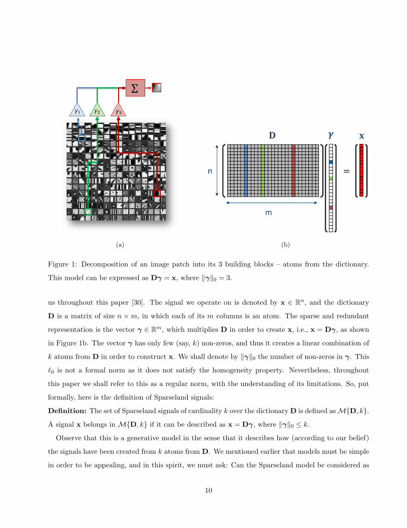
Let’s take a closer look at this model, as depicted in Figure 1a. We started with a patch of size

8 × 8 pixels, thus 64 values. The first thing to observe is that we have converted it to a vector of

length 256 carrying the weights of each of the atoms in the mixture that generates this patch. Thus,

our representation is redundant. However, this vector is also very sparse, since only few of the atoms

participate in this construction. Imagine, for example, that only 3 atoms are used. In this case,

the complete information about the original patch is carried by 6 values: 3 stating which atoms are

involved, and 3 determining their weights. Thus, this model manages to reduce the dimensionality of

the patch information, a key property in exposing the structure in our data.

An interesting analogy can be drawn between this model and our world’s chemistry. The model’s

dictionary and its atoms should remind the reader of Mendeleev’s periodic table. In our world, every

molecule is built of few of the fundamental elements from this table, and this parallels our model

assumption that states that signals are created from few atoms as well. As such, we can regard the

Sparseland model as an adoption of the core rational of chemistry to data description.

Let’s make the Sparseland model somewhat more precise, and introduce notations that will serve

9

(a) (b)

Figure 1: Decomposition of an image patch into its 3 building blocks – atoms from the dictionary.

This model can be expressed as Dγ = x, where ‖γ‖0 = 3.

us throughout this paper [30]. The signal we operate on is denoted by x ∈ Rn, and the dictionary

D is a matrix of size n ×m, in which each of its m columns is an atom. The sparse and redundant

representation is the vector γ ∈ Rm, which multiplies D in order to create x, i.e., x = Dγ, as shown

in Figure 1b. The vector γ has only few (say, k) non-zeros, and thus it creates a linear combination of

k atoms from D in order to construct x. We shall denote by ‖γ‖0 the number of non-zeros in γ. This

`0 is not a formal norm as it does not satisfy the homogeneity property. Nevertheless, throughout

this paper we shall refer to this as a regular norm, with the understanding of its limitations. So, put

formally, here is the definition of Sparseland signals:

Definition: The set of Sparseland signals of cardinality k over the dictionary D is defined asMD, k.

A signal x belongs in MD, k if it can be described as x = Dγ, where ‖γ‖0 ≤ k.

Observe that this is a generative model in the sense that it describes how (according to our belief)

the signals have been created from k atoms from D. We mentioned earlier that models must be simple

in order to be appealing, and in this spirit, we must ask: Can the Sparseland model be considered as

10

simple? Well, the answer is not so easy, since this model raises major difficulties in its deployment,

and this might explain its late adoption. In the following we shall mention several such difficulties,

given in an ascending order of complexity.

3.3 Sparseland Difficulties: Atom Decomposition

The term atom-decomposition refers to the most fundamental problem of identifying the atoms that

construct a given signal. Consider the following example: We are given a dictionary having 2000

atoms, and a signal known to be composed of a mixture of 15 of these. Our goal now is to identify

these 15 atoms. How should this be done? The natural option to consider is an exhaustive search over

all the possibilities of choosing 15 atoms out of the 2000, and checking per each whether they fit the

measurements. The number of such possibilities to check stands on an order of 2.4e+ 37, and even if

each of this takes one pico-second, billions of years will be required to complete this task!

Put formally, atom decomposition can be described as the following constrained optimization prob-

lem:

minγ‖γ‖0 s.t. x = Dγ. (1)

This problem seeks the sparsest explanation of x as a linear combination of atoms from D. In a more

practical version of the atom-decomposition problem, we may assume that the signal we get, y, is an

ε-contaminated version of x, and then the optimization task becomes

minγ‖γ‖0 s.t. ‖y −Dγ‖2 ≤ ε. (2)

Both problems above are known to be NP-Hard, implying that their complexity grows exponentially

with the number of atoms in D. So, are we stuck?

The answer to this difficulty came in the form of approximation algorithms, originally meant to

provide exactly that – an approximate solution to the above problems. In this context we shall

mention greedy methods such as the Orthogonal Matching Pursuit (OMP) [31] and the Thresholding

algorithm, and relaxation formulations such as the Basis Pursuit (BP) [27].

While it is beyond the scope of this paper to provide a detailed description of these algorithms,

we will say a few words on each, as we will return to use them later on when we get closer to the

connection to neural networks. Basis Pursuit takes the problem posed in Equation (2) and relaxes

11

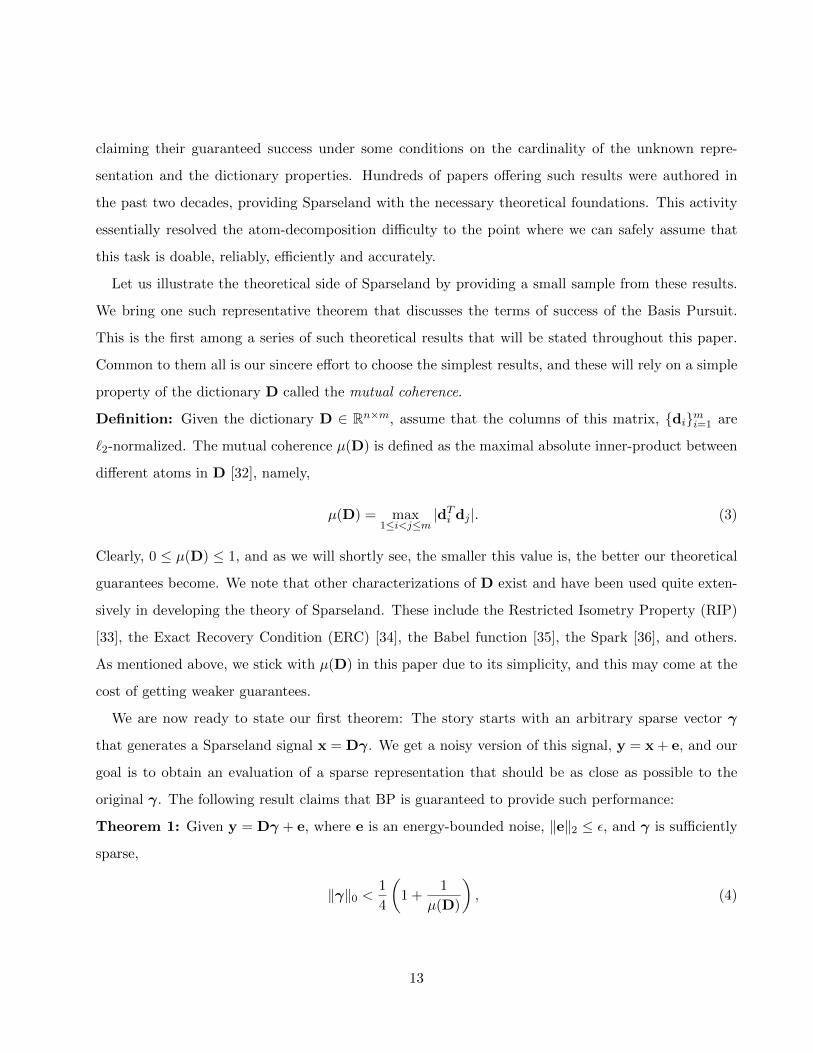
0 200 400 600 800 1000 1200 1400 1600 1800 2000-5

-4

-3

-2

-1

0

1

2

3

4

Original Sparse VectorOMPBPThresholding

Figure 2: Illustration of Orthogonal Matching Pursuit (OMP), Basis Pursuit (BP) and Thresholding

in approximating the solution of the atom decomposition problem, for a dictionary with 2000 atoms.

it by replacing the `0 by an `1-norm. With this change, the problem is convex and manageable in

reasonable time.

Greedy methods such as the OMP solve the problem posed in Equation (2) by adding one non-zero

at a time to the solution, trying to reduce the error ‖y−Dγ‖2 as much as possible at each step, and

stopping when this error goes below ε. The Thresholding algorithm is the simplest and crudest of

all pursuit methods – it multiplies y by DT , and applies a simple shrinkage on the resulting vector,

nulling small entries and leaving the rest almost untouched.

Figure 2 presents an experiment in which these three algorithms were applied on the scenario we

described above, in which D has 2000 atoms, and an approximate atom-decomposition is performed

on noisy signals that are known to be created from few of these atoms. The results shown suggest

that these three algorithms tend to succeed rather well in their mission.

3.4 Sparseland Difficulties: Theoretical Foundations

Can the success of the pursuit algorithms be explained and justified? One of the grand achievements of

the field of Sparseland is the theoretical analysis that accompanies many of these pursuit algorithms,

12

claiming their guaranteed success under some conditions on the cardinality of the unknown repre-

sentation and the dictionary properties. Hundreds of papers offering such results were authored in

the past two decades, providing Sparseland with the necessary theoretical foundations. This activity

essentially resolved the atom-decomposition difficulty to the point where we can safely assume that

this task is doable, reliably, efficiently and accurately.

Let us illustrate the theoretical side of Sparseland by providing a small sample from these results.

We bring one such representative theorem that discusses the terms of success of the Basis Pursuit.

This is the first among a series of such theoretical results that will be stated throughout this paper.

Common to them all is our sincere effort to choose the simplest results, and these will rely on a simple

property of the dictionary D called the mutual coherence.

Definition: Given the dictionary D ∈ Rn×m, assume that the columns of this matrix, dimi=1 are

`2-normalized. The mutual coherence µ(D) is defined as the maximal absolute inner-product between

different atoms in D [32], namely,

µ(D) = max1≤i<j≤m

|dTi dj |. (3)

Clearly, 0 ≤ µ(D) ≤ 1, and as we will shortly see, the smaller this value is, the better our theoretical

guarantees become. We note that other characterizations of D exist and have been used quite exten-

sively in developing the theory of Sparseland. These include the Restricted Isometry Property (RIP)

[33], the Exact Recovery Condition (ERC) [34], the Babel function [35], the Spark [36], and others.

As mentioned above, we stick with µ(D) in this paper due to its simplicity, and this may come at the

cost of getting weaker guarantees.

We are now ready to state our first theorem: The story starts with an arbitrary sparse vector γ

that generates a Sparseland signal x = Dγ. We get a noisy version of this signal, y = x + e, and our

goal is to obtain an evaluation of a sparse representation that should be as close as possible to the

original γ. The following result claims that BP is guaranteed to provide such performance:

Theorem 1: Given y = Dγ + e, where e is an energy-bounded noise, ‖e‖2 ≤ ε, and γ is sufficiently

sparse,

‖γ‖0 <1

4

(1 +

1

µ(D)

), (4)

13

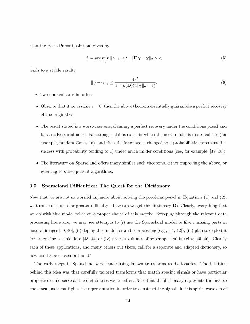
then the Basis Pursuit solution, given by

γ = arg minγ‖γ‖1 s.t. ‖Dγ − y‖2 ≤ ε, (5)

leads to a stable result,

‖γ − γ‖2 ≤4ε2

1− µ(D)(4‖γ‖0 − 1). (6)

A few comments are in order:

• Observe that if we assume ε = 0, then the above theorem essentially guarantees a perfect recovery

of the original γ.

• The result stated is a worst-case one, claiming a perfect recovery under the conditions posed and

for an adversarial noise. Far stronger claims exist, in which the noise model is more realistic (for

example, random Gaussian), and then the language is changed to a probabilistic statement (i.e.

success with probability tending to 1) under much milder conditions (see, for example, [37, 38]).

• The literature on Sparseland offers many similar such theorems, either improving the above, or

referring to other pursuit algorithms.

3.5 Sparseland Difficulties: The Quest for the Dictionary

Now that we are not so worried anymore about solving the problems posed in Equations (1) and (2),

we turn to discuss a far greater difficulty – how can we get the dictionary D? Clearly, everything that

we do with this model relies on a proper choice of this matrix. Sweeping through the relevant data

processing literature, we may see attempts to (i) use the Sparseland model to fill-in missing parts in

natural images [39, 40], (ii) deploy this model for audio-processing (e.g., [41, 42]), (iii) plan to exploit it

for processing seismic data [43, 44] or (iv) process volumes of hyper-spectral imaging [45, 46]. Clearly

each of these applications, and many others out there, call for a separate and adapted dictionary, so

how can D be chosen or found?

The early steps in Sparseland were made using known transforms as dictionaries. The intuition

behind this idea was that carefully tailored transforms that match specific signals or have particular

properties could serve as the dictionaries we are after. Note that the dictionary represents the inverse

transform, as it multiplies the representation in order to construct the signal. In this spirit, wavelets of

14

various kinds were used for 1D signals [19], 2D-DCT for image patches, and Curvelets [47], Contourlets

[48], and Shearlets [20] were suggested for images.

While seeming reasonable and elegant, the above approach was found to be quite limited in real

applications. The obvious reasons for this weakness were the partial match that exists between a

chosen transform and true data sources, and the lack of flexibility in these transforms that would

enable them to cope with special and narrow families of signals (e.g., face images, or financial data).

The breakthrough in this quest of getting appropriate dictionaries came in the form of dictionary

learning. The idea is quite simple: if we are given a large set of signals believed to emerge from a

Sparseland generator, we can ask what is the best dictionary that can describe these sparsely. In the

past decade we have seen a wealth of dictionary learning algorithms, varied in their computational

steps, in their objectives, and in their basic assumptions on the required D. These algorithms gave

Sparseland the necessary boost to become a leading model, due to the added ability to adapt to any

data source, and match to its content faithfully. In this paper we will not dwell too long on this branch

of work, despite its centrality, as our focus will be the model evolution we are about to present.

3.6 Sparseland Difficulties: Model Validity

We are listing difficulties that the Sparseland model encountered, and in this framework we mentioned

the atom-decomposition task and the pursuit algorithms that came to resolve it. We also described

the quest for the dictionary and the central role of dictionary learning approaches in this field. Beyond

these, perhaps the prime difficulty that Sparseland poses is encapsulated in the following questions:

Why should this model be trusted to perform well on a variety of signal sources? Clearly, images are

not made of atoms, and there is no dictionary behind the scene that explains our data sources. So,

what is the appeal in this specific model?

The answers to the above questions are still being built, and they take two possible paths. On the

empirical front, Sparseland has been deployed successfully in a wide variety of fields and for various

tasks, leading time and again to satisfactory and even state-of-the-art results. So, one obvious answer

to the above question is the simple statement “We tried it, and it works!”. As we have already said

above, a model cannot be proven to be correct, but it can be tested with real data, and this is the

essence of this answer.

The second branch of answers to the natural repulse from Sparseland has been more theoretically

15

Figure 3: Trends of publications for sparsity-related papers [Clarivate’s Web of Science, as of January

2018].

oriented, tying this model to other, well-known and better established, models, showing that it gen-

eralizes and strengthens them. Connections have been established between Sparseland and Markov

Random Field models, Gaussian-Mixture-Models (GMM) and other union-of-subspaces constructions

[30]. Indeed, the general picture obtained from the above suggests that Sparseland has a universal

ability to describe information content faithfully and effectively, due to the exponential number of

possible supports that a reasonable sized dictionary enables.

3.7 Sparseland Difficulties: Summary

The bottom line to all this discussion is the fact that, as opposed to our first impression, Sparseland

is a simple yet flexible model, and one that can be trusted. The difficulties mentioned have been

fully resolved and answered constructively, and today we are armed with a wide set of algorithms and

supporting theory for deploying Sparseland successfully for processing signals.

The interest in this field has grown impressively over the years, and this is clearly manifested by

the exponential growth of papers published in the arena, as shown in Figure 3. Another testimony to

the interest in Sparseland is seen by the wealth of books published in the past decade in this field –

see references [30, 49, 50, 51, 52, 19, 53, 54, 55, 56]. This attention brought us to offer a new MOOC

(Massive Open Online Course), covering the theory and practice of this field. This MOOC, given

under edX, started on October 2017, and already has more than 2000 enrolled students. It is expected

16

to be open continuously for all those who are interested in getting to know more about this field.

3.8 Local versus Global in Sparse Modeling

Just before we finish this section, we turn to discuss the practicalities of deploying Sparseland in image

processing. The common practice in many of such algorithms, and especially the better performing

ones, is to operate on small and fully overlapping patches. The prime reason for this mode of work

is the desire to harness dictionary learning methods, and these are possible only for low-dimensional

signals such as patches. The prior used in such algorithms is therefore the assumption that every patch

extracted from the image is believed to have a sparse representation with respect to a commonly built

dictionary.

After years of using this approach, questions started surfacing regarding this local model assumption,

and the underlying global model that may operate behind the scene. Consider the following questions,

all referring to a global signal X that is believed to obey such a local behavior – having a sparse

representation w.r.t. a local dictionary D for each of its extracted patches:

• How can such a signal be synthesized?

• Do such signals exist for any D?

• How should the pursuit be done in order to fully exploit the believed structure in X?

• How should D be trained for such signals?

These tough questions started being addressed in recent works [57, 14], and this brings us to our next

section, in which we dive into a special case of Sparseland – the Convolutional Sparse Coding (CSC)

model, and resolve this global-local gap.

17

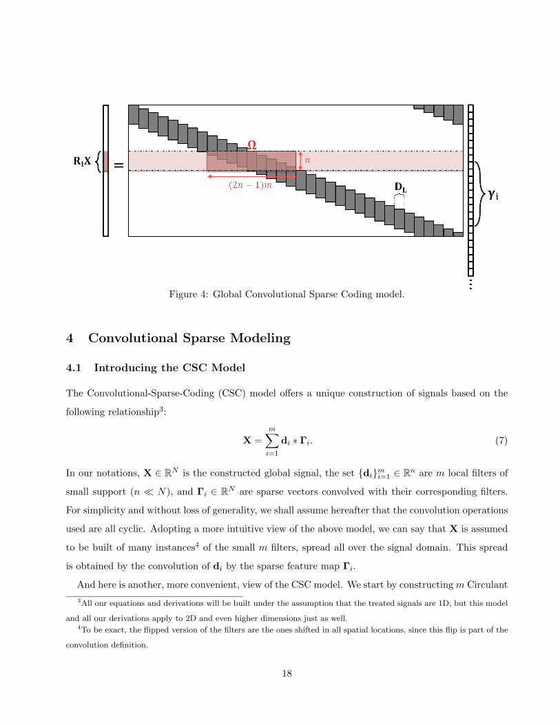
Figure 4: Global Convolutional Sparse Coding model.

4 Convolutional Sparse Modeling

4.1 Introducing the CSC Model

The Convolutional-Sparse-Coding (CSC) model offers a unique construction of signals based on the

following relationship3:

X =

m∑i=1

di ∗ Γi. (7)

In our notations, X ∈ RN is the constructed global signal, the set dimi=1 ∈ Rn are m local filters of

small support (n N), and Γi ∈ RN are sparse vectors convolved with their corresponding filters.

For simplicity and without loss of generality, we shall assume hereafter that the convolution operations

used are all cyclic. Adopting a more intuitive view of the above model, we can say that X is assumed

to be built of many instances4 of the small m filters, spread all over the signal domain. This spread

is obtained by the convolution of di by the sparse feature map Γi.

And here is another, more convenient, view of the CSC model. We start by constructing m Circulant

3All our equations and derivations will be built under the assumption that the treated signals are 1D, but this model

and all our derivations apply to 2D and even higher dimensions just as well.4To be exact, the flipped version of the filters are the ones shifted in all spatial locations, since this flip is part of the

convolution definition.

18

matrices Ci ∈ RN×N , representing the convolutions by the filters di. Each of these matrices is banded,

with only n populated diagonals. Thus, the global signal X can be described as

X =∑m

i=1 CiΓi = [C1 C2 · · · Cm]

Γ1

Γ2

...

Γm

= DΓ. (8)

The concatenated Circulant matrices form a global dictionary D ∈ RN×mN , and the gathered sparse

vectors Γi lead to the global sparse vector Γ ∈ RmN . Thus, just as said above, CSC is a special case of

Sparseland, built around a very structured dictionary being a union of banded and Circulant matrices.

Figure 4 presents the obtained dictionary D, where we permute its columns to obtain a sliding block

diagonal form. Each of the small blocks in this diagonal is the same, denoted by DL – this is a local

dictionary of size n×m, containing the m filters as its columns.

4.2 Why Should We Consider the CSC?

Why are we interested in the CSC model? Because it resolves the global-local gap we mentioned

earlier. Suppose that we extract an n-length patch from X taken in location i. This is denoted by

multiplying X by the patch-extractor operator Ri ∈ Rn×N , pi = RiX. Using the relation X = DΓ,

we have that pi = RiX = RiDΓ. Note that the multiplication RiD extracts n rows from the

dictionary, and most of their content is simply zero. In order to remove their empty columns, we

introduce the stripe extraction operator Si ∈ R(2n−1)m×mN that extracts the non-zero part in this

set of rows: RiD = RiDSTi Si. Armed with this definition, we observe that pi can be expressed as

pi = RiDSTi SiΓ = Ωγi. The structure of Ω, referred to as the stripe dictionary, appears in Figure 4,

showing that Ω = RiDSTi is a fixed matrix regardless of i. The notation γi = SiΓ stands for a stripe

of (2n− 1)m elements from Γ.

And now we get to the main point of all this description: As we move from location i to i+ 1, the

patch pi+1 = Ri+1X equals Ωγi+1. The stripe vector γi+1 is a shifted version of γi by m elements.

Other than that, we observe that the extracted patches are all getting a sparse description of their

content with respect to a common dictionary Ω, just as assumed by the locally-operating algorithms.

Thus, CSC furnishes a way to make our local modeling assumption valid, while also posing a clear

19

global model for X. In other words, the CSC model offers a path towards answering all the above

questions we have posed in the context of the global-local gap.

4.3 CSC: New Theoretical Foundations

Realizing that CSC may well be the missing link to all the locally-operating image processing algo-

rithms, and recalling that it is a special case of Sparseland, we should wonder whether the classic

existing theory of Sparseland provides sufficient foundations for it as well. Using Theorem 3.4 to the

case in which the signal we operate upon is Y = DΓ + E , where ‖E‖2 ≤ ε and D is a convolutional

dictionary, the condition for success of the Basis Pursuit is

‖Γ‖0 <1

4

(1 +

1

µ(D)

). (9)

Interestingly, the Welch bound offers a lower-bound on the best achievable mutual coherence of our

dictionary [58], being

µ(D) ≥

√m− 1

m(2n− 1)− 1. (10)

For example, for m = 2 filters of length n = 200, this value is ≈ 0.035, and this value necessarily

grows as m is increased. This implies that the bound for success of the BP stands on ‖Γ‖0 < 7.3. In

other words, we allow the entire vector Γ to have only 7 non-zeros (independently of N , the size of X)

for the ability to guarantee that BP will recover a close-enough sparse representation. Clearly, such

a statement is meaningless, and the unavoidable conclusion is that the classic theory of Sparseland

provides no solid foundations whatsoever to the CSC model.

The recent work reported in [14] offers an elegant way to resolve this difficulty, by moving to a new,

local, measure of sparsity. Rather than counting the number of non-zeros in the entire vector Γ, we

run through all the stripe representations, γi = SiΓ for i = 1, 2, 3, . . . , N , and define the relevant

cardinality of Γ as the maximal number of non-zeros in these stripes. Formally, this measure can be

defined as follows:

Definition: Given the global vector Γ, we define its local cardinality as

‖Γ‖s0,∞ = max1≤i≤N

‖γi‖0. (11)

20

In this terminology, it is an `0,∞ measure since we count number of non-zeros, but also maximize over

the set of stripes. The superscript s stands for the fact that we sweep through all the stripes in Γ,

skipping m elements from γi to γi+1.

Intuitively, if ‖Γ‖s0,∞ is small, this implies that all the stripes are sparse, and thus each patch in

X = DΓ has a sparse representation w.r.t. the dictionary Ω. Recall that this is exactly the model

assumption we mentioned earlier when operating locally. Armed with this local-sparsity definition, we

are now ready to define CSC signals, in the same spirit of the Sparseland definition:

Definition: The set of CSC signals of cardinality k over the convolutional dictionary D is defined as

SD, k. A signal X belongs to SD, k if it can be described as X = DΓ, where ‖Γ‖s0,∞ ≤ k.

Could we use these new notions of the local sparsity and the CSC signals in order derive novel

and stronger guarantees for the success of pursuit algorithms for the CSC model? The answer, as

given in [14], is positive. We now present one such result, among several others that are given in that

work, referring in this case to the Basis Pursuit algorithm. Just before presenting this theorem, we

note that the notation ‖E‖p2,∞ appearing below stands for computing the `2-norm on fully overlapping

sliding patches (hence the letter ‘p’) extracted from E, seeking the most energetic patch. As such, this

quantifies a local measure of the noise, which serves the following theorem:

Theorem 2: Given Y = DΓ + E, and Γ that is sufficiently locally-sparse,

‖Γ‖s0,∞ <1

3

(1 +

1

µ(D)

), (12)

the Basis Pursuit algorithm

Γ = arg minΓ

1

2‖Y −DΓ‖22 + λ‖Γ‖1 (13)

with λ = 4‖E‖p2,∞ satisfies the following:

• The support of Γ is contained in that of the original Γ,

• The result is stable: ‖Γ− Γ‖∞ ≤ 7.5‖E‖p2,∞,

• Every entry in Γ bigger than 7.5‖E‖p2,∞ is found, and

• The solution Γ is unique.

21

Note that the expression on the number of non-zeros permitted is similar to the one in the classic

Sparseland analysis, being O(1/µ(D)). However, in this theorem this quantity refers to the allowed

number of non-zeros in each stripe, which means that the overall number of permitted non-zeros in

Γ becomes proportional to O(N). As such, this is a much stronger and more practical outcome,

providing the necessary guarantee for various recent works that used the Basis Pursuit with the CSC

model for various applications [59, 60, 61, 62, 63, 64].

4.4 CSC: Operating Locally While Getting Global Optimality

The last topic we would like to address in this section is the matter of computing the global BP

solution for the CSC model while operating locally on small patches. As we are about to see, this

serves as a clarifying bridge to traditional image processing algorithms that operate on patches. We

discuss one such algorithm, originally presented in [65] – the slice-based pursuit.

In order to present this algorithm, we break Γ into small non-overlapping blocks of length m

each, denoted as αi and termed “needles”. A key observation this method relies on is the ability to

decompose the global signal X into the sum of small pieces, which we call “slices”, given by si = DLαi.

By positioning each of these in their location in the signal canvas, we can construct the full vector X:

X = DΓ =

m∑i=1

RTi DLαi =

m∑i=1

RTi si. (14)

By being the transposed of the patch-extraction operator, RTi ∈ RN×n places an n-dimensional patch

into its corresponding location in the N -dimensional signal X by padding it with N − n zeros. Then,

armed with this new way to represent X, the BP penalty can be restated in terms of the needles and

the slices,

minsii,αii

1

2

∥∥∥∥∥Y −m∑i=1

RTi si

∥∥∥∥∥2

2

+ λm∑i=1

‖αi‖1 s.t. si = DLαiNi=1 . (15)

This problem is entirely equivalent to the original BP penalty, being just as convex. Using ADMM

[66] to handle the constraints (see the details in [65]), we obtain a global pursuit algorithm that

iterates between local BP on each slice (that is easily managed by LARS [67] or any other efficient

solver), and an update of the slices that aggregates the temporal results into one estimated global

signal. Interestingly, if this algorithm initializes the slices to be patches from Y and applies only one

22

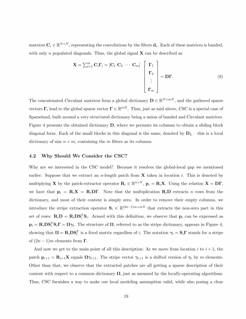
Figure 5: Comparison between patches (top row) and their respective slices (bottom) for each path,

extracted from natural images.

such round of operations, the resulting process aligns with the patch-based sparsity-inspired image

denoising algorithm [68]. Figure 5 shows the slices and their corresponding patches in an image, and

as can be clearly seen, the slices are simpler and thus easier to represent sparsely.

The above scheme can be extended to serve for the training of the CSC filters, DL. All that is

needed is to insert a “dictionary-update” stage in each iteration, in which we update DL based on

the given slices. This stage can be performed using the regular K-SVD algorithm [69] or any other

dictionary learning alternative, where the patches to train on are these slices. As such, the overall

algorithm relies on local operations and can therefore leverage all the efficient tools developed for

Sparseland over the last 15 years, while still solving the global CSC model – its learning and pursuit.

5 Multi-layered Convolutional Sparse Modeling

In this Section we arrive, at last, to the main serving of this paper, namely, connecting Sparseland

and the CSC model to deep learning and Convolutional Neural Networks (CNN). Preliminary signs

of this connection could already be vaguely identified, as there are some similarities between these

two disciplines. More specifically, both involve the presence of convolution operations, sparsifying

operations such as shrinkage or ReLU, and both rely on learning from data in order to better fit the

treatment to the given information source.

The above early signs did not go unnoticed, and motivated series of fascinating contributions that

aimed to bring an explanation to CNN’s. For instance, Bruna and Mallat [4] borrowed elements

from wavelet theory to demonstrate how one can build a network of convolutional operators while

providing invariance to shifts and deformations – properties that deep CNN’s are claimed to have.

Another interesting line of work comes from the observation that several pursuit algorithms can be

decomposed as several iterations of linear operators and a non-linear threshold, and therefore allow for

23

Figure 6: Illustration of the Forward Pass of a Convolutional Neural Network. The first feature map

is given by Z1 = ReLU(W1Y + b1), where W1 is a convolutional operator.

a CNN-based implementation. The seminal Learned Iterative Soft Thresholding Algorithm (LISTA)

[70] showed that one can indeed train such a network by unrolling iterative shrinkage iterations, while

achieving significantly faster convergence. In fact, CNN based pursuits can be even be shown to

outperform traditional sparse coding methods in some challenging cases [71].

In this section our goal is to make this connection much more precise and principled, and thus we

start by briefly recalling the way CNN’s operate.

5.1 A Brief Review of Conv-Nets

We shall assume that we are given an input image Y ∈ RN , of dimensions√N ×

√N . A classic

feed-forward CNN operates on Y by applying series of convolutions and non-linearities [72]. Our goal

in this section is to clearly formulate these steps.

In the first layer, Y is passed through a set of m1 convolutions5, using small-support filters of size√n0 ×

√n0. The output of these convolutions is augmented by a bias value and then passed through

a scalar-wise Rectified Linear Unit (ReLU) of the form ReLU(z) = max(0, z), and the result Z1 is

stored in the form of a 3D-tensor of size√N ×

√N ×m1, as illustrated in Figure 6. In matrix-vector

form, we could say that Y has been multiplied by a convolutional matrix W1 of size Nm1 ×N , built

5In this case as well, these convolutions are assumed cyclic.

24

by concatenating vertically a set of m1 circulant matrices of size N ×N . This is followed by the ReLU

step: Z1 = ReLU(W1Y + b1). Note that b1 is a vector of length Nm1, applying a different threshold

per each filter in the resulting tensor.

The second layer obtains the tensor Z1 and applies the same set of operations: m2 convolutions

with small spatial support (√n1 ×

√n1) and across all m1 channels, and a ReLU non-linearity. Each

such filter weights together (i.e., this implements a 2D convolution across all feature maps) the m1

channels of Z1, which explains the length mentioned above. Thus, the output of the second layer is

given by Z2 = ReLU(W2Z1 + b2), where W2 is a vertical amalgam of m2 convolutional matrices of

size N ×Nm1.

The story may proceed this way with additional layers sharing the same functional structure. A

variation to the above could be pooling or stride operations, both coming to reduce the spatial resolu-

tion of the resulting tensor. In this paper we focus on the stride option, which is easily absorbed within

the above description by sub-sampling the rows in the corresponding convolution matrices. We note

that recent work suggests that pooling can be replaced by stride without a performance degradation

([73, 74]).

To summarize, for the two layered feed-forward CNN, the relation between input and output is

given by

f(Y) = ReLU (W2ReLU (W1Y + b1) + b2) . (16)

5.2 Introducing the Multi-Layered CSC (ML-CSC) Model

We return now to the CSC model with an intention to extend it by introducing a multi-layered version

of it. Our starting point is the belief that the ideal signal we operate on, X, is emerging from the

CSC model, just as described in Section 4. Thus, X = D1Γ1 where D1 is a convolutional dictionary

of size N ×Nm1, and Γ1 is locally-sparse, i.e., ‖Γ1‖s0,∞ = k1 m1(2n0− 1), where m1 is the number

of filters in this model and n0 is their length.

We now add another layer to the above-described signal: We assume that Γ1 itself is also believed

to be produced from a CSC model of a similar form, namely, Γ1 = D2Γ2, where D2 is another

convolutional dictionary of size Nm1 ×Nm2, and ‖Γ2‖s0,∞ = k2 m2(2n1m1 − 1), where m2 is the

number of filters in this model and n1 is their length.

25

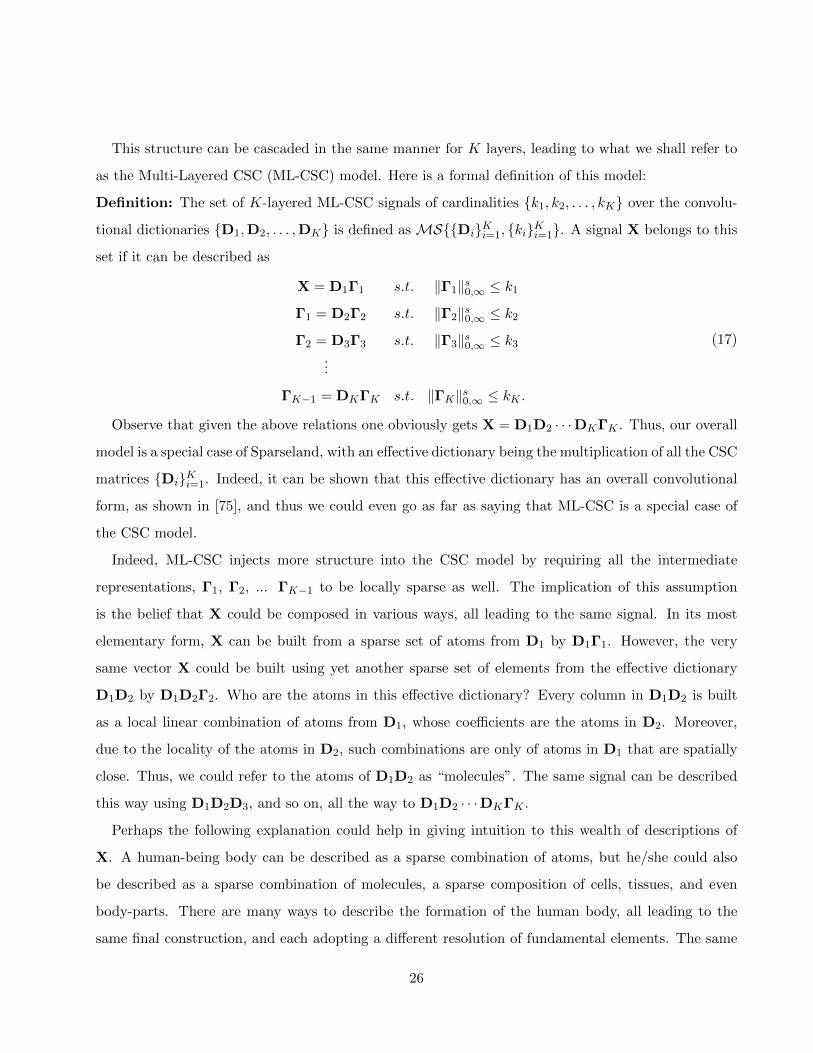
This structure can be cascaded in the same manner for K layers, leading to what we shall refer to

as the Multi-Layered CSC (ML-CSC) model. Here is a formal definition of this model:

Definition: The set of K-layered ML-CSC signals of cardinalities k1, k2, . . . , kK over the convolu-

tional dictionaries D1,D2, . . . ,DK is defined as MSDiKi=1, kiKi=1. A signal X belongs to this

set if it can be described as

X = D1Γ1 s.t. ‖Γ1‖s0,∞ ≤ k1

Γ1 = D2Γ2 s.t. ‖Γ2‖s0,∞ ≤ k2

Γ2 = D3Γ3 s.t. ‖Γ3‖s0,∞ ≤ k3...

ΓK−1 = DKΓK s.t. ‖ΓK‖s0,∞ ≤ kK .

(17)

Observe that given the above relations one obviously gets X = D1D2 · · ·DKΓK . Thus, our overall

model is a special case of Sparseland, with an effective dictionary being the multiplication of all the CSC

matrices DiKi=1. Indeed, it can be shown that this effective dictionary has an overall convolutional

form, as shown in [75], and thus we could even go as far as saying that ML-CSC is a special case of

the CSC model.

Indeed, ML-CSC injects more structure into the CSC model by requiring all the intermediate

representations, Γ1, Γ2, ... ΓK−1 to be locally sparse as well. The implication of this assumption

is the belief that X could be composed in various ways, all leading to the same signal. In its most

elementary form, X can be built from a sparse set of atoms from D1 by D1Γ1. However, the very

same vector X could be built using yet another sparse set of elements from the effective dictionary

D1D2 by D1D2Γ2. Who are the atoms in this effective dictionary? Every column in D1D2 is built

as a local linear combination of atoms from D1, whose coefficients are the atoms in D2. Moreover,

due to the locality of the atoms in D2, such combinations are only of atoms in D1 that are spatially

close. Thus, we could refer to the atoms of D1D2 as “molecules”. The same signal can be described

this way using D1D2D3, and so on, all the way to D1D2 · · ·DKΓK .

Perhaps the following explanation could help in giving intuition to this wealth of descriptions of

X. A human-being body can be described as a sparse combination of atoms, but he/she could also

be described as a sparse combination of molecules, a sparse composition of cells, tissues, and even

body-parts. There are many ways to describe the formation of the human body, all leading to the

same final construction, and each adopting a different resolution of fundamental elements. The same

26

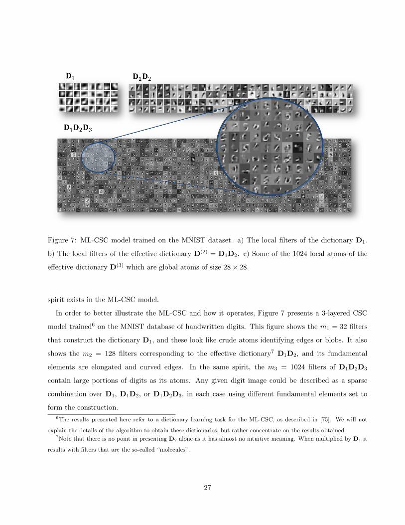
Figure 7: ML-CSC model trained on the MNIST dataset. a) The local filters of the dictionary D1.

b) The local filters of the effective dictionary D(2) = D1D2. c) Some of the 1024 local atoms of the

effective dictionary D(3) which are global atoms of size 28× 28.

spirit exists in the ML-CSC model.

In order to better illustrate the ML-CSC and how it operates, Figure 7 presents a 3-layered CSC

model trained6 on the MNIST database of handwritten digits. This figure shows the m1 = 32 filters

that construct the dictionary D1, and these look like crude atoms identifying edges or blobs. It also

shows the m2 = 128 filters corresponding to the effective dictionary7 D1D2, and its fundamental

elements are elongated and curved edges. In the same spirit, the m3 = 1024 filters of D1D2D3

contain large portions of digits as its atoms. Any given digit image could be described as a sparse

combination over D1, D1D2, or D1D2D3, in each case using different fundamental elements set to

form the construction.

6The results presented here refer to a dictionary learning task for the ML-CSC, as described in [75]. We will not

explain the details of the algorithm to obtain these dictionaries, but rather concentrate on the results obtained.7Note that there is no point in presenting D2 alone as it has almost no intuitive meaning. When multiplied by D1 it

results with filters that are the so-called “molecules”.

27

5.3 Pursuit Algorithms for ML-CSC Signals: First Steps

Pursuit algorithms were mentioned throughout this paper, making their first appearance in the context

of Sparseland, and later appearing again in the CSC. The pursuit task is essentially a projection

operation, seeking the signal closest to the given data while belonging to the model, be it Sparseland,

the CSC model or the ML-CSC. When dealing with a signal X believed to belong to the ML-CSC

model, a noisy signal Y = X+E (‖E‖2 ≤ ε) is projected to the model by solving the following pursuit

problem:

Find ΓiKi=1 s.t.

‖Y −D1Γ1‖2 ≤ ε , ‖Γ1‖s0,∞ ≤ k1

Γ1 = D2Γ2 , ‖Γ2‖s0,∞ ≤ k2

Γ2 = D3Γ3 , ‖Γ3‖s0,∞ ≤ k3...

ΓK−1 = DKΓK , ‖ΓK‖s0,∞ ≤ kK

(18)

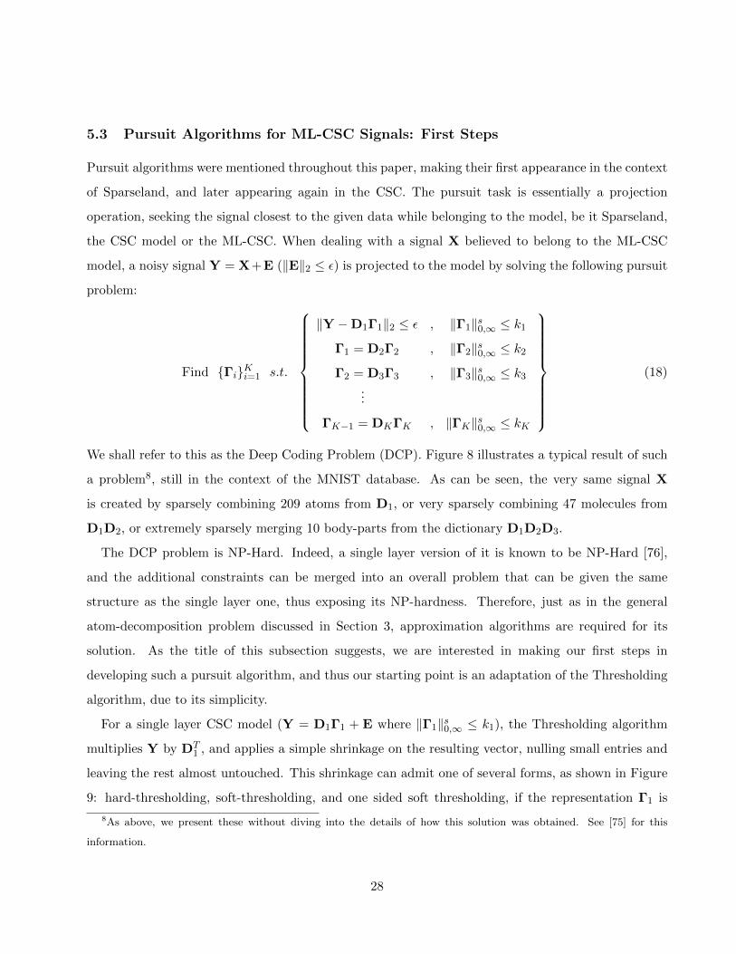
We shall refer to this as the Deep Coding Problem (DCP). Figure 8 illustrates a typical result of such

a problem8, still in the context of the MNIST database. As can be seen, the very same signal X

is created by sparsely combining 209 atoms from D1, or very sparsely combining 47 molecules from

D1D2, or extremely sparsely merging 10 body-parts from the dictionary D1D2D3.

The DCP problem is NP-Hard. Indeed, a single layer version of it is known to be NP-Hard [76],

and the additional constraints can be merged into an overall problem that can be given the same

structure as the single layer one, thus exposing its NP-hardness. Therefore, just as in the general

atom-decomposition problem discussed in Section 3, approximation algorithms are required for its

solution. As the title of this subsection suggests, we are interested in making our first steps in

developing such a pursuit algorithm, and thus our starting point is an adaptation of the Thresholding

algorithm, due to its simplicity.

For a single layer CSC model (Y = D1Γ1 + E where ‖Γ1‖s0,∞ ≤ k1), the Thresholding algorithm

multiplies Y by DT1 , and applies a simple shrinkage on the resulting vector, nulling small entries and

leaving the rest almost untouched. This shrinkage can admit one of several forms, as shown in Figure

9: hard-thresholding, soft-thresholding, and one sided soft thresholding, if the representation Γ1 is

8As above, we present these without diving into the details of how this solution was obtained. See [75] for this

information.

28

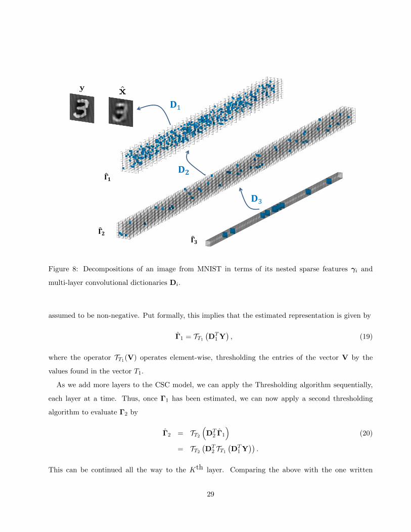
Figure 8: Decompositions of an image from MNIST in terms of its nested sparse features γi and

multi-layer convolutional dictionaries Di.

assumed to be non-negative. Put formally, this implies that the estimated representation is given by

Γ1 = TT1(DT

1 Y), (19)

where the operator TT1(V) operates element-wise, thresholding the entries of the vector V by the

values found in the vector T1.

As we add more layers to the CSC model, we can apply the Thresholding algorithm sequentially,

each layer at a time. Thus, once Γ1 has been estimated, we can now apply a second thresholding

algorithm to evaluate Γ2 by

Γ2 = TT2(DT

2 Γ1

)(20)

= TT2(DT

2 TT1(DT

1 Y)).

This can be continued all the way to the Kth layer. Comparing the above with the one written

29

− 10 − 8 − 6 − 4 − 2 0 2 4 6 8 10− 10

− 8

− 6

− 4

− 2

0

2

4

6

8

10Hard

Soft

Soft Non-Negative

Figure 9: Hard, Soft and one sided Soft thresholding operators.

previously for the feed-forward CNN,

f(Y) = ReLU (W2ReLU (W1Y + b1) + b2) , (21)

reveals a striking resemblance. These two formulas express the same procedure: a set of convolutions

applied on Y, followed by a non-linearity with a threshold, and proceeding this way as we dive into

inner layers. The transposed dictionary Di plays the role of a set of convolutions, the threshold Tk

parallels the bias vector bk, and the shrinkage operation stands for the ReLU. So, the inevitable con-

clusion is this: Assuming that our signals emerge from the ML-CSC model, the Layered-Thresholding

algorithm for decomposing a given measurements vector Y is completely equivalent to the forward

pass in convolutional neural networks.

The pursuit algorithm we have just presented, or the forward pass of the CNN to that matter,

estimates the sparse representations ΓkKk=1 that explain our signal. Why bother computing these

hidden vectors? An additional assumption in our story is the fact that the labels associated with the

data we are given are believed to depend on these representations in a linearly separable way, and

thus given ΓkKk=1, classification (or regression) is facilitated. In this spirit, a proper estimation of

these vectors implies better classification results.

30

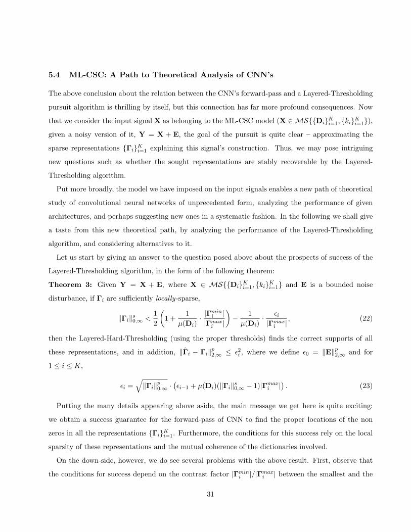
5.4 ML-CSC: A Path to Theoretical Analysis of CNN’s

The above conclusion about the relation between the CNN’s forward-pass and a Layered-Thresholding

pursuit algorithm is thrilling by itself, but this connection has far more profound consequences. Now

that we consider the input signal X as belonging to the ML-CSC model (X ∈MSDiKi=1, kiKi=1),

given a noisy version of it, Y = X + E, the goal of the pursuit is quite clear – approximating the

sparse representations ΓiKi=1 explaining this signal’s construction. Thus, we may pose intriguing

new questions such as whether the sought representations are stably recoverable by the Layered-

Thresholding algorithm.

Put more broadly, the model we have imposed on the input signals enables a new path of theoretical

study of convolutional neural networks of unprecedented form, analyzing the performance of given

architectures, and perhaps suggesting new ones in a systematic fashion. In the following we shall give

a taste from this new theoretical path, by analyzing the performance of the Layered-Thresholding

algorithm, and considering alternatives to it.

Let us start by giving an answer to the question posed above about the prospects of success of the

Layered-Thresholding algorithm, in the form of the following theorem:

Theorem 3: Given Y = X + E, where X ∈ MSDiKi=1, kiKi=1 and E is a bounded noise

disturbance, if Γi are sufficiently locally-sparse,

‖Γi‖s0,∞ <1

2

(1 +

1

µ(Di)· |Γ

mini |

|Γmaxi |

)− 1

µ(Di)· εi|Γmaxi |

, (22)

then the Layered-Hard-Thresholding (using the proper thresholds) finds the correct supports of all

these representations, and in addition, ‖Γi − Γi‖p2,∞ ≤ ε2i , where we define ε0 = ‖E‖p2,∞ and for

1 ≤ i ≤ K,

εi =√‖Γi‖p0,∞ ·

(εi−1 + µ(Di)(‖Γi‖s0,∞ − 1)|Γmaxi |

). (23)

Putting the many details appearing above aside, the main message we get here is quite exciting:

we obtain a success guarantee for the forward-pass of CNN to find the proper locations of the non

zeros in all the representations ΓiKi=1. Furthermore, the conditions for this success rely on the local

sparsity of these representations and the mutual coherence of the dictionaries involved.

On the down-side, however, we do see several problems with the above result. First, observe that

the conditions for success depend on the contrast factor |Γmini |/|Γmaxi | between the smallest and the

31

largest non-zero in the representations. This implies that for high-contrasted vectors, the conditions

for success are much more strict. This sensitivity is not an artifact of the analysis, but rather a true

and known difficulty that the Thresholding algorithm carries with it.

Another troubling issue is an error growth that is seen as we proceed through the layers of the model.

This growth is expected, due to the sequentiality of the Layered-Thresholding algorithm, propagating

the errors and magnifying them from one layer to the next. Indeed, another problem is the fact that

even if E is zero, namely, we are lucky to operate on a pure ML-CSC signal, the Layered-Thresholding

algorithm induces an error in the inner layers, just as well.

5.5 ML-CSC: Better Pursuit and Implications

In the above analysis we have exposed good features of the Layered-Thresholding, alongside some

sensitivities and weaknesses. Recall that the Thresholding algorithm is the simplest and crudest

possible pursuit for sparsity-based signals. Why should we stick to it, if we are aware of better

techniques? This takes us to the next discussion, in which we propose an alternative layered pursuit,

based on the Basis Pursuit.

Consider the first layer of the ML-CSC model, described by the relations X = D1Γ1 and ‖Γ1‖s0,∞ ≤

k1. This is in fact a regular CSC model, for which Theorem 4.3 provides the terms of success of the

Basis Pursuit, when applied on a noisy version of such a signal, Y = X + E. Thus, solving

Γ1 = arg minΓ1

1

2‖Y −D1Γ1‖22 + λ1‖Γ1‖1 (24)

with a properly chosen λ1 is guaranteed to perform well, giving a stable estimate of Γ1.

Consider now the second layer in the ML-CSC model, characterized by Γ1 = D2Γ2 and ‖Γ2‖s0,∞ ≤

k2. Even though we are not given Γ1, but rather a noisy version of it, Γ1, our analysis of the first

stage provides an assessment of the noise power in this estimate. Thus, a second Basis Pursuit can be

performed,

Γ2 = arg minΓ2

1

2‖Γ1 −D2Γ2‖22 + λ2‖Γ2‖1 (25)

with a properly chosen λ2, and this again leads to a guaranteed stable estimate of Γ2.

We may proceed in this manner, proposing the Layered-BP algorithm. Interestingly, such an algo-

rithmic structure, coined Deconvolutional Networks [77], was proposed in the deep learning literature

32

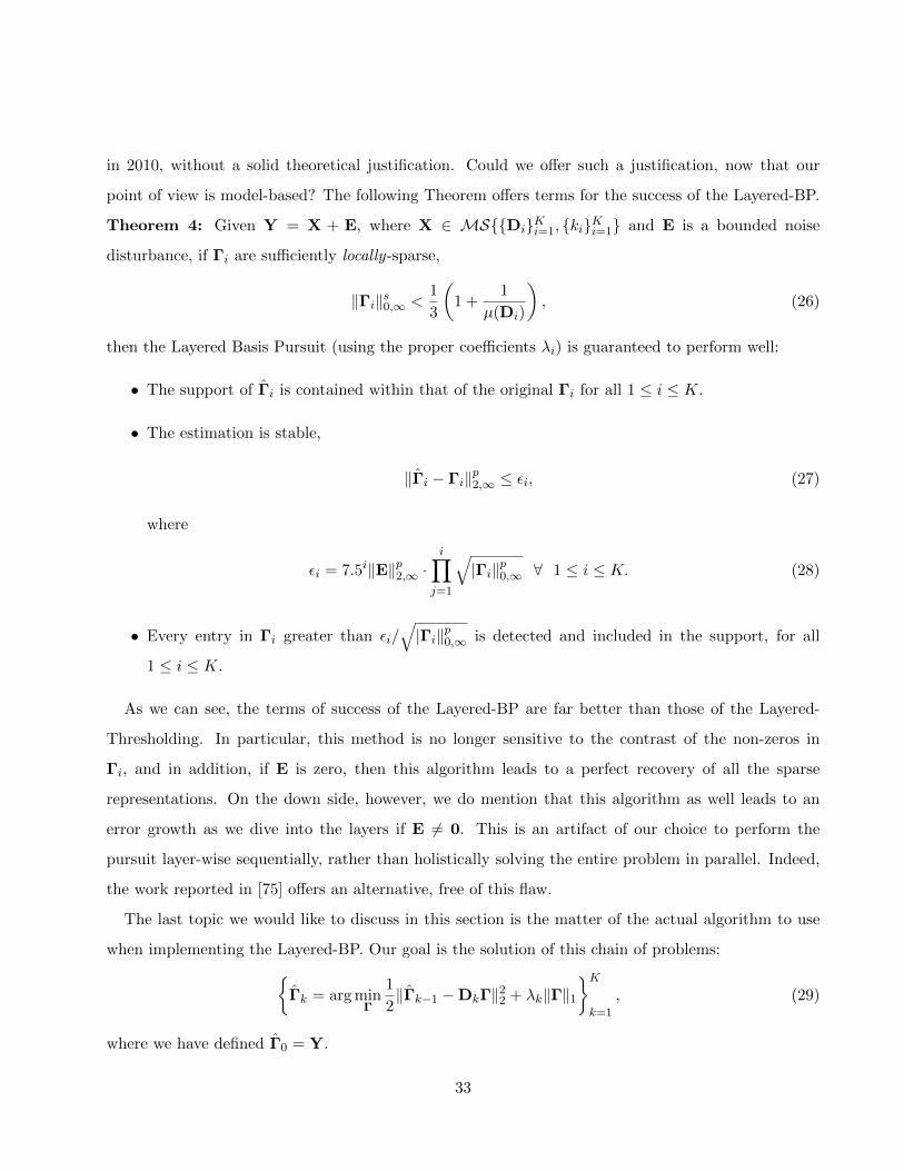
in 2010, without a solid theoretical justification. Could we offer such a justification, now that our

point of view is model-based? The following Theorem offers terms for the success of the Layered-BP.

Theorem 4: Given Y = X + E, where X ∈ MSDiKi=1, kiKi=1 and E is a bounded noise

disturbance, if Γi are sufficiently locally-sparse,

‖Γi‖s0,∞ <1

3

(1 +

1

µ(Di)

), (26)

then the Layered Basis Pursuit (using the proper coefficients λi) is guaranteed to perform well:

• The support of Γi is contained within that of the original Γi for all 1 ≤ i ≤ K.

• The estimation is stable,

‖Γi − Γi‖p2,∞ ≤ εi, (27)

where

εi = 7.5i‖E‖p2,∞ ·i∏

j=1

√|Γi‖p0,∞ ∀ 1 ≤ i ≤ K. (28)

• Every entry in Γi greater than εi/√|Γi‖p0,∞ is detected and included in the support, for all

1 ≤ i ≤ K.

As we can see, the terms of success of the Layered-BP are far better than those of the Layered-

Thresholding. In particular, this method is no longer sensitive to the contrast of the non-zeros in

Γi, and in addition, if E is zero, then this algorithm leads to a perfect recovery of all the sparse

representations. On the down side, however, we do mention that this algorithm as well leads to an

error growth as we dive into the layers if E 6= 0. This is an artifact of our choice to perform the

pursuit layer-wise sequentially, rather than holistically solving the entire problem in parallel. Indeed,

the work reported in [75] offers an alternative, free of this flaw.

The last topic we would like to discuss in this section is the matter of the actual algorithm to use

when implementing the Layered-BP. Our goal is the solution of this chain of problems:Γk = arg min

Γ

1

2‖Γk−1 −DkΓ‖22 + λk‖Γ‖1

Kk=1

, (29)

where we have defined Γ0 = Y.

33

An appealing approximate solver for the core BP problem minΓ12‖Y−DΓ‖22+λ‖Γ‖1 is the Iterative

Soft Thresholding Algorithm (ISTA) [78], which applies the following iterative procedure9:

Γt = Tλ(Γt−1 + DT

(Y −DΓt−1

)). (30)

Thus, if each of the K layers of the model is managed using J iterations of the ISTA algorithm, and

these steps are unfolded to form a long sequential process, we get an architecture with K · J layers

of a linear convolution operation followed by an element-wise non-linearity, reminding very much the

recurrent neural network structure. For example, for a model with K = 10 layers and using J = 50

iterations of ISTA, the network obtained contains 500 layers (with a recurrent structure), and this

gives a very illuminating perspective to the depth of typical networks.

Observe that our insight as developed above suggests that each J iterations in this scheme should

use the same dictionary Dk, and thus when learning the network we can force this parameter sharing,

reducing the number of overall learned parameters by factor 50. Moreover, recalling the comment on

LISTA networks and their advantage in terms of number of unfolding [70], if one frees the convolutional

operators from being defined by the respective dictionary, such a network could be implemented with

significantly fewer layers.

6 Concluding Remarks

6.1 Summary of this Paper

We started this paper by highlighting the importance of models in data processing, and then turned

to describe one of these in depth: Sparseland, a systematic and highly effective such model. We then

moved to Convolution Sparse Coding (CSC), with the hope to better treat images and other high-

dimensional signals while operating locally, and accompanied this migration with the introduction of

a new theory to substantiate this model. This brought us naturally to the Multi-Layered CSC (ML-

CSC), which gave us a bridge to the realm of deep learning. Specifically, we have shown that handling

ML-CSC signals amounts to convolutional neural networks of various forms, all emerging naturally

as deployments of pursuit algorithms. Furthermore, we have seen that this new way of looking at

these architectures can be accompanied by an unprecedented ability to study their performance, and

9Assuming the dictionary has been normalized so that ‖D‖2 = 1.

34

identify the weaknesses and strengths of the ingredients involved. This was the broad story of this

paper, and there are two main take-home messages emerging from it:

• The backbone of our story are three parametric models for managing signals: Sparseland, CSC,

and ML-CSC. All three are generative models, offering an explanation of the data by means of

how it is synthesized. We have seen that this choice of models is extremely beneficial for both

designing algorithms for serving such signals, and enabling their theoretical analysis.

• The multi-layered CSC model puts forward an appealing way to explain the motivation and

origin of some common deep learning architectures. As such, this model and the line of thinking

behind it poses a new platform for understanding and further developing deep learning solutions.

We hope that this work will provide some of the foundations for the much-desired theoretical

justification of deep learning.

6.2 Future Research Directions and Open Problems

The ideas we have outlined in this paper open up numerous new directions for further research, and

we conclude by listing some of the more promising ones:

• Dictionary Learning: A key topic that we have deliberately paid less attention to in this paper

is the need to train the obtained networks to achieve their processing goals. In the context of

the ML-CSC model, this parallels the need to learn the dictionaries DkKi=k and the threshold

vectors. Observe that all the theoretical study we have proposed relied on an unsupervised

regime, in which the labels play no role. This should remind the readers of auto-encoders, in

which sparsity is the driving force behind the learning mechanism. Further work is required in

order to extend the knowledge on dictionary learning, both practical and theoretical, in order

to bring it to the ML-CSC model, and with this offer new ways to learn neural networks. The

first such attempt appears in [75], and some of its results have been brought above.

The idea of training a series of cascaded dictionaries for getting an architecture mimicking that

of deep learning has in fact appeared in earlier work [77, 79, 80, 81, 82, 83]. However, these

attempts took an applicative and practical point of view, and were never posed within the

context of a solid mathematical multi-layered model of the data, as in this work. In [77] and

35

[79] the authors learned a set of convolutional dictionaries over multiple layers of abstraction

in an unsupervised manner. In [80, 81] the authors suggested using back-propagation rules for

learning multi-layered (non-convolutional) dictionaries for CIFAR10 classification, motivated by

earlier work [82, 83] that showed how this was possible for a single layer setting. We believe that

some of these ideas could become helpful in developing novel multi-layered dictionary learning

algorithms, while relating to our formal model, thus preserving the relevance of its theoretical

analysis.

• Pursuit Algorithms: We introduced layered versions of the Thresholding and the Basis Pursuit,

and both are clearly sub-optimal when it comes to projecting a signal to the ML-CSC model.

Could we do better than these? The answer is positive, and such a progress has already appeared

in [75]. Still, there is room for further improvements, both in handling the various layers in

parallel and not sequentially, and also in better serving the local-sparsity we are after. Recall

that better pursuit algorithms implies new architectures, and with them new horizons to the

deep learning practice.

• Theoretical Analysis: The study presented here represents the very first steps in a road that

could take us to far better and more informative performance bounds. The analysis we have

shown is a worst-case one, and as such, it is too pessimistic. Also, all of it relies strongly on

the mutual coherence, a worst-case study that tends to present a gloomy perspective on the

prospects of the investigated algorithms. In addition, as we migrate from the layered pursuit

algorithms to more sophisticated solutions, we may expect better and more encouraging bounds.

More broadly, a complete theory for deep learning cannot limit itself to the data model and

the architectures emerging from it, as this work does. Missing in our picture are answers to

intriguing questions on the learning, optimization, and generalization performance facets of

neural networks. We believe that these topics could be addressed while still relying on data

models, of the kind posed in this work.

• Improving the Model: Labels play no role in the study presented in this paper, and we have

replaced them by the quest to recover the proper supports of the ideal representations or vectors

close to them in terms of the `2 norm. While we did explain the underlying assumption behind

this line of thinking, a broader model that takes the labels into account is very much needed.

36

Indeed, rather than modeling the incoming signals, perhaps we should focus our modeling on

the function that connects these to their corresponding labels.

• Deployment to Practice: There is no doubt in our minds that the true and ultimate test for

the theory we present will be its ability to push the practice and performance of deep learning

further. The provided explanations on the used CNN architectures is a great start, but it must be

followed by better understanding of more advanced ideas such as pooling, batch-normalization,

dropout and many other ideas that were found useful in practice. Beyond these, we hope to

see this theory lead to new ideas that are simply impossible to develop without the systematic

approach that the model-based theory unravels.

References

[1] V. Papyan, Y. Romano, and M. Elad, “Convolutional neural networks analyzed via convolutional sparse

coding,” To appear in JMLR. arXiv preprint arXiv:1607.08194, 2016.

[2] A. B. Patel, T. Nguyen, and R. G. Baraniuk, “A probabilistic theory of deep learning,” arXiv preprint

arXiv:1504.00641, 2015.

[3] N. Tishby and N. Zaslavsky, “Deep learning and the information bottleneck principle,” 2015 IEEE Infor-

mation Theory Workshop (ITW), pp. 1–5, 2015.

[4] J. Bruna and S. Mallat, “Invariant scattering convolution networks,” IEEE transactions on pattern analysis

and machine intelligence, vol. 35, no. 8, pp. 1872–1886, 2013.

[5] B. D. Haeffele and R. Vidal, “Global optimality in neural network training,” in IEEE Conference on

Computer Vision and Pattern Recognition, pp. 7331–7339, 2017.

[6] P. Chaudhari and S. Soatto, “Stochastic gradient descent performs variational inference,” arXiv preprint

arXiv:1710.11029, 2017.

[7] P. Grohs, T. Wiatowski, and H. Bolcskei, “Deep convolutional neural networks on cartoon functions,” in

IEEE International Symposium on Information Theory (ISIT), 2016.

[8] H. Bolcskei, P. Grohs, G. Kutyniok, and P. Petersen, “Optimal approximation with sparsely connected

deep neural networks,” arXiv preprint arXiv:1705.01714, 2017.

[9] R. Giryes, G. Sapiro, and A. M. Bronstein, “Deep neural networks with random gaussian weights: A

universal classification strategy,” CoRR, abs/1504.08291, 2015.

37

[10] E. Haber and L. Ruthotto, “Stable architectures for deep neural networks,” arXiv preprint

arXiv:1705.03341, 2017.

[11] N. Cohen, O. Sharir, and A. Shashua, “On the expressive power of deep learning: A tensor analysis,” in

29th Annual Conference on Learning Theory (V. Feldman, A. Rakhlin, and O. Shamir, eds.), vol. 49 of

Proceedings of Machine Learning Research, (Columbia University, New York, New York, USA), pp. 698–

728, PMLR, 23–26 Jun 2016.

[12] J. Sokolic, R. Giryes, G. Sapiro, and M. R. Rodrigues, “Robust large margin deep neural networks,” IEEE

Transactions on Signal Processing 65(16), pp. 4265–4280, 2016.

[13] H. Mhaskar, Q. Liao, and T. Poggio, “Learning functions: when is deep better than shallow,” arXiv preprint

arXiv:1603.00988, 2016.

[14] V. Papyan, J. Sulam, and M. Elad, “Working locally thinking globally: Theoretical guarantees for convo-

lutional sparse coding,” IEEE Transactions on Signal Processing, vol. 65, no. 21, pp. 5687–5701, 2017.

[15] G. K. Wallace, “The jpeg still picture compression standard,” IEEE transactions on consumer electronics,

vol. 38, no. 1, pp. xviii–xxxiv, 1992.

[16] S. Z. Li, Markov random field modeling in image analysis. Springer Science & Business Media, 2009.

[17] A. Bouhamidi and K. Jbilou, “Sylvester tikhonov-regularization methods in image restoration,” Journal of

Computational and Applied Mathematics, vol. 206, no. 1, pp. 86–98, 2007.

[18] L. I. Rudin, S. Osher, and E. Fatemi, “Nonlinear total variation based noise removal algorithms,” Physica

D: Nonlinear Phenomena, vol. 60, no. 1, pp. 259 – 268, 1992.

[19] S. Mallat, A wavelet tour of signal processing: the sparse way. Academic press, 2008.

[20] G. Kutyniok and D. Labate, “Introduction to shearlets,” Shearlets, pp. 1–38, 2012.

[21] J. Portilla, V. Strela, M. J. Wainwright, and E. P. Simoncelli, “Image denoising using scale mixtures of

Gaussians in the wavelet domain.,” IEEE Transactions on Image Processing., vol. 12, pp. 1338–51, Jan.

2003.

[22] D. Zoran and Y. Weiss, “From learning models of natural image patches to whole image restoration,” 2011

International Conference on Computer Vision, ICCV., pp. 479–486, Nov. 2011.

[23] P. Chatterjee and P. Milanfar, “Is denoising dead?,” IEEE Transactions on Image Processing, vol. 19,

no. 4, pp. 895–911, 2010.

[24] A. Levin and B. Nadler, “Natural image denoising: Optimality and inherent bounds,” in Computer Vision

and Pattern Recognition (CVPR), 2011 IEEE Conference on, pp. 2833–2840, IEEE, 2011.

38

[25] D. Wrinch and H. Jeffreys, “Xlii. on certain fundamental principles of scientific inquiry,” The London,

Edinburgh, and Dublin Philosophical Magazine and Journal of Science, vol. 42, no. 249, pp. 369–390, 1921.

[26] S. Mallat and Z. Zhang, “Matching Pursuits With Time-Frequency Dictionaries,” IEEE Trans. Signal

Process., vol. 41, no. 12, pp. 3397–3415, 1993.

[27] S. S. Chen, D. L. Donoho, and M. A. Saunders, “Atomic Decomposition by Basis Pursuit,” SIAM Review,

vol. 43, no. 1, pp. 129–159, 2001.

[28] B. A. Olshausen and D. J. Field, “Sparse coding with an overcomplete basis set: A strategy employed by

v1?,” Vision research, vol. 37, no. 23, pp. 3311–3325, 1997.

[29] D. L. Donoho and X. Huo, “Uncertainty principles and ideal atomic decomposition,” IEEE Transactions

on Information Theory, vol. 47, no. 7, pp. 2845–2862, 2001.

[30] M. Elad, Sparse and Redundant Representations: From Theory to Applications in Signal and Image Pro-

cessing. Springer Publishing Company, Incorporated, 1st ed., 2010.

[31] Y. C. Pati, R. Rezaiifar, and P. S. Krishnaprasad, “Orthogonal Matching Pursuit: Recursive Function

Approximation with Applications to Wavelet Decomposition,” Asilomar Conf. Signals, Syst. Comput.

IEEE., pp. 40–44, 1993.

[32] D. Donoho, M. Elad, and V. Temlyakov, “Stable recovery of sparse overcomplete representations in the

presence of noise,” Information Theory, IEEE Transactions on, vol. 52, pp. 6–18, Jan 2006.

[33] E. J. Candes and T. Tao, “Decoding by linear programming,” Information Theory, IEEE Transactions on,

vol. 51, no. 12, pp. 4203–4215, 2005.

[34] J. Tropp, “Greed is Good: Algorithmic Results for Sparse Approximation,” IEEE Transactions on Infor-

mation Theory, vol. 50, no. 10, pp. 2231–2242, 2004.

[35] J. A. Tropp, A. C. Gilbert, S. Muthukrishnan, and M. J. Strauss, “Improved sparse approximation over

quasiincoherent dictionaries,” in Image Processing, 2003. ICIP 2003. Proceedings. 2003 International Con-

ference on, vol. 1, pp. I–37, IEEE, 2003.

[36] D. L. Donoho and M. Elad, “Optimally sparse representation in general (nonorthogonal) dictionaries via

`1 minimization,” Proceedings of the National Academy of Sciences, vol. 100, no. 5, pp. 2197–2202, 2003.

[37] E. J. Candes, J. Romberg, and T. Tao, “Robust uncertainty principles: Exact signal reconstruction

from highly incomplete frequency information,” IEEE Transactions on information theory, vol. 52, no. 2,

pp. 489–509, 2006.

39

[38] K. Schnass and P. Vandergheynst, “Average performance analysis for thresholding,” IEEE Signal Processing

Letters, vol. 14, no. 11, pp. 828–831, 2007.

[39] Z. Xu and J. Sun, “Image inpainting by patch propagation using patch sparsity,” IEEE transactions on

image processing, vol. 19, no. 5, pp. 1153–1165, 2010.

[40] J. Sulam and M. Elad, “Large inpainting of face images with trainlets,” IEEE Signal Processing Letters,

vol. 23, pp. 1839–1843, Dec 2016.

[41] M. D. Plumbley, T. Blumensath, L. Daudet, R. Gribonval, and M. E. Davies, “Sparse representations in

audio and music: from coding to source separation,” Proceedings of the IEEE, vol. 98, no. 6, pp. 995–1005,

2010.

[42] M. G. Jafari and M. D. Plumbley, “Fast dictionary learning for sparse representations of speech signals,”

IEEE Journal of Selected Topics in Signal Processing, vol. 5, no. 5, pp. 1025–1031, 2011.

[43] L. Zhu, E. Liu, and J. H. McClellan, “Seismic data denoising through multiscale and sparsity-promoting

dictionary learning,” Geophysics, 2015.

[44] Y. Chen, J. Ma, and S. Fomel, “Double-sparsity dictionary for seismic noise attenuation,” Geophysics,

2016.

[45] Y. Peng, D. Meng, Z. Xu, C. Gao, Y. Yang, and B. Zhang, “Decomposable nonlocal tensor dictionary

learning for multispectral image denoising,” in Proceedings of the IEEE Conference on Computer Vision

and Pattern Recognition, pp. 2949–2956, 2014.

[46] A. S. Charles, B. A. Olshausen, and C. J. Rozell, “Learning sparse codes for hyperspectral imagery,” IEEE

Journal of Selected Topics in Signal Processing, vol. 5, no. 5, pp. 963–978, 2011.

[47] E. J. Candes and D. L. Donoho, “Curvelets, multiresolution representation, and scaling laws,” in Proc.

SPIE, vol. 4119, pp. 1–12, 2000.

[48] M. N. Do and M. Vetterli, “The contourlet transform: an efficient directional multiresolution image repre-

sentation.,” IEEE Trans. image Process., vol. 14, pp. 2091–106, Dec. 2005.

[49] S. Foucart and H. Rauhut, A mathematical introduction to compressive sensing, vol. 1. Birkhauser Basel,

2013.

[50] V. M. Patel and R. Chellappa, Sparse representations and compressive sensing for imaging and vision.

Springer Science & Business Media, 2013.

[51] Y. C. Eldar and G. Kutyniok, Compressed sensing: theory and applications. Cambridge University Press,

2012.

40

[52] Y. C. Eldar, Sampling Theory: Beyond Bandlimited Systems. Cambridge University Press, 2015.

[53] J.-L. Starck, F. Murtagh, and J. M. Fadili, Sparse image and signal processing: wavelets, curvelets, mor-

phological diversity. Cambridge university press, 2010.

[54] T. Hastie, R. Tibshirani, and M. Wainwright, Statistical learning with sparsity: the lasso and generaliza-

tions. CRC press, 2015.

[55] A. Y. Carmi, L. Mihaylova, and S. J. Godsill, Compressed sensing & sparse filtering. Springer, 2014.

[56] J. J. Thiagarajan, K. N. Ramamurthy, P. Turaga, and A. Spanias, “Image understanding using sparse

representations,” Synthesis Lectures on Image, Video, and Multimedia Processing, vol. 7, no. 1, pp. 1–118,

2014.

[57] D. Batenkov, Y. Romano, and M. Elad, “On the global-local dichotomy in sparsity modeling,” arXiv

preprint arXiv:1702.03446, 2017.

[58] L. R. Welch, “Lower bounds on the maximum cross correlation of signals (corresp.),” Information Theory,

IEEE Transactions on, vol. 20, no. 3, pp. 397–399, 1974.

[59] F. Heide, W. Heidrich, and G. Wetzstein, “Fast and flexible convolutional sparse coding,” in Computer

Vision and Pattern Recognition (CVPR), 2015 IEEE Conference on, pp. 5135–5143, IEEE, 2015.

[60] H. Bristow and S. Lucey, “Optimization Methods for Convolutional Sparse Coding,” tech. rep., June 2014.

[61] B. Wohlberg, “Efficient algorithms for convolutional sparse representations,” IEEE Transactions on Image

Processing, vol. 25, pp. 301–315, Jan. 2016.

[62] S. Gu, W. Zuo, Q. Xie, D. Meng, X. Feng, and L. Zhang, “Convolutional sparse coding for image super-

resolution,” in Proceedings of the IEEE International Conference on Computer Vision, pp. 1823–1831,

2015.

[63] Y. Zhu and S. Lucey, “Convolutional sparse coding for trajectory reconstruction,” Pattern Analysis and

Machine Intelligence, IEEE Transactions on, vol. 37, no. 3, pp. 529–540, 2015.

[64] H. Zhang and V. M. Patel, “Convolutional sparse coding-based image decomposition.,” in BMVC, 2016.

[65] V. Papyan, Y. Romano, J. Sulam, and M. Elad, “Convolutional dictionary learning via local processing,”

in The IEEE International Conference on Computer Vision (ICCV), Oct 2017.

[66] S. Boyd, N. Parikh, E. Chu, B. Peleato, and J. Eckstein, “Distributed optimization and statistical learning

via the alternating direction method of multipliers,” Foundations and Trends R© in Machine Learning, vol. 3,

no. 1, pp. 1–122, 2011.

41

[67] B. Efron, T. Hastie, I. Johnstone, R. Tibshirani, et al., “Least angle regression,” The Annals of statistics,

vol. 32, no. 2, pp. 407–499, 2004.

[68] M. Elad and M. Aharon, “Image denoising via sparse and redundant representations over learned dictio-

naries.,” IEEE Trans. Image Process., vol. 15, pp. 3736–3745, Dec. 2006.

[69] M. Aharon, M. Elad, and A. M. Bruckstein, “K-SVD: An Algorithm for Designing Overcomplete Dictio-

naries for Sparse Representation,” IEEE Trans. on Signal Process., vol. 54, no. 11, pp. 4311–4322, 2006.

[70] K. Gregor and Y. LeCun, “Learning fast approximations of sparse coding,” in Proceedings of the 27th

International Conference on Machine Learning (ICML-10), pp. 399–406, 2010.

[71] B. Xin, Y. Wang, W. Gao, D. Wipf, and B. Wang, “Maximal sparsity with deep networks?,” in Advances

in Neural Information Processing Systems, pp. 4340–4348, 2016.

[72] Y. LeCun, Y. Bengio, and G. Hinton, “Deep learning,” Nature, vol. 521, no. 7553, pp. 436–444, 2015.

[73] J. Springenberg, A. Dosovitskiy, T. Brox, and M. Riedmiller, “Striving for simplicity: The all convolutional

net,” in ICLR (workshop track).

[74] K. He, X. Zhang, S. Ren, and J. Sun, “Deep residual learning for image recognition,” in Proceedings of the

IEEE conference on computer vision and pattern recognition, pp. 770–778, 2016.

[75] J. Sulam, V. Papyan, Y. Romano, and M. Elad, “Multi-layer convolutional sparse modeling: Pursuit and

dictionary learning,” arXiv preprint arXiv:1708.08705, 2017.

[76] B. K. Natarajan, “Sparse approximate solutions to linear systems,” SIAM journal on computing, vol. 24,

no. 2, pp. 227–234, 1995.

[77] M. D. Zeiler, D. Krishnan, G. W. Taylor, and R. Fergus, “Deconvolutional networks,” in Computer Vision

and Pattern Recognition (CVPR), 2010 IEEE Conference on, pp. 2528–2535, IEEE, 2010.

[78] I. Daubechies, M. Defrise, and C. De Mol, “An iterative thresholding algorithm for linear inverse problems

with a sparsity constraint,” Communications on pure and applied mathematics, vol. 57, no. 11, pp. 1413–

1457, 2004.

[79] K. Kavukcuoglu, P. Sermanet, Y.-L. Boureau, K. Gregor, M. Mathieu, and Y. L. Cun, “Learning convo-

lutional feature hierarchies for visual recognition,” in Advances in neural information processing systems,

pp. 1090–1098, 2010.

[80] S. C. W. Tim, M. Rombaut, and D. Pellerin, “Multi-layer dictionary learning for image classification,” in

International Conference on Advanced Concepts for Intelligent Vision Systems, pp. 522–533, 2016.

42

[81] X. Sun, N. M. Nasrabadi, and T. D. Tran, “Supervised multilayer sparse coding networks for image

classification,” arXiv preprint arXiv:1701.08349, 2017.

[82] J. A. Bagnell and D. M. Bradley, “Differentiable sparse coding,” in In Advances in neural information

processing systems (NIPS), pp. 113–120, 2009.

[83] J. Mairal, F. Bach, and J. Ponce, “Task-driven dictionary learning,” IEEE transactions on pattern analysis

and machine intelligence 34(4), pp. 791–804, 2012.

43