The Annals of Statistics1996, Vol. 24, No. 5, 2178–2198

BAYESIAN MODELS FOR SPARSE PROBABILITY TABLES

By Jim Q. Smith and Catriona M. Queen

University of Warwick and University of Kent

We wish to make inferences about the conditional probabilities p�y�x�,many of which are zero, when the distribution of X is unknown and oneobserves only a multinomial sample of the Y variates. To do this, fixed like-lihood ratio models and quasi-incremental distributions are defined. It isshown that quasi-incremental distributions are intimately linked to decom-posable graphs and that these graphs can guide us to transformations of Xand Y which admit a conjugate Bayesian analysis on a reparametrizationof the conditional probabilities of interest.

1. Introduction. An n ×m matrix of probabilities �p�i; j�� needs to beestimated, where p�i; j� = P�X = xi; Y = yj�. Many of these joint probabil-ities are zero, but the margins of X and Y are nondegenerate, so that

P�X = xi� = θi > 0; 1 ≤ i ≤ n; u = �θ1; : : : ; θn�T

and

P�Y = yj� = ψj > 0; 1 ≤ j ≤m; c = �ψ1; : : : ; ψm�T:

A random sample r = �r1; r2; : : : ; rm�T of the Y variables is taken, so that therandom vector R associated with r has a multinomial distribution Mn�N;c�,where N =∑m

j=1 rj.If the conditional distribution of Y given X is fully specified, then inter-

est centers on the margins u of X and this becomes an inverse problem [seeGrandy (1985) and Vardi and Lee (1993)]. This particular setting was dis-cussed in some detail by Dickey, Jiang and Kadane (1987) and posterior dis-tributions on u were found, which under appropriate prior distributions aregeneralized Dirichlets [Carlson (1977); Dickey (1983)]. In this paper we con-centrate on the dual problem comparable to the one above. When m > n it isshown that, even if u, the margin of X, is unknown it is possible to learn atleast something about the conditional probabilities of Y � X from the multi-nomial observation r. Furthermore, we show that it is sometimes possibleto perform a conjugate analysis on parameters related to these conditionalprobabilities.

Everything that is learned about p�y � x� and u comes from observing R,which is informative about p�y � x� and u only through its margin c. Since Ris only m dimensional, a general model to learn about p�y � x� and u is clearlyoverparametrized. To overcome this overparametrization, we shall choose to

Received April 1994; revised January 1996.AMS 1991 subject classifications. Primary 62F15; secondary 62H17.Key words and phrases. Bayesian probability estimation, constraint graph, contingency tables,

decomposable graph, generalized Dirichlet distributions, separation of likelihood.

2178

2179

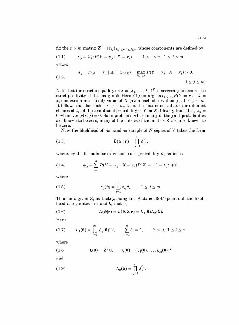
fix the n×m matrix Z = �zij�1≤i≤n;1≤j≤m whose components are defined by

�1:1� zij = λ−1j P�Y = yj �X = xi�; 1 ≤ i ≤ n; 1 ≤ j ≤m;

where

�1:2�λj = P�Y = yj �X = xi∗�j�� = max

1≤i≤nP�Y = yj �X = xi� > 0;

1 ≤ j ≤m:

Note that the strict inequality on l = �λ1; : : : ; λm�T is necessary to ensure thestrict positivity of the margin c. Here i∗�j� = arg max1≤i≤nP�Y = yj � X =xi� indexes a most likely value of X given each observation yj, 1 ≤ j ≤ m.It follows that for each 1 ≤ j ≤ m, λj is the maximum value, over differentchoices of xi, of the conditional probability of Y on X. Clearly, from (1.1), zij =0 whenever p�i; j� = 0. So in problems where many of the joint probabilitiesare known to be zero, many of the entries of the matrix Z are also known tobe zero.

Now, the likelihood of our random sample of N copies of Y takes the form

�1:3� L�c � r� =m∏j=1

ψrjj ;

where, by the formula for extension, each probability ψj satisfies

�1:4� ψj =n∑i=1

P�Y = yj �X = xi�P�X = xi� = λjξj�u�;

where

�1:5� ξj�u� =n∑i=1

zijθi; 1 ≤ j ≤m:

Thus for a given Z, as Dickey, Jiang and Kadane (1987) point out, the likeli-hood L separates in u and l, that is,

�1:6� L�c�r� = L�u;l�r� = L1�u�L2�l�:Here

�1:7� L1�u� =m∏j=1

�ξj�u��rj;n∑i=1

θi = 1; θi > 0; 1 ≤ i ≤ n;

where

�1:8� j�u� = ZTu; j�u� = �ξ1�u�; : : : ; ξm�u��T

and

�1:9� L2�l� =m∏j=1

λrjj ;

2180

where, for conditional probabilities to sum to unity, we require

�1:10� Zl = 1; 0 < l < 1;

where 0 and 1 denote n vectors of 0’s and 1’s, respectively.Note that, ignoring awkward positivity constraints, the dimensions of the

constrained linear spaces u, l and c are, respectively, n−1,m−n andm−1, sothe dimension of c is the same as �u;l�. In this paper we shall consider a classof models called fixed likelihood ratio models. These models assume that thematrix Z is given and that the vector l of largest conditional probabilities ofY � X and the vector u of marginal probabilities on X, are unknowns. Then,by using the likelihood of (1.6), inferences can be made about l and u. Animportant feature of fixed likelihood ratio models is that they utilize the sep-aration (1.6); that is, if u and l are a priori independent in a Bayesian model,then they will remain independent after observing r. Here we shall concen-trate on the inferences that can be made about l, a vector of probabilities ofY conditional on X.

The characteristics of fixed likelihood ratio models are determined largelyby the pattern of zeros in the joint probability table �p�i; j�� and hence inthe Z matrix. In Section 2 it is shown how this pattern can be usefully clas-sified in terms of a graph. In Sections 3 and 4 a class of distributions over�X;Y�, called quasi-incremental, is introduced, which is shown to admit auseful reparametrization of l that allows for a conjugate Bayesian analysisin terms of mixtures of Dirichlet distributions. Despite the proliferation ofnumerical methods in Bayesian statistics, conjugate analyses with plausiblepriors are always interesting because they specify the class of transformationsfrom prior to posterior induced by a particular likelihood and hence give an un-derstanding of why we obtain the results we do. In Sections 4 and 5 it is shownhow to use the graph of a distribution on �X;Y� to discover a transformationof �X;Y� to �τ1�X�; τ2�Y�� which makes this conjugate Bayesian analysis assimple as possible. Sometimes conditions exist when these transformationslead to a particularly simple conjugate analysis in which the components of lcan be expressed as products of independent variates. In Section 6 we outlinethe application of these models in two very different settings. Finally, Section7 discusses why we believe that fixed likelihood ratio models are most validwhen �X;Y� is quasi-incremental.

2. Graphs and the depiction of a probability model. There are var-ious graphs which can be usefully employed to depict a zero–nonzero config-uration in Z. One that is particularly useful for analyzing the conditionalprobability vector l is the primal-constraint graph or briefly graph, G�Z�, ofZ [Dechter and Pearl (1987); Dechter, Dechter and Pearl (1990)]. The “con-straints” here are those imposed by condition (1.10).

The m nodes of G�Z� are labelled by the m possible values of Y. Two nodesj1 and j2 are joined by an undirected edge iff there exists a value i�j1; j2�such that both p�i; j1� > 0 and p�i; j2� > 0. Equivalently, j1; j2, are joined

2181

by an edge iff there is a row (the ith) such that zij1and zij2

are both strictlypositive.

Notice that all joint distributions with the same pattern of nonzero and zerojoint probabilities have the same graph. Let the matrix Z∗ = �z∗ij� be definedby

�2:1� z∗ij ={

0; if zij = 01; if zij > 0;

where Z = �zij�. The differential noninformedness hypothesis (dnh) used byRubin (1976) and Dawid and Dickey (1977) gives a model for which Z = Z∗. Ina sense described in these papers, models satisfying the dnh are models whichare most conservative—or noninformative—about the relationship between Xand Y among all those which respect the zeros in the probability table. Ingeneral, for any graph G there is a set of probability distributions satisfyingthe dnh, and a set of Z∗, called the G-set, whose graph is G.

There are several reasons why these graphs of probability models are im-portant. The first is that, unlike the matrix Z itself, G�Z� is invariant under1–1 transformations of the margins of X and Y. Thus, if X′ = τ1�X� andY′ = τ2�Y�, τ1; τ2 are bijections and Z′ corresponds to the conditional prob-ability ratios of X′ against Y′, then G�Z� = G�Z′�. The second is that theyemphasize in an evocative way the fundamental structure of the problem viathe zeros of the joint mass function. The third is that they can be used to findconvenient reparametrizations of the vector l so that a conjugate analysis canbe performed.

A subgraph of a graph G is said to be complete iff there is an edge con-necting each pair of its nodes. The cliques of a graph are those of its completesubgraphs which are not properly contained in any other complete subgraph.Let

Y �i� = �jx p�i; j� > 0; 1 ≤ j ≤m�be called the range sets of Y given X. Note that in the notation of Section 1,

Y �i� = �jx zij > 0; 1 ≤ j ≤m�:We shall call the joint distribution of �X;Y� graphical if Y �i�, 1 ≤ i ≤ n,form the cliques of G�Z∗�. It will be shown later that many interesting jointprobability models are in fact graphical.

A graph is called decomposable if its n′ cliques C�1�; : : : ; C�n′� can be in-dexed in a compatible order so that

�2:2� S�i� = C�i� ∩{i−1⋃`=1

C�`�}⊆ C�p�i��; 2 ≤ i ≤ n′;

for some p�i�, 1 ≤ p�i� ≤ i−1. Probability distributions on �X;Y� which havedecomposable graphs will be central to this paper.

Decomposable graphs have been studied for some time and many of theirproperties are well known. One important result [see Lauritzen, Speed and

2182

Vijagan (1984)] is that a graph is decomposable iff it contains no chordlesscycle of length greater than or equal to 4. This enables condition (2.2) to bechecked by eye. There are also quick ways of finding a compatible orderingof cliques from a given graph, for example, maximum cardinality search [seeTarjan and Yannakakis (1984); Lauritzen and Spiegelhalter (1988)]. It willbe shown in Sections 4 and 5 that these results concerning graphical modelsenable the identification of the useful reparametrization of l mentioned above.

Figure 1 gives a selection of graphs of graphical joint distributions. By theresult above it is easy to check that all but G1 and G2 are decomposable. G1is not decomposable because it has the chordless four cycle �1;2;3;4;1� whileG2 is not decomposable because of the chordless five cycle �1;2;3;4;6;1�.

3. Quasi-incremental joint distributions. In this section a useful classof joint distributions on �X;Y� is considered which contains models in which,in the very weak sense defined below, X is increasing in Y. First some nota-tion: let the residuals Y �i� of Y on X be defined by

�3:1�Y �1� = Y �1�;

Y �i� = Y �i�\i−1⋃`=1

Y �`�; 2 ≤ i ≤ n;

where for two sets A and B, A\B denotes the set of elements of A whichare not in B and where �Y �i�� are the range sets of Y given X defined inSection 2. If Y = �y1; : : : ; ym�, the set of possible values of Y, then clearly�Y �1�; : : : ; Y �n�� form a partition of Y .

Definition 3.1. Say Y is recursive in X if for some p�i� < i the followingstatements hold:

(i) Y �i� 6= φ; 1 ≤ i ≤ n;(ii) Y �i�\Y �i� ⊆ Y �p�i��; 2 ≤ i ≤ n.

[Henceforth let p�i� denote the least index for i with the property above.]

(iii) Say Y is quasi-incremental in X if it is recursive in X and for eachyj ∈ Y �i�\Y �i�, 1 ≤ j ≤m, 2 ≤ i ≤ n,

P�Y = yj �X = xp�i�� ≥ P�Y = yj �X = xi�with strict inequality for some value of yj ∈ Y �p�i��.

The notion of Y being quasi-incremental in X is pertinent when the rangeY of Y is larger than the range of X and the joint probability table of �X;Y�is sparse in nonzero entries.

Condition (i) demands that as the value xi−1 is increased to xi, 2 ≤ i ≤ n,at least one “higher” value of Y becomes a possibility. Condition (ii) requiresthat the collection of values in Y �i�\Y �i� be contained in a single lower in-dexed range set Y �p�i��. Thus, informally as xi−1 is increased to xi the rangeY �p�i��, 1 ≤ p�i� ≤ i− 1, is shifted up to Y �i�.

2183

Fig. 1. Some graphical models.

2184

The final condition (iii) concerns the magnitude of probabilities of observingyj ∈ Y �p�i�� ∩ Y �i� given xp�i� compared with xi. It states that were oneto believe that xi and xp�i� were equally probable, then one would believe�yj; xp�i��, the pair of values associated with the lower value of X, to be atleast as probable as �yj; xi�. In this sense the relationship between �X;Y�could be said to be positively skewed. Notice that by fixing the matrix Z, theratios of the two conditional probabilities on either side of the inequalitiesin (iii) are fixed. It can also be seen that, under the dnh, by dividing (iii) bythe expression for λj in (1.2), condition (iii) is automatically satisfied providedthat the containment condition in (ii) is always strict.

It is easy to check whether a matrix Z corresponds to a quasi-incrementaldistribution on �X;Y�. Explicitly, if Z = �zij�, then zij should have the fol-lowing properties.

1. There exist values t�1�; : : : ; t�n�, with t�`� > 0, 1 ≤ ` ≤ n and∑n`=1 t�`� =m,

such that z1j = 1 for 1 < j ≤ t�1�, z1j = 0 for t�1� < j ≤m.2. In addition, for i, 2 ≤ i ≤ n,

(a) there exists a row p�i�, 1 < p�i� < i, such that

0 ≤ zij ≤ zp�i�; j ≤ 1; 1 ≤ j ≤i−1∑`=1

t�`�

with strict inequality for some j, such that∑p�i�−1`=1 t�`� < j <

∑p�i�`=1 t�`�;

(b) zij = 1 for j such that∑i−1`=1 t�`� < j ≤

∑i`=1 t�`�;

(c) zij = 0 for∑i`=1 t�`� < j ≤m.

Here t�`�, 1 ≤ ` ≤ n, is just the number of values in Y �`�.Of course, when X is a function of Y,

Y �i� = Y �i�; 1 ≤ i ≤ n;soY is trivially quasi-incremental inX. Another way of interpreting this classof models is that they allow some skewed noise into a functional relationshipbetween X and Y.

The following result shows that the more interesting recursive distributionsare graphical and furthermore that there is a very close link between thesejoint distributions and decomposable graphs.

Theorem 3.1. Suppose no range set of Y contains any other and Y is re-cursive in X. Then the following statements hold:

(i) The joint distribution of X;Y is graphical.(ii) The graph of Z�X;Y� is decomposable.

Furthermore, given u and l, every decomposable graph is the graph of aunique dnh distribution on �X;Y�.

Proof. (i) Go by contradiction and suppose G is not graphical. Since, byhypothesis, no range set is contained in any other, this supposes that G has

2185

a clique which is not itself a range set. So, in particular, there must exist avalue of the index i, 1 ≤ i ≤ n, and two possible values of Y, y�1� and y�2�, say,such that

y�1� ∈ Y �i� and y�2� ∈i−1⋃`=1

Y �`�\Y �i�

with y�1� and y�2� connected by an edge in G. However, for y�1� and y�2� to beconnected by an edge, they must lie in some range set Y �i′�, i′ > i. Choose i′

to be the smallest index with this property. Then it is easily seen that property(ii) of Definition 3.1 is violated for Y �i′�, so G must be graphical.

(ii) Note that �u;l� and the range sets of Y on X define a unique dnhdistribution. The result is now immediate from comparing (2.2) and Defini-tion 3.1(ii). 2

It will be shown in Section 5 that the link between recursive distributionsand decomposable graphs contained in Theorem 3.1 proves useful in defininga straightforward conjugate Bayesian analysis for l.

4. Reparametrizing quasi-incremental distributions. In the Intro-duction it was mentioned that l could often be reparametrized to allow asimple conjugate Bayesian analysis. Here is a useful reparametrization of aquasi-incremental distribution.

Notice that under conditions (i)–(iii) of Definition 3.1, if yj ∈ Y �i�, then

�4:1� P�Y = yj �X = xi� = λj; 1 ≤ j ≤m:

Write

λi = P�Y ∈ Y �i� �X = xi�;(4.2)

ρk�i� = P�Y = yj �X = xi; yj ∈ Y �i��;(4.3)

where

�4:4� j =

i−1∑`=1

t�`� + k; if 2 ≤ i ≤ n;

k; if i = 1;

such that t�i� = #Y �i� is the number of elements in Y �i�. Note that λi > 0,ρk�i� > 0, k = 1; : : : ; t�i�, and

∑t�i�k=1 ρk�i� = 1, i = 1; : : : ; n. Write

r = �r�1�; : : : ;r�n��T where r�i� = �ρ1�i�; : : : ; ρt�i��i��:

By the rules of probability we have that l and r are related by the equations

�4:5� λj = λiρk�i� for yj ∈ Y �i�; 1 ≤ j ≤m;

2186

where the indices k and j are related as in (4.4). Substituting (4.1) into theprobability constraint (1.10) gives λi as a function of r. Thus

λ1 = 1

and

λi = 1−∑

jx yj∈⋃i−1`=1 Y �`�

zijλj; 2 ≤ i ≤ n:(4.6)

Equation (4.6) can be written as an explicit function of r by repeated sub-stitution of λj by (4.5) and (4.6). In fact λi�r� is a polynomial function of�r�1�; : : : ;r�i− 1��.

It is easy but tedious to verify that condition (iii) of Definition 3.1 is neces-sary and sufficient to ensure that the probability constraints are equivalent to(4.6) and do not impose further constraints on the simplicies �r�1�; : : : ;r�n��[Queen (1991); Smith and Queen (1992)].

From (1.9), the likelihood of the reparametrization r of l can now be writtenas

�4:7� L2�r� =n∏i=1

λrii

t�i�∏k=1

�ρk�i��rk�i�

such that

rk�i� = rj;

where k and j are related as in (4.4) and

ri =t�i�∑k=1

rk�i�;

where λi are defined as functions of r from (4.6) and r�i� satisfy the simplexconstraints

t�i�∑k=1

ρk�i� = 1; ρk�i� > 0; 1 ≤ k ≤ t�i�; 1 ≤ i ≤ n:

The likelihood above is functionally more complicated than the original. How-ever, it is familiar, being a discrete mixture of multinomial likelihoods. Thesimple constraints on r allow common prior distributions like independentDirichlets to be used in a Bayesian analysis. Furthermore, r is just a vectorof conditional probabilities so that it is at least plausible to set a proper priordistribution over these.

The obvious choice of prior density p2�r� on r would be of the form

p2�r� ∝n∏i=1

λαii

t�i�∏k=1

�ρk�i��αk�i�;

2187

where αk�i� > 0, 1 ≤ k ≤ t�i�, 1 ≤ i ≤ n, and

αi =t�i�∑k=1

αk�i�:

The posterior density after observing r = �r1; : : : ; rm� would then clearly takethe same form with αi and αk�i� replaced by αi + ri and αk�i� + rk�i�, re-spectively, where ri and rk�i� are defined above. We shall call this familynested generalized Dirichlet densities. Their moments are straightforward tocalculate for moderate sizes of N = ∑m

j=1 rj. For large N, since the posteriordensity is log concave, the posterior mode and its associated matrix of secondderivatives of the log density are easy to calculate numerically.

Thus by specifying a matrix of probability ratios Z of the form above, it ispossible to perform a Bayesian analysis on a family of distributions on �X;Y�consistent with this Z which is conjugate in the unknown probability vectors�u;l�. Two examples of how this conjugate analysis works out on the vectorl are given below.

Example 4.1. Assume X takes three values �x1; x2; x3� and Y the fivevalues (y1, y2, y3, y4, y5) and that the matrix Z of probability ratios isgiven by

Z =

1 1 0 0 0

0 0:5 1 0 0

0 0 1 1 1

:

Here r = �r�1�;r�2�;r�3��T, where r�1� = �ρ1�1�; ρ2�1��; ρ1�2� = 1, r�3� =�ρ1�3�; ρ2�3�� and from (4.2) and (4.6),

�λ1; λ2; λ3� = �1;1− 0:5ρ2�1�;0:5ρ2�1��and

�r1; r2; r3� = �r1 + r2; r3; r4 + r5�:So by (4.7) we find that the likelihood L2�r� separates into

L2�r� = L�1�2 �r�1��L

�2�2 �r�3��;

where

L�1�2 �r�1�� = �ρ1�1��r1�1− ρ1�1��r2+r4+r5�1− 0:5ρ2�1��r3; 0 < ρ1�1� < 1;

L�2�2 �r�3�� = ρ1�3�r4�1− ρ1�3��r5; 0 < ρ1�3� < 1:

The nested Dirichlet conjugate density sets r�1� and r�3� are a priori indepen-dent with r�3� having a beta density and r�1� having a generalized Dirichletdensity [see Dickey, Jiang and Kadane (1987)]. A posteriori r�1� and r�3� re-main independent, the beta and generalized Dirichlet density being updatedin the usual fashion. The Bayesian analysis of the conditional probabilities

2188

associated with y4 and y5 as governed by r�3� is particularly simple, sincethe associated values of Y are only possible if X takes the single value x3.

Example 4.2. This time we consider a family of joint probabilities on�X;Y� with range dimensions 4 and 7, respectively, and Z given by

Z =

1 1 0 0 0 0 0

0 1 1 1 0 0 0

0 0 0:5 1 1 1 0

0 0 0 0 0 0:5 1

:

The conjugate Bayesian analysis on l proceeds as follows.Here

r = �ρ1�1�; ρ2�1�; ρ1�2�; ρ2�2�; ρ1�3�; ρ2�3�;1�T

and

�λ1; λ2; λ3; λ4� = �1; ρ1�1�;1− �1− 0:5ρ1�2��ρ1�1�;1− 0:5ρ2�3�λ3�

L2�r� = L�1�2 �r�1��L

�2�2 �r�2��r�1��L

�3�2 �r�3��r�1��;

where

L�1�2 �r�1�� = �ρ1�1��r1+r3+r4�ρ2�1��r2; ρ1�1� + ρ2�1� = 1;

L�2�2 �r�2��r�1�� = ρ1�2�r3ρ2�2�r4 λ

r5+r63 ; ρ1�2� + ρ2�2� = 1;

L�3�2 �r�3��r�1�;r�2�� = ρ1�3�r5ρ2�3�r6�1− 0:5λ3ρ2�3��r7; ρ1�3� + ρ2�3� = 1:

Now for simplicity assume that a priori ρ1�1�, ρ1�2� and ρ1�3� have inde-pendent beta distributions so that their joint density takes the product formf1�r�1��; f2�r�2��; f3�r�3��. Then, the posterior joint density of r takes theform

f3�r�3��r�1�;r�2�; r� = I−13 L

�3�2 �r�3��r�1�;r�2��f3�r�3��;

f2�r�2��r�1�; r� = I−12 I3L

�2�2 �r�2��r�1��f2�r�2��;

f1�r�1��r� = I−11 I2L

�1�2 �r�1��f�r�1��;

where I3, I2 and I1 are the proportionality constants that ensure f3�·�r�,f2�·�r� and f1�·�r� integrate to unity, I2 being a function of r�1� and r and I3being a function of r�1�, r�2� and r.

Note that f3�r�3��r�1�;r�2�; r� is a generalized Dirichlet density. Further-more, since λ3 is a polynomial in r�1� of degree 2, I3 is a polynomial in r�1�of degree 2r7, making f2 a discrete mixture of generalized Dirichlet densities.

Similarly I2 is a polynomial of degree 2�r5+r6+r7� so a posteriori f�r�1��r�is a mixture of generalized Dirichlets.

2189

Note that the posterior margins on the space r in such examples are oftenalgebraically complex. However, it is straightforward, if tedious, to calculatethe posterior moments of r (and hence l) explicitly [see Geng and Asano (1989)for an explicit demonstration of such methods in an analogous problem]. Alter-natively, since under this reparametrization the posterior density on r is logconcave, numerical methods for calculating various margins via Monte Carlotechniques [e.g., see Tanner and Wong (1987)] can be modified so that theyconverge very quickly [see, e.g., Gilks (1992)].

5. Choosing the simplest compatible ordering. In Section 2 we men-tioned that the class of dnh models had been used by other authors to modelconservatively the relationship between X and Y. If the dnh property holdsand Y is quasi-incremental in X, then the graph G of �X;Y� can be usedto discover a transformation �X;Y� → �τ1�X�; τ2�Y�� which gives rise to themost tractable reparametrization of the vector l of conditional probabilities.We now show that these reparametrizations assign to l a family of distri-butions which contains the class of hyper-Dirichlet distributions [Dawid andLauritzen (1993)] as a special case. Tarjan and Yannakakis’ (1984) algorithmimplies that if a graph is decomposable, there are at least n compatible or-derings associated with it, where n is the number of its cliques. A compatibleordering of nodes in G can therefore be chosen which defines a transformation�τ1; τ2� on �X;Y� which makes �τ1�X�; τ2�Y�� recursive through the equiva-lence of (2.2) and Definition 3.1(ii). This ordering can be found quickly fromG by using a maximal cardinality search or in simple problems, by eye. Thereparametrization given in Section 4 may not only depend upon G�Z�, butalso on Z as well.

For example, the matrix Z given below gives rise to a quasi-incrementaldistribution on �X;Y�; however, so does Z′, and both Z and Z′ define thesame class of models.

Z =

1 1 1 0 0

0 1 1 1 0

0 1 0 0 1

; Z′ =

1 1 0 0 0

0 1 1 1 0

0 1 0 1 1

:

The graphs G4�Z� and G4�Z′� are given in Figure 1. The transformation�X;Y� → �τ1�X�; τ2�Y�� is given by

�τ1�x1�; τ1�x2�; τ1�x3�� = �x3; x2; x1�;

�τ2�y1�; τ2�y2�; τ2�y3�; τ2�y4�; τ2�y5�� = �y5; y2; y4; y3; y1�:Following Section 4, the transformations of l to r and r′ with respect to com-patible orderings associated with Z and Z′, respectively, are different, namely,

L2�r� = �ρ1�1��r1+r4�ρ2�1��r2�ρ3�1��r3�ρ1�1� + ρ3�1��r5;

ρ1�1� + ρ2�1� + ρ3�1� = 1;

2190

and

L2�r′� = ρ′1�1�r1+r3+r4+r5ρ′2�1�r2ρ′1�2�r3+r5ρ′2�2�r4;

ρ′1�1� + ρ′2�1� = 1; ρ′1�2� + ρ′2�2� = 1:

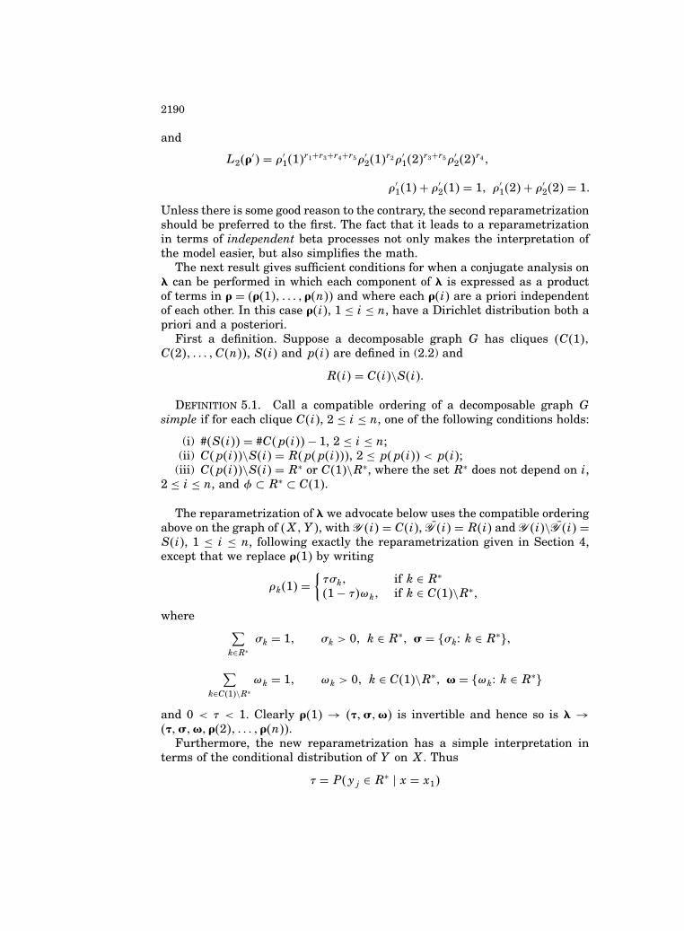
Unless there is some good reason to the contrary, the second reparametrizationshould be preferred to the first. The fact that it leads to a reparametrizationin terms of independent beta processes not only makes the interpretation ofthe model easier, but also simplifies the math.

The next result gives sufficient conditions for when a conjugate analysis onl can be performed in which each component of l is expressed as a productof terms in r = �r�1�; : : : ;r�n�� and where each r�i� are a priori independentof each other. In this case r�i�, 1 ≤ i ≤ n, have a Dirichlet distribution both apriori and a posteriori.

First a definition. Suppose a decomposable graph G has cliques �C�1�;C�2�; : : : ; C�n��, S�i� and p�i� are defined in (2.2) and

R�i� = C�i�\S�i�:

Definition 5.1. Call a compatible ordering of a decomposable graph Gsimple if for each clique C�i�, 2 ≤ i ≤ n, one of the following conditions holds:

(i) #�S�i�� = #C�p�i�� − 1, 2 ≤ i ≤ n;(ii) C�p�i��\S�i� = R�p�p�i���, 2 ≤ p�p�i�� < p�i�;

(iii) C�p�i��\S�i� = R∗ or C�1�\R∗, where the set R∗ does not depend on i,2 ≤ i ≤ n, and φ ⊂ R∗ ⊂ C�1�.

The reparametrization of l we advocate below uses the compatible orderingabove on the graph of �X;Y�, with Y �i� = C�i�, Y �i� = R�i� and Y �i�\Y �i� =S�i�, 1 ≤ i ≤ n, following exactly the reparametrization given in Section 4,except that we replace r�1� by writing

ρk�1� ={τσk; if k ∈ R∗�1− τ�ωk; if k ∈ C�1�\R∗;

where∑k∈R∗

σk = 1; σk > 0; k ∈ R∗; s = �σkx k ∈ R∗�;

∑

k∈C�1�\R∗ωk = 1; ωk > 0; k ∈ C�1�\R∗; v = �ωkx k ∈ R∗�

and 0 < τ < 1. Clearly r�1� → �t;s;v� is invertible and hence so is l →�t;s;v;r�2�; : : : ;r�n��.

Furthermore, the new reparametrization has a simple interpretation interms of the conditional distribution of Y on X. Thus

τ = P�yj ∈ R∗ � x = x1�

2191

and, for each yj ∈ R∗,σj = P�yj � x = x1; yj ∈ R∗�

and, for each yj ∈ Y�1�\R∗,ωj = P�yj � x = x1; yj ∈ Y�1�\R∗�:

Theorem 5.1. If the graph G of a joint distribution of �X;Y� is decompos-able and admits a simple compatible ordering and �X;Y� satisfies the dnh,then the conditional probability vector l can be reparametrized to �τ;s;v;r�2�; : : : ;r�n��. If each of the �n+2� parameter vectors is given an independentDirichlet distribution, then posterior to observing r, �τ;s;v;r�2�; : : : ;r�n��will remain independent and each will still have a Dirichlet distribution.Each component of l will be expressed as a product of single components from�τ;s;v;r�2�; : : : ;r�n��.

Furthermore, two families of these prior distributions associated with dif-ferent compatible parametrizations of G are equivalent in the sense that theygive an identical family of distributions over l.

Proof. It is sufficient to show that under the conditions of the theo-rem, λi, 1 ≤ i ≤ n, as defined in (4.2), is a product of terms in �τ;1 −τ;s;v;r�2�; : : : ;r�n��, since r�1� is clearly a product of terms in �τ;1 −τ;s;v�. Go by induction on i. The theorem is clearly true for i = 1 sinceλi = 1, so suppose it is true for all `, 1 ≤ ` ≤ i− 1.

From Definition 5.1: if (i), then λi = λj�i�, where j�i� is the only elementin C�p�i��\S�i� and so λi = λsρk�s� for some s < i − 1 such that j�i� =∑s−1r=1 t�r� + k; if (ii), then λi = λp�p�i��, p�p�i�� < i; if (iii), then λi = τ or�1 − τ�. In all these cases under the inductive hypothesis, λi takes the rightproduct form and so the first part of the theorem is proved.

To prove uniqueness, suppose G admits a simple compatible ordering. Inthis ordering, let Y �i�\Y �i� have q�i� elements, Y �i� have t�i� elements andwrite l�i� = �l�1��i�;l�2��i��, where for 2 ≤ i ≤ n, l

�1�k �i�, 1 ≤ k ≤ q�i�, is the

kth lowest indexed component of l lying in Y �i�\Y �i� and l�2�` �i�, 1 ≤ ` ≤ t�i�,

is the `th lowest indexed component of Y �i�.By the construction above we can set, a priori, l�2��i� to be dependent on

l�1��i� only through the sum of the components of l�1��i�, that is,

�5:1� l�2��i��l�1��i� = l�2��i��( q�i�∑k=1

λ�1�k �i� = 1− λi

); 2 ≤ i ≤ n;

and we can also set l�2��i��l�1��i� to have an arbitrary Dirichlet distribution apriori. It is immediate from the properties of the Dirichlet distribution [John-ston and Kolz (1972)] that under the construction above the vector l�1� ofcomponents in Y �1� has been set to have an arbitrary Dirichlet distributionas a prior. By induction on i, it follows that, since l�1��i� is a subvector ofl�p�i��, 2 ≤ i ≤ n and so �1 − λi�−1l�1��i� is Dirichlet [Johnson and Kotz

2192

(1972)] and (5.1) holds that l�i� has a Dirichlet distribution [Johnson andKotz (1972)] 2 ≤ i ≤ n.

It follows from Dawid and Lauritzen [(1993) page 1304] that our prior fam-ily over �τ;s;w;r�2�; : : : ;r�n�� gives the (uniquely specified) hyper-Dirichletfamily of prior distributions over l. Since this is true for any simple compatibleordering, the uniqueness is proven.

Example 5.1. It is easy to check that G5 of Figure 1 admits a simple com-patible ordering. Thus transform �X;Y� so that Y �1� = �y3; y4�, Y �2� =�y1; y2; y3�, Y �3� = �y1; y2; y5; y6� and Y �4� = �y5; y6; y7�. Under this or-dering C�2� and C�3� satisfy (i) and C�4� satisfies (ii) of Definition 5.1:

L2�l� = �ρ1�2��r1�ρ2�2��r2�ρ1�3��r5�ρ2�3��r6τ�r1+r2+r4+r7��1− τ��r3+r5+r6�;

where

�λ1; λ2; λ3; λ4; λ5; λ6; λ7� = �ρ1�2�τ; ρ2�2�τ;1−τ; τ; ρ1�3��1−τ�; ρ2�3��1−τ�; τ�:

Here σ and ω are simply 1.

Sometimes it is rather difficult to check by eye for a compatible ordering ofa graph which has this property. The following construction is often useful.

Definition 5.2. Call a graph H the contraction of a graph G if it has thefollowing properties.

(a) The nodes ofH are maximal complete subsets of nodes ofG which sharethe same neighbors (other than themselves) in G.

(b) An edge between nodes J1 and J2 in H exists iff there is an edge�j1; j2� ∈ G for every j1 ∈ J1 and j2 ∈ J2.

In Figure 2,H3 is the contraction of the decomposable graphG3 of Figure 1.A contraction H is useful because: (1) H is no more complicated than G and(2) under the obvious mapping, the cliques of H correspond to the cliques ofG, as do their intersections and complements.

Fig. 2. A contraction graph of G3.

2193

Because of the property (b) it is possible to useH to identify an independentDirichlet breakdown of probabilities of �X;Y� with an associated G, evenwhen G is quite complicated.

Example 5.2. Once H3 is constructed from G3 of Figure 1 it is clear thatthe clique �1;2;3;4;5� of G3 ���1;2;3�; �4;5�� of H3� breaks G3 into twocomponents. Thus in the construction of Theorem 5.1 set R∗ = �1;2;3�,

C�1� = �1;2;3;4;5�; C�2� = �4;5;6;7�; C�3� = �4;5;7;8�;

C�4� = �1;2;3;9�; C�5� = �1;2;3;10�:Then

L2�l� = σr11 σ

r22 σ

r33 ω

r44 ω

r55 �ρ1�2��r6+r8�ρ2�2��r7τr1+r2+r3+r6+r7+r8�1−τ�r4+r5+r9+r10;

where∑3j=1 σj = 1,

∑5j=4ωj = 1 and

∑2j=1pj�2� = 1, 0 ≤ τ ≤ 1. The transform

of l is

l = �τσ1; τσ2; τσ3; �1− τ�ω4; �1− τ�ω5; τρ1�2�; τρ2�2�; τρ1�2�; �1− τ�; �1− τ��:

6. Two examples of the use of fixed likelihood ratio models. One ofthe main features of fixed likelihood models is that all odds ratios OR(i, i′,j, j′), 1 ≤ i, i′ ≤ n, 1 ≤ j, j′ ≤m,

�6:1� OR�i; i′; j; j′� = P�Y = yj�X = xi�P�Y = yj�X = xi′�

P�Y = yj′ �X = xi�P�Y = yj′ �X = xi′�

;

are functions of the Z matrix, so all fixed likelihood ratio models have fixedodds ratios. Typically in the applications we have studied it is reasonable, atleast in the first instance, to assume that Z is fixed in time but that both themargin u of X and the selected conditional probabilities of Y�X encoded in lmove as a time series. The separation of (1.6) allows these two time series tobe analyzed independently of one another.

The issue we address in this section is the scope of applicability of such mod-els. We shall concentrate our attention on two areas. The first is derived fromthe statistical analysis of certain marketing models. This was the motivatingexample for this work and is now well studied [Queen (1994); Queen, Smithand James (1994)]. The second relates to the area of probability estimation inmedical probabilistic expert systems.

Example 6.1 (Statistics of marketing). In this application, Y labels a setof competing brands and X labels categories of purchasers of these brands.The distribution of X varies slowly from week to week reflecting the chang-ing demography, aspirations, affluence and so on of the potential customers.However, brand sales are typically volatile, being subject to many stochasticcovariates, which include promotions directed to retail outlets, who are re-warded financially for displaying a brand more prominently, and promotions

2194

directed at the general customer such as TV advertising, money-off offers orlarger pack offers.

Within this setting, notice first that there is some flexibility not only inthe choice of Y—through which brands are included in the study—but alsoconsiderable modelling choice in how X, the category list of customers, is de-fined. So, in practice, X can be chosen so that many of the Z entries arezeros; indeed, this is recommended by various market researchers [see, e.g.,Grover and Srinivasan (1987)]. For example, X could be defined in terms ofthe needs of the customer, where a brand will either satisfy the list of needsof the purchaser or not [see, e.g., Queen (1994)]. For the fixed likelihood ratiomodel to be valid it is necessary that, within the period of study, promotionswhich affect brand sales act in an even-handed way across types of purchaserin the sense that the odds ratio of (6.1) remains unchanged. In the types ofmarkets we have studied, the empirical evidence available suggests that thisinvariance holds, at least approximately, and is plausible unless the promo-tions employed by a brand target a specific type of customer [Queen, Smith andJames (1994)]. Again in a large number of markets it appears empirically thata good working hypothesis is that the joint distribution is quasi-incremental.The index i seems to be related to the sophistication of the brand required bythat category of customer.

Despite these arguments, we are still left with the practical problem of howto specify the nonzero elements ofZ. There are essentially two ways to do this:the first is empirical; the second is to introduce new modelling assumptions.For some products, at infrequent periods, large sample surveys are performedwhich allow for the direct measurement of the nonzero elements zij of Z sothat

zij =#�xi; yj�

#�xi∗�j�; yi�

[#�xi�

#�xi∗�j��

]−1

; 1 ≤ i ≤ n;1 ≤ j ≤m;

where xi∗�j� is the type of purchaser most likely to buy brand yj and #�xi; yj�is the number of purchases made by customer type xi of brand yj and so on.The vectors �l;u� can then be allowed to develop as a time series while Z isheld fixed to allow prediction of future brand sales.

When such sampling data are not available it is possible to derive Z from abehavioral model like the one outlined below. A customer walks into a shop andwith probability θi she is of type i. She first picks one of the brands �Y = yj�with probability ψj which does not depend on i, where

∑mj=1 ψj = 1. After

looking at the selected brand, if she decides it is appropriate [i.e., yj ∈ Y �i�],she buys it; if it is inappropriate, she replaces it on the shelf and picks anotherbrand yj′ with probability ψj′�1 − ψj�−1. She repeats this process until shehas bought a brand.

Under this model, X and Y are independent. If yj /∈ Y �i�,

zij =P�Y = yj�X = xi�P�Y = yj�X = xi∗�j��

= 0:

2195

On the other hand, if yj ∈ Y �i�,

zij =P�Y = yj�X = xi�P�Y = yj�X = xi∗�j��

= P�Y = yj�X = xi�P�Y ∈ Y �i��X = xi�

P�Y ∈ Y �i∗�j���X = xi∗�j��P�Y = yj�X = xi∗�j��

;

which, since X and Y are independent,

= P�Y ∈ Y �i∗�j���P�Y ∈ Y �i��

= π�i∗�j��π�i� ; j ∈ Y �i�;1 ≤ i ≤ n;

where �1 − π�i�� is the probability a customer of type i replaces her firstchosen brand on the shelf. This probability can be estimated, at least in prin-ciple, directly from an experiment. If we are completely ignorant about thesereplacement probabilities, it seems reasonable to set them all equal and thisthen gives the dnh model discussed in detail in Section 5. It can be shown thatwhen these replacement probabilities are not equal, for quasi-incremental dis-tributions at least, it is sometimes possible to redefine the categories i so thatthey are (at least approximately) equal. This trick is not always available forother fixed likelihood ratio models, however. Finally, if p = �π�1�; : : : ; π�n�� isdeemed uncertain, then its distribution can be updated in the light of r in theusual way using the conjugate predictive probabilities of r�p = r�Z. However,it should be noted that there are technical reasons why the distribution ofr�p depends only weakly on p and in practice the posterior distribution of p�roften tends to be very close to the prior.

Example 6.2 (Environmental medicine). Here we let Y label the (set of)symptom(s) first reported to a doctor and X the patient’s disease category.One reason why our class of models is suitable in this case is that thereoften exists a partial logical relationship between symptoms and diseases;that is, by definition a disease cannot be observed unless certain symptomsappear. Another reason is that, for elicitation purposes, the conditioning inour parametrization of symptom, given disease, is the right way round.

Consider the following hypothetical study on the effects of air pollution onhealth. Assume that various disease conditions make the individual more sus-ceptible to certain subsets of pollutants. Suppose the first reported data aresymptoms such as ulcers, headaches, dizziness, dyspnea, diarrhea and eczema,and that exposure to particular pollutants causes one or more of the symptomsin susceptible individuals but not in the insusceptible. As in the last exam-ple, l will be treated as an unknown and stochastic; that is, the probabilitythat a most susceptible individual exhibits certain symptoms will change intime (due to differing effects of pollution, in combination with other factors,

2196

over time), in location and in category of patient. Furthermore, the probabil-ities u of different diseases being observed is also modelled as depending ontime, location and category of individual. However, we do assume that Z isfixed. In particular, this will imply that the relative toxicity of two pollutantsmeasured over different categories of disease, as measured by the odds ratio,will be invariant—in this context a reasonable assumption at least in the firstinstance.

As in the last example, the fixed likelihood ratio model can be seen asthe product of censoring—in this case the censoring occurs when individualsexposed to a potentially toxic substance are immune and so are not counted.Thus let Y = yj correspond to an individual’s first exposure to a pollutantwhich can cause symptoms yj, 1 ≤ j ≤ m. Assuming Y is independent ofX and that each individual will be exposed at random to a succession ofvalues of yj, the arguments in the last example give us a fixed likelihood ratiomodel provided that π�i�—the probability that an individual with disease iis exposed first to a pollutant to which she is susceptible—is known. Again,but perhaps less plausibly, if diseases are classified in a way which makesπ�i� = π�1�, 2 ≤ i ≤ n, then we have a dnh model.

7. Graphical dnh joint distributions without a simple ordering.When a graphical distribution on �X;Y� is not quasi-incremental, the con-straints (1.10) can become more active. Strange implications can then arisewhich suggest that fixed likelihood ratio models might be dubious. Considerthe graphical dnh models defined by graphs G1 and G2 of Figure 1.

Using the reparametrization of l to r as defined in Sections 4 and 5, areparametrization of G1 gives r = �τ;1 − τ;1;1�. This is one dimensionalrather than the expected m − n = 0 dimensional solution space and has l ofthe form

λ = �τ;1− τ;1− τ; τ�:It is easily checked that the additional dimension in λ arises because theprobability vector u on the margins of X is unidentifiable. Notice, however,that a conjugate beta analysis can be performed on l if this dnh model isconsidered appropriate.

Even stranger, it can easily be shown that no dnh model on �X;Y� canexist which has range sets defined by G2. By using the reparametrizationof Section 4, where C�1� = �6;7�, C�2� = �1;5;6�, C�3� = �1;2;5�, C�4� =�2;3;5�, C�5� = �3;4;5�, C�6� = �4;5;6�, C�7� = �7;8;12�, C�8� = �8;9;12�,C�9� = �9;10;12�, C�10� = �10;11;12� and C�11� = �7;11;12�, set

r = �ρ1�1�; ρ2�1�; ρ1�2�; ρ2�2�;1;1;1; ρ1�7�; ρ2�7�;1;1;1�;where ρ1�1�; ρ1�2�; ρ1�7� < 1 and

∑2j=1 ρj�2� =

∑2j=1 ρj�7� = 1.

Unfortunately though, since �X;Y� is not quasi-incremental there are twoextra constraints from (1.10), namely,

ρ2�1�ρ1�1� = ρ1�1�

2197

and

ρ1�1�ρ1�7� = ρ2�1�:

Estimating r�1� from these equations gives

�1+ ρ1�2��−1 + �1+ ρ1�7��−1 = 1;

which has no solution if ρ1�2� and ρ1�7� are strictly positive. Other examplescan be constructed when the dnh is not assumed where under fixed likelihoodratio models such non-existence problems arise.

These examples illustrate that fixed likelihood ratio models may have un-desirable modelling implications. Such models seem best suited to be used inconjunction with quasi-incremental distributions.

Acknowledgment. We would like to thank the referees for their veryhelpful comments on an earlier version of this paper.

REFERENCES

Carlson, B. C. (1977). Special Functions of Applied Mathematics. Academic Press, New York.Dawid, A. P. and Dickey, J. M. (1977). Likelihood and Bayesian inference from selectively re-

ported data. J. Amer. Statist. Assoc. 72 845–850.Dawid, A. P. and Lauritzen, S. L. (1993). Hyper Markov laws in the statistical analysis of de-

composable graphical models. Ann. Statist. 21 1272–1317.Dechter, R., Dechter, A. and Pearl, J. (1990). Optimisation in constraint networks. In Influence

Diagrams, Belief Nets and Decision Analysis (R. M. Oliver and J. Q. Smith, eds.) 411–425. Wiley, New York.

Dechter, R. and Pearl, J. (1987). Network-based heuristics for constraint satisfaction problems.Artificial Intelligence 34 1–38.

Dickey, J. M. (1983). Multiple hypergeometric functions: probabilistic interpretations of statisti-cal uses. J. Amer. Statist. Assoc. 78 628–637.

Dickey, J. M., Jiang, J. and Kadane J. B. (1987). Bayesian methods for censored categoricaldata. J. Amer. Statist. Assoc. 82 773–781.

Geng, Z. and Asano, C. (1989). Bayesian estimation methods for catagorical data with misclas-sification. Comm. Statist. Theory Methods 18 2935–2954.

Gilks, W. R. (1992). Bayes derivative-free adaptive rejection sampling for Gibbs sampling. InBayesian Statistics (J. M. Bernardo, J. O. Berger, A. P. Dawid and A. F. M. Smith, eds.)641–649. Oxford Science Publications.

Grandy, W. T., Jr. (1985). Incomplete information in generalised inverse problems. In MaximumEntropy and Bayesian Methods in Inverse Problems (C. R. Smith and W. T. Grandy, Jr.,eds.) 41–72. Reidel, Boston.

Grover, R. and Srinivasan, V. (1987). A simultaneous approach to market segmentation andmarket structuring. Journal of Marketing Research 3 139–153.

Johnson, N. L. and Kotz, S. (1972). Distributions in Statistics, Continuous Multivariate Distri-butions. Wiley, New York.

Lauritzen, S. L., Speed, T. P. and Vijagan, K. (1984). Decomposable graphs and hypergraphs.J. Austral. Math. Soc. Ser. A 36 12–29.

Lauritzen, S. and Spiegelhalter, D. J. (1988). Local computations with probabilities on graphi-cal structures and their applications to expert systems (with discussion). J. Roy. Statist.Soc. Ser. B 50 157–224.

Queen, C. M. (1991). Bayesian graphical forecasting models for business time series. Ph.D. dis-sertation, Univ. Warwick.

2198

Queen, C. M. (1994). Using the multi-regression dynamic model to forecast brand sales in acompetitive product market. The Statistician 43 87–98.

Queen, C. M., Smith, J. Q. and James, D. M. (1994). Bayesian forecasts in markets with over-lapping structures. International Journal of Forecasting 10 209–233.

Rubin, D. B. (1976). Inference and missing data. Biometrika 63 581–592.Smith, J. Q. and Queen, C. M. (1992). Bayesian models of partially segmented markets. Research

Report 232, Univ. Warwick.Tanner, M. A. and Wong, W. H. (1987). The calculation of posterior distributions by data aug-

mentation. J. Amer. Statist. Assoc. 82 528–550.Tarjan, R. E. and Yannakakis, M. (1984). Simple linear time algorithms to test chordality of

graphs, test acyclicity of hypergraphs and selectively reduce acyclic hypergraphs. SIAMJ. Comput. 13 566–579.

Vardi, Y. and Lee, D. (1993). From image deblurring to optimal investments: maximum likelihoodsolutions for positive linear inverse problems (with discussion). J. Roy. Statist. Soc.Ser. B 55 569–612.

Department of StatisticsUniversity of WarwickCoventry CV4 7ALEngland

Institute of Mathematics and StatisticsUniversity of KentCanterburyKent CT2 7NFEnglandE-mail: c.m.queen@ukc.ac.uk