Discrete Sparse Fourier Hermite Approximations in High ...
128
Syracuse University Syracuse University SURFACE SURFACE Mathematics - Dissertations Mathematics 12-2012 Discrete Sparse Fourier Hermite Approximations in High Discrete Sparse Fourier Hermite Approximations in High Dimensions Dimensions Ashley Prater Syracuse University Follow this and additional works at: https://surface.syr.edu/mat_etd Part of the Mathematics Commons Recommended Citation Recommended Citation Prater, Ashley, "Discrete Sparse Fourier Hermite Approximations in High Dimensions" (2012). Mathematics - Dissertations. 70. https://surface.syr.edu/mat_etd/70 This Dissertation is brought to you for free and open access by the Mathematics at SURFACE. It has been accepted for inclusion in Mathematics - Dissertations by an authorized administrator of SURFACE. For more information, please contact [email protected].
-
Upload
khangminh22 -
Category
Documents
-
view
4 -
download
0
Transcript of Discrete Sparse Fourier Hermite Approximations in High ...
Syracuse University Syracuse University
SURFACE SURFACE
Mathematics - Dissertations Mathematics
12-2012
Discrete Sparse Fourier Hermite Approximations in High Discrete Sparse Fourier Hermite Approximations in High
Dimensions Dimensions
Ashley Prater Syracuse University
Follow this and additional works at: https://surface.syr.edu/mat_etd
Part of the Mathematics Commons
Recommended Citation Recommended Citation Prater, Ashley, "Discrete Sparse Fourier Hermite Approximations in High Dimensions" (2012). Mathematics - Dissertations. 70. https://surface.syr.edu/mat_etd/70
This Dissertation is brought to you for free and open access by the Mathematics at SURFACE. It has been accepted for inclusion in Mathematics - Dissertations by an authorized administrator of SURFACE. For more information, please contact [email protected].
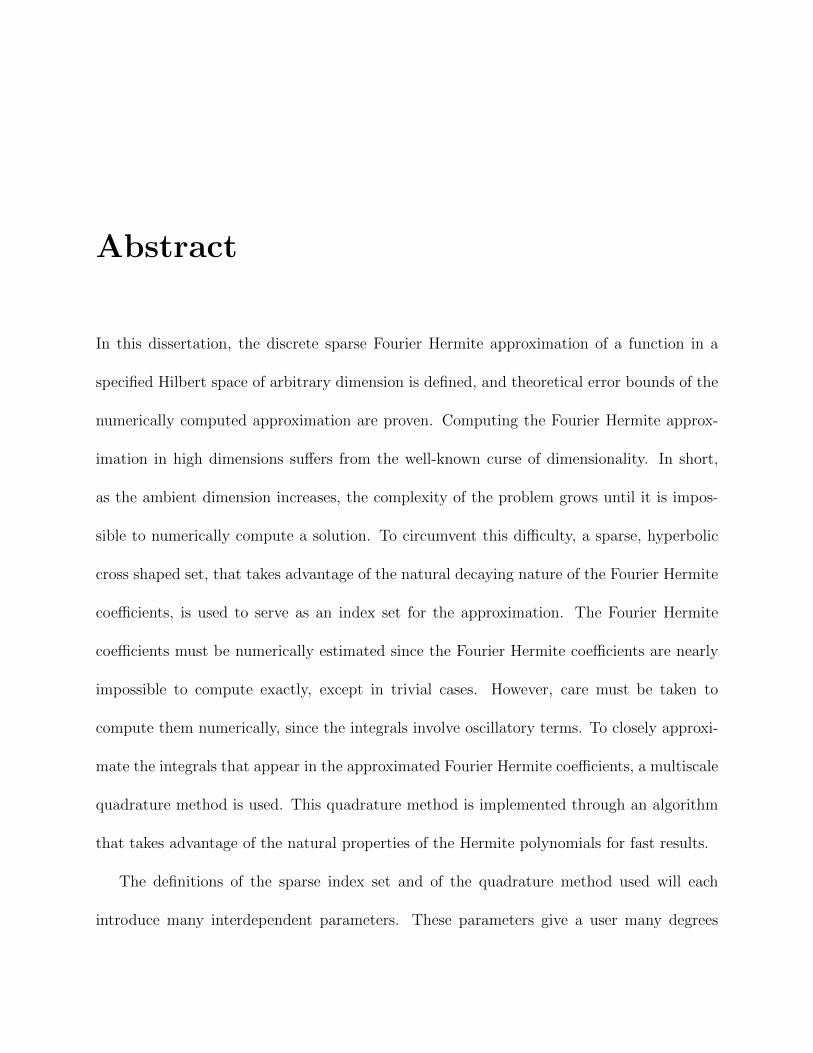
Abstract
In this dissertation, the discrete sparse Fourier Hermite approximation of a function in a
specified Hilbert space of arbitrary dimension is defined, and theoretical error bounds of the
numerically computed approximation are proven. Computing the Fourier Hermite approx-
imation in high dimensions suffers from the well-known curse of dimensionality. In short,
as the ambient dimension increases, the complexity of the problem grows until it is impos-
sible to numerically compute a solution. To circumvent this difficulty, a sparse, hyperbolic
cross shaped set, that takes advantage of the natural decaying nature of the Fourier Hermite
coefficients, is used to serve as an index set for the approximation. The Fourier Hermite
coefficients must be numerically estimated since the Fourier Hermite coefficients are nearly
impossible to compute exactly, except in trivial cases. However, care must be taken to
compute them numerically, since the integrals involve oscillatory terms. To closely approxi-
mate the integrals that appear in the approximated Fourier Hermite coefficients, a multiscale
quadrature method is used. This quadrature method is implemented through an algorithm
that takes advantage of the natural properties of the Hermite polynomials for fast results.
The definitions of the sparse index set and of the quadrature method used will each
introduce many interdependent parameters. These parameters give a user many degrees

of freedom to tailor the numerical procedure to meet his or her desired speed and accuracy
goals. Default guidelines of how to choose these parameters for a general function f that will
significantly reduce the computational cost over any naive computational methods without
sacrificing accuracy are presented. Additionally, many numerical examples are included to
support the complexity and accuracy claims of the proposed algorithm.
Discrete Sparse Fourier Hermite Approximations in High Dimensions
by
Ashley Prater
B.S., Kansas State University, 2002
M.S., Kansas State University, 2005
Submitted in partial fulfillment of the requirements for the degree of
Doctor of Philosophy in Mathematics.
Syracuse University, December 2012

Copyright c©Ashley Prater 2012
All Rights Reserved

Acknowledgements
I wish to thank many people for their support during my academic career.
I am extremely grateful for all of the help and support given to me by my advisor Professor
Yuesheng Xu. He has expanded my vision as a mathematician here in the United States, and
also through supporting me to study with mathematicians around the world. I am looking
forward to continuing our studies together.
I am grateful to have the support of Professor Lixin Shen, and I am very happy that
he and I will be working together closely next year while he will be visiting the Air Force
Research Lab in Rome, NY.
I am thankful for the support of all of the faculty members at Syracuse University, but
am especially thankful for each of my committee members: Chairwoman Yingbin Liang
and members Dan Coman, Eugene Poletsky, Lixin Shen, Andrew Vogel, and Yuesheng Xu.
Thanks to each of you for contributing your time and efforts to this project.
I am grateful for all the support from my friends, particularly all of the other mathematics
graduate students at Syracuse University.
Finally, I am very pleased to have infinite support from my family: Robert and Janet
Prater, Erica and Brandon Rivenbark, Ian Riley and Rachel Lowery.
v
Contents
Abstract i
Acknowledgements v
1 Introduction 1
1.1 Motivation . . . . . . . . . . . . . . . . . . . . . . . . . . . . . . . . . . . . . 2
1.2 Problem Statement and Challenges . . . . . . . . . . . . . . . . . . . . . . . 3
1.3 Previous Work . . . . . . . . . . . . . . . . . . . . . . . . . . . . . . . . . . 4
1.4 New Contributions . . . . . . . . . . . . . . . . . . . . . . . . . . . . . . . . 5
2 Sparse Fourier Hermite Expansions 8
2.1 Preliminaries . . . . . . . . . . . . . . . . . . . . . . . . . . . . . . . . . . . 8
2.2 Fourier Hermite Series . . . . . . . . . . . . . . . . . . . . . . . . . . . . . . 18
2.3 Hyperbolic Cross Sparse-Grid Approximation . . . . . . . . . . . . . . . . . 22
3 Discretization Part 1: Removing the Tails 27
3.1 Definitions and Strategies . . . . . . . . . . . . . . . . . . . . . . . . . . . . 28
3.2 Gaussian Quadrature . . . . . . . . . . . . . . . . . . . . . . . . . . . . . . . 30
vi
3.3 A Two-Fold Strategy: Selecting the Location of the Cut . . . . . . . . . . . 31
4 Discretization Part 2: Approximate the Body 41
4.1 Linear Spline Interpolation . . . . . . . . . . . . . . . . . . . . . . . . . . . . 42
4.2 Heirarchical Lagrange Interpolation . . . . . . . . . . . . . . . . . . . . . . . 48
4.3 Multiscale Interpolation . . . . . . . . . . . . . . . . . . . . . . . . . . . . . 53
4.4 Discrete Sparse Approximations . . . . . . . . . . . . . . . . . . . . . . . . . 57
5 Discrete Sparse Fourier Hermite Approximations 65
6 Implementation 73
7 Numerical Results 88
A Various Results 100
Vita 113
vii
List of Figures
2.1 A few Hermite polynomials . . . . . . . . . . . . . . . . . . . . . . . . . . . 10
2.2 The Full Grid Index Sets Y232 and Y3
32. . . . . . . . . . . . . . . . . . . . . . 20
2.3 The Sparse Grid Index Sets L232 and L3
32. . . . . . . . . . . . . . . . . . . . . 23
3.1 Plots of H2N(x)ω(x) for different choices of N . . . . . . . . . . . . . . . . . . 33
3.2 Plots of1
n!2n
∫ ∞A
H2n(x)ω(x)dx for various n with N = 50. . . . . . . . . . . 37
3.3 Semi-log plot of y = erfc(x). . . . . . . . . . . . . . . . . . . . . . . . . . . . 38
3.4 Plots of erfcinv
(1
N2s+1 logd−12 N
)and an estimate for various s and d against
values of N . . . . . . . . . . . . . . . . . . . . . . . . . . . . . . . . . . . . . 39
4.1 Plot of a typical Bi(x). . . . . . . . . . . . . . . . . . . . . . . . . . . . . . . 42
4.2 Nodal Basis and Multiscale Basis for F2, taking V0 = −A/3, A/3 and A = 1. 52
4.3 Nodal Basis and Multiscale Basis for F2, taking V0 =
−A7,3A
7,5A
7
and
A = 1. . . . . . . . . . . . . . . . . . . . . . . . . . . . . . . . . . . . . . . . 52
4.4 Plots of all of the Lagrange cardinal polynomials in F2, where V0 = −1/3, 1/3. 63
4.5 Plots of all of the Lagrange cardinal polynomials in F2, where V0 =−1
7, 3
7, 5
7
. 64
5.1 Plot of the estimate k ≈ (3m+ 2) log2N
2m log2 log2Nfor different m. . . . . . . . . . . . 72
viii
6.1 Levels of dependence in the recurrence relation from equation (6.15) for d = 1. 81
6.2 Blocks of computation steps from Algorithm 6.3. . . . . . . . . . . . . . . . . 82
7.1 Plots of Fourier-Hermite approximations from Example 1 with m = 3, d = 2. 90
7.2 Cross sections from the Fourier Hermite Approximation of Example 1 with
d = 3. . . . . . . . . . . . . . . . . . . . . . . . . . . . . . . . . . . . . . . . 91
7.3 Three cross sections of the Fourier Hermite approximation of the function
from Example 2 with N = 30, d = 3. . . . . . . . . . . . . . . . . . . . . . . 93
7.4 Plots of the function and its Fourier-Hermite approximation from Example 3. 95
7.5 Plots of the function and its Fourier-Hermite approximation from Example 4. 97
7.6 Plot of the Fourier-Hermite approximation from Example 5 with N = 10. . . 98
ix
Chapter 1
Introduction
A common exercise encountered while studying mathematics is to decompose an certain
object in terms of a given basis. Some classical examples include decomposing functions in
terms of the bases formed by the piecewise linear hat functions, by wavelets, or by trigono-
metric polynomials. Such a decomposition is of interest to applied mathematicians, scientists
and engineers, but is also powerful for pure mathematicians. In this dissertation, the basis
consisting of the set of polynomials that are pairwise orthogonal in the Hilbert space L2ω(Rd)
with the d-dimensional Gaussian weight function ω is used. Given the representation of a
function in terms of this Fourier Hermite basis, a sparse, discrete approximation is described,
and bounds for the approximation error and computational complexity are discussed. Addi-
tionally, in this dissertation it is shown that it is possible to achieve a good approximation
error estimate while maintaining a low computational cost. The primary approximation er-
ror result is given in Theorem 5.6, and the primary computational cost estimate is given in
Theorem 6.10.
1
CHAPTER 1. INTRODUCTION 2
1.1 Motivation
The Hermite decomposition of a function is of particular interest and usefulness for several
reasons. Every decomposition system is limited by the properties of the basis set. The
collection of the Hermite polynomials enjoy two unique properties that make them a very
good representation system in a wide variety of settings. First, the orthogonality over the
entire plane Rd makes them an appropriate description basis for objects that do not have a
boundary, periodicity, or asymptotic decay at infinity. This makes them particularly power-
ful when used to numerically compute the solution of types of differential equations that may
be encountered in modeling large systems over an infinite time domain, including applica-
tions in environmental science, climate change, and astrophysics. The second mathematical
property that makes the Hermite polynomial decomposition desirable over other possible ba-
sis sets is that the Hermite polynomials are orthogonal with respect to the Gaussian weight
function. Systems involving the Gaussian weight are pervasive throughout the mathematical
sciences including statistics, analysis, and differential equations and are necessary to describe
phenomena throughout all disciplines in the natural sciences.
The Hermite polynomials are necessary for the solution of Schrodinger’s equation, which
is a non-linear second-order differential equation used in the model of a quantum simple
harmonic oscillator in quantum mechanics. The quantum simple harmonic oscillator is an
important model in physics [7]. A simple version of the model is taught in undergraduate
physics courses, yet it is still an area of active research [21], [23].
Additionally, the Hermite polynomials enjoy a form of rotational invariance. If a function
has a representation in terms of finitely many normalized Hermite polynomials, then any
CHAPTER 1. INTRODUCTION 3
rotation of the function has a representation in terms of the same number of normalized
Hermite polynomials [17]. Because of this property, the Hermite polynomials have been
employed in many areas of image processing including medical imaging, optics and satellite
images [8], [17], [19], [20].
1.2 Problem Statement and Challenges
The problem motivating this work is to find a fast, accurate approximation to an arbitrary
given function in terms of the Hermite polynomials. Specifically, for any f ∈ L2ω(Rd), where
ω(x) := e−x2
is the Gaussian weight function, can a good approximation to the full Fourier-
Hermite representation
f(x) =∑n∈Nd
0
cnHn(x),
where Hn is a Hermite polynomial and cn is the corresponding transform coefficient, be found
quickly?
Many challenges are encountered in attempting to achieve this task. First, the high-
dimensional nature of the problem suffers from the so-called ‘curse of dimensionality’ [4].
To reduce its effect, the number of terms in the sum over the infinite lattice Nd0 must be
reduced while simultaneously ensuring that the truncated sum very nearly approximates the
full series. Second, the transform coefficients are defined via integrals over the entire plane
Rd, and involve highly oscillatory terms. An accurate and realistic quadrature approach
must be taken to ensure the numerically computed coefficients will not contribute enough
error to destroy the overall accuracy of the sum. Finally, how can the methods used be
designed to optimize the tradeoffs between accuracy and computational complexity?

CHAPTER 1. INTRODUCTION 4
1.3 Previous Work
Discretization of problems using sparse grids has been a popular method to overcome the
curse of dimensionality [3], [5], [12], [13], [16], [18]. It has been shown to be effective in re-
ducing the computational complexity of problems while maintaining a decent approximation
order. Bungartz and Griebel [5] published an important review article discussing interpola-
tion methods on sparse grids. I employed a hyperbolic cross shaped sparse grid index set,
a strategy that has proven successful for other authors as well. Professor Yuesheng Xu and
Ying Jiang [12] used the hyperbolic cross shaped index set to compute the sparse Fourier ex-
pansion of a d dimensional function. They showed that approximating the Fourier expansion
of a function f in a Sobolev space with regularity s by considering only terms corresponding
with elements in the hyperbolic cross shaped index set yielded relative error on the order of
O(N−s), where N is the number of index points of the sparse grid in a single dimension. Jie
Shen and Li-Lian Wang [25] also have studied methods of approximating an expansion of
a function in terms of Hermite functions over the hyperbolic cross shaped index set. They
showed that for a function f in a Korobov-type space with smoothness parameter s, the
spectral approximation has relative error O(s(d−1)s(s2
)ds/2N−s/2).
Many scholars who have studied or used Fourier-Hermite approximations have used the
Gaussian quadrature to compute the transform coefficients [2], [9], [11], [17]. This seems
like a natural choice, since the Gaussian quadrature theory and orthogonal polynomials go
hand in hand. Indeed, in theoretical settings, the results have a simple elegance and admit
very good approximation error. In practical settings, however, this method has a number
of shortcomings. In order to guarantee a small error using Gaussian quadrature methods,
CHAPTER 1. INTRODUCTION 5
it is necessary for the function f to be approximated to be in the space C2N(Rd) for a
large parameter N . This is a very strict requirement, since functions describing real world
phenomena are often not that smooth. Moreover, Gaussian quadrature methods require
knowledge about the data at prescribed nodes, namely the Hermite-Gaussian nodes which
are the zeros of the Hermite polynomial of degree N . These nodes are not uniformly spaced,
but in real world applications, data are almost always sampled at regular intervals. So using
a Gaussian quadrature method to approximate the coefficients is not a practical approach
for applied settings.
Many authors have used a Fourier-Hermite expansion for applications in image process-
ing. Therefore, very little work has been done in finding fast methods to approximate the
transform coefficients in higher dimensions. Instead, most research in this area has been
focused in only one or two spatial dimensions [2], [11], [17].
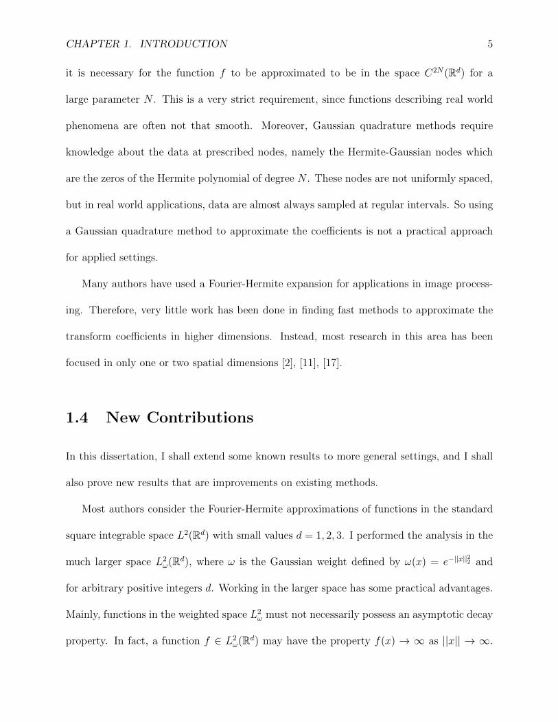
1.4 New Contributions
In this dissertation, I shall extend some known results to more general settings, and I shall
also prove new results that are improvements on existing methods.
Most authors consider the Fourier-Hermite approximations of functions in the standard
square integrable space L2(Rd) with small values d = 1, 2, 3. I performed the analysis in the
much larger space L2ω(Rd), where ω is the Gaussian weight defined by ω(x) = e−||x||
22 and
for arbitrary positive integers d. Working in the larger space has some practical advantages.
Mainly, functions in the weighted space L2ω must not necessarily possess an asymptotic decay
property. In fact, a function f ∈ L2ω(Rd) may have the property f(x) → ∞ as ||x|| → ∞.
CHAPTER 1. INTRODUCTION 6
This subtle change in the class of functions to be considered has a profound effect on the
applicability of the results. My results can be applied toward numerically solving differential
equations where the solutions do not have boundary conditions or asymptotic decay. Such
problems arise in astrophysics, quantum mechanics, models describing natural phenomena
such as population overcrowding or climate change, and pure mathematics. Additionally,
since I abandoned the Gaussian quadrature approach for approximating the coefficients, I
am able to impose a much more relaxed smoothness requirement on the functions to be
considered, thereby enlarging the space of candidate functions even more.
As mentioned above, much of the interest in Hermite polynomial decompositions has come
from the image processing community. Therefore much of the research has been limited to
few spatial dimensions. However, these low dimension problems that are processed only on
defined limited domains do not take advantage of all of the nice properties of the Hermite
expansions. The Hermite polynomials are unique in that they are ω-orthogonal over all
of Rd, but image processing uses only locally orthogonal properties. However, the global
orthogonality may be very useful in approximating functions or solutions to PDEs that do
not have any boundary conditions in a very large dimensional settings. Therefore, I shall
prove theoretical approximation errors and develop computational algorithms with relatively
low computational complexity using an arbitrarily large dimension d.
As discussed earlier, I believe the Gaussian quadrature method is often not a good ap-
proach for computing the transform coefficients in high dimensions for practical settings.
Therefore I used a truncated multiscale piecewise polynomial interpolation method to ap-
proximate the coefficients. Although using heirarchical approaches is not a novel idea, this
is a new approach for this particular problem. Since I am employing this method on func-
CHAPTER 1. INTRODUCTION 7
tions over unbounded domains, it is necessary to introduce many interdependent parameters
whose values must be chosen carefully to balance each other, the computational cost of eval-
uating all of the coefficients, and the overall accuracy achieved by the approximation. As
new contributions to the field, I shall develop the framework for finding these parameters,
prove the approximation and complexity orders using these values, and develop algorithms
to find the coefficient values quickly.
Chapter 2
Sparse Fourier Hermite Expansions
I shall begin by listing some basic definitions, properties, and some fundamental results
involving the Hermite polynomials. Then I shall define the decomposition of a function in
terms of the Hermite polynomial basis. This decomposition, given in Definition 2.9, and
finding ways to approximate it quickly and accurate is the focus of this dissertation.
2.1 Preliminaries
In the following, a vector will be denoted by boldface type or a bar over the variable. For
the sake of readability, if it is clear from the context that the variable is multidimensional,
standard typeface will be used.
For a vector x = (x1, x2, . . . , xd) ∈ Rd, the square of the standard `2 norm is defined
as ||x||22 :=∑x2j and the standard `1 norm as |x| :=
∑|xj|. The d-dimensional Gaussian
weight is defined via
ω(x) := e−||x||22 = e−(x21+x22+···+x2d).
8
CHAPTER 2. SPARSE FOURIER HERMITE EXPANSIONS 9
The weighted L2 space over Rd is defined by
L2ω(Rd) :=
Lebesgue measurable f : Rd → R with ||f ||ω <∞
,
where ||f ||ω is the Gaussian weighted norm induced by the inner product
〈f, g〉ω :=
∫Rd
f(x)g(x)ω(x) dx.
The error function is defined as
erf(x) :=2√π
∫ x
0
e−t2
dt, (2.1)
and the complimentary error function as
erfc(x) :=2√π
∫ ∞x
e−t2
dt, (2.2)
for any x ∈ R. Notice limx→∞
erf(x) = 1.
The following notations will be needed. The d-dimension factorial is given by
n! := (n1!)(n2!) · · · (nd!), and the d-dimension Kronecker delta is defined via
δn,m :=
1 if nj = mj for all j = 1, 2, . . . , d
0 otherwise
.
For two d-dimensional vectors x and y, the notation xy meansd∏j=1
xyjj , and for a scalar x and
CHAPTER 2. SPARSE FOURIER HERMITE EXPANSIONS 10
vector y, the notation xy means x|y|. The following notation for higher order derivatives in
d dimensions will also be needed in subsequent sections:
∂n
∂xn=
∂n1
∂xn11
· · · ∂nd
∂xndd
.
The set of the nonnegative integers will be denoted by N0.
Definition 2.1. Let n ∈ N0. The nth univariate Hermite polynomial Hn : R → R is given
by
Hn(x) := (−1)nex2 dn
dxn
(e−x
2).
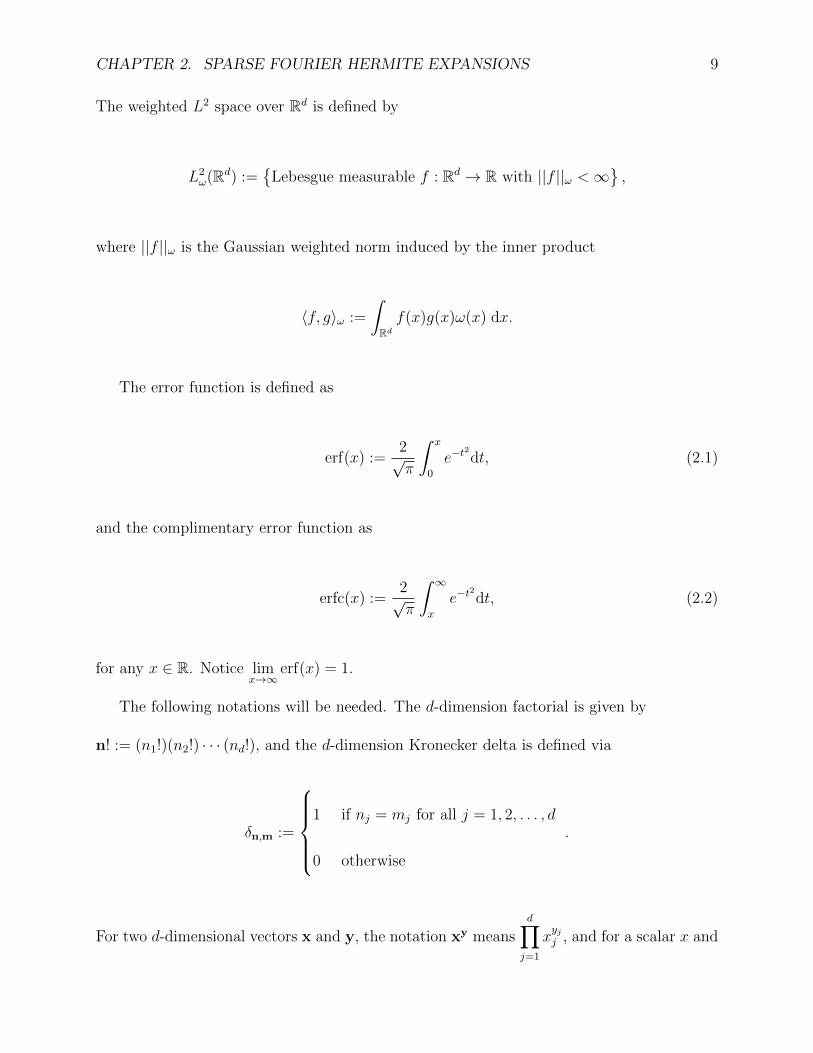
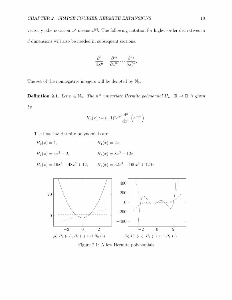
The first few Hermite polynomials are
H0(x) = 1, H1(x) = 2x,
H2(x) = 4x2 − 2, H3(x) = 8x3 − 12x,
H4(x) = 16x4 − 48x2 + 12, H5(x) = 32x5 − 160x3 + 120x.
−2 0 2
0
20
(a) H0 (- -), H1 (..) and H2 (–)
−2 0 2
−400
−200
0
200
400
(b) H3 (- -), H4 (..) and H5 (–)
Figure 2.1: A few Hermite polynomials
CHAPTER 2. SPARSE FOURIER HERMITE EXPANSIONS 11
The Hermite polynomials form an orthogonal set in L2ω(R). It is well-known [27] that
〈Hn, Hm〉ω :=
∫ ∞−∞
Hn(x)Hm(x)e−x2
dx = n!2n√πδn,m,
where δn,m is 1 if m = n and zero otherwise. In addition, the Hermite polynomials enjoy the
following properties [27]:
• Three-Term Recurrence: Hn+1(x) = 2xHn(x)− 2nHn−1(x).
• H ′n(x) = 2nHn−1(x), and H(k)n (x) = 2k n!
(n−k)!Hn−k(x).
• Hn is a solution to the differential equation u′′ − 2xu′ + 2nu = 0
• Hn : n ∈ N0 forms a complete orthogonal system in L2ω(R).
A d-dimensional Hermite polynomial is simply a tensor product of the univariate poly-
nomials.
Definition 2.2. For n ∈ Nd0 and x ∈ Rd, we define the nth Hermite polynomial as
Hn(x) :=d∏j=1
Hnj(xj).
Alternatively, one may write
Hn(x) = (−1)|n|e||x||22∂|n|
∂xn
(e−||x||
22
).
A few three dimensional Hermite polynomials are
CHAPTER 2. SPARSE FOURIER HERMITE EXPANSIONS 12
H(0,0,0)(x, y, z) = 1, H(2,1,1)(x, y, z) = 16x2yz − 8yz,
H(2,2,0)(x, y, z) = 16x2y2 − 8x2 − 8y2 + 4, H(3,0,1)(x, y, z) = 16x3z − 24xz,
H(0,4,0)(x, y, z) = 16y4 − 48y2 + 12.
The d-dimensional Gaussian weight ω is exactly equal to the product of its univariate
cases. This means that for functions where the variables can be separated (as with the
Hermite polynomials), then the inner product can be easily computed one spatial dimension
at a time. In more detail, for any m,n ∈ Nd0,
〈Hm, Hn〉ω =
∫Rd
Hm(x)Hn(x)ω(x) dx
=d∏
k=1
∫RHmk
(x)Hnk(x)ω(x) dx
=d∏
k=1
〈Hmk, Hnk
〉ω
=d∏
k=1
nk!2nk√πδmk,nk
= n!2nπd/2δm,n.
This section concludes with some basic theorems involving the Hermite polynomials.
Theorem 2.3. Let n ∈ Nd. Define n− 1 := (nj − 1)dj=1. Then
∂
∂x(Hn−1(x)ω(x)) = (−1)dHn(x)ω(x).
CHAPTER 2. SPARSE FOURIER HERMITE EXPANSIONS 13
Proof. First consider the univariate case. Observe that ω′(x) = −2xω(x). Then for n = 1,
d
dx(H0(x)ω(x)) =
d
dx(ω(x)) = −2xω(x) = −H1(x)ω(x).
Using the three term recurrence, for any integer n ≥ 2,
d
dx(Hn−1(x)ω(x)) = H ′n−1(x)ω(x) +Hn−1(x)ω′(x)
= 2(n− 1)Hn−2(x)ω(x)− 2xHn−1(x)ω(x)
= −[2xHn−1(x)− 2(n− 1)Hn−2(x)]ω(x)
= −Hn(x)ω(x).
Then for the multivariate case:
∂
∂x(Hn−1(x)ω(x)) =
(∂
∂x1
· · · ∂∂xd
)Hn−1(x)ω(x)
=d∏j=1
d
dxjHnj−1(xj)ω(xj)
=d∏j=1
(−1)Hnj(xj)ω(xj)
= (−1)dHn(x)ω(x).
Corollary 2.4. Let n ∈ N0. Then
∫ x
0
Hn+1(t)ω(t)dt = (−1) (Hn(x)ω(x)−Hn(0)) . (2.3)
CHAPTER 2. SPARSE FOURIER HERMITE EXPANSIONS 14
Theorem 2.5. For any n ∈ Nd0,
∂
∂x(Hn(x)) = 2d
(d∏j=1
nj
)Hn−1(x).
Proof. Consider a single dimension first. The theorem is easy to verify for n = 1, 2. In those
cases,
H ′1(x) = (2x)′ = 2 = 2H0(x), (for n = 1),
and
H ′2(x) = (4x2 − 2)′ = 8x = 2nH1(x), (for n = 2.)
Suppose the theorem is true for some positive integers n− 2 and n− 1. Then the statement
of the theorem can be shown to be true for n by an application of the three term recurrence.
H ′n(x) = (2xHn−1(x)− 2(n− 1)Hn−2(x))′
= 2Hn−1(x) + 2xH ′n−1(x)− 2(n− 1)H ′n−2(x)
= 2Hn−1(x) + 4(n− 1)xHn−2(x)− 4(n− 1)(n− 2)Hn−3(x)
= 2Hn−1(x) + 2(n− 1) (2xHn−2(x)− 2(n− 2)Hn−3(x))
= 2Hn−1(x) + 2(n− 1)Hn−1(x)
= 2nHn−1(x),
as desired. Therefore, by induction, the theorem is true when d = 1 and for all n ≥ 1.
In several dimensions, the statement of the theorem can be shown to be true using a
CHAPTER 2. SPARSE FOURIER HERMITE EXPANSIONS 15
product of the univariate case. In fact,
∂
∂x(Hn(x)) =
d∏j=1
d
dxjHnj
(xj) =d∏j=1
2njHnj(xj) = 2d
(d∏j=1
nj
)Hn−1(x).
Theorem 2.6. Denote the largest root of Hn by x∗n. For any n ∈ N0,
Hn(x) ≤ 2nxn,
for all x ≥ x∗n.
Proof. Proceed by induction on n.
The cases n = 0, 1 are trivially true since H0 ≡ 1 and H1(x) = 2x ≤ 21x1.
Suppose the statement of the theorem is true for some positive integer n. Define a
function f(x) := 2n+1xn+1. Since x∗n+1 ≥ 0, we know that 0 = Hn+1(x∗n+1) ≤ f(x∗n+1).
Furthermore, it is well known that the zeros of orthogonal polynomials are interlaced. This
fact guarantees that the largest root of Hn+1 is larger than the largest root of Hn for every
nonnegative integer n.
CHAPTER 2. SPARSE FOURIER HERMITE EXPANSIONS 16
Thus for all x ≥ x∗n+1 > x∗n,
d
dxHn+1(x) = (n+ 1)Hn(x)
≤ (n+ 1)2nxn, (via the induction step)
≤ (n+ 1)2n+1xn
=d
dxf(x).
Therefore Hn+1(x) ≤ f(x) for all x ≥ x∗n+1 for this n.
Induction on n promises that the statement is true for all n ∈ N0.
Theorem 2.7. For any n ∈ N0, the integral of the square of the nth Hermite polynomial can
be written a a combination of products of Hermite polynomials and the error function via
∫ x
0
H2n(t)ω(t)dt =
n−1∑k=0
n!2k
(n− k)!Hn−k(x)Hn−k−1(x)ω(x) + n!2n−1
√π erf(x).
Proof. Using Theorem 2.3, for any integer k ≥ 1,
d
dx(Hk−1(x)ω(x)) = −Hk(x)ω(x).
For any non-negative integer n, the product Hn(x)Hn−1(x) is an odd polynomial (Theorem
A.3), and therefore for any n ≥ 1, Hn(0)Hn−1(0) = 0. One can use integration by parts to
CHAPTER 2. SPARSE FOURIER HERMITE EXPANSIONS 17
see that
∫ x
0
H2n(t)ω(t)dt =
∫ x
0
(Hn(t))(Hn(t)ω(t))dt
=
∫ x
0
(Hn(t))(−Hn−1(t)ω(t))′dt
= Hn(t)Hn−1(t)ω(t)|x0 −∫ x
0
(−2n)H2n−1(t)ω(t)dt
= Hn(x)Hn−1(x)ω(x) + 2n
∫ x
0
H2n−1(t)ω(t)dt.
Continue to apply the above procedure to get
∫ x
0
H2n(t)ω(t)dt =
n−1∑k=0
n!2k
(n− k)!Hn−k(x)Hn−k−1(x)ω(x) + n!2n
∫ x
0
ω(x)dx
=n−1∑k=0
n!2k
(n− k)!Hn−k(x)Hn−k−1(x)ω(x) + n!2n−1
√π erf(x).
Corollary 2.8. Let n ∈ N0. Then
∫ ∞0
H2n+1(t)ω(t)dt = n!2n−1
√π.
CHAPTER 2. SPARSE FOURIER HERMITE EXPANSIONS 18
Proof. In Theorem 2.7, let x tend to positive infinity.
∫ ∞0
H2n+1(t)ω(t)dt = lim
x→∞
∫ x
0
H2n+1(t)ω(t)dt
= limx→∞
(n−1∑k=0
n!2k
(n− k)!Hn−k(x)Hn−k−1(x)ω(x) + n!2n−1
√π erf(x)
)
=n−1∑k=0
n!2k
(n− k)!limx→∞
(Hn−k(x)Hn−k−1(x)ω(x)) + n!2n−1√π.
The interchange of the sum and limit will be justified since the sum is finite.
Note that
0 ≤ limx→∞
(Hn−k(x)Hn−k−1(x)ω(x)) = limx→∞
Hn−k(x)Hn−k−1(x)
e−x2
≤ limx→∞
(2x)2n−2k−1
e−x2,
by Theorem 2.6.
By L’Hopital’s Rule for limits ([26]), limx→∞
(2x)2n−2k−1
e−x2= 0 for any integers n and k.
Therefore, ∫ ∞0
H2n+1(t)ω(t)dt = n!2n−1
√π.
2.2 Fourier Hermite Series
In the previous section, it was observed that d-dimensional Hermite polynomials are orthogo-
nal in L2ω(Rd) because the univariate Hermite polynomials are orthogonal in L2
ω(R). It is well
CHAPTER 2. SPARSE FOURIER HERMITE EXPANSIONS 19
known that the set of the Hermite polynomials forms a complete orthogonal set in L2ω(Rd),
and therefore also forms a basis. This property will be used throughout the remainder of
this dissertation to find a good approximation of a given function f ∈ L2ω(Rd) in terms of
only a few well-chosen elements in this basis.
Definition 2.9. For any f ∈ L2ω(Rd), the Fourier-Hermite expansion of f is given by
f(x) =∑n∈Nd
0
cnHn(x),
where the coefficients cn are defined via
cn =〈f,Hn〉ωn!2nπd/2
.
It is impractical to try to calculate the Hermite-Fourier expansion over the entire index set
Nd0. One would like to find the coefficients only for small values of |n|, and would be justified
in doing so. The coefficients cn from Definition 2.9 decay very rapidly as |n| increases. For
each f , there exists a finite positive constant C such that cn ≤ C/(n!2n). This is due to the
fact that since f ∈ L2ω(Rd), the norm ||f ||ω is bounded above by a finite positive constant
C1. Then
cn :=〈f,Hn〉ω||Hn||2ω
≤ ||f ||ω||Hn||ω||Hn||2ω
≤ C1
||Hn||ω=
C
n!2n.
An approximation to the Hermite-Fourier expansion of f over a finite full grid index set is
considered first.
CHAPTER 2. SPARSE FOURIER HERMITE EXPANSIONS 20
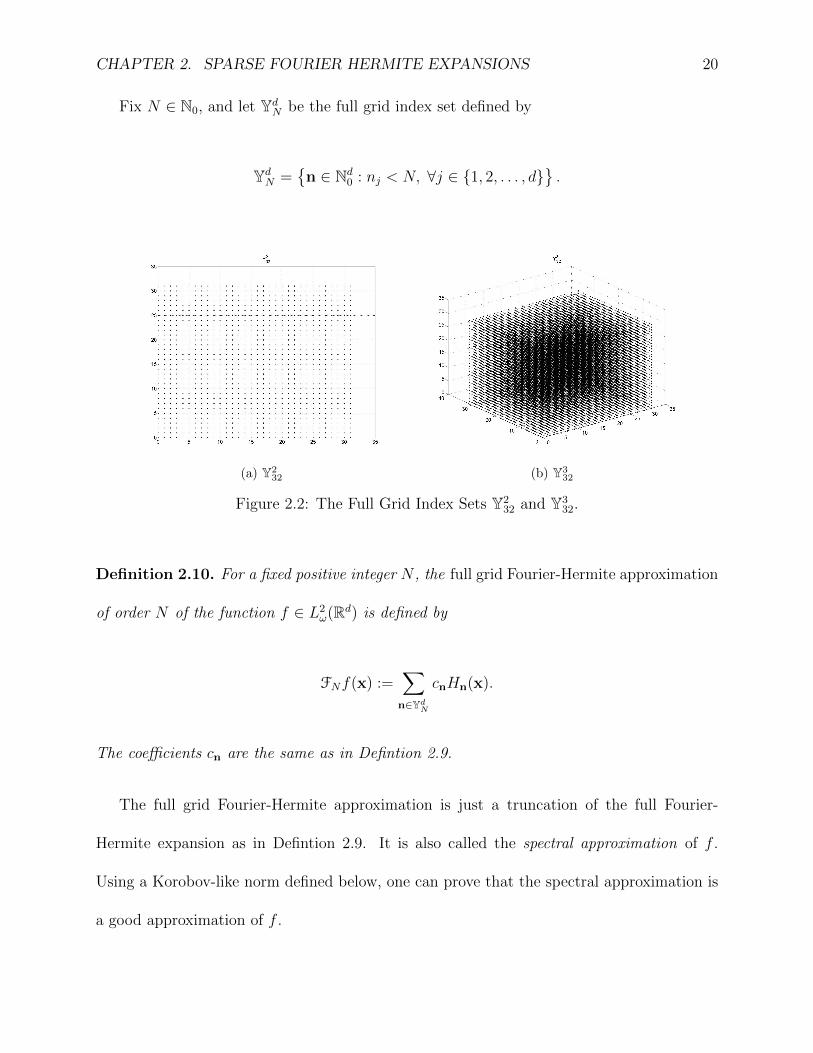
Fix N ∈ N0, and let YdN be the full grid index set defined by
YdN =
n ∈ Nd
0 : nj < N, ∀j ∈ 1, 2, . . . , d.
(a) Y232 (b) Y3
32
Figure 2.2: The Full Grid Index Sets Y232 and Y3
32.
Definition 2.10. For a fixed positive integer N , the full grid Fourier-Hermite approximation
of order N of the function f ∈ L2ω(Rd) is defined by
FNf(x) :=∑n∈Yd
N
cnHn(x).
The coefficients cn are the same as in Defintion 2.9.
The full grid Fourier-Hermite approximation is just a truncation of the full Fourier-
Hermite expansion as in Defintion 2.9. It is also called the spectral approximation of f .
Using a Korobov-like norm defined below, one can prove that the spectral approximation is
a good approximation of f .
CHAPTER 2. SPARSE FOURIER HERMITE EXPANSIONS 21
For a fixed number s > 0 and functions φ, ψ ∈ L2ω(Rd), define
〈φ, ψ〉κs :=∑n∈Nd
0
〈φ,Hn〉ω〈ψ,Hn〉ωn!2nπd/2
d∏j=1
(1 + nj)2s.
By Theorem A.1, 〈·, ·〉κs defines an inner product. Denote the induced norm on L2ω(Rd) by
|| · ||κs , and let the space Hs(Rd) ⊂ L2ω(Rd) denote the collection of all functions f such that
||f ||κs <∞.
Theorem 2.11. For any s > 0, f ∈ L2ω(Rd) and N ∈ N,
||f − FNf ||ω ≤ N−s||f ||κs .
Proof. The Fourier-Hermite expansion of f has the form∑n∈Nd
0
cnHn(x). Since the Hermite
polynomials are an orthogonal basis of L2ω(Rd), a generalization of Parseval’s identity can be
used (See Theorem A.5).
||f − FNf ||2ω =
∣∣∣∣∣∣∣∣∣∣∣∣∑
n∈Nd0\Yd
N
cnHn
∣∣∣∣∣∣∣∣∣∣∣∣2
ω
=∑
n∈Nd0\Yd
N
|cn|2||Hn||2ω.
The right hand side simplifies to∑
n∈Nd0\Yd
N
|〈f,Hn〉ω|2
n!2nπd/2. Then multiply and divide by the factor
∏dj=1(1 + nj)
2s to obtain
||f − FNf ||2ω =∑
n∈Nd0\Yd
N
|〈f,Hn〉ω|2
n!2nπd/2
d∏j=1
(1 + nj)2s
d∏j=1
(1 + nj)−2s.
Since no n occurring in the summation index set is an element of YdN , it follows that
CHAPTER 2. SPARSE FOURIER HERMITE EXPANSIONS 22
nja ≥ N for some ja. Then
d∏j=1
(1 + nj)−2s =
d∏j=1
1
(nj + 1)2s≤ 1
(1 + nja)2s≤ 1
(1 +N)2s≤ 1
N2s,
We have shown ||f − FNf ||2ω ≤ N−2s||f ||2κs as desired.
2.3 Hyperbolic Cross Sparse-Grid Approximation
Although having infinitely many coefficients to compute can be avoided by truncating the
Fourier-Hermite expansion and summing only over the index set YdN , in high dimensions the
cardinality of this index set is still too large to allow quick computation of the projections,
since the full grid index set YdN contains Nd elements. The size of the index set used
for the truncation needs to be drastically reduced to allow timely computations, but must
be designed to keep the approximation results obtained with the full grid approximation.
Considering the nature of decay of the coefficients cn, a hyperbolic cross index set is used to
satisfy these requirements.
Fix N ∈ N0, and let LdN be the sparse grid index set defined by
LdN =
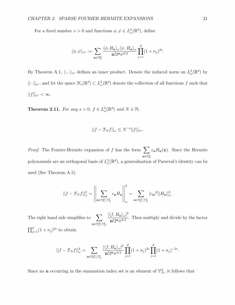
n ∈ Nd
0 :d∏j=1
(nj + 1) ≤ N
.
The sparse grid index set contains O(N logd−1N) elements ([12]). In the case d = 2 or 3
and N = 32, which are very moderate values for d and N , comparison between Figures 2.2
and 2.3 illustrate the huge computational advantage in using the sparse grid index set over
the full grid index set.
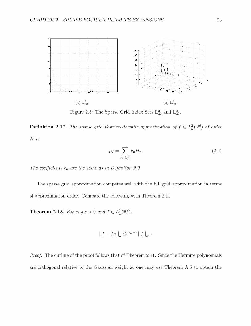
CHAPTER 2. SPARSE FOURIER HERMITE EXPANSIONS 23
(a) L232 (b) L3
32
Figure 2.3: The Sparse Grid Index Sets L232 and L3
32.
Definition 2.12. The sparse grid Fourier-Hermite approximation of f ∈ L2ω(Rd) of order
N is
fN =∑n∈Ld
N
cnHn. (2.4)
The coefficients cn are the same as in Definition 2.9.
The sparse grid approximation competes well with the full grid approximation in terms
of approximation order. Compare the following with Theorem 2.11.
Theorem 2.13. For any s > 0 and f ∈ L2ω(Rd),
||f − fN ||ω ≤ N−s ||f ||κs .
Proof. The outline of the proof follows that of Theorem 2.11. Since the Hermite polynomials
are orthogonal relative to the Gaussian weight ω, one may use Theorem A.5 to obtain the
CHAPTER 2. SPARSE FOURIER HERMITE EXPANSIONS 24
following:
||f − fN ||2ω =
∣∣∣∣∣∣∣∣∣∣∣∣∑n∈Nd
0
cnHn −∑n∈Ld
N
cnHn
∣∣∣∣∣∣∣∣∣∣∣∣2
ω
=∑
n∈Nd0\Ld
N
|cn|2||Hn||2ω
=∑
n∈Nd0\Ld
N
∣∣∣∣〈f,Hn〉ω||Hn||2ω
∣∣∣∣2 ||Hn||2ω
=∑
n∈Nd0\Ld
N
〈f,Hn〉2ω||Hn||2ω
=∑
n∈Nd0\Ld
N
〈f,Hn〉2ω||Hn||2ω
d∏j=1
(1 + nj)2s
d∏j=1
(1 + nj)−2s.
The set LdN is the collection of all multi-indices n such that nj > 0 and∏d
j=1(1 + nj) ≤ N .
Therefore for all n ∈ Nd0 \ LdN ,
d∏j=1
(1 + nj) ≥ N ⇒d∏j=1
(1 + nj)−2s ≤ N−2s.
Thus
||f − fN ||2ω ≤∑
n∈Nd0\Ld
N
〈f,Hn〉2ω||Hn||2ω
d∏j=1
(1 + nj)2sN−2s ≤ ||f ||2κsN−2s.
The following regularity result holds.
Theorem 2.14. For fixed 0 < k < s, and f ∈ L2ω(Rd),
||f − fN ||κk ≤ Nk−s||f ||κs .
CHAPTER 2. SPARSE FOURIER HERMITE EXPANSIONS 25
Proof. Let∑n∈Nd
0
cnHn be the Fourier-Hermite expansion of f . Then
||f − fN ||2κk =∑n∈Nd
0
〈f − fN , Hn〉2ωn!2nπd/2
d∏j=1
(nj + 1)2k.
Since f − fN =∑
n∈Nd0\Ld
N
cnHn, it follows that
〈f − fN , Hn〉ω =
cn||Hn||2ω, if n ∈ Nd
0 \ LdN
0, if n ∈ LdN
.
Also, note that
|cn|2||Hn||4ω =〈f,Hn〉2ω||Hn||4ω
||Hn||4ω = 〈f,Hn〉2ω.
Therefore
||f − fN ||2κk =∑
n∈Nd0\Ld
N
|cn|2||Hn||4ωn!2nπd/2
d∏j=1
(1 + nj)2k
=∑
n∈Nd0\Ld
N
〈f,Hn〉2ωn!2nπd/2
d∏j=1
(1 + nj)2k
=∑
n∈Nd0\Ld
N
〈f,Hn〉2ωn!2nπd/2
d∏j=1
(1 + nj)2s
d∏j=1
(1 + nj)2(k−s).
Since the index set for the summation includes no values from LdN , it follows that
CHAPTER 2. SPARSE FOURIER HERMITE EXPANSIONS 26
∏dj=1(1 + nj) ≥ N . Therefore
||f − fN ||2κk ≤ N2(k−s)∑
n∈Nd0\Ld
N
〈f,Hn〉2ωn!2nπd/2
d∏j=1
(1 + nj)2s
= N2(k−s)||f ||2κs
as desired.
Chapter 3
Discretization Part 1: Removing the
Tails
One difficulty encountered in approximating Fourier-Hermite approximations has now been
overcome. Summations over an infinite index set must be avoided, so in the previous chapters
the index set was truncated first to a finite full grid and then to a finite sparse grid, and the
error arising from the truncations has been analyzed. However, to compute the full grid and
sparse grid approximations as in Definitions 2.10 and 2.12, one needs to exactly compute the
coefficients cn which, if even possible, are difficult and computationally consuming. The next
few chapters of this dissertation focus on the development of a scheme for the approximation
of the integrals ∫Rd
f(x)Hn(x)ω(x)dx (3.1)
appearing in the coefficients cn of the Fourier-Hermite expansions of f in such a way to
keep the approximation order obtained in the previous chapter. To accomplish this, first the
27
CHAPTER 3. DISCRETIZATION PART 1: REMOVING THE TAILS 28
integrands are considered only over a compact subset Id of Rd, then a quadrature method
based on multiscale interpolation is used to approximately evaluate the integral
∫Id
f(x)Hn(x)ω(x)dx. (3.2)
One may be tempted to choose an arbitrarily large set Id, which would indeed guarantee
the integral in Equation (3.2) is approximately equal to the integral in Equation (3.1). How-
ever, this would be foolish since it would force a more computationally exhaustive quadrature
method to be used to numerically compute the integral in (3.2). Therefore the set Id should
be chosen just large enough to ensure the two integrals are within an acceptable margin or
error.
In this chapter, I shall show how to find an appropriate compact set Id and prove that
the error between the two integrals in Equations (3.1) and (3.2) is bounded. The next
chapter will develop and analyze a quadrature method to numerically compute the integral
in Equation (3.2).
3.1 Definitions and Strategies
In general, for any quadrature method used, the following definition applies.
Definition 3.1. For any function f ∈ L2ω(Rd), let Q(f,n) be a quadrature rule used to
approximate the integral 〈f,Hn〉ω with error ε(f,n). The discrete sparse Fourier-Hermite
CHAPTER 3. DISCRETIZATION PART 1: REMOVING THE TAILS 29
approximation of f is
fQ,N :=∑n∈Ld
N
cQ,nHn, with cQ,n =Q(f,n)
||Hn||2ω.
Notice that this is similar to Definition 2.12, but with each 〈f,Hn〉ω replaced with Q(f,n).
Theorem 3.2. Let fN be as in Definition 2.12 and fQ,N be as in Definition 3.1. Then
||fN − fQ,N ||2ω ≤∑n∈Ld
N
ε2(f,n)
n!2nπd/2.
Proof. Use the generalized Parseval’s identity. (Theorem A.5.)
||fN − fQ,N ||2ω =∑n∈Ld
N
|cn − cQ,n|2||Hn||2ω
=∑n∈Ld
N
∣∣∣∣〈f,Hn〉ω||Hn||2ω
− Q(f,n)
||Hn||2ω
∣∣∣∣2 ||Hn||2ω
=∑n∈Ld
N
|〈f,Hn〉ω −Q(f,n)|2
||Hn||2ω
=∑n∈Ld
N
ε2(f,n)
n!2nπd/2.
This theorem agrees with intuition; the error should depend on how well the quadrature
method performs, but should also be smaller if higher degree polynomials are used in the
approximation. Now it remains to pick a quadrature method that not only has a very good
error term ε, but that also is computationally cheap.
CHAPTER 3. DISCRETIZATION PART 1: REMOVING THE TAILS 30
3.2 Gaussian Quadrature
Since the integrands include a sequence of orthogonal polynomials, one’s first instinct may
be to use the Gaussian quadrature method to approximate the integrals. In one dimension,
for a function g ∈ C2N(R), the Gaussian quadrature method guarantees
∫ ∞−∞
g(x)ω(x) dx =N−1∑i=0
Aig(xi) +N !√π
(2N)!2Ng(2N)(ξ), (3.3)
for some ξ ∈ R, and with the nodes xi being the zeros of the Nth Hermite polynomial and
the weights given by Ai =2N−1(N − 1)!
√π
N2[HN−1(xi)]2[1], [22]. Simply replace g by f · Hn for the
desired result. Denote the Hermite-Gaussian quadrature rule by QG(f, n). Then Theorem
3.2 becomes
||fN − fN ||2ω ≤N−1∑n=0
ε2G(f, n)
n!2n√π
=N−1∑n=0
1
n!2n√π
(N !√π
(2N)!2N
)2 ∣∣(fHn)(2N)(ξ)∣∣2
=N−1∑n=0
1
n!2n√π
(N !√π
(2N)!2N
)2∣∣∣∣∣
2N∑i=0
(2N
i
)f (2N−i)(ξ)H(i)
n (ξ)
∣∣∣∣∣2
.
One may stop there and notice a glaring problem with this method, even in the one di-
mensional case. Summations of high order derivatives of f are being taken. Therefore this
method requires f to be very smooth. However, this cannot be guaranteed, and even if this
condition is met, f may have very large total variation. If f is highly oscillatory, then the
error term may blow up beyond repair. Authors have widely ignored this fact, instead opting
to say merely that this method will yield an exact result if fHn is a polynomial of degree
CHAPTER 3. DISCRETIZATION PART 1: REMOVING THE TAILS 31
less than or equal to 2N . Of course, this implies that f must already be a polynomial, so
writing it in terms of Hermite polynomials is a trivial exercise. It becomes clear that a better
course would be to abandon this method, and opt for ones that are equipped to handle a
wider class of functions.
3.3 A Two-Fold Strategy: Selecting the Location of
the Cut
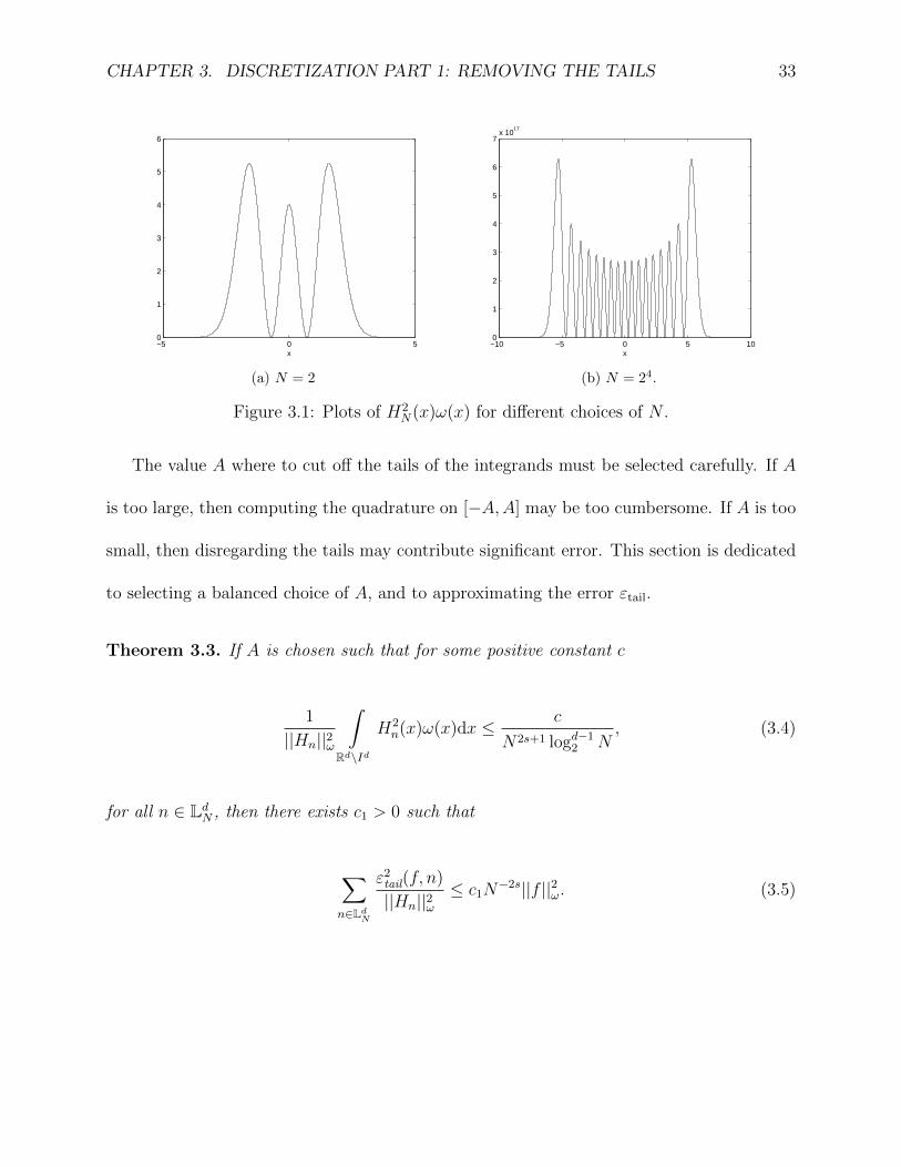
If f ∈ L2ω(Rd), then it is reasonable to expect the bulk of the integral 〈f,Hn〉ω to come from
some bounded domain in Rd, and for the contribution from the so-called ‘tail’ portion
∫|x|1
f(x)Hn(x)ω(x) dx
to be small. Eventually, the weight ω should be the dominant function in the integrand,
and thus the integrand should become quite small. See Figure 3.1 for an illustration of this
phenomenon.
Fix a positive number A to be determined later, and let I = [−A,A]. Split the integral
into two pieces and approximate each separately. That is,
∫Rd
f(x)Hn(x)ω(x) dx =
∫Id
f(x)Hn(x)ω(x) dx +
∫Rd\Id
f(x)Hn(x)ω(x) dx.
A quadrature method will be used to approximate the ‘inside’ integral, and the ‘tail’
integral will be estimated. This procedure has two sources of error- the error from truncating
CHAPTER 3. DISCRETIZATION PART 1: REMOVING THE TAILS 32
the interval of integration and the error from the quadrature method used to approximate the
‘inside’ integral. In this chapter, I shall show how to bound the error from the ‘tail’ integral.
In the subsequent chapters, I shall show how an appropriate quadrature method can be
developed to estimate the ‘inside’ integral well while keeping the computational complexity
low.
For motivation, let us investigate the error from the tail portions in one dimension first.
The inner product to be approximated can be decomposed as
〈f,Hn〉ω =
∫I
f(x)Hn(x)ω(x) dx+
∫R\I
f(x)Hn(x)ω(x) dx.
If this integral is approximated by
〈f,Hn〉ω ≈∫I
Pf(x)Hn(x)ω(x)dx,
where the portion of the integral over R \ I is discarded, and Pf is an approximation of f to
be defined later, then the error ε as in Definition 3.1 has two components. It can be written
as
ε(f, n) = εmiddle(f, n) + εtail(f, n),
where εmiddle(f, n) is the error from the quadrature method over I, and εtail(f, n) is the value
of the integral over R \ I which is to be discarded in the computation of the discretized
coefficient. It is desirable for the two sources of error to have the same order. Since A is to
be fixed in a manner that depends only on the fixed values N and s, it is not included in
the notation of the error.
CHAPTER 3. DISCRETIZATION PART 1: REMOVING THE TAILS 33
−5 0 50
1
2
3
4
5
6
x
(a) N = 2
−10 −5 0 5 100
1
2
3
4
5
6
7x 10
17
x
(b) N = 24.
Figure 3.1: Plots of H2N(x)ω(x) for different choices of N .
The value A where to cut off the tails of the integrands must be selected carefully. If A
is too large, then computing the quadrature on [−A,A] may be too cumbersome. If A is too
small, then disregarding the tails may contribute significant error. This section is dedicated
to selecting a balanced choice of A, and to approximating the error εtail.
Theorem 3.3. If A is chosen such that for some positive constant c
1
||Hn||2ω
∫Rd\Id
H2n(x)ω(x)dx ≤ c
N2s+1 logd−12 N
, (3.4)
for all n ∈ LdN , then there exists c1 > 0 such that
∑n∈Ld
N
ε2tail(f, n)
||Hn||2ω≤ c1N
−2s||f ||2ω. (3.5)
CHAPTER 3. DISCRETIZATION PART 1: REMOVING THE TAILS 34
Proof. Let S be a Lebesgue measurable set. Define the indicator function on S via
χS(x) :=
1, if x ∈ S,
0, if x /∈ S.
Since εtail(f, n) = 〈f,Hnχ(Rd\Id)〉ω ≤ ||f ||ω||Hnχ(Rd\Id)||ω,
∑n∈Ld
N
ε2tail(f, n)
||Hn||2ω≤ ||f ||2ω
∑n∈Ld
N
||Hnχ(Rd\Id)||2ω||Hn||2ω
= ||f ||2ω∑n∈Ld
N
1
||Hn||2ω
∫Rd\Id
H2n(x)ω(x)dx
≤ c||f ||2ω∑n∈Ld
N
1
N2s+1 logd−12 N
, (by assumption)
≤ c1||f ||2ωN2s+1 logd−1
2 N
(N logd−1
2 N)
= c1N−2s||f ||2ω.
Note: The value of c1 is equal to the value of c times the constant occurring in the size of
the index set LdN .
Now a guideline for choosing A satisfying the assumption of Theorem 3.3 must be devel-
oped.
Theorem 3.4. If A is chosen such that
A ≥ max
erfc
(1
N2s+1 logd−12 N
), x∗N−1
CHAPTER 3. DISCRETIZATION PART 1: REMOVING THE TAILS 35
then there exists a positive constant c such that for all n ∈ LdN ,
1
||Hn||2ω
∫Rd\Id
H2n(x)ω(x)dx ≤ c
N2s+1 logd−12 N
. (3.6)
Proof. If n = (n1, n2, . . . , nd) ∈ LdN , then denote the first d− 1 coordinates as
nd = (n1, n2, . . . , nd−1).
The set Rd \ Id can be decomposed as[(Rd−1 \ Id−1)× I
]∪[Rd−1 × (R \ I)
]. For if
xd ∈ I, then xd must satisfy xd ∈ Rd−1 \ Id−1. However, if xd ∈ R \ I, then x ∈ Rd \ Id for
any xd ∈ Rd−1.
Using this notation and observation, the left side of Equation (3.6) can be written as
1
||Hn||2ω
∫Rd\Id
H2n(x)ω(x)dx =
=1
||Hn||2ω
∫(Rd−1\Id−1)×I
H2n(x)ω(x)dx+
1
||Hn||2ω
∫Rd−1×(R\I)
H2n(x)ω(x)dx
=
1
||Hnd||2ω
∫Rd−1\Id−1
H2nd
(x)ω(x)dx
1
||Hnd||2ω
∫I
H2nd
(x)ω(x)dx
+
+
1
||Hnd||2ω
∫Rd−1
H2nd
(x)ω(x)dx
1
||Hnd||2ω
∫R\I
H2nd
(x)ω(x)dx
≤ 1
||Hnd||2ω
∫Rd−1\Id−1
H2nd
(x)ω(x)dx+1
||Hnd||2ω
∫R\I
H2nd
(x)ω(x)dx.
Notice the first term in the above inequality is similar to the original term in the string of
CHAPTER 3. DISCRETIZATION PART 1: REMOVING THE TAILS 36
inequalities. Therefore, let us continue in this manner to get
1
||Hn||2ω
∫Rd\Id
H2n(x)ω(x)dx =
≤ 1
||Hnd||2ω
∫Rd−1\Id−1
H2nd
(x)ω(x)dx+1
||Hnd||2ω
∫R\I
H2nd
(x)ω(x)dx
≤ · · ·
≤d∑
k=1
1
||Hnk||2ω
∫R\I
H2nk
(x)ω(x)dx
=d∑
k=1
2
||Hnk||2ω
∫ ∞A
H2nk
(x)ω(x)dx.
Since the constant c can (and is expected to) depend on d, it suffices to pick a value A
such that
1
n!2n
∫ ∞A
H2n(x)ω(x)dx ≤ 1
N2s+1 logd−12 N
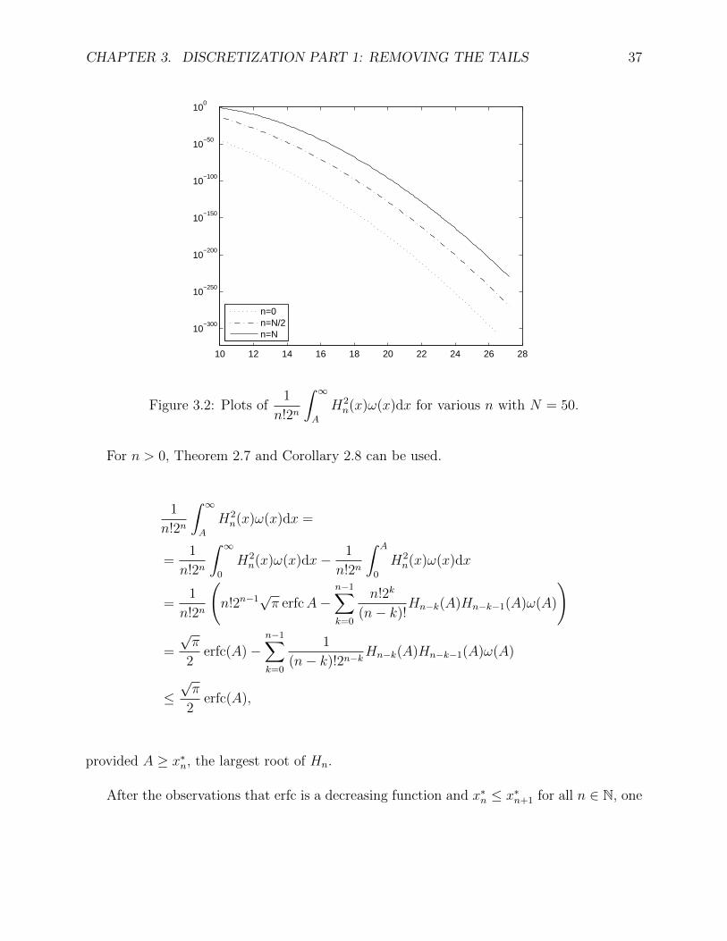
,
for all n = 0, 1, . . . , N − 1. Figure 3.2 suggests this should be possible for a moderate value
of A.
If n = 0, this reduces to finding A such that
√π
2erfc(A) ≤ 1
N2s+1logd−1
2 N.
CHAPTER 3. DISCRETIZATION PART 1: REMOVING THE TAILS 37
10 12 14 16 18 20 22 24 26 28
10−300
10−250
10−200
10−150
10−100
10−50
100
n=0n=N/2n=N
Figure 3.2: Plots of1
n!2n
∫ ∞A
H2n(x)ω(x)dx for various n with N = 50.
For n > 0, Theorem 2.7 and Corollary 2.8 can be used.
1
n!2n
∫ ∞A
H2n(x)ω(x)dx =
=1
n!2n
∫ ∞0
H2n(x)ω(x)dx− 1
n!2n
∫ A
0
H2n(x)ω(x)dx
=1
n!2n
(n!2n−1
√π erfcA−
n−1∑k=0
n!2k
(n− k)!Hn−k(A)Hn−k−1(A)ω(A)
)
=
√π
2erfc(A)−
n−1∑k=0
1
(n− k)!2n−kHn−k(A)Hn−k−1(A)ω(A)
≤√π
2erfc(A),
provided A ≥ x∗n, the largest root of Hn.
After the observations that erfc is a decreasing function and x∗n ≤ x∗n+1 for all n ∈ N, one
CHAPTER 3. DISCRETIZATION PART 1: REMOVING THE TAILS 38
can conclude that the desired result holds for any A satisfying
A ≥ max
erfc
(1
N2s+1 logd−12 N
), x∗N−1
. (3.7)
The value of c that holds in the above computations is c =2d√π
.
0 5 10 15 2010
−200
10−150
10−100
10−50
100
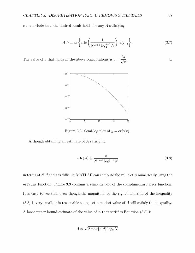
Figure 3.3: Semi-log plot of y = erfc(x).
Although obtaining an estimate of A satisfying
erfc(A) ≤ c
N2s+1 logd−12 N
(3.8)
in terms of N, d and s is difficult, MATLAB can compute the value of A numerically using the
erfcinv function. Figure 3.3 contains a semi-log plot of the complimentary error function.
It is easy to see that even though the magnitude of the right hand side of the inequality
(3.8) is very small, it is reasonable to expect a modest value of A will satisfy the inequality.
A loose upper bound estimate of the value of A that satisfies Equation (3.8) is
A ≈√
2 maxs, d log2N.
CHAPTER 3. DISCRETIZATION PART 1: REMOVING THE TAILS 39
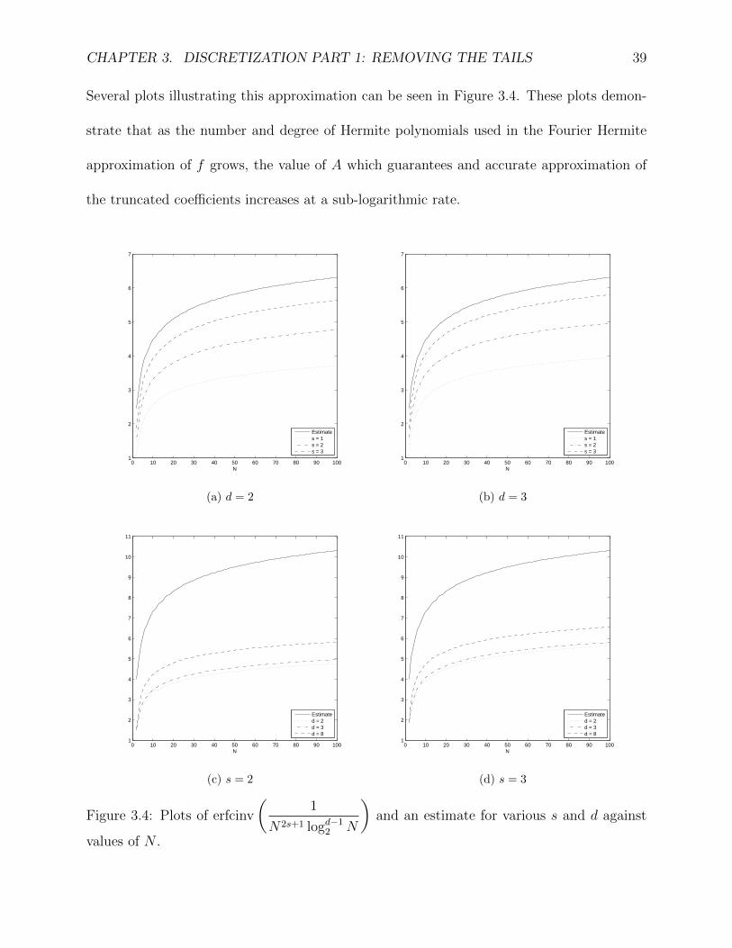
Several plots illustrating this approximation can be seen in Figure 3.4. These plots demon-
strate that as the number and degree of Hermite polynomials used in the Fourier Hermite
approximation of f grows, the value of A which guarantees and accurate approximation of
the truncated coefficients increases at a sub-logarithmic rate.
0 10 20 30 40 50 60 70 80 90 1001
2
3
4
5
6
7
N
Estimates = 1s = 2s = 3
(a) d = 2
0 10 20 30 40 50 60 70 80 90 1001
2
3
4
5
6
7
N
Estimates = 1s = 2s = 3
(b) d = 3
0 10 20 30 40 50 60 70 80 90 1001
2
3
4
5
6
7
8
9
10
11
N
Estimated = 2d = 3d = 8
(c) s = 2
0 10 20 30 40 50 60 70 80 90 1001
2
3
4
5
6
7
8
9
10
11
N
Estimated = 2d = 3d = 8
(d) s = 3
Figure 3.4: Plots of erfcinv
(1
N2s+1 logd−12 N
)and an estimate for various s and d against
values of N .
CHAPTER 3. DISCRETIZATION PART 1: REMOVING THE TAILS 40
An approximation for the largest root of Hn is given in [24] as
x∗n ≈√
2(n+ 1)− (2(n+ 1))1/3.
Therefore the condition of A in Equation (3.7) can be updated, and we shall choose the
parameter A in the following manner:
A = max
√(2(N + 1)− (2(N + 1))1/3), erfcinv
(1
N2s+1 logd−12 N
).
This value of A is very modest, so it will not force the quadrature method, which will
be developed in the next chapter, to consume any unnecessary computational resources.
However, it depends on N , s, and d and is defined to be sufficiently large to ensure that
when the integral in Equation (3.1) is replaced with the integral in Equation (3.2) for every
value of n ∈ LdN , then the resulting entire Fourier Hermite approximates a function f within
N−s.
Chapter 4
Discretization Part 2: Approximate
the Body
There are several viable possibilities for approximating the integral
∫Id
f(x)Hn(x)ω(x)dx
after the interval I has been determined. After briefly introducing a univariate quadrature
method based on linear spline interpolation, I shall then discuss in depth a multivariate
multiscale method based on piecewise polynomial interpolation.
Although the former method is easy to implement and provides elegant results, the latter
is less specific and applies to a wider class of functions f of which to approximate. The
multiscale method is the one adopted by the subsequent chapters of this dissertation, and it
will be used in the development of algorithm and computational results to be presented.
41
CHAPTER 4. DISCRETIZATION PART 2: APPROXIMATE THE BODY 42
4.1 Linear Spline Interpolation
One possibility is using a quadrature method based on linear spline interpolation. Let T be
a natural number, and choose T + 1 nodes inside I = [−A,A].
−A = t0 < t1 < · · · < tT = A
Let Bi be the ith linear B-spline defined by
Bi(x) =
x−titi+1−ti if ti ≤ x ≤ ti+1,
ti+2−xti+2−ti+1
if ti+1 ≤ x ≤ ti+2,
0 otherwise.
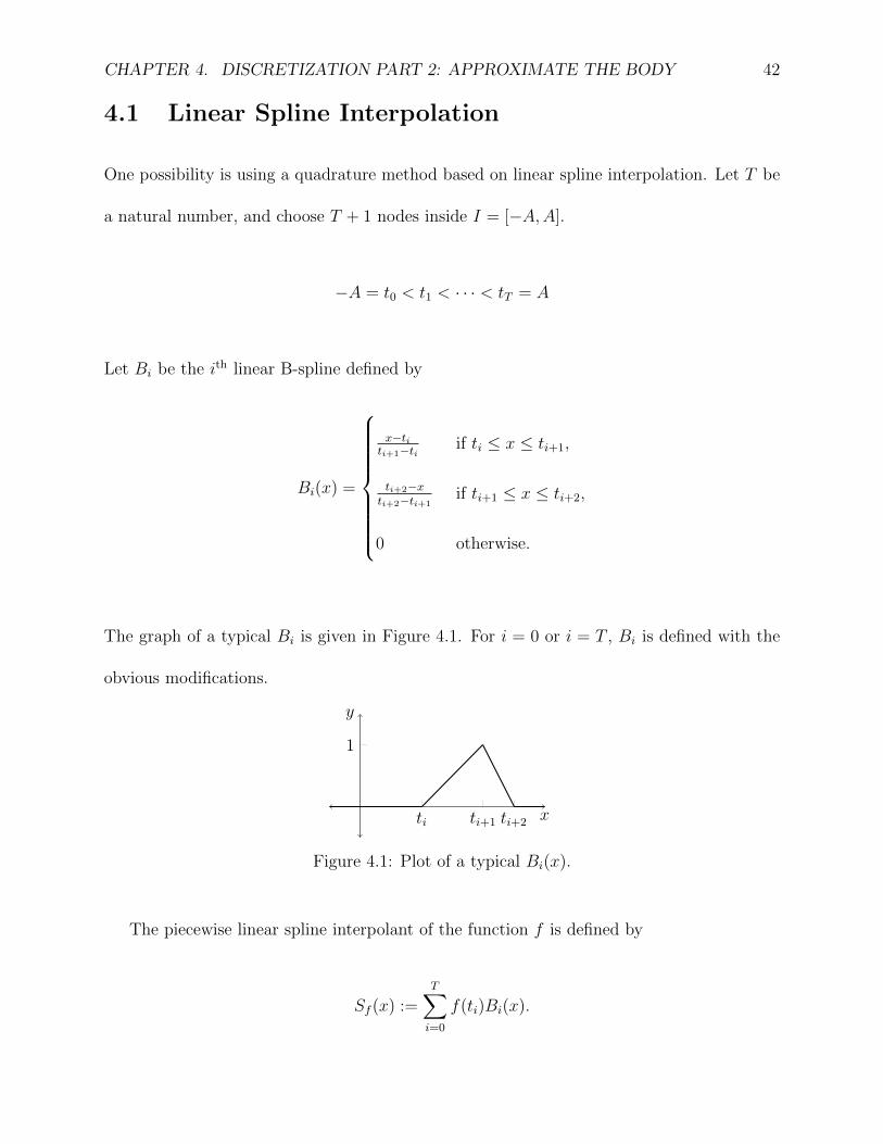
The graph of a typical Bi is given in Figure 4.1. For i = 0 or i = T , Bi is defined with the
obvious modifications.
ti ti+1 ti+2
1
x
y
Figure 4.1: Plot of a typical Bi(x).
The piecewise linear spline interpolant of the function f is defined by
Sf (x) :=T∑i=0
f(ti)Bi(x).
CHAPTER 4. DISCRETIZATION PART 2: APPROXIMATE THE BODY 43
Denote the interpolation error by
Ef (x) := f(x)− Sf (x).
Let | · |∞,Id : L2ω(Rd)→ R be defined via
|f |∞,Id := supx∈Id|f(x)|, for any f ∈ L2
ω(Rd).
From Theorem A.2, | · |∞,Id defines a seminorm.
It is well-known [10, 15] that the linear spline interpolation error is by bounded by
∆2
8|f ′′|∞,I , where ∆ = maxti+1 − ti|i = 0 : T − 1. Using this method, the ‘middle’ error
εmiddle as defined in the previous chapter takes the form
εmiddle(f, n) :=
∣∣∣∣∣∣∫I
Ef (x)Hn(x)ω(x) dx
∣∣∣∣∣∣ . (4.1)
Theorem 4.1. Let f ∈ L2ω(Rd) ∩ C2(Id). For any n ∈ LdN , there exists a positive constant
C such that the quadrature error εmiddle(f, n) as in Equation (4.1) with maximum step size
∆, is bounded above by
εmiddle ≤ C∆2√n!2n|f ′′|∞,I .
Proof. First, the weighted L2 norm of the interpolation error function will be bounded. In
CHAPTER 4. DISCRETIZATION PART 2: APPROXIMATE THE BODY 44
fact, it is observed that
||Ef ||2ω =
∫ ∞−∞
E2f (x)ω(x) dx
≤∫ ∞−∞
∆4
64|f ′′|2∞,Iω(x) dx
=∆4
64|f ′′|2∞,I
∫ ∞−∞
ω(x) dx
=∆4√π
64|f ′′|∞,I .
This inequality is now used below.
εmiddle(f, n) =
∣∣∣∣∣∣∫I
Ef (x)Hn(x)ω(x) dx
∣∣∣∣∣∣= |〈EfχI , Hn〉ω|
≤ ||EfχI ||ω ||Hn||ω
≤ ∆2|f ′′|∞,I ||Hn||ω
= C∆2√n!2n|f ′′|∞,I .
Note that the constant C does not depend on n.
Let | · |W 2,∞(Id) denote the Sobolev semi-norm on L2ω(Rd) ∩ C2(Rd) defined via
|f |W 2,∞(Id) := |f ′′|∞,Id , for any f ∈ L2ω(Rd) ∩ C2(Rd).
Corollary 4.2. Let f ∈ L2ω(R) ∩C2(I). For any n ∈ LN , there exists a positive constant C
CHAPTER 4. DISCRETIZATION PART 2: APPROXIMATE THE BODY 45
such that for any fixed maximum step size ∆,
N−1∑n=0
ε2middle(f, n)
n!2n√π≤ C∆4N |f |2W 2,∞(I).
Proof. The proof is a direct consequence of Lemma 4.1.
N−1∑n=0
ε2middle(f, n)
n!2n√π≤
N−1∑n=0
(C1∆2
√n!2n|f ′′|∞,I
)2
n!2n√π
= C∆4|f ′′|2∞,IN−1∑n=0
1
= C∆4N |f ′′|2∞,I
= C∆4N |f |2W 2,∞(I).
Using the piecewise linear spline method for obtaining a quadrature method in one di-
mension can give a good error estimate. Define an approximation to the Fourier-Hermite
series of a function f as
fN :=∑n∈LN
cnHn,
where the coefficients cn are found via truncation as in the previous chapter, and linear spline
interpolation. I.e.
cn :=1
||Hn||2ω
∫I
Sf (x)Hn(x)ω(x)dx.
Theorem 4.3. Let f ∈ L2ω(R) ∩ C2(I). Fix a constant s > 0. Choose the parameter A as
in Theorem 3.3, and choose the nodes ti such that ∆ ≤ N−(2s+1)/4. There exists a positive
CHAPTER 4. DISCRETIZATION PART 2: APPROXIMATE THE BODY 46
constant C such that
||fN − fN ||ω ≤ CN−s√||f ||2ω + |f |2W 2,∞(I).
Proof. Since 0 ≤ (a− b)2 for any real values a and b, it follows that
0 ≤ (a− b)2 = a2 − 2ab+ b2
⇒ a2 + 2ab+ b2 ≤ 2a2 + 2b2
⇒ (a+ b)2 ≤ 2(a2 + b2).
Therefore, (εtail(f, n) + εmiddle(f, n))2 ≤ 2(ε2tail(f, n) + ε2
middle(f, n)). Combine this with The-
orem 3.2 to get
||fN − fN ||2ω ≤ 2
(N−1∑n=0
ε2tail(f, n)
n!2n√π
+N−1∑n=0
ε2middle(f, n)
n!2n√π
).
From Lemma 4.2 and Theorem 3.3, for some positive constants C1 and C2,
||fN − fN ||2ω ≤ C1N−2s||f ||2ω + C2∆4N |f |2W 2,∞(I)
≤ C1N−2s||f ||2ω + C2N
−2s|f |2W 2,∞(I).
Therefore, there exists a positive constant C such that
||fN − fN ||2ω ≤ CN−2s(||f ||2ω + |f |2W 2,∞(I)
).
CHAPTER 4. DISCRETIZATION PART 2: APPROXIMATE THE BODY 47
Now we are ready to present a theorem describing the error from replacing the exact
infinitely expanded Fourier-Hermite series with the sparse-grid truncation computed with
approximated coefficients.
Theorem 4.4. Let f ∈ L2ω(R) ∩ C2(I). Fix a constant s > 0. Choose the parameter A as
in Theorem 3.3, and choose the nodes ti such that ∆ ≤ N−(2s+1)/4. There exists a positive
constant C such that
||f − fN ||ω ≤ CN−s(||f ||κs +
√||f ||2ω + |f |2W 2,∞(I)
).
Proof. From the triangle inequality,
||f − fN ||ω ≤ ||f − fN ||ω + ||fN − fN ||ω.
Combine Theorems 2.13 and 4.3 to obtain the result
||f − fN ||ω ≤ CN−s(||f ||κs +
√||f ||2ω + |f |2W 2,∞(I)
).
It is expected to have three contributions to the error since there are three steps to
the approximation. First, the index set is truncated so that only finitely many terms of the
Fourier-Hermite series are computed. Then the coefficients of those terms must be computed.
To this end, a two-step method is introduced. The second contribution to the error is from
CHAPTER 4. DISCRETIZATION PART 2: APPROXIMATE THE BODY 48
throwing out the tails of the interval over which the integrals are computed. Finally, the
third contribution to the error is from the quadrature method used on the remaining portion
of the interval. These results are good, but using linear spline interpolation is not always an
appropriate choice. In order for the above described method to work, the function f must be
continuous and possess a smooth derivative of order at least two. A more general approach
based on piecewise polynomial interpolation, which does not assume continuity, is developed
in the next few sections.
4.2 Heirarchical Lagrange Interpolation
The ideas from this section can be found in [6], but are included here for completeness.
Another possibility for approximating the middle portion of the integral is using a quadra-
ture method based on piecewise polynomial interpolation. To accommodate a fast algorithm,
it is desirable for the piecewise polynomial interpolation to have a multiscale scheme. To
achieve this, the interpolating polynomials will be related to a refinable set.
Choose two contractive mappings φ0 and φ1 on I defined by
φ0(x) :=x− A
2, and φ1(x) :=
x+ A
2.
Define Ψ := φ0, φ1. Then I is an invariant set relative to the mappings Ψ. A subset V ⊂ I
is called refinable relative to the mappings Ψ if Ψ(V ) ⊂ V . For example, the following sets
CHAPTER 4. DISCRETIZATION PART 2: APPROXIMATE THE BODY 49
are refinable relative to Ψ:
−A3,A
3
,
−A5,A
5
, −A, 0, A , and
−A7,3A
7,5A
7
.
Let V0 be a refinable set relative to the mappings Ψ of size m. Say
V0 = −A < v0,1 < v0,1 < · · · < v0,m−1 < A.
Associated with V0 are the Lagrange cardinal polynomials of degree m− 1 defined by
`0,r(x) :=m−1∏
q=0,q 6=r
x− v0,q
v0,r − v0,q
.
One may now approximate f by a combination of these cardinal polynomials. In effect,
f would be approximated by its interpolating polynomial of degree m− 1 with nodes in V0.
However, for a higher degree of accuracy, one may want to refine the sets and instead use
a piecewise polynomial interpolation. This is a desirable method. To achieve this accuracy
without sacrificing computational speed, a multiscale method will be developed.
Define a sequence of sets by Vj := Ψj(V0). It is necessary for each to be refinable.
Theorem 4.5. Let Ψ = φi be a collection of contractible mappings, and let V0 be a set
that is refinable relative to Ψ. Then each Vj = Ψj(V0) is also refinable relative to Ψ.
Proof. By assumption, Ψ(V0) ⊂ V0. Suppose Ψj(V0) ⊂ Ψj−1(V0) for some j ∈ N0. Then
Ψj+1(V0) = Ψ(Ψj(V0)) ⊂ Ψ(Ψj−1(V0)) = Ψj(V0).
CHAPTER 4. DISCRETIZATION PART 2: APPROXIMATE THE BODY 50
Therefore, by induction on j, each set Vj := Ψj(V0) is refinable.
These refinable sets will be used as a foundation of the multiscale construction of the
piecewise polynomial interpolation of f . The jth layer of the multiscale piecewise polynomial
will introduce information about f only on the set Vj \ Vj−1. The multiscale method is
excellent for interpolating oscillatory functions. If a higher order of accuracy is needed, then
it is easy to refine the interpolation. Only the finer details need to be added while keeping
all of the work that has already been done.
Define two linear operators Tρ : L∞(I)→ L∞(I) by
(Tρf) (x) :=
f φ−1
ρ (x), x ∈ φρ(I)
0, x /∈ φρ(I)
for ρ = 0, 1. These linear operators will be used successively to define new spaces.
Let F0 = span`0,r|r ∈ 0, 1, . . . ,m− 1, and define
FM := T0FM−1 ⊕ T1FM−1. (4.2)
Since FM−1 ⊂ FM for each M ∈M, FM may be decomposed as FM = FM−1 ⊕GM . Repeat-
edly apply this equation and let G0 = F0 to obtain
FM = GM ⊕GM−1 ⊕ · · · ⊕G0. (4.3)
This is the multiscale decomposition of FM ; to obtain FM , one needs only to find the new
CHAPTER 4. DISCRETIZATION PART 2: APPROXIMATE THE BODY 51
basis functions that are not already included in FM−1.
It is now necessary to describe the bases of FM and GM . First, consider how each
cardinal function `0,r behaves under an application of T0 or T1. Both will yield a hori-
zontal compression by a factor of 1/2, and T0 gives a horizontal shift of −A/2, T1 a hor-
izontal shift of A/2. As the linear operators are successively applied, the effects are com-
pounded. Let PM = ρ1, ρ2, . . . , ρM | ρi = 0 : 1, and define TPM= TρMTρM−1
· · ·Tρ1 . Then
FM = span TPM(`0,r) : r ∈ 0, 1, . . . ,m− 1. Let us rewrite these basis functions in a more
manageable way. Let η(PM) =∑M
i=1 ρi2i. Then the functions `M,r for r = 0, 1, . . . , 2Nm− 1
form a basis for FN , and can be obtained from the functions `0,r′ by
`M,r = TPM`0,r′ , r = mη(PM) + r′. (4.4)
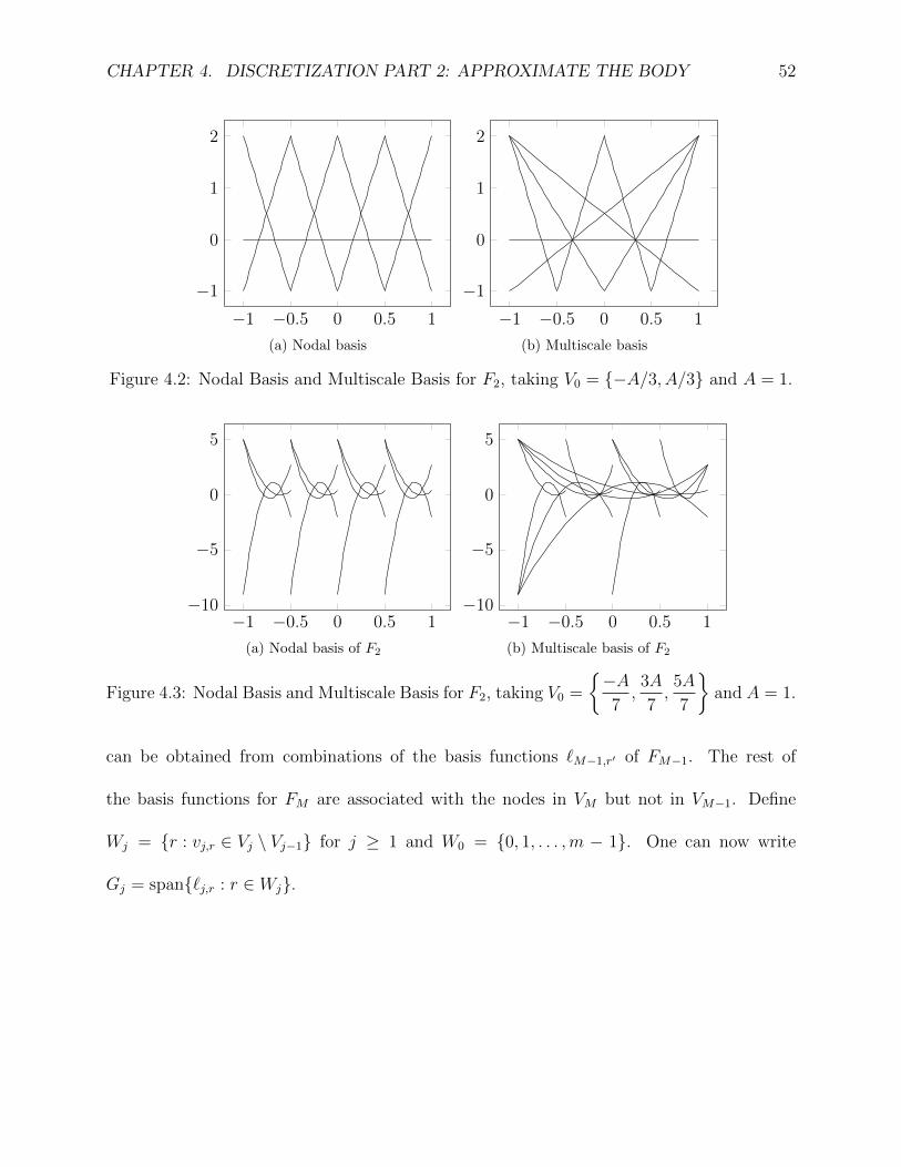
Plots of all of the basis functions in F2 using the nodal form as in equation (4.2) and
the multiscale form as in equation (4.3) are given in the Figures 4.2 and 4.3. Plots of the
individual basis functions are given near the end of the chapter in Figures 4.4 and 4.5. Figure
4.2 uses m = 2 and the initial refinable set V0 =
−A3,A
3
, which is symmetric about the
origin. For this choice of V0, F2 consists of the following Lagrange cardinal polynomials:
F2 = `0,0, `0,1, `1,0, `1,3, `2,0, `2,3, `2,4, `2,7 .
Figure 4.3 uses m = 3 and a skewed refinable set. Both use A = 1 for convenience.
The collection of all of the interpolation nodes used for the basis functions `M,r is exactly
the set VM . Because of the refinability of the sets VM , many of the basis functions `M,r
CHAPTER 4. DISCRETIZATION PART 2: APPROXIMATE THE BODY 52
−1 −0.5 0 0.5 1
−1
0
1
2
(a) Nodal basis
−1 −0.5 0 0.5 1
−1
0
1
2
(b) Multiscale basis
Figure 4.2: Nodal Basis and Multiscale Basis for F2, taking V0 = −A/3, A/3 and A = 1.
−1 −0.5 0 0.5 1−10
−5
0
5
(a) Nodal basis of F2
−1 −0.5 0 0.5 1−10
−5
0
5
(b) Multiscale basis of F2
Figure 4.3: Nodal Basis and Multiscale Basis for F2, taking V0 =
−A7,3A
7,5A
7
and A = 1.
can be obtained from combinations of the basis functions `M−1,r′ of FM−1. The rest of
the basis functions for FM are associated with the nodes in VM but not in VM−1. Define
Wj = r : vj,r ∈ Vj \ Vj−1 for j ≥ 1 and W0 = 0, 1, . . . ,m − 1. One can now write
Gj = span`j,r : r ∈ Wj.
CHAPTER 4. DISCRETIZATION PART 2: APPROXIMATE THE BODY 53
4.3 Multiscale Piecewise Polynomial Interpolation
Applying a multiscale piecewise polynomial interpolation method to approximate the integral
∫I
f(x)Hn(x)ω(x)dx
is a new contribution to this area of study. The main result from this subsection is found in
Theorem 4.6.
Define the interpolation projection PM : C(I)→ FM of a function f : R→ R by
PMf :=2Mm−1∑r=0
f(vM,r)`M,r, for all f ∈ C(I). (4.5)
This is the ‘nodal’ interpolation operator. To develop the multiscale decomposition of the
interpolation operator, define the difference operator as Qj := Pj − Pj−1 for j ≥ 1, and
Q0 = P0. Then the interpolation projection can be written as PMf =∑M
j=0 Qjf , for all
f ∈ C(I). Notice that the operators Qj are associated with the Lagrange cardinal functions
with nodes in the sets Wj. These basis functions enjoy the property `i,j(vi,j) = 1. However,
due to scaling, `i,j(vk,l) is not always zero if (i, j) 6= (k, l). (See figure 4.2.) Therefore, to
write an explicit formula for each Qjf , a new functional must be introduced taking this
property into account. Suppose one wanted to write PM and each Qj as
Qjf =∑r∈Wj
ηj,r(f)`j,r (4.6)
CHAPTER 4. DISCRETIZATION PART 2: APPROXIMATE THE BODY 54
and
PMf =M∑j=0
∑r∈Wj
ηj,r(f)`j,r. (4.7)
Then it is proven in [12] that ηj,r must be defined via
η0,r(f) = f(v0,r), and ηj,r(f) = f(vj,r)−m−1∑q=0
f(vj−1,mb r
2mc+q
)aq,r mod 2m, (4.8)
for j 6= 0, where aq,k = `0,q(v1,k).
The formula in equation (4.7) is the multiscale piecewise polynomial interpolation of f .
It interpolates f exactly on each node vM,r for r ∈ Z2Mm, and it defines a polynomial of
degree m− 1 on each subinterval Ij,r, where Ij,i := [−A+ i2−j+1A, −A+ (i+ 1)2−j+1A] for
each j = 0, 1, . . . ,M and i ∈ Z2j .
Recall that the goal is to replace f in the following integral
∫I
f(x)Hn(x)ω(x) dx (4.9)
by the piecewise polynomial to obtain the approximation
∫I
(PMf)(x)Hn(x)ω(x) dx. (4.10)
Define a space that consists of all functions that are smooth on each subinterval Ij,i via
XmM(I) :=
f : R→ R such that f (α) ∈ C(IM,i),∀i ∈ Z2M , α ≤ m
, (4.11)
CHAPTER 4. DISCRETIZATION PART 2: APPROXIMATE THE BODY 55
with seminorm
|f |XmM (I) := max
|f (α)|
∣∣IM,i
: α ≤ m, i ∈ Z2M
.
Notice functions in XmM(I) are not necessarily continuous, only piecewise continuous.
Theorem 4.6. Fix M ∈ N0. For all f ∈ L2ω(R)∩Xm
M(I), there exists a positive constant C
such that the error in estimating the integral in equation (4.9) by the integral in (4.10) can
be bounded by
∣∣∣∣∣∣∫I
(f − PMf) (x)Hn(x)ω(x) dx
∣∣∣∣∣∣ ≤ CAm2−mM+n/2
√n! |f |Xm
M (I)
(m− 1)!.
Proof. On each subinterval IM,i, PMf is a polynomial of degree m− 1. Fix i ∈ Z2M and let
x ∈ IM,i. Then there exists some constant ξx ∈ IM,i such that
|(PMf)(x)− f(x)| = 1
(m− 1)!
∣∣f (m)(ξx)∣∣ · m−1∏
j=0
∣∣x− vM,2im+j
∣∣≤|f |Xm
M (I)
(m− 1)!
m−1∏j=0
∣∣x− vM,2im+j
∣∣≤|f |Xm
M (I)
(m− 1)!
m−1∏j=0
|IM,i|
≤ (2−M+1A)m|f |Xm
M (I)
(m− 1)!
CHAPTER 4. DISCRETIZATION PART 2: APPROXIMATE THE BODY 56
Now insert this estimate into the integral.
∣∣∣∣∣∣∫I
(f − PMf) (x)Hn(x)ω(x) dx
∣∣∣∣∣∣ =
∣∣∣∣∣∣∣2M−1∑i=0
∫IM,i
(f − PMf) (x)Hn(x)ω(x) dx
∣∣∣∣∣∣∣≤
2M−1∑i=0
Am|f |XmM (I)
2m(M+1)(m− 1)!
∫IM,i
|Hn(x)|ω(x) dx
=Am|f |Xm
M (I)
2m(M+1)(m− 1)!
∫I
|Hn(x)|ω(x) dx
The remaining integral can be estimated using Jensen’s inequality.
∫I
|Hn(x)|ω(x) dx ≤
∫I
H2n(x)ω(x) dx
1/2
≤√n!2n√π.
Therefore one can write for a positive constant C = π1/4,
∣∣∣∣∣∣∫I
(f − PMf) (x)Hn(x)ω(x) dx
∣∣∣∣∣∣ ≤ CAm2−mM+n/2
√n!
(m− 1)!|f |Xm
M (I) .
Since A was chosen so that the bulk of each f(x)Hn(x)ω(x) occurs in the interval I, a
quadrature method based on the piecewise polynomial interpolation gives a good approxi-
mation even over all of R.
Corollary 4.7. Fix M ∈ N0. Fix a positive integer m, and choose some 0 < s < m. Let A
be chosen as in Theorem 3.3. For all f ∈ L2ω(R)∩Xm
M(I), there exists a positive constant C
CHAPTER 4. DISCRETIZATION PART 2: APPROXIMATE THE BODY 57
such that
∣∣∣∣∣∣∫R
(f − PMf) (x)Hn(x)ω(x) dx
∣∣∣∣∣∣ ≤ C
(N−s||f ||ω +
Am2−mM+n/2√n!
(m− 1)!|f |Xm
M (I)
).
Proof. Each of the cardinal functions `M,i is identically zero outside of the interval I. There-
fore PMf(x) = 0 for all x ∈ R \ I. Combine the results of Theorems 3.3 and 4.6.
An observation about the preceding Corollary is in order. Supposing A,N, and m are
fixed, in order to achieve a decent discrete approximation as in (4.9), one must choose an
appropriately large value for M . This is expected though; the refinement of subintervals
must be sufficiently small for an acceptable approximation of f . Guidelines for choosing M
are formalized in the next chapter.
Now that the theory has been developed for the discrete sparse Fourier Hermite approx-
imation based on multiscale piecewise polynomial interpolation in one dimension, it can
extended to higher dimensions by the use of the tensor product. The following section does
this.
4.4 High Dimension Discrete Sparse Fourier Hermite
Approximations
The formulae in the preceding section can be extended to a high dimensional setting by use
of the tensor product. This section contains several important theorems which will facilitate
the analysis of the discrete sparse Fourier Hermite approximation of a function, which is
defined in Definition 4.13.
CHAPTER 4. DISCRETIZATION PART 2: APPROXIMATE THE BODY 58
The d dimensional Lagrange polynomials and the d dimensional functionals η are given
by
`N,r := `N,r1 ⊗ `N,r2 ⊗ · · · ⊗ `N,rd ,
`j,r := `j1,r1 ⊗ `j2,r2 ⊗ · · · ⊗ `jd,rd ,
ηj,r := ηj1,r1 ⊗ ηj2,r2 ⊗ · · · ⊗ ηjd,rd ,
for any M ∈ N and any j, r ∈ Nd0. Let W d
M = WM ×WM × · · · ×WM , and
vM,r = (vN,r1 , vN,r2 , . . . , vN,rd) ∈ W dN . We define PdM := ⊗dk=1PM .
Notice that PdMf =∑
vM,r∈V dMf(vM,r)`M,r. This is the full grid interpolation projection of
f onto F dM . Also define Qj := Qj0 ⊗ Qj1 ⊗ · · · ⊗ Qjd . For the multiscale interpolation, use
the high dimensional tensor product version of equations (4.6) and (4.7). It is proven in [12]
that
PdMf =∑
j∈ZdM+1
∑r∈Wj
ηj,r(f)`j,r, (4.12)
and
Qjf =∑r∈Wj
ηj,r(f)`j,r. (4.13)
It follows immediately that the tensor product multiscale Lagrange interpolation of f can
be written as
PdMf =∑
j∈ZdM+1
Qjf.
To reduce computational cost, I shall again use the ideas from Section 2.2, and compute
the sum over a hyperbolic cross index set. For a fixed positive integer M , consider the sparse
CHAPTER 4. DISCRETIZATION PART 2: APPROXIMATE THE BODY 59
grid index set SdM defined by
SdM :=
j ∈ ZdM+1 :
d∑k=1
jk ≤M + 1
.
Definition 4.8. For a function f : Rd → Rd, the multiscale sparse grid interpolation of f
is given by
SdMf :=∑j∈SdM
∑r∈Wj
ηj,r(f)`j,r. (4.14)
Note that SdMf =∑j∈SdM
Qjf . In higher dimensions, the multiscale sparse grid interpolant
SdM will be used instead of PdM . To establish the approximation order, first some definitions
and lemmas are needed.
For any j ∈ SM and i ∈ Z2j , define Ij,i = −A+ i2−j+1A.
Define the collection of sets
Vj := Ψj1(V0)×Ψj2(V0)× · · · ×Ψjd(V0),
for any j ∈ Nd0. For any j ∈ SdM and i ∈ Zd
2j, define Ωj,i := ⊗dk=1 [Ijk,ik , Ijk,ik+1].
The operator Qj is bounded. The following theorem appears in [12].
Theorem 4.9. There exists a positive constant c such that for all f ∈ C(Id) and j ∈ Nd0,
||Qjf ||∞ ≤ c||f ||∞ (4.15)
CHAPTER 4. DISCRETIZATION PART 2: APPROXIMATE THE BODY 60
Extend the space XmM(I) to higher dimensions via the following:
XmM(Id) =
f : Rd → R : f (α)|Ωj,i
∈ C(Ωj,i), ∀j ∈ SdM , r ∈ Wj, |α|∞ ≤ m, (4.16)
with seminorm
|f |XmM (Id) := max
|f (α)|∞,Ωj,i
: α ∈ Nd0, |α|∞ ≤ m,∀j ∈ SdM , r ∈ Wj
.
Then the operators Qj are bounded for f in this new space as shown in the next lemma.
Lemma 4.10. For fixed d and M in N, there exists a positive constant c such that for all
f ∈ XmM(Id) and j ∈ Nd
0 with |j| > 0,
||Qjf ||∞ ≤ c
(A
2
)m2−m|j||f |Xm
M (Id). (4.17)
The proof closely follows that of Lemma 2.10 in [12].
With these tools, now the multiscale sparse grid Lagrange interpolation error can be
investigated.
Theorem 4.11. For fixed positive integers d and M , there exists a positive constant c such
that for all f ∈ XmM(Id),
∣∣∣∣(PdM − SdM)f∣∣∣∣∞ ≤ cAmMd−12−m(M+d)|f |Xm
M (Id).
CHAPTER 4. DISCRETIZATION PART 2: APPROXIMATE THE BODY 61
Proof. It follows immediately from (4.12), (4.14), and (4.13) that
(PdM − SdM
)f =
∑j∈Zd
M+1\SdM
Qjf.
Therefore
||(PdM − SdM
)f ||∞ ≤
∑j∈Zd
M+1\SdM
||Qjf ||∞
≤ cAm2−md ||f ||XmM (Id)
∑j∈Zd
M+1\SdM
2−m|j|
≤ cAmMd−12−m(M+d)||f ||XmM (Id).
The last inequality follows from the estimate∑
j∈ZdM+1\S
dM
2−m|j| ≤ cMd−12−mM from Lemma
3.7 in [5].
Now this estimate can be used to bound the difference between f and its sparse multiscale
interpolation SdMf .
Theorem 4.12. For fixed positive integers d and M , there exists a positive constant c such
that for all functions defined on Id with the property f ∈ XmM(Id),
∣∣∣∣f − SdMf∣∣∣∣∞,Id ≤ cAmMd−12−m(M+d)|f |Xm
M (Id).
Proof. Since PdMf is precisely piecewise polynomial interpolation of f , there exists a positive
CHAPTER 4. DISCRETIZATION PART 2: APPROXIMATE THE BODY 62
constant c such that
||f − PdMf ||∞,Id ≤ c2−mM |f |XmM (Id).
Now, by the triangle inequality
||f − SdMf ||∞,Id ≤ ||f − PdMf ||∞,Id + ||PdMf − SdMf ||∞,
and then by substituting the above result with the one from Theorem 4.11 yields the desired
result.
Now equipped with facts about SdMf , we are ready to define the discrete sparse Fourier
Hermite approximation of f .
Definition 4.13. For fixed positive integers M , N , and m, and for any function f ∈
L2ω(Rd) ∩Xm
M(Id), the discrete sparse Fourier Hermite approximation of f is given by
fM,N :=∑n∈Ld
N
cM,nHn,
where the discrete coefficients can be found via the formula
cM,n :=〈SdMf,Hn〉ω
n!2nπd/2. (4.18)
Developing framework that leads to and supports the discrete sparse Fourier Hermite
approximation has been the main purpose of this paper so far. From here out, the discussion
will focus on its approximation analysis, numerical implementation, and use in applications.
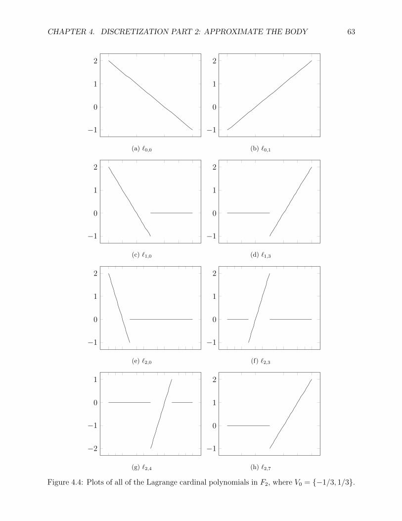
CHAPTER 4. DISCRETIZATION PART 2: APPROXIMATE THE BODY 63
−1
0
1
2
(a) `0,0
−1
0
1
2
(b) `0,1
−1
0
1
2
(c) `1,0
−1
0
1
2
(d) `1,3
−1
0
1
2
(e) `2,0
−1
0
1
2
(f) `2,3
−2
−1
0
1
(g) `2,4
−1
0
1
2
(h) `2,7
Figure 4.4: Plots of all of the Lagrange cardinal polynomials in F2, where V0 = −1/3, 1/3.
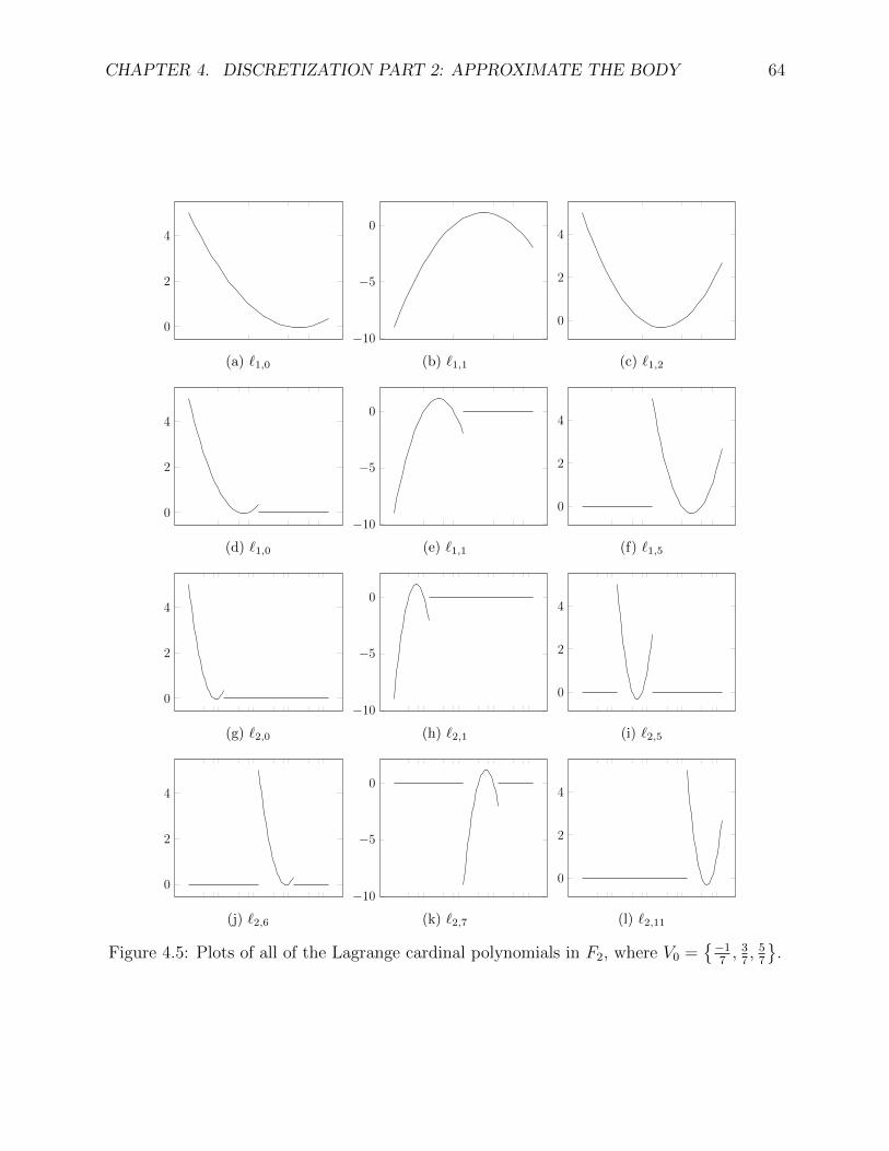
CHAPTER 4. DISCRETIZATION PART 2: APPROXIMATE THE BODY 64
0
2
4
(a) `1,0
−10
−5
0
(b) `1,1
0
2
4
(c) `1,2
0
2
4
(d) `1,0
−10
−5
0
(e) `1,1
0
2
4
(f) `1,5
0
2
4
(g) `2,0
−10
−5
0
(h) `2,1
0
2
4
(i) `2,5
0
2
4
(j) `2,6
−10
−5
0
(k) `2,7
0
2
4
(l) `2,11
Figure 4.5: Plots of all of the Lagrange cardinal polynomials in F2, where V0 =−1
7, 3
7, 5
7
.
Chapter 5
Discrete Sparse Fourier Hermite
Approximations
In the previous chapter, I focused on approximating the coefficients of the Fourier Hermite
series using a quadrature method featuring truncation and piecewise polynomial interpo-
lation. Before delving into computational issues in approximating the coefficients, I shall
verify that they do not contribute too much error to the overall approximated series.
Fix two positive integers M and N . The integer N will determine the number of terms
appearing in the sparse representation of the Fourier Hermite series, and the integer M will
determine the number of piecewise polynomial segments used for the quadrature method to
approximate the coefficients.
Definition 5.1. The discrete sparse Fourier Hermite approximation of a given function
65
CHAPTER 5. DISCRETE SPARSE FOURIER HERMITE APPROXIMATIONS 66
f ∈ Hs(Rd) ∩XmM(Id) is given by
fM,N :=∑n∈Ld
N
cM,nHn,
where the coefficients cM,n are computed using the methods described in the previous chapter.
That is,
cM,n =1
||Hn||2ω
∫IdSdMf(x)Hn(x)ω(x) dx.
It is of course desirable for fM,N to approximate the Fourier Hermite series of f well.
There are three main sources of error: from using a sparse index set, from truncating the
intervals over which the integrals for the coefficients are computed, and from using a quadra-
ture method to compute the integral over the remaining interval. To simplify notation when
considering the error, denote the sparse Fourier Hermite series that do not have the third
source of error by fN , with Fourier coefficients cn. That is,
fN :=∑n∈Ld
N
cnHn,
where
cn :=1
||Hn||2ω
∫Id
f(x)Hn(x)ω(x) dx.
Using the triangle inequality, the error between f and fM,N can be bounded by
||f − fM,N ||ω ≤ ||f − fN ||ω + ||fN − fN ||ω + ||fN − fM,N ||ω. (5.1)
The error of the first term was discussed in Chapter 2. The error of the second and third

CHAPTER 5. DISCRETE SPARSE FOURIER HERMITE APPROXIMATIONS 67
terms will depend on the parameters A, m and M . These parameters will need to be chosen
in such a way that each term in (5.1) contributes approximately the same order of error.
The purpose of this chapter is to show how these parameters can be chosen in a way that
will ensure the total approximation error is small.
Recall from Theorem 2.13 that for any f ∈ Hs(Rd) ⊂ L2ω(Rd) with s > 0,
||f − fN ||ω ≤ N−s||f ||κs . (5.2)
The following two lemmas bound the error from the second norm appearing in equation
(5.1)
Lemma 5.2. For any subset S of Rd, let χS denote the characteristic function that is equal
to 1 on S and 0 everywhere else. Define the interval I := [−A,A], where the parameter A is
chosen as in Theorems 3.3 and 3.4. Let f ∈ L2ω(Rd). For a fixed positive integer N ,
||fN − fN ||ω ≤ ||f ||ω
∑n∈Ld
N
||HnχRd\Id ||2ω||Hn||2ω
1/2
.
Proof. By the definitions of fN and fN , ||fN − fN ||2ω =∑n∈Ld
N
(cn − cn)2 ||Hn||2ω.
The difference between the exact and truncated coefficients can be bounded by
|cn − cn| =1
||Hn||2ω
∣∣∣∣∫Rd\Id
f(x)Hn(x)ω(x) dx
∣∣∣∣=
1
||Hn||2ω
∣∣〈f,Hnχ(Rd\Id)〉ω∣∣
≤||f ||ω||Hnχ(Rd\Id)||ω
||Hn||2ω.
CHAPTER 5. DISCRETE SPARSE FOURIER HERMITE APPROXIMATIONS 68
Therefore ||fN − fN ||2ω ≤ ||f ||2ω∑n∈Ld
N
||Hnχ(Rd\Id)||2ω||Hn||2ω
.
Lemma 5.3. Let f ∈ Hs(Rd), with 0 < s, and choose the parameter A as in Theorems 3.3
and 3.4. Then there exists a positive constant c such that
||fN − fN ||ω ≤ CN−s||f ||ω. (5.3)
Proof. Notice that 〈f,Hnχ(Rd\Id)〉ω = εtail(f, n). Then apply Theorem 3.3.
Finally, the third term in equation (5.1) is bounded as in the following lemma.
Lemma 5.4. Let f ∈ L2ω(Rd) ∩ Xm
M(Id). Choose the parameter A as described above. For
fixed M,N ∈ N0,
||fN − fM,N ||ω ≤ C||f − SdMf ||∞,Id
∑n∈Ld
N
||HnχId ||2ω||Hn||2ω
1/2
.
Proof. The expansions of fN and fM,N differ only in their coefficients:
||fN − fM,N ||2ω =
∣∣∣∣∣∣∣∣∣∣∣∣∑n∈Ld
N
(cn − cM,n)Hn
∣∣∣∣∣∣∣∣∣∣∣∣2
ω
=∑n∈Ld
N
|cn − cM,n|2||Hn||2ω.
By the definitions of cn and cM,n,
|cn − cM,n| =1
||Hn||2ω
∣∣∣∣∫Id
(f − SdMf
)(x)Hn(x)ω(x) dx
∣∣∣∣
=
∣∣〈(f − SdMf)χId , HnχId〉ω∣∣
||Hn||2ω.
CHAPTER 5. DISCRETE SPARSE FOURIER HERMITE APPROXIMATIONS 69
Then, by Cauchy Schwarz, the numerator of the previous quantity is bounded above by
||(f − SdMf)χId ||ω||HnχId ||ω. Finally,
||(f − SdMf)χId ||2ω =
∫Id
(f − SdMf)2(x)ω(x) dx
||f − SdMf ||2∞,Id∫Id
ω(x) dx
≤ C||f − SdMf ||2∞,Id ,
for some positive constant C.
Theorem 5.5. Suppose f ∈ Hs(Rd) ∩XmM(Id) such that 0 < s < m. Let A be chosen as in
Theorems 3.3 and 3.4. Choose k such that
A ≤ C logk2 N
k(d−1)/mN1+1/m,
for some positive constant C, and set M = dlog2(logk2 N)e.
Then
||fN − fM,N ||ω ≤ CN−s|f |XmM (Id).
Proof. Let ε be chosen such that s+ ε ≤ m.
CHAPTER 5. DISCRETE SPARSE FOURIER HERMITE APPROXIMATIONS 70
From Lemma 5.4 and Theorem 4.12,
||fN − fM,N ||ω ≤ C||f − SdMf ||∞,Id
∑n∈Ld
N
||HnχId ||2ω||Hn||2ω
1/2
≤ C||f − SdMf ||∞,Id
∑n∈Ld
N
1
1/2
≤ C√N(log
d−12
2 N)||f − SdMf ||∞,Id
≤ C√N(log
d−12
2 N)AmMd−12−mM |f |XmM (Id).
Since M ≥ log2(logk2 N), it follows that 2−mM ≤ log−mk2 N . Therefore
||fN − fM,N ||ω ≤ C√N(log
d−12
2 N)AmMd−12−mM |f |XmM (Id)
≤ C√N(log
d−12
2 N)Amkd−1(logd−12 log2N)(log−mk2 N)|f |Xm
M (Id)
≤ C(
log3(d−1)/22 N
) √Nkd−1
logmk2 NAm|f |Xm
M (Id).
Then using the condition on A and the assumption on m gives the result
||fN − fM,N ||ω ≤ C(logd−1
2 N)N−m|f |Xm
M (Id)
≤ C(logd−1
2 N)N−(m+ε)|f |Xm
M (Id)
≤ CN−s|f |XmM (Id).
CHAPTER 5. DISCRETE SPARSE FOURIER HERMITE APPROXIMATIONS 71
It seems natural that the number of refinements of the multiscale interpolation method
used to help compute integrals over the interval Id should depend on the size of Id. This is
why it is necessary for the parameter k, which depends on N , to be present in the choice of M .
However, the astute reader will have noticed that several of the accuracy results in previous
chapters were not tight. Therefore choosing k dependent on N is sufficient to guarantee the
presented accuracy, but is not necessary. Indeed, as we will see, the upper bound for the
given value of k has very slow growth compared to N . As suggested in Figure 5.1, the size
of k is several orders of magnitude smaller than N . Additionally, in most applications, the
size of N will be fixed, or at least have an upper bound. Therefore in practical settings, one
is free to choose the parameter k, independent of N .
For large N , the size of A will be determined by the location of x∗N , the largest root of
HN . As was remarked earlier, x∗N ≈√
2N − (2N)1/3. Using this bound for A, one can see k
will satisfy the assumption in Theorem 5.4 if
N (3m+1)/2kd−1 ≤ c logmk2 N, (5.4)
for some positive constant c and for all N larger than some N0. An approximation for k that
satisfies Equation (5.4) is
k =(3m+ 2) log2N
2m log2 log2N. (5.5)
A plot of this estimate of k versus N , for N ranging from 10 to 106, is given in Figure 5.1.
One can see that although k depends on N , it’s growth is very very slow.
Combining Equations (5.1), (5.2) and (5.3) with Theorem 5.5 yields the following Theo-
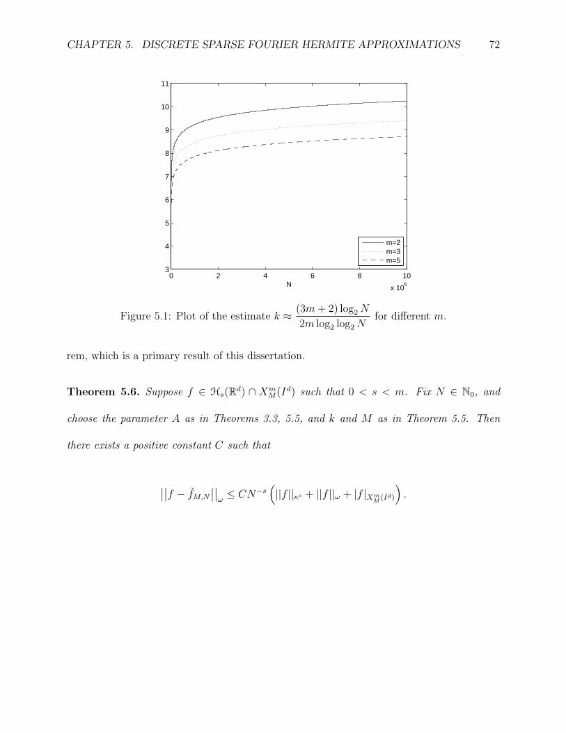
CHAPTER 5. DISCRETE SPARSE FOURIER HERMITE APPROXIMATIONS 72
0 2 4 6 8 10
x 106
3
4
5
6
7
8
9
10
11
N
m=2m=3m=5
Figure 5.1: Plot of the estimate k ≈ (3m+ 2) log2N
2m log2 log2Nfor different m.
rem, which is a primary result of this dissertation.
Theorem 5.6. Suppose f ∈ Hs(Rd) ∩ XmM(Id) such that 0 < s < m. Fix N ∈ N0, and
choose the parameter A as in Theorems 3.3, 5.5, and k and M as in Theorem 5.5. Then
there exists a positive constant C such that
∣∣∣∣f − fM,N
∣∣∣∣ω≤ CN−s
(||f ||κs + ||f ||ω + |f |Xm
M (Id)
).
Chapter 6
Implementation
For a given function f ∈ L2ω(Rd) and a positive integer N , the construction of the discrete
sparse Fourier Hermite approximation as in Definition 5.1 requires computing the coefficients
cM,N . The topic of this section is to find a fast, reliable, accurate way to compute the
multiscale discretization of the coefficients in the sparse Fourier Hermite expansion of f .
This chapter switches discussion between univariate and multivariate cases, so the bold-
face notation will be used to denote vectors.
The terms involved in the Fourier Hermite expansion have very large magnitude, so for
numerical considerations, the problem will be recast. The normalized Hermite polynomials
are defined as
hn :=Hn
||Hn||ω. (6.1)
Note that several different inner products and norms have been used throughout this dis-
sertation. ‘Normalization’ here refers to the fact that ||hn||ω = 1. Using the normalized
73
CHAPTER 6. IMPLEMENTATION 74
Hermite polynomials, the Fourier Hermite series of f can be written as
f =∑n∈Nd
0
dnhn, (6.2)
where dn = 〈f, hn〉ω. Notice this expression is equivalent to the expansion (2.11). The
coefficients cn have two copies of the norm ||Hn||ω in their denominators. To derive the
expansion (6.2) from (2.11), move one copy of ||Hn||ω from the coefficient to the polynomial
part Hn. That is, for each n ∈ Nd0,
dnhn = 〈f, hn〉ωhn =〈f,Hn〉ωHn
||Hn||2ω= cnHn.
Similarly, the discrete sparse Fourier Hermite approximation of f in Definition 5.1 can
be written as
fM,N =∑n∈Ld
N
dM,nhn, (6.3)
with the coefficients given by dM,n := 〈SdMf, hn〉ω. Observe dM,n = ||Hn||ω cM,n.
From Equation (4.14) and the above observation, it holds that
〈SdMf, hn〉ω =∑j∈SdM
∑r∈Wd
j
ηj,r(f)〈`j,r, hn〉ω.
Let
Aj,r(n) :=
∫Id`j,r(x)hn(x)ω(x)dx
for each j ∈ SdM , r ∈Wj and n ∈ Nd0. Then the coefficients in computing the discrete sparse
CHAPTER 6. IMPLEMENTATION 75
Fourier Hermite approximation (6.3) can be computed via
dM,n = 〈SdM , hn〉ω =∑j∈SdM
∑r∈Wd
j
ηj,r(f)Aj,r(n),
and the discrete sparse Fourier Hermite approximation of f can be computed via
fM,N(x) =∑n∈Ld
N
∑j∈SdM
∑r∈Wj
ηj,r(f)Aj,r(n)hn(x). (6.4)
To achieve the goal of finding a fast and good discrete sparse Fourier Hermite approxi-
mation, one must have algorithms to quickly and accurately compute the quantities Aj,r(n)
and ηj,r(f). First, the collection Aj,r(n) will be considered.
It is fortunate that the terms Aj,r(n), which approximate high dimensional oscillatory
integrals, do not need to be further approximated by a quadrature formula. Since the
Lagrange cardinal polynomials, the Hermite polynomials, and the Gaussian weight function
used in the definition of Aj,r(n) are all defined in higher dimensions using tensor products,
it follows that
Aj,r(n) =d∏
k=1
∫Id
`jk,rk(xk)hnk(xk)ω(xk) dxk =
d∏k=1
Ajk,rk(nk). (6.5)
As such, an evaluation scheme needs to be developed only for the univariate case.
Therefore, for now, consider the case when d = 1. Each `j,r is a polynomial of degree
m−1 on a subinterval of [−A,A], and is equal to zero everywhere else. We use this property
along with Theorem 2.3 to compute the integrals Aj,r(n) quickly and without introducing
any additional quadrature error.
CHAPTER 6. IMPLEMENTATION 76
To shorten notation, denote the subintervals of I = [−A,A] by Ii,j = −A + i2−j+1A for
any i ∈ N2j and j ∈ N0. Then
supp (`j,r) =[Ib r
mc,j , Ib r
mc+1,j
],
and
Aj,r(n) =
∫ Ib rm c+1,j
Ib rm c,j
`j,r(x)hn(x)ω(x) dx. (6.6)
Since each `j,r is a polynomial of degree m− 1, Equation (6.6) can now be written as
Aj,r(n) =m−1∑p=0
bj,r(p)[Fp,n
(Ib r
mc+1,j
)− Fp,n
(Ib r
mc,j)], (6.7)
where `j,r(x) =∑m−1
p=0 bj,r(p)xp for x ∈ supp(`j,r), and the functionals Fp,n(x) are defined as
follows.
Definition 6.1. For each p ∈ 0, 1, . . . ,m− 1, n ∈ L1N and x ∈ I, define
Fp,n(x) =
∫ x
0
tphn(t)ω(t) dt.
The functionals can be computed exactly in an iterative way.
Theorem 6.2. For each j ∈ 0, 1, . . . ,M, r ∈ Wj and x ∈ I, the following equations hold.
1. For all x,
F0,0(x) =4√π
2erf(x). (6.8)
CHAPTER 6. IMPLEMENTATION 77
2. For all x,
F1,0(x) =1− ω(x)
2 4√π
(6.9)
3. For all x and all p ≥ 2,
Fp,0(x) =−xp−1ω(x)
2 4√π
+
(p− 1
2 4√π
)Fp−2,0(x). (6.10)
4. For all x and integers n > 0,
F0,n(x) =−hn−1(t)ω(t)√
2n
∣∣∣∣x0
. (6.11)
5. For all x and integers n ≥ 1,
F1,n(x) =
√n+ 1
2F0,n+1(x) +
√n
2F0,n−1(x) (6.12)
6. For all x and integers p ≥ 0,
Fp,1(x) =√
2Fp+1,0(x). (6.13)
7. For all x, integers p ≥ 0 and integers n ≥ 2,
Fp,n(x) =
√2
nFp+1,n−1(x)−
√n− 1
nFp,n−2(x). (6.14)
CHAPTER 6. IMPLEMENTATION 78
8. For all x, integers n ≥ 1 and integers p ≥ 2,
Fp,n(x) =−xp−1hn(x)ω(x)
2+
(p− 1
2
)Fp−2,n(x) +
√n
2Fp−1,n−1(x). (6.15)
Proof. 1. From the definition of erf x, F0,0(x) =4√π2
erf(x).
2. Equation (6.9) follows from the observation tω(t) = −12ω′(t).
3. Use integration by parts to derive Equation (6.10). If p ≥ 2, then
Fp,0(x) =14√π
∫ x
0
tpω(t)dt
=14√π
∫ x
0
tp−1 · tω(t)dt
=−1
2 4√π
∫ x
0
td−1ω′(t)dt
=−tp−1ω(t)
2 4√π
∣∣∣∣x0
+p− 1
2 4√π
∫ x
0
tp−2ω(t)dt
=−xp−1ω(x)
2 4√π
+p− 1
2 4√πFp−2,0(x).
4. Equation (6.11) follows from Corollary 2.4, and that
Hn−1
||Hn||ω=
Hn−1√n!2n√π
=Hn−1√
2n||Hn−1||ω=hn−1√
2n.
CHAPTER 6. IMPLEMENTATION 79
Then
F0,n(x) =
∫ x
0
hn(t)ω(t)dt =
∫ x
0
Hn(t)ω(t)
||Hn||ωdt
=−Hn−1(t)ω(t)
||Hn||ω
∣∣∣∣x0
=−hn−1(t)ω(t)√
2n
∣∣∣∣x0
.
5. Equation (6.12) follows from the observation that for all n ≥ 1,
tHn(t) =Hn+1
2(t) + nHn−1(t)
following from the three term recurrence of the Hermite polynomials. Then
thn(t) =Hn+1(t)
2√n!2n√π
+nHn−1(t)√n!2n√π
=
√n+ 1
2hn+1 +
√n
2hn−1(t).
6. Since H1(t) = 2t,
F1,k(x) =
∫ x
0
tph1(t)ω(t)dt =
√2√π
∫ x
0
tp+1ω(t)dt
=√
2
∫ x
0
tp+1h0(t)ω(t)dt =√
2Fp+1,0(x).
CHAPTER 6. IMPLEMENTATION 80
7. Using the recurrence relation Hn(t) = 2tHn−1(t)− 2(n− 1)Hn−2(t) for n ≥ 2,
Fp,n(x) =
∫ x
0
tphn(t)ω(t)dt
=
∫ x
0
tp(
2tHn−1(t)− 2(n− 1)Hn−2(t)
||Hn||ω
)ω(t)dt
=
√2
n
∫ x
0
tp+1hn−1(t)ω(t)dt−√n− 1
n
∫ x
0
tphn−2(t)ω(t)dt
=
√2
nFp+1,n−1(x)−
√n− 1
nFp,n−2(x).
8. The final formula can be recovered using integration by parts. Notice
h′n(t) =H ′n(t)
||Hn||ω=
2nHn−1(t)
||Hn||ω=
2nHn−1(t)√2n||Hn−1||ω
=√
2nhn−1(t).
Then, if p ≥ 2,
Fp,n(x) =
∫ x
0
tphn(t)ω(t)dt
=−1
2
∫ x
0
tp−1hn(t)ω′(t)dt
=−tp−1hn(t)ω(t)
2
∣∣∣∣x0
+1
2
∫ x
0
[tp−1hn(t)
]′ω(t)dt
=−tp−1hn(t)ω(t)
2
∣∣∣∣x0
+1
2
∫ x
0
[(p− 1)tp−2hn(t) +
√2ntp−1hn−1
]ω(t)dt
=−tp−1hn(t)ω(t)
2
∣∣∣∣x0
+p− 1
2Fp−2,n(x) +
√n
2Fp−1,n−1(x)
=−xp−1hn(x)ω(x)
2+p− 1
2Fp−2,n(x) +
√n
2Fp−1,n−1(x).
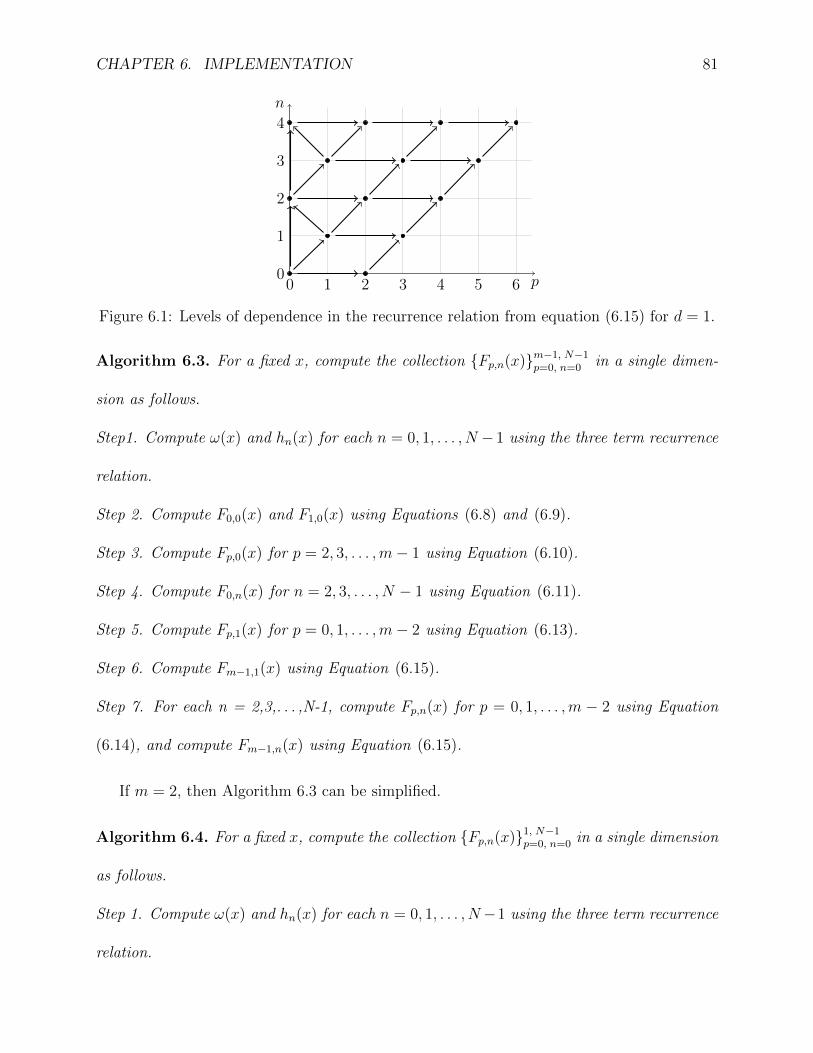
CHAPTER 6. IMPLEMENTATION 81
p
n
0 1 2 3 4 5 60
1
2
3
4
Figure 6.1: Levels of dependence in the recurrence relation from equation (6.15) for d = 1.
Algorithm 6.3. For a fixed x, compute the collection Fp,n(x)m−1, N−1p=0, n=0 in a single dimen-
sion as follows.
Step1. Compute ω(x) and hn(x) for each n = 0, 1, . . . , N − 1 using the three term recurrence
relation.
Step 2. Compute F0,0(x) and F1,0(x) using Equations (6.8) and (6.9).
Step 3. Compute Fp,0(x) for p = 2, 3, . . . ,m− 1 using Equation (6.10).
Step 4. Compute F0,n(x) for n = 2, 3, . . . , N − 1 using Equation (6.11).
Step 5. Compute Fp,1(x) for p = 0, 1, . . . ,m− 2 using Equation (6.13).
Step 6. Compute Fm−1,1(x) using Equation (6.15).
Step 7. For each n = 2,3,. . . ,N-1, compute Fp,n(x) for p = 0, 1, . . . ,m − 2 using Equation
(6.14), and compute Fm−1,n(x) using Equation (6.15).
If m = 2, then Algorithm 6.3 can be simplified.
Algorithm 6.4. For a fixed x, compute the collection Fp,n(x)1, N−1p=0, n=0 in a single dimension
as follows.
Step 1. Compute ω(x) and hn(x) for each n = 0, 1, . . . , N−1 using the three term recurrence
relation.
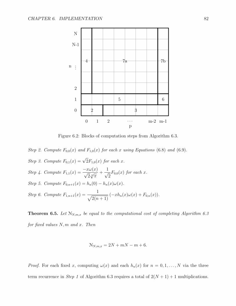
CHAPTER 6. IMPLEMENTATION 82
0 1 2 . . . m-2 m-1p
0
1
2
...
N-1
N
n
2 3
4
5 6
7a 7b
Figure 6.2: Blocks of computation steps from Algorithm 6.3.
Step 2. Compute F0,0(x) and F1,0(x) for each x using Equations (6.8) and (6.9).
Step 3. Compute F0,1(x) =√
2F1,0(x) for each x.
Step 4. Compute F1,1(x) =−xω(x)√
2 4√π
+1√2F0,0(x) for each x.
Step 5. Compute F0,n+1(x) = hn(0)− hn(x)ω(x).
Step 6. Compute F1,n+1(x) =1√
2(n+ 1)(−xhn(x)ω(x) + F0,n(x)).
Theorem 6.5. Let NN,m,x be equal to the computational cost of completing Algorithm 6.3
for fixed values N,m and x. Then
NN,m,x = 2N +mN −m+ 6.
Proof. For each fixed x, computing ω(x) and each hn(x) for n = 0, 1, . . . , N via the three
term recurrence in Step 1 of Algorithm 6.3 requires a total of 2(N + 1) + 1 multiplications.
CHAPTER 6. IMPLEMENTATION 83
Computing Step 2 requires only a single multiplication. Since multiplication and division by
2 can be achieved by only shifting digits in binary, computing Fp,0(x) for each x and each p
via Equation (6.10) requires two multiplications. Therefore Step 3 of Algorithm 6.3 requires
2(m− 3) multiplications. Computing Equation (6.11) for each x and n can be accomplished
in one multiplication, so Step 4 requires N − 3 multiplications. Since Equation (6.13) is
multiplication by 2, Step 5 is free for each x. Equation (6.14) requires one multiplication
and Equation (6.15) requires four multiplications for each x, p, and n. Therefore Step 6
requires exactly 4 multiplications and Step 7 requires (N − 3)(m− 1) + 4.
Therefore, altogether the computational cost of completing all steps associated with
Algorithm 6.3 in one dimension for fixed values N,m and x is the total computation cost
from each step: 2N +mN −m+ 6.
For each fixed value j ∈ S1M , to compute the collection
Aj,r(n) : r ∈ Wj, n = 0 : N − 1 via Equation (6.7) and Algorithm 6.3, requires evaluating
each Fp,n at 2j + 1 values of x. Namely at the points in the collection Is,j : s = 0 : 2j.
Theorem 6.6. Fix positive integers N and m. To fully compute the collection
Fp,n(Ii,j) : p ∈ Zm, n ∈ ZN , j ∈ ZM , i ∈ Z2j (6.16)
requires (2N +mN −m+ 6)(2M+1 − 1) multiplications.
Proof. From the previous Theorem, we know that for each Ii,j, computing the collection
Fp,n(Ii,j) for all p ∈ Zm and all n ∈ ZN requires 2N + mN −m + 6 multiplications. The
CHAPTER 6. IMPLEMENTATION 84
cardinality of the set of all Ii,j of interest is
|j ∈ ZM , i ∈ Zj| =M∑j=0
2j = 2M+1 − 1.
Corollary 6.7. Let N,m be fixed positive integers. Choose M = dlog2 logk2 Ne, where k is
chosen as in Theorem 5.5. Then the computational complexity of computing the collection
Aj,r(n) : j ∈ S1
M , r ∈ Wj, n ∈ ZN
(6.17)
using Equation (6.7) is O(N logk2 N).
In several dimensions, the values Aj,r(n) are defined using products as in Equation (6.5).
If they are computed naively, this will require d multiplications for each (j, r,n).
Algorithm 6.8. Let N,m be fixed positive integers. Choose M = dlog2 log 2kNe, where k is
chosen as in Theorem 5.5. Compute the collection
Aj,r(n) : n ∈ LdN , j ∈ SdM , r ∈Wj
as follows.
Step 1. Compute the single dimension collection
Aj,r(n) : j ∈ ZM , r ∈Wj, n ∈ ZN
CHAPTER 6. IMPLEMENTATION 85
using Algorithm 6.3.
Step 2. For each n ∈ LdN , compute the sum
cn =∑j∈SdM
∑r∈Wj
d∏k=1
Ajk,rk(nk).
Theorem 6.9. Let N,m be fixed positive integers. Choose M = dlog2 log 2kNe where k is
chosen as in Theorem 5.5. Computing the collection
Aj,r(n) : n ∈ LdN , j ∈ SdM , r ∈Wj
via Algorithm 6.8 requires O(N log2(d−1)+k2 N) multiplications.
Proof. From Corollary 6.7, computing the collection
Aj,r(n) : n ∈ ZN , j ∈ ZM , r ∈Wj
as in Step 1 of Algorithm 6.8 requires O(N logk2 N) multiplications. These values should be
stored in memory for future use.
The cardinality of the set LdN is O(N logd−12 N), and the cardinality of the set
j ∈ SdM , r ∈Wj
is Md−12M ≤ ckd−1 logd−12 (log2N) logk2 N for some constant c. Therefore the cardinality of
CHAPTER 6. IMPLEMENTATION 86
the index set n ∈ LdN , j ∈ SdM , r ∈Wj
is O(Nkd−1 logd−1
2 (log2N) logd−1+k2 N) = O(N log
2(d−1)+k2 N), using the estimate of k given
in Equation (5.5).
For each triplet (j, r,n) in this index set, we require d multiplications of the univariate
quantities stored in memory to compute Aj,r(n).
Therefore the cost of computing Aj,r(n) for all j ∈ SdM , r ∈ Wj and n ∈ LdN is
O(N log2(d−1)+k2 N). The sum of all of these as in Step 2 of Algorithm 6.8 does not con-
tribute any additional multiplications.
The valuesηj,r(f) : j ∈ SdM , r ∈Wj
defined in Equation (4.8) are computed using the
Algorithm written by Xu and Jiang appearing in [12]. It is proven therein that the complexity
to compute the set using their algorithm is O(N logd−12 N).
Now we come to the primary result concerning the computational cost of the sparse
discrete Fourier Hermite approximation scheme proposed in this dissertation.
Theorem 6.10. Let N,m be fixed positive integers. Let M = dlog2 logk2 Ne where k is chosen
as in Theorem 5.5. Then the cost of computing the inner product
〈SdM(f), Hn〉ω
for all n ∈ LdN is O(N log2(d−1)+k2 N).
CHAPTER 6. IMPLEMENTATION 87
Proof. Recall the inner products are decomposed via the formula
〈SdM(f), Hn〉ω =∑j∈SdM
∑r∈Wj
ηj,r(f)Aj,r(n).
We compute Aj,r(n) in O(N log2(d−1)+k2 N) multiplications. We compute ηj,r(f) in
O(N logd−12 N) multiplications.
To compute the sum, we require one multiplication for each pair (j, r) in the index set
j ∈ SdM , r ∈Wj, a set of cardinality O(logd−1+k2 N).
Therefore the entire collection can be computed using O(N log2(d−1)+k2 N) multiplications.
Chapter 7
Numerical Results
In this chapter, numerical examples are presented to demonstrate the accuracy and compu-
tational efficiency of Algorithm 6.3, which numerically computes cn,M , the coefficients in the
discrete sparse Fourier Hermite approximation of a given function f . The computer program
is run on an HP ENVY laptop with an Intel i5 2.67 GHz CPU and 4GB RAM. The machine
precision of the computer used is 2.2204e− 016.
In the numerical examples, use ‘Err’ to denote the relative error, which is computed as
Err =||f − fM,N ||ω√
||f ||2κs + ||f ||2ω + |f |2Xm
M (Id)
.
The presented results verify the theoretical error estimate from Theorem 5.6 if Err < N−s.
The computing time in seconds spend calculating the coefficients cM,n for all n ∈ LdN is
denoted by ‘CT’. The compression ratio CR denotes the value |LdN |/Nd. The value MN
is the actual number of multiplications used to compute the Fourier Hermite coefficients.
Since the compression ratio depends only on N and d, it needs to be investigated in only
88
CHAPTER 7. NUMERICAL RESULTS 89
one example.
As discussed in Chapter 5, the parameter k may be fixed independently of N . In the
following examples, the value of k will be specified in a manner that does not depend on N ,
however, we will still achieve, or even beat, the desired approximation accuracy.
The first two examples use multivariate polynomials that are separable in each variable.
These examples are designed to demonstrate the accuracy of the proposed algorithm. Since
the example functions are polynomials, it is trivial to express them each as a finite Fourier
Hermite series, and the error of the proposed discrete sparse Fourier Hermite approximation
is easy to compute. Note that although the two example functions admit a finite Fourier
Hermite series expression, the proposed method does not guarantee the approximation will
equal the exact expansion. This is because of the quadrature method used to numerically
compute the coefficients. It will compute the coefficients within an acceptable tolerance, but
it will not produce a termwise exact result.
The theoretical results presented in this paper guarantee a global approximation relative
to the weighted L2 norm. However, as the reader will see from the Figures appearing in this
section, the computed approximations in fact give very good pointwise approximations on
the interval Id.
Example 7.1. Consider in this example the function f1,d(x) :=∏d
j=1 x2j , for x ∈ Id and
d = 2, 3, 4. The parameters will be set as m = 3 and s = 2.99. The value k is fixed at 3 and
is not chosen to depend on N .
To compute the accuracy of the algorithm in this example, first the exact Fourier Hermite
series of f must be computed. Using the standard definition of the Hermite polynomials, as
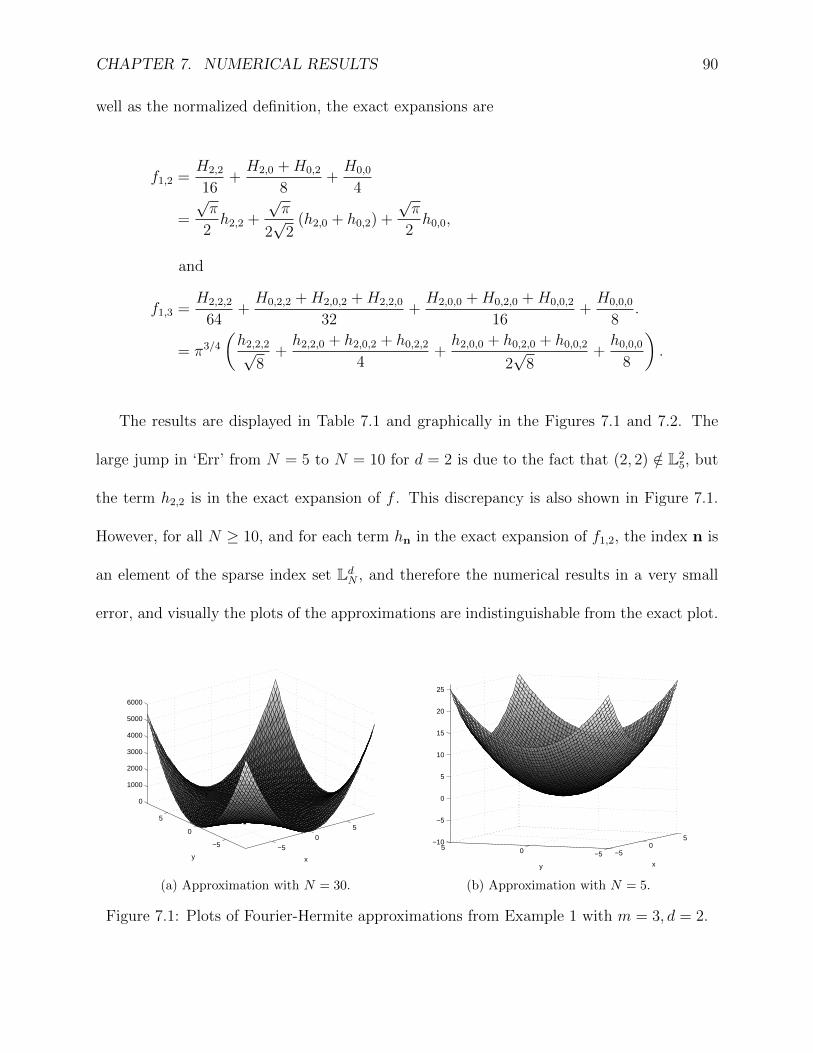
CHAPTER 7. NUMERICAL RESULTS 90
well as the normalized definition, the exact expansions are
f1,2 =H2,2
16+H2,0 +H0,2
8+H0,0
4
=
√π
2h2,2 +
√π
2√
2(h2,0 + h0,2) +
√π
2h0,0,
and
f1,3 =H2,2,2
64+H0,2,2 +H2,0,2 +H2,2,0
32+H2,0,0 +H0,2,0 +H0,0,2
16+H0,0,0
8.
= π3/4
(h2,2,2√
8+h2,2,0 + h2,0,2 + h0,2,2
4+h2,0,0 + h0,2,0 + h0,0,2
2√
8+h0,0,0
8
).
The results are displayed in Table 7.1 and graphically in the Figures 7.1 and 7.2. The
large jump in ‘Err’ from N = 5 to N = 10 for d = 2 is due to the fact that (2, 2) /∈ L25, but
the term h2,2 is in the exact expansion of f . This discrepancy is also shown in Figure 7.1.
However, for all N ≥ 10, and for each term hn in the exact expansion of f1,2, the index n is
an element of the sparse index set LdN , and therefore the numerical results in a very small
error, and visually the plots of the approximations are indistinguishable from the exact plot.
−5
0
5
−5
0
5
0
1000
2000
3000
4000
5000
6000
x
y
(a) Approximation with N = 30.
−50
5
−505−10
−5
0
5
10
15
20
25
x
y
(b) Approximation with N = 5.
Figure 7.1: Plots of Fourier-Hermite approximations from Example 1 with m = 3, d = 2.
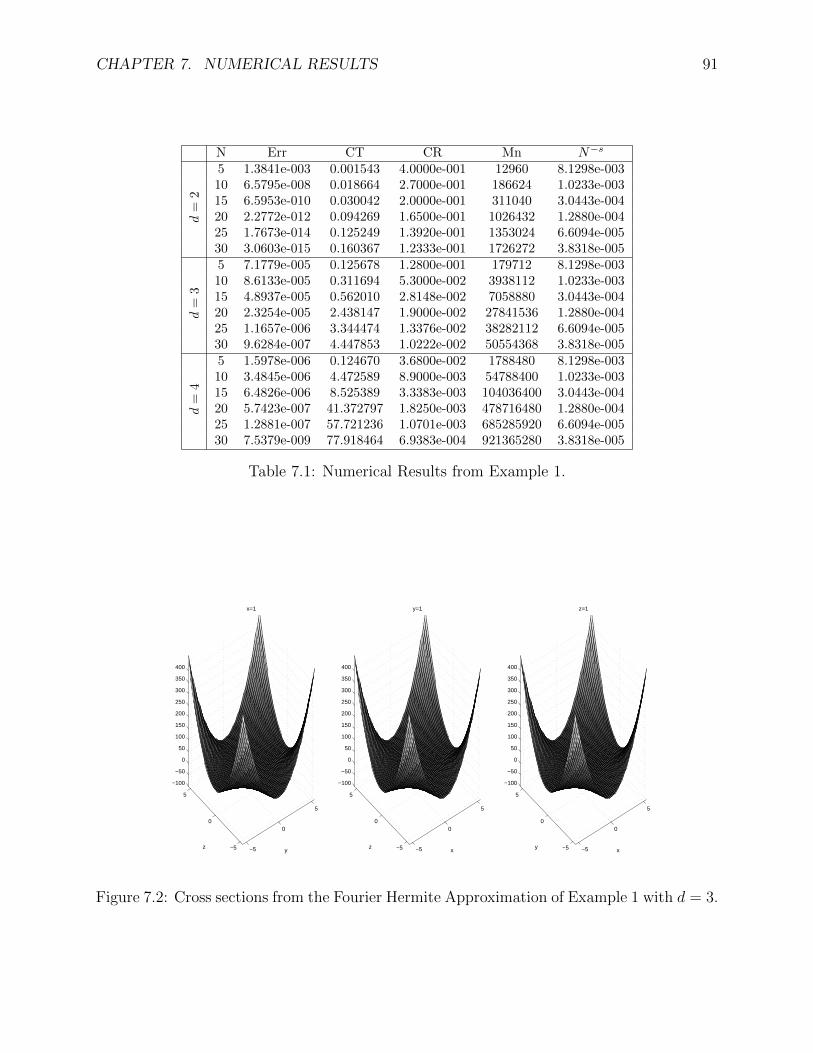
CHAPTER 7. NUMERICAL RESULTS 91
N Err CT CR Mn N−s
d=
2
5 1.3841e-003 0.001543 4.0000e-001 12960 8.1298e-00310 6.5795e-008 0.018664 2.7000e-001 186624 1.0233e-00315 6.5953e-010 0.030042 2.0000e-001 311040 3.0443e-00420 2.2772e-012 0.094269 1.6500e-001 1026432 1.2880e-00425 1.7673e-014 0.125249 1.3920e-001 1353024 6.6094e-00530 3.0603e-015 0.160367 1.2333e-001 1726272 3.8318e-005
d=
3
5 7.1779e-005 0.125678 1.2800e-001 179712 8.1298e-00310 8.6133e-005 0.311694 5.3000e-002 3938112 1.0233e-00315 4.8937e-005 0.562010 2.8148e-002 7058880 3.0443e-00420 2.3254e-005 2.438147 1.9000e-002 27841536 1.2880e-00425 1.1657e-006 3.344474 1.3376e-002 38282112 6.6094e-00530 9.6284e-007 4.447853 1.0222e-002 50554368 3.8318e-005
d=
4
5 1.5978e-006 0.124670 3.6800e-002 1788480 8.1298e-00310 3.4845e-006 4.472589 8.9000e-003 54788400 1.0233e-00315 6.4826e-006 8.525389 3.3383e-003 104036400 3.0443e-00420 5.7423e-007 41.372797 1.8250e-003 478716480 1.2880e-00425 1.2881e-007 57.721236 1.0701e-003 685285920 6.6094e-00530 7.5379e-009 77.918464 6.9383e-004 921365280 3.8318e-005
Table 7.1: Numerical Results from Example 1.
−5
0
5
−5
0
5
−100
−50
0
50
100
150
200
250
300
350
400
y
x=1
z −5
0
5
−5
0
5
−100
−50
0
50
100
150
200
250
300
350
400
x
y=1
z −5
0
5
−5
0
5
−100
−50
0
50
100
150
200
250
300
350
400
x
z=1
y
Figure 7.2: Cross sections from the Fourier Hermite Approximation of Example 1 with d = 3.
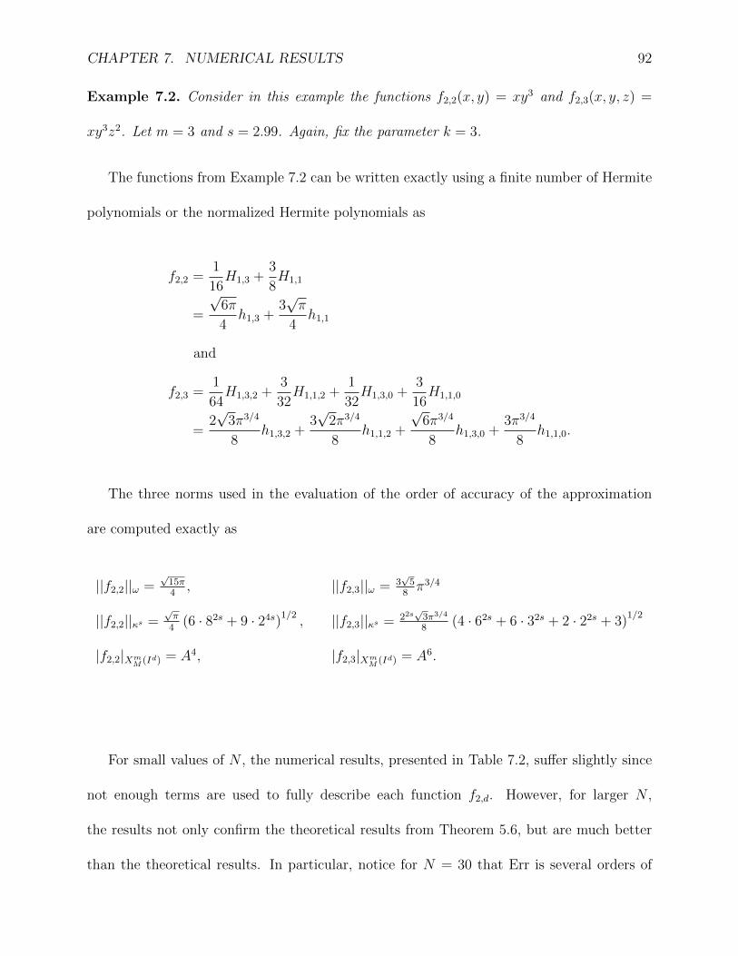
CHAPTER 7. NUMERICAL RESULTS 92
Example 7.2. Consider in this example the functions f2,2(x, y) = xy3 and f2,3(x, y, z) =
xy3z2. Let m = 3 and s = 2.99. Again, fix the parameter k = 3.
The functions from Example 7.2 can be written exactly using a finite number of Hermite
polynomials or the normalized Hermite polynomials as
f2,2 =1
16H1,3 +
3
8H1,1
=
√6π
4h1,3 +
3√π
4h1,1
and
f2,3 =1
64H1,3,2 +
3
32H1,1,2 +
1
32H1,3,0 +
3
16H1,1,0
=2√
3π3/4
8h1,3,2 +
3√
2π3/4
8h1,1,2 +
√6π3/4
8h1,3,0 +
3π3/4
8h1,1,0.
The three norms used in the evaluation of the order of accuracy of the approximation
are computed exactly as
||f2,2||ω =√
15π4, ||f2,3||ω = 3
√5
8π3/4
||f2,2||κs =√π
4(6 · 82s + 9 · 24s)
1/2, ||f2,3||κs = 22s
√3π3/4
8(4 · 62s + 6 · 32s + 2 · 22s + 3)
1/2
|f2,2|XmM (Id) = A4, |f2,3|Xm
M (Id) = A6.
For small values of N , the numerical results, presented in Table 7.2, suffer slightly since
not enough terms are used to fully describe each function f2,d. However, for larger N ,
the results not only confirm the theoretical results from Theorem 5.6, but are much better
than the theoretical results. In particular, notice for N = 30 that Err is several orders of
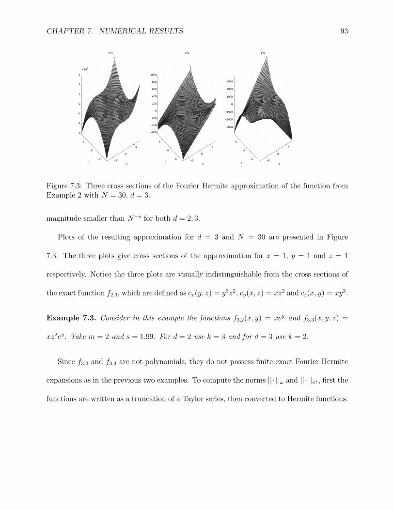
CHAPTER 7. NUMERICAL RESULTS 93
−5
0
5
−5
0
5
−3
−2
−1
0
1
2
3
x 104
y
x=1
z−5
0
5
−5
0
5
−600
−400
−200
0
200
400
600
800
1000
x
y=1
z−5
0
5
−5
0
5
−3000
−2000
−1000
0
1000
2000
3000
x
z=1
y
Figure 7.3: Three cross sections of the Fourier Hermite approximation of the function fromExample 2 with N = 30, d = 3.
magnitude smaller than N−s for both d = 2, 3.
Plots of the resulting approximation for d = 3 and N = 30 are presented in Figure
7.3. The three plots give cross sections of the approximation for x = 1, y = 1 and z = 1
respectively. Notice the three plots are visually indistinguishable from the cross sections of
the exact function f2,3, which are defined as cx(y, z) = y3z2, cy(x, z) = xz2 and cz(x, y) = xy3.
Example 7.3. Consider in this example the functions f3,2(x, y) = xey and f3,3(x, y, z) =
xz2ey. Take m = 2 and s = 1.99. For d = 2 use k = 3 and for d = 3 use k = 2.
Since f3,2 and f3,3 are not polynomials, they do not possess finite exact Fourier Hermite
expansions as in the previous two examples. To compute the norms || · ||ω and || · ||κs , first the
functions are written as a truncation of a Taylor series, then converted to Hermite functions.
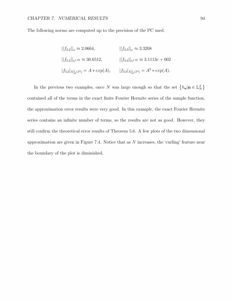
CHAPTER 7. NUMERICAL RESULTS 94
The following norms are computed up to the precision of the PC used.
||f3,2||ω ≈ 2.0664, ||f3,3||ω ≈ 3.3208
||f3,2||κ1.99 ≈ 30.6512, ||f3,3||κ1.99 ≈ 3.1113e+ 002
|f3,2|X2M (I2) = A ∗ exp(A), |f3,3|X2
M (I3) = A3 ∗ exp(A).
In the previous two examples, once N was large enough so that the sethn|n ∈ LdN
contained all of the terms in the exact finite Fourier Hermite series of the sample function,
the approximation error results were very good. In this example, the exact Fourier Hermite
series contains an infinite number of terms, so the results are not as good. However, they
still confirm the theoretical error results of Theorem 5.6. A few plots of the two dimensional
approximation are given in Figure 7.4. Notice that as N increases, the ‘curling’ feature near
the boundary of the plot is diminished.
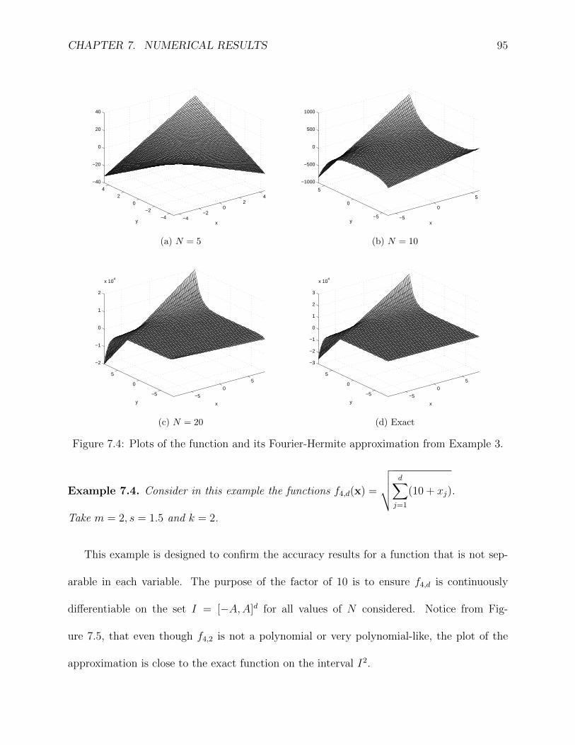
CHAPTER 7. NUMERICAL RESULTS 95
−4−2
02
4
−4−2
02
4
−40
−20
0
20
40
x
y
(a) N = 5
−5
0
5
−5
0
5
−1000
−500
0
500
1000
x
y
(b) N = 10
−5
0
5
−5
0
5
−2
−1
0
1
2
x 104
x
y
(c) N = 20
−5
0
5
−5
0
5
−3
−2
−1
0
1
2
3
x 104
x
y
(d) Exact
Figure 7.4: Plots of the function and its Fourier-Hermite approximation from Example 3.
Example 7.4. Consider in this example the functions f4,d(x) =
√√√√ d∑j=1
(10 + xj).
Take m = 2, s = 1.5 and k = 2.
This example is designed to confirm the accuracy results for a function that is not sep-
arable in each variable. The purpose of the factor of 10 is to ensure f4,d is continuously
differentiable on the set I = [−A,A]d for all values of N considered. Notice from Fig-
ure 7.5, that even though f4,2 is not a polynomial or very polynomial-like, the plot of the
approximation is close to the exact function on the interval I2.
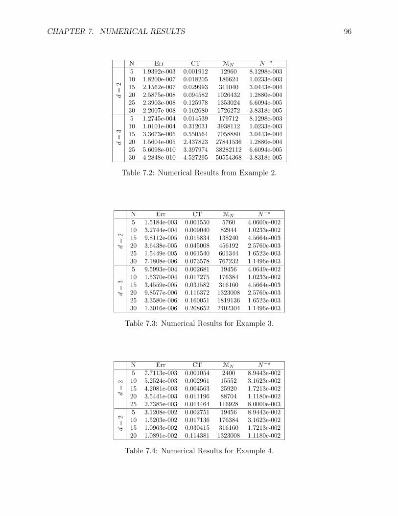
CHAPTER 7. NUMERICAL RESULTS 96
N Err CT MN N−s
d=
2
5 1.9392e-003 0.001912 12960 8.1298e-00310 1.8200e-007 0.018205 186624 1.0233e-00315 2.1562e-007 0.029993 311040 3.0443e-00420 2.5875e-008 0.094582 1026432 1.2880e-00425 2.3903e-008 0.125978 1353024 6.6094e-00530 2.2007e-008 0.162680 1726272 3.8318e-005
d=
35 1.2745e-004 0.014539 179712 8.1298e-00310 1.0101e-004 0.312031 3938112 1.0233e-00315 3.3673e-005 0.550564 7058880 3.0443e-00420 1.5604e-005 2.437823 27841536 1.2880e-00425 5.6098e-010 3.397974 38282112 6.6094e-00530 4.2848e-010 4.527295 50554368 3.8318e-005
Table 7.2: Numerical Results from Example 2.
N Err CT MN N−s
d=
2
5 1.5184e-003 0.001550 5760 4.0600e-00210 3.2744e-004 0.009040 82944 1.0233e-00215 9.8112e-005 0.015834 138240 4.5664e-00320 3.6438e-005 0.045008 456192 2.5760e-00325 1.5449e-005 0.061540 601344 1.6523e-00330 7.1808e-006 0.073578 767232 1.1496e-003
d=
3
5 9.5993e-004 0.002681 19456 4.0649e-00210 1.5370e-004 0.017275 176384 1.0233e-00215 3.4559e-005 0.031582 316160 4.5664e-00320 9.8577e-006 0.116372 1323008 2.5760e-00325 3.3580e-006 0.160051 1819136 1.6523e-00330 1.3016e-006 0.208652 2402304 1.1496e-003
Table 7.3: Numerical Results for Example 3.
N Err CT MN N−s
d=
2
5 7.7113e-003 0.001054 2400 8.9443e-00210 5.2524e-003 0.002961 15552 3.1623e-00215 4.2081e-003 0.004563 25920 1.7213e-00220 3.5441e-003 0.011196 88704 1.1180e-00225 2.7385e-003 0.014464 116928 8.0000e-003
d=
2
5 3.1208e-002 0.002751 19456 8.9443e-00210 1.5203e-002 0.017136 176384 3.1623e-00215 1.0963e-002 0.030415 316160 1.7213e-00220 1.0891e-002 0.114381 1323008 1.1180e-002
Table 7.4: Numerical Results for Example 4.
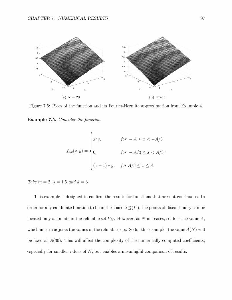
CHAPTER 7. NUMERICAL RESULTS 97
−5
0
5
−5
0
5
3.5
4
4.5
5
5.5
x
y
(a) N = 20
−5
0
5
−5
0
5
3
3.5
4
4.5
5
5.5
x
y
(b) Exact
Figure 7.5: Plots of the function and its Fourier-Hermite approximation from Example 4.
Example 7.5. Consider the function
f5,2(x, y) =
x2y, for − A ≤ x < −A/3
0, for − A/3 ≤ x < A/3
(x− 1) ∗ y, for A/3 ≤ x ≤ A
.
Take m = 2, s = 1.5 and k = 3.
This example is designed to confirm the results for functions that are not continuous. In
order for any candidate function to be in the space XmM(Id), the points of discontinuity can be
located only at points in the refinable set VM . However, as N increases, so does the value A,
which in turn adjusts the values in the refinable sets. So for this example, the value A(N) will
be fixed at A(30). This will affect the complexity of the numerically computed coefficients,
especially for smaller values of N , but enables a meaningful comparison of results.
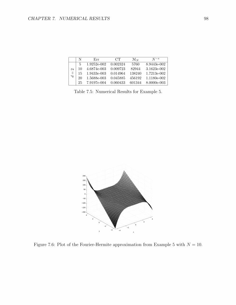
CHAPTER 7. NUMERICAL RESULTS 98
N Err CT MN N−s
d=
2
5 1.9252e-002 0.002324 5760 8.9443e-00210 4.6874e-003 0.009723 82944 3.1623e-00215 1.9433e-003 0.014964 138240 1.7213e-00220 1.5688e-003 0.045885 456192 1.1180e-00225 7.9197e-004 0.060433 601344 8.0000e-003
Table 7.5: Numerical Results for Example 5.
−4
−2
0
2
4
−4
−2
0
2
4
−200
−150
−100
−50
0
50
100
150
200
x
y
Figure 7.6: Plot of the Fourier-Hermite approximation from Example 5 with N = 10.

Appendices
99
Appendix A
Various Results
Theorem A.1. For a positive fixed value s, let
〈·, ·〉κs : L2ω(Rd)× L2
ω(Rd)→ R
be defined via
〈f, g〉κs :=∑n∈Nd
0
〈f,Hn〉ω〈g,Hn〉ωn!2nπd/2
d∏j=1
(1 + nj)2s,
for any functions f, g ∈ L2ω(Rd). Then 〈·, ·〉κs defines an inner product.
Proof. Notice the map is symmetric since for any f, g ∈ L2ω(Rd),
〈f, g〉κs =∑n∈Nd
0
〈f,Hn〉ω〈g,Hn〉ωn!2nπd/2
d∏j=1
(1 + nj)2s
=∑n∈Nd
0
〈g,Hn〉ω〈f,Hn〉ωn!2nπd/2
d∏j=1
(1 + nj)2s
= 〈g, f〉κs .
100
APPENDIX A. VARIOUS RESULTS 101
The map is linear in the first argument since
〈αf, g〉κs =∑n∈Nd
0
〈αf,Hn〉ω〈g,Hn〉ωn!2nπd/2
d∏j=1
(1 + nj)2s
= α∑n∈Nd
0
〈f,Hn〉ω〈g,Hn〉ωn!2nπd/2
d∏j=1
(1 + nj)2s
= α〈f, g〉κs ,
and
〈f + g, h〉κs =∑n∈Nd
0
〈f + g,Hn〉ω〈h,Hn〉ωn!2nπd/2
d∏j=1
(1 + nj)2s
=∑n∈Nd
0
〈f,Hn〉ω〈h,Hn〉ωn!2nπd/2
d∏j=1
(1 + nj)2s +
∑n∈Nd
0
〈g,Hn〉ω〈h,Hn〉ωn!2nπd/2
d∏j=1
(1 + nj)2s
= 〈f, h〉κs + 〈g, h〉κs ,
for any f, g, h ∈ L2ω(Rd) and α ∈ R.
Since each term in the sum
〈f, f〉κs =∑n∈Nd
0
〈f,Hn〉2ωn!2nπd/2
d∏j=1
(a+ nj)2s
is non-negative, 〈f, f〉κs ≥ 0 for every f ∈ L2ω(Rd). Additionally, if 〈f, f〉κs = 0, then it
follows that 〈f,Hn〉ω must equal 0 for every n ∈ L2ω(Rd). Since Hn is a complete orthogonal
collection in L2ω(Rd), this guarantees f ≡ 0. Therefore the map is positive definite.
Since the map 〈·, ·〉κs is symmetric, linear, and positive definite, it defines an inner product
APPENDIX A. VARIOUS RESULTS 102
on L2ω(Rd).
Theorem A.2. Let | · |∞,Id : L2ω(Rd)→ R be defined via
|f |∞,Id := supx∈Id|f(x)|, for any f ∈ L2
ω(Rd).
Then | · |∞,Id is a seminorm.
Proof. Note that for any f, g ∈ L2ω(Rd) and α ∈ R,
|αf |∞,Id = supx∈Id|αf(x)|
= |α| supx∈Id|f(x)|
= |α||f |∞,Id ,
|f + g|∞,Id = supx∈Id|f(x) + g(x)|
≤ supx∈Id|f(x)|+ sup
y∈Id|g(y)|
= |f |∞,Id + |g|∞,Id ,
and clearly |f |∞,Id ≥ 0. However, if |f |∞,Id = 0, this does not mean f ≡ 0, but only that
f |Id ≡ 0.
Therefore | · |∞,Id defines a seminorm.
Theorem A.3. Let Hn(x) be the univariate Hermite polynomial of degree n, for n ∈ N0. If
APPENDIX A. VARIOUS RESULTS 103
n is odd, then Hn contains only odd powers of x. If n is even, then Hn has only even powers
of x.
Proof. We will proceed by induction on n.
The theorem is clearly true for n = 0, since Hn(x) ≡ 1.
Suppose it is true for some integer n− 1. Then, by Theorem 2.5,
H ′n(x) = 2nHn−1(x).
If n is an even integer, then n− 1 is an odd integer, and therefore, by the assumption, Hn−1
is polynomial with all odd-degree powers of x. Thus H ′n is an odd polynomial, and so one
can conclude that Hn is an even polynomial.
If n is an odd integer, then n − 1 is an even integer, and then Hn−1 and H ′n are both
even polynomials. Thus Hn is a polynomial, but this does not yet show Hn is an odd
polynomial. However, one can conclude Hn−2 is an odd polynomial. Therefore, by the three
term recurrence,
Hn(x) = 2(0)Hn−1(0)− 2nHn−2(x) = 0,
for any integer n ≥ 2, and H1(0) = 0 since H1(x) = 2x. Thus we have shown Hn is an odd
polynomial.
Therefore the theorem is true for any non-negative integer n.
In a single dimension, some formulas for the direct computation of integrals involving
the Gaussian weight are included below.
1.
∫ b
a
e−x2
dx = erf(x)|ba
APPENDIX A. VARIOUS RESULTS 104
2.
∫ b
a
xe−x2
dx = −1
2e−x
2
∣∣∣∣ba
3. For m > 2 even,
∫ b
a
xme−x2
dx =
=
−xm−1
2e−x
2 −m/2−1∑j=1
∏ji=1(m− 2i+ 1)
2j+1xm−2j−1e−x
2
+(m− 1)!!
2m/2erf(x)
∣∣∣∣∣∣b
a
4. For m > 1 odd,
∫ b
a
xme−x2
dx =
=
−1
2xm−1e−x
2 −m−1
2∑j=1
∏ji=1(m− 2i+ 1)
2j+1xm−2j−1e−x
2
∣∣∣∣∣∣b
a
.
Lemma A.4. For any m,n ∈ N0, the product HmHn can be written as the sum
HmHn =
minm,n∑i=0
2i
i!
m!
(m− i)!n!
(n− i)!Hm+n−2i.
Proof. If n = 0, then the summation reduces to the single term Hm. If n = 1 and m ≥ 1,
then the summation is Hm+1 + 2mHm−1. By the three term recurrence of the Hermite
polynomials, this is equal to 2xHm which is HnHm. Since the statement is symmetric in m
and n, we have shown that it is true for any pair (m,n) with either m ≤ 1 or n ≤ 1.
We now proceed by induction. Consider a pair (m,n + 1) with n ≥ 1 and n + 1 ≤ m.
Suppose the statement of the lemma is true for the pairs (m,n) and (m,n−1). For notational
convenience, denote2i
i!
m!
(m− i)!n!
(n− i)!by γ(m,n, i). Then using the three term recurrence
APPENDIX A. VARIOUS RESULTS 105
and the induction step gives
HmHn+1 = Hm (2xHn − 2nHn−1)
= 2x (HmHn)− 2n (HmHn−1)
= 2x
(n∑i=0
γ(m,n, i)Hm+n−2i
)− 2n
(n−1∑i=0
γ(m,n− 1, i)Hm+n−1−2i
).
Using the three term recurrence, the first summation in the previous line can be rewritten
in the form
n∑i=0
γ(m,n, i)2xHm+n−2i =
=n∑i=0
γ(m,n, i) [Hm+n−2i+1 + 2(m+ n− 2i)Hm+n−2i−1]
=
(n∑i=0
γ(m,n, i)Hm+n−2i+1
)+
(n∑i=0
γ(m,n, i)2(m+ n− 2i)Hm+n−2i−1
)
=
(Hm+n+1 +
n∑i=1
γ(m,n, i)Hm+n−2i+1
)+
+
(2n+1m!
(m− n− 1)!Hm−n−1 +
n−1∑i=0
γ(m,n, i)2(m+ n− 2i)Hm+n−2i−1
)
=Hm+n+1 +2n+1m!
(m− n− 1)!Hm+n−1 +
(n−1∑i=0
γ(m,n, i+ 1)Hm+n−2i−1
)+
+
(n−1∑i=0
γ(m,n, i)2(m+ n− 2i)Hm+n−2i−1
),
after re-indexing to obtain the last equality.
Now consider a combination of the γ terms that will arise when the results of the last
APPENDIX A. VARIOUS RESULTS 106
two strings of equalities are combined.
γ(m,n, i+ 1) + 2(m+ n− 2i)γ(m,n, i)− 2(n− i)γ(m,n, i) =
= γ(m,n, i+ 1) + 2(m− i)γ(m,n, i)
=
(2i+1
(i+ 1)!
m!
(m− i− 1)!
n!
(n− i− 1)!
)+
(2(m− i)2i
i!
m!
(m− i)!n!
(n− i)!
)=
(2i+1
(i+ 1)!
m!
(m− i− 1)!
n!
(n− i− 1)!
)+
(2i+1
i!
m!
(m− i− 1)!
n!
(n− i)!
)=
(2i+1
i!
m!
(m− i− 1)!
n!
(n− i− 1)!
)(1
i+ 1+
1
n− i
)=
(2i+1
i!
m!
(m− i− 1)!
n!
(n− i− 1)!
)(n+ 1
(i+ 1)(n− i)
)=
2i+1
(i+ 1)!
m!
(m− i− 1)!
(n+ 1)!
(n− i)!
= γ(m,n+ 1, i+ 1).
Combining all the previous results gives
HmHn+1 = Hm+n+1 +2n+1m!
(m− n− 1)!Hm+n−1+
+
(n−1∑i=0
(γ(m,n, i+ 1) + γ(m,n, i)2[(m+ n− 2i)− (n− i)])Hm+n−2i−1
)
= Hm+n+1 +2n+1m!
(m− n− 1)!Hm+n−1 +
(n−1∑i=0
γ(m,n+ 1, i+ 1)Hm+n−2i−1
)
= Hm+n+1 +2n+1m!
(m− n− 1)!Hm+n−1 +
(n∑i=1
γ(m,n+ 1, i)Hm+n−2i+1
)
=n+1∑i=0
γ(m,n+ 1, i)Hm+n+1−2i.
So the statement of the lemma is true for (m,n + 1) with m ≥ n + 1 ≥ 2. Therefore, by
APPENDIX A. VARIOUS RESULTS 107
symmetry, the lemma is true for all pairs of nonnegative integers m and n.
Parseval’s identity [14] generalizes to collections of complete orthogonal systems.
Theorem A.5. Let Hn∞n=0 be the collection of Hermite polynomials. Let f ∈ L2ω(R). If
the Fourier Hermite expansion of f is∑∞
n=0 cnHn, then
||f ||2ω =∞∑n=0
|cn|2||Hn||2ω.
Proof. The collection of Hermite polynomials can be normalized.
Let hn := Hn/||Hn||ω. Then f can be expressed in terms of the normalized Hermite polyno-
mials:
f =∞∑n=0
cnHn
=∞∑n=0
cn||Hn||ωHn
||Hn||ω
=∞∑n=0
dnhn,
where dn := cn||Hn||ω for each n ∈ N0.
Since Hn is a complete orthogonal system in L2ω(R), so is hn. By the classical
APPENDIX A. VARIOUS RESULTS 108
Parseval’s identity,
||f ||2ω =∞∑n=0
|dn|2
=∞∑n=0
|cn|2||Hn||2ω.
Bibliography
[1] Milton Abramowitz and Irene A. Stegun. Handbook of Mathematical Functions with
Formulas, Graphs, and Mathematical Tables. Dover Publications, 1964.
[2] Julian Aguirre and Judith Rivas. Hermite pseudospectral approximations. an error
estimate. Journal of Mathematical Analysis and Applications, 304:189 – 197, 2005.
[3] Volker Barthelmann, Erich Novak, and Klaus Ritter. High dimensional polynomial
interpolation on sparse grids. Advances in Computational Mathematics, 12:273–288,
2000.
[4] Richard E. Bellman. Dynamic Programming. Princeton University Press, 1957.
[5] Hans-Joachim Bungartz and Michael Griebel. Sparse grids. Acta Numer., 13:147–269,
2004.
[6] Zhongyin Chen, Charles A. Micchelli, and Yuesheng Xu. A construction of interpolating
wavelets on invariant sets. Mathematics of Computation, 68:1569 – 1587, 1999.
[7] Carl W David. The harmonic oscillator, the hermite polynomial solutions. Technical
report, University of Connecticut, 2006.
109
BIBLIOGRAPHY 110
[8] B. Escalante-Ramirez, J. L. Silvan-Cardenas, and H. Yuen-Zhuo. Optic flow estimation
using the Hermite transform. In A. G. Tescher, editor, Society of Photo-Optical Instru-
mentation Engineers (SPIE) Conference Series, volume 5558 of Society of Photo-Optical
Instrumentation Engineers (SPIE) Conference Series, pages 632–643, November 2004.
[9] Daniele Funaro and Otared Kavian. Approximation of some diffusion evolution equa-
tions in unbounded domains by hermite functions. Math. Comp, 57:597–619, 1991.
[10] Walter Gautschi. Numerical analysis, an introduction. Birkhauser Boston Inc., Boston,
MA, 1997.
[11] Ben-yu Guo, Jie Shen, and Cheng-long Xu. Spectral and pseudospectral approximations
using hermite functions: application to the dirac equation. Advances in Computational
Mathematics, 19:35 – 55, 2003.
[12] Ying Jiang and Yuesheng Xu. Fast discrete algorithms for sparse Fourier expansions of
high dimensional functions. J. Complexity, 26(1):51–81, 2010.
[13] Ying Jiang and Yuesheng Xu. B-spling quasi-interpolation on sparse grids. J. Complex-
ity, 27(5):266 – 488, 2011.
[14] Yitzhak Katznelson. An Introduction to Harmonic Analysis. Dover Books on Advanced
Mathematics. New York: Dover Publications, 1976.
[15] David Kincaid and Ward Cheney. Numerical analysis. Brooks/Cole Publishing Co.,
Pacific Grove, CA, second edition, 1996. Mathematics of scientific computing.
BIBLIOGRAPHY 111
[16] Frances Y. Kuo and Ian H. Sloan. Lifting the curse of dimensionality. Notices of the
AMS, 52:1320–1329, 2005.
[17] Gregory Leibon, Daniel N. Rockmore, Wooram Park, Robert Taintor, and Gregory S.
Chirikjian. A fast hermite transform. Theoretical Computer Science, 409:211 – 228,
2008.
[18] Fang Liu and Aihui Zhou. Two-scale boolean galerkin discretizations for fredholm
integral equations of the second kind. SIAM Journal of Numerical Analysis, 45:296 –
312, 2007.
[19] R. Mikulevicius and B.L. Rozovskii. Fourier-hermite expansions for nonlinear filtering.
Theory Probab. Appl., 44, 1999.
[20] Wooram Park, Gregory Leibon, Daniel N. Rockmore, and Gregory S. Chirikjian. Ac-
curate image rotation using hermite expansions. Trans. Img. Proc., 18(9):1988–2003,
September 2009.
[21] T G Philbin. Quantum dynamics of the damped harmonic oscillator. New Journal of
Physics, 14(8):083043, 2012.
[22] Philip Rabinowitz and Philip Davis. Methods of Numerical Integration. Academic Press,
New York, 1975.
[23] J. Garcia Ravelo, A. L. Truillo, A. Queijeiro, and J. J. Pena. Alternative approach to
solve the 1-d quantum harmonic oscillator. Lat. Am. J. Phys. Educ., 4, Nov 2010.
BIBLIOGRAPHY 112
[24] Jie Shen and Li-Lian Wang. Some recent advances on spectral methods for unbounded
domains. Communications in Computational Physics, 5(2 – 4):195 – 241, 2009.
[25] Jie Shen and Li-Lian Wang. Sparse spectral approximations of high-dimensional prob-
lems based on hyperbolic cross. SIAM Journal of Numerical Analysis, 48(3):1087 –
1109, 2012.
[26] J. Stewart. Calculus. Stewart’s Calculus Series. Thomson Brooks/Cole, 2007.
[27] Gabor Szeg o. Orthogonal polynomials. Colloquium Publications of the Americal Math-
ematical Society, 23, 1939.
Vita
The author grew up in Kansas City, Missouri, and earned B.S. and M.S. degrees in Mathe-
matics from Kansas State University in 2002 and 2005 respectively.
She came to Syracuse University in 2006 to study Mathematics with Professor Yuesheng
Xu. As a graduate student she had many fantastic opportunities to enrich her studies. In
2008 she visited the Jet Propulsion Laboratory of NASA to help investigate possible future
scientific missions. During the summer of 2009, she was awarded the East Asian and Pacific
Summer Institutes fellowship from the NSF to study mathematics at the Chinese Academy
of Sciences in Beijing, China. This was a fruitful trip, and she visited the Academy again
the following December. During summer 2010 she studied for two months at Sun-Yat Sen
University in Guangzhou, China with Professors Yuesheng Xu and Lixin Shen.
During summer 2012 she began a relationship with the Air Force Research Laboratory
in Rome, NY. She worked along with Bruce Suter at the lab to identify ways the Air Force
could apply compressive sensing techniques in their technologies.
She is looking forward to starting a National Research Council postdoctoral fellowship
at the Air Force Research Lab starting in January 2013.
Ashley Prater [email protected]
Education PhD Mathematics, Emphasis in Numerical AnalysisSyracuse University, Dec 2012
MS Mathematics, Emphasis in Complex AnalysisKansas State University, May 2005
BS Mathematics, Kansas State University, May 2002
PhD Dissertation:Discrete Sparse Grid Fourier-Hermite Approximations in High Dimen-sions.Found novel methods to approximate a high dimensional signal via sparsemeasurements, while quickly approximating the transform coefficients us-ing a multiscale representation.
Duties as a Graduate Student: Perform primary, independent researchof new mathematics. Review literature, identify intelligence gaps, anddevelop data and theorems to close gaps. Prepare reports, present findingsto diverse audience, and defend activity to PhD advisor and committee.
Research National Research Council Postdoctoral FellowshipExperience Air Force Research Laboratory, Rome NY, Starting Jan 2013
Air Force Research Laboratory, Rome NYSummer Visiting Faculty Program, Rome Research Corporation Contrac-torApr - Sep 2012Duties: Perform primary research on compressive sampling and signalprocessing. Provide mathematical and algorithmic framework to improveefficiency and effectiveness of sensing systems. Develop and improve stateof the art algorithms to be implemented in signal collection systems. Pro-vide technical and analytical support.
Research Sun Yat-Sen University, Guangzhou ChinaExperience Visiting Scholar(Continued) Summer 2010
Duties: Conduct research on generalized Fourier series with PhD advi-sor. Teach conversational English workshops to Chinese graduate studentcounterparts.
National Science Foundation EAPSI FellowshipChinese Academy of Sciences, Beijing ChinaSummer 2009Duties: Perform research with host university on multiscale collocationmethods for solving Fredholm integral equations of the second kind. In-vited to visit the Chinese Academy of Sciences again separate from theEAPSI program during Dec 2009 - Jan 2010.
Jet Propulsion Laboratory, Pasadena CANASA Planetary Science Summer SchoolSummer 2008Duties: Member of power systems and science objectives teams for aca-demic mission to Jupiter’s Io moon. Provide technical analysis and math-ematical expertise to support designs. Prioritize objectives, identify waysto reduce cost, and defend expenses necessary to achieve scientific goals.Prepare and present technical reports.
PhD Research Supported by NSF GrantsSummer 2008 with PI Tadeusz IwaniecSummers 2010 and 2011 with PI Yuesheng Xu
Papers Discrete Sparse Grid Fourier-Hermite Approximations: Theory and Ap-plicationsWith Yuesheng Xu. In preparation
Efficient Composite Signal Separation and Data Reduction using `1 mini-mizationWith Bruce Suter and Lixin Shen. In preparation
Conference ‘Distributed Spectrum Sensing and Analysis’and SeminarPresentations
AMS Eastern Sectional Meeting, Rochester Institute of Technology, Sept2012
‘Solving High Dimensional Problems using Multiscale Methods’Applied Mathematics Seminar, Syracuse University, Fall 2011
‘Sparse Grid Fourier-Hermite Expansions’New York Regional Graduate Mathematics Conference, Spring 2011
‘Computer Aided Proofs: History and Introduction’Syracuse Mathematics Graduate Student Colloquium, Spring 2011
‘Sparse Fourier Expansions’New York Regional Graduate Mathematics Conference, Spring 2010
‘Optical Character Recognition’Syracuse Mathematics Graduate Student Colloquium, Spring 2010
Programming Signal Separation using Compressive Sampling Techniquesand Projects Programmed using MATLAB at AFRL
Spectrum Sensing Testbed for Compressive Sampling AlgorithmsProgrammed using MATLAB, C++, GNUradio at AFRL
Sparse Discrete High Dimension Generalized Fourier Series Approxima-tionsProgrammed using MATLAB, for PhD Thesis
Manifestations of Simple Connectivity throughout Varied Disciplines inMathematicsfor Master’s Degree
Parabolic and Hyperbolic Equations in One Space DimensionNumerical Schemes for PDEs project
Skills MATLAB, LaTeX, HTML, CSS, Word, ExcelSOA/CAS Course 1 Actuary Examination

University Syracuse University, College of EngineeringTeaching Engineering Academic Excellence Workshop Course Developer
Aug 2011 - May 2012Duties: Act as a liaison between Syracuse University’s EngineeringSchool and Mathematics Department. Coordinate and lead weekly work-shops with undergraduate student leaders. Design assignments and col-laborative learning exercises for engineering students to apply lessonsfrom mathematics courses immediately to fundamental engineering con-cepts.
Syracuse University, Department of MathematicsTeaching AssistantAug 2006 - Dec 2011Duties: Primary instructor for courses including Calculus 1 & 2, Prob-ability, Statistics. Co-coordinated large lecture sections (3 courses of130+ students) in Fall 2009. Prepare and deliver lectures, write relevantassignments, record and calculate grades, provide continuous feedbackto students.
Activities Multivariate Splines Workshop and Summer SchoolUniversity of Georgia, Athens GA, May 2008
Syracuse University Mathematics Department Undergraduate Commit-teeAug 2011 - Aug 2012
Syracuse University Future Professoriate ProgramAug 2009 - Aug 2012
Syracuse University Women in MathematicsAug 2009 - Aug 2012
Master’s Degree Examination Committee
Ecole speciale militaire de Saint-CyrGuer FranceWinter 2011
Mathematics Graduate Organization; WebmasterAug 2010 - July 2011
New York Regional Graduate Mathematics Conference; Co-OrganizerSpring 2011
Women in Science and Engineering FellowAug 2009 - May 2011