Lighthouse Taxonomy: Delivering Solutions for Sparse Linear ...

Lighthouse Taxonomy: Delivering Solutions for Sparse

Linear Systems

by

Javed Hossain

B.S. in Computer Science, 2010

A thesis submitted to the

Faculty of the Graduate School of the

University of Colorado in partial fulfillment

of the requirements for the degree of

Master of Science

Department of Computer Science

2013

This thesis entitled:Lighthouse Taxonomy: Delivering Solutions for Sparse Linear Systems

written by Javed Hossainhas been approved for the Department of Computer Science

Elizabeth Jessup

Clayton Lewis

Date

The final copy of this thesis has been examined by the signatories, and we find that both thecontent and the form meet acceptable presentation standards of scholarly work in the above

mentioned discipline.

iii

Hossain, Javed (M.S., Computer Science)

Lighthouse Taxonomy: Delivering Solutions for Sparse Linear Systems

Thesis directed by Professor Elizabeth Jessup

Many different fields of science and engineering rely on linear algebra computations for solv-

ing problems and creating simulations. These computations are expensive and can often become

the most time-consuming part of the simulations. Writing computer programs for doing scientific

computation is a difficult task and optimizing those programs for better performance is even more

difficult. A large number of software libraries are available for solving matrix algebra related prob-

lems. It is good to have many choices. However, finding the suitable software package for solving

a particular linear algebra problem can itself become a major challenge. Finding the appropriate

routines, integrating them to a larger application and optimizing them is a complicated process

that requires expertise in computer programming, numerical linear algebra, mathematical software,

compilers, and computer architecture. We have been studying ways to ease the process of creating

and using high-performance matrix algebra software. The Lighthouse Taxonomy is the product of

our attempt to face the daunting challenges of high-performance numerical linear algebra computa-

tion. Like a lighthouse that helps sailors navigate their ships in the dark seas, the Lighthouse guides

the numerical linear algebra practitioners through the dark seas of numerical software development.

Lighthouse is an open-source web application that currently serves as a guide to the dense linear

system solver routines from one of the most widely used numerical linear algebra package known

as LAPACK. We have been working on expanding the Lighthouse framework for the production of

matrix algebra software by adding support for sparse matrix algebra computations and integrating

high-performance parallel numerical libraries. We are particularly interested in a scientific toolkit

called PETSc because of its efficiency, unique features and widespread popularity. In this thesis, we

explain the process of integrating the sparse linear solvers from PETSc to the Lighthouse Taxonomy

and how this could be beneficial to the scientific computing community.

iv

Acknowledgements

I would like to thank my thesis adviser Professor Elizabeth Jessup. Without her continuous

help and guidance, I would have gotten lost in the stormy seas of numerical linear algebra.

I would also like to thank Dr. Boyana Norris for her kind support, especially for helping me

learn how to write programs using PETSc.

I want to thank Dr. Sa-Lin Bernstein for guiding me through the process of learning Django.

I would also like to thank Professor Clayton Lewis. I learned a great deal about designing

user interfaces from his work.

v

Contents

Chapter

1 Introduction 1

2 Background 5

2.1 Support routines . . . . . . . . . . . . . . . . . . . . . . . . . . . . . . . . . . . . . . 5

2.1.1 BLAS: Basic Linear Algebra Subprograms . . . . . . . . . . . . . . . . . . . . 5

2.1.2 Vendor-supplied and other support routine libraries . . . . . . . . . . . . . . 6

2.2 Dense direct solver packages . . . . . . . . . . . . . . . . . . . . . . . . . . . . . . . . 6

2.3 Sparse direct solver packages . . . . . . . . . . . . . . . . . . . . . . . . . . . . . . . 6

2.4 Sparse iterative solver packages . . . . . . . . . . . . . . . . . . . . . . . . . . . . . . 7

2.5 Preconditioners . . . . . . . . . . . . . . . . . . . . . . . . . . . . . . . . . . . . . . . 8

2.6 Code optimization tools . . . . . . . . . . . . . . . . . . . . . . . . . . . . . . . . . . 9

2.7 Domain-specific compilers . . . . . . . . . . . . . . . . . . . . . . . . . . . . . . . . . 11

3 Lighthouse Taxonomy 12

3.1 Existing taxonomies . . . . . . . . . . . . . . . . . . . . . . . . . . . . . . . . . . . . 12

3.2 The main goals of Lighthouse . . . . . . . . . . . . . . . . . . . . . . . . . . . . . . . 13

3.3 Lighthouse for LAPACK . . . . . . . . . . . . . . . . . . . . . . . . . . . . . . . . . . 14

3.4 User interfaces . . . . . . . . . . . . . . . . . . . . . . . . . . . . . . . . . . . . . . . 15

3.4.1 Simple search . . . . . . . . . . . . . . . . . . . . . . . . . . . . . . . . . . . . 15

3.4.2 Advanced Search . . . . . . . . . . . . . . . . . . . . . . . . . . . . . . . . . . 16

vi

3.4.3 Keyword search . . . . . . . . . . . . . . . . . . . . . . . . . . . . . . . . . . . 17

3.5 Build to Order (BTO) BLAS System . . . . . . . . . . . . . . . . . . . . . . . . . . . 18

3.6 My Contributions to Lighthouse . . . . . . . . . . . . . . . . . . . . . . . . . . . . . 21

4 Integrating PETSc Linear Solvers into Lighthouse 25

4.1 PETSc . . . . . . . . . . . . . . . . . . . . . . . . . . . . . . . . . . . . . . . . . . . . 26

4.1.1 KSP: Krylov subspace methods . . . . . . . . . . . . . . . . . . . . . . . . . . 26

4.1.2 PC: Preconditioners . . . . . . . . . . . . . . . . . . . . . . . . . . . . . . . . 27

4.1.3 Structure and features of PETSc . . . . . . . . . . . . . . . . . . . . . . . . . 27

4.1.4 Why we like PETSc . . . . . . . . . . . . . . . . . . . . . . . . . . . . . . . . 29

4.2 Primary use cases . . . . . . . . . . . . . . . . . . . . . . . . . . . . . . . . . . . . . . 29

4.3 User interface . . . . . . . . . . . . . . . . . . . . . . . . . . . . . . . . . . . . . . . . 32

4.3.1 Normal flow . . . . . . . . . . . . . . . . . . . . . . . . . . . . . . . . . . . . . 33

4.3.2 Alternate Flow . . . . . . . . . . . . . . . . . . . . . . . . . . . . . . . . . . . 37

4.4 Matrix properties . . . . . . . . . . . . . . . . . . . . . . . . . . . . . . . . . . . . . . 40

4.4.1 Principal component analysis of the matrix properties . . . . . . . . . . . . . 43

4.5 Dataset . . . . . . . . . . . . . . . . . . . . . . . . . . . . . . . . . . . . . . . . . . . 47

4.6 Methods used for solving linear systems . . . . . . . . . . . . . . . . . . . . . . . . . 48

4.7 Machine learning techniques . . . . . . . . . . . . . . . . . . . . . . . . . . . . . . . . 49

4.7.1 Support Vector Machine (SVM) . . . . . . . . . . . . . . . . . . . . . . . . . 51

4.8 Test results . . . . . . . . . . . . . . . . . . . . . . . . . . . . . . . . . . . . . . . . . 52

4.8.1 How Lighthouse uses SVM . . . . . . . . . . . . . . . . . . . . . . . . . . . . 54

4.8.2 Training and testing time . . . . . . . . . . . . . . . . . . . . . . . . . . . . . 55

5 Conclusions 56

vii

Bibliography 57

Appendix

A Hardware and software details 64

viii

Tables

Table

4.1 Reduced feature set and approximate computation time. . . . . . . . . . . . . . . . . 47

4.2 Various statistics of our dataset. . . . . . . . . . . . . . . . . . . . . . . . . . . . . . 48

4.3 SVM classification results for the sequential case. . . . . . . . . . . . . . . . . . . . . 53

4.4 SVM classification results for the parallel case. . . . . . . . . . . . . . . . . . . . . . 53

4.5 Classifier training and testing times. . . . . . . . . . . . . . . . . . . . . . . . . . . . 55

A.1 Hardware details. . . . . . . . . . . . . . . . . . . . . . . . . . . . . . . . . . . . . . . 64

A.2 Software details. . . . . . . . . . . . . . . . . . . . . . . . . . . . . . . . . . . . . . . 65

ix

Figures

Figure

3.1 Tools used for making Lighthouse . . . . . . . . . . . . . . . . . . . . . . . . . . . . . 16

3.2 Beginning of a simple search . . . . . . . . . . . . . . . . . . . . . . . . . . . . . . . . 17

3.3 A simple search in its mid-stage . . . . . . . . . . . . . . . . . . . . . . . . . . . . . . 18

3.4 The result of a simple search . . . . . . . . . . . . . . . . . . . . . . . . . . . . . . . 19

3.5 Help content about the task “equilibrate a matrix” . . . . . . . . . . . . . . . . . . . 20

3.6 First step of Advanced Search . . . . . . . . . . . . . . . . . . . . . . . . . . . . . . . 20

3.7 Various options in an advanced search . . . . . . . . . . . . . . . . . . . . . . . . . . 21

3.8 Keyword Search interface . . . . . . . . . . . . . . . . . . . . . . . . . . . . . . . . . 22

3.9 Build to Order BLAS system . . . . . . . . . . . . . . . . . . . . . . . . . . . . . . . 22

3.10 Reordering routines . . . . . . . . . . . . . . . . . . . . . . . . . . . . . . . . . . . . . 23

3.11 Lighthouse poster . . . . . . . . . . . . . . . . . . . . . . . . . . . . . . . . . . . . . . 24

4.1 PETSc libraries . . . . . . . . . . . . . . . . . . . . . . . . . . . . . . . . . . . . . . . 28

4.2 Lighthouse for PETSc homepage. . . . . . . . . . . . . . . . . . . . . . . . . . . . . . 33

4.3 Matrix upload options. . . . . . . . . . . . . . . . . . . . . . . . . . . . . . . . . . . . 34

4.4 Selecting a matrix file. . . . . . . . . . . . . . . . . . . . . . . . . . . . . . . . . . . . 35

4.5 Options for solution type. . . . . . . . . . . . . . . . . . . . . . . . . . . . . . . . . . 35

4.6 Submitting the form. . . . . . . . . . . . . . . . . . . . . . . . . . . . . . . . . . . . . 36

4.7 Downloading the PETSc program. . . . . . . . . . . . . . . . . . . . . . . . . . . . . 36

x

4.8 Options for users who choose not to upload their matrix. . . . . . . . . . . . . . . . 37

4.9 Uploading matrix property file. . . . . . . . . . . . . . . . . . . . . . . . . . . . . . . 38

4.10 Submitting the form in alternate flow. . . . . . . . . . . . . . . . . . . . . . . . . . . 39

4.11 Eigenvalues of the principal components. . . . . . . . . . . . . . . . . . . . . . . . . . 44

4.12 First principal component. . . . . . . . . . . . . . . . . . . . . . . . . . . . . . . . . . 44

4.13 Second principal component. . . . . . . . . . . . . . . . . . . . . . . . . . . . . . . . 45

4.14 Third principal component. . . . . . . . . . . . . . . . . . . . . . . . . . . . . . . . . 45

4.15 Fourth principal component. . . . . . . . . . . . . . . . . . . . . . . . . . . . . . . . . 46

4.16 Accuracy of classifiers for symmetric matrices. . . . . . . . . . . . . . . . . . . . . . . 50

4.17 Accuracy of classifiers for unsymmetric matrices. . . . . . . . . . . . . . . . . . . . . 50

4.18 Options for users who choose not to upload their matrix. . . . . . . . . . . . . . . . 52

Chapter 1

Introduction

Linear algebra calculations are essential in many different fields of science and engineering.

Atmospheric science [1], structural engineering [2], quantum physics [3] and many other fields

heavily rely on linear algebra computations for problem solving and creating simulations. These

computations can be very time-consuming depending on the size of the problem. Lowering the time

needed to do these computations can significantly enhance the performance of the applications [4].

It is important to cut down these cost because the size and complexity of scientific computations

keep pushing the boundaries of memory and processor technology. Writing computer programs

for scientific application is very hard. It is even harder to optimize those programs to improve

their performance. Sometimes the performance achieved by the scientific applications is far less

than the peak available performance. Many applications achieve 10% or less of the peak available

performance [5].

A myriad of software libraries are freely available for linear algebra computations. It is

good to have many choices, but it can also become a problem. Sometimes, finding the suitable

software package for solving a particular linear algebra problem can be a challenging task. To give a

rough idea of how many software libraries are out there, we will briefly discuss the number libraries

available for solving various types of linear algebra problems. For basic linear algebra operations,

such as matrix-vector, vector-vector and matrix-matrix operations, there are at least twenty-two

libraries available [6]. Fifteen libraries are available for higher level operations like solving a dense

system of linear equations and finding eigenvalues of a dense matrix using a finite sequence of

2

operations. A dense matrix is a matrix that is primarily populated by nonzero elements. The

solvers that uses methods that take a finite sequence of operations to solve a problem are called

direct solvers. At least fifteen direct solver packages exist for solving sparse linear systems. A

matrix is considered sparse if it is mostly populated by zeros. Twenty-six iterative solver packages

are available for solving the sparse systems of linear equations. Iterative solvers use methods that

generate a sequence of improving approximate solutions for a class of problems. Iterative methods

usually start with an initial guess of the solution and stop when the termination criteria is met.

Ten iterative solver packages are available for solving sparse eigenvalue problems. Each of these

libraries consist of large numbers of routines, ranging from a few hundreds to well over a thousand.

Deciding which software package to use among so many available options and then choosing the

appropriate routines from that package to write a program requires a lot of skill and research work.

Some linear algebra problems deal with matrices of enormous sizes. Working with matrices

that have hundreds of thousands of entries calls for very powerful computing resources and highly

efficient programming and optimization techniques to fully utilize those computing resources. In

addition to that, to successfully apply various solvers that are available one has to know which

solver is appropriate for what kind of problem. For individuals with little or no computer science

and numerical linear algebra background, writing and optimizing programs for solving problems of

such huge proportion is extremely challenging, if not impossible.

We have been studying ways to ease the process of creating and using high-performance

matrix algebra software. Converting a matrix algebra problem from mere algorithm to highly

optimized implementation is a complicated process. First, the programmers have to create efficient

implementations from ground up or identify the appropriate numerical routines out of thousands

available ones. Then they have to find ways to make these routines run efficiently on the architecture

at hand. After that, the process of integrating the routines into a larger application can be very

time consuming and difficult. Then the tuning of the routines can be done in various different ways.

Three of the most common approaches are: optimizing code fragments manually; using available

libraries that have been tuned for the key numerical algorithms; and, sometimes, performing loop-

3

level code optimizations using compiler-based source transformation tools. At each step of the

optimization process, the programmer is confronted with many different of possibilities. To be

able to identify and apply the appropriate techniques requires expertise in numerical computation,

mathematical software, compilers, and computer architecture.

Lighthouse Taxonomy is the product of our attempt to face the daunting challenges of

high-performance numerical linear algebra computation. Lighthouse is a guide to the linear system

solver routines from LAPACK [7] (described in more detail in Chapter 3, Sec. 3.3). We have been

working on expanding the Lighthouse framework for the production of matrix algebra software by

adding support for sparse matrix algebra computations, integrating high-performance parallel nu-

merical libraries, and automating the process of adding new methods and libraries to the taxonomy.

Lighthouse is the first framework that fuses a matrix algebra software collection with code genera-

tion and tuning capabilities. Lighthouse produces a high-performance implementation of a matrix

algebra problem from its algorithmic description. It provides carefully designed user interfaces to

assist users of different backgrounds so that they can easily use the numerical software and code

generation and tuning tools.

Chapter 2 reviews a number of software libraries that provide support for solving various

kind numerical linear algebra problems. It starts by surveying the libraries that offer support

routines that is, the routines for performing the most basic level linear algebra operations. In the

later sections the dense and sparse direct solver packages are discussed followed by sparse iterative

solver packages and libraries that provide preconditioners. Preconditioning is a technique that

converts a problem into a form that is more suitable for numerical solution. Finally, it talks about

various optimization tools and domain-specific compilers.

Chapter 3 is about the Lighthouse Taxonomy at its current stage. It begins by discussing

some of the existing taxonomies and their shortcomings. Then it explains the main objectives and

components of the Lighthouse, reviewing the tools used for building the taxonomy and the user

interfaces. It discusses in detail the main linear algebra package that Lighthouse includes. Later

it explains the user interfaces through which the user can search the dense linear solver routines.

4

It also includes a brief record of the contributions that I have made so far. The chapter ends by

explaining the main topic of this thesis which is adding support for solving sparse linear systems

to Lighthouse.

Chapter 4 explains the process of adding support for solving sparse linear algebra problems

to Lighthouse using a scientific toolkit known as PETSc (Portable, Extensible Toolkit for Scientific

Computation). PETSc is a collection of routines and data structures that provide the building

blocks for developing parallel numerical solution of partial differential equations (PDEs) and other

related problems in high-performance computing. This chapter describes the unique features of

PETSc and why we chose to integrate it into Lighthouse. Next, it presents the main use cases to

give an idea of how the users will be using PETSc through Lighthouse. Then, it explains how we

implemented the use cases and talks about the user interface. Later in the chapter, a summary of

the data that has been collected is presented. Next, is reviews the technique that we applied to

the data to improve the performance of this new extension to Lighthouse. The chapter ends with

a discussion on the results.

Chapter 5 provides some concluding remarks and briefly discusses future work.

Chapter 2

Background

A multitude of numerical and tuning software is available for matrix algebra computations

and their optimization. In this chapter, we survey a variety of such software, providing examples

that might be appropriate for the Lighthouse taxonomy. Section 2.1 reviews the support routine

libraries that provide support for basic linear algebra computations. Section 2.2 mentions various

direct solver packages for dense matrices. Section 2.3 and section 2.4 talk about the direct and

iterative solver packages for sparse matrix algebra computations respectively. Section 2.5 briefly

reviews the software libraries that are used for preconditioning sparse matrices. Sections 2.6 and

2.7 discuss various optimization tools and domain specific compilers for numerical linear algebra

computations.

2.1 Support routines

There are many support routine packages available for basic vector and matrix operations.

Some of the widely used support routine packages are reviewed in the following subsections.

2.1.1 BLAS: Basic Linear Algebra Subprograms

The BLAS [8] are Fortran77 routines for performing basic vector and matrix operations.

The Level 1 BLAS perform scalar, vector and vector-vector operations, the Level 2 BLAS perform

matrix-vector operations, and the Level 3 BLAS perform matrix-matrix operations. The BLAS

are commonly used in the development of other software packages for higher level matrix algebra

6

operations.

2.1.2 Vendor-supplied and other support routine libraries

BLAS-based vendor-supplied dense matrix algebra libraries include AMD’s ACML [9], Ap-

ple’s Accelerate Framework [10], IBM’s ESSL [11], HP’s MLIB [12], Intel’s MKL [13], Oracle’s Sun

Performance Library [14], Cray’s LibSci [15] and so on. uBLAS [16] is a C++ library that offers

3 levels of BLAS functionality for dense, packed and sparse matrices. Blitz++ [17] is a C++ class

library for scientific computing that provides dense arrays and vectors, random number generators,

and small vectors for representing vector fields. The Template Numerical Toolkit (TNT) [18] is

a collection of interfaces and reference implementations of numerical objects useful for scientific

computing in C++. TNT defines interfaces for basic data structures, such as multidimensional

arrays and sparse matrices, commonly used in numerical applications.

2.2 Dense direct solver packages

One of the most popular dense direct solver packages is LAPACK (Linear Algebra PACKage)

[19], which provides routines for solving systems of simultaneous linear equations, least-squares

solutions of linear systems of equations, eigenvalue problems, singular value problems and more.

Among the other dense linear algebra solvers are Pliris [20], FLENS [21], Elemental [22] and rejtrix

[23]. A number of dense linear algebra libraries have been developed for multicore architectures.

For example, Matrix Algebra on GPU and Multicore Architectures (MAGMA) [24], Parallel Linear

Algebra Package (PLAPACK) [25], Parallel Linear Algebra for Scalable Multi-core Architectures

(PLASMA) [26], Scalable Linear Algebra PACKage (ScaLAPACK) [27] and PRISM [28].

2.3 Sparse direct solver packages

A large number of direct solvers are available for sparse matrix algebra computation. NIST

S-BLAS provides a library of basic routines for performing sparse linear algebra operations and

includes support for all four precision types (single, double precision real and complex) and Level

7

1, 2, and 3 operations [29]. SPARSE [30], SPOOLES [31] are libraries for solving sparse real

and complex linear systems of equations. In addition to that, SPARSE can also be used to solve

transposed systems, find determinants, and estimate errors caused by ill-conditioned systems of

equations and instability in the computations. SparseLib++ [32] is another C++ class library

for platform independent efficient sparse matrix computations. CHOLMOD [33] is a collection of

ANSI C routines that provides support for sparse Cholesky factorization and updating/downdating.

DSPACK [34] uses direct methods on multiprocessors and networks for solving sparse linear systems.

HSL [35] is a set of state-of-the-art packages for solving sparse linear systems of equations and

eigenvalue problems. MUMPS (MUltiforntal Massively Parallel sparse direct Solver) [36] can be

used for solving large linear systems, parallel factorization, iterative refinement, backward error

analysis, partial factorization, Schur complement matrix and so on. PSPASES (Parallel SPArse

Symmetric dirEct Solver) [37] is a high performance, scalable, parallel, MPI-based library that

provides support for solving linear systems of equations involving sparse symmetric positive definite

matrices. A general purpose library is SuperLU [38]. It performs LU decomposition with partial

pivoting and solves the triangular system through forward and backward substitution. TAUCS [39]

provides support for various factorizations, iterative solvers, matrix operations, matrix generators,

preconditioning and so on. Amesos [40] is a direct solver package that attempts to make solving

a system of linear equations as easy as possible. UMFPACK [41] is a collection of routines that

uses Unsymmetric MultiFrontal method to solve unsymmetric sparse linear systems. y12m [42] is

a FORTRAN subroutine for solving sparse systems of linear equations by Gaussian elimination.

2.4 Sparse iterative solver packages

PETSc [43] is a collection of data structures and routines that provides scalable methods

for preconditioning and solving sparse linear and nonlinear systems. ViennaCL [44] focuses on

common linear algebra operations and solving large systems of equations using iterative methods.

AGMG (AGregation-based algebraic MultiGrid) [45] offers an efficient method for solving large

systems arising from the discretization of scalar second order elliptic PDEs. BILUM [46] uses Krylov

8

subspace methods preconditioned by some multi-level block ILU preconditioning techniques to solve

general sparse linear systems. BlockSolve95 [47] is a package of routines that can used for solving

large sparse symmetric systems on massively parallel distributed memory systems and networks

of workstations. SPARSKIT [48] and Iterative Template Library (ITL) [49] are generic iterative

solvers for sparse matrix computation. Sparse Linear Algebra Package (SLAP) [50] and IML++

(Iterative Methods Library) [51] provide iterative methods for solving large sparse symmetric and

nonsymmetric linear systems of equation. Parallel Iterative Methods (PIM) [52] contains Fortran

77 routines that use various iterative methods for solving systems of linear equations in a parallel

computing environment. Researchers at CERFACS have developed a set of routines for real and

complex, single and double precision arithmetic designed for serial, shared and distributed memory

computers [53]. pARMS (parallel Algebraic Recursive Multilevel Solvers) [54] is a collection of

parallel solvers that rely on a Recursive Multi-level ILU factorization for solving distributed sparse

linear systems of equations. A scalable parallel library - Lis (Library of Iterative Solvers) [55]

uses iterative methods to solve linear equations and standard eigenvalue problems with real sparse

matrices. A scientific library called HIPS (Hierarchical Iterative Parallel Solver) [56] offers an

efficient parallel iterative solver for very large sparse linear systems. ITPACK [57] is a set of four

packages for solving large sparse linear systems. Iterative Solvers (ITSOL) [58] package provides a

library of iterative solvers for general sparse linear systems of equations.Trilinos [59] is a software

framework for the solution of large-scale, complex multi-physics engineering and scientific problems.

Trilinos is unique for its focus on software packages. Belos [60] is a Trilinos package that provides

iterative linear solvers and a great linear solver developer framework. Komplex [61] is another

Trilinos package that contains solvers for complex valued linear systems.

2.5 Preconditioners

Many preconditioners have been developed for conditioning problems into a form that is more

suitable for numerical solution. ILUPACK [62], which is based on inverse-based ILUs, can be used

for conditioning general real and complex matrices and real and complex symmetric positive definite

9

systems. BPKIT [63] is a toolkit that provides block preconditioners. MLD2P4 [64] is a package of

parallel algebraic multi-level preconditioners. AztecOO, IFPACK, IFPACK2, ML, Teko are some

Trilinos packages that provide a variety of preconditioners [59]. Hypre library [65] has several

families of high performance preconditioned algorithms that are focused on the scalable solution of

very large sparse linear systems. MSPAI (Modified Sparse Matrix Inverse) [66] preconditioner is an

extended version of the SPAI [67] preconditioner. FSPAI [68] is a preconditioner for large sparse

and ill-conditioned symmetric positive definite systems of linear equations.

2.6 Code optimization tools

There are various tools available for optimizing BLAS routines. GotoBLAS2 [69] uses new

algorithms and memory techniques to optimize performance of the BLAS routines. Vendor supplied

BLAS libraries [9, 10, 13, 12, 14, 11] also provide highly optimized BLAS routines. OpenBLAS

[70] is based on GotoBLAS2 [69] and provides an optimized BLAS library for new architectures.

Further performance improvement is possible using various techniques. An expert can manually

transform the code by unrolling loops, blocking for multiple levels of cache, inserting prefetch in-

structions. However, this is a time consuming process and requires high level of expertise. It reduces

readability, maintainability and performance portability of the code [71]. Using the appropriate

tuned libraries can greatly improve performance and does not require complex programming by the

user. But these libraries often provide limited functionality. ATLAS (Automatically Tuned Linear

Algebra Software) [72] provides portable optimal linear algebra software. It offers a complete BLAS

API and a small subset of the LAPACK API and can achieve performance comparable to machine-

specific tuned libraries. Using PHiPAC (Portable High Performance ANSI C) [73] it is possible to

automatically reach very high performance on BLAS 3 routines for matrix-matrix operations for

a given architecture/compiler. Active Harmony [74] is a software architecture under development

that focuses on adapting to heterogeneous and changing environments. It supports distributed

execution of computational objects through dynamic a execution environment, automatic applica-

tion adaptation and shared-data interfaces. Orio [75] uses annotated source code to optimize low

10

level performance of a fragment of code. It tunes the same operation using different optimization

parameters, generating many versions of the same piece of code. Then it selects the best among the

different versions of the tuned code by performing an empirical search. The Berkeley Benchmark-

ing and Optimization (BeBOP) [76] Group is working on automating the process of performance

tuning, specifically the computational kernels that are widely used in scientific computation and

information retrieval.

Many rudimentary resource-intensive scientific computing tasks, for example solving linear

systems, can be done using many different algorithms. The selection of the right algorithms that are

well suited for the task at hand and machine architecture is crucial. Selecting appropriate algorithms

can be difficult because of the sheer number of algorithmic choices. Self Adapting Large-scale Solver

Architecture (SALSA) [77, 78] tries to facilitate the process of finding suitable linear and nonlinear

system solvers using statistical techniques such as principal component analysis. SALSA uses an

automated data analyzer to find out unnecessary information about the structure of input data,

then it creates a data model to express the information as structured metadata and finally, with a

self-adapting decision engine, it combines the metadata and other information such as its history of

earlier performances to select the best library and algorithm for the problem. SALSA has a history

database, a meta-data vocabulary and an analysis module to aid this selection process. Over

time a SALSA system becomes more intelligent by learning from previous performances, tuning its

heuristics and coming up with new ones. A different approach is taken by NetSolve [79] which helps

the users to solve complex scientific problems remotely through a client-server system. It lets the

users access both hardware and software resources that are distributed over a network. Searching

through the computational resources available on a network, NetSolve picks the best one to solve

the problem and returns the solution to the user. Since NetSolve provides only the solution to the

problem instead of an optimized implementation of it, users looking for optimized implementations

of the algorithms to solve the problem have little or no use of the system.

11

2.7 Domain-specific compilers

Domain-specific compilers and special purpose languages can provide more options for opti-

mization of matrix algebra algorithms. MAJIC (MATLAB Just-In-Time Compiler) [80] employs a

mathematical framework in order to exploit the semantic properties of matrix operations in loop-

based languages such as MATLAB and FORTRAN. The Broadway compiler [81] allows automatic

customization of software libraries to increase portability and efficiency across different hardware

and software environments. The Formal Linear Algebra Methods Environment (FLAME) [82] at-

tempts to simplify the development of dense linear algebra libraries by incorporating a new notation

for expressing algorithms, a method of systematic derivation of algorithms, APIs, and tools for au-

tomatic derivation, implementation and analysis of algorithms and implementations. The Build to

Order BLAS (BTO) [83] compiler uses a scalable search algorithm to select the best combination

of loop fusion, array contraction and multi-threading to achieve high performance.

Tuning tools of these sorts are usually designed and developed by compiler researchers. As

a result, the interfaces are based on concepts not accessible to most computational scientists.

The existing annotation languages and syntaxes for transformations such as loop unrolling, cache-

blocking are very complicated and result in steep learning curves.

Chapter 3

Lighthouse Taxonomy

Lighthouse is a web application designed for helping scientists, engineers, students and linear

algebra enthusiasts with the implementation of the high-performance matrix algebra computations.

Like a lighthouse that helps sailors navigate their ships in the dark seas, Lighthouse guides the

numerical linear algebra practitioners through the dark seas of numerical software development.

It is the first framework that attempts to combine a matrix algebra software ontology with code

generation and tuning capabilities. Lighthouse will offer all of the software needed to take a linear

algebra problem from its algorithmic description to a high-performance implementation.

Section 3.1 of this chapter describes the existing taxonomies and their shortcomings. Section

3.2 explains the main objectives of Lighthouse. Section 3.3 describes the LAPACK routine search

engine that has been partially implemented followed by Section 3.4 covering the different user

interfaces that Lighthouse currently has. Section 3.5 talks about the tuning tool Lighthouse uses

for automatic code optimization. Section 3.6 discusses my personal contribution to the development

of Lighthouse.

3.1 Existing taxonomies

There are some numerical software taxonomies that let users find stand-alone algorithms,

download codes, compile, optimize or use the code through a domain-specific web interface. Netlib

[84] and GAMS [85] offer extensive collections of numerical software but it is not always easy to

find the right files or routines using the searching service they provide. For example, on Netlib, a

13

simple keyword search “solve linear system” can return routines for solving various matrix algebra

problems, conference papers, documentation files, and broken links. Moreover, these taxonomies

do not provide enough information about the right routines or files they do return. GAMS provides

a single sentence or partial sentence for each piece of software it returns, which is rarely enough.

Netlib’s search results vary widely in detail. Some items contain just the file name whereas some

items contain a lot of information. The LAPACK Search Engine [86] provides help with various

LAPACK-related language but in the end delivers only the code but no additional information

regarding how to use it.

These taxonomies use function level indexing, which is categorizing the routines contained

in the libraries based on their functionalities. This technique, however, cannot accommodate high-

level operations for which no library implementation is available or for which complex software

packages such as PETSc [43] or Trilinos [59] are required. As a result, it can be very challenging or

impossible to represent and maintain the functionality of large toolkits, such as PETSc, in existing

taxonomies.

3.2 The main goals of Lighthouse

Lighthouse attempts to address three main challenges of numerical linear algebra computa-

tions. First, a huge amount of software is available for numerical linear algebra computation and

finding the appropriate software for solving a particular problem can be quite difficult. Lighthouse

provides a collection of the most widely used software and a user-friendly web interface to find the

suitable software for solving various linear algebra problems. Second, writing matrix algebra code in

general is not easy for individuals without computer science backgrounds. Lighthouse offers a code

generation service for producing code from the algorithmic description of a linear algebra problem.

And third, optimizing matrix algebra code is a daunting task and optimization is absolutely nec-

essary for producing high-performance code. It requires expertise in compiler construction, code

optimization, and computer architecture. Lighthouse provides an optimization facility to help users

create high-performance matrix algebra code. Our target is to make the Lighthouse taxonomy easy

14

to use and to provide enough information about all routines included in the taxonomy so that a

computational scientist seeking to build a good implementation will understand what the various

parts entail.

3.3 Lighthouse for LAPACK

The development of Lighthouse was inspired by the potential of the LAPACK Search Engine

[86]. LAPACK (Linear Algebra PAckage) is a software package written in Fortran 90. It provides

routines for solving the most important numerical linear algebra problems, that is, solving systems

of linear equations, least-square solutions of linear systems of equations, eigenvalue and singular

value problems. It also provides routines for various matrix factorization methods such as LU de-

composition, Cholesky and QR facrozation, Schur and generalized Schur factorization. In addition,

LAPACK also offers routines for reordering Schur factorization and estimating condition numbers

of matrices. It can handle dense and banded matrices, however it does not provide support for

handling sparse matrices. It can also handle real and complex numbered matrices in both single

and double precision. All the routines rely on the Basic Linear Algebra Subprograms (BLAS)

which is the de facto support routine package for performing basic level linear algebra operations.

LAPACK tries to exploit the level 3 BLAS, which are routines for doing various matrix multipli-

cation and solving triangular systems of linear equations. Since the Level 3 BLAS routines loosely

coupled, using these routines promotes high efficiency on many high-performance computers. If

these routines are provided by the hardware manufacturer, the efficiency of these routines can be

very high.

The Lighthouse taxonomy is continuously expanding and currently includes over a thousand

LAPACK subroutines. The taxonomic information is stored in a relational database. First, the

subroutines are grouped by the types of tasks they perform. The system then sorts and identifies

eleven different matrix types based on five different storage properties. Then it categorizes the

subroutines based on whether they handle single or double precision numbers and real or complex

numbers. This allows very fast searching of the routines based on any combination of task, matrix

15

type, storage format, precision level and number type.

Lighthouse is developed using some of the most popular open-source tools currently avail-

able. The main infrastructure of Lighthouse is built on the Django framework [87], an open source

high-level Python Web framework. Django provides a dynamic database access application pro-

gramming interface (API) and supports an automatic administrative interface that makes future

data maintenance simple and convenient. For storing the taxonomic information, Lighthouse uses

a MySQL [88] database, the world’s most widely used open source database management system.

In addition, Lighthouse uses Haystack [89], a modular search application for Django that offers

powerful database queries and multiple search indices. For additional functionalities, Lighthouse

uses a JavaScript toolkit called Dojo [90]. Dojo is an open source modular JavaScript library de-

signed to aid rapid development of cross-platform, JavaScript/Ajax-based applications and web

sites. AJAX is a collection of interrelated web development techniques used on the client-side to

create asynchronous web applications. To ease the process of integrating Dojo into the main Django

project, a reusable Django application called Dojango [91] is used. Lighthouse uses two other open

source Django applications, dajax and dajaxice [92], for fast and easy implementation of AJAX

(Asynchronous JavaScript and XML). Figure 3.1 shows the software tools used for building the

Lighthouse.

3.4 User interfaces

Lighthouse provides three different graphical user interfaces to help users of different back-

grounds to use the numerical software. Each interface offers the code generation service and tuning

tools included in the taxonomy. The following subsections discuss more on the components of the

Lighthouse user interfaces.

3.4.1 Simple search

The Simple Search interface guides the users through a series of increasingly detailed questions

describing the problems they wish to solve. New questions are automatically generated based on

16

Figure 3.1: Lighthouse is built with powerful open-source tools, such as Django, MySQL, and Dojo.

the responses to the earlier questions. Figure 3.2 shows the beginning of a simple search.

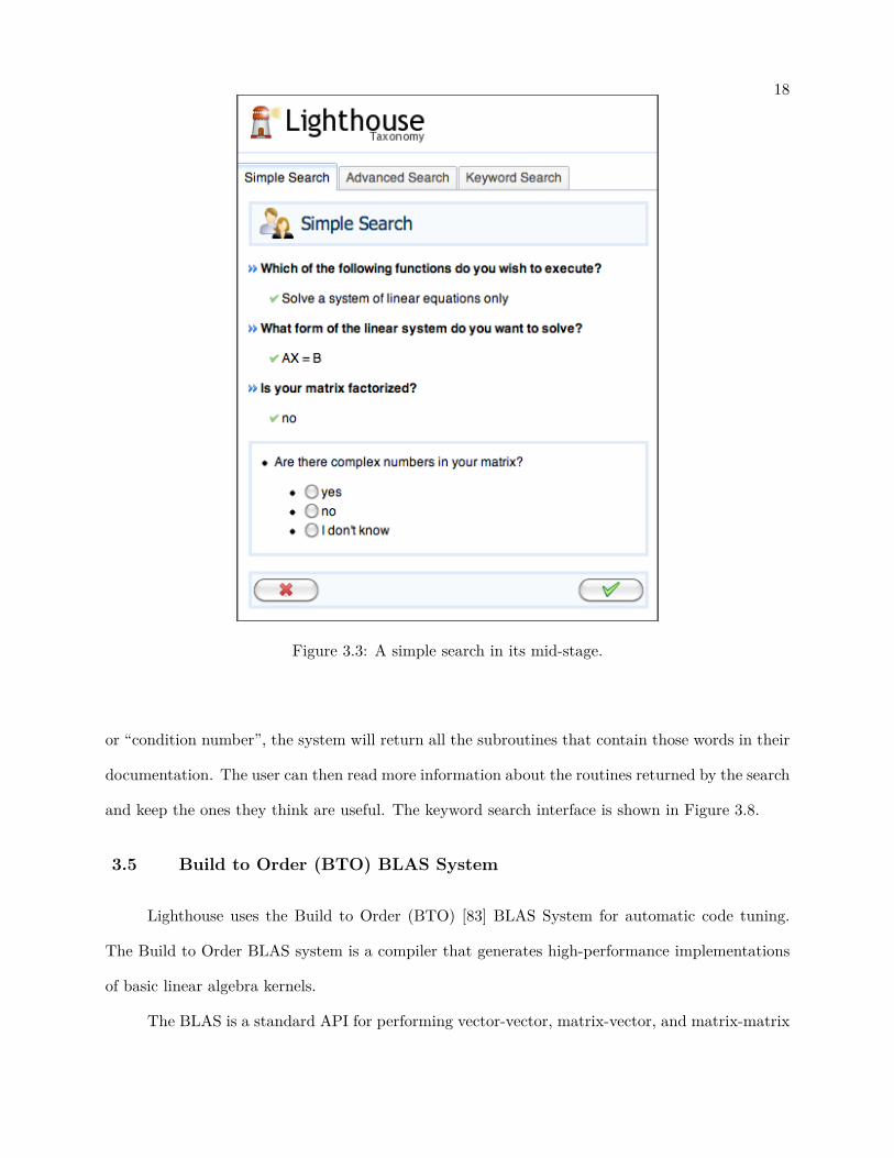
After the user chooses what they want to compute (Figure 3.2) Lighthouse generates more detailed

questions as shown in Figure 3.3, where three questions have been answered and the next question

is being asked. Once the user has answered all the questions, Lighthouse returns a single routine

in the search result area of the interface.

Figure 3.4 shows all the questions answered on the left part of the interface and the routine

Lighthouse found on the result area on the right. Information about the questions can be accessed

via help buttons located next to the questions allowing users to learn about various numerical linear

algebra terms and concepts. Figure 3.5 illustrates the use of help buttons that appear next the

questions in a simple search.

3.4.2 Advanced Search

The Advanced Search interface has been designed specifically for users who are familiar with

LAPACK. First it asks the user what type of routines they would like to search for. Figure 3.6

shows the first step of advanced search.

17

Figure 3.2: Beginning of a simple search.

After the user selects which type of routines they are looking for (Figure 3.6), Lighthouse

then provides a form containing various options that the user can select (Figure 3.7) and Lighthouse

will return all the routines that fit the specified options in the search result area. Then the user

can pick the routines they think are appropriate for solving the problem at hand or simply search

again with different options.

3.4.3 Keyword search

The Keyword Search interface is much simpler than the other interfaces. It works in a similar

way as Netlib’s keyword search does. The user has to enter keywords such as “solve linear systems”

18

Figure 3.3: A simple search in its mid-stage.

or “condition number”, the system will return all the subroutines that contain those words in their

documentation. The user can then read more information about the routines returned by the search

and keep the ones they think are useful. The keyword search interface is shown in Figure 3.8.

3.5 Build to Order (BTO) BLAS System

Lighthouse uses the Build to Order (BTO) [83] BLAS System for automatic code tuning.

The Build to Order BLAS system is a compiler that generates high-performance implementations

of basic linear algebra kernels.

The BLAS is a standard API for performing vector-vector, matrix-vector, and matrix-matrix

19

Figure 3.4: The result of a simple search.

operations. Traditionally, each routine in the BLAS has been implemented manually by hand by a

highly skilled programmer. The Build to Order BLAS compiler automates the implementation of

the BLAS standard as well as any sequence of basic linear algebra operations.

The user of the Build to Order BLAS compiler writes down a specification for a sequence

of matrix and vector operations together with a description of the input and output parameters.

The compiler then tries out many different choices of how to implement, optimize, and tune those

operations for the user’s computer hardware. The compiler chooses the best option, which is output

as a C file that implements the specified operations.

Under the script tab of the Lighthouse interface, users can write their computation in a

high-level MATLAB-like syntax. Then, by interfacing with BTO compiler, Lighthouse generates

optimized C implementations of the input script. The users are then able to download the code,

modify it, and integrate it into the larger application context. Figure 3.9 illustrates the Lighthouse

20

Figure 3.5: Help content about the task âĂĲEquilibrate a matrixâĂİ.

Figure 3.6: First step of Advanced Search.

interface for tuning code.

21

Figure 3.7: Various options in an advanced search.

3.6 My Contributions to Lighthouse

I joined the Lighthouse team on March 21, 2012. I spent slightly over a month learning

Django and getting familiar with Lighthouse and its major components. For the next couple of

22

Figure 3.8: Keyword Search interface.

Figure 3.9: Lighthouse interface for tuning code using the BTO system.

months (May - June 2012) I designed and added many icons to various parts of Lighthouse and

updated the CSS and HTML for enhancing the overall look of the user interfaces. In July and

23

August, I mostly worked with JavaScript and AJAX to improve the client-side interactions such as

form validation, added drag and drop functionality for the Advanced Search, updated the session

management part of selected routines and implemented routine reordering which allows the user to

change the order of the selected routines in the work area. The routine reordering pane is shown

in Figure 3.10.

Figure 3.10: Reordering selected routines in the Lighthouse work area.

In Fall 2012, I took the numerical linear algebra class with Dr. Elizabeth Jessup in order to learn

more about dense and sparse systems of linear equations, various algorithms for solving them,

methods for solving eigenvalue problems, preconditioning and various other important topics in

numerical linear algebra. In October, I started learning about PETSc and how to write programs

using the library it provides. On November 2, I presented a poster about Lighthouse at the Rocky

Mountain Celebration of Women in Computing Conference in Fort Collins, Colorado. On December

17, I proposed to add PETSc linear solvers to Lighthouse and write my Masters thesis about it.

24

Figure 3.11: The Lighthouse poster presented at SIAM 2013 Computational Science and EngineeingConference.

I continued learning and experimenting with PETSc and various iterative solvers. I also spent

some time trying to learn how to use a matrix analysis module called AnaMod. On February

27, I attended the 2013 SIAM Conference on Computational Science and Engineering in Boston,

Massachusetts where undergraduate research assistant Paul Givens and I presented an updated

version of the Lighthouse poster. Figure 3.11 shows a screenshot of the poster we presented. Next,

I began the process of integrating PETSc into Lighthouse, which is the main topic of this thesis

(discussed in more detail in Chapter 4).

Chapter 4

Integrating PETSc Linear Solvers into Lighthouse

Sparse matrices often appear in various fields of science and engineering when solving par-

tial differential equations. Writing PETSc programs to solve sparse linear systems can be very

challenging for individuals with little or no programming experience. Since PETSc is one of the

most widely used software packages for sparse matrix algebra operations, having Lighthouse to

provide PETSc programs to solve them will be highly beneficial to the scientific computing com-

munity. What will be even more helpful is to enable Lighthouse to make intelligent suggestions

on which Krylov subspace method and preconditioner to apply for solving a particular system of

linear equations as quickly as possible. In order to do that, first, we formed a dataset consisting of

a large number of real sparse matrices and solved them using various different combinations Krylov

subspace methods and preconditioners to record their performances. Then we computed various

properties of the matrices to create a set of features. Next, we applied machine learning techniques

to train Lighthouse and tested it to check its ability to make good suggestions.

This chapter describes the process of adding the functionalities of PETSc linear solvers to

Lighthouse and training it to provide helpful suggestions to the users. Section 4.1 describes various

features of PETSc and explains why we chose to integrate PETSc into Lighthouse. Section 4.2

discusses the main use cases. Section 4.3 presents the user interface for using the PETSc func-

tionalities. Section 4.4 explains the matrix properties we extracted and their analysis. Section 4.5

talks about our matrix dataset. Section 4.6 talks about the methods we used for solving the linear

systems. Sections 4.7 discusses the machine learning methods we employed. Section 4.8 concludes

26

the chapter with a discussion on the results.

4.1 PETSc

The Portable, Extensible Toolkit for Scientific Computation (PETSc) is a collection of rou-

tines and data structures that provide the building blocks for developing parallel numerical solution

of partial differential equations (PDEs) and other related problems in high-performance computing

[93]. PETSc is an open source software package written in the C programming language. It is

developed and maintained by Argonne National Laboratory. The development of PETSc began

several years ago, and since then it has evolved into a powerful set of tools. It is now the world’s

most widely used parallel numerical software library for partial differential equations and sparse

matrix computations.

PETSc contains a growing collection of parallel linear and nonlinear equation solvers and

time integrators that can be employed in application codes written in C, C++, Fortran, Python,

and MATLAB. At the time of this writing, the latest version of PETSc is 3.4, released publicly

on May 13, 2013. PETSc uses the Message Passing Interface (MPI) [94] standard for all inter-

process communication. The following subsections briefly review Krylov subspace methods and

preconditioners, describe the structure of PETSc and explain why we chose PETSc.

4.1.1 KSP: Krylov subspace methods

KSP methods are among the most successful methods currently available in numerical linear

algebra. These methods are designed for solving nonsingular systems of the form,

Ax = b, (4.1)

where A is the matrix representation of a linear operator, b is the right-hand-side vector, and x is

the solution vector. A Krylov subspace of dimension r is defined by the linear subspace spanned

by the images of b under the first r powers of A, that is,

27

Kr(A, b) = span{b, Ab,A2b, ..., Ar−1b}. (4.2)

Modern iterative methods for solving large systems of linear equations avoid matrix-matrix opera-

tions. Instead, these methods multiply vectors by the matrix and work with the resulting vectors.

Starting with a vector b first Ab is computed, then that vector is multiplied by A to obtain A2b

and so on. The algorithms that uses this technique are referred to as Krylov subspace methods.

4.1.2 PC: Preconditioners

In most modern numerical codes for the iterative solution of a linear system, a Krylov sub-

space method is used in combination with a preconditioner. In numerical linear algebra, a pre-

conditioner P of a matrix A is a matrix such that P−1A has a smaller condition number than A,

where the condition number is a scalar value associated with the linear equation Ax = b that gives

a bound on how inaccurate the solution x will be after approximation.

4.1.3 Structure and features of PETSc

PETSc is made up of a variety of libraries for manipulating different kinds of objects such

as vectors, matrices and the operations one would like to perform on the objects. The objects

and operations in PETSc were designed and implemented by highly experienced computational

scientists with decades of experiences with scientific computation. The following list describes

some of the main PETSc modules and their functionalities.

• Vectors (Vec): This module provide the vector operations required for setting up and

solving large-scale linear and nonlinear problems.

• Matrices (Mat): A large suite of data structures and code for the manipulation of parallel

sparse matrices. It includes four different parallel matrix data structures, each appropriate

for a different type of problem.

28

• Krylov Subspace Methods (KSP): This module provides parallel implementations of many

popular Krylov subspace iterative methods. All of the methods are coded and ready to use

with any preconditioner and any matrix data structures.

• Preconditioners (PC): A collection of sequential and parallel preconditioners.

• Index Sets (IS): For creating and manipulating various types of index sets.

Figure 4.1: Hierarchical Organization of PETSc libraries.

The hierarchical infrastructure of PETSc provides a solid foundation for the development of large-

scale scientific applications. It also lets the users apply the most appropriate abstraction level for

a particular problem and easily customize and extend both algorithms and implementations. It

separates the various problems of parallelism from the choice of algorithms. PETSc’s hierarchical

organization is illustrated in figure 4.1. At the lowest level there are BLAS and MPI libraries. The

29

libraries that provide matrix, vector and index set operations rely on the BLAS and MPI libraries.

Next, the PC and KSP libraries use the libraries from the level below them and finally the SNES

and TS libraries make use of the PC and KSP libraries. The application code written by a PETSc

user is at the highest level of abstraction, meaning the application code simply uses these libraries

without having to deal with the underlying details of their implementations.

4.1.4 Why we like PETSc

Each of the PETSc modules contains an abstract interface and implementations using spe-

cific data structures, allowing PETSc to provide neat and effective codes for the different stages of

solving PDEs. PETSc’s modular and clean design makes comparing and using different algorithms

very easy, which is one of the main reasons we decided to integrate PETSc linear solvers into

Lighthouse. We wanted to experiment with various Krylov subspace methods and preconditioners

and PETSc provides the perfect environment for such experimentations. PETSc allows executing a

program from the command line using a variety of settings. A simple script can be written to solve

a particular system using varying number of processes, KSP methods and proconditioners. This

particular features has proven to be very useful for our purpose. Moreover, PETSc’s clean and thor-

ough documentation and hundreds of well-commented example codes provide a great environment

for learning programming in PETSc.

Some of the other popular software packages that offer sparse iterative solvers are SPARSKIT

[48], SLAP [50], ITPACK [57], ITSOL [58], ViennaCL [44], Belos package [60] by Trilinos [59]. How-

ever, none of these packages provide the rich and unique environment for sparse matrix algebra

computations that PETSc does.

4.2 Primary use cases

In this section we present the main use cases to show how a user will interact with Lighthouse

(the system) in order to have a PETSc program generated. In software engineering, a use case is a

list of steps that illustrates how users will perform a task using a software application or a website.

30

It outlines the behavior of a system, from the point of view of a user, as it responds to the user’s

requests. In the Unified Modeling Language (UML) [95], a user who interacts with the system is

known as an “actor”. Preconditions of a use case specify circumstances that must be true before a

use case is invoked. Postconditions of a use case list possible situations that the system can be in

after the use case is executed. The normal or basic flow of a use case is the flow of actions that is

considered normal or usual for the system. Alternate flows are the alternative actions that can be

performed. Following are the two main use cases.

Use case: 1

Use case name: Selecting the main task

Actors: User

Preconditions: The user is at the Lighthouse for PETSc homepage

Postconditions: The user is on the web page that handles the task user selected

Normal Flow:

(1) Lighthouse provides the user with a list of tasks that they can choose from.

(2) The user selects the task they would like to perform.

(3) User submits the form by clicking the submit button.

(4) Lighthouse presents the appropriate page to the user based on the task they chose.

Use case: 2

Use Case Name: Solving a linear system

Actors: User

Preconditions: User is at the âĂŸSolve a Sparse Linear SystemâĂŹ page

Postconditions: User has the archive file that contains a PETSc program and necessary instructions

for solving their system of linear equations.

31

Normal Flow:

(1) Lighthouse asks the user if they want to upload their matrix.

(2) User chooses to upload their matrix.

(3) Lighthouse provides the user with a file browser for selecting the matrix file.

(4) User selects the matrix file.

(5) Lighthouse asks the user if they want a sequential solution or a parallel solution.

(6) User selects the type of solution they want.

(7) User submits the form.

(8) Lighthouse generates a PETSc program in C programming language, a makefile, a text file

containing the command line options and a readme file.

(9) Lighthouse then creates an archive file containing the files generated in step 8.

(10) Lighthouse provides the user with a download link of the archive file.

(11) User downloads the archive file.

(12) Lighthouse deletes any file from the server that the user had uploaded.

Alternate Flows:

2A1: User does not want to upload their matrix.

(1) User chooses not to upload their matrix.

(2) Lighthouse asks the user if they would like to download a PETSc program to compute the

matrix properties themselves and upload the output of the program or download a general

PETSc program for solving a sparse system of linear equations.

(3) User chooses to download the matrix property computation program.

32

(4) Lighthouse provides a link to an archive file containing the matrix property computation

program and other necessary files.

(5) User downloads the file.

(6) User computes the matrix properties using the downloaded program.

(7) User returns to Lighthouse and selects the option for uploading the matrix property file.

(8) Lighthouse provides the user with a file browser for selecting the matrix property file.

(9) User selects the matrix property file.

(10) Lighthouse asks the user if they want a sequential solution or a parallel solution.

(11) User selects the type of solution they want.


(13) The use case continues from step 8 of the normal flow.

2A1.2A: User chooses to download the general PETSc program for solving a sparse system of linear

equations.


(2) The use case continues from step 8 of the normal flow.

These uses cases provide the foundation for building an interactive system that will enable users

to have PETSc programs generated for solving their sparse linear systems.

4.3 User interface

In this section, we discuss the web user interface through which users interact with the

system. It is built using the same set of tools that we used for developing the LAPACK and BTO

user interfaces of Lighthouse discussed in chapter 3. The user interface is presented using the

screen-shots taken from the Lighthouse for PETSc website.

33

4.3.1 Normal flow

Figure 4.2 shows the Lighthouse for PETSc homepage. On the right part of the homepage,

in the Instructions tab, Lighthouse provides the user with information about what this website

does followed by instructions on how to use the website. On the left part, in the PETSc Simple

Search tab, Lighthouse asks the user which task they would like to perform and provides the

options. Initially, the other tabs labeled PETSc Code tab (appears next to the Instructions tab),

Command-line Options and Makefile tabs (appear under the Instructions tab) do not have any

contents but they become available after Lighthouse prepares the files for the user.

Figure 4.2: Lighthouse for PETSc homepage.

Once the user has selected the task ‘Solve a system of linear equations’ and submits the form,

Lighthouse asks the user whether they want to upload their matrix (shown in Figure 4.3). If the

user chooses to upload their matrix, as shown in Figure 4.4, Lighthouse provides a file picker for

the user to select their matrix file.

34

Figure 4.3: Matrix upload options.

After the user selects a matrix file, Lighthouse asks the user whether they want a sequential

or parallel solution (Figure 4.5). Once the user selects the type of solution they would like to

have, Lighthouse asks the user to submit the form (Figure 4.6). After the user submits the form,

Lighthouse tells the user that they can download their program (Figure 4.7). At this stage, the

code, makefile for compiling the code and commands for running the program can be viewed in

their respective tabs before downloading them.

35

Figure 4.4: Selecting a matrix file.

Figure 4.5: Options for solution type.

36

Figure 4.6: Submitting the form.

Figure 4.7: Downloading the PETSc program.

37

4.3.2 Alternate Flow

If the user chooses to not to upload their matrix, Lighthouse provides the following three

options to the user (Figure 4.8).

1. Download a PETSc program for computing matrix properties

2. Download a general PETSc program for solving a linear system

3. Upload matrix properties computed using our program

Figure 4.8: Options for users who choose not to upload their matrix.

If the user chooses to download the PETSc program for computing matrix properties and sub-

mits the form, they are provided with an archive file containing the matrix property computation

program and other necessary files. If the user decides to download a general PETSc program for

solving a linear system, Lighthouse gives them a PETSc program for solving a linear system and

38

other necessary files but does not suggest any specific Krylov subspace method or preconditioner.

This option is for the users who know what Krylov method and preconditioner they want to use or

experiment with.

Figure 4.9: Uploading matrix property file.

If the user selects the option for uploading a matrix property file that they prepared using the first

option, Lighthouse lets the user select the file using a file picker (Figure 4.9).

39

Figure 4.10: Submitting the form in alternate flow.

Once they select the matrix property file, Lighthouse asks them whether they want a sequential or

a parallel solution. After the user selects their desired option, Lighthouse asks them to submit the

form (Figure 4.10). After the user submits the form, they are provided with an archive file that

includes the program and other required files to run the program.

40

4.4 Matrix properties

We computed thirty properties for each of the matrices in our dataset. These properties play

a very crucial role in building our system. We use these properties to form our feature set. In

machine learning, a feature specifies a quantitative value of a property of an object. For example,

row is an property of a matrix and the number of rows of a matrix is the row feature of that matrix.

In this section, we explain the properties we computed. Consider the following m×m matrix A.

Am,m =

a1,1 a1,2 · · · a1,m

a2,1 a2,2 · · · a2,m

...... . . . ...

am,1 am,2 · · · am,m

Following is a list of all the properties of A that we compute.

(1) Dimension: The number of rows and columns of square matrix A.

(2) Nonzeros: The total number of nonzero entries, that is, the number of entries in A for

which ai,j 6= 0 is true, where i and j are positive integers and 1 ≤ i ≤ m and 1 ≤ j ≤ m.

(3) Max. nonzeros per row: The maximum number of nonzero entries in a row of A.

(4) Min. nonzeros per row: The minimum number of nonzero entries in a row of A.

(5) Avg. nonzeros per row: The average number of nonzero entries in a row of A.

(6) Dummy rows: The number of rows of A with only one nonzero entry.

(7) Dummy rows kind: The dummy rows kind of A can be one of the following three. First

kind, every dummy row of A has entry 1 at the main diagonal position. Second kind, every

dummy row of A has a nonzero entry at the main diagonal position but it is not always 1.

Third kind, the nonzero entry is not on the diagonal.

(8) Hard numeric value symmetry: If A is equal to its transpose, that is, A = AT , then

the value of this property is 1. Otherwise, it is 0.

41

(9) Hard nonzero pattern symmetry: If A has the same nonzero pattern as its transpose

AT , that is, for every nonzero entry ai,j of A, AT has a nonzero entry ai,j , then the value

of this property is 1. Otherwise, it is 0.

(10) Soft numeric value symmetry: The soft numeric value symmetry v of A is,

v = 1− (12

∑mi=1

∑mj=1 |si,j |/

∑mi=1

∑mj=1 |ai,j |), where S = (si,j) is 1

2(A−AT ), the antisym-

metric part of A.

(11) Soft nonzero pattern symmetry: The ratio of the number of nonzero entries ai,j in A,

for which, there exist no entry aj,i in A, to the total number of nonzero entries in A.

(12) Trace: The sum of all the diagonal entries of A. The trace of A is ∑mi=1 ai,i.

(13) Absolute trace: The sum of the absolute values of all the diagonal entries of A. The

absolute trace of A is ∑mi=1 |ai,i|.

(14) One norm: The maximum absolute column sum of A. More precisely, the one norm of A

is max1≤j≤m

(∑mi=1 |ai,j |).

(15) Infinity norm: The maximum absolute row sum of A. The infinity norm of A is

max1≤i≤m

(∑mj=1 |ai,j |).

(16) Frobenius norm: The square root of the sum of all the entries of A squared. The

Frobineus norm of A is√∑m

i=1∑m

j=1 a2i,j .

(17) Symmetric infinity norm: The infinity norm of the symmetric part of A. The symmetric

part of A is 12(A+AT ).

(18) Symmetric Frobenius norm: The Frobenius norm of the symmetric part of A.

(19) Antisymmetric infinity norm: The infinity norm of the antisymmetric part of A.

(20) Antisymmetric Frobenius norm: The Frobenius norm of the antisymmetric part of A.

42

(21) Row diagonal dominance: This property is 0, if, for any row i of A, the absolute value

of the diagonal entry in that row is smaller than the sum of the absolute values of the

non-diagonal entries. That is, |ai,i| <∑

j 6=i |ai,j | for all j.

This property is 1, if |ai,i| ≥∑


This property is 2, if |ai,i| >∑


(22) Column diagonal dominance: This property is 0, if, for any column j of A, the absolute

value of the diagonal entry in that column is smaller than the sum of the absolute values

of the non-diagonal entries. That is, |aj,j | <∑

i 6=j |ai,j | for all i.

This property is 1, if |aj,j | ≥∑


This property is 2, if |aj,j | >∑


(23) Max. row variance: The maximum row variance of A. The row variance of any row i is

1m

∑mj=1(ai,j − µ)2, where µ = 1

m

∑mj=1 ai,j .

(24) Max. column variance: The maximum column variance of A. The column variance of

any column j is 1m

∑mi=1(ai,j − µ)2, where µ = 1

m

∑mi=1 ai,j .

(25) Diagonal average: The arithmetic mean of the absolute values of the diagonal entries of

A. More precisely, diagonal average of A is 1m

∑mi=1 |ai,i|.

(26) Diagonal variance: The variance of the diagonal entries of A, that is, 1m

∑mi=j=1(ai,j−µ)2,

where µ = 1m

∑mi=1 ai,i.

(27) Diagonal sign: This property indicates the diagonal sign pattern. Diagonal sign of A is

-2 if all diagonal entries of A are negative, -1 if all are nonpositive, 0 if all are zeros, 1 if all

are nonnegative, 2 if all are positive, 3 if some are negative and some or none are zero and

some are positive.

(28) Diagonal nonzeros: The number of nonzero entries in the diagonal of A.

(29) Lower bandwidth: The smallest number p such that any entry ai,j = 0 when i > j + p.

43

(30) Upper bandwidth: The smallest number p such that any entry ai,j = 0 when i < j − p.

4.4.1 Principal component analysis of the matrix properties

Principal Component Analysis (PCA) [96] is a statistical technique for identifying patterns in

data and representing data in a form that highlights the similarities and differences in the data. The

patterns found in the data can be used for compressing the data. Performing PCA on a set of data

involves adjusting the data set is so that its mean is zero, then computing the covariance matrix

of the data set and then finding the eigenvalues and eigenvectors of the covariance matrix. Finally,

the eigenvectors are sorted from highest to lowest based on their corresponding eigenvalues. The

eigenvector with the highest eigenvalue is the first principal component of the data set. The largest

values in the first principal component indicates that the corresponding variables or dimensions

account for the highest variance in the data set. Principal components with lower eigenvalues

indicate which variables do not provide much information about the variance of the data set.

For the purpose of PCA, we created a data set containing 860 data points where each data

point is a 30-dimensional vector. Each vector represents a matrix and the entries in the vector

correspond to the properties of the matrix. Then using Matlab’s Statistics toolbox, we performed

PCA to find out which of the thirty properties account for the most variability in the data. Figure

4.11 provides a bar plot of the eigenvalues of the principal components sorted from highest to lowest

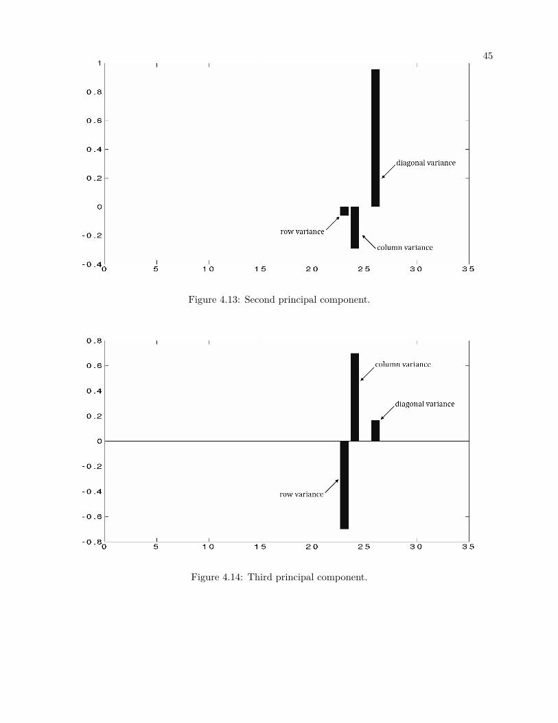
based on their eigenvalues. Figure 4.12 shows the first principal component and it tells us that the

row, column and diagonal variances account for the most variance in the data. Figure 4.13, 4.14

and 4.15 show the second, third and fourth principal components respectively and indicate how

much information various matrix features provide.

44

Figure 4.11: Eigenvalues of the principal components.

Figure 4.12: First principal component.

45

Figure 4.13: Second principal component.

Figure 4.14: Third principal component.

46

Figure 4.15: Fourth principal component.

Based on the PCA results, we decided to use fifteen features out of the thirty features we computed.

Table 4.1 shows the reduced feature set and the computation time for each feature for 860 matrices.

The computation times were recorded using the hardware and software specified in Table A.1 and

A.2.

47Reduced feature set and computation time

Matrix feature Computation time

Row variance 9.90s

Column variance 11.47s

Diagonal variance 0.16s

Number of nonzeros 1.97s

Number of rows 0.06s

Frobenius norm 0.03s

Symmetric Frobenius norm 13.34s

Anti-symmetric Frobenius norm 13.24s

One norm 0.21s

Infinity norm 0.07s

Symmetric infinity norm 13.33s

Anti-symmetric infinity norm 13.44s

Max. nonzeros per row 1.95s

Trace 0.06s

Absolute Trace 0.15s

Total time 79.38s

Table 4.1: Reduced feature set and approximate computation time.

4.5 Dataset

Our dataset consists of 860 sparse matrices downloaded from the The University of Florida

Sparse Matrix Collection [97]. All the matrices are real and square. The Table 4.2 shows the names

and sizes of the matrices that have the minimum and maximum dimension, lowest and highest

number of nonzero entries, highest row and column variances. It also shows how many symmetric,

unsymmetric, diagonally dominant matrices are there in our dataset.

48Dataset statistics

Matrix property Value Matrix name

Minimum dimension 5×5 cage3

Maximum dimension 46772×46772 bcsstm39

Minimum nonzeros 19 cage3

Maximum nonzeros 1137732 spiral E

Maximum row variance 2.02902e36 mcca

Maximum column variance 1.54208e36 mcca

Numerically symmetric matrices 211 n/a

Numerically unsymmetric matrices 649 n/a

Structurally symmetric matrices 377 n/a

Structurally unsymmetric matrices 483 n/a

Diagonally dominant matrices 67 n/a

Diagonally nondominant matrices 793 n/a

Table 4.2: Various statistics of our dataset.

4.6 Methods used for solving linear systems

We formed 860 systems of linear equations using the matrices from our dataset and right-hand

side vectors with all their entries set to 1. Then we solved the systems using a number of different

methods, i.e., various combinations of the following Krylov subspace methods and preconditioners

(and also without any preconditioner).

Krylov subspace methods:

(1) Conjugate Gradient (CG) [98]

(2) Conjugate Gradient Squared (CGS) [99]

(3) BiConjugate Gradient (BICG) [100]

49

(4) BiConjugate Gradient Stabilized (BiCGSTAB) [101]

(5) Generalized Minimal Residual (GMRES) [102]

(6) Flexible Generalized Minimal Residual (FGMRES) [103]

(7) Transpose-Free Quasi-Minimal Residual (TFQMR) [104]

Preconditioners:[105]

(1) ILU(0), ILU(1), ILU(2) (sequential)

(2) Jacobi (sequential), Block Jacobi (parallel)

(3) SOR (sequential and parallel)

(4) ASM (parallel)

We observed which methods succeed at solving a particular system and which do not. For each

system, we picked the method that converged fastest with solve time tlowest and any other method

that converged within the time 1.1× tlowest.

4.7 Machine learning techniques

Machine learning is a branch of artificial intelligence that focuses on building and studying

systems that can learn from data. A variety of machine learning techniques has been developed

for decision making, clustering, pattern recognition, classification and other tasks. Some of the

widely used machine learning techniques are decision trees, artificial neural networks, support vector

machines, case based reasoning, classification and regression trees [106]. A research work has been

conducted on comparing performances of various machine learning techniques such as Naive Bayes

Classifier (NB), Support Vector Machine (SVM), Alternating Decision Tree (ADT), Decision Stump

(DS), Instance-based Learning (IB1, IBk), for selecting linear solvers using matrix features similar

to ours [107]. The accuracies of all the machine learning techniques from that research work is

shown in Figure 4.16 (results for symmetric matrices) and 4.17 (results for unsymmetric matrices).

50

Figure 4.16: Accuracy of classifiers for symmetric matrices [106].

Figure 4.17: Accuracy of classifiers for unsymmetric matrices [106].

51

We can see that SVM achieves the highest accuracies for both symmetric and unsymmetric matrices.

Based on these results, we decided to use SVM for our purposes.

4.7.1 Support Vector Machine (SVM)

Support Vector Machine is an machine learning approach where the SVM takes a set of

training data consisting of observations from two classes, then tries to separate the observations

from the two classes and predicts, for each input, which of the two possible classes forms the output.

Consider k training data points DT , where each input xi is a point on an n-dimensional space and

belongs two either of the two classes yi = 1 or −1, that is,

DT = {(xi, yi)} where i = 1...k, yi ∈ {−1, 1}, x ∈ <n.

In our case, we assume the data points are linearly separable. So we can draw a line on a graph

of x1 vs x2 and separate the two classes when n = 2. If n > 2 then we draw a hyperplane on

graphs of x1, x2...xn to separate the points. This hyperplane is defined by w·x + b = 0, where ·

denotes the dot product, w is normal to the hyperplane and b is a scalar value. b||w|| is the offset

of the hyperplane from the origin along w. Support Vectors are the points that are closest to the

separating hyperplane. The goal of the SVM is to orientate this hyperplane in such a way that

it is as far away as possible from the closest members of both classes. We then select w and b so

that the training data points can be expressed by xi·w + b ≥ 1 for yi = 1 and xi·w + b ≤ −1 for

yi = −1. Figure 4.18 shows a linear hyperplane with support vectors circled.

52

Figure 4.18: Support Vector Machine, hyperplane separating members of two classes.

We used the SVM classifier from Matlab’s Bioinformatics Toolbox. For preparing the training

data point for a matrix, we formed a vector containing fifteen features of that matrix and a scalar

value indicating which KSP and PC were used to solve the linear system. If a certain pair of KSP

and PC gives the fastest solution in tlowest seconds or a near fastest solution within 1.1 × tlowest

seconds, then the data point belongs to Class 1. If a pair of KSP and PC does not give the fastest

or a near fastest solution, then the data point belongs to Class 2.

For the sequential case, we solved each matrix in our dataset of 860 matrices sequentially

with forty-one different methods (i.e., pairs of KSP and PC) giving us 860×41 = 35260 data points,

where each one is a 16-dimensional vector. For the parallel case, we solved 860 matrices using four

processes with twenty-seven different methods. The number of methods used for the parallel case

is lower than the sequential case because we used six different preconditioning techniques for the

sequential case but only four preconditioning techniques for the parallel case. The number of data

points for the parallel case is 860× 27 = 23220 and each data point is a 16-dimensional vector.

4.8 Test results

We used k-fold cross-validation [109] with k = 10 for calculating the accuracy of our system.

k-fold cross-validation is a method for estimating the accuracy of a model. The data set is parti-

53

tioned into k subsets which are known as ‘folds’. In each iteration of training and testing, one of

the k subsets is used as the test set and the rest of the k− 1 subsets are combined and used as the

training set. The error from all k iterations are averaged. Every sample in the dataset gets used

for testing exactly one time and gets used for training k − 1 times.

We present our results in the form of confusion matrices [109]. A confusion matrix shows

the actual and predicted classifications. Table 4.3 shows the SVM classification results for the

sequential case and Table 4.4 shows the classification results for the parallel case.

Actual

Class 1 Class 2

PredictedClass 1 a = 1031 b = 4821

Class 2 c = 322 d = 29086

Table 4.3: SVM classification results for the sequential case.

The entries in the confusion matrix have the following meaning:

• a = number of correct predictions that an instance belongs to Class 1,

• b = number of incorrect predictions that an instance belongs to Class 1,

• c = number of incorrect predictions that an instance is belongs to Class 2,

• d = number of correct predictions that an instance belongs to Class 2.

Actual

Class 1 Class 2

PredictedClass 1 a = 175 b = 3400

Class 2 c = 792 d = 18853

Table 4.4: SVM classification results for the parallel case.

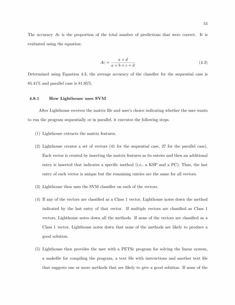
54

The accuracy Ac is the proportion of the total number of predictions that were correct. It is

evaluated using the equation:

Ac = a+ d

a+ b+ c+ d(4.3)

Determined using Equation 4.3, the average accuracy of the classifier for the sequential case is

85.41% and parallel case is 81.95%.

4.8.1 How Lighthouse uses SVM

After Lighthouse receives the matrix file and user’s choice indicating whether the user wants

to run the program sequentially or in parallel, it executes the following steps.

(1) Lighthouse extracts the matrix features.

(2) Lighthouse creates a set of vectors (41 for the sequential case, 27 for the parallel case).

Each vector is created by inserting the matrix features as its entries and then an additional

entry is inserted that indicates a specific method (i.e., a KSP and a PC). Thus, the last

entry of each vector is unique but the remaining entries are the same for all vectors.

(3) Lighthouse then uses the SVM classifier on each of the vectors.

(4) If any of the vectors are classified as a Class 1 vector, Lighthouse notes down the method

indicated by the last entry of that vector. If multiple vectors are classified as Class 1

vectors, Lighthouse notes down all the methods. If none of the vectors are classified as a

Class 1 vector, Lighthouse notes down that none of the methods are likely to produce a

good solution.

(5) Lighthouse then provides the user with a PETSc program for solving the linear system,

a makefile for compiling the program, a text file with instructions and another text file

that suggests one or more methods that are likely to give a good solution. If none of the

55

methods are predicted to give a good solution, Lighthouse notifies the user through the

web user interface instead of providing them with any file.

4.8.2 Training and testing time

Table 4.5 shows the average training and testing times for the sequential and parallel cases.

The computation times were collected using the hardware and software specified in Table A.1 and

A.2.

Classifier training and testing time

Training time Training instances Testing time Test instances

Sequential case 349.10s 31734 2.85s 3526

Parallel case 66.75s 20898 0.61s 2322

Table 4.5: Classifier training and testing times.

Chapter 5

Conclusions

In this chapter we present our conclusions about the method we developed for enabling

Lighthouse to provide the users with PETSc programs and helpful suggestions about which KSP

and PC they should use. We then present our ideas for future work.

We have added a new functionality to Lighthouse that allows users to download PETSc

programs for solving sparse linear systems using an interactive web user interface. In addition,

we developed a technique that enables Lighthouse to take in a matrix from a user, analyze it and

recommend them which Krylov method and preconditoner can give them the fastest solution.

As part of our future work, we will add support for solving sparse linear systems in parallel

using a computer cluster. Then, we will repeat the same process for adding support for solving

sparse complex systems of linear equation using PETSc.

Bibliography

[1] R. C. Whaley and D. B. Whalley, “Tuning high performance kernels through empirical com-pilation,” in The 2005 International Conference on Parallel Processing (ICPP-05), June 2005.

[2] B. Spencer, T. Finholt, I. Foster, C. Kesselman, C. Beldica, J. Futrelle, S. Gullapalli, P. Hub-bard, L. Liming, D. Marcusiu, L. Pearlman, C. Severance, and G. Yang, “NEESgrid: Adistributed collaboratory for advanced earthquake engineering experiment and simulation,”in The 13th World Conference on Earthquake Engineering, Vancouver, B.C., Canada, August2004.

[3] G. Vidal, “Efficient simulation of one-dimensional quantum many-body systems,” PhysicalReview Letters, vol. 93(4), pp. 1–4, 2004.

[4] T.-H. Chen and C. C.-P. Chen, “Efficient large-scale power grid analysis based on precondi-tioned krylov-subspace iterative methods,” in Proceedings of Design Automation Conference,Las Vegas, NV, 2001, pp. 559–562.

[5] W. Gropp, D. Kaushik, D. Keyes, and B. Smith, “Toward realistic performance bounds forimplicit CFD codes,” in Proceedings of Parallel CFD’99. Elsevier, 1999.

[6] “Freely Available Software for Linear Algebra (May 2013),” http://www.netlib.org/utk/people/JackDongarra/la-sw.html, accessed: 2013-07-6.

[7] “LAPACK: Linear Algebra PACKage,” http://www.netlib.org/lapack/, accessed: 2013-07-6.

[8] J. J. Dongarra, J. D. Croz, I. S. Duff, and S. Hammarling, “A set of level 3 basic linearalgebra subprograms,” ACM Transactions on Mathematical Software (TOMS), vol. 16, pp.1–17, 1990.

[9] “AMD Core Math Library (ACML),” http://developer.amd.com/tools-and-sdks/cpu-development/amd-core-math-library-acml/, accessed: 2013-07-6.

[10] “Mac Developer Library, Accelerate Framework Reference,” https://developer.apple.com/library/mac/#documentation/Accelerate/Reference/AccelerateFWRef/ index.html,accessed: 2013-07-6.

[11] “Engineering and Scientific Subroutine Library (ESSL) and Parallel ESSL,” http://www-03.ibm.com/systems/software/essl/, accessed: 2013-07-6.

58

[12] “HP’s Mathematical Software Library (MLIB),” http://h21007.www2.hp.com/portal/site/dspp/menuitem.863c3e4cbcdc3f3515b49c108973a801/?ciid=c008a8ea6ce02110a8ea6ce02110275d6e10RCRD, accessed: 2013-07-6.

[13] “Intel Math Kernel Library (Intel MKL),” http://software.intel.com/en-us/intel-mkl/, ac-cessed: 2013-07-6.

[14] “Sun Performance Library,” http://docs.oracle.com/cd/E24457 01/html/E21987/gkezy.html, accessed: 2013-07-6.

[15] “LibSci,” http://www.nersc.gov/users/software/programming-libraries/math-libraries/libsci/, accessed: 2013-07-6.

[16] “uBLAS Overview,” http://www.boost.org/doc/libs/1 51 0/libs/numeric/ublas/doc/overview.htm, accessed: 2013-07-6.

[17] “The Blitz++ Library,” http://blitz.sourceforge.net/, accessed: 2013-07-6.

[18] “Template Numerical Toolkit,” http://math.nist.gov/tnt/overview.html, accessed: 2013-07-6.

[19] E. Anderson, Z. Bai, C. Bischof, J. Demmel, J. Dongarra, J. D. Croz, A. Greenbaum, S. Ham-marling, A. McKenney, S. Ostrouchov, and D. Sorensen, LAPACK Users’ Guide, 3rd ed.,1999.

[20] “Pliris,” http://trilinos.sandia.gov/packages/pliris/index.html, accessed: 2013-07-6.

[21] “FLENS,” http://apfel.mathematik.uni-ulm.de/∼lehn/FLENS/index.html, accessed: 2013-07-6.

[22] “Elemental,” https://code.google.com/p/elemental/, accessed: 2013-07-6.

[23] “Solutions for Systems of Linear Equations,” http://www.rejonesconsulting.com/, accessed:2013-07-6.

[24] “Matrix Algebra on GPU and Multicore Architectures,” http://icl.cs.utk.edu/magma/, ac-cessed: 2013-07-6.

[25] “PLAPACK: High Performance through High Level Abstraction,” http://www.cs.utexas.edu/users/plapack/icpp98/index.html, accessed: 2013-07-6.

[26] “PLASMA: Parallel Linear Algebra for Scalable Multi-core Architectures,” http://icl.cs.utk.edu/plasma/, accessed: 2013-07-6.

[27] “ScaLAPACK: Scalable Linear Algebra PACKage,” http://www.netlib.org/scalapack/, ac-cessed: 2013-07-6.

[28] “PRISM: Parallel Research on Invariant Subspace Methods,” http://www.mcs.anl.gov/prism/, accessed: 2013-07-6.

[29] I. S. Duff, “An overview of the sparse basic linear algebra subprograms: The new stan-dard from the blas technical forum,” ACM Transactions on Mathematical Software (TOMS),vol. 28, pp. 239–267, 2002.

59

[30] “SPARSE 1.3 - Netlib,” http://www.netlib.org/sparse/, accessed: 2013-07-6.

[31] “SPOOLES 2.2: SParse Object Oriented Linear Equations Solver,” http://www.netlib.org/linalg/spooles/spooles.2.2.html, accessed: 2013-07-6.

[32] “SparseLib++,” http://math.nist.gov/sparselib++/, accessed: 2013-07-6.

[33] “CHOLMOD,” http://www.cise.ufl.edu/research/sparse/cholmod/, accessed: 2013-07-6.

[34] “DSCPACK: Domain-Separator Codes For Solving Sparse Linear Systems,” http://www.cse.psu.edu/∼raghavan/Dscpack/, accessed: 2013-07-6.

[35] “The HSL Mathematical Software Library,” http://www.hsl.rl.ac.uk/index.html, accessed:2013-07-6.

[36] “MUMPS : a parallel sparse direct solver,” http://graal.ens-lyon.fr/MUMPS/, accessed:2013-07-6.

[37] “PSPASES: Parallel SPArse Symmetric dirEct Solver,” http://www-users.cs.umn.edu/∼mjoshi/pspases/index.html, accessed: 2013-07-6.

[38] “SuperLU,” http://crd-legacy.lbl.gov/∼xiaoye/SuperLU/, accessed: 2013-07-6.

[39] “TAUCS,” http://www.tau.ac.il/∼stoledo/taucs/, accessed: 2013-07-6.

[40] “Amesos,” http://trilinos.sandia.gov/packages/amesos/, accessed: 2013-07-6.

[41] “UMFPACK: unsymmetric multifrontal sparse LU factorization package,” http://www.cise.ufl.edu/research/sparse/umfpack/, accessed: 2013-07-6.

[42] “y12m,” http://www.netlib.org/y12m/, accessed: 2013-07-6.

[43] “PETSc: Portable, Extensible Toolkit for Scientific Computation,” http://www.mcs.anl.gov/petsc/index.html, accessed: 2013-07-6.

[44] “ViennaCL,” http://viennacl.sourceforge.net/, accessed: 2013-07-6.

[45] “AGMG âĂŞ Iterative solution with Aggregation-based algebraic MultiGrid,” http://homepages.ulb.ac.be/∼ynotay/AGMG/, accessed: 2013-07-6.

[46] “BILUM,” http://www.cs.uky.edu/∼jzhang/bilum.html, accessed: 2013-07-6.

[47] “BlockSolve95,” http://ftp.mcs.anl.gov/pub/BlockSolve95/, accessed: 2013-07-6.

[48] “SPARSKIT: A basic tool-kit for sparse matrix computations,” http://www-users.cs.umn.edu/∼saad/software/SPARSKIT/, accessed: 2013-07-6.

[49] “ITL: The Iterative Template Library,” http://www.osl.iu.edu/research/itl/, accessed: 2013-07-6.

[50] “SLAP: Sparse Linear Algebra Package,” http://www.netlib.org/slap/readme, accessed:2013-07-6.

60

[51] J. Dongarra, A. Lumsdaine, R. Pozo, and K. Remington, “A Sparse Matrix Library in C++for High Performance Architectures,” in Proceedings of the Second Object Oriented NumericsConference, Sun River, OR, 1994.

[52] “PIM: Parallel Iterative Methods,” http://chasqueweb.ufrgs.br/∼rudnei.cunha/pim.html, ac-cessed: 2013-07-6.

[53] “The Parallel Algorithms Project at CERFACS,” http://www.cerfacs.fr/algor/Softs/, ac-cessed: 2013-07-6.

[54] “pARMS: parallel Algebraic Recursive Multilevel Solvers ,” http://www-users.cs.umn.edu/∼saad/software/pARMS/, accessed: 2013-07-6.

[55] “Lis: a Library of Iterative Solvers for Linear Systems,” http://www.ssisc.org/lis/, accessed:2013-07-6.

[56] “HIPS: Hierarchical Iterative Parallel Solver,” http://hips.gforge.inria.fr/, accessed: 2013-07-6.

[57] “ITPACK,” http://www.netlib.org/itpack/, accessed: 2013-07-6.

[58] “ITSOL: ITERATIVE SOLVERS package,” http://www-users.cs.umn.edu/∼saad/software/ITSOL/, accessed: 2013-07-6.

[59] “The Trilinos Project,” http://trilinos.sandia.gov/packages/, accessed: 2013-07-6.

[60] “Belos: Next-Generation Iterative Solver Package,” http://trilinos.sandia.gov/packages/belos/, accessed: 2013-07-6.

[61] “Komplex: Complex Linear Solver Package,” http://trilinos.sandia.gov/packages/komplex/,accessed: 2013-07-6.

[62] “ILUPACK,” http://www.icm.tu-bs.de/∼bolle/ilupack/, accessed: 2013-07-6.

[63] “BPKIT: Block Preconditioning Toolkit B,” http://sourceforge.net/projects/bpkit/, ac-cessed: 2013-07-6.

[64] “MLD2P4: Multi-Level Domain Decomposition Parallel Preconditioners Package based onPSBLAS,” http://www.mld2p4.it/, accessed: 2013-07-6.

[65] “Hypre,” http://acts.nersc.gov/hypre/, accessed: 2013-07-6.

[66] “MSPAI: Modified Sparse Approximate Inverses,” http://www5.in.tum.de/wiki/index.php/MSPAI, accessed: 2013-07-6.

[67] M. J. Grote and T. Huckle, “Parallel preconditioning with sparse approximate inverses,”SIAM Journal on Scientific Computing, vol. 8(3), pp. 838–853, 1997.

[68] “FSPAI: Factorized Sparse Approximate Inverses,” http://www5.in.tum.de/wiki/index.php/FSPAI, accessed: 2013-07-6.

[69] “GotoBLAS2,” http://www.tacc.utexas.edu/tacc-software/gotoblas2, accessed: 2013-07-6.

[70] “OpenBLAS,” http://xianyi.github.io/OpenBLAS/, accessed: 2013-07-6.

61

[71] S. Goedecker and A. Hoisie, Performance optimization of numerically intensive codes.SIAM, 2001.

[72] R. C. Whaley, A. Petitet, and J. J. Dongarra, “Automated empirical optimization of softwareand the ATLAS project,” Parallel Computing, vol. 27, pp. 3–35, 2001.

[73] “PHiPAC: Portable High Performance ANSI C,” http://www1.icsi.berkeley.edu/∼bilmes/phipac/, accessed: 2013-07-6.

[74] “Active Harmony,” http://www.dyninst.org/harmony, accessed: 2013-07-6.

[75] “Orio: An Annotation-Based Empirical Performance Tuning Framework,” http://trac.mcs.anl.gov/projects/performance/wiki/Orio, accessed: 2013-07-6.

[76] “BeBOP: Berkeley Benchmarking and OPtimization,” http://bebop.cs.berkeley.edu/, ac-cessed: 2013-07-6.

[77] J. Demmel, J. Dongarra, V. Eijkhout, E. Fuentes, A. Petitet, R. Vuduc, R. C. Whaley, andK. Yelick., “Self adapting linear algebra algorithms and software,” in Proceedings of theIEEE, vol. 93, pp. 293–312.

[78] “SALSA,” http://icl.cs.utk.edu/salsa/overview/index.html, accessed: 2013-07-6.

[79] “NetSolve,” http://icl.cs.utk.edu/netsolve/overview/index.html, accessed: 2013-07-6.

[80] V. Menon and K. Pingali, “High-level semantic optimization of numerical codes,” in ICS ’99:Proceedings of the 13th International Conference on Supercomputing. New York, NY, USA:ACM Press, 1999, pp. 434–443.

[81] S. Z. Guyer and C. L. Broadway, “A compiler for exploiting the domain-specific semantics ofsoftware libraries,” in Proceedings of the IEEE, vol. 93(2), February 2005, pp. 342–357.

[82] “FLAME,” http://www.cs.utexas.edu/∼flame/web/, accessed: 2013-07-6.

[83] J. G. Siek, I. Karlin, and E. R. Jessup, “Build to order linear algebra kernels,” in Workshop onPerformance Optimization for High-Level Languages and Libraries (POHLL 2008), Miami,FL, April 2008, pp. 1–8.

[84] “Netlib Repository,” http://www.netlib.org/, accessed: 2013-07-6.

[85] “GAMS: The General Algebraic Modeling System,” http://www.gams.com/, accessed: 2013-07-6.

[86] E. Jessup, B. Bolton, B. Enosh, F. Ma, and T. Nguyen, “LAPACK Internet Interface andSearch Engine,” http://www.cs.colorado.edu/∼jessup/lapack/, accessed: 2013-07-6.

[87] “Django: The Web framework for perfectionists with deadlines,” https://www.djangoproject.com/, accessed: 2013-07-6.

[88] “MySQL: The world’s most popular open source database,” http://www.mysql.com/, ac-cessed: 2013-07-6.

[89] “Haystack: Modular search for django,” http://haystacksearch.org/, accessed: 2013-07-6.

62

[90] “Dojo Toolkit,” http://dojotoolkit.org/, accessed: 2013-07-6.

[91] “dojango,” https://code.google.com/p/dojango/, accessed: 2013-07-6.

[92] “django-dajax and django-dajaxice,” http://www.dajaxproject.com/, accessed: 2013-07-6.

[93] S. Balay, J. Brown, , K. Buschelman, V. Eijkhout, W. D. Gropp, D. Kaushik, M. G. Knep-ley, L. C. McInnes, B. F. Smith, and H. Zhang, “PETSc users manual,” Argonne NationalLaboratory, Tech. Rep. ANL-95/11 - Revision 3.4, 2013.

[94] “The message passing interface MPI standard,” http://www.mcs.anl.gov/research/projects/mpi/, accessed: 2013-07-10.

[95] “UML Resource Page,” http://www.uml.org/, accessed: 2013-07-6.

[96] L. Smith, “A tutorial on principal components analysis,” http://www.cs.otago.ac.nz/cosc453/student tutorials/principal components.pdf, February 2002.

[97] “The university of florida sparse matrix collection,” http://www.cise.ufl.edu/research/sparse/matrices/, accessed: 2013-07-10.

[98] M. R. Hestenes and E. Steifel, “Methods of conjugate gradients for solving linear systems,”Journal of Research of the National Bureau of Standards, vol. 49, pp. 409–436, 1952.

[99] P. Sonneveld, “Cgs, a fast lanczos-type solver for nonsymmetric linear systems,” SIAMJournal on Scientific and Statistical Computing, vol. 10, pp. 36–52, 1989.

[100] R. Fletcher, “Conjugate gradient methods for indefinite systems,” vol. 506, pp. 73–89, 1976.

[101] H. A. van der Vorst, “Bicgstab: A fast and smoothly converging variant of bicg for the solutionof nonsymmetric linear systems,” SIAM Journal on Scientific and Statistical Computing,vol. 13, pp. 631–644, 1992.

[102] Y. Saad and M. H. Schultz, “Gmres: A generalized minimal residual algorithm for solvingnonsymmetric linear systems,” SIAM Journal on Scientific and Statistical Computing, vol. 7,p. 856âĂŞ869, 1986.

[103] Y. Saad, “A flexible inner-outer preconditioned gmres algorithm,” SIAM Journal on Scientificand Statistical Computing, vol. 14, pp. 461–469, 1993.

[104] R. W. Freund, “A transpose-free quasi-minimal residual algorithm for non-hermitian linearsystems,” SIAM Journal on Scientific and Statistical Computing, vol. 14, p. 470âĂŞ482, 1993.

[105] Y. Saad, Iterative Methods for Sparse Linear Systems, 2nd edition. Philadelpha, PA: SIAM,2003.

[106] Y. Singh, P. K. Bhatia, and O. Sangwan, “A review of studies on machine learning tech-niques,” International Journal of Computer Science and Security, vol. 1(1).

[107] B. Toth, “Cost effective machine learning approaches for linear solver selection,” Master’sthesis, Pennsylvania State University, 2009.

[108] T. Fletcher, “Support vector machines explained,” http://www.tristanfletcher.co.uk/SVM%20Explained.pdf, 2009.

63

[109] F. Provost and R. Kohavi, “Gloassry of terms,” pp. 271–274, 1998.

[110] “Eigen,” http://eigen.tuxfamily.org/index.php, accessed: 2013-07-6.

[111] “Quern: a sparse QR library,” http://www.cs.ubc.ca/∼rbridson/quern/, accessed: 2013-07-6.

[112] “LSQR: Sparse Equations and Least Squares,” http://www.stanford.edu/group/SOL/software/lsqr.html, accessed: 2013-07-6.

Appendix A

Hardware and software details

Hardware profile

Hardware Details

Processor

Name: Intel Core i7 3770K

Code name: Ivy Bridge

Core speed: 3.50GHz

Instruction set: 64-bit

Number of cores: 4

Number of threads: 8

L2 cache: 4 × 256KB

L3 cache: 8MB

Memory

Size: 24GB

Type: DDR3

Speed: 1600MHz

Hard disk driveSize: 1TB

Rotation speed: 7200 rpm

Motherboard ASUS P8Z77-V PRO

Table A.1: Hardware details.

65Software details

Software type Name Details

Operating system Ubuntu

Version: 12.04 LTS

Code name: Precise Pangolin

Architecture: 64-bit

Release date: 2012-04-26

Application software PETScVersion: 3.4.0


Application software MATLAB

Version: R2013a 64-bit

Toolbox: Bioinformatics, Statistics, Optimization


Table A.2: Software details.

Lighthouse Taxonomy: Delivering Solutions for Sparse Linear ...

Documents

Transcript of Lighthouse Taxonomy: Delivering Solutions for Sparse Linear ...