Applying Differential Privacy with Sparse Vector Technique

Applying Differential Privacy with Sparse VectorTechnique

by

Yan Chen

Department of Computer ScienceDuke University

Date:Approved:

Ashwin Machanavajjhala, Supervisor

Ronald Parr

Jun Yang

Jerome P Reiter

Dissertation submitted in partial fulfillment of the requirements for the degree ofDoctor of Philosophy in the Department of Computer Science

in the Graduate School of Duke University2018

Abstract

Applying Differential Privacy with Sparse Vector Technique

by

Yan Chen

Department of Computer ScienceDuke University

Date:Approved:

Ashwin Machanavajjhala, Supervisor

Ronald Parr

Jun Yang

Jerome P Reiter

An abstract of a dissertation submitted in partial fulfillment of the requirements forthe degree of Doctor of Philosophy in the Department of Computer Science

in the Graduate School of Duke University2018

Copyright c© 2018 by Yan ChenAll rights reserved except the rights granted by the

Creative Commons Attribution-Noncommercial Licence

http://creativecommons.org/licenses/by-nc/3.0/us/

Abstract

In today’s fast-paced developing digital world, a wide range of services such as web

services, social networks, and mobile devices collect a large amount of personal data

from their users. Although sharing and mining large-scale personal data can help

improve the functionality of these services, it also raises privacy concerns for the

individuals who contribute to the data.

Differential privacy has emerged as a de facto standard for analyzing sensitive

data with strong provable privacy guarantees for individuals. There is a rich litera-

ture that has led to the development of differentially private algorithms for numerous

data analysis tasks. The privacy proof of these algorithms are mainly based on (a)

the privacy guarantees of a small number of primitives, and (b) a set of composition

theorems that help reason about the privacy guarantee of algorithms based on the

used private primitives. In this dissertation, we focus on the usage of one popular

differentially private primitive, Sparse Vector Technique, which can support multiple

queries with limited privacy cost.

First, we revisit the original Sparse Vector Technique and its variants, proving

that many of its variants violate the definition of differential privacy. Furthermore,

we design an attack algorithm demonstrating that an adversary can reconstruct the

true database with high accuracy having access to these “broken” variants.

Next, we utilize the original Sparse Vector Technique primitive to design new

solutions for practical problems. We propose the first algorithms to publish regression

iv

diagnostics under differential privacy for evaluating regression models. Specifically,

we create differentially private versions of residual plots for linear regression as well

as receiver operating characteristic (ROC) curves and binned residual plot for logistic

regression. Comprehensive empirical studies show these algorithms are effective and

enable users to evaluate the correctness of their model assumptions.

We then make use of Sparse Vector Technique as a key primitive to design a novel

algorithm for differentially private stream processing, supporting queries on stream-

ing data. This novel algorithm is data adaptive and can simultaneously support

multiple queries, such as unit counts, sliding windows and event monitoring, over a

single or multiple stream resolutions. Through extensive evaluations, we show that

this new technique outperforms the state-of-the-art algorithms, which are specialized

to particular query types.

v

Contents

Abstract iv

List of Tables ix

List of Figures x

Acknowledgements xii

1 Introduction 1

2 Differential Privacy and Sparse Vector Technique 8

2.1 Differential Privacy . . . . . . . . . . . . . . . . . . . . . . . . . . . . 8

2.1.1 ε-differential privacy . . . . . . . . . . . . . . . . . . . . . . . 8

2.1.2 Composition properties of differential privacy . . . . . . . . . 9

2.1.3 Laplace Mechanism . . . . . . . . . . . . . . . . . . . . . . . . 10

2.2 Sparse Vector Technique . . . . . . . . . . . . . . . . . . . . . . . . . 11

2.2.1 Shortage before Sparse Vector Technique . . . . . . . . . . . . 11

2.2.2 Original Sparse Vector Technique . . . . . . . . . . . . . . . . 11

2.2.3 Utility of Sparse Vector Technique . . . . . . . . . . . . . . . 14

3 Privacy Properties of Variants on Sparse Vector Technique 17

3.1 Variants of Sparse Vector Technique . . . . . . . . . . . . . . . . . . . 17

3.2 Generalized Private Threshold Testing . . . . . . . . . . . . . . . . . 19

3.2.1 Description of Generalized Private Threshold Testing . . . . . 19

3.2.2 Privacy Analysis of GPTT based on Previous Works . . . . . 21

vi

3.2.3 The Failure Privacy Guarantee of GPTT . . . . . . . . . . . . 23

3.2.4 Reconstructing Data using GPTT . . . . . . . . . . . . . . . . 27

3.3 Generalized Version of Sparse Vector Technique . . . . . . . . . . . . 33

3.3.1 Description of Generalized Sparse Vector Technique . . . . . . 33

3.3.2 Privacy Analysis of Generalized Sparse Vector Technique . . . 34

3.3.3 Utility Analysis of Generalized Sparse Vector Technique . . . 35

4 Differentially Private Regression Diagnostics 37

4.1 Introduction . . . . . . . . . . . . . . . . . . . . . . . . . . . . . . . . 37

4.2 Residual Plot . . . . . . . . . . . . . . . . . . . . . . . . . . . . . . . 41

4.2.1 Review of Residual Diagnostics . . . . . . . . . . . . . . . . . 41

4.2.2 Private Residual Plots . . . . . . . . . . . . . . . . . . . . . . 43

4.2.3 Evaluation . . . . . . . . . . . . . . . . . . . . . . . . . . . . . 46

4.3 ROC Curves . . . . . . . . . . . . . . . . . . . . . . . . . . . . . . . . 56

4.3.1 Review of ROC curves . . . . . . . . . . . . . . . . . . . . . . 56

4.3.2 Private ROC curves . . . . . . . . . . . . . . . . . . . . . . . . 58

4.3.3 Evaluation . . . . . . . . . . . . . . . . . . . . . . . . . . . . . 63

4.4 Binned Residual Plot . . . . . . . . . . . . . . . . . . . . . . . . . . . 70

4.4.1 Review of Binned Residual Plots . . . . . . . . . . . . . . . . 70

4.4.2 Private Binned Residual Plot . . . . . . . . . . . . . . . . . . 71

4.4.3 Evaluation . . . . . . . . . . . . . . . . . . . . . . . . . . . . . 74

4.5 Conclusions . . . . . . . . . . . . . . . . . . . . . . . . . . . . . . . . 80

5 Differentially Private Stream Processing 81

5.1 Introduction . . . . . . . . . . . . . . . . . . . . . . . . . . . . . . . . 81

5.2 Preliminaries . . . . . . . . . . . . . . . . . . . . . . . . . . . . . . . 84

5.2.1 Stream data model . . . . . . . . . . . . . . . . . . . . . . . . 84

vii

5.2.2 Queries on streams . . . . . . . . . . . . . . . . . . . . . . . . 85

5.2.3 Privacy for Streams . . . . . . . . . . . . . . . . . . . . . . . . 88

5.2.4 Privacy Semantics . . . . . . . . . . . . . . . . . . . . . . . . 89

5.3 Private Stream Release under PeGaSus . . . . . . . . . . . . . . . . . 91

5.3.1 Design of the Perturber . . . . . . . . . . . . . . . . . . . . . . 93

5.3.2 Design of the Grouper . . . . . . . . . . . . . . . . . . . . . . 93

5.3.3 Design of the Smoother . . . . . . . . . . . . . . . . . . . . . . 96

5.3.4 Error analysis of smoothing . . . . . . . . . . . . . . . . . . . 97

5.4 Multiple Query Support under PeGaSus . . . . . . . . . . . . . . . . 99

5.5 Query on a Hierarchy of Aggregated States . . . . . . . . . . . . . . . 101

5.5.1 Hierarchical-Stream PGS . . . . . . . . . . . . . . . . . . . . . 101

5.5.2 Hierarchical-Stream PGS With Pruning . . . . . . . . . . . . 102

5.6 Evaluation . . . . . . . . . . . . . . . . . . . . . . . . . . . . . . . . . 105

5.6.1 Unit counting query on a single target state . . . . . . . . . . 106

5.6.2 Sliding window query on a single target state . . . . . . . . . 108

5.6.3 Event monitoring on a single target state . . . . . . . . . . . . 109

5.6.4 Unit counting query on hierarchical aggregated streams; mul-tiple target states . . . . . . . . . . . . . . . . . . . . . . . . . 111

5.7 Conclusion . . . . . . . . . . . . . . . . . . . . . . . . . . . . . . . . . 112

6 Related Works 113

7 Conclusion 118

Bibliography 120

Biography 126

viii

List of Tables

1.1 Example dataset of people with different ages . . . . . . . . . . . . . 2

3.1 Overview of Real Datasets for Reconstruction . . . . . . . . . . . . . 31

3.2 Success Rate of Empirical Datasets Reconstruction under Different ε . 32

3.3 Success Rate of Empirical Datasets Reconstruction for small counts([0,5]) under Different ε . . . . . . . . . . . . . . . . . . . . . . . . . . 32

4.1 Discriminatory power of PriRP . . . . . . . . . . . . . . . . . . . . . 52

4.2 Average Regret in terms of Similarity Values . . . . . . . . . . . . . . 54

4.3 Discriminatory Power of PriROC . . . . . . . . . . . . . . . . . . . . 66

4.4 Average Regret in terms of AUC Error and Symmetric Difference . . 67

4.5 Discriminatory Power of Binned Residual Plot under non-private setting 77

5.1 An overview of the streams derived from real WiFi access points con-nection traces. . . . . . . . . . . . . . . . . . . . . . . . . . . . . . . 105

ix

List of Figures

4.1 Residual plots for one confidential dataset randomly sampled fromeach of generative scenarios (n “ 5000). . . . . . . . . . . . . . . . . . 47

4.2 Differentially private versions of the residual plots from Figure 4.1generated via PriRP with ε P t0.1, 1u. . . . . . . . . . . . . . . . . . 48

4.3 Comparison of similarity values for simulated confidential and privateresidual plots. . . . . . . . . . . . . . . . . . . . . . . . . . . . . . . . 50

4.4 Residual plots based on private model b with n “ 5000 . . . . . . . . 53

4.5 Residual plots for a linear regression of income and log(income) onseveral explanatory variables for 2000 Current Population Survey data. 53

4.6 Performance on different choice of perturbation algorithm . . . . . . . 54

4.7 Confidential and differentially private ROC curves using PriROC atε “ 1 (top) and ε “ 0.1 (bottom). . . . . . . . . . . . . . . . . . . . . 62

4.8 Comparison of AUC error. . . . . . . . . . . . . . . . . . . . . . . . . 65

4.9 Comparison of symmetric difference between confidential and privateROC curves. . . . . . . . . . . . . . . . . . . . . . . . . . . . . . . . 66

4.10 Effect of Budget Split in terms of AUC error and Symmetric Difference 68

4.11 Performance on different choice of perturbation algorithm . . . . . . . 68

4.12 Binned residual plots for one confidential dataset randomly sampledfrom both models with scale n “ 50000. . . . . . . . . . . . . . . . . . 75

4.13 Differentially private versions of binned residual plots from Figure 4.12generated via PriBRP with ε P t1, 0.1u . . . . . . . . . . . . . . . . . 76

4.14 Comparison of shape difference between simulated confidential andprivate binned residual plots. . . . . . . . . . . . . . . . . . . . . . . 78

x

4.15 Effect of Budget Split in terms of Shape Difference . . . . . . . . . . 79

5.1 Overview of PeGaSus. . . . . . . . . . . . . . . . . . . . . . . . . . . 92

5.2 Stream visualizations of the ”High 5” for the first 8000 time steps. . . 106

5.3 Error for the unit counting query on streams with a single target state.The y-axis reports log10 of the scaled total L1 error. . . . . . . . . . 107

5.4 Smoothing strategy comparison for unit workload on various streams. 108

5.5 Error for the sliding window queries. The x-axis represents the windowsize as 2x. The y-axis reports log10 of the average L1 error. . . . . . . 108

5.6 ROC curve for detecting jumping and dropping points on streamHigh 5 under different settings. . . . . . . . . . . . . . . . . . . . . . 110

5.7 ROC curve for detecting low signal points on stream High 5 underdifferent settings. . . . . . . . . . . . . . . . . . . . . . . . . . . . . . 111

5.8 Unit counting query on hierarchical aggregated streams among multi-ple target states. . . . . . . . . . . . . . . . . . . . . . . . . . . . . . 111

xi

Acknowledgements

I am most grateful to my advisor Ashwin Machanavajjhala. Completing the thesis

would not happen without the mentorship from him. Ashwin has been a generous

and inspiring advisor. He always had many positive suggestions to my research and

gave me a lot of instructions helping me get over kinds of obstacles when I was

doing my research. Since I am an international student coming from a non-English

speaking country, I faced lots of trouble having a good English writing. Ashwin was

very patient and helped me do a lot of practice. Ashwin’s ability, friendliness and

generosity in sharing his wisdom and experience make me enjoy working with him.

I have a great pleasure of collaborating with many brilliant scholars over the years.

I would like to thank all my co-authors for their support and everything I have learned

from them. Special thanks to Michael Hay, Gerome Miklau, Jerry Reiter, Andres

F. Barrientos, Jean-Francois Paiment, Dan Zhang and Sidney Feygin. Thanks also

to my entire thesis committee: Ashwin Machanavajjhala, Jun Yang, Ron Parr and

Jerry Reiter.

I will also show many thanks to all the previous and current members, Xi He,

Nisarg Raval, Ios Kotsogiannis, Sam Haney, Ben Stoddard and Maryam Fanaeepour,

from our privacy team. It was very interesting and helpful discussing kinds of projects

with these smart people. All the discussions inspire my own research. I will thank

all the other members from the Duke database group. The weekly database group

meetings enrich my research insight and I learned a lot of different domain knowledge

xii

from it.

Many thanks to all my friends for making my time so much meaningful and

enjoyful in the graduate school. Special thanks to my friend Qi Guan, my tennis

partner. I played much better tennis now.

Finally, I will show my highest appreciation to my parents for their endless love

and support. My parents teach me to be an independent person, and most impor-

tantly, they teach me how to be a good man. Thank you for always believing me,

always supporting me, and for all the sacrifices you have made because of me. I love

you so much.

This work was supported in part by the National Science Foundation under grants

1253327, 1408982, 1443014; and by DARPA and SPAWAR under contract N66001-

15-C-4067.

xiii

1

Introduction

The increasing digitization of personal information in the form of medical records,

administrative and financial records, social networks, location trajectories, and so

on, creates new avenues for data analytics research. Sharing and mining of this large

scale personal data help improve the quality of people’s life. However, sharing and

analyzing the data, or even deriving aggregates over the data raise concerns over

the confidentiality of individual participants in the dataset. As a result, privacy-

preserving data analysis has been recently given significant attention.

A wealth of literature shows that anonymization techniques that redact iden-

tifiers, coarsen attributes, or even systems that allow users to query the database

indiscriminately, do not prevent determined adversaries from being able to learn

sensitive properties of individuals [19]. In an earlier work, some experiments have

been conducted on the 1990 U.S. Census summary data to determine how many

individuals within geographically situated populations had infrequent combinations

of demographic values [56]. One important finding is that even after removing the

unique identifiers like social security number, still approximately 87% of the pop-

ulation in the United States can be uniquely identified just based on the values of

1

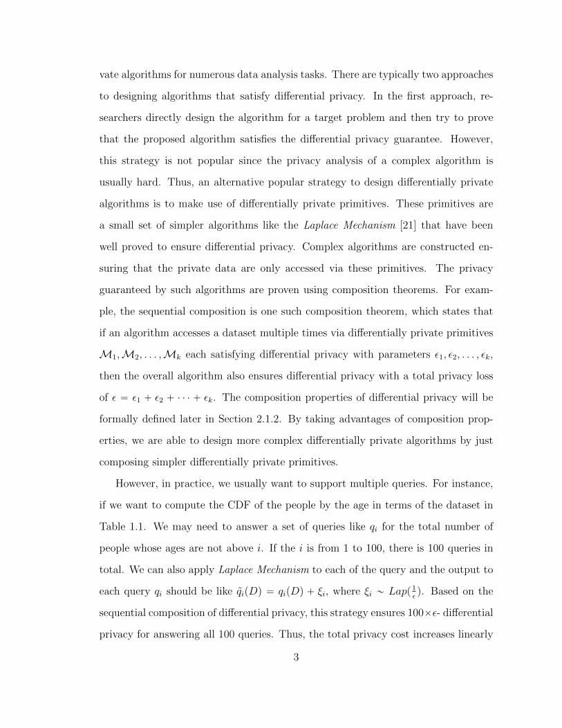
Table 1.1: Example dataset of people with different ages

Age . . . 20 21 22 23 24 25 26 . . .# of people . . . 10 15 70 20 15 45 12 . . .

gender, full date of birth, and the 5-digit zip code.

Differential privacy [21] was first proposed over a decade ago and has now be-

come a de facto standard for privacy protection due to its provable guarantee and

nice composition properties. Informally, a (randomized) algorithm ensures differen-

tial privacy if its output distributions are approximately the same when executed on

two input databases that only differ in a single individual’s record. This requirement

prevents any attacker with access to the output of differentially private algorithms

from learning anything substantial about the presence or absence of any single in-

dividual. The privacy level under differential privacy is represented by a parameter

ε, which is usually called the privacy budget, with smaller values corresponding to

stronger privacy guarantees. In order to achieve differential privacy, the basic idea

is to introduce noise to the output. Laplace Mechanism [21], which will be formally

defined in Section 2.1.3, is a standard method for achieving differential privacy. Ba-

sically, Laplace Mechanism injects Laplace noise to perturb the output for ensuring

differential privacy.

Example 1. Given a dataset about the age information of people, we derive a his-

togram (shown in Table 1.1), reporting the number of people associated with different

ages. Suppose we want to ask one query “How many people whose ages are within

20 and 25” and we apply Laplace Mechanism with total privacy budget ε. The re-

turned private answer should be equal to something like 175 ` ξ, where ξ „ Lapp1εq

is a random variable drawn from the Laplace distribution with mean 0 and the scale

parameter β “ 1ε.

There is a rich literature [19] that has led to the development of differentially pri-

2

vate algorithms for numerous data analysis tasks. There are typically two approaches

to designing algorithms that satisfy differential privacy. In the first approach, re-

searchers directly design the algorithm for a target problem and then try to prove

that the proposed algorithm satisfies the differential privacy guarantee. However,

this strategy is not popular since the privacy analysis of a complex algorithm is

usually hard. Thus, an alternative popular strategy to design differentially private

algorithms is to make use of differentially private primitives. These primitives are

a small set of simpler algorithms like the Laplace Mechanism [21] that have been

well proved to ensure differential privacy. Complex algorithms are constructed en-

suring that the private data are only accessed via these primitives. The privacy

guaranteed by such algorithms are proven using composition theorems. For exam-

ple, the sequential composition is one such composition theorem, which states that

if an algorithm accesses a dataset multiple times via differentially private primitives

M1,M2, . . . ,Mk each satisfying differential privacy with parameters ε1, ε2, . . . , εk,

then the overall algorithm also ensures differential privacy with a total privacy loss

of ε “ ε1 ` ε2 ` ¨ ¨ ¨ ` εk. The composition properties of differential privacy will be

formally defined later in Section 2.1.2. By taking advantages of composition prop-

erties, we are able to design more complex differentially private algorithms by just

composing simpler differentially private primitives.

However, in practice, we usually want to support multiple queries. For instance,

if we want to compute the CDF of the people by the age in terms of the dataset in

Table 1.1. We may need to answer a set of queries like qi for the total number of

people whose ages are not above i. If the i is from 1 to 100, there is 100 queries in

total. We can also apply Laplace Mechanism to each of the query and the output to

each query qi should be like qipDq “ qipDq ` ξi, where ξi „ Lapp1εq. Based on the

sequential composition of differential privacy, this strategy ensures 100ˆε- differential

privacy for answering all 100 queries. Thus, the total privacy cost increases linearly

3

in terms of the number of answered queries, which is not good in practice when there

is a large number of queries to be answered with a limited privacy budget. We may

either quickly use up of all the privacy budget or we can only spend a small portion

of the privacy budget to each query (introducing too much noise).

Prior work has shown that when we merely care about the identity of the queries

that lie above (or below) a given threshold instead of requiring the numeric answers

to the queries, it is possible to save the total privacy cost. As a result, by getting

rid of the numeric value answers, we can reduce the total privacy cost to be only

based on the number of queries that are above (or below) the given threshold rather

than the total number of queries [22]. Therefore, if there is a large number of queries

to be tested but only very few of them are actually above a given threshold, there

is a possible huge saving of privacy cost. The basic idea of algorithm, called the

Sparse Vector Technique, is to introduce noise to both threshold value and the query

answers. Then it outputs the identity of each tested query by comparing the noisy

query answer to the noisy threshold value. The algorithm will stop when it finds the

pre-defined number of queries that are above the given threshold.

Example 2. We still use the same dataset from Table 1.1. Suppose we have a

sequence of queries qi ““How many people whose ages are within 20 and 20 + i”,

where i “ 1, 2, . . . . Assume that we are applying Sparse Vector Technique with the

threshold θ “ 110 and the privacy budget ε “ 8 (the injected noise goes to zero), and

we only need to find one query that is above the given threshold. The Sparse Vector

Technique works as follows: (1) It tests the first query q1 “ 25 ă θ and outputs a

label showing q1 is below the threshold. (2) It tests the second query q2 “ 105 ă θ

and outputs a label showing q2 is below the threshold. (3) It tests the third query

q3 “ 125 ą θ, outputs a label showing q3 is above the threshold and then stops the

algorithm.

4

C. Dwork et al. [22] even proved that the noise scale under Sparse Vector Tech-

nique for testing k queries is Oplogpkqq, while the noise scale will become to be Opkq if

applying Laplace Mechanism with sequential composition. Sparse Vector Technique

is one differentially private primitive that helps reduce privacy cost as well as the

output error, and as such we would like to use it for designing novel algorithms to

solve practical problems under differential privacy.

Sparse Vector Technique has become a popular differentially private primitive for

building differentially private algorithms for a number of tasks [28, 51]. Recent work

[14, 37, 55] has further explored the possibility of extending Sparse Vector Technique

to eliminate the dependence of privacy cost even on the number of queries above (or

below) the threshold. The proposed Sparse Vector Technique variants try to add less

noise to each test query and allow more queries to be tested under the same privacy

level.

In this dissertation, we critically analyze the incorrect extensions of Sparse Vector

Technique in terms of its privacy guarantee. We found out that many of these variants

indeed violate differential privacy. Adversaries can even reconstruct the input data

based on the output of mechanisms designed under those variants. We further make

use of the correct version of Sparse Vector Technique as a key differentially private

primitive to propose novel algorithms for solving multiple practical problems with

differential privacy guarantee. We summarize the contributions of this dissertation

as follows.

1. Understanding Privacy Properties of Variants on Sparse Vector Tech-

nique: In this study, we critically analyze the privacy properties of multiple

variants of Sparse Vector Technique from the previous works, showing that

these variants do actually not satisfy differential privacy. We show specific

examples of neighboring datasets, queries and outputs that violate the require-

5

ment of differential privacy. We display an attack and demonstrate that these

variants make it possible for adversaries to reconstruct the real frequency of

the input data with high probability. We also propose a correct generalized

version of Sparse Vector Technique.

2. Differentially Private Regression Diagnostics: In this research, we fo-

cus on the problem of privacy-preserving diagnosing regression models. We

develop several new algorithms for doing differentially private regression diag-

nostics. In particular, we take advantage of the idea from the Sparse Vector

Technique, designing the first algorithm PriRP for computing differentially

private residual plots , which is a popular diagnostic tool for evaluating the

model fit for linear regression. We also propose the new algorithms PriBRP

for computing binned residual plots and PriROC for computing ROC curves

under differential privacy, which are diagnostic tools for measuring the model

fit as well as the predictive power for logistic regression. Comprehensive exper-

iments show that the proposed private diagnostic algorithms provide trustful

diagnostic information.

3. Differentially Private Stream Processing: In this work, we design Pe-

GaSus, a novel algorithm for answering a large class of continuous queries over

real-time data streams under differential privacy. The PeGaSus uses a com-

bination of a Perturber, a data-adaptive Grouper (by using the idea of Sparse

Vector Technique) and a query specific Smoother to simultaneously support a

range of query workloads over multiple resolutions over the stream. A thorough

empirical evaluation, on real-world data streams, shows that by using different

query specific Smoother methods, PeGaSus outperforms the state-of-the-art

algorithms specialized to given workloads.

The rest of this dissertation is organized as follows. We provide a detailed back-

6

ground on Differential Privacy and Sparse Vector Technique in Chapter 2. In Chap-

ter 3, we analyze the variants of Sparse Vector Technique, and propose attacks for

deriving sensitive information from the incorrect variants. We then present new so-

lutions to solve the problem of doing regression diagnostics under differential privacy

in Chapter 4. In Chapter 5, we discuss differentially private stream processing. Ex-

isting related works are presented in Chapter 6, and finally the conclusion of this

dissertation is discussed in Chapter 7.

7

2

Differential Privacy and Sparse Vector Technique

2.1 Differential Privacy

In this section, we explore the notion of differential privacy from multiple perspective.

2.1.1 ε-differential privacy

Differential privacy, first introduced by [17, 21], aims to protect the private informa-

tion of any single individual by limiting the privacy risk raised by the data of the

individual is used by certain analysis, compared with the result when the data is

not used. In other words, differential privacy guarantees that the information which

adversaries get from the outputs of any analysis with or without the presence of any

single individual is approximately the same, so that it will help hide the presence or

absence of any single individual from the adversaries who access to the outputs.

The formal definition of differential privacy depends on the notion of neighboring

datasets. We call D and D1 are neighboring datasets, if D1 differs from D by only

adding or removing one single record (|D ‘ D1| “ 1). The record can be defined

differently based on different applications and different privacy object. For example,

one record can contain all the location information associate with one single individ-

8

ual, or one record can represent a single connection of one user to one WiFI sensor

within a 5 minutes time interval. Then we can formally define differential privacy as

follows:

Definition 1 (ε-differential privacy). Let A be a randomized algorithm that takes as

input the form of dataset D and outputs an element from a set of possible outputs

O. Then A satisfies ε-differential privacy if for any pair of neighboring datasets D

and D1, and @O Ă O,

PrrApDq P Os ď eε ˆ PrrApD1q P Os. (2.1)

The value of ε, called privacy budget, controls the privacy risk and limits how

much an adversary can distinguish one dataset from its neighboring datasets given

the output. Smaller ε’s correspond to stronger privacy protection. Intuitively, dif-

ferentially private algorithms guarantee that the output distributions from any two

neighboring datasets are close enough such that the adversaries cannot tell which

one of the neighboring datasets is the input by just assessing to the output.

2.1.2 Composition properties of differential privacy

The following composition properties hold for differentially private algorithms [19].

Suppose A1p¨q and A2p¨q be two algorithms ensuring ε1´ and ε2´differential privacy,

respectively.

• Sequential Composition: Computing both A1pDq and A2pDq on the same

dataset D satisfies ε1 ` ε2-differential privacy.

• Parallel Composition: Let A and B be disjoint subsets of the domain, where

A X B “ H. Computing A1pD X Aq and A1pD X Bq ensures ε1-differential

privacy.

9

• Postprocessing: For any algorithm A3, releasing A3pA1pDqq still satisfies

ε1-differential privacy for any D. That is, post-processing an output of a dif-

ferentially private algorithm does not incur any additional loss of privacy.

The composition properties of differential privacy allow people to execute multiple

differentially private computations and reason about the cumulative privacy risk.

Thus, complex differentially private algorithms can be built by composing simpler

private building blocks. In each application, we can bound the total privacy risk so

we impose a total ε “privacy budget” and allocate a portion of the budget to each

private computation.

2.1.3 Laplace Mechanism

An arbitrary numerical function f can be made differentially private by injecting

noise to its output. The amount of noise depends on the sensitivity of the function.

Definition 2 (Sensitivity). Let f be a function that maps datasets to Rn. The

sensitivity denoted as ∆pfq, is defined to be the maximum L1 distance between the

function outputs from any pair of neighboring datasets D1 and D2,

∆pfq “ maxD1,D2:|D1‘D2|“1

||fpD1q ´ fpD2q||1. (2.2)

The most widely used differentially private building block, which is used for

publishing data or answering queries in a differentially private manner, is called

Laplace Mechanism [21]. Laplace Mechanism achieves differential privacy by injecting

noise from Laplace distribution calibrated to the sensitivity.

Definition 3 (Laplace Mechanism). Given a function f that maps datasets to Rn,

the Laplace Mechanism outputs fpDq`η, where η is a vector of independent random

variables drawn from a Laplace distribution with the probability density function ppx |

λq “ 12λe´|x|{λ, where λ “ ∆pfq{ε.

10

Theorem 1. Laplace Mechanism satisfies ε-differential privacy.

2.2 Sparse Vector Technique

In this section, we explore the preliminaries about Sparse Vector Technique.

2.2.1 Shortage before Sparse Vector Technique

The composition properties of differential privacy allow people to analyze the total

privacy risk raised by multiple private computations. For example, if we have a

algorithm A, say Laplace Mechanism, that satisfies ε-differential privacy. We apply

A for answering multiple queries Q “ q1, q2, q3, . . . , qk. If we spend each ε privacy

budget on every computation of qi, the total privacy budget used will be accumulated

as kˆ ε under the sequential composition property of differential privacy. Note that,

the more privacy budget consumed, the higher privacy risk encountered. Thus, the

privacy risk will be proportional to the number of queries (or computations) we make.

If there is too many queries, we are either hard to yield reasonable privacy guarantees

when spending fixed privacy budget on each query, or generate poor outputs with

fixed total privacy budget (by spending too little budget on each query).

2.2.2 Original Sparse Vector Technique

There are some situations that people only care about the identity of the queries

that lie above (or below) a certain threshold, instead of the actual numerical values

of the queries. For instance, when people are doing feature selections in order to

reduce the domain of a regression model, they may only care about the features

whose scores are above some threshold instead of their real score values. Another

example is that when doing frequent item mining task, we only want to indicate

the items with frequency above a given threshold and do not care about their real

frequency counts.

11

Fortunately, C. Dwork et al. found that, by discarding the numeric answers to

the queries and merely reporting the identity of queries that lie above or below a

certain threshold, we may save a lot of privacy budget reducing the privacy risk. In

fact, the total privacy budget (or the total privacy risk) will only increase with the

number of queries which actually lie above (or below) the threshold, rather than with

the total number of queries. If we know that the set of queries that lie above (or

below) the given threshold is much smaller than the total number of queries (which

indicates a sparse answer vector), there will be a huge saving in terms of the privacy

budget cost.

Algorithm 1 Sparse Vector Technique

Input: Dataset D, a stream of queries q1, q2, . . . with bounded sensitivity ∆,threshold θ, a cutoff point c and privacy budget εOutput: a stream of answers

1: θ Ð θ ` Lapp2∆{εq, countÐ 02: for each query i do3: vi Ð Lapp4c∆{εq

4: if qipDq ` vi ě θ then5: Output J, countÐ count` 16: else7: Output K8: end if9: if count ““ c then10: Abort11: end if12: end for

The first version of the Sparse Vector Technique was proposed by [22]. Algo-

rithm 1 presents the details of it. The inputs of Sparse Vector Technique include a

stream of queries Q “ tq1, q2, . . . u, where each q P Q has sensitivity bounded by ∆,

a threshold θ separating the identity of queries, a cutoff point c limiting the number

of queries with identity above the threshold to output at most. For every target-

ing query, Sparse Vector Technique outputs either J, showing the query is above the

threshold, or K, indicating the query is below the threshold. It works as the following

two steps:

12

1. Perturb the threshold θ by injecting noise drawn from the Laplace distribution

with scale 2∆ε

, getting θ.

2. Perturb each query qi by adding Laplace noise with scale 4c∆ε

, getting qi. Then

it outputs J when qi ě θ, and K otherwise.

Sparse Vector Technique will stop when it detects c J queries.

Theorem 2. Sparse Vector Technique satisfies ε-differential privacy.

Proof. Suppose D and D1 are any two neighboring input datasets. Let any output

O “ OK X OJ, where OK and OJ contains the set of queries labeled as K and J,

respectively. The cutoff point c indicates that |OJ| “ c. Then we have

PrrApDq “ Os “

ż 8

´8

Prrθ “ tspź

qPOK

PrrqpDq ă tsqpź

qPOJ

PrrqpDq ě tsqdt (2.3)

Since the sensitivity of all the queries are bounded by ∆, which means that

|qpDq ´ qpD1q| ď ∆ for @q P O. Thus, we have

PrrqpDq ă ts ď PrrqpD1q ă t`∆s (2.4)

Let qpDq “ qpDq ` v, where v is the independent Laplace noise injected in the line

13

4 of Algorithm 1. We can derive that

PrrApDq “ Os

“

ż 8

´8

Prrθ “ tspź

qPOK

PrrqpDq ă tsqpź

qPOJ

PrrqpDq ě tsqdt

ď

ż 8

´8

eε{2Prrθ “ t`∆spź

qPOK

PrrqpDq ă tsqpź

qPOJ

PrrqpDq ě tsqdt

ď

ż 8

´8


qPOK

PrrqpD1q ă t`∆sqpź

qPOJ

Prrv ě t´ qpDqsqdt

ď

ż 8

´8


qPOK

PrrqpD1q ă t`∆sq

ˆpź

qPOJ

eε{2cPrrv ě pt`∆q ´ qpD1qsqdt

“ eεż 8

´8

Prrθ “ t`∆spź

qPOK

PrrqpD1q ă t`∆sqpź

qPOJ

PrrqpD1q ě t`∆sqdt

“ eεPrrApD1q “ Os (2.5)

2.2.3 Utility of Sparse Vector Technique

We analyze the accuracy in terms of the outputs from Sparse Vector Technique

proposed in Algorithm 1.

Definition 4 (pα, βq-accuracy). Suppose an algorithm outputs a stream of o1, o2, ¨ ¨ ¨ P

tK,Ju˚ in the response to a stream queries q1, q2, . . . . We say the output is pα, βq-

accurate with respective to a threshold θ, if with probability at most β, we have for

all oi “ K:

qipDq ě θ ´ α (2.6)

14

and for all oi “ J:

qipDq ď θ ` α (2.7)

Theorem 3. The outputs from Sparse Vector Technique is pα, βq-accurate for

α “8c∆plog k ` logp2{βq

ε, (2.8)

where k is the total number of queries tested.

Proof. In terms of the noise added to the threshold θ, we know that θ´θ „ Lapp2∆εq.

Then we have that

Prr|θ ´ θ| ě tˆ2∆

εs “ e´t

ñ Prr|θ ´ θ| ěα

2s “ e´

εα4∆ (2.9)

When setting the quantity to be at most β{2, we require

e´εα4∆ ď

β

2

ñ α ě4∆ logp2{βq

ε(2.10)

Similarly, for each query q, we know that q ´ q „ Lapp4c∆εq. Thus we will have

Prr|q ´ q| ěα

2s “ e´

εα8c∆ (2.11)

By using a union bound, we have

PrrmaxiPrks

|qi ´ qi| ěα

2s ď k ˆ e´

εα8c∆ (2.12)

We also set the quantity to be at most β{2 and we will have

k ˆ e´εα

8c∆ ďβ

2

ñ α ě8c∆plog k ` logp2{βq

ε(2.13)

15

By combining the above two analysis, we will have

Prr|θ ´ θ| `maxiPrks

|qi ´ qi| ě αs ď β, (2.14)

when α ě 8c∆plog k`logp2{βqε

, which proves Theorem 3.

16

3

Privacy Properties of Variants on Sparse VectorTechnique

In this Chapter, I will introduce multiple variants of Sparse Vector Technique pro-

posed in the previous literatures and critically analyze the privacy properties of these

variants, showing that these variants actually do not ensure differential privacy for

any finite ε. We identify a subtle error in their privacy analysis and further show

that an adversary can use the variants to recover counts from input datasets with

high probability. We will also introduce a new correct generalized version of Sparse

Vector Technique.

3.1 Variants of Sparse Vector Technique

As shown in Algorithm 1, the privacy budget spent in the original Sparse Vector

Technique depends mainly on the number of tested queries that are above the given

threshold (that can be called “positive” queries). Recent works have explored the

possibility of extending the Sparse Vector Technique to eliminate this dependence

even on the number of “positive” queries.

17

Algorithm 2 The Variant of SVT in [37]

Input: Dataset D, query set Q with bounded sensitivity ∆, threshold θ and privacybudget εOutput: a stream of answers tK,Ju|Q|

1: ε1 Ð ε{4, ε2 Ð 3ε{4

2: θ Ð θ ` Lapp∆{ε1q3: for each query qi P Q do4: vi Ð Lapp∆{ε2q

5: if qipDq ` vi ě θ then6: Output J7: else8: Output K9: end if10: end for

J. Lee et al. proposed one variant of Sparse Vector Technique (shown in Algo-

rithm 2) for achieving differentially private frequent itemsets mining [37]. In their

work, they used the Sparse Vector Technique variant for checking whether the tar-

geted itemset has the frequency more than a given threshold θ. In Algorithm 2,

the noisy threshold is computed by using ε4

privacy budget, and each single query

is perturbed by using an independent 3ε4

privacy budget, which does not depend on

the number of “positive” queries.



1: θ Ð θ ` Lapp∆{εq2: for each query qi P Q do3: if qipDq ě θ then4: Output J5: else6: Output K7: end if8: end for

B. Stoddard et al. extended the Sparse Vector Technique (displayed in Algo-

rithm 3) on doing feature selection for classification tasks [55]. In their work, the

authors applied their proposed variant of Sparse Vector Technique for determining

the choice of features by selecting ones whose scores are above certain pre-defined

18

threshold. In Algorithm 3, the entire privacy budget is used for perturbing the

threshold and the real answers to the queries are compared with the noisy threshold.



1: ε1 Ð ε{2, ε2 Ð ε{2



Another variant of Sparse Vector Technique (shown in Algorithm 4) was proposed

by R. Chen et al. in [14] for generating synthetic high-dimensional datasets. They

make use of use their Sparse Vector Technique variant for generating the dependency

graph among all attributes. Specifically, they choose a set of new attributes whose

mutual information score with the previous attribute is above certain threshold. In

the Algorithm 4, half of the privacy budget is spent on computing noisy threshold.

Also, independent privacy budget of the remaining half is used for perturbing each

mutual information score query. The noisy query answers are then compared with

the noisy threshold.

3.2 Generalized Private Threshold Testing

3.2.1 Description of Generalized Private Threshold Testing

All the variants of Sparse Vector Technique introduced in the previous section (Al-

gorithm 2, 3, 4) are trying to eliminate the dependence of the privacy cost on the

number of “positive” queries. The only difference among these variants is the amount

of noise injected to either threshold or each individual query.

19

Algorithm 5 Generalized Private Threshold Testing (GPTT)


1: ε1, ε2 Ð fpεq



We summarize and describe a method called Generalized Private Threshold Test-

ing (GPTT) that generalize all the variants of the Sparse Vector Technique that do

not require a limit on the number of “positive” queries. The details of GPTT is

displayed in Algorithm 5.

GPTT takes as input a dataset D, a set of queries Q “ tq1, q2, . . . , qnu with

bounded sensitivity ∆, a threshold θ and a privacy budget ε. For every query qi P Q,

GPTT outputs either J or K that approximates whether or not the query qi is

above or below the given threshold θ. GPTT works exactly like the original Sparse

Vector Technique - the threshold is perturbed by injecting noise from Laplace noise

with parameter ∆{ε1 and every query answer is also perturbed by adding noise

from independent Laplace noise with parameter ∆{ε2. The output is determined

by comparing the noisy threshold with each noisy query answer. You can see the

difference is that there is no limits on the number of “positive” queries to be tested

and output by the algorithm.

GPTT is a generalization of all the variants presented in the previous section in

terms of the function fpεq for determining the value of both ε1 and ε2. [37] used

GPTT for private itemset mining with ε1 “ ε{4 and ε2 “ 3ε{4. R. Chen et al.

in [14] instantiate GPTT with ε1 “ ε2 “ ε{2, for high-dimensional data release.

20

[55] indicated that the privacy guarantee does not depend on the setting of ε2 and

proposed an instantiation of GPTT with ε1 “ ε and ε2 “ 8, for private feature

selection.

3.2.2 Privacy Analysis of GPTT based on Previous Works

In this section, we derive and extend the privacy analysis from previous works [37],

[14], [55] on our proposed GPTT algorithm. We will show, in Section 3.2.3, that this

privacy analysis is flawed and GPTT (as well as all the instantiations presented in

previous works) does not ensure differential privacy.

Given any set of queriesQ “ tq1, q2, . . . , qnu, we let the vector o “ă v1, v2, . . . , vn ąP

tK,Jun denote the output from GPTT. Given any two neighboring datasets D1

and D2, we assume P1 and P2 be the output distribution of v given the input

dataset D1 and D2, respectively. We use oăt to denote t ´ 1 previous answers (i.e.,

oăt “ă o1, o2, . . . , ot´1 ą). Then, we have

P1poq

P2poq“

śni“1 P1poi | o

ăiqśn

i“1 P2poi | oăiq“

ź

i:oi“J

P1poi “ J | oăiq

P2poi “ J | oăiqˆ

ź

i:oi“K

P1poi “ K | oăiq

P2poi “ K | oăiq(3.1)

Let Hipxq be the probability that qi is classified as “positive” query (i.e. oi “ J),

when the noisy threshold is x. That is,

Hipxq “ Prroi “ J | x, oăis “ Prroi “ J | xs. (3.2)

Since the noisy query is derived by injecting noise from a Laplace distribution

with parameter ∆{ε2, we can denote that the distribution of the noisy query answer

of qi is from a distribution of fpy;µ, λq “ 12λexpp´ |y´µ|

λq, where µ “ qi and λ “ ∆{ε2.

Therefore, we have

Hipxq “

ż 8

x

fpy; qi,∆{ε2qdy “

ż 8

x`∆

fpy; qi `∆,∆{ε2qdy. (3.3)

21

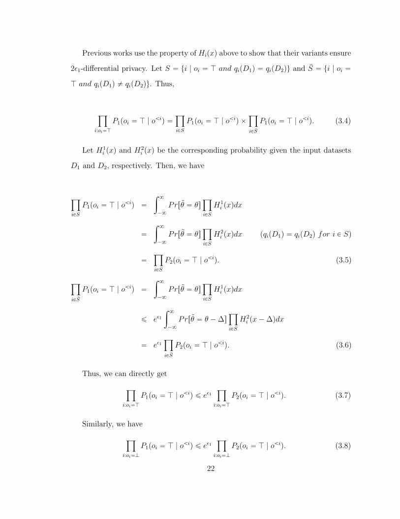
Previous works use the property of Hipxq above to show that their variants ensure

2ε1-differential privacy. Let S “ ti | oi “ J and qipD1q “ qipD2qu and S “ ti | oi “

J and qipD1q ‰ qipD2qu. Thus,

ź

i:oi“J

P1poi “ J | oăiq “

ź

iPS

P1poi “ J | oăiq ˆ

ź

iPS

P1poi “ J | oăiq. (3.4)

Let H1i pxq and H2

i pxq be the corresponding probability given the input datasets

D1 and D2, respectively. Then, we have

ź

iPS


ż 8

´8

Prrθ “ θsź

iPS

H1i pxqdx

“

ż 8

´8

Prrθ “ θsź

iPS

H2i pxqdx pqipD1q “ qipD2q for i P Sq

“ź

iPS

P2poi “ J | oăiq. (3.5)

ź

iPS


ż 8

´8

Prrθ “ θsź

iPS

H1i pxqdx

ď eε1ż 8

´8

Prrθ “ θ ´∆sź

iPS

H2i px´∆qdx

“ eε1ź

iPS

P2poi “ J | oăiq. (3.6)

Thus, we can directly get

ź

i:oi“J

P1poi “ J | oăiq ď eε1

ź

i:oi“J

P2poi “ J | oăiq. (3.7)

Similarly, we have

ź

i:oi“K

P1poi “ J | oăiq ď eε1

ź

i:oi“K

P2poi “ J | oăiq. (3.8)

22

Therefore, P1poq{P2poq ď e2ε1 . We will mention that injecting noise to the queries

is not really required. The proof above will go through even if ε2 goes to infinity.

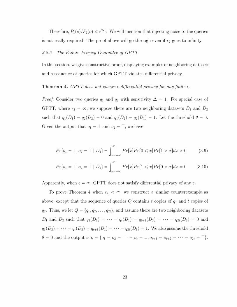
3.2.3 The Failure Privacy Guarantee of GPTT

In this section, we give constructive proof, displaying examples of neighboring datasets

and a sequence of queries for which GPTT violates differential privacy.

Theorem 4. GPTT does not ensure ε-differential privacy for any finite ε.

Proof. Consider two queries q1 and q2 with sensitivity ∆ “ 1. For special case of

GPTT, where ε2 “ 8, we suppose there are two neighboring datasets D1 and D2

such that q1pD1q “ q2pD2q “ 0 and q1pD2q “ q2pD1q “ 1. Let the threshold θ “ 0.

Given the output that o1 “ K and o2 “ J, we have

Prro1 “ K, o2 “ J | D1s “

ż 8

x“´8

PrrxsPrr0 ď xsPrr1 ą xsdx ą 0 (3.9)

Prro1 “ K, o2 “ J | D2s “

ż 8

x“´8

PrrxsPrr1 ď xsPrr0 ą xsdx “ 0 (3.10)

Apparently, when ε “ 8, GPTT does not satisfy differential privacy of any ε.

To prove Theorem 4 when ε2 ă 8, we construct a similar counterexample as

above, except that the sequence of queries Q contains t copies of q1 and t copies of

q2. Thus, we let Q “ tq1, q2, . . . , q2tu, and assume there are two neighboring datasets

D1 and D2 such that q1pD1q “ ¨ ¨ ¨ “ qtpD1q “ qt`1pD2q “ ¨ ¨ ¨ “ q2tpD2q “ 0 and

q1pD2q “ ¨ ¨ ¨ “ qtpD2q “ qt`1pD1q “ ¨ ¨ ¨ “ q2tpD1q “ 1. We also assume the threshold

θ “ 0 and the output is o “ to1 “ o2 “ ¨ ¨ ¨ “ ot “ K, ot`1 “ ot`2 “ ¨ ¨ ¨ “ o2t “ Ju.

23

Then we have

P1poq “ PrrGPTT pD1q “ os

“

ż 8

´8

Prrθ “ zstź

i“1

Prrqi ď zs2tź

i“t`1

Prrqi ą zsdz

“

ż 8

´8

fε1pFε2pzqqtp1´ Fε2pz ´ 1qqtdz

“

ż 8

´8

fε1pFε2pzq ´ Fε2pzqFε2pz ´ 1qqtdz, (3.11)

where fε and Fε are the PDF and CDF, respectively, of the Laplace distribution with

parameter 1{ε. Similarly, we can derive, in terms of datasets D2, that

P2poq “ PrrGPTT pD2q “ os “

ż 8

´8

fε1pFε2pz ´ 1q ´ Fε2pz ´ 1qFε2pzqqtdz. (3.12)

Let P2poq “ α and δ “ |F´1ε1pα{4q|. Since α ď 1, δ is greater than the 75th

percentile of a Laplace distribution with scale 1{ε1. That means,

α

2ě

ż ´δ

´8

fε1ptqdt`

ż 8

δ

fε1ptqdt. (3.13)

Moreover, note that Fε2pz ´ 1q ă Fε2pzq for all z, we have

κpzq “Fε2pzq ´ Fε2pzqFε2pz ´ 1q

Fε2pz ´ 1q ´ Fε2pz ´ 1qFε2pzqą 1. (3.14)

Let κ “ minzPr´δ,δs κpzq and κ ą 1. We can get

α “ P2poq “

ż 8

´8

fε1pFε2pz ´ 1q ´ Fε2pz ´ 1qFε2pzqqtdz

ă

ż

zRr´δ,δs

fε1dz `

ż δ

´δ

fε1pFε2pz ´ 1q ´ Fε2pz ´ 1qFε2pzqqtdz

ďα

2`

ż δ

´δ

fε1pFε2pz ´ 1q ´ Fε2pz ´ 1qFε2pzqqtdz. (3.15)

24

Thus, we can derive

ż δ

´δ

fε1pFε2pz ´ 1q ´ Fε2pz ´ 1qFε2pzqqtdz ą

P2poq

2. (3.16)

Therefore, we get

P1poq “

ż 8

´8

fε1pFε2pzq ´ Fε2pzqFε2pz ´ 1qqtdz

ą

ż δ

´δ

fε1pFε2pzq ´ Fε2pzqFε2pz ´ 1qqtdz

ą

ż δ

´δ

fε1pFε2pz ´ 1q ´ Fε2pz ´ 1qFε2pzqκpzqqtdz

ąκt

2P2poq. (3.17)

Since κ ą 1, for every finite ε ą 1, there exists a value of t such that κt ě 2ε,

which means P1poq ą eεP2poq, violating differential privacy.

We now indicate the subtle error in the privacy analysis shown in Section 3.2.2,

where the previous works ([37], [55], [14]) made.

25

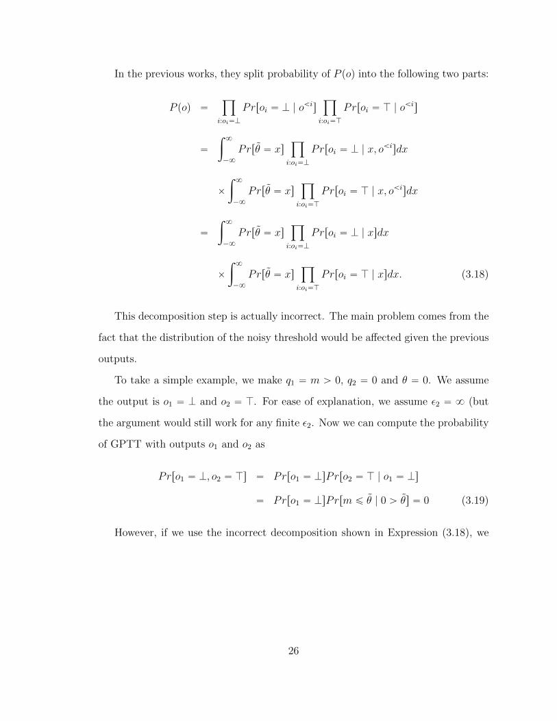
In the previous works, they split probability of P poq into the following two parts:

P poq “ź

i:oi“K

Prroi “ K | oăisź

i:oi“J

Prroi “ J | oăis

“

ż 8

´8

Prrθ “ xsź

i:oi“K

Prroi “ K | x, oăisdx

ˆ

ż 8

´8

Prrθ “ xsź

i:oi“J

Prroi “ J | x, oăisdx

“

ż 8

´8

Prrθ “ xsź

i:oi“K

Prroi “ K | xsdx

ˆ

ż 8

´8

Prrθ “ xsź

i:oi“J

Prroi “ J | xsdx. (3.18)

This decomposition step is actually incorrect. The main problem comes from the

fact that the distribution of the noisy threshold would be affected given the previous

outputs.

To take a simple example, we make q1 “ m ą 0, q2 “ 0 and θ “ 0. We assume

the output is o1 “ K and o2 “ J. For ease of explanation, we assume ε2 “ 8 (but

the argument would still work for any finite ε2. Now we can compute the probability

of GPTT with outputs o1 and o2 as

Prro1 “ K, o2 “ Js “ Prro1 “ KsPrro2 “ J | o1 “ Ks

“ Prro1 “ KsPrrm ď θ | 0 ą θs “ 0 (3.19)

However, if we use the incorrect decomposition shown in Expression (3.18), we

26

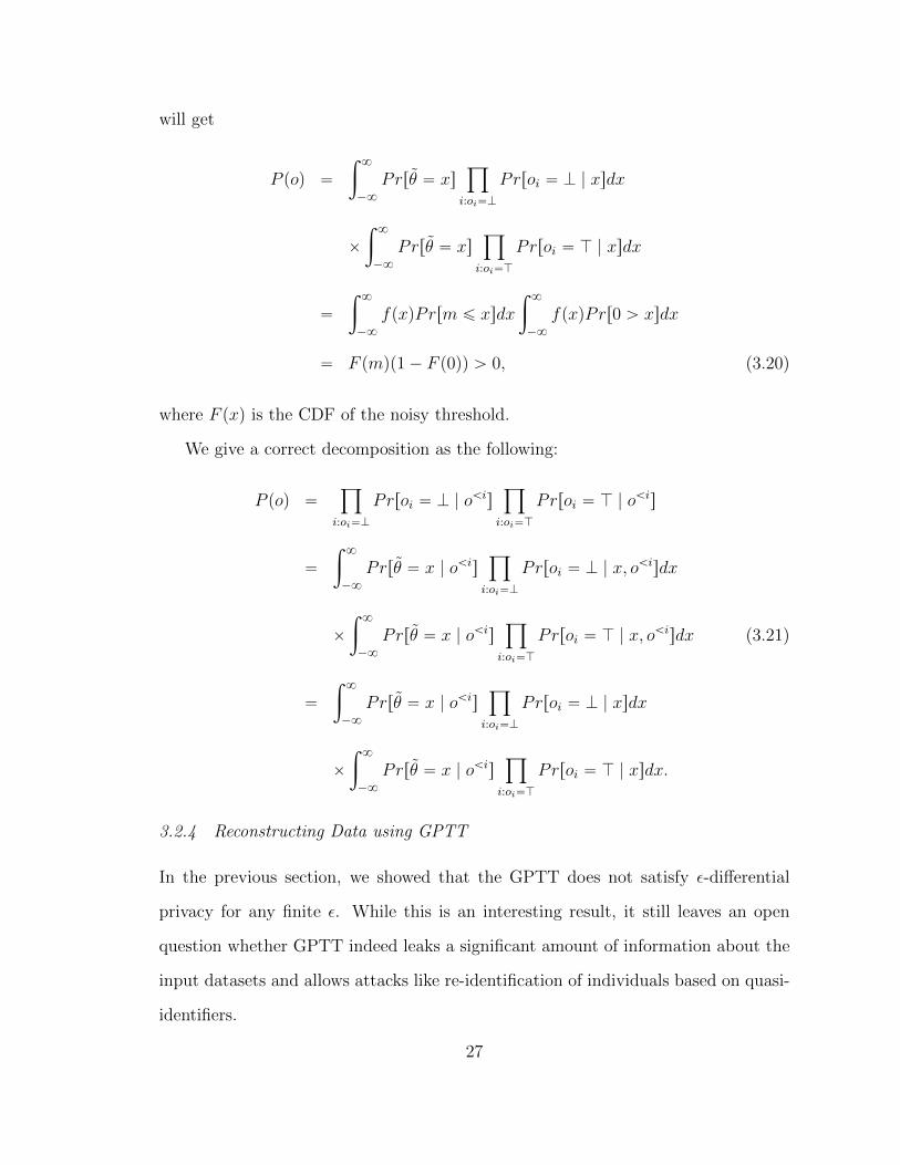
will get

P poq “

ż 8

´8

Prrθ “ xsź

i:oi“K

Prroi “ K | xsdx

ˆ

ż 8

´8

Prrθ “ xsź

i:oi“J

Prroi “ J | xsdx

“

ż 8

´8

fpxqPrrm ď xsdx

ż 8

´8

fpxqPrr0 ą xsdx

“ F pmqp1´ F p0qq ą 0, (3.20)

where F pxq is the CDF of the noisy threshold.

We give a correct decomposition as the following:

P poq “ź

i:oi“K

Prroi “ K | oăisź

i:oi“J

Prroi “ J | oăis

“

ż 8

´8

Prrθ “ x | oăisź

i:oi“K

Prroi “ K | x, oăisdx

ˆ

ż 8

´8


i:oi“J

Prroi “ J | x, oăisdx (3.21)

“

ż 8

´8


i:oi“K

Prroi “ K | xsdx

ˆ

ż 8

´8


i:oi“J

Prroi “ J | xsdx.

3.2.4 Reconstructing Data using GPTT

In the previous section, we showed that the GPTT does not satisfy ε-differential

privacy for any finite ε. While this is an interesting result, it still leaves an open

question whether GPTT indeed leaks a significant amount of information about the

input datasets and allows attacks like re-identification of individuals based on quasi-

identifiers.

27

In this section, we answer this question in the affirmative, and show that GPTT

can disclose the exact counts of domain values with high probability. Exact disclosure

of cells with small counts (especially, cells with counts 0, 1 and 2) reveals the presence

of unique individuals in the data who can be susceptible to re-identification attacks.

We will consider the special case of GPTT where ε2 “ 8. The general case with

finite ε2 can be similarly analyzed.

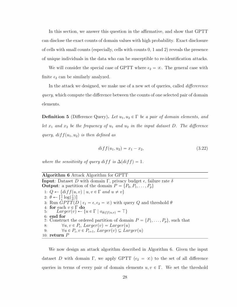
In the attack we designed, we make use of a new set of queries, called differerence

query, which compute the difference between the counts of one selected pair of domain

elements.

Definition 5 (Difference Query). Let u1, u2 P Γ be a pair of domain elements, and

let x1 and x2 be the frequency of u1 and u2 in the input dataset D. The difference

query, diffpu1, u2q is then defined as

diffpu1, u2q “ x1 ´ x2, (3.22)

where the sensitivity of query diff is ∆pdiffq “ 1.

Algorithm 6 Attack Algorithm for GPTT

Input: Dataset D with domain Γ, privacy budget ε, failure rate δOutput: a partition of the domain P “ tP0, P1, . . . , Ppu

1: QÐ tdiffpu, vq | u, v P Γ and u ‰ vu2: θ Ð r1

εlogp1

δqs

3: Run GPTT pD | ε1 “ ε, ε2 “ 8q with query Q and threshold θ4: for each v P Γ do5: Largerpvq Ð tu P Γ | odiffpu,vq “ Ju6: end for7: Construct the ordered partition of domain P “ tP1, . . . , Ppu, such that8: @u, v P Pi, Largerpvq “ Largerpuq9: @u P Pi, v P Pi`1, Largerpvq Ĺ Largerpuq10: return P

We now design an attack algorithm described in Algorithm 6. Given the input

dataset D with domain Γ, we apply GPTT (ε2 “ 8) to the set of all difference

queries in terms of every pair of domain elements u, v P Γ. We set the threshold

28

θ “ r1ε

logp1δqs. Pairs of domain elements u, v P Γ are then grouped together if for each

w P Γ, GPTT gives the same output for diffpu,wq and diffpv, wq. Algorithm 6 will

result in a partition of the entire domain Γ. Furthermore, for each domain element

u P Γ, we define Largerpuq to be the set of domain elements from Γ, where for each

v P Largerpuq, GPTT outputs J for diffpv, uq. These are the domain elements that

ensure xv ´ xu ą θ, where θ is the noisy threshold. We order the partitions at the

end such that every element u P Pi has a bigger Largerpuq set than any element

v P Pj, for j ą i.

We can show that the ordered partitions P imposes an ordering on the counts in

the database D.

Lemma 5. Let D be a dataset from domain Γ. Let P “ tP0, P1, . . . , Ppu be the

ordered partitions of Γ output by Algorithm 6. Then, with probability 1 ´ δ, for all

0 ď l ă m ď p, u P Pl, v P Pm, we have xu ă xv.

Proof. Let θ be the noisy threshold. Since θ “ r1ε

logp1δqs, with probability at least

1 ´ δ, θ ą 0. For any u P Pl and v P Pm, we know Largerpvq Ĺ Largerpuq. Thus,

there exists w P Γ such that xw ´ xu ą θ but xw ´ xv ď θ. Therefore, xu ă xv.

Let Si Ă Γ denote the set of domain elements whose frequency in D is equal to

i. It is easy to see that for every Si, there is some P ˚ P P output by Algorithm 6

such that Si Ă P ˚. We next show that, for certain datasets, there exists an m ą 0

such that the sets of domain elements with frequency between [0, m] can be exactly

reproduced in the partition from Algorithm 6.

Theorem 6. Let P “ tP0, P1, . . . , Ppu be the ordered partitions output by Algorithm 6

based on the input D with parameter ε. Let D be a dataset such that Si ‰ H for

all i P r0, ks. That is, D contain at least one domain element with frequency equal

to 0, 1, . . . , k. Let α “ r1ε

logp1δqs. If k ą 2α, with probability at least 1 ´ δ, for all

i P r0,ms, Pi “ Si, where m “ k ´ 2α.

29

Proof. Since θ “ α “ r1ε

logp1δqs, with probability at least 1 ´ δ, the noisy threshold

will be within r0, 2αs. For the dataset D such that Si ‰ H for all i P r0, ks, where

k ą 2α, let i P r0,m´ 1s. Suppose u P Si and v P Si`1, then we have

Largerpuq “ tz | xz ą θ ` iu

Largerpvq “ tz | xz ą θ ` i` 1u (3.23)

Since i P r0,m´1s, with probability at least 1´ δ, θ` i ď m´1`2α ă k. Thus,

we have

Srθ`is Ă Largerpuq ´ Largerpvq ‰ H (3.24)

Therefore, we have Largerpuq Ĺ Largerpvq and Si, Si`1 will not appear in the

same partition P ˚ P P .

Furthermore, since we know S0, S1, . . . , Sm belong to separate partitions from P

and we have P “ tP0, P1, . . . , Ppu be the ordered partitions. Thus, we have Pi “ Si

for i P r0,ms.

Theorem 6 shows that, for datasets that have domain elements with frequency

equal to i for all i P r0, ks, we can exactly tell the domain elements with frequency

within r0, k´2αs with high probability. A number of datasets satisfy this assumption.

For instance, the datasets that are drawn from a Zipfian distribution, where the size

of Si is in expectation inversely proportional to the count i, and thus all small counts

will have support for datasets of sufficiently large size. We also tested our attack

algorithm on a number of real-world datasets.

Table 3.1 displays the overview of some real-world datasets. Adult is a histogram

constructed from U.S. Census data [40] on the attribute of “capital loss”. Medical-

Cost is a histogram of personal medical expenses from the survey of United States

department of health, human services in 2007. Income is the histogram on “personal

income” attribute from [36]. HepPh is a histogram constructed using the citation

30

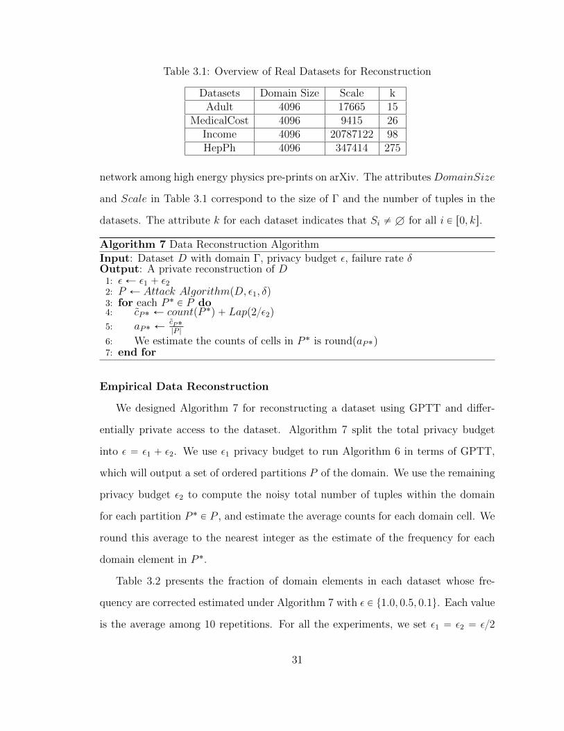
Table 3.1: Overview of Real Datasets for Reconstruction

Datasets Domain Size Scale kAdult 4096 17665 15

MedicalCost 4096 9415 26Income 4096 20787122 98HepPh 4096 347414 275

network among high energy physics pre-prints on arXiv. The attributes DomainSize

and Scale in Table 3.1 correspond to the size of Γ and the number of tuples in the

datasets. The attribute k for each dataset indicates that Si ‰ H for all i P r0, ks.

Algorithm 7 Data Reconstruction Algorithm

Input: Dataset D with domain Γ, privacy budget ε, failure rate δOutput: A private reconstruction of D1: εÐ ε1 ` ε22: P Ð Attack AlgorithmpD, ε1, δq3: for each P ˚ P P do4: cP˚ Ð countpP ˚q ` Lapp2{ε2q

5: aP˚ ÐcP˚|P |

6: We estimate the counts of cells in P ˚ is round(aP˚)7: end for

Empirical Data Reconstruction

We designed Algorithm 7 for reconstructing a dataset using GPTT and differ-

entially private access to the dataset. Algorithm 7 split the total privacy budget

into ε “ ε1 ` ε2. We use ε1 privacy budget to run Algorithm 6 in terms of GPTT,

which will output a set of ordered partitions P of the domain. We use the remaining

privacy budget ε2 to compute the noisy total number of tuples within the domain

for each partition P ˚ P P , and estimate the average counts for each domain cell. We

round this average to the nearest integer as the estimate of the frequency for each

domain element in P ˚.

Table 3.2 presents the fraction of domain elements in each dataset whose fre-

quency are corrected estimated under Algorithm 7 with ε P t1.0, 0.5, 0.1u. Each value

is the average among 10 repetitions. For all the experiments, we set ε1 “ ε2 “ ε{2

31

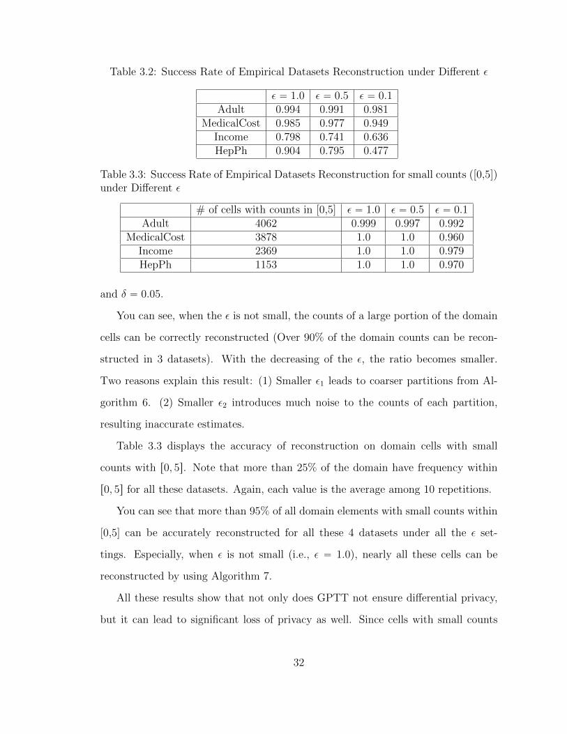
Table 3.2: Success Rate of Empirical Datasets Reconstruction under Different ε

ε “ 1.0 ε “ 0.5 ε “ 0.1Adult 0.994 0.991 0.981

MedicalCost 0.985 0.977 0.949Income 0.798 0.741 0.636HepPh 0.904 0.795 0.477

Table 3.3: Success Rate of Empirical Datasets Reconstruction for small counts ([0,5])under Different ε

# of cells with counts in [0,5] ε “ 1.0 ε “ 0.5 ε “ 0.1Adult 4062 0.999 0.997 0.992

MedicalCost 3878 1.0 1.0 0.960Income 2369 1.0 1.0 0.979HepPh 1153 1.0 1.0 0.970

and δ “ 0.05.

You can see, when the ε is not small, the counts of a large portion of the domain

cells can be correctly reconstructed (Over 90% of the domain counts can be recon-

structed in 3 datasets). With the decreasing of the ε, the ratio becomes smaller.

Two reasons explain this result: (1) Smaller ε1 leads to coarser partitions from Al-

gorithm 6. (2) Smaller ε2 introduces much noise to the counts of each partition,

resulting inaccurate estimates.

Table 3.3 displays the accuracy of reconstruction on domain cells with small

counts with r0, 5s. Note that more than 25% of the domain have frequency within

r0, 5s for all these datasets. Again, each value is the average among 10 repetitions.

You can see that more than 95% of all domain elements with small counts within

[0,5] can be accurately reconstructed for all these 4 datasets under all the ε set-

tings. Especially, when ε is not small (i.e., ε “ 1.0), nearly all these cells can be

reconstructed by using Algorithm 7.

All these results show that not only does GPTT not ensure differential privacy,

but it can lead to significant loss of privacy as well. Since cells with small counts

32

can be reconstructed with very high probability (ą 95%) from the output of GPTT,

accessing to the data via GPTT allows re-identification attacks. Hence, we believe

that systems whose privacy stems from GPTT are not safe to use.

3.3 Generalized Version of Sparse Vector Technique

We have discussed the incorrect variants of Sparse Vector Technique proposed in

the previous works. In the section, we present another generalized version of Sparse

Vector Technique, which relaxed the conditions in terms of the threshold settings.

Specifically, we allow different thresholds to be compared with different queries. Also

the compared threshold can also be dependent on the input dataset.

3.3.1 Description of Generalized Sparse Vector Technique

Algorithm 8 Generalized Sparse Vector Technique

Input: Dataset D, a stream of queries Q “ q1, q2, . . . with bounded sensitivity ∆1,a set of threshold functions Θ “ θ1, θ2, . . . with bounded sensitivity ∆2 ,a cutoff point c and privacy budget εOutput: a stream of answers P tK,Ju

1: αÐ Lapp2p∆1`∆2q

ε2: for each query i “ 1, 2, . . . do

3: vi Ð Lapp4cp∆1`∆2q

εq, countÐ 0

4: if qipDq ` vi ě θipDq ` α then5: Output J, countÐ count` 16: else7: Output K8: end if9: if count ““ c then10: Abort11: end if12: end for

Algorithm 8 displays our proposed generalized Sparse Vector Technique. It takes

as inputs a stream of queries Q “ tq1, q2, . . . u, where each q P Q has sensitivity

bounded by ∆1, another stream of threshold functions Θ “ tθ1, θ2, . . . , u, where each

θ P Θ has bounded sensitivity ∆2, a cutoff point c limiting the number of queries

with identity above the threshold to output and a privacy budget ε. Algorithm 8 will

33

give a stream of outputs from tK,Ju with at most c J. Algorithm 8 works based on

the following two steps:

1. Generate a random noise α from the Laplace distribution with scale 2p∆1`∆2q

ε.

2. Perturb each query qi by adding Laplace noise with scale 4cp∆1`∆2q

ε, getting qi.

Then it outputs J, when qipDq ě θipDq ` α, and K otherwise.

Algorithm 8 will stop, when it outputs c J values.

3.3.2 Privacy Analysis of Generalized Sparse Vector Technique

Theorem 7. The generalized Sparse Vector Technique (Algorithm 8) ensures ε-

differential privacy.

Proof. Suppose D and D1 are any two neighboring datasets. Let any output O “

OKXOJ, where OK and OJ contain the set of queries labeled as K and J, respectively.

The cutoff point c indicates that |OJ| “ c. Then we have

PrrApDq “ Os

“

ż 8

´8

Prrα “ tspź

iPOK

PrrqipDq ă θipDq ` αqpź

iPOJ

PrrqipDq ě θipDq ` αsqdt.

(3.25)

Let qipDq “ qipDq`vi, where vi is the independent Laplace noise injected to each

query in the line 4 of Algorithm 8. Then, we can derive

34

PrrApDq “ Os

“

ż 8

´8

Prrα “ tspź

iPOK

PrrqipDq ă θipDq ` tqpź

iPOJ

PrrqipDq ě θipDq ` tsqdt

ď

ż 8

´8

eε{2Prrα “ t`∆1 `∆2spź

iPOK

PrrqipDq ă θipDq ` tq

ˆpź

iPOJ

PrrqipDq ě θipDq ` tsqdt

ď

ż 8

´8


iPOK

PrrqipD1q ă θipD

1q ` t`∆1 `∆2q

ˆpź

iPOJ

Prrvi ě θipDq ` t`∆1 `∆2 ´ qipDqsqdt

ď

ż 8

´8


iPOK

PrrqipD1q ă θipD

1q ` t`∆1 `∆2q

ˆpź

iPOJ

eε{2cPrrvi ě θipD1q ` t`∆1 `∆2 ´ qipD

1qsqdt

“ eεż 8

´8

Prrα “ tspź

iPOK

PrrqipD1q ă θipD

1q ` tqp

ź

iPOJ

PrrqipD1q ě θipD

1q ` tsqdt.

“ eεPrrApD1q “ Os (3.26)

3.3.3 Utility Analysis of Generalized Sparse Vector Technique

We also analyze the utility of the generalized Sparse Vector Technique.

Theorem 8. The outputs from generalized Sparse Vector Technique is pγ, βq-accurate

for

γ “8cp∆1 `∆2qplog k ` logp2{βq

ε, (3.27)

35

where k is the total number of queries tested.

Proof. The noise α „ Lapp2p∆1`∆2q

εq, and we have

Prr|α| ě tˆ2p∆1 `∆2q

εs “ e´t

ñ Prr|α| ěγ

2s “ e

´εγ

4p∆1`∆2q . (3.28)

When setting this quantity to be at most β{2, we require

e´

εγ4p∆1`∆2q ď

β

2

ñ γ ě 4p∆1 `∆2q logp2{βq{ε. (3.29)

Similarly, for each query qi, the injected noise vi „ Lapp4cp∆1`∆2q

εq. Thus, we

have

Prr|vi| ěγ

2s “ e

´εγ

8cp∆1`∆2q . (3.30)

By using a union bound, we have

PrrmaxiPrks

|vi| ěγ

2s ď k ˆ e

´εγ

8cp∆1`∆2q . (3.31)

We also set the quantity to be at most β{2 and we have

k ˆ e´

εγ8cp∆1`∆2q ď

β

2

ñ γ ě8cp∆1 `∆2qplog k ` logp2{βq

ε. (3.32)

By combining the above two analysis, we will have

Prr|α| `maxiPrks

|vi| ě αs ď β, (3.33)

when γ ě 8cp∆1`∆2qplog k`logp2{βqε

, which proves the theorem.

36

4

Differentially Private Regression Diagnostics

In this Chapter, we focus on solving the problem of doing regression diagnostics under

differential privacy. We will use the Sparse Vector Technique as a key differentially

private primitive for designing some components of the algorithms.

4.1 Introduction

The increasing digitization of personal information increased concerns over ensuring

the confidentiality of the individuals from whom such data are collected. And dif-

ferential privacy was proposed for protecting the sensitive information of individuals

from being inferred by attackers.

We consider contexts where analysts, working under privacy constraints, seek to

explain or predict some outcome y from a multi-variate set of variables x. Absent

privacy constraints, the go-to tool for this task is regression modeling.

For continuous outcomes, the most popular model is linear regression, in which

we assume that y “ β0 ` β ¨ x` ξ, where the βs are called coefficients, and ξ is the

error assumed to be from the normal distribution Np0, σ2q with zero mean and some

unknown fixed standard deviation σ.

37

For binary outcomes (y P t0, 1u), the most popular model is logistic regression,

in which we assume that y, given x, has a Bernoulli distribution with probability

P py “ 1 | xq where logrP py “ 1 | xq{p1 ´ P py “ 1 | xqqs “ β0 ` β ¨ x. One can use

non-linear functions of x in the predictor function in either model.

Regression is used for two primary tasks – explain associations between the out-

come and the explanatory variable and predict the outcome on unseen data. The

former is especially important in public health, epidemiology, and the social sciences,

where the scientific questions typically focus on whether specific variables are impor-

tant (e.g., statistically significant) or unimportant predictors of the outcome. For

example, in a linear regression seeking to explain salaries from demographic vari-

ables, a social scientist might be interested in whether or not the coefficient (β) for

an explanatory variable indicating “sex is female” is statistically significant, given

the other variables in the model. The validity of such inferences depends critically on

the reasonableness of the assumptions underpinning the model. For example, if the

analyst specifies a linear relationship between salary and age (in years) in the model,

but the true generative relationship is quadratic (as it generally is), it is pointless to

interpret the inferences for the coefficient for age from the ordinary least squares fit.

The fitted model completely misrepresents the association. Thus, besides estimating

the parameters of the model, analysts must be able to evaluate how well the posited

model assumptions fit the theoretical assumptions underpinning regression analyses

for the data at hand. Similarly, when regression is used for prediction, analysts must

be able to assess the extent to which the model can predict outcomes accurately for

unseen data (e.g., out of sample records).

Absent privacy constraints, analysts have a variety of tools to diagnose the fit

and predictive power of regression models. Model fit for linear regression is typically

assessed by examining the distribution of residuals, which are observed values minus

predicted values (defined formally in Section 4.2). For logistic regression, model

38

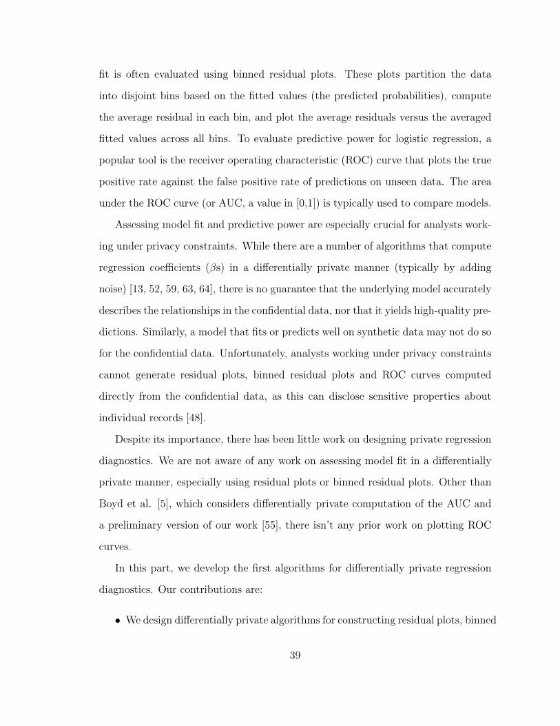
fit is often evaluated using binned residual plots. These plots partition the data

into disjoint bins based on the fitted values (the predicted probabilities), compute

the average residual in each bin, and plot the average residuals versus the averaged

fitted values across all bins. To evaluate predictive power for logistic regression, a

popular tool is the receiver operating characteristic (ROC) curve that plots the true

positive rate against the false positive rate of predictions on unseen data. The area

under the ROC curve (or AUC, a value in [0,1]) is typically used to compare models.

Assessing model fit and predictive power are especially crucial for analysts work-

ing under privacy constraints. While there are a number of algorithms that compute

regression coefficients (βs) in a differentially private manner (typically by adding

noise) [13, 52, 59, 63, 64], there is no guarantee that the underlying model accurately

describes the relationships in the confidential data, nor that it yields high-quality pre-

dictions. Similarly, a model that fits or predicts well on synthetic data may not do so

for the confidential data. Unfortunately, analysts working under privacy constraints

cannot generate residual plots, binned residual plots and ROC curves computed

directly from the confidential data, as this can disclose sensitive properties about

individual records [48].

Despite its importance, there has been little work on designing private regression

diagnostics. We are not aware of any work on assessing model fit in a differentially

private manner, especially using residual plots or binned residual plots. Other than

Boyd et al. [5], which considers differentially private computation of the AUC and

a preliminary version of our work [55], there isn’t any prior work on plotting ROC

curves.

In this part, we develop the first algorithms for differentially private regression

diagnostics. Our contributions are:

• We design differentially private algorithms for constructing residual plots, binned

39

residual plots and ROC curves. While the algorithms are based on well-known

building blocks for answering range queries on databases, their application to

assessing regression models is novel.

• Plotting residuals for linear regression under differential privacy is challenging,

since a priori there is no bound on residuals. Hence, we first design a differen-

tially private algorithm for linear regression to estimate bounds on residuals,

and then use private space partitioning techniques to visualize the density of

the residuals in the bounded region. Using synthetic datasets, we perform con-

trolled experiments showing that an analyst can determine whether or not the

regression assumptions are satisfied when the product of the dataset size and

ε exceeds 1000.

• On real datasets, our private ROC curves approximate the true ROC curves

well. Moreover, when the product of the privacy loss ε and dataset size is at

least 1000, our techniques can distinguish ROC curves with 0.025 difference in

AUC.

• Using synthetic datasets, we display that our generated private binned residual

plot preserves the pattern observed in the real binned residual plot. Empir-

ically, we show the differentially private binned residual plots provide useful

diagnostic information when the product of data scale and ε is more than

20000.

• Analysts are trained to assess model fit by visual inspection. In addition to

having low error, our algorithms can preserve the visual characteristics of these

plots.

Organization: In Section 4.2, we present our differentially private algorithm for

computing residual plots and a comprehensive empirical evaluation of its perfor-

40

mance. In Section 4.3, we present the differentially private algorithm for plotting

ROC curves and evaluate its utility. In Section 4.4, we present the algorithm for

computing differentially private binned residual plots and empirically evaluate its

performance. We conclude in Section 4.5.

4.2 Residual Plot

In this section, we introduce a differentially private algorithm for computing distri-

butions of residuals for linear regression, which are used to verify model fit for linear

regression. As far as we know, this is the first work on generating plots of residuals

under differential privacy.

4.2.1 Review of Residual Diagnostics

Let D “ tpyi,xiq : i P rnsu be a confidential training dataset. Linear regression

models the outcome as:

yi “ β0 `

pÿ

j“1

βjxij ` ξi, ξi „ Np0, σ2q, @i. (4.1)

Here, β “ pβ0, . . . , βpq is the pp ` 1q ˆ 1 vector of true regression coefficients; these

are unknown and estimated from D, typically using ordinary least squares (OLS).

The model is based on four key assumptions. One is that each ξi is independent,

so that individual outcomes are independent; we take this as given. The remaining

assumptions are listed below in order of decreasing importance.

1. At any value of xi, Epyi | xiq “ β0 `řpj“1 βjxij.

2. At any value of xi, the true variance of y values around the regression line is

constant, i.e., V arpyi | xiq “ σ2.

3. At any value of xi, ξi follows a normal distribution.

41

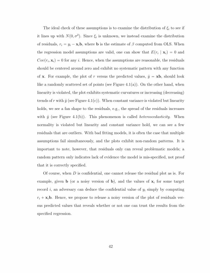
The ideal check of these assumptions is to examine the distribution of ξi to see if

it lines up with Np0, σ2q. Since ξi is unknown, we instead examine the distribution

of residuals, ri “ yi ´ xib, where b is the estimate of β computed from OLS. When

the regression model assumptions are valid, one can show that Epri | xiq “ 0 and

Covpri,xiq “ 0 for any i. Hence, when the assumptions are reasonable, the residuals

should be centered around zero and exhibit no systematic pattern with any function

of x. For example, the plot of r versus the predicted values, y “ xb, should look

like a randomly scattered set of points (see Figure 4.1(a)). On the other hand, when

linearity is violated, the plot exhibits systematic curvatures or increasing (decreasing)

trends of r with y (see Figure 4.1(c)). When constant variance is violated but linearity

holds, we see a fan shape to the residuals, e.g., the spread of the residuals increases

with y (see Figure 4.1(b)). This phenomenon is called heteroscedasticity. When

normality is violated but linearity and constant variance hold, we can see a few

residuals that are outliers. With bad fitting models, it is often the case that multiple

assumptions fail simultaneously, and the plots exhibit non-random patterns. It is

important to note, however, that residuals only can reveal problematic models; a

random pattern only indicates lack of evidence the model is mis-specified, not proof

that it is correctly specified.

Of course, when D is confidential, one cannot release the residual plot as is. For

example, given b (or a noisy version of b), and the values of xi for some target

record i, an adversary can deduce the confidential value of yi simply by computing

ri ` xib. Hence, we propose to release a noisy version of the plot of residuals ver-

sus predicted values that reveals whether or not one can trust the results from the

specified regression.

42

Algorithm 9 PriRPInput: Dataset D, a safe model β, εOutput: a private residual plot1: Step 1: Compute the bound of residuals and predicted values with ε1 budget.2: Step 2: Perturb the residual plots within the bound above with the left ε2 “ ε ´ ε1

budget.

4.2.2 Private Residual Plots

An important challenge in releasing differentially private residual plots is that we do

not have a prior knowledge of bounds on either the predicted y or the residuals r

(other than that they are in p´8,8q). Deriving tight upper and lower bounds on y

and r is extremely important:

• Recent work [6] has proven the impossibility of releasing distributions (specif-

ically CDFs) under differential privacy on infinite domains.

• Differentially private algorithms need to add noise to regions in the domain

that have no support. Thus, even if one knew upper and lower bounds on the

values, it is beneficial to obtain tighter bounds where most of the data reside

in order to minimize noise.

• We also need the bounds to not exclude a large fraction of the py, rq pairs in

order to correctly observe trends.

Hence, we propose PriRP (see Algorithm 9) for constructing ε-differentially pri-

vate residual plots that proceeds in two steps: 1) compute bounds on the range of

predicted y and residuals r that cover most of the records in the original dataset

using ε1 of the total ε budget, and 2) release the distribution of y versus r within the

bounds using the remaining budget ε2 “ ε´ε1. We next describe these steps in detail.

Computing private bounds: Given a list of real numbers D “ tz1, z2, . . . , znu, we

would like to identify bounds p´b, bq such that at least a θ fraction of the numbers

43

Algorithm 10 Private BoundsInput: Dataset D, unit µ, private budget ε, threshold θOutput: a value d (indicating a bound r´d, ds)

1: θ Ð θ ˆ n` Lapp2{εq, dÐ µ2: while True do3: q Ð number of x P D within bound r´d, ds

4: if q ` Lapp4{εq ă θ then dÐ d ˚ 25: else return d6: end if7: end while

are contained in p´b, bq with probability of at least p1 ´ αq. We can not use prior

work on releasing quantiles under differential privacy (e.g., Algorithm 2 in [53]) since

they assume knowledge of a weak upper and lower bound on the input data.1

Our approach, shown in Algorithm 10, is an application of the Sparse Vector

Technique [19]. The algorithm successively poses queries of the form qi ““number

of observations in D within the bounds r´µ ˚ 2i, µ ˚ 2is”, where i “ 0, 1, . . . and

µ is a scaling constant. The algorithm stops when the noisy answer to query qi “

qi`Lapp4{εq exceeds about a θ fraction of the data (i.e. qi ą N “ θ ¨ n`Lapp2{εqq.

Theorem 9. Let D denote a list of real numbers. Algorithm 10 satisfies ε-differential

privacy. Moreover, if a θ fraction of elements in D lie in r´µ ¨ 2k, µ ¨ 2ks, then with

probability at least 1 ´ β, the output bounds will contain at least θ ´ α fraction of

elements in D, where α “ 8plogpk´1q`logp2{βqqn¨ε

.

Proof. From [19], we know that Algorithm 10 satisfies ε-differential privacy. More-

over, suppose the algorithm stops after answering ` ` 1 queries, then we can show

(using [19]) that with probability at least 1 ´ β, q``1 ě n ¨ pθ ´ α`q, where α` “

8plogp`q`logp2{βqqn¨ε

. The algorithm outputs bounds r´µ ¨ 2``1, µ ¨ 2``1s. If ` ` 1 ě k,

then the output bounds are guaranteed to contain a θ fraction of the elements in D.

Otherwise, `` 1 ă k implies α` ă α giving us the desired result.

As an illustration of Theorem 9, suppose a θ fraction of D lie within r´µ ¨ 210, µ ¨

1 Moreover, the quality of these algorithms also depends on how tight the assumed bounds are.

44

210s, and let n¨ε ě 470. With probability ě 0.95, the bounds output by Algorithm 10

contains at least a θ´0.1 fraction of the elements in D. Note that the error depends

on (i) the product of n and ε, as well as (ii) µ. The former is a proxy for the amount

of signal that can be extracted from the data. µ represents a unit quantity for the

elements in D, and should be set neither too large nor too small.

Application to residual plots: We use Algorithm 10 to estimate bounds on y and

r separately, expending ε1{2 privacy budget each time. We set µ based on the type

of y. For example, when y describes an integer-valued outcome with few levels (e.g.,

a test score), it makes sense to set µ “ 1. When the attribute describes a long-tailed

variable (e.g., salary), it is better to set µ “ 1000. In our experiments, n is known

and θ is usually set to 0.95. We set ε1 “ mint0.3, 470εnu ˆ ε. Based on the illustration

above, ε1 “470n

results in bounds covering around θ fraction of records with high

probability. To avoid ε1 getting too large, we set it to 0.3ε for small n.

Perturbing residual plots: We visualize the relationships between y vs r by pri-

vately estimating the 2D probability density inside the bounded region output by

Algorithm 10. This can be done using private space partitioning techniques in three

steps – discretization, perturbation and sampling.

Discretization: We first discretize the bounded region into m2 grid cells of equal

size. We then construct a histogram h with m2 counts, where the count in each cell

represents the number of records inD with values pyi, riq contained in that cell. Based

on analysis similar to [39], we set m “

b

N0ε10

, where N0 is the number of records in

D that have pyi, riq in the bounded region. Rather than estimating N0 noisily (with

some loss in privacy budget), we approximate N0 using θ2ˆn, the expected number

of records that are captured in the bounded region by Algorithm 10.

Perturbation: Recent work [31] shows that DAWA is one of the best algorithms for

45

privately answering range queries over 2D histograms. DAWA works by first ordering

the cells in the histogram according to a Hilbert curve, and then grouping together

contiguous ranges of cells (in this ordering) that have similar counts. DAWA noisily

computes the total counts for each of these groups, and reconstructs the original cell

counts by assuming that all cell counts within a group are the same. Partitioning the

cells into groups of similar counts allows DAWA to minimize the total noise added.

The noisy histogram counts h are postprocessed to ensure non-negativity (by

setting negative values to 0), and integrality (by rounding to the nearest integer) to

get h. This is the only step that consults the private database D with ε2 budget.

Sampling: The perturbed residual plot is constructed by sampling N0 points

uniformly from each grid cell based on h.

Theorem 10. PriRP ensures ε-differential privacy.

Proof. Computing bounds on y and r each consumes ε12

privacy budget. For the

process of perturbing residual plots, the discretization and perturbation process are

implemented using a ε2-differentially private algorithm for computing 2D histogram

of counts. The sampling step does not access the sensitive data and hence will not

incur any loss of privacy. By applying sequential composition property of differential

privacy, PriRP satisfies ε1 ` ε2 “ ε-differential privacy.

4.2.3 Evaluation

In this section, we comprehensively evaluate the quality of residual plots output by

our algorithm PriRP, and whether or not an analyst can determine model fit using

the noisy residual plots. We design the following experiments.

1. We show that noisy residual plots can help analysts correctly identify whether

or not the confidential data satisfy the regression assumptions (linearity and

equal variance) using synthetic datasets.

46

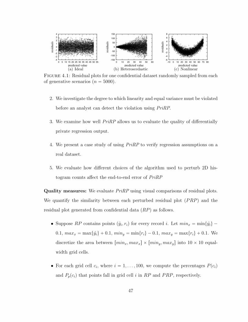
-4

-3

-2

-1

0

1

2

3

4

0 5 10 15 20 25 30 35 40 45 50 55

resi

du

als

predicted value

(a) Ideal

-150

-100

-50

0

50

100

150

0 10 20 30 40 50 60

resi

du

als

predicted value

(b) Heteroscedastic

-6

-4

-2

0

2

4

6

8

-10 0 10 20 30 40 50 60 70 80

resi

du

als

predicted value

(c) Nonlinear

Figure 4.1: Residual plots for one confidential dataset randomly sampled from eachof generative scenarios (n “ 5000).

2. We investigate the degree to which linearity and equal variance must be violated

before an analyst can detect the violation using PriRP.

3. We examine how well PriRP allows us to evaluate the quality of differentially

private regression output.

4. We present a case study of using PriRP to verify regression assumptions on a

real dataset.

5. We evaluate how different choices of the algorithm used to perturb 2D his-

togram counts affect the end-to-end error of PriRP

Quality measures: We evaluate PriRP using visual comparisons of residual plots.

We quantify the similarity between each perturbed residual plot (PRP ) and the

residual plot generated from confidential data (RP ) as follows.

• Suppose RP contains points (yi, ri) for every record i. Let minx “ mintyiu ´

0.1, maxx “ maxtyiu ` 0.1, miny “ mintriu ´ 0.1, maxy “ maxtriu ` 0.1. We

discretize the area between rminx,maxxs ˆ rminy,maxys into 10 ˆ 10 equal-

width grid cells.

• For each grid cell ci, where i “ 1, . . . , 100, we compute the percentages P pciq

and Pppciq that points fall in grid cell i in RP and PRP , respectively.

47

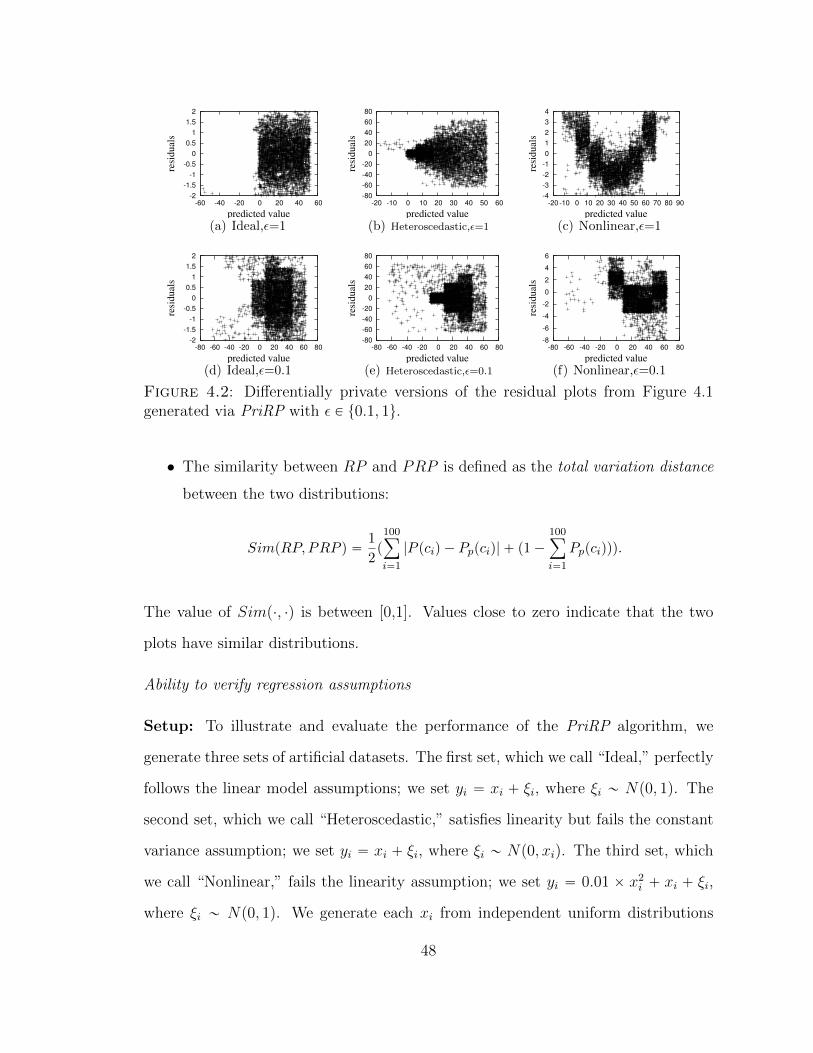
-2

-1.5

-1

-0.5

0

0.5

1

1.5

2

-60 -40 -20 0 20 40 60

resi

du

als

predicted value

(a) Ideal,ε=1

-80

-60

-40

-20

0

20

40

60

80

-20 -10 0 10 20 30 40 50 60

resi

du

als

predicted value

(b) Heteroscedastic,ε=1

-4

-3

-2

-1

0

1

2

3

4

-20 -10 0 10 20 30 40 50 60 70 80 90

resi

du

als

predicted value

(c) Nonlinear,ε=1

-2

-1.5

-1

-0.5

0

0.5

1

1.5

2

-80 -60 -40 -20 0 20 40 60 80

resi

du

als

predicted value

(d) Ideal,ε=0.1

-80

-60

-40

-20

0

20

40

60

80

-80 -60 -40 -20 0 20 40 60 80re

sid

ual

spredicted value

(e) Heteroscedastic,ε=0.1

-8

-6

-4

-2

0

2

4

6

-80 -60 -40 -20 0 20 40 60 80

resi

du

als

predicted value

(f) Nonlinear,ε=0.1

Figure 4.2: Differentially private versions of the residual plots from Figure 4.1generated via PriRP with ε P t0.1, 1u.

• The similarity between RP and PRP is defined as the total variation distance

between the two distributions:

SimpRP,PRP q “1

2p

100ÿ

i“1

|P pciq ´ Pppciq| ` p1´100ÿ

i“1

Pppciqqq.

The value of Simp¨, ¨q is between [0,1]. Values close to zero indicate that the two

plots have similar distributions.

Ability to verify regression assumptions

Setup: To illustrate and evaluate the performance of the PriRP algorithm, we

generate three sets of artificial datasets. The first set, which we call “Ideal,” perfectly

follows the linear model assumptions; we set yi “ xi ` ξi, where ξi „ Np0, 1q. The

second set, which we call “Heteroscedastic,” satisfies linearity but fails the constant

variance assumption; we set yi “ xi ` ξi, where ξi „ Np0, xiq. The third set, which

we call “Nonlinear,” fails the linearity assumption; we set yi “ 0.01 ˆ x2i ` xi ` ξi,

where ξi „ Np0, 1q. We generate each xi from independent uniform distributions

48

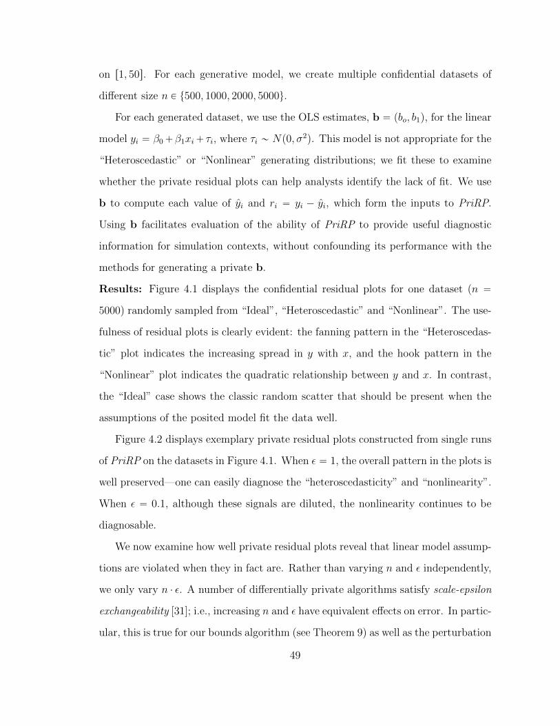
on r1, 50s. For each generative model, we create multiple confidential datasets of

different size n P t500, 1000, 2000, 5000u.

For each generated dataset, we use the OLS estimates, b “ pbo, b1q, for the linear

model yi “ β0`β1xi` τi, where τi „ Np0, σ2q. This model is not appropriate for the

“Heteroscedastic” or “Nonlinear” generating distributions; we fit these to examine

whether the private residual plots can help analysts identify the lack of fit. We use

b to compute each value of yi and ri “ yi ´ yi, which form the inputs to PriRP.

Using b facilitates evaluation of the ability of PriRP to provide useful diagnostic

information for simulation contexts, without confounding its performance with the

methods for generating a private b.

Results: Figure 4.1 displays the confidential residual plots for one dataset pn “

5000q randomly sampled from “Ideal”, “Heteroscedastic” and “Nonlinear”. The use-

fulness of residual plots is clearly evident: the fanning pattern in the “Heteroscedas-

tic” plot indicates the increasing spread in y with x, and the hook pattern in the

“Nonlinear” plot indicates the quadratic relationship between y and x. In contrast,

the “Ideal” case shows the classic random scatter that should be present when the

assumptions of the posited model fit the data well.

Figure 4.2 displays exemplary private residual plots constructed from single runs

of PriRP on the datasets in Figure 4.1. When ε “ 1, the overall pattern in the plots is

well preserved—one can easily diagnose the “heteroscedasticity” and “nonlinearity”.

When ε “ 0.1, although these signals are diluted, the nonlinearity continues to be

diagnosable.

We now examine how well private residual plots reveal that linear model assump-

tions are violated when they in fact are. Rather than varying n and ε independently,

we only vary n ¨ ε. A number of differentially private algorithms satisfy scale-epsilon

exchangeability [31]; i.e., increasing n and ε have equivalent effects on error. In partic-

ular, this is true for our bounds algorithm (see Theorem 9) as well as the perturbation

49

0

0.05

0.1

0.15

0.2

0.25

0.3

0.35

0.4

0 0.2 0.4 0.6 0.8 1

Pro

bab

ilit

ySimilarity

I

H

N

(a) s500,ε=1

0

0.05

0.1

0.15

0.2

0.25

0.3

0.35

0.4

0 0.2 0.4 0.6 0.8 1

Similarity

I

H

N

(b) s1000,ε=1

0

0.1

0.2

0.3

0.4

0.5

0.6

0.7

0.8

0 0.2 0.4 0.6 0.8 1

Similarity

I

H

N

(c) s2000,ε=1

0

0.1

0.2

0.3

0.4

0.5

0.6

0.7

0.8

0 0.2 0.4 0.6 0.8 1

Similarity

I

H

N

(d) s5000,ε=1

Scale TVD(I,H) TVD(I,N)

500 0.959 0.902

1000 0.997 0.996

2000 1 1

5000 1 1

(e) TVD, ε=1

0

0.05

0.1

0.15

0.2

0.25

0.3

0.35

0.4

0 0.2 0.4 0.6 0.8 1

Pro

bab

ilit

y

Similarity

I

H

N

(f) s500,ε=0.1

0

0.05

0.1

0.15

0.2

0.25

0.3

0.35

0.4

0 0.2 0.4 0.6 0.8 1

Similarity

I

H

N

(g) s1000,ε=0.1

0

0.05

0.1

0.15

0.2

0.25

0.3

0.35

0.4

0 0.2 0.4 0.6 0.8 1

Similarity

I

H

N

(h) s2000,ε=0.1

0

0.05

0.1

0.15

0.2

0.25

0.3

0.35

0.4

0 0.2 0.4 0.6 0.8 1

Similarity

I

H

N

(i) s5000,ε=0.1

Scale TVD(I,H) TVD(I,N)

500 0.471 0.276

1000 0.658 0.433

2000 0.857 0.676

5000 0.974 0.908

(j) TVD, ε=0.1

Figure 4.3: Comparison of similarity values for simulated confidential and privateresidual plots.

algorithm DAWA [31], and is reflected in our experiments.

We compute the distribution of similarity values between the real “Ideal” resid-

ual plot and the noisy plots from different models (“Ideal”, “Heteroscedastic” and

“Nonlinear”) using 1000 independently generated noisy plots in each case. In each

plot in Figure 4.3, the distributions labeled I, H and N represent the empirical dis-

tribution of the similarity of the noisy “Ideal”, “Heteroscedastic” and “Nonlinear”

residual plot, respectively, with the true “Ideal” residual plot. When nε ě 1000, H

and N are well separated from I. Even at nε “ 500, we see little overlap between H

50

and I as well as N and I. This means that at nε ě 500, an analyst is still likely to

correctly tell whether it is in the “Ideal” case by using the noisy residual plot.

Figure 4.3(e), 4.3(j) confirm this using total variation distance (TVD) between

I vs. H and I vs. N . The TVD exceeds 0.95 when nε ě 1000 and is ě 0.9 when

nε ě 500.

Discriminatory power

We investigate the degree to which linearity and equal variance assumptions must

be violated to be detectable using PriRP.

Setup: We generate data from the following three models, sampling each xi from a

uniform distribution on [0,50].

1. M1: yi “ xi ` ξi, ξi „ Np0, 1q

2. M2: yi “ xi ` ξi, ξi „ Np0, αxi ` 1q

3. M3: yi “ xi ` γx2i ` ξi, ξi „ Np0, 1q

When α and γ are close to zero, the violation from the standard linear model

assumptions can be considered minor, so that using M1 (instead of M2 or M3) is not

unreasonable.

First, in the non-private setting, for any dataset generated from model Mk, k P

t1, 2, 3u with fixed α and γ, let Tk represent the probability distribution of the

counts in the 100 grid cells overlaid on the confidential residual plot. Let Dk =

TVDpTk, ErT1sq be the TVD between Tk and the expected value of T1. Using 1000

simulated datasets, we generate 1000 values of pD1, D2, D3q for the specified values

of α and γ.

Using these 1000 draws, we find the minimum values of α and γ such that the

TVDpD1, D2q and TVDpD1, D3q are at least 0.95. We should be able to differentiate

51

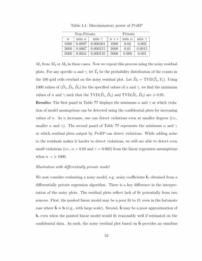
Table 4.1: Discriminatory power of PriRP

Non-Private Privaten min α min γ nˆ ε min α min γ

1000 0.0097 0.000301 1000 0.02 0.0022000 0.0067 0.000215 2000 0.01 0.00155000 0.0041 0.000135 5000 0.008 0.001

M1 from M2 or M3 in these cases. Now we repeat this process using the noisy residual

plots. For any specific α and γ, let Tk be the probability distribution of the counts in

the 100 grid cells overlaid on the noisy residual plot. Let Dk = TVDpTk, T1q. Using

1000 values of pD1, D2, D3q for the specified values of α and γ, we find the minimum

values of α and γ such that the TVDpD1, D2q and TVDpD1, D3q are ě 0.95.

Results: The first panel in Table ?? displays the minimum α and γ at which viola-

tion of model assumptions can be detected using the confidential plots for increasing

values of n. As n increases, one can detect violations even at smaller degrees (i.e.,

smaller α and γ). The second panel of Table ?? represents the minimum α and γ

at which residual plots output by PriRP can detect violations. While adding noise

to the residuals makes it harder to detect violations, we still are able to detect even

small violations (i.e., α “ 0.02 and γ “ 0.002) from the linear regression assumptions

when n ¨ ε ě 1000.

Illustration with differentially private model

We now consider evaluating a noisy model, e.g. noisy coefficients b, obtained from a

differentially private regression algorithm. There is a key difference in the interpre-

tation of the noisy plots. The residual plots reflect lack of fit potentially from two

sources. First, the posited linear model may be a poor fit to D, even in the fortunate

case where b « b (e.g., with large scale). Second, b may be a poor approximation of

b, even when the posited linear model would fit reasonably well if estimated on the

confidential data. As such, the noisy residual plot based on b provides an omnibus

52

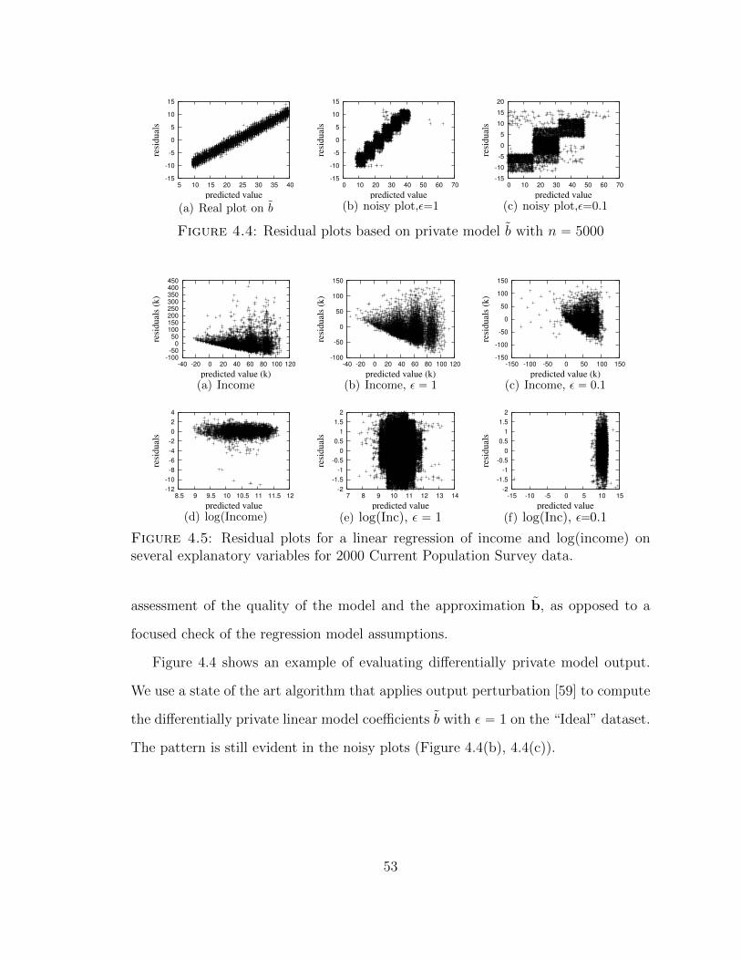
-15

-10

-5

0

5

10

15

5 10 15 20 25 30 35 40

resi

du

als

predicted value

(a) Real plot on b

-15

-10

-5

0

5

10

15

0 10 20 30 40 50 60 70

resi

du

als

predicted value

(b) noisy plot,ε=1

-15

-10

-5

0

5

10

15

20

0 10 20 30 40 50 60 70

resi

du

als

predicted value

(c) noisy plot,ε=0.1

Figure 4.4: Residual plots based on private model b with n “ 5000

-100

-50

0

50

100

150

200

250

300

350

400

450

-40 -20 0 20 40 60 80 100 120

resi

du

als

(k)

predicted value (k)

(a) Income

-100

-50

0

50

100

150

-40 -20 0 20 40 60 80 100 120

resi

du

als

(k)

predicted value (k)

(b) Income, ε “ 1

-150

-100

-50

0

50

100

150

-150 -100 -50 0 50 100 150

resi

du

als

(k)

predicted value (k)

(c) Income, ε “ 0.1

-12

-10

-8

-6

-4

-2

0

2

4

8.5 9 9.5 10 10.5 11 11.5 12

resi

du

als

predicted value

(d) log(Income)

-2

-1.5

-1

-0.5

0

0.5

1

1.5

2

7 8 9 10 11 12 13 14

resi

du

als

predicted value

(e) log(Inc), ε “ 1

-2

-1.5

-1

-0.5

0

0.5

1

1.5

2

-15 -10 -5 0 5 10 15

resi

du

als

predicted value

(f) log(Inc), ε“0.1

Figure 4.5: Residual plots for a linear regression of income and log(income) onseveral explanatory variables for 2000 Current Population Survey data.

assessment of the quality of the model and the approximation b, as opposed to a

focused check of the regression model assumptions.

Figure 4.4 shows an example of evaluating differentially private model output.

We use a state of the art algorithm that applies output perturbation [59] to compute

the differentially private linear model coefficients b with ε “ 1 on the “Ideal” dataset.

The pattern is still evident in the noisy plots (Figure 4.4(b), 4.4(c)).

53

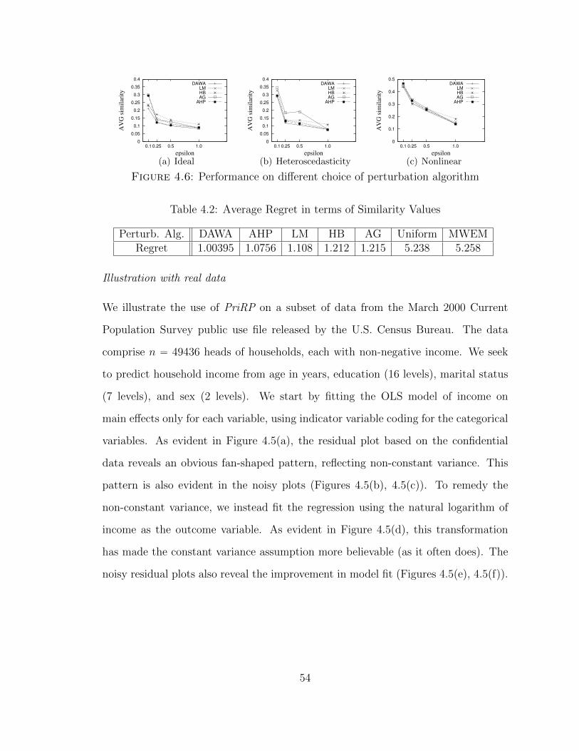
0

0.05

0.1

0.15

0.2

0.25

0.3

0.35

0.4

0.1 0.25 0.5 1.0

AV

G s

imil

arit

y

epsilon

DAWA

LM

HB

AG

AHP

(a) Ideal

0

0.05

0.1

0.15

0.2

0.25

0.3

0.35

0.4

0.1 0.25 0.5 1.0

AV

G s

imil

arit

y

epsilon

DAWA

LM

HB

AG

AHP

(b) Heteroscedasticity

0

0.1

0.2

0.3

0.4

0.5

0.1 0.25 0.5 1.0

AV

G s

imil

arit

y

epsilon

DAWA

LM

HB

AG

AHP

(c) Nonlinear

Figure 4.6: Performance on different choice of perturbation algorithm

Table 4.2: Average Regret in terms of Similarity Values

Perturb. Alg. DAWA AHP LM HB AG Uniform MWEMRegret 1.00395 1.0756 1.108 1.212 1.215 5.238 5.258

Illustration with real data

We illustrate the use of PriRP on a subset of data from the March 2000 Current

Population Survey public use file released by the U.S. Census Bureau. The data

comprise n “ 49436 heads of households, each with non-negative income. We seek

to predict household income from age in years, education (16 levels), marital status

(7 levels), and sex (2 levels). We start by fitting the OLS model of income on

main effects only for each variable, using indicator variable coding for the categorical

variables. As evident in Figure 4.5(a), the residual plot based on the confidential

data reveals an obvious fan-shaped pattern, reflecting non-constant variance. This

pattern is also evident in the noisy plots (Figures 4.5(b), 4.5(c)). To remedy the

non-constant variance, we instead fit the regression using the natural logarithm of

income as the outcome variable. As evident in Figure 4.5(d), this transformation

has made the constant variance assumption more believable (as it often does). The

noisy residual plots also reveal the improvement in model fit (Figures 4.5(e), 4.5(f)).

54

Choice of perturbation algorithm

Finally, we evaluate how different choices of perturbation algorithms in the second

step of PriRP for perturbing residuals affect the performance of PriRP.

The problem of releasing the joint probability density over 2 dimensions has

received a lot of attention in the differential privacy literature. Table 4.2 lists a set

of algorithms which can be used to privately compute 2D densities (as well as answer

range queries over the 2D domain). LM represents Laplace Mechanism. Uniform only

perturbs the total count and assumes uniform distribution on the domain. HB [? ]

uses noisy estimates of multiple hierarchical equiwidth histograms (i.e., discretized

at different grid sizes). DAWA [38], AHP [66] and AG [47] partition the space and

then use the Laplace Mechanism to estimate the fraction of points in each partition.

MWEM [29] assumes uniform distribution on the domain first and then updates the

distribution by sampling the querie which has the poorest answer based on current

distribution.

Figure 4.6 shows the comparison results on three different datasets (“Ideal”, “Het-

eroscedasticity” and “Nonlinear”) with scale = 5000. In each figure, we compare the

average similarity value among 20 trials of using PriRP with different 2D perturba-

tion algorithms on various ε settings. Uniform and MWEM are not shown because

their results are much worse than the 5 algorithms shown in the figures. From Fig-

ure 4.6, we can see DAWA performs the best in terms of all datasets and ε settings.

The performance of algorithms across different datasets and ε values can be sum-

marized using a measure called regret, introduced in prior works [31] and [35]. Let

M be a set of algorithms, and let S be a set of pairs of (dataset, ε). Then, the regret

of algorithm M˚ P M on a specific dataset D at a specific ε is defined as

regretpM˚q “

ErrorpM˚pD, εqq

minMPMtMpD, εqu. (4.2)

55

The (dataset, ε) specific regret measure computes how much worse algorithm

M˚’s error is compared to the error of the algorithm with the least error on that

dataset at that ε. The average regret of an algorithm M˚ on a set S is given by

regretpM˚q “ avgpD,εqPS

ErrorpM˚pD, εqq

minMPMtMpD, εqu. (4.3)

The regret value is greater or equal to 1. The smaller the regret is, the better

the algorithm performs. Regret equals 1 means the corresponding algorithm always

performs the best in terms of all (dataset, ε) settings. Table 4.2 validates our choice

of DAWA as the algorithm of choice in PriRP, as it has the least regret amongst all

the algorithms we considered.

4.3 ROC Curves

We now present an algorithm of computing differentially private ROC curves for

logistic regression. The algorithm could be used to evaluate the predictive power of

any binary classifier.

4.3.1 Review of ROC curves

Let Draw “ tpyi,xiq : i P rnsu be a confidential dataset. The logistic regression model

posits P pyi “ 1 | xiq “ πi, where logp πi1´πi

q “ β0 `řpj“1 xijβj. Let b “ pb0, . . . , bpq

be the maximum likelihood estimate of β “ pβ0, . . . , βpq. For any xi, we compute

predicted probabilities,

ppxiq “ P pyi “ 1 | xiq “exppb0 `

řpj“1 xijbjq

1` exppb0 `řpj“1 xijbjq

. (4.4)

Analysts often evaluate the fit of a logistic regression model by comparing ppxiq to

yi. Ideally, ppxiq tends to be large when yi “ 1, and tends to be small when yi “ 0.

To facilitate these comparisons, it is convenient to convert ppxiq into a predicted

56

outcome, yi P t0, 1u, by setting yi “ 1 when ppxiq ą θ and yi “ 0 otherwise. Here, θ

is an analyst-defined threshold.

For any given θ, using all n values of pyi, yiq, we can quantify the accuracy of the

logistic regression model on a test set D as follows. True positives, TP pθq, are the

individuals in D with true and predicted outcomes equal to 1, i.e., pyi “ 1, yi “ 1q.

False positives, FP pθq, are individuals with pyi “ 0, yi “ 1q. We use the notation

TP pθq, FP pθq to denote both the set of individuals and the cardinality of them.

Let n1 and n0 be the number of individuals with yi “ 1 and yi “ 0, respectively.

The true-positive rate TPRpθq is the probability that an individual in D with yi “ 1

is correctly classified with yi “ 1. The false-positive rate FPRpθq, is the probability

that an individual in D with yi “ 0 is wrongly classified with yi “ 1. Thus, we have

TPRpθq “TP pθq

n1

and FPRpθq “FP pθq

n0

. (4.5)

The ROC curve is defined by plotting TPRpθq versus FPRpθq over all possible

θ. It starts at p0, 0q for θ “ 1 and ends at p1, 1q for θ “ 0. It can be approximated

numerically by computing Equation 1 over a large set of candidate θ values, say Θ.

The area under the ROC curve, abbreviated as AUC, is often used to evaluate the

accuracy of the logistic regression. When the regression predicts the outcomes in D

accurately, the ROC curve is close to the left and upper boundary, so that AUC is

close to 1. When the regression predicts the outcomes in D poorly, the ROC curve

is close to the 45˝ line from (0,0) to (1,1), and the AUC is around 0.5.

Recent work [43] shows that releasing actual ROC curves computed directly from

Equation 4.5 can allow attackers with prior knowledge to reconstruct D. For an

extreme yet illustrative example, suppose an attacker knows all of D except for

pyi,xiq. Given the ROC curve based on Equation 4.5, the attacker can determine

the unknown yi by simply enumerating over all values of pyi,xiq, and finding the value

that reproduces the given ROC curve. Hence, directly releasing the ROC curve may

57

Algorithm 11 PriROCInput: Dataset D, a safe model β, εOutput: a private ROC curve1: Step 1: Select a set of thresholds in terms of predictons of D on β with ε1 privacy

budget.2: Step 2: Compute the private TPR and FPR values based on the selected thresholds

above with the left ε2 “ ε´ ε1 budget.3: Step 3: Post-process private TPR and FPR values to make the private ROC curve

consistent with the monotonicity of real ROC curves.

leak information, inspiring us to create a differentially private method for generating

ROC curves.

4.3.2 Private ROC curves

To generate ROC curves, we need to determine Θ, to compute TPR and FPR

values on all chosen thresholds, and to ensure the monotonicity of TPR and FPR

values for a valid ROC curve. Under differential privacy, we cannot directly use

Θ “ tppxiq : xi P D, i P rnsu (the predicted probabilities for each individual). Simply

using LM to compute TPR and FPR values may introduce large noise due to its

high sensitivity (2|Θ| ` 1).

We propose an algorithm PriROC (Algorithm 11) that addresses these concerns

in three steps: 1) Select a set of thresholds that are used for computing the TPR

and FPR values with ε1 privacy budget. 2) Compute the private TPR and FPR

values in terms of all the chosen thresholds with the left privacy budget ε2 “ ε´ ε1.

3) Post-process the results in order to make it a valid ROC curve. We next describe

these steps in details.

Choosing thresholds: There are two important considerations when choosing Θ.

The number of thresholds must (a) be large enough to accurately approximate the

ROC curve, and (b) be small enough to ensure accuracy (despite perturbation) and

efficiency (as we will see later, the runtime of our algorithm is Op|Θ|2log|Θ|q).

A data-independent strategy for picking Θ is to choose the thresholds uniformly

from r0, 1s. More precisely, if we fix |Θ| “ N , we set Θ “ t0, 1N, . . . , N´1

N, 1u. We

58

call this strategy N -FixedSpace. This strategy works well when the predictions

P “ tppxiq|xi P D, i P rnsu are uniformly spread out in r0, 1s. Since, N -FixedSpace

is data independent, ε1 “ 0, and all the privacy budget can be used for computing

the TPR and FPR values. However, N -FixedSpace may be ineffective when pre-

dictions are skewed. For instance, suppose all the predictions ppxiq are either ă 1N

,

or ą 1 ´ 1N

. The ROC curve is then approximated with just 2 points (TPRp 1Nq,

FPRp 1Nq) and (TPRp1 ´ 1

Nq, FPRp1 ´ 1

Nq), possibly resulting in a significant loss

in accuracy in the AUC.

For this potential shortcoming, we present s-RecursiveMedians (Algorithm 12),

a data-dependent strategy that recursively selects thresholds by finding the median

among the current data points such that there are roughly the same number of indi-

viduals between any two thresholds. Algorithm 12 takes as input the privacy budget

for choosing thresholds ε1, depth of the recursion s, and the multiset of predictions

P . Each of the s recursive steps uses a privacy budget of γ “ ε1{s.

The algorithm recursively calls a subroutine FindMedians to compute the noisy

median of all predictions within the range p`, rq. Initially, p`, rq “ p0, 1q. Since

the median function fmed has a high global sensitivity (equal to r ´ `), we use the

smooth sensitivity framework [45] to compute the noisy median. In Algorithm 12,

S˚fmed,γ{2pP q represents the smooth sensitivity of fmed on P with privacy budget γ{2.

When the global sensitivity of a function ∆pfq is high, we can use a data dependent

sensitivity function S˚f,εpDq instead to ensure privacy. S˚f,εpDq is an upper bound

on the (local) sensitivity of f at the input database (i.e. the maximum change in

function output on between D and its neighbors) and is smooth (i.e., S˚f,εpDq is

close to S˚f,εpD1q, when D and D1 are neighbors). Given S˚f,εp¨q, one way to ensure

ε-differential privacy is by perturbing the true output fpDq using 8ε¨S˚f,εpDq¨η, where

η is random noise sampled from the distribution 91{p1 ` |η|2q. We refer the reader

59

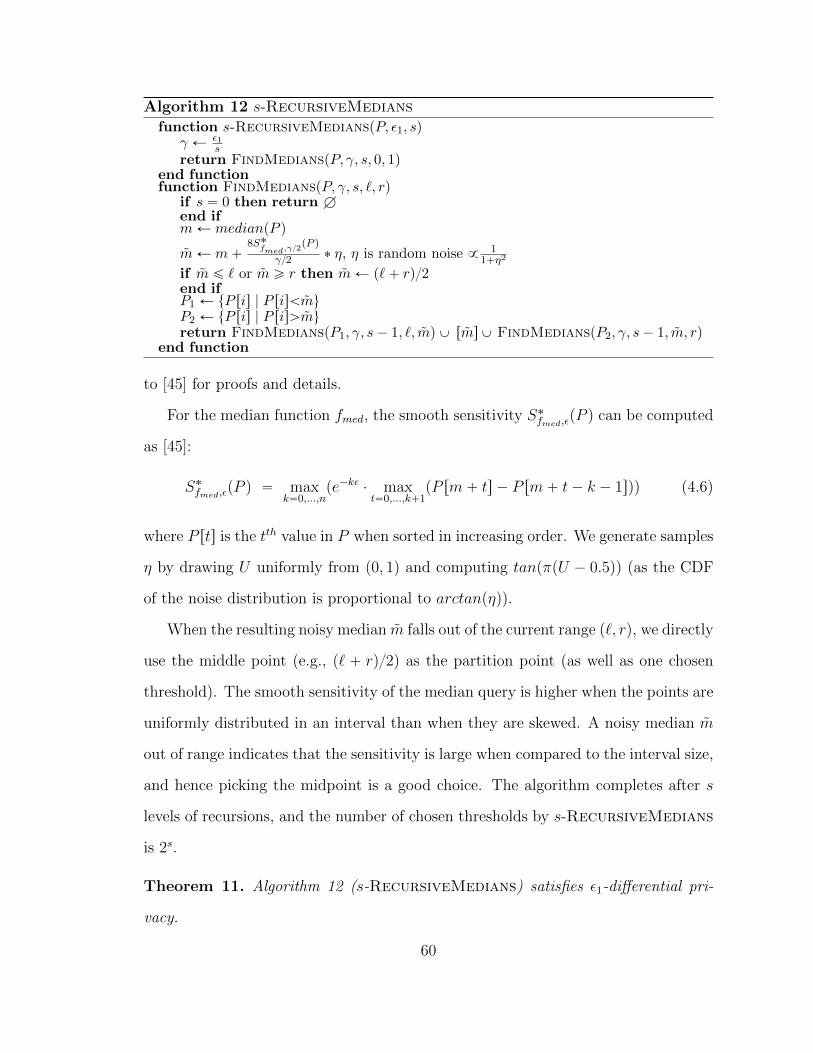
Algorithm 12 s-RecursiveMediansfunction s-RecursiveMedians(P, ε1, s)

γ Ð ε1s

return FindMedianspP, γ, s, 0, 1qend functionfunction FindMedians(P, γ, s, `, r)

if s “ 0 then return Hend ifmÐ medianpP q

mÐ m`8S˚fmed,γ{2

pP q

γ{2 ˚ η, η is random noise 9 11`η2

if m ď ` or m ě r then mÐ p`` rq{2end ifP1 Ð tP ris | P risămuP2 Ð tP ris | P risąmureturn FindMedianspP1, γ, s´ 1, `, mq Y rmsY FindMedianspP2, γ, s´ 1, m, rq

end function

to [45] for proofs and details.

For the median function fmed, the smooth sensitivity S˚fmed,εpP q can be computed

as [45]:

S˚fmed,εpP q “ maxk“0,...,n

pe´kε ¨ maxt“0,...,k`1

pP rm` ts ´ P rm` t´ k ´ 1sqq (4.6)

where P rts is the tth value in P when sorted in increasing order. We generate samples

η by drawing U uniformly from p0, 1q and computing tanpπpU ´ 0.5qq (as the CDF

of the noise distribution is proportional to arctanpηq).

When the resulting noisy median m falls out of the current range p`, rq, we directly

use the middle point (e.g., p` ` rq{2) as the partition point (as well as one chosen

threshold). The smooth sensitivity of the median query is higher when the points are

uniformly distributed in an interval than when they are skewed. A noisy median m

out of range indicates that the sensitivity is large when compared to the interval size,

and hence picking the midpoint is a good choice. The algorithm completes after s

levels of recursions, and the number of chosen thresholds by s-RecursiveMedians

is 2s.

Theorem 11. Algorithm 12 (s-RecursiveMedians) satisfies ε1-differential pri-

vacy.

60

Proof. Computing the median of a set of points by using FindMedians satisfies

γ{2 “ ε1{2s-differential privacy. In each recursive step, there are at most two parti-

tions different in neighboring databases. Since the depth of the recursion is bounded

by s, s-RecursiveMedians satisfies ε12sˆ2ˆs “ ε1-differential privacy by sequential

composition.

Computing noisy TPR and FPR values: Suppose we are given a set of thresh-

olds Θ “ tθ1, . . . , θ`u to use for approximating the ROC curve, where θk ą θk`1 for

all k, θ0 “ 1, and θ` “ 0. By definition, TP pθ`q “ n1 and FP pθ`q “ n0. The sets

tTP pθkq : k P r`su and tFP pθkq : k P r`su each correspond to a set of prefix range

queries.

Let RTPΘ “ trTP1 , . . . , rTP` u, where rTPk is the number of individuals i P D with

yi “ 1 and θk´1 ě ppxiq ą θk. Clearly, TP pθkq is the sum of the first k elements

in RTPΘ . We can define RFP

Θ similarly, thereby showing each FP pθkq is also a prefix

range query on RFPΘ .

A recent experimental study of differentially private algorithms for answering

range queries [31] indicates that DAWA [38] is a good algorithm for answering prefix

range queries. DAWA additionally approximates the histograms RTPΘ and RFP

Θ by

grouping together cells with similar counts. We compute the TP and FP values

privately using half of the remaining privacy budget for each one. Prefix range

queries are computed on RTPΘ to get the TP values and on RFP

Θ to get the FP

values, which in turn are used to construct the noisy TPRpθq and FPRpθq values.

Since all subsequent steps do not use the original data, the fact that releasing TPRpθq

and FPRpθq satisfies ε-differential privacy follows from the privacy of DAWA. We

spend the remaining ε2 “ ε´ ε1 budget on computing private TPR and FPR values,

ε22

for each.

Ensuring monotonicity: The noisy TPR and FPR values generated using the al-

61

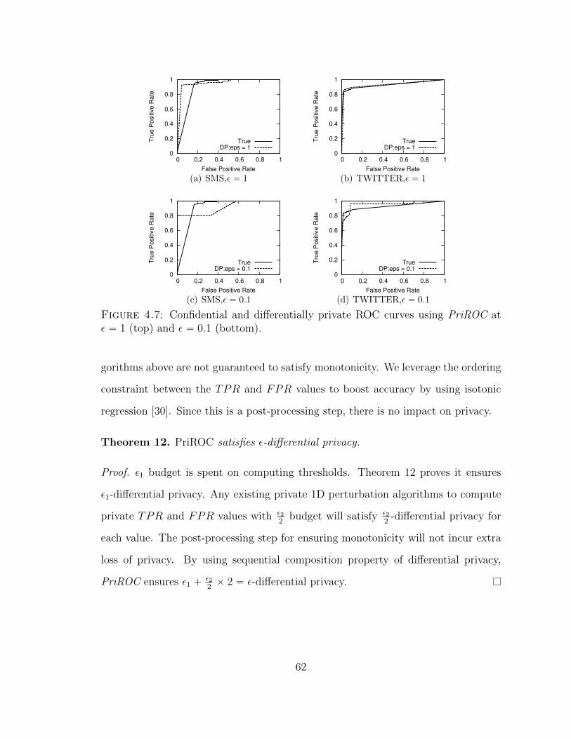
0

0.2

0.4

0.6

0.8

1

0 0.2 0.4 0.6 0.8 1

Tru

e P

ositiv

e R

ate

False Positive Rate

TrueDP:eps = 1

(a) SMS,ε “ 1

0

0.2

0.4

0.6

0.8

1

0 0.2 0.4 0.6 0.8 1

Tru

e P

ositiv

e R

ate

False Positive Rate

TrueDP:eps = 1

(b) TWITTER,ε “ 1

0

0.2

0.4

0.6

0.8

1

0 0.2 0.4 0.6 0.8 1

Tru

e P

ositiv

e R

ate

False Positive Rate

TrueDP:eps = 0.1

(c) SMS,ε “ 0.1

0

0.2

0.4

0.6

0.8

1

0 0.2 0.4 0.6 0.8 1

Tru

e P

ositiv

e R

ate

False Positive Rate

TrueDP:eps = 0.1

(d) TWITTER,ε “ 0.1

Figure 4.7: Confidential and differentially private ROC curves using PriROC atε “ 1 (top) and ε “ 0.1 (bottom).

gorithms above are not guaranteed to satisfy monotonicity. We leverage the ordering

constraint between the TPR and FPR values to boost accuracy by using isotonic

regression [30]. Since this is a post-processing step, there is no impact on privacy.

Theorem 12. PriROC satisfies ε-differential privacy.

Proof. ε1 budget is spent on computing thresholds. Theorem 12 proves it ensures

ε1-differential privacy. Any existing private 1D perturbation algorithms to compute

private TPR and FPR values with ε22

budget will satisfy ε22

-differential privacy for

each value. The post-processing step for ensuring monotonicity will not incur extra

loss of privacy. By using sequential composition property of differential privacy,

PriROC ensures ε1 `ε22ˆ 2 “ ε-differential privacy.

62

4.3.3 Evaluation

We now evaluate the quality of the ROC curves output by PriROC. Our experiments

focus on:

1. Visually inspecting whether the ROC curves output by PriROC are close to

the true ROC curves generated using the confidential predictions.

2. Measuring the average absolute difference between the AUC of the true ROC

curve and the AUC of noisy ROC curves output by PriROC.

3. Measuring the similarity between true and noisy ROC curves by computing

symmetric difference between them.

4. Quantifying the discriminatory power of private ROC curves; i.e., whether they

can discriminate between “good” and “bad” classifiers.

5. Evaluating the sensitivity of PriROC’s performance to changing the amount

of privacy budget allocated to choosing thresholds (ε1) and estimating counts

(ε2).

6. Evaluating the sensitivity of PriROC’s performance to the choice of the algo-

rithm used to compute noisy TPR and FPR values.

Dataset: We use two text classification datasets - raw-Twitter and raw-SMS.

The raw-Twitter dataset [27] was collected for the task of sentiment classification.

Each tweet is associated with a binary sentiment outcome – positive or negative. The

dataset contains 1.6 million tweets from which we randomly sampled 6840 tweets for

our experiments. The raw-SMS dataset [2] contains 5574 SMS messages associated

with spam/ham outcome variable. For both datasets, we use a vector of binary

explanatory variables representing presence or absence of individual words (excluding

stop words).

63

raw-Twitter and raw-SMS are randomly divided into training sets (contain-

ing 90% records) and test sets (containing 10% records). We use differentially private

empirical risk minimization [13] to compute a logistic regression model on the train-

ing set. We apply the private model on the two test datasets to obtain predictions,

which we call SMS and Twitter. SMS contains 558 records, and each record has

a true label yi P t0, 1u as well as a prediction P pyi “ 1 | xiq P r0, 1s. In SMS, 481

out of 558 records have label 1. Twitter contains 684 records, 385 of which have

label 1.

Algorithms: We consider our proposed two strategies for selecting Θ. The first uses

the s-RecursiveMedians strategy, setting |Θ| “ 210 and spending 0.2ε budget to

select thresholds. These parameters were empirically chosen (we fix them in our

experiment) to trade off error with efficiency, which is not shown in the paper. We

refer to the resulting private algorithm for ROC curves as PriROC. The second

strategy for selecting Θ uses fixed thresholds selected uniformly from r0, 1s. Here, we

again set |Θ| “ 210, and we dedicate the full ε to perturb the TPR and FPR values.

We call the resulting differentially private algorithm for ROC curves PriROC-fix.

For both PriROC and PriROC-fix, we apply many different algorithms to perturb

the TPR and FPR values. In section 4.3.6, we will show that DAWA is the best

perturbation algorithm in terms of both datasets and different ε settings. So we will

use DAWA as the default perturbation algorithm in PriROC.

We also compare with Boyd et al’s [5] algorithm for directly computing the AUC,

and call that SmoothS.

Visualizing ROC curves

Figure 4.7 displays the ROC curves computed on confidential data and one randomly

generated differentially private ROC curve at ε = 1 and 0.1 using PriROC on both

SMS and Twitter. The PriROC curves track the confidential ROC curves quite

64

-2

-1.5

-1

-0.5

0

0.5

1.0 0.5 0.25 0.1

Log M

ean L

1 E

rror

Epsilon

SmoothS

PriROC-fix

PriROC

(a) SMS

-2

-1.5

-1

-0.5

0

0.5

1.0 0.5 0.25 0.1

Log M

ean L

1 E

rror

Epsilon

SmoothS

PriROC-fix

PriROC

(b) TWITTER

Figure 4.8: Comparison of AUC error.

well for all datasets and ε settings. The reason why PriROC is more accurate for

Twitter than for SMS is that the prediction distribution of SMS is more skewed

than Twitter, so s-RecursiveMedians performs better on Twitter.

AUC error

Figure 4.8 reports the comparison of AUC error for PriROC, PriROC-fix and SmoothS

on both SMS (Figure 4.8(a)) and Twitter (Figure 4.8(b)). For each figure, the

x-axis represents different ε settings and the y-axis shows the log10 of the mean L1

error between the confidential AUC and the private AUC over 20 repetitions. Both

PriROC and PriROC-fix have significantly lower errors than SmoothS under both

datasets and all ε settings. Using s-RecursiveMedians to choose thresholds results

in better AUC accuracy compared to using fixed thresholds.

ROC similarity

Even when two ROC curves have the same AUC, they may look quite different. Here,

we directly examine how close the real and private ROC curves are by computing the

symmetric difference between them; i.e., the mean area between the true and private

curves. We compare three methods: PriROC, PriROC-fix, and SmoothS (SmoothS

computes data independent, symmetric binormal ROC curves [5]). Figure 4.9 dis-

plays the symmetric differences (averaged over 20 trials) between the confidential

65

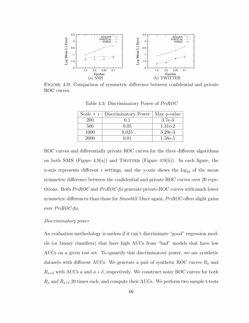
-2

-1.5

-1

-0.5

0

0.5

1.0 0.5 0.25 0.1

Log M

ean L

1 E

rror

Epsilon

SmoothS

PriROC-fix

PriROC

(a) SMS

-2

-1.5

-1

-0.5

0

0.5

1.0 0.5 0.25 0.1

Log M

ean L

1 E

rror

Epsilon

SmoothS

PriROC-fix

PriROC

(b) TWITTER

Figure 4.9: Comparison of symmetric difference between confidential and privateROC curves.

Table 4.3: Discriminatory Power of PriROC

Scale ˆ ε Discriminatory Power Max p-value200 0.1 3.7e-3500 0.05 1.31e-21000 0.025 3.29e-32000 0.01 1.58e-5

ROC curves and differentially private ROC curves for the three different algorithms

on both SMS (Figure 4.9(a)) and Twitter (Figure 4.9(b)). In each figure, the

x-axis represents different ε settings, and the y-axis shows the log10 of the mean

symmetric difference between the confidential and private ROC curves over 20 repe-

titions. Both PriROC and PriROC-fix generate private ROC curves with much lower

symmetric differences than those for SmoothS. Once again, PriROC offers slight gains

over PriROC-fix.

Discriminatory power

An evaluation methodology is useless if it can’t discriminate “good” regression mod-

els (or binary classifiers) that have high AUCs from “bad” models that have low

AUCs on a given test set. To quantify this discriminatory power, we use synthetic

datasets with different AUCs. We generate a pair of synthetic ROC curves Ra and

Ra`δ with AUCs a and a` δ, respectively. We construct noisy ROC curves for both

Ra and Ra`δ 20 times each, and compute their AUCs. We perform two sample t-tests

66

Table 4.4: Average Regret in terms of AUC Error and Symmetric Difference

Perturbation Algorithm DAWA AHP HB LM MWEM UniformAUC Regret 1 2.126 2.634 3.032 14.472 14.543SD Regret 1 1.745 2.071 2.605 10.403 10.443

(between noisy AUCs generated from Ra and Ra`δ, respectively) and test whether

the mean noisy AUC generated from Ra is significantly different (p-value ă 0.05)

from the mean noisy AUC generated from Ra`δ. We say the noisy AUC computed

using PriROC at data size n and privacy ε has discriminatory power δ, if @a, the

noisy AUC values for Ra have a significantly different mean than noisy AUC values

for Ra`δ.

Table 4.3 displays the discriminatory power of private ROC curves. We generate

ROC curves with AUC a P A = t0.95, 0.925, . . . , 0.7u. We report the smallest δ (in

multiples of 0.025) at which noisy AUCs have significantly different means for Ra and

Ra`δ for a, a ` δ P A. We report the max p-value attained for all such comparisons

Ra and Ra`δ. Smaller p-values imply the AUC computed using PriROC are more

discriminating between Ra and Ra`δ. Larger n ¨ ε products allow us to discriminate

between ROC curves with smaller differences in AUC with more significance.

In summary, ROC curves computed by PriROC satisfy ε-differential privacy, and

closely match the true ROC curves both visually and in terms of qualitative measures

like AUC and symmetric difference. Moreover, for n ¨ ε ě 1000, private ROC curves

can discriminate between “good” and “bad” models even if they differ in AUC by

only 0.025.

Sensitivity to budget split

We evaluate the effect of budget split on the performance of PriROC. Recall that

we split the total privacy budget ε into two parts - ε1 “ ρε for choosing the set of

thresholds, and ε2 “ p1´ ρqε for computing noisy TPR and FPR values. We call ρ

67

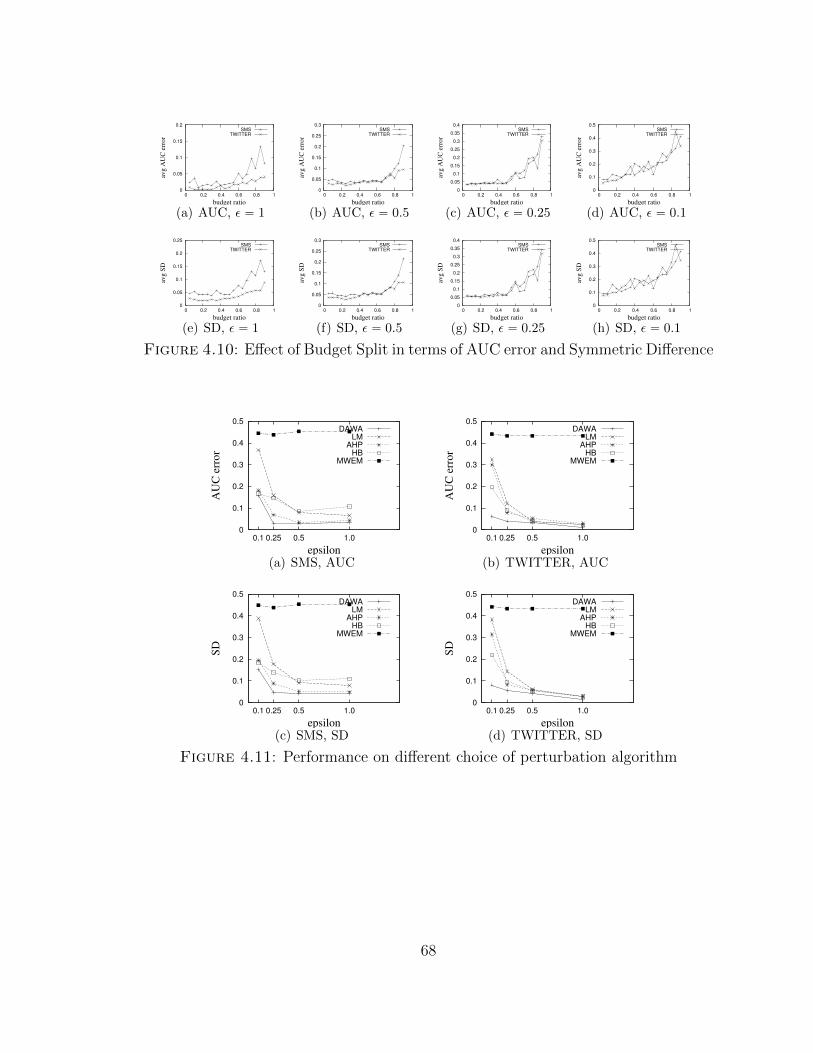
0

0.05

0.1

0.15

0.2

0 0.2 0.4 0.6 0.8 1

avg

AU

C e

rro

r

budget ratio

SMS

TWITTER

(a) AUC, ε “ 1

0

0.05

0.1

0.15

0.2

0.25

0.3

0 0.2 0.4 0.6 0.8 1

avg

AU

C e

rro

r

budget ratio

SMS

TWITTER

(b) AUC, ε “ 0.5

0

0.05

0.1

0.15

0.2

0.25

0.3

0.35

0.4

0 0.2 0.4 0.6 0.8 1

avg

AU

C e

rro

r

budget ratio

SMS

TWITTER

(c) AUC, ε “ 0.25

0

0.1

0.2

0.3

0.4

0.5

0 0.2 0.4 0.6 0.8 1

avg

AU

C e

rro

r

budget ratio

SMS

TWITTER

(d) AUC, ε “ 0.1

0

0.05

0.1

0.15

0.2

0.25

0 0.2 0.4 0.6 0.8 1

avg

SD

budget ratio

SMS

TWITTER

(e) SD, ε “ 1

0

0.05

0.1

0.15

0.2

0.25

0.3

0 0.2 0.4 0.6 0.8 1

avg

SD

budget ratio

SMS

TWITTER

(f) SD, ε “ 0.5

0

0.05

0.1

0.15

0.2

0.25

0.3

0.35

0.4

0 0.2 0.4 0.6 0.8 1

avg

SD

budget ratio

SMS

TWITTER

(g) SD, ε “ 0.25

0

0.1

0.2

0.3

0.4

0.5

0 0.2 0.4 0.6 0.8 1

avg

SD

budget ratio

SMS

TWITTER

(h) SD, ε “ 0.1

Figure 4.10: Effect of Budget Split in terms of AUC error and Symmetric Difference

0

0.1

0.2

0.3

0.4

0.5

0.1 0.25 0.5 1.0

AU

C e

rror

epsilon

DAWA

LM

AHP

HB

MWEM

(a) SMS, AUC

0

0.1

0.2

0.3

0.4

0.5

0.1 0.25 0.5 1.0

AU

C e

rror

epsilon

DAWA

LM

AHP

HB

MWEM

(b) TWITTER, AUC

0

0.1

0.2

0.3

0.4

0.5

0.1 0.25 0.5 1.0

SD

epsilon

DAWA

LM

AHP

HB

MWEM

(c) SMS, SD

0

0.1

0.2

0.3

0.4

0.5

0.1 0.25 0.5 1.0

SD

epsilon

DAWA

LM

AHP

HB

MWEM

(d) TWITTER, SD

Figure 4.11: Performance on different choice of perturbation algorithm

68

the budget ratio. When the budget ratio ρ is high (close to 1), most of the privacy

budget is spent on choosing thresholds resulting in more noise being added to TPR

and FPR values. One the other hand, a small budget ratio (close to 0) would result

in more noise added to the first step, which may result in thresholds that do not

adequately capture the distribution of the TPR and FPR values. Figure 4.10 shows

the results in terms of both AUC error and symmetric difference for different budget

ratio settings. Each figure includes two curves for SMS and Twitter. Every point

reports the average value of 20 trials. We can observe that for all settings of ε, large ρ

values close to 1 result in an inordinate loss in performance, whereas the performance

is relatively stable for a wider range of smaller ρ values. ρ “ 0.2 is good choice across

datasets and across different ε values.

Sensitivity to choice of perturbation algorithm

Finally, we evaluate how the choice of perturbation algorithm for perturbing TPR

and FPR values affects the performance of PriROC. Table 4.4 lists a set of algorithms

for perturbing TPR and FPR values. Figure 4.11 shows the results for both datasets

(SMS and Twitter) on both error metrics (AUC error and symmetric difference).

In each figure, we compare the average corresponding value among 20 trials of using

PriROC with different perturbation algorithms for computing private FPR and TPR

values on various ε settings. Uniform is not shown in the figures since it works even

worse than MWEM. From figure 4.11, we can see DAWA performs the best in terms

of all datasets and ε settings. Table 4.4 also displays the optimal choice of DAWA by

computing the regret in terms of AUC error and symmetric difference for different

algorithms among all (dataset, ε) settings. The regret of DAWA for both AUC

error and symmetric difference is 1, which shows the consistent out-performance of

choosing DAWA as perturbation algorithm in PriROC.

69

4.4 Binned Residual Plot

We now present the first differentially private algorithm for computing binned resid-

ual plots for analyzing model fit of logistic regression.

4.4.1 Review of Binned Residual Plots

Let Draw “ tpyi,xiqq : i P rnsu be the confidential dataset. As reviewed (in sec-

tion 4.3.1), in logistic regression, the prediction of each yi can be computed as

ppxiq “ P pyi “ 1 | xiq “exppb0 `

řpj“1 xijbjq

1` exppb0 `řpj“1 xijbjq

, (4.7)

where b “ pb0, . . . , bpq is the maximum likelihood estimate of the coefficients.

The residual of each point is ri “ yi´ppxiq. Hence, ri ě 0 when yi “ 1 and ri ď 0

when yi “ 0. As such, a plot of residuals versus predicted values is not especially

informative. It appears as two straight lines, one with non-negative values for cases

with yi “ 1 and one with non-positive values for cases with yi “ 0.

Instead, we use binned residual plots to examine the fit of logistic regression. To

make the binned residual plot, the data are split into several bins of roughly equal

sample size based on the predictions ppxiq. Within each bin, the average value of

ppxiq and average value of ri are computed. We then plot the average residuals versus

the average predicted values across all bins.

A good fit of logistic regression in terms of binned residual plot shows a pattern

of randomly scattered set of points (see Figure 4.12(a)). When logp ppxiq1´ppxiq

q is not

linear in terms of xi, the binned residual plot may show systematic curvatures or

bins with extreme average residuals (see Figure 4.12(b)).

Again, when D is confidential, we cannot directly release the true binned residual

plot. If an attacker knows the real binned residual plot and all other input data

except one record, the attacker can reconstruct the missing record by using the

70

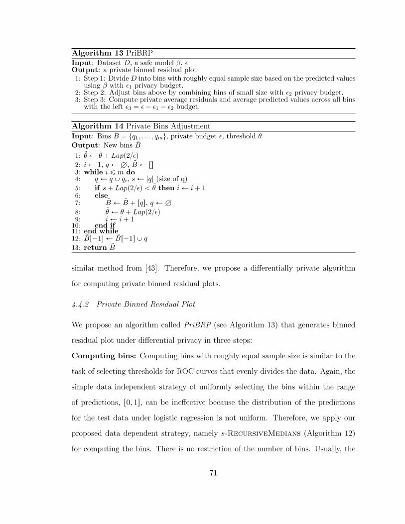
Algorithm 13 PriBRPInput: Dataset D, a safe model β, εOutput: a private binned residual plot1: Step 1: Divide D into bins with roughly equal sample size based on the predicted values

using β with ε1 privacy budget.2: Step 2: Adjust bins above by combining bins of small size with ε2 privacy budget.3: Step 3: Compute private average residuals and average predicted values across all bins

with the left ε3 “ ε´ ε1 ´ ε2 budget.

Algorithm 14 Private Bins AdjustmentInput: Bins B “ tq1, . . . , qmu, private budget ε, threshold θ

Output: New bins B

1: θ Ð θ ` Lapp2{εq

2: iÐ 1, q ÐH, B Ð rs3: while i ď m do4: q Ð q Y qi, sÐ |q| (size of q)

5: if s` Lapp2{εq ă θ then iÐ i` 16: else7: B Ð B ` rqs, q ÐH

8: θ Ð θ ` Lapp2{εq9: iÐ i` 110: end if11: end while12: Br´1s Ð Br´1s Y q

13: return B

similar method from [43]. Therefore, we propose a differentially private algorithm

for computing private binned residual plots.

4.4.2 Private Binned Residual Plot

We propose an algorithm called PriBRP (see Algorithm 13) that generates binned

residual plot under differential privacy in three steps:

Computing bins: Computing bins with roughly equal sample size is similar to the

task of selecting thresholds for ROC curves that evenly divides the data. Again, the

simple data independent strategy of uniformly selecting the bins within the range

of predictions, r0, 1s, can be ineffective because the distribution of the predictions

for the test data under logistic regression is not uniform. Therefore, we apply our

proposed data dependent strategy, namely s-RecursiveMedians (Algorithm 12)

for computing the bins. There is no restriction of the number of bins. Usually, the

71

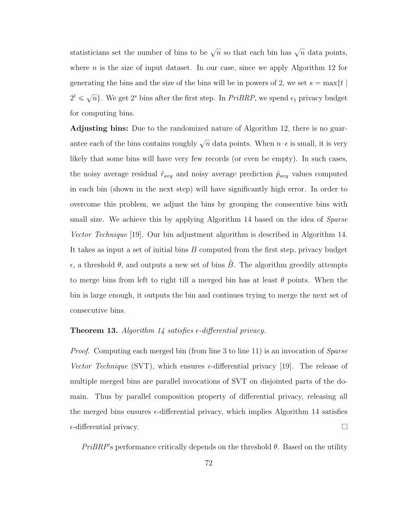
statisticians set the number of bins to be?n so that each bin has

?n data points,

where n is the size of input dataset. In our case, since we apply Algorithm 12 for

generating the bins and the size of the bins will be in powers of 2, we set s “ maxtt |

2t ď?nu. We get 2s bins after the first step. In PriBRP, we spend ε1 privacy budget

for computing bins.

Adjusting bins: Due to the randomized nature of Algorithm 12, there is no guar-

antee each of the bins contains roughly?n data points. When n ¨ε is small, it is very

likely that some bins will have very few records (or even be empty). In such cases,

the noisy average residual ravg and noisy average prediction pavg values computed

in each bin (shown in the next step) will have significantly high error. In order to

overcome this problem, we adjust the bins by grouping the consecutive bins with

small size. We achieve this by applying Algorithm 14 based on the idea of Sparse

Vector Technique [19]. Our bin adjustment algorithm is described in Algorithm 14.

It takes as input a set of initial bins B computed from the first step, privacy budget

ε, a threshold θ, and outputs a new set of bins B. The algorithm greedily attempts

to merge bins from left to right till a merged bin has at least θ points. When the

bin is large enough, it outputs the bin and continues trying to merge the next set of

consecutive bins.

Theorem 13. Algorithm 14 satisfies ε-differential privacy.

Proof. Computing each merged bin (from line 3 to line 11) is an invocation of Sparse

Vector Technique (SVT), which ensures ε-differential privacy [19]. The release of

multiple merged bins are parallel invocations of SVT on disjointed parts of the do-

main. Thus by parallel composition property of differential privacy, releasing all

the merged bins ensures ε-differential privacy, which implies Algorithm 14 satisfies

ε-differential privacy.

PriBRP’s performance critically depends on the threshold θ. Based on the utility

72

analysis of Sparse Vector Technique, the size of output bins will be greater than

θ´ 4plogpkq`logp2{γqqε

with probability 1´γ, where k is the number of answered queries.

In the Algorithm 14, we set θ “ n2tˆ2

`4 logp2{γq

ε, ignoring logpkq term (empirically k

is usually small). The goal is that the adjusted bins have size greater than half of

the size of real non-private bins with roughly 1´ γ probability (γ is set to be 0.9 in

the experiment). In PriBRP, we spend ε2 budget on adjusting bins.

Computing average residuals and predictions: Given a set of bins, we directly

apply the Laplace Mechanism (LM) for computing average residuals and predictions

within each bin. Suppose the bin under consideration is q “ rl, rs, where 0 ď l ă

r ď 1. Let Lq denote the set of points whose predictions are within rl, rs. That is

Lq “ ti P rns | l ď ppxiq ď ru (4.8)

Suppose m “ |Lq| denoting the size of Lq, then the average residual and prediction

values can be computed:

ravg “totrm

, totr “ÿ

iPLq

ri (4.9)

pavg “totpm

, totp “ÿ

iPLq

ppxiq. (4.10)

We compute the private average residuals and predictions as follows:

1. We compute the private size m “ m`Lapp∆pmqεq, where the sensitivity ∆pmq “

2 under bounded differential privacy.

2. We compute the private sum of predictions ˜totp “ totp`Lapp∆ptotpq

ε), where the

sensitivity ∆ptotpq “ r ´ l. Then the private average prediction is pavg “˜totpm

.

3. We compute the private sum of residuals ˜totr “ totr ` Lapp∆ptotrqε

), where the

sensitivity ∆ptotrq “ 1` r´ l. Then the private average residual is ravg “˜totrm

.

73

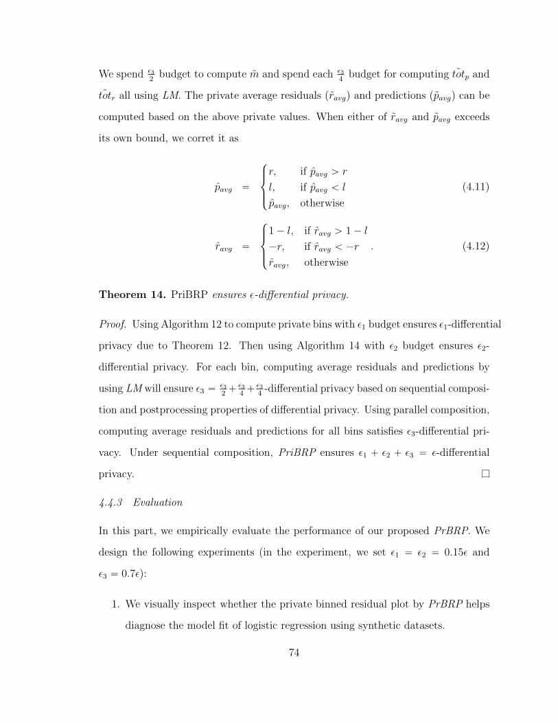
We spend ε32

budget to compute m and spend each ε34

budget for computing ˜totp and

˜totr all using LM. The private average residuals (ravg) and predictions (pavg) can be

computed based on the above private values. When either of ravg and pavg exceeds

its own bound, we corret it as

pavg “

$

’

&

’

%

r, if pavg ą r

l, if pavg ă l

pavg, otherwise

(4.11)

ravg “

$

’

&

’

%

1´ l, if ravg ą 1´ l

´r, if ravg ă ´r

ravg, otherwise

. (4.12)

Theorem 14. PriBRP ensures ε-differential privacy.

Proof. Using Algorithm 12 to compute private bins with ε1 budget ensures ε1-differential

privacy due to Theorem 12. Then using Algorithm 14 with ε2 budget ensures ε2-

differential privacy. For each bin, computing average residuals and predictions by

using LM will ensure ε3 “ε32` ε3

4` ε3

4-differential privacy based on sequential composi-

tion and postprocessing properties of differential privacy. Using parallel composition,

computing average residuals and predictions for all bins satisfies ε3-differential pri-

vacy. Under sequential composition, PriBRP ensures ε1 ` ε2 ` ε3 “ ε-differential

privacy.

4.4.3 Evaluation

In this part, we empirically evaluate the performance of our proposed PrBRP. We

design the following experiments (in the experiment, we set ε1 “ ε2 “ 0.15ε and

ε3 “ 0.7ε):

1. We visually inspect whether the private binned residual plot by PrBRP helps

diagnose the model fit of logistic regression using synthetic datasets.

74

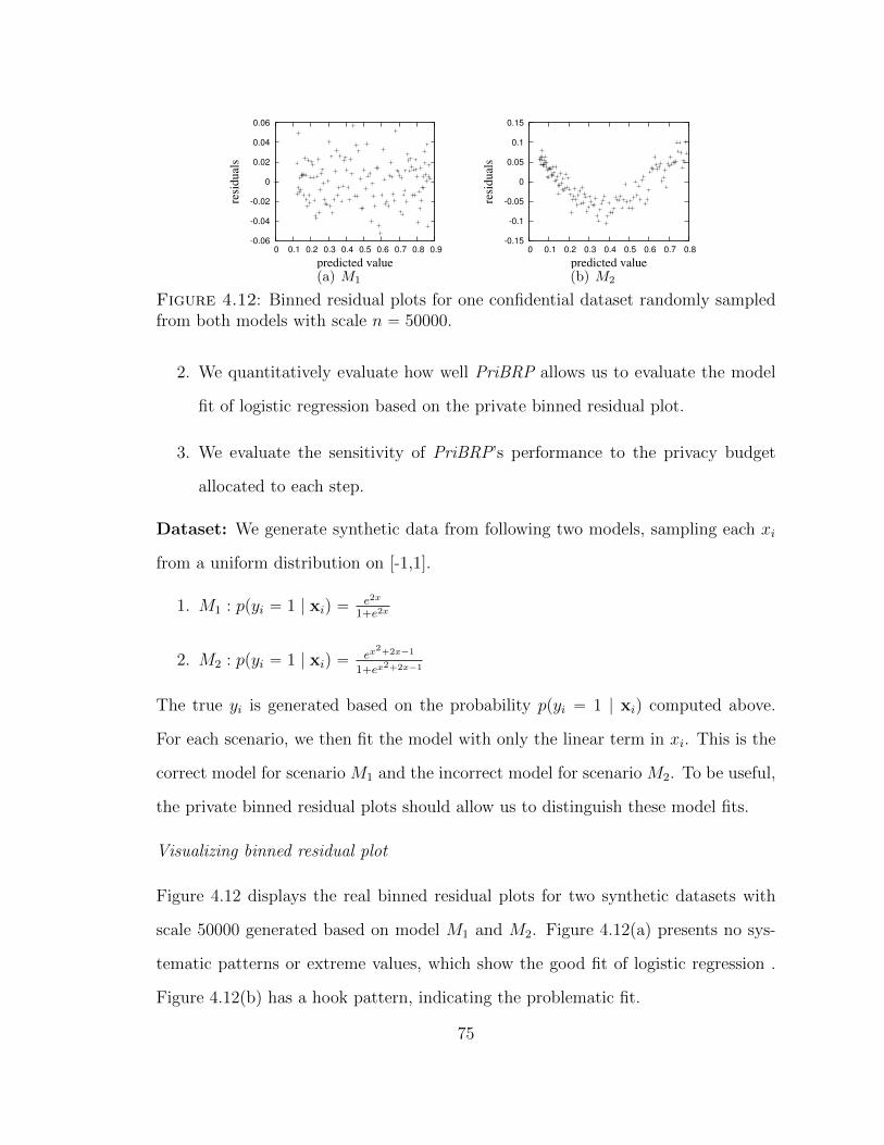
-0.06

-0.04

-0.02

0

0.02

0.04

0.06

0 0.1 0.2 0.3 0.4 0.5 0.6 0.7 0.8 0.9

resi

dual

s

predicted value

(a) M1

-0.15

-0.1

-0.05

0

0.05

0.1

0.15

0 0.1 0.2 0.3 0.4 0.5 0.6 0.7 0.8

resi

dual

s

predicted value

(b) M2

Figure 4.12: Binned residual plots for one confidential dataset randomly sampledfrom both models with scale n “ 50000.

2. We quantitatively evaluate how well PriBRP allows us to evaluate the model

fit of logistic regression based on the private binned residual plot.

3. We evaluate the sensitivity of PriBRP’s performance to the privacy budget

allocated to each step.

Dataset: We generate synthetic data from following two models, sampling each xi

from a uniform distribution on [-1,1].

1. M1 : ppyi “ 1 | xiq “e2x

1`e2x

2. M2 : ppyi “ 1 | xiq “ex

2`2x´1

1`ex2`2x´1

The true yi is generated based on the probability ppyi “ 1 | xiq computed above.

For each scenario, we then fit the model with only the linear term in xi. This is the

correct model for scenario M1 and the incorrect model for scenario M2. To be useful,

the private binned residual plots should allow us to distinguish these model fits.

Visualizing binned residual plot

Figure 4.12 displays the real binned residual plots for two synthetic datasets with

scale 50000 generated based on model M1 and M2. Figure 4.12(a) presents no sys-

tematic patterns or extreme values, which show the good fit of logistic regression .

Figure 4.12(b) has a hook pattern, indicating the problematic fit.

75

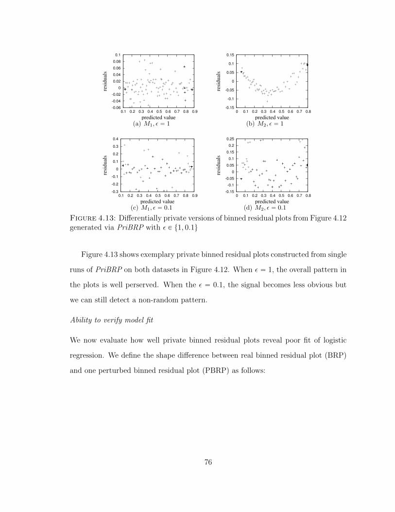
-0.06

-0.04

-0.02

0

0.02

0.04

0.06

0.08

0.1

0.1 0.2 0.3 0.4 0.5 0.6 0.7 0.8 0.9

resi

dual

s

predicted value

(a) M1, ε “ 1

-0.15

-0.1

-0.05

0

0.05

0.1

0.15

0 0.1 0.2 0.3 0.4 0.5 0.6 0.7 0.8

resi

dual

s

predicted value

(b) M2, ε “ 1

-0.3

-0.2

-0.1

0

0.1

0.2

0.3

0.4

0.1 0.2 0.3 0.4 0.5 0.6 0.7 0.8 0.9

resi

dual

s

predicted value

(c) M1, ε “ 0.1

-0.15

-0.1

-0.05

0

0.05

0.1

0.15

0.2

0.25

0 0.1 0.2 0.3 0.4 0.5 0.6 0.7 0.8

resi

dual

s

predicted value

(d) M2, ε “ 0.1

Figure 4.13: Differentially private versions of binned residual plots from Figure 4.12generated via PriBRP with ε P t1, 0.1u

Figure 4.13 shows exemplary private binned residual plots constructed from single

runs of PriBRP on both datasets in Figure 4.12. When ε “ 1, the overall pattern in

the plots is well perserved. When the ε “ 0.1, the signal becomes less obvious but

we can still detect a non-random pattern.

Ability to verify model fit

We now evaluate how well private binned residual plots reveal poor fit of logistic

regression. We define the shape difference between real binned residual plot (BRP)

and one perturbed binned residual plot (PBRP) as follows:

76

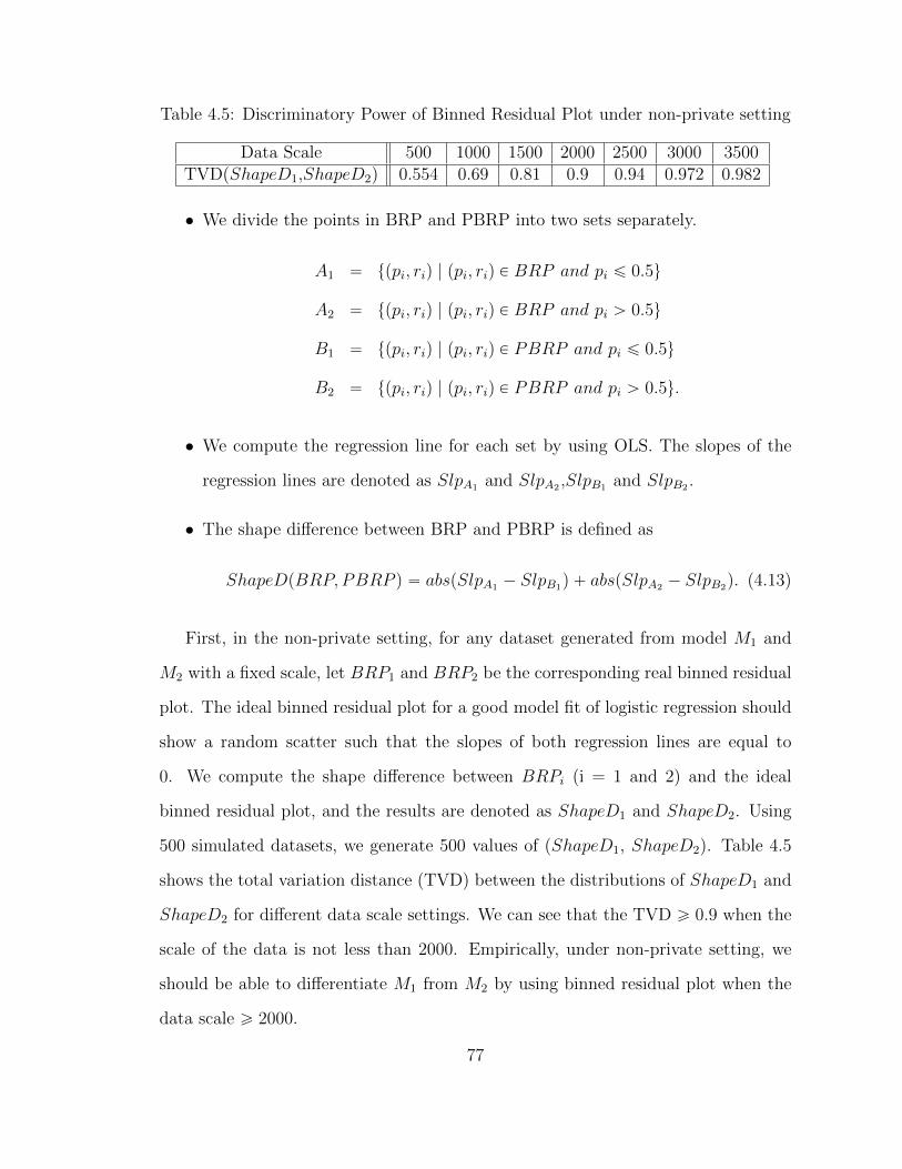
Table 4.5: Discriminatory Power of Binned Residual Plot under non-private setting

Data Scale 500 1000 1500 2000 2500 3000 3500TVD(ShapeD1,ShapeD2) 0.554 0.69 0.81 0.9 0.94 0.972 0.982

• We divide the points in BRP and PBRP into two sets separately.

A1 “ tppi, riq | ppi, riq P BRP and pi ď 0.5u

A2 “ tppi, riq | ppi, riq P BRP and pi ą 0.5u

B1 “ tppi, riq | ppi, riq P PBRP and pi ď 0.5u

B2 “ tppi, riq | ppi, riq P PBRP and pi ą 0.5u.

• We compute the regression line for each set by using OLS. The slopes of the

regression lines are denoted as SlpA1 and SlpA2 ,SlpB1 and SlpB2 .

• The shape difference between BRP and PBRP is defined as

ShapeDpBRP, PBRP q “ abspSlpA1 ´ SlpB1q ` abspSlpA2 ´ SlpB2q. (4.13)

First, in the non-private setting, for any dataset generated from model M1 and

M2 with a fixed scale, let BRP1 and BRP2 be the corresponding real binned residual

plot. The ideal binned residual plot for a good model fit of logistic regression should

show a random scatter such that the slopes of both regression lines are equal to

0. We compute the shape difference between BRPi (i = 1 and 2) and the ideal

binned residual plot, and the results are denoted as ShapeD1 and ShapeD2. Using

500 simulated datasets, we generate 500 values of (ShapeD1, ShapeD2). Table 4.5

shows the total variation distance (TVD) between the distributions of ShapeD1 and

ShapeD2 for different data scale settings. We can see that the TVD ě 0.9 when the

scale of the data is not less than 2000. Empirically, under non-private setting, we

should be able to differentiate M1 from M2 by using binned residual plot when the

data scale ě 2000.

77

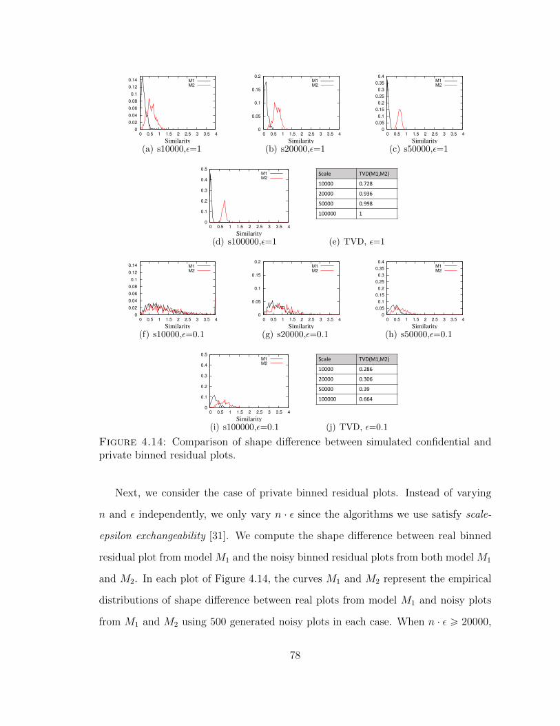
0

0.02

0.04

0.06

0.08

0.1

0.12

0.14

0 0.5 1 1.5 2 2.5 3 3.5 4

Similarity

M1

M2

(a) s10000,ε=1

0

0.05

0.1

0.15

0.2

0 0.5 1 1.5 2 2.5 3 3.5 4

Similarity

M1

M2

(b) s20000,ε=1

0

0.05

0.1

0.15

0.2

0.25

0.3

0.35

0.4

0 0.5 1 1.5 2 2.5 3 3.5 4

Similarity

M1

M2

(c) s50000,ε=1

0

0.1

0.2

0.3

0.4

0.5

0 0.5 1 1.5 2 2.5 3 3.5 4

Similarity

M1

M2

(d) s100000,ε=1

Scale TVD(M1,M2)

10000 0.728

20000 0.936

50000 0.998

100000 1

(e) TVD, ε=1

0

0.02

0.04

0.06

0.08

0.1

0.12

0.14

0 0.5 1 1.5 2 2.5 3 3.5 4

Similarity

M1

M2

(f) s10000,ε=0.1

0

0.05

0.1

0.15

0.2

0 0.5 1 1.5 2 2.5 3 3.5 4

Similarity

M1

M2

(g) s20000,ε=0.1

0

0.05

0.1

0.15

0.2

0.25

0.3

0.35

0.4

0 0.5 1 1.5 2 2.5 3 3.5 4

Similarity

M1

M2

(h) s50000,ε=0.1

0

0.1

0.2

0.3

0.4

0.5

0 0.5 1 1.5 2 2.5 3 3.5 4

Similarity

M1

M2

(i) s100000,ε=0.1

Scale TVD(M1,M2)

10000 0.286

20000 0.306

50000 0.39

100000 0.664

(j) TVD, ε=0.1

Figure 4.14: Comparison of shape difference between simulated confidential andprivate binned residual plots.

Next, we consider the case of private binned residual plots. Instead of varying

n and ε independently, we only vary n ¨ ε since the algorithms we use satisfy scale-

epsilon exchangeability [31]. We compute the shape difference between real binned

residual plot from model M1 and the noisy binned residual plots from both model M1

and M2. In each plot of Figure 4.14, the curves M1 and M2 represent the empirical

distributions of shape difference between real plots from model M1 and noisy plots

from M1 and M2 using 500 generated noisy plots in each case. When n ¨ ε ě 20000,

78

0

0.2

0.4

0.6

0.8

1

0 0.1 0.2 0.3 0.4 0.5

avg S

hap

eD

budget ratio

M1

M2

(a) ε “ 1

0.5

1

1.5

2

2.5

3

3.5

4

0 0.1 0.2 0.3 0.4 0.5

avg S

hap

eD

budget ratio

M1

M2

(b) ε “ 0.1Figure 4.15: Effect of Budget Split in terms of Shape Difference

two curves are well separated, which means an analyst can distinguish the good fit

and poor fit by using noisy binned residual plot. Figure 4.14(e) and 4.14(j) comfirm

this finding by using total variation distance between M1 and M2 curves. The total

variation distance is over 0.9 when n ¨ ε ě 20000.

Sensitivity to budget split

We evaluate the effect of budget split on the performance of PriBRP. In PriBRP,

we split the total privacy budget ε into three parts - ε1 for computing initial bins,

ε2 for adjusting bins and ε3 for computing average residuals and predictions. We

let ε1 “ ε2 “ ρε and ε3 “ p1 ´ 2ρqε, where ρ is called the budget ratio. When ρ is

high (close to 0.5), most of the privacy budget is spent on computing bins so that

more noise will be injected to average residuals and predictions. On the other hand,

a small ratio brings more noise for generating bins so that the generated bins may

not equally partition the data. Figure 4.15 displays the results in terms of shape

difference for different budget ratio settings. Each figure includes two curves for

datasets from model M1 and M2 with scale 10000. Each point reports the average

shape difference between the real binned residual plot and one perturbed binned

residual plot by PriBRP among 100 trials under the corresponding budget split. We

can observe that for both settings of ε, a range of a smaller ρ values lead to relatively

better performance in terms of the shape difference for both datasets. ρ “ 0.15 is a

79

good choice across datasets and across different ε values.

4.5 Conclusions

It is not possible using only the output of private algorithms or estimates based

on synthetic data. Thus, we present differentially private diagnostic tools for linear

and logistic regression that help analysts assess the quality of the assumptions and

predictive capabilities of regression models. Some algorithms (PriROC and PriBRP)

make use of Sparse Vector Technique for designing their sub-modules.

More broadly, we believe that this work is the first step toward building provably

private verification servers [50], or query systems that allow users to assess the quality

of inferences made on synthetic data. Verification servers would permit analysts to

gauge whether or not their analyses on synthetic data result in reliable conclusions,

thus achieving the twin goals of privacy and utility.

80

5

Differentially Private Stream Processing

In this Chapter, we design novel differentially private solutions to support queries

on streaming datasets, where Sparse Vector Technique was also applied as a key

primitive in the design of the algorithm.

5.1 Introduction

A number of emerging application domains rely on personal data processed in a

streaming manner. Streaming data is the foundation of the Internet of Things [3]

and prevalent in domains like environmental sensing, traffic management, health

monitoring, and financial technology. Such data is typically captured and analyzed

continuously and, because of the volume of the data, it is often processed as it arrives,

in real time.

Since this data may report on individuals’ location, health status, or other sen-

sitive state, directly releasing the data, or even aggregates computed from the data

stream can violate privacy [16, 20]. In particular, continually updating statistics over

time leaks more and more information to the attackers, potentially causing harmful

privacy leakage [7].

81

In this part, we propose a novel technique for releasing continuous query an-

swers on real time streams under differential privacy. Our technique combines a

Perturber, which generates a stream of noisy counts, and an independent module

called a Grouper, which computes a partition of the data received so far. The Grouper

privately finds partitions of the data which have small absolute deviations from their

average. The final module, called the Smoother, combines the output of both the

Perturber and the Grouper, generating the final private estimate of a query answer

at each time step. The Perturb-Group-Smooth technique (or PGS, the inspiration

for “PeGaSus”) is data-adaptive: it offers improved accuracy for streams that have

sparse or stable counts because the Grouper detects these regions and the Smoother

uses knowledge of these regions to infer better estimates.

PeGaSus not only helps release accurate differentially private streams (individual

counts at each time step) but can also simultaneously support multiple alternative

query workloads including window sum queries and event monitoring queries like

finding jumping and dropping points or detecting low signal points in the stream.

These different tasks can be solved by reusing the output of the Perturber and the

Grouper, and just modifying the Smoother method, without incurring any additional

privacy budget. Surprisingly, for many of these workloads, using our data dependent

strategy outperforms state-of-the-art algorithms that are designed specifically for the

corresponding query workload.

We propose extensions to PeGaSus to answer counting queries at different hier-

archical resolutions on the stream. These extensions allow us to model typical query

workloads that appear in building or network monitoring, where analysts are inter-

ested in both streams generated by individual sensors (or IP addresses), but also in

aggregate streams generated by groups of sensors (or groups of IP addresses).

In summary, we make the following contributions:

82

‚ We design PeGaSus, a novel technique for answering a large class of continuous

queries over real time data streams under differential privacy.

‚ PeGaSus uses a combination of a Perturber, a data-adaptive Grouper and a query

specific Smoother to simultaneously support a range of query workloads over

multiple resolutions over the stream.

‚ The Grouper and Smoother in combination offers improved accuracy for streams

that have sparse or stable counts.

‚ A thorough empirical evaluation on a real data stream collected from 4000 WiFi

access points from a large educational institution shows that, by using different

query specific Smoother methods, PeGaSus outperforms the previous state-of-the-

art algorithms specialized to given workloads. For example, our data dependent

algorithm can compute more accurate sliding window queries than the previous

state-of-the-art algorithm that is designed for a specific sliding window workload

for all window sizes w ď 28.

The paper is organized as follows. Section 5.2 reviews the streaming data model,

queries on streams, and the semantics of privacy on streams. In Section 5.3, we

describe the Perturb-Group-Smooth (PeGaSus) algorithm. In Section 5.4, we show

how the framework can support multiple query workload by applying different query

specific Smoother methods. In Section 5.5, we discuss how to extend PeGaSus to

answer counting queries at different hierarchical resolutions on the stream. Com-

prehensive experiments on a real data stream are presented in Section 5.6. The

conclusion is made in Section 5.7.

83

5.2 Preliminaries

5.2.1 Stream data model

We define the source stream D as an infinite sequence of tuples. Each tuple is of the

form pu, s, tq and is an element from the domain dom “ U ˆS ˆ T where U is set of

user identifiers, S is a set of possible states, and T is an (infinite) set of timestamps.

Each pu, s, tq records an atomic event, namely that user u was observed in state s

at time t. Note that this single stream could contain events from multiple sources –

these would be encoded as different states (elements of S).

To simplify presentation, we represent time using logical timestamps letting T “

t1, 2, 3, . . . u. The rationale is that the analysis tasks we consider in Section 5.2.2

emit an aggregate summary of the stream periodically (e.g. every 5 minutes) and

thus logical time t “ 1 can be understood as capturing all events that happened

within the first reporting period. Furthermore, this implies that the a tuple pu, s, tq

does not describe a specific, instanteous event but rather it encodes the aggregate

behavior of user u during the time step t. Therefore, the states S encode the state

of a user during the logical time step t. We illustrate with an example.

Example 3. Consider a data stream management system that collect data from WiFi

access points (APs) distributed across buildings on a campus. Users correspond to

mac addresses of individual devices that connect to WiFi access points. The set of

time steps could represent the aggregated activity of a user over time intervals of

5 minutes each. Thus, time steps t and t ` 1 would differ in wall clock time of 5

minutes. Finally, if there are m WiFi access points on campus, then we could have

m ` 1 states: a state sK that represents “user did not make a successful connection

to any AP”, and m states sp, one for each AP p, that represents “user made at least

one successful connection to the AP p”.

The tuples in D arrive in order by time. Thus if pu1, s1, t1q arrives after pu, s, tq it

84

must be that t ď t1. We use Dt to represent a stream prefix: the set of tuples that

arrive on or before time t.

5.2.2 Queries on streams

In this paper, we consider a number of queries on the private stream D. The answer

to a query on D is itself a stream. We focus on counting queries as well as other

queries that can be derived from counting queries.

Queries on a single target state

A counting query takes a specific target state s and reports, for each time step t,

the number of users who were observed in state s at time t. More formally, let Cpsq

be the infinite stream Cpsq “ c1psq, c2psq, . . . where ctpsq “ |tpu1, s1, t1q P Dt | t

1 “

t and s1 “ su|. Let Ctpsq denote the prefix stream of Cpsq up to time t. When clear

from context, we drop the s and just use C “ c1, c2, . . . .

Note that the answer to the query should be generated in “real time” – i.e., ct

should be produced before any tuple p¨ , ¨ , t` 1q is observed.

Example 4. An analyst might want to visualize the counts of the number of users

who had at least one successful connection in a time step at access point AP1. Hence,

the target state is sAP1, CtpsAP1q represents the number of users with at least one

successful connection to AP1 in time step t, and CpsAP1q represents the stream of

counts.

The counting query defined above is referred to as a Unit query. We also support

additional queries, all of which can be derived from C.

Sliding Windows A sliding window query with window size w and target state s

reports, for each time step t, the total number of times a user has been observed in

state s in the most recent w time steps. More formally, let SW ps, wq be an infinite

85

stream SW ps, wq “ sw1, sw2, . . . , where swtps, wq “ |tpu1, s1, t1q P Dt | t ´ w ă t1 ď

t and s1 “ su|. Observe that the sliding window query answers can also be derived

by summing corresponding counts in query Cpsq: swtps, wq “řtt1“t´w`1 ct1psq.

Event Monitoring While each tuple in the stream D captures an atomic event, the

analyst may be interested in monitoring certain patterns in the event stream. We

call this task event monitoring and consider monitoring event patterns that can be

derived from the counting query stream C.

We define the event monitoring query as follows. Let EMps, w, f, Bq “ b1, b2, . . .

be an infinite stream of bits where b1 “ 1 if the monitored event has occurred at

time t and 0 otherwise. The inputs to the query EM are the target state s, a desired

window size w, an abitrary function f that computes on a window of w counts and

boolean function B that computes on the ouptut of f . The bit bt is computed as

bt “ Bpfpct´w`1, . . . , ctqq. We give two examples of event monitoring queries.

‚ Jumping and dropping point: This query monitors whether the count has changed

by at least δ from the count w time units ago. Thus, f computes the absolute

difference between the current count and the count received w time steps before,

fpct´w`1, . . . , ctq “ |ct´ ct´w`1| and B compares that difference to a threshold δ,

Bpxq “ 1 if x ě δ and is 0 otherwise.

‚ Low signal: This query monitors whether the total count in a sliding window is

smaller than δ. Thus, f computes the total count, fpct´w`1, . . . , ctq “řti“t´w`1 ci

and B is again a threshold function, Bpxq “ 1 if x ă δ and is 0 otherwise.

Queries on multiple target states

Our approach also supports queries on multiple target states. Let ts1, . . . , smu Ď S

denote the set of states the analyst is interested in. We support three variants. First,

the analyst can simply issue multiple queries where each query is on a single target

86

state (i.e., any one of the queries defined previously). We illustrate this with an

example.

Example 5. An analyst might be interested in the unit query for the states sp cor-

responding to all access points p within a specific building, as well as a low signal

event monitoring query EMpsq, w, . . . q, for all access points q housed in conference

rooms across campus.

Second, we also support queries on aggregations of target states. We denote a

single aggregation as agg Ď ts1, s2, . . . , smu. Any query that is defined for a single

target state can also be defined over an aggregation of target states by replacing any

equality condition on the state (s1 “ s) with set membership condition (s1 P agg).

For example, an aggregated counting query is denoted Cpaggq and it produces a

stream of answers Cpaggq “ cpaggq1, cpaggq2, . . . where cpaggqt “ř

iPagg ctpsiq.

Finally, the analyst may wish to ask a query about more than one aggregation of

states. Let AGG “ tagg1, agg2, ...u denote a collection of aggregations. We consider

the special case where this collection has a hierarchical structure.

Definition 6. A set of aggregations AGG “ tagg1, agg2, ...u is hierarchical if for any

two aggregations agg1, agg2 P AGG, they satisfy one of the following two properties:

1. agg1 Ă agg2 or agg2 Ă agg1.

2. agg1 X agg2 “ H.

Intuitively, a set of hierarchical aggregations AGG can be represented as a tree

or a forest, where any child aggregation contains a subset of states that its parent

aggregation covers and any two child aggregations with the same parent aggregation

cover two disjoint sets of states. We use levelpagg | AGGq to denote the level of

agg P AGG. levelpagg | AGGq “ 1 if agg has no parent aggregation in AGG. If

87

agg1, agg2 P AGG and agg1 is the child aggregation of agg2, levelpagg1 | AGGq “

levelpagg2 | AGGq ` 1.

Example 6. An analyst might be interested in aggregate counts of successful connec-

tions at the level of individual sensors, as well as for aggregations of sensors within

the same room, same floor, and the same building on campus. For each room r,

let aggr denote the aggregation of states sp, where p is an access point in room r.

Similarly, for a floor f and building b, we can define aggregations aggf and aggb that

aggregate states sp, where p is in the floor f or building b, respectively. These set of

aggregations form a hierarchy. An analyst might be interested in the unit query for

aggregate states at floors and building as well as a low signal event monitoring query

EMpaggr, w, . . . q, for all room r on campus.

5.2.3 Privacy for Streams

Two stream prefixes Dt and D1t are considered neighbors if they differ by addition or

removal of a single tuple; i.e., |Dt‘D1t| “ 1 where ‘ indicates symmetric difference.

The algorithms we consider in this paper operate on stream prefixes.

We define privacy for streams as follows, similarly to event differential privacy

[4, 23].

Definition 7 (ε-differential privacy). Let A be a randomized algorithm that takes as

input a stream prefix of arbitrary size and outputs an element from a set of possible

outputs O. Then A satisfies ε-differential privacy if for any pair of neighboring

stream prefixes Dt and D1t, and @O Ď O,

PrrApDtq P Os ď eε ˆ PrrApD1tq P Os (5.1)

The parameter ε controls the privacy risk and smaller ε corresponds to stronger

privacy protection. The semantics of this privacy guarantee are discussed further in

Section 5.2.4.

88

Remark: We make an assumption that each user can be in at most k different

states s during one time period. Without loss of generality, we assume k “ 1 in our

application. If k ą 1, we can simply normalize the counts (a user who is in k states

at time t contributes 1{k rather than 1 to the corresponding counting queries) or

increase the amount of noise injected in our algorithm in order to provide privacy

protection in terms of any single user during one time period.

5.2.4 Privacy Semantics

In this section, we discuss the semantics of privacy ensured by Definition 7 and justify

our choice of this privacy goal.

The privacy ensured by Definition 7 can be interpreted in terms of (a) plausible

deniability, and (b) disclosure of secrets to adversaries. Let φuptq and φ1uptq be two

mutually exclusive boolean properties about a user u at time step t. Examples of

such properties could be that a user was in building B1 at time t and building B2

at time t, respectively. An algorithm M satisfying Definition 7 allows a user to deny

that φ1uptq is true rather than φuptq since for all neighboring streams Dt,D1t such that

φuptq is true on Dt and φ1uptq is true on D1t, and for all output sets O P rangepAq,

we have:

PrrApDtq “ Os ď eεPrrApD1tq “ Os (5.2)

Plausible deniability holds even for properties that span larger time windows,

albeit to a lesser extent and degrades with the length of the time window. That is,

if φupt, kq and φ1upt, kq are two mutually exclusive boolean properties about a user u

that span a time window of rt´ k` 1, ts, then for all streams Dt,D1t such that φuptq

is true on Dt and φ1uptq is true on D1t, and that differ only in the states in the time

window rt´ k ` 1, ts, and for all output sets O P rangepAq, we have:

PrrApDtq “ Os ď ek¨εPrrApD1tq “ Os (5.3)

89

Thus our definition also captures the more general w-event privacy [33]. And,

if a time step corresponds to 5 minutes, and an algorithm A satisfies Definition 7

with ε “ 0.1, then for properties that span 10 minutes, we get privacy at a level

ε “ 0.2, and for properties that span 1 hour, we get privacy at a level of ε “ 1.2. If

the protected window size goes to infinity (k is unbounded), one can extend existing

negative results [16] to show that it is impossible to release accurate statistics at each

time and offer privacy.

Next we explore the semantics of Definition 7 in terms of disclosure of secrets to

adversaries, which can be done in terms of the Pufferfish framework [? ]. One can

show that if an algorithm A satisfies Definition 7, then the adversary’s posterior odds

that φuptq is true vs φ1uptq is true after seeing the output of A, for any pair of mutually

exclusive secrets that span a single time step, is no larger than eε times the adversary’s

prior odds. However, this strong privacy guarantee only holds under the restrictive

assumptions that an adversary is not aware of possible correlations between a user’s

states across time steps. With knowledge of correlations, an adversary can learn

sensitive properties of a user within a time step even from outputs of differentially

private algorithms [34, 41, 61].

Recent work [9, 54] has provided methods for deriving an ε1 ą ε (but no more than

k ˆ ε in terms of any protected window with size k), such that algorithms satisfying

Definition 7 with parameter ε offer a weaker ε1 bound on privacy loss, even when

records are correlated across time steps. The effective privacy guarantee is closer to

ε and much smaller than k ˆ ε.

Therefore, for the rest of the paper, we only concern ourselves with developing

algorithms that ensure Definition 7 while minimizing error. We emphasize that our

proposed algorithms that satisfy Definition 7 simultaneously ensure all of the above

provable privacy guarantees, but with different value of ε. Hence, algorithms that

satisfy Definition 7 are important building blocks for releasing streaming data with

90

provable guarantees, and allows those guarantees to be configured.

5.3 Private Stream Release under PeGaSus

In this section we describe a novel, data-dependent method for private, real-time

release of query answers on data streams. Our algorithm consists of a novel combi-

nation of data perturbation and online partitioning, followed by post-processing.

We first present the algorithm for computing a unit counting query in a single

target state. In 5.4, we explain how the algorithm can be adapted to answer other

kinds of queries on a single target state and in 5.5, we explain an extension to the

algorithm to support multiple queries over hierarchical aggregations of states. The

input to the algorithm is the true answers to the unit counting query C. The output

of the algorithm is C “ c1, c2, . . . , an infinite stream where ct is an estimate of the

true answer ct.

The three main modules of our algorithm are as follows:

• Perturber: The Perturber consumes the input stream, adds noise to each

incoming element of the stream, and releases a stream of noisy counts.

• Grouper: The Grouper consumes the input stream and groups elements of

the stream seen so far.

• Smoother: The Smoother performs post-processing using the output of both

above modules.

The Perturber is a standard noise-addition mechanism, but the Grouper carries

out an important role of partitioning data into regions that can be well-approximated

by a uniform sub-stream. The Smoother then combines this information with the

output of the Perturber. The result is a data-dependent algorithm which can reduce

error for streams with properties that are commonly witnessed in practice.

91

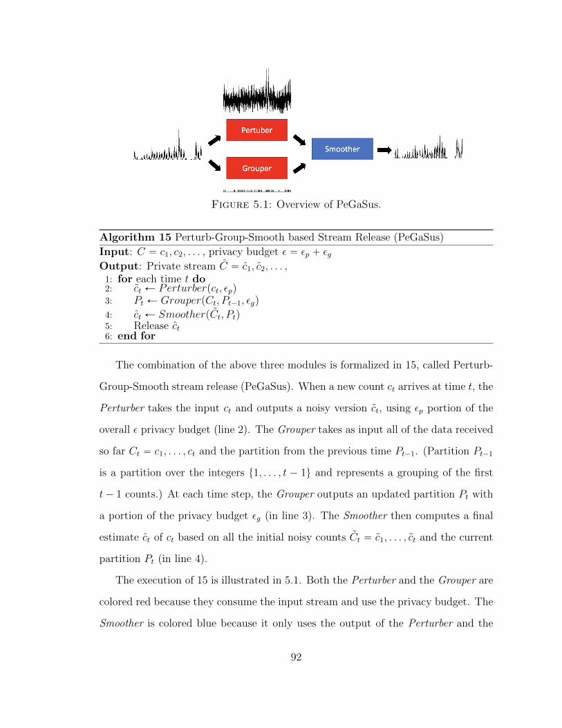
Figure 5.1: Overview of PeGaSus.

Algorithm 15 Perturb-Group-Smooth based Stream Release (PeGaSus)

Input: C “ c1, c2, . . . , privacy budget ε “ εp ` εgOutput: Private stream C “ c1, c2, . . . ,1: for each time t do2: ct Ð Perturberpct, εpq3: Pt Ð GrouperpCt, Pt´1, εgq

4: ct Ð SmootherpCt, Ptq5: Release ct6: end for

The combination of the above three modules is formalized in 15, called Perturb-

Group-Smooth stream release (PeGaSus). When a new count ct arrives at time t, the

Perturber takes the input ct and outputs a noisy version ct, using εp portion of the

overall ε privacy budget (line 2). The Grouper takes as input all of the data received

so far Ct “ c1, . . . , ct and the partition from the previous time Pt´1. (Partition Pt´1

is a partition over the integers t1, . . . , t ´ 1u and represents a grouping of the first

t´ 1 counts.) At each time step, the Grouper outputs an updated partition Pt with

a portion of the privacy budget εg (in line 3). The Smoother then computes a final

estimate ct of ct based on all the initial noisy counts Ct “ c1, . . . , ct and the current

partition Pt (in line 4).

The execution of 15 is illustrated in 5.1. Both the Perturber and the Grouper are

colored red because they consume the input stream and use the privacy budget. The

Smoother is colored blue because it only uses the output of the Perturber and the

92

Grouper.

Theorem 15. When the Perturber satisfies εp-differential privacy and the Grouper

satisfies εg-differential privacy, 15 ensures εp ` εq “ ε-differential privacy.

The above theorem follows directly from the sequential composition and post-

processing properties of differential privacy.

15 forms the basis of a number of algorithm variants we consider throughout

the paper. In the remainder of this section, we describe below the design of each

module, and basic variants for the Smoother. We also include theoretical analysis

that illustrates cases where smoothing can reduce error. ?? describe extensions to

the algorithm for other kinds of queries.

5.3.1 Design of the Perturber

The Perturber takes input ct at each time t and outputs a noisy version ct. We use

the Laplace Mechanism as the implementation of the Perturber.

5.3.2 Design of the Grouper

Next we describe the Deviation based Grouper (DBG) (16), a differentially private

method for online partitioning which chooses partitions that approximately (subject

to distortion introduced for privacy) minimizes a quality score based on deviation.

Recall that this module runs independently of the Perturber and does not consume

its output. Instead the Grouper takes as input all of the data received so far, Ct “

c1, . . . , ct at time t, and outputs a partition of Ct. At any time t, the stream seen so

far has been partitioned into contiguous groups. All but the most recent group are

closed and will not be changed, but the most recent group may continue to grow as

new elements arrive, until it is eventually closed.

To evaluate the quality of a potential group, we use the deviation function, which

measures the absolute difference of a set of counts from its average. Let G be a

93

Algorithm 16 Deviation based Grouper (DBG)

Input: Ct “ c1, . . . , ct, the previous partition Pt´1, εg, θOutput: Pt (a partition of t1, . . . , tu)

1: if t “ 1 then2: Pt´1 ÐH and let G be closed, empty group.3: else4: GÐ Last group from Pt´1

5: end if6: if G has been closed then7: Pt Ð Pt´1 Y tttuu and let the last group ttu be open.

8: θ Ð θ ` Lapp4{εgq9: else10: θ Ð θprev Ź θprev cached from previous call.

11: if pdevpCtrGY ttusq ` Lapp8{εgqq ă θ then12: Pt Ð Pt´1 with G replaced by GY ttu and G still open.13: else14: Pt Ð Pt´1 Y tttuu and close both group G and ttu.15: end if16: end if17: θprev Ð θ Ź cache θprev for subsequent calls.18: Return Pt

group of indexes of data Ct “ c1, . . . , ct, CtrGs be the set of corresponding counts in

Ct and denote by |G| the size of the group. Then the deviation of CtrGs is denoted

devpCtrGsq and is defined:

devpCtrGsq “ÿ

iPG

ˇ

ˇ

ˇ

ˇ

ci ´

ř

iPG ci|G|

ˇ

ˇ

ˇ

ˇ

. (5.4)

When the devpCtrGsq is small, the counts in CtrGs are approximately uniform and

the Smoother can exploit this.

Algorithm 16 takes as input the stream seen so far, Ct, the latest partition, Pt´1,

along with εg and a user-defined deviation threshold θ which influences the acceptable

deviation in a partition. Because the algorithm uses the sparse vector technique [19],

it maintains a noisy threshold θprev used at the previous time. When a new data ct

arrives at time t, we check the status of the last group G from the previous partition

Pt´1. If G is closed, we put ct into a new open group and reset the noisy threshold

(in line 6-8). Otherwise, we compute the deviation of the CtrGYttus and compare a

94

noisy version of the deviation value with the noisy threshold. If the noisy deviation

is smaller than the noisy threshold, we add {t} into the open G (in line 11-12).

Otherwise, we add a new group {t} into the partition and close both G and ttu (in

line 14).

The following example explains how the Grouper defined in Algorithm 16 would

run, assuming for simplicity an infinite privacy budget (so that the noise added in

lines 8 and 11 is zero).

Example 7. Consider a stream of counts C5 “ r5, 5, 6, 9, 10s and a threshold θ “ 2.

At time 1, the Grouper generates a partition P1 containing a single open group G

with a single index: G “ t1u and P1 “ tGu. At time 2, the latest group G “ t1u is

open and devpC2rt1, 2usq “ devpr5, 5sq “ 0. Because the deviation is less than θ, we

add the current data into G and keep G open. P2 still contains a single group G. At

time 3, the latest group G “ t1, 2u is open and devpr5, 5, 6sq “ 43ă θ. We still add

the current data into G and keep G open. At time 4, the latest group G “ t1, 2, 3u

is open but devpr5, 5, 6, 9sq “ 5.5 ą θ. Thus we close G “ t1, 2, 3u and create the

second group t4u which is also closed. Thus, P4 “ tt1, 2, 3u, t4uu. At time 5, the

latest group G “ t4u is closed, so we start with a new open group G “ t5u. The final

output at time 5 is P5 “ tt1, 2, 3u, t4u, t5uu .

With a realistic (non-infinite) setting for εg, the Grouper runs in a similar manner

but noise is added to both the threshold and to the deviations that are compared

with the threshold. Therefore, the output partitions will differ.

To prove the privacy of Algorithm 16 we make use of the following lemma:

Lemma 16 (Sensitivity of deviation [38]). The global sensitivity of the deviation

function ∆pdevq is bounded by 2.

Theorem 17. Using Algorithm 16 to generate a partition at every time ensures

εg-differential privacy.

95

Proof. The algorithm is an implementation of the Sparse Vector Technique [19] on

multiple disjoint sub-streams applied to the dev function. Because the sensitivity

of dev is bounded by 2 (Lemma 16), the noise added to the threshold, in line (4),

is computed as Lapp4{εgq “ Lapp2∆pdevq{εgq. In line (7), the noise added to the

deviation value is Lapp8{εgq “ Lapp4∆pdevq{εgqq and εg-differential privacy follows

from the original definition of the Sparse Vector Technique. In addition, the derived

streams from two neighboring source streams can only differ by 1 at one time. By

parallel composition, Algorithm 16 satisfies εg-differential privacy.

5.3.3 Design of the Smoother

The Smoother computes the final estimate ct for each ct received at time t based on

all the noisy counts Ct from the Perturber, in combination with the current partition

Pt. Suppose the last group G “ tt´ k, . . . , t´ 1, tu from Pt contains current index t

with the previous k indexes. Given this output from the Grouper, there are several

post-processing methods we may apply to generate an estimate, ct, that improves

upon ct. These are alternatives for the Smoother in Algorithm 15:

1. AverageSmoother: We use the average noisy counts of the data indexed in

group G to be the estimate of the current data.

ct “

ř

iPG ci|G|

. (5.5)

2. MedianSmoother: We use the median noisy counts of the data indexed in group

G to be the estimate of the current data.

ct “ mediantci | i P Gu. (5.6)

3. JSSmoother: We apply James-Stein estimator [? ] to update the noisy count

96

of the current data based on the noisy counts of the data indexed in group G.

ct “ p1´p|G| ´ 1qτ 2

ř

iPGpci ´ avgq2q ˆ pct ´ avgq ` ct, (5.7)

where avg “ř

iPG ci|G|

and τ 2 is the variance. We assume uniformity on each group

and apply James-Stein estimator to let each estimate shrink to the mean (we

can only use the noisy mean here).

We theoretically analyze the effect of AverageSmoother in the next section and em-

pirically evaluate all three variants in Section 5.6. We conclude this section with an

example.

Example 8. Continuing from Example 7, we have a stream of true counts C5 “

t5, 5, 6, 9, 10u with noisy counts from the Perturber of C5 “ t5.6, 4.4, 6.7, 9.5, 10.2u

and a final partition P5 “ tt1, 2, 3u, t4u, t5uu from the Grouper. We now illus-

trate how the final estimates C5 would have been produced using MedianSmoother

as Smoother. Recall that each ct is released in real-time based on Pt, the groups at

time t, and not the final grouping P5. At time 1, P1 “ tt1uu and the last group

is G “ t1u, c1 “ mediant5.6u “ 5.6. At time 2, the last group is G “ t1, 2u,

c2 “ mediant5.6, 4.4u “ 5. At time 3, the last group is G “ t1, 2, 3u, c3 “

mediant5.6, 4.4, 6.7u “ 5.6. At time 4, P4 “ tt1, 2, 3u, t4uu and the last group

is G “ t4u, so c4 “ mediant9.5u “ 9.5. At time 5, the last group G “ t5u,

c5 “ mediant10.2u “ 10.2. Thus, the final estimates are C5 “ t5.6, 5, 5.6, 9.5, 10.2u.

5.3.4 Error analysis of smoothing

We now formally analyze how the online grouping and post-processing smoother may

help for improving the output utility.

Theorem 18. Suppose one group G in the resulting partition from Grouper contains

n indexes, i` 1, i` 2, . . . , i` n. Assume that C is produced using AverageSmoother

97

as the Smoother. Then CrGs, the resulting estimate for group G, will have lower

expected error than CrGs, formally stated as

E›

›

›CrGs ´ CrGs

›

›

›

2ď E

›

›

›CrGs ´ CrGs

›

›

›

2

provided that the deviation of CrGs satisfies

devpCrGsq ď

a

2pn´ lnn´ 1q

p1` lnpn´ 1qqεp

Proof. In terms of C which are generated from Perturber by applying Laplace Mech-

anism, we have E›

›

›CrGs ´ CrGs

›

›

›

2“ nˆ 2

ε2p. At each time i`k, G “ ti`1, . . . , i`ku.

By using AverageSmoother, ci`k “ci`1`¨¨¨`ci`k

k. Then we have

E›

›

›CrGs ´ CrGs

›

›

›

2“ E

`

nÿ

k“1

pci`1 ` ¨ ¨ ¨ ` ci`k

k´ ci`kq

2˘

“

nÿ

k“2

pavgk ´ ci`kq2`

nÿ

k“1

1

kˆ

2

ε2p

ă plnn` 1q ˆ2

ε2p`

nÿ

k“2

pavgk ´ ci`kq2

ď plnn` 1q ˆ2

ε2p`

nÿ

k“2

p|avgk ´ avgn| ` |avgn ´ ci`k|q2

ď plnn` 1q ˆ2

ε2p` p

nÿ

k“2

|avgk ´ avgn| `nÿ

k“2

|avgn ´ ci`k|q2

ď plnn` 1q ˆ2

ε2p` p

nÿ

k“2

|avgk ´ avgn| ` devpCrGsqq2

ď plnn` 1q ˆ2

ε2p` p

n´1ÿ

k“2

1

kˆ devpCrGsq ` devpCrGsqq2

ă plnn` 1q ˆ2

ε2p` p1` lnpn´ 1qq2devpCrGsq2 (5.8)

98

where avgk “ci`1`¨¨¨`ci`k

kfor k P r1, ns.

Therefore, when devpCrGsq ď

?2pn´lnn´1q

p1`lnpn´1qqεp, we have

E›

›

›CrGs ´ CrGs

›

›

›

2ď E

›

›

›CrGs ´ CrGs

›

›

›

2(5.9)

Theorem 18 implies that when the Grouper finds a group with large size but small

deviation value, using the AverageSmoother can reduce the error of the estimates.

Many realistic data streams are either sparse or have stable counts, which suggests

that smoothing can help reduce error. Although we only theoretically analyze the

AverageSmoother as the Smoother, we empirically compare the three different post-

processing strategies on many real streams, which will be shown in Section 5.6. We

find that Grouper often finds large groups with low deviation and MedianSmoother

consistently generates the most accurate noisy streams under all settings. Thus,

in our algorithms, we apply the MedianSmoother as default to be the Smoother to

compute the final estimate for each receive data.

5.4 Multiple Query Support under PeGaSus

The previous section describes how the PeGaSus algorithm (Algorithm 15) can be

used to generate C, a differentially private answer to a given unit counting query

C. In this section, we describe how to adapt the algorithm to answer the other

queries described in Section 5.2.2, specifically the Sliding Window query and Event

Monitoring queries.

A distinctive feature of our approach is that we use the same basic PeGaSus

algorithm for these queries and change only the Smoother. This is possible because

the answers to these queries can be derived from C. Our approach uses the noisy

counts Ct along with the group information Pt to then do appropriate smoothing for

99

Algorithm 17 Window Sum Smoother (WSS)

Input: Ct “ c1, . . . , ct, Pt, wOutput: swt1: swt Ð 02: for each G P Pt such that GX tt´ w ` 1, . . . , tu ‰ H do3: cÐ mediantci | i P Gu4: swt Ð swt ` cˆ |GX tt´ w ` 1, . . . , tu|5: end for6: Return swt

the specific query. Recall that the Smoother does not take private data as input and

only post-processes the outputs of the differentially private Perturber and Grouper

subroutines. Therefore, we can swap out Smoother without impacting the privacy

guarantee. An added benefit of this approach is that we can simultaneously support

all three kinds of queries – counting, sliding window, and event monitors – all using

a single privacy budget.

For sliding window queries, we propose a new post-processing strategy called

Window Sum Smoother (WSS), which is shown in Algorithm 17. The basic idea is

that, at time t, for every ct1 contained in the sliding window (t1 P rt ´ w ` 1, ts),

we use the MedianSmoother to compute an estimate ct1 for the count at time t1.

To compute the answer to the sliding window query, we simply sum up the counts

within the window w.

Note that this is subtly different from the approach described in Section 5.3

because the estimate ct1 for some t1 in the sliding window is based on its group

G which may include counts received after t1 and up to time t. Thus, Window

Sum Smoother may provide a better estimate than just using MedianSmoother as

described in Section 5.3.3. We make this comparison empirically in Section 5.6 and

we also compare against the state of the art technique for sliding window queries [4].

For event monitoring queries, the Smoother depends on the particular event

monitor. For detecting jumps or drops, since we need the count at time t and

the count received at time t ´ w ` 1, we simply use the MedianSmoother in the

100

experiment. Actually, we may do better by also smoothing ct´w`1 using its group G

as defined at time t. For detecting low signal points, we need a sliding window query

at each timestamp. Thus we use the Window Sum Smoother. Once the counts have

been appropriately smoothed, we pass the estimated counts into the event monitor

functions B and f to generate an event stream (as described in Section 5.2.2).

5.5 Query on a Hierarchy of Aggregated States

In this section, we describe an extension to PeGaSus to support queries on multiple

target states as well as aggregations of states. Recall from Section 5.2.2 that the

analyst can request queries on a set of states ts1, . . . , smu Ď S and can also ask

queries about aggregations of states. We focus in particular on the setting in which

the analyst has specified a hierarchy of aggregations AGG and a query on each

agg P AGG.

For ease of presentation, we describe our approach assuming that the analyst has

requested a unit counting query on each agg P AGG. However, our approach extends

easily to sliding windows and event monitoring using an extension analogous to what

was described in Section 5.4.

5.5.1 Hierarchical-Stream PGS

First, we observe that we can answer the queries over hierarchical aggregations by

simply treating each aggregation as a separate stream and running any single-stream

algorithm on each input stream. Therefore, our first solution is to run PeGaSus on

each stream, an algorithm we refer to as Hierarchical-Stream PeGaSus (HS-PGS).

Formally, given a set of aggregations AGG and a corresponding set of input streams

Cpaggq “ c1paggq, c2paggq, . . . for each agg P AGG, the algorithm HS-PGS executes

PeGaSuspCpaggq, ε{hq for each agg P AGG where h is the height of AGG.

Theorem 19. Hierarchical-Stream PeGaSus satisfies ε-differential privacy.

101

Proof. The proof follows from (a) the privacy guarantee of PeGaSus (Theorem 15),

(b) parallel composition of differential privacy across each level of the hierarchy,

and (c) the sequential composition of differential privacy between the h hierarchy

levels.

5.5.2 Hierarchical-Stream PGS With Pruning

We next describe an enhancement of Hierarchical-Stream PeGaSus that is designed

to lower error when many of the input streams in the aggregation hierarchy are

sparse.

The hierarchy implies a monotonicity constraint on the counts in the streams:

the counts cannot decrease as one moves up the hierarchy. More formally, for any

agg1, agg2 P AGG such that agg1 Ă agg2, then for every time step t in streams

Cpagg1q and Cpagg2q, it must be that ctpagg1q ď ctpagg2q. Therefore, if the aggre-

gated stream Cpagg2q is observed to have a “small” count at time t, all the aggregated

streams Cpagg1q will also have small counts at time t if agg1 Ă agg2. In such cases,

it will be wise to prune the count ctpagg1q to be zero rather than consume privacy

budget trying to estimate a smaller count. Pruning small counts also has the benefit

that privacy budget that would have been spent on these counts can be saved and

spent on non-pruned counts.

We use this pruning idea to modify our approach as follows. At each time step,

the hierarchy is traversed and streams with small counts at this time step are pruned;

any streams that remain unpruned are fed into the usual PeGaSus algorithm. Note

that pruning only affects the current time step; a pruned stream at time t may

become unpruned at time t` 1.

Algorithm 18 presents our solution, which is called Hierarchical-Stream PeGaSus

with Pruning. The function Prune (lines 1-17) describes a differentially private

algorithm for pruning the hierarchy. This function is based on the idea of the Sparse

102

Vector Technique [19]. Essentially, it checks each aggregation agg P AGG from level

1 to level h. If the current agg has been pruned, all its children are automatically

pruned. Otherwise, we compare this aggregation’s current count, ctpaggq, against

a user-specified threshold β (line 8). If the count is below threshold, it prunes all

the children of agg. Further, the privacy budget that would have been spent on the

descendants is saved (line 10). To ensure privacy, Laplace noise is added to both the

count ctpaggq and the threshold β.

The Hierarchical-Stream PeGaSus with Pruning algorithm itself is described on

lines 18-29. At each time step, it calls Prune. Then, for each aggregation, if it

has been pruned, it simply outputs a count of 0 (line 21). Otherwise, it applies the

PeGaSus algorithm to the stream (lines 23-25) where the privacy budget passed to

Perturber and Grouper is adjusted based on what has been pruned and the height of

the tree.

In our implementation, there is a small modification to Grouper in that we

skip over past time steps that were pruned and therefore consider potentially non-

contiguous groups.

To prove the privacy guarantee of Algorithm 18, we analyze the Prune function.

Theorem 20. The Prune function in Algorithm 18 satisfies ε-differential privacy.

Proof. For any two neighboring source streaming datasets, they derive the neighbor-

ing multiple streams that only differ by 1 at one timestamp on one single stream.

In terms of AGG, there is at most one list of aggregations at different levels that

cover this single stream. Function Prune can be treated as an implementation of the

Sparse Vector Technique from [19], which ensures ε-differential privacy.

Theorem 21. Algorithm 18 satisfies ε-differential privacy.

Proof. For any two neighboring source streaming datasets, they derive the neighbor-

ing multiple streams that only differ by 1 at one timestamp on one single stream.

103

Algorithm 18 Hierarchical-Stream PeGaSus with Pruning (PHS-PGS)

Input: AGG with h levels, streams Cpaggq for each agg P AGG, privacy budgetε “ εpr ` εp ` εg, threshold β

Output: Streams Cpaggq for each agg P AGG

1: function Prune(AGG, ctpaggq for each agg P AGG, ε, β)2: PrunedÐH, εAGG ÐH3: for level i “ 1 to h do4: for each agg P AGG at level i do5: if agg P Pruned then6: Add every child of agg to Pruned7: Add εagg “ 0 to εAGG8: else if pctpaggq ` Lapp2{εqq ă pβ ` Lapp2{εqq then9: Add every child of agg to Pruned

10: Add εagg “ h´ i` 1 to εAGG11: else12: Add εagg “ 1 to εAGG13: end if14: end for15: end for16: Return Pruned, εAGG17: end function18: for each timestamp t do19: Pruned, εAGG Ð PrunepAGG, ctpaggq for each agg P AGG, εpr, β)20: for each agg P AGG do21: if agg P Pruned then ctpaggq Ð 022: else23: ctpaggq Ð Perturberpctpaggq,

εaggpεp`εgq

h´

εghq

24: Pt Ð GrouperpCtpaggq, Pt´1,εghq

25: ctpaggq Ð SmootherpCtpaggq, Ptq26: end if27: Output ctpaggq28: end for29: end for

Calling function Prune at every timestamp with εpr privacy budget ensures εpr-

differential privacy based on Theorem 20. For the pruned aggregated streams, we set

the count to be 0, which will not leak any information. For the non-pruned aggre-

gated streams, we apply the similar algorithm with Algorithm 15 to compute noisy

counts at each timestamp. Based on the analysis of Theorem 15 and sequential com-

position of differential privacy on the aggregation set with h levels, releasing noisy

counts at every timestamp will satisfy εp`εg-differential privacy. Thus, Algorithm 18

satisfies ε “ εpr ` εp ` εg-differential privacy.

104

Table 5.1: An overview of the streams derived from real WiFi access points connec-tion traces.

Stream Name # of target states Length Total countLow 5 1 57901 2846Med 5 1 57901 101843High 5 1 57901 2141963Multi 5 128 20000 646254

5.6 Evaluation

In this section we evaluate the proposed algorithms on real data streams for a variety

of workloads. We design the following experiments:

1. We evaluate answering unit counting queries on data streams with a single

target state.

2. We evaluate answering sliding window queries on data streams with a single

target state.

3. We evaluate event monitoring (detecting jumping and dropping points as well

as low signal points) on data streams with a single target state.

4. We evaluate answering unit counting queries on a collection of hierarchical

aggregations using data streams with multiple target states.

Dataset: Our source data comes from real traces, taken over a six month period,

from approximately 4000 WiFi access points (AP) distributed across the campus of a

large educational institution. Each time a user device makes a successful connection

to any AP, a tuple pu, s, tq will be recorded in the trace, meaning user u successfully

connected to AP s at time t. We set the time interval to be 5 minutes and the

derived stream, for any single AP s, is denoted Cpsq “ c1psq, c2psq, . . . , and reports

the number of users who successfully connected to AP s in each time interval. For

the evaluation of data streams with a single target state, we pick three representative

105

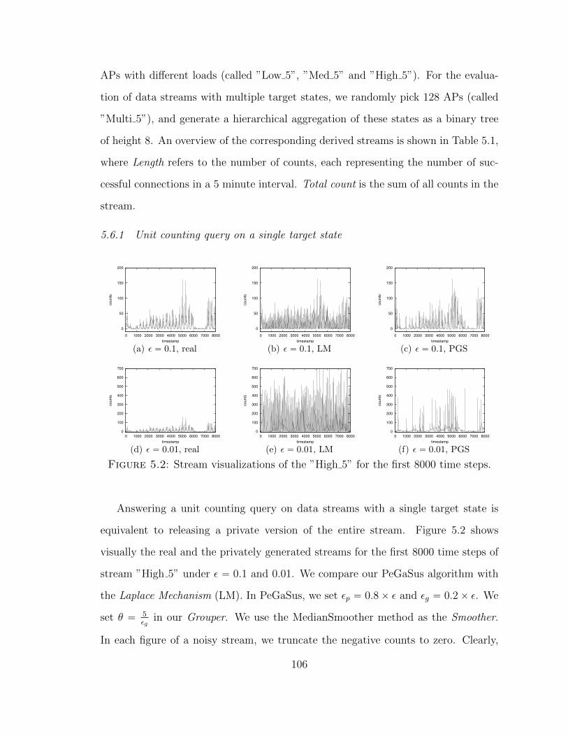
APs with different loads (called ”Low 5”, ”Med 5” and ”High 5”). For the evalua-

tion of data streams with multiple target states, we randomly pick 128 APs (called

”Multi 5”), and generate a hierarchical aggregation of these states as a binary tree

of height 8. An overview of the corresponding derived streams is shown in Table 5.1,

where Length refers to the number of counts, each representing the number of suc-

cessful connections in a 5 minute interval. Total count is the sum of all counts in the

stream.

5.6.1 Unit counting query on a single target state

0

50

100

150

200

0 1000 2000 3000 4000 5000 6000 7000 8000

counts

timestamp

(a) ε “ 0.1, real

0

50

100

150

200

0 1000 2000 3000 4000 5000 6000 7000 8000

counts

timestamp

(b) ε “ 0.1, LM

0

50

100

150

200

0 1000 2000 3000 4000 5000 6000 7000 8000

counts

timestamp

(c) ε “ 0.1, PGS

0

100

200

300

400

500

600

700

0 1000 2000 3000 4000 5000 6000 7000 8000

counts

timestamp

(d) ε “ 0.01, real

0

100

200

300

400

500

600

700

0 1000 2000 3000 4000 5000 6000 7000 8000

counts

timestamp

(e) ε “ 0.01, LM

0

100

200

300

400

500

600

700

0 1000 2000 3000 4000 5000 6000 7000 8000

counts

timestamp

(f) ε “ 0.01, PGS

Figure 5.2: Stream visualizations of the ”High 5” for the first 8000 time steps.

Answering a unit counting query on data streams with a single target state is

equivalent to releasing a private version of the entire stream. Figure 5.2 shows

visually the real and the privately generated streams for the first 8000 time steps of

stream ”High 5” under ε “ 0.1 and 0.01. We compare our PeGaSus algorithm with

the Laplace Mechanism (LM). In PeGaSus, we set εp “ 0.8ˆ ε and εg “ 0.2ˆ ε. We

set θ “ 5εg

in our Grouper. We use the MedianSmoother method as the Smoother.

In each figure of a noisy stream, we truncate the negative counts to zero. Clearly,

106

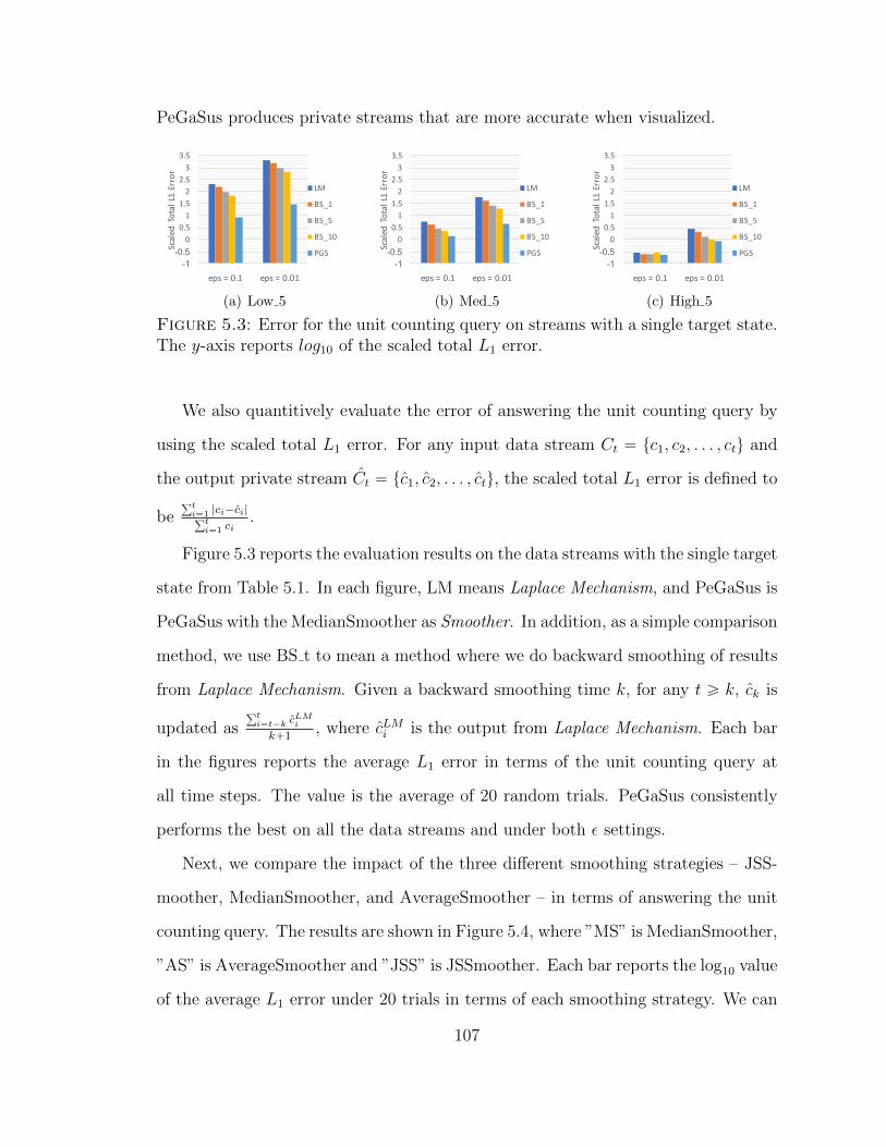
PeGaSus produces private streams that are more accurate when visualized.

-1 -0.5

00.51

1.52

2.53

3.5

eps=0.1 eps=0.01

ScaledTotalL1Error

LM

BS_1

BS_5

BS_10

PGS

(a) Low 5

-1 -0.5

00.51

1.52

2.53

3.5

eps=0.1 eps=0.01

ScaledTotalL1Error

LM

BS_1

BS_5

BS_10

PGS

(b) Med 5

-1 -0.5

00.51

1.52

2.53

3.5

eps=0.1 eps=0.01

ScaledTotalL1Error

LM

BS_1

BS_5

BS_10

PGS

(c) High 5

Figure 5.3: Error for the unit counting query on streams with a single target state.The y-axis reports log10 of the scaled total L1 error.

We also quantitively evaluate the error of answering the unit counting query by

using the scaled total L1 error. For any input data stream Ct “ tc1, c2, . . . , ctu and

the output private stream Ct “ tc1, c2, . . . , ctu, the scaled total L1 error is defined to

beřti“1 |ci´ci|řti“1 ci

.

Figure 5.3 reports the evaluation results on the data streams with the single target

state from Table 5.1. In each figure, LM means Laplace Mechanism, and PeGaSus is

PeGaSus with the MedianSmoother as Smoother. In addition, as a simple comparison

method, we use BS t to mean a method where we do backward smoothing of results

from Laplace Mechanism. Given a backward smoothing time k, for any t ě k, ck is

updated asřti“t´k c

LMi

k`1, where cLMi is the output from Laplace Mechanism. Each bar

in the figures reports the average L1 error in terms of the unit counting query at

all time steps. The value is the average of 20 random trials. PeGaSus consistently

performs the best on all the data streams and under both ε settings.

Next, we compare the impact of the three different smoothing strategies – JSS-

moother, MedianSmoother, and AverageSmoother – in terms of answering the unit

counting query. The results are shown in Figure 5.4, where ”MS” is MedianSmoother,

”AS” is AverageSmoother and ”JSS” is JSSmoother. Each bar reports the log10 value

of the average L1 error under 20 trials in terms of each smoothing strategy. We can

107

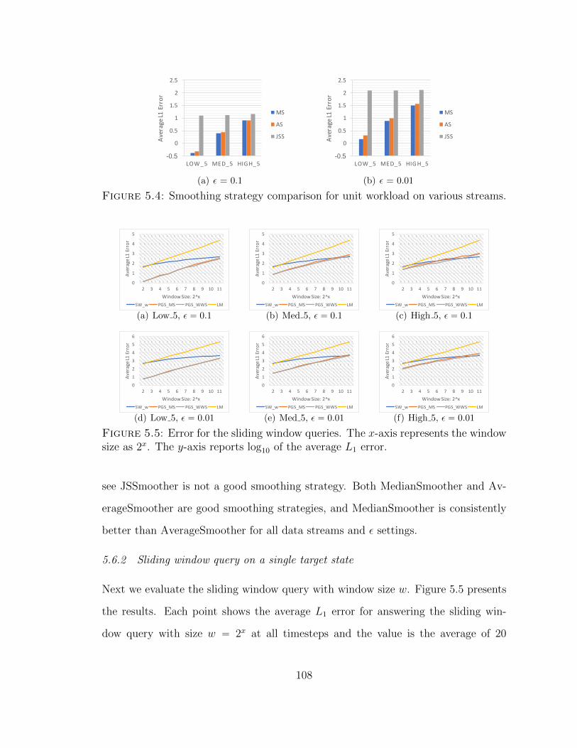
-0.5

0

0.5

1

1.5

2

2.5

LOW_5 MED_5 HIGH_5Av

erageL1Error

MS

AS

JSS

(a) ε = 0.1

-0.5

0

0.5

1

1.5

2

2.5

LOW_5 MED_5 HIGH_5

AverageL1Error

MS

AS

JSS

(b) ε = 0.01

Figure 5.4: Smoothing strategy comparison for unit workload on various streams.

0

1

2

3

4

5

2 3 4 5 6 7 8 9 10 11

AverageL1Error

WindowSize:2^xSW_w PGS_MS PGS_WWS LM

(a) Low 5, ε “ 0.1

0

1

2

3

4

5

2 3 4 5 6 7 8 9 10 11

AverageL1Error


(b) Med 5, ε “ 0.1

0

1

2

3

4

5

2 3 4 5 6 7 8 9 10 11

AverageL1Error


(c) High 5, ε “ 0.1

0

1

2

3

4

5

6

2 3 4 5 6 7 8 9 10 11

AverageL1Error


(d) Low 5, ε “ 0.01

0

1

2

3

4

5

6

2 3 4 5 6 7 8 9 10 11

AverageL1Error


(e) Med 5, ε “ 0.01

0

1

2

3

4

5

6

2 3 4 5 6 7 8 9 10 11Av

erageL1Error


(f) High 5, ε “ 0.01

Figure 5.5: Error for the sliding window queries. The x-axis represents the windowsize as 2x. The y-axis reports log10 of the average L1 error.

see JSSmoother is not a good smoothing strategy. Both MedianSmoother and Av-

erageSmoother are good smoothing strategies, and MedianSmoother is consistently

better than AverageSmoother for all data streams and ε settings.

5.6.2 Sliding window query on a single target state

Next we evaluate the sliding window query with window size w. Figure 5.5 presents

the results. Each point shows the average L1 error for answering the sliding win-

dow query with size w “ 2x at all timesteps and the value is the average of 20

108

trials. In each sub-figure, LM represents using Laplace Mechanism to answer the

unit counting query first, then computing the sliding window query based on the

noisy unit counting query answers. SW w is the state-of-the-art data independent

algorithm for computing the sliding window query in terms of a fixed window size w

[8]. SW w generates binary trees on every consecutive window of w counts and per-

turbs each node query of each binary tree. Then, any sliding window query with size

w can be derived as the sum of the prefix and suffix of any two neighboring binary

trees. PGS MS and PGS WWS are variants of PeGaSus with MedianSmoother as

Smoother and Algorithm 17 as Smoother.

As shown in the figure, LM introduces excessive error. PGS WWS always per-

forms better than PGS MS demonstrating the benefit of using a different Smoother

for this workload. PGS WWS computes more accurate sliding window queries when

w is not greater than 256 compared with the state of the art algorithm SW w. When

the window size becomes larger, SW w becomes better because SW w is designed

specifically for the sliding window query with window size w while our PeGaSus may

introduce a large bias into a large sliding window query. We emphasize that PeGaSus

can simultaneously support all sliding window queries instead of having to split the

privacy budget and design algorithms for each sliding window workload with a fixed

window size.

5.6.3 Event monitoring on a single target state

In this experiment we consider event monitoring queries on the ”High 5” data stream.

Figure 5.6 displays the ROC curves for detecting jumping and dropping points on

streams with a single target state. In each sub-figure, LM represents using Laplace

Mechanism to generate a noisy stream and doing event monitoring on the noisy

stream. PeGaSus uses the MedianSmoother as Smoother. We use a fixed window

size w and threshold δ to compute the ground truth in terms of the real stream. We

109

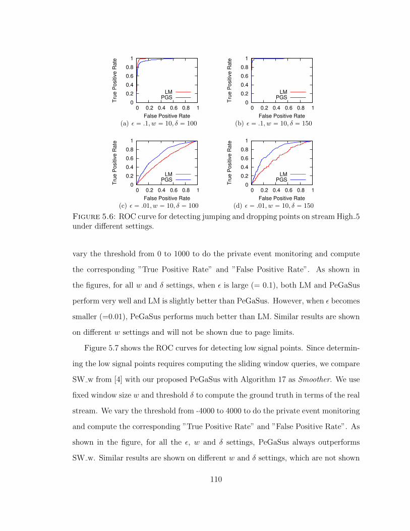
0

0.2

0.4

0.6

0.8

1

0 0.2 0.4 0.6 0.8 1

Tru

e P

ositiv

e R

ate

False Positive Rate

LM

PGS

(a) ε “ .1, w “ 10, δ “ 100

0

0.2

0.4

0.6

0.8

1

0 0.2 0.4 0.6 0.8 1

Tru

e P

ositiv

e R

ate

False Positive Rate

LM

PGS

(b) ε “ .1, w “ 10, δ “ 150

0

0.2

0.4

0.6

0.8

1

0 0.2 0.4 0.6 0.8 1

Tru

e P

ositiv

e R

ate

False Positive Rate

LM

PGS

(c) ε “ .01, w “ 10, δ “ 100

0

0.2

0.4

0.6

0.8

1

0 0.2 0.4 0.6 0.8 1

Tru

e P

ositiv

e R

ate

False Positive Rate

LM

PGS

(d) ε “ .01, w “ 10, δ “ 150

Figure 5.6: ROC curve for detecting jumping and dropping points on stream High 5under different settings.

vary the threshold from 0 to 1000 to do the private event monitoring and compute

the corresponding ”True Positive Rate” and ”False Positive Rate”. As shown in

the figures, for all w and δ settings, when ε is large (= 0.1), both LM and PeGaSus

perform very well and LM is slightly better than PeGaSus. However, when ε becomes

smaller (=0.01), PeGaSus performs much better than LM. Similar results are shown

on different w settings and will not be shown due to page limits.

Figure 5.7 shows the ROC curves for detecting low signal points. Since determin-

ing the low signal points requires computing the sliding window queries, we compare

SW w from [4] with our proposed PeGaSus with Algorithm 17 as Smoother. We use

fixed window size w and threshold δ to compute the ground truth in terms of the real

stream. We vary the threshold from -4000 to 4000 to do the private event monitoring

and compute the corresponding ”True Positive Rate” and ”False Positive Rate”. As

shown in the figure, for all the ε, w and δ settings, PeGaSus always outperforms

SW w. Similar results are shown on different w and δ settings, which are not shown

110

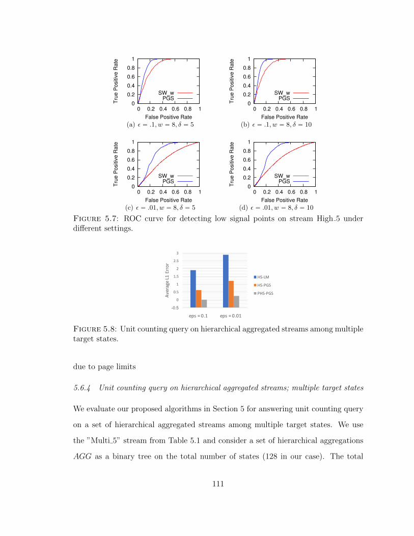
0

0.2

0.4

0.6

0.8

1

0 0.2 0.4 0.6 0.8 1

Tru

e P

ositiv

e R

ate

False Positive Rate

SW_wPGS

(a) ε “ .1, w “ 8, δ “ 5

0

0.2

0.4

0.6

0.8

1

0 0.2 0.4 0.6 0.8 1

Tru

e P

ositiv

e R

ate

False Positive Rate

SW_wPGS

(b) ε “ .1, w “ 8, δ “ 10

0

0.2

0.4

0.6

0.8

1

0 0.2 0.4 0.6 0.8 1

Tru

e P

ositiv

e R

ate

False Positive Rate

SW_wPGS

(c) ε “ .01, w “ 8, δ “ 5

0

0.2

0.4

0.6

0.8

1

0 0.2 0.4 0.6 0.8 1

Tru

e P

ositiv

e R

ate

False Positive Rate

SW_wPGS

(d) ε “ .01, w “ 8, δ “ 10

Figure 5.7: ROC curve for detecting low signal points on stream High 5 underdifferent settings.

-0.5

0

0.5

1

1.5

2

2.5

3

eps=0.1 eps=0.01

AverageL1Error

HS-LM

HS-PGS

PHS-PGS

Figure 5.8: Unit counting query on hierarchical aggregated streams among multipletarget states.

due to page limits

5.6.4 Unit counting query on hierarchical aggregated streams; multiple target states

We evaluate our proposed algorithms in Section 5 for answering unit counting query

on a set of hierarchical aggregated streams among multiple target states. We use

the ”Multi 5” stream from Table 5.1 and consider a set of hierarchical aggregations

AGG as a binary tree on the total number of states (128 in our case). The total

111

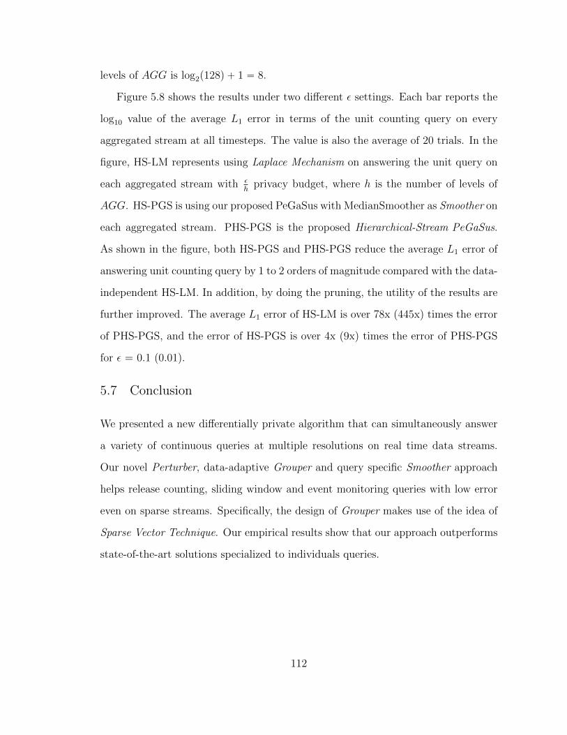
levels of AGG is log2p128q ` 1 “ 8.

Figure 5.8 shows the results under two different ε settings. Each bar reports the

log10 value of the average L1 error in terms of the unit counting query on every

aggregated stream at all timesteps. The value is also the average of 20 trials. In the

figure, HS-LM represents using Laplace Mechanism on answering the unit query on

each aggregated stream with εh

privacy budget, where h is the number of levels of

AGG. HS-PGS is using our proposed PeGaSus with MedianSmoother as Smoother on

each aggregated stream. PHS-PGS is the proposed Hierarchical-Stream PeGaSus.

As shown in the figure, both HS-PGS and PHS-PGS reduce the average L1 error of

answering unit counting query by 1 to 2 orders of magnitude compared with the data-

independent HS-LM. In addition, by doing the pruning, the utility of the results are

further improved. The average L1 error of HS-LM is over 78x (445x) times the error

of PHS-PGS, and the error of HS-PGS is over 4x (9x) times the error of PHS-PGS

for ε = 0.1 (0.01).

5.7 Conclusion

We presented a new differentially private algorithm that can simultaneously answer

a variety of continuous queries at multiple resolutions on real time data streams.

Our novel Perturber, data-adaptive Grouper and query specific Smoother approach

helps release counting, sliding window and event monitoring queries with low error

even on sparse streams. Specifically, the design of Grouper makes use of the idea of

Sparse Vector Technique. Our empirical results show that our approach outperforms

state-of-the-art solutions specialized to individuals queries.

112

6

Related Works

We discuss the related works from various domains below.

Sparse Vector Technique.

The idea of Sparse Vector Technique was first proposed in [22]. After that, both

previous works from [51] and [28] made use of Sparse Vector Technique for answering

queries in an interactive setting.

Multiple variants of Sparse Vector Technique [14, 37, 55] were introduced in some

previous works in order to eliminate the dependence of the privacy cost in terms of the

number of “positive” queries. [37] proposed a variant of Sparse Vector Technique for

selecting frequent itemsets under differential privacy. [14] designed another variant

of Sparse Vector Technique for differentially private generation of high-dimensional

datasets. Another different variant of Sparse Vector Technique was proposed in [55]

in order to achieve privacy-preserving feature selections. The only difference among

these variants is the amount of noise injected to either threshold or each testing

query. In this dissertation, we have shown that all these variants actually do not

ensure differential privacy.

There are some following works after our work on critically analyzing the in-

113

correctness of the previous Sparse Vector Technique variants. Both [65] and [42]

discussed the violations of differential privacy of the variants. There is also further

analysis about optimizing budget allocation for Sparse Vector Technique shown in

[42].

Private Learning and Evaluation.

Private models for regression and classification has been a popular area of ex-

ploration for privacy research. Previous works have produced differentially private

training algorithms for Naive Bayes classification [58], decision trees [26], logistic

and linear regression [13, 52, 59, 63, 64]. These works only output the noisy model

parameters.

Apart from classifier training, Chaudhuri el al. [12] present a generic algorithm for

differentially private parameter tuning and model selection. However, this work does

not assume a blackbox classifier, and makes strong stability assumptions about the

training algorithm. In contrast, our algorithms are classifier agnostic. Additionally

Thakurtha et al. [57] present an algorithm for model selection again assuming strong

stability assumptions about the model training algorithm. We would like to note that

the work in these paper is in some sense orthogonal to the feature selection algorithms

we present, and can be used in conjunction with the results in the paper (for instance,

to choose the right threshold τ or the right number of features to select). Sheffet’s

algorithm [52] additionally outputs confidence intervals for the model parameters.

No prior work considers model diagnostics.

ROC curves are used to quantify the prediction accuracy of binary classifiers.

However, directly releasing the ROC curve may reveal the sensitive information of

the input dataset [43]. Kairouz et al. provided inequalities governing the trade-off

between false-alarm and missed-detection in [32]. Boyd et al. computed the AUC

and a variant of ROC curve called symmetric binormal ROC curve by using smooth

sensitivity [5]. Chaudhuri et al. [12] proposes a generic technique for evaluating a

114

classifier on a private test set. However, they assume that the global sensitivity of

the evaluation function is low (a small constant). Their work is inapplicable since the

sufficient statistics for generating the ROC curve (the set of true and false positive

counts) have a high global sensitivity. The idea of releasing perturbed residual plots

was first suggested by [48], who suggested that remote query systems returning

regression parameter estimates also return residual plots with random noise added

to the residuals from the confidential regression; see also [46]. The noise distribution

did not satisfy differential privacy, or any other formal guarantee. Similar ideas were

used for logistic regressions by [49].

Private Stream Processing.

Privacy-preserving data release has been studied for the past decade. Lots of

differentially private techniques [1, 15, 21, 29, 30, 38, 39, 47, 60–62, 66] have been

proposed for counting queries for static datasets.

Dwork adapted differential privacy to a continual observation setting [18], which

focused on a 0/1 stream and proposed a cascading buffer counter for counting the

number of 1s under event-level differential privacy. Mir et al. studied pan-private

algorithms for estimating distinct count, moments and the heavy-hitter count on

data streams in [44], which preserves differential privacy even if the internal memory

of the algorithms is compromised. Chan et al. studied the application of monitoring

the heavy hitters across a set of distributed streams in [11].

Some prior works focus on continual real-time release of aggregated information

from streams [4, 8, 10, 25, 33]. Fan et al. proposed Fast, an adaptive system to

release real-time aggregate statistics under differential privacy by using sampling and

filtering. Their algorithm is based on a different privacy model, user-level differential

privacy. In [10], Chan et al. used the same privacy model with us. But they focus

on a different single task that releasing prefix sums in terms of the streaming data

counts. For the input stream with known bounded length T , it generates a binary

115

tree defined on the stream and perturbs the node counts of the binary tree. Then

each prefix range query is computed based on a set of perturbed nodes. For streams

with unbounded length, it spends half of the privacy budget on perturbing every

range query between 2i ` 1 and 2i`1. Then it generates a binary tree on every sub-

stream between 2t ` 1 and 2t`1 for each i “ 1, 2, . . . , and perturbs the node counts

with the remaining half of the privacy budget. Any prefix sum at timestamp k,

where 2i ă“ k ă 2i`1, can be computed based on the range queries between 2i ` 1

and 2i`1 for all i ď t and the noisy nodes from the binary tree between 2t ` 1 and

2t`1. The authors proved that the error of each release at timestamp t is Oplogptqq.

Bolot et al. used the same privacy model with us and proposed an algorithm for

releasing sliding window query on data streams with a fixed window size w. The

basic idea is also to generate binary trees on every consecutive w data points and

perturbs each node of the binary trees. The sliding window query at each timestamp

can be derived as the sum of the suffix and prefix of two consecutive binary trees.

This is the state-of-the art algorithm for releasing sliding window query answers. But

the algorithm is designed for any fixed window size, which means we may split the

budget for answering multiple sliding window queries with different window sizes.

Cao et al. [8] studied on a different task of answering a set of special prefix sum

queries with at timestamps in the form of j ˆ s, where s is the step size chosen

from some pre-defined step size set. The proposed algorithms sample some step sizes

from the step size set and then only perturb the window queries in terms of the

chosen step sizes. Then the prefix range query from the workload can be computed

by composition of these perturbed window queries. Kellaris et al. first proposed

another privacy model called w-event differential privacy [33], which is a balance

between user-level and event-level differential privacy and designed algorithms for

releasing private data under w-event differential privacy.

Finally, Dwork et al. proposed a differentially private online partition algorithm

116

for counting under continual observations [24]. Like our Grouper module, this algo-

rithm also employs the idea of Sparse Vector Technique [19]. However, our Grouper

differs from Dwork et al. in the following important ways: (1) their algorithm is

designed for computing partitions such that total counts of each partition are similar

while ours is to find groups such that the elements in each group share similar counts.

(2) Using deviation function can help the Grouper to detect contiguous intervals in

the stream that have a stable value (even if the values are high). On the other hand,

using the total only lets us group together intervals that have counts close to zero.

117

7

Conclusion

In this dissertation, we discuss the use of one popular differentially private primitive,

Sparse Vector Technique, for designing new techniques to solve practical problems

under differential privacy.

In the first topic described in Chapter 3, we critically analyze multiple variants of

Sparse Vector Technique proposed in the previous work. We show that these variants

do not ensure differential privacy, and adversaries can even reconstruct real database

by accessing to these variants. We also introduce another generalized version of

Sparse Vector Technique.

In the second topic shown in Chapter 4, we make use of the original Sparse Vector

Technique primitive, proposing multiple new techniques for achieving regression di-

agnostics under differential privacy. Specifically, we propose PriRP for differentially

private evaluation of the model fit for linear regression. We also propose two algo-

rithms PriROC and PriBRP, achieving the evaluation of logistics regression under

differential privacy in terms of the predictive power as well as the model fit.

In the third topic displayed in Chapter 5, we introduce a novel algorithm, Pe-

GaSus, for achieving privacy-preserving streaming data query answering by using

118

Sparse Vector Technique as a key primitive. Compared with previous works, the new

PeGaSus algorithm is data-adaptive, where the injected noise is tuned in terms of the

input streaming data. PeGaSus can also simultaneously support multiple workloads

without splitting the privacy budget and beat the previous state-of-the-art solutions

designed for each specific workload.

We provide comprehensive evaluations for our proposed new techniques. Our

works solve several challenging problems and make differential privacy practical on

multiple domains.

119

Bibliography

[1] Acs, G., Castelluccia, C., and Chen, R. (2012), “Differentially Private HistogramPublishing through Lossy Compression,” in 2012 IEEE 12th International Con-ference on Data Mining, pp. 1–10.

[2] Almeida, T. A., Hidalgo, J. M. G., and Silva, T. P. (2012), “Towards SMS SpamFiltering: Results under a New Dataset,” International Journal of InformationSecurity Science, pp. 1–18.

[3] Atzori, L., Iera, A., and Morabito, G. (2010), “The Internet of Things: A Survey,”Comput. Netw., 54, 2787–2805.

[4] Bolot, J., Fawaz, N., Muthukrishnan, S., Nikolov, A., and Taft, N. (2013), “Pri-vate Decayed Predicate Sums on Streams,” in Proceedings of the 16th Interna-tional Conference on Database Theory, ICDT ’13, pp. 284–295, New York, NY,USA, ACM.

[5] Boyd, K., Lantz, E., and Page, D. (2015), “Differential Privacy for ClassifierEvaluation,” in ACM Workshop on Artificial Intelligence and Security, pp. 15–23.

[6] Bun, M., Nissim, K., Stemmer, U., and Vadhan, S. (2015), “Differentially PrivateRelease and Learning of Threshold Functions,” in FOCS, pp. 634–649.

[7] Calandrino, J. A., Kilzer, A., Narayanan, A., Felten, E. W., and Shmatikov, V.(2011), “”You Might Also Like:” Privacy Risks of Collaborative Filtering,” in 2011IEEE Symposium on Security and Privacy, pp. 231–246.

[8] Cao, J., Xiao, Q., Ghinita, G., Li, N., Bertino, E., and Tan, K.-L. (2013), “Effi-cient and Accurate Strategies for Differentially-private Sliding Window Queries,”in Proceedings of the 16th International Conference on Extending Database Tech-nology, EDBT ’13, pp. 191–202, New York, NY, USA, ACM.

[9] Cao, Y., Yoshikawa, M., Xiao, Y., and Xiong, L. (2017), “Quantifying DifferentialPrivacy under Temporal Correlations,” ICDE.

[10] Chan, T.-H. H., Shi, E., and Song, D. (2011), “Private and Continual Releaseof Statistics,” ACM Trans. Inf. Syst. Secur., 14, 26:1–26:24.

120

[11] Chan, T.-H. H., Li, M., Shi, E., and Xu, W. (2012), “Differentially Private Con-tinual Monitoring of Heavy Hitters from Distributed Streams,” in Proceedings ofthe 12th International Conference on Privacy Enhancing Technologies, PETS’12,pp. 140–159, Berlin, Heidelberg, Springer-Verlag.

[12] Chaudhuri, K. and Vinterbo, S. A. (2013), “A Stability-based Validation Pro-cedure for Differentially Private Machine Learning,” in Advances in Neural Infor-mation Processing Systems, pp. 2652–2660.

[13] Chaudhuri, K., Monteleoni, C., and Sarwate, A. D. (2011), “Differentially Pri-vate Empirical Risk Minimization,” Journal of Machine Learning Research, 12,1069–1109.

[14] Chen, R., Xiao, Q., Zhang, Y., and Xu, J. (2015), “Differentially Private High-Dimensional Data Publication via Sampling-Based Inference,” in Proceedings ofthe 21th ACM SIGKDD International Conference on Knowledge Discovery andData Mining, KDD ’15, pp. 129–138, New York, NY, USA, ACM.

[15] Cormode, G., Procopiuc, C., Srivastava, D., Shen, E., and Yu, T. (2012), “Dif-ferentially Private Spatial Decompositions,” in 2012 IEEE 28th International Con-ference on Data Engineering, pp. 20–31.

[16] Dinur, I. and Nissim, K. (2003), “Revealing Information While Preserving Pri-vacy,” in Proceedings of the Twenty-second ACM SIGMOD-SIGACT-SIGARTSymposium on Principles of Database Systems, PODS ’03, pp. 202–210, New York,NY, USA, ACM.

[17] Dwork, C. (2006), “Differential privacy,” in in ICALP, pp. 1–12, Springer.

[18] Dwork, C. (2010), “Differential Privacy in New Settings,” in Proceedings of theTwenty-first Annual ACM-SIAM Symposium on Discrete Algorithms, SODA ’10,pp. 174–183, Philadelphia, PA, USA, Society for Industrial and Applied Mathe-matics.

[19] Dwork, C. and Roth, A. (2014), “The algorithmic foundations of differentialprivacy,” Foundations and Trends in Theoretical Computer Science, 9, 211–407.

[20] Dwork, C. and Yekhanin, S. (2008), “New Efficient Attacks on Statistical Dis-closure Control Mechanisms,” in Proceedings of the 28th Annual Conference onCryptology: Advances in Cryptology, CRYPTO 2008, pp. 469–480, Berlin, Heidel-berg, Springer-Verlag.

[21] Dwork, C., McSherry, F., Nissim, K., and Smith, A. (2006), “Calibrating Noiseto Sensitivity in Private Data Analysis,” TCC’06, pp. 265–284, Berlin, Heidelberg,Springer-Verlag.

121

[22] Dwork, C., Naor, M., Reingold, O., Rothblum, G. N., and Vadhan, S. (2009),“On the Complexity of Differentially Private Data Release: Efficient Algorithmsand Hardness Results,” in Proceedings of the Forty-first Annual ACM Symposiumon Theory of Computing, STOC ’09, pp. 381–390, New York, NY, USA, ACM.

[23] Dwork, C., Naor, M., Pitassi, T., and Rothblum, G. N. (2010), “DifferentialPrivacy Under Continual Observation,” in Proceedings of the Forty-second ACMSymposium on Theory of Computing, STOC ’10, pp. 715–724, New York, NY,USA, ACM.

[24] Dwork, C., Naor, M., Reingold, O., and Rothblum, G. N. (2015), Pure Differ-ential Privacy for Rectangle Queries via Private Partitions, pp. 735–751, SpringerBerlin Heidelberg, Berlin, Heidelberg.

[25] Fan, L. and Xiong, L. (2012), “Real-time Aggregate Monitoring with DifferentialPrivacy,” in Proceedings of the 21st ACM International Conference on Informationand Knowledge Management, CIKM ’12, pp. 2169–2173, New York, NY, USA,ACM.

[26] Friedman, A. and Schuster, A. (2010), “Data Mining with Differential Privacy,”in KDD, pp. 493–502, New York, NY, USA, ACM.

[27] Go, A., Bhayani, R., and Huang, L. (2009), “Twitter sentiment classificationusing distant supervision,” CS224N Project Report, Stanford, pp. 1–12.

[28] Hardt, M. and Rothblum, G. N. (2010), “A multiplicative weights mechanismfor privacy-preserving data analysis,” in In FOCS, pp. 61–70.

[29] Hardt, M., Ligett, K., and McSherry, F. (2012), “A Simple and Practical Al-gorithm for Differentially Private Data Release,” in Proceedings of the 25th In-ternational Conference on Neural Information Processing Systems, NIPS’12, pp.2339–2347, USA, Curran Associates Inc.

[30] Hay, M., Rastogi, V., Miklau, G., and Suciu, D. (2010), “Boosting the Accuracyof Differentially Private Histograms Through Consistency,” Proc. VLDB Endow.,3, 1021–1032.

[31] Hay, M., Machanavajjhala, A., Miklau, G., Chen, Y., and Zhang, D. (2016),“Principled Evaluation of Differentially Private Algorithms Using DPBench,” inProceedings of the 2016 International Conference on Management of Data, SIG-MOD ’16, pp. 139–154, New York, NY, USA, ACM.

[32] Kairouz, P., Oh, S., and Viswanath, P. (2015), “The Composition Theoremfor Differential Privacy,” in Proceedings of the 32nd International Conference inMachine Learning(ICML), pp. 1376–1385.

122

[33] Kellaris, G., Papadopoulos, S., Xiao, X., and Papadias, D. (2014), “DifferentiallyPrivate Event Sequences over Infinite Streams,” Proc. VLDB Endow., 7, 1155–1166.

[34] Kifer, D. and Machanavajjhala, A. (2011), “No Free Lunch in Data Privacy,” inProceedings of the 2011 ACM SIGMOD International Conference on Managementof Data, SIGMOD ’11, pp. 193–204, New York, NY, USA, ACM.

[35] Kotsogiannis, I., Machanavajjhala, A., Hay, M., and Miklau, G. (2017), “Pythia:Data Dependent Differentially Private Algorithm Selection,” in Proceedings of the2017 ACM International Conference on Management of Data, SIGMOD ’17, pp.1323–1337, New York, NY, USA, ACM.

[36] K.S.Ruggles, J. and R.Goeken (2010), “Integrated public use microdata series:Version 5.0,” .

[37] Lee, J. and Clifton, C. W. (2014), “Top-k Frequent Itemsets via DifferentiallyPrivate FP-trees,” KDD ’14, pp. 931–940, New York, NY, USA, ACM.

[38] Li, C., Hay, M., Miklau, G., and Wang, Y. (2014), “A Data- and Workload-Aware Query Answering Algorithm for Range Queries Under Differential Privacy,”PVLDB, 7, 341–352.

[39] Li, N., Yang, W., and Qardaji, W. (2013), “Differentially Private Grids forGeospatial Data,” in ICDE, pp. 757–768.

[40] Lichman, M. (2013), “UCI Machine Learning Repository,” .

[41] Liu, C., Chakraborty, S., and Mittal, P. (2016), “Dependence Makes You Vul-nerable: Differential Privacy Under Dependent Tuples,” in NDSS.

[42] Lyu, M., Su, D., and Li, N. (2017), “Understanding the Sparse Vector Techniquefor Differential Privacy,” Proc. VLDB Endow., 10, 637–648.

[43] Matthews, G. and Harel, O. (2013), “An examination of data confidentialityand disclosure issues related to publication of empirical ROC curves.” Academicradiology, 20, 889.

[44] Mir, D., Muthukrishnan, S., Nikolov, A., and Wright, R. N. (2011), “Pan-private Algorithms via Statistics on Sketches,” in Proceedings of the ThirtiethACM SIGMOD-SIGACT-SIGART Symposium on Principles of Database Systems,PODS ’11, pp. 37–48, New York, NY, USA, ACM.

[45] Nissim, K., Raskhodnikova, S., and Smith, A. (2007), “Smooth sensitivity andsampling in private data analysis,” in STOC, pp. 75–84.

123

[46] O’Keefe, C. M. and Good, N. M. (2009), “Regression output from a remoteanalysis system,” Data & Knowledge Engineering, 68.

[47] Qardaji, W., Yang, W., and Li, N. (2013), “Understanding Hierarchical Methodsfor Differentially Private Histograms,” PVLDB, 6.

[48] Reiter, J. P. (2003), “Model diagnostics for remote access servers,” Statisticsand Computing, 13, 371–380.

[49] Reiter, J. P. and Kohnen, C. N. (2005), “Categorical data regression diagnosticsfor remote servers,” Journal of Statistical Computation and Simulation, 75, 889–903.

[50] Reiter, J. P., Oganian, A., and Karr, A. F. (2009), “Verification servers: En-abling analysts to assess the quality of inferences from public use data,” Compu-tational Statistics and Data Analysis, 53, 1475–1482.

[51] Roth, A. and Roughgarden, T. (2010), “Interactive Privacy via the MedianMechanism,” in Proceedings of the Forty-second ACM Symposium on Theory ofComputing, STOC ’10, pp. 765–774, New York, NY, USA, ACM.

[52] Sheffet, O. (2015), “Differentially Private Least Squares: Estimation, Confi-dence and Rejecting the Null Hypothesis,” CoRR, abs/1507.02482.

[53] Smith, A. (2011), “Privacy-preserving Statistical Estimation with Optimal Con-vergence Rates,” in STOC, pp. 813–822.

[54] Song, S., Wang, Y., and Chaudhuri, K. (2017), “Pufferfish Privacy Mechanismsfor Correlated Data,” in Proceedings of the 2017 ACM International Conference onManagement of Data, SIGMOD ’17, pp. 1291–1306, New York, NY, USA, ACM.

[55] Stoddard, B., Chen, Y., and Machanavajjhala, A. (2014), “Differentially PrivateAlgorithms for Empirical Machine Learning,” CoRR, abs/1411.5428.

[56] Sweeney, L. (2000), “Simple Demographics Often Identify People Uniquely,” .

[57] Thakurta, A. G. and Smith, A. (2013), “Differentially private feature selectionvia stability arguments, and the robustness of the lasso,” in Conference on Learn-ing Theory, pp. 819–850.

[58] Vaidya, J., Shafiq, B., Basu, A., and Hong, Y. (2013), “Differentially PrivateNaive Bayes Classification,” in International Conferences on Web Intelligence, pp.571–576.

[59] Wu, X., Fredrikson, M., Wu, W., Jha, S., and Naughton, J. F. (2015), “Revis-iting Differentially Private Regression: Lessons From Learning Theory and theirConsequences,” CoRR, abs/1512.06388.

124

[60] Xiao, X., Wang, G., and Gehrke, J. (2011), “Differential Privacy via WaveletTransforms,” vol. 23, pp. 1200–1214, Piscataway, NJ, USA, IEEE EducationalActivities Department.

[61] Xiao, Y., Xiong, L., Fan, L., Goryczka, S., and Li, H. (2014), “DPCube: Dif-ferentially Private Histogram Release Through Multidimensional Partitioning,”Trans. Data Privacy, 7, 195–222.

[62] Xu, J., Zhang, Z., Xiao, X., Yang, Y., and Yu, G. (2012), “Differentially Pri-vate Histogram Publication,” ICDE ’12, pp. 32–43, Washington, DC, USA, IEEEComputer Society.

[63] Zhang, J., Zhang, Z., Xiao, X., Yang, Y., and Winslett, M. (2012), “Func-tional mechanism: regression analysis under differential privacy,” Proceedings ofthe VLDB Endowment, 5, 1364–1375.

[64] Zhang, J., Xiao, X., Yang, Y., Zhang, Z., and Winslett, M. (2013), “PrivGene:Differentially Private Model Fitting Using Genetic Algorithms,” in SIGMOD, pp.665–676.

[65] Zhang, J., Xiao, X., and Xie, X. (2016), “PrivTree: A Differentially PrivateAlgorithm for Hierarchical Decompositions,” in Proceedings of the 2016 Interna-tional Conference on Management of Data, SIGMOD ’16, pp. 155–170, New York,NY, USA, ACM.

[66] Zhang, X., Chen, R., Xu, J., Meng, X., and Xie, Y. (2014), Towards AccurateHistogram Publication under Differential Privacy, pp. 587–595.

125

Biography

Yan Chen was born at July 9th, in Chonqqing, a big city located in the south west

of China. He received his B.S. in Computer Science from Peking University, Beijing,

China, in 2013. He also got a minor degree in Statistics from Peking University in

2013 as well. In the Fall 2013, Yan entered Duke University as a Ph.D. student in the

Department of Computer Science. He worked on the research about data privacy

under the supervision of prof. Ashwin Machanavajjhala. Yan received his Ph.D.

degree in Computer Science at May, 2018.

126

Applying Differential Privacy with Sparse Vector Technique

Documents

Transcript of Applying Differential Privacy with Sparse Vector Technique