Differential cross section and recoil polarization measurementsfor the γp→ K+Λ reaction using CLAS at Jefferson Lab

M. E. McCracken,1, 2 M. Bellis,1, ∗ C. A. Meyer,1 M. Williams,1, † K. P. Adhikari,29 M. Anghinolfi,19 J. Ball,9

M. Battaglieri,19 B.L. Berman,41 A.S. Biselli,13 D. Branford,12 W.J. Briscoe,41 W.K. Brooks,36, 34 V.D. Burkert,34

S.L. Careccia,29 D.S. Carman,34 P.L. Cole,17 P. Collins,4, ‡ V. Crede,15 A. D’Angelo,20, 31 A. Daniel,28 N. Dashyan,40

R. De Vita,19 E. De Sanctis,18 A. Deur,34 B Dey,1 S. Dhamija,14 R. Dickson,1 C. Djalali,33 D. Doughty,10, 34

M. Dugger,4 R. Dupre,3 A. El Alaoui,3 P. Eugenio,15 S. Fegan,37 A. Fradi,21 M.Y. Gabrielyan,14 K.L. Giovanetti,23

F.X. Girod,9, § J.T. Goetz,5 W. Gohn,11 R.W. Gothe,33 K.A. Griffioen,39 M. Guidal,21 K. Hafidi,3 H. Hakobyan,36, 40

C. Hanretty,15 N. Hassall,37 K. Hicks,28 M. Holtrop,26 Y. Ilieva,33, 41 D.G. Ireland,37 H.S. Jo,21 D. Keller,28

M. Khandaker,27 P. Khetarpal,30 W. Kim,24 A. Klein,29 F.J. Klein,8 V. Kubarovsky,34, 30 S.V. Kuleshov,36, 22

V. Kuznetsov,24 K. Livingston,37 M. Mayer,29 J. McAndrew,12 M.E. McCracken,1 B. McKinnon,37 M.D. Mestayer,34

T Mineeva,11 M. Mirazita,18 V. Mokeev,32, 34 B. Moreno,9 K. Moriya,1 B. Morrison,4 H. Moutarde,9 E. Munevar,41

P. Nadel-Turonski,8, § S. Niccolai,21 G. Niculescu,23 I. Niculescu,23 M. Osipenko,19 A.I. Ostrovidov,15 K. Park,33, 24, §

S. Park,15 E. Pasyuk,4 S. Anefalos Pereira,18 Y. Perrin,25 S. Pisano,21 O. Pogorelko,22 S. Pozdniakov,22

J.W. Price,6 S. Procureur,9 Y. Prok,38, ¶ D. Protopopescu,37 B. Quinn,1 B.A. Raue,14, 34 G. Ricco,19

M. Ripani,19 B.G. Ritchie,4 G. Rosner,37 P. Rossi,18 F. Sabatie,9 M.S. Saini,15 J. Salamanca,17 D. Schott,14

R.A. Schumacher,1 E. Seder,11 H. Seraydaryan,29 Y.G. Sharabian,34 D.I. Sober,8 D. Sokhan,12 S.S. Stepanyan,24

P. Stoler,30 S. Strauch,33, 41 M. Taiuti,19 D.J. Tedeschi,33 S. Tkachenko,29 M. Ungaro,11, 30 B .Vernarsky,1

M.F. Vineyard,35 D. Watts,12 E. Voutier,25 L.B. Weinstein,29 D.P. Weygand,34 M.H. Wood,7, 33 and L. Zana26

(The CLAS Collaboration)1Carnegie Mellon University, Pittsburgh, Pennsylvania 15213

2Washington & Jefferson College, Washington, PA 153013Argonne National Laboratory, Argonne, Illinois 604414Arizona State University, Tempe, Arizona 85287-1504

5University of California at Los Angeles, Los Angeles, California 90095-15476California State University, Dominguez Hills, Carson, CA 90747

7Canisius College, Buffalo, NY 142088Catholic University of America, Washington, D.C. 20064

9CEA, Centre de Saclay, Irfu/Service de Physique Nucleaire, 91191 Gif-sur-Yvette, France10Christopher Newport University, Newport News, Virginia 23606

11University of Connecticut, Storrs, Connecticut 0626912Edinburgh University, Edinburgh EH9 3JZ, United Kingdom

13Fairfield University, Fairfield, Connecticut 0682414Florida International University, Miami, Florida 33199

15Florida State University, Tallahassee, Florida 3230616The George Washington University, Washington, DC 20052

17Idaho State University, Pocatello, Idaho 8320918INFN, Laboratori Nazionali di Frascati, 00044 Frascati, Italy

19INFN, Sezione di Genova, 16146 Genova, Italy20INFN, Sezione di Roma Tor Vergata, 00133 Rome, Italy

21Institut de Physique Nucleaire ORSAY, Orsay, France22Institute of Theoretical and Experimental Physics, Moscow, 117259, Russia

23James Madison University, Harrisonburg, Virginia 2280724Kyungpook National University, Daegu 702-701, Republic of Korea

25LPSC, Universite Joseph Fourier, CNRS/IN2P3, INPG, Grenoble, France26University of New Hampshire, Durham, New Hampshire 03824-3568

27Norfolk State University, Norfolk, Virginia 2350428Ohio University, Athens, Ohio 45701

29Old Dominion University, Norfolk, Virginia 2352930Rensselaer Polytechnic Institute, Troy, New York 12180-3590

31Universita’ di Roma Tor Vergata, 00133 Rome Italy32Skobeltsyn Nuclear Physics Institute, Skobeltsyn Nuclear Physics Institute, 119899 Moscow, Russia

33University of South Carolina, Columbia, South Carolina 2920834Thomas Jefferson National Accelerator Facility, Newport News, Virginia 23606

35Union College, Schenectady, NY 1230836Universidad Tecnica Federico Santa Marıa, Casilla 110-V Valparaıso, Chile

37University of Glasgow, Glasgow G12 8QQ, United Kingdom38University of Virginia, Charlottesville, Virginia 22901

arX

iv:0

912.

4274

v2 [

nucl

-ex]

23

Dec

200

9

2

39College of William and Mary, Williamsburg, Virginia 23187-879540Yerevan Physics Institute, 375036 Yerevan, Armenia

41The George Washington University, Washington, DC 200521(Dated: December 23, 2009)

We present measurements of the differential cross section and Λ recoil polarization for theγp→ K+Λ reaction made using the CLAS detector at Jefferson Lab. These measurements coverthe center-of-mass energy range from 1.62 to 2.84 GeV and a wide range of center-of-mass K+

production angles. Independent analyses were performed using the K+pπ− and K+p (missing π−)final-state topologies; results from these analyses were found to exhibit good agreement. Thesedifferential cross section measurements show excellent agreement with previous CLAS and LEPSresults and offer increased precision and a 300 MeV increase in energy coverage. The recoil polar-ization data agree well with previous results and offer a large increase in precision and a 500 MeVextension in energy range. The increased center-of-mass energy range that these data represent willallow for independent study of non-resonant K+Λ photoproduction mechanisms at all productionangles.

PACS numbers: 11.80.Cr,11.80.Et,13.30.Eg,14.20.Gk,14.20.Jn,14.40.Aq,25.20.Lj,25.75.Dw

I. INTRODUCTION

The γp→ K+Λ reaction is a promising channel forthe study of excited nucleon resonances. Because of thepseudoscalar nature of the K+ and the self-analyzing de-cay of the Λ baryon, measurement of all polarizationobservables for this channel is experimentally possible.Precise measurements of these polarization observables,in addition to the unpolarized differential cross section(dσ/d cos θc.m.K , where θc.m.K is the K+ polar angle in thecenter-of-mass frame), will lead to a full characterizationof the channel and an exciting opportunity to assess thecontributions of resonant and non-resonant photoproduc-tion mechanisms. The channel is further simplified by theisospin structure of the final state, which allows couplingonly to I = 1

2 N∗ intermediate states and not the I = 3

2∆∗ states.

Previous large-acceptance measurements of theγp→ K+Λ differential cross section have been madeby the SAPHIR [1, 2, 3] and CLAS [4] collaborations.The most recent SAPHIR results [3] are formed fromroughly 5.2 × 104 events and span the center-of-massenergy (

√s) range from threshold (1.61 GeV) to

≈ 2.4 GeV. The previous CLAS results draw fromapproximately 5.6 × 105 events and represent the

√s

range from threshold to 2.5 GeV. Though differingby an order of magnitude in statistics, these resultsdo exhibit troubling discrepancies. The SAPHIR re-sults are systematically lower (≈ 20%) than those ofCLAS at forward angles. While both results show an

∗Current address:Stanford University, Stanford, CA 94305†Current address:Imperial College London, London, SW7 2AZ, UK‡Current address:Catholic University of America, Washington,D.C. 20064§Current address:Thomas Jefferson National Accelerator Facility,Newport News, Virginia 23606¶Current address:Christopher Newport University, Newport News,Virginia 23606

enhancement in dσ/d cos θc.m.K at√s ≈ 1.9 GeV, this

enhancement is much more pronounced in the CLASresults (especially for cos θc.m.K & 0). Other cross sectionmeasurements from LEPS at forward [5] and backward[6] angles appear to agree with the CLAS results, butdo not overlap with the regions of the CLAS/SAPHIRdiscrepancy.

These differences have led to difficulties in interpreta-tion of the N∗ contributions to K+Λ production. Severalstudies have found evidence for contributions of differentresonances dependent upon which results are considered.The dσ/d cos θc.m.K shape discrepancy at

√s ≈ 1.9 GeV

is especially problematic, and partial-wave analyses haveproduced varied explanations for resonant contributionsin this region, including D13 [7], P13 [8], P11 [9], andS11 [10] states.

In this paper, we present measurements of theγp→ K+Λ differential cross section and Λ recoil polar-ization (PΛ) taken from the CLAS g11a dataset. We haveproduced separate analyses using the K+pπ− and K+p(missing π−) topologies and found these results to be inagreement. The K+Λ measurements presented are themost precise to date, and represent an extension of theobserved

√s range for dσ/d cos θc.m.K and PΛ of 300 MeV

and 500 MeV, respectively. These dσ/d cos θc.m.K resultsshow agreement with previous CLAS and LEPS resultsand the PΛ results agree well with previous world data.

With several theory groups already pursuing single-and coupled-channel partial-wave analyses including theγp → K+Λ reaction, the results presented herein willoffer new constraints to pre-existing models. The finecenter-of-mass-energy binning of these results, especiallythe Λ recoil polarization, are especially interesting asthey show previously unseen structure. These results alsopresent the first large acceptance measurements of the re-action at center-of-mass energies between 2.53 GeV and2.84 GeV, an energy regime in which production appearsto be dominated by non-resonant processes. Previouspartial-wave analyses have produced non-resonant mod-els by constraining only to forward production angle data

3

or by fitting both resonant and non-resonant componentssimultaneously. These dσ/d cos θc.m.K and PΛ data couldallow for independent study of non-resonant productionmechanisms at all production angles.

II. EXPERIMENTAL SETUP

Data were collected with the CEBAF Large Accep-tance Spectrometer (CLAS) located in Experimental HallB at the Thomas Jefferson National Accelerator Facilityin Newport News, Virginia. The present results are fromthe analysis of the CLAS g11a dataset, collected duringthe period of May 17 - July 29, 2004. Photons were pro-duced via the bremsstrahlung process using a 4.023 GeVelectron beam incident on a gold foil. The Hall B tag-ger assembly facilitated measurement of the energies ofrecoil electrons using a dipole magnetic field and scintil-lator hodoscope; these electron energies were then usedto calculate the energy of associated photons [11]. Aftercollimation, these photons were incident on the physicstarget, a cylindrical kapton chamber 40 cm in length and4 cm in diameter, filled with liquid hydrogen. Measure-ments of the target temperature and pressure allowed forcalculation of the target density with a relative uncer-tainty of 0.2%.

The CLAS detector is composed of tracking and tim-ing detector subsystems arranged with six-fold symme-try about the beamline (i.e. in six sectors). Trajecto-ries of charged particles were deflected by a non-uniformtoroidal magnetic field with a maximum magnitude of1.8 T. Placement of the physics target allowed for recon-struction of charged tracks leaving the target at polarangles between 8◦ and 140◦. Charged particle trackingwas accomplished with three sets of wire drift chambersper sector. Event timing information was supplied bythe start counter, a thin, segmented scintillation detec-tor placed between the physics target and the innermosttracking components, and the time-of-flight (TOF) wall,a bank of 48 scintillator bars located beyond the outer-most tracking component in each sector. The detectorsubsystems combined to produce an average relative mo-mentum resolution of approximately 0.5%. A more de-tailed description of the CLAS detector can be found inRef. [12].

Event triggering required coincident signals from thephoton tagger and the CLAS level 1 trigger. The CLASlevel 1 trigger required that two different sectors observea coincidence between timing signals from the TOF andstart counter scintillators. The signal from the taggerconsisted of an OR combination of roughly two-thirdsof the tagger’s timing scintillators, which correspondedto photons of energy greater than 1.58 GeV. The timingscintillators corresponding to lower-energy photons wereomitted from the trigger in order to reduce the number ofrecorded events generated by photons below the produc-tion threshold for many hadronic final states. While thenumber of such events was greatly reduced by this trig-

ger, events generated by photons with energies between≈1.0 GeV and 1.58 GeV could be recorded due to an ac-cidental coincidence with a recoil electron in one of thevalid tagger elements. For the photon spectrum belowthis energy, a flux renormalization was applied based onthe probability of such events. With this trigger, physicsevents were recorded and written to disk at a rate of 5kHz, only a small fraction of which were relevant to thisanalysis.

III. DATA AND EVENT SELECTION

The loose electronics trigger described in the last sec-tion allowed for a large number of events to be recorded(≈ 20 × 109). Because only a small fraction of theseevents were γp → K+Λ signal, a series of data selec-tion cuts was developed to omit events irrelevant to thisanalysis (background).

Before physics analysis, the dataset was calibrated.Timing spectra of the photon tagger, start counter, andTOF subsystems were investigated and corrected. Drifttimes from each of the tracking chambers and pulses fromTOF scintillators were compared and calibrated. Afterthese corrections were made, tracks were “reconstructed”from raw tracking signals and matched with hits in thestart counter and TOF detectors. Energy and momen-tum corrections were then applied to individual tracks toaccount for imperfections in the magnetic field map anddetector alignment, and energy losses for particles thattraveled through the target, detector material, and air.Small corrections were also applied to incident photonenergies to account for slight deformations in the taggerhodoscope geometry.

As the CLAS detector is optimized for detection ofcharged particles, only the charged decay mode of the Λ(Λ→ pπ−) was considered in this analysis. Two separateanalyses of this reaction were performed: a three-trackanalysis requiring detection of all three of the final-stateparticles, and a two-track analysis requiring only the re-construction of K+ and p tracks. Possible three-trackdata events were skimmed from the dataset using a 4-constraint kinematic fit to the γp → K+pπ− hypothe-sis. Both permutations for the positive track mass hy-potheses were tested in all kinematic fits. This fit im-posed energy and momentum conservation by varyingthe three-momenta of the detected particles within theirmeasurement uncertainties assuming that no undetectedparticles were involved in the event (missing energy andthree-momentum were constrained to zero for a total offour constraints). A probability that each event camefrom the desired reaction (confidence level) was then cal-culated from the variations in momenta and the mea-surement uncertainties. For the three-track data, eventswith confidence levels less than 1% were removed fromthe analysis.

Possible two-track data events were selected by per-forming a 1-constraint kinematic fit to the γp → K+p

4

(missing π−) hypothesis and removing events with con-fidence levels < 5%. Because the π− was not recon-structed, this fit imposed only a single constraint thatthe missing mass be that of a π−. In order to produceresults for which uncertainties are dominated by system-atic rather than statistical uncertainties, it was sufficientto analyze only 28% of the full dataset in producing thetwo-track sample. Both data samples were then sepa-rated into 10-MeV-wide

√s bins. The uncertainty in the

resulting differential cross section measurements due todifferences in signal lost to the confidence level cuts indata and Monte Carlo was estimated to be 3% [13].

IV. BACKGROUND REDUCTION

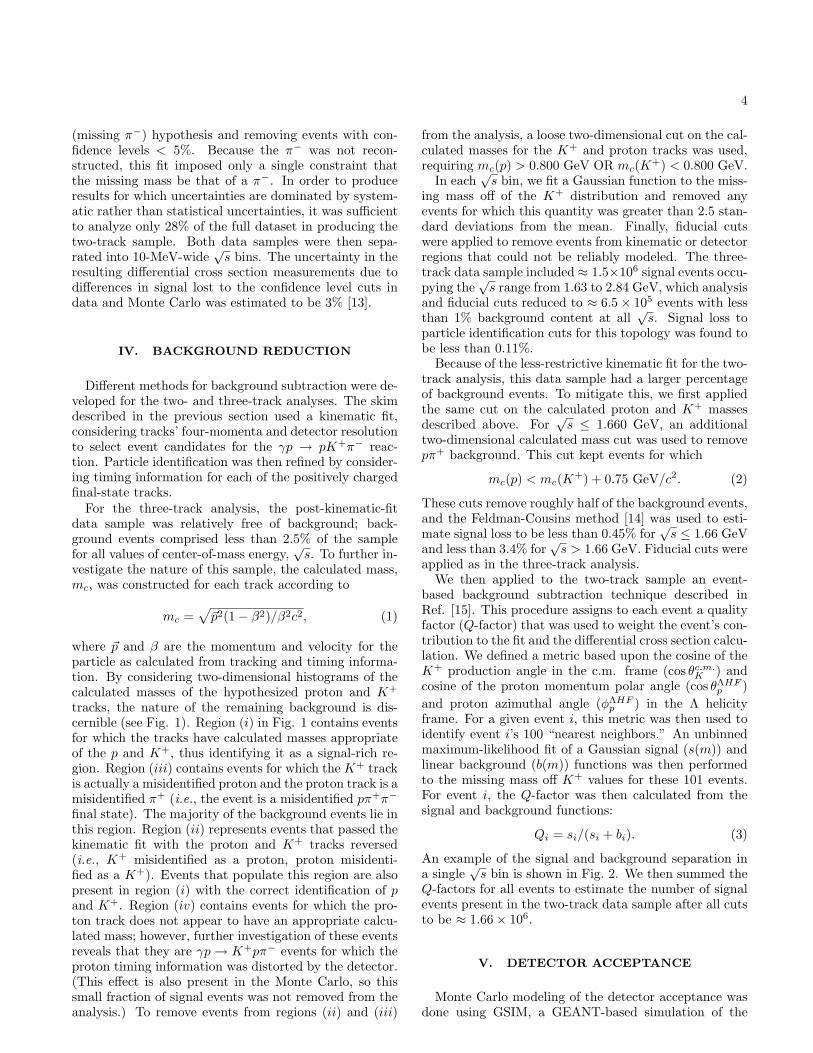
Different methods for background subtraction were de-veloped for the two- and three-track analyses. The skimdescribed in the previous section used a kinematic fit,considering tracks’ four-momenta and detector resolutionto select event candidates for the γp → pK+π− reac-tion. Particle identification was then refined by consider-ing timing information for each of the positively chargedfinal-state tracks.

For the three-track analysis, the post-kinematic-fitdata sample was relatively free of background; back-ground events comprised less than 2.5% of the samplefor all values of center-of-mass energy,

√s. To further in-

vestigate the nature of this sample, the calculated mass,mc, was constructed for each track according to

mc =√~p2(1− β2)/β2c2, (1)

where ~p and β are the momentum and velocity for theparticle as calculated from tracking and timing informa-tion. By considering two-dimensional histograms of thecalculated masses of the hypothesized proton and K+

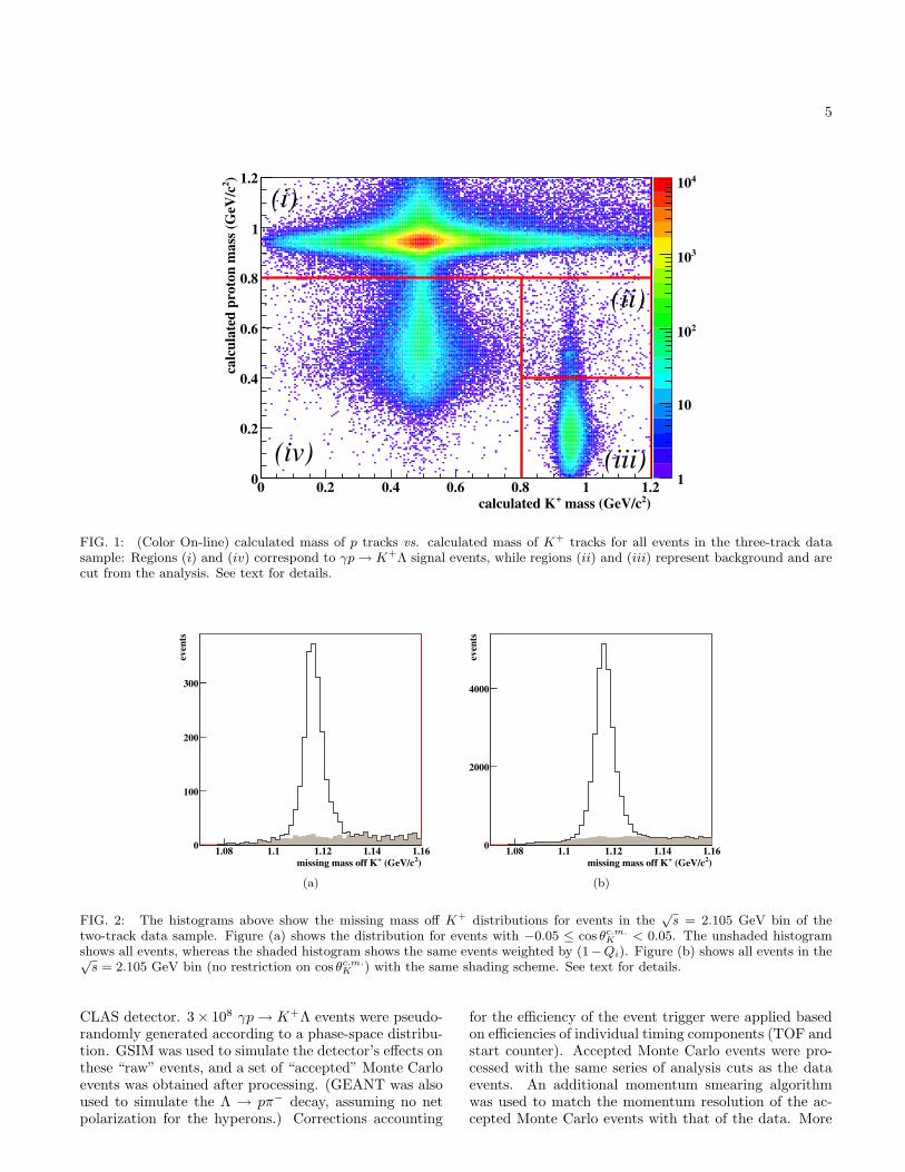
tracks, the nature of the remaining background is dis-cernible (see Fig. 1). Region (i) in Fig. 1 contains eventsfor which the tracks have calculated masses appropriateof the p and K+, thus identifying it as a signal-rich re-gion. Region (iii) contains events for which the K+ trackis actually a misidentified proton and the proton track is amisidentified π+ (i.e., the event is a misidentified pπ+π−

final state). The majority of the background events lie inthis region. Region (ii) represents events that passed thekinematic fit with the proton and K+ tracks reversed(i.e., K+ misidentified as a proton, proton misidenti-fied as a K+). Events that populate this region are alsopresent in region (i) with the correct identification of pand K+. Region (iv) contains events for which the pro-ton track does not appear to have an appropriate calcu-lated mass; however, further investigation of these eventsreveals that they are γp→ K+pπ− events for which theproton timing information was distorted by the detector.(This effect is also present in the Monte Carlo, so thissmall fraction of signal events was not removed from theanalysis.) To remove events from regions (ii) and (iii)

from the analysis, a loose two-dimensional cut on the cal-culated masses for the K+ and proton tracks was used,requiring mc(p) > 0.800 GeV OR mc(K+) < 0.800 GeV.

In each√s bin, we fit a Gaussian function to the miss-

ing mass off of the K+ distribution and removed anyevents for which this quantity was greater than 2.5 stan-dard deviations from the mean. Finally, fiducial cutswere applied to remove events from kinematic or detectorregions that could not be reliably modeled. The three-track data sample included ≈ 1.5×106 signal events occu-pying the

√s range from 1.63 to 2.84 GeV, which analysis

and fiducial cuts reduced to ≈ 6.5× 105 events with lessthan 1% background content at all

√s. Signal loss to

particle identification cuts for this topology was found tobe less than 0.11%.

Because of the less-restrictive kinematic fit for the two-track analysis, this data sample had a larger percentageof background events. To mitigate this, we first appliedthe same cut on the calculated proton and K+ massesdescribed above. For

√s ≤ 1.660 GeV, an additional

two-dimensional calculated mass cut was used to removepπ+ background. This cut kept events for which

mc(p) < mc(K+) + 0.75 GeV/c2. (2)

These cuts remove roughly half of the background events,and the Feldman-Cousins method [14] was used to esti-mate signal loss to be less than 0.45% for

√s ≤ 1.66 GeV

and less than 3.4% for√s > 1.66 GeV. Fiducial cuts were

applied as in the three-track analysis.We then applied to the two-track sample an event-

based background subtraction technique described inRef. [15]. This procedure assigns to each event a qualityfactor (Q-factor) that was used to weight the event’s con-tribution to the fit and the differential cross section calcu-lation. We defined a metric based upon the cosine of theK+ production angle in the c.m. frame (cos θc.m.K ) andcosine of the proton momentum polar angle (cos θΛHF

p )and proton azimuthal angle (φΛHF

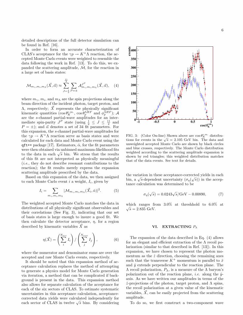
p ) in the Λ helicityframe. For a given event i, this metric was then used toidentify event i’s 100 “nearest neighbors.” An unbinnedmaximum-likelihood fit of a Gaussian signal (s(m)) andlinear background (b(m)) functions was then performedto the missing mass off K+ values for these 101 events.For event i, the Q-factor was then calculated from thesignal and background functions:

Qi = si/(si + bi). (3)

An example of the signal and background separation ina single

√s bin is shown in Fig. 2. We then summed the

Q-factors for all events to estimate the number of signalevents present in the two-track data sample after all cutsto be ≈ 1.66× 106.

V. DETECTOR ACCEPTANCE

Monte Carlo modeling of the detector acceptance wasdone using GSIM, a GEANT-based simulation of the

5

)2 mass (GeV/c+calculated K0 0.2 0.4 0.6 0.8 1 1.2

)2

calc

ula

ted

pro

ton

ma

ss (

GeV

/c

0

0.2

0.4

0.6

0.8

1

1.2

1

10

210

310

410

(i)

(iv)

(ii)

(iii)

FIG. 1: (Color On-line) calculated mass of p tracks vs. calculated mass of K+ tracks for all events in the three-track datasample: Regions (i) and (iv) correspond to γp→ K+Λ signal events, while regions (ii) and (iii) represent background and arecut from the analysis. See text for details.

)2 (GeV/c+missing mass off K

1.08 1.1 1.12 1.14 1.16

even

ts

0

100

200

300

(a)

)2 (GeV/c+missing mass off K

1.08 1.1 1.12 1.14 1.16

even

ts

0

2000

4000

(b)

FIG. 2: The histograms above show the missing mass off K+ distributions for events in the√s = 2.105 GeV bin of the

two-track data sample. Figure (a) shows the distribution for events with −0.05 ≤ cos θc.m.K < 0.05. The unshaded histogramshows all events, whereas the shaded histogram shows the same events weighted by (1−Qi). Figure (b) shows all events in the√s = 2.105 GeV bin (no restriction on cos θc.m.K ) with the same shading scheme. See text for details.

CLAS detector. 3× 108 γp→ K+Λ events were pseudo-randomly generated according to a phase-space distribu-tion. GSIM was used to simulate the detector’s effects onthese “raw” events, and a set of “accepted” Monte Carloevents was obtained after processing. (GEANT was alsoused to simulate the Λ → pπ− decay, assuming no netpolarization for the hyperons.) Corrections accounting

for the efficiency of the event trigger were applied basedon efficiencies of individual timing components (TOF andstart counter). Accepted Monte Carlo events were pro-cessed with the same series of analysis cuts as the dataevents. An additional momentum smearing algorithmwas used to match the momentum resolution of the ac-cepted Monte Carlo events with that of the data. More

6

detailed descriptions of the full detector simulation canbe found in Ref. [16].

In order to form an accurate characterization ofCLAS’s acceptance for the γp → K+Λ reaction, the ac-cepted Monte Carlo events were weighted to resemble thedata following the work in Ref. [13]. To do this, we ex-panded the scattering amplitude, M, for the reaction ina large set of basis states:

Mmγ ,mi,mΛ( ~X, ~α) ≈112∑

J= 12

∑P=±

AJP

mγ ,mi,mΛ( ~X, ~α), (4)

where mγ , mi, and mΛ are the spin projections along thebeam direction of the incident photon, target proton, andΛ, respectively; ~X represents the physically significantkinematic quantities (cos θc.m.K , cos θΛHF

p and φΛHFp ); A

are the s-channel partial-wave amplitudes for an inter-mediate spin-parity JP state (using 1

2 ≤ J ≤ 112 and

P = ±); and ~α denotes a set of 34 fit parameters. Forthis expansion, the s-channel partial-wave amplitudes forthe γp → K+Λ reaction serve as basis states and werecalculated for each data and Monte Carlo event using theqft++ package [17]. Estimators, α, for the fit parameterswere then obtained via unbinned maximum-likelihood fitsto the data in each

√s bin. We stress that the results

of this fit are not interpreted as physically meaningful(i.e., they do not describe resonant contributions to thereaction); the fit results merely express the expansionscattering amplitude prescribed by the data.

Based on this expansion of the data, we then assignedto each Monte Carlo event i a weight, Ii, given by

Ii =∑

mγ ,mi,mΛ

|Mmγ ,mi,mΛ( ~Xi, α)|2. (5)

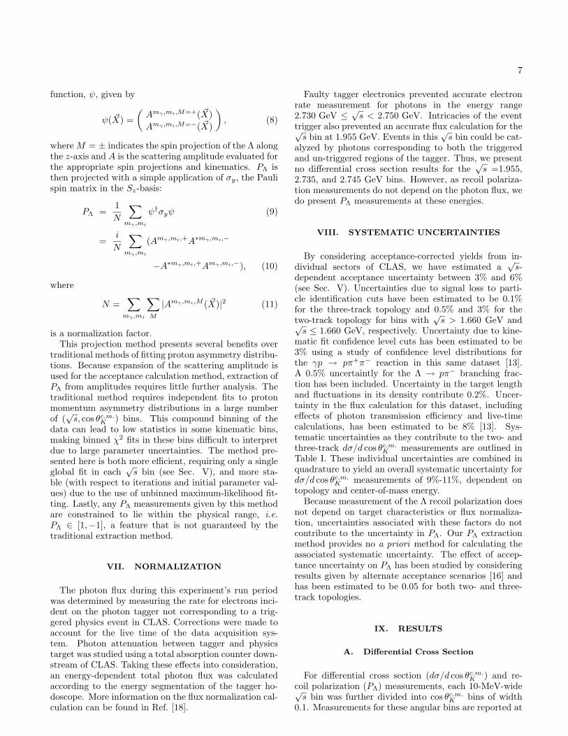
The weighted accepted Monte Carlo matches the data indistributions of all physically significant observables andtheir correlations (See Fig. 3), indicating that our setof basis states is large enough to insure a good fit. Wethen calculate the detector acceptance, η, for a regiondescribed by kinematic variables ~X as

η( ~X) =

(Nacc∑i

Ii

)/

Nraw∑j

Ij

, (6)

where the numerator and denominator sums are over theaccepted and raw Monte Carlo events, respectively.

It should be noted that this expansion method of ac-ceptance calculation replaces the method of attemptingto generate a physics model for Monte Carlo generationvia iteration, a method that can be complicated if back-ground is present in the data. This expansion methodalso allows for separate calculation of the acceptance foreach of the six sectors of CLAS. To estimate systematicuncertainties in this acceptance calculation, acceptance-corrected data yields were calculated independently foreach sector of CLAS in twelve

√s bins. By considering

)c.m.

Kθcos(-1 -0.5 0 0.5 1

even

ts

0

50

100

150

200

250

300

350

400

FIG. 3: (Color On-line) Shown above are cos θc.m.K distribu-tions for events in the

√s = 2.105 GeV bin. The data and

unweighted accepted Monte Carlo are shown by black circlesand blue crosses, respectively. The Monte Carlo distributionweighted according to the scattering amplitude expansion isshown by red triangles; this weighted distribution matchesthat of the data events. See text for details.

the variation in these acceptance-corrected yields in eachbin, a

√s-dependent uncertainty (ση(

√s)) in the accep-

tance calculation was determined to be

ση(√s) = 0.0243

√s/GeV− 0.00890, (7)

which ranges from 3.0% at threshhold to 6.0% at√s = 2.835 GeV.

VI. EXTRACTING PΛ

The expansion of the data described in Eq. (4) allowsfor an elegant and efficient extraction of the Λ recoil po-larization (similar to that described in Ref. [13]). In thisexpansion, we have chosen to represent the photon mo-mentum as the z direction, choosing the remaining axessuch that the transverse K+ momentum is parallel to xand y extends perpendicular to the reaction plane. TheΛ recoil polarization, PΛ, is a measure of the Λ baryon’spolarization out of the reaction plane, i.e. along the y-axis. As we have written our amplitudes in terms of thez-projections of the photon, target proton, and Λ spins,the recoil polarization at a given value of the kinematicvariables, ~X, can be easily projected from the scatteringamplitude.

To do so, we first construct a two-component wave

7

function, ψ, given by

ψ( ~X) =(Amγ ,mi,M=+( ~X)Amγ ,mi,M=−( ~X)

), (8)

where M = ± indicates the spin projection of the Λ alongthe z-axis and A is the scattering amplitude evaluated forthe appropriate spin projections and kinematics. PΛ isthen projected with a simple application of σy, the Paulispin matrix in the Sz-basis:

PΛ =1N

∑mγ ,mi

ψ†σyψ (9)

=i

N

∑mγ ,mi

(Amγ ,mi,+A∗mγ ,mi,−

−A∗mγ ,mi,+Amγ ,mi,−), (10)

where

N =∑mγ ,mi

∑M

|Amγ ,mi,M ( ~X)|2 (11)

is a normalization factor.This projection method presents several benefits over

traditional methods of fitting proton asymmetry distribu-tions. Because expansion of the scattering amplitude isused for the acceptance calculation method, extraction ofPΛ from amplitudes requires little further analysis. Thetraditional method requires independent fits to protonmomentum asymmetry distributions in a large numberof (√s, cos θc.m.K ) bins. This compound binning of the

data can lead to low statistics in some kinematic bins,making binned χ2 fits in these bins difficult to interpretdue to large parameter uncertainties. The method pre-sented here is both more efficient, requiring only a singleglobal fit in each

√s bin (see Sec. V), and more sta-

ble (with respect to iterations and initial parameter val-ues) due to the use of unbinned maximum-likelihood fit-ting. Lastly, any PΛ measurements given by this methodare constrained to lie within the physical range, i.e.PΛ ∈ [1,−1], a feature that is not guaranteed by thetraditional extraction method.

VII. NORMALIZATION

The photon flux during this experiment’s run periodwas determined by measuring the rate for electrons inci-dent on the photon tagger not corresponding to a trig-gered physics event in CLAS. Corrections were made toaccount for the live time of the data acquisition sys-tem. Photon attenuation between tagger and physicstarget was studied using a total absorption counter down-stream of CLAS. Taking these effects into consideration,an energy-dependent total photon flux was calculatedaccording to the energy segmentation of the tagger ho-doscope. More information on the flux normalization cal-culation can be found in Ref. [18].

Faulty tagger electronics prevented accurate electronrate measurement for photons in the energy range2.730 GeV ≤

√s < 2.750 GeV. Intricacies of the event

trigger also prevented an accurate flux calculation for the√s bin at 1.955 GeV. Events in this

√s bin could be cat-

alyzed by photons corresponding to both the triggeredand un-triggered regions of the tagger. Thus, we presentno differential cross section results for the

√s =1.955,

2.735, and 2.745 GeV bins. However, as recoil polariza-tion measurements do not depend on the photon flux, wedo present PΛ measurements at these energies.

VIII. SYSTEMATIC UNCERTAINTIES

By considering acceptance-corrected yields from in-dividual sectors of CLAS, we have estimated a

√s-

dependent acceptance uncertainty between 3% and 6%(see Sec. V). Uncertainties due to signal loss to parti-cle identification cuts have been estimated to be 0.1%for the three-track topology and 0.5% and 3% for thetwo-track topology for bins with

√s > 1.660 GeV and√

s ≤ 1.660 GeV, respectively. Uncertainty due to kine-matic fit confidence level cuts has been estimated to be3% using a study of confidence level distributions forthe γp → pπ+π− reaction in this same dataset [13].A 0.5% uncertaintly for the Λ → pπ− branching frac-tion has been included. Uncertainty in the target lengthand fluctuations in its density contribute 0.2%. Uncer-tainty in the flux calculation for this dataset, includingeffects of photon transmission efficiency and live-timecalculations, has been estimated to be 8% [13]. Sys-tematic uncertainties as they contribute to the two- andthree-track dσ/d cos θc.m.K measurements are outlined inTable I. These individual uncertainties are combined inquadrature to yield an overall systematic uncertainty fordσ/d cos θc.m.K measurements of 9%-11%, dependent ontopology and center-of-mass energy.

Because measurement of the Λ recoil polarization doesnot depend on target characteristics or flux normaliza-tion, uncertainties associated with these factors do notcontribute to the uncertainty in PΛ. Our PΛ extractionmethod provides no a priori method for calculating theassociated systematic uncertainty. The effect of accep-tance uncertainty on PΛ has been studied by consideringresults given by alternate acceptance scenarios [16] andhas been estimated to be 0.05 for both two- and three-track topologies.

IX. RESULTS

A. Differential Cross Section

For differential cross section (dσ/d cos θc.m.K ) and re-coil polarization (PΛ) measurements, each 10-MeV-wide√s bin was further divided into cos θc.m.K bins of width

0.1. Measurements for these angular bins are reported at

8

Error pK+π−pK+(π−)√

s < 1.66 GeV√s ≥ 1.66 GeV

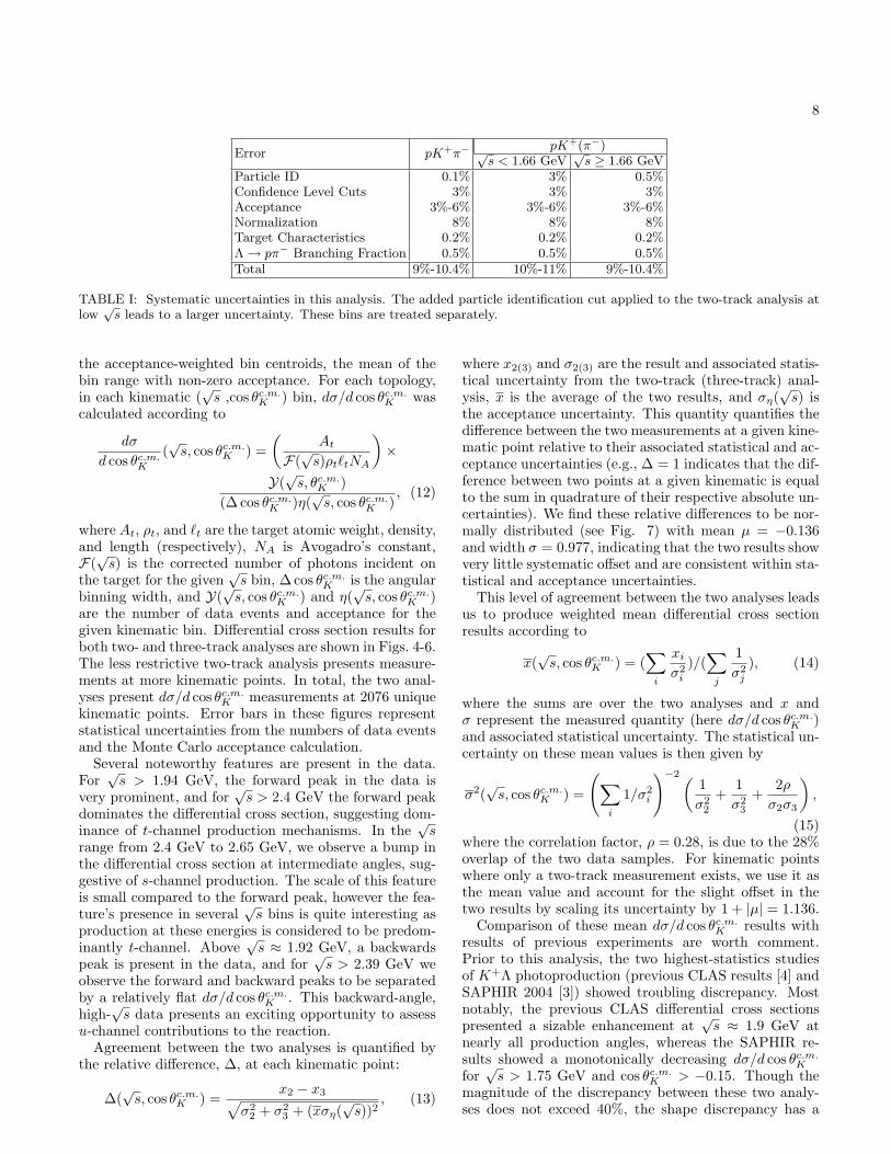
Particle ID 0.1% 3% 0.5%Confidence Level Cuts 3% 3% 3%Acceptance 3%-6% 3%-6% 3%-6%Normalization 8% 8% 8%Target Characteristics 0.2% 0.2% 0.2%Λ→ pπ− Branching Fraction 0.5% 0.5% 0.5%Total 9%-10.4% 10%-11% 9%-10.4%

TABLE I: Systematic uncertainties in this analysis. The added particle identification cut applied to the two-track analysis atlow√s leads to a larger uncertainty. These bins are treated separately.

the acceptance-weighted bin centroids, the mean of thebin range with non-zero acceptance. For each topology,in each kinematic (

√s ,cos θc.m.K ) bin, dσ/d cos θc.m.K was

calculated according to

dσ

d cos θc.m.K

(√s, cos θc.m.K ) =

(At

F(√s)ρt`tNA

)×

Y(√s, θc.m.K )

(∆ cos θc.m.K )η(√s, cos θc.m.K )

, (12)

where At, ρt, and `t are the target atomic weight, density,and length (respectively), NA is Avogadro’s constant,F(√s) is the corrected number of photons incident on

the target for the given√s bin, ∆ cos θc.m.K is the angular

binning width, and Y(√s, cos θc.m.K ) and η(

√s, cos θc.m.K )

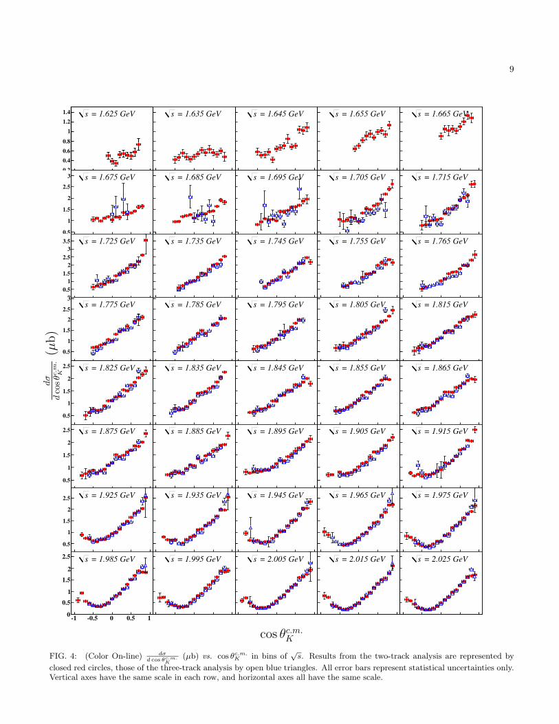
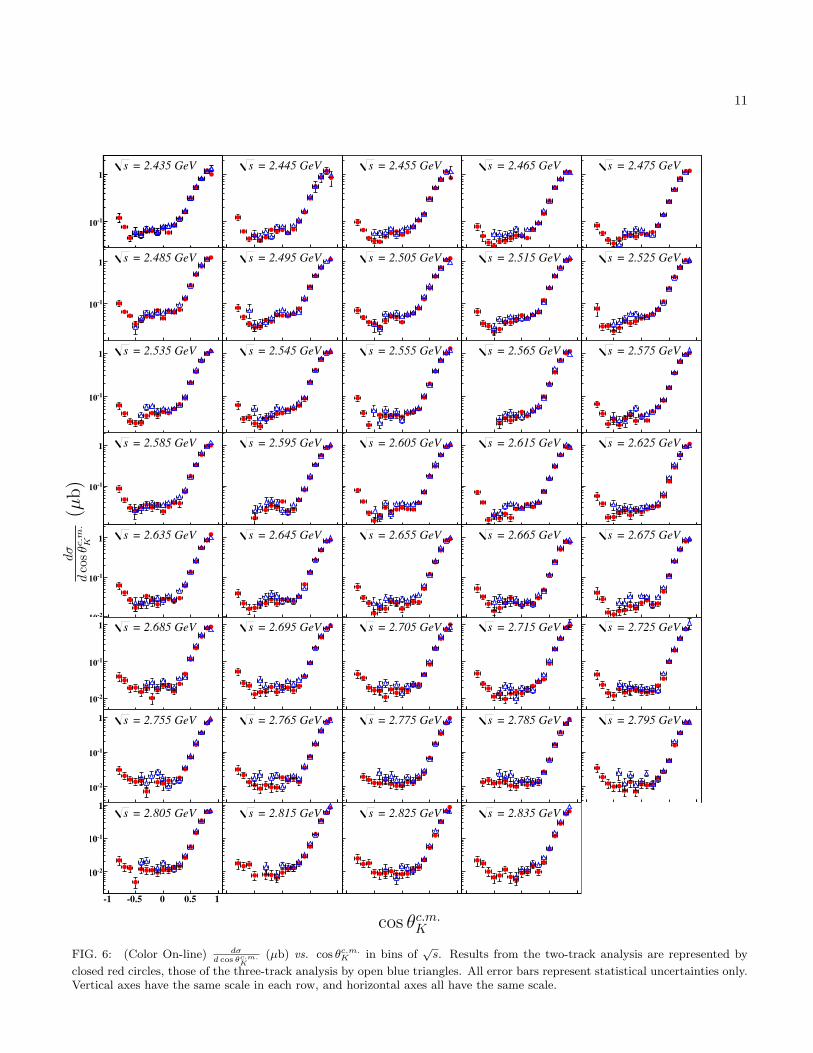
are the number of data events and acceptance for thegiven kinematic bin. Differential cross section results forboth two- and three-track analyses are shown in Figs. 4-6.The less restrictive two-track analysis presents measure-ments at more kinematic points. In total, the two anal-yses present dσ/d cos θc.m.K measurements at 2076 uniquekinematic points. Error bars in these figures representstatistical uncertainties from the numbers of data eventsand the Monte Carlo acceptance calculation.

Several noteworthy features are present in the data.For√s > 1.94 GeV, the forward peak in the data is

very prominent, and for√s > 2.4 GeV the forward peak

dominates the differential cross section, suggesting dom-inance of t-channel production mechanisms. In the

√s

range from 2.4 GeV to 2.65 GeV, we observe a bump inthe differential cross section at intermediate angles, sug-gestive of s-channel production. The scale of this featureis small compared to the forward peak, however the fea-ture’s presence in several

√s bins is quite interesting as

production at these energies is considered to be predom-inantly t-channel. Above

√s ≈ 1.92 GeV, a backwards

peak is present in the data, and for√s > 2.39 GeV we

observe the forward and backward peaks to be separatedby a relatively flat dσ/d cos θc.m.K . This backward-angle,high-

√s data presents an exciting opportunity to assess

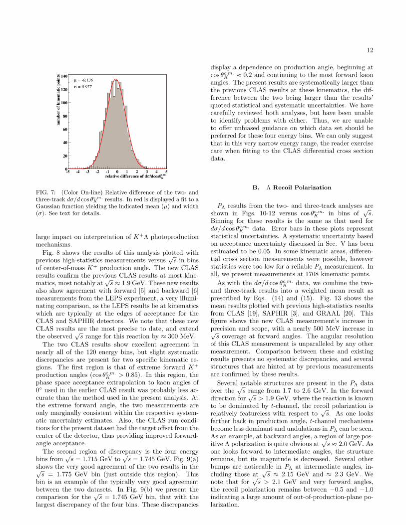
u-channel contributions to the reaction.Agreement between the two analyses is quantified by

the relative difference, ∆, at each kinematic point:

∆(√s, cos θc.m.K ) =

x2 − x3√σ2

2 + σ23 + (xση(

√s))2

, (13)

where x2(3) and σ2(3) are the result and associated statis-tical uncertainty from the two-track (three-track) anal-ysis, x is the average of the two results, and ση(

√s) is

the acceptance uncertainty. This quantity quantifies thedifference between the two measurements at a given kine-matic point relative to their associated statistical and ac-ceptance uncertainties (e.g., ∆ = 1 indicates that the dif-ference between two points at a given kinematic is equalto the sum in quadrature of their respective absolute un-certainties). We find these relative differences to be nor-mally distributed (see Fig. 7) with mean µ = −0.136and width σ = 0.977, indicating that the two results showvery little systematic offset and are consistent within sta-tistical and acceptance uncertainties.

This level of agreement between the two analyses leadsus to produce weighted mean differential cross sectionresults according to

x(√s, cos θc.m.K ) = (

∑i

xiσ2i

)/(∑j

1σ2j

), (14)

where the sums are over the two analyses and x andσ represent the measured quantity (here dσ/d cos θc.m.K )and associated statistical uncertainty. The statistical un-certainty on these mean values is then given by

σ2(√s, cos θc.m.K ) =

(∑i

1/σ2i

)−2(1σ2

2

+1σ2

3

+2ρσ2σ3

),

(15)where the correlation factor, ρ = 0.28, is due to the 28%overlap of the two data samples. For kinematic pointswhere only a two-track measurement exists, we use it asthe mean value and account for the slight offset in thetwo results by scaling its uncertainty by 1 + |µ| = 1.136.

Comparison of these mean dσ/d cos θc.m.K results withresults of previous experiments are worth comment.Prior to this analysis, the two highest-statistics studiesof K+Λ photoproduction (previous CLAS results [4] andSAPHIR 2004 [3]) showed troubling discrepancy. Mostnotably, the previous CLAS differential cross sectionspresented a sizable enhancement at

√s ≈ 1.9 GeV at

nearly all production angles, whereas the SAPHIR re-sults showed a monotonically decreasing dσ/d cos θc.m.Kfor√s > 1.75 GeV and cos θc.m.K > −0.15. Though the

magnitude of the discrepancy between these two analy-ses does not exceed 40%, the shape discrepancy has a

9

dσ

dco

sθc.m.

K(µ

b)

-1 -0.5 0 0.5 10.2

0.4

0.6

0.8

1

1.2

1.4 = 1.625 GeVs

-1 -0.5 0 0.5 10.5

1

1.5

2

2.5

3 = 1.675 GeVs

-1 -0.5 0 0.5 10

0.5

1

1.5

2

2.5

3

3.5 = 1.725 GeVs

-1 -0.5 0 0.5 1

0.5

1

1.5

2

2.5

3

= 1.775 GeVs

-1 -0.5 0 0.5 1

0.5

1

1.5

2

2.5 = 1.825 GeVs

-1 -0.5 0 0.5 1

0.5

1

1.5

2

2.5 = 1.875 GeVs

-1 -0.5 0 0.5 1

0.5

1

1.5

2

2.5 = 1.925 GeVs

-1 -0.5 0 0.5 10

0.5

1

1.5

2

2.5 = 1.985 GeVs

-1 -0.5 0 0.5 10.2

0.4

0.6

0.8

1

1.2

1.4 = 1.635 GeVs

-1 -0.5 0 0.5 10.5

1

1.5

2

2.5

3 = 1.685 GeVs

-1 -0.5 0 0.5 10

0.5

1

1.5

2

2.5

3

3.5 = 1.735 GeVs

-1 -0.5 0 0.5 1

0.5

1

1.5

2

2.5

3

= 1.785 GeVs

-1 -0.5 0 0.5 1

0.5

1

1.5

2

2.5 = 1.835 GeVs

-1 -0.5 0 0.5 1

0.5

1

1.5

2

2.5 = 1.885 GeVs

-1 -0.5 0 0.5 1

0.5

1

1.5

2

2.5 = 1.935 GeVs

-1 -0.5 0 0.5 10

0.5

1

1.5

2

2.5 = 1.995 GeVs

-1 -0.5 0 0.5 10.2

0.4

0.6

0.8

1

1.2

1.4 = 1.645 GeVs

-1 -0.5 0 0.5 10.5

1

1.5

2

2.5

3 = 1.695 GeVs

-1 -0.5 0 0.5 10

0.5

1

1.5

2

2.5

3

3.5 = 1.745 GeVs

-1 -0.5 0 0.5 1

0.5

1

1.5

2

2.5

3

= 1.795 GeVs

-1 -0.5 0 0.5 1

0.5

1

1.5

2

2.5 = 1.845 GeVs

-1 -0.5 0 0.5 1

0.5

1

1.5

2

2.5 = 1.895 GeVs

-1 -0.5 0 0.5 1

0.5

1

1.5

2

2.5 = 1.945 GeVs

-1 -0.5 0 0.5 10

0.5

1

1.5

2

2.5 = 2.005 GeVs

-1 -0.5 0 0.5 10.2

0.4

0.6

0.8

1

1.2

1.4 = 1.655 GeVs

-1 -0.5 0 0.5 10.5

1

1.5

2

2.5

3 = 1.705 GeVs

-1 -0.5 0 0.5 10

0.5

1

1.5

2

2.5

3

3.5 = 1.755 GeVs

-1 -0.5 0 0.5 1

0.5

1

1.5

2

2.5

3

= 1.805 GeVs

-1 -0.5 0 0.5 1

0.5

1

1.5

2

2.5 = 1.855 GeVs

-1 -0.5 0 0.5 1

0.5

1

1.5

2

2.5 = 1.905 GeVs

-1 -0.5 0 0.5 1

0.5

1

1.5

2

2.5 = 1.965 GeVs

-1 -0.5 0 0.5 10

0.5

1

1.5

2

2.5 = 2.015 GeVs

-1 -0.5 0 0.5 10.2

0.4

0.6

0.8

1

1.2

1.4 = 1.665 GeVs

-1 -0.5 0 0.5 10.5

1

1.5

2

2.5

3 = 1.715 GeVs

-1 -0.5 0 0.5 10

0.5

1

1.5

2

2.5

3

3.5 = 1.765 GeVs

-1 -0.5 0 0.5 1

0.5

1

1.5

2

2.5

3

= 1.815 GeVs

-1 -0.5 0 0.5 1

0.5

1

1.5

2

2.5 = 1.865 GeVs

-1 -0.5 0 0.5 1

0.5

1

1.5

2

2.5 = 1.915 GeVs

-1 -0.5 0 0.5 1

0.5

1

1.5

2

2.5 = 1.975 GeVs

-1 -0.5 0 0.5 10

0.5

1

1.5

2

2.5 = 2.025 GeVs

cos θc.m.K

FIG. 4: (Color On-line) dσd cos θc.m.

K(µb) vs. cos θc.m.K in bins of

√s. Results from the two-track analysis are represented by

closed red circles, those of the three-track analysis by open blue triangles. All error bars represent statistical uncertainties only.Vertical axes have the same scale in each row, and horizontal axes all have the same scale.

10

dσ

dco

sθc.m.

K(µ

b)

-1 -0.5 0 0.5 1

-110

1

= 2.035 GeVs

-1 -0.5 0 0.5 1

-110

1

= 2.085 GeVs

-1 -0.5 0 0.5 1

-110

1

= 2.135 GeVs

-1 -0.5 0 0.5 1

-110

1

= 2.185 GeVs

-1 -0.5 0 0.5 1

-110

1

= 2.235 GeVs

-1 -0.5 0 0.5 1

-110

1

= 2.285 GeVs

-1 -0.5 0 0.5 1

-110

1

= 2.335 GeVs

-1 -0.5 0 0.5 1

-110

1 = 2.385 GeVs

-1 -0.5 0 0.5 1

-1

1

= 2.045 GeVs

-1 -0.5 0 0.5 1

-1

1

= 2.095 GeVs

-1 -0.5 0 0.5 1

-1

1

= 2.145 GeVs

-1 -0.5 0 0.5 1

-1

1

= 2.195 GeVs

-1 -0.5 0 0.5 1

-1

1

= 2.245 GeVs

-1 -0.5 0 0.5 1

-1

1

= 2.295 GeVs

-1 -0.5 0 0.5 1

-1

1

= 2.345 GeVs

-1 -0.5 0 0.5 1

-1

1 = 2.395 GeVs

-1 -0.5 0 0.5 1

-1

1

= 2.055 GeVs

-1 -0.5 0 0.5 1

-1

1

= 2.105 GeVs

-1 -0.5 0 0.5 1

-1

1

= 2.155 GeVs

-1 -0.5 0 0.5 1

-1

1

= 2.205 GeVs

-1 -0.5 0 0.5 1

-1

1

= 2.255 GeVs

-1 -0.5 0 0.5 1

-1

1

= 2.305 GeVs

-1 -0.5 0 0.5 1

-1

1

= 2.355 GeVs

-1 -0.5 0 0.5 1

-1

1 = 2.405 GeVs

-1 -0.5 0 0.5 1

-1

1

= 2.065 GeVs

-1 -0.5 0 0.5 1

-1

1

= 2.115 GeVs

-1 -0.5 0 0.5 1

-1

1

= 2.165 GeVs

-1 -0.5 0 0.5 1

-1

1

= 2.215 GeVs

-1 -0.5 0 0.5 1

-1

1

= 2.265 GeVs

-1 -0.5 0 0.5 1

-1

1

= 2.315 GeVs

-1 -0.5 0 0.5 1

-1

1

= 2.365 GeVs

-1 -0.5 0 0.5 1

-1

1 = 2.415 GeVs

-1 -0.5 0 0.5 1

-1

1

= 2.075 GeVs

-1 -0.5 0 0.5 1

-1

1

= 2.125 GeVs

-1 -0.5 0 0.5 1

-1

1

= 2.175 GeVs

-1 -0.5 0 0.5 1

-1

1

= 2.225 GeVs

-1 -0.5 0 0.5 1

-1

1

= 2.275 GeVs

-1 -0.5 0 0.5 1

-1

1

= 2.325 GeVs

-1 -0.5 0 0.5 1

-1

1

= 2.375 GeVs

-1 -0.5 0 0.5 1

-1

1 = 2.425 GeVs

cos θc.m.K

FIG. 5: (Color On-line) dσd cos θc.m.

K(µb) vs. cos θc.m.K in bins of

√s. Results from the two-track analysis are represented by

closed red circles, those of the three-track analysis by open blue triangles. All error bars represent statistical uncertainties only.Vertical axes have the same scale in each row, and horizontal axes all have the same scale.

11

dσ

dco

sθc.m.

K(µ

b)

-1 -0.5 0 0.5 1

-110

1

= 2.435 GeVs

-1 -0.5 0 0.5 1

-110

1 = 2.485 GeVs

-1 -0.5 0 0.5 1

-110

1 = 2.535 GeVs

-1 -0.5 0 0.5 1

-110

1 = 2.585 GeVs

-1 -0.5 0 0.5 1

-210

-110

1 = 2.635 GeVs

-1 -0.5 0 0.5 1

-210

-110

1 = 2.685 GeVs

-1 -0.5 0 0.5 1

-210

-110

1 = 2.755 GeVs

-1 -0.5 0 0.5 1

-210

-110

1 = 2.805 GeVs

-1 -0.5 0 0.5 1

-1

1

= 2.445 GeVs

-1 -0.5 0 0.5 1

-1

1 = 2.495 GeVs

-1 -0.5 0 0.5 1

-1

1 = 2.545 GeVs

-1 -0.5 0 0.5 1

-1

1 = 2.595 GeVs

-1 -0.5 0 0.5 1

-2

-1

1 = 2.645 GeVs

-1 -0.5 0 0.5 1

-2

-1

1 = 2.695 GeVs

-1 -0.5 0 0.5 1

-2

-1

1 = 2.765 GeVs

-1 -0.5 0 0.5 1

-2

-1

1 = 2.815 GeVs

-1 -0.5 0 0.5 1

-1

1

= 2.455 GeVs

-1 -0.5 0 0.5 1

-1

1 = 2.505 GeVs

-1 -0.5 0 0.5 1

-1

1 = 2.555 GeVs

-1 -0.5 0 0.5 1

-1

1 = 2.605 GeVs

-1 -0.5 0 0.5 1

-2

-1

1 = 2.655 GeVs

-1 -0.5 0 0.5 1

-2

-1

1 = 2.705 GeVs

-1 -0.5 0 0.5 1

-2

-1

1 = 2.775 GeVs

-1 -0.5 0 0.5 1

-2

-1

1 = 2.825 GeVs

-1 -0.5 0 0.5 1

-1

1

= 2.465 GeVs

-1 -0.5 0 0.5 1

-1

1 = 2.515 GeVs

-1 -0.5 0 0.5 1

-1

1 = 2.565 GeVs

-1 -0.5 0 0.5 1

-1

1 = 2.615 GeVs

-1 -0.5 0 0.5 1

-2

-1

1 = 2.665 GeVs

-1 -0.5 0 0.5 1

-2

-1

1 = 2.715 GeVs

-1 -0.5 0 0.5 1

-2

-1

1 = 2.785 GeVs

-1 -0.5 0 0.5 1

-2

-1

1 = 2.835 GeVs

-1 -0.5 0 0.5 1

-1

1

= 2.475 GeVs

-1 -0.5 0 0.5 1

-1

1 = 2.525 GeVs

-1 -0.5 0 0.5 1

-1

1 = 2.575 GeVs

-1 -0.5 0 0.5 1

-1

1 = 2.625 GeVs

-1 -0.5 0 0.5 1

-2

-1

1 = 2.675 GeVs

-1 -0.5 0 0.5 1

-2

-1

1 = 2.725 GeVs

-1 -0.5 0 0.5 1

-2

-1

1 = 2.795 GeVs

cos θc.m.K

FIG. 6: (Color On-line) dσd cos θc.m.

K(µb) vs. cos θc.m.K in bins of

√s. Results from the two-track analysis are represented by

closed red circles, those of the three-track analysis by open blue triangles. All error bars represent statistical uncertainties only.Vertical axes have the same scale in each row, and horizontal axes all have the same scale.

12

c.m.

Kθ/dcosσrelative difference of d

-5 -4 -3 -2 -1 0 1 2 3 4 5

nu

mb

er o

f k

inem

ati

c p

oin

ts

0

20

40

60

80

100

120

140 = -0.136µ

= 0.977σ

FIG. 7: (Color On-line) Relative difference of the two- andthree-track dσ/d cos θc.m.K results. In red is displayed a fit to aGaussian function yielding the indicated mean (µ) and width(σ). See text for details.

large impact on interpretation of K+Λ photoproductionmechanisms.

Fig. 8 shows the results of this analysis plotted withprevious high-statistics measurements versus

√s in bins

of center-of-mass K+ production angle. The new CLASresults confirm the previous CLAS results at most kine-matics, most notably at

√s ≈ 1.9 GeV. These new results

also show agreement with forward [5] and backward [6]measurements from the LEPS experiment, a very illumi-nating comparison, as the LEPS results lie at kinematicswhich are typically at the edges of acceptance for theCLAS and SAPHIR detectors. We note that these newCLAS results are the most precise to date, and extendthe observed

√s range for this reaction by ≈ 300 MeV.

The two CLAS results show excellent agreement innearly all of the 120 energy bins, but slight systematicdiscrepancies are present for two specific kinematic re-gions. The first region is that of extreme forward K+

production angles (cos θc.m.K > 0.85). In this region, thephase space acceptance extrapolation to kaon angles of0◦ used in the earlier CLAS result was probably less ac-curate than the method used in the present analysis. Atthe extreme forward angle, the two measurements areonly marginally consistent within the respective system-atic uncertainty estimates. Also, the CLAS run condi-tions for the present dataset had the target offset from thecenter of the detector, thus providing improved forward-angle acceptance.

The second region of discrepancy is the four energybins from

√s = 1.715 GeV to

√s = 1.745 GeV. Fig. 9(a)

shows the very good agreement of the two results in the√s = 1.775 GeV bin (just outside this region). This

bin is an example of the typically very good agreementbetween the two datasets. In Fig. 9(b) we present thecomparison for the

√s = 1.745 GeV bin, that with the

largest discrepancy of the four bins. These discrepancies

display a dependence on production angle, beginning atcos θc.m.K ≈ 0.2 and continuing to the most forward kaonangles. The present results are systematically larger thanthe previous CLAS results at these kinematics, the dif-ference between the two being larger than the results’quoted statistical and systematic uncertainties. We havecarefully reviewed both analyses, but have been unableto identify problems with either. Thus, we are unableto offer unbiased guidance on which data set should bepreferred for these four energy bins. We can only suggestthat in this very narrow energy range, the reader exercisecare when fitting to the CLAS differential cross sectiondata.

B. Λ Recoil Polarization

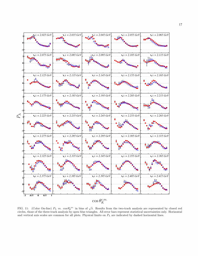
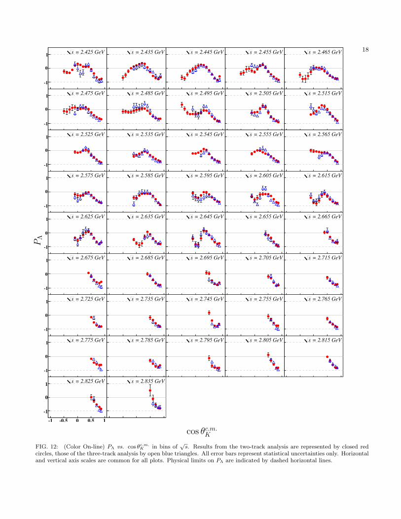
PΛ results from the two- and three-track analyses areshown in Figs. 10-12 versus cos θc.m.K in bins of

√s.

Binning for these results is the same as that used fordσ/d cos θc.m.K data. Error bars in these plots representstatistical uncertainties. A systematic uncertainty basedon acceptance uncertainty discussed in Sec. V has beenestimated to be 0.05. In some kinematic areas, differen-tial cross section measurements were possible, howeverstatistics were too low for a reliable PΛ measurement. Inall, we present measurements at 1708 kinematic points.

As with the dσ/d cos θc.m.K data, we combine the two-and three-track results into a weighted mean result asprescribed by Eqs. (14) and (15). Fig. 13 shows themean results plotted with previous high-statistics resultsfrom CLAS [19], SAPHIR [3], and GRAAL [20]. Thisfigure shows the new CLAS measurement’s increase inprecision and scope, with a nearly 500 MeV increase in√s coverage at forward angles. The angular resolution

of this CLAS measurement is unparalleled by any othermeasurement. Comparison between these and existingresults presents no systematic discrepancies, and severalstructures that are hinted at by previous measurementsare confirmed by these results.

Several notable structures are present in the PΛ dataover the

√s range from 1.7 to 2.6 GeV. In the forward

direction for√s > 1.9 GeV, where the reaction is known

to be dominated by t-channel, the recoil polarization isrelatively featureless with respect to

√s. As one looks

farther back in production angle, t-channel mechanismsbecome less dominant and undulations in PΛ can be seen.As an example, at backward angles, a region of large pos-itive Λ polarization is quite obvious at

√s ≈ 2.0 GeV. As

one looks forward to intermediate angles, the structureremains, but its magnitude is decreased. Several otherbumps are noticeable in PΛ at intermediate angles, in-cluding those at

√s ≈ 2.15 GeV and ≈ 2.3 GeV. We

note that for√s > 2.1 GeV and very forward angles,

the recoil polarization remains between −0.5 and −1.0indicating a large amount of out-of-production-plane po-larization.

13

dσ

dco

sθc.m.

K(µ

b)

1.6 1.8 2 2.2 2.4 2.6 2.8

0

0.5

1

< -0.75c.m.

Kθ cos≤-0.85

1.6 1.8 2 2.2 2.4 2.6 2.8

0

0.5

1

1.5 < -0.45c.m.

Kθ cos≤-0.55

1.6 1.8 2 2.2 2.4 2.6 2.8

0

0.5

1

< -0.15c.m.

Kθ cos≤-0.25

1.6 1.8 2 2.2 2.4 2.6 2.8

0

0.5

1

1.5 < 0.15

c.m.

Kθ cos≤0.05

1.6 1.8 2 2.2 2.4 2.6 2.8

0

0.5

1

1.5

2 < 0.45c.m.

Kθ cos≤0.35

1.6 1.8 2 2.2 2.4 2.6 2.80

1

2

3 < 0.75

c.m.

Kθ cos≤0.65

1.6 1.8 2 2.2 2.4 2.6 2.8

0

0.5

1

< -0.65c.m.

Kθ cos≤-0.75

1.6 1.8 2 2.2 2.4 2.6 2.8

0

0.5

1

1.5 < -0.35c.m.

Kθ cos≤-0.45

1.6 1.8 2 2.2 2.4 2.6 2.8

0

0.5

1

< -0.05c.m.

Kθ cos≤-0.15

1.6 1.8 2 2.2 2.4 2.6 2.8

0

0.5

1

1.5 < 0.25

c.m.

Kθ cos≤0.15

1.6 1.8 2 2.2 2.4 2.6 2.8

0

0.5

1

1.5

2 < 0.55c.m.

Kθ cos≤0.45

1.6 1.8 2 2.2 2.4 2.6 2.80

1

2

3 < 0.85

c.m.

Kθ cos≤0.75

1.6 1.8 2 2.2 2.4 2.6 2.8

0

0.5

1

< -0.55c.m.

Kθ cos≤-0.65

1.6 1.8 2 2.2 2.4 2.6 2.8

0

0.5

1

1.5 < -0.25c.m.

Kθ cos≤-0.35

1.6 1.8 2 2.2 2.4 2.6 2.8

0

0.5

1

< 0.05c.m.

Kθ cos≤-0.05

1.6 1.8 2 2.2 2.4 2.6 2.8

0

0.5

1

1.5 < 0.35

c.m.

Kθ cos≤0.25

1.6 1.8 2 2.2 2.4 2.6 2.8

0

0.5

1

1.5

2 < 0.65c.m.

Kθ cos≤0.55

1.6 1.8 2 2.2 2.4 2.6 2.80

1

2

3 < 0.95

c.m.

Kθ cos≤0.85

√s (GeV)

FIG. 8: (Color On-line) dσ/d cos θc.m.K (µb) vs.√s (GeV) in bins of cos θc.m.K . The results of this analysis are shown by closed

red circles. The 2006 CLAS results (Bradford, et al. [4]) are shown by open blue triangles, 2004 SAPHIR [3] results are shownby open green diamonds, and the LEPS results [5, 6] are shown by open black crosses.

14

c.m.

Kθcos

-0.5 0 0.5 1

b)

µ (

Kc.m

.θ

/dco

sσ

d

0.5

1

1.5

2

2.5 CLAS (2005): W = 1.78 GeV

this analysis: W = 1.775 GeV

(a)

c.m.

Kθcos

-0.5 0 0.5 1

b)

µ (

Kc.m

.θ

/dco

sσ

d

0.5

1

1.5

2

2.5 CLAS (2005): W = 1.74 GeV

this analysis: W = 1.745 GeV

(b)

FIG. 9: (Color On-line) dσ/d cos θc.m.K vs. cosθc.m.K resultsfrom this analysis (blue) and the 2005 CLAS analysis [4] (red).Fig. 9(a) shows results corresponding the

√s = 1.775 GeV

bin of this analysis. Fig. 9(b) shows those of the√s =

1.745 GeV bin. Comparisons in this bin are typical of a four-bin-wide systematic discrepancy between the two datasets.See text for discussion.

C. Model Comparison

For first-order interpretation of features in the data,we compare the average dσ/d cos θc.m.K and PΛ data (asprescribed by Eq. 14) to the predictions of several con-temporary models of K+ photoproduction. Figs. 14-16show the data and predictions of these models vs.

√s in

bins of cos θc.m.K .The Kaon-MAID model [21] is an isobar model that

treats non-resonant contributions to the channel ast-channel exchanges of K+, K∗(892), and K1(1270)mesons. Though the Kaon-MAID model is versatile,the predictions shown here are from a model fit only toSAPHIR data. Resonant contributions to the channel areattributed to the established N(1650) S11, N(1710) P11,and N(1720) P13 states, as well as a N(1900) D13 “miss-ing” resonance state necessitated by the enhancementof the differential cross section at

√s ≈ 1900 GeV. As

this model was fit to data of a somewhat limited energyrange, predictions are only available below

√s = 2200

MeV. Because it was tuned to the previous SAPHIRdata, scale agreement between the Kaon-MAID modeland the present data cannot be expected. However, con-clusions can be drawn from comparisons of specific fea-tures of the data and the model.

The second model for comparison is the Regge-Plus-Resonance (RPR) model [22] developed by the group atthe University of Ghent. This model treats non-resonantcontributions with two Regge-ized t-channel exchangesdescribed by a K+ Regge trajectory and a K∗ Reggetrajectory (both with rotating phases), an elegant de-scription requiring only three free fit parameters. AsRegge models are often considered valid only for smallexchange momenta, the RPR model was tuned only toforward-angle (cos θc.m.K > 0.3) differential cross sectionand polarization data from CLAS and previous high-energy data [23]. Resonant contributions in the RPRmodel are the N(1650) S11, N(1710) P11, N(1720) P13,and N(1900) P13 states, as well as a “missing” D13 statewith a mass of 1900 MeV. It should not be surprising thatthis model agrees well with the current dσ/d cos θc.m.K re-sults; agreement between these results and the previousCLAS results is satisfactory at most kinematics.

The final model included here is that of the Bonn-Gatchina (BG) group [9], which is the result of a large-scale coupled-channel partial-wave analysis of K+Λ,K+Σ0, and K0Σ+, pπ0, nπ+ and pη photoproductiondata. It should be noted that the model was constrainedto γp → K+Λ differential cross section, recoil polariza-tion, and beam asymmetry data. This model employsthe operator expansion method, which projects t- andu-channel amplitudes into s-channel partial waves. Res-onant production in the K+Λ channel is represented bysignificant contributions of the N(1650) S11 and N(1730)P13 states, as well as two “newly observed” N(1840) P11

and N(2170) D13 states.Comparison of these models to the new cross section

results presents some notable observations. Though theKaon-MAID model displays an almost global scale dis-crepancy, it is evident that the model’s treatment ofthe cross section at

√s ≈ 1.9 GeV (using a “missing”

D13 state) is too weak. We also note that the Kaon-MAID model overestimates the differential cross sectionfor slightly backward angles and

√s > 2.0 GeV. The

RPR and BG models, as they have been tuned to previ-ous CLAS results match the present results well at mostkinematics. Slight discrepancies exist for the BG modelat middle angles and

√s ≈ 1.9 GeV and for the BG

and RPR models at forward angles and√s ≈ 1.7 GeV

and√s > 2.4 GeV. At low

√s, it is possible that

these discrepancies can be accounted for by re-tuning thestrengths of s-channel resonances included.

One feature of the new cross section results that is notreproduced by the models is the slight bump visible atcos θc.m.K ≈ 0.0 and

√s ≈ 2.1 GeV. The PDG lists several

N∗ states with single-star-rated couplings to K+Λ near

15

this mass, however, a more systematic analysis of thedata should be performed before associating the featurewith a given state.

Agreement of these model predictions and the presentPΛ data is not as good. Recall that previous polar-ization data for this reaction were sparse compared tothe present results. At backward production angles(cos θc.m.K < −0.15), we see both the Kaon-MAID andBG models failing to reproduce the large positive polar-ization of the Λ at

√s ≈ 2.0 GeV. At cos θc.m.K ≈ −0.5,

the models also fail to reproduce the negative Λ po-larization for

√s > 2.2 GeV. At intermediate angles

(−0.15 ≤ cos θc.m.K < 0.35), the BG model reproducesthe recoil polarization for

√s < 1.85 GeV, however all

three models fail to reproduce the series of bumps in PΛ

above√s ≈ 1.85 GeV. As the recoil polarization appears

to be very sensitive to the nature of the resonances in-cluded, as well as interference between resonances andbetween resonances and non-resonant mechanisms, thesediscrepancies could mean that the set of resonances thateach of these models employs is either incomplete or in-correct. It is worth note that for extreme forward angles,only the RPR model seems to accurately describe therecoil polarization (though some further tuning of themodel for 0.6 ≤ cos θc.m.K < 0.8 is called for), lendingcredence to the Regge-ized meson exchange treatment ofnon-resonant production.

X. CONCLUSIONS

In conclusion, these CLAS γp → K+Λ differentialcross section and Λ recoil polarization results presentedhere are the most precise to date and offer a significantextension of the observed center-of-mass energy range.We have presented results from independent analyses of

the data and found them to demonstrate satisfying agree-ment.These analyses provide dσ/ cos θc.m.K and PΛ mea-surements at 2076 and 1708 kinematic points, respec-tively. The dσ/d cos θc.m.K data show satisfying agreementwith previous CLAS and LEPS results, while extendingthe observed

√s range by 300 MeV. These results also

provide overwhelming support for the previous CLAS re-sult regarding its discrepancy with SAPHIR results. ThePΛ results presented here agree well with all previous re-sults and extend the observed

√s range by 500 MeV.

These high-precision measurements show a rich structurein both observables which present an interesting oppor-tunity for interpretation of K+Λ photoproduction mech-anisms.

Acknowledgments

The authors thank the staff and administration ofthe Thomas Jefferson National Accelerator Facility whomade this experiment possible. Thanks also go to PieterVancraeyveld of the University of Ghent and UlrikeThoma and Andrey Sarantsev of the Bonn-Gatchinagroup for their help in obtaining the model predictionsshown in this paper. This work was supported in partby the U.S. Department of Energy (under grant No. DE-FG02-87ER40315); the National Science Foundation; theItalian Istituto Nazionale di Fisica Nucleare; the FrenchCentre National de la Recherche Scientifique; the FrenchCommissariat a l’Energie Atomique; an Emmy NoetherGrant from the Deutsche Forschungsgemeinschaft; theU.K. Research Council, S.T.F.C.; and the National Re-search Foundation of Korea. The Southeastern Uni-versities Research Association (SURA) operated Jeffer-son Lab under United States DOE contract DE-AC05-84ER40150 during this work.

[1] M. Bockhorst et al., Z. Phys. C 63, 37 (1994).[2] M. Q. Tran et al., Phys. Lett. B 445, 20 (1998).[3] K. H. Glander et al., Eur. Phys. J. A 19, 2 (2004).[4] R. Bradford et al., Phys. Rev. C 73, 035202 (2006).[5] M. Sumihama et al., Phys. Rev. C 73, 035214 (2006).[6] K. Hicks et al., Phys. Rev. C 76, 042201R (2007).[7] T. Mart and C. Bennhold, Phys. Rev. C 61, 012201

(1999).[8] V. Shklyar, H. Lenske, and U. Mosel, Phys. Rev. C 72,

015210 (2005).[9] A. V. Sarantsev, V. A. Nikonov, A. V. Anisovich, E.

Klempt, and U. Thoma, Eur. Phys. J. A 25, 441-453(2005).

[10] B. Julia-Dıaz, B. Saghai, F. Tabakin, W.-T. Chiang, T.-S. H. Lee, and Z. Li, Nucl. Phys. A 755, 463-466 (2005).

[11] D. I. Sober et al., Nucl. Inst. Meth. A440, 263 (2000).[12] B. Mecking et al., Nucl. Inst. Meth. A503, 513 (2003).[13] M. Williams et al. [CLAS Collaboration], accepted for

publication in Phys. Rev. C, (2009). arXiv:0908.2910

[nucl-ex].[14] G. J. Feldman and R. D. Cousins, Phys. Rev. D 57, 3873-

3889 (1998).[15] M. Williams, M. Bellis, and C. A. Meyer, JINST 4

P10003, (2009).[16] M. E. McCracken, Ph. D. Thesis, Carnegie Mellon Uni-

versity, 2007.www.jlab.org/Hall-B/general/clas thesis.html.

[17] M. Williams, Comp. Phys. Comm. 180, 1847 (2009).[18] M. Williams et al. [CLAS Collaboration], Phys. Rev.

C80, 045213 (2009)[19] J. W. C. McNabb et al., Phys. Rev. C 69, 042201 (2004).[20] A. Lleres et al., Eur. Phys. J. A 31, 79 (2007).[21] F.X. Lee, T. Mart, C. Bennhold, H. Haberzettl, L.E.

Wright, Nucl. Phys. A695, 237 (2001)[22] T. Corthals, J. Ryckebusch, and T. Van Cauteren, Phys.

Rev. C 73, 045207 (2006).[23] A. M. Boyarski et al., Phys. Rev. Lett. 22, 1131 (1969).

16

PΛ

-1 -0.5 0 0.5 1

-1

0

1 = 1.625 GeVs

-1 -0.5 0 0.5 1

-1

0

1 = 1.675 GeVs

-1 -0.5 0 0.5 1

-1

0

1 = 1.725 GeVs

-1 -0.5 0 0.5 1

-1

0

1 = 1.775 GeVs

-1 -0.5 0 0.5 1

-1

0

1 = 1.825 GeVs

-1 -0.5 0 0.5 1

-1

0

1 = 1.875 GeVs

-1 -0.5 0 0.5 1

-1

0

1 = 1.925 GeVs

-1 -0.5 0 0.5 1

-1

0

1 = 1.975 GeVs

-1 -0.5 0 0.5 1

-1

0

1 = 1.635 GeVs

-1 -0.5 0 0.5 1

-1

0

1 = 1.685 GeVs

-1 -0.5 0 0.5 1

-1

0

1 = 1.735 GeVs

-1 -0.5 0 0.5 1

-1

0

1 = 1.785 GeVs

-1 -0.5 0 0.5 1

-1

0

1 = 1.835 GeVs

-1 -0.5 0 0.5 1

-1

0

1 = 1.885 GeVs

-1 -0.5 0 0.5 1

-1

0

1 = 1.935 GeVs

-1 -0.5 0 0.5 1

-1

0

1 = 1.985 GeVs

-1 -0.5 0 0.5 1

-1

0

1 = 1.645 GeVs

-1 -0.5 0 0.5 1

-1

0

1 = 1.695 GeVs

-1 -0.5 0 0.5 1

-1

0

1 = 1.745 GeVs

-1 -0.5 0 0.5 1

-1

0

1 = 1.795 GeVs

-1 -0.5 0 0.5 1

-1

0

1 = 1.845 GeVs

-1 -0.5 0 0.5 1

-1

0

1 = 1.895 GeVs

-1 -0.5 0 0.5 1

-1

0

1 = 1.945 GeVs

-1 -0.5 0 0.5 1

-1

0

1 = 1.995 GeVs

-1 -0.5 0 0.5 1

-1

0

1 = 1.655 GeVs

-1 -0.5 0 0.5 1

-1

0

1 = 1.705 GeVs

-1 -0.5 0 0.5 1

-1

0

1 = 1.755 GeVs

-1 -0.5 0 0.5 1

-1

0

1 = 1.805 GeVs

-1 -0.5 0 0.5 1

-1

0

1 = 1.855 GeVs

-1 -0.5 0 0.5 1

-1

0

1 = 1.905 GeVs

-1 -0.5 0 0.5 1

-1

0

1 = 1.955 GeVs

-1 -0.5 0 0.5 1

-1

0

1 = 2.005 GeVs

-1 -0.5 0 0.5 1

-1

0

1 = 1.665 GeVs

-1 -0.5 0 0.5 1

-1

0

1 = 1.715 GeVs

-1 -0.5 0 0.5 1

-1

0

1 = 1.765 GeVs

-1 -0.5 0 0.5 1

-1

0

1 = 1.815 GeVs

-1 -0.5 0 0.5 1

-1

0

1 = 1.865 GeVs

-1 -0.5 0 0.5 1

-1

0

1 = 1.915 GeVs

-1 -0.5 0 0.5 1

-1

0

1 = 1.965 GeVs

-1 -0.5 0 0.5 1

-1

0

1 = 2.015 GeVs

cos θc.m.K

FIG. 10: (Color On-line) PΛ vs. cos θc.m.K in bins of√s. Results from the two-track analysis are represented by closed red

circles, those of the three-track analysis by open blue triangles. All error bars represent statistical uncertainties only. Horizontaland vertical axis scales are common for all plots. Physical limits on PΛ are indicated by dashed horizontal lines.

17

PΛ

-1 -0.5 0 0.5 1

-1

0

1 = 2.025 GeVs

-1 -0.5 0 0.5 1

-1

0

1 = 2.075 GeVs

-1 -0.5 0 0.5 1

-1

0

1 = 2.125 GeVs

-1 -0.5 0 0.5 1

-1

0

1 = 2.175 GeVs

-1 -0.5 0 0.5 1

-1

0

1 = 2.225 GeVs

-1 -0.5 0 0.5 1

-1

0

1 = 2.275 GeVs

-1 -0.5 0 0.5 1

-1

0

1 = 2.325 GeVs

-1 -0.5 0 0.5 1

-1

0

1 = 2.375 GeVs

-1 -0.5 0 0.5 1

-1

0

1 = 2.035 GeVs

-1 -0.5 0 0.5 1

-1

0

1 = 2.085 GeVs

-1 -0.5 0 0.5 1

-1

0

1 = 2.135 GeVs

-1 -0.5 0 0.5 1

-1

0

1 = 2.185 GeVs

-1 -0.5 0 0.5 1

-1

0

1 = 2.235 GeVs

-1 -0.5 0 0.5 1

-1

0

1 = 2.285 GeVs

-1 -0.5 0 0.5 1

-1

0

1 = 2.335 GeVs

-1 -0.5 0 0.5 1

-1

0

1 = 2.385 GeVs

-1 -0.5 0 0.5 1

-1

0

1 = 2.045 GeVs

-1 -0.5 0 0.5 1

-1

0

1 = 2.095 GeVs

-1 -0.5 0 0.5 1

-1

0

1 = 2.145 GeVs

-1 -0.5 0 0.5 1

-1

0

1 = 2.195 GeVs

-1 -0.5 0 0.5 1

-1

0

1 = 2.245 GeVs

-1 -0.5 0 0.5 1

-1

0

1 = 2.295 GeVs

-1 -0.5 0 0.5 1

-1

0

1 = 2.345 GeVs

-1 -0.5 0 0.5 1

-1

0

1 = 2.395 GeVs

-1 -0.5 0 0.5 1

-1

0

1 = 2.055 GeVs

-1 -0.5 0 0.5 1

-1

0

1 = 2.105 GeVs

-1 -0.5 0 0.5 1

-1

0

1 = 2.155 GeVs

-1 -0.5 0 0.5 1

-1

0

1 = 2.205 GeVs

-1 -0.5 0 0.5 1

-1

0

1 = 2.255 GeVs

-1 -0.5 0 0.5 1

-1

0

1 = 2.305 GeVs

-1 -0.5 0 0.5 1

-1

0

1 = 2.355 GeVs

-1 -0.5 0 0.5 1

-1

0

1 = 2.405 GeVs

-1 -0.5 0 0.5 1

-1

0

1 = 2.065 GeVs

-1 -0.5 0 0.5 1

-1

0

1 = 2.115 GeVs

-1 -0.5 0 0.5 1

-1

0

1 = 2.165 GeVs

-1 -0.5 0 0.5 1

-1

0

1 = 2.215 GeVs

-1 -0.5 0 0.5 1

-1

0

1 = 2.265 GeVs

-1 -0.5 0 0.5 1

-1

0

1 = 2.315 GeVs

-1 -0.5 0 0.5 1

-1

0

1 = 2.365 GeVs

-1 -0.5 0 0.5 1

-1

0

1 = 2.415 GeVs

cos θc.m.K

FIG. 11: (Color On-line) PΛ vs. cos θc.m.K in bins of√s. Results from the two-track analysis are represented by closed red

circles, those of the three-track analysis by open blue triangles. All error bars represent statistical uncertainties only. Horizontaland vertical axis scales are common for all plots. Physical limits on PΛ are indicated by dashed horizontal lines.

18

PΛ

-1 -0.5 0 0.5 1

-1

0

1 = 2.425 GeVs

-1 -0.5 0 0.5 1

-1

0

1 = 2.475 GeVs

-1 -0.5 0 0.5 1

-1

0

1 = 2.525 GeVs

-1 -0.5 0 0.5 1

-1

0

1 = 2.575 GeVs

-1 -0.5 0 0.5 1

-1

0

1 = 2.625 GeVs

-1 -0.5 0 0.5 1

-1

0

1 = 2.675 GeVs

-1 -0.5 0 0.5 1

-1

0

1 = 2.725 GeVs

-1 -0.5 0 0.5 1

-1

0

1 = 2.775 GeVs

-1 -0.5 0 0.5 1

-1

0

1 = 2.825 GeVs

-1 -0.5 0 0.5 1

-1

0

1 = 2.435 GeVs

-1 -0.5 0 0.5 1

-1

0

1 = 2.485 GeVs

-1 -0.5 0 0.5 1

-1

0

1 = 2.535 GeVs

-1 -0.5 0 0.5 1

-1

0

1 = 2.585 GeVs

-1 -0.5 0 0.5 1

-1

0

1 = 2.635 GeVs

-1 -0.5 0 0.5 1

-1

0

1 = 2.685 GeVs

-1 -0.5 0 0.5 1

-1

0

1 = 2.735 GeVs

-1 -0.5 0 0.5 1

-1

0

1 = 2.785 GeVs

-1 -0.5 0 0.5 1

-1

0

1 = 2.835 GeVs

-1 -0.5 0 0.5 1

-1

0

1 = 2.445 GeVs

-1 -0.5 0 0.5 1

-1

0

1 = 2.495 GeVs

-1 -0.5 0 0.5 1

-1

0

1 = 2.545 GeVs

-1 -0.5 0 0.5 1

-1

0

1 = 2.595 GeVs

-1 -0.5 0 0.5 1

-1

0

1 = 2.645 GeVs

-1 -0.5 0 0.5 1

-1

0

1 = 2.695 GeVs

-1 -0.5 0 0.5 1

-1

0

1 = 2.745 GeVs

-1 -0.5 0 0.5 1

-1

0

1 = 2.795 GeVs

-1 -0.5 0 0.5 1

-1

0

1 = 2.455 GeVs

-1 -0.5 0 0.5 1

-1

0

1 = 2.505 GeVs

-1 -0.5 0 0.5 1

-1

0

1 = 2.555 GeVs

-1 -0.5 0 0.5 1

-1

0

1 = 2.605 GeVs

-1 -0.5 0 0.5 1

-1

0

1 = 2.655 GeVs

-1 -0.5 0 0.5 1

-1

0

1 = 2.705 GeVs

-1 -0.5 0 0.5 1

-1

0

1 = 2.755 GeVs

-1 -0.5 0 0.5 1

-1

0

1 = 2.805 GeVs

-1 -0.5 0 0.5 1

-1

0

1 = 2.465 GeVs

-1 -0.5 0 0.5 1

-1

0

1 = 2.515 GeVs

-1 -0.5 0 0.5 1

-1

0

1 = 2.565 GeVs

-1 -0.5 0 0.5 1

-1

0

1 = 2.615 GeVs

-1 -0.5 0 0.5 1

-1

0

1 = 2.665 GeVs

-1 -0.5 0 0.5 1

-1

0

1 = 2.715 GeVs

-1 -0.5 0 0.5 1

-1

0

1 = 2.765 GeVs

-1 -0.5 0 0.5 1

-1

0

1 = 2.815 GeVs

cos θc.m.K

FIG. 12: (Color On-line) PΛ vs. cos θc.m.K in bins of√s. Results from the two-track analysis are represented by closed red

circles, those of the three-track analysis by open blue triangles. All error bars represent statistical uncertainties only. Horizontaland vertical axis scales are common for all plots. Physical limits on PΛ are indicated by dashed horizontal lines.

19P

Λ

1.6 1.8 2 2.2 2.4 2.6 2.8

-1

-0.5

0

0.5

1 < -0.75

c.m.

Kθ cos≤-0.85

1.6 1.8 2 2.2 2.4 2.6 2.8

-1

-0.5

0

0.5

1 < -0.45

c.m.

Kθ cos≤-0.55

1.6 1.8 2 2.2 2.4 2.6 2.8

-1

-0.5

0

0.5

1 < -0.15

c.m.

Kθ cos≤-0.25

1.6 1.8 2 2.2 2.4 2.6 2.8

-1

-0.5

0

0.5

1 < 0.15

c.m.

Kθ cos≤0.05

1.6 1.8 2 2.2 2.4 2.6 2.8

-1

-0.5

0

0.5

1 < 0.45

c.m.

Kθ cos≤0.35

1.6 1.8 2 2.2 2.4 2.6 2.8

-1

-0.5

0

0.5

1 < 0.75

c.m.

Kθ cos≤0.65

1.6 1.8 2 2.2 2.4 2.6 2.8

-1

-0.5

0

0.5

1 < -0.65

c.m.

Kθ cos≤-0.75

1.6 1.8 2 2.2 2.4 2.6 2.8

-1

-0.5

0

0.5

1 < -0.35

c.m.

Kθ cos≤-0.45

1.6 1.8 2 2.2 2.4 2.6 2.8

-1

-0.5

0

0.5

1 < -0.05

c.m.

Kθ cos≤-0.15

1.6 1.8 2 2.2 2.4 2.6 2.8

-1

-0.5

0

0.5

1 < 0.25

c.m.

Kθ cos≤0.15

1.6 1.8 2 2.2 2.4 2.6 2.8

-1

-0.5

0

0.5

1 < 0.55

c.m.

Kθ cos≤0.45

1.6 1.8 2 2.2 2.4 2.6 2.8

-1

-0.5

0

0.5

1 < 0.85

c.m.

Kθ cos≤0.75

1.6 1.8 2 2.2 2.4 2.6 2.8

-1

-0.5

0

0.5

1 < -0.55

c.m.

Kθ cos≤-0.65

1.6 1.8 2 2.2 2.4 2.6 2.8

-1

-0.5

0

0.5

1 < -0.25

c.m.

Kθ cos≤-0.35

1.6 1.8 2 2.2 2.4 2.6 2.8

-1

-0.5

0

0.5

1 < 0.05

c.m.

Kθ cos≤-0.05

1.6 1.8 2 2.2 2.4 2.6 2.8

-1

-0.5

0

0.5

1 < 0.35

c.m.

Kθ cos≤0.25

1.6 1.8 2 2.2 2.4 2.6 2.8

-1

-0.5

0

0.5

1 < 0.65

c.m.

Kθ cos≤0.55

1.6 1.8 2 2.2 2.4 2.6 2.8

-1

-0.5

0

0.5

1 < 0.95

c.m.

Kθ cos≤0.85

√s (GeV)

FIG. 13: (Color On-line) PΛ vs.√s (GeV) in bins of cos θc.m.K . Results of this analysis are represented by red circles, previous

CLAS (McNabb, et al. [19]) results by blue triangles, SAPHIR 2004 (Glander, et al. [3]) by green triangles, and GRAAL 2007(Lleres, et al. [20]) by black squares. Physical limits on PΛ are indicated by dashed horizontal lines.

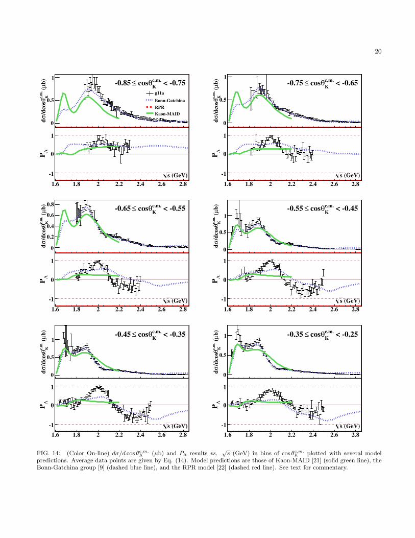
20

1.6 1.8 2 2.2 2.4 2.6 2.8

b)

µ (

c.m

.

Kθ

/dco

sσ

d 0

0.5

1 < -0.75

c.m.

Kθ cos≤-0.85

g11a

Bonn-Gatchina

RPR

Kaon-MAID

(GeV) s

1.6 1.8 2 2.2 2.4 2.6 2.8

ΛP

-1

0

11.6 1.8 2 2.2 2.4 2.6 2.8

b)

µ (

c.m

.

Kθ

/dco

sσ

d 0

0.5

1

< -0.65c.m.

Kθ cos≤-0.75

(GeV) s

1.6 1.8 2 2.2 2.4 2.6 2.8

ΛP

-1

0

1

1.6 1.8 2 2.2 2.4 2.6 2.8

b)

µ (

c.m

.

Kθ

/dco

sσ

d 0

0.2

0.4

0.6

0.8 < -0.55

c.m.

Kθ cos≤-0.65

(GeV) s

1.6 1.8 2 2.2 2.4 2.6 2.8

ΛP

-1

0

11.6 1.8 2 2.2 2.4 2.6 2.8

b)

µ (

c.m

.

Kθ

/dco

sσ

d

0

0.5

1

< -0.45c.m.

Kθ cos≤-0.55

(GeV) s

1.6 1.8 2 2.2 2.4 2.6 2.8

ΛP

-1

0

1

1.6 1.8 2 2.2 2.4 2.6 2.8

b)

µ (

c.m

.

Kθ

/dco

sσ

d

0

0.5

1 < -0.35

c.m.

Kθ cos≤-0.45

(GeV) s

1.6 1.8 2 2.2 2.4 2.6 2.8

ΛP

-1

0

11.6 1.8 2 2.2 2.4 2.6 2.8

b)

µ (

c.m

.

Kθ

/dco

sσ

d

0

0.5

1 < -0.25c.m.

Kθ cos≤-0.35

(GeV) s

1.6 1.8 2 2.2 2.4 2.6 2.8

ΛP

-1

0

1

FIG. 14: (Color On-line) dσ/d cos θc.m.K (µb) and PΛ results vs.√s (GeV) in bins of cos θc.m.K plotted with several model

predictions. Average data points are given by Eq. (14). Model predictions are those of Kaon-MAID [21] (solid green line), theBonn-Gatchina group [9] (dashed blue line), and the RPR model [22] (dashed red line). See text for commentary.

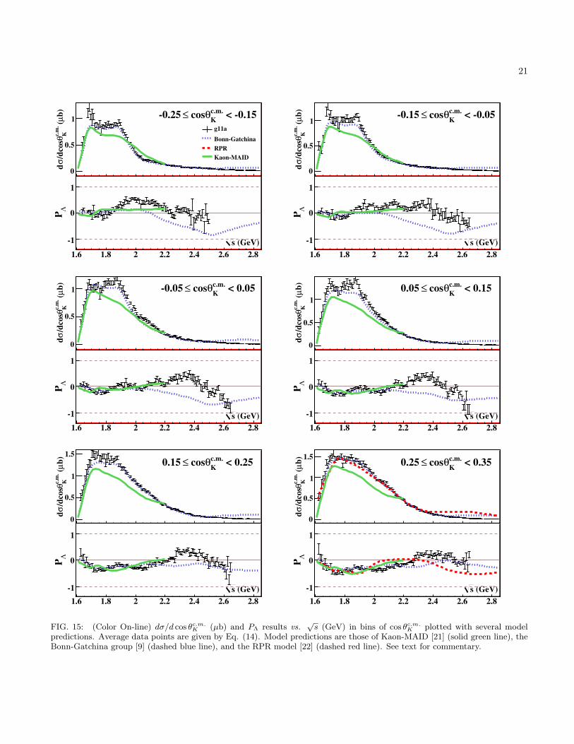
21

1.6 1.8 2 2.2 2.4 2.6 2.8

b)

µ (

c.m

.

Kθ

/dco

sσ

d

0

0.5

1 < -0.15

c.m.

Kθ cos≤-0.25

g11a

Bonn-Gatchina

RPR

Kaon-MAID

(GeV) s

1.6 1.8 2 2.2 2.4 2.6 2.8

ΛP

-1

0

11.6 1.8 2 2.2 2.4 2.6 2.8

b)

µ (

c.m

.

Kθ

/dco

sσ

d

0

0.5

1 < -0.05

c.m.

Kθ cos≤-0.15

(GeV) s

1.6 1.8 2 2.2 2.4 2.6 2.8

ΛP

-1

0

1

1.6 1.8 2 2.2 2.4 2.6 2.8

b)

µ (

c.m

.

Kθ

/dco

sσ

d

0

0.5

1 < 0.05c.m.

Kθ cos≤-0.05

(GeV) s

1.6 1.8 2 2.2 2.4 2.6 2.8

ΛP

-1

0

11.6 1.8 2 2.2 2.4 2.6 2.8

b)

µ (

c.m

.

Kθ

/dco

sσ

d

0

0.5

1

< 0.15c.m.

Kθ cos≤0.05

(GeV) s

1.6 1.8 2 2.2 2.4 2.6 2.8

ΛP

-1

0

1

1.6 1.8 2 2.2 2.4 2.6 2.8

b)

µ (

c.m

.

Kθ

/dco

sσ

d

0

0.5

1

1.5

< 0.25c.m.

Kθ cos≤0.15

(GeV) s

1.6 1.8 2 2.2 2.4 2.6 2.8

ΛP

-1

0

11.6 1.8 2 2.2 2.4 2.6 2.8

b)

µ (

c.m

.

Kθ

/dco

sσ

d

0

0.5

1

1.5 < 0.35

c.m.

Kθ cos≤0.25

(GeV) s

1.6 1.8 2 2.2 2.4 2.6 2.8

ΛP

-1

0

1

FIG. 15: (Color On-line) dσ/d cos θc.m.K (µb) and PΛ results vs.√s (GeV) in bins of cos θc.m.K plotted with several model

predictions. Average data points are given by Eq. (14). Model predictions are those of Kaon-MAID [21] (solid green line), theBonn-Gatchina group [9] (dashed blue line), and the RPR model [22] (dashed red line). See text for commentary.

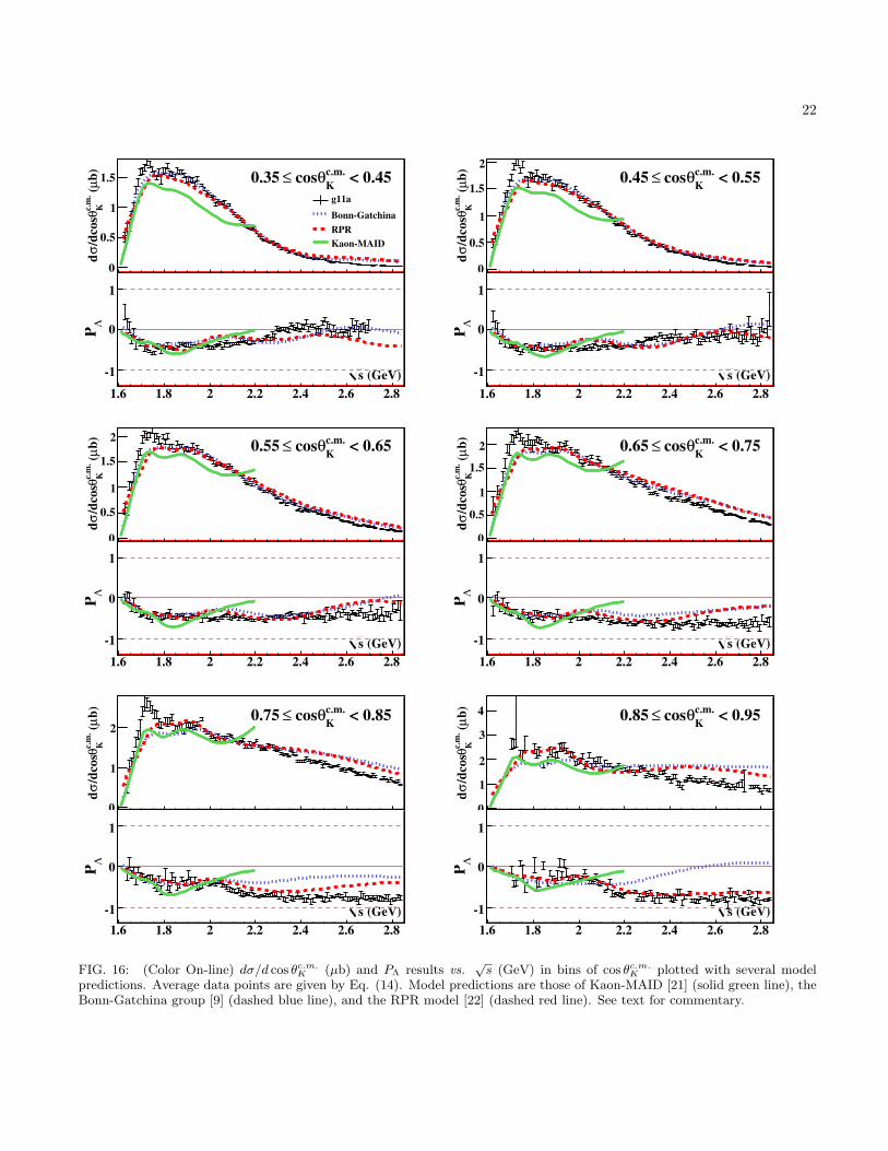
22

1.6 1.8 2 2.2 2.4 2.6 2.8

b)

µ (

c.m

.

Kθ

/dco

sσ

d

0

0.5

1

1.5 < 0.45c.m.

Kθ cos≤0.35

g11a

Bonn-Gatchina

RPR

Kaon-MAID

(GeV) s

1.6 1.8 2 2.2 2.4 2.6 2.8

ΛP

-1

0

11.6 1.8 2 2.2 2.4 2.6 2.8

b)

µ (

c.m

.

Kθ

/dco

sσ

d

0

0.5

1

1.5

2

< 0.55c.m.

Kθ cos≤0.45

(GeV) s

1.6 1.8 2 2.2 2.4 2.6 2.8

ΛP

-1

0

1

1.6 1.8 2 2.2 2.4 2.6 2.8

b)

µ (

c.m

.

Kθ

/dco

sσ

d

0

0.5

1

1.5

2 < 0.65

c.m.

Kθ cos≤0.55

(GeV) s

1.6 1.8 2 2.2 2.4 2.6 2.8

ΛP

-1

0

11.6 1.8 2 2.2 2.4 2.6 2.8

b)

µ (

c.m

.

Kθ

/dco

sσ

d

0

0.5

1

1.5

2 < 0.75c.m.

Kθ cos≤0.65

(GeV) s

1.6 1.8 2 2.2 2.4 2.6 2.8

ΛP

-1

0

1

1.6 1.8 2 2.2 2.4 2.6 2.8

b)

µ (

c.m

.

Kθ

/dco

sσ

d

0

1

2 < 0.85

c.m.

Kθ cos≤0.75

(GeV) s

1.6 1.8 2 2.2 2.4 2.6 2.8

ΛP

-1

0

11.6 1.8 2 2.2 2.4 2.6 2.8

b)

µ (

c.m

.

Kθ

/dco

sσ

d

0

1

2

3

4 < 0.95c.m.

Kθ cos≤0.85

(GeV) s

1.6 1.8 2 2.2 2.4 2.6 2.8

ΛP

-1

0

1

FIG. 16: (Color On-line) dσ/d cos θc.m.K (µb) and PΛ results vs.√s (GeV) in bins of cos θc.m.K plotted with several model

predictions. Average data points are given by Eq. (14). Model predictions are those of Kaon-MAID [21] (solid green line), theBonn-Gatchina group [9] (dashed blue line), and the RPR model [22] (dashed red line). See text for commentary.