Decays of bottom mesons emitting tensor mesons in the final state using the...
32
1 DECAYS OF BOTTOM MESONS EMITTING TENSOR MESON IN FINAL STATE USING ISGW II MODEL Neelesh Sharma, Rohit Dhir* and R.C. Verma Department of Physics, Punjabi University, Patiala-147 002, INDIA; *School of Physics and Material Science, Thapar University, Patiala-147 004, INDIA. Abstract In this paper, we investigate phenomenologically two-body weak decays of the bottom mesons emitting pseudoscalar/vector meson and a tensor meson. Form factors are obtained using the improved ISGW II model. Consequently, branching ratios for the CKM-favored and CKM-suppressed decays are calculated. PACS no (s): 13.25.Hw, 12.39.Jh, 12.39.St
Transcript of Decays of bottom mesons emitting tensor mesons in the final state using the...

1
DECAYS OF BOTTOM MESONS EMITTING
TENSOR MESON IN FINAL STATE
USING ISGW II MODEL
Neelesh Sharma, Rohit Dhir* and R.C. Verma
Department of Physics, Punjabi University,
Patiala-147 002, INDIA;
*School of Physics and Material Science,
Thapar University, Patiala-147 004, INDIA.
Abstract
In this paper, we investigate phenomenologically two-body
weak decays of the bottom mesons emitting pseudoscalar/vector
meson and a tensor meson. Form factors are obtained using the
improved ISGW II model. Consequently, branching ratios for the
CKM-favored and CKM-suppressed decays are calculated.
PACS no (s): 13.25.Hw, 12.39.Jh, 12.39.St

2
I. INTRODUCTION
Experimental results are available for the branching ratios of several B-meson
decay modes. Many theoretical works have been done to understand exclusive hadronic B
decays in the framework of the generalized factorization, QCD factorization or flavor
SU(3) symmetry. Weak hadronic decays of the B-mesons are expected to provide a rich
phenomenology yielding a wealth of information for testing the standard model and for
probing strong interaction dynamics. However, these decays involve nonperturbative
strong processes which cannot be calculated from the first principles. Thus,
phenomenological approaches [1-5] have generally been applied to study them using
factorization hypothesis. It involves expansion of the transition amplitudes in terms of a
few invariant form factors which provide essential information on the structure of the
mesons and the interplay of the strong and weak interactions. This scheme has earlier
been employed to study the weak hadronic decays of B-meson to s-wave mesons [5-12].
B-mesons, being heavy, can also emit heavier mesons such as p-wave mesons, which
have attracted theoretical attention recently. However, there exist only a few works on the
hadronic B decays [13-17] that involve a tensor meson in the final state using the
frameworks of flavor SU(3) symmetry and the generalized factorization. In the next few
years new experimental data on rare decays of B mesons would become available from
the B factories such as KEK, Belle, Babar, BTeV, LHC. It is expected that improved
measurements or new bounds will be obtained on the branching ratios for various decay
modes and many decay modes with small branching ratios may also be observed for the
first time.
In this paper, we analyze two-body hadronic decays of −B , 0B and 0
sB mesons to
pseudoscalar (P (0-)) /vector (V (1
-)) and tensor (T (2+)) mesons in the final state, for
whom the experiments have provided the following branching ratios [18,19]:
0 4
2( ) (7.8 1.4) 10B B Dπ− − −→ = ± × ,
6
2 10)5.22.8()( −−− ×±=→ fBB π , 0.4 6
2 0.5( ) (1.3 ) 10B B K f− − + −
−→ = × ,
)( 2
−− → KBB η = 6(9.1 3.0) 10−± × ,
)( 0
2
0 KBB η→ = 6(9.6 2.1) 10−± × ,
)( 2
00 fDBB → = 4(1.2 0.4) 10−± × , 0 0
2( )B B Kφ→ = 6(7.8 1.3) 10−± × , 0 4
2( ) 3.0 10B B aπ ± −→ < ×∓ , (1) 0 6
2( ) 6.9 10B B Kπ− − −→ < × ,
)( 2
0 +−→ aDBB s
4109.1 −×< , 0 5
2( ) 1.8 10B B Kπ + − −→ < × , 0 3
2( ) 2.2 10B B Dπ − + −→ < × ,
0 3
2( ) 4.7 10B B Dρ− − −→ < × ,
3
3
2( ) 1.5 10B B Kρ− − − −→ < × , 3
2( ) 3.4 10B B Kφ− − −→ < × ,
0 3
2( ) 7.2 10B B aρ− − −→ < × , 0 4
2( ) 2.0 10s
B B D a+ − −→ < × ,
0 3
2( ) 4.9 10B B Dρ − + −→ < × ,
0 0 0 3
2( ) 1.1 10B B Kρ −→ < × .
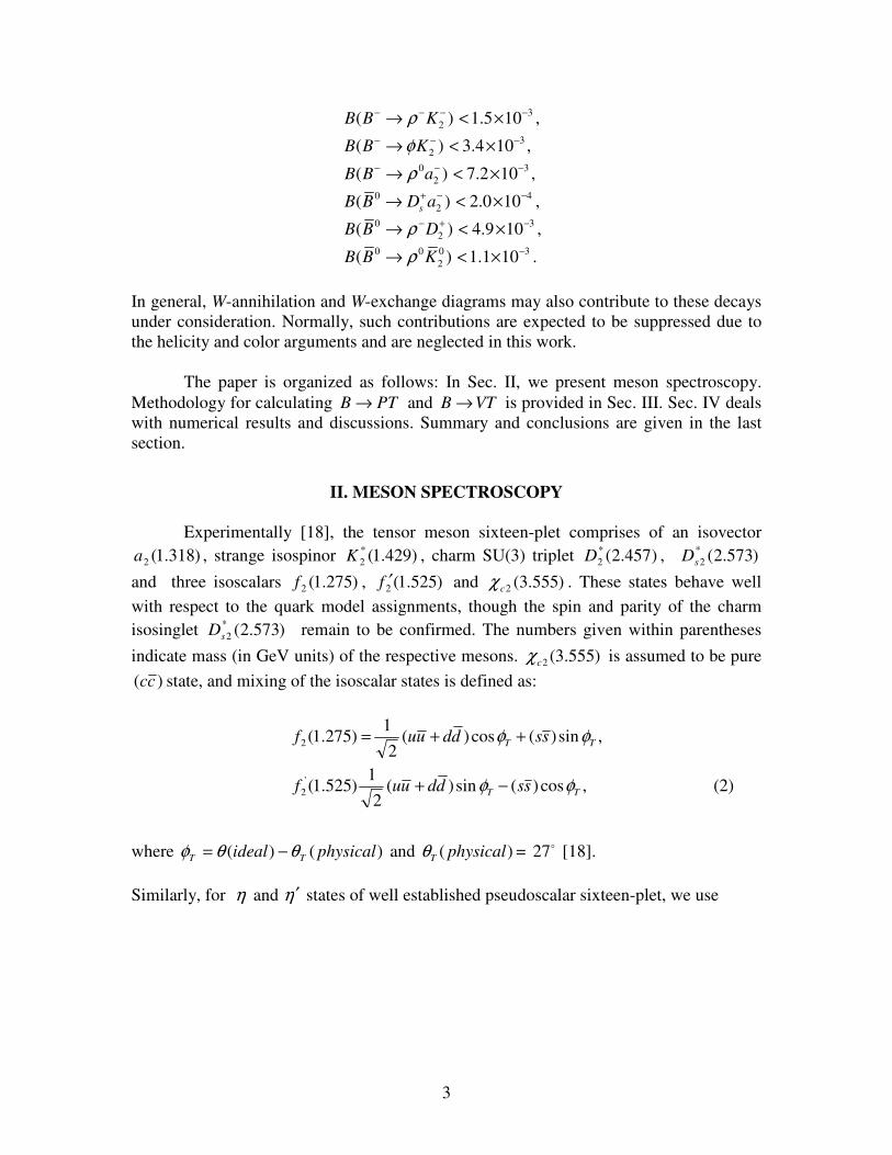
In general, W-annihilation and W-exchange diagrams may also contribute to these decays
under consideration. Normally, such contributions are expected to be suppressed due to
the helicity and color arguments and are neglected in this work.
The paper is organized as follows: In Sec. II, we present meson spectroscopy.
Methodology for calculating B PT→ and B VT→ is provided in Sec. III. Sec. IV deals
with numerical results and discussions. Summary and conclusions are given in the last
section.
II. MESON SPECTROSCOPY
Experimentally [18], the tensor meson sixteen-plet comprises of an isovector
)318.1(2a , strange isospinor )429.1(*
2K , charm SU(3) triplet )457.2(*
2D , )573.2(*
2sD
and three isoscalars )275.1(2f , )525.1(2f ′ and )555.3(2cχ . These states behave well
with respect to the quark model assignments, though the spin and parity of the charm
isosinglet )573.2(*
2sD remain to be confirmed. The numbers given within parentheses
indicate mass (in GeV units) of the respective mesons. )555.3(2cχ is assumed to be pure
)( cc state, and mixing of the isoscalar states is defined as:
,cos)(sin)(2
1)525.1(
,sin)(cos)(2
1)275.1(
'
2
2
TT
TT
ssdduuf
ssdduuf
φφ
φφ
−+
++=
(2)
where )()( physicalideal TT θθφ −= and )( physicalTθ = 27� [18].
Similarly, for η and η′ states of well established pseudoscalar sixteen-plet, we use

4
,sin)(cos)(2
1)958.0(
,cos)(sin)(2
1)547.0(
PP
PP
ssdduu
ssdduu
φφη
φφη
++=′
−+=
(3)
where )()( physicalideal pp θθφ −= and we take ( ) 15.4P physicalθ = − � [18]. cη is taken
as
)()979.2( ccc =η . (4)
Similarly, for ω and φ states of well established pseudoscalar sixteen-plet, we use
1(0.783) ( ) cos ( )sin ,
2
1(1.019) ( )sin ( ) cos ,
2
V V
V V
uu dd ss
uu dd ss
ω φ φ
φ φ φ
= + +
= + −
(5)
where ( ) ( )V V
ideal physicalφ θ θ= − and we take ( ) 39V
physicalθ = � [18]. /J ψ is taken
as
/ (3.097) ( )J ccψ = . (6)
III. METHODOLOGY
A. Weak Hamiltonian
For bottom changing 1=∆b decays, the weak Hamiltonian involves the bottom
changing current,
ubcb VbuVbcJ )()( +=µ , (7)
where jiji qqqq )1()( 5γγ µ −≡ denotes the weak V-A current. QCD modified weak
Hamiltonian is then given below:

5
i) for decays involving cb → transition,
*
1 2
*
1 2
*
1 2
*
1 2
{ [ ( )( ) ( )( )]2
[ ( )( ) ( )( )]
[ ( )( ) ( )( )]
[ ( )( ) ( )( )]},
FW cb ud
cb cs
cb us
cb cd
GH V V a cb du a db cu
V V a cb sc a sb cc
V V a cb su a sb cu
V V a cb dc a db cc
= + +
+ +
+ +
+
(8a)
ii) for decays involving ub → transition,
*
1 2
*
1 2
*
1 2
*
1 2
{ [ ( )( ) ( )( )]2
[ ( )( ) ( )( )]
[ ( )( ) ( )( )]
[ ( )( ) ( )( )]},
FW ub cs
ub ud
ub us
ub cd
GH V V a ub sc a sb uc
V V a ub du a db uu
V V a ub su a sb uu
V V a ub dc a db uc
= + +
+ +
+ +
+
(8b)
where 5(1 )i j i j
q q q qµγ γ≡ − denotes the weak V-A current and ijV are the well-known
CKM matrix elements, 1a and 2a are the QCD coefficients. By factorizing matrix
elements of the four-quark operator contained in the effective Hamiltonian (6), one can
distinguish three classes of decays [20]:
• class I transition caused by color favored diagram: the corresponding decay
amplitudes are proportional to 1a , where )(1
)()( 211 µµµ cN
cac
+= , and cN is
the number of colors.
• class II transition caused by color suppressed diagram: the corresponding decay
amplitudes in this class are proportional to 2a i.e. for the color suppressed modes
).(1
)()( 122 µµµ cN
cac
+=
• class III transition caused by both color favored and color suppressed diagrams:
these decays experience the interference of color favored and color suppressed
diagrams.
We follow the general convention of large cN limit to fix the QCD coefficients
11 ca ≈ and 22 ca ≈ , where [20,21]:
12.1)(1 =µc , 26.0)(2 −=µc at 2
bm≈µ . (9)
6
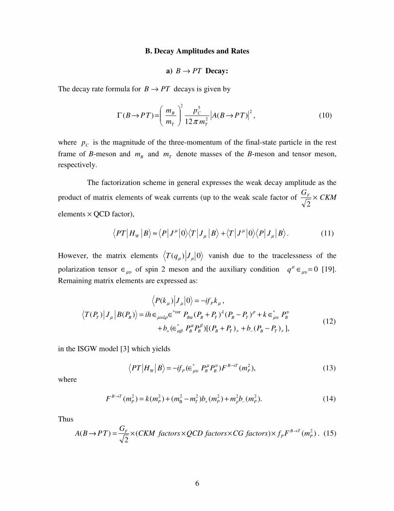
B. Decay Amplitudes and Rates
a) PTB → Decay:
The decay rate formula for PTB → decays is given by
2
2
52
)(12
)( TPBAm
p
m
mTPB
T
C
T
B →
=→Γ
π, (10)
where Cp is the magnitude of the three-momentum of the final-state particle in the rest
frame of B-meson and B
m and Tm denote masses of the B-meson and tensor meson,
respectively.
The factorization scheme in general expresses the weak decay amplitude as the
product of matrix elements of weak currents (up to the weak scale factor of 2
FG× CKM
elements × QCD factor),
0 0WPT H B P J T J B T J P J Bµ µ
µ µ≈ + . (11)
However, the matrix elements 0)( µµ JqT vanish due to the tracelessness of the
polarization tensor µυ∈ of spin 2 meson and the auxiliary condition 0=∈µυµ
q [19].
Remaining matrix elements are expressed as:
µµµ kifJkP P−=0)( ,
* *
*
( ) ( ) ( ) ( )
( )[( ) ( ) ],
T B B B T B T B
B B B T B T
T P J B P ih P P P P P k P
b P P P P b P Pµ µ
υα λ ρ υµ µυλρ α µυ
α βαβ+ −
= ∈ ∈ + − + ∈
+ ∈ + + − (12)
in the ISGW model [3] which yields
),()( 2*
P
TB
BBPW mFPPifBHPT→∈−= υµ
µυ (13)
where
2 2 2 2 2 2 2
B( ) ( ) ( ) ( ) ( ).B T
P P T P p PF m k m m m b m m b m→
+ −= + − + (14)
Thus
2( ) ( ) ( )2
B TFP P
GA B PT CKM factors QCD factors CG factors f F m→→ = × × × × . (15)

7
b) B VT→ Decay:
The decay rate formula for B VT→ is,
2
7 5 32
4( ) [ ]
48
FV V V V
T
GB V T f p p p
mΓ → = α + β + γ
π
� � �, (16)
where Vp is the magnitude of the three-momentum of the final-state particle V or T
( Vp = Tp ) in the rest frame of Bc meson. α , β and γ , respectively, are quadratic
functions of the form factors, are given by
4 28
cBm bα += ,
2 2 2 2 2 2 2 22 [6 2( ) ]c cB V T B T Vm m m h m m m kb kβ += + − − + , (17)
2 2 25T V
m m kγ = .
Here also the decay amplitude can be expressed as the product of matrix
elements of weak currents (up to the weak scale factor of 2
FG× CKM elements×QCD
factor):
0WVT H B V J T J Bµ
µ∼ , (18)
due to vanishing 0T Jµ matrix element. Here
*0 V VV J m fµ µ=∈ , (19)
where *
µ∈ and V
f denote the polarization four-vector of V and the decay constant of the
vector meson. Relations (14) and (21) yields
2( ),cB T
W c V V VVT H B m f F m→= (20)
where
* ( ) [ ( ) ( ) ( ) ( ) ]c
c
B T
B T V V V VF P P ih g P P k b P P gµνρσ µ ρ µρ
αβ µ ρ αν β σ α β α βε δ δ→
+=∈ + + + , (21)
leading to
* 2( ) ( ) ( )2
cB TFV V V
GA B V T CKM factors QCD factors m f F mαβ
αβ→→ = × × × ∈ . (22)
8
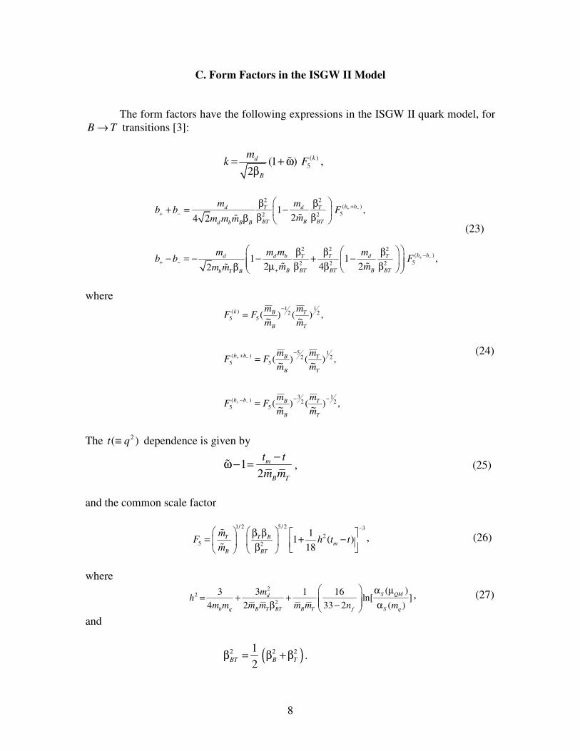
C. Form Factors in the ISGW II Model
The form factors have the following expressions in the ISGW II quark model, for
B T→ transitions [3]:
( )
5(1 )2
kd
B
mk F= + ω
βɶ ,
2 2
( )
52 2
2 2 2( )
52 2 2
1 ,24 2
1 1 ,2 4 22
b bd dT T
BT B BTd b B B
b bd d b dT T T
B BT BT B BTb T B
m mb b F
mm m m
m m m mb b F
m mm m
+ −
+ −
+
+ −
−
+ −
+
β β+ = −
β ββ
β β β− = − − + − µ β β ββ
ɶɶ
ɶ ɶɶ
(23)
where
,)~()~(
,)~()~(
,)~()~(
21
23
5
)(
5
21
25
5
)(
5
21
21
5
)(
5
−−−
−+
−
=
=
=
−+
−+
T
T
B
Bbb
T
T
B
Bbb
T
T
B
Bk
m
m
m
mFF
m
m
m
mFF
m
m
m
mFF
(24)
The 2( )t q≡ dependence is given by
12
m
B T
t t
m m
−ω − =ɶ , (25)
and the common scale factor
1/ 2 5/ 2 3
2
5 2
11 ( )
18
T T Bm
B BT
mF h t t
m
− β β
= + − β
ɶ
ɶ, (26)
where
2
2
2
( )33 1 16ln[ ]
4 2 33 2 ( )
S QMd
b q B T BT B T f S q
mh
m m m m m m n m
α µ= + + β − α
, (27)
and
( )2 2 21
2BT B Tβ = β +β .

9
m~ is the sum of the mesons constituent quarks masses, m is the hyperfine averaged
physical masses, nf is the number of active flavors, which is taken to be five in the present
case, 2)( TBm mmt −= is the maximum momentum transfer and
1
1 1
d bm m
−
+
µ = +
, (28)
Here, d
m is the spectator quark mass in the decaying particle. For s
B T→ transitions,
dm is replaced with
sm . We take the following constituent quark masses (in GeV):
mu = md = 0.33, ms = 0.55, mc = 1.82, mb = 5.20, (29)
which are taken from the ISGW II model [3] which treats mesons as composed of the
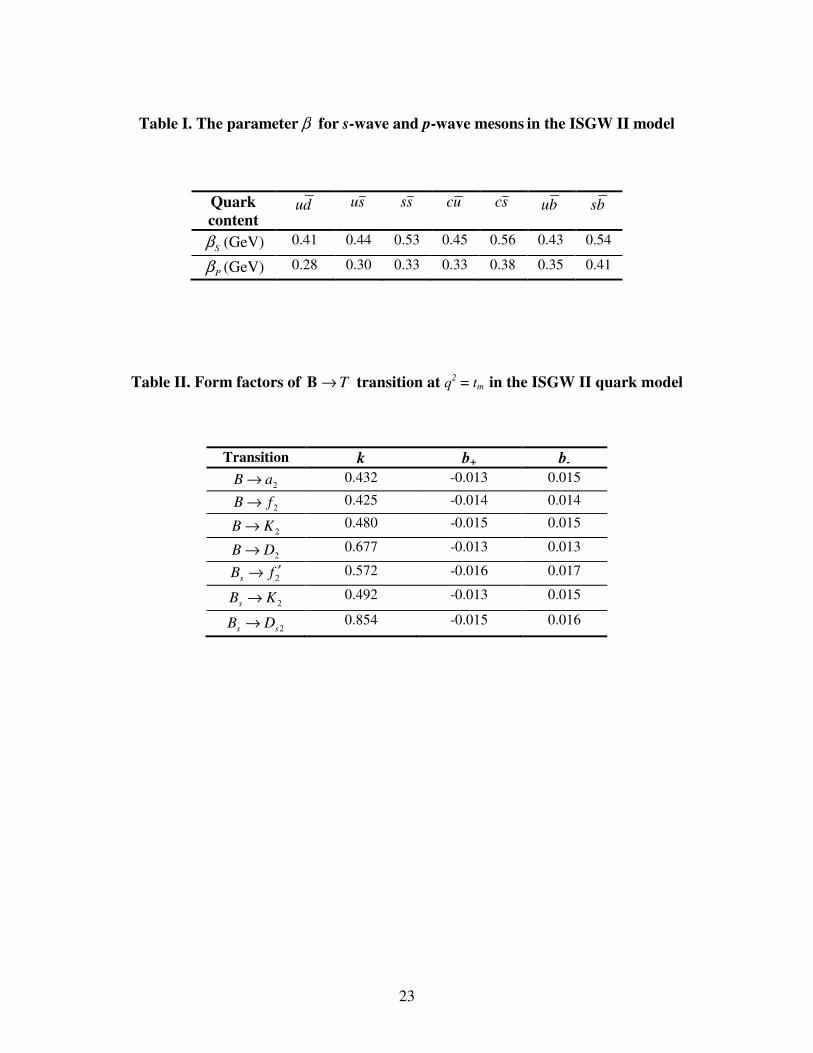
constituent quarks. Values of the parameter β for different s-wave and p-wave mesons
are given in the Table I. We obtain the form factors describing TB → transitions which
are given in Table II at q2 = tm.
IV. NUMERICAL RESULTS AND DISCUSSIONS
For numerical calculations, we use the following values of the decay constants
(given in GeV) of the pseudoscalar [13, 18, 21, 22] and vector mesons:
131.0=ππππf , 160.0=Kf , 223.0=Df , 294.0=sDf ,
133.0=ηηηηf , 126.0=′ηηηηf and 400.0=c
fηηηη . (30)
and
0.221fρ = , * 0.220K
f = , * 0.245D
f = , * 0.273sD
f = ,
0.195fω = , 0.229fφ = , / 0.411J
f ψ = . (31)
We calculate branching ratios of B-meson decays in CKM-favored and CKM-suppressed
modes involving cb → and ub → transitions. The results for B PT→ decay modes
are given in column III of the Tables III, IV, V(a) and V(b) and for B VT→ decay modes
are given in column III of the Tables VI, VII, VIII(a) and VIII(b) for various possible
modes. We make the following observations:

10
I) For PTB → meson decays:
1. PTB → decays involving cb → transition
a) 1, 1, 0b C S∆ ∆ ∆= = = mode :
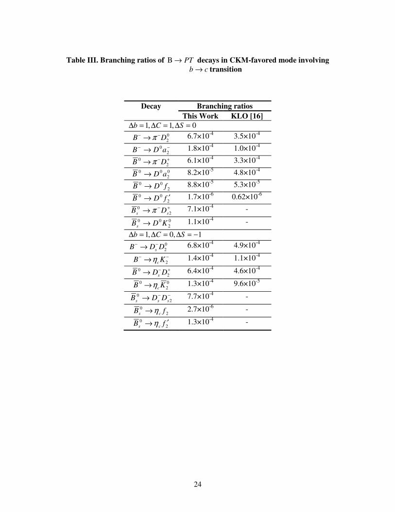
i. Calculated branching ratio 0
2( )B B Dπ− −→ = 6.7×10⁻⁴
agrees well
with the experiment value [19] 4(7.8 1.4) 10−± × , and 0
2( )B B Dπ − +→ = 6.1×10⁻⁴
, is well below the experimental upper
limit 32.2 10−< × .
ii. Branching ratios of other dominant modes are 0
2( )B B D a− −→ =
1.8×10⁻⁴
, 0
2( )s s
B B Dπ − +→ = 7.1×10⁻⁴
, and 0 0 0
2( )s
B B D K→ =
1.1×10⁻⁴
. We hope that these values are within the reach of the
furure experiments.
iii. Decays 0
2
00 aDB → and 2
00 fDB → have branching ratios of the
order of 10-5
, since these involve color-suppressed spectator
process. The branching ratio of 0 0
2B D f ′→ decay is further
suppressed due to the 2 2f f ′− mixing being close to the ideal
mixing.
iv. Decays −+−+′→ 22
0
2
0
2
0
2
00 //// KDaDDDDB sηηπ +−
2/ sDK and
−+→ 2
0
2
00 / aDDKB ss are forbidden in the present analysis due to
the vanishing matrix element between the vacuum and tensor
meson. However, these may occur through an annihilation
mechanism. The decays −+→ 2
0
2
00 / aDDB π may also occur
through elastic final state interactions (FSIs).
b) 1,0,1 −=∆=∆=∆ SCb mode :
i. Dominant modes are found to have branching ratios: 0
2( )s
B B D D− −→ = 6.8×10
-4, 2( )
cB B Kη− −→ = 1.4×10
-4,
0
2( )s
B B D D− +→ = 6.4×10
-4, 0 0
2( )c
B B Kη→ = 1.3×10⁻⁴
, 0
2( )s s s
B B D D− +→ = 7.7×10
-4 and 0
2( )s c
B B fη ′→ = 1.3×10⁻⁴
.
ii. Decays 0 0
2 2/s s
B D D D D− − −→ 2/ (1 )
cK Pχ− , −+→ 2
0
sDDB +−
2/ DDs
0
2/ (1 )c
K Pχ and 2
00
csB χπ→ 2/ cηχ 2/ cχη′ −+2/ DD

11
0
2
0/ DD 0
2
0
2
0
22 //// aDDDDDD css η+−−+ are forbidden in our work.
Penguin diagrams may cause −− → 2
0
sDDB0
2/ DDs
− and
−+→ 2
0
sDDB+−
2/ DDs decays, however these are likely to remain
suppressed as these decays require cc pair to be created.
c) 0,0,1 =∆=∆=∆ SCb mode :
i. For dominant decays, we predict 0
2( )B B D D− −→ = 2.5×10
-5,
0
2( )B B D D− +→ = 2.4×10
-5 and 0
2( )s s
B B D D− +→ = 2.9×10
-5.
ii. Decays )1(/ 22
0PDDB cχπ −−− → , +−→ 2
0
2
00 / ss DDDDB
−+2/ DD
−+
2
0
2
0 // ss DDDD )1(/)1(/ 22
0PP cc ηχχπ )1(/ 2 Pcχη ′ and
−+→ 22
00 / DDKB scs χ are forbidden in our analysis. Annihilation
diagrams, elastic FSI and penguin diagrams may generate these
decays to the naked charm mesons. However, decays emitting
charmonium )1(2 Pcχ remains forbidden in the ideal mixing limit.
d) 1,1,1 −=∆=∆=∆ SCb mode :
i. Branching ratios of the dominant decays are 0
2( )B B K D− −→ =
4.8×10⁻⁵
, 0
2( )B B K D− +→ = 4.5×10
-5 and 0
2( )s s
B B K D− +→ =
5.2×10⁻⁵
.
ii. Decays −+→ 2
0
2
00 / KDDKB and 0 0 0 0
2 2 2/ /s
B D D D− +→ π π η
−+−+′2
0
2
0
2
0
2 //// KDaDaDD sη are forbidden in our analysis.
Annihilation diagrams do not contribute to these decays. However,
these may acquire nonzero branching ratios through elastic FSI.
12
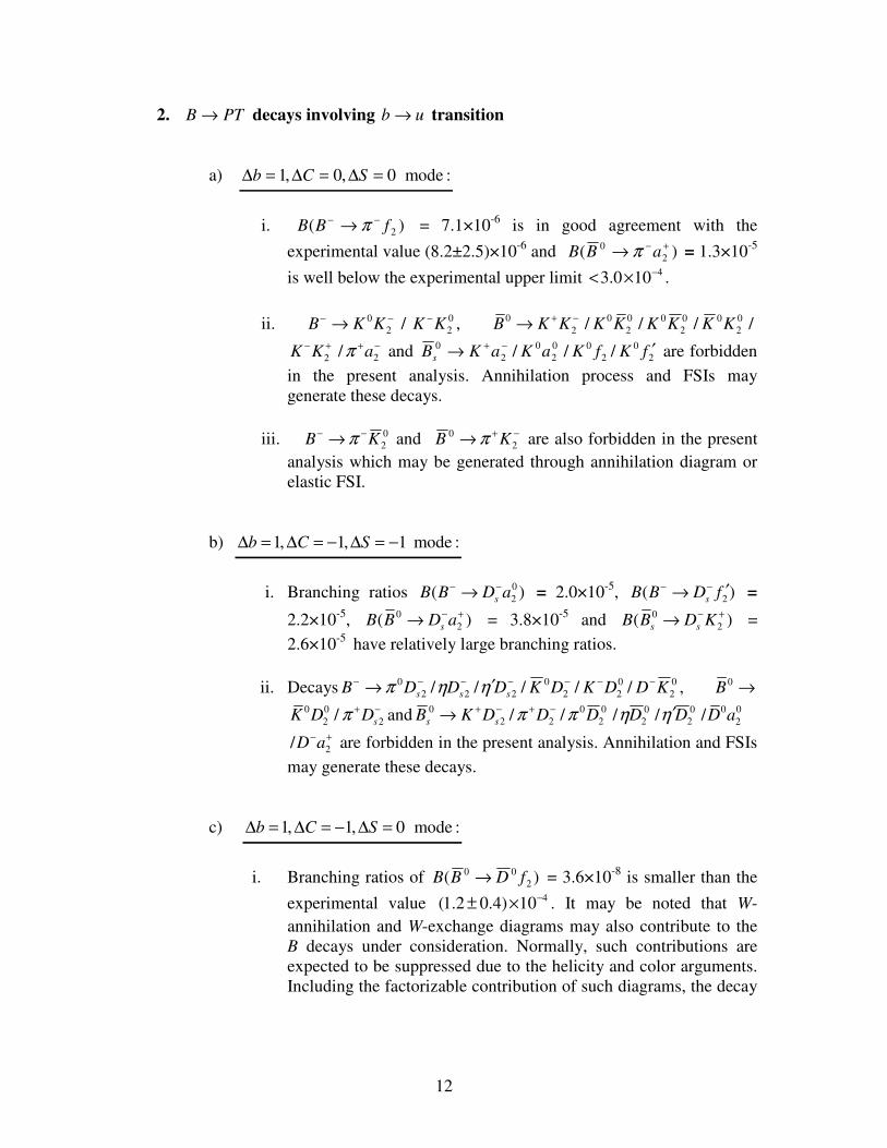
2. PTB → decays involving ub → transition
a) 0,0,1 =∆=∆=∆ SCb mode :
i. )( 2fBB −− → π = 7.1×10⁻⁶
is in good agreement with the
experimental value (8.2±2.5)×10-6
and )( 2
0 +−→ aBB π = 1.3×10⁻⁵
is well below the experimental upper limit 4100.3 −×< .
ii. 0
22
0 / KKKKB −−− → , 0
2B K K+ −→ 0 0
2/ K K 0
2
0/ KK 0
2
0/ KK /
2K K− + −+
2/ aπ and 0
2
0
2
0 / aKaKBs
−+→ 2
0
2
0 // fKfK ′ are forbidden
in the present analysis. Annihilation process and FSIs may
generate these decays.
iii. 0
2KB −− → π and −+→ 2
0 KB π are also forbidden in the present
analysis which may be generated through annihilation diagram or
elastic FSI.
b) 1, 1, 1b C S∆ = ∆ = − ∆ = − mode :
i. Branching ratios 0
2( )s
B B D a− −→ = 2.0×10
-5, 2( )
sB B D f
− − ′→ =
2.2×10⁻⁵
, 0
2( )s
B B D a− +→ = 3.8×10
-5 and
0
2( )s s
B B D K− +→ =
2.6×10⁻⁵
have relatively large branching ratios.
ii. Decays 0
2
0
22
0
222
0 ///// KDDKDKDDDB sss
−−−−−−− ′→ ηηπ , 0B → 0 0
2 2/s
K D Dπ + − and 0
2
0
22
0 // DDDKB ss ππ −+−+→ 0
2/ Dη 0
2/ Dη′ 0 0
2/D a
2/D a− + are forbidden in the present analysis. Annihilation and FSIs
may generate these decays.
c) 1, 1, 0b C S∆ = ∆ = − ∆ = mode :
i. Branching ratios of )( 2
00 fDBB → = 3.6×10⁻⁸
is smaller than the
experimental value 4(1.2 0.4) 10−± × . It may be noted that W-
annihilation and W-exchange diagrams may also contribute to the
B decays under consideration. Normally, such contributions are
expected to be suppressed due to the helicity and color arguments.
Including the factorizable contribution of such diagrams, the decay
13
amplitude of 2
00 fDB → get modified to (leaving aside the scale
factor *
2cdub
F VVG
)
)( 2
00 fDBA → = )(cos2
1 2
22
D
fB
TD mFfa→φ +
2 2
2
1cos ( )
2
f D
B T Ba f F mφ → . (32)
Using B
f = 0.176 GeV, we find that the experimental branching
ratio )( 2
00 fDBB → requires )( 22
B
DfmF
→ = -9.99 GeV. This in
turn enhances the branching ratio for 2fDB −− → to 1.2×10⁻⁴
.
ii. Dominant decay is B( +−→ 2
0 aDB ) = 1.2×10⁻⁶
and next order
dominant decays are B( 2fDB −− → ) = 6.9×10⁻⁷
B( 0
2aDB −− → )
= 6.5×10⁻⁷
and B( +−→ 2
0KDBs ) = 8.3×10
-7.
iii. Decays 0 0 0 0
2 2 2 2 2 2/ / / / /s s
B K D D D D D D K− − − − − − −′→ π π η η −
2/ Dcη , +−−+−+ ′→ 2
0
2
0
2
0
2
0
22
0 ///// KDDDDDDKB ss ηηππ −2/ Dcη and
0
2
00DKBs → are forbidden in the present analysis. Annihilation
diagrams may generate these decays.
d) 1, 0, 1b C S∆ = ∆ = ∆ = − mode :
i. 2( )B B K f− −→ = 0.54×10
-6 is smaller than the experimental value
0.4 6
0.5(1.3 ) 10+ −
− × . This decay mode is also likely to have contribution
from the W-annihilation and W-exchange processes. Including the
factorizable contribution of such diagrams, the decay amplitudes of
2B K f− −→ get modified to (putting aside the scale factor
*
2
Fub us
GV V )
2( )A B K f− −→ = )(cos
2
1 2
12
K
fB
TK mFfa→φ +
2 2
1
1cos ( )
2
f K
B T Ba f F mφ → . (33)

14
As it is not possible to evaluate the form factor 2f KF
→ at 2
Bm even
in the phenomenological models, it is treated as a free parameter.
Taking B
f = 0.176 GeV, we find that the experimental branching
ratio 2( )B B K f− −→ = 0.4 6
0.5(1.3 ) 10+ −
− × requires 2 2( )f K
BF m
→ = -
0.083 GeV. This value in turn enhances the branching ratio for
2B K f− −→ through the W-annihilation contibution to 1.3×10
-6.
ii. Branching ratios of )( 2
−− → KBB η = 1.2×10⁻⁸
is small than the
experimental value 6(9.1 3.0) 10−± × . Similar to 2B K f− −→ decay,
this decay mode is also likely to have contribution from the W-
annihilation and W-exchange processes. Including the factorizable
contribution of such diagrams, the decay amplitudes of 2KB η→
get modified to (leaving aside the scale factor *
2usub
F VVG
)
)( 2
−− → KBA η = )(sin2
1 2
22
ηη φ mFfaKB
P
→+
)(sin2
1 2
22
B
K
PB mFfaηφ →
)( 0
2
0 KBA η→ = )(sin2
1 2
22
ηη φ mFfaKB
P
→+
)(sin2
1 2
22
B
K
PB mFfaηφ →
. (34)
For B
f = 0.176 GeV, we find that the experimental branching ratio
)( 2
−− → KBB η = 6(9.1 3.0) 10−± × requires )( 22
B
KmF
η→= - 3.03
GeV. This in turn enhances the branching ratio for 0
2
0 KB η→ to
8.1×10⁻⁶
, which is consistent with the experimental value 6(9.6 2.1) 10−± × .
iii. Decays −−− → 2
00
2 / aKKB π , 0
2
0
2
0 / aKKB −+→ π 2
0
2
0 // fKfK ′
and +−−+−+→ 2
0
2
0
2
0
2
0
2
0 //// aaaKKKKBs πππ 0
2
0
2
00
2 /// aKKa ηη ′
are forbidden in the present analysis. Annihilation and FSIs may
generate these decays.

15
II) For B VT→ meson decays:
1. B VT→ decays involving cb → transition
a) 1, 1, 0b C S∆ ∆ ∆= = = mode :
i. In the present analysis, branching ratios 0
2( )B B Dρ− −→ =1.3×10⁻³
and 0
2( )B B Dρ − +→ = 1.2×10⁻³
, consistent with the experimental
upper limit 34.7 10−< × and 34.9 10−< × .
ii. Dominant decay has branching ratio 0
2( )s s
B B Dρ − +→ = 2.1×10⁻³
.
iii. Due to the vanishing matrix element between the vacuum and
tensor meson, the following decays: 0 0 0 0 0
2 2 2/ /B D D Dρ ω φ→ * *
2 2/ / /s
D a D K+ − + − *
2sK D
− + and 0 *0 0 *
2 2/s s
B K D D a+ −→ are forbidden
in the present analysis. But, these may appear through annihilation
diagrams. Like B PT→ decays, here also, 0 0 0 *
2 2/B D D aρ + −→
may occur through elastic final state interactions (FSIs).
b) 1,0,1 −=∆=∆=∆ SCb mode :
i. Branching ratios of dominant decays are 0 *
2( )s s s
B B D D− +→ =
1.3×10⁻³
, 0 *
2( )s
B B D D− +→ = 1.1×10
-3 and *
2( )s
B B D D− − +→ =
1.1×10⁻³
.
ii. Analogous to B PT→ , *0
2sB D D
− −→ *
2/ (1 )c
K Pχ− , 0 *
2sB D D
+ −→ *0
2/ (1 )c
K Pχ and 0 0
2s cB ρ χ→
2/
cωχ 2/
cφχ *
2/D D+ −
*0 0
2/D D*
2/s s
D D+ − *
2/D D− + *0 0 0
2 2/ /D D aψ decays are forbidden in this
work. *0
2sB D D
− −→ * 0
2/s
D D− and 0 *
2sB D D
+ −→ *
2/s
D D− + decays
may get contribution through penguin diagrams. However
requirement of cc pair creation may suppress these decays.
16
c) 0,0,1 =∆=∆=∆ SCb mode :
i. Here also, dominant decays have the branching ratios of the order
of 10-5
except the decay 0
2B fψ ′→ whose branching ratios
comes out to be 2.0×10⁻⁷
.
ii. Forbidden decays in this mode are *0
2 2/ (1 )c
B D D Pρ χ− − −→ , 0 *0 0 *
2 2/s s
B D D D D− +→ *
2/D D+ − *0 0 *
2 2/ /s s
D D D D+ − 0
2/ (1 )c
Pρ χ
2/ (1 )c
Pωχ 2/ (1 )c
Pφχ and 0 *0 *
2 2/s c s
B K D Dχ + −→ . Annihilation
diagrams, elastic FSI and penguin diagrams may generate these
decays emitting naked charm mesons. However, decays emitting
charmonium )1(2 Pcχ remain forbidden in the ideal mixing limit.
d) 1,1,1 −=∆=∆=∆ SCb mode :
i. The only dominant decay has branching ratio 0 *
2( )s s
B B K D− +→ =
1.1×10⁻⁴
.
ii. In this mode 0 *0 0 *
2 2/B K D D K+ −→ and 0 0 0 0
2 2 2/ /s
B D D Dρ ρ ω− +→ 0 * *0 0 *
2 2 2 2/ / / /s
D D a D a D Kφ + − + − decays are forbidden in our analysis.
These decays do not acquire contribution from annihilation
process. However, elastic FSI may generate nonzero branching
ratios for these decays.
2. B VT→ decays involving ub → transition
a) 0,0,1 =∆=∆=∆ SCb mode :
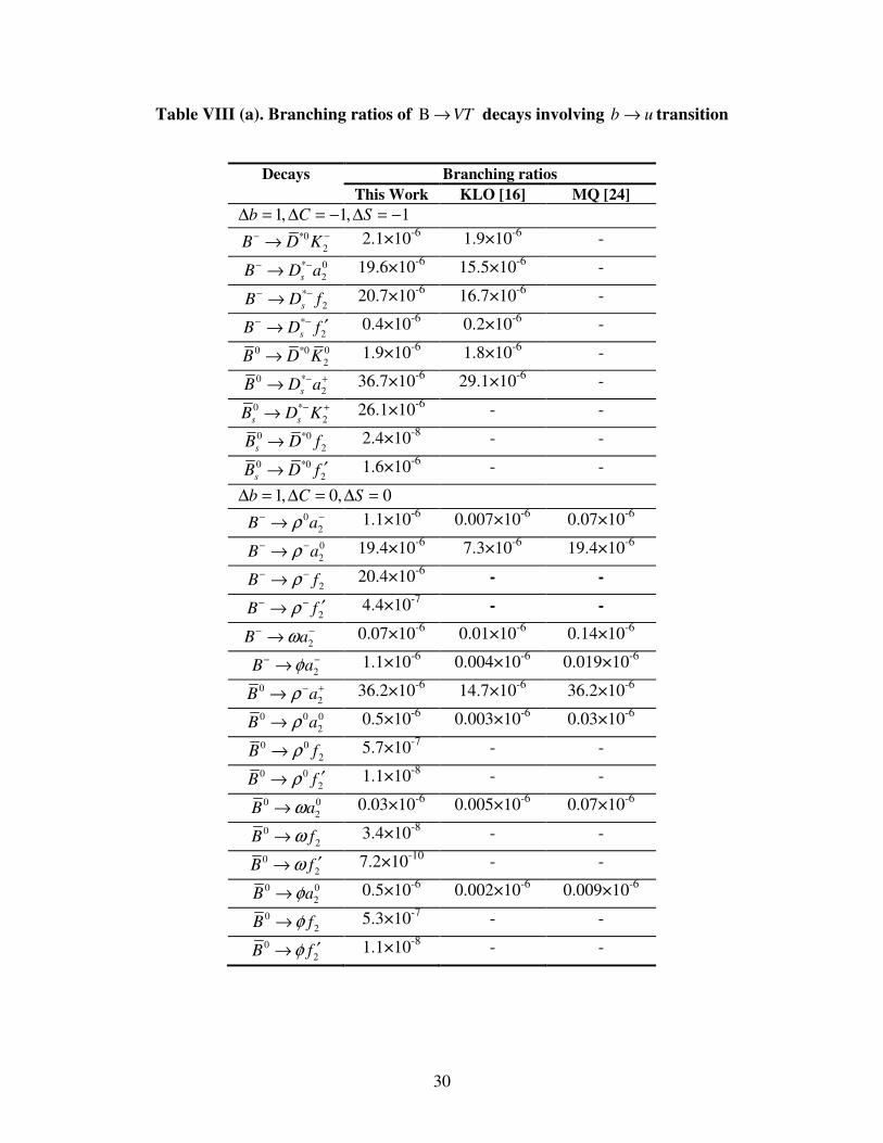
i. 0
2( )B B aρ− −→ = 1.1×10⁻⁶
is well below the experimental upper
limit 47.2 10−< × .
ii. Branching ratios 0
2( )B B aρ− −→ = 19.4×10⁻⁶
and 0
2( )B B aρ − +→ =
36.2×10⁻⁶
match well with the numerical values predicted by the J.
Muñoz and N. Quintero [24].
iii. In the present analysis *0 * 0
2 2/B K K K K− − −→ ,
0 *
2B K K+ −→ *0 0
2/K K*0 0
2/K K / *
2K K− +
2/ aρ + − and 0 *
2 /s
B K a+ −→
17
*0 0
2K a*0 *0
2 2/ /K f K f ′ decays are forbidden. But these may get
contribution from annihilation process and FSIs.
iv. Decays 0
2B Kρ− −→ and 0
2B Kρ + −→ , which may be generated
through annihilation diagram or elastic FSI, are also forbidden in
the present analysis.
b) 1, 1, 1b C S∆ = ∆ = − ∆ = − mode :
i. Obtained branching ratio 0 *
2( )s
B B D a− +→ = 3.7×10
-5 is well
below the experimental upper limit 42.0 10−< × .
ii. Also in this mode, 0
2 /s
B Dρ− −→ 2 2/s s
D Dω φ− − *0
2/ /K D− * 0
2 /K D−
* 0
2D K− , 0 *0 0
2 2/s
B K D Dρ + −→ and 0 * 0 0
2 2 2/ /s s
B K D D Dρ ρ+ − + −→ 0
2/ Dω 0
2/ Dφ *0 0 *
2 2/ /D a D a− + decays are forbidden. Though, these
may appear through annihilation and FSIs.
c) 1, 1, 0b C S∆ = ∆ = − ∆ = mode :
i. Dominant decays are B( *
2B D a− − +→ ) = 1.8×10
-6, B( *
2B D f− −→ )
= 1.8×10⁻⁶
and B( 0 *
2sB D K
− +→ ) = 1.0×10⁻⁶
.
ii. Here also, *0 0 0 * 0
2 2 2 2 2 2/ / / / /s s
B K D D D D D D Kρ ρ ω φ− − − − − − −→ , 0 * 0 0 0 0 *
2 2 2 2 2 2/ / / / /s s
B K D D D D D D Kρ ρ ω φ+ − + − − +→ and 0
sB →
*0 0
2K D*
2/K D+ − decays are forbidden. Annihilation diagrams may
generate these decays.
d) 1, 0, 1b C S∆ = ∆ = ∆ = − mode :
i. Branching ratios of 0
2( )B B Kρ− −→ = 0.006×10⁻⁶
, 2( )B B Kφ− −→
= 0.006×10⁻⁶
and 0 0 0
2( )B B Kρ→ = 0.05×10⁻⁶
are well below the
experimental upper limit 31.5 10−< × , 33.4 10−< × and 31.1 10−< × . 0 0
2( )B B Kφ→ = 0.05×10⁻⁶
is well below the only experimentally
observed value 6(7.8 1.3) 10−± × .
18
ii. Decays 0 *0
2 2/B K K aρ− − −→ , 0 *0 0
2 2/B K K aρ + −→ *0
2/K f *0
2/K f ′
and 0 *0 0 *0 0 0 0
2 2 2 2/ / /s
B K K K K a aρ ρ+ −→ 2/ aρ − + 0
2/ aω 0
2/ aφ are
forbidden in the present analysis. These may appear via
annihilation and FSIs.
V. SUMMARY AND CONCLUSIONS
In this paper, we have studied hadronic weak decays of bottom mesons emitting
pseudoscalar/vector and tensor mesons. The matrix elements 0)( µµ JqT vanish due to
the tracelessness of the polarization tensor µυ∈ of spin 2 meson and the auxiliary
condition 0=∈µυµ
q . Therefore, either color-favored or color-suppressed diagrams
contribute. Therefore, the analysis of these decays is free of constructive or destructive
interference for color-favored and color-suppressed diagrams. We employ ISGW II
model [3] to determine the B T→ form factors appearing in the decay matrix element of
weak currents involving cb → and ub → transitions. Consequently, we have obtained
the decay amplitudes and calculated the branching ratios of /B PT VT→ decays in
CKM-favored and CKM-suppressed modes. We make the following conclusions:
(i) B PT→ decays:
Decays involving cb → transition have larger branching ratios of the order of
10-4
to 10-8
and decays involving ub → transition have branching ratios of the order of
10-5
to 10-11
. Dominant decay modes involving cb → transition are B( 0
2DDB s
−− → ) =
6.8×10⁻⁴
, B( 0
2DB −− → π ) = 6.7×10⁻⁴
, B( +−→ 2
0DDB s ) = 6.4×10
-4, B( +−→ 2
0 DB π ) =
6.1×10⁻⁴
, B( −− → 2
0aDB ) = 1.8×10⁻⁴
, B( −− → 2KB cη ) = 1.4×10⁻⁴
, B( 0
2
0KB cη→ ) =
1.3×10⁻⁴
, B( 0
2s s sB D D
− +→ ) = 7.7×10⁻⁴
, B( +−→ 2
0
ss DB π ) = 7.1×10⁻⁴
, B( 2
0fB cs
′→ η ) =
1.3×10⁻⁴
and B( 0
2
00KDBs → ) = 1.1×10
-4. Experimentally, the branching ratios of only
five decay modes are measured and upper limits are available for six other decays. We
find that the calculated branching ratio )( 2fBB −− → π = 7.1×10⁻⁶
is in good agreement
with the experimental value (8.2±2.5)×10-6
whereas B( 2fKB −− → ) = 5.4×10⁻⁷
is smaller
than the experimental value 0.4 6
0.5(1.3 ) 10+ −
− × . B -decay requires contribution from W-
annihilation diagram to bridge the gap between theoretical and experimental value.
(ii) B VT→ decays:
Here again, decays involving cb → transition have branching ratios ranging
from 10-3
to 10-7
, while decays involving ub → transition have branching ratios range
from 10-5
to 10-11
. Branching ratios of dominant decay modes are B( 0
2s sB Dρ − +→ ) =

19
2.1×10⁻³
, B( 0
2B Dρ− −→ ) = 1.8×10⁻³
, B( 0
2B Dρ − +→ ) = 1.7×10⁻³
, B( 0 *
2s s sB D D
− +→ ) =
1.3×10⁻³
, B( * 0
2sB D D
− −→ ) = 1.1×10⁻³
and B( 0 *
2sB D D
− +→ ) = 1.1×10⁻³
. In contrast to
the charm meson decays, the experimental data show constructive interference for B
meson decays involving both the color-favored and color-suppressed diagrams, giving
08.010.11 ±=a and 02.020.02 ±=a . In the present analysis, the decay amplitude is
proportional to only one QCD coefficient either 1a (for color favored diagram) or 2a (for
color suppressed diagram), therefore our results remains unaffected from the interference
pattern.
(iii) Comparison with other models
We also compare our results with branching ratios calculated in the other models
[17,23,24]. The predicted branching ratios in KLO [17] shown in 3rd
column of tables III
to VIII (b), while the prediction of MQ [24] are given in 4th
column of tables V(a), V(b),
VIII(a) and VIII(b). The prediction of KLO [17] are in general smaller as compared to the
present branching ratios because of the difference in the form factors since different
quark masses have been used in the two works.
MQ [24] have recently studied few charmless decays of PTB → and B VT→
mode. Some of the branching ratios are smaller than our numerical value of branching
ratios, while the others are large as compared to the present predictions, particularly for
ηor ′η emitting decays. The disagreement with their predictions may be attributed to the
difference in the form factors obtained in the covariant light-front approach (CLF) and
inclusion of the non-factorizable contributions in their results. It may be noted that the
form factors at small 2q obtained in the CLF and ISGW II quark model agrees within
40% [3]. However, when 2q increases 2( )h q , 2( )b q+ and 2( )b q− increases more rapidly
in the covariant light front model than in the ISGW II model. Another important fact is
that the behavior of the form factor k in both models is different, especially, for the
decay 2B Kφ→ . The form factor 2( )k mφ is bigger in ISGW II quark model than in light
front quark model and decay constants used to calculate the numerical values are
different in both the works.
Branching ratios have also been calculated by Cheng [25]. For PTB → decays
his predictions B( 0
2DB −− → π ) = 6.7×10⁻⁴
and B( +−→ 2
0 DB π ) = 6.1×10⁻⁴
match well
with the numerical branching ratios obtained in the present work. However, the other
branching ratios B( 0
2DDB s
−− → ) = 4.2×10⁻⁴
, B( +−→ 2
0DDB s ) = 3.8×10
-4 and
B( +−→ 2
0
ss DB π ) = 3.8×10⁻⁴
are different from our results owing to the different values
used for the decay constant sD
f . For B VT→ decays his predictions B( 0
2B Dρ− −→ ) =
1.8×10⁻³
, B( * 0
2sB D D
− −→ ) = 1.1×10⁻³
, B( 0
2B Dρ − +→ ) = 1.7×10⁻³
, B( 0 *
2sB D D
− +→ ) =
1.0×10⁻³
and B( 0
2s sB Dρ − +→ ) = 2.1×10
-3 match well with the numerical branching ratios
obtained in the present work.

20
The Belle collaboration is currently searching for some PTB → and B VT→
modes and their preliminary results indicate that the branching ratios for these may not be
very small compared to PPB → modes. We hope our predictions would be within the
reach of the current experiments. Observation of these decays in the B experiments such
as Belle, Babar, BTeV, LHC and so on will be crucial in testing the ISGW II and other
quark models as well as validity of the factorization scheme.
Acknowledgement
One of the authors (N. S.) is thankful to the University Grant Commission, New Delhi,
for the financial assistance.

21
References
1. M. Wirbel, B. Stech and M. Bauer, Z. Phys. C 29 (1985) 637; M. Bauer, B. Stech
and M. Wirbel, Z. Phys. C 34 (1987) 103; M. Wirbel, Prog. Part. Nucl. Phys. 21
(1988) 33, and references therein.
2. N. Isgur, D. Scora, B. Grinstein and M.B. Wise, Phys. Rev. D 39 (1989) 799, and
references therein.
3. D. Scora and N. Isgur, Phys. Rev. D 52 (1995) 2783, and references therein.
4. J. Bjorken, in New Developments in High-Energy Physics Proceddings of 4th
Workshop, Crete, Greece,1988, edited by E.G. Floratos and A Verganelakis
[Nucl. Phys. B (Proc. Suppl.) 11 (1989) 325]; J.M. Cline, W. F. Palmer and G.
Kramer, Phys. Rev. D 40 (1989) 793; A. Deandrea et. al., Phys. Lett. B 318
(1993) 549; W. Jaus, Phys. Rev. D 41 (1990) 3394; M. Tanimoto, K. Goda and K.
Senba, ibid. 42 (1994) 3741; Fayyazuddin and Riazuddin, ibid. 49 (1994) 3385.
5. T. Mannel, W. Roberts and Z. Ryzak, Phys. Lett. B 248 (1990) 392; M.J. Dugan
and B. Grinstein, ibid. 255 (1991) 583, and references therein; A Ali and T.
Mannel, ibid. 264 (1991) 447; G. Kramer, T. Mannel and W.F. Palmer, Z. Phys. C
55 (1992) 497; A.F. Falk, M.B. Wise and I. Dunietz, Phys. Rev. D 51 (1995)
1183.
6. M. Neubert, V. Rieckert, B. Stech, and Q. P. Xu, in Heavy Flavours, edited by
A.J. Buras and H. Lindner, World Scientific, Singapore, 1992 and references
therein; S. Stone, talk presented at 5th Int. Symposium on Heavy Flavor Physics,
Montrêal, July 6-10, 1993.
7. T.E. Browder and K. Honscheid, Prog. Part. Nucl. Phys. 35 (1995) 81, and
references therein.
8. M. Gourdin, A.N. Kamal and X.Y. Pham, Phys. Rev. Lett. 73 (1994) 3197; A.N.
Kamal and T.N. Pham, Phys. Rev. D 50 (1994) 395; M. Gourdin et al., Phys. Lett.
B 333 (1994) 507.
9. M.S. Alam et al., Phys. Rev. D 50 (1994) 43.
10. S.M. Sheikholeslami and R.C. Verma, Int. J Mod. Phys. A 7 (1992).
11. G. Kramer and W.F. Palmer, Phys. Rev. D 46 (1992) 3197.
12. C.E. Carlson and J. Milana, Phys. Rev. D 49 (1994) 5908.
13. A.C. Katoch and R.C. Verma, Phys. Rev. D 52 (1995) 1717; 55 (1997) 7316 (E).

22
14. G. Lopez Castro and J.H. Munoz, Phys. Rev. D 55 (1997) 5581.
15. J.H. Munoz, A.A. Rojas and G. Lopez Castro, Phys. Rev. D 59 (1999) 077504.
16. C.S. Kim, B.H. Lim and Sechul Oh, Eur. Phys. J. C 22 (2002) 683; Eur. Phys. J.
C 22 (2002) 683; C.S. Kim, J.P. Lee and Sechul Oh, hep-ph/0205262; Phys. Rev.
D 67 (2003) 014002.
17. C.S. Kim, J.P. Lee and Sechul Oh, Phys. Rev. D 67 (2003) 014011.
18. C. Amsler et al. (Particle Data Group), Phys. Lett. B 667 (2008).
19. Belle Collaboration, K. Abe et al., Phys. Rev. D 69 (2004) 112002.
20. Sechul Oh, Phys. Rev. D 60 (1999) 034006; M. Gronau and J.L. Rosner, ibdi. 61,
(2000) 073008.
21. D. Spehler and S.F. Novaes, Phys. Rev. D 44 (1991) 3990.
22. Rohit Dhir, Neelesh Sharma and R.C. Verma, J. Phys. G: Nucl. Part. Phys. 35
(2008) 085002.
23. C. H. Chen and C.Q. Geng, Phys. Rev. D 75 (2007) 054010.
24. J. Muñoz and N. Quintero, J. Phys. G: Nucl. Part. Phys. 36 (2009) 095004.
25. H.Y Cheng, Phys. Rev. D 68 (2003) 094005.
23
Table I. The parameter β for s-wave and p-wave mesons in the ISGW II model
Quark
content du su ss uc sc bu bs
Sβ (GeV) 0.41 0.44 0.53 0.45 0.56 0.43 0.54
Pβ (GeV) 0.28 0.30 0.33 0.33 0.38 0.35 0.41
Table II. Form factors of T→B transition at q2 = tm in the ISGW II quark model
Transition k b+ b-
2aB → 0.432 -0.013 0.015
2fB → 0.425 -0.014 0.014
2KB → 0.480 -0.015 0.015
2DB → 0.677 -0.013 0.013
2fBs′→ 0.572 -0.016 0.017
2KBs → 0.492 -0.013 0.015
2ss DB → 0.854 -0.015 0.016
24
Table III. Branching ratios of PT→B decays in CKM-favored mode involving
cb → transition
Decay Branching ratios
This Work KLO [16]
0,1,1 =∆=∆=∆ SCb
0
2DB −− → π 6.7×10⁻⁴
3.5×10⁻⁴
−− → 2
0aDB 1.8×10⁻⁴
1.0×10⁻⁴
+−→ 2
0 DB π 6.1×10⁻⁴
3.3×10⁻⁴
0
2
00 aDB → 8.2×10⁻⁵
4.8×10⁻⁴
2
00 fDB → 8.8×10⁻⁵
5.3×10⁻⁵
2
00 fDB ′→ 1.7×10⁻⁶
0.62×10⁻⁶
+−→ 2
0
ss DB π 7.1×10⁻⁴
-
0
2
00KDBs → 1.1×10
-4 -
1,0,1 −=∆=∆=∆ SCb 0
2DDB s
−− → 6.8×10⁻⁴
4.9×10⁻⁴
−− → 2KB cη 1.4×10⁻⁴
1.1×10⁻⁴
+−→ 2
0DDB s 6.4×10
-4 4.6×10
-4
0
2
0KB cη→ 1.3×10
-4 9.6×10
-5
−−→ 2
0
sss DDB 7.7×10⁻⁴
-
2
0fB cs η→ 2.7×10
-6 -
2
0fB cs
′→ η 1.3×10⁻⁴
-

25
Table IV. Branching ratios of PT→B decays in CKM-suppressed mode involving
cb → transition
Decay Branching ratios
This Work KLO [16]
1,1,1 −=∆=∆=∆ SCb
0
2DKB −− → 4.8×10⁻⁵
2.5×10⁻⁵
−− → 2
0KDB 8.7×10⁻⁶
7.3×10⁻⁶
+−→ 2
0 DKB 4.5×10⁻⁵
2.4×10⁻⁵
0
2
00 KDB → 8.1×10⁻⁶
6.8×10⁻⁶
+−→ 2
0
ss DKB 5.2×10⁻⁵
-
2
00fDBs → 9.9×10
-8 -
2
00fDBs
′→ 6.7×10⁻⁶
-
0,0,1 =∆=∆=∆ SCb 0
2DDB −− → 2.5×10⁻⁵
2.2×10⁻⁵
−− → 2aB cη 9.2×10⁻⁶
4.9×10⁻⁶
+−→ 2
0 DDB 2.4×10⁻⁵
2.1×10⁻⁵
0
2
0aB cη→ 4.3×10
-6 2.3×10
-6
2
0fB cη→ 4.8×10
-6 2.7×10
-6
2
0fB c
′→ η 6.7×10⁻⁸
0.02×10⁻⁶
+−→ 2
0
ss DDB 2.9×10⁻⁵
-
0
2
0KB cs η→ 6.9×10
-6 -

26
Table V (a). Branching ratios of PT→B decays involving ub → transition
Decays Branching ratios
This Work KLO [16] MQ [24]
1,1,1 −=∆−=∆=∆ SCb
−− → 2
0KDB 1.3×10⁻⁶
1.2×10⁻⁶
-
0
2aDB s
−− → 2.0×10⁻⁵
9.4×10⁻⁶
-
2fDB s
−− → 2.2×10⁻⁵
1.×10-5
-
2fDB s′→ −− 4.3×10
-7 0.12×10
-6 -
0
2
00 KDB → 1.2×10⁻⁶
1.1×10⁻⁶
-
+−→ 2
0aDB s 3.8×10
-5 1.8×10
-5 -
+−→ 2
0KDB ss 2.6×10
-5 - -
0 0
2sB D f→ 1.5×10
-8 - -
2
00fDBs
′→ 1.0×10⁻⁶
- -
0,0,1 =∆=∆=∆ SCb
0
2aB −− → π 6.7×10⁻⁶
2.6×10⁻⁶
4.38×10⁻⁶
2fB −− → π 7.1×10⁻⁶
- -
2fB ′→ −− π 1.5×10⁻⁷
- -
−− → 2
0aB π 0.38×10⁻⁶
0.001×10⁻⁶
0.015×10⁻⁶
−− → 2aB η 0.23×10⁻⁶
0.29×10⁻⁶
45.8×10⁻⁶
−− ′→ 2aB η 0.13×10⁻⁶
1.31×10⁻⁶
71.3×10⁻⁶
+−→ 2
0 aB π 13.0×10⁻⁶
4.88×10⁻⁶
8.19×10⁻⁶
0
2
00 aB π→ 0.18×10⁻⁶
0.0003×10⁻⁶
0.007×10⁻⁶
2
00 fB π→ 1.9×10⁻⁷
- -
2
00 fB ′→ π 3.9×10⁻⁹
- -
0
2
0 aB η→ 0.11×10⁻⁶
0.14×10⁻⁶
25.2×10⁻⁶
2
0 fB η→ 1.1×10⁻⁷
- -
2
0 fB ′→ η 2.4×10⁻⁹
- -
0
2
0 aB η ′→ 0.06×10⁻⁶
0.62×10⁻⁶
43.3×10⁻⁶
2
0 fB η ′→ 6.3×10⁻⁸
- -
2
0 fB ′′→ η 1.3×10⁻⁹
- -
+−→ 2
0KBs π 7.8×10
-6 - -
0
2
00KBs π→ 2.2×10
-7 - -
0
2
0KBs η→ 1.3×10
-7 - -
0
2
0KBs η ′→ 7.5×10
-8 - -

27
Table V (b). Branching ratios of PT→B decays involving ub → transition
Decays Branching ratios
This Work KLO [16] MQ [24]
1,0,1 −=∆=∆=∆ SCb
0
2aKB −− → 0.51×10⁻⁶
0.31×10⁻⁶
0.39×10⁻⁶
2fKB −− → 5.4×10⁻⁷
- -
2fKB ′→ −− 1.5×10⁻⁸
- -
−− → 2
0KB π 0.02×10⁻⁶
0.09×10⁻⁶
0.15×10⁻⁶
−− → 2KB η 0.01×10⁻⁶
0.03×10⁻⁶
1.19×10⁻⁶
−− ′→ 2KB η 0.007×10⁻⁶
1.40×10⁻⁶
2.70×10⁻⁶
+−→ 2
0 aKB 0.95×10⁻⁶
0.58×10⁻⁶
0.73×10⁻⁶
0
2
00 KB π→ 0.02×10⁻⁶
0.08×10⁻⁶
0.13×10⁻⁶
0
2
0 KB η→ 0.01×10⁻⁶
0.03×10⁻⁶
1.09×10⁻⁶
0
2
0 KB η′→ 0.006×10⁻⁶
1.3×10⁻⁶
2.46×10⁻⁶
+−→ 2
0KKBs 5.9×10
-7 - -
2
00fBs π→ 1.9×10
-10 - -
2
00fBs
′→ π 1.4×10⁻⁸
- -
2
0fBs η→ 1.1×10
-10 - -
2
0fBs
′→η 8.3×10⁻⁹
- -
2
0fBs η′→ 6.5×10
-11 - -
2
0fBs
′′→ η 4.7×10⁻⁹
- -
0,1,1 =∆−=∆=∆ SCb
0
2aDB −− → 6.5×10⁻⁷
- -
2fDB −− → 6.9×10⁻⁷
- -
2fDB ′→ −− 1.4×10⁻⁷
- -
−− → 2
0aDB 7.3×10⁻⁸
- -
+−→ 2
0 aDB 1.2×10⁻⁶
- -
0
2
00 aDB → 3.4×10⁻⁸
- -
2
00 fDB → 3.6×10⁻⁸
- -
2
00 fDB ′→ 7.1×10⁻¹⁰
- -
+−→ 2
0KDBs 8.3×10
-7 - -
0
2
00KDBs → 4.6×10
-8 - -

28
Table VI. Branching ratios of B VT→ decays in CKM-favored mode involving
cb → transition
Decay Branching ratios
This Work KLO [16]
0,1,1 =∆=∆=∆ SCb
0
2B Dρ− −→ 1.9×10⁻³
1.0×10-3
*0
2B D a− −→ 2.6×10
-4 1.7×10
-4
0
2B Dρ − +→ 1.8×10⁻³
0.92×10⁻³
0 *0 0
2B D a→ 1.2×10⁻⁴
0.78×10⁻⁴
0 *0
2B D f→ 1.3×10⁻⁴
0.84×10⁻⁴
0 *0
2B D f ′→ 2.6×10⁻⁶
1.1×10⁻⁶
0
2s sB Dρ − +→ 2.1×10
-3 -
0 *0 0
2sB D K→ 1.7×10
-4 -
1,0,1 −=∆=∆=∆ SCb * 0
2sB D D
− −→ 1.1×10⁻³
1.2×10⁻³
2B Kψ− −→ 4.6×10⁻⁴
3.8×10⁻⁴
0 *
2sB D D
− +→ 1.1×10⁻⁴
1.1×10⁻³
0 0
2B Kψ→ 4.3×10⁻⁴
3.5×10⁻⁴
0 *
2s s sB D D
− +→ 1.3×10⁻³
-
0
2sB fψ→ 8.3×10
-6 -
0
2sB fψ ′→ 4.3×10
-4 -

29
Table VII. Branching ratios of B VT→ decays in CKM-suppressed mode involving
cb → transition
Decay Branching ratios
This Work KLO [16]
1,1,1 −=∆=∆=∆ SCb * 0
2B K D− −→ 9.7×10
-5 5.2×10
-5
*0
2B D K− −→ 1.4×10
-5 1.2×10
-5
0 *
2B K D− +→ 9.1×10
-5 4.9×10
-5
0 *0 0
2B D K→ 1.3×10⁻⁵
1.1×10⁻⁵
0 *
2s sB K D
− +→ 1.1×10⁻⁴
-
0 *0
2sB D f→ 1.6×10
-7 -
0 *0
2sB D f ′→ 1.1×10
-5 -
0,0,1 =∆=∆=∆ SCb * 0
2B D D− −→ 6.1×10
-5 5.3×10
-5
2B aψ− −→ 2.6×10⁻⁵
1.6×10⁻⁵
0 *
2B D D− +→ 5.7×10
-5 5.0×10
-5
0 0
2B aψ→ 12.3×10⁻⁶
7.7×10⁻⁶
0
2B fψ→ 13.3×10⁻⁶
8.4×10⁻⁶
0
2B fψ ′→ 0.2×10⁻⁶
0.09×10⁻⁶
0 *
2s sB D D
− +→ 1.2×10⁻⁵
-
0 0
2sB Kψ→ 2.1×10
-5 -
30
Table VIII (a). Branching ratios of B VT→ decays involving ub → transition
Decays Branching ratios
This Work KLO [16] MQ [24]
1,1,1 −=∆−=∆=∆ SCb *0
2B D K− −→ 2.1×10
-6 1.9×10
-6 -
* 0
2sB D a
− −→ 19.6×10⁻⁶
15.5×10⁻⁶
-
*
2sB D f
− −→ 20.7×10⁻⁶
16.7×10⁻⁶
-
*
2sB D f
− − ′→ 0.4×10⁻⁶
0.2×10⁻⁶
-
0 *0 0
2B D K→ 1.9×10⁻⁶
1.8×10⁻⁶
-
0 *
2sB D a
− +→ 36.7×10⁻⁶
29.1×10⁻⁶
-
0 *
2s sB D K
− +→ 26.1×10⁻⁶
- -
0 *0
2sB D f→ 2.4×10
-8 - -
0 *0
2sB D f ′→ 1.6×10
-6 - -
0,0,1 =∆=∆=∆ SCb 0
2B aρ− −→ 1.1×10⁻⁶
0.007×10⁻⁶
0.07×10⁻⁶
0
2B aρ− −→ 19.4×10⁻⁶
7.3×10⁻⁶
19.4×10⁻⁶
2B fρ− −→ 20.4×10⁻⁶
- -
2B fρ− − ′→ 4.4×10⁻⁷
- -
2B aω− −→ 0.07×10⁻⁶
0.01×10⁻⁶
0.14×10⁻⁶
2B aφ− −→ 1.1×10⁻⁶
0.004×10⁻⁶
0.019×10⁻⁶
0
2B aρ − +→ 36.2×10⁻⁶
14.7×10⁻⁶
36.2×10⁻⁶
0 0 0
2B aρ→ 0.5×10⁻⁶
0.003×10⁻⁶
0.03×10⁻⁶
0 0
2B fρ→ 5.7×10⁻⁷
- -
0 0
2B fρ ′→ 1.1×10⁻⁸
- -
0 0
2B aω→ 0.03×10⁻⁶
0.005×10⁻⁶
0.07×10⁻⁶
0
2B fω→ 3.4×10⁻⁸
- -
0
2B fω ′→ 7.2×10⁻¹⁰
- -
0 0
2B aφ→ 0.5×10⁻⁶
0.002×10⁻⁶
0.009×10⁻⁶
0
2B fφ→ 5.3×10⁻⁷
- -
0
2B fφ ′→ 1.1×10⁻⁸
- -

31
0
2sB Kρ − +→ 2.3×10
-5 - -
0 0 0
2sB Kρ→ 6.4×10
-7 - -
0 0
2sB Kω→ 4.0×10
-8 - -
0 0
2sB Kφ→ 6.4×10
-7 - -

32
Table VIII (b). Branching ratios of B VT→ decays involving ub → transition
Decays Branching ratios
This Work KLO [16] MQ [24]
1,0,1 −=∆=∆=∆ SCb
* 0
2B K a− −→ 1.0×10
-6 1.9×10
-6 2.8×10
-6
*
2B K f− −→ 1.1×10
-6 - -
*
2B K f− − ′→ 2.3×10
-8 - -
0
2B Kρ− −→ 0.06×10⁻⁶
0.253×10⁻⁶
0.74×10⁻⁶
2B Kω− −→ 0.004×10⁻⁶
0.112×10⁻⁶
0.06×10⁻⁶
2B Kφ− −→ 0.06×10⁻⁶
2.2×10⁻⁶
9.2×10⁻⁶
0 *
2B K a− +→ 1.9×10
-6 3.5×10
-6 7.3×10
-6
0 0 0
2B Kρ→ 0.05×10⁻⁶
0.235×10⁻⁶
0.68×10⁻⁶
0 0
2B Kω→ 0.003×10⁻⁶
0.104×10⁻⁶
0.053×10⁻⁶
0 0
2B Kφ→ 0.05×10⁻⁶
2.0×10⁻⁶
8.5×10⁻⁶
0 *
2sB K K
− +→ 1.2×10⁻⁶
- -
0 0
2sB fρ→ 5.6×10
-10 - -
0 0
2sB fρ ′→ 4.1×10
-8 - -
0
2sB fω→ 3.5×10
-11 - -
0
2sB fω ′→ 2.6×10
-9 - -
0
2sB fφ→ 5.6×10
-10 - -
0
2sB fφ ′→ 4.1×10
-8 - -
0,1,1 =∆−=∆=∆ SCb
* 0
2B D a− −→ 9.6×10
-7 - -
*
2B D f− −→ 1.0×10
-6 - -
*
2B D f− − ′→ 2.1×10
-8 - -
*0
2B D a− −→ 1.1×10
-7 - -
0 *
2B D a− +→ 1.8×10
-6 - -
0 *0 0
2B D a→ 5.0×10⁻⁸
- -
0 *0
2B D f→ 5.3×10⁻⁸
- -
0 *0
2B D f ′→ 1.1×10⁻⁹
- -
0 *
2sB D K
− +→ 1.2×10⁻⁶
- -
0 *0 0
2sB D K→ 7.0×10
-8 - -