This content has been downloaded from IOPscience. Please scroll down to see the full text.

Download details:

This content was downloaded by: anupama2phy

IP Address: 111.93.5.194

This content was downloaded on 13/06/2014 at 07:57

Please note that terms and conditions apply.

Baryonic transition decays

View the table of contents for this issue, or go to the journal homepage for more

2014 J. Phys. G: Nucl. Part. Phys. 41 065002

(http://iopscience.iop.org/0954-3899/41/6/065002)

Home Search Collections Journals About Contact us My IOPscience

Journal of Physics G: Nuclear and Particle Physics

J. Phys. G: Nucl. Part. Phys. 41 (2014) 065002 (15pp) doi:10.1088/0954-3899/41/6/065002

Baryonic b → s l l transition decays

Rupak Dutta1,2, Anupama Bhol1 and Anjan K Giri1

1 Indian Institute of Technology Hyderabad, Hyderabad 502205, India2 National Institute of Technology Silchar, Silchar 788010, India

E-mail: rupak@iith.ac.in, ph10p004@iith.ac.in and giria@iith.ac.in

Received 19 December 2013, revised 27 March 2014Accepted for publication 3 April 2014Published 30 April 2014

AbstractFlavor changing neutral current decays of B meson mediated via b → s l ltransition process, where l represents an electron, a muon, or a tau lepton,provide promising probes for physics beyond the standard model. In thiscontext, we use the most general effective Hamiltonian for b → s l l processand study the branching ratio and various asymmetries of B− → � pμ+ μ−

four body baryonic decays of B meson. We also see the effect of various newphysics couplings in this decay mode. Within the standard model, the branchingratio of B− → � pμ+ μ− decay mode is found to be 1.08 × 10−7 and hencecan be tested in the forthcoming or future B factories.

Keywords: B meson, baryons, semileptonic, FCNC, new physics

(Some figures may appear in colour only in the online journal)

1. Introduction

Over the last decade, weak decays of B meson to meson-meson final states have not onlyconfirmed and established the Cabibbo–Kobayashi–Maskawa (CKM) mechanism of quarkflavor mixing and CP violation in the quark sector to a very high degree of precision but alsoprovided a strong ground to test the nature of flavor changing neutral currents (FCNC) viab → s ll transition decays. Due to the large mass of B meson, it can also decay to final statesthat contain a baryon–antibaryon pair. Although almost 7% [1] of all the B meson decayscontain baryons in the final state, but the exploration in this field is less in comparison todecays with mesons in the final state. In particular, we have very little knowledge about themechanism behind these baryonic decays and more generally, about the mechanism behindhadron fragmentation into baryons.

ARGUS [2] reported the first baryonic decay mode which was later ruled out by CLEO[3]. Exclusive decay of B mesons to a charmed baryon was first reported by CLEO [4] inwhich they measured the branching ratios of B− → �+

c pπ− and B0 → �+c pπ+ π− decay

modes. In recent years, many exclusive baryonic B meson decays have been found by the

0954-3899/14/065002+15$33.00 © 2014 IOP Publishing Ltd Printed in the UK 1

J. Phys. G: Nucl. Part. Phys. 41 (2014) 065002 R Dutta et al

two b-factories, BABAR [5] and Belle [6]. Several theoretical approaches such as flavorsymmetry approach [7], pole model [8, 9], the diquark model [10], QCD sum rule [11], andthe factorization formalism [12, 13] have been proposed in order to explain the mechanismbehind these baryonic B decays.

Baryonic B decays have two very common and unique features. First, there is anenhancement at the threshold in dibaryon invariant mass distribution and it is experimentallyobserved in many three body decay modes [14–28]. Second, the largest branching fractionfor baryonic B decays come with moderate multiplicities of 3–4 hadrons in the final state.Baryonic B meson decay branching fraction hierarchy is Br3−body < Br5−body < Br4−body

[29]. This is quite different from B meson decays to meson only final states and a propertheoretical understanding is yet to be achieved. Similarly, branching fraction of a threebody final state is larger than its two body counterpart. The three body decays are morepreferable due to the threshold enhancement in the dibaryon invariant mass distribution whichsharply peaks at low values with emitted meson carrying much energy. However, for a twobody decay, the invariant mass of the baryon-antibaryon pair is MB and hence these decaymodes are not preferred. Several theoretical approaches have been proposed to explain thethreshold enhancement in the dibaryon invariant mass distribution [30–43]. In principle, thethreshold enhancement mechanism can be very easily understood in terms of a simple shortdistance picture [44]. The observed angular distributions in various decay modes such asB− → p pπ−, �+

c pπ+, and � pγ [17, 21, 22] decays are consistent with this short distancepicture, however, this simple picture fails to explain the observed angular correlations inthe penguin dominated B → p p K− [16, 22] and B− → � pπ− [20] decays. It is worthmentioning that the threshold enhancement mechanism plays a crucial role in case of baryonicB decays and understanding this mechanism will be the key to interpret the physics behindthese baryonic B decays.

In the standard model (SM), the inclusive FCNC processes are mediated via electroweakbox and penguin type diagrams. Tree level diagrams do not contribute to these decay processes.New physics (NP) particles, in principle, can enter through these loop processes and competewith the SM processes. This can lead to modifications of branching fractions or angulardistributions of the particles in these decay modes. Consequently, the exclusive rare radiativedecays such as B0

s → φγ and rare leptonic and semileptonic decays such as B(d,s) → l+ l−

and B0 → K∗0l+ l− are potentially good places to look for NP. Very recently, the LHCb

[45] and CMS [46] have reported new results on Bd, s → μ+ μ− decays and branchingratio of Bd → μ+ μ− decay is found to be higher than the SM value by a factor of 3.5.Although the branching ratio of Bs → μ+ μ− decay mode is in good agreement withthe SM prediction [47], but recent measurement [48] suggests a sizable width difference��s = 0.116 ± 0.018(stat) ± 0.006(syst) ps−1 of Bs meson which points towards NP. A lotof phenomenological work have been done in this regard [49]. Again, the recent measurementof the angular observable in Bd → K∗ μ+ μ− decay mode by LHCb [50] differs from theSM expectation. These results, if persist in future precision experiments, would be a definitehint of physics beyond the SM and, in principle, will affect any FCNC decays mediated viab → s l l transition process. Lot of theoretical studies have been done to interpret the datausing various NP scenarios [51]. The theoretical prediction of a semileptonic B → M l l decaybranching fraction depends mainly on the hadronic B → M transition form factors, which,in principle, can be calculated using various models such as quark models, lattice QCD, lightcone sum rules, and heavy quark effective theory. Like mesonic decays, one can also studythe baryonic semileptonic decay modes such as B → B B′ l l and investigate the theoreticalmodeling of B → B B′ transition form factors. In [52], the authors have used perturbativeQCD approach for the B → pp transition form factors and predicted the SM branching ratio

2

J. Phys. G: Nucl. Part. Phys. 41 (2014) 065002 R Dutta et al

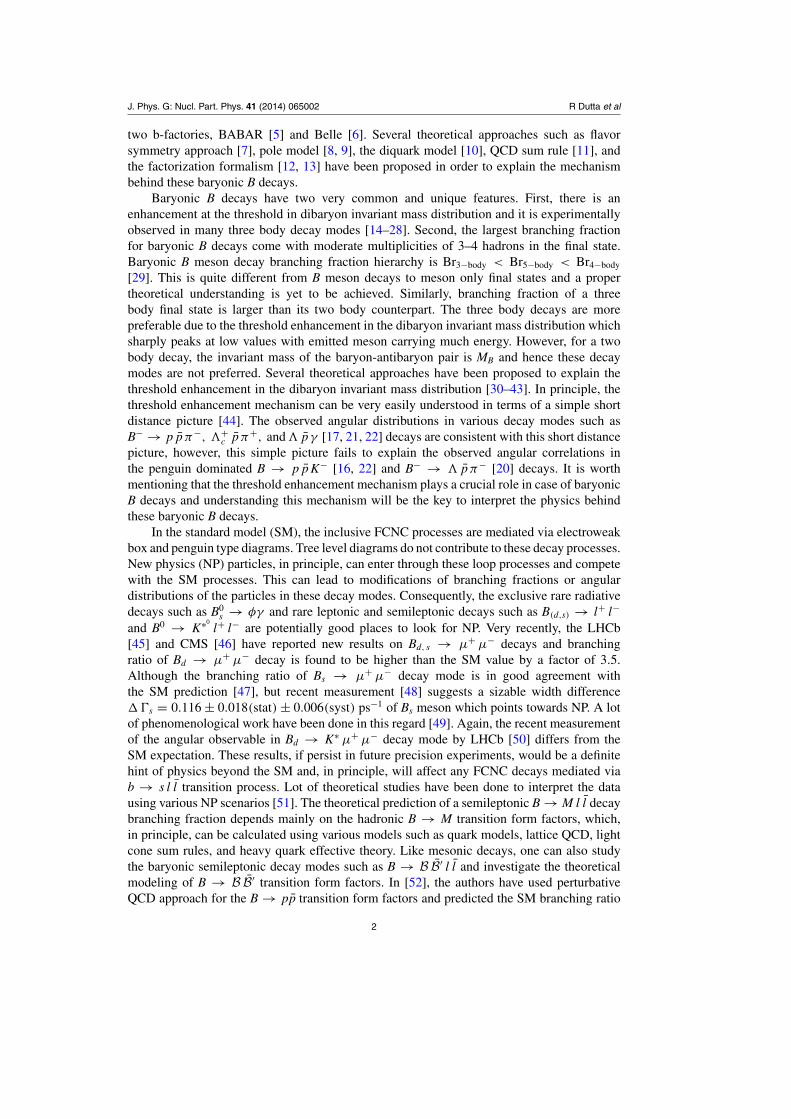
Figure 1. Penguin and box diagram contributing to the B → � pμ+ μ− decay mode.

of four body exclusive semileptonic baryonic B− → pp l νl decays. The SM prediction of(1.0, 1.0, 0.5) × 10−4 for l = e, μ, and τ , however, differs significantly from the recentlymeasured branching fraction of (5.8+2.4

−2.1(stat.) ± 0.9(syst.)) × 10−6 [53]. Hence, a carefulinvestigation of the theoretical modeling of the baryonic transition form factors in B decays isnecessary in light of this new information. More recently, in [54], the authors have calculatedthe branching ratio of the rare B− → � pνν decay process within the SM using the sameapproach as in [52] for the B → � p transition form factors. Moreover, the exclusive modesof baryonic and mesonic decays are good places to search for exotic baryons beyond the SMsuch as dibaryon, pentaquark, and exotic mesons (glueball, tetraquark). In this paper, we focusmainly on the baryonic B decays, particularly B → �pμ+ μ− decay mode, as an exclusive Bdecay mediated via the b → s l l transition to test the nature of the FCNCs. In this context, weuse the most general effective Hamiltonian in the presence of NP and see the effect of each NPcoupling on various observables in a model independent way. We predict the branching ratioof B → �pμ+ μ− decay mode and obtain asymmetries in angular distributions and tripleproduct correlations in the SM and in the presence of NP.

The paper is organized as follows. We begin, in section 2, with a description of theeffective Hamiltonian for b → s l l transition decay process and briefly review the B → BB′

transition form factors and their QCD counting rules. We then define several observables inB− → �pμ+ μ− decays. In section 3, we present all the input parameters that are used forour numerical simulations and report the branching ratio and various asymmetries for theB− → � pμ+ μ− decay mode. We conclude with a summary of our results in section 4.

2. Theory

Exclusive B− → �pμ+ μ− decays mediated via b → s l l transition process is governed bythe electroweak box and penguin type diagrams. The relevant Feynman diagrams responsiblefor this decay process are shown in figure 1.

We employ the effective Hamiltonian for �B = �S = 1 transition and write the amplitudefor b → s l l transition as [55]

M(b → s ll) = α GF√2π

λt

∑i

[Ci Oi + Ci′ Oi

′ ] + h.c., (1)

where GF is the Fermi constant and λt = V ∗ts Vtb, where Vts and Vtb are CKM matrix elements.

The electromagnetic coupling constant is denoted by α. The relevant operators considered inour analysis are given by

O7 = −2 i mbpν

p2sσμν bR lγ μ l, O′

7 = −2 i mbpν

p2sσμν bL lγ μ l,

O8 = sγμ bR lγ μ l , O′8 = sγμ bL lγ μ l ,

3

J. Phys. G: Nucl. Part. Phys. 41 (2014) 065002 R Dutta et al

O9 = sγμ bR lγ μ γ5 l , O′9 = sγμ bL lγ μ γ5 l ,

OS = mb s bR l l , O′S = mb s bL l l ,

OP = mb s bR l γ5 l , O′P = mb s bL l γ5 l, (2)

where, O7(O′7) and O8(O′

8) represent the magnetic penguin operators and O9(O′9) represents

the electromagnetic penguin operator. Here, mb is the mass of the b quark and bR, L =b (1±γ5)/2. The operators Oi

′ are obtained from the operators Oi by making the replacementsbR ↔ bL. The invariant mass square of the lepton pair is denoted by p2 = M2

ll. The Wilson

coefficients are denoted by C7, C8, and C9 for the unprimed operators, whereas, C′7, C′

8,and C′

9 for the primed operators, respectively. Similarly, CS(C′S) and CP(C′

P) denote theWilson coefficients corresponding to the scalar OS(O′

S) and pseudoscalar OP(O′P) operators,

respectively. The primed operators O′7,8,9 and OS, P(O′

S, P) are highly suppressed in the SM.With the effective Hamiltonian of equation (1), the amplitude for B− → �p ll can be

factorized into hadronic and leptonic parts as

A(B− → �p l l) = α GF√2π

λt

{− 2 i

C7 mb

p2〈�p|sσμν pν bR|B〉 lγ μ l + C8 〈�p|sγμ bR|B〉lγ μ l

+C9 〈�p|sγμ bR|B〉 lγ μ γ5 l + CS mb 〈�p|s bR|B〉 l l

+CP mb 〈�p|s bR|B〉 lγ5 l − 2 iC7

′ mb

p2〈�p|sσμν pν bL|B〉 lγ μ l

+C8′ 〈�p|sγμ bL|B〉lγ μ l + C9

′ 〈�p|sγμ bL|B〉 lγ μ γ5 l

+CS′ mb 〈�p|s bL|B〉 l l + CP

′ mb 〈�p|s bL|B〉 lγ5 l

}. (3)

The explicit form of the matrix element for B → BB′ depends on the parameterization. Wepattern our analysis after that of Geng et al, [41, 54], and, indeed, adopt a common notation.With Lorentz invariance, the most general form of the B → BB′ transition matrix elementsdue to the scalar, pseudoscalar, vector, and axial vector currents are [41, 54]

〈BB′|s b|B〉 = iu(pB)( fA p + fP) γ5 v(pB′ ),

〈BB′|s γ5 b|B〉 = iu(pB)( fV p + fS)v(pB′ ),

〈BB′|sγμb|B〉 = iu(pB)[g1γμ + g2 iσμν pν + g3 pμ + g4 qμ + g5 rμ]γ5 v(pB′ ),

〈BB′|sγμγ5 b|B〉 = iu(pB)[ f1γμ + f2 iσμν pν + f3 pμ + f4 qμ + f5 rμ]v(pB′ ), (4)

where q = pB + pB′ , p = pB −q, and r = pB′ − pB. In the large t limit, where t ≡ q2 ≡ m2BB′ ,

the various form factors such as fi and gi vary as 1/t3 since we need three hard gluons to induceB → BB′ transition: two for creating the baryon antibaryon pair and one additional gluon forthe spectator quark in B meson. There are experimental evidences of the threshold enhancementin many three body baryonic B decays, which, in principle, can be linked to the asymptoticbehavior of the various form factors in pQCD counting rules. However, non-observation ofthe threshold enhancement in ++ pπ− decay mode and asymmetric angular distributions inB− → pp K−, B → �+

c pπ−, and B → � pγ decay modes suggest that the form factorsdepend not only on the dibaryon invariant mass t but also depend on the invariant mass ofone of the baryons and the invariant mass of the emitted meson. The momentum dependenceof the form factors has been studied within the pole model framework where the dominantcontributions come from the baryon and meson intermediate states. The t dependence of theform factors arises due to the meson intermediate state whereas the dependence of the formfactors on the invariant mass of one of the baryons and the emitted meson comes from thelow lying baryon intermediate state. In this paper, we follow [41, 42, 54] and parameterize

4

J. Phys. G: Nucl. Part. Phys. 41 (2014) 065002 R Dutta et al

the form factors in a power series of the inverse of the dibaryon invariant mass squared m2BB′ .

The dependence of the form factors on other variables such as the invariant mass of one of thebaryons and the invariant mass of the lepton pair are contained in the coefficients, D fi and Dgi .In this parameterization, the form factors fi and gi are written as

fi = D fi

t3, gi = Dgi

t3, (5)

where, the constants D fi and Dgi can be expressed in terms of the reduced parameters D|| andDj

|| by using SU (3) flavor and SU (2) spin symmetries. That is

Dg1 = D f1 = −√

3

2D||,

Dgj = − D f j = −√

3

2Dj

||, ( j = 2, 3, 4, 5) (6)

where these constants are determined by the measured data in B → ppM decays [41]. Werefer to [42] for all omitted details. Using equation of motion, one can relate fA, fV , fS, and fP

to fi and gi as

(mb − ms) fA = g1, (mb − ms) fP = g3 p2 + g4 (p · q) + g5 (r · p),

−(mb + ms) fV = f1, −(mb + ms) fS = f3 p2 + f4 (p · q) + f5 (r · p), (7)

where the terms containing g2 and f2 vanish because of the antisymmetric nature of σμν .Similarly, using the equation of motion, we write the tensor currents in terms of scalar,pseudoscalar, vector, and axial vector currents. That is

〈BB′|s pν i σμν b|B〉 = q′μ〈BB′|s b|B〉 − (mb + ms)〈BB′|s γμ b|B〉,

〈BB′|s pν i σμνγ5 b|B〉 = q′μ〈BB′|s γ5 b|B〉 + (mb − ms)〈BB′|s γμ γ5 b|B〉, (8)

with q′ = pB + q. Here mb and ms denote mass of b and s quark, respectively. Here we assumethat all the quarks inside the meson and baryons are on their mass shell.

The differential decay rate for the four body decay can be expressed as

d� = |M|2218 π8 M3

B q2 p2λ1/2

(M2

B, q2, p2)λ1/2

(q2, M2

B, M2B′

)

×λ1/2(p2, M2

l , M2l

)dq2 dp2

3∏1

d�i, (9)

where λ(x, y, z) = x2 + y2 + z2 − 2 x y − 2 y z − 2 z x and d�i = d(cos θi) dφi. Here θ1(φ1)

is the polar (azimuthal) angle between the � p plane and ll plane in the B meson rest frame.We define θ2(φ2) as the polar (azimuthal) angle between the outgoing � and �p system inthe rest frame of the � p whereas θ3(φ3) as the polar (azimuthal) angle between the outgoingl and ll system in the rest frame of the l l. Now the branching ratio is given by

BR = �(B− → � p l l)

�B−, (10)

where �B− is the total decay width of B− meson. We define asymmetries in angular distributionsas

Aθ =∫ 1

0d(BR)

d cos θd cos θ − ∫ 0

−1d(BR)

d cos θd cos θ∫ 1

0d(BR)

d cos θd cos θ + ∫ 0

−1d(BR)

d cos θd cos θ

, (11)

where, θ = θL and θB. Here θB defines the angle between p� and the �p line of flight directionin the rest frame of �p system and θL defines the angle between pl and the ll line of flight

5

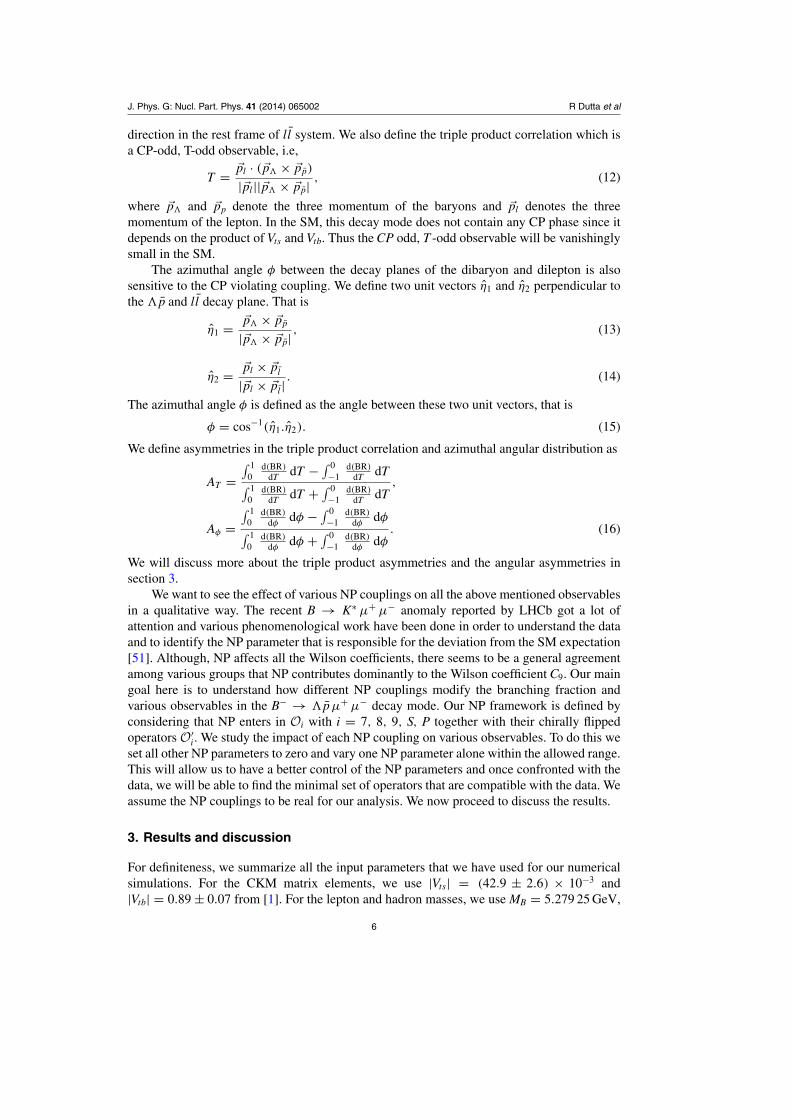
J. Phys. G: Nucl. Part. Phys. 41 (2014) 065002 R Dutta et al

direction in the rest frame of ll system. We also define the triple product correlation which isa CP-odd, T-odd observable, i.e,

T = �pl · (�p� × �pp)

|�pl ||�p� × �pp| , (12)

where �p� and �pp denote the three momentum of the baryons and �pl denotes the threemomentum of the lepton. In the SM, this decay mode does not contain any CP phase since itdepends on the product of Vts and Vtb. Thus the CP odd, T -odd observable will be vanishinglysmall in the SM.

The azimuthal angle φ between the decay planes of the dibaryon and dilepton is alsosensitive to the CP violating coupling. We define two unit vectors η1 and η2 perpendicular tothe �p and ll decay plane. That is

η1 = �p� × �pp

|�p� × �pp| , (13)

η2 = �pl × �pl

|�pl × �pl |. (14)

The azimuthal angle φ is defined as the angle between these two unit vectors, that is

φ = cos−1(η1.η2). (15)

We define asymmetries in the triple product correlation and azimuthal angular distribution as

AT =∫ 1

0d(BR)

dT dT − ∫ 0−1

d(BR)

dT dT∫ 10

d(BR)

dT dT + ∫ 0−1

d(BR)

dT dT,

Aφ =∫ 1

0d(BR)

dφdφ − ∫ 0

−1d(BR)

dφdφ∫ 1

0d(BR)

dφdφ + ∫ 0

−1d(BR)

dφdφ

. (16)

We will discuss more about the triple product asymmetries and the angular asymmetries insection 3.

We want to see the effect of various NP couplings on all the above mentioned observablesin a qualitative way. The recent B → K∗ μ+ μ− anomaly reported by LHCb got a lot ofattention and various phenomenological work have been done in order to understand the dataand to identify the NP parameter that is responsible for the deviation from the SM expectation[51]. Although, NP affects all the Wilson coefficients, there seems to be a general agreementamong various groups that NP contributes dominantly to the Wilson coefficient C9. Our maingoal here is to understand how different NP couplings modify the branching fraction andvarious observables in the B− → �pμ+ μ− decay mode. Our NP framework is defined byconsidering that NP enters in Oi with i = 7, 8, 9, S, P together with their chirally flippedoperators O′

i. We study the impact of each NP coupling on various observables. To do this weset all other NP parameters to zero and vary one NP parameter alone within the allowed range.This will allow us to have a better control of the NP parameters and once confronted with thedata, we will be able to find the minimal set of operators that are compatible with the data. Weassume the NP couplings to be real for our analysis. We now proceed to discuss the results.

3. Results and discussion

For definiteness, we summarize all the input parameters that we have used for our numericalsimulations. For the CKM matrix elements, we use |Vts| = (42.9 ± 2.6) × 10−3 and|Vtb| = 0.89 ± 0.07 from [1]. For the lepton and hadron masses, we use MB = 5.279 25 GeV,

6

J. Phys. G: Nucl. Part. Phys. 41 (2014) 065002 R Dutta et al

Table 1. Branching ratio and various angular asymmetries for B− → � pμ+ μ− withinthe SM.

SM values BR×10−7 AθL × 10−2 AθB × 10−2 AT × 10−5 Aφ × 10−2

Central value 1.08 2.79 −6.71 2.71 4.851σ range (0.57, 1.90) (2.72, 2.89) (−5.62, −7.53) (2.49, 3.14) (4.76, 4.88)

M� = 1.115 683 GeV, Mp = 0.938 27 GeV, and Mμ = 0.105 658 GeV [1], respectively. Forquark masses, we use mb = 4.18 GeV and ms = 0.095 GeV [1]. For the Wilson coefficients,we use the values reported in [56]. That is

C7 = −0.313, C8 = 4.344, C9 = −4.669. (17)

The Wilson coefficients associated with the primed operators O′i and the scalar and

pseudoscalar operators OS,P, O′S,P are assumed to be zero in the SM. For the baryonic form

factors fi and gi, we use the values of D||’s reported in [54]. That is

D|| = 67.7 ± 16.3 GeV5, D2|| = −187.3 ± 26.6 GeV4, D3

|| = −840.1 ± 132.1 GeV4,

D4|| = − 10.1 ± 10.8 GeV4, D5

|| = −157.0 ± 27.1 GeV4. (18)

First, we report the value of the branching ratio and various asymmetries within the SM.In the SM, the relevant operators for our analysis are the non-primed operators (Oi), wherei = 7, 8, and 9, respectively. All the primed operators (O′

i) and the scalar (OS, O′S) and the

pseudoscalar (OP, O′P) operators are ignored. The SM prediction of the branching ratio and

various asymmetries for the B → �pμ+ μ− decay mode is reported in table 1, where, forthe central values we have used the central values of all the input parameters. The theoreticaluncertainties in the calculation of the decay branching fractions come from various inputparameters. first, there are uncertainties associated with well-known input parameters such asquark masses, meson masses, and lifetime of the mesons. We ignore these uncertainties asthese are not important for our analysis. Second, there are uncertainties that are associated withnot so well-known hadronic input parameters such as form factors and the CKM elements.In order to realize the effect of the above-mentioned uncertainties on various observables, wevary these theory inputs within 1σ of their central values and obtain the 1σ allowed ranges inall the different observables. The results are reported in table 1.

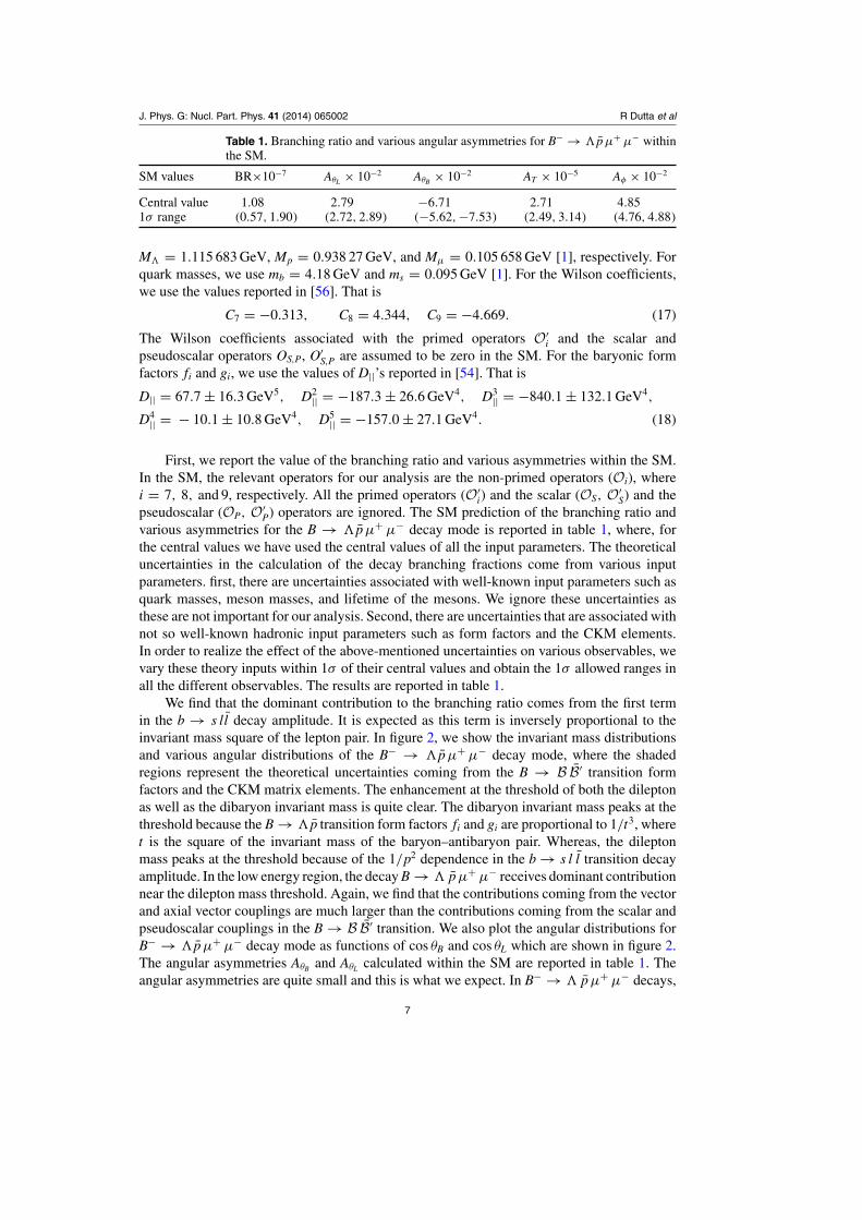
We find that the dominant contribution to the branching ratio comes from the first termin the b → s ll decay amplitude. It is expected as this term is inversely proportional to theinvariant mass square of the lepton pair. In figure 2, we show the invariant mass distributionsand various angular distributions of the B− → �pμ+ μ− decay mode, where the shadedregions represent the theoretical uncertainties coming from the B → B B′ transition formfactors and the CKM matrix elements. The enhancement at the threshold of both the dileptonas well as the dibaryon invariant mass is quite clear. The dibaryon invariant mass peaks at thethreshold because the B → �p transition form factors fi and gi are proportional to 1/t3, wheret is the square of the invariant mass of the baryon–antibaryon pair. Whereas, the dileptonmass peaks at the threshold because of the 1/p2 dependence in the b → s l l transition decayamplitude. In the low energy region, the decay B → � pμ+ μ− receives dominant contributionnear the dilepton mass threshold. Again, we find that the contributions coming from the vectorand axial vector couplings are much larger than the contributions coming from the scalar andpseudoscalar couplings in the B → B B′ transition. We also plot the angular distributions forB− → �pμ+ μ− decay mode as functions of cos θB and cos θL which are shown in figure 2.The angular asymmetries AθB and AθL calculated within the SM are reported in table 1. Theangular asymmetries are quite small and this is what we expect. In B− → � pμ+ μ− decays,

7

J. Phys. G: Nucl. Part. Phys. 41 (2014) 065002 R Dutta et al

0

2e-08

4e-08

6e-08

8e-08

1e-07

1.2e-07

1.4e-07

0 0.5 1 1.5 2 2.5 3 3.5

dB

/dm

μμ(G

eV

-1)

mμμ(GeV)

0

5e-08

1e-07

1.5e-07

2e-07

2.5e-07

3e-07

3.5e-07

0 0.5 1 1.5 2 2.5 3 3.5

dB

/dm

λp(G

eV

-1)

mλp(GeV)

0

5e-09

1e-08

1.5e-08

2e-08

-1 -0.5 0 0.5 1

dB

/dco

s(θ L

)

cos(θL)

0

5e-09

1e-08

1.5e-08

2e-08

2.5e-08

-1 -0.5 0 0.5 1

dB

/dco

s(θ B

)

cos(θB) 0

2e-08

4e-08

6e-08

8e-08

1e-07

1.2e-07

1.4e-07

1.6e-07

-1 -0.5 0 0.5 1

dB

/dco

s(φ)

cos(φ)

0

1e-08

2e-08

3e-08

4e-08

5e-08

6e-08

7e-08

8e-08

-1 -0.5 0 0.5 1

dB

/dT

T

Figure 2. Effect of NP coupling CNP7 on various observables. The shaded region (yellow

band) represents the SM prediction with the theoretical uncertainties coming from thetransition form factors and the CKM matrix elements. The black curve correspondsto the central values of the SM, whereas the red and the blue curve correspond toCNP

7 = 0.03 and −0.15, respectively.

Table 2. Branching ratio (×10−7) of B− → � pμ+ μ− once the NP is switched on.

CNP7 CNP

8 CNP9 C′

7 C′8 C′

9 CS, C′S, CP, C′

P

(0.50, 3.44) (0.57, 2.09) (0.49, 2.23) (1.65, 3.01) (0.65, 2.24) (0.60, 2.02) (1.50, 4.30)

the � and p pick up the energetic s and u quarks, respectively. The threshold enhancementensures that, in the rest frame of the B meson, the � and p move collinearly. Thus, in theboosted frame of � p, the dilepton will move away from the dibaryon system and hence thedistribution should be symmetric as functions of cos θB and cos θL. We also show the angulardistribution for B− → �pμ+ μ− decay mode as a function of the triple product correlationT and the azimuthal angle cos φ. The triple product asymmetry AT and the azimuthal angularasymmetry Aφ calculated within the SM are reported in table 1. These are vanishingly smallas expected. Any deviation from the SM expectation will be a definite hint of beyond the SMphysics.

Now we proceed to discuss the effect of various NP couplings on the above mentionedobservables in a qualitative way. For definiteness, we report the 95% CL range of each NPcoupling that are taken from [57, 58]. We assume that all the coefficients are real.

CNP7 = (−0.15, 0.03), CNP

8 = (−1.1, 1.6), CNP9 = (−1.2, 1.6),

C′7 = (−0.4, 0.3), C′

8 = (−2.0, 4.0), C′9 = (−3.0, 1.0),

CS, C′S = (−0.7, 0.7), CP, C′

P = (−1.0, 1.0) (19)

The branching ratio for the B− → �pμ+ μ− decay mode is listed in table 2 with the variousNP couplings. The range in each observable is obtained by using the range of NP parametersin equation (19). It is clear that the deviation from the SM prediction is more if one includethe NP effects in CS, CP, C′

S, and C′P simultaneously.

8

J. Phys. G: Nucl. Part. Phys. 41 (2014) 065002 R Dutta et al

0

2e-08

4e-08

6e-08

8e-08

1e-07

1.2e-07

1.4e-07

0 0.5 1 1.5 2 2.5 3 3.5

dB

/dm

μμ(G

eV

-1)

mμμ(GeV)

0

5e-08

1e-07

1.5e-07

2e-07

2.5e-07

3e-07

3.5e-07

0 0.5 1 1.5 2 2.5 3 3.5

dB

/dm

λp(G

eV

-1)

mλp(GeV)

0

5e-09

1e-08

1.5e-08

2e-08

-1 -0.5 0 0.5 1

dB

/dco

s(θ L

)

cos(θL)

0

5e-09

1e-08

1.5e-08

2e-08

2.5e-08

-1 -0.5 0 0.5 1

dB

/dco

s(θ B

)

cos(θB) 0

2e-08

4e-08

6e-08

8e-08

1e-07

1.2e-07

1.4e-07

1.6e-07

-1 -0.5 0 0.5 1

dB

/dco

s(φ)

cos(φ)

0

1e-08

2e-08

3e-08

4e-08

5e-08

6e-08

7e-08

8e-08

-1 -0.5 0 0.5 1

dB

/dT

T

Figure 3. Effect of NP coupling CNP8 on various observables. The shaded region (yellow

band) represents the SM prediction with the theoretical uncertainties coming from thetransition form factors and the CKM matrix elements. The black curve corresponds tothe central values of the SM, whereas the red and the blue correspond to CNP

8 = −1.1and 1.6, respectively.

We consider various NP scenarios. First, we assume that NP affects the Wilson coefficientC7 only. In figure 2, we show the effect of NP associated with the operator O7. In this case, theNP will modify the dipole operator coefficientC7 only. We allow for sizable modifications to thedipole Wilson coefficient. We show the effect of NP on various observables for CNP

7 = −0.15and 0.03. We see an enhancement of about 100% at the threshold of the invariant massdistribution of the lepton pair. This is expected as the dipole operators in B → �pμ+μ−

decay amplitude is directly proportional to 1/p2, where p2 is the invariant mass square ofthe lepton pair. Similar enhancement is seen in the invariant mass distribution of the baryonpair as well. Again, it is worth mentioning that, NP has a significant effect on the angulardistributions for θL and θB. The NP effects on these observables are illustrated in the middlepanel of figure 2. For CNP

7 = −0.15, the shape of the distribution curve changes drastically.Once the NP is switched on, the angular distribution curve peaks at cos θL = −1, whereas,SM distribution peaks at cos θL = 1. Thus, it is clear that once the NP coupling is present,there can be a significant deviation from the SM expectation and depending on the value ofthe NP coupling, the shape of the distribution curve may or may not change. However, we donot expect to see a sizable deviation in the shape of the cos θB distribution curve. Similarly,although, there is deviation from the SM expectation in the azimuthal angular distribution andthe triple product correlation, these distribution curves remain symmetric with respect to theorigin. This is expected as the NP coupling CNP

7 is real and we do not expect to see any CPviolation.

In figure 3, we show the effect of NP associated with the semileptonic operator O8,i.e, we assume that NP affects the Wilson coefficient C8 only. We show the effect on variousobservables for two different values of the NP coupling. We setCNP

8 = −1.1 and 1.6. Although,we observe a slight change in the invariant mass distribution curve, as can be seen from figure 3,such kind of NP coupling mainly affects the angular distribution, leaving all other observablesapproximately SM like. We see that the angular distributions for θB and θL are significantly

9

J. Phys. G: Nucl. Part. Phys. 41 (2014) 065002 R Dutta et al

0

2e-08

4e-08

6e-08

8e-08

1e-07

1.2e-07

1.4e-07

0 0.5 1 1.5 2 2.5 3 3.5

dB

/dm

μμ(G

eV

-1)

mμμ(GeV)

0

5e-08

1e-07

1.5e-07

2e-07

2.5e-07

3e-07

3.5e-07

0 0.5 1 1.5 2 2.5 3 3.5

dB

/dm

λp(G

eV

-1)

mλp(GeV)

0

5e-09

1e-08

1.5e-08

2e-08

-1 -0.5 0 0.5 1

dB

/dco

s(θ L

)

cos(θL)

0

5e-09

1e-08

1.5e-08

2e-08

2.5e-08

-1 -0.5 0 0.5 1

dB

/dco

s(θ B

)

cos(θB) 0

2e-08

4e-08

6e-08

8e-08

1e-07

1.2e-07

1.4e-07

1.6e-07

-1 -0.5 0 0.5 1

dB

/dco

s(φ)

cos(φ)

0

1e-08

2e-08

3e-08

4e-08

5e-08

6e-08

7e-08

8e-08

-1 -0.5 0 0.5 1

dB

/dT

T

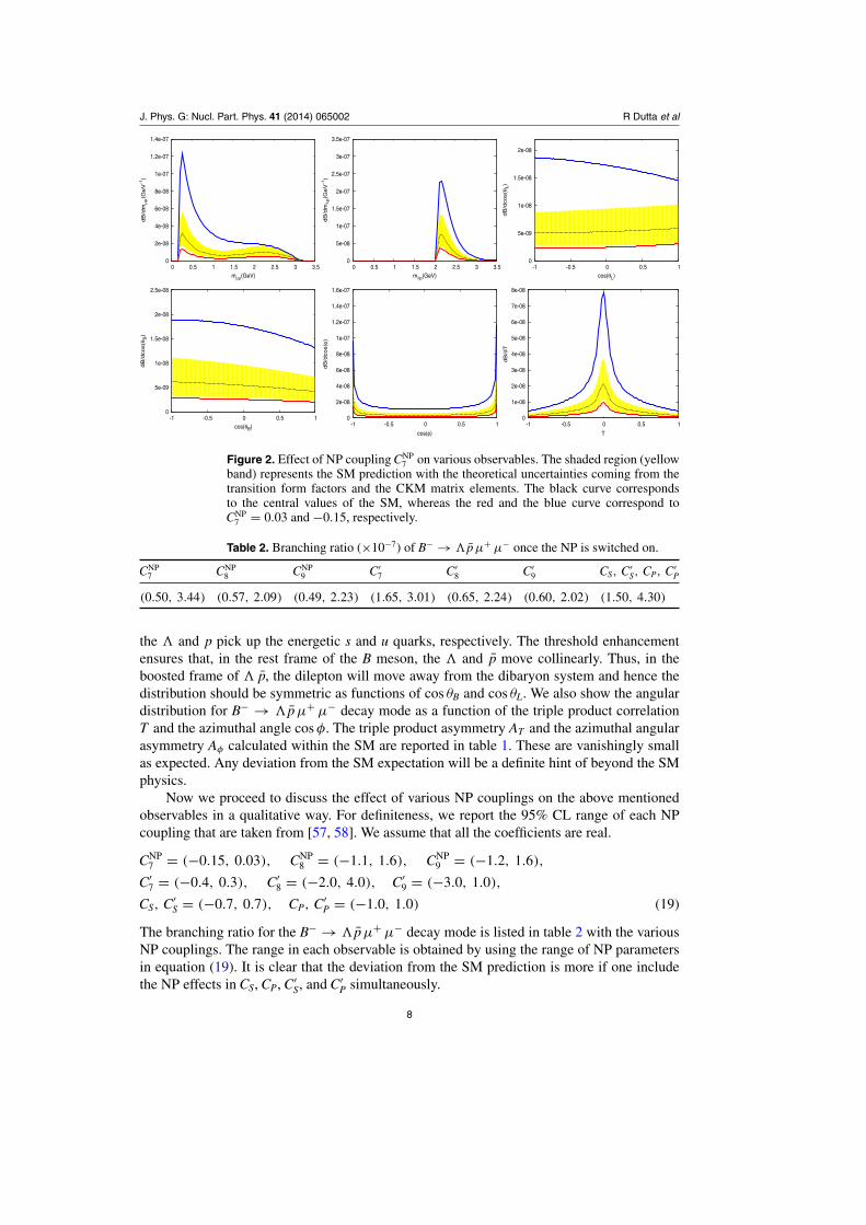
Figure 4. Effect of NP coupling CNP9 on various observables. The shaded region (yellow

band) represents the SM prediction with the theoretical uncertainties coming from thetransition form factors and the CKM matrix elements. The black curve corresponds tothe central values of the SM, whereas the red and the blue correspond to CNP

9 = 1.6and −1.2, respectively.

different from the SM once the NP coupling is switched on. Again, for the azimuthal angulardistribution and triple product correlation, the distribution curves remain symmetric withrespect to the origin as expected since the NP coupling CNP

8 is real.Similar pattern is observed once the NP coupling associated with the operator O9 is

switched on. We use NP in C9 and see the effects on various observables for CNP9 = −1.2

and 1.6, respectively. We see a significant deviation from the SM in the angular distribution,leaving all other observables approximately SM like. The effects of this NP coupling on variousobservables are shown in figure 4.

Now we look at the primed operators O′i. In the SM, the Wilson coefficients associated

with these chirally flipped operators are suppressed and are assumed to be zero. Once weswitched on the NP in these primed operators, the angular distribution differs significantlyfrom the SM. We show the effects of these NP parameters on various observables infigures 5–7, respectively. There is deviation in the invariant mass distribution for NP inC′

7. Although, we see an enhancement of more than 100% in the branching ratio from the SMexpectation, the shape remains similar to that of the SM as can be seen from figure 5. Theeffect of C′

8 and C′9 on the angular distributions as functions of cos θL and cos θB is significant

as can be seen from figures 6 and 7. However, the effect of these NP is negligible on all otherobservables such as invariant mass distribution, the azimuthal angular distribution, and thetriple product correlation.

In figure 8, we show the NP effect associated with the primed and non-primed scalar andpseudoscalar operators on various observables. We consider simultaneous NP effects in allthe four Wilson coefficients, i.e, we consider NP in CS, CP, C′

S, and C′P simultaneously. In the

SM, these are suppressed and are assumed to be zero for our analysis. However, it may notbe negligible in the presence of NP. We see that the invariant mass spectra as functions ofthe invariant masses m� p and mμ+ μ− differ significantly from their SM expectation. We seea huge peak at large invariant mass of the lepton pair. Thus, in the presence of such NP, the

10

J. Phys. G: Nucl. Part. Phys. 41 (2014) 065002 R Dutta et al

0

2e-08

4e-08

6e-08

8e-08

1e-07

1.2e-07

1.4e-07

0 0.5 1 1.5 2 2.5 3 3.5

dB

/dm

μμ(G

eV

-1)

mμμ(GeV)

0

5e-08

1e-07

1.5e-07

2e-07

2.5e-07

3e-07

3.5e-07

0 0.5 1 1.5 2 2.5 3 3.5

dB

/dm

λp(G

eV

-1)

mλp(GeV)

0

5e-09

1e-08

1.5e-08

2e-08

-1 -0.5 0 0.5 1

dB

/dco

s(θ L

)

cos(θL)

0

5e-09

1e-08

1.5e-08

2e-08

2.5e-08

-1 -0.5 0 0.5 1

dB

/dco

s(θ B

)

cos(θB) 0

2e-08

4e-08

6e-08

8e-08

1e-07

1.2e-07

1.4e-07

1.6e-07

-1 -0.5 0 0.5 1

dB

/dco

s(φ)

cos(φ)

0

1e-08

2e-08

3e-08

4e-08

5e-08

6e-08

7e-08

8e-08

-1 -0.5 0 0.5 1

dB

/dT

T

Figure 5. Effect of NP coupling C′7 on various observables. The shaded region (yellow

band) represents the SM prediction with the theoretical uncertainties coming from thetransition form factors and the CKM matrix elements. The black curve corresponds tothe central values of the SM, whereas the red and the blue correspond to C′

7 = −0.4 and0.3, respectively.

0

2e-08

4e-08

6e-08

8e-08

1e-07

1.2e-07

1.4e-07

0 0.5 1 1.5 2 2.5 3 3.5

dB

/dm

μμ(G

eV

-1)

mμμ(GeV)

0

5e-08

1e-07

1.5e-07

2e-07

2.5e-07

3e-07

3.5e-07

0 0.5 1 1.5 2 2.5 3 3.5

dB

/dm

λp(G

eV

-1)

mλp(GeV)

0

5e-09

1e-08

1.5e-08

2e-08

-1 -0.5 0 0.5 1

dB

/dco

s(θ L

)

cos(θL)

0

5e-09

1e-08

1.5e-08

2e-08

2.5e-08

-1 -0.5 0 0.5 1

dB

/dco

s(θ B

)

cos(θB) 0

2e-08

4e-08

6e-08

8e-08

1e-07

1.2e-07

1.4e-07

1.6e-07

-1 -0.5 0 0.5 1

dB

/dco

s(φ)

cos(φ)

0

1e-08

2e-08

3e-08

4e-08

5e-08

6e-08

7e-08

8e-08

-1 -0.5 0 0.5 1

dB

/dT

T

Figure 6. Effect of NP coupling C′8 on various observables. The shaded region (yellow

band) represents the SM prediction with the theoretical uncertainties coming from thetransition form factors and the CKM matrix elements. The black curve corresponds tothe central values of the SM, whereas the red and the blue correspond to C′

8 = −2.0 and4.0, respectively.

11

J. Phys. G: Nucl. Part. Phys. 41 (2014) 065002 R Dutta et al

0

2e-08

4e-08

6e-08

8e-08

1e-07

1.2e-07

1.4e-07

0 0.5 1 1.5 2 2.5 3 3.5

dB

/dm

μμ(G

eV

-1)

mμμ(GeV)

0

5e-08

1e-07

1.5e-07

2e-07

2.5e-07

3e-07

3.5e-07

0 0.5 1 1.5 2 2.5 3 3.5

dB

/dm

λp(G

eV

-1)

mλp(GeV)

0

5e-09

1e-08

1.5e-08

2e-08

-1 -0.5 0 0.5 1

dB

/dco

s(θ L

)

cos(θL)

0

5e-09

1e-08

1.5e-08

2e-08

2.5e-08

-1 -0.5 0 0.5 1

dB

/dco

s(θ B

)

cos(θB) 0

2e-08

4e-08

6e-08

8e-08

1e-07

1.2e-07

1.4e-07

1.6e-07

-1 -0.5 0 0.5 1

dB

/dco

s(φ)

cos(φ)

0

1e-08

2e-08

3e-08

4e-08

5e-08

6e-08

7e-08

8e-08

-1 -0.5 0 0.5 1

dB

/dT

T

Figure 7. Effect of NP coupling C′9 on various observables. The shaded region (yellow

band) represents the SM prediction with the theoretical uncertainties coming from thetransition form factors and the CKM matrix elements. The black curve corresponds tothe central values of the SM, whereas the red and the blue correspond to C′

9 = −3.0 and1.0, respectively.

0

2e-08

4e-08

6e-08

8e-08

1e-07

1.2e-07

1.4e-07

0 0.5 1 1.5 2 2.5 3 3.5

dB

/dm

μμ(G

eV

-1)

mμμ(GeV)

0

5e-08

1e-07

1.5e-07

2e-07

2.5e-07

3e-07

3.5e-07

0 0.5 1 1.5 2 2.5 3 3.5

dB

/dm

λp(G

eV

-1)

mλp(GeV)

0

5e-09

1e-08

1.5e-08

2e-08

-1 -0.5 0 0.5 1

dB

/dco

s(θ L

)

cos(θL)

0

5e-09

1e-08

1.5e-08

2e-08

2.5e-08

-1 -0.5 0 0.5 1

dB

/dco

s(θ B

)

cos(θB) 0

2e-08

4e-08

6e-08

8e-08

1e-07

1.2e-07

1.4e-07

1.6e-07

-1 -0.5 0 0.5 1

dB

/dco

s(φ)

cos(φ)

0

1e-08

2e-08

3e-08

4e-08

5e-08

6e-08

7e-08

8e-08

-1 -0.5 0 0.5 1

dB

/dT

T

Figure 8. Effect of NP couplings CS, CP, C′S, and C′

P on various observables. The shadedregion (yellow band) represents the SM prediction with the theoretical uncertaintiescoming from the transition form factors and the CKM matrix elements. The blackcurve corresponds to the central values of the SM. The red curve corresponds toCS, C′

S = −0.7 andCP, C′P = −1.0, whereas the blue curve corresponds toCS, C′

S = 0.7and CP, C′

P = 1.0.

12

J. Phys. G: Nucl. Part. Phys. 41 (2014) 065002 R Dutta et al

peak of the distribution is no longer at the threshold. Although, there is significant deviation ofthe angular distributions for θL and θB from the SM expectation, the shape of the distributioncurves remain similar to the SM. Similarly, we do not see any asymmetry in the azimuthalangular distribution and triple product correlation.

4. Conclusion

Flavor changing neutral current process mediated via b → (d, s) ll transition decay processis a loop mediated process and, in principle, can get significant corrections from NP effects. Alot of experimental as well as theoretical work have been done in this context with a meson inthe final state. Recent measurements of Bd,s → μ+ μ− and B → K∗ μ+ μ− decays differ fromthe standard model expectation and if they persist in future precision experiments, it will be adefinite hint of beyond the standard model physics. This will, in turn, affect any FCNC decaysmediated via b → s l l transition process such as baryonic B → B B′ ll decays. In this context,we construct the most general effective Hamiltonian for the semileptonic B− → �pμ+μ−

decay process and look at the effect of NP couplings on various observables in a qualitativeway. We assume that all the Wilson coefficients of the operators get modified due to NPeffects and see the effect of each NP coupling on various observables. We also assume thatall the NP couplings are real. This B− → �pμ+ μ− decay mode is important for severalreasons. First, the study of such modes is complementary to the study of B → K∗ μ+ μ−

mediated via b → s l l transition process. Second, its empirical study can be complementaryto other baryonic B decays and one can, in principle, investigate the theoretical modeling ofthe B → B B′ transition form factors.

Within the SM, we find the branching ratio of B− → �pμ+μ− decay mode to be1.08×10−7. We see that the deviation from the SM prediction is quite significant if we includethe NP in CS, CP, C′

S, and C′P simultaneously. The asymmetries in the triple product correlations

are found to be vanishingly small as expected since, in the SM, this decay mode depends onlyon Vts and Vtb, CKM matrix elements. Again, we see that the azimuthal angular distributionand the triple product correlation remain symmetric with respect to the origin once we includethe NP effects. This is expected because all the NP couplings are real and hence we do notexpect to find any CP violation in this decay mode. The effect of CNP

7 on the invariant massdistribution and the angular distributions as functions of cos θL and cos θB is quite significant.Again, in case of NP in C8 and C9, we see that only the angular distributions as functions ofcos θL and cos θB are significantly different from the SM prediction. Similar pattern is observedin case of NP in all the primed coefficients. However, if we switch on NP in CS, CP, C′

S, andC′

P simultaneously, we see a significant deviation from the SM prediction in the invariant massspectrum as function of the invariant mass mμ+ μ− . The peak of the distribution shifts towardsthe large invariant mass of the lepton pair.

Current experimental results suggest new physics in FCNC decays mediated via b →(s, d) l l transition processes. Precision measurements in future B experiments will help inidentifying the nature of the new physics. Again, a better theoretical understanding of theB → B B′ transition form factors will improve our estimates in future.

Acknowledgments

RD and AKG would like to thank BRNS, Government of India, for financial support.

References

[1] Beringer J et al (Particle Data Group) 2012 Phys. Rev. D 86 010001[2] Albrecht H et al (ARGUS Collaboration) 1988 Phys. Lett. B 209 119

13

J. Phys. G: Nucl. Part. Phys. 41 (2014) 065002 R Dutta et al

[3] Bebek C et al (CLEO Collaboration) 1989 Phys. Rev. Lett. 62 8[4] Fu X et al (CLEO Collaboration) 1997 Phys. Rev. Lett. 79 3125[5] Aubert B et al (BABAR Collaboration) 2002 Nucl. Instrum. Methods A 479 1[6] Abashian A et al (Belle Collaboration) 2002 Nucl. Instrum. Methods A 479 117[7] Gronau M and Rosner J L 1988 Phys. Rev. D 37 688

Eilam G, Gronau M and Rosner J L 1989 Phys. Rev. D 39 819Sheikholeslami S M and Khanna M P 1991 Phys. Rev. D 44 770Sheikholeslami S M, Sidana G K and Khanna M P 1992 Int. J. Mod. Phys. A 7 1111

[8] Deshpande N G, Trampetic J and Soni A 1988 Mod. Phys. Lett. A 3 749[9] Jarfi M, Lazrak O, Le Yaouanc A, Oliver L, Pene O and Raynal J C 1991 Phys. Rev. D

43 1599[10] Ball P and Dosch H G 1991 Z. Phys. C 51 445[11] Chernyak V L and Zhitnitsky I R 1990 Nucl. Phys. B 345 137[12] Kaur G and Khanna M P 1992 Phys. Rev. D 46 466[13] Cheng H-Y and Yang K-C 2002 Phys. Rev. D 66 014020[14] Wang M Z et al (Belle Collaboration) 2003 Phys. Rev. Lett. 90 201802[15] Wang M Z et al (Belle Collaboration) 2004 Phys. Rev. Lett. 92 131801[16] Wang M-Z et al (Belle Collaboration) 2005 Phys. Lett. B 617 141[17] Lee Y-J et al (Belle Collaboration) 2005 Phys. Rev. Lett. 95 061802[18] Lee Y-J et al (BELLE Collaboration) 2004 Phys. Rev. Lett. 93 211801[19] Aubert B et al (BaBar Collaboration) 2005 Phys. Rev. D 72 051101[20] Wang M-Z et al (Belle Collaboration) 2007 Phys. Rev. D 76 052004[21] Wei J T et al (BELLE Collaboration) 2008 Phys. Lett. B 659 80[22] Gabyshev N et al (Belle and BELLE Collaborations) 2006 Phys. Rev. Lett. 97 242001[23] Aubert B et al (BaBar Collaboration) 2007 Phys. Rev. D 76 092004[24] Chen J H et al (Belle Collaboration) 2008 Phys. Rev. Lett. 100 251801[25] Abe K et al (Belle Collaboration) 2002 Phys. Rev. Lett. 89 151802[26] Aubert B et al (BaBar Collaboration) 2006 Phys. Rev. D 74 051101[27] Aubert B et al (BABAR Collaboration) 2010 Phys. Rev. D 82 091102[28] Aubert B et al (BABAR Collaboration) 2009 arXiv:0908.2202 [hep-ex][29] del Amo Sanchez P et al (BABAR Collaboration) 2012 Phys. Rev. D 85 092017[30] Hou W-S and Soni A 2001 Phys. Rev. Lett. 86 4247[31] Rosner J L 2003 Phys. Rev. D 68 014004[32] Cheng H-Y 2006 Int. J. Mod. Phys. A 21 4209[33] Chua C-K, Hou W-S and Tsai S-Y 2002 Phys. Lett. B 544 139[34] Cheng H-Y and Yang K-C 2002 Phys. Rev. D 66 094009[35] Cheng H-Y and Yang K-C 2002 Phys. Rev. D 65 054028

Cheng H-Y and Yang K-C 2002 Phys. Rev. D 65 099901 (erratum)[36] Kerbikov B, Stavinsky A and Fedotov V 2004 Phys. Rev. C 69 055205[37] Bugg D V 2004 Phys. Lett. B 598 8[38] Haidenbauer J, Meissner U-G and Sibirtsev A 2006 Phys. Rev. D 74 017501[39] Laporta V 2007 Int. J. Mod. Phys. A 22 5401[40] Chua C-K, Hou W-S and Tsai S-Y 2002 Phys. Rev. D 66 054004[41] Geng C Q and Hsiao Y K 2006 Phys. Rev. D 74 094023[42] Chen C-H, Cheng H-Y, Geng C Q and Hsiao Y K 2008 Phys. Rev. D 78 054016[43] Geng C Q and Hsiao Y K 2012 Phys. Rev. D 85 017501[44] Suzuki M 2007 J. Phys. G: Nucl. Part. Phys. 34 283[45] Aaij R et al (LHCb Collaboration) 2013 Phys. Rev. Lett. 111 101805[46] Chatrchyan S et al (CMS Collaboration) 2013 Phys. Rev. Lett. 111 101804[47] Buras A J, Girrbach J, Guadagnoli D and Isidori G 2012 Eur. Phys. J. C 72 2172[48] Aaij R et al (LHCb Collaboration) LHCb-CONF-2012-002[49] De Bruyn K, Fleischer R, Knegjens R, Koppenburg P, Merk M, Pellegrino A and Tuning N 2012

Phys. Rev. Lett. 109 041801Fleischer R 2013 Nucl. Phys. Proc. Suppl. 241–242 135Becirevic D, Kosnik N, Mescia F and Schneider E 2013 Nucl. Phys. Proc. Suppl. 234 177Fleischer R 2012 arXiv:1212.4967 [hep-ph]Buras A J, Fleischer R, Girrbach J and Knegjens R 2013 J. High Energy Phys. JHEP07(2013)77Knegjens R 2013 PoS Beauty 2013 053

14

J. Phys. G: Nucl. Part. Phys. 41 (2014) 065002 R Dutta et al

Altmannshofer W 2013 PoS Beauty 2013 024Misra B and Saha J P 2013 arXiv:1308.2518 [hep-ph]

[50] Aaij R et al (LHCb Collaboration) 2013 Phys. Rev. Lett. 111 191801[51] Descotes-Genon S, Matias J and Virto J 2013 Phys. Rev. D 88 074002

Altmannshofer W and Straub D M 2013 Eur. Phys. J. C 73 2646Gauld R, Goertz F and Haisch U 2014 Phys. Rev. D 89 015005Buras A J and Girrbach J 2013 J. High Energy Phys. JHEP12(2013)009Gauld R, Goertz F and Haisch U 2014 J. High Energy Phys. JHEP01(2014)069Beaujean F, Bobeth C and van Dyk D 2013 arXiv:1310.2478 [hep-ph]Datta A, Duraisamy M and Ghosh D 2014 Phys. Rev. D 89 071501Horgan R R, Liu Z, Meinel S and Wingate M 2013 arXiv:1310.3887 [hep-ph]Descotes-Genon S, Matias J and Virto J 2013 arXiv:1311.3876 [hep-ph]Buras A J, De Fazio F, Girrbach J and Carlucci M V 2013 J. High Energy Phys. JHEP02(2013)023Buras A J, De Fazio F and Girrbach J 2013 J. High Energy Phys. JHEP02(2013)116

[52] Geng C Q and Hsiao Y K 2011 Phys. Lett. B 704 495[53] Tien K J et al (M. Z. Wang for the Belle Collaboration) 2013 arXiv:1306.3353 [hep-ex][54] Geng C Q and Hsiao Y K 2012 Phys. Rev. D 85 094019[55] Buras A J and Munz M 1995 Phys. Rev. D 52 186

Misiak M 1993 Nucl. Phys. B 393 23Misiak M 1995 Nucl. Phys. B 439 461 (erratum)Grinstein B, Savage M J and Wise M B 1989 Nucl. Phys. B 319 271Sinha N and Sinha R 1997 arXiv:hep-ph/9707416

[56] Ali A, Ball P, Handoko L T and Hiller G 2000 Phys. Rev. D 61 074024[57] Altmannshofer W, Paradisi P and Straub D M 2012 J. High Energy Phys. JHEP04(2012)008[58] Becirevic D, Kosnik N, Mescia F and Schneider E 2012 Phys. Rev. D 86 034034

15