Growth in transition countries

Growth in transition countriesBigBangversusGradualism

Roberto Dell’Anno* and Stefania Villa***University of Salerno. E-mail: [email protected]

**KU Leuven, Belgium and University of Foggia, Italy. E-mail: [email protected].

Abstract

This study analyzes the impact of the speed of transition reforms on economic growth intransition countries in the context of the debate on ‘big-bang vs. gradualist approach’. Itbuilds a new indicator for the speed of transition reforms based on a three-way principalcomponent analysis. It shows that: (i) the speed of transition reforms Granger-causes eco-nomic growth and there is no reverse causation; (ii) the impact of contemporaneous speedof transition reforms on economic growth is negative, but becomes positive in the longerhorizon; and (iii) other factors, such as initial conditions and macroeconomic stabilizationprogrammes, also drive economic growth. Although the first two results are robust to dif-ferent estimators, the impact of control variables depends on the econometric specification.

JEL classifications: P21, O43, C33.Keywords: Speed of transition, economic growth, three-way principal componentsanalysis.

1. Introduction

Transition countries have experienced profound macroeconomic, political, social andcultural changes since the fall of the Berlin wall.1 And among them different transi-tion and growth paths have occurred. According to Roland (2000, p. 1), ‘controversies

Received: May 22, 2012; Acceptance: January 28, 2013

1 Transition is ‘the widely accepted term for the thorough going political and economic changes’ in ex-com-munist countries to establish market-oriented economies (Murrell, 2008).

Economics of TransitionVolume 21(3) 2013, 381–417DOI: 10.1111/ecot.12018

� 2013 The AuthorsEconomics of Transition � 2013 The European Bank for Reconstruction and Development.Published by Blackwell Publishing Ltd, 9600 Garsington Road, Oxford OX4 2DQ, UK and 350 Main St, Malden, MA 02148, USA

focused very quickly on the speed of transition’. Two main, and opposite, views pre-vail in the literature. The first, the so-called Washington consensus, supports a BigBang or shock therapy approach to transition (Murphy et al., 1992; Berg et al., 1999;among others). According to this view, a quick and simultaneous introduction of allreforms (see Roland, 2000) delivers definite efficiency gains in introducing a success-ful market economy. The second view, the so-called gradualist approach, proposes agradual reform path, relying on the flexibility of experimentation with an adequatesequencing of reforms (for example, Aghion and Blanchard, 1994; Roland, 2000).There are examples of success and failure for both views: the Czech Republic success-fully implemented a big bang policy, differently from Hungary and Russia (seeRoland, 2000 for a detailed discussion); China successfully experienced a gradualreform path (Feltenstein and Nsouli, 2003). A third strand of literature focuses on abig bang approach along certain dimensions and gradualism along other dimensions(Kornai, 1990; Blanchard et al., 1991; Fischer and Gelb, 1991).

Economic growth is a complex phenomenon; therefore, focussing on a soledimension, such as the speed of transition reforms, might lead to false inferences.According to Falcetti et al. (2006) and De Melo et al. (2001), the link between reformsand economic growth in transition countries should be re-examined taking intoaccount a variety of factors, such as initial conditions and macroeconomic stabiliza-tion programmes.

This article provides empirical evidence to contribute to the debate on ‘big bangvs. gradualism’ in transition countries and it makes three major contributions.

First, it builds a new indicator of the speed of transition reforms based on aninnovative procedure, the three-way Principal Component Analysis (PCA), origi-nally applied by Tucker (1966) in psychometrics and then used in other disciplinessuch as chemometrics and recently economics (Henrion, 1994; Barbieri et al., 1999;Pardo et al., 2004; Mourao, 2008). Roland (2000, p. 12) emphasizes that focusing onindividual reforms might lead to a wrong picture of transition: ‘there are, for exam-ple, evident complementarities between privatization and price liberalization’. Thecomposite index of transition built in this article provides a single dimension for alltransition indicators published by the European Bank for Reconstruction and Devel-opment (EBRD). The percentage change in this index over time is defined as thespeed of transition reforms (speed of transition, henceforth).

Second, this article builds on the analysis by Falcetti et al. (2006), focussing on thelink between the speed of transition and economic growth at different time horizons. Ina panel analysis of the Central and Eastern Europe (CEE) and the Commonwealth ofIndependent States (CIS) transition countries2 for the period 1990–2008, we study: (i)the influence of the speed of reforms on economic growth as well as the reverse linkfrom economic growth to speed of transition; (ii) the dynamic effects of reforms; and(iii) the role of other factors in explaining economic growth in transition countries, suchas initial conditions, macroeconomic stabilization programmes and external demand.

2 See Appendix A for the list of countries.

� 2013 The AuthorsEconomics of Transition � 2013 The European Bank for Reconstruction and Development

382 Dell’Anno and Villa

Third, this article presents different econometric methodologies to test the natureof the relationship between the speed of transition and economic growth. Panel unitroot tests, Granger causality and the optimal lag length between the reforms andtheir effects on economic growth are employed as a preliminary analysis. Then, themodel specifications are substantially two: (i) a static panel model, examining theeffect of contemporaneous speed of transition on economic growth; and (ii) adynamic panel model, examining whether the speed of transition leads to better eco-nomic performances over time.

The main results are as follows. First, we show that the three-way PCA is moreappropriate than traditional two-way PCA to build an overall index of speed oftransition when three-dimensional datasets are used. Second, the speed of transitionGranger-causes economic growth and there is no evidence of reverse causation.Third, the impact of contemporaneous speed of transition is negative, but in thelonger horizon it becomes positive, reaching the maximum benefit with a 3-yearlag. This result is robust to different estimators and model specifications. Fourth,when controlling for endogeneity by system GMM, the control variables such asthe country’s external demand, macroeconomic stabilization programmes and thecountry’s initial conditions have a lower, often insignificant, impact on economicgrowth.

The structure of the article is as follows. Section 2 presents some data on eco-nomic growth in transition countries and discusses the main contributions of theempirical literature whereas Section 3 illustrates the main strands of the theoreticalliterature. Section 4 explains and builds the composite index of speed of transitioncomputed with the three-way PCA. Section 5 presents the econometric methodol-ogy, the results and the robustness exercises. Section 6 draws the main conclusionson the relationship between economic growth and speed of transition.

2. Transition: Stylised facts and empirical literature

The 29 countries in which the EBRD operates have experienced different growthpaths.3 In 2009, Tajikistan was the poorest country with a GDP per capita (PPP) of1,791 constant 2005 international dollars while Slovenia was the richest, with a GDPper capita of 16,405 constant 2005 international dollars. In the period 1990–2009, theaverage GDP growth rates were negative in Kyrgyz Republic, Moldova, Serbia, Taji-kistan and Ukraine and positive in the others. Many countries experienced a nega-tive growth rate in the years immediately following independence, whereas in allthe countries the average growth rates between 2000 and 2009 were positive, eventaking into account the effects of the 2007–2009 crisis. There are potential problemsin the data for transition countries; for example, the initial decline in GDP could be

3 Economic growth is measured by the growth rate of real GDP, as standard, and data are taken from theWorld Bank Development indicator database.


Growth in Transition Countries 383

over-estimated (Foster and Stehrer, 2007). However, alternative measures of eco-nomic growth, based on estimates of electricity use, have their own problems (Falc-etti et al., 2006). Bearing this caveat in mind and given the absence of alternativegood indicators, official data are used.

Figure 1 reports the paths of weighted and unweighted indexes of the annualaverage of GDP per capita, PPP (constant 2005 international dollars) for 27 transitioncountries, with the exception of Bosnia and Herzegovina (BiH) and Montenegrobecause of missing values in the early 1990s. The index is normalized to 100 in 1990for all countries. At the beginning of the transition process there was a significantfall in real GDP, which started to recover many years later. This path is robust to thesize of the different economies, with the two indexes virtually coincident. Variousreasons have been provided to explain the output fall, such as the credit crunchhypothesis, the role of network externalities and the monopoly behaviour by enter-prises after liberalization (see Roland, 2000, for a detailed discussion).

In the empirical literature the impact of reforms on economic growth can besummarized in the study by Falcetti et al. (2006). According to them, a consensusemerges on the three sets of variables affecting economic growth in transition coun-tries. First, macroeconomic stabilization is essential for growth. Second, althoughinitial conditions do matter, their influence on growth is declining steadily overtime. And third, the impact of structural reforms is strong and robust. The

60

80

100

120

140

1990

1991

1992

1993

1994

1995

1996

1997

1998

1999

2000

2001

2002

2003

2004

2005

2006

2007

2008

2009

2010

Unweighted average GDP Weighted average GDP

Figure 1. Weighted and unweighted indexes of the annual average ofGDP per capita

Source: Own elaboration based on GDP per capita, PPP (constant 2005 international $) – World DevelopmentIndicators, Washington, DC: World Bank. (27 transition countries with the exception of BiH and Montenegro).



https://www.researchgate.net/publication/222827823_Reforms_and_Growth_in_Transition_Re-examining_the_Evidence?el=1_x_8&enrichId=rgreq-1a739cf69ca13f2f63d3dde72b50a7a3-XXX&enrichSource=Y292ZXJQYWdlOzI2MTE3OTc1OTtBUzoxNjU2Mzk2Mzc0NDY2NTZAMTQxNjUwMjk3NTI4NQ==



https://www.researchgate.net/publication/222429287_Modeling_transformation_in_CEECs_using_smooth_transitions?el=1_x_8&enrichId=rgreq-1a739cf69ca13f2f63d3dde72b50a7a3-XXX&enrichSource=Y292ZXJQYWdlOzI2MTE3OTc1OTtBUzoxNjU2Mzk2Mzc0NDY2NTZAMTQxNjUwMjk3NTI4NQ==

relationship between different types of reforms and growth is discussed in Fidrmuc(2003), among many others. Fidrmuc uses 5-year moving averages and estimatesseparate cross-section regressions for each period. The liberalization index (an aver-age of EBRD indicators), which is instrumented in the regressions, is positive andsignificant in the early period (1990–1994, 1991–1995), but not in the last period(1996–2000). Overall, the introduction of wide-ranging democracy did not in factadversely affect economic growth in transition countries.

The relationship between the speed of transition and economic growth has beenless explored in the empirical literature and results are mixed. Fischer and Sahay(2000) are in favour of the big bang approach. In a panel of 25 transition countriesfrom 1989 to 1998 they find that the faster the speed of reforms, the higher the eco-nomic growth and the quicker the recovery. In a panel of 25 transition countriesfrom 1989 to 2001, Staehr (2005) finds that the effects from the speed of reforms oneconomic growth are mostly absent, but early reforms leave the transition country alonger period in which to reap the benefits of reforms. Possible negative short-termeffects of rapid reforms are likely to be modest, and could be balanced by possiblepositive medium-term effects. Therefore, in his study, speed per se has no discernibleimpact on growth. Foster and Stehrer (2007) employ a logistic smooth transitionregression in a sample of 10 CEE countries with different sample periods for eachcountry and use a dummy to indicate whether the country is a fast or gradual refor-mer. They find that differences in the speed of reforms have little impact on thedepth and length of the transitional recession or on the response of long-termgrowth to reforms. Merlevede and Schoors (2007), in a panel of 25 transition coun-tries using three-stage least squares estimators, find that new reforms affect eco-nomic growth negatively, whereas the level of past reforms leads to higher growthand attracts FDI. Fidrmuc and Tichit (2009) use component factor analysis to con-struct an index for the measure of progress in implementing market-orientedreforms. They find evidence of three breaks and, thus, four different models ofgrowth; overall, the effect of reform on growth is positive.

3. An analytical framework for economic growth and speed ofreforms

The theoretical literature on economic growth in transition countries highlights dif-ferent mechanisms through which the speed of reforms affects economic growth.There are a variety of approaches explaining such a complex phenomenon, whichinvolves political, social and economic aspects (see Roland, 2000; and Marangos,2002 and 2005, among others). This section focuses on three main strands of litera-ture: (i) the literature following a ‘general equilibrium’ approach in a Ramsey-typegrowth model; (ii) the role of the ‘critical mass’ in affecting the profitability ofrestructuring in the transition towards a market economy; and (iii) the literature on



https://www.researchgate.net/publication/222513166_Economic_Reform_Democracy_and_Growth_during_Post-Communist_Transition?el=1_x_8&enrichId=rgreq-1a739cf69ca13f2f63d3dde72b50a7a3-XXX&enrichSource=Y292ZXJQYWdlOzI2MTE3OTc1OTtBUzoxNjU2Mzk2Mzc0NDY2NTZAMTQxNjUwMjk3NTI4NQ==


https://www.researchgate.net/publication/24084553_On_the_Speed_of_Economic_Reform_-_A_Tale_of_the_Tortoise_and_the_Hare_Evidence_from_Transition_Countries?el=1_x_8&enrichId=rgreq-1a739cf69ca13f2f63d3dde72b50a7a3-XXX&enrichSource=Y292ZXJQYWdlOzI2MTE3OTc1OTtBUzoxNjU2Mzk2Mzc0NDY2NTZAMTQxNjUwMjk3NTI4NQ==

https://www.researchgate.net/publication/4991800_The_Political_Economy_of_Shock_Therapy?el=1_x_8&enrichId=rgreq-1a739cf69ca13f2f63d3dde72b50a7a3-XXX&enrichSource=Y292ZXJQYWdlOzI2MTE3OTc1OTtBUzoxNjU2Mzk2Mzc0NDY2NTZAMTQxNjUwMjk3NTI4NQ==


https://www.researchgate.net/publication/227352808_Mind_the_Break_Accounting_for_Changing_Patterns_of_Growth_during_Transition_Economic_Systems?el=1_x_8&enrichId=rgreq-1a739cf69ca13f2f63d3dde72b50a7a3-XXX&enrichSource=Y292ZXJQYWdlOzI2MTE3OTc1OTtBUzoxNjU2Mzk2Mzc0NDY2NTZAMTQxNjUwMjk3NTI4NQ==

the political economy of the choice of reform strategies. The choice of these model-ling strategies is first based on the fact that any single model is not able to captureall the mechanisms through which the speed of transition affects economic growth.Hence the choice of one approach over the others would inevitably be arbitrary.These three, then, are the prevailing strands of literature on this topic.4 And finally,these different approaches allow us to deal with many aspects of the causal linkbetween speed of transition and economic growth, such as investment decisions,network externalities and the role of government.

The seminal contribution by Aghion and Blanchard (1994) focuses on sector real-location of labour in the transition process, due to the transfer of labour from thestate sector to the new and more productive private sector, in a partial equilibriummodel. In the presence of labour market frictions, there are three possible scenarios:(i) an unemployment rate which is too low keeps wages up and reduces the speedof labour reallocation; (ii) an unemployment rate which is too high is associatedwith unemployment benefits, hence implying a fiscal burden; and (iii) in betweenthere is the optimal rate of unemployment and the corresponding optimal speed oflabour reallocation (see also Roland, 2000).

Castanheira (2003) extends the model by Aghion and Blanchard (1994) in a Ram-sey-type model to study the effects of capital accumulation constraints and of labourmarket frictions on the process of transition. We briefly sketch his model to shedsome light on: (i) the possible mechanisms linking the speed of reforms to economicoutcomes; and (ii) the role played by the fiscal instruments in reaching the optimalspeed of transition. The economy is populated by agents producing a single good ina competitive market using labour, capital in the state sector and capital in the pri-vate sector as factors for production. The representative agent maximizes the follow-ing intertemporal utility function:

Vt ¼Z 1

0UðCtÞe�qtdt; ð1Þ

where Ct is consumption and q is the subjective discount rate.Agents can be unemployed, employed in a private firm or employed in a state

firm. The latter have productivity A(s), whereas workers in the private firms haveproductivity �A. It is assumed that �A > A(s). Total output is then given by thefollowing:

Yt ¼ Ys Ls;t� �þ Yp;t;with Ys Ls;t

� � ¼Z Ls;t

0A sð Þds; ð2Þ

where Li is employment in sector i, with i = s, p, Ys and Yp are the value added ineach sector. The jobs in the state sector are indexed according to their productivity.There are two possible scenarios: perfect labour markets and labour market

4 Although there are other influential contributions (for instance Murphy et al., 1992), a comprehensive surveyon the topic is beyond the scope of this article.



https://www.researchgate.net/publication/4910009_Public_finance_and_the_optimal_speed_of_transition?el=1_x_8&enrichId=rgreq-1a739cf69ca13f2f63d3dde72b50a7a3-XXX&enrichSource=Y292ZXJQYWdlOzI2MTE3OTc1OTtBUzoxNjU2Mzk2Mzc0NDY2NTZAMTQxNjUwMjk3NTI4NQ==

imperfections �a la Aghion and Blanchard (1994). In the latter case, wages, which areidentical across the two sectors, depend positively on the interest rate, and the num-ber of jobs created in the private sector, _Lp;t; and negatively on the unemploymentrate, Ut. In the case of perfect labour markets, the equilibrium wage equalizesdemand and supply and wages become zero when there is excess supply. For sim-plicity, labour is supplied inelastically, Lst ¼ �L; and unemployment is equal to:

Ut ¼ L� Ls;t � Lp;t: ð3Þ

Although capital in the state sector is present since the beginning of transition,capital in the private sector can be accumulated only by saving from households.Workers in the private sectors are productive only if matched with one unit of capi-tal. Therefore, the capital stock in the private sector is Lp,t = Kt. The resource con-straint completes the model:

Yt ¼ Ctþ It: ð4Þ

Assuming that there is no depreciation, the law of motion of capital is given asfollows:

_Kt ¼ _Lp;t ¼ Yt � Ct: ð5Þ

This is a key equation of the model as it states that a process of ‘creative destruc-tion’ determines transition, that is productivity growth is caused by two simulta-neous factors: (i) job destruction of state firms; and (ii) capital accumulation due tothe creation of jobs in private firms. This model obviously does not capture theentire mechanism through which the speed of transition affects economic growth,but it highlights the importance of the capital accumulation channel.

Castanheira discusses different scenarios. In the first best case scenario with thesocial planner, welfare is maximized when non-productive jobs in the state sectorare discontinued from the outset of transition, whereas productive jobs are only dis-continued when the private sector faces a short supply of labour. When marketforces alone determine consumption, as well as the pace of job destruction in thestate sector, the presence of labour market rigidities generates excessive job destruc-tion in the state sector, causing a reduction in labour and capital income. This leadsto lower income, hence lower national savings. At the same time wage rigiditiesdetermine a decrease in the return to capital, depressing capital accumulation. Thesetwo effects initially lead to a pronounced output fall. The market economy is opti-mal only if wages are perfectly flexible – although there is empirical evidence onlabour market imperfections. In the case of government intervention, modelled assubsidies to state firms to delay or prevent job destruction, the government canfinance its intervention by imposing (i) lump-sum taxes; (ii) direct taxes; or (iii) indi-rect taxes. In the first case, this second-best policy under sticky wages leads to a



faster (and welfare improving) job destruction and speed of transition comparedwith the market economy, but slower than the social planner solution. This resultalso requires intertemporal commitment of the government. In the case of directtaxes, under sticky wages the third-best policy of the government induces slowertransition and higher unemployment in the first phase of transition compared withthe lump-sum taxes case. The government can reach the optimal speed of transitionif it commits to a policy of moderate subsidies decreasing over time and uses anindirect tax as a fiscal instrument.

The second strand of literature discusses the role of network externalities in theprocess of restructuring towards a market economy. Sacco and Scarpa (2000) pres-ent a partial equilibrium model to study the dynamics of an industry in which agiven number of firms compete. In this literature a trade-off emerges: in the case ofrestructuring at time t a worker gets a lower wage at time t, but in the future thereare prospects of higher earnings. In the case of no-restructuring, the worker gains inthe short run due to the higher current wage, but at the cost of lower investmentand a higher probability of liquidation of the firm in the future. Two possible oppo-site outcomes can emerge depending on the number of firms that have restructured.First, in the case of restructuring by many firms, there is an incentive for other firmsto restructure because of the increase in aggregate demand and penalties that ineffi-cient firms can suffer from market competition. Hence there exists a positivenetwork externality. However if this ‘critical mass’ is not reached, then the economygoes back to the status quo. The theory of the ‘big push’ (Rosenstein-Rodan, 1943;Murphy et al., 1989; among others) can be interpreted in the light of these spillovereffects that take place in the process of transition towards the market economy.Murphy et al. (1989) present both a one-period economy where the firms decide toindustrialize or not and a dynamic model of investment.5 In the context of transi-tion, industrialization can be interpreted as investment in transition reforms. Themain implications of their analysis for the speed of transition are as follows: first, thereform implies a trade-off between the short and the long run. Transition reformslead to a reduction in current profits and to a rise in future cash flow due to thelong-run profitability of investment. Second, the ‘more firms invest, the greater isthe cumulative increase in profits and therefore income resulting from a positive netpresent value investment by the last firm’ (Murphy et al., 1989, p.1009). Hence tran-sition reforms are profitable and this generates the condition for the big push. How-ever another equilibrium can exist if reforms lead to a reduction in a firm’s profit,reducing aggregate income: in such a case the no-reform equilibrium is sustained.And third, the government can stimulate reforms in many sectors simultaneously,leading to a boost in income and welfare.

The third strand of literature discusses the role of government in the speed oftransition. Sachs (1993, p. xiii) states that ‘the problem of reform is mostly politicalrather than a social or even economic one’. Bruno (2006) investigates the interactions

5 See the article by Murphy et al. (1989) for the analytical aspects.



https://www.researchgate.net/publication/4910057_Optimal_speed_of_transition_with_a_shrinking_labour_force_and_under_uncertainty?el=1_x_8&enrichId=rgreq-1a739cf69ca13f2f63d3dde72b50a7a3-XXX&enrichSource=Y292ZXJQYWdlOzI2MTE3OTc1OTtBUzoxNjU2Mzk2Mzc0NDY2NTZAMTQxNjUwMjk3NTI4NQ==

https://www.researchgate.net/publication/24108668_Industrialization_and_Big_Push?el=1_x_8&enrichId=rgreq-1a739cf69ca13f2f63d3dde72b50a7a3-XXX&enrichSource=Y292ZXJQYWdlOzI2MTE3OTc1OTtBUzoxNjU2Mzk2Mzc0NDY2NTZAMTQxNjUwMjk3NTI4NQ==



https://www.researchgate.net/publication/51993013_The_Problems_of_Industrialization_of_Eastern_and_South-Eastern_Europe?el=1_x_8&enrichId=rgreq-1a739cf69ca13f2f63d3dde72b50a7a3-XXX&enrichSource=Y292ZXJQYWdlOzI2MTE3OTc1OTtBUzoxNjU2Mzk2Mzc0NDY2NTZAMTQxNjUwMjk3NTI4NQ==

among unemployment, speed of transition and non-employment policies in the lightof the trade-off governments can face when pushing people out of the labour forcewhich, on one hand, reduces the level of unemployment, but, on the other, impliesgrowing budget costs due to the presence of an inactive population. Within the stan-dard trade theory, Wei (1997) investigates the political economy of the choicebetween two reform strategies, Big Bang or Gradualism. He presents a two-periodsmall open economy with three sectors: (i) an export sector, x, composed of fouragents; (ii) an import sector, y, composed of three agents; and (iii) an import sector,z, composed of three agents. The import sectors receive tariff protection from thegovernment. In this model the reform consists of removing the tariffs. The reformcan be implemented in two different ways: remove the two tariffs at the same time(big bang) or remove the two tariffs in two steps (gradualism). The model explicitlyconsiders switching costs from one sector to another. In the case of the big bang,people in the import sector would vote against the reform because their expectedutility after the reform is lower than the utility under the status quo, whereas thegradualist approach would be implemented because it has a majority support ateach stage. Therefore, in the presence of uncertainty, a gradualist approach may bepolitically more sustainable than a big bang strategy, because it splits the resistanceforces and allows unopposed political support for the reform. However, with popu-lar support for the reform programmme from the beginning, a big bang approach isbetter both because it brings the benefits faster and because it is politically preferredto various schemes of partial or gradual reforms.

Each strand of literature presented examines a specific aspect of the reform in thetransition towards a market economy: the transfer of labour from the state sector tothe new private sector, privatization, the general restructuring of firms, and theremoval of tariff protection. Each of the models discusses different mechanismsthrough which the speed of reforms affects economic growth and the role of govern-ment. Hence, in the light of these theoretical contributions it is now possible to lookat the empirical part of the article.

4. Creating an overall index of the speed of transition

This section proposes an overall index of the transition process over the period1989–2010. In establishing the proxy variable for the speed of transition, a broadaggregate indicator of institutional change in transition is constructed from theEBRD indices of structural and institutional reforms. These indices rank institutionsin transition relative to the standards of the industrialized market economies (seeRaiser et al., 2001; Di Tommaso et al., 2007, among many others). All transitioncountries and transition indicators published by EBRD are included, (except thoseof Turkey and the Railway sector). Details of sources and definitions of all variablesare provided in Appendix A. When a country reaches 4+ , it has achieved the stan-dards in this dimension of a typical advanced industrial economy, and no further



advances in reform along this dimension are reflected in the transition score. Ahigher score means more progress in that dimension than a lower score, but thereshould be no presumption that the difference between a score of 1 and 2, for exam-ple, is the same as between 2 and 3. In fact, many countries have found it relativelyeasy to make the first steps (1–2), but much harder to complete the process.

Subsection 4.1 explains the three-way PCA which is a special case of MultiplePrincipal Component Analysis (MPCA), the econometric methodology used to buildthe index in Subsection 4.2.

4.1 Three-way Principal Component Analysis

According to Russell et al. (2000), MPCA is a dimensionality reduction techniqueand allows a much easier interpretation of the information present in the dataset asit directly takes into account its three-way structure.6 In particular the Tucker3model is the most common one for performing three-way PCA (Pardo et al., 2004).7

The Tucker3 method is an extension of two-way PCA which preserves the origi-nal three-way structure of the data during model development. It decomposes dataarrays X into three orthonormal loading matrices, denoted by A (I 9 P), B (T 9 Q),C (K 9 R) and the core matrix G (P 9 Q 9 R), which can be interpreted as a loadingmatrix as in the classical two-way case. The Tucker3 model for a 3-way array X withelements xitk has the form:

xitk ¼XPp¼1

XQq¼1

XRr¼1

aipbtqckrgpqr þ eitk; ð6Þ

where the values aip, btq and ckr are the elements of the component matrices A, B andC, respectively, and gpqr denotes the elements (p, q, r) of the three-way core matrix G(Kroonenberg, 1992). This method allows for extraction of different numbers of fac-tors in each of the dimensions (namely countries, time and variables) and the num-ber of factors in each mode is not necessarily the same. The core array gpqr is anotherrelevant difference between two-way and three-way PCA. Although in standardtwo-way PCA, there are no interactions among PCs, the three-way PCA allows forsuch interactions. All loading vectors in one mode (can) interact with all loadingvectors in the other modes, and the strengths of these interactions are given in thecore array. The squared element g2pqr reflects the amount of variation explained byfactor p, from the first mode, factor q from the second mode and factor r from thethird mode. The largest squared elements of G indicate the most important factorsthat describe X.

6 Although PCA could also be applied to a three-dimensional dataset (Countries 9 Time 9 Variables) bytransforming data, results could be difficult to interpret because the information of the three modes can bemixed (Pardo et al., 2004).7 For a comprehensive analysis of this approach see Kroonenberg (1983, 2008).



https://www.researchgate.net/publication/223470865_Application_of_Two-Way_and_Three-Way_Principal_Component_Analysis_to_the_Interpretation_of_Chemical_Fractionation_Results_Obtained_by_the_Use_of_the_BCR_Fractionation_Procedure?el=1_x_8&enrichId=rgreq-1a739cf69ca13f2f63d3dde72b50a7a3-XXX&enrichSource=Y292ZXJQYWdlOzI2MTE3OTc1OTtBUzoxNjU2Mzk2Mzc0NDY2NTZAMTQxNjUwMjk3NTI4NQ==

https://www.researchgate.net/publication/243773000_Data-Driven_Methods_for_Fault_Detection_and_Diagnosis_in_Chemical_Processes?el=1_x_8&enrichId=rgreq-1a739cf69ca13f2f63d3dde72b50a7a3-XXX&enrichSource=Y292ZXJQYWdlOzI2MTE3OTc1OTtBUzoxNjU2Mzk2Mzc0NDY2NTZAMTQxNjUwMjk3NTI4NQ==

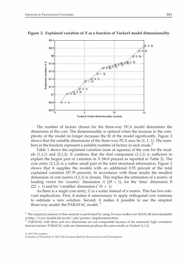
The number of factors chosen for the three-way PCA model determines thedimension of the core. The dimensionality is optimal when the increase in the com-plexity of the model no longer increases the fit of the model significantly. Figure 2shows that the suitable dimensions of the three-way PCA may be (1, 1, 1). The num-bers in the brackets represent a suitable number of factors in each mode.8

Table 1 shows the explained variation (sum of squares) of the core for the mod-els (1,1,1) and (2,1,2). It confirms that the first component (1,1,1) is sufficient toexplain the largest part of variation in X (96.8 percent as reported in Table 2). Thecore entry (2,1,2) is a rather small part of the total structural information. Figure 2shows that it supplies the models with an additional 0.55 percent of the totalexplained variation (97.35 percent). In accordance with these results the smallestdimension of core matrix (1,1,1) is chosen. This implies the estimation of a matrix ofloading vector for ‘country’ dimension A (29 9 1), for the ‘time’ dimension B(22 9 1) and for ‘variables’ dimension C (9 9 1).

As there is a single core entry, G is a scalar instead of a matrix. This has two rele-vant implications. First, it makes it unnecessary to apply orthogonal core rotationsto estimate a new solution. Second, it makes it possible to use the simplestthree-way model: the PARAFAC model. 9

0 5 10 1596.6

96.8

97

97.2

97.4

97.6

97.8

98

98.2

98.4

(1 1 1)

(1 2 2)(1 3 3)

(2 2 1)

(2 1 2)(3 3 1)

(3 1 3)

(2 2 2)(2 3 2)(2 2 3)

(3 2 2)(2 3 3)

(3 2 3)

(3 3 2)

(3 3 3)

Tucker3 model dimensionality (sorted)

Exp

lain

ed v

aria

tion

of X

Figure 2. Explained variation of X as a function of Tucker3 model dimensionality

8 The empirical analysis of this research is performed by using N-ways toolbox for MATLAB (downloadableat http://www.models.life.ku.dk/~pih/parafac/chap0contents.htm).9 PARAFAC with three and two dimensions are not computable because of the extremely high correlationbetween factors. PARAFAC with one dimension produces the same results as Tucker3 (1,1,1).



The estimated coefficients and the fitting of alternative models are very similar.Therefore, the Tucker3 (1,1,1) is chosen because it is the most parsimonious. As thesquares of factor loadings represent the proportion of the total unit variance of theindicator which is explained by the factor, Table 2 reports the estimated squares ofloadings of the matrixes A, B and C estimated by Tucker3 (1, 1, 1). The most relevantvariables of reform towards a market-oriented economy are those for whichckr > 0.11.10 Table 2 reveals that the EBRD’s indicators most relevant to explainingthe variability in the overall index of transition process are: Price liberalization,Trade and Forex system and Small scale privatization.

The choice of three-way PCA vs. a simpler two-way PCA can be explainedon the basis of two main factors. First, three-way PCA is more efficient at maxi-mizing the explained variance of a three-dimensional dataset (97 percent vs. 84

Table 1. Core matrix with dimensionality (1,1,1) and (2,2,2)

G (1,1,1) G (2,2,2)

Index toelements gpqr

Explained var. ofthe core (percent)

Coreentry

Index toelements gpqr

Explained var. ofthe core (percent)

Coreentry

1 1 1 1 100 204.91 1 1 1 99.086 �204.912 2 1 2 0.516 �14.793 2 2 1 0.205 �9.324 1 2 2 0.187 8.91

Table 2. Squared loadings of matrix C estimated by Tucker3 (1,1,1) and PCA

Tucker3 PCA

BR Banking reform & interest rate liberalization 0.089 0.123CP Competition policy 0.062 0.113ER Enterprise restructuring 0.069 0.115LSP Large scale privatization 0.108 0.121PL Price liberalization 0.200 0.112SM Securities markets & non-bank financial institutions 0.063 0.108SSP Small scale privatization 0.172 0.112TS Trade & Forex system 0.173 0.091OIR Overall infrastructure reform 0.064 0.105

Explained variation in X (%) 96.80 84.06

10 By considering that each variable explains the same quota of variability in the index, the loading should be1/9 = 0.111. Therefore, the transition indicators with higher loadings have a major role in the index of overalltransition reform.



percent). Second, two-way PCA makes it harder to interpret the leading factorsof transition reforms. In particular, the greatest variation in transition occurredin the first 5 years and it occurred mainly in the speed of price liberalization,foreign trade liberalization and small scale privatization. The unlike variableshave the highest factor loadings under Tucker3, differently from PCA. To com-pare three-way PCA with the most known two-way PCA, the last two rows ofTable 3 show the overall indexes of transition estimated by two-way PCA and thearithmetic average.11 According to these results three-way PCA is a more appropri-ate methodology compared with two-way PCA because the former better identifiestrend, explains a larger portion of the variance and provides a clear interpretation ofleading factors of transition reforms.

4.2 The overall index of the speed of transition

In this section the loadings of the Tucker3 (1,1,1) are employed to calculate an indexof the speed of transition. This index can be derived in two steps.

Analogously to two-way PCA, the factor loadings are the correlation coefficientsbetween the nine proxies of the transition index and the latent factors. Therefore, thefirst step consists of estimating the overall transition reform index according to thefollowing formula:

TIit ¼ 0:089BRit þ 0:062CPit þ . . .þ 0:064OIRit; ð7Þ

where i = 1, 2,…, 29 (countries) and t = 1989, 1990,…, 2010. Table 3 reports the esti-mated index of transition reforms.

Figure 3 shows the trend of transition index calculated as annual (unweightedand weighted for the GDP per capita at PPP)12 average for the 29 countries of thesample. The dotted line represents the hypothetical gradualist trend to fill the gapbetween the average of minimum and maximum values in 21 years. The graphicalanalysis reveals a nonlinear concave progress of transition reforms towards a decen-tralized economy.

The second step is to calculate the growth rates of the (unweighted) overall indexof transition; this variable is defined throughout the article as the speed of transition(ST). According to this index, 1992 is the year with the highest acceleration ofreform.

Data on ST are used to investigate the relationship with the growth rates of realGDP per capita; the dynamics of speed of transition reforms provide some insightsinto the Big Bang vs. Gradualism controversy. The index of ST is greater than 80 forPoland, the Czech Republic and Russia. No other country experiences such high

11 Details of two-way PCA are available from the authors upon request.12 Missing values in GDP per capita at PPP make it impossible to estimate 24 weights over 638. These missingweights are replaced with the estimated weights of the following year.



Tab

le3.

Ove

rallindex

oftran

sition

reform

s

Cou

ntries

1989

1990

1991

1992

1993

1994

1995

1996

1997

1998

1999

2000

2001

2002

2003

2004

2005

2006

2007

2008

2009

2010

Max

Min

Gap

Alban

ia1.00

1.00

1.17

2.03

2.43

2.56

2.86

2.98

2.98

2.98

3.01

3.28

3.31

3.31

3.31

3.36

3.36

3.38

3.41

3.47

3.51

3.51

3.51

1.00

2.51

Arm

enia

1.00

1.00

1.00

1.81

1.88

1.96

2.48

2.95

3.00

3.12

3.14

3.14

3.26

3.32

3.37

3.43

3.52

3.52

3.52

3.56

3.56

3.56

3.56

1.00

2.56

Azerbaijan

1.00

1.00

1.00

1.33

1.54

1.54

1.90

2.10

2.50

2.72

2.74

2.76

2.82

2.94

2.96

2.99

3.04

3.04

3.04

3.04

3.04

3.04

3.04

1.00

2.04

Belarus

1.00

1.00

1.00

1.33

1.64

1.70

2.21

2.05

1.90

1.63

1.58

1.70

1.83

1.94

2.00

2.00

2.00

2.00

2.03

2.15

2.24

2.31

2.31

1.00

1.31

BiH

1.85

2.05

2.05

1.35

1.35

1.17

1.17

1.59

1.94

2.41

2.41

2.51

2.61

2.73

2.87

2.90

2.93

2.97

3.03

3.12

3.12

3.14

3.14

1.17

1.97

Bulga

ria

1.00

1.17

2.07

2.21

2.41

2.64

2.61

2.63

3.13

3.13

3.29

3.45

3.53

3.58

3.61

3.67

3.69

3.77

3.77

3.81

3.81

3.81

3.81

1.00

2.81

Croatia

1.87

2.07

2.25

2.42

2.68

3.07

3.18

3.36

3.40

3.40

3.45

3.54

3.56

3.61

3.67

3.72

3.72

3.74

3.76

3.76

3.78

3.78

3.78

1.87

1.91

Czech

Rep

.1.00

1.00

2.51

3.10

3.40

3.57

3.57

3.68

3.76

3.78

3.83

3.85

3.88

3.90

3.92

3.94

3.99

3.99

3.99

3.99

3.99

3.99

3.99

1.00

2.99

Eston

ia1.00

1.29

1.55

2.07

2.97

3.42

3.53

3.61

3.70

3.74

3.82

3.89

3.94

3.96

3.96

4.01

4.03

4.07

4.07

4.07

4.07

4.07

4.07

1.00

3.07

Maced

onia

1.85

2.07

2.25

2.31

2.45

2.92

2.98

3.11

3.11

3.16

3.16

3.26

3.26

3.26

3.32

3.46

3.46

3.51

3.53

3.56

3.60

3.60

3.60

1.85

1.75

Geo

rgia

1.00

1.00

1.00

1.47

1.71

1.71

2.32

2.90

3.18

3.27

3.29

3.39

3.39

3.39

3.39

3.42

3.48

3.48

3.54

3.54

3.54

3.54

3.54

1.00

2.54

Hun

gary

1.53

2.14

2.64

2.90

3.27

3.53

3.72

3.78

3.94

3.99

4.01

4.03

4.03

4.03

4.03

4.05

4.09

4.09

4.09

4.09

4.09

4.07

4.09

1.53

2.57

Kaz

akhstan

1.00

1.00

1.00

1.51

1.79

1.95

2.64

3.06

3.21

3.23

3.11

3.13

3.19

3.19

3.21

3.27

3.27

3.32

3.32

3.32

3.29

3.29

3.32

1.00

2.32

Kyrgy

zRep

.1.00

1.00

1.00

1.72

2.16

2.99

3.20

3.22

3.25

3.25

3.28

3.28

3.28

3.30

3.33

3.40

3.40

3.40

3.40

3.40

3.40

3.40

3.40

1.00

2.40

Latvia

1.00

1.00

1.33

2.27

2.69

3.25

3.25

3.44

3.46

3.46

3.54

3.60

3.65

3.76

3.84

3.84

3.86

3.86

3.89

3.89

3.88

3.88

3.89

1.00

2.89

Lith

uania

1.00

1.27

1.33

1.90

2.83

3.14

3.27

3.36

3.40

3.40

3.47

3.54

3.65

3.78

3.81

3.81

3.89

3.91

3.93

3.93

3.93

3.93

3.93

1.00

2.93

Moldov

a1.00

1.00

1.00

1.68

1.95

2.25

2.90

2.92

2.96

3.05

3.05

3.13

3.18

3.18

3.14

3.17

3.28

3.28

3.33

3.39

3.39

3.39

3.39

1.00

2.39

Mon

golia

1.00

1.00

1.50

1.76

2.17

2.17

2.19

2.42

2.87

2.91

3.02

3.09

3.14

3.17

3.30

3.33

3.35

3.35

3.44

3.48

3.48

3.48

3.48

1.00

2.48

Mon

tene

gro

1.85

2.05

2.05

2.07

2.07

1.70

1.70

1.70

1.72

1.33

1.89

2.09

2.22

2.67

2.75

2.80

3.07

3.10

3.20

3.23

3.23

3.27

3.27

1.33

1.93

Poland

1.44

2.60

2.68

2.92

3.29

3.40

3.48

3.62

3.67

3.79

3.79

3.83

3.88

3.88

3.88

3.88

3.95

3.97

3.97

3.97

3.97

4.03

4.03

1.44

2.59

Rom

ania

1.00

1.00

1.41

1.93

2.23

2.68

2.83

2.78

3.11

3.26

3.35

3.41

3.45

3.45

3.47

3.55

3.58

3.62

3.67

3.69

3.69

3.71

3.71

1.00

2.71

Rus

sian

Fed.

1.00

1.00

1.06

2.24

2.57

2.72

2.94

3.20

3.28

2.81

2.78

2.94

3.02

3.15

3.23

3.25

3.24

3.29

3.29

3.29

3.29

3.29

3.29

1.00

2.29

Serbia

1.85

2.05

2.05

2.07

2.07

1.70

1.70

1.70

1.72

1.65

1.65

1.68

2.30

2.69

2.75

2.81

2.95

3.05

3.07

3.18

3.24

3.26

3.26

1.65

1.61

Slov

akRep

.1.00

1.00

2.51

3.02

3.26

3.37

3.41

3.52

3.53

3.59

3.63

3.66

3.71

3.82

3.87

3.92

3.94

3.96

3.96

3.96

3.98

3.96

3.98

1.00

2.98



Tab

le3.

(Con

tinued

)

Cou

ntries

1989

1990

1991

1992

1993

1994

1995

1996

1997

1998

1999

2000

2001

2002

2003

2004

2005

2006

2007

2008

2009

2010

Max

Min

Gap

Slov

enia

1.85

2.12

2.31

2.42

3.09

3.18

3.25

3.39

3.42

3.55

3.58

3.60

3.63

3.65

3.65

3.65

3.65

3.65

3.65

3.67

3.67

3.67

3.67

1.85

1.82

Tajikistan

1.00

1.00

1.00

1.51

1.50

1.50

1.98

2.05

2.11

2.38

2.42

2.59

2.63

2.69

2.69

2.74

2.80

2.83

2.83

2.83

2.85

2.94

2.94

1.00

1.94

Turkm

enistan

1.00

1.00

1.00

1.00

1.00

1.27

1.45

1.45

1.66

1.63

1.63

1.58

1.51

1.51

1.51

1.51

1.51

1.51

1.51

1.74

1.74

1.74

1.74

1.00

0.74

Ukraine

1.00

1.00

1.00

1.10

1.28

1.61

2.44

2.62

2.84

2.78

2.84

2.90

2.93

3.08

3.13

3.15

3.24

3.27

3.32

3.43

3.39

3.39

3.43

1.00

2.43

Uzb

ekistan

1.00

1.00

1.00

1.33

1.57

2.29

2.49

2.49

2.36

2.25

2.13

2.11

2.25

2.25

2.23

2.23

2.29

2.34

2.34

2.34

2.34

2.34

2.49

1.00

1.49

Av.

3PCA

1.21

1.34

158

1.96

2.25

2.45

2.68

2.82

2.94

2.95

3.00

3.07

3.14

3.21

3.25

3.28

3.33

3.35

3.38

3.41

3.42

3.43

3.43

1.21

2.22

Av.

PCA

1.13

1.22

1.39

1.66

1.93

2.13

2.34

2.47

2.58

2.61

2.66

2.72

2.78

2.87

2.90

2.95

3.00

3.03

3.06

3.10

3.11

3.12

3.12

1.13

1.99

Arith.a

ver.

1.13

1.22

1.40

1.68

1.94

2.14

2.35

2.48

2.59

2.62

2.67

2.74

2.80

2.88

2.91

2.96

3.01

3.04

3.07

3.11

3.12

3.13

3.13

1.13

2.00



levels. Croatia and Macedonia are the only countries displaying an index with avalue lower than 20, suggesting a gradual path, whereas Estonia is an active refor-mer country in particular in the years immediately following independence. Serbiaand Montenegro experienced acceleration in reforms later than other countries,around 2000. These patterns are consistent with the general interpretation of Croa-tia’s path as more gradual than Poland’s and with Russia’s as one of the most radi-cal, but not persistent in the former Soviet Union. In the latest years the index isclose to zero if not negative for most countries.

5. Econometric background and model specifications

This section presents the econometric analysis of the relationship between the speedof transition and economic growth.13

Before beginning any econometric estimation, it is important to test the reliabilityof the series to obtain consistent results. It is well established that the non-stationa-rity of the variables can lead to a spurious regression. As a result, unit root tests arecarried out on variables as a first step. Testing for the unit root in panel frameworkis more powerful compared with performing a separate unit root test for each indi-vidual time series (Levin and Lin, 1993). In Appendix B, Table B1 shows several unit

1.0

1.5

2.0

2.5

3.0

3.5

1989

1990

1991

1992

1993

1994

1995

1996

1997

1998

1999

2000

2001

2002

2003

2004

2005

2006

2007

2008

2009

2010

Big Bang Unweighted GDP Gradualist Unweighted GDP

Big Bang Weighted GDP Gradualist Weighted GDP

Figure 3. Weighted and unweighted overall indexes of transition reforms

13 Compared to the 29 countries listed in Table 3, due to the presence of missing values, the following coun-tries are excluded: Azerbaijan, Bosnia and Herzegovina, Montenegro and Turkmenistan.



root tests for the panel data. According to the results, the speed of transition andeconomic growth are stationary. This result implies that these two variables cannotbe cointegrated.

The second step of the analysis is to detect short-run Granger causality runningfrom economic growth – the growth rate of real GDP per capita (Ggdp) – to speed oftransition and/or vice versa.14 This analysis is also useful to specify an appropriatedynamic structure for the multivariate panel models presented in Subsection 5.1.The standard causality test developed by Granger (1969) is widely used to testwhether past changes in one variable help to explain current changes in other vari-ables. The following bivariate regressions are run:

Ggdpij ¼ a0 þ a1Ggdpij�1 þ . . .þ alGgdpij�l þ b1STij�1 þ . . .þ blSTij�l þ uij; ð8Þ

STij ¼ a0 þ a1STij�1 þ . . .þ alSTij�l þ b1Ggdpij�1 þ . . .þ blGgdpij�l þ uij: ð9Þ

The v2- and F- statistics for the joint hypothesis: H0: b1 = b2 = … = bl are reported inTable 4. Two sets of Granger causality tests are shown according to different infor-mation; in particular, Schwartz and Hanan–Quinn information criteria suggest usingtwo lags, whereas Akaike and Final Predictor error information criteria suggestincluding up to eight lags.

Table 4. Granger causality test statistics

Lags Obs H0:Ggdp does notGranger cause ST

H0: ST does not Grangercause Ggdp

Chi-sq(F-stat)

P -value(P-value)

Chi-sq(F-stat)

P -value(P -value)

2† 415 1.993 0.369 81.281 0.000***(0.997) (0.370) (40.640) (0.000***)

8‡ 265 10.360 0.240 38.389 0.000***(1.295) (0.247) (4.799) (0.000***)

Notes: †Optimum lag length according to Schwartz and Hanan–Quinn information criteria.‡Optimum lag length according to Akaike information criterion and Final Predictor error. See L€utkepohl(1991) for details on lag length criteria. Tests performed with Eviews 7.1. *** denotes significance at 1 percentlevel.

14 An interesting avenue of research would be to investigate the relationship between the persistence ofreform (that is the variance of the index of transition) and economic growth. In the econometric estimation wefind some preliminary results that the persistence of reforms also exerts a positive effect on economic growth.However, we prefer to focus the analysis on the speed of transition to provide results comparable with the lit-erature on the optimal speed of transition presented in Section 3.



Table 4 shows robust empirical evidence rejecting the hypothesis that speed oftransition does not Granger cause the growth rate of real GDP. Therefore, Grangercausality runs one-way from ST to Ggdp and not the other way.

The third step of the empirical analysis aims at examining the relationshipbetween the speed of transition and economic growth. In the light of previousresults, (i) ST should be considered as a cause of economic growth instead of viceversa; (ii) ST can be treated as an exogenous variable; and (iii) to preserve an ade-quate sample size, the dynamic panel specification should include at least two lags.

We employ a variety of econometric specifications to test the robustness of theresults: a static model using the least squares dummy variable (LSDV) estimator, adynamic model using LSDV, LSDVC and the system generalized method ofmoment (GMM) estimators.

5.1 Panel data analysis

This section presents a panel data analysis that covers 25 countries with a maximumof 368 annual observations corresponding to the period 1990–2008. As is standard inthe literature, a set of control variables is added to take into account further potentialcauses of the economic growth and reduce the potential omitted-variables bias.

The basic static model is as follows (model I):

Ggdpit ¼di þ kt þ b1STit þ b2ICitþ b3Inflit þ b4Sch2it þ b5ExGrit þ b6PRit þ b7CLitþ eit; ð10Þ

where di are cross-sectional dummies; kt are time dummies. In some regressions thisvariable is substituted with a time trend variable. The variable ST is the speed oftransition. As control variables some of the most common sources of economicgrowth proposed in this strand of literature are included: IC is the initial conditionindex for each country. ‘Initial condition’ is a proxy variable to control for the poten-tial impact of different starting positions on later economic performance, similar toDe Melo et al. (2001), Falcetti et al. (2002, 2006) and Fischer and Sahay (2000), amongothers. The proxy presented in this article consists of a composite index computedon the basis of PCA. The full list of variables used and of details on how to build thiscomposite index are provided in Appendix C. Infl is the annual inflation rate and isincluded to take into account the macroeconomic stabilization policies. In the mainliterature, two alternative variables are used to test the impact of sound macroeco-nomic policies in transition countries: the annual inflation rate and fiscal balanceover GDP. The former is considered here following Radulescu and Barlow (2002),who using extreme bound analysis find that the only robust determinant of growthis inflation. The gross enrolment rate of secondary school (Sch2) is considered to con-trol for human capital. Following Falcetti et al. (2006), we consider: (i) a weightedaverage of real GDP growth in partner trading countries, where the weights are theshare of total exports to each country (ExGr); and (ii) a proxy of civil liberties and




https://www.researchgate.net/publication/222516549_Defying_the_Odds_Initial_Conditions_Reforms_and_Growth_in_the_First_Decade_of_Transition?el=1_x_8&enrichId=rgreq-1a739cf69ca13f2f63d3dde72b50a7a3-XXX&enrichSource=Y292ZXJQYWdlOzI2MTE3OTc1OTtBUzoxNjU2Mzk2Mzc0NDY2NTZAMTQxNjUwMjk3NTI4NQ==


rule of law (CL)15 published by Freedom House. To control for the role of politicalreforms that also happened in the period under study (such as democratization,political competition), an additional proxy of institutional quality is included in theregressions. Following Pavletic and Sattler (2009), we use the political rights index(PR)16 published by Freedom House.

This empirical literature usually includes foreign direct investments as share ofGDP, as a control variable, to examine the effects on a host country’s developmenteffort. However, as it is not statistically significant, it is dropped from the regres-sions to save degrees of freedom.

According to Hausman (1978) tests for correlated random effects, the LSDV esti-mator is consistent. Therefore it is always preferable to random effects in the modelspecification. Anyway, as a robustness check, the estimates obtained by a regressionwith random effects (model II and IIa) are also reported to compare with the corre-sponding model estimated by LSDV (model III and IIIa).

The unrestricted specification including the dummies of interest (cross-sec-tion and/or period effects) are estimated first to test the significance of whichkind of fixed effects should be included in the regressions. Subsequently thejoint significance of all the effects, as well as the joint significance of the cross-section effects and the period effects, are tested separately. The results suggestthat the cross-section and time period effects are statistically significant formodels I and Ia (Table 5) and model IV, V, VI and VII (Table 6), whereascross-section effects are usually not significant when the lagged value of eco-nomic growth is included as explanatory variable in the panel specification.LSDV models are specified by including two-way, one-way and one-way withtime trend instead of period dummies. The main findings are: (i) previousalternative models generate qualitatively similar results; and (ii) the findingschange strongly when moving from static models (from I to IIIa) to dynamicpanel data specifications with the lagged value of the dependent variable.

From residual diagnostics, there is evidence that both random and fixedpanel models exhibit heteroscedasticity and, in the static regressions, also serialcorrelation. To take this into account two estimators are computed: (i) the‘White Period’, which accommodates both arbitrary heteroscedasticity andwithin cross-section serial correlation (Arellano, 1987; White, 1980); and (ii) the‘White Diagonal’, which computes White coefficient covariance estimates thatare robust to observation-specific heteroscedasticity in the disturbances, but not

15 Civil liberties allow for freedom of expression and belief, associational and organizational rights, rule oflaw and personal autonomy without interference from the state (Freedom in the World, 2012, http://www.free-domhouse.org/report/freedom-world-2012/methodology.)16 Political rights enable people to participate freely in the political process, including having the right to votefreely for distinct alternatives in legitimate elections, compete for public office, join political parties and orga-nizations and elect representatives who have a decisive impact on public policies and are accountable to theelectorate (Freedom in the World, 2012).



https://www.researchgate.net/publication/228576530_Institutional_Persistence_or_Reform_Self-Enforcing_Modernization_and_Stagnation_in_Transition_Countries?el=1_x_8&enrichId=rgreq-1a739cf69ca13f2f63d3dde72b50a7a3-XXX&enrichSource=Y292ZXJQYWdlOzI2MTE3OTc1OTtBUzoxNjU2Mzk2Mzc0NDY2NTZAMTQxNjUwMjk3NTI4NQ==

https://www.researchgate.net/publication/239667512_A_Heteroscedastic-Consistent_Covariance_Matrix_and_a_Direct_Test_of_Heteroscedasticity?el=1_x_8&enrichId=rgreq-1a739cf69ca13f2f63d3dde72b50a7a3-XXX&enrichSource=Y292ZXJQYWdlOzI2MTE3OTc1OTtBUzoxNjU2Mzk2Mzc0NDY2NTZAMTQxNjUwMjk3NTI4NQ==

https://www.researchgate.net/publication/4777798_Computing_Robust_Standard_Errors_for_Within-Group_Estimators?el=1_x_8&enrichId=rgreq-1a739cf69ca13f2f63d3dde72b50a7a3-XXX&enrichSource=Y292ZXJQYWdlOzI2MTE3OTc1OTtBUzoxNjU2Mzk2Mzc0NDY2NTZAMTQxNjUwMjk3NTI4NQ==

Tab

le5.

Dep

enden

tvariable:G

rowth

rate

ofreal

GDP–static

mod

el

Mod

elLSDV

(I)

LSDV

(Ia)

Ran

dom

(II)

Ran

dom

(IIa)

LSDV

(III)

LSDV

(IIIa)

ST�0

.076

**(�

1.98

)�0

.079

**(�

2.12

)�0

.178

***

(�3.85

)�0

.181

***

(�3.09

)�0

.154

***

(�3.09

)�0

.160

***

(�3.32

)IC

*t�0

.005

(�1.52

)�0

.006

(�1.58

)�0

.001

(�0.52

)�0

.001

(�0.91

)�0

.004

*(�

1.80

)�0

.005

*(�

1.82

)Inflation

�0.002

***

(�4.40

)�0

.002

***

(�3.79

)�0

.002

***

(�3.84

)�0

.002

***

(�3.71

)�0

.002

***

(�3.52

)�0

.001

***

(�2.84

)2n

dscho

olen

r.rate

�0.210

**(�

2.44

)�0

.224

**(�

2.51

)�0

.112

**(�

2.07

)�0

.100

**(�

1.97

)�0

.282

***

(�2.95

)�0

.274

***

(�2.96

)E9Gr

0.76

6***

(2.57)

0.78

1***

(2.72)

0.74

7***

(3.47)

0.72

4***

(3.27)

0.74

7***

(3.74)

0.75

5***

(4.03)

Political

righ

ts–

�0.422

(�0.63

)–

�0.216

(�0.37

)–

�0.920

(�1.27

)Civillib

ertie

s–

�0.328

(�0.39

)–

0.02

1(0.03)

–0.31

5(0.42)

Tim

etren

d–

–0.60

2***

(5.78)

0.61

4***

(5.23)

0.90

4***

(4.34)

0.89

7***

(4.62)

Cross-effect

Fixed

Fixed

Ran

dom

Ran

dom

Fixed

Fixed

Tim

eeffect

Fixed

Fixed

––

––

Rob

ustS

EW

hite

period

White

period

White

period

White

period

White

period

White

period

Adj-R

20.66

00.65

90.57

10.56

80.60

60.60

6Durbin-W

ats.

1.24

11.24

31.15

61.16

01.28

61.30

9Obs.(N/T)

368

(25/

19)

366

(25/

19)

368

(25/

19)

366

(25/

19)

368

(25/

19)

366

(25/

19)

Note:

***,**

and*den

otesign

ificanc

eat

the1pe

rcen

t,5pe

rcen

tan

d10

percen

tleve

l,resp

ectiv

ely;

constant

anddum

miesva

riab

lesareno

trepo

rted

.The

numbe

rsin

parenthe

sesarethet-ratio

s.Rob

ustC

ovarianc

emetho

dkn

ownas

‘White

Period

’isap

pliedto

LSD

Van

drand

ommod

els

asthey

have

autocorrelated

residua

ls.



to serial correlation. Table 5 shows estimation results from the staticspecification.

In models I and Ia, the coefficient on ST is negative and statistically significant,indicating that the speed of transition has a negative contemporaneous impact onthe growth rate of real GDP. This result is consistent with the theoretical literaturepresented in Section 3. In particular this static specification captures: (i) the outputfall due to the process of ‘creative destruction’ under laisser-faire in a Ramsey-typemodel; and (ii) the trade-off between short and long run in terms of profitability ofreform in the literature on network externalities. Adjustment costs of the reformshave been explored by Nsouli et al. (2005) among others.

As far as control variables are concerned, the coefficient on initial conditionsmultiplied by time is negative, but statistically not significant; the negative coeffi-cient implies that the impact of initial conditions on growth is falling over time,as in Falcetti et al. (2006).17 The coefficient on inflation is negative and significant.This suggests that macroeconomic stabilization in the form of lower inflation ratehas a positive impact on the growth rate of real GDP. The variable enrolment insecondary education is meant to capture human capital. Its coefficient is negativeand significant in the three models. Even if the mainstream literature supports apositive sign, for transition countries there are two main reasons for this result.First, since the fall of the Berlin wall, several transition countries have experi-enced a decreasing trend in the enrolment rates. This path diverges from thewell-known J-curve trend of real GDP observed in transition counties (seeFigure 1). Second, as Murphy et al. (2005, p. 8) point out, although under thecommunist system the universal education was a priority, the type of educationin the transition countries ‘with emphasis on memorization at the expense of ana-lytical and critical thinking, and perhaps premature specialization if not over-spe-cialization may be ill-suited for the needs of a market economy’. AlthoughMurphy et al.’s (2005) findings may support an insignificant effect of the enrol-ment rate on the economic growth for transition countries, the first reason maymotivate the estimated negative sign due to the divergence between the paths ofGDP and enrolment rate.

The coefficient on the control variable ExGr is positive, highlighting the impor-tance of external demand; this variable broadly captures the positive effect of open-ness on growth.

The proxies of institutional context (PR and CL) are not statistically significant(both jointly and separately). This result is consistent with the analytical frameworkpresented in Section 3, which considers reforms such as enterprise restructuring,privatization and price liberalization – all included in our overall index of transition.Moreover, this result is also consistent with previous empirical literature. Falcettiet al. (2002) assume that civil liberties affect reforms, but not growth. Fidrmuc (2003)

17 The IC-index takes a positive value the worse the initial condition. The negative coefficient on the term ICitindicates that the direct negative effect of bad initial conditions declines as transition time goes by.






https://www.researchgate.net/publication/24110174_The_Speed_of_Adjustment_and_the_Sequencing_of_Economic_Reforms_Issues_and_Guidelines_for_Policymakers?el=1_x_8&enrichId=rgreq-1a739cf69ca13f2f63d3dde72b50a7a3-XXX&enrichSource=Y292ZXJQYWdlOzI2MTE3OTc1OTtBUzoxNjU2Mzk2Mzc0NDY2NTZAMTQxNjUwMjk3NTI4NQ==

finds that democracy is highly correlated with liberalization, but it has an ambigu-ous effect on growth.

In models II, IIa, III and IIIa the time trend has been added following Falcettiet al. (2006). The positive and significant coefficient captures the general increase inthe GDP growth rate, after the initial fall shown in Figure 1. The results of models Iand Ia are confirmed in models II, IIa, III and IIIa; the negative coefficient on initialconditions becomes significant in the latter model, where cross-effects are fixed.

Consistent with the dynamic properties of Ggdp and ST, dynamic versions of theprevious regression (models from IV to XII) are also estimated.18 Following Falcettiet al. (2006), from models VI–IX the current value of ST as explanatory variable forgrowth is excluded. Differently from their analysis, in these models a longer lagstructure for the variable ST is included. This model specification implies theassumption that the structural reforms do not only have a short-run effect on theeconomic growth. In particular, lagging up to 5 years implies a sufficient time totake into account almost all the effects of reforms on the economic system. Thebenchmark dynamic specification is an autoregressive distributed lag (ADL) model,(model VII):

Ggdpit ¼ kt þ b1Ggdpit�1 þ b2STit þ b3STit�1 þ . . .þ b7STit�5 þ b8ICitþ b9Inflitþ b10Sch2it þ b11ExGrit þ eit: ð11Þ

As Nickell (1981) demonstrates, the LSDV estimator for autoregressive paneldata models is not consistent for finite time periods. Kiviet (1995) suggests an alter-native estimator (LSDVC) to correct downward-biased estimates in the LSDV esti-mator with a lagged dependent variable. LSDV (model X) and LSDVC (model XI)estimates are compared to have evidence of the size and consequences of this bias.Even though LSDVC estimates may be unreliable for a misspecification of fixedeffects, these estimates are useful to verify that downward-biased coefficients of theLSDV estimator do not have a relevant effect on the findings. Table 6 shows the esti-mation results for the dynamic specification.

Models IV–VI includes different lags of ST. Model IV includes two lags of ST inaddition to the contemporaneous value; the coefficients on 1-year and 2-year lagsare not statistically significant whereas the speed of transition has (still) a negativecontemporaneous impact on the GDP growth rate. Therefore, with few lags the neg-ative effect prevails. The signs of the control variables are unchanged, confirmingthe previous results. Model V introduces lagged ST at time t�2, t�3 and t�4: thecoefficient on the 2-year lag is negative as in model IV, whereas the coefficients onthe 3-year and 4-year lags are positive and statistically significant. This dynamicspecification further supports the results of the static specification on the trade-offbetween short-run costs and long-term benefits of the speed of reforms, consistently

18 As Civil Liberties and Political Rights are also not statistically significant they are dropped from the regres-sions, in the dynamic specification, to save degrees of freedom.







Tab

le6.

Dep

enden

tvariable:G

rowth

rate

ofreal

GDP–dyn

amic

mod

el(LSDV/LSDVC)

LSDV

(IV)

LSDV

(V)

LSDV

(VI)

LSDV

(VII)

LSDV

(VIII)

LSDV

(IX)

LSDV

(X)

LSDVC(XI)

ST�0

.109

**(�

2.45

)–

�0.006

(�0.11

)0.03

8(0.61)

––

––

STt�

1�0

.041

(�1.43

)–

0.02

9(0.70)

�0.017

(�0.35

)�0

.017

(�0.35

)–

�0.022

(�0.38

)�0

.022

(�0.38

)ST

t�2

�0.035

(�1.48

)�0

.023

(�0.52

)�0

.008

(�0.40

)0.06

3(1.61)

0.05

7*(1.52)

0.03

5(1.00)

0.07

3*(1.82)

0.07

4**

(1.83)

STt�

3–

0.05

1**

(2.06)

0.05

2***

(2.78)

0.04

9*(1.72)

0.05

1*(1.81)

0.05

1*(1.76)

0.03

8(1.39)

0.04

7(1.33)

STt�

4–

0.04

5**

(2.55)

–0.02

6**

(2.09)

0.02

2**

(2.21)

0.02

2**

(2.24)

0.01

3(1.32)

0.01

1(0.62)

STt�

5–

––

0.02

4**

(2.15)

0.02

3**

(2.09)

0.02

4**

(2.09)

0.01

4(1.33)

0.01

3(0.02)

Ggd

pt�

1–

–0.27

5***

(2.83)

0.43

9***

(6.93)

0.43

0***

(6.71)

0.41

2***

(6.45)

0.29

5***

(4.65)

0.37

6***

(4.22)

IC*t

�0.006

*(�

1.66

)�0

.005

(�1.13

)�0

.003

*(�

1.77

)�0

.002

***

(�4.42

)�0

.002

***

(�4.55

)�0

.002

***

(�4.74

)�0

.001

(�0.32

)0.00

0(0.01)

Inflation

�0.002

***

(�4.08

)�0

.002

*(�

1.83

)�0

.001

***

(�3.66

)�0

.009

**(�

2.04

)�0

.001

**(�

2.13

)�0

.009

**(�

2.03

)�0

.013

**(�

2.13

)�0

.012

***

(�2.77

)2n

dsch.

enrol.

�0.208

**( �

2.24

)�0

.120

(�1.58

)�0

.088

(�1.59

)0.02

8(1.25)

�0.003

(1.21)

0.02

8(1.20)

0.03

1(0.71)

0.03

0(0.40)



Tab

le6.

(Con

tinued

)

LSDV

(IV)

LSDV

(V)

LSDV

(VI)

LSDV

(VII)

LSDV

(VIII)

LSDV

(IX)

LSDV

(X)

LSDVC(XI)

E9

Gr

0.74

6**

(2.22)

1.13

6***

(2.76)

0.68

6**

(2.24)

�0.018

(�0.13

)�0

.028

(�0.20

)–

0.50

5***

(2.81)

0.43

3(0.08)

Tim

etren

d–

––

––

–0.26

4*(1.85)

0.19

9(0.353

)

Cross

-effect

Fixed

Fixed

Fixed

––

–Fixed

Fixed

Tim

eeffect

Fixed

Fixed

Fixed

Fixed

Fixed

Fixed

––

Rob

ustS

EW

hite

period

White

period

White

diago

nal

White

diago

nal

White

diago

nal

White

diago

nal

White

diago

nal

Kiviet

Adj-R

20.44

90.53

60.64

00.50

60.50

60.49

30.46

7–

Durb-W

ats

1.24

91.05

01.60

21.62

91.62

81.74

81.60

3–

Obs.

(N/T)

293

(25/

14)

317

(25/

15)

338

(25/

16)

293

(25/

14)

293

(25/

14)

297

(25/

14)

293

(25/

14)

293

(25/

14)

Note:

***,**

and*den

otesign

ificanc

eat

the1pe

rcen

t,5pe

rcen

tan

d10

percen

tleve

l,resp

ectiv

ely;

constant

anddum

miesva

riab

lesareno

trepo

rted

.The

numbe

rsin

parenthe

sesarethet-ratio

s.Rob

ustC

ovarianc

emetho

dkn

ownas

‘White

Period

’isap

pliedto

LSD

Van

drand

ommod

elIV

asthey

have

autocorrelated

residu

als.Fo

rmod

elwith

lagg

eddep

enden

tvalue

(from

Vto

IX)c

ompu

tedstan

darderrors

arerobu

stto

observa-

tionsp

ecifiche

terosced

astic

ityin

thedisturban

ces,bu

tare

notrob

usttocorrelationbe

tweenresidua

lsfordifferen

tobserva

tions.F

orLSD

VCKiviet

(1995)

correctio

nestim

ator

isap

plied.T

heconsistent

estim

ator

chosen

toinitializethebias

correctio

nistheAnd

ersonan

dHsiao

(1982)

estim

ator.



with the analytical framework presented in Section 3. The other models test therobustness of the previous results. In particular, model VI includes lags from zero tothree of ST and the lagged growth rate of real GDP.

Model VII and VIII and IX includes up to five lags of ST. In model VII the coeffi-cients on ST from t to t�2 are not statistically significant whereas the lagged termsfrom 3 up to 5 years have positive effects on economic growth. With respect tomodel VI, the coefficient not only on the third lag of ST is positive and significantbut also on the fourth and fifth lags, suggesting that the benefits of past level ofreforms last some years. The signs of the coefficients on the control variables areunchanged; the variable initial condition is significant, whereas the proxy on humancapital is not statistically significant. The same conclusions apply to models VIII andIX, which, respectively, do not include contemporaneous value of ST and lag fromzero to one of ST.

Models X and XI include a time trend instead of time dummies. This is an indi-rect test of the size of downward bias in the estimates of LSDV estimator withlagged dependent variable. The comparison between the estimates of the LSDV esti-mator (the model X) and the LSDVC19 estimates (model XI) shows that the down-ward bias has no relevant effect on statistical significance and estimates of the mainfindings. For the sake of brevity, Table 6 omits regressions with the lagged values ofenrolment in secondary education and inflation. These estimates confirm the previ-ous analysis in which the exclusion of the annual inflation rate becomes insignifi-cant. According to this result, the system GMM estimator proposed by Arellano andBover (1995) and Blundell and Bond (1998) is considered appropriate to account forthe potential endogeneity of the explanatory variables.20 Bond et al. (2001) recom-mend the use of the system GMM estimator for growth empirics. This is due to thefact that the number of periods used in the standard growth literature is usuallysmall21 and the variables considered are generally persistent. Some literature ontransition reforms and growth also investigates the effectiveness of system GMM(De Melo et al., 2001; Falcetti et al., 2006).

To implement this GMM approach the lagged dependent variable (growth rateof real GDP) and the inflation rate are treated as endogenous; the indices of speed oftransition and gross enrolment rate of secondary school are handled as predeter-mined; initial conditions and external demand are strictly exogenous.

Following Roodman (2009a,b) one of the main drawback in implementingsystem GMM is that too many instruments can overfit endogenous variables andfail to remove their endogenous components. Roodman (2009a) suggests two

19 This change in the model specification is due to the unavailability of a LSDVC estimator for a model withtwo-way fixed effects.20 Blundell and Bond (2000) argue that the first-difference GMM (Arellano and Bond, 1991) using persistentseries performs poorly due to weak instruments because lagged levels are only weakly correlated with subse-quent first differences.21 The number of instruments tends to explode with T in panel GMM estimations. This makes the GMM esti-mator only applicable when T (time period) is small.




https://www.researchgate.net/publication/4753417_GMM_Estimation_and_Empirical_Growth_Models?el=1_x_8&enrichId=rgreq-1a739cf69ca13f2f63d3dde72b50a7a3-XXX&enrichSource=Y292ZXJQYWdlOzI2MTE3OTc1OTtBUzoxNjU2Mzk2Mzc0NDY2NTZAMTQxNjUwMjk3NTI4NQ==

main techniques to overcome this issue: first, to use only certain lags instead ofall available lags for instruments; and second, to combine instruments throughaddition into smaller sets (so-called instruments collapsing). We apply both tech-niques: lags 2 (lag 1) through 4 (3) are included for the equation in differences,and lag 1 (lag 0) through 4 (3) for the level equation for endogenous (predeter-mined) variables.22

To verify the reliability of the GMM estimates, the robust version of Sargan’s(1958) test (Hansen J-statistic) is applied to check for the validity of instrumentalvariables. As we have an unbalanced panel with gaps, the sample is maximizedby using the forward orthogonal deviation (Arellano and Bover, 1995) instead ofthe first-difference approach. Finally, we report standard error estimates com-puted by Windmeijer’s (2005) finite-sample correction for the two-step covariancematrix.

Table 7 shows the estimation results for the system GMM estimator.First, Table 7 provides additional evidence in favour of previous results. In par-

ticular, Models XII and XIII include contemporaneous values of ST. These regres-sions reveal that ST has a negative impact on the GDP growth rate. Models XIV–XIX introduce lagged values of ST. The coefficients on ST at different lags confirmthat the speed of transition does not have a significant impact on growth in the shortterm, whereas in the third year the impact becomes positive and significant. Similarto Staehr (2005), the coefficient on lagged GDP growth rate is positive and statisti-cally significant, reflecting that it tracks its past trends and, on an annual basis, thereare no strong divergences in GDP from its long-run path. Similar to previous esti-mates, when the specification includes a larger time horizon of ST (Models XVIIIand XIX), the impact of ST on economic growth becomes positive. Therefore, thespeed of transition exerts an immediate negative, and not significant, impact ongrowth as the adjustment costs prevail in the years immediately following the tran-sition. Similar to previous literature (Selowsky and Martin, 1997; Merlevede, 2003,among others), in a longer horizon – after 3 years – the relationship flips and thespeed of transition positively affects the growth rate of real GDP.

The signs of the control variables are similar to LSDV, but often become statisti-cally insignificant. As long as initial conditions and the secondary enrolment ratioare concerned, the results coming from GMM estimation are consistent with thefindings of Murphy et al. (2005).

As the estimates of speed of transition are not robust between the dynamic andstatic model, dynamic regression is the best choice to examine the effect of ST oneconomic growth for a variety of reasons: (i) the statistically significant coefficients

22 Roodman (2009a) suggests the inclusion of time dummies to make the hypothesis of no correlation acrosscountries in the idiosyncratic disturbances more likely to hold. However, in our sample if time dummies areincluded in model specifications the number of instruments exceed the number of countries (i.e., ‘rule ofthumb’ of preserving estimates by the inclusion of too many instruments does not hold). Taking into accountthat there is also empirical evidence that time dummies are, both jointly and separately, insignificantly differ-ent from zero, we opt not to include time dummies in the estimated regressions.



https://www.researchgate.net/publication/4990276_Reform_reversals_and_output_growth_in_transition_economies?el=1_x_8&enrichId=rgreq-1a739cf69ca13f2f63d3dde72b50a7a3-XXX&enrichSource=Y292ZXJQYWdlOzI2MTE3OTc1OTtBUzoxNjU2Mzk2Mzc0NDY2NTZAMTQxNjUwMjk3NTI4NQ==

https://www.researchgate.net/publication/5163954_Reforms_and_Economic_Growth_in_Transition_Economies_Complementarity_Sequencing_and_Speed?el=1_x_8&enrichId=rgreq-1a739cf69ca13f2f63d3dde72b50a7a3-XXX&enrichSource=Y292ZXJQYWdlOzI2MTE3OTc1OTtBUzoxNjU2Mzk2Mzc0NDY2NTZAMTQxNjUwMjk3NTI4NQ==

https://www.researchgate.net/publication/4726051_Policy_Performance_and_Output_Growth_in_the_Transition_Economies?el=1_x_8&enrichId=rgreq-1a739cf69ca13f2f63d3dde72b50a7a3-XXX&enrichSource=Y292ZXJQYWdlOzI2MTE3OTc1OTtBUzoxNjU2Mzk2Mzc0NDY2NTZAMTQxNjUwMjk3NTI4NQ==

https://www.researchgate.net/publication/223928547_Another_Look_at_Instrumental_Variable_Estimation_of_Error_Component_Models?el=1_x_8&enrichId=rgreq-1a739cf69ca13f2f63d3dde72b50a7a3-XXX&enrichSource=Y292ZXJQYWdlOzI2MTE3OTc1OTtBUzoxNjU2Mzk2Mzc0NDY2NTZAMTQxNjUwMjk3NTI4NQ==

Tab

le7.

Dep

enden

tvariable:G

rowth

rate

ofreal

GDP–dyn

amic

mod

el(system

GMM)

Mod

elGMM

(XII)

GMM

(XIII)

GMM

(XIV

)GMM

(XV)

GMM

(XVI)

GMM

(XVII)

GMM

(XVIII)

GMM

(XIX)

ST�0

.188

***

(�2.93

)�0

.175

***

(�2.87

)�0

.191

***

(�2.92

)�0

.188

***

(�2.87

)�0

.190

***

(�3.04

)�0

.165

***

(�2.48

)�0

.025

(�0.44

)�0

.002

(�0.03

)ST

t�1

––

0.01

5(0.18)

0.00

6(0.11)

�0.015

(�0.30

)�0

.010

(�0.20

)0.03

7(1.21)

0.01

8(0.40)

STt�

2–

––

––

0.00

7(0.22)

�0.007

(�0.27

)�0

.039

(�0.85

)ST

t�3

––

––

––

0.04

3*(1.79)

0.05

2**

(2.11)

STt�

4–

––

––

––

0.00

2(0.18)

Ggd

p t�1

0.46

7***

(3.20)

0.47

7**

(2.69)

0.47

1**

(2.72)

0.44

2***

(3.21)

0.42

5***

(3.33)

0.50

8***

(4.04)

0.58

5***

(6.55)

0.57

8***

(6.99)

IC*t

�0.001

(0.76)

�0.001

**(�

2.34

)�0

.001

*(�

1.94

)0.00

2(1.01)

�0.001

(�0.76

)�0

.001

(�1.62

)0.00

0(0.16)

�0.001

(�0.59

)Inflation

�0.001

(�0.46

)�0

.001

(�0.46

)�0

.001

(�0.53

)�0

.001

(�0.59

)–

––

–

2ndsch.enr.

�0.104

(�1.22

)0.01

9(0.84)

0.02

0(0.76)

�0.173

(�1.69

)0.02

6(1.59)

0.02

9*(1.92)

0.00

2(0.19)

0.00

9(0.58)

E9Gr

0.44

3*(1.91)

0.24

5(0.93)

0.24

9(0.88)

0.50

5*(1.86)

0.65

1*(1.87)

0.53

9*(1.86)

0.66

4**

(2.46)

0.68

3*(2.02)

Tim

etrend

–0.14

2(0.331

)0.13

8(0.95)

––

––

–



Tab

le7.

(Con

tinued

)

Mod

elGMM

(XII)

GMM

(XIII)

GMM

(XIV

)GMM

(XV)

GMM

(XVI)

GMM

(XVII)

GMM

(XVIII)

GMM

(XIX)

Con

stan

t10

.63

(1.49)

––

16.26*

(1.92)

––

––

#instrumen

ts23

2324

2418

1920

21

Han

sen(P-value

)0.17

50.14

60.11

40.17

10.41

30.33

50.69

60.69

6

GMM

instrumen

tsforleve

ls†:(P-value

)Exclud.G

r.‡

0.31

30.07

00.04

20.33

70.08

40.16

80.81

20.93

5Differen

ce§

0.12

20.73

00.84

30.10

10.95

40.89

80.28

10.08

3

IV†:(P-value

)Exclud.G

r.‡

0.10

40.35

80.31

10.08

60.18

80.26

50.66

30.64

4Differen

ce§

0.90

90.05

30.05

70.84

60.37

10.48

20.53

40.41

8Obs.(#

coun

t.)36

1(25)

361(25)

361(25)

361(25)

361(25)

356(25)

338(25)

317(25)

Notes:**

*,**

and*den

otesign

ificanc

eat

the1pe

rcen

t,5pe

rcen

tan

d10

percen

tleve

l,resp

ectiv

ely;

constant

anddum

miesva

riab

lesareno

trepo

rted

.The

numbe

rsin

parenthe

sesarethet-ratio

s.†D

ifferen

ce-in

-Han

sentestsof

exog

eneity

ofinstrumen

tsub

sets.P

-value

sgreaterthan

usua

lsignificanc

eleve

lsim

plythat

wecann

otreject

thenu

llthat

theinstrumen

tsus

edin

GMM

andIV

partsareva

lid.

‡Han

sentest

exclud

inggrou

p.The

nullhy

pothesisisthat

exclud

edinstrumen

ts,a

sagrou

p,areno

tcorrelated

with

inde

pend

entva

riab

les(tho

sewhich

wereassu

med

tobe

endog

enou

s).

§The

nullhy

pothesisisthat

theinstrumen

tsareexog

enou

s.



on Ggdpt–1 and STt–i; (ii) the Granger causality test performed in the previous sec-tion; (iii) the reduction in the autocorrelation in the residuals shown by the Durbin–Watson statistics; and (iv) the robustness of the main results using the LSDV,LSDVC and system GMM estimators.

According to these findings, there is adequate empirical support that thebig bang approach to transition reforms has better consequences for economicperformance. These effects become observable only after a time lag of (at least)three years. Thus, empirical analysis reveals that the reform transition processcannot be evaluated in the (very) short term, but the process causes anincrease in growth rate of GDP after 3 to 5 years. Consistently with the strandof theoretical literature presented in Section 3, transition causes an output fallat the beginning of the process.

6. Conclusions

This article examines the effects of the speed of transition on the growth rate of realGDP in a sample of transition countries in the period 1990–2008. It first introduces anew methodological approach to estimate an overall index of transition reformsusing three-way PCA (Tucker3). This methodology is more appropriate than thetwo-way PCA or simple average generally used in this strand of literature (Fidrmuc,2003; Falcetti et al., 2006, among others). This result may itself be a valuable contri-bution to the existing literature. Then, we test if the new index of transition reformscorroborates the main results of the literature on the link between the speed of tran-sition and economic growth. Our analysis benefits from a wider sample size(18 years), which allows a lag structure more complex than that employed in theprevious literature, more sophisticated approaches to estimating the index of transi-tion reform and several estimation approaches to investigating the relationshipbetween growth and speed of transition reforms.

The main results are as follows. First, Granger causality analysis revealsthat the growth rate of real GDP does not cause speed of transition as Grangercausality runs one-way only from speed of transition to economic growth.Second, in the static specification the speed of reforms has a contemporaneousnegative impact on economic growth. In the dynamic specification, the pastlevel of reforms leads to higher economic growth and this effect reaches itsgreatest value with a lag of 3 years. Therefore, the speed of transition has aJ-curve effect on GDP growth: a negative contemporaneous effect which ismore than compensated by subsequent gains. In this respect, a big bangapproach to transition delivers benefits in the longer term which offset the ini-tial adjustment costs. This result is robust to different models’ specificationsand econometric approaches. The presence of this trade-off between short andlong run is also consistent with the theoretical literature (Sacco and Scarpa,2000; Castanheira, 2003, among others). Third, other factors affect economic




https://www.researchgate.net/publication/4864739_Critical_mass_effect_and_restructuring_in_the_transition_towards_a_market_economy?el=1_x_8&enrichId=rgreq-1a739cf69ca13f2f63d3dde72b50a7a3-XXX&enrichSource=Y292ZXJQYWdlOzI2MTE3OTc1OTtBUzoxNjU2Mzk2Mzc0NDY2NTZAMTQxNjUwMjk3NTI4NQ==





growth in transition countries; however, their impacts are not robust to differ-ent estimators. Although external demand seems to drive economic growth forany estimator, the statistical significance of initial conditions and macroeco-nomic stabilization programmes is not robust when controlling for endogeneityby system GMM.

The results presented in this article can offer some avenues for future research.The reduced form model used in the estimations cannot capture the entire mecha-nism through which the speed of reforms affects economic outcomes or the role thatgovernment can play in reaching the optimal speed of transition. From a theoreticalpoint of view, a dynamic general equilibrium model would be an appropriateframework to analyze these issues. Another interesting extension in this empiricalliterature may be to investigate the relationship between the persistence of transitionreforms and economic growth. This topic, partially missing in this strand of litera-ture, is on our agenda for future research.

References

Aghion, P. and Blanchard, O. J. (1994). ‘On the speed of transition in Central Europe’, inFischer, S. and Rotemberg, J. (eds), NBER Macroeconomics Annual 1994, Cambridge, MA:The MIT Press, pp. 283–319.

Anderson, T. W. and Hsiao, C. (1982). ‘Formulation and estimation of dynamic models usingpanel data’, Journal of Econometrics, 18, pp. 47–82.

Arellano, M. (1987). ‘Computing robust standard errors for within-groups estimators’, OxfordBulletin of Economics and Statistics, 49, pp. 431–434.

Arellano, M. and Bond, S. (1991). ‘Some tests of specification for panel data: Monte Carlo evi-dence and an application to employment equations’, Review of Economic Studies, 58, pp.277–297.

Arellano, M. and Bover, O. (1995). ‘Another look at the instrumental-variable estimation oferror-components models’, Journal of Econometrics, 68, pp. 29–51.

Barbieri, P., Andersson, C. A., Massart, L. D., Predonzani, S., Adami, G. and Reisenhofer, E.(1999). ‘Modeling bio-geochemical interactions in the surface waters of the Gulf ofTrieste by 3-way principal component analysis (PCA)’, Analytica Chimica Acta, 398, pp.227–235.

Berg, A., Borensztein, E., Sahay, R. and Zettelmeyer, J. (1999). ‘The evolution of output intransition economies: Explaining the differences’, IMF Working Paper, WP/99/73(Washington, DC: IMF).

Blanchard, O., Dornbusch, R., Krugman, P., Layard, R. and Summers, L. (1991). Reform in East-ern Europe, Cambridge, MA: The MIT Press.

Blundell, R. and Bond, S. (1998). ‘Initial conditions and moment restrictions in dynamic paneldata models’, Journal of Econometrics, 87, pp. 115–143.

Blundell, R. and Bond, S. (2000). ‘GMM Estimation with persistent panel data: An applicationto production functions’, Econometric Reviews, 19(3), pp. 321–340.

Bond, S. R., Hoeffler, A. and Temple, J. (2001). ‘GMM estimation of empirical growth models’,Discussion Paper No. 2048, London: Centre for Economic Policy Research.



https://www.researchgate.net/publication/5177040_On_the_Speed_of_Transition_in_Central_Europe?el=1_x_8&enrichId=rgreq-1a739cf69ca13f2f63d3dde72b50a7a3-XXX&enrichSource=Y292ZXJQYWdlOzI2MTE3OTc1OTtBUzoxNjU2Mzk2Mzc0NDY2NTZAMTQxNjUwMjk3NTI4NQ==



https://www.researchgate.net/publication/223823705_Formulation_and_Estimation_of_Dynamic_Models_Using_Panel_Data?el=1_x_8&enrichId=rgreq-1a739cf69ca13f2f63d3dde72b50a7a3-XXX&enrichSource=Y292ZXJQYWdlOzI2MTE3OTc1OTtBUzoxNjU2Mzk2Mzc0NDY2NTZAMTQxNjUwMjk3NTI4NQ==

https://www.researchgate.net/publication/223823705_Formulation_and_Estimation_of_Dynamic_Models_Using_Panel_Data?el=1_x_8&enrichId=rgreq-1a739cf69ca13f2f63d3dde72b50a7a3-XXX&enrichSource=Y292ZXJQYWdlOzI2MTE3OTc1OTtBUzoxNjU2Mzk2Mzc0NDY2NTZAMTQxNjUwMjk3NTI4NQ==



https://www.researchgate.net/publication/239152372_Modeling_bio-geochemical_interactions_in_the_surface_waters_of_the_Gulf_of_Trieste_by_3-way_principal_component_analysis_PCA?el=1_x_8&enrichId=rgreq-1a739cf69ca13f2f63d3dde72b50a7a3-XXX&enrichSource=Y292ZXJQYWdlOzI2MTE3OTc1OTtBUzoxNjU2Mzk2Mzc0NDY2NTZAMTQxNjUwMjk3NTI4NQ==




https://www.researchgate.net/publication/30525774_Reform_in_Eastern_Europe?el=1_x_8&enrichId=rgreq-1a739cf69ca13f2f63d3dde72b50a7a3-XXX&enrichSource=Y292ZXJQYWdlOzI2MTE3OTc1OTtBUzoxNjU2Mzk2Mzc0NDY2NTZAMTQxNjUwMjk3NTI4NQ==

https://www.researchgate.net/publication/30525774_Reform_in_Eastern_Europe?el=1_x_8&enrichId=rgreq-1a739cf69ca13f2f63d3dde72b50a7a3-XXX&enrichSource=Y292ZXJQYWdlOzI2MTE3OTc1OTtBUzoxNjU2Mzk2Mzc0NDY2NTZAMTQxNjUwMjk3NTI4NQ==



https://www.researchgate.net/publication/24079517_GMM_Estimation_With_Persistent_Panel_Data_An_Application_to_Production_Functions?el=1_x_8&enrichId=rgreq-1a739cf69ca13f2f63d3dde72b50a7a3-XXX&enrichSource=Y292ZXJQYWdlOzI2MTE3OTc1OTtBUzoxNjU2Mzk2Mzc0NDY2NTZAMTQxNjUwMjk3NTI4NQ==

https://www.researchgate.net/publication/24079517_GMM_Estimation_With_Persistent_Panel_Data_An_Application_to_Production_Functions?el=1_x_8&enrichId=rgreq-1a739cf69ca13f2f63d3dde72b50a7a3-XXX&enrichSource=Y292ZXJQYWdlOzI2MTE3OTc1OTtBUzoxNjU2Mzk2Mzc0NDY2NTZAMTQxNjUwMjk3NTI4NQ==



https://www.researchgate.net/publication/5126951_The_Evolution_of_Output_in_Transition_Economies_-_Explaining_the_Differences?el=1_x_8&enrichId=rgreq-1a739cf69ca13f2f63d3dde72b50a7a3-XXX&enrichSource=Y292ZXJQYWdlOzI2MTE3OTc1OTtBUzoxNjU2Mzk2Mzc0NDY2NTZAMTQxNjUwMjk3NTI4NQ==



https://www.researchgate.net/publication/4859318_Initial_Conditions_and_Moment_Restrictions_in_Dynamic_Panel_Data_Models?el=1_x_8&enrichId=rgreq-1a739cf69ca13f2f63d3dde72b50a7a3-XXX&enrichSource=Y292ZXJQYWdlOzI2MTE3OTc1OTtBUzoxNjU2Mzk2Mzc0NDY2NTZAMTQxNjUwMjk3NTI4NQ==

https://www.researchgate.net/publication/4859318_Initial_Conditions_and_Moment_Restrictions_in_Dynamic_Panel_Data_Models?el=1_x_8&enrichId=rgreq-1a739cf69ca13f2f63d3dde72b50a7a3-XXX&enrichSource=Y292ZXJQYWdlOzI2MTE3OTc1OTtBUzoxNjU2Mzk2Mzc0NDY2NTZAMTQxNjUwMjk3NTI4NQ==

Bruno, R. L. (2006). ‘Optimal speed of transition with a shrinking labour force and underuncertainty’, Economics of Transition, 14(1), pp. 69–100.

Castanheira, M. (2003). ‘Public finance and the optimal speed of transition uncertainty’, Eco-nomics of Transition, 11(3), pp. 435–462.

Choi, I. (2001). ‘Unit root tests for panel data’, Journal of International Money and Finance, 20,pp. 249–272.

De Melo, M., Denizer, C., Gelb, A. and Tenev, S. (2001). ‘Circumstances and choice: The roleof initial conditions and policies in transition economies’, World Bank Economic Review, 15(1), pp. 1–31.

Di Tommaso, M. L., Raiser, M. and Weeks, M. (2007). ‘Home grown or imported? Initial con-ditions, external anchors and the determinants of institutional reform in the transitioneconomies’, The Economic Journal, 117, pp. 858–881.

Falcetti, E., Raiser, M. and Sanfey, P. (2002). ‘Defying the odds: Initial conditions,reforms, and growth in the first decade of transition’, Journal of Comparative Econom-ics, 30, pp. 229–250.

Falcetti, E., Lysenko, T. and Sanfey, P. (2006). ‘Reforms and growth in transition: Re-examin-ing the evidence’, Journal of Comparative Economics, 34(3), pp. 421–445.

Feltenstein, A. and Nsouli, S. M. (2003). ‘“Big Bang” versus gradualism in economic reforms:An intertemporal analysis with an application to China’, IMF Staff Papers, 50(3), pp. 458–480.

Fidrmuc, J. (2003). ‘Economic reform, democracy and growth during post-communist transi-tion’, European Journal of Political Economy, 19, pp. 583–604.

Fidrmuc, J. and Tichit, A. (2009). ‘Mind the break! Accounting for changing patterns of growthduring transition’, Economic System, 33(2), pp. 138–154.

Fischer, S., Gelb, A. (1991). ‘The process of socialist economic transformation’, Journal of Eco-nomic Perspectives, 5, pp. 91–106.

Fischer, S. and Sahay, R. (2000). ‘The transition economies after ten years’, Working Paper No.00/30, Washington, DC: IMF.

Foster, N. and Stehrer, R. (2007). ‘Modeling transformation in CEECs using smooth transi-tions’, Journal of Comparative Economics, 35, pp. 57–86.

Granger, C. W. J. (1969). ‘Investigating causal relations by econometric models and cross-spec-tral methods’, Econometrica, 37(3), pp. 424–438.

Hausman, J. (1978). ‘Specification tests in econometrics’, Econometrica, 46, pp. 1251–1272.Henrion, R. (1994). ‘N-way principal component analysis theory, algorithms and applica-

tions’, Chemometrics and Intelligent Laboratory Systems, 25, pp. 1–23.Im, K. S., Pesaran, H. M., Shin, Y. (2003). ‘Testing for unit roots in heterogeneous panels’, Jour-

nal of Econometrics, 115, pp. 53–74.Kiviet, J. F. (1995). ‘On bias, inconsistency, and efficiency of various estimators in dynamic

panel models’, Journal of Econometrics, 68, pp. 53–78.Kornai, J. (1990). The Road to a Free Economy, New York: Norton.Kroonenberg, P. M. (1983). Three-mode Principal Component Analysis: Theory and Applications,

Leiden, The Netherlands: DSWO Press.Kroonenberg, P. M. (1992). ‘‘Three-mode component models: A survey of the literature’, stat-

istica applicata’, Italian Journal of Applied Statistics, 4(4), pp. 619–633.Kroonenberg, P. M. (2008). Applied Multiway Data Analysis, New Jersey: Wiley Interscience,

John Wiley & Sons.










https://www.researchgate.net/publication/256509140_N-way_Principal_Component_Analysis_Theory_Algorithms_and_Applications?el=1_x_8&enrichId=rgreq-1a739cf69ca13f2f63d3dde72b50a7a3-XXX&enrichSource=Y292ZXJQYWdlOzI2MTE3OTc1OTtBUzoxNjU2Mzk2Mzc0NDY2NTZAMTQxNjUwMjk3NTI4NQ==

https://www.researchgate.net/publication/256509140_N-way_Principal_Component_Analysis_Theory_Algorithms_and_Applications?el=1_x_8&enrichId=rgreq-1a739cf69ca13f2f63d3dde72b50a7a3-XXX&enrichSource=Y292ZXJQYWdlOzI2MTE3OTc1OTtBUzoxNjU2Mzk2Mzc0NDY2NTZAMTQxNjUwMjk3NTI4NQ==





https://www.researchgate.net/publication/4894847_Home_Grown_or_Imported_Initial_Conditions_External_Anchors_and_the_Determinants_of_Institutional_Reform_in_the_Transition_Economies?el=1_x_8&enrichId=rgreq-1a739cf69ca13f2f63d3dde72b50a7a3-XXX&enrichSource=Y292ZXJQYWdlOzI2MTE3OTc1OTtBUzoxNjU2Mzk2Mzc0NDY2NTZAMTQxNjUwMjk3NTI4NQ==



https://www.researchgate.net/publication/4726756_The_Process_of_Socialist_Economic_Transformation?el=1_x_8&enrichId=rgreq-1a739cf69ca13f2f63d3dde72b50a7a3-XXX&enrichSource=Y292ZXJQYWdlOzI2MTE3OTc1OTtBUzoxNjU2Mzk2Mzc0NDY2NTZAMTQxNjUwMjk3NTI4NQ==

https://www.researchgate.net/publication/4726756_The_Process_of_Socialist_Economic_Transformation?el=1_x_8&enrichId=rgreq-1a739cf69ca13f2f63d3dde72b50a7a3-XXX&enrichSource=Y292ZXJQYWdlOzI2MTE3OTc1OTtBUzoxNjU2Mzk2Mzc0NDY2NTZAMTQxNjUwMjk3NTI4NQ==

https://www.researchgate.net/publication/5123544_The_Transition_Economies_After_Ten_Years?el=1_x_8&enrichId=rgreq-1a739cf69ca13f2f63d3dde72b50a7a3-XXX&enrichSource=Y292ZXJQYWdlOzI2MTE3OTc1OTtBUzoxNjU2Mzk2Mzc0NDY2NTZAMTQxNjUwMjk3NTI4NQ==

https://www.researchgate.net/publication/5123544_The_Transition_Economies_After_Ten_Years?el=1_x_8&enrichId=rgreq-1a739cf69ca13f2f63d3dde72b50a7a3-XXX&enrichSource=Y292ZXJQYWdlOzI2MTE3OTc1OTtBUzoxNjU2Mzk2Mzc0NDY2NTZAMTQxNjUwMjk3NTI4NQ==

https://www.researchgate.net/publication/263457982_'On_Bias_Inconsistency_and_Efficiency_of_Various_Estimators_Dynamic_Panel_Data_Models'?el=1_x_8&enrichId=rgreq-1a739cf69ca13f2f63d3dde72b50a7a3-XXX&enrichSource=Y292ZXJQYWdlOzI2MTE3OTc1OTtBUzoxNjU2Mzk2Mzc0NDY2NTZAMTQxNjUwMjk3NTI4NQ==

https://www.researchgate.net/publication/263457982_'On_Bias_Inconsistency_and_Efficiency_of_Various_Estimators_Dynamic_Panel_Data_Models'?el=1_x_8&enrichId=rgreq-1a739cf69ca13f2f63d3dde72b50a7a3-XXX&enrichSource=Y292ZXJQYWdlOzI2MTE3OTc1OTtBUzoxNjU2Mzk2Mzc0NDY2NTZAMTQxNjUwMjk3NTI4NQ==

https://www.researchgate.net/publication/222536415_Unit_Root_Tests_for_Panel_Data?el=1_x_8&enrichId=rgreq-1a739cf69ca13f2f63d3dde72b50a7a3-XXX&enrichSource=Y292ZXJQYWdlOzI2MTE3OTc1OTtBUzoxNjU2Mzk2Mzc0NDY2NTZAMTQxNjUwMjk3NTI4NQ==


https://www.researchgate.net/publication/243779184_Three-Mode_Principal_Component_Analysis_Theory_and_Applications?el=1_x_8&enrichId=rgreq-1a739cf69ca13f2f63d3dde72b50a7a3-XXX&enrichSource=Y292ZXJQYWdlOzI2MTE3OTc1OTtBUzoxNjU2Mzk2Mzc0NDY2NTZAMTQxNjUwMjk3NTI4NQ==

https://www.researchgate.net/publication/243779184_Three-Mode_Principal_Component_Analysis_Theory_and_Applications?el=1_x_8&enrichId=rgreq-1a739cf69ca13f2f63d3dde72b50a7a3-XXX&enrichSource=Y292ZXJQYWdlOzI2MTE3OTc1OTtBUzoxNjU2Mzk2Mzc0NDY2NTZAMTQxNjUwMjk3NTI4NQ==





https://www.researchgate.net/publication/5222058_Big_Bang_Versus_Gradualism_in_Economic_Reforms_An_Intertemporal_Analysis_with_An_Application_to_China?el=1_x_8&enrichId=rgreq-1a739cf69ca13f2f63d3dde72b50a7a3-XXX&enrichSource=Y292ZXJQYWdlOzI2MTE3OTc1OTtBUzoxNjU2Mzk2Mzc0NDY2NTZAMTQxNjUwMjk3NTI4NQ==



https://www.researchgate.net/publication/4814098_Specification_Tests_in_Econometrics?el=1_x_8&enrichId=rgreq-1a739cf69ca13f2f63d3dde72b50a7a3-XXX&enrichSource=Y292ZXJQYWdlOzI2MTE3OTc1OTtBUzoxNjU2Mzk2Mzc0NDY2NTZAMTQxNjUwMjk3NTI4NQ==

https://www.researchgate.net/publication/283617632_Investigating_Causal_Relations_by_Econometric_Models_and_Cross-Spectral_Methods?el=1_x_8&enrichId=rgreq-1a739cf69ca13f2f63d3dde72b50a7a3-XXX&enrichSource=Y292ZXJQYWdlOzI2MTE3OTc1OTtBUzoxNjU2Mzk2Mzc0NDY2NTZAMTQxNjUwMjk3NTI4NQ==

https://www.researchgate.net/publication/283617632_Investigating_Causal_Relations_by_Econometric_Models_and_Cross-Spectral_Methods?el=1_x_8&enrichId=rgreq-1a739cf69ca13f2f63d3dde72b50a7a3-XXX&enrichSource=Y292ZXJQYWdlOzI2MTE3OTc1OTtBUzoxNjU2Mzk2Mzc0NDY2NTZAMTQxNjUwMjk3NTI4NQ==

https://www.researchgate.net/publication/229731837_Applied_Multiway_Data_Analysis?el=1_x_8&enrichId=rgreq-1a739cf69ca13f2f63d3dde72b50a7a3-XXX&enrichSource=Y292ZXJQYWdlOzI2MTE3OTc1OTtBUzoxNjU2Mzk2Mzc0NDY2NTZAMTQxNjUwMjk3NTI4NQ==

https://www.researchgate.net/publication/229731837_Applied_Multiway_Data_Analysis?el=1_x_8&enrichId=rgreq-1a739cf69ca13f2f63d3dde72b50a7a3-XXX&enrichSource=Y292ZXJQYWdlOzI2MTE3OTc1OTtBUzoxNjU2Mzk2Mzc0NDY2NTZAMTQxNjUwMjk3NTI4NQ==

https://www.researchgate.net/publication/283409724_Testing_for_Unit_Roots_in_Heterogeneous_Panels?el=1_x_8&enrichId=rgreq-1a739cf69ca13f2f63d3dde72b50a7a3-XXX&enrichSource=Y292ZXJQYWdlOzI2MTE3OTc1OTtBUzoxNjU2Mzk2Mzc0NDY2NTZAMTQxNjUwMjk3NTI4NQ==


Levin, A. and Lin, C. (1993). ‘Unit root test in panel data: New results’, Department of Eco-nomics Discussion paper No. 93- 56. University of California, San Diego.

Levin, A., Lin, C. and Chu, C. J. (2002). ‘Unit root tests in panel data: Asymptotic and finite-sample properties’, Journal of Econometrics, 108, pp. 1–24.

L€utkepohl, H. (1991). Introduction to Multiple Time Series Analysis. New York: Springer-Verlag.Maddala, G. S., Wu, S. (1999). ‘A comparative study of unit root tests with panel data and a

new simple test’, Oxford Bulletin of Economics and Statistics, 61, pp. 631–652.Marangos, J. (2002). ‘The political economy of shock therapy’, Journal of Economic Surveys, 16

(1), pp. 263–293.Marangos, J. (2005). ‘A political economy approach to the neoclassical gradualist model of

transition’, Journal of Economic Surveys, 19(2), pp. 41–76.Merlevede, B. (2003). ‘Reform reversals and output growth in transition economies’, The Eco-

nomics of Transition, 11(4), pp. 649–669.Merlevede, B. and Schoors, K. (2007). ‘On the speed of economic reform – a tale of the tortoise

and the hare: Evidence from transition countries’, Journal of economic policy reform, 10(1),pp. 29–50.

Mourao, P. R. (2008). ‘Towards a Puviani fiscal illusion index’, Hacienda Publica Espanola, 187(4), pp. 49–86.

Murphy, K. M., Shleifer, A. and Vishny, R. W. (1989). ‘Industrialization and the Big Push’,Journal of Political Economy, 97(5), pp. 1003–1026.

Murphy, K. M., Shleifer, A. and Vishny, R. W. (1992). ‘The transition to a market economy:Pitfalls of partial reform’, Quarterly Journal of Economics, 107(3), pp. 889–906.

Murphy, R., Petric, M. and Sprout, R. (2005). ‘Education in Eastern Europe and Eurasia’,Working Paper Series on the Transition Countries No. 2. USAID/E&E, Washington,DC.

Murrell, P. (2008). ‘Transition and institutions’, in: Steven, N. Durlauf and Lawrence, E. Blume(eds.), The New Palgrave Dictionary of Economics, Palgrave Macmillan.

Nickell, S. J. (1981). ‘Biases in dynamic models with fixed effects’, Econometrica, 49, pp. 1417–1426.

Nsouli, S. M., Rached, M. and Funke, N. (2005). ‘The speed of adjustment and the sequencingof economic reforms: Issues and guidelines for policymakers’, International Journal of SocialEconomics, 32(9), pp. 740–766.

Pardo, R., Helena, B. A., Cazurro, C., Guerra, C., Deb�an, L., Guerra, C. M. and Vega, M.(2004). ‘Application of two-way and three-way principal component analysis to the inter-pretation of chemical fractionation results obtained by the use of the B.C.R. fractionationprocedure’, Analytica Chimica Acta, 523, pp. 125–132.

Pavletic, I. and Sattler, T. (2009). ‘Institutional persistence or reform: Self-enforcing moderni-zation and stagnation in transition countries’, proceedings of the 5th ECPR General Con-ference, 10–12 September 2009, Potsdam, Germany: Potsdam Universit€at.

Radulescu, R. and Barlow, D. (2002). ‘The relationship between policies and growth in transi-tion countries’, Economics of Transition, 10(3), pp. 719–745.

Raiser, M., Di Tommaso, M. and Weeks, M. (2001). ‘The measurement and determinants ofinstitutional change: Evidence from transitional economies’, Working Papers No. 60,EBRD, London.

Roland, G. (2000). Transition and Economics: Politics, Markets and Firms. Cambridge, MA: MITPress.













https://www.researchgate.net/publication/4895140_Biases_In_Dynamic-Models_With_Fixed_Effects?el=1_x_8&enrichId=rgreq-1a739cf69ca13f2f63d3dde72b50a7a3-XXX&enrichSource=Y292ZXJQYWdlOzI2MTE3OTc1OTtBUzoxNjU2Mzk2Mzc0NDY2NTZAMTQxNjUwMjk3NTI4NQ==

https://www.researchgate.net/publication/4895140_Biases_In_Dynamic-Models_With_Fixed_Effects?el=1_x_8&enrichId=rgreq-1a739cf69ca13f2f63d3dde72b50a7a3-XXX&enrichSource=Y292ZXJQYWdlOzI2MTE3OTc1OTtBUzoxNjU2Mzk2Mzc0NDY2NTZAMTQxNjUwMjk3NTI4NQ==

https://www.researchgate.net/publication/4764956_A_Political_Economy_Approach_to_the_Neoclassical_Gradualist_Model_of_Transition?el=1_x_8&enrichId=rgreq-1a739cf69ca13f2f63d3dde72b50a7a3-XXX&enrichSource=Y292ZXJQYWdlOzI2MTE3OTc1OTtBUzoxNjU2Mzk2Mzc0NDY2NTZAMTQxNjUwMjk3NTI4NQ==

https://www.researchgate.net/publication/4764956_A_Political_Economy_Approach_to_the_Neoclassical_Gradualist_Model_of_Transition?el=1_x_8&enrichId=rgreq-1a739cf69ca13f2f63d3dde72b50a7a3-XXX&enrichSource=Y292ZXJQYWdlOzI2MTE3OTc1OTtBUzoxNjU2Mzk2Mzc0NDY2NTZAMTQxNjUwMjk3NTI4NQ==




https://www.researchgate.net/publication/23991509_Towards_a_Puviani's_Fiscal_Illusion_Index?el=1_x_8&enrichId=rgreq-1a739cf69ca13f2f63d3dde72b50a7a3-XXX&enrichSource=Y292ZXJQYWdlOzI2MTE3OTc1OTtBUzoxNjU2Mzk2Mzc0NDY2NTZAMTQxNjUwMjk3NTI4NQ==

https://www.researchgate.net/publication/23991509_Towards_a_Puviani's_Fiscal_Illusion_Index?el=1_x_8&enrichId=rgreq-1a739cf69ca13f2f63d3dde72b50a7a3-XXX&enrichSource=Y292ZXJQYWdlOzI2MTE3OTc1OTtBUzoxNjU2Mzk2Mzc0NDY2NTZAMTQxNjUwMjk3NTI4NQ==







https://www.researchgate.net/publication/4758968_The_relationship_between_policies_and_growth_in_transition_countries?el=1_x_8&enrichId=rgreq-1a739cf69ca13f2f63d3dde72b50a7a3-XXX&enrichSource=Y292ZXJQYWdlOzI2MTE3OTc1OTtBUzoxNjU2Mzk2Mzc0NDY2NTZAMTQxNjUwMjk3NTI4NQ==

https://www.researchgate.net/publication/4758968_The_relationship_between_policies_and_growth_in_transition_countries?el=1_x_8&enrichId=rgreq-1a739cf69ca13f2f63d3dde72b50a7a3-XXX&enrichSource=Y292ZXJQYWdlOzI2MTE3OTc1OTtBUzoxNjU2Mzk2Mzc0NDY2NTZAMTQxNjUwMjk3NTI4NQ==

https://www.researchgate.net/publication/24091368_The_Transition_to_a_Market_Economy_Pitfalls_of_Partial_Reform?el=1_x_8&enrichId=rgreq-1a739cf69ca13f2f63d3dde72b50a7a3-XXX&enrichSource=Y292ZXJQYWdlOzI2MTE3OTc1OTtBUzoxNjU2Mzk2Mzc0NDY2NTZAMTQxNjUwMjk3NTI4NQ==

https://www.researchgate.net/publication/24091368_The_Transition_to_a_Market_Economy_Pitfalls_of_Partial_Reform?el=1_x_8&enrichId=rgreq-1a739cf69ca13f2f63d3dde72b50a7a3-XXX&enrichSource=Y292ZXJQYWdlOzI2MTE3OTc1OTtBUzoxNjU2Mzk2Mzc0NDY2NTZAMTQxNjUwMjk3NTI4NQ==

https://www.researchgate.net/publication/4778145_A_Comparative_Study_of_Unit_Root_Tests_with_Panel_Data_and_New_Simple_Test?el=1_x_8&enrichId=rgreq-1a739cf69ca13f2f63d3dde72b50a7a3-XXX&enrichSource=Y292ZXJQYWdlOzI2MTE3OTc1OTtBUzoxNjU2Mzk2Mzc0NDY2NTZAMTQxNjUwMjk3NTI4NQ==


https://www.researchgate.net/publication/227458508_Transition_and_Economics_Politics_Markets_And_Firms?el=1_x_8&enrichId=rgreq-1a739cf69ca13f2f63d3dde72b50a7a3-XXX&enrichSource=Y292ZXJQYWdlOzI2MTE3OTc1OTtBUzoxNjU2Mzk2Mzc0NDY2NTZAMTQxNjUwMjk3NTI4NQ==

https://www.researchgate.net/publication/227458508_Transition_and_Economics_Politics_Markets_And_Firms?el=1_x_8&enrichId=rgreq-1a739cf69ca13f2f63d3dde72b50a7a3-XXX&enrichSource=Y292ZXJQYWdlOzI2MTE3OTc1OTtBUzoxNjU2Mzk2Mzc0NDY2NTZAMTQxNjUwMjk3NTI4NQ==

Roodman, D. (2009a). ‘How to do xtabond2: An introduction to difference and system GMMin Stata’, Stata Journal, 9(1), pp. 86–136.

Roodman, D. (2009b). ‘A note on the theme of too many instruments’, Oxford Bulletin of Eco-nomics and Statistics, 71(1), pp. 135–158.

Rosenstein-Rodan, P. (1943). ‘Problems of industrialisation of Eastern and South-eastern Eur-ope’, Economic Journal, 53, pp. 202–211.

Russell, E. L. and Chiang, L. H. and Braatz, R. D. (2000). Data-Driven Techniques for FaultsDetection and Diagnosis in Chemical Processes, London: Springer.

Sacco, P, Scarpa, C (2000). ‘Critical mass effect and restructuring in the transition towards amarket economy’, European Economic Review, 44, pp. 587–608.

Sachs, J. (1993). Poland’s Jump to Market Economy. Cambridge, MA: MIT Press.Sargan, J. (1958). ‘The estimation of economic relationships using instrumental variables’, Eco-

nometrica, 26, pp. 393–415.Selowsky, M. and Martin, R. (1997). ‘Policy performance and output growth in transition

economies’, American Economic Review, 87(2), pp. 349–353.Staehr, K. (2005). ‘Reforms and economic growth in transition economies: Complementarity,

sequencing and speed’, European Journal of Comparative Economics, 2(2), pp. 177–202.Tucker, L. R. (1966). ‘Some mathematical notes on three-mode factor analysis’, Psychometrika,

31, pp. 279–311.Wei, S. (1997). ‘Gradualism versus big bang: Speed and sustainability of reforms’, Canadian

Journal of Economics, 30(4b), pp. 1234–1247.White, H. (1980). ‘A heteroskedasticity-consistent covariance matrix and a direct test for heter-

oskedasticity’, Econometrica, 48, pp. 817–838.Windmeijer, F. (2005). ‘A finite sample correction for the variance of linear efficient two-step

GMM estimators’, Journal of Econometrics, 126(1), pp. 25–51.

Appendix A: Database

The dataset covers the period from 1989 to 2010 and includes the following 29 tran-sition countries: Albania, Armenia, Azerbaijan, Belarus, Bosnia and Herzegovina,Bulgaria, Croatia, Czech Repubblic, Estonia, Georgia, Hungary, Kazakhstan, Ky-rgyz Republic, Latvia, Lithuania, Macedonia, Moldova, Mongolia, Montenegro,Poland, Romania, Russian Federation, Serbia, Slovak Republic, Slovenia, Tajikistan,Turkmenistan, Ukraine and Uzbekistan.

With reference to the EBRD database, Turkey is excluded due to many missingdata values. For the Czech Republic, EBRD indexes are available up to 2007. TheCzech Republic graduated from the EBRD in 2007 and gained the status of the onlyex-communist country that has become a shareholder within EBRD and no longer aborrower. To replace missing values, it is assumed that from 2008 to 2010 the EBRDindicators have the same values as those reported for 2007. EBRD datasets are freelyavailable from: http://www.ebrd.com/downloads/research/economics/macroda-ta/tic.xls.

The measurement scale for the indicators ranges from 1 to 4.33, where 1 repre-sents little or no change from a rigid centrally planned economy and 4.33 represents



https://www.researchgate.net/publication/23968199_A_Note_on_the_Theme_of_Too_Many_Instruments?el=1_x_8&enrichId=rgreq-1a739cf69ca13f2f63d3dde72b50a7a3-XXX&enrichSource=Y292ZXJQYWdlOzI2MTE3OTc1OTtBUzoxNjU2Mzk2Mzc0NDY2NTZAMTQxNjUwMjk3NTI4NQ==

https://www.researchgate.net/publication/23968199_A_Note_on_the_Theme_of_Too_Many_Instruments?el=1_x_8&enrichId=rgreq-1a739cf69ca13f2f63d3dde72b50a7a3-XXX&enrichSource=Y292ZXJQYWdlOzI2MTE3OTc1OTtBUzoxNjU2Mzk2Mzc0NDY2NTZAMTQxNjUwMjk3NTI4NQ==

https://www.researchgate.net/publication/227349602_How_To_Do_xtabond2_An_Introduction_to_Difference_and_System_GMM_in_Stata?el=1_x_8&enrichId=rgreq-1a739cf69ca13f2f63d3dde72b50a7a3-XXX&enrichSource=Y292ZXJQYWdlOzI2MTE3OTc1OTtBUzoxNjU2Mzk2Mzc0NDY2NTZAMTQxNjUwMjk3NTI4NQ==

https://www.researchgate.net/publication/227349602_How_To_Do_xtabond2_An_Introduction_to_Difference_and_System_GMM_in_Stata?el=1_x_8&enrichId=rgreq-1a739cf69ca13f2f63d3dde72b50a7a3-XXX&enrichSource=Y292ZXJQYWdlOzI2MTE3OTc1OTtBUzoxNjU2Mzk2Mzc0NDY2NTZAMTQxNjUwMjk3NTI4NQ==







https://www.researchgate.net/publication/23573690_Poland's_Jump_to_Market_Economy?el=1_x_8&enrichId=rgreq-1a739cf69ca13f2f63d3dde72b50a7a3-XXX&enrichSource=Y292ZXJQYWdlOzI2MTE3OTc1OTtBUzoxNjU2Mzk2Mzc0NDY2NTZAMTQxNjUwMjk3NTI4NQ==

https://www.researchgate.net/publication/5005245_Gradualism_versus_Big_Bang_Speed_and_Sustainability_of_Reforms?el=1_x_8&enrichId=rgreq-1a739cf69ca13f2f63d3dde72b50a7a3-XXX&enrichSource=Y292ZXJQYWdlOzI2MTE3OTc1OTtBUzoxNjU2Mzk2Mzc0NDY2NTZAMTQxNjUwMjk3NTI4NQ==

https://www.researchgate.net/publication/5005245_Gradualism_versus_Big_Bang_Speed_and_Sustainability_of_Reforms?el=1_x_8&enrichId=rgreq-1a739cf69ca13f2f63d3dde72b50a7a3-XXX&enrichSource=Y292ZXJQYWdlOzI2MTE3OTc1OTtBUzoxNjU2Mzk2Mzc0NDY2NTZAMTQxNjUwMjk3NTI4NQ==

https://www.researchgate.net/publication/247868563_The_Estimation_of_Economic_Relationship_Using_Instrumental_Variables?el=1_x_8&enrichId=rgreq-1a739cf69ca13f2f63d3dde72b50a7a3-XXX&enrichSource=Y292ZXJQYWdlOzI2MTE3OTc1OTtBUzoxNjU2Mzk2Mzc0NDY2NTZAMTQxNjUwMjk3NTI4NQ==

https://www.researchgate.net/publication/247868563_The_Estimation_of_Economic_Relationship_Using_Instrumental_Variables?el=1_x_8&enrichId=rgreq-1a739cf69ca13f2f63d3dde72b50a7a3-XXX&enrichSource=Y292ZXJQYWdlOzI2MTE3OTc1OTtBUzoxNjU2Mzk2Mzc0NDY2NTZAMTQxNjUwMjk3NTI4NQ==

https://www.researchgate.net/publication/17948167_Some_mathematical_notes_on_three-mode_factor_analysis?el=1_x_8&enrichId=rgreq-1a739cf69ca13f2f63d3dde72b50a7a3-XXX&enrichSource=Y292ZXJQYWdlOzI2MTE3OTc1OTtBUzoxNjU2Mzk2Mzc0NDY2NTZAMTQxNjUwMjk3NTI4NQ==

https://www.researchgate.net/publication/17948167_Some_mathematical_notes_on_three-mode_factor_analysis?el=1_x_8&enrichId=rgreq-1a739cf69ca13f2f63d3dde72b50a7a3-XXX&enrichSource=Y292ZXJQYWdlOzI2MTE3OTc1OTtBUzoxNjU2Mzk2Mzc0NDY2NTZAMTQxNjUwMjk3NTI4NQ==







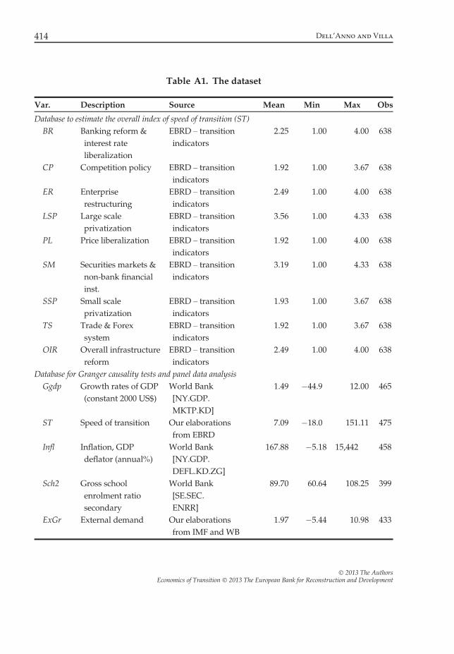
Table A1. The dataset

Var. Description Source Mean Min Max Obs

Database to estimate the overall index of speed of transition (ST)BR Banking reform &

interest rateliberalization

EBRD – transitionindicators

2.25 1.00 4.00 638

CP Competition policy EBRD – transitionindicators

1.92 1.00 3.67 638

ER Enterpriserestructuring


2.49 1.00 4.00 638

LSP Large scaleprivatization


3.56 1.00 4.33 638

PL Price liberalization EBRD – transitionindicators

1.92 1.00 4.00 638

SM Securities markets &non-bank financialinst.


3.19 1.00 4.33 638

SSP Small scaleprivatization


1.93 1.00 3.67 638

TS Trade & Forexsystem


1.92 1.00 3.67 638

OIR Overall infrastructurereform


2.49 1.00 4.00 638

Database for Granger causality tests and panel data analysisGgdp Growth rates of GDP

(constant 2000 US$)World Bank[NY.GDP.MKTP.KD]

1.49 �44.9 12.00 465

ST Speed of transition Our elaborationsfrom EBRD

7.09 �18.0 151.11 475

Infl Inflation, GDPdeflator (annual%)

World Bank[NY.GDP.DEFL.KD.ZG]

167.88 �5.18 15,442 458

Sch2 Gross schoolenrolment ratiosecondary

World Bank[SE.SEC.ENRR]

89.70 60.64 108.25 399

ExGr External demand Our elaborationsfrom IMF and WB

1.97 �5.44 10.98 433



the standards of an industrialized market economy. The reform scores reflect theassessments of EBRD economists using the criteria described in the methodologicalnotes.

Appendix B: Panel unit root analysis

In this Appendix the univariate unit root analysis and panel cointegration tests forthe variables included in the model are summarized. The small sample size is amajor limitation for unit root testing and also for cointegration analysis. EViews 7.1is used.

Table A1. (Continued)

Var. Description Source Mean Min Max Obs

PR Political rights Freedom House– Freedom inthe World

3.30 1 7 459

CL Civil liberties Freedom House– Freedom inthe World

3.40 1 7 459

Database to estimate (IC) initial condition by PCAGDP GDP per capita PPP

in 1990World Bank[NY.GDP.MKTP.PP.KD]

8,193 2,003 16,405 26

URB Urbanization(% of pop.in 1990)

World Bank [SP.IRB.TOTL.IN.ZS]

57.22 31.70 75.20 26

DIST Geographicaldistancefrom EU (km)

Falcetti et al. (2006) 2,416 722 6,815 26

TRADE Trade (% GDP)in 1990

World Bank[NE.TRD.GNFS.ZS]

74.76 11.90 169.29 26

Y_SOC Years undersocialism

Falcetti et al. (2006) 56.58 41.00 74.00 26

EM_AG Employmentshare inagriculture(1990)

World Bank[SL.AGR.EMPL.ZS]

22.96 5.00 44.00 26

IC Initial conditions Own calculations 49.11 0.02 100 26



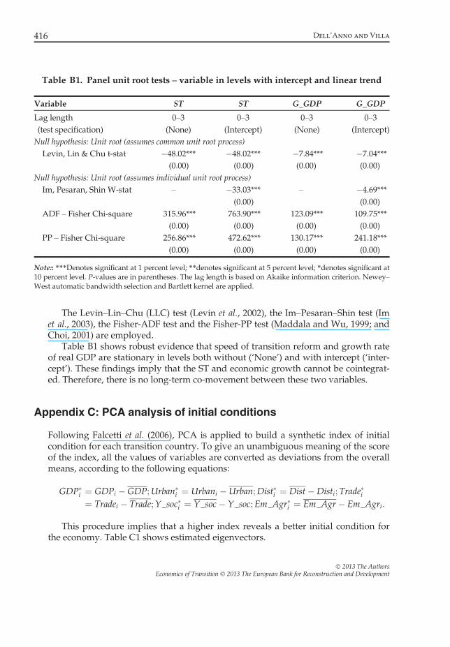
The Levin–Lin–Chu (LLC) test (Levin et al., 2002), the Im–Pesaran–Shin test (Imet al., 2003), the Fisher-ADF test and the Fisher-PP test (Maddala and Wu, 1999; andChoi, 2001) are employed.

Table B1 shows robust evidence that speed of transition reform and growth rateof real GDP are stationary in levels both without (‘None’) and with intercept (‘inter-cept’). These findings imply that the ST and economic growth cannot be cointegrat-ed. Therefore, there is no long-term co-movement between these two variables.

Appendix C: PCA analysis of initial conditions

Following Falcetti et al. (2006), PCA is applied to build a synthetic index of initialcondition for each transition country. To give an unambiguous meaning of the scoreof the index, all the values of variables are converted as deviations from the overallmeans, according to the following equations:

GDP�i ¼ GDPi � GDP;Urban�i ¼ Urbani �Urban;Dist�i ¼ Dist�Disti;Trade�i¼ Tradei � Trade;Y soc�i ¼ Y soc� Y soc;Em Agr�i ¼ Em Agr� Em Agri:

This procedure implies that a higher index reveals a better initial condition forthe economy. Table C1 shows estimated eigenvectors.

Table B1. Panel unit root tests – variable in levels with intercept and linear trend

Variable ST ST G_GDP G_GDP

Lag length(test specification)

0–3(None)

0–3(Intercept)

0–3(None)

0–3(Intercept)

Null hypothesis: Unit root (assumes common unit root process)Levin, Lin & Chu t-stat �48.02***

(0.00)�48.02***(0.00)

�7.84***(0.00)

�7.04***(0.00)

Null hypothesis: Unit root (assumes individual unit root process)Im, Pesaran, Shin W-stat – �33.03***

(0.00)– �4.69***

(0.00)ADF – Fisher Chi-square 315.96***

(0.00)763.90***(0.00)

123.09***(0.00)

109.75***(0.00)

PP – Fisher Chi-square 256.86***(0.00)

472.62***(0.00)

130.17***(0.00)

241.18***(0.00)

Note:: ***Denotes significant at 1 percent level; **denotes significant at 5 percent level; *denotes significant at10 percent level. P-values are in parentheses. The lag length is based on Akaike information criterion. Newey–West automatic bandwidth selection and Bartlett kernel are applied.









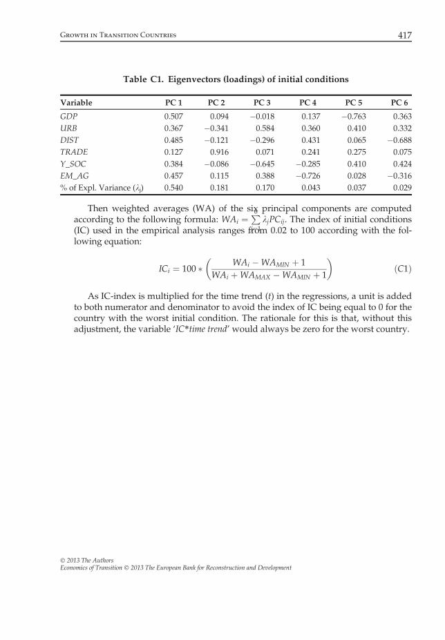
Then weighted averages (WA) of the six principal components are computedaccording to the following formula: WAi ¼

P6j¼1

kjPCij. The index of initial conditions(IC) used in the empirical analysis ranges from 0.02 to 100 according with the fol-lowing equation:

ICi ¼ 100 � WAi �WAMIN þ 1WAi þWAMAX �WAMIN þ 1

� �ðC1Þ

As IC-index is multiplied for the time trend (t) in the regressions, a unit is addedto both numerator and denominator to avoid the index of IC being equal to 0 for thecountry with the worst initial condition. The rationale for this is that, without thisadjustment, the variable ‘IC*time trend’ would always be zero for the worst country.

Table C1. Eigenvectors (loadings) of initial conditions

Variable PC 1 PC 2 PC 3 PC 4 PC 5 PC 6

GDP 0.507 0.094 �0.018 0.137 �0.763 0.363URB 0.367 �0.341 0.584 0.360 0.410 0.332DIST 0.485 �0.121 �0.296 0.431 0.065 �0.688TRADE 0.127 0.916 0.071 0.241 0.275 0.075Y_SOC 0.384 �0.086 �0.645 �0.285 0.410 0.424EM_AG 0.457 0.115 0.388 �0.726 0.028 �0.316% of Expl. Variance (kj) 0.540 0.181 0.170 0.043 0.037 0.029



Growth in transition countries

Documents

Transcript of Growth in transition countries