THE GROWTH OF TURKEY IN WORLD TRADE: OPPORTUNITY OR THREAT FOR MENA COUNTRIES?

Marouane Alaya and Imed Mezghani

Working Paper 763

September 2013

Send correspondence to: Imed Mezghani Al-Imam Muhammad Ibn Saud Islamic University, Kingdom of Saudi Arabia imedmezghani@yahoo.fr

First published in 2013 by The Economic Research Forum (ERF) 21 Al-Sad Al-Aaly Street Dokki, Giza Egypt www.erf.org.eg Copyright © The Economic Research Forum, 2013 All rights reserved. No part of this publication may be reproduced in any form or by any electronic or mechanical means, including information storage and retrieval systems, without permission in writing from the publisher. The findings, interpretations and conclusions expressed in this publication are entirely those of the author(s) and should not be attributed to the Economic Research Forum, members of its Board of Trustees, or its donors.

1

Abstract

The aim of this paper is to study the impact of the emergence of the Turkish economy on the MENA region. We focus on two channels through which MENA countries and Turkey interact, namely FDI and trade flows. We use different econometric techniques and estimation methods to find that crowding-in effects are more likely than the competitive threat of Turkish economy.

JEL Classification: F14, F21, C50.

Keywords: Trade, FDI, MENA countries.

ملخص

تتفاعل ونحن نركز على قناتین. الھدف من ھذه الورقة ھو دراسة تأثیر ظھور االقتصاد التركي في منطقة الشرق األوسط

ارة دفقات التج ي المباشر وت ي االستثمار األجنب ا، وھ اد . من خاللھا بلدان الشرق األوسط وتركی الیب االقتص نستخدم أس

.القتصاد التركيمن امن تھدید التنافسیة للحدوث د أن آثار االزدحام ھي أكثر عرضة جنتقدیر لالمختلفة وأسالیب الالقیاسي

2

1. Introduction According to the World Bank, Turkey has become the 15th largest economy in the world. The growth of its GDP is on average 6% per year from 2002 to 2011. The success of turkey is seen both with admiration and apprehension by policy makers in neighboring MENA countries and elsewhere. Without doubt, the growth of the Turkish economy is far from being a zero sum game for the MENA region. Short and long term effects could be important especially those concerning the foreign direct investment and trade flows from and towards MENA countries. The purpose of this work is to find out what the consequences of the emergence of the Turkish economy are for its neighboring countries. There are a range of channels (trade, FDI, governance, migration, finance, tourism, etc.) through which individual countries interact with other economies, in their regions or elsewhere. In this study we will focus on two interaction channels namely FDI and trade flows. Geographical proximity, historical and political factors are among the reasons to expect a blooming trade between Turkey and MENA region. On the other hand, we presume that similarities in the stages of economic development, resources endowment and factor costs will generate competition effects between MENA countries and Turkey in trade and FDI flows. As a consequence, the economic impact of the crowding in and diversion effect on both sides may be significant. Although the emergence of the Turkish economy cannot be ignored by MENA countries, its impact on the region is difficult to identify due to the presence of direct and indirect spillovers effects. Unfortunately we only have little understanding about this issue. These are the questions motivating the analysis. We focus especially on the impact of the Turkey’s trade growth on the exports of the other MENA countries. Thus, we study the link between the rapid growth of Turkey’s exports and MENA trade flows from two perspectives: first, from the viewpoint of Turkey as a fast-growing export market and as source of imports for MENA countries and second, with regard to its potential effects on MENA trade flows with other markets. In addition we discuss the potential crowding in/out effect between FDI flows attracted by the Turkish economy and those attracted by the MENA region. These questions will be investigated econometrically using a number of regression specifications and alternatives estimations methods. Results show that the opportunities created by the rapid expansion of the Turkish economy are more likely than the competitive threat of Turkish economy outlined by some scholars.

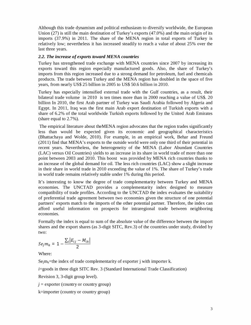
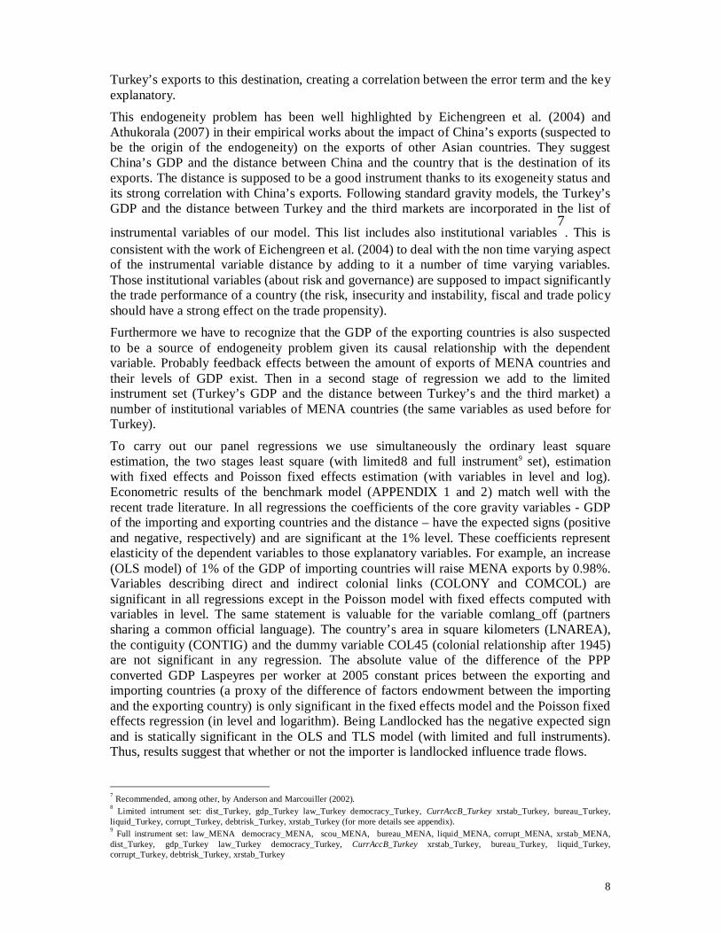
2. A Snapshot of Turkish Trade According to the Trade Profile report published by the WTO in 2012, the rank of Turkey in world Trade in 2011 is 32 for exports and 20 for imports. Since the 1980s Turkey’s trade flows increased regularly and maintained an upward trend in the last decade. In 2011 exports and imports respectively reached the value of US$134,918 million and US$240,842 million, representing a share in world total exports of 0.74% and a share in world total imports of 1.31%. A breakdown in Turkey’s total trade by main commodity group in 2011 shows that agricultural products, fuels and mining products, manufactures explain respectively 11.8%, 8.9% and 77.2% of total exports and 7.3,%, 30.8% and 59% of total imports. 2.1. The new trade strategy of Turkey: A will to go global In power since 2002, the AKP party has changed the worldwide Turkish geo-politic strategy thanks to a new foreign policy (Babacan, 2010). The undisputed architect of Turkey’s new foreign policy, Ahmet Davutoglu, minister of foreign affairs position since 2009, is considered as the policymaker who shaped the country foreign policy since the early days of AK party government in 2002. The Ahmet Davutoglu’s doctrine is to diversify trade partners by the conclusion of huge number of bilateral free trade agreements.

3

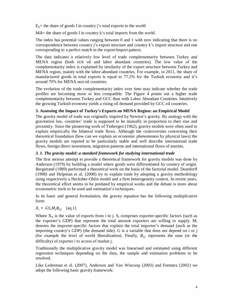
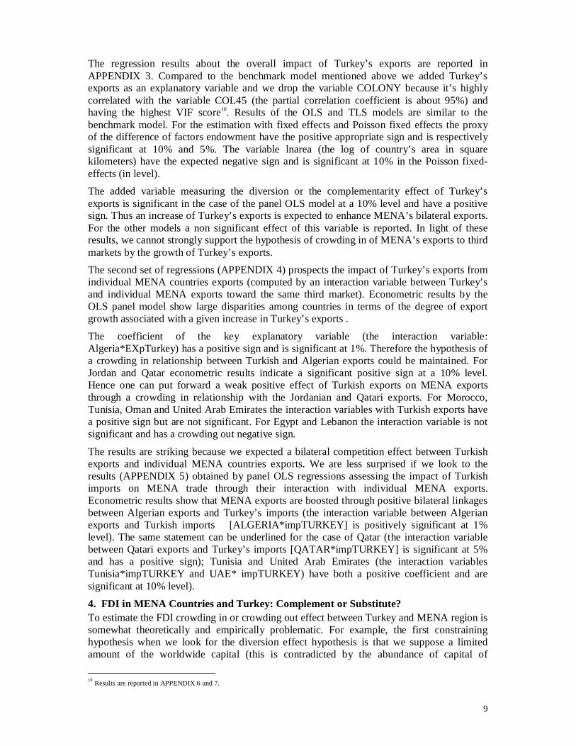
Although this trade dynamism and political enthusiasm to diversify worldwide, the European Union (27) is still the main destination of Turkey’s exports (47.0%) and the main origin of its imports (37.9%) in 2011. The share of the MENA region in total exports of Turkey is relatively low; nevertheless it has increased steadily to reach a value of about 25% over the last three years.

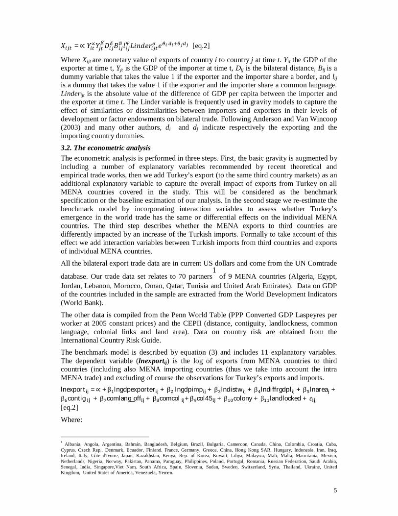
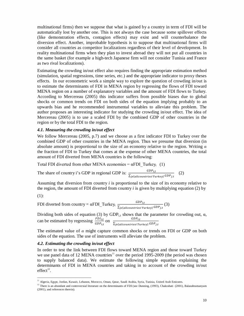
2.2. The increase of exports toward MENA countries Turkey has strengthened trade exchange with MENA countries since 2007 by increasing its exports toward this region especially manufactured goods. Also, the share of Turkey’s imports from this region increased due to a strong demand for petroleum, fuel and chemicals products. The trade between Turkey and the MENA region has doubled in the space of five years, from nearly US$ 25 billion in 2005 to US$ 50.6 billion in 2010. Turkey has especially intensified external trade with the Gulf countries, as a result, their bilateral trade volume in 2010 is ten times more than in 2000 reaching a value of US$. 20 billion In 2010, the first Arab partner of Turkey was Saudi Arabia followed by Algeria and Egypt. In 2011, Iraq was the first main Arab export destination of Turkish exports with a share of 6.2% of the total worldwide Turkish exports followed by the United Arab Emirates (share equal to 2.7%). The empirical literature about theMENA region advocates that the region trades significantly less than would be expected given its economic and geographical characteristics (Bhattachaya and Wolde, 2010). For example, in an empirical work, Behar and Freund (2011) find that MENA’s exports to the outside world were only one third of their potential in recent years. Nevertheless, the heterogeneity of the MENA (Labor Abundant Countries (LAC) versus Oil Countries) yields to an increase in its share in world trade of more than one point between 2003 and 2010. This boost was provided by MENA rich countries thanks to an increase of the global demand for oil. The less rich countries (LAC) show a slight increase in their share in world trade in 2010 exceeding the value of 1%. The share of Turkey’s trade in world trade remains relatively stable under 1% during this period. It’s interesting to know the degree of trade complementarity between Turkey and MENA economies. The UNCTAD provides a complementarity index designed to measure compatibility of trade profiles. According to the UNCTAD the index evaluates the suitability of preferential trade agreement between two economies given the structure of one potential partners’ exports match to the imports of the other potential partner. Therefore, the index can afford useful information on prospects for intraregional trade between neighboring economies.

Formally the index is equal to sum of the absolute value of the difference between the import shares and the export shares (as 3-digit SITC, Rev.3) of the countries under study, divided by two:

푆푒 푚 = 1 −∑ 퐸 −푀

2

Where: Sejmk=the index of trade complementarity of exporter j with importer k.

i=goods in three digit SITC Rev. 3 (Standard International Trade Classification) Revision 3, 3-digit group level).

j = exporter (country or country group) k=importer (country or country group)

4

Eij= the share of goods I in country j’s total exports to the world

Mik= the share of goods I in country k’s total imports from the world. The index has potential values ranging between 0 and 1 with zero indicating that there is no correspondence between country j’s export structure and country k’s import structure and one corresponding to a perfect match in the export/import pattern.

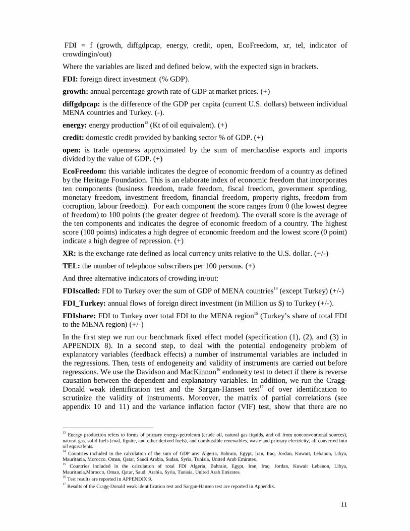
The data indicates a relatively low level of trade complementarity between Turkey and MENA region (both rich oil and labor abundant countries). The low value of the complementarity index is explained by similarity of the export structure between Turkey and MENA region, mainly with the labor-abundant countries. For example, in 2011, the share of manufactured goods in total exports is equal to 77.2% for the Turkish economy and it’s around 70% for MENA non oil countries.

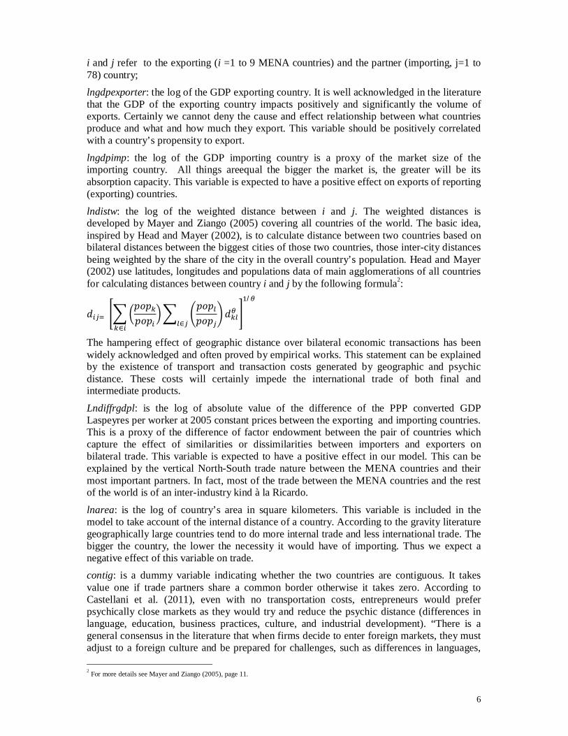
The evolution of the trade complementarity index over time may indicate whether the trade profiles are becoming more or less compatible. The Figure 4 points out a higher trade complementarity between Turkey and GCC than with Labor Abundant Countries. Intuitively the growing Turkish economy yields a rising oil demand provided by GCC oil countries.

3. Assessing the Impact of Turkey’s Exports on MENA Region: an Empirical Model The gravity model of trade was originally inspired by Newton’s gravity. By analogy with the gravitation law, countries’ trade is supposed to be mutually in proportion to their size and proximity. Since the pioneering work of Tinbergen (1962), gravity models were often used to explain empirically the bilateral trade flows. Although the controversies concerning their theoretical foundation (how can we explain an economic phenomenon by physical laws) the gravity models are reputed to be particularly stable and well describe international trade flows, foreign direct investment, migration patterns and international flows of tourists. 3. 1. The gravity model: a standard framework for studying international trade The first serious attempt to provide a theoretical framework for gravity models was done by Anderson (1979) by building a model where goods were differentiated by country of origin. Bergstrand (1989) performed a theoretical work on the basis of the factorial model. Deardorff (1998) and Helpman et al. (2008) try to explain trade by adopting a gravity methodology using respectively a Hecksher-Ohlin model and a firm heterogeneity context. In recent years, the theoretical effort seems to be predated by empirical works and the debate is more about econometric tools to be used and estimation’s techniques.

In its basic and general formulation, the gravity equation has the following multiplicative form:

푋 = 퐺푆 푀 ∅ [eq.1]

Where Xij is the value of exports from i to j. Si comprises exporter-specific factors (such as the exporter’s GDP) that represent the total amount exporters are willing to supply. Mi denotes the importer-specific factors that explain the total importer’s demand (such as the importing country’s GDP) (the demand side). G is a variable that does not depend on i or j (for example the level of world liberalization). Finally, ∅ represents the ease (or the difficulty) of exporter i to access of market j. Traditionally the multiplicative gravity model was linearised and estimated using different regression techniques depending on the data, the sample and estimation problems to be resolved.

Like Lederman et al. (2007), Anderson and Van Wincoop (2003) and Feenstra (2002) we adopt the following basic gravity framework:

5

푋 =∝ 푌∝푌 퐷 퐵∅ 푙 퐿푖푛푑푒푟 푒 [eq.2]

Where Xijt are monetary value of exports of country i to country j at time t. Yit the GDP of the exporter at time t, Yjt is the GDP of the importer at time t, Dij is the bilateral distance, Bij is a dummy variable that takes the value 1 if the exporter and the importer share a border, and lij is a dummy that takes the value 1 if the exporter and the importer share a common language. Linderijt is the absolute value of the difference of GDP per capita between the importer and the exporter at time t. The Linder variable is frequently used in gravity models to capture the effect of similarities or dissimilarities between importers and exporters in their levels of development or factor endowments on bilateral trade. Following Anderson and Van Wincoop (2003) and many other authors, di and dj indicate respectively the exporting and the importing country dummies. 3.2. The econometric analysis The econometric analysis is performed in three steps. First, the basic gravity is augmented by including a number of explanatory variables recommended by recent theoretical and empirical trade works, then we add Turkey’s export (to the same third country markets) as an additional explanatory variable to capture the overall impact of exports from Turkey on all MENA countries covered in the study. This will be considered as the benchmark specification or the baseline estimation of our analysis. In the second stage we re-estimate the benchmark model by incorporating interaction variables to assess whether Turkey’s emergence in the world trade has the same or differential effects on the individual MENA countries. The third step describes whether the MENA exports to third countries are differently impacted by an increase of the Turkish imports. Formally to take account of this effect we add interaction variables between Turkish imports from third countries and exports of individual MENA countries. All the bilateral export trade data are in current US dollars and come from the UN Comtrade

database. Our trade data set relates to 70 partners1

of 9 MENA countries (Algeria, Egypt, Jordan, Lebanon, Morocco, Oman, Qatar, Tunisia and United Arab Emirates). Data on GDP of the countries included in the sample are extracted from the World Development Indicators (World Bank).

The other data is compiled from the Penn World Table (PPP Converted GDP Laspeyres per worker at 2005 constant prices) and the CEPII (distance, contiguity, landlockness, common language, colonial links and land area). Data on country risk are obtained from the International Country Risk Guide. The benchmark model is described by equation (3) and includes 11 explanatory variables. The dependent variable (lnexportij) is the log of exports from MENA countries to third countries (including also MENA importing countries (thus we take into account the intra MENA trade) and excluding of course the observations for Turkey’s exports and imports. lnexport =∝ +β lngdpexporter + β lngdpimp + β lndistw + β lndiffrgdpl + β lnarea +β contig + β comlang_off + β comcol +β col45 + β colony + β landlocked + ε [eq.2] Where:

1 Albania, Angola, Argentina, Bahrain, Bangladesh, Belgium, Brazil, Bulgaria, Cameroon, Canada, China, Colombia, Croatia, Cuba, Cyprus, Czech Rep., Denmark, Ecuador, Finland, France, Germany, Greece, China, Hong Kong SAR, Hungary, Indonesia, Iran, Iraq, Ireland, Italy, Côte d'Ivoire, Japan, Kazakhstan, Kenya, Rep. of Korea, Kuwait, Libya, Malaysia, Mali, Malta, Mauritania, Mexico, Netherlands, Nigeria, Norway, Pakistan, Panama, Paraguay, Philippines, Poland, Portugal, Romania, Russian Federation, Saudi Arabia, Senegal, India, Singapore,Viet Nam, South Africa, Spain, Slovenia, Sudan, Sweden, Switzerland, Syria, Thailand, Ukraine, United Kingdom, United States of America, Venezuela, Yemen.

6

i and j refer to the exporting (i =1 to 9 MENA countries) and the partner (importing, j=1 to 78) country; lngdpexporter: the log of the GDP exporting country. It is well acknowledged in the literature that the GDP of the exporting country impacts positively and significantly the volume of exports. Certainly we cannot deny the cause and effect relationship between what countries produce and what and how much they export. This variable should be positively correlated with a country’s propensity to export.

lngdpimp: the log of the GDP importing country is a proxy of the market size of the importing country. All things areequal the bigger the market is, the greater will be its absorption capacity. This variable is expected to have a positive effect on exports of reporting (exporting) countries.

lndistw: the log of the weighted distance between i and j. The weighted distances is developed by Mayer and Ziango (2005) covering all countries of the world. The basic idea, inspired by Head and Mayer (2002), is to calculate distance between two countries based on bilateral distances between the biggest cities of those two countries, those inter-city distances being weighted by the share of the city in the overall country’s population. Head and Mayer (2002) use latitudes, longitudes and populations data of main agglomerations of all countries for calculating distances between country i and j by the following formula2:

푑 푝표푝푝표푝

∈

푝표푝푝표푝 푑

∈

/

The hampering effect of geographic distance over bilateral economic transactions has been widely acknowledged and often proved by empirical works. This statement can be explained by the existence of transport and transaction costs generated by geographic and psychic distance. These costs will certainly impede the international trade of both final and intermediate products.

Lndiffrgdpl: is the log of absolute value of the difference of the PPP converted GDP Laspeyres per worker at 2005 constant prices between the exporting and importing countries. This is a proxy of the difference of factor endowment between the pair of countries which capture the effect of similarities or dissimilarities between importers and exporters on bilateral trade. This variable is expected to have a positive effect in our model. This can be explained by the vertical North-South trade nature between the MENA countries and their most important partners. In fact, most of the trade between the MENA countries and the rest of the world is of an inter-industry kind à la Ricardo.

lnarea: is the log of country’s area in square kilometers. This variable is included in the model to take account of the internal distance of a country. According to the gravity literature geographically large countries tend to do more internal trade and less international trade. The bigger the country, the lower the necessity it would have of importing. Thus we expect a negative effect of this variable on trade. contig: is a dummy variable indicating whether the two countries are contiguous. It takes value one if trade partners share a common border otherwise it takes zero. According to Castellani et al. (2011), even with no transportation costs, entrepreneurs would prefer psychically close markets as they would try and reduce the psychic distance (differences in language, education, business practices, culture, and industrial development). “There is a general consensus in the literature that when firms decide to enter foreign markets, they must adjust to a foreign culture and be prepared for challenges, such as differences in languages, 2 For more details see Mayer and Ziango (2005), page 11.

7

lifestyles, cultural standards, consumer preferences, and purchasing power (Sousa and Bradley, 2006, p.49). Trade between two contiguous countries is expected to be larger than trade between countries that do not share a border.

landlocked: dummy variable set equal to 1 for landlocked countries. Access to water or sea distance reduce transport cost and relatively facilitate the fluidity of trade. Thus being landlocked risks hampering trade and development. We expect a negative sign of this variable since landlocked countries will face higher transport cost.

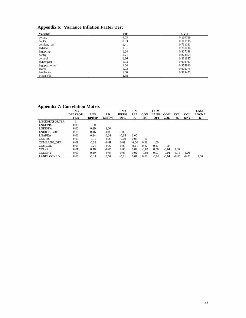
comlang_off: is a dummy variable equal to 1 if trade partners share a common official language. Transactions, trade, exchange and communication become easier and more convenient when the two partners share the same language. comcol, col45 and colony: are dummy variables describing colonial ties (direct and indirect links). Colonial links captures the effect of having had a common colonizer or having been colonized by another country in the past. The common-colonizer variable (comcol) indicates if trading partners have had a common colonizer after 1945. The variable colony demonstrates whether or not any two countries have ever had a colonial link (colony).col45 shows if they have had a colonial relationship after 1945 or not. We expect a positive relationship of these dummies with the dependent variables since a direct or indirect colonial relationship is supposed to reduce cultural differences between two countries. Panel regressions are performed over the period 2000-2009 using four alternative estimation techniques (Panel Ordinary Least Square (OLS), Panel Two Stages Least Square (TLS), Panel fixed effects regression (FE) and conditional fixed effects Poisson regression). In gravity models, multicolinearity and endogeneity are generally the most commonly encountered problems. To deal with these potential problems we run the regressions with a weighted least-squares procedure, employing a White correction for heteroskedasticity to ensure heteroskedasticity-consistent standard errors. In addition we test the presence of multicolinearity by the standard test for multicolinearity (the variance inflation factor (VIF) test) and by examining the matrix of partial correlations. The VIF test shows a static equal to 2.58 which is an evidence of absence of multicolinearity. In addition all independent variables have a value lower than the threshold level of 10 reflecting an absence of multicolinearity3. Furthermore, the matrix of partial correlations indicates that there are no serious problems of multicolinearity between the explanatory variables included in the regressions. The only exception is concerning the two variables colony and col45 having a partial correlation around 94%. To deal with this problem the variable colony will be dropped from the benchmark model in the subsequent regressions4. Furthermore we use instrumental variables to take account of the potential endogeneity problem of Turkey’s exports when it is added to the benchmark model as an explanatory variable5. The use of instruments is always advisable to avoid any suspicion of endogeneity. The endogeneity occurs when there is a causal relationship between the dependent and the explanatory variables and/or the presence of unobserved factors. In this case, the problem is to find the right instruments i.e., uncorrelated with the error term. Unobserved factors6 that increase exports from a MENA country to a third country will also probably increase 3 As a rule of thumb, a variable whose VIF values are greater than 10 may merit further investigation. Tolerance, defined as 1/VIF, is used by many researchers to check on the degree of collinearity. A tolerance value lower than 0.1 is comparable to a VIF of 10. It means that the variable could be considered as a linear combination of other independent variables 4 For the multicolinearity VIF test and the matrix of partial correlations see Appendix 6 and 7. 5 We run the Sargan-Hansan test to examine the “validity” of the instrumental variables. 6 For example, an improvement in consumer purchasing power worldwide, consumer tastes change, improvement in consumer sentiment worldwide, technology progress lowering transport costs.

8

Turkey’s exports to this destination, creating a correlation between the error term and the key explanatory. This endogeneity problem has been well highlighted by Eichengreen et al. (2004) and Athukorala (2007) in their empirical works about the impact of China’s exports (suspected to be the origin of the endogeneity) on the exports of other Asian countries. They suggest China’s GDP and the distance between China and the country that is the destination of its exports. The distance is supposed to be a good instrument thanks to its exogeneity status and its strong correlation with China’s exports. Following standard gravity models, the Turkey’s GDP and the distance between Turkey and the third markets are incorporated in the list of

instrumental variables of our model. This list includes also institutional variables7

. This is consistent with the work of Eichengreen et al. (2004) to deal with the non time varying aspect of the instrumental variable distance by adding to it a number of time varying variables. Those institutional variables (about risk and governance) are supposed to impact significantly the trade performance of a country (the risk, insecurity and instability, fiscal and trade policy should have a strong effect on the trade propensity). Furthermore we have to recognize that the GDP of the exporting countries is also suspected to be a source of endogeneity problem given its causal relationship with the dependent variable. Probably feedback effects between the amount of exports of MENA countries and their levels of GDP exist. Then in a second stage of regression we add to the limited instrument set (Turkey’s GDP and the distance between Turkey’s and the third market) a number of institutional variables of MENA countries (the same variables as used before for Turkey).

To carry out our panel regressions we use simultaneously the ordinary least square estimation, the two stages least square (with limited8 and full instrument9 set), estimation with fixed effects and Poisson fixed effects estimation (with variables in level and log). Econometric results of the benchmark model (APPENDIX 1 and 2) match well with the recent trade literature. In all regressions the coefficients of the core gravity variables - GDP of the importing and exporting countries and the distance – have the expected signs (positive and negative, respectively) and are significant at the 1% level. These coefficients represent elasticity of the dependent variables to those explanatory variables. For example, an increase (OLS model) of 1% of the GDP of importing countries will raise MENA exports by 0.98%. Variables describing direct and indirect colonial links (COLONY and COMCOL) are significant in all regressions except in the Poisson model with fixed effects computed with variables in level. The same statement is valuable for the variable comlang_off (partners sharing a common official language). The country’s area in square kilometers (LNAREA), the contiguity (CONTIG) and the dummy variable COL45 (colonial relationship after 1945) are not significant in any regression. The absolute value of the difference of the PPP converted GDP Laspeyres per worker at 2005 constant prices between the exporting and importing countries (a proxy of the difference of factors endowment between the importing and the exporting country) is only significant in the fixed effects model and the Poisson fixed effects regression (in level and logarithm). Being Landlocked has the negative expected sign and is statically significant in the OLS and TLS model (with limited and full instruments). Thus, results suggest that whether or not the importer is landlocked influence trade flows.

7 Recommended, among other, by Anderson and Marcouiller (2002). 8 Limited intrument set: dist_Turkey, gdp_Turkey law_Turkey democracy_Turkey, CurrAccB_Turkey xrstab_Turkey, bureau_Turkey, liquid_Turkey, corrupt_Turkey, debtrisk_Turkey, xrstab_Turkey (for more details see appendix). 9 Full instrument set: law_MENA democracy_MENA, scou_MENA, bureau_MENA, liquid_MENA, corrupt_MENA, xrstab_MENA, dist_Turkey, gdp_Turkey law_Turkey democracy_Turkey, CurrAccB_Turkey xrstab_Turkey, bureau_Turkey, liquid_Turkey, corrupt_Turkey, debtrisk_Turkey, xrstab_Turkey

9

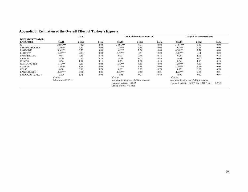
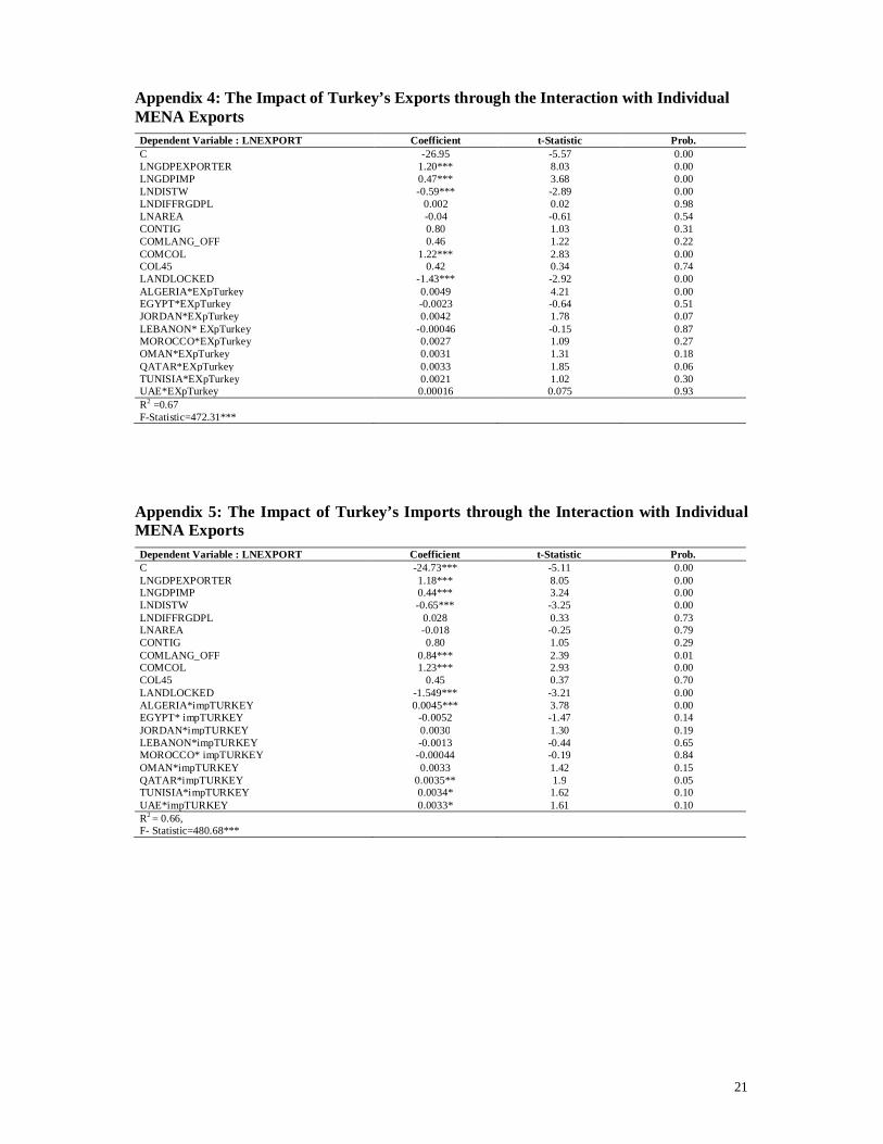
The regression results about the overall impact of Turkey’s exports are reported in APPENDIX 3. Compared to the benchmark model mentioned above we added Turkey’s exports as an explanatory variable and we drop the variable COLONY because it’s highly correlated with the variable COL45 (the partial correlation coefficient is about 95%) and having the highest VIF score10. Results of the OLS and TLS models are similar to the benchmark model. For the estimation with fixed effects and Poisson fixed effects the proxy of the difference of factors endowment have the positive appropriate sign and is respectively significant at 10% and 5%. The variable lnarea (the log of country’s area in square kilometers) have the expected negative sign and is significant at 10% in the Poisson fixed-effects (in level). The added variable measuring the diversion or the complementarity effect of Turkey’s exports is significant in the case of the panel OLS model at a 10% level and have a positive sign. Thus an increase of Turkey’s exports is expected to enhance MENA’s bilateral exports. For the other models a non significant effect of this variable is reported. In light of these results, we cannot strongly support the hypothesis of crowding in of MENA’s exports to third markets by the growth of Turkey’s exports. The second set of regressions (APPENDIX 4) prospects the impact of Turkey’s exports from individual MENA countries exports (computed by an interaction variable between Turkey’s and individual MENA exports toward the same third market). Econometric results by the OLS panel model show large disparities among countries in terms of the degree of export growth associated with a given increase in Turkey’s exports .

The coefficient of the key explanatory variable (the interaction variable: Algeria*EXpTurkey) has a positive sign and is significant at 1%. Therefore the hypothesis of a crowding in relationship between Turkish and Algerian exports could be maintained. For Jordan and Qatar econometric results indicate a significant positive sign at a 10% level. Hence one can put forward a weak positive effect of Turkish exports on MENA exports through a crowding in relationship with the Jordanian and Qatari exports. For Morocco, Tunisia, Oman and United Arab Emirates the interaction variables with Turkish exports have a positive sign but are not significant. For Egypt and Lebanon the interaction variable is not significant and has a crowding out negative sign.

The results are striking because we expected a bilateral competition effect between Turkish exports and individual MENA countries exports. We are less surprised if we look to the results (APPENDIX 5) obtained by panel OLS regressions assessing the impact of Turkish imports on MENA trade through their interaction with individual MENA exports. Econometric results show that MENA exports are boosted through positive bilateral linkages between Algerian exports and Turkey’s imports (the interaction variable between Algerian exports and Turkish imports [ALGERIA*impTURKEY] is positively significant at 1% level). The same statement can be underlined for the case of Qatar (the interaction variable between Qatari exports and Turkey’s imports [QATAR*impTURKEY] is significant at 5% and has a positive sign); Tunisia and United Arab Emirates (the interaction variables Tunisia*impTURKEY and UAE* impTURKEY) have both a positive coefficient and are significant at 10% level).

4. FDI in MENA Countries and Turkey: Complement or Substitute? To estimate the FDI crowding in or crowding out effect between Turkey and MENA region is somewhat theoretically and empirically problematic. For example, the first constraining hypothesis when we look for the diversion effect hypothesis is that we suppose a limited amount of the worldwide capital (this is contradicted by the abundance of capital of

10 Results are reported in APPENDIX 6 and 7.

10

multinational firms) then we suppose that what is gained by a country in term of FDI will be automatically lost by another one. This is not always the case because some spillover effects (like demonstration effects, contagion effects) may exist and will counterbalance the diversion effect. Another, improbable hypothesis is to suppose that multinational firms will consider all countries as competitor localizations regardless of their level of development. In reality multinational firms when they plan to invest abroad they will not put all countries in the same basket (for example a high-tech Japanese firm will not consider Tunisia and France as two rival localizations). Estimating the crowding in/out effect also requires finding the appropriate estimation method (simulation, spatial regressions, time series, etc.) and the appropriate indicator to proxy theses effects. In our econometric work a simple way to explore the question of crowding in/out is to estimate the determinants of FDI in MENA region by regressing the flows of FDI toward MENA region on a number of explanatory variables and the amount of FDI flows to Turkey. According to Mercereau (2005) this indicator suffers from possible biases due to global shocks or common trends on FDI on both sides of the equation implying probably to an upwards bias and he recommended instrumental variables to alleviate this problem. The author proposes an interesting indicator for studying the crowding in/out effect. The idea of Mercereau (2005) is to use a scaled FDI by the combined GDP of other countries in the region or by the total FDI to the region.

4.1. Measuring the crowding in/out effect We follow Mercereau (2005, p.7) and we choose as a first indicator FDI to Turkey over the combined GDP of other countries in the MENA region. Thus we presume that diversion (in absolute amount) is proportional to the size of an economy relative to the region. Writing α the fraction of FDI to Turkey that comes at the expense of other MENA countries, the total amount of FDI diverted from MENA countries is the following:

Total FDI diverted from other MENA economies = αFDI_Turkeyt (1)

The share of country i’s GDP in regional GDP is: ,∑ ,{ / }

(2)

Assuming that diversion from country i is proportional to the size of its economy relative to the region, the amount of FDI diverted from country i is given by multiplying equation (2) by

(1):

FDI diverted from country = αFDI_Turkeyt ,∑ ,{ / }

(3)

Dividing both sides of equation (3) by GDPi,t shows that the parameter for crowding out, α, can be estimated by regressing ,

, on ,

∑ ,{ / }

The estimated value of α might capture common shocks or trends on FDI or GDP on both sides of the equation. The use of instruments will alleviate the problem. 4.2. Estimating the crowding in/out effect In order to test the link between FDI flows toward MENA region and those toward Turkey we use panel data of 12 MENA countries11 over the period 1995-2009 (the period was chosen to supply balanced data). We estimate the following simple equation explaining the determinants of FDI in MENA countries and taking in to account of the crowding in/out effect12. 11 Algeria, Egypt, Jordan, Kuwait, Lebanon, Morocco, Oman, Qatar, Saudi Arabia, Syria, Tunisia, United Arab Emirates. 12 There is an abundant and controversial literature on the determinants of FDI (see Dunning, (1993), Chakrabati (2001), Balasubramanyam (2001), and references therein).

11

FDI = f (growth, diffgdpcap, energy, credit, open, EcoFreedom, xr, tel, indicator of crowdingin/out) Where the variables are listed and defined below, with the expected sign in brackets.

FDI: foreign direct investment (% GDP). growth: annual percentage growth rate of GDP at market prices. (+)

diffgdpcap: is the difference of the GDP per capita (current U.S. dollars) between individual MENA countries and Turkey. (-).

energy: energy production13 (Kt of oil equivalent). (+) credit: domestic credit provided by banking sector % of GDP. (+)

open: is trade openness approximated by the sum of merchandise exports and imports divided by the value of GDP. (+)

EcoFreedom: this variable indicates the degree of economic freedom of a country as defined by the Heritage Foundation. This is an elaborate index of economic freedom that incorporates ten components (business freedom, trade freedom, fiscal freedom, government spending, monetary freedom, investment freedom, financial freedom, property rights, freedom from corruption, labour freedom). For each component the score ranges from 0 (the lowest degree of freedom) to 100 points (the greater degree of freedom). The overall score is the average of the ten components and indicates the degree of economic freedom of a country. The highest score (100 points) indicates a high degree of economic freedom and the lowest score (0 point) indicate a high degree of repression. (+)

XR: is the exchange rate defined as local currency units relative to the U.S. dollar. (+/-)

TEL: the number of telephone subscribers per 100 persons. (+) And three alternative indicators of crowding in/out:

FDIscalled: FDI to Turkey over the sum of GDP of MENA countries14 (except Turkey) (+/-) FDI_Turkey: annual flows of foreign direct investment (in Million us $) to Turkey (+/-).

FDIshare: FDI to Turkey over total FDI to the MENA region15 (Turkey’s share of total FDI to the MENA region) (+/-)

In the first step we run our benchmark fixed effect model (specification (1), (2), and (3) in APPENDIX 8). In a second step, to deal with the potential endogeneity problem of explanatory variables (feedback effects) a number of instrumental variables are included in the regressions. Then, tests of endogeneity and validity of instruments are carried out before regressions. We use the Davidson and MacKinnon16 endoneity test to detect if there is reverse causation between the dependent and explanatory variables. In addition, we run the Cragg-Donald weak identification test and the Sargan-Hansen test17 of over identification to scrutinize the validity of instruments. Moreover, the matrix of partial correlations (see appendix 10 and 11) and the variance inflation factor (VIF) test, show that there are no

13 Energy production refers to forms of primary energy-petroleum (crude oil, natural gas liquids, and oil from nonconventional sources), natural gas, solid fuels (coal, lignite, and other derived fuels), and combustible renewables, waste and primary electricity, all converted into oil equivalents. 14 Countries included in the calculation of the sum of GDP are: Algeria, Bahrain, Egypt, Iran, Iraq, Jordan, Kuwait, Lebanon, Libya, Mauritania, Morocco, Oman, Qatar, Saudi Arabia, Sudan, Syria, Tunisia, United Arab Emirates. 15 Countries included in the calculation of total FDI Algeria, Bahrain, Egypt, Iran, Iraq, Jordan, Kuwait Lebanon, Libya, Mauritania,Morocco, Oman, Qatar, Saudi Arabia, Syria, Tunisia, United Arab Emirates. 16 Test results are reported in APPENDIX 9. 17 Results of the Cragg-Donald weak identification test and Sargan-Hansen test are reported in Appendix.

12

serious problems of multicolinearity between the explanatory variables included in the regressions. The variable suspected to be the source of endogeneity (inward FDI in Turkey) was instrumented by a number of risk score indicators of the Turkish economy: Law_Turkey (law and order), CurrAccB_Turkey (current account balance as a percent of GDP), xrstab_Turkey (exchange rate stability) bureau_Turkey (bureaucracy) debtrisk_Turkey (risk points for foreign debt as a percent of GDP).

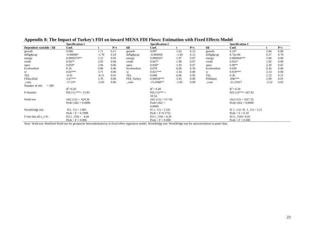
Econometric results of the fixed effect model (see APPENDIX8) indicate that the most coefficients of explanatory variables have the hypothesized signs and are significant at different conventional levels. The specification (1) including the scalled FDI (FDI to Turkey over the sum of GDP of MENA countries) as a proxy of crowding in/out shows that this variable is significant at a 1% level and has a positive sign. Therefore, it can be argued that the crowding in effect is more plausible. This is confirmed by specification (1) and (2) including respectively two alternative measures of diversion or crowding in effect (annual flows of foreign direct investment to Turkey and FDI to Turkey over total FDI to the MENA region). The difference of the GDP per capita (current US$s) between individual MENA countries and Turkey is a proxy of the difference of wage levels in the absence of sufficient data on wages. A large difference may be a source of a trade-off for multinational firms to choose between investing in MENA countries or in Turkey. As a result, the probability of competition or substitution effect will be higher. Results show that this variable is significant (at 10% level) only in specification (1). Economic growth is not significant in specification (1) and (2) (but is too close to a 10% level of significance) and becomes significant at 10% in specification (3). Growth, market size and scale economies are the main determinants of horizontal FDI (market seeking FDI). For vertical FDI (which is the most important kind of FDI in MENA region) the economic growth can also play a positive role, at least it will be felt by foreign firms as a good sign of economic stability.

The variable energy (a proxy of resources endowment) has the positive suitable sign and is respectively significant at 5%, 10% and 1% levels in specification (1), (2) and (3). This confirms that the motivation to invest in MENA of an important number of firms is access to natural resources particularly gas and petroleum. For the three specifications the variable credit (a proxy of access to finance) has the appropriate sign and is significant at 10% level. Trade openness is crucial for vertical multinational firms which by definition are firms with several stages of production located in different countries, where different stages are connected by intermediate product flows and the majority of finished products are sold in the parent country. In the model, the proxy of trade openness (OPEN) is respectively significant at 10% in the specification (1) and (2) and 5% in specification (3). The variable indicating the degree of economic freedom of a country is not significant at any statistical conventional level. The exchange rate has a positive sign and is significant at a 1% level. Hence an increase of the exchange rate (i.e. a depreciation of the local currency) will increase the amount of FDI to MENA region. This is an expected result since a large number of foreign subsidiaries, located in these countries, adopt a vertical strategy and thus need to re-export the production towards their countries of origin or to other countries. So a depreciation of local currency will affect positively their competitiveness by lowering factor costs in the host country and/or increasing the competitiveness of the products being exported. The proxy of infrastructure (the number of telephone subscribers per 100 persons) is not significant may be because we didn’t consider the accurate indicator of infrastructure. These results should be however treated with caution due to the presence of potential problems of endogeneity leading to biased estimation.

13

Econometric results of the fixed effect model with instrumental variables (see APPENDIX 9) provide evidence of crowding in effect in specification (4) and (5) including respectively FDIscalled and FDI_Turkey as indicators of the crowding in/out. In the specification (5) FDIshare (FDI to Turkey over total FDI to the MENA region) has a positive sign but is not significant indicating in that case the existence of neutral relationship between FDI toward Turkey and FDI flows attracted by MENA economies. In the three specifications [(4), (5) and (6)] explanatory variables have the suitable sign (except for the variable TEL which has a wrong negative sign in specification (4) and (5). Growth, ENERGY, CREDIT and OPEN are significant in the three specifications. The proxy of the difference of wage levels and the measure of economic freedom are significant only in the specification (4).The exchange rate is not significant in specification (5) but the TEL

variable is 18.

Regarding the results of these different specifications we can highlight that the hypothesis of a positive relationship between inward FDI in Turkey and FDI flows to MENA countries can be maintained. One can wonder how this can occur. We are less surprised if we recognize that spillovers really exist even if we are not always able to prove their presence. These spillovers take many forms (demonstration effects, learning by watching, imitation, etc.) and play an important role in boosting simultaneously the attractiveness of Turkey and its neighboring countries. A tournament between neighboring countries to attract FDI may encourage governments: to improve the quality of the governance (more transparency, fighting corruption); to enhance the business climate (by making economic reforms, adopting appropriate trade and fiscal policies); to invest in infrastructure and in human skills. The result will be a positive synergy effect between contiguous countries through imitation behavior. In addition an increase in the FDI flows to a given neighboring country will be probably felt as a risk decline in the whole region

5. Conclusion According to econometric results we can advance that trade complementarity between Turkey and MENA countries is relatively weak (the bad news) however we can note the absence of a competitive threat of the Turkish economy (the good news). Thus an important potential of cooperation exists without really a high risk of diversion effect. Splitting the value chain between Turkey and some MENA countries and creating a regional trade network could be an interesting alternative.

Regarding the results of estimations we can also highlight a positive relationship between FDI in Turkey and MENA countries. The challenging question is to really know the key channels through which the attractiveness of MENA region is enhanced by FDI flows toward the Turkish economy. The presence of spillover effects seems to be a convincing argument even if we are not able to quantify them or to prove them. Also, the distinction between direct and indirect impacts is problematic. In part this is because the indirect effects are hard to compute. However, in many cases the indirect impacts may in fact be much more significant than the direct ones.

Strengthening MENA’s trade and investment links with Turkey is not only an option but a win-win strategy and a real opportunity for the diversification of the MENA’s exports basket. How to profit from the fast growing Turkish economy, is a question that needs much more attention. Furthermore, moving from partnership to friendships through the creation of a free trade area should be a common project and should be seriously considered.

18 Results from specification (6) should be treated with caution because there is a doubt about the validity of the instrumental variables as shown by the Sargan test.

14

References Acar, M. and Aydin, L. (2011), “Turkey’s Shifting Axis to the East: Implications of Regional

Integration with the Neighborhood”, 14th Annual Conference on Global Analysis “Governing Global Challenges: Climate Change, Trade, Finance and Development “, Venice, Italy, June 16-18.

Anderson J.E (1979), “A theoretical foundation for the gravity equation”, American Economic Review 69: 106-116. Anderson, J. E. and van Wincoop, E. (2003), “Gravity with gravitas: a solution to the border puzzle”, American Economic Review 93: 170–92.

Anderson, James and Douglas Marcouiller (2002), “Insecurity and the Pattern of Trade: An Empirical Investigation,” Review of Economics and Statistics 84, pp.342-352.

Athukorala, P.C. (2007), “The Rise of China and East Asian Export Performance: Is the Crowding-out Fear Warranted?” Working Paper No. 2007/10, The Australien National University.

Babacan M (2010), “Whither Axis Shift : A perspective from Turkey’s Foreign Trade”, SETA Policy Report, Report No. 4, November.

Balasubramanyam, V.N. (2001), “Foreign Direct Investment in Developing Countries: Determinants and Impact”, OECD Global Forum: New Horizons and Challenges for Foreign Direct Investment in the 21st Century, 2001, Mexico

Barry Eichengreen, B., Yeongseop, R. and Tong (2004), “The impact of China on the exports of other Asian countries”, Working Paper No.10768, NBER.

Behar, A. and Freund, C. (2011), “The Trade Performance of the Middle East and North Africa”, Middle East and North Africa Working Paper Series No. 53, The World Bank.

Bektasoglu B, Befus T and Brockmeier (2012), “Moving toward EU or MENA ? Comparing Alternative Turkish Foreign Policies Utilizing the GTAP Framework”, miméo.

Bergstrand JH (1989), “The generalized gravity equation, monopolistic competition, and the factor-proportions theory in international trade”, The Review of Economics and Statistics 71: 143-15.

Bhattachaya R and Wolde H (2010), “Constraints on Trade in MENA Region”, IMF Working Paper, IMF/10/31.

Chakrabati A. (2001), “The Determinants of Foreign Direct Investment: Sensitivity Analyses of Cross-Country Regressions”, Kyklos, Vol. 54, Fasc.1, pp. 89-114.

Davide Castellani, D., Palmero, A.J. and Antonello Zanfei, A., (2011), “The Gravity of R&D FDIs”, Working Papers No.6, Facoltà di Economia, Italy.

Deardorff A (1998) Determinants of bilateral trade: Does gravity work in a neoclassical world? In: Frankel J.A (ed) The Regionalization of the World Economy, 1st edition. University of Chicago Press, Chicago.

Dunning, J-H. (1993), Multinational Enterprises and the Global Economy, Addison Wesley Workingham.

Feenstra, Robert C. 2002. “Border Effects and the Gravity Equation: Consistent Methods for Estimation.” Scottish Journal of Political Economy 49 (5): 491-506.

Helpman E, Melitz M, Rubinstein Y (2008) Estimating trade flows: Trading partners and trading volumes. Quartely Journal of Economics 123: 441-487

15

Lederman, D., Olarreaga, M.and Soloaga, I. (2007), “The Growth of China and India in World Trade: Opportunity or Threat for Latin America and the Caribbean?”, Policy Research Working Paper No. 4320, The World Bank.

MAYER, T. and S. ZIGNAGO (2005), “Market Access in Global and Regional Trade”, CEPII Working Paper 2.

MAYER, T. and S. ZIGNAGO (2011), “Notes on CEPII’s distances measures: The GeoDist database”, Document de Travail, No.25, CEPII.

pp. 7-32. Sousa, C.M.P. and Bradley, F. (2006) “Cultural distance and psychic distance: Two peas in a

pod?” Journal of International Marketing. Vol. 14, Iss.1, pp. 49–70. Tinbergen, J. (1962), Shaping the World Economy, Twentieth Century Fund, New York.

Turkish Statistical Institute (2010), “Foreign Trade Statistics Yearbook”, TSI, Printing Division, Ankara, November.

WTO (2012), Trade Profiles 2012, World Trade Organization, Geneva

Figure 1: Turkey’s Trade Structure in 2010 (%)

Figure 2: Share of EU and MENA in Total Turkish Exports

Source: Authors’ calculations based on Turkstat data

0

20

40

60

80

100

Exports

Imports

0

10

20

30

40

50

60

2000 2001 2002 2003 2004 2005 2006 2007 2008 2009 2010 2011

MENA

17

Figure 3: Share of MENA Group Countries in World Trade of Goods and Services (%)

Source:UN Comtrade database, staff calculation based on: index= (XMENA + MMENA)/(Xworld + MWorld) Figure 4: Evolution of Trade Complementarity Index between Turkey and MENA Countries Group

Source: Author’s calculation from the UNCTAD Data Base

0

1

2

3

4

5

2003 2004 2005 2006 2007 2008 2009 2010

MENA

Turkey

GCC

LAC

.2.2

2.2

4.2

6.2

8

2000 2001 2002 2003 2004 2005 2006 2007 2008 2009 2010 2011Year

MENA GCCLabor Abundant Countries

18

Data Source Variables Source foreign direct investment (% GDP) foreign direct investment in million US $

United Nations Conference on Trade and Development, UNCTAD Statistics database online, 2011. http://unctadstat.unctad.org

Domestic credit provided by banking sector (% of GDP) Telephone lines (per 100 people) Annual percentage growth rate of GDP at market prices GDP per capita (current US$) Energy production (Kt of oil equivalent). GDP (current US$)

World Bank, World Development Indicators database online, 2011. http://data.worldbank.org/indicator

PPP Converted GDP Laspeyres per worker at 2005 constant prices Openess

Penn World Tables

Distance, contiguity, landlockness, common language, colonial links and land area

CEPII

- Bureau: describes the institutional strength and quality of bureaucracy. High points (the highest score is equal to 4 points and the worst score is equal to 0) are given to countries where bureaucracy has the strength and expertise to govern without drastic changes in policy or interruptions in government services. - International Liquidity Risk: is the net international liquidity as months of import cover (the total estimated official reserves for a given year, converted into US dollars at the average exchange rate for that year). Values range from 0 to 5 (higher values correspond to better cover). - Exchange Rate Stability: this variable indicates the exchange rate stability (the appreciation or depreciation of a currency against the US dollar) elaborated by ICRG. Values range from 0 to 10 (higher values correspond to better stability). - Corruption: This is an assessment of corruption within the political system. A score of 6 points equates to very low risk and a score of 0 points to very high risk. - Law and Order: law and order are assessed separately, with each sub-component comprising zero to three points. The law sub-component is an assessment of the strength and impartiality of the legal system, while the order sub-component is an assessment of popular observance of the law. Thus, a country can enjoy a high rating of 3 in terms of its judicial system, but a low rating of 1 if it suffers from a very high crime rate or if the law is routinely ignored without effective sanction (for example, widespread illegal strikes). - Foreign Debt as a % of GDP: the estimated gross foreign debt in a given year, converted into US dollars at the average exchange rate for that year, is expressed as a percentage of the gross domestic product converted into US dollars at the average exchange rate for that year. The highest score is equal to 10 points and the worst score is equal to 0. - Democratic Accountability: This is a measure of how responsive a government is to its people, on the basis that the less responsive it is, the more likely it is that the government will fall, peacefully in a democratic society, but possibly violently in a non-democratic one. The score range between 0 and 6. The highest number of risk points (lowest risk) is assigned to Alternating Democracies, while the lowest number of risk points (highest risk) is assigned to autarchies.

International Country Risk Guide (ICRG), The PRS Group, Inc. 2010

19

Appendix 1: The Benchmark Model (OLS, TLS) Dependent Variable : OLS TLS (limited instrument set) TLS (full instrumented set) lnexport Coeff . t-Statistic Prob. Coefficient t-Statistic Prob. Coefficient t-Statistic Prob. C -32.21*** -7.34 0.00 -34.51*** -6.83 0.00 -31.10*** -6.50 0.00 LNGDPEXPORTER 1.21*** 7.88 0.00 1.23*** 6.88 0.00 1.07*** 6.07 0.00 LNGDPIMP 0.98*** 10.34 0.00 1.00*** 9.08 0.00 0.98*** 8.87 0.00 LNDISTW -0.86*** -4.74 0.00 -0.87*** -4.72 0.00 -0.86*** -4.72 0.00 LNDIFFRGDPL 0.03 0.30 0.75 0.14 0.77 0.44 0.26 1.53 0.12 LNAREA -0.06 -0.84 0.39 -0.05 -0.77 0.44 -0.04 -0.52 0.60 CONTIG 0.90 1.49 0.13 0.86 1.40 0.16 0.95 1.52 0.12 COMLANG_OFF 1.23*** 4.21 0.00 1.34*** 4.46 0.00 1.28*** 4.24 0.00 COMCOL 1.21*** 3.44 0.00 1.18*** 3.31 0.00 1.20*** 3.36 0.00 COL45 -0.66 -0.65 0.51 -0.69 -0.68 0.49 -0.60 -0.61 0.54 COLONY 1.08*** 2.72 0.00 0.96** 2.27 0.02 0.87** 2.18 0.02 LANDLOCKED -1.60*** -2.55 0.01 -1.58*** -2.50 0.01 -1.60*** -2.55 0.01

R2 = 0.63 F***=688.38

R2 = 0.64 overidentification test of all instruments: Hansen J statistic= 2.909 Chi-sq(4) P-val = 0.5732

R2 = 0.64 overidentification test of all instruments: Hansen J statistic = 5.205 Chi-sq(5) P-val = 0.3914

Note: The standard errors of the regression coefficients have been derived using White consistent cross-section standard errors & covariance. ***, **,* represent respectively statistical significance at 1, 5 and 10% level. Appendix 2: The Benchmark Model (Panel FE, Poisson FE) Dependent Variable : LNEXPORT

Panel FE Poisson fixed-effects (log)

Poisson fixed-effects (level)

Variables Coef. t P>t Coef. z P>z Coef. z P>z cons -16.85*** -6.69 0.00 lngdpexporter 0.63*** 4.61 0.00 0.04*** 5.15 0.00 7.31E-12*** 3.18 0.00 lngdpimp 1.03*** 12.20 0.00 0.07*** 11.50 0.00 3.28E-13*** 7.13 0.00 lndistw -1.24*** -8.52 0.00 -0.08*** -9.23 0.00 -0.00023*** -3.43 0.00 lndiffrgdpl 0.05* 2.05 0.07 0** 2.06 0.04 4.69E-06*** 2.35 0.01 lnarea 0.01 1.41 0.19 0 1.36 0.17 -2.25E-08 -1.57 0.11 contig -0.19 -0.47 0.65 -0.02 -1.15 0.25 0.46 1.13 0.25 comlang_off 1.72*** 6.56 0.00 0.11*** 7.13 0.00 -0.52*** -2.79 0.00 comcol 1.15*** 4.19 0.00 0.07*** 4.48 0.00 0 0.02 0.98 col45 1.77*** 4.37 0.00 0.09*** 3.29 0.00 0.6 1.36 0.17 colony -1.67*** -8.06 0.00 -0.11*** -6.59 0.00 0.78*** 4.25 0.00 landlocked -0.09 -0.49 0.63 -0.01 -0.54 0.59 -0.16 -1.32 0.18 Number of obs = 7722 R2 = 0.5431 ; F test that all u_i=0:

F ***(8, 7702) = 78.03 Prob > F = 0.00

Log likelihood = -18907.807 Wald chi2(11) = 3.46e+17 Prob > chi2 = 0.00

Log likelihood = -2.772e+12 Wald chi2(7) = 4.30e+17 Prob > chi2 = 0.00

20

Appendix 3: Estimation of the Overall Effect of Turkey’s Exports OLS TLS (limited instrument set) TLS (full instrumented set)

DEPENDENT Variable : LNEXPORT Coeff. t-Stat Prob. Coeff. t-Stat Prob. Coeff. t-Stat Prob. C -34.91*** -7.62 0.00 -34.05*** -6.31 0.00 -31.07*** -5.93 0.00 LNGDPEXPORTER 1.20*** 7.80 0.00 1.23*** 6.88 0.00 1.07*** 6.13 0.00 LNGDPIMP 0.91*** 8.59 0.00 1.02*** 7.74 0.00 0.98*** 7.54 0.00 LNDISTW -0.74*** -3.84 0.00 -0.89*** -4.51 0.00 -0.86*** -4.40 0.00 LNDIFFRGDPL 0.04 0.35 0.73 0.13 0.74 0.45 0.26 1.52 0.12 LNAREA -0.07 -1.07 0.28 -0.05 -0.73 0.46 -0.04 -0.51 0.60 CONTIG 0.94 1.57 0.11 0.85 1.37 0.16 0.94 1.50 0.13 COMLANG_OFF 1.16*** 3.90 0.00 1.36*** 4.38 0.00 1.29*** 4.15 0.00 COMCOL 1.26*** 3.55 0.00 1.17*** 3.26 0.00 1.20*** 3.35 0.00 COL45 0.38 0.39 0.70 0.27 0.26 0.79 0.27 0.27 0.78 LANDLOCKED -1.58*** -2.50 0.01 -1.58*** -2.50 0.01 -1.60*** -2.55 0.01 LNEXPORTTURKEY 0.19* 1.71 0.08 -0.03 -0.21 0.83 -0.01 -0.03 0.97

R2=0.65 F-Statistic=123.38***

R2=0.64 overidentification test of all instruments: Hansen J statistic = 3.042 Chi-sq(3) P-val = 0.3851

R2=0.64 overidentification test of all instruments: Hansen J statistic = 5.107 Chi-sq(4) P-val = 0.2765

21

Appendix 4: The Impact of Turkey’s Exports through the Interaction with Individual MENA Exports Dependent Variable : LNEXPORT Coefficient t-Statistic Prob. C -26.95 -5.57 0.00 LNGDPEXPORTER 1.20*** 8.03 0.00 LNGDPIMP 0.47*** 3.68 0.00 LNDISTW -0.59*** -2.89 0.00 LNDIFFRGDPL 0.002 0.02 0.98 LNAREA -0.04 -0.61 0.54 CONTIG 0.80 1.03 0.31 COMLANG_OFF 0.46 1.22 0.22 COMCOL 1.22*** 2.83 0.00 COL45 0.42 0.34 0.74 LANDLOCKED -1.43*** -2.92 0.00 ALGERIA*EXpTurkey 0.0049 4.21 0.00 EGYPT*EXpTurkey -0.0023 -0.64 0.51 JORDAN*EXpTurkey 0.0042 1.78 0.07 LEBANON* EXpTurkey -0.00046 -0.15 0.87 MOROCCO*EXpTurkey 0.0027 1.09 0.27 OMAN*EXpTurkey 0.0031 1.31 0.18 QATAR*EXpTurkey 0.0033 1.85 0.06 TUNISIA*EXpTurkey 0.0021 1.02 0.30 UAE*EXpTurkey 0.00016 0.075 0.93 R2 =0.67 F-Statistic=472.31***

Appendix 5: The Impact of Turkey’s Imports through the Interaction with Individual MENA Exports Dependent Variable : LNEXPORT Coefficient t-Statistic Prob. C -24.73*** -5.11 0.00 LNGDPEXPORTER 1.18*** 8.05 0.00 LNGDPIMP 0.44*** 3.24 0.00 LNDISTW -0.65*** -3.25 0.00 LNDIFFRGDPL 0.028 0.33 0.73 LNAREA -0.018 -0.25 0.79 CONTIG 0.80 1.05 0.29 COMLANG_OFF 0.84*** 2.39 0.01 COMCOL 1.23*** 2.93 0.00 COL45 0.45 0.37 0.70 LANDLOCKED -1.549*** -3.21 0.00 ALGERIA*impTURKEY 0.0045*** 3.78 0.00 EGYPT* impTURKEY -0.0052 -1.47 0.14 JORDAN*impTURKEY 0.0030 1.30 0.19 LEBANON*impTURKEY -0.0013 -0.44 0.65 MOROCCO* impTURKEY -0.00044 -0.19 0.84 OMAN*impTURKEY 0.0033 1.42 0.15 QATAR*impTURKEY 0.0035** 1.9 0.05 TUNISIA*impTURKEY 0.0034* 1.62 0.10 UAE*impTURKEY 0.0033* 1.61 0.10 R2 = 0.66, F- Statistic=480.68***

22

Appendix 6: Variance Inflation Factor Test Variable VIF 1/VIF colony 9.03 0.110729 col45 8.93 0.111936 comlang_off 1.41 0.711161 lndistw 1.31 0.761036 lngdpimp 1.24 0.807158 contig 1.21 0.823865 comcol 1.16 0.861657 lndiffrgdpl 1.04 0.960997 lngdpexporter 1.04 0.965930 lnarea 1.02 0.979778 landlocked 1.00 0.999475 Mean VIF 2.58

Appendix 7: Correlation Matrix

LNG DPEXPOR

TER LNG

DPIMP LN

DISTW

LND IFFRG

DPL

LN ARE

A CONTIG

COM LANG_OFF

COM COL

COL45

COLONY

LAND LOCKE

D LNGDPEXPORTER 1 LNGDPIMP 0,09 1,00 LNDISTW 0,05 0,19 1,00 LNDIFFRGDPL 0,15 0,16 -0,05 1,00 LNAREA 0,00 0,34 0,26 -0,14 1,00 CONTIG 0,05 -0,10 -0,35 -0,09 0,07 1,00 COMLANG_OFF 0,01 -0,33 -0,41 0,01 -0,04 0,31 1,00 COMCOL 0,04 -0,26 -0,22 0,00 -0,11 0,22 0,27 1,00 COL45 0,01 0,18 -0,05 0,06 0,02 -0,02 0,06 -0,04 1,00 COLONY 0,00 0,19 -0,05 0,06 0,02 -0,02 0,07 -0,04 0,94 1,00 LANDLOCKED 0,00 -0,14 0,00 -0,01 0,01 0,00 -0,06 -0,04 -0,03 -0,03 1,00

23

Appendix 8: The Impact of Turkey's FDI on inward MENA FDI Flows: Estimation with Fixed Effects Model Specification 1 Specification 2 Specification 3

Dependent variable : fdi Coef. t P>t fdi Coef. t P>t fdi Coef. t P>t growth 0.096 1.71 0.11 growth 0.097 1.62 0.13 growth 0.14* 2.06 0.06 diffgdpcap -0.00006* -1.79 0.10 diffgdpcap -0.000058 -1.69 0.12 diffgdpcap 8.72e-06 0.27 0.79 energy 0.0000274** 2.12 0.05 energy 0.000025* 1.97 0.07 energy 0.000044*** 3.60 0.00 credit 0.047* 2.05 0.06 credit 0.047* 1.98 0.07 credit 0.052* 1.82 0.09 open 0.059* 2.06 0.06 open 0.058* 1.93 0.07 open 0.09** 2.20 0.05 Ecofreedom 0.10 0.86 0.40 Ecofreedom 0.078 0.69 0.50 Ecofreedom 0.039 0.45 0.66 xr 0.02*** 3.71 0.00 xr 0.021*** 3.54 0.00 xr 0.019*** 3.53 0.00 TEL -0.01 -0.11 0.91 TEL 0.008 0.06 0.95 TEL 0.20 1.52 0.15 FDIscalled 3.67*** 3.76 0.00 FDI_Turkey 0.00018*** 3.93 0.00 FDIshare .046*** 2.99 0.01 _cons -17.23* -2.05 0.06 _cons -15.20687* -1.85 0.09 _cons -21.21817 -2.52 0.02 Number of obs = 180 R2=0.50 R2= 0.49 R2= 0.39 F-Statistic F(9,11) ***= 15.83 F(9,11)*** =

20.54

F(9,11)***= 267.92

Wald test chi2 (12) = 629.36 Prob>chi2 = 0.0000

chi2 (12) = 517.82 Prob>chi2 = 0.0000

chi2 (12) = 1027.35 Prob>chi2 = 0.0000

Wooldridge test F(1, 11) = 1.861 Prob > F = 0.1998

F( 1, 11) = 2.101 Prob > F=0.1751

F( 1, 11)= F( 1, 11) = 3.21 Prob > F = 0.10

F test that all u_i=0: F(11, 159) = 4.44 Prob > F = 0.000

F(11, 159) = 4.20 Prob > F = 0.000

F(11, 159)= 6.02 Prob > F = 0.000

Note: Wald test: Modified Wald test for groupwise heteroskedasticity in fixed effect regression model. Wooldridge test: Wooldridge test for autocorrelation in panel data.

24

Appendix 9: The Impact of Turkey's FDI on Inward MENA FDI Flows: Fixed Effect Estimation with Instrumental Variables Specification (4) Specification (5) Specification (6)

Dependent Variable: FDI Coef. z P>z fdi Coef. z P>z fdi Coef. z P>z growth 0.091* 1.87 0.06 growth 0.093* 1.87 0.06 growth 0.14*** 3.25 0.00 diffgdpcap -0.000068* -1.66 0.09 diffgdpcap -0.000064* -1.56 0.11 diffgdpcap 8.44e-06 0.25 0.80 energy 0.000025** 1.93 0.05 energy 0.000024* 1.78 0.07 energy 0.000044*** 2.83 0.00 credit 0.047*** 3.90 0.00 credit 0.047*** 3.84 0.00 credit 0.052*** 2.67 0.00 open 0.055*** 2.87 0.00 open 0.054** 2.78 0.00 open 0.097*** 3.66 0.00 Ecofreedom 0.10* 1.67 0.09 Ecofreedom 0.08 1.28 0.20 Ecofreedom 0.039 0.66 0.50 xr 0.026** 2.08 0.03 xr 0.022* 1.72 0.08 xr 0.019 0.86 0.39 TEL -0.036 -0.39 0.69 TEL -0.009 -0.11 0.91 TEL 0.20 2.02 0.04 FDIscalled 4.05*** 5.29 0.00 FDI_Turkey 0.0002*** 5.24 0.00 FDIshare 0.044 1.45 0.14 Number of obs = 180 R2 =0.49 R2 =0.49 R2 = 0.39 F-Statistic F( 9, 159 = 16.2*** F(9, 159) =

16.22*** F( 9, 159) = 8.56***

Underidentification test (Anderson canon. corr. LM statistic):

90.621 Chi-sq(5) P-val = 0.0000

101.933 Chi-sq(5) P-val = 0.0000

72.019 Chi-sq(5) P-val = 0.0000

Weak identification test (Cragg-Donald Wald F statistic): Stock-Yogo weak ID test critical values: 5% maximal IV relative bias 18.37 10% maximal IV relative bias 10.83 20% maximal IV relative bias 6.77 30% maximal IV relative bias 5.25 10% maximal IV size 26.87 15% maximal IV size 15.09 20% maximal IV size 10.98 25% maximal IV size 8.84

36.305

47.829

26.096

Sargan statistic (overidentification test of all instruments): 6.735 Chi-sq(4) P-val = 0.15

6.484 Chi-sq(4) P-val = 0.16

20.500 Chi-sq(4) P-val = 0.00

25

Appendix 10: Matrix of Partial Correlations FDISCA

LLED FDI_TURKEY CREDIT TEL XR OPENK Ecofreedom FDIshare ENERGY

GROWTH

FDISCALLED 1.000 FDI_TURKEY 0.968 1.000 CREDIT 0.009 0.007 1.000 TEL 0.093 0.088 0.070 1.000 XR 0.000 0.002 0.710 0.065 1.000 OPENK 0.173 0.179 -0.038 0.512 -0.263 1.000 Ecofreedom -0.010 -0.010 -0.062 0.641 -0.096 0.655 1.000

FDIshare 0.547 0.446 -0.006 -

0.020 -0.025 0.051 0.010 1.000 ENERGY 0.064 0.068 -0.435 0.205 -0.211 0.053 0.138 -0.013 1.000

Appendix 11: Variance Inflation Factor Test Variable VIF 1/VIF Variable VIF 1/VIF Variable VIF 1/VIF credit 2.58 0.387378 credit 2.58 0.387614 credit 2.57 0.389323 tel 2.41 0.415424 tel 2.42 0.412802 tel 2.38 0.419867 xr 2.38 0.420726 xr 2.38 0.420099 xr 2.37 0.421835 diffgdpcap 2.25 0.445190 diffgdpcap 2.26 0.443089 diffgdpcap 2.22 0.449671 openk 1.94 0.515688 openk 1.95 0.512228 openk 1.81 0.551196 overallscore 1.66 0.603436 overallscore 1.65 0.604759 overallscore 1.56 0.642285 energy 1.55 0.643772 energy 1.55 0.643241 energy 1.51 0.663733 growth 1.27 0.784544 growth 1.28 0.783921 growth 1.23 0.809948 FDIscalled 1.16 0.859027 FDI_Turkey 1.17 0.852009 FDIshare 1.01 0.989680 Mean VIF 1.91 Mean VIF 1.92 Mean VIF 1.85