determinants of educational attainment in egypt and mena
223
DETERMINANTS OF EDUCATIONAL ATTAINMENT IN EGYPT AND MENA: A MICROECONOMETRIC APPROACH MENSHAWY GALAL MOHAMED BADR BSc (Hons), MSc Thesis submitted to the University of Nottingham for the degree of Doctor of Philosophy July, 2012
-
Upload
khangminh22 -
Category
Documents
-
view
2 -
download
0
Transcript of determinants of educational attainment in egypt and mena

DETERMINANTS OF
EDUCATIONAL ATTAINMENT IN EGYPT AND MENA:
A MICROECONOMETRIC APPROACH
MENSHAWY GALAL MOHAMED BADR
BSc (Hons), MSc
Thesis submitted to the University of Nottingham for the degree of Doctor of Philosophy
July, 2012

Abstract
Using TIMSS data set on MENA countries, this study examines the determinants of
educational outcome and gender inequality of learning in eight selected countries.
The complicated structure of the data has been considered carefully during all the
stages of the analysis employing plausible values and jackknife standard error
technique to accommodate the measurement error of the dependant variable and
the clustering of students in classes and schools.
The education production functions provide broad evidence from mean and
quantile analysis of very low returns to schooling; few school variables are
significant and none have effects across countries and quantiles. In general, student
characteristics were far more important than school factors in explaining test scores,
but there was considerable variability across countries in which specific factors were
significant. Strikingly, computer usage was found to influence students’
performance negatively in six MENA countries. Only Turkey and Iran had a
significant positive effect of computer usage on maths achievements.
Gender inequality of academic achievement has been investigated thoroughly using
mean and quantile decomposition analysis. There is mixed picture of gender
inequality across the eight countries with three pro‐boys, three pro‐girls and two
gender‐neutral. This exercise gives no general pattern of gender inequality across
MENA. A detailed analysis of Egyptian students’ achievements explains the
differential gap between school types, notably being single or mixed sex and Arabic
or language schools. Single‐sex schools perform better than mixed schools
especially for girls. The single‐sex language schools are more effective than the
Arabic single sex school. This confirms the dominance of the language schools and
is also related to the style and social‐economic status of enrolled students.
The University of Nottingham ii

Acknowledgements
ʺAll praise is due to Allah” and “whoever do not thank people do not thank Allah”
Working on this thesis has been a learning process that has far exceeded any of my
expectations. I would like to acknowledge the people who have contributed in this
regard.
First and foremost I offer my sincerest gratitude to my supervisors Oliver Morrissey
and Simon Appleton whose knowledge and research experience gave both scope
and focus to my own research. They put me on the right track, gave me the support
and the time to learn and to be productive. They opened their doors to me without
any limitations. Whatever I would say I will never fulfil their rights on myself.
In my daily work I have been blessed with a friendly and cheerful group of fellow
students. Thanks to my colleagues at the school of economics; special thanks goes to
Paul Atherton, Festus Ebo Turkson, Emmanuel Ammisah and Zehang Wang. I
would like also to thank the University of Nottingham for their hospitality and the
great facilities they offer to accommodate the different cultures and religions. I
would like to thank Sarah Nolan, postgraduate secretary, for her help which started
even before my arrival to the UK and continues till this day.
I would also like to thank my family for the support they provided me through my
entire life and in particular, I must acknowledge my wife and my son, Mohamed,
without their love, encouragement and patience, I would not have finished this
thesis.
In conclusion, I would like to express my gratitude to my country Egypt and I
recognize that this research would not have been possible without the financial
support and Scholarship fund from my lovely country Egypt.
The University of Nottingham iii

Dedication
To my wife, my children Mohamed and Maryam,
Also special dedication to my grandma, and my family
I also dedicate this thesis to the brave youth of
the 25th of January revolution in Egypt.
The University of Nottingham iv

Table of Contents
Abstract .................................................................................................................................. ii
Acknowledgements ............................................................................................................. iii
Dedication ............................................................................................................................. iv
Chapter 1 INTRODUCTION AND LITERATURE REVIEW .......................................... 1
1.1 Introduction ................................................................................................................. 1
1.2 Literature Review ........................................................................................................ 3
1.2.1 Estimation problems of EPF and possible solutions ....................................... 7
1.2.2 Inequality in education ....................................................................................... 8
Chapter 2 OVERVIEW OF THE DATA ........................................................................... 14
2.1 The TIMSS student performance data .................................................................... 14
2.2 TIMSS sample design ............................................................................................... 15
2.3 TIMSS analysis and complexity of the data .......................................................... 16
2.3.1 Computing Sampling variance using the JRR technique ............................. 16
2.3.2 Plausible Values (PVs) ....................................................................................... 17
2.4 MENA characteristics ............................................................................................... 19
2.5 Comparative descriptive statistics for MENA countries in TIMSS .................... 23
2.5.1 International Benchmarks ................................................................................. 26
Chapter 3 EDUCATIONAL ATTAINMENT DETERMINANTS IN MENA ............. 91
3.1 Introduction ............................................................................................................... 91
3.2 Background ................................................................................................................ 93
3.3 Literature Review ...................................................................................................... 96
3.4 Empirical model ........................................................................................................ 99
3.4.1 Education Production Function (EPF) .......................................................... 100
The University of Nottingham v

3.4.2 Meta Regression Analysis (MRA) .................................................................. 101
3.4.3 Quantile regression .......................................................................................... 103
3.5 Results ....................................................................................................................... 104
3.5.1 Family backgrounds and student performance ........................................... 104
3.5.2 School resources, teacher characteristics and performance ....................... 110
3.5.2.1 School fixed effects .................................................................................... 112
3.5.3 Meta‐Analysis results ...................................................................................... 112
3.5.3.1 The home influence on performance: ..................................................... 113
3.5.3.2 Computer usage reduces performance .................................................. 118
3.5.3.3 The school influence on performance .................................................... 118
3.5.4 Quantile Regressions: Heterogeneity of Covariates Effects by Performance
(ability) ......................................................................................................................... 119
3.6 Conclusion ............................................................................................................... 121
Appendix A ‐3: Quantile Estimates ................................................................................ 126
Chapter 4 GENDER DIFFERENTIALS IN MATHS TEST SCORES IN MENA ....... 132
4.1 Introduction ............................................................................................................. 132
4.2 Gender Inequality in Education: Context and MENA ....................................... 136
4.2.1 Test Score Performance in MENA Countries ............................................... 136
4.3 Methods .................................................................................................................... 141
4.3.1 The Oaxaca‐Blinder Decomposition Framework ........................................ 142
4.3.2 Mean decomposition ....................................................................................... 144
4.3.3 Quantile Decomposition ................................................................................. 146
4.3.3.1 Recentered Influence Function RIF (unconditional quantiles) ........... 146
4.3.3.2 Recentered Influence Function RIF and Reweighting ......................... 148
4.4 Empirical results ...................................................................................................... 150
The University of Nottingham vi

4.4.1 Decomposition results of the mean gender gap .......................................... 151
4.4.2 Decomposition results along the educational achievement distribution . 154
4.4.3 Quantile decomposition results for Saudi Arabia and Iran (without
teachers’ variables) .................................................................................................... 161
4.5 Conclusion ............................................................................................................... 162
Appendix A ‐4: Mean Decompositions .......................................................................... 165
Appendix B ‐4: Quantile Decompositions ..................................................................... 174
Appendix C ‐4:Quantile Decomposition Do‐file .......................................................... 193
Chapter 5 SCHOOL EFFECTS ON STUDENTS TEST SCORES IN EGYPT ............... 29
5.1 Introduction ............................................................................................................... 29
5.2 Egypt’s education system ........................................................................................ 30
5.3 Data and descriptive statistics ................................................................................. 32
5.3.1 Egypt in TIMSS 2007 .......................................................................................... 32
5.3.2 Descriptive statistics on home background and school resources .............. 36
5.4 The Empirical model ................................................................................................ 42
5.5 Main Results .............................................................................................................. 43
5.5.1 Students background ......................................................................................... 43
5.5.1.1 Parental education ...................................................................................... 43
5.5.1.2 Home possessions and books at home: Socio‐Economic Status (SES) . 46
5.5.1.3 Nationality and home spoken language .................................................. 47
5.5.1.4 Gender Differences ..................................................................................... 48
5.5.1.5 Type of community and Poverty Levels .................................................. 48
5.5.1.6 Computer usage and game consoles ........................................................ 48
5.5.2 Teacher characteristics and School background ............................................ 49
5.6 Further analysis using interactions......................................................................... 53
The University of Nottingham vii

5.6.1 Gender interactions ............................................................................................ 54
5.6.2 Parentsʹ Education and high SES ..................................................................... 55
5.6.3 Parentsʹ education effect and Parental support ............................................. 56
5.6.4 Parental education interaction with computer usage ................................... 57
5.7 School Effects and school types .............................................................................. 58
5.7.1 School fixed effects ............................................................................................. 58
5.7.2 Arabic and English schools ............................................................................... 61
5.7.2.1 Splitting sample using test language ........................................................ 62
5.7.2.2 Test language different effect on maths and science achievements ..... 64
5.7.2.3 Test language and home spoken language ............................................. 65
5.7.3 Schools type by sex composition ..................................................................... 66
5.8 Extensions .................................................................................................................. 69
5.8.1 Testing for accountability and autonomy ....................................................... 69
5.9 Conclusions ................................................................................................................ 70
Appendix A ‐5: Descriptive statistics and further estimations ..................................... 73
Appendix B ‐5: Principal component for home possessions ......................................... 88
Chapter 6 CONCLUSIONS.............................................................................................. 197
6.1 Introduction ............................................................................................................. 197
6.2 Summary of findings .............................................................................................. 198
6.3 Future research ........................................................................................................ 201
Bibliography ...................................................................................................................... 202
The University of Nottingham viii

List of Figures
Figure 1‐1: Loss in the Human Development Index due to Inequality by regions ... 10
Figure 2‐1: Gross Enrolment Rates in MENA (1970‐2003) (%) ..................................... 22
Figure 2‐2: MENA enrolment ratio of primary education ............................................ 22
Figure 2‐3: Population Pyramid in MENA, 2007 ............................................................ 28
Figure 3‐1: Distribution of student achievements by subject ........................................ 33
Figure 3‐2: Distribution of student Maths achievement by school language ............ 34
Figure 3‐3: Distribution of student Maths achievement by gender ............................. 34
Figure 3‐4: Distribution of student Science achievement by school language ........... 35
Figure 3‐5: Distribution of student science achievement by gender ............................ 35
Figure 4‐1: Hanushek and Woessmann estimates of the test scores relation to
Growth .................................................................................................................................. 94
Figure 4‐2: Maths test scores and GDP per capita for TIMSS selected countries ....... 95
Figure 4‐3: Maths test scores and GDP per capita for TIMSS (without high income
Arab oil countries) .............................................................................................................. 95
Figure 4‐4: Forest plot displaying an inverse‐variance weighted fixed effect meta‐
analysis for the effect of education determinants on student performance ............. 114
Figure 4‐5: Forest plot displaying an inverse‐variance weighted fixed effect meta‐
analysis for the effect of education determinants on student performance ............. 115
Figure 4‐6: Forest plot displaying an inverse‐variance weighted fixed effect meta‐
analysis for the effect of education determinants on student performance ............. 116
Figure 4‐7: Forest plot displaying an inverse‐variance weighted fixed effect meta‐
analysis for the effect of education determinants on student performance ............. 117
Figure 5‐1: Gender Inequality Index (GII), 1995 and 2008 .......................................... 132
Figure 5‐2: Test scores distribution by gender across MENA countries ................... 135
Figure 5‐3: Test scores gap between boys and girls in MENA across quantiles ...... 139
The University of Nottingham ix

Figure 5‐4: Relative distribution of maths test scores in MENA countries by gender
(boys as reference) ............................................................................................................. 140
The University of Nottingham x

List of Tables
Table 2.1: MENA selected indicators of 2007 .................................................................. 21
Table 2.2: School Enrolment Ratios by Gender in Selected MENA Countries. .......... 21
Table 2.3: Gross enrolment ratios in Arab states and the World, 1999 and 2006 ....... 23
Table 2.4: TIMSS sample for MENA selected countries ................................................ 24
Table 2.5: Average maths and science scale scores of TIMSS 2007 countries (8th
grade) .................................................................................................................................... 25
Table 2.6: TIMSS International Mathematics Benchmarks ............................................ 26
Table 2.7: Percentage of Students Reaching the TIMSS International Benchmarks in
Mathematics ......................................................................................................................... 27
Table 3.1: Descriptive Statistics of included variables ................................................... 37
Table 3.2: Percentages of students, Parents education and average test scores ......... 41
Table 3.3: Distribution of students whose peers are affluent at different schools ..... 42
Table 3.4: Estimates of Family, School Background on Maths and Science
Performance ......................................................................................................................... 44
Table 3.5: Test language frequently spoken at home and students’ achievement ..... 47
Table 3.6: Estimates of Family, School Background on Maths and Science
Performance using class size Instrumental Variables (IV) ............................................ 52
Table 3.7: Class size (IV) identification tests ................................................................... 53
Table 3.8: Family, School Background and Performance differences between boys
and girls ................................................................................................................................ 53
Table 3.9: Estimates of Family, Student and Schools fixed effect on Test scores ....... 60
Table 3.10: Test scores means for Maths and Science cognitive domains by test
language ............................................................................................................................... 61
Table 3.11: Splitting TIMSS sample by test language .................................................... 63
Table 3.12: number of students and schools in the TIMSS sample by school type .... 67
The University of Nottingham xi

The University of Nottingham xii
Table 3.13: Effects of Attending Single‐Sex vs. Co‐education Schools for Boys and
Girls (maths) ........................................................................................................................ 68
Table 3.14: Effects of Attending Single‐Sex vs. Co‐education Schools for Boys and
Girls (science) ....................................................................................................................... 68
Table 4.1: Descriptive statistics of Education Production Function variables .......... 105
Table 4.2: Determinants of education in MENA, Education Production Function
estimates ............................................................................................................................. 106
Table 4.3: Meta‐Analysis of the determinants of maths achievements for MENA .. 113
Table 4.4: Quantile Regression Results Summary for MENA .................................... 120
Table 5.1 : Students (%) by international benchmarks of maths test scores ............. 137
Table 5.2: Maths test scores decomposition by gender in MENA .............................. 151
Table 5.3: Detailed decomposition results grouped into main categories ................ 151
Table 5.4: Summary of mean test scores decomposition results across MENA ....... 152
Table 5.5 : Quantile Decomposition by Main Categories: countries where boys do
better ................................................................................................................................... 157
Table 5.6: Quantile Decomposition by Main Categories: Countries with no Gender
gap ....................................................................................................................................... 159
Table 5.7: Quantile Decomposition by Main Categories: Countries with pro‐girls gap
............................................................................................................................................. 160
Table 5.8: Quantile Decomposition by Main Categories: Saudi Arabia and Iran
(without teachers’ variables) ........................................................................................... 162

Chapter 1. Introduction and Literature Review
Chapter 1
INTRODUCTION AND LITERATURE REVIEW
1.1 Introduction
This thesis investigates the determinants of education achievement in Middle East
and North Africa countries with special focus on Egypt. The determinants of
education achievement are key factors affecting the quality of education and hence
the human capital capacity in the developing countries. This thesis investigates the
main determinants of education analysing both the role of family background and
of school factors on students’ performance. It also addresses the inequalities in the
distribution of education achievement due to differences in performance between
boys and girls. This introductory chapter lays out the motivation and the context for
studying the quality of education.
Building a developed economy requires a high rate of economic growth, which in
part depends on improvements in productivity and better education is likely to lead
to higher productivity. The new growth models introduce human capital as a vital
driving force to growth. Economic growth ‐ improvements in a society’s overall
standards of living ‐ and economic development have been studied by economists
since Adam Smith. Economists are particularly concerned with analysis of sources
of economic growth and divergence and convergence between developed and
developing countries. Theodore W. Schultz (1961) claimed that human capital,
“knowledge, information, ideas, skills, and health of individuals”, is the major
explanation behind these differences. Although the concept of human capital
originated in the 1950s, and its development is associated with the work of Mincer
(1958) and Becker (1965), relevant concerns were evident in the nineteenth century.
Concern initially focused on the role of workers at the industrial revolution in the
United Kingdom, and then other industrial countries, in terms of work division and
specialization and learning by doing. However, the human capital concept of
modern neoclassical economics dates to the late 1950s: Jacob Mincer’s article
“Investment in human capital and personal income distribution” in 1958 and Gary
The University of Nottingham 1

Chapter 1. Introduction and Literature Review
Becker’s book “Human Capital” in 1964. Human capital in this view is similar to
physical capital. Investment in building human capital by education, training and
health will lead to higher productivity. Individual success as well as countries
economic development mainly depends on how much they invest on building
capabilities efficiently and comprehensively (Becker 1994).
Human capital played a role in the rapid growth of Asian countries (Japan, Hong
Kong, Taiwan, and South Korea since the 1960s), even if less important than
physical capital accumulation. However, the early literature on human capital did
not formulate a relationship between development and human capital investment;
endogenous growth models have done this (Barro 1991; Lucas 1988).
The role of human capital in economic growth implies that policies toward building
capabilities of humans through investment in education, health, and other fields are
important for their influence on economic growth and on income distribution.
Families choose to invest in human capital of their children expecting high returns
in the future. International organizations argue that investment in education is a
policy priority (Becker 1995). However, evidence from the literature shows that
governments need guidance on how to improve educational outcomes (Glewwe
2002). Schools are not the only way to ensure growth, but play a large role in
building human capital.
Economic research on school effectiveness and school quality emerged in developed
countries much earlier than in developing countries. The focus of the early studies
was on the quantity of education. Nonetheless, recent policy concerns revolve
around quality issues (Hanushek 2005b). Hanushek and Kimko (2000) found a solid
link between differences in education achievement and differences in economic
growth. While researchers and policy makers stress the importance of education for
economic growth, it is difficult to identify or quantify the impact (Glewwe and
Kremer 2006); results suggest that what matters more than the quantity of education
is the quality of that education. There are now numerous studies on quality of
education and the factors influencing this for developed and developing countries,
although few for Arab countries.
The University of Nottingham 2

Chapter 1. Introduction and Literature Review
Riddell (2008) dates the start of school effectiveness research in developed countries
to the Coleman Report for the United States. Coleman et.al (1966) used a production
function approach to explore the input‐output relationship between school
resources and individual student achievements. The second wave of research, from
the late 1980s, moved to investigate process variables (teachers, classroom practices)
suggested by education theory. The most recent wave focuses on the hierarchical
relationship among students, schools, classes, teachers, and different resources in
different locations in each country. This suggests that qualitative measure of
education and cognitive achievement tests are better than other quantitative
measures such as literacy or enrolment rates as an indicator for future economic
opportunities (Woessmann 2004).
Policy interventions to improve education can be derived by input – output
analysis, especially those inputs perceived to be relevant for policy. Such
information is important at the school management level as well as at the macro‐
policy level of finances, school integration and accountability. The concept of a
production function can be introduced to model maximum achievable output for
given inputs. Firms are seeking to maximize profits by taking rational decisions
about the level of production and the mix of inputs, given product demand, input
prices and the production function (Hanushek 1979). This represents the theoretical
foundation to production function studies which has been extensively used to assess
the determinants of education quality. Education production functions differ from
standard firms’ production functions because the maximand is output rather than
profit, especially in the state sector, and the purpose of analysis is to identify
determinants of educational outcomes.
1.2 Literature Review
The research on economics of education has examined many factors that have
potentials of positive improve to the learning outcomes. School infrastructure,
school organization, teachers’ characteristics and preparation all have been under
empirical investigation. There exists an extensive literature on the effects of home
background and school resources (or school inputs) on student outcomes
The University of Nottingham 3

Chapter 1. Introduction and Literature Review
(Ammermüller et al. 2005; Behrman et al. 1997; Behrman 1994; Fertig 2003; Glewwe
2002; Glewwe and Kremer 2006; Glewwe and Miguel 2007; Glewwe et al. 2011;
Kingdon 1996; Krugger 2003; Rivkin et al. 2005; Woessmann 2004) and Hanushek
(1995, 1998, 2003, 2005, 2006, 2007, 2008,2009), , b, b)all try to identify the
characteristics that affect the performance of students and some consider which
public policies could improve the quality of education.
Behrman (2010) conceives of education as the acquisition of knowledge and skills
that increase productivity analysing the process from a development economics
point of view. So education is an essential component in the development process.
From this perspective education encompasses not only formal education but also
any form of experience and knowledge gained through life. Inputs that increase
productivity through acquiring knowledge and skills are the determinants of
education in the educational production function.
One issue of particular concern for education policy is whether increasing school
resources would have significant positive effects on student outcomes. Whether
school inputs matter for educational and labour‐market outcomes of students are an
issue of great public policy concern. There are many outputs from education and
many inputs to the production process, and this makes estimation of educational
production functions complicated. Besides school resources, inputs related to family
background and the local community are important. Education outputs could be
split into: (1) student performance on cognitive tests (while in school), (2)
educational attainment after school (most often measured by years of education) or
(3) labour‐market outcomes (particularly earnings) later in life. There is debate over
whether school resources have significant effects on the three measures of output.
We are more concerned on the first type of output in the developing countries in
general and with a special focus on the Middle East and North Africa region.
Studies on the determinants of students achievements in developing countries are
fewer in number than those on developed countries (Hanushek 1995). The first part
of this review will focus on studies conducted in developing countries using
education production functions. The second part of the review will highlight studies
The University of Nottingham 4

Chapter 1. Introduction and Literature Review
incorporating the international school performance datasets in MENA, Programme
for International Student Assessment (PISA) and Trends in International
Mathematics and Science Study (TIMSS).
Numerous reviews on school effectiveness have been published since the late
nineties. Authors have published reviews on school effectiveness and education
production functions across the world such as Fuller & Clarke (1994), Hanushek
(1995), Scheerens (2000; 2007) and Glewwe (2002). Studies carried out in developing
countries show that resource input variables have considerably more impact than is
commonly found in developed countries (Hanushek 1995; Scheerens 2000).
Nonetheless, these studies have been criticized for methodological and sample
selection bias issues (Glewwe, (2002).
Recently, Glewwe et al.(2011) review the past 20 years research on economics of
education focused on production function and resources allocation in developing
countries. They considered 79 studies which met their criteria of empirical quality
and address the area of the review. The impact of school and teacher variables
impact on students’ learning seem to be ambiguous especially when they limit the
study to the 43 high quality studies. The main impacts appear to come from having
a fully functioning school, teachers with greater knowledge of the subject they
teach, a longer school day, the provision of tutoring and lower teacher absence. It is
clear from this review the limited number of high quality studies on developing
countries. Randomized controlled trials (RCT) studies are too few to draw any
general conclusion about any of the interesting variables in the review. Among
those reviewed studies none targeted MENA countries except for two on Turkey
(Engin‐Demir 2009; Kalender and Berberoglu 2009).
Engin‐Demir (2009) uses part of dataset from a larger research project on “light
work1 and schooling” to investigate the relative importance of selected family,
individual and school related factors on student academic performance of Ankara
urban poor primary schools. It is found that family background and school
1 ‘‘Light work’’ is defined as work that does not interfere with schooling and it is not exploitative, harmful or hazardous to a child’s development (International Labour Organization (ILO), 2002).
The University of Nottingham 5

Chapter 1. Introduction and Literature Review
characteristics accounted for around 5% of the variation in student academic
achievement. Student characteristics including gender, work status, well‐being at
school, grade and parental support found to explain 15% of variations in students
performance in a weighted composite of maths, Turkish and science scores. Student‐
teacher ratio and teacher training have a strong effect on academic achievements.
The other work cited (Kalender and Berberoglu 2009)focused on student activities in
the class room which is beyond the scope of this study.
The emergence of international standardized tests of student performance enriched
research on quality of education. The comparable cross country measures reveals
significant differences in achievement for the same years of schooling. Studies
incorporating TIMSS data are very useful to compare developing countries.
Using the TIMSS‐R (1999) dataset, Howie (2003) investigated the importance of
language in explaining variations in achievement in mathematics in South Africa (a
proxy for ethnic heterogeneity). The main finding is that students who spoke
English or Afrikaans at home scored significantly higher than those speaking
African languages due to the heterogeneity of student home language and language
of instruction at school. Student’s perceptions of the importance of maths are
significant as well. Rural areas are also found to perform worse than urban.
Woessmann (2003b) finds that international differences in student test scores (in
maths and science), using TIMSS data, are caused not by differences in school
resources, but are mainly due to differences in educational institutions. Woessmann
(2005a) reported that in five high‐performing East Asian economies, family
background is a strong predictor of student performance in Korea and Singapore,
while Hong Kong and Thailand achieve more equalized outcomes. School
autonomy over salaries and regular homework assignments are related to higher
student performance. There is no evidence that smaller classes improve student
performance in East Asia. Similar results found in Eastern Europe countries during
transition, student background accounted for the most part of academic
achievement variations with differences across two groups of countries based on
cultural differences (Ammermüller et al. 2005).
The University of Nottingham 6

Chapter 1. Introduction and Literature Review
Comparative studies are very useful to gain insights on strengths and weaknesses of
education systems. Ammermuller used PISA data to decompose the gap of maths
test score between Germany and Finland. He employed Oaxaca‐Blinder and Juhn,
Murphy and Peirce (JMP) methods to investigate the mean and the distributional
gap (Ammermueller 2007). The JMP residual imputation approach deals with
residuals over quantiles to explain the aggregate gap. It does not provide a detailed
decomposition and it is difficult to implement in general cases with conditionality
on explanatory variables. It is found that German students and schools have on
average more favourable characteristics, but experience much lower returns to these
characteristics in terms of test scores than Finnish students. The role of school types
being public or private, single sex or coeducation and domestic language or foreign
language school remains ambiguous.
1.2.1 Estimation problems of EPF and possible solutions
Estimating education production functions faces a number of practical difficulties:
omitted variable bias, sample selection bias, inaccurate data due to measurement
errors, aggregation bias using inappropriate levels of analysis (using school level
variables to explain student‐level differences), endogeneity between school inputs
and student performance, functional form e.g. linear, log linear, or additive, model
specification and measuring the dependant variable (Kremer 1995; Todd and
Wolpin 2003; Vignoles et al. 2000). “One approach toward addressing the problems
of omitted variable, measurement error, and endogenous program placement is
instrumental variables (IV)” (Glewwe and Kremer 2006:16). However, it is not easy
to find good instruments (variables correlated with the observed variable but not
correlated with the error term) and instrumental variables can only identify the
effect for a sub‐set of the total population (Vignoles et al. 2000).
Randomised trials and natural experiments have been utilised to overcome some of
the methodological problems raised above. Randomized control trials (RCT) are
conducted to compare a “treatment” group and a “control” group selected
randomly from a number of observations with no systematic differences.
Characteristics change in response to treatment (Hawthorne and John Henry effects)
The University of Nottingham 7

Chapter 1. Introduction and Literature Review
and sample selection and attrition are serious problems facing random trials if not
organized carefully (Glewwe 2002). Natural experiments on the other hand make
use of any natural exogenous variation in school input level. The main benefit of
research taking advantage of natural experiments if well implemented is that it
introduces a new approach to estimate policy effects without additional
assumptions (Todd and Wolpin 2003).
RCTs are not protected from criticism; they suffer from substantial problems due to
their experimental nature. There are important lessons to be drawn from a
systematic evaluation of production function estimates, while paying attention to
the quantitative problems identified by Glewwe (2002).
The lack of data and limited financial resources devoted to research in the
developing countries and the authoritarian regimes in MENA restrict the
application of the above mentioned techniques. Therefore, the retrospective data
drawn from the TIMSS 2007 round will be used here. The next chapter will
introduce it.
1.2.2 Inequality in education
Inequalities and outcome differences between several groups could be in earnings,
school attainment and other factors. Johnes (2006) argued that growth depends on
initial income, the investment to GDP ratio, school enrolment rates, schooling
quality, schooling distribution, openness, growth amongst trading partners, and a
measure of political stability. The quantity, quality and distribution of educational
(inequality and discrimination) attainment have an impact on social outcomes, such
as child mortality, fertility, education of children and income distribution. Which
factors of education system or home background characteristics are responsible for
the different gender outcomes in academic achievements? And to what extent do
gaps really refer to discrimination and educational distribution issues? There have
been trials to measure and quantify the effect of educational attainment and
distribution on economic and social outcomes (Barro and Lee 2010) but they mostly
focused on the quantity of education not on quality.
The University of Nottingham 8

Chapter 1. Introduction and Literature Review
Equal educational achievements for men and women have been regarded as one of
the main drivers of economic and social development across the world different
regions such as East Asia, Southeast Asia and Latin America. However, regions
such as South Asia, West Asia, the MENA, and sub‐Saharan Africa who did not
invest enough in education of female have limited contributions of women in the
economic and social progress (Schultz 2002).
There is evidence, especially in South Asia, that discrimination against females in
the labour force follows discrimination in education. Estimates of private wage
returns to schooling in Pakistan indicate lower rates for women than men; but as the
social benefits expected from educated women to the household is believed to be
high, discrimination against female education could lead to slower economic
growth in addition to having adverse social implications (Alderman et al. 1996;
Alderman and King 1998). Allowing for the impact of female education on fertility
and education of the next generation, girls have higher marginal (social) returns to
education (Klasen and Lamanna 2009). Thus, discrimination against female
education is socially costly and may be problem in MENA countries.
The thesis addresses one aspect of this, gender differentials in educational
attainment, and considers implications for policy on education. There are several
reasons to suggest gender inequality, such as different skill levels of boys and girls,
different pace in acquisition of skills and different ages for the appearance of certain
skills. This could lead to unequal treatment in school choice or fields of study at
higher levels of education between boys and girls. Streaming based on girls’
advantage in reading and literacy and boys’ perceived advantage in maths can
affect choice and success in subjects and earnings after graduation.
Another reason for skill differences is related to gender combination of teachers and
students. Parental and social prejudices about field of study and future occupations
affect educational choices and could affect the educational outcomes. While
streaming could be postponed to later years to overcome the negative effects on
boys and girls, prejudices and expectations are difficult to uncover in a formal
framework (Münich et al. 2012).
The University of Nottingham 9

Chapter 1. Introduction and Literature Review
Family background is a key source of inequality in education. Intergenerational
association of some specific characteristics may give rise to some form of
discrimination whether intended or unintended. Family status, social connection
and parental investments in their children are a clear illustration of one of the
discrimination mechanisms. A better educated family with good networks will
advantage their children in a form that would not be possible for children from a
disadvantaged background through high quality child care or better jobs. Capital
market imperfections with credit constraints will lead to lack of financial resources
to poor families’ children. If a poor family wanted to send their talented child to a
good university but they cannot borrow the money to finance it, it is a form of
discrimination against the poor. Whenever such discriminations exist, a policy
interaction in the education system that reduces or eliminates the effect of family
background is a necessity (Münich et al. 2012).
Figure 1‐1: Loss in the Human Development Index due to Inequality by regions
Note: Numbers inside bars are the percentage share of total losses due to inequality attributable to each HDI component. Source: HDRO calculations using data from the HDRO database, Human Development Report, 2010
Human Development Report HDR (2010) present estimates of the total loss in
human development due to multidimensional inequalities, the loss in health,
Education and living standards and the effects of inequality on country HDI rank.
The University of Nottingham 10

Chapter 1. Introduction and Literature Review
People in Sub‐Saharan Africa suffer the largest HDI losses because of substantial
inequality across all three dimensions, followed by South Asia and the Arab States
(Figure 1‐1). In other regions the losses are more directly attributable to inequality in
a single dimension. Considerable losses in the Arab States can generally be traced to
the unequal distribution of education. According to the report, Egypt and Morocco,
for example, each lose 28 percent of their HDI largely because of inequality in
education (Klugman and Programme 2010). Inequality in education accounts for the
largest share (57%) of the ‘losses’ in HDI in Arab states. This suggests that reducing
inequalities in education is a very important area for reform in MENA.
Gender inequalities in education have been an issue of concern for a number of
decades. Initially, attention tended to focus on differences in enrolment rates but
these have largely been eliminated with the achievement of universal primary
education so attention has shifted to gender differences in the quality of education
and completion rates for basic and secondary education (Hanushek and
Woessmann 2008). Measuring school attainment by grades completed addresses an
aspect of inequality but may not capture quality; gender differences could affect the
quality of education received even if girls progress at the same pace or faster than
boys in developing countries (Grant and Behrman 2010). The World Bank statistics
on education indicate that with increasing completion rates for girls, the gender gap
of grade completion dropped to four percent in 2005 in developing countries
(EdStats 2008). This does not imply decreasing inequality in the quality of
education, although it is clearly desirable.
Macdonald et al. (2010) investigate the relationship between wealth and gender
inequality in cognitive skills in Latin America using PISA data. School
characteristics appear to affect wealth inequality more than household
characteristics, although there is only a weak association between school
competency and wealth.
Tansel (2002) uses data from the household income and expenditure survey of
Turkey in 1994 to examine the determinants of school attainment of boys and girls.
Using ordered probit models, it is found that educational attainment is strongly
The University of Nottingham 11

Chapter 1. Introduction and Literature Review
related to household income, parents’ education, urban areas and self employed
father where girls benefit more from higher income at the primary, middle and high
school.
Using primary data from Jordan’s capital city Amman as a representative for
MENA, Nadereh et.al (2011) examines the determinants of female labour supply
from the conservative societies’ immigrants, such as countries from the Middle East
and North Africa (MENA) region, in Europe. Their research focuses on the role of
education, especially higher education, and social norms in MENA on the choice of
women to work outside home. Though the region has achieved substantial progress
in educating women, its Female Labour Force Participation (FLFP) remains the
lowest among all regions. Employing a single equation probit model, they found
that higher education (post‐ secondary/university/post‐university) has a positive
and significant impact on FLFP compared to secondary and below. Conversely,
there is a strong negative association between traditional social norms and the
participation of women in the labour force.
Dancer et.al (2007) use data on school enrolment from the 1997 Egypt Integrated
Household Survey (EIHS) to investigate how the residence place being urban‐rural
interacts with child gender on the decision of investment in schooling. From a
multinomial logistic model, it is found that urban boys are more likely to enrol in
schools and have some schooling rather than females. Mother’s education in rural
areas has a strong positive impact on schooling decisions about girls. On the other
hand, father’s education affects positively the enrolment likelihood of both boys and
girls. The Upper Egypt (south) residents are less likely to enrol to school
nevertheless of their gender. The Upper rural Egypt population in general are
disadvantaged in schooling enrolment. Despite its importance, the literature has no
studies on educational production in Egypt. Studies on Egypt tried to explore the
education problems in Egypt (Hanushek and Lavy, 1994; Hanushek et al, 2007; and
Lloyd et al, 2001) however, their focus was on enrolment, dropouts, and linkages to
quality.
The lack of evidence on inequality of schooling as an important factor for economic
and social development in MENA requires a deeper analysis to give insights for the
The University of Nottingham 12

Chapter 1. Introduction and Literature Review
The University of Nottingham 13
policy makers. As has been discussed above, the literature is almost has very few
studies including MENA countries. In addition, most of the studies whether on
developed or developing countries consider the enrolment element of schooling.
The analysis requires another important dimension to be considered, that is quality.
Gender inequality can be clearly seen from some practices in the society such as
exclusion or not sending girls to schools. Nonetheless, inequality could be more
complex or hidden in some preferences and home practices that affect the
educational achievement of those boys or girls in school.
The thesis is structured as follow; the second chapter introduces an overview of the
TIMSS dataset used in this study, presents descriptive statistics on MENA selected
countries education mainly from TIMSS in addition to other sources and discusses
the characteristics of MENA region. The third chapter analyses in detail the
determinants of education and school effects on the quality of education in Egypt.
This chapter contribute to the debate of schools effects on learning outcomes by
examining the school heterogeneity impact (Arabic vs. Language) on student
performance and gender inequality. The fourth chapter investigates the
determinants of education in MENA. Three models are employed for the cross‐
country analysis in addition to school fixed effects for the production function
model. First, we estimate an educational production function for each country to
examine the effect of school resources and family characteristics (SES) on test score
achievements in maths and science. Second, Meta‐analysis is employed to identify
any factors that are significant across the set of countries. Third, quantile regressions
are employed to assess if the influence of factors on attainment varies according to
the level of attainment. The fifth chapter deals with gender inequality through
decomposition analysis of learning outcomes in MENA. The decomposition analysis
investigates the gap on average and across distribution by applying unconditional
quantile proposed by Fortin et.al (2010) on the complex TIMSS data. The sixth
chapter finishes with a concise conclusion drawing together the research.

Chapter 2. Overview of the Data
Chapter 2
OVERVIEW OF THE DATA
This chapter discusses the TIMSS dataset used in this study and presents descriptive
statistics on MENA selected countries education mainly from TIMSS in addition to
other sources.
2.1 The TIMSS student performance data
The Trends in International Mathematics and Science Study (TIMSS) is a large
scale cross country comprehensive dataset, first conducted in 1995 by the
International Association for the Evaluation of Educational Achievement (IEA), an
independent international cooperative of national research institutions and
government agencies. Members of the IEA are top educational research institutions
from participating countries in Africa, Asia, Australia, Europe, Middle East, North
Africa, and the Americas. The aim of TIMSS is to provide internationally
comparative assessment data on student performance with respect to a certain
curricula for maths and science. It provides a rich array of information on
achievement and the context in which learning occurs. TIMSS 2007 was conducted
at the fourth and eighth grades in 59 participating countries and 8 benchmarking
participants.
The TIMSS database provides individual student‐level performance data in maths
and science, with supporting information reported by student, teacher, and school
principal for nationwide representative samples of students in each of the countries.
TIMSS data set has some unique features compared to other international
assessment programs (such as PISA2): it aims to assess the actual curriculum which
is the focus of the school; TIMSS covers the common curricula in the majority of
participating countries; TIMSS targeted population is a specific grade not age which
2 The OECD Programme for International Student Assessment (PISA) is meant to assess how well students approaching the end of compulsory schooling are prepared to meet real‐life challenges, rather than to master their curriculum.
The University of Nottingham 14

Chapter 2. Overview of the Data
might be better to assess the effectiveness of particular schooling policies; and
TIMSS provides family and teacher background information.
2.2 TIMSS sample design
Each participating country followed a two‐stage stratified cluster sample design. At
the first stage a country randomly sampled the schools to be tested, then one or two
classes were randomly chosen at the second stage from the specified grade and all
students of that class were tested in both maths and science. This design yielded a
representative sample of students within each country. Schools were excluded for
many reasons such as being geographically remote, very small or for students with
disability but exclusion rates of schools did not exceed 3% of the total school
population. Students from selected schools were excluded if they could not take the
exams in the test language or they have a disability. School stratification was
employed in TIMSS to enhance the precession of the survey results. A minimum of
150 schools is required to meet the TIMSS sampling standards. All countries used
measure of size (MOS) of the school as implicit stratification; however, other explicit
and implicit stratifications were applied individually by each country.
Data for this study is from the achievement test booklets, the student
questionnaires, the teacher questionnaire and the school questionnaire. Student
achievement data are merged with background data from questionnaires for each
individual student. TIMSS background data questionnaires include information
about student and family background; such information is provided by the student
about parents level of education, nationality, number of books at home, and
information about student themselves such as sex and age. Maths and science
teacher background questionnaire provide information about teacher characteristics
such as gender, education, years of experience and teaching license. The school
questionnaire, answered by school principal, provides information on the
community location of the school, percentage of affluent or disadvantage students
at school, class size and availability of school resources. Merging TIMSS data
requires using the link files and sorting certain variables to get the right merger of
all the data files without losing any information.
The University of Nottingham 15

Chapter 2. Overview of the Data
2.3 TIMSS analysis and complexity of the data
The TIMSS database is quite complex, in particular due to the multi‐stage sample
design and use of imputed scores (also known as plausible values). The stratified
multi‐stage sampling complicates the task of computing standard errors when using
large scale survey data. Sampling weights can be used to obtain population
estimates and re‐sampling technique should be used to get unbiased estimates.
TIMSS uses the jackknife repeated replication technique (JRR) , for its simplicity of
computation, to estimate unbiased sample errors of estimates (Foy and Olson 2009).
The use of sampling weights is necessary for representative estimates. When
responses are weighted the results for the total number of students represented by
the individual student is assessed. Each assessed student’s sampling weight should
be the product of : (1) the inverse of the school’s probability of selection, (2) an
adjustment for school‐level non‐response, (3) the inverse of the classroom’s
probability of selection, and (4) an adjustment for student‐level non‐response
(Williams et al. 2009).
2.3.1 Computing Sampling variance using the JRR technique
The estimation of the standard errors that are required in order to undertake the
tests of significance is complicated by the complex sample and assessment designs
which both generate error variance. Together they mandate a set of statistically
complex procedures in order to estimate the correct standard errors. As a
consequence, the estimated standard errors contain a sampling variance component
estimated by Jackknife Repeated Replication (JRR).
The first step to compute the variance with replication is to calculate the estimate of
interest from the full sample as well as each subsample or replication. The variation
between the replication estimates and the full‐sample estimate is then used to
estimate the variance for the full sample. The formula to compute a t statistic from
the sample of a country is:
The University of Nottingham 16

Chapter 2. Overview of the Data
2jrr
1Var (t) = [ t (J ) - t (S) ]
H
hh =∑
( 2.1)
s.e. (t) = ( 2.2)
Where t(S) is the statistic of interest for the whole sample computed with the whole
sampling weights, t(Jh) the corresponding statistic using the hth jackknife replication
sample jh and the replication sampling weights and V is the Variance. The total
number of replications is 75 (H=75). In the TIMSS 2007 analyses, 75 replicate weights
were computed for each country regardless of the number of actual zones within the
country. If a country had fewer than 75 zones, then the number of zones within the
country was made equal to the overall sampling weight. Consequently, the
computation of the JRR variance estimate for any statistic required the computation
of the statistic up to 76 times, once to obtain the statistic for the full sample based on
the overall weights and up to 75 times to obtain the statistics for each of the
jackknife replicate samples.
In practice, weights of students in the hth zone are recoded to zero to be excluded
from the replication and are multiplying by two the weights of the remaining
students within the hth pair. Each sampled student was assigned a vector of 75
replicate sampling weights (Olson et al. 2008a). This will account for the part of the
error related to the school clusters. The other part is related to the dependant
variable measurement from using plausible values.
2.3.2 Plausible Values (PVs)
The TIMSS tests were designed so that each student answers just a subset of the
mathematics and science items in the assessment rather than all questions. Each
student was assigned only one booklet, such that a representative sample of
students answered each item. Eighth grade students were allowed 90 minutes for
this test. Approximately, for all maths and science, 47% of the items were in
multiple‐choice and 53% were constructed‐responses. In multiple‐choice, correct
responses items were awarded one point each, while constructed‐response items
could have partial credits with fully correct answers being awarded two points.
The University of Nottingham 17

Chapter 2. Overview of the Data
Given the need to have student scores on the entire assessment for analysis
purposes, TIMSS 2007 used Item Response Theory (IRT) scaling to summarize
student achievement on the assessment and to provide accurate measures of trends
from previous assessments. The TIMSS’ IRT3 scaling approach used multiple
imputation—or “plausible values”—methodology to obtain proficiency scores in
maths and science for all students (Foy and Olson 2009).
Plausible values represent the range of abilities that a student might reasonably
have if he responded to all the items, given the student’s item responses. Plausible
values provide a general methodology that can be used in a systematic way for most
population statistics of interest. Using standard statistical tools to estimate
population characteristics, plausible values are also useful for the computation of
standard errors estimates in large‐scale surveys where the focus of interest is
population parameters and not individual students (Wu 2005).
The plausible values methodology was employed in TIMSS 2007 to guarantee the
accuracy of estimates of the proficiency distributions for the TIMSS’ whole
population and comparisons between subpopulations. Plausible values are not
intended to be estimates of individual student scores, but rather are imputed scores
for like students—students with similar response patterns and background
characteristics in the sampled population—that may be used to estimate population
characteristics correctly (Olson et al. 2008a: 231).
So each student in TIMSS 2007 has five plausible values for maths and science, as
well for each of maths content (algebra, geometry, numbers, and data and chances)
and science content (biology, chemistry, physics, earth science) and cognitive
domains (knowing, applying and reasoning) for maths and science. To avoid the
measurement error of using one plausible value or the average of them, each
analysis should be replicated five times, using a different plausible value each time,
3“Three distinct IRT models, depending on item type and scoring procedure, were used in the analysis of the TIMSS 2007 assessment data. Each is a “latent variable” model that describes the probability that a student will respond in a specific way to an item in terms of the student’s proficiency, which is an unobserved, or “latent”, trait, and various characteristics (or “parameters”) of the item”(Foy, Galia, and Li, TIMSS 2007 Technical Report :226) .
The University of Nottingham 18

Chapter 2. Overview of the Data
and the results combined into a single result that includes information on standard
errors that incorporate both sampling and imputation error (Foy and Olson 2009).
To sum up, estimating the point estimate of a statistic from TIMSS with plausible
values requires computation of the specific statistics for each plausible value and
then taking the average of the 5 plausible values statistics:
( )5
11 / 5 i
PVθ θ
=
= ∑ ( 2.3)
The sampling variance is the sum of average sampling variance for the 5 plausible
values and an imputation variance. The average sampling variance is computed by
estimating the sampling variance associated with each plausible value and
averaging them. The imputation variance is determined by estimating the variance
of the five estimates of using the normal method of calculating the variance:
( ) ( )5 2
1Imputation variance 1/ 4 i
PVθ θ
=
= −∑ ( 2.4)
The sampling variance is then simply the average sampling variance across the 5
PV’s plus 1.2 times the imputation variance. As before, the standard error is the
square root of the sampling variance. Note that in working with plausible values,
one cannot simply estimate the average of the 5 plausible values and use the
resulting score as your dependent variable. This results in biased estimates of the
standard errors of any calculated statistic (Willms and Smith 2005). For estimations
involving TIMSS test scores, one must estimate the sampling variance for each of the
PVs using the Jackknife as shown above.
2.4 MENA characteristics
The country context in which the data are collected is important to interpret the
results. Salehi‐Isfahani (2010) highlights some characteristics of MENA4 economies
which are related to human capital development: high income from natural
4 The MENA Region, following World Bank classification, includes: Algeria, Bahrain, Djibouti, Egypt, Iran, Iraq, Israel, Jordan, Kuwait, Lebanon, Libya, Malta, Morocco, Oman, Qatar, Saudi Arabia, Syria, Tunisia, United Arab Emirates, West Bank and Gaza, Yemen and we added Turkey for its similarity to be a benchmark.
The University of Nottingham 19

Chapter 2. Overview of the Data
resources (oil) that is related to high individual consumption relative to low
productivity, rapid growth of youth population accompanied by high rates of
unemployment and low participation of women in labour market and low
productivity of education though high investment in schooling.
MENA countries share many characteristics and differ in many aspects. They share
religion, culture, geographical place, desert climate in most areas, language (with
exceptions), history and poor education systems. Nonetheless, MENA has a high
degree of heterogeneity especially in areas of human development such as health
and education5. Studying MENA as a one region could be motivated by the
similarities, but made possible and interesting by the heterogeneity of income and
institutions.
MENA countries can be classified into three groups by their levels of per capita
income. First, there are the high per capita income oil‐rich countries of Bahrain,
Kuwait, Oman, Qatar, United Arab Emirates, Saudi Arabia and Libya. Second,
middle income countries are some large oil exporting countries (Algeria, Iran and
Iraq) as well as Egypt, Syria, Jordan, Lebanon, Tunisia, Morocco, Palestine and
Turkey. Third, the low income countries include Djibouti, Sudan and Yemen. The
largest share of MENA’s population falls in the middle income category with more
than three quarters of the region’s people.
The population size and incomes of the MENA countries are diverse but the
majority of economies in the region are oil‐based. Table 2.1 shows that in our TIMSS
sample Saudi, Turkey, and Iran have higher GDP per capita followed by Algeria
and Tunisia; with Egypt, Jordan and Syria having the lowest income. The variety of
income levels provides one motivation to investigate education quality across these
countries.
The populations of Egypt, Turkey and Iran each exceed 70 million compared to less
than 20 million in each of Jordan, Syria, and Tunisia. Women represent less than one
third of the labour market force in all countries. Public spending on education as a
5 Some degree of variation in a sample is, of course, necessary for statistical estimation.
The University of Nottingham 20

Chapter 2. Overview of the Data
percentage of the GDP is below 7% at most (in Saudi Arabia this is below military
expenditure).
Table 2.1: MENA selected indicators of 2007
Country GDP per capita, PPP (constant 2005 international $)
GDP per capita, PPP (current international $)
GDP (constant 2000 US$) Millions
Population, total Millions
Female (% of total Labour force)
Military expenditure (% of GDP)
Public spending on education, total (% of GDP)
Algeria 7305.14 7764.58 73085 34 31.00 2.91
Egypt 4955.16 5266.80 135869 77 23.93 2.50 3.68
Iran 10285.53 10932.41 151803 71 29.43 2.87 5.49
Jordan 4851.32 5156.43 13497 6 22.25 5.81
Saudi Arabia 20242.88 21516.01 238834 26 15.53 9.21 6.39
Syria 4406.92 4684.08 26879 19 20.38 4.10 4.85
Tunisia 7101.99 7548.65 27118 10 26.50 1.38 7.06
Turkey 12488.23 13949.65 372619 70 25.96 2.17
SOURCE: World Development indicators.
Table 2.2 indicates that MENA selected countries have very high primary net
enrolment rates. The net enrolment for secondary education is not available in most
of those countries. The gross enrolment ratios however reflect a better situation
compared to other developing regions of the world according to the World Bank
indicators.
Table 2.2: School Enrolment Ratios by Gender in Selected MENA Countries.
Country School Enrolment 2007 (%net)
Primary Secondary
Male Female Total Private % of total Total Female Male
Algeria 96.32 94.72 95.54 0.20
Egypt 95.48 91.66 93.62 7.79
Iran 99.09 99.90 99.48 5.24
Jordan 88.26 90.00 89.11 32.57
Saudi Arabia 84.82 84.15 84.49 8.21 73.05 75.76 70.29
Syria 4.15 65.56 64.49 66.58
Tunisia 97.29 98.20 97.73 1.44
Turkey 95.56 92.96 94.28 74.95 70.27 79.49
SOURCE: World Bank Edstats.
MENA societies expanded the education enrolment faster than other regions of the
world except East Asia. However high rates of unemployment among youth and
low productivity from education suppressed the potential of this achievement
The University of Nottingham 21

Chapter 2. Overview of the Data
(Dhillon and Yousef 2009; Yousef 2004). Despite impressive progress, the average
level of education among the population is still lower in MENA than in East Asia
and Latin America. The average gross enrolment rate in secondary schools in
MENA in 2003 was 75 percent, compared to 78 and 90 percent for East Asia and
Latin America, respectively(Galal 2007).
Figure 2‐1: Gross Enrolment Rates in MENA (1970‐2003) (%)
SOURCE: World Bank, 2007
Figure 2‐2: MENA enrolment ratio of primary education
SOURCE: World Bank Education stats.
Figure 2‐2 shows that most of MENA region countries achieved or about to achieve
the universal enrolment rates for primary education. The lack of accurate and
The University of Nottingham 22
Chapter 2. Overview of the Data
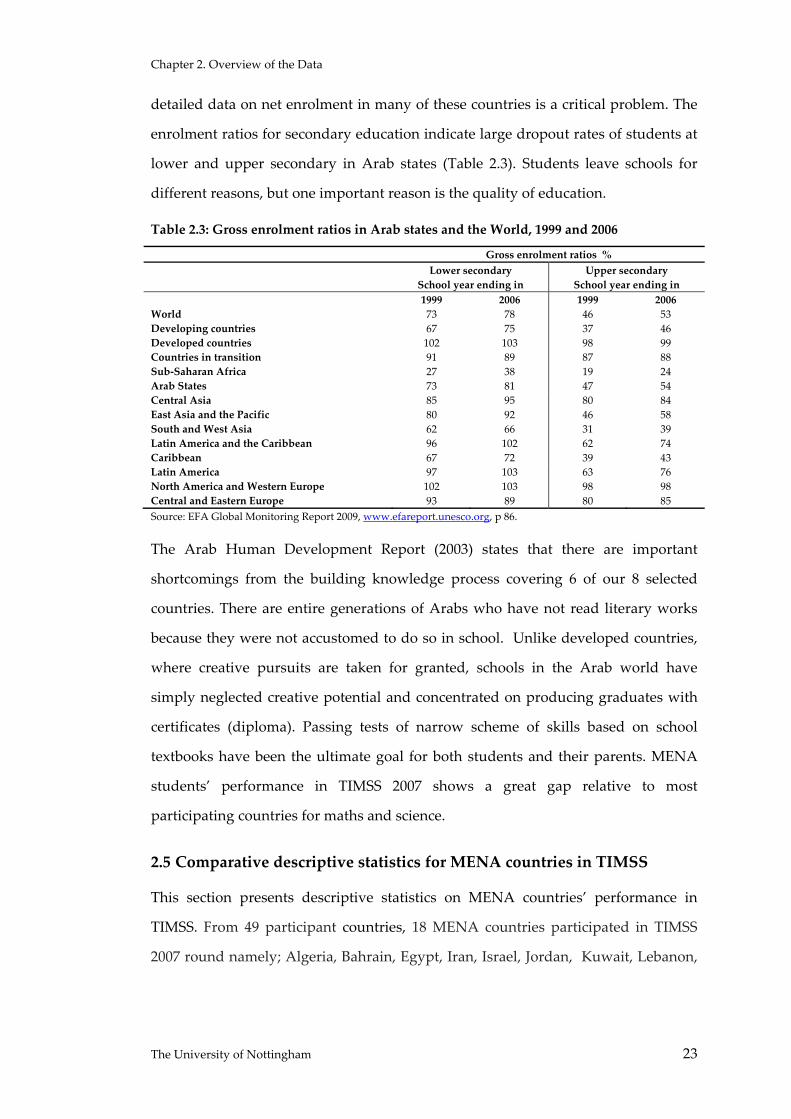
detailed data on net enrolment in many of these countries is a critical problem. The
enrolment ratios for secondary education indicate large dropout rates of students at
lower and upper secondary in Arab states (Table 2.3). Students leave schools for
different reasons, but one important reason is the quality of education.
Table 2.3: Gross enrolment ratios in Arab states and the World, 1999 and 2006
Gross enrolment ratios % Lower secondary Upper secondary School year ending in School year ending in 1999 2006 1999 2006World 73 78 46 53 Developing countries 67 75 37 46 Developed countries 102 103 98 99 Countries in transition 91 89 87 88 Sub‐Saharan Africa 27 38 19 24 Arab States 73 81 47 54 Central Asia 85 95 80 84 East Asia and the Pacific 80 92 46 58 South and West Asia 62 66 31 39 Latin America and the Caribbean 96 102 62 74 Caribbean 67 72 39 43 Latin America 97 103 63 76 North America and Western Europe 102 103 98 98 Central and Eastern Europe 93 89 80 85 Source: EFA Global Monitoring Report 2009, www.efareport.unesco.org, p 86.
The Arab Human Development Report (2003) states that there are important
shortcomings from the building knowledge process covering 6 of our 8 selected
countries. There are entire generations of Arabs who have not read literary works
because they were not accustomed to do so in school. Unlike developed countries,
where creative pursuits are taken for granted, schools in the Arab world have
simply neglected creative potential and concentrated on producing graduates with
certificates (diploma). Passing tests of narrow scheme of skills based on school
textbooks have been the ultimate goal for both students and their parents. MENA
students’ performance in TIMSS 2007 shows a great gap relative to most
participating countries for maths and science.
2.5 Comparative descriptive statistics for MENA countries in TIMSS
This section presents descriptive statistics on MENA countries’ performance in
TIMSS. From 49 participant countries, 18 MENA countries participated in TIMSS
2007 round namely; Algeria, Bahrain, Egypt, Iran, Israel, Jordan, Kuwait, Lebanon,
The University of Nottingham 23

Chapter 2. Overview of the Data
Morocco, Oman, Palestinian National Authority, Qatar, Saudi Arabia, Syria,
Tunisia, Turkey, United Arab Emirates (Dubai), and Yemen.
This study considers the eighth grade students at 8 countries: Algeria, Egypt, Iran,
Jordan, Saudi Arabia, Syria, Tunisia, and Turkey. The remaining countries are
excluded for different reasons; sample issues stated by TIMSS team (Morocco and
Yemen); small countries similar to a selected country’s education system, such as
Bahrain, Kuwait, Lebanon, Oman, Qatar, and (Dubai) from United Arab Emirates;
or countries have totally different education system like Israel and Palestinian
National Authority.
Following TIMSS guidelines for sampling, Table 2.4 presents the sample for each of
the countries and shows the full population size. The large number of schools in
Iran and Turkey reflects the size of the population. Egypt has the second largest 8th
grade population but half the number of schools less populous of Turkey. All the
selected countries tested the students only in the official language of the country
except Egypt which also tested in English. One class was chosen for the sample
except for Saudi Arabia and Tunisia when the measure of size (school population) is
greater than or equal to 140 and 375 students, respectively.
Table 2.4: TIMSS sample for MENA selected countries
Country 8th grade population 8th grade TIMSS sample Testing language Schools Students Schools Students Classes Algeria 3891 624353 149 5447 1 Arabic Jordan 1691 108856 200 5251 1 Arabic Saudi Arabia 6271 332479 165 4243 1, 2 if MOS ≥140 Arabic Syria 3756 270389 150 4650 1 Arabic Tunisia 804 176555 150 4080 1, 2 if MOS ≥375 Arabic Iran 29956 1475368 208 3981 1 Farsi Turkey 16112 1163836 146 4498 1 Turkish Egypt 8179 1342127 233 6582 1 Arabic, English NOTE: MOS measure of size indicates the number of students in school SOURCE: TIMSS technical report 2007.
A common factor among MENA countries is the low performance of its students in
maths and science relative to international peers. Surprisingly, MENA’s lowest
performing countries are among the highest in per capita income. Saudi Arabia,
Qatar, Oman, Kuwait exhibit poor performance in maths and science. Qatar has the
highest per‐capita income among MENA countries and indeed among the top ten
around the world. Saudi Arabia is classified as a high income non OECD country
though it is average performance is the lowest in MENA. An exception is of Turkey
The University of Nottingham 24

Chapter 2. Overview of the Data
with both the highest GDP per capita in the sample and the highest test scores. The
general picture, however, is low achievements in all countries with average test
scores below 450 points.
Table 2.5: Average maths and science scale scores of TIMSS 2007 countries (8th grade)
Country Maths (s.e.) Country Science (s.e.) Chinese Taipei 598 4.5 Singapore 567 4.4 Korea, Republic of 597 2.7 Chinese Taipei 561 3.7 Singapore 593 3.8 Japan 554 1.9 Hong Kong SAR 572 5.8 Korea, Republic of 553 2.0 Japan 570 2.4 England 542 4.5 Hungary 517 3.5 Hungary 539 2.9 England 513 4.8 Czech Republic 539 1.9 Russian Federation 512 4.1 Slovenia 538 2.2 United States 508 2.8 Hong Kong SAR 530 4.9 Lithuania 506 2.3 Russian Federation 530 3.9 Czech Republic 504 2.4 United States 520 2.9 Slovenia 501 2.1 Lithuania 519 2.6 TIMSS scale average 500 0.0 Australia 515 3.6 Armenia 499 3.5 Sweden 511 2.6 Australia 496 3.9 TIMSS scale average 500 0.0 Sweden 491 2.3 Scotland 496 3.4 Malta 488 1.2 Italy 495 2.8 Scotland 487 3.7 Armenia 488 5.8 Serbia 486 3.3 Norway 487 2.2 Italy 480 3.0 Ukraine 485 3.5 Malaysia 474 5.0 Jordan 482 4.0 Norway 469 2.0 Malaysia 471 6.0 Cyprus 465 1.6 Thailand 471 4.3 Bulgaria 464 5.0 Serbia 470 3.2 Israel 463 3.9 Bulgaria 470 5.9 Ukraine 462 3.6 Israel 468 4.3 Romania 461 4.1 Bahrain 467 1.7 Bosnia and Herzegovina 456 2.7 Bosnia and Herzegovina 466 2.8 Lebanon 449 4.0 Romania 462 3.9 Thailand 441 5.0 Iran, Islamic Republic of 459 3.6 Turkey 432 4.8 Malta 457 1.4 Jordan 427 4.1 Turkey 454 3.7 Tunisia 420 2.4 Syrian Arab Republic 452 2.9 Georgia 410 6.0 Cyprus 452 2.0 Iran, Islamic Republic of 403 4.1 Tunisia 445 2.1 Bahrain 398 1.6 Indonesia 427 3.4 Indonesia 397 3.8 Oman 423 3.0 Syrian Arab Republic 395 3.8 Georgia 421 4.8 Egypt 391 3.6 Kuwait 418 2.8 Algeria 387 2.1 Colombia 417 3.5 Colombia 380 3.6 Lebanon 414 5.9 Oman 372 3.4 Egypt 408 3.6 Palestinian National Authority 367 3.5 Algeria 408 1.7 Botswana 364 2.3 Palestinian National Authority 404 3.5 Kuwait 354 2.3 Saudi Arabia 403 2.4 El Salvador 340 2.8 El Salvador 387 2.9 Saudi Arabia 329 2.9 Botswana 355 3.1 Ghana 309 4.4 Qatar 319 1.7 Qatar 307 1.4 Ghana 303 5.4 SOURCE: International Association for the Evaluation of Educational Achievement (IEA), Trends in International Mathematics and Science Study (TIMSS) 2007
The University of Nottingham 25
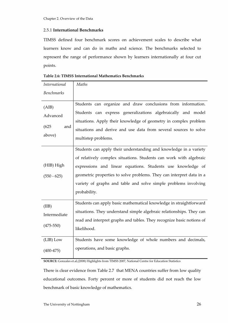
Chapter 2. Overview of the Data
2.5.1 International Benchmarks
TIMSS defined four benchmark scores on achievement scales to describe what
learners know and can do in maths and science. The benchmarks selected to
represent the range of performance shown by learners internationally at four cut
points.
Table 2.6: TIMSS International Mathematics Benchmarks
International
Benchmarks
Maths
(AIB)
Advanced
(625 and
above)
Students can organize and draw conclusions from information.
Students can express generalizations algebraically and model
situations. Apply their knowledge of geometry in complex problem
situations and derive and use data from several sources to solve
multistep problems.
(HIB) High
(550 ‐ 625)
Students can apply their understanding and knowledge in a variety
of relatively complex situations. Students can work with algebraic
expressions and linear equations. Students use knowledge of
geometric properties to solve problems. They can interpret data in a
variety of graphs and table and solve simple problems involving
probability.
(IIB)
Intermediate
(475‐550)
Students can apply basic mathematical knowledge in straightforward
situations. They understand simple algebraic relationships. They can
read and interpret graphs and tables. They recognize basic notions of
likelihood.
(LIB) Low
(400‐475)
Students have some knowledge of whole numbers and decimals,
operations, and basic graphs.
SOURCE: Gonzales et.al,(2008) Highlights from TIMSS 2007, National Centre for Education Statistics
There is clear evidence from Table 2.7 that MENA countries suffer from low quality
educational outcomes. Forty percent or more of students did not reach the low
benchmark of basic knowledge of mathematics.
The University of Nottingham 26

Chapter 2. Overview of the Data
Table 2.7: Percentage of Students Reaching the TIMSS International Benchmarks in Mathematics
Advanced(625)
High(550)
Intermediate (475)
Low (400)
Below 400
Jurisdiction Percent Percent Percent Percent Algeria # # 7 41 59Armenia 6 27 63 88 Australia 6 24 61 89 Bahrain # 3 19 49 Bosnia and Herzegovina 1 10 42 77 Botswana # 1 7 32 Bulgaria 4 20 49 74 Chinese Taipei 45 71 86 95 Colombia # 2 11 39 Cyprus 2 17 48 78 Czech Republic 6 26 66 92 Egypt 1 5 21 47 53El Salvador # # 3 20 England 8 35 69 90 Georgia 1 7 26 56 Ghana # # 4 17 Hong Kong SAR 31 64 85 94 Hungary 10 36 69 91 Indonesia # 4 19 48 Iran, Islamic Rep. of 1 5 20 51 49Israel 4 19 48 75 Italy 3 17 54 85 Japan 26 61 87 97 Jordan 1 11 35 61 39Korea, Rep. of 40 71 90 98 Kuwait # # 6 29 Lebanon 1 10 36 74 Lithuania 6 30 65 90 Malaysia 2 18 50 82 Malta 5 26 60 83 Norway # 11 48 85 Oman # 2 14 41 Palestinian Natʹl Auth. # 3 15 39 Qatar # # 4 16 Romania 4 20 46 73 Russian Federation 8 33 68 91 Saudi Arabia # # 3 18 82Scotland 4 23 57 85 Serbia 5 24 57 83 Singapore 40 70 88 97 Slovenia 4 25 65 92 Sweden 2 20 60 90 Syrian Arab Republic # 3 17 47 53Thailand 3 12 34 66 Tunisia # 3 21 61 39Turkey 5 15 33 59 41Ukraine 3 15 46 76 United States 6 31 67 92 # Rounds to zero. NOTE: Benchmarks refer to the percentage of students who reached each cut‐point score along the scale (400, 475, 550, and 625). SOURCE: Data from the International Association for the Evaluation of Educational Achievement (IEA), Trends in International Mathematics and Science Study (TIMSS), 2007.
The University of Nottingham 27

Chapter 2. Overview of the Data
The University of Nottingham 28
Figure 2‐3: Population Pyramid in MENA, 2007
SOURCE: The International Data Base (IDB), US Census Bureau 2012
MENA’s demographic distribution of the population indicates a large share for
youth and young children (Figure 2‐3). The main challenge facing these countries
(as evidenced in the ‘Arab Spring’) is reform, equality, and freedom. Education is
important to achieve those goals but education as shown suffers from poor quality
outputs. To work out a successful transitional period and to achieve the goals of
development, MENA countries should pay attention to education reform and focus
on the quality not the quantity. Inequality, gender or classes, in education and
employment, should be defined and removed from the new societies in MENA. One
important step toward achieving those goals is to define the determinants of
education quality and the sources of gender inequality in the educational output.

Chapter 3. School Effects on Students Test Scores in Egypt
Chapter 3
SCHOOL EFFECTS ON STUDENTS TEST SCORES IN EGYPT
3.1 Introduction
This chapter uses data from large comprehensive international student achievement
tests – Trends in International Mathematics and Science Study (TIMSS) – to estimate
the impact of parental education, other measures of Social‐Economic status (SES)
and school inputs on students’ achievements in Egypt. Although there are now
numerous studies on the factors influencing education quality in developed and
developing countries (Hanushek and Lavy 1994; Hanushek and Woessmann 2007;
Lloyd et al. 2001), few include Arab countries and studies on Egypt focus on
education problems such as enrolment and dropout rates and how these affect
quality.
Human capital quality measured by cognitive achievement tests directly and
indirectly influences productivity and long‐run growth. It is a research priority to
investigate sources of human capital quality. Governments, the main education
services provider around the world, should apply rational, efficient, and equitable
policies based on true research results (Hanushek and Luque, 2003; Woessmann,
2003).
This study estimates the impact of student characteristics and family background on
the one hand (the set of student variables) and teacher’s characteristics and school
resources on the other (the set of school variables), on cognitive achievement in
Egypt. The broad question addressed is: what are the major determinants,
distinguishing Social‐Economic Status (SES) and school inputs, of students’
cognitive achievements (as captured by test scores)? Using test scores for 8th grade
(age 14) students in mathematics and science for 2007, we examine the influence of
SES and school variables. The literature on education production functions reveals
no clear systematic relationship between school resources and student achievement;
The University of Nottingham 29

Chapter 3. School Effects on Students Test Scores in Egypt
teacher quality is the only factor that usually has a significant influence (Hanushek
1995).
The chapter is structured as follows. Section 3.2 provides an overview of education
in Egypt. Section 3.3 describes the TIMSS data for Egypt. Section 3.4 outlines the
empirical model and section 3.5 discusses the results: core findings and further
analysis with specific attention to school fixed effects and the impact of test
language and section 3.9 concludes.
3.2 Egypt’s education system
With more than 17 million students, 821 thousand teachers and 40 thousand schools,
the Egyptian education system is one of the largest in the world and the largest in
MENA (Middle East North African Countries)6. The Egyptian education system is
divided into Al‐Azharite system (Islamic school) and a secular system. The first is
supervised by ALAZHAR7 and accounts for 9.8% of students while the secular
system includes Arabic, language and religious schools; the 90.2 percent of all
students in the secular system are divided into public and private education sectors
(comprising 83 percent and 7.2 percent, respectively)8. All are under the supervision
of the Ministry of Education. Since 1981, free compulsory education is provided at
the primary and preparatory stages.
The school enrolment age is 6 years. The 9 years of basic education is divided into
six years primary stage and 3 years preparatory stage or lower secondary (ISCED 2).
Vocational preparatory education is provided to serve slow learners in primary and
preparatory education. The preparatory stage (grade 9 at age 15) exit exam (held at
the governorates9 level) determines whether students are qualified for general or
vocational secondary school. The secondary stage is divided into vocational (3 to 5
years) and general academic (3 years) schools. The test scores of the secondary
school exit examination (country level) determine their access to higher education
6 UNESS, (2008), Arab Republic of Egypt, p 18 7 ALAZHAR is an Official mosque and university at Cairo, the world centre of Sunni Islamic learning. 8 Ministry of Education strategic plan, (2008), Egypt 9 A governorate is an administrative division of a country. It is equivalent to a state or province.
The University of Nottingham 30

Chapter 3. School Effects on Students Test Scores in Egypt
which includes universities and institutes (3 to 6 years). Students upgrade to the
following year is conditional on their exams’ results, so there is grade repetition
(Ministry of Education 2008).
Both mixed and single sex education is provided in Egypt. Typically, boys and girls
attend mixed classes at the primary level with single sex‐schools being mainly at the
preparatory level. In the rural areas where there are insufficient students to create
two schools, students enrolled in the same school with either mixed or single sex
classes.
Tables A‐5.1–A‐5.3 in Appendix A‐5 show selected poverty, social, and educational
characteristics of Egypt compared to MENA10 and lower middle income countries.
The figures show Egypt in a good position regarding enrolment compared to
MENA except for pre‐primary enrolment. However, 3.1 percent repeaters in
primary stage and 5 percent drop out which is relatively high interruption in the
education system.
The Egyptian education system is highly centralised regarding administration,
curriculum and examination. The Ministry of Education has the main responsibility
for all education issues, collaborating with the ministry of Finance and the
governorates regarding other organizational and financial issues. The Egyptian
education system diagnostic identifies the following as issues: shortage of school
buildings at the basic education level, existence of poor quality vocational
preparatory education, weak participation of the private and cooperative sectors in
education, high repetition rates in basic education, poor reading and writing skills
of pupils in basic education, increases in the education wage bill (large number of
employees not high wages), administrative jobs are overstaffed (1:1.26), shortages in
basic education qualified teachers (41percent do not have university degree),
training mismatch with the actual needs of teachers, curricula problems, existence of
traditional teaching and evaluation methods, and the spread of private tutoring11.
10 Middle‐East and North Africa countries 11 National Strategic Plan for Pre‐University Education Reform in Egypt (2007/08 ‐ 2011/12), P 249
The University of Nottingham 31

Chapter 3. School Effects on Students Test Scores in Egypt
3.3 Data and descriptive statistics
The Trends in International Mathematics and Science Study (TIMSS) carried out by
the International Association for the Evaluation of Educational Achievement (IEA),
an independent organization, collects data on students at fourth (9‐10 years) and
eighth (14‐15 years) grade for a large sample of countries to give comparative
assessments dedicated to improving teaching and learning in maths and science for
students around the world.
This study relies on data from TIMSS on student tests results with extensive
information from the student background questionnaire and teachers and school
characteristics for both maths and science. The TIMSS target population is fourth
and eighth grades. Each participant country followed a uniform sampling approach
applied by TIMSS team to assure high quality standards. A two stage stratified
cluster design was followed: at the first level a random schools sample is selected
and within each of these schools one or two classes are selected at the second stage
randomly. All students in a selected class were tested for both maths and science.
Two main issues need to be addressed in using TIMSS; the complex multi‐stage
sample design mentioned above and the use of imputed scores or “plausible values”
(Foy and Olson 2009).
3.3.1 Egypt in TIMSS 2007
Egypt has 8,179 schools with 1,342,127 students at the eighth grade. The selected
TIMSS sample for Egypt is 233 schools with 6,582 students which produces an
estimated population of 1,059,228 students. There are 234 teachers of integrated
science and 234 teachers of maths. TIMSS tests for maths and science are
administered in both Arabic and English while the background questionnaire is
administered only in Arabic.
Table A‐ 3.4 in the appendix shows average achievement of maths and science in
Egypt and some developed and developing countries. The substantial difference in
maths scores between Egypt and Spain, US, England, and Japan is evident (it
exceeds 100 points). The situation compared to other Arab and MENA countries is
mixed; while Egyptian students’ achievement is higher than Algeria, Morocco,
The University of Nottingham 32

Chapter 3. School Effects on Students Test Scores in Egypt
Kuwait, Saudi Arabia, Oman and Qatar, it is lower than Turkey, Israel, Iran, Dubai,
Lebanon, Jordan, Tunisia, Bahrain and Syria. In Sub‐Saharan African countries such
as Ghana and Botswana, students’ achievement in maths is behind that in Egypt.
In Egypt, the TIMSS sample was 49.5 percent girls. The overview concentrates on
the Egypt 2007 TIMSS maths scores with some comparison to the 2003 round.
Egypt maths scores declined from 406 in 2003 to 391 points in 2007 representing a
statistically significant decline of 15 points. Girls’ maths achievement scores
declined from 406 in 2003 to 397 in 2007, whereas boys’ achievement declined
significantly from 406 to 384. Gender differences in achievement scores were not
significant in 2003 (less than one point difference) whereas they were at the 95%
level in 2007 (girls 13 points higher on average).
Science test scores achievements declined from 421 in 2003 to 408 in 2007 on
average. This fall of 13 points is statistically significant at the 5% level Appendix A‐5
(Table A‐ 3.5). The distribution of marks from Figure 3‐1 to Figure 3‐5 indicates that
students do better in science in general. Girls outperform boys and language schools
outperform Arabic schools for both maths and science. The test scores appear to be
normally distributed.
Figure 3‐1: Distribution of student achievements by subject
0.0
01.0
02.0
03.0
04kd
ensi
ty
0 200 400 600 800Mean of five plausible values
Math Science
Distribution of students achievement in Math and Science
The University of Nottingham 33

Chapter 3. School Effects on Students Test Scores in Egypt
Figure 3‐2: Distribution of student Maths achievement by school language
0.0
01.0
02.0
03.0
04.0
05Kd
ensi
ty
0 200 400 600 800Mean of five plausible values for mathematics
Arabic English
Distribution of student achievement in Arabic and English schools
Figure 3‐3: Distribution of student Maths achievement by gender
0.0
01.0
02.0
03.0
04K
dens
ity
0 200 400 600 800Mean of plausible values mathematics
Girls Boys
Distribution of student achievement by gender
The University of Nottingham 34

Chapter 3. School Effects on Students Test Scores in Egypt
Figure 3‐4: Distribution of student Science achievement by school language
0.0
01.0
02.0
03.0
04.0
05Kd
ensi
ty
0 200 400 600 800Mean plausible values Science
Arabic English
Distribution of student achievement by school type
Figure 3‐5: Distribution of student science achievement by gender
0.0
01.0
02.0
03.0
04K
dens
ity
0 200 400 600 800Mean plausible values Science
Girls Boys
Distribution of student achievement by gender
The University of Nottingham 35

Chapter 3. School Effects on Students Test Scores in Egypt
As explained in Chapter 2, TIMSS benchmark scores on achievement scales describe
what learners know and can do in maths and science. Table A‐ 3.6 in the appendix
indicates that 53 percent of Egyptian students do not even satisfy the low
international benchmark (which is that students have some knowledge of whole
numbers and decimals, operations, and basic graphs) of maths compared to 48% of
students in 2003 TIMSS and 45% for science.
Arab countries such as Jordan and Tunisia fare better than Egypt with 39% of
students below the low benchmark; Bahrain is slightly better and Syria has the same
percentage as in Egypt; in Oman, Algeria, Morocco, Qatar, and Saudi Arabia
performance was much worse. Students’ average age in the TIMSS 2007 sample for
Egypt is 14.11. Younger and older students perform less well in maths than students
of average age.
Student performance in maths with respect to the language of testing shows a large
gap in favour of those tested in English. The direct conclusion from these means
could be misleading because of the difference in the sample size between the two
groups and because some possible third variables could be influential, such as
language schools having more school resources and students from higher income
families.
Egyptian learners performed relatively well in algebra and geometry and less well
in the learning domains of numbers, data and chance. The TIMSS 2007 maths was
designed to have three main cognitive categories to measure different types of
abilities of the learners. The three cognitive domains are: knowing, applying and
reasoning. Egyptian students show better performance in knowing and reasoning
cognitive skills compared to applying.
3.3.2 Descriptive statistics on home background and school resources
As mentioned previously, the TIMSS data set is very large and supplemented by
different questionnaires with a total of 88 questions: 33 are answered by the
students, 33 are answered by teachers, and 22 are answered by school principal.
The University of Nottingham 36

Chapter 3. School Effects on Students Test Scores in Egypt
Table 3.1: Descriptive Statistics of included variables (a) (b)
Family and student background Mean std. dev. Teacher characteristics and school resources
Mean std. dev.
Mother education level Test language12 Not finished elementary school 0.25 0.43 Arabic 0.97 0.16 Elementary/middle school 0.26 0.44 English 0.02 0.16 Secondary school 0.11 0.31 Teacher gender 2 years of post secondary school 0.12 0.32 Male 0.71 0.45 University degree or higher 0.08 0.28 Female 0.20 0.40 Do not know/missing 0.19 0.39 Teacher years of experience13 12.20 8.61 Father education level Teaching certificate Not finished elementary school 0.15 0.35 Yes 0.65 0.48 Elementary/middle school 0.28 0.45 No 0.16 0.37 Secondary school 0.12 0.33 Availability of school resources MATHS 2 years of post secondary school 0.17 0.37 High 0.27 0.44 University degree or higher 0.10 0.30 Medium 0.67 0.47 Do not know/missing 0.18 0.38 Low 0.05 0.23 Parents nationality Teacher formal education Both parents are Egyptians 0.77 0.42 Not university degree 0.03 0.16 Only one parent or neither parent 0.19 0.39 University degree 0.82 0.39 Number of books at your home Postgraduate studies 0.06 0.23 None or few 0.67 0.47 Type of community One bookcase (26 to 100 books) 0.21 0.41 More than 50000 people 0.46 0.50 Two bookcases or more 0.09 0.29 Less than 50000 people 0.51 0.50 Home possessions Perc. of disadvantaged std High 0.12 0.33 Less than 50 percent 0.52 0.50 Medium 0.36 0.48 More than 50 percent 0.43 0.50 Low 0.41 0.49 Class size for maths Gender of student Less than 41 0.42 0.49 Boy 0.51 0.50 41 or more 0.56 0.50 Test language spoken at home SCIENCE Always 0.66 0.47 Availability of school resources for science Almost always, sometimes, or never 0.32 0.47 High 0.374 0.484 Computer use Medium 0.570 0.495 Both at home and school 0.21 0.41 Low 0.039 0.194 Either home or school 0.56 0.50 Pc only at places other than home or none at all
0.16 0.37
PlayStation or similar games Yes 0.37 0.48 No 0.59 0.49 Note: Sample size is 6582, all variable are dummy except for teacher experience and class size included in some estimations as continuous. “Do not know” responses are treated as missing; note that it is the students who answer the questions.
For many questions a list of possible answers is provided, for example parental
educational attainment lists seven categories. Preliminary analysis using the full
range of categories revealed that many variables have no significant effect on test
scores and/or have many missing observations. Where appropriate and justified by
12 The un‐weighted descriptive statistics indicates 82% for Arabic and 18% for English 13 Note: it is included as continuous
The University of Nottingham 37

Chapter 3. School Effects on Students Test Scores in Egypt
this analysis, we have combined or omitted categories. This section outlines the
coding we use for the explanatory variables.
Table 3.1 panel (a) presents the descriptive statistics for student characteristics,
family background and Social‐Economic status (SES) for Egypt. Parental education
includes mother’s education and father’s education measured by the highest
educational level attained for each of them measured in six categories: not finished
elementary school; finished elementary or middle school; finished secondary school;
2 years of post secondary school; University degree or higher; and “don’t know”.
The share of students in the TIMSS sample of Egypt whose mothers have not
finished elementary school is 20 percent compared to 12 percent for fathers;
mother’s with university degree or higher (postgraduate studies)14 are 12 percent
compared to 16 percent for fathers. Approximately 15 percent of the students
reported they do not know their mothers’ highest educational level attained, and a
similar percentage does not know their fathers’ educational level attained.
The number of books in the students’ home is coded in three categories: none or few
books; one bookcase full of books; and two bookcases or more. The share of
students from homes with no or few books is 63 percent compared to 25 percent
with one bookcase and 13 percent with two bookcases or more.
The home possessions index, used as a proxy for family SES, is coded as high,
medium or low. This index is constructed using data from four selected variables
investigating different types of possessions: computer; study desk; internet
connection; and satellite TV channels. Those variables were selected out of eight
variables indicating home possessions using principal component analysis to
identify the most influential variables for constructing the index. The construction of
an index is problematic. The absence of a convenient approach of selecting variables
to proxy living standards were shown by Montgomery et al. (2000), who argue that
most studies used ad‐hoc strategy to select variables. Recent studies employed
principal component analysis (PCA) to derive Social‐Economic Status (SES) indices
14 The coding refers to postgraduate education but may not mean a Masters or PhD; it is likely to refer to other higher or professional qualification.
The University of Nottingham 38
Chapter 3. School Effects on Students Test Scores in Egypt
from data sets which have no income measures such as Demographic Health
Surveys (DHS) (Filmer and Pritchett 2001; McKenzie 2005).
PCA was employed to capture the most influential variables among eight variables.
A home possession index was then constructed using the most influential variables
based on their shares in explaining the variation in the PCA. The share of students
who coded high is 24 percent, 36 percent coded low and 39 percent coded medium
(Appendix B‐5).
Parents’ nationality is measured by two categories: both parents are Egyptian; one
or both have foreign nationality. Almost 84 percent of students are of Egyptian
parents. The test language is either Arabic or English. The majority of students took
the TIMSS maths test in Arabic (83 percent of the sample). “How often the language
of testing spoken at home?” is measured by two categories: always spoken at home;
and with “almost always”, “sometimes”, and “never” combined into one category15.
Two more variables were introduced to investigate their impact on student
achievement. Computer use is coded in three categories: both at home and school
(28 percent); either at home or school (56 percent); and only at places other than
home/school or not at all (16 percent). Empirical evidence from a study on “home
computer use and development of human capital” indicates that home computer
use had significantly lowered the Romanian students’ grades in Maths, English, and
Romanian especially for low‐income children (Malamud and Pop‐Eleches 2011).
Students were asked if they have a PlayStation or similar games at home; 42 percent
responded yes and 58 percent said no. The effect of this on test scores is ambiguous;
it could reduce scores if access to games is a distraction from study at home, but if
having such games is an indicator of household wealth it may be positively
associated with test scores if students from wealthier households tend to perform
better (the index of possessions is our only control for household assets).
Table 3.1 panel (b) reports descriptive statistics for Teachers’ characteristics and
school resources. 80 percent of maths teachers are men. Teachers’ experience is
15 ‘Almost always’ is combined with other group to capture any other language spoken at home (so ‘always’ means only one language spoken)
The University of Nottingham 39

Chapter 3. School Effects on Students Test Scores in Egypt
measured by years of teaching which we coded in three categories: less than 10
years experience (35 percent for maths); 11 to 19 years (38 percent); and 20 years or
more (27 percent). Some 82 percent of teachers have a teaching certificate. Teachers’
formal education level attained is coded in three categories: below university degree
(two percent); university degree (89 percent); and postgraduate degree.
The type of community is used as a proxy for the population distribution to
distinguish urban (the school is in a community with more than 50000 people) and
rural (a community with less than 50000 people). School locations are almost evenly
divided: 55 percent of students come from communities with more than 50000
people and 45 percent come from communities of less than 50000 people. The
percentage of students in a school from disadvantaged homes (a question answered
by teachers) is used as a proxy for the impact of being in disadvantaged areas on
student performance.
School resources are measured by two variables, class size and an index of
availability of school resources for maths instruction. Class size is coded in two
categories: classes with 41 students or more (47 percent) and classes with less than
41 students (53 percent). The index of availability of school resources for maths
instruction, constructed by TIMSS, is based on school principals’ responses to a
series of questions about shortages affecting instruction.
Ten areas of shortage or inadequacies (rated on a four point scale: none = 1, a little =
2, some = 3, and a lot = 4) which could affect delivering maths instruction in a proper
way were included in the index computation. General areas include: 1) Instructional
materials (e.g., textbook); 2) Budget for supplies (e.g., paper, pencils); 3) School
buildings and grounds; 4) Heating/cooling and lighting systems; and 5)
Instructional space (e.g., classrooms); and maths‐specific areas: 6) Computers for
maths instruction; 7) Computer software for maths instruction; 8) Calculators for
maths instruction; 9) Library materials relevant to maths instruction; and 10) Audio‐
visual resources for maths instruction (Olson et al. 2008b). The index of school
resources for maths instruction index is coded in three levels: high; medium (57
percent); and low (four percent).
The University of Nottingham 40

Chapter 3. School Effects on Students Test Scores in Egypt
Table 3.2: Percentages of students, Parents education and average test scores
Education level Mother Father Maths Science Maths Science Percent mean se mean se Percent mean se mean se
Not finished Elementary 25.66 375.48 5.29 394.82 4.66 15.2 363.91 6.02 384.88 5.24 Elementary/middle 26.35 385.32 4.64 404.54 4.84 29.38 384.1 4.8 403.58 4.11 Secondary 10.93 421.06 6.28 438.82 5.8 12.69 408.13 6.22 423.96 6.1 post secondary (2 years) 12.14 438.34 5.32 451.56 5.32 17.19 437.43 4.92 453.01 5.04 University degree 3.66 404.95 10.56 423.85 9.67 4.38 410.61 7.39 423.49 7.34 Postgraduate studies 4.94 391.12 6.88 394.54 7.81 5.98 394.84 7.29 403.38 8.14 I do not know 16.32 378.65 5.3 398.27 5.48 15.18 372.54 5.24 393 5.42
It is clear from Table 3.2 that parents’ education is associated with achievement. The
highest achievers are those whose parents have intermediate to higher education
(first degree). The teacher is the core of creating a supportive environment for
learning process. TIMSS has information on the teaching staff, academic preparation
for teaching, teachers’ professional development and their readiness to teach TIMSS
curriculum topics. The majority of Egyptian TIMSS maths teachers are aged
between 30 and 39 years. The older the teacher the higher student performance is a
clear relation from Table A‐ 3.7. In Egypt, about 20 percent of maths learners were
taught by females and 80 percent by males, without a significant difference in
achievement. The average teaching experience of Egyptian teachers is 14.5 years.
The results for teacher education level and achievements are mixed and no clear
relation could be stated. However, it seems from Table A‐ 3.8 that teacher
satisfaction is positively correlated with teachers’ performance and so students’
performance. Average scores are also positively correlated with teachers’
satisfaction.
The average class size in Egypt is 37 students with a great dispersion in sizes. The
most common class size is 40 students which is high relative to the top performing
countries. Table A‐ 3.9 shows a tendency towards better performance with lower
class size for maths and science.
The disadvantage of TIMSS data for Egypt is that they do not include data on
regional distribution of school (urban/rural) or on (private/public) status. Schools
with a high percentage of students from disadvantaged homes perform worse than
those in schools with fewer disadvantaged students (Table A‐ 3.10).
The University of Nottingham 41

Chapter 3. School Effects on Students Test Scores in Egypt
Table 3.3: Distribution of students whose peers are affluent at different schools
Percentage of affluent students Arabic schools English language schools TotalN % N % N %
Less than 10% 2,068 42 38 3 2106 32 11 to 25 % 1,552 31 18 2 1570 24 26 to 50 % 579 12 56 5 635 10 More than 50 % 766 15 990 88 1756 27 Missing 497 9 18 2 515 8 Total 5,462 100 1,120 100 6582 100
Students were tested in either Arabic or English; we assume that those tested in
Arabic are enrolled in Arabic schools and the others are in English language schools.
The English language schools in Egypt are mainly private schools but there are also
public experimental language schools, but TIMSS does not identify these. The data
indicate a bigger share of affluent students enrolled language schools (Table 3.3).
3.4 The Empirical model
The underlying model is very straightforward. The output of the educational
process is directly related to a group of inputs by an education production function
(EPF). We use student standardized achievements in test scores as a measure of
output. Inputs include characteristics of schools, teachers, and other non‐student
variables and student SES variables such as family characteristics and home
resources. We estimate an education production function of the following form:
0 1 2is is s isA F Sβ δ δ ε= + + + ( 3.1)16
Where A is the test score of student i in school17 s, F is a vector of family background
variables and S is a vector of school characteristics variables. The coefficient vectors
α, 1δ and 2δ are to be estimated. The error term ε has two components as we have
two‐stage stratified sample, the imputation error on student’s level and the sample
error at the school level. Table 3.1 described in detail the variables included in our
estimations.
16 We include D, a vector of dummy variables for each variable both in F and S to capture the effect of missing observations; a dummy takes the value 1 for observation with missing data and 0 otherwise (the variables themselves are set to zero if their values are missing). 17 Egypt’s sample selects only one class from each school, simplifying notation to students and schools only.
The University of Nottingham 42

Chapter 3. School Effects on Students Test Scores in Egypt
School inputs and school choice will be the parents’ decision; parents may make
residential choice to ensure that their children are taught in a good school (small
class size, good teachers or available facilities). Parents, teachers, and schools make
choices that might give rise to a non‐causal association between school inputs and
student achievement even after controlling for family background. This makes the
empirical investigation complex seeking identification and examining the sources of
the effects by different techniques and methodologies to ensure the right
interpretations of results.
3.5 Main Results
The results of estimating the education production functions, equation ( 3.1), for
TIMSS achievement test scores in Egypt are discussed comparatively for maths and
science (Table 3.4). The explanatory variables are organized in blocks, starting with
measures of family background and student characteristics, followed by teacher
characteristics and school features. In addition a critical look is paid to possible role
of school type, interaction effects, school fixed effects and test language differences.
The dependant variables are the plausible values for test scores in maths and
Science.
3.5.1 Students background
We employ three sets of dummy variables to reflect the family background of
students: the father’s education level, the mother’s education level, and the number
of books at home. We also include various variables to capture a broader picture of
student background and socio‐economic status.
3.5.1.1 Parental education
For Maths, student level variables have the largest and most significant coefficients
in the production function. Children of a mother with secondary or two years post‐
secondary education perform better than children of a mother with elementary or
middle school. The results suggest a significant 17 point test score increase for
students if their mother has two years’ post‐secondary education (compared to
mother with no education or did not finish elementary school) and 15 point increase
The University of Nottingham 43

Chapter 3. School Effects on Students Test Scores in Egypt
if the mother has secondary education. Although scores are lower for students
whose mother finished university or postgraduate studies, this is not significant.
Table 3.4: Estimates of Family, School Background on Maths and Science Performance
Dependant variable : students’ test scores (the mean of 5 plausible values)
Maths N=6582 R2 .2422
Science N=6582 R2 .2193
Family and student background Mother education level b se b se Elementary/middle school ‐3.036 (5.101) ‐1.276 (4.868) Secondary school 14.987** (6.216) 16.464*** (5.510) 2 years of post‐secondary school 17.584*** (6.703) 17.526** (7.172) University degree or higher ‐6.723 (6.918) ‐9.847 (6.582) No or not finished elementary(omitted) Father education level Elementary/middle school 13.683** (6.561) 11.773** (5.312) Secondary school 26.310*** (6.012) 21.762*** (5.680) 2 years of post‐secondary school 35.144*** (5.403) 33.667*** (6.584) University degree or higher 10.611 (6.631) 5.898 (6.699) Never or not finished elementary(omitted) Number of books at your home One bookcase 11.126*** (4.313) 12.069** (4.798) Two bookcases or more 0.850 (6.280) ‐1.033 (6.761) No or few books(omitted) Both parents Egyptian=1 49.427*** (5.106) 47.361*** (5.071) Home possession index High 34.731*** (4.372) 35.658*** (5.997) Medium 18.558*** (3.532) 18.467*** (4.228) Student gender (male =1) ‐9.342* (5.422) ‐16.499*** (5.501) Testing Lang. spoken at home (always=1) ‐17.994*** (3.721) ‐16.935*** (4.165) Type of community (more than 50000 people = 1) 9.816 (6.513) 13.031* (7.234) Less than 50000 people (omitted) Computer use Both at home and school ‐21.879*** (4.965) ‐31.587*** (6.537) Either home or school ‐21.822*** (4.233) ‐25.630*** (4.457) Other places or none (omitted) PlayStation or similar games yes = 1 ‐19.533*** (3.073) ‐14.602*** (3.197) Teacher characteristics and school resources Test language (Arabic=1) ‐40.758*** (12.087) ‐14.025 (12.033) Teacher gender ( male = 1) ‐0.642 (7.657) ‐2.516 (6.353) Teacher years of experience 1.065*** (0.388) ‐0.221 (0.521) Teaching certificate 8.057 (9.587) 0.740 (7.426) Availability of school resources for instruction Medium ‐3.214 (7.580) ‐1.360 (8.648) Low ‐19.639 (13.745) ‐16.327 (17.100) Teacher formal education completed University ‐5.361 (23.189) ‐13.289 (16.125) Postgraduate studies ‐13.253 (24.771) ‐22.468 (21.729) Not university (omitted) Percentage of disadvantaged std (more than 50%=1) ‐7.040 (6.254) ‐11.697** (5.764) Cass size (more than 41 =1) ‐4.920 (6.393) ‐4.934 (6.546) Less than 41 (omitted) Constant 400.594*** (28.554) 432.479*** (23.783) Controls for missing included Yes Yes Sampling weights of TIMSS are used, Jackknife standard errors in parentheses, Significance levels: * p<0.10, ** p<0.05, *** p<0.01. Note: Teacher experience square when included all coefficient are essentially the same except teacher experience is insignificant for maths.
The University of Nottingham 44

Chapter 3. School Effects on Students Test Scores in Egypt
Similar results are obtained for father’s education. Fathers who completed middle
and secondary school increase test score by 13 and 26 points respectively compared
to those who did not complete primary education. Having a father with university
or postgraduate education has the lowest (and insignificant) impact on test scores
compared to a father who did not complete primary education (but not significant),
while a father who completed two years post‐secondary has the greatest impact (an
increase of 35 points).
These findings are broadly in line with previous studies finding that parental
education is important (Hanushek 2002; Woessmann 2004). However, one difference
compared to results for many other countries, especially developed countries, is that
the effect appears non‐monotonic. In Egypt, have more educated parents is
associated with higher scores up to parents with post‐secondary (but pre‐
University) education but the effect of more education becomes negative beyond
this (although, for fathers, scores are still higher compared to not having completed
primary education). The lower impact of parents with university or postgraduate
education may be because both parents are working so there is less home support
for study, or it could be that the most educated parents have relatively lower
aspirations for their children compared to pre‐University educated parents (who
want their children to have a better education than they had themselves).
Father’s education appears more important than mother’s for student performance
in Egypt. Levels of education attained indicate a larger influence of fathers’
education than mothers’ on student test scores as well as a positive effect at all
levels compared to negative coefficients for mother’s highest and lowest levels of
education.
Student achievement in science is better than maths: average scores in science are
higher by 18 points. The coefficients estimates from the regression for the science
test scores are similar to the maths estimates with respect to parent’s education and
books at student’s home.
Parents’ education follows the same non‐monotonic pattern of impact as for Maths.
A student whose mother completed secondary or post‐secondary education (but not
The University of Nottingham 45

Chapter 3. School Effects on Students Test Scores in Egypt
university) performs better compared to students whose mother did not finish her
primary education, by 17 and 18 points respectively. Fathers’ education has an
increasing impact on performance in science: completing middle school increases
test scores by 12 points compared to a father with no education, completing
secondary school improves test scores by 22 points, and completing post secondary
(two years) adds 34 points. Parents with university degree or higher have no
significant impact on their children’s performance in science.
3.5.1.2 Home possessions and books at home: Socio‐Economic Status (SES)
The third indicator of family background is the number of books in the students’
home. Only having one bookcase made a significant difference, increasing test
scores by 11 points for maths and 12 points for science compared to students from
homes with no or few books. It is surprising that having two bookcases or more was
not significant. One possible explanation is that those students who answered two
bookcases or more are misreporting (bookcases could be of different sizes or they
may be including magazines and newspapers, though the questionnaire told them
not to count them). Another explanation supports the conjecture for parental
education if highly educated parents have more books at home but give less support
to their children in study.
The home possessions index (a proxy for the SES of the family) suggests that the
impact of family SES on students’ educational achievements is large and significant:
a high level of SES increases test scores by 35 and 36 points for math and science
respectively and medium levels by 19 and 18 points compared to the reference
group of low SES. The effect of high SES is double the effect of medium level SES.
Private tutoring, or ‘shadow education’, is prevalent in Egypt and is likely to be one
mechanism by which SES influences achievement. The tutoring market includes all
types of schools and students at different stages of education depend on different
types of tutoring. The most focused concentration is on the ninth grade and the
secondary stage exit exams. Although, private tutoring is prohibited by law; this is
not enforced and hence ignored (Hartmann 2008). The ninth grade exams
determine whether the student will be qualified to go to a ‘prestigious’ general
The University of Nottingham 46

Chapter 3. School Effects on Students Test Scores in Egypt
secondary which will lead to university, and the secondary stage exit exams
determine which colleges may admit a student. All grades with yearly exit exams
create pressure on families for private tutoring.
3.5.1.3 Nationality and home spoken language
Native students perform better than non‐natives for maths and science (the effect
magnitude is slightly less for science). Students of Egyptian parents perform
significantly better than students with one or both parents being foreign. The
dummy variable for nationality has the largest effect on student test scores of all the
significant explanatory variables ‐ a 49 and 47 point test score increase in maths and
science respectively. This is in line with findings from Woessmann (2004) on Europe
and the US.
One surprising result is that students who always speak the test language at home
perform significantly less well than those who speak another language. The results
suggest 18 and 17 point increases if the language spoken at home is not always the
test language for maths and science respectively. Out of the students who always
speak the test language at home (61% of TIMSS sample), 88.7% of them took the
Arabic test and only 11.3% took the English version of science test. However both
English and Arabic test takers exhibit the counterintuitive result that always
speaking the test language is associated with lower performance.
Table 3.5: Test language frequently spoken at home and students’ achievement
Home spoken lang. Language of testing N % total Maths Science
Mean se Std.dev Mean se Std.dev Always Arabic 3551 54.77 382.96 (4.06) 96.11 401.55 (3.96) 95.31
4003 (61.75) English 452 6.97 467.4 (10.07) 84.81 456.19 (12.46) 86.64
Almost always Arabic 797 12.29 415.29 (5.02) 104.59 431.35 (5.45) 104.64
1129 (17.41) English 332 5.12 490.45 (5.82) 71.88 484.25 (7.4) 74.99
Sometimes Arabic 861 13.28 398.39 (6.53) 99.83 417.93 (6.21) 101.37
1048 (16.17) English 187 2.88 492.64 (9.01) 72.11 476.44 (6.1) 73.08
Never Arabic 160 2.47 370.38 (13.06) 101.31 392.71 (13.29) 101.47
303 (4.67) English 143 2.21 488.57 (12.86) 87.1 468.01 (15.23) 87.8
Descriptive statistics (Table 3.5) show that students who took the English test
perform better at all levels of regularity of speaking the language at home. Students
The University of Nottingham 47

Chapter 3. School Effects on Students Test Scores in Egypt
who speak other languages at home beside the test language perform better than
students who either always or never speak the test language at home. Re‐estimating
using a different default category test language shows that students who speak the
language of testing either ʺalmost alwaysʺ, ʺsometimesʺ or ʺneverʺ perform
statistically significantly better by 22 points of test scores in maths higher than
students who ʺalwaysʺ speak the test language at home. As ‘natives’ perform better
this suggest either poor performing non‐Egyptian Arabs or better performing
Egyptians in ‘multi‐lingual’ households.
3.5.1.4 Gender Differences
The gender gap in general is weakly significant (10%) except for science where girls
outperform boys by 13 points (statistically significant at the 5% level). Nevertheless,
girls generally perform better than boys in both TIMSS tests (see further analysis in
subsection 0). This is only true in 2007‐ there was no significant difference in 2003
(Table A‐ 3.5).
3.5.1.5 Type of community and Poverty Levels
Neighbourhood poverty is represented by the proportion of disadvantaged students
in the school. It is not statistically significantly related to students’ performance in
maths. However, it does have a significant negative impact on science test scores.
Students who go to a school with more than 50% of students disadvantaged
perform worse by 12 points in science test scores than students who attend schools
with less than 50% of students disadvantaged.
We use the type of community as a proxy for the urban or rural nature of the school
location. Urban community has positive and significant effect only on science
achievements at 10% significance level: cities and bigger communities have more
association with achievements in science than rural or small communities. Other
divisions of type of community have no significant effect.
3.5.1.6 Computer usage and game consoles
The availability of home computers and video game consoles like PlayStations or
similar games, represent a major innovation in the Egyptian life style, culture and
The University of Nottingham 48

Chapter 3. School Effects on Students Test Scores in Egypt
traditions. Surprisingly, students who use a computer at home and/or at school
perform significantly worse than those who do not use computer at all (22 points
less for maths). The impact of games consoles is similar, presumably providing a
distraction to students.
The effect of using computers on test scores is much worse for science. Using
computer at both places reduces student test scores by 32 point; using a computer
either at home or at school reduces test scores by 26 point. Having games consoles
reduces student test scores by 15 points. Including a more disaggregation
categorization of computer usage does not change the findings of the chosen
categories (Appendix A‐5, Table A‐ 3.12).
3.5.2 Teacher characteristics and School background
While intuition suggests that teachers are extremely important in affecting student
achievement, few of their observed characteristics are found to have a significant
impact. Only teacher experience, measured by years teaching and its square to test
for decreasing returns to experience, has a statistically significant impact. While the
two forms are not identically significant, they are jointly different from zero at 5% of
significance, and when the squared teacher experience term is dropped, teacher
experience in years has a significant positive effect on test scores.
School background and resource endowment are measured by an index for the
availability of school resources and by class size. The school resources availability
index18 has no effect on performance, although low school resources are associated
with lower test scores for both maths and science. Class size is one of the most
important measures of school endowment in the literature but also shows no
significant influence on student performance.
TIMSS provides the actual number of students and dummy variables for three
groups of class size: high (41 or more), medium (25 to 40), and low (1 to 24). With
ʺhighʺ as the default, neither the ʺlowʺ or ʺmediumʺ dummies were significant. The
18 The index is composed using factor analysis technique including five major school variables and five subject specific indicators for both Math and science (TIMSS Technical report, 2009). Disaggregating the index indicates very few significant effects for some levels and suffers from multicollinearity.
The University of Nottingham 49

Chapter 3. School Effects on Students Test Scores in Egypt
World Bank has argued it is only when class sizes reach the ʺlargeʺ category that
they start to impede performance. We employed both variables alternatively and the
results do not change. However, including only the ʺlargeʺ dummy (and so
combining the other two as the default) reveals no significant effect in Egypt. These
findings are counter‐intuitive but nonetheless in line with many previous studies
since the Coleman report in 1966 (Woessmann, 2003, 2004; Hanushek, 2007).
The last remaining finding concerns the impact of the test language used in the
TIMSS test. The results differ for maths and science: testing language is insignificant
for science, but students who take the maths test in English perform significantly
better than those who take the test in Arabic. This striking finding is subject to
further investigation later, in subsection 3.7.2.
3.5.2.1 Class size endogeneity and Instrumental Variables (IV)
The problem in estimating class size effects is that many factors might influence
such decision which might affect the casual relationship between class size and
student performance. Parents and/or school could influence the placement decision.
For example, parents might choose less crowded classes for their children based on
their performance; and teachers and school principals might sort student into
differently sized classes based on behavioural or academic reasons. This may be bias
the estimates of education production function by the endogeneity of class size with
respect to student performance.
To solve this issue, we need to identify class size effect that relies only on exogenous
variation in class size. The school fixed effects eliminates the effects of between
school sorting. However, the within school sorting may still affect our estimates.
Therefore, instrumental variables (IV) approach needed to eliminate the
endogenous biased effect of class size and make sure that the estimates is based on
the exogenous part of the effect.
The valid instrumental variable should be highly correlated with the class size
measure variable and uncorrelated with test scores. Woessmann and West (2006)
instrumented the class size effect using TIMSS data by the average class size at the
grade level. Akerhielm (1995) used the average class size and the eighth grade
The University of Nottingham 50

Chapter 3. School Effects on Students Test Scores in Egypt
enrolment in the school as instruments for the actual class size. Akerhielm
constructed the variable by taking the average class size of all the students in the
school in a given subject that responded to the NELS survey. Both studies claimed
that the two instruments are valid and are correlated directly with the actual class
size and are unrelated to the student performance. Nonetheless, Woessmann and
West criticized the usage of grade enrolment in the school as it might be directly
influence test scores away from class size.
In our case, TIMSS data provide the two variables. From the school questionnaire,
the school principal answered a question on the average class size of the eighth
grade and reported the total number of students at the eighth grade. (Altinok and
Kingdon 2012) suggested using the differences between the two subjects class size
as an instrument, unfortunately this is invalid in the case of Egypt as students
placed in the same class room for all subjects.
Since TIMSS chooses one class from each school it is not possible to run the fixed
effect instrumental variable approach or using pupil teacher ratio as an instrument
for class size. So, we employ the two instruments together and separately in the first
instance and investigate the validity using the proper tests of under‐identification
test, weak instrument or weak identification test and over‐identification test.
The estimates of class size IV use the five plausible values of maths and science test
scores and jackknife standard errors to deal with clustering. The two instruments
show significant effect on actual class size in the first stage which suggests a
relevance of the selected instruments. The under‐identification test is an LM test of
whether the equation is identified, i.e., that the excluded instruments are ʺrelevantʺ,
meaning correlated with the endogenous regressor, i.e. actual class size. The test
results (Table 3.7) show that we reject the null of under‐identification in favour of
identified model. The weak instrument ʺWeak identificationʺ arises when the
chosen instruments are correlated with the endogenous regressor (class size), but
only weakly.
The University of Nottingham 51

Chapter 3. School Effects on Students Test Scores in Egypt
Table 3.6: Estimates of Family, School Background on Maths and Science Performance using class size Instrumental Variables (IV)
Dependant variable : students’ test scores (the mean of 5 plausible values)
Maths
N=6582 R2 .2422
Maths Class Size (IV)
N=6221 R2 .2366
Science
N=6582 R2 .2197
Science Class Size (IV)
N=6123 R2 .2181 Family and student background Mother education level b Se b Se b Se b se Elementary/middle school -2.91 (5.09) -2.79 (5.20) -1.27 (4.87) -1.98 (4.91) Secondary school 15.04** (6.15) 15.65** (6.33) 16.65*** (5.40) 17.39*** (5.72) 2 years of post-secondary school 17.38*** (6.69) 18.10*** (6.87) 17.34** (7.07) 17.16** (7.43)
University degree or higher -6.46 (6.84) -5.62 (7.17) -9.81 (6.59) -11.26* (6.83) No or not finished elementary(omitted)
Father education level Elementary/middle school 13.72** (6.56) 13.25** (6.72) 12.03** (5.31) 11.32* (5.81) Secondary school 26.31*** (5.97) 25.61*** (6.11) 21.85*** (5.69) 21.43*** (5.85) 2 years of post-secondary school 34.97*** (5.40) 34.41*** (5.41) 33.81*** (6.60) 33.62*** (6.66)
University degree or higher 10.51 (6.61) 9.51 (6.68) 6.05 (6.68) 5.83 (6.86) Never or not finished elementary(omitted) Number of books at your home One bookcase 11.28*** (4.28) 11.35** (4.40) 12.19** (4.81) 13.09** (5.08) Two bookcases or more 1.16 (6.27) 1.70 (6.39) -0.83 (6.79) 0.79 (6.96) No or few books(omitted) Both parents Egyptian=1 49.20*** (5.15) 48.95*** (5.36) 47.29*** (5.23) 47.18*** (5.33) Home possession index High 34.30*** (4.36) 34.34*** (4.54) 35.63*** (5.93) 35.36*** (6.17) Medium 18.45*** (3.50) 19.15*** (3.72) 18.46*** (4.20) 19.00*** (4.36) Student gender (male =1) -9.76* (5.59) -8.08 (5.67) -16.07*** (5.51) -15.39*** (5.69) Testing Lang. spoken at home (always=1) -18.12*** (3.74) -18.48*** (3.93) -14.17 (12.10) -16.56*** (4.38)
Type of community (more than 50000 people = 1) 10.27 (6.54) 9.27 (6.79) 13.27* (7.21) 12.39* (7.51)
Less than 50000 people (omitted) Computer use Both at home and school -22.16*** (4.99) -21.19*** (5.13) -31.84*** (6.55) -30.29*** (6.79) Either home or school -22.14*** (4.28) -21.47*** (4.47) -25.94*** (4.48) -24.85*** (4.70) Other places or none (omitted)
PlayStation or similar games yes = 1 -19.69*** (3.09) -20.19*** (3.21) -14.68*** (3.18) -14.09*** (3.34)
Teacher characteristics and school resourcesTest language (Arabic=1) -40.76*** (12.09) -40.61*** (13.33) -17.00*** (4.16) -18.68 (12.50) Teacher gender ( male = 1) -0.27 (7.62) -0.18 (7.74) -2.40 (6.37) -0.78 (6.58) Teacher years of experience 1.06*** (0.39) 1.10*** (0.39) -0.17 (0.51) -0.23 (0.54) Teaching certificate 7.95 (9.48) 8.89 (10.09) 1.04 (7.40) 2.45 (7.57) Availability of school resources for instruction Medium -2.31 (7.73) -2.26 (7.72) -0.21 (8.87) 0.51 (9.58) Low -16.77 (13.91) -21.38 (16.11) -14.53 (17.98) -24.49 (23.51)
Teacher formal education completed University -4.54 (22.71) -6.31 (23.81) -13.12 (15.99) -14.28 (16.20) Postgraduate studies -14.08 (24.41) -13.13 (25.87) -22.35 (21.75) -25.42 (21.40) Not university (omitted) Percentage of disadvantaged std (more than 50%=1) -6.67 (6.18) -6.89 (6.38) -11.07* (5.80) -12.94** (6.43)
Class size -0.51 (0.35) -0.26 (0.54) -0.38 (0.34) -0.31 (0.52) Constant 416.17*** (30.67) 406.88*** (37.72) 442.70*** (24.74) 443.79*** (28.62) Controls for missing included Yes Yes Yes Yes
Sampling weights of TIMSS are used, Jackknife standard errors in parentheses, Significance levels: * p<0.10, ** p<0.05, *** p<0.01. Note: Teacher experience square when included all coefficient are essentially the same except teacher experience is insignificant for maths.
The University of Nottingham 52

Chapter 3. School Effects on Students Test Scores in Egypt
Table 3.7: Class size (IV) identification tests
Test Maths Science statistic p‐value statistic p‐value 1) Underidentification test (Kleibergen‐Paap rk LM statistic) 2095.757 0.0000 2080.747 0.0000 2) Weak identification test (Cragg‐Donald Wald F statistic) 3763.350 3608.959 (Kleibergen‐Paap rk Wald F statistic) 3218.623 2561.549 Stock‐Yogo weak ID test critical values: 10% maximal IV size 19.93
15% maximal IV size 11.59 20% maximal IV size 8.75 25% maximal IV size 7.25 3) Hansen J statistic (over‐identification test of all instruments) 1.456 0.2276 0.728 0.3934
A weak instrument will perform poorly in estimations. The t‐stats of the
instruments estimates of the first sage indicate highly significant correlations. The
test F‐statistics is greater than the reported critical value at 10% suggesting a good
instrument. The over‐identification test fails to reject the null hypothesis of valid
instruments. As shown the estimates of IV‐class size indicate no different effect
though we were not able to control for between school sorting biases.
3.6 Further analysis using interactions
To elaborate on the main findings, a series of interaction terms were used to explore
three issues: gender differences, home spoken language, and parents’ education and
how they vary with respect to other influential factors. Table 3.8 reports significant
results for gender interactions (full details in Appendix A‐5).
Table 3.8: Family, School Background and Performance differences between boys and girls
DV: Test scores Maths n (6582) R2 .243 Science n (6582) R2 .243
Variables B se Interaction for a boy b se Interaction for a
boy Elementary/middle school mother 13.92* (7.85) ‐18.19** (8.57) 13.39* (7.68) ‐18.02** (8.38)
Both parents Egyptian=1 39.87*** (7.35) 16.35** (8.17) 39.18*** (7.65) 16.20** (8.08) Test Language spoken at home (always=1) ‐26.52*** (4.67) 16.38** (6.84) ‐28.61*** (5.17) 20.30*** (7.20)
PlayStation or similar games yes = 1 ‐13.99*** (4.79) ‐10.69* (6.49) ‐13.38** (5.24) ‐10.56 (6.97)
Test language (Arabic=1) ‐39.88* (23.29) ‐10.60 (26.46) ‐35.12** (17.19) ‐15.01 (20.02) Medium school resources 10.56 (9.82) ‐22.27** (10.87) 12.24 (10.44) ‐25.63** (11.91) Teacher education University degree ‐0.47 (20.23) ‐13.00 (20.84) ‐34.46** (14.02) 39.99* (20.68)
Teacher postgraduate ‐22.14 (24.71) 10.02 (26.62) ‐59.91*** (16.32) 75.79*** (28.76) % disadvantaged students (>50%=1) ‐17.71** (8.71) 19.42* (10.74) ‐18.35** (8.96) 17.99 (11.94)
Note: Jackknife Standard errors in parenthesis & (*** p<0.01, ** p<0.05, * p<0.1)
The University of Nottingham 53

Chapter 3. School Effects on Students Test Scores in Egypt
3.6.1 Gender interactions
To elaborate on gender differences in student achievement, a dummy variable for
being a boy was interacted with each of the other explanatory variables (Table A‐
3.13). Where gender interactions are significant, this implies there are significant
differences between the effects of associated explanatory variables on boys and girls
(i.e. if the sample were split by sex, the coefficients would be significantly different).
Gender differences between coefficients are significant at the 5% level for motherʹs
education, parentsʹ nationality, home spoken language and school resources (game
consoles and the proportion of disadvantaged students in the school are significant
at the 10% level). Girls tend to do better if maternal education is at elementary or
middle levels, whereas boys do better if both parents are Egyptian. This suggests
some preference toward boys from Egyptian parents. Girls who always speak the
test language (typically Arabic) at home perform less well by 26 points than other
girls, but the corresponding effect on boys is less, reducing test scores by 10 points.
Interacting test language and home spoken language conditioned on gender
indicates no significant difference between boys and girls. Having video games
consoles has a worse effect on boys than on girls. Boys therefore seem more
vulnerable to distraction by entertainment games, possibly due to peer effects and
the greater freedom given to boys at home.
The impact of a medium level of school resources for maths instruction is
significantly different; girls seem to do better when there are more school resources.
Students go to schools near to where they live if they cannot afford the cost of
transportation to go to a different school. Students who go to a school which has
more than 50% of its students coming from disadvantaged families perform
significantly different based on their gender. Girls do much worse in such
situations, with an 18 point decrease in maths test scores, ceteris paribus. This result
might reflect gender bias in poor areas toward boys.
For Science, four significant differences between boys and girls emerged. First, a
mother who completed middle school has a significantly larger impact on girls’
performance than on boys’. Maternal education at the lowest level has a more
The University of Nottingham 54

Chapter 3. School Effects on Students Test Scores in Egypt
important role in girls’ education than boys compared to the highest levels of
mother’s education. Second, parent’s nationality affects boys more than girls: both
parents of Egyptian nationality correspond to 16 points in favour of boys. This
might suggest a gender bias regarding how much attention Egyptian families give
to boys (science and math seen as basics for studying medicine and engineering ‘the
prestigious degrees). Third, always speaking the test language at home has a
significantly more negative effect on girls than on boys. Fourth, the index of school
resources availability has more effect on girls. This indicates that more school
resources could play a compensating role for the lack of home support for girls
learning science.
The teachersʹ level of formal education has significantly different impacts on the
achievement of boys and girls. Teachers with postgraduate education or a
university degree are associated with lower girls’ performance by 60 and 34 points
respectively compared to teachers who have no university education. For boys, the
corresponding effects are insignificant. There is no clear explanation for the
negative impact of teacher’s education on girls’ performance or the gap between the
impacts on the sexes. The level of education is similar for male and female teachers.
Testing for teacher gender effect on boys and girls indicates; a) girls taught by
male/female teacher keen to perform better than boys taught by male/female
teacher, b) there is no significant effect of teacher gender on girls while boys taught
by female teacher do worse than those taught by a male teacher. We have to keep in
mind that girls outperform boys on average in maths.
3.6.2 Parentsʹ Education and high SES
Parents’ education’s non‐monotonic impact on cognitive achievement requires
further investigation. Since the information on parental education was provided by
students, one possibility is that it is reporting error which leads to the apparent non‐
monotonicity. Academically weaker students may exaggerate the education of their
parents to make up their bad performance and this ‘top level’ may not all mean
university, leading to a downward bias in its estimated effect. However, the
distribution of parents’ level of education from TIMSS is similar to the distribution
The University of Nottingham 55

Chapter 3. School Effects on Students Test Scores in Egypt
of population education according to the 2006 population census in Egypt. The only
exception is that census data show a lower percentage with postgraduate or
equivalent studies.
To investigate further the effect of parents’ education we interact parent’s education
levels with the status of high home possessions index (to proxy high SES). However,
one should be careful here in drawing conclusions given the over‐representation of
postgraduate education in TIMSS. The results in (Table A‐ 3.15) indicate that a
student whose mother has a university degree or higher but does not have a high
level of home possessions performs significantly worse than a mother with high
home possessions. The impact on performance differs significantly for home
possessions and the size of difference is 24.8 points of test scores. This means that
students whose mother has a university degree or postgraduate degree and has a
high level of home possessions perform better by 12 points (25 ‐ 13). We observe the
same patterns for father’s education.
Before drawing a general conclusion let us look first at the results from the
interaction term of father’s education with high home possession index. Fathers
who completed higher level of education and in high SES affect children’s
performance more than those in low SES. This result is implied from the significant
difference between the two cases. This is to say that parents’ education at the
highest level [university/PG] should be accompanied by high SES to increase
students’ performance.
3.6.3 Parentsʹ education effect and Parental support
We use measures of parental support as reported by the students’ maths teachers.
We excluded this measure from the core estimates because of likely endogeneity but
explore it here to see if the puzzling negative effect of having highly educated
parents’ is related to their lack of support for their childrenʹs studies. A high
parental support increases student test scores on math and science column (1) Table
A‐ 3.16. However, the inclusion of parental support variables does not change the
non‐monotonic effect of parents’ education. The parents’ level of support is
different for different level of education of parents. The share of high supportive
The University of Nottingham 56

Chapter 3. School Effects on Students Test Scores in Egypt
parents who got a post secondary education but not a university degree is more
than those with university degree.
Column (2) in Table A‐ 3.16 shows the interaction estimates of father’s education
with the high level of parental support. The results indicate that there is significant
difference for the high level of parental support for highly educated father
compared to low level of support. The difference reaches 27 points for maths and 20
point for science achievement. A mother education interaction indicates no
significant difference for the highly supportive parents at any level of mother’s
education. Those results, for parent’s education interaction with parental support,
indicate that father’s support is more important for better achievement than
maternal support. In societies where the man has the main earning responsibility
better educated fathers may invest more in their children’s education. This type of
monetary support could be directly related to the phenomenon of private tutoring.
The interpretation of parental support here takes the form of the ability to afford the
alternative form of education or what is called the shadow education. Similar
results apply to science scores column (3) and (4) Table A‐ 3.16 with one difference
that medium parental support would work significantly for better achievements for
both mother and father.
3.6.4 Parental education interaction with computer usage
Social changes are influenced by technological developments. We have looked at
how some IT technologies have affected Egyptian students and their families.
However, the impact of computing resources could be different across students with
different parental backgrounds (i.e. parental education). We explore this by using
interaction terms between computer use and parental education. For students
whose fathers have a university degree or higher level of education, using
computers both at home and at school does not appear to affect their achievement
(see Table A‐ 3.17). In general higher parent’s education reduces the negative impact
of computer use. Similar results apply to science scores. These results go in line with
the findings of Malamud and Pop‐Eleches (2011) on the home computer use effect
on children in Romania.
The University of Nottingham 57

Chapter 3. School Effects on Students Test Scores in Egypt
Parents with higher education have a significant reducing effect on the harm caused
by computer usage by Egyptian students. The negative effects of computer usage on
test scores were reduced in families with highly educated parents for both maths
and science.
3.7 School Effects and school types
Controlling for observable school and teacher characteristics in education
production function indicates that school level variables are not so important in
explaining the variations in students’ achievements. It is the ability to control for
unobservable school fixed effects that allows the identification of school effects. The
school fixed effects accounts for unobserved differences, i.e. all school level factors
that do not vary for students in that school and that affect the learning of students.
3.7.1 School fixed effects
We introduce school fixed effects estimation with student and family characteristics.
School invariant variables drop out since they are perfectly collinear with school
fixed effects. Under this approach, we estimate the pure effect of student and family
level variables (SES), by controlling for the unobserved heterogeneity across schools.
Dummy variables for each school absorb the effects on students’ achievements
particular to each school. This model will assess whether some schools are more
productive than others, but cannot determine which school qualities matter
(Gamoran and Long 2006). This strategy will eliminate all variation between
schools. To implement school fixed effects, a vector of dummy variables Z for each
school is included in model ( 3.1), leading to equation ( 3.2)
0 1 2is s is is isA F Dα δ δ ε= Ζ + + + ( 3.2)
Where A is the student’s test scores of student i in school s, Z is a vector of dummy
variables one for each school and F is a vector of family background variables. The
coefficient vectors 0α , 1δ and 2δ are to be estimated. The D vector of dummy variables
accounts for missing observations as above and ε is the error term. Controlling for
school fixed effects should also reduce the effect of student unobserved ability if
The University of Nottingham 58

Chapter 3. School Effects on Students Test Scores in Egypt
students are grouped across schools by similar levels of ability. We first estimate a
null model with only fixed effects ( 0 sα Ζ ), equation ( 3.3), to assess the existence and
the magnitude of raw differences in student achievement across schools in TIMSS.
0 s isisA α= εΖ + ( 3.3)
Then we move to the main specification in equation ( 3.2) to check the genuine
differences at school level in Egypt. The crucial assumption for consistent estimates
is that the school dummies Z and the student and family characteristics F included
in the regression equation are not correlated with the error term. While all school
and teacher characteristics S will be eliminated.
Using normal estimation techniques will not return consistent estimates since it
does not correct for ‘alpha inflation’ and does not take care of measurement error
yielded by plausible values (Wu 2005). The alpha inflation emerges from the
correlation of students in the same class; if we do not allow for this clustering effect,
the estimates will give lower standard errors. The solution proposed by the TIMSS
technical report is to use the jackknife technique to calculate correct standard errors.
The use of plausible values as mentioned before yields some measurement error
since it based on the Item Response Theory. We employ the five plausible values to
correct for measurement error in using IRT and employ jack‐knife repeated
replication to remove standard error bias. Along with the fact that we are seeking
population estimates which require using weights, we included all this in the
specification for school fixed effects.
From model ( 3.1) estimates we obtained a broad picture which shows that the major
impacts come from student and family characteristics rather than school level
characteristics. The school fixed‐effects address the question of how this picture
changes once we control for all school level factors including those unobserved.
In the school fixed‐effects regression father’s education is still more important than
mother’s. Highly educated mothers reduce maths performance by 12 points
compared to mothers without primary education. The non monotonic impact of
The University of Nottingham 59

Chapter 3. School Effects on Students Test Scores in Egypt
parents’ education is still evident. Student and family background characteristics
appear to be the same in terms of sign and significance but with lower values.
Table 3.9: Estimates of Family, Student and Schools fixed effect on Test scores
DV : Test scores ( 5 plausible values) Maths ScienceFamily and student background b se b se Mother education level Elementary/middle school ‐1.383 (4.668) ‐0.563 (4.271) Secondary school 8.361 (6.027) 8.388* (4.946) 2 years of post secondary school 7.411 (6.473) 5.346 (6.042) University degree or higher ‐12.367* (6.480) ‐17.149*** (5.475) Father education level Elementary/middle school 9.278 (7.053) 7.781 (5.349) Secondary school 19.981*** (6.263) 15.582*** (5.127) 2 years of post secondary school 27.290*** (5.720) 26.154*** (6.182) University degree or higher 4.950 (6.043) 0.686 (6.230) Both parents Egyptian 46.604*** (3.843) 46.288*** (4.493) Books at home (one bookcase) 7.670* (4.089) 9.800** (4.646) Books at home (two bookcases or more) 3.460 (4.015) 2.107 (4.641) Home possessions index High 22.391*** (4.175) 22.752*** (5.818) Medium 12.360*** (3.219) 12.181*** (4.276) Student gender (male =1) 2.758 (4.998) 3.502 (5.509) Testing spoken at home (always=1) ‐12.428*** (3.780) ‐11.424*** (3.845) Computer use Both at home and school ‐20.010*** (4.500) ‐29.546*** (6.342) Either home or school ‐18.025*** (3.962) ‐21.953*** (4.610) PlayStation ( yes = 1) ‐17.746*** (3.238) ‐13.413*** (3.045) Constant 371.562*** (7.239) 392.628*** (6.520) Missing obs. Controls Yes Yes Adjusted‐ R‐ squared .3889 .3739 N 6582 6582 Jackknife standard errors in parenthesis, Significance levels: * p<0.10, ** p<0.05, *** p<0.01
Finally, having estimated the school fixed effects it is of interest to see what
percentage of this measure of ‘student’s achievement’ is explained by the observed
characteristics for students and families. Table A‐ 3.18 and A‐5.19 show the null
model which includes only school dummies panel (4), column (1) estimates without
school level variables, column (2) replicates the basic model estimates for
comparison, and column (3) gives the school fixed effects estimates. Our controls for
students and family background characteristics and school and teacher
characteristics explain only about 24% of student’s achievements. Column (1)
indicates that controls for student and family background only explain 21% of
maths achievements and 20% of science. Adding school fixed effects raises the
explained variation in ‘student achievement’ to 39% for maths and 37 for science.
School dummies were tested for joint significance and they are jointly highly
significant. That finding indicates that there is a large variation in school effects.
One possible source of variation might be the difference between different school
The University of Nottingham 60

Chapter 3. School Effects on Students Test Scores in Egypt
types, namely single‐sex versus mixed (coeducation) schools and/or Arabic and
language schooling. Egypt’s TIMSS dataset does not provide information on types
of schooling. To overcome this limitation we will use both the gender composition
of schools and the test language as proxies for this differentiation.
3.7.2 Arabic and English schools
Egypt performed TIMSS in two languages: Arabic and English. English test takers
would typically attend language schools and the rest of students attend Arabic
schools. TIMSS sampled private and public schools but provided no information to
classify the schools. Students who took the English TIMSS test performed
significantly better than those who took the Arabic version of the test (Table 3.10).
The TIMSS test questions can be categorised into three cognitive domains
measuring student’s performance in terms of Knowing, Applying and Reasoning
for each subject. We tested for the mean differences in each domain between the two
samples of students (Arabic and English test language). Taking the test in English
could be a proxy for higher SES and for school choice as students who take exam in
English, presumably, come from higher status family backgrounds with support at
many levels (attending language schools, receiving more home resources and
private tutoring).
The mean test scores of students who always speak the test language at home ‐
either Arabic or English ‐ is significantly lower than for students who do not always
speak the test language at home (Table A‐ 3.20).
Table 3.10: Test scores means for Maths and Science cognitive domains by test language
Subject Maths Maths cognitive domains scores
Science Science cognitive domains scores
Sample Mean/se
Total Knowing
Applying
Reasoning
Total Knowing
Applying
Reasoning
Full N=6582
390.56 (3.57)
393.28 (3.58)
392.10 (3.61)
396.50 (3.38)
408.24 (3.56)
403.80 (3.56)
434.03 (3.85)
395.44 (3.36)
Arabic (A) N=5462
388.01 (3.70)
390.79 (3.75)
389.41 (3.78)
394.27 (3.52)
406.51 (3.68)
402.00 (3.65)
432.64 (4.00)
393.68 (3.41)
English (E) N=1120
481.98 (6.35)
482.54 (6.02)
488.29 (8.20)
476.39 (5.820
470.21 (7.49)
468.41 (7.80)
483.96 (10.48)
458.34 (10.77)
T‐test
Dif Sig (se)
‐93.97 ***
(7.53)
‐91.75 ***
(7.54)
‐98.88 ***
(9.56)
‐82.12 ***
(6.94)
‐63.69 ***
(8.33)
‐66.41 ***
(8.18)
‐51.32 ***
(11.64)
‐64.66 ***
(10.50) Significance levels: * p<0.10, ** p<0.05, *** p<0.01. Data are from TIMSS 2007 for Egypt. .s.e in parenthesis
The University of Nottingham 61

Chapter 3. School Effects on Students Test Scores in Egypt
T‐test for means equality of Arabic and English groups, Dif. Indicates the difference, Sig is the significant
However, introducing interaction terms for how frequently the test languages are
spoken at home and natives with test language shows no significant difference
between Arabic and English test takers. These findings suggest that the difference is
a matter of SES; it is neither home practice nor nationality as it appears from simple
comparisons.
The test language interacted with the index of home possessions – a proxy for SES –
allows us to see whether the effect of the test language is different depending on the
studentʹs SES (Table A‐ 3.21). The results show a statistically significant relation
between the SES and the test language. High SES background reduces the negative
effect of being tested in Arabic. This is in line with the findings on parental support
and parental education above. These findings support the assumption made in the
main results section that students who took the English test are coming from high
income families and this increases their scores. However this finding raises the issue
of the endogeneity of school choice. We will return to this issue in the next sub‐
section, which describes estimates obtained from separate samples for the testing
language (to capture the two school type’s effects).
3.7.2.1 Splitting sample using test language
Students who took the English version of TIMSS most probably attended language
school while the others, who took the Arabic test, attended Arabic schools (private
or public). Descriptive statistics show that of 5462 students that took the test in
Arabic only 13% have high SES. By contrast, two thirds of the 1120 students tested
in English had high SES. Re‐estimating the basic model on separate samples,
Table 3.11 presents the results for language schools and Arabic schools in terms of
population (weighted) estimates as presented in Chapter 2. Regarding SES and
school choice, the findings indicate that the home possessions index has a highly
significant effect on student achievements in Arabic schools for maths and science.
For English language test takers the effect of SES is insignificant for both maths and
science. Not just this but SES is negative, it could be home possessions index not
discriminating at higher end or sample selection issue (only smart poor go to
The University of Nottingham 62

Chapter 3. School Effects on Students Test Scores in Egypt
language schools). For students that took the test in Arabic, scores are significantly
higher for those with high SES.
Table 3.11: Splitting TIMSS sample by test language
DV : Test scores(PVs) Maths Science Family and student background English Arabic English Arabic Mother education level b se b se b se b se
Elementary/middle school ‐18.914 (59.977) ‐3.104 (5.102) 43.516 (141.108) ‐1.272 (4.926)
Secondary school ‐6.063 (62.366) 14.440** (6.240) 32.693 (111.973) 16.550*** (5.583)
2 years of post secondary school
‐20.907 (55.128) 19.293*** (6.840) 28.632 (107.381) 19.429*** (7.388)
University degree or higher ‐26.795 (59.968) ‐8.175 (7.207) 18.674 (108.446) ‐11.466* (6.750)
Father education level
Elementary/middle school ‐2.043 (29.639) 13.489** (6.595) 56.753 (70.908) 11.590** (5.329)
Secondary school 1.722 (48.385) 26.451*** (6.083) 62.126 (93.864) 21.802*** (5.713)
2 years of post secondary school
20.486 (24.633) 36.358*** (5.539) 83.055 (66.418) 34.760*** (6.707)
University degree or higher 24.890 (25.880) 8.493 (6.832) 87.730 (68.196) 3.700 (6.874)
Both parents Egyptian=1 22.612*** (8.244) 50.761*** (4.947) 22.137* (13.056) 48.267*** (4.967)
one book case 17.637*** (6.086) 11.177** (4.413) 16.198** (6.960) 12.036** (4.911)
Two book cases 14.936*** (5.286) 0.841 (6.442) 14.625** (6.477) ‐1.684 (6.994)
Home possession index
High ‐19.623 (18.229) 36.265*** (4.589) ‐31.879 (29.672) 37.467*** (6.132)
Medium ‐21.912 (20.136) 18.374*** (3.591) ‐26.281 (22.132) 18.240*** (4.240)
Boy student 16.737* (9.900) ‐9.729* (5.565) 2.700 (12.995) ‐17.209*** (5.597)
Testing lang. spoken at home (always=1)
‐14.333* (8.535) ‐17.613*** (3.806) ‐14.514 (9.751) ‐16.818*** (4.256)
computer use
Both at home and school 36.574** (17.783) ‐22.573*** (5.050) 17.081 (24.639) ‐32.058*** (6.649)
Either home or school 26.755** (13.452) ‐22.249*** (4.282) 13.130 (17.647) ‐25.668*** (4.566)
PlayStation or similar game yes = 1
‐15.940** (6.483) ‐19.676*** (3.136) ‐14.344** (6.601) ‐14.573*** (3.286)
Teacher characteristics and school resources
Teacher gender ( male = 1) ‐6.777 (16.619) ‐0.598 (7.793) 1.342 (13.341) ‐2.034 (6.459)
Teacher years of experience 0.008 (0.910) 1.102*** (0.405) ‐1.424 (2.968) ‐0.210 (0.530)
Teaching certificate 1.976 (17.653) 8.402 (9.650) ‐25.179 (17.214) 1.398 (7.519)
Availability of school resources
Medium ‐24.227** (9.701) ‐1.864 (7.785) ‐36.134** (18.307) ‐0.104 (8.960)
Low ‐8.795 (22.848) ‐18.159 (14.145) ‐13.015 (24.597) ‐15.366 (17.566)
Teacher formal education
University 17.025 (64.303) ‐5.995 (23.002) ‐10.509 (36.605) ‐13.941 (16.228)
Postgraduate studies 0.000 (57.912) ‐13.536 (24.780) ‐2.225 (26.527) ‐24.749 (22.327)
Type of community (>50000 = 1)
‐2.927 (16.750) 9.568 (6.565) ‐2.827 (10.692) 13.015* (7.262)
% disadvantaged std (> 50%=1)
‐8.822 (16.054) ‐6.773 (6.293) ‐16.877 (24.318) ‐11.660** (5.827)
class size (more than 41 =1) 8.561 (19.751) ‐5.828 (6.608) ‐1.316 (22.356) ‐5.714 (6.753)
Constant 439.443*** (86.048) 358.361*** (27.205) 418.940*** (101.515) 417.234*** (22.690)
Controls for missing included Yes Yes Yes Yes
Adjusted‐ R2 .21479 .23055 .19467 .21623
N 1120 5462 1120 5462
Jackknife standard errors in parenthesis, Significance levels: * p<0.10, ** p<0.05, *** p<0.01. Data are from TIMSS 2007 for Egypt.
Parents’ education is not significant for students tested in English. For students
tested in Arabic father’s education matters more than mother’s education with each
The University of Nottingham 63

Chapter 3. School Effects on Students Test Scores in Egypt
level of paternal education below university raising performance. Only maternal
education at the middle level (secondary or post secondary) significantly raises
student achievement.
In general, the Arabic schools results are the same as the full sample. Native parents
affect scores for students tested in Arabic much more than if tested in English. The
size of the effect of Egyptian parents on their children’s achievements in Arabic
schools is twice the effect for those in language schools. Having one or two
bookcases at home increases test scores for students in language schools. Language
education might stress more on reading, making the presence of books in the home
more important.
The gender effect is different in size and direction between the two types; boys
outperform girls in language schools but girls do better in Arabic schools. Computer
usage has positive significant effect in language schools. This effect is only for
maths, the effect on science in insignificant. Computer use has a highly significant
negative impact on maths and science in Arabic schools which seems to dominate in
the full model estimation. Play‐Station has negative effect on both types of schools
for maths and science. Medium school resources reduce achievement in language
schools compared to high level of resources. Teacher’s experience matters only in
Arabic schools with very small effect.
3.7.2.2 Test language different effect on maths and science achievements
Table 3.10 shows that the means are significantly different for all three cognitive
domains and for the total test scores for both maths and science. The least
statistically significant difference and the highest standard errors are in the
cognitive domain of applying in the science test. Figure A‐ 3.1 clearly shows that
there are differences in the test scores distributions as well as the superiority of the
English language takers for maths. The picture is not so clear for the science (Figure
A‐ 3.2) distributions for cognitive domains, but still indicates higher test scores
distributions for the English language students.
Estimates of student, family and school impact on test scores show a highly
significant effect of English as the test language on maths test scores for each of the
The University of Nottingham 64

Chapter 3. School Effects on Students Test Scores in Egypt
cognitive domains (Table A‐ 3.22). Given the better performance of students in
English language schools, it is expected to have the same performance in science.
The striking result is that English schools students are indifferent from their peers in
Arabic schools in science achievement. The test language has an insignificant effect
on science test scores. For the cognitive domains of knowing and reasoning for
science, the effects of English are statistically significant at the 10% level. To
understand why language schools do not seem to have an advantage in the
applying science domain, we investigated the science curriculum questionnaire
which contains the responses provided by the National Research Coordinators of
the participating countries to the TIMSS 2007.
Egypt’s science curriculum questionnaire states that the national science curriculum
places a lot of emphasis on knowing basic facts and principles, with some emphasis
on providing explanations to what is being studied and to link up what students are
learning to their daily life. Unfortunately, very little emphasis is placed on
observing natural phenomena and describing what is seen, designing and planning
experiments or investigations, conducting experiments or investigations, and
integrating science with other subjects. The nature of the science curricula does not
encourage understanding the application of science, and this may be why scores in
the applying science domain is not influenced by the type of school (or testing
language).
These findings shed light on some reasons for the frequently stated problem of
mismatch between the graduate acquired skills and the required skills of the labour
market especially technical and practical skills. There is little provision for the
application of subjects learnt in school especially science. As we have argued, this
problem stems from the poor nature of the curricula and hence there need for a
reform in the science curricula.
3.7.2.3 Test language and home spoken language
One curious finding was that students who always speak the test language at home
perform worse, ceteris paribus, than others. We use the sub‐samples split by test
language to see if this finding holds true for both those tested in Arabic and those
The University of Nottingham 65

Chapter 3. School Effects on Students Test Scores in Egypt
tested in English. We find that the overall finding is driven by the results for
students tested in Arabic, who perform significantly worse in maths and science if
they always speak Arabic at home (compared to sometimes or never). The effects of
speaking the test language at home on test scores are weaker or insignificant for
those tested in English (Table 3.11).
We can only speculate on why always speaking the test language at home is
associated with lower test scores, particularly if tested in Arabic. The most plausible
explanation is that it is related to (lower) SES. For those tested in Arabic a possibility
is that households in which a language other than Arabic is spoken (sometimes) at
home are higher income and/or have motivated immigrant parents. For those tested
in English, it may be that only Egyptian (Arabic speaking) students from high
income families go to language schools. However, as was said, there is not enough
information to support those explanations ‐ they need further investigations either
by studies on instruction language or on teaching and evaluation methods in Egypt.
3.7.3 Schools type by sex composition
There is a profound debate on single‐sex schools versus coeducation in empirical
research. One side supports single sex schools, especially for girls. The empirical
evidence, however, indicates mixed findings to support this claim. For example, Lee
et.al (1990) claimed that single sex schools improve girls‘ performance in maths in
Nigeria. Recent reviews though criticized those findings for sample selection bias
with teachers’ gender in their study. Eisenkopf et.al (2011) natural experiment
analysis on upper‐secondary school in Switzerland shows positive effect of single‐
sex education on the maths achievements but not in German. Nonetheless, empirical
evidence generally shows it less likely for girls to do better than boys in mixed
schools, specifically in science (Carpenter and Hayden 1987).
The Egyptian education system tends to be single‐sex education system after the
primary stage. The sample consists of 6582 students in 233 Egyptian 8th grade
classes. The TIMSS design sampled a single class in each school, 79 of them mixed
and 154 single‐sex classes. Of the sample, 34% are boys in boys’ school, 34% are
The University of Nottingham 66

Chapter 3. School Effects on Students Test Scores in Egypt
girls in girls’ school, 17% are boys in mixed school and 15% are girls in mixed
school.
Average test scores for maths and science are higher in single‐sex schools. The mean
gaps are statistically significant 18 and 17 points in maths and science respectively.
Table 3.12: number of students and schools in the TIMSS sample by school type
Type of school Number of schools
Percent of total school
Number of students
Maths test scores
Science test scores
Mixed schools 79 32 2084 379 396Girls ‐ 31 997 377 395 Boys ‐ 33 1087 381 397
Single‐sex schools 154 68 4498 396 414
Girls 74 69 2261 410 429 Boys 80 67 2237 385 398 Total 233 100 6582 391 408
Test scores gap for girls between mixed and single sex schools 33*** 34***
Test scores gap for boys between mixed and single sex schools 4 1
Disaggregating by gender, girls who go to single‐sex schools outperform those who
go to mixed school but boys’ performance is not statistically significantly different
between the school types. The results of the education production function across
school‐type are presented in Table A‐ 3.25 and Table A‐ 3.27 for maths and science
respectively. Students who attend a single‐sex school exhibit more differences in
achievement compared to co‐educational school. Girls who attend a single‐sex
school outperform boys in similar schools by 18 points in maths and 26 points in
science. Teachers’ gender has no effect on academic performance either in single‐sex
or in mixed school.
Do the educational production functions for boys and girls differ in different types
of schools? To answer this question we estimated our model on four subsamples
split by gender school type in Table 3.13 and Table 3.14. Factors influencing
students’ achievement in mixed schools are fewer than those of single sex schools,
and signs vary. Computer usage affects performance negatively except for boys in
mixed schools. Teacher experience increases the performance only in boys’ schools.
Teaching certificate and teacher’s university degree have contradictory effects on
girls’ performance.
The University of Nottingham 67

Chapter 3. School Effects on Students Test Scores in Egypt
Table 3.13: Effects of Attending Single‐Sex vs. Co‐education Schools for Boys and Girls (maths)
DV: maths test scores Boys’ schools Boys in mixed schools
Girls’ schools Girls in mixed schools
Average maths scores 385 382 408 376
VARIABLES B se b se B se b se
Parents education Upper‐sec
28.25** (11.27) 35.96** (14.08) 8.74 (8.28) 16.74 (20.61)
One bookcases 15.05** (6.64) 11.56 (12.31) 7.84* (4.50) 4.12 (15.61)
Test language Arabic ‐83.45** (35.47) ‐22.77 (23.85) ‐65.82** (26.46) ‐15.10 (23.58)
Test Language Spoken always
‐12.19* (6.79) ‐6.70 (6.94) ‐21.63*** (5.43) ‐26.23** (10.37)
PC at H&SCL ‐32.63*** (7.03) ‐10.05 (15.23) ‐21.83** (9.37) ‐27.76* (16.63)
PC at H/SCL ‐29.38*** (6.16) ‐8.50 (12.95) ‐18.77*** (7.14) ‐25.08* (13.35)
Teacher Experience 1.97*** (0.73) ‐0.18 (2.07) 0.40 (0.45) 0.36 (1.76)
Teaching Certificate ‐6.19 (16.50) 32.33* (16.58) ‐26.17** (12.68) 7.63 (16.06)
Medium SCL Resources
‐18.68** (7.89) ‐0.23 (33.89) 14.17 (12.52) 7.44 (29.18)
Teacher has University Degree
0.00 (75.17) 0.00 (164.6) 44.41** (20.30) ‐46.09 (140.17)
Poverty 50% Disadvantaged
‐1.25 (9.29) ‐6.55 (27.76) ‐31.17*** (11.54) ‐1.60 (18.33)
Constant 370.65*** (107.48) 412.86*** (160.0) 464.89*** (112.71) 442.89** (193.41)
Observations 2237 1087 2261 997
Note: Jackknife Standard errors in parenthesis & (*** p<0.01, ** p<0.05, * p<0.1)
Table 3.14: Effects of Attending Single‐Sex vs. Co‐education Schools for Boys and Girls (science)
DV: science test scores Boys’ schools Boys in mixed
schools Girls’ schools Girls in mixed schools
Average science scores 400 399 428 393
VARIABLES B se b se B se b se Parents education Upper‐sec 27.65*** (8.70) 29.09* (15.58) 5.25 (9.73) 13.90 (15.83)
Post‐sec not UNI 37.19*** (9.54) 27.46 (19.28) 23.19** (9.81) 26.90* (15.92)
Natives 51.25*** (6.42) 64.51*** (8.37) 33.39*** (8.66) 54.03*** (13.15)
One bookcases 14.59** (6.87) 16.52 (10.60) 13.03** (5.93) 8.72 (14.54) Home possess Medium 18.19*** (5.68) 3.02 (13.16) 18.28*** (5.59) 9.03 (9.38)
Test language spoken Always ‐10.74 (7.54) 1.27 (8.99) ‐21.15*** (5.40) ‐26.64** (11.92)
PC at H&SCL ‐39.24*** (8.54) ‐13.98 (17.85) ‐23.27** (10.44) ‐36.63** (15.48)
PC at H/SCL ‐31.80*** (6.51) ‐8.39 (15.12) ‐19.63** (8.03) ‐21.98** (10.14) School Resources Medium ‐24.34** (11.48) 1.71 (46.67) 25.49 (15.77) ‐5.75 (31.96)
Urban communitypopulation>50000 20.68* (10.92) 13.79 (27.95) 4.08 (12.64) 14.54 (19.58)
Poverty 50% Disadvantaged ‐10.16 (12.45) ‐2.05 (24.46) ‐33.70*** (8.97) ‐23.83 (15.17)
Constant 477.42*** (54.96) 425.59*** (55.92) 474.21*** (38.95) 483.09*** (50.45)
Observations 2237 1087 2261 997 Note: Jackknife Standard errors in parenthesis & (*** p<0.01, ** p<0.05, * p<0.1)
The University of Nottingham 68

Chapter 3. School Effects on Students Test Scores in Egypt
Medium school resources reduce students’ performance in boys’ schools. Girls’
schools located in a socially disadvantaged area have lower maths test scores by 31
points. The number of books at home significantly increases student achievements
only in single‐sex schools. The effect of number of books for boys is almost twice
that for girls for maths.
The same findings hold for students’ performance in science, except for test
language which is not more significant on the gender‐school type disaggregation.
Teacher’s factors have no effect on performance in science. A larger community
increases boys’ science performance in boys’ schools. In general, it seems that mixed
schools have a different production function than single sex schools.
3.8 Extensions
Finally we test for parents and students attitudes using measures of the level of
parental support and student motivation. The level of parental support has a clear
impact on performance (Table A‐ 3.23). An increase of parental support from
medium to higher levels doubles the effect on test scores (from 15 to 31 point)
compared to low levels of parental support. Students with higher educational
aspiration perform significantly better compared to students with lower aspiration.
Students were asked “How far do you expect to go in school?” Students who expect
to go to university or postgraduate studies perform significantly better (by 23
points) compared to students with less expectations (only to complete secondary or
middle school education or at most two years post secondary education). The
coefficients on other variables are unaffected except that the effect of mothers with
university education becomes significant and negative (by 14 points in math)
compared to a mother with no education or did not complete primary school.
Science estimates indicate the same patterns of effects for parental support and
students’ aspiration.
3.8.1 Testing for accountability and autonomy
The literature on economics of education describes and discusses different types of
reform and their effects. From input based reform to incentive and accountability
The University of Nottingham 69

Chapter 3. School Effects on Students Test Scores in Egypt
based reform, many studies address this issue and try to focus on the effectiveness
and efficiency of such reforms (Hanushek 2003; Pritchett and Filmer 1999;
Woessmann 2003a). Accountability is measured by whether data about schools are
publicly available and whether parents have a say over the schools affairs. School
autonomy involves pedagogical autonomy, facing competition, and freedom to hire
and fire besides decentralization of education system. It is difficult to address these
issues for Egypt as data on accountability and school autonomy is very limited.
School competition and freedom to hire and fire are only applicable for private
schools which represent a small percentage of education services suppliers.
TIMSS does ask for information on parental involvement in school activities,
although there is no indication of how effective this is. Pedagogical autonomy is
measured in TIMSS by asking teachers whether they participated in professional
development in subject pedagogy in the past two years. We use these two variables
in Table A‐ 3.24: pedagogical autonomy appears to have no effect whereas parental
involvement in school activity has a significant effect on student performance
medium, low and very low levels of involvement are associated with lower test
scores than high level of involvement.
3.9 Conclusions
The aim of this chapter was to estimate the determinants of educational outcomes of
the Egyptian students. Using cross‐section data from TIMSS 2007 to estimate a
reduced form education production function, the nature of the data requires
working with plausible values and employing the jackknife technique to calculate
the correct standard errors. These issues were all addressed before proceeding with
econometric analysis ( Chapter 2). This chapter estimates an educational production
for Egypt to determine the influence of family background and school inputs on 8th
grade students’ performance in the TIMSS achievement tests for maths and science.
A simple set of conclusions could be drawn from this analysis for 1) students’
characteristics and home background, 2) teachers characteristics and school
resources. The impact of parental education on students’ cognitive skills is strong
but appears non monotonic. For example, with father’s education both the highest
The University of Nottingham 70

Chapter 3. School Effects on Students Test Scores in Egypt
and lowest levels reduce performance relative to intermediate levels. Given the non
monotonic effect of parents’ education we explored some interactions with different
proxies for SES and assets. The estimates suggest that higher home possessions are
always associated with significant positive effects on achievements.
The results suggest that socio‐economic variables (SES) are more important than
school level variables, although not always in the anticipated way. Number of books
at home is found to increase achievements when above few, i.e. for one bookcase
compared to no, but there is no additional effect of even more bookcases. These
results go against the findings of Ammermuller et.al.(2005) which suggest an
increasing effect with more books at home in Europe. A likely explanation is that
beyond few books the measure is very imprecise. School and teaching practices
place too much emphasis on ‘spoon feeding’ with little encouragement for self‐
learning through wider reading or going to libraries, so having many books at home
may confer no clear benefit.
School fixed effects do show variation, but this is mainly due to unobserved factors
rather than measured teacher characteristics or school resources. There were two
main suspected effects related to school types through gender composition and the
test language. Our research found a significant link between school type and
student performance in Egypt; first, language schools appear to have better scores
than Arabic schools. Second, single‐sex schools do better than mixed schools
(especially for girls).
Students tested in English (who presumably attend a language school)
outperformed students tested in Arabic suggesting that Language schools
outperform Arabic schools. The test language effect turns to have no impact on
science achievement. Splitting TIMSS sample based on test language into Arabic
and ‘English’ schools changed the results dramatically indicating two different
production functions. The coefficients’ effects for most of the variables differ
between Arabic and English language schools. The different effects pattern are
similar for math and science for each type of schools except for the effect of urban
The University of Nottingham 71

Chapter 3. School Effects on Students Test Scores in Egypt
community which increases science test scores and schools placed in disadvantaged
areas which reduces student achievement in science of Arabic schools’ students.
Single‐sex schools work better than mixed schools especially for girls. Furthermore,
single‐sex language schools are more effective than Arabic single sex schools. This
confirms the dominance of the language schools and is as well related to the style
and social‐economic status of enrolled students. Those findings should be taken
with careful interpretations. The school selectivity issue is a valid point in this
context; one should expect higher SES and higher education for those who enrolled
in the language schools. However, controlling for SES implies significant effect in
Arabic school but not in language schools.
The other general finding is that school observed variables have ambiguous effects
on test scores, consistent with the common finding in the literature (Glewwe and
Kremer 2006; Hanushek 1995) that the evidence about observable school inputs
influence on school quality is not precise. Unlike maths estimates, community type
and school location have significant effects on science achievements. Living in a
highly populated area (presumably urban community) has a positive significant
impact on achievements. Schools which have more than 50% of the students come
from disadvantaged homes exhibit lower student performance while urban
communities and rich areas have positive effect on science achievements. Those
findings could have some policy implications regarding giving more attention to
schools in poor areas and investigating further on the possible reasons behind such
effects.
The University of Nottingham 72

Chapter 3. School Effects on Students Test Scores in Egypt
Appendix A‐5: Descriptive statistics and further estimations
Table A‐ 3.1: Basic statistics on selected characteristics for Egypt
Poverty and Social Status in 2007 Egypt Middle East& North Africa
Lower middle- income countries
Population, mid-year (millions) 75.5 313 3,437 GNI per capita (Atlas method, US$) 1,580 2,794 1,887 GNI (Atlas method, US$ billions) 119.5 876 6,485 Average annual growth, 2001-07 Population (%) 1.8 1.8 1.1 Labor force (%) 2.8 3.6 1.5 Most recent estimate (latest year available, 2001-07) Poverty (% of population below national poverty line) .. .. .. Urban population (% of total population) 43 57 42 Life expectancy at birth (years) 71 70 69 Infant mortality (per 1,000 live births) 29 34 41 Child malnutrition (% of children under 5) 5 .. 25 Access to an improved water source (% of population) 98 89 88 Literacy (% of population age 15+) 71 73 89 Gross primary enrolment (% of school-age population) 105 105 111 Male 107 108 112 Female 102 103 109 Source: World Bank, Egypt, Arab Rep. at a glance. This table was produced from the Development Economics LDB database. Note: 2007 data are preliminary estimates.
Table A‐ 3.2: Basic statistics on education, Egypt and MENA 2007
MENA Egypt Gross enrolment rate (%), pre-primary, total 20.86 17.24 Net enrolment rate (%), primary level, total 90.45 95.75 Net enrolment rate (%), secondary, total 66.7 .. Gross enrolment rate (%), tertiary, total 25.89 34.75 Gender parity index (GPI), gross enrolment ratio in primary education 0.96 0.95 Gross intake rate to grade 1, total .. 103.33 Drop-out rate (%), primary .. 3.17 Percentage of repeaters (%), primary 6.53 3.10 Out-of-school children, primary, total 3060056 231884 Primary completion rate, total 91.12 98.45 Percentage of repeaters (%), secondary .. 7.3 Primary education, teachers (% trained) .. .. Secondary education, teachers (% trained) .. .. Pupil-teacher ratio, primary 22.05 27.08 Pupil-teacher ratio, secondary 18.66 17.08 Public education expenditure as % of GDP .. 3.75
Source: World Bank, EdStats
Table A‐ 3.3: Access, Coverage and Efficiency of education in Egypt
Total Male Female Gross Intake in Grade 1 (%) 103 105 102 Primary Gross Enrolment Ratio (%) (6 years) 105 108 102 Primary Repeaters (% of primary cohort) 3.1 3.9 2.2 Primary Drop Out Rate (%) 5 6 4 Primary Completion Rate (%) 99 101 96 Expected Primary Completion Rate (%) 98 99 97 Number of Primary Age Children Out of School (thousands) 232 10 222 Primary Gender Parity Index (GER ratio)19 0.95 Secondary Gross Enrolment Ratio (%) (6 years) 88 91 85 Lower Secondary (%) (3 years) 98 102 95 Upper Secondary (%) (3 years) 77 79 75 Vocational and Technical (% of secondary enrolment) 30.3 0.3 0.3 Secondary Gender Parity Index (GER ratio)a 0.94 .. .. Sources: UNESCO Institute for Statistics (UIS), World Bank, UNAIDS, ILO, Household Surveys, IMF, Country. Data are for the most recent year available in 2000-2005.
19 Gender Parity Index (GPI) refers to the ratio of the female to male gross enrolment ratios. A GPI of 1 indicates parity between sexes.
The University of Nottingham 73

Chapter 3. School Effects on Students Test Scores in Egypt
Table A‐ 3.4: Average maths and science scale scores of Egypt and some selected countries
COUNTRY N of students
Maths (Mean)
(s.e.) COUNTRY N of students
Science (Mean)
(s.e.)
Japan 4312 569.81 (2.41) Japan 5524 553.82 (1.9) England 4025 513.4 (4.82) England 4048 541.5 (4.48) United States 7377 508.45 (2.83) United States 7593 519.99 (2.86) Spain (Basque country) 2296 498.56 (2.99) Spain (Basque Country) 2323 497.71 (2.96) Italy 4408 479.63 (3.04) Italy 4408 495.15 (2.82) Malaysia 4466 473.89 (5.03) United Arab Emirates
(Dubai) 3315 488.87 (2.76)
Norway 4627 469.22 (1.98) Norway 4743 486.76 (2.19) Israel 3294 463.25 (3.95) Jordan 5251 481.72 (3.96) United Arab Emirates (Dubai) 3195 460.62 (2.37) Malaysia 4466 470.8 (6.03) Lebanon 3786 449.06 (3.98) Israel 3416 467.87 (4.34) Turkey 4498 431.81 (4.75) Bahrain 4247 467.45 (1.72) Jordan 5251 426.89 (4.12) Iran 3981 458.93 (3.59) Tunisia 4080 420.41 (2.43) Turkey 4498 454.16 (3.71) Iran, Islamic Republic of 3981 403.38 (4.12) Syria, Arab Republic of 4770 451.98 (2.89) Bahrain 4230 398.07 (1.57) Tunisia 4080 444.9 (2.12) Indonesia 4203 397.11 (3.81) Indonesia 4203 426.99 (3.37) Syria, Arab Republic of 4650 394.84 (3.76) Oman 4752 422.5 (2.96) Egypt 6582 390.56 (3.57) Kuwait 4091 417.96 (2.82) Algeria 5447 386.75 (2.14) Lebanon 3786 413.61 (5.93) Morocco 3060 380.78 (2.97) Egypt 6582 408.24 (3.56) Oman 4752 372.43 (3.37) Algeria 5447 408.06 (1.74) Palestinian National Authority 4378 367.15 (3.55) Palestinian National
Authority 4378 404.13 (3.5)
Botswana 4208 363.54 (2.27) Saudi Arabia 4269 403.25 (2.45) Kuwait 4091 353.67 (2.32) Morocco 3079 401.83 (2.9) Saudi Arabia 4243 329.34 (2.85) Botswana 4208 354.53 (3.05) Ghana 5294 309.37 (4.36) Qatar 7377 318.85 (1.73) Qatar 7184 306.79 (1.37) Ghana 5508 303.27 (5.36)
Table A‐ 3.5: T‐test of gender differences in test scores for TIMSS in Egypt
Maths Science Group Obs. Mean Std. Err. Std. Dev. Mean Std. Err. Std. Dev.
2007Girls 3258 397.26 1.71 97.86 416.80 1.70 96.95 Boys 3324 383.98 1.77 102.12 399.86 1.75 101.02 diff 13.27 2.50 16.94 2.44 t‐stats 5.38 6.94
2003Girls 3118 406.32 1.60 89.14 421.62 1.79 99.74 Boys 3534 405.50 1.60 94.93 420.54 1.79 106.65 diff 0.83 2.27 1.08 2.54 t‐stats 0.36 0.42
2003 vs. 20072003 6652 405.89 1.13 92.26 421.05 1.27 103.46 2007 6582 390.56 1.25 101.80 408.25 1.22 99.38 diff 15.33 1.69 12.80 1.76 t‐stats 9.077 7.26
The University of Nottingham 74

Chapter 3. School Effects on Students Test Scores in Egypt
Table A‐ 3.6: Percentage of students at each benchmark by gender
Maths Science Performance group N of cases Percent N of cases Percent
Girls
Below 400 1389 50 1182 42 From 400 to 475 922 27 964 29 From 475 to 550 673 17 766 21 From 550 to 625 243 5 314 8 Above 625 31 1 31 1
Boys
Below 400 1616 56 1447 49 From 400 to 475 827 25 891 26 From 475 to 550 605 15 679 18 From 550 to 625 232 4 269 6 Above 625 45 1 38 1
Total
Below 400 3005 53 2629 45 From 400 to 475 1748 26 1855 28 From 475 to 550 1278 16 1445 19 From 550 to 625 475 5 584 7 Above 625 76 1 69 1
Table A‐ 3.7: Teachers age, percentages of students and average scores
Age of teacher Maths Science Freq. Percent mean se Freq. Percent Mean se under 25 84 1.82 327.8 26.09 104 1.9 410.43 10.41 25 to 29 444 7.87 358.23 17.38 974 18.35 406.34 7.92 30 to 39 2989 52.35 391.28 5.61 2573 39.16 397.66 6.85 40 to 49 2116 33.83 396.13 6.21 2718 38.34 418.4 5.74 50 to 59 321 4.05 432.12 16.01 67 2.25 409.96 29.12 60 or older 38 0.07 533.06 5.18
Table A‐ 3.8: Teachers job satisfaction, by average test scores and students percentages
Job satisfaction Maths science Freq. Percent mean se Freq. Percent mean se very high 1787 25.18 394.53 7.15 1758 25.7 422.84 6.36 high 2099 33.53 394.66 6.58 2606 40.19 408.87 5.46 medium 2165 34.67 388.06 6.5 1753 29.02 396.15 8.65 low 331 4.35 372.35 20 236 3.06 389.65 19.64 very low 105 2.27 357.84 34.19 125 2.02 391.16 26.92
Table A‐ 3.9: Class size, percentages of students and average test scores
Class size Maths science Freq. Percent mean se Freq. Percent mean se 1 to 24 328 4.02 410.04 12.8 273 3.98 419.52 13.63 25 to 40 3067 53.18 394.72 4.93 3007 53.21 411.37 5.2 41 or more 2981 42.8 386.05 5.59 3027 42.81 404.15 5.42
Table A‐ 3.10: Percent of Economic Disadvantage Students and Maths scale scores in Egypt
Students economic background (% disadvantaged)
Maths science
Freq. Percent mean se Freq. Percent mean se Below 10 % 1148 10.47 416.71 17.44 1148 10.47 430.39 15.93 11 to 25% 735 11.07 399.37 11.31 735 11.07 418.58 11.6 26 to 50% 1130 23.73 390.87 5.52 1130 23.73 410.55 6.17 More than 50% 2757 54.73 379.82 4.76 2757 54.73 397.93 4.77
The University of Nottingham 75

Chapter 3. School Effects on Students Test Scores in Egypt
Table A‐ 3.11: Allocation of school sample in Egypt‐ eighth grade
Explicit Stratum Totalsampledschools
IneligibleSchools
Participating Schools Non‐ParticipatingSampled Schools
Sampled Schools
1st Replacement
2st Replacement
Public – Cairo 18 0 18 0 0 0 Public – Alexandria 22 0 22 0 0 0 Public – All other regions 120 0 119 1 0 0 Experimental Language 25 0 25 0 0 0 Free Private 2 0 2 0 0 0 Private 25 0 24 1 0 0 Private Language 25 4 21 0 0 0 Total 237 4 231 2 0 0 Source: TIMSS 2007 Technical Report, p 374.
Table A‐ 3.12: Estimated effect of computer usage four categories (maths)
VARIABLES b se
Pc both at home and at school ‐30.13*** (6.13) Pc at home but not at school ‐31.44*** (5.95) Pc at school but not at home ‐24.57*** (5.67) Pc only at other places ‐4.71 (6.78) Lower‐sec EDC 7.64 (5.97) Upper‐sec 23.65*** (6.51) Post‐sec not UNI 34.80*** (6.99) University degree 4.02 (6.86) Natives 48.48*** (5.28) One bookcases 10.68** (4.36) Two bookcases 2.14 (6.37) Home possess H 61.15*** (5.43) Home possess M 41.58*** (4.80) Boy student ‐10.08* (5.44) TL spoken ALs ‐20.27*** (3.77) Male teacher 1.88 (7.59) T. Experience 1.02*** (0.36) T. Certificate 8.45 (9.48) M SCL RCS ‐5.07 (7.13) L SCL RSC ‐22.72 (14.23) T. UNI Degree 0.29 (21.28) COMMU.>50000 10.77 (6.72) Pov 50% Disadv ‐9.34 (5.93) Class size ‐0.71 (1.35) Class size Sqr 0.00 (0.02) Constant 352.23*** (32.43)
The University of Nottingham 76

Chapter 3. School Effects on Students Test Scores in Egypt
Table A‐ 3.13: Family, School Background and Performance differences between boys and girls
DV: Test scores Maths n (6582) R2 .243 Science n (6582) R2 .243
Variables B se Interaction for a boy b Se Interaction for a
boy Mother education level No or not finished elementary 11.44 (9.9) ‐9.59 (12.41) 10.03 (9.88) ‐9.75 (12.32) Elementary/middle school 13.92* (7.85) ‐18.19** (8.57) 13.39* (7.68) ‐18.02** (8.38) Secondary school 28.24*** (9.7) ‐10.64 (11.51) 28.79*** (9.45) ‐12.95 (11.24) 2 years of post-secondary school 25.88*** (9.42) ‐2.60 (12.31) 26.79*** (9.55) ‐4.81 (12.55)
Father education level No or not finished elementary ‐8.19 (9.220 ‐5.92 (13.67) ‐9.40 (9.27) ‐4.33 (13.93) Elementary/middle school ‐2.62 (9.32) 9.82 (10.32) ‐3.04 (9.04) 10.74 (10) Secondary school 5.37 (9.28) 18.73 (13.25) 5.28 (8.93) 20.20 (13.02) 2 years of post-secondary school 24.87*** (9.19) ‐2.91 (9.67) 24.76*** (8.89) ‐2.24 (9.86)
Both parents Egyptian=1 39.87*** (7.35) 16.35** (8.17) 39.18*** (7.65) 16.20** (8.08) No of books at your home One bookcase 8.17 (5.97) 6.31 (8.6) 6.32 (6.02) 7.45 (8.69) Two bookcases or more ‐1.60 (7.57) 2.71 (11.16) ‐1.01 (7.73) 3.54 (11.23) Home possession index High 33.41*** (7.65) 3.19 (10.59) 35.05*** (7.34) ‐0.21 (10.21) Medium 19.18*** (4.25) ‐1.63 (7.83) 19.06*** (4.1) ‐1.31 (7.63) Student gender (male =1) ‐10.80 (35.7) ‐ ‐36.97 (38.11) ‐ Test Language spoken at home (always=1) ‐26.52*** (4.67) 16.381** (6.84) ‐28.61*** (5.17) 20.30*** (7.2)
Computer use Both at home and school ‐24.85*** (8.82) 5.88 (11.72) ‐23.11*** (8.35) 2.33 (11.09) Either home or school ‐23.83*** (6.37) 2.67 (8.16) ‐22.17*** (6.02) 0.19 (8.02) PlayStation or similar games yes = 1 ‐13.99*** (4.79) ‐10.686* (6.49) ‐13.38** (5.24) ‐10.56 (6.97)
Test language (Arabic=1) ‐39.88* (23.29) ‐10.60 (26.46) ‐35.12** (17.19) ‐15.01 (20.02) Teacher characteristics and school resources
Teacher gender ( male = 1) ‐2.77 (8.14) 7.67
(10.24) 1.81 (8.66) ‐7.48 (10.97)
Teacher years of experience 1.03** (0.42) 0.00 (0.6) ‐0.37 (0.61) ‐0.17 (0.79) Teaching certificate 7.40 (10.73) ‐3.29 (11.01) 8.31 (9.12) ‐13.19 (10.75) Availability of school resources
Medium 10.56 (9.82) ‐22.270** (10.87) 12.24 (10.44) ‐25.63** (11.91) Low ‐20.38 (21.71) 2.13 (24.3) ‐38.24 (25.77) 27.14 (28.64) Teacher formal education University ‐0.47 (20.23) ‐13.00 (20.84) ‐34.46** (14.02) 39.99* (20.68) Postgraduate studies ‐22.14 (24.71) 10.02 (26.62) ‐59.91*** (16.32) 75.79*** (28.76) Type of community (> 50000 people = 1) 6.22 (7.9) 4.77 (9.65) 8.38 (8.16) 7.31 (9.87)
% disadvantaged std (>50%=1) ‐17.71** (8.71) 19.42* (10.74) ‐18.35** (8.96) 17.99 (11.94)
Class size (more than 41 =1) ‐8.45 (7.51) 5.24 (12.23) ‐4.65 (8.1) ‐5.09 (10.78) Constant 413.60*** (36.12) 458.69*** (26.71) Controls for missing included Yes Yes TIMSS Sampling weights employed, Jackknife standard errors in parentheses, Significance levels: * p<0.10, ** p<0.05, *** p<0.01. Data is from TIMSS 2007 for Egypt. Omitted categories are: university degree or higher, foreigners, no or few books, low home possessions, girl, not always, other or none, no, English, female, no, high resources, not university, less than 50000, less than 50%, less than41 .
The University of Nottingham 77

Chapter 3. School Effects on Students Test Scores in Egypt
Table A‐ 3.14: Population (10 years & over), by educational status & sex in Egypt, results of 2006 pop. Census (percentage)
Illiterate
Read
&
write
Illiteracy Below
intermediate Intermediate
Above
intermediate
University
degree
Above
university
degree
NA
Male 22.34 13.41 1.21 20.84 28.18 2.82 10.8 0.32 0.08
Female 37.26 10.45 0.72 17.95 23.31 2.23 7.85 0.02 0.08
Total 29.64 11.96 0.97 19.42 25.8 2.53 9.35 0.24 0.08
Source: Central Agency for Public Mobilization and Statistics (CAPMAS), 2006 Census. (NA: Not Available)
Table A‐ 3.15: Estimates of Parents’ Education Interaction with Home Possession (high)
Maths Science (1) mother interaction (2) father interaction (3) mother interaction (4) father interaction Mother EDC Elementary/middle SCL
-2.215 (5.066) -1.350 (5.362)
Secondary school 14.579** (6.611) 16.194** (6.872) Post secondary SCL 17.644** (7.050) 19.620*** (7.566) Uni or PG -12.510* (7.352) -10.958 (7.800) Father EDC Elementary/middle SCL
14.647** (6.614) 14.669** (6.663)
Secondary school 27.269*** (5.787) 27.523*** (5.918) Post secondary not uni 37.048*** (5.471) 37.146*** (5.842) Uni or PG 4.561 (7.269) 4.648 (7.264) HPI (high) X Elementary
-9.908 (13.140) -19.827 (16.451) -9.466 (13.483) -18.173 (16.545)
HPI (high) X Secondary
3.231 (12.699) -11.107 (15.701) 2.487 (13.671) -10.354 (16.357)
HPI (high) X Post sec 1.895 (10.186) -9.591 (11.779) 2.615 (10.356) -7.077 (11.945) HPI (high) X Uni/PG 24.856* (12.806) 21.991** (10.961) 25.623** (13.031) 22.143* (11.336) Home Possessions (high)
32.078*** (7.305) 38.098*** (8.635) 32.655*** (7.762) 37.822*** (9.172)
Constant 398.338*** (28.701) 397.594*** (28.879) 434.905*** (23.174) 433.858*** (23.461) Other variables and controls for missing
Yes Yes Yes Yes
Significance levels: * p<0.10, ** p<0.05, *** p<0.01. Data are from TIMSS 2007 for Egypt.
Table A‐ 3.16: Estimates of Parents’ Education Interaction with High Parental Support (PS)
Maths Science (1)model with PS (2) Interaction of father
education X PS (3) model with PS (4) Interaction of father
education X PS Mother education Elementary/middle Scl -2.60 (5.06) -2.21 (5.46) Secondary school 14.40** (6.31) 15.79** (6.42) Post-secondary Scl 16.57** (6.67) 17.22** (7.40) Uni or PG -7.69 (6.83) -5.99 (7.26) Father Education Elementary/middle Scl 13.75** (6.57) 13.318** (6.599) 12.80* (6.67) 12.989* (6.949) Secondary Scl 26.23*** (6.01) 24.767*** (6.687) 25.22*** (6.11) 26.981*** (6.700) Post-secondary school 35.21*** (5.51) 37.733*** (5.614) 34.48*** (5.79) 38.392*** (6.711) Uni or PG 10.23 (6.58) 4.975 (7.102) 9.02 (6.67) 2.354 (8.291) PS ( high) 26.66*** (8.72) 23.338** (11.072) 31.34*** (8.64) 32.202*** (10.009) PS ( Medium) 8.52 (6.54) 8.587 (6.547) 14.95* (7.94) 14.699* (7.951) PS (high) X Elementary 2.861 (10.541) -0.864 (10.369) PS (high) X Secondary 10.547 (13.229) -6.738 (12.408) PS (high) X Post sec -11.008 (10.544) -11.715 (9.852) PS (high) X Uni or PG 27.225** (12.395) 19.253* (10.747) Constant 366.59*** (26.64) 367.602*** (27.322) 406.17*** (26.56) 405.745*** (26.099) Other variables and controls for missing yes yes yes yes
Significance levels: * p<0.10, ** p<0.05, *** p<0.01. Data are from TIMSS 2007 for Egypt.
The University of Nottingham 78

Chapter 3. School Effects on Students Test Scores in Egypt
Table A‐ 3.17: Interaction of Parents’ highest level Education and computer use PC (both at home and school)
Maths Science Parents highest level of EDC b se b se lower-secondary 11.637* (6.183) 7.436 (5.160) upper-secondary 29.164*** (6.861) 23.400*** (5.548) post-secondary not uni 35.791*** (7.140) 29.443*** (7.231) university degree -3.632 (7.240) -11.099* (6.112) Lower SEC X PC -1.938 (11.445) -1.298 (11.666) Upper SEC X PC 7.446 (11.867) 1.603 (11.031) Post SEC X PC 20.969* (11.072) 23.176* (11.888) Uni X PC 39.162*** (11.774) 33.125*** (10.609) PC home and SCL -34.105*** (8.368) -42.187*** (10.454) PC home or SCL -21.435*** (4.160) -25.176*** (4.422) Constant 399.747*** (28.788) 437.151*** (24.375) Other variables and controls for missing Yes Yes Significance levels: * p<0.10, ** p<0.05, *** p<0.01. Data are from TIMSS 2007 for Egypt
Table A‐ 3.18: Estimates of Family, Student and Schools on Test scores and fixed effect estimates (Maths)
DV : Test scores ( 5 plausible values) (1) (2) (3) OLS no school controls OLS school controls School Fixed Effects Family and student background b se b se b se Mother education level Elementary/middle school -1.355 (5.068) -3.036 (5.101) -1.383 (4.668) Secondary school 18.809*** (5.936) 14.987** (6.216) 8.361 (6.027) 2 years of post secondary school 25.365*** (6.791) 17.584*** (6.703) 7.411 (6.473) University degree or higher 0.114 (7.085) -6.723 (6.918) -12.367* (6.480) Father education level Elementary/middle school 15.136** (6.591) 13.683** (6.561) 9.278 (7.053) Secondary school 28.509*** (6.107) 26.310*** (6.012) 19.981*** (6.263) 2 years of post secondary school 41.145*** (5.475) 35.144*** (5.403) 27.290*** (5.720) University degree or higher 15.773** (6.552) 10.611 (6.631) 4.950 (6.043) Both parents Egyptian 49.557*** (5.348) 49.427*** (5.106) 46.604*** (3.843) Books at home (one bookcase) 9.737** (4.440) 11.126*** (4.313) 7.670* (4.089) Books at home (two bookcases or more) 0.275 (6.501) 0.850 (6.280) 3.460 (4.015) Home possessions index High 47.605*** (4.728) 34.731*** (4.372) 22.391*** (4.175) Medium 22.654*** (3.836) 18.558*** (3.532) 12.360*** (3.219) student gender (male =1) -10.569* (5.393) -9.342* (5.422) 2.758 (4.998) Testing lang. spoken at home (always=1) -19.586*** (3.905) -17.994*** (3.721) -12.428*** (3.780) Computer use Both at home and school -21.085*** (5.183) -21.879*** (4.965) -20.010*** (4.500) Either home or school -22.008*** (4.301) -21.822*** (4.233) -18.025*** (3.962) PlayStation ( yes = 1) -19.289*** (3.192) -19.533*** (3.073) -17.746*** (3.238) Teacher characteristics and school resources Test language (Arabic=1) -40.758*** (12.087) Teacher gender ( male = 1) -0.642 (7.657) Teacher years of experience 1.065*** (0.388) Teaching certificate 8.057 (9.587) Medium school resources -3.214 (7.580) Low school resources -19.639 (13.745) Teacher formal EDC (university=1) -5.361 (23.189) Teacher formal EDC(PG=1) -13.253 (24.771) Type of community (> 50000 = 1) 9.816 (6.513) % of disadvantaged std (> 50%=1) -7.040 (6.254) Class size (more than 41 =1) -4.920 (6.393) Constant 365.975*** (8.602) 400.594*** (28.554) 371.562*** (7.239) Missing obs. Controls Yes Yes Yes Adjusted- r square .2124 .2422 .3889 N 6582 6582 6582 (4) The Null Model Maths Only School Dummies Included R2.2972 N 6582 Significance levels: * p<0.10, ** p<0.05, *** p<0.01. Data are from TIMSS 2007 for Egypt.
The University of Nottingham 79

Chapter 3. School Effects on Students Test Scores in Egypt
Table A‐ 3.19: Estimates of Family, Student and Schools on Test scores and fixed effect estimates (Science)
DV : Test scores ( 5 plausible values) (1) (2) (3)
OLS no school controls OLS school controls School Fixed Effects Family and student background b se b se b se Mother education level Elementary/middle school -0.000 (4.690) -1.276 (4.868) -0.563 (4.271) Secondary school 19.525*** (5.220) 16.464*** (5.510) 8.388* (4.946) 2 years of post secondary school 22.429*** (6.837) 17.526** (7.172) 5.346 (6.042) University degree or higher -5.148 (6.649) -9.847 (6.582) -17.149*** (5.475) Father education level Elementary/middle school 12.985** (5.422) 11.773** (5.312) 7.781 (5.349) Secondary school 23.775*** (5.614) 21.762*** (5.680) 15.582*** (5.127) 2 years of post secondary school 38.545*** (6.343) 33.667*** (6.584) 26.154*** (6.182) University degree or higher 9.680 (6.780) 5.898 (6.699) 0.686 (6.230) Both parents Egyptian 49.138*** (4.803) 47.361*** (5.071) 46.288*** (4.493) Books at home (one bookcase) 12.326** (4.904) 12.069** (4.798) 9.800** (4.646) Books at home (two bookcases or more) -1.239 (6.947) -1.033 (6.761) 2.107 (4.641) Home possessions index High 44.628*** (5.793) 35.658*** (5.997) 22.752*** (5.818) Medium 21.734*** (4.326) 18.467*** (4.228) 12.181*** (4.276) student gender (male =1) -14.159*** (5.249) -16.499*** (5.501) 3.502 (5.509) Testing lang. spoken at home (always=1) -18.339*** (3.926) -16.935*** (4.165) -11.424*** (3.845) computer use Both at home and school -30.885*** (6.687) -31.587*** (6.537) -29.546*** (6.342) Either home or school -26.122*** (4.572) -25.630*** (4.457) -21.953*** (4.610) PlayStation ( yes = 1) -14.804*** (3.089) -14.602*** (3.197) -13.413*** (3.045) Teacher characteristics and school resources Test language (Arabic=1) -14.025 (12.033) Teacher gender ( male = 1) -2.516 (6.353) Teacher years of experience -0.221 (0.521) Teaching certificate 0.740 (7.426) Medium school resources -1.360 (8.648) Low school resources -16.327 (17.100) Teacher formal EDC (university=1) -13.289 (16.125) Teacher formal EDC(PG=1) -22.468 (21.729) Type of community (> 50000 = 1) 13.031* (7.234) % of disadvantaged std (> 50%=1) -11.697** (5.764) Class size (more than 41 =1) -4.934 (6.546) Constant 390.212*** (7.869) 432.479*** (23.783) 392.628*** (6.520) Missing obs. Controls Yes Yes Yes Adjusted- r square .2016 .2193 .3739 N 6582 6582 6582 (4) The Null Model Science
Only School Dummies Included R2 .2807 N 6582 Significance levels: * p<0.10, ** p<0.05, *** p<0.01. Data are from TIMSS 2007 for Egypt.
The University of Nottingham 80

Chapter 3. School Effects on Students Test Scores in Egypt
Table A‐ 3.20: Average test scores on student’s home spoken language, parents’ nationality, and test language
Home spoken lang. Born in country N % total Maths Science
Mean se Std.dev Mean se Std.dev Always Both parents 3274 52.06 396.25 3.78 95.21 414.25 3.89 93.72
3904 (62.08%) Only one parent 441 7.01 341.32 9.07 89.75 357.89 7.9 90.4
Neither parent 189 3.01 331.51 8.03 79.27 355.01 7.22 78.22
Almost always Both parents 945 15.03 433.98 5.01 100.07 448.08 5.19 100.79
1109 (17.63%) Only one parent 129 2.05 372.2 12.37 101.34 387.84 13.46 98.75
Neither parent 35 0.56 340.62 22.29 91.07 361.03 24.16 85.4
Sometimes Both parents 838 13.32 417.12 6.54 96.65 435.16 6.41 97.79
992(15.77%) Only one parent 118 1.88 358.14 14.85 97.69 374.89 13.61 95.88
Neither parent 36 0.57 389.94 22.31 90.46 400.01 19.86 92.47
Never Both parents 227 3.61 410.41 10.75 101.82 424.35 12.29 99.02
284 (4.52%) Only one parent 43 0.68 332.9 23.32 98.43 357.03 33.48 100.77
Neither parent 14 0.22 311.25 41.2 87.99 344.93 45.3 78.03
Table A‐ 3.21: Interaction of test language and Home Possession Index
Dependant Variable : students’ Maths Test Scores (5 Plausible Values) Maths Science Family and student background b se b se ARABIC TEST LANGUAGE -86.533*** (29.436) -86.086*** (25.488) High Home possess -19.975 (23.585) -17.834 (21.974) Medium Home possess -15.459 (20.233) -16.675 (21.378) Arabic X High possessions 56.487** (24.506) 55.145** (23.088) Arabic X Medium possessions 33.893 (20.757) 35.638 (21.962) Other variables and Controls for missing included yes yes Significance levels: * p<0.10, ** p<0.05, *** p<0.01. Data are from TIMSS 2007 for Egypt.
The University of Nottingham 81

Chapter 3. School Effects on Students Test Scores in Egypt
Figure A‐ 3.1: Distribution of students test scores for Maths cognitive domain by test language
0.0
02.0
04.0
06K
dens
ity
0 200 400 600 800Mean of Test Scores 5 PVs
A-KNOWING M E-KNOWING MA-APPLYING M E-APPLYING MA-REASONING M E-REASONING M
(A: Arabic and E: English)
Figure A‐ 3.2: Distribution of students test scores for Science cognitive domain by test language
0.0
02.0
04.0
06Kd
ensi
ty
0 200 400 600 800Mean of Test Scores (5PVs)
A-KNOWING S E-KNOWING SA-APPLYING S E-APPLYING SA-REASONING S E-REASONING S
(A: Arabic and E: English)
The University of Nottingham 82

Chapter 3. School Effects on Students Test Scores in Egypt
Table A‐ 3.22: Family, School Background (TEST LANGUAGE) and test scores
Dependant Variable : Test Scores ( 5 Plausible Values)
Maths Science Knowing Applying Reasoning
Maths Science Maths Science Maths Science
Family controls Yes Yes Yes Yes Yes Yes Yes Yes
Arabic Test language
-40.758*** (12.087)
-14.025 (12.033)
-43.656*** (12.714)
-18.952* (11.475)
-45.696*** (14.384)
0.664 (13.945)
-33.211*** (12.761)
-22.120* (12.857)
School controls Yes Yes Yes Yes Yes Yes Yes Yes
Missing O. controls Yes Yes Yes Yes Yes Yes Yes Yes
Constant 400.594*** (28.554)
432.479*** (23.783)
402.050*** (28.965)
433.873*** (24.913)
412.824*** (34.570)
446.340*** (26.752)
401.147*** (24.418)
426.953*** (21.786)
Jackknife standard errors in parentheses, Significance levels: * p<0.10, ** p<0.05, *** p<0.01. Data are from TIMSS 2007
Table A‐ 3.23: Parental support and student’s motivation
DV : Test scores(PVs) Maths Science b se b se
Level of parental support High/very high 25.507*** (8.808) 31.124*** (8.096) Medium 8.673 (6.489) 14.819* (7.817) Low/very low (omitted) Student’s expectation of education level University or higher 24.026*** (3.689) 23.305*** (3.788) Below university (omitted) Other controls included Yes Yes Controls for missing observations Yes Yes Constant 358.239*** (28.431) 389.339*** (25.768) Significance levels: * p<0.10, ** p<0.05, *** p<0.01. Data are from TIMSS 2007 for Egypt.
Table A‐ 3.24: Parental involvement and teachers pedagogical autonomy effects on test scores
DV : Test scores(PVs) Maths Science Parental involvement b se b se Medium -24.912** (11.175) 0.184 (9.967) Low -29.535*** (11.143) -13.515 (10.229) Very low -40.689*** (11.953) -17.992* (10.814) High/very high (omitted) - - - - Autonomy (yes = 1) -0.047 (7.810) -3.620 (8.022) Other controls included Yes Yes Controls for missing observations Yes Yes Constant 402.779*** (20.225) 440.996*** (23.411) Significance levels: * p<0.10, ** p<0.05, *** p<0.01. Data are from TIMSS 2007 for Egypt.
The University of Nottingham 83

Chapter 3. School Effects on Students Test Scores in Egypt
Table A‐ 3.25: Estimates across different schools for maths test scores
DV: maths test scores All schools Mixed schools single‐sex schools
VARIABLES b se b se b se
Lower‐sec EDC 7.60 (5.92) 4.29 (10.73) 5.83 (6.84)
Upper‐sec 23.48*** (6.42) 24.92* (14.96) 18.57** (7.59)
Post‐sec not UNI 33.29*** (6.99) 32.84** (15.25) 28.65*** (7.51)
University degree 1.31 (6.82) ‐0.46 (14.23) ‐1.66 (7.30)
Natives 48.65*** (5.19) 60.87*** (9.09) 45.79*** (4.90)
One bookcases 10.29** (4.33) 8.02 (9.23) 10.10** (3.96)
Two bookcases 1.95 (6.23) ‐0.46 (12.28) 6.01 (6.33)
Home possess H 56.66*** (5.20) 43.55*** (12.88) 54.79*** (5.68)
Home possess M 41.17*** (4.79) 37.27*** (7.44) 38.15*** (5.45)
Boy student ‐9.87* (5.42) 4.59 (5.34) ‐17.50** (7.93)
Test language Arabic ‐42.83*** (11.32) ‐18.29 (20.86) ‐53.33*** (16.05)
TL spoken ALs ‐18.94*** (3.79) ‐16.09*** (5.78) ‐17.75*** (4.54)
PC at H&SCL ‐26.33*** (5.08) ‐17.60* (10.68) ‐28.51*** (5.20)
PC at H/SCL ‐23.69*** (4.24) ‐16.39* (9.04) ‐25.08*** (4.53)
Male teacher 1.27 (7.59) 7.69 (20.35) ‐2.58 (7.04)
T. Experience 0.98*** (0.36) ‐0.08 (1.79) 1.20** (0.54)
T. Certificate 7.22 (9.47) 21.12 (12.95) ‐1.57 (11.96)
M SCL RCS ‐2.63 (7.26) 1.53 (30.60) ‐7.57 (7.26)
L SCL RSC ‐19.55 (13.85) ‐27.44 (32.53) ‐1.81 (13.00)
T. UNI Degree 0.14 (20.69) ‐9.07 (70.88) 20.00 (22.90)
COMMU.>50000 10.06 (6.61) 23.82 (31.13) 7.60 (6.51)
Pov 50% Disadv ‐8.18 (5.85) ‐4.15 (20.95) ‐12.94** (6.28)
Class size ‐0.62 (1.33) ‐3.71 (4.96) 0.28 (1.58)
Class size Sqr 0.00 (0.02) 0.03 (0.07) ‐0.00 (0.02)
Constant 390.94*** (32.89) 416.09*** (97.81) 382.77*** (42.38)
Observations 6582 2084 4498
Note: Jackknife Standard errors in parenthesis & (*** p<0.01, ** p<0.05, * p<0.1)
The University of Nottingham 84

Chapter 3. School Effects on Students Test Scores in Egypt
Table A‐ 3.26: Effects of Attending Single‐Sex vs. Co‐education Schools for Boys and Girls (maths)
DV: maths test scores Boys’ schools Boys in mixed schools
Girls’ schools Girls in mixed schools
Average maths scores 385 382 408 376
VARIABLES b se b se b se b se
Lower‐sec EDC 5.88 (9.87) 10.29 (14.88) 5.41 (7.92) ‐0.55 (12.75)
Upper‐sec 28.25** (11.27) 35.96** (14.08) 8.74 (8.28) 16.74 (20.61)
Post‐sec not UNI 33.75*** (10.49) 32.66* (17.56) 22.71** (8.83) 36.88* (19.95)
University degree 0.83 (10.72) 11.83 (14.13) ‐3.19 (9.17) ‐8.60 (20.77)
Natives 54.70*** (6.29) 63.28*** (8.52) 31.56*** (7.14) 54.88*** (14.07)
One bookcases 15.05** (6.64) 11.56 (12.31) 7.84* (4.50) 4.12 (15.61)
Two bookcases 6.74 (9.72) 4.42 (15.88) 3.10 (9.05) ‐5.97 (18.12)
Home possess H 48.21*** (8.68) 41.10** (16.18) 58.82*** (6.28) 44.57*** (16.40)
Home possess M 31.82*** (7.84) 30.76** (14.03) 42.60*** (6.29) 44.69*** (12.85)
Boy student 0.00 (0.00) 0.00 (0.00) 0.00 (0.00) 0.00 (0.00)
Test language Arabic ‐83.45** (35.47) ‐22.77 (23.85) ‐65.82** (26.46) ‐15.10 (23.58)
TL spoken ALs ‐12.19* (6.79) ‐6.70 (6.94) ‐21.63*** (5.43) ‐26.23** (10.37)
PC at H&SCL ‐32.63*** (7.03) ‐10.05 (15.23) ‐21.83** (9.37) ‐27.76* (16.63)
PC at H/SCL ‐29.38*** (6.16) ‐8.50 (12.95) ‐18.77*** (7.14) ‐25.08* (13.35)
Male teacher 4.23 (10.28) 9.66 (25.04) ‐6.39 (8.98) 4.29 (18.80)
T. Experience 1.97*** (0.73) ‐0.18 (2.07) 0.40 (0.45) 0.36 (1.76)
T. Certificate ‐6.19 (16.50) 32.33* (16.58) ‐26.17** (12.68) 7.63 (16.06)
M SCL RCS ‐18.68** (7.89) ‐0.23 (33.89) 14.17 (12.52) 7.44 (29.18)
L SCL RSC 12.05 (25.69) ‐35.98 (32.63) 13.10 (37.81) ‐15.51 (43.52)
T. UNI Degree 0.00 (75.17) 0.00 (164.6) 44.41** (20.30) ‐46.09 (140.17)
COMMU.>50000 14.57 (10.12) 21.08 (36.48) 2.24 (8.36) 24.06 (28.15)
Pov 50% Disadv ‐1.25 (9.29) ‐6.55 (27.76) ‐31.17*** (11.54) ‐1.60 (18.33)
Class size 2.11 (2.92) ‐5.71 (5.37) ‐2.42 (5.45) ‐1.18 (7.85)
Class size Sqr ‐0.04 (0.05) 0.07 (0.09) 0.03 (0.07) ‐0.01 (0.11)
Constant 370.65*** (107.48) 412.86*** (160.0) 464.89*** (112.71) 442.89** (193.41)
Observations 2237 1087 2261 997
Note: Jackknife Standard errors in parenthesis & (*** p<0.01, ** p<0.05, * p<0.1)
The University of Nottingham 85

Chapter 3. School Effects on Students Test Scores in Egypt
Table A‐ 3.27: Differences across schools for science test scores
DV: science test scores All schools Mixed schools single‐sex schools
VARIABLES b se b se b se
Lower‐sec EDC 6.24 (4.91) 1.30 (7.84) 5.61 (5.90)
Upper‐sec 21.33*** (5.40) 17.81 (11.43) 19.00*** (6.80)
Post‐sec not UNI 33.24*** (6.43) 27.23* (14.78) 32.72*** (6.64)
University degree ‐4.47 (5.71) ‐9.52 (12.99) ‐5.04 (6.57)
Natives 48.49*** (5.21) 61.33*** (9.04) 42.23*** (5.29)
One bookcases 12.96*** (4.77) 11.81 (9.66) 13.15*** (4.51)
Two bookcases 0.53 (6.69) ‐3.64 (14.41) 2.26 (6.75)
Home possess H 32.36*** (5.59) 33.72*** (12.42) 29.46*** (6.09)
Home possess M 16.21*** (4.04) 6.70 (8.67) 18.88*** (4.15)
Boy student ‐16.21*** (5.75) 6.06 (5.61) ‐26.32*** (7.97)
Test language Arabic ‐16.21 (12.33) ‐8.66 (19.31) ‐32.84* (17.08)
TL spoken ALs ‐17.47*** (4.22) ‐12.81 (8.59) ‐16.38*** (4.69)
PC at H&SCL ‐32.59*** (6.62) ‐24.94** (11.37) ‐32.56*** (6.89)
PC at H/SCL ‐25.94*** (4.52) ‐16.84* (8.90) ‐25.83*** (4.68)
Male teacher ‐1.40 (6.44) 8.83 (15.13) ‐3.96 (6.51)
T. Experience ‐0.14 (0.55) ‐1.37 (1.05) 0.38 (0.71)
T. Certificate 1.17 (7.34) ‐2.68 (14.77) 7.05 (8.83)
M SCL RCS ‐2.53 (9.54) ‐3.31 (38.91) 0.86 (10.56)
L SCL RSC ‐19.69 (17.25) ‐47.17 (36.28) ‐1.70 (22.26)
T. UNI Degree ‐11.82 (16.17) ‐35.05 (33.77) ‐4.83 (20.08)
COMMU.>50000 13.40* (7.71) 14.67 (22.69) 11.02 (8.32)
Pov 50% Disadv ‐13.14** (5.84) ‐13.63 (17.79) ‐17.04*** (6.42)
Class size 0.00 (0.00) 0.00 (0.00) 0.00 (0.00)
Class size Sqr ‐1.18 (1.36) ‐2.49 (3.40) ‐0.54 (1.63)
Constant 438.45*** (25.67) 448.04*** (43.47) 444.19*** (27.72)
Observations 6582 2084 4498
Note: Jackknife Standard errors in parenthesis & (*** p<0.01, ** p<0.05, * p<0.1)
The University of Nottingham 86

Chapter 3. School Effects on Students Test Scores in Egypt
The University of Nottingham 87
Table A‐ 3.28: Effects of Attending Single‐Sex vs. Co‐education Schools for Boys and Girls (science)
DV: science test scores Boys’ schools Boys in mixed
schools Girls’ schools Girls in mixed schools
Average science scores 400 399 428 393
VARIABLES B se b se B se b se
Lower‐sec EDC 7.95 (7.40) 4.05 (11.85) ‐0.19 (8.32) 0.87 (11.07)
Upper‐sec 27.65*** (8.70) 29.09* (15.58) 5.25 (9.73) 13.90 (15.83)
Post‐sec not UNI 37.19*** (9.54) 27.46 (19.28) 23.19** (9.81) 26.90* (15.92)
University degree ‐2.48 (10.37) 2.37 (15.05) ‐10.46 (9.50) ‐17.15 (19.02)
Natives 51.25*** (6.42) 64.51*** (8.37) 33.39*** (8.66) 54.03*** (13.15)
One bookcases 14.59** (6.87) 16.52 (10.60) 13.03** (5.93) 8.72 (14.54)
Two bookcases 2.68 (10.17) ‐1.89 (18.93) 4.02 (9.04) ‐12.79 (17.99)
Home possess H 26.91*** (7.51) 32.87* (19.87) 31.79*** (8.48) 34.07** (15.93)
Home possess M 18.19*** (5.68) 3.02 (13.16) 18.28*** (5.59) 9.03 (9.38)
Boy student 0.00 (0.00) 0.00 (0.00) 0.00 (0.00) 0.00 (0.00)
Test language Arabic ‐58.78 (38.72) ‐13.57 (23.42) ‐41.47 (28.93) ‐4.90 (20.64)
TL spoken ALs ‐10.74 (7.54) 1.27 (8.99) ‐21.15*** (5.40) ‐26.64** (11.92)
PC at H&SCL ‐39.24*** (8.54) ‐13.98 (17.85) ‐23.27** (10.44) ‐36.63** (15.48)
PC at H/SCL ‐31.80*** (6.51) ‐8.39 (15.12) ‐19.63** (8.03) ‐21.98** (10.14)
Male teacher ‐9.96 (9.99) 6.51 (19.35) ‐4.34 (11.10) 10.49 (13.55)
T. Experience ‐0.86 (1.00) ‐0.86 (1.33) 0.78 (0.87) ‐1.73 (1.06)
T. Certificate 1.23 (14.23) ‐7.68 (15.47) 9.24 (13.04) 1.28 (15.39)
M SCL RCS ‐24.34** (11.48) 1.71 (46.67) 25.49 (15.77) ‐5.75 (31.96)
L SCL RSC 10.92 (32.28) ‐44.32 (37.12) 11.34 (72.51) ‐47.29 (38.47)
T. UNI Degree ‐1.95 (33.27) ‐48.48 (41.18) ‐31.58 (19.34) ‐33.02 (30.38)
COMMU.>50000 20.68* (10.92) 13.79 (27.95) 4.08 (12.64) 14.54 (19.58)
Pov 50% Disadv ‐10.16 (12.45) ‐2.05 (24.46) ‐33.70*** (8.97) ‐23.83 (15.17)
Class size 0.00 (0.00) 0.00 (0.00) 0.00 (0.00) 0.00 (0.00)
Class size Sqr ‐2.11 (1.96) ‐0.90 (3.77) ‐0.54 (1.85) ‐3.77 (3.33)
Constant 477.42*** (54.96) 425.59*** (55.92) 474.21*** (38.95) 483.09*** (50.45)
Observations 2237 1087 2261 997
Note: Jackknife Standard errors in parenthesis & (*** p<0.01, ** p<0.05, * p<0.1)

Chapter 4. Educational Attainment Determinants in MENA
Appendix B‐5: Principal component for home possessions
In this appendix we explain how we adopted the student’s home possession index
using principal component factor. The TIMSS data do not provide a measure of
income or expenditure for family or students; however students were asked if they
have certain items at their home. The items were basically related to the learning
purposes but in the meanwhile could be seen as a reflection of socio‐economic
status. Egyptian students were asked if they have calculator (bs4gth01), computer
(bs4gth02), study desk (bs4gth03), dictionary (bs4gth04), internet connection
(bs4gth05), TV (bs4gth06), satellite TV channels (bs4gth07) and Telephone
(bs4gth08). We use this information to construct an index for home possessions
using principal factor analysis.
bs4gth08 0.3873 0.2447 .5144 bs4gth07 0.3856 -0.2022 .5418 bs4gth06 0.2878 0.5473 .3986 bs4gth05 0.3736 -0.4950 .3114 bs4gth04 0.3396 0.1862 .6409 bs4gth03 0.3629 -0.0333 .6381 bs4gth02 0.3866 -0.4005 .3903 bs4gth01 0.2871 0.3980 .5762 Variable Comp1 Comp2 Unexplained
Principal components (eigenvectors)
Comp8 .476743 . 0.0596 1.0000 Comp7 .589967 .113224 0.0737 0.9404 Comp6 .658069 .0681024 0.0823 0.8667 Comp5 .717967 .0598983 0.0897 0.7844 Comp4 .768566 .0505991 0.0961 0.6947 Comp3 .80052 .0319532 0.1001 0.5986 Comp2 1.25086 .450344 0.1564 0.4985 Comp1 2.7373 1.48644 0.3422 0.3422 Component Eigenvalue Difference Proportion Cumulative
Rotation: (unrotated = principal) Rho = 0.4985 Trace = 8 Number of comp. = 2Principal components/correlation Number of obs = 5806
. pca bs4gth01 bs4gth02 bs4gth03 bs4gth04 bs4gth05 bs4gth06 bs4gth07 bs4gth08 , comp(2)
The University of Nottingham 88

Chapter 4. Educational Attainment Determinants in MENA
bs4gth08 0.1231 0.4413 .5144 bs4gth07 0.4216 0.1087 .5418 bs4gth06 -0.1537 0.5990 .3986 bs4gth05 0.6091 -0.1165 .3114 bs4gth04 0.1270 0.3659 .6409 bs4gth03 0.2914 0.2188 .6381 bs4gth02 0.5554 -0.0377 .3903 bs4gth01 -0.0541 0.4878 .5762 Variable Comp1 Comp2 Unexplained
Rotated components
Principal Component Analysis is a multivariate statistical technique used to reduce
the number of variables in a data set from n correlated variables by creating
uncorrelated indices or components. Each component is a linear weighted
combination of the initial variables. The weights are given by eigenvectors of the
correlation matrix or co‐variance matrix if the data are standardized. The assets that
more asymmetrically distributed among households are given more weights in
PCA. The eigenvalue (variance) indicates the explained percentage of variation in
the total data for each Principal component. A common method in PCA is to select
the components which eigenvalue exceeds one. PCA could be used as a guidance to
figure out the most influential variables among number of variables measuring
wealth of households.
.51
1.5
22.
53
Eig
enva
lues
0 2 4 6 8Number
Scree plot of eigenvalues after pca
The University of Nottingham 89

Chapter 4. Educational Attainment Determinants in MENA
The University of Nottingham 90
PCA indicates two factors with Eigen value greater than one. The choice might be to
incorporate only one factor. The first factor has four variables explaining the most of
its variations. The index could be chosen and include in the model as a continuous
independent variable, though the interpretation of the estimates of this index would
not be clear. Alternatively, the index might be categorized to indicate some
reasonable meaning. Another approach is to use the PCA analysis to determine the
main variable which then could be averaged together to give some indicator of the
difference among the sample.
bs4gth08 0.1231 0.4413 bs4gth07 0.4216 0.1087 bs4gth06 -0.1537 0.5990 bs4gth05 0.6091 -0.1165 bs4gth04 0.1270 0.3659 bs4gth03 0.2914 0.2188 bs4gth02 0.5554 -0.0377 bs4gth01 -0.0541 0.4878 Variable Comp1 Comp2
sum of squares(column-loading) = 1Scoring coefficients for orthogonal varimax rotation
From the variable loading weights of factor one above, we can see that the main
influential variables of the first factor are (2, 3, 5 and 7): computer, study desk,
internet connection and satellite TV channels. We used the average of those
variables to generate a three level index of home possessions. Besides including the
chosen index other indexes have been tried out and it did not change the main
findings. In the mean while the chosen index is more of representative to the
important home possessions which reflect the socio‐economic status of students’
family and easy to interpret.

Chapter 4. Educational Attainment Determinants in MENA
Chapter 4
EDUCATIONAL ATTAINMENT DETERMINANTS IN MENA
4.1 Introduction
Education is central to human capital capacity‐building, a major determinant of
economic development, but the Middle East and North Africa (MENA) suffers from
many problems regarding education (Lietz et al. 2008). In this work we try to
investigate and assess the determinants of educational attainment in MENA
countries (in comparison to the more detailed study of Egypt in chapter five). The
aim is to identify the factors that need to be addressed in designing policies to
improve the quality of education in MENA countries. The lack of evidence on
determinants of education in MENA is mainly due to lack of data, hence no large‐
scale testing of micro level data. The Trends in International Mathematics and
Science Study (TIMSS) offers comprehensive data on international student
achievement test scores which have the advantage of being comparable across
countries. In TIMSS, eighth grade students of representative samples have been
tested in maths and science; data include test scores, family background, school
resources, and teacher characteristics. Comparative data such as TIMSS permit
analysis of the factors influencing differences in education achievements across
MENA countries, provided the data are of sufficient quality and the research design
is appropriate (Glewwe 2002).
Empirical estimates of the determinants of educational attainment of students are
focused on education production function to explore the relationship between
students’ educational outcomes and their inputs from family background as well as
from school resources. Such evidence provides the foundation for many policy
discussions and initiatives in developed countries (Woessmann 2005b). However,
few developing countries have been fully analysed, especially Middle East and
North Africa countries (MENA). Empirical evidence on MENA is even lower than
the share of other developing regions such as sub Saharan Africa (SSA), Latin
The University of Nottingham 91

Chapter 4. Educational Attainment Determinants in MENA
America or southern Asia. For example, Ghana, Kenya, Bangladesh, India, Pakistan,
Indonesia, Argentina, Bolivia, and Brazil are covered in the Glewwe et.al (2011)
review, but only Turkey from MENA region is included.
This study tries to fill this gap by estimating education production functions using
data on a representative sample of lower secondary students in eight MENA
countries. This allows a comparison of the determinants of student performance
between MENA countries and with other developing and developed countries. The
main contribution is to identify any differences across MENA countries, with
specific comparison to Egypt, in the factors determining educational achievements
using comparable data on test scores. The meta‐regression analysis allows us to
evaluate and synthesise the effects of different variables across countries. Including
quantile regression analysis allows for heterogeneity in the effect of school and
family variables across the distribution of test scores.
We begin with a brief overview of some relevant characteristics of MENA countries
in Section 4.2, covering Algeria, Egypt, Jordan, Iran, Saudi Arabia, Syria, Turkey and
Tunisia. The eight countries share similarities in religion, language (except for Iran
and Turkey), culture, history, geographical and to some extent political features.
There are economic differences in terms of wealth from natural resources, per capita
income and population. Although Egypt is the poorest country with GDP per capita
below the MENA average, Egyptian students perform better than Algeria and Syria.
TIMSS provides comparable data for the eight MENA countries; the data and
summary statistics are discussed in chapter two in detail, we will refer to important
points in the next section.
The econometric methods are outlined in Section 4.4. Three methods are employed
for the cross‐country analysis in addition to school fixed effects for the production
function model. First, we estimate an educational production function for each
country to examine the effect of school resources and of socioeconomic family
characteristics (SES) on test score achievements in maths and science. Second, Meta‐
analysis is employed to identify any factors that are significant across the set of
The University of Nottingham 92

Chapter 4. Educational Attainment Determinants in MENA
countries. Third, quantile regressions are employed to assess if the influence of
factors on attainment varies according to the level of attainment.
The study tackles three research questions: what are the main determinants of
student performance in each country? How do the results vary across distributions
and across different education systems in MENA? Is MENA educational production
different from or similar to other educational systems? The potential determinants
groups are family background measures (SES) and school resources measures.
Microeconometric student‐level least‐squares regressions, weighted by sampling
probabilities and adjusted for clustering within schools are adopted in order to
address the first question. A meta‐analysis method is applied to address the
comparability question and get a synthesis of the results. Quantile regressions are
applied to investigate the differences across the distribution taking into
consideration the sampling weights and clustering. Also, the study considers school
fixed effects estimates to exploit the variation among students based on their family
inputs.
4.2 Background
Growth rates compared to educational achievements globally indicate some positive
relationship. Hanushek and Woessmann (2005), using data on education and GDP
per capita across world’s regions (Figure 4‐1) show a positive relation between
education output and GDP per capita growth rates. Given levels of GDP per capita
of MENA, MENA performs lower than predicted compared to other developing
regions as shown in Figure 4‐1. The inclusion of MENA dummy is not significant in
such a regression. Figure 4‐2 and Figure 4‐3 show the relation between GDP per
capita and test scores across selected countries.
The Arab oil countries have high GDP per capita but still underperformed in
education outcomes. The eight MENA countries share unity of culture, language
(except Iran and Turkey), history and geography that promotes some similarity in
educational systems (Saber 1977). Although some countries possess natural
resources, economic development performance has been poor; net growth rates (in
non‐oil economies) are very low compared to many other developing countries, and
The University of Nottingham 93

Chapter 4. Educational Attainment Determinants in MENA
even the high growth oil economies have relatively low levels of human
development. Unemployment is high and human capital formation is low compared
to the rest of the world.
Figure 4‐1: Hanushek and Woessmann estimates of the test scores relation to Growth
Sub-Saharan Africa
Latin America
Middle East and North Africa
Commonwealth OECD
Northern EuropeCentral Europe
Southern Europe
Note: Asia w/o JapanAsia
-2-1
01
2e(
gro
wth
gdpp
erca
pita
1960
2000
| X
)
-100 -50 0 50e( testscores | X )
coef = .02306867, se = .00125826, t = 18.33
Excluding oil countries changes the relations to be more positive. The low education
outcome is clear from Figure 4‐3 where Algeria, Egypt, Syria, Iran, Turkey, Jordan
and Saudi Arabia (excluded from this figure) are below the 450 point level of maths.
The findings indicate a motivation to investigate more about this relation in MENA.
The education outcome of developing countries in Sub‐Saharan Africa and South
Eastern Asia might be more sensible in terms of comparability. The Southern and
Eastern Africa Consortium for Monitoring Educational Quality (SACMEQ) provides
data for the six grade students in the Southern and Eastern African countries for
maths and reading. The maths scores are comparable to the TIMSS scores as they
based on the same methodology and statistical foundations. The average maths
scores for the set of countries (Botswana, Kenya, Lesotho, Malawi, Mauritius,
Mozambique, Namibia, Seychelles, South Africa, Swaziland, Tanzania, Uganda,
Zambia, Zanzibar and Zimbabwe) in 2007 is 509.5 points which above the average
of MENA (412).
The University of Nottingham 94

Chapter 4. Educational Attainment Determinants in MENA
Figure 4‐2: Maths test scores and GDP per capita for TIMSS selected countries
DZA
AUTCZE
EGYIDN IRN
ISRITA
JPN
JOR
KOR
KWT
LBN
MYS
OMN
QAT
ROM
RUS
SAU
SGP
SYRTUN
TUR
UKR
USA
300
400
500
600
Test
sco
res
0 20000 40000 60000 80000 100000GDP per capita
Figure 4‐3: Maths test scores and GDP per capita for TIMSS (without high income Arab oil countries)
DZA
AUTCZE
EGYIDN
IRN
ISR
ITA
JPN
JOR
KOR
LBN
MYS
ROM
RUS
SGP
SYR
TUNTUR
UKR
USA
400
450
500
550
600
Test
sco
res
0 10000 20000 30000 40000 50000GDP per capita
The University of Nottingham 95

Chapter 4. Educational Attainment Determinants in MENA
4.3 Literature Review
The Coleman Report (Equality of Educational Opportunity, 1966) initiated large
theoretical debates and enriched the economics of education empirical research
using education production functions. United States research on education has
focused on resources effects especially class size effects. Hanushek (1995)
summarizes studies on developing countries which provide evidence on education
production function. Glewwe (2002) criticized many of the developing countries
studies for the lack of methodological and data quality. Developing countries
including Latin America, South Asia and sub‐Saharan Africa have their share of the
literature, although in most of the cases a single country study is undertaken. In
MENA countries there is nothing to match any of those developed or even
developing countries literature.
Heyneman (1997) discussed the educational quality in MENA and argued it is not a
financial problem but it might be a culture problem, and the inefficient allocation of
educational resources follows the central planning era concept of a school system to
provide graduates for the public sector with planned fields of study. At the ninth
grade, an exit examination determines student track, whether to go to university or
to lower demand technical school, with the intention of restricting the number of
university graduates. The lack of empirical evidence on MENA and the lack of
available data restricted further research.
The vast majority of research on education quality is on industrialized or developed
countries. However, research on developing countries has shifted from education
quantity to education quality with increasing availability of measures of student
performance in academic tests (Glewwe and Kremer 2006). As many of these
studies suffer from serious methodological shortcomings, we have to be careful
reviewing them (Glewwe 2002).
Examining the quality and efficiency of private and public education in India,
Kingdon (1996) used data collected in 1991 from 902 students aged 13‐14 in 30
schools in urban Lucknow in Uttar Pradesh, India. Estimating education production
function for cognitive achievements (reading and mathematics) Kingdon examined
The University of Nottingham 96

Chapter 4. Educational Attainment Determinants in MENA
the impact of three school level variables (class size, index of physical facilities and
teaching aids, and time of academic instructions per week) and five teacher
variables (years of general education, years of general training, years of teaching
experience, salaries in rupees per month, and teacher’s average division). The most
influential variables were the school resources, length of structured teaching time
per week, school management type and teacher’s cognitive skills. Class size, teacher
training and teacher experience have no significant impact on student’s
achievements and years of teacher education is only just significant (at 10% level).
Glewwe and Jacoby (1994) used data from the 1991 Ghana Living Standards Survey
and written tests covering reading (in English), mathematics and abstract thinking
given to middle school students. Collective data about schools attended and
teachers were used to estimate the impact on students’ achievements in the tests.
Only teaching experience was found to be significant and its impact was indirect
through raising the grade level attained by students. Repairing roof leaks and
providing blackboards have an impact on raising cognitive achievement of students
on maths and reading.
Glewwe (2002) summarizes studies on Brazil, Ghana, India, and Jamaica. The
estimated effects from Harbison and Hanushek (1992) for Brazil were relatively
small. Only school facilities, writing materials, textbooks and teacher salary were
significant. In Jamaica the largest impact was a change from never using textbooks
to regular use in every lesson.
Exploring the effectiveness of In‐Service Education and Training (INSET) in
Namibia, O’Sullivan (2001) showed how to implement and benefit from putting the
training mechanism in the right context. Implementing the INSET model for 99
lower primary teachers and 46 senior primary English teachers in 31 primary
schools she collected data by interviews, semi‐structured and unstructured
observations, lesson observations, assessment of learners’ work, and an examination
of documents. She described factors of success to be school based and school
focused programmes, objective training to teacher’s needs, preferring trainers
related to classroom realities, cyclical and complementary courses, open training to
The University of Nottingham 97

Chapter 4. Educational Attainment Determinants in MENA
add new practices and skills, supervision and follow up after training, and training
should be planned and formal. School effectiveness studies focus on the educational
process itself rather than examining resources per se.
Hanushek (1995) claimed in his review for developing countries that school
resources or inputs have no impact on student’s achievements. Kremer (1995)
argued for an alternative interpretation from the same studies that five of the six
variables (teacher’s education, experience, and salary; expenditure per pupil, and
physical facilities) raised test scores. However, he noted that some have a small
impact and the teacher pupil ratio has no positive effect. Heyneman and Loxley
(1983) argue that the impact of school and teacher quality is greater than family
socioeconomic status on student performance in developing countries compared to
developed countries (Heyneman‐Loxley effect).
Although results from the 1970s supported the claim, Baker, Gosling and Letendre
(2002) and Hanushek and Luque (2003) do not find support in developing countries.
In their study on schools, teachers, and educational income in developing countries
Glewwe and Kremer (2006) describe the impact of additional resources inputs on
educational achievements as mixed. Retrospective studies show limited impact
while experiments and randomized trials, recently conducted in middle‐income
countries, show more mixed results. Good governance practices and reforms giving
more autonomy to schools are better than giving incentives to teachers for
improving student achievement.
The research findings from developed countries do not necessarily work for
developing countries. Developing countries are very heterogeneous in nature and
are not like industrialized countries. Each country has different socio‐economic
status, school practices, teachers, students, cultures, geography, and political
systems. In‐depth research at a country level, in context and with good data, is
required to address the methodological and estimation problems.
Studies using TIMSS Dataset
Woessmann (2003a) studies educational production in East Asia based on
international comparable micro level data collected from TIMSS 1995. Investigating
The University of Nottingham 98

Chapter 4. Educational Attainment Determinants in MENA
the influence of family background and schooling policies on students’
achievements, he estimated education production function for each of the five
highly performing counties (Japan, Korea, Hong Kong, Thailand, and Singapore).
He found that resource allocation especially class size is not strongly related to
student’s achievements, more institutional schooling policies regarding school
autonomy (Japan and Singapore), homework policy (Hong Kong, Japan and
Singapore) might increase educational performance, and parents participation in the
teaching process in Hong Kong gives superior achievements.
Exploring efficiency and equity in schools around the world, Hanushek and Luque
(2003), used data from TIMSS 1995 on 37 countries, investigate the impact of
resources policies such as improving teacher education or reducing class size on
cognitive achievements both in developing and developed countries. Also, they test
for Heyneman‐Loxley effect in developing countries. They state that “across the
sampled countries, the overall strength of resources in obtaining better student
performance appears rather limited, but it is more positive than in the
corresponding analyses of the US achievement.” (Hanushek and Luque 2003: p497).
Nonetheless, this variation is not specific to poor countries or countries that began
with low levels of resources. They found that the Heyneman‐Loxley effect, using
alternative methods, does not hold.
To sum up, the existing literature on education production functions is ambiguous
regarding the relationship between school resources and student achievements;
institutional reform, school autonomy and accountability do appear to be important.
Glewwe and Kremer (2006) argue that future EPF studies can improve results by
increasing the sample size. TIMSS data set offers the opportunity for further
research based on its comprehensive nature.
4.4 Empirical model
To assess the role of school and student background characteristics on performance
we use a standard education production function (EPF) for test scores. For
comparability it is important to consider country differences and avoid aggregation
bias from pooling country data, so we estimate education production function for
The University of Nottingham 99

Chapter 4. Educational Attainment Determinants in MENA
each country separately. The EPF specification and variables is based on the
literature and employs a common set of characteristics of student background and
school resources to test their impact on cognitive achievements across MENA
countries. The dependent variables are math test scores, using plausible values as
discussed in the previous chapter. The literature suggests there are no or minimal
effects of school resources on attainment so we explicitly test this; between school
variation is examined by applying school fixed effects estimation across countries.
Given the presence of unobserved country‐specific factors, a simple comparison of
separate estimates for each country is not fully informative for identifying the most
important determinants of educational attainment. To address this we use Meta
regression analysis to investigate significant effects across countries: “Meta‐analysis
is the empirical analysis of all previously reported empirical estimates (or tests) on a
given subject. It employs the same statistical tools available to any empirical
researchers but has the advantage of a more comprehensive, more integrative
perspective” (Stanley and Doucouliagos, 2010, p. 180) .
Meta‐analysis is very common in medical research and recently in economic studies
(Coric and Pugh 2008; Doucouliagos and Paldam 2008; Stanley 2001). The EPF and
meta‐regressions identify average effects of a variable for a sample. However, the
effect of school or family characteristics may vary depending on (unobserved)
student ability. One way of addressing this is quantile regressions, where the
coefficient on explanatory variables is allowed to vary across the distribution of test
scores. The three techniques employed are explained in more detail below.
4.4.1 Education Production Function (EPF)
We estimate an education production function of the following form:
0 1 2ics ics cs ics icsA F S Dβ δ δ α= + + + +ε ( 4.1)
Where A is the test score of student i in class c in school s (MENA selected samples are
different across countries. Some countries select only one class from each school, simplifying
notation to students and schools only, and some select two classes.), F is a vector of family
background variables and S is a vector of school characteristics variables. The
The University of Nottingham 100

Chapter 4. Educational Attainment Determinants in MENA
coefficient vectors α, 1δ and 2δ are to be estimated. We include D, a vector of dummy
variables for each variable both in F and S to capture the effect of missing
observations; a dummy takes the value 1 for observation with missing data and 0
otherwise (the variables themselves are set to zero if their values are missing). The
error term ε has two components as we have a two‐stage stratified sample, the
imputation error on student’s level and the sample error at the school level.
Employing EPF on TIMSS data is complicated by the fact that TIMSS uses a two
stage stratified sample and IRT (Item Response Theory) for performance
measurement. This requires employing plausible values for the dependant variable
and the jackknife technique to calculate the correct (robust) standard errors (as
detailed in the previous chapter).
To control for differences across schools and estimate the pure effect of family and
home on performance, we incorporate a school fixed effects estimate. The inclusion
of dummy variables for school effect on the education production function gives the
required fixed effect estimates.
4.4.2 Meta Regression Analysis (MRA)
To find the reliable determinants across countries we conduct a meta regression
analysis. In this approach the key concern is whether there is a systematic effect of
any given variable on the dependant variable and whether a significant effect
remains after controlling for differences across studies. Meta regression analysis
(MRA) is a statistical tool to synthesise the output of different studies to determine
variables with systematic effects; following Stanley and Jarrell (1989) the
specification takes the form:
( )1
j 1, 2 NK
j k jk jk
f Z eβ α=
= + + = …∑ ( 4.2)
Where the dependant variable, fj is the estimated coefficients on variable j, β is the
‘true value’ of the coefficient across studies (N=8 MENA countries), Zjk are the
independent variables which control for any different characteristics across j, αk is
the meta regression coefficient which measures the biasing effect from variations in
k, and ej is the disturbance term. The heteroskedasticity of estimates requires
The University of Nottingham 101

Chapter 4. Educational Attainment Determinants in MENA
estimating a weighted least squares version of equation ( 4.2) by dividing through by
estimated standard errors (SEj) controlling for sample size differences to yield ( 4.3),
where the dependant variable becomes the t‐statistics of the estimates.
Weighted Least Squares MRA:
11
1 Kjk
j k jkj j
Zt
SE SEβ α ν
=
⎛ ⎞= + +⎜ ⎟⎜ ⎟
⎝ ⎠∑ ( 4.3)
We conduct a meta‐analysis to summarize and evaluate the findings from our
comparative EPF estimates for MENA, based on a uniform analysis of the same
specification based on comparable TIMSS 2007 data. The estimates from such
analysis should not carry any systematic variation from outside the specification,
such as different authors, publication, or different data so the Zjk variables are
dropped. The MRA accounts for differences or sources of bias across studies,
making the application relatively simple. This analysis has the advantage of giving
the required precision of the investigated effect over the normal vote‐counting
procedure. In vote‐counting the effects are counted based on its direction and
significance and do not account for sample differences. However, the estimates from
equation ( 4.3) give us the average weighted impact of each variable across the
sample and show which predictors are the consistent determinants of performance
in MENA selected countries.
A meta‐analysis will often be to estimate the overall or combined effect. If some
studies were more precise than others we would want to assign more weight to
the studies that carried more information. Rather than compute a simple mean
of the effect sizes we compute a weighted mean, with more weight given to
some studies and less weight given to others. There are two models used in
meta‐analysis to assign weights, the fixed effect model and the random effects
model. The fixed effect model assumes that all studies in the meta‐analysis
share a common true effect size which means that all factors which could
influence the effect size are the same in all the study populations, and therefore
the effect size is the same in all the study populations. It follows that the
observed effect size varies from one study to the next only because of the
The University of Nottingham 102

Chapter 4. Educational Attainment Determinants in MENA
random error inherent in each study. By contrast, the random effects model
assumes that the studies were drawn from populations that differ from each
other in ways that could impact on the treatment effect. It follows that the effect
size will vary from one study to the next for two reasons. The first is random
error within studies, as in the fixed effect model. The second is true variation in
effect size from one study to the next (Borenstein et al. 2011). In here we employ
the fixed effect meta‐analysis as we estimate the same model for all countries. So we
are expecting the same effect from all the studies, therefore different weights are
assigned relative to the precession of the effect in each country.
4.4.3 Quantile regression
Our baseline model will be re‐estimated using quantile regression to examine
whether student background and school resources have different effects at various
points of the achievement distribution. Following Buchinsky (1998), a simple
quantile regression model can be written as
, ( | )ii i i i iy x u Quant y x x
θθ θ θβ β= + = ( 4.4)
Where ( |i i )y x
⊗
, i=1,…., n is a sample of population, yi is the dependant variable
and xi is a (k 1) vector of explanatory variables, Quant θ ( |i i )y x is the conditional
quantile of yi conditional on the vector of explanatory variables xi and θ (0,1)
assuming that Quant θ (u θ | xi)=0.
The θ th conditional quantile regression estimator for β is obtained by the
minimization of the weighted sum of absolute value of errors as in equation ( 4.5)
min
{ ; } { ; }| | (1 ) |
i i i i
i i i ii y x i y x
y x y xβ β
|β θ β θ≥ <
⎡ ⎤− + − −⎢ ⎥
⎣ ⎦∑ ∑ β ( 4.5)
Quantile regression will allow for the impact of explanatory variables on
educational attainment to be analysed along the distribution. For example, the
impact of parental education at the 25th quantile of the conditional test scores
distribution might be compared and examined against the impact at the median and
the 75th quantile, holding all other variables constant. Quantile regression will allow
The University of Nottingham 103

Chapter 4. Educational Attainment Determinants in MENA
The University of Nottingham 104
us to check the robustness of our OLS estimates based on the errors distributions.
QR is based on a weighted sum of absolute deviations which give a robust measure
of location on the distribution scale (Buchinsky, 1998) Since TIMSS uses five
plausible values for the test scores, we should repeat QR five times to get the correct
estimates. We used the jackknife technique to calculate robust standard errors.
4.5 Results
Table 4.1 presents descriptive statistics on the student, family background and
resource endowments of the schools. The descriptive are weighted by the sampling
probabilities of each student to give a representative statistics for each country’s
population. The samples are rather evenly divided between boys and girls in each
country. A rough comparison among the MENA countries, family background
measures suggest a relatively high share of students from lowly educated
backgrounds in Turkey, Tunisia, Syria, and Algeria, and a relatively large share of
students from highly educated backgrounds in Egypt, Jordan and Saudi Arabia. The
smallest class sizes in the country sample are observed in Iran with an average of
about 27 students per class. In Egypt average class sizes are about 38 which the
highest average in MENA. Male teachers are dominating the math teaching
profession in Egypt, Iran and Tunisia. Except of Saudi Arabia, students in MENA
countries attend schools with a large share of relatively disadvantaged students.
Table 4.2 reports the results of the family background and school resources
regression on maths scores for the different MENA countries. It shows measures of
educational backgrounds of parents, followed by student characteristics, school‐
level measure including teacher background and school resources, and finally
community location and poverty levels.
4.5.1 Family backgrounds and student performance
The education level attained by the parents is strongly related to student
achievements in all MENA countries. The estimations use all the information
available for the parents’ education including dummy for each category:

Table 4.1: Descriptive statistics of Education Production Function variables
The University of N
ottingham
105
Chapter 4. Educational A
ttainment D
eterminants in M
ENA
DV: Maths test scores ALG EGY IRN JOR KSA SYR TUN TUR Mean S.D. Mean S.D. Mean S.D. Mean S.D. Mean S.D. Mean S.D. Mean S.D. Mean S.D. Lower‐sec EDC 0.26 0.44 0.23 0.42 0.25 0.43 0.08 0.27 0.16 0.37 0.24 0.43 0.24 0.43 0.49 0.50 Upper‐sec 0.21 0.41 0.12 0.32 0.19 0.39 0.27 0.44 0.20 0.40 0.22 0.42 0.26 0.44 0.21 0.41 Post‐sec not UNI 0.12 0.33 0.23 0.42 0.12 0.33 0.18 0.39 0.04 0.21 0.23 0.42 0.17 0.37 0.04 0.19 University degree 0.15 0.35 0.20 0.40 0.14 0.35 0.30 0.46 0.32 0.47 0.15 0.35 0.13 0.33 0.09 0.28 Natives ‐ ‐ 0.81 0.39 0.96 0.19 0.65 0.48 0.74 0.44 0.83 0.37 0.91 0.29 0.96 0.20 One bookcases 0.16 0.37 0.24 0.43 0.18 0.39 0.30 0.46 0.25 0.43 0.22 0.42 0.21 0.41 0.24 0.43 Two bookcases 0.06 0.24 0.12 0.33 0.15 0.35 0.19 0.39 0.17 0.37 0.12 0.32 0.08 0.27 0.15 0.36 Home possess H 0.32 0.47 0.39 0.49 0.34 0.47 0.50 0.50 0.45 0.50 0.33 0.47 0.34 0.47 0.36 0.48 Home possess M 0.50 0.50 0.39 0.49 0.36 0.48 0.38 0.48 0.36 0.48 0.45 0.50 0.46 0.50 0.50 0.50 Boy Student 0.51 0.50 0.51 0.50 0.55 0.50 0.47 0.50 0.47 0.50 0.49 0.50 0.48 0.50 0.53 0.50 TL spoken ALs 0.39 0.49 0.61 0.49 0.57 0.50 0.74 0.44 0.61 0.49 0.72 0.45 0.08 0.28 0.76 0.43 PC at H&SCL 0.05 0.23 0.27 0.45 0.06 0.23 0.54 0.50 0.16 0.37 0.35 0.48 0.03 0.17 0.27 0.45 PC at H/SCL 0.30 0.46 0.53 0.50 0.35 0.48 0.37 0.48 0.58 0.49 0.44 0.50 0.44 0.50 0.54 0.50 Male teacher 0.57 0.50 0.73 0.45 0.60 0.49 0.45 0.50 0.45 0.50 0.44 0.50 0.63 0.48 0.56 0.50 T. Experience 16.45 10.13 12.64 8.52 15.40 9.34 9.32 7.72 9.76 7.02 11.22 8.91 10.82 9.33 9.91 9.34 T. Certificate 0.58 0.49 0.69 0.46 ‐ ‐ 0.79 0.41 ‐ ‐ 0.79 0.41 0.82 0.39 1.00 0.06 M SCL RCS 0.76 0.43 0.56 0.50 0.70 0.46 0.71 0.46 0.73 0.44 0.79 0.41 0.71 0.45 0.66 0.47 L SCL RSC 0.08 0.27 0.05 0.21 0.15 0.35 0.06 0.24 0.15 0.36 0.05 0.21 0.22 0.42 0.25 0.43 T. UNI Degree 0.13 0.34 0.88 0.33 0.50 0.50 0.90 0.30 0.92 0.27 0.44 0.50 0.93 0.26 0.75 0.44 COMMU.>50000 0.44 0.50 0.53 0.50 0.61 0.49 0.49 0.50 0.54 0.50 0.46 0.50 0.26 0.44 0.70 0.46 Pov 50% Disadv 0.47 0.50 0.42 0.49 0.42 0.49 0.40 0.49 0.17 0.38 0.46 0.50 0.48 0.50 0.63 0.48 Class size 31.28 15.30 37.68 10.90 26.75 6.57 36.74 10.81 29.61 19.37 31.70 10.24 29.19 10.66 33.68 13.25 (Sampling weights applied for all countries)

The University of N
ottingham
106
Chapter 4. Educational A
ttainment D
eterminants in M
ENA
Table 4.2: Determinants of education in MENA, Education Production Function estimates
DV: Maths test scores Saudi Arabia Algeria Egypt Syria Iran Tunisia Jordan Turkey
Coef. s.e. Coef. s.e. Coef. s.e. Coef. s.e. Coef. s.e. Coef. s.e. Coef. s.e. Coef. s.e.
Lower‐sec EDC 0.19 5.41 ‐6.522** 2.88 7.33 5.97 0.52 6.69 2.38 4.24 ‐11.19*** 3.97 ‐4.10 9.38 7.72 4.89
Upper‐sec ‐0.81 4.73 2.96 2.89 22.88*** 6.42 ‐6.62 6.48 14.28*** 5.13 ‐7.802* 4.16 11.33* 6.73 31.07*** 6.50
Post‐sec not UNI 15.27 9.88 5.60 3.74 33.79*** 7.02 15.58** 6.79 17.84** 8.17 1.34 4.74 40.83*** 8.05 45.26*** 10.29
University degree 18.62*** 5.81 0.10 3.48 3.11 6.88 20.34** 7.94 36.62*** 8.39 10.72** 5.15 34.89*** 7.43 88.34*** 10.73
Natives ‐10.13** 5.05 ‐ ‐ 48.86*** 5.11 19.47*** 5.65 20.55** 9.78 24.27*** 5.63 ‐5.93 3.69 42.29*** 8.84
One bookcases 14.31*** 5.12 11.44*** 2.72 10.57** 4.32 6.226* 3.40 21.36*** 3.95 17.94*** 3.12 14.70*** 4.67 25.29*** 3.71
Two bookcases 9.070* 4.82 5.61 4.48 2.14 6.33 1.57 4.43 10.86* 5.77 33.64*** 4.51 20.60*** 5.48 27.25*** 5.74
Home possess H 51.24*** 4.94 16.44*** 4.23 58.99*** 5.30 41.03*** 5.27 13.71* 7.72 35.38*** 5.04 57.03*** 7.00 28.44*** 8.94
Home possess M 24.93*** 4.56 14.21*** 3.70 41.22*** 4.77 29.22*** 4.90 11.67*** 4.00 15.90*** 3.83 48.53*** 5.88 18.29*** 6.41
Boy Student ‐10.90 12.79 6.845*** 1.79 ‐10.65* 5.50 18.66*** 5.56 5.59 11.38 22.58*** 2.06 ‐20.74 22.71 7.852** 3.55
TL spoken ALs ‐4.14 3.44 0.72 2.12 ‐20.12*** 3.76 2.94 4.98 12.90*** 4.57 ‐15.46*** 4.32 ‐11.05** 4.81 28.68*** 4.61
PC at H&SCL ‐15.39** 6.19 ‐14.21*** 4.61 ‐26.32*** 5.17 ‐13.02** 5.48 73.64*** 22.14 ‐31.44*** 6.67 1.59 7.56 31.77*** 8.44
PC at H/SCL ‐13.64*** 3.95 ‐3.28 2.99 ‐23.78*** 4.30 ‐13.52*** 5.07 14.90** 6.34 ‐11.65*** 2.72 ‐22.42*** 7.22 12.74** 6.49
Male teacher ‐5.20 12.61 4.65 4.05 1.42 7.54 0.30 7.37 ‐8.26 11.99 ‐5.06 3.24 4.02 23.10 9.27 7.50
T. Experience 0.13 0.33 ‐0.32 0.29 1.008*** 0.36 0.36 0.47 0.17 0.37 0.473** 0.20 0.60 0.54 0.74 0.71
T. Certificate ‐ ‐ 3.75 3.87 8.14 9.66 ‐7.93 9.36 ‐ ‐ 2.44 5.94 1.79 9.74 27.27 27.59
M SCL RCS ‐10.81 10.79 ‐2.97 6.54 ‐5.15 7.12 10.60 13.86 ‐18.06* 9.82 ‐1.34 5.82 ‐7.97 10.28 ‐25.61** 11.63
L SCL RSC ‐17.33 12.17 0.55 8.67 ‐22.65 14.26 12.83 20.43 ‐26.88** 11.03 ‐2.01 6.99 ‐2.64 14.99 ‐34.26** 13.48
T. UNI Degree ‐13.53 17.51 ‐2.87 5.33 0.08 21.17 10.24 6.99 3.30 5.17 ‐5.33 7.98 12.30 17.28 6.93 15.88
COMMU.>50000 14.55*** 4.63 1.39 3.36 10.45 6.55 ‐6.34 8.80 16.88** 6.92 0.16 3.27 20.96*** 7.63 17.42** 8.16
Pov 50% Disadv ‐3.83 5.59 1.27 3.93 ‐9.18 5.92 ‐23.16*** 8.30 ‐10.59* 5.82 ‐8.081** 3.66 ‐15.67* 9.21 ‐31.69*** 8.97
Class size ‐0.59 0.56 1.702* 0.93 ‐0.69 1.34 ‐3.41 3.11 ‐0.46 2.01 ‐4.537*** 1.28 ‐0.91 2.18 ‐0.14 1.41
Class size Sq 0.01 0.01 ‐0.02 0.02 0.00 0.02 0.05 0.05 0.01 0.04 0.104*** 0.03 ‐0.01 0.03 0.00 0.02
Constant 346.3*** 25.97 336.9*** 16.23 351.3*** 32.21 409.0*** 52.53 365.1*** 25.95 417.8*** ‐22.25 412.9*** 49.40 304.4*** 44.93
(Jackknife standard errors, p<0.01, p<0.05, p<0.1 & dummy controls for missing values included)

Chapter 4. Educational Attainment Determinants in MENA
namely parents whose highest education level is lower secondary, finished upper
secondary, some post‐secondary education, and finished university, with parents
with no secondary education (i.e. no, or no more than, primary) as reference
category.
Across MENA countries, the relationship between student’s maths performance and
parents’ level of education is weak in Algeria and Saudi Arabia and non‐monotonic
in Jordan and Egypt. There are two countries, Algeria and Egypt, where the
difference in maths performance between students whose parents finished
university and students whose parents did not finish lower secondary education is
not statistically significant. However, in Algeria, students whose parents finished
lower secondary education have significantly lower performance in math compared
to students whose parents had no lower secondary education. In Egypt, students
whose parent had finished upper secondary or some post‐secondary education
perform statistically better than student whose parents had no lower secondary
education. In Tunisia, Students whose parents have lower or upper secondary
education are doing worse than those students whose parents have no education or
did not finish primary stage. The same case is for lower secondary education level
parents. These two results could not be explained from the data we have. The only
suggestion is that it might be the parents’ ability who affected their path to more
schooling compared to poverty reasons to leave school for non‐ educated parents.
Heritable ability has been to be a likely source of intergenerational correlations
between parents and children (Behrman and Rosenzweig 2002; Behrman et al. 1999).
At the other extreme, the difference is the largest in Turkey at 88.34 point of test
scores in favour of student whose parents had a university degree compared to
student whose parent had no secondary education. The effect size in both Jordan
(35) and Iran (37) is quite close to the observed effect in Western European countries
and below the United States observed effect (52 points [but this must be in
comparison to a higher average so proportionally will be quite similar])
(Woessmann 2005b).
The University of Nottingham 107

Chapter 4. Educational Attainment Determinants in MENA
The second indicator of family background measures is number of bookcases in the
student’s home. That measure will be correlated with parental education and both
will be correlated with other unobserved family characteristics such as ability,
motivation and capability to help children at home with respect to school matters.
Each student was asked in TIMSS questionnaire to report the total number of
bookcases at their home, excluding newspapers, magazines or school books. These
two indicators act as proxies of socio‐economic and educational background of
student. This measure was included in three categories; has two or more bookcases
at home, one bookcase and the reference category of very little or no books at home.
Again, Algeria, Egypt and Syria show insignificant effect of homes with more than
two bookcases compared to homes with very little or no books. Tunisia has the
largest effect with Turkey in second place, with students from home with two
bookcases performing better in maths test by 33.64 and 27.25 points respectively.
The effect of homes with one bookcase is statistically significant across all countries;
the lowest effect is for Syria, Egypt, and Algeria. The books effect for Tunisia and
Turkey is quite similar to the effect in Europe where the number of books increases
the performance monotonically. Turkey and Tunisia are the only two countries in
MENA who adopt a secular political system and they are quite mixed and closely
related to the Europe which suggests some sort of culture impact.
Native students outperform non‐natives in all countries except in Saudi Arabia
where students with Saudi parents do worse by 10 significant points than non‐
Saudis (Algeria sampled 100% Algerian students in their sample and the effect of
native parents was insignificant in Jordan). Home possessions are measured by an
index of three categories, namely high, medium and low home possessions. Each
student was asked to report if they have certain items at their home, then an index is
constructed using this information20. Home possessions being high or medium
show the expected significant positive effect on maths performance in all countries.
The largest effect size is in Egypt and Jordan followed by Saudi Arabia and Syria
and the lowest effect size was in Iran where students who have high home
20 Both average index and factor analysis index were introduced with no differences, so for comparability and simplicity we included the average index.
The University of Nottingham 108

Chapter 4. Educational Attainment Determinants in MENA
possession do better by 13.7 point test score in maths compared to student with low
home possessions.
Student’s gender indicated a significant different effect between boys and girls,
where boys outperform girls in Algeria, Syria, Tunisia, and Turkey and girls
outperform in Egypt, the effect was insignificant in Saudi Arabia, Iran, and Jordan.
Though, the school fixed effects estimates indicate the sign of this coefficient is
consistent across countries. This result will be further investigated in the next
chapter.
Students were asked if they use a computer at home and school, at home but not
school, at school but not at home, other places, or no computer at all. Computer
usage is re‐categorized into three groups; using computer both at home and school,
either at home or school, and the reference group is no computer to measure the
effect of using computer under supervision compared to no computer or using it
without supervision.21 Students who use a computer perform worse (statistically
significant) than students who do not use computer at home or school in all MENA
countries except in Iran and Turkey. This surprising result will be discussed later.
The largest effect is in Iran where a student who uses computer both at home and
school performs better by 73.6 point test score in maths.
The computer usage without enough and well prepared curricula and teacher will
be a waste of time and resources. The Turkish model would help to show why
computers increase achievements compared to the negative impact in other
countries. This finding is not uniquely for MENA countries, similar effect found in
Romania where introducing computers at school make the students perform worse
(Malamud and Pop‐Eleches 2011). The reason was that computers benefit more if
the curricula include applications and research using computers. Another problem
might be the need to internet connection with computers besides learning a
universal language at early age to help benefit more of computer usage.
21 The full classification and comparison of using computer is further explored for Egypt.
The University of Nottingham 109

Chapter 4. Educational Attainment Determinants in MENA
With respect to test language and home spoken language, student was asked to
report how frequently the test language is spoken at home. Test language always
spoken at home affected student performance in math significantly negatively in
Egypt, Tunisia, and Jordan; the effect significantly increases test scores in both Iran
and Turkey.
4.5.2 School resources, teacher characteristics and performance
This section presents the results for school resources and location represented in
equation ( 4.1) by the vector S which contains measures of teacher characteristics
including: teacher gender, teaching experience, teaching certificate, teacher’s level of
education; school resources availability, class size, and some other location
measures (community type if the population is greater than 50000 person and
poverty measure of catchment area of the school by percentage of disadvantage
students who attend this school).
Teacher characteristics do not make a difference for student performance in MENA
countries except for teaching experience in Egypt and Tunisia. However, the effect is
very small, a one year more of teaching experience increases student’s maths test
scores by 1 point in Egypt and less than half point in Tunisia.
School resources availability is measured by an index of required components for
schooling and teaching different subjects classified into high, medium, and low.
School principals were asked to report the level of these resources in their schools.
The impact of a shortage in school resources is found to be statistically significant in
only Iran and Turkey. Students who attend a school where resources availability
was medium performed worse than students who attend a high resources
availability school by 18 point test scores in Iran and quarter standard deviation of
math test scores in Turkey. The effect size increases the gap if the student attends a
school with low level of resources.
The results indicate the effect of school on student performance is only significant in
two MENA countries, Iran and Turkey. Form a policy perspective this would imply
that increasing resources availability in the two countries will increase maths
The University of Nottingham 110

Chapter 4. Educational Attainment Determinants in MENA
performance substantially, but begs the question of why school resources shortages
do not make any difference on student performance in the other MENA countries.
For class size, a measure of number of students in the class and the class size
squared are used. Across MENA, one class from each sampled school is chosen in
TIMSS except in Tunisia where two classes are chosen to fulfil the sample
requirements. The class size effect features in the literature of school resources effect
on student performance, with no general agreement on the effect. For MENA
countries, class size has a statistically significant effect only for Algeria and Tunisia.
The effect is different for the two countries; a larger class increases maths
performance in Algeria but reduces scores in Tunisia (class size may increase
performance after some point but by a very small amount, implied from the class
size squared effect).
School community, the school external environment, might have an effect on
students’ performance. A school located where the community population is more
than 50,000 increases student maths performance in Saudi Arabia, Iran, and Turkey.
This measure could be viewed as a proxy for community classification into urban or
rural. The results indicate a more positive impact on student performance in urban
communities compared to students who attend a school in less populated
communities. The other important measure of school environment is whether the
school is located in a poor or affluent community. Students who attend school
where most of students are disadvantaged or poor perform worse than students
who attend more affluent students’ schools. The effect is significant in Syria, Iran,
Tunisia, and Turkey.
There is in essence little positive relationship between student performance and
more of the measured school resources variables in MENA. These findings go in line
with the previous research in economics of education field that found no strong or
systematic relationship between larger school resources and student performance in
both developed and developing countries (Hanushek 1995; Hanushek 2003;
Hanushek and Luque 2003; Hanushek and Rivkin 1997; Woessmann 2003a).
The University of Nottingham 111

Chapter 4. Educational Attainment Determinants in MENA
4.5.2.1 School fixed effects
A specification that includes a whole set of school dummies to control for school
fixed effects (SFE) is employed to estimate the education production functions of
MENA countries. Any systematic between‐school variation stemming from any
source is thereby removed when estimating the family background and student
characteristics effects. However, controlling for school fixed‐effects means that we
are unable to explore the effect of school‐level determinants of learning such as
school resources, teachers’ qualifications and class size. It gives finer estimates for
the impact of student level variables.
The school fixed effect estimates (Appendix Table A‐ 4.10) do not show major
differences from the baseline model. As expected the explanatory power of the SFE
model is higher than the full model (Table A‐ 4.9). The changes mostly related to
estimate for Iran, controlling for any unobservable from the school side variables by
SFE changes the majority of home background and student characteristics indicators
effects. Native students, home spoken language, computer usage at home or school,
and more books at home turn to be insignificant, whereas the gender indicator
shows a significant effect in favour of boys.
4.5.3 Meta‐Analysis results
The variations present in the baseline results of the education production functions
in MENA with this uniform analysis do not provide a general view of determinants
of education; one way to do this is by “vote counting” for each of the variables.
Column 2 of Table 4.3 shows the number of significant effects for each of the
variables and determines the effect direction being positive or negative.
Then, by the majority in either case, a variable is judged to have positive or negative
effect. It is a superficial method since it doesn’t account for the difference between
the effect sample size and standard error. The alternative is to use meta‐analysis
introduced in the previous section. Table 4.3 also shows the results of the meta‐
regression analysis. The last column shows un‐weighted effect of average coefficient
to compare with MRA weighted estimates. The MRA results indicate dominance of
home background and family (SES) effects on students’ performance in maths
The University of Nottingham 112

Chapter 4. Educational Attainment Determinants in MENA
The University of Nottingham 113
across MENA. The fourteen significant indicators of educational determinants on
student performance are presented using forest plots(Lewis and Clarke 2001)
displaying an inverse‐variance weighted fixed effect meta‐analysis Figures 4.4 to
4.7.
Table 4.3: Meta‐Analysis of the determinants of maths achievements for MENA
DV: t‐statistics of the coefficient estimates
Meta‐regression analysis (FE)
Vote‐counting Average un‐weighted effect
Coef. se Pos. (sig) Neg. (sig) average coefficient Lower‐sec EDC ‐2.289 (2.429) 5(0) 3(2) ‐0.41 Upper‐sec 5.110 (4.141) 5(4) 3(1) 8.54 Post‐sec not UNI 14.41** (5.331) 8(5) ‐ 22.17 University degree 14.54* (7.245) 8(6) ‐ 26.87 Native parents! 13.88 (8.265) 5(5) 2(1) 17.31 One bookcases 14.90*** (2.206) 8(8) ‐ 15.28 Two bookcases 13.69** (4.368) 8(5) ‐ 13.78 Home possess H 37.80*** (6.073) 8(8) ‐ 37.73 Home possess M 22.73*** (4.374) 8(8) ‐ 25.43 Boy Student 11.63** (3.483) 5(4) 3(1) 2.44 TL spoken ALs ‐1.398 (4.703) 4(2) 4(3) ‐0.69 PC at H&SCL ‐12.78* (6.653) 3(2) 5(5) 0.87 PC at H/SCL ‐9.302** (3.801) 2(2) 6(5) ‐7.62 Male teacher ‐0.152 (1.915) 5 3 0.17 T. Experience 0.352** (0.149) 7(2) 1 0.41 T. Certificate! 2.595 (2.044) 5 1 4.12 M SCL RCS ‐6.099* (2.854) 1 7(2) ‐7.76 L SCL RSC ‐9.786* (4.830) 2 6(2) ‐11.43 T. UNI Degree 1.664 (1.631) 5 3 2.57 COMMU.>50000 6.243* (2.977) 7(4) 1 9.38 Pov 50% Dis‐adv ‐8.029** (3.069) 1 7(5) ‐12.70 Class size ‐0.586 (0.601) 1(1) 7(1) ‐1.14 Class size sq 0.00564 (0.00691) 5(1) 3 0.02 ! No. of observation for native parents is 7 [no Algeria] and teaching certificate is 6 [no Saudi Arabia and Iran]
4.5.3.1 The home influence on performance:
The influence of home background, socio‐economic status and parents’ education is
very clear across MENA countries from the meta‐analysis. Nine indicators show
significant impact on math performance in the meta‐analysis; parents level of
education (post‐secondary but not university and university degree or higher), level
of home possessions (high or medium), number of books at student home (one or
more than two book cases) as a proxy for SES, student gender, and computer usage
(used both at home and school or used only at one place; home or school).
The significant effects of the family indicators on student performance from the
meta‐analysis are positive in all indicators except for computer usage. Figure 4‐4
and Figure 4‐5 exhibit the forest plot of these indicators. The forest plot figures show
the heterogeneity among the indicator effect across countries.

Figure 4‐4: Forest plot displaying an inverse‐variance weighted fixed effect meta‐analysis for the effect of education determinants on student performance
The University of N
ottingham
114
Chapter 4. Educational A
ttainment D
eterminants in M
ENA
Overall (I-squared = 83.2%, p = 0.000)
IRN
TUR
Study
KSA
TUN
ID
JOR
EGY
ALG
SYR
14.41 (10.13, 18.69)
17.90 (1.91, 33.88)
45.38 (25.28, 65.48)
15.46 (-4.01, 34.92)
1.29 (-8.02, 10.60)
ES (95% CI)
41.66 (25.84, 57.48)
33.83 (20.08, 47.57)
5.60 (-1.72, 12.92)
16.27 (3.34, 29.20)
100.00
7.18
4.54
%
4.84
21.18
Weight
7.33
9.71
34.24
10.98
14.41 (10.13, 18.69)
17.90 (1.91, 33.88)
45.38 (25.28, 65.48)
15.46 (-4.01, 34.92)
1.29 (-8.02, 10.60)
ES (95% CI)
41.66 (25.84, 57.48)
33.83 (20.08, 47.57)
5.60 (-1.72, 12.92)
16.27 (3.34, 29.20)
100.00
7.18
4.54
%
4.84
21.18
Weight
7.33
9.71
34.24
10.98
0-65.5 0 65.5
Post-secondary not university
Overall (I-squared = 91.7%, p = 0.000)
Study
TUN
JOR
EGY
ID
TUR
SYR
IRN
ALG
KSA
14.54 (10.44, 18.64)
10.65 (0.58, 20.72)
35.63 (21.05, 50.21)
3.12 (-10.29, 16.54)
ES (95% CI)
88.32 (67.26, 109.37)
21.10 (6.02, 36.18)
36.70 (20.19, 53.20)
0.10 (-6.72, 6.92)
19.34 (7.88, 30.80)
100.00
%
16.56
7.90
9.33
Weight
3.79
7.39
6.16
36.09
12.79
14.54 (10.44, 18.64)
10.65 (0.58, 20.72)
35.63 (21.05, 50.21)
3.12 (-10.29, 16.54)
ES (95% CI)
88.32 (67.26, 109.37)
21.10 (6.02, 36.18)
36.70 (20.19, 53.20)
0.10 (-6.72, 6.92)
19.34 (7.88, 30.80)
100.00
%
16.56
7.90
9.33
Weight
3.79
7.39
6.16
36.09
12.79
0-109 0 109
University degree
Overall (I-squared = 65.7%, p = 0.005)
KSA
SYR
JOR
ID
ALG
TUR
IRN
TUN
EGY
Study
14.90 (12.37, 17.44)
14.52 (4.49, 24.55)
6.45 (-0.12, 13.02)
14.75 (5.60, 23.91)
ES (95% CI)
11.44 (6.12, 16.77)
25.25 (17.98, 32.52)
21.35 (13.62, 29.09)
17.96 (11.81, 24.12)
10.47 (1.93, 19.00)
100.00
6.38
14.83
7.65
Weight
22.62
12.13
10.70
16.91
8.79
%
14.90 (12.37, 17.44)
14.52 (4.49, 24.55)
6.45 (-0.12, 13.02)
14.75 (5.60, 23.91)
ES (95% CI)
11.44 (6.12, 16.77)
25.25 (17.98, 32.52)
21.35 (13.62, 29.09)
17.96 (11.81, 24.12)
10.47 (1.93, 19.00)
100.00
6.38
14.83
7.65
Weight
22.62
12.13
10.70
16.91
8.79
%
0-32.5 0 32.5
one bookcase at home
Overall (I-squared = 83.2%, p = 0.000)
EGY
Study
IRN
KSA
TUN
ALG
SYR
TUR
JOR
ID
13.69 (10.19, 17.20)
2.04 (-10.38, 14.45)
10.83 (-0.46, 22.12)
9.03 (-0.42, 18.47)
33.52 (24.67, 42.36)
5.61 (-3.17, 14.38)
1.60 (-7.02, 10.21)
27.16 (15.90, 38.43)
20.49 (9.76, 31.22)
ES (95% CI)
100.00
7.97
%
9.65
13.78
15.71
15.98
16.56
9.69
10.67
Weight
13.69 (10.19, 17.20)
2.04 (-10.38, 14.45)
10.83 (-0.46, 22.12)
9.03 (-0.42, 18.47)
33.52 (24.67, 42.36)
5.61 (-3.17, 14.38)
1.60 (-7.02, 10.21)
27.16 (15.90, 38.43)
20.49 (9.76, 31.22)
ES (95% CI)
100.00
7.97
%
9.65
13.78
15.71
15.98
16.56
9.69
10.67
Weight
0-42.4 0 42.4
Two or more bookcases at home

Figure 4‐5: Forest plot displaying an inverse‐variance weighted fixed effect meta‐analysis for the effect of education determinants on student performance
The University of N
ottingham
115
Chapter 4. Educational A
ttainment D
eterminants in M
ENA
Overall (I-squared = 89.6%, p = 0.000)
IRN
ID
SYR
KSA
EGY
Study
TUN
ALG
JOR
TUR
37.80 (33.95, 41.64)
13.74 (-1.43, 28.90)
ES (95% CI)
41.43 (31.35, 51.51)
50.67 (41.08, 60.25)
59.09 (48.65, 69.52)
35.39 (25.52, 45.26)
16.44 (8.15, 24.73)
56.63 (42.86, 70.40)
28.49 (11.00, 45.99)
100.00
6.43
Weight
14.56
16.10
13.58
%
15.18
21.53
7.80
4.83
37.80 (33.95, 41.64)
13.74 (-1.43, 28.90)
ES (95% CI)
41.43 (31.35, 51.51)
50.67 (41.08, 60.25)
59.09 (48.65, 69.52)
35.39 (25.52, 45.26)
16.44 (8.15, 24.73)
56.63 (42.86, 70.40)
28.49 (11.00, 45.99)
100.00
6.43
Weight
14.56
16.10
13.58
%
15.18
21.53
7.80
4.83
0-70.4 0 70.4
High level of Home possessions
Overall (I-squared = 86.6%, p = 0.000)
KSA
SYR
IRN
TUN
TUR
Study
JOR
ID
EGY
ALG
22.73 (19.59, 25.87)
24.45 (15.62, 33.29)
29.21 (19.46, 38.96)
11.69 (3.84, 19.54)
15.85 (8.31, 23.38)
18.34 (5.79, 30.90)
48.41 (36.81, 60.02)
ES (95% CI)
41.24 (31.84, 50.64)
14.21 (6.96, 21.45)
100.00
12.64
10.39
16.00
17.40
6.26
%
7.33
Weight
11.17
18.81
22.73 (19.59, 25.87)
24.45 (15.62, 33.29)
29.21 (19.46, 38.96)
11.69 (3.84, 19.54)
15.85 (8.31, 23.38)
18.34 (5.79, 30.90)
48.41 (36.81, 60.02)
ES (95% CI)
41.24 (31.84, 50.64)
14.21 (6.96, 21.45)
100.00
12.64
10.39
16.00
17.40
6.26
%
7.33
Weight
11.17
18.81
0-60 0 60
Medium level of Home possessions
Overall (I-squared = 88.3%, p = 0.000)
KSA
IRN
EGY
ID
TUR
TUN
ALG
JOR
SYR
Study
11.63 (9.30, 13.97)
-11.71 (-37.40, 13.98)
5.66 (-16.56, 27.87)
-10.65 (-21.40, 0.10)
ES (95% CI)
7.88 (0.92, 14.83)
22.59 (18.54, 26.64)
6.84 (3.34, 10.35)
-20.08 (-64.49, 24.32)
18.98 (7.63, 30.33)
100.00
0.83
1.10
4.71
Weight
11.26
33.19
44.40
0.28
4.23
%
11.63 (9.30, 13.97)
-11.71 (-37.40, 13.98)
5.66 (-16.56, 27.87)
-10.65 (-21.40, 0.10)
ES (95% CI)
7.88 (0.92, 14.83)
22.59 (18.54, 26.64)
6.84 (3.34, 10.35)
-20.08 (-64.49, 24.32)
18.98 (7.63, 30.33)
100.00
0.83
1.10
4.71
Weight
11.26
33.19
44.40
0.28
4.23
%
0-64.5 0 64.5
Boy student
Overall (I-squared = 88.7%, p = 0.000)
JOR
ID
Study
TUR
EGY
TUN
ALG
SYR
IRN
KSA
-12.78 (-17.18, -8.39)
1.63 (-13.16, 16.41)
ES (95% CI)
31.73 (15.21, 48.25)
-26.31 (-36.45, -16.17)
-31.48 (-44.58, -18.39)
-14.21 (-23.23, -5.18)
-12.81 (-23.62, -2.00)
73.66 (30.31, 117.01)
-15.27 (-27.49, -3.05)
100.00
8.82
Weight
%
7.06
18.76
11.25
23.66
16.50
1.03
12.92
-12.78 (-17.18, -8.39)
1.63 (-13.16, 16.41)
ES (95% CI)
31.73 (15.21, 48.25)
-26.31 (-36.45, -16.17)
-31.48 (-44.58, -18.39)
-14.21 (-23.23, -5.18)
-12.81 (-23.62, -2.00)
73.66 (30.31, 117.01)
-15.27 (-27.49, -3.05)
100.00
8.82
Weight
%
7.06
18.76
11.25
23.66
16.50
1.03
12.92
0-117 0 117
PC -Both at home and school

Figure 4‐6: Forest plot displaying an inverse‐variance weighted fixed effect meta‐analysis for the effect of education determinants on student performance
The University of N
ottingham
116
Chapter 4. Educational A
ttainment D
eterminants in M
ENA
Overall (I-squared = 85.3%, p = 0.000)
ID
TUR
KSA
JOR
ALG
TUN
EGY
IRN
SYR
Study
-9.30 (-12.15, -6.45)
ES (95% CI)
12.75 (0.04, 25.46)
-13.67 (-21.51, -5.82)
-22.70 (-36.88, -8.52)
-3.28 (-9.14, 2.58)
-11.64 (-16.93, -6.36)
-23.82 (-32.21, -15.42)
14.90 (2.48, 27.32)
-13.52 (-23.57, -3.48)
100.00
Weight
5.04
13.23
4.05
23.69
29.12
11.54
5.28
8.06
%
-9.30 (-12.15, -6.45)
ES (95% CI)
12.75 (0.04, 25.46)
-13.67 (-21.51, -5.82)
-22.70 (-36.88, -8.52)
-3.28 (-9.14, 2.58)
-11.64 (-16.93, -6.36)
-23.82 (-32.21, -15.42)
14.90 (2.48, 27.32)
-13.52 (-23.57, -3.48)
100.00
Weight
5.04
13.23
4.05
23.69
29.12
11.54
5.28
8.06
%
0-36.9 0 36.9
PC -Both at home or school
Overall (I-squared = 35.4%, p = 0.146)
ID
TUR
JOR
KSA
TUN
SYR
IRN
EGY
ALG
Study
0.35 (0.12, 0.59)
ES (95% CI)
0.74 (-0.66, 2.13)
0.59 (-0.47, 1.66)
0.15 (-0.49, 0.79)
0.54 (0.14, 0.94)
0.39 (-0.63, 1.40)
0.17 (-0.54, 0.89)
1.01 (0.31, 1.72)
-0.31 (-0.88, 0.25)
100.00
Weight
2.81
4.86
13.50
34.28
5.34
10.71
11.07
17.44
%
0.35 (0.12, 0.59)
ES (95% CI)
0.74 (-0.66, 2.13)
0.59 (-0.47, 1.66)
0.15 (-0.49, 0.79)
0.54 (0.14, 0.94)
0.39 (-0.63, 1.40)
0.17 (-0.54, 0.89)
1.01 (0.31, 1.72)
-0.31 (-0.88, 0.25)
100.00
Weight
2.81
4.86
13.50
34.28
5.34
10.71
11.07
17.44
%
0-2.13 0 2.13
Teacher experience
Overall (I-squared = 64.0%, p = 0.007)
SYR
ID
IRN
TUR
EGY
KSA
JOR
TUN
ALG
Study
6.24 (2.74, 9.74)
-7.17 (-24.99, 10.65)
ES (95% CI)
16.86 (3.28, 30.43)
17.45 (1.44, 33.46)
10.26 (-2.71, 23.23)
14.74 (5.69, 23.80)
21.34 (6.40, 36.28)
0.20 (-6.32, 6.72)
1.39 (-5.19, 7.97)
100.00
3.86
Weight
6.64
4.78
7.28
14.93
5.48
28.78
28.26
%
6.24 (2.74, 9.74)
-7.17 (-24.99, 10.65)
ES (95% CI)
16.86 (3.28, 30.43)
17.45 (1.44, 33.46)
10.26 (-2.71, 23.23)
14.74 (5.69, 23.80)
21.34 (6.40, 36.28)
0.20 (-6.32, 6.72)
1.39 (-5.19, 7.97)
100.00
3.86
Weight
6.64
4.78
7.28
14.93
5.48
28.78
28.26
%
0-36.3 0 36.3
Community is more than 50000
Overall (I-squared = 60.3%, p = 0.014)
KSA
Study
TUR
IRN
EGY
SYR
JOR
TUN
ID
ALG
-8.03 (-11.82, -4.24)
-3.70 (-14.74, 7.33)
-31.76 (-49.35, -14.17)
-10.59 (-21.98, 0.81)
-9.14 (-20.76, 2.47)
-23.59 (-39.91, -7.26)
-15.76 (-33.85, 2.33)
-8.33 (-15.53, -1.14)
ES (95% CI)
1.27 (-6.43, 8.96)
100.00
11.80
%
4.65
11.07
10.66
5.39
4.39
27.76
Weight
24.27
-8.03 (-11.82, -4.24)
-3.70 (-14.74, 7.33)
-31.76 (-49.35, -14.17)
-10.59 (-21.98, 0.81)
-9.14 (-20.76, 2.47)
-23.59 (-39.91, -7.26)
-15.76 (-33.85, 2.33)
-8.33 (-15.53, -1.14)
ES (95% CI)
1.27 (-6.43, 8.96)
100.00
11.80
%
4.65
11.07
10.66
5.39
4.39
27.76
Weight
24.27
0-49.3 0 49.3
50% of students are disadvataged

Chapter 4. Educational A
ttainment D
eterminants in M
ENA
Notes for Figures 3.4 to 3.7: The dotted line represent the average effect, the diamond shape is the effect size and confidence interval, the solid line is
the no effect line and the grey box is the effect from each study and its size represent its weight in the overall effect. The heterogeneity test, I‐squared value,
represents the percentage of variation across studies attributable to heterogeneity (Harris et al. 2008). The value of I 2 ranges between 0 (no heterogeneity) to
100%. The estimates of I‐squared of all family indicators are high, indicating large variation in the true effects across MENA countries. The p‐value of the I‐
squared test is less important in small studies meta‐analysis; however a visual inspection of confidence intervals overlapping is of more importance. The
effects are regarded as homogenous if the confidence intervals of all the studies overlap. Nonetheless, larger CI implies an imprecise effect.
Figure 4‐7: Forest plot displaying an inverse‐variance weighted fixed effect meta‐analysis for the effect of education determinants on student performance
Overall (I-squared = 35.5%, p = 0.145)
TUR
SYR
ID
KSA
TUN
ALG
EGY
IRN
JOR
Study
-9.79 (-17.39, -2.18)
-33.89 (-60.36, -7.43)
13.45 (-28.12, 55.03)
ES (95% CI)
-17.08 (-41.13, 6.97)
-1.92 (-15.41, 11.57)
0.55 (-16.44, 17.53)
-22.37 (-50.05, 5.30)
-26.88 (-48.52, -5.24)
-3.28 (-32.77, 26.22)
100.00
8.26
3.35
Weight
10.00
31.79
20.05
7.55
12.35
6.65
%
-9.79 (-17.39, -2.18)
-33.89 (-60.36, -7.43)
13.45 (-28.12, 55.03)
ES (95% CI)
-17.08 (-41.13, 6.97)
-1.92 (-15.41, 11.57)
0.55 (-16.44, 17.53)
-22.37 (-50.05, 5.30)
-26.88 (-48.52, -5.24)
-3.28 (-32.77, 26.22)
100.00
8.26
3.35
Weight
10.00
31.79
20.05
7.55
12.35
6.65
%
0-60.4 0 60.4
Low-availability of school resources
Overall (I-squared = 0.0%, p = 0.482)
KSA
TUR
ID
IRN
EGY
TUN
JOR
SYR
ALG
Study
-6.10 (-11.90, -0.29)
-10.49 (-31.89, 10.92)
-25.35 (-48.20, -2.51)
ES (95% CI)
-18.04 (-37.28, 1.21)
-5.12 (-19.09, 8.86)
-1.01 (-12.21, 10.18)
-7.91 (-28.08, 12.26)
8.80 (-19.51, 37.11)
-2.97 (-15.79, 9.84)
100.00
7.35
6.45
Weight
9.09
17.25
26.87
8.28
4.20
20.51
%
-6.10 (-11.90, -0.29)
-10.49 (-31.89, 10.92)
-25.35 (-48.20, -2.51)
ES (95% CI)
-18.04 (-37.28, 1.21)
-5.12 (-19.09, 8.86)
-1.01 (-12.21, 10.18)
-7.91 (-28.08, 12.26)
8.80 (-19.51, 37.11)
-2.97 (-15.79, 9.84)
100.00
7.35
6.45
Weight
9.09
17.25
26.87
8.28
4.20
20.51
%
0-48.2 0 48.2
Medium-availability of school resources
The University of N
ottingham
117

Chapter 4. Educational Attainment Determinants in MENA
4.5.3.2 Computer usage reduces performance
The impact of using computers in MENA reduces maths test scores. The aggregate
effect of computer usage on maths scores is statistically significant with negative
effect. The forest plot shows that this effect has two exceptions, Iran and Turkey,
where the effect is positive for the two indicators of computer usage.
Descriptive statistics of computer usage categories across MENA indicates large
differences (Table A.2 in the appendix). Considering the two countries with positive
effect of computer usage on performance, Iran and Turkey show large differences
on the reference group (not using computer at all) shares; Iran more than 45% of the
sample do not use computer at all but in Turkey only 4% do not use computer at all.
Running regression over the full range of categories does not show much difference.
4.5.3.3 The school influence on performance
The school level variables are mostly insignificant in country context, whereas the
meta‐analysis indicates general significant effects for teacher’s experience, school
resources, poverty, and school location on performance. The largest effect is for
school resources followed by poverty and community type variables.
Teacher experience increases maths scores by 0.35 point, the effect size mainly
driven by Tunisia and Egypt. The heterogeneity test is insignificant (I‐squared
value) which means 35% of the observed variances between studies is due to real
differences in the effect size across countries of low resources. The medium and low
school resources affects student attainment in maths negatively compared to
students who attend schools with higher school resources. The negative effect size is
mainly driven by the large significant effects in Iran and Turkey. The urban
community effect size is increasing maths scores as expected but the heterogeneity
is too large (64%) with a p–value of 0.007. As explained above the p‐value is not of
much power in heterogeneity test with small sample of studies which means one
cannot assume homogeneity. The effect size is based on the significant effect in
Saudi Arabia, Iran, Jordan and Turkey. Students in disadvantaged areas will attain
less in maths by 8 points on average; the heterogeneity test is significant (i.e. we
reject the null of heterogeneity).
The university of Nottingham 118

Chapter 4. Educational Attainment Determinants in MENA
The university of Nottingham 119
4.5.4 Quantile Regressions: Heterogeneity of Covariates Effects by Performance (ability)
The quantile regression model allows estimating the entire conditional distribution
of Y given X. A more complete picture of student characteristics, home background,
teachers’ characteristics and school inputs effects can be provided by conditional
quantile estimations. The estimates are focused on three quantiles .25, .50 and .75.
The dependent variable is maths test scores. Sampling weights are employed and
jackknife standard errors are reported as shown earlier.
The estimates of the uniform quantile analysis across MENA countries indicate
some differences across test scores distributions. Table 4.4 presents a summary of
the quantile estimates, the full estimates are in Appendix Tables A3.1 to A3.8. For
student and family background; parents’ level of education show large effect
differences across quantiles compared to average effects in most of the countries.
The home possessions effect is persistent across quantiles for all MENA countries
except at top quantile for Iran and Turkey and median for Iran. The computer usage
(both home and school) indicates different effects across quantiles for Saudi Arabia,
Algeria and Syria. For School inputs and location; teacher experience effect has
changed at the median in Egypt and appears to have no effect at all quantiles in
Tunisia. The level of school resources availability for maths teaching effect remains
for lower and median in Iran and Turkey but not at the top. The community effect is
insignificant at the lower quantile in Jordan and both lower and median in Turkey.
The poverty effect is insignificant at the median and top quantiles in Iran and at the
lower and top quantiles in Jordan.
There are two main findings that might be of policy interest; the school resources
effects and computer usage. The school resources, as shown in OLS estimates,
affects the performance negatively in Iran and Turkey if it is below the highest level
of availability. The quantile estimates clearly show that the effect is only present at
the lower and median quantiles in both countries which could be interpreted as
targeting the low and medium resources school and increasing the availability of
resources would achieve improvement for low performing students.

Table 4.4: Quantile Regression Results Summary for MENA
The University of N
ottingham
120
Chapter 4. Educational A
ttainment D
eterminants in M
ENA
DV: math scores (5pv) SAUDI ALGERIA EGYPT SYRIA IRAN TUNISIA JORDAN TURKEY
.25 .50 .75 .25 .50 .75 .25 .50 .75 .25 .50 .75 .25 .50 .75 .25 .50 .75 .25 .50 .75 .25 .50 .75 Lower-sec EDC ‐ Upper-sec + + + + + + + + Post-sec not UNI + + + + + + + + + + + + University degree + + + + + + + + + + + + + Native parents na na na + + + + + + + + + ‐ + + + One bookcases + + + + + + + + + + + + + + Two bookcases + + + + + + + + + Home possess H + + + + + + + + + + + + + + + + + + + + + Home possess M + + + + + + + + + + + + + + + + + + + + Boy Student + + + + + + + + TL spoken ALs ‐ ‐ ‐ + + ‐ ‐ + + + PC at H&SCL ‐ ‐ ‐ ‐ ‐ ‐ ‐ + + + ‐ ‐ ‐ + + + PC at H/SCL ‐ ‐ ‐ ‐ ‐ ‐ + ‐ ‐ ‐ ‐ Male teacher T. Experience + + T. Certificate na na na na na na M SCL RCS ‐ ‐ ‐ ‐ L SCL RSC ‐ ‐ ‐ ‐ T. UNI Degree COMMU.>50000 + + + + + + + + + Pov 50% Disadv ‐ ‐ ‐ ‐ ‐ ‐ ‐ ‐ Class size + ‐ ‐ Class size Sq + + + Note: (+) indicate positive effect, (‐) negative effect and (na) not available data for this variable so excluded.

Chapter 4. Educational Attainment Determinants in MENA
On the other hand, this finding confirms the insignificant effect of school resources
in other MENA countries which might be investigated more from the curriculum
point of view. The computer usage works in the same way as school resources,
however it significantly reduces the attainment of students in all countries except
Iran and Turkey.
The median regression can be viewed as a test of the ordinary least squared results
for robustness against outliers. The conditional quantile function at the median
minimizes the sum of absolute residuals which is less sensitive to outliers than OLS.
In this logic, median regressions may be better depicting the central tendency of the
data. As shown from Table 4.4, in most countries the mean and the median are
parallel. Nevertheless, some country estimates do differ between mean and median
suggesting biasness due to outliers. For example, home possessions estimates are
slightly larger at the median than the average OLS estimates which seems to be a
downward bias of the mean estimates.
A more detailed investigation of the quantile regressions reveals more variations
along the maths scores distribution. For Saudi Arabia, a parent with university
education affects achievements at the median and top quantiles by 18 and 22 points
increase of maths test scores (Appendix Table A‐3.1) but not at the lower. Number
of books at home is significant only at top quantile for one bookcase. Computer
usage (both at home and school) is significantly reducing performance at the lower
quantile and at median for using at home or school.
For Algeria, student in a home with one bookcase would achieve more at median
and top quantile. Home possessions as proxy for wealth affect performance
positively along the distribution; a wealthy family’s (high home possessions) effect
decreases across quantiles, however it increases for the medium home possessions
across quantiles.
For Egypt, the effects are parallel to the average estimates except for the student
gender effect which is insignificant across quantiles and the number of books at
home effect which is significant only at the top quantile for one book case.
The University of Nottingham 121

Chapter 4. Educational Attainment Determinants in MENA
For Syria, parents education is only significant at the top quantile, explained as
more variation across students’ ability distribution. The negative effects of computer
usage are insignificant at the lower quantile indicating more variations. The
deleterious impact of poor community (% of disadvantaged students at school)
becomes more accentuated as one move up the distribution which suggests a policy
intervention in those poor societies will benefit the good as well as the low
performers.
For Iran, the home possessions effect (high or medium) is only significant at the
lower quantile, perhaps reflecting a sense of inequity due to home possessions. The
other significant change is for school resources at the top quantile, a medium or low
school resources would not make any differences of the achievements of top ability
student but would significantly reduce the scores of lower and medium ability
student. The computer usage increases performance toward the top of the
distribution. The impact of parental education becomes stronger as one move up the
distribution, as does the positive impact of home computer use. Those results
indicate more involvement of parents is needed to the less achiever.
For Tunisia, a top ability student would suffer with less educated parents by 14
points less. A medium wealth family would affect student performance at median
and top quantile but cannot rescue a low ability student. Computer usage tend to
affect the performance along the distribution with increasing rate toward the top
performers, however using computer either at home or school does not affect low
ability students. The poverty effect tends to be insignificant in quantile analysis
compared to least squared analysis. Class size effect with quadratic term indicating
an inverted U‐shaped relation where the class size increase affects performance
negatively till the class size of 21 then it tend to increase performance. A note worth
mentioning here is that Tunisia sampled two classes from some schools.
For Jordan, books at home benefit the top performers and more books would benefit
the medium and the top performers. Computer usage negatively affects students at
the lower and median when used either at home or at school. The large community
The University of Nottingham 122

Chapter 4. Educational Attainment Determinants in MENA
affect the median and top performers rather than the low ability students. The
poverty effect is insignificant at the lower and the median.
For Turkey, the effects are almost the same across the distribution except for the
wealth, school resources, gender and large community indicators. Home
possessions and school resources affects the students with lower ability rather than
top ability students however the effect works against each other. Gender differences
and large community effects are significant only at the top quantile. The impact of
poor school resources affect the less a wears off as one goes up the distribution,
suggesting more negative influence on students with low abilities. A policy
intervention to raise such poor resources will help those students to move up on the
distribution.
4.6 Conclusion
This chapter investigates education production functions for students in eight
MENA countries school systems. Using TIMSS dataset to identify the determinants
of educational achievement (measured as test scores in Maths), what all of the
countries have in common is relatively low test scores, compared to other countries
of similar income for which TIMSS data are available. Whilst it is not possible to
explain why these countries have low scores by global standards we try to draw
some inferences by identifying factors that explain differences in performance
across students in each country.
The results presented here are the first concrete evidence on educational production
functions for the most of MENA countries. The broad evidence is of very low
returns to schooling‐ few school variables are significant and none have effects
across countries and quantiles. Two broad types of factors were distinguished:
student characteristics including home environment (e.g. gender, parental
education, home resources) and school resources (e.g. class size, teacher experience,
IT equipment). In general, student characteristics were far more important than
school factors in explaining test scores, but there was considerable variability across
countries in which specific factors were significant. Certain factors that appeared
The University of Nottingham 123
Chapter 4. Educational Attainment Determinants in MENA
important in countries with relatively high scores, such as Turkey, were either
insignificant or had very low coefficients (small effects) in the other countries so
these help account for the low performance.
The meta‐regression analysis indicates some common factors and indentifies some
variations between MENA countries with respect to those significant influences.
Family background proxies, parental education and number of books at home seem
to present the largest effect on student’s performance in maths in the three top
performing countries, Tunisia, Jordan and Turkey. The number of books effect was
the lowest in Egypt and Syria. Home possessions are the most consistent effect
across MENA countries. The gender differences of maths performance are
significant in MENA, though a lot of variation is notable. In some countries boys do
better (Algeria, Syria and Tunisia) whereas in other girls do better (Jordan, Egypt,
and Saudi Arabia). Further investigation regarding gender differences would
clarify the sources of such gap (see chapter 4).
One striking finding is the effect of computer usage on student’s maths performance
in MENA countries. Computer usage is found to influence student performance
negatively in six MENA countries. Only Turkey and Iran are found to have a
significant positive effect of computer usage on maths achievements. The computer
usage finding has more solid evidence in Turkey where a bigger share of students
use computer compared to Iran. This result suggests the importance of directive
usage of ICT both at home and school to improve performance; it is not only the
availability of ICT which will push the performance up. This begs questions about
how computers have been used in those countries compared to Turkey.
In terms of school level effects, there is not much evidence that teachers’
qualification cause better performance in MENA. School resources availability is
found to have statistically significant effect on performance in MENA countries
form meta‐analysis, though this effect is driven by the significant effect from Turkey
and Iran. Other factors such as community type and disadvantaged students
influence student’s performance across MENA countries but with only limited
significance.
The University of Nottingham 124

Chapter 4. Educational Attainment Determinants in MENA
This chapter covered more detailed analysis on the heterogeneity of the
determinants of educational production through quantile regressions. There are two
main findings that might be of policy interest; the school resources effects and
computer usage. The school resources effect is only present at the lower and median
quantiles in Iran and Turkey, which could be interpreted as targeting the low and
medium resources school and increasing the availability of resources would achieve
improvement for low performing students. The quantile analysis confirms the
insignificant effect of school resources in other MENA countries which might be
investigated more from the curriculum point of view. The computer usage works in
the same way as school resources; however it significantly reduces the attainment of
students in all countries except Iran and Turkey.
The University of Nottingham 125

Chapter 4. Educational Attainment Determinants in MENA
Appendix C‐3: Quantile Estimates
Table A‐ 4.1: Quantile Regression Estimates for Saudi Arabia
DV: Maths test score .25 s.e .50 s.e .75 s.eLower‐sec EDC ‐7.404 (10.191) 0.453 (10.141) 4.166 (7.503) Upper‐sec ‐2.942 (9.752) 0.352 (10.433) ‐0.771 (10.133) Post‐sec not UNI 10.209 (19.881) 16.058 (13.031) 19.049 (14.038) University degree 14.449 (10.622) 18.239** (9.095) 21.532*** (8.081) Native parents ‐9.114 (8.061) ‐12.811 (8.482) ‐12.602 (10.287) One bookcases 11.592 (9.259) 14.065 (9.122) 14.706* (8.497) Two bookcases 5.508 (8.118) 11.588 (11.559) 12.137 (8.821) Home possess H 54.145*** (14.627) 52.676*** (9.789) 50.316*** (9.450) Home possess M 27.121* (14.023) 26.915*** (9.927) 23.808** (9.943) Boy Student ‐20.122 (36.454) ‐13.768 (33.334) ‐11.559 (46.043) TL spoken ALs ‐4.461 (6.945) ‐3.005 (6.209) ‐6.673 (6.021) PC at H&SCL ‐17.374* (10.290) ‐16.750 (10.710) ‐14.816 (9.396) PC at H/SCL ‐15.787** (6.895) ‐15.238* (7.987) ‐13.168 (8.184) Male teacher 2.131 (36.994) ‐1.352 (34.295) ‐2.276 (43.288) T. Experience 0.021 (0.556) 0.216 (0.617) 0.373 (0.447) M SCL RCS ‐11.898 (15.268) ‐10.095 (12.024) ‐14.391 (11.554) L SCL RSC ‐22.108 (17.420) ‐18.444 (13.168) ‐17.936 (17.615) T. UNI Degree/pg ‐16.663 (14.220) ‐10.626 (19.775) ‐12.792 (16.874) COMMU.>50000 13.536** (6.041) 14.620* (8.365) 14.817** (6.207) Pov 50% Disadv ‐4.972 (8.975) ‐3.910 (9.881) ‐3.051 (6.863) Class size ‐0.256 (0.804) ‐0.759 (0.803) ‐0.655 (0.934) Class size Sq 0.003 (0.009) 0.007 (0.008) 0.005 (0.009) Constant 302.998*** (25.198) 345.808*** (28.368) 396.445*** (23.452)
• No teaching certificate variable available for Saudi Arabia. All teacher PG merged with university degree for QR.
Table A‐ 4.2: Quantile Regression Estimates for Algeria
DV: Maths test score .25 s.e .50 s.e .75 s.eLower‐sec EDC ‐3.749 (7.381) ‐6.400 (4.304) ‐8.885 (5.492) Upper‐sec 3.485 (6.060) 1.947 (5.530) 1.671 (6.147) Post‐sec not UNI 4.773 (7.286) 4.387 (4.647) 5.281 (9.102) University degree 0.191 (7.383) ‐1.230 (5.046) ‐1.042 (7.977) Native parents ‐ ‐ ‐ ‐ ‐ ‐ One bookcases 9.586 (6.586) 11.583** (4.675) 14.772** (7.119) Two bookcases 2.923 (11.903) 4.596 (7.589) 9.837 (7.406) Home possess H 17.321** (6.913) 16.885*** (5.347) 15.656* (8.656) Home possess M 12.369* (6.796) 14.538*** (5.135) 16.173* (8.328) Boy Student 6.577* (3.955) 7.425** (3.326) 7.449 (4.560) TL spoken ALs 0.976 (4.217) 1.209 (2.843) 1.123 (4.066) PC at H&SCL ‐15.281 (10.137) ‐14.252* (7.826) ‐14.069 (11.949) PC at H/SCL ‐5.602 (5.595) ‐2.266 (4.390) ‐1.188 (4.891) Male teacher 3.692 (6.566) 3.754 (5.327) 5.929 (4.542) T. Experience ‐0.261 (0.362) ‐0.245 (0.388) ‐0.294 (0.398) T. Certificate 2.544 (7.993) 2.661 (5.459) 4.109 (5.337) M SCL RCS ‐0.110 (11.644) ‐3.443 (5.365) ‐3.755 (12.196) L SCL RSC 3.590 (16.950) 0.308 (9.920) 0.378 (12.289) T. UNI Degree/pg ‐5.786 (12.135) ‐4.064 (7.234) ‐0.389 (10.990) COMMU.>50000 ‐1.445 (6.706) 0.376 (4.564) 3.010 (4.892) Pov 50% Disadv 0.546 (7.251) 1.017 (4.486) 0.231 (4.580) Class size 1.617 (1.614) 1.452 (0.921) 2.200* (1.258) Class size Sq ‐0.015 (0.027) ‐0.014 (0.016) ‐0.026 (0.021) Constant 298.147*** (30.349) 341.087*** (14.238) 367.868*** (26.688)
• All native Algerian • All teacher PG merged with university degree for QR.
The University of Nottingham 126

Chapter 4. Educational Attainment Determinants in MENA
Table A‐ 4.3: Quantile Regression Estimates for Egypt
DV: Maths test score .25 s.e .50 s.e .75 s.eLower‐sec EDC 8.931 (10.951) 8.878 (12.032) 7.759 (10.842) Upper‐sec 25.544** (10.171) 25.300* (13.542) 24.096* (14.636) Post‐sec not UNI 33.534*** (10.027) 35.434** (14.976) 34.687*** (12.613) University degree 2.967 (9.799) 2.085 (13.077) 0.641 (13.400) Native parents 45.989*** (9.423) 52.355*** (11.440) 51.328*** (9.211) One bookcases 11.487 (8.731) 11.843 (9.084) 12.169* (7.249) Two bookcases ‐0.423 (10.389) 3.482 (13.610) 6.788 (8.530) Home possess H 60.950*** (9.901) 59.683*** (11.617) 57.952*** (10.005) Home possess M 38.920*** (10.570) 42.815*** (10.168) 42.844*** (8.605) Boy Student ‐11.589 (8.082) ‐9.281 (8.440) ‐9.140 (7.861) TL spoken ALs ‐19.376*** (6.944) ‐20.933** (8.180) ‐21.524*** (6.558) PC at H&SCL ‐35.163*** (8.945) ‐26.648** (10.544) ‐22.885* (13.459) PC at H/SCL ‐25.986*** (6.692) ‐23.612*** (7.549) ‐24.750** (12.112) Male teacher ‐1.468 (9.925) 1.723 (11.849) 5.781 (8.685) T. Experience 1.250** (0.627) 1.109 (0.756) 0.880** (0.402) T. Certificate 13.436 (9.907) 6.762 (13.134) 4.158 (10.316) M SCL RCS ‐5.995 (10.090) ‐5.935 (11.293) ‐4.602 (7.709) L SCL RSC ‐15.226 (23.502) ‐20.408 (19.291) ‐23.853 (20.405) T. UNI Degree/pg ‐10.262 (34.588) 1.009 (22.969) ‐1.168 (23.011) COMMU.>50000 13.942 (9.484) 9.604 (11.506) 7.068 (6.876) Pov 50% Disadv ‐10.443 (10.676) ‐8.960 (12.679) ‐8.560 (8.359) Class size ‐1.004 (2.772) ‐0.892 (3.836) ‐0.158 (2.938) Class size Sq 0.007 (0.040) 0.007 (0.050) ‐0.005 (0.040) Constant 307.041*** (58.421) 347.608*** (74.460) 403.368*** (59.858)
• All teacher PG merged with university degree for QR
Table A‐ 4.4: Quantile Regression Estimates for Syria
DV: Maths test score .25 s.e .50 s.e .75 s.eLower‐sec EDC 0.534 (12.692) 1.043 (11.769) ‐1.553 (11.348) Upper‐sec ‐2.365 (13.258) ‐7.275 (11.828) ‐9.211 (8.144) Post‐sec not UNI 15.404 (13.006) 18.147 (14.579) 18.103* (10.497) University degree 21.917 (13.447) 20.686 (13.242) 23.127** (11.676) Native parents 21.251** (9.548) 20.183** (8.589) 19.766 (13.404) One bookcases 6.497 (6.259) 7.354 (7.359) 6.423 (7.911) Two bookcases ‐1.501 (7.082) 1.787 (9.924) 8.537 (13.094) Home possess H 39.268*** (12.173) 44.052*** (9.143) 41.066*** (13.219) Home possess M 28.146*** (10.295) 29.942** (12.184) 29.724** (12.190) Boy Student 17.091 (10.882) 20.590*** (7.175) 20.574** (8.730) TL spoken ALs 3.270 (8.940) 2.268 (6.457) 3.312 (9.206) PC at H&SCL ‐9.210 (9.223) ‐15.594** (7.201) ‐14.883** (7.529) PC at H/SCL ‐12.232 (8.762) ‐15.023** (7.546) ‐11.887 (8.598) Male teacher ‐1.446 (10.480) 2.696 (8.004) 3.206 (10.695) T. Experience 0.511 (0.614) 0.445 (0.537) 0.271 (0.679) T. Certificate ‐14.116 (11.262) ‐9.847 (10.857) ‐4.055 (13.848) M SCL RCS 7.616 (23.437) 6.438 (13.897) 16.022 (16.544) L SCL RSC 16.449 (37.976) 13.514 (21.130) 16.145 (25.098) T. UNI Degree/pg 12.570 (10.856) 11.047 (8.347) 8.308 (10.742) COMMU.>50000 3.666 (9.176) ‐3.917 (10.684) ‐14.516 (10.704) Pov. 50% Disadv. ‐19.633** (9.768) ‐21.613** (9.768) ‐29.148*** (10.114) Class size ‐1.953 (3.068) ‐2.551 (2.459) ‐3.068 (4.565) Class size Sq 0.019 (0.055) 0.027 (0.042) 0.039 (0.079) Constant 335.835*** (51.963) 401.073*** (47.209) 453.854*** (75.069)
• All teacher PG merged with university degree for QR
The University of Nottingham 127

Chapter 4. Educational Attainment Determinants in MENA
Table A‐ 4.5: Quantile Regression Estimates for Iran
Iran .25 s.e .50 s.e .75 s.eLower‐sec EDC ‐0.542 (5.808) 5.178 (5.642) 6.260 (7.392) Upper‐sec 8.346 (8.043) 16.169** (7.799) 19.095* (9.845) Post‐sec not UNI 10.095 (11.856) 17.748* (10.588) 25.299** (11.405) University degree 28.169* (15.938) 37.863*** (12.318) 46.421*** (12.996) Native parents 25.494*** (8.755) 17.944 (13.780) 19.161 (15.640) One bookcases 21.518*** (7.413) 22.684*** (5.122) 21.629*** (8.282) Two bookcases 10.123 (9.765) 15.428** (6.663) 9.362 (10.749) Home possess H 17.968* (10.152) 12.969 (11.162) 12.279 (13.708) Home possess M 14.677** (5.999) 9.642 (6.510) 9.905 (7.885) Boy Student 4.549 (14.112) 5.347 (10.612) 9.981 (16.655) TL spoken ALs 15.698** (6.229) 15.398*** (5.550) 9.896 (7.286) PC at H&SCL 54.151** (24.610) 74.711*** (22.409) 90.767** (38.980) PC at H/SCL 10.557 (10.109) 13.968 (10.275) 19.242** (8.580) Male teacher ‐8.330 (14.373) ‐5.092 (10.175) ‐7.862 (15.641) T. Experience 0.362 (0.554) 0.150 (0.372) ‐0.141 (0.459) M SCL RCS ‐20.332* (10.772) ‐16.578** (7.928) ‐16.676 (15.522) L SCL RSC ‐29.151** (13.369) ‐26.655*** (9.651) ‐25.673 (17.733) T. UNI Degree/pg 2.576 (5.954) 3.085 (5.073) 2.567 (6.876) COMMU.>50000 15.148* (8.383) 16.237** (6.535) 19.734** (8.750) Pov 50% Disadv ‐11.796* (6.128) ‐11.011 (7.895) ‐10.727 (7.661) Class size ‐0.321 (2.234) ‐0.333 (2.331) ‐0.324 (1.790) Class size Sq 0.020 (0.045) 0.012 (0.043) 0.009 (0.039) Constant 307.385*** (27.777) 362.100*** (30.322) 411.786*** (34.821)
• No teaching certificate variable available for Iran. All teacher PG merged with university degree for QR
Table A‐ 4.6: Quantile Regression Estimates for Tunisia
DV: Maths test score .25 s.e .50 s.e .75 s.eLower‐sec EDC ‐8.770 (7.736) ‐7.827 (5.553) ‐14.683** (6.562) Upper‐sec ‐6.828 (6.681) ‐5.901 (6.260) ‐11.720 (7.725) Post‐sec not UNI 2.507 (10.924) 3.881 (9.531) ‐1.083 (7.787) University degree 7.903 (9.979) 11.284* (5.947) 10.093 (7.859) Native parents 25.374*** (8.830) 21.701** (10.655) 20.963*** (7.961) One bookcases 13.620** (6.016) 17.023*** (5.162) 22.755*** (4.621) Two bookcases 28.728*** (8.272) 37.604*** (7.538) 40.659*** (8.708) Home possess H 29.803*** (8.205) 36.436*** (7.952) 41.655*** (10.393) Home possess M 11.814 (8.205) 16.647*** (6.020) 20.447*** (7.655) Boy Student 23.946*** (4.714) 23.671*** (4.367) 22.341*** (3.710) TL spoken ALs ‐13.951 (9.049) ‐13.263** (5.913) ‐14.065** (5.563) PC at H&SCL ‐29.903*** (10.389) ‐33.398** (13.493) ‐37.309* (19.423) PC at H/SCL ‐9.075 (5.887) ‐11.666* (6.172) ‐12.456** (5.094) Male teacher ‐5.055 (4.578) ‐3.739 (5.618) ‐5.344 (4.628) T. Experience 0.491 (0.408) 0.461 (0.399) 0.329 (0.349) T. Certificate 2.985 (9.218) 1.114 (9.739) ‐0.629 (7.048) M SCL RCS ‐1.265 (6.400) ‐0.891 (12.976) ‐0.338 (9.470) L SCL RSC ‐5.744 (10.296) ‐1.540 (13.205) ‐0.594 (9.573) T. UNI Degree/pg ‐3.442 (10.322) ‐0.860 (13.503) ‐6.896 (10.121) COMMU.>50000 0.510 (6.005) ‐0.883 (5.572) 0.148 (5.105) Pov 50% Disadv ‐10.261 (6.523) ‐8.209 (6.922) ‐5.009 (5.272) Class size ‐4.810 (3.228) ‐4.465*** (1.621) ‐3.933* (2.143) Class size Sq 0.114* (0.059) 0.107*** (0.037) 0.095*** (0.037) Constant 377.375*** (54.233) 407.388*** (32.604) 451.905*** (41.376)
• All teacher PG merged with university degree for QR
The University of Nottingham 128

Chapter 4. Educational Attainment Determinants in MENA
Table A‐ 4.7: Quantile Regression Estimates for Jordan
DV: Maths test score .25 s.e .50 s.e .75 s.eLower‐sec EDC ‐7.205 (19.891) ‐4.306 (19.318) 2.910 (23.469) Upper‐sec 11.935 (11.697) 11.022 (12.969) 12.019 (16.548) Post‐sec not UNI 43.125** (17.587) 46.593*** (13.519) 41.512** (20.075) University degree 33.046** (14.499) 35.323** (14.401) 39.924** (18.909) Native parents ‐0.793 (7.531) ‐4.472 (9.004) ‐11.255* (6.366) One bookcases 15.397 (10.937) 17.190 (10.626) 17.792*** (6.195) Two bookcases 22.888 (14.482) 23.689** (9.861) 21.017*** (7.681) Home possess H 59.939*** (14.845) 65.609*** (15.913) 61.080*** (17.402) Home possess M 48.655*** (13.824) 52.980*** (13.358) 56.609*** (17.596) Boy Student ‐16.285 (31.077) ‐15.221 (36.095) ‐14.538 (17.680) TL spoken ALs ‐11.790 (10.173) ‐9.784 (8.132) ‐11.720 (7.903) PC at H&SCL ‐0.383 (15.860) ‐1.688 (11.288) ‐3.600 (19.635) PC at H/SCL ‐29.034** (14.409) ‐23.160** (11.000) ‐20.036 (18.757) Male teacher ‐7.074 (32.837) ‐1.470 (36.794) 5.204 (19.093) T. Experience 0.465 (0.820) 0.597 (0.868) 0.652 (0.676) T. Certificate ‐2.089 (12.059) ‐1.103 (10.716) 6.020 (12.183) M SCL RCS ‐10.906 (20.610) ‐8.795 (11.095) ‐9.263 (11.311) L SCL RSC ‐4.990 (29.674) ‐0.432 (19.928) ‐3.297 (13.521) T. UNI Degree 15.224 (29.096) 13.648 (22.369) 3.904 (14.963) COMMU.>50000 16.593 (14.179) 21.256** (9.468) 25.813** (10.375) Pov 50% Disadv ‐19.561 (13.383) ‐19.357* (11.270) ‐9.456 (11.017) Class size ‐0.710 (4.245) ‐1.371 (2.370) ‐0.840 (2.862) Class size Sq ‐0.006 (0.054) ‐0.002 (0.031) ‐0.009 (0.037) Constant 353.893*** (95.756) 422.251*** (50.514) 472.493*** (60.542)
• All teacher PG merged with university degree for QR
Table A‐ 4.8: Quantile Regression Estimates for Turkey
DV: Maths test score .25 s.e .50 s.e .75 s.eLower‐sec EDC 3.837 (12.674) 8.749 (7.934) 13.433 (11.676) Upper‐sec 26.639* (14.061) 34.699*** (10.617) 37.741** (15.185) Post‐sec not UNI 38.910* (21.543) 51.630** (25.729) 60.593*** (18.763) University degree 86.225*** (19.898) 104.110*** (13.679) 104.445*** (15.142) Native parents 31.970*** (12.216) 43.365*** (14.606) 45.630** (21.469) One bookcases 27.837*** (7.465) 25.632*** (7.808) 25.174** (11.711) Two bookcases 22.506** (9.905) 29.453*** (10.659) 31.612*** (10.598) Home possess H 34.148*** (12.581) 34.843** (14.143) 21.537 (28.577) Home possess M 21.483* (10.995) 24.953** (10.915) 14.802 (24.770) Boy Student 6.991 (6.270) 7.603 (6.434) 10.141* (6.002) TL spoken ALs 28.518*** (6.942) 30.022*** (8.178) 32.731*** (7.809) PC at H&SCL 25.929** (11.145) 29.470** (11.869) 35.641*** (11.571) PC at H/SCL 10.024 (10.995) 11.123 (10.146) 13.711 (12.319) Male teacher 12.182 (9.737) 13.453 (9.982) 6.783 (12.640) T. Experience 0.668 (1.232) 0.798 (1.114) 0.694 (1.136) M SCL RCS ‐40.726*** (14.639) ‐28.674** (12.426) ‐12.878 (14.724) L SCL RSC ‐52.426*** (15.456) ‐34.109** (13.705) ‐18.508 (19.348) T. UNI Degree 8.195 (27.882) 11.546 (20.750) 3.926 (22.950) COMMU.>50000 12.866 (10.647) 11.465 (10.700) 20.607* (11.372) Pov 50% Disadv ‐26.298** (11.485) ‐30.549*** (11.714) ‐36.133*** (13.957) Class size 0.254 (1.650) 0.637 (1.956) 0.272 (2.264) Class size Sq ‐0.008 (0.022) ‐0.014 (0.024) ‐0.008 (0.030) Constant 287.667*** (53.572) 305.785*** (56.636) 365.433*** (68.029)
• All teacher PG merged with university degree for QR
The University of Nottingham 129

Chapter 4. Educational Attainment Determinants in MENA
The University of Nottingham 130
Table A‐ 4.9: Models power of explanation
Country Average R‐square Full model School Fixed Effects (SFE) Saudi Arabia .1849 .2881 Algeria .0471 .1478 Egypt .2458 .3913 Syria .1534 .4180 Iran .2798 .4428 Tunisia .2370 .3086 Jordan .2344 .4275 Turkey .3204 .4552

The University of N
ottingham
131
Table A‐ 4.10: School fixed effects estimates for MENA
Chapter 4. Educational A
ttainment D
eterminants in M
ENA
DV: Maths test scores
KSA se ALG se EGY se SYR se IRN se TUN se JOR se TUR se
Lower‐sec EDC ‐1.482 (4.846) ‐7.115*** (2.708) 4.629 (5.449) 3.052 (4.394) 2.246 (4.361) ‐13.422*** (4.265) ‐9.264 (7.963) 6.911 (4.598)
Upper‐sec ‐2.030 (4.248) 1.954 (2.743) 16.267*** (6.229) ‐4.307 (4.502) 10.281** (4.702)
‐
‐10.788*** (4.187) 3.576 (5.903) 20.502*** (5.842)
Post‐sec not UNI 11.723 (9.185) 2.327 (3.407) 23.815*** (6.655) 15.360*** (4.665) 7.091 (7.289) ‐3.626 (4.637) 25.353*** (5.949) 21.997** (9.160)
University degree 14.115** (5.980) ‐2.907 (3.376) ‐6.219 (6.504) 16.881*** (5.272) 13.073* (6.764) 2.631 (5.279) 23.174*** (6.471) 55.928*** (8.037)
Native parents ‐10.651** (4.353) ‐ 45.717*** (3.943) 16.153*** (4.328) 15.746 (9.924) 22.210*** (5.342) 0.000 (3.389) 32.631*** (8.773)
One bookcases 11.681** (4.990) 11.976*** (2.703) 7.034* (4.087) 6.080* (3.113) 15.545*** (3.985) 16.315*** (3.282) 12.066*** (4.595) 18.843*** (3.328)
Two bookcases 5.758 (4.211) 7.023 (4.567) 3.921 (4.136) 3.043 (3.582) 7.170 (5.097) 32.905*** (4.498) 12.163** (5.118) 23.343*** (5.432)
Home possess H 45.540*** (4.685) 15.949*** (3.965) 40.655*** (4.662) 26.749*** (4.250) 5.623 (6.853) 34.422*** (5.407) 50.797*** (5.978) 17.965** (7.864)
Home possess M 23.169*** (4.461) 14.344*** (3.519) 32.608*** (4.076) 21.414*** (4.070) 7.260** (3.680) 17.328*** (4.052) 44.705*** (5.288) 17.383*** (5.806)
Boy Student 27.266 (30.133) 7.134*** (1.734) 1.454 (4.987) 13.700*** (4.341) 24.049** (11.612) 22.413*** (2.098) 12.721 (10.851) 9.778*** (3.266)
TL spoken AL ‐3.148 (3.837) 0.885 (2.060) ‐13.976*** (3.734) ‐2.309 (3.762) 3.858 (4.343) ‐16.986*** (4.331) ‐11.479*** (4.410) 28.152*** (4.249)
PC H&SCL ‐13.347** (6.218) ‐15.585*** (4.208) ‐24.004*** (4.501) ‐10.650** (4.165) 24.215* (14.482) ‐30.723*** (6.543) ‐0.766 (6.034) 28.695*** (6.008)
PC H or SCL ‐10.362*** (3.917) ‐4.033 (2.891) ‐19.627*** (3.900) ‐8.724** (3.984) 4.205 (6.405) ‐12.418*** (2.662) ‐18.735*** (5.908) 12.394*** (4.493)
Male T. 6.264 (14.423)
T. Experience 0.269 (3.887) 0.964 (1.172)
T. Certificate 23.822 (21.835)
M SCL RCS
L SCL RSC
T. UNI Degree ‐21.716 (25.260) ‐45.715 (59.089)
COMMU.>50 000
Pov 50% DisAdv
Class size ‐5.012 (31.913) ‐7.816 (126.986)
Class size sq 0.014 (0.455) 0.162 (1.906)
Constant 454.167 (513.391) 373.854*** (4.638) 332.432*** (19.240) 362.011*** (8.117) 363.076*** (12.633) 473.290 (2,157.811) 382.081*** (12.942) 326.413*** (11.729)
Note: Tunisia sampled two classrooms per school having at least 375 students and Saudi Arabia sampled two classrooms per school having at least 140 students
(Jackknife standard errors), p<0.01, p<0.05, p<0.1 & dummy controls for missing values include

Chapter 5. Gender Differentials on Maths Test Scores in MENA
Chapter 5
GENDER DIFFERENTIALS IN MATHS TEST SCORES IN
MENA
5.1 Introduction
Women tend to be disadvantaged in terms of job opportunities and wages. This gap
is at least partially due to a significant gender gap in educational levels which
remain large in many countries (World Development Report 2012). The Gender
Inequality Index (GII) reflects women’s disadvantage in three dimensions—
reproductive health, empowerment and the labour market. The index shows the
loss in human development due to inequality between female and male
achievements in these dimensions. It ranges from 0, which indicates that women
and men fare equally, to 1, which indicates that women fare as poorly as possible in
all measured dimensions.
Figure 5‐1: Gender Inequality Index (GII), 1995 and 2008
0
0.1
0.2
0.3
0.4
0.5
0.6
0.7
2005 2008 Source: HDRO calculations based on UNICEF (2011), UNDESA (2011), IPU (2011), Barro and Lee (2010), UNESCO (2011) and ILO (2011).
The University of Nottingham 132

Chapter 5. Gender Differentials on Maths Test Scores in MENA
The health dimension is measured by two indicators: maternal mortality ratio and
the adolescent fertility rate. The empowerment dimension is also measured by two
indicators: the share of parliamentary seats held by each sex and by secondary and
higher education attainment levels. The labour dimension is measured by women’s
participation in the work force (Klugman 2011).The GII reflects high inequality in
MENA countries also countries vary with inequality level. Algeria has the largest
gap and turkey is the least as shown in Figure 5‐1.
The gender gap is potentially due to difference in the types of human capital
women and men have from the same level of education. For example, there is
considerable evidence of a strong correlation between math test scores, math based
curriculum, mathematical majors in college and future income earned. Those
findings suggest that observed differences in math skills between boys and girls at
school can explain part of the wage gap (Bharadwaj et al. 2012). Hence it is
important to tackle the differences of maths skills and the role played by numerous
factors starting from early childhood, such as parental education, family
background, parents’ expectations, schooling and teachers’ characteristics. It is
important for the process of human capital building to know when and how
differences between men and women begin to develop to understand and to explain
the gender gap in wages and job opportunities.
The previous chapter estimated education production functions for a sample of
eight MENA countries using TIMSS to identify the determinants of educational
achievement (measured as test scores in Maths), and demonstrated considerable
variation across the countries. This chapter investigates the gender differentials in
maths achievements in the MENA countries, i.e. the performance of girls compared
to boys. We investigate the factors that may explain the differentials within
countries and the differences across countries. As for the previous chapter, two
broad types of factors are distinguished: student characteristics including home
environment and school resources.
Economic and political inclusion of females is a fundamental development
challenge for the MENA region, as gender inequality is quite widespread (World
The University of Nottingham 133

Chapter 5. Gender Differentials on Maths Test Scores in MENA
The University of Nottingham 134
Bank 2010). Women in MENA face limited labour market mobility, a mismatch of
skills from school with labour market requirement (although this is a problem for all
students), and legal, institutional or cultural restrictions. As shown in Chapter 2,
there has been progress in enrolment ratios for girls so that the enrolment gender
gap has largely disappeared for primary education (World Bank 2010). Enrolment
differences in secondary education are evident in the few countries for which data
are available but are not consistent, with the rate for girls higher than boys in Saudi
Arabia but lower in Syria and Turkey. However, it is the quality of education that is
most important for labour productivity, and gender differences in achievement will
have labour market ramifications. Appleton (1995) argues that poor performance for
girls is related to gender inequality of time within poor families, hence educational
outcome is related to the home background. The principal aim of this chapter is to
assess the extent of gender differences in test scores for the MENA countries.
Perhaps surprisingly, there is no common pattern of gender differences in maths
test scores across countries, although the differences across countries are marked.
As shown in Figure 5‐2, in two countries there is no difference (Iran and Turkey,
bottom row), in three girls perform better (Egypt, Jordan and Saudi Arabia, top row)
and in three boys perform better (Algeria, Syria and Tunisia, middle row). The
median scores are close to 400 for all countries but the distributions are quite
different – notably narrow and peaked for Algeria and Tunisia, flatter for Egypt,
Jordan and especially Turkey. This implies that it is important to investigate gender
differences across the distribution of scores.
This chapter adds to the literature in two ways. First, to our knowledge, there is no
other study using test scores (to capture cognitive skills and education quality) to
characterize and investigate the determinants of the education gender gap in a
sample of MENA countries. Second, we employ mean and quantile decomposition
analysis to identify any covariates contributing to the gender difference at points in
the distribution, facilitating a richer exploration of the data.

Figure 5‐2: Test scores distribution by gender across MENA countries
Chapter 5. G
ender Differentials on M
aths Test Scores in MEN
A
The University of N
ottingham
135
0.0
02.0
04.0
06.0
08Den
sity
0 200 400 600 800Egypt Math Scores
0.0
02.0
04.0
06.0
08Den
sity
0 200 400 600 800Jordan Math Scores
0.0
02.0
04.0
06.0
08Den
sity
0 200 400 600 800Saudi Arabia Math Scores
0.0
02.0
04.0
06.0
08Den
sity
0 200 400 600 800Tunisia Math Scores
0.0
02.0
04.0
06.0
08Den
sity
0 200 400 600 800Syria Math Scores
0.0
02.0
04.0
06.0
08Den
sity
0 200 400 600 800Algeria Math Scores
0.0
02.0
04.0
06.0
08Den
sity
0 200 400 600 800Iran Math Scores
0.0
02.0
04.0
06.0
08Den
sity
0 200 400 600 800 Turkey Math Scores
MENA Countries Maths Scores by gender
Girls
Boys

Chapter 5. Gender Differentials on Maths Test Scores in MENA
Decomposition analysis offers a means to analyse the differences in outcomes
between groups, males and females in our case. The original literature on
decomposition and many subsequent studies addressed wage inequality especially
by gender (Blinder 1973; Oaxaca 1973). Fortin, Firpo, and Lemieux (2010) provide
the theoretical framework and a comprehensive discussion of decomposition
techniques. The methods are relatively simple when applied to the mean estimates
using standard Oaxaca‐Blinder decomposition, but the mean is not a good
representation of the whole distribution. Inequality at the top and bottom of the
distribution may be particularly interesting and techniques have been developed for
decomposition analysis across the entire distribution. The main challenge is to
construct a counterfactual distribution with acceptable assumptions and consistent
estimates. These methods are reviewed in Section 4.3.
The structure of the chapter is as follows. Section 5.1 provides a brief overview of
related literature, section 5.2 present backgrounds on gender inequality in education
in MENA (more detail can be found in Chapter 2) and discusses the TIMSS data for
MENA. Section 5.3 outlines the decomposition methods employed in the chapter,
and Section 5.4 provides and discusses the decomposition results (detailed results
are in the Appendix). Section 5.5 concludes with a consideration of implications for
education policy to reduce inequality.
5.2 Gender Inequality in Education: Context and MENA
5.2.1 Test Score Performance in MENA Countries
As discussed in Chapter 3, test score performance in MENA countries is low by
international, and even developing country (given incomes), standards. Although
the low levels of performance apply to boys and girls, the differences vary across
the MENA countries. Table 5.1 shows the mean scores and percentage of boys and
girls with test scores at or below various TIMSS international benchmarks for the
MENA countries. About half or more of students fall below the lowest benchmark
(400 represents basic knowledge) in all countries except Jordan, Tunisia and Turkey
(the only countries where mean scores for boys and girls are above 400, Iran being at
400 for girls and slightly above for boys). About 80% of Saudi students do not meet
The University of Nottingham 136

Chapter 5. Gender Differentials on Maths Test Scores in MENA
the lowest benchmark requirement in mathematics, with only three percent above
the 475 point benchmark. Few MENA countries have significant shares of students
achieving more than 550 points, except Turkey (15% of boys and girls), Jordan (12%
of girls and 10% of boys) and to a lesser extent Iran and Egypt (6% girls and 5%
boys).
In addition to the generally low performance across countries, a striking feature is
that there is no relationship between the gender bias and overall performance. The
three countries with the highest mean scores include one with a bias in favour of
girls (Jordan), one in favour of boys (Tunisia) and one with no bias (Turkey); Iran,
with no bias, is the next best in performance.
Table 5.1 : Students (%) by international benchmarks of maths test scores
Country sex Mean Benchmarks
Below 400 From 400 to 475 From 475 to 550 From 550 to 625 At or Above 625
Egypt Girls 399 50 27 17 5 1 Boys 384 56 25 15 4 1
Jordan Girls 438 35 28 25 10 2 Boys 418 42 25 22 9 1
Saudi Girls 343 79 18 3 0 0 Boys 320 84 13 2 0 0
Iran Girls 407 47 32 15 5 1 Boys 400 51 30 14 4 1
Turkey Girls 431 40 27 18 10 5 Boys 432 41 26 18 10 5
Tunisia Girls 410 45 37 16 2 0 Boys 432 32 43 21 4 0
Syria Girls 389 57 29 12 2 0 Boys 404 47 33 17 3 0
Algeria Girls 385 61 32 6 0 0 Boys 390 57 35 7 0 0
Note: Relates to students in school grade 8 (about 14 years old)
Source: Own calculations from TIMSS 2007
The worst performer has a gender bias towards girls (Saudi) whereas the next worst
has a bias towards boys (Algeria). Of the remaining two, Egypt has a bias towards
girls, and Syria towards boys. This implies that, at least in terms of means, factors
that explain performance may not be the same as factors that explain gender
differences.
Appendix Table A‐ 5.1 provides descriptive statistics of maths test scores for each
country with the mean, standard deviation, coefficient of variation, skewness and
central peak and shape measured by kurtosis. The coefficient of variation (CV)
The University of Nottingham 137

Chapter 5. Gender Differentials on Maths Test Scores in MENA
The University of Nottingham 138
captures the ‘spread’ of the distribution. This is least for Algeria and Tunisia with
compressed distributions around the mean, and largest for Turkey. The skewness
statistic captures the asymmetry of the distribution of scores around the mean; if the
distribution is skewed to the right it is positive (above the mean), to the left it is
negative (mildly so for Jordan), or if equal to zero it is symmetrical around the mean
(normal distribution). Test scores tend to be symmetric and close to a normal
distribution; in no country does skewness exceed boundaries of (+0.5 to ‐0.5). There
is positive skewness but not very pronounced for Turkey (especially boys) and even
less so for Iran (especially girls), so both have a relatively larger number of strong
performers (as suggested in Table 5.1).
The kurtosis statistic indicates the weight in the tails of the distribution; if it is
positive there is a greater likelihood of higher extreme values from the mean
(greater weight to the right), if it is negative there is greater weight below the mean.
Kurtosis is positive in all countries, but close to the bound for a normal distribution
(3), as would be expected given the low mean and median values. The percentiles
threshold tests scores show substantial differences across distributions among
MENA by gender, illustrated in Figure 5‐2and Figure 5‐3.
Figure 5‐2 exploits the differences between boys and girls. The first row comprises
the three countries (Egypt, Jordan and Saudi Arabia) where girls outperform boys,
illustrated by the dark shading to the right of the mean. The middle row shows the
countries (Tunisia, Syria and Algeria) where boys outperform girls, so the dark
shading is to the left of the mean. Although there are no significant differences in
mean scores in Iran and Turkey (final row), the dark shading shows differences
between boys and girls in parts of the distribution.

Figure 5‐3: Test scores gap between boys and girls in MENA across quantiles
The University of N
ottingham
139
Chapter 5. G
ender Differentials on M
aths Test Scores in MEN
A
-40
-20
020
4060
Mat
hs S
core
s Diff
eren
tial
0 .2 .4 .6 .8 1Quantile
Egypt
-40
-20
020
4060
Mat
hs S
core
s Diff
eren
tial
0 .2 .4 .6 .8 1QuantileJordan
-40
-20
020
4060
Mat
hs S
core
s Diff
eren
tial
0 .2 .4 .6 .8 1Quantile
Saudi Arabia
-40
-20
020
4060
Mat
hs S
core
s Diff
eren
tial
0 .2 .4 .6 .8 1QuantileTurkey
-40
-20
020
4060
Mat
hs S
core
s Diff
eren
tial
0 .2 .4 .6 .8 1QuantileTunisia
-40
-20
020
4060
Mat
hs S
core
s Diff
eren
tial
0 .2 .4 .6 .8 1Quantile
Syria
-40
-20
020
4060
Mat
hs S
core
s Diff
eren
tial
0 .2 .4 .6 .8 1QuantileAlgeria
-40
-20
020
4060
Mat
hs S
core
s Diff
eren
tial
0 .2 .4 .6 .8 1Quantile
Iran
Maths Scores Gap Trend across Quantiles Girls - Boys (MENA Countries)

Chapter 5. G
ender Differentials on M
aths Test Scores in MEN
A
Figure 5‐4: Relative distribution of maths test scores in MENA countries by gender (boys as reference)
.5
1
1.5
2
2.5
0
Rel
ativ
e D
ensi
ty
300 400 500625
0 .2 .4 .6 .8 1Proportion of Reference Group
Egypt
.5
1
1.5
2
2.5
0
Rel
ativ
e D
ensi
ty
300 400 500 625
0 .2 .4 .6 .8 1Proportion of Reference Group
Jordan
.5
1
1.5
2
2.5
0
Rel
ativ
e D
ensi
ty
300 400 500625
0 .2 .4 .6 .8 1Proportion of Reference Group
Saudi
.5
1
1.5
2
2.5
0
Rel
ativ
e D
ensi
ty
300 400 500625
0 .2 .4 .6 .8 1Proportion of Reference Group
Iran
.5
1
1.5
2
2.5
0
Rel
ativ
e D
ensi
ty
300 400 500625
0 .2 .4 .6 .8 1Proportion of Reference Group
Syria
.5
1
1.5
2
2.5
0
Rel
ativ
e D
ensi
ty
300 400 500 625
0 .2 .4 .6 .8 1Proportion of Reference Group
Tunisia
.5
1
1.5
2
2.5
0
Rel
ativ
e D
ensi
ty
300 400 500625
0 .2 .4 .6 .8 1Proportion of Reference Group
Algeria
.5
1
1.5
2
2.5
0
Rel
ativ
e D
ensi
ty
300 400 500 625
0 .2 .4 .6 .8 1Proportion of Reference Group
Turkey
The University of N
ottingham
140

Chapter 5. Gender Differentials on Maths Test Scores in MENA
The quantiles distribution of test scores differences (girls – boys) in Figure 5‐3
illustrate the gap across the distribution. The horizontal solid line represents the
mean gap (the dotted lines show the standard deviation); for example, the mean test
scores gap is 13 points in favour of girls in Egypt. The gap is not symmetric across
distributions. In the three countries where girls do better than boys at the mean the
distribution tends to be downward sloping, i.e. girls do considerably better at lower
levels of performance, but among those with higher test scores there is no
difference, and in Egypt boys do better. Although there is no mean difference in Iran
or Turkey, the distribution is downward sloping: girls do considerably better at
lower levels of performance but boys do better at higher levels (especially in Iran).
Thus, the mean disguises considerable differences at the tails, especially in Iran. The
distribution is much flatter in the countries where boys do better, slightly upward
sloping for Algeria and Tunisia, and somewhat U shaped for Syria, but always
negative (except the top performers in Algeria, where girls do slightly better).
The distribution of the gender gap differences is illustrated in a more comparable
way with the relative distributions in Figure 5‐4. Relative distribution is a non‐
parametric method to analyze differences between groups graphically (Handcock
and Morris 1998). The method compares the relative ranks of two groups using one
as the reference (boys in Figure 5‐4). Taking Syria as an example, a relatively high
percentage of girls are at the bottom quantiles, so girls comprise a larger share of
worst performers compared to boys, whereas a relatively greater share of boys are
in the top quantiles. This is even more pronounced in Tunisia and less pronounced
in Algeria, the two other countries where boys do better on average. In the three
countries where girls do better on average, girls are ‘over‐represented’ in the top
quantiles. The relative distribution is very flat in Turkey and quite flat in Iran.
5.3 Methods
The best known decomposition technique in economics is the Oaxaca‐Blinder
decomposition method originally used in labour economics to decompose earnings
gaps between groups, such as gender, to study wage discrimination (Oaxaca, 1973;
Blinder, 1973). The exposition here draws heavily on Fortin, Lemieux, and Firpo
The University of Nottingham 141

Chapter 5. Gender Differentials on Maths Test Scores in MENA
(FFL), especially for the quantile decompositions and empirical implementations
(Fortin et al. 2011).
5.3.1 The Oaxaca‐Blinder Decomposition Framework
The main objective of the Oaxaca‐Blinder method is to identify the sources of
changes in the distribution of outcomes between different states of the world. The
Oaxaca‐Blinder decomposition splits the overall differences into two components,
the first attributable to differences in pay‐off structure and the second attributable to
observable characteristics differences. An education production function of the
following form is estimated for both groups:
,0 1 2 , K g bKis Kis Ks Kis KisT F S Dβ δ δ α ε == + + + + ( 5.1)
Where T is the test score of student i in class c in school s (the c subscript is omitted
for convenience as most MENA countries select only one class from each school), F
is a vector of family background variables and S is a vector of teacher and school
characteristics variables. D is a vector of dummy variables for each variable in F and
S to capture missing observations; a dummy takes the value 1 for observations with
missing data and 0 otherwise (the variables themselves are set to zero if their values
are missing). The coefficient vectors α, 1δ and 2δ are to be estimated. The error term ε
has two components as we have a two‐stage stratified sample, the imputation error
on student’s level and the sample error at the school level.
We are interested in comparing the test scores distributions under the two mutually
exclusive states of the world, being a boy (b) or a girl (g)
,( , ), K g bK KT m ε == Χ ( 5.2)
where ε represent the unobservable characteristics. This implies that the test scores
distributions can vary between the two groups of students due to: 1) differences
in the returns to variables in the education production function, ; 2)
differences in the distribution of observable characteristics (X), which include
covariates for student, family, and school characteristics; and 3) differences in the
unobservable characteristics
( )T
m (.)K
( )ε .
The University of Nottingham 142

Chapter 5. Gender Differentials on Maths Test Scores in MENA
The Oaxaca‐Blinder decomposition and its derivatives rely on estimating a
counterfactual distribution of the outcome of interest under certain conditions. For
example, we might be interested to know the distribution of the test scores that girls
(g) would have experienced under the conditions prevailing for boys (b). Let K
indicate student’s gender group, and g|K=bT b|K=gT
T |K=bFb
represent the counterfactual test
scores for the boys and girls respectively. Let stand for the distribution of the
outcome for boys. We can think of distributional statistics such as mean and
quantiles as a real‐valued functional of the relevant distributions. This allows us to
express any distributional statistic of the test scores distribution as
Tb
( )bT |K=bθ F .
Following FFL the overall differences in the distribution of achievements between
boys and girls can be written as:
( ) ( )| |b b g gO T K T KF Fθ θ θΔ = − ( 5.3)
Splitting this overall difference into its components entails a comparison between
the actual and the counterfactual scores distributions. Using the above
counterfactuals we can write this decomposition as:
( ) ( ) ( ) ( )| | | |b g g gO T K b T K b T K b T G gF F F Fθ θ θ θ θ= = =⎡ ⎤ ⎡Δ = − + −⎣ ⎦ ⎣ =
⎤⎦ ( 5.4)
Simplifying the notation by replacing the distributional function by the sample
averages, the decomposition is:
b g g gb b bO X X X Xθgβ β βΔ = − + − β
( ) ( )b g gb bO X X Xθgβ β βΔ = − + − ( 5.5)
This aggregate decomposition could be shown as two components as in equation
( 5.6); the first component ( ) is the characteristics or the endowment effect, known
also as composition effect (X) as it reflects differences in the distributions of X’s
between the boys test score distribution in group b and girls distribution of group g;
the second ( ) represents the returns effect (R) and is known also as the
educational response effect (in labour economics decomposition known as structure
effect) since it reflects the differences in coefficients.
θXΔ
θRΔ
The University of Nottingham 143

Chapter 5. Gender Differentials on Maths Test Scores in MENA
O X Rθ θ θΔ = Δ + Δ ( 5.6)
This decomposition requires two assumptions to hold. First, there are no general
equilibrium effects. Second, unobservable factors are conditionally independent of
the groups of interest, given the observables. The underlying assumptions of the
aggregate decomposition make it easy to split the contribution of each covariate by
detailed decomposition.
Empirical implementation of OB decomposition of the mean differences presents a
number of issues, such as the choice of omitted group (Oaxaca and Ransom 1998)
and non‐linearity of the conditional mean function (Barsky et al. 2002). As some
variables may be significant for one gender but not the other there is no unique
reference group so we perform the analysis with both male and female as reference.
To allow for the possibility of non‐linearity we employ a hybrid of the reweighting
technique suggested by DiNardo, Fortin and Lemieux DFL (1996) and the
recentered influence function (RIF) developed by Firpo, Fortin, and Lemieux FFL
(2010), a mixed methods approach that provides a better estimates than the linear
alternative for overall decomposition in the presence of non‐linearity.
5.3.2 Mean decomposition
Following the literature (Ammermueller 2007; Jann 2008; Lauer 2000) we employ
both twofold and a threefold decomposition that differs slightly from the two parts
Oaxaca‐Blinder decomposition presented in equation ( 5.6). In two‐fold
decomposition, the boy’s group coefficients correspond to the “non‐discriminating”
coefficients (returns to characteristics); assuming that there is a difference in boys
and girls coefficients. This suggests that family and school pay more attention to
boys’ education outcome in accordance to their marginal product but discriminate
against girls. On the other hand, it is also plausible that family and school
concentrate on girls’ education at their marginal product but favour boys. In that
case, it would be appropriate to value the characteristics gap by the girl rather than
the boy coefficients (Lauer 2000).
The University of Nottingham 144

Chapter 5. Gender Differentials on Maths Test Scores in MENA
Neumark (1988) proposed to determine the “non‐discriminating” coefficient vector
of the pooled sample of the two groups. Alternatively, Cotton (1988) preferred a
weighted average of the two group coefficients, where the weights are the
respective proportions of boys and girls in the sample. The choice of the “non‐
discriminating” reference affects the results and remains somewhat arbitrary. The
discrimination interpretation is superficial; first, part of the characteristics
component may also be due to discrimination in characteristics, and second, part of
the coefficient component may not be attributable to discrimination, for example
unobservable factors influence individual’s productivity. The three‐fold
decomposition is a more acceptable alternative in that case since it will not be
interpreted in terms of discrimination. The total score gap between boys and girls
grouped at the mean are expressed as:
b gOT T TΔ = − ( 5.7)
Where g and b subscripts denote girls and boys and bars denotes weighted
averages. The total maths score gap can be decomposed into three effects,
characteristics, returns (coefficients), and characteristics‐return interaction based on
the WLS estimates of the EPF. The standard two part decomposition identifies two
effects (characteristics and returns). The three‐fold decomposition includes the
interaction:
( ) ( ) ( )(b g g b gg b g b gT X X X X Xβ β β β βΔ = − + − + − − ) ( 5.8)
where X comprises the explanatory variables chosen in the production function. The
first right hand side of the decomposition equation represents the characteristics
effect; it shows how much girls would have scored if they had the same
characteristics as boys. The second term represents the returns effect, how girls
would have performed if they had the same coefficients as boys. The final part is the
interaction between characteristics and returns, the effect of having different
characteristics and coefficients. This decomposition is formulated from the
viewpoint of girls. That is, the differences are weighted by the coefficients of girls to
determine the characteristics effect. The returns effect measures the expected change
in the girls’ mean outcome if they had the boys’ coefficients.
The University of Nottingham 145

Chapter 5. Gender Differentials on Maths Test Scores in MENA
5.3.3 Quantile Decomposition
The Oaxaca‐Blinder decomposition only applies to the differences in the mean, but
decomposing over the mean does not allow for the distribution over quantiles,
which was shown above to vary. Ideally the decomposition of test scores should be
over the entire distribution. Juhn, Murphy, and Peirce (JMP) (Juhn et al. 1993),
DiNardo, Fortin, Lemieux (DFL) (DiNardo et al. 1996), and Machado and Mata
(MM) (Machado and Mata 2005) have proposed methods to decompose over
quantiles and other distributional measures. Each method has limitations:
heteroskedasticity with JMP, the curse of dimensions with DFL, and MM is
computationally intensive. A general limitation to these methods is that only the
conditional quantile interpretation is valid in the quantile regressions.
Firpo, Fortin, and Lemieux (2009) proposed an alternative where the estimated
coefficient can be seen as the change of the mean value of the covariates on the
unconditional quantile. This method offers a consistent computable aggregate and
detailed decomposition of quantiles and overcomes the limitations of conditional
quantile interpretations. The FFL method provides a way to measure the single
covariate contribution to the differences, close to the Chernozhukov, Fernandez‐Val
and Melly (2009) method of estimating proportions and inverting back to quantiles.
Both provide detailed decomposition in the spirit of traditional OB decomposition
of the mean (Fortin et al. 2011).
5.3.3.1 Recentered Influence Function RIF (unconditional quantiles)
Firpo, Fortin and Lemieux (2009) proposed a regression approach to estimate the
impact of the mean value of explanatory variables on the unconditional quantile.
This method differs from the conditional quantile regression (Koenker 2005;
Koenker and Bassett 1978) as it is based on unconditional quantile regression
methodology. This is a two stage method. The first stage is to estimate a regression
of a transformation of the unconditional quantile of the cognitive achievements
variable on the explanatory variables, the Recentered Influence Function (RIF). This
permits the estimation of standard partial effects, the Unconditional Partial Effects
The University of Nottingham 146

Chapter 5. Gender Differentials on Maths Test Scores in MENA
(UQPE). The second stage uses these estimates to generate Oaxaca‐Blinder
decomposition for quantiles of interest.
The Firpo, Fortin and Lemieux method replaces the dependant variable (T) with a
transformation based on the proposed recentered influence function. The RIF for the
quantile of interest is formally defined as τq
( )( )( ; ) ( ; )
T
I T qR IF T q q IF T q qf q
ττ τ τ τ
τ
τ − ≤= + = + ( 5.9)
Where qτ can be estimated by the sample quantile, I(.) is an indicator function for
whether the outcome variable is smaller or equal to the quantile, and Tf is the
marginal density function of T can be estimated using Kernel density. FFL explains
the recentered influence function in light of linear transformation of the associated
function. RIF is equal to the population ‐quantile of the unconditional distribution
of T plus the influence function. Since the expected value of the influence function is
equal to zero, the expected value of the RIF will equal the corresponding
distributional statistics, in our case quantile. The RIF’s regression for the τth quantile
of the distribution of T can be expressed as
τ
[ ]( ; ) |E RIF T q xτ so that the
unconditional or marginal quantile is equal to:
( ) ( ); , |Tq E RIF T q F x dF xτ τ= ⎡ ⎤⎣ ⎦⋅∫ ( 5.10)
Empirical implementation requires two main assumptions for the counterfactual
distribution to hold and make sensible interpretations. The conditional
independence assumption of “ignorability” is to rule out the possible confounding
effects of unobservable on observable characteristics. Second, the “overlapping
support” assumption requires an overlap in covariates across groups, so that no
observable variable uniquely identifies one of the groups only to be included (Fortin
et al. 2010).
The expected value of the linear approximation of the RIF regression of the quantile
of interest is equal to the expected value of the true conditional expectation, since
the expected value of the approximation error is zero (Fortin et al. 2010). This allows
for a simple and meaningful extension of the Oaxaca‐Blinder decomposition to the
The University of Nottingham 147

Chapter 5. Gender Differentials on Maths Test Scores in MENA
RIF regressions. The decomposition components of quantiles following OB
approach can be written as:
The returns Effect
( ).qgR b gXτ β βΔ = − , and
The characteristics effect
( ).qb gX bX Xτ βΔ = −
Since this linear specification is a local approximation, the β estimation is based on
different covariates distributions that may not hold if there are large changes in the
covariate. This could lead to a bias in the decomposition. A reweighted
decomposition analysis is also used to overcome non‐linearity problems if they exist
and to provide a robustness check of the base estimation.
The use of linear approximation allows for a detailed decomposition that separates
the contribution of each single or group of covariate to the various elements of the
aggregate decomposition. The returns and the characteristics effect detailed
decomposition could be expressed as:
( ), ,
2
,K
qgkR gk b
k
Xττ τγ γ
=
Δ = −∑ k
( ) ,1
Kq
gk bkx bkk
X Xττγ
=
Δ = −∑ ( 5.11)
The problem of omitted group choice for the dependant variables is present in
quantile decomposition as for the mean. The solution for this problem is by using a
sensible reasoning following the theory and literature. The RIF’s regressions offer a
path independent detailed decomposition, where the order of computing different
elements of the detailed decomposition does not affect the results.
5.3.3.2 Recentered Influence Function RIF and Reweighting
The linearity assumption might not hold in all situations, preventing consistent
estimates of coefficients and characteristics effects (Barsky et al. 2002). To overcome
this problem, a hybrid of FFL recentered influence function decomposition and DFL
reweighting approach is employed in this analysis. Reweighting is a way to
The University of Nottingham 148

Chapter 5. Gender Differentials on Maths Test Scores in MENA
construct a counterfactual distribution. The idea is simply to reweight the group of
interest to look like the other group and apply the decomposition of RIF. We may
ask what the distribution of test scores of girls would look like if they had the same
X’s as boys. To estimate this counterfactual distribution a reweighting factor Ψ(X) is
used to replace the marginal distribution of X for girls with the marginal
distribution of X for boys.
Pr( | 1) Pr( 1 | ) / Pr( 1)( ) for K=b,gPr( | 0) Pr( 0 | ) / Pr( 0)
b b b
b b b
X K K X KXX K K X K
= = =Ψ = =
= = = ( 5.12)
The reweighting factor could be estimated by a probability model of being a boy.
Empirical applications suggest estimating probit or logit models, then using the
estimated probabilities of being a boy to compute a reweighted value for each
observation of girls group. In MENA gender decomposition, the counterfactual
distribution of achievements of girls is constructed by reweighting the
characteristics of girls so that they look like those of boys, holding the conditional
distribution of girls fixed. When the boys group is used as reference the above
specification is reversed. This is applied in our analysis to check that the choice of
reference group does not have a major effect on the decomposition results. For the
reweighting factor to be representative the reweighted sample should be tested for
equality with the reweighting group and if found to be unequal, interactions should
be included.
The characteristics effect and the coefficients effect for reweighted decomposition
could be formally used to check the specification error and the reweighting error
when compared to the estimates from OB decomposition without reweighting. In
practice, a third sample of girls with boys’ weights is constructed to run two Oaxaca
decompositions from which we extract the pure characteristics and coefficient
effects. The first is with boys sample and the reweighted sample to get the pure
educational response effect. The second is with girls sample and the reweighted
sample to get the pure composition effect. The characteristics effect is divided into a
pure effect and a specification error component qX , eΔ . Similarly, the coefficient
The University of Nottingham 149

Chapter 5. Gender Differentials on Maths Test Scores in MENA
effect is divided into pure effect and reweighting error component which goes
to zero in large samples (Fortin et al. 2011). The characteristics effect is written as:
,qR eΔ
01 0 01 0101 0 0 0( ) (q q q
)qX X X X Xτ q
γ γ γΔ = − + − γ ( 5.13)
01 0 010 01( ) (q q
X X X 0 )q
γ γ γ= − + −
, ,q qX p X e= Δ + Δ
The returns effect is
1 01 1 011 01 01 01)q
( ) (q q qq
R X X X Xτ
γ γ γΔ = − + − γ ( 5.14)
1 11 01( ) ( )q q
X X X 01 01
qγ γ γ= − + −
, ,q qR p R= Δ + Δ e
5.4 Empirical results
Decomposition results are split into two main specifications under the mean, one for
the twofold decomposition and the other for the threefold decomposition,
considering both boys and girls as the reference group. The quantile decomposition
results are under two specifications; the first using the recentered influence function
and the second employing a hybrid of RIF with reweighting. As a range of
decomposition methods are applied for eight countries, many tables of econometric
results are generated. All detailed results are presented in Appendix tables and
summary tables (for mean decomposition) and preferred or baseline results (for the
quantile decomposition) are included below.
As observed already, the eight MENA countries fall into three groups: three
countries where girls outperform boys (Egypt, Jordan, Saudi Arabia), three where
boys outperform girls (Algeria, Syria, and Tunisia), and two with no significant
difference (Turkey and Iran). The results of similar countries will be discussed
together and compared to the other groups. Turkey is taken as the benchmark
country as there is no difference in achievements of boys and girls and the
distribution of gender differences is very flat.
The University of Nottingham 150

Chapter 5. Gender Differentials on Maths Test Scores in MENA
5.4.1 Decomposition results of the mean gender gap
Two decompositions of mean maths score differences between boys and girls are
undertaken, with both boys and girls as the reference group. The Oaxaca‐Blinder
twofold decomposition distinguishes the characteristics (also called explained,
endowment or composition) effect and the coefficient (unexplained, returns or
educational response) effect. The threefold decomposition includes, in addition to
these, the interaction effect. The score gap is defined as the difference between the
predicted WLS score for the boys and the predicted WLS score for girls. Therefore
the gap is positive if the boys perform better than girls and negative if boys perform
worse. Appendix Table A‐ 5.2 to Table A‐ 5.9 present all results: the left part of the
tables has the twofold decomposition and the right panel has the threefold
decomposition.
Table 5.2: Maths test scores decomposition by gender in MENA Algeria Syria Tunisia Turkey Iran Jordan Saudi Arabia EgyptBoys 389.4 403.8 431.3 431.6 400.2 417.1 318.5 384 (2.229) (5.061) (2.655) (4.995) (6.090) (5.626) (3.981) (4.587) Girls 384.1 387.3 410.4 432.1 407.2 437.6 341.4 397.3 (2.422) (4.390) (2.769) (5.288) (5.295) (6.420) (3.614) (4.995) Difference 5.302*** 16.43*** 20.98*** ‐0.543 ‐6.987 ‐20.47** ‐22.83*** ‐13.27** (1.805) (5.653) (2.408) (3.888) (8.059) (8.832) (5.008) (6.445) Characteristics ‐1.749*** ‐1.760 ‐1.789 ‐8.694*** ‐0.394 11.91 11.86 ‐0.403 (0.577) (5.133) (1.286) (1.985) (41.53) (23.46) (14.36) (12.55) Coefficient 7.050*** 18.19*** 22.77*** 8.151** ‐6.592 ‐32.38 ‐34.69** ‐12.87 (1.828) (6.226) (2.034) (3.638) (42.14) (23.79) (14.66) (14.49) Note: The gap equals boy minus girl so (+) favours boys and (‐) favours girls, Jackknife Standard errors in () & (*** p<0.01, ** p<0.05, * p<0.1)
Table 5.3: Detailed decomposition results grouped into main categories
Parents Home School Constant Algeria Char. ‐0.219 (0.255) ‐1.316*** (0.374) 0.555 (0.400) Coef. 0.264 (3.319) ‐0.0470 (4.796) ‐25.81* (15.47) 35.61* (18.87) Syria Char. 0.471 (0.562) ‐0.0156 (1.076) 0.299 (4.343) Coef. 4.777 (8.260) ‐4.717 (10.83) ‐17.51 (106.7) 35.84 (112.4) Tunisia Char. 0.454 (0.313) ‐0.597 (0.567) ‐0.746 (0.572) Coef. 2.591 (6.506) ‐11.47* (6.446) ‐25.62 (20.87) 59.14*** (21.01) Turkey Char. ‐1.269 (0.787) ‐5.421*** (1.046) ‐1.353 (0.916) Coef. ‐6.551 (7.843) ‐17.48 (16.07) ‐44.77 (40.05) 79.55* (42.95) Iran Char. ‐0.613 (0.872) ‐1.970 (3.008) 6.216 (38.99) Coef. 0.409 (5.127) 2.196 (8.770) 74.82 (57.77) ‐86.43 (69.91) Jordan Char. ‐0.554 (1.267) ‐3.535 (2.181) 19.63 (21.69) Coef. 5.959 (9.801) ‐6.969 (17.71) 0.706 (101.7) ‐29.90 (118.2) Saudi Arabia Char. 0.0228 (0.609) ‐10.46*** (1.977) 19.80 (14.28)
Coef. ‐10.02 (6.302) 16.28 (12.22) 45.79 (33.33) ‐91.70** (39.74) Egypt Char. ‐0.781 (0.780) 0.128 (1.663) 5.898 (23.70) Coef. 2.688 (7.253) 7.173 (11.57) 59.20 (219.1) ‐92.92 (264.0) Note: The gap equals boy minus girl so (+) favours boys and (‐) favours girls, Jackknife Standard errors in
The University of Nottingham 151

Chapter 5. Gender Differentials on Maths Test Scores in MENA
parentheses (*** p<0.01, ** p<0.05, * p<0.1)
Table 5.4: Summary of mean test scores decomposition results across MENA
Class of
prefer variables Algeria Syria Tunisia
Turkey
Iran Jordan
Saudi Arabia
Egypt
Parents
Lower‐sec EDC ‐R Upper‐sec ‐C ‐C ‐C BR Post‐sec not UNI ‐C BR University degree +C Native parents NA ‐C
BR ‐C BR ‐C ,+R +R ‐R +R
Home
One bookcases ‐C ‐C ‐C BR ‐C BRR Two bookcases ‐C, +R
,‐I
Home possess High
‐C, +R. +I
Home possess Medium
‐C ‐R,‐C,GR
‐C
TL spoken ALs ‐C,‐R ‐C +R PC at H&SCL ‐C, GR ‐C, BR ‐C PC at H/SCL +C ‐C, BR +C +C
School (incl.
Location)
T. Certificate ‐R Male teacher ‐C +R +R T. Experience M SCL RCS +R ‐R L SCL RSC ‐R T. UNI Degree COMMU.>50000 Disadv. ‐R ‐C Class size +R Class size square
Note: (+) indicates pro boy effect, (‐) indicates pro girl effect, (C) indicates characteristics effect and (R) indicates Returns effect. GR: girls as reference and BR boys as reference. BRR boys as reference reweighted.
The performance gap is affected by coefficient and characteristics effects, Table 5.2
to 4.4 summarise the significant results of these effects. Countries presented by
favouring order starting from left by countries favouring boys, no favouring, and
favouring girls. The total gap (Table 5.2) indicates significant differentials of maths
performance between boys and girls in six countries. Turkey and Iran do not exhibit
gender performance differences on average. The total characteristics gap shows a
significant effect only in Algeria and Turkey. That is if boys had similar
characteristics to girls they would achieve better test scores in both countries. The
characteristics effect is larger in Turkey compared to Algeria. The coefficient effect,
which reflects the educational production process (the ‘returns’ to variables in the
The University of Nottingham 152

Chapter 5. Gender Differentials on Maths Test Scores in MENA
EPF), generally, contributes more toward the gender performance gap. The
coefficient effect advantages boys in Algeria, Syria, Tunisia and Turkey. That is, if
girls had the same production process as boys they would achieve higher maths
scores by the amount of the coefficient gap. However, this effect advantages girls in
Saudi Arabia. That is, if a Saudi boy had the same education process as girls on
average he would improve his maths score by 35 points.
Disaggregating total gaps by type of variables explain the sources of the overall
effects. For gender neutral countries, Turkey has a relatively high number of
significant variables (Appendix Table A‐ 5.5). Although there is no mean difference,
home and parents’ characteristics tend to favour girls (indicated as –C in Table 5.4;
Table 5.3 shows this is primarily due to the effect of home characteristics), i.e. girls
tend to be from households with more favourable characteristics. However, boys
with native parents and two bookcases at home tend to do better than girls with
those characteristics, i.e. the coefficients favour boys (indicated by +R in Table 5.4,
although Table 5.3 shows that home coefficients overall are insignificant); the
exception is if the test language is always spoken at home, in which case girls do
better (‐R). Overall there is a trade‐off (Table 5.2): characteristics tend to have an
effect that favours girls but coefficients (returns) tend to favour boys. The significant
constant (Table 5.3) indicates some generic effect that favours boys but is not
captured by the variables included.
Few variables are significant for Iran (Appendix Table A‐ 5.6) and neither
characteristics nor coefficients are significant overall (Table 5.2 and 4.3). Some
characteristics tend to favour girls (parental education, test language spoken at
home and having a male teacher) whereas some coefficients tend to favour boys
(they do better if they have native parents or in larger classes), as shown in Table
5.4. As there is no mean difference in these two countries the implication is that the
differential effects of some characteristics (either values or coefficients) cancel out on
average. If the characteristics are distributed differently for boys and girls we may
observe score gaps at parts of the distribution. For example, if students with the
lowest scores are more likely to be in disadvantaged areas we would expect girls to
The University of Nottingham 153

Chapter 5. Gender Differentials on Maths Test Scores in MENA
do better at the lower end of the distribution in Turkey (‐C on ‘Disadv’ ). This is
explored below.
There are few significant variables for countries where boys outperform girls,
perhaps because the total mean gap between boys and girls is quite small for
Algeria, Syria and Tunisia, at 5, 16, and 21 points respectively (Table 5.2). The total
gap is mostly due to the differences in returns as the gap due to coefficients is
significantly positive for Algeria (7 points), Syria (18) and Tunisia (23), whereas the
total negative characteristics effect is small and only significant for Algeria (Table
4.3). However, the only significant individual coefficient effects favour girls (‐R in
Table 5.4), it is overall coefficient effects for schools (Algeria) and home (Tunisia)
that account for the bias in favour of boys (Table 5.3). It is not possible to identify
any specific factors explaining why boys do better in these countries; indeed girls
tend to have some more favourable home characteristics than boys (Table 5.4). We
consider below if this may be because of differential effects across the distribution.
A number of variables are significant for countries where girls do better (the final
three countries in the tables, see Appendix Table A‐ 5.7, Table A‐ 5.8 and Table A‐ 5.9
for details). The overall effect due to coefficients is negative and greater in absolute
value than that due to characteristics, although only significant for Saudi Arabia
(Table 5.2; Table 5.3 shows this is due to home factors), suggesting that insofar as
there are significant indicators girls tend to do better because they tend to have
better returns. However, individual significant characteristics (mostly related to
home or parents) favour girls, although coefficients tend to favour boys (Table 5.4).
There is a suggestion for Saudi Arabia, and to a lesser extent Jordan, that certain
school factors can offset this to some extent (as coefficients favour boys). As for the
other countries, the next sub‐section explores if differences across the distribution
help identify any core factors explaining gender differences.
5.4.2 Decomposition results along the educational achievement distribution
Quantile decomposition prevails to mean decomposition as it captures the gap
along the distribution rather than only at the mean. The kernel density function
distribution graphs in Figure 5‐2, as well as the quantile differentials from Figures
The University of Nottingham 154

Chapter 5. Gender Differentials on Maths Test Scores in MENA
4.2 and 4.3, show different overlaps between boys’ and girls’ maths scores
distributions at different points. This might reflect differences across the upper and
bottom tails of the scores distributions. The decomposition of maths achievements
along 10th, 50th, and 90th quantiles reveals these expected gender differentials in
MENA. The discussion of quantile results will follow the same country sequence of
presentation as for the mean.
Quantile decompositions under two specifications are employed for maths scores
gap between boys and girls, with both boys and girls as reference group. As
discussed in the methods section, the first specification uses RIF and employs the
decomposition technique suggested by FFL (2010). The modified hybrid
decomposition under the second specification uses a combination of both the FFL
decomposition based on RIF and the reweighting technique proposed by DFL
(DiNardo et al. 1996) to handle the possible nonlinearity relation between the
dependent variable with the explanatory variables.
The results of overall math gap decompositions across quantiles are presented in
tables 4.5 to 4.7 using the RIF‐reweighting technique (FFL&DFL) and boys as the
reference group. Under this specification, the characteristics effect shows the
differentials using covariates groups (parents, home and school) between boys and
girls (boys distribution reweighted to look like girls) under the production process
of boys (boys’ coefficients estimates). That is, if girls have similar characteristics to
boys how would they perform (better or worse)? The coefficients effect represents
the differences between the coefficients of boys and girls (boys distribution
reweighted to look like girls) evaluated at the girls’ characteristics. That is to say if
girls had the same education production process as boys, what they would achieve
in maths? Appendix B Tables B4.1 to B4.18 presents all the detailed results using
boys as the reference group in Tables B4.1 to B4.8 and girls as the reference in the
remaining tables. Each table reports 10th, 50th and 90th quantiles under the two
specifications.
The reweighted regression decomposition differs from the standard Oaxaca‐Blinder
decomposition in two ways. First, the specification error (equal to zero if the model
The University of Nottingham 155

Chapter 5. Gender Differentials on Maths Test Scores in MENA
is linear) adjusts the characteristics effect if the model specification is not linear.
Second, the returns effect is based on comparing coefficient estimates of the boys
and the weighted estimate of boys sample to look like girls as shown in the methods
section. The reweighting error is the complement to the pure returns effect and
should go to zero when the reweighting factor is consistent.
a) Countries with Pro‐Boys Gap
There are persistent and mostly significant gaps in maths performance across the
distribution for countries where boys outperform girls; these tend to decrease as one
moves up quantiles. The significant characteristics effect (attributable to home)
tends to favour girls in Algeria and Tunisia but not in Syria (Table 5.5), but the
coefficients effect favours boys overall in the three countries (significant except for
the bottom quantile in Syria). That is, if boys have similar home characteristics to
girls they would do better in maths scores, whereas, if girls had the same
coefficients as boys they would attain better maths scores. Overall, the coefficients
effect dominates the characteristics effect in Algeria, Tunisia, and Syria.
The significant characteristics effects favouring girls in Algeria are concentrated on
the home background, where the numbers of books as an indicator of SES and home
possessions as a proxy for families’ wealth are the main driving forces (Appendix
Table B‐ 5.1). These differentials imply that relative to boys more girls are from better
SES and wealthy families.
For Syria, overall characteristics and sub‐groups (parents, home and school) are
insignificant. Nonetheless, some significant background variables favour girls: more
girls with high home possessions; more going to school in disadvantaged areas and
boys at bottom and median have more access to computers either at school or at
home. Total coefficient effect shows significant differences between boys and girls in
median and top quantile. At the median, boys with native parents have higher
returns (Appendix Table B‐ 5.2), so perhaps parents favour boys.
The University of Nottingham 156

Chapter 5. Gender Differentials on Maths Test Scores in MENA
Table 5.5 : Quantile Decomposition by Main Categories: countries where boys do better
Algeria Syria Tunisia
10th Q 50th Q 90th Q 10th Q 50th Q 90th Q 10th Q 50th Q 90th Q
Boys 314.0 389.6 466.7 296.6 405.7 510.8 349.5 429.7 515.3
(3.323) (2.628) (2.454) (6.700) (5.767) (5.520) (4.498) (3.169) (4.277)
Girls 307.5 382.9 461.9 285.9 385.0 492.6 326.1 407.1 499.9
(3.221) (2.819) (2.582) (6.494) (4.977) (5.169) (3.338) (3.189) (3.814)
Difference 6.537 6.653 4.812 10.67 20.73 18.22 23.46 22.52 15.38
(3.156) (2.396) (2.849) (7.993) (6.812) (5.975) (4.150) (3.833) (4.808)
Char. Total ‐1.325 ‐1.395 ‐2.156 ‐2.894 ‐0.00472 ‐0.800 ‐2.150 ‐1.820 ‐0.387
(0.597) (0.503) (0.997) (3.391) (3.261) (3.262) (0.634) (0.657) (0.790)
Parents ‐0.365 ‐0.110 ‐0.299 ‐1.327 ‐0.385 0.405 ‐0.683 ‐0.566 0.443
(0.325) (0.279) (0.444) (0.713) (0.628) (0.739) (0.482) (0.380) (0.345)
Home ‐1.012 ‐1.233 ‐1.915 0.692 0.372 ‐0.574 ‐0.720 ‐0.672 ‐0.394
(0.422) (0.364) (0.705) (1.038) (0.881) (0.952) (0.345) (0.260) (0.384)
School 0.622 0.481 0.528 ‐0.989 1.335 0.886 ‐0.555 ‐0.702 ‐0.703
(0.552) (0.393) (0.447) (2.889) (3.344) (3.133) (0.371) (0.327) (0.462)
Specification error 0.0352 0.212 0.0276 ‐1.239 ‐0.285 ‐0.407 ‐0.415 ‐0.0120 ‐0.0567
(0.621) (0.518) (0.935) (1.843) (1.088) (1.578) (0.847) (0.340) (0.416)
Coeff. Total 8.087 8.178 7.033 13.58 22.48 15.39 26.31 25.02 15.90
(3.193) (2.278) (3.104) (9.484) (8.133) (9.324) (4.095) (3.399) (4.242)
Parents 3.391 ‐1.919 ‐0.402 20.98 21.47 6.023 21.05 19.94 0.313
(7.694) (4.907) (6.489) (22.41) (14.04) (19.57) (27.38) (14.94) (21.20)
Home 6.722 ‐0.132 0.284 ‐0.183 ‐6.647 ‐9.253 ‐16.06 ‐11.84 ‐8.545
(9.665) (6.416) (8.062) (26.97) (15.59) (17.61) (15.31) (8.278) (8.011)
School ‐24.34 ‐25.09 ‐30.75 ‐20.14 ‐5.783 ‐26.23 ‐40.7 ‐28.24 13.21
(44.96) (30.65) (23.53) (102.7) (120.3) (120.8) (34.80) (64.15) (75.08)
Reweighting error ‐0.260 ‐0.341 ‐0.092 1.224 ‐1.463 4.039 ‐0.291 ‐0.668 ‐0.080
(0.602) (0.430) (0.601) (5.699) (5.718) (7.047) (0.909) (1.033) (1.506)
Constant 24.48 39.05 42.16 13.5 14.11 51.77 70.97 45.97 8.491
(50.01) (37.34) (29.12) (105.3) (130.5) (130.1) (40.16) (62.47) (72.46)
Note: 5% or higher significance is bold, 10% is italic. Jackknife standard errors in parenthesis.
For Tunisia, the overall coefficients effect which advantages boys dominates the
characteristics effect which advantages girls across quantiles. The home
characteristics effect favours girls with most of the subgroups of characteristics are
significant (Appendix Table B‐ 5.3). The coefficient effect variables show only
significant effects for class size and its square term and the effects cancel out.
b) Countries with no gender gap
For Turkey (Table 5.6), there is no mean or quantile gender difference. Nonetheless,
total characteristics effect advantages girls across quantiles. Disaggregating, home
The University of Nottingham 157

Chapter 5. Gender Differentials on Maths Test Scores in MENA
and parents characteristics benefit girls along the distribution and school
characteristics favour girls at the median and top quantile. On the other hand, the
coefficients effect favours boys at the median and top of distribution (but
insignificant for each group of factors). If girls had the same characteristics as boys
they would perform worse, but if they had similar education process they would
perform better.
The overall effect is insignificant since the characteristics and the coefficient effects
cancel out. The detailed decomposition (Appendix Table B‐ 5.4) implies no persistent
pattern of results across quantiles. Compared to boys, girls at bottom quantiles are
more likely to be from native families and always speak the test language (Turkish)
at home. At the median, girls are more likely to be from more educated families,
with more books at home, more wealthy families, and residents of poorer areas. At
the top quantile, relative to boys there are more girls from well‐educated families
with more books at home who go to school in poorer areas.
For Iran, at the bottom quantile the total gap and coefficients effect are significant (at
10%) favouring girls. Disaggregating by the types of variable, only community type
coefficient effect is significant, and is pro‐girls in the bottom quantile (Appendix
Table B‐ 5.5). At the median the significant overall coefficients effect significantly
favours girls; however, the significant coefficients (Appendix Table B‐ 5.5) favour
boys (who have books at home). The constant is significant at the median
suggesting some generic effect that favours girls but is not captured by the variables
included. At the top quantile, two specific characteristics effects favour boys
(parents with university degrees and computer usage at home and school); that is to
say if a similar proportion of girls as boys come from highly educated families and
have more computer usage at home and school, they would perform better in maths
by 8 and 4 test score points, respectively. The specification error and reweighting
error are large in absolute values but insignificant, (discussed in the subsection
5.4.3).
The University of Nottingham 158

Chapter 5. Gender Differentials on Maths Test Scores in MENA
Table 5.6: Quantile Decomposition by Main Categories: Countries with no Gender gap
Turkey Iran
VARIABLES 10th Q 50th Q 90th Q 10th Q 50th Q 90th Q
Boys 295.9 424.3 584.1 287.5 397.8 517.4
(4.821) (5.205) (8.536) (7.344) (6.456) (9.796)
Girls 298.1 424.3 577.7 303.7 404.5 514.9
(7.729) (6.057) (7.330) (5.504) (5.387) (10.17)
Difference ‐2.190 ‐0.0535 6.344 ‐16.24 ‐6.689 2.475
(6.928) (4.704) (7.251) (9.314) (8.398) (14.02)
Char.
Total ‐5.654 ‐10.08 ‐10.32 66.30 60.13 60.14
(1.564) (1.231) (1.882) (75.28) (85.85) (69.05)
Parents ‐1.300 ‐2.003 ‐1.947 0.742 3.950 14.20
(0.786) (0.591) (0.631) (3.540) (4.671) (16.60)
Home ‐3.069 ‐6.105 ‐5.985 12.53 20.16 21.61
(1.372) (1.019) (1.492) (20.35) (29.59) (23.26)
School ‐0.692 ‐1.652 ‐2.044 58.97 39.48 24.61
(0.526) (0.638) (1.087) (65.40) (60.48) (43.62)
Specification error ‐0.0758 ‐0.245 0.744 ‐12.74 38.92 69.76
(1.736) (1.480) (2.365) (63.72) (52.29) (107.0)
Coeff.
Total 4.147 9.724 14.73 ‐63.05 ‐73.11 ‐21.31
(7.007) (4.400) (7.627) (33.34) (33.48) (78.97)
Parents 63.17 33.59 ‐0.641 11.04 23.44 ‐68.43
(53.32) (29.15) (30.80) (39.06) (44.53) (206.1)
Home ‐58.48 ‐5.044 4.201 ‐27.84 ‐23.56 ‐1.405
(38.02) (19.23) (23.31) (31.63) (15.27) (53.93)
School ‐115.9 ‐6.92 ‐78.34 ‐27.61 38.33 131.6
(124.0) (86.69) (84.80) (79.69) (62.72) (159.9)
Reweighting error ‐0.607 0.550 1.194 ‐6.753 ‐32.630 ‐106.100
(1.770) (1.953) (2.575) (20.12) (25.50) (117.1)
Constant 117.4 ‐10.85 96.29 ‐25.09 ‐112.3 ‐69.71
(110.2) (97.19) (101.8) (72.93) (65.55) (328.2)
Note: 5% or higher significance is bold, 10% is italic. Jackknife standard errors in parenthesis.
c) Countries with pro‐girls gap
There are some differences across quantiles for countries where girls outperform
boys (Table 5.7). The overall significant gender gap in performance decreases across
quantiles in the three countries except for the top quantile in Jordan and Egypt.
Overall effects due to characteristics and coefficient are insignificant except for the
median coefficients effect in Saudi Arabia.
For Jordan, the quantiles’ detailed decomposition (Appendix Table B‐ 5.6) does not
identify any individual characteristic that favours girls. Only one coefficient
The University of Nottingham 159

Chapter 5. Gender Differentials on Maths Test Scores in MENA
significantly favours girls (being resident of a larger community compared to small
at the median).
Table 5.7: Quantile Decomposition by Main Categories: Countries with pro‐girls gap
Jordan Saudi Arabia Egypt
VARIABLES 10th Q 50th Q 90th Q 10th Q 50th Q 90th Q 10th Q 50th Q 90th Q
Boys 274.0 422.9 551.7 216.9 317.7 423.5 248.7 384.8 517.0
(7.372) (6.733) (4.355) (5.569) (5.359) (4.361) (7.345) (5.288) (5.725)
Girls 311.9 441.2 559.9 250.8 342.0 434.1 266.1 399.2 524.1
(8.635) (7.779) (5.762) (5.555) (4.030) (3.902) (7.242) (6.077) (4.614)
Difference ‐37.86 ‐18.38 ‐8.183 ‐33.88 ‐24.27 ‐10.55 ‐17.38 ‐14.37 ‐7.164
(10.99) (10.53) (7.273) (7.671) (7.012) (5.760) (9.133) (7.599) (7.788)
Char.
Total 18.51 ‐4.246 ‐2.832 ‐1.477 13.65 ‐9.293 ‐4.031 ‐3.588 0.823
(25.79) (28.49) (18.06) (35.21) (15.43) (42.98) (4.400) (2.847) (2.527)
Parents ‐2.466 ‐2.223 ‐2.528 1.073 7.453 15.22 ‐2.290 ‐4.228 ‐2.082
(2.148) (3.489) (2.957) (5.518) (5.588) (8.347) (0.831) (0.645) (0.666)
Home ‐6.177 ‐8.957 ‐3.673 ‐4.638 ‐0.581 ‐1.444 0.378 ‐0.871 0.164
(7.161) (10.38) (5.652) (5.385) (5.493) (7.476) (1.287) (0.989) (1.065)
School 14.34 3.741 7.610 19.40 24.68 ‐9.691 8.848 11.08 0.525
(21.76) (24.68) (16.68) (38.42) (18.86) (38.27) (38.63) (37.25) (9.872)
Specification errror ‐3.584 3.663 5.902 ‐48.68 ‐114.1 ‐18.70 ‐0.689 0.642 0.0373
(9.892) (10.71) (8.817) (59.00) (24.91) (44.13) (1.342) (1.273) (1.217)
Coeff.
Total ‐15.00 ‐22.95 ‐28.07 48.44 115.1 114.1 ‐15.16 ‐13.82 7.243
(26.72) (48.78) (32.72) (195.2) (18.45) (83.30) (13.47) (23.31) (9.706)
Parents 110.6 57.15 0.604 12.74 ‐8.199 25.88 9.373 33.71 21.35
(108.1) (66.52) (26.89) (180.2) (23.24) (32.42) (26.11) (14.89) (16.81)
Home 37.38 ‐129.1 54.42 30.26 1.513 84.01 ‐2.974 5.199 19.61
(138.9) (147.1) (64.61) (178.1) (22.04) (73.35) (23.75) (20.86) (19.26)
School 58.02 ‐190.7 155.5 194.6 50.76 109.3 143.8 162.4 ‐100.3
(184.1) (276.1) (417.6) (341.4) (52.80) (50.80) (190.7) (375.5) (98.59)
Reweighting error ‐37.780 5.151 16.820 ‐32.170 ‐38.93 ‐96.680 2.497 2.396 ‐0.781
(34.74) (58.91) (32.07) (176.2) (13.84) (71.07) (11.81) (22.62) (6.461)
Constant ‐246.6 254.3 ‐249.2 ‐233.2 70.66 ‐117.1 ‐181.5 ‐235.0 62.06
(252.3) (317.1) (476.0) (686.5) (69.64) (73.63) (224.8) (447.9) (115.3)
Note: 5% or higher significance is bold, 10% is italic. Jackknife standard errors in parenthesis.
For Saudi Arabia, the overall effect due to coefficients is significant at the median
with significant specification and reweighting error indicating problems with the
weighting factor and large reweighted error difference indicating probability of
nonlinear relationship between maths scores and the covariates. These issues are
addressed below. At the top quantile, parents’ characteristics and returns to schools
characteristics favour boys.
The University of Nottingham 160

Chapter 5. Gender Differentials on Maths Test Scores in MENA
For Egypt, the overall effects due to characteristics and coefficients are insignificant;
some individual parents and home characteristics are significant across quantiles
and favour girls. The coefficient effects are mixed: medium school resources returns
favour girls compared to high school resources at median and top quantile; returns
to disadvantaged poor area schools favour boys at top quantile and native parents’
returns at median advantage boys.
5.4.3 Quantile decomposition results for Saudi Arabia and Iran (without teachers’
variables)
The estimates of the uniform quantile decompositions across MENA countries
indicate some large specification error and reweighting error for Saudi Arabia and
Iran. The misspecification of the reweighting factor implies reweighting error and
the specification error suggests a nonlinear relationship. The two countries have
single sex education system where boys and girls attend separate schools. This is
related to teacher’s gender as they should be the same as student’s gender. The
overlapping assumption required for the decomposition to be consistent might be
violated by including teacher’s covariates in the regressions estimates, so estimates
without teachers’ covariates are presented in Table 5.8. The specification and
reweighting errors are now insignificant and this supports the argument of the
gender separation effect related to teachers’ covariates.
There are changes in the detailed decomposition results for Saudi Arabia and Iran:
the overall effect due to characteristics is significant in favour of girls across
quantiles in Saudi Arabia and at the median for Iran. The coefficient effect is larger
than characteristics effect at bottom and median favouring girls in Saudi Arabia. The
total significant gap between boys and girls at the bottom quantile in Iran is mostly
driven by the coefficient effect. At the median in Iran, however the total differentials
gap is insignificant, the overall effect due to characteristics is significant and
favouring girls. The significant effects of characteristics are mostly driven by the
home characteristics that favour girls in both countries. The only significant effect of
coefficient is for Iranian parents favouring boys.
The University of Nottingham 161

Chapter 5. Gender Differentials on Maths Test Scores in MENA
Table 5.8: Quantile Decomposition by Main Categories: Saudi Arabia and Iran (without teachers’ variables)
Saudi Arabia Iran
VARIABLES 10th Q 50th Q 90th Q 10th Q 50th Q 90th Q
Boys 216.9 317.7 423.5 287.5 397.8 517.4
(5.569) (5.359) (4.361) (7.344) (6.456) (9.796)
Girls 250.8 342.0 434.1 303.7 404.5 514.9
(5.555) (4.030) (3.902) (5.504) (5.387) (10.17)
Difference ‐33.88 ‐24.27 ‐10.55 ‐16.24 ‐6.689 2.475
(7.671) (7.012) (5.760) (9.314) (8.398) (14.02)
Char.
Total ‐8.711 ‐7.853 ‐7.890 ‐2.966 ‐4.477 ‐4.741
(4.187) (2.676) (3.023) (2.661) (2.049) (3.156)
Parents 0.327 0.369 1.325 ‐0.454 ‐0.954 ‐0.739
(0.808) (0.756) (0.960) (0.548) (0.457) (0.770)
Home ‐10.10 ‐9.769 ‐10.77 ‐2.407 ‐2.412 ‐2.144
(2.719) (1.592) (2.854) (1.041) (1.228) (1.601)
School 0.0677 0.851 0.676 0.836 ‐0.768 ‐1.820
(2.476) (1.952) (1.944) (1.970) (1.614) (2.003)
Specification error 2.363 1.332 1.839 ‐0.0782 ‐0.0772 0.614
(2.323) (2.309) (2.183) (1.465) (1.367) (2.705)
Coeff.
Total ‐33.70 ‐22.78 ‐7.794 ‐15.33 1.336 11.92
(11.25) (7.109) (8.031) (7.668) (6.818) (9.614)
Parents ‐0.676 ‐8.123 ‐27.59 31.66 41.11 12.00
(22.88) (13.27) (17.45) (35.15) (23.51) (21.31)
Home 22.56 8.300 22.64 8.527 10.03 ‐5.624
(28.04) (20.51) (14.23) (13.47) (10.72) (14.70)
School 37.03 46.96 29.96 63.35 15.18 76.60
(46.16) (31.83) (48.47) (83.85) (64.49) (71.36)
Reweighting error 6.165 5.027 3.290 2.130 ‐3.470 ‐5.320
(8.513) (5.669) (7.066) (5.503) (6.714) (9.232)
Constant ‐99.63 ‐74.18 ‐35.42 ‐118.9 ‐68.87 ‐75.88
(53.75) (40.10) (59.43) (84.82) (70.55) (79.53)
Note: 5% or higher significance is bold, 10% is italic. Jackknife standard errors in parenthesis.
5.5 Conclusion
This chapter analyses the differences between maths test scores of boys and girls for
Algeria, Egypt, Jordan, Iran, Saudi Arabia, Syria, Tunisia and Turkey with mean
and quantile gender gap decompositions. The decomposition estimates present a
mixed picture within and across countries so it is difficult to identify a general
pattern of the determinants of gender inequalities in MENA. In part this is because
decomposition analysis is complicated by the need for distributional assumptions. It
is also because the TIMSS test scores are difficult to analyse as one has to use the
The University of Nottingham 162

Chapter 5. Gender Differentials on Maths Test Scores in MENA
range of plausible values. Mostly, however, it is because the determinants of test
scores, and hence of gender differences, are difficult to identify for any country and
there are notable differences across countries (including cultural and traditions).
Given these caveats, some tentative implications can be drawn.
The gender‐gap of students’ maths test scores split MENA selected countries into
three groups: first, pro‐boys countries where the maths achievements gap is in
favour of boys (Algeria, Syria and Tunisia); second, pro‐girls countries where girls
outperform boys (Jordan, Saudi Arabia and Egypt); third, gender neutral countries
(Iran and Turkey). In countries where girls outperform boys the gender gap in
performance is greater than that of pro‐boys countries.
The gender gap of maths performance is not always consistent with the findings of
the gender indicator from the education production functions for some countries. In
chapter 3, control for school, teacher and home background variables in the
education production function and find that student’s gender indicator shows a
significant effect on academic achievement in five of the eight countries. A positive
significant effect indicating boys outperform girls is found in Algeria, Syria, Tunisia
where the gap is pro‐boy, but also Turkey; a negative effect so that girls outperform
boys is found in Egypt (which is pro‐girl); the coefficient is insignificant in Saudi
Arabia, Iran and Jordan. The gender effect is in favour of boys when controlling for
the unobservable school variables in the school fixed effects model for Iran.
These findings have been investigated in detail through gender decomposition
analysis of the maths achievements on the mean and across the distribution by
quantile regression. In countries where there is a pro‐boys gap, the coefficients effect
at the mean and across quantiles dominates the characteristics effect, which suggests
that the transformation process of certain variables favours boys, though none of the
covariates’ groups show significant effects. From the policy point of view, the school
effect for these countries does not show any significant effect. The coefficients effect
confirms the findings from the education production functions that the gender effect
is favouring boys in Algeria, Syria, Tunisia and Turkey.
The University of Nottingham 163

Chapter 5. Gender Differentials on Maths Test Scores in MENA
The University of Nottingham 164
The pro‐girls countries show the same patterns in general. Although, gender
indicators were insignificant in Jordan, Saudi Arabia and Iran, the quantile
decomposition implies that gender gaps are not consistent across quantiles and
supports the average effect on the production functions. The large gaps at the
bottom quantiles and the median for Saudi Arabia and Jordan compared to the top
suggest possible pure differences between boys and girls which could be
neutralized by the top quantile small gap to imply insignificant effect of the gender
indicator.
There is a general tendency of the gender gap to close toward the top quantile in
almost all countries except for Syria. The general conclusion to be drawn from this
analysis is that though there is a gender gap in learning, there are no clear patterns
or factors influencing this gap from our controls. The mechanisms by which the
gaps are created might need more investigation in terms of, for example, the school
type and private or group tutoring which might not be captured by decomposition
analysis.

The University of N
ottingham
165
Appendix A‐4: Mean Decompositions
Chapter 5. G
ender Differentials on M
aths Test Scores in MEN
A
Table A‐ 5.1: Descriptive statistics of tests scores in MENA countries
Algeria Egypt Iran Jordan Saudi Arabia Syria Tunisia Turkey
Boy(B),Girl(G) G B G B G B G B G B G B G B G B
N (%) 49 51 49 51 46 54 48 52 48 52 52 48 52 48 47 53
mean 385 390 399 384 407 400 438 418 343 320 389 404 410 432 431 432
max 574 580 707 743 678 727 694 746 550 587 624 678 641 624 820 831
min 90 216 87 75 157 163 128 41 108 94 142 121 214 213 121 112
range 484 363 620 668 521 564 566 705 443 493 482 557 427 411 699 718
s.d. 59 57 97 101 82 89 95 106 70 79 80 84 67 63 106 109
se(mean) 1.14 1.09 1.69 1.75 1.94 1.90 1.80 2.14 1.47 1.76 1.61 1.74 1.46 1.42 2.32 2.23
skewness 0.06 0.04 ‐0.08 ‐0.04 0.25 0.16 ‐0.17 ‐0.20 ‐0.05 0.00 0.01 ‐0.07 0.19 0.05 0.23 0.31
kurtosis 2.98 2.82 2.61 2.64 2.93 2.86 2.65 2.55 2.74 2.80 2.85 2.89 2.82 2.86 2.68 2.89
p10 310 317 269 250 307 285 312 275 255 220 290 297 325 352 300 297
p25 345 351 333 311 347 339 372 340 294 266 335 345 364 389 356 356
p50 383 390 400 386 404 399 440 420 344 319 387 406 405 431 422 424
p75 425 428 470 456 461 457 509 501 393 374 444 463 457 474 506 503
p90 463 467 524 513 514 516 558 551 433 425 494 513 500 514 575 581
CV 15.32 14.62 24.31 26.30 20.15 22.25 21.69 25.36 20.41 24.69 20.57 20.79 16.34 14.58 24.59 25.23

The University of N
ottingham
166
Table A‐ 5.2: Algeria Mean Decomposition
Chapter 5. G
ender Differentials on M
aths Test Scores in MEN
A
VARIABLES Two fold decompositionBoys are reference group
Two fold decompositionGirls are reference group
Three fold decompositionGirls are reference group
Three fold decompositionBoys are reference group
Char. Coef. Char. Coef. Char. Coef. Interactions Char. Coef. Interactions Lower-sec EDC 0.00565 -0.681 0.00381 -0.679 0.00381 -0.681 0.00184 0.00565 -0.679 -0.00184 (0.109) (1.378) (0.101) (1.377) (0.101) (1.378) (0.0103) (0.109) (1.377) (0.0103) Upper-sec -0.156 0.593 -0.0579 0.495 -0.0579 0.593 -0.0980 -0.156 0.495 0.0980 (0.159) (1.264) (0.152) (1.055) (0.152) (1.264) (0.213) (0.159) (1.055) (0.213) Post-sec not UNI -0.110 -0.177 -0.143 -0.144 -0.143 -0.177 0.0329 -0.110 -0.144 -0.0329 (0.115) (0.949) (0.148) (0.774) (0.148) (0.949) (0.176) (0.115) (0.774) (0.176) University degree 0.0414 0.529 -0.0526 0.623 -0.0526 0.529 0.0940 0.0414 0.623 -0.0940 (0.0916) (0.773) (0.131) (0.909) (0.131) (0.773) (0.140) (0.0916) (0.909) (0.140) One bookcases -0.715** 1.140 -0.421** 0.846 -0.421** 1.140 -0.294 -0.715** 0.846 0.294 (0.292) (1.038) (0.183) (0.762) (0.183) (1.038) (0.286) (0.292) (0.762) (0.286) Two bookcases -0.0324 -0.113 -0.0444 -0.101 -0.0444 -0.113 0.0119 -0.0324 -0.101 -0.0119 (0.0467) (0.550) (0.0445) (0.491) (0.0445) (0.550) (0.0597) (0.0467) (0.491) (0.0597) Home possess H 0.0482 -1.656 0.0664 -1.674 0.0664 -1.656 -0.0182 0.0482 -1.674 0.0182 (0.166) (2.145) (0.254) (2.172) (0.254) (2.145) (0.0931) (0.166) (2.172) (0.0931) Home possess M -0.354* 1.033 -0.307 0.987 -0.307 1.033 -0.0468 -0.354* 0.987 0.0468 (0.214) (3.266) (0.205) (3.116) (0.205) (3.266) (0.152) (0.214) (3.116) (0.152) TL spoken Als -0.00515 -0.662 0.0518 -0.719 0.0518 -0.662 -0.0570 -0.00515 -0.719 0.0570 (0.0818) (1.678) (0.121) (1.829) (0.121) (1.678) (0.155) (0.0818) (1.829) (0.155) PC at H&SCL -0.245* 0.333 -0.418 0.507 -0.418 0.333 0.174 -0.245* 0.507 -0.174 (0.148) (0.430) (0.255) (0.654) (0.255) (0.430) (0.239) (0.148) (0.654) (0.239) PC at H/SCL -0.0130 -0.124 -0.0115 -0.125 -0.0115 -0.124 -0.00146 -0.0130 -0.125 0.00146 (0.0544) (1.478) (0.0738) (1.496) (0.0738) (1.478) (0.0283) (0.0544) (1.496) (0.0283) Male teacher 0.110 -0.260 0.122 -0.272 0.122 -0.260 -0.0118 0.110 -0.272 0.0118 (0.109) (2.583) (0.168) (2.706) (0.168) (2.583) (0.130) (0.109) (2.706) (0.130) T. Experience -0.0119 0.204 -0.0124 0.205 -0.0124 0.204 0.000484 -0.0119 0.205 -0.000484 (0.0905) (3.918) (0.0868) (3.921) (0.0868) (3.918) (0.0126) (0.0905) (3.921) (0.0126) T. Certificate! -0.000789 -4.735* 0.0427 -4.778* 0.0427 -4.735* -0.0435 -0.000789 -4.778* 0.0435 (0.0276) (2.485) (0.125) (2.532) (0.125) (2.485) (0.136) (0.0276) (2.532) (0.136) M SCL RCS 0.0288 -2.021 0.0101 -2.002 0.0101 -2.021 0.0187 0.0288 -2.002 -0.0187 (0.0450) (4.420) (0.0512) (4.384) (0.0512) (4.420) (0.0381) (0.0450) (4.384) (0.0381) L SCL RSC -0.0172 0.663 0.0113 0.634 0.0113 0.663 -0.0285 -0.0172 0.634 0.0285 (0.0353) (0.688) (0.0407) (0.656) (0.0407) (0.688) (0.0491) (0.0353) (0.656) (0.0491) T. UNI Degree -0.00923 0.381 -0.0286 0.401 -0.0286 0.381 0.0194 -0.00923 0.401 -0.0194 (0.0431) (0.701) (0.0534) (0.735) (0.0534) (0.701) (0.0355) (0.0431) (0.735) (0.0355) COMMU.>50000 0.0163 -2.482 -0.0522 -2.414 -0.0522 -2.482 0.0685 0.0163 -2.414 -0.0685 (0.0482) (1.777) (0.0820) (1.736) (0.0820) (1.777) (0.0906) (0.0482) (1.736) (0.0906) Disadv -0.00304 -0.873 -0.0184 -0.858 -0.0184 -0.873 0.0154 -0.00304 -0.858 -0.0154 (0.0364) (1.817) (0.0533) (1.794) (0.0533) (1.817) (0.0434) (0.0364) (1.794) (0.0434) Class size 0.568 -38.13 1.183 -38.75 1.183 -38.13 -0.615 0.568 -38.75 0.615 (0.739) (34.17) (1.082) (34.69) (1.082) (34.17) (0.630) (0.739) (34.69) (0.630) Class size sq -0.126 21.44 -0.382 21.70 -0.382 21.44 0.256 -0.126 21.70 -0.256 (0.332) (22.66) (0.555) (22.91) (0.555) (22.66) (0.355) (0.332) (22.91) (0.355) Constant 35.61* 35.61* 35.61* 35.61* (18.87) (18.87) (18.87) (18.87) Total (Expl/Unexpl) -1.749*** 7.050*** -1.327** 6.629*** -1.327** 7.050*** -0.422 -1.749*** 6.629*** 0.422 (0.577) (1.828) (0.566) (1.816) (0.566) (1.828) (0.661) (0.577) (1.816) (0.661)
Raw Gap Boys Girls Total Gap Boys Girls Total Gap 389.4 384.1 5.302*** 389.4 384.1 5.302*** (2.229) (2.422) (1.805) (2.229) (2.422) (1.805)
Jackknife Standard errors in parentheses *** p<0.01, ** p<0.05, * p<0.1 (parents nationality not included in Algeria) dummy for missing included.

The University of N
ottingham
167
Table A‐ 5.3: Syria Mean Decomposition
Chapter 5. G
ender Differentials on M
aths Test Scores in MEN
A
VARIABLES Two fold decompositionBoys are reference group
Two fold decompositionGirls are reference group
Three fold decompositionGirls are reference group
Three fold decompositionBoys are reference group
Char. Coef. Char. Coef. Char. Coef. Interactions Char. Coef. Interactions Lower-sec EDC -0.0310 0.734 0.00730 0.696 0.00730 0.734 -0.0383 -0.0310 0.696 0.0383 (0.119) (2.460) (0.0975) (2.333) (0.0975) (2.460) (0.133) (0.119) (2.333) (0.133) Upper-sec 0.0960 1.765 0.375 1.486 0.375 1.765 -0.279 0.0960 1.486 0.279 (0.347) (2.528) (0.308) (2.121) (0.308) (2.528) (0.409) (0.347) (2.121) (0.409) Post-sec not UNI 0.373 2.339 0.182 2.530 0.182 2.339 0.191 0.373 2.530 -0.191 (0.334) (2.426) (0.234) (2.631) (0.234) (2.426) (0.217) (0.334) (2.631) (0.217) University degree 0.00259 0.181 0.00243 0.182 0.00243 0.181 0.000160 0.00259 0.182 -0.000160 (0.320) (1.666) (0.359) (1.662) (0.359) (1.666) (0.0448) (0.320) (1.662) (0.0448) Native parents -1.129** 9.430 -0.601 8.903 -0.601 9.430 -0.527 -1.129** 8.903 0.527 (0.532) (6.965) (0.394) (6.576) (0.394) (6.965) (0.450) (0.532) (6.576) (0.450) One bookcases -0.0666 -0.395 -0.0864 -0.375 -0.0864 -0.395 0.0198 -0.0666 -0.375 -0.0198 (0.101) (1.646) (0.129) (1.558) (0.129) (1.646) (0.0902) (0.101) (1.558) (0.0902) Two bookcases -0.0179 0.409 0.00119 0.390 0.00119 0.409 -0.0191 -0.0179 0.390 0.0191 (0.0571) (0.952) (0.0416) (0.906) (0.0416) (0.952) (0.0840) (0.0571) (0.906) (0.0840) Home possess H -1.883 0.583 -1.806 0.506 -1.806 0.583 -0.0769 -1.883 0.506 0.0769 (1.288) (3.853) (1.236) (3.373) (1.236) (3.853) (0.485) (1.288) (3.373) (0.485) Home possess M 0.429 1.417 0.384 1.462 0.384 1.417 0.0442 0.429 1.462 -0.0442 (0.615) (4.344) (0.500) (4.493) (0.500) (4.344) (0.174) (0.615) (4.493) (0.174) TL spoken Als 0.150 2.651 -0.000406 2.801 -0.000406 2.651 0.151 0.150 2.801 -0.151 (0.311) (5.908) (0.229) (6.224) (0.229) (5.908) (0.335) (0.311) (6.224) (0.335) PC at H&SCL 0.328 -3.167 0.155 -2.995 0.155 -3.167 0.173 0.328 -2.995 -0.173 (0.415) (3.515) (0.423) (3.322) (0.423) (3.515) (0.194) (0.415) (3.322) (0.194) PC at H/SCL 1.057* -6.237 0.359 -5.539 0.359 -6.237 0.698 1.057* -5.539 -0.698 (0.572) (3.882) (0.390) (3.413) (0.390) (3.882) (0.535) (0.572) (3.413) (0.535) Male teacher 1.332 5.076 -1.340 7.749 -1.340 5.076 2.673 1.332 7.749 -2.673 (2.062) (4.528) (1.741) (6.708) (1.741) (4.528) (2.305) (2.062) (6.708) (2.305) T. Experience 0.134 -11.87 -0.907 -10.83 -0.907 -11.87 1.041 0.134 -10.83 -1.041 (0.778) (10.40) (1.295) (9.549) (1.295) (10.40) (1.502) (0.778) (9.549) (1.502) T. Certificate! 0.190 -2.959 0.125 -2.893 0.125 -2.959 0.0655 0.190 -2.893 -0.0655 (0.627) (10.08) (0.329) (9.970) (0.329) (10.08) (0.432) (0.627) (9.970) (0.432) M SCL RCS 0.00862 -11.63 0.0924 -11.72 0.0924 -11.63 -0.0837 0.00862 -11.72 0.0837 (0.129) (18.59) (0.968) (18.74) (0.968) (18.59) (0.919) (0.129) (18.74) (0.919) L SCL RSC 0.0248 -0.736 2.163 -2.875 2.163 -0.736 -2.139 0.0248 -2.875 2.139 (1.639) (0.926) (2.674) (3.948) (2.674) (0.926) (3.107) (1.639) (3.948) (3.107) T. UNI Degree 0.953 2.759 0.463 3.248 0.463 2.759 0.489 0.953 3.248 -0.489 (1.003) (4.622) (0.786) (5.450) (0.786) (4.622) (0.878) (1.003) (5.450) (0.878) COMMU.>50000 0.142 2.411 0.395 2.158 0.395 2.411 -0.253 0.142 2.158 0.253 (0.455) (5.542) (0.775) (5.009) (0.775) (5.542) (0.674) (0.455) (5.009) (0.674) Disadv -3.889 -9.660* -1.250 -12.30* -1.250 -9.660* -2.639 -3.889 -12.30* 2.639 (2.976) (5.590) (1.216) (6.973) (1.216) (5.590) (2.529) (2.976) (6.973) (2.529) Class size 3.612 55.55 6.081 53.08 6.081 55.55 -2.468 3.612 53.08 2.468 (3.642) (222.0) (12.71) (211.2) (12.71) (222.0) (11.08) (3.642) (211.2) (11.08) Class size sq -1.727 -33.52 -3.707 -31.54 -3.707 -33.52 1.979 -1.727 -31.54 -1.979 (2.453) (127.2) (9.054) (119.6) (9.054) (127.2) (7.974) (2.453) (119.6) (7.974) Constant 12.95 12.95 12.95 12.95 (112.7) (112.7) (112.7) (112.7) Total (char/coef) -1.760 18.19*** -0.507 16.94** -0.507 18.19*** -1.253 -1.760 16.94** 1.253 (5.133) (6.226) (5.524) (6.892) (5.524) (6.226) (6.226) (5.133) (6.892) (5.261)
Raw Gap Boys Girls Total Gap Boys Girls Total Gap 403.8 387.3 16.43*** 403.8 387.3 16.43*** (5.061) (4.390) (5.653) (5.061) (4.390) (5.653)
Jackknife Standard errors in parentheses *** p<0.01, ** p<0.05, * p<0.1

The University of N
ottingham
168
Table A‐ 5.4: Tunisia Mean decomposition
Chapter 5. G
ender Differentials on M
aths Test Scores in MEN
A
VARIABLES Two fold decompositionBoys are reference group
Two fold decompositionGirls are reference group
Three fold decompositionGirls are reference group
Three fold decompositionBoys are reference group
Char. Coef. Char. Coef. Char. Coef. Interactions Char. Coef. Interactions Lower-sec EDC 0.234 1.315 0.384 1.165 0.384 1.315 -0.150 0.234 1.165 0.150 (0.220) (2.432) (0.280) (2.161) (0.280) (2.432) (0.279) (0.220) (2.161) (0.279) Upper-sec 0.0272 2.503 0.157 2.374 0.157 2.503 -0.130 0.0272 2.374 0.130 (0.0942) (2.052) (0.157) (1.938) (0.157) (2.052) (0.138) (0.0942) (1.938) (0.138) Post-sec not UNI -0.00284 -0.818 0.0176 -0.838 0.0176 -0.818 -0.0205 -0.00284 -0.838 0.0205 (0.0449) (1.577) (0.0541) (1.623) (0.0541) (1.577) (0.0904) (0.0449) (1.623) (0.0904) University degree 0.182 0.0261 0.179 0.0296 0.179 0.0261 0.00356 0.182 0.0296 -0.00356 (0.174) (1.248) (0.206) (1.420) (0.206) (1.248) (0.173) (0.174) (1.420) (0.173) Native parents -0.780** 11.11 -0.467 10.79 -0.467 11.11 -0.313 -0.780** 10.79 0.313 (0.378) (7.716) (0.318) (7.506) (0.318) (7.716) (0.228) (0.378) (7.506) (0.228) One bookcases -0.432* 0.502 -0.379* 0.450 -0.379* 0.502 -0.0527 -0.432* 0.450 0.0527 (0.230) (1.566) (0.230) (1.402) (0.230) (1.566) (0.165) (0.230) (1.402) (0.165) Two bookcases 0.264 -1.030 0.404 -1.170 0.404 -1.030 -0.140 0.264 -1.170 0.140 (0.275) (0.748) (0.398) (0.835) (0.398) (0.748) (0.162) (0.275) (0.835) (0.162) Home possess H 0.647 -4.835 0.992 -5.180 0.992 -4.835 -0.345 0.647 -5.180 0.345 (0.442) (3.149) (0.713) (3.366) (0.713) (3.149) (0.357) (0.442) (3.366) (0.357) Home possess M -0.272 -7.033* -0.716* -6.589* -0.716* -7.033* 0.444 -0.272 -6.589* -0.444 (0.200) (3.713) (0.423) (3.498) (0.423) (3.713) (0.340) (0.200) (3.498) (0.340) TL spoken Als -0.200 0.0264 -0.205 0.0310 -0.205 0.0264 0.00462 -0.200 0.0310 -0.00462 (0.188) (0.635) (0.172) (0.751) (0.172) (0.635) (0.116) (0.188) (0.751) (0.116) PC at H&SCL -0.290 -0.0193 -0.283* -0.0258 -0.283* -0.0193 -0.00650 -0.290 -0.0258 0.00650 (0.184) (0.394) (0.167) (0.524) (0.167) (0.394) (0.133) (0.184) (0.524) (0.133) PC at H/SCL -0.283 -0.978 -0.233 -1.028 -0.233 -0.978 -0.0496 -0.283 -1.028 0.0496 (0.216) (2.266) (0.222) (2.383) (0.222) (2.266) (0.117) (0.216) (2.383) (0.117) Male teacher 0.00279 0.506 0.00327 0.505 0.00327 0.506 -0.000478 0.00279 0.505 0.000478 (0.0855) (3.211) (0.113) (3.215) (0.113) (3.211) (0.0287) (0.0855) (3.215) (0.0287) T. Experience -0.172 0.413 -0.159 0.400 -0.159 0.413 -0.0130 -0.172 0.400 0.0130 (0.189) (3.068) (0.214) (2.967) (0.214) (3.068) (0.109) (0.189) (2.967) (0.109) T. Certificate! -0.00881 -2.106 -0.0271 -2.088 -0.0271 -2.106 0.0183 -0.00881 -2.088 -0.0183 (0.0469) (4.658) (0.0435) (4.627) (0.0435) (4.658) (0.0538) (0.0469) (4.627) (0.0538) M SCL RCS -0.00634 -0.229 -0.00529 -0.230 -0.00529 -0.229 -0.00105 -0.00634 -0.230 0.00105 (0.0340) (5.393) (0.0338) (5.417) (0.0338) (5.393) (0.0272) (0.0340) (5.417) (0.0272) L SCL RSC 0.0532 -0.958 -1.20e-05 -0.905 -1.20e-05 -0.958 0.0532 0.0532 -0.905 -0.0532 (0.0990) (1.816) (0.102) (1.716) (0.102) (1.816) (0.110) (0.0990) (1.716) (0.110) T. UNI Degree 0.0363 -2.456 0.0219 -2.442 0.0219 -2.456 0.0145 0.0363 -2.442 -0.0145 (0.109) (14.03) (0.0489) (13.95) (0.0489) (14.03) (0.108) (0.109) (13.95) (0.108) COMMU.>50000 0.00634 0.156 -0.00175 0.164 -0.00175 0.156 0.00810 0.00634 0.164 -0.00810 (0.0535) (1.126) (0.0583) (1.188) (0.0583) (1.126) (0.0703) (0.0535) (1.188) (0.0703) Disadv -0.0586 0.193 -0.0614 0.196 -0.0614 0.193 0.00281 -0.0586 0.196 -0.00281 (0.129) (2.464) (0.133) (2.502) (0.133) (2.464) (0.0395) (0.129) (2.502) (0.0395) Class size 0.875 -41.35 0.635 -41.11 0.635 -41.35 0.240 0.875 -41.11 -0.240 (1.279) (42.95) (1.229) (42.70) (1.229) (42.95) (0.254) (1.279) (42.70) (0.254) Class size sq -1.442 25.41 -1.111 25.08 -1.111 25.41 -0.331 -1.442 25.08 0.331 (1.283) (26.39) (1.202) (26.04) (1.202) (26.39) (0.352) (1.283) (26.04) (0.352) Constant 44.01* 44.01* 44.01* 44.01* (22.78) (22.78) (22.78) (22.78) Total (char/coef) -1.789 22.77*** -1.509 22.49*** -1.509 22.77*** -0.280 -1.789 22.49*** 0.280 (1.286) (2.034) (1.344) (2.178) (1.344) (2.034) (0.721) (1.286) (2.178) (0.721)
Raw Gap Boys Girls Total Gap Boys Girls Total Gap 431.3 410.4 20.98*** 431.3 410.4 20.98*** (2.655) (2.769) (2.408) (2.655) (2.769) (2.408)
Jackknife Standard errors in parentheses *** p<0.01, ** p<0.05, * p<0.1 (only Tunisia have 2 classes chosen from each school)

The University of N
ottingham
169
Table A‐ 5.5: Turkey Mean decomposition
Chapter 5. G
ender Differentials on M
aths Test Scores in MEN
A
VARIABLES Two fold decompositionBoys are reference group
Two fold decompositionGirls are reference group
Three fold decompositionGirls are reference group
Three fold decompositionBoys are reference group
Char. Coef. Char. Coef. Char. Coef. Interactions Char. Coef. Interactions Lower-sec EDC -0.0552 -5.618 -0.212 -5.461 -0.212 -5.618 0.157 -0.0552 -5.461 -0.157 (0.102) (5.072) (0.180) (4.933) (0.180) (5.072) (0.198) (0.102) (4.933) (0.198) Upper-sec -0.886* -0.156 -0.907** -0.135 -0.907** -0.156 0.0206 -0.886* -0.135 -0.0206 (0.497) (2.526) (0.450) (2.180) (0.450) (2.526) (0.347) (0.497) (2.180) (0.347) Post-sec not UNI 0.0396 -0.433 0.0523 -0.446 0.0523 -0.433 -0.0126 0.0396 -0.446 0.0126 (0.246) (0.595) (0.298) (0.617) (0.298) (0.595) (0.0615) (0.246) (0.617) (0.0615) University degree -0.360 -0.556 -0.392 -0.524 -0.392 -0.556 0.0324 -0.360 -0.524 -0.0324 (0.638) (1.270) (0.656) (1.201) (0.656) (1.270) (0.0746) (0.638) (1.201) (0.0746) Native parents -0.538* 36.44* -0.187 36.09 -0.187 36.44* -0.351 -0.538* 36.09 0.351 (0.291) (22.15) (0.199) (21.95) (0.199) (22.15) (0.263) (0.291) (21.95) (0.263) One bookcases -0.836** 0.772 -0.736** 0.672 -0.736** 0.772 -0.100 -0.836** 0.672 0.100 (0.426) (1.762) (0.331) (1.528) (0.331) (1.762) (0.246) (0.426) (1.528) (0.246) Two bookcases -1.911*** 3.214** -0.907** 2.210** -0.907** 3.214** -1.004** -1.911*** 2.210** 1.004** (0.451) (1.520) (0.437) (1.087) (0.437) (1.520) (0.470) (0.451) (1.087) (0.470) Home possess H 0.446 -6.099 0.884 -6.537 0.884 -6.099 -0.438 0.446 -6.537 0.438 (0.517) (4.096) (0.830) (4.432) (0.830) (4.096) (0.441) (0.517) (4.432) (0.441) Home possess M -0.468 -3.592 -0.670 -3.390 -0.670 -3.592 0.202 -0.468 -3.390 -0.202 (0.466) (6.324) (0.549) (5.962) (0.549) (6.324) (0.365) (0.466) (5.962) (0.365) TL spoken Als -1.757*** -12.60* -2.971*** -11.39* -2.971*** -12.60* 1.214 -1.757*** -11.39* -1.214 (0.519) (7.300) (0.773) (6.553) (0.773) (7.300) (0.790) (0.519) (6.553) (0.790) PC at H&SCL -0.00600 0.204 -0.00585 0.204 -0.00585 0.204 -0.000146 -0.00600 0.204 0.000146 (0.409) (3.322) (0.500) (3.340) (0.500) (3.322) (0.0930) (0.409) (3.340) (0.0930) PC at H/SCL -0.778* 0.0792 -0.770 0.0719 -0.770 0.0792 -0.00738 -0.778* 0.0719 0.00738 (0.455) (6.574) (0.623) (5.970) (0.623) (6.574) (0.612) (0.455) (5.970) (0.612) Male teacher -0.137 -2.356 -0.217 -2.276 -0.217 -2.356 0.0807 -0.137 -2.276 -0.0807 (0.193) (4.227) (0.294) (4.069) (0.294) (4.227) (0.182) (0.193) (4.069) (0.182) T. Experience -0.153 -2.814 -0.222 -2.745 -0.222 -2.814 0.0690 -0.153 -2.745 -0.0690 (0.286) (7.976) (0.366) (7.772) (0.366) (7.976) (0.206) (0.286) (7.772) (0.206) T. Certificate! -0.0216 -17.18 -0.0422 -17.16 -0.0422 -17.18 0.0206 -0.0216 -17.16 -0.0206 (0.0218) (26.56) (0.0473) (26.53) (0.0473) (26.56) (0.0322) (0.0218) (26.53) (0.0322) M SCL RCS 0.0225 -1.908 0.0201 -1.905 0.0201 -1.908 0.00237 0.0225 -1.905 -0.00237 (0.374) (9.797) (0.368) (9.769) (0.368) (9.797) (0.0360) (0.374) (9.769) (0.0360) L SCL RSC -0.230 0.0990 -0.233 0.102 -0.233 0.0990 0.00273 -0.230 0.102 -0.00273 (0.468) (3.680) (0.475) (3.773) (0.475) (3.680) (0.0962) (0.468) (3.773) (0.0962) T. UNI Degree 0.0133 -9.604 0.325 -9.915 0.325 -9.604 -0.312 0.0133 -9.915 0.312 (0.316) (10.91) (0.512) (11.26) (0.512) (10.91) (0.373) (0.316) (11.26) (0.373) COMMU.>50000 -0.00838 5.253 -0.00509 5.250 -0.00509 5.253 -0.00330 -0.00838 5.250 0.00330 (0.375) (5.352) (0.236) (5.353) (0.236) (5.352) (0.140) (0.375) (5.353) (0.140) Disadv -0.897* 0.149 -0.904* 0.156 -0.904* 0.149 0.00658 -0.897* 0.156 -0.00658 (0.478) (5.610) (0.487) (5.860) (0.487) (5.610) (0.252) (0.478) (5.860) (0.252) Class size 0.295 -47.86 -0.223 -47.34 -0.223 -47.86 0.519 0.295 -47.34 -0.519 (0.667) (50.67) (0.714) (50.00) (0.714) (50.67) (0.952) (0.667) (50.00) (0.952) Class size sq -0.189 27.37 0.376 26.81 0.376 27.37 -0.565 -0.189 26.81 0.565 (0.551) (23.65) (0.688) (23.01) (0.688) (23.65) (0.887) (0.551) (23.01) (0.887) Constant 48.26 48.26 48.26 48.26 (46.50) (46.50) (46.50) (46.50) Total (char/coef) -8.694*** 8.151** -8.573*** 8.030** -8.573*** 8.151** -0.121 -8.694*** 8.030** 0.121 (1.985) (3.638) (2.269) (3.613) (2.269) (3.638) (1.470) (1.985) (3.613) (1.470)
Raw Gap Boys Girls Total Gap Boys Girls Total Gap Boys Girls Total Gap 431.6 432.1 -0.543 431.6 432.1 -0.543 431.6 432.1 -0.543 (4.995) (5.288) (3.888) (4.995) (5.288) (3.888) (4.995) (5.288) (3.888)
Jackknife Standard errors in parentheses *** p<0.01, ** p<0.05, * p<0.1

The University of N
ottingham
170
Table A‐ 5.6: Iran Mean Decomposition
Chapter 5. G
ender Differentials on M
aths Test Scores in MEN
A
VARIABLES Two fold decompositionBoys are reference group
Two fold decompositionGirls are reference group
Three fold decompositionGirls are reference group
Three fold decompositionBoys are reference group
Char. Coef. Char. Coef. Char. Coef. Interactions Char. Coef. Interactions Lower-sec EDC 0.0151 -1.872 -0.0391 -1.818 -0.0391 -1.872 0.0541 0.0151 -1.818 -0.0541 (0.0952) (2.430) (0.138) (2.373) (0.138) (2.430) (0.216) (0.0952) (2.373) (0.216) Upper-sec -0.707* 1.538 -0.387 1.217 -0.387 1.538 -0.321 -0.707* 1.217 0.321 (0.402) (1.884) (0.394) (1.506) (0.394) (1.884) (0.386) (0.402) (1.506) (0.386) Post-sec not UNI 0.310 0.491 0.222 0.578 0.222 0.491 0.0876 0.310 0.578 -0.0876 (0.370) (1.279) (0.381) (1.490) (0.381) (1.279) (0.219) (0.370) (1.490) (0.219) University degree -0.216 0.191 -0.204 0.179 -0.204 0.191 -0.0119 -0.216 0.179 0.0119 (0.560) (1.477) (0.712) (1.352) (0.712) (1.477) (0.178) (0.560) (1.352) (0.178) Native parents -0.421 31.20* -0.00535 30.78* -0.00535 31.20* -0.416 -0.421 30.78* 0.416 (0.287) (17.49) (0.230) (17.30) (0.230) (17.49) (0.323) (0.287) (17.30) (0.323) One bookcases 0.0856 0.436 0.0750 0.446 0.0750 0.436 0.0106 0.0856 0.446 -0.0106 (0.514) (1.335) (0.402) (1.375) (0.402) (1.335) (0.119) (0.514) (1.375) (0.119) Two bookcases -0.100 -1.639 -0.428 -1.312 -0.428 -1.639 0.328 -0.100 -1.312 -0.328 (0.284) (1.454) (0.316) (1.184) (0.316) (1.454) (0.343) (0.284) (1.184) (0.343) Home possess H 0.0855 4.102 0.0138 4.174 0.0138 4.102 0.0717 0.0855 4.174 -0.0717 (0.845) (3.440) (0.0519) (3.576) (0.0519) (3.440) (0.842) (0.845) (3.576) (0.842) Home possess M -0.406 4.652 -0.0991 4.345 -0.0991 4.652 -0.307 -0.406 4.345 0.307 (0.468) (2.981) (0.213) (2.803) (0.213) (2.981) (0.373) (0.468) (2.803) (0.373) TL spoken Als -1.160 -2.786 -1.619* -2.327 -1.619* -2.786 0.459 -1.160 -2.327 -0.459 (1.088) (5.776) (0.920) (4.816) (0.920) (5.776) (0.963) (1.088) (4.816) (0.963) PC at H&SCL -0.595 -0.571 -0.718 -0.448 -0.718 -0.571 0.123 -0.595 -0.448 -0.123 (1.320) (1.704) (1.389) (1.552) (1.389) (1.704) (0.283) (1.320) (1.552) (0.283) PC at H/SCL 0.169 -2.486 0.312 -2.629 0.312 -2.486 -0.143 0.169 -2.629 0.143 (0.409) (2.770) (0.695) (2.922) (0.695) (2.770) (0.334) (0.409) (2.922) (0.334) Male teacher 5.929 4.009 -22.03** 31.96 -22.03** 4.009 27.95 5.929 31.96 -27.95 (41.69) (5.962) (10.76) (49.40) (10.76) (5.962) (43.52) (41.69) (49.40) (43.52) T. Experience 0.226 -8.838 1.268 -9.881 1.268 -8.838 -1.043 0.226 -9.881 1.043 (0.765) (10.30) (1.468) (11.41) (1.468) (10.30) (1.573) (0.765) (11.41) (1.573) M SCL RCS -0.423 -13.39 -0.112 -13.70 -0.112 -13.39 -0.311 -0.423 -13.70 0.311 (1.907) (12.19) (0.464) (12.43) (0.464) (12.19) (1.536) (1.907) (12.43) (1.536) L SCL RSC 0.0639 -5.684 0.0125 -5.632 0.0125 -5.684 0.0514 0.0639 -5.632 -0.0514 (2.232) (3.816) (0.283) (3.709) (0.283) (3.816) (1.962) (2.232) (3.709) (1.962) T. UNI Degree -0.489 2.073 -0.157 1.741 -0.157 2.073 -0.333 -0.489 1.741 0.333 (0.806) (5.609) (0.540) (4.684) (0.540) (5.609) (0.947) (0.806) (4.684) (0.947) COMMU.>50000 0.165 -1.953 0.210 -1.998 0.210 -1.953 -0.0450 0.165 -1.998 0.0450 (1.055) (6.884) (0.983) (7.021) (0.983) (6.884) (0.205) (1.055) (7.021) (0.205) Disadv -1.472 -3.726 -0.388 -4.810 -0.388 -3.726 -1.084 -1.472 -4.810 1.084 (1.399) (4.871) (0.920) (6.313) (0.920) (4.871) (1.556) (1.399) (6.313) (1.556) Class size 3.607 202.1* -6.568 212.3* -6.568 202.1* 10.17 3.607 212.3* -10.17 (5.263) (118.6) (6.730) (125.4) (6.730) (118.6) (10.00) (5.263) (125.4) (10.00) Class size sq -2.269 -100.6 5.304 -108.2 5.304 -100.6 -7.573 -2.269 -108.2 7.573 (4.031) (63.05) (6.899) (68.01) (6.899) (63.05) (9.057) (4.031) (68.01) (9.057) Constant -115.5 -115.5 -115.5 -115.5 (75.74) (75.74) (75.74) (75.74) Total (char/coef) -0.394 -6.592 -24.43* 17.44 -24.43* -6.592 24.04 -0.394 17.44 -24.04 (41.53) (42.14) (12.96) (11.66) (12.96) (42.14) (43.56) (41.53) (11.66) (43.56)
Raw Gap Boys Girls Total Gap Boys Girls Total Gap 400.2 407.2 -6.987 400.2 407.2 -6.987 (6.090) (5.295) (8.059) (6.090) (5.295) (8.059)
Jackknife Standard errors in parentheses *** p<0.01, ** p<0.05, * p<0.1 (teaching certificate (licence) not included for Iran)

The University of N
ottingham
171
Table A‐ 5.7: Jordan Mean Decomposition
Chapter 5. G
ender Differentials on M
aths Test Scores in MEN
A
VARIABLES Two fold decompositionBoys are reference group
Two fold decompositionGirls are reference group
Three fold decompositionGirls are reference group
Three fold decompositionBoys are reference group
Char. Coef. Char. Coef. Char. Coef. Interactions Char. Coef. Interactions Lower-sec EDC 0.0258 0.555 0.116 0.465 0.116 0.555 -0.0904 0.0258 0.465 0.0904 (0.178) (1.229) (0.200) (1.029) (0.200) (1.229) (0.214) (0.178) (1.029) (0.214) Upper-sec -0.908* 3.171 -0.307 2.570 -0.307 3.171 -0.601 -0.908* 2.570 0.601 (0.547) (3.708) (0.511) (3.020) (0.511) (3.708) (0.708) (0.547) (3.020) (0.708) Post-sec not UNI -1.630* 2.009 -1.250* 1.629 -1.250* 2.009 -0.380 -1.630* 1.629 0.380 (0.867) (2.966) (0.646) (2.381) (0.646) (2.966) (0.597) (0.867) (2.381) (0.597) University degree 1.979** 1.027 1.763** 1.243 1.763** 1.027 0.216 1.979** 1.243 -0.216 (0.860) (3.245) (0.833) (3.911) (0.833) (3.245) (0.670) (0.860) (3.911) (0.670) Native parents 0.216 -9.463** -0.0571 -9.189** -0.0571 -9.463** 0.273 0.216 -9.189** -0.273 (0.283) (4.635) (0.191) (4.450) (0.191) (4.635) (0.443) (0.283) (4.450) (0.443) One bookcases -0.642** 3.831 -0.240 3.428 -0.240 3.831 -0.403 -0.642** 3.428 0.403 (0.313) (2.443) (0.202) (2.241) (0.202) (2.443) (0.261) (0.313) (2.241) (0.261) Two bookcases 0.0728 1.492 0.0471 1.518 0.0471 1.492 0.0257 0.0728 1.518 -0.0257 (0.336) (1.767) (0.243) (1.785) (0.243) (1.767) (0.103) (0.336) (1.785) (0.103) Home possess H 0.170 -2.450 0.185 -2.466 0.185 -2.450 -0.0157 0.170 -2.466 0.0157 (1.898) (6.560) (2.057) (6.565) (2.057) (6.560) (0.178) (1.898) (6.565) (0.178) Home possess M -2.279* -1.649 -2.461** -1.466 -2.461** -1.649 0.183 -2.279* -1.466 -0.183 (1.215) (5.566) (1.196) (5.008) (1.196) (5.566) (0.586) (1.215) (5.008) (0.586) TL spoken Als -0.677 -6.743 -0.302 -7.118 -0.302 -6.743 -0.374 -0.677 -7.118 0.374 (0.559) (7.285) (0.345) (7.597) (0.345) (7.285) (0.429) (0.559) (7.597) (0.429) PC at H&SCL -0.0827 0.462 -0.0604 0.439 -0.0604 0.462 -0.0223 -0.0827 0.439 0.0223 (0.267) (6.383) (0.214) (6.078) (0.214) (6.383) (0.309) (0.267) (6.078) (0.309) PC at H/SCL -0.0797 -2.477 -0.0575 -2.500 -0.0575 -2.477 -0.0222 -0.0797 -2.500 0.0222 (0.806) (4.902) (0.569) (4.951) (0.569) (4.902) (0.245) (0.806) (4.951) (0.245) Male teacher 16.49 0.795** -27.92 45.20* -27.92 0.795** 44.41* 16.49 45.20* -44.41* (21.18) (0.405) (21.77) (24.54) (21.77) (0.405) (24.18) (21.18) (24.54) (24.18) T. Experience -0.0630 -13.27 0.217 -13.55 0.217 -13.27 -0.280 -0.0630 -13.55 0.280 (0.652) (9.792) (1.552) (10.26) (1.552) (9.792) (2.166) (0.652) (10.26) (2.166) T. Certificate! 0.00101 0.314 -0.0156 0.331 -0.0156 0.314 0.0166 0.00101 0.331 -0.0166 (0.793) (14.08) (0.436) (14.91) (0.436) (14.08) (0.880) (0.793) (14.91) (0.880) M SCL RCS 0.124 -18.57 -0.0268 -18.42 -0.0268 -18.57 0.151 0.124 -18.42 -0.151 (1.369) (14.51) (0.330) (14.07) (0.330) (14.51) (1.591) (1.369) (14.07) (1.591) L SCL RSC -0.0213 -6.194** 0.0208 -6.236** 0.0208 -6.194** -0.0421 -0.0213 -6.236** 0.0421 (1.437) (2.915) (1.390) (3.168) (1.390) (2.915) (2.816) (1.437) (3.168) (2.816) T. UNI Degree -1.356 40.25 0.676 38.22 0.676 40.25 -2.032 -1.356 38.22 2.032 (1.552) (30.99) (1.721) (29.35) (1.721) (30.99) (2.736) (1.552) (29.35) (2.736) COMMU.>50000 1.705 -3.824 2.430 -4.549 2.430 -3.824 -0.725 1.705 -4.549 0.725 (1.728) (7.098) (2.298) (8.320) (2.298) (7.098) (1.501) (1.728) (8.320) (1.501) Disadv 1.426 0.277 1.483 0.220 1.483 0.277 -0.0574 1.426 0.220 0.0574 (1.828) (7.964) (1.619) (6.360) (1.619) (7.964) (1.617) (1.828) (6.360) (1.617) Class size 0.770 53.95 2.573 52.14 2.573 53.95 -1.803 0.770 52.14 1.803 (3.678) (169.1) (4.701) (163.9) (4.701) (169.1) (6.156) (3.678) (163.9) (6.156) Class size sq 1.635 -54.63 -2.038 -50.96 -2.038 -54.63 3.672 1.635 -50.96 -3.672 (4.686) (84.37) (3.927) (78.90) (3.927) (84.37) (7.096) (4.686) (78.90) (7.096) Constant 48.26 48.26 48.26 48.26 (46.50) (46.50) (46.50) (46.50) Total (char/coef) 11.91 -32.38 -28.92 8.455 -28.92 -32.38 40.83* 11.91 8.455 -40.83* (23.46) (23.79) (21.79) (20.41) (21.79) (23.79) (23.57) (23.46) (20.41) (23.57)
Raw Gap Boys Girls Total Gap Boys Girls Total Gap 417.1*** 437.6*** -20.47** 417.1*** 437.6*** -20.47** (5.626) (6.420) (8.832) (5.626) (6.420) (8.832)
Jackknife Standard errors in parentheses *** p<0.01, ** p<0.05, * p<0.1

The University of N
ottingham
172
Table A‐ 5.8: Saudi Arabia Mean Decomposition
Chapter 5. G
ender Differentials on M
aths Test Scores in MEN
A
VARIABLES Two fold decompositionBoys are reference group
Two fold decompositionGirls are reference group
Three fold decompositionGirls are reference group
Three fold decompositionBoys are reference group
Char. Coef. Char. Coef. Char. Coef. Interactions Char. Coef. Interactions Lower-sec EDC 0.168 -3.361** -0.151 -3.042** -0.151 -3.361** 0.319 0.168 -3.042** -0.319 (0.206) (1.690) (0.157) (1.546) (0.157) (1.690) (0.322) (0.206) (1.546) (0.322) Upper-sec 0.197 -3.019 -0.126 -2.697 -0.126 -3.019 0.323 0.197 -2.697 -0.323 (0.204) (2.012) (0.191) (1.776) (0.191) (2.012) (0.347) (0.204) (1.776) (0.347) Post-sec not UNI -0.177 0.227 -0.133 0.183 -0.133 0.227 -0.0440 -0.177 0.183 0.0440 (0.176) (0.731) (0.184) (0.583) (0.184) (0.731) (0.151) (0.176) (0.583) (0.151) University degree -0.111 -4.538 -0.279 -4.370 -0.279 -4.538 0.168 -0.111 -4.370 -0.168 (0.275) (3.321) (0.506) (3.228) (0.506) (3.321) (0.266) (0.275) (3.228) (0.266) Native parents 0.552 -0.385 0.527 -0.360 0.527 -0.385 0.0252 0.552 -0.360 -0.0252 (0.392) (6.746) (0.364) (6.321) (0.364) (6.746) (0.449) (0.392) (6.321) (0.449) One bookcases -1.802** 3.074 -0.833 2.105 -0.833 3.074 -0.969 -1.802** 2.105 0.969 (0.818) (2.894) (0.640) (1.988) (0.640) (2.894) (0.931) (0.818) (1.988) (0.931) Two bookcases -0.405 -0.380 -0.515 -0.270 -0.515 -0.380 0.111 -0.405 -0.270 -0.111 (0.433) (1.815) (0.338) (1.277) (0.338) (1.815) (0.539) (0.433) (1.277) (0.539) Home possess H -6.764*** 12.00* -3.954*** 9.189* -3.954*** 12.00* -2.810* -6.764*** 9.189* 2.810* (1.649) (6.303) (1.408) (4.903) (1.408) (6.303) (1.605) (1.649) (4.903) (1.605) Home possess M 0.455 7.009 0.184 7.280 0.184 7.009 0.270 0.455 7.280 -0.270 (0.639) (5.096) (0.261) (5.305) (0.261) (5.096) (0.459) (0.639) (5.305) (0.459) TL spoken Als -0.787 -1.788 -0.374 -2.202 -0.374 -1.788 -0.413 -0.787 -2.202 0.413 (0.743) (4.000) (0.505) (4.893) (0.505) (4.000) (0.926) (0.743) (4.893) (0.926) PC at H&SCL -3.132** -0.637 -1.967 -1.802 -1.967 -0.637 -1.165 -3.132** -1.802 1.165 (1.403) (1.030) (1.648) (2.940) (1.648) (1.030) (1.930) (1.403) (2.940) (1.930) PC at H/SCL 2.064** -2.693 1.492** -2.121 1.492** -2.693 0.573 2.064** -2.121 -0.573 (0.924) (4.779) (0.695) (3.742) (0.695) (4.779) (1.054) (0.924) (3.742) (1.054) Male teacher 14.71 0.124 -39.66 54.49* -39.66 0.124 54.36* 14.71 54.49* -54.36* (14.05) (0.0781) (24.93) (30.31) (24.93) (0.0781) (30.24) (14.05) (30.31) (30.24) T. Experience 0.0451 -7.401 2.219 -9.575 2.219 -7.401 -2.174 0.0451 -9.575 2.174 (1.013) (6.804) (2.697) (9.129) (2.697) (6.804) (2.881) (1.013) (9.129) (2.881) M SCL RCS -0.0642 25.53* 1.133 24.34* 1.133 25.53* -1.197 -0.0642 24.34* 1.197 (0.452) (13.34) (2.862) (12.52) (2.862) (13.34) (3.019) (0.452) (12.52) (3.019) L SCL RSC 0.784 3.198 2.004 1.978 2.004 3.198 -1.220 0.784 1.978 1.220 (1.521) (4.059) (2.031) (2.536) (2.031) (4.059) (1.990) (1.521) (2.536) (1.990) T. UNI Degree -0.206 12.58 -0.608 12.98 -0.608 12.58 0.402 -0.206 12.98 -0.402 (0.884) (24.92) (1.217) (25.97) (1.217) (24.92) (1.486) (0.884) (25.97) (1.486) COMMU.>50000 -0.392 0.193 -0.381 0.182 -0.381 0.193 -0.0109 -0.392 0.182 0.0109 (1.368) (4.407) (1.050) (4.123) (1.050) (4.407) (0.436) (1.368) (4.123) (0.436) Disadv 0.271 -2.156 0.00708 -1.891 0.00708 -2.156 0.264 0.271 -1.891 -0.264 (0.832) (2.209) (0.106) (1.977) (0.106) (2.209) (0.824) (0.832) (1.977) (0.824) Class size -1.127 45.12 0.887 43.11 0.887 45.12 -2.014 -1.127 43.11 2.014 (3.096) (48.51) (1.385) (46.18) (1.385) (48.51) (3.910) (3.096) (46.18) (3.910) Class size sq 5.873 -28.35 -1.969 -20.51 -1.969 -28.35 7.842 5.873 -20.51 -7.842 (7.615) (26.66) (2.715) (19.15) (2.715) (26.66) (8.226) (7.615) (19.15) (8.226) Constant -94.56** -94.56** -94.56** -94.56** (40.45) (40.45) (40.45) (40.45) Total (char/coef) 11.86 -34.69** -43.88* 21.05 -43.88* -34.69** 55.74* 11.86 21.05 21.05 (14.36) (14.66) (25.02) (25.59) (25.02) (14.66) (30.69) (14.36) (25.59) (25.59)
Raw Gap Boys Girls Total Gap Boys Girls Total Gap 318.5*** 341.4*** -22.83*** 318.5*** 341.4*** -22.83*** (3.981) (3.614) (5.008) (3.981) (3.614) (5.008)
Jackknife Standard errors in parentheses *** p<0.01, ** p<0.05, * p<0.1 (teaching certificate (licence) not included for Saudi Arabia)

The University of N
ottingham
173
Table A‐ 5.9: Egypt Mean Decomposition
Chapter 5. G
ender Differentials on M
aths Test Scores in MEN
A
VARIABLES Two fold decompositionBoys are reference group
Two fold decompositionGirls are reference group
Three fold decompositionGirls are reference group
Three fold decompositionBoys are reference group
Char. Coef. Char. Coef. Char. Coef. Interactions Char. Coef. Interactions Lower-sec EDC -0.319 1.008 -0.204 0.892 -0.204 1.008 -0.116 -0.319 0.892 0.116 (0.308) (3.220) (0.258) (2.863) (0.258) (3.220) (0.387) (0.308) (2.863) (0.387) Upper-sec -0.653 2.609 -0.294 2.251 -0.294 2.609 -0.358 -0.653 2.251 0.358 (0.447) (1.835) (0.219) (1.591) (0.219) (1.835) (0.379) (0.447) (1.591) (0.379) Post-sec not UNI 0.0173 1.042 0.0147 1.045 0.0147 1.042 0.00266 0.0173 1.045 -0.00266 (0.736) (2.166) (0.479) (2.201) (0.479) (2.166) (0.258) (0.736) (2.201) (0.258) University degree 0.236 0.897 0.0172 1.115 0.0172 0.897 0.218 0.236 1.115 -0.218 (0.287) (1.712) (0.332) (2.136) (0.332) (1.712) (0.452) (0.287) (2.136) (0.452) Native parents -1.745 15.01** -1.162 14.42** -1.162 15.01** -0.584 -1.745 14.42** 0.584 (1.604) (6.785) (1.013) (6.502) (1.013) (6.785) (0.671) (1.604) (6.502) (0.671) One bookcases -0.323 2.214 -0.122 2.012 -0.122 2.214 -0.202 -0.323 2.012 0.202 (0.204) (1.951) (0.142) (1.769) (0.142) (1.951) (0.188) (0.204) (1.769) (0.188) Two bookcases 0.0228 0.510 -0.0105 0.544 -0.0105 0.510 0.0333 0.0228 0.544 -0.0333 (0.0582) (1.126) (0.0624) (1.204) (0.0624) (1.126) (0.0849) (0.0582) (1.204) (0.0849) Home possess H 0.658 -2.694 0.787 -2.824 0.787 -2.694 -0.130 0.658 -2.824 0.130 (1.615) (2.468) (1.939) (2.558) (1.939) (2.468) (0.347) (1.615) (2.558) (0.347) Home possess M -1.104 -6.111 -1.504 -5.710 -1.504 -6.111 0.401 -1.104 -5.710 -0.401 (0.788) (4.390) (1.010) (4.152) (1.010) (4.390) (0.364) (0.788) (4.152) (0.364) TL spoken Als -0.443 10.45** -1.021 11.03** -1.021 10.45** 0.578 -0.443 11.03** -0.578 (0.404) (4.575) (0.738) (4.808) (0.738) (4.575) (0.444) (0.404) (4.808) (0.444) PC at H&SCL -1.382** 0.275 -1.461** 0.354 -1.461** 0.275 0.0794 -1.382** 0.354 -0.0794 (0.627) (2.216) (0.614) (2.819) (0.614) (2.216) (0.613) (0.627) (2.819) (0.613) PC at H/SCL 2.503*** 0.396 2.571*** 0.328 2.571*** 0.396 -0.0674 2.503*** 0.328 0.0674 (0.788) (5.741) (0.835) (4.765) (0.835) (5.741) (0.979) (0.788) (4.765) (0.979) Male teacher 0.890 4.835 -0.174 5.899 -0.174 4.835 1.065 0.890 5.899 -1.065 (1.525) (6.424) (1.134) (7.865) (1.134) (6.424) (1.481) (1.525) (7.865) (1.481) T. Experience -0.652 2.184 -0.546 2.078 -0.546 2.184 -0.106 -0.652 2.078 0.106 (1.124) (8.418) (1.048) (8.027) (1.048) (8.418) (0.401) (1.124) (8.027) (0.401) T. Certificate! 0.0710 4.954 0.0185 5.006 0.0185 4.954 0.0525 0.0710 5.006 -0.0525 (0.379) (7.664) (0.158) (7.766) (0.158) (7.664) (0.279) (0.379) (7.766) (0.279) M SCL RCS 0.394 -13.64* -0.224 -13.02* -0.224 -13.64* 0.618 0.394 -13.02* -0.618 (0.808) (7.704) (0.568) (7.213) (0.568) (7.704) (1.283) (0.808) (7.213) (1.283) L SCL RSC -0.0625 0.862 -0.139 0.939 -0.139 0.862 0.0766 -0.0625 0.939 -0.0766 (0.529) (1.130) (0.939) (1.430) (0.939) (1.130) (0.494) (0.529) (1.430) (0.494) T. UNI Degree 3.279 22.87 0.798 25.35 0.798 22.87 2.482 3.279 25.35 -2.482 (20.79) (191.6) (1.742) (212.3) (1.742) (191.6) (20.78) (20.79) (212.3) (20.78) COMMU.>50000 0.758 0.729 0.646 0.842 0.646 0.729 0.112 0.758 0.842 -0.112 (0.817) (4.289) (0.755) (4.973) (0.755) (4.289) (0.687) (0.817) (4.973) (0.687) Disadv. 0.0456 10.18 0.637 9.590 0.637 10.18 -0.592 0.0456 9.590 0.592 (0.272) (6.347) (1.493) (6.049) (1.493) (6.347) (1.342) (0.272) (6.049) (1.342) Class size -0.259 65.30 1.999 63.04 1.999 65.30 -2.258 -0.259 63.04 2.258 (2.715) (153.4) (4.880) (148.0) (4.880) (153.4) (5.383) (2.715) (148.0) (5.383) Class size sq 1.279 -47.12 -1.522 -44.32 -1.522 -47.12 2.800 1.279 -44.32 -2.800 (2.979) (85.69) (4.263) (80.57) (4.263) (85.69) (5.299) (2.979) (80.57) (5.299) Constant -100.4 -100.4 -100.4 -100.4 (234.0) (234.0) (234.0) (234.0) Total (char/coef) -0.403 -12.87 -1.920 -11.35** -1.920 -12.87 1.517 -0.403 -11.35** -1.517 (12.55) (14.49) (3.927) (5.581) (3.927) (14.49) (12.16) (12.55) (5.581) (12.16)
Raw Gap Boys Girls Total Gap Boys Girls Total Gap 384.0 397.3 -13.27** 384.0 397.3 -13.27** (4.587) (4.995) (6.445) (4.587) (4.995) (6.445)
Jackknife Standard errors in parentheses *** p<0.01, ** p<0.05, * p<0.1

The University of N
ottingham
174
Appendix B‐4: Quantile Decompositions
Chapter 5. G
ender Differentials on M
aths Test Scores in MEN
A

The University of N
ottingham
175
Table B‐ 5.1: Algeria detailed decomposition of maths test scores by gender (boys as reference)
Chapter 5. G
ender Differentials on M
aths Test Scores in MEN
A
VARIABLES Without reweighting
Boys are reference group F(x) for Boys Reweighted to
Girls Without reweighting
Boys are reference group F(x) for Boys Reweighted to
Girls Without reweighting
Boys are reference group F(x) for Boys Reweighted to Girls
10th quantile 50th quantile 90th quantile Explained Unexplained Explained Unexplained Explained Unexplained Explained Unexplained Explained Unexplained Explained Unexplained
Lower-sec EDC 0.00236 0.989 -0.000343 0.696 0.00626 -1.107 -0.000909 -1.467 0.00762 -0.994 -0.00111 -0.931 (0.104) (3.053) (0.0123) (2.931) (0.0615) (1.866) (0.00722) (1.871) (0.148) (2.140) (0.0178) (2.219) Upper-sec -0.251 1.761 -0.256 1.514 -0.117 -0.0496 -0.119 -0.395 -0.144 -0.123 -0.147 -0.244 (0.267) (2.473) (0.273) (2.682) (0.235) (2.402) (0.234) (2.361) (0.342) (2.604) (0.339) (2.448) Post-sec not UNI -0.151 0.667 -0.154 0.573 -0.0630 -0.623 -0.0641 -0.661 -0.246 0.262 -0.250 0.429 (0.224) (1.937) (0.227) (1.834) (0.139) (1.184) (0.140) (1.173) (0.279) (1.835) (0.256) (1.750) University degree 0.0432 0.934 0.0450 0.608 0.0716 0.731 0.0746 0.603 0.0944 0.373 0.0983 0.345 (0.245) (1.823) (0.241) (1.825) (0.113) (1.125) (0.114) (1.140) (0.191) (1.759) (0.200) (1.818) One bookcases -0.464 0.398 -0.454 0.358 -0.711** 1.236 -0.696*** 1.168 -1.185** 2.937 -1.159*** 2.754 (0.348) (1.803) (0.306) (1.757) (0.330) (1.261) (0.265) (1.312) (0.566) (2.465) (0.443) (2.689) Two bookcases 0.00147 0.197 0.00140 0.17 -0.0173 -0.182 -0.0165 -0.317 -0.0774 -0.102 -0.0740 0.0618 (0.117) (1.133) (0.0874) (1.131) (0.0582) (0.760) (0.0525) (0.775) (0.0920) (0.996) (0.0714) (0.991) Home possess H 0.0527 -0.985 0.0917 -0.73 0.0566 -1.456 0.0984** -1.814 0.0223 -3.941 0.0387 -3.701 (0.216) (4.476) (0.0618) (4.572) (0.193) (2.773) (0.0491) (2.944) (0.108) (3.088) (0.0634) (3.315) Home possess M -0.377 3.962 -0.428* 4.433 -0.362 0.564 -0.410** 0.455 -0.385 1.737 -0.437** 1.361 (0.262) (5.660) (0.219) (5.598) (0.258) (4.013) (0.171) (4.041) (0.311) (4.538) (0.208) (4.635) TL spoken ALs 0.0883 0.731 0.0880 0.541 0.0184 -0.0427 0.0183 -0.129 -0.143 -2.692 -0.143 -3.068 (0.151) (3.282) (0.153) (3.231) (0.136) (2.444) (0.129) (2.402) (0.158) (2.582) (0.135) (2.753) PC at H&SCL -0.285 0.654 -0.276 0.588 -0.205 0.512 -0.199 0.566 -0.169 0.0739 -0.164 -0.0393 (0.273) (0.715) (0.237) (0.789) (0.170) (0.575) (0.154) (0.583) (0.271) (0.890) (0.260) (0.900) PC at H/SCL -0.0217 0.894 -0.0348 1.362 -0.0183 -0.708 -0.0294 -0.0614 0.0139 2.597 0.0223 2.916 (0.101) (2.658) (0.0469) (2.839) (0.0766) (1.934) (0.0347) (2.076) (0.0309) (2.873) (0.0300) (2.544) Male teacher 0.0829 0.0601 0.0718 -0.0413 0.0685 -0.558 0.0593 -0.498 0.142 -0.231 0.123 -0.209 (0.173) (4.054) (0.136) (4.165) (0.131) (3.554) (0.114) (3.895) (0.163) (4.756) (0.141) (4.667) T. Experience -0.00896 4.613 -0.0124 4.666 -0.0158 -3.592 -0.0219 -3.199 -0.0101 3.859 -0.0140 4.493 (0.0464) (9.983) (0.0308) (9.657) (0.175) (5.387) (0.0504) (5.310) (0.0432) (6.885) (0.0306) (7.369) T. Certificate! 0.00712 -3.738 0.00801 -3.385 -0.000230 -3.650 -0.000259 -3.304 0.00435 -4.788 0.00489 -4.676 (0.0530) (5.570) (0.0412) (5.852) (0.0287) (3.539) (0.0306) (3.631) (0.0687) (4.455) (0.0427) (5.287) M SCL RCS 0.0117 -0.465 0.0123 -1.603 0.0239 -1.883 0.0251 -1.339 0.0714 -4.904 0.0750 -3.37 (0.0795) (13.03) (0.0845) (13.74) (0.0572) (5.683) (0.0560) (5.578) (0.101) (9.082) (0.106) (7.501) L SCL RSC -0.0190 0.330 -0.00945 0.229 -0.0194 0.547 -0.00966 0.705 0.00419 0.881 0.00208 0.94 (0.0698) (1.695) (0.0313) (1.683) (0.0472) (1.099) (0.0258) (1.116) (0.0488) (1.431) (0.0279) (1.351) T. UNI Degree -0.0138 0.952 -0.0122 1.051 -0.0135 0.398 -0.0120 0.452 0.0227 0.431 0.0201 0.595 (0.0932) (1.419) (0.0608) (1.662) (0.0668) (1.005) (0.0441) (1.013) (0.140) (1.594) (0.0764) (1.639) COMMU.>50000 0.0473 -3.920 0.0403 -3.641 0.0189 -2.021 0.0161 -1.822 -0.0387 -1.633 -0.0330 -1.509 (0.0883) (3.805) (0.0690) (3.440) (0.0551) (2.250) (0.0462) (2.305) (0.0823) (3.453) (0.0635) (3.572) Pov 50% Disadv 0.00161 -3.466 0.00188 -3.718 -0.0143 0.738 -0.0166 0.721 -0.00847 1.141 -0.00988 0.676 (0.0590) (3.893) (0.0645) (3.968) (0.0455) (2.947) (0.0518) (3.004) (0.0770) (3.507) (0.0639) (3.477) Class size 0.689 -25.96 0.707 -34.35 0.501 -38.89 0.514 -46.07 0.524 -42.75 0.537 -49.09 (1.185) (76.10) (0.960) (75.29) (0.879) (62.48) (0.714) (65.39) (0.827) (61.10) (0.876) (61.67) Class size sq -0.181 11.80 -0.185 16.46 -0.0717 24.77 -0.0732 29.27 -0.173 18.39 -0.177 21.4 (0.636) (46.79) (0.458) (46.13) (0.368) (37.72) (0.333) (38.06) (0.413) (39.61) (0.462) (39.83) Constant 19.08 24.48 36.65 39.05 40.74 42.16 (47.58) (50.01) (34.31) (37.34) (29.48) (29.12) Total (Expl/Unexpl) -1.552** 8.089*** -1.325** 8.087** -1.736*** 8.389*** -1.395*** 8.178*** -2.209* 7.021** -2.156** 7.033** (0.748) (3.136) (0.597) (3.193) (0.656) (2.333) (0.503) (2.278) (1.165) (3.091) (0.997) (3.104)
Raw Gap Boys Girls Total Gap Boys Girls Total Gap Boys Girls Total Gap 314.0*** 307.5*** 6.537** 389.6*** 382.9*** 6.653*** 466.7*** 461.9*** 4.812*
(3.323) (3.221) (3.156) (2.628) (2.819) (2.396) (2.454) (2.582) (2.849) Jackknife Standard errors in parentheses, *** p<0.01, ** p<0.05, * p<0.1 (parents nationality not included in Algeria, Native parents) Dummy controls for missing observations included.

The University of N
ottingham
176
Table B‐ 5.2: Syria detailed decomposition of maths test scores by gender (boys as reference)
Chapter 5. G
ender Differentials on M
aths Test Scores in MEN
A
VARIABLES Without reweighting
Boys are reference group F(x) for Boys Reweighted to
Girls Without reweighting
Boys are reference group F(x) for Boys Reweighted to
Girls Without reweighting
Boys are reference group F(x) for Boys Reweighted to Girls
10th quantile 50th quantile 90th quantile Explained Unexplained Explained Unexplained Explained Unexplained Explained Unexplained Explained Unexplained Explained Unexplained
Lower-sec EDC -0.0325 1.887 -0.0253 1.834 -0.0544 0.836 -0.0423 -0.459 -0.0878 2.021 -0.0682 -1.542 (0.260) (4.528) (0.165) (4.890) (0.144) (3.336) (0.0942) (3.588) (0.286) (4.064) (0.160) (5.186) Upper-sec -0.281 3.810 -0.383 4.427 0.185 0.612 0.252 0.383 0.258 1.794 0.351 -0.84 (0.444) (3.286) (0.563) (3.824) (0.360) (2.954) (0.504) (3.690) (0.488) (3.353) (0.657) (4.362) Post-sec not UNI 0.452 4.998 0.561 4.457 0.409 1.633 0.509* 1.885 0.485 3.058 0.603 2.129 (0.354) (4.261) (0.355) (4.595) (0.346) (3.221) (0.277) (3.523) (0.568) (3.548) (0.419) (4.514) University degree 0.00228 0.924 0.128 1.31 0.00310 -0.445 0.174 -1.219 0.00334 0.0460 0.188 -0.249 (0.185) (2.419) (0.107) (3.201) (0.381) (1.962) (0.144) (2.041) (0.481) (2.440) (0.156) (3.065) Native parents -1.533** 8.023 -1.608** 8.956 -1.218** 15.79* -1.278*** 20.89* -0.637 5.867 -0.668 6.526 (0.761) (14.37) (0.744) (14.94) (0.593) (9.190) (0.441) (11.07) (0.571) (10.97) (0.572) (13.90) One bookcases -0.0781 -0.825 -0.0644 -0.565 -0.0713 -0.110 -0.0587 -0.295 -0.0533 -0.649 -0.0439 -0.671 (0.107) (2.350) (0.0852) (2.121) (0.109) (2.139) (0.0804) (2.332) (0.187) (3.323) (0.126) (3.570) Two bookcases 0.0383 0.455 0.0183 0.877 -0.0106 0.339 -0.00507 0.466 -0.0914 0.312 -0.0436 -1.372 (0.0637) (1.934) (0.0301) (1.863) (0.0541) (1.310) (0.0281) (1.731) (0.254) (2.323) (0.108) (2.696) Home possess H -2.072 5.683 -1.778** 2.854 -2.068 0.206 -1.774*** -1.465 -1.577 -0.0711 -1.353* -0.346 (1.333) (6.072) (0.775) (4.990) (1.381) (5.491) (0.679) (5.926) (1.304) (7.412) (0.733) (8.278) Home possess M 0.570 6.680 0.463 1.548 0.491 2.326 0.398 0.508 0.291 -0.0271 0.236 0.723 (0.600) (8.112) (0.282) (8.326) (0.715) (6.771) (0.288) (7.088) (0.590) (7.649) (0.222) (9.309) TL spoken ALs 0.613 6.104 0.337 2.676 0.0688 3.480 0.0378 -1.753 -0.0592 -0.724 -0.0325 -5.032 (0.644) (13.26) (0.340) (14.98) (0.320) (6.066) (0.175) (7.210) (0.479) (8.920) (0.263) (11.88) PC at H&SCL 0.310 -1.990 0.263 -1.858 0.377 -2.594 0.321 -0.944 0.158 -1.260 0.134 -1.383 (0.395) (6.021) (0.235) (7.341) (0.436) (5.204) (0.271) (5.344) (0.318) (5.854) (0.236) (6.276) PC at H/SCL 1.214 -6.914 1.454** -5.715 1.214* -7.163 1.453*** -3.165 0.442 -1.636 0.529 -1.172 (0.753) (6.854) (0.683) (8.296) (0.632) (5.261) (0.528) (5.750) (0.650) (7.716) (0.732) (8.350) Male teacher 0.303 6.637 0.300 5.963 1.325 5.257 1.315 5.657 3.042 4.998 3.020 5.935 (2.731) (5.790) (2.717) (5.793) (2.322) (5.172) (2.309) (5.279) (2.358) (5.616) (2.357) (6.088) T. Experience 0.218 -12.97 0.107 -9.876 -0.100 -10.63 -0.0494 -6.198 0.356 -13.06 0.176 -12.76 (1.015) (13.49) (0.488) (12.78) (1.050) (13.16) (0.486) (13.94) (0.875) (10.80) (0.421) (11.29) T. Certificate! 0.250 -1.723 0.540 -3.721 0.299 -8.560 0.646 -10.76 0.0410 -0.917 0.0886 -2.054 (1.005) (16.43) (0.657) (15.68) (0.989) (14.64) (0.627) (15.23) (0.475) (15.24) (0.620) (17.91) M SCL RCS -0.0535 -6.710 -0.0105 -10.05 0.0294 -7.921 0.00577 -11.12 0.00735 -21.58 0.00144 -29.04 (0.547) (25.40) (0.361) (23.97) (0.485) (23.01) (0.408) (22.42) (0.389) (19.85) (0.230) (20.33) L SCL RSC -1.527 -1.000 -1.467 -1.756 0.970 -0.507 0.932 -0.686 0.0552 -0.804 0.0530 -1.058 (2.844) (1.410) (2.569) (1.629) (2.206) (0.994) (2.008) (1.026) (1.387) (0.944) (1.327) (1.006) T. UNI Degree 1.485 3.883 1.526 1.506 0.911 2.514 0.936 0.902 0.186 1.581 0.192 -2.244 (1.360) (7.914) (1.112) (6.857) (1.296) (5.429) (1.006) (5.671) (0.772) (6.390) (0.764) (7.148) COMMU.>50000 -0.843 2.102 -0.673 0.162 0.296 1.607 0.236 -1.171 0.835 3.952 0.666 0.508 (1.159) (8.543) (0.867) (8.299) (0.599) (5.768) (0.483) (6.390) (1.246) (7.255) (0.956) (7.545) Pov 50% Disadv -3.405 -9.241 -3.407* -7.052 -4.224 -11.65* -4.226** -9.161 -4.459 -9.608 -4.461*** -9.886 (2.657) (7.310) (1.939) (6.623) (3.289) (6.716) (1.831) (6.786) (3.265) (6.014) (1.731) (7.043) Class size 5.118 -22.81 2.613 44.27 3.802 55.96 1.941 71.86 2.536 134.9 1.295 112.2 (6.193) (207.9) (3.295) (207.0) (3.880) (237.6) (2.028) (243.4) (3.599) (260.4) (1.854) (261.3) Class size sq -2.605 10.14 -0.520 -39.58 -2.018 -30.34 -0.402 -45.1 -0.718 -92.89 -0.143 -87.84 (4.981) (119.5) (1.964) (120.0) (2.676) (133.6) (0.733) (137.5) (3.014) (149.7) (0.795) (150.3) Constant 16.05 13.50 11.09 14.11 4.382 51.77 (107.9) (105.3) (128.1) (130.5) (129.7) (130.1) Total (Expl/Unexpl) -5.365 16.03* -2.894 13.58 -2.476 23.21*** -0.00472 22.48*** 2.483 15.74* -0.800 15.39*
(6.551) (9.299) (3.391) (9.484) (5.920) (7.581) (3.261) (8.133) (6.932) (8.257) (3.262) (9.324) Raw Gap Boys Girls Total Gap Boys Girls Total Gap Boys Girls Total Gap
296.6*** 285.9*** 10.67 405.7*** 385.0*** 20.73*** 510.8*** 492.6*** 18.22*** (6.700) (6.494) (7.993) (5.767) (4.977) (6.812) (5.520) (5.169) (5.975)
Jackknife Standard errors in parentheses, *** p<0.01, ** p<0.05, * p<0.1, Dummy controls for missing observations included

The University of N
ottingham
177
Table B‐ 5.3: Tunisia detailed decomposition of maths test scores by gender (boys as reference)
Chapter 5. G
ender Differentials on M
aths Test Scores in MEN
A
VARIABLES Without reweighting
Boys are reference group F(x) for Boys Reweighted to
Girls Without reweighting
Boys are reference group F(x) for Boys Reweighted to
Girls Without reweighting
Boys are reference group F(x) for Boys Reweighted to Girls
10th quantile 50th quantile 90th quantile Explained Unexplained Explained Unexplained Explained Unexplained Explained Unexplained Explained Unexplained Explained Unexplained
Lower-sec EDC 0.137 1.926 0.142 1.87 0.163 1.779 0.169 2.212 0.438 0.0804 0.454 0.468 (0.454) (4.722) (0.450) (4.907) (0.317) (3.151) (0.234) (3.283) (0.381) (4.253) (0.299) (4.416) Upper-sec 0.0285 1.274 0.0303 1.809 -0.0159 2.786 -0.0169 3.166 0.0753 3.398 0.0801 4.115 (0.187) (4.098) (0.199) (3.909) (0.133) (3.705) (0.119) (3.713) (0.181) (4.397) (0.167) (4.601) Post-sec not UNI 0.00490 -0.163 0.00578 0.288 -0.000391 -0.861 -0.000461 -0.63 -0.0195 -1.348 -0.0230 -0.828 (0.0597) (3.351) (0.0707) (3.194) (0.0567) (1.975) (0.0427) (2.094) (0.155) (3.037) (0.0541) (3.199) University degree 0.135 0.394 0.145 0.322 0.109 -0.0676 0.117 0.0384 0.448 0.315 0.481 0.513 (0.349) (3.443) (0.353) (3.358) (0.137) (1.351) (0.133) (1.481) (0.407) (4.188) (0.312) (4.204) Native parents -1.001* 17.89 -1.007*** 16.76 -0.829** 15.30 -0.834*** 15.15 -0.546** -2.035 -0.549*** -3.956 (0.566) (18.13) (0.369) (18.39) (0.378) (10.51) (0.215) (10.40) (0.241) (11.08) (0.176) (11.08) One bookcases -0.240 0.452 -0.248* 0.5 -0.438* 0.604 -0.452** 0.292 -0.778 2.649 -0.802*** 2.213 (0.163) (1.987) (0.150) (1.977) (0.259) (2.861) (0.219) (2.647) (0.481) (2.928) (0.265) (2.913) Two bookcases 0.0261 -0.587 0.0268 -0.374 0.258 -0.209 0.265** -0.107 0.547 -2.371 0.562*** -2.239 (0.109) (0.804) (0.113) (0.837) (0.246) (1.067) (0.127) (1.016) (0.532) (1.669) (0.182) (1.692) Home possess H 0.606 -4.665 0.593* -4.569 0.741 -4.524 0.726*** -4.35 0.545 -4.533 0.534** -5.257 (0.509) (6.931) (0.326) (6.776) (0.565) (3.992) (0.209) (4.158) (0.472) (4.240) (0.223) (4.459) Home possess M -0.172 -8.920 -0.167 -9.178 -0.424 -6.661 -0.410** -5.479 -0.204 -5.455 -0.197 -6.001 (0.350) (8.198) (0.308) (8.987) (0.271) (5.026) (0.194) (5.152) (0.235) (3.666) (0.180) (3.897) TL spoken ALs -0.222 -0.535 -0.228* -0.369 -0.167 0.123 -0.171 0.0248 -0.268 -0.0314 -0.275*** -0.0648 (0.197) (1.163) (0.132) (1.141) (0.181) (0.937) (0.117) (0.976) (0.167) (0.694) (0.0987) (0.713) PC at H&SCL -0.293 0.217 -0.280 -0.0088 -0.356 -0.257 -0.340*** -0.307 -0.127 0.310 -0.121 0.252 (0.215) (0.866) (0.200) (0.876) (0.229) (0.655) (0.113) (0.650) (0.129) (0.443) (0.0971) (0.429) PC at H/SCL -0.422 -1.197 -0.418** -2.06 -0.292 -1.953 -0.289** -1.917 -0.0944 2.867 -0.0936 2.553 (0.299) (7.059) (0.208) (6.532) (0.259) (3.351) (0.114) (3.358) (0.125) (3.229) (0.104) (3.283) Male teacher 0.00285 2.004 0.00112 3.065 0.00370 1.074 0.00145 1.434 0.000129 3.451 5.09e-05 4.53 (0.142) (4.871) (0.0437) (4.705) (0.0855) (4.506) (0.0267) (4.313) (0.0352) (5.841) (0.0124) (5.841) T. Experience -0.0998 -1.872 -0.105 -2.545 -0.172 -1.247 -0.181 -1.116 -0.204 4.540 -0.213 4.73 (0.217) (9.484) (0.221) (9.310) (0.233) (3.777) (0.113) (3.820) (0.360) (7.125) (0.205) (6.947) T. Certificate! -0.00521 -5.228 -0.00597 -3.74 -0.0280 1.019 -0.0321 2.386 0.0380 -2.525 0.0435 -1.784 (0.0910) (6.867) (0.0708) (6.465) (0.0779) (10.10) (0.0771) (10.21) (0.0785) (12.39) (0.0987) (12.71) M SCL RCS 0.0160 5.638 0.0236 6.018 -0.0100 -0.467 -0.0147 0.488 0.00792 -0.976 0.0117 -0.0104 (0.120) (8.403) (0.0789) (7.203) (0.168) (11.28) (0.0778) (11.61) (0.0752) (12.97) (0.0590) (13.33) L SCL RSC 0.0624 -0.0445 0.0739 0.336 0.0919 -1.668 0.109 -1.365 -0.125 1.598 -0.148 1.692 (0.211) (3.523) (0.242) (2.836) (0.175) (3.533) (0.166) (3.434) (0.230) (4.211) (0.181) (4.219) T. UNI Degree -0.0157 19.27 -0.0161 17.63 0.0451 -3.018 0.0461 -3.176 0.0375 -16.10 0.0383 -17.29 (0.0776) (18.95) (0.0722) (21.09) (0.147) (22.98) (0.0856) (21.08) (0.180) (39.26) (0.157) (38.47) COMMU.>50000 0.0195 0.276 0.0229 0.89 2.40e-05 -0.252 2.81e-05 0.215 0.0284 1.144 0.0332 0.797 (0.0693) (1.945) (0.0810) (1.798) (0.0958) (1.606) (0.0916) (1.487) (0.134) (2.655) (0.141) (2.653) Pov 50% Disadv -0.0835 -2.390 -0.0892 -2.327 -0.0964 -2.132 -0.103 -1.191 0.00426 5.093 0.00455 5.338 (0.0783) (5.243) (0.0650) (5.095) (0.196) (4.415) (0.0761) (4.080) (0.0601) (5.551) (0.0542) (5.470) Class size 0.944 -116.4** 0.809 -125.1** 0.955 -52.43 0.818 -63.21 0.842 24.25 0.721 16.59 (1.301) (52.32) (0.635) (51.27) (1.456) (116.7) (0.632) (122.5) (1.389) (89.93) (0.510) (87.50) Class size sq -1.471 62.77* -1.270* 65.11** -1.559 29.66 -1.346* 37.3 -1.384 -8.148 -1.195* -1.387 (1.303) (32.80) (0.732) (31.95) (1.510) (65.31) (0.754) (67.52) (1.250) (47.97) (0.643) (44.34) Constant -98.18 -233.2 49.21 45.97 7.250 8.491 (63.97) (686.5) (61.00) (62.47) (72.07) (72.46) Total (Expl/Unexpl) -2.373** 25.83*** -2.150*** 26.31*** -2.383* 24.90*** -1.820*** 25.02*** -0.419 15.80*** -0.387 15.90*** (1.146) (4.056) (0.634) (4.095) (1.359) (3.486) (0.657) (3.399) (1.853) (4.291) (0.790) (4.242)
Raw Gap Boys Girls Total Gap Boys Girls Total Gap Boys Girls Total Gap 349.5*** 326.1*** 23.46*** 429.7*** 407.1*** 22.52*** 515.3*** 499.9*** 15.38*** (4.498) (3.338) (4.150) (3.169) (3.189) (3.833) (4.277) (3.814) (4.808)
Jackknife Standard errors in parentheses, *** p<0.01, ** p<0.05, * p<0.1, Dummy controls for missing observations included

The University of N
ottingham
178
Table B‐ 5.4: Turkey detailed decomposition of maths test scores by gender (boys as reference)
Chapter 5. G
ender Differentials on M
aths Test Scores in MEN
A
VARIABLES Without reweighting
Boys are reference group F(x) for Boys Reweighted to
Girls Without reweighting
Boys are reference group F(x) for Boys Reweighted to
Girls Without reweighting
Boys are reference group F(x) for Boys Reweighted to Girls
10th quantile 50th quantile 90th quantile Explained Unexplained Explained Unexplained Explained Unexplained Explained Unexplained Explained Unexplained Explained Unexplained
Lower-sec EDC -0.0118 1.672 -0.0133 2.077 -0.0994 -7.450 -0.112 -7.391 -0.170 -2.110 -0.192 -1.66 (0.368) (9.911) (0.271) (10.40) (0.186) (7.826) (0.160) (7.614) (0.204) (5.474) (0.127) (4.776) Upper-sec -0.493 0.754 -0.508 1.786 -1.166* -0.144 -1.201*** 0.109 -0.693 -0.898 -0.714 -0.75 (0.480) (4.961) (0.491) (4.733) (0.697) (3.929) (0.414) (4.214) (0.552) (4.003) (0.476) (3.851) Post-sec not UNI 0.0155 -0.251 0.0154 -0.127 0.0522 0.0712 0.0518 0.0717 0.0306 -2.194 0.0304 -2.538* (0.0407) (0.858) (0.0192) (0.835) (0.354) (0.993) (0.0780) (0.973) (0.284) (1.694) (0.0714) (1.479) University degree -0.00728 -1.211 -0.00726 -0.878 -0.251 -1.431 -0.250** -1.088 -0.876 0.129 -0.873** -2.162 (0.119) (1.776) (0.0791) (1.753) (0.408) (1.483) (0.116) (1.550) (1.390) (3.862) (0.358) (3.886) Native parents -0.869 47.06 -0.787*** 60.31 -0.543** 44.43 -0.492*** 41.89 -0.220 9.198 -0.199 6.469 (0.581) (42.77) (0.256) (50.09) (0.251) (30.17) (0.158) (29.06) (0.205) (26.41) (0.160) (27.38) One bookcases -0.402 0.274 -0.348 0.2 -0.959* 0.244 -0.830*** 0.552 -1.306* 5.008 -1.130*** 2.919 (0.380) (3.258) (0.271) (3.431) (0.505) (2.628) (0.194) (2.871) (0.711) (3.799) (0.378) (4.117) Two bookcases -0.727 1.783 -0.741 1.877 -1.679*** 2.001 -1.711*** 2.441 -3.616*** 7.174* -3.687*** 5.638 (0.604) (2.692) (0.625) (3.076) (0.511) (2.408) (0.480) (2.631) (1.138) (4.153) (0.960) (5.307) Home possess H 0.598 -10.04 0.538 -7.595 0.663 -5.138 0.596** -3.743 -0.0892 -5.958 -0.0802 -7.194 (0.878) (10.56) (0.467) (10.25) (0.527) (6.451) (0.291) (6.374) (0.431) (7.589) (0.396) (7.432) Home possess M -0.549 -19.50 -0.520 -16.83 -0.671 -0.889 -0.635** -0.195 0.0528 4.792 0.0500 2.767 (0.798) (18.14) (0.579) (17.16) (0.423) (8.568) (0.310) (7.956) (0.259) (6.531) (0.249) (8.644) TL spoken ALs -1.380* -25.19 -1.398* -22.58 -2.642*** -3.090 -2.677*** -0.538 -0.156 -17.47 -0.158 -19.34 (0.816) (16.04) (0.829) (17.49) (0.769) (9.856) (0.705) (11.06) (0.884) (12.75) (0.895) (12.84) PC at H&SCL -0.00260 -4.366 -0.0763 -4.671 -0.00499 -2.300 -0.146 -1.992 -0.0115 12.02* -0.337 10.62 (0.224) (8.159) (0.103) (7.750) (0.306) (4.874) (0.117) (4.538) (0.766) (6.363) (0.219) (6.695) PC at H/SCL -0.542 -8.490 -0.523 -8.886 -0.726 -2.986 -0.701 -1.569 -0.665 11.31 -0.642 8.797 (0.845) (14.61) (0.770) (14.87) (0.598) (8.420) (0.546) (7.437) (0.615) (8.178) (0.560) (8.536) Male teacher -0.294 -0.350 -0.284 0.832 -0.251 0.390 -0.242 -1.075 0.313 -10.84 0.301 -8.282 (0.344) (9.717) (0.247) (9.498) (0.240) (6.243) (0.182) (6.182) (0.474) (10.55) (0.335) (10.68) T. Experience -0.0380 -0.342 -0.0440 -0.671 -0.186 -3.827 -0.216 -1.322 -0.205 -5.366 -0.238 -1.786 (0.288) (19.31) (0.265) (20.61) (0.422) (11.49) (0.283) (8.873) (0.412) (15.64) (0.463) (12.86) T. Certificate! 0.0110 -74.72 0.0137 -100.5 -0.0321 -16.62 -0.0399 -16.33 -0.0381 -0.0530 -0.0474 -6.883 (0.0824) (84.68) (0.102) (102.2) (0.0239) (68.19) (0.0294) (79.18) (0.0404) (23.32) (0.0494) (22.93) M SCL RCS 0.0166 3.639 -0.0793 5.741 0.0361 -7.414 -0.173 -2.878 0.00267 6.796 -0.0128 5.764 (0.300) (11.26) (0.155) (10.41) (0.571) (13.92) (0.296) (13.84) (0.0701) (28.68) (0.107) (30.35) L SCL RSC -0.254 0.566 -0.140 1.991 -0.324 -1.941 -0.178 -0.0282 0.0395 5.950 0.0217 5.726 (0.567) (6.337) (0.298) (6.169) (0.623) (4.664) (0.322) (4.707) (0.302) (10.50) (0.169) (10.93) T. UNI Degree 0.172 6.982 0.188 4.75 0.203 -8.913 0.223 -10.34 -0.538 -27.07 -0.591 -24.07 (0.348) (24.60) (0.359) (26.18) (0.407) (14.70) (0.387) (11.58) (0.903) (24.40) (0.892) (20.93) COMMU.>50000 -0.0109 14.36 -0.0423 15.47 -0.00552 4.757 -0.0213 4.647 -0.0101 -0.858 -0.0391 -1.508 (0.569) (12.08) (0.192) (12.60) (0.260) (6.996) (0.0864) (7.768) (0.558) (10.58) (0.191) (10.53) Pov 50% Disadv -0.379 1.626 -0.421 -1.989 -0.807* 3.491 -0.897** 2.129 -1.806* -8.898 -2.008*** -6.182 (0.282) (9.401) (0.311) (9.290) (0.464) (7.753) (0.409) (7.329) (0.939) (12.13) (0.692) (12.67) Class size 0.237 -89.04 0.193 -68.87 -0.765 7.609 -0.622 24.61 2.323 -106.9 1.889 -100.7 (0.537) (88.53) (0.437) (84.03) (0.818) (86.33) (0.592) (81.21) (2.391) (111.4) (1.333) (114.2) Class size sq -0.109 37.60 -0.0763 27.41 0.733 -0.198 0.513 -6.335 -1.885 62.03 -1.321 59.54 (0.453) (38.50) (0.323) (35.77) (0.709) (39.04) (0.456) (36.32) (1.765) (51.07) (0.925) (53.07) Constant 123.9 117.4 10.67 -10.85 86.91 96.29 (85.88) (110.2) (91.12) (97.19) (101.7) (101.8) Total (Expl/Unexpl) -6.409*** 4.219 -5.654*** 4.147 -9.579*** 9.525** -10.08*** 9.724** -8.819*** 15.16* -10.32*** 14.73*
(2.195) (6.755) (1.564) (7.007) (1.989) (4.376) (1.231) (4.400) (3.351) (8.050) (1.882) (7.627) Raw Gap Boys Girls Total Gap Boys Girls Total Gap Boys Girls Total Gap
295.9*** 298.1*** -2.190 424.3*** 424.3*** -0.0535 584.1*** 577.7*** 6.344 (4.821) (7.729) (6.928) (5.205) (6.057) (4.704) (8.536) (7.330) (7.251)
Jackknife Standard errors in parentheses, *** p<0.01, ** p<0.05, * p<0.1, Dummy controls for missing observations included

The University of N
ottingham
179
Table B‐ 5.5: Iran detailed decomposition of maths test scores by gender (boys as reference)
Chapter 5. G
ender Differentials on M
aths Test Scores in MEN
A
VARIABLES Without reweighting
Boys are reference group F(x) for Boys Reweighted to
Girls Without reweighting
Boys are reference group F(x) for Boys Reweighted to
Girls Without reweighting
Boys are reference group F(x) for Boys Reweighted to Girls
10th quantile 50th quantile 90th quantile Explained Unexplained Explained Unexplained Explained Unexplained Explained Unexplained Explained Unexplained Explained Unexplained
Lower-sec EDC 0.101 -5.306 2.152 8.919 -0.0174 -2.509 -0.369 9.443 0.0225 -0.821 0.478 10.44 (0.301) (5.514) (4.389) (12.42) (0.0743) (3.178) (1.363) (16.75) (0.155) (3.418) (2.424) (18.55) Upper-sec -0.0751 -1.052 0.241 3.369 -0.805* 0.155 2.584 2.155 -1.263* 6.726** 4.053 5.179 (0.589) (4.128) (1.800) (5.538) (0.485) (2.365) (3.288) (7.003) (0.672) (3.406) (4.982) (9.515) Post-sec not UNI 0.0953 -0.818 0.470 0.781 0.257 -1.237 1.269 -0.487 0.620 3.995* 3.058 -2.615 (0.250) (1.609) (1.237) (2.404) (0.301) (1.775) (2.532) (3.723) (0.898) (2.366) (7.636) (17.04) University degree 0.0307 -0.957 -0.435 1.995 -0.128 -1.892 1.808 -1.269 -0.546 3.242 7.748* -2.134 (0.319) (2.494) (1.705) (3.112) (0.344) (1.917) (1.454) (4.624) (1.645) (3.196) (4.304) (4.484) Native parents -0.579 36.77 -1.686 -4.024 -0.461 47.70** -1.342 13.59 -0.391 6.656 -1.141 -79.29 (0.573) (31.52) (3.095) (31.51) (0.284) (21.97) (1.695) (26.50) (0.238) (19.08) (1.483) (196.5) One bookcases 0.00773 -1.910 0.277 -2.525 0.0924 0.470 3.311 3.836* 0.168 3.209 6.022 -4.511 (0.0548) (1.711) (1.451) (2.588) (0.471) (1.940) (3.959) (2.234) (1.018) (3.089) (8.311) (7.375) Two bookcases 0.220 -2.339 -0.778 -1.505 -0.0913 -1.723 0.322 2.734** -0.267 -2.336 0.944 1.752 (0.491) (2.019) (1.936) (1.114) (0.294) (2.011) (1.042) (1.376) (0.435) (3.221) (1.488) (14.02) Home possess H 0.0273 1.924 1.369 -3.276 0.0867 2.901 4.346 -3.553 0.170 9.029 8.506 5.938 (0.236) (5.260) (4.641) (12.90) (1.128) (6.244) (8.905) (8.023) (1.623) (7.062) (11.93) (21.95) Home possess M -0.478 4.065 0.485 -7.878 -0.427 5.508 0.434 -2.229 -0.381 6.888 0.387 8.526 (0.668) (5.821) (0.720) (21.60) (0.429) (4.238) (0.499) (10.84) (0.474) (4.889) (0.510) (29.16) TL spoken ALs -1.767 2.214 7.383 -7.994 -1.590 -0.953 6.640 -7.677 -0.168 -9.476 0.703 -5.145 (1.291) (7.903) (13.18) (7.180) (1.473) (7.231) (13.46) (5.365) (1.177) (9.028) (4.790) (31.56) PC at H&SCL -0.232 -0.120 0.808 -0.927 -0.418 0.666 1.457 -0.974 -1.235 -3.193 4.304* -6.37 (0.762) (1.097) (0.697) (1.001) (0.798) (1.620) (0.973) (1.534) (2.743) (5.058) (2.207) (5.739) PC at H/SCL 0.196 -1.536 2.982 -3.739 0.240 1.374 3.653 -2.56 0.0490 -6.329 0.747 -1.594 (0.720) (4.683) (7.753) (4.962) (0.471) (5.346) (5.357) (4.955) (0.244) (5.575) (4.008) (15.06) Male teacher 8.091 4.387 8.709 4.612 0.378 3.375 0.407 7.087 9.413 3.963 10.13 10.54 (55.08) (7.465) (55.95) (2.828) (38.27) (5.675) (38.48) (4.586) (36.57) (6.101) (37.64) (10.52) T. Experience 0.528 -1.084 3.013 -5.037 0.275 -4.118 1.567 -1.255 -0.414 -25.60 -2.362 2.125 (1.342) (16.92) (8.987) (13.42) (0.977) (13.21) (5.874) (13.17) (1.080) (17.28) (7.915) (32.56) T. Certificate! M SCL RCS -0.316 -10.20 -11.94 3.206 -0.370 -7.677 -13.99 6.297 -0.681 -25.20 -25.74 -13.79 (1.821) (11.27) (21.65) (10.96) (1.570) (12.41) (18.98) (11.24) (3.577) (30.71) (44.21) (31.88) L SCL RSC 0.0785 -8.479* 35.02 -0.856 0.0629 -4.645 28.05 -1.012 0.0599 -4.579 26.75 -8.639 (2.832) (4.632) (43.54) (3.146) (2.102) (4.397) (33.09) (3.485) (2.763) (7.893) (46.91) (10.78) T. UNI Degree 0.447 -7.431 -2.198 -3.336 -0.458 2.114 2.252 2.978 -1.546 13.55 7.596 7.582 (1.598) (9.660) (7.025) (7.591) (0.889) (6.089) (3.876) (6.134) (1.808) (9.493) (6.620) (16.78) COMMU.>50000 -0.0877 -17.46* -3.319 -14.98* 0.208 -0.564 7.892 -12.33 0.338 11.89 12.81 1.286 (0.390) (10.21) (7.277) (7.919) (1.354) (9.181) (12.86) (8.329) (2.281) (9.861) (20.31) (18.59) Pov 50% Disadv -1.638 -4.198 5.257 0.423 -1.811 -3.163 5.812 0.253 -1.309 -6.943 4.201 -12.31 (1.644) (7.575) (6.825) (5.800) (1.607) (5.558) (8.376) (4.313) (2.013) (9.199) (8.585) (12.59) Class size 13.49 259.3 93.62 -56.39 2.824 158.3 19.60 28.72 -5.745 218.7 -39.87 218.7 (13.47) (208.3) (136.6) (195.8) (5.624) (137.7) (39.73) (160.0) (9.812) (183.4) (102.1) (361.5) Class size sq -9.036 -106.9 -69.21 44.75 -1.582 -76.09 -12.11 7.587 4.060 -136.3 31.10 -73.95 (11.26) (108.4) (123.0) (111.1) (4.564) (72.57) (36.73) (97.54) (8.364) (100.9) (92.57) (224.5) Constant -162.2 -25.09 -120.2 -112.3* -65.76 -69.71 (107.7) (72.93) (87.77) (65.55) (95.95) (328.2) Total (Expl/Unexpl) 8.943 -25.18 66.30 63.05* -6.725 0.0366 60.13 -73.11** -4.121 6.596 60.14 -21.31 (55.52) (55.83) (75.28) (33.34) (37.70) (38.61) (85.85) (33.48) (37.25) (38.08) (69.05) (78.97)
Raw Gap Boys Girls Total Gap Boys Girls Total Gap Boys Girls Total Gap 287.5*** 303.7*** -16.24* 397.8*** 404.5*** -6.689 517.4*** 514.9*** 2.475 (7.344) (5.504) (9.314) (6.456) (5.387) (8.398) (9.796) (10.17) (14.02)
Jackknife Standard errors in parentheses, *** p<0.01, ** p<0.05, * p<0.1, Dummy controls for missing observations included

The University of N
ottingham
180
Table B‐ 5.6: Jordan detailed decomposition of maths test scores by gender (boys as reference)
Chapter 5. G
ender Differentials on M
aths Test Scores in MEN
A
VARIABLES Without reweighting
Boys are reference group F(x) for Boys Reweighted to
Girls Without reweighting
Boys are reference group F(x) for Boys Reweighted to
Girls Without reweighting
Boys are reference group F(x) for Boys Reweighted to Girls
10th quantile 50th quantile 90th quantile Explained Unexplained Explained Unexplained Explained Unexplained Explained Unexplained Explained Unexplained Explained Unexplained
Lower-sec EDC -0.0559 1.335 0.0115 14.44 0.0998 -0.367 -0.0205 -1.633 -0.147 1.850 0.0301 -0.293 (0.481) (3.498) (0.199) (14.97) (0.341) (1.941) (0.432) (8.300) (0.183) (1.648) (0.178) (3.034) Upper-sec -1.738 3.852 -1.161 41.99 -0.842 1.422 -0.563 24.62 -0.742 7.396 -0.496 6.764 (1.234) (7.692) (1.934) (37.75) (0.730) (5.612) (0.625) (21.51) (0.583) (5.131) (0.742) (8.208) Post-sec not UNI -1.501 2.047 0.434 24.3 -1.907* -0.0170 0.551 11.18 -1.657** 6.526** 0.479 -0.842 (1.079) (5.884) (1.142) (24.13) (1.049) (5.366) (1.252) (16.17) (0.715) (3.326) (0.964) (4.137) University degree 1.767 0.887 -1.725 26.88 2.221** -0.761 -2.168 15.57 2.513** 4.485 -2.453 -1.397 (1.379) (6.339) (2.444) (32.38) (1.055) (5.540) (2.431) (20.45) (1.151) (4.403) (2.575) (6.506) Native parents 0.127 -10.31 -0.0255 2.996 0.114 -6.303 -0.0229 7.421 0.440 -15.92* -0.0887 -3.629 (0.259) (11.69) (0.537) (25.33) (0.424) (7.964) (1.175) (23.11) (0.508) (9.268) (1.442) (22.73) One bookcases -0.564 2.010 0.592 -14.13 -0.737* 4.718 0.774 2.009 -0.551 1.515 0.579 0.648 (0.357) (4.458) (0.536) (11.33) (0.401) (3.601) (0.783) (13.61) (0.344) (3.440) (0.526) (6.912) Two bookcases 0.0261 0.232 -0.351 -2.513 0.101 2.310 -1.357 -4.272 0.0835 1.005 -1.125 2.987 (0.0387) (2.853) (0.488) (5.266) (0.379) (3.186) (1.189) (6.188) (0.555) (3.742) (2.068) (7.723) Home possess H 0.239 -3.518 -6.592 14.81 0.184 -5.208 -5.078 -63.84 0.0503 3.448 -1.388 -8.56 (2.491) (17.79) (7.975) (72.74) (2.203) (8.699) (6.894) (58.45) (0.631) (7.372) (2.361) (23.82) Home possess M -4.056** 5.031 1.704 34.01 -1.998 -7.493 0.839 -73.91 -0.601 0.532 0.252 -2.681 (2.002) (17.59) (4.843) (61.86) (1.283) (7.223) (3.095) (59.43) (0.578) (6.009) (0.902) (18.97) TL spoken ALs -0.305 -1.465 -0.861 13.62 -1.069 -12.00 -3.022 -43.01 -0.457 -0.623 -1.293 8.692 (0.581) (14.44) (2.123) (38.87) (0.945) (9.461) (3.993) (26.69) (0.501) (10.32) (2.125) (23.13) PC at H&SCL 0.315 -6.763 0.797 0.0442 -0.197 3.369 -0.499 47.7 -0.277 -0.651 -0.700 30.31 (0.979) (12.48) (1.892) (15.38) (0.425) (10.42) (1.048) (40.40) (0.371) (8.965) (0.822) (37.52) PC at H/SCL -0.175 -10.43 -1.467 -8.456 -0.0732 -2.696 -0.614 6.228 0.000147 1.860 0.00123 23.02 (1.839) (12.72) (3.076) (21.54) (0.719) (7.387) (1.379) (34.52) (0.186) (7.593) (0.433) (25.57) Male teacher 23.44 1.316* 22.96 0.235 14.96 0.523 14.66 0.401 13.30 0.863 13.02 1.286 (21.85) (0.726) (21.41) (1.157) (27.44) (0.520) (26.96) (1.442) (21.63) (0.593) (21.22) (0.852) T. Experience 0.0648 -3.342 -0.294 -25.08 -0.0503 -13.33 0.229 -34.43 -0.175 -23.45** 0.793 -98.68 (0.364) (14.53) (1.124) (38.88) (0.381) (11.92) (0.923) (66.17) (1.593) (9.639) (2.876) (60.09) T. Certificate! 0.276 8.646 -0.839 -4.717 0.0401 -0.557 -0.122 8.166 0.0131 -1.648 -0.0399 17.61 (0.857) (16.52) (2.502) (34.28) (1.025) (17.71) (2.671) (85.72) (0.827) (15.36) (2.941) (50.80) M SCL RCS 0.140 -22.26 0.296 -44.8 0.112 -21.16 0.237 -59.19 0.133 -11.71 0.281 -109.9 (1.755) (16.77) (3.881) (37.51) (0.711) (18.59) (1.819) (79.92) (1.370) (14.92) (3.104) (77.84) L SCL RSC -0.0257 -6.501* -3.524 -5.699 -0.0223 -7.862** -3.058 -11.89 -0.0179 -3.769 -2.445 -15.56 (1.823) (3.342) (2.283) (5.034) (1.094) (3.359) (2.155) (9.549) (1.169) (3.109) (1.725) (10.42) T. UNI Degree -1.713 55.01 0.158 57.63 -1.224 34.30 0.113 -26.64 -0.529 25.90 0.0490 46.39 (2.561) (40.57) (4.889) (38.64) (1.593) (34.77) (2.571) (76.46) (0.914) (35.17) (1.050) (65.03) COMMU.>50000 0.452 -8.241 0.0890 -21.58 2.316 -3.664 0.456 -79.98*** 1.851 -1.388 0.364 -14.27 (1.393) (9.902) (0.512) (17.68) (2.124) (8.102) (4.389) (24.92) (1.724) (6.710) (3.721) (18.67) Pov 50% Disadv 2.139 -1.786 0.564 -9.768 1.838 -1.984 0.485 46.52 0.327 6.246 0.0861 -9.626 (2.575) (9.604) (5.048) (19.26) (2.025) (10.17) (3.021) (29.12) (1.227) (7.522) (0.866) (16.81) Class size 0.958 -27.11 -2.889 171.3 1.979 -27.12 -5.966 -51.91 -0.0892 172.3 0.269 690.1 (6.916) (207.4) (15.81) (467.6) (3.741) (180.8) (9.999) (839.6) (3.462) (172.3) (8.961) (870.3) Class size sq 0.725 -10.98 -2.180 -59.47 1.094 -18.12 -3.289 18.21 1.586 -95.96 -4.770 -351.8 (6.401) (111.1) (15.79) (269.7) (5.386) (91.09) (12.70) (487.6) (3.663) (86.07) (10.21) (389.1) Constant -19.02 -246.6 56.07 254.3 -106.0 -249.2 (161.7) (252.3) (122.6) (317.1) (133.7) (476.0) Total (Expl/Unexpl) 13.68 -51.54** 18.51 -15.00 11.56 -29.94 -4.246 22.95 15.50 -23.68 -2.832 -28.07 (22.31) (20.53) (25.79) (26.72) (29.48) (29.45) (28.49) (48.78) (23.50) (24.65) (18.06) (32.72)
Raw Gap Boys Girls Total Gap Boys Girls Total Gap Boys Girls Total Gap 274.0*** 311.9*** -37.86*** 422.9*** 441.2*** -18.38* 551.7*** 559.9*** -8.183 (7.372) (8.635) (10.99) (6.733) (7.779) (10.53) (4.355) (5.762) (7.273)
Jackknife Standard errors in parentheses, *** p<0.01, ** p<0.05, * p<0.1, Dummy controls for missing observations included

The University of N
ottingham
181
Table B‐ 5.7: Saudi Arabia detailed decomposition of maths test scores by gender (boys as reference)
Chapter 5. G
ender Differentials on M
aths Test Scores in MEN
A
VARIABLES Without reweighting
Boys are reference group F(x) for Boys Reweighted to
Girls Without reweighting
Boys are reference group F(x) for Boys Reweighted to
Girls Without reweighting
Boys are reference group F(x) for Boys Reweighted to Girls
10th quantile 50th quantile 90th quantile Explained Unexplained Explained Unexplained Explained Unexplained Explained Unexplained Explained Unexplained Explained Unexplained
Lower-sec EDC 0.268 -2.092 -1.751 11.57 0.141 -4.004 -0.919 -2.813 0.154 -3.463 -1.003 -1.654 (0.332) (3.257) (2.098) (48.66) (0.278) (2.455) (1.389) (4.912) (0.357) (2.957) (1.640) (5.177) Upper-sec 0.0751 -1.964 1.706 0.902 0.210 -3.836 4.764 -4 0.352 -3.315 7.987 0.767 (0.257) (4.015) (4.873) (40.13) (0.268) (2.725) (6.000) (3.892) (0.444) (3.453) (8.255) (3.145) Post-sec not UNI -0.0625 -0.0203 0.235 4.078 -0.273 0.354 1.027 -1.014 -0.102 -0.0371 0.382 2.787 (0.233) (1.131) (0.690) (17.92) (0.298) (1.049) (0.770) (0.930) (0.269) (1.464) (0.934) (3.099) University degree -0.0404 -1.648 0.490 36.38 -0.106 -6.067 1.291 -6.635 -0.187 -5.795 2.272 18.23 (0.149) (5.286) (1.773) (85.48) (0.160) (3.883) (1.552) (5.834) (0.483) (6.603) (2.777) (21.09) Native parents 0.0955 -0.842 0.393 -40.18 0.313 6.114 1.290 6.262 1.357 -6.378 5.586** 5.757 (0.547) (10.61) (2.135) (61.56) (0.436) (7.333) (1.780) (13.75) (1.020) (12.05) (2.585) (21.98) One bookcases -0.814 2.170 0.0699 -24.52 -1.630 0.993 0.140 -2.017 -2.683 5.528 0.230 12.09 (1.108) (5.380) (0.408) (60.97) (1.010) (3.624) (2.247) (4.764) (1.692) (5.574) (3.388) (11.52) Two bookcases 0.147 -0.680 -0.202 -17.69 -0.369 -0.775 0.507 -0.763 -1.208 -0.0716 1.660 7.696 (0.802) (3.317) (1.085) (50.63) (0.531) (2.549) (0.721) (2.116) (0.960) (3.558) (1.269) (9.321) Home possess H -8.180*** 17.77 9.278 22.52 -6.917*** 12.87 7.846 -3.118 -5.237** 9.336 5.940 24.84 (3.125) (16.31) (9.013) (92.00) (1.695) (9.816) (5.960) (15.98) (2.118) (9.285) (5.279) (30.41) Home possess M 0.783 15.70 -16.00* 6.076 0.472 6.857 -9.647** -6.655 0.174 2.820 -3.556 -6.776 (1.107) (9.639) (8.710) (79.69) (0.557) (8.315) (4.799) (8.500) (0.313) (5.385) (3.142) (4.490) TL spoken ALs -0.274 3.099 -0.767 10.83 -0.688 -1.857 -1.924 3.434 -1.457 -4.600 -4.076 38.91 (1.111) (5.741) (3.104) (44.82) (1.090) (5.735) (3.305) (8.023) (1.191) (7.529) (3.408) (33.19) PC at H&SCL -4.775*** -1.356 -4.175** 2.428 -3.305* -0.871 -2.889 0.469 -0.894 0.859 -0.781 0.337 (1.611) (1.787) (2.005) (9.851) (1.730) (1.522) (1.898) (1.351) (2.091) (1.515) (1.857) (1.766) PC at H/SCL 3.168*** -10.93 7.158** 30.62 2.384** -2.736 5.387** 10.16** -0.381 9.397 -0.861 6.909 (1.149) (10.04) (3.033) (34.89) (1.049) (6.398) (2.605) (4.498) (1.649) (9.143) (3.732) (9.181) Male teacher 17.98 0.149 17.70 -0.19 25.21 0.152 24.83 -0.116 -19.00 -0.0288 -18.71 -0.424 (36.14) (0.261) (35.59) (1.043) (19.82) (0.120) (19.46) (0.170) (36.55) (0.0828) (36.00) (0.323) T. Experience -0.562 -10.26 -0.456 55.05 0.130 -9.188 0.105 -9.668 0.611 -4.447 0.496 -4.331 (1.562) (9.855) (1.339) (162.5) (1.241) (7.784) (1.060) (9.691) (1.279) (7.865) (1.042) (12.52) T. Certificate! M SCL RCS -0.140 16.83 -0.799 -12.61 -0.248 32.73** -1.417 25.67*** 0.433 19.61 2.474 27.73** (0.501) (15.33) (3.315) (92.71) (0.616) (15.01) (3.196) (9.605) (0.678) (20.80) (4.275) (12.99) L SCL RSC 0.776 1.666 -1.197 -16.93 0.484 4.929 -0.747 7.552** 1.221 2.250 -1.885 20.39* (1.974) (5.560) (2.562) (36.01) (1.623) (4.828) (2.213) (3.344) (1.983) (5.535) (2.599) (11.59) T. UNI Degree -0.164 9.304 0.0434 38.83 -0.0127 17.29 0.00336 -14.13 -0.476 11.53 0.126 -76.4 (0.894) (27.16) (0.174) (267.3) (1.059) (27.55) (0.520) (39.26) (2.123) (47.37) (0.706) (81.14) COMMU.>50000 -0.311 1.047 4.999 -5.216 -0.358 -0.841 5.758 -5.655 -0.603 2.833 9.693* 2.568 (1.395) (7.515) (5.466) (142.9) (1.479) (6.356) (4.100) (8.539) (1.908) (7.440) (5.096) (9.263) Pov 50% Disadv 0.0792 0.205 -0.530 -14.29 0.362 -3.049 -2.421 1.737 0.115 -0.697 -0.766 8.225 (0.357) (3.172) (1.712) (36.45) (1.201) (2.792) (1.872) (2.546) (0.291) (2.784) (1.593) (5.720) Class size -0.0638 21.81 0.0251 331.2 -1.187 52.15 0.468 100.3 -0.784 37.97 0.309 317.7 (2.814) (78.84) (1.210) (979.7) (2.747) (54.39) (2.098) (87.15) (4.561) (70.19) (3.365) (209.4) Class size sq 1.300 -12.32 -0.383 -181.2 6.428 -33.05 -1.895 -54.92 4.859 -23.23 -1.433 -186.2 (10.32) (40.88) (3.308) (531.7) (7.016) (27.90) (2.613) (49.18) (12.38) (42.20) (4.531) (126.2) Constant -98.18 -233.2 -121.9** 70.66 -41.07 -117.1 (63.97) (686.5) (60.51) (69.64) (58.80) (73.63) Total (Expl/Unexpl) 11.00 -44.89 -1.477 48.44 23.07 -47.34** 13.65 115.1*** -19.67 9.116 -9.293 114.1 (36.23) (34.60) (35.21) (195.2) (20.94) (19.79) (15.43) (18.45) (34.32) (33.67) (42.98) (83.30)
Raw Gap Boys Girls Total Gap Boys Girls Total Gap Boys Girls Total Gap 216.9*** 250.8*** -33.88*** 317.7*** 342.0*** -24.27*** 423.5*** 434.1*** -10.55* (5.569) (5.555) (7.671) (5.359) (4.030) (7.012) (4.361) (3.902) (5.760)
Jackknife Standard errors in parentheses, *** p<0.01, ** p<0.05, * p<0.1, Dummy controls for missing observations included

The University of N
ottingham
182
Table B‐ 5.8: Egypt detailed decomposition of maths test scores by gender (boys as reference)
Chapter 5. G
ender Differentials on M
aths Test Scores in MEN
A
VARIABLES Without reweighting
Boys are reference group F(x) for Boys Reweighted to
Girls Without reweighting
Boys are reference group F(x) for Boys Reweighted to
Girls Without reweighting
Boys are reference group F(x) for Boys Reweighted to Girls
10th quantile 50th quantile 90th quantile Explained Unexplained Explained Unexplained Explained Unexplained Explained Unexplained Explained Unexplained Explained Unexplained
Lower-sec EDC -0.119 -1.889 -0.120 -1.177 -0.603 4.003 -0.607 4.905 -0.157 1.194 -0.158 0.315 (0.597) (7.652) (0.624) (6.698) (0.499) (5.206) (0.402) (6.242) (0.381) (3.838) (0.390) (4.472) Upper-sec -0.351 0.731 -0.378 0.418 -0.851* 3.781 -0.917*** 3.647 -0.796 5.105* -0.859*** 3.761 (0.333) (4.135) (0.271) (3.874) (0.515) (2.429) (0.278) (3.176) (0.507) (2.746) (0.333) (2.867) Post-sec not UNI 0.00654 -0.673 0.000372 -0.817 0.0179 1.164 0.00102 1.694 0.0246 2.329 0.00140 1.189 (0.251) (4.749) (0.126) (4.277) (0.745) (2.773) (0.370) (3.120) (0.850) (4.696) (0.417) (4.843) University degree -0.0120 -0.322 -0.0128 -0.369 0.203 1.661 0.216 1.859 0.583 2.418 0.621 2.286 (0.495) (4.285) (0.521) (3.872) (0.401) (2.074) (0.430) (2.358) (0.476) (2.482) (0.473) (2.874) Native parents -1.398 6.533 -1.779** 11.32 -2.295 22.78*** -2.921*** 21.60** -1.327 15.34* -1.689*** 13.8 (1.333) (16.02) (0.757) (19.82) (2.075) (8.730) (0.519) (9.775) (1.222) (7.825) (0.367) (9.346) One bookcases -0.249 2.713 -0.280 2.463 -0.338 1.053 -0.380 -0.19 -0.360 2.619 -0.405 1.595 (0.199) (2.998) (0.218) (2.737) (0.230) (3.297) (0.244) (3.134) (0.335) (3.393) (0.258) (3.049) Two bookcases -0.0226 0.442 -0.00992 0.898 -0.0190 -0.382 -0.00834 -0.289 0.109 1.366 0.0478 1.21 (0.122) (2.047) (0.0676) (2.060) (0.187) (1.616) (0.0873) (1.712) (0.0960) (1.576) (0.0442) (1.552) Home possess H 0.529 -7.679 0.693 -5.262 0.799 -1.932 1.046 -1.262 0.609 0.303 0.797 -1.304 (1.480) (5.672) (0.610) (6.548) (1.928) (4.115) (0.771) (4.158) (1.518) (4.464) (0.598) (4.542) Home possess M -0.991 -13.54 -1.103* -11.35 -1.334 -6.865 -1.484** -2.782 -0.786 -2.204 -0.875* -0.4 (0.777) (12.67) (0.609) (13.86) (1.004) (7.173) (0.622) (8.178) (0.565) (6.563) (0.451) (7.443) TL spoken ALs 0.0541 12.19 0.0564 10.56 -0.516 11.42* -0.538 11.1 -0.805 8.510 -0.840*** 11.13 (0.361) (8.039) (0.363) (8.553) (0.580) (6.714) (0.344) (7.731) (0.653) (7.288) (0.318) (7.477) PC at H&SCL -1.601* 1.324 -1.522** -0.809 -1.793* -0.980 -1.704*** -1.845 0.129 3.442 0.123 2.514 (0.862) (4.196) (0.699) (4.881) (0.962) (3.252) (0.637) (3.572) (0.434) (3.223) (0.414) (3.268) PC at H/SCL 2.666 2.216 2.543 0.531 2.305** 3.403 2.198*** 0.469 1.380* 8.318 1.316* 4.857 (1.667) (12.08) (1.552) (13.13) (0.986) (9.082) (0.820) (9.467) (0.812) (9.492) (0.692) (10.60) Male teacher -0.117 7.558 -0.114 3.896 1.455 5.920 1.414 3.165 0.805 -2.345 0.783 -3.579 (2.259) (9.412) (2.169) (9.710) (2.036) (9.740) (1.836) (10.98) (1.524) (9.594) (1.397) (11.05) T. Experience -0.997 5.121 0.349 4.445 -0.809 -0.114 0.283 -2.565 0.0263 -2.750 -0.00922 -8.268 (1.325) (17.24) (0.972) (18.59) (1.234) (12.79) (0.944) (14.45) (0.566) (12.11) (0.286) (12.84) T. Certificate! 0.207 16.68 0.801 15.28 0.0902 5.973 0.350 7.261 -0.0972 -13.12 -0.377 -14.89 (0.830) (13.91) (0.641) (12.98) (0.550) (8.582) (0.424) (9.065) (1.133) (10.60) (0.742) (10.97) M SCL RCS -0.0441 -4.099 -0.0333 -5.334 0.557 -19.47* 0.421 -23.16** 0.591 -19.79** 0.446 -21.84** (0.884) (14.64) (0.457) (13.50) (1.265) (10.38) (0.446) (10.72) (1.086) (10.02) (0.429) (10.32) L SCL RSC 0.0371 1.935 0.0668 2.152 -0.0916 0.631 -0.165 1.06 -0.0902 0.549 -0.163 0.791 (0.186) (2.638) (0.228) (2.407) (0.803) (1.522) (0.188) (1.996) (0.548) (1.192) (0.167) (1.373) T. UNI Degree 4.608 54.38 5.658 50.85 5.534 46.30 6.795 57.82 -1.744 -42.05 -2.141 -47.01 (31.25) (289.0) (38.28) (172.3) (30.42) (280.9) (37.27) (353.3) (7.870) (73.00) (9.656) (80.35) COMMU.>50000 0.964 -1.524 1.050 -0.675 0.789 -0.160 0.859 0.798 0.868 7.832 0.946 8.121 (1.077) (7.090) (1.141) (6.471) (1.080) (5.315) (0.815) (5.981) (1.129) (5.600) (0.857) (5.975) Pov 50% Disadv 0.128 8.858 0.0601 11.93 0.198 11.26 0.0931 12.87 -0.345 14.55* -0.163 16.77** (0.696) (7.788) (0.280) (8.037) (0.351) (8.456) (0.160) (9.068) (0.654) (8.239) (0.276) (8.506) Class size -0.601 105.1 -0.635 185.6 -0.947 134.2 -1.001 274.9 1.747 -136.8 1.847 -31.38 (3.383) (169.8) (2.976) (168.9) (3.632) (228.5) (3.356) (280.6) (4.612) (149.0) (3.665) (138.7) Class size sq 1.610 -70.19 1.646 -124.3 1.988 -83.53 2.033 -169.8 -0.631 61.62 -0.645 0.951 (3.268) (94.30) (3.105) (94.77) (4.319) (127.0) (3.790) (161.5) (4.209) (83.84) (3.621) (79.27) Constant -158.0 -181.5 -172.5 -235.0 83.50 62.06 (356.5) (224.8) (343.2) (447.9) (129.9) (115.3) Total (Expl/Unexpl) -1.235 -16.14 -4.031 -15.16 -0.477 -13.89 -3.588 -13.82 0.237 -7.400 0.823 7.243 (18.90) (20.90) (4.400) (13.47) (17.98) (20.39) (2.847) (23.31) (7.173) (8.619) (2.527) (9.706)
Raw Gap Boys Girls Total Gap Boys Girls Total Gap Boys Girls Total Gap 248.7*** 266.1*** -17.38* 384.8*** 399.2*** -14.37* 517.0*** 524.1*** -7.164 (7.345) (7.242) (9.133) (5.288) (6.077) (7.599) (5.725) (4.614) (7.788)
Jackknife Standard errors in parentheses, *** p<0.01, ** p<0.05, * p<0.1, Dummy controls for missing observations included

The University of N
ottingham
183
Table B‐ 5.9: Algeria detailed decomposition of maths test scores by gender (girls as reference)
Chapter 5. G
ender Differentials on M
aths Test Scores in MEN
A
VARIABLES Without reweighting
Girls are reference group F(x) for girls Reweighted to
Boys Without reweighting
Girls are reference group F(x) for girls Reweighted to
Boys Without reweighting
Girls are reference group F(x) for girls Reweighted to Boys
10th quantile 50th quantile 90th quantile Explained Unexplained Explained Unexplained Explained Unexplained Explained Unexplained Explained Unexplained Explained Unexplained
Lower-sec EDC 0.00503 0.986 0.0146 0.783 0.00327 -1.104 0.00948 -1.036 0.00493 -0.992 0.0143 -1.196 (0.131) (3.051) (0.0257) (3.117) (0.0663) (1.864) (0.0171) (1.904) (0.139) (2.135) (0.0239) (2.154) Upper-sec 0.0396 1.470 0.0389 1.302 -0.125 -0.0414 -0.123 -0.174 -0.164 -0.103 -0.161 -0.350 (0.411) (2.065) (0.404) (2.135) (0.309) (2.005) (0.303) (1.977) (0.257) (2.175) (0.258) (2.127) Post-sec not UNI -0.0276 0.543 -0.0272 0.530 -0.179 -0.508 -0.176 -0.510 -0.197 0.213 -0.194 0.180 (0.301) (1.574) (0.292) (1.553) (0.209) (0.963) (0.196) (1.007) (0.187) (1.490) (0.180) (1.531) University degree -0.123 1.100 -0.119 1.241 -0.0582 0.861 -0.0564 0.955 0.0282 0.439 0.0273 0.487 (0.259) (2.142) (0.247) (2.036) (0.174) (1.323) (0.168) (1.306) (0.239) (2.069) (0.230) (1.958) One bookcases -0.362 0.296 -0.367 -0.0466 -0.392* 0.917 -0.398* 0.687 -0.427 2.179 -0.433 1.989 (0.270) (1.330) (0.270) (1.430) (0.226) (0.924) (0.219) (0.924) (0.371) (1.837) (0.374) (1.755) Two bookcases 0.0223 0.176 0.0245 0.0247 -0.0366 -0.163 -0.0401 -0.269 -0.0882 -0.0908 -0.0966 -0.362 (0.0653) (1.011) (0.0691) (0.968) (0.0627) (0.681) (0.0669) (0.689) (0.131) (0.891) (0.0797) (0.865) Home possess H 0.0636 -0.996 0.00603 0.346 0.0726 -1.472 0.00688 -0.660 0.0657 -3.984 0.00622 -3.823 (0.199) (4.517) (0.0392) (4.423) (0.304) (2.808) (0.0620) (3.053) (0.285) (3.118) (0.0597) (3.344) Home possess M -0.198 3.782 -0.170 5.147 -0.336 0.539 -0.288** 1.555 -0.307 1.658 -0.263* 3.057 (0.244) (5.402) (0.195) (5.561) (0.245) (3.834) (0.136) (3.942) (0.226) (4.330) (0.139) (4.397) TL spoken ALs 0.0254 0.794 0.0246 0.111 0.0221 -0.0464 0.0213 -0.397 0.0882 -2.924 0.0853 -3.052 (0.227) (3.546) (0.217) (3.055) (0.144) (2.660) (0.139) (2.513) (0.186) (2.797) (0.167) (2.746) PC at H&SCL -0.625 0.994 -0.665** 0.883 -0.472 0.779 -0.502* 0.629 -0.208 0.112 -0.221 -0.0256 (0.454) (1.116) (0.336) (1.064) (0.311) (0.869) (0.275) (0.842) (0.385) (1.354) (0.412) (1.386) PC at H/SCL -0.0322 0.904 -0.00660 0.673 -0.00995 -0.717 -0.00204 -0.840 -0.0167 2.628 -0.00342 2.613 (0.122) (2.691) (0.0276) (2.633) (0.0810) (1.959) (0.0178) (1.875) (0.122) (2.906) (0.0264) (2.951) Male teacher 0.0802 0.0628 0.0912 -0.0652 0.0938 -0.584 0.107 -0.417 0.152 -0.242 0.173 -0.244 (0.143) (4.231) (0.158) (3.932) (0.196) (3.728) (0.195) (4.107) (0.238) (4.976) (0.224) (4.767) T. Experience -0.0199 4.624 -0.000167 4.377 -0.00730 -3.601 -6.15e-05 -2.246 -0.0193 3.869 -0.000162 3.674 (0.205) (10.03) (0.0707) (10.59) (0.0559) (5.438) (0.0163) (6.179) (0.0554) (6.896) (0.0184) (6.669) T. Certificate! 0.0415 -3.773 0.0316 -4.366 0.0333 -3.683 0.0254 -4.622 0.0484 -4.832 0.0369 -5.164 (0.0952) (5.624) (0.0478) (5.459) (0.107) (3.584) (0.0477) (3.588) (0.131) (4.502) (0.0577) (4.902) M SCL RCS 0.00745 -0.460 0.00810 0.962 0.00645 -1.865 0.00701 -2.155 0.0260 -4.859 0.0283 -7.194 (0.126) (12.89) (0.103) (13.00) (0.0528) (5.632) (0.0569) (5.701) (0.0572) (9.017) (0.0644) (9.050) L SCL RSC -0.00481 0.315 -0.00674 0.237 0.00412 0.524 0.00577 0.356 0.0421 0.843 0.0590 0.228 (0.0665) (1.618) (0.0956) (1.511) (0.0407) (1.052) (0.0714) (1.103) (0.0543) (1.368) (0.0829) (1.371) T. UNI Degree -0.0621 1.000 -0.0719 0.831 -0.0337 0.418 -0.0390 0.422 0.000757 0.453 0.000877 0.491 (0.0786) (1.495) (0.0549) (1.246) (0.0719) (1.062) (0.0731) (1.070) (0.0560) (1.662) (0.0566) (1.652) COMMU.>50000 -0.0609 -3.812 -0.0698 -4.108 -0.0369 -1.965 -0.0423 -2.073 -0.0838 -1.588 -0.0960 -2.490 (0.0951) (3.697) (0.0784) (3.963) (0.0781) (2.191) (0.0735) (2.627) (0.125) (3.365) (0.0829) (3.668) Pov 50% Disadv -0.0595 -3.405 -0.0549 -3.678 -0.00125 0.725 -0.00115 0.280 0.0117 1.121 0.0108 0.804 (0.148) (3.829) (0.0751) (3.647) (0.0514) (2.897) (0.0441) (2.938) (0.0516) (3.432) (0.0440) (3.549) Class size 1.108 -26.38 1.041 -37.25 1.129 -39.52 1.061 -50.26 1.214 -43.44 1.141 -48.52 (1.056) (77.27) (0.856) (67.86) (0.876) (63.51) (0.765) (61.34) (1.210) (61.99) (0.925) (63.05) Class size sq -0.322 11.94 -0.298 19.80 -0.368 25.07 -0.340 31.70 -0.393 18.61 -0.364 21.07 (0.446) (47.29) (0.353) (43.73) (0.364) (38.18) (0.345) (36.89) (0.664) (40.02) (0.512) (41.13) Constant 19.08 21.50 36.65 39.88 40.74 47.96 (47.58) (43.96) (34.31) (34.12) (29.48) (29.51) Total (Expl/Unexpl) -1.614* 8.151*** -1.258** 7.855** -1.483** 8.136*** -1.523*** 7.894*** -0.873 5.685* -1.128 5.703*
(0.908) (3.162) (0.616) (3.169) (0.693) (2.367) (0.477) (2.442) (0.994) (3.100) (0.782) (3.140) Raw Gap Boys Girls Total Gap Boys Girls Total Gap Boys Girls Total Gap
314.0 307.5 6.537** 389.6 382.9 6.653*** 466.7 461.9 4.812* (3.323) (3.221) (3.156) (2.819) (2.819) (2.396) (2.454) (2.582) (2.849)
Jackknife Standard errors in parentheses, *** p<0.01, ** p<0.05, * p<0.1 (parents nationality not included in Algeria, Native parents) Dummy controls for missing observations included.

The University of N
ottingham
184
Table B‐ 5.10: Syria detailed decomposition of maths test scores by gender (girls as reference)
Chapter 5. G
ender Differentials on M
aths Test Scores in MEN
A
VARIABLES Without reweighting
Girls are reference group F(x) for girls Reweighted to
Boys Without reweighting
Girls are reference group F(x) for girls Reweighted to
Boys Without reweighting
Girls are reference group F(x) for girls Reweighted to Boys
10th quantile 50th quantile 90th quantile Explained Unexplained Explained Unexplained Explained Unexplained Explained Unexplained Explained Unexplained Explained Unexplained
Lower-sec EDC 0.0661 1.789 0.0717 3.415 -0.0108 0.792 -0.0117 3.019 0.0177 1.915 0.0193 3.028 (0.221) (4.302) (0.188) (5.763) (0.138) (3.165) (0.147) (3.309) (0.176) (3.869) (0.178) (4.215) Upper-sec 0.322 3.207 0.157 5.330 0.282 0.515 0.137 2.121 0.542 1.510 0.263 2.621 (0.423) (2.772) (0.213) (5.702) (0.398) (2.491) (0.200) (3.055) (0.549) (2.806) (0.271) (3.523) Post-sec not UNI 0.0446 5.405 0.0171 8.877 0.276 1.767 0.106 3.333 0.236 3.307 0.0908 4.899 (0.243) (4.603) (0.0961) (6.997) (0.293) (3.484) (0.173) (3.998) (0.329) (3.855) (0.185) (4.591) University degree 0.00146 0.925 -0.0103 1.407 0.00349 -0.445 -0.0247 0.136 0.00330 0.0461 -0.0233 0.341 (0.294) (2.408) (0.169) (3.106) (0.392) (1.956) (0.243) (2.551) (0.338) (2.399) (0.211) (2.919) Native parents -1.084 7.575 -1.073 12.60 -0.335 14.90* -0.332 12.41 -0.309 5.539 -0.306 3.757 (0.773) (13.56) (0.727) (20.43) (0.479) (8.691) (0.477) (10.36) (0.426) (10.36) (0.410) (8.876) One bookcases -0.119 -0.784 -0.209 -0.280 -0.0768 -0.105 -0.134 0.357 -0.0858 -0.616 -0.150 1.422 (0.136) (2.224) (0.145) (3.309) (0.193) (2.010) (0.181) (2.252) (0.125) (3.167) (0.202) (3.193) Two bookcases 0.0596 0.434 0.143 0.569 0.00515 0.323 0.0123 0.971 -0.0769 0.297 -0.184 0.737 (0.138) (1.847) (0.151) (2.603) (0.0549) (1.252) (0.118) (1.474) (0.139) (2.214) (0.149) (2.474) Home possess H -1.322 4.933 -1.804** 6.860 -2.041 0.179 -2.785*** -0.941 -1.587 -0.0617 -2.165** -4.951 (0.900) (5.238) (0.754) (7.403) (1.507) (4.782) (0.945) (5.462) (1.274) (6.476) (0.977) (7.632) Home possess M 0.362 6.889 0.579* 8.298 0.418 2.399 0.669* -0.0967 0.292 -0.0279 0.467* -2.833 (0.316) (8.415) (0.314) (11.01) (0.628) (6.986) (0.401) (8.515) (0.348) (7.922) (0.256) (7.444) TL spoken ALs 0.266 6.451 0.317 3.473 -0.129 3.678 -0.154 0.742 -0.0181 -0.765 -0.0215 -1.525 (0.469) (13.99) (0.462) (17.48) (0.246) (6.386) (0.308) (7.969) (0.420) (9.427) (0.507) (9.071) PC at H&SCL 0.201 -1.882 0.271 -3.361 0.236 -2.452 0.318 -3.683 0.0893 -1.192 0.120 -0.470 (0.655) (5.703) (0.456) (7.793) (0.520) (4.915) (0.326) (5.431) (0.358) (5.528) (0.373) (5.645) PC at H/SCL 0.441 -6.140 0.296 -11.17* 0.413 -6.362 0.277 -7.250 0.259 -1.453 0.174 -0.404 (0.723) (6.073) (0.489) (6.733) (0.429) (4.641) (0.297) (4.814) (0.626) (6.856) (0.416) (7.300) Male teacher -3.192 10.13 -3.483 8.074 -1.443 8.025 -1.575 5.919 0.411 7.630 0.448 7.195 (2.102) (8.587) (2.219) (9.386) (1.876) (7.698) (2.070) (7.625) (2.752) (8.347) (2.964) (7.072) T. Experience -0.920 -11.83 -1.362 -9.098 -1.032 -9.693 -1.528 -5.918 -0.790 -11.92 -1.170 -9.659 (0.953) (12.40) (1.302) (16.01) (1.963) (11.96) (1.377) (13.98) (1.240) (9.906) (1.272) (10.22) T. Certificate! 0.212 -1.685 -0.0571 -7.266 0.110 -8.371 -0.0296 -7.279 0.0207 -0.897 -0.00558 0.630 (0.420) (16.11) (0.109) (19.07) (0.476) (14.48) (0.143) (15.04) (0.257) (15.02) (0.0800) (16.59) M SCL RCS -0.00520 -6.758 0.00582 -12.38 0.0864 -7.978 -0.0967 -20.10 0.163 -21.73 -0.182 -35.48 (1.103) (25.82) (1.009) (28.05) (0.725) (22.95) (0.690) (28.41) (1.190) (20.25) (1.048) (22.35) L SCL RSC 1.376 -3.902 1.759 -3.387 2.443 -1.981 3.124 -2.298 2.389 -3.138 3.055 -4.144 (3.561) (6.090) (3.361) (8.197) (3.065) (4.266) (3.143) (5.797) (2.520) (3.471) (3.159) (3.530) T. UNI Degree 0.796 4.572 1.080 3.553 0.465 2.960 0.631 3.023 -0.0940 1.862 -0.128 0.916 (1.261) (9.314) (1.467) (9.826) (0.880) (6.400) (0.996) (7.286) (0.968) (7.519) (1.276) (7.287) COMMU.>50000 -0.623 1.881 -1.054 0.350 0.465 1.438 0.787 2.006 1.250 3.537 2.116 5.750 (0.988) (7.693) (1.317) (9.180) (0.917) (5.211) (1.067) (6.146) (1.559) (6.506) (1.452) (7.191) Pov 50% Disadv -0.881 -11.76 -0.994 -6.772 -1.042 -14.83* -1.176 -9.405 -1.835 -12.23 -2.070 -6.366 (1.501) (9.122) (1.532) (14.01) (1.200) (8.288) (1.333) (10.41) (1.575) (7.818) (1.604) (9.062) Class size 4.104 -21.80 6.848 20.80 6.288 53.47 10.49 104.8 8.530 128.9 14.23 165.7 (9.692) (199.3) (14.26) (205.3) (13.51) (225.9) (17.12) (232.2) (14.55) (247.1) (19.40) (239.3) Class size sq -2.006 9.545 -4.249 -18.66 -3.809 -28.55 -8.067 -66.26 -6.204 -87.41 -13.14 -119.7 (6.567) (113.5) (13.88) (115.8) (9.737) (125.2) (16.48) (129.8) (10.78) (139.6) (18.72) (143.1) Constant 16.05 -0.0809 11.09 4.61 4.382 6.999 (107.9) (130.9) (128.1) (134.6) (129.7) (119.0) Total (Expl/Unexpl) -3.606 14.27 -5.520 15.12 0.178 20.55*** -2.137 19.81** 2.005 16.22** -0.0703 15.63** (6.640) (9.915) (5.213) (11.09) (6.259) (7.899) (3.626) (8.889) (5.068) (6.571) (3.303) (6.570)
Raw Gap Boys Girls Total Gap Boys Girls Total Gap Boys Girls Total Gap 296.6 285.9 10.67 405.7 385.0 20.73*** 510.8 492.6 18.22*** (6.700) (6.494) (7.993) (5.767) (4.977) (6.812) (5.520) (5.169) (5.975)
Jackknife Standard errors in parentheses, *** p<0.01, ** p<0.05, * p<0.1, Dummy controls for missing observations included.

The University of N
ottingham
185
Table B‐ 5.11: Tunisia detailed decomposition of maths test scores by gender (girls as reference)
Chapter 5. G
ender Differentials on M
aths Test Scores in MEN
A
VARIABLES Without reweighting
Girls are reference group F(x) for girls Reweighted to
Boys Without reweighting
Girls are reference group F(x) for girls Reweighted to
Boys Without reweighting
Girls are reference group F(x) for girls Reweighted to Boys
10th quantile 50th quantile 90th quantile Explained Unexplained Explained Unexplained Explained Unexplained Explained Unexplained Explained Unexplained Explained Unexplained
Lower-sec EDC 0.357 1.706 0.343 1.553 0.366 1.576 0.352 1.620 0.447 0.0712 0.430 -0.0238 (0.406) (4.185) (0.359) (4.039) (0.303) (2.793) (0.254) (2.902) (0.480) (3.787) (0.332) (3.646) Upper-sec 0.0946 1.208 0.0892 1.336 0.129 2.641 0.121 2.816 0.252 3.222 0.237 3.088 (0.188) (3.884) (0.137) (3.834) (0.155) (3.513) (0.120) (3.472) (0.399) (4.141) (0.169) (4.017) Post-sec not UNI 0.00897 -0.167 0.00768 -0.516 0.0212 -0.883 0.0181 -0.500 0.0142 -1.382 0.0122 -1.269 (0.0777) (3.437) (0.0409) (3.434) (0.0775) (2.028) (0.0294) (2.030) (0.163) (3.112) (0.0685) (3.026) University degree 0.0813 0.448 0.0751 0.268 0.118 -0.0768 0.109 0.0463 0.405 0.358 0.374 0.713 (0.241) (3.913) (0.207) (3.917) (0.190) (1.540) (0.137) (1.508) (0.400) (4.741) (0.359) (4.529) Native parents -0.497 17.38 -0.492 17.02 -0.398 14.87 -0.394 13.62 -0.603 -1.978 -0.598** -2.908 (0.504) (17.65) (0.388) (17.37) (0.382) (10.22) (0.314) (10.09) (0.387) (10.77) (0.286) (11.46) One bookcases -0.193 0.405 -0.183 0.457 -0.375 0.540 -0.355** 0.348 -0.500 2.371 -0.474*** 1.908 (0.223) (1.777) (0.170) (1.787) (0.237) (2.561) (0.149) (2.595) (0.317) (2.619) (0.161) (2.645) Two bookcases 0.106 -0.667 0.102 -0.635 0.287 -0.237 0.276*** -0.397 0.870 -2.694 0.839*** -2.706 (0.147) (0.921) (0.0910) (0.962) (0.269) (1.211) (0.0864) (1.251) (0.797) (1.820) (0.221) (1.816) Home possess H 0.939 -4.998 0.983*** -6.464 1.064 -4.847 1.114*** -5.215 0.868 -4.856 0.909*** -4.742 (0.694) (7.414) (0.356) (8.832) (0.803) (4.286) (0.279) (4.488) (0.706) (4.557) (0.293) (4.581) Home possess M -0.735 -8.357 -0.764* -9.850 -0.844* -6.240 -0.877*** -6.254 -0.548 -5.111 -0.570*** -4.915 (0.626) (7.692) (0.414) (8.281) (0.474) (4.722) (0.306) (4.733) (0.387) (3.438) (0.196) (3.348) TL spoken ALs -0.128 -0.628 -0.125 -0.459 -0.188 0.144 -0.183* 0.118 -0.262 -0.0368 -0.255*** 0.00801 (0.189) (1.375) (0.150) (1.421) (0.195) (1.100) (0.102) (1.059) (0.208) (0.817) (0.0898) (0.788) PC at H&SCL -0.366 0.290 -0.389 0.307 -0.270* -0.344 -0.287* -0.330 -0.231 0.414 -0.245* 0.469 (0.253) (1.148) (0.239) (1.130) (0.161) (0.803) (0.158) (0.813) (0.171) (0.582) (0.127) (0.574) PC at H/SCL -0.361 -1.258 -0.359 -0.735 -0.193 -2.052 -0.192 -1.893 -0.240 3.012 -0.239 3.060 (0.391) (7.417) (0.252) (7.202) (0.280) (3.520) (0.163) (3.551) (0.205) (3.389) (0.150) (3.785) Male teacher 0.00475 2.002 0.00611 1.367 0.00471 1.073 0.00607 0.426 0.00339 3.448 0.00437 3.722 (0.134) (4.862) (0.0382) (4.954) (0.204) (4.512) (0.0582) (4.478) (0.0806) (5.868) (0.0243) (5.987) T. Experience -0.159 -1.813 -0.148 -2.534 -0.212 -1.208 -0.197* -1.004 -0.0610 4.398 -0.0569 5.983 (0.247) (9.202) (0.188) (9.509) (0.294) (3.667) (0.115) (3.374) (0.248) (6.898) (0.165) (6.710) T. Certificate! -0.0505 -5.183 -0.0411 -6.440 -0.0192 1.010 -0.0156 0.537 0.0161 -2.503 0.0131 -1.069 (0.0823) (6.822) (0.0390) (7.689) (0.0458) (10.02) (0.0454) (9.714) (0.100) (12.30) (0.0632) (12.34) M SCL RCS -0.00983 5.663 -0.00484 6.493 -0.00787 -0.469 -0.00388 0.284 0.0124 -0.981 0.00610 -0.891 (0.110) (8.457) (0.0459) (9.019) (0.0512) (11.32) (0.0190) (11.23) (0.180) (13.03) (0.0706) (12.66) L SCL RSC 0.0599 -0.0420 0.0473 -0.00500 -0.000736 -1.575 -0.000580 -1.579 -0.0361 1.509 -0.0284 1.098 (0.173) (3.328) (0.113) (3.564) (0.134) (3.347) (0.108) (3.297) (0.215) (3.986) (0.151) (3.915) T. UNI Degree 0.0978 19.15 0.0935 17.93 0.0273 -3.000 0.0261 1.210 -0.0574 -16.00 -0.0549 -11.16 (0.127) (18.84) (0.0656) (18.57) (0.0939) (22.86) (0.0795) (23.22) (0.149) (39.04) (0.142) (38.93) COMMU.>50000 0.00520 0.291 0.00414 0.695 0.0131 -0.265 0.0104 -0.225 -0.0309 1.204 -0.0246 0.911 (0.110) (2.048) (0.0789) (2.342) (0.0711) (1.687) (0.0526) (1.602) (0.121) (2.819) (0.0678) (2.839) Pov 50% Disadv -0.0487 -2.425 -0.0456 -2.464 -0.0654 -2.163 -0.0612 -1.866 -0.0698 5.167 -0.0654 5.588 (0.153) (5.328) (0.0608) (5.672) (0.146) (4.494) (0.0616) (4.529) (0.114) (5.632) (0.0597) (5.523) Class size 0.269 -115.7** 0.290 -146.4** 0.651 -52.13 0.700 -57.32 0.983 24.11 1.057 28.11 (0.807) (52.05) (0.619) (70.56) (1.484) (116.1) (0.523) (113.1) (1.344) (89.41) (0.658) (79.72) Class size sq -0.654 61.95* -0.718 80.04* -1.173 29.27 -1.287** 33.09 -1.490 -8.042 -1.635* -7.546 (0.980) (32.40) (0.786) (42.51) (1.429) (64.47) (0.656) (63.62) (1.349) (47.32) (0.837) (43.12) Constant 64.47* 85.34* 49.21 47.7 7.250 -4.287
(38.90) (50.54) (61.00) (58.91) (72.07) (69.51) Total (Expl/Unexpl) -2.214* 25.67*** -1.383** 26.06*** -1.665 24.18*** -1.193** 24.21*** -0.680 16.06*** -0.207 16.52*** (1.257) (4.212) (0.601) (4.465) (1.452) (3.727) (0.570) (3.640) (1.779) (4.322) (0.782) (4.259)
Raw Gap Boys Girls Total Gap Boys Girls Total Gap Boys Girls Total Gap 349.5 326.1 23.46*** 429.7 407.1 22.52*** 515.3 499.9 15.38*** (4.498) (3.338) (4.150) (3.169) (3.189) (3.833) (4.277) (3.814) (4.808)
Jackknife Standard errors in parentheses, *** p<0.01, ** p<0.05, * p<0.1, Dummy controls for missing observations included.

The University of N
ottingham
186
Table B‐ 5.12: Turkey detailed decomposition of maths test scores by gender (girls as reference)
Chapter 5. G
ender Differentials on M
aths Test Scores in MEN
A
VARIABLES Without reweighting
Girls are reference group F(x) for girls Reweighted to
Boys Without reweighting
Girls are reference group F(x) for girls Reweighted to
Boys Without reweighting
Girls are reference group F(x) for girls Reweighted to Boys
10th quantile 50th quantile 90th quantile Explained Unexplained Explained Unexplained Explained Unexplained Explained Unexplained Explained Unexplained Explained Unexplained
Lower-sec EDC 0.0349 1.626 0.0265 6.357 -0.307 -7.242 -0.233* -7.517 -0.229 -2.051 -0.174 -2.877 (0.172) (9.653) (0.128) (11.73) (0.247) (7.612) (0.131) (9.241) (0.232) (5.323) (0.119) (5.752) Upper-sec -0.394 0.654 -0.380 2.960 -1.186* -0.125 -1.143*** -0.633 -0.812 -0.779 -0.783* -1.953 (0.443) (4.297) (0.357) (5.017) (0.608) (3.389) (0.396) (4.000) (0.540) (3.471) (0.414) (3.484) Post-sec not UNI 0.0228 -0.258 0.0208 0.151 0.0501 0.0733 0.0457 -0.118 0.0945 -2.258 0.0862 -2.314 (0.186) (0.864) (0.0497) (0.899) (0.212) (1.036) (0.0603) (0.943) (0.591) (1.792) (0.154) (1.861) University degree -0.0779 -1.141 -0.0697 -0.186 -0.334 -1.348 -0.299* -1.241 -0.869 0.121 -0.778* -0.417 (0.228) (1.638) (0.0846) (1.788) (0.534) (1.403) (0.178) (1.483) (1.380) (3.671) (0.442) (3.844) Native parents -0.416 46.61 -0.447 47.99 -0.116 44.00 -0.124 35.54 -0.131 9.109 -0.141 8.939 (0.383) (42.32) (0.410) (44.36) (0.242) (29.89) (0.186) (34.51) (0.219) (26.17) (0.200) (27.84) One bookcases -0.367 0.239 -0.405 0.0205 -0.927* 0.213 -1.024*** 0.911 -0.656 4.358 -0.725* 4.481 (0.292) (2.841) (0.298) (2.818) (0.524) (2.301) (0.351) (2.281) (0.420) (3.279) (0.429) (3.667) Two bookcases -0.170 1.226 -0.166 1.076 -1.053 1.376 -1.030* 1.625 -1.375 4.933* -1.345 3.464 (0.591) (1.860) (0.577) (2.046) (0.703) (1.682) (0.619) (1.511) (1.041) (2.868) (0.992) (3.424) Home possess H 1.320 -10.76 1.440* -10.39 1.033 -5.508 1.127** -5.173 0.339 -6.387 0.370 -1.769 (1.481) (11.40) (0.739) (12.38) (0.934) (6.921) (0.441) (6.667) (0.454) (8.138) (0.425) (9.057) Home possess M -1.646 -18.41 -1.648* -15.79 -0.721 -0.839 -0.721* -0.236 0.322 4.523 0.323 7.966 (1.581) (17.04) (0.895) (17.77) (0.587) (8.090) (0.398) (7.592) (0.316) (6.163) (0.290) (6.835) TL spoken ALs -3.807*** -22.76 -3.630*** -16.60 -2.940*** -2.792 -2.803*** -3.388 -1.839** -15.79 -1.754** -17.16 (1.434) (14.45) (1.131) (16.13) (0.929) (8.895) (0.715) (9.553) (0.857) (11.48) (0.705) (13.27) PC at H&SCL -0.00572 -4.363 0.192 -3.476 -0.00664 -2.299 0.223 -1.401 -0.00291 12.01* 0.0979 9.263 (0.682) (8.178) (0.261) (8.198) (0.549) (4.917) (0.201) (4.986) (0.298) (6.289) (0.144) (5.908) PC at H/SCL -1.332 -7.699 -1.319 -5.855 -1.004 -2.708 -0.994* -0.314 0.388 10.26 0.384 6.681 (1.580) (13.38) (1.529) (13.24) (0.683) (7.661) (0.598) (7.911) (0.720) (7.506) (0.764) (7.190) Male teacher -0.306 -0.338 -0.309 1.253 -0.238 0.377 -0.240 0.945 -0.0582 -10.47 -0.0586 -11.73 (0.427) (9.385) (0.346) (9.439) (0.343) (6.014) (0.256) (5.748) (0.314) (10.14) (0.295) (9.843) T. Experience -0.0464 -0.334 -0.0311 1.013 -0.280 -3.734 -0.188 -4.509 -0.337 -5.234 -0.226 -4.537 (0.456) (18.83) (0.283) (21.62) (0.477) (11.20) (0.252) (11.47) (0.461) (15.25) (0.248) (14.29) T. Certificate! -0.0787 -74.63 -0.0322 -65.59 -0.0521 -16.60 -0.0213 -8.218 -0.0382 -0.0529 -0.0156 -4.512 (0.0724) (84.58) (0.0297) (101.3) (0.0909) (68.10) (0.0371) (62.23) (0.0367) (23.29) (0.0149) (23.94) M SCL RCS 0.0211 3.635 0.125 1.318 0.0269 -7.405 0.159 -9.882 0.0111 6.788 0.0657 6.291 (0.238) (11.23) (0.150) (12.73) (0.604) (13.88) (0.292) (15.36) (0.382) (28.56) (0.263) (25.28) L SCL RSC -0.270 0.581 -0.346 -1.270 -0.270 -1.994 -0.347 -3.198 -0.124 6.114 -0.160 6.851 (0.419) (6.525) (0.303) (7.600) (0.609) (4.782) (0.347) (5.135) (0.471) (10.71) (0.408) (9.888) T. UNI Degree -0.0551 7.209 -0.0458 7.352 0.492 -9.203 0.410 -8.110 0.341 -27.95 0.284 -24.46 (0.805) (25.40) (0.636) (29.88) (0.556) (15.15) (0.436) (15.10) (0.597) (25.16) (0.474) (23.78) COMMU.>50000 -0.00194 14.35 0.00153 11.41 -0.00254 4.754 0.00201 4.600 -0.0107 -0.857 0.00844 -0.234 (0.0760) (12.00) (0.0281) (13.06) (0.147) (6.993) (0.0584) (8.216) (0.444) (10.60) (0.178) (10.95) Pov 50% Disadv -0.451 1.697 -0.378 2.254 -0.961* 3.645 -0.806** 1.588 -1.413* -9.290 -1.185** -10.65 (0.462) (9.824) (0.363) (10.83) (0.578) (8.105) (0.373) (8.243) (0.765) (12.68) (0.493) (12.53) Class size -0.728 -88.07 -0.867 -76.14 -0.682 7.527 -0.813 26.33 1.165 -105.7 1.387 -112.4 (1.224) (87.49) (1.212) (92.88) (1.120) (85.36) (0.983) (74.12) (1.264) (110.0) (1.273) (100.0) Class size sq 0.668 36.82 0.863 33.82 0.729 -0.194 0.942 -6.971 -0.604 60.75 -0.781 63.72 (1.025) (37.64) (1.074) (39.01) (0.982) (38.20) (0.909) (33.75) (0.941) (49.80) (1.149) (45.54) Constant 123.9 86.75 10.67 -2.557 86.91 98.57 (85.88) (98.18) (91.12) (87.98) (101.7) (99.55) Total (Expl/Unexpl) -9.363*** 7.173 -7.400*** 6.312 -9.326*** 9.272** -7.880*** 8.171* -5.947* 12.29* -5.361*** 13.61* (3.023) (7.664) (1.799) (8.227) (2.634) (4.231) (1.474) (4.280) (3.082) (7.202) (1.724) (7.051)
Raw Gap Boys Girls Total Gap Boys Girls Total Gap Boys Girls Total Gap 295.9*** 298.1*** -2.190 424.3*** 424.3*** 0.0535 584.1*** 577.7*** -6.344 (4.821) (7.729) (6.928) (5.205) (6.057) (4.704) (8.536) (7.330) (7.251)
Jackknife Standard errors in parentheses, *** p<0.01, ** p<0.05, * p<0.1, Dummy controls for missing observations included.

The University of N
ottingham
187
Table B‐ 5.13: Iran decomposition of maths test scores by gender (girls as reference)
Chapter 5. G
ender Differentials on M
aths Test Scores in MEN
A
VARIABLES Without reweighting
Girls are reference group F(x) for girls Reweighted to
Boys Without reweighting
Girls are reference group F(x) for girls Reweighted to
Boys Without reweighting
Girls are reference group F(x) for girls Reweighted to Boys
10th quantile 50th quantile 90th quantile Explained Unexplained Explained Unexplained Explained Unexplained Explained Unexplained Explained Unexplained Explained Unexplained
Lower-sec EDC -0.0521 -5.153 -0.0905 -2.584 -0.0899 -2.436 -0.156 -10.33 -0.00125 -0.798 -0.00218 -2.899 (0.231) (5.398) (0.325) (9.737) (0.159) (3.096) (0.218) (11.45) (0.102) (3.312) (0.161) (5.996) Upper-sec -0.295 -0.833 -0.643 -5.256 -0.773 0.123 -1.687* -2.911 0.140 5.323* 0.306 2.136 (0.703) (3.256) (1.406) (6.765) (0.634) (1.857) (0.897) (6.755) (0.432) (2.810) (0.912) (11.79) Post-sec not UNI 0.241 -0.964 1.827 -0.794 0.478 -1.458 3.617 0.529 -0.0935 4.709* -0.707 5.136 (0.502) (1.919) (3.284) (4.179) (0.713) (2.155) (4.382) (3.110) (0.328) (2.745) (2.374) (10.41) University degree -0.0290 -0.897 -0.237 -4.502 -0.246 -1.774 -2.007* -0.690 -0.344 3.039 -2.815 8.761 (0.470) (2.229) (1.148) (4.773) (0.743) (1.718) (1.173) (3.178) (1.411) (3.072) (2.318) (10.41) Native parents -0.0885 36.28 -0.106 -44.50 0.175 47.06** 0.210 -10.67 -0.303 6.567 -0.363 -6.334 (0.447) (31.14) (0.663) (99.62) (0.238) (21.76) (0.292) (37.09) (0.290) (18.83) (0.475) (31.59) One bookcases 0.0540 -1.957 0.671 2.391 0.0810 0.482 1.005 4.619 0.0902 3.287 1.120 -2.518 (0.247) (1.739) (1.139) (5.494) (0.374) (1.988) (1.626) (7.908) (0.518) (3.191) (2.313) (8.798) Two bookcases -0.247 -1.871 -0.773 2.474 -0.436 -1.379 -1.364 -2.166 -0.734 -1.869 -2.299 -7.654 (0.239) (1.589) (0.669) (5.117) (0.415) (1.613) (0.865) (3.303) (0.715) (2.667) (1.546) (6.784) Home possess H -0.00631 1.958 -0.0270 -28.12 0.0360 2.952 0.154 -1.579 0.0119 9.187 0.0510 18.19 (0.425) (5.404) (2.157) (23.55) (0.116) (6.311) (0.400) (13.50) (0.218) (7.513) (0.848) (39.56) Home possess M -0.210 3.797 -0.527 8.978 -0.0637 5.144 -0.160 13.59 0.0734 6.433 0.185 22.72 (0.363) (5.411) (0.843) (10.59) (0.273) (3.988) (0.687) (11.73) (0.267) (4.633) (0.677) (25.30) TL spoken ALs -1.403 1.849 -0.999 18.04 -1.747 -0.796 -1.244 0.879 -1.730 -7.914 -1.232 -8.105 (0.976) (6.582) (0.752) (13.68) (1.352) (6.043) (2.276) (9.125) (1.228) (7.571) (2.014) (15.37) PC at H&SCL -0.258 -0.0939 -0.385 4.020* -0.275 0.523 -0.411 0.375 -1.922 -2.506 -2.876 -5.470 (0.287) (0.829) (0.455) (2.388) (0.450) (1.460) (0.735) (1.198) (4.182) (4.327) (6.252) (18.59) PC at H/SCL 0.284 -1.625 1.125 27.64 0.160 1.453 0.635 11.46 0.414 -6.694 1.639 7.472 (0.615) (4.939) (2.050) (20.23) (0.372) (5.622) (1.230) (18.14) (0.893) (5.968) (2.935) (10.40) Male teacher -22.50* 34.98 -22.76* 13.17 -23.16 26.91 -23.43 26.51 -18.23 31.60 -18.44 94.45* (11.92) (61.21) (11.86) (64.47) (14.56) (47.03) (14.75) (46.56) (19.23) (47.78) (19.53) (54.03) T. Experience 0.656 -1.212 -0.146 0.248 0.760 -4.604 -0.169 2.451 2.607 -28.62 -0.579 -15.33 (1.781) (18.73) (3.366) (30.11) (1.543) (14.74) (2.318) (28.28) (2.420) (19.27) (3.854) (50.81) T. Certificate! M SCL RCS -0.0789 -10.44 -0.542 -24.22 -0.192 -7.856 -1.318 7.468 -0.0956 -25.79 -0.657 42.69 (0.321) (11.60) (1.340) (24.70) (0.617) (12.79) (1.986) (16.78) (0.664) (30.86) (3.358) (42.56) L SCL RSC 0.00176 -8.402** 0.0635 -16.46* 0.0208 -4.603 0.750 0.210 0.0185 -4.538 0.667 13.99 (0.162) (4.211) (0.719) (9.637) (0.606) (4.239) (1.259) (6.937) (0.298) (8.128) (1.517) (15.89) T. UNI Degree -0.745 -6.238 -2.694 -20.91 -0.119 1.775 -0.431 0.796 0.628 11.38 2.273 19.88 (0.874) (8.260) (2.891) (29.42) (0.689) (5.041) (2.457) (17.45) (1.125) (7.837) (3.603) (22.13) COMMU.>50000 0.314 -17.86* 2.226 -11.94 0.221 -0.577 1.569 -11.37 0.0647 12.16 0.458 12.88 (1.077) (10.45) (4.720) (15.63) (0.728) (9.314) (3.534) (25.00) (0.400) (10.08) (2.423) (26.23) Pov 50% Disadv -0.417 -5.420 0.192 -8.840 -0.891 -4.084 0.410 -13.71 0.712 -8.964 -0.328 -8.910 (1.490) (9.793) (2.535) (28.21) (1.138) (7.165) (2.953) (30.77) (2.182) (12.13) (3.197) (27.17) Class size 0.439 272.3 1.379 180.8 -5.142 166.2 -16.14 -0.282 -16.75 229.7 -52.58 13.33 (6.209) (219.4) (22.72) (224.0) (5.784) (144.9) (23.78) (168.3) (16.04) (192.2) (75.92) (271.1) Class size sq -0.987 -115.0 -4.242 -88.02 4.147 -81.82 17.81 30.20 14.32 -146.5 61.52 -27.89 (4.960) (116.6) (24.40) (148.9) (5.692) (78.07) (26.73) (115.4) (17.48) (107.5) (85.69) (171.8) Constant -162.2 11.50 -120.2 -32.45 -65.76 -136.6 (107.7) (221.5) (87.77) (134.4) (95.95) (150.0) Total (Expl/Unexpl) -27.38** 11.14 -29.80** 2.585 -27.04* 20.35 -26.88 14.03 -15.17 17.65 -14.71 38.57* (11.43) (12.83) (12.25) (15.86) (16.42) (15.22) (19.94) (13.05) (22.25) (20.44) (21.60) (21.02)
Raw Gap Boys Girls Total Gap Boys Girls Total Gap Boys Girls Total Gap 287.5*** 303.7*** -16.24* 397.8*** 404.5*** -6.689 517.4*** 514.9*** 2.475 (7.344) (5.504) (9.314) (6.456) (5.387) (8.398) (9.796) (10.17) (14.02)
Jackknife Standard errors in parentheses, *** p<0.01, ** p<0.05, * p<0.1, Dummy controls for missing observations included.

The University of N
ottingham
188
Table B‐ 5.14: Jordan decomposition of maths test scores by gender (girls as reference)
Chapter 5. G
ender Differentials on M
aths Test Scores in MEN
A
VARIABLES Without reweighting
Girls are reference group F(x) for girls Reweighted to
Boys Without reweighting
Girls are reference group F(x) for girls Reweighted to
Boys Without reweighting
Girls are reference group F(x) for girls Reweighted to Boys
10th quantile 50th quantile 90th quantileExplained Unexplained Explained Unexplained Explained Unexplained Explained Unexplained Explained Unexplained Explained Unexplained
Lower-sec EDC 0.162 1.118 0.972 -9.295 0.0400 -0.308 0.240 -3.552 0.155 1.549 0.930 -0.900 (0.522) (2.928) (3.104) (7.896) (0.240) (1.619) (1.309) (3.584) (0.221) (1.389) (1.169) (6.226) Upper-sec -1.008 3.122 -4.401 -19.72 -0.573 1.152 -2.502 -6.587 0.660 5.994 2.884 -14.53 (1.390) (6.268) (5.679) (27.14) (0.811) (4.546) (3.483) (14.35) (0.884) (4.085) (3.403) (20.75) Post-sec not UNI -1.114 1.660 -5.235 -28.35 -1.910* -0.0138 -8.980*** -3.085 -0.424 5.292** -1.991 2.409 (1.130) (4.778) (4.246) (19.79) (1.026) (4.355) (2.911) (9.707) (0.507) (2.653) (2.404) (17.74) University degree 1.580 1.074 19.28 -65.32* 2.381* -0.921 29.06*** -29.35 1.570* 5.428 19.16* -12.83 (1.636) (7.689) (15.11) (37.86) (1.280) (6.730) (9.834) (23.06) (0.943) (5.289) (10.35) (35.00) Native parents -0.171 -10.01 -2.342 -9.257 -0.0685 -6.121 -0.935 -36.00 -0.0201 -15.46* -0.274 -71.69 (0.605) (11.35) (3.908) (6.392) (0.192) (7.723) (1.814) (47.76) (0.217) (8.913) (2.688) (60.87) One bookcases -0.353 1.799 -2.205 10.92 -0.241 4.222 -1.506 -1.750 -0.392 1.356 -2.447 -12.54 (0.407) (3.999) (2.313) (22.00) (0.273) (3.276) (1.521) (20.24) (0.347) (3.081) (1.756) (18.11) Two bookcases 0.0221 0.236 1.795 6.295 0.0610 2.349 4.961 10.49 0.0662 1.022 5.387 23.12 (0.0737) (2.904) (3.316) (14.73) (0.328) (3.240) (5.020) (15.48) (0.291) (3.818) (4.606) (16.49) Home possess H 0.261 -3.541 42.05*** -49.34 0.217 -5.242 34.97*** 6.720 0.0281 3.470 4.527 -32.18 (2.984) (17.91) (14.08) (52.77) (2.498) (8.678) (7.026) (22.47) (0.296) (7.476) (4.753) (66.28) Home possess M -3.499* 4.474 -28.40*** -32.33 -2.829** -6.662 -22.96*** -13.51 -0.542 0.473 -4.398 -20.49 (2.122) (15.66) (10.77) (41.29) (1.423) (6.564) (4.979) (22.03) (0.498) (5.343) (3.892) (34.96) TL spoken ALs -0.223 -1.547 0.849 2.674 -0.403 -12.67 1.532 41.60 -0.423 -0.657 1.608 32.94 (0.400) (15.23) (1.417) (11.58) (0.497) (9.835) (1.308) (93.56) (0.523) (10.83) (1.617) (30.03) PC at H&SCL -0.0114 -6.436 0.0883 -2.492 -0.0345 3.206 0.266 17.17 -0.308 -0.620 2.378 27.60 (0.526) (11.87) (4.153) (83.18) (0.423) (9.877) (2.852) (69.37) (0.633) (8.588) (2.172) (23.39) PC at H/SCL -0.0811 -10.53 3.171 -18.38 -0.0490 -2.720 1.915 -13.84 -0.0166 1.877 0.647 -11.87 (0.368) (13.02) (3.159) (63.37) (0.635) (7.452) (1.773) (58.14) (0.0738) (7.651) (1.708) (31.78) Male teacher -50.07 74.83* -54.90 49.51* -14.27 29.75 -15.64 10.50 -34.90 49.06 -38.27 43.83 (35.41) (43.65) (38.82) (25.80) (27.87) (30.11) (30.47) (40.24) (35.15) (32.48) (38.28) (43.51) T. Experience 0.135 -3.412 2.400 19.51 0.231 -13.61 4.098 3.114 0.320 -23.94** 5.680 13.03 (0.615) (15.02) (4.274) (38.83) (1.811) (12.22) (5.040) (57.62) (2.286) (9.465) (5.013) (41.44) T. Certificate! -0.181 9.104 -1.104 -2.069 0.0696 -0.587 0.424 14.82 0.100 -1.736 0.611 -43.34 (0.540) (17.48) (2.728) (49.35) (0.518) (18.69) (2.988) (40.12) (0.538) (16.24) (2.137) (69.88) M SCL RCS -0.0411 -22.08 -1.737 3.144 -0.0599 -20.99 -2.529 21.83 0.0376 -11.61 1.587 1.801 (0.407) (16.32) (4.824) (48.73) (0.559) (18.18) (4.869) (35.90) (0.222) (14.69) (3.616) (42.62) L SCL RSC 0.0185 -6.546* -2.697 -9.063 0.0312 -7.916** -4.543** -6.386 0.00779 -3.795 -1.136 -6.785 (1.200) (3.757) (1.931) (7.596) (2.099) (3.587) (2.294) (11.10) (0.846) (2.982) (2.275) (7.085) T. UNI Degree 1.064 52.23 6.624 18.59 0.508 32.57 3.160 42.47 0.778 24.60 4.845 97.56 (2.023) (38.40) (10.69) (58.78) (1.952) (32.85) (10.35) (114.8) (1.804) (33.26) (9.441) (75.75) COMMU.>50000 2.014 -9.803 4.179 -0.884 3.010 -4.358 6.247 6.531 2.114 -1.652 4.387 -21.91 (2.217) (11.36) (6.835) (31.34) (2.730) (9.583) (8.500) (23.38) (2.016) (7.955) (6.015) (40.36) Pov 50% Disadv 1.769 -1.416 7.616 10.59 1.427 -1.573 6.145 -8.591 1.621 4.953 6.976 -14.82 (1.577) (7.718) (5.339) (21.12) (2.037) (8.159) (6.059) (17.34) (1.856) (6.008) (4.362) (21.26) Class size 0.0527 -26.20 0.760 -454.8 1.073 -26.21 15.49 -294.3 5.667 166.5 81.78 52.33 (3.445) (201.0) (59.05) (382.9) (4.810) (175.2) (55.23) (503.7) (7.911) (166.9) (55.36) (346.1) Class size sq -0.0131 -10.24 -0.140 332.5 -0.124 -16.90 -1.321 101.4 -4.864 -89.51 -51.74 -80.69 (3.780) (104.1) (51.05) (295.2) (4.111) (85.05) (44.13) (344.8) (6.016) (80.53) (42.45) (213.6) Constant -19.02 266.3 56.07 124.6 -106.0 76.89 (161.7) (255.3) (122.6) (315.3) (133.7) (403.1) Total (Expl/Unexpl) -56.70* 18.84 -3.506 -2.114 -15.28 -3.103 45.35 -33.53 -28.36 20.18 42.03* -14.75 (34.29) (34.48) (36.78) (49.49) (27.78) (26.62) (32.74) (27.65) (34.28) (33.71) (24.01) (34.85)
Raw Gap Boys Girls Total Gap Boys Girls Total Gap Boys Girls Total Gap 274.0 311.9 -37.86*** 422.9 441.2 -18.38* 551.7 559.9 -8.183 (7.372) (8.635) (10.99) (6.733) (7.779) (10.53) (4.355) (5.762) (7.273)
Jackknife Standard errors in parentheses, *** p<0.01, ** p<0.05, * p<0.1, Dummy controls for missing observations included.

The University of N
ottingham
189
Table B‐ 5.15: Saudi Arabia decomposition of maths test scores by gender (girls as reference)
Chapter 5. G
ender Differentials on M
aths Test Scores in MEN
A
VARIABLES Without reweighting
Girls are reference group F(x) for girls Reweighted to
Boys Without reweighting
Girls are reference group F(x) for girls Reweighted to
Boys Without reweighting
Girls are reference group F(x) for girls Reweighted to Boys
10th quantile 50th quantile 90th quantileExplained Unexplained Explained Unexplained Explained Unexplained Explained Unexplained Explained Unexplained Explained Unexplained
Lower-sec EDC 0.0700 -1.894 0.737 -2.876 -0.239 -3.624 -2.512 -1.659 -0.174 -3.134 -1.836 -1.782 (0.194) (2.947) (1.943) (2.885) (0.286) (2.253) (1.574) (2.233) (0.215) (2.685) (1.467) (2.445) Upper-sec -0.135 -1.754 4.950 -1.251 -0.200 -3.426 7.353 -2.376 -0.00259 -2.961 0.0950 -3.562 (0.513) (3.524) (12.24) (2.130) (0.238) (2.434) (6.756) (2.553) (0.188) (3.080) (7.095) (2.795) Post-sec not UNI -0.0664 -0.0164 -0.342 0.215 -0.205 0.285 -1.055 1.091 -0.109 -0.0299 -0.561 0.378 (0.176) (0.917) (0.823) (0.735) (0.278) (0.841) (0.776) (0.838) (0.156) (1.187) (0.831) (1.054) University degree -0.101 -1.587 -2.741 0.205 -0.331 -5.843 -8.946*** 1.925 -0.402 -5.581 -10.86*** 4.033 (0.442) (5.147) (4.024) (3.792) (0.513) (3.768) (2.777) (3.727) (0.538) (6.342) (3.895) (5.021) Native parents 0.0405 -0.787 -0.154 -1.014 0.713 5.715 -2.715* -4.130 0.940 -5.961 -3.578* -19.05** (0.533) (9.937) (1.865) (7.513) (0.453) (6.836) (1.619) (6.145) (0.647) (11.28) (2.126) (8.838) One bookcases -0.131 1.486 0.984 1.341 -1.317 0.680 9.921* 3.112 -0.941 3.786 7.092 5.402* (1.068) (3.682) (8.045) (2.393) (0.828) (2.499) (5.741) (2.217) (0.743) (3.826) (5.594) (3.047) Two bookcases -0.0512 -0.482 -0.176 -0.424 -0.595 -0.549 -2.042 0.831 -1.228** -0.0507 -4.216** 2.871 (0.807) (2.331) (2.636) (1.912) (0.461) (1.791) (1.545) (1.275) (0.621) (2.517) (1.805) (2.035) Home possess H -4.018* 13.61 -17.15* 25.98*** -3.902* 9.859 -16.66** 21.85*** -3.050** 7.149 -13.02** 16.36** (2.345) (12.40) (9.752) (8.456) (2.086) (7.568) (8.036) (4.404) (1.528) (7.124) (5.359) (6.449) Home possess M 0.177 16.31 7.629 21.76*** 0.208 7.121 8.935 13.40** 0.0652 2.929 2.807 5.371 (0.305) (10.18) (12.64) (6.188) (0.373) (8.632) (9.877) (5.222) (0.217) (5.579) (6.423) (4.329) TL spoken ALs -0.990 3.815 -3.524 -2.197 -0.259 -2.285 -0.922 -4.402 -0.394 -5.663 -1.404 -8.502 (0.806) (7.065) (2.852) (6.084) (0.686) (6.991) (2.409) (5.749) (1.043) (9.247) (3.639) (5.552) PC at H&SCL -2.296 -3.835 -12.58 -8.212*** -1.713 -2.463 -9.386 -5.938** -2.464 2.429 -13.51 -2.208 (3.197) (5.083) (17.33) (2.677) (2.154) (4.255) (11.73) (2.771) (2.074) (4.295) (11.36) (3.620) PC at H/SCL 0.846 -8.604 3.976 -12.77*** 1.803* -2.154 8.475* -9.868*** 1.617 7.400 7.600 0.376 (1.730) (7.922) (8.159) (4.476) (0.973) (5.031) (4.546) (3.596) (1.221) (7.213) (5.425) (6.944) Male teacher -47.33 65.45 -50.26 17.59 -41.37 66.73 -43.93 24.85 -6.372 -12.65 -6.767 -19.47 (102.8) (103.7) (109.2) (35.64) (41.41) (49.93) (43.88) (20.45) (10.30) (35.18) (10.90) (37.52) T. Experience 2.453 -13.28 6.102 -3.693 2.829 -11.89 7.038 -0.644 1.917 -5.753 4.770 1.474 (3.106) (13.00) (6.039) (7.262) (2.868) (10.38) (5.094) (5.848) (2.850) (10.48) (5.016) (6.245) T. Certificate! M SCL RCS 0.649 16.04 -4.408 4.179 1.287 31.20** -8.735*** 6.375 1.353 18.69 -9.181** -7.469 (1.823) (14.74) (3.321) (12.88) (3.338) (13.95) (3.195) (12.23) (3.508) (19.67) (3.794) (15.60) L SCL RSC 1.411 1.031 3.699 -1.289 2.364 3.049 6.197** -0.816 2.079 1.392 5.451 -2.011 (1.807) (3.343) (2.784) (2.878) (1.985) (3.049) (2.686) (2.430) (2.466) (3.370) (3.332) (2.773) T. UNI Degree -0.461 9.601 -1.687 -1.803 -0.565 17.85 -2.067 3.085 -0.844 11.90 -3.088 -11.88 (1.167) (28.32) (2.138) (25.03) (0.772) (28.34) (2.606) (18.74) (1.625) (49.33) (2.907) (46.11) COMMU.>50000 -0.252 0.988 -4.435 6.467 -0.406 -0.793 -7.152 7.253* -0.443 2.673 -7.798* 11.33** (0.492) (7.151) (4.415) (5.536) (1.419) (5.948) (4.654) (4.409) (0.746) (6.875) (4.435) (4.585) Pov 50% Disadv 0.104 0.180 -4.096 -0.476 -0.0118 -2.675 0.464 -2.500 0.0291 -0.611 -1.143 -0.729 (0.613) (2.754) (10.45) (1.686) (0.120) (2.444) (8.614) (2.361) (0.332) (2.459) (8.319) (2.031) Class size 0.910 20.84 0.887 -18.35 1.140 49.82 1.111 5.693 0.911 36.28 0.887 -2.933 (2.766) (75.33) (2.500) (73.98) (1.567) (51.92) (1.520) (46.24) (1.554) (66.70) (1.446) (80.43) Class size sq -2.109 -8.914 -3.017 13.14 -2.715 -23.91 -3.883 -0.267 -1.566 -16.80 -2.240 3.836 (3.857) (29.58) (5.379) (38.99) (3.501) (20.19) (5.026) (27.67) (2.648) (30.28) (3.774) (42.89) Constant -98.18 -52.22 -121.9** 9.239 -41.07 188.8** (63.97) (46.31) (60.51) (62.63) (58.80) (76.34) Total (Expl/Unexpl) -53.08 19.20 -67.25 -16.15 -44.59 20.32 -54.64 69.21 -9.002 -1.552 -44.63** 159.5*** (103.3) (100.2) (109.0) (44.13) (40.77) (43.67) (45.79) (42.24) (11.92) (13.29) (17.36) (44.19)
Raw Gap Boys Girls Total Gap Boys Girls Total Gap Boys Girls Total Gap 216.9 250.8 -33.88*** 317.7 342.0 -24.27*** 423.5 434.1 -10.55* (5.569) (5.555) (7.671) (5.359) (4.030) (7.012) (4.361) (3.902) (5.760)
Jackknife Standard errors in parentheses, *** p<0.01, ** p<0.05, * p<0.1, Dummy controls for missing observations included.

The University of N
ottingham
190
Table B‐ 5.16: Egypt decomposition of maths test scores by gender (girls as reference)
Chapter 5. G
ender Differentials on M
aths Test Scores in MEN
A
VARIABLES Without reweighting
Girls are reference group F(x) for girls Reweighted to
Boys Without reweighting
Girls are reference group F(x) for girls Reweighted to
Boys Without reweighting
Girls are reference group F(x) for girls Reweighted to Boys
10th quantile 50th quantile 90th quantile Explained Unexplained Explained Unexplained Explained Unexplained Explained Unexplained Explained Unexplained Explained Unexplained
Lower-sec EDC -0.336 -1.671 -0.352 -2.040 -0.143 3.543 -0.149 4.305 -0.0193 1.057 -0.0202 2.270 (0.728) (6.772) (0.757) (9.188) (0.366) (4.638) (0.391) (5.719) (0.353) (3.401) (0.370) (4.143) Upper-sec -0.250 0.631 -0.235 1.582 -0.331 3.262 -0.311 4.311* -0.0952 4.404* -0.0892 6.339** (0.512) (3.574) (0.455) (4.455) (0.306) (2.081) (0.287) (2.223) (0.287) (2.382) (0.264) (2.873) Post-sec not UNI 0.00825 -0.674 0.0332 -1.114 0.0150 1.167 0.0601 1.363 0.0187 2.335 0.0751 3.508 (0.110) (4.762) (0.0592) (6.490) (0.502) (2.800) (0.199) (2.613) (0.871) (4.706) (0.340) (5.436) University degree 0.0665 -0.401 0.0639 -0.833 -0.202 2.066 -0.194 1.431 -0.00568 3.007 -0.00546 3.385 (0.910) (5.319) (0.881) (6.586) (0.422) (2.592) (0.391) (2.960) (0.446) (3.102) (0.425) (3.684) Native parents -1.144 6.279 -0.904 1.275 -1.409 21.89*** -1.114** 17.15* -0.730 14.74* -0.577* 9.051 (1.132) (15.42) (0.627) (17.86) (1.277) (8.296) (0.540) (9.067) (0.850) (7.521) (0.333) (7.079) One bookcases -0.00158 2.466 -0.00175 3.230 -0.242 0.957 -0.267 1.552 -0.121 2.381 -0.134 2.394 (0.202) (2.722) (0.231) (3.245) (0.293) (3.014) (0.222) (3.205) (0.169) (3.058) (0.186) (3.287) Two bookcases -0.0515 0.471 -0.0522 0.660 0.00598 -0.407 0.00606 -0.289 0.0197 1.455 0.0199 0.0949 (0.108) (2.182) (0.107) (2.056) (0.0745) (1.749) (0.0689) (1.710) (0.0975) (1.682) (0.0761) (1.822) Home possess H 0.899 -8.049 0.331 -5.063 0.892 -2.025 0.328 -3.245 0.594 0.317 0.219 2.736 (2.353) (5.861) (0.782) (6.349) (2.114) (4.285) (0.715) (4.996) (1.288) (4.707) (0.431) (5.444) Home possess M -1.879 -12.65 -1.683** -7.535 -1.784 -6.414 -1.598*** -7.757 -0.931 -2.059 -0.834** -0.378 (1.324) (11.98) (0.694) (12.85) (1.212) (6.732) (0.590) (8.326) (0.610) (6.136) (0.349) (6.583) TL spoken ALs -0.620 12.87 -0.509 13.42 -1.147 12.05* -0.943** 12.57* -1.275 8.981 -1.048** 8.065 (0.627) (8.501) (0.361) (10.21) (0.854) (7.066) (0.422) (7.489) (0.901) (7.640) (0.497) (8.898) PC at H&SCL -1.983 1.706 -2.040** 3.132 -1.510* -1.262 -1.554* -2.236 -0.864 4.435 -0.889 6.300 (1.218) (5.375) (0.887) (6.774) (0.846) (4.242) (0.809) (4.351) (0.809) (4.110) (0.819) (4.583) PC at H/SCL 3.044** 1.839 3.181** 2.562 2.884** 2.824 3.015** 1.846 2.796* 6.902 2.923* 10.21 (1.418) (10.05) (1.428) (11.07) (1.244) (7.530) (1.267) (8.624) (1.608) (7.891) (1.654) (8.718) Male teacher -1.781 9.223 -1.756 8.693 0.151 7.224 0.149 6.290 1.322 -2.861 1.303 -3.554 (2.588) (11.58) (2.437) (14.83) (1.458) (11.85) (1.428) (11.86) (1.581) (11.68) (1.409) (11.03) T. Experience -0.748 4.872 -1.388 9.843 -0.814 -0.108 -1.511 1.723 -0.108 -2.616 -0.200 -4.403 (1.927) (16.40) (1.674) (20.82) (1.567) (12.23) (1.161) (13.68) (0.252) (11.53) (0.463) (12.92) T. Certificate! 0.0298 16.85 0.0456 7.090 0.0269 6.037 0.0412 -3.644 0.0418 -13.26 0.0641 -18.87* (0.189) (14.05) (0.191) (14.45) (0.171) (8.665) (0.124) (8.784) (0.335) (10.40) (0.152) (11.24) M SCL RCS -0.230 -3.913 -0.303 1.162 -0.325 -18.59* -0.429 -19.03** -0.306 -18.89** -0.403 -19.30** (0.608) (14.07) (0.790) (14.52) (0.559) (9.791) (0.518) (9.285) (1.128) (9.593) (0.594) (8.624) L SCL RSC -0.135 2.107 -0.0919 2.474 -0.148 0.687 -0.101 0.544 -0.139 0.598 -0.0948 0.867 (0.563) (3.028) (0.179) (3.609) (1.324) (1.762) (0.466) (1.726) (0.786) (1.355) (0.274) (1.473) T. UNI Degree -1.292 60.28 -1.209 62.74 0.511 51.32 0.478 58.90 2.819* -46.61 2.637** -37.09 (2.265) (320.3) (2.174) (322.9) (2.223) (311.4) (2.075) (311.6) (1.596) (80.93) (1.262) (80.96) COMMU.>50000 1.199 -1.759 1.163 -3.885 0.813 -0.185 0.789 -3.402 -0.340 9.040 -0.330 6.405 (1.141) (8.154) (1.008) (8.891) (1.106) (6.154) (0.716) (5.892) (0.702) (6.457) (0.607) (6.462) Pov 50% Disadv 0.642 8.343 0.773 5.160 0.852 10.61 1.025 8.492 0.500 13.70* 0.602 9.904 (2.047) (7.529) (1.034) (10.10) (1.999) (8.000) (0.871) (8.105) (1.037) (7.758) (0.563) (7.279) Class size 3.034 101.5 2.770 122.2 3.696 129.6 3.373 166.9 -2.986 -132.1 -2.725 -132.7 (9.537) (164.3) (5.901) (156.6) (7.564) (220.4) (6.032) (283.0) (4.069) (144.8) (3.386) (158.1) Class size sq -2.562 -66.02 -2.517 -77.36 -2.976 -78.57 -2.924 -92.21 3.032 57.96 2.978 64.69 (8.866) (89.17) (5.821) (91.38) (6.493) (119.2) (5.663) (152.1) (3.661) (79.45) (3.205) (85.75) Constant -158.0 -172.9 -172.5 -181.1 83.50 76.37 (356.5) (350.8) (343.2) (349.6) (129.9) (137.7) Total (Expl/Unexpl) -4.731 -12.65 -4.590 -13.82 -1.849 -12.52* -2.852 -12.39 0.316 -7.480 0.770 8.078
(5.777) (9.289) (3.395) (8.840) (4.895) (7.077) (3.106) (7.622) (4.273) (6.595) (3.083) (6.851) Raw Gap Boys Girls Total Gap Boys Girls Total Gap Boys Girls Total Gap
248.7 266.1 -17.38* 384.8 399.2 -14.37* 517.0 524.1 -7.164 (7.345) (7.242) (9.133) (5.288) (6.077) (7.599) (5.725) (4.614) (7.788)
Jackknife Standard errors in parentheses, *** p<0.01, ** p<0.05, * p<0.1, Dummy controls for missing observations included.
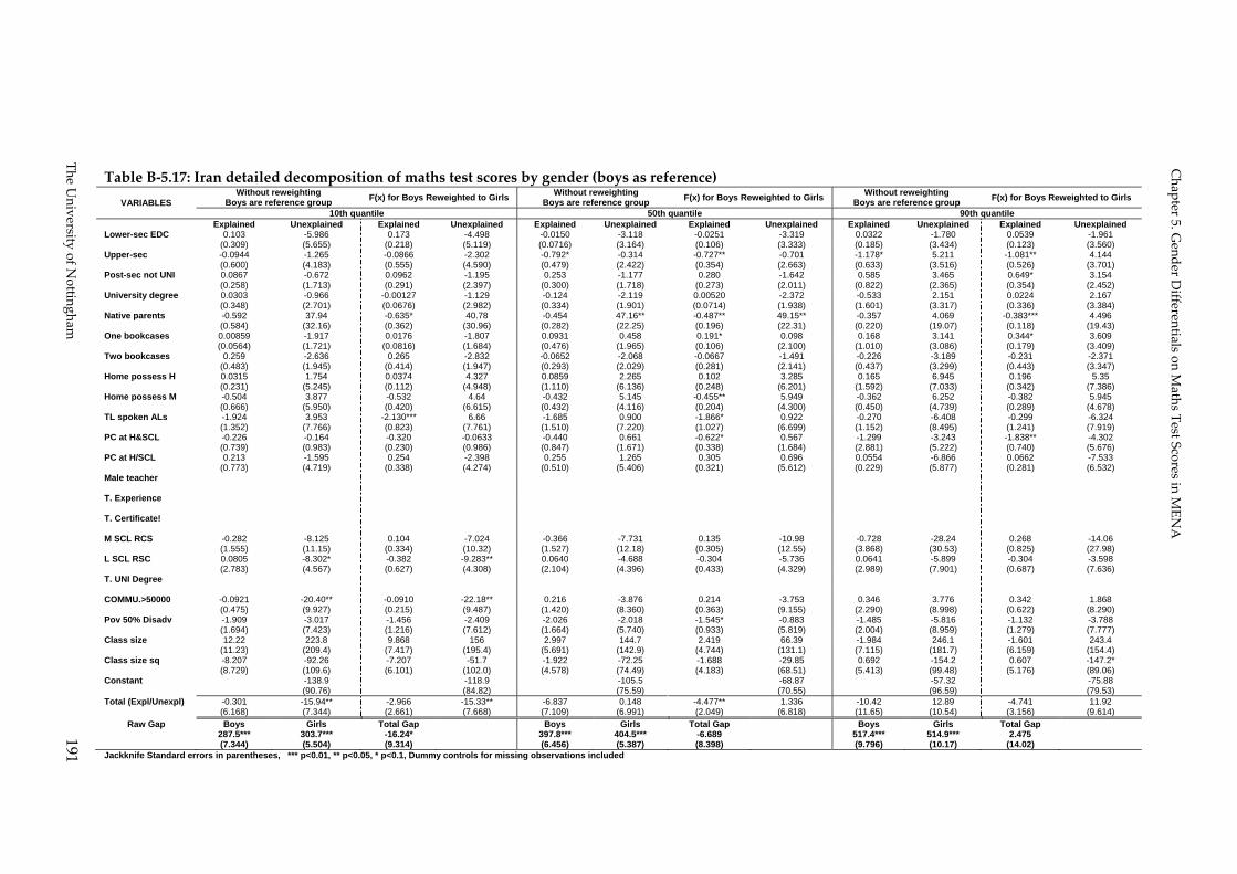
The University of N
ottingham
191
Table B‐ 5.17: Iran detailed decomposition of maths test scores by gender (boys as reference)
Chapter 5. G
ender Differentials on M
aths Test Scores in MEN
A
VARIABLES Without reweighting
Boys are reference group F(x) for Boys Reweighted to Girls Without reweightingBoys are reference group F(x) for Boys Reweighted to Girls Without reweighting
Boys are reference group F(x) for Boys Reweighted to Girls
10th quantile 50th quantile 90th quantileExplained Unexplained Explained Unexplained Explained Unexplained Explained Unexplained Explained Unexplained Explained Unexplained
Lower-sec EDC 0.103 -5.986 0.173 -4.498 -0.0150 -3.118 -0.0251 -3.319 0.0322 -1.780 0.0539 -1.961 (0.309) (5.655) (0.218) (5.119) (0.0716) (3.164) (0.106) (3.333) (0.185) (3.434) (0.123) (3.560) Upper-sec -0.0944 -1.265 -0.0866 -2.302 -0.792* -0.314 -0.727** -0.701 -1.178* 5.211 -1.081** 4.144 (0.600) (4.183) (0.555) (4.590) (0.479) (2.422) (0.354) (2.663) (0.633) (3.516) (0.526) (3.701) Post-sec not UNI 0.0867 -0.672 0.0962 -1.195 0.253 -1.177 0.280 -1.642 0.585 3.465 0.649* 3.154 (0.258) (1.713) (0.291) (2.397) (0.300) (1.718) (0.273) (2.011) (0.822) (2.365) (0.354) (2.452) University degree 0.0303 -0.966 -0.00127 -1.129 -0.124 -2.119 0.00520 -2.372 -0.533 2.151 0.0224 2.167 (0.348) (2.701) (0.0676) (2.982) (0.334) (1.901) (0.0714) (1.938) (1.601) (3.317) (0.336) (3.384) Native parents -0.592 37.94 -0.635* 40.78 -0.454 47.16** -0.487** 49.15** -0.357 4.069 -0.383*** 4.496 (0.584) (32.16) (0.362) (30.96) (0.282) (22.25) (0.196) (22.31) (0.220) (19.07) (0.118) (19.43) One bookcases 0.00859 -1.917 0.0176 -1.807 0.0931 0.458 0.191* 0.098 0.168 3.141 0.344* 3.609 (0.0564) (1.721) (0.0816) (1.684) (0.476) (1.965) (0.106) (2.100) (1.010) (3.086) (0.179) (3.409) Two bookcases 0.259 -2.636 0.265 -2.832 -0.0652 -2.068 -0.0667 -1.491 -0.226 -3.189 -0.231 -2.371 (0.483) (1.945) (0.414) (1.947) (0.293) (2.029) (0.281) (2.141) (0.437) (3.299) (0.443) (3.347) Home possess H 0.0315 1.754 0.0374 4.327 0.0859 2.265 0.102 3.285 0.165 6.945 0.196 5.35 (0.231) (5.245) (0.112) (4.948) (1.110) (6.136) (0.248) (6.201) (1.592) (7.033) (0.342) (7.386) Home possess M -0.504 3.877 -0.532 4.64 -0.432 5.145 -0.455** 5.949 -0.362 6.252 -0.382 5.945 (0.666) (5.950) (0.420) (6.615) (0.432) (4.116) (0.204) (4.300) (0.450) (4.739) (0.289) (4.678) TL spoken ALs -1.924 3.953 -2.130*** 6.66 -1.685 0.900 -1.866* 0.922 -0.270 -6.408 -0.299 -6.324 (1.352) (7.766) (0.823) (7.761) (1.510) (7.220) (1.027) (6.699) (1.152) (8.495) (1.241) (7.919) PC at H&SCL -0.226 -0.164 -0.320 -0.0633 -0.440 0.661 -0.622* 0.567 -1.299 -3.243 -1.838** -4.302 (0.739) (0.983) (0.230) (0.986) (0.847) (1.671) (0.338) (1.684) (2.881) (5.222) (0.740) (5.676) PC at H/SCL 0.213 -1.595 0.254 -2.398 0.255 1.265 0.305 0.696 0.0554 -6.866 0.0662 -7.533 (0.773) (4.719) (0.338) (4.274) (0.510) (5.406) (0.321) (5.612) (0.229) (5.877) (0.281) (6.532) Male teacher T. Experience T. Certificate! M SCL RCS -0.282 -8.125 0.104 -7.024 -0.366 -7.731 0.135 -10.98 -0.728 -28.24 0.268 -14.06 (1.555) (11.15) (0.334) (10.32) (1.527) (12.18) (0.305) (12.55) (3.868) (30.53) (0.825) (27.98) L SCL RSC 0.0805 -8.302* -0.382 -9.283** 0.0640 -4.688 -0.304 -5.736 0.0641 -5.899 -0.304 -3.598 (2.783) (4.567) (0.627) (4.308) (2.104) (4.396) (0.433) (4.329) (2.989) (7.901) (0.687) (7.636) T. UNI Degree COMMU.>50000 -0.0921 -20.40** -0.0910 -22.18** 0.216 -3.876 0.214 -3.753 0.346 3.776 0.342 1.868 (0.475) (9.927) (0.215) (9.487) (1.420) (8.360) (0.363) (9.155) (2.290) (8.998) (0.622) (8.290) Pov 50% Disadv -1.909 -3.017 -1.456 -2.409 -2.026 -2.018 -1.545* -0.883 -1.485 -5.816 -1.132 -3.788 (1.694) (7.423) (1.216) (7.612) (1.664) (5.740) (0.933) (5.819) (2.004) (8.959) (1.279) (7.777) Class size 12.22 223.8 9.868 156 2.997 144.7 2.419 66.39 -1.984 246.1 -1.601 243.4 (11.23) (209.4) (7.417) (195.4) (5.691) (142.9) (4.744) (131.1) (7.115) (181.7) (6.159) (154.4) Class size sq -8.207 -92.26 -7.207 -51.7 -1.922 -72.25 -1.688 -29.85 0.692 -154.2 0.607 -147.2* (8.729) (109.6) (6.101) (102.0) (4.578) (74.49) (4.183) (68.51) (5.413) (99.48) (5.176) (89.06) Constant -138.9 -118.9 -105.5 -68.87 -57.32 -75.88 (90.76) (84.82) (75.59) (70.55) (96.59) (79.53) Total (Expl/Unexpl) -0.301 -15.94** -2.966 -15.33** -6.837 0.148 -4.477** 1.336 -10.42 12.89 -4.741 11.92 (6.168) (7.344) (2.661) (7.668) (7.109) (6.991) (2.049) (6.818) (11.65) (10.54) (3.156) (9.614)
Raw Gap Boys Girls Total Gap Boys Girls Total Gap Boys Girls Total Gap 287.5*** 303.7*** -16.24* 397.8*** 404.5*** -6.689 517.4*** 514.9*** 2.475 (7.344) (5.504) (9.314) (6.456) (5.387) (8.398) (9.796) (10.17) (14.02)
Jackknife Standard errors in parentheses, *** p<0.01, ** p<0.05, * p<0.1, Dummy controls for missing observations included

The University of N
ottingham
192
Chapter 5. G
ender Differentials on M
aths Test Scores in MEN
A
Table B‐ 5.18: Saudi Arabia detailed decomposition of maths test scores by gender (boys as reference) VARIABLES
Without reweighting Boys are reference group
F(x) for Boys Reweighted to Girls
Without reweightingBoys are reference group
F(x) for Boys Reweighted to Girls
Without reweightingBoys are reference group
F(x) for Boys Reweighted to Girls
10th quantile 50th quantile 90th quantile Explained Unexplained Explained Unexplained Explained Unexplained Explained Unexplained Explained Unexplained Explained Unexplained
Lower-sec EDC 0.265 -2.158 0.223 0.406 0.140 -4.171* 0.118 -3.506 0.161 -3.654 0.135 -3.75 (0.328) (3.229) (0.277) (2.772) (0.278) (2.409) (0.217) (2.602) (0.361) (3.003) (0.244) (3.886) Upper-sec 0.0755 -2.121 0.0808 -1.166 0.211 -4.055 0.226 -3.477 0.353 -3.611 0.378 -4.927 (0.254) (4.059) (0.233) (5.522) (0.268) (2.654) (0.301) (3.186) (0.439) (3.426) (0.409) (3.906) Post-sec not UNI -0.0647 -0.0184 -0.0214 0.873 -0.275 0.345 -0.0911 0.286 -0.0972 -0.0917 -0.0322 0.0501 (0.232) (1.127) (0.0987) (1.220) (0.299) (1.036) (0.140) (1.195) (0.270) (1.453) (0.109) (1.665) University degree -0.0384 -2.147 -0.0517 2.059 -0.114 -6.393 -0.153 -5.107 -0.198 -6.024 -0.266 -8.36 (0.148) (5.461) (0.184) (8.656) (0.173) (3.941) (0.178) (4.103) (0.501) (6.516) (0.367) (7.411) Native parents 0.114 -0.595 0.0963 -2.848 0.322 6.632 0.271 3.681 1.319 -5.324 1.110* -10.61 (0.549) (10.69) (0.444) (12.53) (0.433) (7.391) (0.361) (8.664) (1.007) (12.50) (0.572) (14.45) One bookcases -0.805 1.956 -0.704 -2.141 -1.635 0.701 -1.431* -0.151 -2.691 5.451 -2.355* 4.748 (1.097) (5.315) (0.944) (5.095) (1.014) (3.619) (0.806) (3.913) (1.683) (5.522) (1.405) (5.125) Two bookcases 0.175 -0.724 0.153 -2.526 -0.365 -0.693 -0.319 -1.099 -1.247 0.127 -1.091 -0.764 (0.811) (3.411) (0.667) (3.345) (0.527) (2.528) (0.448) (2.889) (0.978) (3.604) (0.750) (3.779) Home possess H -8.230*** 17.32 -8.311*** 14.71 -6.902*** 11.98 -6.969*** 8.774 -5.157** 8.488 -5.207*** 3.638 (3.098) (16.04) (2.349) (18.94) (1.709) (9.616) (1.249) (11.01) (2.119) (9.249) (1.664) (7.531) Home possess M 0.783 15.57 0.934 12.61 0.464 6.334 0.554* 3.265 0.166 2.606 0.198 1.246 (1.111) (9.543) (0.618) (12.95) (0.546) (8.193) (0.288) (9.838) (0.301) (5.350) (0.199) (4.974) TL spoken ALs -0.316 2.948 -0.279 9.945 -0.662 -1.692 -0.585 -1.229 -1.396 -4.268 -1.233 -2.661 (1.088) (5.715) (0.968) (7.252) (1.096) (5.798) (0.973) (7.094) (1.141) (7.341) (0.929) (6.949) PC at H&SCL -4.877*** -1.403 -4.498*** -0.47 -3.174* -0.748 -2.927** -0.587 -0.747 0.894 -0.689 1.286 (1.650) (1.814) (1.482) (2.153) (1.663) (1.473) (1.468) (1.451) (2.122) (1.564) (1.939) (1.884) PC at H/SCL 3.230*** -10.95 2.603*** -9.574 2.369** -2.216 1.909** -0.673 -0.492 10.01 -0.397 15.15 (1.181) (10.05) (0.846) (13.82) (1.051) (6.393) (0.835) (6.714) (1.650) (9.239) (1.333) (9.898) Male teacher T. Experience T. Certificate! M SCL RCS -0.147 17.58 -0.244 15.22 -0.219 33.97** -0.364 30.43** 0.429 21.05 0.710 8.545 (0.515) (15.40) (0.944) (16.52) (0.537) (13.62) (0.882) (14.15) (0.704) (21.20) (1.232) (26.38) L SCL RSC 0.768 2.029 0.266 1.842 0.702 4.766 0.243 2.958 1.449 2.197 0.501 -1.053 (1.972) (5.542) (0.598) (6.175) (1.688) (4.762) (0.509) (4.272) (2.135) (5.710) (0.631) (6.870) T. UNI Degree COMMU.>50000 -0.327 0.0542 -0.382 2.4 -0.365 -1.515 -0.426 -3.688 -0.640 2.262 -0.747 -2.874 (1.440) (6.940) (0.703) (9.577) (1.445) (5.527) (0.675) (5.949) (2.047) (6.933) (0.845) (8.264) Pov 50% Disadv 0.0629 -0.230 0.0510 -0.0192 0.279 -2.665 0.226 -3.155 0.0919 -1.209 0.0745 -2.089 (0.276) (2.924) (0.210) (2.887) (0.868) (2.763) (0.306) (2.665) (0.238) (2.486) (0.194) (2.138) Class size -0.195 26.77 -0.0318 49.75 -0.995 48.91 -0.162 56.89 0.288 19.10 0.0470 54.06 (2.926) (77.35) (0.530) (95.21) (2.794) (54.48) (0.738) (51.64) (2.458) (48.16) (0.543) (71.06) Class size sq 1.706 -15.49 0.408 -32.16 5.580 -31.47 1.334 -36.48 0.378 -10.24 0.0904 -26.63 (10.49) (40.75) (2.322) (47.43) (6.816) (27.06) (1.423) (27.87) (7.285) (25.80) (1.727) (38.78) Constant -80.53 -99.63* -82.39** -74.18* -42.53 -35.42 (53.53) (53.75) (42.00) (40.10) (45.73) (59.43) Total (Expl/Unexpl) -6.703 -27.18*** -8.711** -33.70*** -3.853 -20.42*** -7.853*** -22.78*** -5.601 -5.601 -7.890*** -7.794 (9.462) (9.810) (4.187) (11.25) (6.248) (6.960) (2.676) (7.109) (7.068) (7.068) (3.023) (8.031)
Raw Gap Boys Girls Total Gap Boys Girls Total Gap Boys Girls Total Gap 216.9*** 250.8*** -33.88*** 317.7*** 342.0*** -24.27*** 423.5*** 434.1*** -10.55* (5.569) (5.555) (7.671) (5.359) (4.030) (7.012) (4.361) (3.902) (5.760)
Jackknife Standard errors in parentheses, *** p<0.01, ** p<0.05, * p<0.1, Dummy controls for missing observations included

Chapter 5. Gender Differentials on Maths Test Scores in MENA
Appendix C‐4:Quantile Decomposition Do‐file
* Quantile decomposition on Turkey *
*Inequality analysis using reweight hybrid with Recentered Influence Function (RIF) for quantiles *
**ALL PLAUSIBLE VALUES**
#delimit ;
clear all;
capture log close;
set more off;
set mem 500m;
local date: di %d date(c(current_date),ʺDMYʺ);
cd ʺE:\Fourth chapter\Data and Do\Turkeyʺ;
log using AN_RIF_TURF`dateʹ.log, replace;
*generating the counterfactual sample group*;
use mergedturM ; tab itsex, gen(itsex); gen male = itsex2; gen female = itsex1;
save temp01,replace; keep if male==0; replace male=2; save temp2, replace;
use temp01, clear; append using temp2;
*Defining variables*;
do var_define;
* Interactions;
*”These interactions are necessary for producing proper weights, revise demographic changes and employ (Balck et al 2009)ʺ;*
*we do not need interactions here we have run the “hotelling” test for mean equality and it proves equality*
*Testing of mean equality‐RE‐Weight.do*
***********************************************************************************************;
*keep the used variables only to fasten the jackknife calculations’
# delimit;
*generate local for covariates to save space and time it is repeatedly generated and used;
Local controls bsdgedup2 bsdgedup3 bsdgedup4 bsdgedup5 TURparents
onebookcases twobookcases homepossessH homepossessM bs4golanALWS
PChomeandSCL PChomeorSCL bt4gsexM bt4gtaut1 bt4gtlceyes bcdsrmiM bcdsrmiL bt4gfedcuni bc4gcomuG50 bc4gsbedG50P bt4mstud1 bt4mstud2;
The University of Nottingham 193

Chapter 5. Gender Differentials on Maths Test Scores in MENA
*generate local for missing observations controls;
Local control_missing DMbsdgedup DMbsdgborn DMbs4gbook DMhomepossessinx DMbs4golan DMbsdgcavl DMbt4gsex DMbt4gtaut DMbt4gtlce DMbcdsrmi DMbt4gfedc DMbc4gcomu DMbc4gsbed DMbt4mstud;
Keep `controls’ `contol_missing’ totwgt female male bsmmat* jkzone jkrep;
************************************************************************;
*************** compute weights; *************** Probit for male effect;
probit male `controls’ `control_missing’ [iweight= totwgt] if male==0 | male==1 ;
predict malew, p;
summ malew , detail;
summ male [aweight=totwgt] if male==0 | male==1 ;
gen pbar=r(mean);
replace totwgt= totwgt*(malew/(1‐malew))*((1‐pbar)/pbar) if male==2;
*investigate bandwidth as double the normal weight or use the exact the graph will compare them;
twoway (kdensity bsmmat01 [aw=totwgt] if male==0 | male==1, lcolor(black) )(kdensity bsmmat01[aw=totwgt] if male==0 | male==1, width(38) ///
lcolor(red) )(kdensity bsmmat01[aw=totwgt] if male==0 | male==1, width(9) lcolor(green) );
*******************************************************************************************;
** get recentered influence functions for 10, 50 and 90 centiles;
****defining the program to do the work;
program define rifgen;
foreach var of local 0{;
forvalues it = 0(1)2 { ;
pctile valx=`varʹ if male==`itʹ [aweight=totwgt], nq(100) ;
kdensity `varʹ [aweight= totwgt] if male==`itʹ, at(valx) gen(evalt`itʹ denst`itʹ) width(19) nograph ;
forvalues qt = 10(40)90 { ;
local qc = `qtʹ/100.0;
gen rif_`varʹ`itʹ_`qtʹ=evalt`itʹ[`qtʹ]+`qcʹ/denst`itʹ[`qtʹ] if `varʹ>=evalt`itʹ[`qtʹ] & male==`itʹ;
replace rif_`varʹ`itʹ_`qtʹ=evalt`itʹ[`qtʹ]‐(1‐`qcʹ)/denst`itʹ[`qtʹ] if `varʹ<evalt`itʹ[`qtʹ]& male==`itʹ;
};
The University of Nottingham 194

Chapter 5. Gender Differentials on Maths Test Scores in MENA
drop valx;
};
drop eval* denst*;
};
end;
*Running the program for the five plausible values, this will generate the RIF for them at all the required quantiles;
rifgen bsmmat01 bsmmat02 bsmmat03 bsmmat04 bsmmat05;
program drop rifgen;
******************************************************************************************;
# delimit;
foreach var of varlist bsmmat01 bsmmat02 bsmmat03 bsmmat04 bsmmat05{;
gen rifat`varʹ=.;
};
forvalues qt = 10(40)90 { ;
di ʺevaluating quantile= ʺ `qtʹ;
** get decomposition without reweighing [E(X_1|t=1)‐ E(X_0|t=0)]B_0 ;
foreach var of varlist bsmmat01 bsmmat02 bsmmat03 bsmmat04 bsmmat05{;
replace rifat`varʹ=rif_`varʹ0_`qtʹ if male==0;
replace rifat`varʹ=rif_`varʹ1_`qtʹ if male==1;
};
*running estimates for the quantile decomposition without reweighting*;
pv `controls’ `control_missing’ [aweight= totwgt] if male==0 | male==1, cmd(oaxaca) pv(rifat*)cmdops(by(male) weight(0) swap detail (groupDM:`control_missing’) relax) jkzone(jkzone) jkrep(jkrep) jrr timss;
*save estimates*;
est sto WRa`varʹ_`qtʹ;
matrix Ra`qtʹ=e(b);
**************************************************************************************;
foreach var of varlist bsmmat01 bsmmat02 bsmmat03 bsmmat04 bsmmat05{;
replace rifat`varʹ=.;
*** get characteristics effects with reweighing [E(X_0|t=1)‐ E(X_0|t=0)]B_c as explained in chapter 4 ;
replace rifat`varʹ=rif_`varʹ2_`qtʹ if male==2;
replace rifat`varʹ=rif_`varʹ0_`qtʹ if male==0;
The University of Nottingham 195
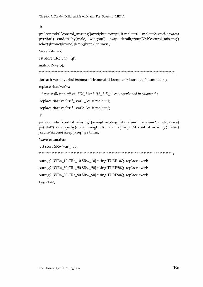
Chapter 5. Gender Differentials on Maths Test Scores in MENA
The University of Nottingham 196
};
pv `controls’ `control_missing’[aweight= totwgt] if male==0 | male==2, cmd(oaxaca) pv(rifat*) cmdops(by(male) weight(0) swap detail(groupDM:`control_missing’) relax) jkzone(jkzone) jkrep(jkrep) jrr timss ;
*save estimes;
est store CRc`varʹ_`qtʹ;
matrix Rc=e(b);
*********************************************************************************************;
foreach var of varlist bsmmat01 bsmmat02 bsmmat03 bsmmat04 bsmmat05{;
replace rifat`varʹ=.;
*** get coefficients effects E(X_1|t=1)*[B_1‐B_c] as unexplained in chapter 4 ;
replace rifat`varʹ=rif_`varʹ1_`qtʹ if male==1;
replace rifat`varʹ=rif_`varʹ2_`qtʹ if male==2;
};
pv `controls’ `control_missing’ [aweight=totwgt] if male==1 | male==2, cmd(oaxaca) pv(rifat*) cmdops(by(male) weight(0) detail (groupDM:`control_missing’) relax) jkzone(jkzone) jkrep(jkrep) jrr timss;
*save estimates;
est store SRw`varʹ_`qtʹ;
********************************************************************************************;
outreg2 [WRa_10 CRc_10 SRw_10] using TURF10Q, replace excel;
outreg2 [WRa_50 CRc_50 SRw_50] using TURF50Q, replace excel;
outreg2 [WRa_90 CRc_90 SRw_90] using TURF90Q, replace excel;
Log close;

Chapter 6. Conclusions
Chapter 6
CONCLUSIONS
6.1 Introduction
The aims of this study were to examine the determinants of educational learning
outcomes and gender inequality of educational outcomes in MENA countries. The
literature indicates quite important links between education, human capital and
economic growth. There has been substantial attention to the education process in
developed countries. Reviews of education production functions and comparative
studies have been employed to gain better understanding of school effectiveness to
enhance educational quality and help building up human capital (Hanushek, 1995,
Behrman, 2010, Glewwe et.al, 2011). High quality empirical studies are available to
guide policy makers to the most effective ways to enhance the learning outcomes.
The education production function framework considers schools as production
units that produce learning depending on inputs from school resources and teacher
characteristics given student characteristics. To increase the performance of
students, a relevant mix of these factors should be identified and employed under
the predefined constraints such as budget limit of schools.
The education component in human capital has been considered a vital player in
economic growth in developed countries. Countries in transition like MENA
countries after the so called Arab‐Spring should invest in human capital building
and increase understanding of the driving forces of better outcomes of education.
The inequality is a major challenge in such a region where income distribution is
biased in favour of small minorities.
Given the central role of students’ educational performance for the future economic
prospects of societies, the empirical results of education production functions
estimated for the eight MENA countries in this study could have substantial
implications for educational and social policies in the region. For the MENA
countries, the evidence for the first time reveals the impact of family background
The University of Nottingham 197

Chapter 6. Conclusions
and schooling policies in the different school systems. By examining the
determinants of educational performance in the best performing MENA countries,
other countries can derive lessons for education policy.
The distortions of education distributions among groups were argued to have a
substantial influence on the social and economic outcomes in part of the developing
countries. The thesis adds to the literature by addressing the gender inequality of
educational outcomes (achievement) in MENA region and so examines inequality in
outcomes rather than enrolment (inputs). The comparative and uniform country
analysis of MENA countries using appropriate techniques allow us to draw many
conclusions and contributions, while still leaving open several future possible
research questions.
6.2 Summary of findings
MENA countries share many characteristics although they also differ in many
aspects. They have common characteristics such as religion, culture, geographical
place, desert climate in most areas, language (with exceptions) and history; they
share a relatively low performance of educational outcomes compared to other
countries of similar income for which TIMSS data are available. The poor
performance of MENA countries is the first conclusion to be drawn from this study.
This study provides, for the first time, concrete evidence on educational production
functions in MENA. The literature indicates a debate over the effectiveness of school
factors on the quality of the outcomes (Hanushek, 1995, Glewwe et.al, 2011). We
find here the overall impact of school level variables on performance across the
whole range of countries is very weak except for Turkey. This suggests a special
difference in the Turkish education system production process to the other
countries. The dominance of home background and student characteristics effects
on the learning outcomes in MENA paradoxically implies more attention needs to
be given to the school factors. The insignificant impacts of observed school
characteristics and teachers’ qualifications do not mean that schools are not
important, but they are not effective and the mechanisms through which they work
need more investigation. The school factors include a lot of endogenous variables
The University of Nottingham 198

Chapter 6. Conclusions
which affect the learning outputs which show more variations come from the school
side when the school fixed effects technique has been employed. The significant
effect of school resources in Turkey and Iran explain more differences across the
education systems. Although, it seems that school level variables play little role in
general, the detailed investigation in Egypt shows major differences come from
school type reflecting differences in resources and practices in those schools.
The meta‐regression analysis identifies some common patterns for home
background side, though the striking finding is the negative effect of computer
usage across countries. Except for Iran and Turkey, computer usage has a negative
impact on the learning outcomes of students in MENA. Policy should focus on the
issue of ICT in the learning process as providing ICT facilities does not appear to
effective. The success story of Turkey might be of interest to get more insight of how
a more effective ICT policy could enhance the quality of learning. Family
background proxies, parental education and number of books at home seem to have
the largest effects on student’s performance in maths in the three top performing
countries (Tunisia, Jordan and Turkey). The number of books effect was the lowest
in Egypt and Syria. Home possessions are the variables with the most consistent
effect across MENA countries. Those findings go in line with literature findings in
most regions of the world (Hanushek, 1995, Woessmann, 2002, and Glewwe e.al,
2011).
Grant and Behrman (2010) argue that female students progress through school at
the same pace as or faster than their male peers. Schooling attainment, as measured
by grades of school completed, does not necessarily accurately reflect the learning
outcomes of children. There might be large variations in school quality and home
background which may have implications for gender differences in learning despite
the same level of schooling attainment. If girls are likely to attend different types of
schools than boys, tend to take different classes than boys, are treated differently
than boys in the same classes, or are treated differently outside of school than boys
are, this might have an effect on the equality of learning quality between boys and
girls.
The University of Nottingham 199

Chapter 6. Conclusions
Investigating the gender gap in learning outcomes in MENA is another contribution
of this study. The gender differences in maths performance are significant, though
mixed results were found across countries. The gap is pro‐boys in Algeria, Syria and
Tunisia and pro‐girls in Jordan, Egypt, and Saudi Arabia. The role of gender in the
education production function is different across the countries. The decomposition
analysis on the mean and along the distribution provides a major contribution to the
investigation of gender inequality in outcomes. MENA countries do not exhibit a
common pattern across quantiles with respect to gender effects; in pro‐boys
countries the gap is larger at the bottom of the distributions and tends to decrease.
This may explain the insignificant estimates from the OLS average estimates in
some countries. The pro‐girls countries show more of a gap in maths across all
quantiles. In the gender‐neutral country, Turkey, although there is no gender
difference overall, this reflects the countervailing balance of two effects: the
characteristics effect which favours girls and the coefficients effect which favours
boys. This begs a policy question of why schools are not able to offset the gender
inequality aspect from home variables.
The findings confirm Glewwe’s (2002) advice to use the country context instead of
aggregation of regions to draw concrete conclusions for policy makers for each
country. The final contribution of this thesis is centred around the effect of school
type on Egyptian students. This was investigated thoroughly in terms of schools’
sex composition and school language of instruction. The research found a significant
link between school type and student performance in Egypt; first, language schools
appears to have better scores than Arabic schools. Second, single‐sex schools do
better than mixed schools (especially for girls). This last finding provides a partial
explanation of the gender gap in Egypt which could not be determined from the
decomposition analysis.
The detailed investigation of the factors affecting the learning outcomes in Egypt
revealed many important findings; first the curriculum, and the teaching practices
related to it, is a very influential determinant of the final output especially when we
look to the learning components and how this is related to the future labour market.
The effect of the number of books goes partially against Ammermuller et.al (2005)
The University of Nottingham 200

Chapter 6. Conclusions
The University of Nottingham 201
where the effect of number of books found to increase achievements monotonically
in Europe it is found that having many books has no effect on achievements in
Egypt.
6.3 Future research
Future research should consider some questions related to the parallel education
system, or what is known as the shadow education, which is based on private
tutoring. This phenomenon is very common across MENA countries though no
comparative data is available. The shadow education may be a major source of
inequality if the families used it more to favour boys or girls to get better education
or certain fields of study.
Another future research point would examine the progress and the discrepancies of
country records on TIMSS studies. For example, Egypt participated in two rounds
2003 and 2007 between which there was a change on the number of years of primary
education from 5 years at 2003 to 6 years at 2007. One could use to explore the
difference between these two cohorts.
The low performance of the Gulf Cooperation Council (GCC) rich oil countries is a
paradox worthy of further investigation. With high availability of funds and
facilities for school resources, the poor performance across those countries is
shocking.
Woessmann (2007) raised the argument about school autonomy and institutional
reform and indicated more attention should be paid to these aspects in developing
countries research. The public sector dominance and the static laws of bureaucracy
in MENA countries limit school autonomy and education reform from the
institutional perspective. This situation needs investigation.

Bibliography
Akerhielm, Karen. 1995. ʺDoes class size matter?ʺ Economics of Education Review 14(3):229‐241.
Alderman, H., J.R. Behrman, D.R. Ross and R. Sabot. 1996. ʺDecomposing the gender gap in cognitive skills in a poor rural economy.ʺ The Journal of Human Resources 31(1):229‐254.
Alderman, Harold and Elizabeth M. King. 1998. ʺGender differences in parental investment in education.ʺ Structural Change and Economic Dynamics 9(4):453‐468.
Altinok, Nadir and Geeta Kingdon. 2012. ʺNew Evidence on Class Size Effects: A Pupil Fixed Effects Approach*.ʺ Oxford Bulletin of Economics and Statistics 74(2):203‐234.
Ammermueller, Andreas. 2007. ʺPISA: What makes the difference?ʺ Empirical Economics 33(2):263‐287.
Ammermüller, Andreas, Hans Heijke and Ludger Woessmann. 2005. ʺSchooling quality in Eastern Europe: Educational production during transition.ʺ Economics of Education Review 24(5):579‐599.
Appleton, S. 1995. ʺThe Interaction between Poverty and Gender in Human Capital Accumulation: the Case of the Primary Leaving Examination in Cote dʹlvoire.ʺ Journal of African Economies 4(2):192‐224.
Baker, D.P., B. Goesling and G.K. LeTendre. 2002. ʺSocioeconomic Status, School Quality, and National Economic Development: A Cross‐National Analysis of the ʺHeynemanan‐Loxley Effectʺ on Mathematics and Science Achievement.ʺ Comparative Education Review 46(3):291‐312.
Barro, R.J. 1991. ʺEconomic Growth in a Cross Section of Countries.ʺ The Quarterly Journal of Economics 106(2):407‐443.
Barro, R.J. and J.W. Lee. 2010. ʺA new data set of educational attainment in the world, 1950‐2010.ʺ National Bureau of Economic Research.
Barsky, Robert, John Bound, Kerwin Kofi Charles and Joseph P. Lupton. 2002. ʺAccounting for the Black‐White Wealth Gap: A Nonparametric Approach.ʺ Journal of the American Statistical Association 97(459):663‐673.
Becker, G.S. 1994. Human Capital: A Theoretical and Empirical Analysis with Special Reference to Education (3rd Edition). 3rd Edition: NBER.
Becker, Gary S. 1965. ʺA Theory of the Allocation of Time.ʺ The Economic Journal 75(299):493‐517.
The University of Nottingham 202

Behrman, J. R., S. Khan, D. Ross and R. Sabot. 1997. ʺSchool quality and cognitive achievement production: A case study for rural Pakistan.ʺ Economics of Education Review 16(2):127‐142.
Behrman, J.R. and M.R. Rosenzweig. 2002. ʺDoes increasing womenʹs schooling raise the schooling of the next generation?ʺ American Economic Review:323‐334.
Behrman, Jere R 2010. ʺChapter 73 ‐ Investment in Education‐Inputs and Incentives.ʺ In Handbook of Development Economics, eds. Dani Rodrik and Mark Rosenzweig: Elsevier.
Behrman, Jere R. 1994. ʺEducational performance of the poor: Lessons from rural northeast Brazil.ʺ Journal of Economic Literature 32(1):152‐154.
Behrman, Jere R., Andrew D. Foster, Mark R. Rosenzweig and Prem Vashishtha. 1999. ʺWomenʹs Schooling, Home Teaching, and Economic Growth.ʺ Journal of Political Economy 107(4):682‐714.
Bharadwaj, Prashant, Giacomo De Giorgi, David Hansen and Christopher Neilson. 2012. ʺThe Gender Gap in Mathematics: Evidence from Low‐ and Middle‐Income Countries.ʺ National Bureau of Economic Research Working Paper Series No. 18464.
Blinder, Alan S. 1973. ʺWAGE DISCRIMINATION: REDUCED FORM AND STRUCTURAL ESTIMATES.ʺ Journal of Human Resources 8(4):436‐455.
Borenstein, M., L.V. Hedges, J.P.T. Higgins and H.R. Rothstein. 2011. Introduction to meta‐analysis: Wiley.
Campbell, E.Q., J.S. Coleman, C.J. Hobson, J. McPartland, A.M. Mood, F.D. Weinfeld and R.L. York. 1966. ʺEquality of educational opportunity.ʺ Washington DC: US Government Printing Office.
Carpenter, Peter and Martin Hayden. 1987. ʺGirlsʹ Academic Achievements: Single‐Sex Versus Coeducational Schools in Australia.ʺ Sociology of Education 60(3):156‐167.
Chernozhukov, V., I. Fernandez‐Val and B. Melly. 2009. ʺInference on counterfactual distributions.ʺ MIT Department of Economics Working Paper No. 08‐16.
Coric, Bruno and Geoff Pugh. 2008. ʺThe effects of exchange rate variability on international trade: a meta‐regression analysis.ʺ Applied Economics 42(20):2631‐2644.
Cotton, J. 1988. ʺOn the decomposition of wage differentials.ʺ The review of economics and statistics 70(2):236‐243.
The University of Nottingham 203

Dancer, Diane and Anu Rammohan. 2007. ʺDeterminants of Schooling in Egypt: The Role of Gender and Rural/Urban Residence.ʺ Oxford Development Studies 35(2):171‐195.
Dhillon, N. and T. Yousef. 2009. Generation in waiting: the unfulfilled promise of young people in the Middle East: Brookings Inst Pr.
DiNardo, John, Nicole M. Fortin and Thomas Lemieux. 1996. ʺLabor Market Institutions and the Distribution of Wages, 1973‐1992: A Semiparametric Approach.ʺ Econometrica 64(5):1001‐1044.
Doucouliagos, Hristos and Martin Paldam. 2008. ʺAid effectiveness on growth: A meta study.ʺ European Journal of Political Economy 24(1):1‐24.
EdStats. 2008. ʺEducation Statistics.ʺ World Bank.
Eisenkopf, Gerald, Zohal Hessami, Urs Fischbacher and Heinrich Ursprung. 2011. ʺAcademic Performance and Single‐Sex Schooling: Evidence from a Natural Experiment in Switzerland.ʺ CESIFO WORKING PAPER NO. 3592 SSRN eLibrary.
Engin‐Demir, Cennet. 2009. ʺFactors influencing the academic achievement of the Turkish urban poor.ʺ International Journal of Educational Development 29(1):17‐29.
Fertig, Michael. 2003. ʺWhoʹs to Blame? The Determinants of German Studentsʹ Achievement in the PISA 2000 Study.ʺ SSRN eLibrary.
Filmer, Deon and Lant Pritchett. 2001. ʺEstimating Wealth Effects Without Expenditure Data—Or Tears: An Application To Educational Enrollments In States Of India.ʺ Demography 38(1):115‐132.
Firpo, Sergio, Nicole M. Fortin and Thomas Lemieux. 2009. ʺUnconditional Quantile Regressions.ʺ Econometrica 77(3):953‐973.
Fortin, N., T. Lemieux and S. Firpo. 2010. ʺDecomposition methods in economics.ʺ National Bureau of Economic Research Working Paper Series No. 16045.
Fortin, Nicole, Thomas Lemieux and Sergio Firpo. 2011. ʺDecomposition Methods in Economics.ʺ In Handbook of Labor Economics, eds. Orley Ashenfelter and David Card: Elsevier.
Foy, P. and JF Olson. 2009. ʺTIMSS 2007 user guide for the international database.ʺ Chestnut Hill, MA: TIMSS & PIRLS International Study Center, Boston College.
Fuller, B. and P. Clarke. 1994. ʺRaising school effects while ignoring culture? Local conditions and the influence of classroom tools, rules, and pedagogy.ʺ Review of educational research 64(1):119‐157.
The University of Nottingham 204

Galal, A. 2007. The Road Not Traveled: Education Reform in the MENA Region: World Bank.
Gamoran, Adam and Daniel A. Long. 2006. ʺEquality of Educational opportunity: A 40‐Year Retrospective.ʺ wisconson center of Education Research(WCER Workin Paper No. 2006‐9).
Glewwe, Paul. 2002. ʺSchools and Skills in Developing Countries: Education Policies and Socioeconomic Outcomes.ʺ Journal of Economic Literature 40(2):436‐482.
Glewwe, Paul and Hanan Jacoby. 1994. ʺStudent Achievement and Schooling Choice in Low‐Income Countries.ʺ Journal of Human Resources 29(3):843‐864.
Glewwe, Paul and Michael Kremer. 2006. ʺChapter 16 Schools, Teachers, and Education Outcomes in Developing Countries.ʺ In Handbook of the Economics of Education, eds. E. Hanushek and F. Welch: Elsevier.
Glewwe, Paul and Edward A. Miguel. 2007. ʺChapter 56 The Impact of Child Health and Nutrition on Education in Less Developed Countries.ʺ In Handbook of Development Economics, eds. T. Paul Schultz and A. Strauss John: Elsevier.
Glewwe, Paul W., Eric A. Hanushek, Sarah D. Humpage and Renato Ravina. 2011. ʺSchool Resources and Educational Outcomes in Developing Countries: A Review of the Literature from 1990 to 2010.ʺ National Bureau of Economic Research Working Paper Series No. 17554.
Gonzales, P., T. Williams, L. Jocelyn, S. Roey, D. Kastberg and S. Brenwald. 2008. ʺHighlights from TIMSS 2007: Mathematics and Science Achievement of US Fourth‐and Eighth‐Grade Students in an International Context. NCES 2009‐001.ʺ National Center for Education Statistics:112.
Grant, Monica J. and Jere R. Behrman. 2010. ʺGender Gaps in Educational Attainment in Less Developed Countries.ʺ Population and Development Review 36(1):71‐89.
Handcock, Mark S. and Martina Morris. 1998. ʺRelative Distribution Methods.ʺ Sociological Methodology 28(1):53‐97.
Hanushek, E.A. 1995. ʺInterpreting recent research on schooling in developing countries.ʺ The World Bank Research Observer 10(2):227‐246.
Hanushek, E.A. and V. Lavy. 1994. School quality, achievement bias, and dropout behavior in Egypt: World Bank Publications.
Hanushek, Eric A. 1979. ʺCONCEPTUAL AND EMPIRICAL ISSUES IN THE ESTIMATION OF EDUCATIONAL PRODUCTION FUNCTIONS.ʺ Journal of Human Resources 14(3):351‐388.
The University of Nottingham 205

Hanushek, Eric A. 1998. ʺConclusions and controversies about the effectiveness of.ʺ Economic Policy Review (19320426) 4(1):11.
Hanushek, Eric A. 2002. ʺChapter 30 Publicly provided education.ʺ In Handbook of Public Economics, eds. J. Auerbach Alan and Feldstein Martin: Elsevier.
Hanushek, Eric A. 2003. ʺThe Failure of Input‐Based Schooling Policies.ʺ Economic Journal 113(485):F64‐F98.
Hanushek, Eric A. 2005a. ʺThe Economics of School Quality.ʺ German Economic Review 6(3):269‐286.
Hanushek, Eric A. 2005b. ʺWhy Quality Matters in Education.ʺ Finance & Development 42(2):15‐19.
Hanushek, Eric A. 2006a. ʺAlternative school policies and the benefits of general cognitive skills.ʺ Economics of Education Review 25(4):447‐462.
Hanushek, Eric A. 2006b. ʺChapter 14 School Resources.ʺ In Handbook of the Economics of Education, eds. E. Hanushek and F. Welch: Elsevier.
Hanushek, Eric A. and Dennis D. Kimko. 2000. ʺSchooling, Labor‐Force Quality, and the Growth of Nations.ʺ The American Economic Review 90(5):1184‐1208.
Hanushek, Eric A. and Javier A. Luque. 2003. ʺEfficiency and equity in schools around the world.ʺ Economics of Education Review 22(5):481.
Hanushek, Eric A. and Steven G. Rivkin. 2009. ʺHarming the best: How schools affect the black‐white achievement gap.ʺ Journal of Policy Analysis & Management 28(3):366‐393.
Hanushek, Eric A. and Ludger Woessmann. 2007. ʺThe Role of School Improvement in Economic Development.ʺ National Bureau of Economic Research Working Paper Series No. 12832.
Hanushek, Eric A. and Ludger Woessmann. 2008. ʺThe Role of Cognitive Skills in Economic Development.ʺ Journal of Economic Literature 46(3):607‐668.
Hanushek, Erik A. and Steven G. Rivkin. 1997. ʺUnderstanding the Twentieth‐Century Growth in U.S. School Spending.ʺ Journal of Human Resources 32(1):35‐68.
Harris, R., M. Bradburn, J. Deeks, R. Harbord, D. Altman and J. Sterne. 2008. ʺMetan: fixed‐and random‐effects meta‐analysis.ʺ Stata Journal 8(1):3.
Hartmann, S. 2008. ʺThe informal market of education in Egypt: private tutoring and its implications.ʺ Institut für Ethnologie und Afrikastudien Working Paper 88.
The University of Nottingham 206

Heyneman, S.P. 1997. ʺThe quality of education in the Middle East and North Africa (MENA).ʺ International Journal of Educational Development 17(4):449‐466.
Heyneman, Stephen P. and William A. Loxley. 1983. ʺThe Effect of Primary‐School Quality on Academic Achievement Across Twenty‐nine High‐ and Low‐Income Countries.ʺ American Journal of Sociology 88(6):1162‐1194.
Howie, Sarah J. 2003. ʺConditions of schooling in South Africa and the effects on mathematics achievement.ʺ Studies In Educational Evaluation 29(3):227‐241.
Jann, B. 2008. ʺA Stata implementation of the Blinder‐Oaxaca decomposition.ʺ Stata Journal 8(4):453‐479.
Johnes, Geraint. 2006. ʺEducation and Economic Growth.ʺ Available at SSRN: http://ssrn.com/abstract=893021 or http://dx.doi.org/10.2139/ssrn.893021.
Juhn, Chinhui, Kevin M. Murphy and Brooks Pierce. 1993. ʺWage Inequality and the Rise in Returns to Skill.ʺ Journal of Political Economy 101(3):410‐442.
Kalender, Ilker and Giray Berberoglu. 2009. ʺAn Assessment of Factors Related to Science Achievement of Turkish Students.ʺ International Journal of Science Education 31(10):1379‐1394.
Kingdon, Geeta. 1996. ʺTHE QUALITY AND EFFICIENCY OF PRIVATE AND PUBLIC EDUCATION: A CASE‐STUDY OF URBAN INDIA.ʺ Oxford Bulletin of Economics & Statistics 58(1):57‐82.
Klasen, Stephan and Francesca Lamanna. 2009. ʺThe Impact of Gender Inequality in Education and Employment on Economic Growth: New Evidence for a Panel of Countries.ʺ Feminist Economics 15(3):91‐132.
Klugman, J. 2011. ʺHuman Development Report 2011‐Sustainability and Equity: A Better Future for All.ʺ In United Nations Development Programme.
Klugman, J. and United Nations Development Programme. 2010. Human Development Report 2010: The Real Wealth of Nations: Pathways to Human Development: Palgrave Macmillan.
Koenker, R. 2005. Quantile regression. Cambridge: Cambridge Univirsity Press.
Koenker, R. and G. Bassett. 1978. ʺRegression quantiles.ʺ Econometrica 46(1):33‐50.
Kremer, M. 1995. ʺResearch on Schooling: What We Know and What We Donʹt: A Comment.ʺ World Bank Research Observer 10(2):247‐254.
Krugger, Alan B. 2003. ʺECONOMIC CONSIDERATIONS AND CLASS SIZE.ʺ Economic Journal 113(485):F34‐F63.
The University of Nottingham 207

Lauer, C. 2000. ʺGender wage gap in West Germany: how far do gender differences in human capital matter?ʺ ZEW Discussion Papers(00‐07).
Lee, V.E. and M.E. Lockheed. 1990. ʺThe effects of single‐sex schooling on achievement and attitudes in Nigeria.ʺ Comparative Education Review 34(2):209‐231.
Lewis, S. and M. Clarke. 2001. ʺForest plots: trying to see the wood and the trees.ʺ Bmj 322(7300):1479‐1480.
Lietz, P., H. Wagemaker, O. Neuschmidt and J. Hencke. 2008. ʺEducational issues in the middle east North Africa region : outcomes of the IEA Arab region training seminar series 2006/2007.ʺ
Lloyd, Cynthia B., Sahar El Tawila, Wesley H. Clark and Barbara S. Mensch. 2001. Determinants of educational attainment among adolescents in Egypt: does school quality make a difference? New York: Population Council.
Lucas, Robert E., Jr. 1988. ʺOn the mechanics of economic development.ʺ Journal of Monetary Economics 22(1):3‐42.
Machado, José A. F. and José Mata. 2005. ʺCounterfactual decomposition of changes in wage distributions using quantile regression.ʺ Journal of Applied Econometrics 20(4):445‐465.
Malamud, Ofer and Cristian Pop‐Eleches. 2011. ʺHome Computer Use and the Development of Human Capital.ʺ The Quarterly Journal of Economics 126(2):987‐1027.
McKenzie, David. 2005. ʺMeasuring inequality with asset indicators.ʺ Journal of Population Economics 18(2):229‐260.
Mincer, Jacob. 1958. ʺInvestment in Human Capital and Personal Income Distribution.ʺ Journal of Political Economy 66(4):281‐302.
Ministry of Education. 2008. ʺstrategic plan.ʺ Egypt Ministry of Education.
Montgomery, Mark, Michele Gragnolati, Kathleen Burke and Edmundo Paredes. 2000. ʺMeasuring living standards with proxy variables.ʺ Demography 37(2):155‐174.
Münich, D., E. Plug, G. Psacharopoulos and M. Schlotter. 2012. ʺEquity in and through Education and Training:
Indicators and Priorities.ʺ In European Expert Network on Economics of Education (EENEE).
The University of Nottingham 208

Nadereh, Chamlou, Muzi Silvia and Ahmed Hanane. 2011. ʺUnderstanding the Determinants of Female Labor Force Participation in the Middle East and North Africa Region: The Role of Education and Social Norms in Amman.ʺ AlmaLaurea Inter‐University Consortium.
Neumark, David. 1988. ʺEmployersʹ Discriminatory Behavior and the Estimation of Wage Discrimination.ʺ Journal of Human Resources 23(3):279‐295.
OʹSullivan, Margo C. 2001. ʺThe inset strategies model: an effective inset model for unqualified and underqualified primary teachers in Namibia.ʺ International Journal of Educational Development 21(2):93‐117.
Oaxaca, R.L. and M. Ransom. 1998. ʺCalculation of approximate variances for wage decomposition differentials.ʺ Journal of Economic and Social Measurement 24:55‐61.
Oaxaca, Ronald. 1973. ʺMale‐Female Wage Differentials in Urban Labor Markets.ʺ International Economic Review 14(3):693‐709.
Olson, JF, MO Martin and IVS Mullis. 2008a. ʺTIMSS 2007 technical report.ʺ Chestnut Hill, MA: TIMSS & PIRLS International Study Center, Boston College. Retrieved November 20:2009.
Olson, John F., Michael O. Martin and Ina V.S. Mullis. 2008b. ʺTIMSS 2007 Technical Report.ʺ International Association for the Evaluation of Educational Achievement (IEA).
Pritchett, Lant and Deon Filmer. 1999. ʺWhat education production functions really show: a positive theory of education expenditures.ʺ Economics of Education Review 18(2):223‐239.
Riddell, A. 2008. Factors influencing educational quality and effectiveness in developing countries: A review of research: GTZ.
Rivkin, Steven G., Eric A. Hanushek and John F. Kain. 2005. ʺTEACHERS, SCHOOLS, AND ACADEMIC ACHIEVEMENT.ʺ Econometrica 73(2):417‐458.
Saber, M.E.D. 1977. ʺDevelopment and Adult Education in the Arab States: An Analysis of Some Issues.ʺ The Arab Educational Cultural and Scientific Organization, Cairo, Egypt and The International Council for Adult Education, Toronto , Canada.
Salehi‐Isfahani, Djavad. 2010. ʺHuman Development in the Middle East and North Africa.ʺ Human Development Report Office (HDRO), United Nations Development Programme (UNDP).
Scheerens, J. 2000. ʺImproving school effectiveness.ʺ Unesco, International Institute for Educational Planning.
The University of Nottingham 209

Scheerens, J., H. Luyten, R. Steen and Y. Luyten‐de Thouars. 2007. ʺReview and meta‐analyses of school and teaching effectiveness.ʺ Enschede: Department of Educational Organisation and Management, University of Twente.
Schultz, T. Paul. 2002. ʺWhy governments should invest more to educate girls.ʺ World Development 30(2):207‐225.
Schultz, Theodore W. 1961. ʺINVESTMENT IN HUMAN CAPITAL.ʺ American Economic Review 51(1):1.
Stanley, T. D. and Stephen B. Jarrell. 1989. ʺMETA‐REGRESSION ANALYSIS: A QUANTITATIVE METHOD OF LITERATURE SURVEYS.ʺ Journal of Economic Surveys 3(2):161‐170.
Stanley, T.D. 2001. ʺWheat from chaff: Meta‐analysis as quantitative literature review.ʺ The Journal of Economic Perspectives 15(3):131‐150.
Stanley, TD and H. Doucouliagos. 2010. ʺPicture this: a simple graph that reveals much ado about research.ʺ Journal of Economic Surveys 24(1):170‐191.
Tansel, Aysit. 2002. ʺDeterminants of school attainment of boys and girls in Turkey: individual, household and community factors.ʺ Economics of Education Review 21(5):455‐470.
Todd, P.E. and K.I. Wolpin. 2003. ʺOn the Specification and Estimation of the Production Function for Cognitive Achievement*.ʺ The Economic Journal 113(485):F3‐F33.
UNDP. 2003. ʺThe Arab Human Development report 2003: building a knowledge society.ʺ In United Nations Development Programme (UNDP), New York, USA.
Vignoles, A., R. Levacic, J. Walker, S. Machin and D. Reynolds. 2000. ʺThe relationship between resource allocation and pupil attainment: a review.ʺ Centre for the Economics of Education, LSE.
Williams, T., D. Ferraro, S. Roey, S. Brenwald, D. Kastberg, L. Jocelyn, C. Smith, P. Stearns and P. Gonzales. 2009. ʺTIMSS 2007 US technical report and user guide.ʺ NCES.
Willms, J.D. and T. Smith. 2005. ʺA manual for conducting analyses with data from TIMSS and PISA.ʺ In Montreal: UIS. (Report prepared for the UNESCO Institute for Statistics.).
Woessmann, Ludger. 2003a. ʺEducational Production in East Asia: The Impact of Family Background and Schooling Policies on Student Performance.ʺ IZA Discussion Paper No. 745; Kiel Working Paper No. 1152. Available at SSRN: http://ssrn.com/abstract=392063.
The University of Nottingham 210

The University of Nottingham 211
Woessmann, Ludger. 2003b. ʺSchooling Resources, Educational Institutions and Student Performance: the International Evidence.ʺ Oxford Bulletin of Economics and Statistics 65(2):117‐170.
Woessmann, Ludger. 2004. ʺHow Equal are Educational Opportunities? Family Background and Student Achievement in Europe and the US.ʺ SSRN eLibrary.
Woessmann, Ludger. 2005a. ʺEducational Production in East Asia: The Impact of Family Background and Schooling Policies on Student Performance.ʺ German Economic Review 6(3):331‐353.
Woessmann, Ludger. 2005b. ʺEducational production in Europe.ʺ Economic Policy 20(43):445‐504.
Woessmann, Ludger and Martin West. 2006. ʺClass‐size effects in school systems around the world: Evidence from between‐grade variation in TIMSS.ʺ European Economic Review 50(3):695‐736.
World Bank. 2010. ʺBridging the Gap: Improving Capabilities and Expanding Opportunities for Women in the Middle East and North Africa Region.ʺ World Bank Middle East and North Africa Region
Wu, bio Margaret. 2005. ʺThe role of plausible values in large‐scale surveys.ʺ Studies In Educational Evaluation 31(2‐3):114‐128.
Yousef, Tarik M. 2004. ʺDevelopment, Growth and Policy Reform in the Middle East and North Africa since 1950.ʺ The Journal of Economic Perspectives 18(3):91‐115.