arX

iv:0

809.

1157

v1 [

hep-

th]

6 S

ep 2

008

Preprint typeset in JHEP style - HYPER VERSION TIFR/TH/08-33

Constraints on “rare” dyon decays

Sunil Mukhi ∗, and Rahul Nigam †

Tata Institute of Fundamental Research,

Homi Bhabha Rd, Mumbai 400 005, India

Abstract: We obtain the complete set of constraints on the moduli of N = 4 su-

perstring compactifications that permit “rare” marginal decays of 14-BPS dyons to

take place. The constraints are analysed in some special cases. The analysis extends

in a straightforward way to multi-particle decays. We discuss the possible relation

between general multi-particle decays and multi-centred black holes.

Keywords: String theory.

∗Email: mukhi@tifr.res.in†Email: rahulnig@theory.tifr.res.in

Contents

1. Introduction 1

2. Marginal stability for N = 4 dyons 3

3. Rare dyon decays 6

3.1 Analysis and implicit solution 6

3.2 Explicit solution: special cases 8

3.3 General charges, “triangular” moduli 14

3.4 Explicit solution: the general case 16

4. Multi-particle decays 18

5. Multi-centred black holes 19

6. Conclusions 25

1. Introduction

Recent developments have given us a much better understanding of the degeneracy

counting formula for 14-BPS dyons in N = 4 string compactifications. This formula

has been considerably refined from its original form in Ref.[1] where it was first

proposed. One such refinement consists of specifying the integration contour in the

degeneracy formula and noting that different contours can lead to different answers

for the degeneracy [2, 3] (for a review, see Ref.[4]). The effect of varying the inte-

gration contours is in the form of discontinuous jumps in the degeneracy whenever

the contour crosses a pole in the integration variable and picks up the corresponding

residue. This has been interpreted as due to the decay of some 14-BPS dyons into a

pair of 12-BPS dyons at curves of marginal stability, which are computed using the

BPS mass formula.

Because for large charges the decaying states are black holes, a mechanism is

needed to explain exactly how these decay on curves of marginal stability. The

– 1 –

answer turns out to be [5, 6] that 14-BPS black holes (for a given set of charges) exist

both in single-centre and multi-centre varieties. For the latter, the separations of

the centres are determined by the moduli [7]. If we specialise to two-centred dyons

with both centres being 12-BPS, then it was shown in Ref.[5] that as we approach a

curve of marginal stability the two centres fly apart to infinity. On the other side

of the curve the constraint equation has no solutions. This explains (in principle,

though no method is known to explicitly count states of a two-centred black hole) the

phenomenon of marginal stability and jumping in the counting formula, in terms of

the disintegration of two-centred black holes. It should be noted that the degeneracy

of single-centred black holes with the same charges does not vary across moduli space,

therefore they exist either everywhere or nowhere.

In these developments, the only type of marginal decay that plays a role is into

two 12-BPS final states. Also, the only multi-centred black holes needed to complete

the explanation are those with a pair of 12-BPS centres. Though the correspondence

between these two situations was derived for some special cases, it is believed to

hold in general, namely for any charge vectors and any point in the entire SL(2)U(1)

×SO(6,22)

SO(6)×SO(22)moduli space of N = 4 compactifications.

However, there are many more types of marginal decays in the theory, and in

one sense they are far more generic. These decays are into a pair of 14-BPS final

states, or into three or more final states each of which can be 12-BPS or 1

4-BPS. In

another sense these decays are “rare”, as it has been shown [8, 9, 10] (at least for

unit-torsion initial dyons) that they take place on curves of marginal stability that

have a co-dimension > 1 in the moduli space. Therefore these have been labelled

“rare decays”. In particular they cannot lead to jumps in the degeneracy formula1.

Nevertheless the existence of such decay modes is of importance in understanding

the behaviour of dyons as we move around in moduli space, and we will study them

here for their own sake as well as for possible interesting physical consequences that

they may turn out to have.

In Ref.[9] these curves were precisely characterised as circles on the torus moduli

space. But because of their higher codimension they also need some conditions to

be satisfied in the remaining part of the moduli space. Though the need for such

conditions was demonstrated in Refs.[8, 9, 10], the precise conditions have not yet

1For higher-torsion initial dyons the curves can be of codimension 1, but the degeneracy (or

rather, index) is still not expected to jump, because of fermion zero modes. We will focus largely

on unit-torsion dyons in this paper.

– 2 –

been worked out. In this paper we will completely characterise the codimension > 1

subspace on which rare decays can take place.

It is also known that there exist multi-centred dyonic black holes with two 14-BPS

centres, or three or more centres each of which can be 12- or 1

4-BPS. However, because

the degeneracy formula does not jump at curves of marginal stability, these multi-

centred dyons have not played a role in studies of dyons in N = 4 compactifications.

In particular they have not been related to marginal decays into two 14-BPS final

states or multiple final states, and in fact such a relation does not seem necessary

for the state-counting problem. Nevertheless, in what follows we will argue that the

relation between curves of marginal stability and multi-centred black holes flying

apart is quite generic.

In what follows, we start by briefly reviewing what is known about “rare”

marginal decays in N = 4 compactifications. Then we find a precise form for the

constraints on moduli space in order for such rare decays to take place. We exam-

ine and solve these constraints in a variety of special cases, to give a flavour of what

they look like. Then using some known results on T-duality orbits, we will obtain the

constraints in the general case. Next we recursively identify the loci of marginal sta-

bility for multi-particle decays. Finally we examine the special-geometry formula for

generic multi-centred black holes and write it in a form that relates their separations

to curves of marginal stability for n ≥ 2-body decays.

2. Marginal stability for N = 4 dyons

The electric and magnetic charge vectors of a dyon in an N = 4 string compactifica-

tion are elements of a 28 dimensional integral charge lattice of signature (6, 22). The

formulae for BPS mass involve a 28 × 28 matrix L, which in our basis will be taken

to be:

0 II6 0

II6 0 0

0 0 −II16

(2.1)

as well as a 28× 28 matrix M of moduli satisfying MLMT = L. The inner product

of charge vectors appearing in the BPS mass is taken with the matrix L+M . In the

heterotic basis where the compactification is specified by a constant metric Gij , an

antisymmetric tensor field Bij and constant gauge potentials AIi (where i = 1, 2, · · · , 6

– 3 –

and I = 1, 2, · · · , 16), this matrix is [11, 12]:

L+M =

G−1 1 + G−1(B + C) G−1A

1 + (−B + C)G−1 (G − B + C)G−1(G + B + C) (G − B + C)G−1A

AT G−1 AT G−1(G + B + C) AT G−1A

(2.2)

Here C is a symmetric 6×6 matrix constructed from A as C = 12AT A, more concretely

Cij = 12AI

i AIj .

In this basis we parametrise the charge vectors explicitly as:

~Q =

~Q′(6)

~Q′′(6)

~Q′′′(16)

, ~P =

~P ′(6)

~P ′′(6)

~P ′′′(16)

(2.3)

where we have broken up the original vectors into three parts with 6,6 and 16 com-

ponents respectively. In subsequent discussions we will not explicitly write out the

subscripts (6), (16) that appear in the above formula.

The BPS mass formula for 14-BPS dyons in N = 4 compactifications is as

follows[13, 14]:

mBPS( ~Q, ~P )2 =1√τ 2

( ~Q − τ̄ ~P ) ◦ ( ~Q − τ ~P ) + 2√

τ2

√∆( ~Q, ~P ) (2.4)

where

∆( ~Q, ~P ) ≡ (Q ◦ Q) (P ◦ P ) − (P ◦ Q)2 (2.5)

The inner products of charge vectors appearing in this formula are of the form:

Q ◦ P ≡ ~QT (L + M)~P (2.6)

The matrix L + M has 22 zero eigenvalues and therefore the inner product only

contains a projected set of 6 components from the original 28 components of the

charge vector. Explicitly, the zero eigenvectors take the form:

G + B + C AI

−1 0

0 −1

(2.7)

where each column of the above matrix describes an independent zero eigenvector.

It is convenient to replace the inner product on charge vectors in Eq. (2.6) by an

ordinary product acting on some projected vectors. To do this, define√

L + M as a

– 4 –

28× 28 matrix satisfying√

L + MT√

L + M = L+M . This will be ambiguous upto

a “gauge” freedom but we will select a specific solution that is particularly useful,

namely:

√L + M =

E−1 E−1(G + B + C) E−1A

0 0 0

0 0 0

(2.8)

With this matrix it is evident that the projected charges only have their first 6

components nonzero, namely for any arbitrary vectors ~Q, ~P the projected vectors

~QR, ~PR defined by:

~QR =√

L + M ~Q, ~PR =√

L + M ~P (2.9)

are 6-component vectors. The components of these vectors are moduli dependent and

not quantised. On the projected vectors, one only needs to consider ordinary inner

products, for example ~QTR

~QR is equal (by construction) to ~QT (L + M) ~Q. Hence in

what follows we will denote this quantity either by ~Q◦ ~Q or equivalently by ~QR · ~QR,

and analogously for other inner products.

Within the 6-dimensional projected charge space, the electric and magnetic

charge vectors of the initial dyon span a 2-dimensional plane. Decay of a 14-BPS dyon

into a set of decay products with quantised charge vectors (~Q(1), ~P (1)), · · · , ( ~Q(n), ~P (n))

can take place only when the plane spanned by the projected charge vectors of each

decay product coincides with this plane (this is the condition for all states to be

mutually 14-BPS): (

~Q(i)R

~P(i)R

)=

(mi ri

si ni

)(~QR

~PR

)(2.10)

When there are just two decay products and both are 12-BPS, the pair of decay

products defines a 2-plane. Charge conservation then implies that this plane coincides

with the plane of the original charge vectors, so in this very special case the above

requirement imposes no conditions on the moduli. Indeed, the numbers mi, ri, si, ni

are then integers and the above relation holds between the full (quantised) charge

vectors, not only the projected ones. Marginal decay takes place on a wall of marginal

stability whose equation is explicitly known (see Ref.[2] and references therein). In all

other cases, the numbers mi, ri, si, ni are non-integral and moduli-dependent. Then

the above condition puts additional constraints on the background moduli M . Our

goal here is to identify these constraints explicitly.

– 5 –

For a two-body decay into 14-BPS constituents, once the constraints are satisfied

and we find the numbers m1, r1, s1, n1 (the corresponding numbers m2, r2, s2, n2 are

determined by charge conservation) the condition for marginal decay is expressed in

terms of the curve [9]:

(τ1 −

m1 − n1

2s1

)2

+

(τ2 +

E

2s1

)2

=1

4s21

((m1 − n1)

2 + 4r1s1 + E2)

(2.11)

Here we have restricted to the case of unit-torsion dyons, so we have put m = n = 1

with respect to the notation in Ref.[9]. Also, E is defined by:

E ≡ 1√∆

(~Q(1) ◦ ~P − ~P (1) ◦ ~Q

)(2.12)

Interestingly the numerator of this quantity is the Saha angular momentum between

one of the final-state dyons and the initial state, evaluated with respect to the moduli

at infinity. Exchanging the role of the two final-state dyons sends E → −E. It also

sends m1−n1 → (1−m1)− (1−n1) = −(m1−n1) and r1, s1 → −r1,−s1. The curve

of marginal stability is invariant under this set of transformations, as it should be.

We now turn to the detailed study general two-body decays into 14-BPS con-

stituents. We will find explicit expressions for the numbers m1, r1, s1, n1 in terms of

the quantised charge vectors ~Q, ~P , ~Q1, ~P1 and the moduli M . We will also explicitly

characterise the loci in moduli space where such rare decays are allowed.

3. Rare dyon decays

3.1 Analysis and implicit solution

It will be useful to define a quartic scalar invariant of four different vectors by:

∆( ~A, ~B; ~C, ~D) ≡ det

(~A ◦ ~C ~A ◦ ~D

~B ◦ ~C ~B ◦ ~D

)= ( ~A ◦ ~C)( ~B ◦ ~D) − ( ~A ◦ ~D)( ~B ◦ ~C) (3.1)

As explained above, the “◦” product is the moduli-dependent inner product involving

the matrix L + M . The above quantity is antisymmetric under exchange of the first

pair or last pair of vectors, and symmetric under exchange of the two pairs. The

quartic invariant of two variables defined earlier is a special case of this new invariant:

∆( ~Q, ~P ) = ∆( ~Q, ~P ; ~Q, ~P ) (3.2)

– 6 –

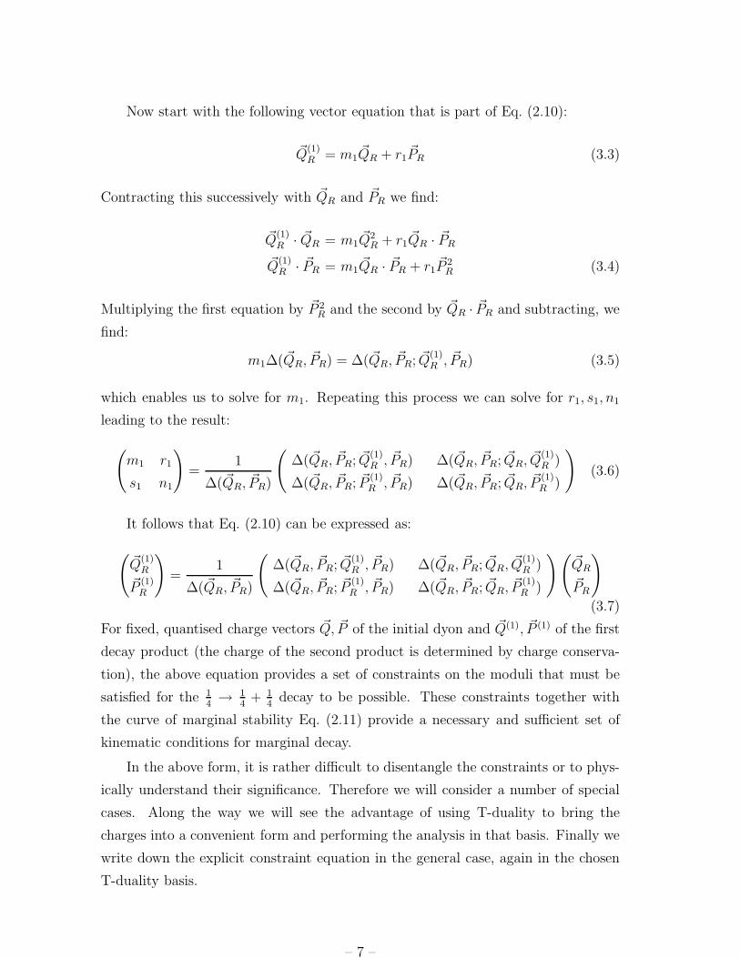
Now start with the following vector equation that is part of Eq. (2.10):

~Q(1)R = m1

~QR + r1~PR (3.3)

Contracting this successively with ~QR and ~PR we find:

~Q(1)R · ~QR = m1

~Q2R + r1

~QR · ~PR

~Q(1)R · ~PR = m1

~QR · ~PR + r1~P 2

R (3.4)

Multiplying the first equation by ~P 2R and the second by ~QR · ~PR and subtracting, we

find:

m1∆( ~QR, ~PR) = ∆( ~QR, ~PR; ~Q(1)R , ~PR) (3.5)

which enables us to solve for m1. Repeating this process we can solve for r1, s1, n1

leading to the result:

(m1 r1

s1 n1

)=

1

∆( ~QR, ~PR)

(∆( ~QR, ~PR; ~Q

(1)R , ~PR) ∆( ~QR, ~PR; ~QR, ~Q

(1)R )

∆( ~QR, ~PR; ~P(1)R , ~PR) ∆( ~QR, ~PR; ~QR, ~P

(1)R )

)(3.6)

It follows that Eq. (2.10) can be expressed as:

(~Q

(1)R

~P(1)R

)=

1

∆( ~QR, ~PR)

(∆( ~QR, ~PR; ~Q

(1)R , ~PR) ∆( ~QR, ~PR; ~QR, ~Q

(1)R )

∆( ~QR, ~PR; ~P(1)R , ~PR) ∆( ~QR, ~PR; ~QR, ~P

(1)R )

)(~QR

~PR

)

(3.7)

For fixed, quantised charge vectors ~Q, ~P of the initial dyon and ~Q(1), ~P (1) of the first

decay product (the charge of the second product is determined by charge conserva-

tion), the above equation provides a set of constraints on the moduli that must be

satisfied for the 14→ 1

4+ 1

4decay to be possible. These constraints together with

the curve of marginal stability Eq. (2.11) provide a necessary and sufficient set of

kinematic conditions for marginal decay.

In the above form, it is rather difficult to disentangle the constraints or to phys-

ically understand their significance. Therefore we will consider a number of special

cases. Along the way we will see the advantage of using T-duality to bring the

charges into a convenient form and performing the analysis in that basis. Finally we

write down the explicit constraint equation in the general case, again in the chosen

T-duality basis.

– 7 –

3.2 Explicit solution: special cases

(i) 12-BPS final states

The case where the decay products are 12-BPS should provide no constraints on

the moduli as this is a “non-rare” decay. This provides a check on our equations.

Inserting the 12-BPS conditions:

~P (1) = k1~Q(1), ~P (2) = k2

~Q(2) (3.8)

we find that:(

m1 r1

s1 n1

)= (k2 − k1)

∆( ~Q(1)R , ~Q

(2)R )

∆( ~QR, ~PR)

(k2 −1

k1k2 −k1

)(3.9)

We also have:

∆( ~QR, ~PR) = (k2 − k1)2∆( ~Q

(1)R , ~Q

(2)R ) (3.10)

Substituting in the above equation, we find:

(m1 r1

s1 n1

)=

1

k2 − k1

(k2 −1

k1k2 −k1

)(3.11)

At this stage all moduli-dependence has disappeared from the matrix, and equation

Eq. (2.10) indeed provides no constraints on the moduli. Rather, it reduces to an

identity. It is also easy to see that k1 − k2 divides the torsion of the original dyon,

so if we are also considering the unit-torsion case then k1 − k2 = 1 and mi, r1, s1, n1

are all manifestly integral [2].

(ii) Special charges and moduli

The next special case we will study has a restricted set of charges. Additionally,

some of the background moduli are set to a specific value, namely zero in the chosen

coordinates. We then examine the constraints on the remaining moduli. In choosing

special values for the moduli, we should in principle avoid loci of enhanced gauge

symmetry where the dyons we are studying would become massless.

Let us restrict ourselves to special initial-state charges given by:

~Q′ = (Q′1, 0, · · · , 0), ~Q′′ = (Q′′

1, 0, · · · , 0), ~Q′′′ = 0 (3.12)

and

~P ′ = (0, P ′2, 0, · · · , 0), ~P ′′ = (0, P ′′

2 , 0, · · · , 0), ~P ′′′ = 0 (3.13)

– 8 –

Next we set Bij = 0 = AIi as well as Gij = 0, i 6= j. The above restrictions allow

us to choose the orthonormal frames Eai to be diagonal:

Eii = Ri, i = 1, 2, · · · , 6 (3.14)

with Ri the radii of the six compactified directions in the heterotic basis.

In the restricted subspace of moduli space that we are considering here, the

matrix√

L + M reduces to:

√L + M =

E−1 E 0

0 0 0

0 0 0

(3.15)

with E given as in Eq. (3.14). Therefore the projected initial-state charge vectors

are:

~QR =

Q′

1

R1+ Q′′

1R1

0

...

0

, ~PR =

0P ′

2

R2+ P ′′

2 R2

0

...

0

(3.16)

For this configuration we clearly have ~QR · ~PR = 0 and therefore the quartic invariant

∆ is:

∆(QR, PR) =

(Q′

1

R1

+ Q′′1R1

)2(P ′

2

R2

+ P ′′2 R2

)2

(3.17)

We take the decay products to have generic charges ~Q(1), ~P (1) and ~Q(2), ~P (2)

subject of course to the requirement that they add up to ~Q, ~P . We then have:

~Q(1)R =

Q(1)′

1

R1+ Q

(1)′′

1 R1

Q(1)′

2

R2+ Q

(1)′′

2 R2

...

Q(1)′

6

R6+ Q

(1)′′

6 R6

, ~P(1)R =

P(1)′

1

R1+ P

(1)′′

1 R1

P(1)′

2

R2+ P

(1)′′

2 R2

...

P(1)′

6

R6+ P

(1)′′

6 R6

(3.18)

– 9 –

Now we can compute the quartic invariants appearing in Eq. (3.7):

∆( ~QR, ~PR; ~Q(1)R , ~PR) =

(Q′

1

R1+ Q′′

1R1

)(Q

(1)′

1

R1+ Q

(1)′′

1 R1

)(P ′

2

R2+ P ′′

2 R2

)2

∆( ~QR, ~PR; ~QR, ~Q(1)R ) =

(Q′

1

R1+ Q′′

1R1

)2(

Q(1)′

2

R2+ Q

(1)′′

2 R2

)(P ′

2

R2+ P ′′

2 R2

)

∆( ~QR, ~PR; ~P(1)R , ~PR) =

(Q′

1

R1+ Q′′

1R1

)(P

(1)′

1

R1+ P

(1)′′

1 R1

)(P ′

2

R2+ P ′′

2 R2

)2

∆( ~QR, ~PR; ~QR, ~P(1)R ) =

(Q′

1

R1+ Q′′

1R1

)2(

P(1)′

2

R2+ P

(1)′′

2 R2

)(P ′

2

R2+ P ′′

2 R2

)

Had we not taken E to be diagonal, the expressions above would have quickly become

very complicated to write down.

Inserting the above expressions, and cancelling some common factors, the con-

straint equation Eq. (3.7) becomes:

(Q′

1

R1+ Q′′

1R1

)(P ′

2

R2+ P ′′

2 R2

)~Q

(1)R =

(Q

(1)′

1

R1+ Q

(1)′′

1 R1

)(P ′

2

R2+ P ′′

2 R2

)~QR +

(Q′

1

R1+ Q′′

1R1

)(Q

(1)′

2

R2+ Q

(1)′′

2 R2

)~PR

(Q′

1

R1+ Q′′

1R1

)(P ′

2

R2+ P ′′

2 R2

)~P

(1)R =

(P

(1)′

1

R1+ P

(1)′′

1 R1

)(P ′

2

R2+ P ′′

2 R2

)~QR +

(Q′

1

R1+ Q′′

1R1

)(P

(1)′

2

R2+ P

(1)′′

2 R2

)~PR

(3.19)

These are 6+6 equations. However, the first two components of each set are iden-

tically satisfied, as one can easily check. This is expected, and follows from the

structure of Eq. (2.10) from which m1, r1, s1, n1 were determined. The remaining

four components of each equation give the desired constraints on the moduli. Be-

cause of the way we have chosen ~Q, ~P , the RHS already vanishes on components 3

to 6, so the constraint is simply that the LHS vanishes. That in turn sets to zero the

components 3 to 6 of the vectors ~Q(1)R and ~P

(1)R . Thus we find the constraints:

Q(1)′

i

Ri

+ Q(1)′′

i Ri = 0, i = 3, 4, 5, 6

P(1)′

i

Ri

+ P(1)′′

i Ri = 0, i = 3, 4, 5, 6 (3.20)

– 10 –

If the components of ~Q(1), ~P (1) are all nonvanishing, this implies that:

Ri =

√√√√−Q(1)′

i

Q(1)′′

i

=

√√√√− P(1)′

i

P(1)′′

i

, i = 3, 4, 5, 6 (3.21)

In this special case the constraint equations have some particular features. First of

all, for generic charge vectors ~Q(1) and ~P (1), there are no solutions. To have any

solutions at all, one must choose the charges of the decay products in such a way

that the second equality in the above equation can be satisfied. In other words, the

sign of Q(1)′

i and Q(1)′′

i must be opposite (for i = 3, 4, 5, 6), and the same has to

be true for P (1). In this case we find four constraints on the moduli, which fix the

compactification radii R3, R4, R5, R6.

For this special case, the numbers m1, r1, s1, n1 in Eq. (2.10) are given by:

m1 =Q

(1)′

1R1

+Q(1)′′

1 R1

Q′

1R1

+Q′′

1R1

, r1 =

Q(1)′

2

R2+ Q

(1)′′

2 R2

P ′

2

R2+ P ′′

2 R2

s1 =P

(1)′

1R1

+P(1)′′

1 R1

Q′

1R1

+Q′′

1R1

, n1 =

P(1)′

2

R2+ P

(1)′′

2 R2

P ′

2

R2+ P ′′

2 R2

(3.22)

We see that m1, s1 depend only on R1 and r1, n1 depend only on R2.

So far the decay products were taken to have generic charges (consistent of course

with charge conservation). The situation changes if we choose less generic decay

products. Earlier we took all components of ~Q(1), ~P (1) are nonvanishing. However

if Q(1)′

i = Q(1)′′

i = P(1)′

i = P(1)′′

i = 0 for any i ∈ 3, 4, 5, 6 then the corresponding

constraint Eq. (3.20) is trivially satisfied. In this situation we will have a reduced

number of constraints. As an example if the above situation holds for all directions

except i = 3 and ifQ

(1)′

3

Q(1)′′

3

=P

(1)′

3

P(1)′′

3

then there is only a single constraint coming from

the above equations. The curve of marginal stability provides one more constraint, so

the decay will take place on a codimension-2 subspace of the restricted moduli space

in which we are working for this class of examples. The fact that in some situations

there are no solutions (for example if we do not satisfy that Q(1)′

i and Q(1)′′

i have

opposite signs for i = 3, 4, 5, 6) simply means that our restricted moduli space fails

to intersect the marginal stability locus in that case.

If the charges Q(1)′

i , Q(1)′′

i , P(1)′

i , P(1)′′

i vanish for all i ∈ 3, 4, 5, 6 then there are no

constraints (beyond the curve of marginal stability). It is easily seen that this is the

case where the final states are both 12-BPS.

– 11 –

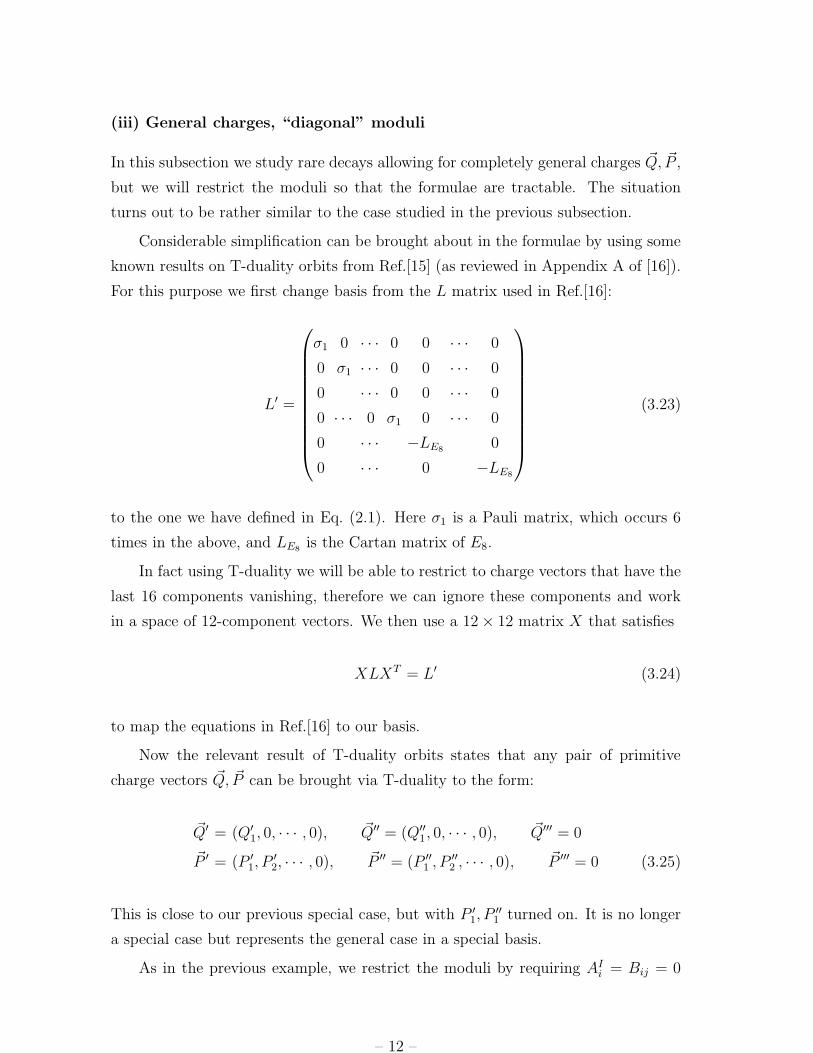
(iii) General charges, “diagonal” moduli

In this subsection we study rare decays allowing for completely general charges ~Q, ~P ,

but we will restrict the moduli so that the formulae are tractable. The situation

turns out to be rather similar to the case studied in the previous subsection.

Considerable simplification can be brought about in the formulae by using some

known results on T-duality orbits from Ref.[15] (as reviewed in Appendix A of [16]).

For this purpose we first change basis from the L matrix used in Ref.[16]:

L′ =

σ1 0 · · · 0 0 · · · 0

0 σ1 · · · 0 0 · · · 0

0 · · · 0 0 · · · 0

0 · · · 0 σ1 0 · · · 0

0 · · · −LE8 0

0 · · · 0 −LE8

(3.23)

to the one we have defined in Eq. (2.1). Here σ1 is a Pauli matrix, which occurs 6

times in the above, and LE8 is the Cartan matrix of E8.

In fact using T-duality we will be able to restrict to charge vectors that have the

last 16 components vanishing, therefore we can ignore these components and work

in a space of 12-component vectors. We then use a 12 × 12 matrix X that satisfies

XLXT = L′ (3.24)

to map the equations in Ref.[16] to our basis.

Now the relevant result of T-duality orbits states that any pair of primitive

charge vectors ~Q, ~P can be brought via T-duality to the form:

~Q′ = (Q′1, 0, · · · , 0), ~Q′′ = (Q′′

1, 0, · · · , 0), ~Q′′′ = 0

~P ′ = (P ′1, P

′2, · · · , 0), ~P ′′ = (P ′′

1 , P ′′2 , · · · , 0), ~P ′′′ = 0 (3.25)

This is close to our previous special case, but with P ′1, P

′′1 turned on. It is no longer

a special case but represents the general case in a special basis.

As in the previous example, we restrict the moduli by requiring AIi = Bij = 0

– 12 –

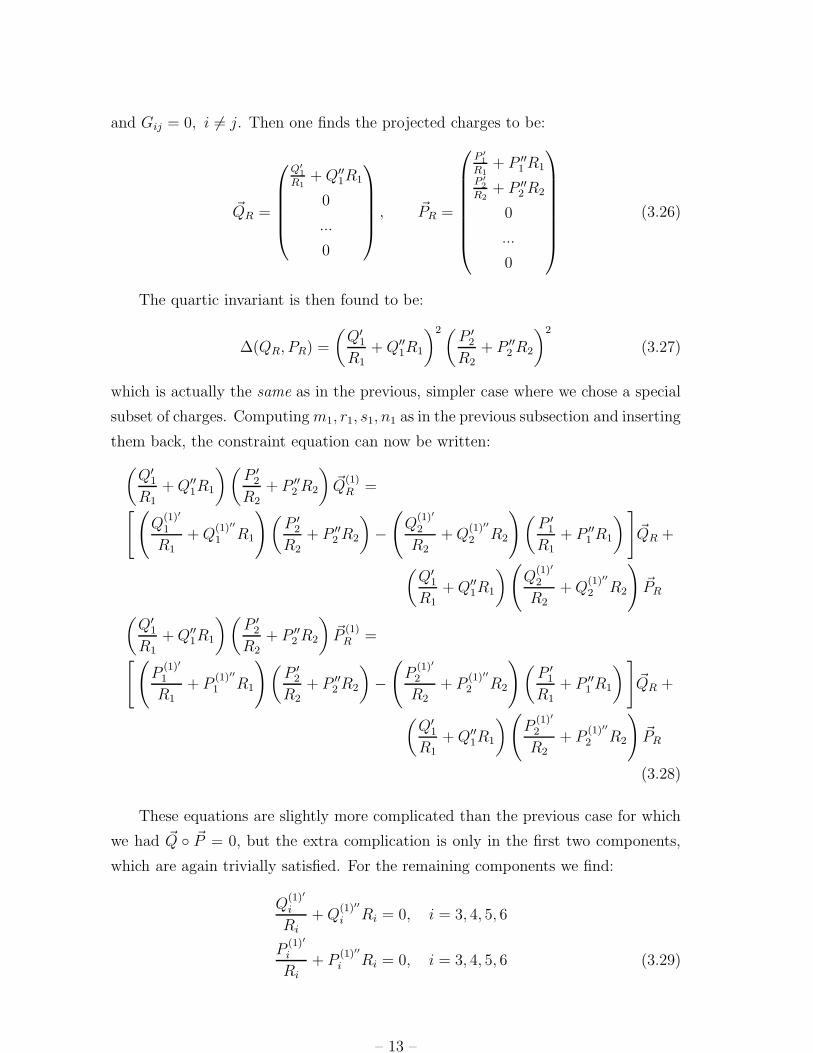
and Gij = 0, i 6= j. Then one finds the projected charges to be:

~QR =

Q′

1

R1+ Q′′

1R1

0

...

0

, ~PR =

P ′

1

R1+ P ′′

1 R1

P ′

2

R2+ P ′′

2 R2

0

...

0

(3.26)

The quartic invariant is then found to be:

∆(QR, PR) =

(Q′

1

R1

+ Q′′1R1

)2(P ′

2

R2

+ P ′′2 R2

)2

(3.27)

which is actually the same as in the previous, simpler case where we chose a special

subset of charges. Computing m1, r1, s1, n1 as in the previous subsection and inserting

them back, the constraint equation can now be written:

(Q′

1

R1

+ Q′′1R1

)(P ′

2

R2

+ P ′′2 R2

)~Q

(1)R =

[(Q

(1)′

1

R1

+ Q(1)′′

1 R1

)(P ′

2

R2

+ P ′′2 R2

)−(

Q(1)′

2

R2

+ Q(1)′′

2 R2

)(P ′

1

R1

+ P ′′1 R1

)]~QR +

(Q′

1

R1+ Q′′

1R1

)(Q

(1)′

2

R2+ Q

(1)′′

2 R2

)~PR

(Q′

1

R1+ Q′′

1R1

)(P ′

2

R2+ P ′′

2 R2

)~P

(1)R =

[(P

(1)′

1

R1+ P

(1)′′

1 R1

)(P ′

2

R2+ P ′′

2 R2

)−(

P(1)′

2

R2+ P

(1)′′

2 R2

)(P ′

1

R1+ P ′′

1 R1

)]~QR +

(Q′

1

R1+ Q′′

1R1

)(P

(1)′

2

R2+ P

(1)′′

2 R2

)~PR

(3.28)

These equations are slightly more complicated than the previous case for which

we had ~Q ◦ ~P = 0, but the extra complication is only in the first two components,

which are again trivially satisfied. For the remaining components we find:

Q(1)′

i

Ri

+ Q(1)′′

i Ri = 0, i = 3, 4, 5, 6

P(1)′

i

Ri

+ P(1)′′

i Ri = 0, i = 3, 4, 5, 6 (3.29)

– 13 –

These are exactly the same as the constraints we found in the previous case. The

analysis is therefore also the same: the constraints cannot be satisfied for generic

charges because our restricted moduli space need not intersect the marginal stability

locus. When they can be satisfied there are at most four constraints, though there

will be less if some of the decay product charges vanish.

3.3 General charges, “triangular” moduli

In this subsection we restrict the moduli in the most minimal way consistent with

finding a simple form of the constraint equation. The restriction will be a kind of

“triangularity” condition:

(G + B + C)i1 = (G + B + C)i2 = 0, i = 3, 4, 5, 6 (3.30)

with no separate constraints on G, B, A other than the above.

As before, we use T-duality to put the initial charges into the form of Eq. (3.25).

Thereafter, we are still free to make T-duality transformations involving the last four

components of ~Q′ and ~Q′′ and all 16 components of ~Q′′′. The T-duality group is thus

restricted to an SO(4, 20; ZZ). These transformations will affect the charges of the

decay products while leaving the initial dyon unchanged. Using them we bring the

electric charges of the first decay product to the form:

~Q(1)′ = (Q(1)′

1 , Q(1)′

2 , Q(1)′

3 , · · · , 0),

~Q(1)′′ = (Q(1)′′

1 , Q(1)′′

2 , Q(1)′′

3 , · · · , 0),

~Q(1)′′′ = 0 (3.31)

Finally we use an SO(3, 19; ZZ) subgroup of T-duality that preserves all the charge

vectors that we have so far fixed, to bring the magnetic charges of the first decay

product to the form:

~P (1)′ = (P(1)′

1 , P(1)′

2 , P(1)′

3 , P(1)′

4 , · · · , 0),

~P (1)′′ = (P(1)′′

1 , P(1)′′

2 , P(1)′′

3 , P(1)′′

4 , · · · , 0),

~P (1)′′′ = 0 (3.32)

The charges of the second decay product are determined by charge conservation.

– 14 –

Now we use the form of the projection matrix√

L + M and write out Eq. (2.10)

explicitly, after first multiplying through by Eij :

Q(1)′

i + (G + B + C)ijQ(1)′′

j = m1Q′i + m1(G + B + C)ijQ

′′j

+ r1P′i + r1(G + B + C)ijP

′′k

P(1)′

i + (G + B + C)ijP(1)′′

j = s1Q′i + s1(G + B + C)ijQ

′′j

+ n1P′i + n1(G + B + C)ijP

′′j (3.33)

This is a set of 6 + 6 equations. Recall that Cij = AIi A

Ij .

We immediately see that for our choice of T-duality frame for the initial charges,

as well as using the “triangularity” condition, the RHS of the above equations van-

ishes for i = 3, 4, 5, 6. Hence we find the constraint equations still in a relatively

simple form:

Q(1)′

i + (G + B + C)ijQ(1)′′

j = 0, i = 3, 4, 5, 6

P(1)′

i + (G + B + C)ijP(1)′′

j = 0, i = 3, 4, 5, 6 (3.34)

These are then the 4+4 constraints on rare dyon decays, though still with the tri-

angularity restriction on moduli and in a specific T-duality frame. They must be

supplemented by the curve of marginal stability, for which we need to know the

numbers m1, r1, s1, n1.

The first two components of each line of equations Eq. (3.33) determine the

values of m1, r1, s1, n1. From the first line of those equations we find:

Q(1)′

1 + (G + B + C)1i

−→Q

(1)′′

i = m1Q′1 + m1(G + B + C)1iQ

′′i + r1P

′1 + r1(G + B + C)1iP

′′i

Q(1)′

2 + (G + B + C)2iQ(1)′′

i = r1P′2 + r1(G + B + C)2iP

′′i (3.35)

Solving for r1 from the second equation above, we get:

r1 =Q

(1)′

2 + (G + B + C)2iQ(1)′′

i

P ′2 + (G + B + C)2iP

′′i

(3.36)

Inserting this in the first equation determines m1:

m1 =(P ′

2 + (G + B + C)2iP′′i

)−1(Q′

1 + (G + B + C)1iQ′′i

)−1

×[(

Q(1)′

1 + (G + B + C)1iQ(1)′′

i

)(P ′

2 + (G + B + C)2iP′′i

)

−(Q

(1)′

2 + (G + B + C)2iQ(1)′′

i

)(P ′

1 + (G + B + C)1iP′′i

)](3.37)

– 15 –

Similarly we solve for s1, n1 from the second line of Eq. (3.33) and find:

n1 =P

(1)′

2 + (G + B + C)2iP(1)′′

i

P ′2 + (G + B + C)2iP

′′i

s1 =(P ′

2 + (G + B + C)2iP′′i

)−1(Q′

1 + (G + B + C)1iQ′′i

)−1

×[(

P(1)′

1 + (G + B + C)1iP(1)′′

i

)(P ′

2 + (G + B + C)2iP′′i

)

−(P

(1)′

2 + (G + B + C)2iP(1)′′

i

)(P ′

1 + r(G + B + C)1iPi

)](3.38)

Admittedly these are somewhat complicated expressions for the numbers m1, r1, s1, n1

that one needs to plug in to determine the curve of marginal stability on the torus

moduli space. It is conceivable that a more opportune choice of variables could sim-

ply them further. Nevertheless, the constraints Eq. (3.34) on the remaining moduli

are rather simple.

3.4 Explicit solution: the general case

We now turn to the case where the initial and final charges are completely general

and the moduli are generic as well. Most of the relevant analysis has already been

done in previous subsections and it only remains to write down the result. However,

as we will see, the equations rapidly become messy – despite the use of T-duality

transformations - once we use completely general moduli.

Let us again start by writing out Eq. (2.10) explicitly, but now without any

condition on the moduli. After multiplying through by Eij , we find the equations:

Q(1)′

i + (G + B + C)ijQ(1)′′

j = m1Q′i + m1(G + B + C)ijQ

′′j

+ r1P′i + r(G + B + C)ijP

′′k

P(1)′

i + (G + B + C)ijP(1)′′

j = s1Q′i + s1(G + B + C)ijQ

′′j

+ n1P′i + n1(G + B + C)ijP

′′j (3.39)

which are actually the same as Eq. (3.33) that we had before. The difference is that

the RHS no longer vanishes for any of the components (earlier that was guaranteed

by the triangularity condition that we had assumed on the moduli). Notice that even

in the most general case, we have gained something by fixing the initial and final

state charges using T-duality. The last 16 components of these charges have all been

set to 0, and the result is that most of the terms involving the gauge field moduli

– 16 –

AIi have disappeared. The only appearance of these moduli is through Cij = AI

i AIj

which in turn only appears in the combination G + B + C.

This time our strategy will be to choose any 4 equations from the above set of 12

to determine the variables m1, n1, r1, s1. Then in the remaining 8 equations we insert

these values for the variables and obtain the desired constraint equations. Picking

the first 2 components for each charge vector, we find:

Q(1)′

1 + (G + B + C)1iQ(1)′′

i = m1Q′1 + m1(G + B + C)1iQ

′′i + r1P

′1 + r(G + B + C)1iP

′′i

Q(1)′

2 + (G + B + C)2iQ(1)′′

i = r1P′2 + r1(G + B + C)2iP

′′i (3.40)

Solving for r1 from the second equation above, we get:

r1 =Q

(1)′

2 + (G + B + C)2iQ(1)′′

i

P ′2 + (G + B + C)2iP

′′i

(3.41)

and inserting this in the first equation, we find m1:

m1 =(P ′

2 + (G + B + C)2iP′′i

)−1(Q′

1 + (G + B + C)1iQ′′i

)−1

×[(

Q(1)′

1 + (G + B + C)1iQ(1)′′

i

)(P ′

2 + (G + B + C)2iP′′i

)

−(Q

(1)′

2 + (G + B + C)2i

−→Q

(1)′′

i

)(P ′

1 + r(G + B + C)1iPi

)](3.42)

Similarly we solve for s1, n1 from the second equation and find:

n1 =P

(1)′

2 + (G + B + C)2iP(1)′′

i

P ′2 + (G + B + C)2iP

′′i

(3.43)

and

s1 =(P ′

2 + (G + B + C)2iP′′i

)−1(Q′

1 + (G + B + C)1iQ′′i

)−1

×[(

P(1)′

1 + (G + B + C)1iP(1)′′

i

)(P ′

2 + (G + B + C)2iP′′i

)

−(P

(1)′

2 + (G + B + C)2iP(1)′′

i

)(P ′

1 + (G + B + C)1iPi

)](3.44)

We feed in these values of m1, n1, r1, s1 into the remaining 8 equations to find the

most general constraint equations on the moduli:

Q(1)′

i + (G + B + C)ijQ(1)′′

j = m1

(Q′

i + (G + B + C)ijQ′′j

)+ r1

(P ′

i + (G + B + C)ijP′′j

)

P(1)′

i + (G + B + C)ijP(1)′′

j = s1

(Q′

i + (G + B + C)ijQ′′j

)+ n1

(P ′

i + (G + B + C)ijP′′j

)

(3.45)

– 17 –

here i = 3, 4, 5, 6, and m1, n1, r1, s1 are given in the above equations. We see that the

values of m1, n1, r1, s1 come out the same as in the previous special case, however the

constraints are much more complicated and – unlike in all the previous special cases

– depend explicitly on these numbers. Nevertheless, the above equations embody the

most general kinematic constraints on moduli space to allow a two-body decay of a

dyon of charges ~Q, ~P into 14-BPS final state with charges ~Q(1) and ~P (1) (the charges

of the second state being, as always, determined by charge conservation). It is quite

conceivable that a more detailed study of possible T-duality bases will allow us to

further simplify the most general case, and we leave such an investigation for the

future.

4. Multi-particle decays

So far in this work, as well as in previous work[9], we have written down conditions for

decay of a dyon into two 14-BPS final states. One could certainly imagine extending

these considerations to three or more final states. Indeed, it turns out rather simple

to do so and we will here discuss an iterative way to obtain the relevant formulae.

Consider the decay of a dyon of charges ( ~Q, ~P ) into n decay products of charges

( ~Q(1), ~P (1)), ( ~Q(2), ~P (2)), · · · ( ~Q(n), ~P (n)). The condition for marginality of such a de-

cay is the condition for the original dyon to go into two decay products of charges

( ~Q(1), ~P (1)) and∑n

i=2(~Q(i), ~P (i)), along with the condition for the second decay prod-

uct to further decay into say ( ~Q(2), ~P (2)) and∑n

i=3(~Q(i), ~P (i)). The latter condition

must in turn be iterated. Each of these is a two-body decay (with both final states

being 14-BPS) so we already know the condition for each one to take place. The in-

tersection of all these loci will give the marginal stability locus for the multiparticle

decay.

There is a simpler way to iterate the condition. Instead of looking at the curve

where the second decay product decays into further subconstituents, as above, we

can simply consider the collection of all marginal stability loci for the decays:

(~QR

~PR

)→(

~Q(i)R

~P(i)R

)+

(~QR − ~Q

(i)R

~PR − ~P(i)R

), i = 1, 2, · · · , n (4.1)

For each of these, the curve is precisely Eq. (2.11) with the subscript “1” replaced

– 18 –

by “i”. We write it as:

C(mi, ri, si, ni) ≡(

τ1 −mi − ni

2si

)2

+

(τ2 +

Ei

2si

)2

− 1

4s2i

((mi−ni)

2 +4risi +E2i

)= 0

(4.2)

where

Ei ≡1√∆

(~Q(i) ◦ ~P − ~P (i) ◦ ~Q

)(4.3)

In addition to this curve we have the constraints on the remaining moduli as in Sec.3

above. Those too can be expressed in terms of the single decay product labelled “i”.

Now to find the condition for a multi-dyon decay, we simply take the intersection of

all these loci of marginal stability. As the number of final states increases, we will

generically find loci of marginal stability of increasing codimension.

5. Multi-centred black holes

It was argued in Refs.[5, 6] that the curves of marginal stability for decays of the

form:

14-BPS → 1

2-BPS + 1

2-BPS (5.1)

are also the curves of disintegration for two-centred 14-BPS black holes whose centres

are individually 12-BPS. The method used in these works, which we will summarise

and extend below, was to use a constraint equation due to Denef [7] to express the

separation between the centres of such a black hole in terms of charges and moduli.

Requiring that the separation be infinite places a condition on charges and moduli

which turns out to be precisely the curve of marginal stability, Eq. (2.11), specialised

to this decay.

Now Denef’s constraint equation is not confined to two-centred black holes alone,

but applies to any number of centres. It has a different limitation: it is defined in

the context of N = 2, rather than N = 4 compactifications, and relies on special

geometry. Nevertheless, for the cases to which it applies, we can certainly use it in

the N = 4 context. We will do so and will find the perhaps surprising result that the

curves of marginal stability for generic decays to n final states, which we discussed in

Sec.4 above, are precisely reproduced by the constraint equations for multi-centred

black holes. This suggests a more generic relationship between multi-particle decays

and multi-centred black holes than has been previously considered.

– 19 –

The constraint equation on multi-centred dyons, (see for example Ref.[5]2) reads

as follows. Let p(i)I , q(i)I be the charges of the i-th centre where i = 1, 2, · · · , N .

These charges are expressed in the special-geometry basis3. Let the 3-vector ~ri be

the location of the i-th centre. And let the moduli be encoded in the standard

holomorphic special-geometry variables XI , FI . Then the constraint equations are:

p(i)I Im (FI∞) − q(i)I Im (XI

∞) +1

2

∑

j 6=i

p(i)Iq(j)I − q

(i)I p(j)I

|~ri − ~rj|= 0 (5.2)

Here the subscript ∞ indicates that the corresponding moduli are measured at spatial

infinity (for brevity of notation we will drop it when there is no risk of ambiguity).

Note that the numerators inside the summation correspond to the Saha angular

momentum between each pair of centres.

These are N equations for (N

2) pairwise distances between the centres. We

analyse them following the procedure in Ref.[5] for the two-centred case. First of all,

one of the equations is redundant. Adding all the equations, we find:

pI Im (FI∞) − qI Im (XI∞) = 0 (5.3)

where (pI , qI) are the charges of the entire black hole. This provides one real

constraint on the extra modulus X0∞. As the above equation is invariant under

XI → λXI for real XI , as well as under XI → −XI , we see that the magnitude of

X0 is undetermined by this condition, while the phase is determined (in terms of the

XI , I = 1, 2, 3) upto a two-fold ambiguity. Another real constraint is now imposed

in the form of a “gauge condition”:

XIF̄I − X̄IFI = −i (5.4)

This determines the magnitude of X0 but leaves intact the two-fold ambiguity in

the phase. The remaining N − 1 equations then provide constraints on the (N

2)

separations.

For the case N = 2 we therefore have a single equation, which completely deter-

mines the separation between the two centres. This works as follows. The relevant

part of the theory is described by the holomorphic prepotential:

F = −X1X2X3

X0(5.5)

2A sign in equation (3.2) of Ref.[5] should be corrected so that it reads X1

X0 = −τ . This leads to

some sign changes in other equations there.3As we will see, this differs by an interchange of some components from the standard basis used

in N = 4 compactifications.

– 20 –

where the XI are complex scalar fields related to a subset of the K3 × T 2 moduli,

namely τ = τ1 + iτ2 describing the 2-torus complex structure, and

M = diag(R̂−2, R−2, R̂2, R2) (5.6)

describing a 2-parameter subset of the remaining moduli (including the K3 moduli).

The precise relationship is:

X1

X0= −τ,

X2

X0= iRR̂,

X3

X0= i

R̂

R(5.7)

The gauge condition Eq. (5.4) then tells us that:

|X0∞|2 =

1

8R̂2 τ2

(5.8)

As in the previous sections, we will consider a dyon with charges ( ~Q, ~P ), but

now each taken to be 4-component (the first two components should be thought of

as two of the six ~Q′ and the second two components constitute two of the six ~Q′′.

The charges correspond to unit torsion, namely:

g.c.d.(QiPj − PiQj) = 1 (5.9)

We begin by determining the modulus X0 in terms of the T-duality invariants P ◦P, Q◦Q, P ◦Q, where as before the inner products are defined in terms of the moduli

at infinity, e.g. P ◦ P = P T (L + M)P .

As promised, we will use the transcription between the natural electric-magnetic

basis ~P , ~Q for the type IIB superstring and the natural basis pI , qI for special geom-

etry (see for example Ref. [5]):

qI = (Q1, P1, Q4, Q2), pI = (P3,−Q3, P2, P4) (5.10)

In addition we have:

Im (F0) = R̂2 Im (X0τ), Im (F1) = R̂2 Im (X0),

Im (F2) =R̂

RRe (X0τ), Im (F3) = RR̂ Re (X0τ)

(5.11)

while

Im (X0) = Im (X0), Im (X1) = − Im (X0τ),

Im (X2) = RR̂ Re (X0), Im (X3) =R̂

RRe (X0)

(5.12)

– 21 –

Inserting these into Eqs.(5.3),(5.8), one finds:

X0 =1

(2√

2R̂τ2)

√∆τ̄ + i (Q ◦ P τ̄ − Q ◦ Q)√

Q ◦ Q MBPS

(5.13)

where MBPS is the BPS mass given by Eq. (2.4).

Now let us assume our dyon has n centres of charges ( ~Q(i), ~P (i)):(

~Q(i)

~P (i)

)=

(mi ri

si ni

)(~Q

~P

), i = 1, 2, · · · , n (5.14)

with mi, ri, si, n1 integers satisfying:n∑

i=1

mi =n∑

i=1

ni = 1,n∑

i=1

ri =n∑

i=1

si = 0 (5.15)

From Eq. (5.10) we find that the charges of the decay products in the qI , pJ basis

are given by:

q(i)I = (miQ1 + riP1, siQ1 + niP1, miQ4 + riP4, miQ2 + riP2)

p(i)I = (siQ3 + niP3,−(miQ3 + riP3), siQ2 + niP2, siQ4 + niP4)(5.16)

Now the first term in Eq. (5.2) can be written:

p(i)I Im (FI)−q(i)I Im (XI) = R̂ Re

(−X0 X0τ

)(mi ri

si ni

)(Q2

R+ RQ4 − i(Q1

R̂+ R̂Q3)

P2

R+ RP4 − i(P1

R̂+ R̂P3)

)

(5.17)

The invariants P ◦ P, Q ◦ Q, Q ◦ P are given by:

Q ◦ Q =

(Q1

R̂+ R̂Q3

)2

+

(Q2

R+ RQ4

)2

P ◦ P =

(P1

R̂+ R̂P3

)2

+

(P2

R+ RP4

)2

Q ◦ P =

(Q1

R̂+ R̂Q3

)(P1

R̂+ R̂P3

)+

(Q2

R+ RQ4

)(P2

R+ RP4

)(5.18)

The column vector in Eq. (5.17) depends on four combinations of Qi, Pi and therefore

cannot in general be expressed in terms of T-duality invariants. Therefore we restrict

to the special case, discussed in particular in Ref.[5], for which Q1 = Q3 = 0. In this

case only three independent combinations appear in the column vector and it is easy

to show that:

p(i)I Im (FI) − q(i)I Im (XI) = R̂ ReX0

(−1 τ

)(mi ri

si ni

)(√Q ◦ Q

Q◦P+i√

∆√Q◦Q

)

=s1

√∆

2√

2 τ2 MBPS

C(mi, ri, si, ni)

(5.19)

– 22 –

where C(mi, ri, si, ni) is the curve of marginal stability for multiparticle decays, de-

fined in Eq. (4.2).

The numerator of the second term in Eq. (5.2), denoted:

Jij ≡ p(i)Iq(j)I − p(j)Iq

(i)I (5.20)

is the angular momentum between each pair of decay products evaluated in the

moduli-independent norm. We will denote the pairwise separation between the cen-

tres by:

Lij = |~ri − ~rj | (5.21)

Note that Jij = −Jji and Lij = Lji.

Inserting the above results into Eq. (5.2), one finds that it can be expressed as

follows:

C̃i +∑

j 6=i

Jij

Lij

= 0 (5.22)

where

C̃i ≡si

√∆√

2 τ2 MBPS

C(mi, ri, si, ni) (5.23)

Clearly the first term in Eq. (5.22) depends only on the charges of a single centre

(as well as the initial charges) while the second term depends on the charges of

a pair of centres. Note that we have∑

i C̃i = 0. Thus we have shown that the

curves of marginal stability for multi-centred decays appear also from considerations

of multi-centred black holes and the constraints on the locations of their centres.

In the special case considered previously [5, 6] where the dyon has two 12-BPS

centres, the corresponding curve of marginal stability is of codimension 1. In this

case it is known that the degeneracy of states jumps as we cross the curve. From

the supergravity point of view, it was suggested in the N = 2 context in Ref.[7] and

shown more explicitly in the present N = 4 context in Refs.[5, 6], that this decay

occurs as a result of the two centres flying apart to infinity at a curve of marginal

stability. This is seen by specialising Eq. (5.22) to this case. As long as J12 6= 0, the

separation L12 → ∞ when C̃i → 0. Moreover for a fixed sign of J12, the separation

L12 can be positive only on one side of the curve of marginal stability. On the other

side it is negative, which indicates that the corresponding two-centred black hole

does not exist.

Now let us return to the more general case where there are two centres but both

are 14-BPS. As we have seen, in this case the locus of marginal stability is not a wall

– 23 –

in moduli space, but rather a curve of codimension ≥ 2. Therefore the degeneracy

formula cannot jump as one crosses the curve. Hence one need not have expected

any relationship between marginal decays and multi-centred dyons. Nevertheless, we

see that Eq. (5.22) continues to hold in the more general case (with the limitation

that the charges are those that can be embedded in an N = 2 compactification).

We interpret this as evidence that the relationship between dyon decay and the

disintegration of multi-centred black holes holds more generally than required by

the degeneracy formula. Therefore we conjecture that even with the most general

charges, n-centred black holes exist in N = 4 string compactifications with generic14-BPS centres for which Eq. (5.22) holds true. It would be worth trying to prove that

this is the case, or else to show that such solutions do not exist beyond the cases that

can be embedded in the charge space and moduli space of N = 2. An intermediate

possibility also exists: that in N = 4 compactifications such multi-centred black

holes do exist with arbitrary charges, but only on a subspace of the moduli space.

Examining Eq. (5.22) one sees that if the marginal stability condition C̃i = 0 is

satisfied for a particular i, then we must have:∑

j 6=i

Jij

Lij

= 0 (5.24)

One possible solution is to have Lij → ∞ for all j 6= i. This means the ith centre

has been taken infinitely far away from all the others, in agreement with the picture

of marginal decay that we developed in Section 4 above. Since the pairwise Saha

angular momenta Jij ≡ P (i) ·Q(j)−P (j) ·Q(i) cannot all be positive in every equation

(since Jij = −Jji) there could be other configurations where the C̃i = 0, except in

the case of two centres. It is not clear to us how these other solutions should be

interpreted.

Note that in the above equation the angular momentum is measured with respect

to moduli-independent inner product P · Q ≡ P T LQ unlike the angular momentum

appearing in the curve of marginal stability Eq. (4.2) which is computed using the

moduli-dependent inner product P ◦Q ≡ P T (L+M)Q. One may think of the latter

evolving to the former as we follow the attractor flow from infinity to the horizon of

the black hole. However it would be nice to have a better physical understanding of

the role of dyonic angular momenta in these discussions4.4As is well-known, the dyonic angular momentum plays a physical role in the wall-crossing

formulae [7, 17, 5, 6, 18, 19] that describe how the degeneracy jumps, but in the present discussions

there are no walls or jumps.

– 24 –

6. Conclusions

In this work we have obtained the loci of marginal stability for decays of 14-BPS dyons

into any number of BPS constituents in N = 4 string compactifications. These loci

appear as equations constraining the 132 + 2 moduli, more precisely as a curve of

marginal stability in the upper-half-plane that represents a torus moduli space (in

the basis of type IIB on K3 × T 2, this is the geometric torus) as well as some more

complicated equations on the remaining moduli. While in this paper we worked with

unit-torsion initial dyons, it should be quite straightforward to extend our results to

general torsion. We showed how to extend our analysis to multi-particle decays, and

found a relation between the loci of marginal stability obtained in this way and the

supergravity constraints on pairwise separations of the centres of multi-centred black

holes.

The physical role of “rare” marginal dyon decays, namely all those other than of

a 14-BPS dyon into two 1

2-BPS dyons, has yet to be explored. Because such decays

take place on loci of codimension ≥ 2 in moduli space, they do not form “domain

walls” across which the degeneracy can jump. Therefore they do not affect the basic

entropy or dyon counting formulae. However it is certainly possible that they have

other interesting physical effects which may emerge on further investigation.

Acknowledgements

We would like to thank Anindya Mukherjee, Suresh Nampuri and Ashoke Sen for

very helpful discussions. The work of S.M. was supported in part by a J.C. Bose

Fellowship of the Government of India. We are grateful to the people of India for

generously supporting research in string theory.

References

[1] R. Dijkgraaf, E. P. Verlinde, and H. L. Verlinde, Counting Dyons in N = 4 String

Theory, Nucl. Phys. B484 (1997) 543–561, [hep-th/9607026].

[2] A. Sen, Walls of Marginal Stability and Dyon Spectrum in N=4 Supersymmetric

String Theories, JHEP 05 (2007) 039, [hep-th/0702141].

[3] A. Dabholkar, D. Gaiotto, and S. Nampuri, Comments on the Spectrum of CHL

Dyons, JHEP 01 (2008) 023, [hep-th/0702150].

– 25 –

[4] A. Sen, Black Hole Entropy Function, Attractors and Precision Counting of

Microstates, arXiv:0708.1270.

[5] A. Sen, Two Centered Black Holes and N=4 Dyon Spectrum, JHEP 09 (2007) 045,

[arXiv:0705.3874].

[6] M. C. N. Cheng and E. Verlinde, Dying Dyons Don’t Count, JHEP 09 (2007) 070,

[arXiv:0706.2363].

[7] F. Denef, Supergravity Flows and D-brane Stability, JHEP 08 (2000) 050,

[hep-th/0005049].

[8] A. Sen, Rare Decay Modes of Quarter BPS Dyons, JHEP 10 (2007) 059,

[arXiv:0707.1563].

[9] A. Mukherjee, S. Mukhi, and R. Nigam, Dyon Death Eaters, JHEP 10 (2007) 037,

[arXiv:0707.3035].

[10] A. Mukherjee, S. Mukhi, and R. Nigam, Kinematical Analogy for Marginal Dyon

Decay, arXiv:0710.4533.

[11] J. Maharana and J. H. Schwarz, Noncompact Symmetries in String Theory, Nucl.

Phys. B390 (1993) 3–32, [hep-th/9207016].

[12] A. Sen, Electric Magnetic Duality in String Theory, Nucl. Phys. B404 (1993)

109–126, [hep-th/9207053].

[13] M. Cvetic and D. Youm, Dyonic BPS Saturated Black Holes of Heterotic String on a

Six Torus, Phys. Rev. D53 (1996) 584–588, [hep-th/9507090].

[14] M. J. Duff, J. T. Liu, and J. Rahmfeld, Four-dimensional String-String-String

Triality, Nucl. Phys. B459 (1996) 125–159, [hep-th/9508094].

[15] C. Wall, On the Orthogonal Groups of Unimodular Quadratic Forms, Math. Annalen

147 (1962) 328.

[16] S. Banerjee and A. Sen, Duality Orbits, Dyon Spectrum and Gauge Theory Limit of

Heterotic String Theory on T6, JHEP 03 (2008) 022, [arXiv:0712.0043].

[17] F. Denef and G. W. Moore, Split States, Entropy Enigmas, Holes and Halos,

hep-th/0702146.

[18] E. Diaconescu and G. W. Moore, Crossing the Wall: Branes vs. Bundles,

arXiv:0706.3193.

– 26 –

[19] M. C. N. Cheng and E. P. Verlinde, Wall Crossing, Discrete Attractor Flow, and

Borcherds Algebra, arXiv:0806.2337.

– 27 –