Study of �B0 ! D0���� decays

A. Kuzmin,1 K. Abe,8 I. Adachi,8 H. Aihara,45 D. Anipko,1 K. Arinstein,1 V. Aulchenko,1 T. Aushev,13,18 S. Bahinipati,4

A. M. Bakich,40 V. Balagura,13 E. Barberio,21 M. Barbero,7 A. Bay,18 I. Bedny,1 K. Belous,12 U. Bitenc,14 I. Bizjak,14

S. Blyth,24 A. Bondar,1 A. Bozek,27 M. Bracko,8,14,20 T. E. Browder,7 M.-C. Chang,5 Y. Chao,26 A. Chen,24 K.-F. Chen,26

W. T. Chen,24 B. G. Cheon,3 R. Chistov,13 Y. Choi,39 Y. K. Choi,39 J. Dalseno,21 M. Dash,49 A. Drutskoy,4 S. Eidelman,1

D. Epifanov,1 N. Gabyshev,1 A. Garmash,51 T. Gershon,8 A. Go,24 G. Gokhroo,41 B. Golob,14,19 H. Ha,16 J. Haba,8

K. Hayasaka,22 H. Hayashii,23 M. Hazumi,8 D. Heffernan,32 T. Hokuue,22 Y. Hoshi,43 S. Hou,24 W.-S. Hou,26

Y. B. Hsiung,26 T. Iijima,22 K. Ikado,22 A. Imoto,23 K. Inami,22 A. Ishikawa,45 H. Ishino,46 R. Itoh,8 M. Iwasaki,45

Y. Iwasaki,8 J. H. Kang,50 P. Kapusta,27 H. Kawai,2 T. Kawasaki,29 H. Kichimi,8 H. J. Kim,17 Y. J. Kim,6 K. Kinoshita,4

P. Krizan,14,19 P. Krokovny,8 R. Kulasiri,4 R. Kumar,33 C. C. Kuo,24 Y.-J. Kwon,50 S. E. Lee,37 T. Lesiak,27 S.-W. Lin,26

G. Majumder,41 F. Mandl,11 T. Matsumoto,47 S. McOnie,40 W. Mitaroff,11 K. Miyabayashi,23 H. Miyake,32 H. Miyata,29

Y. Miyazaki,22 R. Mizuk,13 G. R. Moloney,21 Y. Nagasaka,9 E. Nakano,31 M. Nakao,8 Z. Natkaniec,27 S. Nishida,8

O. Nitoh,48 S. Noguchi,23 T. Ohshima,22 S. Okuno,15 S. L. Olsen,7 Y. Onuki,35 P. Pakhlov,13 G. Pakhlova,13 H. Park,17

L. S. Peak,40 R. Pestotnik,14 L. E. Piilonen,49 A. Poluektov,1 H. Sahoo,7 Y. Sakai,8 N. Satoyama,38 T. Schietinger,18

O. Schneider,18 J. Schumann,25 C. Schwanda,11 A. J. Schwartz,4 K. Senyo,22 M. Shapkin,12 H. Shibuya,42 B. Shwartz,1

V. Sidorov,1 A. Sokolov,12 A. Somov,4 S. Stanic,30 M. Staric,14 H. Stoeck,40 K. Sumisawa,8 T. Sumiyoshi,47 S. Y. Suzuki,8

F. Takasaki,8 K. Tamai,8 N. Tamura,29 M. Tanaka,8 G. N. Taylor,21 Y. Teramoto,31 X. C. Tian,34 K. Trabelsi,7

T. Tsuboyama,8 T. Tsukamoto,8 S. Uehara,8 T. Uglov,13 K. Ueno,26 Y. Unno,3 S. Uno,8 P. Urquijo,21 Y. Usov,1 G. Varner,7

K. E. Varvell,40 S. Villa,18 C. H. Wang,25 M.-Z. Wang,26 Y. Watanabe,46 E. Won,16 C.-H. Wu,26 Q. L. Xie,10

B. D. Yabsley,40 A. Yamaguchi,44 Y. Yamashita,28 M. Yamauchi,8 L. M. Zhang,36 Z. P. Zhang,36

V. Zhilich,1 and A. Zupanc14

(Belle Collaboration)

1Budker Institute of Nuclear Physics, Novosibirsk2Chiba University, Chiba

3Chonnam National University, Kwangju4University of Cincinnati, Cincinnati, Ohio 45221

5Department of Physics, Fu Jen Catholic University, Taipei6The Graduate University for Advanced Studies, Hayama, Japan

7University of Hawaii, Honolulu, Hawaii 968228High Energy Accelerator Research Organization (KEK), Tsukuba

9Hiroshima Institute of Technology, Hiroshima10Institute of High Energy Physics, Chinese Academy of Sciences, Beijing

11Institute of High Energy Physics, Vienna12Institute of High Energy Physics, Protvino

13Institute for Theoretical and Experimental Physics, Moscow14J. Stefan Institute, Ljubljana

15Kanagawa University, Yokohama16Korea University, Seoul

17Kyungpook National University, Taegu18Swiss Federal Institute of Technology of Lausanne, EPFL, Lausanne

19University of Ljubljana, Ljubljana20University of Maribor, Maribor

21University of Melbourne, Victoria22Nagoya University, Nagoya

23Nara Women’s University, Nara24National Central University, Chung-li25National United University, Miao Li

26Department of Physics, National Taiwan University, Taipei27H. Niewodniczanski Institute of Nuclear Physics, Krakow

28Nippon Dental University, Niigata29Niigata University, Niigata

30University of Nova Gorica, Nova Gorica31Osaka City University, Osaka

PHYSICAL REVIEW D 76, 012006 (2007)

1550-7998=2007=76(1)=012006(11) 012006-1 © 2007 The American Physical Society

32Osaka University, Osaka33Panjab University, Chandigarh

34Peking University, Beijing35RIKEN BNL Research Center, Upton, New York 1197336University of Science and Technology of China, Hefei

37Seoul National University, Seoul38Shinshu University, Nagano

39Sungkyunkwan University, Suwon40University of Sydney, Sydney NSW

41Tata Institute of Fundamental Research, Bombay42Toho University, Funabashi

43Tohoku Gakuin University, Tagajo44Tohoku University, Sendai

45Department of Physics, University of Tokyo, Tokyo46Tokyo Institute of Technology, Tokyo

47Tokyo Metropolitan University, Tokyo48Tokyo University of Agriculture and Technology, Tokyo

49Virginia Polytechnic Institute and State University, Blacksburg, Virginia 2406150Yonsei University, Seoul

51Princeton University, Princeton, New Jersey 08544(Received 29 November 2006; published 30 July 2007)

We report the results of a study of neutral B meson decays to the D0���� final state, where the D0 isfully reconstructed. The results are obtained from an event sample containing 388� 106 B �B-meson pairscollected in the Belle experiment at the KEKB e�e� collider. The total branching fraction of the three-body decay B� �B0 ! D0����� � �8:4� 0:4�stat� � 0:8�syst�� � 10�4 has been measured. The inter-mediate resonant structure of these three-body decays has been studied. From a Dalitz plot analysis wehave obtained the product of the branching fractions for D��2 and D��0 production: B� �B0 ! D��2 ��� �B�D��2 ! D0��� � �2:15� 0:17�stat� � 0:29�syst� � 0:12�mod�� � 10�4, and B� �B0 ! D��0 ��� �B�D��0 ! D0��� � �0:60� 0:13�stat� � 0:15�syst� � 0:22�mod�� � 10�4. This is the first observationof the �B0!D��0 �� decay. The �B0!D0�0 and D0f2 branching fractions are measured to be: B� �B0!D0�0�� �3:19�0:20�stat��0:24�syst��0:38�mod���10�4, and B� �B0 ! D0f2� � �1:20� 0:18�stat� �0:21�syst� � 0:32�mod�� � 10�4.

DOI: 10.1103/PhysRevD.76.012006 PACS numbers: 13.25.Hw, 14.40.Lb, 14.40.Nd

I. INTRODUCTION

The decay �B0 ! D0���� includes intermediate statesD��

���, where D��’s are P-wave excitations of states

containing one charmed and one light (q � u; d) quarkthat decay to the D0�� final state. Figure 1 shows thespectrum and the allowed transitions of c �q-meson states. Inthe heavy-quark limit, the c-quark spin ~sc decouples fromthe other degrees of freedom, and the total angular mo-mentum of the light quark which is the sum of orbitalmomentum ( ~L) and light quark spin ( ~sq) ~jq � ~L� ~sq is agood quantum number. Four P-wave states with the quan-tum numbers (JP): 0��jq � 1=2�, 1��jq � 1=2�, 1��jq �3=2�, and 2��jq � 3=2� are expected; these are usuallylabeled as D�0, D01, D1, and D�2, respectively.

The two jq � 3=2 states have narrow widths of about20–40 MeVand are well established [1–11]. The measuredmasses agree with model predictions [12–15]. The remain-ing jq � 1=2 states are expected to be broad and decay viaS waves. The B! D�� decay process provides a way tostudy D�� production. Angular analysis of the decay prod-ucts can be used to determine D�� meson quantum num-

bers. These results also provide a test of heavy-quarkeffective theory (HQET) and QCD sum rules [16,17].

A study of neutral D��0 production in charged B-decayshas been recently reported by Belle [18], where four D��

states are observed and the production rates of the broad(j � 1=2) states are found to be of the same order ofmagnitude as those for the narrow (j � 3=2) states. This

1.8

2

2.2

2.4

2.6

2.8

GeV

/c2 L=0

jq 1/2

JP 0- 1-

D

D*

0+ 1+ 1+ 2+

1/2 3/2L=1

D0*

D1’

D1D2

*

π S-

wav

e

π D-w

ave

FIG. 1 (color online). Spectrum of c �q-meson excitations. Thelines indicate possible one-pion transitions. The D�0, D01 mesonsare broad which is indicated by shaded areas.

A. KUZMIN et al. PHYSICAL REVIEW D 76, 012006 (2007)

012006-2

paper describes an analysis of the �B0 ! D0���� decaythat is performed in a manner similar to that of the previousBelle analysis of the �B0 ! D����� decay [19]. The resultspresented here supersede those of Ref. [19].

The neutral B decay to D��� is described only by thetree diagram shown in Fig. 2(a) while for the charged Bdecay to D���, the amplitude receives contributions fromboth a tree and a color-suppressed diagram as shown inFig. 2(b) and 2(c).D�� tree-diagram production amplitudes are described

by the Isgur-Wise functions �1=2 and �3=2. According to aQCD sum rule [16,17], �1=2 �3=2 and one would expectsuppression of decays to the broad state. The observationthat the production rates of the broad (j � 1=2) states arecomparable with those of the narrow (j � 3=2) statesindicates either a large contribution of the color-suppresseddiagram or the violation of the sum rule. Measurement ofthe decay rates of the neutral B allows one to test thecontribution of the tree-diagram only and also test theQCD sum rule.

In this analysis, the final state contains two pions ofopposite sign, and these can originate from resonant statessuch as the �0, f0, f2, etc. While the possible presence of�� resonant structures complicates the analysis, it alsoprovides useful information about the mechanism of thesedecays.

II. THE BELLE DETECTOR

The Belle detector [20] is a large-solid-angle magneticspectrometer that consists of a silicon vertex detector(SVD), a 50-layer central drift chamber (CDC) for chargedparticle tracking and specific ionization measurement(dE=dx), an array of aerogel threshold Cerenkov counters(ACC), time-of-flight scintillation counters (TOF), and anarray of 8736 CsI(Tl) crystals for electromagnetic calo-rimetry (ECL) located inside a superconducting solenoidcoil that provides a 1.5 T magnetic field. An iron flux return(KLM) located outside the coil is instrumented to detectK0L mesons and identify muons. We use a GEANT-based

Monte Carlo (MC) simulation to model the response of thedetector and determine its acceptance [21].

Separation of kaons and pions is accomplished by com-bining the responses of the ACC and the TOF with dE=dxmeasurements in the CDC to form a likelihood L�h�whereh � ��� or (K). Charged particles are identified as pions orkaons using the likelihood ratio (R):

R �K� �L�K�

L�K� �L���;

R��� �L���

L�K� �L���� 1�R�K�:

A more detailed description of the Belle particle identifi-cation can be found in Ref. [22].

III. EVENT SELECTION

A data sample of 357 fb�1 (388� 106 B �B events) col-lected at the ��4S� resonance is used in this analysis.Candidate �B0 ! D0���� events are selected, where theD0 mesons decay via the D0 ! K��� mode. The signal-to-noise ratios for other D0 decay modes are found to besignificantly lower and, therefore, these are not used. (Theinclusion of charge conjugate states is implied by defaultthroughout this paper.)

Charged tracks are selected with requirements based onthe average hit residuals and impact parameters relative tothe interaction point. We require that the polar angle ofeach track be in the angular range of 17–150 and that thetrack transverse momentum be greater than 50 MeV=c.

Charged kaon candidates are identified by the require-ment R�K�> 0:6, which has an efficiency of 90% and apion misidentification probability of approximately 10%.For pion candidates we require R���> 0:2. Kaon andpion candidates are rejected if the track is positively iden-tified as an electron.

Candidate D0 mesons are K��� combinations with aninvariant mass within �12 MeV=c2 of the nominal D0

mass, which corresponds to �2:5�K�. We reject D0 can-didates that, when combined with any�0 in the event, has avalue of MD�0 �MD0 that is within �2:5 MeV=c2 of thenominal D�0 �D0 mass difference.B meson candidates are identified by their center-of-

mass (c.m.) energy difference �E � �PiEi� � Eb, and

the beam-constrained mass Mbc �����������������������������E2

b � �Pi ~pi�

2q

, whereEb �

���sp=2 is the beam energy in the ��4S� c.m. frame,

and ~pi and Ei are the c.m. three-momenta and energies,respectively, of the B meson candidate decay products. Weselect events satisfying Mbc > 5:25 GeV=c2 and j�Ej<0:10 GeV.

To suppress the large continuum background (e�e� !q �q, where q � u; d; s; c), topological variables are used.Since the produced B mesons are almost at rest in the c.m.frame, the signal-event shapes tend to be isotropic whilecontinuum q �q events tend to have a two-jet structure. Weuse the angle between the thrust axis of the B candidate andthat of the rest of the event (�thrust) to discriminate betweenthese two cases. The distribution of j cos�thrustj is stronglypeaked near j cos�thrustj � 1 for q �q events and is nearlyflat for ��4S� ! B �B events. We require j cos�thrustj< 0:8,which eliminates about 83% of the continuum backgroundwhile retaining about 80% of signal events.

b

d

u_

c d

_

d_

B- 0

π-

D**+

b

d

u_

c u

_

u_

B-

π-

D**0

b

c

u

_

d u

_

u_

B-

π-

D**0

(a) (b) (c)

FIG. 2 (color online). Quark-line diagrams for neutral (a) andcharged (b and c) B decays.

STUDY OF �B0 ! D0���� DECAYS PHYSICAL REVIEW D 76, 012006 (2007)

012006-3

There are events for which two or more track combina-tions pass all the selection criteria. According to MCsimulation, this occurs primarily because of the misrecon-struction of the low momentum pion from D�� ! D�decays. To avoid multiple entries, the combination thathas the minimum difference of z coordinates at the inter-action point, jz�1

� z�2j, of the tracks corresponding to the

pions from B! D�1�2 are selected [23]. This selectionalso suppresses combinations that include pions from K0

Sdecays. In the case of multiple D! K� combinations, theone with the invariant mass closest to the D0 mass isselected.

IV. �B0 ! D0���� BRANCHING FRACTION

The D0���� final state, together with three-body andquasi-two-body contributions, includes the two-body�B0 ! D���� decay followed by the decay D�� !D0��. We obtain the branching fraction of the three-body decay �B0 ! D0���� excluding the contribution of�B0 ! D����. Using the MD� �MD mass difference, we

subdivide the total sample into two subsamples as follows.Events that have a D� combination with MD� �MD

within 3 MeV=c2 (� 6�) of the nominal D�� �D0

mass difference are denoted below as sample (2); the restof theD�� events are denoted as sample (1). Sample (2) isused to crosscheck our procedures.

The Mbc and �E distributions for �B0 ! D0����

events are shown in Fig. 3. The distributions are plottedfor events that satisfy the selection criteria for the othervariable: j�Ej< 25 MeV and jMbc �mBj< 7 MeV=c2

for the Mbc and �E histograms, respectively, where mBis the nominal B mass. Distinct signals are evident in all ofthe distributions.

The background shape is obtained from generic MC datasamples that include B�B� (BC) and B0 �B0 (BN), contin-uum charm production (CC), and continuum with lightquarks (UDS), each corresponding to approximately twicethe luminosity of the experimental data. The D� and ��invariant mass distributions are different for different MCsamples. The branching fractions used in the generic MCare measured with some experimental uncertainty and maynot reproduce the experimental data. To improve the qual-ity of the MC spectra, relative weights of these four com-ponents are determined from a fit to a two-dimensionalDalitz plot (q2 � M2

D� [24] vs q21 � M2

��) distribution forevents in the �E sideband shown in Fig. 4. The fittingfunction represents the sum of the four two-dimensional

0

200

400

5.25 5.26 5.27 5.28 5.29

BC

BNCCUDS

Mbc (GeV/c2)

Nev

/0.5

MeV

/c2

0

100

200

300

5.25 5.26 5.27 5.28 5.29Mbc (GeV/c2)

Nev

/0.5

MeV

/c2

0

100

200

300

400

-0.1 -0.05 0 0.05 0.1

BC

BN

CC

UDS

∆E (GeV)

Nev

/2 M

eV

0

100

200

300

-0.1 -0.05 0 0.05 0.1∆E (GeV)

Nev

/2 M

eV

)(b)(a

)(d)(c

FIG. 3 (color online). Mbc and �E distributions for �B0 ! D0���� events. Sample (1) distributions are shown in (a) and (c); thosefor sample (2) are shown in (b) and (d).

A. KUZMIN et al. PHYSICAL REVIEW D 76, 012006 (2007)

012006-4

histograms with floating weights. Each histogram is deter-mined from its respective MC sample. The weights ob-tained for the four components are: aBC � 1:10� 0:07,aBN � 1:37� 0:22, aCC � 0:52� 0:12, aUDS �0:92� 0:22. The �E background shape is described asFbg��E� �

PiaiFi��E�, where Fi��E� is the �E distri-

bution of the ith component obtained from the MC sample.The signal yield is obtained by fitting the �E distribu-

tion to the sum of two Gaussians with the same mean valueto describe the signal, plus the above-described back-ground function Fbg��E�. The width of the broaderGaussian and the relative normalization of the twoGaussians are fixed to the values obtained from a MCsimulation; the signal and background normalization aswell as the width of the narrow Gaussian are left as freeparameters.

The fitted signal yields are 2909� 115 events and4202� 67 events for samples (1) and (2), respectively.The reconstruction efficiencies �23:4� 0:4�% and �19:0�0:4�% are determined from a MC simulation that uses aDalitz plot distribution that is generated according to themodel described in the next section. Taking into accountB�D0 ! K���� � �3:80� 0:07�% [25], we obtain thefollowing branching fraction:

B � �B0 ! D0����� � �8:4� 0:4� 0:8� � 10�4;

where the first error is statistical and second error issystematic. Various contributions to the systematic errorare listed in Table I for both samples. They include trackingefficiency, particle identification efficiency, limited MCstatistics, and background uncertainty. To estimate thebackground uncertainty we performed a fit of the signaldata Dalitz plot for four different methods of describingbackground with weights of the separate components setto: unity, the results of the fit of the data in both sidebands;and left and right sideband separately. The obtained dif-

ferences are included in the systematic uncertainty. Wealso varied the relative weights of MC within their errors.The contribution of the nonresonant �B0 ! K������� isestimated using the K� mass sidebands of the D massregion and is negligible.

The value of B� �B0 ! D0����� improves and super-sedes the previous Belle result B� �B0 ! D0����� ��8:0� 1:6� � 10�4 [26]. The value of the branching frac-tion B� �B0 ! D����� is obtained using sample (2) and thePDG value B�D�� ! D0��� � �67:7� 0:5�% [25]. Theresult is B� �B0 ! D����� � �2:22� 0:04� 0:19� �10�3, which is somewhere lower than the CLEO resultB� �B0 ! D����� � �2:81� 0:25� � 10�3 [27].

A. B! D�� Dalitz plot analysis

For the decay of a spin zero state to three spinlessparticles, two variables are required to describe the decaykinematics; we use the D0�� and ���� invariant massessquared, M2

D� and M2��, respectively.

To analyze the dynamics of B! D�� decays, sam-ple (1) events with �E and Mbc within the signal region���E� ��Mbc �mB��=��E�

2 � ��Mbc �mB�=�Mbc�2 < 4

are selected. The parameters ��E � 11 MeV, �Mbc�

2:7 MeV=c2, and � � 0:9 are determined from a fit toexperimental data; the coefficient � accounts for the cor-relation between Mbc and �E.

To test and correct the shape of the background, we useevents from the �E sidebands, which are defined as:���E� 65 MeV� ��Mbc �mB��=��E�

2 � ��Mbc �

mB�=�Mbc�2 < 4. Figure 4 shows the signal and sideband

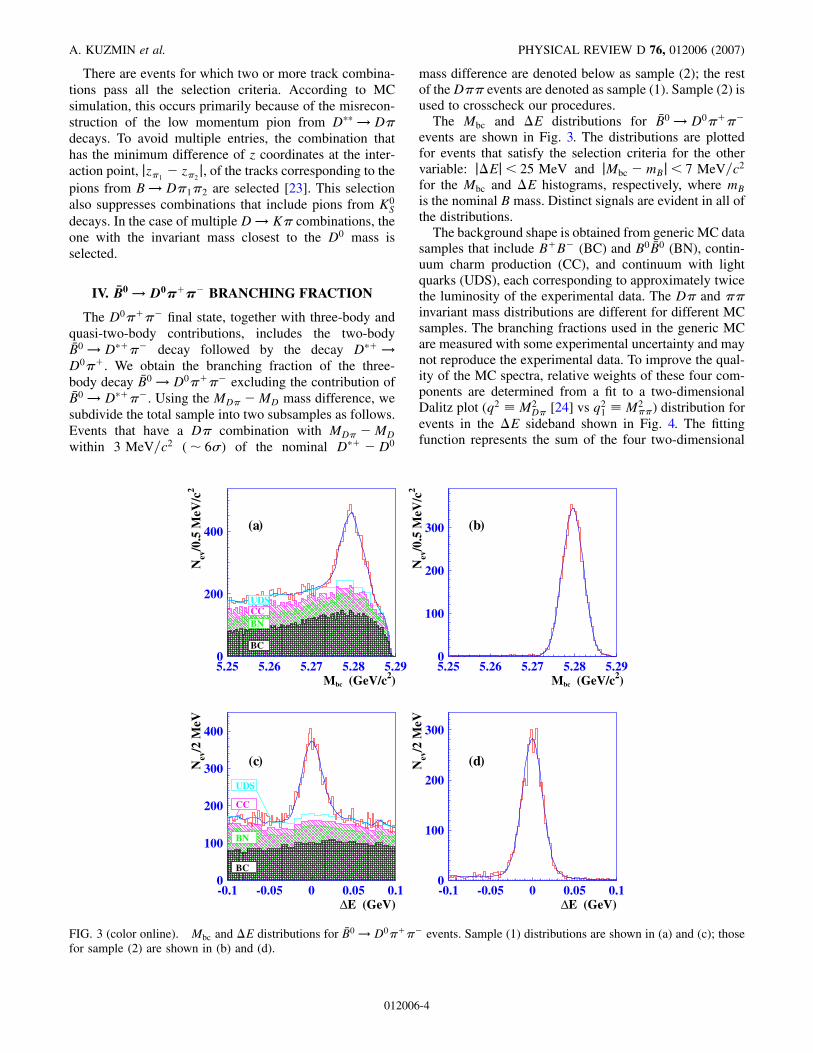
regions in the Mbc-�E plane.The D� and �� mass distributions for the signal events

(sample 1) are shown in Fig. 5. In theD�mass distributiona narrow peak corresponding to D�2 is evident. The ��mass distribution shows a peak corresponding to the �meson as well as a structure at the 1:2–1:3 GeV=c2 massregion that is presumably due to f0�1370� and f2�1270�production.

The M2D� and M2

�� Dalitz plot distributions for thesignal and sideband regions are shown in Fig. 6. TheDalitz plot boundary is fixed by the decay kinematics andthe masses of the daughter particles. In order to have thesame Dalitz plot boundary for both signal and sideband

TABLE I. The systematic uncertainties for the �B0 !D0���� branching fraction measurement.

Sample (1) Sample (2)

Particle identification 5% 5%Background uncertainty 5% 1%Tracking efficiency 4.4% 5.4%MC statistics 3% 3%B�D;D�� uncertainty 2.4% 2.5%Total 9.2% 8.1%

FIG. 4 (color online). The experimental distribution in the(Mbc-�E) plane. The ellipses show the signal (1) and sidebandregions (2 and 3).

STUDY OF �B0 ! D0���� DECAYS PHYSICAL REVIEW D 76, 012006 (2007)

012006-5

event samples, fits where the K� mass is constrained toMD and D�� mass to mB are performed. The mass-constrained fits also slightly improve the accuracy ofM2D� and M2

��.To extract the amplitudes and phases of different inter-

mediate states, an unbinned fit to the Dalitz plot is per-formed using the method described in Ref. [18]. The eventdensity function in the Dalitz plot includes both the signaland background functions.

The backgrounds in the Dalitz plot are mostly combina-torial and have neither resonant structure [Fig. 6(b)] norspecific helicity behavior. The normalization and shape ofthe background in the signal region and delta E sideband isslightly different so we cannot use the sideband to get thebackground shape. To obtain the shape we use the genericMC which is separated into four components mentionedabove. To improve consistency of data and MC we fit thedata Dalitz plot in the sideband region to the sum of theMC contribution with the floating weights. After theweights are obtained we plot the MC Dalitz plot with these

weights. The obtained distribution is parametrized by asmooth two-dimensional function which is used for theunbinned fit. The number of background events in thesignal region is scaled according to the relative areas ofthe signal and sideband regions.

There is no general method to describe a three-bodyamplitude. In this paper we represent the D�� amplitudeas the sum of Breit-Wigner function contributions fordifferent intermediate two-body states. Such an approachis not exact because it is neither analytic nor unitary anddoes not take into account a complete description of thefinal-state interactions. Nevertheless, the sum of Breit-Wigner functions describes the main features of the am-plitude behavior and allows one to find and distinguish thecontributions of two-body intermediate states, their inter-ference, and the effective parameters of these states. Wefollowed the same approach in the analysis of charged Bdecays [18].

In the D0���� final state, a combination of the D0

meson and a pion can form a vector meson D��, a tensor

0

10

20

30

0 2.5 5 7.5 10 12.5Mππ

2 (GeV/c2)2

MD

π2 (G

eV/c

2 )2

0

10

20

30

0 2.5 5 7.5 10 12.5Mππ

2 (GeV/c2)2

MD

π2 (G

eV/c

2 )2

)(b)(a

FIG. 6 (color online). The Dalitz plot for (a) signal events; (b) sideband events.

0

25

50

75

100

2 2.25 2.5 2.75 3MDπ (GeV/c2)

0

50

100

150

0 0.5 1 1.5 2Mππ (GeV/c2)

)(b)(a

FIG. 5 (color online). D� (a) and �� (b) mass distributions for sample (1) events with corresponding (�� or D�) helicity anglescos�h > 0. The points with error bars correspond to the signal region events, the hatched region indicates the background obtainedfrom generic MC events normalized to the sideband data. The open histogram shows the fitted function after efficiency correction.

A. KUZMIN et al. PHYSICAL REVIEW D 76, 012006 (2007)

012006-6

meson D��2 , or a scalar state D��0 ; the axial vector mesonsD�1 and D0�1 cannot decay to two pseudoscalars because ofangular momentum and parity conservation. The region ofD0�� invariant mass that corresponds to the D�� is ex-cluded from the fit by requiring jMD� �MD� j>3 MeV=c2. However, in B-meson decay, a virtual D��

(referred to as D�v) can be produced off shell with MD�above the D0�� production threshold and such a processcan contribute to the amplitude. Another virtual hadronthat can be produced in this combination is B�� (referred toas B�v): B! B�v�, and B�v ! D�. For the mass of B�� aswell as the mass and width of the D��, we use the PDGvalues [25]; the width of virtual B�� is determined by weakprocesses and is taken equal to zero. To describe the ��system we include �,!, f2�1270�, and three scalar mesonsf0�600�, f0�1370�, and f0�980�. The masses and widths ofthe �, !, and f2�1270� mesons are fixed at their PDGvalues; the parameters of the scalar mesons are takenfrom the published papers on the f0�600� [28], f0�1370�[29], and f0�980� [29].

The contributions from the intermediate states listedabove are included in the signal-event density (S�q2; q2

1�)parametrization as a coherent sum of the correspondingamplitudes together with a possible constant amplitude(aps). The phases of the amplitudes are defined relativeto D�2:

S�q2; q21� � jaD�2A

D�2�q2; q21� � aD�0e

i�D�0AD

�0�q2; q2

1�

� aD�vei�D�v AD

�v�q2; q2

1� � a�ei���A��q2; q2

1�

� r!��ei�!A!�q2; q2

1��

� af2ei��f2

����Af2�q2; q21�

� af0�600�ei��f0�600�����Af0�600��q2; q2

1�

� af0�980�ei��f0�980�����Af0�980��q2; q2

1�

� af0�1370�ei��f0�1370�����Af0�1370��q2; q2

1�

� aB�vei�B�v AB

�v�q2; q2

1� � apsei�ps j2; (1)

where q2 � M2D� and q2

1 � M2��,

Pia

2i � 1. The relative

amplitude and phase of the ! meson are expressed viathose of the �meson. The relative phase is taken from �-!interference measurements [30], and the relative amplitude(r!�� � a!=a�) is recalculated using that value.Assuming that the � and ! mesons produced in B0 decayemerge from the d �d pair, the relative amplitude is expectedto satisfy a relation r!���B� � �3r!�����.

We use the approach described in [18], where eachresonance is described by a relativistic Breit-Wigner func-tion with a q2 dependent width and an angular dependencethat corresponds to the spin and parity of the intermediate-and final-state particles. The � meson amplitude is de-scribed by the Gounaris-Sakurai parametrization [31].We take into account transition form factors for hadron

transitions using the Blatt-Weisskopf parametrization [32]with a hadron scale r � 1:6 �GeV=c��1.

The variation of the detection efficiency over the Dalitzplot is taken into account by the minimization procedure.The efficiency dependence enters the likelihood functiononly through the normalization term. The normalization isobtained based on a large MC sample generated uniformlyover the Dalitz plane, processed with the same selectioncriteria as the data and multiplied with the model used to fitthe data. The detector resolution for the invariant mass ofthe D����� combination is about 2.5 �3:5� MeV=c2,which is much smaller than the narrowest peak width of30–40 MeV=c2. Hence convolution of the described pa-rametrization with the resolution is not necessary. Themass and width of the broad (D�) resonance, MD��0

�

2308 MeV=c2, �0D��0� 276 MeV=c2 are taken from our

D��0 measurement [18].Table II gives the fit results for different models. The

contributions of different states are characterized by theirfractions, which are defined as:

fi �a2i

RjAi�Q�j2dQR

jPkake

i�kAk�Q�j2dQ

; (2)

where Ai�Q� is the corresponding amplitude, and ai and�iare the amplitude coefficients and phases obtained from thefit. The integration is performed over all available phasespace characterized by the multidimensional vector Q (fordecay to 3 spinless particles, dQ � dq2dq2

1), and i is one ofthe intermediate states: D�2, D�0, �, f2, f0, D�v, B�v, or theconstant term aps. The sum of the individual fractions fimay be different from unity because of interference. Theproduct of the branching fractions of the B meson is ex-pressed via the fraction fi:

B B!i�Bi!D� �NsigfiNB �B

; (3)

where Nsig is the efficiency-corrected number of the re-constructed D�� events and NB �B is the number of B �Bpairs produced.

Table II contains information on the likelihood changerelative to the main set, and 2 values obtained as the sumof 2 for four histograms: projections ofMD� and M�� fornegative and positive helicities of theD� and �� systems,respectively [33]. 2’s of two projections can be correlatedso to determine a probability corresponding to 2 weperform toy MC generating the distribution on the Dalitzplot with a density corresponding to the experimental dataand calculate 2. We used 1000 generated MC samples todetermine the 2 distribution and list the probability valuesin the table.

The fit gives a statistically significant contribution fromoff-shell D�v� production; the addition of the off-shell B�vamplitude does not improve the likelihood value signifi-cantly. The inclusion of the three-particle phase space term

STUDY OF �B0 ! D0���� DECAYS PHYSICAL REVIEW D 76, 012006 (2007)

012006-7

improves the likelihood value, however there is no reasonto expect a constant amplitude with no momentum depen-dence over such a wide range of final particle momenta.Table III shows that the likelihood changes significantly

when the broad resonance D�0 is removed or treated aseither a vector or a tensor. The change of likelihood�2 lnL=L0 � 51 for 2 additional degrees of freedom(amplitude and phase of D�0) corresponds to a significanceof 6:8� [34]. The significance is calculated based on thelnL difference.

The branching fractions of D�2 and D�0 remain constantwithin errors for different models. The set of states used forthe final results are D�2, D�0, D�v, �, f2 and the three above-listed f0’s, corresponding to column 1 in Table II.

The values of the D��2 resonance mass and width ob-tained from the fit are:

TABLE III. Changes in likelihood for different quantum num-ber assignments for the broad resonance.

No broad state 0� 1� 2�

�2 lnL=L0 51 0 28 272=Ndof 659=605 629=603 652=603 640=603C.L. (%) 16 32 19 25

TABLE II. The fit results for different sets of amplitudes. Option 1 is used as the main set of amplitudes for the final results. Thepresented errors are statistical only.

Options 1 2 3 4 5

States D�2, D�0, D�v,�, f2, f00s

D�2, D�0,�, f2, f00s

D�2, D�0, D�v,�, f2, f00s, B

�v

D�2, D�0, D�v,�, f2, f00s� ps

D�2, D�v,�, f2, f00s

�2 lnL=L0 0 69.5 �2:7 �13:0 51.3N1 2181� 64 2174� 64 2223� 71 2264� 65 2111� 62BB!D�2�

BD�2!D��10�4� 2:15� 0:16 2:23� 0:12 2:15� 0:18 2:26� 0:18 2:51� 0:14

MD�2, (MeV=c2) 2465:7� 1:8 2461:9� 1:6 2465:2� 1:9 2464:9� 1:6 2465:5� 1:7

�D�2 , (MeV=c2) 49:7� 3:8 49:0� 3:9 49:3� 4:1 51:5� 3:8 55:4� 4:0BB!D�0�

BD�0!D��10�4� 0:60� 0:13 0:61� 0:10 0:50� 0:13 0:79� 0:11 0

�D�0�3:00� 0:13 �2:28� 0:17 �2:88� 0:17 �2:66� 0:11 0

MD�0, (MeV=c2) 2308.0 2308.0 2308.0 2308.0 2308.0

�D�0 , (MeV=c2) 276.0 276.0 276.0 276.0 276.0BB!D�v�BD�v!D��10�4� 0:88� 0:13 0 0:85� 0:14 0:74� 0:11 0:66� 0:10�D�v �2:62� 0:15 0 �2:53� 0:17 �2:59� 0:13 �3:04� 0:20BB!D�B�!���10�4� 3:19� 0:20 2:94� 0:15 3:15� 0:21 3:07� 0:14 3:26� 0:18�� 2:25� 0:19 1:45� 0:22 1:81� 0:31 1:73� 0:15 1:89� 0:15M�, (MeV=c2) 775.6 775.6 775.6 775.6 775.6��, (MeV=c2) 144.0 144.0 144.0 144.0 144.0BB!Df2

Bf2!���10�4� 0:68� 0:10 0:64� 0:08 0:64� 0:09 0:54� 0:08 0:65� 0:08�f2

2:97� 0:21 2:48� 0:16 2:77� 0:20 2:32� 0:13 2:91� 0:17Mf2

, (MeV=c2) 1275.0 1275.0 1275.0 1275.0 1275.0�f2

, (MeV=c2) 185.0 185.0 185.0 185.0 185.0BB!Df0�600�Bf0�600�!���10�4� 0:68� 0:08 0:72� 0:09 0:72� 0:09 0:47� 0:08 0:58� 0:07�f0�600� �0:44� 0:09 �0:42� 0:09 �0:40� 0:10 �0:43� 0:11 �0:32� 0:10Mf0

, (MeV=c2) 513.0 513.0 513.0 513.0 513.0�f0

, (MeV=c2) 335.0 335.0 335.0 335.0 335.0BB!Df0�980�Bf0�980�!���10�4� 0:08� 0:04 0:11� 0:04 0:08� 0:04 0:04� 0:02 0:08� 0:03�f0�980� �2:48� 0:47 2:68� 0:37 �3:07� 0:51 2:87� 0:37 �2:85� 0:32Mf0

, (MeV=c2) 978.0 978.0 978.0 978.0 978.0�f0

, (MeV=c2) 44.0 44.0 44.0 44.0 44.0BB!Df0�1370�Bf0�1370�!���10�4� 0:21� 0:10 0:24� 0:06 0:18� 0:06 0:15� 0:04 0:25� 0:10�f0�1370� �1:52� 0:56 3:08� 0:35 �2:43� 0:62 �2:75� 0:28 �2:00� 0:38Mf0

, (MeV=c2) 1434.0 1434.0 1434.0 1434.0 1434.0�f0

, (MeV=c2) 173.0 173.0 173.0 173.0 173.0BB!B�v�BB�v!D��10�4� 0 0 0:74� 0:76 0 0�B�v 0 0 1:09� 0:51 0 0�ps 0 0 0 0:22� 0:14 0Bps�10�4� 0 0 0 0:33� 0:18 02=Ndof 629=603 680=605 632=601 618=601 659=605C.L. (%) 32 10 29 34 17

A. KUZMIN et al. PHYSICAL REVIEW D 76, 012006 (2007)

012006-8

MD��2� �2465:7� 1:8� 0:8�1:2

�4:7� MeV=c2;

�D��2 � �49:7� 3:8� 4:1� 4:9� MeV;

where the third error is model uncertainty. These parame-ters are consistent with but more precise than previousmeasurements performed by CLEO MD�02

� �2463� 3�

3� MeV=c2 [8] and FOCUS �D�2 � �34:1� 6:5�4:2� MeV [35].

The product of the branching fraction for D�2 productionobtained from the fit is:

B � �B0 ! D��2 ��� �B�D��2 ! D0���

� �2:15� 0:17� 0:29� 0:12� � 10�4;

where the three errors are statistical, systematic, and amodel-dependent error, respectively. We observe the pro-duction of the broad scalar D��0 state with the productbranching fraction,

B � �B0 ! D��0 ��� �B�D��0 ! D0���

� �0:60� 0:13� 0:15� 0:22� � 10�4:

This is the first observation of this decay (the interpretationof the neutral partner of this state is still a subject oftheoretical discussion [36]). The relative phase of the D�0amplitude is

�0 � 3:00� 0:13� 0:10� 0:43:

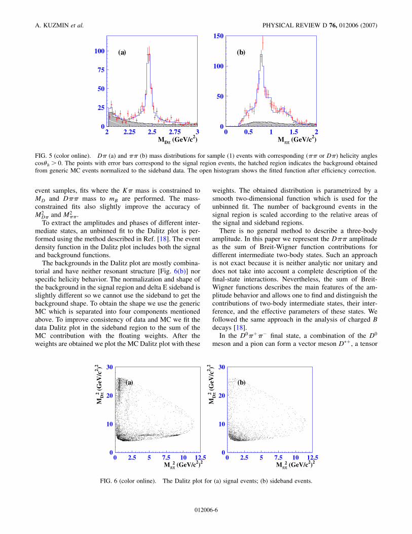
The D� helicity angle distributions for MD� regionscorresponding to the D�2 and D�0 are shown in Fig. 7(a)and 7(b), respectively, together with the efficiency-corrected fitting function. The histogram in the region ofthe D�2 meson clearly indicates a Dwave. The distributionsin the other regions show reasonable agreement betweenthe fitting function and the data.

The uncertainty of the background is one of the mainsources of systematic error. It is estimated by comparingthe fit results of the default fit, the fit where the weights ofthe individual four background categories are set to unity,and fit where only upper or lower �E sideband was used toobtain the background shape. The fit is also performed withmore restrictive and looser cuts on �E, Mbc, and MD thatchange the signal-to-noise ratio by factors of about two.The results obtained are consistent with each other and themaximum difference is taken as an additional estimate ofthe systematic uncertainty. The systematic errors on the Bimeasurements (Eq. (3)) for the individual intermediatestates include uncertainties in track reconstruction andparticle identification efficiency, as well as the error inthe D0 ! K��� absolute branching fraction. The modeluncertainties are estimated by comparing fit results for thecase of different models and for values of the parameter rof the transition form factor [32] from 0 to 3 �GeV=c��1.

The �� helicity angle distributions for M�� rangescorresponding to the �, f2 and the region below the �,where the broad resonance dominates, are shown in Fig. 8.For the positive helicity region, where the D� contributionis suppressed, a clear P-wave structure for the � andD-wave structure for the f2 is observed. The scalar com-ponent parameters cannot be determined from the fit. Thisprocess can also have contributions from nonresonantbackground. The product branching fraction for the f2 is

B � �B0 ! D0f2�B�f2 ! �����

� �0:68� 0:10� 0:12� 0:18� � 10�4:

Taking into account the branching fraction B�f2 !��� � 0:847�0:025

�0:012 [25] and the corresponding Clebsch-Gordan coefficients, we obtain

0

20

40

60

80

100

-1 -0.5 0 0.5 1cosθh

0

100

200

300

400

-1 -0.5 0 0.5 1cosθh

)(b)(a

FIG. 7 (color online). D� helicity angle distributions for data (points) and MC (histogram). The hatched distribution shows thebackground from the �E sideband region with the appropriate normalization. (a) corresponds to the D�2 region jMD� � 2:46j<0:1 GeV=c2; (b) the D�0 region jMD� � 2:30j< 0:1 GeV=c2.

STUDY OF �B0 ! D0���� DECAYS PHYSICAL REVIEW D 76, 012006 (2007)

012006-9

B � �B0 ! D0f2� � �1:20� 0:18� 0:21� 0:32� � 10�4;

B� �B0 ! D0�0� � �3:19� 0:20� 0:24� 0:38� � 10�4:

The phases relative to the D�2 amplitude are �� � 2:25�0:19� 0:20�0:21

�0:99 and �f2� 2:97� 0:21� 0:13� 0:45.

B. Results and discussion

The branching fraction products obtained for the narrow(j � 3=2) resonances are similar to the published resultsfor charged B decays as shown in Table IV. The measuredvalues of the branching fractions for the broad D��0 reso-nances in neutral B decays are, however, significantlylower than those for charged B decays. Preliminary dataon �B0 ! D�0���� decay [19] shown in Table IV indi-cates a similar behavior for D001 and D0

1 production. Onepossible explanation for this phenomenon is that forcharged B decay to D���, the amplitude receives contri-butions from both tree and color-suppressed diagrams asshown in Fig. 2. For the color-suppressed diagrams, how-ever, D��’s are produced by another mechanism and theamplitudes are characterized by the decay constants fD�3=2�

and fD�1=2�, with fD�3=2� fD�1=2�. The production of thebroad resonances D�00 and D001 in charged B decay isamplified by the color-suppressed amplitude. As shownin [37], in such a case both �1=2 fits to the sum rule andthe value of fD�1=2� are consistent with theoreticalestimates.

V. CONCLUSION

A study of neutral B-meson decays to D0���� isreported. We measure the total branching fraction of thethree-body D0���� decays, obtaining B� �B0 !D0����� � �8:4� 0:4� 0:8� � 10�4. The intermediateresonant structure of these three-body decays is studied.The D0���� final state is described by the production ofD�0;2�

� with subsequent decays D�0;2 ! D�, and also byD�, Df2, and Df0, where f0 is a broad scalar (��)structure. From a Dalitz plot analysis we obtain the mass,width, and product of the branching fractions for the D��2 :

MD��2� �2465:7� 1:8� 0:8�1:2

�4:7� MeV=c2;

�D��2 � �49:7� 3:8� 4:1� 4:9� MeV;

B� �B0 ! D��2 ��� �B�D��2 ! D0���

� �2:15� 0:17� 0:29� 0:12� � 10�4:

We observe the production of the broad scalar D��0 statewith the product branching fraction

B � �B0 ! D��0 ��� �B�D��0 ! D0���

� �0:60� 0:13� 0:15� 0:22� � 10�4:

This is the first observation of this decay. The phase of theD�0 amplitude relative to that of the D�2 is determined to be:

�0 � 3:00� 0:13� 0:10� 0:43:

The B! D� and Df2 branching fractions are measuredto be:

TABLE IV. Comparison of product branching fractions for neutral and charged B decays.

Neutral B Charged B [18]

B� �B! D�2���B�D�2 ! D�� �2:15� 0:17� 0:29� 0:12� � 10�4 �3:4� 0:3� 0:6� 0:4� � 10�4

B� �B! D�2���B�D�2 ! D��� �2:45� 0:42�0:35�0:39

�0:45�0:17� � 10�4 [19] �1:8� 0:3� 0:3� 0:2� � 10�4

B� �B! D1���B�D1 ! D��� �3:68� 0:60�0:71�0:65

�0:40�0:30� � 10�4 [19] �6:8� 0:7� 1:3� 0:3� � 10�4

B� �B! D�0��B�D�0 ! D�� �0:60� 0:13� 0:15� 0:22� � 10�4 �6:1� 0:6� 0:9� 1:6� � 10�4

B� �B! D01���B�D01 ! D��� <0:7� 10�4 at 90% C.L. [19] �5:0� 0:4� 1:0� 0:4� � 10�4

0

100

200

300

-1 -0.5 0 0.5 1cosθh

0

20

40

60

80

100

-1 -0.5 0 0.5 1cosθh

0

20

40

60

80

100

-1 -0.5 0 0.5 1cosθh

(a) (b) (c)

FIG. 8 (color online). �� helicity angle distributions for data (points) and MC (histogram). The hatched distribution shows thebackground distribution from the �E sideband region with appropriate normalization. (a) corresponds to the � region jM�� � 0:78j<0:2 GeV=c2; (b) the f2 region jM�� � 1:20j< 0:1 GeV=c2; (c) the f0 region M�� < 0:60 GeV=c2.

A. KUZMIN et al. PHYSICAL REVIEW D 76, 012006 (2007)

012006-10

B � �B0 ! D0�0� � �3:19� 0:20� 0:24� 0:38� � 10�4;

B� �B0 ! D0f2� � �1:20� 0:18� 0:21� 0:32� � 10�4;

and the phases relative to the D�2 amplitude are:

�� � 2:25� 0:19� 0:20�0:21�0:99;

�f2� 2:97� 0:21� 0:13� 0:45:

This is the first observation of the �B0 ! D0f2 decay.

ACKNOWLEDGMENTS

We thank the KEKB group for the excellent operation ofthe accelerator, the KEK Cryogenics group for the efficientoperation of the solenoid, and the KEK computer groupand the National Institute of Informatics for valuable com-puting and Super-SINET network support. We acknowl-

edge support from the Ministry of Education, Culture,Sports, Science, and Technology of Japan and the JapanSociety for the Promotion of Science; the AustralianResearch Council and the Australian Department ofEducation, Science and Training; the National ScienceFoundation of China under Contract No. 10175071; theDepartment of Science and Technology of India; the BK21program of the Ministry of Education of Korea and theCHEP SRC program of the Korea Science and EngineeringFoundation; the Polish State Committee for ScientificResearch under Contract No. 2P03B 01324; the Ministryof Science and Technology of the Russian Federation; theMinistry of Education, Science and Sport of the Republicof Slovenia; the National Science Council and the Ministryof Education of Taiwan; and the U.S. Department ofEnergy.

[1] H. Albrecht et al. (ARGUS Collaboration), Phys. Rev.Lett. 56, 549 (1986).

[2] H. Albrecht et al. (ARGUS Collaboration), Phys. Lett. B221, 422 (1989).

[3] H. Albrecht et al. (ARGUS Collaboration), Phys. Lett. B232, 398 (1989).

[4] J. C. Anjos et al. (Tagged Photon SpectrometerCollaboration), Phys. Rev. Lett. 62, 1717 (1989).

[5] P. Avery et al. (CLEO Collaboration), Phys. Rev. D 41,774 (1990).

[6] P. L. Frabetti et al. (E687 Collaboration), Phys. Rev. Lett.72, 324 (1994).

[7] P. Avery et al. (CLEO Collaboration), Phys. Lett. B 331,236 (1994); 342, 453(E) (1995).

[8] T. Bergfeld et al. (CLEO Collaboration), Phys. Lett. B340, 194 (1994).

[9] D. Bloch et al. (DELPHI Collaboration), ReportNos. CERN-OPEN-2000-015, DELPHI-98-128-CONF-189, 1998, p. 12.

[10] D. Bloch et al. (DELPHI Collaboration), ReportNo. DELPHI-2000-106-CONF 405.

[11] D. Buskulic et al. (ALEPH Collaboration), Z. Phys. C 73,601 (1997).

[12] N. Isgur and M. B. Wise, Phys. Rev. Lett. 66, 1130 (1991).[13] J. L. Rosner, Comments Nucl. Part. Phys. 16, 109 (1986).[14] S. Godfrey and R. Kokoski, Phys. Rev. D 43, 1679 (1991).[15] A. F. Falk and M. E. Peskin, Report No. SLAC-PUB-6311,

1993.[16] N. Uraltsev, Phys. Lett. B 501, 86 (2001).[17] A. Le Yaouanc et al., Phys. Lett. B 520, 25 (2001).[18] K. Abe et al. (Belle Collaboration), Phys. Rev. D 69,

112002 (2004).[19] K. Abe et al. (Belle Collaboration), arXiv:hep-ex/

0412072.[20] A. Abashian et al. (Belle Collaboration), Nucl. Instrum.

Methods Phys. Res., Sect. A 479, 117 (2002).[21] Events are generated with a modified version of the CLEO

group’s QQ program (http://www.lns.cornell.edu/public/

CLEO/soft/QQ); the detector response is simulated usingGEANT, R. Brun et al., GEANT 3.21, CERN ReportNo. DD/EE/84-1, 1984.

[22] E. Nakano, Nucl. Instrum. Methods Phys. Res., Sect. A494, 402 (2002).

[23] The z coordinate of the track is defined as the z coordinateof the track point closest to the beam in the r-� plane. Thez axis is opposite to the positron beam direction.

[24] We use D0�� and �D0�� for �B0 and B0 decays, respec-tively.

[25] W.-M. Yao et al. (Particle Data Group), J. Phys. G 33, 1(2006).

[26] A. Satpathy et al. (Belle Collaboration), Phys. Lett. B 553,159 (2003).

[27] G. Brandenburg et al. (CLEO Collaboration), Phys. Rev.Lett. 80, 2762 (1998).

[28] H. Muramatsu et al., Phys. Rev. Lett. 89, 251802 (2002).[29] E. M. Aitala et al., Phys. Rev. Lett. 86, 765 (2001).[30] R. R. Akhmetshin et al. (CMD-2 Collaboration), Phys.

Lett. B 527, 161 (2002).[31] G. J. Gounaris and J. J. Sakurai, Phys. Rev. Lett. 21, 244

(1968).[32] J. Blatt and V. Weisskopf, Theoretical Nuclear Physics

(John Wiley & Sons, New York, 1952), p. 361.[33] The overall 2 is calculated as the sum of the 2’s from

four distributions: two 160-bin histograms of MD� forpositive and negative helicities of the D� system, andtwo 150-bin histograms M�� with positive and negativehelicities of the �� system. The number of degrees offreedom is calculated as the number of bins minus thenumber of free parameters.

[34] S. S. Wilks, Ann. Math. Stat. 9, 60 (1938).[35] J. M. Link et al. (FOCUS Collaboration), Phys. Lett. B

586, 11 (2004).[36] M. E. Bracco, A. Lozea, R. D. Matheus, F. S. Navarra, and

M. Nielsen, Phys. Lett. B 624, 217 (2005).[37] F. Jugeau, A. Le Yaouanc, L. Oliver, and J. C. Raynal,

Phys. Rev. D 72, 094010 (2005).

STUDY OF �B0 ! D0���� DECAYS PHYSICAL REVIEW D 76, 012006 (2007)

012006-11