A New Method for Auto-Calibrated ObjectTracking ?

Paul Duff1, Michael McCarthy1, Angus Clark1, Henk Muller1, Cliff Randell1,Shahram Izadi2, Andy Boucher3, Andy Law3, Sarah Pennington3, and Richard

Swinford3

1 Department of Computer Science, University of Bristol, U.K.2 Microsoft Research, Cambridge, U.K.

3 Royal College of Art, U.K.

duff@cs.bris.ac.uk

Abstract. Ubiquitous computing technologies which are cheap and easyto use are more likely to be adopted by users beyond the ubiquitous com-puting community. We present an ultrasonic-only tracking system thatis cheap to build, self-calibrating and self-orientating, and has a conve-nient form factor. The system tracks low-power tags in three dimensions.The tags are smaller than AAA batteries and last up to several years ontheir power source. The system can be configured to track either multiplenear-stationary objects or a single fast moving object. Full test results areprovided and use of the system within a home application is discussed.

1 Introduction

Position sensing is an important aspect of pervasive computing. As a form ofcontext input, it provides context-aware applications with the ability to modelrelationships between users and their environment. With this information, ap-plications can provide a number of useful interactions in scenarios ranging froman audio tour-guide to an augmented reality application.

Narrowband ultrasonic positioning is an attractive form of positioning be-cause it is low cost. Transducers are cheap and readily available, and expensive,high-precision oscillators are unnecessary because ultrasonic signals travel rela-tively slowly when compared to other signals such as RF. There are a numberof narrowband ultrasound systems described in the literature that compute po-sitions using a variety of different techniques. Some, such as the Active Bat [1],perform position tracking where a single governing application tracks multipleobjects within a framework. Others perform positioning, where each object cal-culates its own private position, such as the systems developed at the Universityof Bristol [2, 3].

? Funding for this work is received from the U.K. Engineering and Physical SciencesResearch Council as part of the Equator IRC, GR-N-15986.

Polaroid 40LT12transmitter

CR1220 lithiumcell battery

AAA battery forsize comparison

Fig. 1. Ultrasonic Tag

The issue of cost addressed by these applications, however, does not considerthe expense of setting up and configuring the infrastructure supporting them.The uptake of positioning technologies by users outside of the ubiquitous com-puting community relies on us making them accessible. This term refers to allcosts surrounding the technology:

– component cost;– configuration expense;– power consumption;– form factor.

We have developed an object tracker that addresses each of these issues. Un-like most systems that utilise RF and ultrasound, including the Active Bat andCricket [4], our system uses only ultrasonic signals. The absence of RF cir-cuitry improves the power consumption, component cost, and form factor of tagstracked by the application. Our prototype tags are smaller than AAA batteries,run on 3V CR1220 cell batteries (see Fig. 1), and weigh 8 grammes (includingCR1220 battery). We have also developed auto-calibration and self-orientationapplications that greatly reduce the time and expertise needed to set-up theinfrastructure, making it easier for artists and non-experts to use. Furthermore,the system can be configured to track either multiple near-stationary objects ora single fast moving object. The total component cost for the system, includingthe infrastructure and one tag, is around $100.

We explore the use of the ultrasonic system for tracking objects as they movearound the home. In this test, non-technical researchers installed and used thesystem without any ‘expert’ help. A discussion of the use of the tracker as a partof this project is presented at the end of the paper.

2 System Description

The tracking system consists of a set of fixed receivers and one or more trans-mitting tags. The tags are each powered by a 3V coin cell battery. A PIC micro-controller on each tag controls the periodic activation of a 40kHz narrowband

R2

R0

R1

U

α

α

α

d1

d0

Zero receiver is R2, ie. d2 = 0

Fig. 2. Ultrasonic tracking. U is the position of the transmitter tag, R0, R1, R2 arethree receiver positions

ultrasonic transducer. In the case of a single object tracking system, the tagchirps regularly with an operational life of several months. In the case of mul-tiple objects that are to be tracked individually, each tag chirps with a specificsignature (described in detail in Sect. 5.1). The operational life increases to sev-eral years because chirping is less frequent.

The receivers are connected to a controller which determines the relativetiming of the input signals. The controller sends the recorded timing informationover a serial cable to a PC running the tracking software. The system requires atleast four receivers in order to locate objects (discussed in Sect. 3). We use sixfor the system described here in order to provide some redundancy and increaseaccuracy. The maximum range of the tags is around 8m; this is sufficient toprovide coverage for a room of 6×6m, for example.

When a signal emitted by a tag is detected by the nearest receiver, it isassigned a relative distance of zero metres. As the chirp travels outward from itssource, the other receivers detect it after an additional delay. By factoring withthe speed of sound, these delays can be converted into relative distances. Hencefor a system using m receivers, the distances can be expressed as follows:

di + α = |Ri −U | (0 ≤ i < m) (1)

Here di is a relative distance measured using receiver position Ri, U is theorigin of the chirp, and α is an unknown offset. Note that the nearest receiverRz will always give a relative distance dz = 0. We refer to receiver Rz as thezero receiver. Figure 2 shows a 2D example of this arrangement.

The constant offset α can be eliminated by observing that for the zero receiverRz:

α = |Rz −U | (2)

Hence we are left with a system of equations in terms of fixed receiver positionsRi, the chirp origin U , and measured relative distances di. We assume a fixed

speed of sound, though it is possible to estimate this at the cost of an additionalreceiver [5]. Note that this is only feasible once the system is calibrated.

di = |Ri −U | − |Rz −U | (0 ≤ i < m, i 6= z) (3)

In the next section we describe how we determine the positions of the trackingsystem’s fixed receivers Ri by auto-calibration, using an approach similar tocalibrating a positioning system [9]. In Sect. 4 we describe the auto-orientationalgorithm, while in Sect. 5 we examine two alternative methods for determiningthe chirp origin U .

3 Auto-calibration

Tracking is only possible once the positions of the receivers Ri are known. Aswe do not want to rely on people surveying the space by hand, our aim is todetermine the positions of Ri algorithmically. To accomplish this, we take asingle transmitting tag and move it around the room, taking care to collect dis-tance readings from all parts of the room. This stage takes around 30 seconds, incontrast to taking measurements manually which can take 20 minutes or more,especially when receivers are mounted out of reach. In our experience, manualmeasurements require the work of two people, and often involve reaching awk-wardly and noting down large numbers of distances and offsets. Auto-calibrationobviates the need for this inconvenient process.

Once we have a representative set of distance measurements, we aim tosolve (4), where m receivers and c tag positions are used, and only distancesdij are known. There are thus m receiver positions Ri, c zero receivers Rzj

, andc tag positions U j to be determined.

dij = |Ri −U j | − |Rzj−U j | (0 ≤ i < m, i 6= zj , 0 ≤ j < c) (4)

A solution can only be found if there is more information known about the systemthan is unknown and to be computed—the system must be over-specified. Eachunknown receiver position has three degrees of freedom in 3D space that must befound. Additionally, each new tag position contributes a further three unknowns.This is balanced by m − 1 relative positions and one zero receiver index gainedwith each new chirp transmission.

Six degrees of freedom can also be eliminated by describing the planar re-lationship between the first receiver and two others. By fixing the co-ordinatesof one receiver, we set an origin for the 3D space in which solutions will becomputed. The remaining three co-ordinates set the axes for the 3D co-ordinatesystem. In this way we avoid a situation where the same solution could be ro-tated or translated to produce an infinite number of solutions. Setting the axesleads to an arbitrarily rotated solution, a problem that is solved in Sect. 4.

The approximate constraint generalised to a system of m receivers and cchirp transmission positions is:

3(c + m)− 6 < (c− 1)m (5)

The constraint is an under-bound; in reality an excess of known data is neededfor good results. Readings from the same location are redundant as they will notcontribute any additional information to the system. The algorithm must alsobe able to handle noisy measurements from the ultrasonic sensors.

It is clear from (5) that we must use a minimum of four receivers in order toover-specify the system. In the case of our six receiver example, this constraintsuggests that at least six sets of relative distance data are needed, though moreare desirable.

Given perfect data, it would be possible to find perfect solutions for the re-ceiver and tag positions, balancing (4). In practice this is not possible, sincedistance readings have a limited granularity and are subject to noise and distor-tions. We can only hope to minimise the overall error and find a best fit for theunknown values.

Taking a least squares approach to error minimisation, we express the prob-lem in terms of a minimisation function F , as shown in (6).

F =m−1∑

i=0, i 6=zj

c−1∑j=0

(dij − |Ri −U j |+ |Rzj

−U j |)2 (6)

We use the Levenberg-Marquardt nonlinear least squares fitting algorithm [6],as it is reasonably suited to problems of high dimensionality. Attempts usingother techniques such as Simulated Annealing [7] revealed that they convergeless reliably on good solutions. We use an implementation provided within theGNU Scientific Library (GSL) [8], and refer to this central part of the algorithmas the solver.

As a randomised search process, the solver is not guaranteed to produce agood solution on any one occasion. We therefore execute the solver multipletimes, using different seed values and input data to increase the probabilityof finding receiver positions accurately. The most promising solutions can thenbe selected according to quality heuristics. This process is repeated in severalrounds, where each round applies more demanding criteria for convergence thanthe previous one.

At the end of a round, we select the most promising 10% of the candidatesolutions [9]. The best solutions are taken forward to the next round, and theprocess repeated until there is a final set of candidate solutions remaining. Inthis way we survey the search space broadly without a prohibitive computationcost.

The remaining candidate solutions are then each represented in terms of thedistance between respective pairs of receivers. This representation is independentof the origin and rotation of the solution, and hence can be used to comparedifferent solutions. We can expect that two geometrically similar solutions willshare similar distances between corresponding receiver pairs, even if one solutionis rotated with respect to the other. There are 15 distances between the sixreceivers, hence we describe the solution as a point in a 15-dimensional space.We found that good solutions cluster around one point in this 15-dimensionalspace, while poor solutions are scattered at lower density in other arrangements.

xy

z

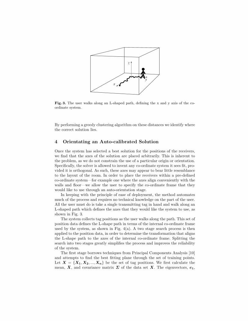
Fig. 3. The user walks along an L-shaped path, defining the x and y axis of the co-ordinate system.

By performing a greedy clustering algorithm on these distances we identify wherethe correct solution lies.

4 Orientating an Auto-calibrated Solution

Once the system has selected a best solution for the positions of the receivers,we find that the axes of the solution are placed arbitrarily. This is inherent tothe problem, as we do not constrain the use of a particular origin or orientation.Specifically, the solver is allowed to invent any co-ordinate system it sees fit, pro-vided it is orthogonal. As such, these axes may appear to bear little resemblanceto the layout of the room. In order to place the receivers within a pre-definedco-ordinate system—for example one where the axes align conveniently with thewalls and floor—we allow the user to specify the co-ordinate frame that theywould like to use through an auto-orientation stage.

In keeping with the principle of ease of deployment, the method automatesmuch of the process and requires no technical knowledge on the part of the user.All the user must do is take a single transmitting tag in hand and walk along anL-shaped path which defines the axes that they would like the system to use, asshown in Fig. 3.

The system collects tag positions as the user walks along the path. This set ofposition data defines the L-shape path in terms of the internal co-ordinate frameused by the system, as shown in Fig. 4(a). A two stage search process is thenapplied to the position data, in order to determine the transformation that alignsthe L-shape path to the axes of the internal co-ordinate frame. Splitting thesearch into two stages greatly simplifies the process and improves the reliabilityof the system.

The first stage borrows techniques from Principal Components Analysis [10]and attempts to find the best fitting plane through the set of training points.Let X = {X1,X2, ...,Xn} be the set of tag positions. We first calculate themean, X, and covariance matrix Σ of the data set X. The eigenvectors, e1,

0 x0

y

0

z

0 x0y

0

z

0 x0

y

0

z

(a) (b) (c)

Fig. 4. The L-shaped path defined by user. (a) shown in the internal co-ordinate sys-tem, (b) transformed onto the XY-plane, (c) aligned with the axes.

e2, e3 of the covariance matrix define an alternative orthogonal basis. If weorder the eigenvectors by their corresponding eigenvalues, each axis accountsfor a diminishing proportion of the variance present in the data. In our systemthe first two eigenvectors will lie on the plane defined by the L-shaped path (ie.the XY-plane), while the third eigenvector accounts for any variations in heightalong the path (ie. the z-axis).

Converting the points to this new co-ordinate system, we get:

X′i = [e1, e2, e3]T (Xi − X) (7)

where e denotes the normalised vector e.We have now arrived at a co-ordinate system where the L-shape lies on the

XY-plane, and with height represented by the z-axis, as shown in Fig. 4(b). Thenext stage is to find the translation T = [tx, ty, 0]T , and the rotation around thez-axis, Rz(rz), that will align the L-shape path with the x and y-axis, and withthe corner located at the origin.

In order to achieve this, we first project the set of points X′ onto the XY-plane, thereby removing any height variations present along the L-shaped path.Next we apply an adaptive simulated annealing algorithm [7, 11] that minimisesthe following energy function.

E(tx, ty, rz) =n∑

i=1

e2xi × e2

yi (8)

where exi

eyi

0

= Rz(X′i − T ) (9)

The energy function captures the notion that the L-shape should be alignedto the axes. However, the system has no knowledge as to which section of theL-shape should be located on the x-axis, and which should be located on they-axis. We therefore examine the start and end points of the L-shape to ensurethat they lie on the positive x-axis and positive y-axis respectively, updating therotation Rz as required (+90o, +180o or +270o).

The transformations derived above can be combined to give a single homo-geneous transformation. The result yields a transformation that converts pointsfrom the internal co-ordinate frame used by the system to the co-ordinate framedefined by the user, as shown in Fig. 4(c). This transformation is applied toall subsequent points thereby providing position information in the co-ordinateframe specified by the user.

The current implementation assumes the L-path specified by the user lies onthe XY-plane. The system could easily be extended to allow the user to specifywhich co-ordinate plane (XY, XZ or YZ) the L-shape should reside. However, thisintroduces further complexity for the user and in most cases will be unnecessary.

5 Tracking Objects

Our system can be used to track multiple objects with a low resolution in time,or a single object with a high time resolution (33Hz).

5.1 Multiple Objects

A fully calibrated system can be used to track one or more ultrasonic transmit-ters. It is often desirable to track multiple objects, each with a transmitting tagattached. In order to track individual objects reliably, each tag needs to transmita signature that uniquely identifies the source, separating it from backgroundnoise and signals from other tags.

Estimator In order to determine the position U of a tag, we solve the systemof equations described in (10).

di = |Ri −U | − |Rz −U | (0 ≤ i < m, i 6= z) (10)

The receiver positions Ri are known from the auto-calibration stage, and rela-tive distances di are measured by the system when the tag transmits. The zeroreceiver Rz is determined trivially by checking the relative distances recordedby each receiver. To solve the system of equations for U , we use a least-squaresminimisation process very similar to that described in Sect. 3. However, sincethere is much more known information in the system, we only need to run theLevenberg-Marquardt algorithm once to find a solution.

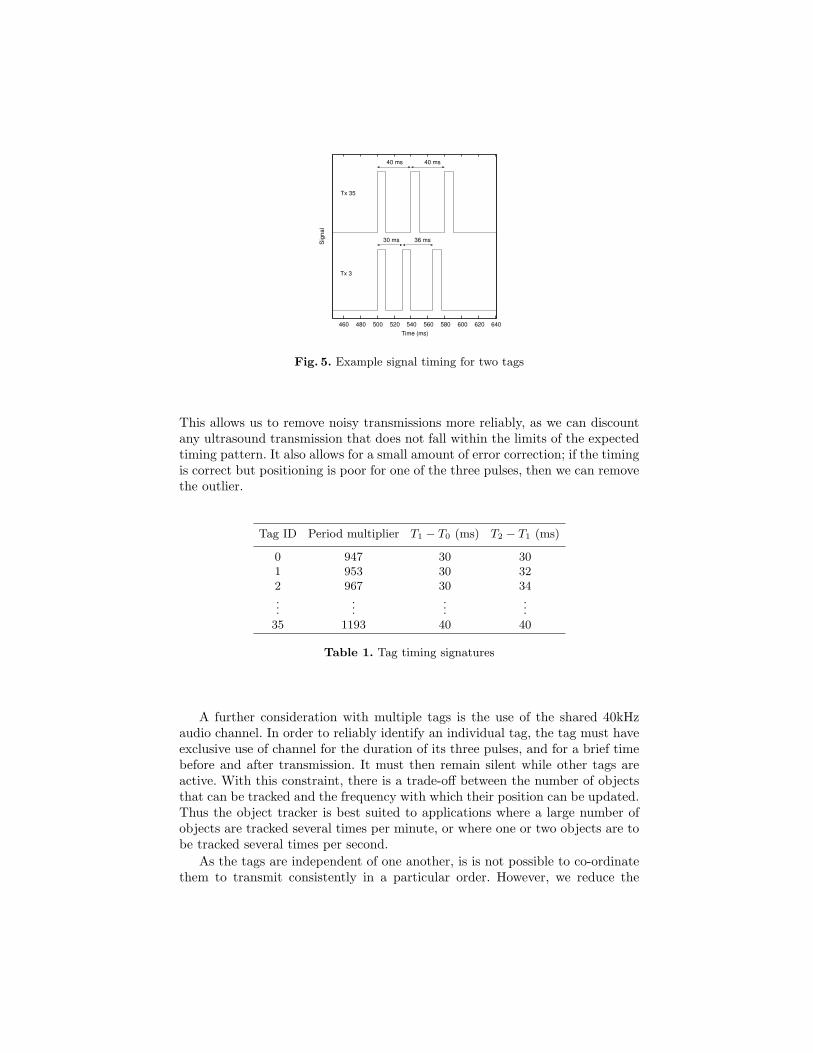
As we have opted to use cheap ultrasonic transmitters with a narrow trans-mission frequency range, it is not feasible to encode the signature by altering thefrequency of the transmitted ultrasound wave. Instead, the tags are configured totransmit three short pulses in quick succession. The time between transmissionof each of the pulses is selected from a set of six discrete durations, varying from30-40ms. These durations are permuted so that each tag has a unique timingsignature, as illustrated in Fig. 5.

We expect that the computed positions of a tag will be virtually the samefor each of the three pulses, as the tag cannot move very far between pulses.

460 480 500 520 540 560 580 600 620 640S

igna

l

Time (ms)

40 ms 40 ms

30 ms 36 ms

Tx 35

Tx 3

Fig. 5. Example signal timing for two tags

This allows us to remove noisy transmissions more reliably, as we can discountany ultrasound transmission that does not fall within the limits of the expectedtiming pattern. It also allows for a small amount of error correction; if the timingis correct but positioning is poor for one of the three pulses, then we can removethe outlier.

Tag ID Period multiplier T1 − T0 (ms) T2 − T1 (ms)

0 947 30 301 953 30 322 967 30 34...

......

...35 1193 40 40

Table 1. Tag timing signatures

A further consideration with multiple tags is the use of the shared 40kHzaudio channel. In order to reliably identify an individual tag, the tag must haveexclusive use of channel for the duration of its three pulses, and for a brief timebefore and after transmission. It must then remain silent while other tags areactive. With this constraint, there is a trade-off between the number of objectsthat can be tracked and the frequency with which their position can be updated.Thus the object tracker is best suited to applications where a large number ofobjects are tracked several times per minute, or where one or two objects are tobe tracked several times per second.

As the tags are independent of one another, is is not possible to co-ordinatethem to transmit consistently in a particular order. However, we reduce the

-140

-120

-100

-80

-60

30 40 50 60 70 80 90 100 110

Y (c

m)

X (cm)

Auto-calibratedManually calibrated

Measured circle

-140

-135

-130

-125

-120

35 40 45 50

Y (c

m)

X (cm)

Auto-calibratedManually calibrated

Measured circle

Fig. 6. Moving transmitter track (left) and close-up (right)

likelihood of a collision between one or more tags by configuring each tag topause for a different length of time after transmitting a set of pulses. By carefullychoosing these times to be a constant multiple of the set of prime numbers,we can avoid aliasing, where two tags collide regularly. Table 1 shows possiblesignal timing patterns for a set of transmitting tags. Note that the prime periodmultipliers are approximate, since each tag has its own clock which will driftwith respect to other tag clocks.

Performance The auto-calibration algorithm was executed using a set of recor-ded distances as described in Sect. 3. Execution time for calibration was approx-imately 5 minutes on a 1GHz Pentium processor. The best solution was thenused to track a transmitting tag. The computed track was compared with amanually measured ground truth, plus a track computed using manually cali-brated receivers. Figure 6 shows an aerial view of these three tracks, overlaidto give an indication of the scale of their accuracies. The close-up view showsthe region of greatest difference between the tracks. The slightly lower accuracyof the auto-calibrated result is clear, with computed positions jumping aroundmore erratically than in the manually calibrated track.

We observe a systematic scaling error, resulting in an error of 5-7 cm in thebottom part of the track. This may have been caused by a consistent offset inthe distance data recorded. It is important to note that the systematic errorswill drop out of the system if it is trained with information about the positionsof objects in a room. Often we are only interested in knowing that we are nextto some object, rather than precise co-ordinates for measuring distances.

The reproducibility of results using the auto-calibrated system was anal-ysed using sets of over 1000 readings taken at stationary transmission positions.Running this data through both a manually calibrated and an auto-calibratedtracker revealed some variability in the placing of points even after systematicerrors were taken into account. These radial errors give a better indication ofhow reproducible results are using the tracking system. Table 2 shows accuracies

SEP 50% SEP 95% RMS

Manually calibrated system 1.28 2.71 1.70Auto-calibrated system 1.87 4.02 2.29

Ratio manual/auto 0.68 0.68 0.74

Table 2. 50% and 95% SEPs and RMS errors given in centimetres

of the system in terms of 50% and 95% spherical error probability (SEP) androot mean square error (RMS).

The SEP and RMS values all show that on average the manually calibratedsystem performs a little better than the auto-calibrated one, though not sig-nificantly so. The errors for the auto-calibrated system are still well within thelimits of many applications that currently use manually calibrated systems, andthe ratios indicate that the distributions of errors are similar in both cases.RMS values give a more representative indication of the system’s consistency atproducing results.

5.2 Single Object

The system can also change modes to track a single object to a high degree ofaccuracy. By giving one mobile device a monopoly on the 40kHz audio channelwe are able to increase the ultrasound transmission rate to frequencies up to33Hz. This gives our system a shorter response time and allows us to trackobjects moving at higher velocities and accelerations. When we receive regularreadings from one object, we can use a more effective method to calculate thisobject’s position.

Estimator The estimator we use for this mode of operation is the Kalmanfilter [12]. Although it is not well suited for the large transmission periods ofthe multiple object tracker, the Kalman filter does fit well with the new track-ing conditions. Specifically, it is more efficient and predictable than Levenberg-Marquardt, it uses knowledge of the previous system state, and it provides amethod for modelling the dynamics of the system. In our filter, we employ aposition-velocity model that assumes the velocity of the tracked object is con-stant and subject to acceleration ‘noise’. In the following process equations, Uand V are the position and velocity of the tag, P is the transmission period andE is the transmission time.

Uk = Uk−1 + Pk−1 · V k−1

V k = V k−1

Ek = Ek−1 + Pk−1

Pk = Pk−1

The state vector falls from these equations as [ U V E P ]T .

0.0 0.2 0.4 0.6 0.8 -1.6 -1.4 -1.2 -1.0 -0.8-0.6

-0.5

-0.4

-0.3

z (Meters)

x (Meters) y (Meters)

z (Meters)

σz = 1.2 cm

-1.6

-1.4

-1.2

-1.0

-0.8

-0.6

-0.2 0.0 0.2 0.4 0.6 0.8 1.0

y (M

eter

s)

x (Meters)

60 cm

(a) (b)

Fig. 7. Path of single tag operating at 33Hz, (a) 3D view showing position along z-axis,(b) 2D view showing position along x and y axes.

For each receiver i, we have one measurement equation that relates the state,the known position of the receiver, Ri (from auto-calibration), and the speed ofsound, v, to the reception time of the signal, Ti.

Ti = E +

∣∣U −Ri

∣∣v

(11)

Although the reception times recorded by each receiver are obtained almostinstantaneously, we integrate the measurements with the filter in a serial fash-ion. This method, known as single-constraint-at-a-time (SCAAT) Kalman filter-ing [13], provides advantages in terms of efficiency and outlier detection.

Performance Figure 7 shows the path of a tag mounted on the back of anoffice chair. The chair was spun on its base, rolled, and spun again to create thetwo circles illustrated. The height of the tag was kept constant throughout asis reflected by the accuracy of the filter along the z-axis. In terms of standarddeviation from the mean position, this value is 1.2cm. To gauge the dynamicaccuracy in the x-y plane, we compare the diameter of the circles in Fig. 7 tothe true 60cm swivel diameter of the chair. The circles are approximately 6%smaller than the diameter created by the chair. We attribute the discrepancyto errors in the value used for the speed of sound, a non-ideal arrangementof the receivers having a high dilution of precision, varying transmitter-receiverincident angles, and errors in the positions of the receivers from auto-calibration.The stationary 3D accuracy of the system, in terms of spherical error probabilityover a 40 second time frame, is 5mm for 95% of the readings and 6mm for 99%.

With these accuracies, the single object tracking system could be used withapplications such as home gaming systems (Xbox, PlayStation, etc.) and motiontracking for animation. Fused with inertial sensors, the system also has thepotential to be used with augmented or virtual reality applications. A combined

Fig. 8. Initial design sketches for an application that tracks possessions, shows usageover time and re-advertises “ignored” objects using channels in the home.

ultrasonics-inertial-sensor approach has been used successfully by InterSense Inc.in a number of their high performance products [14–16].

6 Explorations of Ultrasonic Tracking within the HomeEnvironment

We have been developing a series of interactive scenarios based around trackingobjects within the home. The scenarios follow earlier studies involving domesticprobes and experiments within the home [17, 18]. In this environment we wantto experiment with designs without having to repeatedly calibrate a trackingsystem by hand. This is very much work in progress, but our initial experimentsoffer interesting insights into the use of such a system, and its practical impactand value for Ubicomp applications.

Below we use the term engineer to denote a person who designs ultrasonicsystems, and the term designer to denote a person who designs ubicomp expe-riences. A user is someone who interacts with the final experience.

6.1 A Motivating Scenario

Our aim is to track a series of objects within the home, in order to indicatecurrent object positions and patterns of usage. Small objects are tagged andregistered with an application running on a computer connected to the ultrasoniccontroller. The application shows a list of registered possessions and allows newitems to be added. The designer can specify a name, description and photo tomap onto an underlying tag ID. During tracking, 3D co-ordinates of the tags aretime-stamped and added to a database.

The database is used to provide a map view of the current position of eachobject, and a graph (called the “affection radar”) that plots the distance eachobject has moved over time. Whilst many objects achieve high initial attention,the novelty often quickly fades. The affection radar allows the user to reflect onan object’s changing patterns of usage. The data can also be used by applications.

Fig. 9. An initial deployment of the ultrasonic tracker within the home. Tag attachedto a remote control (top left). Ultrasonic controller (bottom left) and receivers attachedto walls (right).

For example, objects that have become old, ignored or unused could re-advertisethemselves to the user through output channels in the home in the form of anoccasionally appearing photo. An initial set of design sketches for the application,including the affection radar and re-advertising objects, is shown in Fig. 8.

6.2 Experiments with Ultrasonic Tracking in the Home

In order to realise the scenario described previously, we conducted various trialsof the ultrasonic tracker within domestic environments. Key technical questionswere: How easy is it to set up? How fine-grained is the tracking in practice? Wealso need to consider key design questions, such as whether movement is a goodmetric for determining usage, and how often different types of object move.

Figure 9 shows an installation of the system within the home of a designer.The receivers were fixed to the walls of the space to provide coverage over theliving room. Tags were attached to various objects in the home to show movementaround the space. These included a chair, remote control, camera, and books.Tag data captured by the receivers were relayed onto a connected laptop, whereabsolute 3D coordinates were calculated and logged. Initially this recorded datawas processed using visualisation software back in the design studio, and onlyconsole output was available to verify readings in real-time. After refinement,the visualisation software was also deployed in the home to provide real-timegraphical feedback to users.

The system was installed manually at first, and later using auto-calibrationto compare experiences. Manual installation involved a designer measuring theco-ordinates of the receivers relative to a point of origin in the middle of theroom. Measurements were entered manually into an application running on alaptop. The space contained large household objects (tables, chairs and so on),some of which had to be cleared so that distances could be calculated between

Fig. 10. One example of ultrasonic data visualisations.

the point of origin and the receivers. This added to the initial disruption causedby the placement of receivers.

During tracking, readings for each tag were displayed in the console. Thedesigner used a simple test to verify these readings: manually measure the X, Yand Z distances between corners of a chest of drawers and compare these withdistances calculated with a tag. This simple test revealed poor tracking accuracydue to human errors introduced during receiver measurement, and poor coverageof the room. Manual calibration was repeated several times until coverage andaccuracy were deemed acceptable. This involved repositioning and recalculationof receiver coordinates, with an engineer to help take measurements. This addedconsiderably to the time taken to calibrate the system.

In contrast, the auto-calibration process took considerably less effort andtime. To accomplish this, the designer ran software on the laptop, which cap-tured data from a single tag. The designer moved the tag around the room, takingcare to collect distance readings from all parts of the room. After approximatelyone minute, the designer stopped data capture on the laptop and ran the auto-calibration software. Within approximately 5 minutes a solution had been found,and transmitting tags were tracked in absolute 3D co-ordinates. Various activi-ties were performed to test the tracking capabilities of the system. For example,moving slowly around a dining table or moving from one corner of the room tothe centre, and viewing whether the visualisations plotted a similar path. Thedesigner also used a tape measure to manually resolve the 3D coordinates of atag, testing these against the data generated on the laptop. These tests showedpromising results, indicating reliable tracking accuracy of 7cm. After some mi-nor tweaking of receiver positions, rerunning of auto-calibration software, andretesting (using methods described previously), the designer achieved a trackingaccuracy of 3cm.

Spatial information captured from the tracking system was interfaced with adesign tool called Processing [19]—a popular high-level programming language

used to rapidly prototype graphical applications. Visualisations were generatedbased on this data, including maps highlighting an object’s trajectory througha space, activity maps indicating areas in which objects predominately resided,and maps showing areas in which line of sight to one or more receivers wasoccluded. For example, the occlusion map in Fig. 10 shows a view of the homewhere line of sight was occluded by large objects such as a dining table or a sofa(shown in light grey). They also illustrated whether objects did indeed movefrequently, and where in the space they were most often used.

6.3 Initial Reflections

Initial trials of the ultrasonic system within a number of domestic settings showedpromising results and allowed us to refine our application designs further. Duringour trials, we found several advantages to using auto-calibration over a manualapproach:

– The ability to quickly reposition receivers and retest in order to maximisecoverage and tracking accuracy within the space. The accuracy and cover-age of ultrasonic trackers is clearly heavily dependent on the placement ofreceivers. We found a need to reconfigure receiver positions several times inorder to improve tracking and coverage. This process is greatly simplified ifthe designer can avoid re-measuring receiver distances each time manually.

– The ability to minimise human errors being introduced by manually measur-ing receiver coordinates. We also found that errors crept in during manualcalibration, requiring designers to re-measure receiver positions, a processthat would often become frustrating.

– The ability for a single non-technical designer to setup the tracker. In ourexperience, manual measurements require the work of two people, and ofteninvolve reaching awkwardly and noting down large numbers of distances andoffsets, and carrying out calculations. Non-technical designers can find thisprocess daunting. Auto-calibration obviates the need for this inconvenientprocess.

During these initial tests, we found that the auto-calibration algorithm workswell for most arrangements of receivers. Tracking was most accurate when thereceivers were set up on the ceiling and walls to avoid reduced precision in the Z-axis. Care was also taken to point the receivers toward the centre of the trackingarea, to maximise the chance of receivers detecting tag transmissions.

Our visualisations indicated that smaller objects such as books, electronicitems and toys move much more than larger objects such furniture, as expected.Often patterns arise over a period when viewing the paths of objects through aspace—for example, in our deployment the remote control often followed a setpath from the shelf by the CD player to the coffee table and back. Therefore onemust be careful in using movement as a metric for determining usage, as thisonly applies to certain objects which are small enough to be mobile and theireveryday interaction relies on movement (such as a camera).

Initially, when the system was deployed it was passively capturing data to beprocessed asynchronously back in the design studio. At this early stage, partici-pants felt that these tests were a little intrusive, voicing concerns about privacyand the ways that data would be used. This level of intrusiveness began to fadeonce the users were provided with more feedback and control over the data cap-ture. For example, in the second series of tests visualisation software ran on thehome desktop, and could be stopped and restarted by the user at any point. Par-ticipants felt much more comfortable living with the system when they could seethe information captured in real-time, and could choose when it was appropriatefor the system to begin capture.

These initial experiments also showed that during everyday use, certain ob-jects would move in and out of a room frequently. As an extension to the scenarioone could imagine a setup that incorporated several ultrasonic systems, one ineach room—this, however, raises issues about setup time and data managementacross multiple receiver boxes. Designers also suggested whether more coarsegrained tracking technologies could be used to compliment the ultrasonics sys-tem, particularly for objects that only move short distances.

Our experiments have shown the viability of using an ultrasonic trackingsystem as a low cost, fine grained mechanism for tracking objects. We are nowmoving to realise the interactive applications described earlier.

7 Conclusions and Future Work

We have presented an ultrasonic-only tracking system aimed at users beyond theubiquitous computing community. The system uses algorithms to self-calibrateand self-orient, so that little technical knowledge is required for setup. It givesthe user an easy way to calibrate the system and for aligning the system withthe user’s origin and principal axes (by walking along an imaginary L).

Tracking is performed in one of two alternative modes, providing a choicebetween tracking multiple near-stationary objects, or one object at a high fre-quency. The mode can be changed without a need to re-calibrate the receiver in-frastructure. Where multiple objects are tracked, each object is preprogrammedwith a unique pulse timing signature.

The results show that tracking multiple objects using an auto-calibratedsystem can be performed to an RMS accuracy of approximately 2.3cm, which issufficient for our target applications. Single object tracking achieves accuraciesof around 3cm in the dynamic case.

We have deployed our system in the home and allowed designers to createan installation. This has provided experience using the system in a more typicalsetting than the laboratory, and we have described some initial reflections thatmay be of use to other researchers wishing to implement a tracking system.Future work is planned to further the accessibility of the system to designers,including the use of toolkits that provide a more meaningful interface to thesystem’s outputs.

References

1. A. Ward, A. Jones, and A. Hopper. A New Location Technique for the ActiveOffice. In IEEE Personnel Communications, volume 4 no.5, pages 42–47, October1997.

2. C. Randell and H. Muller. Low Cost Indoor Positioning System. In Gregory D.Abowd, editor, Ubicomp 2001: Ubiquitous Computing, pages 42–48. Springer-Verlag, Sept 2001.

3. Michael McCarthy and Henk L. Muller. RF Free Ultrasonic Positioning. In Sev-enth International Symposium on Wearable Computers. IEEE Computer Society,October 2003.

4. Nissanka B. Priyantha, Anit Chakraborty, and Hari Balakrishnan. The CricketLocation-Support System. In Mobile Computing and Networking, pages 32–43,August 2000.

5. Ajay Mahajan and Maurice Walworth. 3-D Position Sensing Using the Differ-ences in the Time-of-Flights from a Wave Source to Various Receivers. In IEEETransactions on Robotics and Automation, pages 91–94. IEEE, 2001.

6. J. J. More. The Levenberg-Marquardt Algorithm: Implementation and Theory. InG. Watson, editor, Lecture Notes in Mathematics, v630, pages 105–116. SpringerVerlag, 1978.

7. Lester Ingber. Very Fast Simulated Re-annealing. In Mathematical ComputingModelling, pages 967–973, 1989.

8. Brian Gough. GNU Scientific Library - Nonlinear Least Squares Fitting, chapter 36.Network Theory Ltd, 2001.

9. Paul Duff and Henk Muller. Autocalibration Algorithm for Ultrasonic LocationSystems. In Proceedings of the Seventh IEEE International Symposium on Wear-able Computers, pages 62–68. IEEE Computer Society, October 2003.

10. I.T. Jolliffe. Principal Component Analysis. Springer-Verlag, New York, 1986.11. L. Ingber. Adaptive Simulated Annealing (ASA). http://www.ingber.com/.12. R. E. Kalman. A New Approach to Linear Filtering and Prediction. In Journal of

Basic Engineering (ASME), pages 82(D):35–45, March 1960.13. Greg Welch and Gary Bishop. SCAAT: Incremental Tracking with Incomplete In-

formation. In SIGGRAPH 97 Conference Proceedings, Annual Conference Series,August 1997.

14. Eric Foxlin, Michael Harrington, and George Pfeifer. Constellation: a wide-rangewireless motion-tracking system for augmented reality and virtual set applications.In Proceedings of the 25th annual conference on Computer graphics and interactivetechniques, pages 371–378. ACM Press, 1998.

15. Eric Foxlin, Michael Harrington, and Yury Altshuler. Miniature 6-DOF InertialSystem for Tracking HMDs. In Aerosense 98, Orlando, April 1998.

16. Intersense Inc. Website. http://www.isense.com/, 2003.17. W. Gaver, A. Boucher, S. Pennington, and B. Walker. Subjective Approaches to

Design for Everyday Life. In CHI Tutorial, Ft. Lauderdale. ACM Press, 2003.18. W. Gaver, A. Dunne, and E. Pacenti. Cultural Probes. In Interactions Magazine,

volume VI(1), pages 21–29, 1999.19. Processing. Website. http://www.processing.org/.