MAGNETIC INDUCTION TOMOGRAPHY: SINGLE-STEP SOLUTION OF THE 3-D INVERSE PROBLEM FOR DIFFERENTIAL...

INTERNATIONAL JOURNAL OF INFORMATION AND SYSTEMS SCIENCES Volume 2, Number 4, Pages 585-606

©2006 Institute for Scientific Computing and Information

MAGNETIC INDUCTION TOMOGRAPHY: SINGLE-STEP SOLUTION OF THE 3-D INVERSE PROBLEM FOR DIFFERENTIAL IMAGE RECONSTRUCTION

HERMANN SCHARFETTER, PATRICIA BRUNNER AND ROBERT MERWA

Abstract Magnetic induction tomography (MIT) is a low-resolution imaging modality used for reconstructing in 3-D the changes of the complex electrical conductivity in a target object. The measurement principle is based on determining the perturbation ∆B of a primary alternating magnetic field B0, which is coupled from an array of excitation coils to the object under investigation. The corresponding voltages ∆V and V0 induced in a receiver coil carry the information about the conductivity distribution. Potential medical applications comprise the continuous, non-invasive monitoring of tissue alterations which are reflected in the change of the conductivity, such as edema formation, ventilation disorders, wound healing and ischemic processes. MIT requires the solution of an inverse eddy current problem in three dimensions. which is underdetermined, ill-posed and non-linear in the parameters. Absolute imaging requires an iterative solution and suffers from heavy difficulties due to the comparatively low signal/noise ratio (SNR) of available MIT systems. Alternatively differential imaging is much easier and reconstruction can be done with single-step approaches. In this paper regularized single-step Gauss-Newton solutions are shown for state-differential and frequency differential protocols for both simulated and real data. Data were generated for 16 excitation coils and 32 receiver coils with a model of two spherical perturbations within a cylindrical saline tank. Simulated data were generated with a finite-element forward solver and random noise was added. The real data were obtained with an experimental MIT-system. Four different regularization matrices were compared: identity matrix (IM), neighbourhood matrix (NM), truncated singular value decomposition (TSVD) and variance uniformization (VU). A Monte-Carlo study was carried out in order to compare the statistical properties of the reconstruction results. Both simulated and real conductivity perturbations inside a homogeneous cylinder could be localized and resolved for an SNR between 44 and 64 dB. The VU method outperformed all other methods with respect to localization accuracy, resolution and edge sharpness, but, on the other hand, produced larger variance in the images. Frequency differential imaging allows the reconstruction of relative conductivity spectra which can be interpreted quantitatively. Key words: magnetic induction tomography, conductivity imaging, inverse problem, regularization, differential imaging

585

MAGNETIC INDUCTION TOMOGRAPHY: DIFFERENTIAL IMAGE RECONSTRUCTION 586

1. Introduction Magnetic induction tomography (MIT) is a non-invasive and contact-less imaging

modality for reconstructing the changes ∆κ of the complex conductivity distribution κ = σ+jωε0εr in a target object [8][13][14][15][16][21] in three dimensions (ε0: dielectric constant, εr: relative permittivity, σ: real conductivity, ω: angular frequency). In MIT the object is interrogated with an array of excitation (EXC) and receiving coils. Each EXC couples an alternating magnetic field B0 to the object. Changes ∆κ in a target region cause a field perturbation ∆B due to the induction of eddy currents in the object under investigation. The perturbation induces voltage changes ∆V in the receiver coils which can then be used for reconstructing the distribution of ∆κ. For previous reviews of MIT see [8][21][33]. The method has been developed for industrial process tomography already more than 10 years ago and, more recently, also for medical imaging with the aim to characterize biological tissues. Potential medical applications usually aim at the characterization of biological tissues by means of their passive electrical properties, i. e. conductivity and permittivity. The motivation for measuring the electrical properties is their characteristic dependence on the (patho-) physiological state of tissues, especially hydration and membrane disorders. Medical applications so far suggested are:

• imaging of limbs [2] • imaging of the brain, e. g. for the monitoring of brain edema [14][16][24][26] • measurement of human body composition [7] • monitoring of wound healing[23].

In contrast to electrical impedance tomography (EIT) MIT avoids the ill-defined

electrode-skin interface due to its inherently contact-less function. Fig. 1 shows a schematic MIT coil configuration with rectangular coils as receivers and a cylindrical object space. The excitation coils are distributed on two different rings in order to obtain a true 3-D-arrangement.

32 Receiving coils

16 Excitation coils

Object space with conducting object(here cylindrical phantom)

Fig.1 Schematic of a possible coil system for MIT with 16 excitation coils and 32 receiver coils.

H. SCHARFETTER, P. BRUNNER AND R. MERWA

587

This paper is organized as follows: First the inverse eddy current problem in medical MIT is described and the generic mathematical approach for its solution is outlined. Then the current experimental possibilities are sketched so as to impose some important practical boundary conditions for the solution. Then it is shown that technical reasons make differential imaging the method of choice in the case of in-vivo MIT. Two different linear approaches are presented: state-differential and frequency-differential MIT. Relative differential MIT spectroscopy is presented as a special extension of frequency-differential MIT. Finally reconstruction results from both simulated and experimental data are shown for low-contrast objects with conductivities near the physiological range.

2. Methods Inverse eddy current problem:

The reconstruction of the absolute conductivity in a target region Ω requires the solution of a complex inverse eddy current problem. Let

y=Ψ(κ) (1)

be the discretized non-linear forward mapping of the conductivity vector κ to the

vector of induced voltage y. The symbol y shall be used from now on for the voltage instead of the more common symbol ‘V’ in order to avoid confusions with the matrix V of the singular value decomposition. y contains M = a x b entries, a being the number of EXC and b that of receiving coils. Ψ(κ) is given by Maxwell’s equations for harmonic excitation:

0,,0

εωεσκκµ

ω

rjdiv

jcurlcurl

+====

−==

EJHBB

BEJH

in Ω (2)

with H: magnetic field intensity, B magnetic flux density, E electric field strength, J: current density, µ: magnetic permeability. Ω denotes the interior of the object under investigation.

The corresponding inverse problem

κ =Ψ−1(y) (3) is ill-posed and usually underdetermined. Uniqueness of the solution for this inverse

boundary value problem was established in [20] provided that the angular frequency of the AC field ω is not a resonant frequency. The generic approach for the solution of this type of non-linear problem is the application of an iterative scheme such as the regularized Gauss-Newton approach, including an appropriate regularization scheme.


The solution of (3) requires the target region to be discretized into N voxels. Within each voxel i the assigned component κi of the vector of conductivity κ is usually assumed to be constant. Then the optimal estimate κ * of the true parameter vector κ is found iteratively by solving the minimization problem:

( )κκκΨκΨκκ

RRyy mmTTT λ+−−= )))(()))((minarg* . (4)

ym is the measured data vector. R and λ are a regularization matrix and a regularization parameter, respectively, which are required to stabilize the iteration. When applying the Gauss-Newton method starting from an initial guess the parameter vector κ is updated by an increment pk in each iteration step k+1

κ k+1 = κ k + pk

with the update step

κk

TTkk

Tk eGRRGGp ))( 1−+= λ (5)

with . In the generic Gauss-Newton approach the Jacobian

, also called sensitivity matrix, must be recalculated in each iteration step. )))(( mye −= κκ κΨ

κdd κk /Ψ=GThis procedure is the most expensive computational step, the bottleneck being the necessary accurate solution of the forward model and the adjoint system. The Gauss-Newton method is furthermore known to get unstable after a certain number of steps, therefore it is recommendable to provide a suitable line-search strategy in order to correct the step-length in each iteration.

Experimental methods and limitations

Theoretically the reconstruction problem can be solved in the minimum-norm sense if the measured data have very high quality and if the measurement noise is low. However, in practice all measuring systems have a limited signal/noise ratio (SNR) which in turn degrades the image quality.

Technical solutions for the generation of measurement data from biological objects have been presented e. g. in [7][8][13][14][25]. It is difficult to compare them because a standardized method for evaluating the SNR is lacking. Let us define here as SNR the ratio max(|∆y|)/std(y) where std(y) is the standard deviation of the noise voltage. ∆y is the vector of voltage changes in all excitation/sensor combinations when a test object is placed into the empty measurement system. Due to the lack of sufficiently detailed information about the systems built by other groups we use here our own definition of the ‘test object’ which is a saline tank with a diameter of 200 mm, a height of 100 mm and a conductivity of 0.2 S/m placed centrally within the current Graz MIT system [25].

Assuming a purely real conductivity, the SNR increases with the square of the

frequency [8][28]. When one tries to cover the physiologically interesting ß-dispersion range (several tens of kHz – 10 MHz) one has to resolve signals as low as several tens to hundreds of nanovolts at the lower end of the frequency band. This means that with


589

currently available MIT-systems a SNR of more than 60 dB can hardly be reached at frequencies up to 100 kHz with acquisition times in the range of 10 ms.

The situation improves when going up in frequency, but then other problems like

shielding and capacitive coupling become important. Prolonging the acquisition time or averaging also improves the SNR but at the cost of drift stability and velocity. Therefore limited SNR always remains an important issue in medical MIT.

What does that mean for image reconstruction? In practice the boundary of the

observation space may be chosen such that the wires of the ideally infinitely thin receiving coils are embedded in this boundary. The interior space Ω consists of two subdomains: a conducting and a non-conducting part corresponding to the test object and the surrounding air, respectively. A particular problem is the boundary between the object and the surrounding air, because the eddy currents are confined to flow within the object and the voltages induced in the receiving coils depend especially strongly on the currents close to this boundary. As our SNR definition refers to the background object (our tank may be an approximate substitute for a human head), the ‘signal’ is essentially produced by the eddy currents close to the tank radius. A conducting perturbation with a diameter of say 10% of that of the tank and a contrast of 2 yields a much lower contribution. Typically it is by at least 3 orders of magnitude less, i. e. close to or even below the noise floor. This in turn means that a small displacement of the background object can induce a much larger change ∆V than a diagnostically significant change of the conductivity in a comparatively small region of interest. Due to the presence of noise the latter cannot be reliably distinguished any more from motion artifacts. Unfortunately such artifacts cannot be excluded in vivo, because a complete fixation of the body can rarely be achieved in practical settings.

Therefore, though numerical problems can be overcome, a number of technical

problems make absolute MIT quite difficult. In contrast differential imaging may work well in particular cases

(1) The perturbation undergoes a periodic conductivity change with a

frequency which overlaps only minimally with the dominant spectral components of the background movements. In this case the perturbation can be identified by its dynamic change from difference data between two typical states (e. g. respiration: inhaled versus exhaled).

(2) The perturbation shows a typical ß-dispersion, e. g. a frequency contrast. In this case the movement artifact affects the data at both frequencies in the same manner and cancels out as long as the conductivity difference does not change the eddy current distribution in the background significantly. This is approximately the case in typical biological tissues with frequency differences between several tens up to 100% of frequency change.

The problem is similar to that of EIT, where also differential images have been used in

the vast majority of all in-vivo experiments. For generating the experimental data in this paper the Graz MIT prototype was used. It

consists of one excitation coil, 14 receiving coils and one reference coil. In order to


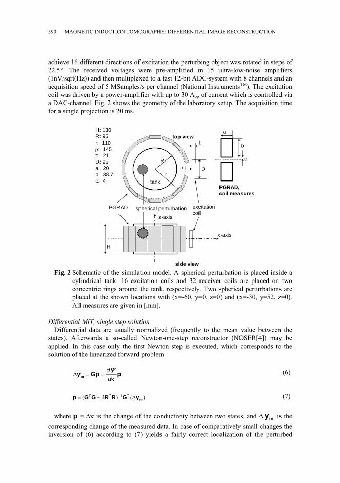
achieve 16 different directions of excitation the perturbing object was rotated in steps of 22.5°. The received voltages were pre-amplified in 15 ultra-low-noise amplifiers (1nV/sqrt(Hz)) and then multiplexed to a fast 12-bit ADC-system with 8 channels and an acquisition speed of 5 MSamples/s per channel (National InstrumentsTM). The excitation coil was driven by a power-amplifier with up to 30 App of current which is controlled via a DAC-channel. Fig. 2 shows the geometry of the laboratory setup. The acquisition time for a single projection is 20 ms.

a

b

c

PGRAD,coil measures

side view

z-axis

x-axis

R

r

ttop view

PGRAD excitationcoil

H

tank

D

H: 130R: 95r: 110ρ: 145t: 21D: 95a: 20b: 38.7c: 4

spherical perturbation

ρ

Fig. 2 Schematic of the simulation model. A spherical perturbation is placed inside a

cylindrical tank. 16 excitation coils and 32 receiver coils are placed on two concentric rings around the tank, respectively. Two spherical perturbations are placed at the shown locations with (x=-60, y=0, z=0) and (x=-30, y=52, z=0). All measures are given in [mm].

Differential MIT, single step solution

Differential data are usually normalized (frequently to the mean value between the states). Afterwards a so-called Newton-one-step reconstructor (NOSER[4]) may be applied. In this case only the first Newton step is executed, which corresponds to the solution of the linearized forward problem

pGpym κddΨ

==∆ (6)

)()( 1

myGRRGGp ∆+= − TTT λ (7) where p = ∆κ is the change of the conductivity between two states, and ∆ is the

corresponding change of the measured data. In case of comparatively small changes the inversion of (6) according to (7) yields a fairly correct localization of the perturbed

my


591

regions. We evaluated the feasibility of this kind of reconstruction in MIT by implementing a NOSER-approach according to (7) under consideration of four different regularization methods.

In a frequency differential approach a voltage change ∆y(fref, f) is evaluated at two frequencies so as to yield a differential conductivity spectrum ∆κ(fref, f) . fref denotes the reference frequency and f a test frequency. In this case also the Gauss-Newton step can be used, assuming that the conductivity change in the observed frequency interval is small enough. Taking the excitation current as a reference, the real part of ∆y corresponds to the real part ∆σ = Re(∆κ). In practice only this real part is evaluated because the imaginary part is usually heavily corrupted by different interferences and systematic errors [28]. Due to the quadratic dependence of the sensitivity on the frequency, the measured voltages must be scaled appropriately. ∆y has to be replaced with the scaled version of the real part [3]:

⎪⎭

⎪⎬⎫

⎪⎩

⎪⎨⎧

⎟⎠⎞

⎜⎝⎛−=∆ )()(Re),(

2

ff

ffff refrefref yyy (8)

This formulation relies on the assumption that the morphology of the sensitivity map does

not depend on the frequency, which is only true for weak perturbation of the primary magnetic field.

The formula can be extended easily to a multi-frequency approach (spectroscopy). However, the values of ∆σ reconstructed with a single step method are usually much lower than the real ones. This is an inherent property of the associated point spread function and the discrepancy gets worse with increasing regularization, i. e. with increasing noise. Therefore the absolute reconstructed values of ∆σ cannot be interpreted quantitatively. However, the ratios of pairs of ∆σ at different frequencies are reconstructed correctly, so that it is possible to obtain relative differential conductivity spectra. Let ∆σ(fi) be the reconstructed conductivity difference between the reference frequency and the frequency fi. Furthermore let ∆σ(f0) be the reconstructed conductivity difference between the reference frequency and an arbitrary base frequency f0. Then the relative differential spectrum is defined as

)()()(

0fffs i

i σσ

∆∆

= (9)

s(f) is dimensionless and has the value 1 at the base frequency f0. Due to the calculation of a ratio s(f) is independent of the scaling factor caused by the particular point spread function and thus neither depends on the regularization nor on the location of the perturbation. Moreover s(f) is a shifted and scaled replica of the original conductivity spectrum which preserves entirely the morphology of the spectrum though it does not allow for the extraction of absolute values.


Calculation of the forward solution and the sensitivity matrix

The forward problem is solved with a previously published finite element program [17] [12], which employs an Ar – V, Ar – formulation with edge elements of second order for the reduced magnetic vector potential Ar and nodal elements of second order for the electric scalar potential V. Boundary conditions on the far boundary (normal component of B vanishes) were prescribed on a spherical surface with a radius sufficiently large such that a change of this radius by 50% resulted in a change of the induced voltages by less than 1 %.

Special attention must be paid to the efficient calculation of the Jacobian G. A mathematically rigorous treatment of this topic has been given in [32]. In our

implementation we exploited the integral formulation published by Mortarelli [19], which is based on a physical mutual energy concept. With this approach the absolute sensitivity dy/dκ for a certain pair of coils is calculated according to (10).

∫Ω

Ω= dIddy

ψφφ LLκ

(10)

with

ψ

ψψψ

φ

φφφ

ωωI

VjI

Vj )()( ∇+=

∇+−=

AL

AL (11)

Aφ, AΨ,Vφ and Vψ

denote the total magnetic vector potential and the electric scalar potential in the region Ω due to currents Iφ and Iψ in the excitation and receiver coils, respectively. The sensitivity matrix dΨ/dκ is then obtained by evaluating (10) for all individual elements and all coil pairs. The exact numerical implementation of (10) was described in detail in [11]. The calculation of the sensitivity map for one pair of coils requires only two forward solutions of the eddy current problem for generating Lφ and LΨ in (11).

Regularization: In EIT the regularization matrix RTR most frequently used is either the identity matrix

I or a discrete spatial derivative operator of first or second order. Such approaches have been discussed extensively in the literature, for a good review see e. g. [10]. Several regularization matrices can be regarded as simple smoothness criteria for the solution but they have also a more general statistical meaning in the framework of Bayesian estimation theory (see e.g. [1]). In case of uncorrelated noise with equal variance for all measurement data the estimator in (7) is a MAP (maximum a posteriori) estimator with RTR being the inverse of the expected cross-correlation matrix of the image E[ppT ].

According to own observations good results can be achieved with variance uniformization [5] which imposes a special assumption of the prior distribution. The objective here is to uniformize the expected variance of the reconstructed conductivity changes over the region Ω, thus providing approximately equal image noise in the center


593

as in the periphery. The algorithm has been described in detail in [5]. Given the covariance matrix F of the voltage changes ∆ and the singular value decomposition of G according to G=UΣV

myT the regularization term is expressed as λRTR = VDVT. In

case that F is a diagonal matrix (uncorrelated noise) with equal entries D becomes a diagonal matrix with:

2

ii

i cd σσ

−= (12)

where c is a free scalar parameter and σi is the ith singular value. After the choice of c the regularization term is entirely determined.

Alternatively also truncated singular value decomposition (TSVD) is very common in

EIT-reconstruction, hence this approach was also implemented for MIT. In this case the inverse solution becomes

mttt y∆= − UVp 1Σ (13)

whereby t denotes the truncation level of the original matrices V, Σ and U, thus

removing the contributions of singular values with index > t.

In this paper the results obtained with four different regularization schemes were compared:

(1) RTR = I. Using the identity matrix is the most simple Tikhonov-regularization method, penalizing high values of the reconstructed conductivity changes. In the following this method will be abbreviated as ‘IM’ .

(2) RTR = N with N the neighbouring matrix defined as:

⎪⎩

⎪⎨

⎧−

==

otherwise0neighboursji,1

jin n

ijN

nn is the number of neighboring elements for element i, where only elements with

common facets are considered as neighbors. N is an approximation of the spatial derivative operator of second order. Due to the irregular structure of the grid this filter is not spatially invariant, nevertheless it gives good results and is common practice for this type of inverse problem. In the following this method will be abbreviated as ‘NM’ .

(3) λRTR= VDVT according to the variance uniformization approach. In the following this method will be abbreviated as ‘VU’ .

(4) TSVD while choosing the truncation level t such as to remove all singular values below an appropriately chosen threshold.


Methods 1 and 2 require the regularization parameter to be chosen optimally while method 3 in addition implies the choice of the tuning parameter c. In practice it turns out that the value of c is uncritical over a very wide range of values because the optimal λ depends on c. That means that c can be fixed at a more or less arbitrary value if a method for the automatic determination of λ is applied. In our case c was set to 0.1.

The regularization parameter λ accounts for the degree of smoothness of the

reconstructed image and determines the condition number of the term (GTG+λRTR) in (7). Several methods for the optimal choice of this parameter have been published in the past, the most well-known ones being L-curves, Generalized Cross-Validation and the Morozov-criterion [10]. Because of its clear physical interpretation we choose the latter method. In this case the optimal λ is the one where the estimated residuals Gp-∆ have the same variance as the measurement noise. The motivation for this criterion is that it is obviously meaningless to make the residuals lower than it is expected from the statistics of the data. This method provided always stable images independently of the regularization matrix and was considered as a good basis for a fair comparison between the different regularization methods.

my

Modeling setup

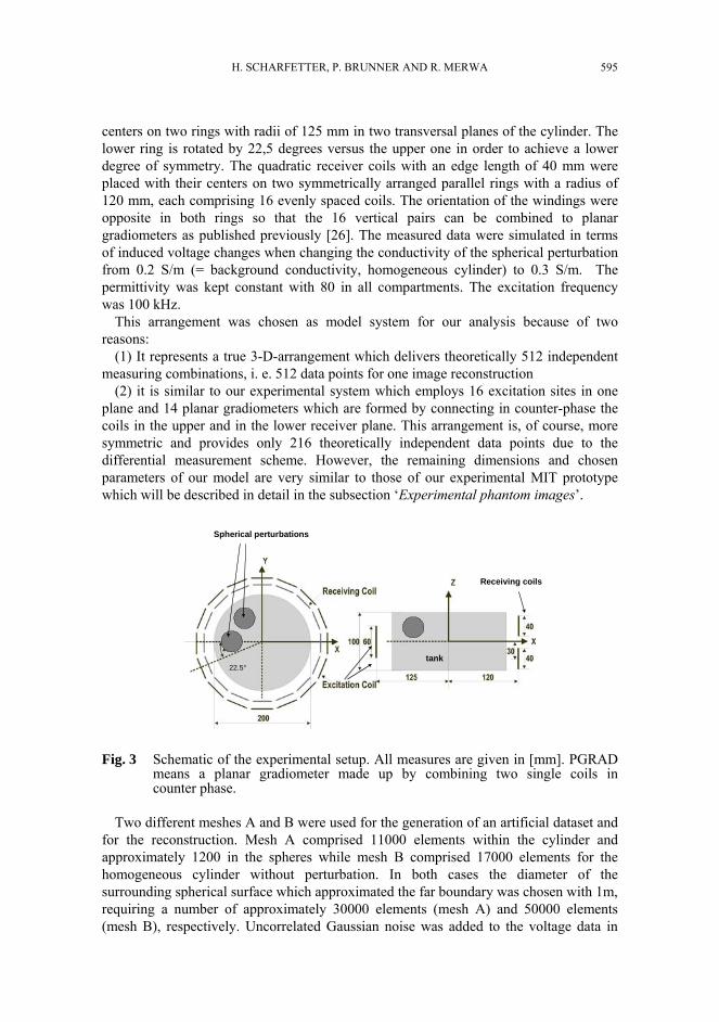
The inverse solver was tested for both the state-differential as well as for the frequency-differential approach with a simple 3-D model comprising a cylindrical conductor with spherical inhomogeneities and an array of 16 excitation coils and 32 receiving coils as shown in fig. 1. The exact geometry is illustrated in fig. 3.

The outer cylinder had a radius and a height of 100 mm, the perturbing spheres had a radius of 20 mm. For state-differential reconstruction two spheres were placed with their centers at (x=-60, y=0, z=0) and (x=-30, y=52 and z=0). For the frequency differential reconstruction one single spherical inhomogeneity (radius 20 mm) was centered at (x=-60, y=0, z=0) [mm]. Its conductivity spectrum was modelled with a Cole-model (14) according to a typical spectrum of tissue in the upper ß-dispersion range:

⎪⎪

⎭

⎪⎪

⎬

⎫

⎪⎪

⎩

⎪⎪

⎨

⎧

⎟⎟⎠

⎞⎜⎜⎝

⎛+

−+= ∞

α

ωω

σσσωσ

C

j1

Re)( 00

(14) with the parameters : σ0=0.033 S/m, σ∞=0.373,S/m, ωC=2π*51006 [rads-1] and

α=0.98. Frequency differential images were then reconstructed from the ∆y between a

reference frequency fref of 300 kHz and the test frequencies 200, 400 and 700 kHz. In contrast to the state-differential case adjacing coils in the upper and lower ring were

combined in counter-phase so as to simulate the 16 planar gradiometers of our real system.

The diameter of the solenoid excitation coils was 60 mm, their height 1 mm and their thickness 1 mm. The exciters were placed in groups of 8 with their


595

centers on two rings with radii of 125 mm in two transversal planes of the cylinder. The lower ring is rotated by 22,5 degrees versus the upper one in order to achieve a lower degree of symmetry. The quadratic receiver coils with an edge length of 40 mm were placed with their centers on two symmetrically arranged parallel rings with a radius of 120 mm, each comprising 16 evenly spaced coils. The orientation of the windings were opposite in both rings so that the 16 vertical pairs can be combined to planar gradiometers as published previously [26]. The measured data were simulated in terms of induced voltage changes when changing the conductivity of the spherical perturbation from 0.2 S/m (= background conductivity, homogeneous cylinder) to 0.3 S/m. The permittivity was kept constant with 80 in all compartments. The excitation frequency was 100 kHz.

This arrangement was chosen as model system for our analysis because of two reasons:

(1) It represents a true 3-D-arrangement which delivers theoretically 512 independent measuring combinations, i. e. 512 data points for one image reconstruction

(2) it is similar to our experimental system which employs 16 excitation sites in one plane and 14 planar gradiometers which are formed by connecting in counter-phase the coils in the upper and in the lower receiver plane. This arrangement is, of course, more symmetric and provides only 216 theoretically independent data points due to the differential measurement scheme. However, the remaining dimensions and chosen parameters of our model are very similar to those of our experimental MIT prototype which will be described in detail in the subsection ‘Experimental phantom images’.

Receiving coils

tank

Spherical perturbations

22.5°

Fig. 3 Schematic of the experimental setup. All measures are given in [mm]. PGRAD means a planar gradiometer made up by combining two single coils in counter phase.

Two different meshes A and B were used for the generation of an artificial dataset and

for the reconstruction. Mesh A comprised 11000 elements within the cylinder and approximately 1200 in the spheres while mesh B comprised 17000 elements for the homogeneous cylinder without perturbation. In both cases the diameter of the surrounding spherical surface which approximated the far boundary was chosen with 1m, requiring a number of approximately 30000 elements (mesh A) and 50000 elements (mesh B), respectively. Uncorrelated Gaussian noise was added to the voltage data in


order to simulate the noise of the receiver channels. This type of noise, although common practice in simulations of this type, is not entirely valid for real situations. In addition the noise of the excitation coils is propagated to all receiver coils, thus resulting in a certain amount of correlated noise in all receiver channels. This phenomenon has been studied in detail for EIT [6], but should be disregarded here for simplicity.

The calculation of the complete sensitivity matrix required 48 forward solutions

according to the Mortarelli-approach.

Evaluation: The following tests were performed: (1) Monte-Carlo-study with 50 state-differential reconstruction runs for each regularization method and an SNR of 64 dB, 50 dB and 44 dB, respectively. The results for 64 dB were plotted as images of the mean reconstructed image values. (2) Comparison of the state-differential images for all methods with an SNR of 64 dB , 50 dB and 44dB . The comparison was done with the following performance measures

- Mean and standard deviation of the image values within the spherical perturbations and within the background. This quantifies the correctness of the reconstructed values as well as the degree of homogeneity;

- maximum reconstructed value (L∞-norm) to account for the extremes; - median and maximum of the filtered images after filtering with a

gradient filter so as to account for he sharpness of the edges of the perturbations;

- outward shift of the spheres in the reconstructed image (fidelity of the location). This shift was determined by localizing the center of gravity for each spot within a wedge-shaped search region with a height of 2.6 times the sphere’s radius and excluding the outermost 2mm as well as the innermost 40mm in radial direction from the center. The restriction of the search region to this volume prevented spurious contributions from outliers and negative image values far away from the real perturbing regions.

(3) Visualization of single state-differential images for those two regularization methods which yielded the best apparent resolution of the two perturbations at an SNR of 64, 50 and 44 dB, respectively. (4) Visualization of single frequency-differential images from data with a simulated SNR of 64 dB. The regularization was done with the unit matrix and a regularization parameter λ of 5.1*10-18. (5) Quantification and visualization of a relative conductivity spectrum reconstructed from the multi-frequency data with the simulated Cole-model.

Experiment l phantom images In order to test the capability of the algorithm for reconstructing images from real data, a

state-differential and a frequency-differential experiment were carried out with the


597

previously mentioned prototype MIT system. For the state-differential measurement an agar-sphere with 2 S/m and a radius of 20 mm was immersed in a saline filled tank with 1 S/m. The measurement frequency was chosen with 306 kHz. State-differential data were simulated by shifting the agar-sphere from its original position (x=0 y=50 z=24) to (x=-50 y=0 z=24) [mm], i. e. by rotating it about the cylinder axis by 90°.

Frequency differential approach

A cylindrical piece of potatoe with a diameter and height of 40 mm, respectively, was placed at [x=65mm, y=0mm, z=40mm] The conductivity of the tank was adjusted to 0.2 S/m and a multi-sine excitation pattern was applied to the EXC. Again the acquisition time per position was 20 ms. After data acquisition a single-step reconstruction was carried out with an fref of 300 kHz and a test frequency f of 400 kHz. Regularization was done with the unit matrix and an optimal regularization parameter according to an SNR of about 40 dB. According to the ß-dispersion of the potato the conductivity difference between 300kHz and 400kHz was only 0,035 S/m as measured with a four-needle electrode array and a commercial impedance analyzer (Solartron 1260). Such a small contrast represents a real challenge for both the measurement system and the reconstruction process.

3. Results

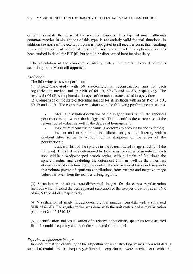
Assuming a SNR of 44 dB the singular values of G begin to drop below the noise level at approximately #200, i. e. G has an effective rank of no more than 200. Fig 4 shows the mean reconstructed images of the Monte-Carlo study with an SNR of 64 dB. The tuning parameters were chosen as listed in table 1.

A

1.95e-02

-7.73e-03

1.99e-02

-6.97e-032.63e-02

-164e-02

2.76e-02

-1.22e-02

IM NM

VU TSVD

Fig 4. dependence of the theoretical normalized resolution on the noise level. Curves are depicted for noise-free data (TSVD with truncation level 512) and TSVD with truncation levels corresponding to a SNR of 44, 50 and 64 dB, respectively.


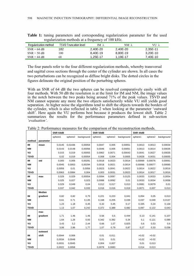
Table 1: tuning parameters and corresponding regularization parameter for the used regularization methods at a frequency of 100 kHz.

Regularization method TSVD Truncation level IM λ NM λ VU λ SNR = 64 dB 182 2,40E-20 2,40E-20 2,35E-11 SNR = 50 dB 100 8,40E-19 8,80E-19 3,20E-10 SNR = 44 dB 68 1,25E-17 1,19E-17 7,40E-10

The four panels refer to the four different regularization methods, whereby transversal and sagittal cross sections through the center of the cylinder are shown. In all cases the two perturbations can be recognized as diffuse bright disks. The dotted circles in the figures delineate the original position of the perturbing spheres.

With an SNR of 64 dB the two spheres can be resolved comparatively easily with all four methods. With 50 dB the resolution is at the limit for IM and NM, the image values in the notch between the two peaks being around 71% of the peak values. TSVD and NM cannot separate any more the two objects satisfactorily while VU still yields good separation. At higher noise the algorithms tend to shift the objects towards the borders of the cylinder, which is also reflected in table 2 when looking at the parameter ‘outward shift’. Here again the VU performs best because it produces the lowest shift. Table 2 summarizes the results for the performance parameters defined in sub-section ‘evaluation’. Table 2: Performance measures for the comparison of the reconstruction methods. SNR 64dB SNR 50dB SNR 44dB

sphere1 sphere2 background sphere1 sphere2 background sphere1 sphere2 background

method parameter

IM mean 0,0145 0,01436 0,00054 0,0047 0,005 0,00051 0,0013 0,0013 0,00034

NM 0,0143 0,0148 0,00056 0,0046 0,005 0,00051 0,0013 0,0014 0,00035 VU 0,015 0,019 0,00055 0,0062 0,0071 0,00043 0,0041 0,0027 0,00035

TSVD 0,02 0,019 0,00054 0,008 0,004 0,0005 0,0028 0,0031 0,00055

IM std 0,005 0,006 0,00291 0,0018 0,0023 0,0014 0,00069 0,00076 0,00061

NM 0,0045 0,0053 0,00294 0,0018 0,0021 0,0014 0,00066 0,00077 0,00065 VU 0,0059 0,01 0,0056 0,0023 0,0041 0,0022 0,0014 0,0022 0,0016

TSVD 0,0063 0,0084 0,004 0,003 0,0031 0,0023 0,0014 0,0017 0,0016

IM max 0,029 0,029 0,00054 0,0094 0,0097 0,0125 0,0033 0,0033 0,0054

NM 0,025 0,027 0,023 0,0088 0,0092 0,01 0,0033 0,0034 0,0058 VU 0,029 0,049 0,04 0,012 0,017 0,013 0,0081 0,0079 0,01

TSVD 0,037 0,042 0,033 0,016 0,016 0,019 0,0071 0,007 0,013

IM Median gradient 0,82 0,82 0,75 0,221 0,223 0,041 0,054 0,05 0,013

NM 0,61 0,71 0,135 0,168 0,205 0,039 0,037 0,049 0,0137

VU 1,23 1,18 0,45 0,32 0,45 0,17 0,335 0,24 0,134

TSVD 1,13 1,07 0,242 0,372 0,389 0,082 0,097 0,122 0,043

IM max gradient 1,71 1,46 1,46 0,56 0,5 0,444 0,13 0,141 0,107

NM 1,64 1,26 0,93 0,342 0,392 0,34 0,1 0,121 0,089

VU 3,43 3,2 2,44 0,66 1,07 0,825 0,6 0,53 0,6 TSVD 3,06 2,86 1,77 1,07 0,79 0,87 0,27 0,33 0,036

IM outward shift 0,0044 0,006 0,01 0,011 >0,02 >0.02

NM 0,0034 0,0048 0,01 0,01 >0,02 >0.02 VU 0,0031 0,0045 0,004 0,007 0,01 0,013

TSVD 0,0022 0,0058 0,0078 0,0083 0,014 0,013


599

At an SNR of 44 dB the images are in general comparatively poor. IM and NM interestingly allow a clear separation of two objects, but their localization is very poor, the outward shift being extremely large. VU still provides a comparatively correct localization at the cost of separability. TSVD fails to produce a clear image.

IM and NM perform nearly identically, also their optimal regularization parameters are almost identical. VU yields, in general, larger reconstructed values in the perturbed regions but also a larger STD. The mean reconstructed values differ from the true perturbation by a factor of up to 7 at an SNR of 64 dB. At higher noise levels the discrepancy increases. This is due to the non-iterative nature of the algorithm, because the iteration step in (7) yields approximately the correct search direction but usually a wrong step width. The highest mean values are provided by VU and TSVD, the drop with the noise levels being lowest. However, on the other hand VU yields the highest standard deviations. Moreover VU tends to produce more pronounced ‘ghost objects’ in the homogeneous region than IM and NM. When comparing the images filtered with the gradient filter the VU yields the highest values, i. e. it appears to be the most edge-preserving method.

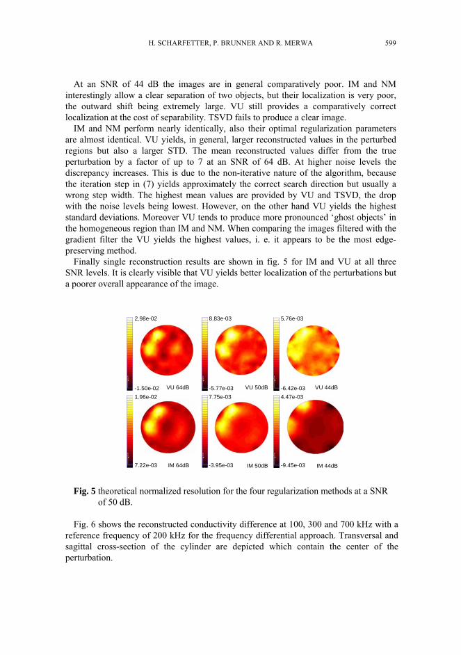
Finally single reconstruction results are shown in fig. 5 for IM and VU at all three SNR levels. It is clearly visible that VU yields better localization of the perturbations but a poorer overall appearance of the image.

VU 64dB VU 50dB

IM 64dB IM 50dB IM 44dB

VU 44dB

2.98e-02

-1.50e-02

8.83e-03

-5.77e-03

5.76e-03

-6.42e-031.96e-02

7.22e-03

7.75e-03

-3.95e-03

4.47e-03

-9.45e-03

Fig. 5 theoretical normalized resolution for the four regularization methods at a SNR

of 50 dB. Fig. 6 shows the reconstructed conductivity difference at 100, 300 and 700 kHz with a

reference frequency of 200 kHz for the frequency differential approach. Transversal and sagittal cross-section of the cylinder are depicted which contain the center of the perturbation.


-6-5-4-3-2-101234x 10-4

200/300 kHz

400/300 kHz

700/300 kHz

Fig. 6 Panel A: CNR for TSVD as a function of the normalized x-coordinate (relative to the cylinder radius) and in dependence on the noise level. Panel B: comparison of the four methods at a SNR of 50dB.

The position of the perturbing sphere is localized fairly correctly, however there is a

certain outward shift and considerable smearing. The latter is probably due to the fact that the sphere was placed in the median plane where the gradiometers have very low sensitivity. Placing the sphere more eccentrically is expected to improve the images considerably. The scaling of the data is clearly visible when comparing the reconstructed differences (see colorbar) with the true ones (-0.012 S/m between 200 and 300 kHz and 0.0089 S/m between 700 and 300 kHz). The resulting factor lies in the range of 20.

Table 3 shows the values of the relative differential spectrum s(f) at 5 discrete

frequencies. The relative error between reconstructed and expected values remained below 2.5 % in any case. In fig. 7 the corresponding graphical representation of the relative spectra is given. Table 3: relative differential spectrum s(f)

frequency true value reconstructed value Relative error kHz S/m S/m 300 1.24 1.217 -1.89 400 1.332 1.309 -1.72 450 1.358 1.330 -2.09 600 1.402 1.377 -1.75 700 1.418 1.386 -2.23


601

200 250 300 350 400 450 500 550 600 650 7001

1.05

1.1

1.15

1.2

1.25

1.3

1.35

1.4

1.45

frequency [kHz]

s(f)

[-] -1.9%

-1.7%-2.1%

-1.8% -2.2%

true

reconstructed

Fig. 7 Mean images of the Monte-Carlo study. Reconstructed |∆κ| (transversal and saggittal

section through the origin) for the spherical perturbations with four different regularization matrices and a SNR of 64 dB.

Experimental images from phantoms: Fig. 8 shows the dynamic image when rotating the agar-sphere about the cylinder axis

by 90°. The top view was obtained as a transversal cross section through the center of the agar-sphere at z=24 mm. The side view is a sagittal cross-section through the cylinder axis, i. e. it shows only the results at the location where the sphere disappears during the experiment. In the top view two spots with the correct sign can be recognized, whereas the mean reconstructed values are again a factor of 7 too low and are therefore not shown explicitly.

Fig. 8 Mean images of the Monte-Carlo study.Reconstructed |∆κ| (transversal and

saggittal section through the origin) for the spherical perturbations with four different regularization matrices and a SNR of 50 dB.


The localization is fairly correct, but the peaks are somewhat shifted. In the side view a ghost object with negative sign appears in addition to the correct spot in the lower half-space. It is placed exactly symmetrical to the median transversal plane which is due to the special symmetrical measurement setup by using gradiometers. The gradiometers produce difference data between the upper and the lower ring of receiver coils. This yields ambiguous measurement data which do not allow to decide whether a positive perturbation has occurred in the upper half of the cylinder or a negative one in the lower half. Thus the algorithm tends to reconstruct two objects. This effect occurs also with simulated data and disappears if the degree of symmetry of the arrangement is lowered. Unfortunately this was not possible up to now with our hardware but will be an important issue for future improvements.

Fig. 9 shows the frequency-differential image of the cylindrical piece of potato.

Transversal and sagittal cross-section of the cylinder are depicted which contain the center of the perturbation.

Fig. 9 Comparison of single-shot images for VU and IM at the three different noise

levels. The position of the potato is localized fairly correctly, however there is a certain

outward shift and considerable smearing due to the low experimental SNR of only 40 dB. This high noise level was due to undulations of the tank medium in response to the rotation of the sample.


603

4. Discussion

The shown results demonstrate the feasibility of image reconstruction from MIT-data with the same methods as suggested for EIT. This finding is not self-evident, as the sensitivity distribution is significantly different in EIT and MIT [27][29][31]. In EIT the region of maximum sensitivity is located in between the equipotential surfaces which meet the surface at the detection electrodes, i. e. within a tube-shaped region which connects injection and detection sites. As shown in [27][29] in MIT the sensitivity is not concentrated within a field tube between excitation and receiver coil but increases with the distance from the tube axis, according to the increase of the eddy current density. This may be the main reason why the reconstructed solution tends to be displaced towards the nearest border of the cylindrical tank, especially at higher noise levels. An extreme case for this effect can be observed if the perturbation is placed exactly in the origin and if the senders and receivers are all in the same plane (image not shown due to space restrictions). Instead of the expected spot in the origin two widely separated spots appear on the cylinder axis close to the top and bottom of the cylinder, respectively. In fact such a coil arrangement cannot distinguish between an object in the center and two objects on the cylinder axis placed symmetrically with respect to the origin, because it is always possible to find two corresponding conductivitiy changes so that the field perturbations in the median plane are the same. Obviously, in this ambiguous situation, the algorithm favors the splitted solution according to the sensitivity distribution. A similar ambiguity occurs when using differential sensors, such as the gradiometers employed in our setup. For getting rid of such artifacts it is very important to use a less symmetric transceiver setup which provides enough spatial information in 3-D.

The low number of significant singular values even at comparatively low noise (64 dB

SNR) suggests that, similar as in EIT, a significant amount of sensor combinations does not provide enough independent information. Intuitively one would expect this finding because there exist pairs of excitation/receiving coils which nearly fulfill the reciprocity condition and hence reduce the amount of useful combinations to about half of the number of possible combinations, i. e. to 256 in our case.

Further investigations should determine the maximum ‘useful’ number of sensors in one plane, i. e. that number beyond which additional sensors do not increase the resolution any more significantly. Adding more sensors off-plane may add more 3-D-information and hence still provide improvement. This possibility has also to be studied in further research.

When comparing the regularization schemes after application of the Morozov-

criterion, the IM and the NM approach yield the smoothest solutions, as expected. However, they also tend to displace the perturbations towards the border of the tank. The best localization is obtained with VU, probably because the imposed variance counteracts somewhat the lower sensitivity in the center of the object. However, VU yielded also the highest STDs, i. e. the less homogeneous images and more pronounced ghosts. The gradient filter revealed VU to produce the sharpest edges of the perturbations. TSVD provides the poorest images at higher noise levels. In terms of separability of the two perturbations VU performs best, especially when also taking into account the correct localization. In neither case, however, the single-step solution


provides the correct values for ∆κ. Even with an SNR of 64 dB the reconstructed differences are too low by a factor of at least 7, thus demonstrating that the method yields the correct search direction but not the correct step size. First experiments with smaller models and at least 10 iterations show that the solution converges towards the correct values. Nevertheless the single-step method may be completely justified in cases where only qualitative changes are sought for or where proportions are to be reconstructed, e. g. in frequency differential spectroscopic imaging. Therefore the area of applicability of a single-step approach has to be analyzed carefully in future work.

At least for the shown examples MIT appears relatively robust against Gaussian measurement noise. Adding noise to the data with an SNR of 64 dB produces a stable and distinct solution. Even an SNR of 44 dB allow the recognition of the two spheres when applying the correct regularization. This result is very important for the practical implementation because, due to technical reasons, MIT is expected to yield low SNR (50 dB) at frequencies as low as 100 kHz, which are interesting for the imaging of pathophysiological processes [28,26]. However, our results have only been achieved with two single focal perturbations with a relatively diameter of 20% of the background object. In a more advanced study the stability and the resolution of the images should be investigated for a series of perturbations with different diameter and spacing. For the monitoring of brain edema, where the processes under investigation are usually focal or even generalized our approach may be sufficiently stable.

As to the detectability of spherical perturbations in a human brain simulation results in [18] have shown that a sphere with a diameter of about 40 mm, a background conductivity of 0.1S/m and a contrast of 2 yields a SNR of 24 dB at 100 kHz when applying 1 A to an excitation coil with 45 turns and a receiver coil with 1 turn. The assumed acquisition time was 200 ms, With our present technology single shot images are generated with an acquisition time of 20 ms, an excitation coil with 5 turns and a current up to 20A. The receiver coils have 40 turns with otherwise unchanged geometry. This means an overall increase in SNR by 28dB. Extrapolating the analysis given in [28], an improvement of the SNR by a factor of 5-10 is still technically possible, thus reaching 50 - 60dB, which is obviously sufficient for producing fairly acceptable difference images.

The last images show how to exploit the frequency dependence of the tissue

conductivity. A multi-frequency approach with measurement frequencies between several tens of kHz and several MHz is expected to significantly increase the available information and thus the quality of the images. Possible applications may then in fact be the same as for EIT (lung function monitoring, lung edema monitoring) and hydration monitoring in the brain. Acknowledgements The authors would like to thank Prof. Oscar Biro from the Institute for Theory and Fundamentals of Electrical Engineering of the Graz University for Technology for his excellent support when implementing the Mortarelli algorithm. References

[1] Adler A. Accounting for erroneous electrode data in electrical impedance tomography Physiol Meas


605

25: 227–238, 2004. [2] Al-Zeibak S. and H.N. Saunders, A feasibility study of in vivo electromagnetic imaging Phys Med

Biol, 38: 151-160, 1993. [3] Brunner P., R. Merwa, A. Missner, J. Rosell, K. Hollaus, H. Scharfetter, Reconstruction of the shape of

conductivity spectra using differential multi-frequency magnetic induction tomography, Physiol Meas, in press

[4] Cheney M., D. Isaacson, J.C.Newell, S. Simske and J. Goble, NOSER: An algorithm for solving the inverse conductivity problem Int J Imag Syst Tech, 2: 66-75, 1990.

[5] Cohen-Bacrie C., Y. Goussard and R. Guardo R, Regularized reconstruction in electrical impedance tomography using a variance uniformization constraint IEEE Trans Med Imaging, 16: 562-571, 1997.

[6] Frangi A. F., P. J. Riu, J. Rosell and M. A Viergever, Propagation of measurement noise through backprojection reconstruction in electrical impedance tomography IEEE Trans on Medical Imaging, 21: 566-578, 2002.

[7] Goss D. et al, Development of electromagnetic inductance tomography (EMT) hardware for determining human body composition Proc 3rd World Congress on Industrial Process Tomography, 377-383, 2003.

[8] Griffiths H., Magnetic induction tomography Meas Sci Technol, 26: 1126-1131, 2001. [9] Griffiths H., W.R. Stewart and W. Gough, Magnetic induction tomography. A measuring system for

biological tissues Ann N Y Acad Sci 873: 335-345, 1999. [10] Hansen P.C., Rank-deficient and discrete ill-posed problems SIAM, Philadelphia, 1998. [11] Hollaus K., C. Magele, R. Merwa and H. Scharfetter, Fast calculation of the sensitivity matrix in magneti

induction tomography by tetrahedral edge finite elements and the reciprocity theorem Physiol Meas, 25159-168, 2004.

[12] Hollaus K., C. Magele, R. Merwa, H. Scharfetter, Numerical Simulation of the Eddy Current Problem in Magnetic Induction Tomography for Biomedical Applications by Edge Elements IEEE Transactions on Magnetics, 40: 623 – 626, 2004.

[13] Karbeyaz U.B., N.G. Gencer, Electrical conductivity imaging via contactless measurements: an experimental study. IEEE Trans Med Imaging, 22: 627 – 635, 2003.

[14] Korjenevshy A., V. Cherepenin, and S. Sapetsky, Magnetic induction tomography: Experimental realization Physiol Meas 21: 89-94, 2000.

[15] Korjenevsky A.V. and V.A. Cherepenin, Progress in realization of magnetic induction tomography Ann N Y Acad Sci, 873: 346-352, 1999.

[16] Korzhenevskii A.V. and V.A. Cherepenin, Magnetic induction tomography J Commun Tech Electron 42: 469-474, 1997.

[17] Merwa R., K. Hollaus, B. Brandstätter and H. Scharfetter. Numerical solution of the general 3D eddcurrent problem for magnetic induction tomography (spectroscopy) , Physiol Meas, 24: 545-554, 2003.

[18] Merwa R., K. Hollaus, O. Biró, H. Scharfetter, Detection of brain oedema using magnetic induction tomography: A feasibility study of the likely sensitivity and detectability Physiol Meas, 25: 347–354, 2004.

[19] Mortarelli J.R., A Generalization of the Geselowitz Relationship Useful in Impedance Plethysmographic Field Calculations IEEE Trans Biomed Eng, 27: 665-667, 1980.

[20] Ola P., L. Päivärinta and E. Somersalo, An inverse boundary value problem in electrodynamics Duke Math J 70 617-653, 1993

[21] Peyton A.J. et al, An overview of electromagnetic inductance tomography: Description of three different systems Meas Sci Technol 7: 261-271, 1996.

[22] R. Casanova, A. Silva and A.R. Borgss, MIT image reconstruction based on edge preserving


regularization Physiol Meas, 25: 195–207, 2004. [23] Riedel C.H., M. Keppelen, S. Nani, R.D. Merges and O. Dössel, Planar system for magnetic induction

conductivity measurement using a sensor matrix, Physiol Meas, 25: 403-411, 2004. [24] Rosell J., R. Casañas and H. Scharfetter, Sensitivity maps and system requirements for Magnetic

Induction Tomography using a planar gradiometer Physiol Meas, 22: 121-130, 2001. [25] Rosell-Ferrer J., R. Merwa, P. Brunner, H. Scharfetter, A multifrequency magnetic induction

tomography system using planar gradiometers: data collection and calibration, Physiol Meas, in press [26] Scharfetter H., H.K. Lackner and J. Rosell, Magnetic induction tomography: Hardware for multi-

frequency measurements in biological tissues Physiol Meas, 22: 131-146, 2001. [27] Scharfetter H., P. Riu, M. Populo and J. Rosell, Sensitivity maps for low-contrast-perturbations

within conducting background in magnetic induction tomography (MIT) Physiol Meas, 23: 195-202, 2002.

[28] Scharfetter H., R. Casañas and J. Rosell, Biological tissue characterization by magnetic induction spectroscopy (MIS): requirements and limitations IEEE Trans Biomed Eng, 50: 870-880, 2003.

[29] Scharfetter H., S. Rauchenzauner, R. Merwa, O. Biró and K. Hollaus, Planar gradiometer for magnetiinduction tomography (MIT): Theoretical and experimental sensitivity maps for a low-contrast phantomPhysiol Meas, 25: 325-333, 2004.

[30] Seagar A.D., D.C. Barber, B.H. Brown. Theoretical limits to sensitivity and resolution in impedance imaging. Clin Phys Physiol Meas, 8: Suppl A, 13-31, 1987.

[31] Soleimani M., Sensitivity maps in three-dimensional magnetic induction tomography, Insight. The Journal of The British Institute of Non-Destructive Testing: 48, 2006.

[32] Somersalo et al, A linearized inverse boundary value problem for Maxwell’s equations J Comp Applied Math, 42: 123–136, 1992.

[33] Tapp H.S. and A.J. Peyton, A State of the Art Review of Electromagnetic Tomography Proc 3rd world congress on industrial process tomography, 340-346, 2003.

[34] Xie C.G., Review of process tomography image reconstruction methods In: Grattan KTV, Augousti AT (Eds). Sensors VI: Technology, Systems and Applications, 341-346. IOP Publishing, 1993.

Institute of Medical Engineering, Graz University of Technology, Austria E-mail: [email protected]

MAGNETIC INDUCTION TOMOGRAPHY: SINGLE-STEP SOLUTION OF THE 3-D INVERSE PROBLEM FOR DIFFERENTIAL...

Documents

Transcript of MAGNETIC INDUCTION TOMOGRAPHY: SINGLE-STEP SOLUTION OF THE 3-D INVERSE PROBLEM FOR DIFFERENTIAL...