Inverse modelling applied geography

(This is a sample cover image for this issue. The actual cover is not yet available at this time.)

This article appeared in a journal published by Elsevier. The attachedcopy is furnished to the author for internal non-commercial researchand education use, including for instruction at the authors institution

and sharing with colleagues.

Other uses, including reproduction and distribution, or selling orlicensing copies, or posting to personal, institutional or third party

websites are prohibited.

In most cases authors are permitted to post their version of thearticle (e.g. in Word or Tex form) to their personal website orinstitutional repository. Authors requiring further information

regarding Elsevier’s archiving and manuscript policies areencouraged to visit:

http://www.elsevier.com/copyright

http://www.elsevier.com/copyright

Author's personal copy

Spatially explicit inverse modeling for urban planning

Ricardo Crespo*, Adrienne Grêt-RegameyInstitute for Spatial and Landscape Planning, Swiss Federal Institute of Technology Zurich, Wolfgang-Pauli-Strasse 15, 8093 Zurich, Switzerland

Keywords:Inverse modelingUrban systemsMixed-GWRHedonic modeling

a b s t r a c t

Urban modeling methods have traditionally followed a forward modeling approach. That is, they usedata from today’s situation to forecast or simulate future states of an urban system. In this paper, wepropose an inverse modeling approach by which we shift our attention from solely forecasting orsimulating future states of an urban system to steering it to a desired state in the future via key variablescharacterizing the system in the present. We first present a theoretical framework for the use of theinverse approach in urban planning. We test the power of the proposed method using a hedonic houseprice model in a metropolitan area in Switzerland to investigate the negative effects of densification onhouse prices. The model is calibrated by mixed geographically weighted regression in order to accountfor spatial variability of both key variables and model outputs. We show how devaluation of house pricescaused by densification can be compensated by different levels of socioeconomic, locational as well asstructural variables. We illustrate and discuss how trade-offs between variables may lead to morefeasible results from an urban planning perspective. We conclude that the proposed method might bevaluable for urban planners for developing implementable spatial plans based on future visions. Inparticular, the fact that other model specifications than hedonic house price model can also be employedto formulate an inverse model application, allows planners to address other type of problems orexternalities from urbanization processes such as urban sprawls, environmental pollution or land useschange.

� 2011 Elsevier Ltd. All rights reserved.

Introduction

Urban systems are complex systems made of a number of indi-vidual components that interact with one another through anintricate network (Baynes, 2009; Bretagnolle, Daudé, & Pumain,2003; Liu, 2008) As Liu (2008) argues, urban systems consist ofa set of elements or subsystems, such as population, land,employment, services and transport, to mention a few. Allcomponents of the system are interacting with each other throughsocial, economic, and spatial mechanisms while they are alsointeracting with components of the environment. Some compo-nents such as urban population are expected to increase extensivelyover the upcoming decades. According to United Nations (2009),more than 50% of the population lives now in urban areas and this isexpected to rise to 70% in 2050. Such rapid increase in the urbanpopulationwill most likely cause people’s welfare to decrease evenlong before 2050. Higher levels of population density in cities are

generally associated with negative externalities such as pollution,traffic congestion and crime, among others, as well as witheconomic disequilibrium in the land and housingmarket. Yet, whileplanners are aware of these rapid changes, adaptation strategiesand approaches tackling these growing challenges are still lacking.

A number of mathematical methods in the literature deal withurban development. The most popular are urban-growth logisticregressions which attempt to examine and forecast urban-growthusing an econometric formulation (e.g. Allen & Lu, 2003; Hu & Lo,2007; Landis & Zhang, 1998), neural-networks modeling bywhich the interaction between the different elements of an urbansystem is studied based on the way biological neural systemsdevelop (e.g. Maithani, Jain, & Arora, 2007; Ou, Zhang, Ren, & Yao,2003; Pijanowski, Brown, Shellito, & Manik, 2002), and gravitymodels which address the interaction between the elements ofurban systems by using a similar formulation to the Newton’s lawof gravity (e.g. Tsekeris & Stathopoulos, 2006). Also, Agent-BasedModels (ABM) and Cellular Automata (CA) have become popularfor representing the actions, behavior and interactions of individualagents in space and time (Batty, 2009). In recent years, ABM and CAtechniques have been particularly useful in modeling urbanexpansion (He, Okada, Zhang, Shi, & Zhang, 2006; Zhang, Zeng,Bian, & Yu, 2010).

* Corresponding author. Institute for Spatial and Landscape Planning, SwissFederal Institute of Technology Zurich, Wolfgang-Pauli-Strasse 15, HIL H 53.1, 8093Zurich, Switzerland. Tel.: þ41 44 633 29 84; fax: þ41 44 633 10 84.

E-mail addresses: [email protected], [email protected] (R. Crespo),[email protected] (A. Grêt-Regamey).

Contents lists available at SciVerse ScienceDirect

Applied Geography

journal homepage: www.elsevier .com/locate/apgeog

0143-6228/$ e see front matter � 2011 Elsevier Ltd. All rights reserved.doi:10.1016/j.apgeog.2011.10.009

Applied Geography 34 (2012) 47e56


The advantage of hedonic house price model is that it allowsexploring characteristics of urban systems. The market value oftradable goods, such as house prices, is linked to measurableattributes of the good being valued, thus providing a description ofthe urban system. The model can be estimated by means ofeconometric techniques such as ordinary least squares (OLS). In thecase of housing market, price of properties are regressed on a set ofsocioeconomic, locational, and structural attributes which aregenerally measured at small areas such as districts or municipali-ties. The relationship between such attributes (explanatory vari-ables) and house prices (response variable) correspond to themodel’s parameter estimates and can be interpreted as theconsumer’s willingness to pay for one additional unit of the cor-responding house’s attribute. Most of the explanatory variablesgenerally employed in modeling house prices correspond to whatWegener (1994) and Liu (2008) have classified as urban subsys-tems, such as: housing (structural characteristic of properties), landuse, employment, population density and location of workplacesamong others. Accordingly, hedonic house price modeling canprovide valuable information on the dynamics and complexity ofurban systems by quantifying and relating a set of urban subsys-tems to a response variable. Numerous applications of house pricemodels can be found in the literature. In particular, examples ofhow hedonic house price models can be used to analyze key vari-ables in urban modeling are given by Nelson (1978), Bender andHwang (1985), Ottensmann, Payton, and Man (2008).

All of the above mentioned methods have been exclusively usedin urban studies to either characterize a current situation bymodeling, or to predict or simulate future scenarios based on datafrom today’s situation. This is what in the literature has beendenoted as the forward problem (Scales & Snieder, 2000), that is,current data is used to fit a model from which predictions orsimulations are derived. In a more recent study, Grêt-Regamey andCrespo (2011) propose the use of an inverse problem approach(Ashter, Borchers, & Thurber, 2005; Scales & Snieder, 2000;Tarantola, 2005) for planning sustainable urban systems. Asopposed to the forward problem, in the inverse problem approach,a set of model’s parameters characterizing a system are derivedfrom a given value for the model’s response. In urban planning, suchgiven value can be defined by stakeholders as a desire future statefor an urban system. Thus, inverse problem approach is intended toshift the focus in urban planning from mostly forecasting futurestates to planning from a future vision.

The paper is divided into two main sections: Firstly, we providea theoretical framework to the inverse problem approach for urbanplanning proposed by Grêt-Regamey and Crespo (2011).We focus onsystem identification’s tools to formulate and solve inverse modelsfor urban systems. Secondly, we illustrate the systematic approach ina metropolitan area in Switzerland using a hedonic house pricemodel showing how to deal with increasing population density.

The inverse approach

In inverse modeling, one deals with concepts and definitionsfrequently used in mathematical and econometric analysis. Yet,

same expressions used by the different communities often refer todifferent concepts. For example, for mathematicians the termparameter refers to any type of quantity that defines certaincharacteristics of a system such as variables, constants or param-eter estimates. While for econometricians parameters refer exclu-sively to linear quantities relating a dependent with theindependents variables. Since we perform an econometric analysisin this study, and in order to avoid any confusion throughout thetext, we will use the notation b to refer to the classical modelparameters defined by econometricians, while q will be used todenote the rest of parameters defining the model whether theyare linear or not.

System identification

System identification is concerned with the formulation andestimation of mathematical models from observed input andoutput data. In the context of the inverse problem, we presenta system identification procedure based on Pajaonk’s (2009)contribution (Fig. 1). The system is defined as follows:

where the input (X) corresponds to quantities that influenceother entities in the system through their relations to them andby this influence the system as a whole. These types of quanti-ties are regarded as independent variables. The output (d) corre-sponds to measurable variables that are determined by both theinput and the system itself. These output variables are alsodenoted as dependent variables. Similarly, disturbances ( 3) area type of input variable whose values cannot be chosen freelyand follow a random probabilistic distribution. Finally, theprocess (G) corresponds to the transformation of input quantitiesto output variables. In econometrics, the process is given by thefunctional form relating the observed value of the dependentvariable to the observed values of the independent variablesthrough unknown parameters which can be estimated bystatistical methods.

Pajonk (2009) and Tarantola (2005) argue that the scientificprocedure for the identification of a system can be divided into thefollowing three steps:

i) Parameterization of the system: Find a minimal set of modelparameters and variables whose values completely charac-terize the system.

ii) Forward modeling: Use of a mathematical formulation tosimulate the system output given values for the modelparameters and the input.

iii) Inverse modeling: Obtain actual values of the model parame-ters given some values for the output of the real system.

If the system is well-quantified and systemparameters are givenbased on either prior knowledge or statistical estimation, theforward model can be used for a physical system to simulate a newsystem output for a new set of system inputs. In contrast, theinverse model requires more sophisticated mathematical tech-niques to be solved as most of the inverse problems are typically ill-posed, that is, the solution of the problem is unstable or not unique.

output (d)(dependent variable)

disturbances (ε)

input (X)(independent variables)

SYSTEM(with process G)

Parameters(β,θ)

Fig. 1. Framework for describing a system defined as processes with input, disturbances, and output.

R. Crespo, A. Grêt-Regamey / Applied Geography 34 (2012) 47e5648


Formulation of the inverse problem

Based on Ashter et al. (2005), Tarantola (2005) and Pajonk(2009), we formulate the inverse model as follows:

d ¼ GðX; b; q; 3Þ (1)

where d is a vector of outputs of the system, X is a matrix of inputvariables, b and q are unknown parameters to be estimated, 3isa vector of unknown disturbances to be estimated. In turn G isa mathematical operator relating the outputs and the inputs ofa system through themodel’s parameters. As such, G can takemanyforms, as ordinary differential equations (ODE) or partial differen-tial equations (PDE) (Ashter et al., 2005). G can also be understoodas a matrix representing the process of the system as described inFig. 1. The set (X,b,q, 3) can be solved for a given value of the vector ofoutputs d by inverting the model in (1) as:

ðX; b; q; 3Þ ¼ G�1ðdÞ (2)

Two points are worth noting from Equation (2). Firstly, thoughthe value of the input variables (X) may be known a priori in manycases, new values for X can be derived from the inverse approachfor a desired value of the output vector d. Secondly, Equation (2)only makes sense if the number of input variables and thenumber of unknown parameters are identical, i.e., G is a squarematrix (Tarantola, 2005).

The interpretation of the solution set (X,b,q, 3) depends not onlyon the phenomenon being modeled but also on the motivation ofthe modeling itself. Engl, Hanke, and Neubauer (2000) argue thatthere are two different motivations for studying inverse modeling.First, one wants to know the past states or parameters of a physicalsystem (this is the case when parameters estimates represent theinitial conditions of the system under study). Second, one wants tofind out how to influence a system via its present state or viaparameters in order to steer it to a different state in the future.Accordingly, inverse modeling has been of great contribution toapplied sciences in fields such as medical imaging (Arridge, 1999;Courdurier, Noo, Defrise, & Kudo, 2008; Louis, 1997) engineeringapplications (Martinez-Luaces, 2009; Schneider, Mossi, Franca, deSousa, & da Silva Neto, 2009; Soemarwoto, Labrujere, Laban, &Yanshah, 2009), geophysical applications (Menke, 1989; Parker,1994; Scales & Tenorio, 2001; Tarduno, Bunge, Sleep, & Hansen,2009).

Ill-posed problem

As stated in point 2.1, most inverse problems are ill-posed. This isa mathematical concept referring to problems inwhich the solutionmay not be unique or it is not stable under perturbations of thedata. In the latter case, it is said that the solution does not dependcontinuously on the data, thus small changes in the observed datavector (d) may result in very different values for solution set(X,b,q, 3). These two undesirable properties make inverse modeldifficult to solve. Methods for dealing with unstable solutions in ill-posed problems are called regularization methods. They basicallyconsist of finding an approximation to the exact solution by usinga family of neighboring well-posed problems. A comprehensivestudy of different regularization methods for solving linear andnon-linear ill-posed inverse problems is given by Engl et al. (2000).

Another alternative to copewith ill-posed inverse problems is toconstrain the space of solutions by using prior information on thephenomenon being modeled. In this respect, Engl et al. (2000)point out that the study of inverse problems involves the ques-tion of how to enforce uniqueness by additional information orassumption on the data. Similarly, Rabino and Lagui (2002) stress

the importance of possessing prior information about the system inquestion derived from own experiences. Prior information can beemployed to delimit the space of possible solutions of the problemas well as to contribute to reduce the instability of solutions. Ina same way, Scales and Snieder (2000) argue that for practicalinverse problems one is interested in patterns that can be used ina meaningful way for making decisions. In practice, these decisionsare usually not based exclusively on the estimated model, butinvolve the integration of other data as well as human expertise.

In this study, we follow the above mentioned guidelines to copewith ill-posed problems by which the space of possible solutions isconstrained. To this end, we use a gray box modeling approachproposed by Pajonk (2009) and Jones, Watton, and Brown (2007). Agray box approach is a type of model identification in which priorinformation on parameter values is employed to tackle the problemof non-unique or/and unstable solutions. Such prior informationmay be provided as a Bayesian prior probability distribution ofparameters or as a more bounded solution interval for all termsfrom the set (X,b,q, 3). In addition, some model parameters can beindependently estimated by an appropriate mathematical methodand then used as such in the inverse modeling. By doing this, thespace of solution is significantly reduced as some parameters of thesystem remain fixed when solving the inverse problem. If weintend to solve the inverse problem for the input set of variables X,we can first estimate the parameters and the disturbance term ofthe system by an appropriate statistical method and subsequentlysolve the inverse problem for the input variables. Thus, Equation (2)becomes:

ðXÞ ¼ G�1ðd; b̂; q̂; 3̂Þ (3)

where ðd; b̂; q̂; 3̂Þ correspond to the parameters and the disturbanceof the model estimated by appropriated statistical methods.Therefore, we focus our motivation on solving the inverse modelbased on the second statement given by Engl et al. (2000), namely,to find out how to influence the output of a system via the inputvariables in order to steer it to a different state in the future.

The case study e planning for increasing population densityin a metropolitan area

The Canton of Zurich (Switzerland) enjoys a prosperous anddynamic economic activity along with one of the highest quality ofliving in the world. The Canton comprises 171 municipalities withan approximate population of 1.3 million inhabitants. The mostpopulated municipality is Zurich City, which comprises about 30%of the whole Canton’s population. Important economic activitiesare the banking sector, insurance companies and manufacturingenterprises. Over the last decade, a strong continuous increase indemand for new residential buildings has been observed. In fact,the Canton of Zurich is nowadays characterized by its high pop-ulation density where empty dwellings are rare and the pressure tobuild new dwellings is high. One of the raising concerns is how canthe negative effects associated with urban densification be miti-gated in order to preserve the high quality of life of such animportant urban area. In the next section, we show how inversemodeling can be used to develop solutions to house price devalu-ations in an urban densification process.

Description and identification of the system: parameterization of thesystem, forward and inverse modeling

As the process of the underlying urban system, we use a hedonichouse price model applied in Grêt-Regamey and Crespo (2011)which is based on the model employed by Loech and Axhausen

R. Crespo, A. Grêt-Regamey / Applied Geography 34 (2012) 47e56 49


(2010), and by Loech (2010). The econometric functional form ofthis process is shown in Equation (4) inwhich the net asking rent ofa property Pi (output), measured in Swiss francs at a location i, isregressed on a set on explanatory variables (input).

Pi ¼ b0 þ b1SQMþ b2ISHOUSEþ b3BUILUNTI20þ b4BUIL21TO30þ b5BUIL81TO90þ b6BUIL91TO06þ b7logðCARTT CBDÞ þ b8PTACCþ b9logðRAILSTATIONÞþ b10HIGHWAYþ b11AIRNOISEþ b12HOTREST JOBS

þ b13POP DENSþ b14FOREIGNERSþ b15TAXLEVELþ b16SLOPEþ b17VIEW LAKEþ b18SOLAR EVEþ 3i ð4Þ

The independent variables are categorized as (i) structural vari-ables: floor area (SQM), type of property (ISHOUSE), and date ofconstruction (BUILTUNTI20 and BUIL..TO..), (ii) socioeconomic vari-ables: number of jobs in hotels and restaurants in the proximity(HOTREST_JOBS), population density (POP_DENS), percentage offoreigners (FOREIGNERS), and tax level of the zone (TAXLEVEL), and(iii) locational variables: Average travel time to the Zurich CentralBusiness District by car in minutes (CARTT_CBD), regional publictransport accessibility to employment (PTACC), distance to the nextrail station (RAILSTATION), presence of a highway in the proximity(HIGHWAY), presence of noise level above 52 dB (AIRNOISE), terrainslope (SLOPE), visibility of the lake (VIEW_LAKE), and evening solarexposure (SOLAR_EVE). Finally, b denotes a parameter to be esti-mated, 3is a random error (disturbance) term to be estimated, whichis assumed to be independently and identically distributed. A moredetailed description of all variables is given in Appendix A.

To estimate the set of b parameters, the hedonic model is cali-brated using data obtained for 8541 geocoded properties throughvarious Swiss real estate online platforms between December 2004and October 2005. The addresses for all dwelling units in thedataset were geocoded at building level and matched with a wideset of spatial variables. The model was first calibrated using ordi-nary least squares regression to produce the beta parameter esti-mates (b̂) reported in Table 1. The model fitting showed a highgoodness-of-fit with and R2 of 0.77. A Moran’s test was performedto check the spatial autocorrelation of residuals. The test showeda statistically significant but rather low spatial autocorrelationamong residuals, with aMoran’s I index (based on the inverse of the

square distance between the locations) equals 0.16. Also, thenegative sign of the POP_DENS parameter estimate indicates thathouse prices are negatively related to population density. In thesameway, the negative sign of the FOREIGNERS parameter estimateshows that house prices drop as the proportion of foreignersbecomes larger in the area.

In order to investigate how different mitigation schemes for thedensification problem vary over space, we calibrated Equation (4)using a mixed geographical weighed regression (GWR)(Fotheringham, Brunsdon, & Charlton, 2002). The functional formof the mixed-GWR used in this study is represented as:

P ¼ Xaba þ Xbbb þ 3 (5)

where P is a vector of themonthly rents of the property, Xa and Xb isthe matrix of explanatory variables associated with global and localcoefficients respectively, ba are the global coefficients (withoutincluding the intercept term), bb is a matrix of location-specificcoefficients (including the intercept term), and 3 is a vector ofresiduals assumed to be random and spatially uncorrelated. In thisstudy, we follow themixed-GWRmodel used by Grêt-Regamey andCrespo (2011) in which global and local variables are classifiedbased on an exploratory data analysis of the independent variables.Thus, variables exhibiting low spatial variability are likely toproduce spurious results in local models so that they are classifiedas global. Further methods for testing the spatial non-stationarityof parameters can be found in Fotheringham et al. (2002) andLeung, Mei, and Zhang (2000). In our model, the global variablesinclude PTACC, RAILSTATION, HIGWHAY, AIRNOISE, SLOPE, TAX-LEVEL, VIEW_LAKE, and SOLAR_EVE. The local variables includeSQM, ISHOUSE, BUILTUNTI20, BUIL..TO.., CARTT_CBD, HOTREST_-JOBS, POP_DENS, and FOREIGNERS.

Compensation scheme by inverse modeling

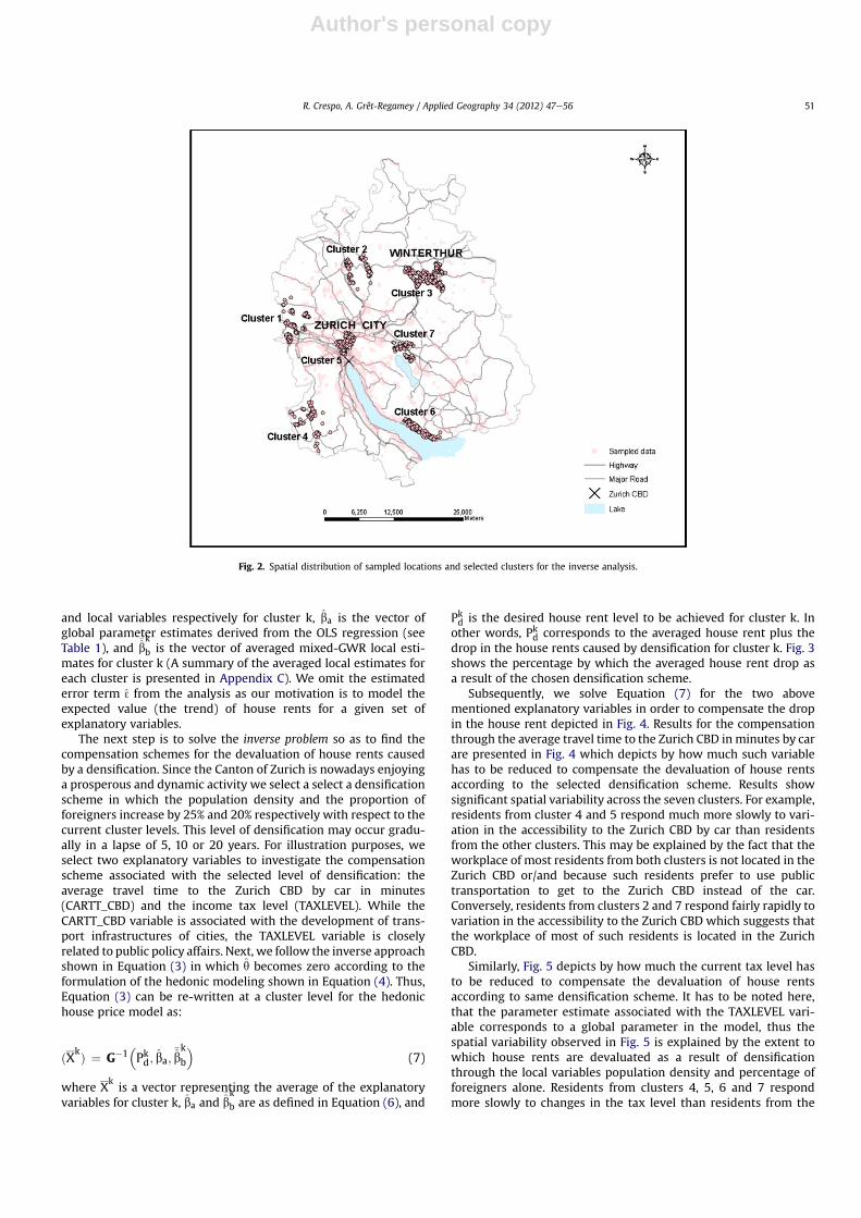
In order to explore the effects of increasing urban populationdensity on house prices in a statistically meaningful way, we selectseven clusters from the sampled locations to perform the densifi-cation analysis. As our intention is to produce spatially explicitresults, points of each cluster are selected and grouped together ina way that the distance to points of the nearest cluster rangesbetween 10 and 15 km. In this manner, each cluster is more likely torepresent a different submarket in the Zurich housing market. Ascan be seen in Fig. 2, cluster 5 is located in Zurich City which is themost populated city in the Canton and probably the most attractivecity for future inhabitants. Cluster 3 corresponds toWinterthur, thesecond most populated city in the Canton, and also a city that hasbeen enjoying and increasing economic activity over the lastdecades. Cluster 6 is located in one of the best-off residential areasin the Canton of Zurich. In fact, this cluster can be used in theanalysis as a representative example of most properties locatedalongside the lake of Zurich (the biggest lake in Fig. 2). In turn,clusters 1, 2, 4, and 7 represent various popular areas for residentswho commute to work in Zurich City. Note that the number, spatialarrangement, and size of clusters are additionally subject to thenumber and spatial distribution of the sampled data. A summary ofthe averaged explanatory variables for each cluster is presented inAppendix B.

At a cluster level, the average of house rent estimates (�̂Pk) isobtained as:

�̂Pk ¼ Xkab̂a þ X

kb�̂bk

b (6)

where k:1,.7 denotes the index of the cluster, Xka and X

kb are

matrices of averaged explanatory variables associated with global

Table 1OLS parameter estimates.

Variable Parameterestimates

Standarized parameterestimates

t-value

SQM 18.9 0.77 128.4*ISHOUSE 290 0.05 8.5*BUILBEF20 106.6 0.04 6.1*BUIL21TO30 166.7 0.03 5.6*BUIL81TO90 �36.4 �0.01 �2.7**BUIL91TO06 50.8 0.02 3.8*Log(CARTT_CBD) �697.4 �0.27 �36.3*PTACC 20.5 0.04 5.8*Log(RAILSTATION) �48.5 �0.04 �7.4*AUTOBAHN �128.7 �0.02 �3.7*AIRNOISE �85.2 �0.03 �5.9*HOTREST_JOBS 0.059 0.05 7.5*POP_DENS �0.708 �0.06 �9.9*FOREIGNERS �628.9 �0.03 �4.6*TAXLEVEL �2.37 �0.04 �6.3*SLOPE 1052 0.04 6.32*VIEW_LAKE 0.077 0.09 15.3*SOLAR_EVE 1073 0.10 17.7*

R-square ¼ 0.77.Moran’s I ¼ 0.16*.*: significant at 0.00% level.**: significant at 0.01% level.



and local variables respectively for cluster k, b̂a is the vector ofglobal parameter estimates derived from the OLS regression (seeTable 1), and

�̂bk

b is the vector of averaged mixed-GWR local esti-mates for cluster k (A summary of the averaged local estimates foreach cluster is presented in Appendix C). We omit the estimatederror term 3̂from the analysis as our motivation is to model theexpected value (the trend) of house rents for a given set ofexplanatory variables.

The next step is to solve the inverse problem so as to find thecompensation schemes for the devaluation of house rents causedby a densification. Since the Canton of Zurich is nowadays enjoyinga prosperous and dynamic activity we select a select a densificationscheme in which the population density and the proportion offoreigners increase by 25% and 20% respectively with respect to thecurrent cluster levels. This level of densification may occur gradu-ally in a lapse of 5, 10 or 20 years. For illustration purposes, weselect two explanatory variables to investigate the compensationscheme associated with the selected level of densification: theaverage travel time to the Zurich CBD by car in minutes(CARTT_CBD) and the income tax level (TAXLEVEL). While theCARTT_CBD variable is associated with the development of trans-port infrastructures of cities, the TAXLEVEL variable is closelyrelated to public policy affairs. Next, we follow the inverse approachshown in Equation (3) in which q̂ becomes zero according to theformulation of the hedonic modeling shown in Equation (4). Thus,Equation (3) can be re-written at a cluster level for the hedonichouse price model as:

ðXkÞ ¼ G�1�Pkd; b̂a;

�̂bk

b

�(7)

where Xkis a vector representing the average of the explanatory

variables for cluster k, b̂a and�̂bk

b are as defined in Equation (6), and

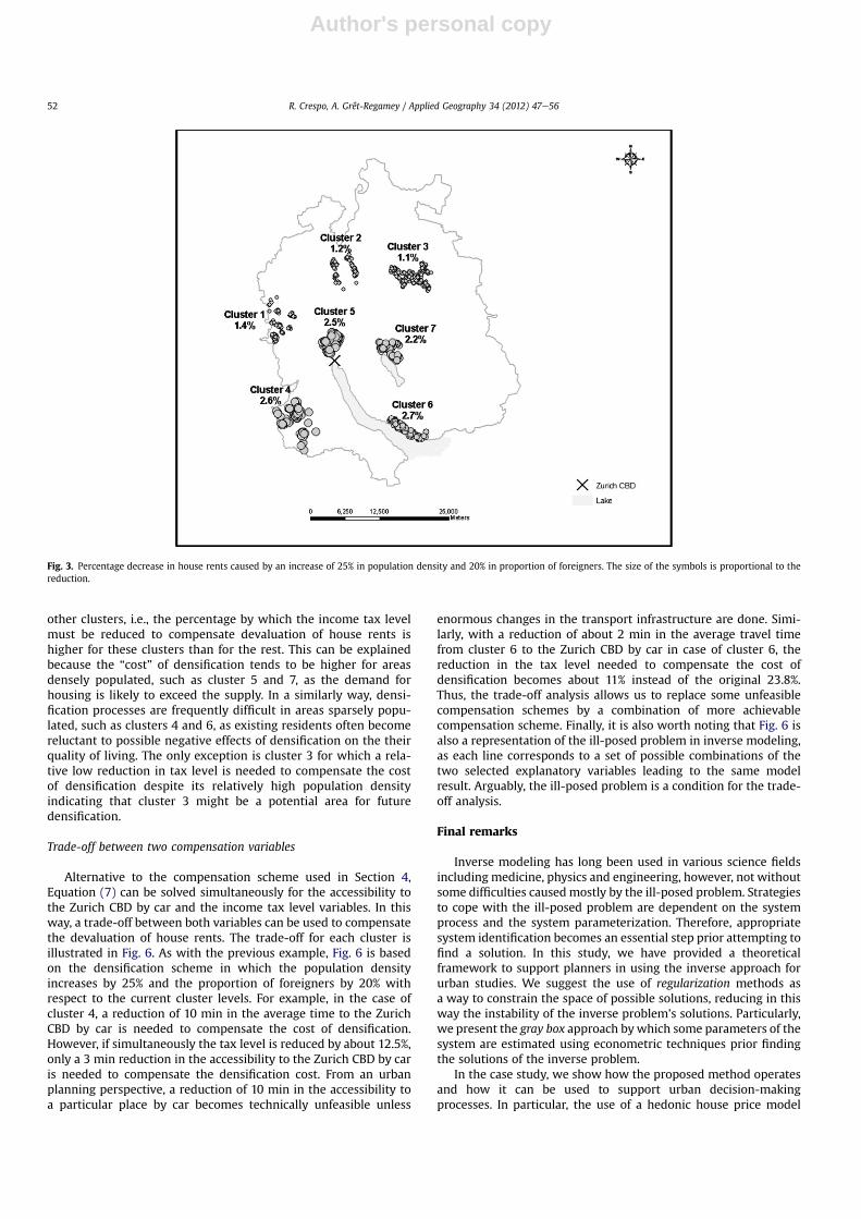
Pkd is the desired house rent level to be achieved for cluster k. Inother words, Pkd corresponds to the averaged house rent plus thedrop in the house rents caused by densification for cluster k. Fig. 3shows the percentage by which the averaged house rent drop asa result of the chosen densification scheme.

Subsequently, we solve Equation (7) for the two abovementioned explanatory variables in order to compensate the dropin the house rent depicted in Fig. 4. Results for the compensationthrough the average travel time to the Zurich CBD in minutes by carare presented in Fig. 4 which depicts by how much such variablehas to be reduced to compensate the devaluation of house rentsaccording to the selected densification scheme. Results showsignificant spatial variability across the seven clusters. For example,residents from cluster 4 and 5 respond much more slowly to vari-ation in the accessibility to the Zurich CBD by car than residentsfrom the other clusters. This may be explained by the fact that theworkplace of most residents from both clusters is not located in theZurich CBD or/and because such residents prefer to use publictransportation to get to the Zurich CBD instead of the car.Conversely, residents from clusters 2 and 7 respond fairly rapidly tovariation in the accessibility to the Zurich CBD which suggests thatthe workplace of most of such residents is located in the ZurichCBD.

Similarly, Fig. 5 depicts by how much the current tax level hasto be reduced to compensate the devaluation of house rentsaccording to same densification scheme. It has to be noted here,that the parameter estimate associated with the TAXLEVEL vari-able corresponds to a global parameter in the model, thus thespatial variability observed in Fig. 5 is explained by the extent towhich house rents are devaluated as a result of densificationthrough the local variables population density and percentage offoreigners alone. Residents from clusters 4, 5, 6 and 7 respondmore slowly to changes in the tax level than residents from the

Fig. 2. Spatial distribution of sampled locations and selected clusters for the inverse analysis.



other clusters, i.e., the percentage by which the income tax levelmust be reduced to compensate devaluation of house rents ishigher for these clusters than for the rest. This can be explainedbecause the “cost” of densification tends to be higher for areasdensely populated, such as cluster 5 and 7, as the demand forhousing is likely to exceed the supply. In a similarly way, densi-fication processes are frequently difficult in areas sparsely popu-lated, such as clusters 4 and 6, as existing residents often becomereluctant to possible negative effects of densification on the theirquality of living. The only exception is cluster 3 for which a rela-tive low reduction in tax level is needed to compensate the costof densification despite its relatively high population densityindicating that cluster 3 might be a potential area for futuredensification.

Trade-off between two compensation variables

Alternative to the compensation scheme used in Section 4,Equation (7) can be solved simultaneously for the accessibility tothe Zurich CBD by car and the income tax level variables. In thisway, a trade-off between both variables can be used to compensatethe devaluation of house rents. The trade-off for each cluster isillustrated in Fig. 6. As with the previous example, Fig. 6 is basedon the densification scheme in which the population densityincreases by 25% and the proportion of foreigners by 20% withrespect to the current cluster levels. For example, in the case ofcluster 4, a reduction of 10 min in the average time to the ZurichCBD by car is needed to compensate the cost of densification.However, if simultaneously the tax level is reduced by about 12.5%,only a 3 min reduction in the accessibility to the Zurich CBD by caris needed to compensate the densification cost. From an urbanplanning perspective, a reduction of 10 min in the accessibility toa particular place by car becomes technically unfeasible unless

enormous changes in the transport infrastructure are done. Simi-larly, with a reduction of about 2 min in the average travel timefrom cluster 6 to the Zurich CBD by car in case of cluster 6, thereduction in the tax level needed to compensate the cost ofdensification becomes about 11% instead of the original 23.8%.Thus, the trade-off analysis allows us to replace some unfeasiblecompensation schemes by a combination of more achievablecompensation scheme. Finally, it is also worth noting that Fig. 6 isalso a representation of the ill-posed problem in inverse modeling,as each line corresponds to a set of possible combinations of thetwo selected explanatory variables leading to the same modelresult. Arguably, the ill-posed problem is a condition for the trade-off analysis.

Final remarks

Inverse modeling has long been used in various science fieldsincluding medicine, physics and engineering, however, not withoutsome difficulties causedmostly by the ill-posed problem. Strategiesto cope with the ill-posed problem are dependent on the systemprocess and the system parameterization. Therefore, appropriatesystem identification becomes an essential step prior attempting tofind a solution. In this study, we have provided a theoreticalframework to support planners in using the inverse approach forurban studies. We suggest the use of regularization methods asa way to constrain the space of possible solutions, reducing in thisway the instability of the inverse problem’s solutions. Particularly,we present the gray box approach bywhich some parameters of thesystem are estimated using econometric techniques prior findingthe solutions of the inverse problem.

In the case study, we show how the proposed method operatesand how it can be used to support urban decision-makingprocesses. In particular, the use of a hedonic house price model

Fig. 3. Percentage decrease in house rents caused by an increase of 25% in population density and 20% in proportion of foreigners. The size of the symbols is proportional to thereduction.



Fig. 4. Reduction in the average time to Zurich CBD by car in minutes to compensate an increase of 25% in population density and 20% in percentage of foreigners. The size of thesymbols is proportional to the reduction.

Fig. 5. Percentage reduction in the income tax level to compensate an increase of 25% in population density and 20% in foreigners. The size of the symbols is proportional to thereduction.



allowed us to show how intrinsic problems related to urbanizationprocesses, such as densification, may negatively affect theeconomic value of properties in a metropolitan area. In this case,the desired outcome for the urban system under study must besuch that the economic loss caused by densification is compensatedby new levels of key variables chosen from a set of house deter-minants. In this study, we select two variables to illustrate thepower of the inverse approach with the densification problem: theincome tax level and the accessibility to the Zurich Central BusinessDistrict (CBD) by car. Of particular interest is the trade-off analysisof possible solutions shown in Fig. 6, because this is a representa-tion of how the ill-posed problem can also be used in favor of urbanplanning.

As a way to minimize the effects of the statistical uncertaintyassociated with the model estimates on the inverse model analysis,we perform the compensation analysis at cluster level and nota single building level. Averaged values of estimates reduced theinherent parameters uncertainty as extreme values are down-weighted so that the bias of predicted values is reduced.However, it is important to note that the accuracy of the results isalso dependent on the size of clusters. In general terms, it is arguedthat the bigger the size of the cluster, the higher the biased of theaveraged local estimates employed in the analysis. The statisticalaccuracy of the results is also subject to the spatial location of theselected clusters as the goodness-of-fit of the econometric tech-nique employed in the analysis (mixed-GWR) is most likely to varyover space. The mixed-GWR estimates tend to be more accurate inareas where the sample data is more densely distributed than inareas where data is scarcer.

In conclusion, despite these statistical limitations, this study hasshown that inverse modeling is a powerful tool for developingspatial plans utilizing future visions, especially if multiple variablesare employed to carry out trade-off analyses In fact, the morevariables are employed in the trade-off analysis, the broader thespace of possible solutions of the model becomes, facilitating in thisway the selection of alternative and feasible solutions for planners.In addition, it is also important to note that inverse approach inurban modeling is not necessarily subject to a specific planningproblem or mathematical model and so other statistical techniquesthan hedonic modeling can be used in future research. For example,

inverse modeling can be used as an alternative or complementaryapproach to traditional logistic land use change models (Bakkeret al., 2005; Verburg, van Eck, de Nijs, Dijst, & Schot, 2004;) aswell as to traditional spatial econometric models employed inregional converge studies as documented in Rey and Montouri(1999).

Further research may also address the inverse modelingapproach using spatio-temporal data. In such case, results of theinverse model might account for the initial conditions of the urbansystem evolving over time. Finally, it is worth pointing out thatinverse model approach can also be used in conjunction withbackcasting (Dreborg, 1996; Holmberg, 1998). For example, whilebackcasting can be employed to identify processes and importantsteps to reach desired future scenarios in sustainable urban plan-ning (Grêt-Regamey & Brunner, 2011), inverse modeling can beused to quantify the feasibility of various developing alternatives inorder to reach such scenarios.

Acknowledgments

The authors would like to thank Michael Löchl and KayAxhausen (Institute for Transport Planning and Systems, ETH Zur-ich) for providing us with the Zurich house price dataset we used tocarry out our work. Such dataset was created and employed byMichael as part of his PhD thesis under the supervision of KayAxhausen.

Appendix A. Descriptive statistics of the model’s variables

Fig. 6. Trade-off between tax level and accessibility to the Zurich CBD by car.

Variable Typea Description Min Max Mean

Response variableRENT C Monthly net asking rent in CHF 476 15,000 1841Explanatory variables1.- Structural variablesSQM C Floor area in square meter 20 400 91.3ISHOUSE D Is 1 if the property is a single

family house, 0 otherwise.0 1

BUILBEF20 D Is 1 if the property was built prior1920, 0 otherwise.

0 1

BUIL21TO30 D Is 1 if the property was builtbetween 1921 and 1930.

0 1

BUIL31TO80b D Is 1 if the property was builtbetween 1931 and 1980.

0 1


0 1


0 1

2.- Locational variablesCARTT_CBD C Average travel time to the Zurich

Central Business District by car inminutes.

8 58.4 29.9

PTACC C Regional public transportaccessibility to employment.

�19.4 12.4 10.7

RAILSTATION C Euclidean distance to next railstation in km.

0.013 5.732 0.911

HIGHWAY D Is 1 if highway located within100 m, 0 otherwise.

0 1

AIRNOISE D Is 1 is daily average air noise isabove 52 dB, 0 otherwise

0 1

SLOPE C Slope by 25 m raster 0.00 0.26 0.036VIEW_LAKE C Visibilityc of lake surface

(>1 sqkm) in hectares0.0 441.8 8887.8

SOLAR_EVE C Evening solar exposure index 0.0 607.1 238.23.- Socioeconomic variablesHOTREST_JOBS C Number of jobs in hotel and

restaurant industry within 1 km.1.2 7083.8 314.0

POP_DENS C Number of inhabitants in hectare 1.0 2004.0 93.5



Appendix B. Summary of the main exploratory variables foreach cluster

(continued )

Variable Typea Description Min Max Mean

FOREIGNERS C Percentage of foreignersd inhectare

0.00 0.50 0.05

TAXLEVEL C Local income tax level aspercentage of the basic cantonaltax

69.0 122.0 110.3

a C ¼ continuous; D ¼ binary.b Reference case, therefore this variable is not included in the calibration of the

hedonic house price model.c Visibility of VIEW_LAKE variable is calculated based on 25 m DEM, not

considering objects such as buildings or trees.d Foreigners are defined as inhabitants with nationalities outside of North-

Western Europe, North America and Australia.

Cluster 1

Number of properties selected 211Average house price (monthly net rent in CHF) 1619Average floor area (SQM) 89.8Number of flats (ISHOUSE ¼ 0) 211Number of properties built prior 1920 (BUILBEFO20) 12Number of properties built between 1921 and 1930 (BUIL21TO30) 2Number of properties built between 1931 and 1980 (BUIL31TO80) 108Number of properties built between 1981 and 1990 (BUIL81TO90) 42Number of properties built between 1991 and 2006 (BUIL91TO06) 47Average travel time to the Zurich CBD by car in minutes (CARTT_CBD) 33.4Regional public transport accessibility to employment (PTACC) 10.8Visibility of lake surface (VIEW_LAKE) 0Average tax level (TAXLEVEL) 106.8Average number of jobs in hotel and restaurant industry within 1 km

(HOTREST_JOBS)91

Average population density in hectare (POP_DENS) 93.5Average proportion of foreigners in hectare (FOREIGNERS) 0.051

Cluster 2

Number of properties selected 233Average house price (monthly net rent in CHF) 1718Average floor area (SQM) 98.5Number of flats (ISHOUSE ¼ 0) 233Number of properties built prior 1920 (BUILUNTI20) 12Number of properties built between 1921 and 1930 (BUIL21TO30) 0Number of properties built between 1931 and 1980 (BUIL31TO80) 88Number of properties built between 1981 and 1990 (BUIL81TO90) 63Number of properties built between 1991 and 2006 (BUIL91TO06) 70Average travel time to the Zurich CBD by car in minutes (CARTT_CBD) 36.3Regional public transport accessibility to employment (PTACC) 9.8Visibility of lake surface (VIEW_LAKE) 0Average tax level (TAXLEVEL) 108.7Average number of jobs in hotel and restaurant industrywithin 1 km (HOTREST_JOBS) 117.4Average population density in hectare (POP_DENS) 83.9Average proportion of foreigners in hectare (FOREIGNERS) 0.042

Cluster 3

Number of properties selected 421Average house price (monthly net rent in CHF) 1473Average floor area (SQM) 83.6Number of flats (ISHOUSE ¼ 0) 421Number of properties built prior 1920 (BUILUNTI20) 40Number of properties built between 1921 and 1930 (BUIL21TO30) 12Number of properties built between 1931 and 1980 (BUIL31TO80) 246Number of properties built between 1981 and 1990 (BUIL81TO90) 54Number of properties built between 1991 and 2006 (BUIL91TO06) 69Average travel time to the Zurich CBD by car in minutes (CARTT_CBD) 43.1Regional public transport accessibility to employment (PTACC) 10.7Visibility of lake surface (VIEW_LAKE) 0Average tax level (TAXLEVEL) 122Average number of jobs in hotel and restaurant industrywithin 1 km (HOTREST_JOBS) 242.8Average population density (POP_DENS) 108.9Average proportion of foreigners (FOREIGNERS) 0.05

(continued)

Cluster 4

Number of properties selected 180Average house price (monthly net rent in CHF) 1877Average floor area (SQM) 106.7Number of flats (ISHOUSE ¼ 0) 180Number of properties built prior 1920 (BUILUNTI20) 19Number of properties built between 1921 and 1930 (BUIL21TO30) 0Number of properties built between 1931 and 1980 (BUIL31TO80) 40Number of properties built between 1981 and 1990 (BUIL81TO90) 53Number of properties built between 1991 and 2006 (BUIL91TO06) 68Average travel time to the Zurich CBD by car in minutes (CARTT_CBD) 39.0Regional public transport accessibility to employment (PTACC) 10.4Visibility of lake surface (VIEW_LAKE) 211.2Average tax level (TAXLEVEL) 188.3Average number of jobs in hotel and restaurant industrywithin 1 km (HOTREST_JOBS) 51.0Average population density (POP_DENS) 61.5Average proportion of foreigners (FOREIGNERS) 0.04

Cluster 5

Number of properties selected 302Average house price (monthly net rent in CHF) 1788Average floor area (SQM) 76.2Number of flats (ISHOUSE ¼ 0) 302Number of properties built prior 1920 (BUILUNTI20) 82Number of properties built between 1921 and 1930 (BUIL21TO30) 32Number of properties built between 1931 and 1980 (BUIL31TO80) 118Number of properties built between 1981 and 1990 (BUIL81TO90) 54Number of properties built between 1991 and 2006 (BUIL91TO06) 16Average travel time to the Zurich CBD by car in minutes (CARTT_CBD) 18.4Regional public transport accessibility to employment (PTACC) 12.0Visibility of lake surface (VIEW_LAKE) 458.1Average tax level (TAXLEVEL) 122Average number of jobs in hotel and restaurant industry within 1 km

(HOTREST_JOBS)1305.8

Average population density (POP_DENS) 141.3Average proportion of foreigners (FOREIGNERS) 0.07

Cluster 6

Number of properties selected 195Average house price (monthly net rent in CHF) 2024Average floor area (SQM) 98.2Number of flats (ISHOUSE ¼ 0) 195Number of properties built prior 1920 (BUILUNTI20) 28Number of properties built between 1921 and 1930 (BUIL21TO30) 7Number of properties built between 1931 and 1980 (BUIL31TO80) 103Number of properties built between 1981 and 1990 (BUIL81TO90) 12Number of properties built between 1991 and 2006 (BUIL91TO06) 45Average travel time to the Zurich CBD by car in minutes (CARTT_CBD) 38.1Regional public transport accessibility to employment (PTACC) 10.2Visibility of lake surface (VIEW_LAKE) 2184.2Average tax level (TAXLEVEL) 96.1Average number of jobs in hotel and restaurant industry within 1 km

(HOTREST_JOBS)67.1


Cluster 7

Number of properties selected 259Average house price (monthly net rent in CHF) 1635Average floor area (SQM) 92.5Number of flats (ISHOUSE ¼ 0) 259Number of properties built prior 1920 (BUILUNTI20) 4Number of properties built between 1921 and 1930 (BUIL21TO30) 0Number of properties built between 1931 and 1980 (BUIL31TO80) 132Number of properties built between 1981 and 1990 (BUIL81TO90) 52Number of properties built between 1991 and 2006 (BUIL91TO06) 71Average travel time to the Zurich CBD by car in minutes (CARTT_CBD) 31.3Regional public transport accessibility to employment (PTACC) 10.8Visibility of lake surface (VIEW_LAKE) 221.7Average tax level (TAXLEVEL) 101.8Average number of jobs in hotel and restaurant industry within 1 km

(HOTREST_JOBS)90.6




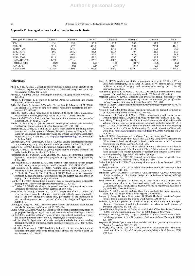
Appendix C. Averaged values local estimates for each cluster

References

Allen, J., & Lu, K. (2003). Modeling and prediction of future urban growth in theCharleston Region of South Carolina: a GIS-based integrated approach.Conservation Ecology, 8(2), art. 2.

Arridge, S. R. (1999). Optical tomography in medical imaging. Inverse Problems, 15,R41eR93.

Ashter, R., Borchers, B., & Thurber, C. (2005). Parameter estimation and inverseproblems. Academic Press.

Bakker, M., Gover, G., Kosmas, C., Vanacker, V., van Oost, K., & Rounsevell, M. (2005).Soil erosion as a driver of land-use change. Agriculture, Ecosystems and Envi-ronment, 105, 467e481.

Batty, M. (2009). Urban modelling. In R. Kitchin, & N. Thrift (Eds.), Internationalencyclopedia of human geography, Vol. 12 (pp. 51e58). Oxford: Elsevier.

Baynes, Y. (2009). Complexity in urban development and management. Journal ofIndustrial Ecology, 13(2), 214e227.

Bender, B., & Hwang, H. (1985). Hedonic house price indices and secondaryemployment centers. Journal of Urban Economics, 17(1), 90e107.

Bretagnolle, A., Daudé, E., & Pumain, D. (2003). From theory to modeling: urbansystems as complex systems. Cybergeo: European Journal of Geography, 13thEuropean Colloquium on Quantitative and Theoretical Geography, Lucca, Italy,September 8e11, article 335. URL. http://cybergeo.revues.org/2420 Consultedon 24 June 2011.

Courdurier, M., Noo, F., Defrise, M., & Kudo, H. (2008). Solving the interior problem ofcomputed tomography using a priori knowledge. Inverse Problems, 24, 065001.

Dreborg, K. H. (1996). Essence of backcasting. Futures, 28(9), 813e828.Engl, H., Hanke, M., & Neubauer, A. (2000). Regularization of inverse problems. the

Netherlands: Kluwer Academic Publishers.Fotheringham, S., Brunsdon, C., & Charlton, M. (2002). Geographically weighted

regression: The analysis of spatial varying relationships. West Sussex: John Wiley& Sons Ltd.

Grêt-Regamey, A., & Brunner, S. H. (2011). Methodischer Rahmen für den Einsatzvon Backcasting zur Anpassung an den Klimawandel. disP, 184(1), 43e51.

Grêt-Regamey, A., & Crespo,, R. (2011). Planning from a future vision: inversemodeling in spatial planning. Environmental and Planning B. doi:10.1068/b37083.

He, C., Okada, N., Zhang, Q., Shi, P., & Zhang, J. (2006). Modeling urban expansionscenarios by coupling cellular automata model and system dynamic model inBeijing, China. Applied Geography, 323e345.

Holmberg, J. (1998). Backcasting: a natural step in operationalising sustainabledevelopment. Greener Management International, 23, 30e50.

Hu, Z., & Lo, C. P. (2007). Modeling urban growth in Atlanta using logistic regression.Computers, Environment and Urban Systems, 31, 667e688.

Jones, D. M., Watton, J., & Brown, K. J. (2007). Comparison of black-, white- andgrey-box models to predict ultimate tensile strength of high-strength hot rolledcoils at the Port Talbot hot spring mill, proceeding of the institution ofmechanical engineers, part L. Journal of Materials: Design and Applications,221(1), 1e9.

Landis, J., & Zhang, M. (1998). The second generation of the California urban futuresmodels. Environment and Planning B, 25, 795e824.

Leung, Y.,Mei, C., & Zhang,W. (2000). Statistical test for spatial nonstationary based ongeographicallyweightedregressionmodel.Environmental andPlanningA, 32, 9e31.

Liu, Y. (2008). Modelling urban development with geographical information systemsand cellular automata. New York: CRC Press/Taylor & Francis Group.

Loech, M. (2010). Application of spatial analysis methods for understandinggeographic variation of prices, demand and market success. ETH, . doi:10.3929/ethz-a-006186826.

Loech, M., & Axhausen, K. (2010). Modelling hedonic rent prices for land use andtransport simulation while considering spatial effects. The Journal of Land Useand Transport, 3(2), 39e63.

Louis, A. (1997). Application of the approximate inverse to 3D X-ray CT andultrasound tomography. In H. Engl, A. Louis, & W. Rendell (Eds.), Inverseproblems in medical imaging and nondestructive testing (pp. 120e133).SpringerMatemathics.

Maithani, S., Jain, R. K., & Arora, M. K. (2007). An artificial neural network basedapproach for modeling urban spatial growth. ITPI Journal, 4(2), 43e51.

Martinez-Luaces, V. (2009). Modeling and inverse-modeling: experiences withO.D.E linear systems in engineering courses. International Journal of Mathe-matical Education in Science and Technology, 40(2), 259e268.

Menke, W. (1989). Geophysical data analysisIn International geophysics series, Vol. 45.Academic Press.

Nelson, J. (1978). Residential choice, hedonic prices, and the demand for urban airquality. Journal of Urban Economics, 5, 357e369.

Ottensmann, J. R., Payton, S., & Man, J. (2008). Urban location and housing priceswithin hedonic model. The Journal of Policy Analysis and Policy, 38(1), 19e35.

Ou, X., Zhang, Y., Ren, J., & Yao, D. (2003). A neural network model for urban trafficvolumes compression. Journal of Systemic Cybernetics and Informatics, 1(4), 1e7.

Pajonk, O. (2009). Overview of systems identification with focus on inverse modeling.Germany: Institute of Scientific Computing, Technical University of Braunsch-weig. URL. http://www.digibib.tu-bs.de/%3fdocid=00030245 Consulted on 24June 2011.

Parker, R. (1994). Geophysical inverse theory. Princeton University Press.Pijanowski, B., Brown, D., Shellito, B., & Manik, G. (2002). Using neural networks and

GIS to forecast land use changes: a land transformation model. Computers,Environment and Urban Systems, 26, 553e575.

Rabino, G., & Lagui, A. (2002). Urban cellular automata: the inverse problem. InS. Bandini, B. Chopard, & M. Tomassini (Eds.), Cellular automata, 5th Interna-tional conference on cellular automata for research and industry, Geneva, Swit-zerland, proceedings (pp. 349e356). Berlin: Springer.

Rey, S., & Montouri, B. (1999). US regional income convergence: a spatial econo-metric perspective. Regional Studies, 33(2), 143e156.

Scales, J., & Snieder, R. (2000). The anatomy of inverse problems. Geophysics, 65(6),1708e1710.

Scales, J., & Tenorio, L. (2001). Prior information and uncertainty in inverse problem.Geophysics, 66, 389e397.

Schneider, P., Mossi, A., Franca, F., de Sousa, F., & da Silva Neto, A. (2009). Applicationof inverse analysis to illumination design. Inverse Problem in Science and Engi-neering, 17, 737e753.

Soemarwoto, B., Labrujere, Th., Laban, M., & Yanshah, H. (2009). Inverse aero-dynamic shape design for improved wing buffet-onset performance. InG. Dulikravich, & M. Tanaka (Eds.), Inverse problems in engineering mechanics II(pp. 419e428). Elsevier Science.

Tarantola, A. (2005). Inverse problem theory and methods for model parameterestimation. Society for Industrial and Applied Mathematics, .

Tarduno, J., Bunge, H., Sleep, N., & Hansen, U. (2009). The bent Hawaiian-Emperorhotspot track: inheriting the mantle wind. Science, 324, 50e53.

Tsekeris, T., & Stathopoulos, A. (2006). Gravity models for dynamic transportplanning: development and implementation in urban network. Journal ofTransport Geography, 14, 152e160.

United Nations, Department of Economics and Social Affairs, Population Division.(2009). World urbanization prospects. The 2009 Revision, New York.

Verburg, P., van Eck, J., de Nijs, T., Dijst, M., & Schot, P. (2004). Determinants of land-use change patterns in the Netherlands. Environmental and Planning B, 31(1),125e150.

Wegener, M. (1994). Operational urban models state of art. Journal of the AmericanPlanning Association, 60(1), 17e29.

Zhang, H., Zeng, Y., Bian, L., & Yu, X. (2010). Modelling urban expansion using agentbased model in the city of Changsha. Journal of Geographical Systems, 20(4),540e556.

Averaged local estimates Cluster 1 Cluster 2 Cluster 3 Cluster 4 Cluster 5 Cluster 6 Cluster 7

SQM 13.1 13.0 13.7 13.7 20.9 17.7 12.3ISHOUSE 561.6 �27.5 473.3 376.3 353.2 786.4 414.0BUILUNTI20 162.2 227.1 51.2 154.6 143.6 99.1 81.2BUIL21TO30 �56.3 664.2 115.1 263.4 10.4 128.6 �81.6BUIL81TO90 34.7 �46.5 �13.4 97.2 �67.9 44.8 38.8BUIL91TO06 191.8 108.6 122.6 192.2 19.7 113.5 298.0Log(CARTT_CBD) �142.0 �831.4 �125.6 �168.5 �107.6 �550.8 �919.3HOTREST_JOBS �0.29 0.26 0.25 1.05 0.075 �0.45 �0.20POP_DENS �0.57 �0.55 �0.14 �2.44 �0.78 �2.9 �0.84FOREIGNERS �1014.0 �980.8 �1229.4 �1598.7 �1239.7 �1893.0 �1664.5


Inverse modelling applied geography

Documents

Transcript of Inverse modelling applied geography