Nisu Dialect Geography

Cathryn Yang

SIL International 2009

SIL Electronic Survey Report 2009-007, June 2009 Copyright © 2008 Cathryn Yang and SIL International All rights reserved

2

Contents Abstract

1. Introduction 1.1 Purpose 1.2 Background 1.3 Nisu phonemic inventory 1.4 Previous classifications of Nisu varieties 1.5 Revised classification of Nisu dialects 1.6 Scope of this research

2. Isoglossic patterns 2.1 Lexical isoglosses 2.2 Phonological isoglosses

2.2.1 Development of / ɬ/ and /tʰ/ 2.2.2 Development of retroflex affricates and fricatives 2.2.3 Development of /ə˞/ and /ɛ/ 2.2.4 Development of *ak

2.3 Morphological isogloss

3. Intelligibility test results 3.1 Background 3.2 Methodology 3.3 Results

3.3.1 Comprehension levels for SP LW (NC) 3.3.2 Comprehension levels for JC GQ (NC) 3.3.3 Comprehension levels for SP NJ (S) text

4 Levenshtein distance 4.1 Background 4.2 Methodology 4.3 Results

4.3.1 Cluster analysis 4.3.2 Correlation between Levenshtein distance and intelligibility

5 Conclusions

Appendix 1: Abbreviations for data locations

Appendix 2: Complete data tables

Appendix 3: RTT results

Appendix 4: Levenshtein distance table

References:

3

Abstract Nisu, a Burmic language spoken in Yunnan, China, is traditionally divided into three dialects: Yuan-jin, E-xin, and Shi-jian (Chen et al., 1985; Zhu, 2005). However, little evidence has been presented to justify this grouping, and the degrees of difference between dialects have been left unexplored. In this research paper, I re-examine Nisu dialect clusters using several complementary methodologies: comparative dialectology, intelligibility testing, and a recently developed quantitative measure of pronunciation differences known as Levenshtein distance (Heeringa, 2004). I propose a basic division between Northern and Southern Nisu, with a subordinate isogloss dividing Northern into Northwestern and North Central. This classification is similar to, but not identical with, the one originally proposed by Chen et al. 1985: Southern is roughly equivalent to Yuan-jin, while Northern encompasses E-xin (Northwestern) and Shi-jian (North Central). The primary differences between the two analyses lie in the supporting evidence and clustering hierarchy. Beyond clarifying the main divisions in Nisu, this research also represents the first application of Levenshtein distance to a tonal language in the Sinosphere, with results to suggest it as a useful tool for future work in Burmic-dialect geography.

1. Introduction

1.1 Purpose This research focuses on the following three questions: 1) what are the differences between Nisu varieties? 2) what are the relative degrees of differences between the varieties, and 3) what impact do these differences have on intelligibility? Each question will be the focus of one of three complementary methodologies. Comparative analysis from dialectology and historical linguistics reveals lexical, phonological, and morphological isoglosses, revealing the geographic distribution of specific linguistic variables.1 Levenshtein distance, a dialectometric tool for measuring linguistic distance, reveals the relative degree of difference between Nisu dialect clusters by measuring the aggregate differences in pronunciation. Intelligibility tests, known as Recorded Text Testing (RTT), show what impact these differences have on inherent intelligibility.

1.2 Background The genetic classification of all Nisu varieties is Sino-Tibetan, Tibeto-Burman, Burmic, Ngwi (formerly Loloish), and Northern Ngwi (Bradley, 1997). Other Northern Ngwi languages are Nasu and Nosu, both spoken to the north of Nisu populations. Nisu are mainly located in south-central Yunnan, which has led Chinese linguists to classify Nisu as a “Southern Yi” dialect (Chen et al., 1985). Bradley (1997) estimates there are 600,000 1 I gratefully acknowledge Yang Liujin of the Honghe Prefecture Ethnic Research Institute and Bai Bibo of Yuxi Teacher’s College for organizing the logistics of data collection. I also wish to thank Ken Chan and Pu Meishan for their contribution to the planning and data collection process; Eric Jackson for his help with the RuG-L04 software, Irene Tucker for her work on the maps; and Dr. David Bradley and Eric Johnson for their comments on earlier versions of this paper. Remaining errors are solely my own.

4

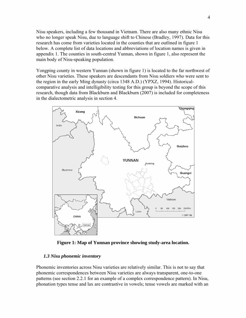
Nisu speakers, including a few thousand in Vietnam. There are also many ethnic Nisu who no longer speak Nisu, due to language shift to Chinese (Bradley, 1997). Data for this research has come from varieties located in the counties that are outlined in figure 1 below. A complete list of data locations and abbreviations of location names is given in appendix 1. The counties in south-central Yunnan, shown in figure 1, also represent the main body of Nisu-speaking population. Yongping county in western Yunnan (shown in figure 1) is located to the far northwest of other Nisu varieties. These speakers are descendants from Nisu soldiers who were sent to the region in the early Ming dynasty (circa 1348 A.D.) (YPXZ, 1994). Historical-comparative analysis and intelligibility testing for this group is beyond the scope of this research, though data from Blackburn and Blackburn (2007) is included for completeness in the dialectometric analysis in section 4.

Figure 1: Map of Yunnan province showing study-area location.

1.3 Nisu phonemic inventory Phonemic inventories across Nisu varieties are relatively similar. This is not to say that phonemic correspondences between Nisu varieties are always transparent, one-to-one patterns (see section 2.2.1 for an example of a complex correspondence pattern). In Nisu, phonation types tense and lax are contrastive in vowels; tense vowels are marked with an

5

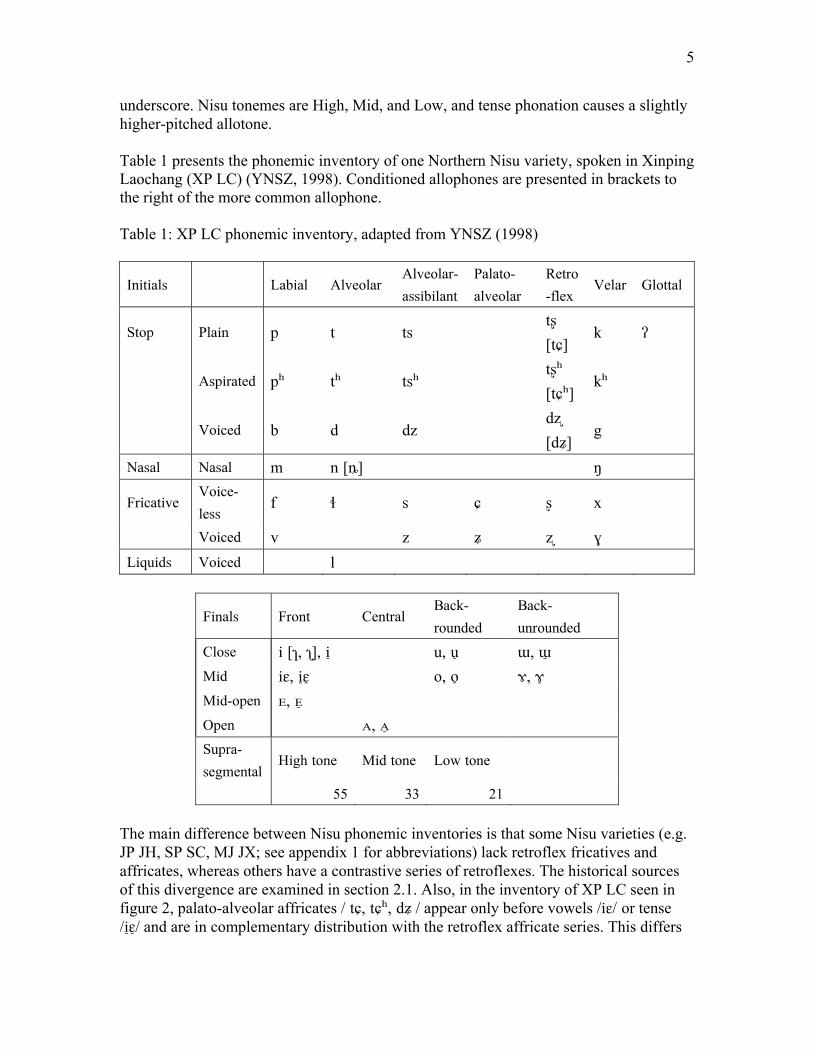
underscore. Nisu tonemes are High, Mid, and Low, and tense phonation causes a slightly higher-pitched allotone. Table 1 presents the phonemic inventory of one Northern Nisu variety, spoken in Xinping Laochang (XP LC) (YNSZ, 1998). Conditioned allophones are presented in brackets to the right of the more common allophone. Table 1: XP LC phonemic inventory, adapted from YNSZ (1998)

Initials Labial Alveolar Alveolar-assibilant

Palato-alveolar

Retro-flex

Velar Glottal

Stop Plain p t ts tʂ [tɕ]

k ʔ

Aspirated pʰ tʰ tsʰ tʂʰ [tɕʰ]

kʰ

Voiced b d dz dʐ [dʑ]

g

Nasal Nasal m n [ȵ] ŋ

Fricative Voice-less

f ɬ s ɕ ʂ x

Voiced v z ʑ ʐ ɣ Liquids Voiced l

Finals Front Central Back-rounded

Back-unrounded

Close i [ɿ, ʅ], i ̠ u, u̠ ɯ, ɯ̠ Mid iɛ, iɛ̠ ̠ o, o̠ ɤ, ɤ̠ Mid-open ᴇ, ᴇ̠ Open ᴀ, ᴀ̠ Supra-segmental

High tone Mid tone Low tone

55 33 21 The main difference between Nisu phonemic inventories is that some Nisu varieties (e.g. JP JH, SP SC, MJ JX; see appendix 1 for abbreviations) lack retroflex fricatives and affricates, whereas others have a contrastive series of retroflexes. The historical sources of this divergence are examined in section 2.1. Also, in the inventory of XP LC seen in figure 2, palato-alveolar affricates / tɕ, tɕʰ, dʑ / appear only before vowels /iɛ/ or tense /iɛ̠/̠ and are in complementary distribution with the retroflex affricate series. This differs

6

from the phonemic inventory of Honghe (Wang, 2003) and Eshan (Chen et al., 1985), where the palato-alveolar affricates do contrast with both alveolar and retroflex affricates.

1.4 Previous classifications of Nisu varieties Chen et al. (1985) classifies Nisu as having three dialects, labeled by key counties: Yuanjiang-Jinping, Shiping-Jianshui, and Eshan-Xinping (abbreviated as the first syllable of each county, i.e. Yuan-Jin, Shi-Jian, and E-Xin). Zhu (2005) and Grimes (2005) echo this classification based on Chen et al. The only difference between Chen et al. and Zhu (2005) is that Zhu refers to Chen’s Yuan-Jin as Yuan-Mo, referring to Mojiang instead of Jinping. Wang (2003) does not group Nisu into separate dialects, instead asserting that speakers of all Nisu varieties can communicate with each other. No justification for this classification scheme is given in any of the sources and is probably based on Chen et al.’s perceptions of difference. Since the dialect labels refer to counties as whole units, it is also unclear what varieties within the counties they are referring to, since different varieties are often found in different parts of the same county. Yuan-jin/Yuan-mo refers to the variety spoken in the following counties: Honghe, Yuanyang, Jinping, Mojiang, Pu’er, Jiangcheng, and Yuanjiang. Zhu (2005) calls this area Southwestern. He further subdivides this group into Yuanyang variety, spoken in Yuanyang and Jinping; and Mojiang variety, spoken in Mojiang, Yuanjiang, Simao, Jiangcheng, Pu’er, and Honghe. Shi-jian includes Nisu spoken in Shiping, Jianshui, Tonghai, Gejiu, Kaiyuan, Mengzi, and Hekou. Zhu (2005) refers to this group as Eastern and further subdivides into Shiping subdialect, spoken in Shiping (Longwu), Jianshui, and Tonghai (Qilu); and Gejiu subdialect, spoken in Gejiu, Kaiyuan, Mengzi, and Pinbian. Shiping subdialect is also spoken in parts of Xinping, Hongta qu, and southeast Eshan, where E-xin speakers are also found. E-xin dialect is spoken in Eshan, Xinping, Yimen, Jiangchuan, and Hongta qu. Zhu (2005) calls this region Northwestern and adds Tonghai and parts of Kunming (including Jinning county). E-xin speakers use the autonym “Nasu,” not to be confused with the other Northern Ngwi Nasu, spoken to the north in Kunming (especially Luquan), and further east into Guizhou.

1.5 Revised classification of Nisu dialects Based on shared linguistic innovations, intelligibility test results, and Levenshtein distance, I propose a revised classification of Nisu varieties. Nisu can be divided into Northern and Southern dialect groups. Southern (S) Nisu roughly corresponds to Chen et al.’s (1985) Yuan-jin group. The geographic region where Southern Nisu is spoken follows along the Honghe river valley and the south-central mountains of the Ailao mountain range; this area is the southern region of the main Nisu population, hence the

7

name Southern. Northern (N) Nisu encompasses Chen et al.’s Shi-jian and E-xin groups: Shi-jian is referred to as North central (NC) and E-xin as Northwestern (NW). There are two main differences between this revised classification scheme and that of Chen et al.. First, Nisu varieties spoken in Jiangcheng, Mojiang, and Lvchun counties are found to linguistically affiliate with NC, not with S; this diverges from their previous classification in the Yuan-jin group. Migration patterns from NC-speaking areas to these three counties in the past 100-150 years explain why these varieties group with NC and not S (Li Guangyun et al., 1990). Secondly, I group NC and NW as two sub-clusters within Northern Nisu dialect group, based on shared innovations, high levels of mutual intelligibility, and low Levenshtein distances. This hierarchy in the dialect clustering differs from Chen et al.’s non-hierarchical grouping of Nisu as three different varieties.

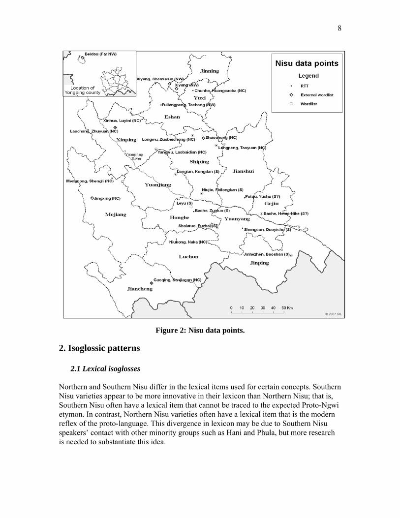
1.6 Scope of this research During 2006, data in the form of word lists and recorded text tests were collected in twenty different Nisu villages, located in S, NC, and NW speaking areas. See appendix 1 for exact location of data points and abbreviations of data point names. Seven other wordlists were compiled from published and unpublished sources (Bradley et al., 2002; Sun et al., 1991; Pu et al., 2005; YNSZ, 1998; Blackburn et al., 2007; Pu, 2005; see appendix 1 for complete list). Data points used in this research are shown in figure 2:

8

Figure 2: Nisu data points.

2. Isoglossic patterns

2.1 Lexical isoglosses Northern and Southern Nisu differ in the lexical items used for certain concepts. Southern Nisu varieties appear to be more innovative in their lexicon than Northern Nisu; that is, Southern Nisu often have a lexical item that cannot be traced to the expected Proto-Ngwi etymon. In contrast, Northern Nisu varieties often have a lexical item that is the modern reflex of the proto-language. This divergence in lexicon may be due to Southern Nisu speakers’ contact with other minority groups such as Hani and Phula, but more research is needed to substantiate this idea.

9

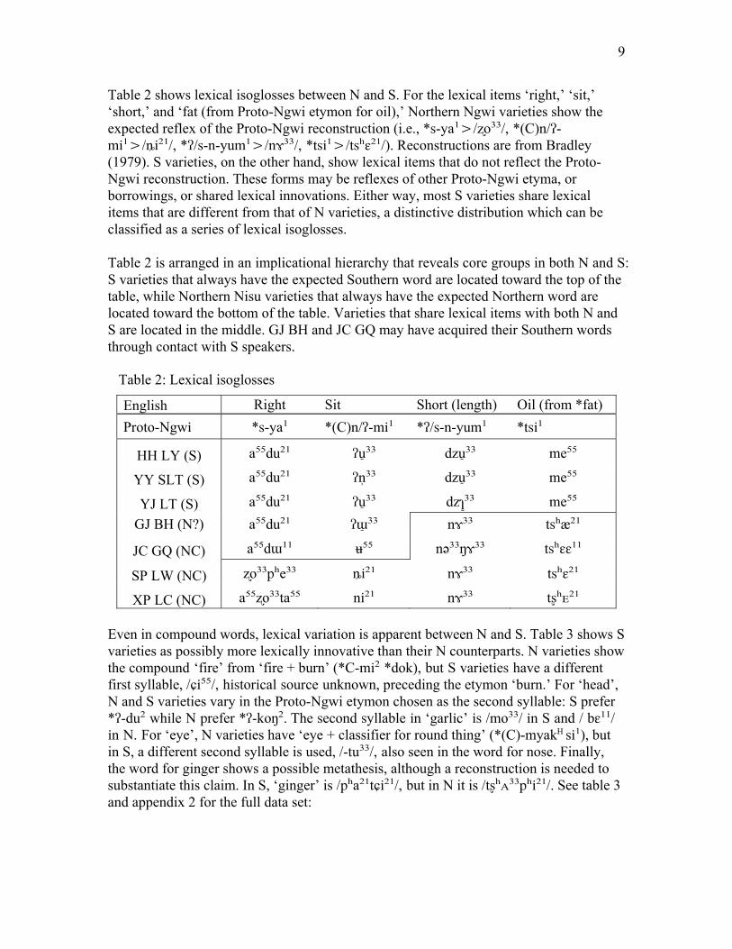
Table 2 shows lexical isoglosses between N and S. For the lexical items ‘right,’ ‘sit,’ ‘short,’ and ‘fat (from Proto-Ngwi etymon for oil),’ Northern Ngwi varieties show the expected reflex of the Proto-Ngwi reconstruction (i.e., *s-ya¹>/ʐo³³/, *(C)n/ʔ-mi¹>/ȵi²¹/, *ʔ/s-n-yum¹>/nɤ³³/, *tsi¹>/tsʰɛ²¹/). Reconstructions are from Bradley (1979). S varieties, on the other hand, show lexical items that do not reflect the Proto-Ngwi reconstruction. These forms may be reflexes of other Proto-Ngwi etyma, or borrowings, or shared lexical innovations. Either way, most S varieties share lexical items that are different from that of N varieties, a distinctive distribution which can be classified as a series of lexical isoglosses. Table 2 is arranged in an implicational hierarchy that reveals core groups in both N and S: S varieties that always have the expected Southern word are located toward the top of the table, while Northern Nisu varieties that always have the expected Northern word are located toward the bottom of the table. Varieties that share lexical items with both N and S are located in the middle. GJ BH and JC GQ may have acquired their Southern words through contact with S speakers.

Table 2: Lexical isoglosses

English Right Sit Short (length) Oil (from *fat) Proto-Ngwi *s-ya¹ *(C)n/ʔ-mi¹ *ʔ/s-n-yum¹ *tsi¹

HH LY (S) a⁵⁵du²¹ ʔu̠³³ dzu ̠³³ me⁵⁵

YY SLT (S) a⁵⁵du²¹ ʔn̩³³ dzu ̠³³ me⁵⁵

YJ LT (S) a⁵⁵du²¹ ʔu̠³³ dzɿ³̠³ me⁵⁵ GJ BH (N?) a⁵⁵du²¹ ʔɯ̠³³ nɤ³³ tsʰæ²¹

JC GQ (NC) a⁵⁵dɯ¹¹ ʉ⁵⁵ nə³³ŋɤ³³ tsʰɛɛ¹¹

SP LW (NC) ʐo³³pʰe³³ ȵi²¹ nɤ³³ tsʰɛ²¹

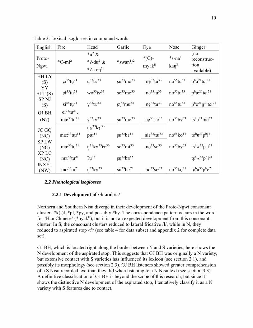
XP LC (NC) a⁵⁵ʐo³³ta⁵⁵ ni²¹ nɤ³³ tʂʰᴇ²¹ Even in compound words, lexical variation is apparent between N and S. Table 3 shows S varieties as possibly more lexically innovative than their N counterparts. N varieties show the compound ‘fire’ from ‘fire + burn’ (*C-mi² *dok), but S varieties have a different first syllable, /ɕi⁵⁵/, historical source unknown, preceding the etymon ‘burn.’ For ‘head’, N and S varieties vary in the Proto-Ngwi etymon chosen as the second syllable: S prefer *ʔ-du² while N prefer *ʔ-koŋ². The second syllable in ‘garlic’ is /mo³³/ in S and / bɛ¹¹/ in N. For ‘eye’, N varieties have ‘eye + classifier for round thing’ (*(C)-myakH si¹), but in S, a different second syllable is used, /-tu³³/, also seen in the word for nose. Finally, the word for ginger shows a possible metathesis, although a reconstruction is needed to substantiate this claim. In S, ‘ginger’ is /pʰa²¹tɕi²¹/, but in N it is /tʂʰᴀ³³pʰi²¹/. See table 3 and appendix 2 for the full data set:

10

Table 3: Lexical isoglosses in compound words

English Fire Head Garlic Eye Nose Ginger

Proto- Ngwi

*C-mi² *u² & *ʔ-du² & *ʔ-koŋ²

*swan¹/² *(C)-myakH

*s-na¹ kaŋ²

(no reconstruc-tion available)

HH LY (S) ɕi⁵⁵tu ̠²¹ u³³tɤ³³ ʂu³³mo³³ ne³̠³tu³³ no⁵⁵tu³³ pʰa²¹tɕi²¹ YY

SLT (S) ɕi⁵⁵tu ̠²¹ wo³³tɤ³³ so³³mo³³ ne³̠³tu³³ no⁵⁵tu³³ pʰæ²¹tɕi²¹ SP NJ

(S) si⁵⁵tu²̠¹ v̩³³tɤ³³ ʂʅ³³mu³³ ne³̠³tu³³ no⁵⁵tu³³ pʰe²¹ŋ³̩³tɕi²¹

GJ BH (N?)

ɕi²¹tu²¹, mæ³³tu²¹ v ̩³³tɤ³³ ʂu³³mo³³ ne³̠³sæ³³ no⁵⁵bɤ²¹ tsʰa²¹me³³

JC GQ (NC) mæː³³tɯ̠¹¹

ŋɤ̠³³kɤ̠³³ pɯ̠¹¹ ʂu³³bɛ¹¹ niɛ³³tɯ³³ no⁵⁵ko ̠¹¹ tɕʰɐ³³pʰi¹̠¹

SP LW (NC) mæ³³tu ̠²¹ ŋ²̩¹kɤ³³tɤ³³ so³³mi³³ ne³̠³sɛ³³ no⁵⁵bɤ²¹ tsʰᴀ³³pʰi²¹

XP LC (NC) mᴇ³³tu ̠²¹ ʔu̠³³ ʂu̠³³bᴇ⁵⁵ tʂʰᴀ³³pʰi²¹

JNXY1 (NW) mɛ˞³³tu²¹ ŋ³̩³kɤ³³ su³³bɛ˞²¹ nɑ³³sɛ˞³³ no⁵⁵ko ̠²¹ tɕʰa³³pʰe²¹

2.2 Phonological isoglosses

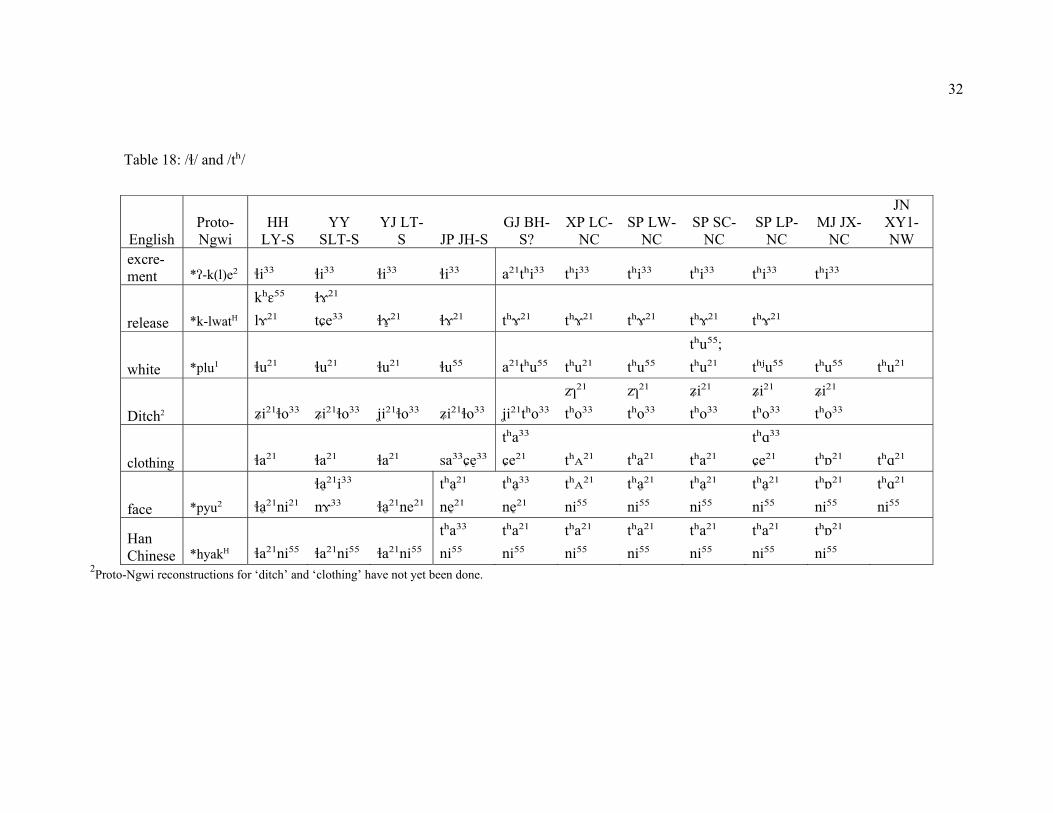
2.2.1 Development of / ɬ/ and /tʰ/

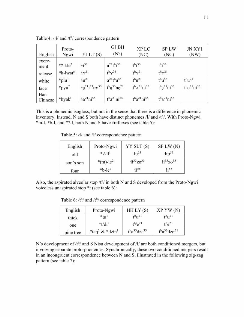
Northern and Southern Nisu diverge in their development of the Proto-Ngwi consonant clusters *k(-)l, *pl, *py, and possibly *hy. The correspondence pattern occurs in the word for ‘Han Chinese’ (*hyakH), but it is not an expected development from this consonant cluster. In S, the consonant clusters reduced to lateral fricative /ɬ/, while in N, they reduced to aspirated stop /tʰ/ (see table 4 for data subset and appendix 2 for complete data set). GJ BH, which is located right along the border between N and S varieties, here shows the N development of the aspirated stop. This suggests that GJ BH was originally a N variety, but extensive contact with S varieties has influenced its lexicon (see section 2.1), and possibly its morphology (see section 2.3). GJ BH listeners showed greater comprehension of a S Nisu recorded text than they did when listening to a N Nisu text (see section 3.3). A definitive classification of GJ BH is beyond the scope of this research, but since it shows the distinctive N development of the aspirated stop, I tentatively classify it as a N variety with S features due to contact.

11

Table 4: / ɬ/ and /tʰ/ correspondence pattern

English Proto-Ngwi YJ LT (S)

GJ BH (N?)

XP LC (NC)

SP LW (NC)

JN XY1 (NW)

excre-ment *ʔ-kle² ɬi³³ a²¹tʰi³³ tʰi³³ tʰi³³ release *k-lwatH ɬɤ̠²¹ tʰɤ²¹ tʰɤ²¹ tʰɤ²¹ white *plu¹ ɬu²¹ a²¹tʰu⁵⁵ tʰu²¹ tʰu⁵⁵ tʰu²¹

face *pyu² ɬa²̠¹i³³nɤ³³ tʰa³̠³ne²̠¹ tʰᴀ²¹ni⁵⁵ tʰa²̠¹ni⁵⁵ tʰɑ²¹ni⁵⁵ Han Chinese *hyakH ɬa²¹ni⁵⁵ tʰa²¹ni⁵⁵ tʰa²¹ni⁵⁵ tʰa²¹ni⁵⁵

This is a phonemic isogloss, but not in the sense that there is a difference in phonemic inventory. Instead, N and S both have distinct phonemes /ɬ/ and /tʰ/. With Proto-Ngwi *m-l, *b-l, and *ʔ-l, both N and S have /ɬ/ reflexes (see table 5):

Table 5: /ɬ/ and /ɬ/ correspondence pattern

English Proto-Ngwi YY SLT (S) SP LW (N)

old *ʔ-li¹ ɬu⁵⁵ ɬɯ⁵⁵

son’s son *(m)-le² ɬi³³zo³³ ɬi³³zo³³

four *b-le² ɬi⁵⁵ ɬi⁵⁵ Also, the aspirated alveolar stop /tʰ/ in both N and S developed from the Proto-Ngwi voiceless unaspirated stop *t (see table 6):

Table 6: /tʰ/ and /tʰ/ correspondence pattern

English Proto-Ngwi HH LY (S) XP YW (N) thick *tu¹ tʰu²¹ tʰu²¹

one *t/di² tʰʲe²¹ tʰe²¹

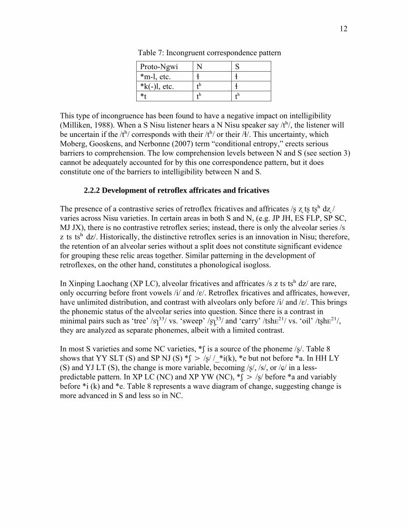
pine tree *taŋ² & *dzin¹ tʰa³³dzɛ³³ tʰa³³dʐɛ˞²¹ N’s development of /tʰ/ and S Nisu development of /ɬ/ are both conditioned mergers, but involving separate proto-phonemes. Synchronically, these two conditioned mergers result in an incongruent correspondence between N and S, illustrated in the following zig-zag pattern (see table 7):

12

Table 7: Incongruent correspondence pattern

Proto-Ngwi N S *m-l, etc. ɬ ɬ *k(-)l, etc. th ɬ *t th th

This type of incongruence has been found to have a negative impact on intelligibility (Milliken, 1988). When a S Nisu listener hears a N Nisu speaker say /tʰ/, the listener will be uncertain if the /tʰ/ corresponds with their /tʰ/ or their /ɬ/. This uncertainty, which Moberg, Gooskens, and Nerbonne (2007) term “conditional entropy,” erects serious barriers to comprehension. The low comprehension levels between N and S (see section 3) cannot be adequately accounted for by this one correspondence pattern, but it does constitute one of the barriers to intelligibility between N and S.

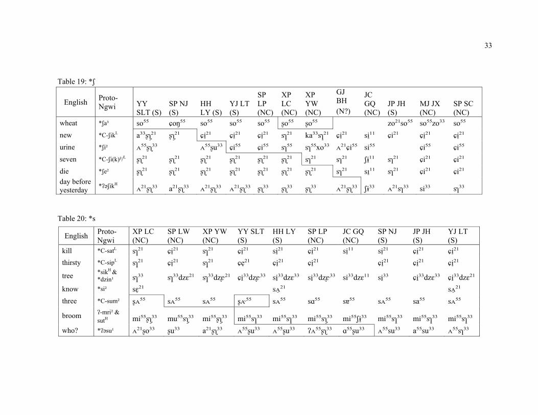
2.2.2 Development of retroflex affricates and fricatives The presence of a contrastive series of retroflex fricatives and affricates /ʂ ʐ tʂ tʂʰ dʐ / varies across Nisu varieties. In certain areas in both S and N, (e.g. JP JH, ES FLP, SP SC, MJ JX), there is no contrastive retroflex series; instead, there is only the alveolar series /s z ts tsʰ dz/. Historically, the distinctive retroflex series is an innovation in Nisu; therefore, the retention of an alveolar series without a split does not constitute significant evidence for grouping these relic areas together. Similar patterning in the development of retroflexes, on the other hand, constitutes a phonological isogloss. In Xinping Laochang (XP LC), alveolar fricatives and affricates /s z ts tsʰ dz/ are rare, only occurring before front vowels /i/ and /ɛ/. Retroflex fricatives and affricates, however, have unlimited distribution, and contrast with alveolars only before /i/ and /ɛ/. This brings the phonemic status of the alveolar series into question. Since there is a contrast in minimal pairs such as ‘tree’ /sɿ³̠³/ vs. ‘sweep’ /ʂʅ³̠³/ and ‘carry’ /tshᴇ²¹/ vs. ‘oil’ /tʂhᴇ²¹/, they are analyzed as separate phonemes, albeit with a limited contrast. In most S varieties and some NC varieties, *ʃ is a source of the phoneme /ʂ/. Table 8 shows that YY SLT (S) and SP NJ (S) *ʃ > /ʂ/ /_*i(k), *e but not before *a. In HH LY (S) and YJ LT (S), the change is more variable, becoming /ʂ/, /s/, or /ɕ/ in a less-predictable pattern. In XP LC (NC) and XP YW (NC), *ʃ > /ʂ/ before *a and variably before *i (k) and *e. Table 8 represents a wave diagram of change, suggesting change is more advanced in S and less so in NC.

13

Table 8: *ʃ

English Proto-Ngwi

YY SLT (S)

SP NJ (S)

HH LY (S)

YJ LT (S)

XP LC (NC)

XP YW (NC)

die *ʃe² ʂʅ²¹ ʂʅ²¹ ʂʅ²¹ ʂʅ²¹ ʂʅ²¹ ʂʅ²¹ seven *C-ʃi(k)²/L ʂʅ²¹ ʂʅ²¹ ʂʅ²¹ ʂʅ²¹ ʂʅ²¹ sɿ²¹ urine *ʃi² ᴀ⁵⁵ʂʅ³³ ᴀ⁵⁵ʂu³³ ɕi⁵⁵ sɿ⁵⁵ sɿ⁵⁵xo³³ new *C-ʃikL a³³ʂʅ²̠¹ ʂʅ²̠¹ ɕi²̠¹ ɕi²̠¹ sɿ²̠¹ ka³³sɿ²̠¹ wheat *ʃa³ so⁵⁵ ɕoŋ⁵⁵ so⁵⁵ so⁵⁵ ʂo⁵⁵ ʂo⁵⁵

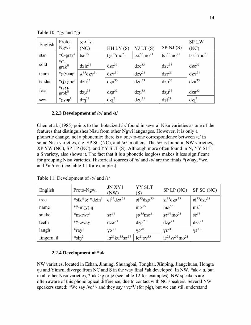
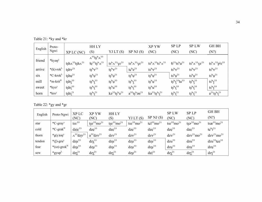
XP LC (NC) and YW (NC), along with the three S varieties nearest to them (e.g. YJ LT, HH LY, and SP NJ), share a split in the consonant clusters *kr, *ky and *gr, *gy. Before rhymes with back vowels such as *o(k), *u(p), *it, and sometimes *a/oŋ, the current reflex tends to be retroflex. In SP LW and SP LP, both NC varieties, this split only occurs before *it and *o (see tables 9 and 10 and appendix 2 for complete data set). The wave diagram patterns seen in tables 9 and 10 suggest that this conditioned split began in Xinping LC and YW, spread southwest to YJ LT, SP NJ and HH LY, and east to SP LW and SP LP. The change did not make it further south to YY SLT, GJ BH, or JP JH. Neither did it spread north to reach NW varieties as in JN XY1 or JN XY2. This suggests that the change may be recent and ongoing. The spread of change results in a differentiation between two sub-clusters within S. Varieties HH LY, YJ LT, and SP NJ all share this split. In contrast, YY SLT and JP JH do not split at all, but instead show reflexes of either alveolar affricates. The overlay of change in the HH LY-YJ LT-SP NJ cluster makes this cluster distinct from other S varieties further to the southeast. Interestingly, Levenshtein distance also uncovers this sub-cluster within S (see section 4.3.1). Table 9: *ky and *kr

Eng-lish

Proto-Ngwi XP LC (NC)

HH LY (S) YJ LT (S) SP NJ (S)

SP LW (NC)

friend *kyaŋ² tʂʰᴀ³³tʂʰᴀ²¹

ᴀ⁵⁵tʂʰᴀ³³ ɬe³̠³tʂʰᴀ²¹ tsʰᴀ³³ɣɛ²¹ tsʰᴀ³³ɣɛ²¹ tsʰᴀ³³ɣɛ²¹

arrive *(k)-rokL tʂʰɤ²¹ tʂʰɤ²¹ tʂʰɤ²¹ tɕʰe²¹ tsʰɤ²¹ six *C-krokL tʂʰu̠²¹ tʂʰu̠²¹ tʂʰu̠²¹ tʂʰu̠²¹ tsʰu̠²¹ mill *m-kritH tʂʰʅ³̠³ tʂʰʅ³̠³ tʂʰu̠³³ tʂʰʅ³̠³ tʂʰʅ³̠³ sweet *kyo¹ tʂʰʅ⁵⁵ tʂʰʅ⁵⁵ tʂʰu⁵⁵ tʂʰʅ⁵⁵ tʂʰʅ⁵⁵

14

Table 10: *gy and *gr

English Proto-Ngwi

XP LC (NC) HH LY (S) YJ LT (S) SP NJ (S)

SP LW (NC)

star *C-gray¹ tsᴇ⁵⁵ tʂɛ⁵⁵mo²¹ tsɛ⁵⁵mo²¹ tɕĩ⁵⁵mo²¹ tsɛ⁵⁵mo²¹

cold *C-grakH dʑiɛ̠³̠³ dʑe³̠³ dʑe³̠³ dʑe³̠³ dʑe³̠³

thorn *g(y)oŋ³ ᴀ⁵⁵dʐɤ²¹ dzɤ²¹ dzɤ²¹ dzɤ²¹ dzɤ²¹ tendon *(ʃ)-gru² dʐu³³ dʐu³³ dʐu³³ dʐu³³ dzu³³

fear *(sə)-grokH dʐu̠³³ dʐu³³ dʐu³³ dʐu̠³³ dzu ̠³³

sew *gyupL dʐʅ²̠¹ dʐʅ²̠¹ dʐu̠²¹ dʑi²̠¹ dʐʅ²̠¹

2.2.3 Development of /ə˞/ and /ɛ/ Chen et al. (1985) points to the rhotacized /ə˞/ found in several Nisu varieties as one of the features that distinguishes Nisu from other Ngwi languages. However, it is only a phonetic change, not a phonemic: there is a one-to-one correspondence between /ɛ/ in some Nisu varieties, e.g. SP SC (NC), and /ə˞/ in others. The /ə˞/ is found in NW varieties, XP YW (NC), SP LP (NC), and YY SLT (S). Although more often found in N, YY SLT, a S variety, also shows it. The fact that it is a phonetic isogloss makes it less significant for grouping Nisu varieties. Historical sources of /ɛ/ and /ə˞/ are the finals *(w)ay, *we, and *in/m/ŋ (see table 11 for examples). Table 11: Development of /ə˞/ and /ɛ/

English Proto-Ngwi JN XY1 (NW)

YY SLT (S) SP LP (NC) SP SC (NC)

tree *sikH & *dzin¹ ɕi³³dzə˞²¹ ɕi³̠³dʐə˞³³ si³̠³dʐə˞³³ ɕi³̠³dzɛ²¹ name *ʔ-m(y)iŋ¹ mə˞⁵⁵ mə˞⁵⁵ mɛ⁵⁵ snake *m-rwe¹ sə˞⁵⁵ ʂə˞⁵⁵mo²¹ ʂə˞⁵⁵mo²¹ sɛ⁵⁵ teeth *ʔ-cway¹ dzə˞²¹ dʐə˞²¹ dʐə˞²¹ dzɛ²¹ laugh *ray¹ ɣə˞²¹ ɣə˞²¹ ɣɛ²¹ ɣɛ²¹ fingernail *siŋ² lɑ²¹ku³³sə˞³³ le²̠¹sɤ³³ le²̠¹sɤ³³mo²¹

2.2.4 Development of *ak NW varieties, located in Eshan, Jinning, Shuangbai, Tonghai, Xinping, Jiangchuan, Hongta qu and Yimen, diverge from NC and S in the way final *ak developed. In NW, *ak > ɑ,̠ but in all other Nisu varieties, *-ak > e ̠̠or ie̠ (see table 12 for examples)̠. NW speakers are often aware of this phonological difference, due to contact with NC speakers. Several NW speakers stated: “We say /vɑ²̠¹/ and they say / ve²̠¹/ (for pig), but we can still understand

15

each other.” Since this pattern is a one-to-one correspondence between NW /ɑ/̠ and other varieties’ /e ̠/̠, the impact on intelligibility is not serious, as can be seen from the high levels of comprehension shown by NW speakers listening to a NC text (see section 3.3.1).

Table 12: Development of *ak

English Proto-Ngwi YY SLT (S) SP LW (NC) JN XY1 (NW)

bird *s-ŋyakH xe³̠³zo³³ xʲe³̠³ xɑ³³

leaf *C-pakL a³³pʰe²̠¹ ɕi³̠³pʰe²̠¹ ɕi³³pʰɑ²̠¹

eye *(C)-myakH ne³̠³tu³³ ne³̠³sɛ³³ nɑ³³sɛ˞³³

cook; boil *C-dzakH tɕe²̠¹ tɕe²̠¹ wɑ²¹dzɑ²̠¹ 2.3 Morphological isogloss

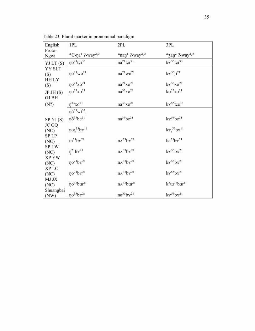
There is also a morphological isogloss between N and S in the variable plural marker in the personal pronoun paradigm. N varieties have /bɤ²¹/, while S varieties have /xo²¹/, /wo²¹/, and /tɕi²¹/. GJ BH shares the S variety morpheme /xo²¹/. S varieties show the reflex for the Proto-Ngwi form *ʔ-way²/³, while N varieties show the etymon for ‘group of humans,’ also seen in Lisu /bu ̠³³/ (Bradley, personal communication). Evidence for NW Nisu is from Shuangbai, in Li (1996). See table 13 for examples and appendix 2 for complete data set: Table 13: Plural marker in personal pronoun paradigm

English 1PL 2PL 3PL Proto-Ngwi *C-ŋa¹ ʔ-way²/³ *naŋ¹ ʔ-way²/³ *ʒaŋ² ʔ-way²/³

YJ LT (S) ŋo²¹tɕi³³ na²¹tɕi³³ kɤ⁵⁵tɕi³³ YY SLT (S) ŋo²¹wo²¹ na²¹wo²¹ kɤ⁵⁵ji²¹ HH LY (S) ŋo²¹xo²¹ na²¹xo²¹ kɤ⁵⁵xo²¹ GJ BH (N?) ŋ³̩³xo²¹ na³³xo²¹ kɤ⁵⁵tɕe³³

SP NJ (S)

ŋo³³wi³³, ŋo³³be²¹ na³³be²¹ kɤ⁵⁵be²¹

SP LW (N) ŋ²̩¹bɤ²¹ nᴀ³³bɤ²¹ kɤ⁵⁵bɤ²¹ XP LC (N) ŋo²¹bɤ²¹ nᴀ³³bɤ²¹ kɤ⁵⁵bɤ²¹ Shuangbai (NW) ŋo³³bɤ²¹ nɑ³³bɤ²¹ kɤ⁵⁵bɤ²¹

16

3. Intelligibility test results

3.1 Background Though problematic, the criterion of “mutual intelligibility” is often invoked in defining whether varieties are dialects of the same language or related languages (Chambers and Trudgill, 1998; Wardhaugh, 1986). One key weakness of this criterion is that non-linguistic criteria, such as political autonomy or shared written tradition, are often more influential in determining the classification of “dialect” vs. “separate language.” In China, Nisu has been classified as a dialect of the “Yi” language, a classification influenced by both linguistic and political factors. Though it is not the purpose of this research to reclassify Nisu in an ethno-political sense, the low level of initial intelligibility between Northern and Southern Nisu and the high level of intelligibility between Northwestern and North Central should be acknowledged in future language planning. The development of intelligibility testing methods was based on the assumption that, all else being equal, speakers of dialects of the same language should be able to understand one another. Casad (1974) presented the framework for RTT and Blair (1990) and Grimes (1995) provided further updates and revisions. Allen (2004) carefully applied RTT procedures to speakers of Bai, another Tibeto-Burman language. In this research, RTT results are used as a relative indicator of the level of comprehension that a Nisu listener has after initial exposure to a different Nisu variety.

3.2 Methodology The testing procedure followed the basic principles presented in Casad (1974) and Blair (1990). Individuals were first interviewed to determine their suitability. Participants were selected whose parents were native to the locale, who themselves grew up in the village, and who had not had long-term (greater than one month) exposure to the varieties being tested. They first listened to a recorded text in their own local variety and answered content questions about it. This served as a further screening procedure, and also helped participants adjust to the testing process. Following the “hometown” test, participants listened to a recording from another Nisu variety. They first listened to the whole text, and then listened again section-by-section. After each section, the test administrator would pause and ask a content question related to the section participants had just heard. Questions were given in either Chinese or, in cases of monolingual Nisu speakers, the local Nisu variety spoken by a translator. Respondents were given the choice of answering in either Nisu or in the local Chinese dialect. One potential threat to validity in this testing method is the role of contact-induced intelligibility, or bi-dialectalism. When speakers of different dialects come in contact, their receptive linguistic ability enables them to adjust to each other’s dialect. Standard deviation above 15% indicates that the higher scores are probably due to contact (Grimes, 1995). Screening participants for long-term exposure offset this potential danger to some

17

extent: no participant was accepted who had lived with other-variety Nisu speakers for more than one month. In general, test results show standard deviations below 15%. However, the test results of GJ BH speakers listening to the SP LW text show a high standard deviation (24%). At least one participant was a local official, who may have had more opportunities to have contact with other N varieties. In this location, the higher score obtained by the official is probably due to bi-dialectalism. In cases where speakers of different varieties are in close proximity to each other, casual and frequent contact was impossible to screen out. Traveling to the neighboring district to take part in that district’s market day and attending countywide Nisu cultural festivals are examples of casual but frequent contact. With casual contact, cross-variety speakers are not living in the same village with each other, but they are interacting for short periods, for example, on a monthly basis. In S varieties SP NJ and YJ LT, contact with speakers of North Central Nisu (represented by SP LW) was casual but frequent, due to proximity. These two locations therefore showed much higher comprehension than other S variety speakers listening to the same NC text. Likewise, a main road connected XP XH (NC) speakers to ES FLP (NW) speakers, and XP XH speakers scored very high on the ES FLP test. Consequently, the RTT results for these locations reflect learned intelligibility rather than initial intelligibility. Without such frequent contact, S varieties SP NJ and YJ LT would probably show low scores for the NC text, as other S varieties did. However, this was not the first time these participants had been exposed to the variety they were being tested on. The standard deviation in RTT results in all these locations was low, however, and the level of comprehension was high. No one got a low score. This leads to the question whether casual, frequent contact would allow other S speakers to obtain high levels of comprehension of N, which is beyond the scope of this research.

3.3 Results The next three sub-sections focus on comprehension levels shown for the RTT texts tested in the most locations: SP LW (NC), JC GQ (NC), and SP NJ (S). Four other texts were pilot-tested and tested: XP YW (NC), ES FLP (NW), YY SC (S), and YY SLT (S). However, since these texts were only tested in one or two other locations, often within their own dialect boundary, these results are not included in the discussion below. A complete chart of RTT scores and their standard deviations for the whole project is given in appendix 3.

3.3.1 Comprehension levels for SP LW (NC) Across N varieties, listeners understood the recorded text from SP LW (NC) at very high levels (in most cases, above 90%). Listeners from S varieties had lower levels of comprehension (ranging from 90% to 30%). See figure 3 for test results and standard deviations for each location.

18

SP NJ and YJ LT, both S varieties, showed higher comprehension of SP LW than other S varieties. Both SP NJ and YJ LT border NC-speaking areas. YJ LT is situated on a mountainside facing a valley where an NC variety is spoken, and interaction between the communities is characterized by frequent, casual contact. SP NJ is located just to the south of the main NC-speaking population. However, SP NJ participants’ reaction to the SP LW text was one of exclusion: “We don’t talk like that” or “I don’t understand this.” When asked how well they understood the text, they consistently reported much lower levels than what they actually scored. These indicators show that SP NJ participants do not consider the SP LW text as comprehensible, even though they obtained high comprehension scores. In contrast to the high-scoring border areas, S listeners in HH LY, JP JH, and GJ BH scored very low on the comprehension test. Since these varieties are less likely to have had casual contact with NC speakers, these scores reflect low inherent intelligibility. Not only did they score low on the test, S participants also reported that they felt they could understand little of what was said, and that the difference with their speech was great. JC GQ scored lower than other NC varieties when listening to SP LW. This may be due to divergence that has occurred in recent history. According to oral history, JC GQ speakers’ ancestors migrated from the Shiping/Xinping area in the past 100-150 years. Since then, there has been little contact between JC GQ speakers and other NC speakers, so the slightly lower scores for JC GQ listeners are not surprising.

0

0.1

0.2

0.3

0.4

0.5

0.6

0.7

0.8

0.9

1

SP LP (NC)

XP XH (NC)

XP YW (NC)

XP LC (NC)

HTQ CH (NC)

JC GQ (NC)

ES FLP (NW)

YJ LT (S)

SP NJ (S)

GJ BH (N?)

HH BH (S)

JP JH (S)

Std. dev.RTT score

Figure 3: Comprehension levels for SP LW (NC).

3.3.2 Comprehension levels for JC GQ (NC)

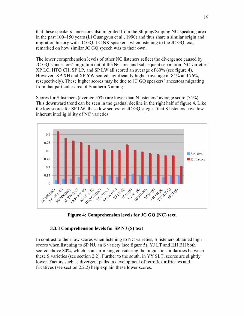
NC speakers from MJ MN and LC NK, who are located closest to JC GQ, received high scores when listening to the JC GQ text (see figure 4). This can be explained by the fact

19

that these speakers’ ancestors also migrated from the Shiping/Xinping NC-speaking area in the past 100–150 years (Li Guangyun et al., 1990) and thus share a similar origin and migration history with JC GQ. LC NK speakers, when listening to the JC GQ text, remarked on how similar JC GQ speech was to their own. The lower comprehension levels of other NC listeners reflect the divergence caused by JC GQ’s ancestors’ migration out of the NC area and subsequent separation. NC varieties XP LC, HTQ CH, SP LP, and SP LW all scored an average of 60% (see figure 4). However, XP XH and XP YW scored significantly higher (average of 84% and 76%, resepectively). These higher scores may be due to JC GQ speakers’ ancestors migrating from that particular area of Southern Xinping. Scores for S listeners (average 55%) are lower than N listeners’ average score (74%). This downward trend can be seen in the gradual decline in the right half of figure 4. Like the low scores for SP LW, these low scores for JC GQ suggest that S listeners have low inherent intelligibility of NC varieties.

0

0.15

0.3

0.45

0.6

0.75

0.9

LC NK (N

C)

XP XH (N

C)

MJ MN (N

C)

XP YW

(NC)

ES FLP (NW

)

XP LC (NC)

HTQ CH (NC)

SP LP (NC)

SP LW (N

C)

YJ LT (S

)

JP JH

(S)

YY SC (S)

GJ BH (N

?)

SP NJ (

S)

HH BH (S)

YY SLT (S)

JS PT (S

)

Std. dev.RTT score

Figure 4: Comprehension levels for JC GQ (NC) text.

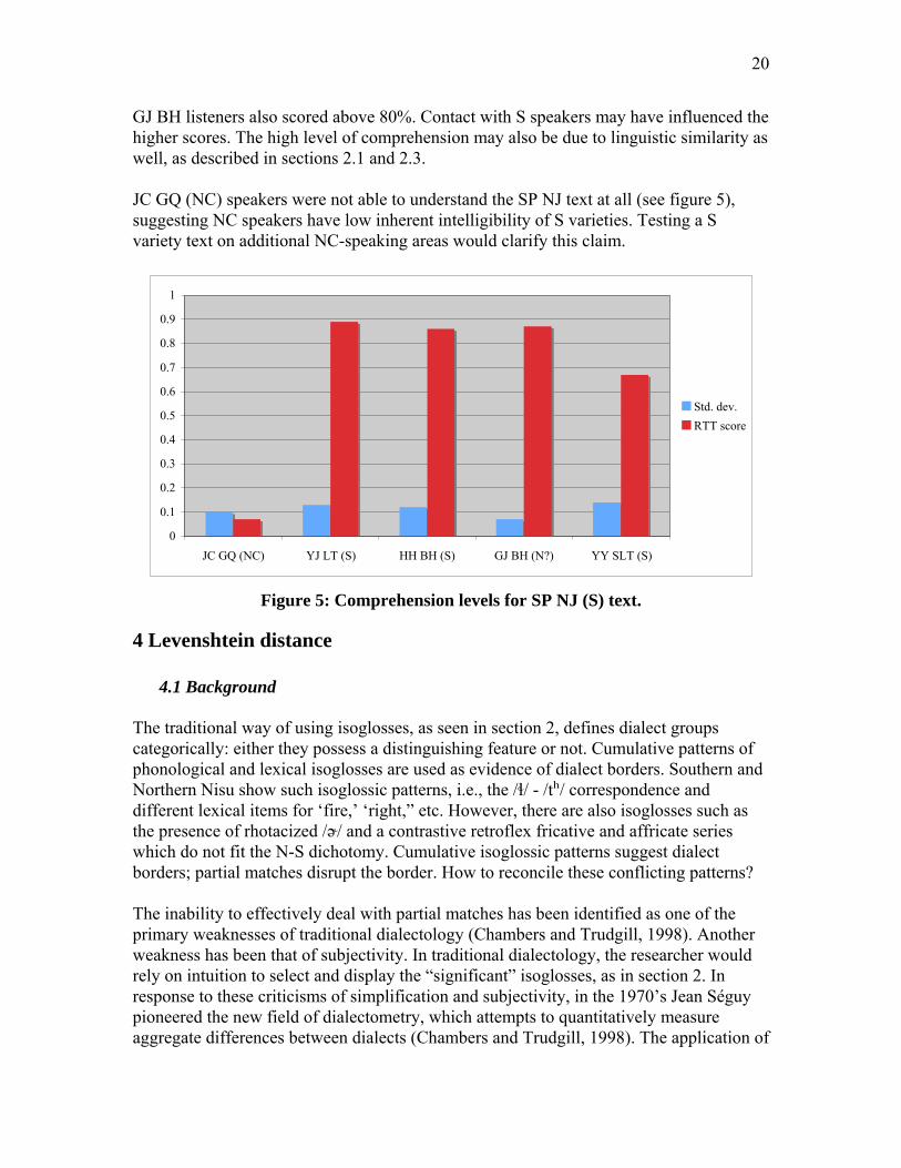
3.3.3 Comprehension levels for SP NJ (S) text

In contrast to their low scores when listening to NC varieties, S listeners obtained high scores when listening to SP NJ, an S variety (see figure 5). YJ LT and HH BH both scored above 80%, which is unsurprising considering the linguistic similarities between these S varieties (see section 2.2). Further to the south, in YY SLT, scores are slightly lower. Factors such as divergent paths in development of retroflex affricates and fricatives (see section 2.2.2) help explain these lower scores.

20

GJ BH listeners also scored above 80%. Contact with S speakers may have influenced the higher scores. The high level of comprehension may also be due to linguistic similarity as well, as described in sections 2.1 and 2.3. JC GQ (NC) speakers were not able to understand the SP NJ text at all (see figure 5), suggesting NC speakers have low inherent intelligibility of S varieties. Testing a S variety text on additional NC-speaking areas would clarify this claim.

0

0.1

0.2

0.3

0.4

0.5

0.6

0.7

0.8

0.9

1

JC GQ (NC) YJ LT (S) HH BH (S) GJ BH (N?) YY SLT (S)

Std. dev.RTT score

Figure 5: Comprehension levels for SP NJ (S) text.

4 Levenshtein distance

4.1 Background The traditional way of using isoglosses, as seen in section 2, defines dialect groups categorically: either they possess a distinguishing feature or not. Cumulative patterns of phonological and lexical isoglosses are used as evidence of dialect borders. Southern and Northern Nisu show such isoglossic patterns, i.e., the /ɬ/ - /tʰ/ correspondence and different lexical items for ‘fire,’ ‘right,” etc. However, there are also isoglosses such as the presence of rhotacized /ə˞/ and a contrastive retroflex fricative and affricate series which do not fit the N-S dichotomy. Cumulative isoglossic patterns suggest dialect borders; partial matches disrupt the border. How to reconcile these conflicting patterns? The inability to effectively deal with partial matches has been identified as one of the primary weaknesses of traditional dialectology (Chambers and Trudgill, 1998). Another weakness has been that of subjectivity. In traditional dialectology, the researcher would rely on intuition to select and display the “significant” isoglosses, as in section 2. In response to these criticisms of simplification and subjectivity, in the 1970’s Jean Séguy pioneered the new field of dialectometry, which attempts to quantitatively measure aggregate differences between dialects (Chambers and Trudgill, 1998). The application of

21

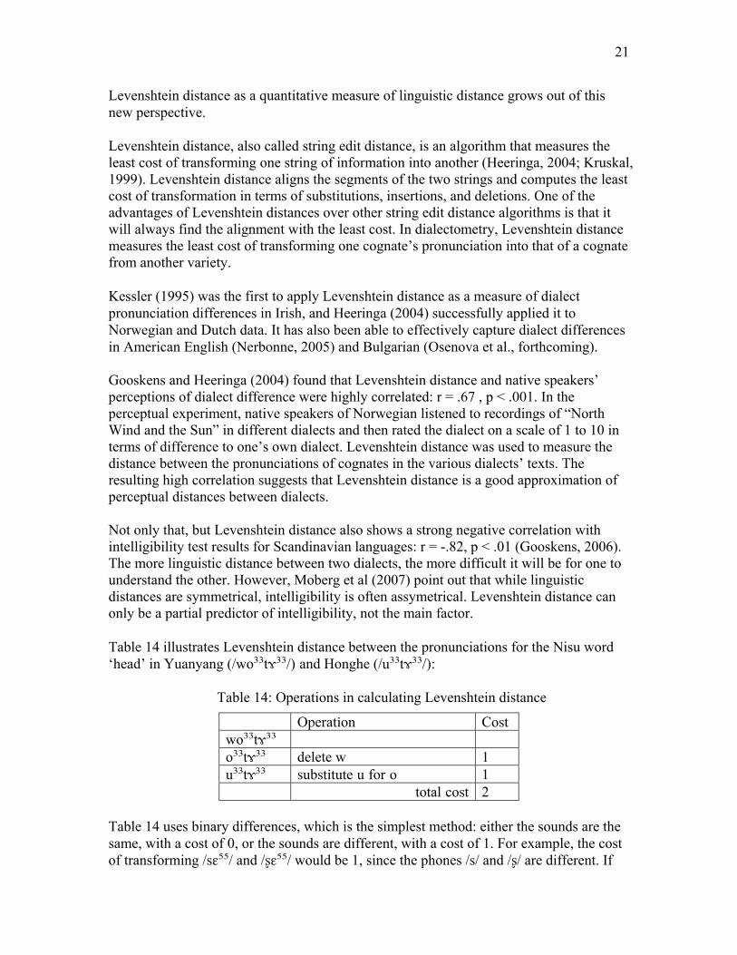
Levenshtein distance as a quantitative measure of linguistic distance grows out of this new perspective. Levenshtein distance, also called string edit distance, is an algorithm that measures the least cost of transforming one string of information into another (Heeringa, 2004; Kruskal, 1999). Levenshtein distance aligns the segments of the two strings and computes the least cost of transformation in terms of substitutions, insertions, and deletions. One of the advantages of Levenshtein distances over other string edit distance algorithms is that it will always find the alignment with the least cost. In dialectometry, Levenshtein distance measures the least cost of transforming one cognate’s pronunciation into that of a cognate from another variety. Kessler (1995) was the first to apply Levenshtein distance as a measure of dialect pronunciation differences in Irish, and Heeringa (2004) successfully applied it to Norwegian and Dutch data. It has also been able to effectively capture dialect differences in American English (Nerbonne, 2005) and Bulgarian (Osenova et al., forthcoming). Gooskens and Heeringa (2004) found that Levenshtein distance and native speakers’ perceptions of dialect difference were highly correlated: r = .67 , p < .001. In the perceptual experiment, native speakers of Norwegian listened to recordings of “North Wind and the Sun” in different dialects and then rated the dialect on a scale of 1 to 10 in terms of difference to one’s own dialect. Levenshtein distance was used to measure the distance between the pronunciations of cognates in the various dialects’ texts. The resulting high correlation suggests that Levenshtein distance is a good approximation of perceptual distances between dialects. Not only that, but Levenshtein distance also shows a strong negative correlation with intelligibility test results for Scandinavian languages: r = -.82, p < .01 (Gooskens, 2006). The more linguistic distance between two dialects, the more difficult it will be for one to understand the other. However, Moberg et al (2007) point out that while linguistic distances are symmetrical, intelligibility is often assymetrical. Levenshtein distance can only be a partial predictor of intelligibility, not the main factor. Table 14 illustrates Levenshtein distance between the pronunciations for the Nisu word ‘head’ in Yuanyang (/wo³³tɤ³³/) and Honghe (/u³³tɤ³³/):

Table 14: Operations in calculating Levenshtein distance

Operation Cost wo³³tɤ³³ o³³tɤ³³ delete w 1 u³³tɤ³³ substitute u for o 1 total cost 2

Table 14 uses binary differences, which is the simplest method: either the sounds are the same, with a cost of 0, or the sounds are different, with a cost of 1. For example, the cost of transforming /sɛ⁵⁵/ and /ʂɛ⁵⁵/ would be 1, since the phones /s/ and /ʂ/ are different. If

22

the sounds were broken down into feature bundles, then the cost would be less than one, since /s/ and /ʂ/ only differ by one feature. However, Heeringa (2004) found that binary measures and gradual measures (i.e. using feature bundles) are equally effective. That is, using binary measures, the correlation to perceptual experiment results was equally high with that of gradual measures. Native speakers are sensitive to very slight differences in pronunciation, so this weighting of small differences makes sense in the context of the relationship between Levenshtein distance and speakers’ perceptions. Levenshtein distance complements traditional dialectology’s main weaknesses: subjectivity and the glossing over of non-overlapping patterns. By measuring aggregate differences, the overall linguistic distance between varieties can be obtained. This provides an objective measure that fully exploits the mass of available data. However, Levenshtein distance has only been used on non-tonal, analytic languages found in Europe. This research is the first time it has ever been applied to tonal, isolating languages in Asia.

4.2 Methodology In order to use this dialectometric tool, I first compiled the sixteen available Nisu wordlists into one comparative wordlist. Nine of the wordlists consist of 390 items, which I elicited and transcribed on location in broad phonetic transcription, in cooperation with native speakers. Li Yongxiang (Bradley et al., 2002) elicited the two NW Nisu wordlists from JN XY in 2002, and I transcribed them in 2007 off a cassette tape recording. Unfortunately, these NW Nisu lists only share 135 items in common with the 390-item wordlists. The wordlists from XP LC (YNSZ, 1998), SP SC (Pu Zhangkai et al., 2005), and MJ JX (Sun, 1991) were transcribed by native speakers and published in lexicons or dictionaries. Most of the words taken from published sources are also on the 390-item list, but not all. XP LC shares 335 items, MJ JX shares 346, and SP SC shares 290. Pu (2005), a native speaker who received training in IPA, provided a transcribed wordlist from JC GQ, which shares 226 items with the 390-item list. Finally, Blackburn and Blackburn (2007), in cooperation with a native speaker, elicited and transcribed the wordlist from Yongping, which shares 268 items. The preceding compilation process introduces two potential threats to the validity of the analysis. Only nine of the wordlists were elicited and transcribed by the same person, and other sources reflect the personal practice of individual transcribers. This introduces the potential of reflecting ‘explorer dialects,’ that is, differences between transcribers’ practices rather than differences in pronunciation. In fact, in the case of UPGMA cluster analysis of JC GQ (see figure 7), the placing of JC GQ outside of Northern Nisu is most likely due to differences between transcribers rather than differences in pronunciation.

23

Also, there is only partial overlap between all the wordlists. For those wordlists with fewer items in common, such as the two JN XY (NW) wordlists with only 135 shared items, there is an unfortunate gap in the data. Those 135 items have a proportionally greater impact on the grouping of JN XY varieties when compared with the weight of the 390 shared items on other varieties’ groupings. This puts the findings for the JN XY wordlists in question, and further evidence such as phonological innovations and intelligibility scores must be called on to substantiate the groupings based on Levenshtein distance. The benefit of including as many Nisu varieties as possible outweighs these potential problems. The option of collecting all wordlists on location was not feasible in the research timeframe, so including wordlists from other sources is a reasonable second-best. Plus, all wordlists were transcribed in broad phonetic transcription, so they do not differ in the level of phonetic detail. In the end, the problems of explorer dialects and incomplete data did not seriously affect the findings, as can be seen from the striking agreement between the Levenshtein distances, the historical-comparative findings, and the intelligibility test scores. The Nisu wordlists were analyzed using the RuG/L04 dialectometry software package developed by Peter Kleiweg (2007). L04 software requires the wordlists to be in machine readable code, not Unicode IPA, so the Unicode transcriptions were converted into XSAMPA code (Wells, 2005). Binary, not feature-based, measures were used, as described above. Insertion, deletions, and substitutions were all weighted the same, at the cost of 1. The mean Levenshtein distance was calculated for each pair of varieties based on the Levenshtein distances between all pairs of items. The L04 software also included various clustering methods such as UPGMA, WPGMA, and Ward’s method and was able to produce dendograms based on the cluster analysis. In order to offset the added weight of longer words, length was normalized by dividing the total cost by the sum of the lengths of the two strings (Kleiweg, 2007). The distances are then expressed as proportions in decimal form. Heeringa et al. (2006), in their evaluation of string edit distance parameters, suggest that not using normalization improves the validity of the Levenshtein distance. But in the case of Nisu, using length normalization consistently gave better results than no normalization. Without normalization, longer words are weighted more heavily in the calculation of the final average. This could especially skew results where not all pairs of strings are available across all locations, as is the case for the wordlists taken from published and unpublished sources. Normalization corrects this potential error. Levenshtein distance has been developed as a measure of pronunciation differences, not lexical differences. As such, lexical variation is usually removed from the wordlists, leaving only cognates to be compared (Gooskens, 2006). But in isolating, polysyllabic languages such as Nisu, the issue of what is and is not a cognate can be more complex than in analytic languages of the kind found in Europe. For compound words, the combination of morphemes may vary between lects. For example, the word for ‘banana’ has the following reflexes in Nisu varieties (see table 15):

24

Table 15: Variation in compound words

English Proto-Ngwi HH LY (S) SP NJ (S) YY SLT (S) SP LP (S)

banana

*s-ŋakH & *b(y)aw² ȵɛ³̠³sɛ³³ ȵɛ³³bɤ³³ ne³̠³ba³³ʂɛ˞³³ ɕɑŋ³³dʐa²¹

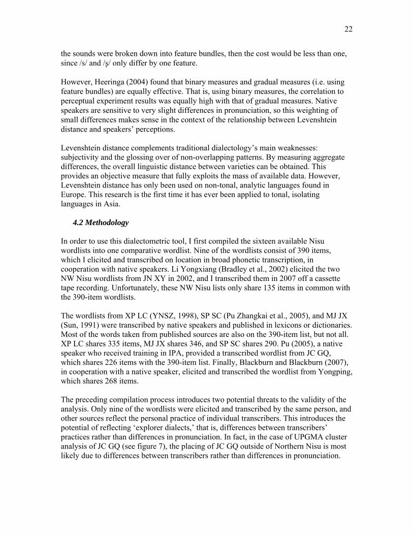
SP LP has a non-cognate loan from Chinese /ɕɑŋ³³dʐa²¹/, and therefore I placed it in a separate file. HH LY adds the syllable /sɛ³³/ from Proto-Ngwi *si² ‘fruit,’ while SP NJ has / bɤ³³/ from *b(y)aw² ‘banana.’ There is thus only a partial cognate match between HH LY and SP NJ, since the syllables /sɛ³³/ and /bɤ³³/ are clearly not cognates. To completely weed out this type of partial lexical variation, one would have to separate out each syllable into separate lines to ensure only cognate syllables are being compared with their cognates. Then all the *s-ŋakH reflexes would be compared to each other in one line, all the *b(y)aw² reflexes in the next, and all the *si² reflexes in a third line. However, I chose not to do this for two reasons. First, to do so would create even more partial matches in the data than there are already, which may skew the results. Also, comparing morphemes below the word level further removes the context in which listeners perceive speech. This weakens the link between Levenshtein distance and both speakers’ perceptions and intelligibility. Instead, I chose to leave in partial matches like that found in table 15. If a pair of varieties shared a lexeme entirely different from other varieties’, I removed those items to another file. For example, if another variety besides Shiping Longpeng also had the loanword for banana (ɕɑŋ³³dʐa²¹), I would place both reflexes in another file to be compared. I also applied Levenshtein distance to the wordlists before weeding out such lexical variation and achieved similar results. In Nisu there are semantically-bleached syllables, such as the prefixes /a²¹-/, /a⁵⁵-/, and suffix /-mo²¹/ attached to nouns, providing phonological bulk to the lexeme. The published word lists, especially Pu (2005) whose dictionary is based on Nisu traditional characters, leave these “filler” syllables out. The wordlists I took in cooperation with native speakers, being more vernacular-based, have frequent recurrences of /a²¹-/, /a⁵⁵-/, and /-mo²¹/. I left these syllables in the word lists, since I deemed it best not to clean up the data any more than was absolutely necessary. XSAMPA code separates diacritics and even some features from their respective base segment, i.e. /ʂ/ is rendered as <s’> whereas /s/ is <s>. It was therefore necessary to “tokenize” the data, that is, provide a way for the software to interpret the XSAMPA code. Using a token table that lists all unique symbols, including a series of glyphs like <s’>, L04 software assigns a unique number code (token) to each symbol, and diacritics are marked as belonging to their base segment (see table 16). Levenshtein distance algorithm is then applied to the new strings of tokens.

25

With tokenization of the data, I was able to lessen the weight of variation that is known not to interfere with comprehension. This was done in the case of the one-to-one correspondence between Jinning’s /ɑ/̠, Xinping’s /iɛ̠/̠, and other Nisu varieties’ /e/̠, reflexes of the *ak final. Speakers of NW Nisu informed me of the correspondence themselves, saying: “We say /vɑ²̠¹/ (pig), and they say /ve²̠¹/, but we both understand each other.” Indeed, the results from intelligibility tests also support this claim (see section 3.3.1). I modified the token table so that the differences between /ɑ/̠, /iɛ̠/̠, and /e/̠ were not eradicated but lessened by half. Table 16 shows two possible token string options for the word ‘pig.’ In token string 1, /ɑ/̠ is coded as “16 17,” /iɛ̠/̠ as “18 19,” and /e/̠ as “14 15,” so each token would be rated as totally different and incur a cost of 1. But in token string 2, I decrease the cost by half: /ɑ/̠ is coded as “16 15,” /iɛ̠/̠ as “17 15,” and /e/̠ as “14 15.” The resulting cost is only .5 (see table 16): Table 16: Tokenization for ‘pig’

Variety IPA XSAMPA code

Token string 1 Token string 2: /ɑ/̠, /iɛ̠/̠, and /e/̠ cost lessened

Jinning Xiyang1 (NW)

vɑ²̠¹ vA_-_L

80 81 16 17 197 183

80 81 16 15 197 183

Xinping Laochang (NC)

viɛ̠²̠¹ viE_-_L 80 81 18 19 197 183 80 81 17 15 197 183

Honghe Leyu (S)

ve²̠¹ ve_-_L

80 81 14 15 197 183 80 81 14 15 197 183

4.3 Results Cronbach’s alpha is used as a measure of internal consistency of data, and an alpha greater than .7 is usually deemed acceptable in the social sciences (Heeringa, 2004). The Cronbach’s alpha for the Nisu wordlists is >.98, so the internal consistency of the data is quite high. See appendix 4 for a complete table of Levenshtein distance between each Nisu variety.

4.3.1 Cluster analysis Cluster analysis is applied to the Levenshtein distance table to reveal how Nisu varieties group together. Using Ward’s method (also known as Minimum variance, see Everett et al. (2001)), the fundamental division between N and S Nisu varieties is clearly seen (see figure 6). S Nisu varieties cluster together with other S varieties, and N varieties with other N. The N Nisu cluster encompasses both NC and NW varieties. Yongping (YP) Nisu is found to be very different from all other Nisu varieties.

26

One anomaly appears to be the presence of GJ BH in the S group, as it shows an important N feature in the phonological development of aspirated stop /tʰ/ (see section 2.2.1). However, as explained in section 2.2.1, GJ BH has had extensive contact with S varieties and shows several S features, which would lead to a smaller Levenshtein distance between other S varieties. Further investigation of GJ BH is necessary to enable a definitive classification of this variety.

Figure 6: Nisu dialect clusters using Ward’s method. Ward’s method is efficient, but has also been criticized for a tendency to create clusters of equal size, even if such clusters do not exist (Kleiweg, 2007). Using another clustering method, the unweighted pair-group method using the average approach (UPGMA) (Everitt et al., 2001), clusters emerge as seen in figure 7:

27

Figure 7: Nisu dialect clusters using UPGMA.

The UPGMA cluster results are very similar to those created by Ward’s method. However, UPGMA show that JC GQ is an outlier, clustered outside the basic division of North and South. I believe this is due to two reasons: 1) First, the phonetician who transcribed the JC GQ wordlist used different transcription practices than other transcribers used. 2) The Levenshtein distance is uncovering differences in transcription practice rather than pronunciation differences. However, the intelligibility tests (see section 3.3.2) do reveal that both Northern and Southern Nisu speakers struggle to adequately comprehend JC GQ Nisu, so this would suggest that JC GQ is significantly different from other Northern varieties. In this sense, Levenshtein distance and intelligibility test results show remarkable cohesion. The striking characteristic of both dendograms above is the high degree of agreement they show with findings from both historical-comparative analysis and intelligibility test results. Even the subgroup within Southern Nisu of HH LY, YJ LT and SP NJ, suggested by the shared innovation in the development of retroflex affricates, is captured by the cluster analysis based on Levenshtein distance. This provides additional support for the original grouping.

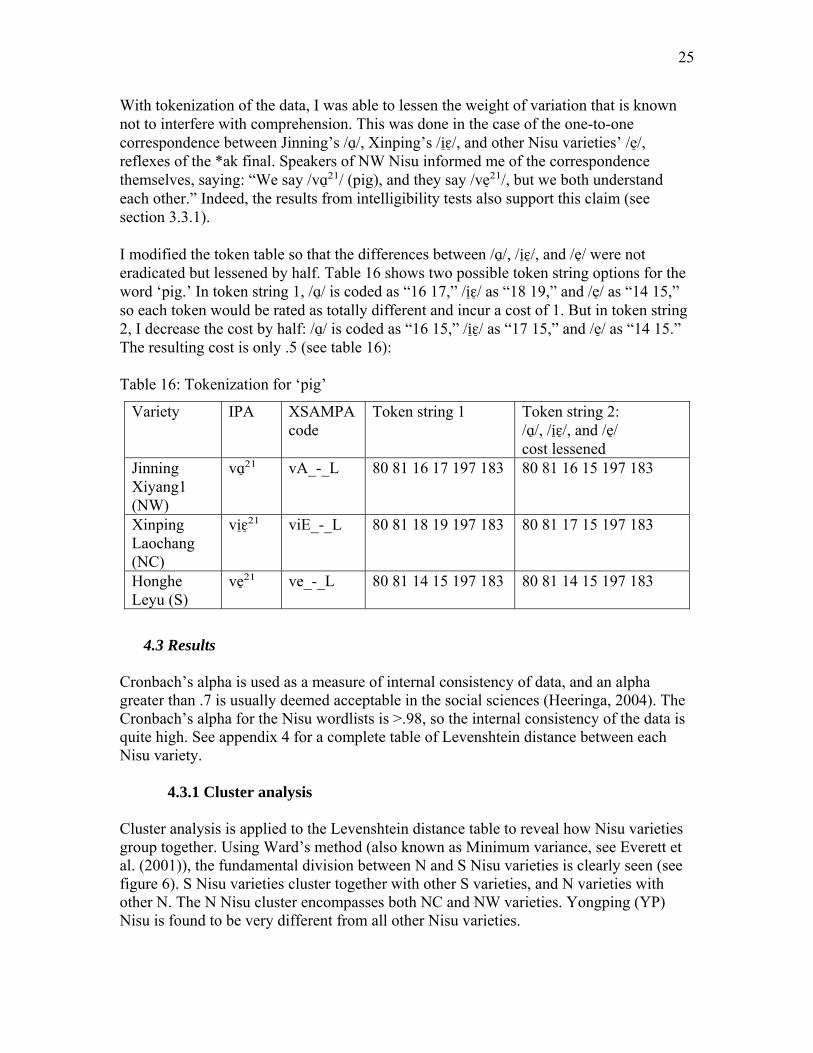
4.3.2 Correlation between Levenshtein distance and intelligibility The Pearson’s correlation coefficient for Levenshtein distance and intelligibility test results show a strong negative correlation: r = -.62, p < .001. This coefficient is slightly weaker than that found by Gooskens (2006) for Norwegian varieties (r = -.82, p < .01), but it is still very strong. The further the Levenshtein distance between two varieties, the lower the probable score listeners will receive on an intelligibility test. Figure 8 shows the scatter plot and best fit line for Levenshtein distance and intelligibility test results:

28

0

0.1

0.2

0.3

0.4

0.5

0.6

0.7

0.8

0.9

1

0.2 0.25 0.3 0.35 0.4 0.45 0.5

Levenshtein distance

Figure 8: Correlation between Levenshtein distance and intelligibility test results.

There are three abnormally low intelligibility scores, seen at the bottom of figure 8. The discrepancy between these results and the others is due to different practices of the test administrators. The low scores are a result of test administrators who did not repeat a section when the participant did not understand the first time. This differed from testers who did repeat sections. This difference probably influenced the abnormally low scores, so these scores are not comparable to the others. If the anomalous scores are removed, the correlation increases to -.79, p < .001. The adjusted scatter plot and best-fit line are seen in figure 9:

5 Conclusions Results from comparative analysis, intelligibility tests, and Levenshtein distance substantiate the claim that Nisu has a basic division between Northern and Southern dialects, and that Northern can be further divided into NC and NW sub-varieties. The complementary methodologies provide triangulation, an ability to look at the question of Nisu dialectology from several different angles. Historical-comparative findings tell us what are the specific differences between varieties; Levenshtein distance clarify the degrees of difference between varieties, and intelligibility tests show what impact those differences have on comprehension. Each method provides a partial, incomplete answer to the question of Nisu dialectology, but together they give a richer, more comprehensive picture. Findings from all three methodologies support the same conclusion: that Nisu can be grouped into Northern and Southern varieties, and that the differences in phonological, lexical, and morphological development are great enough to seriously impact intelligibility between them, with negative implications for the potential sharing of oral or written materials. NC and NW Nisu, on the other hand, show a high level of mutual

29

intelligibility as well as phonological, lexical, and morphological similarity, and thus should be able to use the same oral or written materials. Through this application to a tonal, isolating language, Levenshtein distance proves itself as a dialectometric tool with relevance to languages of diverse typologies. The main adaptation Levenshtein must make in the Sinosphere is the inclusion of non-cognate syllables found in compound words. Tibeto-Burman languages in the Sinosphere often display complex tonal systems, and Levenshtein distance must be adapted to represent this prosodic information. The next step in the development of this tool for Sinospheric languages is determining the optimal representation of tone in the Levenshtein algorithm.

30

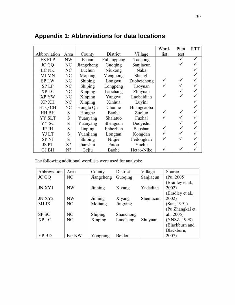
Appendix 1: Abbreviations for data locations

Abbreviation Area County District Village Word-

list Pilot test

RTT

ES FLP NW Eshan Fuliangpeng Tachong JC GQ NC Jiangcheng Guoqing Sanjiacun LC NK NC Luchun Niukong Naka MJ MN NC Mojiang Mengnong Shengli SP LW NC Shiping Longwu Zuobeichong SP LP NC Shiping Longpeng Taoyuan XP LC NC Xinping Laochang Zhuyuan XP YW NC Xinping Yangwu Laobaidian XP XH NC Xinping Xinhua Luyini

HTQ CH NC Hongta Qu Chunhe Huangcaoba HH BH S Honghe Baohe Zuoluo YY SLT S Yuanyang Shalatuo Fuzhai YY SC S Yuanyang Shengcun Duoyishu JP JH S Jinping Jinhezhen Baoshan YJ LT S Yuanjiang Longtan Kongdan SP NJ S Shiping Niujie Feilongkan JS PT S? Jianshui Potou Yuchu GJ BH N? Gejiu Baohe Hetao-Nike

The following additional wordlists were used for analysis:

Abbreviation Area County District Village Source JC GQ NC Jiangcheng Guoqing Sanjiacun (Pu, 2005)

JN XY1 NW Jinning Xiyang Yadadian (Bradley et al., 2002)

JN XY2 NW Jinning Xiyang Shemucun (Bradley et al., 2002)

MJ JX NC Mojiang Jingxing (Sun, 1991)

SP SC NC Shiping Shaochong (Pu Zhangkai et al., 2005)

XP LC NC Xinping Laochang Zhuyuan (YNSZ, 1998)

YP BD Far NW Yongping Beidou

(Blackburn and Blackburn, 2007)

31

Appendix 2: Complete data tables Table 17: Lexical isoglosses in compound words

English Head Garlic Fire Eye Nose Ginger

Proto- Ngwi

*u² & *ʔ-du² & *ʔ-koŋ²

*swan¹/² *C-mi² *(C)-myakH

*s-na¹ kaŋ²

HH LY (S) u³³tɤ³³ ʂu³³mo³³ ɕi⁵⁵tu ̠²¹ ne³̠³tu³³ no⁵⁵tu³³ pʰᴀ²¹tɕi²¹ YY

SLT (S) wo³³tɤ³³ so³³mo³³ ɕi⁵⁵tu ̠²¹ ne³̠³tu³³ no⁵⁵tu³³ pʰæ²¹tɕi²¹

SP NJ (S) v̩³³tɤ³³ ʂʅ³³mu³³ si⁵⁵tu²̠¹ ne³̠³tu³³ no⁵⁵tu³³

pʰe²¹ŋ³̩³ tɕi²¹

JP JH (S) vu ̠³³tɤ³³ so³³mo³³ ɕi³³tu ̠²¹ ȵe³̠³tu³³ no⁵⁵ko ̠²¹ tsʰa³³pɤ²¹

YJ LT (S) u³³tɤ³³ ʂʅ³³bɛ²¹ ɕi⁵⁵tu ̠²¹ ne³̠³tu³³ no⁵⁵bu³³ tʂʰo²¹me³³

GJ BH (N?)

v̩³³tɤ³³ ʂu³³mo³³

mæ³³tu²¹, ɕi²¹tu²¹ ne³̠³sæ³³ no⁵⁵bɤ²¹ tsʰa²¹me³³

SP LP (NC) ŋ³̩³tɤ³³ ʂʅ³³bɛ˞²¹ mə˞³³tu̠²¹ ni³̠³ʂə˞³³ no⁵⁵bɤ²¹ tsʰɑ³³bɛ˞²¹

JC GQ (NC)

ŋɤ̠³³kɤ̠³³ pɯ̠¹¹

ʂu³³ bɛɛ¹¹

mæː³³ tɯ̠¹¹ niɛ³³tɯ³³ no⁵⁵ko ̠¹¹ tɕʰɐ³³pʰi¹̠¹

SP LW (NC)

ŋ²̩¹kɤ³³ tɤ³³ so³³mi³³ mæ³³tu̠²¹ ne³̠³sɛ³³ no⁵⁵bɤ²¹ tsʰᴀ³³pʰi²¹

XP YW (NC) ŋ³̩³kɤ³³ ʂʅ³³bɛ˞²¹ mə˞³³tu̠²¹ ne³̠³ʂɛ³³ no⁵⁵ko²¹ tʂʰa³³mi³³

MJ JX (NC) ŋu̠³³kɯ̠³³ so⁵⁵bɛ²¹ mᴀ̠³³tu ̠²¹ ne³̠³sɛ³³ no⁵⁵ko ̠²¹ tsʰɒ³³pʰe²¹

XP LC (NC) ʔu̠³³ ʂu̠³³bᴇ⁵⁵ mᴇ³³tu ̠²¹ tʂʰᴀ³³pʰi²¹ JN

XY1 (NW) ŋ³̩³kɤ³³ su³³bɛ˞²¹ mɛ˞³³tu²¹ nɑ³³sɛ˞³³ no⁵⁵ko ̠²¹ tɕʰa³³pʰe²¹

s

32

Table 18: /ɬ/ and /tʰ/

English Proto-Ngwi

HH LY-S

YY SLT-S

YJ LT-S JP JH-S

GJ BH-S?

XP LC-NC

SP LW-NC

SP SC-NC

SP LP-NC

MJ JX-NC

JN XY1-NW

excre-ment *ʔ-k(l)e² ɬi³³ ɬi³³ ɬi³³ ɬi³³ a²¹tʰi³³ tʰi³³ tʰi³³ tʰi³³ tʰi³³ tʰi³³

release *k-lwatH

kʰɛ⁵⁵ lɤ²¹

ɬɤ²¹ tɕe³³ ɬɤ̠²¹ ɬɤ²¹ tʰɤ²¹ tʰɤ²¹ tʰɤ²¹ tʰɤ²¹ tʰɤ²¹

white *plu¹ ɬu²¹ ɬu²¹ ɬu²¹ ɬu⁵⁵ a²¹tʰu⁵⁵ tʰu²¹ tʰu⁵⁵ tʰu⁵⁵; tʰu²¹ tʰʲu⁵⁵ tʰu⁵⁵ tʰu²¹

Ditch2 ʑi²¹ɬo³³ ʑi²¹ɬo³³ ʝi²¹ɬo³³ ʑi²¹ɬo³³ ʝi²¹tʰo³³zɿ²¹ tʰo³³

zɿ²¹ tʰo³³

ʑi²¹ tʰo³³

ʑi²¹ tʰo³³

ʑi²¹ tʰo³³

clothing ɬa²¹ ɬa²¹ ɬa²¹ sa³³ɕe³̠³tʰa³³ ɕe²¹ tʰᴀ²¹ tʰa²¹ tʰa²¹

tʰɑ³³ ɕe²¹ tʰɒ²¹ tʰɑ²¹

face *pyu² ɬa²̠¹ni²¹ ɬa²̠¹i³³ nɤ³³ ɬa²̠¹ne²¹

tʰa²̠¹ ne²̠¹

tʰa³̠³ ne²̠¹

tʰᴀ²¹ ni⁵⁵

tʰa²̠¹ ni⁵⁵

tʰa²̠¹ ni⁵⁵

tʰa²̠¹ ni⁵⁵

tʰɒ²¹ ni⁵⁵

tʰɑ²¹ ni⁵⁵

Han Chinese *hyakH ɬa²¹ni⁵⁵ ɬa²¹ni⁵⁵ ɬa²¹ni⁵⁵

tʰa³³ ni⁵⁵

tʰa²¹ ni⁵⁵

tʰa²¹ ni⁵⁵

tʰa²¹ ni⁵⁵

tʰa²¹ ni⁵⁵

tʰa²¹ ni⁵⁵

tʰɒ²¹ ni⁵⁵

2Proto-Ngwi reconstructions for ‘ditch’ and ‘clothing’ have not yet been done.

33

Table 19: *ʃ

English Proto-Ngwi YY

SLT (S) SP NJ (S)

HH LY (S)

YJ LT (S)

SP LP (NC)

XP LC (NC)

XP YW (NC)

GJ BH (N?)

JC GQ (NC)

JP JH (S)

MJ JX (NC)

SP SC (NC)

wheat *ʃa³ so⁵⁵ ɕoŋ⁵⁵ so⁵⁵ so⁵⁵ so⁵⁵ ʂo⁵⁵ ʂo⁵⁵ zo²¹so⁵⁵ so⁵⁵zo³³ so⁵⁵ new *C-ʃikL a³³ʂʅ²̠¹ ʂʅ²̠¹ ɕi²̠¹ ɕi²̠¹ ɕi²̠¹ sɿ²̠¹ ka³³sɿ²̠¹ ɕi²̠¹ si¹̠¹ ɕi²¹ ɕi²̠¹ ɕi²̠¹ urine *ʃi² ᴀ⁵⁵ʂʅ³³ ᴀ⁵⁵ʂu³³ ɕi⁵⁵ ɕi⁵⁵ sɿ⁵⁵ sɿ⁵⁵xo³³ ᴀ²¹ɕi⁵⁵ si⁵⁵ ɕi⁵⁵ ɕi⁵⁵ seven *C-ʃi(k)²/L ʂʅ²¹ ʂʅ²¹ ʂʅ²¹ ʂʅ²¹ ʂʅ²¹ ʂʅ²¹ sɿ²¹ sɿ²¹ ʃɨ¹̠¹ sɿ²¹ ɕi²¹ ɕi²¹ die *ʃe² ʂʅ²¹ ʂʅ²¹ ʂʅ²¹ ʂʅ²¹ ʂʅ²¹ ʂʅ²¹ ʂʅ²¹ sɿ²¹ sɪ¹̠¹ sɿ²¹ ɕi²¹ ɕi²¹ day before yesterday *ʔəʃikH ᴀ²¹ʂʅ³³ a²¹ʂʅ³³ ᴀ²¹ʂʅ³³ ᴀ²¹ʂʅ³³ ʂʅ³³ ʂʅ³³ ʂʅ³³ ᴀ²¹ʂʅ³³ ʃɨ³³ ᴀ²¹sɿ³³ si³³ sɿ³³

Table 20: *s

English Proto-Ngwi

XP LC (NC)

SP LW (NC)

XP YW (NC)

YY SLT (S)

HH LY (S)

SP LP (NC)

JC GQ (NC)

SP NJ (S)

JP JH (S)

YJ LT (S)

kill *C-satL sɿ²̠¹ ɕi²̠¹ sɿ²̠¹ ɕi²̠¹ si²̠¹ ɕi²̠¹ si¹̠¹ si²̠¹ ɕi²̠¹ ɕi²̠¹ thirsty *C-sipL sɿ²̠¹ ɕi²̠¹ sɿ²̠¹ ɕe²̠¹ ɕi²̠¹ ɕi²̠¹ ɕi²̠¹ ɕi²̠¹ ɕi²̠¹

tree *sikH & *dzin¹ sɿ³̠³ sɿ³̠³dzɛ²¹ sɿ³̠³dʐɛ˞²¹ ɕi³̠³dʐɛ˞³³ si³̠³dzɛ³³ si³̠³dʐɛ˞³³ si³³dzɛ¹¹ si³̠³ ɕi³̠³dzɛ³³ ɕi³̠³dzɛ²¹

know *si² sɛ²̠¹ sᴀ̠²¹ sᴀ̠²¹ three *C-sum² ʂᴀ⁵⁵ sᴀ⁵⁵ sᴀ⁵⁵ ʂᴀ˞⁵⁵ sᴀ⁵⁵ sɑ⁵⁵ sɐ⁵⁵ sᴀ⁵⁵ sa⁵⁵ sᴀ⁵⁵

broom ʔ-mri² & sutH mi⁵⁵ʂʅ³̠³ mu⁵⁵sʅ³̠³ mi⁵⁵ʂʅ³̠³ mi⁵⁵sɿ³̠³ mi⁵⁵sɿ³̠³ mi⁵⁵sʅ³̠³ mi⁵⁵ʃɨ³̠³ mi⁵⁵sɿ³̠³ mi⁵⁵sɿ³̠³ mi⁵⁵sɿ³̠³

who? *ʔəsu¹ ᴀ²¹ʂo³³ ʂu³³ a²¹ʂʅ³³ ᴀ⁵⁵ʂu³³ ᴀ⁵⁵ʂu³³ ʔᴀ⁵⁵ʂʅ³³ ɑ⁵⁵ʂu³³ ᴀ⁵⁵su³³ a⁵⁵su³³ ᴀ⁵⁵sɿ³³

34

Table 21: *ky and *kr

English Proto-Ngwi XP LC (NC)

HH LY (S) YJ LT (S) SP NJ (S)

XP YW (NC)

SP LP (NC)

SP LW (NC)

GH BH (N?)

friend *kyaŋ² tʂhᴀ³³tʂhᴀ²¹

ᴀ⁵⁵tʂʰᴀ³³ ɬe³̠³tʂʰᴀ²¹ tsʰᴀ³³ɣɛ²¹ tsʰᴀ³³ɣɛ²¹ tsʰᴀ³³tsʰᴀ²¹ ɬi²¹tsʰɑ²¹ tsʰᴀ³³ɣɛ²¹ tsʰᴀ³³pʲe³³

arrive *(k)-rokL tʂhɤ²¹ tʂʰɤ²¹ tʂʰɤ²¹ tɕʰe²¹ tsʰɤ²¹ tsʰɤ²¹ tsʰɤ²¹ tsʰɤ²¹ six *C-krokL tʂhu ̠²¹ tʂʰu̠²¹ tʂʰu̠²¹ tʂʰu̠²¹ tʂʰu̠²¹ tsʰu̠²¹ tsʰu̠²¹ tsʰu̠²¹ mill *m-kritH tʂhʅ³̠³ tʂʰʅ³̠³ tʂʰu̠³³ tʂʰʅ³̠³ tʂʰu̠³³ tʂʰʅ³̠³lu³³ tʂʰʅ³̠³ tsʰɿ³̠³ sweet *kyo¹ tʂhʅ⁵⁵ tʂʰʅ⁵⁵ tʂʰu⁵⁵ tʂʰʅ⁵⁵ tʂʰu⁵⁵ tʂʰʅ⁵⁵ tʂʰʅ⁵⁵ tsʰɿ⁵⁵ horn *kro¹ tʂhʅ²¹ tʂʰʅ²¹ kə³³tʂʰu²¹ a⁵⁵tʂʰən²¹ ka³³tʂʰʅ²¹ tʂʰʅ²¹ tʂʰʅ²¹ a²¹tʂʰʅ²¹

Table 22: *gy and *gr

English Proto-Ngwi XP LC (NC)

XP YW (NC)

HH LY (S) YJ LT (S) SP NJ (S)

SP LW (NC)

SP LP (NC)

GH BH (N?)

star *C-gray¹ tsᴇ⁵⁵ tʂɛ⁵⁵mo²¹ tʂɛ⁵⁵mo²¹ tsɛ⁵⁵mo²¹ tɕĩ⁵⁵mo²¹ tsɛ⁵⁵mo²¹ tʂə˞⁵⁵mo²¹ tsæ⁵⁵mo²¹ cold *C-grakH dʑiɛ̠³̠³ dʑe³̠³ dʑe³̠³ dʑe³̠³ dʑe³̠³ dʑe³̠³ dʑe³̠³ tɕʰi²¹ thorn *g(y)oŋ³ ᴀ⁵⁵dʐɤ²¹ a⁵⁵dzɤ²¹ dzɤ²¹ dzɤ²¹ dzɤ²¹ dzɤ²¹ dzɤ²¹mo²¹ dzɤ²¹mo²¹ tendon *(ʃ)-gru² dʐu³³ dʐʅ³³ dʐu³³ dʐu³³ dʐu³³ dzu³³ dzu³³ dzu³³tɕe³³ fear *(sə)-grokH dʐu̠³³ dʐu ̠³³ dʐu³³ dʐu³³ dʐu̠³³ dzu̠³³ dzu̠³³ dzu̠³³ sew *gyupL dʐʅ²̠¹ dʐʅ²̠¹ dʐʅ²̠¹ dʐu ̠²¹ dʑi²̠¹ dʐʅ²̠¹ dʐʅ²̠¹ dzɿ²̠¹

35

Table 23: Plural marker in pronominal paradigm

English 1PL 2PL 3PL Proto-Ngwi *C-ŋa¹ ʔ-way²/³ *naŋ¹ ʔ-way²/³ *ʒaŋ² ʔ-way²/³

YJ LT (S) ŋo²¹tɕi³³ na²¹tɕi³³ kɤ⁵⁵tɕi³³ YY SLT (S) ŋo²¹wo²¹ na²¹wo²¹ kɤ⁵⁵ji²¹ HH LY (S) ŋo²¹xo²¹ na²¹xo²¹ kɤ⁵⁵xo²¹

JP JH (S) ŋo³³xo²¹ na³³xo²¹ ko⁵⁵xo²¹ GJ BH (N?) ŋ³̩³xo²¹ na³³xo²¹ kɤ⁵⁵tɕe³³

SP NJ (S)

ŋõ³³wi³³, ŋõ³³be²¹ na³³be²¹ kɤ⁵⁵be²¹

JC GQ (NC) ŋoːˌ³³bɤ¹¹ kɤˌ⁵⁵bɤ¹¹ SP LP (NC) m̩²¹bɤ²¹ nᴀ³³bɤ²¹ ha⁵⁵bɤ²¹ SP LW (NC) ŋ²̩¹bɤ²¹ nᴀ³³bɤ²¹ kɤ⁵⁵bɤ²¹ XP YW (NC) ŋo²¹bɤ²¹ nᴀ³³bɤ²¹ kɤ⁵⁵bɤ²¹ XP LC (NC) ŋo²¹bɤ²¹ nᴀ³³bɤ²¹ kɤ⁵⁵bɤ²¹ MJ JX (NC) ŋo³³bɯ²¹ nᴀ³³bɯ²¹ kʰɯ³³bɯ²¹ Shuangbai (NW) ŋo³³bɤ²¹ nɑ³³bɤ²¹ kɤ⁵⁵bɤ²¹

36

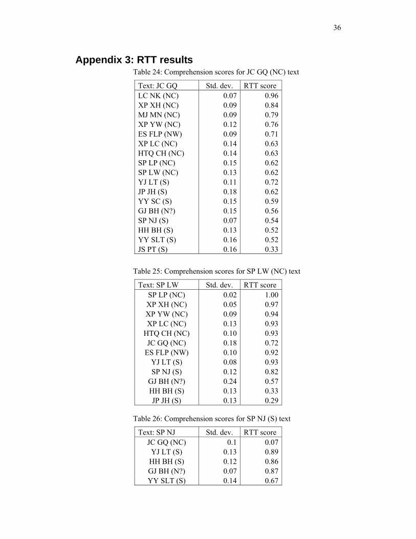
Appendix 3: RTT results Table 24: Comprehension scores for JC GQ (NC) text

Text: JC GQ Std. dev. RTT score LC NK (NC) 0.07 0.96XP XH (NC) 0.09 0.84MJ MN (NC) 0.09 0.79XP YW (NC) 0.12 0.76ES FLP (NW) 0.09 0.71XP LC (NC) 0.14 0.63HTQ CH (NC) 0.14 0.63SP LP (NC) 0.15 0.62SP LW (NC) 0.13 0.62YJ LT (S) 0.11 0.72JP JH (S) 0.18 0.62YY SC (S) 0.15 0.59GJ BH (N?) 0.15 0.56SP NJ (S) 0.07 0.54HH BH (S) 0.13 0.52YY SLT (S) 0.16 0.52JS PT (S) 0.16 0.33

Table 25: Comprehension scores for SP LW (NC) text

Text: SP LW Std. dev. RTT score SP LP (NC) 0.02 1.00XP XH (NC) 0.05 0.97XP YW (NC) 0.09 0.94XP LC (NC) 0.13 0.93

HTQ CH (NC) 0.10 0.93JC GQ (NC) 0.18 0.72

ES FLP (NW) 0.10 0.92YJ LT (S) 0.08 0.93SP NJ (S) 0.12 0.82

GJ BH (N?) 0.24 0.57HH BH (S) 0.13 0.33JP JH (S) 0.13 0.29

Table 26: Comprehension scores for SP NJ (S) text

Text: SP NJ Std. dev. RTT score JC GQ (NC) 0.1 0.07YJ LT (S) 0.13 0.89HH BH (S) 0.12 0.86GJ BH (N?) 0.07 0.87YY SLT (S) 0.14 0.67

37

Table 27: Comprehension scores for other texts

Text Listeners XP YW YY SC ES FLP YY SLT

Format: RTT score/ Standard deviation XP LC 1.00/.02 JP JH 0.92/.08 YY SLT 0.98/.05 XP XH 0.99/.03 JC GQ 0.20/.11 0.29/.23 HH BH 0.69/.16

38

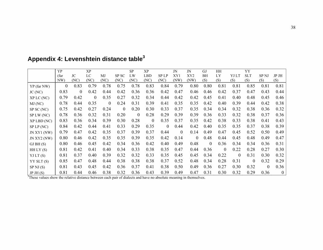
Appendix 4: Levenshtein distance table3

YP (far NW)

JC (NC)

XP LC (NC)

MJ (NC)

SP SC (NC)

SP LW (NC)

XP LBD (NC)

SP LP (NC)

JN XY1 (NW)

JN XY2 (NW)

GJ BH (S)

HH LY (S)

YJ LT (S)

YY SLT (S)

SP NJ (S)

JP JH (S)

YP (far NW) 0 0.83 0.79 0.78 0.75 0.78 0.83 0.84 0.79 0.80 0.80 0.81 0.81 0.85 0.81 0.81JC (NC) 0.83 0 0.42 0.44 0.42 0.36 0.36 0.42 0.47 0.46 0.46 0.42 0.37 0.47 0.43 0.44XP LC (NC) 0.79 0.42 0 0.35 0.27 0.32 0.34 0.44 0.42 0.42 0.45 0.41 0.40 0.48 0.45 0.46MJ (NC) 0.78 0.44 0.35 0 0.24 0.31 0.39 0.41 0.35 0.35 0.42 0.40 0.39 0.44 0.42 0.38SP SC (NC) 0.75 0.42 0.27 0.24 0 0.20 0.30 0.33 0.37 0.35 0.34 0.34 0.32 0.38 0.36 0.32SP LW (NC) 0.78 0.36 0.32 0.31 0.20 0 0.28 0.29 0.39 0.39 0.36 0.33 0.32 0.38 0.37 0.36XP LBD (NC) 0.83 0.36 0.34 0.39 0.30 0.28 0 0.35 0.37 0.35 0.42 0.38 0.33 0.38 0.41 0.43SP LP (NC) 0.84 0.42 0.44 0.41 0.33 0.29 0.35 0 0.44 0.42 0.40 0.35 0.35 0.37 0.38 0.39JN XY1 (NW) 0.79 0.47 0.42 0.35 0.37 0.39 0.37 0.44 0 0.14 0.49 0.47 0.45 0.52 0.50 0.49JN XY2 (NW) 0.80 0.46 0.42 0.35 0.35 0.39 0.35 0.42 0.14 0 0.48 0.44 0.45 0.48 0.49 0.47GJ BH (S) 0.80 0.46 0.45 0.42 0.34 0.36 0.42 0.40 0.49 0.48 0 0.36 0.34 0.34 0.36 0.31HH LY (S) 0.81 0.42 0.41 0.40 0.34 0.33 0.38 0.35 0.47 0.44 0.36 0 0.22 0.28 0.27 0.30YJ LT (S) 0.81 0.37 0.40 0.39 0.32 0.32 0.33 0.35 0.45 0.45 0.34 0.22 0 0.31 0.30 0.32YY SLT (S) 0.85 0.47 0.48 0.44 0.38 0.38 0.38 0.37 0.52 0.48 0.34 0.28 0.31 0 0.32 0.29SP NJ (S) 0.81 0.43 0.45 0.42 0.36 0.37 0.41 0.38 0.50 0.49 0.36 0.27 0.30 0.32 0 0.36JP JH (S) 0.81 0.44 0.46 0.38 0.32 0.36 0.43 0.39 0.49 0.47 0.31 0.30 0.32 0.29 0.36 0

3These values show the relative distance between each pair of dialects and have no absolute meaning in themselves.

39

References: Allen, Bryan. 2004. Bai dialect survey: Yunnan Minority Language Commission and SIL

International Joint Publication Series. Kunming: Yunnan Minzu Chubanshe. Blackburn, P.L. and Blackburn, Laura. 2007. Yongping Nisu wordlist. Dali: SIL East

Asia Group. Blair, Frank. 1990. Survey on a shoestring: SIL and UTA Publications in Linguistics 96.

Dallas: SIL. Bradley, David. 1979. Proto-Loloish: Scandinavian Institute of Asian Studies Monograph

No. 39. London: Curzon Press. Bradley, David (ed.). 1997. Tibeto-Burman languages of the Himalayas. Papers in

Southeast Asian Linguistics No. 14. Canberra: Pacific Linguistics. Bradley, David, Bradley, Maya and Li, Yongxiang. 2002. Jinning Nasu wordlists.

Melbourne: La Trobe University. Casad, Eugene H. 1974. Dialect intelligibility testing: SIL Publications in Linguistics and

Related Fields 38. Dallas: SIL. Chambers, J. K. and Trudgill, Peter. 1998. Dialectology. New York: Cambridge

University Press. Chen, Shinlin, Bian, Shiming and Li, Xiuqing. 1985. Yiyu Jianzhi [Outline of the Yi

language]: Zhongguo shaoshu minzu yuyan jianzhi congshu. Beijing: Minzu Chubanshe.

Chen, Shilin, Bian, Shiming and Li, Xiuqing. 1985. Yiyu jianzhi [Outline of the Yi language]: Zhongguo shaoshu minzu yuyan jianzhi congshu. Beijing: Minzu Chubanshe.

Everitt, Brian, Landau, Sabine and Leese, Morven. 2001. Cluster analysis. London: Oxford University Press.

Gooskens, Charlotte. 2006. Linguistic and extra-linguistic predictors of Inter-Scandinavian intelligibility. Linguistics in the Netherlands 2006, ed. by Jeroen van de Weijer and Bettelou Los, 101–13. Amsterdam: John Benjamins.

Gooskens, Charlotte and Heeringa, Wilbert. 2004. Perceptive Evaluation of Levenshtein Dialect Distance Measurements Using Norwegian Dialect Data. Language Variation and Change, 16.189–207.

Grimes, Joseph E. 1995. Language survey reference guide. Dallas: SIL. Heeringa, Wilbert. 2004. Measuring pronunciation differences with Levenshtein Distance,

Humanities Computing, University of Groningen: PhD dissertation. Heeringa, Wilbert, Kleiweg, Peter, Gooskens, Charlotte and Nerbonne, John. 2006.

Evaluation of string distance algorithms for dialectology. Paper presented at J. Nerbonne and E. Hinrichs (eds.) Linguistic Distances Workshop at the joint conference of International Committee on Computational Linguistics and the Association for Computational Linguistics, Sydney, July, 2006, 51–62.

Kessler, Brett. 1995. Computational dialectology in Irish Gaelic. Proceedings of the European ACL, 60–67. Dublin.

Kleiweg, Peter. 2007. RuG/L04. http://www.let.rug.nl/~kleiweg/indexs.html. Groningen: University of Groningen.

40

Kruskal, Joseph. 1999. An overview of sequence comparison. Time Warps, String Edits and Macromolecules: The Theory and Practice of Sequence Comparison, ed. by David Sankoff and Joseph Kruskal, 1–44. Stanford: CSLI.

Li Guangyun, Li Fuchun and Simao Xingzheng Gongshu Minwei. 1990. Simao shaoshu minzu [Simao minority nationalities]. Kunming: Yunnan Minzu chubanshe.

Li, Shengfu. 1996. Yi yu nanbu fangyan yanjiu [Research on Southern Yi]. Beijing: Minzu chubanshe.

Milliken, Margaret E. 1988. Phonological Divergence and Intelligibility: A Case Study of English and Scots, Cornell University: PhD dissertation.

Morberg, Jens, Gooskens, Charlotte and Nerbonne, John 2007. Conditional entropy as a measure of linguistic remoteness between related languages. Proceedings of Computational Linguistics in the Netherlands 2006 ed. by Ineke Schuurman. Amsterdam: Rodopi.

Osenova Petya, Heeringa, Wilbert and Nerbonne, John. Forthcoming. A Quantitative Analysis of Bulgarian Dialect Pronunciation. Zeitschrift für Slavische Philologie.

Pu Meishan. 2005. Jiangcheng Nisu Wordlist. Kunming: SIL East Asia Group. Pu Zhangkai, Kong Yun and Pu Meixiao. 2005. Diannan Yi wen zidian [A dictionary of

South Yunnan Yi]: Yunnan Minzu Guji Congshu [Yunnan Nationalities Ancient Book series, Yi collection]. Kunming: Yunnan Minzu Chubanshe.

Sun, Hongkai (ed.) 1991. Zangmian Yuyin he Cihui [Tibeto-Burman Sound Systems and Lexicons]. Beijing: Zhongguo Shehui Kexue Chubanshe.

Wang, Chengyou. 2003. Yi Yu Fangyan Bijiao [Comparative Study of Yi Dialects]. Chengdu: Sichuan Minzu Chubanshe.

Wardhaugh, Ronald. 1986. An introduction to sociolinguistics. New York, NY, USA: Blackwell.

Wells, John. 2005. Sampa Computer Readable Phonetic Alphabet. vol. 2007. http://www.phon.ucl.ac.uk/home/sampa/. London: University College London.

YNSZ. 1998. Editorial Committee, eds. Shaoshuminzu Yuyan Wenzi Zhi [Ethnic minority scripts and languages].vol. 59: Yunnan Shengzhi [Yunnan Provincial Gazetteer]. Kunming: Yunnan Renmin Chubanshe.

YPXZ. 1994. Yongping xian zhi [Yongping County Annals]. Kunming: Yunnan ren min chu ban she.

Zhu, Wenxu. 2005. Yi Yu Fangyan Xue [Yi Dialect Studies]. Beijing: Zhongyang Minzu Daxue Chubanshe.