An Efficient Evolutionary Algorithmfor Solving Incrementally Structured Problems

Jason Ansel Maciej Pacula Saman Amarasinghe Una-May O’ReillyComputer Science and Artificial Intelligence Laboratory

Massachusetts Institute of TechnologyCambridge, MA, USA

{jansel,mpacula,saman,unamay}@csail.mit.edu

ABSTRACTMany real world problems have a structure where smallproblem instances are embedded within large problem in-stances, or where solution quality for large problem instancesis loosely correlated to that of small problem instances. Thisstructure can be exploited because smaller problem instancestypically have smaller search spaces and are cheaper to eval-uate. We present an evolutionary algorithm, INCREA, whichis designed to incrementally solve a large, noisy, computa-tionally expensive problem by deriving its initial populationthrough recursively running itself on problem instances ofsmaller sizes. The INCREA algorithm also expands andshrinks its population each generation and cuts off workthat doesn’t appear to promise a fruitful result. For fur-ther efficiency, it addresses noisy solution quality efficientlyby focusing on resolving it for small, potentially reusablesolutions which have a much lower cost of evaluation. Wecompare INCREA to a general purpose evolutionary algo-rithm and find that in most cases INCREA arrives at thesame solution in significantly less time.

Categories and Subject DescriptorsI.2.5 [Artificial Intelligence]: Programming Languagesand Software; D.3.4 [Programming Languages]: Proces-sors—Compilers

General TermsAlgorithms, Experimentation, Languages

1. INTRODUCTIONAn off-the-shelf evolutionary algorithm (EA) does not typ-

ically take advantage of shortcuts based on problem prop-erties and this can sometimes make it impractical becauseit takes too long to run. A general shortcut is to solve asmall instance of the problem first then reuse the solution ina compositional manner to solve the large instance which is

Permission to make digital or hard copies of all or part of this work forpersonal or classroom use is granted without fee provided that copies arenot made or distributed for profit or commercial advantage and that copiesbear this notice and the full citation on the first page. To copy otherwise, torepublish, to post on servers or to redistribute to lists, requires prior specificpermission and/or a fee.GECCO’11, July 12–16, 2011, Dublin, Ireland.Copyright 2011 ACM 978-1-4503-0557-0/11/07 ...$10.00.

of interest. Usually solving a small instance is both simpler(because the search space is smaller) and less expensive (be-cause the evaluation cost is lower). Reusing a sub-solutionor using it as a starting point makes finding a solution toa larger instance quicker. This shortcut is particularly ad-vantageous if solution evaluation cost grows with instancesize. It becomes more advantageous if the evaluation resultis noisy or highly variable which requires additional evalua-tion sampling.

This shortcut is vulnerable to local optima: a small in-stance solution might become entrenched in the larger solu-tion but not be part of the global optimum. Or, non-lineareffects between variables of the smaller and larger instancesmay imply the small instance solution is not reusable. How-ever, because EAs are stochastic and population-based theyare able to avoid potential local optima arising from smallinstance solutions and address the potential non-linearityintroduced by the newly active variables in the genome.

In this contribution, we describe an EA called INCREAwhich incorporates into its search strategy the aforemen-tioned shortcut through incremental solving. It solves in-creasingly larger problem instances by first activating onlythe variables in its genome relevant to the smallest instance,then extending the active portion of its genome and prob-lem size whenever an instance is solved. It shrinks andgrows its population size adaptively to populate a gene poolthat focuses on high performing solutions in order to avoidrisky, excessively expensive, exploration. It assumes that fit-ness evaluation is noisy and addresses the noise adaptivelythroughout the tuning process.

Problems of practical value with this combination of op-portunity and requirements exist. We will exemplify the IN-CREA technique by solving a software engineering problemknown as autotuning. We are developing a programminglanguage named Petabricks which supports multi-core pro-gramming. In our case, autotuning arises as a final taskof program compilation and occurs at program installationtime. Its goal is to select parameters and algorithmic choicesfor the program to make it run as fast as possible. Becausea program can have varying size inputs, INCREA tunes theprogram for small input sizes before incrementing them upto the point of the maximum expected input sizes.

We proceed in the following manner: Section 2 describescompilation autotuning, and elaborates upon how it exhibitsthe aforementioned properties of interest. Section 3 de-scribes the design of INCREA. Section 4 discuss its relationto other relevant EAs. Section 5 experimentally comparesINCREA to a general purpose EA. Section 6 concludes.

2. AUTOTUNINGWhen writing programs that require performance, the

programmer is often faced with many alternate ways to im-plement a set of algorithms. Most often the programmerchooses a single set based on manual testing. Unfortunately,with the increasing diversity in architectures, finding one setthat performs well everywhere is impossible for many prob-lems. A single program might be expected to run on a small,embedded cell phone, a multi-core desktop or server, a clus-ter, a grid, or the cloud. The appropriate algorithmic choicesmay be very different for each of these architectures.

An example of this type of hand coding of algorithmscan be found in the std::sort routine found in the C++Standard Template Library. This routine performs mergesort until there are less than 15 elements in a recursive callthen switches to insertion sort. This cutoff is hardcoded,even though values 10 times larger can perform better onmodern architectures and entirely different algorithms, suchas bitonic sort, can perform better on parallel vector ma-chines [3].

This motivates the need for an autotuning capability. Theprogrammer should be able to provide a choice of algorithms,describe a range of expected data sizes, and then pass tothe compiler the job of experimentally determining, for anyspecific architecture, what cutoff points apply and what al-gorithms are appropriate for different data ranges.

The autotuners in this paper operate on programs writ-ten in the PetaBricks programming language [3] which al-lows the programmer to express algorithmic choices at thelanguage level without committing to any single one, or anycombination thereof. The task of choosing the fastest al-gorithm set is delegated to an auotuner which makes thedecision automatically depending on input sizes to each al-gorithm (and an overall target input size) and a target ar-chitecture.

2.1 The Autotuning ProblemThe autotuner must identify selectors that will determine

which choice of an algorithm will be used during a programexecution so that the program executes as fast as possi-ble. Formally, a selector s consists of ~Cs = [cs,1, . . . , cs,m−1]

∪ ~As = [αs,1, . . . , αs,m] where ~Cs are the ordered interval

boundaries (cutoffs) associated with algorithms ~As. Duringprogram execution the runtime function SELECT choosesan algorithm depending on the current input size by refer-encing the selector as follows:

SELECT (input, s) = αs,i s.t. cs,i > size(input) ≥ cs,i−1

wherecs,0 = min(size(input)) and cs,m = max(size(input)).

The components of ~As are indices into a discrete set of ap-plicable algorithms available to s, which we denoteAlgorithmss.The maximum number of intervals is fixed by the PetaBrickscompiler. An example of a selector for a sample sorting al-gorithm is shown in Figure 1.

In addition to algorithmic choices, the autotuner tunesparameters such as blocking sizes, sequential/parallel cutoffsand the number of worker threads. Each tunable is eithera discrete value of a small set indexed by an integer or ainteger in some positive bounded range.

Formally, given a program P , hardware H and input sizen, the autotuner must identify the vector of selectors and

αs,1 = 1

cs,1

=

150 MaxInputSize0

cs,2

=

106

input size

0: RadixSort

1: InsertionSort

2: QuickSort

3: BogoSort

αs,2 = 2 αs,3 = 0

Algorithmss:

Figure 1: A selector for a sample sorting algorithmwhere ~Cs = [150, 106] and ~As = [1, 2, 0]. The selec-tor selects the InsertionSort algorithm for input sizesin the range [0; 150), QuickSort for input sizes inthe range [150, 106) and RadixSort for [106,MAXINT ).BogoSort was suboptimal for all input ranges and isnot used.

vector of tunables such that the following objective functionexecutionT ime is satisfied:

arg mins,t

executionT ime(P,H, n)

2.2 Properties of the Autotuning ProblemThree properties of autotuning influence the design of an

autotuner. First, the cost of fitness evaluation depends heav-ily on on the input data size used when testing the candi-date solution. The autotuner does not necessarily have touse the target input size. For efficiency it could use smallersizes to help it find a solution to the target size because isgenerally true that smaller input sizes are cheaper to teston than larger sizes, though exactly how much cheaper de-pends on the algorithm. For example, when tuning matrixmultiply one would expect testing on a 1024× 1024 matrixto be about 8 times more expensive than a 512×512 matrixbecause the underlying algorithm has O(n3) performance.While solutions on input sizes smaller than the target sizesometimes are different from what they would be when theyare evolved on the target input size, it can generally be ex-pected that relative rankings are robust to relatively smallchanges in input size. This naturally points to “bottom-up”tuning methods that incrementally reuse smaller input sizetests or seed them into the initial population for larger inputsizes.

Second, in autotuning the fitness of a solution is its fitnessevaluation cost. Therefore the cost of fitness evaluation isdependant on the quality of a candidate algorithm. A highlytuned and optimized program will run more quickly than arandomly generated one and it will thus be fitter. This im-plies that fitness evaluations become cheaper as the overallfitness of the population improves.

Third, significant to autotuning well is recognizing the factthat fitness evaluation is noisy due to details of the paral-lel micro-architecture being run on and artifacts of concur-rent activity in the operating system. The noise can comefrom many sources, including: caches and branch prediction;races between dependant threads to complete work; operat-ing system artifacts such as scheduling, paging, and I/O;

and, finally, other competing load on the system. This leadsto a design conflict: an autotuner can run fewer tests, risk-ing incorrectly evaluating relative performance but finishingquickly, or it can run many tests, likely be more accuratebut finish too slowly. An appropriate strategy is to runmore tests on less expensive (i.e. smaller) input sizes.

The INCREA exploits incremental structure and handlesthe noise exemplified in autotuning. We now proceed todescribe a INCREA for autotuning.

3. A BOTTOM UP EA FOR AUTOTUNING

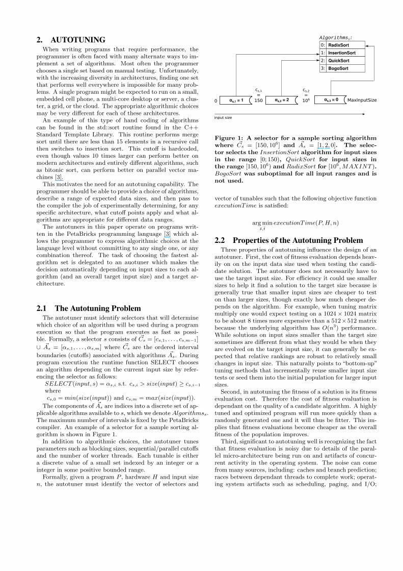
RepresentationThe INCREA genome, see Figure 2, encodes a list of selec-tors and tunables as integers each in the range [0,MaxV al)where MaxV al is the cardinality of each algorithm choiceset for algorithms and MaxInputSize for cutoffs. Each tun-able has a MaxV al which is the cardinality of its value setor a bounded integer depending on what it represents.

In order to tune programs of different input sizes thegenome represents a solution for maximum input size andthroughout the run increases the “active” portion of it start-ing from the selectors and tunables relevant to the smallestinput size. It has length (2m + 1)k + n, where k is thenumber of selectors, m the number of interval cutoffs withineach selector and n the number of other tunables definedfor the PetaBricks program. As the algorithm progressesthe number of “active” cutoff and algorithm pairs, which wecall “choices” for each selector in the genome starts at 1 andthen is incremented in step with the algorithm doubling thecurrent input size each generation.

selector2

c α c α α c α c α α t t t t

2m+1 2m+1 n

selector1

0 c1,1 c1,2 MaxInputSizeα1,1 α1,2 α1,3

0 c2,1 c2,2 MaxInputSizeα2,1 α2,2 α2,3

tunables

t1, t

2, t

3, t

4[

[

Figure 2: A sample genome for m = 2, k = 2 and n =4. Each gene stores either a cutoff cs,i, an algorithmαs,i or a tunable value ti.

Fitness evaluationThe fitness of a genome is the inverse of the correspondingprogram’s execution time. The execution time is obtainedby timing the PetaBricks program for a specified input size.

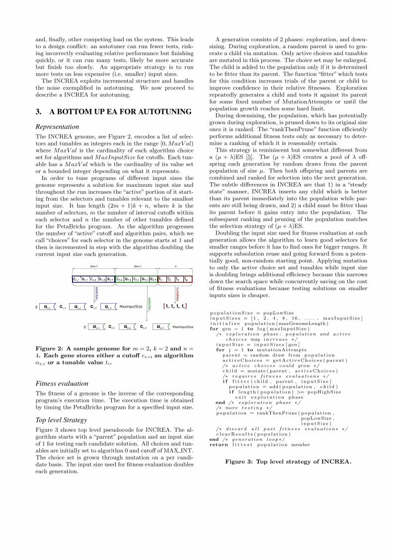
Top level StrategyFigure 3 shows top level pseudocode for INCREA. The al-gorithm starts with a “parent” population and an input sizeof 1 for testing each candidate solution. All choices and tun-ables are initially set to algorithm 0 and cutoff of MAX INT.The choice set is grown through mutation on a per candi-date basis. The input size used for fitness evaluation doubleseach generation.

A generation consists of 2 phases: exploration, and down-sizing. During exploration, a random parent is used to gen-erate a child via mutation. Only active choices and tunablesare mutated in this process. The choice set may be enlarged.The child is added to the population only if it is determinedto be fitter than its parent. The function “fitter” which testsfor this condition increases trials of the parent or child toimprove confidence in their relative fitnesses. Explorationrepeatedly generates a child and tests it against its parentfor some fixed number of MutationAttempts or until thepopulation growth reaches some hard limit.

During downsizing, the population, which has potentiallygrown during exploration, is pruned down to its original sizeonce it is ranked. The “rankThenPrune” function efficientlyperforms additional fitness tests only as necessary to deter-mine a ranking of which it is reasonably certain.

This strategy is reminiscent but somewhat different froma (µ + λ)ES [5]. The (µ + λ)ES creates a pool of λ off-spring each generation by random draws from the parentpopulation of size µ. Then both offspring and parents arecombined and ranked for selection into the next generation.The subtle differences in INCREA are that 1) in a “steadystate” manner, INCREA inserts any child which is betterthan its parent immediately into the population while par-ents are still being drawn, and 2) a child must be fitter thanits parent before it gains entry into the population. Thesubsequent ranking and pruning of the population matchesthe selection strategy of (µ+ λ)ES.

Doubling the input size used for fitness evaluation at eachgeneration allows the algorithm to learn good selectors forsmaller ranges before it has to find ones for bigger ranges. Itsupports subsolution reuse and going forward from a poten-tially good, non-random starting point. Applying mutationto only the active choice set and tunables while input sizeis doubling brings additional efficiency because this narrowsdown the search space while concurrently saving on the costof fitness evaluations because testing solutions on smallerinputs sizes is cheaper.

popu la t i onS i z e = popLowSizei npu tS i z e s = [ 1 , 2 , 4 , 8 , 16 , . . . . , maxInputSize ]i n i t i a l i z e populat ion (maxGenomeLength )for gen = 1 to l og ( maxInputSize )

/∗ exp lora t ion phase : populat ion and ac t i v echoices may increase ∗/

i nputS i z e = inputS i z e s [ gen ]for j = 1 to mutationAttempts

parent = random draw from populat ionac t iveCho i c e s = getAct iveCho ices ( parent )/∗ ac t i v e choices could grow ∗/ch i l d = mutate ( parent , a c t i veCho i c e s )/∗ requ i res f i t n e s s eva lua t ions ∗/i f f i t t e r ( ch i ld , parent , i nputS i z e )

populat ion = add ( populat ion , c h i l d )i f l ength ( populat ion ) >= popHighSize

e x i t exp l o r a t i on phaseend /∗ exp lora t ion phase ∗//∗ more t e s t i n g ∗/populat ion = rankThenPrune ( populat ion ,

popLowSize ,i nputS i z e )

/∗ discard a l l past f i t n e s s eva lua t ions ∗/c l e a rRe su l t s ( populat ion )

end /∗ generation loop ∗/return f i t t e s t populat ion member

Figure 3: Top level strategy of INCREA.

Mutation OperatorsThe mutators perform different operations based on the typeof value being mutated. For an algorithmic choice, thenew value is drawn from a uniform probability distribu-tion [0, ||Algorithmss|| − 1]. For a cutoff, the existing valueis scaled by a random value drawn from a log-normal dis-tribution, i.e. doubling and halving the existing value areequally likely. The intuition for a log-normal distribution isthat small changes have larger effects on small values thanlarge values in autotuning. We have confirmed this intuitionexperimentally by observing much faster convergence timeswith this type of scaling.

The INCREA mutation operator is only applied to choicesthat are in the active choice list for the genome. INCREAhas one specialized mutation operator that adds anotherchoice to the active choice list of the genome and sets thecutoff to 0.75 times the current input size while choosing thealgorithm randomly. This leaves the behavior for smaller in-puts the same, while changing the behavior for the currentset of inputs being tested. It also does not allow a new al-gorithm to be the same as the one for the next lower cutoff.

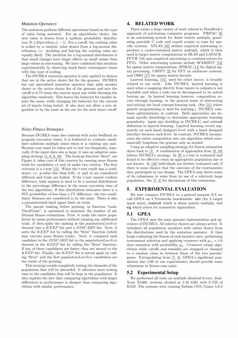
Noisy Fitness StrategiesBecause INCREA must also contend with noisy feedback onprogram execution times, it is bolstered to evaluate candi-date solutions multiple times when it is ranking any pair.Because care must be taken not to test too frequently, espe-cially if the input data size is large, it uses an adaptive sam-pling strategy [1, 8, 9, 16] . The boolean function“fitter”, seeFigure 4, takes care of this concern by running more fitnesstrials for candidates s1 and s2 under two criteria. The firstcriterion is a t-test [13]. When the t-test result has a confi-dence, i.e. p-value less than 0.05, s1 and s2 are considereddifferent and trials are halted. If the t-test cannot confirmdifference, least squares is used to fit a normal distributionto the percentage difference in the mean execution time ofthe two algorithms. If this distribution estimates there is a95% probability of less than a 1% difference, the two candi-dates’ fitnesses are considered to be the same. There is alsoa parameterized hard upper limit on trials.

The parent ranking before pruning, in function “rank-ThenPrune”, is optimized to minimize the number of ad-ditional fitness evaluations. First, it ranks the entire popu-lation by mean performance without running any additionaltrials. It then splits the ranking at the populationLowSizeelement into a KEEP list and a DISCARD list. Next, itsorts the KEEP list by calling the “fitter” function (whichmay execute more fitness trials). Next, it compares eachcandidate in the DISCARD list to the populationLowSizeelement in the KEEP list by calling the “fitter” function.If any of these candidates are faster, they are moved to theKEEP list. Finally, the KEEP list is sorted again by call-ing “fitter” and the first populationLowSize candidates arethe result of the pruning.

This strategy avoids completely testing the elements of thepopulation that will be discarded. It allocates more testingtime to the candidate that will be kept in the population. Italso exploits the fact that comparing algorithms with largerdifferences in performance is cheaper than comparing algo-rithms with similar performance.

4. RELATED WORKThere exists a large variety of work related to PetaBrick’s

approach of autotuning computer programs. PHiPAC [6]is an autotuning system for dense matrix multiply, gener-ating portable C code and search scripts to tune for spe-cific systems. ATLAS [18] utilizes empirical autotuning toproduce a cache-contained matrix multiply, which is thenused in larger matrix computations in BLAS and LAPACK.FFTW [10] uses empirical autotuning to combine solvers forFFTs. Other autotuning systems include SPARSITY [12]for sparse matrix computations, SPIRAL [14] for digital sig-nal processing, UHFFT [2] for FFT on multicore systems,and OSKI [17] for sparse matrix kernels.

Layered learning, [15], used for robot soccer, is broadlyrelated to our work. Like INCREA, layered learning isused when a mapping directly from inputs to outputs is nottractable and when a task can be decomposed to be solvedbottom up. In layered learning however, composition oc-curs through learning, in the general sense of abstractingand solving the local concept-learning task. (See [11] wheregenetic programming is used for learning.) INCREA com-bines optimizations, in contrast. Both approaches use do-main specific knowledge to determine appropriate learninggranularity: input size doubling in INCREA) and subtaskdefinition in layered learning. Layered learning occurs sep-arately on each hand designed level with a hand designedinterface between each level. In contrast, INCREA incorpo-rates the entire composition into one algorithm which auto-matically lengthens the genome only as needed.

Using an adaptive sampling strategy for fitness estimationdates back to [1]. A combination of approaches from [9, 16]inform INCREA’s strategy. In [9] a t-test is evaluated andfound to be effective when an appropriate population size isnot known. In [16] individuals are further evaluated only ifthere is some chance that the outcome of the tournamentsthey participate in can change. The GPEA may derive someof its robustness to noise from its use of a relatively largepopulation. See [7, 4] for discussions of this robustness.

5. EXPERIMENTAL EVALUATIONWe now compare INCREA to a general purpose EA we

call GPEA on 4 Petabricks benchmarks: sort (for 2 targetinput sizes), matmult which is dense matrix multiply, andeig which solves for symmetric eigenvalues.

5.1 GPEAThe GPEA uses the same genome representation and op-

erators of INCREA. All selector choices are always active. Itinitializes all population members with values drawn fromthe distributions used by the mutation operator. It thenloops evaluating the fitness of each member once, performingtournament selection and applying crossover with pxo = 1.0then mutation with probability pµ. Crossover swaps algo-rithms while cutoffs and tunables are swapped or changedto a random value in between those of the two parents’genes. Extrapolating from [7, 4], GPEA’s significant pop-ulation size (100 in our experiments) should provide somerobustness to fitness case noise.

5.2 Experimental SetupWe performed all tests on multiple identical 8-core, dual-

Xeon X5460, systems clocked at 3.16 GHz with 8 GB ofRAM. The systems were running Debian GNU/Linux 5.0.3

function f i t t e r ( s1 , s2 , i nputS i z e )while s1 . evalCount < evalsLowerLimit

eva lua t eF i tn e s s ( s1 , i nputS i z e )endwhile s2 . evalCount < evalsLowerLimit

eva lua t eF i tn e s s ( s2 , i nputS i z e )endwhile t rue

/∗ Sing le t a i l e d T−t e s t assumes each sample ’ s mean i s normally d i s t r i b u t e d .I t repor ts p r o b a b i l i t y tha t sample means are same under t h i s assumption ∗/

i f t t e s t ( s1 . eva l sResu l t s , s2 . eva lRe su l t s ) < PvalueLimit /∗ s t a t i s t i c a l l y d i f f e r e n t ∗/return mean( s1 . eva lRe su l t s ) > mean( s2 . eva lRe su l t s )

end/∗ Test2Equal i ty : Use l e a s t squares to f i t a normal d i s t r i b u t i on to the percentage

d i f f e r ence in the mean performance of the two algori thms . I f t h i sd i s t r i b u t i on est imates there i s a 95% pro ba b i l i t y of l e s s than a 1%d i f f e r ence in true means , consider the two algori thms the same . ∗/

i f Test2Equal i ty ( s1 . eva lResu l t s , s2 . eva lRe su l t s )return f a l s e

end/∗ need more information , choose s1 or s2 based on the h i ghes t expected

reduct ion in standard error ∗/whoToTest = mostInformative ( s1 , s2 ) ;i f whoToTest == s1 and s1 . testCount < evalsUpperLimit

eva lua t eF i tn e s s ( s1 , i nputS i z e )e l i f s2 . testCount < evalsUpperLimit

eva lua t eF i tn e s s ( s2 , i nputS i z e )else

/∗ inconc lus i ve re su l t , no more eva l s l e f t ∗/return f a l s e

endend /∗ whi le ∗/

end /∗ f i t t e r ∗/

Figure 4: Pseudocode of function “fitter”.

Parameter Value

confidence required 70%max trials 5min trials 1population high size 10population low size 2mutationAttempts 6standard deviation prior 15%

(a) INCREA

Parameter Value

mutation rate 0.5crossover rate 1.0population size 100tournament size 10generations 100evaluations per candidate 1

(b) GPEA

Figure 5: INCREA and GPEA Parameter Settings.

with kernel version 2.6.26. For each test, we chose a tar-get input size large enough to allow parallelism, and smallenough to converge on a solution within a reasonable amountof time. Parameters such as the mutation rate, populationsize and the number of generations were determined exper-imentally and kept constant between benchmarks. Parame-ter values we used are listed in Figure 5.

5.3 INCREA vs GPEAIn practice we might choose parameters of either INCREA

or GPEA to robustly ensure good autotuning or allow theprogrammer to vary them while tuning a particular problemand architecture. In the latter case, considering how quicklythe tuner converges to the final solution is important. Tomore extensively compare the two tuners, we ran each tuner30 times for each benchmark.

Table 1 compares the tuners mean performance with 30runs based on time to convergence and the performance ofthe final solution. To account for noise, time to convergenceis calculated as the first time that a candidate was found thatwas within 5% of the best fitness achieved. For all of thebenchmarks except for eig, both tuners arrive at nearly the

same solutions, while for eig INCREA finds a slightly bettersolution. For eig and matmult, INCREA converges an orderof magnitude faster than GPEA. For sort, GPEAconvergesfaster on the small input size while INCREA converges fasteron the larger input size. If one extrapolates convergencestimes to larger input sizes, it is clear that INCREA scales alot better than GPEA for sort.

INCREA GPEA SS?

sort-220 Convergence 1464.7± 1992.0 599.2± 362.9 YES (p = 0.03)Performance 0.037± 0.004 0.034± 0.014 NO

sort-223 Convergence 2058.2± 2850.9 2480.5± 1194.5 NOPerformance 0.275± 0.010 0.276± 0.041 NO

matmultConvergence 278.5± 185.8 2394.2± 1931.0 YES (p = 10−16)Performance 0.204± 0.001 0.203± 0.001 NO

eigConvergence 92.1± 66.4 627.4± 530.2 YES (p = 10−15)Performance 1.240± 0.025 1.250± 0.014 YES (p = 0.05)

Table 1: Comparison of INCREA and GPEA interms of mean time to convergence in seconds andin terms of execution time of the final configura-tion. Standard deviation is shown after the ± sym-bol. The final column is statistical significance de-termined by a t-test. (Lower is better)

Figure 6 shows aggregate results from 30 runs for both IN-CREA and GPEA on each benchmark. INCREA generallyhas a large amount of variance in its early generations, be-cause those generations are based on smaller input sizes thatmay have different optimal solutions than the largest inputsize. However, once INCREA reaches its final generationit exhibits lower variance than than GPEA. GPEA tendsto converge slowly with gradually decreasing variance. Notethat the first few generations for INCREA are not shown be-cause, since it was training on extremely small input sizes, itfinds candidates candidates that exceed the timeout set by

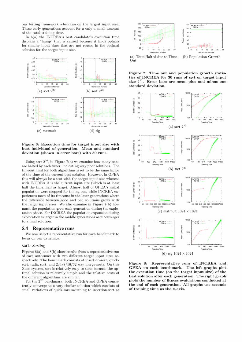
our testing framework when run on the largest input size.These early generations account for a only a small amountof the total training time.

In 6(a) the INCREA’s best candidate’s execution timedisplays a “hump” that is caused because it finds optimafor smaller input sizes that are not reused in the optimalsolution for the target input size.

0

0.05

0.1

0.15

0.2

0.25

0.3

0 5 10 15 20 25 30

Bes

t Can

dida

te (s

)

Generation Number

INCREAGPEA

(a) sort 220

0

0.5

1

1.5

2

2.5

3

0 5 10 15 20 25 30

Bes

t Can

dida

te (s

)

Generation Number

INCREAGPEA

(b) sort 223

0

0.5

1

1.5

2

2.5

3

0 5 10 15 20 25 30

Bes

t Can

dida

te (s

)

Generation Number

INCREAGPEA

(c) matmult

1

1.2

1.4

1.6

1.8

2

0 5 10 15 20 25 30

Bes

t Can

dida

te (s

)

Generation Number

INCREAGPEA

(d) eig

Figure 6: Execution time for target input size withbest individual of generation. Mean and standarddeviation (shown in error bars) with 30 runs.

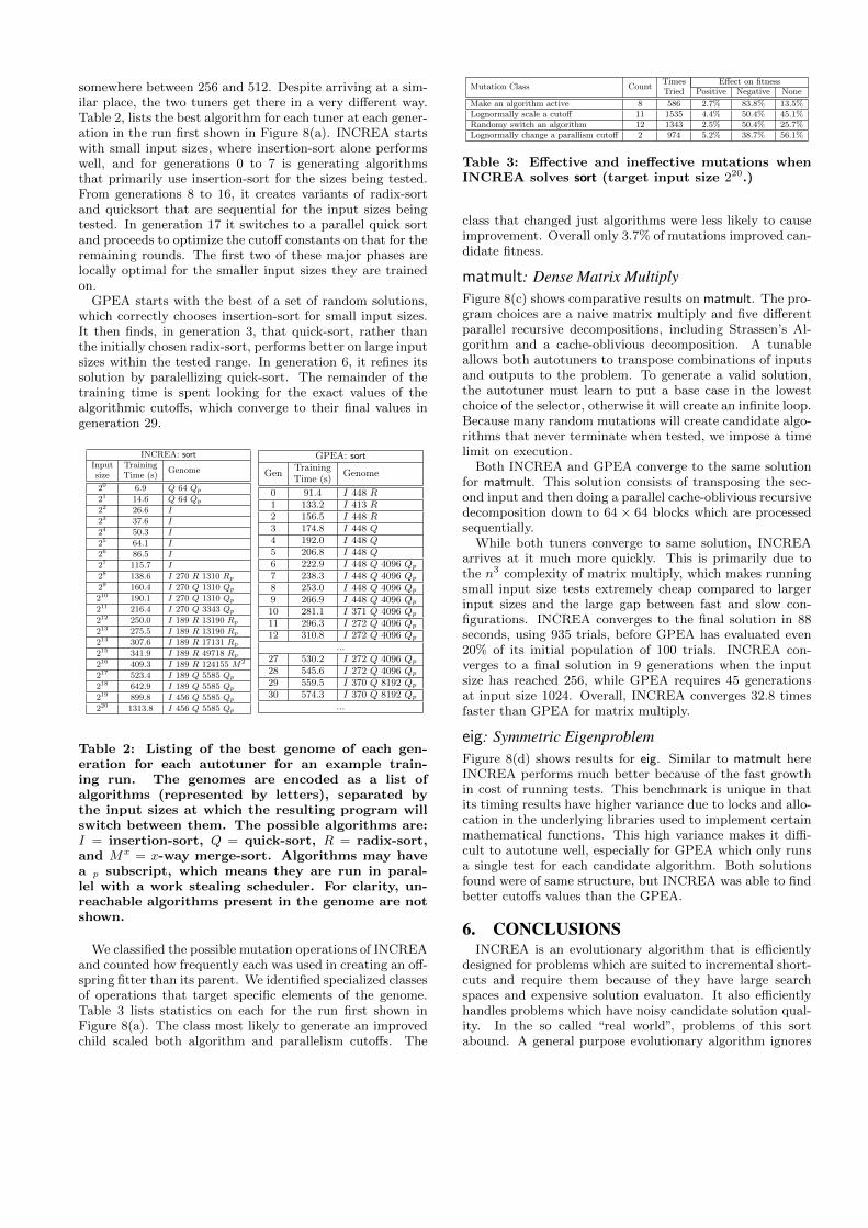
Using sort-220, in Figure 7(a) we examine how many testsare halted by each tuner, indicating very poor solutions. Thetimeout limit for both algorithms is set to be the same factorof the time of the current best solution. However, in GPEAthis will always be a test with the target input size whereaswith INCREA it is the current input size (which is at leasthalf the time, half as large). Almost half of GPEA’s initialpopulation were stopped for timing out, while INCREA ex-periences most of its timeouts in the later generations wherethe difference between good and bad solutions grows withthe larger input sizes. We also examine in Figure 7(b) howmuch the population grew each generation during the explo-ration phase. For INCREA the population expansion duringexploration is larger in the middle generations as it convergesto a final solution.

5.4 Representative runsWe now select a representative run for each benchmark to

focus on run dynamics.

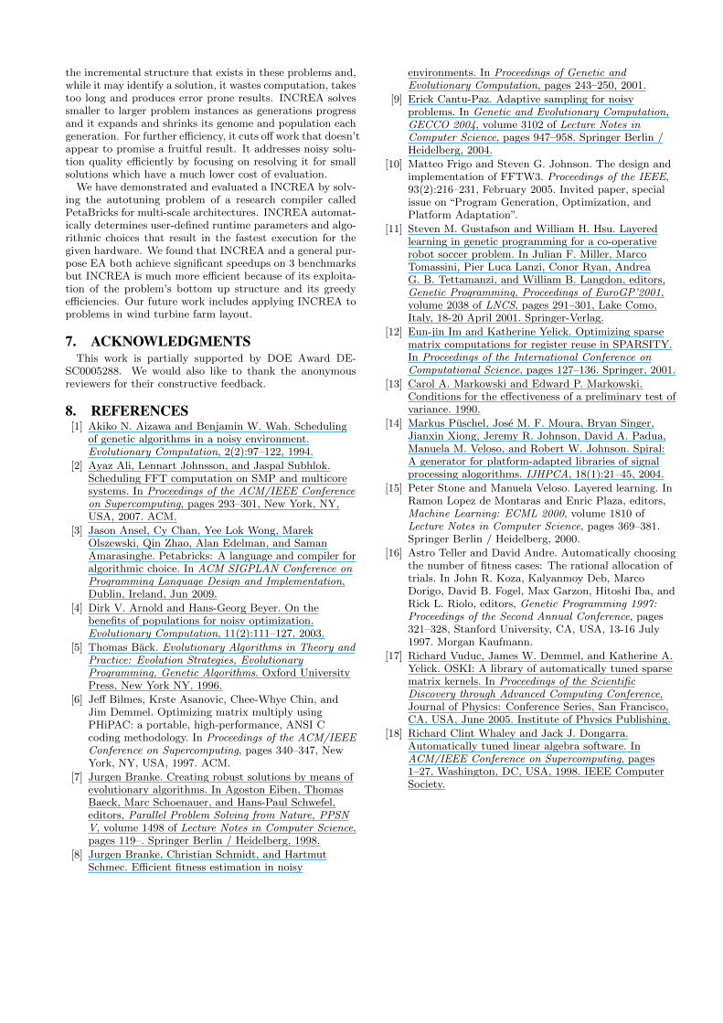
sort: SortingFigures 8(a) and 8(b) show results from a representative runof each autotuner with two different target input sizes re-spectively. The benchmark consists of insertion-sort, quick-sort, radix sort, and 2/4/8/16/32-way merge-sorts. On thisXeon system, sort is relatively easy to tune because the op-timal solution is relatively simple and the relative costs ofthe different algorithms are similar.

For the 220 benchmark, both INCREA and GPEA consis-tently converge to a very similar solution which consists ofsmall variations of quick-sort switching to insertion-sort at

-50

0

50

100

150

200

250

0 5 10 15 20 25 30

Test

Tim

eout

s

Generation Number

INCREAGPEA

(a) Tests Halted due to TimeOut

0

20

40

60

80

100

120

0 5 10 15 20 25 30

Add

ed c

andi

date

s

Generation Number

INCREAGPEA

(b) Population Growth

Figure 7: Time out and population growth statis-tics of INCREA for 30 runs of sort on target inputsize 220. Error bars are mean plus and minus onestandard deviation.

0

0.1

0.2

0.3

0.4

0.5

60 120 240 480 960 1920

Bes

t Can

dida

te (s

)

Training Time

INCREAGPEA

100

1000

10000

60 120 240 480 960 1920

Test

s C

ondu

cted

Training Time

INCREAGPEA

(a) sort 220

0

0.2

0.4

0.6

0.8

1

60 180 540 1620 4860 14580

Bes

t Can

dida

te (s

)

Training Time

INCREAGPEA

100

1000

10000

60 180 540 1620 4860 14580

Test

s C

ondu

cted

Training Time

INCREAGPEA

(b) sort 223

0

0.5

1

1.5

2

2.5

3

60 120 240 480 960 1920 3840 7680

Bes

t Can

dida

te (s

)

Training Time

INCREAGPEA

100

1000

10000

60 120 240 480 960 1920 3840 7680

Test

s C

ondu

cted

Training Time

INCREAGPEA

(c) matmult 1024× 1024

1

1.5

2

2.5

3

60 240 960 3840 15360

Bes

t Can

dida

te (s

)

Training Time

INCREAGPEA

100

1000

10000

60 240 960 3840 15360

Test

s C

ondu

cted

Training Time

INCREAGPEA

(d) eig 1024× 1024

Figure 8: Representative runs of INCREA andGPEA on each benchmark. The left graphs plotthe execution time (on the target input size) of thebest solution after each generation. The right graphplots the number of fitness evaluations conducted atthe end of each generation. All graphs use secondsof training time as the x-axis.

somewhere between 256 and 512. Despite arriving at a sim-ilar place, the two tuners get there in a very different way.Table 2, lists the best algorithm for each tuner at each gener-ation in the run first shown in Figure 8(a). INCREA startswith small input sizes, where insertion-sort alone performswell, and for generations 0 to 7 is generating algorithmsthat primarily use insertion-sort for the sizes being tested.From generations 8 to 16, it creates variants of radix-sortand quicksort that are sequential for the input sizes beingtested. In generation 17 it switches to a parallel quick sortand proceeds to optimize the cutoff constants on that for theremaining rounds. The first two of these major phases arelocally optimal for the smaller input sizes they are trainedon.

GPEA starts with the best of a set of random solutions,which correctly chooses insertion-sort for small input sizes.It then finds, in generation 3, that quick-sort, rather thanthe initially chosen radix-sort, performs better on large inputsizes within the tested range. In generation 6, it refines itssolution by paralellizing quick-sort. The remainder of thetraining time is spent looking for the exact values of thealgorithmic cutoffs, which converge to their final values ingeneration 29.

INCREA: sortInput Training

Genomesize Time (s)

20 6.9 Q 64 Qp21 14.6 Q 64 Qp22 26.6 I

23 37.6 I

24 50.3 I

25 64.1 I

26 86.5 I

27 115.7 I

28 138.6 I 270 R 1310 Rp29 160.4 I 270 Q 1310 Qp210 190.1 I 270 Q 1310 Qp211 216.4 I 270 Q 3343 Qp212 250.0 I 189 R 13190 Rp213 275.5 I 189 R 13190 Rp214 307.6 I 189 R 17131 Rp215 341.9 I 189 R 49718 Rp216 409.3 I 189 R 124155 M2

217 523.4 I 189 Q 5585 Qp218 642.9 I 189 Q 5585 Qp219 899.8 I 456 Q 5585 Qp220 1313.8 I 456 Q 5585 Qp

GPEA: sort

GenTraining

GenomeTime (s)

0 91.4 I 448 R1 133.2 I 413 R2 156.5 I 448 R3 174.8 I 448 Q4 192.0 I 448 Q5 206.8 I 448 Q6 222.9 I 448 Q 4096 Qp7 238.3 I 448 Q 4096 Qp8 253.0 I 448 Q 4096 Qp9 266.9 I 448 Q 4096 Qp10 281.1 I 371 Q 4096 Qp11 296.3 I 272 Q 4096 Qp12 310.8 I 272 Q 4096 Qp

...27 530.2 I 272 Q 4096 Qp28 545.6 I 272 Q 4096 Qp29 559.5 I 370 Q 8192 Qp30 574.3 I 370 Q 8192 Qp

...

Table 2: Listing of the best genome of each gen-eration for each autotuner for an example train-ing run. The genomes are encoded as a list ofalgorithms (represented by letters), separated bythe input sizes at which the resulting program willswitch between them. The possible algorithms are:I = insertion-sort, Q = quick-sort, R = radix-sort,and Mx = x-way merge-sort. Algorithms may havea p subscript, which means they are run in paral-lel with a work stealing scheduler. For clarity, un-reachable algorithms present in the genome are notshown.

We classified the possible mutation operations of INCREAand counted how frequently each was used in creating an off-spring fitter than its parent. We identified specialized classesof operations that target specific elements of the genome.Table 3 lists statistics on each for the run first shown inFigure 8(a). The class most likely to generate an improvedchild scaled both algorithm and parallelism cutoffs. The

Mutation Class CountTimes Effect on fitnessTried Positive Negative None

Make an algorithm active 8 586 2.7% 83.8% 13.5%Lognormally scale a cutoff 11 1535 4.4% 50.4% 45.1%Randomy switch an algorithm 12 1343 2.5% 50.4% 25.7%Lognormally change a parallism cutoff 2 974 5.2% 38.7% 56.1%

Table 3: Effective and ineffective mutations whenINCREA solves sort (target input size 220.)

class that changed just algorithms were less likely to causeimprovement. Overall only 3.7% of mutations improved can-didate fitness.

matmult: Dense Matrix MultiplyFigure 8(c) shows comparative results on matmult. The pro-gram choices are a naive matrix multiply and five differentparallel recursive decompositions, including Strassen’s Al-gorithm and a cache-oblivious decomposition. A tunableallows both autotuners to transpose combinations of inputsand outputs to the problem. To generate a valid solution,the autotuner must learn to put a base case in the lowestchoice of the selector, otherwise it will create an infinite loop.Because many random mutations will create candidate algo-rithms that never terminate when tested, we impose a timelimit on execution.

Both INCREA and GPEA converge to the same solutionfor matmult. This solution consists of transposing the sec-ond input and then doing a parallel cache-oblivious recursivedecomposition down to 64 × 64 blocks which are processedsequentially.

While both tuners converge to same solution, INCREAarrives at it much more quickly. This is primarily due tothe n3 complexity of matrix multiply, which makes runningsmall input size tests extremely cheap compared to largerinput sizes and the large gap between fast and slow con-figurations. INCREA converges to the final solution in 88seconds, using 935 trials, before GPEA has evaluated even20% of its initial population of 100 trials. INCREA con-verges to a final solution in 9 generations when the inputsize has reached 256, while GPEA requires 45 generationsat input size 1024. Overall, INCREA converges 32.8 timesfaster than GPEA for matrix multiply.

eig: Symmetric EigenproblemFigure 8(d) shows results for eig. Similar to matmult hereINCREA performs much better because of the fast growthin cost of running tests. This benchmark is unique in thatits timing results have higher variance due to locks and allo-cation in the underlying libraries used to implement certainmathematical functions. This high variance makes it diffi-cult to autotune well, especially for GPEA which only runsa single test for each candidate algorithm. Both solutionsfound were of same structure, but INCREA was able to findbetter cutoffs values than the GPEA.

6. CONCLUSIONSINCREA is an evolutionary algorithm that is efficiently

designed for problems which are suited to incremental short-cuts and require them because of they have large searchspaces and expensive solution evaluaton. It also efficientlyhandles problems which have noisy candidate solution qual-ity. In the so called “real world”, problems of this sortabound. A general purpose evolutionary algorithm ignores

the incremental structure that exists in these problems and,while it may identify a solution, it wastes computation, takestoo long and produces error prone results. INCREA solvessmaller to larger problem instances as generations progressand it expands and shrinks its genome and population eachgeneration. For further efficiency, it cuts off work that doesn’tappear to promise a fruitful result. It addresses noisy solu-tion quality efficiently by focusing on resolving it for smallsolutions which have a much lower cost of evaluation.

We have demonstrated and evaluated a INCREA by solv-ing the autotuning problem of a research compiler calledPetaBricks for multi-scale architectures. INCREA automat-ically determines user-defined runtime parameters and algo-rithmic choices that result in the fastest execution for thegiven hardware. We found that INCREA and a general pur-pose EA both achieve significant speedups on 3 benchmarksbut INCREA is much more efficient because of its exploita-tion of the problem’s bottom up structure and its greedyefficiencies. Our future work includes applying INCREA toproblems in wind turbine farm layout.

7. ACKNOWLEDGMENTSThis work is partially supported by DOE Award DE-

SC0005288. We would also like to thank the anonymousreviewers for their constructive feedback.

8. REFERENCES[1] Akiko N. Aizawa and Benjamin W. Wah. Scheduling

of genetic algorithms in a noisy environment.Evolutionary Computation, 2(2):97–122, 1994.

[2] Ayaz Ali, Lennart Johnsson, and Jaspal Subhlok.Scheduling FFT computation on SMP and multicoresystems. In Proceedings of the ACM/IEEE Conferenceon Supercomputing, pages 293–301, New York, NY,USA, 2007. ACM.

[3] Jason Ansel, Cy Chan, Yee Lok Wong, MarekOlszewski, Qin Zhao, Alan Edelman, and SamanAmarasinghe. Petabricks: A language and compiler foralgorithmic choice. In ACM SIGPLAN Conference onProgramming Language Design and Implementation,Dublin, Ireland, Jun 2009.

[4] Dirk V. Arnold and Hans-Georg Beyer. On thebenefits of populations for noisy optimization.Evolutionary Computation, 11(2):111–127, 2003.

[5] Thomas Back. Evolutionary Algorithms in Theory andPractice: Evolution Strategies, EvolutionaryProgramming, Genetic Algorithms. Oxford UniversityPress, New York NY, 1996.

[6] Jeff Bilmes, Krste Asanovic, Chee-Whye Chin, andJim Demmel. Optimizing matrix multiply usingPHiPAC: a portable, high-performance, ANSI Ccoding methodology. In Proceedings of the ACM/IEEEConference on Supercomputing, pages 340–347, NewYork, NY, USA, 1997. ACM.

[7] Jurgen Branke. Creating robust solutions by means ofevolutionary algorithms. In Agoston Eiben, ThomasBaeck, Marc Schoenauer, and Hans-Paul Schwefel,editors, Parallel Problem Solving from Nature, PPSNV, volume 1498 of Lecture Notes in Computer Science,pages 119–. Springer Berlin / Heidelberg, 1998.

[8] Jurgen Branke, Christian Schmidt, and HartmutSchmec. Efficient fitness estimation in noisy

environments. In Proceedings of Genetic andEvolutionary Computation, pages 243–250, 2001.

[9] Erick Cantu-Paz. Adaptive sampling for noisyproblems. In Genetic and Evolutionary Computation,GECCO 2004, volume 3102 of Lecture Notes inComputer Science, pages 947–958. Springer Berlin /Heidelberg, 2004.

[10] Matteo Frigo and Steven G. Johnson. The design andimplementation of FFTW3. Proceedings of the IEEE,93(2):216–231, February 2005. Invited paper, specialissue on “Program Generation, Optimization, andPlatform Adaptation”.

[11] Steven M. Gustafson and William H. Hsu. Layeredlearning in genetic programming for a co-operativerobot soccer problem. In Julian F. Miller, MarcoTomassini, Pier Luca Lanzi, Conor Ryan, AndreaG. B. Tettamanzi, and William B. Langdon, editors,Genetic Programming, Proceedings of EuroGP’2001,volume 2038 of LNCS, pages 291–301, Lake Como,Italy, 18-20 April 2001. Springer-Verlag.

[12] Eun-jin Im and Katherine Yelick. Optimizing sparsematrix computations for register reuse in SPARSITY.In Proceedings of the International Conference onComputational Science, pages 127–136. Springer, 2001.

[13] Carol A. Markowski and Edward P. Markowski.Conditions for the effectiveness of a preliminary test ofvariance. 1990.

[14] Markus Puschel, Jose M. F. Moura, Bryan Singer,Jianxin Xiong, Jeremy R. Johnson, David A. Padua,Manuela M. Veloso, and Robert W. Johnson. Spiral:A generator for platform-adapted libraries of signalprocessing alogorithms. IJHPCA, 18(1):21–45, 2004.

[15] Peter Stone and Manuela Veloso. Layered learning. InRamon Lopez de Montaras and Enric Plaza, editors,Machine Learning: ECML 2000, volume 1810 ofLecture Notes in Computer Science, pages 369–381.Springer Berlin / Heidelberg, 2000.

[16] Astro Teller and David Andre. Automatically choosingthe number of fitness cases: The rational allocation oftrials. In John R. Koza, Kalyanmoy Deb, MarcoDorigo, David B. Fogel, Max Garzon, Hitoshi Iba, andRick L. Riolo, editors, Genetic Programming 1997:Proceedings of the Second Annual Conference, pages321–328, Stanford University, CA, USA, 13-16 July1997. Morgan Kaufmann.

[17] Richard Vuduc, James W. Demmel, and Katherine A.Yelick. OSKI: A library of automatically tuned sparsematrix kernels. In Proceedings of the ScientificDiscovery through Advanced Computing Conference,Journal of Physics: Conference Series, San Francisco,CA, USA, June 2005. Institute of Physics Publishing.

[18] Richard Clint Whaley and Jack J. Dongarra.Automatically tuned linear algebra software. InACM/IEEE Conference on Supercomputing, pages1–27, Washington, DC, USA, 1998. IEEE ComputerSociety.