Sudan University of Science and Technology Faculty of Engineering

Aeronautical Engineering Department

Structured Robust Control for a Hang Glider

Thesis Submitted in Partial Fulfillment of the Requirements for the Degree of Bachelor of Engineering. (BEng Honor)

By: 1. Fatimah AL-Tayib Abduallah Mohammed 2. Zahra Ibrahim Jalabi Abdulrahman

Supervised By: Dr. Elfatih Guma Hamdi Gubara

October, 2017

I

اآليــة قال تعالى :

﴿ يمت قوم قال ة ىل كنت ان ر ه ورزقين ريب من ب نا رزقام ن ريد وما حسالفمك تطعت ما االصالح اال ريد عنه ان هنامك اىل ما قي وما اس اال توف ليه ب﴾ تولكت ن واليه

ة –سورة هود ي ﴾٨٨﴿ا

II

ABSTRACT No one can deny the significant role of gliders in founding the aviation industry, so far in its evolutionary progress. Gliders are eco-friendly as they exploit the energy from the atmosphere from mother nature without a necessity for a power plant and they remain a loft in air by soaring utilizing the updrafts and air currents. Nevertheless, they are still limited in aspects of range, endurance, speed, control and stability. However, nowadays, the aviation industry seeks to go green as a result of the great air pollution caused by the large amounts of smokes and gases generated from the massive amount of fuel combustion. Maybe using modern automation technologies and making use of some glider’s features, but at the same time maintain the performance and the efficiency of the modern aircrafts can lead to new green innovations in the field of aviation. This thesis is proposing a design of a controller for the Hiway Demon hang glider to guarantee the stability of the system with certain level of performance and to enhance the system’s rejection to the disturbances affecting it drastically during soaring. The controllers are designed using classical (Inversion Formula) control technique and advanced (robust) control technique. The nonlinear state-space model of the aircraft is linearized. After that, it is decoupled into lateral and longitudinal models. The longitudinal model is reduced to short period model in order to facilitate the analysis and the design of the controllers. The pitch rate channel is stabilized, while the lateral model suffered of instability problems, but a suggestion proposing to apply a Multi-DOF controller on the model in the near future. The controllers are evaluated in terms of disturbance rejection, noise attenuation and control efforts. The robust control approach has exhibited better convenience for such application than the classical control approach especially in term of disturbance rejection.

III

دـالتجري اآلن في تطورها. وحتى ,الشراعية في تأسيس صناعة الطيرانلطائرات ل يمكن ألحد أن ينكر الدور الهامال

رة ضروالإن الطائرات الشراعية صديقة للبيئة ألنها تستغل الطاقة من الغالف الجوي من الطبيعة األم دون وعلى الرغم وتيارات الهواء. عمدة الهوائيةاستخدام األء من خالل في الهوا ى طافية، وتبقصدر توليد قدرةلم

، والسرعة، والتحكم بقاء في الجوالمدى، والقدرة على الكفي جوانب حدودة األداء ذلك، فإنها ال تزال م مننتيجة لتلوث لك ذ و حفاظ علي البيئةالطيران لل مؤوسسةفي الوقت الحاضر، تسعى إال أنه . يةواالستقرار

قود. الو حرقهائلة من ال اتكميالوالغازات الناتجة عن دخنةكبيرة من األالكميات الالهواء الكبير الناجم عن شراعية، ولكن في نفس الطائرة الميزات مالحديثة واالستفادة من بعض تمتةتقنيات األ عن طريق استخدامربما

جديدة للحفاظ على البتكارات اذهأن يؤدي فمن الممكنداء وكفاءة الطائرات الحديثة الحفاظ على أب الوقت Hiway Demonطائرة شراعيةلل اقتراح لتصميم وحدة تحكم يفي مجال الطيران. هذه األطروحة ه البيئة

من األداء وتعزيز رفض النظام مستوى معين ل الطائرةنظام من شأنها ضمان استقرار الوحدة هذه وام تقنية تحكم كالسيكي . تم تصميم وحدات التحكم باستخدالتحليقتؤثر عليه بشكل كبير خالل الضطرابات التيل شراعيةال لطائرةالحصول على النموذج الرياضي ل . تم) التحكم المتين(متقدمة وتقنية تحكم نعكاس)صيغة اال(

تخفيض ثم تمإلى نماذج جانبية وطولية. هفصلها تم خطي. بعدنموذج الغير خطي إلى جذالنمو تحويل ثم تمالتحكم. واستقرت قناة معدل النموذج الطولي إلى نموذج فترة قصيرة من أجل تسهيل التحليل وتصميم وحدات

ح يقترح ااقترثمة شاكل عدم االستقرار، ولكنعانى النموذج الجانبي من مبينما ج الطوليذفي النمو تأرجحالعلى النموذج في المستقبل القريب. تم تقييم وحدات التحكم الحرية ات درجات متعددة منذتطبيق وحدة تحكم

كبرأمالئمة ت طريقة التحكم المتينوأظهر. جهد المتحكم وتوهين الضوضاء و من حيث رفض االضطراب، .وخاصة في حالة رفض االضطراب طريقة التحكم الكالسيكي من طبيقتال اهذمثل ل

IV

ACKNOWLEDGEMENT Unlimited thanks and profound gratitude to Allah who granted us with power, will and knowledge to complete this thesis, and whom without, this humble project wouldn't have seen the light or even emerged into this final form. Also, deep thanks mixed with a lot of appreciation to the superb, Dr. Elfatih Guma who was more than a supervisor for us. We are so grateful to him as he devoted his time to share knowledge with us and exerted unlimited efforts so as to achieve what we achieved in this project. Not forgetting his amazing way introducing us to this fascinating field of research. A special gratitude goes to the adorable, Ms. Raheeg Wahbi for her endless support, encouragement and her huge efforts. Our thank is also extended to our dear senior and our mentor Safa Abd Elwahab for her continuous help and support. Last but not the least we would like to thank Mr. Musab Mohammed and everyone who contributed in the fulfilment of our project.

V

DEDICATION We dedicate this research to our great parents who always stood by our sides, motivated us and provided the best they can to help us achieving our goals and never saved any efforts to make all our dreams come true. We also dedicate this research to our family for their unlimited support, to our brothers and sisters who encouraged us a lot and all our friends and colleagues.

VI

Table of Contents i ............................................................................................................................ اآليــة ABSTRACT ............................................................................................................. ii iii ....................................................................................................................... التجريـدACKNOWLEDGEMENT ....................................................................................... iv DEDICATION ......................................................................................................... v Table of Contents .................................................................................................... vi List of Figures........................................................................................................... x List of Tables ......................................................................................................... xiii List of Symbols...................................................................................................... xiv List of Abbreviations ............................................................................................. xvi 1 Chapter One: Introduction ..................................................................................... 1

1.1 Overview......................................................................................................... 1 1.2 Problem Statement .......................................................................................... 1 1.3 Aim and Objectives ........................................................................................ 2

1.3.1 Aim .......................................................................................................... 2 1.3.2 Objectives ................................................................................................ 2

1.4 Proposed Solution ........................................................................................... 2 1.5 Methodology ................................................................................................... 2 1.6 Thesis Outlines ............................................................................................... 4

2 Chapter Two: Literature Review ........................................................................... 5 2.1 History and Background ................................................................................. 5

2.1.1 Introduction.............................................................................................. 5 2.2 Glider .............................................................................................................. 7 2.3 Launching Techniques .................................................................................... 7

2.3.1 Foot Launching (Hang gliders) ................................................................ 7 2.3.2 Self-Launching ........................................................................................ 8

VII

2.3.3 Winch Launching..................................................................................... 8 2.3.4 Aero-Tow ................................................................................................. 8

2.4 Types of Soaring ............................................................................................. 8 2.4.1 Gust Soaring ............................................................................................ 9 2.4.2 Dynamic Soaring ..................................................................................... 9 2.4.3 Static Soaring ......................................................................................... 10

2.5 Thermal Model ............................................................................................. 12 2.6 Stability: A Requirement for All Airplanes .................................................. 13 2.7 Aircraft Dynamics ........................................................................................ 15

2.7.1 Equations of Motion .............................................................................. 15 2.7.2 The Dynamic Stability Modes ............................................................... 15

2.8 Significance of Automatic Flight Control .................................................... 20 2.9 Control Techniques ....................................................................................... 20

2.9.1 Classical Control Techniques ................................................................ 21 2.9.2 Modern Control Techniques .................................................................. 21

2.10 Similar Work and Previous Studies ............................................................ 24 2.10.1 First Relevant Report ........................................................................... 24 2.10.2 Second Relevant Report ...................................................................... 25 2.10.3 Statement of Argument ........................................................................ 25

3 Chapter Three: Modeling, Analysis and Control Design .................................... 27 3.1 Mathematical Modeling of the Aircraft ........................................................ 27

3.1.1 Significance of Mathematical Modeling: .............................................. 27 3.1.2 Reference Coordinate Systems .............................................................. 27 3.1.3 Equations of Motion: ............................................................................. 29 3.1.4 Linearization of Equation of Motion ..................................................... 39

VIII

3.2 Analysis ........................................................................................................ 42 3.2.1 Separation of the Equations of Aircraft Motion .................................... 42

3.3 Control Design .............................................................................................. 47 3.3.1 Controller Order Reduction and Model Order Reduction ..................... 47 3.3.2 Comparison Between Full Model and Approximate Model.................. 49 3.3.3 A Classical Control Design Approach (The inversion Formula) .......... 52 3.3.4 Robust Control Design Approach (Structured Robust Control) ............ 58 3.3.5 Controllers Evaluation ........................................................................... 63

4 Chapter Four: Results and Discussion ................................................................. 64 4.1 Aerospace Performance Specifications ........................................................ 64

4.1.1 System’s Specifications in Frequency Domain ..................................... 67 4.1.2 System’s Specifications in Time Domain ............................................. 69

4.2 Results of the Full and Reduced Models Comparisons ................................ 71 4.2.1 Time history ........................................................................................... 73 4.2.2 Energy Distribution ............................................................................... 75

4.3 Computation of Stability Regions and Small Gain Theory Test .................. 77 4.4 Satisfying of Small Gain Theorem ............................................................... 79 4.5 Classical Controller Evaluation .................................................................... 81

4.5.1 Disturbance Rejection ............................................................................ 81 4.5.2 Noise Attenuation .................................................................................. 82 4.5.3 Control Effort......................................................................................... 84

4.6 Robust Control Evaluation ........................................................................... 85 4.6.1 Disturbance Rejection ............................................................................ 85 4.6.2 Noise Attenuation .................................................................................. 87 4.6.3 Control Effort......................................................................................... 88

IX

5 Chapter Five: Conclusion and Future Work ........................................................ 92 5.1 Conclusion .................................................................................................... 92 5.2 Future Work .................................................................................................. 92

References .............................................................................................................. 95 Appendices ............................................................................................................. 97

Appendix A ......................................................................................................... 97 Appendix B ....................................................................................................... 100

X

List of Figures Figure(2- 1):A human-powered ornithopter [2] ....................................................... 5 Figure(2- 2):Orville Wright (left) and Dan Tate (right) launching the Wright 1902

glider off the east slope of the Big Hill, Kill Devil Hills, North Carolina on October 17, 1902. Wilbur Wright is flying the glider [2] ................................. 6

Figure(2- 3): Glider Launching Techniques [2] ....................................................... 7 Figure(2- 4):Dryden Wind Turbulence model [5] .................................................... 9 Figure(2- 5):Shear flow on the leeward side of a ridge [5] .................................... 10 Figure(2- 6):Thermals Lift [4] ............................................................................... 11 Figure(2- 7): Ridge Lift [4]..................................................................................... 11 Figure(2- 8): Wave Lift [4] ..................................................................................... 12 Figure(2- 9):Computational updraft model [5] ....................................................... 13 Figure(2- 10):A graphical example of dynamically stable aircraft [6] ................... 14 Figure(2- 11):A graphical example of dynamically unstable aircraft motion [6] .. 14 Figure(2- 12):A stable short period pitching oscillation [7] ................................... 16 Figure(2- 13):The roll subsidence mode [7] ........................................................... 18 Figure(2- 14):The spiral mode development [7] .................................................... 19 Figure(2- 15):The oscillatory Dutch roll mode [7] ................................................. 20 Figure(2- 16):Various Control Techniques ............................................................ 21 Figure(2- 17): Classification of uncertainty [8] ...................................................... 23 Figure (3- 1):Body and stability frames definition [8] ........................................... 28 Figure (3- 2):Body and inertial axes systems [8].................................................... 29 Figure (3- 3): Orientation of relative wind with body axis system [8] ................... 31 Figure (3- 4): Relationship between body and inertial frames [8]......................... 33 Figure (3- 5): Gravitational force acting on a conventional aircraft [8] ................. 36 Figure (3- 6): The aircraft motions ......................................................................... 38 Figure (3- 7) : Linearization methods. .................................................................... 40 Figure (3- 8 ): Controller Order Reduction Ways. ................................................. 48 Figure (3- 9): Comparison between Full Model and Approximate Model. ............ 49 Figure (3- 10): Unity feedback control structure. ................................................... 52

....................................................................................................................................

XI

Figure (3- 11): Nyquist plot of functions C (s) and C (s)-1 [15] ............................ 53 Figure (3- 12): Admissible domain and graphical design of compensators ( jω, KI)

moving point A to B [15] ............................................................................... 55 Figure (3- 13): Design specifications gain margin GM, phase margin PM, gain

crossover frequency and phase crossover frequency [16] ................... 55 Figure (3- 14): Graphical representation on the Nyquist plane of admissible values

of and ∅ for PID, PD and PI compensators [16] ................................... 56 Figure (3- 15): Robust Control Systems. ................................................................ 58 Figure (3- 16): Feedback system with Additive Uncertainty [10] .......................... 59 Figure (3- 17): Standard closed loop system for controller synthesis [10]............. 60 Figure (3- 18): Control Evaluation block diagram in Simulink. ............................ 63 Figure (4- 1): Singular Values of uncompensated longitudinal plant. ................... 65 Figure (4- 2): Singular Values of Uncompensated Lateral Plant. .......................... 66 Figure (4- 3): Bode diagram of uncompensated pitch rate channel. ....................... 67 Figure (4- 4): Bode Diagram of Uncompensated Roll Rate Channel. .................... 68 Figure (4- 5): Step response of pitch rate channel. ................................................. 69 Figure (4- 6): Step response of roll rate .................................................................. 70 Figure (4- 7): The time responses for the full order model and the reduced order

model for ......................................................................................................... 74 Figure (4- 8): The time responses for the full order model and the reduced order

model for long period. .................................................................................... 74 Figure (4- 9):Bars of Hankel singular values of longitudinal states ....................... 75 Figure (4- 10): Bars of Hankel singular values of lateral states ............................. 76 Figure (4- 11): Stability Regions of PID controller in PD plane, γ = 1. ................. 77 Figure (4- 12): Stability Regions of PID controller in PI plane, γ = 1. .................. 78 Figure (4- 13): Small Gain Theory Satisfying Test in PD plane. ........................... 79 Figure (4- 14): Small Gain Theory Satisfying Test in PI plane. ............................. 80 Figure (4- 15): Disturbance Rejection in pitch Rate channel for a classical

controller. ........................................................................................................ 81 Figure (4- 16): Noise Attenuation in Pitch Rate Channel by Classical Controller. 83

....................................................................................................................................

XII

Figure (4- 17): Control effort of Classical Controller ............................................ 84 Figure (4- 18): Pitch Rate Channel Response to a Step Disturbance using a Robust

Controller. ....................................................................................................... 85 Figure (4- 19): Noise Attenuation in Pitch Rate Channel by Robust Controller .... 87 Figure (4- 20): Control effort of Robust Controller................................................ 88 Figure (4- 21): Comparison between Robust and Classical Controller according to

Disturbance rejection. ..................................................................................... 89 Figure (4- 22): Comparison between Robust and Classical Controller according to

Noise Attenuation. .......................................................................................... 90

XIII

List of Tables Table (4- 1): Stability margin parameters of uncompensated pitch rate channel. .. 67 Table (4- 2): Stability margin parameters of uncompensated roll rate channel. .... 68 Table (4- 3): System’s Specifications in Time Domain for pitch channel . ........... 70 Table (4- 4): System’s Specifications in Time Domain for roll rate channel. ........ 71 Table (4- 5): numerical comparison for longitudinal motions between the full order

and the reduced order models. ........................................................................ 72 Table (4- 6): numerical comparison for lateral motions between the full order and

the reduced order models. ............................................................................... 73 Table (4- 7): Robust controller gains in PI and PD planes. .................................... 80 Table (4- 8):Time taken to reject 50% and 95% of the disturbance for classical

controller. ........................................................................................................ 81 Table (4- 9): Robust controller’s disturbance Rejection......................................... 86

XIV

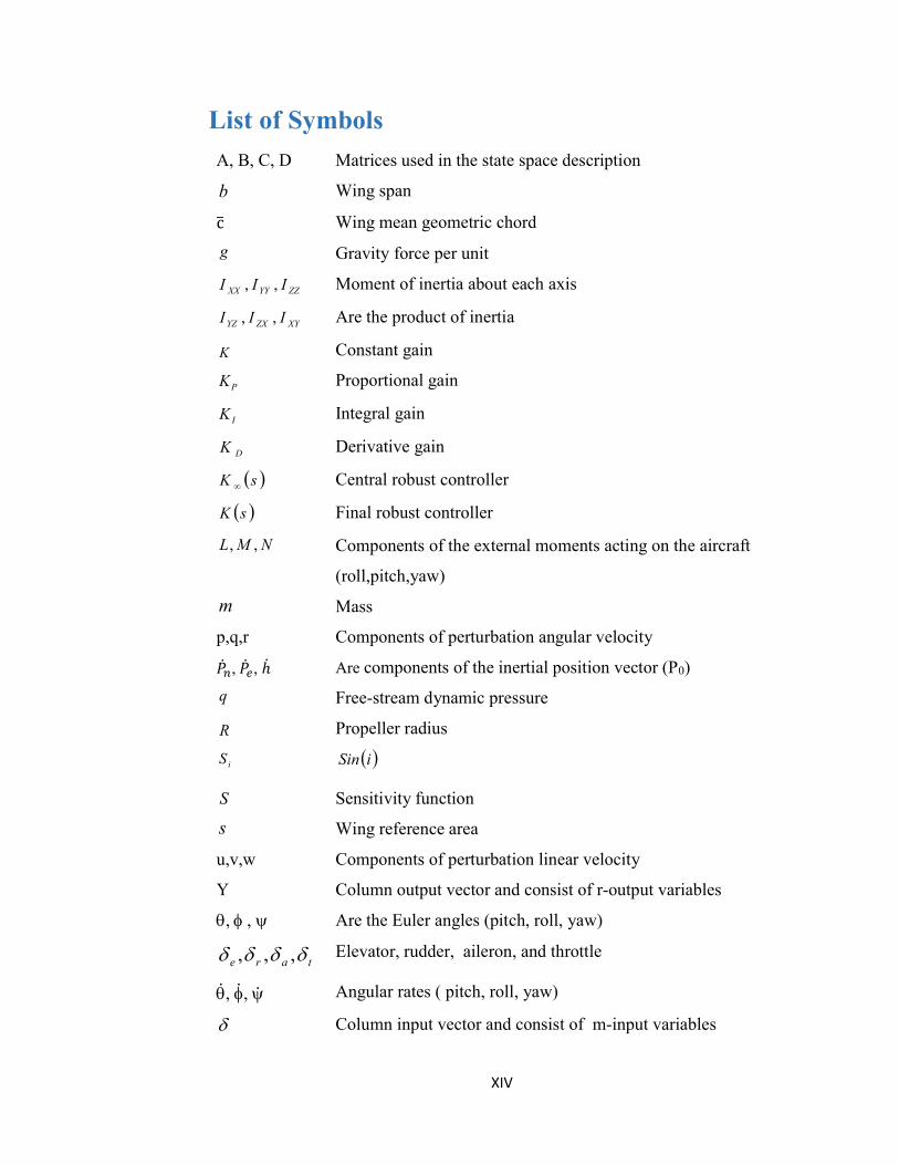
List of Symbols A, B, C, D Matrices used in the state space description b Wing span c Wing mean geometric chord g Gravity force per unit

ZZYYXX III ,, Moment of inertia about each axis XYZXYZ III ,, Are the product of inertia

K Constant gain PK Proportional gain IK Integral gain DK Derivative gain sK Central robust controller

sK Final robust controller NML ,, Components of the external moments acting on the aircraft

(roll,pitch,yaw) m Mass p,q,r Components of perturbation angular velocity

, , ℎ Are components of the inertial position vector (P0) q Free-stream dynamic pressure R Propeller radius

iS iSin S Sensitivity function s Wing reference area u,v,w Components of perturbation linear velocity Y Column output vector and consist of r-output variables , , Are the Euler angles (pitch, roll, yaw)

tare ,,, Elevator, rudder, aileron, and throttle , , Angular rates ( pitch, roll, yaw) Column input vector and consist of m-input variables

XV

Angle of attack Sideslip angle

B Angular velocity

XVI

List of Abbreviations MIMO Multi Input Multi Output SDOF Single Degree of Freedom TDOF Two Degree of Freedom

1

1 Chapter One: Introduction 1.1 Overview

Human has extended efforts in perusing the skies with man-made flying objects for over 2,000 years. Gliders became the groundwork for massive aircraft, engine technology, and further developments in aerodynamics. [1] The hang glider doesn’t have a lot of controlling surfaces like the conventional aircrafts, as it depends mainly on the control bar to direct its motion exploiting the thermals (updrafts) to stay aloft in air as much as possible. However, because such aircraft doesn’t have thrust due to the absence of a power plant along the flight path, the glider will be under the influence of various accelerating forces and drastic disturbances in all directions and these factors cause it to deviate from its desired path. This will limit the control as well as the maneuverability of it, especially that both are desired by sport gliders and most aircrafts in general. This motivated the designers to apply the automatic control theory to enhance the stability as well as the performance of the system. [2]

1.2 Problem Statement In aspect of weight, the hang glider is a very light aircraft compared to other types of aircrafts. It is drastically affected by various accelerating forces, perturbations, gusts and continuous disturbances during its soaring. In traditional control of the hang glider, the pilot positions himself relative to the wing by ‘pushing and pulling’ on the control bar. However, this process is exhausting and sometimes it’s hard to control the glider in the presence of strong disturbances. So, there a necessity to enhance the stability and the performance of the hang glider system against different types of disturbances. So, here comes the automatic control into picture.

2

1.3 Aim and Objectives 1.3.1 Aim

• To design different controllers utilizing classical and modern control design techniques that would enhance the stability and the performance of the system as well as to provide it with an excellent immunity to reject the drastic disturbances that may affect the hang glider’s body.

1.3.2 Objectives • To analyze the transient motion of the hang glider. • To design a control system that would guarantee the stability of the system with a certain level of performance.

1.4 Proposed Solution The research is a proposition to design two controllers utilizing two control techniques which are: (the inversion formulae carried out using Nyquist plane) as a classical control technique and the robust control technique. The data of the hang glider are gathered in a state-space model and the transient motion of the model is analyzed. Then, the controllers are established in order to achieve the aerospace standard performance specifications for control systems. Eventually, control evaluations are performed in order to assess which of the control design techniques is more convenient for the hang glider’s system.

1.5 Methodology The methodology embraces theoretical, analytical, numerical and simulation methods. In this thesis, the case study is a fixed wing hang glider. Generally, the methodology follows four main steps: In the first step, the hang glider’s data are all gathered in a state space model. Then, the hang glider’s motion is analyzed and studied in the second step. After that, the controllers are designed utilizing classical and robust control design techniques in the third step. Finally, in the fourth step, the control evaluation is performed on the designed controllers to assess which of the two control design techniques is more convenient with the hang glider’s system. The procedure is illustrated with more details in the flowchart below:

3

4

1.6 Thesis Outlines Chapter One gives a brief introduction about the project; identifying the aim, problem definition and the proposed solution. Chapter Two includes more detailed information about the gliders, aviation evolution and control techniques. The modeling, analysis and control setup are included in Chapter Three. While, all the results are discussed in Chapter Four. Finally, Chapter Five includes the conclusion of the thesis aided with future work.

5

2 Chapter Two: Literature Review 2.1 History and Background

2.1.1 Introduction Since the ancient time, humans kept pursuing their dream of flying by

sketching, analyzing and developing intricate designs in an attempt to imitate the flight of birds. Leonardo da Vinci sketched various flying machines consisted of number of wing designs in his 15th century manuscripts including a human-powered ornithopter shown in Figure (2-1), the name derived from the Greek word for bird. Later on, when others began to experiment with his designs, it became apparent that the human body could not sustain flight by flapping wings like birds. The fantasy of human flight continued to capture the imagination of many, but it was not until 1799 when Sir George Cayley, a Baronet in Yorkshire, England, conceived a craft with stationary wings to provide lift, flappers to provide thrust, and a movable tail to provide control. [2]

Figure(2- 1):A human-powered ornithopter [2]

The human flight attempts continued with Otto Lilienthal who was a German pioneer of human flight and became known as the Glider King. He was the first person to make well-documented, repeated, successful gliding flights beginning in 1891. He followed an experimental approach established earlier by Sir George Cayley. Newspapers and magazines published photographs of Lilienthal gliding,

6

favorably influencing public and scientific opinion about the possibility of flying machines becoming practical.

By the early 1900s, the famous Wright Brothers were experimenting with gliders and gliding flight in the hills of Kitty Hawk, North Carolina. The Wrights developed a series of gliders while experimenting with aerodynamics, which was crucial to developing a workable control system. Many historians, and most importantly the Wrights themselves, pointed out that their game plan was to learn flight control and become pilots specifically by soaring. [2]

Figure(2- 2):Orville Wright (left) and Dan Tate (right) launching the Wright 1902 glider off the east slope of the Big Hill, Kill Devil Hills, North Carolina on October 17, 1902. Wilbur Wright is

flying the glider [2]

By 1906, the sport of gliding was progressing rapidly and by 1911, Orville Wright had set a world duration record of flying his motor less craft for 9 minutes and 45 seconds. Wolfgang Klemperer came later and broke the Wright Brothers 1911 soaring duration record with a flight of 13 minutes using ridge lift. In 1928, Austrian Robert Krefeld proved that thermal lift. could be used by a sailplane to gain altitude by making a short out and return flight. In 1929, the National Glider Association was founded in Detroit, Michigan and soaring had grown into a diverse and interesting sport. Modern high performance gliders are made from composite materials and take advantage of highly refined aerodynamics and control systems. Today, soaring pilots use sophisticated instrumentation, including global

7

positioning system (GPS) and altitude information (variometer) integrated into electronic glide computers to go farther, faster, and higher than ever before. [2]

2.2 Glider “The Federal Aviation Administration (FAA) defines a glider as a heavier-than-air aircraft that is supported in flight by the dynamic reaction of the air against its lifting surfaces, and whose free flight does not depend principally on an engine.” [2]

2.3 Launching Techniques There are different launching techniques that helps the glider reaching the desired soaring altitude. They are illustrated in Figure (2-3):

Figure(2- 3): Glider Launching Techniques [2]

2.3.1 Foot Launching (Hang gliders) In this type of launching, the pilot uses his feet to run generating a high speed

then jumps from a high hill or mountain then soar utilizing the updrafts as shown in Figure(2-3-a). “Hang-gliders are piloted aircraft having cloth wings and minimal structure. Some hang-gliders look like piloted kites, while others resemble maneuverable parachutes.” [3]

8

2.3.2 Self-Launching From its name it doesn’t need any auxiliary equipment like the other types of launching techniques to reach the soaring altitude. An engine is installed into the glider as it will only help the glider taking off and climbing until reaching the desired soaring altitude as shown in figure(2-3-b). Then, the engine is shut down and at that once the motor glider will display the same flight characteristics as nonpowered gliders. The pilot soar normally utilizing the updrafts provided by the atmosphere. [2]

2.3.3 Winch Launching In winch launching technique, the bottom of the glider is connected by a cable

to the winch as illustrated in Figure(2-3-c). The winch is powered by an engine on the ground and once it’s activated, the glider is pulled along the ground at high speed toward the winch and takes off. In a short amount of time, the glider gains substantial altitude during this process and releases the winch line before continuing flight. [4]

2.3.4 Aero-Tow In this launching technique, a powered airplane is connected to the glider

towing it into the air using a long rope as shown in Figure(2-3-d). Inside the cockpit, the glider pilot uses a quick release mechanism to release the tow rope as soon as the glider reaches the desired altitude. Once the rope is released, the tow plane turns in opposite directions and the glider starts soaring. [4]

2.4 Types of Soaring Many soaring methods are actively researched but generally soaring can be

categorized into - gust, dynamic and static soaring. Gust soaring extracts energy from a turbulent condition to improve flight performance, utilized by vultures and petrels to exhibit better flight performance in turbulence condition compared to their normal gliding, while dynamic soaring extracts energy from the shear flow in the atmospheric boundary layer; albatrosses are known to trail ships in the open sea for days, by using dynamic soaring, almost without flapping their wings. Finally, static soaring utilizes upward moving air mass (updraft) to sustain flight, exemplified by

9

condors and vultures that have used updraft mostly in the form of thermals to migrate and forage. [5]

2.4.1 Gust Soaring The gust is a strong sudden burst of wind. When the profile is continuous, the gust structure is referred to as turbulence. The Turbulence is also observed in between thermals, whereby the duration of gust is usually only a few seconds. The motion of a gust is unpredictable, but it’s statistically represented by a (stochastic) model in which can be used for simulation analysis. Figure (2-4) shows an example of Dryden Wind Turbulence model. [5]

Figure(2- 4):Dryden Wind Turbulence model [5]

2.4.2 Dynamic Soaring

The horizontal wind in the boundary layer that has a velocity gradient profile due to the frictional force from the surface is known as shear flow. Wind closer to the surface is slowed down by friction, thus velocity increases with altitude. The Shear flow is common in the open sea, and is successfully used by albatross to sustain flight. However, on land, the shear flow that is suitable for dynamic soaring is restricted to mountain ridges that satisfy a certain condition - a specific strength and

10

profile of the moving air over the mountain ridge capable of creating a well-defined boundary, as illustrated in Figure (2-5). Dynamic soaring methods extract energy from shear flow by flying in a pattern of diving downwind, turning, and climbing upwind, then turning and diving downwind again. [5]

Figure(2- 5):Shear flow on the leeward side of a ridge [5]

2.4.3 Static Soaring

An updraft is a vertical current of rising air. There are three forms of updraft - orographic lift, mountain wave, and thermal Thermals

They are columns of rising air created by the heating of the Earth’s surface. The air layers near the ground expand and rise as the surface of the Earth is heated. The layers continue transferring the heat to the air layers above them, producing thermal air currents as shown in Figure (2-6). When a glider pilot is "thermalling," they are finding and riding those thermal columns. [4]

11

Figure(2- 6):Thermals Lift [4]

Ridge Lift

“It’s created by winds blowing against mountains, hills or other ridges. Along the windward side of the mountain, a band of lift is formed where air is redirected upward by the terrain. Typically, ridge lift extends only a few hundred feet higher than the terrain which produces it. Pilots have been known to go "ridge soaring" for thousands of miles along mountain chains.’’[4] . The ridge lift is illustrated in Figure (2-7).

Figure(2- 7): Ridge Lift [4]

12

Wave Lift This type of static soaring is similar to ridge lift in that it is created when wind meets a mountain. However, wave lift is created on the leeward (downwind) side of the peaks by winds passing over top of the mountain as clearly shown in Figure (2-8). Wave lift can reach thousands of feet high, and gliders riding on wave lift can reach altitudes of 35,000+ feet. [4]

Figure(2- 8): Wave Lift [4]

2.5 Thermal Model

As mentioned previously the glider remain a quite sustainable flight by hitting the thermals to remain aloft for the longest possible endurance. So, the locating of the thermal is an essential issue that must be taken in consideration when analyzing the fight dynamic of the glider and hence it should be involved as a flight control parameter beside the wind trajectory. A Graphical representation of a thermal model shown in Figure (2-9), MATLAB’s built-in function contour slice was used to create this figure. The color of the contour lines that form the thermal model represents the updraft vertical velocity. The velocity is stronger at the center of a thermal and weaker at the outer radius, which resembles a normal distribution. Downdraft is found at the top portion of the thermal model, which is represented by blue contour lines. Some additional characteristics of a thermal were incorporated in this simulation, such as height, radius and vertical velocity of a thermal are time

13

dependent variables; they are affected by the amount of sunlight, time of day, atmospheric condition, geographic location, and ground surface properties. Also, the position of a thermal tends to drift in the prevailing wind direction. [5]

Figure(2- 9):Computational updraft model [5]

2.6 Stability: A Requirement for All Airplanes

“Airplanes of all sizes must be capable of stable, trimmed flight in order to be controllable by a human pilot and useful for various applications. Stable flight by a human pilot is possible only if the airplane possesses static stability, a characteristic that requires aerodynamic forces on the airplane to act in a direction that restores the plane to a trimmed condition after a disturbance. Dynamic stability requires that any oscillations in aircraft motion that result from disturbances away from equilibrium flight conditions must eventually dampen out and return to an equilibrium or “trimmed” condition. Certain dynamic instabilities can be tolerated by a human pilot, depending mostly upon pilot skill and experience.” [6]

14

Dynamic Stability An airplane owns a dynamic stability if the amplitudes of any oscillatory

motions induced by disturbances eventually decrease to zero relative to a steady-state flight condition. Graphical representations of dynamic stability and instability are shown in Figures (2-10) and (2-11). To study dynamic stability, it is necessary to analyze the well-known differential equations of aircraft motion. For small perturbations, these equations can be decoupled into longitudinal and lateral-directional portions, with 3 degrees of freedom in each. [6]

Figure(2- 10):A graphical example of dynamically stable aircraft [6]

Figure(2- 11):A graphical example of dynamically unstable aircraft motion [6]

15

2.7 Aircraft Dynamics 2.7.1 Equations of Motion

The equations of motion of an aeroplane are those equations that express the flight dynamics and aerodynamic characteristics of the aeroplane related to quantifiable stability and control enabling a sufficient description of the flying and the handling qualities. the equations of motion can be in a simple form describing small perturbation motion about trim only or they can be complex, but completely descriptive embracing static stability, dynamic stability, aero elastic effects, atmospheric disturbances and control system dynamics simultaneously for a given aeroplane configuration. [7]

2.7.2 The Dynamic Stability Modes 2.7.2.1 Longitudinal Dynamic Stability Modes

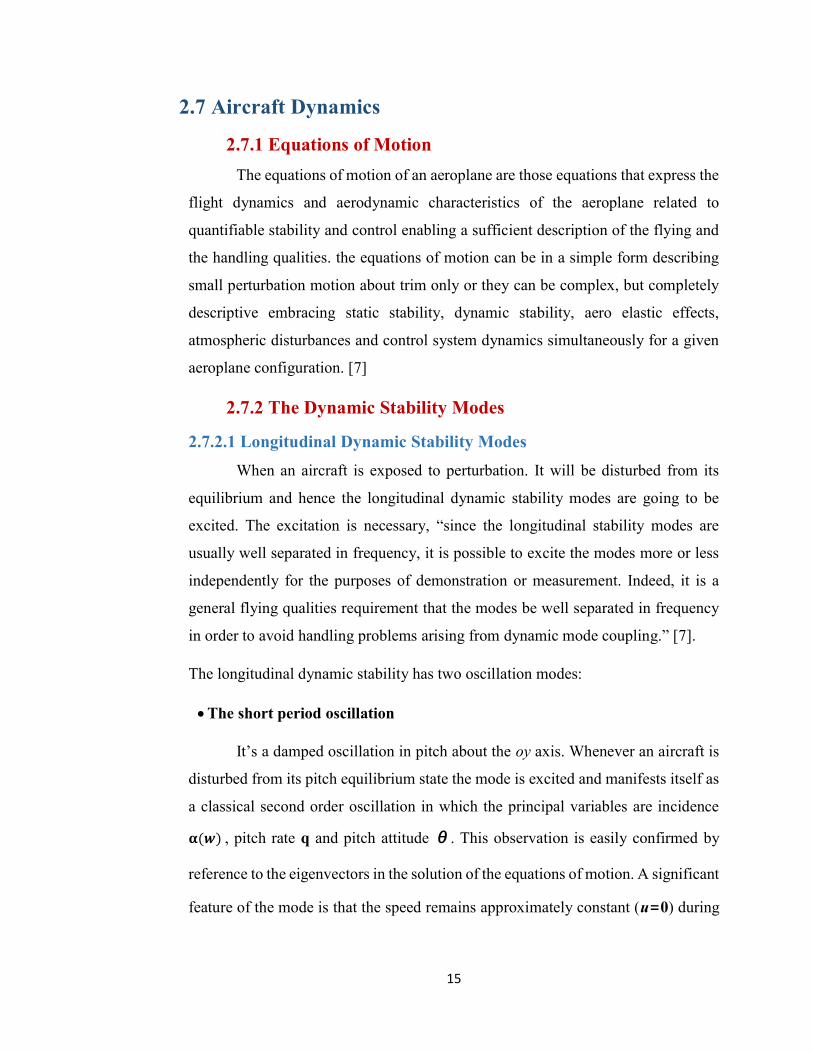
When an aircraft is exposed to perturbation. It will be disturbed from its equilibrium and hence the longitudinal dynamic stability modes are going to be excited. The excitation is necessary, “since the longitudinal stability modes are usually well separated in frequency, it is possible to excite the modes more or less independently for the purposes of demonstration or measurement. Indeed, it is a general flying qualities requirement that the modes be well separated in frequency in order to avoid handling problems arising from dynamic mode coupling.” [7]. The longitudinal dynamic stability has two oscillation modes: The short period oscillation

It’s a damped oscillation in pitch about the oy axis. Whenever an aircraft is disturbed from its pitch equilibrium state the mode is excited and manifests itself as a classical second order oscillation in which the principal variables are incidence

( ) , pitch rate q and pitch attitude θ. This observation is easily confirmed by reference to the eigenvectors in the solution of the equations of motion. A significant feature of the mode is that the speed remains approximately constant (u=0) during

16

a disturbance. Also the inertia and momentum effects ensure that speed response in the time scale of the mode is negligible since the mode’s period is short.

The short period can be simulated as in Figure (2-12) where the aircraft behaves as if it were restrained by a torsional spring about the oy axis. A pitch disturbance from trim equilibrium causes the “spring’’ to produce a restoring moment, thereby giving rise to an oscillation in pitch. The oscillation is damped and this can be interpreted as a viscous damper. The damping arises from the motion of the tailplane during the oscillation as it behaves as a kind of viscous paddle damper. The total observed mode dynamics depend not only on the tailplane contribution, but also on the magnitudes of the additional contributions from other parts of the airframe. [7]

Figure(2- 12):A stable short period pitching oscillation [7]

The long period oscillation (Phugoid Oscillation)

The phugoid mode is most commonly a lightly damped low frequency oscillation in speed u which couples into pitch attitude θ and height h. A significant feature of this mode is that (the incidence α(w) remains substantially constant)

17

during a disturbance. However, it is clear that the phugoid appears, to a greater or lesser extent, in all of the longitudinal motion variables but the relative magnitudes of the phugoid components in incidence α(w) and in pitch rate q are very small.

Hence, the phugoid is classical damped harmonic motion resulting in the aircraft flying a gentle sinusoidal flight path about the nominal trimmed height datum. As large inertia and momentum effects are involved ,the motion is necessarily relatively slow such that the angular accelerations, and ( ), are insignificantly small. Consequently, the natural frequency of the mode is low and since drag is designed to be low so the damping is also low. [7]

2.7.2.2 lateral–Directional Modes The Roll Subsidence mode

It’s a non-oscillatory lateral characteristic which is usually substantially decoupled from the spiral and Dutch roll modes. Since it is non-oscillatory, it is described by a single real root of the characteristic polynomial, and it manifests itself as an exponential lag characteristic in rolling motion. The aeromechanical principles governing the behavior of the mode are shown in Figure (2-13) and as can be seen from it, the aircraft is viewed from the rear so the indicated motion is shown in the same sense as it would be experienced by the pilot. Assuming that the aircraft is constrained to the single degree of freedom motion in roll about the ox axis only, and that it is initially in trimmed wings level flight. [7]

18

Figure(2- 13):The roll subsidence mode [7]

So, in the rolling motion, the wing experiences a component of velocity normal to the wing. This results in a small increase in incidence on the down-going starboard wing and a small decrease in incidence on the up-going port wing. The resulting differential lift gives rise to a restoring rolling moment as indicated. The corresponding resulting differential induced drag would also give rise to a yawing moment, but it’s usually ignored as it’s very small. Thus, the roll rate builds up exponentially until the restoring moment balances the disturbing moment and a steady roll rate is established. [7] The spiral mode

Likewise, the spiral is also non-oscillatory and is determined by the other real root in the characteristic polynomial. When excited, the mode dynamics are usually slow to develop and involve complex coupled motion in roll, yaw and sideslip. The dominant aeromechanical principles governing the mode dynamics are shown in Figure (2-14). The lateral static stability and the directional static stability of the aeroplane play an important role in identifying the spiral mode’s characteristics [7]

19

Figure(2- 14):The spiral mode development [7]

The Dutch Roll mode

It’s a classical damped oscillation in yaw, about the oz axis of the aircraft, which couples into roll and, to a lesser extent, into sideslip. The complex interaction between all three lateral–directional degrees of freedom forms the motion being described by the Dutch roll mode. Its characteristics are described by the pair of complex roots in the characteristic polynomial. Generally, the Dutch roll mode is the lateral–directional equivalent of the longitudinal short period mode. Since the moments of inertia in pitch and yaw are of similar magnitude the frequency of the Dutch roll mode and the longitudinal short period mode are of similar order. Yet, the fin is usually less effective than the tailplane as a damper and the damping of the Dutch roll mode is often insufficient. [7]. Figure (2-15) illustrates the oscillatory motion of the Dutch Roll mode.

20

Figure(2- 15):The oscillatory Dutch roll mode [7]

2.8 Significance of Automatic Flight Control

All aerospace applications are constrained by standard requirements to validate comfortable, safe and smooth flight. Thus, the dynamic responses have to be smooth enough not posing significant overshoots or exceeding time domain constraints, and remain within limitations of the airframe. To address and solve such problems of the aircraft, automatic flight control systems are designed utilizing both classical and advanced techniques. In this thesis, both classical and robust control design techniques in frequency domain are chosen as examples to classical and advanced techniques. The design process is started by obtaining a mathematical model of the aircraft and analyzing its motion in the frequency domains. [8]

2.9 Control Techniques Control is the process of checking the current performance of the system

against pre-determined standards to ensure adequate progress and satisfactory results to reach a certain degree of domination on the system.There have been several methods and techniques developed for both time and frequency domains but in they can be classified as shown in Figure (2-16).

21

Figure(2- 16):Various Control Techniques

Here are some techniques observed:

2.9.1 Classical Control Techniques For its simplicity, the classical control such as PID controller is probably the

most-used feedback control design. "PID" means Proportional-Integral-Derivative, referring to the three terms operating on the error signal to produce a control signal. A manipulation or a tuning of the three terms which is often done iteratively without specific knowledge of a plant model can guarantee the desired closed loop dynamics. The proportional term will only ensure the stability while the integral term permits the rejection of a step disturbance and the derivative term is used to provide damping or shaping of the response. PID controllers are the most well established class of control systems: however, they cannot be used in several more complicated cases, especially if MIMO systems are considered [8].

2.9.2 Modern Control Techniques Unlike the classical control, the advanced control utilizes the state space

representation in which a mathematical model of a physical system is represented as a set of input, output and state variables related by first-order differential

22

equations. Thus, variables representing inputs, outputs and states are expressed in terms of matrix form. The state space representation provides a convenient and compact way to model and analyze systems with multiple inputs and outputs [8]. There are many advanced control techniques with the main objective to overcome disadvantages of classical techniques. When dealing with multi-conflict objectives it is intended to improve performance and stability robustness, besides saving cost and time for designing control systems utilizing available technology. [8] 2.9.2.1 Adaptive Control

It is a control system that has the ability to adjust its characteristics in a changing environment in order to maintain an optimal operation according to some specified criteria. It is either model reference or self-tuning which requires some kind of identification for the plant dynamics. [8] 2.9.2.2 Predictive Control

A predictive control is a controller that is based on the predictive model of the plant. The model is used to predict the future output based on the historical information of the plant as well as the future input. It calculates, the future control action based on a penalty or performance function. The optimization of predictive control is limited to a moving time interval and is carried on continuously on-line. The moving time interval is sometimes called a temporal window. A predictive control is based on three elements: predictive model, optimization in range of a temporal window, and feedback correction. [8] 2.9.2.3 Optimal Control

It is a control system devoted to find a feasible controller transfer the system state from a given initial condition toward the objective set. [8] 2.9.2.4 Intelligent Control

Intelligent control referred to a control that uses various artificial intelligence techniques such as learning control, expert control, fuzzy control, and neural network control.[8]

23

2.9.2.1 Robust Control A controller said to be robust when it manipulates the unknown plants with

unknown dynamics subjected to unknown disturbances. Robust control is an approach to controller design that explicitly deals explicitly with uncertainty. There are several reasons to interpret this uncertainty: imperfect plant data, time varying plant, higher order dynamic, non-linearity, complexity, skills. Several techniques of robust control have been developed, either in time domain or frequency domain such as 2 or . The design of robust control is based on the worst case scenario, therefore it is well suited to applications where stability and reliability are the top priorities, plant dynamics are known, and variation ranges for uncertainties can be estimated [8]. Uncertainty

As mentioned previously that robust control approach is generally concerned with uncertainties and how to deal with them. Uncertainty or (plant mismatch) is considered as one of the sophisticated and challenging problems in robust control The uncertainty affects both robustness and performance of control system. The uncertainty sources are classified into the following two sets, as shown in Figure (2-17) [8].

Figure(2- 17): Classification of uncertainty [8]

24

1. Disturbance signals which include: Wind guest signal Sensor noise signal Actuator signal

2. Dynamic Perturbation, which represents the difference between the

mathematical model and the actual dynamics of the system in operation. The typical sources of this uncertainty include:

Unmodeled dynamics at high frequency. Neglected nonlinearities in the model. Effect of deliberate reduced-order models. System-parameter variations due to environmental changes and Torn- and-

Worn factors.

2.10 Similar Work and Previous Studies A lot of work have been done in the field of automatic flight control. A variety of methods have been used to enhance the stability and adjust the dynamics responses as well as the performance of the aircraft by developing efficient control systems that would guarantee all of this in most flight conditions including; cruising, climbing, descending or even soaring. The thesis has followed the same methods and methodologies of the following case studies.

2.10.1 First Relevant Report A paper for Lorenzo Ntogramatzidis, Roberto Zanasi and Stefania Cuoghi carried a title of “A Unified Analytical Design Method of Standard Controllers using Inversion Formulae” published Italy, October 16, 2012 had presented a comprehensive range of design techniques for the synthesis of the standard compensators (Lead and Lag networks as well as PID controllers). The design of a standard compensators with the desired specifications is carried out using the inversion formulae and Nyquist plots in the frequency domain. [9]

25

Evaluation The paper exhibited the synthesis of the standard PID controllers as well as Lead and lag networks implementing the Inversion Formulae, which enabled the compensators to be addressed without a significant increase in the design complexity as it gave an explicit relationship between the desired specifications and the compensator’s gains. This method will be used as a classical control approach as it's very simple and gives fine results.

2.10.2 Second Relevant Report A paper for Elfatih G. Hamdi, Gamal M. Sayed EL-Bayoumi and Ayman H. M. Kasem titled by “Structured Robust Control for small UAV” was published in the 3rd International Workshop on Numerical Modelling in Aerospace Sciences, NMAS 2015, 06-07 May 2015, Bucharest, Romania. The paper was devoted to design a structured robust control system to stabilize the attitude of small UAV against additive uncertainties. PI controller and static gain are considered as structure for robust control synthesis. The design procedure had been performed using two control configurations: Single degree of freedom (SDOF) controller and Two degree of freedom (TDOF) controller to achieve some advantages. [10] Evaluation

The paper presented different issues in structured robust control systems design such as the stabilizing of the PI controller by computing the stability regions in the Kp-Kd plane, as well as the design procedures for small UAV’s longitudinal autopilot and the tuning of TDOF robust controller was also performed. The results were very accurate and a lot of problems have been solved as well as the robust control guaranteed the stability of the system with certain level of performance. The same methodology will be followed as a robust control approach in order to achieve the desired design goals.

2.10.3 Statement of Argument The previous relevant reports exhibited two types of control techniques: The first report observed a classical control technique by the mean of the (inversion

26

formula) which is very simple and provide an evident relationship between the coveted system’s specifications and the gains of the PID using direct formulas. However, as classical control in general poses some short comings and this motivate us to design a second controller utilizing robust control approach which is a very powerful mathematical framework where the variations range of uncertainties can be estimated explicitly. Thus, our project will be based on both methods following the classical and the robust control approaches to design two different PID controllers.

27

3 Chapter Three: Modeling, Analysis and Control Design In this chapter; the methodology, the methods, the tools and all the approaching techniques that had been implemented in this project are explained in an explicit and orderly manner. Starting up with the mathematical model of the hang glider, moving up to the transient analysis of the aircraft motion and expounding the control setup. Finally, an evaluation of the controllers will be performed.

3.1 Mathematical Modeling of the Aircraft 3.1.1 Significance of Mathematical Modeling:

Understanding the dynamical response of an aircraft to the movement of its control surfaces is essential for designing an aircraft flight control system. This understanding requires flight testing of the aircraft, and because of the high cost of building and flight testing a real aircraft, the importance of aircraft mathematical models goes far beyond control system design. Building the aircraft mathematical model requires the knowledge of how the aerodynamic forces and moments acting on an aircraft are created, how they are modeled mathematically, and how the data for the models are gathered. Consequently, the equations of aircraft’s motion and its control systems must be completely understood. The equations of motion, their methods of solution and characteristic responses associated with them are derived in this chapter. For building such model the characteristics and aerodynamic data for the underlying aircraft will be needed, and consequently they are developed briefly in the next subsection. [11]

3.1.2 Reference Coordinate Systems “To describe the motion of an aircraft, it is necessary, first, to define the

following coordinate systems for formulation of the equations of motion.

28

• Earth Axis System: This is a coordinate frame with its origin at the center of the Earth, translating with Earth, but with a fixed orientation relative to the stars.

• Aircraft-Body Coordinate Frame: This frame is a right-handed orthogonal frame, attached to the aircraft, with its origin positioned to the aircraft center of gravity. From the Figure (3-1) the axes of this frame are defined as follows: XB-axis is in the aircraft's plane of symmetry, positive in forward direction and coincides with some reference line in the aircraft (longitudinal). ZB-axis is in the aircraft's plane of symmetry, and positive in downward direction. YB-axis is perpendicular to the XB-ZB plane and positive to right (starboard) wing.

Figure (3- 1):Body and stability frames definition [8]

29

Figure (3- 2):Body and inertial axes systems [8]

. • Stability Axis System:

This frame is constructed when the forward direction of OXB-axis coincides with the aircraft velocity VT vector during a trim flight condition, and is used to simplify the aerodynamic calculations, as shown in Figure (3-3).

• North-East-Down (NED)Frame: This frame moves with the aircraft and is vertically below the aircraft c.g, so that the aircraft X-Y plane is tangent to the Earth's surface.” [8]

3.1.3 Equations of Motion: The applied forces and moments on the aircraft and the resulting response of the aircraft are traditionally described by a set of equations known as the aircraft equations of motion. An aircraft has six degrees of freedom (if it is assumed to be rigid), as it can move forward, sideways, and down; as well as it can rotate about its axes with yaw, pitch, and roll. Hence, to describe the state of this system which has six degrees of freedom, values of the six variables are needed, however these variables are actually unknowns. So, in order to solve for these six unknowns, six simultaneous equations are necessary. [12]

30

3.1.3.1 Assumptions Derivation of the equations of motion follows a very simple pattern starting

from Newton's second law for translational and rotational motions. The equations of motion that govern the translational and rotational motions of the aircraft are derived using the following assumptions as in [12]: 1. The aircraft is rigid. 2. NED (Local) frame is treated as an inertial frame. 3. The mass of the aircraft is constant with respect to time. 4. The aircraft is symmetric about the body xz plane; hence = 0 and = 0. Starting from Newton's second law for translational motions:

= ( ) (3-1)

Where is the sum of the externally applied forces and mV is linear momentum. Also, Newton's second law for rotational motions is:

= ( ) (3-2)

Where is the sum of the externally applied moments and is angular momentum. 3.1.3.2 Flight Vector Definition To clarify the aircraft motion, the linear and angular velocity vectors as well as the external forces and moments vectors are defined in Cartesian coordinates as follow:

= + + (3-3) = + + (3-4) = + + (3-5) = + + (3-6)

, where , a, are unit vectors in the body frame axis.

31

The above vectors are measured with respect to the inertial frame, but are positioned in the body frame which indicated by subscript B. The linear velocity vector can be written in polar form as follows:

Figure (3- 3): Orientation of relative wind with body axis system [8]

= + + (3-7)

= tan ( ) (3-8)

= sin (3-9)

Where: is the aircraft speed. Following the assumptions stated in order to obtain the derivation of the equations of motion, the equations from (3-1) to (3-9) can be manipulated and written in terms of scalar as follow:

VRWQUmX (3-10) WPURVmY (3-11) UQVPWmZ (3-12)

xzyyzzxzxx PQIIIQRIRIPL (3-13) xzzzxxyy IRPIIPRIQM 22 (3-14)

32

xzxxyyxzzz QRIIIPQIPIRN (3-15) The equations from (3-10) to (3-15) are a set of six, non-linear, coupled,

differential equations. Therefore, we can conclude that the translational equation describes the aircraft with respect to its three translational degrees of freedom, while the rotational equation describes the aircraft with respect to its three rotational degrees of freedom. Newton's second law, therefore, yields six equations for the six degrees of freedom of a rigid body. [11,12] 3.1.3.3 Aircraft Attitude and Frames Transformation

The equations of motion derived in (3-10) to (3-15) characterize the aircraft motion with respect to the body frame. Thus, to relate this motion to the inertial frame, it is necessary to determine the orientation of the body frame with respect to the inertial frame. This can be realized using three Euler’s angles representation which defines a set of transformations from one frame to another. The transformation, that depends upon a sequence of frames rotations about each other, can be established as follows [8], Figure (3-4): 1. Rotate the inertial frame axes XE, YE, ZE through azimuthal angle about the ZE- axis, nose right (positive yaw), to reach some intermediate axes X1, Y1, Z1. 2. Rotate the axes X1, Y1, Z1 through elevation angle about the Y1-axis, nose up (positive pitch), to reach some intermediate axes X2, Y2, Z2. 3. Rotate the axes X2, Y2, Z2 through bank angle about the X2-axis, right wing down (positive roll) to reach the body axes XB, YB, ZB.

If the sequence of rotations started from the body to the inertial frame, the sequence roll, pitch, and yaw must be followed. With the help of Figure (3-4) and using of the direction cosines technique, the individual rotation matrices can be written as follows:

10000

CSSC

B yaw-rotation (3-16)

33

CS

SCB

0010

0 pitch-rotation (3-17)

CSSCB

00

001 roll- rotation

(3-18)

Figure (3- 4): Relationship between body and inertial frames [8]

If B is referred to be the complete transformation matrix from the inertial frame to the body frame, then it can be constructed from the above individual rotation matrices as follows:

BBBB (3-19) and,

=1 0 00 ∅ ∅0 − ∅ ∅

× ∅ 0 − ∅0 1 0∅ 0 ∅

× − 0− 0

0 0 1

(3-20)

34

= −

− − + ∅ ∅ + ∅ −

Where:

iC denotes to the icos iS denotes to the isin

3.1.3.4 External Forces and Moments The aircraft model is completed by rearranging the equations (3-10) ~ (3-15) to

describe the external forces and moments that acting on the aircraft. These forces and moments are due to: aerodynamic effect, gravitational effect, and movement of aerodynamic controls, power level, and the effect of atmospheric disturbances. If, initially, the steady trimmed flight conditions with zero roll, sideslip, and yaw angles, are chosen, the effect of atmosphere should be neglected. Also the hang glider is a powerless aircraft (it flies without a power plant by the mean of soaring). So no propulsive model is needed. [8] Aerodynamic Forces and Moments

Since the aerodynamic force and moment are resolved into the body frame, it may be formulated in terms of aircraft geometric properties and dimensionless coefficients as:

xa qsCX is the axial (drag) force (3-21) ya qsCY is the side force (3-22)

za qsCZ is the normal (lift) force (3-23) La qsbCL is the rolling moment (3-24)

Ma CcqsM is the pitching moment (3-25) Na qsbCN is the yawing moment (3-26)

35

Gravitational Forces and Moments It is well known that the gravitational force acts on the center of gravity (c.g). Since the c.g. coincides with the center of mass, no moment will be generated due to the gravitational force [15]. However, after resolving it along the body frame via the transformation matrix, the gravitational force can be written as follows, Figure (3-5):

EB

B

mgZ

YX

GG

G00

(3-27)

Substituting the transformation matrix B using equation (3.20) yields to the following:

coscossincos

sin

mgmg

mg

ZYX

GG

G

(3-28)

And: 0 GGG NML (3-29)

36

Figure (3- 5): Gravitational force acting on a conventional aircraft [8]

3.1.3.5 Dynamic and Kinematic Equations of Motion

The orientation of the aircraft with respect to the inertial frame is determined by the Euler angles. To realize this object, the angular velocity vector is written in terms of Euler angles rate as follows:

kjiB (3-30) After resolving the unit vectors into the body frame, the Euler angular velocity is given as follows:

RQP

seccossecsin0sincos0

tancostansin1

(3-31)

Where: P, Q, R are taken from the output of the rate gyroscopes strapped to the aircraft.

Because of the frames transformation using Euler angles we now have six equations of motion which have six unknown variables already, in addition to three

37

extra unknown variables (which are the angular rates (∅, ,) generated from the rotational kinematic motion). It’s worth mentioning that there are also translational kinematic equations of motions which are referred as (the navigation equations) whereas the three rotational kinematic equations are referred as (auxiliary equations) as they will adequately help us solving the six equations of motion.

Kinematics and dynamics are two branches of classical Mechanics that deal with the motion of particles. These two branches play an important role in the derivation of equations of motion.

• Kinematics: It’s a branch of classical mechanics which describes the motion of points,

bodies (objects) and systems of bodies (group of objects) without consideration of the causes of motion. It’s a field of study is often referred to as the “geometry of motion’’.

• Dynamics:

It’s a branch of classical mechanics that studies the forces and torques and their effect on motion. It tries to understand the forces that are forcing the object or bodies of object into motion. In a dynamic motion, researchers study how a physical system might develop or alter over time and study the causes of those changes.

• Key difference: Kinematics gives the values of change of objects, while dynamics will provide the reasoning behind the change in the objects. [13]

According to this, a rigid aircraft with fixed wings and six degree of freedom is experiencing two types of motions; kinematic and dynamic motion as shown in Figure (3-6).

38

Figure (3- 6): The aircraft motions

A rigid aircraft with fixed wings has twelve equations of motion (six kinematic and six dynamic). These equations representing the aircraft motion can be found in [11] and can be summarized as follows: Three Translational-Kinematic equations (Navigation equations) The three components of the inertial position vector (P0) are given as follows:

= U cos cos + V(−cos sin + sin sin cos +W(sin sin + cos sin cos)

(3-32)

= U cos sin + V (cos cos + sin sin sin) + W (−sin cos + cos sin sin)

(3-33)

ℎ = U sin − V sin cos − W cos cos (3-34)

Three Rotational-Kinematic equations (Auxiliary equations) = P + sin tan Q + cos tan R (3-35) = cos Q − sin R (3-36) Ψ = sin sec Q + cos sec R (3-37)

Three Translational -Dynamics (Forces equations)

39

Three Rotational-Dynamics (Moments equations)

L = I P − I R + P Q + I − I Q R (3-41) M = I Q − I (P − R ) + (I − I )P R (3-42) L = I R − I P + P Q I − I + I Q R (3-43)

3.1.4 Linearization of Equation of Motion

Unfortunately, the equations of motion from (3-35) to (3-43) are non-linear first order coupled differential equations. In order to make the analysis and the design of the controller feasible we need to linearize these equations. In accordance to the complexity of the problem, linearization of the equations brings about especially desirable simplifications. The linearized model, nonetheless, gives quite adequate results for engineering purposes over a wide range of applications; because the major aerodynamic effects are nearly linear functions of the variables of interest, and because quite large disturbances in flight may correspond to relatively small disturbances in the linear and angular velocities. [12]. There are various techniques and methods for the linearization of the non-linear equations. We can classify them into two main methods:

= ( + Q W − VR ) (3-38) = ( + U R − P W ) (3-39) = ( + V P − UQ ) (3-40)

40

Figure (3- 7) : Linearization methods.

In this thesis, the linearized model of the equations of motion will be

developed using an analytical method for linearization known by the “small disturbance theory” or the “small perturbation theory”. 3.1.4.1 Small Disturbance Theory

The small perturbation theory is based on a simple technique used for linearizing a set of differential equations. In aircraft flight dynamics, the aerodynamic forces and moments are assumed to be functions of the instantaneous values of the perturbation velocities, control deflections, and of their derivatives. They are obtained in the form of a Taylor series in these variables, and the expressions are linearized by excluding all higher-order terms. [ 11,12]

In applying the small-disturbance theory, we assume that the motion of the air plane consists of small deviations about steady flight condition given as follow:

= + ∆ = + ∆ = + ∆ (3-44)

= + ∆ = + ∆ = + ∆ = + ∆ Y= + ∆ = + ∆ = + ∆ = + ∆ = + ∆

δ = δ + ∆δ For convenience, the reference flight condition is assumed to symmetric and

the propulsive forces are assumed to remain constant. this implies that : = == = = = 0. Furthermore, if we initially align the x axis so that it is

along the direction of the airplanes velocity vector, then = 0

41

This yields that change in aerodynamic forces and moments are functions of the motion variables ∆ , ∆ . and so forth. The aerodynamic derivatives usually the most important for conventional airplane motion analysis follow:

∆ = ∆ + ∆ + ∆ + ∆ (3-45)

∆ = ∆ + ∆ + ∆ + ∆ (3-46)

∆ = ∆ + ∆ + ∆ + ∆ + ∆ + ∆ (3-47)

∆ = ∆ + ∆ + ∆ + ∆ + ∆ (3-48)

∆ = ∆ + ∆ + ∆ + ∆ + ∆

+ ∆

(3-49)

∆ = ∆ + ∆ + ∆ + ∆ + ∆ (3-50) So, the linearized small-disturbance longitudinal and lateral rigid body equation of motion can be given as follow: The Linearized Longitudinal Equations

− ∆ − ∆ + ( cos )∆ = ∆ + ∆ (3-51)

- ∆ + (1 − ) − ∆ - + − sin ∆ =∆ + ∆

(3-52)

- ∆ − + ∆ +( − ) ∆ = ∆ +∆

(3-53)

42

The Linearized Lateral Equations

− ∆ − ∆ + ( cos )∆ = ∆ (3-54)

- ∆ + − ∆ −( + ) ∆ = ∆ + ∆ (3-55)

- ∆ − + ∆ +( − ) ∆ = ∆ + ∆ (3-56)

3.2 Analysis 3.2.1 Separation of the Equations of Aircraft Motion

The linearized equations from (3-51) to (3-56) are ordinary linear differential equations and can be written as a set of first-order differential equations known as the “state equation” and the “output equation” respectively as in equations (3-57) and (3-58) :

= + (3-57) y = Cx + Du (3-58)

Where: x is called the “state vector”, y is called the “output vector”, u is called the “input vector”, A is called the “state matrix”, B is called the “input matrix”, C is called the “output matrix”, D is the “direct transition matrix”.

43

For a rigid aircraft, the linearized equations could be split into two uncoupled sets. This decoupling occurs when the sideslip and bank anglers are set to zero values. These sets are:

1) Longitudinal Equations that has: , , , as states, throttle setting and elevator deflection as inputs.

2) Lateral Equations that has: v, p, r, ϕ and ψ as states, ailerons deflection and rudder deflection as inputs.

For the longitudinal motion, the stability derivatives is often insignificant while the is often ignored if the trim forward speed is large. The longitudinal motion Jacobian matrix for a hang glider can be found in [11] and can be written as:

= 0 − cos− sin

+0 0 1− sin

0

(3-59)

= (3-60)

=0 0

(3-61)

= Where is the longitudinal control angle.

(3-62)

Also, the steady state representation of the hang glider’s lateral motion can be written as:

44

=

+ − 0 0

0 0 00 1 0 0 00 0 1 0 0. . . . .

(3-63)

=

.

.

(3-64)

=

.0

00.

(3-65)

= (3-66)

Where is lateral control angle The values of longitudinal stability derivatives as well as the lateral stability derivatives are included in appendix (A). The operating point chosen for this case study corresponds to 10.8 m/s velocity. The homogeneous solutions equation of (3-57) are always exponential of the form:

= (3-67) Where and are the eigenvalues and the eigenvectors of the system, respectively. Substituting the value of x, we obtain the following: | I – A | = 0 (3-68) , where I is the identity matrix and are also called the characteristic roots. The dynamic stability is established from the knowledge of eigenvalues of the state coefficient matrix A, which can be found by solving the equation:

45

| I - A|=0 (3-69) This determinant is known as the stability determinant, and the equation obtained from expanding this determinant is called the characteristic equation of the dynamic system.

The type of the aircraft response is determined from the roots of its characteristic equation. If the roots are real, the response will be either a pure divergence or a pure subsidence, depending upon whether the roots are positive or negative. If the roots are complex, the motion will be either a damped or an undammed sinusoidal oscillation. The characteristic equation determined from the state coefficient matrix , is a quadratic polynomial in , and can be expressed as:

+ + + + = 0 (3-70) Solving this quadratic leads to two sets of complex roots indicating two damped sinusoidal oscillations in the following manner: ( + 2 ⍵ λ + ⍵ ) ( + 2 ⍵ λ + ⍵ ) = 0 (3-71) , where and are the damping ratios of the phugoid mode and the short mode, respectively. ⍵ and ⍵ are the natural frequencies of the phugoid mode and the short mode, respectively. Also the characteristic roots can be expressed as: λ , = ± i (3-72) 3.2.1.1 Longitudinal Modes Equation (3-71) depends on two main factors: The first factor corresponds to a mode of motion called phugoid mode:

The damping of which is usually very low, and is sometimes negative, so that the mode is unstable and the oscillation grows with time, The second factor corresponds to a mode of motion called the short period mode

46

It corresponds to a rapid, relatively well-damped motion. Considering the decoupled longitudinal dynamics, it is possible to excite separately the short-period and phugoid modes. In the phugoid case, are varied, with, ⍺ almost constant; while in the short period case ⍺ , and are varied, with speed kept constant. More details can be found in [11] 3.2.1.2 Lateral Modes

The characteristic equation determined from the state coefficient matrix yields to an aquatic (of fifth degree) equation as follow: λ (λ + e) (λ + f)( + 2 ⍵ λ + ⍵ ) = 0 (3-73) Where e and f are the values of the spiral and the roll subsidence roots. The largest real root is the roll subsidence and the smallest is the spiral. Also, and ⍵ are the damping ratio and the natural frequency of the Dutch roll mode respectively. The simple term in λ at the beginning of the characteristic equation corresponds to the heading mode. Because λ = 0, once an aircraft’s heading has been changed, there is no natural tendency for the aircraft to be restored to its equilibrium heading. The roots will be such that the airplane response can be characterized by the following motions: (1) Spiral Mode: A slowly convergent or divergent motion. (2) Rolling Mode: A highly convergent motion. (3) Dutch Roll Mode: A lightly damped oscillatory motion having a low frequency. After decoupling the hang glider’s model into longitudinal and lateral motions. The next step is to test the open loop system’s specifications and compare them with the “control systems standard aerospace performance specifications”. The model’s specifications have been estimated in both time and frequency domains. They are observed and discussed in Chapter Four. According to the results of the analysis the system is obviously unstable in both longitudinal and lateral motions. So, a decision

47

is to be made to solve the problems of the system’s stability, robustness and performance and in order to reach the standard performance specifications of the aerospace applications. All, which can be achieved by designing a control system.

3.3 Control Design As previously concluded in the latter section that. Towards the objective of

achieving the standard aerospace performance specifications for control systems and to guarantee the stability of the system with some level of performance, a classical control approach carried out using Nyquist plane implementing the inversion formula and a robust control approach are used to design two controllers.

3.3.1 Controller Order Reduction and Model Order Reduction

3.3.1.1 Controller Order Reduction Due to the high-order controllers, the robust control system design

necessitates the reduction of the control system order. It is well-known that advanced control theories produce high order controllers compared to classical techniques. The theory produces a controller that, at least, is the same order as the system model plus the added weights. The order can be reduced using several ways as depicted in Figure (3-14).Also, more details can be found in [8]

48

Figure (3- 8 ): Controller Order Reduction Ways.

1. Reduce the order of the plant model prior to controller design, or 2. Reduce the controller in the final stage, or 3. Direct design of low-order controllers. The researchers in this thesis, will follow the first path. The hang glider model

will be reduced to an approximated model. Then two controllers will be designed using classical and advanced techniques resulting in low-order controllers. 3.3.1.2 Model Order Reduction

Model order reduction (MOR) is a technique for reducing the computational complexity of mathematical models in numerical simulations of large-scale dynamical systems and control systems. The reduced-order model (ROM) can then be evaluated with lower accuracy but in significantly less time. [14] In pursuing to perform the analysis and the design of the controllers, an approximate model which is a reduced model of the original model, but saves as much as possible of the full model’s specifications and behavior is going to be considered as the nominal plant coveted to be controlled. So an approximation for the decoupled linearized equations (3-51) to (3-56) is going to be performed.

49

3.3.2 Comparison Between Full Model and Approximate Model

This subsection will perform a comparison between the full model and the approximate model to identify which model exactly is going to represent the full model the most. The execution of the comparison is summarized in Figure (3-15) as follow:

Figure (3- 9): Comparison between Full Model and Approximate Model.

3.3.2.1 Longitudinal Approximations

The full model of the longitudinal motion can be reduced into: either short period approximation or phugoid approximation [8]. If the motion of an aircraft is referred to the body axes [7], then

Short Period Approximations It’s limited to side velocity and pitch rate states, i.e. the longitudinal state

coefficient matrix in (3-59) reduces to the following:

= (3-74)

50

Phugoid Approximations It’s limited to the axial velocity and pitch angle states, i.e. the longitudinal

state coefficient matrix in (3-59) reduces to the following:

= (3-75)

3.3.2.2 Lateral Approximations Likewise, the lateral approximations are based on assumptions neglecting

some terms for example as they are very small perturbations, due to high speed, small sideslip motion … etc. The approximation for both longitudinal and lateral with the related assumptions can be found in details in [11]. The lateral assumptions yield to the following equations: Spiral Approximations

= (3-76)

Roll Approximations = (3-77)

Dutch Roll approximations − + = 0

= − + = ( )

(3-78)

The eigenvalues for the full order model and the reduced order model are obtained and arranged in Chapter Four.

51

3.3.2.3 Numerical Comparison The numerical comparison is performed for both longitudinal and lateral

motions between the full order and the reduced order models. The comparison is done in accordance to time of half amplitude ( / ) and period of half amplitude (P). The period of oscillation is related to the imaginary part of the root according to the relation: Period = (3-79)

A measure of the rate of growth or decay of the oscillation can be obtained from the time for halving or doubling the initial amplitude. The expression for the time for halving the amplitude is:

/ = .| | (3-80)

3.3.2.4 Graphical Comparison The graphical comparison will be performed by two means the first

comparison done in accordance to the transient response for both full and reduced order models, where the second comparison is done in accordance to the energy distributions over the state using Hankel norm approximation technique. The results of the numerical and the graphical comparisons are observed in Chapter Four. According to these results, in aspect of the fidelity in representing the full model; The longitudinal approximations seem to be closer than the lateral approximations. In particular, the short period approximation was the closest to the full model. So, we will choose the short period reduced model to represent the full model of the hang glider system. So, the nominal plant that is desired to be controlled will be the short period model.

52

3.3.3 A Classical Control Design Approach (The inversion Formula)

3.3.3.1 Classical Control Problem Definition For the unity feedback control system illustrated in Figure (3-20).

Figure (3- 10): Unity feedback control structure.

Where is the nominal dynamic model for a system to be controlled and C is the controller to be designed. Referring to the Figure (3-10) a classical control problem can be stated as follows: Given a nominal model of the system to be controlled , it coveted to find a controller C that would satisfy the design goals (standard specifications). According to Figure (2-17), there exist several classical design methods (which can be used to obtain a desired controller so as to meet a certain level of standard specifications) among them Nyquist (inversion formula) method which is used in this thesis. Furthermore, controllers can be classified according to their structures (order) into first order (lead, lag, PI, PD) controllers or second order (lead-lag, lag-lead, PID) controllers. For this thesis, PID controller is selected and the nominal model is the short period reduced model.

53

3.3.3.2 The Inversion Formula The classical form of the transfer function C (s) is the following:

( ) = + + (3-81)

The Frequency response of C (s) can be given as:

( ) = + ( − ) (3-82)

First Statement Let ( ) and ( ) denote the sets of all the PID compensators C (s) and C (s)-1 , having the same parameter :

= ( ) (1)| > 0, > 0} (3-83) = 1

( ) ( ) ∈ } (3-84)

Figure (3- 11): Nyquist plot of functions C (s) and C (s)-1 [15]

Then the graphical representation of each element of on the Nyquist plane is a vertical straight-line r as illustrated in Figure(3-11-a) as it passes through point ( ,0). On the other hand, the shape of the frequency response of each element of

54

set is a circle with a center and a radius which are both equal to 2 as shown in Figure (3-11-b). Second Statement Let C(s) be the controller that moves the point A = of plant G (s) at frequency (ω ) to a suitable point B = of the complex plane. Where C (jω ) = . Hence, point A can be moved to point B if a value C( jω ) exists such that : B = C( jω ) ·A , that is if and only if the following conditions hold:

= (3-85) = + (3-86)

Given that point B ∈ ℂ , then the “admissible domain of PID compensator C(s) for reaching point B’’ can be defined as a set ( ) as follows:

= ∈ ℂ|∃ , , > 0, ∃ 0: C(jω).A=B} (3-87) The point A = G (jω ). on the frequency response of the plant at the desired crossover frequency ω can be moved by the controller C(s) to the point B only if A belongs to admissible domain . More explanation can be found in [15] So, as we have the two points A and B in the complex plane ℂ, the PID Inversion Formulae are defined as follows:

( , ) = cos( − ) ,( , ) = sin( − ),

(3-88)

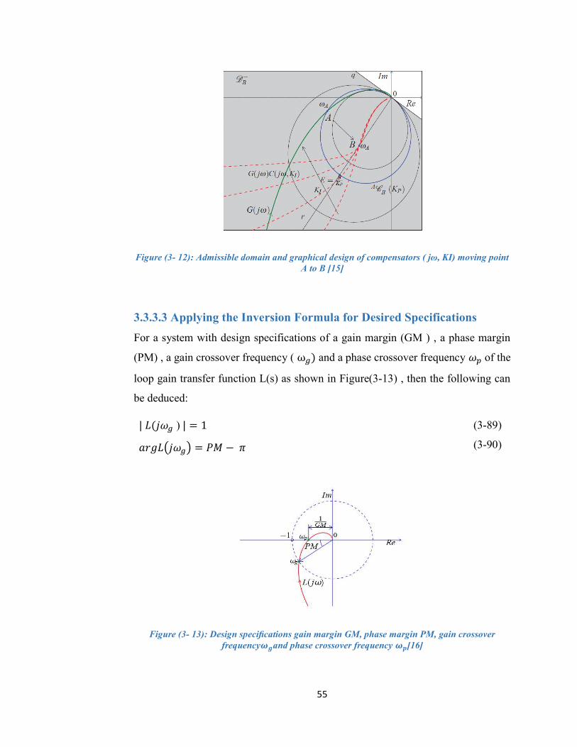
55

Figure (3- 12): Admissible domain and graphical design of compensators ( jω, KI) moving point

A to B [15] 3.3.3.3 Applying the Inversion Formula for Desired Specifications For a system with design specifications of a gain margin (GM ) , a phase margin (PM) , a gain crossover frequency ( ω ) and a phase crossover frequency of the loop gain transfer function L(s) as shown in Figure(3-13) , then the following can be deduced:

| ( ) | = 1 = −

(3-89) (3-90)

Figure (3- 13): Design specifications gain margin GM, phase margin PM, gain crossover

frequency and phase crossover frequency [16]

56

The loop gain frequency response can be written as: | ( )| = | ( )| ( ) ( ( ) ∅( )) (3-91)

As the loop gain is a product of the controller transfer function with the nominal plant transfer function, where ( ) = | ( )| ( ) ( ) = ( ) ∅( ) in the polar form. Via the Inversion Formulae, all the remaining parameters of the compensator can be found considering the case of Figure (3-13), using equations (3-89) to (3-91). This yields:

= 1/ ∅ = − −

(3-92) (3-93)

Where ≝ M( ) and ∅ ≝ ∅( ). 3.3.3.4 Features of the Inversion Formula The inversion formula is a very simple method that gives an explicit relationship between the specification requirements parameters and the gains of the PID controller. So by specifying the desired specification, the gains can be easily found using direct formulas. From Figure (3-14), it can be seen the constraints of and∅ .

Figure (3- 14): Graphical representation on the Nyquist plane of admissible values of and

∅ for PID, PD and PI compensators [16]

57

The inversion formula has some hypothesis or impositions such as: Imposition of the Ratio Td/Ti The ratio = / is an important parameter. When σ −1 ≥ 4, then the zeros of the PID controller are real, and they are complex conjugate when σ −1 < 4. There are certain formulas to estimate the controller’s gain. More details in [16] Imposition of GM In the case of unconstrained Ki is to fix the gain margin to a certain value GM. Now the parameters Kp, Ti, Td > 0 of the PID controller must be determined, however Ti > 0 and Td > 0 satisfy, if and only if: 0 < < π and < 1 (3-94) If (3.) is satisfied, then the values of Kp, Ti and Td can be given as:

= 1

= 1

= 1 −

(3-95) (3-96) (3-97)

In this thesis, the values of the controller’s gains are going to be based on certain impositions that would satisfy the standard performance specification for aerospace applications control systems, which are (a gain margin GM= 1.6327, a phase margin PM= 160° and a gain crossover frequency = 5). Substituting these values in equations from (3-92) to (3-97), then the classical controller’s values are going to be:

= 47°. 2708 = 0.6125 = 0.4156 = 4.6186 = 1.1998

(3-98)

58

As can be seen from the above, the inversion formulae gave an explicit relationship between the stability margins and the gains of the controller. Classical control has many good features as it has a good static performance as well as most of its design techniques are simple. In addition to that, it provides a good reliability and robustness for the system. However, it has short comings too such as its weak dynamic performance and sometimes its bad function on uncertain systems. Thus, these short comings motivate us to switch to robust control.

3.3.4 Robust Control Design Approach (Structured Robust Control)

3.3.4.1 Robust Control Problem Definition A robust system is a system that holds up the perturbations that might affect

the system's functional body under exceptional circumstances and it does not break or damage easily. Robust control is an approach to controller design that explicitly deals with uncertainty. Generally, robust control methods are designed to function properly provided that uncertain parameters or disturbances are found within some (typically compact) set. [8] Generally, robust control systems can be classified in terms of the structure of the robust system into two systems: Structured and non-structured robust control systems as illustrated in Figure (3-15).

Figure (3- 15): Robust Control Systems.

59

A robust control problem can be stated starting with a feedback system with additive uncertainty as illustrated in control system block diagram, Figure (3-16).

Figure (3- 16): Feedback system with Additive Uncertainty [10]

Where: r: is the reference input signal. e: is the error signal. K : is the controller. u: is the manipulated signal. w: is the additive weight. Δ: is an unknown, stable perturbation. d: is the disturbance signal. G : is the nominal plant model. G : is the perturbed plant. y: is the output signal. The frequency response for each block can be written according to [10] as:

60

( ) = ( ) + ( ) (3-99)

( ) = + (3-100)

W( ) = ( ) + ( ) (3-101) A transfer function from and can be given by:

= − 1 + = (3-102)

= , where S is sensitivity function.

For good tracking and disturbance rejection, the sensitivity function has to be minimized by shaping the loop function, = , steeply (high gain) in the low frequency band. In order to meet the design specifications a weighting function is used. For robust controller synthesis, the block diagram in Figure (3-16) can be rearranged into its corresponding standard form as shown in Figure (3-17)

Figure (3- 17): Standard closed loop system for controller synthesis [10]

. Where R= is the reference disturbance = [ r d ] , = and : is the shaped generalized plant model. The tunable block is gathered into single block , and the other parts of diagram are grouped into single block . Also, more details can be found in [10] A robust stabilization problem can be stated according to small gain theorem as: Given a perturbed plant ∆, and an unknown but stable transfer function ∆ , the

61

closed loop system is robustly stable if stabilizes the nominal plant and the following constraint holds:

∥ ∥ =∥ ∥ ≤ (3-103) Where γ is positive scalar and in this thesis equals to 1. Recalling the phase definition, the robust stability constraint in equation (3-103) can be written as:

∅ ≤ (3-104)

Where: ( ) = | ( ) ( ) ( )| = | ( ) ( )|

| ( ) ( ) | ∀ ω ϵ [0, ∞)is the magnitude of the closed loop system, a∅( ) = −∠ ( ) ( ) ( ), ∀ ω ϵ [0, ∞) and ϕ ϵ [0,2π] is the phase shift of the closed loop system. From equation (3-104), the intersection of all robust controllers forms an invariant set where all ∈ satisfy the constraint in equation (3-103). A characteristic polynomial of the perturbed closed loop system is given by:

( , , ) = 1 + ( ) ( ) − ( ) ( ) ∅ (3-105) Consequently, for each value of ϕ( ω) ϵ [0,2π] ∀ ω ϵ [0,∞) there are ( ω) ∀ ω ϵ [0,∞) on the boundary of equation (3-105). Also, at the same equation, the stability of the closed loop system depends on the locations of the roots of the characteristic equation. The system is Hurwitz stable if and only if all the roots of the characteristic polynomial (3-105) are located in the left-half of the s-plane. Substituting equations (3-99), (3-100), and (3-101) into equation (3-105) yields,

( , , ) = 1 + [ ( ) + ( )] +

− [ ( ) + ( )] + (cos + ) (3-106)

62

Thus the problem is switched to find the values of , that will make the closed loop poles of the system Hurwitz stable. Now, our target here is to compute the boundaries of the PI controller stability regions. ω ≠ 0 and ϕ ∈[0, 2π]. In this thesis only ϕ ∈ [0, π] is considered since ϕ [π, 2π] is mirror image. Therefore, the obtained controller gains, for example in PI plane can be given as:

( , , )= - ( ) [ ( ) ( ) ]( ) (3-107)

( , , ) = ( ) + 1 [ ( )sin + ( ) cos ]( )

(3-108)

Where:

( ) = | ( )| + | ( )| + ( ) + [ ( ) cos − ( ) sin ] + ( ) + [ ( )sin + ( ) cos ]

(3-109)

As mentioned previously that the nominal plant coveted to be controlled will be the short period approximate model since maintained as much as possible of the full order model’s behavior and specifications. The transfer function of pitch rate with time delay is given as:

( ) = 7.46 + 16.81 + 3.665 + 7.907 (3-110)

Where the mean value of the time delay lies in range of {0.05, 0.25}. Here, the time delay with a value equal to τ = 0.1 is chosen. The additive weight W represents the design specifications in the frequency domain. The determination of is an iterative process. Since there is no rule to be followed to select the desired weight, one can start with the exact integrator. Here, an approximate integrator is chosen, and its transfer function is written as follows:

63

( ) = + 1 (3-111) a and b parameters are designed by iterative simulation of the pitch rate response until the satisfactory shape is obtained. [10]

3.3.5 Controllers Evaluation The thesis has proposed the designs of two controllers following two different

control design techniques; a classical control approach and a robust control approach. The two controllers will be evaluated in terms of disturbance rejection, control effort and noise attenuation in order to assess their efficiency and performance. The block diagram in Figure (3-18) shows the simulation for the system used to perform the evaluation of the controllers and the results of the controllers evaluation are shown in Chapter Four.

Figure (3- 18): Control Evaluation block diagram in Simulink.

64

4 Chapter Four: Results and Discussion This chapter observes the results for the analysis of the hang glider’s motion. Also, comparisons between full and reduced order models are shown. In addition to a computation of the stability regions of the PID controller while following the robust control design technique. Moreover, a test for the small gain theory stratification is done. Finally, a control evaluation is performed in order to see which control approach (classical or robust) is more appropriate for the hang glider model.

4.1 Aerospace Performance Specifications The specifications of the control systems are generally related to transient

and frequency response such as overshoot, speed of response, phase margin and gain margin. Some specifications concerning the aerospace applications and have to be satisfied by the autopilot such as [17]: rise time 0.5 second, maximum peak overshoot percentage 5% and reject 50% of the disturbance within 1.5 second and 95% within 4 second. Toward these objectives; the classical and advanced controllers are to be designed and evaluated. Singular values of the open loop longitudinal uncompensated system are determined in order to appoint which one of the longitudinal channels may guarantee the desired performance and robustness of the system.

65

Figure (4- 1): Singular Values of uncompensated longitudinal plant.

Discussion It is clear from Figure (4-1) that the pitch rate state guarantees the performance and robustness requirements better than the other states since its singular value shape revealed that it has highest gain in the low frequency region and lowest gain in the high frequency region relative to the singular values shapes associated to the other states. Also the singular values for the uncompensated lateral plant are obtained as shown in figure (4-2).

66

Figure (4- 2): Singular Values of Uncompensated Lateral Plant.

Discussion Again but this time among the lateral plant, Figure (4-2) conspicuously shows that the roll rate state guarantees the performance and robustness requirements better than the other states since its singular value shape appears clearly to have highest gain in the low frequency region and lowest gain in the high frequency region relative to the singular values shapes associated to the other states. The motion of the hang glider model is analyzed and studied. A test for the model’s performance specifications in both time and frequency domains has been performed in order to check the model’s satisfaction for the standard aerospace performance specifications of the control systems.

67

4.1.1 System’s Specifications in Frequency Domain Stability Margins of Pitch Rate Channel The gain margin (GM), phase margin (PM), and the bandwidth of the uncompensated pitch rate channel loop are obtained from the bode plot, Figure (4-3), and placed in Table (4-1).

Table (4- 1): Stability margin parameters of uncompensated pitch rate channel. System Setting Stability Margin Parameters Uncompensated

Pitch Rate Channel Loop

Gain Margin (GM) in [dB]

Phase Margin (PM) in [deg]

Bandwidth [rad/s]

-16.5 - 41.1402 ∞

Figure (4- 3): Bode diagram of uncompensated pitch rate channel.

68

Discussion From table (4-1) and Figure (4-3), it is clear that the open-loop of the pitch channel system is not stable since its phase margin is negative. Thus, a decision is to be made about the compensation of the negative phase margin, then increase the stability of the closed loop system. Stability Margins of Roll Rate Channel

The gain margin (GM), phase margin (PM), and the bandwidth of the uncompensated pitch rate channel loop are obtained from the bode plot, Figure (4-4), and placed in Table (4-2).

Table (4- 2): Stability margin parameters of uncompensated roll rate channel.

System Setting Stability Margin Parameters Uncompensated

Roll Rate channel Loop

Gain Margin (GM) in [dB]

Phase Margin (PM) in [deg]

Bandwidth [rad/s]

∞ ∞ ∞

Figure (4- 4): Bode Diagram of Uncompensated Roll Rate Channel.

69

Discussion From table (4-2) and Figure (4-4), it is clear that the open-loop of the roll rate is posing a problem since the results of all the stability margins tend to turn to infinity. Thus, the lateral plant is unstable.

4.1.2 System’s Specifications in Time Domain The step response of the open loop pitch rate channel is shown in Figure (4-5). The pitch rate channel’s performance is also quantified and placed in Table (4-3).

Figure (4- 5): Step response of pitch rate channel.

70

Table (4- 3): System’s Specifications in Time Domain for pitch channel .

Discussion It can be seen from the step response in Figure (4-5) and table (4-3) that the system is unstable since the step is exhibiting a divergence oscillating behavior as well as the performance level shows that the level of performance is very bad, hence a treatment for the system’s performance is very necessary. Likewise, the step response of the open loop roll rate channel is illustrated in Figure (4-6). The roll rate channel’s performance is determined and filled in Table (4-4).

Figure (4- 6): Step response of roll rate

System Settings

Performance Level Rise Time

[s]

Peak Time

[s]

Settling Time

[s]

Overshoot %

Pitch Rate Channel

NAN ∞ NAN NAN

71

Table (4- 4): System’s Specifications in Time Domain for roll rate channel.

Discussion The step response of the roll rate channel in Figure (4-6) is kind of exhibiting a better response than the pitch rate channel. As it starts with a converging oscillation at the beginning and then remains constant. Also the quantified performance in table (4-4) shows that the system still needs to be rectified to reach the desired performance level and stability of the system.

4.2 Results of the Full and Reduced Models Comparisons Longitudinal Modes eigenvalues Short period eigenvalues λsh1,2 = −2.0083 ± 2.1861i (Full-order) λsh1,2 = −1.8324 ± 2.1329i (Reduced-order) Long period eigenvalues λph1,2 = 0.0894 ± 1.1535i (Full-order) λph 1,2 = -0.1730 (Reduced-order)

System Settings

Performance Level Rise Time

[s]

Peak Time

[s]

Settling Time

[s]

Overshoot %

Roll Rate Channel

0.0192 1.3191 13.4742 272.4301

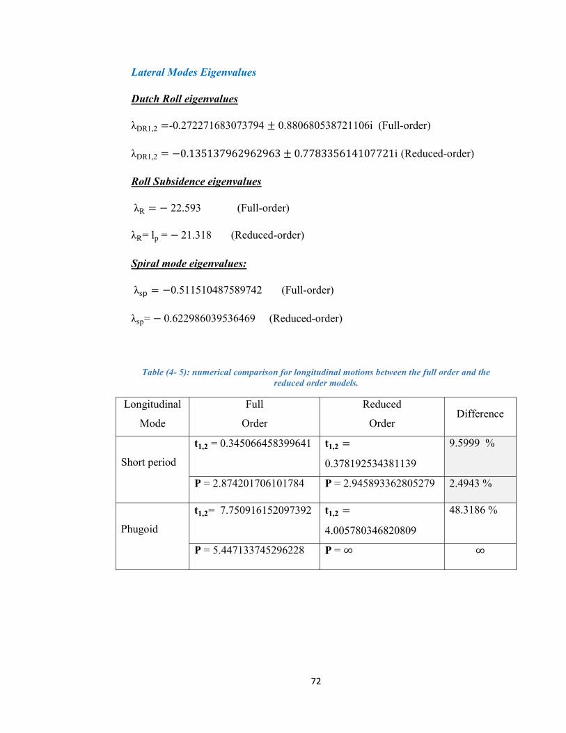
72

Lateral Modes Eigenvalues Dutch Roll eigenvalues λDR1,2 =-0.272271683073794 ± 0.880680538721106i (Full-order) λDR1,2 = −0.135137962962963 ± 0.778335614107721i (Reduced-order) Roll Subsidence eigenvalues λR = − 22.593 (Full-order) λR= lp = − 21.318 (Reduced-order) Spiral mode eigenvalues: λs = −0.511510487589742 (Full-order) λsp= − 0.622986039536469 (Reduced-order)

Table (4- 5): numerical comparison for longitudinal motions between the full order and the reduced order models.

Longitudinal Mode

Full Order

Reduced Order Difference

Short period

t1,2 = 0.345066458399641 t1,2 = 0.378192534381139

9.5999 %

P = 2.874201706101784 P = 2.945893362805279 2.4943 % Phugoid

t1,2= 7.750916152097392 t1,2 = 4.005780346820809

48.3186 %

P = 5.447133745296228 P = ∞ ∞

73

Table (4- 6): numerical comparison for lateral motions between the full order and the reduced order models.

Lateral Mode

Full-order Reduced-order Difference

Dutch Roll , = 2.545251831466350 , = 5.128092689912228 101.4768 % P = 7.134465939605992 P =8.072591300325618 13.1492 %

Spiral , = 1.354810931180402 , =1.112384477372277 NaN P = ∞ P = ∞ 17.8937 %

Roll Subsidence

, = 0.030673217368211 , = 0.032507739938080

NaN

P = ∞ P = ∞ 5.9809 %

Discussion From the Table (4-5) and Table (4-6), it can be clearly seen that the short-period approximation is closer to the original model than the phugoid approximation. So the short approximation can be considered as a good representative for the full model, where the lateral approximations is manifesting a significant difference from the original model.

4.2.1 Time history The time responses for the full order model and the reduced order model for

both short and long periods had are illustrated in Figure (4-7) and Figure (4-8) respectively to show how which of the two periods exactly is closer to the original glider’s model.

74

Figure (4- 7): The time responses for the full order model and the reduced order model for

Short period.

Figure (4- 8): The time responses for the full order model and the reduced order model for long

period.

75

4.2.2 Energy Distribution Furthermore, another way of graphical comparison can be executed using

Hankel norm approximation technique. Herman Hankel established a method to measure the energy distributed over the states of a system by determining Hankel’s singular values, those in which can give us a measure of how much energy is stored in each state.[8] The distributions of the energy for both longitudinal and lateral motions are drawn by the means of Hankel singular value for each state as illustrated in Figure (4-9) and Figure (4-10).

Figure (4- 9):Bars of Hankel singular values of longitudinal states

76

Figure (4- 10): Bars of Hankel singular values of lateral states

Discussion From Figure (4-10) and according to Hankel’s energy distribution method, the states which store low energy can be eliminated in order to reduce the model and those which store high energy are valid to represent the original model. Here the short states are carrying most of the longitudinal motion’s energy. The lateral is not going to be used since it showed a significant difference between approximate and full order model in the previous comparisons. Comparisons Summary The longitudinal approximations exhibited better similarity to the full model than the lateral approximations. In particular, the short period mode of the longitudinal approximate model seemed to the best representative for the full model behavior. So the short period is going to our new nominal plant that we want to control using both classical and robust controllers.

77

4.3 Computation of Stability Regions and Small Gain Theory Test

Figure (4-11) and (4-12) show the stable and non-stable regions of the PID controller. In this thesis, PD and PI planes are used in the robust control approach.

Figure (4- 11): Stability Regions of PID controller in PD plane, γ = 1.

78

Figure (4- 12): Stability Regions of PID controller in PI plane, γ = 1.

Discussion As can be clearly seen from Figure (4-11), that any point ( (ω,ϕ,γ), d(ω,ϕ,γ)) ,also from Figure (4-12), any point ( (ω,ϕ,γ), i(ω,ϕ,γ)) is sensitive to variations in frequency and phase. Also, in the PD planes Ki remain fixed with a value of 0. 9995. On the other hand, in the PI plane, Kd remains fixed with a value of 0.1. For both figures, it can be manifested that as he frequency ω increases, the point

( (ω,ϕ,γ), (ω,ϕ,γ)) in PI plane or the point ( (ω,ϕ,γ), i(ω,ϕ,γ)) in the PI plane moves in a particular direction along the stability boundary that starts at ω = 0 and ω = ω respectively. Furthermore, because of the uncertainty effect on the system dynamics: the phase shift is changed from ϕ = 0 up to ϕ = π , as a result the stability boundaries are also changed corresponding to it, i.e. the region of stability decreases when phase shift increases and vice versa. The red bounding curve in both PI and PD planes refers to the set of nominal controllers. Finally, the yellow shaded area is the robust stability region, where for any controller located among this invariant set,

79

all its gains will absolutely be insensitive to the uncertainty that affected the system phase shift.

4.4 Satisfying of Small Gain Theorem A test has been made for two controllers located among the PD plane, Figure (4-11) and also two controllers in the PI plane, Figure (4-12). As can be seen that the blue star in both figures is located inside the robust stability region this is going to be referred as the point of robust controller, while the red star is located outside the robust region and it’s going to be referred as nominal controller. The two points are going to be tested to check if they satisfy the small gain theorem to assess the results obtained. A theory satisfying test is performed in both PD and the PI planes for the robust and the nominal controllers and illustrated in Figures (4-13) and (4-14) respectively.

Figure (4- 13): Small Gain Theory Satisfying Test in PD plane.

80

Figure (4- 14): Small Gain Theory Satisfying Test in PI plane.

Discussion A summary for the satisfactory of the robust and the nominal controllers for the small gain theory can be made, as can be seen from Figures (4-13) and (4-14) that the robust controller magnitude hasn’t exceeded 1, hence it means it passed the test and by that it satisfies the small gain theory. On the other hand, it can be clearly seen that the nominal controller has exceed the magnitude of 1, hence it failed in the test and of course this for both planes. In simple words, stability is ensured for any point among the robust region, but it’s not always guaranteed outside it. There are no warranties. Table (4-7) shows the gains values of the robust controller in PD and PI planes. The points were estimated from Figures (4-11) and (4-12).

Table (4- 7): Robust controller gains in PI and PD planes.

Plane Robust Controller Note - 1.237 6.908 0.1 is fixed - 1.1872 0.99995 0.05 is fixed

81

4.5 Classical Controller Evaluation

4.5.1 Disturbance Rejection Recalling back to Figure (3-18), a step disturbance is injected to the system and the response of the pitch rate channel due to this step disturbance while utilizing a classical controller was plotted in Figure (4-15). Also the time taken to reject 50% and 95% of the disturbance is placed in table (4-8).

Figure (4- 15): Disturbance Rejection in pitch Rate channel for a classical controller.

Table (4- 8):Time taken to reject 50% and 95% of the disturbance for classical controller.

Disturbance Rejection (%) Time (sec) 50 % 0.65765 95% 0.8543

82

Discussion Figure (4-15) reveals the pitch rate response to a step disturbance in rad/s in the y axis, where 0.01 rad/s is equivalent to 1% and time in seconds in the x axis. As the pitch rate response starts from zero and remains constant for a very short while until 0.5 second. At the same instant, a step disturbance hits the channel leading the pitch rate response to rise up rapidly forming a vertical line to reach 100%, then it falls down rapidly reaching a point where 50% of the disturbance is being rejected in about 0.65 second and after 0.2 second, the disturbance is rejected by 95%. Again, returning to zero amplitude being rejected by 100%, the disturbance keeps dropping below zero until 1.2 second. Then, climbing a little bit above zero reaching 10% in 2 seconds. Again, falling a bit below zero till 3 seconds time. Finally, remaining constant at zero being fully rejected and indicating that the classical controller had successfully rejected the step disturbance.

4.5.2 Noise Attenuation A reference command with a Gaussian – Markov white noise of the following specifications: (a time constant of 0.1, a seed of 23341, a variance of 1 and a sample time of 0.01) both are being injected to the system of the (classical controller and the short period reduced model). The response of the pitch rate channel is shown in Figure (4-16).

83

Figure (4- 16): Noise Attenuation in Pitch Rate Channel by Classical Controller.

Discussion As can be clearly seen from Figure (4-16), the y axis represents the pitch rate channel response to the reference command with white noise in (rad/s) and the x axis represents the time in seconds. As the pitch rate response - denoted by red line- starts from zero remaining constant and sticking to the tracking reference – denoted by blue line- until 1 second time. Directly after that, it goes up rapidly and smoothly with no ripples reaching a maximum of 1.35 rad/s corresponding to 1.5 second, falling again below 1 rad/s corresponding to 2.5 second. After that, climbing up a little bit above 1 rad/s and dropping again to it corresponding to 4 seconds, remaining at the same value oscillating about 1 rad/s with small ripples for the whole left period of time. The classical controller designed using the inversion formula was capable of attenuating the Gauss – Markov white noise as the response

84

embodied the shape of the reference command with very small ripples. However, it wasn’t able to reduce the overshoot in general.

4.5.3 Control Effort A reference is applied to the system and the response plotted in Figure (4-17) is the output from the classical PID controller.

Figure (4- 17): Control effort of Classical Controller

Discussion As shown from Figure (4-17), the x axis is the time in seconds and the y axis is the effort exerted by the classical controller as a respond to the pilot’s command. Here, the response starts from zero and remains at the same value until a time of 1 second. Once a reference command is applied to the system by the pilot, the controller tries to control this input and this produces a sharp rise in the control effort forming a straight vertical line reaching a maximum of 1200 (output scale unit). Then, the control effort drops quickly at the same instant to zero and remaining there for the rest of the period as the command is already finished and controlled. The value of 1200 is unreasonable. But generally, it’s preferable that for a reference command, the effort being exerted by the controller should be very low because a high effort requires a large power consumption, hence a larger weight, size and memory storage

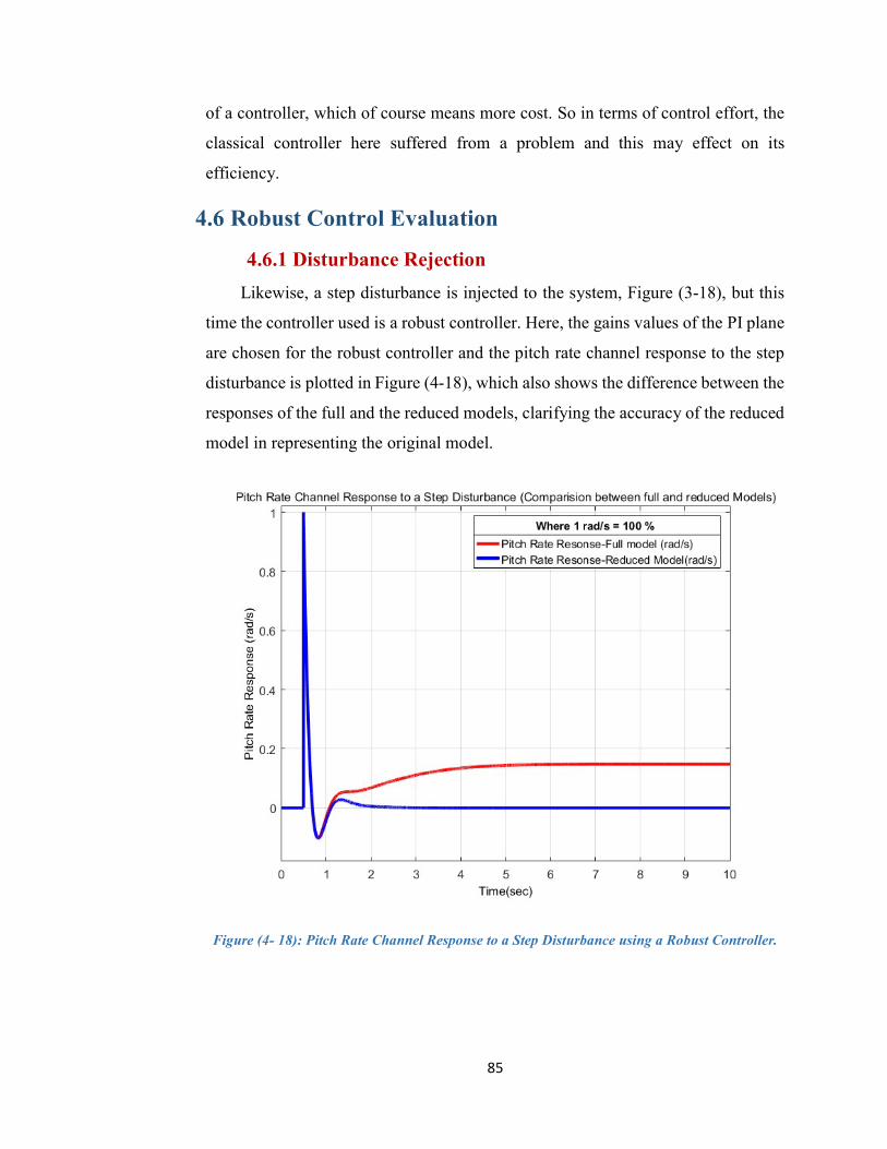
85

of a controller, which of course means more cost. So in terms of control effort, the classical controller here suffered from a problem and this may effect on its efficiency.

4.6 Robust Control Evaluation 4.6.1 Disturbance Rejection

Likewise, a step disturbance is injected to the system, Figure (3-18), but this time the controller used is a robust controller. Here, the gains values of the PI plane are chosen for the robust controller and the pitch rate channel response to the step disturbance is plotted in Figure (4-18), which also shows the difference between the responses of the full and the reduced models, clarifying the accuracy of the reduced model in representing the original model.

Figure (4- 18): Pitch Rate Channel Response to a Step Disturbance using a Robust Controller.

86

Discussion As Figure (4-18) manifests the pitch rate channel response to a step disturbance in the presence of a robust controller. The x axis shows the time in seconds, while the y axis shows the pitch rate response to a step disturbance in (rad/s). Where 0.01 rad/s is equivalent to 1%. It can be clearly seen that from time 0 to 1 second, both full and reduced order models responses are exhibiting the same behavior. As they start from a zero amplitude response remaining at the same value until 0.5 second. At the same moment, a step disturbance hits the system suddenly causing the pitch rate responses for full and reduced models to rise up rapidly forming a vertical line reaching a maximum of (100 % = 1 rad/s). Again at the same moment, the pitch rate responses decline rapidly from 1 rad/s to 0 rad/s crossing a point where the step disturbance is rejected by 50% corresponding to 0.56 second. As the responses continue to fall reaching a point where 95% of the disturbance is being rejected at 0.67 second. The responses keep dropping reaching zero amplitude and decline bellow it for a second, then climbing up again to 5 % corresponding to 1.35 second. Among all this time, full and reduced model responses are identical. However, after 1.35 second the disturbance is fully rejected as the pitch rate response of the reduced model remains at zero level until the end of the period. On the other hand, the pitch rate response of the full model climbs up to reach 10% or 0.1 rad/s and then remains somehow flat at the same level until the end of the period. The figure summarizes two points; the first point is: the robust controller has successfully rejected the disturbance, while the second point is: the full and reduced order models somehow have similar behaviors, with a small difference generated from the reduction in the accuracy of the reduced model as a result of neglecting some terms. In spite of that, the reduced order model was capable of representing the full order model. Table (4-9) shows the time taken to reject 50% and 95$ of the disturbance while using a robust controller.

Table (4- 9): Robust controller’s disturbance Rejection. Disturbance Rejection (%) Time(sec)

50% 0.5668 95% 0.6767

87

4.6.2 Noise Attenuation Again referring back to Figure (3-18), a reference command with a Gauss –Markov white noise are injected to the system, but this time while utilizing a robust controller instead of classical. Figure (4-19) shows the pitch rate channel response to the reference and the white noise.

Figure (4- 19): Noise Attenuation in Pitch Rate Channel by Robust Controller

Discussion From Figure (4-19), the y axis represents the pitch rate channel response to the reference command with white noise in (rad/s), while the x axis represents the time in seconds. This time the controller used is robust. As can be clearly seen from Figure (4-19), the pitch rate response - denoted by purple line - starts from zero with small ripples remaining constant and sticking to the tracking reference – denoted by blue dashed line- until 1 second time. Directly after that, both pitch response and the tracking reference climb up rapidly and smoothly with no ripples. Where the pitch rate reaches a maximum of 1.1 rad/s corresponding to 1.25 second and the tracking

88

reference reaches a maximum of 1.35 corresponding to 1.5 second. After 1.5 second both keep oscillating about 1 rad/s. However, the tracking reference has a larger amplitude with larger oscillations, soon remaining constant at 1 rad/s corresponding to 4.5 seconds and until the end of the whole period. Where the pitch rate response is somehow constant going a little bit (up and down) about 1 rad/s since 1.5 second with small ripples as they get smaller with time. The pitch response keeps acting with the same behavior until the end of the period. The robust controller was not just capable of attenuating the Gauss – Markov white noise injected to the system, but it was also capable of reducing the overshoot. Moreover, it had a faster response than the tracking reference. All these advantages reveals that the robust controller is exhibiting better performance and efficiency.

4.6.3 Control Effort Same process is performed as in classical control effort evaluation, but this time for robust controller. Figure (4-20) reveals the control being exerted by the controller in respond to the pilot’s command.

Figure (4- 20): Control effort of Robust Controller

89

Discussion As can be shown from Figure (4-20), the robust controller is manifesting a better performance than the classical controller in terms of the effort exerted by the controller because at the time of 1 second in the x axis, the effort of the controller sharply forms a vertical line rising up reaching a maximum value of 51(output scale unit) in the y axis. On the other hand, as have been shown previously that the classical controller’s effort was 1200(output scale unit). So, there is a significant difference between them and this means that the robust controller gives more reasonable effort, hence less power consumption, less weight, less size and of course a cheaper cost. Comparison Another comparison is done between the classical and robust controllers in terms of disturbance rejection and noise attenuation.

Figure (4- 21): Comparison between Robust and Classical Controller according to Disturbance

rejection.

90

Figure (4-21) manifests clearly a comparison between the two (classical and Robust) controllers in terms of disturbance rejection. As it can be witnessed that the robust controller- denoted by red line - is faster in rejecting the step disturbance and even with less oscillations than the classical controller – denoted by blue dashed line-, hence the robust controller is exhibiting a better dynamic response than the classical controller. Also, this can even be much clearer numerically from Tables (4-8) and (4-9).

Figure (4- 22): Comparison between Robust and Classical Controller according to Noise

Attenuation.

Also Figure (4-22) shows a comparison between the classical and the robust controllers, which again indicates that the robust is much better in terms of noise attenuation too. Summary The controllers evaluations has been performed in terms of disturbance rejection, noise attenuation and control effort. Generally, both classical and robust

91

controllers guaranteed the stability of the system with a good level of performance and both were capable of meeting the standard performance specifications of the aerospace applications for control systems. The implementation of the inversion formula as a classical control approach as well as the utilization of the robust control approach as a modern control technique were both successful and gave fine results. In conclusion, robust controller revealed better performance compared to classical controller, this stands to reason that when dealing with uncertain systems such as the hang glider system - that is drastically exposed to different types of disturbances -, robust control will always be better than classical control as it deals explicitly with the variation in uncertainty.

92

5 Chapter Five: Conclusion and Future Work By the end of this project, a lot of skills have been earned and important knowledge acquired. The harmonic clasping between automatic control theory, aviation and programming opened the chance to explore new worlds and embody theories into real life applications.

5.1 Conclusion In short, the thesis was an attempt to solve the problem of the drastic disturbances and uncertainties affecting the hang glider system by proposing a design of a controller that would guarantee the stability of the system with certain level of performance. Classical control design technique (inversion formula) and robust control design technique had been proposed to meet the “standard aerospace performance specifications for control systems”. Generally, the hang glider model motion was analyzed and studied as it suffered from lots of instability problem discussed in chapter four. In this aspect, the longitudinal channel was reduced to short period and the pitch rate channel had been stabilized. However, the lateral channel hasn’t been stabilized yet, but a further work to solve it is stated below. All the objectives had been met successfully, the standard aerospace performance specifications have been well satisfied as well as the controllers evaluations exhibited better stability and performance by the robust controller than the classical controller which ensure the appropriateness of the robust technique for such application in rejecting the disturbances and overcoming measurement noise.

5.2 Future Work Here are some suggestions for a further work to be done:

1. The research was an attempt to solve the problem of the drastic disturbances that affect the hang glider by designing a robust controller that guaranteed the stability of the system with some level of performance (nominal performance). It’s well-known that there is a conflict between the stability and the performance of the controller which is usually solved by a trade-off

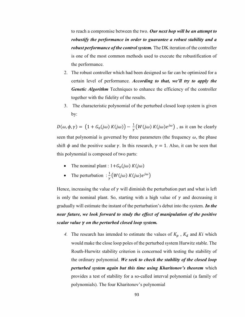
93

to reach a compromise between the two. Our next hop will be an attempt to robustify the performance in order to guarantee a robust stability and a robust performance of the control system. The DK iteration of the controller is one of the most common methods used to execute the robustification of the performance.

2. The robust controller which had been designed so far can be optimized for a certain level of performance. According to that, we’ll try to apply the Genetic Algorithm Techniques to enhance the efficiency of the controller together with the fidelity of the results.

3. The characteristic polynomial of the perturbed closed loop system is given by:

( , , ) = 1 + ( ) ( ) − ( ) ( ) , as it can be clearly seen that polynomial is governed by three parameters (the frequency , the phase shift and the positive scalar . In this research, = 1. Also, it can be seen that this polynomial is composed of two parts:

The nominal plant : 1+ ( ) ( ) The perturbation : ( ) ( )

Hence, increasing the value of will diminish the perturbation part and what is left is only the nominal plant. So, starting with a high value of and decreasing it gradually will estimate the instant of the perturbation’s debut into the system. In the near future, we look forward to study the effect of manipulation of the positive scalar value on the perturbed closed loop system.

4. The research has intended to estimate the values of , and which would make the close loop poles of the perturbed system Hurwitz stable. The Routh-Hurwitz stability criterion is concerned with testing the stability of the ordinary polynomial. We seek to check the stability of the closed loop perturbed system again but this time using Kharitonov’s theorem which provides a test of stability for a so-called interval polynomial (a family of polynomials). The four Kharitonov’s polynomial

94

5. In our pursuit of developing the autonomous soaring, we intend to study the exploiting of the updrafts (thermals) by the glider during soaring mode and to establish a general thermal model in an attempt to extend the glider’s range together with the endurance.

6. The lateral channel of the hang glider suffered from significant stability problems, a Multi-DOF controller is suggested to be applied on the lateral channel as such controller provides better stability and performance and would solve the channel’s problem.

95

References [1] History of Aviation Aircrafts through time. Available: http://www.e-

aircraftsupply.com/history-of-aviation-aircrafts-through-time/ [2] F. A. Administration, Glider Flying Handbook. 2003. [3] N. A. a. S. A. (NASA). Gliders. Available:

https://www.grc.nasa.gov/www/k-12/airplane/glider.html [4] How Gliders Fly, And How They're Different Than Powered Aircraft.

Available: http://www.boldmethod.com/blog/article/2015/02/your-guide-to-glider-flying/

[5] Z. Li and E. A. Mehiel, "Modeling and Simulation of Autonomous Thermal Soaring with Horizon Simulation Framework," in AIAA Modeling and Simulation Technologies Conference, 2014, p. 1341.

[6] T. M. Foster and W. J. Bowman, "Dynamic stability and handling qualities of small unmanned-aerial-vehicles," Brigham Young University. Department of Mechanical Engineering, 2005.

[7] M. V. Cook, Flight dynamics principles: a linear systems approach to aircraft stability and control. Butterworth-Heinemann, 2012.

[8] C. E. E. G. H. Gubara, "Robust UAV Flight Control Systems ", Cairo 2008.

[9] L. Ntogramatzidis, R. Zanasi, and S. Cuoghi, "A unified analytical design method of standard controllers using inversion formulae," arXiv preprint arXiv:1210.3812, 2012.

[10] E. G. Hamdi, G. M. S. EL-Bayoumi, and A. H. Kasem, "Structured Robust Control for Small UAV," INCAS Bulletin, vol. 7, no. 2, p. 81, 2015.

[11] R. C. Nelson, Flight stability and automatic control. WCB/McGraw Hill New York, 1998.

[12] E. A. Ca, "Volume II Flying Qualities Phase," 1988. [13] Difference between Kinematics and Dynamics. Available:

http://www.differencebetween.info/difference-between-kinematics-and-dynamics

[14] Model Order Reduction. Available: https://en.wikipedia.org/wiki/Model_order_reduction

[15] R. Zanasi and S. Cuoghi, "Direct methods for the synthesis of PID compensators: analytical and graphical design," in IECON 2011-37th Annual Conference on IEEE Industrial Electronics Society, 2011, pp. 552-557: IEEE.

96

[16] L. Ntogramatzidis, R. Zanasi, and S. Cuoghi, "A unified analytical design method of standard controllers using inversion formulae," arXiv preprint arXiv:1210.3812, 2012.

[17] A. G. E.-M. a. I. M. E.-A. G.A.Elsheikh, "Performance Enhancement of Longe Range Missile Using Robust Control Design."

[18] M. V. C. a. M. Spottiswoode, "Modelling the flight dynamics of the hang glider," The Aeronautical Journal, 2006.

[19] Hiway Hang Gliders. Available: http://www.british-hang-gliding-history.com/manufacturers/hiway/demon.html

97

Appendices Appendix A

Figure(A- 1): Hiway Demon Hang glider [19]

98

Table(A- 1):Hiway Demon Configuration [18]

Total mass m 111 kg Wing span 10 m Wing area 16⋅26

chord length 1.626 m Hang strap length 1.2 m

Pilot mass 80 kg Wing mass 31 kg

Reference chord length 1.626 m LE of c ′ from nose 1.26 m

apposition on c ′ 0.215 Hang point position on c ′ 0.246

Control frame attachment on c ′ 0.185 Pilot drag coefficient 0⋅009

Table(A- 2):Equivalent longitudinal dimensionless stability derivatives referred to wind axes[18]

Table(A- 3):Equivalent lateral dimensionless stability derivatives. Referred to wind axes [18]

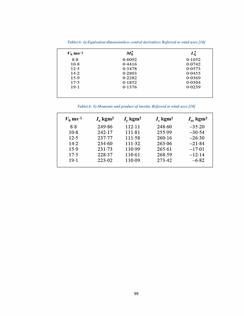
99

Table(A- 4):Equivalent dimensionless control derivatives Referred to wind axes [18]

Table(A- 5):Moments and product of inertia. Referred to wind axes [18]

100

Appendix B (MATLAB CODES) Longitudinal full Order Model and Reduced order model code clc clear all close all g=9.81; m=111;uo=10.8;costhe=0.0089;sinthe=-0.0012; Xu=-0.1730; Xw=0.6538; Xq=0.0881; Zu=-1.4208; Zw=-2.2535; Zq=-0.063; Mu=0.2685; Mw=-0.4402; Mq=-1.4113;Mde=7.46; We=-0.0507; %-----------------------------nominal model------------------- a=[ Xu Xw (Xq-We) -m*g*costhe; Zu Zw (uo+Zq) -m*g*sinthe; Mu Mw Mq 0;0 0 1 0] b=[0;0;Mde;0] cq=[0 0 1 0]%pitch rate vector cu=[1 0 0 0];%axial velocity vector cw=[0 1 0 0];%side velocity vector cth=[0 0 0 1];%pitch angle vector d=0; [num,den]=ss2tf(a,b,cth,d) printsys(num,den) r= roots(den) for n=1:length(r) if real(r(n))<0.0 disp('airplane is stable') else disp('airplane is not stable') end end %-----------------Short mode and phugoid mode----------------------------- imagr1=imag(r(1)) imagr2=imag(r(2)) imagr3=imag(r(3)) imagr4=imag(r(4)) for m=1:4 if imagr1>imagr3 disp('short period mode roots are') rs1=r(m) rs2=r(m) nsh=real(r(m)) wsh=imag(r(m)) perd_sh=(2*pi)/wsh t_hf_sh=0.693/abs(nsh) cy_sh=0.11*(abs(wsh)/abs(nsh)) end if imagr3<imagr1 disp('phugoid mode roots are') rp1=r(m) rp2=r(m)

101

nph=real(r(m)) wph=imag(r(m)) perd_ph=(2*pi)/wph t_hf_ph=0.693/abs(nph) cy_ph=0.11*(abs(wph)/abs(nph)) end end %--------- Ash=[-2.2535 10.7370; -0.4402 -1.4113] Bsh=[0;7.4600] Csh=[0 1]; d=0 lam_sh=eig(Ash) Aph=[-.1730 -9.6913; 0 0] Bph=[0;0] Cs=[0 1] lam_ph= eig(Aph) [V,D]=eig(Ash) [F,R]=eig(a) bb=[0 0 0 0 ]'; cc=[0 0 0 0]; bs=[0 0 ]' cs=[0 0 ]; d=0; t=0:0.01:2.5; X1=real(V(1:2,1)) X2=real(F(1:4,1)) [y1,x1]=initial(Ash,bs,cs,d,X1,t); ws=[1 0]*x1'; qs=[0 1 ]*x1'; [y2,x2]=initial(a,bb,cc,d,X2,t); u=[1 0 0 0]*x2'; w=[0 1 0 0]*x2'; q=[0 0 1 0]*x2'; th=[0 0 0 1]*x2'; figure(1) plot(t,w,'r .-',t,q,'g .-',t,ws,'b -',t,qs,'m -') grid on; title('Short period full and approximate ');ylabel('Amplitute');xlabel('Time (s)') legend('side veolcity full model(m/s)','pitch rate full model (rad/s)','side veolcity aprox(m/s)','pitch rate aprox (rad/s)') [G,M]=eig(Ash) X3=real(G(1:2,1)) [y3,x3]=initial(Aph,bs,cs,d,X3,t); up=[1 0]*x3'; thp=[0 1 ]*x3'; figure(2) plot(t,u,'r .-',t,th,'g .-',t,up,'b -',t,thp,'m -') grid on; title('phugoid full and approximate ');ylabel('Amplitute');xlabel('Time (s)') legend('axial veolcity full model(m/s)','pitch angle full model (rad/s)','axial veolcity aprox(m/s)','pitch angle aprox (rad/s)')

102

Inversion Formula Code clc clear all s=tf('s'); G=(7.46*s + 16.8111 )/( s^2 + 3.6648* s + 7.9068);%short period Tf wg=5; C=evalfr(G,j*wg); Mg= 1/abs(C) Gm=1/Mg % For certain Mg PM=160*(pi/180);% For Certain PM phi=PM-(pi+angle(C))% Phi among range (-pi/2,pi/2) %% Mg impositions Ti=Mg*sin(phi)/wg; Td=(1-Mg*cos(phi))/(wg*Mg*sin(phi)) alpha=(Mg*cos(phi)-1)/(Mg*(Mg-cos(phi))); sig=Ti/Td; sig2 =1/sig % Ti/Td imposition satisfied > 4 Kp=Mg*cos(phi) Ki=Kp/Ti Kd=Ki*Td pid_eq=Kp*(1+(1/Ti*s)+Td*s) %% Short period jacobean matrix Ash=[-2.2535 10.7370; -0.4402 -1.4113]; Bsh=[0;7.4600]; Csh=[0 1]; d=0;