Robust Functional Principal Components: a projection-pursuit

approach ∗

Lucas BaliDepartamento de Matematicas and Instituto de Calculo, FCEyN, Universidad de Buenos Aires and CONICET

Graciela BoenteDepartamento de Matematicas and Instituto de Calculo, FCEyN, Universidad de Buenos Aires and CONICET

David E. TylerDepartment of Statistics, Rutgers University

Jane–Ling WangDepartment of Statistics,University of California at Davis

June 19, 2011

Abstract

In many situations, data are recorded over a period of time and may be regarded as real-izations of a stochastic process. In this paper, robust estimators for the principal componentsare considered by adapting the projection pursuit approach to the functional data setting. Ourapproach combines robust projection–pursuit with different smoothing methods. Consistency ofthe estimators are shown under mild assumptions. The performance of the classical and robustprocedures are compared in a simulation study under different contamination schemes.

Key Words: Fisher–consistency, Functional Data, Principal Components, Outliers, RobustEstimation

AMS Subject Classification: MSC 62G35 MSC 62G20

∗This research was partially supported by Grants X018 from Universidad of Buenos Aires, pid 112-200801-00216from conicet and pict 821 from anpcyt, Argentina (L. Bali and G. Boente), NSF grant DMS-0906773 (D. E.Tyler), and NSF Grant DMS-0906813 (J-L. Wang).

1

1 Introduction

Analogous to classical principal components analysis (PCA), the projection-pursuit approach torobust PCA is based on finding projections of the data which have maximal dispersion. Instead ofusing the variance as a measure of dispersion, a robust scale estimator sn is used for the maximiza-tion problem. This approach was introduced by Li and Chen (1985), who proposed estimators basedon maximizing (or minimizing) a robust scale. In this way, the first robust principal componentvector is defined as

a = argmaxa:∥a∥=1

sn(atx1, · · · ,atxn),

and the subsequent principal component vectors are obtained by imposing orthogonality conditions.In the multivariate setting, Li and Chen (1985) argue that the breakdown point for this projection-pursuit based procedure is the same as that of the scale estimator sn. Later on, Croux and Ruiz–Gazen (2005) derived the influence functions of the resulting principal components, while theirasymptotic distribution was studied in Cui et al. (2003). A maximization algorithm for obtaininga was proposed in Croux and Ruiz–Gazen (1996).

The aim of this paper is to adapt the projection pursuit approach to the functional data setting.We focus on functional data that are recorded over a period of time and regarded as realizationsof a stochastic process, often assumed to be in the L2 space on a real interval. Various choices ofrobust scales, including the median of the absolute deviation about the median (mad) and some ofits variants which are discussed in Rousseeuw and Croux (1993), will be explored and compared.

Principal components analysis, which was originally developed for multivariate data, has beensuccessfully extended to accommodate functional data, and is usually referred to as functional PCA.It can be described as follows. Let X(t) : t ∈ I be a stochastic process defined in (Ω,A, P ) withcontinuous trajectories and finite second moment, where I ⊂ R is a finite interval. Without lossof generality, we may assume that I = [0, 1]. We will denote the covariance function by γX(t, s) =cov (X(t), X(s)), and the corresponding covariance operator by ΓX . We then have γX(t, s) =∑∞

j=1 λjϕj(t)ϕj(s), where ϕj : j ≥ 1 and λj : j ≥ 1 are respectively the eigenfunctions and

the eigenvalues of the covariance operator ΓX with λj ≥ λj+1. Moreover,∑∞

j=1 λ2j = ∥ΓX∥2F =∫ 1

0

∫ 10 γ2X(t, s)dtds < ∞. Let Y =

∫ 10 α(t)X(t)dt = ⟨α,X⟩ be a linear combination of the process

X(s), so that var(Y ) = ⟨α,ΓXα⟩. The first principal component is defined as the random variableY1 = ⟨α1, X⟩ such that

var(Y1) = supα:∥α∥=1

var (⟨α,X⟩) = supα:∥α∥=1

⟨α,ΓXα⟩, (1)

where ∥α∥2 = ⟨α, α⟩. Therefore, if λ1 > λ2, the solution of (1) is related to the eigenfunctionassociated with the largest eigenvalue of the operator ΓX , i.e., α1 = ϕ1 and var(Y0) = λ1 . Dauxoiset al. (1982) derived the asymptotic properties of the principal components of functional data, whichare defined as the eigenfunctions of the sample covariance operator. Rice and Silverman (1991)proposed to smooth the principal components by a roughness penalization method and suggested aleave-one-subject-out cross validation method to select the smoothing parameter. Silverman (1996)and Ramsay and Silverman (2005) introduced smooth principal components for functional data,also based on roughness penalty methods, while Boente and Fraiman (2000) considered a kernel–based approach. More recent work on estimation of the principal components and the covariancefunction includes Gervini (2006), Hall and Hosseini-Nasab (2006), Hall et al. (2006) and Yao andLee (2006).

The literature on robust principal components in the functional data setting is rather sparse.To our knowledge, the first attempt to provide estimators of the principal components that areless sensitive to anomalous observations was due to Locantore et al. (1999), who considered thecoefficients of a basis expansion. Their approach, however, is multivariate in nature. Gervini (2008)

2

studied a fully functional approach to robust estimation of the principal components by consideringa functional version of the spherical principal components defined in Locantore et al. (1999) butassuming a finite and known number of principal components in order to ensure Fisher–consistency.Hyndman and Ullah (2007) proposed a method combining a robust projection–pursuit approachand a smoothing and weighting step to forecast age–specific mortality and fertility rates observedover time. However, they did not study its properties in detail.

In this paper, we introduce several robust estimators of the principal components in the func-tional data setting and establish their strong consistency. Our approach uses a robust projection–pursuit combined with various smoothing methods and our results hold even if the number ofprincipal components is not finite. In this sense, it provides the first rigorous attempt to tackle thechallenging properties of robust functional PCA.

In Section 2, the robust estimators of the principal components, based on both the raw andsmoothed approaches, are introduced. Consistency results and the asymptotic robustness of theprocedure are given in Section 3, while the selection of the smoothing parameters for the smoothprincipal components is discussed in Section 4. The results of a Monte Carlo study are reported inSection 5. Section 6 contains some concluding remarks and appendix A provides conditions underwhich one of the crucial assumptions hold. Most proofs are relegated to Appendix B.

2 The estimators

We consider several robust approaches in this section and define them on a separable Hilbert spaceH keeping in mind that the main application will be H = L2(I). From now on and throughoutthe paper, Xi : 1 ≤ i ≤ n denote realizations of the stochastic process X ∼ P in a separableHilbert space H. Thus, Xi ∼ P are independent stochastic processes that follow the same law.This independence condition could be relaxed since we only need the strong law of large numbersto hold in order to guarantee that the results established in this paper hold.

2.1 Raw robust projection–pursuit approach

Based on the property (1) of the first principal component and given σr(F ) a robust scale functional,the raw (meaning unsmoothed) robust functional principal component directions are defined as

ϕr,1(P ) = argmax∥α∥=1

σr (P [α])

ϕr,m(P ) = argmax∥α∥=1,α∈Bm

σr (P [α]) , 2 ≤ m ,(2)

where P [α] stands for the distribution of ⟨α,X⟩ when X ∼ P , and Bm = α ∈ H : ⟨α, ϕr,j(P )⟩ =0, 1 ≤ j ≤ m− 1. We will denote the mth largest eigenvalues by

λr,m(P ) = σ2r(P [ϕr,m]) = max

∥α∥=1,α∈Bm

σ2r (P [α]) . (3)

Since the unit ball is weakly compact, the maximum above is attained if the scale functional σr is(weakly) continuous.

Next, denote by s2n : H → R the function s2n(α) = σ2r (Pn[α]), where σr(Pn[α]) stand for

the functional σr computed at the empirical distribution of ⟨α,X1⟩, . . . , ⟨α,Xn⟩. Analogously,σ : H → R will stand for σ(α) = σr(P [α]). The components in (2) will be estimated empirically by

ϕ1 = argmax∥α∥=1

sn(α)

ϕm = argmaxα∈Bm

sn(α) 2 ≤ m,(4)

3

where Bm = α ∈ H : ∥α∥ = 1, ⟨α, ϕj⟩ = 0 , ∀ 1 ≤ j ≤ m− 1. The estimators of the eigenvaluesare then computed as

λm = s2n(ϕm) , 1 ≤ m . (5)

2.2 Smoothed robust principal components

Sometimes instead of raw functional principal components, smoothed ones are of interest. Theadvantages of smoothed functional PCA are well documented, see for instance, Rice and Silverman(1991) and Ramsay and Silverman (2005). One compelling argument is that smoothing is a regular-ization tool that might reveal more interpretable and interesting feature of the modes of variationfor functional data. Rice and Silverman (1991) and Silverman (1996) proposed two smoothing ap-proaches by penalizing the variance and the norm, respectively. To be more specific, Rice and Silver-man (1991) estimate the first principal component by maximizing over ∥α∥ = 1, the objective func-tion var (⟨α,X⟩)− τ⌈α, α⌉, where var stands for the sample variance and ⌈α, β⌉ =

∫ 10 α′′(t)β′′(t)dt.

Silverman (1996) proposed a different way to penalize the roughness by defining the penalized innerproduct ⟨α, β⟩τ = ⟨α, β⟩+τ⌈α, β⌉. Then, the smoothed first direction ϕ1 is the one that maximizesvar (⟨α,X⟩) over over ∥α∥τ = 1 subject to the condition that ∥ϕ1∥2τ = ⟨ϕ1, ϕ1⟩τ = 1.

Silverman (1996) obtained consistency results of the norm–penalized principal components es-timators under the assumption that ϕj have finite roughness, i.e., ⌈ϕj , ϕj⌉ < ∞. Clearly thesmoothing parameter τ needs to converge to 0 in order to get consistency results.

Let us consider Hs, the subset of “smooth elements”of H. In order to obtain consistency results,we need ϕr,j(P ) ∈ Hs, or ϕr,j(P ) belongs to the closure, Hs, of Hs. Let D : Hs → H, a linearoperator that we will call the “differentiator”. Using D, we will define the symmetric positivesemidefinite bilinear form ⌈·, ·⌉ : Hs × Hs → R, where ⌈α, β⌉ = ⟨Dα,Dβ⟩. The “penalizationoperator” is then defined as Ψ : Hs → R, Ψ(α) = ⌈α, α⌉, and the penalized inner product as⟨α, β⟩τ = ⟨α, β⟩+ τ⌈α, β⌉. Therefore, ∥α∥2τ = ∥α∥2 + τΨ(α). As in Pezzulli and Silverman (1993),we will assume that the bilinear form is closable.

Remark 2.2.1. The most common setting for functional data is to choose H = L2(I), Hs = α ∈L2(I), α is twice differentiable, and

∫I(α

′′(t))2dt < ∞, Dα = α′′ and ⌈α, β⌉ =∫I α

′′(t)β′′(t)dt sothat Ψ(α) =

∫I(α

′′(t))2dt.

Let σr(F ) be a robust scale functional and define s2n(α) and σ(α) as in Section 2.1. Then, wecan adapt the classical procedure by defining the smoothed robust functional principal componentsestimators either

a) by penalizing the norm asϕpn,1 = argmax

∥α∥τ=1s2n(α) = argmax

β =0

s2n(β)

⟨β, β⟩+ τ⌈β, β⌉ϕpn,m = argmax

α∈Bm,τ

s2n(α) 2 ≤ m,(6)

where Bm,τ = α ∈ H : ∥α∥τ = 1, ⟨α, ϕpn,j⟩τ = 0 , ∀ 1 ≤ j ≤ m− 1;

b) or by penalizing the scale asϕps,1 = argmax

∥α∥=1

s2n(α)− τ⌈α, α⌉

ϕps,m = argmax

α∈Bs,m

s2n(α)− τ⌈α, α⌉

2 ≤ m,

(7)

where Bps,m = α ∈ H : ∥α∥ = 1, ⟨α, ϕps,j⟩ = 0 , ∀ 1 ≤ j ≤ m− 1.

4

The eigenvalue estimators are thus defined as

λps,m = s2n(ϕps,m) (8)

λpn,m = s2n(ϕpn,m). (9)

2.3 Sieve approach for robust functional principal components

A different approach can be defined that is related to B−splines, and more generally, the method ofsieves. The sieve method involves approximating an infinite–dimensional parameter space Θ by aseries of finite–dimensional parameter spaces Θn, that depend on the sample size n and estimatingthe parameter on the spaces Θn, not Θ.

Let δii≥1 be a basis of H and define Hpn the linear space spanned by δ1, . . . , δpn and by Spn =α ∈ Hpn : ∥α∥ = 1 , i.e., Hpn = α ∈ H : α =

∑pnj=1 ajδj and Spn = α ∈ H : α =

∑pnj=1 ajδj ,

a = (a1, . . . , apn)t such that ∥α∥2 =

∑pnj=1

∑pns=1 ajas⟨δj , δs⟩ = 1. Note that Spn approximates the

unit sphere S = α ∈ H : ∥α∥ = 1. Define the robust sieve estimators of the principal componentsas

ϕsi,1 = argmaxα∈Spn

sn(α)

ϕsi,m = argmaxα∈Bn,m

sn(α) 2 ≤ m,(10)

where Bn,m = α ∈ Spn : ⟨α, ϕsi,j⟩ = 0 , ∀ 1 ≤ j ≤ m− 1, and define the eigenvalue estimators as

λsi,m = s2n(ϕsi,m) . (11)

Some of the more frequently used bases in the analysis of functional data are the Fourier, polyno-mial, spline, or wavelet bases (see, for instance, Ramsay and Silverman, 2005).

3 Consistency results

In this section, we show that under mild conditions the functionals ϕr,m(P ) and λr,m(P ) areweakly continuous. Moreover, we state conditions that guarantee the consistency of the estimatorsdefined in Section 2. Our results hold in particular for, but are not restricted to, the functionalelliptical families defined in Bali and Boente (2009). We recall here their definition for the sake ofcompleteness.

Let X be a random element in a separable Hilbert space H. Let µ ∈ H and Γ : H → H bea self–adjoint, positive semidefinite and compact operator. We will say that X has an ellipticaldistribution with parameters (µ,Γ), denoted as X ∼ E(µ,Γ), if for any linear and bounded operatorA : H → Rd, AX has a multivariate elliptical distribution with parameters Aµ and Σ = AΓA∗,i.e., AX ∼ Ed(Aµ,Σ), where A∗ : Rp → H stands for the adjoint operator of A. As in thefinite–dimensional setting, if the covariance operator, ΓX , of X exists then, ΓX = a Γ, for somea ∈ R.

The following transformation can be used to obtain random elliptical elements. Let V1 be aGaussian element in H with zero mean and covariance operator ΓV1 , and let Z be a random variableindependent of V1. Given µ ∈ H, defineX = µ+Z V1. Then, X has an elliptical distribution E(µ,Γ)with the operator Γ being proportional to ΓV1 and with no moment conditions required. It is worthnoting that the converse holds if all the eigenvalues of Γ are positive. Specifically, if X ∼ E(µ,Γ)and the eigenvalues of Γ are positive, then, X = µ+ZV for some mean zero Gaussian process V andrandom variable Z ∈ R, which is independent of V . This result can be obtained as a corollary tothe theorem in Kingman (1972), which states that if a random variable can be embedded within asequence of spherical random vectors of dimension k for any k = 1, 2, . . ., then the random variable

5

must be distributed as a scale mixture of normals. For random elements which admit a finite

Karhunen Loeve expansion, i.e., X(t) = µ(t) +∑q

j=1 λ12j Ujϕj(t), the assumption that X has an

elliptical distribution is analogous to assuming that U = (U1, . . . , Uq)t has a spherical distribution.

This finite expansion was considered, for instance, by Gervini (2008).To derive the consistency of the proposed estimators, we need the following assumptions.

S1. sup∥α∥=1

∣∣s2n(α)− σ2(α)∣∣ a.s.−→ 0

S2. σ : H → R is a weakly continuous function, i.e., continuous with respect to the weak topologyin H.

Remark 3.1.

i) Assumption S1 holds for the classical estimators based on the sample variance since theempirical covariance operator, Γ, is consistent in the unit ball. Indeed, as shown in Dauxoiset al. (1982), ∥Γ−ΓX∥ a.s.−→ 0, which entails that sup∥α∥=1

∣∣s2n(α)− σ2(α)∣∣ ≤ ∥Γ−ΓX∥ a.s.−→ 0.

However, this assumption can be harder to verify for other scale functionals since the unitsphere S = ∥α∥ = 1 is not compact. The weaker conditions sup∥α∥τ=1

∣∣s2n(α)− σ2(α)∣∣ a.s.−→ 0

or supα∈Spn

∣∣s2n(α)− σ2(α)∣∣ a.s.−→ 0 can be introduced for the smoothed proposals in Section

2.2., since the set α ∈ Spn is compact. Some more general conditions on the scale functionalthat guarantee S1 are stated in Appendix A.

ii) If the scale functional σr is a continuous functional (with respect to the weak topology),then S2 follows. This is because if αk → α, as k → ∞, then ⟨αk, X⟩ ω−→ ⟨α,X⟩ and hence,σr(P [αk]) → σr(P [α]). For the case when the scale functional is taken to be the standarddeviation and the underlying probability P has a covariance operator ΓX , we see from therelationship σ2(α) = ⟨α,ΓXα⟩ that condition S2 holds, even though the standard deviationitself is not a weakly continuous functional.

iii) If X has an elliptical distribution E(µ,Γ), then there exists a positive constant c such thatfor any α ∈ H, σ2

r (P [α]) = c⟨α,Γα⟩. Furthermore, it immediately follows that the functionσ : H → R defined as σ(α) = σR(P [α]) is weakly continuous. Moreover, since there exists ametric d generating the weak topology in H and the closed ball Vr = α : ∥α∥ ≤ r is weaklycompact, we see that S2 implies that σ(α) is uniformly continuous with respect to the metricd and hence, with respect to the weak topology, over Vr. Weakly uniform continuity is usedin some of the results presented later in this section.

iv) The Fisher-consistency of the functionals defined through (2) follows immediately from theprevious result if the underlying distribution is elliptical. More generally, let us consider thefollowing assumption

S3. there exists a constant c > 0 and a self–adjoint, positive semidefinite and compactoperator Γ, such that for any α ∈ H, we have σ2(α) = c⟨α,Γα⟩.

Let X ∼ P be a random element such that S3 holds. Denote by λ1 ≥ λ2 ≥ . . . the eigenvaluesof Γ and by ϕj the eigenfunction associated to λj . Then, we have that ϕr,j(P ) = ϕj andλr,j(P ) = c λj .

As in the finite–dimensional setting, the scale functional σr can be calibrated to attain Fisher–consistency of the eigenvalues.

v) Assumption S3 ensures that we are estimating the target directions. It may seem restrictivesince it is difficult to verify outside the family of elliptical distributions except when the scale istaken to be the standard deviation. However, even in the finite-dimensional case, asymptotic

6

properties have been derived only under similar restrictions. For instance, both Li and Chen(1985) and Croux and Ruiz–Gazen (2005) assume an underlying elliptical distribution inorder to obtain consistency results and influence functions, respectively. Also, in Cui et al.(2003) the influence function of the projected data is assumed to be of the form h(x,a) =2σ(F [a])IF(x, σa;F0), where F [a] stands for the distribution of atx when x ∼ F . Thiscondition, though, primarily holds when the distribution is elliptical.

Before stating the consistency results, we first establish some notations and then prove the con-tinuity of the eigenfunction and eigenvalue functionals. Denote by Lm−1 the linear space spannedby ϕr,1, . . . , ϕr,m−1 and let Lm−1 be the linear space spanned by the first m− 1 estimated eigen-

functions, i.e., by ϕ1, . . . , ϕm−1, ϕps,1, . . . , ϕps,m−1, ϕpn,1, . . . , ϕpn,m−1 or ϕsi,1, . . . , ϕsi,m−1,where it will be clear in each case which linear space we are considering. Finally, for any linearspace L, πL : H → L stands for the orthogonal projection onto the linear space L, which exists ifL is a closed linear space. In particular, πLm−1 , πLm−1

and πHpnare well defined.

The following Lemma is useful for deriving the consistency and continuity of the eigenfunctionestimators. In this lemma and in the subsequent proposition and theorems, it should be noted that⟨ϕ, ϕ⟩2 → 1 implies, under the same mode of convergence, that the sign of ϕ can be chosen so thatϕ → ϕ. Throughout the rest of this section, ϕr,j(P ) and λr,j(P ) stand for the functionals definedthrough (2) and (3). For the sake of simplicity, denote by λr,j = λr,j(P ) and ϕr,j = ϕr,j(P ).Assume that λr,1 > λr,2 > . . . > λr,q > λr,q+1 for some q ≥ 2 and that, for 1 ≤ m ≤ q, ϕr,j areunique up to changes in their sign.

Lemma 3.1. Let ϕm ∈ S be such that ⟨ϕm, ϕj⟩ = 0 for j = m. If S2 holds, we have that

a) If σ2(ϕ1)a.s.−→ σ2(ϕr,1), then, ⟨ϕ1, ϕr,1⟩2

a.s.−→ 1.

b) Given 2 ≤ m ≤ q, if σ2(ϕm)a.s.−→ σ2(ϕr,m) and ϕs

a.s.−→ ϕr,s, for 1 ≤ s ≤ m− 1, we have that

for 1 ≤ m ≤ q, ⟨ϕm, ϕr,m⟩2 a.s.−→ 1.

Let dpr(P,Q) stands for the Prohorov distance between the probability measures P and Q.Thus, Pn

ω−→ P if and only if dpr(Pn, P ) → 0. Proposition 3.1 below establishes the continuity ofthe functionals defined as (2) and (3) hence, the asymptotic robustness of the estimators derivedfrom them, as defined in Hampel (1971). As it will be shown in Appendix A, the uniform conver-gence required in assumption ii) is satisfied, for instance, if σr is a continuous scale functional.

Proposition 3.1. Assume that S2 holds and that

sup∥α∥=1 |σr(Pn[α])− σr(P [α])| → 0 whenever Pnω−→ P .

Then, for any sequence Pn such that Pnω−→ P , we have that

a) λr,1(Pn) → λr,1 and σ2(ϕr,1(Pn)) → σ2(ϕr,1).

b) ⟨ϕr,1(Pn), ϕr,1⟩2 → 1.

c) For any 2 ≤ m ≤ q, if ϕr,s(Pn) → ϕr,s, for 1 ≤ s ≤ m−1, then, λr,m(Pn) → σ2(ϕr,m) = λr,mand σ2(ϕr,m(Pn)) → σ2(ϕr,m).

d) For 1 ≤ m ≤ q, ⟨ϕr,m(Pn), ϕr,m⟩2 → 1.

7

3.1 Consistency of the raw robust estimators

Theorem 3.1 establishes the consistency of the raw estimators of the principal components. Theproof of the theorem is similar to that of Proposition 3.1.

Theorem 3.1. Let ϕm and λm be the estimators defined in (4) and (5), respectively. Under S1and S2, we have that

a) λ1a.s.−→ σ2(ϕr,1) and σ2(ϕ1)

a.s.−→ σ2(ϕr,1).

b) ⟨ϕ1, ϕr,1⟩2a.s.−→ 1.

c) Given 2 ≤ m ≤ q, if ϕsa.s.−→ ϕr,s, for 1 ≤ s ≤ m − 1, then λm

a.s.−→ σ2(ϕr,m) and σ2(ϕm)a.s.−→

σ2(ϕr,m).

d) For 1 ≤ m ≤ q, ⟨ϕm, ϕr,m⟩2 a.s.−→ 1.

3.2 Consistency of the smoothed robust approach via penalization of the norm

Recall that Hs is the subspace of H of smooth elements α such that Ψ(α) = ⌈α, α⌉ = ∥Dα∥2 < ∞.To derive the consistency of the proposals given by (6) and (7), we will need one of the followingassumptions in S4.

S4. a) ϕr,j ∈ Hs, ∀j or b) ϕr,j ∈ Hs, ∀j.

Condition S4b) generalizes the assumption of smoothness required in Silverman (1996), and holds,for example, when Hs is a dense subset of H.

For the sake of simplicity, denote by Tk = L⊥k the linear space orthogonal to ϕ1, . . . , ϕk and by

πk = πTk the orthogonal projection with respect to the inner product defined in H. On the other

hand, let πτ,k be the projection onto the linear space orthogonal to ϕpn,1, . . . , ϕpn,k in the space Hs

in the inner product ⟨·, ·⟩τ , i.e., for any α ∈ Hs, πτ,k(α) = α−∑k

j=1⟨α, ϕpn,j⟩τ ϕpn,j . Moreover, let

Tτ,k be the linear space orthogonal to Lk with the inner product ⟨·, ·⟩τ . Thus, πτ,k is the orthogonal

projection onto Tτ,k with respect to this inner product.

Theorem 3.2. Let ϕpn,m and λpn,m be the estimators defined in (6) and (9), respectively. More-over, assume conditions S1, S2 and S4b) holds. If τ = τn → 0, τn ≥ 0, then

a) λpn,,1a.s.−→ σ2(ϕr,1) and σ2(ϕpn,1)

a.s.−→ σ2(ϕr,1)

b) τ⌈ϕpn,1, ϕpn,1⌉a.s.−→ 0, and so, ∥ϕpn,1∥

a.s.−→ 1.

c) ⟨ϕpn,1, ϕr,1⟩2a.s.−→ 1.

d) Given 2 ≤ m ≤ q, if ϕpn,ℓa.s.−→ ϕr,ℓ and τ⌈ϕpn,ℓ, ϕpn,ℓ⌉

a.s.−→ 0, for 1 ≤ ℓ ≤ m − 1, then

λpn,ma.s.−→ σ2(ϕr,m), σ2(ϕpn,m)

a.s.−→ σ2(ϕr,m), τ⌈ϕpn,m, ϕpn,m⌉ a.s.−→ 0 and so, ∥ϕpn,m∥ a.s.−→ 1.

e) For 1 ≤ m ≤ q, ⟨ϕpn,m, ϕr,m⟩2 a.s.−→ 1.

8

3.3 Consistency of the smoothed robust approach via penalization of the scale

Consistency of the proposal given by (7) under assumption S4a) is given below.

Theorem 3.3. Let ϕps,m and λps,m be the estimators defined in (7) and (8), respectively. Moreover,assume conditions S1, S2 and S4a) hold. If τ = τn → 0, τn ≥ 0, then

a) λps,1a.s.−→ σ2(ϕr,1) and σ2(ϕps,1)

a.s.−→ σ2(ϕr,1). Moreover, τ⌈ϕpn,1, ϕpn,1⌉a.s.−→ 0.

b) ⟨ϕps,1, ϕr,1⟩2a.s.−→ 1.

c) Given 2 ≤ m ≤ q, if ϕps,ℓa.s.−→ ϕr,ℓ, and τ⌈ϕpn,ℓ, ϕpn,ℓ⌉

a.s.−→ 0, for 1 ≤ ℓ ≤ m − 1, then

λps,ma.s.−→ σ2(ϕr,m), σ2(ϕps,m)

a.s.−→ σ2(ϕr,m) and τ⌈ϕpn,m, ϕpn,m⌉ a.s.−→ 0.

d) For 1 ≤ m ≤ q, ⟨ϕps,m, ϕr,m⟩2 a.s.−→ 1.

3.4 Consistency of the robust approach through the method of sieves

The following Theorem establishes the consistency of the estimators of the principal componentsdefined through (10).

Theorem 3.4. Let ϕsi,m and λsi,m be the estimators defined in (10) and (11), respectively. UnderS1 and S2, if pn → ∞, then

a) λsi,1a.s.−→ σ2(ϕr,1) and σ2(ϕsi,1)

a.s.−→ σ2(ϕr,1)

b) Given 2 ≤ m ≤ q, if ϕsi,ℓa.s.−→ ϕr,ℓ, for 1 ≤ ℓ ≤ m − 1, then λsi,m

a.s.−→ σ2(ϕr,m) and

σ2(ϕsi,m)a.s.−→ σ2(ϕr,m)

c) For 1 ≤ m ≤ q, ⟨ϕsi,m, ϕm⟩2 a.s.−→ 1.

4 Selection of the smoothing parameters

The selection of the smoothing parameters is an important practical issue. The most populargeneral approach to address such a selection problem is to use the cross-validation methods. Innonparametric regression, the sensitivity of L2 cross–validation methods to outliers has been pointedout by Wang and Scott (1994) and by Cantoni and Ronchetti (2001), among others. The latteralso proposed more robust alternatives to L2 cross–validation. The idea of robust cross–validationcan be adapted to the present situation. Assume for the moment that we are interested in a fixednumber, ℓ, of components. We propose to proceed as follows.

1. Center the data. i.e., define Xi = Xi − µ where µ is a robust location estimator such asthe trimmed means proposed by Fraiman and Muniz (2001), the depth–based estimators ofCuevas et al. (2007) and Lopez–Pintado and Romo (2007), or the functional median definedin Gervini (2008).

2. For the penalized roughness approaches and for each m in the range 1 ≤ m ≤ ℓ and 0 < τn,

let ϕ(−j)m,τn denote the robust estimator of the mth principal component computed without the

jth observation.

3. Define X⊥j (τn) = Xj − πL(−j)

ℓ

(Xj), where πHs(X) stands for the orthogonal projection of

X onto the linear (closed) space Hs and L(−j)ℓ stands for the linear space spanned by

ϕ(−j)1,τn

, . . . , ϕ(−j)ℓ,τn

.

9

4. Given a robust scale estimator around zero σn, we propose to minimize RCVℓ(τn) =σ2n(∥X⊥

1 (τn)∥, . . . , ∥X⊥n (τn)∥).

By robust scale estimator around zero, we mean that no location estimator is applied to centerthe data. For instance, in the classical setting, we will take σ2

n(z1, . . . , zn) = (1/n)∑n

i=1 z2i while

in the robust situation, one may consider σn(z1, . . . , zn) = median(z1, . . . , zn) or the solution of∑ni=1 χ(zi/σn) = n/2. For large sample sizes, it is well understood that cross-validation methods

can be computationally prohibitive. In such cases, K−fold cross–validation provides a useful alter-native. In the following, we briefly describe a robust K−fold cross–validation procedure suitablefor our proposed estimates.

1. First center the data as above, using Xi = Xi − µ.

2. Partition the centered data set Xi randomly into K disjoint subsets of approximately equal

sizes with the jth subset having size nj ≥ 2,∑K

j=1 nj = n. Let X(j)i 1≤i≤nj be the elements

of the jth subset, and X(−j)i 1≤i≤n−nj denote the elements in the complement of the jth

subset. The set X(−j)i 1≤i≤n−nj will be the training set and X(j)

i 1≤i≤nj the validation set.

3. Similar to Step 2 above but leave the jth validation subset X(j)i 1≤i≤nj out instead of the

jth observation.

4. Define X(j)⊥j (τn) the same way as in Step 2 above, using the validation set. For instance,

X(j)⊥i (τn) = X

(j)i − πL(−j)

ℓ

(X(j)i ), 1 ≤ i ≤ nj , where L(−j)

ℓ stands for the linear space spanned

by ϕ(−j)1,τn

, . . . , ϕ(−j)ℓ,τn

.

5. Given a scale estimator around zero σn, the robust K−fold cross-validation method chooses

the smoothing parameter which minimizesRCVℓ,kcv(τn) =∑K

j=1 σ2n(∥X

(j)⊥1 (τn)∥, . . . , ∥X(j)⊥

nj (τn)∥).

A similar approach can be given to choose pn when considering the sieve estimators.

5 Monte Carlo Study

5.1 Algorithm and notation

All the methods to be considered here are modifications of the basic algorithm proposed by Crouxand Ruiz–Gazen (1996) for the computation of principal components using projection-pursuit.The basic algorithm applies to multivariate data, say m-dimensional, and requires a search overprojections in Rm. To apply the algorithm to functional data, we discretized the domain of theobserved function over m = 50 equally spaced points in I = [−1, 1]. We have also adapted thealgorithm to allow for smoothed principal components and for different methods of centering. Inthis sense, there are three main characteristics which distinguish the different computed estimators:the scale function, the method of centering, and the type of smoothing used.

• Scale function: Three scale functions are considered here: the classical standard deviation(sd), the Median Absolute Deviation (mad) and an M−estimator of scale (M−scale). Thelatter two are robust scale statistics. The M−estimator combines both the robustness ofthe (mad) with the smoothness of the standard deviation. For the M−estimator, we used

as score function χc(y) = min(3 (y/c)2 − 3 (y/c)4 + (y/c)6 , 1

), introduced by Beaton and

Tukey (1974), with tuning constant c = 1.56 and breakdown point 1/2. To compute theM−scale, the initial estimator of scale was the mad.

10

• Centering: For the classical procedures, i.e., those based on sd, we used a point–to–point mean as the centering point. For the robust procedures, i.e., those based on mador M−scale, we used either the L1 median, which is commonly referred to as the spatialmedian, or the point–to–point median to center the data. This avoids the extra complexityassociated with the functional trimmed means or the depth–based estimators. It turned outthat the two robust centering methods produced similar results and so, only the results forthe L1 median are reported.

• Smoothing level τ : For both the classical and robust procedures defined in Section 2.2,a penalization depending on the L2 norm of the second derivative is included, multipliedby a smoothing factor. Note that when τ = 0, the raw estimators defined in Section 2.1are obtained. We also considered smoothing the directional candidates in our algorithm, byusing a kernel smoother for the classical procedures and a local median for the robust ones.However, this turned out to be extremely time consuming, without any noticeable differencein the results.

• Sieve: Two different sieve bases were considered: the Fourier basis, i.e., taking δj to be theFourier basis functions, and the cubic B−spline basis functions. The Fourier basis used inthe sieve method is the same basis used to generate the data.

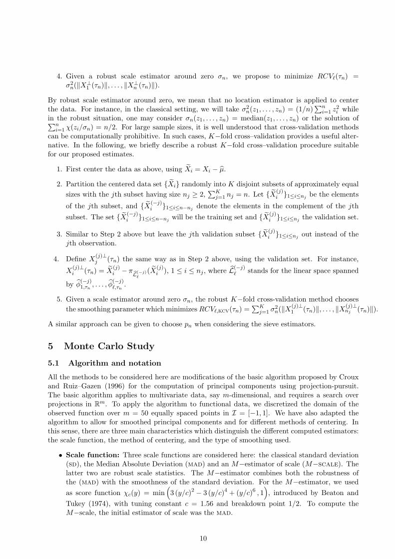
In all Figures and Tables, the estimators corresponding to each scale choice are labeled assd, mad, M−scale. For each scale, we considered four estimators, the raw estimators where nosmoothing is used, the estimators obtained by penalizing the scale function defined in (7), thoseobtained by penalizing the norm defined in (6), and the sieve estimators defined in (10). In allTables, as in Section 2, the jth principal direction estimators related to each method are labelledas ϕj , ϕps,j , ϕpn,j and ϕsi,j , respectively.

When using the penalized estimators, several values for the penalizing parameters τ and ρwere chosen. Since large values of the smoothing parameters make the penalizing term to be thedominant component independently of the amount of contamination considered, we choose τ and ρequal to an−α for α = 3 and 4 and a equal to 0.05, 0.10, 0.15, 0.25, 0.5, 0.75, 1, 1.5 and 2. However,boxplots and density estimators are given only when α = 3 and a = 0.25, 0.75 and 2.

For the sieve estimators based on the Fourier basis, ordered as 1, cos(πx), sin(πx), . . . , cos(qnπx),sin(qnπx), . . ., the values pn = 2qn with qn = 5, 10 and 15 were used, while for the sieve estimatorsbased on the B−splines, the dimension of the linear space considered was selected as pn = 10, 20and 50. The basis for the B-splines is generated from the R function cSplineDes, with the knotsbeing equally spaced in the interval [-1,1] and the number of knots equal to pn + 1. The resultingB−spline basis, though, is not orthonormal. Since it is easier to apply the algorithm for the sieveestimators when an orthonormal basis is used, a Gram-Schmidt orthogonalization is applied to theB−splines basis to obtained a new orthonormal bases spanning the same subspace.

5.2 Simulation settings

The sample was generated using a finite Karhunen-Loeve expansion with the functions, ϕi :[−1, 1] → R, i = 1, 2, 3, where

ϕ1(x) = sin(4πx)

ϕ2(x) = cos(7πx)

ϕ3(x) = cos(15πx) .

It is worth noticing that, when considering the sieve estimators based on the Fourier basis, thethird component cannot be detected when qn < 15, since in this case ϕ3(x) is orthogonal to theestimating space. Likewise, the second component cannot be detected when qn < 7.

11

We performed NR = 1000 replications generating independent samples Xini=1 of size n = 100following the model Xi = Zi1ϕ1 + Zi2ϕ2 + Zi3ϕ3, where Zij are independent random variableswhose distribution will depend on the situation to be considered. The central model, denotedC0, corresponds to Gaussian samples. We have also considered four contaminations of the centralmodel, labelled C2, C3,a, C3,b and C23 depending on the components to be contaminated. Thecentral model and the contaminations can be described as follows. For each of the models, we tookσ1 = 4, σ2 = 2 and σ3 = 1.

• C0: Zi1 ∼ N(0, σ21), Zi2 ∼ N(0, σ2

2) and Zi3 ∼ N(0, σ23).

• C2: Zi2 are independent and identically distributed as 0.8 N(0, σ22) + 0.2 N(10, 0.01), while

Zi1 ∼ N(0, σ21) and Zi3 ∼ N(0, σ2

3). This contamination corresponds to a strong contamina-tion on the second component and changes the mean value of the generated data Zi2 and alsothe first principal component. Note that var(Zi2) = 19.202.

• C3,a: Zi1 ∼ N(0, σ21), Zi2 ∼ N(0, σ2

2) and Zi3 ∼ 0.8 N(0, σ23) + 0.2 N(15, 0.01). This

contamination corresponds to a strong contamination on the third component. Note thatvar(Zi3) = 36.802.

• C3,b: Zi1 ∼ N(0, σ21), Zi2 ∼ N(0, σ2

2) and Zi3 ∼ 0.8 N(0, σ23) + 0.2 N(6, 0.01). This

contamination corresponds to a strong contamination on the third component. Note thatvar(Zi3) = 6.562.

• C23: Zij are independent and such that Zi1 ∼ N(0, σ21), Zi2 ∼ 0.9N(0, σ2

2)+0.1N(15, 0.01) andZi3 ∼ 0.9N(0, σ2

3)+0.1N(20, 0.01). This contamination corresponds to a mild contaminationon the two last components. Note that var(Zi2) = 23.851, and var(Zi3) = 36.901.

We also considered a Cauchy situation, labelled Cc, defined by taking (Zi1, Zi2, Zi3) ∼ C3(0,Σ) withΣ = diag(σ2

1, σ22, σ

23), where Cp(0,Σ) stands for the p−dimensional elliptical Cauchy distribution

centered at 0 with scatter matrix Σ. For this situation, the covariance operator does not exist andthus the classical principal components are not defined.

It is worth noting that the directions ϕ1, ϕ2 and ϕ3 correspond to the classical principal com-ponents for the case C0, but not necessarily for the other cases. For instance, C3,a interchanges theorder between ϕ1 and ϕ3, i.e., ϕ3 is now the first classical principal component, i.e., that obtainedfrom the covariance operator, while ϕ1 is the second and ϕ2 is the third.

5.3 Simulation results

For each situation, we compute the estimators of the first three principal components and thesquare distance between the true and the estimated direction (normalized to have L2 norm 1), i.e.,

Dj =

∥∥∥∥∥ ϕj

∥ϕj∥− ϕj

∥∥∥∥∥2

.

Table 7 to 12 give the mean of Dj over replications for the raw and penalized estimators. Table 7corresponds to the raw and penalized estimators under C0 for the different choices of the penalizingparameters. This table allows to see that a better performance is achieved in most cases with α = 3.Hence, as mentioned above, all the Figures correspond to values of the smoothing parameter equalto τ = an−3. To be more precise, the results in Table 7 show that the best choice for ϕps,jis τ = 2n−3 for all jNote that ρ = 1.5n−3 give quite similar results, when using the M−scale,reducing the error in about a half and a third for j = 2 and 3, respectively. When penalizing thenorm, i.e., when considering ϕpn,j the choice of the penalizing parameter seems to depend both

12

on the component to be estimated and on the estimator to be used. For instance, when using thestandard deviation, the best choice is 0.10n−3, for j = 1 and 2 while for j = 3 a smaller orderis needed to obtain an improvement over the raw estimators. The value τ = 0.75n−4 leads to asmall gain over the raw estimators. For the robust procedures, larger values are needed to see theadvantage of the penalized approach over the raw estimators. For instance, for j = 1, the largerreduction is observed when τ = 2n−3 while for j = 2, the best choices correspond to τ = 0.5n−3

and τ = 0.25n−3 when using the mad and M−scale, respectively. For instance, when using theM−scale, choosing τ = 0.75n−3 lead to a reduction of about 30% and 50% for the first and secondprincipal directions, respectively. On the other hand, when estimating the third component, againsmaller values of τ are needed. Tables 4 and 5 report the mean of Dj over replications for differentsizes of the grid under C0 for some values of the penalizing parameters. The size m = 50 selectedin our study gives a compromise between the performance of the estimators and the computingtime. As it can be seen, some improvement is observed when using m = 250 instead of 50 pointsbut at the expense of multiplying by five the computing time.

Besides, Tables 13 to 18 give the mean of Dj over replications for the sieve estimators. Figures1 to 6 show the density estimates of Dj , for j = 1, 2 and 3, respectively when α = 3 combinedwith a = 1.5 for the estimators penalizing the scale and a = 0.75 for those penalizing the norm.The density estimates were evaluated using the normal kernel with bandwidth 0.6 in all cases. Theplots given in black correspond to the densities of Dj evaluated over the NR = 1000 normallydistributed samples, while those in red, gray, blue and green correspond to C2, C3,a, C3,b and

C23, respectively. Finally, Figures 8 to 13 show the boxplots of the ratio λm/λm for the differenteigenvalue estimators. The classical estimators are labelled sd, while the robust ones mad andms. For the norm or scale–penalized estimators the penalization parameter τ is indicated afterthe estimator type label while for the sieve estimators the parameter pn follows the name of thescale estimator considered. For the Cauchy distribution, the large values obtained for the classicalestimators obscure any differences within the robust procedures and so, separate boxplots for therobust methods only are given at the bottom of Figures 8 to 13.

The simulation confirms the expected inadequate behaviour of the classical estimators, in thepresence of outliers. A bias is observed when estimating the eigenvalues. The poorest efficiency ofthe raw eigenvalue estimates is obtained using the projection–pursuit procedure combined with themad estimator. It is also worth noticing that the level of smoothing τ seems to affect the eigenvalueestimators, introducing a bias even for Gaussian samples. Note that for some contaminations, therobust estimators are also biased. However, the order among them is preserved and so, the targeteigenfunction is in most cases, recovered.

With respect to the principal direction estimation, under contamination, the classical estimatorsdo not estimate the target eigenfunctions very accurately, which can be seen from the shift in thedensity of the norm towards 2. Note that when considering the Cauchy distribution, the maineffect is observed on the eigenvalue estimators since, even if the covariance operator does not exist,the directions seem to be recovered when using the standard deviation. The robust eigenfunctionestimators seem to be affected mainly unaffected by all the contaminations except by C3,a. Inparticular, the projection–pursuit estimators based on an M−scale seem to be more affected bythis contamination. On the other hand, C3,a affects the estimators of the third eigenfunction whenpenalizing the norm. With respect to C3a, the robust estimators obtained penalizing the normϕpn,j show the lower effect among all the competitors. Note that even if the order of the classicaleigenfunctions is modified, as mentioned above, the robust estimators of the first principal directionare not affected by this contamination.

It is worth noting that the classical estimators of the first component are not affected by C3,a

for some values of the smoothing parameter, when penalizing the norm since the penalizationdominates over the contaminated variances. The same phenomena is observed under C3,b whenusing the classical estimators for the selected amount of penalization. For the raw estimators, the

13

sensitivity of the classical estimators under this contamination can be observed in Table 6.As noted in Silverman (1996), for the classical estimators, some degree of smoothing in the

procedure based on penalizing the norm will give a better estimation of ϕj in the L2 sense undermild conditions. In particular, both the procedure penalizing the norm and the scale provide someimprovement with respect to the raw estimators if Ψ(ϕj) < Ψ(ϕℓ), when j < ℓ. This means that theprincipal directions are rougher as the eigenvalues decrease (see Pezzulli and Silverman, 1993 andSilverman, 1996), which is also reflected in our simulation study. The advantages of the smoothprojection pursuit procedures are most striking when estimating ϕ2 and ϕ3 with an M−scale andusing the penalized scale approach.

As expected, when using the sieve estimators, the Fourier basis gives the best performance overall the methods under C0, since our data set was generated using this basis (see Table 13). Thechoice of the B−spline basis give results quite similar to those obtained with ϕps,j .

5.4 K−th fold simulation

Table 1 reports the computing times in minutes for 1000 replications and for a fixed value of τ .This suggests that the leave-one-out cross–validation may be difficult to perform, and so a K−foldapproach is adopted instead. A simulation study was performed where the smoothing parameterτ was selected using the procedure described in Section 4 with K = 4, ℓ = 1. We performed500 replications. The results when penalizing the scale function, i.e., for the estimators definedthrough (7), are reported in Table 2 and in Figure 7. The classical estimators are sensitive tothe considered contaminations and except for contaminations in the third component, the robustcounterpart show their advantage. Note that both C3a and C3b affect the robust estimators whenthe smoothing parameter τ is selected by the robust K−fold cross-validation method.

sd mad M−scaleRaw 5.62 6.98 17.56

Smoothed 7.75 9.00 20.18Smoothed Norm 31.87 33.21 44.04

Table 1: Computing times in minutes for 1000 replications and a fixed value of τ .

Model Scale estimator j = 1 j = 2 j = 3

ϕps,jSD 0.0073 0.0094 0.0078

C0 mad 0.0662 0.0993 0.0634M -scale 0.0225 0.0311 0.0172

SD 1.2840 1.2837 0.0043C2 mad 0.3731 0.3915 0.0504

M -scale 0.4261 0.4286 0.0153SD 1.7840 1.8901 1.9122

C3A mad 0.2271 0.5227 0.5450M -scale 0.2176 0.4873 0.5437

SD 0.0192 0.8350 0.8525C3B mad 0.0986 0.3930 0.3820

M -scale 0.0404 0.2251 0.2285SD 1.7645 0.5438 1.6380

C23 mad 0.2407 0.3443 0.2064M -scale 0.2613 0.3707 0.2174

SD 0.3580 0.4835 0.2287CCauchy mad 0.0788 0.1511 0.1082

M -scale 0.0444 0.0707 0.0434

Table 2: Mean values of ∥ϕj/∥ϕj∥−ϕj∥2 when the penalizing parameter is selected using K−fold cross–validation.

14

6 Concluding Remarks

In this paper, we consider robust principal component analysis for functional data based on aprojection–pursuit approach. The different procedures correspond to robust versions of the un-smoothed principal component estimators, to the estimators obtained penalizing the scale and tothose obtained by penalizing the norm. A sieve approach based on approximating the elements ofthe unit ball by elements over finite–dimensional spaces is also considered. A robust cross-validationprocedure is introduced to select the smoothing parameters. Consistency results are derived for thefour type of estimators. Moreover, the functional related to the unsmoothed estimators is shownto be continuous and so, the related estimators are asymptotically robust.

The simulation study confirms the expected inadequate behaviour of the classical estimators inthe presence of outliers, with the robust procedures performing significantly better. The proposedrobust procedures themselves for the eigenfunctions, however, perform quite similarly to each otherunder the contaminations studied. A study of the influence functions and the asymptotic distribu-tions of the different robust procedures would be useful for differentiating between them. We leavethese important and challenging theoretical problems, though, for future research.

A Appendix A

In this Appendix, we provide conditions under which S1 hold by requiring continuity to the scalefunctional. To derive these results, we will first derive some properties regarding the weak conver-gence of empirical measures that hold not only in L2(I) but in any complete and separable metricspace.

Let M be a complete and separable metric space (Polish space) and B the Borel σ−algebraof M. The Prohorov distance between two probability measures P and Q on M is defined as:dpr(P,Q) = infϵ, P (A) ≤ Q(Aϵ) + ϵ, ∀A ∈ B, where Aϵ = x ∈ M, d(x,A) < ϵ. Theorem A.1shows that, analogously to the Glivenko–Cantelli Theorem in finite–dimensional spaces, on a Polishspace the empirical measures converge weakly almost surely to the probability measure generatingthe observations.

Theorem A.1. Let (Ω,A,P) be a probability space and Xn : Ω → M, n ∈ N, be a sequence ofindependent and identically distributed random elements such that Xi ∼ P . Assume that M is aPolish space and denote by Pn the the empirical probability measure, that is, Pn(A) =

1n

∑n1 IA(Xi)

with IA(Xi) = 1 if Xi ∈ A and 0 elsewhere. Then, Pnω−→ P almost surely, i.e., dpr(Pn, P )

a.s.−→ 0.

Proof. Note that the strong law of large numbers entails that for any borelian set A, Pn(A)a.s.−→

P (A), i.e., Pn(A) → P (A) except for a set NA ⊂ Ω of P-measure zero.Let us show that given j ∈ N, there exists Nj ⊂ Ω such that P(Nj) = 0 and, for any ω /∈ Nj ,

there exists nj(ω) ∈ N such that if n ≥ nj(ω), then dpr(Pn, P ) < 1/j.The fact that M is a Polish space entails that there exists a finite class of disjoint sets Ai, 1 ≤

i ≤ k with diameter smaller than 12j such that

P

(k∪

i=1

Ai

)> 1− 1

2j. (A.1)

Denote by A the class of all the sets that are obtained as a finite union of the Ai, i.e., B ∈ A ifand only if there exists Ai1 , . . . , Aiℓ such that B = ∪ℓ

j=1Aij . Note that A has a finite number ofelements s. For each 1 ≤ i ≤ s, and Bi ∈ A, let NBi ⊂ Ω with P(NBi) = 0 such that if ω /∈ NBi ,then |Pn(Bi)− P (Bi)| → 0. We define Nj =

∪si=1NBi , then P(Nj) = 0.

15

Let ω /∈ Nj , then we have that |Pn(Bi) − P (Bi)| → 0, for 1 ≤ i ≤ s. Hence, there existsnj(ω) ∈ N such that for n ≥ nj(ω) we have that |Pn(B)−P (B)| < 1

2j for any B ∈ A. We will nowshow if n ≥ nj(ω) then dpr(Pn, P ) < 1/j.

Consider B a borelian set and let A be the union of all the sets Ai that intersect B. Note that

A ∈ A and so |Pn(A) − P (A)| < 12j . Therefore, B ⊂ A ∪

(∪ki=1Ai

)cand A ⊂ B1/j . This last

inclusion holds because the sets Ai have diameter smaller than 12j . Thus, using (A.1), we get that

P (B) ≤ P (A) + P

[(k∪

i=1

Ai

)c]= P (A) + 1− P

[(k∪

i=1

Ai

)]< P (A) +

1

2j,

which together with the fact that |Pn(A)−P (A)| < 12j implies that P (B) ≤ P (A)+ 1

2j < Pn(A)+1/j.

Using that A ⊂ B1/j , we get that Pn(A) + 1/j ≤ Pn(B1/j) + 1/j, so P (B) < Pn(B

1/j) + 1/j andthis holds for every B borelian set. Thus, dpr(Pn, P ) < 1/j, as it was desired.

To conclude the proof, we will show that dpr(Pn, P ) → 0 except for a zero P-measure set.Consider all the sets Nj previously defined and let N =

∪j∈NNj . It is clear that P(N ) = 0. Thus,

for any ω /∈ N , we will have that for each j there exists nj = nj(ω) such that d(Pn, P ) < 1/j ifn ≥ nj . This concludes the proof.

Let P be a probability measure in M, a separable Banach space. Then, given f ∈ M∗, whereM∗ stands for the dual space, define P [f ] as the real measure of the random variable f(X), withX ∼ P . Then, we have that

Theorem A.2. Let Pnn∈N and P be probability measures defined on M such that Pnω−→ P ,

i.e., dpr(Pn, P ) → 0. Then, sup∥f∥∗=1 dpr(Pn[f ], P [f ]) → 0.

Proof. Fix ϵ > 0 and let n0 be such that dpr(Pn, P ) < ϵ, for n ≥ n0. We will show thatsup∥f∥∗=1 dpr(Pn[f ], P [f ]) < ϵ, for n ≥ n0 . Fix n ≥ n0.

Using that dpr(Pn, P ) < ϵ and Strassen’s Theorem, we get that there exists Xnn∈N and Xin M such that Xn ∼ Pn, X ∼ P and P(∥Xn − X∥ ≤ ϵ) > 1 − ϵ. Note that for any f ∈ M∗,with ∥f∥∗ = 1, f(Xn) ∼ Pn[f ] and f(X) ∼ P [f ]. Using that |f(Xn) − f(X)| = |f(Xn − X)| ≤∥f∥∗∥Xn −X∥ ≤ ∥Xn −X∥, we get that for any f ∈ M∗, such that ∥f∥∗ = 1,

∥Xn −X∥ ≤ ϵ ⊆ |f(Xn)− f(X)| ≤ ϵ

which entails that

1− ϵ < P(∥Xn −X∥ ≤ ϵ ) ≤ P(|f(Xn)− f(X)| ≤ ϵ), ∀f ∈ M∗, ∥f∥∗ = 1.

Thus, P(|f(Xn)− f(X)| ≤ ϵ) > 1− ϵ, and so, using again Strassen’s Theorem, we get that

Pn[f ](A) ≤ P [f ](Aϵ) + ϵ, ∀A ∈ B, ∀f ∈ M∗, ∥f∥∗ = 1.

Therefore, for any f ∈ M∗ such that ∥f∥∗ = 1, we have that dpr(Pn[f ], P [f ]) ≤ ϵ, i.e.,sup∥f∥∗=1 dpr(Pn[f ], P [f ]) ≤ ϵ concluding the proof.

In the particular, when considering a separable Hilbert space H, if f ∈ H∗ is such that ∥f∥∗ = 1,then f(X) = ⟨α,X⟩ with ∥α∥ = 1. The following result states that when σr is a continuous scalefunctional, uniform convergence can be attained.

Theorem A.3. Let Pnn∈N and P be probability measures defined on a separable Hilbert spaceH, such that Pn

ω−→ P , i.e., dpr(Pn, P ) → 0. Let σr be a continuous scale functional. Then,sup∥α∥=1 |σr(Pn[α])− σr(P [α]))| −→ 0.

16

Proof. Denote by an = sup∥α∥=1 |σr(Pn[α]) − σr(P [α]))|, it is enough to show that L =lim supn→∞ an = 0.

First note that since S = α ∈ H : ∥α∥ = 1 is weakly compact and σr is a continuousfunctional, for each fixed n such that an = 0, there exists αn ∈ S such that

an = |σr(Pn[αn])− σr(P [αn])) . (A.2)

Effectively, let γℓ ∈ S be such that |σr(Pn[γℓ]) − σr(P [γℓ]))| → an, then the weak compactness ofS, entails that there exists a subsequence γℓs such that γℓs converges weakly to γ ∈ H. It is easy tosee that ∥γ∥ ≤ 1. Besides, using that σr is continuous we obtain that |σr(Pn[γℓs ])−σr(P [γℓs ]))| →|σr(Pn[γ])− σr(P [γ]))|, as s → ∞. Hence, |σr(Pn[γ])− σr(P [γ]))| = an which entails that γ = 0.Let γ = γ/∥γ∥, then γ ∈ S and thus |σr(Pn[γ])− σr(P [γ]))| ≤ an. On the other hand, using thatσr is a scale functional we get that

|σr(Pn[γ])− σr(P [γ]))| = |σr(Pn[γ])− σr(P [γ]))|∥γ∥

=an∥γ∥

which implies that ∥γ∥ ≥ 1 leading to ∥γ∥ = 1 and to the existence of a sequence αn ∈ S satifying(A.2).

Let ankbe a subsequence such that ank

→ L, we will assume that ank= 0. Then, using (A.2),

we have that αnk∈ S such that ank

= |σr(Pnk[αnk

]) − σr(P [αnk]))| → L. Using that S is weakly

compact, we can choose a subsequence βj = αnkjsuch that βj converges weakly to β, i.e., for any

α ∈ H, ⟨βj , α⟩ → ⟨β, α⟩. Note that since ∥βj∥ = 1, then ∥β∥ ≤ 1 (β could be 0) and that

ankj= |σr(Pnkj

[βj ])− σr(P [βj ]))| → L (A.3)

For the sake of simplicity denote P (j) = Pnkj. Then, Theorem A.2 entails that

dpr(P(j)[βj ], P [βj ]) ≤ sup

∥α∥=1dpr(P

(j)[α], P [α]) → 0

while the fact that βj converges weakly to β implies that dpr(P [βj ], P [β]) → 0, concluding thatdpr(P

(j)[βj ], P [β]) → 0. The continuity of σr leads to

σr(P(j)[βj ]) → σr(P [β]) . (A.4)

Using again that βj converges weakly to β and the weak continuity of σr we get that

σr(P [βj ]) → σr(P [β]) . (A.5)

Thus, (A.4) and (A.5) imply that σr(P(j)[βj ])−σr(P [βj ]) → 0 and so, from (A.3), L = 0, concluding

the proof.

Moreover, using Theorem A.1, we get the following result that shows that S1 holds if σR is acontinuous scale functional.

Corollary A.1 Let P be a probability measure in a separable Hilbert space H, Pn be the empiricalmeasure of a random sample X1, . . . , Xn with Xi ∼ P , and σR be a continuous scale functional.Then, we have that

sup∥α∥=1

|σr(Pn[α])− σr(P [α]))| a.s.−→ 0.

17

B Appendix B: Proofs

Proof of Lemma 3.1. a) Let N = ω : σ2(ϕ1(ω)) → σ2(ϕr,1) and fix ω /∈ N , then σ2(ϕ1(ω)) →σ2(ϕr,1). Using that S is weakly compact, we have that for any subsequence γℓ of ϕ1(ω) thereexists a subsequence γℓs such that γℓs converges weakly to γ ∈ H. It is easy to see that ∥γ∥ ≤ 1.Besides, using that σ2(ϕ1(ω)) → σ2(ϕr,1), we get that σ

2(γℓs) → σ2(ϕr,1) while on the other hand,the weakly continuity of σ entails that σ2(γℓs) → σ2(γ), as s → ∞. Hence, σ2(γ) = σ2(ϕr,1) whichentails that γ = 0. Let γ = γ/∥γ∥, then γ ∈ S and thus σ2(γ) ≤ σ2(ϕr,1). On the other hand,using that σr is a scale functional we get that

σ(γ) =σ(γ)

∥γ∥=

σ(ϕr,1)

∥γ∥which implies that ∥γ∥ ≥ 1 leading to ∥γ∥ = 1 and so, using the uniqueness of ϕr,1 we obtain that

⟨γ, ϕr,1⟩2 = 1. Therefore, since any subsequence of ϕ1(ω) will have a limit converging either to ϕr,1or −ϕr,1, we obtain a).

b) Write ϕm as ϕm =∑m−1

j=1 ajϕr,j + γm, with ⟨γm, ϕr,j⟩ = 0, 1 ≤ j ≤ m − 1. To obtain b)

we only have to show that ⟨γm, ϕr,m⟩2 a.s.−→ 1. Note that ⟨ϕm, ϕj⟩ = 0, for j = m, implies that

aj = ⟨ϕm, ϕr,j⟩ = ⟨ϕm, ϕr,j − ϕj⟩ + ⟨ϕm, ϕj⟩ = ⟨ϕm, ϕr,j − ϕj⟩. Thus, using that ϕja.s.−→ ϕr,j ,

1 ≤ j ≤ m − 1, and ∥ϕm∥ = 1, we get that aja.s.−→ 0 for 1 ≤ j ≤ m − 1 and so, ∥ϕm − γm∥ a.s.−→ 0.

Note that 1 = ∥ϕm∥2 =∑m−1

j=1 a2j +∥γm∥2, hence, ∥γm∥2 a.s.−→ 1 which implies that ∥ϕm− γm∥ a.s.−→ 0,where γm = γm/∥γm∥. Using that σ(α) is a weakly continuous function and the unit ball is weaklycompact, we obtain that

σ(γm)− σ(ϕm)a.s.−→ 0 . (A.6)

Effectively, let N = Ω − ω : ∥ϕm − γm∥ a.s.−→0, then P(N ) = 1. Fix ω /∈ N and let bn =σ(γm)−σ(ϕm) = σ(γn,m)−σ(ϕn,m). It is enough to show that every subsequence of bn convergesto 0. Denote by bn′ a subsequence, then by the weak compactness of S, there exists a subsequencenj ⊂ n′ such that γnj ,m) and ϕnj ,m) converge weakly to γ and ϕ, respectively. The fact that

∥ϕm − γm∥ → 0, we get that γ = ϕ and so the weak continuity of σ entails that bnj → 0.

The fact that σ2(ϕm)a.s.−→ σ2(ϕr,m) and (A.6) imply that σ(γm)

a.s.−→ σ(ϕr,m). The proof followsnow as in a) using the fact that γm ∈ Cm, with Cm = α ∈ S : ⟨α, ϕr,j⟩ = 0, 1 ≤ j ≤ m − 1 andϕr,m is the unique maximizer of σ(α) over Cm.

Proof of Proposition 3.1. For the sake of simplicity denote by σn(α) = σr(Pn[α]), ϕm =ϕr,m(Pn) and λm = λr,m(Pn). Moreover, let Bm = α ∈ H : ∥α∥ = 1, ⟨α, ϕj⟩ = 0 , ∀ 1 ≤ j ≤m− 1 and Lm−1 the linear space spanned by ϕ1, . . . , ϕm−1.

a) Using ii), we get that an,1 = σ2n(ϕ1) − σ2(ϕ1) → 0 and bn,1 = σ2

n(ϕr,1) − σ2(ϕr,1) → 0 whichimplies that

σ2(ϕr,1) = σ2n(ϕr,1)−bn,1 ≤ σ2

n(ϕ1)−bn,1 = σ2(ϕ1)+an,1−bn,1 ≤ σ2(ϕr,1)+an,1−bn,1 = σ2(ϕr,1)+o(1),

where o(1) stands for a term converging to 0. Therefore, σ2(ϕr,1) ≤ σ2(ϕ1)+o(1) ≤ σ2(ϕr,1)+o(1),

which entails that σ2(ϕ1)a.s.−→ σ2(ϕr,1), concluding the proof of a).

Note that we have not used the weak continuity of σ as a function of α to derive a).

b) Follows as in Lemma 3.1 a).

c) Let 2 ≤ m ≤ q, be fixed and assume that ϕs → ϕr,s, for 1 ≤ s ≤ m − 1. We will begin by

showing that λm → λr,m.

|λm − σ2(ϕr,m)| = | maxα∈Bm

σ2n(α)− max

α∈Bm

σ2(α)| ≤ maxα∈Bm

|σ2n(α)− σ2(α)|+ | max

α∈Bm

σ2(α)− maxα∈Bm

σ2(α)|

18

≤ max∥α∥=1

|σ2n(α)− σ2(α)|+ | max

α∈Bm

σ2(α)− maxα∈Bm

σ2(α)|

≤ o(1) + | maxα∈Bm

σ2(α)− maxα∈Bm

σ2(α)| = o(1) + | maxα∈Bm

σ2(α)− σ2(ϕr,m)| .

Thus, in order to obtain the desired result, it only remains to show maxα∈Bm

σ2(α) → σ2(ϕr,m).We will show that

σ2(ϕr,m) ≤ maxα∈Bm

σ2(α) + o(1) (A.7)

maxα∈Bm

σ2(α) ≤ o(1) + σ2(ϕr,m) (A.8)

Using that ϕs → ϕr,s for 1 ≤ s ≤ m − 1, we obtain that ∥πLm−1− πLm−1∥ → 0. In particular,

we have that ∥πLm−1ϕr,m − πLm−1ϕr,m∥ → 0, which, together with the fact that πLm−1ϕr,m = 0,

implies that πLm−1ϕr,m → 0 and so, ϕr,m − πLm−1

ϕr,m → ϕr,m. Using that ϕr,m = πLm−1ϕr,m +

(ϕr,m − πLm−1ϕr,m), we obtain that ∥ϕr,m − πLm−1

ϕr,m∥ → ∥ϕr,m∥ = 1. Denote by αm =

(ϕr,m − πLm−1ϕr,m)/∥ϕr,m − πLm−1

ϕr,m∥, note that αm ∈ Bm. Then, from the fact that ∥ϕr,m −πLm−1

ϕr,m∥ → 1 and ∥πLm−1ϕr,m∥ → 0, we obtain that ϕr,m = αm + o(1) which together with the

continuity of σ, implies that σ2(αm) → σ2(ϕr,m). Hence,

σ2(ϕr,m) = σ2(αm) + o(1) ≤ maxα∈Bm

σ2(α) + o(1),

where we have used the fact that αm belongs to Bm, concluding the proof of (A.7).To derive (A.8) notice that

maxα∈Bm

σ2(α) = maxα∈Bm

(σ2(α)− σ2

n(α) + σ2n(α)

)≤ max

α∈Bm

|σ2(α)− σ2n(α)|+ σ2

n(ϕm)

≤ maxα∈Bm

(σ2(α)− σ2n(α)) + σ2

n(ϕm)− σ2(ϕm) + σ2(ϕm)

≤ 2 max∥α∥=1

|σ2(α)− σ2n(α)|+ σ2(ϕm) = o(1) + σ2(ϕm) .

Using that πLm−1ϕm = 0 and ∥πLm−1

ϕm − πLm−1 ϕm∥ → 0 (since ∥ϕm∥ = 1) we get that

ϕm = ϕm − πLm−1 ϕm + (πLm−1 − πLm−1)ϕm = ϕm − πLm−1 ϕm + o(1) .

Denote by bm = ϕm − πLm−1 ϕm, then we have that ϕm = bm + o(1), which entails that ∥bm∥ → 1.

Let βm stand for βm = bm/∥bm∥. Note that βm ∈ Bm, then σ(βm) ≤ σ(ϕr,m). On the other hand,

using that ϕm − βm = o(1) and the fact that σ is weakly continuous and S is weakly compact, weobtain, as in Lemma 3.1, that σ(ϕm)− σ(βm) = o(1). Then,

maxα∈Bm

σ2(α) ≤ o(1) + σ2(ϕm) = o(1) + σ2(βm) ≤ o(1) + σ2(ϕr,m) ,

concluding the proof of (A.8) and so, λm = maxα∈Bm

σ2n(α) → σ2(ϕr,m) = λr,m.

Let us show that σ2(ϕm) → σ2(ϕr,m).

|σ2(ϕm)− σ2(ϕr,m)| ≤ |σ2(ϕm)− σ2n(ϕm)|+ |σ2

n(ϕm)− σ2(ϕr,m)|≤ |σ2(ϕm)− σ2

n(ϕm)|+ |λm − σ2(ϕr,m)|≤ sup

∥α∥=1|σ2(α)− σ2

n(α)|+ |λm − σ2(ϕr,m)| .

19

and the proof follows now using ii) and the fact that λm → σ2(ϕr,m).

d) We have already proved that when m = 1 the result holds. We will proceed by induction, wewill assume that ⟨ϕj , ϕr,j⟩2 → 1 for 1 ≤ j ≤ m− 1 and we will show that ⟨ϕm, ϕr,m⟩2 → 1. Using

c) we have that σ2(ϕm) → σ2(ϕr,m) and so, as in Lemma 3.1 b) we conclude the proof.

Proof of Theorem 3.2. To avoid burden notation, we will denote ϕj = ϕpn,j and λj = λpn,,j .a) We will prove that

σ2(ϕr,1) ≥ λ1 + oa.s.(1) (A.9)

and that under S4a)

σ2(ϕr,1) ≤ λ1 + oa.s.(1) , (A.10)

holds. A weaker inequality than (A.10) will be obtained under S4b).Let us prove the first inequality. Using that σ is a scale functional, and that ∥ϕ1∥ ≤ 1, we get

easily that

σ2(ϕr,1) = supα∈S

σ2(α) ≥ σ2

(ϕ1

∥ϕ1∥

)=

σ2(ϕ1

)∥ϕ1∥2

≥ σ2(ϕ1).

On the other hand, S1 entails that an,1 = s2n(ϕ1) − σ2(ϕ1)a.s.−→ 0 and so, σ2(ϕr,1) ≥ σ2(ϕ1) =

s2n(ϕ1) + oa.s.(1) = λ1 + oa.s.(1), concluding the proof of (A.9).We will derive a). Since clearly, S4b) implies S4a), we begin by showing the result under S4a)

to have an idea of the arguments to be used. The extension to S4b) can be made using sometechnical arguments.

i) Assume that S4a) holds, then ϕr,1 ∈ Hs, so that ∥ϕr,1∥τ < ∞. Note that ∥ϕr,1∥τ ≥ ∥ϕr,1∥ = 1,

then, defining β1 = ϕr,1/∥ϕr,1∥τ , we have that ∥β1∥τ = 1, which implies that λ1 = s2n(ϕ1) ≥ s2n(β1).

Again, using S1 we get that bn,1 = s2n(β1)− σ2(β1)a.s.−→ 0, hence,

λ1 ≥ s2n(β1) = σ2(ϕr,1/∥ϕr,1∥τ ) + oa.s.(1) =σ2(ϕr,1)

∥ϕr,1∥2τ+ oa.s.(1) = σ2(ϕr,1) + oa.s.(1)

where, in the last inequality, we have used that ∥ϕr,1∥τ → ∥ϕr,1∥ = 1 since τ → 0, concluding theproof of a) in this case.

ii) Assume that S4b) holds. In this case, we cannot consider ∥ϕr,1∥τ since ϕr,1 does not belong

to Hs, otherwise we argue as in i). Since, ϕr,1 ∈ Hs, we can choose a sequence ϕ1,k ∈ Hs such

that ϕ1,k → ϕr,1, ∥ϕ1,k∥ = 1 and |σ2(ϕ1,k)− σ2(ϕr,1)| < 1/k. Note that for any fixed k, ∥ϕ1,k∥τ ≥∥ϕ1,k∥ = 1 and ∥ϕ1,k∥τ −→ ∥ϕ1,k∥ = 1 since τn −→ 0. Thus, using that λ1 = max∥α∥τ=1 s

2n(α) and

defining β1,k = ϕ1,k/∥ϕ1,k∥τ , we obtain that ∥β1,k∥τ = 1 and λ1 = s2n(ϕ1) ≥ s2n(β1,k).

Note that S1 entails that bn,1 = s2n(β1,k)− σ2(β1,k)a.s.−→ 0, hence,

λ1 ≥ s2n(β1,k) = σ2(β1,k) + oa.s.(1) =σ2(ϕ1,k)

∥ϕ1,k∥2τ+ oa.s.(1) =

σ2(ϕr,1)− 1/k

∥ϕ1,k∥τ+ oa.s.(1) .

Therefore, using (A.9) and the fact that ∥ϕ1,k∥τ ≥ 1, we have that

σ2(ϕr,1) ≥ λ1 +O1,n ≥ σ2(ϕr,1)− 1/k

∥ϕ1,k∥τ+ oa.s.(1) ≥ σ2(ϕr,1)−

(1− 1

∥ϕ1,k∥τ

)σ2(ϕr,1)−

1

k+O2,n ,

20

where Oi,n = oa.s.(1), i = 1, 2. Let N = ∪i=1,2ω : Oi,n(ω) → 0 and fix ω /∈ N . Given ϵ > 0, fix k0such that 1/k0 < ϵ. Let n0 be such that, for n ≥ n0, Oi,n(ω) < ϵ, i = 1, 2 and

0 ≤

(1− 1

∥ϕ1,k0∥τ

)σ2(ϕr,1) < ϵ ,

where we have used that τn → 0 and thus ∥ϕ1,k0∥τ → 1. Then, using

|λ1(ω)− σ2(ϕr,1)| ≤ max|O1,n|, |O2,n|+ 2ϵ ≤ 3ϵ

which entails that λ1a.s.−→ σ2(ϕr,1), as desired.

Using S1, we get that λ1 − σ2(ϕ1) = s2n(ϕ1) − σ2(ϕ1)a.s.−→ 0, using that λ1

a.s.−→ σ2(ϕr,1), we

obtain that σ2(ϕ1)a.s.−→ σ2(ϕr,1), concluding the proof of a).

It is worth noticing that as a consequence of the above results, we get that the followinginequalities converge to equalities

σ2(ϕr,1) ≥ σ2

(ϕ1

∥ϕ1∥

)≥ σ2(ϕ1) = λ1 + oa.s.(1) ,

in particular,

σ2

(ϕ1

∥ϕ1∥

)a.s.−→ σ2(ϕr,1) and σ2(ϕ1)

a.s.−→ σ2(ϕr,1) . (A.11)

b) Note that

τ⌈ϕ1, ϕ1⌉ = 1− ∥ϕ1∥2 = 1− σ2(ϕ1)

σ2(ϕ1/∥ϕ1∥).

Thus, using (A.11) we have that the second term is 1 + oa.s.(1), concluding the proof of b).

c) Note that since ∥ϕ1∥τ = 1, we have that ∥ϕ1∥ ≤ 1. Moreover, from b) ∥ϕ1∥a.s.−→ 1. Let

ϕ1 = ϕ1/∥ϕ1∥. Then, we have that ϕ1 ∈ S and σ(ϕ1) = σ(ϕ1)/∥ϕ1∥. Using that σ2(ϕ1)a.s.−→ σ2(ϕr,1)

and ∥ϕ1∥a.s.−→ 1, we obtain that σ2(ϕ1)

a.s.−→ σ2(ϕr,1) and thus, the proof follows using Lemma 3.1.

d) Let us show that λma.s.−→ σ2(ϕr,m). We begin by proving the following extension of S1

sup∥α∥τ≤1

|σ2(πm−1α)− s2n(πτ,m−1α)|a.s.−→ 0 . (A.12)

Using S1 and the fact that sn is a scale estimator and so, sn(α) = ∥α∥τ sn(α/∥α∥τ ), we get that

sup∥α∥τ≤1

∣∣s2n(α)− σ2(α)∣∣ a.s.−→ 0 (A.13)

Note that

sup∥α∥τ≤1

|σ2(πm−1α)−s2n(πτ,m−1α)| ≤ sup∥α∥τ≤1

|σ2(πm−1α)−σ2(πτ,m−1α)|+ sup∥α∥τ≤1

|σ2(πτ,m−1α)−s2n(πτ,m−1α)|

Using (A.13) and the fact that if ∥α∥τ ≤ 1 then ∥πτ,m−1α∥τ ≤ 1, we get that the second term onthe right hand side converges to 0 almost surely.To conclude the proof of (A.12), it remains to show that

sup∥α∥τ≤1

|σ2(πm−1α)− σ2(πτ,m−1α)|a.s.−→ 0 . (A.14)

21

As in Silverman (1996), using that ϕja.s.−→ ϕr,j and that τΨ(ϕj) = τ⌈ϕj , ϕj⌉

a.s.−→ 0, for 1 ≤ j ≤ m−1,we get that

sup∥α∥τ≤1

∥⟨α, ϕr,j⟩ϕr,j − ⟨α, ϕj⟩τ ϕj∥a.s.−→ 0 for 1 ≤ j ≤ m− 1 (A.15)

Effectively, for any α ∈ Hs such that ∥α∥2τ = ∥α∥2 + τΨ(α) ≤ 1, we have that

∥⟨α, ϕr,j⟩ϕr,j − ⟨α, ϕj⟩τ ϕj∥ ≤ ∥α∥∥ϕr,j − ϕj∥+ ∥ϕj∥∣∣∣⟨α, ϕr,j⟩ − ⟨α, ϕj⟩τ

∣∣∣≤ ∥ϕr,j − ϕj∥+

∣∣∣⟨α, ϕr,j − ϕj⟩+ τ⌈α, ϕj⌉∣∣∣

≤ ∥ϕr,j − ϕj∥+∥ϕr,j − ϕj∥+ (τΨ(α))

12

(τΨ(ϕj)

) 12

≤ ∥ϕr,j − ϕj∥+

∥ϕr,j − ϕj∥+

(τΨ(ϕj)

) 12

and so, (A.15) holds entailing that sup∥α∥τ≤1 ∥πτ,m−1α− πm−1α∥

a.s.−→ 0. Therefore, using that σ isweakly continuous and the unit ball is weakly compact, we get easily that (A.14) holds, concludingthe proof of (A.12).

As in a), we will show thatσ2(ϕr,m) ≥ λm + oa.s.(1) (A.16)

and that when S4a) holdsσ2(ϕr,m) ≤ λm + oa.s.(1) . (A.17)

holds. A weaker inequality than (A.17) will be obtained under S4b).Using again that σ is a scale functional, we get easily that supα∈S∩Tm−1

σ2(α) = supα∈S σ2(πm−1α)and so,

σ2(ϕr,m) = supα∈S∩Tm−1

σ2(α) = supα∈S

σ2(πm−1α) ≥ σ2

(πm−1

ϕm

∥ϕm∥

).

From (A.12) we get that bm = σ2(πm−1ϕm

)− s2n

(πτ,m−1ϕm

)a.s.−→ 0 and so, since πτ,m−1ϕm = ϕm

and ∥ϕm∥ ≤ 1, we get that

σ2(ϕr,m) ≥ σ2

(πm−1

ϕm

∥ϕm∥

)=

σ2(πm−1ϕm

)∥ϕm∥2

≥ σ2(πm−1ϕm

)= s2n

(πτ,m−1ϕm

)+ oa.s.(1) = s2n(ϕm) + oa.s.(1) = λm + oa.s.(1) ,

concluding the proof of (A.16).Let us show that (A.17) holds if S4a) holds.

i) If S4a) holds, ϕr,m ∈ Hs, so that ∥ϕr,m∥τ < ∞ and ∥ϕr,m∥τ → ∥ϕr,m∥ = 1. Using that sn is ascale estimator and the fact that for any α ∈ Hs such that ∥α∥τ = 1 we have that ∥πτ,m−1α∥τ ≤ 1,we get easily that

λm = s2n(ϕm) = sup∥α∥τ=1,α∈Tτ,m−1

s2n(α) = sup∥α∥τ=1

s2n(πτ,m−1α) ≥ s2n

(πτ,m−1ϕr,m∥ϕr,m∥τ

)which together with (A.12) and the fact that ∥ϕr,m∥τ → ∥ϕr,m∥ = 1, entails that

λm ≥ s2n

(πτ,m−1ϕr,m∥ϕr,m∥τ

)= σ2

(πm−1ϕr,m∥ϕr,m∥τ

)+ oa.s.(1)

≥ σ2

(ϕr,m

∥ϕr,m∥τ

)+ oa.s.(1) =

σ2 (ϕr,m)

∥ϕr,m∥2τ+ oa.s.(1) ≥ σ2(ϕr,m) + oa.s.(1)

22

concluding the proof of (A.17) in this case and so, when S4a) holds λma.s.−→ σ2(ϕr,m).

ii) Assume that S4b) holds. As in a), let us consider a sequence ϕm,k ∈ Hs such that ϕm,k → ϕr,m,

as k → ∞, ∥ϕm,k∥ = 1 and |σ2(πm−1ϕm,k) − σ2(ϕr,m)| < 1/k, since πm−1ϕr,m = ϕr,m. Then, for

each fixed k, we have that ∥ϕm,k∥τ −→ ∥ϕm,k∥ = 1 since τ → 0.Using that sn is a scale estimator and the fact that for any α ∈ Hs such that ∥α∥τ = 1 we have

that ∥πτ,m−1α∥τ ≤ 1, we get that

λm = s2n(ϕm) = sup∥α∥τ=1,α∈Tτ,m−1

s2n(α) = sup∥α∥τ=1

s2n(πτ,m−1α) ≥ s2n

(πτ,m−1ϕm,k

∥ϕm,k∥τ

)

Using (A.12) and the fact that |σ2(πm−1ϕm,k)− σ2(ϕr,m)| < 1/k and ∥ϕm,k∥τ ≥ 1, we get that

λm ≥ s2n

(πτ,m−1ϕm,k

∥ϕm,k∥τ

)= σ2

(πm−1ϕm,k

∥ϕm,k∥τ

)+ oa.s.(1)

≥ σ2 (ϕr,m)− 1/k

∥ϕm,k∥2τ+ oa.s.(1)

≥ σ2 (ϕr,m)− σ2 (ϕr,m)

(1− 1

∥ϕm,k∥2τ

)− 1

k+ oa.s.(1)

Therefore, arguing as in a) we obtain that λma.s.−→ σ2 (ϕr,m).

On the other hand, as in a), using S1, we get that λm − σ2(ϕm) = s2n(ϕm) − σ2(ϕm)a.s.−→ 0,

using that λma.s.−→ σ2(ϕr,m), we obtain that σ2(ϕm)

a.s.−→ σ2(ϕr,m).

Thus, it remains to show that τ⌈ϕm, ϕm⌉ a.s.−→ 0. As in a), we have that the following inequalitiesconverge to equalities

σ2(ϕr,m) ≥ σ2

(πm−1

ϕm

∥ϕm∥

)≥ σ2

(πm−1ϕm

)≥ λm + oa.s.(1) . (A.18)

Note that since σ is a scale estimator, we have that

τ⌈ϕm, ϕm⌉ = 1− ∥ϕm∥2 = 1− σ2(πm−1ϕm)

σ2(πm−1ϕm/∥ϕm∥),

which together with (A.18) entails that the second term on the right hand side is 1 + oa.s.(1),concluding the proof of d).

e) Form = 1 the result was derived in c). Let us assume that for 1 ≤ j ≤ m−1, ϕja.s.−→ ϕr,j and that

τ⌈ϕj , ϕj⌉a.s.−→ 0, we will show that ⟨ϕm, ϕr,m⟩2 a.s.−→ 1, i.e., we will use an induction argument. By d)

we already know that τ⌈ϕm, ϕm⌉ a.s.−→ 0 which entails that ∥ϕm∥ a.s.−→ 1. Denote by ϕj = ϕj/∥ϕj∥, itis enough to show that ⟨ϕr,m, ϕm⟩2 a.s.−→ 1. We have that, ⟨ϕm, ϕj⟩τ = 0. Using that τ⌈ϕj , ϕj⌉

a.s.−→ 0,

for 1 ≤ j ≤ m−1, we get that τ⌈ϕj , ϕm⌉ a.s.−→ 0 for 1 ≤ j ≤ m−1 and so, ⟨ϕm, ϕj⟩a.s.−→ 0. Therefore,

arguing as in Lemma 3.1, we can write ϕm as ϕm =∑m−1

j=1 ajϕr,j + γm, with ⟨γm, ϕr,j⟩ = 0,

1 ≤ j ≤ m− 1. To obtain e) it remains to show that ⟨γm, ϕr,m⟩2 a.s.−→ 1. Note that ⟨ϕm, ϕj⟩a.s.−→ 0,

for j = m, implies that aj = ⟨ϕm, ϕr,j⟩ = ⟨ϕm, ϕr,j−ϕj⟩+⟨ϕm, ϕj⟩ = ⟨ϕm, ϕr,j−ϕj⟩+oa.s.(1). Thus,

using that ϕja.s.−→ ϕr,j , 1 ≤ j ≤ m − 1, and ∥ϕm∥ a.s.−→ 1, we get that aj

a.s.−→ 0 for 1 ≤ j ≤ m − 1

and so, ∥ϕm − γm∥ a.s.−→ 0. Note that 1 = ∥ϕm∥2 =∑m−1

j=1 a2j + ∥γm∥2, hence, ∥γm∥2 a.s.−→ 1 which

implies that ∥ϕm − γm∥ a.s.−→ 0, where γm = γm/∥γm∥. Using that σ(α) is a weakly continuous

23

and S is weakly compact, we obtain that σ(γm) − σ(ϕm)a.s.−→ 0 which together with the fact that

σ2(ϕm)a.s.−→ σ2(ϕr,m) and ∥ϕm∥ a.s.−→ 1, implies that σ(γm)

a.s.−→ σ(ϕr,m). The proof follows now asin Lemma 3.1 using the fact that γm ∈ Cm, with Cm = α ∈ S : ⟨α, ϕr,j⟩ = 0, 1 ≤ j ≤ m− 1 andϕr,m is the unique maximizer of σ(α) over Cm.

Proof of Theorem 3.3. To avoid burden notation, we will denote ϕj = ϕps,j and λj = λps,j .a) We will prove that

σ2(ϕr,1) ≥ λ1 + oa.s.(1) (A.19)

and that under S4a)

σ2(ϕr,1) ≤ λ1 + oa.s.(1) , (A.20)

holds.Let us prove the first inequality. We easily get that

σ2(ϕr,1) = supα∈S

σ2(α) ≥ σ2(ϕ1).

On the other hand, S1 entails that an,1 = s2n(ϕ1) − σ2(ϕ1)a.s.−→ 0 and so, σ2(ϕr,1) ≥ σ2(ϕ1) =

s2n(ϕ1) + oa.s.(1) = λ1 + oa.s.(1), concluding the proof of (A.19).We will derive (A.20). Since S4a) holds, we have that ϕr,1 ∈ Hs, so that ∥ϕr,1∥τ < ∞. Note

that

λ1 = s2n(ϕ1) ≥ s2n(ϕ1)− τ⌈ϕ1, ϕ1⌉ = supα∈S

s2n(α)− τ⌈α, α⌉ ≥ s2n(ϕr,1)− τ⌈ϕr,1, ϕr,1⌉. (A.21)

Using that τ → 0, we obtain that τ⌈ϕr,1, ϕr,1⌉ → 0. Also, using S1 we get that s2n(ϕr,1) =σ2(ϕr,1) + oa.s.(1). Therefore, (A.21) can be written as

λ1 ≥ s2n(ϕr,1)− τ⌈ϕr,1, ϕr,1⌉ = σ2(ϕr,1) + oa.s.(1)

Hence, (A.20) follows which together with (A.19) implies that λ1a.s.−→ σ2(ϕr,1). Using S1 we have

thatλ1 − σ2(ϕ1) = s2n(ϕ1)− σ2(ϕ1)

a.s.−→ 0

therefore we also get that σ2(ϕ1)a.s.−→ σ2(ϕr,1)). From the fact that λ1

a.s.−→ σ2(ϕr,1), s2n(ϕr,1)

a.s.−→σ2(ϕr,1), τ → 0 and since

λ1 ≥ s2n(ϕ1)− τ⌈ϕ1, ϕ1⌉ ≥ s2n(ϕr,1)− τ⌈ϕr,1, ϕr,1⌉

we get that τ⌈ϕ1, ϕ1⌉a.s.−→ 0, concluding the proof of a).

b) Follows easily using Lemma 3.1 a), the fact that σ2(ϕ1)a.s.−→ σ2(ϕr,1) and ∥ϕ1∥ = 1.

c) We will prove that

σ2(ϕr,m) ≥ λm + oa.s.(1) (A.22)

and that under S4a)

σ2(ϕr,m) ≤ λm + oa.s.(1) , (A.23)

24

holds. In order to derive (A.22), note that

σ2(ϕr,1) = supα∈S∩Tm−1

σ2(α) = supα∈S

σ2(πm−1α) ≥ σ2(πm−1ϕm). (A.24)

Let us show that σ2(πm−1ϕm) = s2n(πm−1ϕm) + oa.s.(1). Indeed, if α ∈ S, then

|σ2(πm−1α)− s2n(πm−1α)| ≤ |σ2(πm−1α)− σ2(πm−1α)|+ |σ2(πm−1α)− s2n(πm−1α)|. (A.25)

The second term on the right hand side of (A.25) will be oa.s.(1) since S1 holds. Let us show thatthe first one will also be oa.s.(1). Using that ∥πm−1 − πm−1∥

a.s.−→ 0, we get that πm−1αa.s.−→ πm−1α.

Finally, from S2, i.e., the continuity of σ, we get that the first term on the right hand side of (A.25)will be oa.s.(1). Therefore, σ

2(πm−1ϕm) = s2n(πm−1ϕm) + oa.s.(1). Therefore, (A.24) entails that

σ2(ϕr,1) ≥ σ2(πm−1ϕm) = s2n(πm−1ϕm) + oa.s.(1) = s2n(ϕm) + oa.s.(1) = λm + oa.s.(1)

concluding the proof of (A.22).Let us now proof that, under S4a, (A.23) holds.

λm = s2n(ϕm) ≥ s2n(ϕm)− τ⌈ϕm, ϕm⌉ = supα∈S∩Tm−1

s2n(α)− τ⌈α, α⌉

≥ supα∈S

s2n(πm−1α)− τ⌈πm−1α, πm−1α⌉ (A.26)

≥ s2n(πm−1ϕr,m)− τ⌈πm−1ϕr,m, πm−1ϕr,m⌉. (A.27)

Let us show that supα∈S |s2n(πm−1α)− s2n(πm−1α)|a.s.−→ 0. Effectively,

supα∈S

|s2n(πm−1α)− s2n(πm−1α)|

≤ supα∈S

|s2n(πm−1α)− σ2(πm−1α)|+ supα∈S

|σ2(πm−1α)− σ2(πm−1α)|+ supα∈S

|σ2(πm−1α)− s2n(πm−1α)|

≤ supα∈S

|s2n(α)− σ2(α)|+ supα∈S

|σ2(πm−1α)− σ2(πm−1α)|+ supα∈S

|σ2(πm−1α)− s2n(πm−1α)|

The first and third terms of the last inequality converge to 0 almost surely since S1 holds. Thuswe only have to show that supα∈S |σ2(πm−1α)− σ2(πm−1α)| = oa.s.(1). Using that ϕj

a.s.−→ ϕr,j for

1 ≤ j ≤ m − 1, it is easy to show that ∥πm−1 − πm−1∥a.s.−→ 0 since it reduces to a difference of

finite dimensional projections. Therefore, we have uniform convergence in the set α, ∥α∥ ≤ 1.Using that σ is weakly continuous in S = α, ∥α∥ ≤ 1 which is weakly compact we obtain thatsupα∈S |σ2(πm−1α)− σ2(πm−1α)|, converges to 0 almost surely. In conclusion,

supα∈S

|s2n(πm−1α)− s2n(πm−1α)| = oa.s.(1).

Using that τ⌈ϕℓ, ϕℓ⌉a.s.−→ 0, 1 ≤ ℓ ≤ m − 1, analogous arguments to those considered in Pezzulli

and Silverman (1993) and the fact that τ → 0 implies that τ⌈ϕr,m, ϕr,m⌉ = o(1), it is not hard tosee that

τn⌈πm−1ϕr,m, πm−1ϕr,m⌉ a.s.−→ 0.

Those two results essentially allow us to replace πm−1α by πm−1α in (A.27). Therefore,

λm ≥ s2n(πm−1ϕr,m) + oa.s.(1) = supα∈S∩Tm−1

s2n(α)− τ⌈α, α⌉+ oa.s.(1)

≥ s2n(ϕr,m) + oa.s.(1) = σ2(ϕr,m) + oa.s.(1) + oa.s.(1) = σ2(ϕr,m) + oa.s.(1)

25

where we have used S1. Using that

λm ≥ s2n(ϕm)− τ⌈ϕm, ϕm⌉ ≥ σ2(ϕr,m) + oa.s.(1)

and the fact that λm = s2n(ϕm)a.s.−→ σ2(ϕr,m) imply that τ⌈ϕm, ϕm⌉ a.s.−→ 0, concluding the proof of

c).

d) We have already proved that when m = 1 the result holds. We will proceed by induction, wewill assume that ⟨ϕj , ϕr,j⟩2

a.s.−→ 1 for 1 ≤ j ≤ m − 1 and we will show that ⟨ϕm, ϕr,m⟩2 a.s.−→ 1.

By definition ⟨ϕm, ϕj⟩ = 0, for j = m and ϕm ∈ S thus, using the fact that c) entails that

σ2(ϕm)a.s.−→ σ2(ϕr,m) and Lemma 3.1 b), the proof follows.

Proof of Theorem 3.4. For the sake of simplicity, we will avoid the subscript si and we willdenote ϕj = ϕsi,j and λj = λsi,j .a) The proof follows using similar arguments as those considered in the proof of Proposition 3.1.Using S1 we get that

an,1 = s2n(ϕ1)− σ2(ϕ1)a.s.−→ 0 . (A.28)

Let ϕ1,pn = πHpnϕr,1/∥πHpn

ϕr,1∥, then, ϕ1,pn ∈ Spn and ϕ1,pn → ϕr,1. Hence, S2 entails that

σ(ϕ1,pn) → σ(ϕ1) while using S1, we get that s2n(ϕ1,pn)− σ2(ϕ1,pn)a.s.−→ 0. Thus, bn,1 = s2n(ϕ1,pn)−

σ2(ϕ1)a.s.−→ 0. Note that

σ2(ϕr,1) = s2n(ϕ1,pn)− bn,1 ≤ s2n(ϕ1)− bn,1 = σ2(ϕ1) + an,1 − bn,1 ≤ σ2(ϕr,1) + an,1 − bn,1 ,

that is, σ2(ϕr,1)− an,1 + bn,1 ≤ σ2(ϕ1) ≤ σ2(ϕr,1) and so,

σ2(ϕ1)a.s.−→ σ2(ϕr,1) , (A.29)

which together with (A.28) implies that λ1a.s.−→ σ2(ϕr,1).

b) We have that

|λm − σ2(ϕr,m)| = |s2n(ϕm)− σ2(ϕr,m)| = | maxα∈Bn,m

s2n(α)− maxα∈Bm

σ2(α)|

≤ maxα∈Bn,m

|s2n(α)− σ2(α)|+ | maxα∈Bn,m

σ2(α)− maxα∈Bm

σ2(α)|

≤ maxα∈Spn

|s2n(α)− σ2(α)|+ | maxα∈Bn,m

σ2(α)− maxα∈Bm

σ2(α)| . (A.30)

Using S1, we get that the first term on the right hand side of (A.30) converges to 0 almost surely.Thus, it will be enough to show that max

α∈Bn,mσ2(α)

a.s.−→ σ2(ϕr,m), since maxα∈Bm σ2(α) =

σ2(ϕr,m). Using that ϕsa.s.−→ ϕr,s, for 1 ≤ s ≤ m− 1, we get that

∥πLm−1− πLm−1∥

a.s.−→ 0 , (A.31)

which implies that∥πLm−1

ϕm − πLm−1 ϕm∥ a.s.−→ 0 , (A.32)

where ϕm = πHpnϕr,m . On the other hand, using that pn → ∞, we get that ϕm → ϕr,m, thus

∥πLm−1(ϕm − ϕr,m)∥ → 0 which together with (A.32) and the fact that πLm−1ϕr,m = 0, entails

that πLm−1ϕm

a.s.−→ 0 and βm = ϕm − πLm−1ϕm

a.s.−→ ϕr,m. Denoting by am = ∥βm∥, ama.s.−→ 1,

we obtain that αm = βm/ama.s.−→ ϕr,m. Moreover, αm ∈ Bn,m since ϕm ∈ Hpn and ϕj ∈ Hpn ,

26

1 ≤ j ≤ m− 1, implying that maxα∈Bn,m

σ2(α) ≥ σ2(αm). Using the weak continuity of σ, we get

that σ(αm)a.s.−→ σ(ϕr,m), i.e.,

maxα∈Bn,m

σ2(α) ≥ σ2(αm) = σ2(ϕr,m) + oa.s.(1) .

On the other hand,

maxα∈Bn,m

σ2(α) ≤ maxα∈Bn,m

|σ2(α)− s2n(α)|+ s2n(ϕm)

≤ 2 maxα∈Bn,m

|σ2(α)− s2n(α)|+ σ2(ϕm) = oa.s.(1) + σ2(ϕm)

Using (A.31) and the fact that ϕm ∈ Bn,m, ∥ϕm∥ = 1, we get that ϕm = ϕm − πLm−1ϕm =

bm + oa.s.(1), where bm = ϕm − πLm−1 ϕm. Thus ∥bm∥ a.s.−→ 1. Denote βm = bm/∥bm∥, then βm ∈ Bm

which implies that σ(βm) ≤ σ(ϕr,m). Besides, the weak continuity of σ and the weak compactness

of the unit ball entail, as in Lemma 3.1, that σ(βm) − σ(ϕm)a.s.−→ 0, since ϕm − βm = oa.s.(1).

Summarizing,

σ2(ϕr,m) + oa.s.(1) = σ2(αm) ≤ maxα∈Bn,m

σ2(α) ≤ oa.s.(1) + σ2(ϕm) = oa.s.(1) + σ2(βm)

≤ oa.s.(1) + σ2(ϕr,m)

concluding that maxα∈Bn,m

σ2(α)a.s.−→ σ2(ϕr,m) and thus the proof that λm

a.s.−→ σ2(ϕr,m). More-

over, it is easy to see that S1 and the fact that λma.s.−→ σ2(ϕr,m) entail that σ2(ϕm)

a.s.−→ σ2(ϕr,m),since

|σ2(ϕm)− σ2(ϕr,m)| ≤ |σ2(ϕm)− s2n(ϕm)|+ |s2n(ϕm)− σ2(ϕr,m)|= |σ2(ϕm)− s2n(ϕm)|+ |λm − σ2(ϕr,m)|≤ sup

α∈Spn

|σ2(α)− s2n(α)|+ |λm − σ2(ϕr,m)| .

c) We begin by proving that ϕ1a.s.−→ ϕr,1. Using σ2(ϕ1)

a.s.−→ σ2(ϕr,1) and Lemma 3.1a), the result

follows easily since ϕ1 ∈ S. Let us show that if ϕja.s.−→ ϕr,j for 1 ≤ j ≤ m−1 then ⟨ϕm, ϕr,m⟩2 a.s.−→ 1,

which will lead to c). Since ϕja.s.−→ ϕr,j for 1 ≤ j ≤ m − 1, we have that σ2(ϕm)

a.s.−→ σ2(ϕr,m).

Besides, using that ⟨ϕm, ϕj⟩ = 0, j = m and ϕm ∈ S, Lemma 3.1b) concludes the proof.

References

[1] Bali, J. and Boente, G. (2009). Principal points and elliptical distributions from the multivariate settingto the functional case. Statist. Probab. Lett., 79, 1858-1865.

[2] Boente, G. and Fraiman, R. (2000). Kernel-based functional principal components. Statist. Probab.Lett., 48, 335-345.

[3] Cantoni, E. and Ronchetti, E. (2001). Resistant selection of the smoothing parameter for smoothingsplines. Statistics and Computing, 11, 141-146.

[4] Croux, C. and Ruiz–Gazen, A. (1996). A fast algorithm for robust principal components based onprojection pursuit. In Compstat: Proceedings in Computational Statistics, ed. A. Prat, Heidelberg:Physica–Verlag, 211-217.

[5] Croux, C. and Ruiz–Gazen, A. (2005). High Breakdown Estimators for Principal Components: theProjection–Pursuit Approach Revisited. J. Multivar. Anal., 95, 206-226.

27

[6] Cuevas, A., Febrero, M. and Fraiman, R. (2007). Robust estimation and classification for functionaldata via projection-based depth notions. Comp. Statist., 22, 48196.

[7] Cui, H., He, X. and Ng, K. W. (2003). Asymptotic Distribution of Principal Components Based onRobust Dispersions. Biometrika, 90, 953-966.

[8] Dauxois, J., Pousse, A. and Romain, Y. (1982). Asymptotic theory for the principal component analysisof a vector random function: Some applications to statistical inference. J. Multivar. Anal., 12, 136-154.

[9] Fraiman, R. and Muniz, G. (2001). Trimmed means for functional data. Test, 10, 41940.

[10] Gervini, D. (2006). Free-knot spline smoothing for functional data. J. Roy. Statist. Soc. Ser. B, 68,67187.

[11] Gervini, D. (2008). Robust functional estimation using the spatial median and spherical principal com-ponents. Biometrika, 95, 587-600.

[12] Hall, P. and Hosseini–Nasab, M. (2006). On properties of functional principal components analysis. J.Roy. Statist. Soc. Ser. B, 68, 10926.

[13] Hall, P., Muller, H.-G. and Wang, J.-L. (2006). Properties of principal component methods for functionaland longitudinal data analysis. Ann. Statist., 34, 1493517.

[14] Hyndman, R. J. and S. Ullah (2007). Robust forecasting of mortality and fertility rates: A functionaldata approach. Comp. Statist. Data Anal., 51, 4942-4956.

[15] Locantore, N., Marron, J. S., Simpson, D. G., Tripoli, N., Zhang, J. T. and Cohen, K. L. (1999). Robustprincipal components for functional data (with Discussion). Test, 8, 173.

[16] Li, G. and Chen, Z. (1985). Projection–Pursuit Approach to Robust Dispersion Matrices and PrincipalComponents: Primary Theory and Monte Carlo. J. Amer. Statist. Assoc., 80, 759-766.

[17] Lopez–Pintado, S. and Romo, J. (2007). Depth-based inference for functional data. Comp. Statist. DataAnal., 51, 495768.

[18] Pezzulli, S. D. and Silverman, B. W. (1993). Some properties of smoothed principal components analysisfor functional data. Comput. Statist., 8, 1-16.

[19] Ramsay, J. O. and Silverman, B. W. (2005). Functional Data Analysis, 2nd ed. New York: Springer-Verlag.

[20] Rice, J. and Silverman, B. W. (1991). Estimating the mean and covariance structure nonparametricallywhen the data are curves. J. Roy. Statist. Soc. Ser. B, 53, 233-243.

[21] Rousseeuw, P. J. and Croux, C. (1993). Alternatives to the Median Absolute Deviation. J. Amer. Statist.Assoc., 88, 1273-1283.

[22] Silverman, B. W. (1996). Smoothed functional principal components analysis by choice of norm. Ann.Statist., 24, 1-24.

[23] van der Geer, S. (2000). Empirical Processes in M−Estimation. Cambridge University Press.

[24] Wang, F. and Scott, D. (1994). The L1 method for robust nonparametric regression. J. Amer. Stat.Assoc., 89, 65-76.

[25] Yao, F. and Lee, T. C. M. (2006). Penalized spline models for functional principal component analysis.J. R. Statist. Soc. Ser. B, 68, 325.

28

Scale estimator m j = 1 j = 2 j = 3SD 50 0.0080 0.0117 0.0100mad 50 0.0744 0.1288 0.0879

M -scale 50 0.0243 0.0424 0.0295SD 100 0.0078 0.0113 0.0079mad 100 0.0700 0.1212 0.0827

M -scale 100 0.0237 0.0416 0.0271SD 150 0.0077 0.0112 0.0075mad 150 0.0703 0.1216 0.0824

M -scale 150 0.0234 0.0414 0.0268SD 200 0.0077 0.0112 0.0073mad 200 0.0705 0.1223 0.0825

M -scale 200 0.0233 0.0416 0.0269SD 250 0.0077 0.0112 0.0073mad 250 0.0701 0.1212 0.0815

M -scale 250 0.0233 0.0414 0.0267

Table 3: Mean values of ∥ϕj − ϕj∥2 under C0, for the raw estimators, for different sizes m of the grid.

29

Method Scale estimator m a = 0.15 a = 0.5 a = 1j = 1 j = 2 j = 3 j = 1 j = 2 j = 3 j = 1 j = 2 j = 3

ϕps,j SD 50 0.0078 0.0106 0.0090 0.0077 0.0090 0.0074 0.0077 0.0081 0.0064

ϕps,j mad 50 0.0737 0.1187 0.0780 0.0720 0.1061 0.0663 0.0702 0.0929 0.0531

ϕps,j M-scale 50 0.0240 0.0377 0.0249 0.0239 0.0317 0.0187 0.0232 0.0270 0.0136

ϕps,j SD 100 0.0076 0.0095 0.0061 0.0075 0.0079 0.0043 0.0073 0.0069 0.0032

ϕps,j mad 100 0.0698 0.1092 0.0697 0.0687 0.0927 0.0529 0.0668 0.0782 0.0380

ϕps,j M-scale 100 0.0234 0.0345 0.0198 0.0226 0.0269 0.0121 0.0221 0.0231 0.0078

ϕps,j SD 150 0.0076 0.0094 0.0057 0.0075 0.0077 0.0038 0.0072 0.0068 0.0027

ϕps,j mad 150 0.0695 0.1088 0.0692 0.0678 0.0883 0.0483 0.0663 0.0758 0.0346

ϕps,j M-scale 150 0.0231 0.0340 0.0190 0.0224 0.0262 0.0111 0.0218 0.0223 0.0068

ϕps,j SD 200 0.0075 0.0093 0.0054 0.0074 0.0076 0.0036 0.0071 0.0067 0.0025

ϕps,j mad 200 0.0699 0.1080 0.0678 0.0680 0.0880 0.0475 0.0663 0.0751 0.0337

ϕps,j M-scale 200 0.0230 0.0336 0.0186 0.0223 0.0259 0.0106 0.0217 0.0221 0.0065

ϕps,j SD 250 0.0075 0.0093 0.0054 0.0074 0.0075 0.0035 0.0071 0.0066 0.0024

ϕps,j mad 250 0.0695 0.1080 0.0679 0.0679 0.0881 0.0474 0.0661 0.0750 0.0333

ϕps,j M-scale 250 0.0228 0.0333 0.0184 0.0223 0.0258 0.0105 0.0216 0.0219 0.0063

ϕpn,jSD 50 0.0075 0.0075 0.0161 0.0087 0.0095 0.0490 0.0093 0.0113 0.1197

ϕpn,jmad 50 0.0619 0.0731 0.1465 0.0552 0.0650 0.2687 0.0511 0.0658 0.4073

ϕpn,jM-scale 50 0.0203 0.0216 0.0310 0.0193 0.0213 0.0715 0.0192 0.0233 0.1470

ϕpn,jSD 100 0.0075 0.0086 0.0078 0.0073 0.0073 0.0099 0.0075 0.0074 0.0151

ϕpn,jmad 100 0.0675 0.1012 0.0988 0.0617 0.0799 0.1226 0.0603 0.0706 0.1499

ϕpn,jM-scale 100 0.0220 0.0293 0.0250 0.0205 0.0227 0.0257 0.0198 0.0206 0.0297

ϕpn,jSD 150 0.0075 0.0100 0.0073 0.0074 0.0087 0.0073 0.0073 0.0079 0.0077

ϕpn,jmad 150 0.0694 0.1153 0.0864 0.0676 0.1072 0.0994 0.0652 0.0914 0.0997

ϕpn,jM-scale 150 0.0229 0.0371 0.0263 0.0221 0.0306 0.0246 0.0213 0.0264 0.0245

ϕpn,jSD 200 0.0076 0.0107 0.0072 0.0075 0.0099 0.0072 0.0075 0.0091 0.0072

ϕpn,jmad 200 0.0699 0.1183 0.0821 0.0689 0.1138 0.0865 0.0677 0.1119 0.0953

ϕpn,jM-scale 200 0.0232 0.0396 0.0262 0.0226 0.0360 0.0253 0.0222 0.0327 0.0250

ϕpn,jSD 250 0.0076 0.0109 0.0072 0.0075 0.0105 0.0072 0.0075 0.0101 0.0071

ϕpn,jmad 250 0.0700 0.1208 0.0829 0.0695 0.1176 0.0831 0.0690 0.1153 0.0859

ϕpn,jM-scale 250 0.0231 0.0404 0.0263 0.0229 0.0387 0.0259 0.0228 0.0368 0.0255

Table 4: Mean values of ∥ϕj/∥ϕj∥ − ϕj∥2 under C0 when ρ = an−3 and τ = an−3 for different sizes m of the grid.

30

Method Scale estimator m a = 0.15 a = 0.5 a = 1j = 1 j = 2 j = 3 j = 1 j = 2 j = 3 j = 1 j = 2 j = 3

ϕps,j SD 50 0.0080 0.0117 0.0100 0.0080 0.0116 0.0100 0.0080 0.0116 0.0100

ϕps,j mad 50 0.0744 0.1288 0.0879 0.0743 0.1281 0.0872 0.0743 0.1278 0.0869

ϕps,j M-scale 50 0.0243 0.0423 0.0294 0.0243 0.0422 0.0294 0.0243 0.0420 0.0291

ϕps,j SD 100 0.0078 0.0113 0.0079 0.0078 0.0113 0.0079 0.0077 0.0112 0.0078

ϕps,j mad 100 0.0700 0.1211 0.0825 0.0700 0.1211 0.0825 0.0703 0.1212 0.0821

ϕps,j M-scale 100 0.0237 0.0415 0.0271 0.0237 0.0413 0.0268 0.0237 0.0412 0.0267

ϕps,j SD 150 0.0077 0.0112 0.0075 0.0077 0.0111 0.0074 0.0077 0.0111 0.0073

ϕps,j mad 150 0.0703 0.1214 0.0822 0.0704 0.1213 0.0821 0.0703 0.1210 0.0819

ϕps,j M-scale 150 0.0234 0.0413 0.0267 0.0234 0.0411 0.0265 0.0234 0.0408 0.0261

ϕps,j SD 200 0.0077 0.0112 0.0073 0.0077 0.0111 0.0073 0.0076 0.0110 0.0072

ϕps,j mad 200 0.0705 0.1221 0.0823 0.0705 0.1221 0.0823 0.0705 0.1221 0.0823

ϕps,j M-scale 200 0.0233 0.0415 0.0268 0.0233 0.0410 0.0263 0.0233 0.0405 0.0258

ϕps,j SD 250 0.0076 0.0111 0.0072 0.0076 0.0111 0.0072 0.0076 0.0109 0.0070

ϕps,j mad 250 0.0701 0.1210 0.0812 0.0701 0.1205 0.0807 0.0701 0.1204 0.0807

ϕps,j M-scale 250 0.0233 0.0413 0.0265 0.0233 0.0410 0.0263 0.0232 0.0402 0.0255

ϕpn,jSD 50 0.0079 0.0113 0.0100 0.0078 0.0106 0.0098 0.0078 0.0098 0.0096

ϕpn,jmad 50 0.0737 0.1262 0.0885 0.0732 0.1234 0.0927 0.0720 0.1176 0.0965

ϕpn,jM-scale 50 0.0240 0.0407 0.0291 0.0239 0.0384 0.0288 0.0233 0.0350 0.0281

ϕpn,jSD 100 0.0077 0.0113 0.0079 0.0077 0.0111 0.0079 0.0077 0.0109 0.0078

ϕpn,jmad 100 0.0702 0.1215 0.0829 0.0701 0.1212 0.0839 0.0699 0.1195 0.0838

ϕpn,jM-scale 100 0.0237 0.0414 0.0271 0.0236 0.0409 0.0271 0.0235 0.0402 0.0270

ϕpn,jSD 150 0.0077 0.0112 0.0075 0.0077 0.0111 0.0075 0.0077 0.0111 0.0075

ϕpn,jmad 150 0.0704 0.1213 0.0822 0.0704 0.1213 0.0825 0.0703 0.1214 0.0827

ϕpn,jM-scale 150 0.0234 0.0414 0.0268 0.0234 0.0413 0.0268 0.0234 0.0412 0.0268

ϕpn,jSD 200 0.0077 0.0112 0.0073 0.0077 0.0111 0.0073 0.0077 0.0111 0.0073

ϕpn,jmad 200 0.0705 0.1223 0.0826 0.0705 0.1224 0.0827 0.0705 0.1226 0.0830

ϕpn,jM-scale 200 0.0233 0.0416 0.0269 0.0233 0.0416 0.0269 0.0233 0.0415 0.0269

ϕpn,jSD 250 0.0077 0.0112 0.0073 0.0076 0.0111 0.0073 0.0076 0.0111 0.0073

ϕpn,jmad 250 0.0701 0.1212 0.0814 0.0701 0.1212 0.0815 0.0701 0.1211 0.0815

ϕpn,jM-scale 250 0.0233 0.0414 0.0267 0.0233 0.0414 0.0267 0.0233 0.0414 0.0267

Table 5: Mean values of ∥ϕj/∥ϕj∥ − ϕj∥2 under C0 when ρ = an−4 and τ = an−4, for different sizes m of the grid.

31

Scale estimator Model j = 1 j = 2 j = 3 Model j = 1 j = 2 j = 3SD 0.0080 0.0117 0.0100 0.0254 1.6314 1.6554mad C0 0.0744 0.1288 0.0879 C3,b 0.1183 0.6177 0.5971

M−scale 0.0243 0.0424 0.0295 0.0730 0.6274 0.6346SD 1.2308 1.2307 0.0040 1.7825 0.3857 1.7563mad C2 0.3730 0.4016 0.0638 C23 0.2590 0.4221 0.2847

M−scale 0.4231 0.4271 0.0173 0.2879 0.4655 0.3053SD 1.7977 1.8885 1.9139 0.3071 0.4659 0.2331mad C3,a 0.2729 0.8004 0.7922 CCauchy 0.0854 0.1592 0.1100

M−scale 0.3014 0.9660 0.9849 0.0502 0.0850 0.0542

Table 6: Mean values of ∥ϕj − ϕj∥2 for the raw estimators.

32

Method Scale estimator a α = 3 α = 4j = 1 j = 2 j = 3 j = 1 j = 2 j = 3

ϕj SD 0.0080 0.0117 0.0100 0.0080 0.0117 0.0100

ϕj mad 0.0744 0.1288 0.0879 0.0744 0.1288 0.0879

ϕj M−scale 0.0243 0.0424 0.0295 0.0243 0.0424 0.0295

ϕps,j SD 0.05 0.0079 0.0113 0.0097 0.0080 0.0117 0.0100

ϕps,j mad 0.05 0.0739 0.1259 0.0848 0.0744 0.1288 0.0879

ϕps,j M−scale 0.05 0.0242 0.0405 0.0277 0.0243 0.0424 0.0295

ϕps,j SD 0.10 0.0079 0.0109 0.0093 0.0080 0.0117 0.0100

ϕps,j mad 0.10 0.0739 0.1233 0.0823 0.0744 0.1288 0.0879

ϕps,j M−scale 0.10 0.0241 0.0390 0.0262 0.0243 0.0423 0.0295

ϕps,j SD 0.15 0.0078 0.0106 0.0090 0.0080 0.0117 0.0100

ϕps,j mad 0.15 0.0737 0.1187 0.0780 0.0744 0.1288 0.0879

ϕps,j M−scale 0.15 0.0240 0.0377 0.0249 0.0243 0.0423 0.0294

ϕps,j SD 0.25 0.0078 0.0099 0.0082 0.0080 0.0117 0.0100

ϕps,j mad 0.25 0.0730 0.1145 0.0744 0.0744 0.1288 0.0879

ϕps,j M−scale 0.25 0.0239 0.0353 0.0224 0.0243 0.0423 0.0294

ϕps,j SD 0.5 0.0077 0.0090 0.0074 0.0080 0.0116 0.0100

ϕps,j mad 0.5 0.0720 0.1061 0.0663 0.0743 0.1281 0.0872

ϕps,j M−scale 0.5 0.0239 0.0317 0.0187 0.0243 0.0422 0.0294

ϕps,j SD 0.75 0.0077 0.0084 0.0067 0.0080 0.0116 0.0100

ϕps,j mad 0.75 0.0710 0.0982 0.0588 0.0743 0.1280 0.0871

ϕps,j M−scale 0.75 0.0234 0.0287 0.0155 0.0243 0.0422 0.0293

ϕps,j SD 1 0.0077 0.0081 0.0064 0.0080 0.0116 0.0100

ϕps,j mad 1 0.0702 0.0929 0.0531 0.0743 0.1278 0.0869

ϕps,j M−scale 1 0.0232 0.0270 0.0136 0.0243 0.0420 0.0291

ϕps,j SD 1.5 0.0075 0.0075 0.0058 0.0080 0.0116 0.0099

ϕps,j mad 1.5 0.0689 0.0845 0.0449 0.0742 0.1275 0.0866

ϕps,j M−scale 1.5 0.0228 0.0246 0.0112 0.0243 0.0416 0.0287

ϕps,j SD 2 0.0074 0.0071 0.0053 0.0080 0.0115 0.0099

ϕps,j mad 2 0.0688 0.0797 0.0391 0.0742 0.1272 0.0863

ϕps,j M−scale 2 0.0222 0.0229 0.0094 0.0243 0.0413 0.0284

ϕpn,j SD 0.05 0.0076 0.0080 0.0103 0.0079 0.0116 0.0100

ϕpn,j mad 0.05 0.0660 0.0911 0.1130 0.0741 0.1273 0.0875

ϕpn,j M−scale 0.05 0.0214 0.0254 0.0265 0.0242 0.0417 0.0293

ϕpn,j SD 0.10 0.0074 0.0074 0.0128 0.0079 0.0115 0.0100

ϕpn,j mad 0.10 0.0644 0.0801 0.1321 0.0739 0.1267 0.0880

ϕpn,j M−scale 0.10 0.0209 0.0228 0.0285 0.0242 0.0412 0.0291

ϕpn,j SD 0.15 0.0075 0.0075 0.0161 0.0079 0.0113 0.0100

ϕpn,j mad 0.15 0.0619 0.0731 0.1465 0.0737 0.1262 0.0885

ϕpn,j M−scale 0.15 0.0203 0.0216 0.0310 0.0240 0.0407 0.0291

ϕpn,j SD 0.25 0.0080 0.0081 0.0239 0.0078 0.0111 0.0100

ϕpn,j mad 0.25 0.0583 0.0678 0.1848 0.0735 0.1249 0.0892

ϕpn,j M−scale 0.25 0.0198 0.0210 0.0410 0.0240 0.0401 0.0290

ϕpn,j SD 0.5 0.0087 0.0095 0.0490 0.0078 0.0106 0.0098

ϕpn,j mad 0.5 0.0552 0.0650 0.2687 0.0732 0.1234 0.0927

ϕpn,j M−scale 0.5 0.0193 0.0213 0.0715 0.0239 0.0384 0.0288

ϕpn,j SD 0.75 0.0089 0.0103 0.0834 0.0078 0.0101 0.0096

ϕpn,j mad 0.75 0.0526 0.0651 0.3458 0.0728 0.1200 0.0939

ϕpn,j M−scale 0.75 0.0190 0.0220 0.1081 0.0235 0.0366 0.0284

ϕpn,j SD 1 0.0093 0.0113 0.1197 0.0078 0.0098 0.0096

ϕpn,j mad 1 0.0511 0.0658 0.4073 0.0720 0.1176 0.0965

ϕpn,j M−scale 1 0.0192 0.0233 0.1470 0.0233 0.0350 0.0281

ϕpn,j SD 1.5 0.0100 0.0134 0.1905 0.0078 0.0094 0.0097

ϕpn,j mad 1.5 0.0462 0.0648 0.4897 0.0714 0.1107 0.0960

ϕpn,j M−scale 1.5 0.0190 0.0255 0.2241 0.0230 0.0327 0.0275

ϕpn,j SD 2 0.0109 0.0160 0.2608 0.0076 0.0089 0.0096

ϕpn,j mad 2 0.0440 0.0677 0.5736 0.0704 0.1053 0.0971

ϕpn,j M−scale 2 0.0184 0.0271 0.2990 0.0228 0.0312 0.0273

Table 7: Mean values of ∥ϕj/∥ϕj∥ − ϕj∥2, under C0 when τ = an−α.

33

Method Scale estimator a α = 3 α = 4j = 1 j = 2 j = 3 j = 1 j = 2 j = 3

ϕj SD 1.2308 1.2307 0.0040 1.2308 1.2307 0.0040

ϕj mad 0.3730 0.4016 0.0638 0.3730 0.4016 0.0638

ϕj M−scale 0.4231 0.4271 0.0173 0.4231 0.4271 0.0173

ϕps,j SD 0.05 1.2301 1.2300 0.0039 1.2308 1.2307 0.0040

ϕps,j mad 0.05 0.3730 0.3998 0.0619 0.3730 0.4016 0.0638

ϕps,j M−scale 0.05 0.4229 0.4266 0.0169 0.4231 0.4271 0.0173

ϕps,j SD 0.10 1.2296 1.2295 0.0039 1.2308 1.2307 0.0040

ϕps,j mad 0.10 0.3725 0.3992 0.0616 0.3730 0.4016 0.0638

ϕps,j M−scale 0.10 0.4228 0.4264 0.0168 0.4231 0.4271 0.0173

ϕps,j SD 0.15 1.2289 1.2288 0.0039 1.2308 1.2307 0.0040

ϕps,j mad 0.15 0.3722 0.3981 0.0608 0.3730 0.4016 0.0638

ϕps,j M−scale 0.15 0.4219 0.4254 0.0166 0.4231 0.4271 0.0173

ϕps,j SD 0.25 1.2271 1.2271 0.0039 1.2308 1.2307 0.0040

ϕps,j mad 0.25 0.3720 0.3963 0.0589 0.3730 0.4016 0.0638

ϕps,j M−scale 0.25 0.4219 0.4249 0.0162 0.4231 0.4271 0.0173

ϕps,j SD 0.5 1.2228 1.2227 0.0038 1.2308 1.2307 0.0040

ϕps,j mad 0.5 0.3706 0.3906 0.0541 0.3730 0.4016 0.0638

ϕps,j M−scale 0.5 0.4212 0.4233 0.0151 0.4231 0.4270 0.0173

ϕps,j SD 0.75 1.2177 1.2175 0.0037 1.2306 1.2305 0.0040

ϕps,j mad 0.75 0.3687 0.3867 0.0507 0.3730 0.4015 0.0638

ϕps,j M−scale 0.75 0.4201 0.4219 0.0143 0.4231 0.4270 0.0173

ϕps,j SD 1 1.2122 1.2120 0.0037 1.2303 1.2303 0.0040

ϕps,j mad 1 0.3684 0.3852 0.0490 0.3730 0.4014 0.0637

ϕps,j M−scale 1 0.4190 0.4204 0.0137 0.4231 0.4270 0.0173

ϕps,j SD 1.5 1.2017 1.2015 0.0036 1.2302 1.2301 0.0039

ϕps,j mad 1.5 0.3662 0.3804 0.0445 0.3730 0.4013 0.0636

ϕps,j M−scale 1.5 0.4154 0.4161 0.0125 0.4231 0.4270 0.0173

ϕps,j SD 2 1.1921 1.1919 0.0036 1.2302 1.2301 0.0039

ϕps,j mad 2 0.3631 0.3739 0.0403 0.3730 0.4013 0.0636

ϕps,j M−scale 2 0.4131 0.4136 0.0117 0.4230 0.4269 0.0172

ϕpn,j SD 0.05 1.2177 1.2198 0.0056 1.2303 1.2303 0.0040

ϕpn,j mad 0.05 0.3666 0.3820 0.0837 0.3730 0.4000 0.0629

ϕpn,j M−scale 0.05 0.4170 0.4206 0.0226 0.4229 0.4269 0.0174

ϕpn,j SD 0.10 1.2078 1.2123 0.0074 1.2303 1.2303 0.0040

ϕpn,j mad 0.10 0.3637 0.3789 0.1088 0.3726 0.3990 0.0629

ϕpn,j M−scale 0.10 0.4128 0.4184 0.0293 0.4228 0.4265 0.0173

ϕpn,j SD 0.15 1.1934 1.2002 0.0095 1.2303 1.2303 0.0040

ϕpn,j mad 0.15 0.3605 0.3752 0.1297 0.3723 0.3983 0.0632

ϕpn,j M−scale 0.15 0.4092 0.4173 0.0368 0.4226 0.4262 0.0174

ϕpn,j SD 0.25 1.1736 1.1850 0.0148 1.2301 1.2302 0.0040

ϕpn,j mad 0.25 0.3560 0.3736 0.1657 0.3720 0.3966 0.0625

ϕpn,j M−scale 0.25 0.4042 0.4174 0.0513 0.4226 0.4260 0.0175

ϕpn,j SD 0.5 1.1092 1.1319 0.0307 1.2288 1.2289 0.0041

ϕpn,j mad 0.5 0.3379 0.3654 0.2499 0.3719 0.3959 0.0637

ϕpn,j M−scale 0.5 0.3865 0.4121 0.0979 0.4220 0.4248 0.0174

ϕpn,j SD 0.75 1.0430 1.0767 0.0470 1.2277 1.2279 0.0041

ϕpn,j mad 0.75 0.3254 0.3633 0.3172 0.3724 0.3947 0.0645

ϕpn,j M−scale 0.75 0.3707 0.4073 0.1436 0.4220 0.4249 0.0181

ϕpn,j SD 1 0.9727 1.0174 0.0653 1.2279 1.2282 0.0042

ϕpn,j mad 1 0.3111 0.3586 0.3807 0.3726 0.3950 0.0674

ϕpn,j M−scale 1 0.3531 0.3996 0.1832 0.4218 0.4246 0.0185

ϕpn,j SD 1.5 0.8598 0.9248 0.1084 1.2263 1.2269 0.0044

ϕpn,j mad 1.5 0.2876 0.3521 0.4924 0.3723 0.3925 0.0690

ϕpn,j M−scale 1.5 0.3253 0.3895 0.2613 0.4227 0.4254 0.0186

ϕpn,j SD 2 0.7401 0.8205 0.1525 1.2264 1.2271 0.0045

ϕpn,j mad 2 0.2664 0.3454 0.5727 0.3703 0.3922 0.0736

ϕpn,j M−scale 2 0.2987 0.3780 0.3363 0.4205 0.4234 0.0192

Table 8: Mean values of ∥ϕj/∥ϕj∥ − ϕj∥2, under C2 when τ = an−α.

34

Method Scale estimator a α = 3 α = 4j = 1 j = 2 j = 3 j = 1 j = 2 j = 3

ϕj SD 1.7977 1.8885 1.9139 1.7977 1.8885 1.9139

ϕj mad 0.2729 0.8004 0.7922 0.2729 0.8004 0.7922

ϕj M−scale 0.3014 0.9660 0.9849 0.3014 0.9660 0.9849

ϕps,j SD 0.05 1.7976 1.8886 1.9136 1.7977 1.8885 1.9139

ϕps,j mad 0.05 0.2714 0.7840 0.7761 0.2729 0.8004 0.7922

ϕps,j M−scale 0.05 0.3000 0.9555 0.9746 0.3014 0.9659 0.9849

ϕps,j SD 0.10 1.7967 1.8888 1.9135 1.7977 1.8885 1.9139

ϕps,j mad 0.10 0.2707 0.7763 0.7697 0.2729 0.8004 0.7922

ϕps,j M−scale 0.10 0.2990 0.9444 0.9656 0.3014 0.9657 0.9847

ϕps,j SD 0.15 1.7956 1.8890 1.9136 1.7977 1.8885 1.9139

ϕps,j mad 0.15 0.2689 0.7668 0.7609 0.2729 0.8004 0.7922

ϕps,j M−scale 0.15 0.2982 0.9384 0.9598 0.3014 0.9653 0.9844

ϕps,j SD 0.25 1.7930 1.8889 1.9128 1.7977 1.8885 1.9139

ϕps,j mad 0.25 0.2660 0.7449 0.7400 0.2729 0.8004 0.7922

ϕps,j M−scale 0.25 0.2964 0.9235 0.9461 0.3014 0.9653 0.9844

ϕps,j SD 0.5 1.7872 1.8896 1.9117 1.7977 1.8885 1.9139

ϕps,j mad 0.5 0.2622 0.7069 0.7063 0.2729 0.7999 0.7913

ϕps,j M−scale 0.5 0.2912 0.8651 0.8933 0.3014 0.9652 0.9843

ϕps,j SD 0.75 1.7823 1.8900 1.9112 1.7977 1.8885 1.9139

ϕps,j mad 0.75 0.2577 0.6645 0.6678 0.2721 0.7962 0.7884

ϕps,j M−scale 0.75 0.2851 0.8120 0.8457 0.3014 0.9652 0.9843

ϕps,j SD 1 1.7752 1.8904 1.9096 1.7977 1.8885 1.9139

ϕps,j mad 1 0.2555 0.6402 0.6456 0.2721 0.7941 0.7867

ϕps,j M−scale 1 0.2806 0.7728 0.8132 0.3011 0.9632 0.9823

ϕps,j SD 1.5 1.7612 1.8906 1.9071 1.7977 1.8886 1.9139

ϕps,j mad 1.5 0.2469 0.5819 0.5936 0.2721 0.7928 0.7854

ϕps,j M−scale 1.5 0.2701 0.6999 0.7479 0.3009 0.9613 0.9806

ϕps,j SD 2 1.7394 1.8903 1.9067 1.7977 1.8885 1.9139

ϕps,j mad 2 0.2365 0.5259 0.5408 0.2721 0.7925 0.7848

ϕps,j M−scale 2 0.2570 0.6314 0.6856 0.3005 0.9587 0.9778

ϕpn,j SD 0.05 1.1991 1.8687 1.9247 1.7961 1.8884 1.9144

ϕpn,j mad 0.05 0.1654 0.6677 0.9259 0.2712 0.7955 0.7911

ϕpn,j M−scale 0.05 0.1720 0.8166 1.0945 0.2997 0.9664 0.9886

ϕpn,j SD 0.10 0.3089 1.7563 1.9172 1.7929 1.8881 1.9146

ϕpn,j mad 0.10 0.1164 0.5668 0.9717 0.2691 0.7926 0.7920

ϕpn,j M−scale 0.10 0.0986 0.5954 1.0570 0.2988 0.9702 0.9959

ϕpn,j SD 0.15 0.0959 1.6179 1.9006 1.7917 1.8882 1.9151

ϕpn,j mad 0.15 0.0884 0.4555 0.9694 0.2677 0.7908 0.7944

ϕpn,j M−scale 0.15 0.0619 0.4484 1.0327 0.2974 0.9675 0.9972

ϕpn,j SD 0.25 0.0740 1.3619 1.8378 1.7863 1.8886 1.9148

ϕpn,j mad 0.25 0.0648 0.3332 0.9896 0.2645 0.7836 0.7952

ϕpn,j M−scale 0.25 0.0364 0.2517 0.9864 0.2946 0.9643 1.0008

ϕpn,j SD 0.5 0.0812 1.0008 1.6349 1.7720 1.8890 1.9165

ϕpn,j mad 0.5 0.0526 0.2080 0.9771 0.2593 0.7855 0.8131

ϕpn,j M−scale 0.5 0.0276 0.1046 0.9265 0.2873 0.9660 1.0190

ϕpn,j SD 0.75 0.0882 0.9942 1.6186 1.7586 1.8885 1.9184

ϕpn,j mad 0.75 0.0468 0.1606 0.9668 0.2533 0.7831 0.8254

ϕpn,j M−scale 0.75 0.0271 0.0631 0.8130 0.2783 0.9566 1.0271

ϕpn,j SD 1 0.0921 1.0504 1.6565 1.7354 1.8887 1.9200

ϕpn,j mad 1 0.0457 0.1375 0.9365 0.2467 0.7826 0.8418

ϕpn,j M−scale 1 0.0267 0.0527 0.7608 0.2721 0.9635 1.0493

ϕpn,j SD 1.5 0.0980 1.1618 1.7271 1.6922 1.8870 1.9218

ϕpn,j mad 1.5 0.0456 0.1120 0.9501 0.2338 0.7712 0.8603

ϕpn,j M−scale 1.5 0.0266 0.0507 0.7417 0.2553 0.9394 1.0591

ϕpn,j SD 2 0.1031 1.2519 1.7678 1.6482 1.8871 1.9239

ϕpn,j mad 2 0.0446 0.1152 0.9982 0.2216 0.7533 0.8699

ϕpn,j M−scale 2 0.0266 0.0552 0.7756 0.2401 0.9237 1.0732

Table 9: Mean values of ∥ϕj/∥ϕj∥ − ϕj∥2, under C3,a when τ = an−α.

35

Method Scale estimator a α = 3 α = 4j = 1 j = 2 j = 3 j = 1 j = 2 j = 3

ϕj SD 0.0254 1.6314 1.6554 0.0254 1.6314 1.6554

ϕj mad 0.1183 0.6177 0.5971 0.1183 0.6177 0.5971

ϕj M−scale 0.0730 0.6274 0.6346 0.0730 0.6274 0.6346

ϕps,j SD 0.05 0.0251 1.6117 1.6360 0.0254 1.6314 1.6553

ϕps,j mad 0.05 0.1180 0.6116 0.5903 0.1183 0.6177 0.5971

ϕps,j M−scale 0.05 0.0717 0.6097 0.6167 0.0730 0.6274 0.6346

ϕps,j SD 0.10 0.0247 1.5937 1.6182 0.0254 1.6313 1.6553

ϕps,j mad 0.10 0.1177 0.6022 0.5808 0.1183 0.6177 0.5971

ϕps,j M−scale 0.10 0.0703 0.5947 0.6019 0.0730 0.6270 0.6342

ϕps,j SD 0.15 0.0244 1.5743 1.5990 0.0254 1.6312 1.6551

ϕps,j mad 0.15 0.1171 0.5936 0.5724 0.1183 0.6177 0.5971

ϕps,j M−scale 0.15 0.0685 0.5785 0.5867 0.0730 0.6268 0.6340

ϕps,j SD 0.25 0.0235 1.5300 1.5559 0.0254 1.6305 1.6545

ϕps,j mad 0.25 0.1156 0.5622 0.5418 0.1183 0.6177 0.5971

ϕps,j M−scale 0.25 0.0667 0.5488 0.5580 0.0730 0.6266 0.6338

ϕps,j SD 0.5 0.0222 1.3781 1.4045 0.0254 1.6296 1.6537

ϕps,j mad 0.5 0.1109 0.5045 0.4840 0.1183 0.6177 0.5971

ϕps,j M−scale 0.5 0.0603 0.4819 0.4909 0.0730 0.6257 0.6330

ϕps,j SD 0.75 0.0209 1.1843 1.2106 0.0254 1.6288 1.6529

ϕps,j mad 0.75 0.1083 0.4522 0.4347 0.1183 0.6174 0.5969

ϕps,j M−scale 0.75 0.0570 0.4196 0.4296 0.0729 0.6248 0.6320

ϕps,j SD 1 0.0198 0.9222 0.9475 0.0254 1.6276 1.6516

ϕps,j mad 1 0.1033 0.4005 0.3844 0.1183 0.6168 0.5962

ϕps,j M−scale 1 0.0532 0.3641 0.3742 0.0729 0.6244 0.6316

ϕps,j SD 1.5 0.0183 0.4274 0.4473 0.0253 1.6253 1.6493

ϕps,j mad 1.5 0.0950 0.3119 0.2947 0.1183 0.6150 0.5945

ϕps,j M−scale 1.5 0.0452 0.2371 0.2462 0.0729 0.6233 0.6304

ϕps,j SD 2 0.0173 0.1491 0.1640 0.0252 1.6231 1.6472

ϕps,j mad 2 0.0891 0.2514 0.2368 0.1183 0.6150 0.5945

ϕps,j M−scale 2 0.0413 0.1650 0.1714 0.0729 0.6231 0.6302

ϕpn,j SD 0.05 0.0141 0.3471 0.5910 0.0250 1.6211 1.6480

ϕpn,j mad 0.05 0.0750 0.3075 0.5051 0.1180 0.6150 0.5974

ϕpn,j M−scale 0.05 0.0318 0.2159 0.4374 0.0717 0.6201 0.6321

ϕpn,j SD 0.10 0.0131 0.0397 0.1720 0.0246 1.6136 1.6429

ϕpn,j mad 0.10 0.0644 0.1890 0.4423 0.1177 0.6148 0.6011

ϕpn,j M−scale 0.10 0.0264 0.0926 0.3101 0.0709 0.6125 0.6291

ϕpn,j SD 0.15 0.0135 0.0206 0.1199 0.0244 1.6049 1.6370

ϕpn,j mad 0.15 0.0617 0.1394 0.4084 0.1169 0.6121 0.6025

ϕpn,j M−scale 0.15 0.0254 0.0516 0.2415 0.0686 0.6048 0.6273

ϕpn,j SD 0.25 0.0150 0.0177 0.1176 0.0232 1.5875 1.6256

ϕpn,j mad 0.25 0.0576 0.0988 0.3934 0.1146 0.5981 0.5954

ϕpn,j M−scale 0.25 0.0254 0.0350 0.2000 0.0667 0.5938 0.6255

ϕpn,j SD 0.5 0.0170 0.0207 0.1981 0.0220 1.5442 1.5978

ϕpn,j mad 0.5 0.0542 0.0748 0.4397 0.1101 0.5758 0.5913

ϕpn,j M−scale 0.5 0.0254 0.0304 0.1958 0.0610 0.5627 0.6147

ϕpn,j SD 0.75 0.0191 0.0246 0.2803 0.0206 1.4916 1.5622

ϕpn,j mad 0.75 0.0532 0.0707 0.4945 0.1078 0.5644 0.5967

ϕpn,j M−scale 0.75 0.0247 0.0302 0.2358 0.0571 0.5427 0.6149

ϕpn,j SD 1 0.0205 0.0284 0.3638 0.0197 1.4343 1.5216

ϕpn,j mad 1 0.0520 0.0737 0.5518 0.1030 0.5395 0.5857

ϕpn,j M−scale 1 0.0242 0.0308 0.2833 0.0534 0.5158 0.6054

ϕpn,j SD 1.5 0.0229 0.0399 0.5143 0.0180 1.3033 1.4270

ϕpn,j mad 1.5 0.0493 0.0745 0.6525 0.0954 0.4867 0.5626

ϕpn,j M−scale 1.5 0.0241 0.0339 0.3798 0.0471 0.4621 0.5835

ϕpn,j SD 2 0.0240 0.0486 0.6355 0.0172 1.1662 1.3250

ϕpn,j mad 2 0.0473 0.0822 0.7511 0.0892 0.4435 0.5449

ϕpn,j M−scale 2 0.0235 0.0369 0.4719 0.0428 0.4154 0.5639

Table 10: Mean values of ∥ϕj/∥ϕj∥ − ϕj∥2, under C3,b when τ = an−α.

36

Method Scale estimator a α = 3 α = 4j = 1 j = 2 j = 3 j = 1 j = 2 j = 3

ϕj SD 1.7825 0.3857 1.7563 1.7825 0.3857 1.7563

ϕj mad 0.2590 0.4221 0.2847 0.2590 0.4221 0.2847

ϕj M−scale 0.2879 0.4655 0.3053 0.2879 0.4655 0.3053

ϕps,j SD 0.05 1.7824 0.3887 1.7550 1.7825 0.3857 1.7563

ϕps,j mad 0.05 0.2587 0.4195 0.2823 0.2590 0.4220 0.2845

ϕps,j M−scale 0.05 0.2875 0.4628 0.3029 0.2879 0.4655 0.3052

ϕps,j SD 0.10 1.7804 0.3911 1.7529 1.7825 0.3857 1.7563

ϕps,j mad 0.10 0.2577 0.4131 0.2770 0.2590 0.4220 0.2845

ϕps,j M−scale 0.10 0.2872 0.4592 0.2998 0.2879 0.4655 0.3052

ϕps,j SD 0.15 1.7791 0.3953 1.7518 1.7824 0.3874 1.7564

ϕps,j mad 0.15 0.2563 0.4092 0.2735 0.2591 0.4223 0.2844

ϕps,j M−scale 0.15 0.2860 0.4555 0.2966 0.2879 0.4655 0.3052

ϕps,j SD 0.25 1.7779 0.4008 1.7490 1.7824 0.3874 1.7563

ϕps,j mad 0.25 0.2553 0.4037 0.2694 0.2591 0.4223 0.2844

ϕps,j M−scale 0.25 0.2843 0.4485 0.2905 0.2879 0.4655 0.3052

ϕps,j SD 0.5 1.7723 0.4196 1.7363 1.7824 0.3875 1.7563

ϕps,j mad 0.5 0.2530 0.3872 0.2546 0.2591 0.4223 0.2844

ϕps,j M−scale 0.5 0.2823 0.4378 0.2813 0.2879 0.4649 0.3047

ϕps,j SD 0.75 1.7663 0.4342 1.7215 1.7825 0.3877 1.7563

ϕps,j mad 0.75 0.2517 0.3775 0.2454 0.2591 0.4223 0.2844

ϕps,j M−scale 0.75 0.2797 0.4242 0.2694 0.2879 0.4648 0.3046

ϕps,j SD 1 1.7632 0.4571 1.7112 1.7825 0.3878 1.7562

ϕps,j mad 1 0.2496 0.3649 0.2342 0.2591 0.4222 0.2843

ϕps,j M−scale 1 0.2771 0.4138 0.2611 0.2879 0.4646 0.3044

ϕps,j SD 1.5 1.7526 0.4907 1.6835 1.7825 0.3878 1.7562

ϕps,j mad 1.5 0.2435 0.3419 0.2137 0.2591 0.4222 0.2843

ϕps,j M−scale 1.5 0.2728 0.3959 0.2455 0.2879 0.4644 0.3042

ϕps,j SD 2 1.7408 0.5360 1.6523 1.7823 0.3881 1.7559

ϕps,j mad 2 0.2394 0.3232 0.1963 0.2591 0.4216 0.2837

ϕps,j M−scale 2 0.2669 0.3777 0.2299 0.2878 0.4641 0.3039

ϕpn,j SD 0.05 1.5841 1.0675 1.3787 1.7794 0.3924 1.7554

ϕpn,j mad 0.05 0.2120 0.3628 0.4227 0.2583 0.4222 0.2872

ϕpn,j M−scale 0.05 0.2361 0.4120 0.4700 0.2875 0.4657 0.3085

ϕpn,j SD 0.10 1.4791 1.3522 0.8009 1.7785 0.3951 1.7542

ϕpn,j mad 0.10 0.1927 0.3281 0.5028 0.2579 0.4224 0.2892

ϕpn,j M−scale 0.10 0.2114 0.3694 0.5512 0.2864 0.4653 0.3111

ϕpn,j SD 0.15 1.4571 1.4101 0.4440 1.7745 0.4018 1.7516

ϕpn,j mad 0.15 0.1813 0.3015 0.5521 0.2572 0.4227 0.2928

ϕpn,j M−scale 0.15 0.1932 0.3242 0.5842 0.2861 0.4645 0.3126

ϕpn,j SD 0.25 1.4344 1.4216 0.3038 1.7701 0.4189 1.7453

ϕpn,j mad 0.25 0.1642 0.2648 0.6089 0.2550 0.4167 0.2926

ϕpn,j M−scale 0.25 0.1713 0.2642 0.6139 0.2839 0.4628 0.3172

ϕpn,j SD 0.5 1.3906 1.3926 0.4061 1.7568 0.4502 1.7320

ϕpn,j mad 0.5 0.1523 0.2298 0.6664 0.2518 0.4160 0.3055

ϕpn,j M−scale 0.5 0.1540 0.2113 0.6139 0.2816 0.4595 0.3275

ϕpn,j SD 0.75 1.3716 1.3846 0.5333 1.7446 0.4832 1.7208

ϕpn,j mad 0.75 0.1429 0.2126 0.7109 0.2496 0.4077 0.3094

ϕpn,j M−scale 0.75 0.1463 0.1951 0.5917 0.2773 0.4576 0.3400

ϕpn,j SD 1 1.3303 1.3475 0.6386 1.7347 0.5234 1.7066

ϕpn,j mad 1 0.1354 0.2025 0.7465 0.2462 0.4032 0.3156

ϕpn,j M−scale 1 0.1387 0.1837 0.5833 0.2751 0.4572 0.3516

ϕpn,j SD 1.5 1.2728 1.3010 0.8004 1.7113 0.5988 1.6797

ϕpn,j mad 1.5 0.1261 0.1933 0.7833 0.2396 0.3920 0.3269

ϕpn,j M−scale 1.5 0.1299 0.1827 0.6111 0.2691 0.4540 0.3747

ϕpn,j SD 2 1.2048 1.2419 0.9162 1.6962 0.6816 1.6488

ϕpn,j mad 2 0.1194 0.1938 0.8525 0.2365 0.3959 0.3493

ϕpn,j M−scale 2 0.1233 0.1845 0.6364 0.2620 0.4498 0.3917

Table 11: Mean values of ∥ϕj/∥ϕj∥ − ϕj∥2, under C23 when τ = an−α.

37

Method Scale estimator a α = 3 α = 4j = 1 j = 2 j = 3 j = 1 j = 2 j = 3

ϕj SD 0.3071 0.4659 0.2331 0.3071 0.4659 0.2331

ϕj mad 0.0854 0.1592 0.1100 0.0854 0.1592 0.1100

ϕj M−scale 0.0502 0.0850 0.0542 0.0502 0.0850 0.0542

ϕps,j SD 0.05 0.3071 0.4658 0.2329 0.3071 0.4659 0.2331

ϕps,j mad 0.05 0.0855 0.1590 0.1092 0.0854 0.1590 0.1098

ϕps,j M−scale 0.05 0.0501 0.0837 0.0529 0.0502 0.0849 0.0540

ϕps,j SD 0.10 0.3071 0.4656 0.2328 0.3071 0.4659 0.2331

ϕps,j mad 0.10 0.0850 0.1577 0.1082 0.0854 0.1590 0.1098

ϕps,j M−scale 0.10 0.0500 0.0818 0.0512 0.0502 0.0849 0.0540

ϕps,j SD 0.15 0.3071 0.4654 0.2326 0.3071 0.4659 0.2331

ϕps,j mad 0.15 0.0850 0.1561 0.1067 0.0854 0.1590 0.1098

ϕps,j M−scale 0.15 0.0497 0.0806 0.0502 0.0502 0.0849 0.0540

ϕps,j SD 0.25 0.3071 0.4655 0.2323 0.3071 0.4659 0.2331

ϕps,j mad 0.25 0.0849 0.1542 0.1049 0.0854 0.1590 0.1098

ϕps,j M−scale 0.25 0.0497 0.0795 0.0490 0.0502 0.0849 0.0540

ϕps,j SD 0.5 0.3069 0.4645 0.2314 0.3071 0.4659 0.2330

ϕps,j mad 0.5 0.0846 0.1469 0.0976 0.0854 0.1590 0.1098

ϕps,j M−scale 0.5 0.0491 0.0749 0.0444 0.0502 0.0848 0.0540

ϕps,j SD 0.75 0.3069 0.4637 0.2306 0.3071 0.4659 0.2330

ϕps,j mad 0.75 0.0837 0.1391 0.0900 0.0854 0.1590 0.1098

ϕps,j M−scale 0.75 0.0489 0.0724 0.0415 0.0502 0.0848 0.0539

ϕps,j SD 1 0.3069 0.4629 0.2298 0.3071 0.4659 0.2330

ϕps,j mad 1 0.0829 0.1332 0.0841 0.0854 0.1592 0.1097

ϕps,j M−scale 1 0.0487 0.0694 0.0384 0.0501 0.0846 0.0538

ϕps,j SD 1.5 0.3069 0.4610 0.2280 0.3071 0.4659 0.2330

ϕps,j mad 1.5 0.0824 0.1216 0.0728 0.0854 0.1590 0.1096

ϕps,j M−scale 1.5 0.0481 0.0639 0.0333 0.0501 0.0845 0.0537

ϕps,j SD 2 0.3069 0.4593 0.2262 0.3071 0.4659 0.2330

ϕps,j mad 2 0.0815 0.1134 0.0655 0.0855 0.1591 0.1093

ϕps,j M−scale 2 0.0474 0.0606 0.0300 0.0501 0.0841 0.0533

ϕpn,j SD 0.05 0.2750 0.3631 0.2238 0.3066 0.4644 0.2331

ϕpn,j mad 0.05 0.0723 0.1034 0.1273 0.0857 0.1589 0.1103

ϕpn,j M−scale 0.05 0.0436 0.0550 0.0553 0.0499 0.0833 0.0532

ϕpn,j SD 0.10 0.2670 0.3332 0.2298 0.3052 0.4631 0.2339

ϕpn,j mad 0.10 0.0701 0.0891 0.1474 0.0849 0.1574 0.1106

ϕpn,j M−scale 0.10 0.0420 0.0488 0.0627 0.0497 0.0828 0.0535

ϕpn,j SD 0.15 0.2649 0.3258 0.2418 0.3047 0.4592 0.2321

ϕpn,j mad 0.15 0.0684 0.0837 0.1693 0.0848 0.1569 0.1111

ϕpn,j M−scale 0.15 0.0415 0.0468 0.0711 0.0493 0.0814 0.0530

ϕpn,j SD 0.25 0.2544 0.3096 0.2708 0.3042 0.4575 0.2323

ϕpn,j mad 0.25 0.0677 0.0808 0.2166 0.0844 0.1549 0.1118

ϕpn,j M−scale 0.25 0.0408 0.0453 0.0841 0.0491 0.0804 0.0529

ϕpn,j SD 0.5 0.2387 0.2927 0.3304 0.3020 0.4486 0.2310

ϕpn,j mad 0.5 0.0665 0.0798 0.3079 0.0830 0.1503 0.1127

ϕpn,j M−scale 0.5 0.0390 0.0445 0.1245 0.0488 0.0779 0.0535

ϕpn,j SD 0.75 0.2317 0.2941 0.3921 0.2986 0.4404 0.2306

ϕpn,j mad 0.75 0.0643 0.0791 0.3714 0.0830 0.1468 0.1140

ϕpn,j M−scale 0.75 0.0356 0.0426 0.1745 0.0482 0.0755 0.0535

ϕpn,j SD 1 0.2266 0.2903 0.4480 0.2962 0.4374 0.2337

ϕpn,j mad 1 0.0623 0.0801 0.4391 0.0826 0.1401 0.1125

ϕpn,j M−scale 1 0.0338 0.0421 0.2202 0.0475 0.0729 0.0533

ϕpn,j SD 1.5 0.2147 0.2980 0.5370 0.2919 0.4197 0.2259

ϕpn,j mad 1.5 0.0574 0.0810 0.5517 0.0802 0.1306 0.1116

ϕpn,j M−scale 1.5 0.0313 0.0430 0.3212 0.0468 0.0692 0.0536

ϕpn,j SD 2 0.1992 0.2883 0.6208 0.2880 0.4057 0.2242

ϕpn,j mad 2 0.0526 0.0826 0.6515 0.0789 0.1263 0.1156

ϕpn,j M−scale 2 0.0298 0.0449 0.4050 0.0462 0.0660 0.0533

Table 12: Mean values of ∥ϕj/∥ϕj∥ − ϕj∥2, under Cc when τ = an−α.

38

Method Scale estimator pn j = 1 j = 2 j = 3 pn j = 1 j = 2 j = 3Fourier Basis B−splines Basis

ϕsi,j SD 10 0 2 2 10 0.0380 1.9325 1.9744

ϕsi,j mad 10 0 2 2 10 0.0385 1.9335 1.9747

ϕsi,j M−scale 10 0 2 2 10 0.0380 1.9326 1.9744

ϕsi,j SD 20 0.0046 0.0046 2 20 0.0076 0.0117 1.9744

ϕsi,j mad 20 0.0594 0.0594 2 20 0.0588 0.0658 1.9744

ϕsi,j M−scale 20 0.0178 0.0178 2 20 0.0176 0.0246 1.9744

ϕsi,j SD 30 0.0053 0.0097 0.0059 50 0.0076 0.0111 0.0071

ϕsi,j mad 30 0.0703 0.1237 0.0836 50 0.0703 0.1237 0.0836

ϕsi,j M−scale 30 0.0230 0.0410 0.0262 50 0.0230 0.0410 0.0262

Table 13: Mean values of ∥ϕj,si − ϕj∥2, under C0.

Method Scale estimator pn j = 1 j = 2 j = 3 pn j = 1 j = 2 j = 3Fourier Basis B−splines Basis

ϕsi,j SD 10 0 2 2 10 0.0380 1.9325 1.9744

ϕsi,j mad 10 0 2 2 10 0.0404 1.9330 1.9745

ϕsi,j M−scale 10 0 2 2 10 0.0381 1.9326 1.9744

ϕsi,j SD 20 1.1477 1.1477 2 20 1.1472 1.1336 1.9744

ϕsi,j mad 20 0.3536 0.3536 2 20 0.3497 0.3556 1.9744

ϕsi,j M−scale 20 0.4076 0.4076 2 20 0.4053 0.4109 1.9744

ϕsi,j SD 30 1.1477 1.1479 0.0013 50 1.1472 1.1469 0.0022

ϕsi,j mad 30 0.3611 0.3890 0.0583 50 0.3611 0.3890 0.0583

ϕsi,j M−scale 30 0.4081 0.4125 0.0150 50 0.4081 0.4125 0.0150

Table 14: Mean values of ∥ϕj,si − ϕj∥2, under C2.

Method Scale estimator pn j = 1 j = 2 j = 3 pn j = 1 j = 2 j = 3Fourier Basis B−splines Basis

ϕsi,j SD 10 0 2 2 10 0.0380 1.9803 1.9925

ϕsi,j mad 10 0 2 2 10 0.0391 1.9519 1.9817

ϕsi,j M−scale 10 0 2 2 10 0.0380 1.9435 1.9786

ϕsi,j SD 20 0.0044 0.0044 2 20 1.7884 0.0117 1.9744

ϕsi,j mad 20 0.0588 0.0588 2 20 0.0589 0.0691 1.9744

ϕsi,j M−scale 20 0.0204 0.0204 2 20 0.0202 0.0272 1.9744

ϕsi,j SD 30 1.8028 1.8942 1.9412 50 1.7884 1.8932 1.9142

ϕsi,j mad 30 0.2716 0.8199 0.8083 50 0.2716 0.8199 0.8083

ϕsi,j M−scale 30 0.2977 0.9922 1.0013 50 0.2977 0.9922 1.0013

Table 15: Mean values of ∥ϕj,si − ϕj∥2, under C3,a.

39

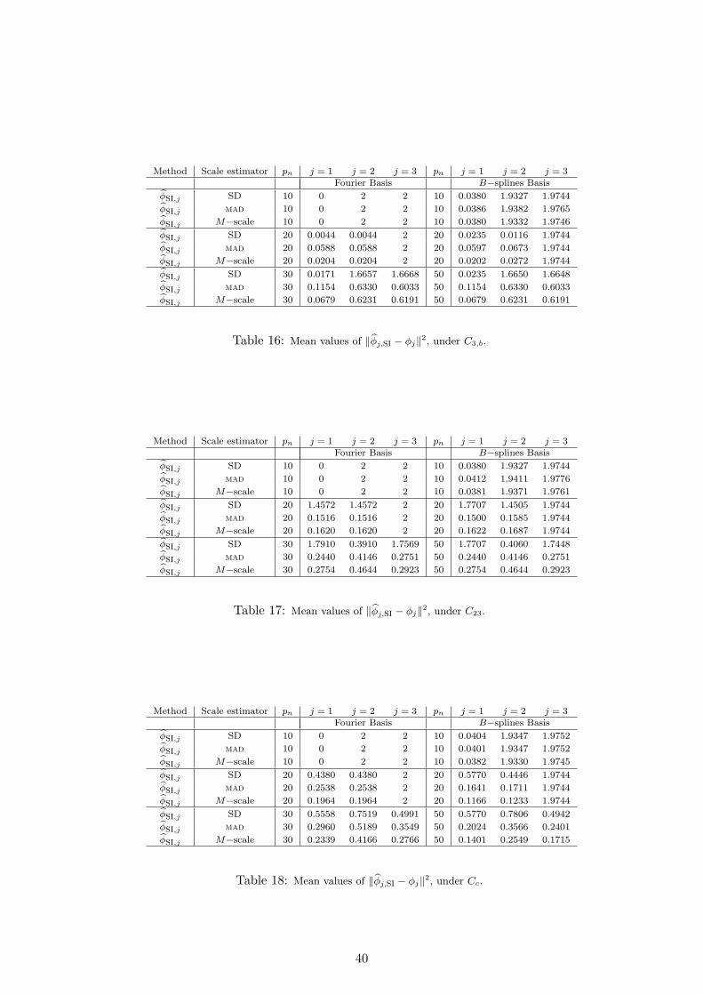
Method Scale estimator pn j = 1 j = 2 j = 3 pn j = 1 j = 2 j = 3Fourier Basis B−splines Basis

ϕsi,j SD 10 0 2 2 10 0.0380 1.9327 1.9744

ϕsi,j mad 10 0 2 2 10 0.0386 1.9382 1.9765

ϕsi,j M−scale 10 0 2 2 10 0.0380 1.9332 1.9746

ϕsi,j SD 20 0.0044 0.0044 2 20 0.0235 0.0116 1.9744

ϕsi,j mad 20 0.0588 0.0588 2 20 0.0597 0.0673 1.9744

ϕsi,j M−scale 20 0.0204 0.0204 2 20 0.0202 0.0272 1.9744

ϕsi,j SD 30 0.0171 1.6657 1.6668 50 0.0235 1.6650 1.6648

ϕsi,j mad 30 0.1154 0.6330 0.6033 50 0.1154 0.6330 0.6033

ϕsi,j M−scale 30 0.0679 0.6231 0.6191 50 0.0679 0.6231 0.6191

Table 16: Mean values of ∥ϕj,si − ϕj∥2, under C3,b.

Method Scale estimator pn j = 1 j = 2 j = 3 pn j = 1 j = 2 j = 3Fourier Basis B−splines Basis

ϕsi,j SD 10 0 2 2 10 0.0380 1.9327 1.9744

ϕsi,j mad 10 0 2 2 10 0.0412 1.9411 1.9776

ϕsi,j M−scale 10 0 2 2 10 0.0381 1.9371 1.9761

ϕsi,j SD 20 1.4572 1.4572 2 20 1.7707 1.4505 1.9744

ϕsi,j mad 20 0.1516 0.1516 2 20 0.1500 0.1585 1.9744

ϕsi,j M−scale 20 0.1620 0.1620 2 20 0.1622 0.1687 1.9744

ϕsi,j SD 30 1.7910 0.3910 1.7569 50 1.7707 0.4060 1.7448

ϕsi,j mad 30 0.2440 0.4146 0.2751 50 0.2440 0.4146 0.2751

ϕsi,j M−scale 30 0.2754 0.4644 0.2923 50 0.2754 0.4644 0.2923

Table 17: Mean values of ∥ϕj,si − ϕj∥2, under C23.

Method Scale estimator pn j = 1 j = 2 j = 3 pn j = 1 j = 2 j = 3Fourier Basis B−splines Basis

ϕsi,j SD 10 0 2 2 10 0.0404 1.9347 1.9752

ϕsi,j mad 10 0 2 2 10 0.0401 1.9347 1.9752

ϕsi,j M−scale 10 0 2 2 10 0.0382 1.9330 1.9745

ϕsi,j SD 20 0.4380 0.4380 2 20 0.5770 0.4446 1.9744

ϕsi,j mad 20 0.2538 0.2538 2 20 0.1641 0.1711 1.9744

ϕsi,j M−scale 20 0.1964 0.1964 2 20 0.1166 0.1233 1.9744

ϕsi,j SD 30 0.5558 0.7519 0.4991 50 0.5770 0.7806 0.4942

ϕsi,j mad 30 0.2960 0.5189 0.3549 50 0.2024 0.3566 0.2401

ϕsi,j M−scale 30 0.2339 0.4166 0.2766 50 0.1401 0.2549 0.1715

Table 18: Mean values of ∥ϕj,si − ϕj∥2, under Cc.

40

j=

1j=

2j=

3

sd

0.0

0.5

1.0

1.5

2.0

0.00.51.01.52.02.5

0.0

0.5

1.0

1.5

2.0

0.00.51.01.52.02.5

0.0

0.5

1.0

1.5

2.0

0.00.51.01.52.02.5

mad

0.0

0.5

1.0

1.5

2.0

0.00.51.01.52.02.5

0.0

0.5

1.0

1.5

2.0

0.00.51.01.52.0

0.0

0.5

1.0

1.5

2.0

0.00.51.01.52.0

M−sc

ale

0.0

0.5

1.0

1.5

2.0

0.00.51.01.52.02.5

0.0

0.5

1.0

1.5

2.0

0.00.51.01.52.02.5

0.0

0.5

1.0

1.5

2.0

0.00.51.01.52.02.5

Figure

1:Density

estimates

ofC(ϕ

j,ϕ

j)withban

dwidth

0.6

when

usingtheraw

estimators.Theblack

lines

correspondto

C0,whilethose

inred,gray,blue,

greenan

dpinkcorrespon

dto

C2,C3,a,C3,b,C23andCc,respectively.

41

j=

1j=

2j=

3

sd

0.0

0.5

1.0

1.5

2.0

0.00.51.01.52.02.5

0.0

0.5

1.0

1.5

2.0

0.00.51.01.52.02.5

0.0

0.5

1.0

1.5

2.0

0.00.51.01.52.02.5

mad

0.0

0.5

1.0

1.5

2.0

0.00.51.01.52.02.5

0.0

0.5

1.0

1.5

2.0

0.00.51.01.52.0

0.0

0.5

1.0

1.5

2.0

0.00.51.01.52.02.5

M−sc

ale

0.0

0.5

1.0

1.5

2.0

0.00.51.01.52.02.5

0.0

0.5

1.0

1.5

2.0

0.00.51.01.52.02.5

0.0

0.5

1.0

1.5

2.0

0.00.51.01.52.02.5

Figure

2:Density

estimates

ofC(ϕ

j,ϕ

j)withban

dwidth

0.6when

usingthescale–penalizedestimators,ϕps,j,withapenalizationofλ=

1.50n−3.

Theblack

lines

correspon

dto

C0,whilethosein

red,gray,blue,

green

andpinkcorrespondto

C2,C3,a,C3,b,C23andCc,respectively.

42

j=

1j=

2j=

3

sd

0.0

0.5

1.0

1.5

2.0

0.00.51.01.52.02.5

0.0

0.5

1.0

1.5

2.0

0.00.51.01.52.02.5

0.0

0.5

1.0

1.5

2.0

0.00.51.01.52.0

mad

0.0

0.5

1.0

1.5

2.0

0.00.51.01.52.02.5

0.0

0.5

1.0

1.5

2.0

0.00.51.01.52.0

0.0

0.5

1.0

1.5

2.0

0.00.20.40.60.81.01.21.4

M−sc

ale

0.0

0.5

1.0

1.5

2.0

0.00.51.01.52.02.5

0.0

0.5

1.0

1.5

2.0

0.00.51.01.52.02.5

0.0

0.5

1.0

1.5

2.0

0.00.51.01.52.0

Figure

3:Density

estimates

ofC(ϕ

j,ϕ

j)withban

dwidth

0.6

when

usingthenorm

–penalizedestimators,ϕpn,j,withapenalizationofλ=

0.75

n−3.Theblack

lines

correspon

dto

C0,whilethosein

red,gray,

blue,

green

andpinkcorrespondto

C2,C3,a,C3,b,C23andCc,respectively.

43

j=

1j=

2j=

3

sd

0.0

0.5

1.0

1.5

2.0

0.00.51.01.52.02.5

0.0

0.5

1.0

1.5

2.0

0.00.51.01.52.02.5

0.0

0.5

1.0

1.5

2.0

0.00.51.01.52.02.5

mad

0.0

0.5

1.0

1.5

2.0

0.00.51.01.52.02.5

0.0

0.5

1.0

1.5

2.0

0.00.51.01.52.02.5

0.0

0.5

1.0

1.5

2.0

0.00.51.01.52.02.5

M−sc

ale

0.0

0.5

1.0

1.5

2.0

0.00.51.01.52.02.5

0.0

0.5

1.0

1.5

2.0

0.00.51.01.52.02.5

0.0

0.5

1.0

1.5

2.0

0.00.51.01.52.02.5

Figure

4:Density

estimates

ofC(ϕ

j,ϕ

j)withban

dwidth

0.6

fortheestimators

ϕsi,j

defined

in(10),

when

pn=

10usingtheFourier

Basis.

Theblack

lines

correspon

dto

C0,whilethosein

red,gray,blue,

green

andpinkcorrespondto

C2,C3,a,C3,b,C23andCc,respectively.

44

j=

1j=

2j=

3

sd

0.0

0.5

1.0

1.5

2.0

0.00.51.01.52.02.5

0.0

0.5

1.0

1.5

2.0

0.00.51.01.52.02.5

0.0

0.5

1.0

1.5

2.0

0.00.51.01.52.02.5

mad

0.0

0.5

1.0

1.5

2.0

0.00.51.01.52.02.5

0.0

0.5

1.0

1.5

2.0

0.00.51.01.52.02.5

0.0

0.5

1.0

1.5

2.0

0.00.51.01.52.02.5

M−sc

ale

0.0

0.5

1.0

1.5

2.0

0.00.51.01.52.02.5

0.0

0.5

1.0

1.5

2.0

0.00.51.01.52.02.5

0.0

0.5

1.0

1.5

2.0

0.00.51.01.52.02.5

Figure

5:Density

estimates

ofC(ϕ

j,ϕ

j)withban

dwidth

0.6

fortheestimators

ϕsi,j

defined

in(10),

when

pn=

20usingtheFourier

Basis.

Theblack

lines

correspon

dto

C0,whilethosein

red,gray,blue,

green

andpinkcorrespondto

C2,C3,a,C3,b,C23andCc,respectively.

45

j=

1j=

2j=

3

sd

0.0

0.5

1.0

1.5

2.0

0.00.51.01.52.02.5

0.0

0.5

1.0

1.5

2.0

0.00.51.01.52.02.5

0.0

0.5

1.0

1.5

2.0

0.00.51.01.52.02.5

mad

0.0

0.5

1.0

1.5

2.0

0.00.51.01.52.02.5

0.0

0.5

1.0

1.5

2.0

0.00.51.01.52.0

0.0

0.5

1.0

1.5

2.0

0.00.51.01.52.0

M−sc

ale

0.0

0.5

1.0

1.5

2.0

0.00.51.01.52.02.5

0.0

0.5

1.0

1.5

2.0

0.00.51.01.52.02.5

0.0

0.5

1.0

1.5

2.0

0.00.51.01.52.02.5

Figure

6:Density

estimates

ofC(ϕ

j,ϕ

j)withban

dwidth

0.6

fortheestimators

ϕsi,j

defined

in(10),

when

pn=

30usingtheFourier

Basis.

Theblack

lines

correspon

dto

C0,whilethosein

red,gray,blue,

green

andpinkcorrespondto

C2,C3,a,C3,b,C23andCc,respectively.

46

j=

1j=

2j=

3

sd

0.0

0.5

1.0

1.5

2.0

0.00.51.01.52.02.5

0.0

0.5

1.0

1.5

2.0

0.00.51.01.52.02.5

0.0

0.5

1.0

1.5

2.0

0.00.51.01.52.02.5

mad

0.0

0.5

1.0

1.5

2.0

0.00.51.01.52.02.5

0.0

0.5

1.0

1.5

2.0

0.00.51.01.52.0

0.0

0.5

1.0

1.5

2.0

0.00.51.01.52.02.5

M−sc

ale

0.0

0.5

1.0

1.5

2.0

0.00.51.01.52.02.5

0.0

0.5

1.0

1.5

2.0

0.00.51.01.52.02.5

0.0

0.5

1.0

1.5

2.0

0.00.51.01.52.02.5

Figure

7:Density

estimates

ofC(ϕ

j,ϕ

j)when

thepenalizationτis

selected

via

K−fold

Cross–validationandthescale–penalizedestimators,

ϕps,j,areused.Theblack

lines

correspon

dto

C0,whilethose

inred,gray,

blue,

green

andpinkcorrespondto

C2,C3,a,C3,b,C23andCc,

respectively.

47

C0

C2

C3,a

SD

MA

DM

SS

D P

S 1

.5M

AD

PS

1.5

MS

PS

1.5

SD

PN

.75

MA

D P

N .7

5M

S P

N .7

5

0.51.01.52.0

SD

MA

DM

SS

D P

S 1

.5M

AD

PS

1.5

MS

PS

1.5

SD

PN

.75

MA

D P

N .7

5M

S P

N .7

5

0.51.01.52.0

SD

MA

DM

SS

D P

S 1

.5M

AD

PS

1.5

MS

PS

1.5

SD

PN

.75

MA

D P

N .7

5M

S P

N .7

5

0.51.01.52.0

C3,b

C23

Cc

SD

MA

DM

SS

D P

S 1

.5M

AD

PS

1.5

MS

PS

1.5

SD

PN

.75

MA

D P

N .7

5M

S P

N .7

5

0.51.01.52.0

SD

MA

DM

SS

D P

S 1

.5M

AD

PS

1.5

MS

PS

1.5

SD

PN

.75

MA

D P

N .7

5M

S P

N .7

5

0.51.01.52.0

SD

MA

DM

SS

D P

S 1

.5M

AD

PS

1.5

MS

PS

1.5

SD

PN

.75

MA

D P

N .7

5M

S P

N .7

5

0200040006000800010000

Cc

MA

DM

SM

AD

PS

1.5

MS

PS

1.5

MA

D P

N .7

5M

S P

N .7

5

1.01.52.02.5

Figure

8:Box

plots

oftheratioλ1/λ1fortheraw

andpenalizedestimators.

48

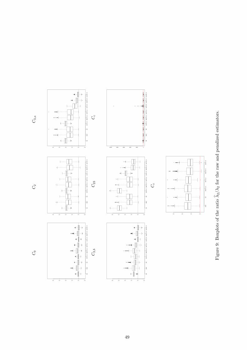
C0

C2

C3,a

SD

MA

DM

SS

D P

S 1

.5M

AD

PS

1.5

MS

PS

1.5

SD

PN

.75

MA

D P

N .7

5M

S P

N .7

5

0.51.01.52.02.53.0

SD

MA

DM

SS

D P

S 1

.5M

AD

PS

1.5

MS

PS

1.5

SD

PN

.75

MA

D P

N .7

5M

S P

N .7

5

0.51.01.52.02.53.0

SD

MA

DM

SS

D P

S 1

.5M

AD

PS

1.5

MS

PS

1.5

SD

PN

.75

MA

D P

N .7

5M

S P

N .7

5

0.51.01.52.02.53.0

C3,b

C23

Cc

SD

MA

DM

SS

D P

S 1

.5M

AD

PS

1.5

MS

PS

1.5

SD

PN

.75

MA

D P

N .7

5M

S P

N .7

5

0.51.01.52.02.53.0

SD

MA

DM

SS

D P

S 1

.5M

AD

PS

1.5

MS

PS

1.5

SD

PN

.75

MA

D P

N .7

5M

S P

N .7

5

0.51.01.52.02.53.0

SD

MA

DM

SS

D P

S 1

.5M

AD

PS

1.5

MS

PS

1.5

SD

PN

.75

MA

D P

N .7

5M

S P

N .7

5

0200040006000800010000

Cc

MA

DM

SM

AD

PS

1.5

MS

PS

1.5

MA

D P

N .7

5M

S P

N .7

5

1.01.52.02.5

Figure

9:Box

plots

oftheratioλ2/λ2fortheraw

andpenalizedestimators.

49

C0

C2

C3,a

SD

MA

DM

SS

D P

S 1

.5M

AD

PS

1.5

MS

PS

1.5

SD

PN

.75

MA

D P

N .7

5M

S P

N .7

5

012345

SD

MA

DM

SS

D P

S 1

.5M

AD

PS

1.5

MS

PS

1.5

SD

PN

.75

MA

D P

N .7

5M

S P

N .7

5

012345

SD

MA

DM

SS

D P

S 1

.5M

AD

PS

1.5

MS

PS

1.5

SD

PN

.75

MA

D P

N .7

5M

S P

N .7

5

012345

C3,b

C23

Cc

SD

MA

DM

SS

D P

S 1

.5M

AD

PS

1.5

MS

PS

1.5

SD

PN

.75

MA

D P

N .7

5M

S P

N .7

5

012345

SD

MA

DM

SS

D P

S 1

.5M

AD

PS

1.5

MS

PS

1.5

SD

PN

.75

MA

D P

N .7

5M

S P

N .7

5

012345

SD

MA

DM

SS

D P

S 1

.5M

AD

PS

1.5

MS

PS

1.5

SD

PN

.75

MA

D P

N .7

5M

S P

N .7

5

05000100001500020000

Cc

MA

DM

SM

AD

PS

1.5

MS

PS

1.5

MA

D P

N .7

5M

S P

N .7

5

0.51.01.52.02.53.03.5

Figure

10:Box

plots

oftheratioλ3/λ3fortheraw

andpenalizedestimators.

50

C0

C2

C3,a

SD

10M

AD

10M

−S

C10

SD

20M

AD

20M

−S

C20

SD

30M

AD

30M

−S

C30

1.01.52.0

SD

10M

AD

10M

−S

C10

SD

20M

AD

20M

−S

C20

SD

30M

AD

30M

−S

C30

1.01.52.0

SD

10M

AD

10M

−S

C10

SD

20M

AD

20M

−S

C20

SD

30M

AD

30M

−S

C30

1.01.52.0

C3,b

C23

Cc

SD

10M

AD

10M

−S

C10

SD

20M

AD

20M

−S

C20

SD

30M

AD

30M

−S

C30

1.01.52.0

SD

10M

AD

10M

−S

C10

SD

20M

AD

20M

−S

C20

SD

30M

AD

30M

−S

C30

1.01.52.0

SD

10M

AD

10M

−S

C10

SD

20M

AD

20M

−S

C20

SD

30M

AD

30M

−S

C30

020040060080010001200

Cc

MA

D10

M−

SC

10M

AD

20M

−S

C20

MA

D30

M−

SC

30

0.00.51.01.52.02.5

Figure

11:Box

plots

oftheratioλ1/λ1forthesieveestimators

when

usingtheFourier

basis.

51

C0

C2

C3,a

SD

10M

AD

10M

−S

C10

SD

20M

AD

20M

−S

C20

SD

30M

AD

30M

−S

C30

0.00.51.01.52.02.53.0

SD

10M

AD

10M

−S

C10

SD

20M

AD

20M

−S

C20

SD

30M

AD

30M

−S

C30

0.00.51.01.52.02.53.0

SD

10M

AD

10M

−S

C10

SD

20M

AD

20M

−S

C20

SD

30M

AD

30M

−S

C30

0.00.51.01.52.02.53.0

C3,b

C23

Cc

SD

10M

AD

10M

−S

C10

SD

20M

AD

20M

−S

C20

SD

30M

AD

30M

−S

C30

0.00.51.01.52.02.53.0

SD

10M

AD

10M

−S

C10

SD

20M

AD

20M

−S

C20

SD

30M

AD

30M

−S

C30

0.00.51.01.52.02.53.0

SD

10M

AD

10M

−S

C10

SD

20M

AD

20M

−S

C20

SD

30M

AD

30M

−S

C30

050100150

Cc

MA

D10

M−

SC

10M

AD

20M

−S

C20

MA

D30

M−

SC

30

0.00.51.01.52.02.5

Figure

12:Box

plots

oftheratioλ2/λ2forthesieveestimators

when

usingtheFourier

basis.

52

C0

C2

C3,a

SD

10M

AD

10M

−S

C10

SD

20M

AD

20M

−S

C20

SD

30M

AD

30M

−S

C30

01234567

SD

10M

AD

10M

−S

C10

SD

20M

AD

20M

−S

C20

SD

30M

AD

30M

−S

C30

01234567

SD

10M

AD

10M

−S

C10

SD

20M

AD

20M

−S

C20

SD

30M

AD

30M

−S

C30

01234567

C3,b

C23

Cc

SD

10M

AD

10M

−S

C10

SD

20M

AD

20M

−S

C20

SD

30M

AD

30M

−S

C30

01234567

SD

10M

AD

10M

−S

C10

SD

20M

AD

20M

−S

C20

SD

30M

AD

30M

−S

C30

01234567

SD

10M

AD

10M

−S

C10

SD

20M

AD

20M

−S

C20

SD

30M

AD

30M

−S

C30

020406080

Cc

MA

D10

M−

SC

10M

AD

20M

−S

C20

MA

D30

M−

SC

30

0246

Figure

13:Box

plots

oftheratioλ3/λ3forthesieveestimators

when

usingtheFourier

basis.

53