WP3000: Toolbox functionality & Algorithm Specification - ESA ...

Deliverable: WP3000:

“Toolbox Functionality and Algorithm Specification Document”

13 February 2007

GOCE User Toolbox Specifications (GUTS) DEVELOPMENT OF ALGORITHMS FOR THE GENERATION OF A GOCE USER TOOLBOX AND

AN ABSOLUTE DYNAMIC TOPOGRAPHY PRODUCT

Ref:

ESA/XGCE-DTEX-EOPS-SW-04-0001 “GOCE User Toolbox Specifications (GUTS)”

Coordinator: Per Knudsen (DNSC)

Deliverable: WP3000: “Toolbox Functionality and Algorithm Specification Document”

Responsible partner: Nansen Centre

Prepared by: Frank Siegismund and Helen Snaith

DOCUMENT CHANGE LOG Rev. Date Sections modified Comments Changed by

0 November 2006 All Draft submitted to ESA Helen Snaith

1 January 2007 All

Corrected reference list Responded to comments from reviewers Helen Snaith

2 February 2007 All

Response to ESA review and change inclusion of formal document material Helen Snaith

WP3000: Toolbox Functionality & Algorithm Specification

i

Table of Contents Table of Contents........................................................................................................................i

Summary of recommendations .................................................................................................iv

Applicable and Reference Documents.......................................................................................v

1 Determination of toolbox functionality ...............................................................................1

1.1 Introduction...................................................................................................................1

1.2 Review of User Toolbox requirements .........................................................................1

1.2.1 Basic functionality .................................................................................................1

1.2.2 Essential .................................................................................................................2

1.2.3 Highly desirable .....................................................................................................3

1.2.4 Desirable but lower priority ...................................................................................4

1.2.5 Functionality requiring extensive computing resources or not yet at consensus...4

1.2.6 Nice added features:...............................................................................................5

1.2.7 Functionality desirable at a future date..................................................................5

2 Pilot applications; determination of filter algorithms ..........................................................7

2.1 Introduction...................................................................................................................7

2.1.1 Filter types and methods ........................................................................................7

2.1.2 Filtering dynamic topography................................................................................8

2.1.3 Error estimates of filtered dynamic topography ....................................................8

2.2 Methods.........................................................................................................................9

2.2.1 Accuracy of filter method ......................................................................................9

2.2.2 Computational cost ..............................................................................................10

2.2.3 Omission error .....................................................................................................12

2.3 Results.........................................................................................................................13

2.3.1 Commission: Filtering the signal .........................................................................13

2.3.2 Effects of the omission error................................................................................18

2.4 Discussion and conclusion..........................................................................................22

3 Structuring functionality; defining workflows...................................................................25

3.1 Main workflow; supported input data.........................................................................26

3.2 Geoid and gravity field computation (synthesis) ........................................................28

3.3 Sea surface height and a-priori dynamic topography selection ..................................30

3.4 Satellite dynamic topography (MDTS) computation..................................................31


ii

3.4.1 Spatial MDTS (default for regional grids and user defined points).....................31

3.4.2 Spectral MDTS (default for global regular grids)................................................32

3.5 Remove-Restore “combined” (MDTC) techniques ....................................................34

3.5.1 Remove-Restore combined technique A .............................................................34

3.5.2 Remove-Restore combined technique B..............................................................36

3.6 Dynamic topography-derived quantities.....................................................................39

3.7 Pre-viewing function...................................................................................................40

4 Algorithm specification .....................................................................................................41

4.1 Conventions and definitions: ......................................................................................42

4.1.1 Standard variable name definitions:.....................................................................42

4.1.2 Conventions .........................................................................................................43

4.2 Algorithms for preference selection............................................................................44

GUT_FA01 selection of required degree and order of expansion................................44

GUT_FA02 Reference system selection:......................................................................46

GUT_FA03 tide system selection.................................................................................47

4.3 Computational algorithms...........................................................................................49

GUT_FA04 Geodetic field computation (SH synthesis) ..............................................49

GUT_FA05 Commission error determination (geoid) .................................................52

GUT_FA06 Omission error determination (geoid) ......................................................55

GUT_FA07 Average determination of SSH or DT ......................................................58

GUT_FA08 Grid adaptation .........................................................................................59

GUT_FA09 Linear filter (spatial).................................................................................60

GUT_FA10 Linear filter (Spherical Harmonic) ...........................................................61

GUT_FA11 Fill gaps on continent ...............................................................................63

GUT_FA12 SH analysis ...............................................................................................64

GUT_FA13 Surface current determination ..................................................................65

GUT_FA14 Difference or Sum of Gridded Fields .......................................................67

5 Input output definition .......................................................................................................68

5.1 Required Input Data files: to be included on the toolbox: ..........................................69

5.1.1 Geoid harmonic expansion (SH & error covariance products)............................69

5.1.2 Mean sea surface height field ..............................................................................69

5.1.3 Mean dynamic topography and associated error covariance products ................70

5.1.4 Sea level Anomaly fields .....................................................................................70


iii

5.1.5 Along track altimetric sea surface height fields...................................................70

5.1.6 Digital Terrain Model ..........................................................................................70

5.2 Optional User Supplied Input Data Files ....................................................................72

5.3 Output Data Formats...................................................................................................73

5.4 File Naming Conventions ...........................................................................................74

6 References............................................................................................................................v

Appendix A: Existing Software Packages ...............................................................................vii

HARMONIC_SYNTH (Version 05/01/2006).....................................................................vii

GRAVSOFT ........................................................................................................................xx

GeoCol .............................................................................................................................xx

GEOIP...........................................................................................................................xxix

HARMEXP..................................................................................................................xxxii

Sphgric ....................................................................................................................... xxxiii

sh_mdt.............................................................................................................................xxxvi


iv

Summary of recommendations We recommend that the first release of the GOCE User Toolbox should prioritise those products and functions, identified in the User Requirement Document [1] that relate to the oceanographic community. This should bring immediate benefit to a community currently unfamiliar with the use of gravity and geodetic products whilst providing basic functionality in support of all science areas. In particular, we recommend that the toolbox focus on the generation of dynamic topography fields, through merging satellite altimeter and GOCE gravity model data, this being a key objective of the GOCE mission.

The trade-off study, carried out in WP3300, investigated the efficiency and accuracy of filtering techniques, an essential part of the generation of dynamic topography fields due to the differences in resolved spatial scales between the altimeter and geodetic data. This study concluded that filtering data in spectral space, particularly in conjunction with a remove-restore technique, provided the best option for a current toolbox implementation. These recommendations are based on our current understanding and expected computational capacity. None of the proposed filtering options should be considered as optimal – they represent the current ‘best’ options within computational constraints and current research. The computational efficiency of the spectral vs spatial filtering, as determined in the trade-off study, assumed the toolbox had access to high levels of computer memory. This may not be true of a practical toolbox implementation, designed to run on more memory-limited systems.

We consider that generation of full variance and covariance data from the calculated geoid model is an important step in the use of GOCE data. However, we do not recommend that propagation of the full errors, from the spherical harmonic error covariances, should be carried out within the toolbox. This is primarily due to the high computational and storage space demands this would place on the toolbox. We recommend further investigation into the possibility of allowing such calculations to be carried out using remote, possibly GRID, computing facilities, using parameters determined from the toolbox.

It was recognised that for completeness, the GOCE User Toolbox could offer the user more sophisticated altimeter data access and manipulation facilities: such as generation of mean sea surfaces or generation of time series of absolute dynamic topography by merging mean dynamic topography and sea level anomaly. However, much of this functionality is provided within the existing BRAT (Basic Radar Altimeter Toolbox) and it is recommended that GUT be able to input altimeter products generated within BRAT, and provide output that be used within BRAT to provided these extended facilities.


v

Applicable and Reference Documents XGCE-DTEX-EOPS-SW-04-0001, Issue 1.3, Statement of Work

XGCE-DTEX-EOPS-SW-04-0001: Development of Algorithms for the Generation of a GOCE User Toolbox and an Absolute Dynamic Topography Product. Proposal in Response to ESA Request for Quotation. Issue 6, 14 December 2005.

GO-ID-HPF-GS-0041: Product Specification for L2 Products and Auxiliary Data Products, Issue 5.0, 28.08.2006

GO-TN-HPF-GS-0111: GOCE Standards. Issue: 2, 22 / 09 / 2006.

GO-MA-HPF-GS-0110: GOCE Level 2 Data Handbook, Issue 3, 22 / 09 / 2006.

GOCE User Toolbox : User Toolbox Requirement Document.


1

1 Determination of toolbox functionality

1.1 Introduction

This report is the output from WP3000 of the GOCE User Toolbox Specification. The study will select the best (in terms of accuracy and computational demands) algorithms to compute the variables listed in the user requirement document [1]. This document will form the basis for the system specification work performed in WP4000 and the prototype and tutorials to be generated in WP5000.

1.2 Review of User Toolbox requirements

The algorithm specification for GUT, as presented in this document, is based on the User Requirement consolidation, as described in [1]. However, determination of the functionality recommended for inclusion in the toolbox must also take into account the computational demands of the algorithms to fulfil the desired functionality and the accuracy that can be achieved by existing, available software, or algorithms that easily can be coded. Some of the algorithms needed for the desired functionality are subject to ongoing research and will not be part of the first release of the toolbox but might be included in later editions.

Since some of the required fields are necessary input for the computation of other products, while others are end products, the user requirements need also to be reviewed in terms of the logical structure of the computations in the toolbox before the provided functionality is determined.

A review of the user requirements has been carried out in order to rank the desired functionality and products. This will allow an evaluation of whether the first release of GUT meets the user requirements and where improvements will be needed.

In deciding on the functionality proposed for the first stage toolbox, we have used the priorities below in the first instance. In some cases, functionality that has been given a lower priority has still been included in the proposed functionality, as the practical decisions on how to incorporate the functionality have a very small overhead in terms of software development. For example, in some cases, existing software that provides high priority functions will also provide the additional functionality with no additional development.

1.2.1 Basic functionality From the user requirements, as determined in the user requirements document, it is imperative, for all applications (geodesy, oceanography and solid earth applications) that the absolute minimal requirement of the toolbox includes:

• Computation of global, gridded geoid heights at a given, user-specified, degree and order of the spherical harmonic expansion (i.e., at a given spatial resolution). User input would be the spatial resolution of the grid and the maximum degree and order of the expansion. Output would be a grid of single-point representations of the geoid.

• Computation of geoid heights at a given spatial resolution (i.e. specified degree and order of the spherical harmonic expansion) at a given point or list of points (e.g. unstructured grid, transect). Input would be a list of user-specified geographic position parameters and


2

the maximum degree and order of the expansion. Output would be the geoid field interpolated to the specified positions.

This essential, basic functionality is required for application of the GOCE data to all scientific areas. At this early stage in the development of the toolbox, we expect that priority should be given to the needs of the oceanographic community in determining the algorithms to be included in the toolbox:

1) The oceanographic community have least experience in the use of gravity information and therefore have the greatest need for support in the use of these data.

2) The oceanographic community provide the largest potential group of users, who have well defined scientific questions and are organised to address these questions, and who would benefit from a toolbox, even of limited functionality.

In the following sections of the document, higher priority has been given to those toolbox functions and algorithms required by the oceanographic community, as identified in the User Requirement Document [1]. In order to provide a toolbox that will generate products that are more than the gridded level 2 products that are generated by the HPF, the toolbox must address at least one application of the data. We consider that the most widely applicable toolbox output is the generation of dynamic topography products to allow the exploration of absolute surface currents – a primary mission aim of the GOCE project.

1.2.2 Essential In addition to the functionality given above, these user functions and products are considered essential outputs of any GOCE user Toolbox, without which, the toolbox would provide no significant advantage over the existing level 2 products.

• Provision of a priori MSSH, MDT and geoid data on a grid

• Computation of a ‘GOCE’ MDT (MSSH-GOCE geoid) at a given spatial resolution and on a given structured or unstructured grid as the difference between the MSSH and the geoid

• Spatial filtering of MSSH consistent with a specific harmonic geoid height field expansion. This includes spectral space filtering of the MSSH.


3

1.2.3 Highly desirable In order for the toolbox to provide functionality that will support a wide range of users and cover the use-cases identified in the URD [1], it is strongly recommended that all of the functions and products identified in this section are implemented,

• Computation of global, gridded gravity anomalies at a given, user-specified, degree and order of the spherical harmonic expansion (i.e., at a given spatial resolution). User input would be the spatial resolution or the grid and the maximum degree and order of the expansion. Output would be gridded gravity anomalies.

• Option to replace geoid heights by geoid slopes (deflection from the vertical) for either the gridded field or the unstructured positions

• The gridded fields should be available as both a single point representation and as area averages

• Change of reference system for the geoid and/or MSSH (reference ellipsoid, tide system)

• Computation of altimetric time-varying absolute dynamic topography as the difference between altimetric fields and a geoid model.

• Interpolation of external MSSH on any regular grid or at given points (unstructured grid, transects etc): This functionality should include procedures to translate (synthesize) and adapt the spherical harmonic information into geoid height information for any location in the world

• If several different geoid fields are available, either within the toolbox or by inclusion of external data fields, input to the calculation of both geoid and gravity anomalies would also be the choice of geoid model or gravity field.

• Handle appropriate ancillary data, e.g., external MDT from ocean in situ/modelled, as well as local geoids, combined CHAMP/GRACE/GOCE geoids, among others

• Provision of tools to produce a global description of a combination of a priori gridded fields (e.g. provided or external MDT, provided or external geoids etc) in spherical harmonics

• Computation of geoid heights, gravity anomalies or deflections of the vertical at a given, user-specified, degree and order of the spherical harmonic expansion (i.e., at a given spatial resolution) at the surface of the terrain. Output would be a grid or as single point representations, and as area averages

• Pre-viewing capabilities for results from the toolbox

• Must be able to select and display a 2D plot of any gridded field or transect calculated or provided within the toolbox (geoid height, MDT, MSSH etc).

• Should display at least 2 fields side by side – e.g. if remove-restore techniques used, select to display the replaced and smoothed residual fields


4

1.2.4 Desirable but lower priority The following functions and products have been identified as providing useful additions to the toolbox, should it be possible to incorporate them. However, their exclusion would not pose a significant threat to the viability of the toolbox and its usage as they represent 'standard' procedures that can be carried out by users outside the toolbox.

• Compute differences / Root Mean Square differences / correlation coefficient / regression slopes between GOCE geoid and external geoids / ‘GOCE’ MDT and external MDT / between absolute altimetric dynamic topography and in-situ absolute dynamic topography / between absolute altimetric geostrophic velocities and in situ geostrophic velocities

• Computation of absolute geostrophic velocities from the spatial gradients of the dynamic topography field

• Extra viewing features

• select and display subsets and transects of data

• display statistical information – eg root mean square differences

• display spectral plots – will need to be calculated elsewhere

1.2.5 Functionality requiring extensive computing resources or not yet at consensus

Whilst computation of the full error covariance matrix for a grid or specified points, and calculation of the cumulative height errors of the geoid height, gravity anomalies and deflections of the vertical, is possible using the algorithms defined in the URD, calculating these values requires access to, and manipulation of, the full spherical harmonic variance / covariance matrices. This would require extensive computational resources, beyond those anticipated as being required to run a toolbox. As such, it has been decided not to include this calculation in a first release of the toolbox.

These computations become important when developing optimal filtering techniques, particularly in combination with the full error covariance information for the input MSSH and a priori dynamic topography fields. Within this project, there has been insufficient time to investigate the possible effect of using of a reduced, block diagonal of the full error covariances, or further investigation in how to make use of the covariances. This should be a priority for further research to inform later releases of the toolbox. AT this stage, calculation of error covariances should be from interpolation of the GOCE level 2 gridded product.

• Computation of geoid heights covariance for any pair of points on the reference ellipsoid or the computation of a full covariance matrix for a given degree and order of the spherical harmonic expansion

• Computation of geoid cumulative height errors and error covariances at a given spatial resolution on a global regular grid or for a list of points. For a regional grid we must introduce the concept of the harmonically downward continued geoid

• Computation of geoid cumulative errors and error covariances associated with geoid heights, gravity anomalies or deflections of the vertical at a given, user-specified, degree and order of the spherical harmonic expansion at a given spatial resolution on a global


5

regular grid or for a list of points. Note: - the level 2 GOCE product, EGM_GER_2, will provide the geoid errors of the delivered gridded geoid heights, EGM_GEO_2. These will be a computationally less demanding way of providing error fields for some of the products that GUT will deliver.

• Covariance error matrix within a chosen degree and order range for commission and with the option of including a model for the omission errors for the GOCE gravity field.

• Determine the parameters in a priori degree variance model for the modelling of the gravity field a priori spectrum (global and/or regional models)

The following functionality would require extra research effort, beyond that available within this project, to inform recommendations for methods of implementation.

• Derive a degree variance model for the MDT and determine statistical properties of the MDT and its associated geostrophic surface currents

• Covariance error matrix within chosen degree and order range for commission and omission error for mean dynamic surface topographies. This needs to include the auxiliary altimetric error covariances on top of the geoid model error covariance

• Option to include the omission errors for the MDT and the associated geostrophic surface currents.

• Derive an optimal filter for the low pass filtering of the altimetric MSSH and/or the MDT derived from the altimetric MSSH and the GOCE geoid.

1.2.6 Nice added features: • data access and the possibility to transfer appropriate data from remote location to local

machine

Must give user the instructions for how to do this if not included in the functionality of the toolbox

1.2.7 Functionality desirable at a future date The User Requirement document suggested some potential toolbox functions that would, ideally, be included, but which at this stage are too immature in terms of application of the underlying science by the wider community.

Examples are:

• Regional geoid solutions starting from the global products. This is not ideal for regional geoid implementation. At a later stage, Level 1b data might be required as the basis for an extended GOCE geoid. Concerning regional geoids, a combination of model solutions using both GOCE and in situ gravity data [2] could be useful and including such regional models for the European Seas would be a useful element of GUTS.

• Methods for dealing with regional geoids and in situ gravity data are often based on a remove-restore algorithm and this would be a sensible extension of this aspect of the GUTS toolbox at a later date.


6

As updates to the GOCE geoid are made available, future releases should include the most recent gridded geoid product from GOCE.

The default MDT should be updated to be consistent with the GOCE geoid used by default in the toolbox.


7

2 Pilot applications; determination of filter algorithms The scientific trade-off study focuses on the different filtering methods. The effect of different filters on the accuracy of the solution is studied along with the computational cost and the cost of implementation of the filters. Other factors in evaluating different filters include their general applicability and their priority, based on known qualities of the individual filters. The results of this study have been used to determine the default filtering and dynamic topography methods in the functionality and algorithm sections.

2.1 Introduction

2.1.1 Filter types and methods For a first classification we differentiate between three types of filters:

geographical space filters: These filters involve a kernel K(x,x') that is convolved with the original field ηD(x') to give the filtered field ηD x( )= K x, ′x( )∫ ηD ′x( )d ′x . Different kernel functions are available, among them a spherical cap, a rectangular cap, a Gaussian or quasi-Gaussian cap, Hanning and Hamming windows.

spectral space filters: Here the field ηD is transformed into coefficients of a suitable expansion; in the current case only spherical harmonic functions Yn(x) of degree and order n=(l,m) are considered. The spectral expansion sn(ηD) is then modified according to the filter kernel Kn and the filtered field is η x( )= KnsnYn x( )

n∑ . The most popular kernel functions are the Pellinen filter (equivalent to a spherical cap in geographical space), a quasi-Gaussian filter (the exact transform of the quasi-Gaussian in geographical space [3]), and a simple boxcar filter (Dirichlet window). The latter has undesirable properties in the geographical space domain.

optimal filters: Optimal interpolation or collocation techniques are used to find the filter kernel as the solution of minimizing an objective function of the type J = ηD − η( ) CD

−1 ηD − η( )+ ηB − η( ) CB−1 ηB − ηT T ( ). This solution is the average

between the original field and a prior estimate ηB weighted by the inverses of the error covariances C

B

D/B associated with the input fields: η = CD−1 + CB

−1( ) CD−1ηD + CB

−1ηB(−1 ). Both and ηCB

−1BB can be zero, resulting in different properties of the solution.

When these linear filters are applied to the full fields directly, we will refer to the method as direct filtering.

In the second approach, the so-called remove-restore (RR) technique, the direct filtering is replaced by combining a prior guess ηB with a filtered residual: with F being some linear filter. In the context of combining a geoid model with altimetric sea surface height (SSH), the residual will be taken between the geoid model and a to-be-constructed “background” geoid model.

B η = ηB + FT ηD − ηB( )T


8

−1

2.1.2 Filtering dynamic topography In the case of filtering dynamic topographies, these are the criteria, that are used to evaluate a filter

• accuracy (distance from a reference solution), formal error description (with or without omission error) and comparison with reference data (to be specified)

• universality (can the filter be used on irregular grids, individual point pairs, etc.?)

• computational cost (CPU time and memory requirements: difficult because these depend strongly on the implementation of the filter)

• cost of implementation (we can only roughly estimate that, e.g. this filter is simple to implement, this filter is available as a prototype, etc ...)

• simplicity in terms of usage (how many parameters are there, e.g., just the maximum degree cut-off or a full error covariance matrix that needs to be specified by the user)

• necessity of having the filter (e.g., do we need an ”optimal” filter?)

Each filter can get a “grade” in each category. The overall “grade” has to be a weighted average of the individual “grades”, where the weights reflect the importance of the individual categories (e.g. is cost of implementation more important than accuracy?).

Technically speaking, we construct a benchmark system which is simple enough, so that all filters can be run within it and complicated enough so that it represents enough features of a real ocean dynamic topography problem. Here we have the choice of using ”real” data, or purely synthetic data, that is, numerical model results that are modified to represent geoid and altimetry data. The advantage of the former is that we are immediately faced with all the difficulties that one normally has with real data and can take these difficulties into account while evaluating the filters. The disadvantage is the same. Using synthetic data and using identical twin experiments enables us to know the results a priori and we can control the biases. We choose the latter approach.

2.1.3 Error estimates of filtered dynamic topography For any filtering method, the filtered field should be associated with an error estimate that is computed in a way consistent with the errors of the original fields and/or prior guesses. In principle this can be achieved by filtering the error covariances CD associated with the input field ηD:

(1) C = FT CDF

To take this a step further, the filtering result itself should implicitly include the prior error estimates. Only the optimal filters do this in a straightforward way (see above). For the optimal filter the posterior error can also be computed rigorously as , in principle. In practice, both the optimal filter and its error estimate is computationally extraordinarily expensive, and approximate methods may be used. Also, reliable estimates of the prior errors C

C = CD−1 + CB

−1( )

B are not available. Although, as the name implies, this method is “optimal”, finding efficient and accurate filters based on this approach is the subject of research and can only be considered as a future part of the GOCE User Toolbox.

B


9

In constructing a (spectral) geoid model, one truncates the spectrum at a certain degree L, usually where the signal to noise ratio exceeds unity. For all degrees (and orders) ≤ L one has the coefficients of the model along with their error co-variances (the commission error) from the collocation process. The signal for degrees > L is not modeled, but it is identified as the omitted signal or omission error. Different models for the omission error exist, but they all have in common, that the omission error is finite, although it can be large depending on the cut-off degree L. The omission error poses a problem when one wishes to construct a dynamic topography (DT) from SSH minus geoid model. It is vital that the scales that are suppressed by the chosen filtering algorithm and therefore become “omission” are matched identically in the SSH and in the geoid. It is very easy to cause aliasing if for the SSH and the geoid model, the represented scales are slightly different (especially at low resolution), because these fields are usually computed with different “basis” functions (grid vs. spherical harmonic functions).

For computing the errors associated with a filtered mean dynamic topography (MDT), the omission error may become an issue that needs to be dealt with. Usually, the geoid model has a lower resolution than the SSH, so the geoid omission error is larger (reaches down to larger scales). The error spectrum of geoid models is blue, that is, errors are very small for small degrees and orders of magnitude larger for degrees near the cut-off degree L. For degrees > L the error is omission error and tapers off according to the chosen omission error model. Previous research [4] has shown that a considerable portion of the omission error can leak into the commission error of the filtered signal, if the involved transformation involves dramatically different basis functions (Legendre function vs. trigonometric functions, spherical harmonics on the sphere vs. eigenfunctions of the error covariance along a hydrographic section).

2.2 Methods

2.2.1 Accuracy of filter method First let us introduce some terminology: The dynamic topography ηD, mean or instantaneous, is the difference between the altimetric sea surface h, (mean or instantaneous) over a reference ellipsoid,, and the geoid height ND, over the same reference ellipsoid, so that ηD = h − ND (2)

The index D stands for data (observations). Because h and ND do not contain the same spatial scales it is common to introduce the (linear) filter (matrix) FT:

η = FT h − ND( ) (3)

Eq. (3) comprises the first method (the direct method) of obtaining a dynamic topography η. The assumption is that the filtering must ensure that the omitted scales in h and ND match each other very closely because these fields vary 100 times more than the residual η.

The second method is called the remove-restore (RR) method and is based on the idea of adding a correction to a prior guess of the dynamic topography ηB, where the index B stands for the prior background. This background can be a high-resolution ocean model or observed dynamic topography. From this we construct a synthetic (background) geoid by

B


10

NB =ND over land

h − ηB over the ocean⎧⎨⎩

The RR-method then adds a (filtered) residual to the background value:

η = ηB +FT ηD − ηB ( )= ηB +FT NB − ND( ) (4)

Depending on the quality of the prior dynamic topography ηB we expect the RR-method to perform better than direct filtering, as additional independent information is used. It is again critical that the filtering ensure a close match of the omitted scales in the two geoids. Using the field h − N

B

D as prior ηBB, results (correctly) in no increment at all. Note that this is still not optimal unless information about the accuracy of the measurements and prior guess enter the algorithm through the filter definition.

With this machinery, we choose a ηT to be the “truth” and a high-resolution “true” geoid NT that also represents the background geoid NB over the ocean. In fact, NB T does not have to be very accurate on the short scales, so the EGM96 (L = 360, [5]) is sufficient. The “true” dynamic topography is a mean taken from a ¼˚ ocean model with data assimilation (OCCAM, Ocean Circulation and Climate Advanced Modelling Project [6, 7]).

The background dynamic topography is taken from a different ocean model with data assimilation (ECCO [8]) to take into account possible errors and biases is the prior during the RR-method. From Eq. (2) we estimate the altimetric measurement h = ηT + NT . To generate an “observed” geoid we remove short scales from NT by applying an appropriate filter G (see also Figure 1):

ND = GT NT

The measure of accuracy of the filter F is expressed as

ηT − FT h − ND( ) and ηT − ηB − FT NB − ND( ) (5)

for the direct method (Eq. 3) and the remove-restore technique (Eq. 4), respectively. || · || is an appropriate L2-norm, for example the root-mean-square (rms).

For testing purposes it is sufficient to use coarse resolution ocean model data (e.g. on a 1 degree grid), and use a “cut-off ” for the coarse-grained geoid ND of L = 70, which corresponds to a resolution (half-wavelength) of 2.5˚ (286 km) spherical distance. In two different cases the filter F is supposed to suppress scales above L = 45 and L = 25, corresponding to scales (half-wavelengths) of 445 km and 800 km, respectively.

For the remove-restore technique, one needs to take into account the error of the prior or background dynamic topography ηB. These errors can be substantial. As an example, we compare the mean dynamic topography η

B

BB of the ECCO2 product and the “truth” ηT of the OCCAM product. The mean dynamic topographies differ by as much as 1 m in the regions of strong topography gradients, that is, strong surface currents (see Figure 2). The rms-difference is 11 cm.

2.2.2 Computational cost Computational cost is estimated based on the used Matlab-code, which is designed for small problems, so that execution time can be favoured over memory requirements. For large


11

problems the algorithms may have to be modified in order to reduce memory requirements at the cost of computational speed. On the other hand, the algorithms used for the geographical filters leave some room for optimization for speed.

Figure 1: EGM96 geoid undulations on a 1˚ grid. Bottom: Smoothed geoid, pseudo-

observations


12

Figure 2: Top: Prior background dynamic topography used in this study. Bottom: Difference

of mean dynamic topography of two different ocean models

2.2.3 Omission error Filtering the error covariance, provided that there is one, is very expensive and time consuming. Therefore, we use an even coarser resolution (4˚, corresponding to 445 km) to test the effect of the omission error on the resulting filtered errors, bearing in mind that the issues with the omission error may increase with decreasing resolution. For geographical space filters it is important that the resulting errors are computed over the ocean only. For the spectral space filters the omission error of the geoid is partially suppressed, if the filter scale is larger than scales associated with the cut-off degree L, however the geoid omission errors created by spectral filtering will not exactly match those of a real space filter.


13

The total error covariance of the dynamic topography is the sum of the commission error covariance CL, the omission error Com and the error of the SSH CSSH. CSSH is taken to be diagonal for simplicity assuming a constant 5 cm error; one could introduce horizontal correlations, but for the current application with a maximum resolution of 445 km we consider the SSH error uncorrelated. For the geoid model we use a preliminary error covariance of the CHAMP mission [9], which is available to degree and order 60, corresponding to 335 km resolution (wavelength), so that our 4˚ grid can just not resolve the full geoid errors. (We can equally well use a covariance model such as that of [10]). We choose a commission cut-off of L = 20, corresponding to 1008 km half-wavelength, which can be resolved by the 4˚ grid. The error information on degrees L + 1 to 180/4 = 45 is then considered “omission” error, because our low-resolution geoid is truncated at L, but the computational (ocean model) grid resolves degree 45. This “omission” error has a cumulative degree variance corresponding to 13 cm. (For a realistic case with an expected resolution of GOCE of L = 200 corresponding to 100 km half wavelength, the target resolution of an ocean model could be 1/4˚, which corresponds to L = 720. The omission error from l = 201 to 720 can contribute to large scales mainly because its cumulative variance is on the order of 20 cm.) In our approach we neglect all omission error beyond the resolution of the computational grid. This error, which is still large, could be taken into account by evaluating the omission error on an even higher resolution grid and averaging it onto the target resolution. However, we assume, somewhat optimistically, that the omission errors of the geoid model and the errors due to grid resolution cancel.

Now we consider two cases: inclusion and exclusion of the omission error before filtering according to Eq. (1). If the filters remove short scales efficiently, the omission error should have little effect on the solution. However, if including the omission error leads to larger errors, particularly of large scale quantities such as the global mean dynamics topography, leakage from short geoid scales to large geographical scales is a problem and needs to be addressed. For the geographical space filters, leakage stems from evaluating the geoid model over the ocean only by applying a realistic land mask to the filter. For spectral space filters the omission error of the geoid can be filtered efficiently (in principle by a box car filter, which unfortunately has bad properties in geographical space), but in order to apply a spectral space filter, the SSH error needs to be transformed into spectral space according to:

Cn, ′nSSH = Y ′n ′x( )CSSH ′x , x( )Yn x( )dxd ′x∫∫

and here again the land mask may cause leakage.

2.3 Results

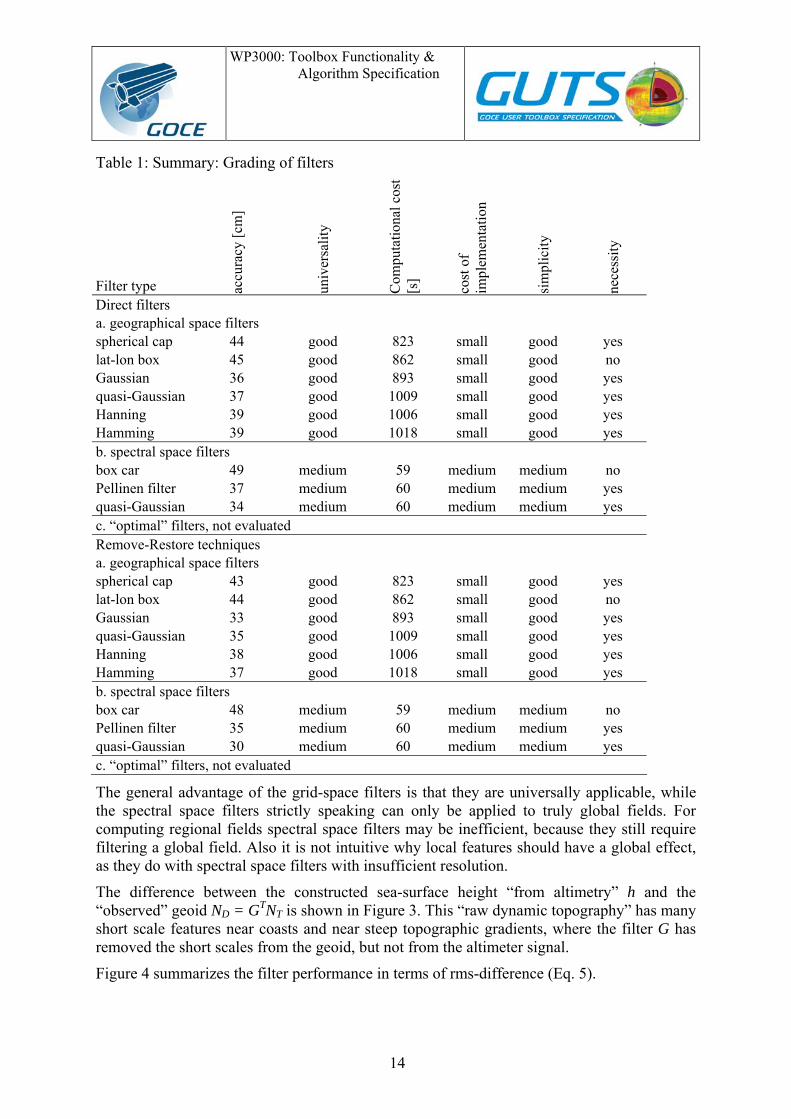
2.3.1 Commission: Filtering the signal Table 1 summarizes the trade-off study. In general, spectral space filters are much faster (factor 16 in our case) than grid-space filters, because the latter involve as many convolutions with the filter kernel as there are grid points, whereas the former involves only one. With increasing resolution, this difference in efficiency may even increase. All filters are simple to implement. Optimization for speed may involve a little more sophistication.


14

Table 1: Summary: Grading of filters

Filter type accu

racy

[cm

]

univ

ersa

lity

Com

puta

tiona

l cos

t [s

]

cost

of

impl

emen

tatio

n

sim

plic

ity

nece

ssity

Direct filters a. geographical space filters spherical cap 44 good 823 small good yes lat-lon box 45 good 862 small good no Gaussian 36 good 893 small good yes quasi-Gaussian 37 good 1009 small good yes Hanning 39 good 1006 small good yes Hamming 39 good 1018 small good yes b. spectral space filters box car 49 medium 59 medium medium no Pellinen filter 37 medium 60 medium medium yes quasi-Gaussian 34 medium 60 medium medium yes c. “optimal” filters, not evaluated Remove-Restore techniques a. geographical space filters spherical cap 43 good 823 small good yes lat-lon box 44 good 862 small good no Gaussian 33 good 893 small good yes quasi-Gaussian 35 good 1009 small good yes Hanning 38 good 1006 small good yes Hamming 37 good 1018 small good yes b. spectral space filters box car 48 medium 59 medium medium no Pellinen filter 35 medium 60 medium medium yes quasi-Gaussian 30 medium 60 medium medium yes c. “optimal” filters, not evaluated

The general advantage of the grid-space filters is that they are universally applicable, while the spectral space filters strictly speaking can only be applied to truly global fields. For computing regional fields spectral space filters may be inefficient, because they still require filtering a global field. Also it is not intuitive why local features should have a global effect, as they do with spectral space filters with insufficient resolution.

The difference between the constructed sea-surface height “from altimetry” h and the “observed” geoid ND = GTNT is shown in Figure 3. This “raw dynamic topography” has many short scale features near coasts and near steep topographic gradients, where the filter G has removed the short scales from the geoid, but not from the altimeter signal.

Figure 4 summarizes the filter performance in terms of rms-difference (Eq. 5).


15

Figure 3: Difference between “altimetric” sea surface height and observed geoid. Note that

the difference reaches more than 10 m. The colour range is restricted to make the figure comparable to following figures of smoothed dynamic topography


16

Figure 4: Comparison of rms-difference between filtered fields and “truth”, for the default

cut-off degree L=25 and for a higher cut-off degree of L=45. Note that with increasing resolution the positive effect of the RR-method decreases

The Gaussian and quasi-Gaussian filters lead to the smallest rms-differences. As expected, the filter with the Dirichlet-window in spectral space is the worst in terms of rms-difference.

As an example, Figure 5 & Figure 6 show the dynamic topographies of Figure 3 after filtering with a quasi-Gaussian [11] and a spherical cap/Pellinen filter, respectively. Each figure contains the results of 4 different methods: Direct filtering with a geographical (grid-) space filter (top left), with a spectral (spherical harmonics) space filter (top right), and with the remove-restore method (bottom left and right). With the remove-restore technique the resulting dynamic topographies contain more small scales (bottom panels) than with the direct method.

There appears to be an advantage, possibly fortuitous, with using a spectral space filter in the representation of marginal and shelf seas, such as the Hudson Bay or the Mediterranean Sea where the “raw” signal is very much depressed. The grid space filters, due to the lack of information over land, cannot reduce this depression, whereas the spectral space filters by construction use (false) geoid information over land and thus can better correct this problem.

The quasi-Gaussian filter appears to be more efficient in removing short scales associated with topographic features than the spherical cap/Pellinen filters, which is reflected in a smaller rms-difference to the truth (cf. Figure 4).


17

Figure 5: Dynamic topography after filtering with a quasi-Gaussian (Jekeli) filter. Top: direct method, bottom: RR-method, left: geographical (grid) space filter, right: spectral (spherical

harmonics) space.


18

Figure 6: Dynamic topography after filtering with a spherical cap/Pellinen filter. Top: direct method, bottom: RR-method, left: geographical (grid) space filter, right: spectral (spherical

harmonics) space

The difference between the remove-restore and direct method in Figure 7 shows the features of the dynamic topography that are omitted in the direct method. However, these features are completely associated with the prior dynamic topography ηB and may contain large errors. B

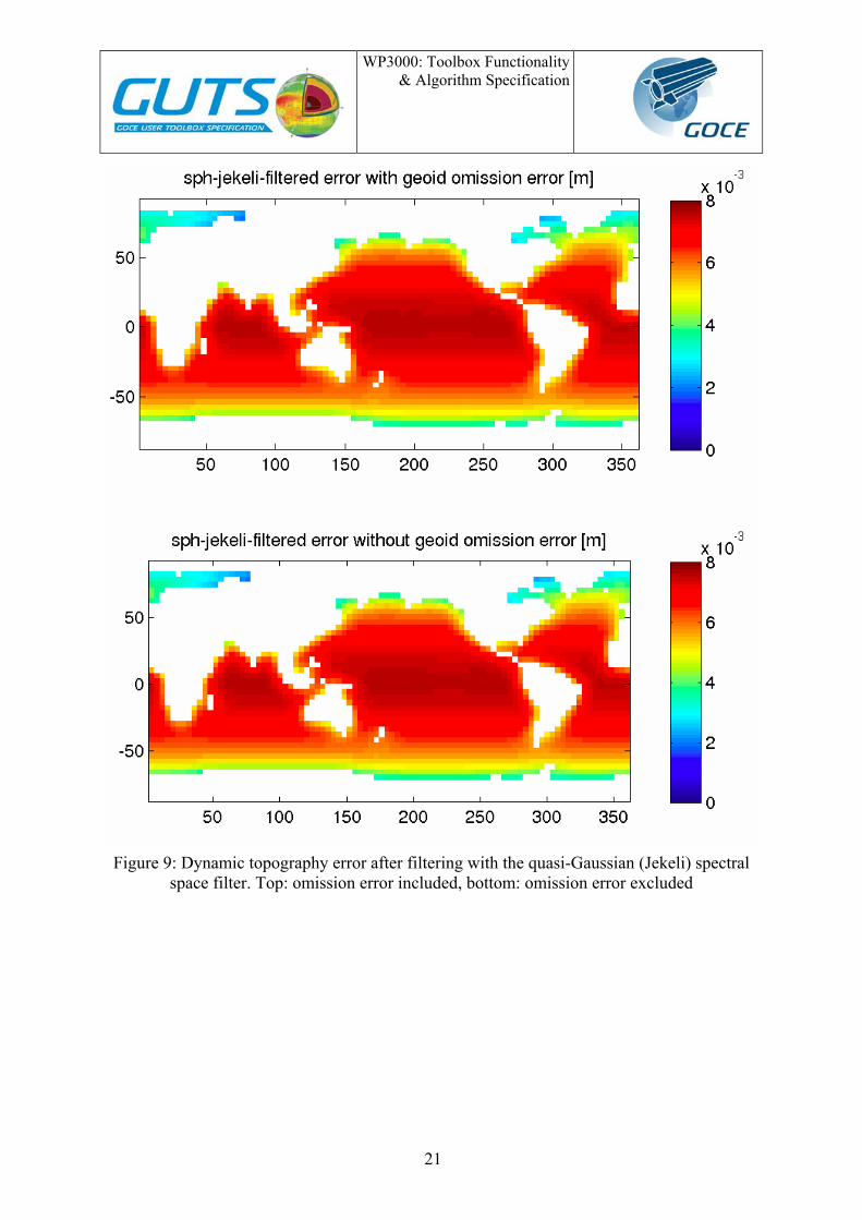
2.3.2 Effects of the omission error For brevity, we consider the effects of the omission error mainly by the example of the quasi-Gaussian (Jekeli) filter. From Figure 8 and Figure 9 it is clear that the spectral space filter reduces the estimated errors more efficiently than the grid-space filter. In the present example the effects of the omission error are small (two orders of magnitude smaller than the error signal) for the spectral space filter, but not negligible for the grid-space filter (Figure 10). In the latter case the magnitude of the omission error effect is about a factor 6 smaller than the error signal. As an example for a large scale feature of the dynamic topography, where all short scale effects, and thus the omission error, is expected to drop out, the error of the global mean of the dynamic topography is estimated (Figure 11). While the mean error is small (and irrelevant for any dynamical considerations), including the omission error increases the mean error by approximately 10% in the case of the grid-space filters. The spectral space filter leads to even smaller errors and they can effectively suppress any omission error effect (by construction).


19

Figure 7: Comparison between the RR-method and the direct method. The difference shows the features of the dynamic topography that are omitted in the direct method. However, these

features are completely associated with the prior dynamic topography ηB and may contain large errors

B


20

Figure 8: Dynamic topography error after filtering with the quasi-Gaussian (Jekeli) grid-

space filter. Top: omission error included, bottom: omission error excluded.


21

Figure 9: Dynamic topography error after filtering with the quasi-Gaussian (Jekeli) spectral

space filter. Top: omission error included, bottom: omission error excluded


22

Figure 10: Difference in quasi-Gaussian-filtered error due to inclusion of moderate omission

error. Top: grid-space filter, bottom: spectral space filter

2.4 Discussion and conclusion

In this section we evaluate the results and give a rough recommendation for choosing an appropriate filter, based on section 2.3. In our testbed examples, the remove-restore technique emerges as superior to the direct filtering method, because it yields the smallest overall rms-differences to the “truth” (not the prior dynamic topography!). The requirement of a prior dynamic topography is not regarded as a restriction, as long as such a prior guess is provided as an integral part of the toolbox along with a simple method to replace the default prior guess with one provided by the user. However, estimating the error of this prior guess remains a difficult issue.


23

Figure 11: Effect of including the omission error on the error estimate of the global mean of

the dynamic topography. Note that for the spectral space filters, the effect is not visible in this plot

Many filter kernels of this study perform reasonably well in smoothing the unfiltered difference between sea-surface height and observed geoid. Based on the global rms-difference between the filtered topography and the truth, the simplest filters, that is the grid-space rectangular (lat-lon) cap, spherical cap, and the spectral space boxcar (Dirichlet-window) filter are not recommended. These grid-space filters have a spectral response with negative side lobes and a boxcar filter in spectral space leads to Gibbs fringes in geographical space.

On the other hand, grid-space filters with a shape that resembles the Gaussian bell curve, such as the quasi-Gaussian kernel of [11], a true Gaussian kernel, and the Hanning and Hamming type windows give the smallest rms-difference between filtered dynamic topography and “truth”.

The spectral versions of the quasi-Gaussian and spherical cap (Pellinen) filters also give small rms-differences. These small differences to the “truth” can be attributed to the good representation of enclosed seas, such as the Hudson Bay and the Mediterranean Sea. The filtering of the geoid, which is implicit in the spectral representation of any geoid model leads to a removal of short scales. However, these scales are present in the sea-surface height data so that the dynamic topography is grossly wrong. In the case of enclosed seas, or near coastlines where the geoid gradients are large (e.g., along South America’s West coast), where grid-space filters fail due to the lack of information on the true geoid gradients, the originally undesired property of a spectral space filter, namely that it uses information of an


24

undefined and therefore arbitrary “sea surface over land”, tends to alleviate the problems of grid-space filters. Therefore the spectral space filters appear to be more accurate than the grid-space filters. However, with increasing resolution and required accuracy, this advantage is believed to vanish, as the spectral space filters always use arbitrary information over land. We stress that the “omission” error of the sea surface height is not considered. This “omission” error (unresolved signal) is difficult to estimate, but we expect, that its effect will be opposite to that of the geoid omission error, that is, larger with spectral space filters than with grid space filters.

Spectral space filters, when applied to the error covariance of the dynamic topography to estimate the errors of the smoothed dynamic topography, lead to smaller and smoother error estimates than grid-space filters. Additionally, by construction, they can suppress the omission error efficiently by matching these errors between the geoid and the MSS. In contrast, filtering the error covariance in grid space leaves a residual of the omission error that contributes to even the larges scales of the dynamic topography.

In this study the error propagation is treated only very approximately and results can only serve as a rough guideline. Only “optimal” filters treat the formal errors rigorously. We have excluded the “optimal” filters from this study, as they may be very expensive computationally; and conceptually, they are still subject to research. In the future, filters based on optimal interpolation or collocation techniques and in combination with the remove-restore technique are expected to provide more reliable estimates of the dynamic topography along with an error estimate.

In conclusion, none of the studied filters entirely satisfy the requirements of producing a reliable dynamic topography. All rms differences exceed 30 cm and are thus too large. However, compared to grid-space filters, spectral (spherical harmonics) space filters generally appear to be more accurate in this study. Filters with a Gaussian-like roll-off give more accurate results than those with sharp cutoffs in either grid-space or spectral space. Spectral space filters are also much faster than grid space filters. Spectral space filters efficiently suppress the geoid omission error (but probably not the sea surface height omission error which is difficult to assess). The major issue of spectral space filters are discontinuities at the land-sea boundary. Therefore we recommend spectral space filters for filtering of global dynamic topography fields, in particular with remove-restore techniques that are designed to reduce this discontinuity. For regional dynamic topography applications, grid-space fields are likely to be more efficient and accurate than spectral (spherical harmonics) filters.

All filters of this study are suboptimal and further investigations into the subject of filtering a geoid and sea surface height or the resulting dynamic topography are sorely required.


25

3 Structuring functionality; defining workflows The functionality as determined by the evaluation of the user requirements in the first part of this report has to be structured in order to provide fast computation of the output fields without reducing functionality and good visibility of the logical structure of all operations accomplishable within the toolbox.

The structure is provided by organizing the functionality of the toolbox into 7 workflows. One workflow, the main workflow, includes the core functionality of the toolbox in a default processing mode and default input data designed for fast access of the main output fields and use in tutorials. The input data used in the main workflow should be included in the toolbox distribution; thus, the main workflow is the ready-to-use playground for novices.

The convenient use of the toolbox including the application of the user’s own data and applications deviating from the main workflow is supported by the remaining 6 sub-workflows organized in six modules:

1. Geoid and gravity field computation

2. Sea surface height and a-priori dynamic topography selection

3. Satellite dynamic topography computation

4. Combined dynamic topography computation

5. Dynamic topography-derived quantities

6. Pre-viewing function

The basic elements in the workflows are the GUT functions (boxes in the workflow diagrams below) as well as input and output fields (rounded boxes in the workflow diagrams). The GUT functions are the lowest processing level that can be accessed by the user when running the toolbox. The computations within a function might contain more than one algorithm as specified in the User Requirement Document. The selection of the algorithm used in a function is in some cases controlled by options provided as input to the function or might be a chain of algorithms, or both in combination.

In this section an overview of the functionality in GUT is presented. The input and output definition of the functions and the link to the algorithm specification in the URD is provided in section 4.


26

3.1 Main workflow; supported input data

GUT comprises a set of functions that can be independently accessed by users. But in addition, pre-defined workflows support convenient use of the toolbox for most applications.

Figure 12 displays the main workflow of the GUT including in- and output fields. This workflow comprises the main functionalities of the toolbox by using input data provided by GUT. No additional data have to be provided by the user. This workflow gives an overview of the functionality of GUT and serves as a basis for the definition of tutorials that are part of the GUT distribution.

Each GUT function defined here is actually a chain of functions that again defines one of the workflows explained in the subsections below but with some restrictions in the options setting and the permitted input data. Different options settings (‘test cases’) are possible and subject to the tutorials set-up.

Computation of geodetic quantities (geoid height, deflections of the vertical and gravity anomaly) is performed on a regional or global grid or at a list of points specified by the user. Each of the three quantities is also provided on a pre-defined grid as part of the Level-2 products.

Figure 12: Main workflow for GOCE User Toolbox.


27

A mean dynamic topography (MDT) is provided, as derived from the geoid height and the mean sea surface height (MSSH) implemented in the toolbox. The MDT is provided in two qualities:

1. as a geodetic or 'satellite only' version (MDTS): the difference of MSSH and geodetic geoid height, filtered using a linear operator.

2. in a combined version (MDTC): where in addition to the MDTS, small scale features are restored by using a remove-restore technique.

The notation of satellite only MDT (MDTS) and combined MDT (MDTC) follows the use of the S and C products from the GRACE mission where the MDTC product includes additional information (in this case from oceanography).

The computation of the MDTC uses information about the small-scale variability in the MDT provided by the a-priori MDT included in the toolbox.

The dynamic topography calculation methods make no distinction between mean or instantaneous fields. Although the following descriptions refer to mean sea surface height (MSSH) and mean dynamic topography (MDT), the methods are equally applicable to instantaneous fields.

MDT slopes and surface geostrophic currents are computed and all input and output fields can be displayed by a previewing functionality.

In addition to the implemented input fields the users can provide their own data for each of the input fields, including a gridded or spherical harmonic representation of the geoid height field, using pre-defined formats with full support of functionality.

User input data supported also include:

1. Gridded sea level anomaly (SLA) or time series of sea surface height (SSH)

2. altimetric along-track SSH relative to specified ellipsoid

3. a regional or global a-priori MDT.


28

3.2 Geoid and gravity field computation (synthesis)

Geoid and gravity field computation is performed in GUT by default as indicated in Figure 13. It is proposed that the toolbox provides computation of:

• Geoid height

• Gravity anomaly

• Deflections of the vertical

Figure 13: Workflow 1a: Geoid and gravity field computation

The fields are by default calculated from the GOCE Level-2 spherical harmonic (SH) coefficients (EGM_GCF_2). Ideally, the associated error fields would be calculated from the level 2 SH variance-covariance matrices (EGM_GVC_2). However, the computational requirements for propagation of error variances form the SH to grid space are too high to be included in a distributed toolbox. This part of the workflow could be developed at a later stage to utilise external computing facilities (local or ESA GRID, for example) using parameters provided from within the toolbox. Instead, the error variance for the default GOCE gravity model will be provided, for maximum degree and order, from the level 2 gridded products and interpolated to the required input grid or point series.


29

The highest degree and order (DO) used in the spherical harmonic expansion is specified by the user. Above the selected maximum DO SH coefficients might be selected from a geoid model included in GUT. User supplied geoid models are also supported.

The fields listed above are provided for a user-specified grid or a list of points. For irregular gridded fields the specified quantity can be determined as either a single point representation or an area average. The fields are evaluated on the reference ellipsoid or on the surface of the terrain by using the implemented or a user-defined digital terrain model.

By default, the commission error variance is provided. The omission error can optionally be added to gain a full error estimate. For the omission error, it has been suggested that a homogenous, isotropic function can be provided for a list of distances specified by the user. In practise, the variance of the omission error will vary and should be calculated regionally.

The reference system (reference ellipsoid and tide system) for the geoid height can be chosen by the user. By default the same system as used for the MSSH is adopted. Thus, the reference system has to be specified in the documentation of the MSSH.

Spatial filters for 2D fields are provided to account for the different omission error scales in geoid height and altimetric SSH for calculation of MDTS. The filters are described in the MDT section.

Figure 14: Workflow 1b: Error computation for geoid and gravity field: Note covariance

calculations are not expected to be implemented in an initial toolbox


30

3.3 Sea surface height and a-priori dynamic topography selection

The dynamic topography as a main GUT product is time dependent and specification of the reference period, or computation of time dependent dynamic topography, is frequently needed. It is suggested that GUT provides two algorithms as links between an archive of SLA, MSSH and dynamic topography fields on one side and the computation of MDT within the toolbox on the other side (Figure 15). The averaging routine reads data from the archive and calculates the mean for a specified period. The output field can than be gridded or computed at specific points as convenient for the subsequent computations in the toolbox. Data in the archive might be given as weekly, monthly and annual fields. Coastal regions could introduce large errors into resultant fields when grid adaptation is carried out (from a source grid to the required output grid occurs). This toolbox will not attempt to resolve these issues, which are dealt with by more specific software tools, such as the Basic Radar Altimeter Toolbox (BRAT).

This workflow has a low priority in the toolbox. A practical alternative, recommended for the initial toolbox release, is to take advantage of the Basic Radar Altimeter Toolbox to provide the necessary functionality in manipulating altimeter data prior to ingestion in to GUT.

Figure 15: Workflow 2: Sea surface height and a-priori MDT selection


31

3.4 Satellite dynamic topography (MDTS) computation

Calculation of the dynamic topography (Figure 16) consists of two consecutive steps: First, the difference of altimetric SSH and the geoid provided upstream in the workflow (see section 3.2) is calculated with the aid of linear filters. This produces the satellite only product: MDTS. In a second step, small-scale structure is added using a remove-restore technique and an a-priori MDT. This provides the combined MDTC product. The computation of the linear filtered satellite only MDTS is described here, the combined technique is described in section 3.5.

Two different methods are provided to compute the MDTS. The first is using the geoid height as provided as output from workflow 1 (section 3.2) and computes the difference compared to a MSSH in geographical (grid-) space. The difference is filtered, using a linear filter, (workflow 3a, see Figure 16). The second method uses expansion of the MSSH into spherical harmonic coefficients and the MDTS is then determined from the difference of MSSH and geoid in spectral space, filtered using a linear filter and transformed to physical space (workflow 3b, see Figure 17). For global grids, the outcome of WP3300 suggests that the spectral (spherical harmonic filtering) option should be the default workflow.

3.4.1 Spatial MDTS (default for regional grids and user defined points) In most cases a geoid height is provided upstream in the Geoid and gravity field computation module (see section 3.2) and thus MSSH and geoid height are adapted to a common grid and reference system. However, both fields might also be provided by the user. Thus a consistency check is done. By default, both grid and reference system of the MSSH field are applied for both fields.

SSH is only provided as gridded MSSH within GUT. The user can provide SSH fields for specific dates or periods as well as along-track data. The surface height and a-priori dynamic topography selection module (see section 3.3) can be used to average the SSH data if required.

The geoid height is subtracted from the MSSH field before performing the linear filter. A number of spatial linear filters are available:

spherical cap

lat-lon box

Gaussian/quasi-Gaussian (=Jekeli)

Hanning/Hamming filters

The user has to define the filter function, the filter width and the output grid. If subsequently the combined technique (see section 3.5.1) is used to improve the small scale structure it is recommended that the filtered MDT is gridded according to the a-priori MDT used in the combined method.

Recommendations from the pilot applications report (see section 2 above) are that a quasi-Gaussian filters provide the best geographical filter characteristics and should be presented as the default option.


32

Figure 16: Workflow 3a: Satellite dynamic topography computation in geographical space

The output of the filter algorithm includes not only the filtered MDTS but also the provision of the filter matrix, which can be used for subsequent computations on the same grid and is especially convenient when time series of dynamic topography are calculated. However, for high resolution, global fields, memory requirements might exceed available resources. Thus, a system-dependent parameter is needed that specifies the upper limit of the matrix dimensions to allow the saving on disk.

3.4.2 Spectral MDTS (default for global regular grids) To use the spectral method the MSSH field has to be provided as a global field. Gaps over land have to be filled before invoking the transformation to SH coefficients. A default global geoid field is provided by GUT for that purpose. The analysis is then performed depending on the selection of maximum degree and order of the spherical harmonics expansion. The determination of the (unfiltered) MDTS is then computed as the difference of spherical harmonic coefficients of the MSSH and the geoid.


33

The MDTS can then be filtered using either one of the spatial linear filters listed in section 3.4.1 above, or one of the supplied spectral linear filters:

Pellini filter (spherical cap in ”geographical space”)

Gaussian/quasi-Gaussian (=Jekeli)

If a spatial filter is selected, the MDTS is transformed into physical space before filtering while the spectral filters operate on the SH coefficients and gridding is done afterwards.

Figure 17: Workflow 3b: Satellite dynamic topography computation in spectral space


34

The output of the filter algorithm includes not only the filtered MDTS but also the filter matrix, which can be used for subsequent computations on the same grid and is especially convenient when time series of dynamic topography are calculated.

3.5 Remove-Restore “combined” (MDTC) techniques

Two variants of a remove-restore “combined” technique are included in GUT. The first utilizes a high-resolution a-priori MDT, eg from hydrodynamic modelling or observations, to restore the small-scale structure in the ‘satellite’ MDTS. This can be defined as: ηC = ηS + (ηa − ηa )

Taking the notation that a is the a-priori, C is the combined solution and S is the satellite solution, with the overbar denoting a filtered solution. The filtered satellite solution here will be the output of the previous MDTS calculation and the filtering can be spatial or spectral – but the filtering of the a-priori MDT must be carried out in the same way.

The second variant takes the a-priori MDT as the basis and restores the large-scale structure by comparing the spectral equivalents of an a-priori geoid (based on the filtered difference of MSSH and a-priori MDT) and the GOCE geoid.

ηC = ηa + ηG − ηa( )

This requires that we use the unfiltered version of MDTS (i.e. direct difference of MSSH – geoid).

For both variants, as for the MDTS calculation, the filtering required can be carried out spatially or spectrally. For practical purposes, it is recommended that user remains within the same filtering space. Particularly for the spectral options, this will mean that the SH analysis of the MSSH field will already exist.

These two variants can be used for different purposes. Method A puts higher priority on the MDTS fields and assumes the high resolution features of the a-priori MDT are consistent with MDTS. The second method puts higher priority on the a-priori MDT and would be appropriate (e.g.) when using an ocean model for the a-priori to provide an improved model surface suitable for data assimilation fields, that was consistent with the ocean model dynamics and the GOCE geoid.

3.5.1 Remove-Restore combined technique A To improve the small-scale structure in the MDTS, a global a-priori MDT is included in GUT. The users might provide their own, global or regional, fields for their specific applications.

The MDT correction is determined as the difference of the filtered a-priori MDT from the unfiltered field. The filter should have the same specifications (filter function and filter width) as the one taken for the GOCE MDTS. If the GOCE MDTS grid diverges from the a-priori grid, the grids have to be adapted and the filter matrix has to be determined within the filter algorithm. Otherwise, the available filter matrix used when computing the GOCE MDTS (see section 3.4) is applied. If grid adaptation is necessary, the GOCE MDTS grid is


35

applied for the a-priori MDT by default. If one or both MDT fields are regional, the user has to specify the region over which to apply the MDT correction.

The MDT correction is added to the GOCE MDTS resulting in the Combined MDTC.

The workflow for this variant using spatial filtering is given in Figure 18 and that using spectral filtering is given in Figure 19.

Figure 18: Workflow 4a: Remove-Restore combined technique A: spatial filtering


36

Figure 19: Workflow 4b: Remove-Restore combined technique A: spectral filtering

3.5.2 Remove-Restore combined technique B The second variant of the remove-restore technique is based on the comparison of an a-priori geoid with the GOCE geoid to improve the large-scale structure in the a-priori MDT. The a-priori geoid is the filtered difference of MSSH and the a-priori MDT. The method is not using the GOCE MDTS as computed in section 3.4 and is, in that sense, an independent way of computing a Combined MDT.

Because of the expansion into spherical harmonic functions, to use the spectral version of this technique not only the MSSH but also the a-priori MDT (or rather a combination of the two) has to be provided as a global field and gaps on land are filled automatically. The effects of coastal discrepancies between the ocean fields and the fields used to fill the continent areas


37

can cause errors that propagate into the ocean interior and how to merge the fields at the coast is still an open science question. The remove restore techniques help to alleviate some of the resulting errors.

For the spatial filtering version (Figure 20), in most cases the MSSH and the a-priori MDT will not be provided on the same grid. The user has to specify a common grid. By default, the MSSH grid is taken. The a-priori MDT is then subtracted from the MSSH to result in the a-priori geoid over the oceans. The geoid is then also subtracted to give the difference between the GOCE and "a-priori" fields. The filter is needed to suppress the small scales in the MSSH that are not present in the a-priori MDT but has to retain the large-scale variability up to wave numbers where the GOCE geoid can be used to improve the a-priori MDT. Recommendations are given on the length scale and the filter function.

Figure 20: Workflow 4c: Remove-Restore combined technique B: spatial filtering

In the spectral version, (Figure 21), the a-priori MSSH and MDT are combined and then expanded into spherical harmonic functions. The difference of the MSSH and MDT in SH coefficients are subtracted from the geoid SH coefficients (the GOCE Level 2 product, or user provided coefficients). The maximum degree and order, up to which the correction should be used, should be specified by the user. The correction can be transformed to physical space and added to the gridded a-priori MDT resulting in the Combined MDTC.


38

Alternatively, the correction is added to the SH representation of the a-priori MDT and the result is transformed to physical space.

Figure 21: Workflow 4d: Remove-Restore combined technique B: spectral filtering


39

3.6 Dynamic topography-derived quantities

The calculation of surface geostrophic currents is done in two steps. First the slope of the surface is determined. The slope calculation can actually be used for all 2D fields that are provided on a grid. The second step is then the calculation of the surface geostrophic currents from the slope of the MDT.

Figure 22: Workflow 5: Dynamic topography-derived quantities

Additional use of the dynamic topography outputs will be facilitated by ingestion of GUT output into the BRAT toolbox.


40

3.7 Pre-viewing function

The pre-viewing functionality is intended as a means of rapidly assessing if a result from the toolbox is suitable, or derive an approximate view of the difference caused by changes in the processing through the toolbox. As such, the functionality is expected to be limited to simple viewing of 2-dimensional fields as contour and surface plots and 2 dimensional graph plots.

It is anticipated that the necessary functionality can be obtained using the VTK package in combination with additional libraries developed for previous ESA toolboxes.

It is anticipated that the user will export results from the toolbox to make use of more sophisticated viewing and printing options available within packages such as MATLAB or GMT.

A global land-sea mask should be provided as part of the previewing function.


41

4 Algorithm specification The algorithms as defined in this section are based on the fundamental algorithms and formulae defined in the User Requirements Document (URD) [1], composited to be consistent with the toolbox functionality as defined in section 3 (above). Each algorithm corresponds to a "processing" block in the workflow definitions. The basic algorithms to be implemented within each defined function are given. Where existing software exists that provides the required functionality, the software is also defined.

For each function, the input is divided into options, input data and output data. Some of the required input data are to be provided with the toolbox as default data sets, such as the GOCE level 2 data sets and a global a-priori MDT. Those data sets are indicated as GUT default data. By choosing the default options the functionality as defined in the main workflow given in section 3.1 (Figure 12) can be fully accessed by the user without providing additional data. When using a different option setting, the user may be required to provide additional data. However, each data set provided with GUT can be replaced by the user’s own data using a format supported by the toolbox.

The potential sources of these parameters, and the final output file format specifications are given in the Input/Output Definitions (section 5).

The algorithms are grouped by type. The first section: "Algorithms for preference selection" are required to provide parameters to other toolbox functions but do not include basic algorithms defined in the URD. The second section, "Computational Algorithms", generate the primary toolbox products, using the functionality of the toolbox as defined in section 3.


42

4.1 Conventions and definitions:

Throughout the algorithm definition document, unless otherwise explicitly defined, the following standard variable name definitions and conventions will be used

4.1.1 Standard variable name definitions: θ is geocentric co-latitude

ϕ is geodetic latitude

λ is longitude

Cnm and Snm are the spherical harmonic coefficients a degree n and order m. An overbar denotes the normalised version.

Pn,m are the associated Legendre functions of degree n and order m. An overbar denotes the normalised version.

Nmax is the maximum degree and order of the expansion.

W is the geopotential

a is the semimajor axis of the ellipsoid used in the determination of the coefficients (The GOCE product standard has not yet been selected)

f is the inverse flattening coefficient of the reference ellipsoid

GM is the product of G, the gravitational constant, and M, the combined mass of the earth and atmosphere, which is known to much better accuracy than either individually (for GOCE products, GM = 3.986004415·1014 m3/s2.

r is the height (from the centre of the earth) at which a value is calculated

ω is the angular rotation of the earth reference

V is the full gravitational potential

U is a reference gravitational potential

γ is the normal gravity at a point Q on the equipotential surface that has UQ = WP at all points.

ζ is the geoid height anomaly


43

4.1.2 Conventions Latitude values are always given in degrees N, i.e. 90˚S is given as -90˚.

Longitude values are always given as degrees E, i.e. 180˚W is given as -180˚.

All heights are given in m.

Gravity Anomalies are given in mgals.

Deflections from the Vertical are given in arcsec.

Regular grid definition requires:

Minimum latitude Maximum latitude Minimum longitude Maximum longitude Latitude grid cell dimension Longitude grid cell dimension

Irregular grid definition requires:

Vector of latitude values of each grid node Vector of corresponding longitude values of each grid node

Data Point definition requires:

Vector of latitude values of each data point Vector of corresponding longitude values of each data point

Reference ellipsoid description coefficients will be in one of the recognised forms:

GM, a, J2, ω

GM, a, f, ω

γa, a, f, ω


44

GUT_FA01

4.2 Algorithms for preference selection

selection of required degree and order of expansion Algorithm is required for all cases where spherical harmonic synthesis is to be used in calculation of a spatial field.

Options: -DO max_DO: max_DO is the maximum degree and order of expansion to use

-Ddeg res_deg: res_deg is the required resolution (half wave length) in degrees latitude

-Dkm res_km: res_km is the required resolution (half wave length) in km.

Input: Data set with spherical harmonic coefficients

GUT default data: EGM_GCF_2

Output: Maximum degree and order of input spherical harmonic coefficients to be used in further calculations

Units: dimensionless

Algorithm: Case:

-: default (no options provided): output: degree and order to use = the maximum degree and order of the spherical harmonic data (provided as input)

-DO: User provided degree and order of coefficients to use: where max_DO > maximum degree (order) of input data:

output = maximum degree (order) of input data where max_DO <= maximum degree (order) of input data:

output = requested degree (order)

-Dkm: User provided preferred highest resolution of calculated field Convert resolution in km (if given) to degrees latitude using:

res_deg = res_km * 90 / 1000 goto –Ddeg

-Ddeg: User provided preferred highest resolution in degrees latitude Convert highest requested resolution in degree latitude to an approximate corresponding degree and order using:

Max_DO = 360 / (2*res_deg) – value to be rounded up to next integer value Revert to -DO above to return maximum degree and order to be used


45

Note – in all cases the returned values must be reported. User should be informed of maximum degree and order in the input data. If a lower degree and order than requested has been returned, user should be explicitly informed of this.

URD Algorithm functionality defined by this algorithm None

Existing software providing this algorithm None


46

GUT_FA02 Reference system selection: Reference system selection is required in all cases where data, referenced to an earth ellipsoid, are to be combined or compared. It is also required for spherical harmonic synthesis calculations.

Where height data (geoid, mean sea surface etc.) are calculated or reported relative to a reference ellipsoid, the definition of the ellipsoid used must be known and consistent with other fields for combination or comparison, e.g. differencing of two geoid fields or generation of a dynamic topography by combination of geoid and sea surface height information. For harmonic synthesis, the values of full reference ellipsoid coefficients used in the geoid model will be required. For conversion of gridded fields, it is assumed that GM and ω will remain constant and only the ellipsoid axis values a and f, will be varied.

The default reference ellipsoid should be that used in the mean sea surface height included within the GOCE User Toolbox (see the I/O Definitions section 5).

The output of this function will be required for:

1) spherical harmonic synthesis calculations

2) conversions of existing spatial fields between reference systems using GUT_104: Change of Reference Ellipsoid in Grid and GUT_105: Change of Reference Ellipsoid in points

Options: -

Input: Preferred reference ellipsoid. (Default: Reference ellipsoid used for GUT a priori mean sea surface height field.)

Output: Reference ellipsoid description coefficients in one of the recognised forms

Algorithm: Select default values

Or

Select data definition coefficients

URD Algorithm functionality defined by this algorithm None:



47

GUT_FA03 tide system selection The tide system used for a gravity field model will be one of three types:

Tide-free (or nontidal) - This geoid would exist for a tide-free Earth with all (direct and indirect) effects of the Sun and Moon removed. Zero-tide - This geoid would exist if the permanent direct effects of the Sun and Moon are removed, but the indirect effect (mean component) related to the elastic deformation of the Earth is retained.

Mean-tide – The normal system used in altimetry where the permanent effects of the tides are retained.

It is expected that either zero or tide-free will be used for the GOCE level 2 products [12]. The tide system used must be known for comparison of gravity field data, e.g. differencing of geoid fields.

Only the degree 2 zonal component (C2,0 component) is affected.

In order to transfer a gravity field spherical harmonic series between tide-free and zero-tide tide systems the following equation has to be applied to the C2,0 coefficient:

C2,0tide− free = C2,0

zero−tide + 4.201×10−9

In order to transfer a spherical harmonic series between mean-tide and zero-tide tide systems the following equation has to be applied to the C2,0 coefficient:

C2,0zero− tide = C2,0

mean − tide + 1.39 × 10−8

The output of this function will be required for:

spherical harmonic synthesis calculations

conversions of existing spatial fields between reference systems using GUT_106: Change of tide system in a grid or GUT_107: Change of tide system at points

Options: -Tmean-tide

-Tzero-tide

-Ttide-free

Default: The tide system used in the GOCE level 2 geoid harmonic analysis (default tide system)

Input: None

Output: Tide system to use: 'zero-tide', 'tide-free' or 'mean-tide'.


48

Algorithm: Selection of default or preferred tide system: 'zero-tide', 'tide-free' or 'mean-tide'



49

GUT_FA04

4.3 Computational algorithms

Geodetic field computation (SH synthesis) Required for determination of geoid height, gravity anomaly and deflections of the vertical (E-W and N-S) by the toolbox.

Although not defined by specific URD functions, it is also required that SH synthesis of non-geodetic fields is carried out: specifically of dynamic topography and dynamic topography correction fields for WorkFlows 3b, 4b and 4d. This could be achieved with the existing software, which include the option of calculating dynamic topography.

Options: -Fg: geoid height computation (default)

-Fa: gravity anomaly computation

-Fd: geoid deflections from the vertical

-Ft: dynamic topography synthesis

-R e/w/n/s: Region of interest in the order western, eastern, northern and southern limits in degrees north of the equator and east of the prime meridian (default: 79.75/-79.75/0.25/359.75). Only used for regular (latitude-longitude) grid.

-I dx/dy: grid increment for regular (latitude-longitude) grid in degrees (default: 0.25/0.25)

-Gg grid_definition_file_x/grid_definition_file_y: An irregular grid is used. The files contain matrices with latitude/ longitude definitions of the grid. The –I and –R options are ignored

-Gu specific_points_definition_file: Specific points are defined by a list given in the file. Two columns are expected containing the longitude in the first and the latitude in the second column. The –I and –R options are ignored.

-H digital_terrain_model: The geodetic field is computed on the terrain as defined in digital_terrain_model. By default the reference ellipsoid is taken. A default terrain model is part of the GUT distribution and is used if no filename is given. –H is ignored if –Fg is selected.

-Ma: The area average for the grid cell is computed. By default the geodetic field is computed on the specified grid points. –Ma is ignored when using –Gu.

Input Data set with spherical harmonic coefficients (GUT default data: EGM_GCF_2)

maximum degree and order of the expansion to use in the computation (from GUT_FA01).

Reference system selection (from GUT_FA02)

Preferred tide system: (from GUT_FA03)


50

Output: For grids:

Depending on output parameter selected:

-Fg: 2D matrix (grid) of geoid (m)

-Fa: 2D matrix (grid) of gravity anomaly (mgals)

-Fd: 2D matrix (grid) of the E-W deflections from the vertical and 2D matrix (grid) of the N-S deflections from the vertical (arcsecs).

-Ft: 2D matrix (grid) of the dynamic topography or dynamic topography correction (m)

Locations of grid nodes as 2 vector arrays of latitudes and longitudes (latitude-longitude grid) or as two matrices (irregular grid) in degrees.

Flag reflecting whether point-wise or area averaged values (-Ma option) have been calculated

For User Specified Points (-Gu):

Depending on output parameter:

-Fg: Vector of geoid at each data point (m)

-Fa: Vector of gravity anomaly at each data point (mgals)

-Fd: Vector of the E-W deflections from the vertical and vector of the N-S deflections from the vertical at each data point (arcsecs).

-Ft: Vector of the dynamic topography or dynamic topography correction at each data point (m).

Locations of data points as 2 vector arrays of latitudes and longitudes (degrees).

For All Cases:

Maximum degree and order and approximate associated spatial scale (in spatial dimensions, i.e. km or degrees lat) of the calculation.

Reference ellipsoid definition of the calculated field

For gravity anomaly or deflections from the vertical – the actual height above the reference ellipsoid for the calculation.

URD Algorithm functionality defined by this algorithm This functional algorithm includes the application of the GUTS algorithms:

GUT_005: Height anomaly in grid format, full

GUT_006: Height anomaly in points, full

GUT_007: Gravity anomaly in grid format, full

GUT_008: Gravity anomaly in points, full

GUT_009: E-W deflections in grid format, full


51

GUT_010: E-W deflections in points, full

GUT_011: N-S deflections in grid format, full

GUT_012: N-S deflections in points, full

The spherical approximation versions of the geodetic field calculations (GUT_001: Grid with geoid height, sph. approx., GUT_002; Grid with gravity anomalies, sph. approx. , GUT_003: Grid with east-west vertical deflections, sph. approx. and GUT_004: Grid with north-south vertical deflections, sph. approx.), used in the GOCE level 2 gridded products, are not recommended for inclusion in the toolbox.

It is also not considered a priority to provide the calculation of reference potential (GUT_108: Calculation of reference potential, grid and GUT_109: Calculation of reference potential, point) in the current implementation of the toolbox.

Existing software providing this algorithm 1) Routines within the GRAVSOFT fortran package [13, 14]. In particular the GEOCOL and

HARMEX programs. These programs currently expect data in external files, but could be re-coded as functions to allow use of previously input data.

2) Harmonic_synth package of Simon A. Holmes and Nikolaos K. Pavlis.

Fortran programme initiated by a series of editable bourne shell scripts.

Current implementation required generation of a specific fortran source code file for each activation. The source code file contains internal parameters that set the required input for the algorithm. This source code is then compiled and executed.

The current implementation of this code uses the spherical harmonic approximations of the required parameters (GUT_001, GUT_002, GUT_003, GUT_004) and would require code changes to implement the ‘full’ calculation as recommended for the toolbox.

Existing package could be recoded rather easily to allow input of required parameters from external script using values defined by required or optional input as specified above.

Alternative software solutions are found in the GSHBUNDLE matlab software of Nico Sneuw. These functions could, potentially, be recoded in fortran to provide the required functionality.


52

GUT_FA05 Commission error determination (geoid) • Ideally, the toolbox would allow the calculation of the full variances and error

covariances using the spherical harmonic error covariance data from the level 2 product: EGM_GVC_2. However, it is recommended that, in order to create a toolbox with realistic computational requirements, the error calculations are restricted to interpolations of the error fields generated from the level 2 gridded products.

The calculation of full error covariances for a grid is considered beyond the scope of the GOCE user toolbox due to computational resource constraints.

Even where it might be considered a possible option, as the full error covariance information available for a high degree and order spherical harmonic expansion of a geoid field is of the order of several Gigabytes in size, it is not feasible to separate the read method from the input data file. The algorithms will need to extract parts of the error covariance matrix data file.

Options: -Fg: geoid height commission error computation (default)

-Fa: gravity anomaly commission error computation

-Fd: geoid deflections from the vertical commission error computation


-I dx/dy: grid increment for regular (latitude-longitude) grid in degrees (default: 0.25/0.25).

-Gg grid_definition_file_x/grid_definition_file_y: An irregular grid is used. The files contain matrices with latitude/ longitude definitions of the grid. The –I and –R options are ignored.


-H digital_terrain_model: The error field is computed on the terrain as defined in digital_terrain_model. By default the reference ellipsoid is taken. A default terrain model is part of the GUT distribution and is used if no filename is given. –H is ignored if –Fg is selected.


-Clon1/lat1/lon2/lat2: The comission error co-variance is computed for the two points defined by lon1/lat1 and lon2/lat2 (longitude/ latitude in degrees). By default only the variances are computed (see options –R, -I, -Gg, -Gu).


53

Input: Data set with error-covariance for spherical harmonic coefficients used in geodetic field

computation (GUT default data: EGM_GVC_2)

maximum degree and order of the expansion used in the geodetic field computation (from GUT_FA01).



Output: For grids:

Depending on geodetic parameter:

-Fg: 2D matrix (grid) of geoid error variance (m2)

-Fa: 2D matrix (grid) of gravity anomaly error variance (mgal2)

-Fd: 2D matrix (grid) of the error variance in the E-W deflections from the vertical and 2D matric (grid) of the error variance in the N-S deflections from the vertical (arcsec2).





-Fg: Vector of geoid error variance at each data point (m2)

-Fa: Vector of gravity anomaly error variance at each data point (mgal2)

-Fd: Vector of the error variance in the E-W deflections from the vertical and vector of the error variance in the N-S deflections from the vertical at each data point (arcsec2).


If co-variances are computed (-C):

2x2-matrix containing variances and co-variance of the two specified points

Locations of the two data points.

For All Cases:




54


URD Algorithm functionality defined by this algorithm GUT_016: Geoid height errors in grid format

GUT_018: Gravity anomaly errors in grid format

GUT_020: E-W deflection errors in grid format

GUT_022: N-S deflection errors in grid format

GUT_017: Geoid height errors in points

GUT_019: Gravity anomaly errors in points

GUT_021: E-W deflection errors in points

GUT_023: N-S deflection errors in points

GUT_025: Geoid height error covariances in points

GUT_027: Gravity anomaly error covariances in points

GUT_029: E-W deflection error covariances in points

GUT_031: N-S deflection error covariances in points

The following URD algorithms will not be implemented, as they require computing resources in excess of those anticipated necessary to run the toolbox.

GUT_024: Geoid height error covariances on a grid

GUT_026: Gravity anomaly error covariances on a grid

GUT_028: E-W deflection error covariances on a in grid

GUT_030: N-S deflection error covariances on a grid

Existing software providing this algorithm Covar.m:

Matlab function to determine errors on a grid based on the covariance matrix


55

GUT_FA06 Omission error determination (geoid) is estimated using a model of the expected power spectrum for all spherical harmonics higher than the maximum degree and order included in the spherical harmonic synthesis.

The calculation of the omission errors will be limited to calculation of:

• the variances for grids of points

• full co-variances for discrete pairs of points

• an isotropic, homogenous covariance function.

The calculation of full error co-variances for a grid is considered beyond the scope of the GOCE user toolbox.

As the full error covariance information available for a high degree and order spherical harmonic expansion of a geoid field is of the order of several Gigabytes in size, it is not feasible to separate the read method from the input data file. The algorithms will need to extract parts of the error covariance matrix data file.

Options: -Fg: geoid height omission error computation (default)

-Fa: gravity anomaly omission error computation

-Fd: geoid deflections from the vertical omission error computation


-I dx/dy: grid increment for regular (latitude-longitude) grid in degrees (default: 0.25/0.25).

-Gg grid_definition_file_x/grid_definition_file_y: An irregular grid is used. The files contain matrices with latitude/ longitude definitions of the grid. The –I and –R options are ignored.


-H digital_terrain_model: The error field is computed on the terrain as defined in digital_terrain_model. By default the reference ellipsoid is taken. A default terrain model is part of the GUT distribution and is used if no filename is given. –H is ignored if –Fg is selected.


-C lon1/lat1/lon2/lat2: The omission error co-variance is computed for the two points defined by lon1/lat1 and lon2/lat2 (longitude/ latitude in degrees). By default only the variances are computed (see options –R, -I, -Gg, -Gu).


56

-F d1/d2/dx: The omission error is provided as an isotropic, homogenous function of distance. The function is evaluated in the intervall [d1,d2] using dx as increment. By default only the variances are computed (see options –R, -I, -Gg, -Gu).

Input: Data set with spherical harmonic coefficients (GUT default data: EGM_GCF_2)

maximum degree and order of the expansion used in the geodetic field computation (from GUT_FA01).



Output: For grids:

Depending on geodetic parameter:

-Fg: 2D matrix (grid) of geoid error variance (m2)

-Fa: 2D matrix (grid) of gravity anomaly error variance (mgal2)

-Fd: 2D matrix (grid) of the error variance in the E-W deflections from the vertical and 2D matric (grid) of the error variance in the N-S deflections from the vertical (arcsec2).





-Fg: Vector of geoid error variance at each data point (m2)

-Fa: Vector of gravity anomaly error variance at each data point (mgal2)

-Fd: Vector of the error variance in the E-W deflections from the vertical and vector of the error variance in the N-S deflections from the vertical at each data point (arcsec2).


If co-variances are computed (-C):

2x2-matrix containing variances and co-variance of the two specified points

Locations of the two data points.

If an isotropic homogenous co-variance function is provided (-F):

Vector of error co-variances


57

Vector of distances corresponding to the error co-variances.

For All Cases:




URD Algorithm functionality defined by this algorithm GUT_032: Geoid height omission error covariances on a grid

GUT_033: Geoid height omission error covariances in points

GUT_034: Gravity anomaly omission error covariances on a grid

GUT_035: Gravity anomaly omission error covariances in points

GUT_036: E-W deflection omission error covariances on a grid

GUT_037: E-W deflection omission error covariances in points

GUT_038: N-S deflection omission error covariances on a grid

GUT_039: N-S deflection omission error covariances in points

Existing software providing this algorithm Some element of the required software exist in the GRAVSOFT GEOCOL program.


58

GUT_FA07 Average determination of SSH or DT This functionality is provided in a simple form to allow the calculation of a mean sea surface height (SSH) or dynamic topography (DT) from existing gridded or collocated locations using a simple pointwise averaging technique. The Basic Radar Altimeter Toolbox (BRAT) provides more advanced algorithms for carrying more complex averaging and gridding and could be used to pre-condition data for input to GUT. However, it is recommended that this simple functionality is retained in GUT for tutorial purposes and simple re-calculation of averaged properties.

No interpolation will be carried out to account for missing data values, and these should be accounted for in the input fields.

Options: none

Input: Time series of 2D matrices or vectors of parameters to be calculated

Output: Returned mean value at each input location : matrix identical in size to each input field.

Algorithm

x =1n

xii=1

n

∑

where x is the property to average, overbar denotes the mean, i is the location of each measurement of property x and n is the total number of unique locations.

The algorithm will only average over the number of valid data measurements – missing data will not be included.




59

GUT_FA08 Grid adaptation Algorithm is required for all cases where gridded fields are supplied and are required to be differenced.

Note: this function is not required where spectral differencing is to be carried out

Options: None

Input: Required new regular grid specification for output fields (default is GUT MSS grid)

Regular grid specification of existing input field

Input data field for

Output: Input data field interpolated to grid locations of the required new grid

Latitude and Longitude values of new grid nodes

URD Algorithm functionality defined by this algorithm GUT_110: Interpolation

Existing software providing this algorithm geoip from the GRAVSOFT package


60

GUT_FA09 Linear filter (spatial) This function will be used for filtering of the dynamic topography, or of mean sea surface fields, ready for combination with geoid models.

The type of filter(s) to be implemented has been determined from the trade-off study examining the filtering.

Options: -Fj scale: Quasi-gaussian (Jekeli) filter with full filter width scale (default option)

-Fg scale: Gaussian filter with full filter width scale

-Fc scale: Spherical cap with diameter scale

-Fhm scale: Hamming window of width scale

-Fhn scale: Hanning window of width scale

-F filter_matrix_file: The filter matrix is read in from a file.

-O filter_matrix_file: The filter matrix is stored in filter_matrix_file. There is a limitation for large grids depending on available resources. The limit grid size should be defined in the toolbox.

Input: Grid specification (default is the default GUT MSS grid specification)

Input field

Output: Filtered version of input field

URD Algorithm functionality defined by this algorithm GUT_102: Grid filtering



61

GUT_FA10 Linear filter (Spherical Harmonic) This function will be used for filtering of a geodetic 2D parameter, especially the dynamic topography, in spherical harmonic space. This is the proposed default option for filtering of MSSH- geoid. The function includes expansion of a gridded field into spherical harmonic coefficients, application of the filter kernel and transformation back to physical space. The analysis and synthesis steps to change between physical space and spectral representation of the geodetic parameter can both be switched off, if spherical coefficients are provided as input or required as output.

Options: -Fj scale: Quasi-gaussian (Jekeli) filter with full filter width scale (default)

-Fc scale: Pellinen filter with full filter width scale

-F filter_matrix_file: The filter matrix is read in from a file.

-O filter_matrix_file: The filter matrix is stored in filter_matrix_file. There is a limitation for large grids depending on available resources. The limit grid size should be defined in the toolbox.

-A: The parameter is given on a regular grid and a transformation to spherical harmonic coefficients is needed (default). –A- indicates that the parameter is given in spectral space and no analysis is necessary.

-S: Transformation into physical space is invoked after filtering (default). –S- indicates that the output is required in spectral space.

-D: The parameter filtered is a dynamic topography. No reference surface is subtracted when transforming to physical space (-S option). Default: Subtraction of reference.

Input: If parameter provided on regular grid (-A option):

Grid specification (default is the default GUT MSS grid specification)

Input field

If parameter is provided in spectral space(-A- option):

Data set with spherical harmonic coefficients

Output: Filtered field on grid (-A option) or as spherical harmonic coefficients (-A- option).



62

Existing software providing this algorithm Spectral filtering is available through the gauss_av function, part of the sh_mdt fortran program or Rory Bingham.

In addition, Matlab routines that were used for the filtering study (section 2) exist and are available from Martin Losch. These routines would need re-coding for use in the toolbox.


63

GUT_FA11 Fill gaps on continent To perform expansion into spherical harmonic coefficients a global field is needed. This function fills gaps in a 2D parameter by replacing ‘NaN’ values by values from a second, globally defined, field, which is defined on the same grid. Where the field to be filled is a dynamic topography field, then zeros will be used for the land values. Where the field to be filled is a geoid or mean sea surface field, then a geoid field will be used. By default, the GOCE geoid will be used.

This function should correctly address the merging of the fields at the coastlines by applying suitable smoothing. However, this smoothing will have an impact on the results of filters applied. The recommended remove restore methods are relatively robust regarding the smoothing and in an initial toolbox we have not recommended any smoothing method. It should be possible for users to include their own smoothing algorithms here, or to supply a complete, global field in place of using this algorithm, where they have already applied their own smoothing.

Input: field to fill (geoid, mean sea surface or dynamic topography)

global field to fill gaps in geodetic field (default GUT gridded geoid)

Output: patched field



64

GUT_FA12 SH analysis Required for all instances where a global gridded field is to be used for spherical harmonic filtering.

Input: Global gridded field

Regular grid specification of input field

Maximum degree and order of spherical harmonic expansion to calculate (from GUT_FA01)

Output: Spherical Harmonic expansion of coefficents of global field

Maximum degree and order included in expansion

URD Algorithm functionality defined by this algorithm GUT_103: Going from geographical space to spectral

Existing software providing this algorithm The shpgric fortran program provides this function for gridded data.

gsha.m: Matlab script, part of the GSHBUNDLE software package of Nico Sneuw.


65

GUT_FA13 Surface current determination Possible for regular gridded data fields or line / transect data.

Options: -T: dynamic topography is provided on a transect (default: topography on 2D grid)

-G: Currents are required on the same grid as the input topography. This involves interpolation on larger scales than the default four point calculation (see algorithm description below)

Input: For 2D dynamic topography:

2D matrix of gridded dynamic topography (m)


For transects:

Vector containing (mean) dynamic topography (m) at points values

2 vectors containing the latitude and longitude coordinates of the points

Output: For 2D dynamic topography:

2 2D matrices of East and North velocities respectively

Locations of grid nodes at which the velocity was calculated, given as 2 vector arrays of latitudes and longitudes (latitude-longitude grid) or as two matrices (irregular grid) in degrees.

For transects:

2 vectors containing East and North components respectively of velocity across the transect

2 vectors containing the latitude and longitude coordinates of the points at which the velocity was calculated.

By default, for gridded data, the velocity values will be calculated for a grid offset by δϕ/2 in latitude and δλ/2 in longitude for the dynamic topography grid (i.e. for a grid offset by ½ grid cell dimension from the input grid. For global grid, the longitude will be wrapped.

By default, for transect data, the velocities will be calculated at the midpoints between each location

Algorithm: GUT_013: Geostrophic velocities in grid

GUT_014: Geostrophic velocities in points.


66

Note for a grid, we use a four point calculation by default, which as per [15] is for a regular grid:

u =−γfR

∂ς i+ .5, j + .5

∂θ∂ς i+ .5, j + .5

∂θ=

14δθ

ς i, j +1 − ς i, j + ς i+1, j +1 − ς i+1, j( )

v =−γ

fRcosθ∂ς i+ .5, j + .5

∂λ∂ς i+ .5, j + .5

∂λ=

14δλ

ς i+1, j +1 − ς i, j +1 + ς i+1, j − ς i, j( )

where h is the dynamic topography defined at points i,j i+1,j i,j+1 and i+1,j+1 are input grid nodes surrounding the output grid node i+.5,j+0.5 respectively, where I and j are the longitude and latitude locations of the input grid nodes separated by δλ and δθ.

If velocity is required on the same grid, 5 point calculations are used:

Existing software providing this algorithm Combination of GUT_slopes.m, GUT_srfcurrnt.m for 5 point calculation.


67

GUT_FA14 Difference or Sum of Gridded Fields Possible for regular gridded data fields or line / transect data.

Required for generation of a “synthetic geoid” field (difference of (M)DT and (M)SSH) necessary for the remove restore techniques, and also for replacing the residuals when using the remove restore technique.

Options: -sum: Provide sum of input fields

-diff: Provide difference of 2 fields

Input: For 2D Fields:

pair of 2D matrices containing values to sum / difference


For transects:

Pair of vector containing values to sum / difference


Output: For 2D Fields:

A 2D matrix of sum (–sum option) or difference (-diff option) of input fields


For transects:

A vector containing sum (–sum option) or difference (-diff option) of input vectors


Algorithm: GUT_100: Grid addition

GUT_101: Grid subtracation.

Existing software providing this algorithm The fc2 program of the GRAVSOFT package.


68

5 Input output definition Within this section, we will identify the input and output files that are required, or are optionally user supplied, for which the toolbox with require input and output methods.

Required input data files should be included within the toolbox package and provide the default for appropriate workflows.

Optional, user supplied, input data files must be in a format that the toolbox is able to input and can be substituted for the supplied input files by the user.

As a minimum requirement, the toolbox documentation must provide the format specifications of the included input data files in order that the user can supply their own data in the same format.

Where the toolbox provides functionality to input a range of input formats, the toolbox documentation must also provide the format specifications (or reference to the appropriate format specification documentation) to enable users to ensure their data are in a compatible format.

[In addition, the toolbox should supply the ability for users to write their own input modules for expansion of the toolbox to cover the widest possible range on input data formats]

All height fields (geoid, mean sea surface, dynamic height, terrain model etc..) must be given relative to a consistent reference ellopsoid. Candidate ellipsoids are:

GRS80 (semi-major axis a = 6378137.0 m, flattening f = 1 / 298.257222101.)

"topex" ellipsoid (semi-major axis a = 6378136.3 m, flattening f = 1 / 298.257)

"Envisat" ellipsoid (semi-major axis a = 6378137, flattening f = 1 / 298.257223563)

Height field requiring reference system conversion.


69

5.1 Required Input Data files: to be included on the toolbox:

5.1.1 Geoid harmonic expansion (SH & error covariance products)

The official HPF GOCE level 2 products: EGM_GOC_2

EGM_GVC_2

These files are in XML IGCEM format [2].

The read method must input to the toolbox:

Spherical harmonic coefficients of the product

Maximum degree and order of the supplied spherical harmonic expansion

Tidal system (for use by GUT_FA002)

Reference ellipsoid definition : GM, r, a,

5.1.2 Mean sea surface height field It is proposed that the included MSS height field is the most recent version of CLS, currently CLS01 [16], or the most recent KMS solution (currently KMS04: http://geodesy.spacecenter.dk/~gocina/publications/4_1_kmss04-lux.pdf). Results of the GOCINA project indicate that the updated, global, KMS solution may be the most appropriate, subject to improved fields being generated by the time of release of the toolkit.

CHARACTERISTICS:

Name CLS01

Reference ellipsoid T/P

Referencing time period 1993-1999 (7 years)

Domain Global (80°S to 82°N) – Oceanwide where altimetric data are available. EGM96 elsewhere and on continents.

Spatial resolution Regular grid with a 1/30° (2 minutes) spacing (i.e. ~4 km)

Grid 10800 points in longitudes / 4861 points in latitude

MSS determination technique Local least square collocation method on a 6’ grid where altimetric data in a 200-km radius are selected. Estimation on a 2’ grid based on SSH-EGM96 values (remove/restore technique to recover the full signal). The inverse method uses local isotropic covariance functions that witness the MSS wavelength content.

Estimation error level YES (in m) – Negative values are flagging coastal areas where the smoothed junction with the continental EGM96 geoid is computed.

Altimetric dataset

T/P 7 years mean profile


70

ERS-1/2 5 years mean profile

GEOSAT 2 years mean profile

ERS-1 geodetic data


2-dimensional matrix of mean sea surface height field (m)

2 vectors containing the latitude and longitude of the grid nodes of the matrix.

Reference ellipsoid GM, r etc (for use by GUT_FA_002)

5.1.3 Mean dynamic topography and associated error covariance products In order to address the complex issues of creating dynamic topography fields that are consistent with the length scales included in the GOCE data, and also try and include the higher resolution capability of altimeter derives mean sea surfaces, it is proposed that he toolbox contains 2 mean dynamic topography data sets.

Primary mean dynamic topography : Contains only scales resolved within GOCE data must be compatible with MSSH field in terms of reference averaging period : an example of the output from the simple, default workflow of the toolbox

Secondary mean dynamic topography : high resolution MDT for use as a-priori in remove restore or similar combined MDT calculations. Candidates include OCCAM model at 1/12 degree


2-dimensional matrix of mean dynamic topography field (m)

2 vectors containing the latitude and longitude of the grid nodes of the matrix.

Reference ellipsoid GM, r etc (for use by GUT_FA_002)

Both products should contain appropriate error covariance data for MDT products:

5.1.4 Sea level Anomaly fields Sea level Anomaly fields: Include eg 12 monthly average fields, relative to MSSH, or 12 annual fields that can be averaged to predefined mssh fields, which can be filtered and added to MDT. Default format files will be the CLS NetCDF format data files.

Alternate MSSH & SLA referenced to different mean periods.

5.1.5 Along track altimetric sea surface height fields Along track SSH and or SLA : either use AVISO products as the default or using BRAT ingestion interface.

5.1.6 Digital Terrain Model Digital terrain model : For use in tutorials, the ETOPO2v2 digital elevation model is recommended (http://www.ngdc.noaa.gov/mgg/fliers/06mgg01.html).

http://www.ngdc.noaa.gov/mgg/fliers/06mgg01.html


71

The CEOS Working Group on Terrain Mapping has recommended the De Montfort University "Altimetry Corrected Elevations" (ACE) as the best 1 km Global DEM


72

5.2 Optional User Supplied Input Data Files

It is anticipated that even a basic GOCE User Toolbox should be capable of accepting input fields from user supplied data files as alternatives to the included data files defined in section 5.1 above.

As a minimum requirement, the toolkit will include the complete format specification of the included data files to enable the user to transform their preferred data source to the appropriate data format. In this case, the toolbox input method must allow:

The selection of an alternative data file for all data inputs

The toolbox should be capable of reading any gridded data field from a GRAVSOFT format ascii file, as defined in the URD

GEOID – ICGEM this is commonly used format and common geoids are all downloadable in ICGEM format

Format must be in a format recognized by the toolbox. Candidate formats include: a) GOCE XML ICGEM [17] b) GRACE SHM-FORMAT (Earth Gravity Spherical Harmonic Model

Format), in use within the GRACE project for Earth gravity model solutions in terms of spherical harmonic coefficients [18].

MSS gridded– in AVISO MSS format

SLA / SSH – can we use BRAT ingestion routines?


73

5.3 Output Data Formats

The toolbox must provide output capability to save all computed fields in standard formats. The standard formats must also include appropriate metadata to describe the saved fields. As the toolbox users will be from a range of scientific disciplines, with a range of discipline specific standards, it is appropriate that at least two output formats are supported for the toolbox products. These formats should be, as far as possible, platform independent and widely recognised by potential post-processing and display software packages. The recommended formats are:

1) ASCII format, following the GRAVSOFT data standards, suitable for all output fields. Additional metadata may be required to describe the product. This will be provided as a separate text file associated with the product.

2) NetCDF format, suitable for all gridded fields. Additional metadata should be included in the file attributes.


74

5.4 File Naming Conventions

It is anticipated that the toolbox users will use the toolbox for data sources beyond those included in the toolbox. As many of these data sources already have appropriate final naming conventions, it is anticipated that the users may wish to use file names that follow these conventions. It is, therefore, inappropriate to enforce any specific file naming conventions on the user supplied input or output data files used by the toolbox.

Default filenames should be suggested for saving files:

GEO

MSSH

MDTS

MDTC

Use GUT products name somehow?

GRAVSOFT format files should use the .dat extension, whilst netcdf should use the cdf extension.

All file naming should be able to be over-ridden by the user.


v

6 References [1] GOCE User Toolbox : User Toolbox Requirement Document.

[2] Haines, K., R. Hipkin, C. Beggan, R. Bingley, F. Hernandez, J. Holt, T. Baker, and R.J. Bingham, Combined use of altimetry and in situ gravity data for coastal dynamics studies. Space Science Reviews, 2003. 108(1-2): 205-216.

[3] Losch, M., trade-off study dynamic topography: truth and difference to prior, in matlab, wp3300-2.pdf, Editor. 2006.

[4] Losch, M., B.M. Sloyan, J. Schröter, and N. Sneeuw, Box inverse models, altimetry and the geoid: Problems with the omission error. Journal of Geophysical Research-Oceans, 2002. 107(C7): -.

[5] Lemoine, F.G., D.E. Smith, L. Kunz, R. Smith, E.C. Pavlis, S.M. Klosko, D.S. Chinn, M.H. Torrence, R.C. Williamson, C.M. Cox, K.E. Rachlin, Y.M. Wang, S.C. Kenyon, R. Salman, R. Trimmer, R.H. Rapp, and R.S. Nerem. The development of the NASA GSFC and DMA joint geopotential model. in International Symposium on Gravity, Geoid and Marine Geodesy (GraGeoMar96). 1996. University of Tokyo, Tokyo, Japan.

[6] Fox, A. and K. Haines, Interpretation of water transformations diagnosed from data assimilation. Journal of Physical Oceanography, 2003. 33: 485–498.

[7] Haines, K. and R.J. Bingham. Mean dynamic topographies (MDTs) in the GOCINA region. in GOCINA Workshop. 2006. Luxembourg.

[8] Wunsch, C. and P. Heimbach, Decadal changes in the North Atlantic meridional overturning and heat flux. J. Phys. Oceanogr., 2006. (in press).

[9] Gerlach, C., L. Foldvary, D. Svehla, T. Gruber, M. Wermuth, N. Sneeuw, B. Frommknecht, H. Oberndorfer, T. Peters, M. Rothacher, R. Rummel, and P. Steigenberger, A CHAMP-only gravity field model from kinematic orbits using the energy integral. Geophysical Research Letters, 2003. 30(20): -.

[10] Knudsen, P. and C.C.Tscherning. Error characteristics of dynamic Topography models derived from altimetry and GOCE gravimetry. in IAG Scientific Assembly. 2005. Cairns.

[11] Jekeli, C., Spherical harmonic analysis, aliasing, and filtering. Journal of Geodesy, 1996. 70(4): 214-223.

[12] McCarthy, D.D. and G. Petit (eds.) IERS Conventions (2003). IERS Technical Note. No. 32. 2004, Verlag des Bundesamtes für Kartographie und Geodäsie: Frankfurt am Main. Available from: http://www.iers.org/iers/publications/tn/tn32/tn32.pdf.

[13] Tscherning, C.C., R. Forsberg, and P.Knudsen. The GRAVSOFT package for geoid determination. in Continental Workshop on the Geoid in Europe. 1992. Prague: Research Institute of Geodesy, Topography and Cartography, Prague.

http://www.iers.org/iers/publications/tn/tn32/tn32.pdf


vi

[14] Tscherning, C.C., P. Knudsen, and R. Forsberg:, Description of the GRAVSOFT package, 4. ed. 1994, Geophysical Institute, University of Copenhagen. Available from: http://cct.gfy.ku.dk.

[15] Abramowitz, M. and I.A. Stegun (eds.) Handbook of Mathematical Functions with Formulas, Graphs, and Mathamatical Tables. Natioan lBureau of Standards Applied Mathematics Series. No. 55. 1964, United States Department of Commerce. Available from: http://www.convertit.com/Go/ConvertIt/Reference/AMS55.ASP.

[16] Mean Sea Surface. Available from: http://www.cls.fr/mss/.

[17] GO-ID-HPF-GS-0041: Product Specification for Level-2 Products and Auxiliary Data Products. Available from: http://esamultimedia.esa.int/docs/GO-ID-HPF-GS-0041_2.0_Product_Specification_Level2.pdf.

[18] Flechtner, F. and J. Ries. GRACE 327-732 (GR-GFZ-FD-001) Gravity Recovery and Climate Experiment. GRACE Gravity Field Solution Data Formats. 2003; Available from: ftp://podaac.jpl.nasa.gov/pub/grace/doc/GR-GFZ-FD-001_v1.1.pdf.

[19] Tscherning, C.C. and P.Knudsen. Determination of bias parameters for satellite altimetry by least-squares collocation. in Hotine - Marussi Symposium. 1986. Rome: Politecnico di Milano.

[20] Tscherning, C.C., Covariance expressions for second and lower order derivatives of the anomalous potential, in Reports of the Department of Geodetic science. 1976, The Ohio State University: Columbus.

[21] Tscherning, C.C., Computation of covariances of derivatives of the anomalous gravity potential in a rotated reference frame. Manuscripta Geodaetica, 1993. 18(3): 115-123.

[22] Sanso, F. and W.-D. Schuh, Finite covariance functions. Bulletin Geodesique, 1987. 61: 331-347.

[23] Tscherning, C.C., Computation of spherical harmonic coefficients and their error estimates using least-squares collocation. Journal of geodesy, 2001. 75(1): 12-18.

[24] Tscherning, C.C., Determination of datum-shift parameters using least squares collocation. Boll. geodesia sc. Aff.,, 1976. XXXV(2).

[25] Sanso, F. and C.C.Tscherning, Fast Spherical Collocation - Theory and Examples. Journal of Geodesy, 2003. 77(1-2): 101_112, DOI 10.1007/s00190_002_0310_.

http://cct.gfy.ku.dk/

http://www.convertit.com/Go/ConvertIt/Reference/AMS55.ASP

http://www.cls.fr/mss/

http://esamultimedia.esa.int/docs/GO-ID-HPF-GS-0041_2.0_Product_Specification_Level2.pdf

http://esamultimedia.esa.int/docs/GO-ID-HPF-GS-0041_2.0_Product_Specification_Level2.pdf

ftp://podaac.jpl.nasa.gov/pub/grace/doc/GR-GFZ-FD-001_v1.1.pdf


vii

Appendix A: Existing Software Packages Use of existing software packages to provide the functionality required for the toolbox.

HARMONIC_SYNTH (Version 05/01/2006)

This package is a fortran 77 based, open source programme to calculate the range of parameters required by GUT_FA003. However, as stands, the program calculates the spherical approximation of the parameters (as per algorithms GUT_001 – GUT_004). The code would require modification to include the full method, recommended to be used in the GOCE Toolbox.

The present version of HARMONIC_SYNTH can perform harmonic synthesis up to degree and order 2700.

HARMONIC_SYNTH is intended primarily for solid spherical harmonic synthesis using high-degree Earth Gravitational Models (EGMs). Quantities can be computed at scattered locations whose coordinates are read from an input file, or on an equiangular grid on the surface of either a mean-earth reference ellipsoid or a geocentric sphere. Ellipsoidal harmonic synthesis can be executed on the surface of the ellipsoid to which the ellipsoidal spectrum is referenced.

Capabilities Table 1 summarizes the computational capabilities of the present version of HARMONIC_SYNTH. The following abbreviations are used in Table 1:

isw: the selection code for the computed quantity quantity: the quantity that is computed g_mn: option for area-means over geographic rectangles on a regular

latitude/longitude grid g_pt: option for point values on a regular latitude/longitude grid scat: option for output at arbitrarily scattered points EGM: requires spherical harmonic gravitational model HGHT: requires spherical harmonic elevation model CORR: requires spherical harmonic correction model EHM: requires ellipsoidal harmonic model units: the units of the computed quantity

isw quantity g_mn g_pt scat EGM HGHT CORR EHM units 00 • x x x x m 01 Dg01 x x x x mGal 02 ht02 x x x x m 03 Dgr x x x x mGal/km 04 •_r x x x x m/km 05 bias x x x x mGal 06 Dgrr x x x x mGal/km2

07 ξ x x x arcsec 08 η x x x arcsec


viii

09 Tr x x x x mGal 10 Ty x x x mGal 11 Tx x x x mGal 12 Trr x x x x E.U. 13 Tyy x x x E.U. 14 Txx x x x E.U. 50 Dg50 x x x mGal 80 N80 x x m 81 N81 x x x m 82 N82 x x x m 100 Dg100 x x x x mGal 101 ht101 x x x x m

Table 1. Summary of the functionality of HARMONIC_SYNTH.

Exact names and formulae for these quantities are as follows. Let (r, ϕ, λ, h) denote (geocentric distance, geocentric latitude, longitude, geodetic height), respectively. Τ is the disturbing potential at the computation point and © is the magnitude of normal gravity at that point. Note that, for the radial derivatives ∂(f)/∂r and ∂2(f)/∂r2, the radial partial differential ∂r is in the direction of increasing radial distance (away from the geocentre). isw=00: "height anomaly" in metres •=Τ/© isw=01: "spherically approximated gravity anomaly" in mGal Dg01= −∂Τ ∂r − 2Τ r isw=02: "elevation" in metres isw=03: "radial gravity anomaly gradient" in mGal per km Dg∂ Dg01( ) ∂r isw=04: "radial height anomaly gradient" in metres per km

ζ r = ∂ζ ∂r = 1 γ( )× ∂Τ ∂r − Τ ∂γ ∂r( ) γ 2 isw=05: "gravity anomaly systematic bias" in mGal isw=06: "gravity anomaly second radial derivative" in mGal per km squared

Dgrr = ∂ 2 Dg01( ) ∂r2 isw=07: "spherically approximated north-south vertical deflection" in arcseconds

ξ = − ∂Τ ∂ϕ( ) γr isw=08: "spherically approximated east-west vertical deflection" in arcseconds

η = − ∂Τ ∂λ( ) γrcosϕ( )

isw=09: "radial component of gravity disturbance" in mGal Τr = ∂(Τ)/∂r (Note that the sign is opposite to convention)

isw=10: "north-south component of gravity disturbance" in mGal Τy = -(∂(Τ)/∂∏)/r isw=11: "east-west component of gravity disturbance" in mGal Tx = -(∂(Τ)/∂•)/(r*cos(∏)) isw=12: "second radial derivative of Τ" in Eotvos Units Τrr = ∂2(Τ)/∂r2

isw=13: "second north-south derivative of Τ" in Eotvos Units Τyy = (1/r)*∂(Τ)/∂r + (1/r2)*∂2(Τ)/∂∏2

isw=14: "second east-west derivative of Τ" in Eotvos Units Τxx = (1/r)* ∂ (Τ)/ ∂r + (tan(∏)/r2)* ∂ (Τ)/ ∂∏ + (1/(r*cos(∏))2) *∂2(Τ)/ ∂•2


ix

isw=50: "linearly approximated gravity anomaly" in mGal Dg50 = ∂ (Τ)/ ∂h +((∂ (©)/∂h))/©)*Τ

isw=80,81,82: "geoid height" in metres (see the section on GEOID HEIGHTS below) isw=100: "spherically approximated gravity anomaly" in mGal (see the section on

ELLIPSOIDAL HARMONICS below) isw=101: "elevation" in metres (see the section on ELLIPSOIDAL HARMONICS below)

Operation The user can run HARMONIC_SYNTH by setting a collection of input parameters, in the parameter statements at the beginning of the main program, to their desired values. These input parameters are grouped under the following classifications:

• General input parameters

• Geodetic reference system

• Gridded computations

• Scattered point computations

• Specialized computations

The following sections describe how to operate HARMONIC_SYNTH by setting the values of these parameters.

General Input Parameters HARMONIC_SYNTH uses the following form for the spherical harmonic expansion of the gravitational potential:ηϕρ

V(r,•,•) = (GM/r)*SUM_n[(a/r)^n SUM_m [(Cnm*cos(m*•)+Snm*sin(m*•))*Pnm(cos(•))]]

for which: V: gravitational potential r: geocentric radial distance •: northern spherical polar distance •: longitude GM: product of Newton's gravitational constant and the mass of the Earth. a: scale factor associated with the coefficients n: spherical harmonic degree m: spherical harmonic order Cnm,Snm: fully-normalized spherical harmonic coefficients of the gravitational potential Pnm: fully-normalized Associated Legendre Function of the first kind SUM_n: summation over degree from n=Nmin to Nmax SUM_m: summation over order from m=0 to n

The following parameters describe the use of HARMONIC_SYNTH for computing gravimetric quantities from a spherical harmonic gravitational model. iumi: is the integer input FORTRAN unit number for any spherical harmonic gravitational

model. This parameter can be set to 1 as a default. lmin: is the minimum harmonic degree required for synthesis of the gravitational spectrum.


x

lmax: is the maximum harmonic degree required for synthesis of the gravitational spectrum. path_mod: is the path to the directory containing any harmonic model to be used by this

program. name_mod: is the name of the ASCII file containing the spectrum of the gravitational model

(see FORMATS AND UNITS FOR INPUT FILES). aegm: is a scale factor used in developing the gravitational model and which scales its

coefficients. It usually represents the length in metres of the semi-major axis of some reference ellipsoid.

gmegm: is also a scale factor used in developing the gravitational model and which scales its coefficients. It represents the EGM value for the product of Newton's gravitational constant and the mass of the Earth. It is input in units of (m3/s2)*105.

isub: is an integer parameter flag for removing a reference field from the input spectrum. Set isub=1 to remove a zonal reference field from the input gravitational spectrum to produce a spectrum of the disturbing potential. Set isub=0 if there is no need to modify the even zonal harmonics of the input spectrum. See THE GEODETIC REFERENCE SYSTEM for a description of the reference field applied to the input spectrum.

igrid: is an integer parameter flag that determines whether to generate values at scattered locations read from an input file, or values on a regular equiangular grid. Set igrid=0 for scattered values, and igrid=1 for an equiangular grid.

isw: is an integer parameter flag for selecting the quantity to be computed. exclude: is the value that flags and replaces any undefined or non-computed quantities in the

output. For example, HARMONIC_SYNTH will return the exclude value for vertical deflections at the exact poles. Set this value to 9999.d0 as a default.

path_out: is the path to the directory in which the output file containing the generated values is to be placed.

name_out: is the name of the output file containing the generated values.

Geodetic Reference System Four parameters are used to define the Geodetic Reference System (GRS) to be used for the synthesis task. Together they uniquely define the mean-earth reference ellipsoid of revolution for the GRS, as well as the associated zonal reference potential field. These four parameters can be either (ae, gm, omega, c20), or (ae, gm, omega, rf) where: ae: is the length (metres) of the semi-major axis of the reference ellipsoid of revolution used

for the GRS. GM: is the GRS value for the product of Newton's gravitational constant and the mass of the

earth. Its units are (m3/s2)*105. omega: is the angular velocity in radians/second assumed for the GRS. C20: is the second degree zonal harmonic coefficient of the Somigliana-Pizzetti gravitational

potential associated with the chosen reference ellipsoid of revolution. rf: is the reciprocal flattening of the reference ellipsoid of revolution.

Notes


xi

1) To select which of the two quantities (C20 or rf) will be used to define the GRS, the defining quantity must be set to its correct value and the NON-defining quantity must be set to zero. The subroutine GRS will return a derived value for the non- defining quantity. The user may observe that choosing to define the GRS with the parameter c20 may yield slightly different values for the derived GRS parameters than those obtained from choosing a value for rf. These differences are due to using double precision (8-byte) FORTRAN rather than extended double precision (16-byte) FORTRAN in the GRS subroutine and can be ignored for all practical purposes.

2) HARMONIC_SYNTH rescales all input spherical harmonic coefficients of the gravitational potential, so that they refer to the GRS scale factors ae and gm, rather than to aegm and gmegm, respectively. This rescaling is applied regardless of the value of the flag "isub". If isub=1, the spherical harmonic coefficients of the disturbing potential are obtained as the difference between two consistently scaled sets of coefficients: the rescaled gravitational potential (input) coefficients minus the corresponding reference zonal GRS coefficients. HARMONIC_SYNTH then uses the GRS values of ae and gm to scale the gravimetric quantity computed from the harmonic summation of the coefficients of the disturbing potential.

3) HARMONIC_SYNTH computes height anomalies with respect to an IDEAL mean-Earth ellipsoid, whose semi-major axis "a" remains (formally) unspecified. This is done by setting lmin=2 (thereby excluding zero and first degree terms from the harmonic summation), regardless of the possible existence of non-zero such terms in the input gravitational potential file.

If the user requires height anomalies with respect to some specific semi-major axis "a", these can be obtained as discussed by Rapp in (Lemoine et al., 1998, chapter 11). The accuracy of such conversion depends inherently on the accuracy of knowledge of the "ideal" values of "GM" and "W0".

Permanent Tide Considerations With regard to the Permanent Tide, in its present form the program HARMONIC_SYNTH assumes that:

a) The defining quantity (c20 or rf) of the GRS is given in the ZERO-TIDE system.

b) The input gravitational potential model's second degree zonal coefficient C(2,0) is given in the TIDE-FREE (also known as NON- TIDAL) system.

HARMONIC_SYNTH converts the model's C(2,0) from TIDE-FREE to ZERO- TIDE, within the main program, in the statement:

dc20 = 3.11080d-8*0.3d0/dsqrt(5.d0)

and, within the subroutine "dhcsin", in the statements:

if (nmin.le.2.and.nmax.ge.2) then Cnm(3,1) = Cnm(3,1) - dc20 endif ! nmin,nmax

If the input gravitational model's C(2,0) is not given in the TIDE- FREE system, the above statements have to be modified accordingly. For any harmonic summation NOT using a spherical harmonic expansion of the gravitational (disturbing) potential, no dc20 correction is applied to the input spectrum. In these cases, the call statement to the "dhcsin" subroutine


xii

will assume a zero value for the dc20 correction factor. For details regarding the permanent tide systems, see Rapp et al. (1991), and the discussion by Rapp in (Lemoine et al., 1998, chapter 11).

Gridded Computations The following parameters are used when computing quantities on a regular equiangular grid (igrid=1). None of these parameters will affect the computation at scattered locations (igrid=0). deast: is the longitude (decimal degrees: 0.d0 to 360.d0) of the eastern boundary of the

computation grid. dwest: is the longitude (decimal degrees: 0.d0 to 360.d0) of the western boundary of the

computation grid. For computations that stride the Greenwich (zero) meridian, use a negative longitude for the western boundary so that dwest is never larger than deast. For global computations, set dwest=0.d0 and deast=360.d0

dnorth: is the latitude (decimal degrees: 90.d0 to -90.d0) of the northern boundary of the computation grid.

dsouth: is the latitude (decimal degrees: 90.d0 to -90.d0) of the southern boundary of the computation grid.

dlon: is the equiangular spacing in longitude (decimal degrees) of the gridded quantities. dlat: is the equiangular spacing in latitude (decimal degrees) of the gridded quantities. iell: is an integer flag for selecting the surface upon which the gridded quantities will be

situated. Set iell=1 to compute values on the GRS mean earth ellipsoid described above in THE GEODETIC REFERENCE SYSTEM. Set iell=0 to compute gridded values on the surface of a geocentric sphere.

rme: is used when computing values on the surface of a geocentric sphere (iell=0). It specifies the radius in metres of this sphere.

alt: is an auxiliary parameter used to vary the radius set in the rme parameter above. In this case, set rme to some constant mean earth value, and use the alt parameter to specify the radial altitude of the actual computation surface above/below this mean earth value. The gridded quantities will be computed on a geocentric sphere of radius rme+alt. Alternatively, simply set alt=0.d0 and vary the rme parameter to determine the radius of the computation sphere.

iglat: is an integer flag that determines the type of latitude by which the computed values will be equally spaced (dlat) along the meridian. Set iglat=0 for equal spacing in geodetic latitude, iglat=1 for equal spacing in geocentric latitude, and iglat=2 for equal spacing in reduced latitude. Note that, for computation on the surface of a sphere (iell=0), HARMONIC_SYNTH will ONLY accept a latitudinal spacing in terms of geocentric latitude (iglat=1).

iflag: is an integer flag for selecting an output of gridded point values or area means. Set iflag=0 to compute gridded point values. Set iflag=1 to compute area means.

A brief explanation of the geometry of the output grid is useful here. To construct the output grid, HARMONIC_SYNTH will first subdivide the total grid area, delineated by dwest, deast, dnorth and dsouth, into equiangular blocks. These blocks are dlat degrees tall and dlon degrees wide. If the grid boundaries have been chosen such that they do not contain an


xiii

integer number of blocks, then it is the eastern and southern boundaries of the output grid that will not correspond exactly to the input parameter values (deast & dsouth) for these boundaries. In this case, HARMONIC_SYNTH will either overshoot or undershoot the eastern and southern boundaries, whichever gives the closest match between the dimensions of the input grid boundary parameters and the actual output grid. In all cases, it is the north-western most block that will lie directly against the northern (dnorth) and western (dwest) boundaries selected in the parameter statement.

For iflag=1, HARMONIC_SYNTH will generate a mean value of the desired quantity over each of these equiangular blocks. For iflag=0, HARMONIC_SYNTH will generate point values. Depending on the value of icell (see next) these point values can be situated either at the center of each of these blocks (the "x" position in the sketch below), or at the corners of these blocks (the "+" position in the sketch below).

icell: is an integer flag used when computing gridded point values (iflag=0). Set icell=1 to compute point values at the center of the equiangular blocks. This option yields an output grid of the same number of rows and columns as the iflag=1 option. The only difference between these two options is that for iflag=0 & icell=1, each output value represents the value of the quantity at the center-point of the cell, whereas for iflag=1 these values represent the mean value over the entire cell. Conversely, set icell=0, to compute point values at all corners of the equiangular blocks. This option will yield an extra row and an extra column compared to the icell=1 option.

Scattered Point Computations The following parameters are used when computing quantities at scattered locations for which the coordinates are read from an input file (igrid=0). None of these parameters will affect the actual values computed for an equiangular grid (igrid=1). iusc: is the integer FORTRAN input unit number for the ASCII input file holding the

coordinates of the scattered points. An explanation of the format of this file is given in the 'FORMATS AND UNITS FOR INPUT FILES' section.

path_pnt: is the path to the directory containing the ASCII input file of coordinate information for the scattered points.

name_pnt: is the name of the ASCII input file containing the coordinate information for the scattered points.

maxpt: is an integer value that sets the maximum number of scattered points for which HARMONIC_SYNTH will generate output in a single execution. If maxpt is less than the number of records in the unit iusc, then HARMONIC_SYNTH will only generate gravimetric quantities for the first maxpt points listed in this file. If maxpt is greater than or equal to the number of records in the unit iusc, then HARMONIC_SYNTH will generate gravimetric quantities for all the points listed in this file. See the section on RAM MANAGEMENT for more on the use of maxpt.

Specialized Computations This section deals with synthesis tasks that use surface spherical harmonics for input spectra, either instead of, or in addition to, the spherical harmonic expansions of the gravitational potential. Output quantities that require such input spectra are (see Table 1):


xiv

isw=2: elevation (m) isw=5: gravity anomaly systematic bias (mGal) isw=80,81,82: geoid height (m)

In addition to the spherical harmonic spectra of the gravitational potential, HARMONIC_SYNTH makes use of two additional classifications of spherical harmonic spectra:

* Surface elevation models

* Correction models

Additional parameters associated with these two model types are as follows.

Elevation model:

iuhi: is the integer FORTRAN input unit number for any spherical harmonic spectrum of elevation. This parameter can be set to 2 as a default.

kmin: is the minimum harmonic degree required for synthesis of the elevation spectrum.

kmax: is the maximum harmonic degree required for synthesis of the elevation spectrum.

name_hgt: is the name of the ASCII file containing the spectrum of the elevation. name_hgt must be in the directory path specified by path_mod.

Notes

1) As shown in Table 1, elevation models are used on their own to compute surface elevations (isw=2) and in conjunction with gravitational potential models to compute geoid heights (isw=81). The values set for the four elevation parameters above will only affect the computation in HARMONIC_SYNTH when isw=2 or isw=81. There is no need to set any valid values for the above four parameters when isw is neither 2 nor 81.

2) The isw=2 option constitutes an unscaled surface spherical harmonic synthesis of the spherical harmonic coefficients in the input unit iuhi. This option can be used for any surface harmonic synthesis task for which the units of the output are completely determined by the units of the input coefficients.

3) To compute gridded (igrid=1) elevations that are equally spaced in terms of geocentric latitude (iglat=1), the user can avoid specifying a GRS by setting iell=0. For iglat=1, setting iell=1 will yield the same result as setting iell=0, except that HARMONIC_SYNTH will require a GRS to be defined. However, to compute gridded elevations that are equally spaced in terms of either geodetic latitude (iglat=0) or reduced latitude (iglat=2), the user must set iell=1 and specify the GRS that will define these latitude measures.

Correction model: iuci: is the integer FORTRAN input unit number for any spherical harmonic spectrum of

correction values. This parameter can be set to 3 as a default. jmin: is the minimum harmonic degree required for synthesis of the correction spectrum. jmax: is the maximum harmonic degree required for synthesis of the correction spectrum. name_cnv: is the name of the ASCII file containing the spectrum of correction values.

name_cnv must be in the directory path specified by path_mod. Notes


xv

1) As shown in Table 1, correction models are used on their own to compute gravity anomaly biases (isw=5) and in conjunction with gravitational potential models to compute geoid heights (isw=82). The values set for the four correction parameters above will only affect the computation in HARMONIC_SYNTH when isw=5 or isw=82. There is no need to set any valid values for the above four parameters when isw is neither 5 nor 82. Note that a correction model used when isw=5 (mGal) will be different from a correction model used when isw=82 (m).

2) The harmonic summation involving elevation and/or correction models may start from as low a degree as zero, while the harmonic summation involving gravitational potential models cannot start from a degree that is less than two.

FORMATS AND UNITS FOR INPUT FILES

HARMONIC COEFFICIENT INPUT FILES

HARMONIC_SYNTH expects ASCII files for the input harmonic models. The first four columns of these files should contain:

COLUMN: 1 2 3 4 degree (n), order (m), Cnm, Snm

These data are read using free FORMAT. For example, the first few lines of an ASCII input file containing a gravitational potential spectrum may look something like:

2 0 -0.484165371736E-03 0.000000000000E+00 2 1 -0.186987635955E-09 0.119528012031E-08 2 2 0.243914352398E-05 -0.140016683654E-05 3 0 0.957254173792E-06 0.000000000000E+00 3 1 0.202998882184E-05 0.248513158716E-06 3 2 0.904627768605E-06 -0.619025944205E-06 3 3 0.721072657057E-06 0.141435626958E-05

Notes

1) The specific ordering of the coefficients within the file is irrelevant. The file may contain the coefficients written such that the "slow" varying index is the degree (as above) or such that the "slow" varying index is the order, or any other ordering whatsoever.

2) HARMONIC_SYNTH expects to read two coefficients even when the record corresponds to a zonal term, i.e., all Sn0 are supposed to be filled with zero values in the input coefficient file. See the S(2,0) and S(3,0) coefficients in the example above.

3) HARMONIC_SYNTH zeroes out all coefficients BEFORE beginning to read values from an input coefficient file.

4) Notes (1) through (3) apply to all types of input coefficient files (gravitational potential, elevation, and correction).

Scattered Point Input File For gravimetric quantities computed at arbitrarily scattered locations from a spherical harmonic spectrum of the gravitational potential, the position of each computation point can be defined either by geodetic or geocentric coordinates. Geodetic coordinates are preceded by an integer flag of it=1, whereas geocentric coordinates are preceded by an integer flag of it=2. Thus the input record in each case should contain:


xvi

(it) (decimal degrees) (decimal degrees) (metres) 1 geodetic latitude longitude geodetic height 2 geocentric latitude longitude geocentric distance

These data are read using free FORMAT. For quantities computed solely from either a surface harmonic spectrum of elevations (isw=2) or of correction values (isw=5), the position of each computation point should be defined by a geodetic latitude & longitude coordinate pair (it=1), or a geocentric latitude and longitude coordinate pair (it=2). In this case the input record should contain:

(it) (decimal degrees) (decimal degrees) 1 geodetic latitude longitude 2 geocentric latitude longitude

Again, these data are read using free FORMAT. In the case of geodetic coordinate entry (it=1) immediately above, HARMONIC_SYNTH will assume the point to be situated on the mean earth ellipsoid (see GEODETIC REFERENCE SYSTEM), and transform the geodetic latitude to geocentric latitude.

Geoid Height Computation HARMONIC_SYNTH provides three options for computing geoid heights (also known as geoid undulations) at scattered points (igrid=0). These options are selected using isw=80, 81 or 82. All three options compute geoid heights through a correction to the height anomaly (•) or the quasi height anomaly (•*).

isw=80:

This option computes the geoid undulation according to the following formulae:

N = • + (Dg_B/©_overbar)*H_ortho

where,

•: height anomaly at the computation point (• in Table 1)

Dg01: free-air anomaly at the computation point (Dg01 in Table 1)

Dg_B: Bouguer anomaly at the computation point, computed from Dg01 and H_ortho using the formula: Dg_B = Dg01 - 0.1119*H_ortho

H_ortho: orthometric height at the computation point

©_overbar: mean normal gravity along the plumbline, computed using Heiskanen and Moritz (1967, Eq. 4-42), using geodetic rather than normal heights.

For this computation, the free-air anomaly and the height anomaly are computed from the gravitational potential model (input unit iumi), for a point whose location is specified by the first three coordinates in the records below. The orthometric height of the computation point is supplied with the other three coordinate data in one of the two following formats:

(it) (dec. degrees) (dec. degrees) (metres) (metres) 1 geodetic_lat. longitude geodetic height orth. height 2 geocentric_lat. longitude geoc. distance orth. height

isw=81:

This option computes the geoid undulation in a manner almost identical to that for the isw=80 option. The only difference here is that the orthometric height is not supplied from the


xvii

coordinate line input, but is instead computed for each point by harmonic synthesis of a spherical harmonic model of the elevation (input unit iuhi), which in this case represents the topographic elevations above mean sea level. The format for the coordinate input file is:

(it) (decimal degrees) (decimal degrees) (metres) 1 geodetic_latitude longitude geodetic height 2 geocentric_latitude longitude geocentric distance

isw=82

This option differs from the previous two options. Here, HARMONIC_SYNTH computes a quasi height anomaly (•*) from a gravitational potential model input from unit iumi. •* is computed for a point residing on the surface of the ellipsoid (geodetic height = zero), whose location is specified by the two coordinates in the records below. HARMONIC_SYNTH also computes, from a predetermined correction model (input unit iuci), the correction term required to convert the quasi height anomaly •* directly to the corresponding geoid undulation. Both •* and this correction term are computed for each input point via harmonic synthesis of the respective spherical harmonic model. In this mode no geodetic or orthometric height information is needed for the computation of the geoid undulation. This mode follows exactly the procedure described in Rapp (1997). Here the format for coordinate input is:

(it) (decimal degrees) (decimal degrees) 1 geodetic_latitude longitude 2 geocentric_latitude longitude

Ellipsoidal Harmonic Synthesis Table 1 shows that HARMONIC_SYNTH provides for two modes of surface ellipsoidal harmonic synthesis:

isw=100: spherically approximated gravity anomaly (mGal)

isw=101: elevation (m)

In both cases, the surface ellipsoidal harmonic synthesis is controlled using the same GENERAL INPUT PARAMETERS as for spherical harmonic synthesis from a gravitational potential model. In these cases we have:

iumi: is the integer input unit for the ellipsoidal harmonic spectrum (set to 1 as a default).

lmin: is the minimum harmonic degree required for synthesis of the ellipsoidal spectrum.

lmax: is the maximum harmonic degree required for synthesis of the ellipsoidal spectrum.

path_mod: as previously specified.

name_mod: is the name of the ASCII file containing the ellipsoidal spectrum. The format for this file is identical to the format for a spherical spectrum.

aegm: is a scale factor applied to the ellipsoidal harmonic spectrum (see below under "isw=100").

gmegm: is a scale factor applied to the ellipsoidal harmonic spectrum (see below under "isw=100").

isub: this parameter should be set to isub=0.

igrid: Set igrid=0 for scattered values on the reference ellipsoid, and igrid=1 for an equiangular grid on the ellipsoid.


xviii

exclude: not used for ellipsoidal harmonic computations.

For isw=100 and isw=101, HARMONIC_SYNTH will only generate values on the reference ellipsoid defined by the parameters in the GEODETIC REFERENCE SYSTEM section above. The input ellipsoidal spectrum must be referenced to the same mean-earth ellipsoid defined by these parameters.

For synthesis at scattered points, the input record for each coordinated location should read:

(it) (decimal degrees) (decimal degrees) 1 geodetic_latitude longitude 2 geocentric_latitude longitude

where both forms of coordinate input define points on the surface of the reference ellipsoid.

isw=100:

This option will generate spherically approximated gravity anomalies of the same form as for Dg01 in Table 1.

Dg100 = -∂ (T)/ ∂r - 2*T/r

However, for isw=100, the input coefficients represent the ellipsoidal spectrum of the harmonic quantity:

r * Dg01 = -r * ∂(T)/∂r - 2*T

In addition, these coefficients are assumed to have been scaled by a factor of (aegm*aegm)/((x-1)*gmegm) where: x=n for all ellipsoidal harmonic degrees ‘n' above n=1 (n=2,3,4,ä) and x=2 for n=0 and n=1. The aegm and gmegm values refer to an arbitrary spherical harmonic spectrum of the gravitational potential against which the ellipsoidal spectrum is being compared, such that:

gnm_e = gmegm/(aegm*aegm) * (x-1) * Cnm_e

where Cnm_e are the ellipsoidal harmonic coefficients required by HARMONIC_SYNTH for isw=100 and "gnm_e" are the coefficients used by Gleason (1988, Eq. 3.1).

Note

Recall that conversions between ellipsoidal and spherical harmonic coefficients do not preserve the maximum degree. See (Jekeli, 1988, page 112) for details. Consider a set of ELLIPSOIDAL harmonic coefficients Cnm_e up to maximum degree N_e. Consider also the corresponding set of SPHERICAL harmonic coefficients Cnm_s, which extend to a sufficient maximum degree N_s, so as to describe the same gravity field as the Cnm_e. In this case, point gravity anomalies (gridded or scattered) generated from the Cnm_e coefficients (isw=100, lmax=N_e, iflag=0) will match the point gravity anomalies generated from the Cnm_s coefficients (isw=01, lmax=N_s, iflag=0) by HARMONIC_SYNTH. With N_e=2160 and N_s=2190, we have verified that the discrepancies between two such global sets of anomalies (5'x5' grid size) never exceeded 0.7 microGal. However, for area-mean value computations on the surface of the ellipsoid (iell=1, igrid=1, iflag=1), the user may observe some small discrepancies between the anomalies computed from Cnm_e and those computed from Cnm_s. These discrepancies arise because, for spherical harmonic synthesis of area-mean values on the surface of the ellipsoid, HARMONIC_SYNTH assumes a constant geocentric radius over each geographic block. Using N_e=2160, N_s=2190 and 5'x5' block-size for area-mean gravity anomaly computation, this discrepancy had a global RMS value of


xix

+/-2.6 microGal and a maximum absolute value of about 0.08 mGal. This type of discrepancy decreases with decreasing meridional extent of the block. Using N_e=2160, N_s=2190 and 1'x5' block-size, its maximum absolute value was found to be about 4.5 microGal and its global RMS value +/-0.1 microGal.

isw=101:

This option will generate elevations (m) from an ellipsoidal harmonic elevation model. It is essentially the ellipsoidal harmonic equivalent of the isw=2 option for spherical harmonic expansions. That is, the isw=101 option performs an unscaled surface ellipsoidal harmonic synthesis of the coefficients in the input unit iumi. Thus this option can be used for any surface ellipsoidal harmonic synthesis task for which the units of the output are completely determined by the units of the input coefficients.

External Routines HARMONIC_SYNTH is written so as to be as self-contained (and "portable" across computing platforms) as possible. Apart from standard FORTRAN 77 intrinsic functions, the only machine- dependent call is that used to read the machine clock and thus time the run. For this purpose, HARMONIC_SYNTH calls the function "secife" which was kindly provided by Heiner Denker in 2001. The user will have to modify this routine to read the internal clock on their platform.

In the present version of HARMONIC_SYNTH calls to the external routine "flush" have been de-activated (commented out). This routine is useful only for monitoring the progress of HARMONIC_SYNTH while this is executing.


xx

GRAVSOFT

The GRAVSOFT suite of software provides similar functionality to the HARMONIC_SYNTH software, but is divided into a number of separate routines.

Here we describe the geocol, geoip and harmexp functions referred to in the algorithm specification section (section 4).

The GRAVSOFT software take input in standard formats, defined in the URD [1].

GeoCol Programmed by : C.C.Tscherning,

University of Copenhagen, Denmark.

2005-04-27, revised 2005-10-10.

The program is copyright by the author first time 1975, and latest 2005. It may be copied and transferred to non-commercial users on the same conditions as other GRAVSOFT programs.

A file http://cct.gfy.ku.dk/geocol17.log contains a record of suspected and corrected errors, updates and planned updates. It also contains test input and output.

The primary function of the program is the computation of an approximation to the anomalous potential of the earth, T, using stepwise least squares collocation, with maximally 3 steps. The computations are done in spherical approximation (logical variable lspher is true) or no approximation is used. In spherical approximation is the radial distance r = RE+h, where h is the ellipsoidal or orthometric height and RE the mean earth radius and the geodetic latitude is put equal to the geocentric latitude.

The program may also be used for the evaluation of a spherical harmonic series or a datum transformation, (logical variables lpot and lncol are .true., see below).

The method requires the specification of (1) one or two sets of observed quantities with known standard deviations and (2) one or two covariance functions, cov1, cov2. Spherical harmonic coefficients may also be used in a remove-restore mode (logical variable lpot is .true.). The sets of observed quantities may consist of data in different files being of different kinds (such as gravity anomalies and height anomalies).

The observations obs(j) are associated to T by a linear functional Lj, to contingent parameters X [19] and to the noise nj according to the equation

Obs(j) = Lj(T) + AJX + nj

The basic covariance functions used are isotropic and harmonic outside a Bjerhammar sphere with radius Ri, where i=1 or 2. They are specified by a set of empirical anomaly degree-variances σ k

2of degree less than an integer variable imax, and by one of three anomaly degree-variance models for the degree- variances of degree greater than imax [20]. The functions depend on the coordinates of two points, P, Q, with radial distances equal to r and r’, respectively and spherical distance psi (ψ), so that the covariance of two values of the anomalous potential are


xxi

covi T P( ),T Q( )( )= cov i t,r, ′ r ( )= ai σ k2 Ai

Pktype k( )R2

r ′ r ⎛ ⎝ ⎜

⎞ ⎠ ⎟

k +1

Pk t( )k = i max+1

∞

∑

t = cos ψ( ),Pk Legendre Polynomials ai, Ai constants and p1 k( )= k −1( ) k −1( ), p2 k( )= k −1( ) k − 2( ) k + ik( )or p3 k( )= k −1( ) k −1( ) k + ik( ) k + ik1( )

The covariances between two quantities are derived by applying the associated functionals Lj on the covariance function [20].

The observations may be potential coefficients, mean or point gravity anomalies (delta g), gravity disturbances (Tr), height anomalies (zeta), deflections of the vertical (ksi, eta), gravity gradients (Tij) and (quasi-harmonic) density contrasts.

A filtering takes place simultaneously with the determination of the anomalous potential. Therefore all observed must have assigned an error estimate either the same for all records in an file or as a value found in the data file in a position right after the data element(s) in the record. If the program is used for gross-error detection, the data analyzed must also have associated an error- estimate.

The observations may be given in a local (e.g. instrumental) frame in which case the attitude angles must be input [21]. They may also have correlated errors, in which case the error-covariance function must be defined, e.g. using the model found in [22].

The determination is made in a number of steps equal to the number of sets of observations. When potential coefficients are used, will these form a separate set. Contributions from a terrain potential may not be computed by this version, but may be input and will then be added to or subtracted from the various quantities. Each dataset (each step) will determine a harmonic function, , and the anomalous potential will be equal to the sum of these functions.

˜ T i

Potential coefficients will determine a function equal to the coefficients ˜ T 0 C ij multiplied by GM and the corresponding (fully normalized) solid spherical harmonics, Vij.

The up to two sets of data different from potential coefficients will each be used to determine constants b(j), which define the harmonic functions . The functions are then equal to the constants multiplied by the covariance between the observations and the value of the anomalous potential in a point, P.

˜ T i

˜ T i P( )= b j covi T P( ),obs j( )( )j =1

N

∑

The estimated approximation to T is then

˜ T P( )= T0 P( )+ ˜ T 1 P( )+ ˜ T 2 P( )

= GM C ijVij P( )+ij

n

∑ cov1 T P( ),obs j( )( )b j( )j =1

N1

∑ + cov2 T P( ),obs j( )( )b j( )j =N1 +1

N2

∑

The constants b(j) are computed by solving one or two system of normal equations, using the subroutine NES.


xxii

b j{ }= C i−1 obs j( ){ }= cov i obs j( ),obs k( )( )+ σ jk{ }−1

obs k( ){ }

In case also parameters X have to be estimated, the equations become slightly more complicated involving the matrix A, formed by the vectors Aj.

˜ T i P( )= covi T P( ),obs j( )( ){ }T

C i−1 obs k( )− Ak

˜ X { }˜ X = ATC i

−1A( )−1ATC i

−1 obs k( ){ }

The main function of the program is, besides the computation of the constants b(i) and the parameter vector X, the prediction of the quantities zeta, ksi,eta, delta g, Tr, gravity gradients, density contrasts in points Q, and the errors or error-correlations of the predicted quantities.

Corrections to a set of spherical harmonics may also be computed (lspharm is put equal to .true.) [23] and compared to a reference set.

Datum-shift parameters may also be determined by the program in the form of the change in the longitude and latitude components of the deflection of the vertical and of the height-anomaly in a point with given latitude and longitude, cf. [24], or one or more of the parameters of a 7-parameter datum shift. In this case observations of the difference between geocentric and local Geodetic coordinates may be used. Bias and tilt parameters may also be determined. The different types of parameters are defined through parameter codes.

The data used to create one solution may be preserved and used in order to re- establish the solution or as a building stone for a new solution. In the first case a logical variable lwrsol must be true and in the second case must the variable lresol be true. The Cholesky-reduced normal equations may also be preserved and used for error-estimation or as building stones for approximations which use more data (logical variable lsaneq is given the value .true.). The different kinds of data are identified using kind-codes.

Data-kind codes and units used in this version: data-kind codes: units: height-anomaly or geoid undulation (use 11 for satellite altimetry) 1 11 meters anomalous potential (t) 51 m**2/s**2 gravity disturbance (-dt/dr)= g-gamma 12 mgal and dt/dr 52 mgal gravity anomaly 2 13 mgal 43 53 vertical gravity anomaly gradient 14 e.u. vertical gravity disturbance gradient 15 e.u. deflection of the vertical, meridian com. 3 16 arcsec 43 56 deflection of the vertical, prime verti. 4 17 arcsec 44 57 gravity anomaly gradient, meridian comp. 18 e.u. gravity anomaly gradient, prime vert. co. 19 e.u. gravity disturbance gradient, meridian co. 60 20 e.u. gravity disturbance gradient, prime vert. 61 21 e.u.


xxiii

second order derivative in northern direction 62 22 e.u. 2 * mixed second order derivative of t 63 23 e.u. second order derivative in eastern direction 64 24 e.u. difference between second order derivatives in prime vertical and meridian planes 25 e.u. pair of deflections of the vertical 5 26 96 arcsec 45 66 pair of horizontal gravity anomaly grad. 28 68 e.u. pair of horizontal gravity disturb. grad. 30 70 e.u. pair of kind (25, 23) 35 75 e.u. second order derivatives (15, 30, 35), only permitted when lncol is true. 37 e.u. fully normalized spherical harmonic coeff. 27 ellipsoidal height difference old minus new datum values 6 meters latitude and cos(latitude)*longitude difference, new minus old datum values. 7 arcsec satellite altimetry cross-over difference 9 meters. anomalous potential 8 m**2/s**2 density contrasts 10 g/cm**3*scale factor

If code 13 is used for gravity, spherical approximation is used, and if code 2 is used, the potential coefficient set approximation is used. Code 13 is recommended in general.

Codes > 40 indicate that a quantity is given in a local reference system, east/north/up. A logical variable lsatp is put true and an integer isat is input equal to 1 if a rotation in the horizontal plane is needed, (then azimuth must be given) and equal to 2, 3 or 4 if a 3D rotation is needed. Then the either the azimuth tilt and roll must be given in decimal degrees or the 3 x 3 rotation matrix (from an East-North-Radial Up frame).

Codes in the interval from 25 to 39 are used to indicate that two quantities (like ksi and eta) are input or predicted simultaneously. In this case error- covariances must not be computed and the data must not have correlated errors. Note, that it is of advantage to use or compute pairs of quantities because covariances or contributions from spherical harmonic expansions may be computed simultaneously for these quantities.

Code=96 indicates use of an ngs format. Codes 42, 45, 70 and 75 were also used in IAG SSG 3.70 and SSG 3.90 cooperation.

Files needed for running the program: Unit number used for temporary permanent 5, 6 standard input and output files yes 8 direct access for normal equations yes if needed later 14 direct access to store rotation elements yes

16 direct access, used to store observation coordinates and the solution yes

17 formatted, used for restart file or result output (lwrsol or lpunch true). yes

18 binary, used for storage of covariance function parameters on binary form. yes


xxiv

19 binary, used for storage of solution. yes 11 formatted used for error in grid yes

9 input unit for potential coefficients formatted or binary depending on "lbin". yes

3

temporary storage of potential coefficients if density anomalies are used or computed, and permanent if lbipot is set true yes

2 temporary storage of contributions from data only associated with parameters. yes

4 or different from other unit numbers, input of data if lin4 is true yes

12 file with detected gross-errors (lerr, lcomp, lstat must be true). yes

An updated list is found as a part of the comments in the program.

Brief summary of input specifications. Details are found in the main program, with reference back to this summary through the numbers (1), (2), ... etc.

(0) input of logical variable, linter, true if interactive input. (It may also be used if the user wants the input instructions to be copied to the output file.)

(1) input of logical variables determining the execution, and contingently names of files holding restart-file, and of normal equation files. most important are: lspher - the computations are made in spherical approximation. ltran - data may have to be transformed from local datum to geocentric system not already defined in Subroutine icosys. lpot - potential coefficients used to compute contribution from a spherical harmonic expansion. lparam- datum or bias parameters to de determined. lncol - no collocation solutions are wanted. liosol- establish or use restart files on character or binary form (units 17, 18 and 19). if liosol is true, input of 5 logical parameters: including the logical lwrsol- write restart file on unit 17.

(1c) if lncol is false, input of number of files used to hold upper symetric part of normal equations, the name of each file, its associated Fortran unit number and its size in number of blocks (note that the block-size may vary between different versions of the program)

(2) input of integer identifying geocentric system. (System definition already given in subroutine icosys).

(3) if ltran is true input of parameters for system in which data contingently are given, and parameters for transformation to geocentric system. The system identification code is 0 for this system.

If linsol is true, jump to (9).

(4) if lpot is true input of specifications for potential coefficients, including a parameter lfm, which is true when the coefficients are in the standard input file (unit 5) and false, if they are input through unit 9. It is possible to input formatted coefficients.

(5) if lfm is true input of coefficients. If lncol is true, jump to (15)


xxv

(6) general specification of covariance function degree- variance model number (1, 2, 3), and the constants ik and/or ik1.

(7) details concerning covariance function: Bjerhammar-sphere radius, Bi, scale factor ai, error-degree-variances, variance of gravity anomalies at zero height (used to calculate scale factor Ai) and contingently variables defining tables used for fast interpolation of values.

(8) if lparm is true, input of logical variable lallp, true if all parameters are of the same kind. If true, followed by parameter codes, otherwise the codes must be given for each data-set. Also the name of a scratch files (unit 2) to be used to hold variance- covariance of parameters. (Only in use, if data independent of T, such as cross-over differences of satellite altimetry, are used).

(9) input of specification (format and sequence of elements) of data set, including value of lin4, true if the observations are input from unit inz (normally equal to 4).

(10) if lin4 is false, then input of observation records from unit 5 else from inz.

When last record is encountered:

(11) input of lstop, true if the data set is the final one contri- buting to the current collocation step, and of lresol, true if the solutions or the reduced normal equation matrix are to be input or re-used, respectively.

If lstop is false, jump to (9)

(12) if lresol is true, input of lsaneq and ifc. lsaneq is true if the ifc first reduced colums of the normal equations are stored.

(13) if ifc is equal to the total number of observations and lresol is true, input of the solutions. (otherwise, the last columns will be established, reduced, and the equations solved).

If the first collocation step now is terminated, input of variables telling whether a second step should be made, otherwise jump to (15).

(14) input of lcref, true if a second step is to be made and of lparm, true if parameters are to be determined in a second step.

If lcref is true, then jump back to (7).

(15) input of lgrid, true if predictions are to be made in a grid, lerno, true if errors of prediction are to be computed or re- produced in output (lncol true), lcomp, true if observed and computed quantities are to be compared (differenced) and lsphar, true if corrections to spherical harmonics are to be determined. If lerno is true, it is possible to compute error-correlations. In this case 3 file-names must be input. If predictions are done in a grid and errors are to be computed it is possible to defer the computation of error-estimates, in which case a file-name to hold covariances must be input. If lspharm is true input of various information concerning spherical Harmonic prediction (15C).

If lgrid and lsphar are false, then input of specifications of quantities to be predicted.

(9) and coordinates of prediction points (10), then jump to (18). (16) input of grid specifications (start point, steps etc.).


xxvi

(17) if lcomp is true, input of observations in the grid points. (18) input of lstop. if it is false, jump to (15), otherwise the program will finish.

Output: If linter is true, all input specifications will be output. If ltest is true, different types of test-output will be available such as covariances and normal equation matrix.

First 20 values of solution vector b(j) as well as estimated parameters, X, will be output (if lparm is .true.).

Names of input and output files will be output.

Predicted quantities with or without error estimates will be output. Error Correlations will be output to a separate file.

If lncol is false, the Cholesky-reduced normal equations are stored in binary form on one or more files. If the program stops before the completion of the reduction of the normal-equations, the already reduced part may be re-used. Therefore the column-number of the last reduced column is output during reduction. This number may then be used as described under input (12).

If lcomp and lerno is true contingent output of suspected gross-errors.

References: In the program text are found references to equations, which are found in the following

papers and reports.

Ref(a): Tscherning, C.C.: Covariance expressions for second and lower order derivatives of the anomalous potential. Reports of the Department of Geodetic science no. 225, The Ohio State University, Columbus, 1976.

Ref(b): Tscherning, C.C..: A fortran IV program for the determination of the anomalous potential using stepwise least squares collocation, Department of Geodetic science, the Ohio State University, Report no. 212, 1974.

Ref(c): Heiskanen W.A. and H.Moritz: Physical Geodesy, 1967.

Ref(d): Tscherning, C.C..: Computation of the second-order derivatives of the normal potential based on the representation by a legendre-series. manuscripta geodaetica, vol.1, pp. 71-92, 1976.

Ref(e): Tscherning, C.C..: Determination of datum-shift parameters using least squares collocation, Boll.geodesia sc. Aff., ann. XXXV, no. 2, 1976.

Ref(f): Tscherning, C.C.: Implementation of algol-procedures for covariance computation on the r4000-computer. The Danish Geodetic institute internal report no. 12, 1976.

Ref(g): Sanso, F. and W.-D. Schuh: Finite covariance functions. Bulletin Geodesique, Vol. 61, pp. 331-347, 1987.

Ref(h): Tscherning, C.C.: Prediction of spherical harmonic coefficients using least-squares collocation. JoG, 2001.


xxvii

Ref(i): Tscherning, C.C.: Local gravity field approximation, Proc. Beijing int. summer school, pp. 277-261, 1984.

Ref(j): Tscherning, C.C. and P.Knudsen: Determination of bias parameters for satellite altimetry by least-squares collocation. Proceedings 1. Hotine - Marussi Symposium, Rome, June 3-6, 1985, pp. 833-852. Politecnico di Milano, 1986.

Ref(k): Tscherning, C.C.: Computation of covariances of derivatives of the anomalous gravity potential in a rotated reference frame. Manuscripta Geodaetica, Vol. 18, no. 3, pp. 115-123, 1993.

Ref(l): Tscherning, C.C.: Geoid determination by least-squares collocation using GRAVSOFT. Lecture Notes "Int. School of the Determination and Use of the Geoid", Milano, Oct., 1994, pp. 135 - 164, published by International Geoid Service, 1994.

Input examples: The following examples are from Ref(l), see also http://www.gfy.ku.dk/~cct/milano21.htm Example 1. Computation of contribution from the spherical harmonic coefficients OSU91 and subtraction of the contribution from gravity data in the file nmfa.

/disk1/cct/dgravsoft/geocol16<<! T Input (0) t f T f F f t f Input (1) t Logical to confirm correctness of input 5 Input (2) OSU91A Input (4) 3.98600500E+14 6378137.0 -484.1655 360 f f T F F (2i3,2d19.12) Format of coefficients /disk1/cct/cctf/osu91a1f Name of file holding coefficients F F t f Input (15) 1 2 3 3 4 5 0 13 -1 0.00 t F F F F f t f F t Input (9) /disk1/cct/cctf/nmfiles/nmfa Name of file holding data 25 Fortran unit number of file nmfa.osu91 Output file name 5.0 Bin-size of histogram t Logical to confirm correctness T F Input (18) – stop

Example 2. Computation of residual geoid heights from gravity anomalies, from which the contribution of OSU91 and the topography have been subtracted.

../../dgravsoft/geocol16<<! t Input (0) t F T T F f F t Input (1) t f f f f f nmrestart 1 Input (1c) nmneq1 20 20 F T f f f f T Confirmation of correctness 5 Input (2) OSU91A Input (4)


xxviii

3.98600500E+14 6378137.0 -484.1655 36 f f T F f (2i3,2d19.12) /cct/cctf/osu91a1f 2 Input (6) 4 -6.061 196.20 360 F f T f Input (7) -1 4 0.207227 /cct/cctf/osu91.edg t Confirmation of correctness -1 2 3 3 4 7 0 -13 -1 1700.00 f F F t F f t t F t Input (9) /cct/cctf/nmfiles/nmfa.rd Name of data file with gravity 25 Fortran unit number 5.0 Bin-size of histogram 32.5 34.5 -107.5 -105.5 Sampling area boundaries 0.2 Common error-estimate t Confirmation of correctness T f Input (11) F F F Input (14) F t f f Input (15) 1 2 3 3 4 0 0 11 -1 1700.0 t f F F F F f T F T Input (9) /cct/cctf/nmfiles/nm.h2 Name of input file with positions 27 Fortran unit number nm.geoid Name of output file 33.0 34.0 -107.0 -106.0 Data sampling boundaries t Confirmation of correctness f Input (18) F t t f Input (15) 1 2 3 3 4 5 6 -5 -1 1700.0 f F F t F F T T F T Input (9) /cct/cctf/nmfiles/nmdfv.rd Data file name (deflections) 21 Fortran unit number 0.2 Bn-size of histogram 33.0 34.0 -107.0 -106.0 Boundaries 0.4 Common error estimate -1.0 Indicator of no gross-error est. t Confirmation of correctness t Input (18)


xxix

GEOIP programmer: rene forsberg, danish geodetic institute.

university of calgary, mar 87. modified october 87, honefoss.

minor changes, rf thessaloniki nov 88

revised for swedish map projection and more points, rf june 89

selection added, greenland aug 12, 1992, rf

new modes for ice etc., nov 1992, rf

allowing grid interpolation outside (with 9999's) in linear mode, dec95

Interpolation (linear or splines) from grid(s) to points or grid to grid.

Also implements subtract/add or 3-D “sandwich” grid interpolation.

UTM grids are fully handled, included UTM to UTM interpolation.

Program for interpolating values from a grid using bilinear or spline interpolation. the grid or the prediction points may be in either geographical or utm coordinates. the spline prediction is performed in a window of size 'nsp' x 'nsp' points around the wanted points, with typical value of nsp being 8 for a good interpolation.

The grid file must be in standard format, i.e. scanned in e-w bands from n to s, initiated by a label (lat1,lat2,lon1,lon2,dlat,dlon). for utm grid northing and easting replaces lat and lon, and additionally ellipsoid number (1: wgs84, 2:ed50, 3:nad27) and utm zone must be given in label. if utm zone 99 is specified, this signals the swedish national projection rt39 (only an approximative transformation is currently implemented, only for geoid use etc.) the program may interpolate from one utm zone to another.

The grid file may be in direct access binary format, as produced by program 'gbin'. the use of direct access format speeds up access time. the program recognizes binary files by a special code (777) written in the first record.

The program attempts to interpolate all points with a distance 'rmin' or more from the margins (for fft applications, e.g., points near the margin are often useless). the program may interpolate in very big grid files, but assumes the prediction points to be reasonably close, reading in the smallest necessary subgrid to perform the wanted interpolations.

Special options:

- the program may interpolate in two grids in the same file. this option is especially designed for deflections of the vertical. the two grids must have identical labels. two grid interpolation is signalled by negative mode or mode > 100, see below. two-grid interpolation can only be done for grid files in txt format.

- two grids representing data in different elevations may be used to interpolate values at some elevation between the two grids. in this case mode = mode+100 must be specified

- the program may also be used to convert a list of terrain corrections into rtm-effects through a bouguer reduction to the interpolated reference level. this approximation is only valid for long-wavelength reference grids. stations at sea (negative heights) will have height set to zero.


xxx

- in bilinear interpolation mode the grid file may contain 9999-values (signals unknown), interpolated values are assigned to 9999 if any unknown values are encountered in the closest 4 points. For grid interpolation the wanted grid may be to large (9999's will be written at unknown values)

program input: gridfile, outputfile, mode, nsp, rmin, lsel (lat1,lat2,lon1,lon2 - for lsel true) (pointfile - for mode 1 - 3 and modes > 10) (idno - for modes 11-14,19-22 etc.) (lint,lat1,lat2,lon1,lon2,dlat,dlon - for mode 4 only) (iell,izone - for utm only) (h1,h2 - for modes > 100 only)

where

mode ...

1: prediction point list in geographic coordinates (degrees) 2: do, with lat and lon given in degrees, minutes, seconds 3: prediction point list in utm coordinates 4: predictions wanted in grid (geographic or utm) 5: individual prediction points in lat, lon (degrees) 6: do, with lat, lon in degrees, minutes, seconds 7: individual prediction points in utm 10: like 1, with a data value in file written after predictions 11: like 1, predictions subtracted from values given in file

(data value must follow after the height) 12: do, but predictions added to values in file 13: like 11, with a second data value for each point not hanged 14: like 12, doc 15: 'pointfile' contains a grid, from which the interpolated

values from 'gridfile' are subtracted i.e. 'outfile' = 'pointfile' - 'gridfile'

16: 'pointfile' contains a grid, to which the interpolated values from gridfile are added.

17: 'pointfile' contains a grid which defines the interpolation points. the given grid values are only used in two-height interpolation mode (117), see below.

18: 'pointfile' contains a grid with unknown values (9999). the unknown values are interpolated from the gridfile, other grid values left untouched.

19: list of terrain corrections converted to rtm anomalies through bouguer reduction to reference level 'gfile'

20: list of free-air anomaly data converted to rtm-reduced data using a bouguer plate approximation only additional input: density

21: conversion of free-air data to Bouguer using grid additional input: density

22: migration of ERS-1 data over ice caps. grid is slope grid in degrees


xxxi

31, 32, ..: like 11, 12, .. for utm coordinates in 'pointfile'

- if mode is negative, mode = abs mode and two grid interpolation is performed (the two grids must be inthe same file, e.g. deflections of the vertical fromprogram "geofour")

- if mode > 100 then point interpolation is done betweentwo grids in different heights using mode = mode-100.the levels to which the two grids refer must be input.if mode=117 then 'pointfile' is assumedto be a height grid defining the interpolation level.

nsp .... spline window size. nsp=0 means bilinear interpolation,nsp=1 is equivalent to a 8x8 spline (nsp=8)

rkm .... minimum required distance to closest edge (km) for interpolation to take place

lsel .. select only data wihin a subregion (lat1-lat2, lon1-lon2) this option only works with point lists

idno .. data number in line (statno,lat,lon,height,d(1),d(2)..) lint ... a logical variable specifying that output should be in

integer grid format (only needed for mode 3 and 4)

Files: unit10 gridfile grid file in standard format unit20 pointfile station list file (no, lat, lon, height, ...) unit30 outfile output file unit31,32 scratch files for intermediate storage of all prediction points in binary format

Input example #1: Simple interpolation of grid file (“geoid.gri”), to obtain linearly interpolated values at point locations in file “points.dat”. Note that the output file name always must be the 2nd file name in the output stream (not very logical, but necessary due to the many options in GEOIP!)

geoip <<! geoid.gri output.dat 1 0 0 points.dat !

Input example #2: Interpolation of grid file with two grids, representing a spherical harmonic gravity grid at heights 0 and 3 km, interpolated at the actual station height in the data file “borneo.rd”, and then subtracted from an observed gravity file “borneo.faa”.

geoip <<! egm96gh.gr ..\data\borneo.rd 113 0 0 f ! mode 113 is the sandwich mode ..\data\borneo.faa 1 ! datano in file 0 3000 ! heights of reference grids !


xxxii

HARMEXP Modification of program from d. arabelos, university of thessaloniki, nov 88, rf. original subroutines from tscherning and goad.

Modified and updated, university of new south wales vax, feb 89

Modified nov 2002,rf (gnu fortran, last binary coeff must be nmax,nmax) (normal gravity field update)

Evaluates geoid, gravity and deflections in grids or points (alternative to GEOCOL)

Program for computing grid of geoid, gravity and deflections from a high degree and order spherical harmonic expansion, using 'gpotdr'.

Output will be in three files (geoid, gravity and ksi/eta) in units of m, mgal, and arcsec, respectively, in standard grid format.

input: coefficient file name,

irefsys, mode

irefsys determines a and gm coefficients: 0: use grs80 constants (i.e., only sum from J2) 1: egm96 with grs80 normal field 2: champ eigen-2 with grs80

* additional input, mode = 1 (grid computation): geoidfile, gravityfile, deflectionfile, nmax, lbin, fi1, fi2, la1, la2, dfi, dla (degrees), h (m)

'lbin' is true for coefficients on binary form. file name 'dummy' or '0' ensures no data of that kind is written.

* mode = 2 (point computation): pointfile outputfile kind, omode

where kind = 1: geoid 2: gravity 3: deflections

omode = 0: list computed values 1: list difference (pointfile - ref.field.) 2: list sum (pointfile + ref.field.)

Input example: Prediction of geoid and gravity effects in a grid. harmexp<<! 0 1 egm96geoid.gri egm96grav.gri 0 360 t 33 37 22 28 .1 .1 0 !


xxxiii

Sphgric Program for the prediction of spherical harmonic coefficients using fast Least_Squares Collocation (LSC) from data gridded equidistantly in longitude. Error estimates are also calculated and error_correlations may be calculated optionally [25].

Programmed 2000_10_31 by cct, update 2006_02_07.

For one given latitude the data must be of the same kind, be in the same altitude and have the same error. However it is possible to have two or more kinds of data associated with the same parallel. Presently 9 kinds of data can be used, identified by an integer code: Data type code units anomalous potential (T) 10 m**2/s**2 geoid height 11 m gravity disturbance 12 mgal gravity anomaly 13 mgal radial gravity gradient (Trr) 15 E.U. derivative in nothern direction, Tn 16 mgal 2. order derivatives Tnr, 20 E.U. 2.order derivative Tnn, 22 E.U. 2. order derivative Tee 24 E.U.

All functionals are of the kind which when applied on a spherical harmonic expansion leaves the terms dependent on longitude unchanged, (expect for the sign for Tee).

Data may be point or mean values. Means are calculated as the mean of nstep*nstep values. Actual value of nstep is found in a parameter statement and must be an odd number.

The data may be generated using a spherical harmonic expansion, input from a file containing data generated by an earlier run of the program or observed values. This may also be used to test the program, i.e. the input and output coefficients should be close (seen in relation to the error estimate).

Note that data_types may be mixed and in different altitudes. In this case either geodetic or geocentric coordinates may be used.

The program may be run in spherical approximation, i.e. so that the distance from the origin is calculated as the sum of the mean earth_radius and the altitude. (Not recommended in general).

The covariance function used may either be represented by a finite Legendre series or as the sum of a Legendre series and a closed expression. See the subroutines covax, covbx and covcx and the references in these modules.

Various testing possibilities have been implemented. The most important is that a full LSC solution may be calculated when the number of data is small. Furthermore an alternative method for calculating associated Legendre functions has been implemented, and the results for the routine (lecurs) may be compared to the simpler spharm0 routine which is based on standard recursion algorithms. Problems are to be expected for high degree and high latitude.


xxxiv

Input: Input may be done interactively or by preparing an input file for batch processing. Input has the following structure in the most simple case: _________________________ INPUT (1) ________________________ use spherical approximation ? (t/f) F _________________________ INPUT (2) ________________________ Test of program ? (T/F) F _________________________ INPUT (3) ________________________ Is the grid equidistant in latitude ? (T/F) T

If the answer here is F (=false), the data and error specifications must be given for each parallel, see INPUT (3.2.1) _ (3.2.4).

_________________________ INPUT (3.1.1) ________________________ input gravsoft grid label (latmin,max,lonmin,max,dlat,dlon) using geodetic latitude. -80.0 80.0 0.0 340.0 20.0 20.0 _________________________ INPUT (3.1.2) ________________________ input altitude of points (m) 300000.0 _________________________ INPUT (3.1.3) ________________________ input functional type (10: anomalous potential, 11: geoid, 13: gravity, 15: Trr 13 _________________________ INPUT (3.1.4) ________________________ input common standard deviation of noise 0.005 _________________________ INPUT (3.1.5) ________________________ are all data mean values (T/F) ? F _________________________ INPUT (4) ________________________ input degree of spherical harmonic expansion to be used for test or comparison purpose 180 ________________________ INPUT (5) ________________________ input name of file with coefficients used for comparison or data generation pcoeff ________________________ INPUT (6) ________________________ input name of file to hold calculated coefficients ccoeff ________________________ INPUT (7) ________________________ read formatted (T/F) ? T ________________________ INPUT (7.1) ________________________ input format e.g. (2I4,2d19.12) (2I4,2d20.12) ________________________ INPUT (8) ________________________ Use of closed expressions ? F

If the answer here is T, input of specifications of the closed expression, see subroutine INCOV, input (6) _ (7D).

________________________ INPUT (8.2.1) ________________________ input minimum and maximal degree of degree_variances 2 180 ________________________ INPUT (8.2.2) ________________________ input name of file with degree_variances (units mgal**2) egm96.edg ________________________ INPUT (9) ________________________ input maximal degree for prediction 8 ________________________ INPUT (10) ________________________ output of error_estimate for max. degree to file ? T ________________________ INPUT (10.1) _______________________ input name of file to hold error_estimates eco8.dat


xxxv

________________________ INPUT (10.2) ________________________ input t if error_correlations are to be computed F ________________________ INPUT (11) ________________________ Input observations from file(s) ? (T/F) F

See Input (11.1.1) _ (11.1.4.1) if the answer is T: IF T, then input of number of files and for each file file_name, number of data_items, and the number in the data list of the data to be used followed (on a new line) t if data are geodetic coordinates and f if they are geocentric. data kind identifier (10, 11, 12, 13, 15, 16, 20, 22, 24) If F, data will be generated by the program from the coefficients.

________________________ INPUT (12) ________________________ Output of observations to file (T/F) F

If the answer is T, input of files names to hold observations. ________________________ INPUT (13) ________________________ Will covariances be input from file (T/F)? F

If T, input of file_names (13.1), otherwise the coefficients are output to one or more files, the name of which must be input. This can be used if the same data points are used again, with a new standard deviation of the error or with new values.

________________________ INPUT (14) _______________________ Output of coefficients and differences to current output? (T/F) T

If the answer is F, only output to the file with name given in Input (6).

For more complex input see the instructions contained in the program file sphgric.f.

Output consist of the input parameters, predicted and observed coefficients, their standard deviation and contingently the error covariances.

A summary of the results are given. If both full LSC and fast LSC are used a comparison of the results is made.

The covariance functions used in fast LSC are stored on a file 'covsph' an overwritten in the next run if not renamed. It may be rather large.


xxxvi

sh_mdt

Author: Rory Bingham, Proudman Oceanographic Laboratory

The program sh_mdt.f90 computes an MDT, filtered if required, by the spectral method. It takes as input a gravity model in the GGM format and a gridded MSS that has been extended globally (as described in Bingham et al). A land mask on the same grid as the MDT is required (Ideally it would use a high resolution land mask that could be interpolated to the required MDT grid) The final output of the program is the spectral MDT (smoothed if spectral smoothing is enabled), and (for spatial filtering) the smoothed MDT, and the residual. The gridded input and gridded output is in a very simple self-descriptive format: number of longitude and latitude points (rows and cols of array), longitudes, latitudes, and data. I have included a result of the program with the parameters as supplied.

The user definable parameters can be found at the beginning of the program. They are:

1. Parameters that define the regular lat/lon grid for the MDT.

2. The desired grace gravity model.

3. The truncation degree.

4. The spectral filter half-weight radius (set to zero if not required), the spatial filter radius (set to zero if not required), and the spatial filter type.

5. Four parameters which determine the reference ellipsoid (note the maths of my program assumes a normal Earth (best fitting) ellipsoid).

The program calls three subroutines:

1. grid2sh - This takes a field on a regular lat/lon grid at from it computes a set of spherical harmonic coefficients.

2. sh_mdt - The takes a set of shperical harmonic coefficients for the gravity model and for the MSS, and the parameters for the reference ellipsoid, and computes an MDT with filtering in the spectral domain if required.

3. filter - This takes a field on a regular lat/lon grid and applies a spatial filter, returning the smoothed field and the residual (the part removed by the filter). The user can choose between a boxcar, a Gaussian, a truncated Gaussian, a Hamming, or a Hanning filter type. The width of the filter specified by the user is the half-weight radius, apart from for the box car where it is the radius. Below these higher level subroutines are more fundemental subroutines:

1. ref_pot - Calculates a reference ellipsoid potential.

2. norm_grav - Computes the normal gravity on the ellipsoid at a given latitude.

3. legendre - Evaluates the fully normalised Legendre functions at required latitude up to a specified degree and order.

4. gd2gc_clat - Converts from geodetic to geocentric colatitude and calculates the area elements on the now irregular grid.


xxxvii

5. gauss_av - Computes the weights for Gaussian filtering in the spectral domain for a given smoothing radius.

6. convert_tide - Converts between tide systems.

WP3000: Toolbox functionality & Algorithm Specification - ESA ...

Documents

Transcript of WP3000: Toolbox functionality & Algorithm Specification - ESA ...