Linear Equivalence and ODE-equivalence

for Coupled Cell Networks

Ana Paula S. Dias†

Dep. de Matematica Pura

Centro de Matematica ‡

Universidade do Porto

Rua do Campo Alegre, 6874169-007 Porto, Portugal

Ian Stewart§

Mathematics Institute

University of WarwickCoventry CV4 7AL

United Kingdom

April 28, 2004

Abstract

Coupled cell systems are systems of ODEs, defined by ‘admissible’ vector fields, as-sociated with a network whose nodes represent variables and whose edges specify cou-plings between nodes. It is known that non-isomorphic networks can correspond to thesame space of admissible vector fields. Such networks are said to be ‘ODE-equivalent’.We prove that two networks are ODE-equivalent if and only if they determine the samespace of linear vector fields; moreover, the variable associated with each node may beassumed 1-dimensional for that purpose. We briefly discuss the combinatorics of theresulting linear algebra problem.

AMS classification scheme numbers: 37C10 20L05

1 Introduction

Networks of nonlinear dynamical systems have become the topic of considerable attentionrecently, mainly because a wide variety of physical and biological systems can naturally bemodelled by such networks, see Wang [12], Stewart [10]. The theoretical understandingof such systems is also under intensive development. Of course, every (finite) network ofdynamical systems can be considered as a single dynamical system, and every dynamicalsystem is trivially a network with only one node and no edges, so it might seem that net-works offer no gain in generality. However, networks possess additional structure, namely,

†Correspondence to A.P.S.Dias. E-mail: apdias@fc.up.pt‡CMUP is supported by Fundacao para a Ciencia e a Tecnologia through Programa Operacional Ciencia,

Tecnologia e Inovacao (POCTI) and Programa Operacional Sociedade da Informacao (POSI) of QuadroComunitario de Apoio III (2000-2006) with Europeen union fundings (FEDER) and national fundings.

§E-mail: ins@maths.warwick.ac.uk

1

canonical observables—the dynamical behaviour of the individual nodes [5]. These observ-ables can be compared, revealing such features as synchrony or phase-relations, and it isprecisely these features that are important in many applications. Any theoretical treatmentof network dynamics must therefore take this additional structure into account, so conven-tional dynamical systems theory must be modified to preserve that structure. The topology(or ‘architecture’) of the network imposes constraints on the dynamics, with the result thatmany new phenomena become ‘generic’ for a given architecture, see for example Golubitskyet al. [4].

A network (or graph) is a schematic representation of a set of dynamical systems (thatis, ordinary differential equations or ODEs) that are coupled together. The nodes of thegraph (‘cells’ of the network) represent the individual dynamical sytems, and the directededges (‘arrows’) represent couplings. One formulation of this idea is known as ‘coupled cellsystems’, and it provides a convenient formal framework for the theory. In this formulation,introduced by Stewart et al. [11] and extended into a technically more convenient formby Golubitsky et al. [7], both arrows and cells are labelled to indicate various ‘types’ ofdynamical behaviour. To each cell c is associated a choice of ‘cell phase space’ Pc, whichwe will assume is a finite-dimensional vector space Rk over R, where k may depend on c.(More generally, it could be a finite-dimensional smooth manifold, but we do not considerthis generalization here.) The overall phase space of the coupled cell system is P , the directproduct of the Pc over all cells c.

Associated with each network G is a class of differential equations on P , which correspondto ‘admissible’ vector fields on P . These are the ODEs that are compatible with the networktopology and the choice of cell phase spaces. The admissible vector fields can be characterisedin terms of an algebraic structure known as the ‘symmetry groupoid’ of the network. Agroupoid is similar to a group, except that product of two elements may not always bedefined. The symmetry groupoid BG consists of all ‘input isomorphisms’ between pairs ofcells c, d—that is, type-preserving bijections between the set of arrows entering cell c andthe corresponding set for cell d. The admissible vector fields then turn out to be preciselythose that are equivariant under a natural action of the groupoid BG on P , in a sense thatgeneralizes the usual notion of equivariance under the action of a group [5, 6].

It was observed in [7] that topologically distinct coupled cell networks can give rise tothe same space of admissible vector fields (for a suitable choice of cell phase spaces), a phe-nomenon known as ‘ODE-equivalence’. The aim of this paper is to investigate the conditionsunder which two networks are ODE-equivalent. Here we prove two main theorems. The first(Theorem 7.1 below) reduces the problem of ODE-equivalence to ‘linear equivalence’, wheretwo networks (with suitably identified phase spaces) are linearly equivalent if they determinethe same space of linear admissible vector fields. (The definition we use is actually moretechnical.) The second (a simple but useful corollary) is that when deciding linear equiva-lence, it can without loss of generality be assumed that each cell phase space is 1-dimensional(Corollary 7.7).

We also discuss the characterization of linearly equivalent networks, reducing this ques-tion to a combinatorial condition in linear algebra. In a sense, this condition completelysolves the problem of linear equivalence, hence of ODE-equivalence. However, the relationbetween network topology and the linear algebra condition is deceptively simple; in par-ticular, there seems to be no straightforward combinatorial condition on the two networks

2

that determines linear equivalence, other than a suitably ‘encoded’ form of the linear algebracondition. This topic will be the subject of future work by Aguiar and Dias [1].

Sections 2, 3, 4 of the paper provide formal definitions for, and basic properties of, coupledcell networks, the associated symmetry groupoid, and admissible vector fields. Section 5defines ODE-equivalence. Section 6 discusses linear equivalence, including a typical examplethat shows how the network topology encodes a linear algebra condition. Section 7 provesthe main theorem that ODE-equivalence is the same as linear equivalence, and deduces as acorollary that linear equivalence does not depend on the choice of cell phase spaces (providedtheir dimensions are at least 1), so that when deciding linear (hence ODE) equivalence, allcells may be assumed to have 1-dimensional phase spaces. Finally Section 8 provides a briefdiscussion of the combinatorial issues associated with linear equivalence.

2 Coupled Cell Networks

A coupled cell network can be represented schematically by a directed graph (see for exampleFigures 1, 2, 3 below) whose nodes correspond to cells and whose edges represent couplings.We employ the following definition, introduced by Golubitskyet al. [7], which permits mul-tiple arrows and self-coupling. This formulation has several technical advantages over themore restricted version described in [11].

Definition 2.1 [7] In the multiarrow formalism, a coupled cell network G consists of:

(a) A finite set C = {1, . . . , n} of nodes (or cells).

(b) An equivalence relation ∼C on the nodes in C.The type or cell label of cell c is the ∼C-equivalence class [c]C of c.

(c) Associated with each node c is a finite set of input terminals I(c). Each input terminali ∈ I(c) is the receptacle for one arrow or edge that begins in tail cell τ(i) and endsin terminal i. That arrow is denoted by e = (τ(i), i), and it has head cell c and headterminal i. Let E denote the set of all arrows.

(d) An equivalence relation ∼E on the edges in E .The type or coupling label of edge e is the ∼E-equivalence class [e]E of e.

(e) Equivalent edges have equivalent tails and heads. That is, if (τ(i), i) ∼E (τ(j), j) wherei ∈ I(c) and j ∈ I(d), then τ(i) ∼C τ(j) and c ∼C d.

We write G = (C, E ,∼C,∼E). 3

Observe that in this definition of coupled cell network, self-coupling is permitted sinceτ(i) = c for a terminal i in cell c is permitted. Also multiarrows are permitted since we canhave τ(i) = τ(j) for two distinct terminals i, j in the same cell c.

Remark 2.2 It is possible to avoid explicit use of terminals since they are in one-to-onecorrespondence with arrows (via the map (τ(i), i) 7→ i). We therefore follow [7] and omitexplicit terminals from all network diagrams. Implicitly, a terminal is determined by thehead end of the corresponding arrow. 3

3

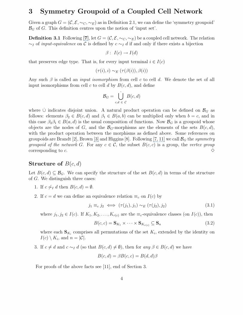
3 Symmetry Groupoid of a Coupled Cell Network

Given a graph G = (C, E ,∼C ,∼E) as in Definition 2.1, we can define the ‘symmetry groupoid’BG of G. This definition centres upon the notion of ‘input set’.

Definition 3.1 Following [7], let G = (C, E ,∼C ,∼E) be a coupled cell network. The relation∼I of input-equivalence on C is defined by c ∼I d if and only if there exists a bijection

β : I(c) → I(d)

that preserves edge type. That is, for every input terminal i ∈ I(c)

(τ(i), i) ∼E (τ(β(i)), β(i))

Any such β is called an input isomorphism from cell c to cell d. We denote the set of allinput isomorphisms from cell c to cell d by B(c, d), and define

BG =⋃

c,d ∈ C

B(c, d)

where ∪ indicates disjoint union. A natural product operation can be defined on BG asfollows: elements β2 ∈ B(c, d) and β1 ∈ B(a, b) can be multiplied only when b = c, and inthis case β2β1 ∈ B(a, d) is the usual composition of functions. Now BG is a groupoid whoseobjects are the nodes of G, and the BG-morphisms are the elements of the sets B(c, d),with the product operation between the morphisms as defined above. Some references ongroupoids are Brandt [2], Brown [3] and Higgins [8]. Following [7, 11] we call BG the symmetrygroupoid of the network G. For any c ∈ C, the subset B(c, c) is a group, the vertex groupcorresponding to c. 3

Structure of B(c, d)

Let B(c, d) ⊆ BG. We can specify the structure of the set B(c, d) in terms of the structureof G. We distinguish three cases:

1. If c 6∼I d then B(c, d) = ∅.

2. If c = d we can define an equivalence relation ≡c on I(c) by

j1 ≡c j2 ⇐⇒ (τ(j1), j1) ∼E (τ(j2), j2) (3.1)

where j1, j2 ∈ I(c). If K1, K2, . . . , Kr(c) are the ≡c-equivalence classes (on I(c)), then

B(c, c) = SK1 × · · · × SKr(c)⊆ Sn (3.2)

where each SKicomprises all permutations of the set Ki, extended by the identity on

I(c) \ Ki, and n = |C|.

3. If c 6= d and c ∼I d (so that B(c, d) 6= ∅), then for any β ∈ B(c, d) we have

B(c, d) = βB(c, c) = B(d, d)β

For proofs of the above facts see [11], end of Section 3.

4

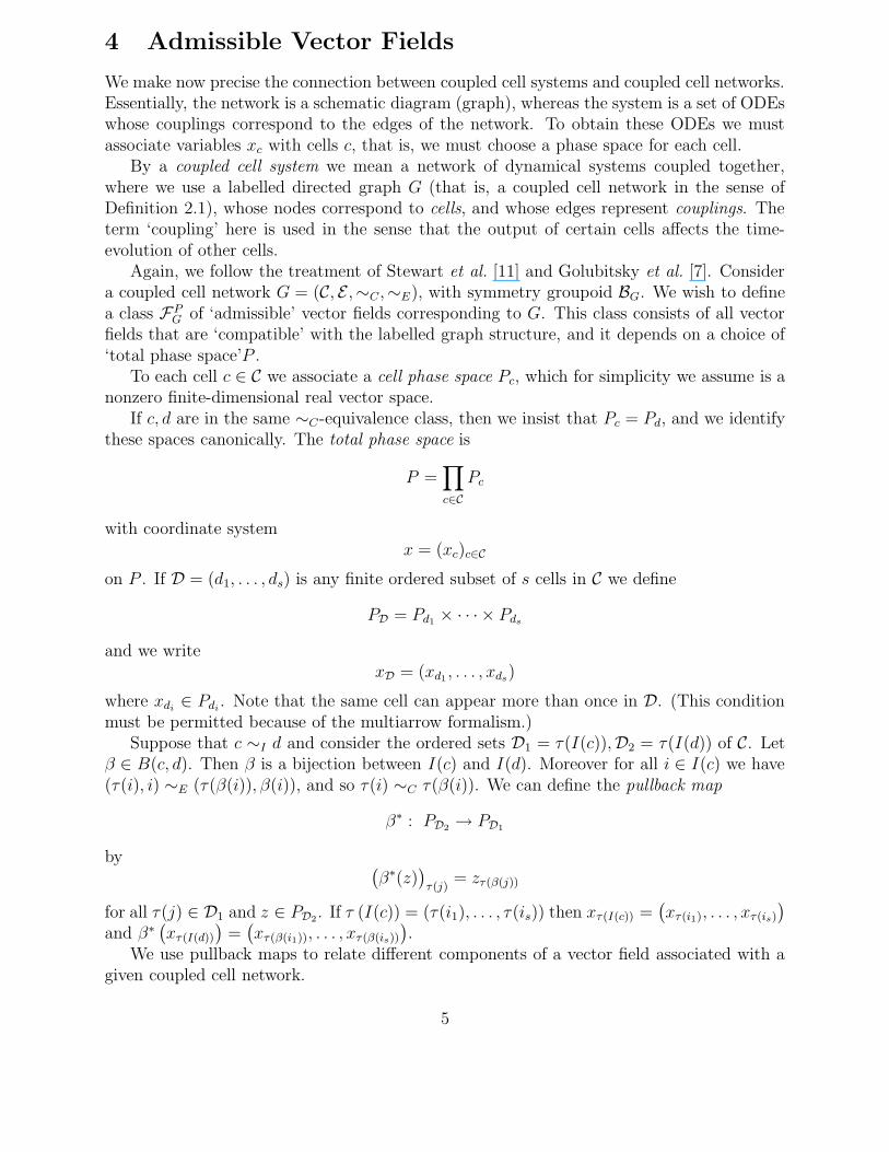
4 Admissible Vector Fields

We make now precise the connection between coupled cell systems and coupled cell networks.Essentially, the network is a schematic diagram (graph), whereas the system is a set of ODEswhose couplings correspond to the edges of the network. To obtain these ODEs we mustassociate variables xc with cells c, that is, we must choose a phase space for each cell.

By a coupled cell system we mean a network of dynamical systems coupled together,where we use a labelled directed graph G (that is, a coupled cell network in the sense ofDefinition 2.1), whose nodes correspond to cells, and whose edges represent couplings. Theterm ‘coupling’ here is used in the sense that the output of certain cells affects the time-evolution of other cells.

Again, we follow the treatment of Stewart et al. [11] and Golubitsky et al. [7]. Considera coupled cell network G = (C, E ,∼C,∼E), with symmetry groupoid BG. We wish to definea class FP

G of ‘admissible’ vector fields corresponding to G. This class consists of all vectorfields that are ‘compatible’ with the labelled graph structure, and it depends on a choice of‘total phase space’P .

To each cell c ∈ C we associate a cell phase space Pc, which for simplicity we assume is anonzero finite-dimensional real vector space.

If c, d are in the same ∼C-equivalence class, then we insist that Pc = Pd, and we identifythese spaces canonically. The total phase space is

P =∏

c∈C

Pc

with coordinate systemx = (xc)c∈C

on P . If D = (d1, . . . , ds) is any finite ordered subset of s cells in C we define

PD = Pd1 × · · · × Pds

and we writexD = (xd1 , . . . , xds

)

where xdi∈ Pdi

. Note that the same cell can appear more than once in D. (This conditionmust be permitted because of the multiarrow formalism.)

Suppose that c ∼I d and consider the ordered sets D1 = τ(I(c)),D2 = τ(I(d)) of C. Letβ ∈ B(c, d). Then β is a bijection between I(c) and I(d). Moreover for all i ∈ I(c) we have(τ(i), i) ∼E (τ(β(i)), β(i)), and so τ(i) ∼C τ(β(i)). We can define the pullback map

β∗ : PD2 → PD1

by (β∗(z)

)τ(j)

= zτ(β(j))

for all τ(j) ∈ D1 and z ∈ PD2. If τ (I(c)) = (τ(i1), . . . , τ(is)) then xτ(I(c)) =(xτ(i1), . . . , xτ(is)

)

and β∗(xτ(I(d))

)=

(xτ(β(i1)), . . . , xτ(β(is))

).

We use pullback maps to relate different components of a vector field associated with agiven coupled cell network.

5

For a given cell c the internal phase space is Pc and the coupling phase space is

Pτ(I(c)) = Pτ(i1) × · · · × Pτ(is)

where as before τ(I(c)) denotes the ordered set of cells (τ(i1), . . . , τ(is)).

Definition 4.1 [7] Let G = (C, E ,∼C,∼E) be a coupled cell network with symmetry group-oid BG. For a given choice of the Pc, a (smooth) vector field f : P → P is BG-equivariantor G-admissible if:

(a) Domain Condition: For any c ∈ C the component fc(x) depends only on the internalphase space variable xc and the coupling phase space variables xτ(I(c)). That is, there

exists a (smooth) function fc : Pc × Pτ(I(c)) → Pc such that

fc(x) = fc

(xc, xτ(I(c))

)

(b) Pullback Condition: For all c, d ∈ C and β ∈ B(c, d)

fd

(xd, xτ(I(d))

)= fc

(xd, β

∗(xτ(I(d))

) )

for all x ∈ P .

3

Theorem 4.2 Let G = (C, E ,∼C ,∼E) be a coupled cell network and BG the correspondingsymmetry groupoid. A vector field f : P → P for a given choice of the Pc is BG-equivariantif and only if for each connected component Q of BG (that is, each ∼I-equivalence class)

(a) fc is B(c, c)-invariant for some c ∈ Q.

(b) For d ∈ Q such that d 6= c, given (any) β ∈ B(c, d), we have

fd

(xd, xτ(I(d))

)= fc

(xd, β

∗(xτ(I(d))

) )

Proof This is a generalization of Lemma [11] 4.5 and is proved the same way. 2

Now we introduce notation for the space of G-admissible vector fields on P :

Definition 4.3 Let G be a coupled cell network. For a given choice of the Pc, define FPG

to consist of all smooth G-admissible vector fields on P . Clearly FPG is a vector space over

R. Like all function spaces, it can be equipped with a variety of topologies, but here onlythe vector space structure is relevant. Let PP

G be the subspace of FPG consisting of the G-

admissible polynomial vector fields on P , and let LPG be the subspace of PP

G consisting of theG-admissible linear vector fields on P . 3

The space of BG-equivariant maps has a natural decomposition according to the ‘con-nected components’ of the groupoid BG, and this decomposition is inherited by the polyno-mial and linear vector fields:

6

Definition 4.4 Let Q ⊆ C be an ∼I -equivalence class. Define

FPG (Q) =

{f ∈ FP

G : fs(x) = 0, ∀s 6∈ Q}

PPG (Q) =

{f ∈ PP

G : fs(x) = 0, ∀s 6∈ Q}

LPG(Q) =

{f ∈ LP

G : fs(x) = 0, ∀s 6∈ Q}

We say that vector fields in FPG (Q), PP

G (Q), and LPG(Q) are supported on Q. 3

Remark 4.5 From the above theorem there are direct sum decompositions

FPG =

⊕

Q

FPG (Q) PP

G =⊕

Q

PPG (Q) LP

G =⊕

Q

LPG(Q)

where Q runs over the ∼I-equivalence classes of G. 3

For detailed proofs see [11], end of Section 4, especially Proposition 4.6.

5 ODE-equivalence

As pointed by Golubitsky et al. [7], in the class of coupled cell networks that permits self-coupling and multiarrows, it is possible for two different coupled cell networks G1 and G2 togenerate the same space of admissible vector fields. Figure 1 shows a simple example, takenfrom Golubitsky et al. [7]. In G1 both cells have the same cell type, and similarly for G2.Suppose that the phase space for all four cells is Rk and identify these spaces canonically.Then the total phase space for both G1 and G2 is Rk × Rk.

The admissible vector fields for G1 have the form

H(x1, x2) = (h(x1, x1, x2), h(x2, x2, x1))

where h : Rk × Rk × Rk → Rk is any smooth function, and the admissible vector fields forG2 have the form

F (x1, x2) = (f(x1, x2), f(x2, x1))

where f : Rk ×Rk → Rk is any smooth function. It is now easy to see that the set {H} ofall H is the same as the set {F} of all F . Namely, given f we can set h(x, y, z) = f(x, z), sothat {H} ⊆ {F}. Given h we can set f(a, b) = h(a, a, b) so that {F} ⊆ {H}. Therefore thespaces FP1

G1and FP2

G2are the same.

For a less trivial example, see Figure 2 of Section 6. Note that the above comparison ofadmissible vector fields involves identifying cells in the two networks, a step that we formalisein general in terms of a bijection between the two sets of cells.

In the next definition, given a coupled cell network Gi and a choice of total phase spacePi for Gi, we denote by Pi,c the cell phase space corresponding to cell c of Ci.

7

1212

Figure 1: Two coupled cell networks G1 (on the left) and G2 (on the right) that generatethe same space of admissible vector fields.

Definition 5.1 Two coupled cell networks G1 and G2 are γ-ODE-equivalent if:

1. There is a bijection γ : C1 → C2 that preserves cell-equivalence and input-equivalence,such that:

2. If we choose cell phase spaces Pc 6= 0 for G1, and define the corresponding choice ofcell phase spaces for G2 by

P2,γ(c) = P1,c

so that the corresponding total phase spaces are

P1 =∏

c∈C1

P1,c P2 =∏

c∈C1

P1,γ(c)

then:

3. The conditionFP1

G1= FP2

G2(5.3)

is satisfied.

Two coupled cell networks G1 and G2 are ODE-equivalent if they are γ-ODE-equivalentfor some bijection γ. 3

Remarks 5.2 (a) The cells of G2 can be renumbered so that γ = id. In this case, weomit explicit reference to γ.

(b) It is shown in Section 7 below that if (5.3) holds for some choice of nonzero cell phasespaces Pc, then it holds for all such choices. We postpone proving this fact until wehave looked at a typical example, which makes the result obvious.

It follows that ODE-equivalence of two networks depends only on their architecture,and not on the particular choice of cell phase spaces. Note, however, the appearanceof the bijection γ that associates cells in the two networks (and must preserve cell-equivalence), and the requirement that Pγ(c) = Pc.

3

Isomorphic networks (in the usual graph-theoretic sense) are always ODE-equivalent. Aspointed out by Golubitsky et al. [7], ODE-equivalent networks are not necessarily isomorphic(see for instance Figure 1). The aim of this paper is to describe necessary and sufficientconditions for two coupled cell networks to be ODE-equivalent. In the next section we definethe notion of ‘linear equivalence’ between two networks. We show in Section 7 that twocoupled cell networks are ODE-equivalent if and only if they are linearly equivalent.

8

6 Linear Equivalence

In this section we define the notion of ‘linear equivalence’ (Definition 6.4 below). We startwith an example to illustrate the ideas involved, and, in particular, the effect of multiplearrows.

Example 6.1 Consider the coupled cell networks G1 and G2 of Figure 2. Here all cells arecell-equivalent in each graph, and the ∼I -equivalence classes of both graphs are:

Q1 = {1, 2, 3}, Q2 = {4}

The identity function on {1, 2, 3, 4} = C1 = C2 preserves cell-equivalence and input-equiva-lence.

2 11

1

1 2 3

4

1 2 3

4

5 5 3

1

5

Figure 2: Coupled cell networks G1 (left) and G2 (right). The number k attached to theright of each edge symbolizes k edges of that type.

First, choose all cell phase spaces to be Pc = R. We now describe the linear admissiblevector fields for both graphs, that is, the spaces LP

G1and LP

G2of linear groupoid-equivariant

maps. Let Yc denote coordinates on the phase space of cell c, for c = 1, . . . , 4, in both graphs.Any linear G1-admissible vector field F = (f1, f2, f3, f4) : R4 → R4 has the form:

f1(Y1) = aY1

f2(Y2) = aY2

f3(Y3) = aY3

f4(Y4, Y1, Y2, Y3) = bY4 + c(5Y1 + Y3) + d(2Y1 + Y2 + Y3)

where a, b, c, d are real constants, and any linear G2-admissible vector field G = (g1, g2, g3, g4) :R4 → R4 has the form:

g1(Y1) = eY1

g2(Y2) = eY2

g3(Y3) = eY3

g4(Y4, Y1, Y2, Y3) = hY4 + j(5Y1 + Y3) + l(5Y2 + 3Y3)

where e, h, j, l are real constants. Now recall Definition 4.1, and use the notation R{z1, . . . , zm}for the real vector space spanned by z1, . . . , zm. It is clear that

R {Y4, 5Y1 + Y3, 2Y1 + Y2 + Y3} = R {Y4, 5Y1 + Y3, 5Y2 + 3Y3} (6.4)

9

since 5Y2+3Y3 = 5(2Y1+Y2+Y3)−2(5Y1+Y3) and 2Y1+Y2+Y3 = 25(5Y1+Y3)+

15(5Y2+3Y3).

Therefore the space LPG1

of linear G1-admissible vector fields on R4 equals the space LPG2

oflinear G2-admissible vector fields on R4. We prove in Theorem 7.1 that this is a necessaryand sufficient condition for the graphs G1 and G2 to be ODE-equivalent. 3

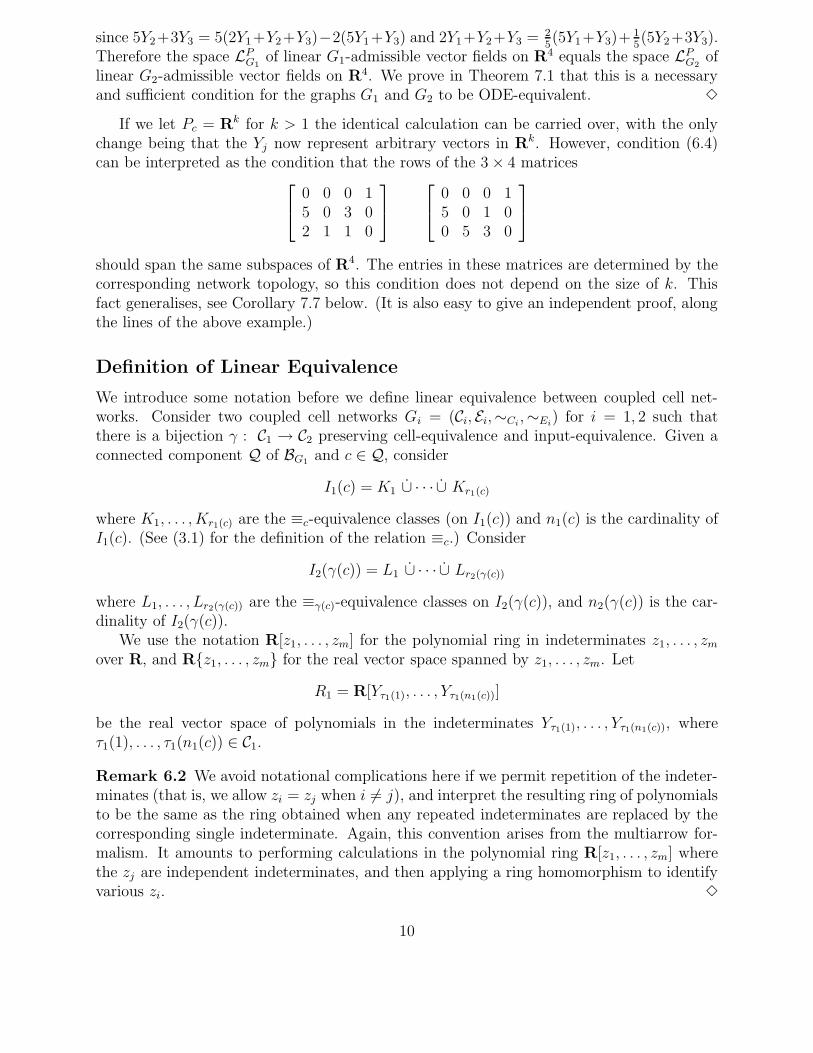
If we let Pc = Rk for k > 1 the identical calculation can be carried over, with the onlychange being that the Yj now represent arbitrary vectors in Rk. However, condition (6.4)can be interpreted as the condition that the rows of the 3 × 4 matrices

0 0 0 15 0 3 02 1 1 0

0 0 0 15 0 1 00 5 3 0

should span the same subspaces of R4. The entries in these matrices are determined by thecorresponding network topology, so this condition does not depend on the size of k. Thisfact generalises, see Corollary 7.7 below. (It is also easy to give an independent proof, alongthe lines of the above example.)

Definition of Linear Equivalence

We introduce some notation before we define linear equivalence between coupled cell net-works. Consider two coupled cell networks Gi = (Ci, Ei,∼Ci

,∼Ei) for i = 1, 2 such that

there is a bijection γ : C1 → C2 preserving cell-equivalence and input-equivalence. Given aconnected component Q of BG1 and c ∈ Q, consider

I1(c) = K1 ∪ · · · ∪ Kr1(c)

where K1, . . . , Kr1(c) are the ≡c-equivalence classes (on I1(c)) and n1(c) is the cardinality ofI1(c). (See (3.1) for the definition of the relation ≡c.) Consider

I2(γ(c)) = L1 ∪ · · · ∪ Lr2(γ(c))

where L1, . . . , Lr2(γ(c)) are the ≡γ(c)-equivalence classes on I2(γ(c)), and n2(γ(c)) is the car-dinality of I2(γ(c)).

We use the notation R[z1, . . . , zm] for the polynomial ring in indeterminates z1, . . . , zm

over R, and R{z1, . . . , zm} for the real vector space spanned by z1, . . . , zm. Let

R1 = R[Yτ1(1), . . . , Yτ1(n1(c))]

be the real vector space of polynomials in the indeterminates Yτ1(1), . . . , Yτ1(n1(c)), whereτ1(1), . . . , τ1(n1(c)) ∈ C1.

Remark 6.2 We avoid notational complications here if we permit repetition of the indeter-minates (that is, we allow zi = zj when i 6= j), and interpret the resulting ring of polynomialsto be the same as the ring obtained when any repeated indeterminates are replaced by thecorresponding single indeterminate. Again, this convention arises from the multiarrow for-malism. It amounts to performing calculations in the polynomial ring R[z1, . . . , zm] wherethe zj are independent indeterminates, and then applying a ring homomorphism to identifyvarious zi. 3

10

LetR2 = R[Yγ−1(τ2(1)), . . . , Yγ−1(τ2(n2(γ(c))))]

be the real vector space of polynomials in the indeterminates Yγ−1(τ2(1)), . . . , Yγ−1(τ2(n2(γ(c)))),where τ2(1), . . . , τ2(n2(γ(c))) ∈ C2.

Consider the subspace Sc1 of R1 defined by

Sc1 = R

Yc,

∑

i∈K1

Yτ1(i), . . . ,∑

i∈Kr1(c)

Yτ1(i)

(6.5)

Thus Sc1 contains the linear polynomials of R1 that are B1(c, c)-invariant. Similarly, let

Sγ(c)2 = R

Yc,

∑

i∈L1

Yγ−1(τ2(i)), . . . ,∑

i∈Lr2(γ(c))

Yγ−1(τ2(i))

⊆ R2 (6.6)

be formed by the linear polynomials of R2 that are B2(γ(c), γ(c))-invariant.

Example 6.3 Recall the coupled cell networks G1 and G2 of Figure 2. For both networks,all cells are cell-equivalent and the ∼I-equivalence classes are Q1 = {1, 2, 3} and Q2 = {4}.Thus the identity function γ on {1, 2, 3, 4} = C1 = C2 preserves cell-equivalence and input-equivalence. Consider Q2 and recall (6.5) and (6.6) where now c = 4 = γ(4). Then

S41 = R {Y4, 5Y1 + Y3, 2Y1 + Y2 + Y3}

andS

γ(4)2 = R {Y4, 5Y1 + Y3, 5Y2 + 3Y3}

As noted earlier, S41 = S

γ(4)2 . Moreover,

Si1 = S

γ(i)2 = R {Yi}

for i = 1, 2, 3.

Definition 6.4 Two coupled cell networks G1 and G2 are γ-linearly equivalent if:

1. There is a bijection γ : C1 → C2 that preserves cell-equivalence and input-equivalence,such that:

2. For each connected component Q of the network G1 and for each c ∈ Q we have

Sc1 = S

γ(c)2

where Sc1, S

γ(c)2 are as defined in (6.5) and (6.6).

Two coupled cell networks G1 and G2 are linearly equivalent if they are γ-linearly equiv-alent for some γ. 3

Note that this definition is independent of the dimensions of the Pc. Again, we mayrenumber to make γ the identity.

11

Example 6.5 We return to Example 6.3. Recall the coupled cell networks G1 and G2 ofFigure 2. Let γ denote the identity on the set {1, 2, 3, 4}. Then G1 and G2 are γ-linearly

equivalent since Sc1 = S

γ(c)2 for all c ∈ {1, 2, 3, 4}. We show in Theorem 7.1 that this is

necessary and sufficient for G1 and G2 to be ODE-equivalent. As a corollary, LPG1

= LPG2

forany choice of P compatible with cell-equivalence.

7 Linear Equivalence and ODE-equivalence

We now come to the main theorem of this paper, which reduces ODE-equivalence to linearequivalence, and its corollary, that the cell phase spaces may be assumed 1-dimensional inthat context. Recall Definition 5.1 of ODE-equivalence and Definition 6.4 of linear equiva-lence of coupled cell networks. Our main result is:

Theorem 7.1 Let γ : C1 → C2 be a bijection that preserves cell-equivalence and input-equivalence. Then two coupled cell networks G1 and G2 are γ-ODE-equivalent if and only ifthey are γ-linearly equivalent.

Proof The proof is divided in two steps. We prove in Proposition 7.2 below that giventwo coupled cell networks G1 and G2 and a bijection γ : C1 → C2 preserving cell-equivalenceand input-equivalence, together with a choice of total phase space P1 for G1 and P2 for G2

according to Definition 5.1, then FP1G1

= FP2G2

if and only if PP1G1

= PP2G2

. The rest of the

proof consists in proving in Proposition 7.3 below that PP1G1

= PP2G2

if and only if G1 andG2 are γ-linearly equivalent for some bijection γ : C1 → C2 preserving cell-equivalence andinput-equivalence. As a corollary, we deduce that PP1

G1= PP2

G2if and only if LP1

G1= LP2

G2, and

that in this context we may without loss of generality assume that all cell phase spaces are1-dimensional. 2

In the rest of the section we state and prove Propositions 7.2 and 7.3.

Proposition 7.2 Let G1 and G2 be two coupled cell networks such that there is bijectionγ : C1 → C2 that preserves cell-equivalence and input-equivalence. Consider a choice of totalphase space P1 =

∏c∈C1

P1,c for G1, and let P2 =∏

c∈C1P1,γ(c) be the corresponding phase

space for G2. Then FP1G1

= FP2G2

if and only if PP1G1

= PP2G2

.

Proof Trivially, if FP1G1

= FP2G2

then PP1G1

= PP2G2

. Suppose now that PP1G1

= PP2G2

. By

Theorem 4.2, every smooth equivariant vector field f ∈ FPi

Giis determined uniquely by its

components fc where c runs through a set of representatives for the connected components(that is, the ∼I -equivalence classes) of the groupoid BGi

. Note that since γ : C1 → C2 isa bijection that preserves input-equivalence, if Q is a connected component of the groupoidBG1 then γ(Q) is a connected component of BG2 , and if R is a set of representatives forthe connected components of BG1 then γ(R) is a set of representatives for the connectedcomponents of BG2 . The only constraints on fc are that it depends only on xc, xτ(I(c)) andis invariant under the vertex group B(c, c). Thus every smooth equivariant vector field f isdetermined uniquely by a finite set of B(c, c)-invariant functions, where c runs through a setof representatives for the connected components of the groupoid. Moreover, if d ∼I c then

12

fd is related to fc by a pullback map β∗ for β ∈ B(c, d). Pullbacks permute variables, hencepreserve smoothness (and also map polynomials to polynomials).

Schwarz [9] proves that in general for any compact Lie group Γ with an orthogonalaction on Rn, if the algebra of Γ-invariant polynomials is generated by ρ1, . . . , ρk (and byHilbert’s basis theorem such a finite basis always exist), then any Γ-invariant C∞-function ofn variables is a C∞-function of the generators ρ1, . . . , ρk. Since PP1

G1= PP2

G2, the vector space

of polynomial B1(c, c)-invariants (where B1(c, c) ⊆ BG1) coincides with the vector space ofpolynomial B2(γ(c), γ(c))-invariants (where B2(γ(c), γ(c)) ⊆ BG2). In particular, the twospaces share a set of invariant polynomial generators. Thus, given an ∼I -equivalence classQ ⊆ C1, the equality

PP1G1

(Q) = PP2G2

(γ(Q))

implies thatFP1

G1(Q) = FP2

G2(γ(Q))

Now Theorem 4.2 implies that FP1G1

= FP2G2

. 2

Proposition 7.3 Assume the conditions of Proposition 7.2. Then

PP1G1

= PP2G2

if and only if G1 and G2 are γ-linearly equivalent.

Before we prove Proposition 7.3, we state and prove two lemmas that explore the structureof the symmetry groupoids of coupled cell networks.

Lemma 7.4 Consider V d11 , . . . , V ds

s where each Vi is a nonzero finite-dimensional vectorspace of dimension ki, and denote coordinates on V di

i by xi = (xi,1, . . . , xi,di). Let

Γ = Sd1 × · · · × Sds

andV = V d1

1 ⊕ · · · ⊕ V ds

s

Define a Γ-action on V by: if σ ∈ Sdi, then

σ · x = (x1, . . . , xi−1, σ · xi, xi+1, . . . , xs)

whereσ · xi = (xi,σ−1(1), . . . , xi,σ−1(di))

Then any real Γ-invariant polynomial is a sum of polynomials of the form

q1(x1)q2(x2) · · · qs(xs)

where for j = 1, . . . , s, each qj(xj) is Sdj-invariant.

13

Proof The idea of the proof is simple but the notation is complicated. Essentially, weuse the fact that any invariant can be obtained as a linear combination of symmetrizedmonomials, so the proof reduces to computations with monomials.

In detail, recall that p : V → R is Γ-invariant if and only if

p(σ · x) = p(x) ∀σ ∈ Γ, x ∈ V

This condition holds if and only if p : V → R is Sdi-invariant, where Sdi

acts nontriviallyonly on V di

i .Denote by Z+

0 the set of nonnegative integers. Monomials in x1 have the form

xI11,1 · · ·x

Id11,d1

where I1, . . . , Id1 ∈ (Z+0 )k1 , and each x

Ij

1,j is a monomial in the k1 components of x1,j.Let p : V → R be a Γ-invariant polynomial, and write it as linear combination of

monomials in x1 with coefficients in R[x2, . . . , xs]. Suppose that p(x) contains a term thatis a scalar multiple of

xI11,1 · · ·x

Id11,d1

q(x2, . . . , xs)

Since p is Sd1 -invariant and Sd1 acts trivially on x2, . . . , xs, then p(x) must also contain

xI11,σ(1) · · ·x

Id1

1,σ(d1) q(x2, . . . , xs)

for all σ ∈ Sd1 . It follows that p(x) contains a scalar multiple of

∑

σ∈Sd1

xI11,σ(1) · · ·x

Id1

1,σ(d1)

q(x2, . . . , xs) = q1(x1) · q(x2, . . . , xs)

where q1(x1) =∑

σ∈Sd1xI1

1,σ(1) · · ·xId1

1,σ(d1). Now we repeat the same argument for q(x2, . . . , xs)

inductively. 2

Remark 7.5 This proof can be presented in a more abstract way: inductively, consider thepolynomial Sdj+1

-invariants over the ring of polynomial invariants for the subgroup Sd1 ×· · · × Sdj

× 1 × · · · × 1. 3

Lemma 7.6 Let V be a nonzero finite-dimensional real vector space of dimension d, anddenote coordinates on V t by y = (y1, . . . , yt). Let Γ = St and consider the action of Γ on V t

defined by:σ · y =

(yσ−1(1), . . . , yσ−1(t)

)(σ ∈ St, y ∈ V )

Then the ring of the Γ-invariant polynomials from V t to R is generated by the set of allΓ-invariant polynomials of the form

yI1 + · · ·+ yI

t

where I ∈ (Z+0 )d and each yI

i is a monomial in the d components of yi.

14

Proof Choose coordinates (y1, . . . , yt) on V t, where yi = (yi,1, . . . , yi,d). Thus, if σ ∈ St,

σ · (y1, . . . , yt) =(yσ−1(1), . . . , yσ−1(t)

)

whereyσ−1(i) =

(yσ−1(i),1, . . . , yσ−1(i),d

)

A real polynomial St-invariant on V t is a linear combination of St-invariants of the form

∑

σ∈St

yI1σ(1) · · ·y

It

σ(t) (7.7)

where Ii ∈ (Z+0 )d.

To continue the proof we need some terminology. Say that a polynomial (7.7) is of typem, where 1 ≤ m ≤ t, if only m sets of indices, without loss of generality, I1, . . . , Im, arenon-zero. That is, Im+1 = · · · = It = (0, . . . , 0), and Ij 6= (0, . . . , 0) for j = 1, . . . , m.

Now observe that if m = 1, then given any I1 ∈ (Z+0 )d, an expression (7.7) of type 1 has

the formpI1(y) =

∑

σ∈St

yI1σ(1) = yI1

1 + · · ·+ yI1t

The proof of the lemma is carried out by induction on the type m of the Γ-invariant poly-nomial. Suppose that any polynomial of the form (7.7) of type less than or equal to m is apolynomial in polynomials of type 1. We prove that the same holds for polynomials of typem + 1. Consider

pI1,...,Im+1(y) =∑

σ∈St

yI1σ(1)y

I2σ(2) · · ·y

Im+1

σ(m+1)

Take the St-invariant polynomial

p(y) = pI1(y) · · ·pIm+1(y)

wherepIi

(y) =∑

σ∈St

yIi

σ(1)

Note that pIj(y) for all j is a Γ-invariant polynomial of type 1. Moreover

p(y) = pI1,...,Im+1(y) +∑

i

βiri(y)

where each βi ∈ R and each ri(y) is an St-invariant of the form (7.7) of type less thanor equal to m. By hypothesis ri(y) is Γ-invariant and can be written as a polynomial inΓ-invariant polynomials of type 1. Thus

pI1,...,Im+1(y) = p(y) −∑

i

βiri(y)

and so pI1,...,Im+1(y) is a Γ-invariant polynomial that can be written as a polynomial of Γ-invariant polynomials of type 1. 2

15

Again, this proof can be presented more abstractly, along the lines of Remark 7.5.

Proof of Proposition 7.3 Let G1, G2 be two coupled cell networks and let γ : C1 → C2

be a bijection that preserves cell-equivalence and input-equivalence. Renumber the cells inC2 so that the bijection γ is the identity. Thus C1 = C2 = C and P1 = P2 = P .

Trivially if PPG1

= PPG2

then for each connected component Q of G1 (and G2) and foreach c ∈ Q we have Sc

1 = Sc2. We now prove the converse. Suppose that for each connected

component Q of G1 (and G2) and for each c ∈ Q we have

Sc1 = Sc

2

Let f be any admissible polynomial vector field in PPG1

. By Theorem 4.2, for any componentQ of BG1 and c ∈ Q, the property of BG1 -equivariance of f on the component

fc : Pc×Pτ(I1(c)) → Pc is equivalent to B1(c, c)-invariance of fc. Moreover, B1(c, c)-invariance

of fc is equivalent to B1(c, c)-invariance of each real component of fc. We choose the samecoordinate system for P1 and P2, and then prove that if Sc

1 = Sc2 then the ring of the

real polynomial B1(c, c)-invariants is the same as the ring of the real polynomial B2(c, c)-invariants. By Lemmas 7.4 and 7.6 the ring of real polynomial B1(c, c)-invariants is generatedas a ring by the real polynomial B1(c, c)-invariants of type 1. Similarly, the ring of realpolynomial B2(c, c)-invariants is generated as a ring by the real polynomial B2(c, c)-invariantsof type 1. Now it is enough to prove that if Sc

1 = Sc2, then any type 1 real polynomial

B1(c, c)-invariant is a real polynomial B2(c, c)-invariant. (Or equivalently, that any type 1real polynomial B2(c, c)-invariant is a real polynomial B1(c, c)-invariant.)

As before, I1(c) = K1 ∪ · · · ∪ Kr1(c) where K1, . . . , Kr1(c) are the ≡c-equivalence classeson I1(c). Thus

B1(c, c) = SK1 × · · · × SKr1(c)

Similarly, I2(c) = L1 ∪ · · · ∪ Lr2(c) where L1, . . . , Lr2(c) are the ≡c-equivalence classes onI2(c), and

B2(c, c) = SL1 × · · · × SLr2(c)

By Lemma 7.4 any real B1(c, c)-invariant polynomial is a product of real SKi-invariant

polynomials. Set Ki = {1, . . . , t}, so that St = SKiand let V t = Pτ(Ki) where V = Pτ(l)

(for any l ∈ Ki) is a non-zero finite-dimensional real vector space. Suppose that V hasdimension d, and denote coordinates on V t by y = (yτ(1), . . . , yτ(t)), where each yτ(i) =(yτ(i),1, . . . , yτ(i),d). Thus, if σ ∈ St then

σ · (yτ(1), . . . , yτ(t)) = (yτ(σ−1(1)), . . . , yτ(σ−1(t)))

whereyτ(σ−1(i)) = (yτ(σ−1(i)),1, . . . , yτ(σ−1(i)),d)

Given I ∈ (Z+0 )d, the polynomial

pI(y) = yIτ(1) + · · · + yI

τ(t)

is St-invariant (and so B1(c, c)-invariant) and

Yτ(1) + · · ·+ Yτ(t) ∈ Sc1

16

where Sc1 is as defined in (6.5). By hypothesis, Sc

1 = Sc2, where Sc

2 is defined in (6.6). Thusthere exist real coefficients α0, α1, α2, . . . , such that

Yτ(1) + · · ·+ Yτ(t) = α0p0(Y ) + αj1pj1(Y ) + αj2pj2(Y ) + · · · (7.8)

where p0(Y ) = Yc and pjp(Y ) =

∑i∈Ljp

Yτ(i) for p ≥ 1. Here Lj1 , Lj2, . . . denote ≡c-equiva-

lence classes on I2(c).We claim that the pjp

(Y ) that appear in (7.8) can be chosen to depend only on Yτ(k), wherethe cell phase space Pτ(k) = Pτ(1). To see this note that for all m ∈ {1, . . . , t} = Ki ⊆ I1(c)we know that since (τ(1), 1) ∼E1 (τ(m), m) then τ(1) ∼C1 τ(m) and so Pτ(1) = Pτ(m). Also,all the cells in the same ≡c-equivalence class are cell-equivalent. Thus if some pjp

(Y ) (withαjp

6= 0) in (7.8) depends on Yτ(l), Yτ(k) such that Pτ(l) = Pτ(1), then as τ(k) ∼C2 τ(l) since(τ(l), l) ∼E2 (τ(k), k) where l, k ∈ Ljp

⊆ I2(c), we have that Pτ(k) = Pτ(l) = Pτ(1). Thisproves the claim.

Set Yτ(j) = yIτ(j) for all j. Substituting all of this into equation (7.8) we get

pI(y) = Yτ(1) + · · ·+ Yτ(t) = qI(y)

where

qI(y) = α0yIc + αj1

∑

i∈Lj1

yIτ(i)

+ αj2

∑

i∈Lj2

yIτ(i)

+ · · ·

is a B2(c, c)-invariant. 2

Corollary 7.7 The following conditions on two networks G1, G2 are equivalent:

(a) G1 and G2 are γ-linearly equivalent.

(b) With the identification γ : C1 → C2, the spaces LPG1

and LPG2

are equal for all P .

(c) With the identification γ : C1 → C2, the spaces LPG1

and LPG2

are equal when all cellphase spaces are taken to be R.

Proof Condition (a) implies γ-ODE-equivalence for any choice of P , and γ-ODE-equivalenceimplies (b) by restricting to linear vector fields. Then (c) is special case of (b). Finally, (c)clearly implies (a). 2

8 Combinatorics of Linear Equivalence

Given two coupled cell networks, G1 and G2, Theorem 7.1 implies that in order to verifytheir ODE-equivalence, we need only check their linear equivalence. That is, we must decidewhether there exists some bijection between the corresponding sets of cells Ci, preservingcell-equivalence and input-equivalence, such that for each c ∈ C1 the vector spaces Sc

1 and

Sγ(c)2 are equal. A problem concerning the topology of networks as directed graphs has now

become a linear algebra problem of finding when two vector spaces of linear polynomials are

17

equal. Standard methods of linear algebra can solve this problem efficiently in any givencase.

It might seem likely that linear equivalence is simpler to work with than ODE-equivalence,in the sense that linear equivalence can be read off easily from the topologies two networksconcerned, modulo elementary linear algebra. But it is not clear whether the above linearalgebra problem can be simplified significantly by exploiting the network topology (say bydefining some kind of ‘normal form’ for the network, with a topological procedure thatreduces any given network to normal form) in a way that is not a trivial encoding of thecorresponding linear algebra computation. To illustrate the combinatorial complexities thatmay arise when determining linear equivalence, we generalize Example 6.1.

Recall Example 6.3, corresponding to the coupled cell networks of Figure 2. The twonetworks are ODE-equivalent since they are linearly equivalent, taking γ to be the identityfunction on C1 = C2 = {1, 2, 3, 4}. Other examples of coupled cell networks can easily beconstructed that are also linearly equivalent to G1 and G2, in the following way. Note thattaking

V = {λ1Y1 + λ2Y2 + λ3Y3 + λ4Y4 : λ1, λ2, λ3, λ4 ∈ R}

thenS4

1 = Sγ(4)2 = {λ1Y1 + λ2Y2 + λ3Y3 + λ4Y4 ∈ V : λ1 + 3λ2 = 5λ3}

4

13

2

a

a

a

b

b

1

2

a3

4

b1

2

b3

4

Figure 3: A coupled cell network with four identical cells, two edge-equivalence classes. Thesymbols ai and bi attached to the right of each edge symbolizes the number of edges of thattype. Thus ai, bi denote nonnegative integers.

Now consider Figure 3. Any coupled cell network with four identical cells and two edge-equivalence classes, as in Figure 3, is γ-linearly equivalent to G1 of Figure 2 provided that

R {Y4, a1Y1 + a2Y2 + a3Y3 + a4Y4, b1Y1 + b2Y2 + b3Y3 + b4Y4} =

{λ1Y1 + λ2Y2 + λ3Y3 + λ4Y4 ∈ V : λ1 + 3λ2 = 5λ3}

Here ai, bi are nonnegative integers and γ is the identity on {1, 2, 3, 4}.Other questions that we can pose include the following. Given an ODE-equivalence class

of coupled cell networks, is there a canonical ‘normal form’ — perhaps a graph, or a set ofgraphs, such that the number of edges is minimal among all the graphs of that ODE-class?Moreover, given a graph G, when can we find a subgraph that is ODE-equivalent to G?These questions are addressed by Aguiar and Dias [1].

18

Acknowledgements

APSD thanks Departamento de Matematica Pura da Faculdade de Ciencias da Universidadedo Porto for granting leave, and the Mathematics Institute of the University of Warwick,where this work was partially carried out, for hospitality. The research of APSD was sup-ported by Centro de Matematica da Universidade do Porto. That of INS was partiallysupported by a grant from the Engineering and Physical Sciences Research Council of theUK, and by NSF grant DMS-0244529.

References

[1] M.A.D. Aguiar and A.P.S. Dias. Linear Equivalence for Coupled Cell Networks, inpreparation.

[2] H. Brandt. Uber eine Verallgemeinerung des Gruppenbegriffes, Math. Ann. 96 (1927)360–366.

[3] R. Brown. From groups to groupoids: a brief survey, Bull. London Math. Soc. 19 (1987)113–134.

[4] M. Golubitsky, M. Nicol, and I. Stewart. Some curious phenomena in coupled cell net-works, J. Nonlin. Sci. 14 (2004) 207–236.

[5] M. Golubitsky and I. Stewart. The Symmetry Perspective: From Equilibrium to Chaosin Phase Space and Physical Space, Progress in Mathematics 200, Birkhauser, Basel2002.

[6] M. Golubitsky, I.N. Stewart, and D.G. Schaeffer. Singularities and Groups in BifurcationTheory, vol. 2, Applied Mathematical Sciences 69, Springer-Verlag, New York 1988.

[7] M. Golubitsky, I. Stewart, and A. Torok. Patterns of synchrony in coupled cell networkswith multiple arrows, to appear.

[8] P.J. Higgins. Notes on Categories and Groupoids, Van Nostrand Reinhold MathematicalStudies 32, Van Nostrand Reinhold, New York 1971.

[9] G.W. Schwarz. Smooth functions invariant under the action of a compact Lie group,Topology 14 (1975) 63–68.

[10] I. Stewart. Networking opportunity, Nature 427 (2004) 601–604.

[11] I. Stewart, M. Golubitsky, and M. Pivato. Symmetry groupoids and patterns of syn-chrony in coupled cell networks, SIAM J. Appl. Dynam. Sys. 2 (2003) 609–646.

[12] X.F. Wang. Complex networks: topology, dynamics and synchronization, Internat. J.Bif. Chaos 12 (2002) 885–916.

19