Konstantinos Efstathiou

Lecture 15: Dynamical Systems and Poincaré Maps MATH 303 ODE and Dynamical Systems

Non-autonomous planar systems

We now consider non-autonomous planar systems of the form

where the functions are periodic in with the same period. Here we will assume that the period is but the same arguments work for any other period

.

x′ = f(x, y, t),y′ = g(x, y, t),

f, g t2π

T

A fundamental property

Lemma. Consider the system of differential equations

where are periodic in with period .

Let be the solution to the initial value problem .

Then the solution to the initial value problem is given by .

x′ = f(x, y, t), y′ = g(x, y, t)

f, g t 2π

(x1(t), y1(t))(x(0), y(0)) = (x0, y0)

(x(2kπ), y(2kπ)) = (x0, y0), k ∈ ℤ(x2(t), y2(t)) = (x1(t − 2kπ), y1(t − 2kπ))

Proof. The proof is a copy of the corresponding proof for the one-dimensional case.

We have so indeed satisfies the given initial condition. Similarly, satisfies the initial condition .

Moreover, and satisfy the system of differential equations since

.

A similar computation shows that .

x2(2kπ) = x1(2kπ − 2kπ) = x1(0) = x0 x2(t)y2(t) y2(2kπ) = y0

x2(t) y2(t)

x′ 2(t) =ddt

[x1(t − 2kπ)] = x′ 1(t − 2kπ)d(t − 2kπ)

dt= x′ 1(t − 2kπ)

= f(x1(t − 2kπ), y1(t − 2kπ), t − 2kπ) = f(x2(t), y2(t), t − 2kπ)

= f(x2(t), y2(t), t)

y′ 2(t) = g(x2(t), y2(t), t)

Poincaré map for non-autonomous periodic systems

Poincaré map

Definition. Consider the system of differential equations

where are periodic in with period . Then the associated Poincaré map sends the point to the point

where is the solution to the given system that satisfies the initial condition .

x′ = f(x, y, t), y′ = g(x, y, t)

f, g t 2πP : ℝ2 → ℝ2 (x0, y0) ∈ ℝ2

P(x0, y0) = (x(2π), y(2π)) (x(t), y(t))(x(0), y(0)) = (x0, y0)

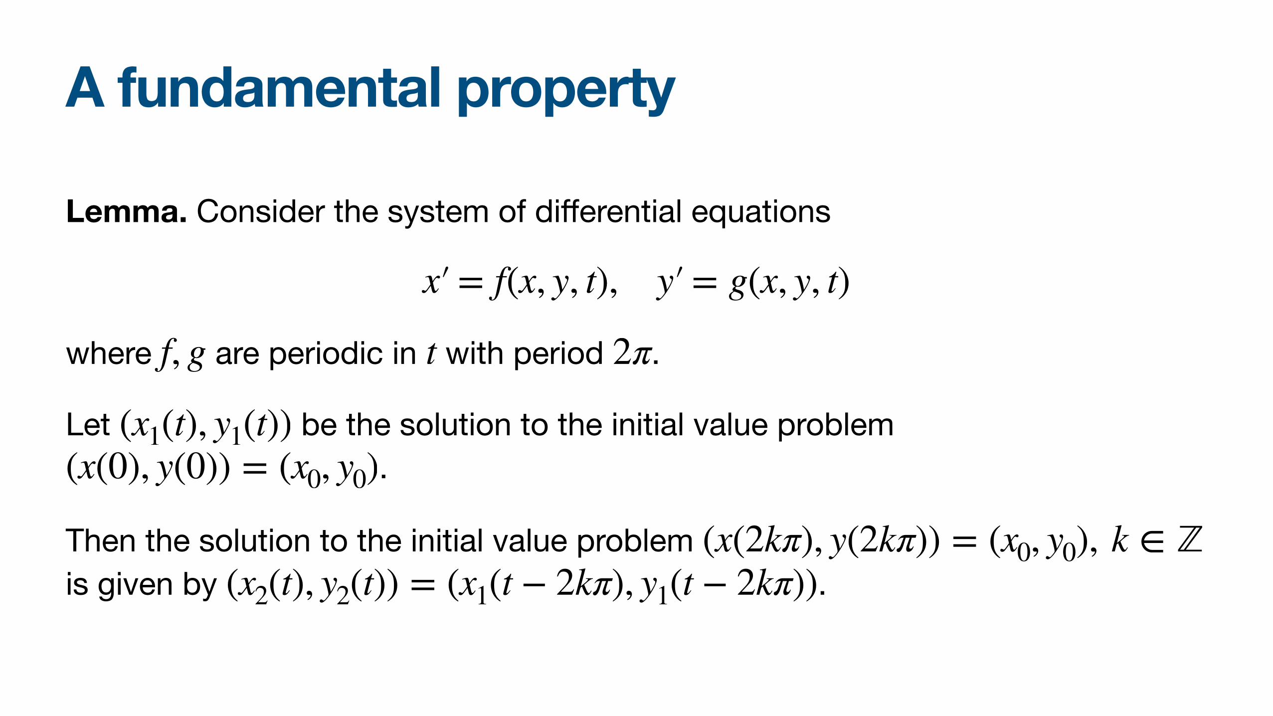
RemarkWith the notation of the previous definition we have

.

This means that the successive points are the points that we would get if we would observe the full, continuous solution curve only at times .

You can think of this as having a system that evolves in a dark room and that someone turns on the light periodically and records the system's state. Because of this interpretation, another name for this Poincaré map is stroboscopic (频 闪) map.

Pk(x0, y0) = (x(2kπ), y(2kπ))

(xk, yk) = Pk(x0, y0)(x(t), y(t))

t = 2kπ, k ∈ ℤ

Mass on spring with external forcingConsider the system

.

For the general solution for is

,

while we also get

.

Remark. The solution for can be obtained by converting the system to a second order equation for and using the methods for solving second order linear non-homogeneous equations with constant coefficients.

x′ = y, y′ = − ω2x + F cos t

ω2 ≠ 1 x

x = A cos(ωt − ϕ) +F

ω2 − 1cos t

y = x′ = − ωA sin(ωt − ϕ) −F

ω2 − 1sin t

xx

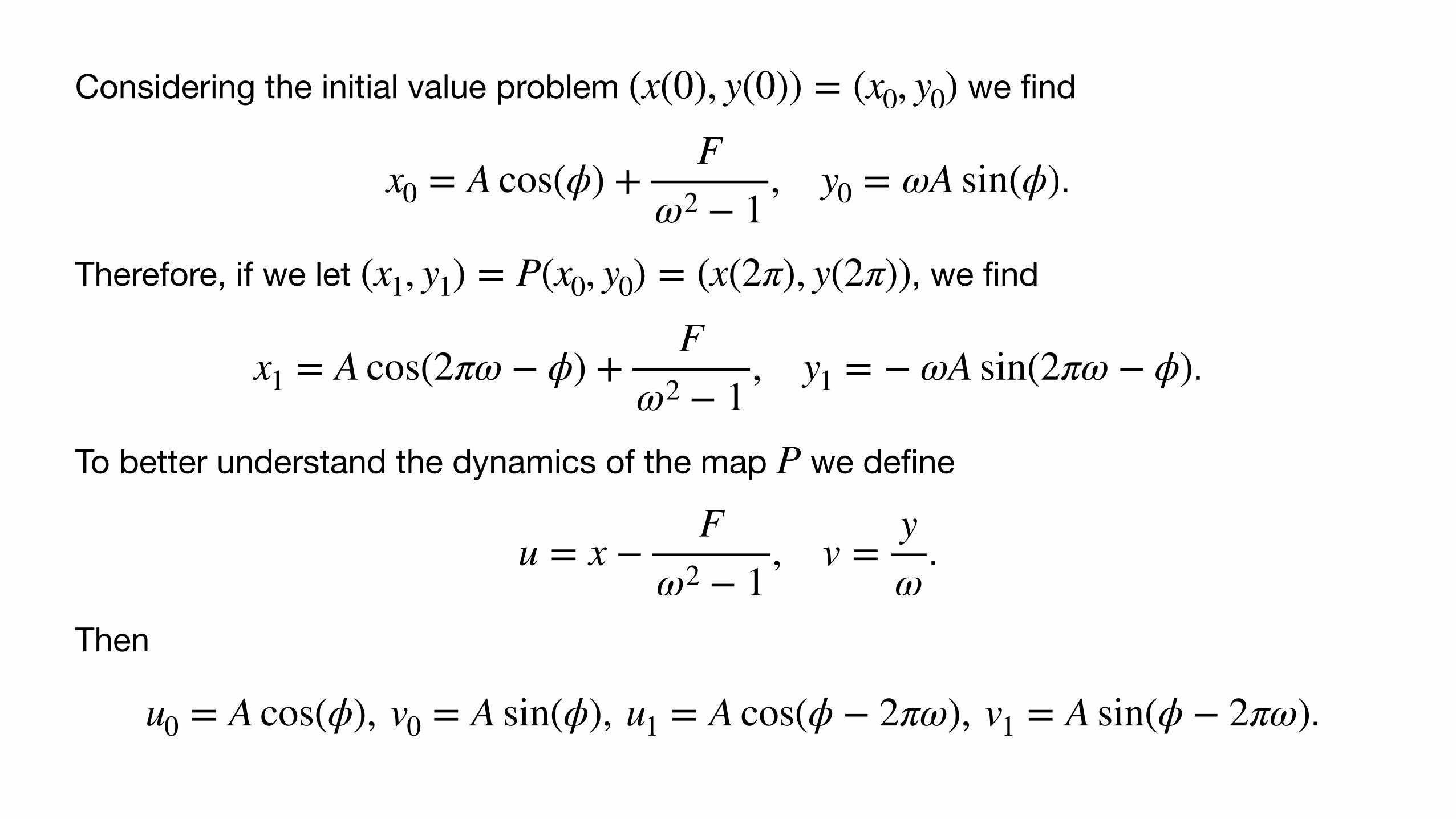
Considering the initial value problem we find

.

Therefore, if we let , we find

.

To better understand the dynamics of the map we define

.

Then

.

(x(0), y(0)) = (x0, y0)

x0 = A cos(ϕ) +F

ω2 − 1, y0 = ωA sin(ϕ)

(x1, y1) = P(x0, y0) = (x(2π), y(2π))

x1 = A cos(2πω − ϕ) +F

ω2 − 1, y1 = − ωA sin(2πω − ϕ)

P

u = x −F

ω2 − 1, v =

yω

u0 = A cos(ϕ), v0 = A sin(ϕ), u1 = A cos(ϕ − 2πω), v1 = A sin(ϕ − 2πω)

To write an expression for in terms of the coordinates we use the expressions

to get

,

.

Therefore,

.

P (u, v)

u0 = A cos(ϕ), v0 = A sin(ϕ), u1 = A cos(ϕ − 2πω), v1 = A sin(ϕ − 2πω)

u1 = A cos ϕ cos(2πω) + A sin ϕ sin(2πω) = cos(2πω)u0 + sin(2πω)v0

v1 = A sin ϕ cos(2πω) − A cos ϕ sin(2πω) = − sin(2πω)u0 + cos(2πω)v0

[u1v1] = [ cos(2πω) sin(2πω)

−sin(2πω) cos(2πω)] [u0v0]

It is even more convenient to define polar coordinates on the plane. Then the relations

become in polar coordinates

.

Therefore, in coordinates the map becomes

.

This means that in the plane the map is a clockwise rotation by angle .

(r, θ) (u, v)

u0 = A cos(ϕ), v0 = A sin(ϕ), u1 = A cos(ϕ − 2πω), v1 = A sin(ϕ − 2πω)

r0 = A, θ0 = ϕ, r1 = A, θ1 = ϕ − 2πω

(r, θ) P

r1 = r0, θ1 = θ0 − 2πω

(u, v)2πω

Remark. The only fixed point of the Poincaré map in this example is or .

Each fixed point corresponds to a periodic orbit of period and therefore, the system has only one such orbit.

Suppose now that where , and have no common factors. Then every point is a periodic point of the Poincaré map with period , since

.

Such periodic points of period correspond to periodic solution of the non-autonomous system with period .

If is irrational then the Poincaré map has no periodic points (except the fixed point which is a periodic point of period 1).

(u, v) = (0,0)(x, y) = (F/(ω2 − 1),0)

2π

ω = p/q p, q ∈ ℤ p, q ≥ 1 p, q(x, y) q

rq = r0, θq = ϕ − 2πωq = ϕ − 2πp ≡ ϕ

q2πq

ω

Forced Duffing equation

The forced Duffing equation is given by

.

Here, the period of the time-dependent term is . For this reason we define the Poincaré map using instead of .

The following code computes the Poincaré map.

x′ = y, y′ = − by + x − x3 + F sin(γt)

2π/γ2π/γ 2π

Below we show a single trajectory of with initial point , different values of , and , .

P (0,0)F b = 0.3 γ = 1.2

-2 -1 0 1 2-2

-1

0

1

2

x

y

F � 0.35

-2 -1 0 1 2-2

-1

0

1

2

x

y

F � 0.2

-2 -1 0 1 2-2

-1

0

1

2

x

y

F � 0.5

Fixed point Period 5 Chaotic attractor

ChaosChaos is associated to sensitive dependence on initial conditions. This means that even if we choose two initial conditions very close to each other, the two trajectories will deviate from each other exponentially fast. In the picture below we consider two initial conditions and for the forced Duffing system from the previous slide. Then we denote by the distance between the two trajectories at "time" and we plot

as a function of . The plots below are for and .

(0,0) (0,10−12)dk k

log dk k F = 0.2 F = 0.5

0 10 20 30 40 50-12

-10

-8

-6

-4

-2

0

k

log(dk)

F � 0.5

0 10 20 30 40 50-15

-14

-13

-12

-11

-10

k

log(dk)

F � 0.2

We observe that for and we have a linear increase

,

that is,

showing the exponential divergence of the two trajectories.

The essence of this phenomenon is that the exact state of the system is fundamentally unpredictable even though the system is deterministic.

However, the chaotic attractors produced for the two initial conditions will look identical.

F = 0.5 k ≤ 20

log dk = ak + b

dk ∼ eak

Poincaré map for autonomous systems

Hénon-Heiles systemWe consider the Hénon-Heiles system in given by

The system has the conserved quantity

.

This can be verified by checking that . represents the mechanical energy of a system and in this context is called the Hamiltonian function.

ℝ4

x′ 1 = y1

y′ 1 = − x1 − 2x1x2

x′ 2 = y2

y′ 2 = − x21 + x2

2 − x2

H =12

(y21 + y2

2) +12

(x21 + x2

2 + 2x21 x2−

23 x3

2)

dH/dt = 0 H

A Poincaré map can be defined in the following way.

Fix the hyperplane in defined by .

On this hyperplane we have . If we consider an

initial condition on then that corresponds to a value for that does not change along the corresponding solution .

Therefore, when the solution reaches again it will be at a point corresponding to . If we keep track only at the intersections of the solution with where

then it is enough to know — and the constant — to be able to determine

and .

Σ ℝ4 x1 = 0

H =12

(y21 + y2

2) +12

(x22− 2

3 x32)

Σ h H(x1(t), y1(t), x2(t), y2(t))

ΣH = h Σ

y1 > 0 (x2, y2) h

y1 = 2h − y22 − x2

2+ 23 x3

2 x1 = 0

So, suppose that we fix and consider a point .

Then define a point by

and .

This point is defined so that it is on and the corresponding value of equals .

h (x(0)2 , y(0)

2 )

(x(0)1 , y(0)

1 , x(0)2 , y(0)

2 ) ∈ ℝ4

x(0)1 = 0 y(0)

1 = 2h − (x(0)2 )2+ 2

3 (x(0)2 )3 − (y(0)

2 )2

ΣH h

Σ

(x(0)2 , y(0)

2 )(x(1)

2 , y(1)2 )

Then consider the solution of the system in with initial condition and track the solution until the first time

when we have with .

Then the Poincaré map is defined by

.

ℝ4

(x(0)1 , y(0)

1 , x(0)2 , y(0)

2 ) ∈ ℝ4 (x1(t), y1(t), x2(t), y2(t))t0 > 0 x1(t0) = 0 y1(t0) > 0

P : ℝ2 → ℝ2

(x(1)2 , y(1)

2 ) = P(x(0)2 , y(0)

2 ) = (x2(t0), y2(t0))

The Mathematica code for defining and computing this Poincaré map is shown below.

Several trajectories of the Poincaré map are shown with different colors for . We observe a chaotic orbit, and "islands" at the centers of which we have fixed points or periodic points.

The fixed points and the periodic points of the Poincaré map correspond to periodic orbits of the system in but we do not know the period of such orbits unless we compute it numerically.

h = 0.125

ℝ4

200 random initial conditions with 1000 points for each corresponding orbit.

Chaotic orbit with 10000 points.Some organized orbits with 1000 points for each.