Optimal control under probability constraint - Hal-Inria

HAL Id: inria-00585861https://hal.inria.fr/inria-00585861

Submitted on 14 Apr 2011

HAL is a multi-disciplinary open accessarchive for the deposit and dissemination of sci-entific research documents, whether they are pub-lished or not. The documents may come fromteaching and research institutions in France orabroad, or from public or private research centers.

L’archive ouverte pluridisciplinaire HAL, estdestinée au dépôt et à la diffusion de documentsscientifiques de niveau recherche, publiés ou non,émanant des établissements d’enseignement et derecherche français ou étrangers, des laboratoirespublics ou privés.

Optimal control under probability constraintPierre Carpentier, Jean-Philippe Chancelier, Guy Cohen

To cite this version:Pierre Carpentier, Jean-Philippe Chancelier, Guy Cohen. Optimal control under probability con-straint. SADCO Kick off, Mar 2011, Paris, France. �inria-00585861�

https://hal.inria.fr/inria-00585861

https://hal.archives-ouvertes.fr

Problem formulationModeling improvement

Stochastic Arrow-Hurwicz algorithmNumerical results

Optimal control under probability constraint

P. Carpentier — ENSTA ParisTechJ.-P. Chancelier — Ecole des Ponts ParisTech

G. Cohen — Ecole des Ponts ParisTech�

This work has been supported byThales-Alenia-Space (Cannes) and CNES (Toulouse)

SADCO Workshop

March 3, 2011

P. Carpentier and SOWG Optimal control under probability constraint March 3, 2011 1 / 31



Presentation outline

1 Problem formulation

2 Modeling improvement

3 Stochastic Arrow-Hurwicz algorithm

4 Numerical results




Satellite model and deterministic optimization problemEngine failureStochastic formulation

1 Problem formulationSatellite model and deterministic optimization problemEngine failureStochastic formulation



4 Numerical results





Satellite model

dr

dt= v ,

dv

dt= −µ r

‖r‖3+

F

mκ , (1a)

dm

dt= − T

g0Ispδ . (1b)

(1a) : 6-dimensional state vector (position r and velocity v).

(1b) : 1-dimensional state vector (mass m including fuel).

κ involves the direction cosines of the thrust and the on-off switchδ of the engine (3 controls), and µ,F ,T , g0, Isp are constants.

The deterministic control problem is to drive the satellite from theinitial condition at ti to a known final position rf and velocity vfat tf (given) while minimizing fuel consumption m(ti)−m(tf).





Deterministic optimization problem

Using equinoctial coordinates for the position and velocity; state vector x ∈ R7,

and cartesian coordinates for the thrust of the engine; control vector u ∈ R3,

the deterministic optimization problem is written as follows:

minu(·)

K(x(tf)

)(2a)

subject to:

x(ti) = xi ,•x (t) = f

(x(t), u(t)

), (2b)

‖u(t)‖ ≤ 1 ∀t ∈ [ti, tf ] , (2c)

C(x(tf)

)= 0 . (2d)





Engine failure

Sometimes, the engine may fail to work when needed: thesatellite drift away from the deterministic optimal trajectory.After the engine control is recovered, it is not always possibleto drive the satellite to the final target at tf .

By anticipating such possible failures and by modifying thetrajectory followed before any such failure occurs, one mayincrease the possibility of eventually reaching the target.But such a deviation from the deterministic optimal trajectoryresults in a deterioration of the economic performance.

The problem is thus to balance the increased probability ofeventually reaching the target despite possible failures againstthe expected economic performance, that is, to quantifythe price of safety one is ready to pay for.





Stochastic formulation (1)

A failure is modeled using two random variables:

tp : random initial time of the failure,td : random duration of the failure.

For every realization (tξp, tξd):

1 u(·) denotes the control used prior to any failure

; u is defined over [ti, tf ] but implemented over [ti, tξp]

and corresponds to an open-loop control,2 the control is 0 in [tξp, t

ξp + tξd],

3 v ξ(·) denotes the control used after the end of the failure

; v ξ is defined over [tξp + tξd, tf ] (if nonempty)and corresponds to a closed-loop strategy v.

The satellite dynamics in the stochastic formulation writes:

xξ(ti) = xi ,•x ξ(t) = f ξ

(xξ(t), u(t), v ξ(t)

).





Stochastic formulation (2)

The problem is to minimize the expected cost (fuel consumption)

w.r.t. the open-loop control u and the closed-loop strategy v,

the probability to hit the target at time tf being at least p.

minu(·)

E(

minvξ(·)

K(xξ(tf)

))(3a)

subject to:

xξ(ti) = xi ,•x ξ(t) = f ξ

(xξ(t), u(t), v ξ(t)

), (3b)

‖u(t)‖ ≤ 1 ∀t ∈ [ti, tf ] , ‖v ξ(t)‖ ≤ 1 ∀t ∈ [tξp + tξd, tf ] , (3c)

P(

C(xξ(tf)

)= 0)≥ p . (3d)




Probability as an expectationCost refinementFinal formulation


2 Modeling improvementProbability as an expectationCost refinementFinal formulation


4 Numerical results





Probability as an expectation

Let I(y) =

{1 if y = 0,

0 otherwise.Then

P(

C(xξ(tf)

)= 0)

= E(I(∥∥C

(xξ(tf)

)∥∥)) .Thus, Problem (3) can (shortly) be written:

minu(·)

E(

minvξ(·)

K(xξ(tf)

))(4a)

s.t. E(I(∥∥C

(xξ(tf)

)∥∥)) ≥ p . (4b)

Formulation (4) opens the possibility to make use of a stochasticArrow-Hurwicz algorithm in order to obtain the solution u](·).





Missing the target should not contribute to the cost

Whenever a failure occurred, setting v ξ ≡ 0 over [tξp + tξd, tf ]

generally makes the satellite misses the target and does notcontribute to the probability constraint,

but it forces fuel consumption to its minimum andcontributes to minimize the cost function.

This yields an artificially good expected cost; however, one is notinterested in what happens whenever the whole mission has failed.

Therefore, a better formulation is to register only scenarios whenthe target is effectively hit; instead of the original expected costin (4), we thus prefer to deal with a conditional expected cost:

E(

K(xξ(tf)

) ∣∣∣ C(xξ(tf)

)= 0)

=E(

K(xξ(tf)

)× I(∥∥C

(xξ(tf)

)∥∥))E(I(∥∥C

(xξ(tf)

)∥∥)) .





Conditional expected cost

The problem is reformulated as

minu(·),v(·)

E(

K(xξ(tf)

)× I(∥∥C

(xξ(tf)

)∥∥))E(I(∥∥C

(xξ(tf)

)∥∥)) (5a)

s.t. E(I(∥∥C

(xξ(tf)

)∥∥)) ≥ p . (5b)

Such a formulation is however not well-suited for the stochasticArrow-Hurwicz algorithm:

a ratio of expectations is not an expectation!





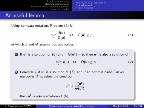
An useful lemma

Using compact notation, Problem (5) is:

minu

J(u)

Θ(u)s.t. Θ(u) ≥ p , (6)

in which J and Θ assume positive values.

1 If u] is a solution of (6) and if Θ(u]) = p, then u] is also a solution of

minu

J(u) s.t. Θ(u) ≥ p . (7)

2 Conversely, if u] is a solution of (7), and if an optimal Kuhn-Tuckermultiplier β] satisfies the condition

β] ≥ J(u])

Θ(u]),

then u] is also a solution of (6).





Back to a cost in expectation

Finally, instead of (5) we aim at solving

minu(·),v(·)

E(

K(xξ(tf)

)× I(∥∥C

(xξ(tf)

)∥∥)) (8a)

s.t. E(I(∥∥C

(xξ(tf)

)∥∥)) ≥ p . (8b)

The cost function again corresponds to a standard expectation!





Final formulation and associated Lagrangian

minu(·)

(E(

minvξ(·)

K(xξ(tf)

)× I(∥∥C

(xξ(tf)

)∥∥)))s.t. µ p − E

(I(∥∥C

(xξ(tf)

)∥∥)) ≤ 0 .

Assuming there exists a saddle point for the associated Lagrangian,we have finally to solve

maxµ≥0

minu(·)

{µ p + E

(minvξ(·)

(K(xξ(tf)

)−µ)×I(∥∥C

(xξ(tf)

)∥∥))} .

Remark: it is convenient to put apart the no-failure event, namely{

tp ≥ tf}

in the problem formulation. For the sake of simplicity, we do not present this

last problem improvement. We will denote by πf the probability of this event.




Algorithm overviewDownstream closed-loop problemSmoothing function ISolving the resulting approximated problem



3 Stochastic Arrow-Hurwicz algorithmAlgorithm overviewDownstream closed-loop problemSmoothing function ISolving the resulting approximated problem

4 Numerical results





Algorithm overview (1)

In order to solve

maxµ≥0

minu(·)

{µ p + E

(minvξ(·)

(K(xξ(tf)

)− µ

)× I(∥∥C

(xξ(tf)

)∥∥)︸︷︷︸W (u, µ, ξ)

)}.

that is,maxµ≥0

minu(·)

{µ p + E

(W (u, µ, ξ)

)},

we use a stochastic Arrow-Hurwicz algorithm (see [2] and [3]).





Algorithm overview (2)

Arrow-Hurwicz algorithm

At iteration k ,

1 draw a failure ξk = (tξk

p , tξk

d ) according to its probability law,

2 update u(·):

uk+1 = ΠB

(uk − εk ∇uW (uk , µk , ξk)

),

3 update µ:

µk+1 = max(

0, µk + ρk(p + ∇µW (uk+1, µk , ξk)

)).





Downstream closed-loop problem

Consider the inner optimization problem:

W (u, ξ, µ) = minvξ(·)

{(K(xξ(tf)

)− µ

)× I(∥∥C

(xξ(tf)

)∥∥)} ,If reaching the target is impossible (C

(xξ(tf)

)6= 0 ∀v ξ),

the best thing to do is to stop immediately: W ≡ 0.

If reaching the target is possible but too expensive (thatis K

(xξ(tf)

)≥ µ), the best thing to do is again to stop

immediately: W ≡ 0.

Therefore, it must be checked that one can reach the targetwhile maintaining fuel consumption below a threshold, andthe corresponding optimal control v ξ∗ (·) must be computed.

At every iteration k, we must evaluate function W as well asits derivatives w.r.t. u(.) and µ. But W is not differentiable!





First difficulty: I is not a smooth function

I(y) =

{1 if y = 0,

0 otherwise, Ir (y) =

(

1− y2

r2

)2if y ∈ [−r , r ],

0 otherwise.

0.2

0.4

0.6

0.8

1.0

0.2

0.4

0.6

0.8

1.0

There are specific rules to drive rk to 0 as the iteration numberk goes to infinity in order to obtain the best asymptotic MeanQuadratic Error of the gradient estimates (see [1]).





Second difficulty: solving the approximated problem

The approximated closed-loop problem to solve at each iteration is:

Wr (uk , ξk , µk) = minvξ(·)

{(K(xξ(tf)

)− µk

)× Ir

(∥∥C(xξ(tf)

)∥∥)} .In this setting, we have to check if the target is reached up to r .

In practice, the solution of the approximated problem is derivedfrom the resolution of two standard optimal control problems.




Brief descriptionResults for different values of pThe price of safety




4 Numerical resultsBrief descriptionResults for different values of pThe price of safety





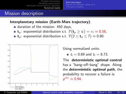
Mission description

Interplanetary mission (Earth-Mars trajectory):

duration of the mission: 450 days,tp: exponential distribution s.t. P

(tp ≥ tf

)= πf ≈ 0.58,

td: exponential distribution s.t. P(2 ≤ td ≤ 7

)≈ 0.80.

Comp. normale wComp. tangentielle sComp. radiale q

0 1 2 3 4 5 6 7 8 9−0.4

−0.2

0.0

0.2

0.4

0.6

0.8

1.0

Using normalized units:

ti = 0.69 and tf = 8.73.

The deterministic optimal controlhas a “bang–off–bang” shape. Alongthe deterministic optimal path, theprobability to recover a failure is:pdet ≈ 0.94.





Parameters tuning

Gradient step length:

εk =a

b + k, ρk =

c

d + k,

usual for a stochastic gradient algorithm.

Smoothing parameter:

rk =α

β + k13

,

MQE reduced by a factor 2000 in about 100.000 iterations.





Masse finale / iterations0 10000 20000 30000 40000 50000 60000 70000 80000 90000 1000000.675

0.676

0.677

0.678

0.679

0.680

0.681

Multiplicateur probabilite / iterations0 10000 20000 30000 40000 50000 60000 70000 80000 90000 1000000.00

0.05

0.10

0.15

0.20

0.25

0.30

0.35


0 1 2 3 4 5 6 7 8 9−0.4

−0.2

0.0

0.2

0.4

0.6

0.8

1.0

Figure: Probability level p < πf






0.675

0.676

0.677

0.678

0.679

0.680

0.681


0.316

0.318

0.320

0.322

0.324

0.326


0 1 2 3 4 5 6 7 8 9−0.4

−0.2

0.0

0.2

0.4

0.6

0.8

1.0

Figure: Probability level p = 0.750






0.674

0.675

0.676

0.677

0.678

0.679

0.680

0.681


0.320

0.322

0.324

0.326

0.328

0.330

0.332


0 1 2 3 4 5 6 7 8 9−0.4

−0.2

0.0

0.2

0.4

0.6

0.8

1.0







0.675

0.676

0.677

0.678

0.679

0.680

0.681


0.325

0.330

0.335

0.340

0.345

0.350

0.355

0.360

0.365


0 1 2 3 4 5 6 7 8 9−0.4

−0.2

0.0

0.2

0.4

0.6

0.8

1.0






Fuel consumption versus probability level

Consommation sans panne / Probabilite0.85 0.90 0.95 1.00

0.3204

0.3206

0.3208

0.3210

0.3212

0.3214

0.3216

0.3218

0.3220

0.3222

Figure: Fuel consumption versus probability level pP. Carpentier and SOWG Optimal control under probability constraint March 3, 2011 29 / 31




Conclusion

Main conclusion

We are able to deal with probability constraints in the optimalcontrol framework.

Future works

From the theoretical point of view:

existence of a saddle point for the constrained problem,smoothing process (results available only for inequalityconstraints).

From the numerical point of view:

efficient solver for the downstream problem,computer parallelization.


Laetitia Andrieu, Guy Cohen and Felisa Vazquez-Abad.

Stochastic Programming with Probability.

arXiv, math.OC 0708.0281, 2007.

Jean-Christophe Culioli and Guy Cohen.

Decomposition/Coordination Algorithms in Stochastic Optimization.

SIAM Journal on Control and Optimization, 28, 1372-1403, 1990.

Jean-Christophe Culioli and Guy Cohen.

Optimisation stochastique sous contraintes en esperance.

CRAS, t.320, Serie I, pp. 75-758, 1995.

Thierry Dargent.

Transfert d’orbite optimal par application du principe du minimum.

Logiciel T 3D, version 2, 19 mars 2004.

Andras Prekopa.

Stochastic Programming.

Kluwer, Dordrecht, 1995.




Thank you for your attention. Any question?


Optimal control under probability constraint - Hal-Inria

Documents

Transcript of Optimal control under probability constraint - Hal-Inria