Variable-width contouring for Additive Manufacturing - HAL-Inria

HAL Id: hal-02568677https://hal.inria.fr/hal-02568677v1

Submitted on 11 May 2020 (v1), last revised 8 Jul 2020 (v2)

HAL is a multi-disciplinary open accessarchive for the deposit and dissemination of sci-entific research documents, whether they are pub-lished or not. The documents may come fromteaching and research institutions in France orabroad, or from public or private research centers.

L’archive ouverte pluridisciplinaire HAL, estdestinée au dépôt et à la diffusion de documentsscientifiques de niveau recherche, publiés ou non,émanant des établissements d’enseignement et derecherche français ou étrangers, des laboratoirespublics ou privés.

Variable-width contouring for Additive ManufacturingSamuel Hornus, Tim Kuipers, Olivier Devillers, Monique Teillaud, Jonàs

Martínez, Marc Glisse, Sylvain Lazard, Sylvain Lefebvre

To cite this version:Samuel Hornus, Tim Kuipers, Olivier Devillers, Monique Teillaud, Jonàs Martínez, et al.. Variable-width contouring for Additive Manufacturing. ACM Transactions on Graphics, Association for Com-puting Machinery, In press, 39 (Siggraph’2020 Conference proceedings), �10.1145/3386569.3392448�.�hal-02568677v1�

https://hal.inria.fr/hal-02568677v1

https://hal.archives-ouvertes.fr

Variable-width contouring for Additive Manufacturing

SAMUEL HORNUS, Université de Lorraine, CNRS, Inria, LORIATIM KUIPERS, Ultimaker and Department of Sustainable Design Engineering, Delft University of TechnologyOLIVIER DEVILLERS and MONIQUE TEILLAUD, Université de Lorraine, CNRS, Inria, LORIAJONÀS MARTÍNEZ, Université de Lorraine, CNRS, Inria, LORIAMARC GLISSE, InriaSYLVAIN LAZARD and SYLVAIN LEFEBVRE, Université de Lorraine, CNRS, Inria, LORIA

(a) (b) (c) (d) (e) (f)

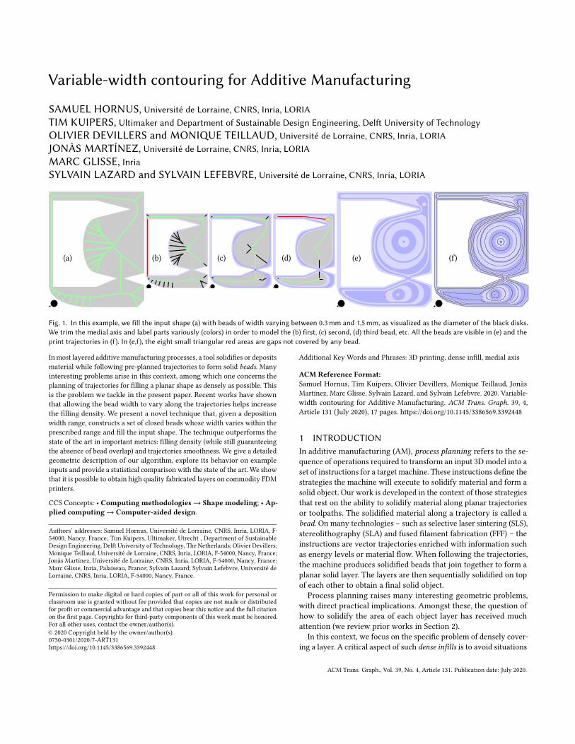
Fig. 1. In this example, we fill the input shape (a) with beads of width varying between 0.3mm and 1.5mm, as visualized as the diameter of the black disks.We trim the medial axis and label parts variously (colors) in order to model the (b) first, (c) second, (d) third bead, etc. All the beads are visible in (e) and theprint trajectories in (f). In (e,f), the eight small triangular red areas are gaps not covered by any bead.

In most layered additive manufacturing processes, a tool solidifies or deposits

material while following pre-planned trajectories to form solid beads. Many

interesting problems arise in this context, among which one concerns the

planning of trajectories for filling a planar shape as densely as possible. This

is the problem we tackle in the present paper. Recent works have shown

that allowing the bead width to vary along the trajectories helps increase

the filling density. We present a novel technique that, given a deposition

width range, constructs a set of closed beads whose width varies within the

prescribed range and fill the input shape. The technique outperforms the

state of the art in important metrics: filling density (while still guaranteeing

the absence of bead overlap) and trajectories smoothness. We give a detailed

geometric description of our algorithm, explore its behavior on example

inputs and provide a statistical comparison with the state of the art. We show

that it is possible to obtain high quality fabricated layers on commodity FDM

printers.

CCS Concepts: • Computing methodologies→ Shape modeling; • Ap-plied computing→ Computer-aided design.

Authors’ addresses: Samuel Hornus, Université de Lorraine, CNRS, Inria, LORIA, F-

54000, Nancy, France; Tim Kuipers, Ultimaker, Utrecht , Department of Sustainable

Design Engineering, Delft University of Technology, The Netherlands; Olivier Devillers;

Monique Teillaud, Université de Lorraine, CNRS, Inria, LORIA, F-54000, Nancy, France;

Jonàs Martínez, Université de Lorraine, CNRS, Inria, LORIA, F-54000, Nancy, France;

Marc Glisse, Inria, Palaiseau, France; Sylvain Lazard; Sylvain Lefebvre, Université de

Lorraine, CNRS, Inria, LORIA, F-54000, Nancy, France.

Permission to make digital or hard copies of part or all of this work for personal or

classroom use is granted without fee provided that copies are not made or distributed

for profit or commercial advantage and that copies bear this notice and the full citation

on the first page. Copyrights for third-party components of this work must be honored.

For all other uses, contact the owner/author(s).

© 2020 Copyright held by the owner/author(s).

0730-0301/2020/7-ART131

https://doi.org/10.1145/3386569.3392448

Additional Key Words and Phrases: 3D printing, dense infill, medial axis

ACM Reference Format:Samuel Hornus, Tim Kuipers, Olivier Devillers, Monique Teillaud, Jonàs

Martínez, Marc Glisse, Sylvain Lazard, and Sylvain Lefebvre. 2020. Variable-

width contouring for Additive Manufacturing. ACM Trans. Graph. 39, 4,Article 131 (July 2020), 17 pages. https://doi.org/10.1145/3386569.3392448

1 INTRODUCTIONIn additive manufacturing (AM), process planning refers to the se-

quence of operations required to transform an input 3D model into a

set of instructions for a target machine. These instructions define the

strategies the machine will execute to solidify material and form a

solid object. Our work is developed in the context of those strategies

that rest on the ability to solidify material along planar trajectories

or toolpaths. The solidified material along a trajectory is called a

bead. On many technologies – such as selective laser sintering (SLS),

stereolithography (SLA) and fused filament fabrication (FFF) – the

instructions are vector trajectories enriched with information such

as energy levels or material flow. When following the trajectories,

the machine produces solidified beads that join together to form a

planar solid layer. The layers are then sequentially solidified on top

of each other to obtain a final solid object.

Process planning raises many interesting geometric problems,

with direct practical implications. Amongst these, the question of

how to solidify the area of each object layer has received much

attention (we review prior works in Section 2).

In this context, we focus on the specific problem of densely cover-

ing a layer. A critical aspect of such dense infills is to avoid situations

ACM Trans. Graph., Vol. 39, No. 4, Article 131. Publication date: July 2020.

https://doi.org/10.1145/3386569.3392448

https://doi.org/10.1145/3386569.3392448

131:2 • Hornus, Kuipers, Devillers, Teillaud, Martínez, Glisse, Lazard and Lefebvre

T 0

T 1

T 2 T 1

T 0

γ

ΓγT 0

T 1

γ

T 2

∂S0

∂S1

∂S2

∂S0

∂S1

∂S2∂S3

Fig. 2. Left. Uniform-width contouring. Beads have constant width 2γ andproduce overfill as self-overlap in the blue areas. The inner red areas are notcovered: we have underfill.Middle. Regularized parallel contouring avoidsoverfill. Beads have constant width 2γ . Right. Variable-width contouring(our technique) models beads with varying width in the range [2γ , 2Γ].

where the produced beads overlap or self-overlap uncovered gaps be-

tween them (underfill). Such issues appearwith common approaches,

where beads are defined as the space between successive shapes,

obtained by an iterated parallel offset (or morphological erosion).

In uniform-width contouring (Figure 2 left), beads of width 2γ are

obtained by applying a parallel offset of width 2γ to the shape, result-

ing in both overfill and underfill [Eiamsa-ard et al. 2003; Yang et al.

2002]. Regularized parallel contouring (Figure 2middle) computes

each nested shape by applying an offset of width 4γ (instead of 2γ )followed by a morphological dilation by a disk of diameter 2γ [MFX

2017]. The beads still follow boundary-parallel trajectories, which

may create underfill but not overfill. Indeed, even in the favorable

case of a feature that is not too sharp, note in the figure how the

nested shapes become sharp after the first two beads are extracted,

which creates a gap at each subsequent step.

While underfill threatens the structural strength, overfill may lead

to fabrication failures [Kuipers et al. 2019; Wenbiao et al. 2002]. A

dense, smooth, and precise fill leads to stronger parts and increased

manufacturing reliability [Kao and Prinz 1998]. To achieve this, we

exploit the ability of many AM processes to vary the solidification

radius dynamically along a deposition trajectory [Ding et al. 2016;

Wang et al. 2019]. However, bead width variations have to remain

within minimum and maximum bounds for proper solidification.

This makes the filling problem harder and of particular interest.

Current processes are nevertheless not optimized for varying width

deposition and there are practical difficulties that we discuss in Sec-

tion 6.2.

We present an algorithm that leaves significantly fewer underfill

(gaps) than existing techniques, guarantees the absence of overfill,

while producing smooth, cyclic deposition trajectories. Its output is

illustrated in Figure 2 right for a simple case, and in Figure 1 for a

more complex case. We give a detailed overview of our algorithm in

Section 3 and a complete geometric description in Section 5.We then

provide in Section 6 an experimental assessment focused on fused

filament processes (FDM) in order to demonstrate the applicability of

the technique. We discuss limitations in the conclusion. In particular,

our algorithm does not achieve a globally minimal underfill; Finding

the global minimum remains an open problem.

The source code for this work is available at https://github.com/

mfx-inria/Variable-width-contouring.

2 PREVIOUS WORKSolidification inside the volume of an object is one of the main

driving factors of fabrication time [Livesu et al. 2017]. Thus, a line

of research explores how to make insides print faster, for instance

with sparse patterns [McMains et al. 2000], thicker layers [Sabourin

et al. 1997], or by maximally emptying the part while still ensur-

ing fabricability under overhang and support constraints [Hornus

and Lefebvre 2018; Lee and Lee 2016; Tricard et al. 2019; Wang

et al. 2017b]. Under the same constraints, other approaches seek

to optimize the internal properties to achieve specific mechanical

objectives, such as balance [Prévost et al. 2013; Wu et al. 2016],

rigidity [Li et al. 2015; Wang et al. 2017a], density [Kuipers et al.

2019] or elastic response orientation [Martínez et al. 2018].

There are, however, many situations where a dense cover is de-

sired, for instance on the tops and bottoms of an object, but also to

increase the strength and rigidity of a piece. A first approach for

densely covering a contour with trajectories is to rely on zig-zag

patterns [McMains et al. 2000]. This strategy, however, leads to un-

derfill and overfill where paths connect to the enclosing contour,

requiring trade-offs [Jin et al. 2013]. A second approach is to follow

contour parallel trajectories [Eiamsa-ard et al. 2003; Yang et al. 2002].

These paths closely follow the contour outline and typically pro-

vide an improved surface finish. Unfortunately, as mentioned in the

introduction, this approach also leaves many gaps where contours

from both sides fail to meet exactly along the medial axis [Kao and

Prinz 1998]. Note that in practice, a few contour parallel paths are

often used first, followed by a zig-zag fill.

Another important concern is to avoid interrupting the solidifica-

tion process, and to produce as-smooth-as-possible trajectories. This

is especially important on extrusion-based systems, where pausing

and resuming the flow is challenging due to pressure buildup. Thus,

several works considered how to reconnect paths into continuous

trajectories, for both zig-zag and contour parallel patterns [Ding

et al. 2014; Jin et al. 2017b; Zhao et al. 2016].

To reduce underfills and overfills, Moesen et al. [2011] consider

how to preserve key features of a part that would otherwise be

removed by the initial offsetting. In particular, the algorithm widens

narrow regions to accommodate a single bead, while preserving the

initial layer topology.

Kao et al. [1998] considered exploiting a varying solidification

width early on. Their proposed method optimizes and modifies the

contour outline to ensure it can be fully filled – without gaps – with

varying width beads between a minimum and maximum bound.

However, to reproduce the original contour the smooth beads have

to be clipped, thus producing many open paths. Ding et al. [2016]

also exploit a varying solidification width to eliminate gaps. The pro-

posed approach is to generate the same number of beads in between

the outer contour and an inner skeleton of the slice. As there are

the same number of beads across, their widths vary simultaneously

to adapt to the local shape thickness around the skeleton: the bead

widths shrink and expand. While this proves effective to generate

beads of varying widths, the technique cannot bound both the small-

est and largest obtained widths: one of the bounds is determined by

the other, and can become arbitrarily small/large. Xiong et al. [2019]

similarly produce varying width beads by contouring a distance field


https://github.com/mfx-inria/Variable-width-contouring

https://github.com/mfx-inria/Variable-width-contouring

Variable-width contouring for Additive Manufacturing • 131:3

computed from the input shape outline. The bounds also cannot be

guaranteed, limiting the applicability to specific parts.

Jin et al. [2017a] reduce gaps and overlaps in narrow areas. After

each successive parallel offset, a medial axis transform of the region

sandwiched between trajectories is constructed. The radii along the

medial axis are used to detect whether the region becomes smaller

or larger than the desired deposition width. If it is too large an

additional segment is inserted along the medial axis to avoid a gap. If

it is too small, the trajectories are locally removed to avoid overflow.

Compared to the methods presented above this method reduces

the bead width variation to a more narrow range independent of

the filled geometry. A similar approach is proposed in a concurrent

work [Kuipers et al. 2020]. The resulting beads also have a preferred

width inmost locations, but a deviatingwidth in the center. However,

that deviation is distributed over several beads near the center of the

shape, which further reduces the bead width variation. Moreover,

the medial axis transform is only computed once, which results

in a considerable computational performance boost. While both

latter works offer clear improvements over the direct contouring

approach, many uncovered areas remain.

We provide discussion and comparisons with respect to these

approaches in Section 6.3.

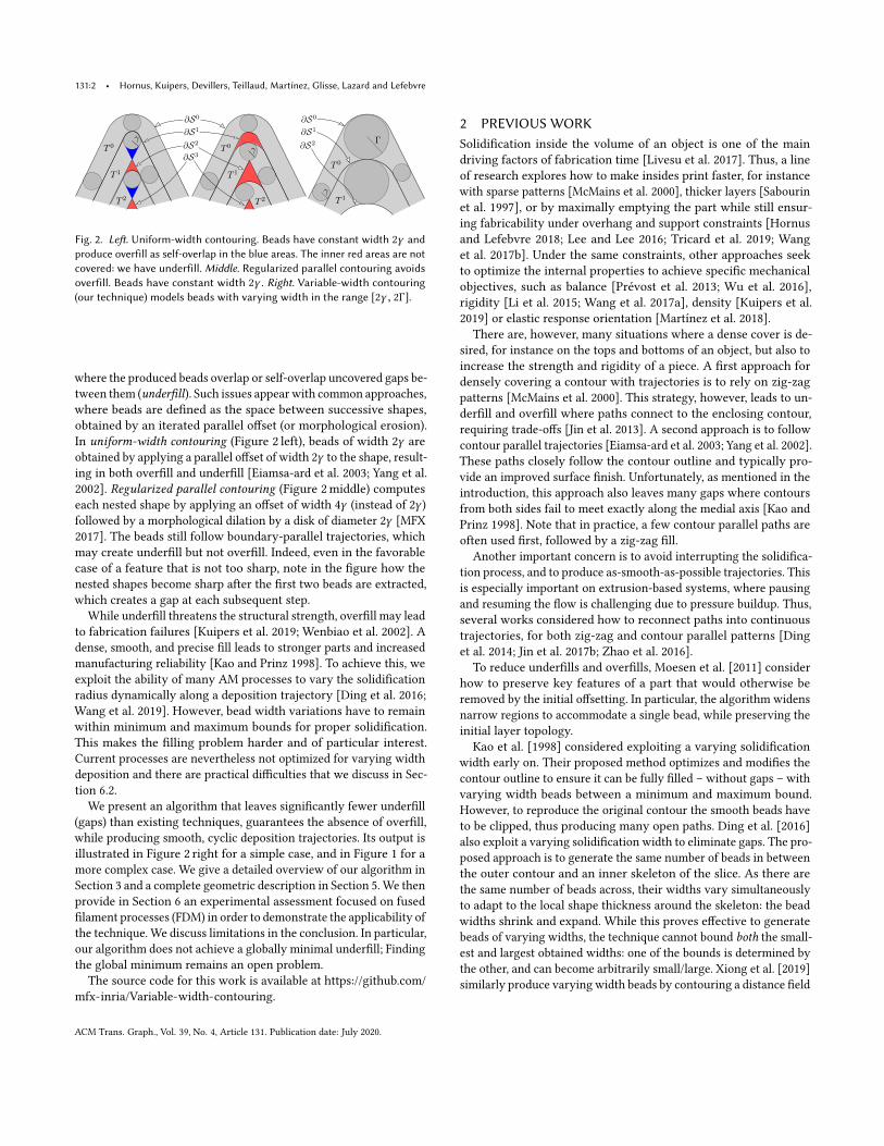
3 KEY IDEASIn this section, we give an overview of our approach and its under-

lying principles. Our algorithm for modeling beads has a standard

structure (Figure 2): starting from a shape S0, we iteratively con-

struct a sequence of nested shapes Sn ⊂ · · · ⊂ S0so that the

difference Si \ Si+1between two successive shapes is, roughly, a

set of topological annuli (Figures 1 (f) and 3 (h)). A bead is then

modeled inside each annulus.

Common state-of-the-art approaches use beads of constant width,

which, as mentioned in the introduction, leave many gaps (see

Figure 2 left andmiddle). A key element of our approach for reducing

the underfill is to use beads of variable width, say within 2γ and 2Γ.Our idea is to determine beads with variable width so that the

nested shapes S0 ⊃ · · · ⊃ Sn become as “round” as possible. Some-

what counter-intuitively, our technique does so by increasing the

bead width along sharp features, where the curvature of the bound-

ary ∂Si of Si is locally maximal. Doing so aims at obtaining smaller

local maxima of curvature along ∂Si+1, so that ∂Si+1

becomes as

circular as possible.

Our approach for computing such sequences of nested shapes and

the corresponding beads strongly relies on their representations as

unions of disks using their medial axes. Recall that the medial axis

of a shape is the (closure of the) set of points that are centers of so-

called medial-axis disks tangent to the shape’s boundary in at least

two points. To each point on the medial axis corresponds the radius

of this disk (see Section 4.2 for more formal definitions). We use the

term sub-axis to denote a subset of the medial axis. The shape is

equal to the union of its medial-axis disks. The nested shapes and

the beads are constructed one from another by manipulating their

medial axes (and their disk-radius functions) in three steps referred

to as Trimming, Collapsing and Shaving. The print trajectories aredefined as the medial axis of each bead, which is sampled and output.

S0 S0

trT 0

S1

¢= S1

(a) (b) (c) (d)

•••

•

S1 S1

tr S2

¢=S2

(e) (f) (g) (h)

Fig. 3. A simple example. The diameters of the black disks illustrate theminimal and maximal bead widths. The medial axis is black where Trimmedand green otherwise (see Table 1). To help the reader, the medial-axis diskscentered at Normal vertices (green) are stroked with dashes. (a) S0 and itsmedial axis. (b) Trimming. (c) Parallel offset of 2γ. The beadT 0 (light blue) isborn. (d) The print trajectory traj(T 0) of the bead T 0. (e) S1 and its medialaxis. (f) Trimming; a single point remains Normal. (g) Parallel offset largerthan 2γ . (h) All four beads and print trajectories. There is no gap.

�

(a) (b) (c)

(d) (e)

trimmingparallel o�set

collapsing

parallel o�set

Ki

traj(T i) ⊂MA(Si \ (Si+1 ∪Ki)

)

: max and min bead widthsSi+1¢

SiSitr

Si+1¢

Si+1

trimming//o�set

//o�set(c)collapsing

Si (a)

Sitr (b)

(d)

Si+1

T i

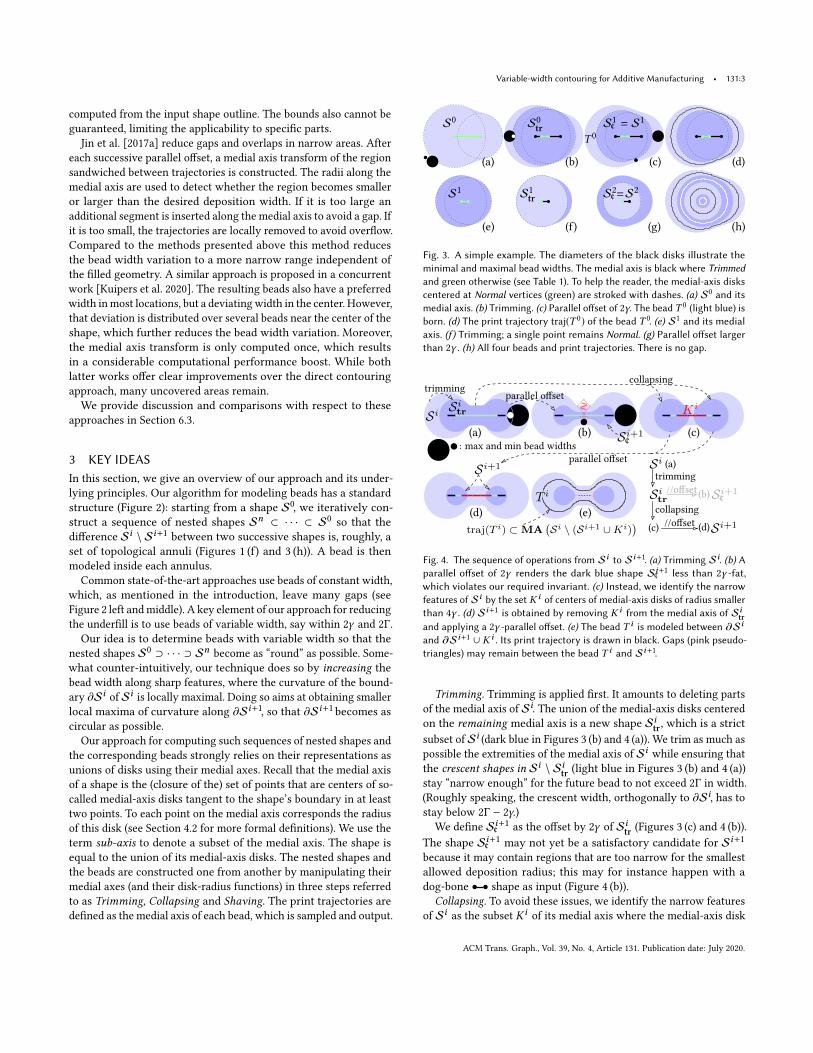
Fig. 4. The sequence of operations from Si to Si+1. (a) Trimming Si. (b) Aparallel offset of 2γ renders the dark blue shape Si+1

¢ less than 2γ -fat,which violates our required invariant. (c) Instead, we identify the narrowfeatures of Si by the set K i of centers of medial-axis disks of radius smallerthan 4γ . (d) Si+1 is obtained by removing K i from the medial axis of Sitrand applying a 2γ -parallel offset. (e) The bead T i is modeled between ∂Si

and ∂Si+1 ∪ K i . Its print trajectory is drawn in black. Gaps (pink pseudo-triangles) may remain between the bead T i and Si+1.

Trimming. Trimming is applied first. It amounts to deleting parts

of the medial axis of Si. The union of the medial-axis disks centered

on the remaining medial axis is a new shape Sitr, which is a strict

subset of Si (dark blue in Figures 3 (b) and 4 (a)). We trim as much as

possible the extremities of the medial axis of Si while ensuring that

the crescent shapes in Si \ Sitr (light blue in Figures 3 (b) and 4 (a))

stay “narrow enough” for the future bead to not exceed 2Γ in width.

(Roughly speaking, the crescent width, orthogonally to ∂Si, has to

stay below 2Γ − 2γ.)We define Si+1

¢as the offset by 2γ of Sitr (Figures 3 (c) and 4 (b)).

The shape Si+1

¢may not yet be a satisfactory candidate for Si+1

because it may contain regions that are too narrow for the smallest

allowed deposition radius; this may for instance happen with a

dog-bone • • shape as input (Figure 4 (b)).

Collapsing. To avoid these issues, we identify the narrow features

of Si as the subset K iof its medial axis where the medial-axis disk



radius is smaller than 4γ (drawn in red in Figure 4 (c,d); recall that the

medial axis of Si+1

¢is included in that of Si ). The narrow features

of Si are then collapsed onto K i: The new shape Si+1

is defined as

the parallel offset (of width 2γ ) of the union of the disks centered on

the medial axis of Sitr from which we remove the Collapsed sub-axis

K i(Figure 4 (d)) and the bead is locally widened in Si \ (Si+1 ∪K i )

to be in contact with ∂Si, ∂Si+1and K i

(Figure 4 (e)).

Constraints on γ , Γ and the shapes. Our approach computes a

sequence of nested shapes Si such that each Si \ Si+1is covered

(possibly with gaps) by closed beads whose width varies between 2γand 2Γ. To avoid gaps between ∂Si and the bead(s) in Si \Si+1

, the

shape Si needs to be 2γ -fat (i.e., all medial-axis disks have radius

at least 2γ ). This is a constraint on S0, but the collapsing phases

ensure that all other Si are 2γ -fat. On the other hand, the collapsing

phase defines, around Collapsed sub-axes, beads of width up to 4γ ;since the largest possible width is 2Γ, we must have 2Γ ≥ 4γ . Insummary, our technique has the following constraints: the shape

S0must be 2γ -fat and the bead width range must satisfy Γ ≥ 2γ .Bead trajectories. When K i

is empty (there is no narrow feature),

Si \ Si+1can be exactly covered, with no overfill nor underfill, by

a closed bead T i = Si \ Si+1whose print trajectory is its medial

axis (Figure 3). However, the presence of a Collapsed sub-axis calls

for a more subtle definition of the beads wherein gaps (underfill)

are unavoidable (see the small pink gaps in Figure 4 (e)). Details

are given in Section 5.2 and Appendix A. We provide two optional

strategies (Section 5.3) to minimize the area of these gaps. The first,

shaving, “trims” the Collapsed sub-axis to widen the bead that wraps

around it. The second, medial axis simplification, erases most of

the problematic branches of K ialtogether, but at the expense of

simplifying (thereby approximating) the shape Si.

Figure 4 bottom-left summarizes how the sequence (Si ) and the

beads are computed. Figures 1, 3 and 17 show other examples of our

technique in action.

4 PRELIMINARIESWe first discuss and emphasize our assumptions on our input shapes

and on the fabrication constraints (Section 4.1). We then recall clas-

sical notions on medial axes (Section 4.2) and describe how we rep-

resent our nested shapes using sequences of medial axis transforms

(Section 4.3). We then discuss our data structure, notation, and how

we process our medial axes by labeling their arcs (Section 4.4). Some

important definitions and notation are also illustrated in Figure 5

and summarized in Table 1.

4.1 Fabrication constraints and admissible input shapesWe assume that a given fabrication machine provides a range of

achievable beadwidths. For example, on a Ultimaker 3, we are able to

vary the bead width within [0.3mm, 1mm] at 0.2mm layer height,

and [0.3mm, 0.7mm] at 0.1mm layer height.

Since the achievable bead width range is hardware-dependent,

we give it as input parameters [2γ , 2Γ] to our technique. Our algo-

rithm guarantees that all output beads have their width varying

in that range. As a consequence of the way we define closed print

trajectories, our initial shape S0needs to be 2γ -fat. Furthermore,

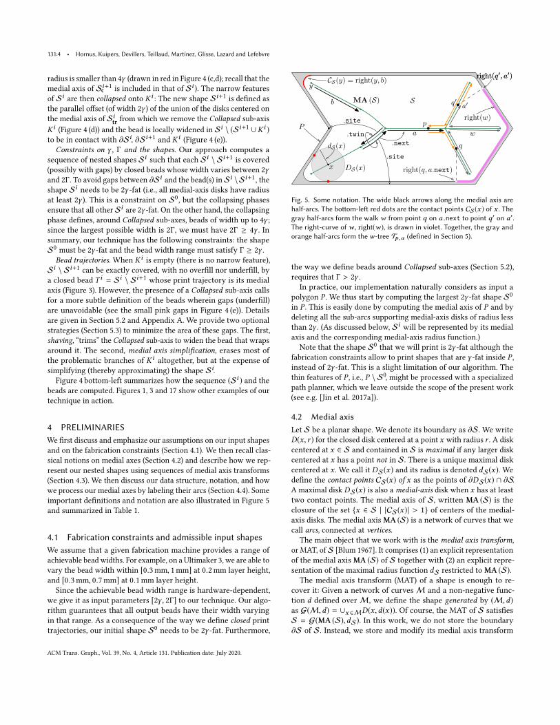
.twin.next

.site

.site

MA (S) S

w

right(q′, a′)

x DS(x)

p

a

dS(x) q

right(q, a.next)

right(w)

a′q′

CS(y) = right(y, b)y

b

P

right(q′, a′)

Fig. 5. Some notation. The wide black arrows along the medial axis arehalf-arcs. The bottom-left red dots are the contact points CS(x ) of x . Thegray half-arcs form the walk w from point q on a .next to point q′ on a′.The right-curve of w , right(w ), is drawn in violet. Together, the gray andorange half-arcs form the w-tree Tp ,a (defined in Section 5).

the way we define beads around Collapsed sub-axes (Section 5.2),

requires that Γ > 2γ .In practice, our implementation naturally considers as input a

polygon P . We thus start by computing the largest 2γ -fat shape S0

in P . This is easily done by computing the medial axis of P and by

deleting all the sub-arcs supporting medial-axis disks of radius less

than 2γ . (As discussed below, Si will be represented by its medial

axis and the corresponding medial-axis radius function.)

Note that the shape S0that we will print is 2γ -fat although the

fabrication constraints allow to print shapes that are γ -fat inside P ,instead of 2γ -fat. This is a slight limitation of our algorithm. The

thin features of P , i.e., P \ S0, might be processed with a specialized

path planner, which we leave outside the scope of the present work

(see e.g. [Jin et al. 2017a]).

4.2 Medial axisLet S be a planar shape. We denote its boundary as ∂S. We write

D(x, r ) for the closed disk centered at a point x with radius r . A disk

centered at x ∈ S and contained in S is maximal if any larger disk

centered at x has a point not in S. There is a unique maximal disk

centered at x . We call it DS(x) and its radius is denoted dS(x). We

define the contact points CS(x) of x as the points of ∂DS(x) ∩ ∂S.A maximal disk DS(x) is also a medial-axis disk when x has at least

two contact points. The medial axis of S, written MA (S) is theclosure of the set {x ∈ S | |CS(x)| > 1} of centers of the medial-

axis disks. The medial axisMA (S) is a network of curves that we

call arcs, connected at vertices.The main object that we work with is the medial axis transform,

or MAT, ofS [Blum 1967]. It comprises (1) an explicit representation

of the medial axisMA (S) of S together with (2) an explicit repre-

sentation of the maximal radius function dS restricted toMA (S).The medial axis transform (MAT) of a shape is enough to re-

cover it: Given a network of curvesM and a non-negative func-

tion d defined overM, we define the shape generated by (M,d)as G(M,d) = ∪x ∈MD(x,d(x)). Of course, the MAT of S satisfies

S = G(MA (S),dS). In this work, we do not store the boundary

∂S of S. Instead, we store and modify its medial axis transform



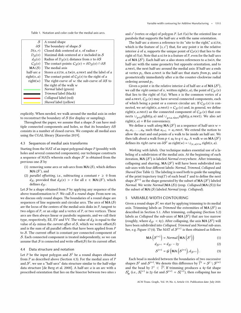
Table 1. Notation and color code for the medial axis arcs.

S A round shape

∂S The boundary of shape S

D(x, r ) Closed disk centered at x , of radius rDS(x) Maximal disk centered at x included in S

dS(x) Radius of DS(x); distance from x to ∂S

CS(x) The contact points: CS(x) = ∂DS(x) ∩ ∂SMA (S) The medial axis

half-arc a Stores a.site, a.twin, a.next and the label of aright(x,a) The contact point of CS(x) to the right of a

right(w) The right-curve of w : the sub-curve of ∂S to

the right of the walkwNormal label (green)Trimmed label (black)

Collapsed label (red)

Shaved label (yellow)

explicitly. When needed, we walk around the medial axis in order

to reconstruct the boundary of S (for display or sampling).

Throughout the paper, we assume that a shape S can have mul-

tiple connected components and holes, so that its boundary ∂S

consists in a number of closed curves. We compute all medial axes

using the CGAL library [Karavelas 2019].

4.3 Sequences of medial axis transformsStarting from the MAT of an input polygonal shape P (possibly with

holes and several connected components), our technique constructs

a sequence of MATs wherein each shape S′ is obtained from the

previous one S by

(1) removing some arcs or sub-arcs from MA (S), which defines

MA (S′), and(2) parallel offsetting, i.e., subtracting a constant r ≥ 0 from

dS , provided that dS(x) > r for all x ∈ MA (S′), whichdefines dS′ .

Let S be a shape obtained from P by applying any sequence of the

above transformation to P . We call S a round shape. From now on,

we discuss only round shapes. The boundaries of a round shape are

sequences of line segments and circular arcs. The arcs of MA (S)are the locus of the centers of the medial-axis disks in P , tangent totwo edges of P , or an edge and a vertex of P , or two vertices. These

arcs are then always linear or parabolic segments, and we call their

type, respectively, EE, EV and VV. The value of dS is equal to the

value of dP minus the current offset of S, which we write offset(S)

and is the sum of all parallel offsets that have been applied from Pto S. The current offset is constant per connected component of

S. Each connected component is treated independently, so we can

assume that S is connected and write offset(S) for its current offset.

4.4 Data structure and notationLet P be the input polygon and Si be a round shapes obtained

from P as described above (Section 4.3). For the medial axes of Pand Si , we use a “half-arcs” data structure similar to the half-edge

data structure [de Berg et al. 2008]. A half-arc a is an arc with a

prescribed orientation that lies on the bisector between two sites s

and s ′ (vertex or edge) of polygon P . Let ℓ(a) be the oriented line or

parabola that supports the half-arc a with the same orientation.

The half-arc a stores a reference to its “site to the right,” a.site,which is the feature of {s, s ′} that, for any point x in the relative

interior a of a, supports the unique point of CP (x) that lies to the

right of ℓ(a). Note that a.site is a feature of P , even for the half-arcs

a ofMA(Si

). Each half-arc a also stores references to a.twin, the

half-arc with the same geometry but opposite orientation, and to

a.next, the next half-arc around the medial axis: If half-arc a ends

at vertex p1, then a.next is the half-arc that starts from p1 and is

geometrically immediately after a in the counter-clockwise radial

ordering around p1.

Given a point x in the relative interior a of half-arc a ofMA(Si

),

we call the right contact of x , written right(x,a), the point of CSi (x)that lies to the right of ℓ(a). When x is the common vertex of aand a.next, CSi (x) may have several connected components, each

of which being a point or a convex circular arc. If CSi (x) is con-nected, we set right(x,a.next) = CSi (x) and, in general, we define

right(x,a.next) as the connected component of CSi (x) that con-nects ∪y∈aright(y,a) and ∪y∈ ˚a .nextright(y,a.next). We also set

right(x,a) = ∅ for conveniency.We define a walk alongMA

(Si

)as a sequence of half-arcsw =

a0,a1, . . . ,an such that ai+1 = ai .next. We extend the notion to

allow the start and end points of a walk to lie inside an half-arc. We

then talk about a walk from p ∈ a0 to q ∈ an . A walkw onMA(Si

)defines its right curve on ∂Si as right(w) = ∪(x ,a)∈w right(x,a).

Working with labels. Our technique makes essential use of a la-

beling of a subdivision of the medial axis. At the beginning of each

iteration,MA(Si

)is labeled Normal everywhere. After trimming,

collapsing and shaving, MA(Si

)will have been subdivided into

sub-axes with four different labels: Normal, Trimmed, Collapsed and

Shaved (See Table 1). The labeling is used both to guide the sampling

of the print trajectory traj(T ) of each bead T and to define the next

shape Si+1as the shape generated by the subset ofMA

(Si

)labeled

Normal. We write Normal (MA (S)) (resp. Collapsed (MA (S))) forthe subset ofMA (S) labeled Normal (resp. Collapsed).

5 VARIABLE-WIDTH CONTOURINGGiven a round shape Si, we start by applying trimming to its medial

axis. Trimming labels as Trimmed the extremities of MA(Si

)as

described in Section 5.1. After trimming, collapsing (Section 5.2)

labels as Collapsed the sub-axes of MA(Si

)that are too narrow

(roughly, where dSi < 4γ ). After collapsing, the axisMA(Si

)will

have been subdivided into Collapsed, Trimmed and Normal sub-axes.See, e.g. Figure 17 (4). The MAT of Si+1

is then obtained as follows:

MA(Si+1

)= Normal

(MA

(Si

))(1)

dSi+1 = dSi − 2γ (2)

Si+1 = G(MA

(Si+1

),dSi+1

). (3)

Each bead is modeled between the boundaries of two successive

shapes Si and Si+1. We denote this difference by T i = Si \ Si+1

and the bead by T i ⊂ T i. If trimming produces a 4γ -fat shapeSitr (i.e., S

i+1

¢is 2γ -fat and Si+1 = Si+1

¢), then collapsing has no



effect and T i can be fully covered by bead loops with width varying

within the prescribed bounds. In that case, it is easy to sample the

print trajectory of the bead, traj(T i ) (see e.g. Figure 3 (h)). This isdetailed in Appendix A. Otherwise, the Collapsed sub-axis of Si is

not empty and the bead cannot fully cover the area T i and leaves

gaps: T i \T i , ∅ (Section 5.2). In a way, trimming tries to minimize

the occurrence of collapsing. When a collapse occurs anyway, we

strive to minimize the area of the gaps with shaving (Section 5.3.1)

and medial axis simplification (Section 5.3.2).

In the next sections, we describe trimming, collapsing, shaving

and medial axis simplification. The sampling of the print trajectories

of the beads is detailed in Appendix A. The proof that the beads

generated with variable-width contouring are free of overfill is

presented in Appendix B.

5.1 TrimmingIn the trimming phase, we cut the branches of MA

(Si

)as much as

possible so as to make the shape “rounder.” This is a very effective

strategy: often, after some iterations the remaining shape becomes

exactly a disk, after which gap-free bead generation becomes trivial

(Figure 3 (g-h)).

We introduce trimming with a simple example (Figure 3), then

generalize trimming to arbitrary input. In (a) we see the input shape

S0which, for the sake of this simple example, is r -fat for some r

larger than 2Γ. MA(Si

)reduces to a single line segment initially

labeled Normal (colored green). Trimming determines a splitting

point on the medial axis at both ends and labels the two extreme

segments as Trimmed (colored black). From (b) to (e), the dark-

blue shape is generated by the remaining Normal sub-axis. Thesplitting points (the endpoints of the green, or Normal, segment in

(b)) are computed so that the maximal width of the crescent shapes

(light blue on either side) is 2Γ − 2γ . The subtraction of 2γ is in

anticipation of the parallel offset of 2γ that happens in (c). There is

no thin feature so collapsing does not apply to this example. The

parallel offset ensures that the bead (the light-blue shape in (c))

has width larger than 2γ and the bound on the crescents’ widths

ensures that the bead is no wider than 2Γ. The beadT 0 = S1 \ S0is

complete and (d) shows its print trajectory as a dark line. In (e), we

see the shape S1from which we start the computation of the next

bead. The medial axis is very short now and trimming is able to

label it entirely Trimmed, but for a single point which stays Normalas needed to provide an inner boundary for the bead T 1

. In (f) we

see the result of trimming. Since MA(S2

)is a point, all subsequent

beads are annuli (g-h).

Before describing the algorithm for trimming, we give a detailed

geometric description of the general case, illustrated in Figure 6.

The trees that we consider for trimming are of a particular kind. We

call them walk-trees or w-trees for short. A w-tree T ⊂ MA(Si

)is obtained by choosing a root point p on MA

(Si

)and one half-

arc a that contains p. The w-tree Tp,a consists of all the points of

MA(Si

)on the walk from p ∈ a to p ∈ a.twin (see Figure 5), if, of

course, that combinatorial walk exists and its corresponding subset

ofMA(Si

)in the plane does not contain any loop. Note that this

forbids to choose the half-arc a on a cycle of MA(Si

)since in that

case,a.twin is not reachable froma. Thew-trees have two important

p

DSi(p)

p0

p1 right(T )x

y

zq

pqd

Si(p)

dSi(q)

|p− q|

w(q, p)

T

Fig. 6. To avoid clutter, the diagram is drawn twice. Left. The crescent % isdelineated with a thin black curve. The medial axis is trimmed at p . Themedial-axis disks at the leaves of the axis are drawn gray. Right. The widthof the crescent at x ,y and z are the diameter of the respective orange circles.The width at z is a local maximum.

properties: First the requirement for aw-tree to be a walk fromp ∈ ato p ∈ a.twin enforces the property that if one cuts the medial axis

at p, then Tp,a is a simply connected component, detached from

the rest. Second and more importantly, the right-curve right(T )

of a w-tree T (see Section 4.4) is a single connected subset of ∂Si,

whereas the right-curve of a random tree inMA(Si

)may consist

of several disconnected curves along ∂Si.

Let T be a w-tree and p its root: p = root(T ). The right-curve of

T, right(T ), is a (connected) sub-curve of ∂Siwhose endpoints, p0

and p1 are contact points of the root p: {p0,p1} ⊂ CSi (p). LabelingT as Trimmed has the effect of replacing the sub-curve right(T ) of

∂Si by the circular arc on ∂DSi (p) from p0 to p1; See Figure 6.

Together, the curve right(T ) and that circular arc bound a “cres-

cent”% that forms part of the beadT i. (Figure 3 (b-c) shows how cres-

cents are integrated into the bead.) To make sure the bead is print-

able, we need to control its maximal width: At a point x ∈ right(T ),

the width of the crescent % is the diameter of the largest disk tan-

gent to right(T ) at x and to DSi (p) (orange color in Figure 6). (The

constraints that we enforce on the w-trees that we work with (see

below) ensure that the width of the crescent is always well de-

fined.) That width may have a local minimum anywhere, along line

segments (e.g. in the neighborhood of x in Figure 6) or convex or

concave circular arcs (e.g. at y in Figure 6). But it can have a local

maximum only along convex circular arcs (e.g. at z in Figure 6).

5.1.1 Constraints from the convex circular arcs. The convex circulararcs along right(T ) are generated by the vertices v of T for which

∂DSi (v) ∩ right(T ) is a circular arc. These vertices include the

leaves of T and some internal vertices. We need to focus only on

these vertices, which we gather in the set conv(T ).

Let q be any vertex in conv(T ). By definition, vertex q generates

a convex circular arc on right(T ) ⊂ ∂Si (see the red circular arc

in Figure 6). The maximum width of % along that arc is denoted

w(q,p) and we havew(q,p) = |p − q | + dSi (q) − dSi (p). The widthw(q,p) is the diameter of the disk (orange color) tangent to right(T )

at the intersection point z of line pq with the circular arc centered

at q (red color). This orange disk is tangent to right(T ) at z and



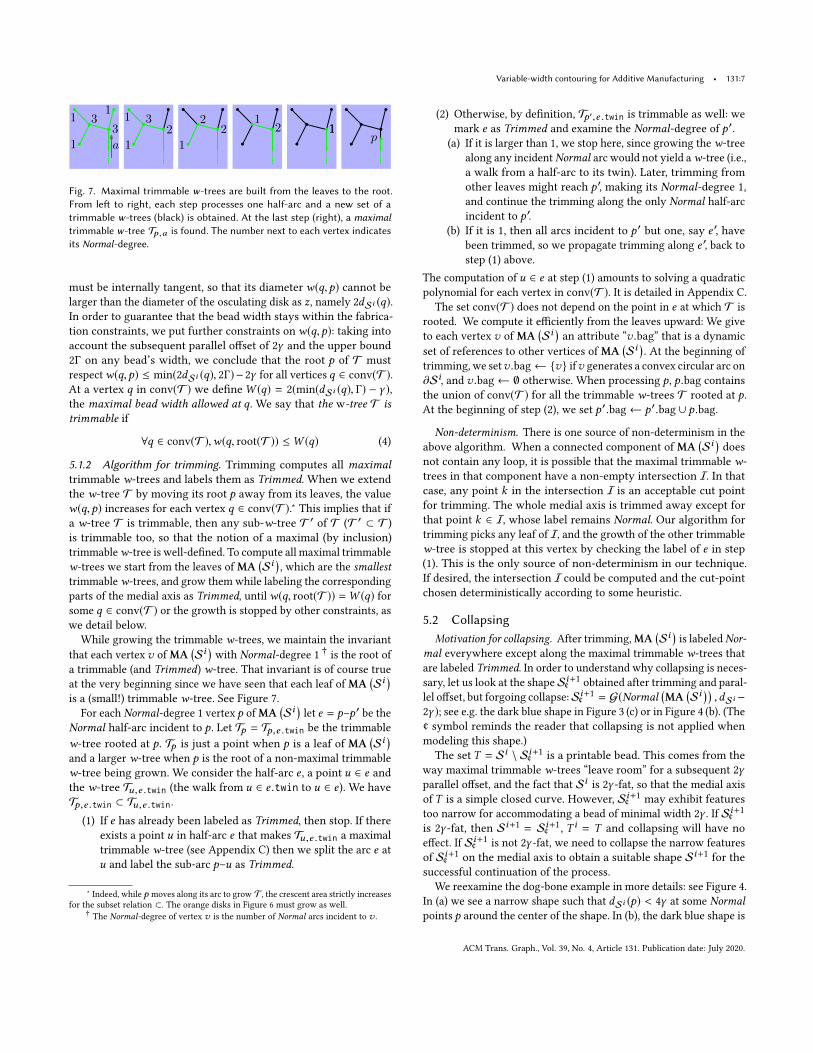
pa1

233 3

22

21 1

1 1

111

1

Fig. 7. Maximal trimmable w-trees are built from the leaves to the root.From left to right, each step processes one half-arc and a new set of atrimmable w-trees (black) is obtained. At the last step (right), a maximaltrimmable w-tree Tp ,a is found. The number next to each vertex indicatesits Normal-degree.

must be internally tangent, so that its diameter w(q,p) cannot belarger than the diameter of the osculating disk as z, namely 2dSi (q).In order to guarantee that the bead width stays within the fabrica-

tion constraints, we put further constraints onw(q,p): taking intoaccount the subsequent parallel offset of 2γ and the upper bound

2Γ on any bead’s width, we conclude that the root p of T must

respectw(q,p) ≤ min(2dSi (q), 2Γ)− 2γ for all vertices q ∈ conv(T ).

At a vertex q in conv(T ) we defineW (q) = 2(min(dSi (q), Γ) − γ ),the maximal bead width allowed at q. We say that the w-tree T istrimmable if

∀q ∈ conv(T ),w(q, root(T )) ≤W (q) (4)

5.1.2 Algorithm for trimming. Trimming computes all maximaltrimmable w-trees and labels them as Trimmed. When we extend

the w-tree T by moving its root p away from its leaves, the value

w(q,p) increases for each vertex q ∈ conv(T ).∗ This implies that if

a w-tree T is trimmable, then any sub-w-tree T ′ of T (T ′ ⊂ T )

is trimmable too, so that the notion of a maximal (by inclusion)

trimmablew-tree is well-defined. To compute all maximal trimmable

w-trees we start from the leaves ofMA(Si

), which are the smallest

trimmable w-trees, and grow them while labeling the corresponding

parts of the medial axis as Trimmed, untilw(q, root(T )) =W (q) forsome q ∈ conv(T ) or the growth is stopped by other constraints, as

we detail below.

While growing the trimmable w-trees, we maintain the invariant

that each vertex v ofMA(Si

)with Normal-degree 1

†is the root of

a trimmable (and Trimmed) w-tree. That invariant is of course trueat the very beginning since we have seen that each leaf of MA

(Si

)is a (small!) trimmable w-tree. See Figure 7.

For each Normal-degree 1 vertex p ofMA(Si

)let e = p–p′ be the

Normal half-arc incident to p. Let Tp = Tp,e .twin be the trimmable

w-tree rooted at p. Tp is just a point when p is a leaf of MA(Si

)and a larger w-tree when p is the root of a non-maximal trimmable

w-tree being grown. We consider the half-arc e , a point u ∈ e andthe w-tree Tu ,e .twin (the walk from u ∈ e .twin to u ∈ e). We have

Tp,e .twin ⊂ Tu ,e .twin.

(1) If e has already been labeled as Trimmed, then stop. If there

exists a point u in half-arc e that makes Tu ,e .twin a maximal

trimmable w-tree (see Appendix C) then we split the arc e atu and label the sub-arc p–u as Trimmed.

∗Indeed, while p moves along its arc to grow T , the crescent area strictly increases

for the subset relation ⊂. The orange disks in Figure 6 must grow as well.

†The Normal-degree of vertex v is the number of Normal arcs incident to v .

(2) Otherwise, by definition, Tp′,e .twin is trimmable as well: we

mark e as Trimmed and examine the Normal-degree of p′.(a) If it is larger than 1, we stop here, since growing the w-tree

along any incidentNormal arc would not yield aw-tree (i.e.,a walk from a half-arc to its twin). Later, trimming from

other leaves might reach p′, making its Normal-degree 1,and continue the trimming along the only Normal half-arcincident to p′.

(b) If it is 1, then all arcs incident to p′ but one, say e ′, havebeen trimmed, so we propagate trimming along e ′, back to

step (1) above.

The computation of u ∈ e at step (1) amounts to solving a quadratic

polynomial for each vertex in conv(T ). It is detailed in Appendix C.

The set conv(T ) does not depend on the point in e at which T is

rooted. We compute it efficiently from the leaves upward: We give

to each vertex v ofMA(Si

)an attribute “v .bag” that is a dynamic

set of references to other vertices ofMA(Si

). At the beginning of

trimming, we setv .bag← {v} ifv generates a convex circular arc on

∂Si, and v .bag← ∅ otherwise. When processing p, p.bag contains

the union of conv(T ) for all the trimmable w-trees T rooted at p.At the beginning of step (2), we set p′.bag← p′.bag ∪ p.bag.

Non-determinism. There is one source of non-determinism in the

above algorithm. When a connected component ofMA(Si

)does

not contain any loop, it is possible that the maximal trimmable w-trees in that component have a non-empty intersection I. In that

case, any point k in the intersection I is an acceptable cut point

for trimming. The whole medial axis is trimmed away except for

that point k ∈ I, whose label remains Normal. Our algorithm for

trimming picks any leaf of I, and the growth of the other trimmable

w-tree is stopped at this vertex by checking the label of e in step

(1). This is the only source of non-determinism in our technique.

If desired, the intersection I could be computed and the cut-point

chosen deterministically according to some heuristic.

5.2 CollapsingMotivation for collapsing. After trimming,MA

(Si

)is labeledNor-

mal everywhere except along the maximal trimmable w-trees thatare labeled Trimmed. In order to understand why collapsing is neces-sary, let us look at the shapeSi+1

¢obtained after trimming and paral-

lel offset, but forgoing collapse:Si+1

¢= G(Normal

(MA

(Si

) ),dSi −

2γ ); see e.g. the dark blue shape in Figure 3 (c) or in Figure 4 (b). (The¢ symbol reminds the reader that collapsing is not applied when

modeling this shape.)

The set T = Si \ Si+1

¢is a printable bead. This comes from the

way maximal trimmable w-trees “leave room” for a subsequent 2γparallel offset, and the fact that Si is 2γ -fat, so that the medial axis

of T is a simple closed curve. However, Si+1

¢may exhibit features

too narrow for accommodating a bead of minimal width 2γ . If Si+1

¢

is 2γ -fat, then Si+1 = Si+1

¢, T i = T and collapsing will have no

effect. If Si+1

¢is not 2γ -fat, we need to collapse the narrow features

of Si+1

¢on the medial axis to obtain a suitable shape Si+1

for the

successful continuation of the process.

We reexamine the dog-bone example in more details: see Figure 4.

In (a) we see a narrow shape such that dSi (p) < 4γ at some Normalpoints p around the center of the shape. In (b), the dark blue shape is



Fig. 8. Left. In red, the Collapsed sub-axis K 0. In dark gray, the medialaxis of T 0 \ K 0. Right. The print trajectory traj(T 0) comprises the cycles of

MA(T 0 \ K 0

)without its branches. The bead T 0 is shaded light-blue. The

gaps (pink) between T 0 and K 0 are very prominent in this example.

Si+1

¢. Its middle part is too narrow: dSi

¢

(p) < 2γ which is equivalent

todSi (p) < 4γ . In (c), we see the result of the collapsing: the sub-axisK i

ofMA(Si

)where dSi < 4γ is marked as Collapsed (red color).

The parallel offset is done only after collapsing (d). The idea of

collapsing is to collapse these narrow parts of Si+1

¢onto the medial

axis. To do so, the bead T = Si \ Si+1

¢around narrow passages is

enlarged until it touches the medial axis in (e).

Collapsing is applied after trimming and before the parallel offset.

Below, we describe collapsing in full generality.

5.2.1 Base collapse. First, the sub-axis of MA(Si

)along which

dSi (x) ≤ 4γ is identified. Then, only the connected components of

this sub-axis that overlap with a Normal arc are labeled Collapsed(drawn in red in the figures). In other words, component that are al-

ready fully Trimmed are ignored, and a component labeled Collapsedmight overwrite both Normal and Trimmed labels.

If a Trimmed maximal w-tree is partially Collapsed, then its root

p is necessarily Collapsed. The disappearance of p from the Normalsub-axis results in the disappearance of the local inner boundary

of the bead supported by ∂DSi (p) (see Figure 6). So, we relabel asNormal each vertex incident to both a Trimmed and a Collapsed arc.

Such a Normal vertex v contributes a disk in Si+1that is suitable

for supporting the inner side of the crescent associated with the

smaller (non-maximal) trimmable w-tree rooted at v .We write K i

for the collapsed sub-axis of MA(Si

): K i = {x ∈

MA(Si

)| x is labeled Collapsed}. To account for the Collapsed sub-

axis, we generalize the modeling of the beadT i as follows. Wemodel

T i indirectly by defining its medial axis, which is also its print trajec-

tory traj(T i ).We consider themedial axisM = MA(Si \ (Si+1 ∪ K i )

)and define the print trajectory for T i as the cycles in M , i.e., we

remove all the branches fromM , see Figure 8. The width of the T i

is naturally defined by the radius function associated to the medial

axisM .

This definition, however, possibly creates large regions in T i thatare not covered by the bead (Figures 4 and 8 right). In Section 5.3

we propose two strategies to reduce such underfill.

5.2.2 Collapsing more to help subsequent trimming. The base col-lapse operation, described above, leaves many Normal vertices inSi+1

with the minimal radius dSi+1 = 2γ . Each of these has a higher

chance to lead to another collapse immediately or a few steps later

if trimming cannot perform well. This happens when the radius at

these points increases slowly. During collapsing however, we have

the freedom to collapse further, up to a radius of 2Γ. In this section,

we examine the case of an EE arc of the medial axis‡and give the

‡Refer to Section 4.3 for the definition of EE, EV and VV.

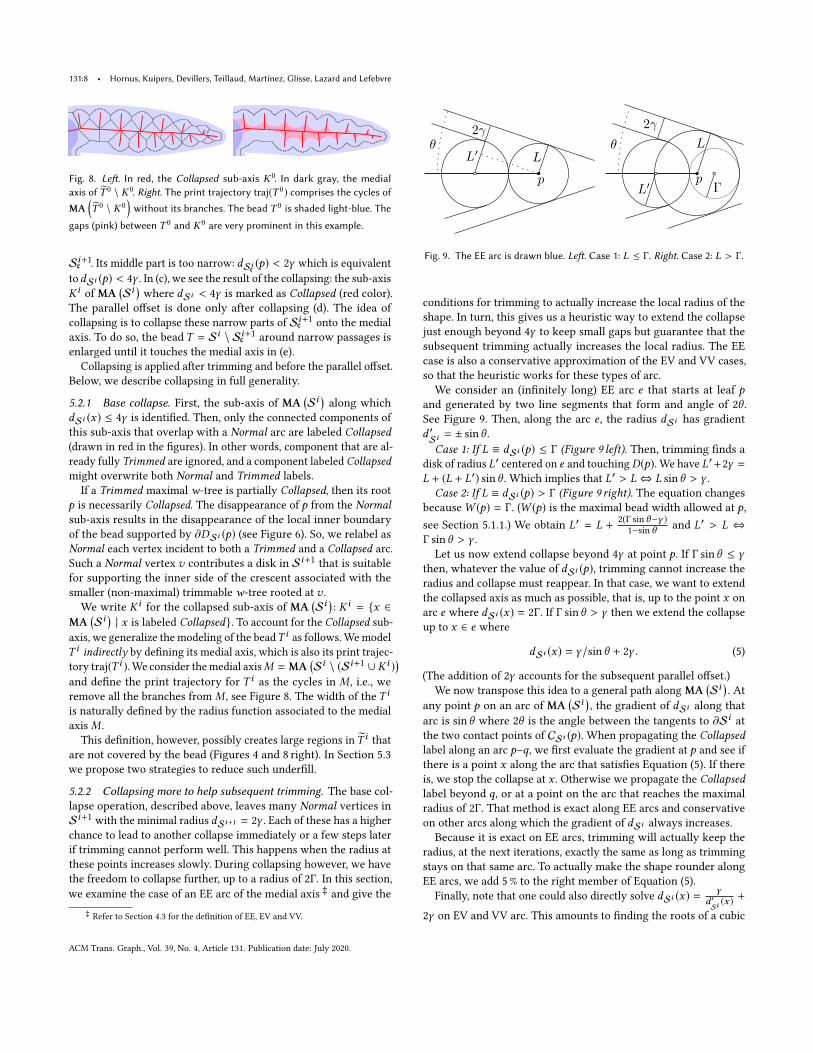
θ

p

L′ L

2γθ

pL′

L

2γ

Γ

Fig. 9. The EE arc is drawn blue. Left. Case 1: L ≤ Γ. Right. Case 2: L > Γ.

conditions for trimming to actually increase the local radius of the

shape. In turn, this gives us a heuristic way to extend the collapse

just enough beyond 4γ to keep small gaps but guarantee that the

subsequent trimming actually increases the local radius. The EE

case is also a conservative approximation of the EV and VV cases,

so that the heuristic works for these types of arc.

We consider an (infinitely long) EE arc e that starts at leaf pand generated by two line segments that form and angle of 2θ .See Figure 9. Then, along the arc e , the radius dSi has gradientd ′Si= ± sinθ .

Case 1: If L ≡ dSi (p) ≤ Γ (Figure 9 left). Then, trimming finds a

disk of radius L′ centered on e and touchingD(p). We have L′+2γ =L + (L + L′) sinθ . Which implies that L′ > L⇔ L sinθ > γ .Case 2: If L ≡ dSi (p) > Γ (Figure 9 right). The equation changes

becauseW (p) = Γ. (W (p) is the maximal bead width allowed at p,

see Section 5.1.1.) We obtain L′ = L +2(Γ sin θ−γ )

1−sin θ and L′ > L ⇔Γ sinθ > γ .Let us now extend collapse beyond 4γ at point p. If Γ sinθ ≤ γ

then, whatever the value of dSi (p), trimming cannot increase the

radius and collapse must reappear. In that case, we want to extend

the collapsed axis as much as possible, that is, up to the point x on

arc e where dSi (x) = 2Γ. If Γ sinθ > γ then we extend the collapse

up to x ∈ e where

dSi (x) = γ/sinθ + 2γ . (5)

(The addition of 2γ accounts for the subsequent parallel offset.)

We now transpose this idea to a general path along MA(Si

). At

any point p on an arc of MA(Si

), the gradient of dSi along that

arc is sinθ where 2θ is the angle between the tangents to ∂Si at

the two contact points of CSi (p). When propagating the Collapsedlabel along an arc p–q, we first evaluate the gradient at p and see if

there is a point x along the arc that satisfies Equation (5). If there

is, we stop the collapse at x . Otherwise we propagate the Collapsedlabel beyond q, or at a point on the arc that reaches the maximal

radius of 2Γ. That method is exact along EE arcs and conservative

on other arcs along which the gradient of dSi always increases.Because it is exact on EE arcs, trimming will actually keep the

radius, at the next iterations, exactly the same as long as trimming

stays on that same arc. To actually make the shape rounder along

EE arcs, we add 5% to the right member of Equation (5).

Finally, note that one could also directly solve dSi (x) =γ

d ′Si(x ) +

2γ on EV and VV arc. This amounts to finding the roots of a cubic



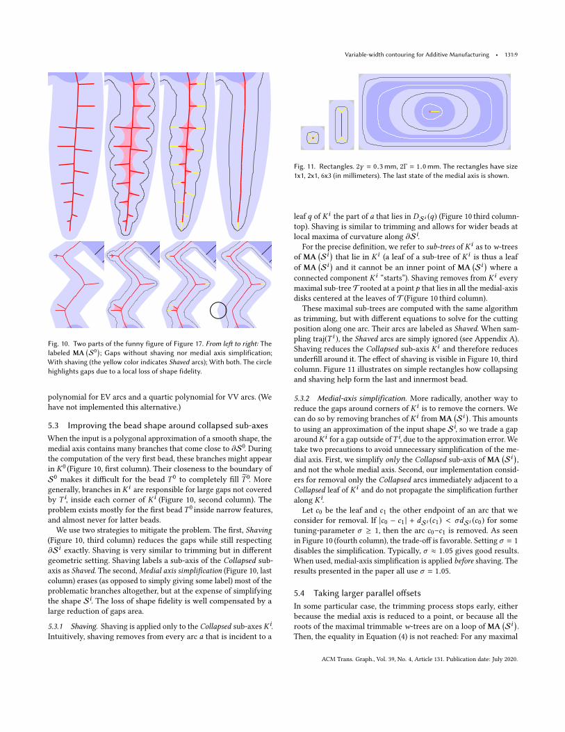
#Fig. 10. Two parts of the funny figure of Figure 17. From left to right: Thelabeled MA

(S0

); Gaps without shaving nor medial axis simplification;

With shaving (the yellow color indicates Shaved arcs); With both. The circlehighlights gaps due to a local loss of shape fidelity.

polynomial for EV arcs and a quartic polynomial for VV arcs. (We

have not implemented this alternative.)

5.3 Improving the bead shape around collapsed sub-axesWhen the input is a polygonal approximation of a smooth shape, the

medial axis contains many branches that come close to ∂S0. During

the computation of the very first bead, these branches might appear

in K0(Figure 10, first column). Their closeness to the boundary of

S0makes it difficult for the bead T 0

to completely fill T 0. More

generally, branches in K iare responsible for large gaps not covered

by T i, inside each corner of K i(Figure 10, second column). The

problem exists mostly for the first bead T 0inside narrow features,

and almost never for latter beads.

We use two strategies to mitigate the problem. The first, Shaving(Figure 10, third column) reduces the gaps while still respecting

∂Si exactly. Shaving is very similar to trimming but in different

geometric setting. Shaving labels a sub-axis of the Collapsed sub-

axis as Shaved. The second,Medial axis simplification (Figure 10, lastcolumn) erases (as opposed to simply giving some label) most of the

problematic branches altogether, but at the expense of simplifying

the shape Si. The loss of shape fidelity is well compensated by a

large reduction of gaps area.

5.3.1 Shaving. Shaving is applied only to the Collapsed sub-axes K i.

Intuitively, shaving removes from every arc a that is incident to a

Fig. 11. Rectangles. 2γ = 0.3mm, 2Γ = 1.0mm. The rectangles have size1x1, 2x1, 6x3 (in millimeters). The last state of the medial axis is shown.

leaf q of K ithe part of a that lies in DSi (q) (Figure 10 third column-

top). Shaving is similar to trimming and allows for wider beads at

local maxima of curvature along ∂Si.

For the precise definition, we refer to sub-trees of K ias to w-trees

of MA(Si

)that lie in K i

(a leaf of a sub-tree of K iis thus a leaf

of MA(Si

)and it cannot be an inner point of MA

(Si

)where a

connected component K i“starts”). Shaving removes from K i

every

maximal sub-tree T rooted at a point p that lies in all the medial-axis

disks centered at the leaves of T (Figure 10 third column).

These maximal sub-trees are computed with the same algorithm

as trimming, but with different equations to solve for the cutting

position along one arc. Their arcs are labeled as Shaved. When sam-

pling traj(T i ), the Shaved arcs are simply ignored (see Appendix A).

Shaving reduces the Collapsed sub-axis K iand therefore reduces

underfill around it. The effect of shaving is visible in Figure 10, third

column. Figure 11 illustrates on simple rectangles how collapsing

and shaving help form the last and innermost bead.

5.3.2 Medial-axis simplification. More radically, another way to

reduce the gaps around corners of K iis to remove the corners. We

can do so by removing branches of K ifromMA

(Si

). This amounts

to using an approximation of the input shape Si, so we trade a gap

aroundK ifor a gap outside ofT i, due to the approximation error. We

take two precautions to avoid unnecessary simplification of the me-

dial axis. First, we simplify only the Collapsed sub-axis ofMA(Si

),

and not the whole medial axis. Second, our implementation consid-

ers for removal only the Collapsed arcs immediately adjacent to a

Collapsed leaf of K iand do not propagate the simplification further

along K i.

Let c0 be the leaf and c1 the other endpoint of an arc that we

consider for removal. If |c0 − c1 | + dSi (c1) < σdSi (c0) for some

tuning-parameter σ ≥ 1, then the arc c0–c1 is removed. As seen

in Figure 10 (fourth column), the trade-off is favorable. Setting σ = 1

disables the simplification. Typically, σ ≈ 1.05 gives good results.

When used, medial-axis simplification is applied before shaving. Theresults presented in the paper all use σ = 1.05.

5.4 Taking larger parallel offsetsIn some particular case, the trimming process stops early, either

because the medial axis is reduced to a point, or because all the

roots of the maximal trimmable w-trees are on a loop ofMA(Si

).

Then, the equality in Equation (4) is not reached: For any maximal



•

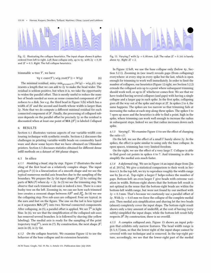
Fig. 12. Illustrating the collapse heuristics. The input shape shows 8 spikesordered from left to right. Left. Base collapse only, up to 4γ , with 2γ = 0.08

and 2Γ = 0.5. Right. The full collapse heuristics.

trimmable w-tree T , we have

∀q ∈ conv(T ),w(q, root(T )) <W (q) (6)

The minimal residual, minT minq∈conv(T) (W (q) −w(q,p)), rep-resents a length that we can add to 2γ to make the bead wider. The

residual is seldom positive, but when it is, we take the opportunity

to widen the parallel offset. This is mostly useful to reduce the num-

ber of beads needed as soon as some connected component of Si

reduces to a disk. See e.g. the third bead in Figure 3 (h) which has a

width of 2Γ and the second and fourth whose width is larger than

2γ . Note that we do compute a different minimal residual for each

connected component ofSi . Finally, the processing of collapsed sub-

axes depends on the parallel offset be precisely 2γ so the residual is

discounted when at least one point of MA(Si

)is labeled Collapsed.

6 RESULTSSection 6.1 illustrates various aspects of our variable-width con-

touring technique with synthetic results. Section 6.2 discusses the

challenges in printing variable-width beads on commodity hard-

ware and show some layers that we have obtained on Ultimaker

printers. Section 6.3 discusses statistics obtained for different dense

infill methods on a dataset of 300 planar shapes.

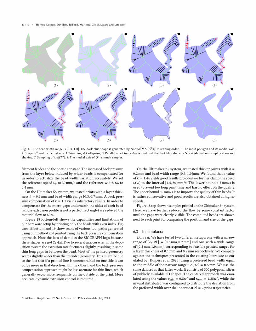
6.1 In silico6.1.1 Modeling a bead, step by step. Figure 17 illustrates the mod-

eling of the first bead on a relatively complex shape. The input

polygon P (1) is a linearization of a smooth shape and we see the

typical numerous medial axis branches due to the sampling of the

boundary. We prepare the 2γ -fat input shape S0(2) by cutting the

parts ofMA (P) where dP < 2γ . In (3) we see the trimming step. We

observe that each trimmed sub-axis is indeed a tree. There is a nice

bushy tree on the left. Zooming in, we can see how each trimmed

tree creates a crescent shape between ∂S0and S0

tr. In (4) we see

the collapsing step. Five sub-axes are collapsed. Four are typical, in

the ears and feet on the figure. The one on the tail is less typical

as it separates MA(S0

)into two Normal connected components.

After collapsing, in (5), a parallel offset is applied. We see T 0in light

blue. In (6), we see that the simplification of the collapsed sub-axes

has removed several branches. Is is followed by shaving (the yellow

labeling). The medial axis is ready for the sampling of the print

trajectory traj(T 0), seen in (7). By construction, the next shape S1,

seen in (8), is 2γ -fat.

6.1.2 On the collapse heuristic. We examine Figure 12 to see the

behavior of the base collapse and its extension heuristic.

Fig. 13. Varying Γ with 2γ = 0.08mm. Left. The value 2Γ = 0.161 is barelyabove 4γ . Right. 2Γ = 2.

In Figure 12 left, we use the base collapse only (below 4γ , Sec-tion 5.2.1). Zooming in (see inset) reveals gaps (from collapsing)

everywhere: at every step in every spike but the last, which is open

enough for trimming to work well immediately. In order to limit the

number of collapses, our heuristics (Figure 12 right, see Section 5.2.2)

extends the collapsed axis up to a point where subsequent trimming

should work well, or up to 2Γ whichever comes first. We see that we

have traded having several collapses (and gaps) with having a single

collapse and a larger gap in each spike. In the first spike, collapsing

goes all the way out of the spike and stops at 2Γ. In spikes 2 to 4, the

same happens. The spikes are too narrow so that trimming fails at

increasing the radius at each step along these spikes. The spikes 5 to

7 open up more and the heuristics is able to find a point, high in the

spike, where trimming can work well enough to increase the radius

in subsequent steps. Indeed we see that radius increases down each

spike.

6.1.3 Varying Γ. We examine Figure 13 to see the effect of changing

the ratio γ/Γ.

On the left, we see the effect of a small Γ barely above 2γ . In the

spikes, the effect is quite similar to using only the base collapse. In

open spaces, trimming has very limited freedom.

On the right, we see the effect of a very large Γ. Collapse is ableto find good cut points in spikes 4 to 7. And trimming is able to

simplify the medial axis much faster.

6.1.4 A deformed ring. We see in Figure 14 an input shape from [Jin

et al. 2017a]. We give a statistical comparison to their work in Sec-

tion 6.3. In the top-left, we try to reproduce roughly the width-range

use by Jin et al.. Top-right: a larger Γ helps reduce the number of

gaps. Bottom-left: an even larger Γ give beads with extreme vari-

ation in width. Bottom-right shows that the bottom-left result is

not optimal in the sense that the bottom-right beads are within the

bottom-left width range, but were not found by our method with

2γ = 0.3mm. That’s because we cautiously use a parallel offset of

2γ . With 2γ = 0.65mmwe force the collapse of the complete medial

axis. Then medial axis simplification and shaving let the two beads

(almost) completely cover the input shape. The bottom-right result

shows only a tiny amount of underfill, at the cost of having (very

subtly) simplified the input shape, while the bottom-left result fully

respects S0. By construction, there is no overfill.

6.1.5 A complex collapsed axis. Figure 15 shows an input poly-

gon that exhibits only narrow features. The bead width range is

[0.3, 0.7]mm, so that the lower right of the input shape cannot be

covered with our technique and is removed. In the top-right pic-

ture, accordingly, we see that the lower-right part of the medial



2γ = 0.3mm

2Γ = 0.7mm

2γ = 0.3mm

2Γ = 1mm

2γ = 0.3mm

2Γ = 2.2mm

2γ = 0.65mm

2Γ = 2.2mm

Fig. 14. Variable-width contouring on Jin’s ring [Jin et al. 2017a] with variousvalues of γ and Γ. Underfill in red. There is no overfill.

Fig. 15. A complex collapsed axis. In reading order: The input polygon andits medial axis. The labeled medial axisMA

(S0

). The labeled medial axis

MA(S1

). The resulting two beads and their trajectories (black forT 0, white

for T 1).

axis has been removed. We also see that remaining thin features

have been collapsed while the upper-left part is wide enough to

afford a regular trimming, during the modeling of the first bead

T 0. On the bottom-left: we see that the remaining medial axis is

0.0

0.5

1.0

1.5

2.0

Leng

th (k

m)

Statistics for the total length (top) and underfill (bottom)2 (mm)

0.71.01.42.0

0.1 0.2 0.3 0.42 (mm)0.0

0.1

0.2

0.3

0.4

Unde

rfill

(% o

f tot

al a

rea) Outer underfill

Inner underfill at 2 = 0.7 mmInner underfill at 2 = 1.0 mmInner underfill at 2 = 1.4 mmInner underfill at 2 = 2.0 mm

Fig. 16. 2γ varies from 0.1 to 0.4 and 2Γ from 0.7 to 2 (see the legend).

completely collapsed for the modeling of the second bead T 1. The

print trajectories of both beads are shown on the bottom-right.

6.1.6 Varying the bead width range. In Figure 16 we look at the totallength of the print trajectories, and inner and outer underfill under

fifteen different bead width ranges, computed over the 300 input

polygons of our dataset. On the top bar plot, we see that increasing

Γ reduces the total length of the print trajectories. On the bottom

bar plot, we see how the outer underfill depends only on γ and the

inner underfill is slightly improved with increasing Γ.

6.2 In plasticoWe have performed test prints on an Ultimaker S5 and an Ultimaker

2+ system using PLA filament in a 0.4 mm nozzle.

Varying the bead widths requires the variation of the extrusion

process, which depends on the movement speed and the pressure

in the system. Changing the pressure inside the system by feeding

an excess or lack of material is a strategy commonly employed by

pressure advance algorithms in order to accomplish constant width

beads under varying movement speeds [Arntsønn 2019]. However,

our printing system has a large distance between the filament feeder

and the nozzle, which means that the amount of material needed

to change the pressure inside the system is prohibitively large. We

therefore employ the back-pressure compensation method proposed

by Kuipers et al. [2020]. The bead width variation is accomplished

by varying the movement speed according to the following formula:

v(w) =f (w)

hw(7)

f (w) = f0 − k (w/w0 − 1) (8)

f0 = v0w0h (9)

where v(w) is the movement speed as a function of the requested

bead widthw , f (w) is the filament outflow, h is the layer thickness,

k is the amount of back pressure compensation and f0 is a constant

reference flow based on the reference speed v0 and the reference

widthw0. The bead width variation is accomplished by changing the

movement speed while keeping the internal pressure in between the



(1) (2) (3) (4)

(5) (6) (7) (8)

Fig. 17. The bead width range is [0.3, 1.0]. The dark blue shape is generated by Normal(MA(S0

)). In reading order. 1: The input polygon and its medial axis.

2: Shape S0 and its medial axis. 3: Trimming. 4: Collapsing. 5: Parallel offset (only dS0 is modified: the dark blue shape is S1). 6: Medial axis simplification andshaving. 7: Sampling of traj(T 0). 8: The medial axis of S1 is much simpler.

filament feeder and the nozzle constant. The increased back pressure

from the layer below induced by wider beads is compensated for

in order to actualize the bead width variation accurately. We set

the reference speed v0 to 30 mm/s and the reference width w0 to

0.4 mm.

On the Ultimaker S5 system, we tested prints with a layer thick-

ness h = 0.1 mm and bead width range [0.3, 0.7]mm. A back pres-

sure compensation of k = 1.1 yields satisfactory results. In order to

compensate for the micro-gaps underneath the sides of each bead

(whose extrusion profile is not a perfect rectangle) we reduced the

material flow to 80 %.

Figure 18 bottom-left shows the capabilities and limitations of

our hardware setup by printing only the beads with even index. Fig-

ures 18 bottom and 19 show scans of various tool paths generated

using our method and printed using the back pressure compensation

approach. Note the loss of detail in the SIGGRAPH logo because

these shapes are not 2γ -fat. Due to several inaccuracies in the depo-

sition system the extrusion rate fluctuates slightly, resulting in some

thin long gaps in between the bead. Most of the printed geometry

seems slightly wider than the intended geometry. This might be due

to the fact that if a printed line is unconstrained on one side it can

bulge more in that direction. On the other hand the back pressure

compensation approach might be less accurate for thin lines, which

generally occur more frequently on the outside of the print. More

accurate dynamic extrusion control is required.

On the Ultimaker 2+ system, we tested thicker prints with h =0.2 mm and bead width range [0.3, 1.0]mm. We found that a value

of k = 1.44 yields good results provided we further clamp the speed

v(w) to the interval [4.5, 30]mm/s. The lower bound 4.5 mm/s is

used to avoid too long print time and has no effect on the quality.

The upper bound 30 mm/s is to improve the quality of thin beads; It

is rather conservative and good results are also obtained at higher

speeds.

Figure 18 top shows 4 samples printed on the Ultimaker 2+ system.

Here, we have further reduced the flow by some constant factor

until the gaps were clearly visible. The computed beads are shown

next to each print for comparing the position and size of the gaps.

6.3 In simulacraData set. We have tested two different setups: one with a narrow

range of [2γ , 2Γ] = [0.3 mm, 0.7 mm] and one with a wide range

of [0.3 mm, 1.0 mm], corresponding to feasible printed ranges for

a layer thickness of 0.1 mm and 0.2 mm respectively. We compare

against the techniques presented in the existing literature as em-

ulated by [Kuipers et al. 2020] using a preferred bead width equal

to the middle of the narrow range, i.e., w∗ = 0.5 mm. We use the

same dataset as that latter work. It consists of 300 polygonal slices

of publicly available 3D shapes. The centered approach was emu-

lated using the values rmin = 0.8w∗ and rmax = 1.25w∗, while theinward distributed was configured to distribute the deviation from

the preferred width over the innermost N = 2 print trajectories.



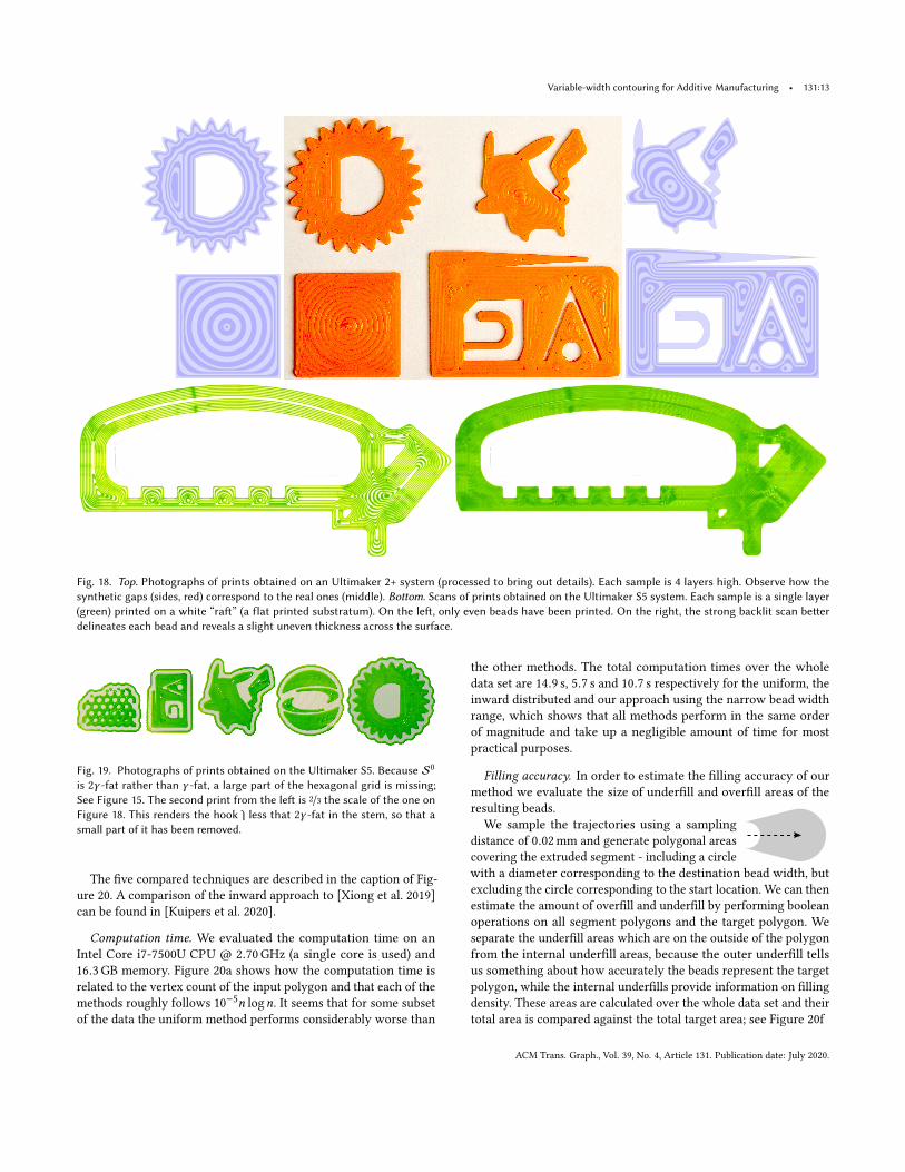
Fig. 18. Top. Photographs of prints obtained on an Ultimaker 2+ system (processed to bring out details). Each sample is 4 layers high. Observe how thesynthetic gaps (sides, red) correspond to the real ones (middle). Bottom. Scans of prints obtained on the Ultimaker S5 system. Each sample is a single layer(green) printed on a white “raft” (a flat printed substratum). On the left, only even beads have been printed. On the right, the strong backlit scan betterdelineates each bead and reveals a slight uneven thickness across the surface.

Fig. 19. Photographs of prints obtained on the Ultimaker S5. Because S0

is 2γ -fat rather than γ -fat, a large part of the hexagonal grid is missing;See Figure 15. The second print from the left is 2/3 the scale of the one onFigure 18. This renders the hook J less that 2γ -fat in the stem, so that asmall part of it has been removed.

The five compared techniques are described in the caption of Fig-

ure 20. A comparison of the inward approach to [Xiong et al. 2019]

can be found in [Kuipers et al. 2020].

Computation time. We evaluated the computation time on an

Intel Core i7-7500U CPU @ 2.70 GHz (a single core is used) and

16.3 GB memory. Figure 20a shows how the computation time is

related to the vertex count of the input polygon and that each of the

methods roughly follows 10−5n logn. It seems that for some subset

of the data the uniform method performs considerably worse than

the other methods. The total computation times over the whole

data set are 14.9 s, 5.7 s and 10.7 s respectively for the uniform, the

inward distributed and our approach using the narrow bead width

range, which shows that all methods perform in the same order

of magnitude and take up a negligible amount of time for most

practical purposes.

Filling accuracy. In order to estimate the filling accuracy of our

method we evaluate the size of underfill and overfill areas of the

resulting beads.

We sample the trajectories using a sampling

distance of 0.02 mm and generate polygonal areas

covering the extruded segment - including a circle

with a diameter corresponding to the destination bead width, but

excluding the circle corresponding to the start location. We can then

estimate the amount of overfill and underfill by performing boolean

operations on all segment polygons and the target polygon. We

separate the underfill areas which are on the outside of the polygon

from the internal underfill areas, because the outer underfill tells

us something about how accurately the beads represent the target

polygon, while the internal underfills provide information on filling

density. These areas are calculated over the whole data set and their

total area is compared against the total target area; see Figure 20f



Because of the discretization involved in sampling our evaluation

falsely reports a background level of overfill, even though we have

proven that no overfill exists in an idealized setting. Even though

the reported overfill is inaccurate, we can safely assume that the

amount of overfill is considerably lower than the overfill of existing

methods. While the error in reported overfill is approximately 0.02 %

the smallest reported overfill on existing techniques is an order of

magnitude larger: 0.3 %.

Because the presented method does not inherently deal with

target areas narrower than 2γ , we see that the outer underfill is

larger than for the existing methods. The areas within [γ , 2γ ] couldbe filled using a different approach which does produce open beads

along the medial axis.

The remaining inner underfill is smaller than the current state of

the art. While the inward distributed method has a total underfill of

0.210 % our method employing a corresponding narrow range only

exhibits 0.050 % underfill. We therefore conclude that our method

for generating densely filling beads is 1/4 as porous as the existing

state of the art.

Extrusion width. Figure 20b shows a histogram of the total length

of the print trajectories where the bead has a width within a bin of

0.01 mm over the whole data set. It also reports on the average and

standard deviation of the width data. We observe that even though

the middle of the range of possible bead widths corresponds with

the average bead width of the data from the existing techniques,

i.e. 0.5 mm, the average bead width of our technique lies below the

middle of the range: 0.36 mm for the narrow bead width range and

0.39 mm for the wide range. This is explained by the fact that beads

of width 2γ occur two orders of magnitude more frequently than

the other bead widths. The variance in bead width in our method is

a lot higher than for the existing methods, which puts extra strain

on the manufacturing system requirements.

Manufacturing time. Because the back pressure compensation

approach adjusts the movement speeds in order to accommodate the

bead width variation, it influences the total time it takes to print the

beads. We therefore report both on the manufacturing time when

using back pressure compensation and in the ideal case where the

(maximum) speeds are unaffected by extrusion width in Figure 20d.

While in the ideal case a wider line width causes a higher extrusion

flow rate in mm3/s, the back pressure compensation approach re-

duces the flow rate for beads wider than the nominal bead widths.

This means that for the ideal case the manufacturing time is mostly

determined by the total trajectories length (Figure 20e), while the

Gcode produced using back pressure compensation is dominated

by the occurrence of wide lines (Figure 20b). While the manufactur-

ing time for the narrow bead width range is smallest when using

back pressure compensation, it is largest in the idealized case. For

hardware systems where the back pressure compensation can be

realized using some form of pressure advance, the manufacturing

time of our method is longer compared to the state of the art. For

our current setup, however, our technique employing the narrow

bead width range outperforms the state of the art.

In order to accurately manufacture beads which exhibit sharp

corners, the print head must decelerate before it comes to a sharp

corner. Our print time estimation simulates the acceleration behav-

ior exhibited by the Ultimaker S5 system. Toolpaths that contain a

large amount of sharp corners therefore take longer to print. We

can see in Figure 20c that our approach produces significantly lower

amounts of sharp corners compared to the existing approaches - es-

pecially around 90°. Our method therefore features to less stringent

requirements on the hardware setup.

Because every separate bead requires a non-extruding travel

move, the number of beads influences the manufacturing time

as well. Moreover, because open polyline trajectories can only be

printed starting from either end they may take longer travel moves

than reaching a closed trajectory, which can be started anywhere.

While the total path counts in Figure 20e of our method are sim-

ilar to the state of the art, all of the trajectories are closed paths,

indicating that travel time is reduced.

7 CONCLUSIONThe technique presented here for variable-width contouring com-

putes a precise mathematical boundary representation of the beads

using only line segments and circular arcs. The print trajectories are

computed as the medial axis of each bead. These two characteristics

allow our technique to guarantee the absence of any inter-bead

overfill or bead self-overlap. The technique also makes extensive

use of the assumption that the width of a bead can vary within

bounds in order to minimize underfill. We believe that the absence

of overfill and the minimal underfill makes our technique attractive

for additive manufacturing.

In practice, we have verified that by carefully adapting the nozzle

speed to their local width, the variable-width beads can be printed

on commodity 3D printers. But the variable-width fused filament

deposition is very sensitive to tiny mechanical or dimensional vari-

ations in the machine. We have also found that the buffers used

by the printers firmware to store and analyse the trajectory are

undersized for our purpose: a very fine sampling (5 µm) would give

smoother bead width variation but the printer chokes on it.

Our technique might then give its fullest on future machines

developed with variable-width solidification in mind.

On the algorithmic side, some limitations and future work should

be noted:

• Currently the technique requires an initial filtering of the

shape so that S0is 2γ -fat, while a nozzle capable of a solidifi-

cation radius of γ can, by definition, fully cover a γ -fat shape.This limitation comes from the way our collapsing opera-

tion is not permitted to model a bead sitting over the medial

axisMA(Si

). A subtler collapsing might be able to remove

that constraint. In the meantime, other existing techniques

designed specifically for thin features can help cover P \ S0.

• The geometric modeling of the beads has some limitations as

well. Clearly, our technique does not find the set of beads that

minimizes underfill. One example is detailed in Section 6.1.4.

Two other examples are shown in Figure 21.

• In considering a 2D dense filling problem, we have ignored

possible gaps between horizontal layers due to bead align-

ments. Can we take these gaps into account or devise a fully

3D contouring scheme that minimizes volumetric underfill?



101 102 103 104

vertex count

10 4

10 3

10 2

10 1

100

com

puta

tion

time

(s)

10 5nlognuniforminwardnarrow

(a) Computation time

0.0 0.2 0.4 0.6 0.8width (mm)

100

101

102

103

104

105

106

107

leng

th (m

m)

=0.50, =0.000=0.50, =0.042=0.50, =0.024=0.36, =0.116=0.39, =0.179

(b) Extrusion widths

0 20 40 60 80 100 120 140 160 180angle (°)

100

101

102

103

104

105

106

107

frequ

ency

uniformcenteredinwardnarrowwide

(c) Site angles

uniform centered inward narrow0

2

4

6

8

10

12

prin

t tim

e (h

rs)

idealk=1.1

(d) Print time

uniform centered inward narrow wide

closedopenlength

(e) Path counts and lengths

uniform centered inward narrow wide0.0

0.2

0.4

0.6

0.8

1.0

1.2

1.4

1.6

area

(%)

overfillouter underfillinner underfill

(f) Over- and underfill

Fig. 20. Statistical analysis of bead generation methods. Our technique employing a range of [2γ , 2Γ] = [0.3 mm, 0.7 mm] is referred to as narrow, whilewide refers to [0.3 mm, 1.0 mm]; inward is the inward distributed technique proposed by [Kuipers et al. 2020]; centered is the method proposed by [Jinet al. 2017a] and uniform refers to the uniform-width contouring. Note the use of a logarithmic scale on the top y-axes and on the top-left x -axis.

Fig. 21. Limitations. Left. A short Collapsed axis (middle) prevents the ex-panded bead to reach it. Right. The two gaps in the center could be replacedby a single one by cutting the input shape between those gaps, into twotriangular shapes.

• On the theoretical front, some natural questions are raised:

What other approach could get less underfill or even find a

global minimum? Can we prove a lower bound on the number

of gaps or their total area that would depend on γ , Γ and in

the input shape? Can we characterize the family of shapes

that can be covered without underfill by beads whose width

varies within [2γ , 2Γ]?

ACKNOWLEDGMENTSWe thank Pierre Bedell for his help with the printers. This research

was initiated at the 17th BellairsWorkshop on Computational Geom-

etry, February 10-16, 2018, co-organized by Sylvain Lazard and Sue

Whitesides. The work was partially supported by Région Grand-Est,

Lorraine Université d’Excellence (ANR-15-IDEX-04-LUE) and ANR

MuFFin (ANR-17-CE10-0002).

REFERENCESTronvoll Sigmund Arntsønn. 2019. Investigating pressure advance algorithms for

filament-based melt extrusion additive manufacturing: theory, practice and simula-

tions. 25, 5 (01 Jan 2019), 830–839. https://doi.org/10.1108/RPJ-10-2018-0275

H. Blum. 1967. A transformation for extracting new descriptors of shape. In Models forthe Perception of Speech and Visual Form, Weinant Wathen Dunn (Ed.). MIT Press,

362–381.

Mark de Berg, Otfried Cheong, Marc van Kreveld, and Mark Overmars. 2008. Computa-tional Geometry: Algorithms and Applications (2 ed.). Springer-Verlag.

Donghong Ding, Zengxi Pan, Dominic Cuiuri, Huijun Li, and Nathan Larkin. 2016.

Adaptive path planning for wire-feed additive manufacturing using medial axis

transformation. Journal of Cleaner Production 133 (2016), 942–952. https://doi.org/

10.1016/j.jclepro.2016.06.036

Donghong Ding, Zengxi Stephen Pan, Dominic Cuiuri, and Huijun Li. 2014. A tool-path

generation strategy for wire and arc additive manufacturing. The internationaljournal of advanced manufacturing technology 73, 1-4 (2014), 173–183.

Kunnayut Eiamsa-ard, Frank W Liou, Robert G Landers, and Howie Choset. 2003.

Toward automatic process planning of a multi-axis hybrid laser aided manufacturing

system: skeleton-based offset edge generation. In ASME 2003 International DesignEngineering Technical Conferences and Computers and Information in EngineeringConference. American Society of Mechanical Engineers, 227–235.

Samuel Hornus and Sylvain Lefebvre. 2018. Iterative carving for self-supporting 3D

printed cavities. In Eurographics 2018 - Short Papers. Delft, Netherlands. https:

//hal.inria.fr/hal-01764291

Yuan Jin, Jianke Du, and Yong He. 2017a. Optimization of process planning for reducing

material consumption in additive manufacturing. Journal of Manufacturing Systems44 (2017), 65–78. https://doi.org/10.1016/j.jmsy.2017.05.003

Yuan Jin, Yong He, Guoqiang Fu, Aibing Zhang, and Jianke Du. 2017b. A non-retraction

path planning approach for extrusion-based additive manufacturing. Robotics andComputer-Integrated Manufacturing 48 (2017), 132 – 144.


https://doi.org/10.1108/RPJ-10-2018-0275

https://doi.org/10.1016/j.jclepro.2016.06.036

https://doi.org/10.1016/j.jclepro.2016.06.036

https://hal.inria.fr/hal-01764291

https://hal.inria.fr/hal-01764291

https://doi.org/10.1016/j.jmsy.2017.05.003


Yu An Jin, Yong He, and Jian Zhong Fu. 2013. An adaptive tool path generation for

fused deposition modeling. In Advanced Materials Research, Vol. 819. Trans TechPubl, 7–12.

Ju-Hsien Kao and Fritz B Prinz. 1998. Optimal motion planning for deposition in layered

manufacturing. In Proceedings of DETC, Vol. 98. 13–16.Menelaos Karavelas. 2019. 2D Segment Delaunay Graphs. In CGAL User and Reference

Manual (5.0 ed.). CGAL Editorial Board. https://doc.cgal.org/5.0/Manual/packages.

html#PkgSegmentDelaunayGraph2

Tim Kuipers, Eugeni L. Doubrovski, JunWu, and Charlie C. L. Wang. 2020. A framework

for adaptive width control of dense contour-parallel toolpaths in fused deposition

modeling. arXiv:2004.13497 [cs.GR] In submission.

Tim Kuipers, Jun Wu, and Charlie C.L. Wang. 2019. CrossFill: Foam Structures with

Graded Density for Continuous Material Extrusion. Computer-Aided Design 114

(2019), 37–50.

Jusung Lee and Kunwoo Lee. 2016. Block-Based Inner Support Structure Generation

Algorithm for 3D Printing Using Fused Deposition Modeling. The InternationalJournal of Advanced Manufacturing Technology (2016). https://doi.org/10.1007/

s00170-016-9239-3

Dawei Li, Ning Dai, Xiaotong Jiang, and Xiaosheng Chen. 2015. Interior Structural

Optimization Based on the Density-Variable Shape Modeling of 3D Printed Objects.

The International Journal of Advanced Manufacturing Technology 83, 9 (2015), 1627–

1635. https://doi.org/10.1007/s00170-015-7704-z

André Lieutier. 2004. Any open bounded subset of Rn has the same homotopy type as

its medial axis. Computer-Aided Design 36, 11 (2004), 1029 – 1046. https://doi.org/

10.1016/j.cad.2004.01.011 Solid Modeling Theory and Applications.

Marco Livesu, Stefano Ellero, Jonàs Martínez, Sylvain Lefebvre, and Marco Attene. 2017.

From 3D Models to 3D Prints: An Overview of the Processing Pipeline. ComputerGraphics Forum 36 (2017), 537–564.

Jonàs Martínez, Samuel Hornus, Haichuan Song, and Sylvain Lefebvre. 2018. Polyhedral

Voronoi diagrams for additive manufacturing. ACM Transactions on Graphics 37, 4(Aug. 2018), 15.

Sara McMains, Jordan Smith, Jianlin Wang, and Carlo Sequin. 2000. Layered manufac-

turing of thin-walled parts. In ASME Design Engineering Technical Conferenced.Inria Team MFX. 2017. IceSL, advanced modeling and slicing for 3D printing. https:

//icesl.loria.fr. Accessed: 2020-04-23.

Maarten Moesen, Tom Craeghs, Jean Pierre Kruth, and Jan Schrooten. 2011. Robust

beam compensation for laser-based additive manufacturing. CAD Computer AidedDesign 43, 8 (2011), 876–888. https://doi.org/10.1016/j.cad.2011.03.004

Romain Prévost, Emily Whiting, Sylvain Lefebvre, and Olga Sorkine-Hornung. 2013.

Make It Stand: Balancing Shapes for 3D Fabrication. ACM Transactions on Graphics(proceedings of ACM SIGGRAPH) 32, 4 (2013), 81:1–81:10.

Emmanuel Sabourin, Scott A. Houser, and Jan Helge Bøhn. 1997. Accurate Exterior, Fast

Interior Layered Manufacturing. Rapid Prototyping Journal 3, 2 (jun 1997), 44–52.

https://doi.org/10.1108/13552549710176662

Thibault Tricard, Frédéric Claux, and Sylvain Lefebvre. 2019. Ribbed support vaults for

3D printing of hollowed objects. Computer Graphics Forum (June 2019).

JunWang, Ting-wei Chen, Yu-an Jin, and Yong He. 2019. Variable bead width of material

extrusion-based additive manufacturing. Journal of Zhejiang University-SCIENCE A20, 1 (01 Jan 2019), 73–82. https://doi.org/10.1631/jzus.A1700236

Weiming Wang, Baojun Li, Sicheng Qian, Yong-Jin Liu, Charlie C. L. Wang, Ligang Liu,

Baocai Yin, and Xiuping Liu. 2017a. Cross section-based hollowing and structural

enhancement. The Visual Computer 33, 6 (2017), 949–960. https://doi.org/10.1007/

s00371-017-1386-5

W. Wang, Y. J. Liu, J. Wu, S. Tian, C. C. L. Wang, L. Liu, and X. Liu. 2017b. Support-

Free Hollowing. IEEE Transactions on Visualization and Computer Graphics (2017).https://doi.org/10.1109/TVCG.2017.2764462

Han Wenbiao, Mohsen Jafari, S.C. Danforth, and Ahmad Safari. 2002. Tool Path-Based

Deposition Planning in Fused Deposition Processes. Journal of ManufacturingScience and Engineering-transactions of The Asme - J MANUF SCI ENG 124 (05 2002).

https://doi.org/10.1115/1.1455026

Jun Wu, Charlie C.L. Wang, Xiaoting Zhang, and Rüdiger Westermann. 2016. Self-

supporting rhombic infill structures for additive manufacturing. Computer-AidedDesign 80 (2016), 32–42. https://doi.org/10.1016/j.cad.2016.07.006

Yi Xiong, Sang-in Park, Suhasini Padmanathan, Audelia Dharmawan, Shaohui Foong,

David Rosen, and Gim Soh. 2019. Process planning for adaptive contour parallel

toolpath in additive manufacturing with variable bead width. International Journal ofAdvanced Manufacturing Technology 105 (12 2019). https://doi.org/10.1007/s00170-

019-03954-1

Y Yang, HT Loh, JYH Fuh, and YG Wang. 2002. Equidistant path generation for

improving scanning efficiency in layered manufacturing. Rapid Prototyping Journal8, 1 (2002), 30–37.

Haisen Zhao, Fanglin Gu, Qi-Xing Huang, Jorge Garcia, Yong Chen, Changhe Tu,

Bedrich Benes, Hao Zhang, Daniel Cohen-Or, and Baoquan Chen. 2016. Connected

Fermat Spirals for Layered Fabrication. ACM Trans. Graph. 35, 4, Article 100 (July2016), 10 pages. https://doi.org/10.1145/2897824.2925958

Appendices

A SAMPLING THE PRINT TRAJECTORIESThis section explains how we sample the medial axis of T i, which is

the trajectory traj(T i ) to be followed by the printer nozzle. traj(T i )is, by construction, a set of closed simple curves that corresponds to

the medial axis of T i from which the branches have been removed.

Branches may appear only around the Collapsed sub-axis K i.

We sample traj(T i ) by projecting an adaptive sampling of its outer

boundary ∂Si onto it. Since all the branches of MA(T i

)do lie “on

the other side of ∂Si,” that is, between traj(T i ) and ∂Si+1, there is

in fact no need to take them into account and they can simply be

ignored. (They are never actually computed.)

The sampling of ∂Si proceeds by walking around each cycle

of MA(Si

), from a half-arc a to the next by following the a.next

reference. For each half-arc a, we sample its right-curve right(a) ⊂∂Si. A sample is defined as a pair (p, t) where p is a point and t is aunit vector tangent to the sampled curve. Each sample (p, t) of ∂Si

is projected onto traj(T i ) along the direction t which is the vector trotated 90 degrees to the left. The projection itself depends on the

label of the half-arc a.

Normal projection. If half-arc a is labeled Normal, then the bead

was locally formed only with parallel offset. The projection of (s, t)is then a translation by α t , where α = γ or some larger value specific

to the component Si, see Section 5.4.

Trimmed projection. Before walking along a Trimmed w-tree, welook at its root v , which is the last Normal vertex visited. While

walking around the w-tree, traj(T ) is locally the bisector between

∂Si and DSi+1 (v). We project the samples (p, t) onto traj(T ) bysolving for x in |p + xt − v | = x + dSi+1 (v). Squaring both sides

and simplifying, we obtain a linear equation. The tangent at the

projected sample point p′ is the normalized average of t and the

tangent to DSi+1 (v) at its point closest to p′.

Collapsed/Shaved projection. Along a walk-cycle in MA(Si

)a

connected Collapsed/Shaved sub-walkw of that cycle, by construc-

tion, either forms the complete cycle or is bounded by Normal ver-tices. Let K be the set of Collapsed arcs in w (ignoring the Shavedones). Along the walkw , the print trajectory traj(T i ) is the bisectorbetween ∂Si and K ∪ Si+1

. Before projecting the samples from

right(w) onto traj(T i ), we gather the relevant parts ofw ∪Si+1in a

set B(w). The set B(w) includes (i) all the arcs ofK that are outside of

Si+1as well as (ii) the medial-axis disks in Si+1

whose boundaries

are crossed byw as the sub-axis exits and enters Si+1. For example,

in Figure 10 (top-left) the set B contains only one disk, the one at

the top. In Figure 17 (6), the two Collapsed walks in the tail exit and

enter S1in two different disks. The projection itself is brute force:

We project each sample s onto the bisector with each element of

B(w) and pick the projected sample closest to s .Samples on traj(T i ) are added adaptively as long as the angle

between the tangents at each end of a line segment is too large,

or the ratio of the radii dT i at each end of the segment is outside

[ 1

1.1 , 1.1], except if the segment is too small.


https://doc.cgal.org/5.0/Manual/packages.html#PkgSegmentDelaunayGraph2

https://doc.cgal.org/5.0/Manual/packages.html#PkgSegmentDelaunayGraph2

https://arxiv.org/abs/2004.13497

https://doi.org/10.1007/s00170-016-9239-3

https://doi.org/10.1007/s00170-016-9239-3

https://doi.org/10.1007/s00170-015-7704-z

https://doi.org/10.1016/j.cad.2004.01.011


https://icesl.loria.fr

https://icesl.loria.fr


https://doi.org/10.1108/13552549710176662

https://doi.org/10.1631/jzus.A1700236

https://doi.org/10.1007/s00371-017-1386-5

https://doi.org/10.1007/s00371-017-1386-5

https://doi.org/10.1109/TVCG.2017.2764462

https://doi.org/10.1115/1.1455026


https://doi.org/10.1007/s00170-019-03954-1

https://doi.org/10.1007/s00170-019-03954-1

https://doi.org/10.1145/2897824.2925958


B ON THE OVERLAPDefinition of overlap. Let c : [0, 1] 7→ R2

be a print trajectory

and Rc : [0, 1] 7→ R the bead radius at point c(t). Let Dc (t) =D(c(t),Rc (t)) be the extrusion disk at parameter t . Let p be a point in

the plane. Let I (p, c) be the set of parameters at which p is contained

in Dc (t): I (p, c) = {t ∈ [0, 1] | Dc (t) ∋ p}. The set I is a set of

intervals in [0, 1]. We define the overlap number O(c,p) of c overp as the number of maximal intervals in I (p, c) (i.e., the number of

connected components).§LetTc be the beadTc = ∪t ∈[0,1]Dc (t). We

say thatTc has no overlap if ∀p ∈ Tc ,O(c,p) = 1. Conversely, a bead

Tc exhibits overlap if it contains one point p such that O(c,p) > 1.

Proof of no overlap. We now prove that variable-width contouring

produces only beads with no overlap. The main ingredient is

Lemma 1. Let S be an open set in R2 and p a point in S. LetM bethe set of points x ∈ MA (S) such that DS(x) ∋ p. Then M has thehomotopy type of a point. (That is,M is a geometric tree.)

Proof. We consider H = ∪x ∈MDS(x) ⊂ S. We prove that

MA (H ) = M (Lemma 2). Since H is an open set, it has the ho-

motopy type of its medial axis [Lieutier 2004]. On the other hand,

H is star shaped (Lemma 3), so it has the homotopy type of a point,

and so hasM = MA (H ). □

Lemmas 2 and 3 are proved below. Let Tc be a bead such that

the image of c is the medial axis of Tc . (This is the case for all thebeads that our algorithm constructs. This is also the case for the

regular parallel contouring but not for uniform parallel contouring.)

We also take c continuous and injective (no back-and-forth along

the medial axis). Let p be a point in Tc . Lemma 1 tells us that I (p, c)has the homotopy type of a point. SinceMA (Tc ) is a simple curve,

then I (p, c) must be a single interval, which proves that we have no

overlap.

Lemma 2. MA (H ) = M .

Proof. The easier half is M ⊂ MA (H ): Let x be a point in M .

DS(x) ⊂ H ⊂ S has at least two contact points on ∂S. These two

contact points are also on the boundary of H , so x ∈ MA (H ).Now we prove that MA (H ) ⊂ M : Let x be a point in MA (H ).

The disk DH (x) is a medial-axis disk in H . It also contains p. Indeed,let y be the point of ∂DH (x) farthest from p. Point y belongs to Hso it lies in a disk D ′ ⊂ H that contains p. By construction of y,p < DH (x) ⇒ D ′ ⊃ DH (x) ⇒ DH (x) is not a medial-axis disk in

H , which is false. So, p ∈ DH (x). Now, let C = ∂H ∩ ∂DH (x) be thecontact points of x w.r.t. H . Suppose that C contains at most one

point on ∂S. Then the points of C not in ∂S lie in the interior of S.

So we can find a diskD ′′ in S that containsDH (x) and also containsp, so that: DH (x) ⊂ D ′′ ⊂ H so DH (x) is not a medial-axis disk in

H , a contradiction. Therefore, C has at least two contact points on

∂S which means that x ∈ M . □

§If the curve c is a loop, as our algorithm produces, if an interval contains 0 and

another contains 1, we count them as a single interval.

Lemma 3. H is star shaped.

Proof. Let q be a point in H . There exists x ∈ M such that

q ∈ DS(x) ⊂ H and, by definition ofM , p also is in DS(x) ⊂ H . So

the segment pq is in H . □

C TRIMMING FORMULASGiven a half-arc e = p–p′, we want to find if there exists a point

u ∈ e wherew(q,u) is equal toW (q) for at least one vertex q ∈ p.bagandw(q′,u) ≤W (q′) for the other vertices q′ of the bag.For each q ∈ p.bag, the equation w(q,u ∈ e) = W (q) can be

transformed into a quadratic equation as we calculate below. We

solve the equation for all vertices q ∈ p.bag. If there is at least onesolution point inside e , we pick the solution point u closest to pand declare the w-tree rooted at u as maximal. Otherwise, trim-

ming continues beyond p′. The Euclidean coordinates of u and q are

written, respectively, (ux ,uy ) and (qx ,qy ). The frame of reference

varies depending on the arc e . Recall that MA(Si

)is a subset of

the medial axis of an input polygon. As such, the arcs ofMA(Si

)are defined as bisectors between vertices and edges of that input

polygon.

Case EE. Arc e is a bisector of two line segments on ∂Si (these

segments are parallel offsets of two edges of the input polygon. Let

2θ be the angle they form. We use the line supporting e as the x-axisand put the origin at the intersection of the supporting lines of the

two segments. Then dSi (u) = ux sinθ and the equation becomes

(ux sinθ +W (q) − dSi (q))2 = (ux − qx )

2 + q2

y .

Case EV. Arc e is a bisector of an input (concave) vertex Q and an

input edge, the arc is parabolic. We take the directrix as the x-axis,in such a way that the focus Q has coordinates (0,h). dSi (u) is thedistance from u to the disk D(Q, offset(Si )) (see Section 4.3 for the

definition of offset(Si )). Then, dSi (u) =u2

x2h +

h2− offset(Si ). We

again obtain (after simplification) a quadratic equation (ux −qx )2 +

(u2

x2h +

h2− qy )

2 =(u2

x2h +

h2− offset(Si ) +W (q) − dS(q)

)2

.

Case VV. Arc e is a bisector between two input vertices P and

Q , the arc is a straight line segment. We take their perpendicular

bisector as the x-axis, in such a way that P and Q have coordinates

(0,h) and (0,−h) respectively. Using Y = − offset(Si ) +W (q) −dSi (q), we obtain

(ux − qx )2 + q2

y = (

√u2

x + h2 + Y )2 (10)

⇔ Z − 2qxux = 2Y

√u2

x + h2, with Z = q2

x + q2

y − h2 − Y 2

(11)

⇒ 0 = u2

x (q2

x − Y2) − uxqxZ +

(Z 2

2

− Y 2h2

). (12)

The last step, from Equation (11) to Equation (12), is an implication,

not an equivalence, so we consider a root of the quadratic polyno-

mial in Equation (12) only if it is also a solution of Equation (10).


Variable-width contouring for Additive Manufacturing - HAL-Inria

Documents

Transcript of Variable-width contouring for Additive Manufacturing - HAL-Inria