Width Parameters on Even-Hole-Free Graphs
141
HAL Id: tel-03342197 https://tel.archives-ouvertes.fr/tel-03342197 Submitted on 13 Sep 2021 HAL is a multi-disciplinary open access archive for the deposit and dissemination of sci- entific research documents, whether they are pub- lished or not. The documents may come from teaching and research institutions in France or abroad, or from public or private research centers. L’archive ouverte pluridisciplinaire HAL, est destinée au dépôt et à la diffusion de documents scientifiques de niveau recherche, publiés ou non, émanant des établissements d’enseignement et de recherche français ou étrangers, des laboratoires publics ou privés. Width Parameters on Even-Hole-Free Graphs Ni Luh Dewi Sintiari To cite this version: Ni Luh Dewi Sintiari. Width Parameters on Even-Hole-Free Graphs. Other [cs.OH]. Université de Lyon, 2021. English. NNT : 2021LYSEN026. tel-03342197
-
Upload
khangminh22 -
Category
Documents
-
view
1 -
download
0
Transcript of Width Parameters on Even-Hole-Free Graphs

HAL Id: tel-03342197https://tel.archives-ouvertes.fr/tel-03342197
Submitted on 13 Sep 2021
HAL is a multi-disciplinary open accessarchive for the deposit and dissemination of sci-entific research documents, whether they are pub-lished or not. The documents may come fromteaching and research institutions in France orabroad, or from public or private research centers.
L’archive ouverte pluridisciplinaire HAL, estdestinée au dépôt et à la diffusion de documentsscientifiques de niveau recherche, publiés ou non,émanant des établissements d’enseignement et derecherche français ou étrangers, des laboratoirespublics ou privés.
Width Parameters on Even-Hole-Free GraphsNi Luh Dewi Sintiari
To cite this version:Ni Luh Dewi Sintiari. Width Parameters on Even-Hole-Free Graphs. Other [cs.OH]. Université deLyon, 2021. English. NNT : 2021LYSEN026. tel-03342197

Numéro National de Thèse : 2021LYSEN026
THESE de DOCTORAT DE L’UNIVERSITE DE LYONopérée par
l’Ecole Normale Supérieure de Lyon
Ecole Doctorale N° 512 École Doctorale en Informatique et Mathématiques de Lyon
Spécialité de doctorat : Théorie des graphesDiscipline : Informatique
Soutenue publiquement le 29/06/2021, par :Ni Luh Dewi SINTIARI
Width Parameters on Even-Hole-Free GraphsParamètres de largeur des graphes sans trous pairs
Devant le jury composé de :
Mme. Kathie CAMERON Professeure, Wilfrid Laurier University RapporteureM. Frédéric HAVET Directeur de recherche, I3S Sophia Antipolis RapporteurM. Edy Tri BASKORO Professeur, Institut Teknologi Bandung ExaminateurMme. Aurélie LAGOUTTE Maître de conférences, LIMOS-UCA ExaminatriceM. Nicolas TROTIGNON Directeur de recherche, ENS de Lyon Directeur de thèse

ii

iii
AcknowledgementsWith my deep gratitude and appreciation to my thesis advisor, Nicolas
Trotignon, for accepting me as his student, and for his continued support and en-couragement throughout this research project. I am immensely grateful for our sci-entific discussions, for our friendly chats in the corridor, for his personal supportin my academic business, for his assistance during my stay in Lyon, and for manyother things which can not be listed here. Nicolas has inspired me in many aspectsof my academic life. He is a great researcher, an excellent advisor, a person with lotsof stories and jokes who can bring a comfortable atmosphere to those around him. Iaspire to be as lively and energetic as he is.
My sincere thanks to the members of my thesis advisory and exam committee:Kathie Cameron, Professor Edy Tri Baskoro, Frédéric Havet, and Aurélie Lagoutte,for their precious time to offer me with helpful feedback on how to improve mywork. I would also like to acknowledge all my collaborators for sharing their knowl-edge and expertise, for their help, and for completing our collaborative projects:Pierre Aboulker, Isolde Adler, Eun Jung Kim, Marcin Pilipczuk, Myriam Preiss-mann, Stéphan Thomassé, and Kristina Vuškovic. Special thanks to Rémi Watrigant,Édouard Bonnet, and Nicolas Bousquet for their valuable guidance throughout mystudies. To Jake Horsfield and Cléophée Robin, I can’t thank you enough for thestimulating discussions and memorable moments that we shared together.
My gratitude also goes to ENS de Lyon for funding this three-year PhD program,through Contrats doctoraux spécifiques pour normaliens. Thanks to the Laboratoirede l’informatique du parallélisme (LIP) for accepting me as part of them: to MALIP,MILIP, and everyone I could not mention one by one, I very much appreciate yourassistance and kind reception. To everyone in MC2, thank you for welcoming mewarmly into the team. I am missing so much our cheerful chats over lunches inthe CROUS cafeteria. I would also like to thank the members of the Départementd’Informatique, particularly to Damien Stehlé and Daniel Hirschkoff who thought-fully guided me throughout my studies, to all the lecturers who have given me theopportunity to become a teaching assistant and learn from them, and to all my teach-ing colleagues for their excellent cooperation. Last but not least I would like to men-tion Christophe Crespelle, thanks to whom I began my journey at ENS de Lyon inthe first place.
My PhD time would not be so enjoyable without the support of my friends andfound family. To PPI Lyon, the doctorants Indonésiens, and all my friends whocannot be listed here, thanks for sharing the beautiful moments, for the stories, andfor cheering me up. Thanks to ibu-ibu Indonesia, who have been our mothers herein Lyon, I will definitely miss your delicious cooking. To all my lab-mates, thanks somuch for the happy distractions to rest my mind outside of my research. To Nicolas’family, many thanks for your warm welcome, for the lunch and dinner invitations,and for the unforgettable moments we passed together during Christmas break inUsson-en-Forez.
Let me also take this moment to thank my beloved parents and sisters, for theirunconditional love and unending support. To my dear Hendra, thanks for your sym-pathetic ears, for always being there, in my joy and in my sorrow. To my relatives,thank you for always wishing the best for me.
Finally, my deep gratitude to everyone who has put their hands to take care ofme and brought me to this step. There are no words that can express how grateful Iam to meet all of you. I will really miss the time we have spent together, and I hopethere will be another moment to make new memories in the future.

iv

v
Contents
Acknowledgements iii
Résumé 1
Summary 5
1 Introduction 91.1 What is Graph Theory . . . . . . . . . . . . . . . . . . . . . . . . . . . . 9
1.1.1 A history of Graph Theory . . . . . . . . . . . . . . . . . . . . . 101.1.2 Graph Theory is everywhere . . . . . . . . . . . . . . . . . . . . 12
1.2 Literature review . . . . . . . . . . . . . . . . . . . . . . . . . . . . . . . 141.2.1 Hereditary classes of graphs . . . . . . . . . . . . . . . . . . . . 151.2.2 Dealing with large graphs: graph decomposition . . . . . . . . 161.2.3 Parameters for graph complexity . . . . . . . . . . . . . . . . . . 181.2.4 Why even-hole-free graphs? . . . . . . . . . . . . . . . . . . . . . 22
From perfect graphs to even-hole-free graphs . . . . . . . . . . . 231.3 Terminology . . . . . . . . . . . . . . . . . . . . . . . . . . . . . . . . . . 271.4 Main contributions of the thesis . . . . . . . . . . . . . . . . . . . . . . . 29
Even-hole-free graphs with no large cliques . . . . . . . . . . . . 29Forbidding more structures and its impacts on the tree-width . 31Publications . . . . . . . . . . . . . . . . . . . . . . . . . . . . . . 32
2 A survey on even-hole-free graphs 332.1 Decomposition of even-hole-free graphs . . . . . . . . . . . . . . . . . . 332.2 The use of cutsets for algorithms . . . . . . . . . . . . . . . . . . . . . . 37
2.2.1 Recognition algorithm . . . . . . . . . . . . . . . . . . . . . . . . 372.2.2 The good and the bad cutsets in the decomposition of even-
hole-free graphs . . . . . . . . . . . . . . . . . . . . . . . . . . . . 392.2.3 Even-hole-free graphs with no star cutset . . . . . . . . . . . . . 41
2.3 Widths of several subclasses of even-hole-free graphs . . . . . . . . . . 442.3.1 Planar case . . . . . . . . . . . . . . . . . . . . . . . . . . . . . . . 442.3.2 Triangle-free case . . . . . . . . . . . . . . . . . . . . . . . . . . . 452.3.3 Cap-free case . . . . . . . . . . . . . . . . . . . . . . . . . . . . . 482.3.4 Diamond-free case . . . . . . . . . . . . . . . . . . . . . . . . . . 502.3.5 Pan-free case . . . . . . . . . . . . . . . . . . . . . . . . . . . . . 512.3.6 Rings . . . . . . . . . . . . . . . . . . . . . . . . . . . . . . . . . . 55
3 Layered wheels 573.1 Summary of the main results . . . . . . . . . . . . . . . . . . . . . . . . 593.2 Construction and tree-width . . . . . . . . . . . . . . . . . . . . . . . . . 603.3 Lower bound on rank-width . . . . . . . . . . . . . . . . . . . . . . . . . 783.4 Upper bound . . . . . . . . . . . . . . . . . . . . . . . . . . . . . . . . . 833.5 Discussion and open problems . . . . . . . . . . . . . . . . . . . . . . . 86

vi
4 A bound on the tree-width 874.1 Known results and summary of the main results . . . . . . . . . . . . . 884.2 Tree-width and minimal separators . . . . . . . . . . . . . . . . . . . . . 894.3 Nested 2-wheels . . . . . . . . . . . . . . . . . . . . . . . . . . . . . . . . 924.4 Bounding the tree-width . . . . . . . . . . . . . . . . . . . . . . . . . . . 954.5 Discussion and open problems . . . . . . . . . . . . . . . . . . . . . . . 101
5 Even-hole-free graphs of bounded degree 1035.1 Subcubic case . . . . . . . . . . . . . . . . . . . . . . . . . . . . . . . . . 1035.2 (Even hole, pyramid)-free graphs of maximum degree 4 . . . . . . . . . 1095.3 Discussion . . . . . . . . . . . . . . . . . . . . . . . . . . . . . . . . . . . 119
6 Conclusion and open problems 1236.1 What can be observed from layered wheels? . . . . . . . . . . . . . . . 1246.2 The grid-minor-like theorem . . . . . . . . . . . . . . . . . . . . . . . . . 125
Bibliography 129

1
Résumé
Un graphe est une structure mathématique (V, E), où V est un ensemble fini (nonvide) d’éléments appelés sommets (ou nœuds), et E est un ensemble fini d’élémentsappelés arêtes, dont chacun a deux sommets associés. Les graphes sont utilisés pourmodéliser toutes sortes d’objets interconnectées, comme les réseaux. Chaque objetdu réseau est représenté par un sommet dans le graphe et les arêtes représentent larelation par paire entre ces objets. Il existe de nombreux problèmes pratiques quipeuvent être modélisés par des graphes, et les graphes ont été appliqués dans denombreux domaines, tels que l’informatique, les réseaux informatiques, les sciencessociales, la physique et la chimie, ou même la linguistique.
FIGURE 1: Un exemple de graphe
Au cours des dernières années, l’étude des graphes s’est considérablementdéveloppée. De nombreux sujets ont été explorés par de nombreux chercheurs dumonde entier. L’un d’eux est la “théorie des stucturelle des graphes”. Ce domainede recherche établit des résultats qui décrivent finement les adjacences dans cer-taines classes de graphes. L’objectif principal est la conception d’algorithmes ef-ficaces, ainsi que d’autres applications. Dans cette thèse, nous étudions un sujetparticulier en théorie structurelle des graphes, qui est appelée “classes héréditairesde graphes”. La principale préoccupation dans ce domaine est d’étudier commentl’exclusion de certaines configurations affecte la structure globale des graphes etquels types de structure permettent des algorithmes efficaces pour les classes degraphes. De nombreuses classes de graphes héréditaires sont étudiées, et dans cettethèse, nous étudions spécifiquement la classe des “graphes sans trous pairs”. Nousallons maintenant la définir formellement.
Graphes sans trous pairs
Un graphe H est appelé un sous-graphe induit d’un graphe G si H peut être obtenuà partir de G en supprimant des sommets (la suppression d’un sommet v signifieque nous supprimons v et toutes les arêtes incidentes à v). Un graphe G est appelésans H s’il ne contient pas H comme sous-graphe induit. Un trou dans un graphe Gest un sous-graphe composé d’un nombre n ≥ 4 de sommets v1, v2, . . . , vn, tel quevivi+1 ∈ E(G) pour i ∈ 1, 2, . . . , n − 1 et v1vn ∈ E(G), et il n’y a pas d’autresarêtes dans le graphe entre ces sommets. Un trou est pair ou impair selon la parité

2 Contents
de n. Par conséquent, les graphes sans trou pair sont simplement les graphes qui necontiennent pas de trou pair comme sous-graphe induit.
L’étude des graphes sans trous pairs est initialement motivée par l’étude de laclasse des graphes de Berge, dans une tentative de prouver la conjecture forte desgraphe parfaits de Claude Berge en 1961. Il s’avère que la technique qui a étédéveloppée pour décomposer des graphes sans trous pairs a effectivement été ap-pliquée sur les graphes de Berge, ce qui a ensuite conduit au théorème fort desgraphes parfaits de Maria Chudnovsky, Neil Robertson, Paul Seymour et RobinThomas, prouvé en 2002. Nous remarquons qu’il existe une sorte de relation dedichotomie entre la classe des graphes de Berge (ou de manière équivalente, appelésgraphes parfaits1) et la classe des graphes sans trous pairs. La classe des graphesde Berge ne contient pas de trous impairs et pas d’anti-trou impairs (un anti-trouest le complément d’un trou, et le complément d’un graphe est obtenu à partir dugraphe original en remplaçant les arêtes par des non-arêtes et des non-arêtes par desarêtes). En plus d’exclure les trous pairs, la classe des graphes sans trous pairs exclutimplicitement tous les anti-trous de longueur au moins 6, car chacun d’eux contienttoujours un trou de longueur 4. Cependant, alors que les problèmes d’optimisationtels que la coloration optimale, la clique maximale, l’ensemble indépendant maximal et lacouverture de clique sont résolubles en temps polynomial pour les graphes graphesde Berge, ce n’est pas le cas pour les graphes sans trous pairs. Ces problèmes (saufla clique maximale) sont encore ouverts de nos jours dans la classe des graphes sanstrous pairs, et la résolution de cette question est devenue l’objectif principal dans cedomaine de recherche.
Paramètres de largeur
Les notions de “largeur de graphe”, telles que tree-width (ou largeur d’arbre, désignépar tw), rank-width (ou largeur de rang, désigné par rw), path-width (ou largeurde chemin, désigné par pw), clique-width (ou largeur de clique, désigné par cw), etquelques autres largeurs ont reçu grande attention ces dernières années. Ces no-tions sont des paramètres mesurant la simplicité/complexité de la structure d’ungraphe. Ils sont vraiment importants dans l’étude de la structure des graphes etils ont de nombreuses applications algorithmiques. Le tree-width, par exemple, estun paramètre mesurant à quel point un graphe est proche d’être un arbre (un ar-bre est un graphe connexe sans cycle), et avoir une petite largeur d’arbre signifieque le graphe est proche de être un arbre. Comme nous le savons, presque tousles problèmes d’optimisation de graphes sont résolubles en temps polynomial pourles arbres, et le théorème de Courcelle (par Bruno Courcelle, 1990) indique que denombreux problèmes d’optimisation de graphes (y compris les quatre problèmesque nous mentionnons dans la Section précédente) peuvent être décidés en linéairetemps sur des graphes de tree-width bornée. Il est donc intéressant d’étudier la tree-width des graphes lorsque l’on essaie de développer un algorithme pour les prob-lèmes d’optimisation des graphes. Dans cette thèse, notre objectif est d’analyser letree-width. Cependant, les paramètres de largeur mentionnés ci-dessus dans la listeci-dessus sont liés les uns aux autres. Pour chaque graphe G, les éléments suivantssont valables [CR05; OS06]:
• rw(G) ≤ cw(G) ≤ 2rw(G)+1;
1Un graphe G est appelé parfait si pour chaque sous-graphe induit H de G, le nombre chromatiquede H est égal à la taille du plus grand sous-graphe complet de H. Le théorème fort des graphes parfaitsaffirme qu’un graphe est parfait si et seulement s’il s’agit de Berge.

Contents 3
• cw(G) ≤ 3 · 2tw(G) − 1;
• tw(G) ≤ pw(G).
En termes de paramètres de largeur, nous remarquons que les graphes sans trouspairs en général ont une tree-width non bornée, car les graphes complets (c’est-à-direles graphes dont tous les sommets deux à deux sont adjacents) sont sans trous pairs,et ils ont une tree-width arbitrairement grande. Par conséquent, le théorème deCourcelle n’est pas applicable dans ce cas. La question est maintenant de savoirce qui permet structurellement des graphes sans trous pairs ayant une tree-widthbornée (ou petite). Cameron et al. [Cam+18] prouvent qu’en excluant les trian-gles (c’est-à-dire graphes complets sur 3 sommets), les graphes sans trous pairs ontune tree-width au plus 5. La preuve est basée sur les résultats structurels completsobtenus par Conforti et al. [Con+00] ce qui montre que la structure des graphes sanstrous pairs ni le triangle est “simple” dans un certain sens, ce qui conduit à unelargeur d’arbre bornée. Il est alors naturel de se demander si cela est vrai en général,c’est-à-dire si l’exclusion de graphes complets sur n sommets donne une tree-widthbornée. Cette question est formellement proposée par Cameron et al. [CCH18].
Le but de cette thèse est d’explorer certains paramètres de largeur sur plusieurssous-classes de graphes sans trous pairs. Nous commençons par étudier la questionposée par Cameron et al. mentionnée ci-dessus. Plus de détails sur le contenu decette thèse, y compris les résultats que nous obtenons au cours de notre étude sontdécrits ci-dessous.
Les grandes lignes de la thèse
• Dans le Chapitre 1, nous donnons une introduction générale aux problèmesque nous étudions dans cette thèse. Dans la Section 1.1 nous donnons uneintroduction générale sur ce qu’est un graphe et de ce qu’est la théorie desgraphes. Dans la Section 1.2, nous donnons une revue de la littérature surle domaine de la théorie strucutrelle des graphes. Dans la Section 1.3, nousintroduisons la terminologie de base, et enfin nous décrivons nos contributionsdans la Section 1.4.
• Dans le Chapitre 2, nous fournissons un aperçu de certains résultats an-térieurs liés aux graphes sans trous pairs. Dans la Section 2.1, nous expliquonsquelques théorèmes de décomposition connus des graphes sans trous pairs.Dans la Section 2.2, nous expliquons l’algorithme de reconnaissance pour lesgraphes sans trous pairs, et nous examinons les ensembles de coupes qui sontutilisés dans la décomposition des graphes sans trous pairs. Dans la Sec-tion 2.3, nous passons en revue quelques résultats sur les paramètres de largeurde plusieurs sous-classes de graphes sans trous pairs.
• Dans le Chapitre 3, nous présentons une construction de quelques famillesde graphes sans trous pairs qui ont une tree-width arbitrairement grande.En particulier, nous prouvons que les graphes sans trou pair ni K4 ont unetree-width non-bornée. Nous établissons une construction d’une famille degraphes que nous nommons “roues étagées” dont la tree-width croit avec lenombre d’étages. Nos résultats sont fortement basés sur l’étude d’une autreclasse de graphes, à savoir la classe des graphes sans thêta ni triangle, quiest fortement liée à la classe des graphes sans trou pair ni K4. La classe des

4 Contents
graphes sans thêta est une superclasse de graphes sans trous pairs, donc laclasse des graphes sans thêta ni triangle intersecte la classe des graphes sanstrou pair ni K4. Nous prouvons que cette classe a une tree-width illimitée. Eneffet, notre construction de roues étagées pour les graphes sans trou pair ni K4est inspirée par la construction pour cette classe. La Section 3.1 présente un ré-sumé de ce chapitre. Les principaux résultats de ce chapitre sont traités dans laSection 3.2. Pour les deux classes, nous donnons un résultat plus fort, en mon-trant que la largeur de rang des deux classes est également non-bornée, ce quiest expliqué dans la Section 3.3. De plus, nous donnons une borne supérieuresur la tree-width des roues étagées dans la Section 3.4.
• Dans le Chapitre 4, nous expliquons comment majorer la tree-width de cer-taines sous-classes de graphes sans trous pairs, ainsi que des sous-classes degraphes sans thêta ni triangle. Dans la Section 4.1, nous mentionnons quelquesrésultats connus sur les largeurs d’arbres de certaines classes de graphes quisont liées à notre étude. Nous prouvons alors qu’en excluant certaines struc-tures (à savoir une subdivision d’une griffe), nous pouvons limiter la tree-width des graphes sans trous pairs, ainsi que des graphes sans thêta ni tri-angle. Pour la preuve, nous établissons une nouvelle méthode pour majorerla tree-width sur des classes de graphes avec petit nombre de clique et petitnombre de séparation. C’est le cœur de la Section 4.2. Certaines propriétés desclasses étudiées qui conduisent à la majoration de la tree-width sont traitéesdans la Section 4.3. Enfin, dans la Section 4.4, nous donnons la preuve de laborne supérieure sur la tree-width.
• Dans le Chapitre 5, nous discutons de la tree-width des graphes sans trouspairs avec un degré maximum borné, en particulier pour un degré maximum 3.Nous fournissons un théorème de structure complet pour les graphes de cetteclasse, ce qui conduit à la majoration de la tree-width. Ces résultats sont traitésdans la Section 5.1. Nous présentons également le théorème de structure desgraphes sans trous pairs de degré maximum 4, pour le cas sans pyramide, quiest donné dans la Section 5.2.
• Dans le Chapitre 6, nous donnons une conclusion et mentionnons quelquesproblèmes ouverts.

5
Summary
A graph is a mathematical data structure that is defined as a pair of sets (V, E),where V is a finite (non-empty) set of elements called vertices (or nodes), and E is afinite set of elements called edges, each of which has two associated vertices. Graphsare used to model all sorts of interconnected things, such as networks. Every objectin the network is represented by a vertex in the graph, and the edges represent apairwise relation between those objects. There are many practical problems that canbe modeled using graphs, and graphs have been applied in many areas of real-worldsystems, such as Computer Science, Computer Networks, Social Science, Physicsand Chemistry, even Linguistics.
FIGURE 2: An example of graph
Since its introduction in the 1800s, the study of graphs has grown considerably.Many topics have been explored by many researchers all over the world. Amongthose topics, one that attracts many researchers is “Structural Graph Theory”. Thisarea of research deals with establishing results that describe various properties ofgraphs. The aim is mostly to utilize them in the design of efficient algorithms, as wellas in other applications. In this thesis, we investigate a particular subject in struc-tural graph theory, which is called “hereditary classes of graphs”. The main concernin this field is to study how excluding certain configurations affects the overall struc-ture of the graphs and what types of structure allows efficient algorithms for graphclasses. There are many hereditary graph classes that are studied, and in this thesis,we specifically study the class of “even-hole-free graphs”. We will now formallydefine it.
Even-hole-free graphs
A graph H is called an induced subgraph of some graph G if H can be obtained fromG by deleting vertices (deleting a vertex v means that we delete v and all edges thatare adjacent to v). A graph G is called H-free if it does not contain H as an inducedsubgraph. A hole is a graph that is made of a number n ≥ 4 of vertices v1, v2, . . . , vn,such that vivi+1 ∈ E(G) for i ∈ 1, 2, . . . , n− 1 and v1vn ∈ E(G), and no other edgebetween those vertices is in the graph. A hole is even or odd depending on the parityof n. Hence, even-hole-free graphs are simply the graphs that do not contain an evenhole as an induced subgraph.

6 Contents
The study of even-hole-free graphs was initially motivated by the study of theso-called class of Berge graphs, in an attempt to prove the Claude Berge’s famousStrong Perfect Graph Conjecture. It turns out that the technique that was developedto decompose even-hole-free graphs was succesfully applied on Berge graphs, whichthen led to the Strong Perfect Graph Theorem by Maria Chudnovsky, Neil Robert-son, Paul Seymour, and Robin Thomas, proved in 2002. We remark that there is a sortof dichotomy relation between the class of Berge graphs (or equivalently, known asperfect graphs2) and the class of even-hole-free graphs. The class of Berge graphs doesnot contain odd holes or odd antiholes (an antihole is the complement of a hole, andcomplement of a graph is obtained from the original graph by replacing edges withnon-edges, and replacing non-edges with edges). Besides excluding even holes, theclass of even-hole-free graphs implicitly excludes all antiholes of length at least 6,because every such antihole always contains a hole of length 4. However, while op-timization problems such as optimal coloring, maximum clique, maximum independentset, and clique cover are solvable in polynomial time on perfect graphs, it is not thecase for even-hole-free graphs. These problems (except maximum clique) are stillopen nowadays in the class of even-hole-free graphs, and solving these problemshas become the main objective in this area of research.
Width parameters
The notions of “graph widths”, such as tree-width (tw), rank-width (rw), path-width(pw), clique-width (cw), and some other widths have received high attention in therecent years. These notions are parameters measuring how simple/complex thestructure of a graph is. They are really important in the study of graph structureand they have many algorithmic applications. Tree-width, for instance, is a parame-ter measuring how close is a graph from being a tree (a tree is a connected graph thatdoes not contain any cycle), and having a small tree-width means that the graph isclose to being a tree. As we know, many graph optimization problems are solvablein polynomial time for trees, and Courcelle’s theorem (by Bruno Courcelle, 1990)states that many graph optimization problems (including the four problems that wemention in the previous section) can be decided in linear time on graphs of boundedtree-width. It is therefore intriguing to study the tree-width of graphs when tryingto develop an algorithm for graph optimization problems. In this thesis, our focus isto analyze tree-width. However, the width parameters mentioned above are relatedto each other. For every graph G, the followings hold [CR05; OS06]:
• rw(G) ≤ cw(G) ≤ 2rw(G)+1;
• cw(G) ≤ 3 · 2tw(G) − 1;
• tw(G) ≤ pw(G).
In terms of width parameters, we remark that even-hole-free graphs in generalhave unbounded tree-width, because complete graphs (that are graphs whose set ofvertices are pairwise adjacent) are even-hole-free, and they have arbitrarily largetree-width. Hence, Courcelle’s theorem is not applicable in this case. The questionnow is what structurally allows even-hole-free graphs having bounded (or small)
2A graph G is called perfect if for every induced subgraph H of G, the chromatic number of H equalsthe size of the largest complete subgraph of H. The Strong Perfect Graph Theorem asserts that a graphis perfect if and only if it is Berge.

Contents 7
tree-width. Cameron et al. [Cam+18] proves that when excluding triangles (i.e. com-plete graphs on 3 vertices), even-hole-free graphs have tree-width at most 5. Theproof is based on the full structural results obtained by Conforti et al. [Con+00],which shows that the structure of (even hole, triangle)-free graphs is “nice” in somesense, that leads to the boundedness on the tree-width. It is then natural to askwhether this holds in general, i.e. whether excluding complete graphs on n ver-tices yields bounded tree-width. This question is formally proposed by Cameronet al. [CCH18].
The goal of this thesis is to explore some width parameters on several subclassesof even-hole-free graphs. We begin by studying the question asked by Cameron etal. that is mentioned above. More details about the content of this thesis, includingthe results that we obtain during our study are described below. We postpone thedefinitions used throughout this outline into the next chapters.
Outline of the thesis
• In Chapter 1, we give a general introduction to the problems that we study inthis thesis. In Section 1.1, we provide a general introduction to what graphsare and what Graph Theory is. In Section 1.2, we give a literature review onthe area of structural graph theory. In Section 1.3, we introduce some basicterminology, and finally we outline our contributions in Section 1.4.
• In Chapter 2, we provide a survey of some prior results related to even-hole-free graphs. In Section 2.1, we explain some known decomposition theoremsof even-hole-free graphs. In Section 2.2, we explain a recognition algorithm foreven-hole-free graphs, and we examine the cutsets that are used in the decom-position of even-hole-free graphs. In Section 2.3, we survey some results onthe width parameters of several subclasses of even-hole-free graphs.
• In Chapter 3, we present a construction of some families of even-hole-freegraphs that have arbitrarily large tree-width. In particular, we prove that (evenhole, K4)-free graphs are of unbounded tree-width. We establish a construc-tion of a family of graphs that we name “layered wheels”, which providesgraphs of increasing arbitrarily high tree-width. Our results are heavily basedon the study of another class of graphs, namely the class of (theta, triangle)-free graphs, which is highly related to the class of (even hole, K4)-free graphs.The class of theta-free graphs is a superclass of even-hole-free graphs, so theclass of (theta, triangle)-free graphs intersects the class of (even hole, K4)-freegraphs. We prove that this class is of unbounded tree-width. Indeed, our con-struction of layered wheels for (even hole, K4)-free graphs is inspired by theconstruction of layered wheels in the class of (theta, triangle)-free graphs. Sec-tion 3.1 provides a summary of this chapter. The main results of this chapterare covered in Section 3.2. For the two classes, we give a stronger result, byshowing that the rank-width of both classes are also unbounded, which is ex-plained in Section 3.3. We moreover give an upper-bound on the tree-width oflayered wheels in Section 3.4.
• In Chapter 4, we explain how to bound the tree-width of some subclasses ofeven-hole-free graphs, as well as subclasses of (theta, triangle)-free graphs. InSection 4.1, we mention some known results on the tree-widths of some classesof graphs that are related to our study. We then prove that by excluding some

8 Contents
structures (namely a subdivision of claw graph), we can bound the tree-widthof even-hole-free graphs (parameterized by the clique number of the graph), aswell as (theta, triangle)-free graphs. For the proof, we establish a new methodto bound the tree-width on classes of graphs with small clique number andsmall separation number. This is the core of Section 4.2. Some properties ofthe classes being studied which lead to the boundedness of the tree-width arecovered in Section 4.3. Finally, in Section 4.4, we give the proof of the upper-bound on the tree-width.
• In Chapter 5, we discuss the tree-width of even-hole-free graphs with boundedmaximum degree, in particular for maximum degree 3. We provide a fullstructure theorem for graphs in this class, which leads to the boundednessof the tree-width. These results are covered in Section 5.1. We also presentthe structure theorem of even-hole-free graphs with maximum degree 4 forthe pyramid-free case, which also leads to the boundedness of the tree-width.This is explained in Section 5.2.
• In Chapter 6, we give a conclusion and mention some open problems whichare related to our discussion in this thesis.
9
Chapter 1
Introduction
1.1 What is Graph Theory
Explaining the idea of Graph Theory with just a few sentences could be a somewhatchallenging task. In particular, when our interlocutors do not work in a field relatedto Mathematics or Computer Science. I still sometimes struggle to find a simple yetelegant answer whenever somebody posed this question:
What is your research domain?
Despite its name, the word “graph” that we use here is unrelated to the picturesof equations drawn in high school algebra courses (which is one of the most com-mon usages of the word), and does not refer to any figures that we often find fromstatistics (like pie charts) as shown below.
(A) (B)
FIGURE 1.1: Graph of a function (A) and graph of a statistic (B) thatwe do not refer to (pictures are taken from google)
The notion of graphs that we are going to talk about in this thesis is an object asshown in Figure 1.2. To have some intuition, let us think of a problem. To organizeour thinking and guide us to a solution, we often draw a connect-the-dots picture.We symbolize the objects related to the problem by “dots”, and we connect themwith “lines” to represent the relationship between the dots. Such connect-the-dotstructures are called graphs (we will soon see a formal definition of graphs).
Graphs might seem to be a very abstract and theoretical structure at first andmight not seem like anything valuable that we could apply to the “real world” —which could be a reason why it evokes skepticism. We use the word “skepticism”because one might be curious, why would anybody spend years studying such a

10 Chapter 1. Introduction
thing? What is Graph Theory, and why does it matter? I believe that Graph Theoryis one of the most beautiful of all human inventions. Many graph theorists wouldagree if I say that the mathematical beauty of graphs gives us pleasure once we startdiving into it. Its abstractness, purity, simplicity, and depth are just beautiful. Never-theless, graphs are everywhere and are indeed really useful. Let me try to convincethe readers about some important aspects of Graph Theory by discussing it fromscratch. We will later discuss more deeply some specific topics that we worked onduring my doctoral program. A good start, perhaps, is to answer the fundamentalquestion, that is taken as the title of this section: What is Graph Theory?
A
C
B
E
FG
H
D
(A) (B)
FIGURE 1.2: (A) Representation of a problem with a graph, which canbe huge depending on the problem (B) Co-authorship network map
of physicians publishing on hepatitis C by Andy Lamb 1
In mathematics, Graph Theory refers to the study of graphs. In this context,graphs are mathematical structures that are widely used to model pairwise relationsbetween objects. As has been written in the previous paragraph, a graph is madeup of dots that are called vertices (or sometimes called nodes) which are connected bylines (not necessarily straight) that are called edges (or links).
1.1.1 A history of Graph Theory
The history of graphs takes us back in time to the 18th century, when Swiss math-ematician Leonhard Euler was trying to solve a problem known as “The SevenBridges of Königsberg”, which was a notable problem in Mathematics. The townof Königsberg in Prussia (now Kaliningrad, Russia) was set on both sides of thePregel River, which flowed through the town, creating two islands. Geographically,the layout of the town is composed of four parts of the land, which are connected bya total of seven bridges as shown in Figure 1.3 (A). The inhabitants of the town wereintrigued by the following question: is it possible to take a walk through the town by vis-iting each area of the town and crossing each bridge only once? In this context, reaching anisland or mainland bank other than via one of the bridges, or accessing any bridgewithout crossing to its other end, are not allowed. The walk itself does not have tostart and end at the same spot 2.
1Taken from: https://www.flickr.com/photos/speedoflife/82739225152However, another version of the problem states that the trip must end in the same place it began.

1.1. What is Graph Theory 11
In 1735, Leonhard Euler proved that the problem has no solution. He recognizedthat the relevant constraints were the four parts of the land and the seven bridges.Euler represented the object as a structure that we now acknowledge as a “moderngraph” (cf. Figure 1.3 (B)). Euler eventually extrapolated a general rule: to be ableto walk in without repeating an edge (which is later known as an Eulerian walk), agraph can have none or two vertices of an odd degree 3; and in this case, the Königs-berg bridge’s graph representation does not have such property. This problem leadsto the concept of “Eulerian Graph”. Since then, the field of Graph Theory has un-dergone remarkable growth over the past centuries. Nowadays, many researchersfrom all over the world explore various topics of study in Graph Theory, and itsapplication is finally exploding.
(A)
A
B
C
D
(B)
FIGURE 1.3: Königsberg bridge illustration 4
Another insightful example. In our previous example, Euler drew a graph wherethe vertices represent different bodies of the town of Königsberg, and each edgelinking two vertices represents whether there exists or not a bridge connecting thecorresponding two cities. This shows how graphs can be used to model a problem.Now let us look at a different scenario.
During my stay in Lyon city, I lived in the 9th district, where the closest subwaystation to my flat is the station “Gare de Vaise”. Every day I had to commute bysubway to LIP, the laboratory where I was working. The closest subway station toLIP is the station “Debourg”. Hence for efficiency, I had to find the shortest wayto reach Debourg station from Gare de Vaise station. In the following figure, youcan see a subway map containing all necessary information about the metro lines inLyon (see Figure 1.4).
As you can observe from the figure, the subway map is represented as a graphwhere every vertex represents a subway stop, and edges represent connections be-tween stops. On my first day in Lyon, I did not have any information about the timeneeded to go from one station to another one, so I just decided to take the route thatpasses through the minimum number of stops and connections. Later as I got usedto the city, I knew exactly the amount of time that it took between two stops, and theamount of time needed to change a subway line (so in this case, to optimize the totaltime to travel, I took into account the time between stops).
In Graph Theory, the problem we are dealing with is related to what is knownas the shortest path problem — which in the latter case, the edges are given a certain
3For the version where the walk starts and ends in the same place, all vertices must of even degrees.4Taken from: https://www.maa.org/sites/default/files/images/cms_upload/Konigsberg_
colour37936.jpg

12 Chapter 1. Introduction
PaquetCroix-
RousseCroix-
Henon
Cuire
Hotelde Ville
Fourviere
VieuxLyon
Minimes
Valmy
Gorgede Loup
Garede Vaise
Perrache
Vict. HugoAmper
Bellecour
Cordeliers
Foch
Massena
Charpennes
Rep. Villeurbanne
FlachetGratte-Ciel
CussetLaurentBonnevay
Brotteaux
Part-Dieu
Place Guichard
Saxe-GambettaGaribaldi
Sans-Souci
Grange-Blanche
Laennec
Mermoz-Pinel
Parilly
Gare deVenissieux
St.Just
JeanMace
PlaceJean Jaures
Debourg
Stade deGerland
Gare d’Oullins
MonplaisirLumiere
FIGURE 1.4: The graph representing Lyon subway network
weight. And hurrah! This problem is solvable in polynomial time, and several al-gorithms to solve it are known (even though in our case, we do not need to care toomuch because the graph we are dealing with is of “small” size).
1.1.2 Graph Theory is everywhere
Graphs are helpful because they can be used to model many different situations.In the examples that we have seen so far, the “underlying graphs” of the problemswe are investigating are pretty simple (it contains only a few vertices and edges).However, we may go further. Instead of dealing with the Lyon subway network,we may deal with the European railway network (consisting of all cities in Europethat have a railway station), which yields a bigger underlying graph. Even further, insome situations, our graph can be tremendously huge. The internet, for example, is avast graph, where every vertex is an individual webpage and edges telling us whichwebsites are linked to which others. It results in a gigantic graph (there are not justtens or hundreds of websites out there, there are billions of them). Another exampleis social media, such as Facebook or Instagram; Graph Theory is also behind them.Graphs can easily model the friendship relation on Facebook: each person is a vertex,and an edge connects two people if they are friends (and there are over 1.6 billionusers of Facebook, so the graph will be huge). Much research has been conductedrelated to those social media, and many of them lie on Graph Theory.
A roadmap, the internet, and social media are examples of networks. A network isa system of connected objects, and we have seen that it can be nicely visualized usinga graph: the objects in your network can be represented as vertices and the connectionsrepresented by edges. This way, graphs can model all sorts of interconnected things.Graph Theory is everywhere because networks are used everywhere. Graphs enableus to model numerous problems that occur in everyday life. It is widely used inmany areas: from links between web pages to friendships in social networks, evento connections between neurons in our brains. Graph Theory is used to model andstudy all kinds of things that affect our daily lives. Wouldn’t the reader agree thatgraphs have tremendous impacts on our world?

1.1. What is Graph Theory 13
(A) (B)
FIGURE 1.5: A friend wheel on Facebook, an example of graphs rep-resenting social network 5
A link to algorithm. Within this deluge of interconnected data, graphs often spanbillions of nodes and interactions between them. Hence, we may end up with allkinds of drawings of graphs, even huge, messy ones. Graph Theory involves thestudy concerning some specific graphs to understand their structures, includinghow we can find the most important structures and summarize them. Despite itswide applications in many real-world problems, as a mathematical field, Graph The-ory leads us from the concrete to the abstract scenario. The motivation behind thestudy of some of the graph properties goes beyond its relevance to some real-worldapplications. Their natural relation to other mathematical preexisting concepts, ortheir mathematical beauty, is sometimes more fascinating to explore. Hence, ourstudy is not limited to types of graphs actually arising in the real-world situation,but we could go far beyond that.
Furthermore, as an integral part of Computer Science topics, Graph Theory alsoconcerns with algorithms. In this context, the area of Structural Graph Theory dealswith establishing results that characterize various properties of graphs and utilizingthem in the design of efficient algorithms and other applications. Graph optimiza-tion, for instance, deals with the problem of maximizing or minimizing some functionrelative to some set (such as the set of vertices, or edges, or a combination of the two),which allows comparison of the different choices for determining which could be the“best” solution. There are much interesting decision and optimization problems thatpeople encounter while exploring Graph Theory. Among all topics studied in thisarea, some of them can be solved efficiently, i.e. in polynomial time (for instance,the shortest path problem that we discussed in the beginning). Nevertheless, manychallenging problems are not polynomial-time solvable for the general graphs. Someknown and well-studied problems of that kind are coloring, maximum independent set,maximum clique, and minimum clique cover problems (we will explain them hereafter).These problems play an important role in Graph Theory. However, they are NP-hardin general [Kar72], which means that it is unlikely that efficient/polynomial-time al-gorithms exist for these problems. Even worse, they are not approximable withinO(n1−ε) for any ε > 0 unless P = NP [Zuc06].
5Taken from: http://www.visualcomplexity.com/vc/project.cfm?id=501)

14 Chapter 1. Introduction
1.2 Literature review
We first of all remark that we postpone the definition of some basic terminology andnotations that are used in this section to Section 1.3.
In some classes where the graphs are “well-structured”, the optimization prob-lems mentioned above (namely coloring, maximum independent set, maximumclique, and minimum clique cover) become polynomial-time solvable. Some exam-ples of the classes for which those problems are polynomial time solvable are theclass of forests (i.e. graphs with no cycle), the class of chordal graphs (i.e. graphs thatdo not contain any hole), and the famous class of perfect graphs (that forbids oddholes and odd antiholes; we will discuss it a bit later). On the other hand, the col-oring problem remains “difficult” when the graphs do not contain the triangle (i.e.clique on three vertices, cf. Figure 1.11), even though excluding the triangle seemsto impose a lot of structure on the input graph. For example, determining whether agraph is 3-colorable remains NP-complete for triangle-free graphs with a maximumdegree of 4 [MP96]. Therefore, one main concern in the area of Structural GraphTheory typically addresses the following question: what structurally yields efficiencyoptimization algorithms for graph classes? In these circumstances, we examine how for-bidding certain substructures as an induced subgraph affects the overall structure ofgraphs in the class.
(A) (B)
FIGURE 1.6: A tree and a forest, graph classes in which many opti-mization problems are efficiently solvable
Let us now explain in more detail the four optimization problems that we men-tioned earlier. Along with it, we introduce three graph parameters that are relatedto those optimization problems. Computing any of them for general graphs is well-known to be NP-hard [Kar72].
• Recall that a clique in graph G is a set of pairwise adjacent vertices. The cliquenumber of G, denoted by ω(G), is the size of the largest (in terms of cardinality)clique in G. The maximum clique problem asks for a maximum clique of thegiven input graph.
• An independent set or stable set of a graph G is a subset of vertices of G thatare pairwise non-adjacent. The independence number (or stability number) of G,denoted by α(G), is the size of the largest independent set in G. In the maxi-mum independent set problem, the input is a graph, and we want to find anindependent set of the maximum cardinality in the graph.
• Coloring (our concern here is vertex coloring) is an assignment of labels called“colors” to the vertices of a graph so that no two adjacent vertices receive thesame color (such a coloring is often called proper). The objective is to minimizethe number of colors in a coloring of a graph. The chromatic number of G, de-noted by χ(G), is the smallest number of colors needed to color the vertices

1.2. Literature review 15
of G properly. Equivalently, one can define the chromatic number of G that isthe smallest k such that V(G) can be partitioned into k independent sets. Acoloring of G with χ(G) colors is called an optimal coloring of G.
• A clique cover is a partition of the vertices of a graph into cliques. A minimumclique cover is a clique cover that uses as few cliques as possible. The minimumsize of the clique cover of graph G is denoted by θ(G). A clique cover of agraph G may be seen as a coloring of the complement graph of G. Note thatcolorings are partitions of the set of vertices but into independent sets (insteadof cliques).
Another interesting yet very important combinatorial problem is graph recogni-tion. We aim to find out if there exists an efficient algorithm to recognize certaingraph classes (for example, whether the input graph belongs to some class, e.g. bi-partite, perfect, etc.). For that purpose, we often need to detect the existence of somespecific structures of the input graph, so it is crucial to understand what structureexists or not in the graphs of the class being studied.
1.2.1 Hereditary classes of graphs
In graph theory, a graph property or graph invariant is a property of graphs that de-pends only on the abstract structure, not on the graph representations such as par-ticular labelings or drawings of the graph. A graph property P is hereditary if it is“inherited” by its induced subgraphs, that is, if every induced subgraph of a graphwith property P also has property P. Hereditary properties provide a general per-spective to study many graph properties, which can be a tool to understand whatstructural properties enable efficient recognition and optimization algorithms. Inthis section, we discuss a particular hereditary property of graphs.
Let H be a graph. A graph G is H-free if it does not contain H (as an inducedsubgraph). For a family of graphs H, G is H-free if for every H ∈ H, G is H-free.A class of graphs that is H-free for some H is hereditary, or equivalently, the classis closed under taking induced subgraphs. For instance, a class of graphs that do notcontain any even hole, or even-hole-free graphs (which is in the title of this thesis)is hereditary, because if G does not contain any even hole, then neither does anyinduced subgraph of G. The converse of the statement also holds: every hereditaryclass I is defined by a set of (minimal) forbidden structures, i.e. there is a set of graphsH such that I is H-free for every H ∈ H.
In recent years, many classes of graphs defined by excluding a family of inducedsubgraphs have been studied, perhaps initially motivated by the study of perfectgraphs (will be explained in more detail in Section 1.2.4). Typical questions in thisfield were whether excluding induced subgraphs affects the global structure of theparticular class in a way that allows us to bound some parameters such as χ andω, or to construct combinatorial algorithms for problems such as maximum clique,maximum independent set, coloring, minimum clique cover, or the graph recogni-tion problem.
A motivating example. An example of classical hereditary graph classes that haveinteresting properties is the class of chordal graphs, namely the class of graphs that donot contain holes (i.e. chordless cycles of length at least 4). It turns out that excludingholes yields a graph class possessing some nice structure, that are useful to solve al-gorithmic problems such as coloring, maximum independent set, maximum clique,

16 Chapter 1. Introduction
and minimum clique cover in polynomial time. If a connected graph is chordal,then either the graph is complete or it contains a complete subgraph whose removaldisconnects the graph into two smaller pieces. Furthermore, chordal graphs can becharacterized by the so-called perfect elimination ordering, namely an ordering of thevertices of the graph such that, for each vertex v, v and the neighbors of v that occurafter v in the order form a clique. This characterization is helpful, for instance, tosolve the maximum clique problem in linear time. Indeed, a chordal graph can haveonly linearly many maximal cliques (while non-chordal graphs may have exponen-tially many). We can list all maximal cliques of a chordal graph by finding a perfectelimination ordering of the graph, form a clique for each vertex v together with theneighbors of v that appear later than v in the perfect elimination ordering, and testwhether each of the resulting cliques is maximal.
Are all hereditary families friendly with algorithmic purposes? Naturally, onemight think that excluding “small” graphs would impose some structure on theclass of graphs from where they being excluded. This often works, for instance,in the class of chordal graphs that we have just discussed: excluding all holes im-plies the graphs to have a simple structure that is suitable for algorithmic purposes.However, this does not always hold in general. As we have discussed earlier, exclud-ing the triangle (i.e. K3 or C3) produces graphs that do not contain a large clique,which might be an indication that the graphs have a constant bound on the num-ber of colors needed to (vertex) color the graphs. However, it is not the case be-cause, in 1955, Jan Mycielski developed graphs that preserve the property of beingtriangle-free and increments the chromatic numbers. These are known as Mycielskigraphs, they are triangle-free but may have an arbitrarily large chromatic number,i.e. χ(G) ≤ f (ω(G)) does not hold for this family of graphs. Another example is theclass of graphs that do not contain an independent set of size three. Graphs in thisclass are highly connected, but it turns out that computing ω(G) for some graph Gcannot be done in polynomial time, unless P = NP [Pol74]. We are interested in thehereditary families of graphs with properties that are easy to handle structurally andalgorithmically.
1.2.2 Dealing with large graphs: graph decomposition
When working with “small” graphs, we can easily understand the structure of thegraphs. Hence solving computational problems is straightforward. One then wouldask: what if we are dealing with massive and complex graphs? An approach that has beenproved to be robust for this purpose, especially on hereditary classes of graphs, isby applying the graph decomposition techniques. Roughly speaking, decomposing agraph means “cutting” the graphs along the so-called cutsets until they cannot bedecomposed anymore.
Definition 1.2.1 (Separator or cutset). Given a connected graph G, a separator or a cutsetof G is a set of vertices S ⊆ V(G) such that removing S from G disconnects G; that is, thegraph induced by V(G) \ S contains at least two connected components.
By decomposing a graph, we obtain a set of simpler graphs called basic graphsand a list L of graph compositions. In this context, a decomposition theorem tells usthat every graph in some class C of graphs can be “broken down” in a tree-like fashion:internal nodes correspond to decompositions inL and leaves correspond to the basicgraphs. A decomposition theorem can be formulated as follows.

1.2. Literature review 17
Theorem 1.2.2 (Structure theorem)
If G belongs to class C, then either G is basic or G has a “special” cutset, meaningthat it can be built from smaller graphs G′ and G′′ that are also in C using aprescribed composition operation in L.
Decomposition is a general concept that plays a vital role for theoretical purposesand algorithms for many classes of graphs. As pointed out by Vuškovic ([Vuš13]),decomposition allows us to understand complex structures of the graphs by break-ing them down into simpler pieces of graphs that are easier to study. Once thesemore superficial structures are understood, this knowledge is propagated back tothe original structure by understanding how their composition behaves. The proofof decomposition theorem usually consists of a sequence of structures present in thegraph to be decomposed in a specific order. Once a structure is decomposed, onemay assume that the graph does not contain the structure for the rest of the proof.The key of every decomposition theorem is to find such sequence/order.
Decomposition techniques have been widely used in the study of graph struc-ture, for instance in the study of the celebrated perfect graphs that we discussed ear-lier. It is also used in the design of algorithms (such as answering decision problemsor designing recognition algorithms) in a divide-and-conquer approach or dynamic pro-gramming. With this approach, the graph is recursively decomposed into a hierarchyof components, so that we obtain a set of simple enough graphs for which the prob-lem we want to solve is “easy” to handle. The solutions of each of the components isthen gradually pieced into larger components in a recursive way to give a solutionto the problem on the original graph.
The key attribute that a problem must have in order this approach to be appli-cable is an optimal substructure, that is, when decomposing the graph, the resultof the decomposition should be “easy” to handle. It is then essential to derive thebest decomposition theorem (if any) that supports this goal. In this case, the choiceof separators used to decompose the graph is crucial. Depending on class C andthe aim of the study, the basic graphs and separators must have some propertiesthat fit our goal when using the decomposition theorem. In many cases, such as fordetection algorithm, we sometimes require that the decomposition theorem is class-preserving, meaning that the graphs obtained from the decomposition are still in theclass. Moreover, to support the divide-and-conquer approach, it is also necessarythat the separators used to decompose the graph are of small size. Hence, there aretwo main concerns on choosing a separator: the structure and the size of the separa-tor.
A classical decomposition. Let us now describe an example of a classical decom-position that has been widely studied and is often chosen as the first step to decom-pose the graph being studied. This is called clique cutset decomposition. Recall that aclique is a set of pairwise adjacent vertices in a graph, so a clique separator or a cliquecutset is simply a separator that induces a clique. The clique cutset decompositionwas first introduced by Tarjan in [Tar85].
Definition 1.2.3 (Clique cutset decomposition, [Tar85]). Given a connected graph Gthat has a clique separator C. Decomposing G using C partition V(G) into three vertex setsA, B, C such that no edges from A to B present in the graph. The graphs GA = G[A ∪ C]and GB = G[B ∪ C] are called blocks of the clique decomposition.
Note that removing a clique from a graph may give several connected compo-nents (at least two of them) — so there are possibly several options of the blocks of

18 Chapter 1. Introduction
decomposition when we decompose a graph using some particular clique separator.We can repeat the decomposition process for every block of the decomposition aslong as a clique separator exists, until no further clique decomposition is possible.We obtain a collection of subgraphs of G, each of which does not contain a cliqueseparator — these are called atoms. Those atoms are joined together in a hierarchythat forms the entire graph G, and such a hierarchy can be represented using a bi-nary tree that is called binary decomposition tree (cf. Figure 1.7). The leaves of the treeform a set of atoms, and the internal nodes form a set of separators used to decom-pose the graph. The binary decomposition tree that corresponds to the given graphis not unique (see the example in Figure 1.7).
a, c, e
a, e
a, e
a, b, c, e a, d, e a, b, c, e
a, c, e a, d, e
b
a
dc
e
FIGURE 1.7: An example of graph and its corresponding binary de-composition trees (from the paper of Tarjan [Tar85])
In the paper of Tarjan [Tar85], an algorithm to find a decomposition by cliqueseparators in time O(nm) is presented, where n and m respectively denote the sizeof the vertex-set and the size of the edge-set of the input graph. Note that graphcombinatorial problems such as coloring, maximum independent set, and maximumclique can be solved efficiently using a divide-and-conquer approach by combiningthe solutions on the atoms to obtain a solution for the entire input graph.
We note that many other types of decompositions exist; each of them has its ad-vantages and drawbacks that may not be suitable for our purpose. We have seen thatclique cutset decomposition can be applied for solving graph problems in a divide-and-conquer fashion. However, we should note that having no clique separator doesnot mean that the graph has a “nice” structure that is easy to deal with. Moreover,clique separators (as well as other type of separators) are better when it has a smallsize. Indeed, if the overlap is large, then the divide-and-conquer approach is not sopromising, because the graphs obtained by decomposing the original graph mightbe not significantly simpler than the original graph, i.e. they might be as complexas the original graph. Therefore, when decomposing a graph, we often need to useseveral types of separators and to be able to combine them systemically — this hasalso been one of the main concerns when one applies the graph decomposition tech-niques.
1.2.3 Parameters for graph complexity
Many combinatorial problems (such as coloring, maximum independent set, max-imum clique, or minimum clique cover) which are NP-hard in general becomepolynomial-time solvable when the graph classes are pretty restricted (in the sensethat they forbid many configurations as induced subgraphs). One question thatmight be of interest is the following: is there a characterization of graph classes for whichthose aforementioned algorithmic problems are polynomial-time solvable? Furthermore, itis known that many NP-hard problems can be solved efficiently on trees. Therefore,

1.2. Literature review 19
it seems natural to ask the following question: could it be true that if our graph re-sembles a tree, then some (if not all) graph problems are efficiently solvable for the graph?.Throughout this section, we will investigate these questions.
The above-aforementioned questions are both answered affirmatively. One candefine a parameter that measures how close a graph from being a tree (in some sensethat we will explain later); and when our graph is “close” to being a tree, then manygraph problems are polynomial-time solvable. Such a parameter is known as tree-width. Intuitively, a graph with low tree-width is “simple” and admits a tree-likestructure (which we usually hope for). Robertson and Seymour popularized the no-tion of tree-width through their analysis of Graph Minor Theory6. Tree-width is animportant graph parameter that is applicable for solving many algorithmic prob-lems. Many results show that NP-hard problems can be solved in polynomial timeon classes of graphs with bounded tree-width (see a survey given by Bodlaender[Bod93b]). For instance, Courcelle et al. [Cou90] described a unified approach to theefficient solution of many combinatorial problems on graph classes of bounded tree-width via the expressibility of the problems in terms of specific logical expressionthat is called monadic second-order logic.
Theorem 1.2.4 (Courcelle et al. [Cou90])
Every graph property definable in the monadic second-order logic of graphs canbe decided in linear time on graphs of bounded tree-width.
However, it is NP-complete to determine whether a given graph G has tree-widthat most a given variable k [ACP87]. Nevertheless, when k is any fixed constant,graphs with tree-width at most k can be recognized, and a width k tree decomposi-tion can be constructed in linear time [Bod93a]. It is therefore of interest to bound thetree-width of certain classes of graphs. There are several other parameters to mea-sure graph complexity that are closely related to tree-width, such as path-width, rank-width, and clique-width (there are many other parameters that are not in the scopeof our discussion, see [HW17] for a list of them), and they are all bounded one byanother.
Similar to tree-width, clique-width of a graph G is a parameter that describes thestructural complexity of the graph. Courcelle, Engelfriet, and Rozenberg [CER93]formulated the concept in 1990. It turns out to be fruitful because it allowsmany hard problems to become tractable on graph classes of bounded clique-width[CMR00] (including coloring and maximum independent set). While bounded tree-width implies bounded clique-width, the converse is not true in general. Clique-width is closely related to tree-width, but unlike tree-width (for which boundednessrequires graph classes to be sparse), clique-width can be bounded even for densegraphs (for instance, n-vertex complete graphs have clique-width 2 but tree-widthn − 1). Hence, clique-width is particularly interesting in the study of algorithmicproperties of hereditary graph classes.
A graph parameter that is equivalent to clique-width (in the sense that one isbounded if and only if the other is bounded) is called rank-width, where the followingbound holds: rw(G) ≤ cw(G) ≤ 2rw(G)+1. Oum and Seymour first introduced thisnotion in [OS06], where they use it to obtain an approximation algorithm for clique-width. They also show that rank-width and clique-width are equivalent, in the sensethat a graph class has bounded rank-width if and only if it has bounded clique-width
6It is believed that the concept had been previously used by Halin in 1976, under a different name.

20 Chapter 1. Introduction
(see [HW17; DJP19] for surveys about them). Let us now define the three notionsmentioned above formally.
Tree-width. We begin by defining the so-called tree decomposition of a graph G, thatis, a pair (T, Xtt∈V(T)), where T is a tree where every node t is assigned a vertexsubset Xt ⊆ V(G), called a bag, such that the following three conditions hold:
(i)⋃
t∈V(T) Xt = V(G), i.e., every vertex of G is in at least one bag.
(ii) For every uv ∈ E(G), there exists a node t of T such that bag Xt contains bothu and v.
(iii) For every u ∈ V(G), the set Tu = t ∈ V(T) : u ∈ Xt, i.e., the set of nodeswhose corresponding bags contain u, induces a connected subtree of T.
Example of graphs and their tree decompositions are given in Figure 1.8. Thewidth of tree decomposition (T, Xtt∈V(T)) equals maxt∈V(T) |Xt| − 1, that is, oneless from the maximum size of its bags. The tree-width of a graph G, denoted bytw(G), is the minimum possible width of a tree decomposition of G. Note that atree itself is a tree decomposition that has tree-width 1 (this is also the reason for theexistence of minus 1 in the definition of tree-width; we want that the tree-width oftrees to be 1).
a
b c
f g hd e
a, b
b, d b, e c, f c, g c, h
a, c
a
a
b c
d
ef
ab c
ac d
ad e
ae f
FIGURE 1.8: A tree graph (top), a cycle (bottom), and their corre-sponding optimal tree decompositions
To compute the tree-width of a graph, one can compute the chordalization of thegraph. We say that a graph H is a chordalization of graph G, if H contains G as asubgraph, and H is chordal. The tree-width of G is defined as one less from the min-imum over the clique number of the chordal graphs that contain G, i.e. the followingholds:
tw(G) = minH is a chordalization of G
ω(H)− 1
Despite its algorithmic implications, the motivation behind tree-width was notinitially related to algorithms. The notion was invented when Robertson and Sey-mour were trying to solve Wagner’s conjecture, which says that, in an infinite setof graphs, one of them is a minor of another. Tree-width has been effective for

1.2. Literature review 21
profound hypothetical investigation of graph minor structure and algorithmic ap-plications. Specifically, numerous NP-hard issues can be tackled productively if theinput graph belongs to a class of graphs of bounded tree-width. However, graphs ofbounded tree-width are usually limited to “sparse” graph classes. For dense graphs,a parameter similar to tree-width does exist, as we explain below.
Clique-width. The clique-width of a graph G (denoted by cw(G)) is defined as theminimum number of labels required to construct G by means of the following fouroperations: (i) creation of a new vertex v with label i; (ii) joining by an edge everyvertex labeled i to every vertex labeled j, where i 6= j; (iii) renaming label i to label j;and (iv) taking disjoint union of two labeled graphs G and H. A sequence of theseoperations that constructs the graph using at most k labels is called a k-expression.In this thesis, however, we will never compute the clique-width of the graph classesbeing discussed (we define it to make sure that we are in total agreement). Havingbounded clique-width is a weaker property than having bounded tree-width (re-call the following inequality: cw(G) ≤ 3 · 2tw(G)−1), but it still has nice algorithmicapplications.
Rank-width. Generally speaking, the rank-width of a graph is the minimum inte-ger k such that the graph can be decomposed into a tree-like structure with leavescorrespond to the vertices of the original graph, by recursively splitting its vertexset so that each cut induces a matrix of rank at most k. Let us present some usefulnotion and definition about rank-width.
For a set X, let 2X denote the set of all subsets of X. For sets R and C, an (R, C)-matrix is a matrix where the rows are indexed by elements in R and columns areindexed by elements in C. For an (R, C)-matrix M, if X ( R and Y ( C, we letM[X, Y] be the submatrix of M where the rows and the columns are indexed by Xand Y respectively. For a graph G = (V, E), let AG denote the adjacency matrix of Gover the binary field (i.e., AG is the (V, V)-matrix, where an entry is 1 if the column-vertex is adjacent to the row-vertex, and 0 otherwise). The cutrank function of G isthe function cutrkG : 2V →N, given by
cutrkG(X) = rank(AG[X, V \ X]),
where the rank is taken over the binary field.A tree is a connected, acyclic graph. A leaf of a tree is a vertex incident to exactly
one edge. For a tree T, we let L(T) denote the set of all leaves of T. A tree vertex thatis not a leaf is called internal. A tree is cubic, if it has at least two vertices and everyinternal vertex has degree 3.
A rank decomposition of a graph G is a pair (T, λ), where T is a cubic tree andλ : V(G) → L(T) is a bijection. If |V(G)| ≤ 1, then G has no rank decomposi-tion. For every edge e ∈ E(T), the connected components of T \ e induce a partition(Ae, Be) of L(T). The width of an edge e is defined as cutrkG(λ
−1(Ae)). The width of(T, λ), denoted by width(T, λ), is the maximum width over all edges of T. The rank-width of G, denoted by rw(G), is the minimum integer k, such that there is a rankdecomposition of G of width k. (If |V(G)| ≤ 1, we let rw(G) = 0.)
The following remark will be used several times.
Remark 1. When computing the tree-width of a graph G, we may always assume thatG has no clique cutset. Indeed, if G contains a clique cutset S, which partition the

22 Chapter 1. Introduction
graph induced by V(G) \ S into a set of connected components G1, G2, . . . , Gk, then
tw(G) = max1≤i≤k
tw(G[Gi ∪ S])
Let Ti be an optimal tree decomposition of the graph Gi ∪ S, and let Bi be a bag ofTi which contains the vertices of S (note that such a bag exists because S is a clique).Then it is possible to obtain an optimal tree decomposition of G by “gluing” each Tialong Bi. For instance, such a gluing can be done by adding a bag B containing S,and adding an edge from the node B to the node Bi for every 1 ≤ i ≤ k. Note thatidentifying two trees at a vertex yields a tree.
1.2.4 Why even-hole-free graphs?
Recall that a graph is called even-hole-free7 if it does not contain even hole (as aninduced subgraph). At this point, one might wonder, among many hereditary graphclasses, why do we choose to study the class of even-hole-free graphs? The reason why“even-hole-free graphs” is written on the title of this thesis is not just an arbitrarychoice because nobody has examined it yet. This last section of this chapter is de-voted to answering this principal question.
So, why is the class of even-hole-free graphs intriguing? To begin with, let usbring our attention back to the class of perfect graphs. The class of perfect graphsseems to be the hereditary class of graphs which drawn the most attention and hasbeen widely studied over the past years. Recall the four graph parameters (χ, α,ω, and θ) that we mention at the beginning of this chapter. Note that the relation:χ(G) ≥ ω(G) holds for any graph G, since a clique of size k needs at least k differentcolors in any proper coloring of G (since the vertices of the clique have to be coloreddifferently). Hence, the clique number gives a natural lower bound for the chromaticnumber of a graph. However, for which graphs does the equality hold? When thechromatic number of every induced subgraph equals the order of the largest cliqueof that subgraph, i.e. χ(H) = ω(H) for every induced subgraph H of G, we say thatthe graph G is perfect. Obviously, not all graphs are perfect, because every odd holeC2k+1 satisfies ω(C2k+1) = 2, but χ(C2k+1) = 3, and by similar reasoning one canshow that every odd antihole is also not perfect. Hence, odd holes and odd antiholesare obstructions8 to a graph being perfect. Are there any other obstructions?
A long-standing conjecture by Claude Berge in 1961 asserted that a graph is per-fect whenever the graph does not contain odd holes and odd antiholes. This conjecturewas known as the Strong Perfect Graph Conjecture, and any graph that forbids suchconfigurations is called Berge graph. A long-term study of this class finally provedthe conjecture, yielding an essential theorem in Structural Graph Theory, namely thecelebrated Strong Perfect Graph Theorem that was proved by Chudnovsky, Robert-son, Seymour, and Thomas in 2002 (the result was published in 2006, see [Chu+06]).The proof of the Strong Perfect Graph Theorem is long and technical, and is basedon a deep structural decomposition of Berge graphs. They show that every Bergegraph with the chromatic number k contains a clique on k vertices, which yields thefollowing.
Theorem 1.2.5 (Strong Perfect Graph Theorem [Chu+06])
A graph is perfect if and only if it is a Berge graph.
7We will sometimes abbreviate it as ehf.8An obstruction is a structure that is forbidden from belonging to a given graph family.

1.2. Literature review 23
Recognizing perfect graphs can be done in polynomial-time [CLV03]. Also, in allperfect graphs, the optimal coloring, maximum clique, maximum independent set,and minimum clique cover problems are all known to be polynomial-time solvable[GLS88]. However, the proof relies on the so-called ellipsoid method from linear pro-gramming (which is impractical), and in some sense, uses less combinatorial struc-ture of the class. Surprisingly, the structural description of perfect graphs does notseem to help much to obtain a purely combinatorial polynomial-time algorithm tosolve any of the optimization problems. This is one of the fundamental questions inthis area that remains open. Nevertheless, the decomposition technique used to provethe theorem has been successfully applied in other graph classes, and in particularfor claw-free graphs (see Figure 1.11 for claw). There is a nice survey on the class ofperfect graphs written by Trotignon (see [Tro13]). In Table 1.1, we give a summaryof the complexity results of the five problems we mentioned above.
However for the class of odd-hole-free graphs (which is a superclass of the classof Berge graphs), most of those problems are NP-complete. The NP-completeness ofcomputing ω follows from the result of Poljak [Pol74]. In the paper, Poljak provesthat for a given graph G, and a graph G′ obtained from G by subdividing twiceevery edge of G, we have the following relation: α(G′) = α(G) + |E(G)|. Sincecomputing α for any graph is NP-complete, computing α is also NP-complete for(C4, C5)-free graphs, because given any graph, one can obtain a (C4, C5)-free graphby subdividing every edge in the graph twice. A class of (C4, C5)-free graphs formsa subclass of odd-hole-free graphs. Computing χ is also NP-complete for odd-hole-free graphs. This is because computing θ is NP-complete for the class of planar (K4,diamond, C4, C5)-free graphs [Krá+01] (note that the complement of this class is asubclass of odd-hole-free graphs). Finally, computing α is also NP-complete for thisclass of graphs, which follows from the fact that coloring (C3, C4, C5)-free graphsis NP-complete [LM17] (and again, the complement of this class forms a subclassof odd-hole-free graphs). Finally, recognition problem can be done in polynomial-time [Chu+20].
From perfect graphs to even-hole-free graphs
Knowing perfect graphs, out of curiosity one might think of the following di-chotomy: if excluding odd holes and odd antiholes enforces some structure, what canwe say about the class excluding even holes or even antiholes?
The study of even-hole-free graphs was initially motivated by perfect graphswhen researchers were trying to develop a technique to “decompose” Berge graphs(that we presented in the previous subsection). The decomposition technique de-veloped during the study of even-hole-free graphs led to proving the Strong PerfectGraph Theorem. The study establishes that these two classes have a similar de-composition (we postpone further discussion about the decomposition of the twoclasses into Chapter 2). Observe that by excluding a hole of length 4 (i.e square, cf.Figure 1.11), we implicitly exclude all antiholes of length at least 6 (because suchan antihole always contains a square). Hence, compared to odd-hole-free graphs(which is a superclass of perfect graphs), there is a “closer similarity” between even-hole-free graphs and perfect graphs.
Despite its similarity with the class of perfect graphs, the class of even-hole-freegraphs is also interesting on its own. The class has received much attention for thepast years; Vuškovic [Vuš10] wrote a survey on problems on this class. The studyof this topic is also motivated by their connection to β-perfect graphs introduced byMarkossian et al. [MGR96]. For a graph G, define β(G) = maxδH + 1 where H

24 Chapter 1. Introduction
is an induced subgraph of G, and δG is the minimum degree of a vertex in G. Con-sider a total ordering of vertices of G by repeatedly removing a vertex of minimumdegree in the subgraph of vertices not yet chosen and placing it after all the remain-ing vertices but before all the vertices already removed. Coloring greedily on thisorder shows that χ(G) ≤ β(G), and we say G is β-perfect if χ(H) = β(H) for everyinduced subgraph H of G. It is easy to see that β-perfect graphs are even-hole-free(note that β(C2k) = 3 and χ(C2k) = 2 for k ≥ 2). Indeed, Markossian et al. [MGR96]show that G (and G) is β-perfect if and only if it does not contain an even hole or aneven antihole, which is an interesting analog of the Strong Perfect Graph Theorem.This idea motivates us to ask what types of structural tools might give new insightsfor even-hole-free graphs.
A decomposition theorem and a recognition algorithm are known for this class(see Chapter 2 for further discussion). However, while the coloring, the maximumindependent set, and the clique cover problems are polynomial-time solvable forperfect graphs, those problems are still open for even-hole-free graphs. On theother hand, finding a maximum clique of an even-hole-free graph can be donein polynomial time, since square-free graph has polynomial number of maximalcliques [Far89] and one can list them all in polynomial time. However, on the posi-tive side, it is known that even-hole-free graphs are χ-bounded (i.e. there exists a func-tion f s.t. for every induced subgraph H of an even-hole-free graph G, we have therelation χ(H) ≤ f (ω(H))), in particular, χ(H) ≤ 2ω(H)− 1 for every H [Add+08;Add+20].
Perfect OHF EHFRecognition P [Chu+05] P [Chu+20] P [Con+02b]
ω P [GLS88] NPC [Pol74] P [Far89]α P [GLS88] ? ?χ P [GLS88] NPC [Krá+01] ?θ P [GLS88] NPC [LM17] ?
TABLE 1.1: Complexity of algorithmic problems on perfect graphs,odd-hole-free graphs, and even-hole-free graphs
Truemper configurations, a link between perfect graphs and even-hole-freegraphs
How are the class of perfect graphs and even-hole-free graphs related one to theother? In this part, we introduce some configurations that play an essential role inthe class structure of even-hole-free graphs.
A pyramid is a graph made of three chordless paths P1 = x . . . a, P2 = x . . . b,P3 = x . . . c, each of length at least 1, two of which have length at least 2, internallyvertex-disjoint, and such that abc is a triangle and no edges exist between the pathsexcept those of the triangle and the three edges incident to x. The vertex x is calledthe apex of the pyramid. Such a pyramid is also referred to as a 3PC(abc, x) or a3PC(∆, ·) (3PC stands for 3-path-configuration).
A prism is a graph made of three vertex-disjoint chordless paths P1 = a . . . a′,P2 = b . . . b′, P3 = c . . . c′ of length at least 1, such that abc and a′b′c′ are triangles andno edges exist between the paths except those of the two triangles. Such a prism isalso referred to as a 3PC(abc, a′b′c′) or a 3PC(∆, ∆).

1.2. Literature review 25
A theta is a graph made of three internally vertex-disjoint chordless paths P1 =a . . . b, P2 = a . . . b, P3 = a . . . b of length at least 2 and such that no edges existbetween the paths except the three edges incident to a and the three edges incidentto b. Such a theta is also referred to as a 3PC(a, b) or a 3PC(·, ·).
Observe that the lengths of the paths in the three definitions above are designedso that the union of any two of the paths induces a hole. A wheel is a graph formedfrom a hole H together with a vertex x that has at least three neighbors in the hole.Such a hole H is called the rim, and such a vertex x is called the center of the wheel.We denote by (H, x), the wheel with rim H and centered at x.
FIGURE 1.9: Prism, pyramid, theta, and wheel (solid lines representedges and dashed lines represent paths of length at least one)
Some authors refer to K4 (the complete graph on four vertices) as a wheel, butin this thesis we do not. A 3-path-configuration is a graph isomorphic to a prism, apyramid, or a theta. A Truemper configuration is a graph isomorphic to one of the 3-path-configurations or a wheel. They appear in a theorem of Truemper [Tru82] thatcharacterizes graphs whose edges can be labeled so that all chordless cycles haveprescribed parities (see [Tru82] for more details). The 3-path-configurations seem tohave first appeared in a paper of Watkins and Mesner [WM67]).
The configurations that Truemper identified in the theorem play an essential rolein understanding the structure of several objects, such as perfect graphs and even-hole-free graphs. A study of classes of graphs forbidding Truemper configurationshas been done over these past years, a survey on research in this area is available,written by Vuškovic [Vuš13]. As explained in the survey, Truemper configurationsplay an essential role in analyzing several important hereditary graph classes. Notethat in each of the 3-path configurations, at least two paths must have the sameparity. Hence, pyramids always contain an odd hole, and thetas and prisms alwayscontain an even hole. Moreover, every wheel that has an even number of spokesalways contains an even hole. So, perfect graphs are pyramid-free while even-hole-freegraphs are (theta, prism, even wheel)-free. Many decomposition theorems for graphclasses are proved by studying how some Truemper configurations are contained inthe graph attached to the rest of the graph. In particular, attachments to a Truemperconfiguration are often used to provide a contradiction when one is working withBerge graphs or even-hole-free graphs. A famous example is in the study of theclass of perfect graphs, which is a class that excludes pyramids but may containprisms. By studying how graphs are structured around prisms, in the sense that howthe rest of the graph is attached to the prisms contained in the graph, one obtainsthe decomposition theorem for perfect graphs, which leads to the celebrated StrongPerfect Graph Theorem [Chu+06]. We will see that this is also the case when discussingeven-hole-free graphs in Chapter 3.
Despite its relation to perfect graphs and even-hole-free graphs, classes of graphsthat forbid some of the Truemper configurations are also intriguing. When a graphdoes not contain any of the Truemper configurations, it turns out that the graph is

26 Chapter 1. Introduction
structured very nicely — we call such a graph universally signable. This characteri-zation of universally signable graphs is then used to obtain the following decompo-sition theorem (cf. Theorem 1.2.6), from which one can derive efficient algorithmsfor finding the size of the largest clique, or the largest independent set, or the small-est clique cover, or coloring the class. Hence, along with the goal mentioned in theprevious paragraph, we would also like to understand better the classes defined byexcluding Truemper configurations.
Theorem 1.2.6 (Universally signable graphs [Con+97])
A connected (3PC(·, ·), 3PC(∆, ·), 3PC(∆, ∆), wheel)-free graph is either a cliqueor a hole, or it has a clique cutset.
Among many classes that forbid Truemper configurations, the most excitingthing for us is the class of theta-free graphs. Indeed, theta-free graphs generalizeclaw-free graphs (since a theta contains claws each centered at the end of the threepaths). Hence it is natural to ask whether it shares the essential features of claw-freegraphs: a structural description (see [CS08]), a polynomial-time algorithm for themaximum independent set (see [FOS11]), an approximation algorithm for the chro-matic number (see [Kin09]), and a polynomial χ-bounding function (see [Hal87]).Furthermore, note that this is a superclass of even-hole-free graphs. Chapter 3 dis-cusses a specific subclass of theta-free graphs, that is, when the triangle are excluded.
Detecting Truemper configurations. Detecting the presence of some of the Truem-per configurations in some given graph is of interest. Even though pyramids,prisms, and thetas seem to have similar features, testing for their presence in somegraphs has different complexity. The table below gives a resume of the complexityfor detecting some of the Truemper configurations.
Structure Complexity ReferenceTheta O(n11) [CS10]Pyramid O(n9) [Chu+05]Prism NPC [MT13]Wheel NPC [DTT13]Theta or pyramid O(n7) [MTV08]Theta or prism O(n35) [CK08]Theta or wheel O(n4m) [RTV20]Pyramid or prism O(n5) [MT13]Pyramid or wheel NPC [DTT13]Prism or wheel NPC [DTT13]Theta, pyramid, or prism O(n7) [MT13; MTV08]Theta, pyramid, or wheel O(n3m) [Dio+20]Theta, prism, or wheel O(n4m) [Dio+20]Pyramid, prism, or wheel NPC [DTT13]Theta, pyramid, prism, or wheel O(nm) [Con+97; Tar85]
TABLE 1.2: Complexity of detecting Truemper configurations (n andm respectively denote the number of vertices and edges in the input
graph)

1.3. Terminology 27
1.3 Terminology
This section introduces some formal mathematical notions about graphs that willbe used throughout this thesis. Other advanced notions and terminology will bedefined later in the relevant sections/subsections.
Graphs. As we have seen in the previous paragraphs, a graph is a mathematicalstructure consisting of vertices (singular: vertex) or nodes9 that are connected by edges.More formally, a graph G is a pair of sets (V, E), where V is a finite non-empty set ofvertices, and E is a finite set of edges, each of which has two associated vertices, i.e.every edge e is a set containing two vertices u, v. The sets V and E are the vertex-setand the edge-set of G, and are denoted by V(G) and E(G).
Sometimes to represent our data, we need to associate a direction with the edgesto indicate a one-way relationship. For this purpose, we assign a direction to theedges of the graphs, which naturally defines directed graph. A graph that is notdirected is called undirected. Sometimes we allow that more than one edge presentbetween two vertices (this is called multiple edges), or allow the existence of an edgethat ends in a single vertex (this is called loop). Graphs that do not have loops ormultiple edges are called simple graphs. In this thesis, unless stated, we always referto undirected simple graphs, and we will often denote a graph with the letter G. Thecomplement of a graph G is the graph G with vertex set V(G) = V(G) and edge setE(G) = [V(G)]2 \ E(G), where [V(G)] denotes the set of all possible edges of G.
Connectivity. Two vertices u and v of a graph that are connected by an edge arecalled adjacent. Vertex u is called a neighbor of v or is adjacent to v. In a graph G, theneighborhood of a vertex v is the set of vertices in G adjacent to v, and we denote it byNG(v). We also denote NG[v] = NG(v) ∪ v, which is called the closed neighborhoodof v. For a subset of vertices A ⊆ V(G), the set of vertices in V(G) \ A which consistsof vertices with at least one neighbor in A is denoted with NG(A) (and we denoteNG[A] = NG(A) ∪ A). When the context is clear, we write N(v), N[v], N(A), andN[A] instead of NG(v), NG[v], NG(A), and NG[A] respectively. The degree of a vertexv in G is defined as degG(v) := |u ∈ V(G) | u, v ∈ E(G)|. The maximum degreeof G, ∆(G), is the maximum degree over all vertices of G.
For disjoint sets A, B ⊆ V(G), we say that A is complete (resp. anticomplete) to B ifall edges (resp. no edges) are present between A and B in G. If A consists of a singlevertex a, then we say that a is complete (resp. anticomplete) to B.
Graph operations and graph drawings. Two graphs G and G′ are isomorphic ifthere is a bijection f between the vertex sets of G and G′ such that any two verticesu and v of G are adjacent in G if and only if f (u) and f (v) are adjacent in G′. Simplyput, two graphs being isomorphic means they are essentially the same but poten-tially not represented by the same drawing. A graph is planar if it can be embeddedin the plane, i.e., it can be drawn on the plane so that its edges intersect only at itsendpoints. Such a drawing is called a planar embedding of the graph.
The edge subdivision operation for an edge uv ∈ E(G) is the deletion of uv from Gand the addition of two edges uw and wv adjacent to the new vertex w. This oper-ation generates a new graph G′ = (V ∪ w, (E \ uv) ∪ uw, wv). A subdivision
9We will use the terms “vertex” and “node” interchangeably in this thesis.

28 Chapter 1. Introduction
of G is a graph that can be derived from G by a sequence of edge subdivision opera-tions. An edge contraction is an operation which removes an edge from a graph whilesimultaneously merging the two vertices that it previously joined, that is, given anedge uv ∈ E(G), replace vertices u and v with a single new vertex x adjacent to allvertices initially adjacent to u or v.
Substructures. A graph H is a subgraph of a graph G, if V(H) ⊆ V(G) andE(H) ⊆ E(G) (i.e., H is obtained from G by a sequence of vertex deletions and edgedeletions). For a set X ⊆ V(G), the subgraph induced by X in G is the subgraph G[X]of G with vertex set X, such that e ∈ E(G[X]) iff e ∈ E(G) and e has both ends in X.A graph H is an induced subgraph of G, if H = G[X] for some X ⊆ V(G) (i.e., H is ob-tained from G by a sequence of vertex deletions). If G contains a graph isomorphicto some graph H as an induced subgraph, we say that G contains H. In this thesis,when we say that G contains H without specifying any particular relation, we meanthat H is an induced subgraph of G. For a set S ⊆ V(G) we let G \ S := G[V(G) \ S]and if S = v is a singleton set, then we write G \ v instead of G \ v. A graphH is a minor of a graph G if a graph isomorphic to H can be constructed from G byrepeated applications of vertex deletion, edge deletion, and edge contraction.
A path in G is a sequence P of distinct vertices p1 . . . pn, where pi pi+1 ∈ E(G)for 1 ≤ i < n. A path is called chordless (or an induced) path, if for i, j ∈ 1, . . . , n,pi pj ∈ E(G) if and only if |i− j| = 1. For two vertices pi, pj ∈ V(P) with j > i, thepath pi pi+1 . . . pj is a subpath of P that is denoted by piPpj. The subpath p2 . . . pn−1is called the interior of P. The vertices p1, pn are the ends of the path, and the verticesin the interior of P are called the internal vertices of P. In this thesis, unless stated, bypath we always mean a chordless path. Sometimes we still write chordless path insteadof just path to emphasize.
A cycle is defined similarly, with the additional properties that n ≥ 4 and p1 = pn.The length of a path P is the number of edges of P. The length of a cycle is definedsimilarly. As in path, we have the notion of the chordless or induced cycle. An edgee ∈ E(G) is a chord of cycle C, if the endpoints of e are vertices of C that are notadjacent on C. We often denote a chordless cycle on n vertices with Cn. A hole is achordless cycle of length at least 4. It is odd or even according to its length (that is itsnumber of edges). An antihole is an induced subgraph H of G, such that H is a holeof G. Note that C3 is a chordless cycle but it is not a hole. The girth of a graph is thelength of the shortest cycle in the graph. See Figure 1.10 for an example of paths andholes.
FIGURE 1.10: A path, a cycle with chord, and an (even) hole
Some particular graphs. Let us now present some particular graphs that will beoften mentioned throughout this thesis.
Recall that a tree is a connected graph that does not contain any cycle (also calledacyclic); trees can be considered as the simplest graphs. A disjoint union of trees iscalled forest (cf. Figure 1.6).

1.4. Main contributions of the thesis 29
A clique in G is a set X ⊆ V(G) of vertices such that v, w ∈ E(G) for every pairv, w ∈ X with v 6= w. A graph K is complete, if V(K) is a clique in K. We denotecomplete graph on n vertices by Kn. The triangle is a graph isomorphic to K3 (or C3).The square is a graph isomorphic to C4 (in this thesis we will use the terms squareand 4-hole interchangeably). A claw is a graph with vertex set v, x, y, z and edgeset vx, vy, vz; the vertex v is called the center of the claw. An independent set in G isa set of pairwise non-adjacent vertices.
FIGURE 1.11: Triangle, square, and claw
A graph is bipartite if its vertex set can be partitioned into two independent sets.It is called complete bipartite if every pair of vertices of the different partite sets areadjacent. The complete bipartite graph whose bipartite components are of size p andq respectively is denoted by Kp,q.
1.4 Main contributions of the thesis
In this thesis, we study the structure of even-hole-free graphs. In particular, westudy some width parameters (such as tree-width and rank-width of the graphs inthe class). We now give a summary of our contribution that will be discussed furtherin Chapter 3, Chapter 4, and Chapter 5.
Even-hole-free graphs with no large cliques
In general, even-hole-free graphs have unbounded tree-width. This is because com-plete graphs are even-hole-free and complete graphs on n vertices have tree-widthn− 1 for any integer n. However, when some configurations are excluded from theclass, the tree-width of the graphs is bounded. In the next chapter, we give a surveyabout some known results on the width of some subclasses of even-hole-free graphs.
This work was initially motivated by a study that was conducted on the classof (even hole, triangle)-free graphs (recall that the triangle is clique on 3 vertices).Cameron, da Silva, Huang, and Vuškovic [Cam+18] prove that the class of even-hole-free graphs that do not contain the triangle has tree-width bounded by someconstant (see Theorem 2.3.7). This is due to the structure theorem which exists forgraphs in this class (see Subsection 2.3.2 for more details). Moreover, when the cliquenumber of an even-hole-free graph G equals t, then excluding a configuration calledcaps and pans (a cap is made of a hole plus one additional vertex adjacent to twoadjacent vertices in the hole, and a pan is made of a hole plus one pendant edgeincident to a vertex of the hole) yields a bound on the tree-width in terms of t (seeSection 2.3 of Chapter 2 for more detail). A natural question to ask, is that whetherthe following generalization of these results holds: is the tree-width of an even-hole-freegraph bounded by some function of its clique number, i.e. whether tw(G) ≤ f (ω(G)) is truefor any graph G that is even-hole-free? Another way to see this question is that whetherbounding the size of the maximum clique yields an upper bound on the tree-widthof the graph. This question was first asked by Cameron, Chaplick, and Hoàng intheir paper [CCH18]].

30 Chapter 1. Introduction
We remark that in the triangle-free case, wheels have an important role to theexistence of the structure theorem. Indeed, (even hole, triangle)-free graphs are de-composed using the so-called star cutset, which arises from a wheel (see Subsec-tion 2.1 for the definition). One important property of wheels in this class is that,when applying decomposition, the choice of wheel used in the decomposition doesnot matter, i.e. we can use any wheel to decompose the graph, in any order. Thismethod is possible because in (even hole, triangle)-free graphs, the graph is nicelystructured around every wheel in the graph. For every wheel W = (H, x), the neigh-borhood of each connected component of G \W is contained in a unique sector of W.In particular, for any two distinct neighbors xi and xj of x on H, x, xi, xj is a cutset(see Theorem 2.3.5 of Section 2.3). When the triangle is allowed, this is no more truebecause wheels in the graph interact in more complex ways. Two wheels of differ-ent centers might share the same rim H (which is not the case in the triangle-freecase), and the neighbors of those two centers might cross in H (see an example inFigure 1.12). Further discussion about wheels in (even hole, triangle)-free graphswill be postponed to Chapter 4 when we discuss the class of (theta, triangle)-freegraphs, a superclass of (even hole, triangle)-free graphs.
x y
FIGURE 1.12: Two wheels in an even-hole-free graph with crossingspokes along the rim (dashed edges represent paths of odd length)
In Chapter 3, we construct a family of even-hole-free graphs with clique num-ber 3 (i.e. the graphs are K4-free) for which the tree-width is unbounded. We callthis family of graphs layered wheels. These constructions show that an even-hole-freegraph with no clique of size 4 may have arbitrarily large tree-width. Indeed, for anyinteger l ≥ 1, we can construct a family of (even hole, K4, pyramid)-free graphs withtree-width at least k. We furthermore explore another class of graphs for our study,namely the class of (triangle, theta)-free graphs. Recall that theta-free graphs form a su-perclass of even-hole-free graphs. Since we forbid the triangle in one class but allowits presence in the other class, these two classes intersect, and the class of (even hole,triangle)-free graphs lies in the intersection of the two (cf. Figure 1.13). The class of(theta, triangle)-free graphs is a “tool” that we use to study the class of (even hole,K4)-free graphs. It turns out that when trying to prove some properties for the classof (even hole, K4)-free graphs, it is “easier” to examine the property first in the classof (theta, triangle)-free graphs, then adapt the technique to be applied in the classof (even hole, K4)-free graphs. The structure of wheels in the two classes of graphshave a similarity, as stated in Lemma 4.3.1 and Lemma 4.3.3 of Chapter 4. Theseinspire the construction of layered wheels in both classes of graphs which have sim-ilar properties. Thus, we have a similar result for the class of (theta, triangle)-freegraphs.
The following theorem covers the results that we will explain further in Chap-ter 3.

1.4. Main contributions of the thesis 31
v2
v3
v4
v2nv1
v2
v3
v4
v2nv1
FIGURE 1.13: An illustration of the forbidden structures in (theta,triangle)-free graphs (left), (even hole, K4)-free graphs (right) and
(even hole, triangle)-free graphs in the intersection
Theorem 1.4.1
For every integers l ≥ 1 and k ≥ 4, there exists a graph Gl,k that is theta-free, allcycles contained in the graph are of length at least k, and the tree-width of thegraph is at least l.
Theorem 1.4.2
For every integers l ≥ 1 and k ≥ 4, there exists a graph Gl,k that is (even hole, K4,pyramid)-free, all holes contained in the graph are of length at least k, and thetree-width of the graph is at least l.
Forbidding more structures and its impacts on the tree-width
We note that the family of layered wheels which provides a lower bound on the tree-width of (even hole, K4)-free graphs needs a “huge” number of vertices to increasesuch a lower bound. More specifically, to get a lower bound l on the tree-width, alayered wheel must contain Ω(kl) vertices for some k ≥ 3. This suggests a conjecturethat the tree-width of an (even hole, K4)-free graph is of a logarithmic function of thesize of the input graph (see Conjecture 6.1.2 of Chapter 6). This conjecture holds forthe family of layered wheels (see Corollary 3.4.5 of Chapter 3).
In an attempt to answer this conjecture, we studied some subclasses of (evenhole, K4)-free graphs when some other configurations are excluded, and where thetree-width is bounded. Let Si,j,k be the tree with a vertex v, from which start threepaths with i, j, and k edges respectively. We show that (even hole, pyramid, Si,j,k)-free graphs have bounded tree-width, as shown in the following theorems. We studythis property for both classes mentioned earlier, namely the class of (theta, triangle)-free graphs and the class of (even hole, K4, pyramid)-free graphs. These results willbe discussed more clearly in Chapter 4. In the following, R(·, ·) denotes the Ramseynumber.
Theorem 1.4.3
For k ≥ 1, every (theta, triangle, Sk,k,k)-free graph G has tree-width at most2(R(3, 4k− 1))3 − 1.
Theorem 1.4.4
For k ≥ 1, every (even hole, pyramid, Kt, Sk,k,k)-free graph G has tree-width atmost (t− 1)(R(t, 4k− 1))3 − 1.
We furthermore note that, in layered wheels, the presence of a large clique minorand high maximum degree are necessary to increase the bound on the tree-width.This fact motivates our study on the class of even-hole-free graphs with no large

32 Chapter 1. Introduction
clique minor and the class of even-hole-free graphs with bounded maximum de-gree. Studies show that both classes have bounded tree-width [ACV20; Abo+cs]. InChapter 5, we present the tree-width of even-hole-free graphs of bounded degree. Inparticular, we study the case when the maximum degree of the graphs is 3 (i.e. whenthe graphs are subcubic). We also study the case when the maximum degree is 4 andthe graph is pyramid-free. For the proof, we establish a full structure theorem ofeven-hole-free subcubic graphs, saying that every even-hole-free subcubic graph ei-ther is a basic graph (which in some sense has a simple structure) or has a “good”separator (cf. Theorem 5.1.2), which yields a constant bound on the tree-width. Thecase for the maximum degree 4 is proved similarly. The following theorems coverour results given in Chapter 5. The theorems are, in fact, proved for the class of(theta, prism)-free graphs that is a superclass of even-hole-free graphs.
Theorem 1.4.5
Every (theta, prism)-free subcubic graph (and therefore every even-hole-free sub-cubic graph) has tree-width at most 3.
Theorem 1.4.6
Every (even hole, pyramid)-free graph of maximum degree 4 has tree-width atmost 4.
Publications
The main results in this thesis are covered in the following publications:
1. N.L.D. Sintiari and N. Trotignon. (Theta, triangle)-free and (even hole, K4)-free graphs. Part 1 : Layered wheels. ArXiv preprint, https://arxiv.org/abs/1906.10998 (appear in Journal of Graph Theory, early view).
2. M. Pilipczuk, N.L.D. Sintiari, S. Thomassé, and N. Trotignon. (Theta, triangle)-free and (even hole, K4)-free graphs. Part 2 : bounds on treewidth. ArXivpreprint, https://arxiv.org/abs/2001.01607 (appear in Journal of Graph The-ory, early view).
3. P. Aboulker, I. Adler, E.J. Kim, N.L.D. Sintiari, and N. Trotignon. On thetree-width of even-hole-free graphs. ArXiv preprint, https://arxiv.org/abs/2008.05504 (accepted, to appear in European Journal of Combinatorics).
We are now preparing a paper about the structure of graphs when all holes in thegraphs are of the same fixed length k ≥ 7. The goal of our study is to have a betterview on the structure of the class, in the sense of a full structure theorem of the class(if any). Note that when k is odd, this class of graphs is a subclass of even-hole-free graphs, hence having knowledge about this class might give an insight abouteven-hole-free graphs in general. This is a joint work with Jake Horsfield, MyriamPreissmann, Cléophée Robin, Nicolas Trotignon, and Kristina Vuškovic. However,in this thesis, we do not discuss about this class of graphs.

33
Chapter 2
A survey on even-hole-free graphs
Recall the four combinatorial problems that we mention in Chapter 1: optimal col-oring, maximum clique, maximum independent set, and minimum clique cover prob-lems. For even-hole-free graphs, it is known that the maximum clique problem ispolynomial-time solvable because a graph without a hole on four vertices has a poly-nomial number of maximal cliques [Far89], and one can list them all in polynomialtime. The three other problems, however, are still open. We are particularly inter-ested in understanding whether the decomposition theorem can be applied in thedesign of polynomial-time algorithms for all these combinatorial problems. Let usbegin this chapter by presenting decomposition theorems of even-hole-free graphs.
2.1 Decomposition of even-hole-free graphs
The decomposition technique for even-hole-free graphs was first developed in theprocess of studying perfect graphs. It turned out that the tools that were used todecompose even-hole-free graphs could also be implemented for perfect graphs. Inthis section, we give a summary of the decomposition theorem of even-hole-freegraphs.
Conforti, Cornuéjols, Kapoor, and Vuskovic in [Con+02a] first studied the struc-ture of even-hole-free graphs, where they presented a decomposition theorem forthis class using the so-called 2-joins and k-star cutsets (we explain the notions below),that was used later to construct a polynomial-time recognition algorithm [Con+02b].Conforti et al. [CCV04] proved the Strong Perfect Graph Conjecture for 4-hole-freegraphs, by decomposing Berge graphs using star cutsets and 2-joins into bipartitegraphs and line graphs1 of bipartite graphs. Later, Chudsnovky et al. used a similarapproach to prove the general case, i.e. when 4-holes are allowed, resulting in theStrong Perfect Graph Theorem. Let us now present the two main ingredients of thedecomposition of even-hole-free graphs, namely the cutsets and the basic graphs.
Star cutset and 2-join
The decomposition theorem that we describe in the following uses two types of cut-sets. A vertex cutset S ⊆ V(G) is a k-star cutset of G if S is comprised of a clique Cof size k and vertices with at least one neighbor in C, i.e. C ⊆ S ⊆ N[C]. We refer toC as the center of S. A 1-star is also referred to as a star, a 2-star as a double star, and3-star as a triple star.
A 2-join 2 In a graph G is a partition of the vertex set of G into (V1, V2), with specialsets (A1, A2, B1, B2), such that the following holds:
1The line graph of G is another graph L(G) that represents the adjacencies between edges of G; aformal definition is given in the next pages, when defining basic graphs.
2In particular, a 2-join is an edge cutset.

34 Chapter 2. A survey on even-hole-free graphs
xxn
xn−1
x3S
x2x1
xxn
xn−1
x3
x1 x2
S
FIGURE 2.1: A star cutset and a block of decomposition
(i) For i = 1, 2, Ai ∪ Bi ⊆ Vi, and Ai and Bi are nonempty and disjoint.
(ii) A1 is complete to A2, B1 is complete to B2, and these are the only adjacenciesbetween V1 and V2.
(iii) For i = 1, 2, the graph induced by Vi, G[Vi], contains a path with one end in Aiand the other in Bi. Furthermore, Vi does not induce a chordless path with oneend in Ai, one end in Bi, and no internal vertex in Ai ∪ Bi.
We note that slightly different definitions of 2-joins are used in different papers.
A1 A2
B1 B2
A1
B1
P2
A2
B2
P1
G1 G2
V1 V2 V1 V2
a2
b2
a1
b1
FIGURE 2.2: 2-join decomposition into two blocks of decomposition
The notion of star cutsets was introduced by Chvátal [Chv85] and 2-join wasfirst introduced by Cornuéjols and Cunningham in [CC85]. The intuition behindthe use of star cutsets and 2-joins in the decomposition of even-hole-free graphsis the necessity of “breaking” a hole of the graph (see Figure 2.3). In particular,for even-hole-free graphs, star cutsets are used to break wheels in the graph beingdecomposed.
When decomposing an even-hole-free graph G using a star cutset or a 2-join, weobtain a set of simpler graphs which is called the blocks of decomposition, which canbe defined as follows:
• Given a graph G and a star cutset S = x, x1, x2, . . . , xn such that G \ S con-tains connected components C1, C2, . . . , Ck. A block of the star cutset decom-position is the graph induced by S ∪ Cj for j ∈ [1, n] (cf. Figure 2.1).
• Suppose that (V1, V2) is a 2-join of a graph G with special sets (A1, A2, B1, B2).The blocks of decomposition w.r.t. the 2-join are the graphs G1 and G2 con-structed in the following way: G1 is the subgraph of G induced by the vertex

2.1. Decomposition of even-hole-free graphs 35
x
v2
v3
vn−1
vn
v1
FIGURE 2.3: Key cutsets in the decomposition which are used tobreak a hole in the graph being decomposed
set V1 plus a marker path P2 = a2 . . . b2 that is a chordless path from a vertex a2complete to A1 to a vertex b2 complete to B1, and whose interior vertices areall of degree two in G1. Block G2 is obtained in a similar way, by replacing V1with a marker path P1 (cf. Figure 2.2). We note that for i ∈ 1, 2, Pi is used to“encode” the chordless paths from A3−i to B3−i in V3−i. Vertices a3−i and b3−irespectively represent vertices in A3−i and B3−i. The length of Pi depends onthe class we are working with. In the case of even-hole-free graphs, note thatall chordless paths in Vi from Ai to Bi with interior in Vi \ (Ai ∪ Bi) are of thesame parity (for otherwise, one of the two paths in Vi together with a path inV3−i from A3−i to B3−i would form an even hole). We can then assign an oddlength ki ≥ 3 (resp. an even length ki ≥ 4) to Pi if the paths in Vi are of odd(resp. even) lengths.
Basic graphs
Recall that a graph is basic if it does not contain any cutset that is used in the decom-position.
Nontrivial basic graph. The following definition of the first basic graphs in thedecomposition theorem of even-hole-free graphs was introduced by Conforti, Cor-nuéjols, Kapoor, and Vuškovic [Con+02a].
Given a graph G, the line graph of G is a graph L(G) that represents the adjacen-cies between edges of G, i.e. there is a one-to-one correspondence between the edgeset of G and the vertex set of L(G), where two vertices of L(G) are adjacent if andonly if the corresponding edges are adjacent in G. Let L be the line graph of a tree (cf.Figure 2.4 for an example). Note that every edge of L belongs to exactly one maximalclique, and every node of L belongs to at most two maximal cliques. The nodes ofL that belong to exactly one maximal clique are called leaf nodes. A clique of L is bigif it is of size at least 3. In the graph obtained from L by removing all edges in bigcliques, the connected components are chordless paths (possibly of length 0). Sucha path P is an internal segment if it has its endnodes in distinct big cliques (when Pis of length 0, it is called an internal segment when the node of P belongs to two bigcliques). The other paths are called leaf segments. Note that one of the endnodes of aleaf segment is a leaf node.
A nontrivial basic graph R is defined as follows: R contains two adjacent nodesx and y, that are called the special nodes. The graph L induced by R \ x, y is theline graph of a tree and contains at least two big cliques. In R, each leaf node of L isadjacent to exactly one of the two special nodes, and no other node of L is adjacentto any of the special nodes. The last condition for R is that no two leaf segmentsof L with leaf nodes adjacent to the same special node have their other endnode inthe same big clique. The internal segments of R are the internal segments of L, and

36 Chapter 2. A survey on even-hole-free graphs
FIGURE 2.4: A tree (in black) and its line graph (in red) — which is aclique tree and is claw-free
the leaf segments of R are the leaf segments of L together with the node in x, y towhich the leaf segment is adjacent.
x
y
FIGURE 2.5: A nontrivial basic graph; blue dashed lines representleaf segments which are of length at least 2 and black dashed lines
represent internal segments which are of length at least 1
The first decomposition theorem obtained for even-hole-free graphs is, in fact,proved for a more general class. A graph is called odd-signable 3 if it is (theta, prism,even wheel)-free. The class of odd-signable graphs forms a superclass of even-hole-free graphs. Many results regarding even-hole-free graphs were proved for the classof 4-hole-free odd-signable graphs. Call a 4-hole-free odd-signable graph basic if itis isomorphic to a clique, a hole, a long pyramid (a long pyramid is a pyramid inwhich three paths composing it are all non-edges), or a nontrivial basic graph. Thefollowing was the first decomposition theorem obtained for even-hole-free graphs,due to Conforti, Cornuéjols, Kapoor, and Vuškovic.
Theorem 2.1.1 (Decomposition of ehf graphs [Con+02a])
A connected 4-hole-free odd-signable graph is either basic, or it has a 2-join ork-star cutset, for k ≤ 3.
A similar decomposition technique used in the decomposition theorem abovewas then applied for Berge graphs. The Strong Perfect Graph Conjecture wasproved for 4-hole-free graphs by decomposing 4-hole-free Berge graphs using star
3The original term was defined differently in [Con+99], but they are essentially equivalent.

2.2. The use of cutsets for algorithms 37
cutsets and 2-joins into bipartite graphs and line graphs of bipartite graphs (Con-forti, Cornuéjols, and Vuškovic [CCV04]). The general case was finally proved byChudnovsky, Robertson, Seymour, and Thomas in [Chu+06], where they decom-pose Berge graphs using skew cutsets 4, 2-joins, and their complements. In 4-hole-free graphs, a skew cutset reduces to a star cutset 5 and a 2-join in the complementimplies a star cutset. It is therefore natural to believe that a similar decompositionwould work for even-hole-free graphs.
In [SV13], da Silva and Vuškovic implemented this idea to obtain a strengtheningof the decomposition theorem (cf. Theorem 2.1.2). The basic graphs for this new de-composition are cliques, holes, long pyramids, and extended nontrivial basic graphs,where an extended nontrivial basic graph of G is a graph R′ consisting of a nontrivialbasic graph R and all nodes v ∈ V(G) \ V(R) such that for some big clique K ofR and for some z ∈ x, y, N(v) ∩ V(R) = V(K) ∪ z. In Figure 2.6, we give anexample of an extended nontrivial basic graph.
x
y
v
K
FIGURE 2.6: An extended nontrivial basic graph with special nodesx, y, v ∈ V(G) \ V(R) with N(v) ∩ V(R) = V(K) ∪ x; dashedlines represent paths of length at least 1 which are the segments of R
Theorem 2.1.2 (Decomposition of EHF graphs strengthening [SV13])
A connected 4-hole-free odd-signable graph is either basic or it has a 2-join or astar cutset.
Theorem 2.1.2 was proved for a superclass of even-hole-free graphs. A simplifieddecomposition is obtained when the class is restricted to even-hole-free graphs. Agraph is a clique tree if each of its maximal 2-connected components is a clique. Agraph is an extended clique tree if it can be obtained from a clique tree by adding atmost two vertices.
Corollary 2.1.3 ([SV13])
A connected even-hole-free graph is either an extended clique tree, or it has a2-join or a star cutset.
2.2 The use of cutsets for algorithms
2.2.1 Recognition algorithm
Conforti, Cornuéjols, Kapoor, and Vuškovic [Con+02b] presented the firstpolynomial-time recognition algorithm for the class of even-hole-free graphs. This
4A skew partition (first defined by Chvátal [Chv85]) of a graph G is a partition (A, B) of V(G) suchthat G[A] is not connected, and G[B] is not anticonnected. In this case, we say that B is a skew cutset.
5From the definition, it is clear that S is a skew cutset if S can be partitioned into (S1, S2) such thatS1 is complete to S2, and in the case of even-hole-free graphs, this yields that S1 or S2 must be a clique(for otherwise, there would exist a square).

38 Chapter 2. A survey on even-hole-free graphs
algorithm was built based on the decomposition algorithm that is presentedin [Con+02a] (see again Section 2.1), and it runs in time O(n40) where n is the sizeof the input graph. This recognition algorithm was later improved by da Silva andVuškovic [SV13] into O(n19). Chang and Lu [CL15] improved this to O(n11) time.The best currently known algorithm is given by Lai, Lu, and Thorup [LLT20] whichruns in O(n9) time.
Let us now explain the ideas behind the decomposition-based recognition algo-rithm. As explained in [Con+02b], standard conditions which have to be satisfied inorder to create a polynomial-time algorithm based on a decomposition theorem arethe following:
(i) checking whether a decomposition of G exists can be done in polynomial time;
(ii) G is in the class if and only if all the decomposition blocks are (i.e. the decom-position is class-preserving);
(iii) when the decomposition is applied recursively to the decomposition blocks,the total number of blocks created is polynomial.
To recognize a class of graphs C based on a decomposition theorem, basic graphsneed to be recognizable easily (in our case, in polynomial time). For even-hole-freegraphs, this works for all basic graphs of the decomposition theorem explained inSection 2.1. A recognition algorithm takes a graph G as input and decomposes it us-ing C-preserving decomposition into a polynomial number of basic “blocks”, whichare then checked, in polynomial time, whether they belong to C. The property (ii)ensures that the original input graph is also in C if all the blocks are in C, and thepolynomial-time complexity result then follows from the property (iii).
The recognition algorithm in [Con+02b] is based on the decomposition theoremexplained in [Con+02a] (also explained in Section 2.1), where graphs in the class aredecomposed using 2-join, and star, double-star, and triple-star cutsets. Whenevera 2-join or a k-star cutset is present in a graph G, the graph is decomposed intotwo or more simpler graphs, that are the blocks of the decomposition. For even-hole-free graphs, the decomposition using star cutsets and 2-joins which we describe inSection 2.1 satisfies (i). However, neither (ii) nor (iii) holds, so this scenario does notwork for obtaining a recognition algorithm for even-hole-free graphs. The problemis that our current definition of blocks of star cutsets is not class-preserving. The2-joins, on the other hand, are still class-preserving. We will explain more about thefact that star cutsets are not always class-preserving in the next section.
To handle the problem in item (ii), Conforti, Cornuéjols, Kapoor, andVuškovic [Con+02b] implemented the so-called cleaning procedure. This techniquewas developed by Conforti and Rao [CR93], which was also the key to obtain apolynomial-time recognition algorithm for Berge graphs [Chu+05]. Given an inputgraph G, the cleaning procedure produces, in polynomial time, a clean graph G′,such that G is even-hole-free if and only if G′ is even-hole-free, and if G containsan even hole then G′ contains a (so-called) clean even hole (namely an even hole forwhich there are no vertices outside the hole that have problematic neighbors on thehole, which can be used as clique centers of star cutsets to break the hole). A cleangraph G can be decomposed recursively into a family of blocks that have no k-starcutsets and satisfy the following property: (i) either G is identified as containing aneven hole during the decomposition process or (ii) when the decomposition processis completed, all blocks in the family are even-hole-free graphs if and only if G is

2.2. The use of cutsets for algorithms 39
even-hole-free. Hence, once the graph is clean, decomposition can be applied safelysince the graph is now class-preserving.
To resolve the problem in item (iii), they take care of the order of cutsets usedto decompose the graph. As was first observed by Chvátal [Chv85], a graph hasa star cutset if and only if it has a dominated node or a full star cutset (a vertexu is dominated by v if u is adjacent to v and N(u) ⊆ N[v], and a star cutset S isfull if S is comprised of a clique and all vertices with at least one neighbor in theclique). Indeed, when u is dominated by v, the set v ∪ N(u) forms a star cutset (itseparates u from the rest of the graph). For the complexity to be polynomial, Confortiet al. [Con+02b] noted that when applying decomposition using k-star cutset, it isimportant to handle dominated vertices properly. In this case, dominated verticesare removed before applying the decomposition. They proved that the total numberof blocks generated by the recursive decomposition with k-star cutsets is polynomialif one first remove dominated vertices and use full star cutsets. For the recognitionalgorithm to work in polynomial, this problem is handled by first decomposing thegraph with star cutsets, then decomposing it with 2-joins, and later dealing with thedominated vertices in a particular way. Indeed, when the graph is clean, removingdominated vertices preserves the graph being even-hole-free. Each of the details inthis paragraph can be found in [Con+02b].
Finally as pointed out in [Con+02b] their recognition algorithm can be used tofind an even hole in graph G, if one exists, in the following way. Let v1, . . . , vn denotethe nodes of G and let H = G. In iteration i, test whether H \ vi contains an evenhole. If the answer is yes, set H = H \ vi and otherwise keep H unchanged. Byperforming n iterations, when the algorithm terminates, the graph H is the desiredeven hole.
2.2.2 The good and the bad cutsets in the decomposition of even-hole-free graphs
Decomposition theorems are often used for proving theorems. For instance, theproof of “The Strong Perfect Graph Conjecture (SPGC)” is based on the decomposi-tion of Berge graphs. This method is done by ensuring that being “perfect” can beproved easily for basic graphs. The cutsets used in the decomposition have proper-ties that cannot occur in a minimum counter-example6 to the SPGC. Decompositiontheorems can also be used for algorithms, such as for the recognition algorithmsdiscussed in the previous section. In some cases, the graph decomposition approachcan be a helpful tool for solving optimization problems. Nevertheless, does it alwayswork?
This question cannot be answered surely, since there are some kinds of decom-position that do not seem to be friendly with optimization problems such as optimalcoloring, maximum clique, maximum independent set, and minimum clique coverproblems. For instance, in perfect graphs, this method has not worked so far. Theproof that the aforementioned optimization problems are polynomial-time solvablefor perfect graphs actually uses the ellipsoid method and is far from using the de-composition of perfect graphs. Similarly, the proof for the maximum clique problemon even-hole-free graphs is not based on the decomposition theorem of even-hole-free graphs. The proof follows from the fact that excluding the 4-hole causes thegraphs to have a polynomial number of maximal cliques and that one can list themin polynomial time. Let us now explain why cutsets are crucial.
6A minimum counter-example to SPGC is a Berge graph, non perfect, and of minimum size.

40 Chapter 2. A survey on even-hole-free graphs
Let S be a node cutset of a graph G, and let C1, . . . , Ck be the connected compo-nents of G \ S. A standard way to construct blocks of decomposition w.r.t. a nodecutset would be to define blocks to be graphs G1, . . . , Gk, where Gi = G[Ci ∪ S]for i = 1, . . . , k (see again Section 2.1 for the definition of blocks of the star-cutsetdecomposition and the 2-join decomposition). We have seen the clique cutset de-composition in Chapter 1 Section 1.2.2. In the context of item (ii) of the three mainrequirements for using a decomposition theorem to construct a polynomial-time al-gorithm (explained in Subsection 2.2.1), clique cutset is an example of a cutset thatworks well when it comes to algorithms. Note that when S is a clique cutset, G con-tains an even (or odd) hole if and only if there exists an i such that Gi contains aneven (or odd) hole, i.e. G is class-preserving. However, such a definition of blocksis not always class-preserving for the class of odd-hole-free graphs or even-hole-freegraphs.
We note that the decomposition theorem of perfect graphs uses skew cutsets,and the decomposition of even-hole-free graphs uses star cutsets. We have seen thatthe problem with star cutsets is that we do not know how to construct the blocksof decomposition that are class-preserving while guaranteeing the polynomial com-plexity of the decomposition tree (see Figure 2.7). Therefore, skew cutsets and starcutsets fail, for instance, when one tries to implement them for recognition algorithm(because we want it to be class-preserving). A graph that is not even-hole-free mightyield blocks of decomposition that are even-hole-free, so this is not applicable whenone wants to implement the decomposition algorithm for constructing a recognitionalgorithm. Furthermore, a star cutset can be very big (as big as all of the vertex setexcept for two vertices). Hence, on even-hole-free graphs, we might end up with anexponential number of blocks even when decomposing only with star cutsets (whichis bad since we hope to build a polynomial-time algorithm). An example is whenin the recursive process, the star cutset used to decompose is always of size n− 2,where n is the size of the current block of decomposition 7.
x x
x x
FIGURE 2.7: Star cutsets are not class-preserving; G contains aneven/odd hole (left) but its block of decomposition does not (right)
On the contrary, 2-joins seem to be more applicable. Trotignon andVuškovic [TV12] constructed combinatorial polynomial-time algorithms for solvingthe weighted version 8 of the maximum clique, maximum independent set, and opti-mal coloring problems for a class of perfect graphs decomposable by 2-joins. They
7Nevertheless, this example is artificial, we have not yet succeeded in creating an example of agraph with this property.
8In the weighted version, the vertices of the input graph is assigned a certain weight (non-negativereal or integer numbers).

2.2. The use of cutsets for algorithms 41
also show that the techniques can also be applied to finding a maximum weightedindependent set for another class of graphs known to be decomposable by 2-joins,namely the class of even-hole-free graphs that do not have a star cutset. However, asshown in [TV12], there is a class of graphs that is fully decomposable by 2-joins intobipartite graphs and line graphs, and for which finding a maximum independentset is NP-hard (note that the complexity of computing maximum independent setin the basic graphs is polynomial). This fact could indicate that having holes all ofthe same parity might give essential properties for the use of 2-joins in computingmaximum independent sets.
For algorithmic purposes, we furthermore require that the set of cutsets usedto decompose the graphs to be non-crossing. Two cutsets S1 and S2 that partitionthe graph into (A1, B1) and (A2, B2) with A1 ∩ B1 = S1 and A2 ∩ B2 = S2 are non-crossing if one of the following holds: A1 ⊆ A2 and B2 ⊆ B1, or A1 ⊆ B2 andA2 ⊆ B1, or B1 ⊆ A2 and B2 ⊆ A1, or B1 ⊆ B2 and A2 ⊆ A1. However, starcutsets are very far from being non-crossing. On the other hand, a non-crossing 2-join decomposition exists when no star cutset is present in the graph [TV12]. In thecase of 2-joins, the marker path used in the process of the decomposition always liesentirely in one side of every subsequent 2-join, that is, when G is decomposed into2-join (V1, V2), the edges between V1 and V2 do not belong to any marker path.
Recall that the decomposition of a graph is done recursively. When we finish de-composing the graph using clique cutsets, then for the rest of the proof we assumethat the graph does not contain a clique cutset. Similarly, after finishing the decom-position using star cutsets, we will never see a star cutset again in the next step. So, atsome point, we will end up with a graph having no star cutset, and it turns out thatwhen this happens, the structure of the graph is less complex. Even-hole-free graphssatisfy this property when they do not contain star cutsets. In [TV12], Trotignon andVuškovic constructed polynomial algorithms to find a maximum clique and maxi-mum independent set in the subclasses of even-hole-free graphs and Berge graphs,which are fully decomposable by only 2-joins.
In [Chu+15], Chudnovsky et al. gave a generalization of such results, namelya polynomial algorithm to compute a maximum independent set on Berge graphswith no balanced skew-partitions 9, and a polynomial algorithm to color them.In [Le18], it is proved that the structure of even-hole-free graphs with no star cut-sets is simple in the sense that they have small rank-width, which yields a bound onthe chromatic number in terms of clique number and the existence of a polynomial-time algorithm to color any graph in this class. We now explain more about thisresult of Le.
2.2.3 Even-hole-free graphs with no star cutset
The critical property of even-hole-free graphs with no star cutset is that they arefully decomposable using only 2-joins as shown by Trotignon and Vuškovic [TV12].Even further, they admit 2-joins with the following property: one of its blocks ofdecomposition is a basic graph called an extreme 2-join in [TV12]. Moreover, the 2-join decomposition is class-preserving, meaning that the blocks of decompositionw.r.t. the 2-join are even-hole-free graphs with no star cutset.
9For a graph G, a partition (A, B) of V(G) is balanced if every path of length at least 3, with ends inB and interior in A, and every antipath of length at least 3, with ends in A and interior in B has evenlength.

42 Chapter 2. A survey on even-hole-free graphs
Lemma 2.2.1 ([TV12])
Let G be a connected even-hole-free graph with no star cutset and (V1, V2) a 2-join of G. Let G1 and G2 be blocks of decomposition w.r.t. this 2-join. Then G1and G2 are connected even-hole-free graphs with no star cutset.
Lemma 2.2.2 ([TV12])
A connected even-hole-free graph with no star cutset is either basic or it has anextreme 2-join.
Furthermore, Le [Le18] showed that in the decomposition of even-hole-freegraphs with no star cutset, it is possible to use non-crossing 2-joins. The sequenceof the 2-join decomposition satisfying those properties can be represented using a2-join decomposition tree. In the following definition, we call a path P in G flat if all theinternal vertices of P have degree 2 in G. We use the following notation for the 2-joindecomposition, keeping the notation used by Le in his paper: when G is decom-posed into 2-join (X1, X2), the corresponding blocks of decomposition are denotedby G1 and G2 respectively, and the corresponding marker paths are denoted by P2and P1 respectively (so, G1 = G[X1 ∪V(P2)] and G2 = G[X2 ∪V(P1)]).
Definition 2.2.3. Let C be a class of graphs and B ⊆ C be the set of basic graphs in C. For agiven graph G ∈ C, a tree TG is a 2-join decomposition tree for G if the following propertieshold.
(i) Every node of TG is a pair (H, S), where H is a graph in C, and S is a set of disjointflat paths of H.
(ii) The root of TG is (G, ∅).
(iii) Every non-leaf node of TG is a pair (G′, S′), where G′ has a 2-join (X1, X2) such thatthe edges between X1 and X2 do not belong to any flat path in S′. Let S1, S2 ⊆ S′ bethe set of the flat paths of S′ in G′[X1], G′[X2] respectively. The node (G′, S′) has twochildren, namely (G1, S1 ∪ P2) and (G2, S2 ∪ P1).
(iv) Every leaf node of TG is (G′, S′) where G′ ∈ B.
Even-hole-free graphs with no star cutset have a simple structure in the followingsense:
Theorem 2.2.4 ([Le18])
Every even-hole-free graph G with no star cutset has rank-width at most 3.
For a given graph G and a rank-decomposition (T, L) which corresponds to G, asubset X ⊆ V(G) is said to be separated in (T, L) if there exists an edge eX of T whichcorresponds to the partition (X, V(G) \ X) of V(G). Let d be an integer, we say thatgraph G has property P(d) if for every set S of disjoint flat paths of length at least 3in G, there is a rank-decomposition (T, L) of G such that the width of (T, L) is atmost d and every flat path P ∈ S is separated in (T, L).
Lemma 2.2.5 ([Le18])
Let C be a class of graphs and B ⊆ C be the set of its basic graphs such thatevery graph G ∈ C has a 2-join decomposition tree. Furthermore, there exists aninteger d ≥ 2 such that every basic graph in B has a property P(d). Then for

2.2. The use of cutsets for algorithms 43
every graph G ∈ C, we have rw(G) ≤ d.
The lemma is proved by showing that in a 2 join decomposition tree TG of G, ev-ery node (G′, S′) of TG admits a rank-decomposition (T, L) such that width(T, L) ≤d and every flat path P ∈ S′ is separated in (T, L). The lemma then follows becausehaving the property for the root of TG implies rw(G) ≤ d. Such a property is satis-fied for every leaf of the tree decomposition which corresponds to the basic graphs.It then can be propagated along the tree in a bottom-up fashion, up to the root of thetree. In each step, a non-leaf node (G′, S′) having child nodes (G1, S1) and (G2, S2)(which actually correspond to the two blocks of decomposition of (G′, S′)) is consid-ered. From the rank-decomposition of (G1, S1) and (G2, S2) (call them (T1, L1) and(T2, L2) respectively), it is possible to obtain a tree decomposition (T, L) of (G′, S′)by “merging” the two trees while maintaining the rank being at most d, and the flatpaths are separated.
To do so, let P2 and P1 be the corresponding marker paths of the decompositioncorresponding to the blocks G1 and G2 respectively. So, P2 ∈ S1 and P1 ∈ S2 becausethey are flat paths. By assumption, the path P2 is separated in (T1, L1) by some edgee1 = u1v1 of T1. So, T1 \ e1 is composed by two subtrees U1 and V1 rooted at u1 and v1respectively, and without loss of generality the leaves of V1 corresponds to the ver-tices of P2. The same holds for the tree decomposition (T2, L2) of G2 (see Figure 2.8).The tree T is built from the two subtrees T1[V(U1) ∪ v1] and T2[V(U2) ∪ v2] atvertices by identifying the vertices u1 with v2 and u2 with v1, and taking the mappingL as the union of two mappings restricted to the partition of the 2-join decomposi-tion. Clearly T is a subcubic tree and the leaves of T correspond to V(G′). Everypath of S′ is separated in (T, L) because a flat path of G′ is a flat path of G1 or G2.Moreover, width((T, L)) ≤ d because the width of the identified edge of T is 2 (asit corresponds to the partition of the 2-join decomposition), and for the other edges,the rank is maintained, because it corresponds to a cut of G′ separating a subset Z ofXi from V(G′) \ Z, and we have cutrkG′(Z) = cutrkGi(Z).
u1
v1
U1
V1
v2
u2
V2
U2
(T1, L1) (T2, L2)
u1
v1
U1
U2
(T, L)
FIGURE 2.8: Rank-decomposition of the two blocks G1 and G2 and arank-decomposition of G′ obtained by identifying u1v1 and v2u2
Le pointed out that the Definition 2.2.3 and Lemma 2.2.5 are not restricted onlyto even-hole-free graphs with no star cutset but also applicable to a more generalclass of graphs. So, this technique might apply to some other classes of graphs withsimilar properties.

44 Chapter 2. A survey on even-hole-free graphs
Because of Lemma 2.2.5, to prove Theorem 2.2.4, it is enough to prove that everybasic graph of the class of even-hole-free graphs with no star cutset admits propertyP(d) for some integer d, which is indeed the case as shown by the following lemma.
Lemma 2.2.6 ([Le18])
Every basic even-hole-free graph with no star cutset satisfies the followings:
(i) For every set S of disjoint flat paths of length at least 3 in G, there is a rank-decomposition (T, L) of G such that the width of (T, L) is at most d; and
(ii) Every flat path P ∈ S is separated in (T, L).
Note that a basic even-hole-free graph with no star cutset is either a clique, ahole, a long pyramid, or an extended nontrivial basic graph (see Figure 2.6 again).The lemma holds for cliques and holes because the rank-width of every clique is atmost 1, and the rank-width of every hole is at most 2. The case for a long pyramidfollows easily from the case where it is an extended nontrivial basic graph. How-ever, the proof for an extended nontrivial basic graph is more involved. More detailsabout computing the rank-width of this class of graphs can be found in [Le18]. Fig-ure 2.9 shows an example of the tree decomposition of an extended nontrivial basicgraph.
3
1
2
4
8
9
10
11
12
13
14
15
16
17
18
19
21
20
22
23
24
25
26
27
2829
56
7
x y x
3
4
5
6
7
2 1
y8
9 13
14
17
1819
1516
21
2226
27
25
29 28
24 23
10
1112
20
FIGURE 2.9: An extended nontrivial basic graph and its rank-decomposition of width 3 as explained in [Le18]
2.3 Widths of several subclasses of even-hole-free graphs
In general, even-hole-free graphs have unbounded tree-width (as well as clique-width or rank-width) because chordal graphs are even-hole-free, and those widthsare unbounded for chordal graphs. Nonetheless, the tree-width and the rank-widthbecome bounded when we restrict to some subclasses of even-hole-free graphs. Thissubject has been widely studied, and in this section, we will review some knownresults. For each subclass, we explain the known results on some width parameters.We also give a sketch of the idea of how such a result is obtained.
2.3.1 Planar case
The first known result regarding tree-width on subclasses of even-hole-free graphswas proved for the planar case. Silva, da Silva, and Sales prove that even-hole-free

2.3. Widths of several subclasses of even-hole-free graphs 45
planar graphs have tree-width at most 49 by showing that every graph in the classdoes not contain the so-called 9× 9-grid minor [SSS10]. Let us give an overview ofthis result.
Theorem 2.3.1 ([SSS10])
Every planar even-hole-free graph has tree-width at most 49.
The proof of Theorem 2.3.1 follows from the fact that when a planar graph con-tains a large grid minor, then it must contain an even hole.
Model of minor. Let G be a graph and H ⊆ G be a minimal induced subgraph ofG containing a graph M as a minor. Since H is minimal, M can be obtained fromH only by edge contractions or deletions (so, no vertex deletions). Every vertex viof M was derived from a subset of vertices of H, denoted by Vi, which induces aconnected subgraph of H. The pair (H,V) where V is the partition of V(H) formedby the sets Vi is called a model of M in G, and Vi is called a node of the model. Notethat vertices vi and vj of M are adjacent if there exists at least one edge of H whoseone end in Vi and the other in Vj. Note that, however, the presence of such an edgebetween two nodes in H does not mean that the corresponding vertices are adjacentin M.
In the case of even-hole-free graphs, we are particularly interested in the exis-tence of a grid-minor in the graphs. The k× l grid is the graph Gk×l = (V, E) whereV = vi,j : 1 ≤ i ≤ k, 1 ≤ j ≤ l, i, n ∈ N and E = (vi,j, vi′,j′) : |i− i′|+ |j− j′| =1. The following theorem guarantees that planar even-hole-free graphs do not con-tain a Gk×l minor model for large k, l. The non-existence of a grid minor of big sizeis enough to guarantee that a graph has small tree-width.
Theorem 2.3.2 ([RST94])
If G is planar and does not contain a (k× k)-grid as a minor, then tw(G) ≤ 6k− 5.
It turns out that when a planar even-hole-free graph contains a grid minor ofsome specific size, then it must contain a forbidden structure. So, graphs in the classcannot contain a big grid-minor. Hence the result follows from Theorem 2.3.2 below.
Theorem 2.3.3 ([SSS10])
Let (H,V) be a G9×9 model, then H contains a theta or a prism. In particular, ifG is a planar even-hole-free graph, then G has no (9× 9)-grid minor.
2.3.2 Triangle-free case
The study of the structure of triangle-free even-hole-free graphs was initiated byConforti, Cornuéjols, Kapoor, and Vuškovic [Con+00]. In their paper, they gavea decomposition theorem for triangle-free even-hole-free graphs. They provedthe theorem for a more general class, namely the class of (triangle, theta, evenwheel)-free graphs10. This decomposition theorem was then applied to construct apolynomial-time algorithm to recognize whether a given input triangle-free graph isodd-signable, in particular, to detect whether a triangle-free graph contains an even
10In the paper, the proof is indeed for odd-signable graphs, because being triangle-free impliesprism-free, see Theorem 2.3.5.

46 Chapter 2. A survey on even-hole-free graphs
hole. Triangle-free odd-signable graphs are decomposed using clique-cutset (as de-fined in Chapter 1) and a typical star cutset that arises from a wheel in the graph (thisis what they call as wheel decomposition). We now discuss the wheel decompositionin more detail.
Definition 2.3.4. Let G be a connected triangle-free graph that contains a wheel (H, v) andlet v1, . . . , vn be the neighbors of v in H, appearing in this order when traversing H. ThenG can be decomposed with wheel (H, v) if the following holds:
• G \ v, v1, . . . , vn contains exactly n connected components Q1, . . . , Qn.
• The intermediate nodes of the sector with endnodes vi and vi+1 belong to Qi and nonode of Qi is adjacent to vj, j 6= i, i + 1.
Informally speaking, every connected component obtained from G by removingv, v1, . . . , vn attaches to a sector. Moreover, such a component is the only connectedcomponent attaching to that sector, and every sector occupies a connected compo-nent. The blocks of such a wheel decomposition is a set of graphs that are inducedby V(Qi) ∪ x, xi, xi+1 for every 1 ≤ i ≤ n. Furthermore, note that it follows fromthe definition, that given a wheel (H, x) in a triangle-free graph G, one can checkin polynomial time whether G can be decomposed with (H, x). The key propertyof the wheel decomposition for graphs in this class is that, any wheel in the graphcan be used to decompose the graph (which is not the case in general for the class ofeven-hole-free graphs).
Cube is the graph formed from a hole of length 6, say h1h2 · · · h6h1 together witha vertex u adjacent to h1, h3, h5 and a vertex v non-adjacent to u and adjacent to h2,h4, h6. A (triangle, theta, even wheel)-free graph has a substantial property relatedto containment of the cube as shown in [Con+00]: if it contains the cube, then theentire graph itself is the cube. The following is a decomposition theorem of graphsin this class.
Theorem 2.3.5 (Decomposition of triangle-free ehf graphs [Con+00])
For any (triangle, theta, even wheel)-free graph G, one of the following holds.
• G is either a K1, K2, a hole, or the cube.
• G has a clique cutset.
• G contains a wheel, and it can be decomposed with any arbitrarily chosenwheel.
It turns out that under certain circumstances, one can construct (triangle, theta,even wheel)-free graphs by “gluing” smaller (triangle, theta, even wheel)-freegraphs along some particular 3-vertex path (see Theorem 3.1 of [Con+00] for moredetails). Based on this fruitful composition theorem, Conforti et al. give a procedureto construct all (triangle, theta, even wheel)-free graphs. The structure theorem saysthat, every (triangle, theta, even wheel)-free graph that is not isomorphic to the cubeand has no clique separators can be built starting from a hole by iteratively gluinga path to the currently constructed graph along some particular 3-vertex path of thegraph (under some particular conditions). Let us define them formally.
A chordless (x, z)-path P is an ear of the hole H if the internal vertices of P belongto V(G)\V(H), vertices x, z have a common neighbor y in H, and (H\y)∪ P induces

2.3. Widths of several subclasses of even-hole-free graphs 47
a hole H′. A graph G is said to be obtained from a graph G′ by an ear addition if thevertices of G\G′ are the internal vertices of an ear of some hole H in G′. Let G beobtained from G′ by adding an (x, z)-ear P with x, z ∈ V(G′). Such ear addition isgood if y has an odd number of neighbors in P, and the following holds.
(i) G′ contains no wheel (H, v) s.t. x, y, z ∈ V(H) and vy ∈ E(G);
(ii) G′ contains no wheel (H, y) s.t. x, z ∈ V(H).
Theorem 2.3.6 (Structure theorem of (triangle, theta, even wheel)-free graphs, [Con+00])
Let G be a connected triangle-free graph that contains at least three vertices, suchthat G is not the cube, and it has no K1 or K2 separator. Then, G is (theta, evenwheel)-free if and only if G can be obtained, starting from a hole, by a sequenceof good ear additions.
y1 z1
x1
x2
z2
y2
z4
y4
x4
x3
y3
z3
y5
x5
z5
x6y6 z6
y7x7
z7
z8y8 x8
x9
z9y9
FIGURE 2.10: An illustration of ear addition
A bound on the tree-width
Applying the aforementioned structure theorem, Cameron et al. [Cam+18] provedthat the tree-width of triangle-free even-hole-free graphs is bounded by some con-stant (it is in fact proved for a superclass, namely (triangle, theta, even wheel)-freegraphs). The result of Corneil and Rotics [CR05] which says that the clique-width ofa graph G is at most 3× 2tw(G)−1, gives an immediate implication of Theorem 2.3.7to the clique-width of graphs in the class (cf. Corollary 2.3.8).
Theorem 2.3.7 (Bounded tree-width, [Cam+18])
Every (triangle, theta, even wheel)-free graph G satisfies tw(G) ≤ 5.
Corollary 2.3.8 (Bounded clique-width, [Cam+18])
Every (triangle, theta, even wheel)-free graph G satisfies cw(G) ≤ 48.

48 Chapter 2. A survey on even-hole-free graphs
Proof. [Sketch of proof of Theorem 2.3.7]We now sketch the proof of Theorem 2.3.7 based on the proof explained
in [Cam+18]. Note that it is enough to bound the tree-width for graphs that containsno clique cutset because gluing along the clique cutsets that are used to decomposeG preserves the tree-width (see Remark 1). One then can show that every (trian-gle, theta, even wheel)-free graph is contained in a chordal graph that has a cliquenumber at most 6. This holds when the graph is the cube or it contains at most twovertices. So, we may assume that the graph is cube-free and contains at least threevertices. Hence, Theorem 2.3.6 holds, i.e. it admits the "ear-addition construction" asdescribed in the previous paragraph. In particular, let P1, . . . , Pq be the sequence ofears in the construction, with Pq being the last ear added. For each i, let Hi be thehole Pi is attached to, let xi and zi be the attachments of Pi in Hi, and let yi be thecommon neighbor of xi and zi in Hi.
From G, it is possible to obtain a triangulation whose clique number is at most 6.Such a triangulated graph T of G can be constructed as follows. For each ear Pi, makexi, yi and zi complete to Pi \ xi, zi, and add the edge xizi. Let H = v1v2 . . . vkv1,then choose any edge, say v1v2 of H, and join v1, v2 to all vertices of H \ v1, v2. Itcan be shown that for 1 ≤ i ≤ q, Si = xi, yi, zi is a clique cutset in T that separatesHi \ Si from Pi \ Si. From this observation, it suffices to show that T[H], and for1 ≤ i ≤ q, T[V(Pi) ∪ yi] are all chordal and have clique number at most 6.
To show that T[H] is chordal, note that the edges that are present in H are eitherthe edges of H itself or edges of type xizi (i.e. it is a short chord of H). If there werea hole C in T[H], then because the two vertices v1, v2 ∈ V(H) cannot be in any hole(they are indeed adjacent to all other vertices of H), the vertex vi of C that are theclosest to v1, v2 must be adjacent to vi+1 and vi+2, hence creating a chord in thehole C, a contradiction. So, T[H] is chordal, and clearly, ω(T[H]) ≤ 5 (since ω(T[H \v1, v2]) = 3 and v1, v2 is complete to V(H) \ v1, v2). We now consider an earPi. Define Gi = G[V(H) ∪ V(P1) ∪ · · · ∪ V(Pi)], and G0 = G[H]. If T[V(Pi) ∪ yi]contains a hole C, then since x1, yi, zi forms a clique, V(C) ⊆ V(Pi) \ xi, zi. SincePi is a chordless path, then by the rule of the triangulation, T[Pi \ xi, zi] contains anedge xjzj. If yj ∈ Pi, then xj, yj, zj forms a triangle in C, a contradiction. Moreover,by the ear-addition construction, yj /∈ Pk for every k > i. So, yj is a vertex of Gi−1,and it follows that yj = yi (because yi is the only vertex of Gi−1 which can have aneighbor in the interior of Pi. Let H′ be the hole obtained by augmenting Hi with Pi.Then the wheel (H′, yj) is contained in Gj−1 and contradicts Pj being a good ear.
2.3.3 Cap-free case
A cap is a graph made of a hole together with a vertex, which is adjacent to exactlytwo adjacent vertices of the hole. (cf. Figure 2.11). In the same paper where a con-stant upper bound on tree-width of the triangle-free even-hole-free graphs is given,Cameron et al. [Cam+18] also come up with an upper bound on the clique-widthand the tree-width for a more general subclass, where triangles are allowed, butcaps are excluded. They give a structure theorem for the class of (even hole, cap)-free graphs, which yields that graphs in the class have clique-width bounded by aconstant (and hence bounded rank-width), and tree-width bounded by a function ofclique number of the graphs. The proof of the boundedness on the clique-width andtree-width relies heavily on the decomposition theorem of (cap, 4-hole)-free odd-signable graphs. Let us now explain this in more detail.
We say that the graph G′ is obtained from a graph G by blowing up vertices of Ginto cliques if G′ consists of the disjoint union of cliques Ku, for every u ∈ V(G), and

2.3. Widths of several subclasses of even-hole-free graphs 49
FIGURE 2.11: A cap
all edges between cliques Ku and Kv if and only if uv ∈ E(G). This is also referredto as substituting clique Ku for vertex u (for all u). The graph G′ is obtained from agraph G by adding a universal clique if G′ consists of G together with a (possiblyempty) clique K, and all edges between vertices of K and vertices of G. Note thatboth of these operations preserve being (cap, 4-hole)-free, i.e., G is (cap, 4-hole)-freeif and only if G′ is (cap, 4-hole)-free. The following is a decomposition theorem of(even hole, cap)-free graphs in [Cam+18].
Theorem 2.3.9 (A structure theorem, Theorem 3.6 of [Cam+18])
Let G be a (cap, 4-hole)-free graph that contains a hole and has no clique cut-set. Let F be any maximal induced subgraph of G with at least 3 vertices that istriangle-free and has no clique cutset. Then G is obtained from F by first blowingup vertices of F into cliques, and then adding a universal clique. Furthermore,any graph obtained by this sequence of operations starting from a (triangle, 4-hole)-free graph with at least 3 vertices and no clique cutset is (cap, 4-hole)-freeand has no clique cutset.
Theorem 2.3.9 tells us that every (cap, 4-hole)-free odd-signable graph with noclique cutset can be obtained starting from a (triangle, 4-hole)-free odd-signablegraph F by first blowing up the vertices into cliques, then sequentially adding uni-versal vertices. From Corollary 2.3.8, we know that the clique-width of F is atmost 48. We remark that substituting a clique K for a vertex of a graph F gives agraph with clique-width at most the maximum of the clique-widths of K and F (wesimply blow each pair of adjacent vertices into cliques, and make them complete).Since the clique-width of a clique on at least two vertices is 2, the blow-up of F hasclique-width at most 48. Adding a universal vertex to a graph with at least one edgedoes not change the clique-width, so the theorem below follows.
Theorem 2.3.10 (Theorem 5.3 of [Cam+18])
If G is (cap, 4-hole)-free odd-signable graph with no clique cutset, then G hasclique-width at most 48.
Applying the structure theorem and following a similar reasoning for the clique-width, we can prove that the tree-width of (cap, 4-hole)-free odd-signable graphsis also bounded by some function of the clique number of the graph. We considerthe graph G constructed as stated in Theorem 2.3.9. We note that Theorem 2.3.7tells us that the graph F of the structure theorem above has tree-width at most 5. Inparticular, there is a triangulation T of F with maximum clique size at most 6. Wecan obtain a triangulation T′ of the blow-up F′ of F by substituting the cliques Kvfor the vertices v of T, which yields that the size of a largest clique in T′ is at most6 maxv |Kv|. Adding a set U of universal vertices, we obtain a triangulation T′′ ofG by adding to T′ the clique induced by U and joining every vertex of U to everyvertex of T′. Since the size of every clique Kv that was substituted cannot be larger

50 Chapter 2. A survey on even-hole-free graphs
than ω(G) − |U|, the largest clique in T′′ has size at most 6(ω(G) − |U|) + |U| =6ω(G)− 5|U| ≤ 6ω(G). Thus G has tree-width at most 6ω(G)− 1.
Theorem 2.3.11 (Theorem 5.4 of [Cam+18])
If G is a (cap, 4-hole)-free odd-signable graph with no clique cutset, then G hastree-width at most 6ω(G)− 1.
2.3.4 Diamond-free case
Diamond is the graph made of a clique on four vertices by removing one edge fromthe clique. In contrast to the other structures that we exclude above, excluding di-amond does not have much effect on the structure of even-hole-free graphs, since[Adl+17], Adler et al. show that there exists a family of (even hole, diamond)-freegraphs whose rank-width can be arbitrarily large. We remark that this class clearlyhas unbounded tree-width because complete graphs are (even hole, diamond)-free.
We now describe a construction of a family of (even hole, diamond)-free graphs(Gd)d≥1 for which the rank-width is unbounded, as explained in the paper of Adleret al. [Adl+17]. For some integers d ≥ 1 and 1 ≤ k ≤ d, let Sd =
⋃dk=1 Sk, where:
Sk = (a1, a2, . . . , ak−1, ak) : a1, a2, . . . , ak−1 ∈ 1, 3, ak ∈ 1, 2, 3, 4.
If u ∈ Sk, then we denote l(u) = k, and say that the length of u is k.In Sd, let denote the lexicographical order defined as follows. For a =
(a1, a2, . . . , ak) ∈ Sd and b = (b1, b2, . . . , bl) ∈ Sd, a b if and only if k ≤ l andai = bi for 1 ≤ i ≤ k, or t = mini : ai 6= bi is well-defined and at < bt.
Let P′d denote the path on vertex set Sd connecting the vertices according tothe lexicographic order, and let Pd be the path obtained from P′d by subdividingevery edge uv ∈ E(P′d) twice if l(u) = l(v) and once, otherwise. Finally, letWd = v1, v2, . . . , vd be a set of (new) vertices, such that vk, for 1 ≤ k ≤ d, is adja-cent to all vertices of Sk and all other vertices of Wd. Then, Gd is the graph inducedby the set Wd ∪V(Pd). Figure 2.12 shows G4.
As proved in the paper [Adl+17], the graph Gd is (even hole, diamond)-free forall d ≥ 1 and Gd has no clique cutset for all d ≥ 2. Moreover, Gd contains a d-vertex clique, that is formed by the set Wd. It is also important to remark that the setSd contains at least 2d+1 vertices, in particular, the size of the graph is exponentialin d. The rank-width of Gd is bounded below by d
3 for every d ≥ 22. Hence, therank-width of Gd grows at least logarithmically with |V(Gd)|, since if d ≥ 22 thenrw(Gd) >
d3 ≥ (log 2|V(Gd)| − 4)/3.
Theorem 2.3.12 ([Adl+17])
The family of (even hole, diamond)-free graphs Gd, d ≥ 2, without clique cutsetshas unbounded rank-width.
Theorem 2.3.12 shows that excluding clique cutsets does not guarantee bound-edness of the rank-width. Note that clique cutset is a particular case of star cutset,and this result is in contrast to the case when star cutsets are excluded because even-hole-free graphs with no star cutset have bounded rank-width [Le18] (see Subsec-tion 2.2.2). However, rw(Gd) ≤ d + 1 for all d ∈ N, because there exists a rank-decomposition of Gd with width at most d + 1 (see Figure 2 of [Adl+17] for furtherexplanation). We furthermore remark that the construction can be easily extendedto (even hole, pyramid, diamond)-free graphs as explained in [Chu+19].

2.3. Widths of several subclasses of even-hole-free graphs 51
FIGURE 2.12: A diamond-free ehf graph that has arbitrarily largerank-width [Adl+17]
2.3.5 Pan-free case
A pan is a graph that consists of a hole and a single vertex with precisely oneneighbor on the hole (cf. Figure 2.13). Cameron, Chaplick, and Hoáng [CCH18]showed that excluding pans yields boundedness on the tree-width of even-hole-freegraphs. They proved that an (even hole, pan)-free graph can be decomposed byclique cutsets into essentially unit circular-arc graphs. Using this structure theorem,they showed that the tree-width of an (even hole, pan)-free graph is bounded by alinear function of its clique number. Let us now explain the structure theorem inmore detail.
FIGURE 2.13: A pan
In order to analyze the width of graphs in this class, let us first present someuseful notions. A graph G is a circular-arc graph if there exists a bijection between itsvertices and a set A of arcs on a circle such that two vertices of G are adjacent if andonly if the two corresponding arcs of A intersect (see Figure 2.14 for an example).A circular-arc graph is proper if no arc contains another. Additionally, G is a unitcircular-arc graph if every arc of A has the same length. It is easy to see that unitcircular-arc graphs are proper and that proper circular-arc graphs are claw-free andhence pan-free. Let G1 and G2 be two vertex-disjoint graphs. The join of G1 and G2

52 Chapter 2. A survey on even-hole-free graphs
is the graph G obtained from G1 and G2 by adding every edge between the verticesof G1 and those of G2.
d
c
e
a
c
de
f
bb
f
a
FIGURE 2.14: A (non-proper) circular-arc graph and a correspondingarc model
Definition 2.3.13. For l ≥ 5, an l-buoy B is a collection of sets B0, B1, . . . , Bl−1 of verticesof G such that each Bi induces a clique, each vertex in Bi has a neighbor in Bi+1 and one inBi−1, and there are no edges between Bi and B \ (Bi−1 ∪ Bi ∪ Bi+1), with subscripts takenmodulo l (cf. Figure 2.15 for an example); the sets Bi are called the bags of the buoy; a buoyis odd or even depending on whether the number of bags (l) is odd or even. We also refer toG[B] as a buoy. A buoy B in a graph G is said to be full when it includes every vertex of G.Due to the cyclic structure of l-buoys, bag Bi of an l-buoy is referred to as the bag Bi(mod l).
As explained in the paper, in an (even hole, pan)-free graph, the structure of l-buoys are quite restricted. For every bag Bi of a buoy B, the vertices of Bi admitdomination ordering both on Bi−1 and Bi+1, i.e. for every vertex u, v ∈ Bi, one of thefollowing holds.
• NBi−1(u) ⊆ NBi−1(v) and NBi+1(u) ⊆ NBi+1(v); or
• NBi−1(v) ⊆ NBi−1(u) and NBi+1(v) ⊆ NBi+1(u).
On Bi−1 (and similarly on Bi+1), if neither u dominates v nor v dominates uhold, then there would exist two vertices u′, v′ ∈ Bi−1 such that uu′, vv′ ∈ E(B) anduv′, u′v /∈ E(B), creating a C4 because uv, u′v′ ∈ E(B). Hence, the first item listedabove holds, and in particular, B is a so-called ring (see Subsection 2.3.6 for the defi-nition). Moreover, if for some vertices u, v ∈ Bi, u dominates v in Bi−1 but not in Bi+1,then there would exist vertices u′ ∈ Bi−1, and v′′ ∈ Bi+1 such that uu′, vv′′ ∈ E(B)and vu′, uv′′ /∈ E(B). This yields a chordless path u′uv′′, and together with a pathfrom u′ to v′′ in B \ Bi, it creates an even hole.
Furthermore, for every buoy B with bags B0, B1, . . . , Bl−1, either Bi−1 ∪ Bi or Bi ∪Bi+1 is a clique. For otherwise, if both Bi−1 ∪ Bi and Bi ∪ Bi+1 are not cliques, thenthere would exist a vertex v ∈ Bi such that v has non-neighbors v′ in Bi−1 and v′′ inBi+1. Such a vertex v exists by the domination ordering of Bi in Bi−1 ∪ Bi+1. Nowconsider a hole in B that goes through v′, v′′, and some vertex u ∈ Bi (such a holeexists by the definition of buoy). Note that the hole uses exactly one vertex of eachbag of the buoy, and vertex v has exactly one neighbor in the hole (namely vertex u),hence creating a pan.
Theorem 2.3.14 ([CCH18])
An l-buoy in an (even hole, pan)-free graph is a unit circular-arc graph.

2.3. Widths of several subclasses of even-hole-free graphs 53
B0 B1 B2 B3 B4
FIGURE 2.15: An example of 5-buoy
We give a sketch of the unit circular-arc representation of (even hole, pan)-freegraphs as explained in the proof of Theorem 2.3.14 in [CCH18] (see Theorem 5 andTheorem 6 of [CCH18] for more details).
To represent an l-buoy B as a circular arc graph, a circle can be partitionedinto l arcs where each of them corresponds to a bag of B. The vertices of ev-ery buoy Bi admit a domination ordering, so we can write Bi =
⋃tij=1 Bi,j, that is
Bi can be partitioned into ti subsets Bi,1, . . . , Bi,ti , such that for every v, v′ ∈ Bi,j,NBi+1(v) = NBi+1(v
′), and for u ∈ Bi,j and v ∈ Bi,j+1, NBi+1(u) ( NBi+1(v). For everyi ∈ 0, 1, . . . , l− 1, the arc from i to i+ 1 is equally partitioned into ti arcs by puttingti equally spaced points (i, 1), . . . , (i, ti), where:
• for each vertex bj ∈ Bi,j, we use the arc from (i) to (i, j); and
• for each vertex b′j ∈ Bi+1,j, we use the arc from (i, j) to (i + 1)
In order to obtain a unit circular-arc representation, the following additional con-dition is needed:
• for each bag Bi, an arc Ai of length ε > 0 is assigned;
• for each i ∈ 0, 1, . . . , l− 1, an arc Ai+ is assigned in the following way: whenBi ∪ Bi+1 is a clique, the length of Ai+ is two units, and otherwise, it has lengthone unit;
• when the arc between (i) and (i + 1) has length 2, only a half of the arc isequally partitioned into ti partitions;
• these arcs are arranged as A0, A0+, A1, A1+, . . . , Al−1, Al−1+ around the cir-cle so that the circle is covered and consecutive arcs intersect in precisely onepoint.
An illustration corresponds to this setting is depicted in Figure 2.16. The topfigure illustrates the case when Bi ∪ Bi+1 does not induce a clique, which means thateach of Bi−1 ∪ Bi and Bi+1 ∪ Bi+2 induces a clique. The bottom figure shows the casewhen Bi ∪ Bi+1 induces a clique. Every arc in the circular-arc graph has length 2 + ε.
Theorem 2.3.15 ([CCH18])
If G is a connected (even hole, pan)-free graph with. Then either:
(i) G is a clique;
(ii) G contains a clique cutset; or
(iii) for every maximal buoy B of G, either B is a full buoy of G, or G is the joinof B and a clique.

54 Chapter 2. A survey on even-hole-free graphs
(i-1)(i,1) (i,ti)(i,ti-1)(i,2) (i,1) (i,ti)(i,ti-1)(i,2)
(i+1)(i)(i,1) (i,ti)(i,ti-1)(i,2)
· · · · · · · · ·
(i+2)
Bi−1 Bi+1 Bi+2Bi︸ ︷︷ ︸︸ ︷︷ ︸ ︸ ︷︷ ︸ ︸ ︷︷ ︸ ︸ ︷︷ ︸︸ ︷︷ ︸ ︸ ︷︷ ︸
Ai−1+ Ai+1+
︸ ︷︷ ︸ ︸ ︷︷ ︸Ai Ai+1
Ai+
length 1 length 1 length 1 length 1 length 1
b′1b′2
b′ti−1
b′ti
bti−1
bti
b1b2
Bi−1 Bi︸ ︷︷ ︸︸ ︷︷ ︸︸ ︷︷ ︸
Ai−1+
︸ ︷︷ ︸Ailength 1 length 1
bti−1
bti
b1b2
Bi+1︸ ︷︷ ︸︸ ︷︷ ︸︸ ︷︷ ︸
Ai+
length 1 length 1
(i-1) (i)
· · · · · ·
(i+1)
FIGURE 2.16: Unit circular-arc representation of buoy
From the structure theorem, the following theorem of the tree-width of (evenhole, pan)-free graphs is derived.
Theorem 2.3.16 ([CCH18])
Every (even hole, pan)-free graph G has tw(G) ≤ 1.5ω(G)− 1.
Proof. First of all, note that for any graph G that is the join of a graph B and aclique K, tw(G) = tw(B) + |V(K)|. Moreover, recall that the tree-width of G is themaximum of the tree-width of every block of the clique decomposition of G. Nowconsider an (even hole, pan)-free graph G. By our previous observation, we mayassume that G has no clique cutset. By Theorem 2.3.15, it is then enough to showthat tw(B) ≤ 1.5ω(B) for any buoy in G.
Recall that for every bag Bi of a buoy B, either Bi ∪ Bi+1 is a clique or Bi−1 ∪Bi is a clique. Consider the unit circular arc representation U of B (as shown inFigure 2.16). Construct a path representation P of B based on its unit circular-arcrepresentation U as follows: each node v ∈ ⋃i∈[0,l−1](i, 1), . . . , (i, ti), (i) of P is abag containing vertices which intersect at point v in U; two nodes of P are adjacentif the points corresponding to those nodes are consecutive in U; the extremities ofT both correspond to point (i) such that Bi is the bag of the buoy B which is ofthe smallest size (so the two extremities of P are bags containing the same set ofvertices). Now by adding all vertices of Bi to the internal nodes of P, we obtain a treedecomposition of B. Note that every bag node of P contains at most ω(B) ≤ ω(G)vertices. Moreover |Bi| ≤ 1
2 ω(G) because Bi is the smallest bag in B. Hence thelargest bag in this tree decomposition has size ω(G) + |Bi| ≤ 1.5ω(G).

2.3. Widths of several subclasses of even-hole-free graphs 55
2.3.6 Rings
For an integer n ≥ 3, a ring on n sets is a graph G whose vertex set can be partitionedinto n cliques X1, . . . , Xn, with the following additional properties:
• for all i ∈ 1, . . . , n and all x, x′ ∈ Xi, either N(x) ⊆ N(x′) or N(x′) ⊆ N(x);
• for all i ∈ 1, . . . , n and all x ∈ Xi, N(x) ⊆ Xi−1 ∪ Xi ∪ Xi+1 (where theaddition of subscripts is modulo n); and
• for all i ∈ 1, . . . , n, there exists a vertex x ∈ Xi that is adjacent to all verticesof Xi−1 ∪ Xi+1.
We remark that in a ring, every hole is of same length. In particular, for n odd,rings are even-hole-free.
It is shown by Hoàng and Trotignon in [HT20] that for some fixed integer n ≥ 3,there exist rings on n sets with arbitrarily large rank-width (or equivalently, clique-width). In fact, their result is not restricted only to rings. For the proof, they constructthe so-called carousels, which are more general than rings, but in some specific casesare rings. We do not include the details of the construction here, and interestedreaders may refer to Section 4 of [HT20] for further explanation. Furthermore, asnoted in [HT20], when n ≥ 5 is an odd integer, rings provides a new construction ofeven-hole- free graphs with arbitrarily large rank-width. The following theorem is amore restricted formulation of Theorem 4.1 of [HT20].
Theorem 2.3.17 ([HT20])
For all integers n ≥ 3 and r ≥ 1, there exists rings on n sets with rank-width atleast r.
We furthermore remark that rings on n sets can be colored in polynomialtime [MPV20].


57
Chapter 3
Layered wheels
The main motivation of this chapter is a better understanding of even-hole-freegraphs. We note that there are some classical perfect graphs which have arbitrarilylarge tree-width (or even rank-width), such as bipartite graphs, or their line graphs.On the other hand, for even-hole-free graphs, apart from complete graphs, it is nottrivial to find classical graphs of large tree-width (or other widths). We have seenin Chapter 2, Section 2.3, that there exists a family of (even hole, diamond)-freegraphs with unbounded rank-width [Adl+17]. However, every existing construc-tion of even-hole-free graphs of arbitrarily large tree-width (or rank-width) containslarge cliques. As explained in Chapter 2, excluding the triangle (i.e. the clique on 3vertices, which means that we exclude all the large cliques) yields bounded tree-width on even-hole-free graphs [Cam+18]. Recall also that when pans and the cliqueon t vertices are excluded, even-hole-free graphs have bounded tree-width [CCH18].
As mentioned in the end of Chapter 2, the work presented in this chapterwas originally motivated by a question asked by Cameron, Chaplick, and Hoàngin [CCH18]: is the tree-width (or clique-width) of an even-hole-free graph bounded by afunction of its clique number?. In this chapter, we give a negative answer to the afore-mentioned question. In particular, we describe a construction called layered wheelwhich is a family of even-hole-free graphs with no clique of size four which mayhave arbitrarily large tree-width. Later, we prove a stronger result that under cer-tain conditions, one might obtain layered wheels with arbitrarily large rank-width(or equivalently, clique-width).
We note that (even hole, pyramid)-free graphs received some attention lately(see [Chu+19]). It is therefore worth noting that even-hole-free layered wheels arepyramid-free (see Theorems 3.2.10 and 3.2.11). We note that it is also possible toobtain a variant of even-hole-free layered wheel that does contain pyramids. Weomit giving the details of this construction, it is of interest because it might givesome ideas of how an even-hole-free graph can be decomposed (or not) around apyramid.
We note that for the classes where we prove unbounded tree-width, the clique-width (and therefore the rank-width) is also large (see Theorems 3.2.15 and 3.3.16).
We postpone the formal definition of layered wheels to Section 3.2 although weuse the term several times before then. Other sources of motivation for this chapterare the following:
• When considering the induced subgraph relation (instead of the minor rela-tion), is there a theorem similar to the celebrated grid-minor theorem of Robert-son and Seymour?
• A better understanding of the classes defined by excluding Truemper configu-rations, particularly the class of theta-free graphs.

58 Chapter 3. Layered wheels
FIGURE 3.1: A grid and a wall
FIGURE 3.2: A subdivision of a grid, of a wall, and the line graphs ofthe former
In the following, we give more details on each of the two items listed above.
The grid-minor theorem
The (k× k)-grid is the graph on the set of vertices (i, j) : 1 ≤ i, j ≤ kwhere two dis-tinct ordered pairs (i, j) and (i′, j′) are adjacent whenever exactly one of the followingholds: |i − i′| = 1 and j = j′, or i = i′ and |j− j′| = 1 (see Figure 3.1). Robertsonand Seymour [RS86] proved that there exists a function f such that every graph withtree-width at least f (k) contains a (k× k)-grid as a minor (see Theorem 4.2.2 givenby Chuzhoy [Chu16] for the best function known so far). This is called the grid-minortheorem. The (k× k)-wall is the graph obtained from the (k× k)-grid by deleting alledges with form (2i + 1, 2j)− (2i + 1, 2j + 1) and (2i, 2j + 1)− (2i, 2j + 2).
Let G be a graph. Subdividing an edge e = uv of G k times, where k ≥ 1, meansdeleting e from G and adding a path uw1 . . . wkv. The k-subdivision of a graph G is thegraph obtained from G by subdividing all its edges k-times (simultaneously). Notethat replacing “grid” by a more specific graph in the grid-minor theorem, such as k-subdivision of a (k× k)-grid, (k× k)-wall, or k-subdivision of a (k× k)-wall providesstatements that are formally weaker (at the expense of a larger function), because alarge grid contains a large subdivision of a grid, a large wall, and a large subdivisionof a wall. However, these trivial corollaries are in some sense stronger, becausewalls, subdivisions of walls, and subdivision of grids are graphs of large tree-widththat are more sparse than grids. So they somehow certify a large tree-width with lessinformation. Since one can always subdivide more, there is no “ultimate” theoremin this direction.
One big open question is whether a theorem similar to the celebrated grid-minortheorem exists in terms of “induced subgraph” instead of “minor”. Simply replacing“minor” with “induced subgraph” in the statement is trivially false, and here is a listof known counter-examples: the complete graph Kk, the complete bipartite graphKk,k, subdivisions of walls, line graphs of subdivisions of walls (see Figure 3.2). Eachof those graphs has a large tree-width, yet does not contain a grid of big size. Oneof our results implicitly show that the previously-given list is not complete. Layeredwheels have large tree-width and do not contain long holes, which implies that they

3.1. Summary of the main results 59
contain no K4, no K2,2, and no line graphs of subdivisions of walls. Moreover, layeredwheels contain no subdivisions of (3, 5)-grids (this is explained after Lemma 3.2.3).In this direction, our objective is to find a complete list to be in the “grid-minor-liketheorem”.
Theta-free graphs
We have pointed out that among the classes forbidding Truemper configuration, theone which has drawn our attention the most is the class of theta-free graphs, becauseit generalizes the class of even-hole-free graphs. In the attempt of finding a struc-tural description of theta-free graphs, a seemingly easy case is when triangles arealso excluded, because then, every vertex of degree at least 3 is the center of a claw(therefore a possible start for a theta), so excluding thetas and triangles should forcesome structure. Supporting this idea, Radovanovic and Vuškovic [RV13] proved thatevery (theta, triangle)-free is 3-colorable. They gave a structural characterization ofthis class of graphs, from which a coloring algorithm with time complexityO(nm) isderived (where n denotes the number of vertices and m the number of edges of theinput graph). Hence, we believed when starting this work that (theta, triangle)-freegraphs have bounded tree-width. But this turned out to be false: layered wheels are(theta, triangle)-free graphs of arbitrarily large tree-width.
Outline of the chapter
In Section 3.1, we give a summary of the main results in this chapter. In Section 3.2,we describe the construction of layered wheels for two classes of graphs: (theta,triangle)-free graphs and (even hole, K4)-free graphs (in fact, we prove it for a morerestricted class namely (even hole, K4, pyramid)-free graphs). We prove that theconstructions actually yield graphs in the corresponding classes (this is non-trivial,see Theorems 3.2.5, 3.2.10, and 3.2.11). We then prove that layered wheels haveunbounded tree-width (see Theorem 3.2.12) and unbounded clique-width (see The-orem 3.2.15).
In Section 3.3, we recall the definition of rank-width. We exhibit (theta, triangle)-free graphs and (even hole, K4)-free graphs with large rank-width. Having un-bounded rank-width trivially follows from Theorem 3.2.15. However, in this sec-tion, we give a more rigorous computation of the lower bound of the rank-width(see Theorem 3.3.16).
In Section 3.4, we give an upper bound on the tree-width of layered wheels. Weprove a stronger result: the so-called path-width of layered wheels is bounded bysome linear function of the number of its layers (see Theorem 3.4.4).
3.1 Summary of the main results
The tree-width, clique-width, rank-width, and path-width of a graph G are denotedby tw(G), cw(G), rw(G), and pw(G) respectively. The following lemma is well-known.
Lemma 3.1.1 (See [CR05] and [OS06])
For every graph G, the followings hold:
• rw(G) ≤ cw(G) ≤ 2rw(G)+1;
• cw(G) ≤ 3 · 2tw(G)−1;

60 Chapter 3. Layered wheels
• tw(G) ≤ pw(G).
The first item of the lemma is proved in [CR05], and the second item is provedin [OS06]. The third item follows because path-width is a special case of tree-width(see Section 3.4). All results presented in this chapter can be summarized in the nexttwo theorems.
Theorem 3.1.2
For all integers l ≥ 1 and k ≥ 4, there exists a graph Gl,k such that the followingshold:
• Gl,k is theta-free and has girth at least k (in particular, Gl,k is triangle-free);
• l ≤ tw(Gl,k) ≤ pw(Gl,k) ≤ 2l;
• l ≤ rw(Gl,k) ≤ cw(Gl,k) ≤ 3 · 2tw(G)−1 ≤ 3 · 22l−1 ≤ |V(Gl,k)|.
Theorem 3.1.3
For all integers l ≥ 1 and k ≥ 4, there exists a graph Gl,k such that the followingshold:
• Gl,k is (even hole, K4, pyramid)-free and every hole in Gl,k has length atleast k;
• l ≤ tw(Gl,k) ≤ pw(Gl,k) ≤ 2l;
• l ≤ rw(Gl,k) ≤ cw(Gl,k) ≤ 3 · 2tw(G)−1 ≤ 3 · 22l−1 ≤ |V(Gl,k)|.
3.2 Construction and tree-width
In this section, we describe the construction of layered wheels for two classes ofgraphs, namely the class of (theta, triangle)-free graphs and the class of (even hole,K4)-free graphs. We also give a lower bound on their tree-width.
(Theta, triangle)-free layered wheels
We now present ttf-layered-wheels which are theta-free graphs of girth at least k, con-taining Kl+1 as a minor, for all integers l ≥ 1, k ≥ 4 (see Figure 3.3).
Construction 3.2.1. Let l ≥ 0 and k ≥ 4 be integers. An (l, k)-ttf-layered-wheel, denotedby Gl,k, is a graph consisting of l + 1 layers, which are paths P0, P1, . . . , Pl . The graph isconstructed as follows.
(A1) V(Gl,k) is partitioned into l + 1 vertex-disjoint paths P0, P1, . . . , Pl . So, V(Gl,k) =V(P0) ∪ · · · ∪V(Pl). The paths are constructed in an inductive way.
(A2) The path P0 consists of a single vertex.
(A3) For every 0 ≤ i ≤ l and every vertex u in Pi, we call ancestor of u any neighbor of u inV(P0)∪ · · · ∪V(Pi−1). The type of u is the number of its ancestors (as we will see, the

3.2. Construction and tree-width 61
construction implies that every vertex has type 0 or 1). Observe that the unique vertexof P0 has type 0. We will see that the construction implies that for every 1 ≤ i ≤ l, theends of Pi are vertices of type 1.
(A4) Suppose inductively that l ≥ 1 and layers P0, P1, . . . , Pl−1 are constructed. The lth-layer Pl is built as follows.
For any u ∈ Pl−1 we define a path BOXu (which will be a subpath of Pl), in thefollowing way (here, for some indexes i and j, ui . . . uj denotes a path with ends ui anduj):
• if u is of type 0, BOXu contains three neighbors of u, namely u1, u2, u3, in suchway that BOXu = u1 . . . u2 . . . u3.
• if u is of type 1, let v be its unique ancestor. BOXu contains six neighbors ofu, namely u1, . . . , u6, and three neighbors of v, namely v1, v2, v3, in such a waythat
BOXu = u1 . . . u2 . . . u3 . . . v1 . . . v2 . . . v3 . . . u4 . . . u5 . . . u6.
The neighbors of u and the neighbors of v in BOXu are of type 1, the other vertices ofBOXu are of type 0. We now specify the lengths of the boxes and how they are connectedto form Pl .
(A5) The path Pl goes through the boxes of Pl in the same order as vertices in Pl−1. Forinstance, if uvw is a subpath of Pl−1, then Pl goes through BOXu, BOXv, and BOXw,in this order along Pl . Note that the vertices of Pl that are in none of the boxes are oftype 0. Note that for u 6= v, we have BOXu ∩ BOXv = ∅.
(A6) Let w, w′ be vertices of type 1 in Pl (so vertices from the boxes), and consecutive in thesense that the interior of wPlw′ contains no vertex of type 1. Then wPlw′ is a path oflength at least k− 2.
(A7) Observe that every vertex in Pl has type 0 or 1.
(A8) There are no other vertices or edges apart from the ones specified above.
FIGURE 3.3: A ttf-layered-wheel G2,4
Observe that the construction is not fully deterministic because in (A6), we justindicate a lower bound on the length of wPlw′, so there may exist different ttf-layered-wheels Gl,k for different values of l and k. This flexibility will be convenientbelow to exhibit ttf-layered-wheels of arbitrarily large rank-width.
Lemma 3.2.2
For 0 ≤ i ≤ l − 1 and i + 1 ≤ j ≤ l, every vertex u ∈ V(Pi) has at least 3j−i
neighbors in Pj.

62 Chapter 3. Layered wheels
Proof. We prove the lemma by induction on j. If j = i + 1, then (A4) implies thatfor every 0 ≤ i ≤ l− 1 and every vertex u in Pi, u has three or six neighbors in Pi+1. Ifj > i + 1, then by the induction hypothesis, every vertex u ∈ V(Pi) has at least 3j−1−i
neighbors in Pj−1. Hence by (A4), it has at least 3 · 3j−1−i = 3j−i neighbors in Pj.
Lemma 3.2.2 implies in particular that every vertex of layer i has neighbors inall layers i + 1, . . . , l. Construction 3.2.1 is in fact the description of an inductivealgorithm that constructs Gl,k. So, the next lemma is clear.
Lemma 3.2.3
For all integers l ≥ 0 and k ≥ 4, there exists an (l, k)-ttf-layered-wheel.
We now prove that Construction 3.2.1 produces a theta-free graph with arbitrar-ily large girth and tree-width. Observe that any subdivision of the (3,5)-grid containsa theta. Thus, Theorem 3.2.5 implies that a ttf-layered-wheel does not contain anysubdivision of (3,5)-grid as mentioned in the introduction.
The next lemma is useful to prove Theorem 3.2.5. For a theta consisting of threepaths P1, P2, P3, the common ends of those paths are called the apexes of the theta. LetG be graph containing a path P. The path P is special if
• there exists a vertex v ∈ V(G \ P) such that |NP(v)| ≥ 3; and
• in G \ v, every vertex of P has degree at most 2.
Note that in the next lemma, we make no assumption on G, which in particularmay contain triangles.
Lemma 3.2.4
Let G be a graph containing a special path P. For any theta that is contained inG (if any), every apex of the theta is not in P.
Proof. Let v be a vertex satisfying the properties as in the definition of specialpath. For a contradiction, suppose that P contains some vertex u which is an apexof some theta Θ in G. Note that u must have degree 3, and is therefore a neighbor ofv. Consider two subpaths of P, u1Pu2 and u2Pu3 such that u ∈ u1, u2, u3 ⊆ N(v)and both u1Pu2, u2Pu3 have no neighbors of v in their interior. This exists since|NP(v)| ≥ 3. Since u is an apex, either H1 = vu1Pu2v or H2 = vu2Pu3v is a holeof Θ. Without loss of generality suppose that V(H1) ⊆ V(Θ). Hence the otherapex of Θ must be also contained in H1. Since u1v, u2v ∈ E(G) and all vertices ofH1 \ u1, v, u2 have degree 2, u1, u2 must be the two apexes of Θ. Since d(u2) = 3,V(u2Pu3) ⊆ Θ. But then v has degree 3 in Θ while not being an apex, a contradiction.This completes the proof.
Theorem 3.2.5
For all integers l ≥ 0 and k ≥ 4, every (l, k)-ttf-layered-wheel Gl,k is theta-freegraph with girth at least k.
Proof. We first show by induction on l that Gl,k has girth at least k. This is clearfor l ≤ 1, so suppose that l ≥ 2 and let H be a cycle in Gl,k whose length is less than k.We may assume that layer Pl contains some vertex of H, for otherwise H is a cyclein Gl−1,k, so it has length at least k by the induction hypothesis. Let P = u . . . v bea path such that V(P) ⊆ V(H) ∩ V(Pl) and with the maximum length among suchpossible paths. Note that P contains at least two vertices. Indeed, if P contains a

3.2. Construction and tree-width 63
single vertex, then such a vertex must have at least two ancestors, since it has degree2 in H, which is impossible by the construction of Gl,k. So u 6= v. Moreover, notethat as P is contained in a cycle, both u and v must have an ancestor. Let u′ and v′
be the ancestor of u and v respectively. By (A6) of Construction 3.2.1 P has lengthat least k − 2. Hence u′uPvv′ has length at least k, so H has length at least k. Thiscompletes the proof.
Now we show that Gl,k is theta-free. For a contradiction, suppose that it containsa theta. Let Θ be a theta with minimum number of vertices, and having u and v asapexes. As above, without loss of generality, we may assume that Pl contains somevertex of Θ. Note that every vertex of Pl is contained in a special path of Gl,k. Hence,by Lemma 3.2.4, u, v /∈ V(Pl). In particular, every vertex of V(Pl)∩V(Θ) has degree2 in Θ.
Let P = x . . . y for some x, y ∈ Pl , be a path such that V(P) ⊆ V(Θ) ∩ V(Pl)and it is inclusion-wise maximal w.r.t. this property. Since every vertex of Pl has atmost one ancestor, x 6= y. Moreover, both x and y must have an ancestor, becauseevery vertex of Θ has degree 2 or 3 in Θ. Let x′ and y′ be the ancestor of x andy respectively. By the maximality of P, both x′ and y′ are also in Θ. Note that novertex in the interior of P is adjacent to x′ or y′, since otherwise such a vertex wouldhave degree 3 in Θ, meaning that it is an apex, a contradiction.
Claim 1. We have x′ 6= y′, x′y′ /∈ E(Gl,k), and some internal vertex of P is of type 1.
Proof of Claim 1. Otherwise, x′ = y′ or x′y′ ∈ E(Gl,k), or every internal vertex of Pis of type 0. In the last case, we also have x′ = y′ ∈ V(Pl−1) or x′y′ ∈ E(Gl,k) bythe construction of Gl,k. Hence, in all cases, V(P) ∪ x′, y′ induces a hole in Θ, thatmust contain both u and v. Since u, v /∈ V(Pl), we have u, v ∈ x′, y′. But this is notpossible as x′ = y′ or x′y′ ∈ E(Gl,k). This proves Claim 1.
We now set P′ = x′xPlyy′ (which is a path by Claim 1).
Claim 2. There exists no vertex of type 0 in Pl−1 that has a neighbor in the interiorof P.
Proof of Claim 2. For a contradiction, let t ∈ V(Pl−1) be of type 0 that has neighbors inthe interior of P. Note that t /∈ V(Θ) because internal vertices of P have degree 2 inΘ. Let Q be the shortest path from x′ to y′ in Gl,k[V(P′)∪ t]. Note that Q is shorterthan P′, because it does not go through one vertex of NP(t). So, P′ can be substitutedfor Q in Θ, which provides a theta from u to v with fewer vertices, a contradiction tothe minimality of Θ. This proves Claim 2.
Claim 3. We may assume that:
• x′ ∈ V(Pl−1) and x′ has type 0.
• y′ /∈ V(Pl−1).
• y′ has a neighbor w in Pl−1 and x′w ∈ E(Gl,k).
• Every vertex in P has type 0, except x, y, and three neighbors of w. Observethat w has type 1 and has three more neighbors in Pl that are not in P.
Proof of Claim 3. Suppose first that x′, y′ are both in Pl−1. Then by Claim 1, the pathx′Pl−1y′ has length at least two. Moreover, by Claim 2, all its internal vertices are oftype 1, because they all have neighbors in the interior of P. It follows that x′Pl−1y′ haslength exactly two. We denote by z its unique internal vertex. Substituting x′zy′ for

64 Chapter 3. Layered wheels
P′, we obtain a theta that contradicts the minimality of Θ. Observe that the ancestorof z is not in V(Θ), because it has three neighbors in P. This proves that x′, y′ are notboth in Pl−1.
So up to symmetry, we may assume that y′ /∈ V(Pl−1). Since y′ has neighborin Pl , it must be that y′ has a neighbor w ∈ V(Pl−1), and that along Pl , one visitsin order three neighbors of w, then y and two other neighbors of y′, and then threeother neighbors of w.
Let w′ be a neighbor of w in Pl−1, chosen so that w′ has neighbors in P. Sincew′ has type 0, by Claim 2, we have w′ = x′. Hence, as claimed, x′ ∈ V(Pl−1) andx′w ∈ E(G). This proves Claim 3.
Let a, b, c, a′, b′, c′ be the six neighbors of w in Pl appearing in this order along Pl ,in such a way that a, b, c ∈ V(P) and a′, b′, c′ /∈ V(P). We have a′, b′, c′ ∩ V(Θ) 6=∅, since otherwise we obtain a shorter theta from u to v by replacing P′ with x′wy′,a contradiction to the minimality of Θ. Let y′′ be the neighbor of y′ in yPla′ closest toa′ along yPla′. Since w /∈ V(Θ), V(y′y′′Plc′) ⊆ V(Θ).
If y′ /∈ u, v, then by replacing x′P′y′y′′Plc′ with x′wc′, we obtain a theta, acontradiction to the minimality of Θ. So, y′ ∈ u, v. Without loss of generality, wemay assume that y′ = v.
If u 6= x′, then by replacing V(x′P′y′y′′Plc′) with x′, w, y′, c′ in Θ, we obtaina theta from w to u which contains fewer vertices than Θ, a contradiction to theminimality of Θ. So, u = x′.
Recall that x′ has type 0. Let z 6= w be the neighbor of x′ in Pl−1. Moreover,let z′ and z′′ be the neighbor of z and x′ in Pl respectively, such that all vertices inthe interior of z′Plz′′ have degree 2. Since Θ goes through P, w /∈ V(Θ). Thereforez, z′, z′′ ∈ V(Θ). This implies the hole zx′z′′Plz′z is a hole of Θ, a contradictionbecause the other apex v = y′ is not in the hole. This completes the proof that Gl,k istheta-free.
Even-hole-free layered wheels
Recall that (even hole, triangle)-free graphs have tree-width at most 5(see [Cam+18]), and as we will see, ttf-layered-wheels of arbitrarily large tree-widthexist. Hence, some ttf-layered-wheels contain even holes (in fact, it can be checkedthat they contain even wheels). We now provide a construction of layered wheelsthat are (even hole, K4)-free, but contain triangles (see Figure 3.5). Its structure issimilar to ttf-layered-wheels, but slightly more complicated.
The construction of ehf-layered-wheels that we are going to discuss emergesfrom the structure of wheels that may exist in a graph of the studied class (namely,even-hole-free graphs with no K4). In the class of even-hole-free graphs, wheels withthe same rim may have different centers. Those centers may be adjacent or not. InFigure 3.4, we give examples of wheels that may exist in an even-hole-free graph.Formally, we do not need to prove that these wheels are even-hole-free, and there-fore we omit the (straightforward) proof.
Now we are ready to describe the construction of ehf-layered-wheel.
Construction 3.2.6. Let l ≥ 1 and k ≥ 4 be integers. An (l, k)-ehf-layered-wheel, denotedby Gl,k, consists of l + 1 layers, which are paths P0, P1, . . . , Pl . We view these paths asoriented from left to right. The graph is constructed as follows.
(B1) V(Gl,k) is partitioned into l + 1 vertex-disjoint paths P0, P1, . . . , Pl . So, V(Gl,k) =V(P0) ∪ · · · ∪V(Pl). The paths are constructed in an inductive way.

3.2. Construction and tree-width 65
Ou Ou
v
Ou,v
Eu,u′′
u
Eu′,u
Ev,w
Ou,w
Ou
Ou
Ou,v
Ou
Ev,w
Eu′,u Eu,u′′Eu Eu
v w
u
FIGURE 3.4: Wheels in an even-hole-free graph whose centers inducean edge or a triangle, with the corresponding zones as described inConstruction 3.2.6 (dashed lines between two vertices represent paths
of odd length)
(B2) The first layer P0 consists of a single vertex r. The second layer P1 is a path such thatP1 = r1P1r2P1r3, where r1, r2, r3 = NP1(r) and for j = 1, 2, rjP1rj+1 is of oddlength at least k− 2.
(B3) For every 0 ≤ i ≤ l and every vertex u in Pi, we call ancestor of u any neighbor of uin Gl,k [P0 ∪ · · · ∪ Pi−1]. The type of u is the number of its ancestors (as we will see,the construction implies that every vertex has type 0, 1, or 2). Observe that the uniquevertex of P0 has type 0, and P1 consists only of vertices of type 0 or type 1. Moreover,we will see that if u is of type 2, then its ancestors are adjacent. Also, the constructionimplies that for every 1 ≤ i ≤ l, the ends of Pi are vertices of type 1.
(B4) Suppose inductively that l ≥ 2 and P0, P1, . . . , Pl−1 are constructed. The lth-layer Plis built as follows.
For all 0 ≤ i ≤ l − 1, any vertex u ∈ V(Pi) has an odd number of neighbors in Pl ,that are into subpaths of Pl that we call zones. These zones are labeled by Eu or Ouaccording to their parity: a zone labeled Eu contains four neighbors of u, and a zonelabeled Ou contains three neighbors of u. All these four or three neighbors are of type 1,and all the other vertices of the zone are of type 0.
There are also zones that contain common neighbors of two vertices u, v. We label themEu,v (or Ou,v). A zone Eu,v (resp. Ou,v) contains four (resp. three) common neighborsof u and v. All these four or three neighbors are of type 2, and all the other vertices ofthe zone are of type 0.
The ends of a zone Eu (resp. Ou) are neighbors of u. The ends of a zone Eu,v (resp.Ou,v) are common neighbors of u and v. Distinct zones are disjoint.
(B5) For any u ∈ Pl−1, we define the box BOXu, which is a subpath of Pl , as follows:
• If u is of type 0 (so it is an internal vertex of Pl−1), then let u′ and u′′ be theneighbors of u in Pl−1, so that u′uu′′ is a subpath of Pl−1. In this case, BOXugoes through three zones Eu′,u, Ou, Eu,u′′ that appear in this order along Pl (seeFigure 3.5).
• If u is of type 1, then let v ∈ Pi, i < l − 1 be its ancestor.

66 Chapter 3. Layered wheels
If u is an internal vertex of Pl−1, then let u′ and u′′ be the neighbors of u in Pl−1,so that u′uu′′ is a subpath of Pl−1. In this case, BOXu is made of five zones Eu′,u,Ou, Ou,v, Ou, Eu,u′′ (see Figure 3.5).If u is the left end of Pl−1, then let u′′ be the neighbor of u in Pl−1. In this case,BOXu is made of four zones Ou, Ou,v, Ou, Eu,u′′ .If u is the right end of Pl−1, then let u′ be the neighbor of u in Pl−1. In this case,BOXu is made of four zones Eu′,u, Ou, Ou,v, Ou.
• If u is of type 2 (so it is an internal vertex of Pl−1), then let v ∈ Pi and w ∈ Pj,j ≤ i be its ancestors. If i = j, we suppose that v and w appear in this orderalong Pi (viewed from left to right). It turns out that either w is an ancestor of v,or v, w are consecutive along some path Pi (because as one can check, all verticesof type 2 that we create satisfy this statement). In this case, BOXu is made of 11zones, namely Eu′,u, Eu, Ev,w, Ou, Ou,v, Ou, Ou,w, Ou, Ev,w, Eu, and Eu,u′′ (seeFigure 3.5).
Note that for any two adjacent vertices u, v ∈ Pl−1, BOXu and BOXv are not disjoint.
(B6) The path Pl visits all the boxes BOX− of Pl in the same order as vertices in Pl−1. Forinstance, if uvw is a subpath of Pl−1, then BOXu, BOXv, and BOXw appear in thisorder along Pl .
(B7) Let u and v be two vertices of Pl , both of type 1 or 2, and consecutive in the sense thatevery vertex in the interior of uPlv is of type 0. If u and v have a common ancestor,then uPlv has odd length, at least k − 2. If u and v have no common ancestor, thenuPlv has even length, at least k− 2.
(B8) Observe that every vertex in Pl has type 0, 1, or 2. Moreover, as stated, every vertex oftype 2 has two adjacent ancestors.
(B9) There are no other vertices or edges apart from the ones specified above.
For the same reason as for ttf-layered-wheels, we allow flexibility in Construc-tion 3.2.6, by just giving lower bounds for the lengths of paths described in (B7). Sothere may exist different ehf-layered-wheels Gl,k for the same value of l and k.
Lemma 3.2.7
For 0 ≤ i ≤ l − 1 and i + 1 ≤ j ≤ l, every vertex u ∈ V(Pi) has at least 3j−i
neighbors in Pj.
Proof. We omit the proof since it is similar to the proof of Lemma 3.2.2.
Lemma 3.2.7 implies that every vertex of layer i has neighbors in all layers i +1, . . . , l. The next lemma is clear.
Lemma 3.2.8
For all integers l ≥ 1 and k ≥ 4, there exists an (l, k)-ehf-layered-wheel.
We need some properties of lengths of some paths in ehf-layered-wheel. It isconvenient to name specific subpaths of boxes first (see Figure 3.5).
• Suppose that u is a vertex in Pl−1 (of any type).
If u is not an end of Pl−1, then a subpath of BOXu is a shared part of BOXu if it iseither the zone Eu′,u or the zone Eu,u′′ . The private part of BOXu is the path fromthe rightmost vertex of Eu′,u to the leftmost vertex of Eu,u′′ .

3.2. Construction and tree-width 67
uu′ u′′Pl−1
Pl
Eu′,u Ou Eu,u′′
uPl−1
Pl
Piv
Eu,u′′Ou OuOu,vEu′,u
u′ u′′
u′ u′′
Eu′,u Eu,u′′Ou
Pj
Pi
Pl
Pl−1
v
w
Ou OuEv,wEu Eu
u
Ou,wOu,v Ev,w
FIGURE 3.5: The neighborhood of a type 0, type 1, or type 2 vertexu ∈ V(Pl−1) in Pl (dashed lines between two vertices in Pl representpaths of odd length, and red edges represent non-internal edges as in
the proof of Theorem 3.2.10)
Otherwise, if u is the left end of Pl−1 (and therefore of type 1), then u has onlyone shared part, that is the zone Eu,u′′ , where u′′ ∈ NPl−1(u). The private partof u is the path from the leftmost vertex of the leftmost zone Ou to the leftmostvertex of Eu,u′′ .
Similarly, if u is the right end of Pl−1, then u has only one shared part, that isthe zone Eu′,u, where u′ ∈ NPl−1(u). The private part of u is the path from therightmost vertex of Eu′,u to the rightmost vertex of the rightmost zone Ou.
Observe that BOXu is edgewise partitioned into a private part and some sharedparts (namely zero if l = 1 and u is the unique vertex of layer P0, one if l > 1and u is an end of Pl−1, two otherwise).
• Suppose that u is of type 1 and v is its ancestor.
If u is not the left end of Pl−1, then the left escape of v in BOXu is the subpath ofBOXu from the rightmost vertex of Eu′,u to the leftmost vertex of Ou,v.
If u is not the right end of Pl−1, then the right escape of v in BOXu is the subpathof BOXu from the rightmost vertex of Ou,v to the leftmost vertex of Eu,u′′ .
• Suppose that u is of type 2 and v, w are its ancestors as in Construction 3.2.6.Note that u is not an end of Pl−1.

68 Chapter 3. Layered wheels
The left escape of v (resp. of w) in BOXu is the subpath of BOXu from the rightmostvertex of Eu′,u to the leftmost vertex of the zone Ev,w that is the closest to Eu′,u.
The right escape of v (resp. of w) in BOXu is the subpath of BOXu from the right-most vertex of the zone Ev,w that is the closest to Eu,u′′ , to the leftmost vertex ofEu,u′′ .
Lemma 3.2.9
Let Gl,k be an ehf-layered-wheel with l ≥ 1 and u be a vertex in the layer Pl−1.Then the following hold:
• Shared parts of BOXu are paths of odd length.
• The private part of BOXu is a path of even length if u is not an end of Pl−1;and it is of odd length otherwise.
• If u has type 1 or 2, then all the left and right escapes of its ancestors inBOXu are paths of even length.
Proof. To check the lemma, it is convenient to follow the path BOXu in Figure 3.5from left to right. In this proof, we refer to Construction 3.2.6, and we follow thenotation given in Figure 3.5.
By (B7), shared parts of BOXu have obviously odd length.If u has type 0, then along the private part of BOXu, one meets 1 common neigh-
bor of u and u′, then 3 private neighbors of u, and then 1 common neighbor of uand u′′. In total, from the leftmost neighbor of u to its rightmost neighbor, one goesthrough 4 subpaths of BOXu, each of odd length by (B7) (2 of the paths are in zones,while 2 of them are between zones). The private part of BOXu has therefore evenlength.
If u has type 1, then the proof is similar. If it is not an end of Pl−1, then along theprivate part of BOXu, one visits 10 subpaths (6 in zones, 4 between zones), each ofodd length by (B7). Otherwise, one visits 9 subpaths (6 in zones, 3 between zones),each of odd length by (B7).
If u has type 2 then u is not an end of Pl−1. Now there are more details to check.Along the private part of BOXu, one visits 32 subpaths. Among them, 22 are in zonesand have odd length by (B7), and 10 are between zones. But 4 of the subpaths be-tween zones have even length by (B7), namely, the paths linking Eu to Ev,w (becauseu ∩ v, w = ∅), Ev,w to Ou,Ou to Ev,w, and Ev,w to Eu. The 6 remaining subpathsbetween zones have odd length by (B7).In total, the private part of BOXu has evenlength as claimed.
For the left and right escapes, the proof is similar. If u is of type 1, then the escapeis made of 4 paths each of odd length. If u is of type 2, then the escape is made ofthepath between zones Ev,w and Eu that is of even length, three paths in zone Eu each ofan odd length, and the path between zone Eu and Eu′,u or Eu,u′′ that is of odd length.So, every left and every right escape is of even length.
Theorem 3.2.10
For all integers l ≥ 1 and k ≥ 4, every (l, k)-ehf-layered-wheel Gl,k is (even hole,K4)-free and every hole in Gl,k has length at least k.
Proof. It is clear from the construction that Gl,k does not contain K4. Moreover, itfollows from (B7) that apart from triangles, any chordless cycle in Gl,k is of length at

3.2. Construction and tree-width 69
least k (we omit the formal proof that is similar to the proof that ttf-layered-wheelshave girth at least k).
For a contradiction, consider an ehf-layered-wheel Gl,k that contains an even holeH. Suppose that l is minimal, and under this assumption that H has minimumlength. Hence, layer Pl contains some vertex of H, for otherwise Gl,k[P0 ∪ · · · ∪ Pl−1]would be a counterexample. Let us start by the following claim.
Let x be a vertex in Pi where 0 ≤ i < l, and y be a neighbor of x in Pl . We say thatxy is an internal edge (see Figure 3.5) if one of the following holds:
• i = l − 1 and y is an internal vertex of BOXx.
• i < l − 1, x is an ancestor of x′ ∈ V(Pl−1), x′ has type 1 or 2, y is in BOXx′ andy is neither the leftmost neighbor of x in BOXx′ nor the rightmost neighbor of xin BOXx′ .
Claim 1. H contains no internal edge.
Proof of Claim 1. Let xy be an internal edge as in the definition and suppose fora contradiction that xy is an edge of H. Let Q = y . . . z be the path of H that isincluded in Pl and that is maximal w.r.t. this property. Let z′ be the ancestor of z thatis in H (it exists by the maximality of Q).
Suppose first that x is in Pl−1. We then set x = u and observe that u has type 0, 1or 2 (see Figure 3.5). If u has type 0, then since uy is internal edge, y is either in thezone Ou, or is among the three rightmost vertices of zone Eu′,u, or is among the threeleftmost vertices of zone Eu,u′′ (where u′ and u′′ are the left and the right neighborsof u respectively in Pl−1 as shown in Figure 3.5). Since no internal vertex of Q isadjacent to u because H is a hole, we have zu ∈ E(G) and z′ = u. So, H = uyQzuand H has odd length by the axiom (B7), a contradiction. If u has type 1 (and ancestorv as represented in Figure 3.5), the proof is similar (note in this case that z′ 6= v forotherwise the triangle uvy would be in H, a contradiction).
If u has type 2 (and ancestors v, w as represented in Figure 3.5) the proof is similarwith some other possibilities. For instance, it can be that y is the rightmost vertexof the leftmost zone Z = Eu. In this case, z can be either the leftmost vertex of thezone Ev,w that is next to Z, or the leftmost vertex of the zone Ou that is closest to Z.In the first case, z′ = v or z′ = w (say z′ = v up to symmetry), so H = uyQzvuand H has odd length by (B7); in the second case, H = uyQzu and H has again oddlength by (B7), a contradiction. Similar situations are when y is the leftmost vertexof the leftmost zone Ou, when y is the rightmost vertex of the rightmost zone Ou andwhen y is the leftmost vertex of the rightmost zone Eu. We omit the details of eachsituation.
Suppose now that x is not in Pl−1. Since x has neighbor in Pl , x is the ancestor ofsome vertex u from Pl−1. If u is of type 1 with ancestor v, then x = v. We observethat y must be the middle vertex of the zone Ou,v. Hence, H = vyQzv and H has oddlength by (B7), a contradiction.
So, u has type 2 and ancestors v, w. Up to symmetry, we may assume that x = v.As in the previous cases, regardless of the position of y in BOXu, we must have eitherH = vyQzv, or H = vyQzuv, or H = vyQzwv (when y is the rightmost vertex of Ou,vand z is the leftmost vertex of Ou,w). In all cases, H has odd length, a contradiction.This proves Claim 1.
Now let P = s . . . t be a subpath of H in Pl such that P is inclusion-wise maximal.So both s and t have an ancestor that is in H. If P contains a single vertex (i.e.,s = t), then s must have two ancestors, say, s1 and s2, which are adjacent by (B3)

70 Chapter 3. Layered wheels
of Construction 3.2.6. Thus s, s1, s2 forms a triangle in H, which is not possible.So P contains at least two vertices and s 6= t. Let u and v be ancestors of s and trespectively, such that u, v ∈ V(H) (possibly u = v, or uv ∈ E(G)).
Recall that all layers are viewed as oriented from left to right. We suppose that sand t appear in this order, from left to right, along Pl .
Claim 2. For every vertex p ∈ V(Pl−1), N(p) ∩V(Pl) 6⊆ V(P).
Proof of Claim 2. Suppose that p ∈ V(Pl−1) and N(p) ∩V(Pl) ⊆ V(P). So, p /∈ V(H).Note that p is an internal vertex of Pl−1, for otherwise, s or t is an end of Pl and hasdegree 2, while having two neighbors in V(H) ∩V(Gl,k \ p), a contradiction.
By (B5), ancestors of p (if any) and the neighbors of p in Pl−1 must also haveneighbors in P. Thus, all of such vertices do not belong to H because P is a sub-path of H. By Lemma 3.2.9, the path BOXp = p′ . . . p′′ has an even length. IndeedBOXp consists of two shared parts (each of odd length) and one private part (of evenlength). It follows that BOXp and p′pp′′ have the same parity, and hence replacingBOXp in H with p′pp′′ yields an even hole with length strictly less than the length ofH, a contradiction to the minimality of H. This proves Claim 2.
Claim 3. Exactly one of u and v is in Pl−1.
Proof of Claim 3. Suppose that both u and v are not in Pl−1. Since u and v haveneighbors in P, each of them has a neighbor in Pl−1 (where such neighbors also havesome neighbor in P). Let u′ and v′ be the respective neighbors of u and v in Pl−1.
If u′ = v′, then u′ is a type 2 vertex in Pl−1. So, H is a hole of form usPtvu, andit has odd length by construction. So u′ 6= v′, and by construction, the interior ofu′Pl−1v′ must contain a vertex w of type 0. It follows that NPl (w) is all contained inP, a contradiction to Claim 2.
Suppose now that both u and v are in Pl−1. By Claim 2, no vertex of Pl−1 has allits neighbors in P. So the interior of uPl−1v contains at most two vertices.
If u = v, then by (B7) P is of odd length, and since V(H) = u ∪ V(P), H isalso of odd length, a contradiction. Similarly if uv ∈ E(G), then by (B7), P is of evenlength, V(H) = u, v ∪V(P), and H has odd length, again a contradiction.
If the interior of uPl−1v contains a single vertex, then let w be this vertex. Let w1(resp. w2) be the neighbor of w in P that is closest to s (resp. t). Note that by (B5),s = w1, t = w2 because both u and v are adjacent to w in Pl−1. So, sPt is the privatepart of BOXw, and by Lemma 3.2.9, it has even length (the parity of the length isthe same as uwv, a subpath of Pl−1). Moreover, by Claim 1, s = V(Eu,w) ∩ V(H)and t = V(Ew,v) ∩ V(H). Also, if w has an ancestor, then such an ancestor musthave neighbors in P, and hence it does not belong to H. Altogether, we see thatNH(w) ⊆ V(usPtv). So, replacing usPtv in H with uwv gives an even hole withlength strictly less than the length of H, a contradiction to the minimality of H.
So the interior of uPl−1v contains two vertices. We let uPl−1v = uww′v, and w1(resp. w′2) be the neighbor of w (resp. w′) in P that is closest to s (resp. t). By (B5), s =w1, t = w′2. So, sPt is edgewise partitioned into the private part of w, the part sharedbetween w and w′, and the private part of w′. By Lemma 3.2.9, sPt has thereforeodd length. In particular, the length of usPtv has the same parity as the length ofuww′v. Moreover, by Claim 1, s = V(Eu,w) ∩ V(H) and t = V(Ew′,v) ∩ V(H).Also, if w or w′ has an ancestor, then such an ancestor must have neighbors in P, andhence it does not belong to H. Altogether, we see that NH(w, w′) ⊆ V(usPtv). So,replacing usPtv in H with uww′v gives an even hole that is shorter than H, again acontradiction to the minimality of H. This proves Claim 3.
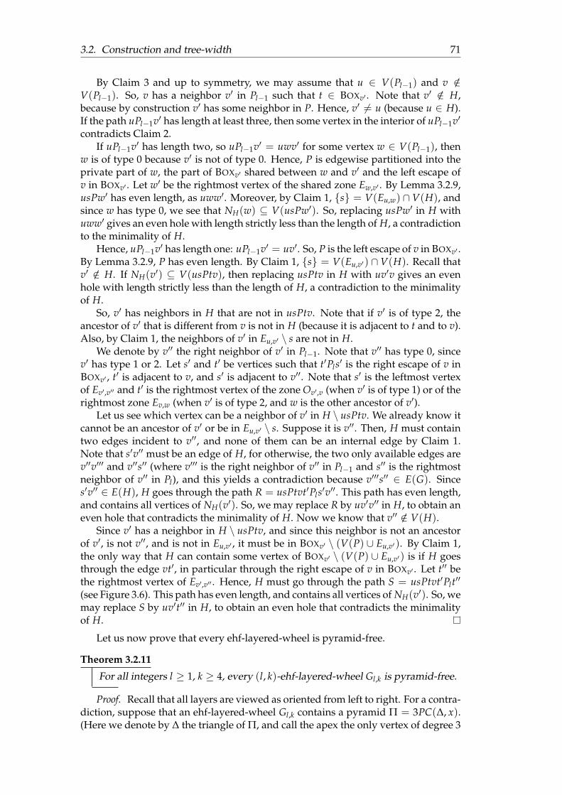
3.2. Construction and tree-width 71
By Claim 3 and up to symmetry, we may assume that u ∈ V(Pl−1) and v /∈V(Pl−1). So, v has a neighbor v′ in Pl−1 such that t ∈ BOXv′ . Note that v′ /∈ H,because by construction v′ has some neighbor in P. Hence, v′ 6= u (because u ∈ H).If the path uPl−1v′ has length at least three, then some vertex in the interior of uPl−1v′
contradicts Claim 2.If uPl−1v′ has length two, so uPl−1v′ = uwv′ for some vertex w ∈ V(Pl−1), then
w is of type 0 because v′ is not of type 0. Hence, P is edgewise partitioned into theprivate part of w, the part of BOXv′ shared between w and v′ and the left escape ofv in BOXv′ . Let w′ be the rightmost vertex of the shared zone Ew,v′ . By Lemma 3.2.9,usPw′ has even length, as uww′. Moreover, by Claim 1, s = V(Eu,w) ∩V(H), andsince w has type 0, we see that NH(w) ⊆ V(usPw′). So, replacing usPw′ in H withuww′ gives an even hole with length strictly less than the length of H, a contradictionto the minimality of H.
Hence, uPl−1v′ has length one: uPl−1v′ = uv′. So, P is the left escape of v in BOXv′ .By Lemma 3.2.9, P has even length. By Claim 1, s = V(Eu,v′) ∩V(H). Recall thatv′ /∈ H. If NH(v′) ⊆ V(usPtv), then replacing usPtv in H with uv′v gives an evenhole with length strictly less than the length of H, a contradiction to the minimalityof H.
So, v′ has neighbors in H that are not in usPtv. Note that if v′ is of type 2, theancestor of v′ that is different from v is not in H (because it is adjacent to t and to v).Also, by Claim 1, the neighbors of v′ in Eu,v′ \ s are not in H.
We denote by v′′ the right neighbor of v′ in Pl−1. Note that v′′ has type 0, sincev′ has type 1 or 2. Let s′ and t′ be vertices such that t′Pls′ is the right escape of v inBOXv′ , t′ is adjacent to v, and s′ is adjacent to v′′. Note that s′ is the leftmost vertexof Ev′,v′′ and t′ is the rightmost vertex of the zone Ov′,v (when v′ is of type 1) or of therightmost zone Ev,w (when v′ is of type 2, and w is the other ancestor of v′).
Let us see which vertex can be a neighbor of v′ in H \ usPtv. We already know itcannot be an ancestor of v′ or be in Eu,v′ \ s. Suppose it is v′′. Then, H must containtwo edges incident to v′′, and none of them can be an internal edge by Claim 1.Note that s′v′′ must be an edge of H, for otherwise, the two only available edges arev′′v′′′ and v′′s′′ (where v′′′ is the right neighbor of v′′ in Pl−1 and s′′ is the rightmostneighbor of v′′ in Pl), and this yields a contradiction because v′′′s′′ ∈ E(G). Sinces′v′′ ∈ E(H), H goes through the path R = usPtvt′Pls′v′′. This path has even length,and contains all vertices of NH(v′). So, we may replace R by uv′v′′ in H, to obtain aneven hole that contradicts the minimality of H. Now we know that v′′ /∈ V(H).
Since v′ has a neighbor in H \ usPtv, and since this neighbor is not an ancestorof v′, is not v′′, and is not in Eu,v′ , it must be in BOXv′ \ (V(P) ∪ Eu,v′). By Claim 1,the only way that H can contain some vertex of BOXv′ \ (V(P) ∪ Eu,v′) is if H goesthrough the edge vt′, in particular through the right escape of v in BOXv′ . Let t′′ bethe rightmost vertex of Ev′,v′′ . Hence, H must go through the path S = usPtvt′Plt′′
(see Figure 3.6). This path has even length, and contains all vertices of NH(v′). So, wemay replace S by uv′t′′ in H, to obtain an even hole that contradicts the minimalityof H.
Let us now prove that every ehf-layered-wheel is pyramid-free.
Theorem 3.2.11
For all integers l ≥ 1, k ≥ 4, every (l, k)-ehf-layered-wheel Gl,k is pyramid-free.
Proof. Recall that all layers are viewed as oriented from left to right. For a contra-diction, suppose that an ehf-layered-wheel Gl,k contains a pyramid Π = 3PC(∆, x).(Here we denote by ∆ the triangle of Π, and call the apex the only vertex of degree 3

72 Chapter 3. Layered wheels
v′Pl−1
Pl
Piv
Ev′,v′′Ov′ Ov′Ov′,vEu,v′ t t′ s′ t′′s
u v′′
u′ u′′
Eu′,u Eu,u′′Ou
Pj
Pi
Pl
Pl−1
v
w
Ou OuEv,wEu Eu
u
Ou,wOu,v Ev,ws t t′ s′ t′′
FIGURE 3.6: The proof of Theorem 3.2.10: in blue is the path S =usPtvt′Plt′′, when v′ is of type 1 (top) and when v′ is of type 2 (bottom)
in Π \ ∆ which in this case is the vertex x.) Suppose that l is minimal, and underthis assumption that Π contains the minimum number of vertices among all pyra-mids in Gl,k. Clearly l ≥ 3, and layer Pl contains some vertex of Π, for otherwiseGl,k[P0 ∪ · · · ∪ Pl−1] would be a counterexample.
The next claim is trivially correct, so we omit the proof.
Claim 1. Any hole in Π contains the apex and two vertices of ∆.
Claim 2. If a vertex of ∆ is in Pl , then it is not in the interior of some zone.
Proof of Claim 2. Suppose that some vertex a of ∆ is in Pl and is in the interior of somezone Z. Then a is of type 2. If Z = Eu′,u for some u′, u ∈ Pl−1, then ∆ = auu′, and wesee that the left or the right neighbor of a in Pl is in Π. Let Q = a . . . b be the subpathof Pl that contains a, that is included in Π, and that is maximal w.r.t. these properties.We see that b is adjacent to u and u′, so that Π contains a diamond, a contradiction.The proof is the same for all other kinds of zones (namely Eu,u′′ , Ev,w, Ou,v, or Ou,w).This proves Claim 2.
Claim 3. The apex x is not in Pl .
Proof of Claim 3. Let us see that x ∈ Pl yields a contradiction. Since x has degree 3 inΠ, it is a vertex of type 1 or 2, so it belongs to some zone.
Suppose first that x is in the interior of some zone Z. If Z = Eu,u′ for someu, u′ ∈ Pl−1, then since x has degree 3 in Π and is not in a triangle of Π, we see thatthe two neighbors of x in Pl are in Π. Also, exactly one ancestor y of x must be in Π.Let Q be the subpath of Pl that contains x, that is included in Π, and that is maximalw.r.t. these properties. We see that the ends of Q are adjacent to y, so that Q and yform a cycle with a unique chord in a pyramid, while not containing a triangle, acontradiction. When Z is another zone, say Eu,u′′ , Ou, Ou,v, etc, the proof is exactlythe same.
Suppose now that x is an end of some zone Z. Again, the two neighbors of x inPl and an ancestor u of x are in Π. So, Π contains the path Q from x to the vertex ywith ancestor u that is next to x along Z. Note that y is in the interior of Z. So, Q and

3.2. Construction and tree-width 73
u form a hole of Π. Apart from x, y, and u, every vertex of H has degree 2, so uy isan edge of ∆, a contradiction to Claim 2. This proves Claim 3.
Claim 4. If u ∈ Pl−1 has type 0 or 1 and is in Π, then no internal vertex of BOXu is inΠ.
Proof of Claim 4. Suppose a ∈ Π is an internal vertex of BOXu. Let Q be the subpathof Pl that contains a, is included in Π, and maximal w.r.t. this property. Since a isan internal vertex of BOXu and u has type 0 or 1, Q and u form a hole H, that mustcontain the apex. Since by Claim 3, the apex is not in Pl , it must be u, and sinceevery internal vertex of Q has degree 2, the two neighbors of u in H are in ∆, acontradiction since they are non-adjacent. This proves Claim 4.
Claim 5. No vertex of ∆ is in Pl .
Proof of Claim 5. Suppose for a contradiction that a is a vertex of ∆ in Pl . So a hastype 2, and in particular, it is not an end of Pl . As every internal vertex of Pl , a isin the interior of some box BOXu. If u is of type 0 or 1, it must be part of ∆, so acontradicts Claim 4. Hence, u is of type 2.
We denote by P = a . . . p a subpath of Π included in BOXu and maximal withthis property. We will now analyze every possible zone where a belongs to, and wewill see that each of the cases yields a contradiction.
Suppose first that a is in a shared zone Z. If Z = Eu′,u, and therefore, ∆ = au′u,then by Claim 2, a is the rightmost vertex of Eu′,u (since it is in the interior of BOXu).Since u′ is of type 0 (because u is of type 2), Claim 4 applied to BOXu′ implies that ais the only vertex of Π in Eu′,u, so p must be the leftmost vertex of the zone Eu that isnext to Eu′,u. So P and u form a hole H of Π, and since u is in ∆, the apex x must bein Pl , a contradiction to Claim 3. The proof is similar when Z = Eu,u′′ .
If Z = Ou,v, then ∆ = auv, and by Claim 2, a is either the leftmost or the rightmostvertex of Ou,v. If a is the leftmost vertex of Ou,v, then p is either the rightmost vertexof the zone Ou (that is on the left of Ou,v) or p is the vertex of type 2 next to a alongOu,v. In either case, P and u form a hole H of Π, and since u is in the triangle ofΠ, the apex x must be in Pl , a contradiction to Claim 3. If a is the rightmost vertexof Ou,v, the proof is similar. By symmetry, the case when Z = Ou,w yields a similarcontradiction.
When a is the rightmost vertex of the leftmost zone Ev,w (that is between Eu andOu when oriented from left), we have ∆ = avw and so u /∈ Π. The proof is again thesame, with a hole H that goes through v. The case when a is the leftmost vertex ofthe rightmost zone Ev,w (that is between Ou and Eu when oriented from left) can bedone in the similar way.
We are left with the case when a is the leftmost vertex of the leftmost zone Ev,w,or the rightmost vertex of the rightmost zone Ev,w. These two cases are symmetric,so we may assume that a is the leftmost vertex of the leftmost zone Ev,w.
It then follows that ∆ = avw. Note that u /∈ Π because a pyramid has only onetriangle. If P goes in the interior of the zone Ev,w, then Π contains a diamond, acontradiction. So, P goes through the zone Eu that is left to Ev,w and contains therightmost vertex of Eu′,u. There are two cases: P contains the zone Eu′,u (so p isthe leftmost vertex of Eu′,u and u′ /∈ Π), or P contains only the rightmost vertex orEu′,u (so p is the rightmost vertex of Eu′,u and u′ ∈ Π). In the first case, we removeP \ p from Π and put instead the edge up; in the second case, we remove P from Πcompletely and put the edge uu′. We obtain a pyramid (with triangle uvw) that isof smaller size than Π — a contradiction, unless u has some neighbor in Π \ (P ∪u′, v, w). Hence, we now suppose such a neighbor z exists.

74 Chapter 3. Layered wheels
Let q be the leftmost vertex of the leftmost zone Ou (that is first met when travers-ing the layer from left to right), and r be the rightmost vertex of Eu,u′′ . Consider thepath Q = qPlr. Observe that z is in Q ∪ u′′ because Q ∪ u′′ contains all possibleneighbors of u in Π \ (P ∪ u′, v, w).
Suppose that some vertex of Q is in Π. Let z′ be the vertex of Π in Q that is theclosest to q along Q. Note that by Claim 3, z′ has degree 2 in Π. Since z′ is the closestvertex to q, it has a neighbor in Π \ Q. In particular, z′ is a type 1 or type 2 vertex,and exactly one of its ancestor is in Π. Since u /∈ Π, such an ancestor is v or w, orpossibly u′′ if u′′ ∈ Π (and only one of them). If z′ ∈ Ou,v, or z′ ∈ Ou,w, or z′ ∈ Ev,w,then there exists a vertex z′′ ∈ Q such that vz′Plz′′v, or wz′Plz′′w, or vz′Plz′′wv is ahole of Π, which in each case contradicts Claim 3. So z′ ∈ Eu,u′′ and the ancestor ofz′ in Π must be u′′ (in particular u′′ ∈ Π). But then, the right neighbor of z′ in Pl isan internal vertex of BOXu′′ that belongs to Π, a contradiction to Claim 4. Therefore,Π ∩Q = ∅.
This means that z = u′′. Note that the neighbors of u′′ in Π cannot contain u(because u /∈ Π), cannot be in Eu,u′′ (because Eu,u′′ is subpath of Q), cannot be in theinterior of BOXu′′ (because u′′ has type 0 and by Claim 4), so they are precisely theright neighbor u′′′ of u′′ in Pl−1 and the rightmost vertex b of Eu′′,u′′′ . But then, u′′u′′′bis a triangle in Π, a contradiction. This proves Claim 5.
The rest of the proof is quite similar to the proof of Theorem 3.2.10, that ehf-layered-wheel contains no even hole.
Let P = s . . . t be a subpath of Π in Pl such that P is inclusion-wise maximal (ands, t appear in this order from left to right). By Claims 3 and 5, every vertex of P hasdegree 2 in Π. Moreover by the maximality of P, each of s and t has an ancestorwhich is also in Π. Note that s 6= t, for otherwise s would be of type 2, and togetherwith its ancestors, it forms a triangle, which contradicts Claim 5. Let u and v be theancestors of s and t respectively, such that u, v ∈ V(Π). By Claims 1, 3, and 5, u 6= vand uv /∈ E(G).
Claim 6. For every vertex p ∈ V(Pl−1), N(p) ∩V(Pl) 6⊆ V(P).
Proof of Claim 6. Suppose that p ∈ V(Pl−1) and N(p) ∩V(Pl) ⊆ V(P). So, p /∈ V(Π).Note that p is an internal vertex of Pl−1, for otherwise, s or t is an end of Pl and hasdegree 2, while having two neighbors in V(Π) ∩V(Gl,k \ p), a contradiction.
By (B5), the ancestors of p (if any) and the neighbors of p in Pl−1 must also haveneighbors in P. Thus, no such vertices belong to Π because P is a subpath of Π.Hence, replacing BOXp = p′ . . . p′′ in Π with p′pp′′ yields a pyramid with strictlyfewer vertices than Π, a contradiction to the minimality of Π. This proves Claim 6.
Let a be a vertex in Pi for some 0 ≤ i < l, and p be a neighbor of a in Pl . We saythat ap is an internal edge if one of the following holds:
• i = l − 1 and p is an internal vertex of BOXa.
• i < l − 1, a is an ancestor of some a′ ∈ V(Pl−1), a′ has type 1 or 2, p is in BOXa′
and p is neither the leftmost neighbor of a in BOXa′ nor the rightmost neighborof a in BOXa′ .
Claim 7. No internal edge is an edge of Π.
Proof of Claim 7. Suppose that p ∈ Pl is the end of an internal edge e that is also anedge of Π. If the other end of e is in Pl−1, we set e = pu and observe that p is in theinterior of BOXu. Otherwise, the other end of e is in Pi, with i < l − 1, we set e = px

3.2. Construction and tree-width 75
and observe that x has a neighbor u in Pl−1. Again, p is an internal vertex of BOXu.Observe that x is either v or w as represented in Figure 3.5.
By Claims 3 and 5, p has degree 2 in Π, so p has a unique neighbor in Π ∩ Pl .Let P = p . . . p′ be the subpath of Pl included in Π, containing p, and maximal withrespect to this property.
It can be checked in Figure 3.5 that P together with u, v, w, uv, uw, or vw formsa hole, that contains the apex and two vertices of ∆ (by Claim 1), a contradiction toClaims 3 and 5. This proves Claim 7.
Claim 8. Exactly one of u and v is in Pl−1.Proof of Claim 8. Suppose that both u and v are not in Pl−1. Since u and v haveneighbors in P, each of them has a neighbor u′ and v′ respectively in Pl−1, such thats ∈ BOXu′ and t ∈ BOXv′ .
If u′ = v′, then u′ is a type 2 vertex in Pl−1. By construction, usPtvu is then ahole of Σ, so it must contains the apex and two vertices of ∆, contradicting Claim 3or Claim 5, since u and v are the only vertices of the hole that are not in Pl .
Since u′ and v′ are vertices with ancestors, by construction, the interior of u′Pl−1v′
contains a vertex w of type 0. It yields that NPl (w) is all contained in P, a contradic-tion to Claim 6.
Suppose now that both u and v are in Pl−1. By Claim 6, no vertex of Pl−1 has allits neighbors in P. So the interior of uPl−1v contains at most two vertices.
If u = v, then usPtu is a hole of Π. Since u is the only vertex in the hole that is notin Pl , by Claim 1, P contains the apex or a vertex of ∆, a contradiction to Claims 3 or 5.Similarly if uv ∈ E(G), then usPtvu is a hole of Π, this again yields a contradiction.
If the interior of uPl−1v contains a single vertex, then let w be this vertex. Letw1 (resp. w2) be the neighbor of w in P that is closest to s (resp. t). It follows byconstruction, that s = w1, t = w2 (because both u and v are adjacent to w in Pl−1).By Claim 7, s = V(Eu,w) ∩ V(Π) and t = V(Ew,v) ∩ V(Π). Also, if w hasan ancestor, then such an ancestor must have neighbors in P, and hence it doesnot belong to Π. Altogether, we see that NΠ(w) ⊆ V(usPtv). So, replacing usPtvin Π with uwv gives a pyramid with fewer vertices than Π, a contradiction to theminimality of Π.
So the interior of uPl−1v contains two vertices. We let uPl−1v = uww′v, and w1(resp. w′2) be the neighbor of w (resp. w′) in P that is closest to s (resp. t). Similar toin the previous case, we know that s = w1, t = w′2; and by Claim 7, s = V(Eu,w) ∩V(Π) and t = V(Ew′,v) ∩ V(Π). Also, if w or w′ has an ancestor, then such anancestor must have neighbors in P, and hence it does not belong to Π. Altogether,we see that NΠ(w, w′) ⊆ V(usPtv). So, replacing usPtv in Π with uww′v gives apyramid with fewer vertices than Π, again a contradiction to the minimality of Π.This proves Claim 8.
By Claim 8 and up to symmetry, we may assume that u ∈ V(Pl−1) and v /∈V(Pl−1). So, v has a neighbor v′ in Pl−1 such that t ∈ BOXv′ . Note that v′ 6= u,for otherwise usPtvu is a hole of Σ, so it contains the apex and two vertices of ∆,a contradiction to Claim 3 or Claim 5. Furthermore, note that the path uPl−1v′ haslength at most two, for otherwise some vertex in the interior of uPl−1v′ contradictsClaim 6.
Suppose that uPl−1v′ has length two, so uPl−1v′ = uwv′ for some vertex w ∈V(Pl−1). Then w is of type 0 because v′ is not of type 0. Let w′ be the rightmostvertex of the shared zone Ew,v′ . By Claim 7, s = V(Eu,w) ∩V(Π), and since w hastype 0, we see that NΠ(w) ⊆ V(usPw′). So, replacing usPw′ in Π with uww′ gives apyramid with fewer vertices than Π, a contradiction to the minimality of Π.

76 Chapter 3. Layered wheels
Hence, uPl−1v′ has length one, i.e. uPl−1v′ = uv′. By Claim 7, s = V(Eu,v′) ∩V(Π). Observe that P is the left escape of v in BOXv′ . So, P goes through the zoneOv′ (when v′ has type 1) or through the zone Ev′ (when v′ has type 2). In particularv′ /∈ Π.
If NΠ(v′) ⊆ V(usPtv), then replacing usPtv in Π with uv′v gives a pyramid withfewer vertices than Π, a contradiction to the minimality of Π. So, v′ has neighbors inΠ that are not in usPtv. Note that if v′ is of type 2, the ancestor of v′ that is differentfrom v is not in Π (because it is adjacent to t and to v, but t /∈ ∆ by Claim 5).
We denote by v′′ the right neighbor of v′ in Pl−1. Note that v′′ has type 0, sincev′ has type 1 or 2. Let s′ and t′ be vertices such that t′Pls′ is the right escape of v inBOXv′ , t′ is adjacent to v and s′ is adjacent to v′′. Note that s′ is the leftmost vertex ofEv′,v′′ and t′ is the rightmost vertex of the zone Ov′,v (when v′ is of type 1) or of therightmost zone Ev,w (when v′ is of type 2, and w is the other ancestor of v′).
Let us see which vertex can be a neighbor of v′ in Π \ usPtv. We already knowit cannot be an ancestor of v′ or be a vertex of Eu,v′ \ s. Suppose it is v′′. Then, Πmust contain two edges incident to v′′, and none of them can be an internal edge byClaim 7. Note that s′v′′ must be an edge of Π, for otherwise, the two only availableedges are v′′v′′′ and v′′s′′ (where v′′′ is the right neighbor of v′′ in Pl−1 and s′′ is therightmost neighbor of v′′ in Pl), and this is a contradiction because v′′′s′′ ∈ E(G).Since s′v′′ ∈ E(Π), Π goes through the path R = usPtvt′Pls′v′′. This path containsall vertices of NΠ(v′). Note that v /∈ ∆, because if so, one of t or t′ should be in ∆, acontradiction to Claim 5. But v can be the apex. If v is not the apex, we may replaceR by uv′v′′ in Π, to obtain a pyramid that contradicts the minimality of Π. If v is theapex, then we may replace R \ v by uv′v′′ in Π, to obtain a pyramid with apex v′ thatcontradicts the minimality of Π. Now we know that v′′ /∈ V(Π).
Since v′ has a neighbor in Π \ usPtv, and since this neighbor is not an ancestorof v′, is not v′′, and is not in Eu,v′ , it must be in BOXv′ \ (V(P) ∪ Eu,v′). By Claim 7,the only way that Π can contain some vertex of BOXv′ \ (V(P) ∪ Eu,v′) is that Π goesthrough the edge vt′, in particular through the right escape of v in BOXv′ and throughthe zone Ev′,v′′ . Let t′′ be the rightmost vertex of Ev′,v′′ . Hence, Π must go throughthe path S = usPtvt′Plt′′. This path contains all vertices of NΠ(v′). Note that v /∈ ∆,because if so, one of t or t′ should be in ∆, a contradiction to Claim 5. But v can be theapex. If v is not the apex, we may replace S by uv′t′′ in Π, to obtain a pyramid thatcontradicts the minimality of Π. If v is the apex, then we may replace S \ v by uv′t′′
in Π, to obtain a pyramid with apex v′ that contradicts the minimality of Π.
Tree-width and clique-width
For any l ≥ 0, ttf-layered-wheels and ehf-layered-wheels on l + 1 layers contain Kl+1as a minor. To see this, note that each vertex in layer Pi, i < l, has neighbors in alllayers i + 1, . . . , l (see Lemma 3.2.2 and Lemma 3.2.7). Hence, by contracting eachlayer into a single vertex, a complete graph on l + 1 vertices is obtained. Since whenH is a minor of G we have tw(H) ≤ tw(G), and since for l ≥ 1, a complete graph onl vertices has tree-width l − 1, we obtain the following.
Theorem 3.2.12
For any l ≥ 0, ttf-layered-wheels and ehf-layered-wheels on l + 1 layers havetree-width at least l.

3.2. Construction and tree-width 77
Gurski and Wanke [GW00] proved that the tree-width is in some sense equiva-lent to the clique-width when some complete bipartite graph is excluded as a sub-graph. Let us state and apply this formally (thanks to Sang-il Oum for pointing thisout to us).
Theorem 3.2.13 (Gurski and Wanke [GW00])
If a graph G contains no K3,3 as a subgraph, then tw(G) ≤ 6 cw(G)− 1.
Lemma 3.2.14
A layered wheel (ttf or ehf) contains no K3,3 as a subgraph.
Proof. Suppose that a ttf-layered-wheel G contains K3,3 as a subgraph. Then,either it contains a theta (if K3,3 is an induced subgraph of G) or it contains a triangle(if K3,3 is not an induced subgraph of G). In each case, there is a contradiction.
Suppose that an ehf-layered-wheel G contains K3,3 as a subgraph. If one sideof the K3,3 is a clique, then G contains a K4. Otherwise, each side of K3,3 containsa non-edge, so G contains K2,2, that is isomorphic to a C4. In both cases, there iscontradiction.
Theorem 3.2.15
For any integers l ≥ 2, k ≥ 4, the clique-width of a layered wheel Gl,k is atleast l+1
6 .
Proof. Follows from Lemma 3.2.14 and Theorems 3.2.13 and 3.2.12.
Observations and open questions
It should be pointed out that by carefully subdividing, one may obtain bipartite ttf-layered-wheels on any number l of layers. This is easy to prove by induction on l.We just sketch the main step of the proof: when building the last layer, assumingthat the previous layers induce a bipartite graph, only the vertices with ancestorsare assigned to one side of the bipartition (and only to one side, since a vertex hasat most one ancestor in a ttf-layered-wheel). The parity of the paths linking verticeswith ancestors can be adjusted to produce a bipartite graph.
It is easy to see that every prism, every theta, and every even wheel contains aneven hole. Therefore, by Theorem 3.2.10 and Theorem 3.2.11, ehf-layered-wheels are(prism, pyramid, theta, even wheel)-free, which is not obvious from their definitions.Note that ehf-layered-wheels contain diamonds (see Conjecture 6.1.4).
However, we note that it is possible to modify Construction 3.2.6 in such a waythat we obtain a layered wheel that is even-hole-free but contains a pyramid. Such aconstruction might be of interest to see what structure one can get in a even-hole-freegraphs by studying how the graph attaches to a pyramid. The construction is doneby modifying axiom (B5) where the two zones Eu’s are deleted. More specifically,if u is of type 2 (so it is an internal vertex of Pl−1), then let v ∈ Pi and w ∈ Pj,j ≤ i be its ancestors. In this case, BOXu is made of only 9 zones, namely Eu′,u, Ev,w,Ou, Ou,v, Ou, Ou,w, Ou, Ev,w, and Eu,u′′ (see Figure 3.7). The fact that this modifiedconstruction keeps the property of the layered wheel being even-hole-free can beproved similarly to Theorem 3.2.10. Notice that Lemma 3.2.9 also remains true forthis modified construction. We remark that a corresponding wheel that is even-hole-free (similar to the one in Figure 3.4) exists considering this modified pattern ofzones.

78 Chapter 3. Layered wheels
uu′ u′′
Eu′,u Ev,w Ev,w Eu,u′′Ou OuOuOu,v Ou,w
Pj
Pi
Pl
Pl−1
v
w
FIGURE 3.7: A modified construction of ehf-layered-wheel Gl,k whichcontain pyramids (dashed lines between two vertices in Pl represent
paths of odd length)
Pj
Pi
Pl−1
Pl
w
s t
v
u u′′ u∗u′
FIGURE 3.8: A pyramid (in blue) that is contained in a modified ehf-layered-wheel Gl,k, for some integers l, k
An example of a pyramid that may be found in such a modified ehf-layered-wheel is given in Figure 3.8. In the figure, u ∈ Pl−1 is a type 2 vertex with ancestorsv ∈ Pi and w ∈ Pj, j < i, u∗ is a common neighbor of v and w in Pl−1 such that uand u∗ are consecutive common neighbors of v and w in some vw-zone in Pl−1, s isthe rightmost vertex of a zone labeled Ev,w ⊆ BOXu in Pl ; and t is the leftmost vertexof the zone labeled Eu,u′′ ⊆ BOXu in Pl where u′′ 6= u′ is adjacent to u in Pl−1. Thepyramid has triangle utu′′ and apex v.
3.3 Lower bound on rank-width
In this section, we prove that there exist ttf-layered-wheels and ehf-layered-wheelswith arbitrarily large rank-width. This follows directly from Theorem 3.2.15 andLemma 3.1.1, but by a direct computation, we provide a better bound. The nextlemma follows directly from the definition of the rank-width defined in Chapter 1Section 1.2.3.
Lemma 3.3.1
Let G be a graph and H be an induced subgraph of G. Then rw(H) ≤ rw(G).
A class C of graphs has bounded rank-width if there exists a constant k ∈ N, suchthat every G ∈ C satisfies rw(G) ≤ k. If such a constant does not exist, then C hasunbounded rank-width. In the following lemmas, we present some basic propertiesrelated to rank-width. Let T be a tree, we call an edge e ∈ E(T) balanced, if the

3.3. Lower bound on rank-width 79
partition (Ae, Be) of L(T) satisfies 13 |L(T)| ≤ |Ae| and 1
3 |L(T)| ≤ |Be|. The followingis well-known (we include a proof for the sake of completeness).
Lemma 3.3.2
Every cubic tree has a balanced edge.
Proof. Let T be a cubic tree with n leaves. We may assume that n ≥ 3, forotherwise, T is a path of length 1, and the only edge of T is balanced.
Let e = ab be an edge of T such that the set of leaves Ae of the connected com-ponent of T \ e that contains a, satisfies |Ae| ≥ |L(T)|/3. Suppose that a and b arechosen subject to the minimality of |Ae|. If |Ae| ≤ 2|L(T)|/3, then e is balanced.Otherwise, |Ae| > 2|L(T)|/3 ≥ 2 so a has two neighbors a′, a′′ different from b.Let A′ (resp. A′′) be the set of leaves of the connected component of T \ aa′ (resp.T \ aa′′) that contains a′ (resp. a′′). Since |Ae| > 2|L(T)|/3 and Ae = A′ ∪ A′′, ei-ther |A′| > |L(T)|/3 or |A′′| > |L(T)|/3. Hence, one of A′ or A′′ contradicts theminimality of |Ae|.
Let us now introduce a notion that is useful to describe how we can representthe structure of layered wheels into a matrix. An n× n matrix M is fuzzy triangular ifm1,1 = 1 and for every i ∈ 2, . . . , n, mi,i = 1 and either m1,i = m2,i = · · · = mi−1,i =0 or mi,1 = mi,2 = · · · = mi,i−1 = 0.
Lemma 3.3.3
Every n× n fuzzy triangular matrix has rank n.
Proof. Let M be an n× n fuzzy triangular matrix. We prove by induction on n,that rank(M) = n. For n = 1, this trivially holds. Suppose that n ≥ 2. If m1,n =m2,n = · · · = mn−1,n = 0, we show that rows r1, . . . , rn of M are linearly independent.Let λ1, . . . , λn ∈ [0, 1] be such that Σn
i=1λiri = 0 (where 0 is the zero vector of lengthn). Since mn,n = 1, we have λn = 0. This implies that Σn−1
i=1 λir′i = 0, where r′i isthe row obtained from ri by deleting its last entry. Since r′1, . . . , r′n−1 are the rows ofan (n − 1) × (n − 1) fuzzy triangular matrix, they are linearly independent by theinduction hypothesis, so λ1 = · · · = λn−1 = 0.
We can prove in the same way that, if mn,1 = mn,2 = · · · = mn,n−1 = 0, then theset of n columns of M is linearly independent. This shows that rank(M) = n.
Let G be a graph and (X, Y) be a partition of V(G). A path P in G is separated by(X, Y) if V(P)∩ X and V(P)∩Y are both non-empty. Note that when P is separatedby (X, Y), there exists a separating edge xy of P whose end-vertices are x ∈ X andy ∈ Y.
Lemma 3.3.4
Let (T, λ) be a rank decomposition of width at most r of a layered wheel withlayers P0, P1, . . . , Pl . Let e be an edge of T, and (X, Y) be the partition of V(G)induced by T \ e. Then there are at most r paths among P0, P1, . . . , Pl that areseparated by (X, Y).
Proof. Suppose for a contradiction that Pi1 , . . . , Pir+1 are layers that are all sepa-rated by (X, Y), where 1 ≤ i1 < · · · < ir+1 ≤ l. For each integer ij, consider aseparating edge xij yij of Pij such that xij ∈ X and yij ∈ Y. Set SX = xi1 , . . . , xir+1and SY = yi1 , . . . , yir+1.
Consider M[SX, SY], the adjacency matrix whose rows are indexed by SX andcolumns are indexed by SY. The definition of layered wheels (see (A6) and (B7)) says

80 Chapter 3. Layered wheels
that when two vertices in a layer are adjacent, at most one of them has ancestors. Itfollows that M[SX, SY] is fuzzy triangular. By Lemma 3.3.3, M[SX, SY] has rank r + 1,a contradiction, because
width(T, λ) ≥ cutrkG(X) = rank(M[X, Y]) ≥ rank(M[SX, SY]) = r + 1.
We need the following lemma in our proof.
Lemma 3.3.5 (See [Adl+17])
Let G be a graph and (T, λ) be a rank decomposition of G whose width is atmost r. Let P be an induced path of G and (X, Y) be the partition of V(G) inducedby T \ e where e ∈ E(T). Then each of P[X] and P[Y] contains at most r + 1connected components.
Now we are ready to describe layered wheels for which we can prove that therank-width is unbounded. Let us first define some terminology that is used in theproof. Recall Construction 3.2.1 of ttf-layered-wheels. Let u and v be two verticesthat are adjacent in a layer Pi for some i ∈ 1, . . . , l − 1, and they appear in thisorder (from left to right) along Pi. Let a be the rightmost vertex of BOXu and b bethe leftmost vertex of BOXv in Pi+1. Let a′ (resp. b′) be the neighbor of a (resp. b) inPi+1 \ BOXu (resp. Pi+1 \ BOXv). The path a′Pi+1b′ is called the uv-bridge. An edge pqin a′Pi+1b′ is called the middle edge of the bridge if the length of the paths a′Pi+1 p andqPi+1b′ are equal.
We have a similar definition for ehf-layered-wheel. For adjacent vertices u and vin Pi+1, the uv-bridge in Pi+1 is the zone labelled Eu,v ⊆ BOXu ∩ BOXv (that we calledin the previous section a shared part). Observe that in both layered wheels, everyinternal vertex of some layer yields two bridges, and each end of a layer yields onebridge. We say that a layered wheel is special if every bridge in all layers has oddlength (and therefore admits a middle edge). The following lemmas are a directconsequence of Construction 3.2.1 and Construction 3.2.6.
Lemma 3.3.6
For all integers l ≥ 1 and k ≥ 4, there exists a special (l, k)-ttf-layered-wheel.
Proof. The result follows because by (A6) of Construction 3.2.1, the path betweenBOXu and BOXv is of length at least k− 2. So for any two adjacent vertices in a layer,the uv-bridge can have any odd length, at least k− 4.
Lemma 3.3.7
For all integers l ≥ 1 and k ≥ 4, any (l, k)-ehf-layered-wheel is special.
Proof. The result follows from the fact that the shared parts have odd length (seeLemma 3.2.9).
Let Gl,k be a layered wheel that is special. Let uv be an edge of some layer Pi,where 1 ≤ i < l, such that u and v appear in this order (from left to right) along Pi.Then we denote by rulv the middle edge of the uv-bridge (again, ru and lv appear inthis order from left to right).
For any vertex v ∈ Pi, 1 ≤ i < l, the domain of v (or the v-domain), denoted byDOM(v) is defined as follows:

3.3. Lower bound on rank-width 81
• if v ∈ V(P0), then DOM(v) = V(P1);
• if v is an internal vertex of Pi, then DOM(v) = V(lvPi+1rv);
• if v is the left end of Pi, then DOM(v) = V(pPi+1rv), where p is the leftmostvertex of BOXv; and
• if v is the right end of Pi, then DOM(v) = V(lvPi+1q), where q is the rightmostvertex of BOXv.
Note that for ttf-layered-wheels, BOXv is completely contained in the v-domain,which is not the case for ehf-layered-wheels. We are now ready to describe the lay-ered wheels that we need.
Definition 3.3.8. For some integer m, a special layered wheel Gl,k is m-uniform, if for everyvertex v ∈ V(Pi), 0 ≤ i ≤ l − 1, DOM(v) contains exactly m vertices.
Observe that by definition, any m-uniform layered wheel is special.
Lemma 3.3.9
For all integers l ≥ 1 and k ≥ 4 and M, there exists an integer m ≥ M and an(l, k)-ttf-layered-wheel that is m-uniform.
Proof. We construct an m-uniform ttf-layered-wheel Gl,k by adjusting the lengthobtained in step (A6) of Construction 3.2.1.
Lemma 3.3.10
For all integers l ≥ 1 and k ≥ 4 and M, there exists an integer m ≥ M and an(l, k)-ehf-layered-wheel that is m-uniform.
Proof. We construct an m-uniform ehf-layered-wheel Gl,k by adjusting the lengthobtained in step (B7) of Construction 3.2.6.
For a vertex v ∈ Pi, 0 ≤ i ≤ l and an integer 0 ≤ d ≤ l− i, the v-domain of depth d,denoted by DOMd(v) is defined as follows.
• DOM0(v) = v and DOM1(v) = DOM(v);
• DOMd(v) =⋃
x∈DOM(v) DOMd−1(x) for d ≥ 1.
Observation 3.3.11. For every v ∈ Pi with 0 ≤ i ≤ l, and for any 0 ≤ d ≤ l − i, we haveDOMd(v) ⊆ V(Pi+d), where the equality holds when i = 0.
Lemma 3.3.12
For every 0 ≤ i ≤ l and 0 ≤ d ≤ i, V(Pi) =⋃
v∈Pi−dDOMd(v). Moreover, for any
distinct u, v ∈ V(Pi−d), DOMd(u) ∩DOMd(v) = ∅.
Proof. The statement simply follows by induction on d.
Lemma 3.3.13
For some integers l, k, m, let Gl,k be an m-uniform layered wheel. For every0 ≤ i ≤ l − 1, v ∈ Pi, and 1 ≤ d ≤ l − i, we have |DOMd(v)| = md.
Proof. The statement simply follows from Lemma 3.3.12 and the m-uniformity:for any vertex v, |DOM1(v)| = m and |DOMd(v)| = m · |DOMd−1(v)|.

82 Chapter 3. Layered wheels
Lemma 3.3.14
For some integers l, k, m, let Gl,k be an m-uniform layered wheel. Denote byGi,k, the subgraph induced by the first i + 1 layers P0, P1, . . . , Pi of Gl,k. Then|V(Gi,k)| < 1
m−1 |V(Pi+1)| for 0 ≤ i ≤ l − 1.
Proof. Recall that V(Pi) = DOMi(r) for every 1 ≤ i ≤ l, with r ∈ V(P0). So byLemma 3.3.13, |V(Pi)| = mi. Moreover, |V(Gi,k)| = Σi
d=0|DOMd(r)| = mi+1−1m−1 . Hence,
the result follows directly.
Lemma 3.3.15
Let l ≥ 2, k ≥ 4, and m ≥ 15 be integers, and (T, λ) be a rank decompositionof an m-uniform layered wheel Gl,k of width at most r. Let e be a balanced edgein T, and (X, Y) be the partition of V(Gl,k) induced by e. Then Pl is separated by(X, Y), and each of X and Y contains an induced subpath of Pl , namely PX andPY where:
|V(PX)|, |V(PY)| ≥⌊|V(Pl)|
3.5(r + 1)
⌋.
Proof. Let first prove that Pl is separated by (X, Y). By Lemma 3.3.14, we knowthat |V(Pl)| > (m− 1)|V(Gl−1,k)|where Gl−1,k = Gl,k \ Pl . Since m− 1 ≥ 14, we have|V(Pl)| > 14
15 |V(Gl,k)|. Hence, Pl cannot be fully contained in X, for otherwise |Y| <1
15 |V(Gl,k)| that would contradict the fact that (X, Y) is a balanced decomposition.By the same reason, Pl is not fully contained in Y. This proves the first statement.
For the second statement, we will only prove the existence of PX (for PY, the proofis similar). Since e is a balanced edge of T, we have |X| ≥ 1
3 |V(Gl,k)|. Clearly,
|V(Pl) ∩ X| ≥ 13|V(Gl,k)| − |V(Gl−1,k)| =
13(|V(Pl)− 2|V(Gl−1,k)|) .
By Lemma 3.3.5, X contains at most r + 1 connected components of Pl . Hence:
|V(PX)| ≥|V(Pl) ∩ X|
r + 1
>|V(Pl)| − 2
m−1 |V(Pl)|3(r + 1)
(1)
=m− 3
3(m− 1)(r + 1)|V(Pl)|
≥ 27(r + 1)
|V(Pl)| (2)
Inequality (1) is obtained from Lemma 3.3.14, and (2) follows because m ≥ 15.
The following theorem is the main result of this section.
Theorem 3.3.16
For l ≥ 2, k ≥ 4, there exists an integer m such that the rank-width of an m-uniform layered wheel Gl,k is at least l.
Proof. Set M = 15 and consider an integer m as in Lemma 3.3.9 (or Lemma 3.3.10),and let Gl,k be m-uniform.

3.4. Upper bound 83
Suppose for a contradiction that rw(Gl,k) = r for some integer r ≤ l − 1. Let(T, λ) be a rank decomposition of Gl,k of width r, and e be a balanced edge of Tthat partitions V(Gl,k) into (X, Y). Let P = P0, P1, . . . , Pl be the set of layers inthe layered wheel, and S be the set of paths in P that are separated by (X, Y). ByLemma 3.3.4, |S| ≤ r.
Note that P0 /∈ S because it contains a single vertex. So, P \ S 6= ∅. Let Pj ∈P \ S , i.e., the vertices of Pj are completely contained either in X or Y. Without lossof generality, we may assume that V(Pj) ⊆ X.
Claim 1. There exists some j such that 1 ≤ j < l.
Proof of Claim 1. Note that l − r ≥ 1, because r ≤ l − 1. So it is enough to prove thatsuch a j ≥ l − r exists. We know that |S| ≤ r ≤ l − 1. If every path Pj ∈ P \ S hasindex j < l − r, then |P \ S| ≤ l − r. This implies |S| ≥ (l + 1)− (l − r) = r + 1, acontradiction, so the left inequality of the statement holds (the bound is tight whenS =
⋃l−r+1≤i≤lPi). Furthermore, by Lemma 3.3.15, Pl ∈ S , so for every Pj that
satisfies the left inequality, we know that j < l. This proves Claim 1.
Now by Lemma 3.3.15, there exists a subpath PY of Pl , such that V(PY) ⊆ Y and|V(PY)| ≥
⌊|V(Pl)|
3.5(r+1)
⌋, with |V(Pl)| = ml (because |V(Pl)| = DOMl(r) where r ∈ P0).
Let P′ be the set of vertices in Pj such that N(v) ∩ V(PY) 6= ∅ for every v ∈ P′.Note that the order (left to right) of the domains of V(Pj) in layer Pl appear in thesame order as the order of V(Pj) in Pj, and by Lemma 3.3.12, for every v 6= v′ ∈ Pj,we have DOMl−j(v) ∩ DOMl−j(v′) = ∅. So P′ induces a path. Moreover, for eachvertex v ∈ P′, we can fix a vertex yv ∈ V(PY) ∩ DOMl−j(v), such that vyv ∈ E(G).Thus for any v 6= v′ ∈ P′, we have yv 6= yv′ , and in particular, vyv, v′yv′ ∈ E(G)and v′yv, vyv′ /∈ E(G). Let us denote SX = V(P′) and SY = yv | v ∈ SX. Observethat there is a bijection between SX and SY, so M[SX, SY] is the identity matrix of size|SX|.
Furthermore, by Lemmas 3.3.12 and 3.3.13, we have |SX| ≥⌊|V(PY)|
|DOMl−j(v)|
⌋=⌊
|V(PY)|ml−j
⌋. By Claim 1, Lemma 3.3.15, and taking m ≥ 4l2, the following holds.
|SX| ≥⌊
ml
3.5(r + 1)ml−j
⌋≥⌊
mj
3.5(r + 1)
⌋≥⌊ m
3.5l
⌋≥⌊
3.5l2
3.5l
⌋≥ l
which yields a contradiction, because
r ≥ width(T, λ) ≥ cutrkGl,k(X) = rank(M[X, Y]) ≥ rank(M[SX, SY]) = |SX| ≥ l.
3.4 Upper bound
Layered wheels have an exponential number of vertices in terms of the number oflayers l. In Section 3.2, we have seen that the tree-width of layered wheels is lower-bounded by l. In this section, we give an upper bound of the tree-width of layeredwheels. As mentioned in the introduction, we indeed prove a stronger result: the so-called path-width of layered wheels is upper-bounded by some linear function of l.Since layered wheels Gl,k contain an exponential number of vertices in terms of thenumber of layers, this implies that tw(Gl,k) = O (log |V(Gl,k)|). Beforehand, let usstate some useful notions.

84 Chapter 3. Layered wheels
Path-width
A path decomposition of a graph G is defined similarly to a tree decomposition exceptthat the underlying tree is required to be a path. Similarly, the width of the pathdecomposition is the size of a largest bag minus one, and the path-width is the min-imum width of a path decomposition of G. The path-width of a graph G is denotedby pw(G). As outlined in the introduction, path decomposition is a special case oftree decomposition. We restate the following lemma that was already mentioned inLemma 3.1.1.
Lemma 3.4.1
For any graph G, tw(G) ≤ pw(G).
Let P be a path, and P1, . . . , Pk be subpaths of P. The interval graph associated toP1, . . . , Pk is the graph whose vertex set is P1, . . . , Pkwith an edge between any pairof paths sharing at least one vertex. So, interval graphs are intersection graphs of aset of subpaths of a path.
Lemma 3.4.2 (See Theorem 7.14 of [Cyg+15])
Let G be a graph, and I be an interval graph that contains G as a subgraph(possibly not induced). Then pw(G) ≤ ω(I)− 1, where ω(I) is the size of themaximum clique of I.
Now, for every layered wheel Gl,k, we describe an interval graph I(Gl,k) suchthat Gl,k is a subgraph of I(Gl,k). We define the scope of a vertex. This is similar to itsdomain, but slightly different (the main difference is that scopes may overlap whiledomains do not). For v ∈ V(Pi), where 0 ≤ i ≤ l − 1, the scope of v, denoted bySCP(v), is defined as follows.
For a ttf-layered-wheel:
• if v ∈ P0, SCP(v) = V(P1);
• if v is in the interior of Pi, then SCP(v) = V(L) ∪ BOXv ∪V(R), where u and ware the left and the right neighbors of v in Pi respectively, and L is the uv-bridgeand R is the vw-bridge;
• if v is the left end of Pi, then SCP(v) = BOXv ∪ V(R) where w is the rightneighbor of v in Pi and R is the vw-bridge;
• if v is the right end of Pi, then SCP(v) = V(L) ∪ BOXv, where u is the leftneighbor of v in Pi and L is the uv-bridge.
For an ehf-layered-wheel:
• SCP(v) = BOXv for every v ∈ Pi, 0 ≤ i ≤ l − 1.
For d ≥ 0, we also define the depth-d scope of each vertex in the layered wheel,which will be denoted by SCPd(v). We define SCP0(v) = v, and
SCPd(v) =⋃
x∈SCP(v)
SCPd−1(x) for 1 ≤ d ≤ l − i.
For a layered wheel Gl,k, we define the interval graph I(Gl,k). For every vertexv ∈ Gl,k, define path P(v) associated to v as follows:

3.4. Upper bound 85
• if v ∈ Pl is not the right end of Pl , then P(v) = vw where w is the right neighborof v;
• if v is the right end of Pl , then P(v) = v;
• if v ∈ Pi with i < l, then P(v) = Pl
[SCPl−i(v)
].
Note that P(v) is a subpath of Pl . The graph I(Gl,k) is the interval graph associatedto P(v) | v ∈ V(Gl,k).
Lemma 3.4.3
For any layered wheel Gl,k and the corresponding interval graph I(Gl,k), Gl,k isa subgraph (possibly not induced) of I(Gl,k).
Proof. It is clear by definition that there is a bijection between V(I(Gl,k)) andV(Gl,k). We show that E(Gl,k) ⊆ E(I(Gl,k)): for any two vertices u, v ∈ Gl,k, ifuv ∈ E(Gl,k) then the corresponding paths P(u) and P(v) share at least one vertex(i.e. V(P(u)) ∩V(P(v)) 6= ∅).
For u, v ∈ Pl where u is on the left of v, this property trivially holds, because bydefinition, P(u) and P(v) both contain v.
If u ∈ Pi for some i < l and v ∈ Pl , then V(P(v)) ⊆ V(P(u)) = SCPl−i(u). Theargument is similar when v ∈ Pi for some i < l and u ∈ Pl .
If u, v ∈ Pi for some i < l, then by definition, SCP(u) ∩ SCP(v) 6= ∅ (they bothcontain the uv-bridge). Let x ∈ SCP(u)∩ SCP(v). Note that for 1 ≤ d ≤ l− i, SCPd(u)and SCPd(v) both contain SCPd−1(x). If u ∈ Pi and v ∈ Pj where 1 ≤ i < j < l,then SCP(v) ⊆ SCPj−i+1(u). So SCPd(v) ⊆ SCPd+j−i(u) for every 1 ≤ d ≤ l − j.The argument is similar when u ∈ Pj and v ∈ Pi where 1 ≤ i < j < l. Hence,V(P(u)) ∩V(P(v)) 6= ∅.
Theorem 3.4.4
For all integers l ≥ 2 and k ≥ 4, we have tw(Gl,k) ≤ pw(Gl,k) ≤ 2l.
Proof. By Lemmas 3.4.1 (third item), 3.4.2 and 3.4.3, it is enough to show thatω(I(Gl,k)) ≤ 2l + 1.
Claim 1. Let u and v be non-adjacent vertices in Pi for some 1 ≤ i ≤ l − 1. Then forany 1 ≤ d ≤ l − i, we have SCPd(u) ∩ SCPd(v) = ∅.
Proof of Claim 1. Let u and v be non-adjacent vertices in Pi, where 1 ≤ i ≤ l − 1 andwithout loss of generality, they appear in this order (from left to right) along Pi. Weprove the statement by induction on d.
For d = 1, it follows from the definition that SCP1(u) ∩ SCP1(v) = ∅ for everypossible i. Suppose for induction that SCPd(u) ∩ SCPd(v) = ∅ for some 1 ≤ d ≤l − i− 1. Note that SCPd(u) and SCPd(v) appear in this order along Pi+d. Moreover,the right end of SCP(u) and the left end of SCP(v) are also non-adjacent (becausethey both are vertices with an ancestor). So for any x ∈ SCP(u) and y ∈ SCP(v), wehave xy /∈ E(Gl,k). It then follows by construction, that for every d ≥ 2, for any x ∈SCPd(u) and y ∈ SCPd(v), we have xy /∈ E(Gl,k), so the induction hypothesis holdsfor the pair x and y. We need to show that SCPd+1(u) ∩ SCPd+1(v) = ∅. Indeed:
SCPd+1(u) ∩ SCPd+1(v) =⋃
x∈SCP(u)
SCPd(x) ∩⋃
y∈SCP(v)
SCPd(y) = ∅,

86 Chapter 3. Layered wheels
which completes our induction. This proves Claim 1.
Let K be a maximum clique in I(Gl,k). By definition, for every u, v ∈ Pl that arenon-adjacent, we have V(P(u)) ∩ V(P(v)) = ∅. So no edge exists between Pu andPv in I(Gl,k). Similarly for non-adjacent vertices u, v ∈ Pi where 1 ≤ i ≤ l − 1, itfollows from Claim 1, that V(P(u)) ∩ V(P(v)) = ∅. Therefore, K contains at mosttwo vertices of every layer Pi, with 1 ≤ i ≤ l. Since K may also contain the uniquevertex in P0, then ω(I(Gl,k)) ≤ 2l + 1 as desired.
The following is immediate.
Corollary 3.4.5
For any integers l ≥ 2 and k ≥ 4, we have tw(Gl,k) = O (log |V(Gl,k)|).
Proof. By Lemma 3.2.2 and Lemma 3.2.7, we know that Gl,k contains at least c · 3l
vertices for some integer c ≥ 3. Hence by Theorem 3.4.4, we have tw(Gl,k) ≤ 2l ≤c′ · log |V(Gl,k)| for some constant c′ > 0.
3.5 Discussion and open problems
High lower bound on the tree-width of layered wheels requires the presence of largeclique minor. Moreover, the existence of a large clique minor in a layered wheelforces the graph to contain a vertex of high degree. These facts arise the followingtwo principal questions:
• Do bounds on the tree-width of even-hole-free graphs exist when the graphshave no large clique minor?
• Do bounds on the tree-width of even-hole-free graphs exist when the maxi-mum degree is bounded?
Those two questions are both answered positively [Abo+cs; ACV20]. We give anoverview of the theorem answering the first question.
Excluding big clique minor. Recall that even-hole-free graphs with no clique ofsize 4 may have arbitrarily large tree-width, and the construction of layered wheelsthat we presented in Chapter 3 must contain a clique minor of big size in order toincrease the bound on the tree-width. It is known that planar even-hole-free graphshave bounded tree-width [SSS10], and planar graphs do not contain K` as a minorfor ` ≥ 5. It is then natural to ask if this condition is necessary, i.e. does excludinglarge clique minor imply bounded tree-width on even-hole-free graphs? A positive answerto the aforementioned question is given in a paper I wrote jointly with Aboulker,Adler, Kim, and Trotignon [Abo+cs], where the following theorem is proved. In thisthesis, we do not explain the details of this result. Interested readers should referto [Abo+cs] for further explanation.
Theorem 3.5.1 ([Abo+cs])
There is a function f : N→N such that every even-hole-free graph not contain-ing K` as a minor has tree-width at most f (`).
In [ACV20] it is proved that even-hole-free graphs with maximum degree t havebounded tree-width. A discussion related to the class of even-hole-free graphs withbounded maximum degree will be given in Chapter 5.

87
Chapter 4
A bound on the tree-width
In the previous chapter, we have seen a construction that we call layered wheel, show-ing that the rank-width and the tree-width of (theta, triangle)-free graphs and (evenhole, K4)-free graphs are unbounded. We have also seen that the family of layeredwheels for both classes share a similar characteristic in some sense. Our main con-cerns in this chapter are the following:
• What are the structures that enforce the unboundedness of the tree-width (aswell as the rank-width) of graphs in the two classes, in the sense that excludingthem bounds the tree-width?
• Understanding the structure of even-hole-free graphs and theta-free graphs.
In this chapter, we prove that when excluding more induced subgraphs, thereis an upper bound on the tree-width. Our results imply that the maximum inde-pendent set problem can be solved in polynomial time for some classes of graphsthat are possibly of interest because they are related to several well known openquestions in the field.
Notation
Let us give some definitions that will be used throughout the chapter.For two vertices s, t ∈ V(G), a set X ⊆ V(G) is an st-separator if s, t /∈ X, and s
and t lie in different connected components of G \ X. An st-separator X is a minimalst-separator if it is an inclusion-wise minimal st-separator. A set X ⊆ V(G) is aseparator if there exist s, t ∈ V(G) such that X is an st-separator in G. A set X ⊆ V(G)is a minimal separator if there exist s, t ∈ V(G) such that X is a minimal st-separatorin G.
When A, B ⊆ V(G), we denote by NB(A) the set of vertices of B \ A that have atleast one neighbor in A. Note that NB(A) is disjoint from A. We write N(a) insteadof N(a) and N[a] for a∪N(a). To avoid too heavy notation, since there is no riskof confusion, when H is an induced subgraph of G, we write NH instead of NV(H).
A vertex x is complete (resp. anticomplete) to A if x /∈ A and x is adjacent to allvertices of A (resp. to no vertex of A). We say that A is complete (resp. anticomplete)to B if every vertex of A is complete (resp. anticomplete) to B (note that this meansin particular that A and B are disjoint).
Outline of the chapter
In Section 4.1, we address some known results on the clique-widths of some heredi-tary graph classes related to the classes that we study, and we state the main resultsof our work. In Section 4.2, we explain our method to bound the tree-width. In

88 Chapter 4. A bound on the tree-width
FIGURE 4.1: A subdivision of a wall and its line graph
Section 4.3, we give two technical lemmas that highlight structural similarities be-tween (theta, triangle)-free graphs and (even hole, pyramid)-free graphs. These willbe used in Section 4.4 where we prove that graphs in our classes do not containminimal separators of large cardinality, implying that their tree-width is bounded.
4.1 Known results and summary of the main results
We denote by Pk the path on k vertices. For three non-negative integers i ≤ j ≤ k, letSi,j,k be the tree with a vertex v, from which start three paths with i, j, and k edgesrespectively. Note that S0,0,k is a path of length k (so, is equivalent to Pk+1) and thatS0,i,j = S0,0,i+j, and the claw is the graph S1,1,1. Note that Si,j,k; 1 ≤ i ≤ j ≤ k is theset of all the subdivided claws and Si,j,k; 0 ≤ i ≤ j ≤ k is the set of all subdividedclaws and paths.
The following results are extracted from [DP16] (but some of them were firstproved in other works). Let HU = P7, S1,1,4, S2,2,2 and HB = P6, S1,1,3. If Hcontains a graph fromHU as an induced subgraph, then the class of (triangle, H)-freegraph has unbounded clique-width (see Theorem 7.ii.6 in [DP16]). If H is containedin a graph from HB, then the class of (triangle, H)-free graphs has bounded clique-width (see Theorem 7.i.3 in [DP16]). Moreover, the clique-width of (triangle, S1,2,2)-free graphs is bounded, see [BMM16] or [DDP17].
It is easy to provide (theta, K4, S1,1,1)-free graphs (or equivalently (claw, K4)-freegraphs) of unbounded clique-width. To do so, consider a wall W, subdivide all edgesto obtain W ′, and take the line graph L(W ′) (see Figure 4.1).
Our main result states that for all fixed non-negative integers i, j, k, t, the follow-ing graph classes have bounded tree-width:
• (theta, triangle, Si,j,k)-free graphs;
• (even hole, pyramid, Kt, Si,j,k)-free graphs.
The exact bounds and the proofs are given in Section 4.4 (Theorems 4.4.6and 4.4.7). In fact, the class on which we actually work is larger. It is a common gen-eralization C of the graphs that we have to handle in the proofs for the two boundsabove. Also, we do not exclude Si,j,k, but some graphs that contain it, namely theso-called l-span-wheels for sufficiently large l. We postpone the definitions of C andof span wheels to Section 4.4. To bound the tree-width, we prove that every graphof large tree-width must contain a large clique or a minimal separator of large cardi-nality, which were defined above.
Our graphs have no large cliques by definition, and by studying their structure,we prove that they cannot contain large minimal separators, implying that their tree-width is bounded. Note that from the celebrated grid-minor theorem, it is easy tosee that every graph of large tree-width contains a subgraph with a large minimal

4.2. Tree-width and minimal separators 89
separator (a column in the middle of the grid contains such a separator). But sincewe are interested in the induced subgraph containment relation, we cannot deleteedges, so the aforementioned separator does not always work. In this case, we haveto rely on our reinforcement to obtain a large minimal separator (see Theorems 4.2.3and 4.2.4).
Algorithmic consequences
It is proved in [Cou90] that in every class of graphs with bounded tree-width, manyalgorithmic problems (such as the optimal coloring or the maximum independentset problems) can be solved in polynomial time. Therefore, our result has applica-tions to several problems, but we here focus on one because the induced subgraphsthat are excluded in the most classical results and open questions about it seem to berelated to our classes. Our results imply that computing an independent set of maxi-mum cardinality can be performed in polynomial time for (theta, triangle, Si,j,k)-freegraphs and (even hole, pyramid, Kt, Si,j,k)-free graphs.
Finding an independent set of maximum cardinality is polynomial-time solv-able for (even hole, triangle)-free graphs [Cam+18] and (even hole, pyramid)-freegraphs [Chu+19]. The complexity of this problem is not known for (even hole, K4)-free graphs and for (theta, triangle)-free graphs. Determining its complexity is also awell known question for Si,j,k-free graphs. It is NP-hard for the class of H-free graphswhenever H is not an induced subgraph of some Si,j,k [Ale83]. It is solvable in poly-nomial time for H-free graphs whenever H is contained in Pk for k = 6 (for H = P5see [LVV14] and for H = P6 see [Grz+19]) or contained in Si,j,k with (i, j, k) ≤ (1, 1, 2)(see [Ale04] and [LM08] for the weighted version). It is solvable in polynomial timefor (P7, triangle)-free graphs [BM18a] and for (S1,2,4, triangle)-free graphs [BM18b].The complexity is not known for H-free graphs whenever H is some Si,j,k that con-tains either P7, S1,1,3, or S1,2,2.
4.2 Tree-width and minimal separators
If a graph has large tree-width, then it contains some sub-structure that is highlyconnected in some sense (grid minor, bramble, tangle, see [HW17]). Theorem 4.2.4seems to be a new statement of that kind. It says that graphs of large tree-widthmust contain either a large clique or a minimal separator of large size. However, itsconverse is false, as shown by K2,t that has tree-width 2 (it is a series-parallel graph)and contains a minimal separator of size t.
The main theorem in this section was suggested by Stéphan Thomassé and im-proved by Marcin Pilipczuk. We will give the proof of both variants. The first vari-ant of the theorem is obtained from the celebrated excluded grid minor theorem ofRobertson and Seymour. The idea is to use a large grid to obtain a large minimalseparator. However, there are technicalities because we are not allowed to deleteedges, so the grid might contain many crossing edges. To find two vertices that can-not be separated by a small separator, one needs to clean the grid. In the following,we give a proof of such a theorem (cf. Theorem 4.2.3). To support the proof, we firstneed to mention the following variant of Menger’s theorem.
Lemma 4.2.1
If A, B ⊆ V(G) are two disjoint sets which are anticomplete to each other, G[A],G[B] are connected, and there exist k internally vertex disjoint A− B paths, then

90 Chapter 4. A bound on the tree-width
there exists an induced subgraph H of G admitting a minimal separator of sizeat least k.
Proof. Let C be a cutset in G such that one connected component A′ of G \ Ccontains A, and another one B′ contains B, and suppose C is minimal w.r.t. thisproperty. Note that C exists since V(G) \ (A ∪ B) is such a cutset. Every vertex in Chas a neighbor in both A′, B′, for otherwise, a vertex from C with no neighbor in A′
or B′ could be removed from C, contradicting its minimality.We now set H = G[A′ ∪ C ∪ B′], and we observe that C is a minimal separator
that separates A′ and B′ in H. Since C must contain at least one vertex in each of theinternally vertex disjoint paths from A to B, we have |C| ≥ k.
As stated above, we furthermore rely on the grid-minor theorem. The best func-tion for the grid-minor theorem known so far is the following, given by Chuzhoy.
Theorem 4.2.2 ([Chu16])
If G has tree-width at least f (k) with f (k) = Ω((k poly log k)19), then G contains
a (k× k)-grid as a minor.
Theorem 4.2.3
Let G be a graph and k be a positive integer. If G does not contain a clique on 2kvertices or an induced subgraph that admits a minimal separator of size k, thenthe tree-width of G is O
((2k poly log 2k)19).
Proof. Suppose that tw(G) = Ω((2k poly log 2k)19). By Theorem 4.2.2, G con-
tains a k × 2k grid minor. So, G contains model for it, namely k × 2k induced sub-graphs Hi,j, for i ∈ 1, . . . , k and j ∈ 1, . . . , k, and there exists an edge betweenHi,j and Hi′,j′ when (i, j) and (i′, j′) are adjacent points in the integer grid.
Consider two distinct columns A and B of the grid. So, A =⋃k
j=1 V(Ha,j) andB =
⋃kj=1 V(Hb,j). If there are no edges between A and B, then they form disjoint
connected induced subgraphs of G, and obviously, there exist k internally disjointpaths linking them (each of these paths go across the k rows of the grid). So, weare done by Lemma 4.2.1. Therefore, we may assume there exists an edge betweenevery pair of columns of the grid. Hence, G contains K2k as a minor.
Let Hi =⋃k
j=1 V(Hi,j) for i = 1, . . . , 2k. Note that, H1, . . . , H2k is a model of K2kin G. Suppose that H1∪ · · · ∪H2k is minimal w.r.t. this property. If for all i = 1, . . . , 2kwe have |V(Hi)| = 1, then G contains a clique of size 2k as a subgraph, so suppose upto symmetry that |V(H2k)| ≥ 2. Let u, v ∈ V(H2k) be two leaves of some spanningtree of H2k. It follows that H2k \ u and H2k \ v are both connected. By the minimalityof H1 ∪ · · · ∪ H2k, H2k \ v is anticomplete to Hi for some i ∈ 1, . . . , 2k − 1. Also,H2k \ u is anticomplete to Hi′ for some i′ ∈ 1, . . . , 2k. Since NG(H2k) ∩V(Hj) 6= ∅for all j ∈ 1, . . . , 2k − 1, we know that one of H2k \ u or H2k \ v contains verticeswith neighbors in at least k sets among V(H1), . . . , V(H2k−1). Up to a relabelling, wemay assume that N(H2k \ v) has a non-empty intersection with each of H1, . . . , Hk.Moreover, we suppose i = k + 1, that is, N(H2k \ v) has an empty intersection withHk+1.
Now, A = V(H2k \ v) and B = V(Hk+1) are two connected subsets, and they canbe linked by k internally vertex-disjoint paths (one through each Hj, j = 1, . . . , k). ByLemma 4.2.1, G contains an induced subgraph with a minimal separator of size atleast k. This completes the proof.

4.2. Tree-width and minimal separators 91
Thanks to Marcin Pilipczuk, we have a better bound than the one given in The-orem 4.2.3. The proof lies heavily on the so-called “potential maximum clique”. Letus define it and explain the proof in more detail.
Theorem 4.2.4
Let G be a graph and let k ≥ 2 and s ≥ 1 be positive integers. If G does notcontain a clique on k vertices or a minimal separator of size larger than s, thenthe tree-width of G is at most (k− 1)s3 − 1.
Before proving Theorem 4.2.4, let us introduce some terminology and state re-sults due to Bouchitté and Todinca [BT01]. For a graph G we denote by CC(G)the set of all connected components of G (viewed as subsets of V(G)). A setF ⊆ [V(G)]2 \ E(G) is a fill-in or chordal completion if G + F = (V(G), E(G) ∪ F)is a chordal graph. A fill-in F is minimal if it is inclusion-wise minimal. If X ⊆ V(G),then every connected component D ∈ CC(G \ X) with N(D) = X is called a com-ponent full to X. Observe that a set X ⊆ V(G) is a minimal separator if and only ifthere exist at least two connected components of G \ X that are full to X. An impor-tant property of minimal separators is that no new minimal separator appears whenapplying a minimal fill-in.
Lemma 4.2.5 (see [BT01])
For every graph G, minimal fill-in F, and minimal separator X in G + F, Xis a minimal separator in G as well. Furthermore, the families of componentsCC((G + F) \ X) and CC(G \ X) are equal (as families of subsets of V(G)).
A set Ω ⊆ V(G) is a potential maximal clique (PMC) if there exists a minimal fill-in F such that Ω is a maximal clique of G + F. A PMC is surrounded by minimalseparators.
Lemma 4.2.6 (see [BT01])
For every PMC Ω in G and every component D ∈ CC(G \Ω), the set N(D) is aminimal separator in G with D being a full component.
The following characterizes PMCs.
Theorem 4.2.7 (see [BT01])
A set Ω ⊆ V(G) is a PMC in G if and only if the following two conditions hold:
(i) for every D ∈ CC(G \Ω) we have N(D) ( Ω;
(ii) for every x, y ∈ Ω either x = y, xy ∈ E(G), or there exists D ∈ CC(G \Ω)with x, y ∈ N(D).
In the second condition of Theorem 4.2.7, we say that a component D covers thenonedge xy.
Lemma 4.2.8
Let G be a graph, k ≥ 2 and s ≥ 1 be integers, and let Ω be a PMC in G with|Ω| > (k − 1)s3. Then there exists in G either a clique of size k or a minimalseparator of size larger than s.
92 Chapter 4. A bound on the tree-width
Proof. By Lemma 4.2.6, we may assume that for every D ∈ CC(G \Ω) we have|N(D)| ≤ s.
Assume first that for every x ∈ Ω the set of non-neighbors of x in Ω (i.e.,Ω \ N[x]) is of size less than s3. Let A0 = Ω and consider the following iterativeprocess. Given Ai for i ≥ 0, pick xi ∈ Ai, and set Ai+1 = Ai ∩ N(xi). The processterminates when Ai becomes empty. Clearly, the vertices x0, x1, . . . induce a clique.Furthermore, by our assumption, |Ai \ Ai+1| ≤ s3. Therefore this process continuesfor at least k steps, giving a clique of size k in G.
Thus we are left with the case when there exists x ∈ Ω with the set Ω \ N[x] ofsize at least s3. Let Y = x ∪ (Ω \ N[x]); we have |Y| > s3, Y ⊆ Ω, and G[Y] isdisconnected.
Consider the following iterative process. At step i, we will maintain a partitionAi of Y into at least two parts and for every A ∈ Ai a set Di(A) ⊆ CC(G \ Ω)with the following property: the sets A ∪ ⋃D∈Di(A) D | A ∈ Ai is the partition ofG[Y∪⋃A∈Ai
⋃D∈Di(A) D] into vertex sets of connected components. In particular, for
every A ∈ Ai and D ∈ Di(A) we have N(D)∩Y ⊆ A. We start withA0 = CC(G[Y])and D0(A) = ∅ for every A ∈ A0.
The process terminates when there exists A ∈ Ai of size larger than s2. Oth-erwise, we perform a step as follows. Pick two distinct A, B ∈ Ai and verticesa ∈ A, b ∈ B. By the properties of Ai, ab /∈ E(G). By Theorem 4.2.7, there existsD ∈ CC(G \Ω) with a, b ∈ N(D). Let A = C ∈ Ai | N(D) ∩ C 6= ∅. Note thatA, B ∈ A. Furthermore, since |N(D)| ≤ s, we have 2 ≤ |A| ≤ s.
We define Ai+1 = (Ai \ A) ∪ ⋃
C∈A C. For every C ∈ Ai+1 ∩ Ai we keepDi+1(C) = Di(C). Furthermore, we set Di+1(
⋃C∈A C) = D ∪ ⋃C∈ADi(C). It is
straightforward to verify the invariant for Ai+1 and Di+1.Furthermore, since every set C ∈ Ai is of size at most s2 while |Y| > s3 we have
that |Ai| > s. Since 2 ≤ |A| ≤ s, we have 2 ≤ |Ai+1| < |Ai|. Consequently, theprocess terminates after a finite number of steps with Ai of size at least 2, Di, andsome A ∈ Ai of size greater than s2.
Let X = A ∪ ⋃D∈Di(A) D and let y ∈ Y \ A. Note that G[X] is connected bythe invariant on Ai and Di, y exists as |Ai| ≥ 2, and y is anticomplete to X. Weuse Theorem 4.2.7: for every a ∈ A fix a component Da ∈ CC(G \Ω) covering thenonedge ya. Since |N(Da)| ≤ s while |A| > s2, the set D = Da | a ∈ A is ofsize greater than s. Since G[X] is connected and y is anticomplete to X, there existsa minimal separator S with y in one full side and X in the other full side. However,then S ∩ D 6= ∅ for every D ∈ D. Hence, |S| ≥ |D| > s. This finishes the proof ofthe lemma.
Proof. [Proof of Theorem 4.2.4]Let G be a graph such that it does not contain a clique on k vertices and a minimal
separator of size larger than s. Let F be a minimal chordal completion of G. ByLemma 4.2.8, every maximal clique of G + F is of size at most (k− 1)s3. Thereforea clique tree of G + F is a tree decomposition of G of width at most (k− 1)s3 − 1, asdesired.
4.3 Nested 2-wheels
Let k ≥ 0 be an integer. A k-wheel is a graph formed by a hole H called the rim to-gether with a set C of k vertices that are not in V(H) called the centers, such that eachcenter has at least three neighbors in the rim. We denote such a k-wheel by (H, C).

4.3. Nested 2-wheels 93
Observe that a 0-wheel is a hole. A 1-wheel is precisely a wheel (see Figure 1.9). Weoften write (H, u) instead of (H, u).
A 2-wheel (H, u, v) is nested if H contains two vertices a and b such that allneighbors of u in H are in one path of H from a to b, while all the neighbors of vare in the other path of H from a to b. Observe that a and b may be adjacent to bothu and v. As we will see in this section, the properties of 2-wheels highlight struc-tural similarities between (theta, triangle)-free graphs and (even hole, pyramid)-freegraphs, in the sense that in both classes, apart from few exceptions, every 2-wheelwith non-adjacent centers is nested.
For a center u of a k-wheel (H, C), a u-sector of H is a subpath of H of length atleast 1 whose ends are adjacent to u and whose internal vertices are not. However,a u-sector may contain internal vertices that are adjacent to v for some center v 6= u.Observe that for every center u, the rim of a wheel is edgewise partitioned into itsu-sectors.
In (theta, triangle)-free graphs
Recall that the cube is the graph formed from a hole of length 6, say h1h2 · · · h6h1together with a vertex u adjacent to h1, h3, h5, and a vertex v non-adjacent to u andadjacent to h2, h4, h6. Note that the cube is a non-nested 2-wheel with non-adjacentcenters.
Lemma 4.3.1
Let G be a (theta, triangle)-free graph. If W = (H, u, v) is a 2-wheel in G suchthat uv /∈ E(G), then W is either a nested wheel or the cube.
Proof. Suppose that W is not a nested wheel. We will prove that W is the cube.
Claim 1. Every u-sector of H contains at most one neighbor of v and every v-sectorof H contains at most one neighbor of u.
Proof of Claim 1. For otherwise, without loss of generality, some u-sector P = x . . . yof H contains at least two neighbors of v. Let x′, y′ be neighbors of v closest to x, yrespectively along P. Note that x′y′ /∈ E(G) because G is triangle-free. Since W isnot nested, H \ P contains some neighbors of v. Note also that H \ P contains someneighbors of u.
So, let Q = z . . . z′ be the path of H \ P that is minimal length and such thatuz ∈ E(G) and vz′ ∈ E(G). Note that z′ is adjacent to either x or y, for otherwiseuzQz′v, uxPx′v, and uyPy′v form a theta from u to v. So suppose up to symmetrythat z′ is adjacent to y. So, v is not adjacent to y since G is triangle-free. It thenfollows that the three paths vz′y, vy′Py, and vx′Pxuy form a theta, a contradiction.This proves Claim 1.
Claim 2. u and v have no common neighbors in H.
Proof of Claim 2. Otherwise, let x be such a common neighbor. Consider a subpathx . . . y of H of maximum length with the property of being a u-sector or a v-sector,and suppose up to symmetry that it is a u-sector. By its maximality, it contains aneighbor of v different from x. So in total it contains at least two neighbors of v, acontradiction to Claim 1. This proves Claim 2.
Claims 1 and 2 prove that |NH(u)| = |NH(v)| and the neighbors of u and valternate along H. So, let x, y, z ∈ NH(u) and x′, y′, z′ ∈ NH(v) be distinct vertices inH with x, x′, y, y′, z, z′ appearing in this order along H. If V(H) = x, y, z, x′, y′, z′,

94 Chapter 4. A bound on the tree-width
then V(H) ∪ u, v induces the cube, so suppose x, y, z, x′, y′, z′ ( V(H). Hence,up to symmetry, we may assume that x, x′, y, y′, z and z′ are chosen such that: xz′ /∈E(G). Note that by the argument mentioned in the beginning of this paragraph, uand v have no other neighbor in the interior of x′(H \ y)x, y′(H \ y)z, and z(H \x)z′. So the three paths vz′(H \ x)z, vy′(H \ y)z, and vx′(H \ y)xuz form a theta, acontradiction.
The following lemma of Radovanovic and Vuškovic shows that the presence ofthe cube in a (theta, triangle)-free graph entails some structure.
Lemma 4.3.2 (see [RV13])
Let G be a (theta, triangle)-free graph. If G contains the cube, then either it is thecube, or it has a clique separator of size at most 2.
In even-hole-free graphs
Let us consider a classical generalization of even-hole-free graphs. Recall that allthetas, prisms, even wheels, and square contain even holes. The class of (theta,prism, even wheel, square)-free graphs is therefore a generalization of even-hole-free graphs that captures the structural properties that we need here.
A proof of the following lemma can be found in [Chu+19] (where it relies onmany lemmas). We include here our self-contained proof for the sake of com-pleteness. Call a wheel proper if it is not a pyramid. A cousin wheel is a 2-wheelmade of a hole H = h1h2 . . . hnh1 and two non-adjacent centers u and v, such thatNH(u) = h1, h2, h3 and NH(v) = h2, h3, h4.
Lemma 4.3.3
Let G be a (theta, prism, pyramid, even wheel, square)-free graph. If W =(H, u, v) is a 2-wheel in G such that uv /∈ E(G), then W is either a nested or acousin wheel. Moreover, if W is nested then |NH(u) ∩ NH(v)| ≤ 1.
Proof. In the case where W = (H, u, v) is nested, it must be that |NH(u) ∩NH(v)| ≤ 1, for otherwise G would contain a square. Since G contains no evenwheel, it is sufficient to consider the following cases.
Case 1: NH(u) = 3 or NH(v) = 3.Assume that W is not a nested wheel. We will prove that W is a cousin wheel.
Without loss of generality, we may assume that |NH(u)| = 3, and let NH(u) =x, y, z. We denote by Px = y . . . z, Py = x . . . z and Pz = x . . . y the three u-sectorsof H.
Suppose xyz is a path of H. Then v must be adjacent to y, for otherwise W isnested, a contradiction. Since V(H) ∪ u and V(H \ y) ∪ u, v do not induce aneven wheel, v has exactly two neighbors in Py. Moreover, the two neighbors of vin Py are adjacent, for otherwise H \ y, u, and v form a theta. Since (H, v) is not apyramid, this means that one of x or z is a neighbor of v. Therefore, W is a cousinwheel.
Now suppose that x, y, z does not induce a path. So xy, yz, and zx are non-edges. Note that v is adjacent to at most one of x, y, or z, because G contains nosquare. Up to symmetry, assume that vx /∈ E(G). Let R be the v-sector of H whichcontains x (in its interior). Since (H, u, v) is not a nested wheel, the ends of R arenot both in Px, or both in Py, or both in Pz. So assume that R = y′ . . . z′ with z′ is in

4.4. Bounding the tree-width 95
the interior of Pz and y′ is not in Pz. If y′ is in Px, then R, u, and v form a theta fromx to z, a contradiction. Hence, y′ is not in Px, so y′ is in the interior of Py.
Call x′ the neighbor of v in H different from y′ and z′. If x′ is not in the interiorof Px, then Px is contained in the v-sector x′Hz′. Thus, there exists a v-sector S whichcontains Px. In particular, the hole made of S and v contains two non adjacent neigh-bors of u, namely y and z. Hence, S, u, and v form a theta from y to z. So, x′ is in theinterior of Px.
This means x, y′, z, x′, y, z′ appear in this order along H. If x′z /∈ E(G), thenthe paths x′(H \ y)z, x′(H \ z)yuz, and x′vy′(H \ x)z form a theta from x′ to z, acontradiction. So, x′z ∈ E(G). By symmetry, x′y ∈ E(G). But then, u, y, x′zinduces a square, a contradiction.
Case 2: NH(u) ≥ 5 and NH(v) ≥ 5
For a contradiction, suppose that (H, u, v) is not a nested wheel. First of all, wehave NH(u) 6= NH(v), for otherwise u, v, and two non-adjacent vertices of NH(u)would form a square. So in H, there exists a neighbor of v that is not adjacent to u.It is therefore well defined to consider the u-sector P = x . . . y of H whose interiorcontains k ≥ 1 neighbors of v, and to choose such a sector with k minimum. Wedenote by x′ the neighbor of x in H \ P, by y′ the neighbor of y in H \ P and byQ = x′ . . . y′ the path H \ P.
Note that u has some neighbor in the interior of Q, because u has at least 5 neigh-bors in H. We now show that v also has some neighbor in the interior of Q. Supposethat this is not the case. Then, the neighborhood of v in H is completely containedin V(P) ∪ x′, y′. Since (H, u, v) is not a nested wheel, v is adjacent to x′ or y′
— and in fact to both of them, for otherwise the hole uxPyu would contain an evennumber (at least 4) of neighbors of v, thus inducing an even wheel, a contradiction.Now since u, v, x, y does not induce a square, up to symmetry we may assumethat vx /∈ E(G). Since |NH(v)| ≥ 5, v has at least 2 neighbors in the interior of P,and so k ≥ 2. Note that u is adjacent to x′, for otherwise, x′ would be the uniqueneighbor of v in the interior of a u-sector, contradicting the minimality of k. Sinceu, v, x′, y′ does not induce a square, we know that u is not adjacent to y′. But then,y′ is the unique neighbor of v in the interior of some u sector, a contradiction to theminimality of k. This proves that v has some neighbor in the interior of Q.
By the fact that each of u and v has some neighbor in the interior of Q, a pathS from u to v whose interior is in the interior of Q exists. Let x′′ (resp. y′′) be theneighbor of v in P closest to x (resp. y) along P. If x′′ = y′′, then x′′ is an internalvertex of P, and so S and P form a theta from u to x′′. If x′′y′′ ∈ E(G), then Sand P form a pyramid. If x′′ 6= y′′ and x′′y′′ /∈ E(G), then S, uxPx′′v, and uyPy′′vform a theta from u to v. Each of the cases yields a contradiction; this completes theproof.
4.4 Bounding the tree-width
In this section, we prove that the tree-width is bounded in (theta, triangle, Si,j,k)-freegraphs and in (even hole, pyramid, Kt, Si,j,k)-free graphs.
For (theta, triangle)-free graphs, by Lemma 4.3.2, we may assume that the graphswe work on are cube-free since the cube itself has small tree-width, and clique sepa-rators of size at most 2 in some sense preserve the tree-width (this will be formalizedin the proofs). For (even hole, pyramid)-free graphs, recall that we first work in asuperclass, namely (theta, prism, pyramid, even wheel, square)-free graphs.

96 Chapter 4. A bound on the tree-width
Since our proof is the same for (theta, triangle, Si,j,k)-free graphs and (even hole,pyramid, Kt, Si,j,k)-free graphs, to avoid duplicating it, we introduce a class C thatcontains all the graphs that we need to consider while entailing the structural prop-erties that we need.
Call butterfly a wheel (H, v) such that NH(v) = a, b, c, d with ab ∈ E(G), bc /∈E(G), cd ∈ E(G) and da /∈ E(G). Let C be the class of all (theta, prism, pyramid,butterfly)-free graphs such that every 2-wheel with non-adjacent centers is either anested or a cousin wheel.
Lemma 4.4.1
If G is a (theta, triangle, cube)-free graph or a (theta, prism, pyramid, even wheel,square)-free graph, then G ∈ C.
Proof. If G is a (theta, triangle, cube)-free graph, then G is theta-free and (prism,pyramid, butterfly)-free (because prisms, pyramids, and butterflies contain trian-gles). Furthermore, every 2-wheel with non-adjacent centers is a nested wheel byLemma 4.3.1.
If G is a (theta, prism, pyramid, even wheel, square)-free graph, then G is (theta,prism, pyramid)-free and butterfly-free (because a butterfly is an even wheel). Fur-thermore, every 2-wheel with non-adjacent centers is either a nested or a cousinwheel by Lemma 4.3.3.
Hence G ∈ C as claimed.
6 proof, we need a special type of k-wheel. A k-span-wheel is a k-wheel (H, C)that satisfies the following properties.
• There exist two non-adjacent vertices x, y in H and we denote by PA = a1 . . . aα
and PB = b1 . . . bβ the two paths of H from x to y, with x = a1 = b1 andy = aα = bβ.
• C ∪ x, y is an independent set.
• There exists an ordering of vertices in C, namely v1, v2, · · · , vk.
• Every vertex of C has neighbors in the interiors of both PA and PB (and at least3 neighbors in H since (H, C) is a k-wheel).
• For every 1 ≤ i < j ≤ k and 1 ≤ i′, j′ ≤ α, if viai′ ∈ E(G) and vjaj′ ∈ E(G) theni′ ≤ j′.
• For every 1 ≤ i < j ≤ k and 1 ≤ i′, j′ ≤ β, if vibi′ ∈ E(G) and vjbj′ ∈ E(G) theni′ ≤ j′.
Informally, a k-span-wheel is such that, walking from x to y along both PA andPB, one first meets all the neighbors of v1, then all neighbors of v2, and so on untilvk. Observe that a 1-span-wheel is a wheel, 2-span-wheel is a nested 2-wheel. Notethat distinct vi and vj may share common neighbors on H (it is even possible thatNPA(v1) = · · · = NPA(vk) = ai).
Observe that in the following theorem, thetas, pyramids, prisms, and butterflieshave to be excluded, since they do not satisfy the conclusion.
Lemma 4.4.2
Let G be a connected graph in C. Let C be a minimal separator in G of sizeat least 2 that is furthermore an independent set, and A and B be connected

4.4. Bounding the tree-width 97
components of G \ C that are full to C. Then:
1. There exist two vertices x and y in C, a path PA from x to y with interiorin A, and a path PB from x to y with interior in B such that all verticesin C \ x, y have neighbors in the interior of both PA and PB. Note thatV(PA) ∪V(PB) induces a hole that we denote by H.
2. (H, C \ x, y) is a (|C| − 2)-span-wheel.
Proof. We first prove 1, by induction on k = |C|. If k = 2, then x, y, PA, and PBexist from the connectivity of A and B, and the conditions on C \ x, y vacuouslyhold. So suppose the result holds for some k ≥ 2, and let us prove it for k + 1. Letz be any vertex from C, and apply the induction hypothesis to C \ z in G \ z. Thisprovides two vertices x, y in C \ z and two paths PA and PB. We denote by H the holeformed by PA and PB.
Claim 1. Every vertex in C \ x, y, z has neighbors in the interior of both PA and PB.
Proof of Claim 1. Follows directly from the induction hypothesis. This proves Claim 1.
Since z has a neighbor in A and A is connected, there exists a path QA = z . . . zAin A ∪ z, such that zA has a neighbor in the interior of PA. A similar path QBexists. We set Q = zAQAzQBzB. We suppose that x, y, PA, PB, QA, and QB are chosensubject to the minimality of Q.
Observe that Q is a chordless path by its minimality and the fact that A and Bare anticomplete. The minimality of Q implies that the interior of Q is anticompleteto the interior of PA and to the interior of PB.
Claim 2. We may assume that Q has length at least 1.
Proof of Claim 2. Otherwise, z = zA = zB, so z has neighbors in the interior of bothPA and PB. Hence, by Claim 1, x, y, PA, and PB satisfy 1. This proves Claim 2.
Let a (resp. a′) be the neighbor of zA in PA closest to x (resp. to y) along PA. Let b(resp. b′) be the neighbor of zB in PB closest to x (resp. to y) along PB.
Claim 3. If a 6= a′ and aa′ /∈ E(G), then z = zA. If b 6= b′ and bb′ /∈ E(G), then z = zB.
Proof of Claim 3. We give a proof only for the statement of a, since the proof for b issimilar.
For suppose a 6= a′, aa′ /∈ E(G), and z 6= zA, let z′ be the neighbor of zA in Q. SetP′A = xPAazaa′PAy and Q′ = z′QzB. Let us prove that x, y, P′A, PB, and Q′ contradictthe minimality of Q. Obviously, Q′ is shorter than Q, so we only have to prove thatevery vertex in C \ z has neighbors in the interior of both P′A and PB. For PB, itfollows from Claim 1. So suppose for a contradiction that a vertex c ∈ C \ z hasno neighbor in the interior of P′A. Since by Claim 1 c has a neighbor c′ in the interiorof PA, c′ is an internal vertex of aPAa′. Since G is theta-free, (H, zA) is a wheel. Notethat (H, c, zA) is not nested because of c′ and some neighbor of c in the interiorof PB (i.e. the neighborhood of c in H is not contained in a unique zA-sector). SinceG ∈ C, by Lemma 4.3.3, (H, c, zA) is a cousin wheel. Since c has neighbors in theinteriors of both PA and PB, this means that x or y is a common neighbor of c andzA, a contradiction to C being an independent set. The proof for the latter statement(with b) is similar. This proves Claim 3.
Claim 4. We may assume that x has neighbors in the interior of Q and y has noneighbor in the interior of Q.

98 Chapter 4. A bound on the tree-width
Proof of Claim 4. We show that if it is not the case, then there is a contradiction. Forsuppose both x and y have a neighbor in the interior of Q, then a path of minimallength from x to y with interior in the interior of Q forms a theta together with PAand PB, a contradiction.
Now suppose that neither x nor y has a neighbor in the interior of Q. Recall thatClaim 2 tells us that zA 6= zB. So either z 6= zA or z 6= zB. Up to symmetry, we mayassume that z 6= zA. Hence by Claim 3, either a = a or aa′ ∈ E(G).
Suppose a = a′. This implies that a is in the interior of PA. If b = b′, then b is inthe interior of PB, so H and Q form a theta from a to b; if bb′ ∈ E(G), then H and Qform a pyramid; and if b 6= b′ and bb′ /∈ E(G), then aPAxPBbzB, aPAyPBb′zB, azAQzBform a theta from a to zB (note that azAQzB has length at least 2 because zA 6= zB), acontradiction. So, aa′ ∈ E(G).
Suppose that bb′ ∈ E(G). Note that |a, a′ ∩ b, b′ ∩ x, y| 6= 2, because x andy are not adjacent. Moreover, |a, a′ ∩ b, b′ ∩ x, y| 6= ∅, for otherwise H andQ form a prism. So, |a, a′ ∩ b, b′ ∩ x, y| = 1. In this last case, we suppose upto symmetry that x = a = b. So, z is in the interior of Q since it is non-adjacent tox — in particular Q has length at least 2. Hence, H and Q form a butterfly (withx = a = b being the center), a contradiction.
So, bb′ /∈ E(G). If b = b′, then b is in the interior of PB; thus PA, PB, and Q forma pyramid (i.e. 3PC(azAa′, b), a contradiction. So, b 6= b′, and hence by Claim 3,zB = z. This means that b 6= x and b′ 6= y (because C is an independent set).Therefore, aPAxPBbz, a′PAyPBb′z, and zAQz form a pyramid (i.e. 3PC(aa′zA, z)), acontradiction.
So, each case leads to a contradiction. Hence, exactly one of x or y has neighborsin the interior of Q, and up to symmetry we may assume it is x. This proves Claim 4.
Claim 5. a′x ∈ E(G) and b′x ∈ E(G).
Proof of Claim 5. First, suppose zA is adjacent to x, i.e. a = x. Then, zA 6= z since Cis an independent set. Note that a = a′ is impossible since zA has neighbors in theinterior of PA. So, by Claim 3, a′x ∈ E(G).
Now suppose zA is not adjacent to x. By Claim 4, x has a neighbor in the inte-rior of Q, so we choose such a neighbor x′ closest to zA along Q. Note that by theminimality of Q, no vertex in the interior of Q has neighbor in the interior of PA andin the interior of PB. Since y is not adjacent to x′ (by Claim 4), x′ has no neighborsin (PA ∪ PB) \ x. We set R = xx′QzA and observe that R has length at least 2.If a 6= a′ and aa′ /∈ E(G), then xPAazA, xPByPAa′zA, and R form a theta from x tozA. If aa′ ∈ E(G), then PA, PB, and R form a pyramid. Therefore a = a′. Note thatxa ∈ E(G), for otherwise, PA, PB, and R form a theta. Hence, a′x ∈ E(G).
The proof for b′x ∈ E(G) is similar. This proves Claim 5.
To conclude the proof of 1, set P′A = zQzAa′PAy and P′B = zQzBb′PBy. By Claim 5,x has neighbors in the interior of both P′A and P′B (these neighbors are a′ and b′). Notethat since a′x, b′x ∈ E(G), the interiors of PA and PB are included in the interiors ofP′A and P′B respectively. Hence, by Claim 1, every vertex of C \ z has neighbors in theinterior of both P′A and P′B.
Hence, the vertices z, y and the paths P′A and P′B show that 1 is satisfied.
Let us now prove 2. Note that (H, C \ x, y) is (|C| − 2)-wheel (this followsbecause G is theta-free, every vertex in C \ x, y has at least three neighbors in H).It remains to prove that it is a (|C| − 2)-span-wheel. Note that it is clearly true if|C| ≤ 3. We set PA = a1 . . . aα and PB = b1 . . . bβ with x = a1 = b1 and y = aα = bβ,

4.4. Bounding the tree-width 99
as in the definition of a k-span-wheel. We just have to exhibit an ordering of thevertices of C \ x, y that satisfies the rest of the definition.
We first define v1, the smallest vertex in the order we aim to construct. Note thatno vertex v ∈ C \ x, y is adjacent to x or y, because C is an independent set. We letv1 be a vertex of C that is adjacent to ai with i minimum. Let j be the smallest integersuch that v1 is adjacent to bj. We suppose that v1 is chosen subject to the minimalityof j. Let i′, j′ be the greatest integers such that v1 is adjacent to ai′ and bj′ . Note that1 < i ≤ i′ < α and 1 < j ≤ j′ < β.
Claim 6. For every w ∈ C \ x, y, v1, we have NH(w) ⊆ V(ai′PAyPBbj′).
Proof of Claim 6. We first note that the 2-wheel (H, v1, w) is not a cousin wheel,because this may happen only when x ∈ N(v1) or y ∈ N(v1) (recall that if it was acousin wheel, NH(v1) would induce a 3-vertex path in H).
Hence, (H, v1, w) is a nested wheel. Suppose that NH(w) 6⊆ V(ai′PAaα) ∪V(bj′PBbβ). This means that w has a neighbor z in ai′−1PAxPBbj′−1. Since (H, v1, w)is a nested wheel, NH(w) is contained in a v1-sector Q of (H, v1). Moreover, sincew has a neighbor in the interior of both PA and PB, we have Q = aiPAxPBbj. SinceH and w form a wheel, w has neighbor in the interior of Q. This contradicts theminimality of i or j. This proves Claim 6.
The order of C \ x, y is now constructed as follows: we remove v1 from C,define v2 as we defined v1 (minimizing i, and then minimizing j), then remove v2,define v3, and so on. This iteratively constructs an ordering of C \ x, y showingthat (H, C \ x, y) is a (|C| − 2)-span-wheel.
For integers t, k ≥ 1, the Ramsey number R(t, k) is the smallest integer n suchthat any graph on n vertices contains either a clique of size t, or an independent setof size k.
Theorem 4.4.3
An (l-span-wheel, Kt)-free graph G ∈ C has tree-width at most (t− 1)(R(t, l +2)− 1)3 − 1.
Proof. Suppose for a contradiction that the tree-width of G is at least(t − 1)(R(t, l + 2) − 1)3. Since G is Kt-free, by Theorem 4.2.4, G admits a minimalseparator D of size at least R(t, l + 2). Let A and B be two connected componentsof G \ D that are full to D. By the definition of Ramsey number, G[D] contains anindependent set C of size l + 2. We define G′ = G[A ∪ C ∪ B], and observe that C isa minimal separator of G′. Hence by Lemma 4.4.2 applied to G′, the graph containsan l-span-wheel, a contradiction.
The following shows that in C, an l-span-wheel with large l contains Si,j,k withlarge i, j, k.
Lemma 4.4.4
If a butterfly-free graph G contains a (4k + 1)-span-wheel with k ≥ 0, then itcontains Sk+1,k+1,k+1.
Proof. Consider a (4k+ 1)-span-wheel in G, with x, y, PA, and PB be as in the def-inition of span-wheel given in the beginning of the current section. Let v1, . . . , v4k+1be the centers of the span wheel. For each i = 1, . . . , 4k + 1, let ai (resp. a′i) bethe neighbor of vi in PA closest to x (resp. to y) along PA. Let bi (resp. b′i) be theneighbor of vi in PB closest to x (resp. to y) along PB. We set Pi = aiPAxPBbi andQi = a′iPAyPBb′i .

100 Chapter 4. A bound on the tree-width
Claim 1. Pi has length at least i + 1 and Qi has length at least 4k + 3− i.
Proof of Claim 1. We prove this by induction on i for Pi. It is clear that P1 has lengthat least 2 since x is not adjacent to v1. Suppose the claim holds for some fixed i ≥ 1,and let us prove it for i + 1. From the induction hypothesis, Pi has length at leasti + 1, and since vi has a neighbor in the interior of Pi+1 (because it has at least threeneighbors in H), the length of Pi+1 is greater than the length of Pi, so Pi+1 has lengthat least i + 2.
The proof for Qi is similar, except we start by proving that Q4k+1 has length atleast 2, and that the induction goes backward down to Q1. This proves Claim 1.
We set l = 2k + 1. So, by Claim 1, Pl and Ql both have length at least 2k + 2.We set v = vl , P = Pl , Q = Ql , a = al , a′ = a′l , b = bl and b′ = b′l . Since G isbutterfly-free, we do not have aa′ ∈ E(G) and bb′ ∈ E(G) simultaneously. So, up tosymmetry we may assume that either a = a′; or a 6= a′ and aa′ /∈ E(G).
If a = a′, let u, u′, and u′′ be three distinct vertices in P such that a, u, u′, and u′′
appear in this order along P, aPu has length k + 1 and bPu′′ has length k− 1 (whichis possible because P has length at least 2k + 1). Let w be in Q and such that aQw haslength k + 1 (which is possible because Q has length at least 2k + 1). The three pathsaPu, avbPu′′, and aQw form an Sk+1,k+1,k+1.
If a 6= a′ and aa′ /∈ E(G), then let u, u′, and u′′ be three distinct vertices in Psuch that a, u, u′, and u′′ appear in this order along P, aPu has length k and bPu′′
has length k. Let w be in Q and such that a′Qw has length k. The three paths vaPu,vbPu′′ and va′Qw form an Sk+1,k+1,k+1.
Recall the following classical result on tree-width that is given in Chapter 1 (cf.Remark 1).
Lemma 4.4.5
The tree-width of a graph G is the maximum tree-width of an induced subgraphof G that has no clique separator.
Theorem 4.4.6
For k ≥ 1, every (theta, triangle, Sk,k,k)-free graph G has tree-width at most2(R(3, 4k− 1))3 − 1.
Proof. By Lemma 4.4.5, it is enough to consider a graph G that does not have aclique separator. If G contains the cube, then Lemma 4.3.2 tells us that G itself is thecube. By classical results on tree-width, the tree-width of the cube is 3 (but the trivialbound 8 would be enough for our purpose), which in particular achieves the givenbound. We may therefore assume that G is cube-free. Moreover, by Lemma 4.4.1,G is in C. Since G is Sk,k,k-free, by Lemma 4.4.4, G contains no (4k− 3)-span-wheel.Moreover, G contains no K3 by assumption. Hence, by Theorem 4.4.3, G has tree-width at most 2(R(3, 4k− 1))3 − 1.
Theorem 4.4.7
For k ≥ 1, every (even hole, pyramid, Kt, Sk,k,k)-free graph G has tree-width atmost (t− 1)(R(t, 4k− 1))3 − 1.
Proof. Since all thetas, prisms, even wheels, and square contain even holes, Gis (theta, prism, pyramid, even wheel, square)-free. So, by Lemma 4.4.1, G is in C.Since G is Sk,k,k-free, by Lemma 4.4.4, G contains no (4k− 3)-span-wheel. Moreover,

4.5. Discussion and open problems 101
FIGURE 4.2: k-turtle and k-ladder (dashed lines represent paths)
G contains no Kt by assumption. Hence, by Theorem 4.4.3, G has tree-width at most(t− 1)(R(t, 4k− 1))3 − 1.
4.5 Discussion and open problems
One possible method to find a maximum weight independent set for a class ofgraphs is by proving that every graph in the class has polynomially many minimalseparators (where the polynomial is in the number of vertices of the graph). This wasfor instance successfully applied to (even hole, pyramid)-free graphs in [Chu+19].Therefore, our result on (even hole, pyramid, Kt, Si,j,k)-free graphs does not settle anew complexity result for the maximum independent set problem (but it might stillbe applicable to other problems).
Note that bounding the number of minimal separators cannot be applied to (evenhole, K4)-free graphs and to (theta, triangle)-free graphs since there exist graphs inboth classes that contain exponentially many minimal separators. These graphs arecalled k-turtle and k-ladder, see Fig 4.2. It is straightforward to check that they haveexponentially many minimal separators (the idea is that a separator can be built bymaking a choice in each edge between two centers of wheel (drawn as “horizontal”edges in Figure 4.2), and there are k of them). Moreover, k-turtles are (theta, triangle)-free (provided that the outer cycle is sufficiently subdivided) and k-ladders are (evenhole, K4)-free.


103
Chapter 5
Even-hole-free graphs of boundeddegree
From the construction of layered wheels explained in Chapter 3, we observe that toobtain a large bound on the tree-width, a layered wheel must contain a large cliqueminor. Moreover, the existence of a large clique minor forces the layered wheel tocontain vertices of high degree — this can be observed for instance from the uniquevertex on the layer 0 (i.e. the topmost layer, see again Figure 3.5). These resultssuggest the following conjecture.
Conjecture 5.0.1. There is a function f : N → N such that every even-hole-free graph ofdegree at most d has tree-width at most f (d).
Outline of the chapter
In Section 5.1, we discuss a special case of Conjecture 5.0.1, that is when d = 3, whichis covered in [Abo+cs]. We present subcubic (even hole, K4)-free graphs, where wegive a structure theorem of the class and prove a constant upper bound on the tree-width of graphs in the class. In Section 5.2, we present (even hole, K4,)-free graphswith maximum degree 4 and where pyramids are excluded. As for the subcubiccase, we also give a structure theorem of the graphs in the class and prove that theyhave bounded tree-width. In Section 5.3, we give conclusion and discuss some openproblems.
5.1 Subcubic case
In this section, we prove that even-hole-free subcubic graphs can be described bya structure theorem, that implies tree-width at most 3. In fact, our result is for amore general class: (theta, prism)-free subcubic graphs. Let us now present the basicgraphs and the separators for the decomposition of graphs in the class.
A wheel that is not a pyramid is a proper wheel. A sector of a wheel (H, x) is asubpath of H whose endnodes are adjacent to x, and whose internal vertices are not.
An extended prism is a graph made of five vertex-disjoint chordless paths of lengthat least one, namely A = a . . . x, A′ = x . . . a′, B = b . . . y, B′ = y . . . b′, C = c . . . c′
such that abc is a triangle, a′b′c′ is a triangle, xy is an edge and no edges exist betweenthe paths except xy and those of the two triangles (see Figure 5.1).
Recall that a subset (possibly empty) of vertices S ⊆ V(G) is a separator of G ifG \ S contains at least two connected components. A clique separator is a separator Sthat is a clique.
A proper separation in a graph G is a triple (a, b, X, Y) satisfying the following.

104 Chapter 5. Even-hole-free graphs of bounded degree
xa a′
c′
y
b′
bc
y b′b
c c′
a′
x
aH
FIGURE 5.1: Two different drawings of an extended prism
(i) a, b, X, Y are disjoint, non-empty and V(G) = a, b ∪ X ∪Y.
(ii) There are no edges from X to Y.
(iii) a and b are non-adjacent.
(iv) a and b have exactly two neighbors in X.
(v) a and b have exactly one neighbor in Y.
(vi) There exists a path from a to b with interior in X, and there exists a path froma to b with interior in Y.
(vii) G[Y ∪ a, b] is not a chordless path from a to b.
A proper separator of G is a pair a, b ⊆ V(G) such that there exists a properseparation (a, b, X, Y).
Let C be the class of (theta, prism)-free subcubic graphs. The cube is the graphmade of a hole v1v2 . . . v6v1 and two non-adjacent vertices x and y such that NH(x) =v1, v3, v5 and NH(y) = v2, v4, v6. Call a graph in C basic if it is isomorphic to achordless cycle, a clique of size at most 4, the cube, a proper wheel, a pyramid, or anextended prism. An example of graph in C that is not basic is given in Figure 5.2.
x1
x2x3
y3
xn−1
p′b′1
p′a′1
p′a′2p′b′2
p′b′3= p′a′3
+ 1
p′a′3
p′a′n−1p′a′n−1+1
p′b′n−1−1
p′b′n−1
pa1
pa3
pb3
pbn
pan
R′3
Q′3
Qn−1
Rn−1
Q2
Q′n
p′a′n = p′b′n
xn
u
v
pa2 = pb2
pa3+1
pb3−1
pan−1
pbn−1 = pan−1+1 yn−1
FIGURE 5.2: An example of non-basic graph in C
We need the following lemma.

5.1. Subcubic case 105
Lemma 5.1.1
Let G be a theta-free subcubic graph, let H be a hole in G, and v ∈ G \ H. Thenv has at most three neighbors in H, and if v has exactly two neighbors in H, thenthey are adjacent.
Proof. Let v ∈ G \ H. Since G is subcubic, dH(v) ≤ 3. If v has exactly twoneighbors in H, but they are non-adjacent then G[H ∪ v] would induce a theta, acontradiction.
Recall that a clique separator in a graph is a separator of the graph that induces aclique. The main theorem of this section is the following.
Theorem 5.1.2
Let G be a (theta, prism)-free subcubic graph. Then one of the following holds:
• G is a basic graph;
• G has a clique separator of size at most 2;
• G has a proper separator.
Proof. Let G be a (theta, prism)-free subcubic graph. We may assume that G hasno clique separator (and is in particular connected for otherwise the empty set is aclique separator).
Claim 1. We may assume that G is (K4, cube)-free.
Proof of Claim 1. If G contains K4, then since G is a subcubic connected graph, G = K4,so G is basic. The proof is similar when G contains the cube. This proves Claim 1.
Claim 2. We may assume that G does not contain a proper wheel.
Proof of Claim 2. Let W = (H, x) be a proper wheel in G. Let a, b, c, be the threeneighbors of x. We call A (B, C, resp.) the path of H from b to c (from a to c, from ato b, resp.) that does not contain a (b, c, resp.). Observe that, since G is subcubic, novertex of G \W has a neighbor in x, a, b, c.
Suppose that some vertex y of G \W has neighbors in the three sectors of W, saya′ in A, b′ in B, and c′ in C. Hence, a, c′, b, a′, c, and b′ appear in this order alongH. If ac′ /∈ E(G), then xaBb′, xcBb′, and xbCc′yb′ induce a theta, so ac′ ∈ E(G).Symmetrically, c′b, ba′, a′c, b′c, and b′a are all in E(G), so H, x, and y induce thecube, a contradiction to (1). It follows that every vertex has neighbors in at most twosectors of W.
If G = W, then G is basic, so suppose that G 6= W. If every component of G \Wattaches to a unique sector or a clique, then G contains a proper separator, that is theends of some sector. So, we may assume that G \W contains a connected componentL whose neighbors in W intersects at least two sectors of W.
Since L is connected, it contains a path P = u . . . v such that u has neighbors ina sector of W (say C up to symmetry), and v has neighbors in another sector of W(say A up to symmetry). Suppose that P is minimal w.r.t. this property. Then eitheru = v and by the second paragraph of this proof, u has no neighbor in B; or u 6= vand, by minimality of P, u has neighbors only in C, v has neighbors only in A, andthe interior of P is anticomplete to W. In each case, we let u′ be the neighbor of uin C closest to a along C and we let v′ be the neighbor of v in A closest to c along A.Note that u′ 6= a, b and v′ 6= b, c because a, b, and c have degree 3 in W. Moreover,because u′ and v′ exist, ab /∈ E(G) and bc /∈ E(G). This implies, ac /∈ E(G) for

106 Chapter 5. Even-hole-free graphs of bounded degree
otherwise, (W, x) would form a pyramid and be a non-proper wheel. Now, the threepaths axc, B, and aCu′uPvv′Ac form a theta, a contradiction. This proves Claim 2.
Claim 3. We may assume that G does not contain an extended prism.
Proof of Claim 3. Let W be an extended prism in G, with notation as in the definition.Suppose that some vertex z of G \W has neighbors in three distinct paths amongA, A′, B, B′, and C, and call Q, R, S these three paths (so Q, R, S ⊆ A, A′, B, B′, C).Since G is subcubic, it follows that z has exactly one neighbor in each of Q, R, S, andthese neighbors are in interiors of these paths. It is easy to check that some hole Hof W contains Q and R. By Lemma 5.1.1, z must have three neighbors in H, so H andz form a proper wheel, a contradiction to (2).
If G = W, then G is basic, so suppose that G 6= W. If every component of G \W iscontained in only V(A), V(A′), V(B), V(B′), or V(C), then G contains a proper sep-arator, that is the ends the path. So, we may assume that G \W contains a connectedcomponent L whose neighbors in W intersects at least two paths of A, A′, B, B′, C.
Since L is connected, it contains a path P = u . . . v such that u has neighbors in apath Q ∈ A, A′, B, B′, C and v has neighbors in another path R ∈ A, A′, B, B′, C.Suppose that P is minimal w.r.t. this property. So by the minimality of P, eitheru = v and by the second paragraph of this proof, u = v has no neighbor inA, A′, B, B′, C \ Q, R; or u 6= v and u has neighbors only in Q, v has neighboronly in R and the interior of P is anticomplete to W.
Note that each of NQ(u) and NR(v) is a vertex or an edge, because u and v havemaximum degree 3 in G. For otherwise, suppose that u has two non-adjacent neigh-bors in Q (resp. in R). Since G is subcubic and Q (resp. R) can be completed to ahole J of W, by Lemma 5.1.1, u has three pairwise non-adjacent neighbors in J, so Gcontains a proper wheel, a contradiction to (2). We may now break into four cases.
Case 1: Q, R = A, A′ or Q, R = B, B′. Up to symmetry, we suppose Q = Aand R = A′. Then, P can be used to find a path from a to a′ that does not contain x,and that together with B, B′ and C form a prism, a contradiction.
Case 2: Q, R = A, B or Q, R = A′, B′. Up to symmetry, we suppose Q = Aand R = B. If u has two adjacent neighbors in A, then A, A′, C, a subpath of B, and Pform a prism. So, u has exactly one neighbor in A, and symmetrically, v has exactlyone neighbor in B. So, A, B, and P form a theta.
Case 3: Q, R = A, B′ or Q, R = B, A′. Up to symmetry, we suppose Q = Aand R = B′. If u has two adjacent neighbors in A, then A, A′, C, a subpath of B′,and P form a prism. So, u has exactly one neighbor in A, and symmetrically, v hasexactly one neighbor in B′. So, A, B′, C, and P form a theta.
Case 4: Q, R is one of A, C, A′, C, B, C or B′, C. Up to symmetry, wesuppose Q = A and R = C. If v has two adjacent neighbors in C, then C, B, B′, asubpath of A and P form a prism. So, v has exactly one neighbor in C. So, C, B, A′,a subpath of A, and P form a theta. This proves Claim 3.
Claim 4. We may assume that G does not contain a pyramid.
Proof of Claim 4. Let W be a pyramid with notation as in the definition (so, abc isthe triangle, and x is the apex). First note that a vertex v ∈ V(G \W) cannot haveneighbors in the three paths P1, P2, and P3, for otherwise there exists a theta from vto x.
If G = W, then G is basic, so suppose that G 6= W. If every component of G \Wattaches to a unique sector, then G contains a proper separator, that is the ends of

5.1. Subcubic case 107
some sector. We may therefore assume that G \W contains a connected componentL whose neighbors in W intersects at least two paths among P1, P2, and P3.
Since L is connected, it contains a path P = u . . . v such that u has neighbors ina path Pi (say P1 up to symmetry), and v has neighbors in another path Pj (say P2up to symmetry). Suppose that P is minimal w.r.t. this property. So by minimality,either u = v and by the first paragraph of this proof, u = v has no neighbor in P3; oru 6= v and u has neighbors only in P1, v has neighbor only in P2, and the interior ofP is anticomplete to W.
Note that each of NP1(u) and NP2(v) is a vertex or an edge. If u = v, this isbecause G contains no proper wheel by (2). If u 6= v, this is because u and v havedegree at most 3 and we apply Lemma 5.1.1.
If NP1(u) and NP2(v) are both edges, then u 6= v (because G is subcubic), so P1, P2,and P form a prism. If each of NP1(u) and NP2(v) is a vertex, then P1, P2, and P form atheta. So, up to symmetry, NP1(u) is a vertex u′, NP2(v) is an edge yz (where x, y, z, bappear in this order along P2). If u′x is not an edge, then V(P) ∪ V(W) \ V(zP2b)induces a theta from u′ to x, so u′x is an edge. Hence, W and P form an extendedprism, a contradiction to (3) This proves Claim 4.
Claim 5. We may assume that G does not contain a hole.
Proof of Claim 5. Let W be a hole in G. First note that a vertex v ∈ V(G \W) cannothave three neighbors in W, for otherwise v and W would form a proper wheel or apyramid, contradicting 2 or 4. So, by Lemma 5.1.1, every vertex of G \W has at mostone neighbor in W, or exactly two neighbors in W that are adjacent.
If G = W, then G is basic, so suppose that G 6= W. If for every component ofG \W, its neighborhood is included in some edge of W, then G has a clique separator,so suppose that for some connected component L of G \W, there exist a, b ∈ V(W)that are non-adjacent and that both have neighbors in L. Since L is connected, thereexists a path P = u . . . v, such that u is adjacent to a and v is adjacent to b. We supposethat a, b, u, v and P are chosen subject to the minimality of P. Note that u 6= v since avertex in G \W cannot have two non-adjacent neighbors in W.
Suppose that some internal vertex of P has a neighbor x in W. So x must beadjacent to a, for otherwise a subpath of P from u to a neighbor of x in P contradictsthe minimality of P. Similarly, x is adjacent to b. If a and b have two commonneighbors in W, say x and y (so W = axbya), and x and y both have neighbors in theinterior of P, then the vertices x and y together with a subpath of P contradict theminimality of P. Hence, x is the unique vertex of W with neighbors in the interiorof P. If u and v each has exactly two adjacent neighbors in W, then W and P forman extended prism, a contradiction to (3). If exactly one of u or v has exactly twoneighbors in W, then W and a subpath of P form a pyramid, a contradiction to (4).So, u and v both have a unique neighbor in W. Now, P and W form a proper wheel,a contradiction to (2).
So, the interior of P is anticomplete to W. Hence, P and W form a theta, a prismor a pyramid, in every case a contradiction to G ∈ C, or to (4). This proves Claim 5.
Claim 6. We may assume that G does not contain a triangle.
Proof of Claim 6. Let W = abc be a triangle in G. If G = W, then G is basic, sosuppose that L is a connected component of G \W. If |N(L)| ≤ 2, then G has aclique separator of size at most 2, so suppose that N(L) = a, b, c.
Let P = u . . . v be a path in L such that u is adjacent to a, v is adjacent to b, andsuppose P is minimal. If u 6= v, then P, a, and b form a hole, a contradiction to (5),so u = v. By (1), u is non-adjacent to c. Hence, a path in L from u to a neighbor of c,together with a, would form a hole, a contradiction to (5). This proves Claim 6.

108 Chapter 5. Even-hole-free graphs of bounded degree
FIGURE 5.3: Two chordal graphs with clique number 4
Now, by (5) and (6), G has no cycle. So, G is a tree. It is therefore a completegraph on at most two vertices (that is basic) or it a has clique separator of size 1.
Let us point out that Theorem 5.1.2 is a full structural description of the class ofsubcubic (theta, prism)-free graphs, in the sense that every graph in the class can beobtained from basic graphs by repeatedly applying some operations: gluing alonga (possibly empty) clique, and an operation called proper gluing that we describenow.
Consider two graphs G1 and G2. Suppose that G1 contains two non-adjacentvertices a1 and b1 of degree 3, and such that a path P1 from a1 to b1 with internalvertices all of degree 2 exists in G1. Suppose that G2 contains two non-adjacentvertices a2 and b2 of degree 2, and such that a path P2 from a2 to b2 with internalvertices all of degree 2 exists in G2. Let G be the graph obtained from the disjointunion of G1 and G2 by removing the internal vertices of P1 and P2, by identifying a1and a2, and by identifying b1 and b2. We say that G is obtained from G1 and G2 by aproper gluing.
We omit the details of the proof and just sketch it. We apply Theorem 5.1.2. IfG is basic, there is nothing to prove. If G has a clique separator, it is obtained bytwo smaller graphs by gluing along a clique. If G has a proper separation, then it isobtained from smaller graphs by a proper gluing. The example of non-basic graphgiven in Figure 5.2 for instance, can be obtained by properly gluing pyramids, properwheels, and extended prisms.
Corollary 5.1.3
Every subcubic (theta, prism)-free graph (and therefore every even-hole-free sub-cubic graph) has tree-width at most 3.
Proof. The proof is by induction. Let us first prove that all basic graphs have tree-width at most 3. First observe that contracting an edge with one vertex of degree 2preserves the tree-width. It follows that all basic graphs, except the cube and theextended prisms, have tree-width at most the tree-width of K4, that is 3. In Figure 5.3,we show a chordal graph J with ω(J) = 4 that contains the cube or the smallestextended prism as a subgraph, showing that here again the tree-width is at most 3.
Now we explain that the two operations namely gluing along a clique and propergluing do not increase the tree-width. The fact that gluing along a clique preservesthe tree-width directly follows from Remark 1. The explanation for proper gluingis similar. If G is a graph obtained by proper gluing two graphs G1 and G2 alongsome paths P1 of G1 and P2 of G2, then we can obtain an optimal tree decomposi-tion of G by combining an optimal tree decomposition of G1 and G2. Indeed, it isstraightforward to see that an optimal tree decomposition T1 containing a path de-composition of P1 (formed by bags of edges of P1) exists for G1. Similarly, such a tree

5.2. (Even hole, pyramid)-free graphs of maximum degree 4 109
decomposition T2 exists for G2. It is also straightforward to see that we can makethe path decomposition of P1 in T1 and the path decomposition of P2 in T2 to be ofthe same length (simply by copying one bag in the shorter path several times untilthe lengths are equal). Now, gluing those optimal tree decompositions yields a treedecomposition T of G, and the width of T is the maximum of the widths of T1 an T2(we may even delete the bags in the interior of the path and preserves the width).This shows that proper gluing does not increase the tree-width.
Since all basic graphs have tree-width at most 3, the result trivially follows.
Note also that all graphs in C can be proved to be planar easily by induction. Allbasic graphs are planar, and gluing along clique separator of size at most 2 or alongproper separator preserves the planarity of the graph. As example, we present inFigure 5.4 a planar representation of the graph shown in Figure 5.2.
x1
x2x3
xn−1
p′b′1
p′a′1
p′a′2p′b′2
p′b′3= p′a′3
+ 1
p′a′3
p′a′n−1p′a′n−1+1
p′b′n−1−1
p′b′n−1
pa1
pa3
pb3
pbn
pan
Q′3
Qn−1
Q2
Q′n
p′a′n = p′b′n
xn
u
v
pa2 = pb2
pa3+1
pb3−1
pan−1
pbn−1 = pan−1+1
yn−1
y3
R′3
Rn−1
FIGURE 5.4: A planar representation of the graph shown in Figure 5.2
5.2 (Even hole, pyramid)-free graphs of maximum degree 4
In this section, we investigate a possible structure theorem describing even-hole-freegraphs with maximum degree at most 4. We call patterns, the graphs that are rep-resented on Figure 5.5 and Figure 5.8. Say that a graph is basic if it is a completegraph or a chordless cycle, or it can be obtained from one of the patterns, by replac-ing dashed lines with paths of length at least two. We believe that an even-hole-freegraph with maximum degree 4 must be either basic or decomposable with a cliqueseparator or a 2-join that we define below. In the end of this chapter we propose aconjecture about the decomposition of graphs in this class.
Recall that a 2-join in a graph G is a partition of V(G) into two sets V1, V2 each ofsize at least 3, such that for i = 1, 2, Vi contains two non-empty disjoint sets Ai, Bi,

110 Chapter 5. Even-hole-free graphs of bounded degree
(a) (b)
x y
(c)
x x
a
b
c
a
a
b
c
c
b
x y
(e)
x
y
(f)b
a c
a′c′
x′′ y′′
y′x′
(i)(h)
p
x
qz
x y
aa
b
b
c
c
c′
x y
(d)
x′
x′′ y′′
y′
(g)
x
ya
b
c
c′
FIGURE 5.5: The wheel family: patterns in the pyramid-free case(solid lines represent edges and dashed edges represent paths of
length at least two)
A1 is complete to A2, B1 is complete to B2, and there are no other edges between V1and V2. Moreover, for i = 1, 2, Vi does not consist of a path with one end in Ai, oneend in Bi and no internal vertex in Ai ∪ Bi.
We now study the structure of even-hole-free graphs of maximum degree 4 whenpyramids are excluded. Let us denote by C, the class of (even hole, pyramid)-freegraphs with ∆(G) ≤ 4. A basic graph in C is one of the following: a chordless cycle,a clique of size at most 5, or one of the graphs shown in Figure 5.5 that we refer toas wheel family. In this section, we will prove that every graph in the class C either isbasic, or has a clique separator, or admits the so-called proper separator for C that wenow define.
For a graph G in the class C, a proper separation for C in G is defined as in the sub-cubic case explained in Section 5.1, except that the items (iv) and (v) in the definitionare replaced by the following condition:
• a and b have at least one neighbor in X, and in Y.
If (a, b, X, Y) is a proper separation for C of G, then a, b is called a proper separatorfor C. Note that proper separation for C is in particular, a 2-join.
The wheel family is a set of wheels as shown in Figure 5.5. Each graph in the figureis made of a hole H and a vertex x that has three neighbors in H (so that, V(H)∪ xforms a wheel), together with a component disjoint from the wheel that contains asingle vertex y (for figure (a) to (h)) or a chordless path P that has neighbors in thewheel (H, x) (for figure (i)). They are called wheel of type a to type-i which correspondto the names represented on the figures. The hole H is called the rim of the wheel,and for wheels of type-a to type-h, vertices x and y are called the centers.

5.2. (Even hole, pyramid)-free graphs of maximum degree 4 111
Basic lemmas
Let us describe some lemmas that will be used in proving the structure theorem forthe class of (even hole, pyramid)-free graphs of maximum degree 4. First of all, werecall the following lemma that appears in [Chu+19] that will be used in our proof.Let H be a hole in a graph and let u be a vertex not in H. We say that x is majorw.r.t. H if NH(x) is not included in a 3-vertex path of H. The following theorem byChudnovsky et al. will be used several times.
Lemma 5.2.1 (see [Chu+19])
Let G be a (square, prism, pyramid, theta, even wheel)-free graph, H ahole in G, and x a major vertex w.r.t. H. If Q is a connected compo-nent of G \ N[x], then there exists an x-sector S = x′ . . . x′′ of H such thatN(Q) ⊆ x′, x′′ ∪ (N(x) \V(H)).
Lemma 5.2.2
Let G ∈ C, H be a hole in G, and v be a vertex in G \ H. Then v has at most threeneighbors in H. Moreover, the following holds:
(i) If v has two neighbors, then its neighbors induce an edge.
(ii) If v has three neighbors, then V(H) ∪ v induces a wheel of type-a ortype-b.
Proof. Since G contains no even wheel, v has at most three neighbors in H. If vhas exactly two neighbors in H but they are non-adjacent, then V(H) ∪ v inducesa theta, a contradiction. If v has three neighbors, then V(H) ∪ v induces a properwheel (i.e. type-a or type-b), because G contains no pyramid.
Lemma 5.2.3
Let G ∈ C, H be a hole in G, and P = u . . . v be a path of length at least onein G \ H, such that both u and v have neighbors in H, and NH(u) ∩ NH(v) = ∅.If P∗ is anticomplete to H, then NH(P) induces a clique.
Proof. Suppose that P = u . . . v is a path in G \ H that satisfies the premise of thelemma. Suppose that NH(P) does not induce a clique.
Suppose that u has one neighbor in H, say u′. If v has one (resp. two neighbors),then V(H) ∪ u, v induces a theta (resp. a pyramid). If v has three neighbors, thenG[H ∪ P] contains a theta from u′ to v.
Now suppose that u has two neighbors in H, say u′ and u′′. Note that u′u′′ ∈E(G), because G is theta-free. By the symmetric case of the previous paragraph, vhas two or three neighbors in H. If v has two neighbors, then V(H) ∪V(P) inducesa prism (when NH(u) ∩ NH(v) = ∅) or an even wheel (when NH(u) ∩ NH(v) 6= ∅).If v has three neighbors, then V(H) ∪ v induces a wheel, and NH(u) is containedin a long sector of the wheel (H, v), so G[H ∪ P] contains a 3PC(uu′u′′, v).
So by symmetry, u and v have three neighbors in H. We may assume that allneighbors of v are in a unique u-sector of H. Indeed, if u is not major, this is obvi-ous, and if u is major, this follows from Lemma 5.2.1 (applied to the component ofG \ N[v] that contains v). Hence, either G[W ∪ P] contains a theta from u to v (whenuv /∈ E(G)) or an even wheel (when uv ∈ E(G)).

112 Chapter 5. Even-hole-free graphs of bounded degree
Lemma 5.2.4
Let G ∈ C, W = (H, x) be a wheel of type-b in G, and v be a vertex in G \W besuch that NW(v) 6= ∅. Then one of the following holds:
(i) NW(v) induces a clique.
(ii) vx /∈ E(G) and NW(v) ⊆ S for some sector S of W.
(iii) vx ∈ E(G) and W ∪ v induces either a wheel of type-f, type-g, or type-h.
Proof. Let W = (H, x) be a wheel of type-b in G. Let a, b, c be the three neighborsof x, appearing in this order along H. We call A (resp. B, C) the path of H from b to c(resp. from a to c, from a to b) that does not contain a (resp. b, c). Let v be a vertex inG \W. Suppose that NW(v) does not induce a clique.
If v has neighbors in the interior of three sectors of W, say a′ in A, b′ in B, andc′ in C, then a, c′, b, a′, c, and b′ appear in this order along H. If ac′ /∈ E(G), thenxaBb′, xcBb′, and xbCc′vb′ induce a theta (when vx /∈ E(G)), or xaBb′, xcBb′, andxvb′ induce a theta (when vx ∈ E(G)). So ac′ ∈ E(G). Symmetrically, c′b ∈ E(G),so x, a, c′, b induces a square, a contradiction. So up to symmetry, we may assumethat v has no neighbor in the interior of A.
Suppose that v has no neighbor in the interior of B and in the interior of C. Ifv is adjacent to a, b, and c, then then V(H) ∪ x, v induces wheel of type-h. If vis adjacent to only two vertices among a, b, c, then V(H) ∪ v induces a theta, acontradiction. If v is adjacent to only a, b, or c, then NW(v) induces a clique. So, wemay assume that v has neighbors in the interior of C.
If v is not adjacent to x, then by Lemma 5.2.1, the neighborhood of v in H iscontained in two vertices among a, b, c, and since V(H) ∪ v cannot induce atheta, v is adjacent only to a, b, or c. Hence, NW(v) induces a clique.
So we may assume that v is adjacent to x. Recall that v has neighbor in the inte-rior of C. Note that v cannot have three neighbors in C, because G contains no evenwheel, and it also cannot have only one neighbor, because G contains no theta. Sov has two neighbors in C, and in particular, V(C) ∪ x, v induces a wheel. Sup-pose that it induces a wheel of type-a. If v has no neighbor in the interior of B, thenV(H) ∪ x, v induces a wheel of type-g. Otherwise, v has one neighbor in the in-terior of B, and consequently, NW(v) = x, a, b′, c′, where b′ and c′ are respectivelythe neighbor of a in B and C, hence V(H) ∪ x, v induces a wheel of type-f.
The proof of the structure theorem
We now ready to prove our main theorem in this section. Let us give an overview ofthe proof. We consider a graph G that is in the class C. Recall that the basic graphsare the followings: chordless cycles, cliques of size at most 5, or one of the graphsin the wheel family (see Figure 5.5). At each step of the proof, we repeatedly pick abasic graph H, and we prove that if G contains H, then either G is equal to H itself,or G has a clique separator or a proper separator for C. Afterwards, we may assumethat G does not contain H. We finish the proof when all basic graphs are considered.
Theorem 5.2.5
Let G be an (even hole, pyramid)-free graph with ∆(G) ≤ 4. Then one of thefollowing holds:
• G is a basic graph;

5.2. (Even hole, pyramid)-free graphs of maximum degree 4 113
• G has a clique separator of size at most 3;
• G has a proper separator for C.
Proof. Let G be an (even hole, pyramid)-free graph with ∆(G) ≤ 4. We mayassume that G is connected, for otherwise the empty set is a clique separator. More-over, we may assume that G is K5-free (because in K5, all vertices are of degree 4,and so if G contains K5, G must be K5 and thus is basic).
Claim 1. We may assume that G does not contain a wheel of type-c and a wheel oftype-d.
Proof of Claim 1. Let W = (H, x, y) be a wheel of type-c or a wheel of type-d in G,and S be the long sector of W. If G = W, then G is a basic graph. So, suppose thatG \W 6= ∅. Since all vertices that are not in S are of degree 4, a component of G \Wcan only attach to S. So, the ends of S form a proper separator for C. This provesClaim 1.
Claim 2. We may assume that G does not contain a wheel of type-e.
Proof of Claim 2. Let W = (H, x, y) be a wheel of type-e in G, with notation as inFigure 5.5. We denote by S = x′Hy′, the long sector of W. We first study how avertex in G \W attaches to W. Let v be a vertex of G \W that has neighbors in W.Note that v can only have neighbors in S ∪ x, y, because the other vertices of Whave degree 4. We show that v attaches to either a clique of size at most 2 of W oronly to the sector S.
Suppose that NW(v) 6⊆ V(S). So v is adjacent to x or y. Note that v cannotbe adjacent to both x and y, because G does not contain a square. Hence, withoutloss of generality, we may assume that v is adjacent to x and not adjacent to y. SetH′ = xx′Sy′y′′x. If v has exactly one neighbor in S, then by Lemma 5.2.2, the neigh-bor of x in S is x′, so NW(x) induces a clique. So we may assume that V(H′) ∪ vinduces a wheel. If (H′, v) is a wheel of type-a, then NW(v) = x, x′, x′′′, where x′′′
is the neighbor of x′ in S. Note that xvx′′′Sy′yx′′x is a hole, and x′ has four neigh-bors in the hole (namely, x, v, x′′′, and x′′), inducing an even wheel, a contradiction.Hence, (H′, v) is a wheel of type-b. Let v′ and v′′ be the neighbor of v in S, note thatv′v′′ /∈ E(G). Hence, v has two neighbors in H that are non-adjacent, contradictingLemma 5.2.2.
Now, if G = W, then G is basic, so suppose that G 6= W. We may furthermoreassume that for every connected component Q of G \W, NW(Q) does not induce aclique, for otherwise G has a clique separator. If every component of G \W attachesto a unique sector, then G contains a proper separator for C, that is the ends of somesector. We may therefore assume that G \W contains a connected component Qwhose neighborhood in W contains x or y. Since Q is connected, it contains a pathP = u . . . v such that both u and v have neighbors in W, where the union of theirneighbors is not a clique, and u is adjacent to x or y. Suppose that P is minimal w.r.t.this property. By the second paragraph of this proof, u 6= v.
So, without loss of generality, we may assume that NW(u) ⊆ x, x′, and vhas some neighbor in (S \ x′) ∪ y. Suppose that P∗ is anticomplete to W. If v hassome neighbor in S \ x′, then the attachment of P in the hole xx′Sy′′x contradictsLemma 5.2.3. So, NW(v) = y. In this case, if u is adjacent to x′, then the at-tachment of P in the hole yy′Sx′x′′y contradicts Lemma 5.2.3. So, NW(u) = x.Consequently, the hole x′x′′yy′Sx′, P and x form a 3PC(xx′x′′, y), a contradiction.
Therefore, some internal vertex of P has neighbors in W. By the minimality of P,NW(P∗) = x′. Hence, there exists only one vertex in P∗ that has neighbor in W,

114 Chapter 5. Even-hole-free graphs of bounded degree
because dW(x′) = 3. Let us call w, such an internal vertex. By Lemma 5.2.3, theneighborhood of the paths uPw on H, wPv on H, and wPv on the hole yx′′x′Sy′ymust induce a clique. Hence, we know that NW(u) = x, NW(w) = x′, andNW(v) = x′′′, where x′′′ is the neighbor of x′ in S. Note that xuPvx′′′Sy′yx′′x is ahole, and x′ has four neighbors in the hole (namely, x, w, x′′′, and x′′), forming aneven wheel. This proves Claim 2.
Claim 3. We may assume that G does not contain a wheel of type-f and type-h.
Proof of Claim 3. Let W = (H, x, y) be a wheel of type-f in G (we keep the notationas in Figure 5.5). Note that x is a major vertex w.r.t. H, and N(x) \ V(H) = y.Now, if G = W, then G is basic, so let Q be a component of G \W. By Lemma 5.2.1,there exists an x-sector S = x′ . . . x′′ such that NW(Q) ⊆ x′, x′′ ∪ y. Since y hasdegree 4 in W, then NW(Q) ⊆ x′, x′′, so x′, x′′ is a proper separator for C.
The proof for type-h is similar. This proves Claim 3.
Claim 4. We may assume that G does not contain a wheel of type-g.
Proof of Claim 4. Let W = (H, x, y) be a wheel of type-g in G, with notation asin Figure 5.5. We denote by A = bHc, B = aHc, and C = aHb, the three sectorsof (H, x). If G = W, then G is basic, so let Q be a connected component of G \W.If NW(Q) does not contain y, then Lemma 5.2.1 implies NW(Q) ⊆ A, NW(Q) ⊆ B,or NW(Q) ⊆ C, implying that G has a proper separator for C. So suppose that NQcontains y.
If NQ contains some vertex of C, then again Lemma 5.2.1 implies NW(Q) ⊆ C.Otherwise, since G is connected, there exists a path P = u . . . v in Q such that u isadjacent to y and v has neighbors in A∪ B. Let u and v be chosen subject to the min-imality of P. So, the interior of P is anticomplete to W, and possibly u = v. If v hasone neighbor (say v′), then H, P, and y form a 3PC(ac′y, v′); if v has two neighbors(say v′ and v′′), then v′v′′ ∈ E(G), thus H, P, and y form a 3PC(ac′y, vv′v′′); and if vhas three neighbors, then the graph induced by H, P, and y contains a 3PC(ac′y, v),a contradiction. This proves Claim 4.
Claim 5. We may assume that G does not contain a wheel of type-a.
Proof of Claim 5. Let W = (H, x) be a wheel of type-a in G, and NH(x) = a, b, cbe such that ab, bc ∈ E(G). Denote by S = aHc, the long sector of W, and setH′ = xaScx. Note that W can be seen as a wheel of form (H′, b), which is a wheelof type-a. We study how a vertex in G \W attaches to W. Let v be a vertex in G \Wthat has neighbor in W. We show that either v attaches to a clique of W, or theneighbors of v in W are contained in S. We suppose that the latter does not hold, i.e.NW(v) 6⊆ V(S). Hence, v is adjacent to x or b.
Suppose first that v is adjacent to both x and b. If v has at most one neighbor in S,then it follows from Lemma 5.2.2, that NW(v) ⊆ x, b, a or NW(v) ⊆ x, b, c, whichyields that NW(v) induces a clique. So, we may assume that v has two neighborsin S, hence it has three neighbors in H; so V(H) ∪ v induces a wheel. If (H, v)is a wheel of type-a, then V(W) ∪ v induces either a wheel of type-c or type-d, acontradiction to Claim 1. Otherwise, (H, v) is a wheel of type-b, so W ∪ v induceswheel of type-f, a contradiction to Claim 3.
So, v is adjacent only to x or only to b, and by the symmetry of (H, x) and (H′, b),we may assume that v is adjacent to x, and not adjacent to b. Note that v has atmost two neighbors in S, for otherwise (H′, v) is an even wheel. If v has at mostone neighbor in S, then by Lemma 5.2.2, NW(v) ⊆ x, a or NW(v) ⊆ x, c, whichyields that NW(v) induces a clique. So, v has two neighbors in S, yielding V(H′) ∪v induces a wheel. In this case, by Lemma 5.2.2 applied to the hole H, the two

5.2. (Even hole, pyramid)-free graphs of maximum degree 4 115
neighbors of v in S are adjacent. So, (H, v) is a wheel of type-a; and in particular,NW(v) = x, a, a′, where a′ is the neighbor of a in S. Hence, W ∪ v induces awheel of type-e (with rim H′ and centers b and v). Hence, our claim that a vertex ofG \W always attaches to a clique of W or is included in the long sector of W holds.
Now, if G = W, then G is basic, so suppose that G 6= W. We may assume thatfor every connected component Q of G \W, NW(Q) does not induce a clique, forotherwise G has a clique separator. If for every connected component of G \W isincluded in S, then a, c is a proper separator for Cof G. We may therefore assumethat G \W contains a connected component Q whose neighborhood in W contains xor b. Since Q is connected, it contains a path P = u . . . v such that both u and v haveneighbors in W, where the union of their neighbors is not a clique, and u is adjacentto x or b. Suppose that P is minimal w.r.t. this property. By what we proved in theprevious paragraph, u 6= v.
Suppose that u is adjacent to both x and b. So, NW(u) ⊆ x, a, b or NW(u) ⊆x, b, c, and NW(P \ u) ⊆ S. In particular, NW(u)∩ NW(v) = ∅ (because b and c areof degree 3 in W). If P∗ is anticomplete to W, then by Lemma 5.2.3, NH(P) induces aclique, which implies that NW(u) = x, b, and NW(v) = a or NW(v) = c. Thisyields a contradiction to the assumption that NW(P) does not induce a clique.
So, some internal vertex of P has neighbors in W; and by the minimality of P,NW(P∗) = a or NW(P∗) = c. Hence, there exists only one internal vertex of Pthat has neighbor in W. Let w be such internal vertex, and up to symmetry assumethat w is adjacent to c. By Lemma 5.2.3, the neighborhood of the paths uPw and wPvrespectively on H also on H′ induces a clique. Hence, NW(u) = x, b and NW(v) =c′, where c′ is the neighbor of c in H \ b. Consequently, V(W) ∪ V(P) inducesa wheel of type-f (with rim buPvc′Sab and centered at x and c), a contradiction toClaim 3. So u is adjacent only to x or only to b.
Up to symmetry, we may therefore assume that u is adjacent to x and not adjacentto b. Suppose that v is not adjacent to b. So, NW(u) ⊆ x, a or NW(u) ⊆ x, c, andNW(v) ⊆ S. In particular, NW(u)∩NW(v) = ∅ (because a and c are of degree 3 in W).Suppose up to symmetry, that NW(u) ⊆ x, a. Suppose that P∗ is anticomplete to H.By Lemma 5.2.3, NH(P) induces a clique. Since NW(P) does not induce a clique, weknow that NH(v) 6⊆ a, i.e. v has some neighbor in S \ a. But then the attachmentof P on H′ contradicts Lemma 5.2.3.
Hence, some internal vertex of P has a neighbor in W. In this case, by the min-imality of P, NW(P∗) ⊆ a, b or NW(P∗) ⊆ b, c. So there exists a unique vertexw in P that has a neighbor in W (because b has degree 3 in W). By the symmetryof a and c, we may assume that NW(P∗) ⊆ a, b. Note that w cannot be adja-cent to both a and b, for otherwise, NW(u) ∪ NW(v) = x, which is not possiblebecause x already has degree 3 in W. If NW(w) = b, then NW(v) = c be-cause NH(wPv) induces a clique by Lemma 5.2.3. Since NW(P) does not induce aclique, NW(u) = x, a. But then, then attachment of the path P on H′ contradictsLemma 5.2.3. So, NW(w) = a. By Lemma 5.2.3, the paths uPw and wPv respec-tively attach on a clique of the hole H and H′. Hence, NW(u) = x and NW(v) = a′,where a′ is the neighbor of a in H \ a. Consequently, V(W) ∪V(P) induces wheel oftype-g (with rim xuPva′Scx and centers a and b), a contradiction to Claim 4.
So, v is adjacent to b. Hence, by what we proved in the beginning, NW(u) inducesa clique and NW(v) induces a clique. Up to symmetry, we may assume that x ⊆NW(u) ⊆ x, a and b ⊆ NW(v) ⊆ b, c. Suppose that P∗ is anticomplete to W.If a /∈ NW(u) or c /∈ NW(v), then NW(P) induces a clique, a contradiction to theassumption. Otherwise, both a ∈ NW(u) and c ∈ NW(v), and the attachment of Pin H contradicts Lemma 5.2.3.

116 Chapter 5. Even-hole-free graphs of bounded degree
Hence, some internal vertex of P has a neighbor in W. Note that in this case,NW(P∗) = a or NW(P∗) = c. So, there is only one internal vertex of P that hasa neighbor in W. Let w ∈ P∗ be that vertex, and up to symmetry, assume that wis adjacent to a. By Lemma 5.2.3, the neighborhood of the path uPw on the hole H′
and the neighborhood of the path wPv on H respectively induces a clique. Hence,NW(u) = x, NW(w) = a, and NW(v) = b, so the definition of P is contra-dicted (i.e. NW(P) induces a clique). This proves Claim 5.
Claim 6. We may assume that G does not contain a wheel of type-i.
Proof of Claim 6. As shown in Figure 5.5, a wheel of type-i is made of a wheel of type-b, say (H, x), with an additional path p . . . q that attaches to the wheel, in the wayas shown in the figure. In Figure 5.6, we present two isomorphic drawings of thewheel. We denote: A = b . . . c, B = p′ . . . c, C = c′ . . . b, L1 = p . . . z, and L2 = c′ . . . z.Set H′ = xpL1zL2qc′Cbx.
x b
p′
a
z
c′
C
p
a
c′
b
z
p′x
c
C
L1
BL1
p
A
c
L2
B
L2
A
FIGURE 5.6: Two isomorphic drawings of wheel of type-i (with rimH and center at x; and with rim H′ and center at a)
Now if G = W, then G is basic, so let Q be a connected component of G \W. Notethat x is a major vertex w.r.t. H, and a is a major vertex w.r.t. H′. Suppose that NW(Q)does not induce a clique. If NW(Q) contains some vertex of A, then Q′ = Q ∪ A is acomponent of G \N[x]. Hence, Lemma 5.2.1 implies that N(Q′) ⊆ b, c, p. Supposethat N(Q′) contains p, which means that NW(Q) contains p. Since Q is connected,there exists a path P = u . . . v in Q such that u is adjacent to p and v has someneighbor v′ in A. Hence, the graph containing Q, p and v′ is a connected componentof G \ N[a] (recall that a is a major vertex w.r.t. H′), thus contradicting Lemma 5.2.1.Hence, NW(Q′) does not contain p, so NW(Q) ⊆ A.
Similarly, we can prove that NW(Q) ⊆ B when NW(Q) contains some vertexof B. Also, by the isomorphism of the two wheels presented in Figure 5.6, we havea similar consequence when NW(Q) contains some vertex of L1 or L2. The remain-ing case is therefore when NW(Q) contains only vertices of C, which implies thatNW(Q) ⊆ C.
Hence, the neighborhood of Q in W is contained in either A, B, C, L1, or L2, whichrespectively yields that either b, c, p′, c, This proves Claim 6.
Claim 7. We may assume that G does not contain a wheel of type-b.
Proof of Claim 7. Let W = (H, x) be a wheel of type-b in G. Let a, b, c, be the threeneighbors of x, appearing in this order along H (see Figure 5.5). We call A (resp. B,C) the path of H from b to c (resp. from a to c, from a to b) that does not contain a(resp. b, c). By Lemma 5.2.4, Claim 3, and Claim 4, for any vertex v in G \W that hasneighbors in W, either NW(v) induces a clique or NW(v) are included in a uniquesector of W (particularly when v is not adjacent to x).
Now, if G = W, then G is basic, so suppose that G 6= W. We may furthermoreassume that for every connected component Q of G \W, NW(Q) does not induce aclique, for otherwise G has a clique separator. If every component of G \W attachesto a unique sector of W, then G contains a proper separator for C, that is the ends of

5.2. (Even hole, pyramid)-free graphs of maximum degree 4 117
some sector. We may therefore assume that G \W contains a connected componentQ whose neighborhood in W contains x or NW(Q) intersects at least two sectorsof W.
First suppose that NW(Q) contains x. Since Q is connected, there exists a pathP = u . . . v in Q such that u is adjacent to x, and v is adjacent to some vertex of H,and NW(P) does not induce a clique. By the first paragraph of this proof, we knowthat NW(u) induces a clique, and NW(v) is contained in a sector of W. This impliesNW(u) ∩ NW(v) = ∅, because the only vertex in W that can be a common neighborof u and v is a, b, or c, but they all have degree 3 in W (so each of them can onlyhave at most one more neighbor in G \W). Let P be chosen such that its length isminimal. By Lemma 5.2.3, we know that some internal vertex of P has neighborsin H. Also by the minimality of P, we know that NW(P∗) = a, or NW(P∗) = b,or NW(P∗) = c. Hence, there exists only one vertex in P∗ that has a neighborin H. Let w be the vertex, and up to symmetry, assume that NW(w) = a. ByLemma 5.2.3, we know that NW(uPw) and NW(wPv) respectively induces a clique.So, NW(u) = x and NW(v) = c′, where c′ is a neighbor of a in H. This meansthat V(W) ∪V(P) induces a wheel of type-i, a contradiction to Claim 6.
So NW(Q) does not contain x. It then follows from Lemma 5.2.1, that NW(Q) iscontained in a sector of W. This proves Claim 7.
Note that now we may assume that G does not contain a theta, a prism, a pyra-mid, or a wheel, so G is the so-called universally signable graph that was discussedin Subsection 1.2.4 of Chapter 1. Hence, by using the characterization of universallysignable graphs (cf. Theorem 1.2.6), we may assume that G is either a hole or a cliqueon 5 vertices (because otherwise, G has a clique separator and the theorem holds).In the following, we give more rigorous proof of this characterization of graphs.
Claim 8. We may assume that G does not contain a hole.Proof of Claim 8. Let W be a hole in G. First note that a vertex v ∈ V(G \W) cannothave three neighbors in W, for otherwise v and W would form a wheel of type-b or apyramid. So, by Lemma 5.2.2, every vertex of G \W has at most one neighbor in W,or exactly two neighbors in W that are adjacent.
If G = W, then G is basic, so suppose that Q is a component of G \W. If NW(Q)is included in some edge of W, then G has a clique separator, so suppose that thereexist a, b ∈ V(W) that are non-adjacent and that both have neighbors in Q. Since Q isconnected, there exists a path P = u . . . v, such that u is adjacent to a and v is adjacentto b. We suppose that a, b, u, v and P are chosen subject to the minimality of P. Notethat u 6= v since a vertex in G \W cannot have two non-adjacent neighbors in W.
If some internal vertex of P has a neighbor x in W, then x must be a commonneighbor of a and b, for otherwise a subpath of P contradicts the minimality of P. Ifa and b have two common neighbors in H, say x and y (so W = axbya), and x andy both have neighbors in the interior of P, then the vertices x and y together witha subpath of P contradict the minimality of P. Hence, x is the unique vertex of Wwith neighbors in P∗. If u has exactly two adjacent neighbors in W, then W and asubpath of P form a pyramid. So, u has a unique neighbor in W, and symmetrically,so does v. Now, P and H form a wheel of type-b, a contradiction to (7).
So, P∗ is anticomplete to W. Hence, P and W form a theta, a prism, or a pyramid,in every case a contradiction to G ∈ C. This proves Claim 8.Claim 9. We may assume that G does not contain a K4.Proof of Claim 9. Let W = abcd be a K4 in G. If G = W, then G is basic, so supposethat Q is a component of G \W. If |NW(Q)| ≤ 3, then G has a clique separator ofsize at most 3, so suppose that NW(Q) = a, b, c, d.

118 Chapter 5. Even-hole-free graphs of bounded degree
Let P = u . . . v be a path in Q such that u is adjacent to a, v is adjacent to b, andsuppose P is minimal. If u 6= v, then P, a, and b form a hole, a contradiction to (8),so u = v. Since G is K5-free, u is non-adjacent either to c or d. Up to symmetry, wemay assume that uc /∈ E(G). Hence, a path in C from u to a neighbor of c, togetherwith a, would form a hole, a contradiction to (8). This proves Claim 9.
Claim 10. We may assume that G does not contain a triangle.
Proof of Claim 10. Let W = abc be a triangle in G. If G = W, then G is basic, sosuppose that Q is a component of G \W. If |NW(Q)| ≤ 2, then G has a cliqueseparator of size at most 2, so suppose that NW(Q) = a, b, c.
Let P = u . . . v be a path in Q such that u is adjacent to a, v is adjacent to b,and suppose P is minimal. If u 6= v, then P, a, and b form a hole, a contradictionto (8), so u = v. By Claim 9, u is non-adjacent to c. Hence, a path in Q from u to aneighbor of c, together with a and c, would form a hole, a contradiction to Claim 8.This proves Claim 10.
Now, by Claim 8 and Claim 10, G has no cycle. So, G is a tree. It is therefore acomplete graph on at most two vertices (that is basic) or it a has clique separator ofsize 1.
Note that Theorem 5.2.5 implies that (even hole, pyramid)-free graphs of maxi-mum degree 4 that contains no pyramid have tree-width bounded by some constant.In [Abo+cs], the following theorem is given.
Theorem 5.2.6 ([Abo+cs])
There exists some constant c, such that every (even hole, pyramid)-free graph ofmaximum degree 4 has tree-width less than c.
We remark that Theorem 5.2.6 is stated differently in the paper (see Theo-rem of [Abo+cs]). The proof relies on the fact that even-hole-free graphs with noclique minor of size n have tree-width bounded in terms of some function that de-pends on n, and moreover, it is proved in the paper that (even hole, pyramid)-freegraphs with maximum degree 4 contain no K6-minor. The constant c here dependson the function used in the proof of the minor-freeness of subcubic even-hole-freegraphs (Theorem 1.1 of [Abo+cs]), which is computable, and it relies heavily on theresult obtained by Fomin, Golovach, and Thilikos (see Corollary 3.3 of [Abo+cs]).
Nevertheless, we can compute the exact tree-width of graphs in the class, in asimilar way as for the subcubic case that we discuss in Section 5.1.
Corollary 5.2.7
Every (even hole, pyramid)-free graph of maximum degree 4 has tree-width atmost 4.
Proof. Note that the two operations gluing along a clique and proper gluing donot increase the tree-width. It is then enough to show that every basic graph in theclass has tree-width at most 4. This would complete the proof.
This property is trivially satisfied when the basic graph is either a chordless cy-cles or cliques of size at most 5. We now check that every graph in the wheel familyshown in Figure 5.5 satisfies this property. Recall that contracting an edge with onevertex of degree 2 preserves the tree-width. So, we need to show that for everywheel W of a certain type in the wheel family (see Figure 5.5), and W ′ be the graphobtained by contracting all edges whose an end is of degree 2 in W, there exist a

5.3. Discussion 119
chordal graph of clique number at most 5 that contains W ′. In Figure 5.7, we pro-vide a list of chordal graphs of clique number 5. The graph shown in Figure 5.7 isa chordal graph that contains W ′ as a subgraph (the naming of each figure corre-sponds to the type of the corresponding wheel from which W ′ is obtained). To checkthat the given graphs on Figure 5.7 are chordal, we make use of a characterization ofchordal graphs, namely: every chordal graph admits a “perfect elimination order-ing”. In the following, we give a perfect elimination ordering for every “contracted”wheel.
• Type a or type b (a, b, c, x)
• Type c or type-h: (a, b, c, x, y)
• Type d or type e: (y′′, x′′, x′, x, y, y′)
• Type g or type-i: (c, c′, a, y, a, b)
• Type f: (x, a′, c, y, a, b, c′)
(a) (b)
x y
(c)
x x
a
b
c
a
a
b
c
c
b
x y
x′′ y′′
y′x′
(i)(h)
xx y
aa
b
b
c
c
c′
x y
x′
x′′ y′′
y′
(g)
x
ya
b
c
c′z
x
y
b
a c
a′c′
(f)(e)(d)
FIGURE 5.7: Chordal graphs containing the contraction of the wheelfamily
5.3 Discussion
The structure of even-hole-free graphs of maximum degree 4 when pyramids areallowed is more complex. We now present an approach to obtain a structure theoremfor even-hole-free graphs of maximum degree 4 when pyramids are allowed. From

120 Chapter 5. Even-hole-free graphs of bounded degree
our initial study, we find that there are many possibilities of “basic graphs” whenpyramids are allowed. In order to describe the structure in a more convenient way,we need to introduce some definition.
Strip system
A graph G is an (X, X′, Y)-strip if:
(i) V(G) = Y ∪ X ∪ X′.
(ii) Y, X, and X′ are disjoint.
(iii) X and X′ are non-empty (possibly Y is empty).
(iv) For every vertex v of Y, v is in some chordless path with one end is in X, andthe other end is in X′, and no interior vertex is in X ∪X′ (such a chordless pathis called an XX′-rung).
(v) Every vertex of X (resp. X′) is contained in a chordless path of G, where oneend is in X, the other is in X′, and no interior vertex is in X ∪ X′ (possibly, thispath is an edge).
An s-graph is a triple S = (V, E, F) such that (V, E ∪ F) is a graph and E ∩ F = ∅.We say that E is the set of non-subdivisible edges and F is the set of subdivisible edgesof S. The graph (V, E ∪ F) is the underlying graph of S and we denote it by GS. Anygraph obtained from GS by subdividing edges from F is a realization of S. A path inthe realization that is obtained by subdividing a subdivisible edge of S is also calleda rung. A strip system obtained from S is any graph Π with the following properties.
• For each vertex v ∈ V(S), there is a non-empty set Xv ⊆ V(Π) (we call it theblob of v).
• For each edge e ∈ F(S), there is a (possibly empty) set Ye ⊆ V(Π).
• The sets Xv with v ∈ V(S) and Ye with e ∈ E(S) are disjoint, andV(Π) =
⋃v∈V(S) Xv ∪
⋃e∈F(S) Ye.
• For every non-subdivisible edge uv ∈ E(S), Xu is complete to Xv.
• For every subdivisible edge uv ∈ F(S), Π[Xu ∪ Xv ∪ Yuv] is an (Xu, Xv, Yuv)-strip.
• For every u ∈ V(S), and v ∈ V(S) such that uv /∈ E(S) ∪ F(S), Xu is anticom-plete to Xv.
• For every v ∈ V(S), and e ∈ F(S) such that v /∈ e, Xv is anticomplete to Ye.
• For every distinct e, f ∈ F(S), Ye is anticomplete to Yf .
We remark that any realization of an s-graph S can be viewed as a strip system(where every blob is of size 1). Let Π be a strip system that is obtained from S, andG be a graph that is obtained from Π by the following operations:
• pick one vertex v from every blob X of Π;
• for every vertices u and v taken from some blobs X and X′, if X is complete toX′, then uv ∈ E(G); otherwise if X ∪ X′ is in some (X, X′, Y)-strip, we pick anXX′-rung Ruv with end-vertices u and v from the strip and include it to G.

5.3. Discussion 121
Then G is a subgraph of Π induced by the union of the setsu : Xu is a blob of Π and Ruv : (Xu, Xv, Yuv) is a strip of Π. Moreover, G isa realization of S. We say that G is extracted from S.
Note that for every strip system Π that is obtained from S, there exists a graph Jthat is extracted from Π and is a realization of S. In particular, for every rung R (resp.for every strong triangle T) of Π, there exists such a graph J such that V(R) ⊆ V(J)(resp. V(T) ⊆ V(J)).
A pattern is a realization of one of the s-graphs. In Figure 5.5, we give a listof some possible patterns for even-hole-free graphs with maximum degree 4 whenthe graph contains a pyramid. Other patterns can be obtained from a pattern inFigure 5.8 by contracting dashed edges. Observe that for every pattern, every vertexin the pattern belongs to some pyramid that is contained in the pattern.
y
v5
w3
w4
w1
w6
v2v3
v6
v4
w2
w5
y
w6
w4
w3
w1
w2v2v3
v1v1
xx
w5
v5
v6v4
(a) (b) (c)
(d) (e)
v2
v1 v3
x
y
w3
w1
w2
x
v5
v6v4
v3
v1 v2
w6
w4w5
y
v1
v3 w3
v2 w2w1
xy
v3v2
v5w1
v6
v4
v1
x
w2
w3
(f)
FIGURE 5.8: Some patterns that contain pyramid, dashed edges rep-resent paths of length at least two
However, we are not sure that our list of patterns is complete for our class, butwe believe that the real list is close to it and, above all, is finite. This should implythat the tree-width is bounded. We conjecture that every even-hole-free graph ofmaximum degree 4 is either a strip system obtained from a realization of one ofthe patterns listed on Figure 5.8, or it has either a clique separator or a “variant of”proper separator. We have made a trial to prove the conjecture, and we suspect thatthe length of the proof is about 20 pages long. The proof is done by the case by caseanalysis as what we did for the pyramid-free case. It is still in progress, and we donot include it in this thesis, .
Furthermore, we wonder whether a similar approach can be extended to even-hole-free graphs of maximum degree d for any fixed integer d. Observe that ford = 3, this is what we actually do in Theorem 5.1.2, since the list of basic graphscan be seen as obtained by a finite list of patterns and proper separator is a specialcase of 2-join. For d ≥ 5, rings (already defined in Chapter 2) become a problem,but an extension of the notion of 2-join might lead to a true statement. We suspect astructure theorem of the following fashion might be true.
Conjecture 5.3.1. Let G be a (theta, prism, even wheel, square)-free graph with maximumdegree d, then one of the following holds.
(i) G is a clique on at most d vertices;

122 Chapter 5. Even-hole-free graphs of bounded degree
(ii) G is a strip system obtained from some s-graph;
(iii) G has a clique separator.
However, from our study of the maximum degree 3 and 4, we observe that thenumber of cases to be checked in the case analysis increase as the maximum degree dincreases. Hence we suspect that in order to prove Conjecture 5.3.1 for any possiblevalue of d might be difficult to be done by hand, and a computer program that cancheck every possible case (in a reasonable time) as what we did in the proofs ofmaximum degree 3 and 4, would be very useful. We need a computer program withthe following specification: given any graph as an input, it can check whether thegraph contains any of the forbidden configurations (i.e. theta, prism, even wheel,square). Starting from a hole, we check what kind of attachments (attaching a vertexor a path with internal vertices are all of degree 2) yield a strip system. If by attachinga vertex or a path, we obtain a graph that is in the class, but it has no clique separatorand it does not belong to any of the existing strip systems, then we define a newstrip system for such a graph. This way, we obtain a list of strip systems for whichthe conjecture above holds, or possibly, so many patterns are discovered that theysuggest an infinite list of patterns, hence disproving the conjecture.

123
Chapter 6
Conclusion and open problems
In this last chapter, we review what we have discussed throughout the thesis, andwe state some open questions.
In Chapter 3, we discuss how excluding big clique affects the general structure ofeven-hole-free graphs. Specifically, we prove that (even hole, K4)-free graphs haveunbounded tree-width. We actually prove it for a more restricted class, becauselayered wheels are pyramid-free. This work was initially motivated by the resultof Cameron et al. [Cam+18] who proved that (even hole, triangle)-free graphs havetree-width bounded by 5. We also give an upper bound on the tree-width of thelayered wheels, which is logarithmic in the size of the layered wheels. This motivatesa conjecture whether the tree-width of (even hole, K4)-free graphs are bounded bysome logarithmic function in the size of the input graphs.
In addition to (even hole, K4)-free graphs, in Chapter 3 we also study the class of(theta, triangle)-free graphs. Note that theta-free graphs form a superclass of even-hole-free graphs, so the class of (theta, triangle)-free graphs and the class of (evenhole, K4)-free graphs intersect. The intersection of these two classes forms the classof (even hole, triangle)-free graphs, and for this class, the tree-width is bounded. Ourstudy indicates that the class of (theta, triangle)-free graphs is in some sense, similarto the class of (even hole, K4)-free graphs. The two classes share similar properties.The results which we prove for (even hole, K4)-free graphs are first proved for (theta,triangle)-free graphs, and by mimicking the technique used in the proof, we prove asimilar result for (even hole, K4)-free graphs. Finally, we remark that all results thatare mentioned in the previous paragraph also hold for (theta, triangle)-free graphs.We also propose similar conjectures for (theta, triangle)-free graphs.
In Chapter 4, we still study the class of (even hole, K4)-free graphs and the classof (theta, triangle)-free graphs. We show that when excluding more induced sub-graphs, there is an upper bound on the tree-width. This study was begun when wewere trying to answer the “logarithmic tree-width” conjecture mentioned above. Weprove that excluding “subdivision of claw” (which we denote by Si,j,k in the corre-sponding chapter) yields graphs with tree-width bounded in terms of the size of thesubdivided claw. For this, we derive a new method to bound the tree-width: weprove that every graph of large tree-width must contain a large clique or a minimalseparator of large cardinality — which was applicable in the class we studied, andpossibly for other classes of graphs.
Finally, in Chapter 5, we study the class of even-hole-free graphs when the max-imum degree is bounded, in particular, for maximum degree equals 3. This studywas motivated by an observation made in the construction of layered wheels. In lay-ered wheels, we observe that in order to increase the lower bound on the tree-width,the constructed graph needs to contain a big clique minor. The existence of a largeclique minor in a layered wheel forces the graph to contain a vertex of high degree.This raises two principal questions: the existence of bounds on the tree-width of

124 Chapter 6. Conclusion and open problems
even-hole-free graphs, in the first case, when the graphs have no large clique minor;and in the second case, when the maximum degree is bounded. We have discussedthe subcubic case and the case of maximum degree 4 that contains no pyramid. Foreach class, we give a full structure theorem that leads to proving that the tree-widthof the class is bounded. In the end of Chapter 5, we propose a conjecture for thegeneral case, namely the class of even-hole-free graphs of maximum degree 4.
In the following section, we mention more specifically some conjectures relatedto the tree-width of some hereditary graph classes. We note that some other openproblems related to the three chapters we describe above are mentioned at the endof the corresponding chapters.
6.1 What can be observed from layered wheels?
Layered wheels provide a family of even-hole-free graphs with unbounded tree-width. However, on the positive side, we note that layered wheels need many ver-tices to increase the tree-width. More specifically, a layered wheel G is made of l + 1layers, where l is an integer. Every layer is a path and |V(G)| ≥ 2l (see Lemma 3.2.2),l ≤ tw(G) ≤ 2l (see Theorems 3.2.12 and 3.4.4). So, the tree-width of a layered wheelis “small” in the sense that it is logarithmic in the size of its vertex set. We wonderwhether such characteristic is general in the sense of the following conjecture.
Conjecture 6.1.1. There exists a constant c such that for any (theta, triangle)-free graph G,the tree-width of G is at most c log |V(G)|.
For this class of graphs, we also need a large number of vertices to grow thetree-width, so we propose the following conjecture.
Conjecture 6.1.2. There exists a constant c such that for any (even hole, K4)-free graph G,the tree-width of G is at most c log |V(G)|.
If Conjecture 6.1.2 holds, then the maximum independent set problem ispolynomial-time solvable for even-hole-free graphs with no K4, due to the followingtheorem. The same consequence holds for (theta, triangle)-free graphs if Conjec-ture 6.1.1 is true.
Theorem 6.1.3 ([Bod88])
For any graph G, given a tree decomposition of width w, the Weighted Maxi-mum Independent Set can be solved in time O(2w · n).
In an attempt to answer this conjecture, we suspect that the existence of a familyof graphs Fl with the following properties is sufficient:
• for every H ∈ Fl , we have |V(H)| ≥ rl for some r > 1; and
• every (even hole, K4, Fl)-free graph has tree-width at most t · l for some t > 0.
We also observe that even-hole-free layered wheels contain diamonds. Recallthat each of (even hole, K4)-free graphs and (even hole, diamond)-free graphs haveunbounded rank-width. We therefore propose the following conjecture.
Conjecture 6.1.4. Even-hole-free graphs with no K4 and no diamonds have bounded tree-width.

6.2. The grid-minor-like theorem 125
In Chapter 5, we have seen that even-hole-free graphs of maximum degree atmost 3 have tree-width at most 3. Abrishami, Chudnovsky, and Vuškovic [ACV20]proved the following generalization of such result 1.
Theorem 6.1.5 ([ACV20])
For every d ≥ 0, there exists an integer k such that C4-free odd-signable graphswith maximum degree at most d have tree-width at most k.
Open questions. For every fixed integer t ≥ 4, it is not known whether (theta,triangle)-free graphs of maximum degree t have bounded tree-width. For t = 1, 2,the tree-width is trivially bounded; and for t = 3, it follows from Corollary 4.3in [Abo+cs], which says that every subcubic even-hole-free graph has tree-widthat most 3. Furthermore, Conjecture 5.3.1 is still open. It is now less interesting toprove this conjecture, because even-hole-free graphs of bounded maximum degreeare known to have bounded tree-width [ACV20]. However, it is still intriguing, sinceit would give another insight into how even-hole-free graphs are structured as themaximum degree increases.
6.2 The grid-minor-like theorem
One key result in the graph-minors seminal project of Robertson and Seymour is thecelebrated “Grid-Minor Theorem”. The theorem states that for every grid H, everygraph whose tree-width is large enough in terms of the size of V(H), contains H asa minor. The following is a theorem similar to the Grid-Minor Theorem, in terms ofsubgraph containment.
Theorem 6.2.1 (Robertson and Seymour [RS86])
There is a function f : N → N such that every graph of tree-width at least f (k)contains a (k× k)-wall as a subgraph.
One big open question in the area of classes of graphs characterized by forbiddeninduced subgraphs is the relation between graphs having large tree-width with theexistence of a list of forbidden configurations, i.e. whether a theorem similar to thegrid-minor theorem exists in the context of induced subgraphs:
Does there exist a list H of graphs such that for some function f , everygraph with tree-width at least f (k) contains a graph H ∈ H as an inducedsubgraph?
Theorem 6.2.1 cannot be strengthened to finding walls as induced subgraphs ingeneral, because the complete graph Kn has tree-width n− 1 and only contains com-plete graphs as induced subgraphs.
A possible list of induced subgraphs that might be contained in a graph withlarge tree-width, as informally proposed by Zdenek Dvorák is the following: Kk,Kk,k, a subdivision of the (k × k)-wall, or the line graph of some subdivision of the(k× k)-wall. Each of those graphs is not contained in any of the other and has tree-width which grows as a function of k. Note that the two first graphs imply the
1Recall that odd-signable graphs are equivalent to (theta, prism, even wheel)-free graphs and itforms a superclass of even-hole-free graphs.

126 Chapter 6. Conclusion and open problems
existence of a big clique minor and those four graphs all imply the existence of a biggrid minor. Layered wheels are graphs for which tree-width grows logarithmicallyin terms of the size of the graphs. They moreover contain none of the graphs inH asan induced subgraph: they contain no Kk for large k because of being K4-free, and noKk,k, a subdivision of the (k× k)-wall, or its line graph because of being even-hole-free. This means that the aforementioned list H given by Dvorák is not complete. A“new” graph that could be included in the list H might be highly related to layeredwheels. In the next paragraphs, we give some variants of Dvorák’s question.
Conjecture 6.1.1 and Conjecture 6.1.2 that are given in the end of Chapter 3 re-flect our belief that constructions similar to layered wheel must have an exponentialnumber of vertices (exponential in the tree-width). It suggests the following variantof Dvorák’s question:
Is it true that for some constant c > 1 and some function f , every graphwith tree-width at least f (k) contains either Kk, Kk,k, a subdivision of the(k × k)-wall, the line graph of some subdivision of the (k × k)-wall, orhas at least c f (k) vertices?
In the paper of Aboulker et al. [Abo+cs], where the proof of Theorem 3.5.1 isgiven, the following stronger result which implies Theorem 3.5.1 is proved. Theo-rem 6.2.2 implies that (theta, prism)-free graphs (which is a superclass of even-hole-free graphs) excluding a fixed minor have bounded tree-width because a graph ex-cluding a theta and a prism cannot contain a subdivision of a (k× k)-wall or the linegraph of a chordless subdivision of a (k× k)-wall as an induced subgraph, as thosetwo graphs respectively contain thetas and prisms. We remark that in the paper,an “(k × k)-wall” is defined differently than the definition we use in this thesis. Inthe following theorem, a subdivision of a wall is chordless if no cycle with a chord iscontained in the graph.
Theorem 6.2.2 (Induced-grid theorem for minor-free graphs [Abo+cs])
For every graph H, there is a function fH : N→N such that every H-minor-freegraph of tree-width at least fH(k) contains a subdivision of a (k× k)-wall or theline graph of a chordless subdivision of a (k× k)-wall as an induced subgraph.
This theorem can also be seen as an advancement towards the question aboutthe “induced” version of the grid-minor theorem that we mention in the previousparagraph. Recall that the construction of layered wheels requires the presence ofa high maximum degree to increase the lower bound on the tree-width and thateven-hole-free graphs of bounded degree have bounded tree-width [ACV20]. Thissuggests the following conjecture:
Conjecture 6.2.3. There is a function f such that if tw(G) > f (k), either G contains asubdivision of a (k× k)-wall, the line graph of a subdivision of a (k× k)-wall, or a vertex ofdegree at least k.
Kristina Vuškovic observed that Kk,k is a (prism, pyramid, wheel)-free graph,or equivalently an only-theta graph (because thetas are the only Truemper config-uration contained in Kk,k). Moreover, walls are only-theta graphs, line graphs ofsubdivisions of walls are only-prism graphs, and triangle-free layered wheels areonly-wheel graphs. Observe that complete graphs contain no Truemper configura-tion, so they are simultaneously only-prism, only-wheel, and only-theta. One may
6.2. The grid-minor-like theorem 127
wonder whether a graph with large tree-width should contain an induced subgraphof large tree-width with a restricted list of induced subgraphs isomorphic to one ofthe Truemper configurations. Hence, we propose the following stronger conjecture.
Conjecture 6.2.4. There is a function f such that if tw(G) > f (k), either G contains a Kk,Kk,k, a subdivision of a (k× k)-wall, the line graph of a subdivision of a (k× k)-wall, or awheel with at least k spokes.


129
Bibliography
[Abo+cs] P. Aboulker, I. Adler, E. J. Kim, N. L. D. Sintiari, and N. Trotignon.“On the tree-width of even-hole-free graphs”. In: CoRR abs/2008.05504(2020, to appear in European Journal of Combinatorics). arXiv: 2008.05504.
[ACP87] S. Arnborg, D. G. Corneil, and A. Proskurowski. “Complexity of findingembeddings in a k-tree”. In: SIAM Journal of Discrete Mathematics 8.2(1987), pp. 277–284.
[ACV20] T. Abrishami, M. Chudnovsky, and K. Vuškovic. “Even-hole-freegraphs with bounded degree have bounded treewidth”. In: CoRRabs/2009.01297 (2020). arXiv: 2009.01297.
[Add+08] L. Addario-Berry, M. Chudnovsky, F. Havet, B. A. Reed, and P. D. Sey-mour. “Bisimplicial vertices in even-hole-free graphs”. In: J. Comb. The-ory, Ser. B 98.6 (2008), pp. 1119–1164.
[Add+20] L. Addario-Berry, M. Chudnovsky, F. Havet, B. A. Reed, and P. D.Seymour. “Corrigendum to "Bisimplicial vertices in even-hole-freegraphs"”. In: J. Comb. Theory, Ser. B 142 (2020), pp. 374–375.
[Adl+17] I. Adler, N.-K. Le, H. Müller, M. Radovanovic, N. Trotignon, and K.Vuškovic. “On rank-width of even-hole-free graphs”. In: Discret. Math.Theor. Comput. Sci. 19.1 (2017).
[Ale04] V. E. Alekseev. “Polynomial algorithm for finding the largest indepen-dent sets in graphs without forks”. In: Discrete Applied Mathematics(2004).
[Ale83] V. E. Alekseev. “On the local restrictions effect on the complexity offinding the graph independence number”. In: Combinatorial-algebraicmethods in applied mathematics (1983).
[BM18a] A. Brandstädt and R. Mosca. “Maximum Weight Independent Sets for(P7, triangle)-free graphs in polynomial time”. In: Discret. Appl. Math.236 (2018), pp. 57–65.
[BM18b] A. Brandstädt and R. Mosca. “Maximum Weight Independent Setsfor (S1,2,4, triangle)-free graphs in polynomial time”. In: CoRRabs/1806.09472 (2018). arXiv: 1806.09472.
[BMM16] A. Brandstädt, S. Mahfud, and R. Mosca. “Bounded clique-width of(S1,2,2, triangle)-free graphs”. In: CoRR abs/1608.01820 (2016). arXiv:1608.01820.
[Bod88] H. L. Bodlaender. “Dynamic programming on graphs with boundedtreewidth”. In: Automata, Languages and Programming, 15th InternationalColloquium, ICALP88, Tampere, Finland, July 11-15, 1988, Proceedings. Ed.by T. Lepistö and A. Salomaa. Vol. 317. Lecture Notes in Computer Sci-ence. Springer, 1988, pp. 105–118.

130 Bibliography
[Bod93a] H. L. Bodlaender. “A linear time algorithm for finding tree-decompositions of small treewidth”. In: Proceedings of the Twenty-FifthAnnual ACM Symposium on Theory of Computing, May 16-18, 1993, SanDiego, CA, USA. Ed. by S. R. Kosaraju, D. S. Johnson, and A. Aggarwal.ACM, 1993, pp. 226–234.
[Bod93b] H. L. Bodlaender. “A tourist guide through treewidth”. In: Acta Cybern.11.1-2 (1993), pp. 1–21.
[BT01] V. Bouchitté and I. Todinca. “Treewidth and minimum fill-in: groupingthe minimal separators”. In: SIAM J. Comput. 31.1 (2001), pp. 212–232.
[BW00] U. Brandes and D. Wagner, eds. Graph-theoretic concepts in ComputerScience, 26th International Workshop, WG 2000, Konstanz, Germany, June15-17, 2000, Proceedings. Vol. 1928. Lecture Notes in Computer Science.Springer, 2000.
[Cam+18] K. Cameron, M. V. G. da Silva, S. Huang, and K. Vuškovic. “Structureand algorithms for (cap, even hole)-free graphs”. In: Discret. Math. 341.2(2018), pp. 463–473.
[CC85] G. Cornuéjols and W. H. Cunningham. “Compositions for perfectgraphs”. In: Discret. Math. 55.3 (1985), pp. 245–254.
[CCH18] K. Cameron, S. Chaplick, and C. T. Hoàng. “On the structure of (pan,even hole)-free graphs”. In: Journal of Graph Theory 87.1 (2018), pp. 108–129.
[CCV04] M. Conforti, G. Cornuéjols, and K. Vuškovic. “Square-free perfectgraphs”. In: J. Comb. Theory, Ser. B 90.2 (2004), pp. 257–307.
[CER93] B. Courcelle, J. Engelfriet, and G. Rozenberg. “Handle-rewriting hyper-graph grammars”. In: J. Comput. Syst. Sci. 46.2 (1993), pp. 218–270.
[Chu+05] M. Chudnovsky, G. Cornuéjols, X. Liu, P. D. Seymour, and K. Vuškovic.“Recognizing Berge graphs”. In: Comb. 25.2 (2005), pp. 143–186.
[Chu+06] M. Chudnovsky, N. Robertson, P. Seymour, and R. Thomas. “The strongperfect graph theorem”. In: Annals of Mathematics 164.1 (2006), pp. 51–229.
[Chu+15] M. Chudnovsky, N. Trotignon, T. Trunck, and K. Vuškovic. “Coloringperfect graphs with no balanced skew-partitions”. In: J. Comb. Theory,Ser. B 115 (2015), pp. 26–65.
[Chu+19] M. Chudnovsky, S. Thomassé, N. Trotignon, and K. Vuškovic. “Maxi-mum independent sets in (pyramid, even hole)-free graphs”. In: CoRRabs/1912.11246 (2019). arXiv: 1912.11246.
[Chu+20] M. Chudnovsky, A. Scott, P. D. Seymour, and S. Spirkl. “Detecting anodd hole”. In: J. ACM 67.1 (2020), 5:1–5:12.
[Chu16] J. Chuzhoy. “Improved bounds for the excluded grid theorem”. In:CoRR abs/1602.02629 (2016). arXiv: 1602.02629.
[Chv85] V. Chvátal. “Star-cutsets and perfect graphs”. In: J. Comb. Theory, Ser. B39.3 (1985), pp. 189–199.
[CK08] M. Chudnovsky and R. Kapadia. “Detecting a theta or a prism”. In:SIAM J. Discret. Math. 22.3 (2008), pp. 1164–1186.
[CL15] H.-C. Chang and H-I. Lu. “A faster algorithm to recognize even-hole-free graphs”. In: J. Comb. Theory, Ser. B 113 (2015), pp. 141–161.

Bibliography 131
[CLV03] G. Cornuéjols, X. Liu, and K. Vuškovic. “A polynomial algorithm forrecognizing perfect graphs”. In: 44th Symposium on Foundations of Com-puter Science (FOCS 2003), 11-14 October 2003, Cambridge, MA, USA, Pro-ceedings. IEEE Computer Society, 2003, pp. 20–27.
[CMR00] B. Courcelle, J. A. Makowsky, and U. Rotics. “Linear time solvable op-timization problems on graphs of bounded clique-width”. In: TheoryComput. Syst. 33.2 (2000), pp. 125–150.
[Con+00] M. Conforti, G. Cornuéjols, A. Kapoor, and K. Vuškovic. “Triangle-freegraphs that are signable without even holes”. In: Journal of Graph Theory34.3 (2000), pp. 204–220.
[Con+02a] M. Conforti, G. Cornuéjols, A. Kapoor, and K. Vuškovic. “Even-hole-free graphs part I: Decomposition theorem”. In: Journal of Graph Theory39.1 (2002), pp. 6–49.
[Con+02b] M. Conforti, G. Cornuéjols, A. Kapoor, and K. Vuškovic. “Even-hole-free graphs part II: Recognition algorithm”. In: Journal of Graph Theory40.4 (2002), pp. 238–266.
[Con+97] M. Conforti, G. Cornuéjols, A. Kapoor, and K. Vuškovic. “Universallysignable graphs”. In: Combinatorica 17.1 (1997), pp. 67–77.
[Con+99] M. Conforti, G. Cornuéjols, A. Kapoor, and K. Vuškovic. “Even andodd holes in cap-free graphs”. In: Journal of Graph Theory 30.4 (1999),pp. 289–308.
[Cou90] B. Courcelle. “The Monadic Second-Order Logic of graphs. I. Recogniz-able sets of finite graphs”. In: Inf. Comput. 85.1 (1990), pp. 12–75.
[CR05] D. G. Corneil and U. Rotics. “On the relationship between clique-widthand treewidth”. In: SIAM J. Comput. 34.4 (2005), pp. 825–847.
[CR93] M. Conforti and M. R. Rao. “Testing balancedness and perfection oflinear matrices”. In: Math. Program. 61 (1993), pp. 1–18.
[CS08] M. Chudnovsky and P. D. Seymour. “Claw-free graphs. IV. Decomposi-tion theorem”. In: J. Comb. Theory, Ser. B 98.5 (2008), pp. 839–938.
[CS10] Maria Chudnovsky and Paul D. Seymour. “The three-in-a-tree prob-lem”. In: Comb. 30.4 (2010), pp. 387–417.
[Cyg+15] M. Cygan, F. V. Fomin, L. Kowalik, D. Lokshtanov, D. Marx, M.Pilipczuk, M. Pilipczuk, and S. Saurabh. Parameterized algorithms.Springer, 2015.
[DDP17] K. K. Dabrowski, F. Dross, and D. Paulusma. “Colouring diamond-freegraphs”. In: J. Comput. Syst. Sci. 89 (2017), pp. 410–431.
[Dio+20] Emilie Diot, Marko Radovanovic, Nicolas Trotignon, and KristinaVuskovic. “The (theta, wheel)-free graphs Part I: Only-prism and only-pyramid graphs”. In: J. Comb. Theory, Ser. B 143 (2020), pp. 123–147.
[DJP19] K. K. Dabrowski, M. Johnson, and D. Paulusma. “Clique-width forhereditary graph classes”. In: CoRR abs/1901.00335 (2019). arXiv: 1901.00335.
[DP16] K. K. Dabrowski and D. Paulusma. “Clique-width of graph classes de-fined by two forbidden induced subgraphs”. In: Comput. J. 59.5 (2016),pp. 650–666.

132 Bibliography
[DTT13] E. Diot, S. Tavenas, and N. Trotignon. “Detecting wheels”. In: CoRRabs/1308.6433 (2013). arXiv: 1308.6433.
[Far89] M. Farber. “On diameters and radii of bridged graphs”. In: Discret.Math. 73.3 (1989), pp. 249–260.
[FOS11] Y. Faenza, G. Oriolo, and G. Stauffer. “An algorithmic decomposition ofclaw-free graphs leading to an O(n3)-algorithm for the weighted stableset problem”. In: Proceedings of the Twenty-Second Annual ACM-SIAMSymposium on Discrete Algorithms, SODA 2011, San Francisco, California,USA, January 23-25, 2011. Ed. by Dana Randall. SIAM, 2011, pp. 630–646.
[GLS88] M. Grötschel, L. Lovász, and A. Schrijver. Geometric algorithms and com-binatorial optimization. Vol. 2. Algorithms and Combinatorics. Springer,1988.
[Grz+19] A. Grzesik, T. Klimosová, M. Pilipczuk, and M. Pilipczuk. “Polynomial-time algorithm for Maximum Weight Independent Set on P6-freegraphs”. In: Proceedings of the Thirtieth Annual ACM-SIAM Symposiumon Discrete Algorithms, SODA 2019, San Diego, California, USA, January6-9, 2019. Ed. by Timothy M. Chan. SIAM, 2019, pp. 1257–1271.
[GW00] F. Gurski and E. Wanke. “The tree-width of clique-width boundedgraphs without Kn,n”. In: Graph-Theoretic Concepts in Computer Science,26th International Workshop, WG 2000, Konstanz, Germany, June 15-17,2000, Proceedings. Ed. by Ulrik Brandes and Dorothea Wagner. Vol. 1928.Lecture Notes in Computer Science. Springer, 2000, pp. 196–205.
[Hal87] R. Halin. “Problems from the world surrounding perfect graphs”. In:Zastowania Matematyki Applicationes Mathematicae vol. 19 (1987), pp. 413–441.
[HT20] C. Hoàng and N. Trotignon. “A class of graphs of large rankwidth”. In:CoRR abs/2007.11513 (2020). arXiv: 2007.11513.
[HW17] D. J. Harvey and D. R. Wood. “Parameters tied to treewidth”. In: Journalof Graph Theory 84.4 (2017), pp. 364–385.
[Kar72] R. M. Karp. “Reducibility among combinatorial problems”. In: Proceed-ings of a symposium on the Complexity of Computer Computations, heldMarch 20-22, 1972, at the IBM Thomas J. Watson Research Center, York-town Heights, New York, USA. Ed. by Raymond E. Miller and James W.Thatcher. The IBM Research Symposia Series. Plenum Press, New York,1972, pp. 85–103.
[Kin09] A. King. “Claw-free graphs and two conjectures on ω, ∆, and χ”. PhDthesis. McGill University, 2009.
[Krá+01] D. Král, J. Kratochvíl, Z. Tuza, and G. J. Woeginger. “Complexity ofcoloring graphs without forbidden induced subgraphs”. In: Graph-Theoretic Concepts in Computer Science, 27th International Workshop, WG2001, Boltenhagen, Germany, June 14-16, 2001, Proceedings. Ed. by An-dreas Brandstädt and Van Bang Le. Vol. 2204. Lecture Notes in Com-puter Science. Springer, 2001, pp. 254–262.
[Le18] N.-K. Le. “Coloring even-hole-free graphs with no star cutset”. In: CoRRabs/1805.01948 (2018). arXiv: 1805.01948.

Bibliography 133
[LLT20] K.-Y. Lai, H.-I. Lu, and M. Thorup. “Three-in-a-tree in near linear time”.In: Proccedings of the 52nd Annual ACM SIGACT Symposium on Theory ofComputing, STOC 2020, Chicago, IL, USA, June 22-26, 2020. Ed. by Kon-stantin Makarychev, Yury Makarychev, Madhur Tulsiani, Gautam Ka-math, and Julia Chuzhoy. ACM, 2020, pp. 1279–1292.
[LM08] V. V. Lozin and M. Milanic. “A polynomial algorithm to find an inde-pendent set of maximum weight in a fork-free graph”. In: J. DiscreteAlgorithms 6.4 (2008), pp. 595–604.
[LM17] V. V. Lozin and D. S. Malyshev. “Vertex coloring of graphs with fewobstructions”. In: Discret. Appl. Math. 216 (2017), pp. 273–280.
[LVV14] D. Lokshantov, M. Vatshelle, and Y. Villanger. “Independent set in P5-free graphs in polynomial time”. In: Proceedings of the Twenty-Fifth An-nual ACM-SIAM Symposium on Discrete Algorithms, SODA 2014, Port-land, Oregon, USA, January 5-7, 2014. Ed. by Chandra Chekuri. SIAM,2014, pp. 570–581.
[MGR96] S. E. Markossian, G. S. Gasparian, and B. A. Reed. “β-Perfect graphs”.In: J. Comb. Theory, Ser. B 67.1 (1996), pp. 1–11.
[MP96] F. Maffray and M. Preissmann. “On the NP-completeness of the k-colorability problem for triangle-free graphs”. In: Discrete Mathematics(1996).
[MPV20] F. Maffray, I. Penev, and K. Vuškovic. “Coloring rings”. In: CoRRabs/1907.11905 (2020). arXiv: 1907.11905.
[MT13] F. Maffray and N. Trotignon. “Algorithms for perfectly contractilegraphs”. In: CoRR abs/1309.0435 (2013). arXiv: 1309.0435.
[MTV08] F. Maffray, N. Trotignon, and K. Vuškovic. “Algorithms for square-3PC(., .)-free berge graphs”. In: SIAM J. Discret. Math. 22.1 (2008),pp. 51–71.
[OS06] S.-i. Oum and P. D. Seymour. “Approximating clique-width andbranch-width”. In: J. Comb. Theory, Ser. B 96.4 (2006), pp. 514–528.
[Pol74] S. Poljak. “A note on stable sets and colorings of graphs”. In: Commen-tationes Mathematicae Universitatis Carolinae 15.2 (1974), pp. 307–309.
[RS86] N. Robertson and P. D. Seymour. “Graph minors. V. Excluding a planargraph”. In: J. Comb. Theory, Ser. B 41.1 (1986), pp. 92–114.
[RST94] N. Robertson, P. D. Seymour, and R. Thomas. “Quickly excluding a pla-nar graph”. In: J. Comb. Theory, Ser. B 62.2 (1994), pp. 323–348.
[RTV20] Marko Radovanovic, Nicolas Trotignon, and Kristina Vuskovic. “The(theta, wheel)-free graphs Part II: Structure theorem”. In: J. Comb. The-ory, Ser. B 143 (2020), pp. 148–184.
[RV13] M. Radovanovic and K. Vuškovic. “A class of three-colorable triangle-free graphs”. In: Journal of Graph Theory 72.4 (2013), pp. 430–439.
[SSS10] A. Silva, A. A. da Silva, and C. L. Sales. “A bound on the treewidthof planar even-hole-free graphs”. In: Discret. Appl. Math. 158.12 (2010),pp. 1229–1239.
[SV13] M. V. G. da Silva and K. Vuškovic. “Decomposition of even-hole-freegraphs with star cutsets and 2-joins”. In: J. Comb. Theory, Ser. B 103.1(2013), pp. 144–183.

134 Bibliography
[Tar85] R. E. Tarjan. “Decomposition by clique separators”. In: Discret. Math.55.2 (1985), pp. 221–232.
[Tro13] N. Trotignon. “Perfect graphs: a survey”. In: CoRR abs/1301.5149(2013). arXiv: 1301.5149.
[Tru82] K. Truemper. “Alpha-balanced graphs and matrices and GF(3)-representability of matroids”. In: Journal of Combinatorial Theory, Series B32 (1982), pp. 112–139.
[TV12] N. Trotignon and K. Vuškovic. “Combinatorial optimization with 2-joins”. In: J. Comb. Theory, Ser. B 102.1 (2012), pp. 153–185.
[Vuš10] K. Vuškovic. “Even-hole-free graphs: a survey”. In: Applicable Analysisand Discrete Mathematics 10.2 (2010), pp. 219–240.
[Vuš13] K. Vuškovic. “The world of hereditary graph classes viewed throughTruemper configurations”. In: Surveys in Combinatorics 2013. Vol. 409.London Mathematical Society Lecture Note Series. Cambridge Univer-sity Press, 2013, pp. 265–326.
[WM67] M. E. Watkins and D. M. Mesner. “Cycles and connectivity in graph”.In: Canadian Journal of Mathematics 19 (1967), pp. 1319–1328.
[Zuc06] D. Zuckerman. “Linear degree extractors and the inapproximability ofmax clique and chromatic number”. In: Proceedings of the 38th AnnualACM Symposium on Theory of Computing, Seattle, WA, USA, May 21-23,2006. Ed. by Jon M. Kleinberg. ACM, 2006, pp. 681–690.