Second Generation Curvelet Transforms Vs Wavelet transforms and Canny Edge Detector for Edge...

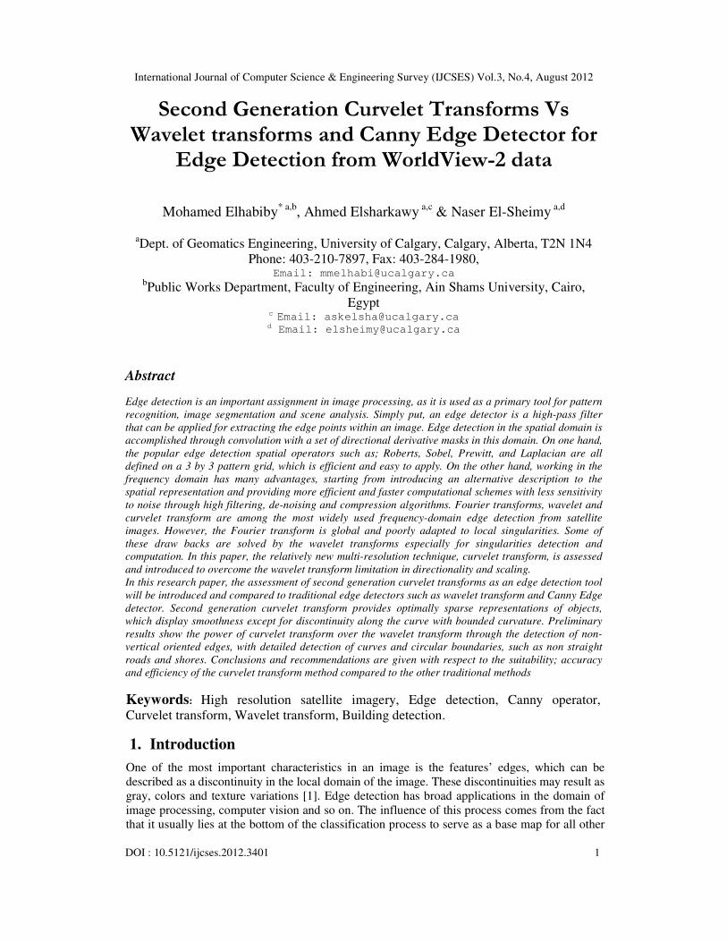
International Journal of Computer Science & Engineering Survey (IJCSES) Vol.3, No.4, August 2012

DOI : 10.5121/ijcses.2012.3401 1

Second Generation Curvelet Transforms Vs Wavelet transforms and Canny Edge Detector for

Edge Detection from WorldView-2 data

Mohamed Elhabiby

* a,b, Ahmed Elsharkawy

a,c & Naser El-Sheimy

a,d

aDept. of Geomatics Engineering, University of Calgary, Calgary, Alberta, T2N 1N4

Phone: 403-210-7897, Fax: 403-284-1980, Email: [email protected]

bPublic Works Department, Faculty of Engineering, Ain Shams University, Cairo,

Egypt c Email: [email protected] d Email: [email protected]

Abstract

Edge detection is an important assignment in image processing, as it is used as a primary tool for pattern

recognition, image segmentation and scene analysis. Simply put, an edge detector is a high-pass filter

that can be applied for extracting the edge points within an image. Edge detection in the spatial domain is

accomplished through convolution with a set of directional derivative masks in this domain. On one hand,

the popular edge detection spatial operators such as; Roberts, Sobel, Prewitt, and Laplacian are all

defined on a 3 by 3 pattern grid, which is efficient and easy to apply. On the other hand, working in the

frequency domain has many advantages, starting from introducing an alternative description to the

spatial representation and providing more efficient and faster computational schemes with less sensitivity

to noise through high filtering, de-noising and compression algorithms. Fourier transforms, wavelet and

curvelet transform are among the most widely used frequency-domain edge detection from satellite

images. However, the Fourier transform is global and poorly adapted to local singularities. Some of

these draw backs are solved by the wavelet transforms especially for singularities detection and

computation. In this paper, the relatively new multi-resolution technique, curvelet transform, is assessed

and introduced to overcome the wavelet transform limitation in directionality and scaling.

In this research paper, the assessment of second generation curvelet transforms as an edge detection tool

will be introduced and compared to traditional edge detectors such as wavelet transform and Canny Edge

detector. Second generation curvelet transform provides optimally sparse representations of objects,

which display smoothness except for discontinuity along the curve with bounded curvature. Preliminary

results show the power of curvelet transform over the wavelet transform through the detection of non-

vertical oriented edges, with detailed detection of curves and circular boundaries, such as non straight

roads and shores. Conclusions and recommendations are given with respect to the suitability; accuracy

and efficiency of the curvelet transform method compared to the other traditional methods

Keywords: High resolution satellite imagery, Edge detection, Canny operator,

Curvelet transform, Wavelet transform, Building detection.

1. Introduction

One of the most important characteristics in an image is the features’ edges, which can be

described as a discontinuity in the local domain of the image. These discontinuities may result as

gray, colors and texture variations [1]. Edge detection has broad applications in the domain of

image processing, computer vision and so on. The influence of this process comes from the fact

that it usually lies at the bottom of the classification process to serve as a base map for all other


2

coming modules. Consequently, the more accurate this process is, the more accurate the whole

classification results.

In this research paper an implementation of the second generation curvelet transform for edge

detection will be introduced and a comparison with wavelet transform and the optimal edge

detector operator, Canny, will be done.

Urban studies, coastal erosion, and agricultural surveys are a few examples where edge detection

can be utilized. In the past few years, the development of edge detection techniques in the

analysis of multi-temporal remote sensing imagery has been intensively growing. For many

years, satellite based remote sensing has been a priceless tool for change detection. No other

platform can constantly revisit an area, quantify and classify land cover or land use on such a

broad scale. Satellite imagery is proving to be a cost-effective alternative to aerial photography,

especially, for the acquisition of Land Cover information[2].

Second generation curvelet transform provides optimally sparse representations of objects,

which display smoothness except for discontinuity along the curve with bounded curvature [3].

Some papers have investigated this technique for edge detection in high-resolution satellite

imagery such as IKONOS or QuickBird, and microscopic imagery, [1, 4-6] which show a great

potential of using curvelet transform in solving edge detection problems.

In the following sections, a brief introduction about implementation of the three methods in edge

detection will be introduced followed by Data used description and methodology section, then

the results and analysis section and finally, the Conclusions.

2. Edge detection techniques 2.1 Canny edge detector

Canny edge detection is an optimal method for step edges detection. Canny used three criteria to

design his edge detector.

• Reliable detection of edges with low probability of missing true edges, and a low

probability of detecting false edges.

• The detected edges should have a minimum distance to the true location of the edge.

• There should be only one response to a single edge (thin lines for edges).

Based on these criteria, the Canny edge detector first smoothes the image to eliminate any

noise, then it finds the image gradient to highlight regions with high derivatives. The regions

with high derivatives are tracked by the algorithm to suppress any pixel that is not at the

maximum (non-maximum suppression). Two thresholds T1 and T2 are then introduced. If the

magnitude of certain pixel is below T1, it is set to zero (none edge), if the magnitude is above T2,

it is made an edge. And if the magnitude is between the two thresholds, then it is set to zero

unless there is a path from this pixel to a pixel with a gradient above T2 [7].

2.2 Wavelet and edge detection Multi-resolution techniques aim at transforming images into a representation where both spatial

and frequency information can be identified [8]. A wavelet transform decomposes images into a

complete set of wavelet functions, which then form a basis, generally orthogonal. These

functions are constructed by translating and dilating a single-mother wavelet which is localized

in both spatial and frequency domain [9]. Once this is completed in discrete steps, the discrete

wavelet transform is obtained, for which there exists an efficient filtering implementation in the

real space. Every wavelet corresponds to a high and low-pass filter. For the most common cases

with dilations by a factor of two, the scheme is called "dyadic" wavelet transform [8].


3

2.3 Curvelet transform

Initial introduction of Curvelet transforms technique was originally introduced by Candes and

Donoho in 1999 as a result of the increasing demand of the presence of effective multi-

resolution analysis that has the ability to overcome the drawbacks of wavelet analysis. The

transform was designed to represent edges and other singularities along curves much more

efficiently than traditional transforms, i.e. using significantly fewer coefficients for a given

accuracy of reconstruction [10]. Later and based on a frequency partition technique, the same

authors proposed a considerably simpler second-generation curvelet transform. This second-

generation curvelet transforms is meant to be easier to understand and use. It is also faster and

less redundant compared to its first generation version [11]. In the new version of curvelet, the

ridgelet transforms was discarded, thus reducing the amount of redundancy in the transform and

increasing the speed considerably. Curvelet transforms is defined in both continuous and digital

domain. Moreover, it can be used for multi-dimensional signals. Since the image-based feature

extraction requires only 2D FDCT, Fast Discrete Curvelet Transforms, the discussion will be

focused on purely two-dimensional applications and implementations [3].

2.4 Discrete Curvelet Transform

Coronae and rotations, as in the continuous-time definition, are not especially adapted to

Cartesian arrays, so it is convenient to replace these concepts by Cartesian equivalents; here,

“Cartesian coronae” based on concentric squares (instead of circles) and shears.

Figure 1 The transition from the continuous-time definition (right) to the discrete-time

definition(left) [3].

Figure 1 (right) illustrates the basic digital tiling where the windows ‘Uj’ smoothly localize the

Fourier transform near the sheared wedges obeying the parabolic scaling. The shaded region

represents one such typical wedge.

Now the Cartesian window is defined as:

Eq.1

Where:


4

Φ is defined as the product of low-pass one dimensional windows:

Eq.2

And Sɵ is the shear matrix:

Hence, the discrete curvelet coefficients are defined as:

Eq.3

According to [3], there are two different digital implementations of FDCT:

• Curvelets via USFFT (Unequally Spaced Fast Fourier Transform)

• And Curvelets via Wrapping.

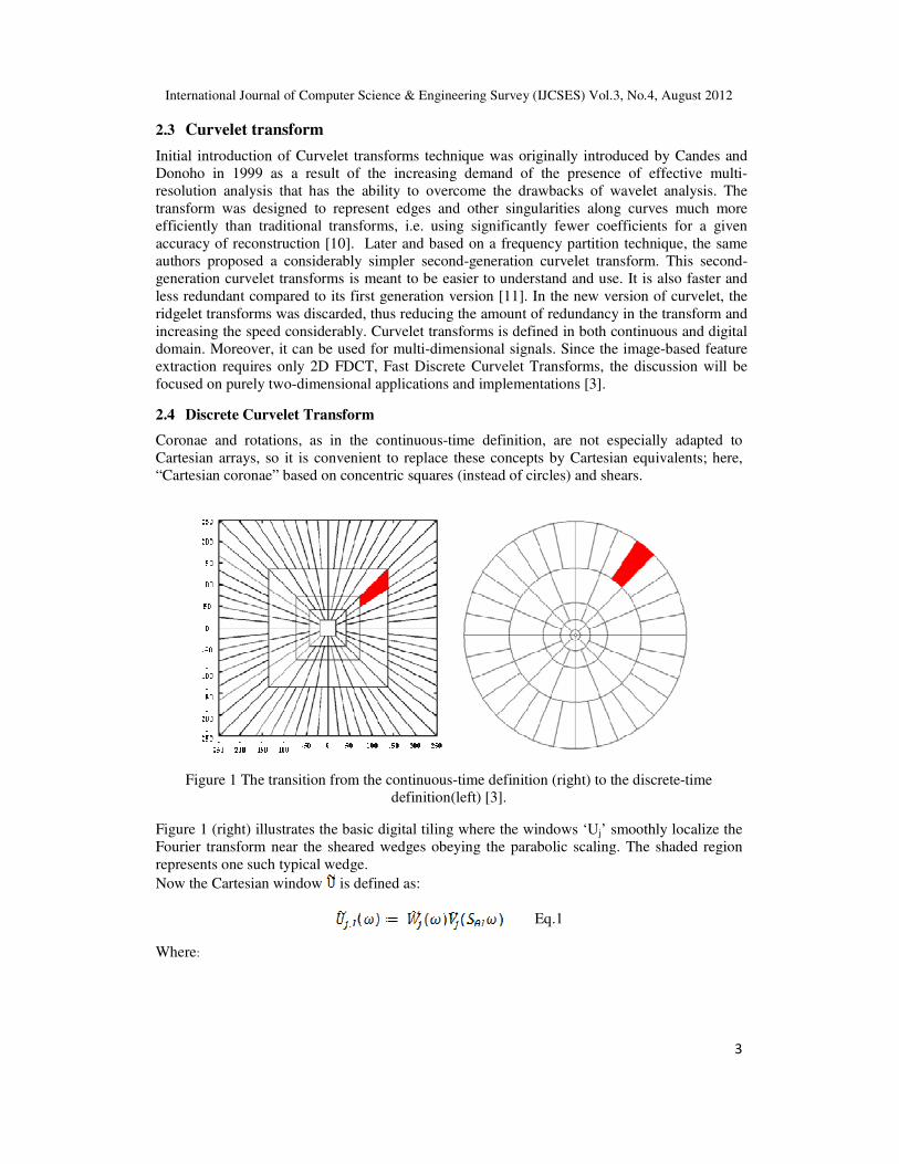
The values of curvelet coefficients depend on how they are aligned in the real image. One can

expect higher coefficients’ values when the curvelet is accurately aligned to a given curve in an

image. A very clear explanation is provided in figure 4. The curvelet named ‘c’ in the figure is

almost perfectly aligned with the curved edge and therefore, has a higher coefficient value.

Curvelets ‘a’ and ‘b’ will have coefficients close to zero as they are quite far from alignment

with the curve [5].

Figure 4 Alignment of curvelets along curved edges [5]

The unique mathematical property for representing curved singularities in a non-adaptive

manner makes the Curvelet transform a higher-dimensional generalization of wavelets.


5

The major advantage of the curvelet transforms compared to the wavelet is that the edge

discontinuity is better approximated by curvelets than wavelets. Curvelets can provide solutions

to the limitations that are apparent in wavelet transform and summarized as follows:

• Curved singularity representation,

• Limited orientation (Vertical, Horizontal and Diagonal)

• And absence of anisotropic element (isotropic scaling)

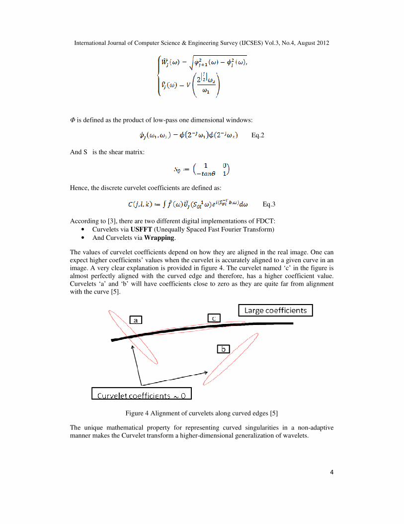
Figure 5 shows the edge representation capability of wavelet (right) and curvelet transform

(left). More wavelets are required for an edge representation using the square shape of wavelets

at each scale, compared to the number of required curvelets, which are of an elongated needle

shape. The main idea here is that the edge discontinuity is better approximated by curvelets

than wavelets. Curvelets can provide solutions for the limitations (curved singularity

representation, limited orientation and absence of anisotropic element) existing in the wavelet

transform.

Figure 5 Representation of curved singularities using wavelets (right) and curvelets (left) [5].

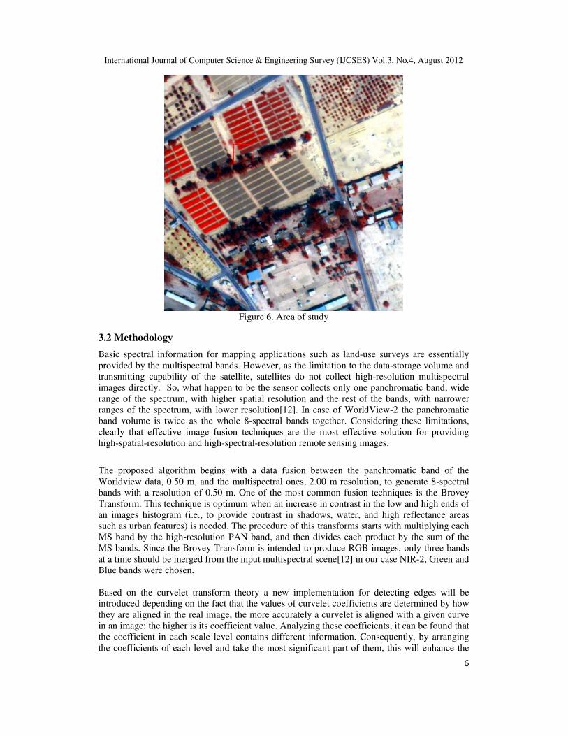
3. Data and Method 3.1 Area of study The study area is a residential area in Ismailia city about 120 KMs to the north east direction

from Cairo the capital of EGYPT. The study area is an urban area comprises scattered

buildings, roads, vegetation areas and shadowed areas. The data was provided by Digital Globe,

http://www.digitalglobe.com. The images were captured on April 7th, 2011 in morning time.

Figure 9 illustrates false-color composite, NIR-2 G B of part of the study area.


6

Figure 6. Area of study

3.2 Methodology

Basic spectral information for mapping applications such as land-use surveys are essentially

provided by the multispectral bands. However, as the limitation to the data-storage volume and

transmitting capability of the satellite, satellites do not collect high-resolution multispectral

images directly. So, what happen to be the sensor collects only one panchromatic band, wide

range of the spectrum, with higher spatial resolution and the rest of the bands, with narrower

ranges of the spectrum, with lower resolution[12]. In case of WorldView-2 the panchromatic

band volume is twice as the whole 8-spectral bands together. Considering these limitations,

clearly that effective image fusion techniques are the most effective solution for providing

high-spatial-resolution and high-spectral-resolution remote sensing images.

The proposed algorithm begins with a data fusion between the panchromatic band of the

Worldview data, 0.50 m, and the multispectral ones, 2.00 m resolution, to generate 8-spectral

bands with a resolution of 0.50 m. One of the most common fusion techniques is the Brovey

Transform. This technique is optimum when an increase in contrast in the low and high ends of

an images histogram (i.e., to provide contrast in shadows, water, and high reflectance areas

such as urban features) is needed. The procedure of this transforms starts with multiplying each

MS band by the high-resolution PAN band, and then divides each product by the sum of the

MS bands. Since the Brovey Transform is intended to produce RGB images, only three bands

at a time should be merged from the input multispectral scene[12] in our case NIR-2, Green and

Blue bands were chosen.

Based on the curvelet transform theory a new implementation for detecting edges will be

introduced depending on the fact that the values of curvelet coefficients are determined by how

they are aligned in the real image, the more accurately a curvelet is aligned with a given curve

in an image; the higher is its coefficient value. Analyzing these coefficients, it can be found that

the coefficient in each scale level contains different information. Consequently, by arranging

the coefficients of each level and take the most significant part of them, this will enhance the


7

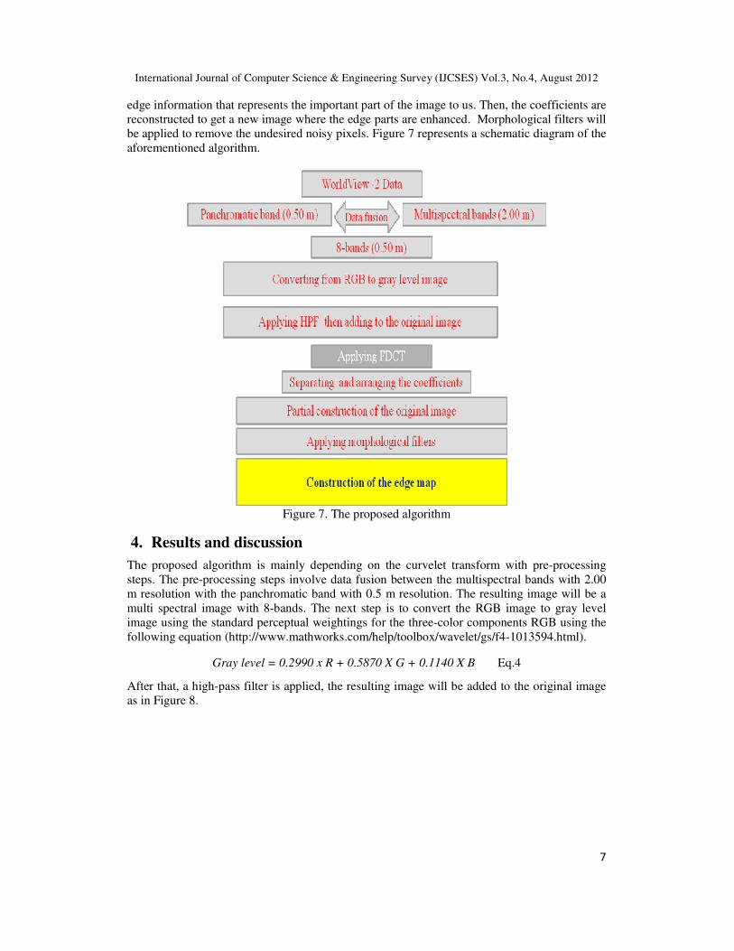
edge information that represents the important part of the image to us. Then, the coefficients are

reconstructed to get a new image where the edge parts are enhanced. Morphological filters will

be applied to remove the undesired noisy pixels. Figure 7 represents a schematic diagram of the

aforementioned algorithm.

Figure 7. The proposed algorithm

4. Results and discussion

The proposed algorithm is mainly depending on the curvelet transform with pre-processing

steps. The pre-processing steps involve data fusion between the multispectral bands with 2.00

m resolution with the panchromatic band with 0.5 m resolution. The resulting image will be a

multi spectral image with 8-bands. The next step is to convert the RGB image to gray level

image using the standard perceptual weightings for the three-color components RGB using the

following equation (http://www.mathworks.com/help/toolbox/wavelet/gs/f4-1013594.html).

Gray level = 0.2990 x R + 0.5870 X G + 0.1140 X B Eq.4

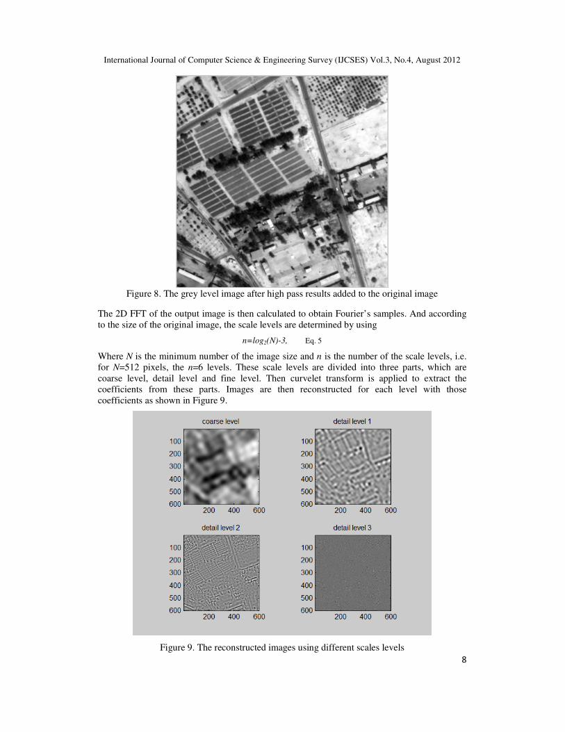
After that, a high-pass filter is applied, the resulting image will be added to the original image

as in Figure 8.


8

Figure 8. The grey level image after high pass results added to the original image

The 2D FFT of the output image is then calculated to obtain Fourier’s samples. And according

to the size of the original image, the scale levels are determined by using

n=log2(N)-3, Eq. 5

Where N is the minimum number of the image size and n is the number of the scale levels, i.e.

for N=512 pixels, the n=6 levels. These scale levels are divided into three parts, which are

coarse level, detail level and fine level. Then curvelet transform is applied to extract the

coefficients from these parts. Images are then reconstructed for each level with those

coefficients as shown in Figure 9.

Figure 9. The reconstructed images using different scales levels


9

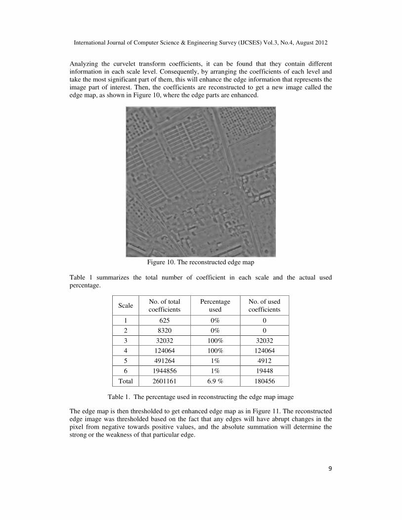
Analyzing the curvelet transform coefficients, it can be found that they contain different

information in each scale level. Consequently, by arranging the coefficients of each level and

take the most significant part of them, this will enhance the edge information that represents the

image part of interest. Then, the coefficients are reconstructed to get a new image called the

edge map, as shown in Figure 10, where the edge parts are enhanced.

Figure 10. The reconstructed edge map

Table 1 summarizes the total number of coefficient in each scale and the actual used

percentage.

Scale No. of total

coefficients

Percentage

used

No. of used

coefficients

1 625 0% 0

2 8320 0% 0

3 32032 100% 32032

4 124064 100% 124064

5 491264 1% 4912

6 1944856 1% 19448

Total 2601161 6.9 % 180456

Table 1. The percentage used in reconstructing the edge map image

The edge map is then thresholded to get enhanced edge map as in Figure 11. The reconstructed

edge image was thresholded based on the fact that any edges will have abrupt changes in the

pixel from negative towards positive values, and the absolute summation will determine the

strong or the weakness of that particular edge.


10

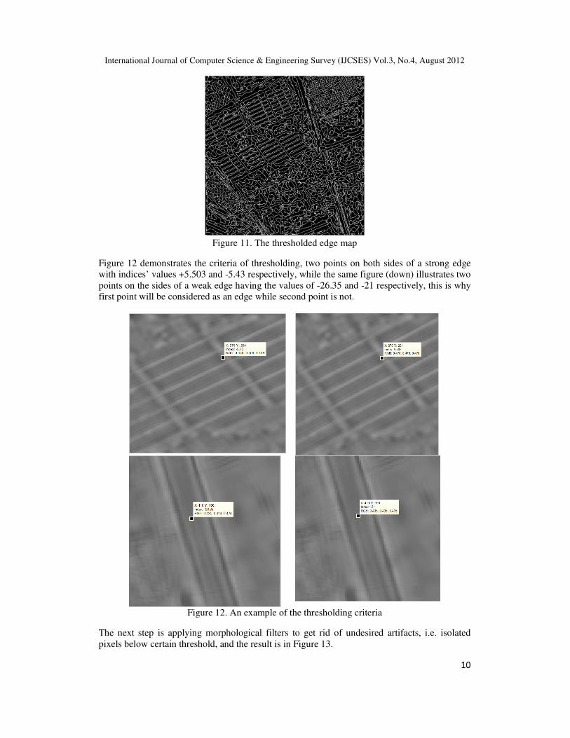
Figure 11. The thresholded edge map

Figure 12 demonstrates the criteria of thresholding, two points on both sides of a strong edge

with indices’ values +5.503 and -5.43 respectively, while the same figure (down) illustrates two

points on the sides of a weak edge having the values of -26.35 and -21 respectively, this is why

first point will be considered as an edge while second point is not.

Figure 12. An example of the thresholding criteria

The next step is applying morphological filters to get rid of undesired artifacts, i.e. isolated

pixels below certain threshold, and the result is in Figure 13.


11

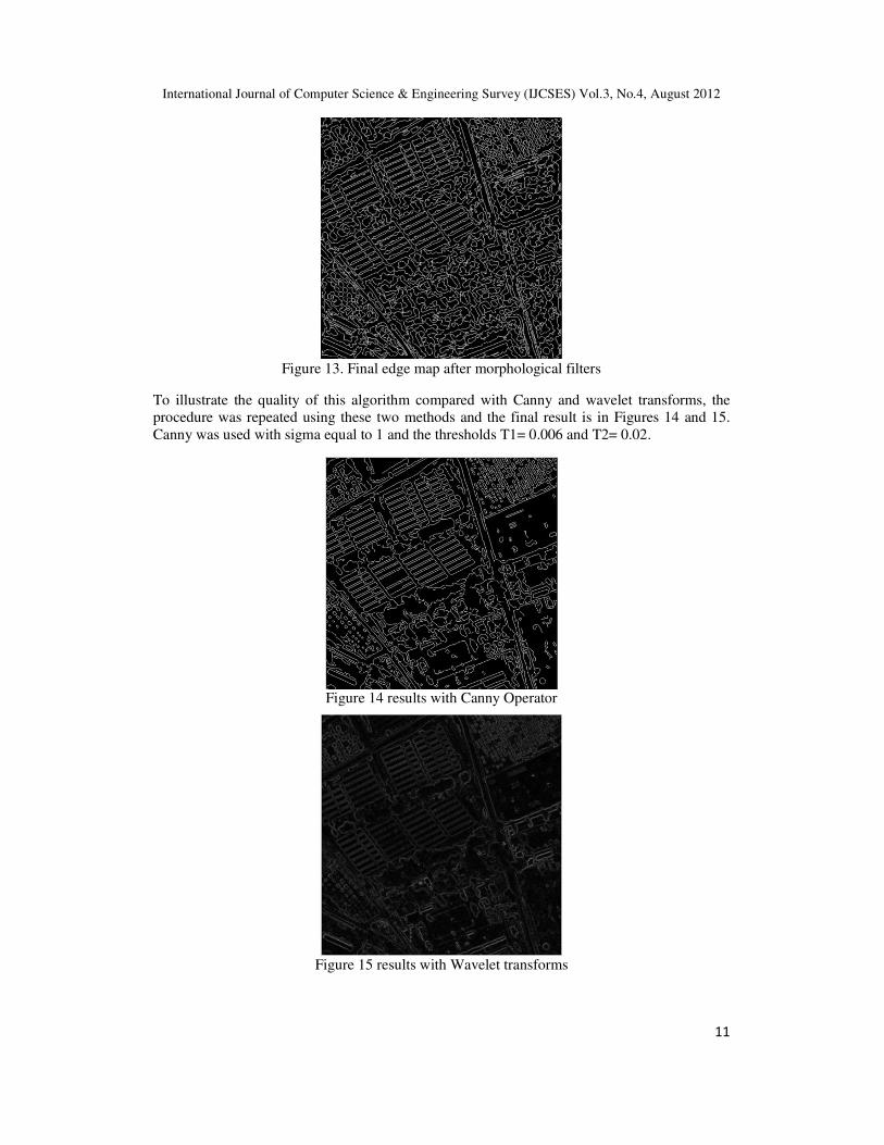
Figure 13. Final edge map after morphological filters

To illustrate the quality of this algorithm compared with Canny and wavelet transforms, the

procedure was repeated using these two methods and the final result is in Figures 14 and 15.

Canny was used with sigma equal to 1 and the thresholds T1= 0.006 and T2= 0.02.

Figure 14 results with Canny Operator

Figure 15 results with Wavelet transforms


12

The result of Canny show almost identical result with the curvelet transforms edge detection

result. The case was different with the wavelet as in the Figure 15, which illustrates the edge

detection result when using the original image as an input to the wavelet transforms.

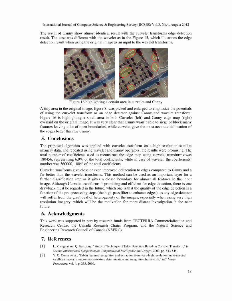
Figure 16 highlighting a certain area in curvelet and Canny

A tiny area in the original image, figure 8, was picked and enlarged to emphasize the potentials

of using the curvelet transform as an edge detector against Canny and wavelet transform.

Figure 16 is highlighting a small area in both Curvelet (left) and Canny edge map (right)

overlaid on the original image. It was very clear that Canny wasn’t able to siege or block many

features leaving a lot of open boundaries, while curvelet gave the most accurate delineation of

the edges better than the Canny.

5. Conclusions

The proposed algorithm was applied with curvelet transform on a high-resolution satellite

imagery data, and repeated using wavelet and Canny operators, the results were promising. The

total number of coefficients used to reconstruct the edge map using curvelet transforms was

180456, representing 6.9% of the total coefficients, while in case of wavelet, the coefficients’

number was 360000, 100% of the total coefficients.

Curvelet transforms give close or even improved delineation to edges compared to Canny and a

far better than the wavelet transforms. This method can be used as an important layer for a

further classification step as it gives a closed boundary for almost all features in the input

image. Although Curvelet transforms is promising and efficient for edge detection, there is one

drawback must be regarded in the future, which one is that the quality of the edge detection is a

function of the pre-processing steps (the high-pass filter to enhance edges), as any edge detector

will suffer from the great deal of heterogeneity of the images, especially when using very high

resolution imagery, which will be the motivation for more distant investigation in the near

future.

6. Acknwledgments

This work was supported in part by research funds from TECTERRA Commercialization and

Research Centre, the Canada Research Chairs Program, and the Natural Science and

Engineering Research Council of Canada (NSERC).

7. References

]1[ L. Zhenghai and Q. Jianxiong, "Study of Technique of Edge Detection Based on Curvelet Transform," in

Second International Symposium on Computational Intelligence and Design, 2009, pp. 543-545.

]2[ Y. O. Ouma, et al., "Urban features recognition and extraction from very-high resolution multi-spectral

satellite imagery: a micro–macro texture determination and integration framework," IET Image

Processing, vol. 4, p. 235, 2010.


13

]3[ E. Candes, et al., "Fast discrete curvelet transforms," Multiscale Modeling & Simulation, vol. 5, pp. 861-

899, 2006.

]4[ T. Geback and P. Koumoutsakos, "Edge detection in microscopy images using curvelets," BMC

Bioinformatics, vol. 10, p. 75, 2009.

]5[ T. Guha and Q. M. J. Wu, "Curvelet Based Feature Extraction," in Face Recognition, M. Oravec, Ed., ed:

InTech, Available from: http://www.intechopen.com/articles/show/title/curvelet-based-feature-extraction,

2010, pp. 35-46.

]6[ M. Xiao, et al., "Edge Detection of Riverway in Remote Sensing Images Based on Curvelet Transform and GVF Snake," presented at the Spatial Accuracy Assessment in Natural Resources and Environmental

Sciences, Shanghai, P. R. China, , 2008.

]7[ J. Canny, "A Computational Approach to Edge Detection," Pattern Analysis and Machine Intelligence,

IEEE Transactions on, vol. PAMI-8, pp. 679-698, 1986.

]8[ S. Livens, et al., "Wavelets for texture analysis, an overview," in Image Processing and Its Applications,

1997., Sixth International Conference on, 1997, pp. 581-585 vol.2.

]9[ S. G. Mallat, "A theory for multiresolution signal decomposition: the wavelet representation," Pattern

Analysis and Machine Intelligence, IEEE Transactions on, vol. 11, pp. 674-693, 1989.

]10[ D. L. Donoho and M. R. Duncan, "Digital curvelet transform: Strategy, implementation and experiments,"

in Wavelet Applications Vii. vol. 4056, H. H. Szu, et al., Eds., ed, 2000, pp. 12-30.

]11[ J. Ma and G. Plonka, "Computing with Curvelets: From Image Processing to Turbulent Flows," Computing

in Science and Engg., vol. 11, pp. 72-80, 2009.

]12[ K .G. Nikolakopoulos, "Comparison of nine fusion techniques for very high resolution data,"

Photogrammetric Engineering and Remote Sensing, vol. 74, pp. 647-659, May 2008.

Second Generation Curvelet Transforms Vs Wavelet transforms and Canny Edge Detector for Edge...

Documents

Transcript of Second Generation Curvelet Transforms Vs Wavelet transforms and Canny Edge Detector for Edge...