Shape from focus using fast discrete curvelet transform

Pattern Recognition 44 (2011) 839–853

Contents lists available at ScienceDirect

Pattern Recognition

0031-32

doi:10.1

� Corr

E-m

moham

jwu@uw

journal homepage: www.elsevier.com/locate/pr

Shape from focus using fast discrete curvelet transform

Rashid Minhas �, Abdul Adeel Mohammed, Q.M. Jonathan Wu

Department of Electrical and Computer Engineering, University of Windsor, Ontario, Canada N9B 3P4

a r t i c l e i n f o

Article history:

Received 15 January 2009

Received in revised form

14 September 2010

Accepted 24 October 2010

Keywords:

Shape from focus

Multifocus

Image fusion

Depth map estimation

Curvelet transform

Contrast limited adaptive histogram

equalization

03/$ - see front matter & 2010 Elsevier Ltd. A

016/j.patcog.2010.10.015

esponding author. Tel.: +1 519 253 3000x486

ail addresses: [email protected] (R. Minha

[email protected] (A. Adeel Mohammed),

indsor.ca (Q.M. Jonathan Wu).

a b s t r a c t

A new method for focus measure computation is proposed to reconstruct 3D shape using image sequence

acquired under varying focus plane. Adaptive histogram equalization is applied to enhance varying

contrast across different image regions for better detection of sharp intensity variations. Fast discrete

curvelet transform (FDCT) is employed for enhanced representation of singularities along curves in an

input image followed by noise removal using bivariate shrinkage scheme based on locally estimated

variance. The FDCT coefficients with high activity are exploited to detect high frequency variations of pixel

intensities in a sequence of images. Finally, focus measure is computed utilizing neighborhood support of

these coefficients to reconstruct the shape and a well-focused image of the scene being probed.

& 2010 Elsevier Ltd. All rights reserved.

1. Introduction

Shape from focus (SFF) is a passive optical method for 3D shapereconstruction from 2D images, which has numerous applicationsin computer vision, range segmentation, consumer video camerasand video microscopy. Performance of SFF techniques is mainlydependent upon the performance of a focus measure. By the termfocus measure, we understand any functional defined on the spaceof image functions which reflects the amount of blurring intro-duced by PSF [46]. Normally, an image captured using CCD device iscorrupted by the blurring effect due to its convolution with a pointspread function (PSF). Focus measures help to prune those pixellocations which are highly degraded and do not carry any usefulinformation for shape reconstruction.

Basic image formation geometry when camera parameters areknown is shown in Fig. 1. Distance of an object from camera lens,i.e., u is required for exact 3D reconstruction of a scene. Depth of ascene, distance of an object from the lens, illumination conditions,camera movements, aberration effects in lens, and movementsin the scene can severely affect depth map (also called shape inliterature) estimation. The distance computation for an object fromthe camera lens becomes a straightforward process if blur circleradius H is equal to zero. If an image detector, ID, is placed at exactdistance v; sharp image Pu, also called as focused image, of an object

ll rights reserved.

2; fax: +1 519 971 3695.

s),

P is formed. The relationship between distance of an object fromcamera lens L, focal distance F of the lens and distance betweenimage detector ID and lens L is given by Gaussian lens law:

1

F¼

1

uþ

1

vð1Þ

The objective of depth map estimation is to determine the depth ofevery point on an object from a camera lens. Depth map estimationis a critical problem in computer vision with numerous applica-tions in robot guidance, 3D feature extraction, pose estimation,medical imaging, range image segmentation, microscopic imaging,seismic data analysis and shape reconstruction. Passive opticalmethods utilizing single CCD to estimate depth maps are mainlydivided into two categories (1) depth from focus (DFF) and (2)depth-from-defocus (DFD). It should be noted that depth fromfocus and shape from focus are the terms interchangeably used inliterature. As an alternative approach, time-of-flight (TOF) sensorsare used to estimate depth by sensing reflected waves from thescene objects. However, noise induction in such measurements isheavily dependent upon light reflections from surrounding objectswhich can complicate depth map computation. TOF sensors areactive, expensive and range limitations restrict their utilization tospecific applications. It is impossible to have a focus plane similar tothe scene depth and generate a sharp focus for all object points. Theobject points appear sharp in images that are present on a focusplane, whereas the blur for image points increase as they moveaway from the focus plane. For scenes with considerably largerdepth, points on the focus plane have a sharp appearance while therest of the scene points are blurred and can be ignored during shape

www.elsevier.com/pr

dx.doi.org/10.1016/j.patcog.2010.10.015

mailto:[email protected]



dx.doi.org/10.1016/j.patcog.2010.10.015

s

OpticalAxis

d/2

2H

P'P''

v s-v

L

q

P

u

ID

FP: Object

ID: Image detector

P': Focused pointP'': Blur circled: Aperture diameter

H: Blur circle radius

Fig. 1. Image formation geometry of a 3D object.

Fig. 2. Image acquisition setup with varying focus plane.

R. Minhas et al. / Pattern Recognition 44 (2011) 839–853840

reconstruction. Practically, we capture a sequence of images in asetup (shown in Fig. 2) with varying focus plane to retain differentscene points that are well focused. An object present on atranslation stage is imaged at different distances from a CCDcamera. The object points present on focus plane will representhigh variations in intensity. As shown in Fig. 2, the object touchesfocus plane after p number of translations. At this point the topportion of the object is well focused and the image of bottom regionis blurred due to its distance from the focus plane. During imageacquisition the translation stage is moved in an upward direction,towards CCD camera, until translation stage touches the focusplane. Clearly, a sequence of images can be acquired by varyingfocal length of the camera lens or translating an object relative tothe camera lens. Such translations are useful in capturing focusedportions of an object on a planar image detector in different frames.The translations of an object and number of acquired imagesdepend upon available resources, required accuracy, object struc-ture and illumination variations.

2. Background work

SFF based techniques are mainly divided into two categoriesi.e., transform and non-transform based SFF. Transform based SFFincludes application of frequency domain methods such as Fourierand discrete cosine transform to extract focused points from differentimages to construct a composite image and estimate depth map of ascene. In pioneering work of transform based SFF, Horn [1] proposeda focusing imaging system by using Fourier transform in analyzingthe frequency spectrum of an image. Pyramid based approaches forfocus computation and wavelet transform based defocus analysishave also been explored to recover a shape [4,9,20]. Mehmood et al.[32] proposed SFF computation utilizing principal component ana-lysis (PCA) of coefficients of transformed images. However, focusmeasure using largest principal components may get severelydegraded by noise since higher principal components representglobal content of an image. Malik and Choi [28] proposed an opticalfocus measure (FMO) that uses optical transfer function in Fourierdomain for 3D shape recovery in the presence of noise. Wavelet basedfocus measures based on energy of wavelet coefficients [46–48] havealso been proposed in the past.

The second class, i.e., non-transform based SFF can be furthersubdivided into three categories: (1) gradient, (2) statistical and(3) approximation based techniques. A comprehensive survey ofvarious neighborhood operators and spatial derivative operatorsfor computation of shape is presented in [3,6,11]. In an early work,Tenenbaum [2] proposed Sobel operator based Tenegrad focusmeasure (FMT) that exploits relationship between well-focusedimage points and its greater information content. Nayyar andNakagawa [5,8] proposed gradient based sum-of-modified-Lapla-cian (FMSML) which has later been improved using polynomialapproximation, i.e., focused image surface (FIS) in [10,12,13] toaccurately follow the actual shape of an object. In [13], improved

results are reported to track arbitrary structures for depth mapcomputation using curved window focus [10]. In curvature focusmeasure (FMC) [16] gray level values are treated as a 3D surfacecalled curvature map, whereas M2 focus measure (FMM2) is basedon the energy of image gradient. Recently, Ahmed and Choi [25]proposed a technique to reconstruct shape using 3D summationbased on FMSML.

The presence of shadows and non-uniform illumination varia-tions in images cause inaccurate and sparse depth maps; to handlesuch situations Mannan et al. [31] proposed a scheme to removesuperfluous shadows or illuminations following two strongassumptions about image acquisition and magnification thatmay, in general, be contradictory to a real life scenario. Exponen-tially decaying function based on distance transform for featuresdetected using SUSAN operator [35] and steerable filters baseddepth map estimation [34] are recent developments in the area ofSFF research. The subclass of non-transform based SFF that utilizesstatistical approach consists of focus measures like gray levelvariance (FMGLV) [12], mean focus measure (FMMean) [16] andentropy based fusion. The last subcategory, approximation basedSFF comprises focus measures based on neural networks [15],neuro-fuzzy systems [24], dynamic programming (DP) [18], poly-nomial approximation [13] and regression [29]. Approximationbased techniques use anyone of aforementioned focus measures forpreprocessing, whereas the requirement of comprehensive rulebase and training data restrict their application to limited domains.Polynomial based approximations provide accurate solution todepth map generation although their computational complexityincreases drastically with the order of the polynomial. Anotherinteresting area in SFF research is based on defocus cues, Pradeepand Rajangopalan [26] proposed estimation of 3D shape usingrelative defocus blur derived from input images to compute theshape of an object. Recently, Hasinoff and Kutulakos [36] proposedconfocal stereo for depth from focus which states that as the lensaperture varies the pixel intensity of visible infocus scene point willvary in a scene-independent way that can be predicted by priorradiometric lens calibration. SFF for color images is not the mainfocus of current paper although researchers have proposed meth-ods for color domain based on segmentation and bilateral filters[22], and HSI space [33].

In this paper a new focus measure is proposed to reconstruct theshape of an object using best focused object points from an inputsequence. Most of the established schemes for SFF perform well forregions with dense texture only. Therefore, their performancedeteriorates in the presence of noise and poor texture. Pyramidbased approaches (such as wavelets) offer promising reconstruc-tion, however, sparsity is highly compromised due to soaringnumber of coefficients to represent singularities along curves. Allnatural and man-made objects are multidimensional and can be

R. Minhas et al. / Pattern Recognition 44 (2011) 839–853 841

represented using a function with singularity along curves. Therepresentation of such functions in wavelet domain is not optimalsince wavelets are suitable for representing point singularities. Wepropose a new focus measure based on curvelet transform thatsupports sparse optimal representation of objects with edges andwave propagators. The proposed framework comprises locallyadapted de-noising and contrast enhancement operations forreliable reconstruction of the objects which are not uniformlyilluminated over all the key points of their structures. In SFF variedillumination conditions on different regions of an image are oftenoverlooked while such conditions can severely deteriorate perfor-mance of SFF techniques.

3. Fast discrete curvelet transform

Fourier series decomposes a periodic function into a sum ofsimple oscillating functions, i.e., sines and cosines. In a Fourierseries sparsity is destroyed due to discontinuities and a largenumber of terms are required to precisely reconstruct a disconti-nuity. Multiresolution analysis tools have been developed toovercome inherent limitations of Fourier series. Many fields ofcontemporary science and technology benefit from multiscale,multiresolution analysis tools for maximum throughput, efficientresource utilization and accuracy. Multiresolution tools renderrobust behavior to study information content of images and signalsin the presence of noise and uncertainty.

Wavelet transform is a well-known multiresolution analysistool capable of conveying accurate temporal and spatial informa-tion. Wavelet transform has been profusely used to addressproblems in data compression, pattern recognition and computervision. Wavelets have better ability to represent objects withpoint singularities in 1D and 2D space. However, Wavelets fail torepresent singularities along curves in 2D. Discontinuities in2D are spatially distributed which leads to extensive interactionbetween discontinuities and wavelet coefficients. Therefore,wavelet representation does not offer sufficient sparsenessfor image analysis. Following wavelets, research communityhas witnessed intense efforts to develop tools with better direc-tional and decomposition capabilities, namely, ridgelets [37] andcontourlets [38].

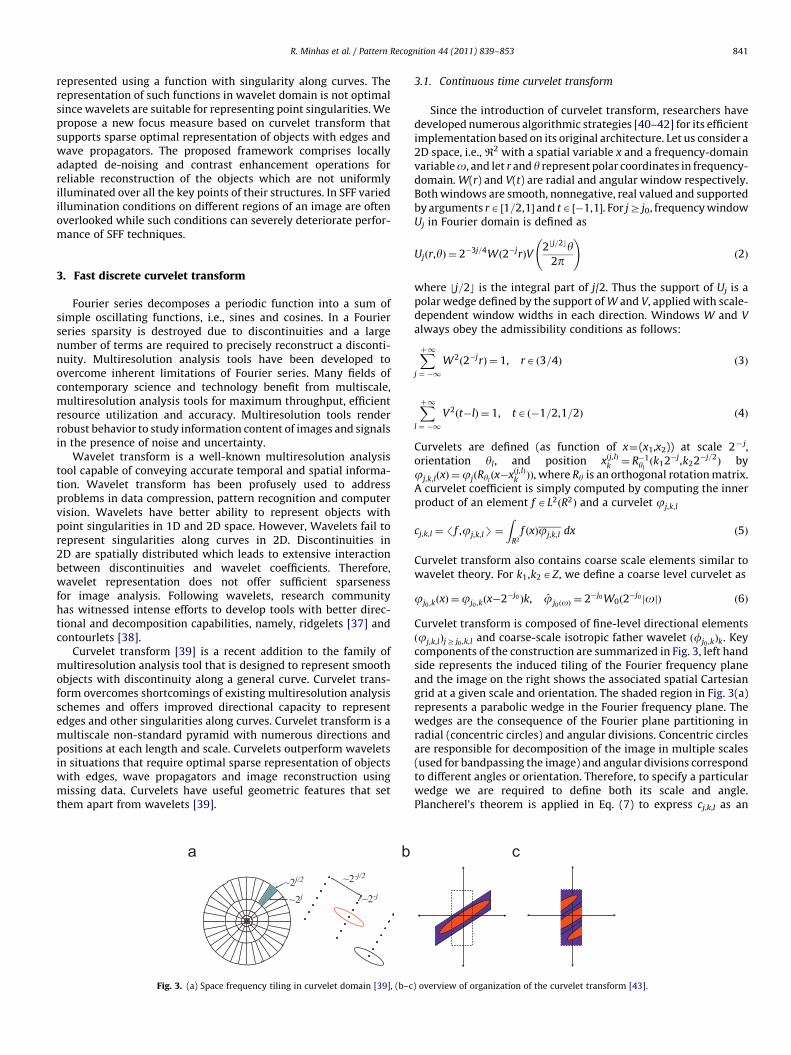
Curvelet transform [39] is a recent addition to the family ofmultiresolution analysis tool that is designed to represent smoothobjects with discontinuity along a general curve. Curvelet trans-form overcomes shortcomings of existing multiresolution analysisschemes and offers improved directional capacity to representedges and other singularities along curves. Curvelet transform is amultiscale non-standard pyramid with numerous directions andpositions at each length and scale. Curvelets outperform waveletsin situations that require optimal sparse representation of objectswith edges, wave propagators and image reconstruction usingmissing data. Curvelets have useful geometric features that setthem apart from wavelets [39].

~2j ~2-j~2j/2 ~2-j/2

Fig. 3. (a) Space frequency tiling in curvelet domain [39], (b–c

3.1. Continuous time curvelet transform

Since the introduction of curvelet transform, researchers havedeveloped numerous algorithmic strategies [40–42] for its efficientimplementation based on its original architecture. Let us consider a2D space, i.e., R2 with a spatial variable x and a frequency-domainvariableo, and let r and y represent polar coordinates in frequency-domain. W(r) and V(t) are radial and angular window respectively.Both windows are smooth, nonnegative, real valued and supportedby arguments rA ½1=2,1� and tA ½�1,1�. For jZ j0, frequency windowUj in Fourier domain is defined as

Ujðr,yÞ ¼ 2�3j=4Wð2�jrÞV2bj=2cy

2p

!ð2Þ

where bj=2c is the integral part of j/2. Thus the support of Uj is apolar wedge defined by the support of W and V, applied with scale-dependent window widths in each direction. Windows W and V

always obey the admissibility conditions as follows:

Xþ1j ¼ �1

W2ð2�jrÞ ¼ 1, rAð3=4Þ ð3Þ

Xþ1l ¼ �1

V2ðt�lÞ ¼ 1, tAð�1=2,1=2Þ ð4Þ

Curvelets are defined (as function of x¼(x1,x2)) at scale 2� j,orientation yl, and position xðj,lÞk ¼ R�1

ylðk12�j,k22�j=2

Þ byjj,k,lðxÞ ¼jjðRyl

ðx�xðj,lÞk ÞÞ, where Ry is an orthogonal rotation matrix.A curvelet coefficient is simply computed by computing the innerproduct of an element f AL2ðR2Þ and a curvelet jj,k,l

cj,k,l ¼/f ,jj,k,lS¼Z

R2

f ðxÞjj,k,l dx ð5Þ

Curvelet transform also contains coarse scale elements similar towavelet theory. For k1,k2AZ, we define a coarse level curvelet as

jj0 ,kðxÞ ¼jj0 ,kðx�2�j0 Þk, jj0ðoÞ ¼ 2�j0 W0ð2�j0 jojÞ ð6Þ

Curvelet transform is composed of fine-level directional elementsðjj,k,lÞjZ j0 ,k,l and coarse-scale isotropic father wavelet ðfj0 ,kÞk. Keycomponents of the construction are summarized in Fig. 3, left handside represents the induced tiling of the Fourier frequency planeand the image on the right shows the associated spatial Cartesiangrid at a given scale and orientation. The shaded region in Fig. 3(a)represents a parabolic wedge in the Fourier frequency plane. Thewedges are the consequence of the Fourier plane partitioning inradial (concentric circles) and angular divisions. Concentric circlesare responsible for decomposition of the image in multiple scales(used for bandpassing the image) and angular divisions correspondto different angles or orientation. Therefore, to specify a particularwedge we are required to define both its scale and angle.Plancherel’s theorem is applied in Eq. (7) to express cj,k,l as an

) overview of organization of the curvelet transform [43].


integral over the entire frequency plane:

cj,k,l ¼1

ð2pÞ2

Zf ðoÞj j,k,lðoÞ do¼ 1

ð2pÞ2

Zf ðoÞUjðRyi

oÞei/xðj,lÞk

,oS do

ð7Þ

3.2. Curvelet transform via wrapping

New implementations of fast discrete curvelet transform (FDCT)are ideal for deployment in large-scale scientific applications due totheir numerical isometry and an utmost 10 folds computationalcomplexity as compared to FFT operating on a similar sized data[39]. We used FDCT via wrapping, described below, in our proposedscheme.

�
Compute 2D FFT coefficients and obtain Fourier samples f ½n1,n2�
where �n=2on1 and n2on=2.
� For each scale j and angle l, form the product ~Uj,l½n1,n2�f ½n1,n2�. � Wrap this product around the origin and obtain ~f j,l½n1,n2� ¼
Wð ~U j,l f Þ [n1,n2], where the range of n1, n2 and y respectively are0on1oL1,j, 0on1oL2,j and ð�p=4,p=4Þ.
� Apply inverse 2D FFT to each ~f j,l and save discrete curvelet
coefficients.

In the first two stages Fourier frequency plane of the image is dividedinto radial and angular wedges owing to the parabolic relationshipbetween a curvelet’s length and width, as demonstrated in Fig. 3(a).Each wedge corresponds to curvelet coefficient at a particular scaleand angle. Step 3 is essentially required to re-index the data aroundthe origin as shown in Fig. 3(b–c). Finally, inverse FFT is applied tocollect discrete curvelet coefficients in the spatial domain. Interestedreaders may refer to [39] for additional details on Curvelet transformvia wrapping.

4. Proposed algorithm

In this paper, a new SFF scheme is proposed to search the imageframes that represent the best focused image for individual pixels.Most of the established focus operators tender high-qualityperformance on dense textured images, however, their perfor-mance deteriorates in the presence of noise, poor texture andsingularities along curves. In our proposed scheme, FDCT pyramidis employed to represent elements with a very high degree ofdirectional specificity which is unavailable in a wavelet domain.FDCT uses anisotropic scaling principle unlike wavelet transformthat preserves isotropic scaling.

For reliable detection of focused image locations, a stablemethod is required that can operate evenly on textured and smoothimage regions. SFF based methods track the frame number for eachindividual image pixel that exhibits the highest focus measure andneglects all the remaining frames for the same pixel. A reliablefocus measure should be monotonic with respect to blur and robustagainst noise. Additionally, a high image blur should lead to a lowfocus measure and vice versa. In practice, all the point spreadfunctions (PSF) that cause blur/defocus have a common character-istic of an unknown low pass filter. Therefore, SFF based methodsattempt to extract high frequency image components since suchregions are minimally affected by a PSF.

It should be noted that shape reconstruction frameworks based onSFF operate in an offline mode along with widely accepted assump-tion of pre-registered images as input. Initially, an input sequence of M

images is acquired with varying focus. Usually, images acquired inunconstrained conditions are unsuitable for viewing due to poorillumination conditions, incoherent noise, shadows, defocused points,viewing angle and texture properties. Various schemes produce small

focus values for image regions with low contrast and illumination.These small focus values further complicate shape reconstructionsince blurred and unfocused image points also generate lower focusmeasures. Hence it is important to pre-process the input sequence inorder to enhance its contrast.

Traditional SFF techniques perform inadequately due to theirinability to deal with high contrast variations across differentimage regions. In the past, different techniques have been proposedfor efficient re-mapping of gray level images to generate a uniformhistogram. Traditional histogram equalization schemes do notpresent an appropriate choice for boosting contrast in images withlarge variations. Contrast limited adaptive histogram equalization(CLAHE) [44] is a well-established method for enhancement of lowcontrast images. CLAHE was originally developed as a re-mappingscheme for medical imaging, however, it has been successfullyapplied in numerous computer vision and image processingapplications. This technique facilitates approximate mapping ofindividual pixels based on bilinear interpolation. The neighborhoodsupport for such interpolation is achieved by dividing images intocontextual regions. We use CLAHE as the only pre-processingoperation on each input image, Ii, to enhance contrast and toreliably compute focus measures.

Next, curvelet coefficients are computed using FDCT via wrapping[39] scheme on contrast enhanced image set. Shape reconstructionrequires one-to-one correspondence between image pixels and itscurvelet representation and this relationship is lost due to FDCTimplementation on the whole image. Therefore, we compute curveletcoefficients for individual pixels of an image (see Fig. 6). To cope withimpulsive noise and lighting conditions, the curvelet transform of acenter pixel is determined using neighboring information inside asliding window of size 5�5. The decision to chose the window size of5�5 is based upon findings of Amir and Choi [29] which proved thatthe optimal size for a sliding window to integrate neighborhoodinformation in a focus measure computation is 5�5. The level andangles in higher stages of FDCT decomposition are mainly dependentupon available resources and required accuracy. We implemented a2-level curvelet decomposition with eight angles to transform ourdata, where first and second level subbands at location (x,y) of ithimage are represented by I

R1

i ðx,yÞ and IR2

i ðx,yÞ, respectively. The finestlevel FDCT coefficients contain higher amplitudes corresponding tosharp intensity changes.

Reconstruction using coefficients with high level of activity(FDCT response computed using Eq. (8)) leads to an image withsharp intensity changes for focused pixels, whereas out of focusimage points are merged into smooth regions in our reconstructedimage. In sample frames, focus is being shifted from the base of asimulated cone to its tip as shown in Fig. 4(a) (left to right). FDCTefficiently represents focused image points with high amplitudeFDCT response as shown in Fig. 4(b) while negligible amplitudes areobserved for non-focused image regions.

To remove noise, we use bivariate shrinkage function whichexploits statistical dependency amongst neighboring curveletcoefficients. Such schemes have been successfully applied tode-noise natural images based on joint statistics of waveletcoefficients [45]. As presented in Fig. 4(b), IRi ð�Þ (subscript removedfor better readability) contains largely two group of values: (1) thatrepresent high frequency intensity variations like edges and curves,(2) that correspond to poor texture and angle points. The detectionof focused image points relates to detection of high frequencyintensity variations. To minimize the effects of illumination varia-tion and to remove curvelet coefficients originating from smoothregions, FDCT response FDCTY at pixel location (x,y) is calculated asa ratio of summed coefficients of both subbands, i.e., I

R1

i and IR2

i :

FDCT iYðx,yÞ ¼

PIR2

i ðx,yÞPIR1

i ðx,yÞð8Þ

1) Noise Removal2) Compute NeighborhoodSupport based Focus Measure

Reconstruct Shape fromFocus and a well- focused

image

MAX-pool pixels based onFDCT Focus Measure

Input Sequence Processing Reconstruction

Curvelet viaWrapping

ContrastEnhancement

Fig. 5. Proposed algorithm for shape from focus based on FMFDCT.

Fig. 4. FDCT response for high frequency intensity variations in an image: (a) Sample frames from simulated cone sequence and (b) FDCT response for varying focus.


The FDCT response FDCT iYðx,yÞ shows monotonicity regarding

defocused image points since IR2

i ð�Þ corresponds to a high-passband, which contains large amplitude coefficients in non-smoothregions. On other hand, I

R1

i ð�Þ represents the coarsest level coeffi-cients that have higher energy in smooth regions, therefore, theratio of summation from the two subbands guarantee a higherfocus value for focused points. Be reminded that the neighborhoodsummation in focus measure computation is applied on FDCTresponse, i.e., FDCTY for individual images of an input sequence.The focus measure FMFDCT using a small neighborhood O of size5�5 around image location (x,y) is computed as

FMFDCT ðx,y,iÞ ¼X

xu,yuAO

FDCT iYðxu,yuÞ, 1r irM ð9Þ

Focus measure computation is a two-step process (1) excerption ofgradient information, (2) embedding neighborhood information tominimize noise effects. Our proposed focus measures, i.e., FMFDCT isalso based on a similar principle. Next, frame number for everypixel location generating the highest FMFDCT value is searched;depth map (DM) and well-focused image ðwÞ are constructed byselecting the frame number and the corresponding pixel valuesbased on the following criterions:

DMðx,yÞ ¼ maxFMFDCT ðx,y,iÞ

i ð10Þ

wðx,yÞ ¼ maxFMFDCT ðx,y,iÞ

Iiðx,yÞ ð11Þ

where i corresponds to frame numbers and Ii(x,y) represents imageintensity at location (x,y) from ith frame. It should be noted thatwell-focused image and reconstructed image are the terms usedinterchangeably to refer to an image generated by combining pixelsof different frames of an input sequence based on a specificcriterion (Eq. (11)). Refer to Figs. 5 and 6 for schematic diagramof our proposed algorithm.

5. Results and discussion

The proposed method is tested using comprehensive datasets ofreal and simulated objects and its performance is compared againstwell-documented SFF methods in literature. The results of theseexperiments are presented in this section to analyze performanceof our proposed technique. Traditional SFF methods included in ourexperiments are Laplacian (FMLaplacian), modified Laplacian (FMML),sum-of-modified Laplacian (FMSML), Tenengrade (FMT), curvature(FMC), gray level variance (FMGLV) and M2 (FMM2) focus measures.We selected these methods in trials since they are the most widelyused and exclusive focus measure operators to estimate depthmaps [2,5,7,8,16,25,28]. Learning based focus measures proposedby Asif et al. [15], and Malik et al. [24] also utilized FMGLV and FMSML,respectively, for initial depth map approximation. We do notcompare our scheme against learning based approaches since theyare based on focus measures which have already been included inour experiments. Furthermore, learning based approaches do not

Decomposition Levels: 2Angles: 8

FMFDCT is the ratio of both summations

Multiple Subbands for Second Level

First Level Subband

Noise Removal (Bivariate Shrinkage)

Curvelet Transform

Fig. 6. Focus measure computation based on FMFDCT.


present a generalized solution and results may significantly varysubject to the selection of training set and rule base. Approximationtechniques [10,12,13] and DP based method [18] used Laplacianbased focus measure for initial processing. SFFs obtained usinglearning, approximation and DP based schemes are time consum-ing, computationally expensive and heavily dependent uponcorrectness of initial approximations. To improve these techniques[24,15,18] our proposed method can also be used for initialestimation. Therefore, we believe that the methods chosen forcomparison are the most distinctive and exclusive focus mea-sures to identify high frequency intensity variations and shapereconstruction.

5.1. Datasets

Before divulging into the performance analysis, a brief descrip-tion of the datasets used in experiments is presented. TraditionalSFF techniques are highly sensitive to texture information for shapereconstruction. We selected four image sequences with varyingtexture properties to rigorously test the stability and robustness ofour proposed method. The first sequence contains 97 images of asimulated cone. This sequence was generated corresponding tolens position at varying distances (varying focus plane) from theobject. The size of each image is 360�360 pixels. The secondexperiment uses a sequence of images of a real cone acquired usinga CCD camera. The second sequence also contains 97 imagesgenerated by focusing a CCD camera on hardboard with whiteand black stripes drawn on the surface to generate a dense textureof ring patterns. The vertical height of the cone is about 79 in with abase diameter of 15 in. The camera displacement between twoconsecutive image frames is approximately 0.03 mm. The thirdsequence used in our experiments is a real slanted planar object.For this sequence, a total of 87 images are acquired correspondingto different lens settings. The slanted planar object contains equallyspaced stripes at a horizontal slope which generate a poor texture.The last dataset consists of a coin object acquired at 68 varyingadjustments for focus plane to capture minute details present onthe surface of a coin. For a detailed description of all image sets refer

to [10,27]; the image sets utilized in our trials have 256 gray levelvalues. For precise performance analysis, we chose a uniformwindows size, i.e., 5�5 for localized summation to computereliable focus measure. Our proposed method can be applied forshape reconstruction and MAX-pool pixels from individual framesto generate a well-focused image. We use various metrics torigorously analyze the quality of reconstruction as well as fusionin following sections.

5.2. Performance analysis

Fig. 7 (top row) shows images of the simulated cone withvarying focus planes and the reconstructed images using FMFDCT.Note that the images of a simulated cone displayed are generatedusing a simulation software based on distances between an objectand the camera lens. In each sub-figure only small portion of thecone resides on a focus plane which is well focused and appearssharp in the image. However, portion of the simulated cone whichis distant from the focus plane appears blurred. Reconstructedimage of the simulated cone obtained using proposed FMFDCT isshown in Fig. 7 (right column) and it is clearly evident that all thepixel are sharp and crisp in the reconstructed image. The imagereconstruction is based upon selection of only those pixels frominput sequence which correspond to the highest response forFMFDCT. In simple words, pixel values from different frames of asequence are MAX-pooled to regenerate a well-focused image.Similarly, Fig. 7 (rows 2–4) shows images of a real cone, slantedplanar object and a coin captured at different lens positionscontrolled by an automated motor. The reconstructed images ofall three objects using FMFDCT are also shown in Fig. 7 (rightcolumn). The reconstructed images are all well focused with sharpintensities and minimal blurring effect.

An interesting investigation is conducted to evaluate whetherthe proposed focus measure generates a high amplitude responseto track the actual structure of an object. A real cone dataset thathas a symmetric structure is used. As shown in Fig. 8 (left column), areal cone sequence is acquired by initially focusing the camera onthe lower portion of the cone and then gradually shifting it away to

1

86

32Fr

ame

Num

ber Row # 1

Dia

gona

l Pix

els

Fig. 8. Left: image acquisition setup for real cone sequence, right: data extraction to draw focus measures for analysis.

Fig. 9. For real cone input sequence, focus measure computed using pixel extracted from (a) row no. 10 and (b) diagonal elements.

SimulatedCone

CoinSequence

PlanarObject

RealCone

Images acquired at varying focusReconstructed

Images

Fig. 7. Columns (a–e) represent images of various sequences taken at different lens settings. Column (f) contains reconstructed well-focused images generated using

FMFDCT focus measure.


the top. This strategy ensures that the focused points at the bottomof the cone are captured in earlier frames, whereas the top portionof the cone is well focused in the latter. FMFDCT of the acquiredframes is computed to generate a volumetric data equal to the sizeof our input sequence. For the sake of simplicity, we analyze focusmeasures for two sub-regions (a) Iið1,yÞ,1r irM,1ryr200,(b) Iiðx,yÞ,1r irM,1rx,yr200 where Ii is the ith image of thearray of M images and each frame is of size 200� 200. The two sub-regions used in our trial are highlighted with white bars in the rightcolumn of Fig. 8. It is noticeable that first strip is excerpted from theouter portion, i.e., the first row of the sequence, whereas the secondset spans pixels across the diagonal. Considering the symmetric

structure of the cone; it is straightforward to visualize that initialimages are expected to contain high intensity variations close tothe boundaries and these variations shift towards the middle insubsequent frames. Focus measures evaluated using the extractedstrips are represented in Fig. 9(a–b) and peak values from differentframes are enclosed inside ellipses. It is evident from Fig. 9(a) thatthe focus response of initial frames is high for exterior imageportions (first and last row/columns), which corresponds tofocused points at the bottom of the cone (see Fig. 8). In case of adiagonal strip, high focus values are obtained from a wide range offrames since diagonal strip runs through both the inner and outerportions of an image. In this situation, the focus measure of the


central region of the cone is generated from the ending frames ofour sequence. A localized response of FMFDCT is observed for focusedpoints in different portions of an input sequence.

Figs. 10 and 11 display reconstructed shapes obtained usingFMFDCT focus measure and traditional SFF methods for differentimage sequences. For ideal simulated cone, it is expected that theshape should be smooth without spikes and must contain a sharptip. The assumption of smooth depth map for a simulated cone isobvious because of controlled lighting conditions without anysuperfluous shadows and measurement errors. Fig. 10(a) shows thedepth maps obtained using traditional SFF methods. It is clear fromplots that some of the traditional SFF methods generate depth mapswith large fluctuations and spikes which demonstrate their incon-sistent and unstable behavior. Depth map obtained using FMFDCT

operator is smooth with considerably sharp and prominent tip.Depth maps obtained from FMSML and FMT focus measures are alsocomparable to our proposed focus measure FMFDCT. However, depthmaps generated by FMSML and FMT do not render sharp tip andsmooth boundaries unlike FMFDCT.

In Fig. 10(b), the shape reconstructed using FMFDCT is mainlysmooth in vertical direction and closely follows the real structure ofthe cone. The depth maps computed using traditional SFF methods(Fig. 10(b)) have spikes which are not present on a real cone objectand actual cone structure is not closely tracked in these depthmaps. Traditional SFF methods exhibit poor performance for depthmap estimation of the real cone due to superfluous shadows and

Fig. 10. Depth maps computed using various focus measure operators for

bad illumination conditions. Our proposed method renders robustbehavior with minimum distortion in estimated depth map.

Reconstructed shapes of a real slanted planar and coin objectsgenerated using FMFDCT and traditional SFF focus measures areshown in Fig. 11(a–b). It is noticeable that FMFDCT clearly outper-forms traditional SFF schemes. The depth maps obtained withFMFDCT are smooth, contains less number of discontinuities andclosely resemble the actual structures of input objects.

In an earlier work, Ahmed and Choi [18] used root mean squareerror metric for accuracy comparison where a reference depth mapof the simulated cone was approximated analytically. Since thenmean square error (MSE) and correlation coefficient (CC) metricshave been profusely used to analyze the performance of variousmethods. Fig. 12(a–b) represents qualitative analysis of reconstruc-tion for various focus measures in terms of MSE and CC. Experi-mental results clearly validate superior performance of ourproposed method with least MSE and high CC values. It shouldbe noted that the reference shapes used in our experiments are theapproximated versions of the real scene objects [27,28,32,34]. FromFig. 12 it is noticeable that FMT and FMSML produce comparableresults to each other but their behavior is not consistently main-tained for all datasets. While the use of FMLaplacian in shapereconstruction shows the worst performance with the highestMSE values.

The size of neighborhood support plays a crucial role in accuratefocus computation and shape reconstruction. Selecting a very small

simulated and real cone sequences (this figure is best viewed in color).

Fig. 11. Depth maps computed using various focus measures for slanted planar object and coin sequences (this figure is best viewed in color).

Mean Square Error Correlation Coefficient

Fig. 12. (a-b) Performance analysis of various methods using MSE and CC criterions.


size for sliding window leads to degraded focus measure due tonoise, whereas larger size of neighborhood support may lead toover-smoothing. In Fig. 13(a–b), we present performance analysisof FMFDCT for varying neighborhood support based on MSE and CC

metrics. It is noticeable that FMFDCT performs consistently better(i.e., smaller MSE and higher CC values) for different datasetsutilizing neighbor support of size 5�5. For MSE analysis of realcone dataset, our proposed focus measure performs slightly better

0

1

2

3

4

5

6

3x3Window Size

Mea

n Sq

uare

Err

or

Simulated Cone Real Cone Planar Object Coin

0.50.55

0.60.65

0.70.75

0.80.85

0.90.95

1

Cor

rela

tion

Coe

ffici

ent

Simulated Cone Real Cone Planar Object Coin

2.8

2.85

2.9

2.95

3

3.05

3.1

3.15

3.2

3.25

Mea

n Sq

uare

Err

or

Decomposition Level 2Decomposition Level 3

0

0.02

0.04

0.06

0.08

0.1

0.12

0.14

0.16

0.18

8Different Methods

Com

puta

tion

Tim

e / F

ram

e

Decomposition Level 2Decomposition Level 3

15x1513x1311x119x97x75x5 3x3Window Size

15x1513x1311x119x97x75x5

2561286432168Different Methods

256128643216

Fig. 13. (a–b) Performance analysis of FMFDCT on varying window size, (c–d) accuracy and computational analysis for varying set of decompositions.


for window of size 7�7, however, remaining focus values for thesame adjustment render poor performance. For CC analysis(Fig. 13(b)), focus measure for simulated cone is badly degradedon increasing size of windows because of over-smoothing forimages containing minimal distortion. The MSE analysis arecomparable for exploiting neighborhood information within5�5 to 7�7 size. Contrary, increasing window size during focuscomputation causes downgraded response for various datasets.From readers point of view it deems necessary to present perfor-mance analysis of FMFDCT for changing decomposition levels andtheir corresponding angels. Bottom row of Fig. 13 represents theanalysis using simulated cone dataset for two different levels ofdecompositions with angles ranging from 8 to 256. Note that thecomputational time is persistently increasing for higher number ofangles. For all angles, time consumed for decomposition level 3 isalways larger than its counterpart in 2nd level of decomposition.However, MSE for third level decomposition shows improvedperformance at the cost of extra computation. The accuracyachieved for both levels utilizing 16 angles are very close whileincreasing number of angles does not guarantee improved perfor-mance which is also evident in Fig. 13(c) by dwindling MSEmeasure. For our proposed scheme, we chose minimal decomposi-tion stage because of lower resource requirement and comparableperformance against higher levels of FDCT decompositions.

As evident from Fig. 7, we also implemented our proposedframework in pixel level fusion of images with varying blur. For faircomparison, we use two different fusion metrics to compare therobustness of our proposed method against chosen focus measures.Wang’s criterion [17] is based on structural similarity index (SSI)which is computed using three elements of local patches: thebrightness similarity of local patch, contrast and structures. Itrepresents a scheme to estimate how and what information istransferred from an input sequence to the reconstructed image:

SSIðIi,wÞ ¼ð2mIi

mwþF1Þð2sIiwþF2Þ

ðm2Iiþm2

wþF1Þðs2Iiþs2

wþF2Þð12Þ

where w represents a well-focused image. It is to be noted that mIi,

mw represent sample means of ith input and the reconstructedimage respectively; sIi ,w is the sample cross correlation of Ii and w.F1 andF2 are the small positive constants to stabilize each term sothat near zero sample means, variance and/or cross correlations donot lead to numerical instability. Following relation is used tomeasure the ability of our proposed algorithm to transfer percep-tually important information [14]:

I1I2wz ¼

PR,Cx ¼ 1,y ¼ 1

I1wðx,yÞGI1 ðx,yÞþPR,C

x ¼ 1,y ¼ 1I2wðx,yÞGI2 ðx,yÞPR,C

x ¼ 1,y ¼ 1 GI1 ðx,yÞGI2 ðx,yÞ

ð13Þ

where I1w and I2w are weighted by GI1 ðx,yÞ and GI2 ðx,yÞ, respec-tively; I1 and I2 belong to the sequence of input images where wrepresents the reconstructed image. The edge preservation index(EPI) I1I2z determines edge information transferred from a sourceimage to the composite image and provides an estimate of theperformance of an algorithm to integrate such information. It isobserved that the above criterion is easily extendable for an inputsequence comprising more than two images:

I1wz ¼

I1wn ðx,yÞ I1w

g ðx,yÞ ð14Þ

I2wz ¼

I2wn ðx,yÞ I2w

g ðx,yÞ ð15Þ

with 0r I1wn ðx,yÞr1 and 0r I2w

n ðx,yÞr1. A value of zero for Iiwn

corresponds to the complete loss of edge information at location(x,y) during reconstruction of image w utilizing input images I1 andI2. Note that I1w

n ðx,yÞ, I2wn ðx,yÞ, I1w

g ðx,yÞ and I2wg ðx,yÞ determine the

loss of perceptual information. In general, edge preservation values,I1wðx,yÞ and I2wðx,yÞ, which belong to pixels with high edge

strength has greater influence on I1 I2wz . Interested readers are

encouraged to refer [14] for implementation details of EPI.Fig. 14 represents performance analysis of various methods

using both quality metrics, i.e., SSI and EPI. Note that terms SSI andEPI in Fig. 14(a–b) represents structural similarity and edge

Table 1The analysis of computational complexity (in seconds) for various methods.

FMLaplacian FMML FMSML FMT FMC FMGLV FMM2 FMFDCT

Simulated cone 10.44 25.54 66.18 65.43 9.48 923.61 68.13 82.60

Real cone 1.88 7.35 20.16 19.43 1.72 276.50 20.38 23.22

Planar object 2.94 6.91 17.80 17.56 1.97 260.12 18.30 25.49

Coin 4.20 11.85 31.34 31.95 3.24 446.82 32.17 29.66

0

0.1

0.2

0.3

0.4

0.5

0.6

0.7

Lapla

cian ML

SML

Tenen

grade

Curvatu

reGLV M2

FDCT

Different Methods

SSI

Simulated ConeReal ConeSlanted PlaneCoin

00.05

0.10.15

0.20.25

0.30.35

0.40.45

Lapla

cian ML

SML

Tenen

grade

Curvatu

reGLV M2

FDCT

Different Methods

EPI

Simulated ConeReal ConeSlanted PlaneCoin

00.05

0.10.15

0.20.25

0.30.35

0.40.45

No. of Frames

SSI

Laplacian ML SML TenengradeCurvature GLV M2 FDCT

00.010.020.030.040.050.060.070.080.09

0.1

EPI

Laplacian ML SML TenengradeCurvature GLV M2 FDCT

101113141720253349No. of Frames

101113141720253349

Fig. 14. (a–b) Performance analysis of various methods (without noise), (c–d) performance analysis of various methods for varying number of frames.


preservation indices respectively. In edge preservation analysis(Fig. 14(b)) the ability of FMM2 is better than FMFDCT for simulatedcone, however, this behavior is inconsistent for input sequencescaptured with larger fluctuations in lighting and structural com-plexities. It is clearly evident that our proposed method has betterability to retain structure and preserve edges of input images into asingle well-focused image. To avoid redundant information, we donot present comparison for other datasets which render a similartrend in performance.

The computational complexity is an important factor to judge theusefulness of any method. All of our experiments are executed inMatLab environment using AMD Turion 64 processor of 1.60 GHzspeed and 1 GB RAM. We present the average computational time(in seconds) of 10 iterations of a similar trial where a neighborhoodsupport is incorporated using a sliding window of size 5� 5. Malikand Choi [27] demonstrated based on evidence based trials that 5�5window sizes is an optimized solution to include neighborhoodinformation to calculate a focus measure. Table 1 presents computa-tional complexities for various focus measures. It is noticeable thatFMGLV is the most expensive amongst traditional shape estimationscheme, whereas FMC has the least computational burden. Thecomputational complexity for our proposed method is comparablewith FMSML, FMT and FMM2 while we are able to achieved higheraccuracy than traditional SFF schemes because of locally adaptedcontrast enhancement and directional specificity of FDCT.

Fig. 14(c–d) presents performance analysis of various methodsusing varying number of input frames. For this trial, the datasetof simulated cone is used which originally consists of 97 images.We gradually start decreasing number of frames from our inputsequence at uniform steps. A maximum deterioration is observed forFMLaplacian using lower number of frames and the stable behaviorof our proposed scheme is corroborated by consistently highervalues of SSI and EPI indices. We also observe dwindling curves inFig. 14(c–d) which reveal an interesting behavior that increasing thenumber of frames does not guarantee perfect shape reconstructionand preservation of important perceptual information. Intuitively,all frames do not carry useful information at all pixel locations andnoisy input also causes performance degradation of a focus measure.

5.3. Noise analysis

The accuracy analysis of various focus measures is presentedin Tables 2 and 3 for datasets corrupted by Gaussian noise ofchanging variance. The variance of induced Gaussian noise rangesbetween 0.00005 and 0.05. The superior performance of FMFDCT

compared with other well-documented methods is evident bythe higher SSI and EPI values in the presence of Gaussian noiseof varying statistical properties. For Gaussian noise of smallervariance, FMM2 and FMGLV focus measures show large fluctuations

Table 2The performance analysis in the presence of Gaussian noise.


(a) Structural similarity analysis (with Gaussian noise of variance 0.00005)

Simulated cone 0.176 0.185 0.185 0.189 0.154 0.205 0.215 0.224

Real cone 0.516 0.3933 0.444 0.440 0.504 0.451 0.449 0.621

Planar object 0.379 0.390 0.428 0.427 0.374 0.409 0.357 0.434

Coin 0.510 0.426 0.515 0.506 0.531 0.514 0.519 0.642

(b) Edge preservation analysis (with Gaussian noise of variance 0.00005)

Simulated cone 0.232 0.154 0.156 0.128 0.200 0.249 0.338 0.351

Real cone 0.330 0.225 0.241 0.238 0.317 0.323 0.348 0.362

Planar object 0.217 0.175 0.182 0.179 0.229 0.249 0.187 0.273

Coin 0.217 0.144 0.206 0.186 0.219 0.219 0.215 0.253

(c) Structural similarity analysis (with Gaussian noise of variance 0.0005)

Simulated cone 0.167 0.174 0.184 0.188 0.154 0.205 0.204 0.229

Real cone 0.480 0.249 0.378 0.373 0.430 0.383 0.385 0.632

Planar object 0.332 0.320 0.415 0.421 0.370 0.404 0.360 0.466

Coin 0.445 0.305 0.444 0.451 0.471 0.452 0.456 0.610

(d) Edge preservation analysis (with Gaussian noise of variance 0.0005)

Simulated cone 0.211 0.108 0.148 0.116 0.194 0.240 0.298 0.298

Real cone 0.287 0.208 0.236 0.221 0.288 0.304 0.314 0.313

Planar object 0.187 0.133 0.176 0.167 0.221 0.241 0.188 0.262

Coin 0.194 0.126 0.184 0.162 0.200 0.193 0.192 0.229

Table 3The performance analysis in the presence of Gaussian noise.


(a) Structural similarity analysis (with Gaussian noise of variance 0.005)

Simulated cone 0.125 0.087 0.164 0.179 0.149 0.187 0.165 0.233

Real cone 0.247 0.080 0.157 0.204 0.203 0.206 0.187 0.552

Planar object 0.259 0.180 0.281 0.382 0.328 0.354 0.307 0.441

Coin 0.258 0.097 0.196 0.259 0.250 0.244 0.239 0.582

(b) Edge preservation analysis (with Gaussian noise of variance 0.005)

Simulated cone 0.098 0.094 0.138 0.098 0.169 0.211 0.185 0.256

Real cone 0.200 0.158 0.197 0.189 0.218 0.248 0.209 0.255

Planar object 0.135 0.104 0.142 0.133 0.185 0.196 0.158 0.231

Coin 0.140 0.080 0.117 0.104 0.139 0.126 0.124 0.193

(c) Structural similarity analysis (with Gaussian noise of variance 0.05)

Simulated cone 0.044 0.011 0.027 0.124 0.077 0.058 0.050 0.209

Real cone 0.055 0.013 0.031 0.077 0.049 0.054 0.046 0.272

Planar object 0.075 0.006 0.054 0.231 0.160 0.191 0.114 0.321

Coin 0.077 0.009 0.032 0.056 0.057 0.050 0.052 0.319

(d) Edge preservation analysis (with Gaussian noise of variance 0.05)

Simulated cone 0.035 0.049 0.061 0.057 0.079 0.073 0.069 0.122

Real cone 0.053 0.068 0.010 0.116 0.1202 0.121 0.112 0.180

Planar object 0.061 0.050 0.074 0.078 0.102 0.100 0.084 0.129

Coin 0.070 0.031 0.049 0.044 0.062 0.057 0.057 0.135


in preserving structural and perceptual information. However,with increasing variance noise our proposed method steadilyoutperformed other focus measures with perceptible difference.

5.4. Comparison with frequency domain schemes

SFF techniques in frequency domain can be sub-categorizedbased on their content representation, i.e., non-pyramid andpyramid. Tariq and Choi’s work in non-pyramid sub-categoryutilizes largest principal components of a transformed imagethrough discrete cosine transform (DCT) [32]. The use of largestprincipal component carries maximum variation to compute theshape of a scene. For pyramid based SFF, wavelet coefficients areused to determine focus measures based on ratio of Euclideannorms of wavelet coefficients [46], energy and absolute sum [48].Let I

w,R1

i ,Iw,R2

i represent coarse and detailed level wavelet coeffi-cients of an input image Ii. The basic idea of Huang et al. scheme [48]

utilizes the energy of detailed image at 4th-level of decomposition

FMHuang1¼XjI

w,R2

i j2 ð16Þ

In addition to the sum-of-squares energy, an alternative measure isthe absolute sum of the wavelet coefficients which is easier tocompute. For a specific level of decomposition, the absolute sum ofthe detailed coefficients is computed as

FMHuang2¼XjI

w,R2

i j ð17Þ

Kautsky’s focus measure [46] represents monotonicity with respectto blur by using ratio of the Euclidean norms of coarse and detailedlevel coefficients.

FMKautsky ¼JI

w,R2

i J

JIw,R1

i Jð18Þ


It is clear that wavelet based focus measures have special treat-ment for high-pass bands which contain large coefficientsonly where the image is not smooth. It also corresponds withour intuitive expectation that the defocus suppresses highfrequencies.

For a fair analysis, we compare our proposed framework againstfocus measures in frequency domain based on pyramid and non-pyramid representations. The original versions of FMHuang utilizethreshold based focus measure computation to eliminate noise.Due to unavailability of information on statistical properties ofnoise the selection of threshold inevitably requires heuristicapproach. Hence a preferred way is the use of focus measurewithout threshold [48].

Fig. 15. Depth maps computed using various focus measures based on multiresolution

(c) FMHuang2[48], (d) FMKautsky [46], (e) FMFDCT.

The implementation of Mehmood and Choi’s work using repre-sentation of DCT of an image using principal component is astraightforward process, whereas FMHuang’s are realized using 4thlevel decomposition in wavelet domain employing 10-tap Daubechiewavelets. The application of FMKautsky is made possible using 2-tapDaubechies and monotonic measures with respect to blur areobserved in noise-free situations.

Fig. 15 displays reconstructed shapes using various frequencydomain schemes for four input sequences. The shapes estimatedusing four datasets are displayed (columns from left to right) inorder of a simulated cone, a real cone, a slanted planar object and acoin sequence. Based on perceptual analysis, it is apparent that theperformance of DCT+PCA [32] is the lowest with maximum spikes

approach (this figure is best viewed in color). (a) DCT+PCA [32], (b) FMHuang1[48],


on reconstructed shape. Our proposed framework obtains the bestperformance with smooth shape reconstruction and minimumnumbers of discontinuities along boundaries for slanted planar andcoin sequences. FMKautsky offers the next best results with a fewspikes along boundaries of first three objects, whereas an undesiredhorizontal artefact is observed for the coin sequence. Furthermore,reconstruction capabilities of FMHuang1

and FMHuang2are compar-

able to each other with a slight improvement noticed for the laterscheme to produce smoother structures and lower number of noisyfluctuations.

6. Conclusion

FDCT is a new multiscale geometric transform that removesinherent limitations of wavelet transform. To compute SFF, FDCT isapplied to the input sequence acquired under varying focusconditions. The coefficients with higher FDCT response correspondto focused image points due to high frequency intensity variationsin an image. Higher amplitude information of curvelet coefficientsis exploited to locate focused points from different image frames. Inaddition, locally adapted de-noising and contrast enhancementoperations add further support to accurately discriminate focusedpoints from images acquired under poor lighting conditions. Indifferent experiments, our proposed method outperformed well-documented SFF techniques and rendered stable behavior in thepresence of measurement noise, superfluous shadows and differingillumination conditions. Our proposed scheme can also be usedto pool all focused points onto a focus plane independent ofscene depth which is unlikely in conventional image acquisition.Collision avoidance, medical imaging, 3D reconstruction, industrialand scientific applications can potentially benefit from our pro-posed technique for shape reconstruction.

6.1. Future work

This work can be further extended to investigate an openproblem to find that which frames contain the most distinctiveand key information to reconstruct a shape. Such information canhelp us to decide the length of an input sequence and improveefficiency of our algorithm.

Acknowledgements

The work is supported in part by the Canada Research Chairprogram, the NSERC Discovery Grant and AUTO21 NCE. Authorsare thankful to curvelet.org team for useful links and would alsolike to express their gratitude to signal and image processing lab,Department of Mechatronics, GIST Korea for providing imagedatasets.

References

[1] B.K.P. Horn, Focusing, MIT Artificial Intelligence Laboratory, 1968, MemoNo. 10.

[2] J.M. Tenenbaum, Accommodations in computer vision, Ph.D. Thesis, StanfordUniversity, 1970.

[3] E. Krotov, Focusing, International Journal of Computer Vision 1 (1987)223–237.

[4] T. Darrell, Pyramid based depth from focus, in: Proceedings of InternationalConference on CVPR, 1988, pp. 504–509.

[5] S.K. Nayyar, Y. Nakagawa, Shape from focus: an effective approach for roughsurfaces, in: CRA, vol. 2, 1990, pp. 218–225.

[6] J.J. Koenderink, A.J. van Doorn, Generic neighborhood operators, IEEE Transac-tions on Pattern Analysis and Machine Intelligence 14 (1992) 597–605.

[7] Y. Xiong, S.A. Schafer, Depth from focusing and defocusing, in: Proceedings ofInternational Conference on Computer Vision and Pattern Recognition, 1993,pp. 68–73.

[8] S.K. Nayyar, Y. Nakagawa, Shape from focus, IEEE Transactions on PatternAnalysis and Machine Intelligence 16 (1994) 824–831.

[9] H. Li, B.S. Majunath, S.K. Mitra, Multisensor image fusion using the wavelettransform, in: Graphical Models and Image Processing, vol. 57, 1995, pp. 235–245.

[10] M. Subbarao, T.-S. Choi, Accurate recovery of three-dimensional shape fromimage focus, IEEE Transactions on Pattern Analysis and Machine Intelligence17 (1995) 266–274.

[11] J. Garding, T. Lindeberg, Direct computation of shape cues using scale adaptedspatial derivative operators, International Journal of Computer Vision 17(1996) 163–191.

[12] T.-S. Choi, M. Asif, J. Yun, Three-dimensional shape recovery from focusedimage surfaces, in: Proceedings of International Conference on Acoustic,Speech and Signal Processing, 1999, pp. 3269–3272.

[13] J. Yun, T.-S. Choi, Accurate 3-D shape recovery using curved window focusmeasure, in: Proceedings of International Conference on Image Processing,1999, pp. 910–914.

[14] C.S. Xydeas, V. Petrovic, Objective image fusion performance measure,Electronics Letters 36 (2000) 308–309.

[15] M. Asif, T.-S. Choi, Shape from focus using multilayer feedforward neuralnetwork, IEEE Transactions on Image Processing 10 (2001) 1670–1675.

[16] F.S. Helmi, S. Scherer, Adaptive shape from focus with an error estimation inlight microscopy, in: Proceedings of the 2nd International Symposium onImage and Signal Processing and Analysis, 2001.

[17] Z. Wang, A.C. Bovik, H.R. Sheikh, E.P. Simoncelli, Image quality assessment:from error measurement to structural similarity, IEEE Transactions on ImageProcessing 13 (1) (2004).

[18] M.B. Ahmed, T.-S. Choi, A heuristic approach for finding best focused image,IEEE Transactions on Circuits Systems and Video Technology 30 (2005)566–574.

[20] M. Asif, A.S. Malik, T.-S. Choi, 3D shape recovery from image defocus usingwavelet analysis, in: Proceedings of International Conference on ImageProcessing, 2005, pp. 1025–1028.

[22] H. Shoji, K. Shirai, M. Ikehara, Shape from focus using color segmentation andbilateral filter, in: Proceedings of 4th Signal Processing Education Workshop,2006, pp. 566–571.

[24] A.S. Malik, T.-S. Choi, Application of passive techniques for three dimensionalcameras, IEEE Transactions on Consumer Electronics (2007) 258–264.

[25] M.B. Ahmed, T.-S. Choi, Application of three-dimensional shape from imagefocus in LCD-TFT display manufacturing, IEEE Transactions on ConsumerElectronics (2007) 1–4.

[26] K.S. Pradeep, A.N. Rajangopalan, Improving shape from focus using defocuscues, IEEE Transactions on Image Processing (2007) 1920–1925.

[27] A.S. Malik, T.-S. Choi, Consideration of illumination effects and optimization ofwindow size for accurate calculation of depth map for 3D shape recovery,Pattern Recognition 40 (2007) 154–170.

[28] A.S. Malik, T.-S. Choi, A Novel algorithm for estimation of depth map usingimage focus for 3D shape recovery in the presence of noise, Pattern Recognition(2007) 2200–2225.

[29] A.S. Malik, T.-S. Choi, Finding best focused points using intersection of twolines, in: Proceedings of International Conference on Image Processing, 2008,pp. 1952–1955.

[31] M.S. Mannan, A.S. Malik, T.-S. Choi, Affects of illumination on 3D recovery,in: Proceedings of International Conference on Image Processing, 2008,pp. 1496–1499.

[32] M.T. Mehmood, W.J. Choi, T.-S. Choi, PCA based method for 3D shape recoveryof microscopic objects from image focus using discrete cosine transform,Microscopy Research and Techniques (2008) 897–907.

[33] H. Zhao, Q. Li, H. Feng, Multi-focus color image fusion in the HIS space using thesum-modified-Laplacian and a coarse edge map, Image and Vision Computing26 (2008) 1285–1295.

[34] R. Minhas, A.A. Mohammed, Q.M. Jonathan Wu, M.A. Sid-Ahmed, 3D shapefrom focus and depth map computation using steerable filters, in: Proceedingsof International Conference on Image Analysis and Recognition, Halifax,Canada, 2009.

[35] P. Mendapara, R. Minhas, Q.M. Jonathan Wu, Depth map estimation usingexponentially decaying focus measure based on SUSAN operator, in: Proceedingsof International Conference on Systems Man and Cybernetics, Texas, USA, 2009.

[36] S.W. Hasinoff, K.N. Kutulakos, Confocal stereo, International Journal ofComputer Vision (2009) 82–104.

[37] M.N. Do, M. Vetterli, The finite ridgelet transform for image representation,IEEE Transactions on Image Processing 12 (1) (2003) 16–28.

[38] M.N. Do, M. Vetterli, The contourlet transform: an efficient directional multi-resolution image representation, IEEE Transactions on Image Processing 14(12) (2005) 2091–2106.

[39] E.J. Candes, L. Demanet, D.L. Donoho, L. Ying, Fast discrete curvelet transforms,Multiscale Modeling and Simulation 5 (3) (2005) 861–899.

[40] J.L. Starck, N. Aghanim, O. Forni, Detecting cosmological non-Gaussian sig-natures by multi-scale methods, Astronomy and Astrophysics 416 (1) (2004)9–17.

[41] J.L. Starck, M. Elad, D.L. Donoho, Redundant multiscale transforms and theirapplication for morphological component analysis, Advances in Imaging andElectron Physics 132 (2004) 287–342.

[42] F.J. Herrmann, U. Boniger, D.J. Verschuur, Nonlinear primary multiple separa-tion with directional curvelet frames, Geophysical International Journal 170(2) (2007) 781–799.

[43] /www.homepages.cae.wisc.edu/ece734/project/s06/eriksson.pptS.

www.homepages.cae.wisc.edu/ece734/project/s06/eriksson.ppt





[44] K. Zuiderveld, Contrast limited adaptive histogram equalization, in:P.S. Heckbert (Ed.), Graphics Gems IV, Academic Press, Cambridge, MA1994,pp. 474–485 (Chapter VIII.5).

[45] L. Sendur, W. Selesnick, Bivariate shrinkage with local variance estimation,IEEE Signal Processing Letters 9 (12) (2002) 438–441.

[46] J. Kautsky, J. Flusser, B. Zitova, S. a, A new wavelet-based measure of imagefocus, Pattern Recognition Letters 23 (2002) 1785–1794.

[47] G. Yang, B.J. Nelson, Wavelet-based autofocusing and unsupervised segmenta-tion of microscopic image, in: Proceedings of the International Conference onIntelligent Robotics and Systems, 2003, pp. 2143–2148.

[48] J.-T. Huang, C.-H. Shen, S.-M. Phoong, H. Chen, Robust measure of imagefocus in the wavelet domain, in: Proceedings of International Symposiumon Intelligent Signal Processing and Communication Systems, 2005,pp. 157–160.

Rashid Minhas is working with Computer Vision and Sensing Systems laboratory, University of Windsor (UWindsor), Canada. He also received his PhD degree in ElectricalEngineering (2010) from UWindsor, Canada. He is the recipient of IITA scholarship (Korea), Fredrick Atkins Graduate Award (UWindsor), and Ministry of Research andInnovation – Post-Doctoral Fellowship, ON, Canada. His research interests include object and action recognition, shape reconstruction and fusion using machine learning andstatistical techniques.

Abdul Adeel Mohammed is a post doctoral fellow at the University of Waterloo, Canada. He received his Ph.D. degree in Electrical Engineering from the University of Windsor,Canada in 2010. He completed his B.E. in 2001 from Osmania University, India, M.A.Sc. in 2005 from Ryerson University, Canada. His main area of research is 3D poseestimation, robotics, computer vision, image compression and coding theory.

Q.M. Jonathan Wu (M’92, SM’09) received his Ph.D. degree in Electrical Engineering from the University of Wales, Swansea, UK, in 1990.From 1995, he worked at the National Research Council of Canada (NRC) for 10 years where he became a senior research officer and group leader. He is currently a Professor

in the Department of Electrical and Computer Engineering at the University of Windsor, Canada. Dr. Wu holds the Tier 1 Canada Research Chair (CRC) in Automotive Sensorsand Sensing Systems. He has published more than 150 peer-reviewed papers in areas of computer vision, image processing, intelligent systems, robotics, micro-sensors andactuators, and integrated micro-systems. His current research interests include 3D computer vision, active video object tracking and extraction, interactive multimedia, sensoranalysis and fusion, and visual sensor networks.

Dr. Wu is an Associate Editor for IEEE Transaction on Systems, Man, and Cybernetics (part A). Dr. Wu has served on the Technical Program Committees and InternationalAdvisory Committees for many prestigious conferences.

Shape from focus using fast discrete curvelet transform

Documents

Transcript of Shape from focus using fast discrete curvelet transform