On Image Reconstruction Algorithms with Discrete Radon Transform

On Image Reconstruction Algorithms with Discrete RadonTransform

Tanuja Srivastava1 and Nirmal Yadav2

Department of MathematicsIndian Institute of Technology Roorkee,

Roorkee, 247667 ,Uttrakhand, [email protected] 2,[email protected]

ABSTRACT

In the present paper a reconstruction algorithm is proposed for Discrete Radon Transformand the reconstruction results are compared with other reconstruction methods.

Keywords:Radon Transform,Discrete Radon Transform,Image Reconstruction.

2000 Mathematics Subject Classification: 44A12,94A08,68U20.

1 Introduction

The integral of a function over hyperplanes, known as Radon Transform, is a continuousmeasure on continuous functions (Deans, 1983).Its inversion, known as inverse Radon Trans-form is also continuous given by Radon in 1917 (Radon, 1917).The Radon Transform approx-imates physical measurements such as raiographs, X-ray or γ-ray measurements etc. Thusits inversion is applicable in various fields,such as medical diagnosis, non-destructive testing,geophysics, astronomy etc.In applications the functions are known as images and the measurements are known as pro-jections, thus inversion is referred as image reconstruction from projections.The differencein mathematical formulation of function and its transform with practical application, requiresto develop algorithms for implementation. The Radon transform is continuous in continuousspace but the measurements observed are finite and countable. One approach is to invertthe transform in finite case and digitize them for implementation. This is known as trans-form methods(Lewitt, 1983). Another recent approach is to digitize the Radon Transform it-self and then find out its inversion in digitized form only(Beylkin, 1987). In this approach,the digitize Radon Transform is known as Finite Radon Transform (FRAT) or Discrete RadonTransform(DRT)(Matus and Flusser, 1993)(Hsung, Lun and Siu, 1996).In the present paper, we propose a reconstruction algorithm based on transform methods forDiscrete Radon Transform and the reconatruction results are compared with that convolutionbackprojection method and one other iterative reconstruction algorithm Modified SimultaneousAlgebraic Reconstruction Technique(MSART)(Srivastava and Nirvikar, 2011).The comparisionhas been done visually as well with respect to mathematical error of l2-error.

International Journal of Applied Mathematics and Statistics,Int. J. Appl. Math. Stat.; Vol. 47; Issue No. 17; Year 2013, ISSN 0973-1377 (Print), ISSN 0973-7545 (Online) Copyright © 2013 by CESER Publications

www.ceser.in/ijamas.html www.ceserp.com/cp-jour www.ceserpublications.com

2 Projection

Let f : R2 → R be the function with finite support domain, thus f : X → R with X ⊆ R2,in this paper X has been taken as unit circle. The image reconstruction requires to find thefunction f from its physical X-ray measurements along several lines covering the domain offunction from various directions. These measurements are taken in two manners, one with aset of source-detector pairs,which is called parallel beam geometry and other with a set of asource and multiple detectors, which is known as fan beam geometry.In the present work, parallel beam geometry has been considered, hence the measurementdata which is called projection data, is defined as loss of intensity along the line joining thesource and detector covering the object.The intensity loss on object is denoted by the functionf , and the center of unit circle is assumed to be origin, with source and detector both placedon circumference of circle, then a line of measurement is the chord of unit circle, which here isdenoted by line (s, θ), where s is the perpendicular distance from origin to the line and θ is theangle the line makes with X-axis, thus the projection data is the sum of intensity absorbed byobject along the line. Let the projection data is denoted as p(s, θ), so

p(s, θ) =∫

(s,θ)f(x, y)dt =

∫ ∫f(x, y)δ(x cos θ + y sin θ − s)dxdy (2.1)

p(s, θ) =∫ T

−Tf(s cos θ − t sin θ, s sin θ + t cos θ)dt (2.2)

Thus the problem is to find f(x, y) given p(s, θ) for a finite set of s and θ over unit circle.

2.1 Radon Transform and its Inverse

This projection data p(s, θ) is Radon Transform of f ∈ R2 over lines (s, θ) i.e.

p(s, θ) = Rf(s, θ) =∫

x.θ=sf(x, y)dxdy

=∫ ∫

R2

f(x, y)δ(x cos θ + y sin θ − s)dxdy (2.3)

with δ being dirac delta function.Thus one method to get function f(x, y) from p(s, θ) is to use inverse Radon Transform to getback the function from Radon Transform, the inverse Radon Transform is given with x = (x, y)as(Natterer, 1986)

f(x) = − 1π

∫ ∞

0

dFX(x − s)s

ds, (2.4)

where FX(s) =12π

∫ π

0Rf(θ, x.θ + s)dθ (2.5)

But this can be used only if Rf or p(s, θ) is known for continuum of s and θ over unit circle(Natterer and Wubbeling, 2001).

International Journal of Applied Mathematics and Statistics

49

2.2 Finite Radon Transform

In practical applications p(s, θ) is known only for a finite number of s and θ spread over unitcircle and the function is also required to be known only on a finite number of points in eitherunit circle or the square containing unit circle (here square will be refer as unit square). Thusin this case f is assumed to be a discrete function defined over discrete points of unit square(or circle) therefore f : Z2 → R. Then projection data can be approximated by finite RadonTransform given by Beylkin(1987) (Beylkin, 1987; Kingston, 2006; Kingston and Svalbe, 2007).f : Z2

p → R where Zp is the finite lattice with modulo p operation with one more element p asZp = {0, 1, 2, ..., p} and the lattice lines are defined as

Ll,k = {(i, j) : j = li + k(modp), i ∈ Zp}, 0 ≤ k < p, (2.6)

Lp,k = {(i, j), j ∈ Zp}. (2.7)

and for a density function f(x, y) finite Radon Transform (FRAT) can be given as

Rlf (k) = FRATf (l, k) =

∑(x,y)εLl,k

f [x, y] (2.8)

while the projection data in discrete case is

p(sk, θl) =∑

(x,y)∈(sk,θl)

f(x, y)

Here difference is in the definition of line Lk,l and (sk, θl). As Lk,l has a ”wrap around” effect.Thus Rl

f (k) will be folded projection data and from p(sk, θl), Rlf (k) can be generated by suitably

identifying l,k of Ll,k with (sk, θl) and folding (sk, θl)’s.Thus using them inversion formula of finite Radon transform can be used which gives exactreconstruction. The reconstruction formula for finite Radon Transform is

f̃(i, j) =∑

(l,k)∈Ki,j

Rlf (k), (i, j) ∈ Z2

p (2.9)

Ki,j = {(l, k) : k = j − li(modp), l ∈ Z2p}

⋃{(p, i)}

But when using this formula for exact reconstruction p(sk, θl), the problem of interpolationand folding could not provide exact reconstruction (Do and Vetterli, 2003).

3 Reconstruction

Using the relationship of Radon transform with the function in Fourier domain, gives anotherreconstruction formula as given by Bracewell [1967], this is based on Fourier slice theorem(Lewitt, 1983).

f̃(x, y) =∫ π

0

∫ ∞

−∞p(s, θ)q(xcosθ + ysinθ − s)dsdθ (3.1)

where q(s) known as convolving function is inverse Fourier Transform of window function usedto band limit the fourier transform of projection data, thus

q(s) =∫ ∞

−∞|ω|W (ω)e−i2πωsdω (3.2)

where ω is fourier frequency (Kak and Slaney, 1988).


50

3.1 Discrete CBP

This reconstruction method is known as convolution backprojection method or CBP algorithm.In practical implementation this method has to be discretized, here we reproduce the discretiza-tion from (Lewitt, 1983)

f̃(mΔx, nΔy) = (Δθ)(Δs)L∑

l=1

K∑k=−K

p(mΔxcosθl + nΔysinθl − kΔs, θl)q(kΔs) (3.3)

In this formula since the discretization is at two place, one at R2, i.e. m × n points forfunction to be reconstructed and for L × K projection data p(s, θ). Thus it is not necessarythat the (xi, yj) point may be on any of L × K lines of projection data, which introduces theinterpolation step i.e. interpolation of the convolved projection data for backprojection sum.The modified formula can be seen in the same reference.

4 Discrete Convolution Backprojection on Discrete Projection Data

Now we have seen that practically we require to reconstruct the function at discrete pointsfrom the projection data measured at discrete lines with discrete views. As in the beginningwe start our problem with parallel lines equidistant and equispaced views, as in this mannerpractical measured data is available. The reconstruction using finite Radon transform hasvery much noise,because of interpolation required as FRAT are not equispace views. Alsothey require to be folded which is again picking and leaving (Do and Vetterli, 2003). As indiscrete implementation of CBP we require interpolation, thus here we propose a modifiedreconstruction method,which lie on given projection data lines. Hence for given p(sk, θl) for K×L lines, we choose only those m×n points which lies on these lines, disposing the interpolation.Thus it will give sharp images without smoothing effect which is result of interpolation.

Thus for given p(sk, θl), we assume

p(sk, θl) =∑

(x,y)∈(sk,θl)

f(x, y) (4.1)

f̃(x, y) =1

mn

∑l

∑k

p(x cos θl + y sin θl − sk)q(sk)

Since we choose (x, y) ∈ (sk, θl), thus interpolation required in equation (3.3) is not required.

5 Modified Simultaneous Algebraic Reconstruction Technique(MSART)

Other reconstruction methods of practical importance are series expansion methods (Censor,1983). In this class, Algebraic Reconstruction Technique (ART) is first used (Gorden, Benderand Herman, 1970)(Gordon, 1974). This is an iterative method, several modifications for thishas been reported in literature. In this work we compared our results of method described insection 3.2 and 3.1 with MSART (Srivastava and Nirvikar, 2011).The drawback of this methodis its iterative nature, thus it is a slow reconstruction method. In MSART the convergence hasbeen accelerated from ART and SART, but still the time it takes to get one iteration is equal to


51

the total time CBP takes to get the reconstruction, while the reconstruction by MSART takesatleast n

2 number of iterations for n × n function image.

6 Results Quality Comparisions

The quality of reconstruction in CBP is also dependent on convolving function. Thus thechoice of convolving function (or window function) is also important in applications mainly afew fixed convolving functions are used, which are known as Ram-Lak For 0 ≤ ε ≤ 1

W (ω) =

⎧⎨⎩{1 − εω

A , |ω| ≤ A,

0, |ω| > A

and Shepp Logan filter (Ramachandran and Lakshminarayanan, 1971; Shepp and Logan,1974)

W (ω) =

⎧⎨⎩

sin(πω2A

)πω2A

, |ω| ≤ A,

0, |ω| > A

The reconstructions are compared on the basis of l2-error defined as (Srivastava, Rathoreand Dhariyal, 1992):

E2 =

√√√√∑(x,y)(f̃(x, y) − f(x, y))2

N(x,y)(6.1)

where N(x,y)= number of points (x, y) on which reconstruction is done, f̃(x, y) and f(x, y)denote the reconstruction and the original function respectively at point (x, y). Another errorreported in the result is absolute error

E1 =1

N(x,y)|f̃(x, y) − f(x, y)| (6.2)

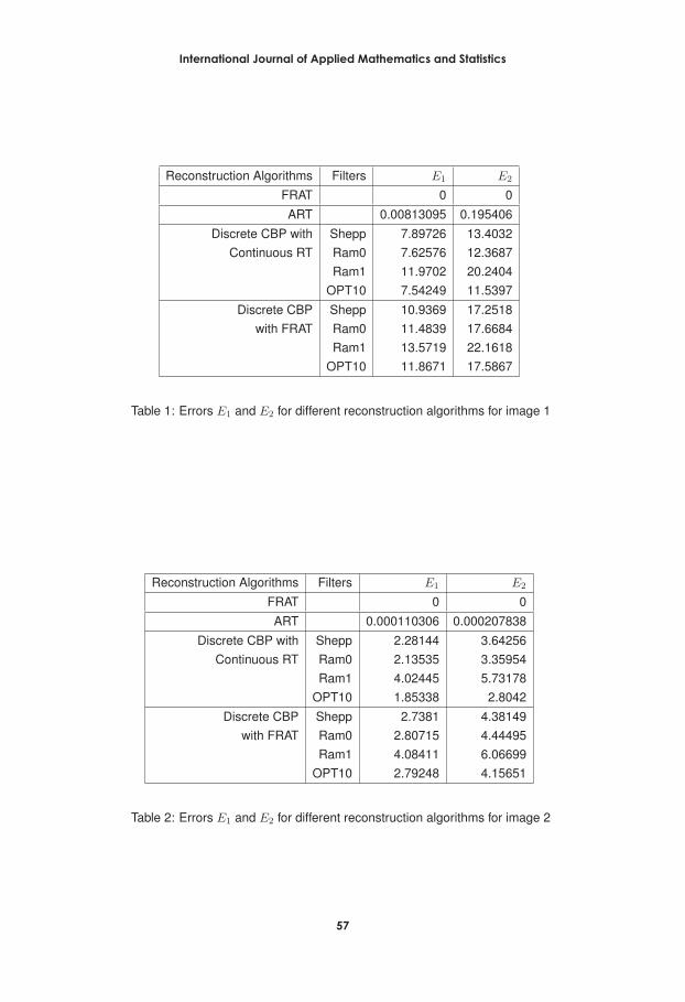
Since the error E2 is reported to be depending on the choice of convolving function q in CBP(Srivastava, 1989), a convolving function which may take care of this error and data scanninggeometry was reported. This has been called as optimal filter.Using the same principles asreported in (Srivastava, Rathore, Dhariyal, Munshi and Rastogi, 1994), the optimal filter func-tion for discrete CBP has been obtained. The reconstruction has been done by CBP algorithmusing Ram-Lak filter for ε = 0 and ε = 1, Shepp filter and optimal filter, by direct inversionof FRAT and by MSART. The reconstruction results are reported in figure 1 to 4 while the er-rors of these reconstructions are reported in table 1 to 4 on four test images. The quality ofreconstruction also varies according to the variations in smoothness of images in every recon-struction method.


52

Figure 1: The Original image 1,its projection, and reconstruction with different algorithms


53



54



55



56

Reconstruction Algorithms Filters E1 E2

FRAT 0 0ART 0.00813095 0.195406

Discrete CBP with Shepp 7.89726 13.4032Continuous RT Ram0 7.62576 12.3687

Ram1 11.9702 20.2404OPT10 7.54249 11.5397

Discrete CBP Shepp 10.9369 17.2518with FRAT Ram0 11.4839 17.6684

Ram1 13.5719 22.1618OPT10 11.8671 17.5867

Table 1: Errors E1 and E2 for different reconstruction algorithms for image 1


FRAT 0 0ART 0.000110306 0.000207838


Ram1 4.02445 5.73178OPT10 1.85338 2.8042


Ram1 4.08411 6.06699OPT10 2.79248 4.15651



57


FRAT 0 0ART 0.00311699 0.00436965


Ram1 1.21023 2.51994OPT10 0.529519 0.802421


Ram1 1.59912 3.52881OPT10 1.11928 1.81389



FRAT 0 0ART 0.00244277 0.00440341


Ram1 2.16883 4.06601OPT10 1.27534 2.12544


Ram1 2.71946 5.09386OPT10 2.1885 3.3371



58

References

Beylkin, G. 1987. Discrete radon transform, IEEE Trans. Acoustics, Speech Signal Process.ASSP 35: 162–172.

Censor, Y. 1983. Finite series expansion reconstruction methods, Proceedings of the IEEE71: 409–419.

Deans, S. R. 1983. Radon Transform and some of its Applications, John Wiley and Sons.

Do, M. N. and Vetterli, M. 2003. The finite ridgelet transform for image representation, IEEETransactions on Image Processing 12: 16–28.

Gorden, R., Bender, R. and Herman, G. T. 1970. Algebraic reconstruction techniques(art) forthree dimensional eletron microscophy and x-ray photography, J.Theor. Biol. 29: 471–481.

Gordon, R. 1974. A tutorial on art, IEEE Transaction on Nuclear Science NS-21: 78–83.

Hsung, T., Lun, D. P. K. and Siu, W. 1996. The discrete periodic radon transform, IEEE Trans-action on Signal Processing 44: 2651–2657.

Kak, A. C. and Slaney, M. 1988. Principles of Computerised Tomographic Imaging, IEEEEngineering in Medical and Biology Society.

Kingston, A. 2006. Orthogonal discrete radon transform over pn x pn images, Signal Process-ing 86: 2040–2050.

Kingston, A. and Svalbe, I. 2007. Generalised finite radon transform for n*n images, Imageand Vision Computing (Elsevier) 25: 1620–1630.

Lewitt, R. N. 1983. Reconstruction algorithms: Transform methods, Proceedings of the IEEE71: 390–408.

Matus, F. and Flusser, J. 1993. Image representation via a finite radon transform, IEEE Trans.Pattern Anal. Mach. Intell. 15: 996–1006.

Natterer, F. 1986. The Mathematics of Computerised Tomography, John Wiley and sons.

Natterer, F. and Wubbeling, F. 2001. Mathematical Methods in Image Reconstruction, SIAM.

Radon, J. 1917. Uber due bestimmung von funktionen durch ihre intergralwerte langsgewissermannigfaltigkeiten (on the determination of functions from their integrals along certainmanifolds, Berichte Saechsische Akademie der Wissenschaften 29: 262–277.

Ramachandran, G. N. and Lakshminarayanan, A. V. 1971. Three dimensional reconstructionfrom radiographs and electron micrographs:application of convolution instead of fouriertransform, Proc.Nat. Acad. Sci. 68: 2236–2240.

Shepp, L. A. and Logan, B. F. 1974. The fourier reconstruction of a head section, IEEE Trans.Nucl. Sci. NS-21: 21–43.


59

Srivastava, T. 1989. Convolution Backprojection Algorithm in Computerized Tomography, PhDthesis, I.I.T.Kanpur.

Srivastava, T. and Nirvikar 2011. Modified simultaneous algebraic reconstruction technique,International Journal of Tomography and Simulation 18.

Srivastava, T., Rathore, R. K. S. and Dhariyal, I. D. 1992. Direct estimates of statistical errorfor convolution back projection algorithm in computerized tomography, Journal of Combi-natorics Information and system sciences 17: 271–287.

Srivastava, T., Rathore, R. K. S., Dhariyal, I. D., Munshi, P. and Rastogi, R. 1994. Design ofoptimal statistical filter for discrete convolution back projection method, American Journalof Mathematical and Management Sciences 14: 229–265.


60

On Image Reconstruction Algorithms with Discrete Radon Transform

Documents

Transcript of On Image Reconstruction Algorithms with Discrete Radon Transform