Computers & Geosciences 57 (2013) 175–182

Contents lists available at SciVerse ScienceDirect

Computers & Geosciences

0098-30http://d

n CorrCampinmobile:

E-municampbrunoho

journal homepage: www.elsevier.com/locate/cageo

Facies recognition using a smoothing process through FastIndependent Component Analysis and Discrete Cosine Transform

Alexandre Cruz Sanchetta a,n, Emilson Pereira Leite b, Bruno César Zanardo Honório b

a Rua Mendeleiev, s/n, Cidade Universitária “Zeferino Vaz”, Barão Geraldo, Campinas, São Paulo 13083-970, Brasilb Rua João Pandiá Calógeras, 51, Cidade Universitária “Zeferino Vaz”, Barão Geraldo, Campinas, São Paulo 13983-970, Brasil

a r t i c l e i n f o

Article history:Received 6 June 2012Received in revised form14 March 2013Accepted 25 March 2013Available online 3 April 2013

Keywords:Discrete Cosine TransformIndependent Component AnalysisAutomatic classificationReservoir characterization

04/$ - see front matter & 2013 Elsevier Ltd. Ax.doi.org/10.1016/j.cageo.2013.03.021

espondence to: Rua Doutor Geraldo de Campas, São Paulo 13083-480, Brasil. Tel.: +55 19 3+55 19 8811 9176.ail addresses: alexandr@dep.fem.unicamp.br (.br (E.P. Leite),norio@gmail.com (B.C.Z. Honório).

a b s t r a c t

We propose a preprocessing methodology for well-log geophysical data based on Fast IndependentComponent Analysis (FastICA) and Discrete Cosine Transform (DCT), in order to improve the success rateof the K-NN automatic classifier. The K-NN have been commonly applied to facies recognition in well-loggeophysical data for hydrocarbon reservoir modeling and characterization.

The preprocess was made in two different levels. In the first level, a FastICA based dimenstionreduction was applied, maintaining much of the information, and its results were classified; In secondlevel, FastICA and DCT were applied in smoothing level, where the data points are modified, so individualpoints have their distance reduced, keeping just the primordial information. The results were comparedto identify the best classification cases. We have applied the proposed methodology to well-log data froma petroleum field of Campos Basin, Brazil. Sonic, gamma-ray, density, neutron porosity and deepinduction logs were preprocessed with FastICA and DCT, and the product was classified with K-NN. Thesuccess rates in recognition were calculated by appling the method to log intervals where core data wereavailable. The results were compared to those of automatic recognition of the original well-log data setwith and without the removal of high frequency noise. We conclude that the application of the proposedmethodology significantly improves the success rate of facies recognition by K-NN.

& 2013 Elsevier Ltd. All rights reserved.

1. Introduction

Well-log data have been used in many areas of geological andgeophysical data analysis, such as in reservoir characterizationwhere models of subsurface properties that take into accountdetails about rock physics and the fluids contained in the rocks areconstructed (Avseth et al., 2005; Coconi-Morales et al., 2010;Doyen, 2007; Dubrule, 1994). Another example is the use ofwell-log data to predict seismic parameters related to Amplitudevs. Offset (AVO) data such as Vp, s, Poisson's ratio sð Þ, amongothers, that aid in the comprehension of reservoirs (Rutheford andWillians, 1989). Well-log data has also been widely used instructural and stratigraphic mapping.

In order to connect the well-log data with other geological orgeophysical information, it is important to correlate them withlithofacies described from core samples. However, such directinformation is often not available to the entire length of the wells,

ll rights reserved.

os Freire, 567, Barão Geraldo,287 6618 (residence),

A.C. Sanchetta), emilson@ige.

mainly because of financial restrictions. Therefore, pattern recog-nition methods must be applied for prediction or classification.

To mention a few examples of application of pattern recogni-tion methods in well-log data, Grana et al. (2012) had constructeda complete statistical workflow for obtaining petrophysical prop-erties at the well location and the corresponding facies classifica-tion; Messina and Langer (2011) have implemented unsupervisedalgorithms based on self-organizing maps and cluster analysis toanalyze and to interpret volcanic tremor data; Turlapaty et al.(2010) proposed a method based on wavelet-based feature extrac-tion and one-class support vector machines to analyze satelliteremote sensing data applied to soil moisture and vegetationmapping; and Rosati and Cardarelli (1997) applied texture featuresbased on gray tone spatial dependence matrices to classifypatterns observed on magnetic anomaly maps.

In fact, all types of data can be separated into several subsets,where each data element present in a random subset containssome information in common with the other elements in thatsubset. In other words, it is possible to classify all elements basedon some common characteristics identified in the data set. This isthe basic principle of automatic classification (MacQueen, 1967).The several approaches to automatic classification can be dividedinto two major groups: supervised methods and unsupervisedmethods (Duda and Hart, 1973; Mitchell, 1997; Schuerman, 1996).

A.C. Sanchetta et al. / Computers & Geosciences 57 (2013) 175–182176

Supervised methods are based on the knowledge of classificationlabels (targets), i.e., it is known that an input sample correspondsto a certain label (e.g. K-Nearest Neighbor, Artificial Neural Net-works). Unsupervised methods cluster the samples into subsetsthrough statistical and other mathematical approaches (e.g.K-Means, Self-Organizing Maps). Supervised methods need a labelto classify, in our case, the core data. The application of supervisedmethods are robust, once we can assume that heterogeneousenvironments are periodic for mathematical simplicity; and com-putations of local problems that should be done on a sufficientlylarge representative elementary volume R.E.V. instead of a singlecell, because random flows have different results than periodicflows (Amaziane et al., 2006). In this work, we have employed theK-Nearest Neighbor (K-NN) method (Toussaint, 2005). K-NN is apattern recognition method that classifies elements in a data setbased on the spatial distribution of a training set.

Many parameters affect the quality of the prediction: choice ofvariables; quality of the measured data; and the associateduncertainty are just a few examples. For spatial classifiers suchas K-NN, the perfect choice would be a set of orthogonal variablesthat do not carry any kind of redundant or misplaced information.However, in practice we often notice high correlations amongdifferent well-log profiles. For example, the well NA04, in Namor-ado Field, sonic log (DT) and neutron porosity log (NPHI) havecross-correlations higher than 0.8 and DT and bulk density log(RHOB) have cross-correlation higher than 0.7 (Carrasquilla andLeite, 2009). Those high correlations mean that the information isredundant, which may jeopardize the performance of the K-NN. Tominimize this problem and to prepare the data for automaticclassification we have applied a multivariate analysis, namelyIndependent Component Analysis (ICA) (Comon, 1994). ICA is ablind source separation method that transforms an input signalinto a new set of independent signals. Statistically, independencemeans that the occurrence of a signal does not have any relationwith the occurrence of another signal contained in the data set(Russell and Norvig, 2002). The independence of the signalsprovides an orthogonal set of new variables such that they canbe understood as individual events. With the aim of reducing thecomputation effort, an iterative algorithm based on the Newton'smethod was developed by Hyvärinen (1999), namely The FastIndependent Component Analysis (FastICA). Independent variablesare necessarily orthogonal, so the FastICA method provides ortho-gonality in the classification. In order to smooth data, we have alsoapplied the Discrete Cosine Transform (DCT) (Rao and Yip, 1990).

In our analysis, we have used well-log data from Campos Basin,which is located in the southeastern portion of Brazil, along thenorth coast of the State of Rio de Janeiro. Campos Basin covers anarea of 100.000 km2 up to a water depth of 3000 m. Particularly,all wells are located in the Namorado Field, which is located on thenorth-central hydrocarbon accumulations zone of the CamposBasin, about 80 km offshore under water depths ranging from140 m to 250 m (Vidal et al., 2007).

2. Fast Independent Component Analysis

Fast Independent Component Analysis (FastICA) is an opti-mized process of Independent Component Analysis (ICA, Comon,1994). ICA is a method for finding underlying factors or compo-nents from multivariate data that are related to Blind SignalSeparation (Hyvärinen et al., 2001). The usual ICA method havesome problems such as maximization of contrast functions,computational cost and/or selection of the learning rate, whileFastICA was proposed to remedy these problems and to convergeto the result faster than ICA (Hyvärinen, 1999).

The FastICA process is based on a fixed-point algorithm, whichis well-known for its speed. The requirement of such speed isjustified by the large number of data points that are used in asingle step of the algorithm (block model). The algorithm hassome improvements when compared to common fixed-pointalgorithms (Burden and Faires, 1985). Besides, the algorithm isparallel, computationally simple and requires little computationalmemory, similarly to some neural algorithms (Hyvärinen et al.,2001).

The fixed-point algorithm is based on the Newton's method(Hyvärinen, 1999), which within the framework of the commonICA reads as

sþ ¼ s−f ðxÞf ′ðxÞ ; ð1Þ

where s is a random non-gaussian initial guess vector which inturn will iteratively converge to sþ through some objectivefunction f ðxÞ. Commonly, objective fuction are filled with negen-tropy equations. Negentropy, the denial of entropy, is a measurethat is maximized when the distributions are as far as possiblefrom a Gaussian distribution (Comon, 1994).

In the case of FastICA, negentropy is used considering thestationarity conditions of Kuhn–Tucker

∇f ðxnÞ þ ∑m

i ¼ 1μi∇giðxnÞ þ ∑

l

j ¼ 1λj∇hjðxnÞ ¼ 0; ð2Þ

where xn is a local minimum, μi and λj are constants called KKTmultipliers, gi are the inequality constraint functions, hj are theequality constraint functions and ∇f ðxnÞ; ∇giðxnÞ and ∇hjðxnÞ aretheir gradients, respectively. These function are optimizedobtained by (Hyvärinen, 1999)

EfxgðsTxÞg−βs¼ 0; ð3Þ

where β ¼ EfsT0xgðsT0xÞg with s0 being the optimal value from theprocess.

Newton's method requires the derivative of negentropy. Actu-ally, because s is a vector, it is necessary to calculate the Jacobian ofthe negentropy. Denoting the negentropy equation as F , itsJacobian is

JFðsÞ ¼ EfxxTg′ðsT xÞg−βI: ð4Þ

In statistical analysis, it is common to apply a whiteningprocess, with eigenvalue decomposition, in the vectors (Franklin,1968). Therefore EfxxT g≈I and we can rewrite JFðsÞ as

JFðsÞ ¼ Efg′ðsT xÞg−βI: ð5Þ

Approximating β for values of s, instead of s0, we can rewritethe fixed-point method in its complete form as

sþ ¼ s−½EfxgðsTxÞg−βs�½Efg′ðsTxÞg−β� ; ð6Þ

where sn ¼ sþ=‖sþ‖. Normalizing the equation by β−Efg′ðsTxÞg, thefixed-point algorithm equation is finally defined as

sþ ¼ EfxgðsTxÞg−Efg′ðsTxÞgs: ð7Þ

The above solution searches for one independent component.In order to find all possible independent components, the methodsimply needs to be applied as much as necessary, justneeding decorrelate the independent components. To performdecorrelation process, it is necessary to calculate n+1 independentcomponents, because we subtract each one projection from theprevious components founded. A deflationary scheme based onGram–Schmidt decorrelation is applied to these subtractions

A.C. Sanchetta et al. / Computers & Geosciences 57 (2013) 175–182 177

(Farina and Studer, 1984)

snþ1 ¼ snþ1− ∑n

i ¼ 1sTnþ1sisi: ð8Þ

Considering that the data was preprocessed with whitening, itis sufficient to renormalize the solution, obtaining snnþ1 ¼ snþ1=

‖snþ1‖.

3. Discrete Cosine Transform

Discrete Cosine Transform (DCT) is a method that allowsexpressing a function in terms of a weighted sum of cosinesoscillating at different frequencies. It is closely related to theDiscrete Fourier Transform (DFT; Oppenheim et al., 2009).

For a sequence of N complex signals x0; x1; ⋯; xN−1, thesequence of their respective DFTs (Blinn, 1993) ℱ0; ℱ1; ⋯; ℱN−1,are

ℱkðωÞ ¼ ∑N−1

n ¼ 0xn cos −

2πN

kn� �

þ i sin −2πN

kn� �� �

: ð9Þ

with k¼ 0; 1; 2⋯;N−1:In particular, it is possible to work only with the real part of the

DFT, which is governed by the cosine function, or with theimaginary part, governed by the sine. This choice leads to twoother transforms that are similar and related to the DFT: theDiscrete Cosine Transform (DCT) and the Discrete Sine Transform(DST). The use of the DCT is focused on data compression or noisesuppression (Rao and Yip, 1990), while the DST is mainly appliedto solve Partial Differential Equations (Martucci, 1994).

Because of its significant data and energy compression, themost widely used procedure for the calculation of the DCT insignal and image processing is the DCT-II method (Rao and Yip,1990), which is summarized in the equation

DCT� IIkðωÞ ¼ ∑N−1

n ¼ 0xncos

π

Nnþ 1

2

� �k

� �: ð10Þ

Multidimensional DCT applications rigorously follow the samedefinitions of the one-dimensional method and are simply repre-sented by a separate product of all cosines along each dimension.For example, if the data is in the form of a matrix, the DCT processimplementation has to transform the data into two dimensions byapplying the equation DCTk1 ;k2 ðωÞ : ℝ2-ℝ2,

DCTk1 ;k2 ðωÞ ¼ ∑N1−1

n1 ¼ 0∑

N2−1

n2 ¼ 0xn1 ;n2 cos

π

N1n1 þ

12

� �k1

� �cos

π

N2n2 þ

12

� �k2

� �;

ð11Þ

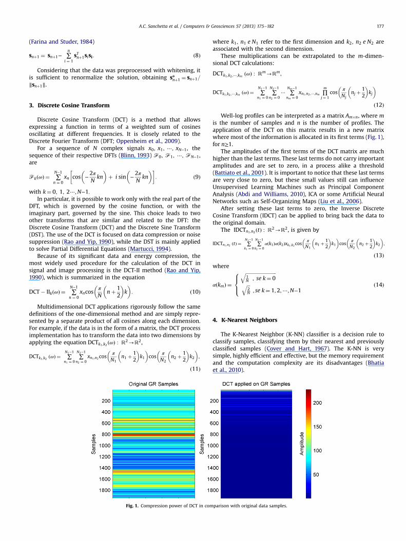
Fig. 1. Compression power of DCT in com

where k1; n1 e N1 refer to the first dimension and k2; n2 e N2 areassociated with the second dimension.

These multiplications can be extrapolated to the m-dimen-sional DCT calculations:

DCTk1 ;k2 ;⋯;km ðωÞ : ℝm-ℝm;

DCTk1 ;k2 ;⋯;km ðωÞ ¼ ∑N1−1

n1 ¼ 0∑

N2−1

n2 ¼ 0⋯ ∑

Nm−1

nm ¼ 0xn1 ;n2 ;⋯;nm ∏

m

j ¼ 1cos

π

Njnj þ

12

� �kj

� �

ð12ÞWell-log profiles can be interpreted as a matrix Am�n, where m

is the number of samples and n is the number of profiles. Theapplication of the DCT on this matrix results in a new matrixwhere most of the information is allocated in its first terms (Fig. 1),for n≥1.

The amplitudes of the first terms of the DCT matrix are muchhigher than the last terms. These last terms do not carry importantamplitudes and are set to zero, in a process alike a threshold(Battiato et al., 2001). It is important to notice that these last termsare very close to zero, but these small values still can influenceUnsupervised Learning Machines such as Principal ComponentAnalysis (Abdi and Williams, 2010), ICA or some Artificial NeuralNetworks such as Self-Organizing Maps (Liu et al., 2006).

After setting these last terms to zero, the Inverse DiscreteCosine Transform (IDCT) can be applied to bring back the data tothe original domain.

The IDCTn1 ;n2 ðtÞ : ℝ2-ℝ2, is given by

IDCTn1 ;n2 ðtÞ ¼ ∑N1−1

k1 ¼ 0∑

N2−1

k2 ¼ 0αðk1Þαðk2Þxk1 ;k2 cos

π

N1n1 þ

12

� �k1

� �cos

π

N2n2 þ

12

� �k2

� �;

ð13Þwhere

αðkmÞ ¼

ffiffiffiffiffiffiffiffiffiffiffiffiffiffiffiffiffiffiffiffiffiffiffiffiffiffi1N ; se k¼ 0

qffiffiffi2N

q; se k¼ 1;2;⋯;N−1

8><>: ð14Þ

4. K-Nearest Neighbors

The K-Nearest Neighbor (K-NN) classifier is a decision rule toclassify samples, classifying them by their nearest and previouslyclassified samples (Cover and Hart, 1967). The K-NN is verysimple, highly efficient and effective, but the memory requirementand the computation complexity are its disadvantages (Bhatiaet al., 2010).

parison with original data samples.

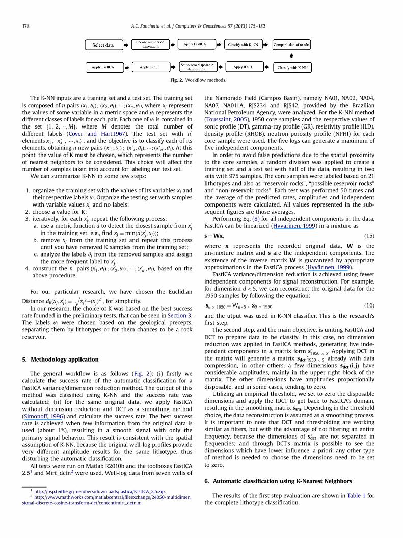
Fig. 2. Workflow methods.

A.C. Sanchetta et al. / Computers & Geosciences 57 (2013) 175–182178

The K-NN inputs are a training set and a test set. The training setis composed of n pairs ðx1; θiÞ; ðx2; θiÞ;⋯; ðxn; θiÞ, where xj representthe values of some variable in a metric space and θi represents thedifferent classes of labels for each pair. Each one of θi is contained inthe set f1; 2;⋯;Mg, where M denotes the total number ofdifferent labels (Cover and Hart,1967). The test set with n

0

elements x10 ; x20 ; ⋯; xn00 , and the objective is to classify each of itselements, obtaining n new pairs ðx′1; θiÞ ; ðx′2; θiÞ;⋯; ðx′n0 ; θiÞ. At thispoint, the value of K must be chosen, which represents the numberof nearest neighbors to be considered. This choice will affect thenumber of samples taken into account for labeling our test set.

We can summarize K-NN in some few steps:

1.

1

2

sion

organize the training set with the values of its variables xj andtheir respective labels θi. Organize the testing set with sampleswith variable values x′j and no labels;

2.

choose a value for K; 3. iteratively, for each x′j, repeat the following process:

a. use a metric function d to detect the closest sample from x′jin the training set, e.g., find xJ ¼minðdðx′j; xjÞÞ;

b. remove xJ from the training set and repeat this processuntil you have removed K samples from the training set;

c. analyze the labels θi from the removed samples and assignthe more frequent label to x′j.

htthtt

al-d

0

4. construct the n pairs ðx′1; θiÞ ; ðx′2; θiÞ ;⋯; ðx′n′; θiÞ, based on the

above procedure.

For our particular research, we have chosen the Euclidian

Distance dEðxJ ; x′JÞ ¼ffiffiffiffiffiffiffiffiffiffiffiffiffiffiffiffiffiffiffiffixj2−ðx′jÞ2

q; for simplicity.

In our research, the choice of K was based on the best successrate founded in the preliminary tests, that can be seen in Section 3.The labels θi were chosen based on the geological precepts,separating them by lithotypes or for them chances to be a rockreservoir.

5. Methodology application

The general workflow is as follows (Fig. 2): (i) firstly wecalculate the success rate of the automatic classification for aFastICA variance/dimension reduction method. The output of thismethod was classified using K-NN and the success rate wascalculated; (ii) for the same original data, we apply FastICAwithout dimension reduction and DCT as a smoothing method(Simonoff, 1996) and calculate the success rate. The best successrate is achieved when few information from the original data isused (about 1%), resulting in a smooth signal with only theprimary signal behavior. This result is consistent with the spatialassumption of K-NN, because the original well-log profiles providevery different amplitude results for the same lithotype, thusdisturbing the automatic classification.

All tests were run on Matlab R2010b and the toolboxes FastICA2.51 and Mirt_dctn2 were used. Well-log data from seven wells of

p://bsp.teithe.gr/members/downloads/fastica/FastICA_2.5.zip.p://www.mathworks.com/matlabcentral/fileexchange/24050-multidimeniscrete-cosine-transform-dct/content/mirt_dctn.m.

the Namorado Field (Campos Basin), namely NA01, NA02, NA04,NA07, NA011A, RJS234 and RJS42, provided by the BrazilianNational Petroleum Agency, were analyzed. For the K-NN method(Toussaint, 2005), 1950 core samples and the respective values ofsonic profile (DT), gamma-ray profile (GR), resistivity profile (ILD),density profile (RHOB), neutron porosity profile (NPHI) for eachcore sample were used. The five logs can generate a maximum offive independent components.

In order to avoid false predictions due to the spatial proximityto the core samples, a random division was applied to create atraining set and a test set with half of the data, resulting in twosets with 975 samples. The core samples were labeled based on 21lithotypes and also as “reservoir rocks”, “possible reservoir rocks”and “non-reservoir rocks”. Each test was performed 50 times andthe average of the predicted rates, amplitudes and independentcomponents were calculated. All values represented in the sub-sequent figures are those averages.

Performing Eq. (8) for all independent components in the data,FastICA can be linearized (Hyvärinen, 1999) in a mixture as

s¼Wx; ð15Þwhere x represents the recorded original data, W is theun-mixture matrix and s are the independent components. Theexistence of the inverse matrix W is guaranteed by appropriateapproximations in the FastICA process (Hyvärinen, 1999).

FastICA variance/dimension reduction is achieved using fewerindependent components for signal reconstruction. For example,for dimension do5, we can reconstruct the original data for the1950 samples by following the equation:

sd � 1950 ¼Wd�5 : x5 � 1950 ð16Þand the utput was used in K-NN classifier. This is the research'sfirst step.

The second step, and the main objective, is uniting FastICA andDCT to prepare data to be classify. In this case, no dimensionreduction was applied in FastICA methods, generating five inde-pendent components in a matrix form s01950 � 5. Applying DCT inthe matrix will generate a matrix sdct 1950 � 5

0 already with datacompression, in other others, a few dimensions sdct0 ði; jÞ haveconsiderable amplitudes, mainly in the upper right block of thematrix. The other dimensions have amplitudes proportionallydisposable, and in some cases, tending to zero.

Utilizing an empirical threshold, we set to zero the disposabledimensions and apply the IDCT to get back to FastICA's domain,resulting in the smoothing matrix ssm. Depending in the thresholdchoice, the data reconstruction is assumed as a smoothing process.It is important to note that DCT and thresholding are workingsimilar as filters, but with the advantage of not filtering an entirefrequency, because the dimensions of sdct0 are not separated infrequencies; and through DCT's matrix is possible to see thedimensions which have lower influence, a priori, any other typeof method is needed to choose the dimensions need to be setto zero.

6. Automatic classification using K-Nearest Neighbors

The results of the first step evaluation are shown in Table 1 forthe complete lithotype classification.

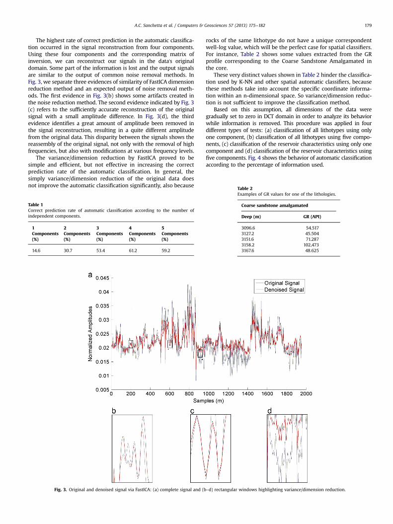
Table 2

A.C. Sanchetta et al. / Computers & Geosciences 57 (2013) 175–182 179

The highest rate of correct prediction in the automatic classifica-tion occurred in the signal reconstruction from four components.Using these four components and the corresponding matrix ofinversion, we can reconstruct our signals in the data's originaldomain. Some part of the information is lost and the output signalsare similar to the output of common noise removal methods. InFig. 3, we separate three evidences of similarity of FastICA dimensionreduction method and an expected output of noise removal meth-ods. The first evidence in Fig. 3(b) shows some artifacts created inthe noise reduction method. The second evidence indicated by Fig. 3(c) refers to the sufficiently accurate reconstruction of the originalsignal with a small amplitude difference. In Fig. 3(d), the thirdevidence identifies a great amount of amplitude been removed inthe signal reconstruction, resulting in a quite different amplitudefrom the original data. This disparity between the signals shows thereassembly of the original signal, not only with the removal of highfrequencies, but also with modifications at various frequency levels.

The variance/dimension reduction by FastICA proved to besimple and efficient, but not effective in increasing the correctprediction rate of the automatic classification. In general, thesimply variance/dimension reduction of the original data doesnot improve the automatic classification significantly, also because

Table 1Correct prediction rate of automatic classification according to the number ofindependent components.

1Components(%)

2Components(%)

3Components(%)

4Components(%)

5Components(%)

14.6 30.7 53.4 61.2 59.2

Fig. 3. Original and denoised signal via FastICA: (a) complete signal and (b

rocks of the same lithotype do not have a unique correspondentwell-log value, which will be the perfect case for spatial classifiers.For instance, Table 2 shows some values extracted from the GRprofile corresponding to the Coarse Sandstone Amalgamated inthe core.

These very distinct values shown in Table 2 hinder the classifica-tion used by K-NN and other spatial automatic classifiers, becausethese methods take into account the specific coordinate informa-tion within an n-dimensional space. So variance/dimension reduc-tion is not sufficient to improve the classification method.

Based on this assumption, all dimensions of the data weregradually set to zero in DCT domain in order to analyze its behaviorwhile information is removed. This procedure was applied in fourdifferent types of tests: (a) classification of all lithotypes using onlyone component, (b) classification of all lithotypes using five compo-nents, (c) classification of the reservoir characteristics using only onecomponent and (d) classification of the reservoir characteristics usingfive components. Fig. 4 shows the behavior of automatic classificationaccording to the percentage of information used.

–d) rectangular windows highlighting variance/dimension reduction.

Examples of GR values for one of the lithologies.

Coarse sandstone amalgamated

Deep (m) GR (API)

3096.6 54.5173127.2 45.5043151.6 71.2873158.2 102,4733167.6 48.625

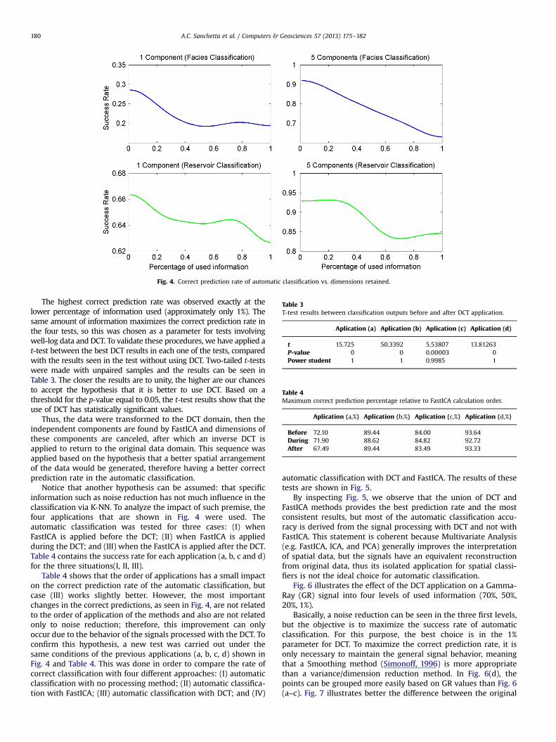
Fig. 4. Correct prediction rate of automatic classification vs. dimensions retained.

Table 3T-test results between classification outputs before and after DCT application.

Aplication (a) Aplication (b) Aplication (c) Aplication (d)

t 15.725 50.3392 5.53807 13.81263P-value 0 0 0.00003 0Power student 1 1 0.9985 1

Table 4Maximum correct prediction percentage relative to FastICA calculation order.

Aplication (a,%) Aplication (b,%) Aplication (c,%) Aplication (d,%)

Before 72.10 89.44 84.00 93.64During 71.90 88.62 84.82 92.72After 67.49 89.44 83.49 93.33

A.C. Sanchetta et al. / Computers & Geosciences 57 (2013) 175–182180

The highest correct prediction rate was observed exactly at thelower percentage of information used (approximately only 1%). Thesame amount of information maximizes the correct prediction rate inthe four tests, so this was chosen as a parameter for tests involvingwell-log data and DCT. To validate these procedures, we have applied at-test between the best DCT results in each one of the tests, comparedwith the results seen in the test without using DCT. Two-tailed t-testswere made with unpaired samples and the results can be seen inTable 3. The closer the results are to unity, the higher are our chancesto accept the hypothesis that it is better to use DCT. Based on athreshold for the p-value equal to 0.05, the t-test results show that theuse of DCT has statistically significant values.

Thus, the data were transformed to the DCT domain, then theindependent components are found by FastICA and dimensions ofthese components are canceled, after which an inverse DCT isapplied to return to the original data domain. This sequence wasapplied based on the hypothesis that a better spatial arrangementof the data would be generated, therefore having a better correctprediction rate in the automatic classification.

Notice that another hypothesis can be assumed: that specificinformation such as noise reduction has not much influence in theclassification via K-NN. To analyze the impact of such premise, thefour applications that are shown in Fig. 4 were used. Theautomatic classification was tested for three cases: (I) whenFastICA is applied before the DCT; (II) when FastICA is appliedduring the DCT; and (III) when the FastICA is applied after the DCT.Table 4 contains the success rate for each application (a, b, c and d)for the three situations(I, II, III).

Table 4 shows that the order of applications has a small impacton the correct prediction rate of the automatic classification, butcase (III) works slightly better. However, the most importantchanges in the correct predictions, as seen in Fig. 4, are not relatedto the order of application of the methods and also are not relatedonly to noise reduction; therefore, this improvement can onlyoccur due to the behavior of the signals processed with the DCT. Toconfirm this hypothesis, a new test was carried out under thesame conditions of the previous applications (a, b, c, d) shown inFig. 4 and Table 4. This was done in order to compare the rate ofcorrect classification with four different approaches: (I) automaticclassification with no processing method; (II) automatic classifica-tion with FastICA; (III) automatic classification with DCT; and (IV)

automatic classification with DCT and FastICA. The results of thesetests are shown in Fig. 5.

By inspecting Fig. 5, we observe that the union of DCT andFastICA methods provides the best prediction rate and the mostconsistent results, but most of the automatic classification accu-racy is derived from the signal processing with DCT and not withFastICA. This statement is coherent because Multivariate Analysis(e.g. FastICA, ICA, and PCA) generally improves the interpretationof spatial data, but the signals have an equivalent reconstructionfrom original data, thus its isolated application for spatial classi-fiers is not the ideal choice for automatic classification.

Fig. 6 illustrates the effect of the DCT application on a Gamma-Ray (GR) signal into four levels of used information (70%, 50%,20%, 1%).

Basically, a noise reduction can be seen in the three first levels,but the objective is to maximize the success rate of automaticclassification. For this purpose, the best choice is in the 1%parameter for DCT. To maximize the correct prediction rate, it isonly necessary to maintain the general signal behavior, meaningthat a Smoothing method (Simonoff, 1996) is more appropriatethan a variance/dimension reduction method. In Fig. 6(d), thepoints can be grouped more easily based on GR values than Fig. 6(a–c). Fig. 7 illustrates better the difference between the original

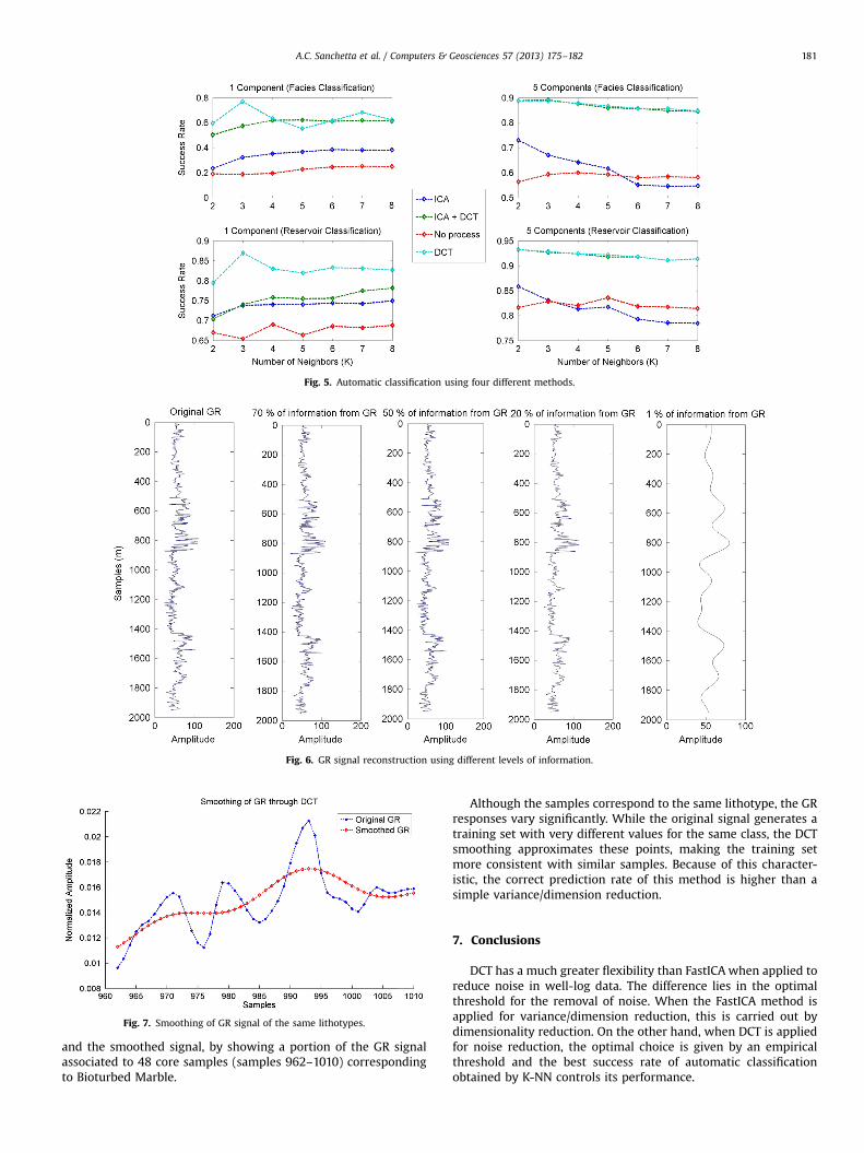
Fig. 5. Automatic classification using four different methods.

Fig. 6. GR signal reconstruction using different levels of information.

Fig. 7. Smoothing of GR signal of the same lithotypes.

A.C. Sanchetta et al. / Computers & Geosciences 57 (2013) 175–182 181

and the smoothed signal, by showing a portion of the GR signalassociated to 48 core samples (samples 962–1010) correspondingto Bioturbed Marble.

Although the samples correspond to the same lithotype, the GRresponses vary significantly. While the original signal generates atraining set with very different values for the same class, the DCTsmoothing approximates these points, making the training setmore consistent with similar samples. Because of this character-istic, the correct prediction rate of this method is higher than asimple variance/dimension reduction.

7. Conclusions

DCT has a much greater flexibility than FastICA when applied toreduce noise in well-log data. The difference lies in the optimalthreshold for the removal of noise. When the FastICA method isapplied for variance/dimension reduction, this is carried out bydimensionality reduction. On the other hand, when DCT is appliedfor noise reduction, the optimal choice is given by an empiricalthreshold and the best success rate of automatic classificationobtained by K-NN controls its performance.

A.C. Sanchetta et al. / Computers & Geosciences 57 (2013) 175–182182

For K-NN, the variance/dimension reduction process improvesthe automatic classification success rate only in 2%. The K-NNautomatic classification accuracy rate was maximized with use ofFastICA and DCT, improving the best result in about 8% and theworst result in about 20%. The best results were achieved in a verysmoothed signal, possibly because the amplitude difference issmoothed, grouping the points which corresponding to the samerock lithotypes. Further studies can be carried out to check theinfluence of the signal variograms in the application of thismethodology.

References

Abdi, H., Willians, L.J., 2010. Principal Component Analysis. WIREs Comp Stat 2,433–459 /http://onlinelibrary.wiley.com/doi/10.1002/wics.101/pdfS.

Amaziane, B., Bourgeat, A., Jurak, M., 2006. Effective macrodifusion in solutetransport through heterogeneous porous media. Multiscale Modeling andSimulation 5, 184–204.

Avseth, P., Mukerji, T., Mavko, G., 2005. Quantitative Seismic Interpretation.Applying Rock Physics to Reduce Interpretation Risk. Cambridge UniversityPress, Cambridge, New York, Melbourne.

Battiato, S., Mancuso, M., Bosco, A., Guarnera, M., 2001. Psychovisual and statisticaloptimization of quantization tables for DCT compression engines. In: Proceed-ings of the 11th International Conference on Image Analysis and Processing,ICIAP'01, Palermo, Italy, p. 602.

Bhatia, N., et al., 2010. Survey of nearest neighbor techniques. International Journalof Computer Science and Information Security 2 (8), 302–305.

Blinn, J.F., 1993. What's the deal with the DCT. IEEE Computer Graphics andApplications 13 (4), 78–83.

Burden, R.L., Faires, J.D., 1985. Numerical Analysis, Third Edition Prindle, Weber &Schimidt, Boston.

Carrasquilla, A., Leite, M.V., 2009. Fuzzy logic in the simulation of sonic log using asinput combinations of gamma ray, resistivity, porosity and density well logsfrom Namorado Oilfield. In: Proceedings of the 11th International Congress ofthe Brazilian Geophysical Society, Salvador, Brazil.

Coconi-Morales, E., Ronquillo-Jarillo, G., Campos-Enríquez, J.O., 2010. Multi-scaleanalysis of well-logging data in petrophysical and stratigraphic correlation.Geofísica Internacional 49 (2), 55–67.

Comon, P., 1994. Independent component analysis: a new concept?. Signal Proces-sing, 36; 287–314.

Cover, T.M., Hart, P.E., 1967. Nearest neighbor pattern classification. IEEE Transac-tions on Information Theory 13 (1), 21–27.

Doyen, P.M., 2007. Seismic reservoir characterization: an earth modelling perspec-tive. EAGE Publications, Houten, The Netherlands.

Dubrule, O., 1994. Estimating or choosing a geostatistical model. In: Dimitrako-poulos, R. (Ed.), Geostatistics for the Next Century. Kluwer Academic Publishers,Dordcrecht, The Netherlands, pp. 3–14.

Duda, R., Hart, P., 1973. Pattern Classification and Scene Analysis. Wiley, New-York.Farina, A., Studer, F.A., 1984. Application of Gram-Schmidt algorithm optimum

radar signal processing. IEEE Proceedings Part F 131, 139–145.Franklin, J.N., 1968. Matrix Theory. Englewood Cliffs: Prentice-Hall. 292 pp.Grana, D., Pirrone, M., Mukerji, T., 2012. Quantitative log interpretation and

uncertainty propagation of petrophysical properties and facies classificationfrom rock-physics modeling and formation evaluation analysis. Geophysics 77,WA45–WA63.

Hyvärinen, A., 1999. Fast and robust fixed-point algorithms for independentcomponent analysis. IEEE Transactions on Neural Networks 10 (3), 626–634.

Hyvärinen, A., Karhunen, J., Oja, E., 2001. Independent Component Analysis. JohnWiley & Sons, Toronto 481 pp.

Liu, Y., Weisberg, R.H., Mooers, C.N.K., 2006. Performance evaluation of the self-organizing map for feature extraction. Journal of Geophysical Research 111,C05018, http://dx.doi.org/10.1029/2005JC003117.

MacQueen, J.B., 1967. Some methods for classification and analysis of multivariateobservations. In: Le Cam, L.M., Neyman, J. (Eds.), Proceedings of the fifthBerkeley Symposium on Mathematical Statistics and Probability, University ofCalifornia Press, pp. 281–297.

Martucci, S.A., 1994. Symmetric convolution and the discrete sine and cosinetransforms. IEEE Transactions on Signal Processing SP-42, 1038–1051.

Messina, A., Langer, H., 2011. Pattern recognition of volcanic tremor data on Mt.Etna (Italy) with KKAnalysis—a software program for unsupervised classifica-tion. Computers and Geosciences 37 (2011), 953–961.

Mitchell, T., 1997. Machine Learning. McGraw-Hill Higher Education, New York 432pp.

Oppenheim, A.V., Schafer, R.W., Buck, J.R., 2009. Discrete-Time Signal Processing,3th ed. Prentice Hall, NJ 1120 pp.

Rao, K.R., Yip, P., 1990. Discrete Cosine Transform: Algorithms, Advantages,Applications. Academic Press, Boston 512 pp.

Rosati, I., Cardarelli, E., 1997. Statistical pattern recognition technique to enhanceanomalies in magnetic surveys. Journal of Applied Geophysics 37 (2), 55–66.

Rutherford, S.R., Willians, R.H., 1989. Amplitude versus offset variations in gassands. Geophysics 54 (06), 680–688.

Russell, S., Norvig, P., 2002. Artificial Intelligence: A Modern Approach. PrenticeHall, Essex, England 478 pp.

Schuerman, J., 1996. Pattern Classification: A Unified View of Statistical and NeuralApproaches. Wiley & Sons, New York 392 pp.

Simonoff, J.S., 1996. Smoothing Methods in Statistics. Springer, New York 368 pp..Toussaint, G.T., 2005. Geometric proximity graphs for improving nearest neighbor

methods in instance-based learning and data mining. International Journal ofComputational Geometry and Applications 15 (2), 101–150.

Turlapaty, A.C., Anantharaj, V.G, Younan, N.H., 2010. A pattern recognition basedapproach to consistency analysis of Geophysical datasets. Computers andGeosciences 36, 464–476.

Vidal, A.C., Sancevero, S.S., Remacre, A.Z., Costanzo, C.P., 2007. Modelagem geoes-tatística 3D da impedância acústica para a caracterização do campo denamorado. Revista Brasileira de Geofísica 25 (3), 295–305.