Advances on the Simplification of Sine–Cosine Equations

Article No. sy980200J. Symbolic Computation (1998) 26, 31–70

Advances on the Simplification of Sine–CosineEquations

JAIME GUTIERREZ AND TOMAS RECIO

Departamento de Matematicas, Estadıstica y Computacion,Universidad de Cantabria, Santander 39071, Spain

In this paper we contribute several results to the approach initiated by Hommel andKovacs (well documented with applications in a recent book by Kovacs (1993)) on thesymbolic simplification of sine–cosine polynomials that arise, for instance, as determiningequations for joint values in robotics inverse kinematic problems. We present, taking intoconsideration for the first time sine–cosine polyomials, fast algorithms for the functionaldecomposition and factorization problems, reducing the solving of such s–c equationsto a sequence of lower degree ones. Moreover, we show that triangularization of a givensine–cosine equation provides a conceptual understanding of the conditions that yieldextraneous roots in the half-angle tangent substitution (and therefore that imply a re-duction of the degree in the determining equation of a given s–c system).

c© 1998 Academic Press

1. Motivations and Main Contributions of the Paper

By a sine–cosine equation we understand a polynomial equality f(s, c) = 0, with f inthe quotient ring K[s, c]/(s2 + c2 − 1), and where K is a field of characteristic zero(typically, a numerical field such as Q or R, or a field of parameters Q(d1, . . . , dm)).Therefore, when we write f(s, c) we consider, throughout this paper, that this expressionis implicitly univariate in some unknown angle θ such that s = sin(θ), c = cos(θ). Ourgoal is finding methods for solving or simplifying equations of the sort f(s, c) = 0; andthus, equivalently, for solving or simplifying systems

f(s, c) = 0,s2 + c2 − 1 = 0.

1.1. interest of the problem

Polynomial systems, where the variables are interpreted as trigonometric functionsof unknown angles, are quite ubiquitous, arising, for instance, in electrical networkingand in molecular kinematics. Here, our applications will be taken from the field of robotkinematics. Besides referring to the many situations described in Kovacs (1993), for thesake of being self-contained, we will outline a few examples of the role of sine–cosinesystems in robotics.

Example 1.1. Given a robot arm with six revolute joints, i.e. a 6R robot (see Figure 1),a typical problem is finding the values of the different joint angles (with respect to some

0747–7171/98/070031 + 40 $30.00/0 c© 1998 Academic Press

32 J. Gutierrez and T. Recio

θ2

θ1θ3

θ4

θ5

θ6

Joint 1 link 6 hand

Figure 1.

Figure 2.

standard way of measuring them) that place the tip (or hand) of the robot at somedesired position and orientation.

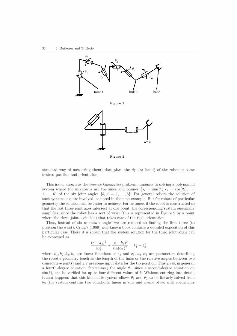
This issue, known as the inverse kinematics problem, amounts to solving a polynomialsystem where the unknowns are the sines and cosines {si = sin(θi), ci = cos(θi), i =1, . . . , 6} of the six joint angles {θi, i = 1, . . . , 6}. For general robots the solution ofsuch systems is quite involved, as noted in the next example. But for robots of particulargeometry the solution can be easier to achieve. For instance, if the robot is constructed sothat the last three joint axes intersect at one point, the corresponding system essentiallysimplifies, since the robot has a sort of wrist (this is represented in Figure 2 by a pointwhere the three joints coincide) that takes care of the tip’s orientation.

Thus, instead of six unknown angles we are reduced to finding the first three (toposition the wrist). Craig’s (1989) well-known book contains a detailed exposition of thisparticular case. There it is shown that the system solution for the third joint angle canbe expressed as

(r − k3)2

4a21

+(z − k4)2

sin(α1)2= k2

1 + k22

where k1, k2, k3, k4 are linear functions of s3 and c3, a1, α1 are parameters describingthe robot’s geometry (such as the length of the links or the relative angles between twoconsecutive joints) and z, r are some input data for the tip position. This gives, in general,a fourth-degree equation determining the angle θ3, since a second-degree equation onsin(θ), can be verified for up to four different values of θ. Without entering into detail,it also happens that this kinematic system allows θ1 and θ2 to be linearly solved fromθ3 (the system contains two equations, linear in sine and cosine of θ2, with coefficients

Advances on the Simplification of Sine–Cosine Equations 33

Figure 3.

polynomials in θ3; equally θ1 can be linearly expressed as a function of θ2 and θ3). Theemphasis here, because of this linearity, is that solving such system is essentially reducedto solving just one second-degree sine–cosine equation.

Moreover, it has been observed that imposing some geometric features on a robot ofthis kind (i.e. requiring that it is constructed so that the first three joints verify somespecific position relative to each other) yields that the determining fourth-degree equationdecomposes into two second-degree equations. For instance, when the first two joint axesintersect, i.e. if the robot parameter a1 = 0 (see Figure 3), then we obtain a quadraticequation in θ3. See also Example 1.5 and Smith and Lipkin (1990) for a precise analysis.

Example 1.2. After decades of research, a symbolic solution (though not in closed form)for the general 6R manipulator inverse kinematics system has been found (see Lee andLiang (1988a), Lee and Liang (1988b) and Raghavan and Roth (1989)). By a cleverelimination method it turns out that in this system θ3 can be determined as the solutionof a sixteenth-degree polynomial in the tangent of θ3/2; then θ1 and θ2 are found bysolving a system of sine–cosine polynomials, linear in these trigonometric functions, withcoefficients in θ3. Of course, the determining sixteenth-degree polynomial can also beexpressed as an eighth-degree polynomial in the sine and cosine of θ3. A mixed symbolic-numeric strategy for solving the 6R systems is presented in Canny and Manocha (1994),see below for further comments on this. It has been noted elsewhere (cf. Kovacs andHommel (1990)) that its solution could be greatly simplified if the determining equationcould be solved by a sequence of lower-degree equations.

Example 1.3. The inverse kinematics problem of the robot ROMIN (see Gonzalez-Lopez and Recio (1993)) can be solved by many different methods, but it is specificallyinteresting since it is one of the few examples in which a new “lazy evaluation method”for solving systems of equations, the dynamic evaluation procedure (Duval, 1990), hasbeen used.

Given a position (a, b, c) of the tip point P and the length of the links m,n (see Figure4), the algebraic kinematic equations of the ROMIN are:

−s1(mc2 + nc3) = a,

c1(mc2 + nc3) = b,

ms2 + ns3 = c,

plus the trigonometric identities: s21 + c21 = 1, s2

2 + c22 = 1, s23 + c23 = 1.


x

x1

z1

y1

y

z θ2

θ1

θ3

m

n

P = (a, b, c)

Figure 4.

After a triangulation, the fourth degree equation determining the angle θ2 is

f(s2, c2) = (−4m2a2 − 4m2c2 − 4m2b2)c22 + (4mcn2 − 4mc3 − 4 cmb2 − 4m3c

−4 cma2)s2 − 2n2c2 + n4 + c4 + b4 + a4 − 2n2a2 + 2 c2a2 + 6m2c2

−2m2n2 +m4 + 2 b2a2 + 2m2b2 + 2m2a2 − 2n2b2 + 2 c2b2.

Now, this equation, can be rewritten as

f(s2, c2) = g(h(s2, c2)) + q(s22 + c22 − 1),

where

g(x) = n4 + b4 + a4 − 2n2c2 + 2 c2a2 + 2 b2a2 + 2m2c2 − 2m2n2 − 2n2a2 + 2 c2b2

+c4 − 2n2b2 − 2m2b2 − 2m2a2 +m4

+(4mcn2 − 4mc3 − 4 cmb2 − 4m3c− 4 cma2)x+(4m2a2 + 4m2b2 + 4m2c2)x2, h(s2, c2) = s2 and

q = 4(b2 + a2 + c2)m2.

This reduces solving a second-degree, sine–cosine equation, to an ordinary, second-degree univariate polynomial equation g = 0, plus a linear, sine–cosine, equation h = ρ,for each root g(ρ) = 0.

Summarizing all the above examples, a polynomial system in the different joint anglesis presented, describing the inverse kinematics problem of a whole robot class or of oneconcrete manipulator. The system unknowns are the sines and cosines of the joint angles,and they have to be solved as a function of the parameters describing the location ofthe robot hand. Roughly speaking, the solution is found by triangulating the system,i.e. deriving a sequence of equations such that the first one contains just one joint anglevariable (the determining equation) and such that each of the following equations containsexactly one joint variable more than the preceeding ones. Replacing the solutions of thedetermining equation for the first variable in the second equation allows us to find thesolutions for the second variable, and so on. After this triangulation procedure, it isusually the case that the complexity of solving the system is concentrated just in solvingthe determining equation, since it has the highest degree. Thus, it is of primordial interestto simplify, when possible, such a univariate sine–cosine equation.


Usually, the determining equation has coefficients that depend on parameters of twosorts: some correspond to the robot class under consideration (length of links, twist anglesbetween joints, offset distances) while others describe generically the position of the endeffector or hand (pose parameters). Therefore, the natural goal is to analyze symbolicallythis equation, finding relations among the robot-class parameters such that, when satis-fied, the determining equation for the joint variables can be easily solved for any positionof the end effector. For instance, in Example 1.1 above, the fact that the three axes of thewrist intersect is expressed by making some robot class parameters zero, yielding thatthe determining equation has a lower degree (four) than in the totally general 6R case(16). Of course, one wants to proceed in the other direction: i.e. first detecting potentialsimplifications of the general equation, and then, finding geometric conditions leading tothem. This kind of analysis could lead to the design of industrially interesting robots,since the availability of simple methods to solve the determining equations is a typicalrequirement in practical situations.

But even working with one concrete robot (such as in Example 1.3, giving m,n spe-cific values), in which class parameters have assigned numerical values, interest is stillheld in the symbolic manipulation of the determining equation. In fact, its coefficientsthen involve the pose parameters and it could be the case that the equation f(s, c) = 0factorizes or decomposes symbolically, i.e. that there are lower-degree polynomials g(x)and h(s, c), such that f(s, c) = g(h(s, c)) mod s2 + c2 − 1, for all values of these param-eters. Then the roots of f = 0 will be the roots of h = ρ, for all roots ρ of g = 0.In this situation we believe that the numerical approach for solving f = 0 benefitssubstantially from reducing its degree, even at the cost of increasing the number ofequations to be solved. For instance, it seems better to solve four fourth-degree equa-tions, or one eighth-degree and eight of second-degree, than a single sixteenth-degreeone. Roughly speaking, finding all roots of an nth-degree equation has a time com-plexity of about n2 operations with any standard procedure. If the equation decom-poses into a sequence of composition factors of degree, say, n1, n2, . . . , nr, such thatn1n2 · · ·nr = n, will give, instead, a n1(n1 + n2(n2 + · · · + n(r−1)(n(r−1) + n2

r) · · ·))complexity, applying iteratively the above solving procedure. In a balanced situation, inwhich every factor is approximately of “the rth root of n” degree, the cost is boundedby rnn

1r = rn

r+1r .

It must be recognized that this last conclusion does not take into consideration theproblem of numerical stability or numerical conditioning of the involved equations. Itseems hard to decide whether a well-conditioned equation could turn, by performing somedecomposition or other kind of simplification procedures, into solving lower-degree, butpoorly conditioned ones. In Canny and Manocha (1994), an efficient symbolic–numericmethod for solving the general 6R manipulator is presented that converts root-findingprocedures into eigenvalue computations of numerical companion matrices. It has theadvantage that the numerical approach to eigenvalues is well understood and that fastalgorithms are available. We ignore it if there is an operation on the companion matricesthat corresponds to the decomposition of the determining equation. Nevertheless, it mustbe said that our aim is to study sine–cosine equations in full generality, and not justthose that appear in robotics. Moreover, even in this case, we are more interested in thesymbolic simplification as a way to guide robot design than on the efficient solution of thedetermining equation of a specific robot, after replacing the class and pose parametersby numerical values, as in Canny and Manocha (1994). Still, we think that automatically


finding all possible simplifications for a general 6R problem is a challenging, non-trivialtask for the algorithms we will propose.

Therefore, in the following we will concentrate on symbolic methods that, by differentmeans, reduce the solution of sine–cosine polynomial equations to (perhaps) several onesof lower degree. The immediate antecedent of our work is the series of recent books andpapers Kovacs and Hommel (1990, 1992, 1993a, b) and Kovacs (1991, 1993). As theydo, we will highlight two kinds of possible simplification procedures: factorization anddecomposition.

1.2. factorization vs. decomposition

Probably the more natural approach to simplification is that of factoring a given sine–cosine equation f mod s2+c2−1. AlthoughK[s, c]/(s2+c2−1) is not a unique factorizationdomain, we can still look for lower-degree factors of f . As a byproduct of our work inthe half-angle tangent substitution, we are able to present (see Section 3) a completefactorization algorithm for sine–cosine polynomials over fields that do not contain thesquare root of −1 (as compared with Kovacs and Hommel (1990, 1992), where onlynecessary conditions are given). If instead of working with one equation we deal witha system of equations, such as in inverse kinematics, the concept of factoring has tobe generalized. The corresponding notion in commutative algebra is to decompose theideal generated by the polynomials in the system into primary components (see Atiyahand MacDonald (1969)). If multiplicity of solutions is not the main concern in solvingthe system, we can go further, considering the prime ideals associated to the primarycomponents as the counterpart to the irreducible factors of the one-equation case. In thisway, the solutions of the given system can be obtained as the union of the zero sets of theprime ideals (as the roots of f = 0 are the union of all zeroes of the irreducible factors off). Of course, if the given system already generates a prime ideal, then no simplificationcan be attained by this procedure.

Moreover, it is often the case that only real solutions are relevant (such as in robotics;here “real” has a concrete meaning assuming the coefficients of the equations are in-cluded in the real field). In this case one should first consider the ideal of all polynomialsvanishing over the set of real solutions of the given system. Such an ideal is called the realradical of the system (see Bochnak et al. (1986) concerning ideals of polynomial equa-tions over the reals). Then this real radical should be decomposed into real prime ideals.Again, the real zero set of the given system would then be the union of the real zeroset of these primes. There are algorithms to perform all these computations (Becker andNeuhaus, 1993). Conceptually speaking, this is the simplest possible way of describingthe real zeros of a system by means of prime ideals: it is the analogy to throwing away,in some equation, those real irreducible factors that do not have any real root, retainingonly linear factors.

The reason we do not enter into the details of this approach is that it was conjecturedin Kovacs (1991) and shown in Gonzalez-Lopez and Recio (1993, 1994) that neither primedecomposition nor real radication consideration will provide essential simplification tothe kinematic equations arising from most general categories of robots (6R, Stewart plat-form, etc.). Even worse, the same happens to any specialized version (i.e. giving numericalvalues to the class parameters) of these classes. In other words, the ideals generated byinverse kinematic equations are already prime and real radical, both considered withnumerical coefficients (i.e. evaluating the class parameters) or in a purely symbolic set-


ting. In fact, it is reasonable to expect that ideals corresponding to generic robots areunsimplifiable: for instance, a similar statement in the context of bivariate homogeneousdecomposition (see below) appears in von zur Gathen and Weiss (1995). But the remark-able property here is that, for whatever numerical values, the specialized ideal remainsalso unsimplifiable.

Therefore, we can say that, at least in robotics, factorization does not play an importantrole towards simplification, although it could be so in the many other instances in whichsine–cosine polynomials are involved.

On the other hand, as pointed out in the above examples, for specific values of therobot geometrical parameters, it is possible to attain functional decomposability. Kovacs(1993) presented a collection of well-documented applications of this approach to con-crete robots, and we direct the reader there in order to have an overview of the powerof this tool. Roughly speaking, a function f(x, y) can be called decomposable if there issome polynomial g(z) in a new variable z and some other function h(x, y), such thatf(x, y) = g(h(x, y)). The natural notion of decomposability for s–c polynomials f(s, c)states, therefore, the existence of a standard polynomial g(x) and of another s–c polyno-mial h(s, c), such that f(s, c) = g(h(s, c)) mod s2 + c2− 1. As in the case of factorization,we look for composition factors which are simpler than the given polynomial (see Section5 for precise definitions). Advanced methods for the decomposition of ordinary multivari-ate polynomials and rational functions (see Gutierrez (1991) and Alonso et al. (1995a))cannot be directly applied to kinematics, as shown in the next example.

Example 1.4. The polynomial f(x, y) = −63 y2+60 yx−8 y−20x+78 cannot be writtenas the composition of two polynomials g(x) and h(x, y) such that: f(x, y) = g(h(x, y)),but f(s, c) = g(h(s, c)) mod s2 + c2−1, where g(x) = 3x2−4x+3 and h(s, c) = 2 c+5 s.

Therefore, s–c decomposability seems the correct notion to understand several sim-plification situations in robotics. It is not only that this kind of decomposition yieldssimplification, but also that it goes the other way.

Example 1.5. Given a general second-degree s–c polynomial:

f(s, c) = A11c2 + 2A12cs+ 2A13c+ 2A22s

2 +A33.

We obtain its normal form:

NF (f(s, c)) = Ac2 +Bcs+ Cc+Ds+ E

where A = A11 −A22, B = 2A12, C = 2A13, D = 2A23, E = A33 +A22.

Then, the Smith–Lipkin condition (see Duffly and Lipkin (1985), Smith and Lipkin(1990) and recall notions of Example 1.1) for the geometric simplification of the 6Rmanipulator with the three last axes intersecting is that the coefficients of its second-degree s–c determining equation satisfy

2CDA−B(C2 −D2) = 0.

It is easy to see that this is equivalent to the condition for decomposability of the givens–c polynomial, i.e. we can find coefficients M,N, T, L,R,Q such that:

Ac2 +Bcs+ Cc+Ds+ E = M(Lc+Rs+Q)2 +N(Lc+Rs+Q) + T


mod s2 + c2 − 1, iff2CDA−B(C2 −D2) = 0.

The idea of considering algorithms for the s–c decomposition problem has already beenstudied in the work of Kovacs and Hommel (1992, 1993b), but their algorithms requirean exponential number of field operations in the input degree; even if their last paperreduces the complexity by magnitudes and the authors state that it satifies all needs inkinematics, it is still exponential. We also must mention in this context the recent workof von zur Gathen and Weiss (1995), on bivariate homogeneous decomposition (BHD): aBHD of a univariate polynomial f(t) is of the form f(t) = g(h(t), k(t)) with polynomialsg(x, y), h(t), k(t), where g(x, y) is a bivariate and homogeneous. The authors present analgorithm for finding such decompositions, but it is also of exponential time complexityin the input degree.

Such BHD decompositions are of interest in kinematics, since s–c polynomials can beconverted, via the tangent half-angle substitution, into a t-polynomial (see Section 3 fordefinitions and notation), where t is the tangent of θ/2. Now, suppose that a quarticmonic polynomial F (t) has a bivariate homogeneous decomposition:

F (t) = G(H(t), J(t)),

with G(x, y), H(t), J(t) quadratic polynomials. This allows us to find the four roots ofF (t) by factoring G(x, y) as G(x, y) = (x − α1y)(x − α2y), and then finding the tworoots of H(t) − αiJ(t), for each i ∈ 1, 2. So, in this case we have reduced the problemof computing the roots of one quartic polynomial to computing roots of three quadraticpolynomials. It is easy to see that if an s–c polynomial f(s, c) is decomposable, thenthe associated univariate t-polynomial T (f) has a bivariate homogeneous decomposition,but not conversely. Thus it could seem, in principle, that BHD decomposition is a finertool in robotics than s–c decomposition. Nevertheless, there is a serious limitation forefficient robotic applications to t-polynomials of degree bigger than six, because the BHDdecomposition algorithm requires factorization procedures over algebraic extensions ofthe field K(t). On the other hand, we do not know concrete examples in robotics, wherethe determining equation has a BHD decomposition, but not a decomposition in the s–csense.

The s–c decomposition method we will present in Section 5 has a low polynomial timecomplexity in the input degree; therefore, we can easily decompose sixteenth-degree s–c polynomials with a small machine such as a Macintosh Centris (see Section 5.4). Ascompared with the previous algorithms Kovacs and Hommel (1992, 1993b), our proceduredoes not require factorizing polynomials; instead, the more difficult step is solving a linearsystem of equations. Moreover, if one allows for enlarging the coefficient field (searchingfor the “irrational” decompositions, in the terminology of Kovacs and Hommel (1993b))our method proceeds exactly as in the simpler case. These results have already beenannounced at the PRoMotion (Planning Robot Motion) workshop, see Recio (1994).

1.3. Grobner basis and minimal polynomial

In this paper there are two other contributions to the simplification of sine–cosine poly-nomials. First, since the work of Buchberger (1989), there has been theoretical interestin the use of Grobner basis algorithms (Cox et al. (1992) for a survey on basic facts onGrobner bases) and methods in order to obtain the triangulation of the collection of kine-matic equations with respect to the set of joint variables (therefore, in theory, allowing


the solution of the inverse kinematics problem). It is also well known that the complexity(in terms of time but also in terms of the size of the involved coefficients) for computingsuch a triangular basis is usually quite high and prevents the use of this method in mostpractical situations. We have been able to find specific formulae (see Section 2) thatdescribe a Grobner basis—for pure lexicographic ordering—of the system:{

f(s, c) = 0,s2 + c2 − 1 = 0.

Such a basis is described in terms of the coefficients of f(s, c) and is valid over any field.In particular, the basis gives (when the ordering s > c is selected, but it will be similarotherwise) the minimal polynomial satisfied by cos(θ), and—in general—the (linear inthe variable s) equation giving, for every value of cos(θ) that is a root of the minimalequation, the value of sin(θ).

The interest of having such explicit formulae for solving the given equation is two-fold(obviously, apart from the fact that one does not need to perform further the Grobnerbasis or resultant computation).

1. There is, a priori, a control on the size of the coefficients of the Grobner basis; inparticular, for the minimal cosine polynomial, they are bounded by the square ofthe given coefficients of the sine–cosine polynomial. It is just in the s-linear equa-tion where coefficient size grows, but following a well studied pattern in computeralgebra (the size of coefficients in the extended GCD algorithm), see Loos (1982)and Gonzalez-Vega (1989).

2. There is a possibility of simplifying (factoring, decomposing) the minimal cosinepolynomial, even when the given s–c polynomial does not allow such simplification(see Examples 2.2 and 2.3). Clearly, the tools developed in Section 2 apply to solvingthe s–c equations (see Section 2.2 and Example 2.5).

1.4. extraneous factors

A classical way of dealing with sine–cosine equations is to introduce the substitutionsin(θ) = 2t

1+t2 , cos(θ) = 1−t21+t2 , where t is the tangent of θ/2, solving for t the resulting

rational expression. It occasionally turns out that a power of 1+t2 can be cancelled out inthis expression. This seems irrelevant when dealing with just one equation, but it is notso when we make such substitution in a system of equations (as in the elimination processto solve the general 6R): the possibility of cancelling a factor of this form might appearat later stages of the elimination procedure, or it can give rise to “false” (i.e. extraneous)roots in the determining equation for a different variable. Looking for values of therobot-class parameters such that the evaluated system has extraneous factors is a way todetermine conditions that yield simpler systems (by cancelling factors out). Our work hereexplores simplification methods linked with the half-angle tangent substitution (existenceof solution to the so-called positive and negative control systems) as introduced in Kovacsand Hommel (1993a). In that paper how to detect a priori the presence of extraneousfactors was analysed (i.e. before performing the substitution and before performing anyelimination procedure) by means of the above controls. We will show how our results ofthe Grobner basis gives a better conceptual insight into this problem and also some actualimprovements (see Section 4). Moreover, in Section 2.3, the classical issue of cocircularity(see Mourrain (1996)) is related to the existence of extraneous factors.


2. Grobner Basis and the Minimal Polynomial of an s–c Polynomial

2.1. minimal polynomial

Let f(s, c) be a sine–cosine polynomial with coefficients over a field K. We will chooseto write f(s, c) in normal or canonical form: i.e. replacing s2 by (1 − c2) as much aspossible. The result is, then, a polynomial of the form A + Bs, where A and B arepolynomials in c only. We note that if the total degree (as a two-variable polynomial)of f(s, c) is n, then there are up to 2n values of the angle θ (when properly counted)satisfying the equation.

Given an s–c polynomial f(s, c) of normal form, A + Bs, let us consider the monicpolynomial on the variable c only, of minimum degree, contained in the the ideal Igenerated by (f(s, c), s2 + c2−1). It is clear that this polynomial appears in the Grobnerbasis of the ideal I with respect to the lex ordering with s > c, since otherwise it couldnot be reduced to zero. On the other hand, this polynomial is not exactly the resultantof A+Bs and s2 + c2− 1 with respect to s. In fact, it is easy to see that the resultant isA2− (1− c2)B2; for instance, Resultants(c2 +sc, s2 + c2−1) = c2(2c2−1), but c(2c2−1)is in the ideal and has lower degree.

Proposition 2.1. The minimum-degree univariate polynomial in the variable c, con-tained in the ideal I = (f(s, c), s2 + c2 − 1), is the monic polynomial associated toP = G(A′2 − (1 − c2)B′2), where G is the greatest common divisor of A,B in K[c],A′ = A

G and B′ = BG .

Proof. It is clear that P belongs to I, since I = (A + Bs, s2 + c2 − 1), P = G(A′ +sB′)(A′ − sB′) mod s2 + c2 − 1, and the product of the first two factors of the lastexpression gives A + Bs. Now suppose that Q is a polynomial only in c, belonging tothe ideal. Then Q is a combination of A + Bs = G(A′ + B′s) and of s2 + c2 − 1, sayQ = L(s, c)G(A′ +B′s) +M(s, c)(s2 + c2 − 1). Next, we express L(s, c) in normal formas C +Ds. Thus,

Q = G(A′C + (1− c2)B′D + s(A′D +B′C)) +M ′(s, c)(s2 + c2 − 1)

after collecting multiples of s2 + c2 − 1 in a new polynomial M ′. Due to the uniquenessof normal forms we conclude that A′D + B′C = 0 and Q = G(A′C + (1 − c2)B′D).Next suppose A′ and B′ are not zero. Then D = −B′CA′ and, being A′ prime with B′,it must divide C. Replacing this value of D in Q = G(A′C + (1 − c2)B′D) we obtainQ = G(A′C − (1−c2)B′2C

A′ ). Call H = CA′ (a polynomial, since division is exact here).

Finally we obtain Q = G(A′2H − (1 − c2)B′2H) and, therefore, Q is a multiple of Pand this is the minimal-degree polynomial. On the other hand, if A (or B) is zero, thenG = B (respectively, G = A), A′ = 0 (respectively B′ = 0), and B′ = 1 (respectivelyA′ = 1). Then, when A′ = 0, we obtain from A′D + B′C = 0 that C = 0 (as B is thennot zero). Thus Q = G(1− c2)B′D, which is, again, a multiple of P (when A′ is zero). IfB′ is zero, then D = 0, and Q = GA′C, also multiple of P when B is zero.

It follows that this minimal polynomial has coefficients of size, roughly, as the square ofthe coefficients in the given s–c polynomial f(s, c). Moreover, we remark that the aboveproof yields a similar, but slightly modified, conclusion (since not every polynomial is


associated with a monic one), when considering A + Bs with coefficients in a uniquefactorization domain, such as a polynomial ring, say, A+Bs ∈ Q[X1, . . . , Xn][s, c].

Example 2.1. Take, over Q[d][s, c] the polynomial A + Bs where A = c − 5, B = 35d.

Then the minimal polynomial is obtained directly by elimination (using some symboliccomputation package) as the only generator of the ideal (A+Bs, s2 + c2 − 1) ∩Q[d][c]:

Ideal(d2c2 − d2 +

259c2 − 250

9c+

6259

);

Now we check that it agrees with our expected result. First, we see that gcd(A,B) is1 and then we compute

P (c) = A2 + (1− c2)B2 = − 955d2c2 +

925d2 + c2 − 10c+ 25

which coincides with the previous polynomial up to a constant factor. 2

Example 2.2. On the other hand, this polynomial P (c) may be “easy” to simplify whilef(s, c) is not. Let us take f(s, c) = 2 c2 + 3 c − 2 sc − 7 s + 1. We can check, with themethods of Sections 3 and 5, that it is irreducible and indecomposable mod s2 + c2 − 1.But the minimal polynomial P (c) = 4 c4 + 20 c3 + 29 c2− 11 c− 24 can be factorized overthe rational numbers:

P (c) = (c+ 1)(4 c3 + 16 c2 + 13 c− 24).

Example 2.3. Now we take f(s, c) = c6 + c4 − 2 c3s + 1, that is irreducible and inde-composable mod s2 + c2 − 1 (using again the techniques of Sections 3 and 5). But theminimal polynomial P (c) = c12 + 2 c10 + 5 c8 − 2 c6 + 2 c4 + 1 can be decomposed as:

d6 + 2 d5 + 5 d4 − 2 d3 + 2 d2 + 1, d = c2.2

2.2. Grobner basis

In this section we want to compute a Grobner basis, using the lexicographic orderwith s > c, of the ideal I = (f(s, c), s2 + c2 − 1), for a given sine–cosine polynomialf(s, c) ∈ K[s, c]. As in Proposition 2.1, let A+Bs be the normal form of f and let G be thegreatest common divisor of A,B in K[c], A′ = A

G , B′ = BG and P (c) = G(A′2−(1−c2)B′2.

Moreover, let M,N be the cofactors of A,B in the extended gcd computation, i.e. suchthat MA+NB = G. Denote by L(s, c) = sG+NA+MB(1− c2). Then:

Proposition 2.2. A Grobner basis of I = (f(s, c), s2 + c2 − 1) is {P (c), L(s, c), s2 +c2 − 1}, if G 6= 1; otherwise it is just {P (c), L(s, c)}.

Proof. First we will show that L is in the ideal I. In fact, in the given ideal it holdsthat A = −sB, and thus:

NA = −sNB and sMA = −s2MBmod s2 + c2 − 1.

Adding the two equalities, we obtain that sG+NA+ (1− c2)MB is in the ideal. Wehave already checked, in Proposition 2.1, that P (c) is also there. Next we prove thatthe leading monomial of every polynomial in I is generated by the leading monomials


of the proposed basis: {s2, lt(P (c)), s·lt(G(c))} (where lt indicates the leading monomialwith respect to the lexical ordering) if G 6= 1; and by {lt(P (c)), s·lt(G(c))}, otherwise.In the first case, if a polynomial g(s, c) is in the ideal and has a monomial involving s toa power greater or equal than two, clearly it is a multiple of s2; if it has no monomialsin s, then it must be a multiple of the minimum polynomial P (c); finally, if it is of theform g = sR(c) + Q(c), then sR + Q must be a multiple of A + Bs, mod(s2 + c2 − 1).Thus sR+Q = (C +Ds)(A+Bs) mod(s2 + c2 − 1), and by the uniqueness of canonicalforms, it follows that R = AD + BC, so it must be a multiple of the gcd(A,B), i.e. ofG. The case G = 1 is trivial.2

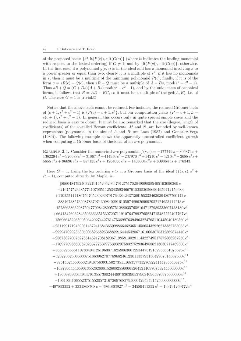
Notice that the above basis cannot be reduced. For instance, the reduced Grobner basisof (c+ 1, s2 + c2 − 1) is {P (c) = c+ 1, s2}, but our computation yields {P = c+ 1, L =s(c + 1), s2 + c2 − 1}. In general, this occurs only in quite special simple cases and thereduced basis is easy to obtain. It must be also remarked that the size (degree, length ofcoefficients) of the so-called Bezout coefficients, M and N , are bounded by well-knownexpressions (polynomial in the size of A and B; see Loos (1982) and Gonzalez-Vega(1989)). The following example shows the apparently uncontrolled coefficient growthwhen computing a Grobner basis of the ideal of an s–c polynomial.

Example 2.4. Consider the numerical s–c polynomial f(s, c) = −177749 s− 806874 c+1362294 c2−926688 c3−31867 c4 +414950 c5−237970 c6 +54210 c7−4216 c8−2688 c7s+5655 c6s+ 96696 c5s− 557135 c4s+ 1264056 c3s− 1438004 c2s+ 809864 cs+ 176343.

Here G = 1. Using the lex ordering s > c, a Grobner basis of the ideal (f(s, c), s2 +c2 − 1), computed directly by Maple, is:

[8960484792403227914520620347912751702649098085405193090369 s−2167575234857741070651125343593466791525520566904959412159683

+11925514418075970523023979176438424373661553324630394807760142 c−3834673857320878379743098402916105974896269992952124653414213 c2

−152366386329875047709842890575128803576581647127989533607438180 c3

+664134269628435066636515307207119107647992765824715482222407767 c4

−1569664522659950342027442761475369976394963224765110445040189560 c5

+2511991719469051437241684365098866462365145865432926213382755055 c6

−2929470292353050068265825368822154445420671610603075312869874440 c7

+2567382700752785146217081820671985813028114322749517572866287250 c8

−1709770986600820233777532775393297583275293649586213030717469500 c9

+863622566611078340412619638718259063061293447519152955661075625 c10

−326270525085033751863962707769682461230113379313042967314687500 c11

+89514624550553249487563931502735111683577332769224144785546875 c12

−16879644546590135526268815260825560065264521109707592445000000 c13

+1960983930449447913557380244499793639053790340965970375000000 c14

−106106416655237515520572167269768379560042953491524000000000 c15,

−497853352 + 3331868708 c− 3984863927 c2 − 34589411352 c3 + 193791269772 c4


Figure 5.

−533397801792 c5 + 976942396828 c6 − 1302962510900 c7 + 1315151818514 c8

−1021659798700 c9 + 613378624075 c10 − 282939548500 c11 + 98628515625 c12

−25180375000 c13 + 4450203125 c14 − 487500000 c15 + 25000000 c16].

Of course, the first polynomial corresponds to L and the second to the minimal poly-nomial P .

In general, given a numerical s–c polynomial f(s, c) = A + Bs, the system {f =0, s2 + c2 − 1 = 0} has twice as many solutions (properly counted) as the degree of f . Acommon way of solving such a system is to rewrite s = sin(θ) and c = cos(θ) as rationalfunctions of the tangent of the half angle θ/2, and to consider the univariate polynomialin the numerator of the resulting expression. This implies a lot of computations and someextra problems due to the potential cancellation of factors (see Section 4). It is easierto solve the system using the polynomials in its Grobner basis. Roughly, the idea is asfollows. First, we notice that the equation A+Bs can be considered as a curve in the s–cplane. This curve decomposes as a product of lines parallel to the s-axis (see Figure 5)and this product is equal to the G = gcd(A,B). For each line, the intersection with theunit circle s2 + c2 − 1 yields two values of s. Removing the common factor G in A+Bsgives a curve which intersects the unit circle in some points, all having for every differentc-coordinate, just one value of the s-coordinate. Thus, the corresponding value of s canbe linearly solved.

Formally speaking, we see that the minimal polynomial P (c) = G(A′2 − (1 − c2)B′2)has a degree equal 2 deg(f) − deg(G). For each root ρ of P (c) = 0 such that G(ρ) 6= 0,B(ρ) must be also different from zero, since B(ρ) = 0 and P (ρ) = 0 imply A(ρ) = 0and thus, having ρ as a common root of A and B, G(ρ) should be zero. So if G(ρ) 6= 0,the value of s can be obtained from the equation A(ρ) +B(ρ)s = 0, that gives only onevalue of s. It is important to remark that such values of s and c automatically verifys2 + c2 − 1 = 0, since the following identity holds:

P = GB′2(s2 + c2 − 1) +G(A′ +B′s)(A′ −B′s). (2.1)

In this way we can obtain 2(deg(f)−deg(G)) roots of the system. To obtain the valueof s corresponding to ρ, alternatively, we can solve L(s, ρ) = 0 directly for s, since

L(s, c) = sG+NA+MB(1− c2) = G(s+NA′ +MB′(1− c2)),


and thus, when G(ρ) 6= 0,

s = (ρ2 − 1)M(ρ)B′(ρ)−N(ρ)A′(ρ).

We claim that solutions P (ρ) = 0, with G(ρ) 6= 0, and the corresponding value for thesine s = (ρ2 − 1)M(ρ)B′(ρ) − N(ρ)A′(ρ), automatically verify both A + sB = 0 ands2 + c2 − 1 = 0. In fact,

A+Bs = A+B(−(1− c2)MB′ −NA′) = A+ (−(1− c2)MB′2G−NA′B′G).

Now, using that P (ρ) = 0, we replace −(1− c2)MB′2G by −MA′2G in the last equality,finally obtaining

A+Bs = A+ (−MA′2G−NA′B′G) = −A′G(−1 +A′M +B′N) = 0.

The claim follows using both this expression and identity (2.1) above.On the other hand, when G(ρ) = 0, we obtain two values of s solving, directly, the

equation (s2 + c2 − 1) = 0. Thus we find, in this way, the remaining 2 deg(G) values ofthe angle θ verifying the system.

Example 2.5. Let us take the numerical s–c polynomial f(s, c) = c6 − 10 c4 + c5s −12 c3s + 25 c2 + 35 sc + 3 c3 − 15 c + 3 sc2 − 21 s = A + sB = c6 − 10 c4 + 25 c2 + 3 c3 −15 c+ s(c5 − 12 c3 + 35 c+ 3 c2 − 21).

We have to compute G = gcd(A,B) = c3 − 5 c + 3, so the minimal polynomial isP (c) = G(A′2 − (1− c2)B′2) = (c3 − 5 c+ 3)(2 c6 − 25 c4 + 88 c2 − 49).

The zeroes of this polynomial, such that G 6= 0, are:

−2.439730614− 0.2075778378√−1,

−2.439730614 + 0.2075778378√−1,

−0.8255944410,0.8255944410,

2.439730614− 0.2075778378√−1,

2.439730614 + 0.2075778378√−1.

For each zero, the value of s is obtained from f(s, c) = A+ sB = 0:

(0.2273749746− 2.227306968√−1,−2.439730614− 0.2075778378

√−1),

(0.2273749746 + 2.227306968√−1,−2.439730614 + 0.2075778378

√−1),

(0.5642639624,−0.8255944410),(−0.5642639614, 0.8255944410),

(−0.2273750280− 2.227306978√−1, 2.439730614− 0.2075778378

√−1),

(−0.2273750280 + 2.227306978√−1, 2.439730614 + 0.2075778378

√−1).

The roots of the polynomial G(c) = 0 are:

−2.490863615, 0.6566204310, 1.834243184.

For each root, the two values of s are obtained from s2 + c2 − 1:

(−2.281315750√−1,−2.490863615), (2.281315750

√−1,−2.490863615),

(−0.7542211941, 0.6566204310), (0.7542211941, 0.6566204310),


(−1.537676188√−1, 1.834243184), (1.537676188

√−1, 1.834243184).

Thus, we have found 2 deg(f) = 2× 6 = 12 solutions in total, although there are onlyfour real solutions. On the other hand, computing the polynomial associated to f(s, c)in the tangent of the half-angle substitution seems, clearly, much more involved.

2.3. parameter specialization

It is often the case in kinematics that the coefficients of f(s, c) are given in a domainwith parametric coefficients, say Q[d1, . . . , dm]. We then write f(s, c) = f(d1, . . . , dm; s, c)to highlight this fact. Rather than solving the sine–cosine equation over some extension ofthe quotient field Q(d1, . . . , dm), one is interested in studying the solution of the special-ized systems, i.e. those obtained by (partially) replacing the parameters {d1, . . . , dm} forreal numerical values {d0

1, . . . , d0m}. As the previous paragraphs show, the structure of the

minimal polynomial P (c) is relevant for solving f(s, c) = 0. Unfortunately, Grobner basesdo not specialize well: it is not true, in general, that the specialization of the minimalpolynomial for f(d1, . . . , dm; s, c) agrees with the minimal polynomial of the specializedsystem f(d0

1, . . . , d0m; s, c). Still some analysis of this situation is possible.

It is clear that the canonical form A(d1, . . . , dm; c)+sB(d1, . . . , dm; c) of f(d1, . . . , dm; s,c) specializes to the canonical form of f(d0

1, . . . , d0m; s, c), since it is obtained rewriting

s2 = 1 − c2. Next, let G(d1, . . . , dm; c) = gcd(A(d1, . . . , dm; c), B(d1, . . . , dm; c)), wherethe gcd is computed in Q(d1, . . . , dm)[c]. Then:

G(d1, . . . , dm; c) gcd(cont(A), cont(B)) = G′(d1, . . . , dm; c)

where cont denotes the content of a polyomial in c with coefficients in Q[d1, . . . , dm] andG′ is the gcd(A,B) ∈ Q[d1, . . . , dm][c]. Now G′(d1, . . . , dm; c) divides A(d1, . . . , dm; c) andB(d1, . . . , dm; c); therefore,G′(d0

1, . . . , d0m; c) divides A(d0

1, . . . , d0m; c) and B(d0

1, . . . , d0m; c)

when A(d01, . . . , d

0m; c) + sB(d0

1, . . . , d0m; c) is not zero (the interesting case), hence it di-

vides the gcd(A(d01, . . . , d

0m; c), B(d0

1, . . . , d0m; c)). It follows that specializing the minimal

polynomial for A(d1, . . . , dm; c) + sB(d1, . . . , dm; c),

A2(d01, . . . , d

0m; c)− (1− c2)B2(d0

1, . . . , d0m; c)

G′(d01, . . . , d

0m; c)

one obtains just a multiple of the minimal polynomial of the specialized system

A(d01, . . . , d

0m; c) + sB(d0

1, . . . , d0m; c).

It follows that the degree of this minimal polynomial can be lower than that of thegeneral case iff the numerator A2(d0

1, . . . , d0m; c) − (1 − c2)B2(d0

1, . . . , d0m; c) has a lower

degree or if G′(d01, . . . , d

0m; c) strictly divides gcd(A(d0

1, . . . , d0m; c), B(d0

1, . . . , d0m; c)). Let n

be the degree of A(d1, . . . , dm; c) + sB(d1, . . . , dm; c) as a polynomial in s, c and supposethat for some numerical values, the coefficients of the terms of highest degree in c ofA2(d1, . . . , dm; c)− (1− c2)B2(d1, . . . , dm; c) vanish. Then,

(coeff(cn))2 + (coeff(scn−1))2 = 0 (2.2)

where coeff(cn), etc . . . , denotes the coefficient of the cn term in A+ sB, etc. . . . Whenwe consider only real numerical values of the parameters, this condition is equivalent to

coeff(cn) = 0 and coeff(scn−1) = 0. (2.3)

Obviously, this condition is equivalent to lowering the total degree of A+ sB as an s–c


polynomial. If we allow complex values for the parameters, condition (2.2) is equivalentto

coeff(cn) +√−1 coeff(scn−1) = 0, (2.4)

or

coeff(cn)−√−1 coeff(scn−1) = 0. (2.5)

Therefore, under these conditions, the specialized system has a lower degree than inthe parametrized case.

The above results can also be interpreted from the point of view of cocircularity. As inMourrain (1996) or Merlet and Lazard (1994), the cocircularity of a two-variable equationis the minimum of the multiplicity of the curve at the two cyclic points of infinity: i.e. theprojective points (1,

√−1, 0), (1,−

√−1, 0), that are the points at infinity of a projective

circle. If we consider our parametrized equation A+ Bs as a curve in the variables s–c,the fact that, for specific values of the parameters, this curve passes through one of thecyclic points, is exactly equivalent to the vanishing of one of (2.4) or (2.5): thus (2.3) isthe condition for having a multiplicity of at least 1 at both points. It is shown in theabove-mentioned papers that cocircularity lowers the degree of intersection of the curveA+Bs with the curve s2 + c2 − 1: Mourrain (1996) shows that the “number of commonpoints properly counted” (i.e. our solutions to the s–c equation) is less than or equal to:

deg(A+Bs) deg(s2 + c2 − 1)− 2 · cocircularity (A+Bs) · cocircularity (s2 + c2 − 1).

Now, the cocircularity of the circle is always 1 and the cocircularity of the s–c curveis at least 1 if (2.4) and (2.5) simultaneously hold. Moreover, the formula above holdswith equality if the two curves have no other common points at infinity, the multiplicityat cyclic points is the same for both and they are not tangent at the cyclic points. It iseasy to see that both A + Bs and s2 + c2 − 1 have no other common points at infinity;moreover the multiplicity of the circle at the cyclic points is 1 and with tangent s = 0in the affine plane that contains such points with c = 1. Further, one can compute themultiplicity and tangents of A + Bs at the cyclic points as a function of the differentcoefficients of this polynomial.

3. Factorization of s–c Equations

In this section we deal with the problem of factoring (over an orderable field) a givensine–cosine polynomial f(s, c), mod s2 + c2 − 1. We will denote, sometimes, its normalform A + Bs by NF (f(s, c)) or NF (f). Since our aim is simplifying the solution of asine–cosine equation, we might assume that the given polynomial is already in normalform and that no polynomials in c can be factored out from f (as this is trivially attainedby an univariate gcd computation). Next we note that f = ghmod s2 + c2 − 1, impliesf = NF (g)NF (h) mod s2 + c2 − 1. Moreover, in this section we deal with an orderablecoefficient field such as Q, Q(d1, . . . , dm), R, etc . . . . (more specifically, all we need isthat −1 is not a square in the field), as is the case in most applications. Then the equalityf = ghmod s2+c2−1, among normal-form polynomials, implies deg(f) = deg(g)+deg(h)(see Lemma 3.1 below). Thus, factoring f over an orderable field essentially means findingpolynomials g(s, c), h(s, c), already in normal form and verifying f = ghmod s2 + c2− 1,plus the conditions: deg(f) > deg(g) and deg(f) > deg(h), in order to avoid trivialfactorizations.


3.1. the defect

In what follows the defect plays an important role in the well-known relation betweenthe trigonometric functions sine and cosine of θ and the tangent of θ/2. The parametriza-tion

s =2t

1 + t2, c =

1− t21 + t2

(3.1)

covers, for finite values of t, the whole unit circle except the point (−1, 0). Thus thevalues s = 0 or c = −1 have to be studied with some care.

Definition 3.1. The defect of an s–c polynomial, def(f) is the maximum power of (c+1)that divides NF (f(s, c)).

Given a polyomial f(s, c), after performing the above substitution of s and c by t-rational functions and clearing denominators we obtain a polynomial T (f) in the variablet (the associated t-polynomial to f(s, c)). Then it is easy to prove the following facts:

1. T (f) has no (t2 + 1) as a factor (by construction).2. The closest integer bigger or equal to deg(T (f))

2 = d(

deg(T (f))2

)e , is equal to

deg(NF (f(s, c)))− def(f(s, c)).

That is:2 deg(NF (f))− 2def(f) = deg(T (f))

or2 deg(NF (f))− 2def(f)− 1 = deg(T (f)).

3. The degree of T (f) is odd iff c+ 1 is a factor in A to a larger power than in B (forinstance, if A = 0 and B 6= 0).

Conversely, if we start with a t-polynomial T (f) without (1 + t2) factor, and we divideT (f) by (1 + t2) to the power d(deg(T (f))

2 )e, and we perform the inverse substitution

t =1− cs

, (3.2)

we obtain an s–c polynomial in normal form and without defect, such that the given T (f)is the associated t-polynomial. Moreover, if we divide by (1+t2) to the power d(deg(T (f))

2 )eplus some natural number r, we obtain an s–c polynomial of defect exactly r. Thus,there is a non-injective mapping from normal form s–c polynomials to t-polynomials notdivisible by (1 + t2), since dividing the given s–c polynomial by a power of (c+ 1) (whenpossible) has no effect in the corresponding t-polynomial.2

The following lemma will be very useful.

Lemma 3.1. Let f, g, h be normal-form polynomials over an orderable field, such thatf = gh, modulo (s2 + c2 − 1). Then:

1. deg(f) = deg(g)+deg(h). Therefore, the constants are the only multiplicative unitsin K[s, c]/(s2 + c2 − 1).


2. T (f) = T (g)T (h).3. def(f) = def(g) + def(h), except when both T (g) and T (h) are of odd degree, and

in this case, def(f) = def(g) + def(h) + 1.

Proof. (i) Assumeg = gnc

n + gn−1cn−1s+ · · · ,

h = hmcm + hm−1c

m−1s+ · · · ,are normal forms of degree n,m, respectively, where gn, gn−1 represent the coeffi-cients of cn and cn−1s in g, and so on. Then, the normal form of gh is (gnhm −gn−1hm−1)cn+m + (gnhm−1 + gn−1hm)cn+m−1s + · · ·. Now, we observe that can-celling both coefficients of total degree n+m implies

gnhm − gn−1hm−1 = 0, gnhm−1 + gn−1hm = 0.

Since we have assumed our polynomials to be of degree n,m, neither both gn, gn−1

nor hm and hm−1 can be zero. But the homogeneous system (in the variableshm, hm−1) has g2

n + g2n−1 as the determinant. Then this system has no non-zero

solution over a field where −1 is not a square. Contradiction.(ii) In fact, performing the substitution of (3.1) in f = gh,mod(s2 + c2− 1), we obtain

that the product of T (g) and T (h) does not divide (1 + t2), since the groundfield does not contain i; therefore, the product of the numerators (T (g), T (h)) anddenominators (powers of 1 + t2) of the irreducible rational fractions associated tog and to h already gives an irreducible fraction, i.e. with the numerator equal toT (f).

(iii) This is easy, considering the above two items and the equalities linking the degreeof a polynomial, its defect and the degree of the associated t-polynomial.2

The equality 1 = (√−1c− s)(

√−1c+ s) mod s2 + c2 − 1 shows that the above lemma

fails if the coefficient field contains√−1. Even so, it is easy to observe that these units

are, essentially, the only ones in such cases. This remark allows us to extend, with somemodifications, the factorization procedure below to arbitrary fields.

3.2. factorization

As stated in the introduction to this section, in order to factor over an orderable fielda given s–c polynomial, mod s2 + c2 − 1, we can assume that the given polynomial is innormal form and has no c-factors; in particular that it has no defect. Moreover, we onlylook for factors that are also in normal form.

Proposition 3.1. Under the above conditions, if there are normal-form polynomialsg, h such that f = gh, mod(s2 + c2 − 1), and deg(f) > deg(g),deg(f) > deg(h), thenT (f) = T (g)T (h) and deg(T (f)) > deg(T (g)),deg(T (f)) > deg(T (h)) (i.e. T (f) is notirreducible as a univariate polynomial in t). Moreover, if deg(T (f)) is even, then it cannothappen that deg(T (g)),deg(T (h)) are both odd.

Proof. Let f = A + Bs, g = C + Ds, h = M + Ns. Then A = CM + DN(1 − c2)


and B = CN + DM , by uniqueness of canonical forms. It follows also that g and hhave no defects, since if, say, g has a defect, then C and D will be divisible by (1 + c)and so will A and B, by the above relations. Considering the associated t-polynomialsT (f), T (g), T (h), we know by the above lemma that T (f) = T (g)T (h) and thus thatdeg(T (f)) = deg(T (g))+deg(T (h)). But deg(T (f)) = 2 deg(f) or deg(T (f)) = 2 deg(f)−1, and the same alternative holds for the other polynomials.

Now, if deg(T (f)) = 2 deg(f), it could happen that deg(T (g)) and deg(T (h)) are,respectively, 2 deg(g), 2 deg(h) or 2 deg(g) − 1 and 2 deg(h) − 1. In the first case weeasily conclude that deg(f) > deg(g),deg(f) > deg(h) implies deg(T (f)) > deg(T (g)),deg(T (f)) > deg(T (h)) and we are done. If both deg(T (g)),deg(T (h)) are odd, then byLemma 3.1, the defect of f cannot be zero (since it is at least one more than the sum ofthe defects of g and h), against the assumption that f has no defect.

If deg(T (f)) = 2 deg(f) − 1, then we must have, say, deg(T (g)) = 2 deg(g) − 1 anddeg(T (h)) = 2 deg(h). Again, deg(T (f)) > deg(T (g)),deg(T (f)) > deg(T (h)) sincedeg(T (f)) 6= deg(T (h)) for parity reasons and deg(T (f)) > deg(T (g)) because deg(f) >deg(g).

Proposition 3.2. Conversely, the existence of a proper factorization of T (f) = GH,allows us to recover a proper factorization of f , except when deg(T (f)) is even and bothdeg(G),deg(H) are odd.

Proof. We must distinguish between two cases:

Case a All deg(T (f),deg(G),deg(H) are even.Here deg(f) = deg(T (f))

2 . Since deg(T (f)) = deg(G) + deg(H), dividing T (f) by

(1 + t2)deg(T (f))

2

is the same as dividing by

(1 + t2)deg(G)

2 (1 + t2)deg(H)

2 .

Thus G and H are converted, by the inverse substitution, into normal form, defect-less factors g, h of f . Let us show that they verify deg(f) > deg(g),deg(f) > deg(h).We have that deg(G) and deg(H) are, respectively, equal to 2 deg(g), 2 deg(h). Sincethe factorization of T (f) is proper, deg(T (f) > deg(G),deg(H), and this directlyyields deg(f) > deg(g),deg(f) > deg(h).

Case b Degree of T (f) is odd. In this case the degrees of G and H must be odd and evenor conversely. Assume the first is odd. Dividing T (f) by:

(1 + t2)deg(T (f))+1

2

is the same as dividing by:

(1 + t2)deg(G)+1

2 (1 + t2)deg(H)

2 .

Thus G and H are converted, by the inverse substitution, into defectless factorsg, h of f . Let us show that they verify deg(f) > deg(g),deg(f) > deg(h). We


have that deg(T (f), deg(G) and deg(H) are, respectively, equal to 2 deg(f) − 1,2 deg(g)−1, 2 deg(h). Since deg(T (f) > deg(G),deg(H), it directly yields deg(f) >deg(g),deg(f) > deg(h).2

We have seen that the existence of a factorization of f into lower-degree factors isequivalent to the existence of a factorization of T (f) into lower-degree factors, not bothof odd degree. Moreover, if T (f) has only a factorization into two odd-degree polynomialsG,H, then it follows that f has no factorization. Still a simplification can be attained insome cases. We must divide Tf by (1+t2)

deg(T (f))+22 , i.e. by (1+t2)

deg(G)+12 (1+t2)

deg(H)+12

to obtain a factorization of (c + 1)f(s, c) via the s–c polynomials g, h associated to Gand H. (Remark: none of these factors will be a multiple of c + 1, because there existsno defect in the associated s–c polynomials to G and H.) Since f cannot be factorized,the best we can hope is to factorize (c + 1)f . Moreover, because of the odd degrees ofG and H, we see that the two factors g, h are of the form: (c + 1)kX(c) + sY (c) andY (−1) 6= 0. Therefore, both have the root c = −1, s = 0 and all the remaining roots willbe roots of f(s, c) = 0. Thus solving f = 0 can be replaced by solving gh = 0. In thiscase deg(f) = deg(g) + deg(h)− 1. If the degree of, say H, is 1, the factorization yieldsno real advantage for solving the s–c equation, since deg(h) = 1,deg(g) = deg(f).

Example 3.1. We consider the following irreducible polynomial f(s, c) ∈ Q[s, c]:

−3/2 c3 − 7/2 sc2 + 7/4 c2 − 5 sc+ 9/2 c− s+ 5/4.

After performing the tangent half-angle substitution (3.1) and clearing denominators,we obtain the associated t-polynomial T (f):

t5 − 7 t4 + 10 t3 + 11 t2 − 19 t+ 6.

Now, we factor T (f) = GH, where

G = t2 − 5 t+ 3, H = t3 − 2 t2 − 3 t+ 2.

We consider the rational functions (Case b):

G

1 + t2,

H

(1 + t2)2

and we perform the inverse substitution (3.2) to these rational functions, yielding:

m(s, c) = c− 5/2 s+ 2, n(s, c) = c2 + c− sc− 1/2s.

We finally obtain a factorization mod the circle:f(s, c) = (c− 5/2 s+ 2)(c2 + c− sc− 1/2s) + (−5/2 c− 5/4)(s2 + c2 − 1).

Example 3.2. Now, we consider the following polynomial f(s, c):

6 c4 − 36 sc3 − 24 c3 + 52 c2 − 104 sc2 − 92 sc+ 56 c+ 6− 24 s.

The associated t-polynomial T (f) is:

32 t8 − 32 t4 + 96 t3 − 160 t6 + 160 t2 − 512 t+ 32 t5 + 96.

Now, we factor T (f) = GH, where

G = 4 t3 − 20 t+ 4, H = 24− 8 t+ 8 t5.


The degrees of G and H are both odd and there is no other factorization, so the bestwe can hope is to factorize a multiple of f(s, c) of the form (c + 1)f(s, c). In the sameway, we have to consider the rational functions :

G

(1 + t2)2,

H

(1 + t2)3

and we perform the inverse substitution (3.2) to these rational functions, yielding:

m(s, c) = c2 − 6 sc+ 2 c− 4 s+ 1, n(s, c) = 3 c3 + 9 c2 + 9 c− 4 sc+ 3.

We finally obtain a factorization of (c+ 1)f(s, c) mod the circle:

f(s, c)(c+1) = 2(c2−6 sc+2 c−4 s+1)(3 c3+9 c2+9 c−4 sc+3)+(−48c2−32c)(s2+c2−1).

4. Simplification by Extraneous Factors

4.1. case of one equation

Let us go back to Section 2.3, 2.4 and 2.5, involving some coefficients of an s–c poly-nomial in normal form f(s, c) = A(c) + B(c)s. As in Section 2.3, let us assume thesecoefficients are polynomials in several parameters (robot class and pose parameters, asexplained in Section 1), i.e. A(c), B(c) ∈ Q[d1, . . . , dm][c]. In Section 2.3 we stated con-ditions that the coefficients should verify in order to lower the degree of the minimalpolynomial of the evaluated s–c polynomial. Here we are going to obtain a different in-terpretation in connection with the associated t-polynomial, introduced in Section 3.1.Suppose that for some numerical values of the geometric or robot-class parameters, oneof the above equations (say (2.4)) is identically zero for all pose parameters. Then oneknows that for such concrete geometric parameters the s–c equation will have less solu-tions than expected. This implies that if we perform in the unevaluated s–c equation thehalf-angle tangent substitution (see Section 3.1 (3.1)) and then we evaluate the parame-ters for the numerical values, some “extraneous” factor (t+

√−1) or (t−

√−1) occurs in

the numerator of the evaluated expression, since the number of solutions is reduced. Theconclusion is that there can be, as shown in the example below, simplifications withoutnecessarily involving second-degree extraneous factors (of course, this involves complexsolutions of (2.4), but such solutions can appear quite naturally as in Kovacs and Hom-mel (1993a, Example 2.1), where d = 5

√−1/3). This possibility is somehow overlooked

in previous work (see Kovacs and Hommel (1993a)), where such simplification is alwayslinked with the existence of factors of the kind 1 + t2. This possibility also seems to benot regarded by Mourrain’s formula (see Mourrain (1996)), which always diminishes byeven quantities the number of solutions of the s–c equation that are lost due to cocir-cularity contributions. Obviously, when we restrict to real solutions of (2.4), if there areany, we will have then an even-number reduction of the minimal-equation degree, sinceboth leading coefficients of A(c) and B(c) will be zero for these values of the parameters.Therefore, in the real case, the contribution of (2.4) is that 1 + t2 appears as a factorin the numerator after the t-substitution. A similar explanation arises from cocircularityconditions.

Example 4.1. Consider the s–c polynomial: f(s, c) = c4d+2 c4−d2sc3−5 dsc3−6 sc3−2 c2 + c3 − 5 c+ s− 3.


The associated t-polynomial T (f) is:−7−4 dt2 +6 dt4−4 dt6 +dt8 +6 d2t3−6 d2t5 +d−2 d2t−10 dt−10 t−32 t2−2 t4−8 t6+t8 + 42 t3 − 30 t5 + 14 t7 + 2 d2t7 + 30 dt3 − 30 dt5 + 10 dt7.In general, the minimal polynomial of the system {f(s, c) = 0, s2 + c2 − 1 = 0} has

degree 8:8 + 30 c+ 38 c2 + (2 d2 + 10 d+ 26)c3 − (−6 d− 18)c4 − (−2 d2 − 20 d− 36)c5−(−d4 − 10 d3 − 37 d2 − 64 d− 43)c6 + (2 d+ 4)c7 + (d4 + 10 d3 + 38 d2 + 64 d+ 40)c8,but for some values of d, satisfying some of (2.3), (2.4) and (2.5) the corresponding

evaluated f(d) has, at most, seven zeroes. Solving each of these equations we obtain thevalues d = −2 (root of (2.3)), d = −3 +

√−1 (root of (2.4)) and d = −3−

√−1 (root of

(2.5)).For instance, if we take d = −3 +

√−1, then f(−3 +

√−1) = −c4 +

√−1c4 + sc3 +√

−1sc3 − 2 c2 + c3 − 5 c+ s− 3, and the minimal polynomial has only seven zeroes:8 + 30 c+ 38 c2 + 12 c3− 2

√−1c3− 6

√−1c4 + 8 c5− 8

√−1c5 + 5 c6− 6

√−1c6− 2 c7 +

2√−1c7.

Moreover, it can be checked that this corresponds with the presence of a factor (t +√−1) in the evaluated t-polynomial, that factors as:(−2 +

√−1

5

) (5 t7 − 2 t6 −

√−1t6 − 13 t5 + 6

√−1t5 − 12 t4 − 11

√−1t4 + 35 t3

+ 20√−1t3 + 14 t2 − 23

√−1t2 + 13 t

+ 14√−1t+ 8− 21

√−1) (t+√−1).

For d = −2, we have f(−2) = c3 − 2 c2 − 5 c+ s− 3 and the minimal polynomial is:8 + 30 c+ 38 c2 + 14 c3 − 6 c4 − 4 c5 + c6.Again, we check that this corresponds with the presence of a factor 1 + t2 in the

t-polynomial:−(1 + t2)(t6 − 2 t5 − t4 − 4 t3 + 15 t2 − 2 t+ 9).

In summary, (2.4) and (2.5) constitute the positive and negative control equationsof Kovacs and Hommel (1993a), but, contrary to that stated there (Section 3.1), bothequations do not need to be satisfied simultaneously, but alternatively, in order to havea “simplification” of the degree of the resulting s–c polynomial, when the solutions ofsuch equations are replaced in the given s–c polynomial. Of course the main objectionto Kovacs and Hommel (1993a), and to our comments here, is that no complex values ofparameters are usually involved in robotic problems; therefore, control equations shouldbe better replaced by the more natural system (2.3), which yields the same real roots.

In fact, this remark makes sense for one s–c equation with parametric coefficients. Butif we extend this analysis to several s–c parametric equations, searching for conditionsthat lead to a simpler system solution, we will have to check whether there is a commonroot for all (say, positive) control equations (2.4) derived from each of the equations ofthe system. We will see that such a common root, even if complex, is just an indicatorof simplification and has no physical interpretation in terms of the robot parameters.

4.2. case of several equations

Let us consider this apparently innocent system:35sd+ c− 5 = 0, s− 3

5cd+ 2 = 0.


We see that the positive control system (2.4)

1 +35d√−1 = 0,

−35d+√−1 = 0,

for both equations has as common root d = 5√−13 and that, analogously, the negative

(2.5) control has as common solution d = − 5√−13 .

This implies that mod s2+c2−1, and for the value, say, d = 5√−13 , each of the equations

of the given system yields a minimal cosine equation of one degree less than expected (it“should” have been (formally) two degree, but it is first degree), of course, with complexcoefficients; but, one does not need to evaluate d to obtain such simplification. In fact, thef(s, c) equation obtained eliminating d in the ideal ( 3

5sd+ c− 5, s− 35cd+ 2, s2 + c2− 1):

Elim(d, Ideal

(35sd+ c− 5, s− 3

5cd+ 2, s2 + c2 − 1

))= Ideal

(s− 5

2c+

12, c2 − 10

29c− 3

29

);

has a degree lower than expected: it “should” have been second-degree in s–c, and, there-fore fourth-degree in c. . . . We remark that the complex value of d that is hidden behindthis simplification does not imply that complex numbers or values of the parameter areinvolved in the usual solving of the above system, nor if we eliminate it with respect to“d”:

Elim(s . . . c, Ideal

(35sd+ c− 5, s− 3

5cd+ 2, s2 + c2 − 1

))= Ideal

(d2 − 700

9

).

Since this behaviour requires only the existence of solutions for the positive (or thenegative) control system, and do not involve the solutions themselves, in the case ofsystems (as it is usual in robotics) where, besides the parameters, the coefficients onlyconsist of real numbers, the satisfiability of system (2.4) implies—by conjugation—thesame for the other system (2.5), and thus we only need to check one of them.

This analysis can be also explained via the half-angle tangent substitution as in Kovacsand Hommel (1993a). Essentially, it involves the following argument: the fact that boththe positive and negative control systems have (separately) a common root for all equa-tions of the given system in s–c, implies that both t =

√−1 and t = −

√−1 are roots

of each of the equations of the associated t-system, after parameter evaluation in thecorresponding common root (a root for the positive control and another one, perhaps,for the negative control system). Of course, the common roots of the control systems are,in general, complex values of the parameters. But it also implies that if we eliminate allthe parameters in the associated t-system, a factor (1+ t2) appears in the resulting equa-tion in t alone, by well known properties of elimination ideals. This elimination makesthe difference with the one variable case, since the elimination procedure does not yieldcomplex coefficients. Thus, converting this t-equation back to the s–c form gives a lowerthan expected degree, but no complex coefficients.

A similar argument can be made without the detour to the half-angle substitution:we homogenize the given system with respect to the s–c variables and then look forsome solutions at infinity in the circle s2 + c2 − 1. This implies looking for values of the


parameters that satisfy the system for the values (1,√−1, 0) and (1,−

√−1, 0) where the

first coordinate is the c-value, the second is the s-value and the last one is the value ofthe homogenizing variable. If there are such values of the parameters, then we know thatin the system there are roots of the s–c elimination equation which lie at infinity whenintersected with the circle. Clearly, a system without this property would have more affineroots and correspondingly a greater degree. Of course this is an argument at geometriclevel and we should be sure that the algebraic elimination reflects well the geometricproperties for the geometric object defined by the system (for instance, that the givensystem defines a radical ideal). But the same prevention holds for the argument of Kovacsand Hommel (1993a): the fact that some roots

√−1 and −

√−1 appear as a solution, does

not immediately imply that they are eliminated if we merely apply algebraic eliminationto the given system. Fortunately, there are results, such as in Gonzalez-Lopez and Recio(1994), that show that in general this is the case for robotic kinematic systems.

Example 4.2. Consider the system of Section 2.2 in Kovacs and Hommel (1993a):

I = Ideal(10s2s1 − 4dc1 + 7, 4ds1 + 5c1 − 1, s22 − ds1 − 5

2s2c1, s21 + c21 − 1);

Elim(d . . . c2, I) = Ideal(2490 c21 + 216 c1 − 1765 c31 − 168− 5850 c41 + 4500 c51 + 168 s1

+3750 c61 − 3125 c71,−5700 c21 + 3000 c1 − 17385 c31 + 288+22675 c41 + 29750 c51 − 32500 c61 − 15625 c71 + 15625 c81).

We obtain an eighth-degree, c1 polynomial, lower than the expected tenth-degree.Next we suppose we had not performed this elimination and we are going to discoverbeforehand this simplification property. Let us consider the equations in the system aspolynomials in s1–c1, and let us write the following conditions for the vanishing of thehighest terms in each equation, using, say, the control system

coeff(cn1 ) +√−1 coeff(s1c

n−11 ) = 0,

yielding the equations

J = Ideal(

10√−1s2 − 4d, 4

√−1d+ 5,−

√−1d− 5

2s2

);

Thus we see that the system has the solutions d = 5√−14 , s2 = 1

2 and, therefore, thatit will simplify.

The same behaviour appears considering the other control system (but we do not reallyneed to check it):

J = Ideal(−10√−1s2 − 4d,−4

√−1d+ 5,

√−1d− 5

2s2

);

Having the solution d = −5√−1

4 and s2 = 12 .

Next let us do the same analysis for a slightly modified system, just replacing d byd+ 1 in one of the equations:

I = Ideal(10s2s1 − 4dc1 − 4c1 + 7, 4ds1 + 5c1 − 1, s22 − ds1

−52s2c1, s

21 + c21 − 1);

Elim(d . . . c2, I) = Ideal(−11850024350090 c21 + 5114748702424 c1 − 5968155398275 c31


+35787289050974 c41 + 55803661416− 27249557499918 c61+603141306456 s1 − 9273122053668 c51 + 12819381869165 c71+3228072837500 c81 − 1881053475000 c91,−10748 c21 + 1656 c1 + 1163 c31+42123 c41 + 288− 52228 c61 − 23198 c51 + 41619 c71+15953 c81 − 21500 c91 + 5000 c10

1 ).

Here the degree in c1 is ten and not eight as in the previous system. Let us see whathappens with the control-system equations in this case:

J = Ideal(−4(d+ 1) + 10s2

√−1, 5 + 4

√−1d,−5

2s2 −

√−1d

)J = Ideal

(10√−1s2 − 4d− 4, 4

√−1d+ 5,−

√−1d− 5

2s2

);

Then both Grobner basis are: [ 1 ].Thus, in this case there is no common solution for the control-system equation.

In Kovacs and Hommel (1993a) this analysis is called the simplification method bydetecting “extraneous” factors, because the fact that a factor (1 + t2) appears in the con-verted system by means of the half-angle substitution is “extraneous” to the affine solvingof such a system. The authors remark also that such a factor, easy to identify directly,can be hidden if the system is solved in some other variables: i.e. if instead of solvingwith respect to s1–c1 we solve with respect to some other joint variable, then it couldhappen that, again, some factors of the determining equation of this joint angle—lookingabsolutely different from (1 + t2)—are linked to the extraneous factor in s1–c1. Thismeans that other values of, say, angle s2–c2 (or length d of a prismatic joint), correspondto roots of the angle s1–c1 at infinity, and should therefore be simplified. However, thisis a dangerous way of reasoning: such values could also be linked to other finite values ofs1–c1, and therefore removing, by them we are losing correct solutions (configurations ofthe robot) of the system. Therefore, we should take care when simultaneously eliminatingall the induced extraneous factors without previously checking the consequences (see theexample below).

In Example 4.2, we checked that the solution s2 = 12 , in fact, is not extraneous since,

besides appearing linked with the cyclic s1–c1 points, we also have the (non-extraneous)system solution:

d =54, s2 =

12, c2 =

√3

2, s1 = −3

5, c1 =

45.

4.3. Rabinowistch’s trick

Finally, we must observe that by directly applying the half-angle substitution it is quitepossible to eliminate extraneous roots by adding to the system the equation (1 + t2)y − 1;this method (Rabinowistch’s trick) is no more costly than the direct elimination proce-dure: it was not studied in Kovacs and Hommel (1993a) since it was considered com-plicated in obtaining general ideal quotients. Recent methods for deciding this specificproblem appear in Alonso et al. (1995b) and Licciardi and Mora (1994), since it is linkedwith the implicitization problem of parametric curves and varieties. The next exampleshows the direct application of this observation.


Example 4.3. Let us consider the system of Example 4.2 :

I = Ideal(f1 = 10s2s1 − 4dc1 + 7, f2 = 4ds1 + 5c1 − 1, f3 = s2

2 − ds1 −52s2c1

).

First s1 and c1 are converted into t-polynomials and we consider the system of thet-polynomials:

Tf1 = 20 s2 t− 4 d+ 4 dt2 + 7 + 7 t2,T f2 = 8 td+ 4− 6 t2,T f3 = 2 s2

2 + 2 s22t

2 − 5 s2 + 5 s2 t2 − 4 td.

We solve the above system:Grobner basis ([Tf1, T f2, T f3], [d, s2, t],plex) =

[8 d− 9 t9 − 139 t− 214 t3 − 28− 336 t2 + 46 t5 + 70 t4 + 336 t6 + 122 t7 − 42 t8,−90 +1936 t2 − 398 t4 + 287 t + 1638 t3 + 350 t5 − 2108 t6 − 938 t7 + 276 t8 + 80 s2 + 63 t9, 4 +133 t2 + 214 t4 + 28 t+ 336 t3 − 70 t5 − 46 t6 − 336 t7 − 122 t8 + 42 t9 + 9 t10].

The unique polynomial involving t in the above Grobner basis is:

4 + 133 t2 + 214 t4 + 28 t+ 336 t3 − 70 t5 − 46 t6 − 336 t7 − 122 t8 + 42 t9 + 9 t10.

Factoring this polynomial, we obtain the extraneous factor 1 + t2:

(3 t+ 1)(t+ 2)(1 + t2)(3 t6 + 7 t5 − 62 t4 + 14 t3 + 37 t2 + 7 t+ 2).

On the other hand, applying Rabinowitsch’s trick, we have to compute the followingGrobner basis:

Grobner basis([Tf1, T f2, T f3, (1 + t2)y − 1], [y, d, s2, t],plex) =[5000 y − 4996 + 56 t+ 5321 t2 + 1155 t3 − 3080 t4 − 938 t5 + 303 t6 + 63 t7, 8 d− 9 t7 −

135 t− 85 t3− 28− 308 t2 + 131 t5 + 378 t4− 42 t6, 80 s2 + 63 t7− 82 + 1998 t2− 2384 t4 +315 t+1351 t3−1001 t5+276 t6, 4+28 t+129 t2+308 t3+85 t4−378 t5−131 t6+42 t7+9 t8].

Now, the unique polynomial on t is:

4 + 28 t+ 129 t2 + 308 t3 + 85 t4 − 378 t5 − 131 t6 + 42 t7 + 9 t8.

Factoring this polynomial we have:

(3 t+ 1)(t+ 2)(3 t6 + 7 t5 − 62 t4 + 14 t3 + 37 t2 + 7 t+ 2).

So, we have eliminated the extraneous factor 1 + t2.

5. Fast Functional Decomposition of s–c Equations

5.1. foundations and notations

Given a sine–cosine polynomial f(s, c), if it decomposes as f(s, c) = g(h(s, c) mods2+c2−1, for some univariate polynomial g(x) and some bivariate polynomial h(s, c), thenit is clear that the same equality applies replacing f, h by its normal forms. Thus, in thissection we will study decomposition procedures assuming f is given in normal form andwe will look for normal-form composition factors h. Since our goal is to simplify solvingsine–cosine equations, we search for factors such that the degree of h is strictly smallerthan the degree of f . As in Section 3, we will assume that

√−1 /∈ K, the coefficient field,


to prevent some complications. Summarizing, the sine–cosine polynomial decompositionproblem can be stated as follows:

Definition 5.1. Given a bivariate, normal form, s–c polynomial f(s, c) in the polyno-mial ring K[s, c], we will say that f(s, c) is decomposable mod the circle if there exista univariate polynomial g(x) ∈ K[x] and a bivariate normal-form polynomial h(s, c) ∈K[s, c] with deg(h(s, c)) < deg(f(s, c)) such that:

f(s, c) = g(h(s, c)) mod s2 + c2 − 1.

Therefore, the decomposition problem for a given f is to decide if such g, h exist and,in the affirmative case, to find them.

From a computational point of view, it is important to know what is the relevance ofextending the coefficient field regarding the existence of decomposition. It is well known(see Gutierrez (1991)) that an ordinary bivariate polynomial f(x, y) ∈ K[x, y] is inde-composable over a field K iff it is indecomposable over any extension of K. We label suchproperty saying that ordinary polynomial decomposition is a rational problem. On thisissue the ordinary rational function decomposition problem differs from ordinary poly-nomial decomposition (see Alonso et al. (1995a)) as well as the sine–cosine polynomialdecomposition problem.

Example 5.1. Let us consider the numerical s–c polynomial, f(s, c) = 2 c2 +cs+1 withcoefficients over the rational numbers field. We can check with the SCDECPOL algorithm(see Section 5.2.2), that it is indecomposable mod the circle over the rational numberfield Q. However, it can be written as a composition, mod the circle, of polynomials withcoefficients over an algebraic extension Q. In fact, take:

g(x) =x2

−4 + 2√

5+

13− 6√

54− 2

√5, h(s, c) = c+ (−2 +

√5)s.

Then f(s, c) = g(h(s, c)) mod s2 + c2 − 1.

This implies that enlarging the coefficient field might lead to the discovery of newdecompositions. We will go back to this issue in Section 5.2.2, showing that our algorithmgives decompositions over any field extension of K where computations are possible(even if

√−1 is in this larger field). Another important aspect that we must consider

is the concept of equivalent decompositions. The idea is to consider as equivalent thosedecompositions that are related via the identity

x =(

(ax+ b)a

− b/a)

= (x/a− b/a) ◦ (ax+ b),

where ◦ denotes functional composition, for some a 6= 0, b ∈ K. Remark that, for all g, has above, this identity implies

g(x) ◦ h(s, c) = g(x) ◦ x ◦ h(s, c) = g(x) ◦ (x/a− b/a) ◦ (ax+ b) ◦ h(s, c)

and collecting the first and the last two (composition) factors in the last equality anapparently different decomposition arises.


Definition 5.2. Two decompositions of an s–c polynomial f(s, c), say:

f(s, c) = NF (g1(h1(s, c))) = NF (g2(h2(s, c)))

are called equivalent if there is a non-constant linear transformation u(x) = ax+b ∈ K[x]such that: ah1(s, c)+b = h2(s, c) and g1(x/a−b/a) = g2(x), i.e. g2(x) = g1(x)◦(x/a−b/a)and h2(s, c) = (ax+ b) ◦ (h1(s, c)).

It is well known (see Gutierrez (1991)) that if an ordinary polynomial f(x, y) has twodecompositions f(x, y) = g1(h1(x, y)) = g2(h2(x, y)) with deg(h1(x, y)) = deg(h2(x, y)),then they are equivalent. Again, this result does not hold for the ordinary rational func-tion decomposition (see Alonso et al. (1995a)), nor for the sine–cosine polynomial de-composition, as illustrated by the following example.

Example 5.2. Let us consider the numerical s–c polynomial:

f(s, c) = 8 c5s− 8 c3s− 6 cs− 12 c4 + 12 c2 + 1.

We have two decompositions, f(s, c) = NF (gi(hi(s, c))), i = 1, 2, where g1(x) =8 − 12x2 + 6x4 − x6, h1(s, c) = c + s and g2(x) = x6, h2(s, c) = c − s. So, we havetwo decompositions of f(s, c) with deg(h1(s, c)) = deg(h2(s, c)) = 1, but they are non-equivalent (by direct checking).

The most interesting decomposition in kinematics is when the composition factorh(s, c) has the smallest possible degree. On the other hand, finding all decompositionsmay be interesting for different applications. For instance, our method can compute allnon-equivalent decompositions, even irrational (in the sense of Example 5.1) decomposi-tions for real coefficients sine–cosine polynomials.

Example 5.3. The polynomial f(s, c) = 8 c5s−8 c3s−6 cs−12 c4 +12 c2 +1 has exactlythe following non-equivalent decompositions f(s, c) = NF (gi(hi(s, c))), i = 1, 2, 3, where

[g1(x) = 8− 12x2 + 6x4 − x6, h1(s, c) = c+ s][g1(x) = x6, h1(s, c) = c− s][g2(x) = 1− 6x+ 12x2 − 8x3, h2(c, s) = cs][g3(x) = 4x2, h3(s, c) = c3 + c2s− 3/2c+ 1/2s].

Besides these general observations, some normal forms of special polynomials turn outto be fundamental in our approach.

Definition 5.3. We define by recurrence the following polynomials in some new inde-terminate Z and with coefficients over the integer numbers:

A0(Z) = 1, B0(Z) = 0Am(Z) = Am−1(Z)− ZBm−1(Z)Bm(Z) = ZAm−1(Z) +Bm−1(Z).

Now it is easy to prove the following basic properties.

Lemma 5.1. For every positive integer m, we have:

(i) Am(Z)2 +Bm(Z)2 = (1 + Z2)m

(ii) Am(Z) + iBm(Z) = (1 + iZ)m, where√−1 = i.


(iii)

Am(Z) =(1 + iZ)m + (1− iZ)m

2.

Bm(Z) =(1 + iZ)m − (1− iZ)m

2i.

(iv) If m is an even natural number, then deg(Am(Z)) = m and deg(Bm(Z) = m − 1.If m is an odd natural number, then deg(Am(Z)) = m− 1 and deg(Bm(Z) = m.

(v) The rational functions Gm(Z) = Bm(ZAm(Z) are conjugate of power polynomials, that

is: Gm(Z) = w ◦ Zm ◦ w−1 (symbol ◦ for rational function composition), where wis the linear fraction w = −iZ+i

1+Z and w−1 = i−ZZ+i = 1+iZ

1−iZ .(vi) All roots of the polynomials Am(Z) = 0 and Bm(Z) = 0 are real. Moreover, they

do not have a common root.

Proof. The proof of the two first items can be done by induction on m. Item (iii)follows by solving the system given by (i) and (ii). Item (iv) is then immediate. Item (v)is immediate, the most difficult part is to remark the structure of this fraction, as stated.For item (vi), in the case of Am(Z), we consider (1+iZ)m

(1−iZ)m = −1 and then we remark that

the conformal mapping (1+iZ)(1−iZ) sends points from the real line onto the unit circle in the

plane R2 = C. For Bm is analogous. Finally, item (i) implies that the imaginary unit isthe only possible common root of Am, Bm, but since all their roots are real they do nothave common roots.

Next, we establish the relation between the normal form of a sine–cosine polynomialwith the polynomials Am(Z) and Bm(Z), defined above:

Lemma 5.2. Let Z0 be an arbitrary element of an extension of the field K, m a positiveinteger number, then we have:

(i) NF (c+ Z0s)m = Am(Z0)cm +Bm(Z0)cm−1s+D(s, c) with m > deg(D(s, c)).(ii) If m is odd, say m = 2k + 1, NF (sm) = (1− c2)ks.

(iii) If m is even, say m = 2k, NF (sm) = (1− c2)k.

Proof. It is straightforward, by induction on m, remarking that NF (c + Z0s)m =NF [(c+ Z0s)NF (c+ Z0s)m−1].

One might deal in a unified way with the above items, by homogenizing the wholesituation, i.e. showing that

NF (Y0c+ Z0s)m = Am(Y0, Z0)cm +Bm(Y0, Z0)cm−1s+D(s, c)

with m > deg(D(s, c)) etc.. . . where Y0, Z0 are elements in some extension of K and whereAm(Y, Z), Bm(Y, Z) represent the homogenization (as polynomials of formal degree m)of Am, Bm via the new variable Y . That is, Am(Y, Z) = Y Am−1(Y, Z) − ZBm−1(Y, Z),Bm(Y, Z) = ZAm−1(Y, Z) + Y Bm−1(Y, Z). This way of thinking, although it makesnotation more complicated, is particularly useful in the following.

Lemma 5.3. Let g(x) = gtxt + · · ·+ g0, a polynomial of degree t and let h(s, c) = hrc

r +


hr−1cr−1s+ · · · a normal form s–c polynomial of degree r. Then NF (g(x) ◦ h(s, c)) has

degree rt.

Proof. Clearly, the higher-degree terms of NF (g(x) ◦ h(s, c)) are the higher-degreeterms of the normal form of (hrcr +hr−1c

r−1s)t = c(r−1)t(hrc+hr−1s)t. By Lemma 5.3,the normal form of (hrc + hr−1s)t is Ar(hr, hr−1)ct + Br(hr, hr−1)ct−1s + D(s, c) witht > deg(D(s, c)). But Ar(hr, hr−1), Br(hr, hr−1) cannot be simultaneously zero. In factAr(Y0, Z0)2 + Br(Y0, Z0)2 = (Y 2

0 + Z20 )r (homogeneous version of Lemma 5.1.), thus if

Ar(hr, hr−1) = 0, Br(hr, hr−1) = 0 then (h2r + h2

r−1) = 0. But there are no non-trivialzeros of Ar, Br verifying this condition (see Lemma 5.1).

Lemma 5.4. (i) NF (g1(x) ◦ h(s, c)) = NF (g2(x) ◦ h(s, c)) implies g1 = g2 (right can-cellation property)

(ii) Two decompositions f(s, c) = NF (g1(h1(s, c))) = NF (g2(h2(s, c))) are equivalentiff K[h1] = K[h2] as subalgebras of K[s, c]/(s2 + c2 − 1).

Proof. Item (i) proceeds by considering that NF (g1(x) ◦ h(s, c)) = NF (g2(x) ◦ h(s, c))implies NF ((g1(x) − g2(x)) ◦ h(s, c)) = 0. Then, by Lemma 5.3, (g1(x) − g2(x)) musthave degree zero, and it follows it must be zero. For item (ii), if the two decompositionsare equivalent, by definition, it is trival that the two subalgebras are equal. Conversely,if K[h1] = K[h2], then there are polynomials p1(x), p2(x) such that h1 = p1(h2), h2 =p2(h1) mod s2 + c2− 1. Then h1 = (p1 ◦ p2)(h1) and h2 = (p2 ◦ p1)(h2) in the circle. Thisimplies, by the Lemma, that both p1 ◦ p2 and p2 ◦ p1 are first degree. Therefore, p1, p2

are linear and inverse to each other.

5.2. the decomposition algorithm

The general techniques developed for solving decomposition problems all tend to divideit into two parts: given the s–c normal form polynomial f(s, c), then

1. to compute “right”, normal form, candidates h(s, c) such that there is a decompo-sition f(s, c) = g(h(s, c)),mod s2 + c2 − 1;

2. to determine the corresponding “left” component g(x);3. to verify that f(s, c) = g(h(s, c)) mod s2 + c2 − 1.

As always the hard part is finding h(s, c), because to determine g(x) from f(s, c) andh(s, c) the most direct way is to explicitly solve a linear system of equations in theindeterminate coefficients of g(x) (with unique solution if it exists, because of the right-cancellation property). This works since, for a given h, the degree of the potential gs isbounded; therefore, we will not detail this point.

Example 5.4. Let K be a field that does not contain√−1. Let f(s, c) ∈ K[s, c] be an

s–c polynomial in normal form:

f(s, c) = Fn(s, c) + Fn−1(s, c) + . . .+ F1(s, c) + F0(s, c)

where Fi(s, c) are homogeneous polynomials of degree i of the form

Fi(s, c) = fi,0ci + fi−1,1c

i−1s


and, where fi,j ∈ K, Fn(s, c) 6= 0 and n is the total degree of the polynomial f(s, c).Now, after Lemma 5.3, for every positive r divisor of n (so that there exists a positiveinteger t with n = rt), we consider the possible, normal-form, candidates h(s, c) of degreer:

h(s, c) = Hr(s, c) +Hr−1(s, c) + · · ·+H1(s, c) +H0(s, c),where Hi(s, c) = hi,0c

i + hi−1,1ci−1s and Hr(s, c) 6= 0.

We would like to distinguish two possible cases.

(a) hr,0 6= 0.(b) hr,0 = 0.

In the first we can restrict to decompositions of f(s, c) such that

hr,0 = 1 and H0 = 0.

In fact, if f(s, c) = NF (g(h(s, c))), we can consider the linear transformation l(x) =hr,0x + h0,0 and we can define: g(l(x)) = g′(x), h′(s, c) = l−1(h(s, c)), where l−1(x) =h−1r,0x− h−1

r,0h0,0, yielding an equivalent decomposition of the f(s, c) with:

h′(s, c) = cr + Zcr−1s+H ′r−1(s, c) + · · ·+H ′1(s, c)

where H ′i(s, c) = Hi(s, c)h−1r,0 and Z = hr−1,1h

−1r,0 . We will say that h′(s, c) is a zero

symmetric, monic polynomial on c of degree r.Likewise, in the second case, we consider decompositions of f(s, c) such that the right

factor h′(s, c) is a zero symmetric, monic polynomial on c and s of degree r.Finally, to include both cases, we will say that the normal form polynomial h(s, c) is

normed iff it is zero symmetric and monic polynomial on c or on c and s.

5.2.1. determining candidates

Let f(s, c) ∈ K[s, c] be a normal form s–c polynomial of total degree n:

f(s, c) = Fn(s, c) + Fn−1(s, c) + · · ·+ F1(s, c) + F0(s, c)

where Fi(s, c) as above. Let r be a divisor of n, so n = rt, and we are looking for anormed polynomial h(s, c) of degree r and for a univariate polynomial g(x) of degree tsuch that f(s, c) = g(h(s, c)) mod s2 + c2−1. So, we have to compute the coefficients hi,jand gk where,

g(X) = gtxt + gt−1x

t−1 + · · ·+ g1x+ g0

so that the following equality holds:

f(s, c) = NF (gth(s, c)t + gt−1h(s, c)t−1 + · · ·+ g1h(s, c) + g0) =

gtNF (h(s, c)t) + gt−1NF (h(s, c)t−1) + · · ·+ g1(NFh(s, c)) + g0.

By Lemma 5.3, it is easy to see that the degree of the second and latter terms in theabove expression is at most r(t− 1) = rt− r = n− r. This fact suggests to define—as inthe ordinary polynomial case—the concept of approximate roots.

Definition 5.4. Let f(s, c) ∈ K[s, c] be a normal-form polynomial of degree n = rt. A


normal-form, degree r, normed polynomial h(s, c) ∈ L[s, c], where L is an extension fieldof K, is a tth approximate root of f(s, c) if there exists α ∈ L such that deg(f(s, c) −αNF (h(s, c)t)) ≤ n− r. 2

Trivially, if g(x) is a univariate polynomial and h(s, c) is a normed polynomial, ofdegrees t and r, respectively, then h(s, c) is a tth approximate root of NF (g(h(s, c))(since its degree will be rt, by Lemma 5.3). The key of the method for decomposing sine–cosine equations is the following result which shows the existence of tth approximateroots and how to compute them. As a consequence we will obtain the calculation off(s, c)-right candidates.

Proposition 5.1. With the above notation, there are exactly t, normed tth approximateroots h(s, c) ∈ K[s, c] of f(s, c), where K is the algebraic closure of K. More precisely:

(i) If fn,0fn−1,1 6= 0, then there are exactly t, monic on c, polynomials, which are tthapproximate roots of f(s, c).

(ii) If fn,0 = 0 and t is an even number, then there are exactly t, monic on c, polyno-mials which are tth approximate roots of f(s, c).

(iii) If fn,0 = 0 and t is an odd number, then there are exactly t − 1, monic on c, andone, monic on c and s, polynomials which are tth approximate roots of f(s, c).

(iv) If fn−1,1 = 0 and t is an odd number, then there are exactly t, monic on c, polyno-mials which are tth approximate roots of f(s, c).

(v) If fn−1,1 = 0 and t is an even number, then there are exactly t − 1, monic on c,and one monic on c and s, polynomials which are tth approximate roots of f(s, c).

Proof. We consider normed polynomials h(s, c) of degree r, with indeterminate coeffi-cients, and an indeterminate gt, and we impose that the terms of degree strictly higherthan r(t− 1) cancel out in the equation:

f(s, c) = gtNF ((Hr + · · ·+H1)t)

= gt

[NF ((Hr)t) +

(t

1

)NF [(Hr)t−1(Hr−1 + · · ·+H1)]

+(t

2

)NF [(Hr)t−2(Hr−1 + · · ·+H1)2] + · · ·

]Now, the degree of the second and latter terms in the above equation is at most

r(t− 1) + (r − 1) = rt− 1 < rt = n. Thus, we can consider the equation

f(s, c) = gtNF (Hr)t, (5.1)

and we determine Hr so that the terms of degree n = rt in this equation cancel eachother, that is:

deg(f(s, c)− gtNF ((Hr)t)) < n.

At this point, we have to distinguish two possibilities for the normed polynomial h:

Case a: h is monic on c.Case b: h is monic on c and s.

Case a: Assume that Hr = cr + Z0cr−1s; then we have to compute values of Z0 and


gt 6= 0 in some extension of K, so that the terms of degree rt cancel each other in (5.1).However,

NF ((Hr)t) = NF (cr + Z0cr−1s)t = c(r−1)t[At(Z0)ct +Bt(Z0)ct−1s+D(s, c)]

with t > deg(D(s, c)) (by Lemma 5.2.(i)).

Thus we have,

NF ((Hr)t) = At(Z0)crt +Bt(Z0)crt−1s+Q(s, c)] with rt > deg(Q(s, c))

and

f(s, c)− gtNF ((Hr)t) = (fn,0 − gtAt(Z0))cn + (fn−1,1 − gtBt(Z0))cn−1s+ · · ·Therefore, the values we are looking for are the solutions of the following system in Z, gt:

fn,0 − gtAt(Z) = 0,fn−1,1 − gtBt(Z) = 0.

We remark that fn,0 6= 0 or fn−1,1 6= 0, therefore no solution of the system simulta-neously makes At(Z) = Bt(Z) = 0; therefore the values of Z satisfying the system areexactly the roots (on some finite extension of K) of the resultant polynomial M(Z):

M(Z) = fn,0Bt(Z)− fn−1,1At(Z)

and then we obtain the corresponding values of gt substituting this value of Z and solvingsome of the above equations.

Next, we will show inductively that the remaining terms Hi(s, c) of NF (h(s, c)) canbe computed by solving a linear system with a unique solution. Suppose we have foundHr, . . . , Hi+1 verifying:

deg(f(s, c)−NF ((Hr + · · ·+Hi+1)t)) < r(t− 1) + (i+ 1).

Then, to find Hi, we arrange the equation

f(s, c) = gtNF ((Hr + · · ·+H1)t)

as

f(s, c) = gt(NF (Hr + · · ·+H1)t) = gt

[(NF (Hr + · · ·+Hi)t)

+(t

1

)NF [(Hr + · · ·+Hi)t−1(Hi−1 + · · ·+H1)]

+(t

2

)NF [(Hr + · · ·+Hi)t−2(Hi−1 + · · ·+H1)2] + · · ·

]and we realize that the degree of the second and higher terms is at most r(t−1)+(i−1) =rt − (r − (i − 1)). Therefore, to cancel the terms of degree rt, rt − 1, . . . , rt − (r − i) =r(t− 1) + i it is enough to study the equation:

deg(f(s, c)−NF ((Hr + · · ·+Hi)t)) < r(t− 1) + i.

Now, we are looking for Hi = hi,0ci + hi−1,1c

i−1s. We have,

NF ((Hr + · · ·+Hi)t) = NF ((Hr + · · ·+Hi+1)t)

+(t

1

)NF [(Hr + · · ·+Hi+1)t−1(hi,0ci + hi−1,1c

i−1s+ · · ·)]+ · · ·


The degree of the third and latter terms is at most r(t−1)+ i−1, so in order to cancelthe terms of degree r(t− 1) + i we only need to consider the equation:

f(s, c) = gt

[NF ((Hr + · · ·+Hi+1)t)

+(t

1

)[NF ((Hr + · · ·+Hi+1)t−1)(hi,0ci + hi−1,1c

i−1s)]]

and to determine hi,0 and hi−1,1 so that terms of degree r(t − 1) + i cancel each other.Operating in the above equation, taking the normal form and again using Lemma 5.2(i),we have that the terms of degree r(t− 1) + i involving hi,0, hi−1,1 are:

[hi,0At−1(Z0)− hi−1,1Bt−1(Z0)]cr(t−1)+i + [hi,0Bt−1(Z0) + hi−1,1At−1(Z0)]cr(t−1)+i−1s.

Now, in order that these terms cancel, we have to solve the following kind of linearalgebraic system:

hi,0At−1(Z0)− hi−1,1Bt−1(Z0) = α

hi,0Bt−1(Z0) + hi−1,1At−1(Z0) = β

where α, β and Z0 are all known; in fact α involves fr(t−1)+i,0 and previously computedterms of Hj , j ≥ i+ 1; the same applies to β = fr(t−1)+i−1,1 + · · ·, and Z0 is a previouslydetermined zero of the polynomial M(Z). The determinant of the above linear systemis At−1(Z0)2 + Bt−1(Z0)2 = (1 + Z2

0 )t−1 (see Lemma 5.1(i)). However, (1 + Z20 )t−1 6= 0

because if, say, i is a root of M(Z) then fn,0fn−1,1

is an imaginary number, against theassumption that

√−1 /∈ K. Thus, there exists a unique solution.

Case b: We have that Hr = cr−1s and we must check if the equation holds:

deg(f(s, c)− gtNF ((Hr)t)) = deg(f(s, c)− gtNF (ct(r−1)st)) < n.

We analyse separately two subcases: t odd and t even.Case b1: If t is an odd number, then the above equation holds iff fn,0 = 0. In this

case gt = fn−1,1, (see Lemma 5.2(ii)). The remaining terms Hi, i = r − 1, . . . , 1 can becomputed as above, yielding a unique solution.

Case b2: If t is an even number, then the above equation holds iff fn−1,1 = 0, in thiscase gt = fn,0, (see Lemma 5.2(iii)). The remaining terms Hi, i = r − 1, . . . , 1 can becomputed as in the above situation.

Finally, in order to know how many tth approximate roots has f(s, c) has, we dividethe counting into several cases (corresponding to the different items in Proposition 5.1):

(i) If fn,0fn−1,1 6= 0, then the polynomial M(Z) has degree t in the variable Z and allits roots are simple (by Lemma 5.1(v)). So, there are exactly t elements, Z ∈ Ksuch that M(Z) = 0. For each root of the above polynomial, we find Z0 = hr−1,1

and gt and the procedure above yields there are exactly t polynomials Hr ∈ K[s, c]which are tth approximate roots and monic polynomials on c.

(ii) If fn,0 = 0 and t is an even number, then M(Z) = fn−1,1At(Z) and deg(Mt(Z)) = t,(see Lemma 5.1(iv)), and there are t simple roots of the polynomial M(Z) and,consequently, we obtain the claim.

(iii) If fn,0 = 0 and t is an odd number, then deg(Mt(Z)) = t− 1 (see Lemma 5.1(iv))and there are exactly t − 1 roots of the polynomial M(Z) and t − 1 monic on cpolynomials which are tth approximate roots; and one monic on c and s polynomialtth approximate root, (see (b1)).


(iv) If fn−1,1 = 0 and t is an odd number, we have M(Z) = fn,0Bt(Z) and deg(M(Z)) =t (see Lemma 5.1(iv)). So, f(s, c) has t monic polynomials on c that are tth ap-proximate roots.

(v) If fn−1,1 = 0 and t is an even number, we haveM(Z) = fn,0Bt(Z) and deg(M(Z)) =t− 1 (see Lemma 5.1(iv)). So, f(s, c) has t− 1 monic polynomials on c that are tthapproximate roots; and one root which is monic on c and s.

Thus, the proof is complete.

5.2.2. the algorithm SCDECPOL

The basic structure of the algorithm is first to compute candidates and then to checkif they have a left component. We now give the details:

M1. Compute the normal form of f(s, c)), n = deg(NF (f(s, c))).M2. Set L = { }. For each divisor k of n, perform M3, M4, M5.M3. Compute normal form candidates h(s, c) of degree k.M4. Check if there is g(x) of degree t, n = tk such that:

NF (f(s, c)) = g(h(s, c)) mod s2 + c2 − 1.

M5. If yes L = L{∪(g(x), NF (h(s, c))}.

The algorithm determines all possible non-equivalent decompositions of a sine–cosinepolynomial. From the computational point of view, the hardest step of the algorithm isdetermining candidates, in step M3 (see Proposition 5.1). In order to compute candidatesmonic on c, we have to find a root of the polynomial M(Z) in the variable Z,

M(Z) = fn,0Bt(Z)− fn−1,1At(Z).

We would distinguish two cases: fn,0fn−1,1 6= 0 and fn,0 = 0 or fn−1,1 = 0.For the first case, we have, by Lemma 5.1(v):

Gt(Z) =Bt(Z)At(Z)

=fn−1,1

fn−1,1= w ◦ Zt ◦ w−1

then,

Zt ◦ w−1 = w−1 ◦ fn−1,1

fn,0,

where w = −iZ+i1+Z and w−1 = i−Z

Z+i = 1+iZ1−iZ .

Thus we only have to compute the tth roots of w−1( fn−1,1fn,0

) and to apply w to theseroots.

For the second case, we have to compute a root Z of the polynomial At(Z) or a rootof the polynomial Bt(Z), again by Lemma 5.1(iii), we have:At(Z) = 0 implies:

(1 + iZ)t

(1− iZ)t= −1

Bt(Z) = 0 implies:(1 + iZ)t

(1− iZ)t= 1.


In other words, we have reduced the main problem to computing the tth roots of anelement in the field K(i). In many practical cases we have precomputed formulae ormethods for extracting such tth roots, such as when K is a subfield of the real numbersor a parametric field Q(d1, . . . , dm) (Trager and Yun, 1976; Gutierrez, 1991). Regardless,the algorithm can decompose sine–cosine polynomials over any field extension of K wherewe can find roots of M(Z) = 0, a very simple polynomial in K[Z]. If the ground fieldK is a subfield of the real numbers, since w−1 takes real numbers to the unit circle(in the complex plane) and w takes the unit circle to the real line, then the algorithmdetermines all “irrational” decompositions of f(s, c) (see Examples 5.1 and 5.8), and wecan also conclude that in this case all decompositions must be real. In this particularcase, we only have to apply the formula for the tth root of a complex number.

5.3. the complexity

For a field K, we denote by RK(t) the number of field operations to extract a tth rootin K(i) and MK(s) the number of field operations in K(i) that it takes to solve a linearsystem of s equations with s variables. The number of arithmetic operations in step M1is cleary linear in n (degree of f). Step M2 needs the information on how many divisors nhas, i.e.O(nδ), where δ is any arbitrarily small positive real number. Step M3 is devoted tocompute candidates; the total complexity of this step is O(nδ(MK(n)+RK(n))). Finally,step M4 is dedicated to checking if there exists g(x) by solving a linear system on theindeterminate coefficients of g(x) (with a unique solution if it exists). Therefore, thecomplete algorithm can be performed within O(nδ(MK(n)+RK(n))) number operationsin the field K. For instance, if K is a subfield of the complex numbers, then the findingroot method is not required and the complexity of computing candidates is dominatedby solving a linear-system equation. So the time bound for this step is O(n3) arithmeticoperations, and, therefore, the complete algorithm can be performed with O(n3) numberoperations in the field K.

5.4. implementation and examples of the algorithm

We briefly discuss our experience gained from implementing the decomposition al-gorithm for an s–c polynomial on MAPLE V. The implementation of all steps of thealgorithm is straightforward. For robotic applications, we would like to distinguish twocases: monic candidates on c and monic candidates on c and s.

For the first case, we have to find a tth root of a multivariate polynomial involvingthe coefficients fn,0, and fn−1,1 which are rational functions that generally contain pa-rameters. The most interesting decomposition in kinematics is when the candidate is offirst degree; in this particular case, the polynomial M(Z) must have degree n in the vari-able Z. Our implementation on MAPLE decomposes the multivariate polynomial andthen looks for power polynomials in the parameters. Most of the time is spent on thisoperation and maybe a more subtle tth root-finding approach could have an even betterperformance (see Trager and Yun (1976) and Zippel (1993)). If our candidate is greaterthan first degree, then in practice most of the time will be spent on the determination ofthe “left component”, i.e. solving linear systems. If we are looking for monic candidateson c and s, in practice, most of the time is also spent on the determination of the “leftcomponents” g(x).

Our procedure SCDECPOL has as input an s–c polynomial f(s, c) and ouputs the list


of lists [g(x), h(s, c)] if f(s, c) has the decomposition NF (f(s, c)) = g(NF (h(s, c)) modthe circle; otherwise SCDECPOL returns the empty list.

The authors were able to decompose s–c polynomials of eighth-degree with 100 digitcoefficients highly complex terms within 20 s of CPU time on an Apple Macintosh Centris650, using MAPLE V. Therefore, we think that the algorithm can now be a useful toolin kinematics and we believe it is reasonable to adopt the decomposition test in solvingthe kinematic equations.

Example 5.4. The s–c polynomial f(s, c) below (see also Kovacs and Hommel (1992))contains two formal parameters a and p. The parameter a could be some link parameterand p may represent some position parameter:

f(s, c) = 18972 c4 − c3(5840 a+ 1752 p)− c2(44892 + 3168 a2 + 2016 ap)+c(6120 a+ 48 a3 + 1764 p+ 48 a2p) + 26019 + 2058 ap+ 18 a3p

+s[(−12096 c3 − c2(12880 a+ 3864 p) + c(13608 + 924 a2 + 588 ap) + 4116 p+336 a2p+ 15400 a+ 336 a3] + 3384 a2 + 13 a4.

In this case K = Q(a, p), and actually, all coefficients belong to the polynomial ringZ[a, p].

We apply the procedure SCDECPOL to f(s, c):

SCDECPOL (f(s, c)) = [13 a4 + 18 a3p+ 150 a2 + (48 a3 + 240 a+ 48 a2p)x+(42 ap+ 66 a2 + 90)x2 + (40 a+ 12 p)x3 + 9x4, c+ 7 s].

Example 5.5. Let us consider the following numerical s–c polynomial f(s, c) with co-efficients over rational number field K = Q:

−4270526070 s+ 61774930046775 c+ 669964656943644 s2c

2327784495058306561186364871 s2c2 − 4460854486596 s2 −933425855495016661185 c2 − 9691328376007048326 sc2 −

107280460040652354123360 s3c+ 81180793210769381823600131204888151 c4

+171619854300504720 c3 + 24168288660858033955475184 s3c2

−1814889107572207526765722824 s3c3 − 22448245171778614340725571593128 sc3

+129056539685518305 sc− 349604600320565643596072385240 c3s2 +13126609881140465919861837965178 c4s2 − 98733455500 + 1854085472287462512 s4

−4176282369914618086019232 c5s3 + 45429059202423915535644349908 c4s3 −464906620050728393546958993120 c5s+ 1685729287411107879583398465933300 c4s+

110934304585807567036032 c6s2 − 2413452111312631432049207712 c5s2

−29851831981936756779881579532000 c5 − 252282079514824702801920 c7 +5798078855747039232 c8 + 4116422604870988090525123200 c6 −

1309662394966451054592 c7s+ 42738874657310635576932096 c6s+62731934734335222034728 s4c2 + 58958321656159136627605287 s4c4

−3140517828291004571049864 s4c3 − 556920985034480917536 s4c.


Applying our SCDECPOL code to the above s–c polynomial yields:

SCDECPOL (f(s, c)) = [−98733455500− 5678975160x− 7888514716224x2

+5798078855747039232x4, c2 − 567859/10056 sc−109387465/10056 c+ 3781/5028 s].

Example 5.6. Let us consider the following numerical s–c polynomial f(s, c), also withcoefficients over the rational number field K = Q:

1055 c2 + 935 sc+ 2341.

Now, we apply our ASCDECPOL code, which uses the implementation of roots ofunity in MAPLE V:

ASCDECPOL (f(s, c)) =[[(−935

2

)(211187

+√

79490187

)x2

+(−935

2

)(211187

+√

79490187

)x+ 2341, c

−(

211187

+√

79490187

)s

]],

[[(−935

2

)(211187−√

79490187

)x2

+(−935

2

)(211187−√

79490187

)x+ 3396, c

−(

422187− 211

187−√

79490187

)s

]].

6. Conclusions

Several methods for simplifying sine–cosine systems solving have been analysed. Some,such as the extraneous root analysis, can be performed before triangularization of thegiven system; some, such as the SCDECPOL algorithm or the factorization are carriedover the highest-degree equation in one joint angle, obtained after triangularization. Wehave shown how, even with parametric coefficients, decomposition can be performed onlow polynomial time. The relation of the different simplification methods with previouswork (BHD decompositions, Grobner bases, cocircularity, geometric conditions for sim-plification, half-angle substitution methods) has been carefully stated. We have remarkedon points of the preceding arguments and tools, and completed them in many instanceswith more conceptual insight.

References——Alonso, C., Gutierrez, J., Recio, T. (1995a). A rational function decomposition algorithm by near-

separated polynomials. J. Symb. Comput., 19, 527-544.——Alonso, C., Gutierrez, J., Recio. T. (1995b). An implicitization algorithm with fewer variables. Comput.

Aided Geomet. Design, 12, 1-8.——Atiyah, M.F., MacDonald, I.G. (1969). Introduction to Commutative Algebra. Addison-Wesley.——Becker, E., Neuhaus, R. (1993). Computation of real radicals of polynomials ideals. Proc. of MEGA-92,

Computational Algebraic Geometry, Eysette, F., Galligo, A., eds, Progress in Mathematics, 109.Birkhauser.


——Bochnak, J., Coste, M., Roy, M-F. (1986). Geometrie Algebrique Reelle. Ergeb. Math. Vol. 12. Springer-Verlag.

——Buchberger, B. (1989). Applications of Grobner bases in non-linear computational geometry. Trends inComputer Algebra. Lect. Notes in Computer Science, 296. Springer-Verlag.

——Canny, J.F., Manocha, D. (1994). Efficient inverse kinematics for general 6R manipulators. IEEE Trans.Robot. Autom. 10-5, 648-657.

——Craig, J. (1989) Introduction to Robotics Mechanics and Control, 2nd edn. Addison-Wesley.——Cox, D., Little, J., O’ Shea, D. (1992). Ideals, Varieties, and Algorithms. Undergraduate Texts in Math-

ematics, Springer-Verlag.——Duffly, J., Lipkin, H. (1985). A vector analysis of robot manipulators. In Beni, G., Hackwood, S.J., eds,

Recent Advances in Robotics, pp. 175–242. Wiley.——Duval, D. (1990). Calculs avec discussion automatique: descriptions et applications. Publ. du depart. de

Mathematiques, Limoges. N. 12.——von zur Gathen, J., Weiss, J. (1995). Homogeneus bivariate decompositions. J. Symb. Comput. 19, 409-

434.——Gonzalez-Lopez, M.J., Recio, T. (1993). The ROMIN inverse geometric model and the dynamic evaluation

method. In Cohen, A., ed., Computer Algebra in Industry. Wiley.——Gonzalez-Lopez, M.J., Recio, T. (1994). On the symbolic insimplification of the general 6R-manipulator

kinematic equations. Proc. ISSAC-94, pp. 354-358. ACM Press.——Gonzalez-Lopez, M.J., Recio, T. (1995a). On the reality of inverse kinematic ideals. Contributions to

General Algebra, 9, 183–195. Verlag Holder-Pichler-Tempsky, Teubner.——Gonzalez-Lopez, M.J., Recio, T. (1995b). Symbolic simplification of kinematic equations. Rigid motion

representation and the Stewart platform case. Actas del Congreso Internacional de Teoria de Anil-los. Universidad de Almeria. Servicio de Publicaciones.

——Gonzalez-Vega, L. (1989). La sucesion de Sturm-Habicht y sus aplicaciones al algebra computacional.Thesis. Universidad de Cantabria.

——Gutierrez, J. (1991). A polynomial decomposition algorithm over factorial domains. C.R. Math. Rep.Acad. Sci. Canada. XIII, 2-3, 81-86.

——Kovacs, P. (1991). Minimum degree solutions for the inverse kinematics problem by application of theBuchberger algorithm. In Stifter, S., Lenarcie, J., eds, Proc. 2nd. Intl. Conf. on Adv. in RobotKinematics, pp. 326–334. Springer-Verlag.

——Kovacs, P. (1993). Rechnergestutzte Symbolische Roboterkinematik. Vieweg Verlag.——Kovacs, P., Hommel, G. (1990). Factorization and decomposition in kinematic equation systems. Techn.

Report 90–23, Inst. fur Technische Informatik. Technische Universitat Berlin.——Kovacs, P., Hommel, G. (1992). Simplification of symbolic inverse kinematic transformations through

functional decomposition. In Parenti-Castelli, V., Lenarcic, J., eds, Proc. 3rd. Intl. Conf. on Adv.in Robot Kinematics, pp. 88–95. Ferrara.

——Kovacs, P., Hommel, G. (1993a). On the tangent-half-angle substitution. In Angeles, J., et al., eds, Proc.Computational Kinematics, pp. 27–39. Kluwer.

——Kovacs, P., Hommel, G. (1993b). Fast functional decomposition of Sine-Cosine-Polynomials. Proc. IEEERobotics and Automation. Atlanta.

——Lee, H-Y., Liang, C-G. (1988a). A new vector theory for the analysis of spatial mechanisms. Mechanismsand Machine Theory 23-3, 209–217.

——Lee, H-Y., Liang, C-G. (1988b). Displacement analysis of the general spatial 7-link 7R. Mechanisms andMachine Theory 23-3, 219–226.

——Licciardi, S., Mora, T. (1994). Implicitization of hypersurfaces and curves by the Primbasissatz and basisconversion. Proc. ISSAC-94, pp. 191–196. ACM Press.

——Loos, R. (1982). Computing in algebraic extensions. In Buchberger, B., Collins, G., Loos, R., eds, Com-puter Algebra and Algebraic Computation, Computing. Supplementum 4, pp. 115–138. Springer-Verlag.

——Merlet, J.P., Lazard, D. (1994). The (true) Stewart plataform has 12 configurations. Proc. IEEE Confer-ence on Robotics-92.

——Mourrain, M. (1994). Enumeration problems in geometry, robotics and vision. In Gonzalez Vega, L.,Recio, T., eds, Proc. MEGA-94. Algorithms in Algebraic Geometry and Applications. Progress inMathematics, 143. Birkhauser.

——Pieper, D., Roth, B. (1969). The kinematics of manipulators under computer control. Proc. of 2nd. Intl.Congress on Theory of Machines and Mechanisms. Vol. 2, pp. 159-169. Zakopane, Poland.

——Raghavan, M., Roth, B. (1989). Kinematic Analysis of the 6R Manipulator of General Geometry. Proc.Intl. Symposium on Robotic Research, Tokyo, pp. 314-320.

——Recio, T. (1994). Simplification of SC-equations. Abstracts of 2nd Workshop on Planning Robot MotionPROMOTION, L’Escala (Spain).

——Smith, D., Lipkin, H. (1990). A summary of the Theory and Applications of the conics method in robotkinematics. Proc. 2nd. Intl. Conf. on Adv. in Robot Kinematics. Linz pp. 81–88. Springer-Verlag.


——Trager, B.M., Yun, D.Y.Y. (1976). Completing nth powers of polynomials. Proc. ISSAC-76, pp. 351–355.ACM Press.

——Zippel, R. (1993). Effective Polynomial Computation. Kluwer Academic Press.

Originally Received 16 January 1995Accepted 29 January 1998

Advances on the Simplification of Sine–Cosine Equations

Documents

Transcript of Advances on the Simplification of Sine–Cosine Equations