NEW METHOD OF SIGNAL DENOISING BY THE PAIRED TRANSFORM

Applied Mathematics and Sciences: An International Journal (MathSJ ), Vol. 1, No. 2, August 2014

1

NEW METHOD OF SIGNAL DENOISING BY THE

PAIRED TRANSFORM Artyom M. Grigoryan and Sree P.K. Devieni

Department of Electrical Engineering, University of Texas at San Antonio, USA

ABSTRACT

A parallel restoration procedure obtained through a splitting of the signal into multiple signals by the

paired transform is described. The set of frequency-points is divided by disjoint subsets, and on each of

these subsets, the linear filtration is performed separately. The method of optimal Wiener filtration of the

noisy signal is considered. In such splitting, the optimal filter is defined as a set of sub filters applied on the

splitting-signals. Two new models of filtration are described. In the first model, the traditional filtration is

reduced to the processing separately the splitting-signals by the shifted discrete Fourier transforms

(DFTs). In the second model, the not shifted DFTs are used over the splitting-signals and sub filters are

applied. Such simplified model for splitting the filtration allows for saving 2� − 4(� + 1) operations of

complex multiplication, for the signals of length � = 2^�, � > 2. .

KEYWORDS

Time-frequency analysis, signal reconstruction, paired transform, Wiener filtration

1. INTRODUCTION

Denoising of a time series signal on multiple channels is possible by splitting it into many signals

which can be processed independently. First and foremost available tool is the Fourier integral

transformation which represents a time signal in frequency bins/objects where time information is

lost completely. Suppressing the noisy frequency objects is the common approach in this method.

The wavelet transformation represents a time signal as scale-time signals where the information

of scale (referred to as “frequency”) and time is preserved. These signals offer faster and better

edge preservation algorithms than the Fourier method. Denoising as classified among a class of

restoration problems has the objective to reconstruct the signal as close as possible to the actual

signal in some distance measure. Restoration of a signal from garbled/incomplete information is

the classical Wiener problem [1]. It solves primarily for a simple specification of the linear

dynamical system, � ∈ ��×�, � < �, which generates the wide-sense stationary random process � ∈ ��. The solution of ��̂ = � is obtained by the minimum-mean squares error method which

is the optimization of the ��-norm ‖� − �‖�, where � ∈ �� is the actual signal. For a class of

wide sense stationary random processes, the linear time invariant system matrix is a circulant-

Toeplitz, so the computation is fast with the fast Fourier transform. Other fast approaches, which

are based on the wavelet coefficients thresholding, introduce considerable artefacts [2]-[5].

Dohono's reconstruction by soft-thresholding of wavelet coefficients is at least as smooth as the

minimum mean squares solution, therefore it removes several of these artefacts. Current parallel

methods for signal restoration or filtration rely on splitting of a complex problem into partial

problems whose independent solutions lead to a list of feasible solutions, or one final solution.

The restoration problem is re-formulated as a set theoretic constrained optimization [7],[8]. The

solution space is usually a Hilbert space, where the original signal is described solely by a family

of constraints arising from a priori knowledge about the problem and from the observed data. We


2

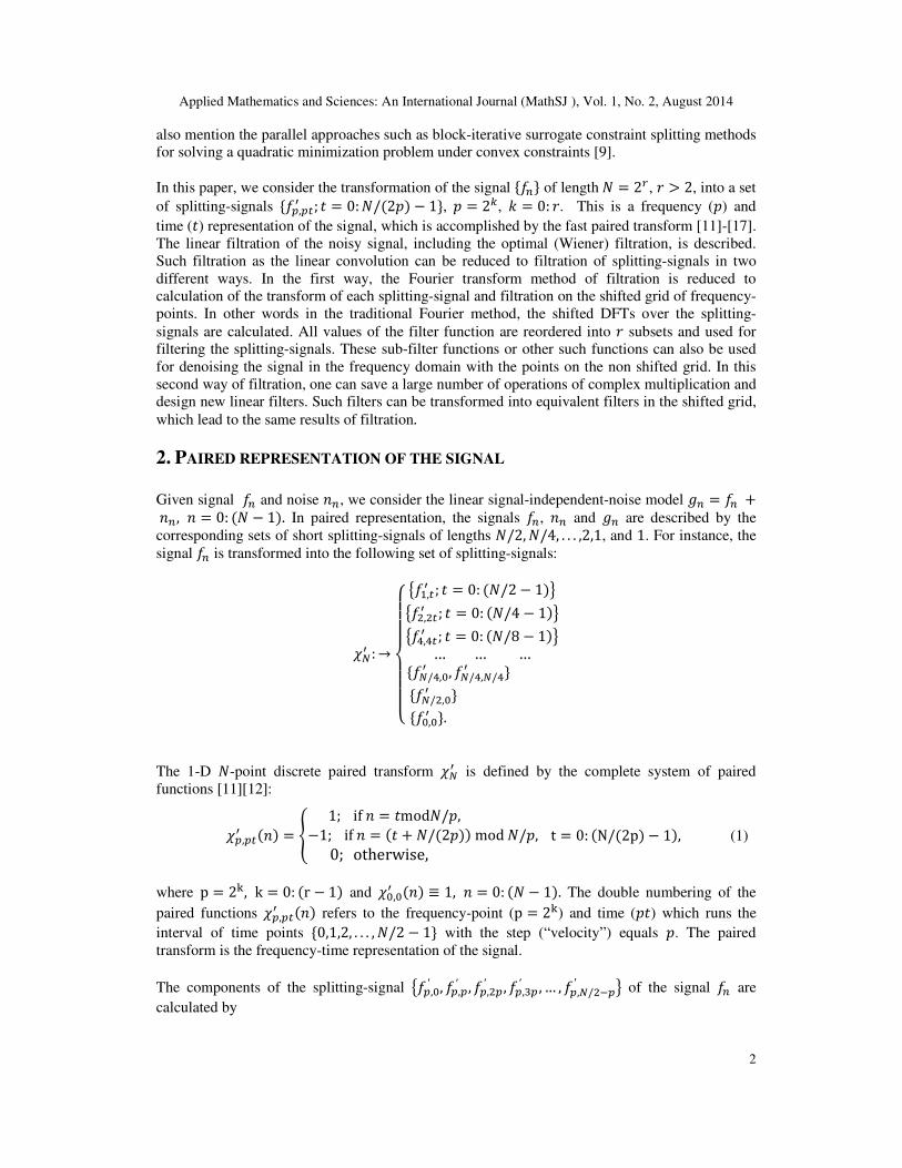
also mention the parallel approaches such as block-iterative surrogate constraint splitting methods

for solving a quadratic minimization problem under convex constraints [9].

In this paper, we consider the transformation of the signal �� of length � = 2!, � > 2, into a set

of splitting-signals ��","$% ; ' = 0: �/(2+) − 1�, + = 2,, - = 0: �. This is a frequency (+) and

time (') representation of the signal, which is accomplished by the fast paired transform [11]-[17].

The linear filtration of the noisy signal, including the optimal (Wiener) filtration, is described.

Such filtration as the linear convolution can be reduced to filtration of splitting-signals in two

different ways. In the first way, the Fourier transform method of filtration is reduced to

calculation of the transform of each splitting-signal and filtration on the shifted grid of frequency-

points. In other words in the traditional Fourier method, the shifted DFTs over the splitting-

signals are calculated. All values of the filter function are reordered into � subsets and used for

filtering the splitting-signals. These sub-filter functions or other such functions can also be used

for denoising the signal in the frequency domain with the points on the non shifted grid. In this

second way of filtration, one can save a large number of operations of complex multiplication and

design new linear filters. Such filters can be transformed into equivalent filters in the shifted grid,

which lead to the same results of filtration.

2. PAIRED REPRESENTATION OF THE SIGNAL

Given signal �� and noise ��, we consider the linear signal-independent-noise model .� = �� + ��, � = 0: (� − 1). In paired representation, the signals ��, �� and .� are described by the

corresponding sets of short splitting-signals of lengths �/2, �/4, . . . ,2,1, and 1. For instance, the

signal �� is transformed into the following set of splitting-signals:

/0% : →233343335 6�7,$% ; ' = 0: (�/2 − 1)86��,�$% ; ' = 0: (�/4 − 1)86�9,9$% ; ' = 0: (�/8 − 1)8… … …��0/9,<% , �0/9,0/9% � ��0/�,<% � ��<,<% �.

=

The 1-D �-point discrete paired transform /0% is defined by the complete system of paired

functions [11][12]:

/","$% (�) = > 1; if � = 'mod�/+, −1; if � = (' + �/(2+)) mod �/+,0; otherwise, = t = 0: (N/(2p) − 1), (1)

where p = 2L, k = 0: (r − 1) and /<,<% (�) ≡ 1, � = 0: (� − 1). The double numbering of the

paired functions /","$% (�) refers to the frequency-point (p = 2L) and time (+') which runs the

interval of time points �0,1,2, . . . , �/2 − 1� with the step (“velocity”) equals +. The paired

transform is the frequency-time representation of the signal.

The components of the splitting-signal 6�",<′ , �","′ , �",�"′ , �",O"′ , … , �",0/�P"′ 8 of the signal �� are

calculated by


3

�","$% = /","$% ∘ �� = R /","$% (�)��0P7�S< , ' = 0: (�/(2+) − 1).

The last one-point splitting-signal is ��<,<% � = �<,<% = �< + �7 + ⋯ + �0P� + �0P7. Example 1 (Case N=8) The matrix of the eight-point discrete paired transform (DPT) is defined

as

U/V% W =

XYYYYYYYYYZ[/7,<% \[/7,7% \[/7,�% \[/7,O% \[/�,<% \

[/�,�% \[/9,<% \[/<,<% \ ]̂̂

^̂̂^̂̂_̂

=XYYYYYYZ1 0 0 0 −1 0 0 00 1 0 0 0 −1 0 00 0 1 0 0 0 −1 00 0 0 1 0 0 0 −11 0 −1 0 1 0 −1 00 1 0 −1 0 1 0 −11 −1 1 −1 1 −1 1 −11 1 1 1 1 1 1 1]̂̂

^̂̂_̂

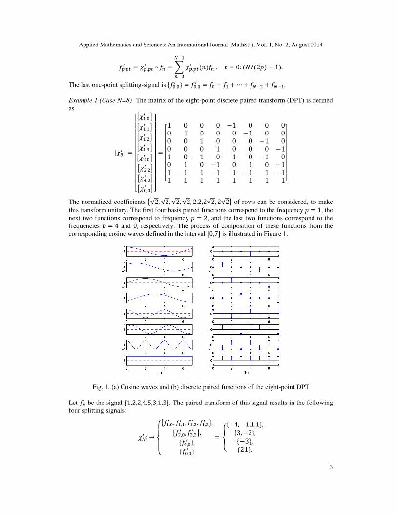
The normalized coefficients 6√2, √2, √2, √2, 2,2,2√2, 2√28 of rows can be considered, to make

this transform unitary. The first four basis paired functions correspond to the frequency + = 1, the

next two functions correspond to frequency + = 2, and the last two functions correspond to the

frequencies + = 4 and 0, respectively. The process of composition of these functions from the

corresponding cosine waves defined in the interval U0,7W is illustrated in Figure 1.

Fig. 1. (a) Cosine waves and (b) discrete paired functions of the eight-point DPT

Let �� be the signal �1,2,2,4,5,3,1,3�. The paired transform of this signal results in the following

four splitting-signals:

/0% : →234356�7,<% , �7,7% , �7,�% , �7,O% 8,6��,<% , ��,�% 8,��9,<% �,��<,<% �

= = d�−4, −1,1,1�,�3, −2�,�−3�,�21�. =


4

Splitting-signals carry the spectral information of the signal ��in different and disjoint subsets of

frequency-points. In paired representation, the splitting of the �-point DFT

e" = R ��f0�"0P7�S< , + = 0: (� − 1), f0 = exp(−h2i/�),

by (� + 1) short DFTs is based on the following formula [16]:

e(��j7)" = ∑ l�",$"% f0/"$ m0/�"P7 $S< f0/(�")�$ , � = 0: (�/(2+) − 1). (2) For the set of frequency-points �+ = 2,; - = 0: (� − 1)�, the disjoint subsets

n"% = �(2� + 1)+ mod �; � = 0: (�/(2+) − 1)� together with n<% = �0� divide the set of � frequency-points o0 = �0, 1, 2, . . . , � − 1�. Therefore,

the splitting-signal generated by the frequency + = 2� is denoted by

�pqr = 6�",<% , �","% , �",�"% , �",O"% , … , �",0/�P"% 8.

2.1. The first and second splitting-signals

To describe the meaning of equation (2), we first consider the + = 1 case, when the first splitting-

signal carries the spectral information of the signal at all odd frequency-points,

e��j7 = ∑ l�7,$% f0$ m0/�P7 $S< f0/��$ , � = 0: (�/2 − 1). (3) The �/2-point DFT over the modified splitting-signal

�sptr = 6�7,<% , �7,7% f7, �7,�% f�, �7,O% fO, … , �7,0/�P7% f0/�P78

equals the �-point DFT of the original signal at odd frequency-points. It should be noted, that the

right part of equation (3) is referred to as the �/2-point shifted DFT (SDFT) on the set of

frequency-points �� + 1/2; � = 0: (�/2 − 1)�, which we denote by

e�j7/�(7) = ∑ �7,$% f0/�$u�jtvw0/�P7 $S< , � + 7� = 7� , O� , x� , … 0P7� . (4) Thus, the �/2-point shifted DFT of the first splitting-signal coincides with the odd-indexed

DFT values of the original signal, e��j7 = e�j7/�(7), � = 0: (�/2 − 1).

For the p = 2 case, the splitting-signal is �pvr = 6��,<% , ��,�% , ��,9% , ��,y% , … , ��,0/�P�% 8 and

e(��j7)� = ∑ l��,�$% f0/�$ m0/9P7 $S< f0/9�$ , � = 0: (�/4 − 1). (5)


5

The �/4-point DFT over the modified splitting-signal �spvr = ��,<% , ��,�% f�, ��,9% f9, ��,y% fy, … , ��,0/�P�% f0/�P�� equals the �-point DFT of the original signal at all frequency-points which are

odd-integer multiple of 2. The right part of equation (5) is referred to as the shifted �/4-point

DFT on the set of frequency-points �� + 1/2; � = 0: (�/4 − 1)�, which is denoted by

e�j7/�(�) = ∑ ��,�$% f0/9$(�j7/�)0/9P7 $S< , � = 0: (�/4 − 1). (6) In the general case + = 2, where - < �, the �-point DFT of the signal �� at frequency-points of n"% is the �/(2+)-point shifted DFT of the splitting-signal �pqr , i.e.,

e(��j7)" = e�j7/�("), � = 0: �/(2+) − 1.

Thus, in paired representation, when the signal is described by the set of splitting-signals, the

DFT of the signal �� is described by a set of shifted DFTs of the splitting-signals. The shifts of

frequency-points are by 0.5.

2.2. Discrete Linear Filters

In this section, we consider the traditional method of DFT for convoluting the signals. Let z", + = 0: (� − 1), be the frequency characteristic of a given linear filter which describes the circular

convolution of the noisy signal .� = �� + �� with the impulse response of the filter, �{� = |� ⊛.�. We denote by ~" and e"� the �-point DFTs of the noisy and filtered signals, respectively.

Then e"� = z"~", for + = 0: (� − 1). The block-diagram of the linear filtration of the noisy

signal is given in Figure 2, where RDFT stands for the reversible DFT.

It follows directly from equation (2) that the process of filtration can be reduced to separate

filtration of splitting-signals, as shown in Figure 3. The �/(2+)-point shifted DFTs of the

splitting-signals �","$% are multiplied by the corresponding filter functions z(��j7)", and then, the

reversible SDFTs are calculated to obtain the filtered splitting-signals.

Fig. 2. Block-diagram of the Fourier transform-based method of filtration of the noisy signal.

Fig. 3. Block-diagram of the Fourier transform-based method of filtration by splitting-signals.


6

The last two one-point splitting-signals .0/�,<% and .<,<% are not shown in the block diagram. The

processing of these splitting-signals is reduced to one multiplication for each. The convoluted

signal �{� is calculated as the inverse �-point paired transform of the filtered splitting-signals.

This convolution can be obtained by calculating the �-point reversible DFT over the transform ~" , + = 0: (� − 1). Thus, the frequency characteristics are permuted onto (� + 1) subsets as 6z"; + = 0: (� − 1)8 → ��z(��j7)" ��0; � = 0: �/(2+) − 1�; + = 1,2,4,8, . . . , �/2�, z<�. The

filter is considered as the set of (� + 1) sub-filters.

Example 2: Consider the signal �� of length � = 256, which is shown in Figure 4(a). The paired

transform of the signal, as the set of splitting-signals ��ptr , �pvr , �p�r , �p�r , … . , �ptv�r , �p�r� is shown

in part b. The vertical dashed lines separate the first seven splitting-signals.

Fig. 4. (a) The signal of length 256 and (b) the 256-point discrete paired transform.

Figure 5 shows the 256-point DFT of the signal in absolute mode in part a. In part b, the same

DFT is shown, but in the order that corresponds to the partition of the frequency-points {0,1,2, ...

, 255} by subsets n7%, n�%, n9%, … , n7�V% , and n<%. The first 128 values corresponds to the 128-point

DFT of the modified splitting-signal �7,$% f$ which is also the 128-point SDFT of the splitting-

signal �7,$% . The next 64 values corresponds to the 64-point DFT of the modified splitting-signal ��,�$% f7�V$ , which is also the 64-point SDFT of the splitting-signal ��,�$% , and so on.


7

Fig. 5. (a) DFT of the signal and (b) DFTs of the modified splitting-signals.

(The transforms are shown in absolute mode.)

We consider the smoothing of the signal by the circular convolution with the impulse response �|�� = �0,0, . . , 0,1,2,3, 5, 3,2,1,0,0, . . . , 0�/17 with value |< = 5. Figure 6 shows the frequency

characteristic z" of |� in absolute mode in part a. In part b, this characteristic is shown in the

same order as e" in part b of Figure 5. These characteristics are used to filter the corresponding

modified splitting-signals and they are separated in the graph by vertical lines.

Fig. 6. (a) DFT of the filter and (b) the reordered filter (both in absolute scale).

The result of convolution of the signal, �{� = �� ⊛ |�, is shown in Figure 7 in part a, along with

nine splitting-signals which were filtered separately in b. Together these splitting-signals define

the filtered signal �{� in a. In other words, the 256-point inverse paired transform over the set of

these splitting-signals ��{ptr , �{pvr , �{p�r , �{p�r , … . , �{ptv�r , �{p�r� is the signal �{�. The following equation

describes the inverse paired transform [14][15],[17]:

�{� = R 12,j7 �{��,�� 0/�%!P7,S< + 1� �{<,<% , � = 0: (� − 1). (7)


8

Fig. 7. (a) Filtered signal and (b) filtered splitting-signals.

All signals in part (a) and (b) are smooth. The last two one-point signal have not been changed,

because the filter was defined with ∑ |� = 1. Thus the process of filtration of the original signal

by the discrete Fourier transform was reduced to separate processing of eight splitting-signals.

These signals were processed by the shifted DFTs.

3. NEW SIMPLIFIED SCHEME OF THE SIGNAL FILTRATION

It should be noted, that the calculation of the �-point DFT by the DFTs of the splitting-signals

corresponds to the paired FFT with �(�) = �/2(� − 3) + 2 operations of multiplication. The

same number of multiplications is required for the reversible DFT. If we propose the process of

filtration of each splitting-signal by the regular (not shifted) DFT, in other words, without

modifying the splitting-signal by the twiddle-coefficients f$, then many multiplications could be

saved. Indeed, let us consider two types of filtration of the first splitting-signal with the block-

diagrams shown in Figure 8.

Fig. 8. Block-diagrams of filtration of the first splitting-signal.

In the first diagram, the splitting-signal is processed in the traditional way, with the �/2-point

shifted DFT, which requires multiplications by the factors f0$ , ' = 0: (�/2 − 1), and then, the

calculation of the �/2-point DFT. In the second diagram, the same filter is used but the shifted

DFTs are substituted by the DFTs, and therefore, it allows for saving �/2 operations of

multiplication by the twiddle factors. To be more accurate, this number is �/2 − 2, because of

two trivial multiplications by f0< = 1 and f00/9 = −h. The same number of multiplications is

saved when using the reversible �/2-point DFT instead of the shifted DFT.


9

We now consider the complete block-diagram of the simplified signal filtration without shifted

DFTs, as shown in Figure 9.

Fig. 9. Block-diagram of the filtration by splitting-signals.

The filtration of the signal by this method saves the following number of operations of complex

multiplication:

∆�(�) = 2U(�/2 − 2) + (�/4 − 2) + (�/8 − 2) + . . . + (8 − 2)W = 2U(� − 8) − 2(� − 3)W = 2� − 4� − 4. For instance when � = 256, such saving equals ∆�(256) = 480. For the method of convolu-tion

with the block-diagram in Figure 3, the total number of required operations of multiplication

equals 2�(�) + � = �(� − 2) + 4. For the � = 256 case, this number is 1540, and the saving

in operations of multiplication is almost 32%.

3.1. Convolution of Splitting-Signals

To describe the process of filtration of the splitting-signals in the frequency-time domain, we

consider in detail this operation over the first-splitting signal. On the set of frequency-points n7%, the application of the filter to the noisy signal .� is described by

e��j7 = ~�j7/�(7) z�j7/�(7) , � = 0 ∶ (�/2 − 1), (8)

where we denote the shifted DFTs by ~�j7/�(7) = ~��j7 and z�j7/�(7) = z��j7.

Let �{� be the filtered signal and �{7,$% be its first splitting-signal, and let |7,$% be the first splitting-

signal of the impulse response of the filter z". Then, the following calculations hold:

�{7,$% f$ = 2� R ~�j7/�(7) z�j7/�(7)0/�P7 $S< f0/�P$�

= 2� R �R �R .7,�% f�|7,�% f�0/�P7�S< �0/�P7

$tS< f0/�$t��0/�P7�S< f0/�P$�

(� = ('7 − �)�� /2) = 2� R �R .7,�% f�|7,�% f�0/�P7�S< � R f0/�($tP$)�0/�P7

�S< 0/�P7$tS<


10

= 2� R �R .7,�% f�|7,�% f�0/�P7�S< � �2 �('7 − ') 0/�P7

$tS<

= R .7,�% f�|7,($P�)�� 0/�% f($P�)�� 0/�. 0/�P7�S<

Thus, we obtain the following:

�{7,$% = ∑ .7,�% |7,($P�)�� 0/�% f0(�P$)f0($P�)�� 0/�0/�P7�S< .

Since 0 ≤ ', � < �/2 and (' − �)mod �/2 = (' − �), if ' ≥ �, and (' − �) mod �/2 = (' − �) + �/2, if ' < �, we have the following:

f0(�P$)f0($P�)�� 0/� = sign(' − �) = � 1, �� ' − � ≥ 0,−1, �� ' − � < 0.= Therefore,

�{7,$% = ∑ .7,�% sign(' − �)|7,($P�)�� 0/�%0/�P7�S< , ' = 0: (�/2 − 1). (9)

We remind here, that the function |7,$% as the function of ' has the period � not �/2, and the

function is “odd,” i.e., |7,P$% = −|7,0/�P$% , ' = 1,2, . . . , (�/2 − 1). Equation (9) can be written as

the linear (not circular) convolution calculated in �/2 points:

�{7,$% = ∑ .7,�% |7,($P�)%0/�P7�S< , ' = 0: (�/2 − 1). (10)

The linear convolution is calculated only in the original time interval �0,1, . . . , �/2 − 1� and can

be calculated by the �-point circular convolution. We call this operation the incomplete circular

linear convolution of length �/2. Let |�7,$% be the extended function 6|�7,$; ' = 0: (� − 1)8 = 6�|7,$% , '; ' = 0: (�/2 − 1)�, �−|7,0/�P$% ; ' = �/2: (� − 1)�8.

Let extended splitting-signal .�7,$ of length � be defined as

�.�7,$ , '; ' = 0: (� − 1)� = 6�.7,$% ; ' = 0: (�/2 − 1)�, �0, 0, 0, . . . , 0�8.

It is not difficult to see, that the following holds:

�{7,$% = ∑ .�7,$|�7,($P�)�� 00/�P7�S< , ' = 0: (�/2 − 1). (11)

The linear convolution of the second and remaining splitting-signals with the filter is described

similarly. Thus, the cyclic convolution of length � can be reduced to (� + 1) incomplete circular

convolutions, when representing the signal in form of splitting-signals. As an example, we

consider the signal of length 512 shown in part a of Figure 10. The paired transform as the set of

ten splitting-signals is shown in b.


11

Fig. 10. (a) Random signal and (b) its splitting-signals.

Figure 11 in part a shows the signal .� = �� + �� with an additive random Gaussian noise ��

which is normally distributed as �(0,17). The first splitting-signal �.7,$% , '; ' = 0: 255� of the

noisy signal is shown in b, and the result of the optimal filtration of this splitting-signal in c. The

result of the optimal filtration of the entire noisy signal .� by ten splitting-signals is shown in d.

The same result is achieved by using the Wiener filter over the noisy signal.

3.2. Parseval’s Theorem and Paired Transform

The normalization of the basic paired functions as /<,<% → /<,<% /√� and /","$% → /","$% /�2+, when ' = 0: (�/(2+) − 1), + = 1,2,4,8, … , �/2, leads to the unitary property of the paired transform.

Therefore, according to Parseval’s’theorem, the difference of two signals �� and �{� in metric ��

can be written as

��l�, �{m = Rl�� − �{�m�0P7�S< = R 12+

!P7,S< R (�","$% − �{","$% )�0/(�")P7

$S< + 1� (�<,<% − �{<,<% )�= R 12+

!P7,S< �� u�pqr , �{pqr w + 1� ��u�p�r , �{p�rw

where we denote + = 2,, and �"� = �� u�pqr , �{pqr w are the differences of splitting-signals of �� and �{� in the same metric. The difference ��l�, �{m can be referred to as the error of estimation, or

filtration of the signal, and �"� as the errors of filtration of the splitting-signals �pqr .


12

Fig. 11. (a) The noisy signal of length 512, (b) the noisy first splitting-signal of length 256, (c) filtered

splitting-signal, and (d) the filtered signal.

It is clear that, the minimization of all errors �"� may give not the best restoration �{ of the signal.

The splitting-signal can be processed separately, but they are not independent. All together they

represent the signal ��. They carry the information of the signal, which is transformed to them

through the paired transform. On the other hand, the minimization of the error ��l�, �{m provides

good, if not the best minimum values for errors �"� for the splitting-signals. The optimal filter as

the set of coefficients, �z" , + = 0: (� − 1)�, after being reordered as �z(��j7)"; � =0: (�/(2+) − 1), + = 2,, - = 0: ��, may be modified or used directly, to define the set of

optimal, or close to optimal filters for splitting-signals. Our preliminary experimental results

show that the set of these filters can be used for filtration of splitting-signals, if we want to save ∆�(�) = 2� − 4� − 4 operations of multiplication. We now consider the results of such

filtration for the Wiener filter. There is a small difference in the results of the filtration of the

signal .�, by the Wiener filter over .� and by the Wiener filters over splitting-signals.

3.3. Traditional Wiener filter (grid is shifted)

When denoising of the signal .� = �� + �� is accomplished by the Wiener filter, the frequency

characteristic of this filter is defined as z" = ��(+)��(+) + ��(+) = 11 + ��/�(+) , + = 0: (� − 1).

Here, ��(+) = ⟨|e"|�⟩ and ��(+) = ⟨|�"|�⟩ denote the power spectra of the original and noise

signals, respectively. The notation ��/�(+) is used for the noise-to-signal ratio, ��(+)/��(+),

and <·> is used for the mathematical expectation of a random variable.

The Wiener filter results in a minimum error of signal reconstruction, ��l�, �{m = min, where �{ is

the inverse Fourier transform of z"~". In paired representation, the Wiener filtration of the noisy

signal .� is reduced to separate processing of splitting-signals. Each splitting-signal .pqr , + ∈ �1,2,4,8, . . . , �/2, 0�, is modified by the cosine and sine waves and then the convolution with

the “impulse response” |","$% is calculated. Thus, in the frequency-time domain (+, +'), the

optimal filtration is achieved by amplifying the splitting-signal prior and after the convolution,


13

.pqr → ¤ ∙ .pqr → ~(��j7)" �¦§ 0 → (z~)(��j7)" �¦§ 0 → ¤ ∙ �{pqr → �{pqr .

Here the vector ¤ is (1, f0/"7 , f0/"� , . . . , f0/"0/�")′. In terms of shifting DFT, this procedure is

described by .pqr → ~�j7/�(") → ~�j7/�(") z�j7/�(") → �{pqr .

The filtration is accomplished by the �/(2+)-point discrete Fourier transform which is calculated

in the shifted frequency grid �� + 1/2; � = 0: (�/(2+) − 1)�. The inverse paired

transform, ��{pqr � → ��{��, can be accomplished by the fast paired transform algorithm [15], or by

the direct calculation (7).

4. FILTRATION OF THE SPLITTING-SIGNALS ON THE NOT SHIFTED GRID

The filtration of splitting-signals described above is performed by the �/(2+)-point shifted

DFTs, when the transforms are defined on the sets of frequency-points �1/2,1 + 1/2,2 +1/2, . . . , �/(2+) − 1/2�. We now consider the DFTs of the splitting-signal in the grid �0,1,2, . . . , �/2 − 1�. In other words, for each frequency-point + = 2,, - < �, together with this

shifted DFT, we consider the �/(2+)-point DFT of the splitting-signal e�% = ∑ �",$"%0/(�")P7 $S< f0/(�")�$ , � = 0: (�/(2+) − 1). (12)

Let .� be the noisy signal, .� = �� + ��. For the + = 1 case, we consider the traditional grid ��; � = 0: (�/2 − 1)� of frequency-points and the �/2-point DFTs e�% , ��% , and ~�% = e�% +��% of the first splitting-signals of ��, ��, and .�, respectively. The block-diagram of optimal

filtration of this splitting-signal by the Fourier transform which is calculated in the traditional

frequency grid is given in Figure 12.

Fig. 12. Block-diagram of filtering the first splitting-signal in the grid �� = 0: (�/2 − 1)�.

If we assume a liner and time invariant model for the splitting-signal of the degraded signal .�,

then the frequency characteristic of the optimal filter in such model would be defined as follows:

z©7(�) = ��t,ªr (�)��t,ªr (�) + ��t,ªr (�) , � = 0: (�/2 − 1). Here ��t,ªr (�) and ��t,ªr (�) are the power spectra of the original and noise splitting-signals,

respectively. Our preliminary results show, that this filter referred to as an optimal filter can be

used effectively for processing the signal. The splitting-signal filtered by z©7(�)

�s7,$% = 2� R Uz�1(�)~�% Wf0/�P�$0/�P7�S< , ' = 0: (�/2 − 1),

differs from the splitting-signal obtained after the Wiener filtration

�{7,$% = 2� R [z�+1/2(1) ~�+1/2(1) \f0/�P(�j7/�)$0/�P7�S< , ' = 0: (�/2 − 1),


14

on the shifted frequency grid �� + 1/2; � = 0: (�/2 − 1)�. The filter characteristic is

calculated in the odd frequency-points by z�j7/�(7) = z��j7 = ��(2� + 1)��(2� + 1) + ��(2� + 1) , � = 0: (�/2 − 1).

This characteristic differs from z©7(�), because the following holds:

��t,ªr (�) = ⟨|e�% |�⟩ ≠ ⟨|e�j7/�(7) |�⟩ = ⟨|e��j7|�⟩ = ��(2� + 1),

and similarly ��t,ªr (�) ≠ ��(2� + 1). Although the Wiener filter applied directly on the noisy

splitting-signal has a larger error than does the Wiener filter on the original noisy signal, i.e., �� u�pqr , �{pqr w ≤ �� u�pqr , �spqr w, the difference between these two errors is small. The similar

reasoning can be used when processing the remaining splitting-signals by the corresponding

characteristics z©"(�), + = 2,4,8, . . . , �/2,0. By splitting the noisy signal, the noise distribution

does not change. Because the basic paired functions are populated by ones, the noise in the

splitting-signals .",$"% = �",$"% + �",$"% is normally distributed. Figure 13 shows the optimal

filtration of the first splitting-signal, when + = 1.

Fig. 13. (a) The first splitting-signal, (b) noisy splitting-signal, and (c) the reconstruction.

The result of restoration of the noisy signal �� after processing all splitting-signals is shown in

Figure 14, which is close to the direct Wiener filtration. The error of such filtration equals 0.103

(and 0.091 when using the direct Wiener filtration).


15

Fig. 14. (a) The random signal with Gaussian noise, and (b) the signal reconstruction.

Figure 15 shows another signal of length 256 in part a, along with the degraded signal in b, and

signal restored by processing separately the splitting-signals in c. The error of such filtration

equals 0.234 (and 0.239 when using the direct Wiener filtration).

In filtration, the Wiener filter is optimal which means the error ��l�, �{m is minimum. The set of

optimal filters for splitting-signals may not improve the result in the optimal filter over the

original signal. However such filtration will be effective, because it allows for saving many

operations of multiplication, 2� − 4� − 4.

Fig. 15. (a) The random signal, (b) signal with Gaussian noise, and (c) the signal reconstruction.

5. OPTIMAL FILTRATION BY SPLITTING-SIGNALS: GENERAL MODEL

In this section, analytical equations are described for equivalent filter functions over the splitting-

signals, when processing them in two models of filtration. Filter functions are called similar, or

equivalent if they lead to the same results of signal filtration �{�. We first describe the filtration of

the splitting-signal 6.7,$% ; ' = 0: (�/2 − 1)8 when this signal is modified and then filtered by the

optimal Wiener sub-filter �z7, zO, zx, . . . , z0P7�. We also consider a such sub-filter with


16

�z©7, z©O, z©x, . . . , z©0/�P7�, which leads to the same result over the splitting-signal, as the optimal

Wiener sub-filter over the modified splitting-signal. The required for that equation

�R .7,$% f0/"�$0/�P7$S< � z©� = �R l.7,$% f$mf0/��$0/�P7

$S< � z��j7

has the simple solution

z©� = ¬~�j7/�(7) /~�(7) z��j7, � = 0: (�/2 − 1). (13)

Here, we denote by ~�j7/�(7) and ~�(7)

the shifted DFT and DFT of the noisy splitting-signal .7,$% , respectively.

As an example, we consider the following linear model of the degraded signal:

.� = �� ∗ ℎ� + ��, � = 0: (� − 1). (14)

For simplicity of calculations, we consider that the random noise and original signal are not

correlated. The Wiener filter is described by the function

z" = �°"|�"|� + ��/�(+) , + = 0: (� − 1),

where �" is the DFT of ℎ�, and �°" denotes the complex conjugate of �". Figure 16 shows the

original signal in part a. The smooth signal in b is the convolution of the signal with the impulse

response ℎ� = [1,2, 3, 2,1\/9. The smooth signal with an additive noise is shown in c. The result

of the Wiener filtration is given in d.

Fig. 16. The signals ��, �� ∗ ℎ�, .�, and filtered signal �{� (from top to button).


17

Figure 17 shows the characteristics of the filter, namely, the function �" in the decibel scale, the

phase of �", the magnitude of the Wiener filter function, and the signal-to-noise ratio.

Fig. 17. Magnitude and phase of �", |z"|, and signal-to-noise ratio (from top to button).

In paired representation, model (14) of the degraded signal is defined by the set of sub-models for

splitting-signals. For the above example, Figure 18 shows the magnitudes and phases of these

sub-filters. The signal-to-noise ratios for these sub-filters are also shown. All sub-filters are

separated by the vertical lines in this drawing. As shown in Section III, each of these sub-models

can be described by the incomplete circular convolution of the extended impulse response ℎ©","$ with the extended splitting-signal .�","$ of the original signal plus the splitting-signal of the

noise,

�{","$% = R .�","�0/"P7�S< ℎ©","($P�)�� 0/" + ��","$ , ' = 0: (�/(2+) − 1).

For example, for the first sub-model when + = 1, we have the equation similar to (11),

�{7,$% = R .�7,�0P7�S< ℎ©7,($P�)�� 0 + ��7,$ , ' = 0: (�/2 − 1).

Given filter function z©� for processing the first splitting-signal, the values of the equivalent filter z" at odd frequency-points are calculated as z��j7 = ¬~�(7)/~�j7/�(7) z©�, � = 0: (�/2 − 1). Similar calculations are valid when considering the remaining splitting-signals. Figure 19 shows

the magnitude of the filter functions z©� and z��j7 in part a and b, respectively.


18

Fig. 18. Magnitudes and phases of sub-filters, and signal-to-noise ratios (from top to button).

Fig. 19. The magnitudes of functions (a) z©� and (b) z��j7.

Let z" , + = 0: (� − 1), be a filter function for processing the signal .�. The filtration of the

signal .� is reduced to filtration of the modified splitting-signals �.","$% f0/"$ ; ' = 0: (�/(2+) −1�, by the sub-filters �z(��j7)"; � = 0: (�/(2+) − 1)�, respectively. Each of these operations

describes the filtration of the corresponding splitting-signal in the shifted frequency grid,

because z(��j7)" = z�j7/�("). The equivalent sub-filters z©� = z©�(")

for processing splitting-signals �.","$% ; ' = 0: (�/(2+) − 1� in the not shifted grid are calculated by z©�(") = ¬~�j7/�(") /~�(") z(��j7)", � = 0: (�/(2+) − 1). For the second splitting-signal, Figure 20 shows the

magnitudes of filter functions z©�(�) and z�(��j7) in part a and b, respectively.


19

Fig. 20. The magnitudes of functions (a) z©�(�) and (b) z�(��j7).

Thus, we have described two different models of signal filtration trough the splitting-signals

when the filter is presented by the set of sub-filters. One model describes the separation of

filtration by the modified splitting-signals, and another model describes the filtration by the

splitting-signals without complex operation of modification, which requires multiplications by the

twiddle coefficients. Equation 13 describes a way of finding the equivalent filters in both models.

6. CONCLUSIONS

The one-dimensional (1-D) signal can be filtered, by transforming the signal of length � =2! , � > 2, into the set of splitting-signals of lengths �/2, �/4, . . . , 2,1, and 1. These splitting-

signals carry the spectral information of the original signal in disjoint subsets of frequency-points

on both shifted and not shifted grids. The traditional filtration, including the optimal Wiener

filtration, can be reduced to filtration of the splitting-signals on the shifted grid. In the time

domain, this process is described by the incomplete circular convolutions of the splitting-signals

with the corresponding characteristics of the filter. The filtration of the splitting-signals can also

be performed on the not shifted grid, and such filtration allows to saving 2(� − � − 2) operations

of complex multiplication. The described models of signals filtration by splittingsignals can be

generalized and used for the two-dimension (2-D) case of signals, or images. For the case when

size of the image is � × �, and 2!, � > 2, the 2-D paired transform [11],[15] represents the image

as the set of (3� − 2) splitting-signals of length �/2, �/4, . . . , 2, and 1. The filtration of the

image can therefore be reduced to the filtration of the splitting-signals as described above for the

1-D case.

References

[1] Alberto Reading Leon-Garcia, (1994) Probability and random processes for electrical engineering,

Addison-Wesley, Mass.

[2] S. G. Chang, Yu Bin, and M. Vetterli, (2000) “Spatially adaptive wavelet thresholding with context

modelling for image denoising,” Image Processing, IEEE Transactions on, vol. 9, no. 9, pp. 1522-

1531.

[3] David L. Donoho and Jain M. Johnstone, “Ideal spatial adaptation by wavelet shrinkage,” Biometrika,

vol. 81, no. 3, pp. 425-455, 1994.

[4] N. Pustelnik, C. Chaux, and J. Pesquet, (2011) “Parallel proximal algorithm for image restoration

using hybrid regularization,” Image Processing, IEEE Transactions on, vol. 20, no. 9, pp. 2450-2462.

[5] V. Ratner and Y. Y. Zeevi, (2011) “Denoising-enhancing images on elastic manifolds,” Image

Processing, IEEE Transactions on, vol. 20, no. 8, pp. 2099-2109.


20

[6] D. L. Donoho, (1995) “De-noising by soft-thresholding,” Information Theory, IEEE Transactions on,

vol. 41, no. 3, pp. 613-627.

[7] P. L. Combettes, (2003) “A block-iterative surrogate constraint splitting method for quadratic signal

recovery," Signal Processing, IEEE Transactions on, vol. 51, no. 7, pp. 1771-1782.

[8] P. L. Combettes, (2001) “Convex set theoretic image recovery with inexact projection algorithms,” in

Image Processing, Proceedings, International Conference on, vol. 1, pp. 257-260.

[9] P. L. Combettes, (1997) “Convex set theoretic image recovery by extrapolated iterations of parallel

subgradient projections,” IEEE Trans. on Image Processing, vol. 6, no. 4, pp. 493-506.

[10] A.M. Grigoryan, and S.S. Agaian, (2000) “Split manageable efficient algorithm for Fourier and

Hadamard transforms,” IEEE Trans. on Signal Processing, vol. 48, no. 1, pp. 172-183.

[11] A.M. Grigoryan and S.S. Agaian, (2003) Multidimensional Discrete Unitary Transforms:

Representation, Partitioning, and Algorithms, New York: Marcel Dekker.

[12] J. U. Anugom and A. M. Grigoryan, (2006) “Method of splitting signals by the paired transform,” in

Industrial Electronics, 2006 IEEE International Symposium on, vol. 1, pp. 548-552.

[13] F.T. Arslan, A.K. Chan, and A.M. Grigoryan, (2006) “Directional denoising of aerial images by

splitting-signals,” in Region 5 Conference, IEEE, pp. 114-119.

[14] A.M. Grigoryan, “Representation of the Fourier transform by Fourier series,” Journal Mathematical

Imaging and Vision, vol. 25, pp. 87-105, 2006.

[15] A.M. Grigoryan, (2001) “2-D and 1-D Multipaired transforms: frequency-time type wavelets,” Signal

Processing, IEEE Transactions on, vol. 49, no. 2, pp. 344-353.

[16] P. Patel, N. Ranganath, and A.M. Grigoryan, (2011) “Performances of Texas Instruments DSP and

Xilinx FPGAS for Cooley-Tukey and Grigoryan FFT algorithms,” Journal of Engineering

Technology, vol. 1, p. 83.

[17] A.M. Grigoryan and M.M. Grigoryan, (2009) Brief Notes in Advanced DSP: Fourier Analysis with

MATLAB, CRC Press Taylor and Francis Group.

Authors

Artyom M. Grigoryan received the MS degrees in mathematics from Yerevan State

University (YSU), Armenia, USSR, in 1978, in imaging science from Moscow Institute of

Physics and Technology, USSR, in 1980, and in electrical engineering from Texas A&M

University, USA, in 1999, and Ph.D. degree in mathematics and physics from YUS, in

1990. In December 2000, he joined the Department of Electrical Engineering, University

of Texas at San Antonio, where he is currently an Associate Professor. SM of IEEE since

1998. He is the author of three books, three book-chapters, two patents, and many journal papers and

specializing in the theory and application of fast Fourier transforms, tensor and paired transforms, unitary

heap transforms, image enhancement, computerized tomography, processing biomedical images, and image

cryptography.

Sree P.K. Devieni is a PhD student in the University of Texas at San Antonio in Electrical Engineering

with a concentration in digital signal and image processing, transforms and wavelets.

NEW METHOD OF SIGNAL DENOISING BY THE PAIRED TRANSFORM

Documents

Transcript of NEW METHOD OF SIGNAL DENOISING BY THE PAIRED TRANSFORM