Differential Equations: A Dynamical Systems Approach
611
Springer New York Berlin Heidelberg Barcelona Hong Kong London Milan Paris Singapore Tokyo Texts in Applied Mathematics 18 Editors J. E. Marsden L. Sirovich M. Golubitsky W.Jager F. John (deceased) Advisor G.Iooss
-
Upload
khangminh22 -
Category
Documents
-
view
1 -
download
0
Transcript of Differential Equations: A Dynamical Systems Approach

Springer New York Berlin Heidelberg Barcelona Hong Kong London Milan Paris Singapore Tokyo
Texts in Applied Mathematics 18
Editors
J. E. Marsden L. Sirovich
M. Golubitsky W.Jager
F. John (deceased)
Advisor G.Iooss

Texts in Applied Mathematics
I. Sirovich: Introduction to Applied Mathematics.
2. Wiggins: Introduction to Applied Nonlinear Dynamical Systems and Chaos. 3. Hale/Ko9ak: Dynamics and Bifurcations. 4. Chorin/Marsden: A Mathematical Introduction to Fluid Mechanics, 3rd ed. 5. Hubbard/West: Differential Equations: A Dynamical Systems Approach: Ordinary
Differential Equations. 6. Sontag: Mathematical Control Theory: Deterministic Finite Dimensional Systems,
2nd ed. 7. Perko: Differential Equations and Dynamical Systems, 2nd ed. 8. Seaborn: Hypergeometric Functions and Their Applications. 9. Pipkin: A Course on Integral Equations. 10. Hoppensteadt/Peskin: Mathematics in Medicine and the Life Sciences.
II. Braun: Differential Equations and Their Applications, 4th ed. 12. Stoer/Bulirsch: Introduction to Numerical Analysis, 2nd ed. 13. Renardy/Rogers: A First Graduate Course in Partial Differential Equations. 14. Banks: Growth and Diffusion Phenomena: Mathematical Frameworks and
Applications. 15. Brenner/Scott: The Mathematical Theory of Finite Element Methods. 16. Van de Velde: Concurrent Scientific Computing. 17. Marsden/Ratiu: Introduction to Mechanics and Symmetry, 2nd ed. 18. Hubbard/West: Differential Equations: A Dynamical Systems Approach: Higher-
Dimensional Systems. 19. Kaplan/Glass: Understanding Nonlinear Dynamics.
20. Holmes: Introduction to Perturbation Methods. 21. CurtainlZwart: An Introduction to Infinite-Dimensional Linear Systems Theory. 22. Thomas: Numerical Partial Differential Equations: Finite Difference Methods. 23. Taylor: Partial Differential Equations: Basic Theory.
24. Merkin: Introduction to the Theory of Stability of Motion. 25. Naber: Topology, Geometry, and Gauge Fields: Foundations. 26. Polderman/Willems: Introduction to Mathematical Systems Theory: A Behavioral
Approach. 27. Reddy: Introductory Functional Analysis with Applications to Boundary-Value
Problems and Finite Elements. 28. Gustafson/Wilcox: Analytical and Computational Methods of Advanced
Engineering Mathematics. 29. Tveito/Winther: Introduction to Partial Differential Equations: A Computational
Approach. 30. Gasquet/Witomski: Fourier Analysis and Applications: Filtering, Numerical
Computation, Wavelets. 31. Bremaud: Markov Chains: Gibbs Fields, Monte Carlo Simulation, and Queues. 32. Durran: Numerical Methods for Wave Equations in Geophysical Fluid Dynamics.
(continued after index)

John H. Hubbard Beverly H . West
Differential Equations: A Dynamical Systems Approach
Higher-Dimensional Systems
With 225 Illustrations
Springer

John H. Hubbard Beverly H. West Department of Mathematics Cornell University Ithaca, NY 14853 USA
Series Editors
F. J 0 h n (deceased) Courant Institute of
Mathematical Sciences New York University New York, NY 10012 USA
M. Golubitsky
J.E. Marsden Department of
Mathematics University of California Berkeley, CA 94720 USA
w.Jager
L. Sirovich Division of Applied
Mathematics Brown University Providence, RI 02912 USA
Department of Mathematics University of Houston Houston, TX 77204-3476 USA
Department of Applied Mathematics Universitat Heidelberg 1m Neuenheimer Feld 294 69120 Heidelberg, Germany
Mathematics Subject Classifications: 34xx, 35xx
Library of Congress Cataloging-in-Publication Data Hubbard, John.
Differential equations: a dynamical systems approach / John Hubbard, Beverly West.
p. cm. - (Texts in applied mathematics: 5, 18) Contents: pt. 1. Ordinary differential equations - pt. 2. Higher
dimensional systems. ISBN-13:978-1-4612-8693-6
1. Differential equations. 2. Differential equations, Partial. I. West, Beverly Henderson, 1939- . II. Title. III. Series. QA371.H77 1990
515".35-<1c20 90-9649
Printed on acid-free paper. © 1995 Springer-Verlag New 'rbrk, Inc.
Softcover reprint of the hardcover I st edition 1995
All rights reserved. This work may not be translated or copied in whole or in part without the written permission of the publisher (Springer-Verlag New York, Inc., 175 Fifth Avenue, New York, NY 10010, USA), except for brief excerpts in connection with reviews or scholarly analysis. Use in connection with any form of information storage and retrieval, electronic adaptation, computer software, or by similar or dissimilar methodology now known or hereafter developed is forbidden. The use of general descriptive names, trade names, trademarks, etc., in this publication, even if the f(lfIner are not especially identified, is not to be taken as a sign that such names, as understood by the Trade Marks and Merchandise Marks Act, may accordingly be used freely by anyone.
Production managed by Hal Henglein; manufacturing supervised by Jacqui Ashri. Photocomposed copy prepared using AMS-TEX and LATEX
9 8 765 4 3
ISBN-13:978-1-4612-8693-6 e-ISBN-13:978-1-4612-4192-8 DO I: 10.1 007/978-1-4612-4192-8
Springer-Verlag New York Berlin Heidelberg A mfmber of BertelsmannSpringer Science+Business Media GmbH

Series Preface
Mathematics is playing an ever more important role in the physical and biological sciences, provoking a blurring of boundaries between scientific disciplines and a resurgence of interest in the modern as well as the classical techniques of applied mathematics. This renewal of interest, both in research and teaching, had led to the establishment of the series: Texts in Applied Mathematics (TAM).
The development of new courses is a natural consequence of a high level of excitement on the research frontier as newer techniques, such as numerical and symbolic computer systems, dynamical systems, and chaos, mix with and reinforce the traditional methods of applied mathematics. Thus, the purpose of this textbook series is to meet the current and future needs of these advances and encourage the teaching of new courses.
TAM will publish textbooks suitable for use in advanced undergraduate and beginning graduate courses, and will complement the Applied Mathematical Sciences (AMS) series, which will focus on advanced textbooks and research level monographs.

Preface
As in Part I, this book concentrates on understanding the behavior of differential equations, rather than on solving the equations. Part I focused on differential equations in one dimension; this volume attempts to understand differential equations in n dimensions.
The existence and uniqueness theory carries over with almost no changes. But the behavior of solutions is not nearly so easy to understand; solutions can be thought of as parametrized curves in Rn, which can knot and link in the most complicated ways and usually do.
We begin in Chapter 6 with a number of examples, often of great historical interest, like the two-body problem, which exhibit some of the questions that will occupy the remainder of the book.
Chapter 7 focuses on linear differential equations with constant coefficients, with the usual paraphernalia of eigenvectors and eigenvalues. This material is the main staple of elementary courses on differential equations, and we also study the material at considerable length. But we put more emphasis on how the signs of the eigenvalues determine the stability of solutions and on the relation between existence of bases of eigenvectors and decoupling.
Associated with this chapter are the linear algebra Appendices L1-L8. An attempt to summarize the relevant material grew and grew, until it reached an absurd length and became practically a textbook on the subject. Most of the material is quite standard, but the treatment of the QR method cannot be found in any textbooks that we know of.
Chapters 8 and 8* represent a serious attempt to understand nonlinear autonomous systems in the plane. Logically they should be one chapter (and were one chapter at one time), but pedagogically this did not work very well. There is a body of material that can be understood without entering into too many technical considerations, and this has been collected in Chapter 8. There we stress linearization and the fact that by qualitative analysis with computer graphics, nonlinear differential equations become essentially as easy to study as linear ones.
Chapter 8* represents a considerably deeper understanding of the same material, eventually leading to the Poincare-Bendixson Theorem and a complete proof of the Pontryagin-Peixoto results, which are the central topics for planar vector fields. Whether it is really wise to include such hard results in a book that hopes to be elementary is something the authors still wonder about.
Chapter 9 is about bifurcations of differential equations in the plane. When modeling a real system, the engineer always imagines he or she has

viii Preface
knobs with which to tune and adjust the system and its models. These knobs represent the parameters of the system, and as one twiddles them, sometimes the behavior of the system changes gradually and sometimes abruptly. These abrupt changes occur at the bifurcating values of the parameters; they are quite well understood for differential equations in the plane. The theoretical underpinnings are built in Chapter 8*, but you can read Chapter 9 at a more superficial but still highly instructive level with only Chapter 8 behind you. We have found that students respond quite well indeed to the material.
Originally, this book was supposed to have four more chapters, covering electrical circuits, classical mechanics, linear differential equations with non-constant coefficients, and iteration in higher dimensions. Because the current volume has become quite lengthy, that material has been relegated to a new Part III.
How to navigate Chapters 8, 8*, and 9
A course can reasonably end with Chapter 8, but Chapter 9 in bifurcation is a topic now easy to approach even in an introductory differential equations course.
Ithaca, New York
Chapter 8*.1
John H. Hubbard Beverly H. West

Acknowledgments
In the 1960s, Hubbard participated in seminars run by Rene Thom and Steve Smale. Their influence pervades this entire book, just as it pervades the entire western school of differential equations.
In a more direct way, the insight of Adrien Douady has shaped our approach to mathematics, and more particularly to differential equations. We are not alone; in France Michele Artigue and Veronique Gautheron were also influenced by Douady, and their excellent and innovative book Systemes Differentiels: Etude Graphique (1983) first explored many of the same problems we have addressed with a similar spirit.
Over the past ten years, we have been encouraged by many colleagues, students, and editors. Particularly valuable have been enthusiasm, suggestions, and new examples from those who have taught more than once from Part I and from earlier versions of Parts II and III-especially Bodil Branner, Anne Noonburg, Peter Papadopol, and Bob Terrell. On a more technical level, A. Douady provided the proof of a key result in Chapter 8*, and John Guckenheimer provided another. We gratefully acknowledge many additional constructive suggestions from colleagues Allan Back, Fred Barber, Paul Blanchard, Clifford Earle, Bjl1Jrn Felsager, G. Roger Livesay, and James E. West.
This book owes its existence to the supporting software MacMath. Programmers, some of whom worked on related programs, have included Mike Abato, Yelena Baranova, Fassil Bekele, Doug Campbell, Marc Christensen, Trey Jones, Derek Noonburg, Marc Parmet, Peter Sisson, and Thomas Yan. However, our final skilled programmer/mathematician Ben Hinkle, in his Extensions of MacMath to Planar Systems and Planar Iterations, has allowed us to begin to more thoroughly explore the phenomena, especially of global bifurcations, of which we write.
Several graduate students, particularly Ben Wittner, Jaiqi Luo, Dierk Schleicher, and Ralph Oberste-Vorth, have carefully provided solutions to problems and helped to clarify many sections. Undergraduates Daniel Brown and Tony Yan, respectively, did the original exploration on a number of examples, and provided some of the excellent pictures in Chapter 9 before it was easy to do so. We are grateful to the many other students and readers who have caught errors before publication, including Alexander Hubbard, Tom Palmer, and John Wang.
The reader cannot conceive of how hard it was to create the exercises, most of which are completely new. Many students and colleagues have contributed dozens of them. These exercises, as well as a better understanding of the material, should help the reader to use computer programs, and the

x Acknowledgments
geometry they represent, in an effective manner. Although the exercises are extensive, they in no sense exhaust the possibilities, either of the theory or the software. There are simply too many directions in which to go. We will be delighted to receive new exercises and examples that illustrate the material, perhaps for inclusion with appropriate acknowledgment in future versions of the book.
Anne Noonburg has cheerfully worked all existing exercises and provided formal solutions for a large selection. Nevertheless, the authors assume complete responsibility for any errors that occur there or elsewhere in the text; we are grateful if overlooked errors are brought to our attention for correction in future printings, and we shall compose a list of errata for Parts I and II.
The seemingly endless task of preparing the illustrations has been shared by the authors, Kristi Morrison, Heather Park, Dawn Porter, and superassistant Katrina Thomas, who has also made at least half of the zillions of copies and kept us organized. We are grateful to Graeme Bailey for artful TeXing of the most vexing displays, to Linda Hill for a memorable final send-off, to those staff at the Cornell Mathematics Department who helped with many prepublication versions, and to the staff at SpringerVerlag for helping us to work around innumerable difficulties in finishing all the parts.
John H. Hubbard Beverly H. West

Contents of Part II
Systems of Ordinary Differential Equations The Higher-Dimensional Theory x' = f(t,x)
Series Preface v
Preface vii
Acknowledgments ix
Chapter 6 Systems of Differential Equations 1
6.1 Graphical Representation of Systems 3 6.2 Theorems for Systems of Differential Equations 12 6.3 Example: Sharks and Sardines 17 6.4 Higher Order Equations 23 6.5 Mechanical Systems with One Degree of Freedom 26 6.6 Essential Size, Conservative Laws 36 6.7 The Two-Body Problem 41 6.8 Flows 47 Chapter 6 Exercises 51
Chapter 7 Systems of Linear Differential Equations 69
7.1 Linear Differential Equations in General 69 7.2 Linearity and Superposition Principles 74 7.3 Linear Differential Equations with Constant Coefficients:
Eigenvectors and Decoupling 79 7.4 Linear Differential Equations with Constant Coefficients:
Exponentials of Matrices 85 7.5 Two by Two Matrices and the Bifurcation Diagram 91 7.6 Eigenvalues and Global Behavior 101 7.7 Nonhomogeneous Linear Equations 106 Chapter 7 Exercises 113
Chapter 8 Systems of Nonlinear Differential Equations 131
8.1 Zeroes of Vector Fields and Their Linearization 132 8.2 Sources are Sources and Sinks are Sinks 141 8.3 Saddles 155 8.4 Limit Cycles 159

xii Contents
8.5 The Poincare-Bendixson Theorem 162 8.6 Symmetries and Volume-Preserving Equations 168 8.7 Chaos in Higher Dimensions 174 8.8 Structural Stability 181 Chapter 8 Exercises 187
Chapter 8* Structural Stability 203
8*.1 Preliminaries for Structural Stability 204 8*.2 Structural Stability of Sinks and Sources 215 8*.3 Time to Pass by a Saddle 218 8*.4 Structural Stability of Limit Cycles 224 8*.5 Why Poincare-Bendixson Rules Out "Chaos" in the Plane 236 8*.6 Structural Stability in the Plane 245 Chapter 8* Exercises 258
Chapter 9 Bifurcations 265
9.1 Saddle-Node Bifurcation 271 9.2 Andronov-Hopf Bifurcations 288 9.3 Saddle Connections 298 9.4 Semistable Limit Cycles 309 9.5 Bifurcation in One-Parameter Families 314 9.6 Bifurcation in Two-Parameter Families 318 9.7 Grand Example 335 Chapter 9 Exercises 344
Appendix L: Linear Algebra 369
L1 Theory of Linear Equations: In Practice 370 L2 Theory of Linear Equations: Vocabulary 383 L3 Vector Spaces and Inner Products 402 L4 Linear Thansformations and Inner Products 411 L5 Determinants and Volumes 424 L6 Eigenvalues and Eigenvectors 440 L7 Finding Eigenvalues: The QR Method 457 L8 Finding Eigenvalues: Jacobi's Method 472 Appendix L Exercises 482 Appendix L Summary 499
Appendix T: Key Theorems From Parts I and III 511
References 521
Answers to Selected Problems 523
Index 589

Contents of Parts I, III, and IV xiii
Contents of Part I
Systems of Ordinary Differential Equations: The One-Dimensional Theory x' = f(t, x)
Chapter 1. Qualitative Methods Field of slopes; sketching of solutions; qualitative description of solutions; fences; funnels and antifunnels; vertical asymptotes.
Chapter 2. Analytic Methods Separation of variables; linear differential equations of first order; variation of parameters; bank accounts and population models; exact differential equations; series solutions.
Chapter 3. Numerical Methods Euler's Method; better numerical methods; analysis of error; finite accuracy; what to do in practice.
Chapter 4. Fundamental Inequality, Existence, and Uniqueness Approximation and error estimate; Lipschitz condition; the Fundamental Inequality; existence and uniqueness; general fence, funnel, and antifunnel theorems.
Chapter 5. Iteration Representation and analysis; the logistic model and quadratic polynomials; Newton's Method; numerical methods as iterative systems; periodic differential equations; iterating in one complex dimension.
Appendix. Asymptotic Development Equivalence and order; definition; first examples; Taylor's Theorem; operations on asymptotic expansions; rules of asymptotic development.
Contents of Part III
Higher-Dimensional Equations continued, x' = f( t, x)
Chapter 10. Electrical Circuits Circuits and graphs; circuit elements and equations; analysis of some circuits; analysis in frequency space; circuit synthesis.
Chapter 11. Conservative Mechanical Systems and Small Oscillations x" = Ax Small oscillations; kinetic energy; Hamiltonian mechanics; stable equilibria of mechanical systems; motion of a system in phase space; oscillation systems with driving force.

xiv Contents of Parts I, III, and IV
Chapter 12. Linear Equations with Nonconstant Coefficients Prufer transforms for second order equations; Euler's differential equation; regular singular points; linearity in general (exclusion of feedback); fundamental solutions
Chapter 13. Iteration in Higher Dimensions Iterating matrices; fixed and periodic points; Henon mappings; Newton's method in several variables; numerical methods as iterative systems.
Contents of Part IV
Partial Differential Equations As Linear Differential Equations in Infinitely Many
Dimensions; Extension of Eigenvector Treatment e.g., x" = r?(82x/8s2 ) = AX
Chapter 14. Wave Equation; Fourier Series x" = c?({J2xjoS2) = AX Wave equation as extension of system of masses and spring; solutions of wave equation; Fourier series.
Chapter 15. Other Partial Differential Equations Heat equation; Schroedinger's equation.
Chapter 16. The Laplacian
Chapter 17. Vibrating Membranes; Bessel Functions Vibrating membranes; the circular membrane; Bessel's equation and its solutions; behavior of Bessel functions near zero and for large q.

6
Systems of Differential Equations In many (in fact, most) cases, differential equations of the form x' = f(t, x) are inadequate for the description of a physical system; more variables are needed to specify its state at any time t. Usually a state of the physical system will be specified by the values of several functions, Xi(t), for i = 1,2, ... ,n. If we know "forces" giving for each of them the derivative x~(t) with respect to time, in terms of the values of all the variables (at that particular time) and perhaps also of time, then the evolution of the physical system can be described by a system of n first order differential equations,
x~ = f(t,XI,X2, ... ,xn ), for i = 1,2, ... ,n, (1)
or as a single first order differential equation in an, where the vectors are usually written in print as boldface, or by hand with arrows; i.e.,
x'(t) = f(t, x) or x' = i(t, x). (2)
In form (2), x(t) or x(t) is a vector [:::~gl in an, with each component
xn(t) Xi(t) a real-valued function of t. If f depends explicitly on t, the equation is called time-dependent or nonautonomous; if f has no explicit dependence on t , the equation is called autonomous. Most of our differential equations will be first order, so unless a different order is explicitly stated, this is what we mean.
In previous courses, you may have heard a great deal about higher order differential equations; in fact, we will cover those here in the subject of systems of differential equations because of the following fact:
Any higher order differential equation can be expressed as a system of first order equations.
That is, an nth order differential equation in a can be considered as a first order differential equation in an.
Example 6.0.1. The second order differential equation x" = -x can also be expressed as a system in a2 :
x' =y
y' = -x.

2 6. Systems of Differential Equations
as you can confirm by differentiating the first equation and substituting the result in the second. A
We shall follow this example further in succeeding sections, and we shall show in Section 6.4 how any higher order differential equation can actually be expressed as a system of first order equations.
Except for linear equations with constant coefficients, which we shall study at length in Chapter 7,
there are very few systems of differential equations that can be solved explicitly.
We shall study in this chapter three systems of differential equations that can nevertheless be analyzed very profitably:
in 6.3, the sharks and sardines equation; in 6.5, the equation of motion of a particle with one degree of freedom; in 6.7, the central force problem.
Still, each of these examples is a particular equation, and the methods used do not generalize to any substantial class.
The qualitative behavior of solutions of differential equations in IRn , for n> 1, is enormously more complicated than the behavior that we examined in Part I , as we shall see in Section 6.1.
In higher dimensions, solutions have ever so much more space in which to get tangled up, and they definitely take advantage of this opportunity. For example, in 1R2 a curve can separate the plane into two parts; not so in 1R3! Even a closed curve in 1R3 encloses nothing--other curves can sneak through and around it.
In Part I of this text we examined a single differential equation in IR 1 ,
with graphs of solutions in 1R2, the tx-plane. The next simplest system is in 1R2, where we seek functions x and y both dependent on t; this will require graphs in 1R3, or txy-space. We shall explore those in Section 6.1, and most of our examples will be of systems in 1R2 throughout this chapter.
But when we consider systems in 1R3 , there is virtually no theory anymore, and our understanding of differential equations of dimension n greater than 3 is practically nil (except, we repeat, for the special case of linear equations with constant coefficients, Chapter 7).
So it may come as a pleasant surprise that the numerical methods of Chapter 3 and the theory of Chapter 4 (including the Fundamental Inequality, existence, and uniqueness theorems) remain virtually unchanged when generalized to systems of differential equations, regardless of the dimension n: the statements, the proofs, and all the formulas require nothing more than an arrow over all the vector quantities to become correct. We shall revisit all of these in Section 6.2.
Throughout this chapter the general theory is in IRn , although most of the specific examples are in 1R2.

6.1. Graphical Representations of Systems 3
6.1 Graphical Representation of Systems
What kind of drawings can we get for systems of differential equations? For an equation x' = f(t,x) in JR\ the direction field is in JR2; in general, for a differential equation in JRn, the direction field will be in JRn+1, which is considerably more difficult to draw and to visualize solutions within, even for n = 2. Let us begin with the simplest case beyond a differential equation in JRI.
DIFFERENTIAL EQUATIONS IN 1R.2; REPRESENTATION IN IR3
Suppose
with solutions
dx/dt = f(t,x,y) dy/dt = g(t, x, y),
x = u(t) y = v(t).
(3)
(4)
A system (3) of differential equations in JR2 gives a direction field in JR3.
Example 6.1.1. Consider the nonlinear, nonautonomous system
x' = Y
y' = x 2 - t,
A drawing of some solutions in txy-space looks like Figure 6.1.1:
y x CD
x versus t
FIGURE 6.1.1. Some solutions to x' = y, y' = x 2 - t.
As you can see on the left of Figure 6.1.1, the solutions in txy-space appear to form a tangle of curves in JR3, especially, for example, when projected onto the plane of a paper or computer screen. It is a real problem to interpret which parts of the picture are in the foreground and which are in the background. •

4 6. Systems of Differential Equations
An individual coordinate function in the tx- or ty-plane can be graphed (simultaneously, with the MacMath software) at the right of Figure 6.1.1; these too are tangled. Since the coordinate functions intersect all over the place, these right-hand graphs are quite different (and less helpful) than those produced by MacMath for equations in ]Ri. With sufficient effort you may be able to sort out which curves correspond (e.g., two of them are marked 1 and 2 respectively on all three graphs). But visualizing how in general x(t) and y(t) synthesize to produce the spatial motion of solutions in ]R3 is extremely difficult.
To begin to sort out some of these difficulties, to the extent that it is possible, we shall return to the important but overly simple Example 6.0.1 of the system in ]R2 resulting from x" = -x: here the result is familiar enough to aid in visualization, and we can discuss the various possible representations of the solutions. Then we shall return to the problem of Example 6.1.1 and give some indication of why it is particularly difficult to represent solutions in a meaningful way.
Example 6.1.2. Consider the system
x' =y y' = -x, (5)
which produces Figure 6.1.2 from a few solutions. This picture is more organized than Figure 6.1.1, but still somewhat jumbled:
y versus t x versus t
FIGURE 6.1.2. Some solutions to x' = y, y' = -x.
For the purpose of untangling the jumbled first impression of Figure 6.1.2, let us jump ahead to the fact (which you might guess from the second order equation x" = -x, or from the coordinate function graphs on the right of Figure 6.1.2, or else can confirm by substitution) that some of the solutions to the system (5) are
x = u(t) = Csint y = v(t) = Ccost.
(6)

6.1. Graphical Representations of Systems 5
For each choice of the constant C, the equations (6) represent in txyspace a circular spiral, moving forward in time, as shown in Figures 6.1.3 and 6.1.4 for several different values of C; each solution starts at t = 0, with Xo = 0, Yo = C. (To show the coordinate functions most clearly, the time axis in Figure 6.1.3 goes only to 10 in each direction; to show the spirals most clearly, the time axis in Figure 6.1.4 (and 6.1.2) runs to 100 in each direction.)
yt xt
FIGURE 6.1.3. Selected solutions to x' = y, y' = -x, with Xo = 0, yo = C.
FIGURE 6.1.4. Selected solutions to x' = y , y' = -x, with Xo = 0, yo = C, but with time axis running to 100 rather than 10. ~

6 6. Systems of Differential Equations
DIFFERENTIAL EQUATIONS IN lR?; PHASE PLANE REPRESENTATION
The two-dimensional solution graphs for x(t) and y(t) are far more confusing than the two-dimensional drawings for one-dimensional differential equations we have used in Part I of this text, because these solutions can cross. Even in the comparatively well-organized pictures of Example 6.1.2, solutions are crossing in the tx- and ty-planes, and those pictures are extremely limited, to solutions with initial conditions t = 0, Xo = 0, Yo = C.
But there is another two-dimensional picture possible, in the xy-plane, called the phase plane (or sometimes the state space or dynamical plane) for a system in ]R2. In Examples 6.1.2 and 6.1.3 we shall see that the phase plane drawing consists of curves that do not cross, an important attribute for analyzing the behavior of the system.
Example 6.1.3. Consider again x' = y, y' = -x. Figure 6.1.5 shows the phase plane portrait (drawn by MacMath) of the solutions corresponding to those shown in Figures 6.1.3 and 6.1.4.
-7
y 7
-7
FIGURE 6.1.5. Trajectories of selected solutions to x' = y, y' = -x, with Xo = 0, yo = C. &
A solution in txy-space (as in the left of Figures 6.1.2,6.1.3, and 6.1.4) is projected onto the xy-phase plane. It is what you would see if you stood high on the t-axis looking down at the xy-plane. This projected curve does not correspond to the actual motion of a solution to the system, but rather it is a "track" or trajectory of the solution in the phase plane. If you compare Figures 6.1.3 and 6.1.5, you should see that the trajectories in the phase plane are indeed the "tracks" left by the solutions for x and y as functions of t, but
the trajectories alone give no information about how a point moves along a trajectory as a function of time.

6.1. Graphical Representations of Systems 7
Nevertheless, the trajectories in the phase plane provide a very useful way to analyze the system, as we shall demonstrate in the examples of Sections 6.3, 6.5, and 6.7.
As you may have noticed, something especially simple about Examples 6.1.2 and 6.1.3 is the fact that this system of differential equations is autonomous, with no explicit dependence on t in the functions for the derivatives. In fact,
it is only an autonomous system that will give a meaningful phase plane portrait,
because then the solutions at different values of to are just time translates of one another, so their projections pile up on the same trajectories.
Look back at Figure 6.1.5 and imagine an ant walking along a solution trajectory. He is always at some point (x(t), y(t)), and at t = 0 he is at (x( 0), y( 0)). Suppose a second ant starts half an hour later at the same point (x(O), y(O)); if the system is autonomous, she will follow the same solution curve, and her later position will always be at (x(t-30), y(t -30)). If, on the other hand, the system were nonautonomous, an ant starting at (x(O), y(O)) half an hour later than the first ant would feel completely different and would be "blown" along a different trajectory.
For a non autonomous system, phase plane trajectories cross over each other and project into an indecipherable mess.
Example 6.1.4. Return to the nonautonomous or time-dependent system x' = y, y' = x 2 - t of Example 6.1.1. Some solutions were shown in Figure 6.1.1; the corresponding phase portrait is as follows:
FIGURE 6.1.6. Phase plane projection for the nonautonomous system x' = y,
y' = x 2 - t. ...
We shall see in Section 6.2 that for autonomous systems, drawings in the xy-phase plane will not only be less of a jumble than Figure 6.1.6, but will not cross. As a result, the study of autonomous systems in ]R2 reduces to

8 6. Systems of Differential Equations
the geometry of nonintersecting curves in the plane, and we can study such systems by phase plane analysis.
In the remainder of this chapter, we shall strictly limit our study of differential equations in ]R2 to autonomous systems, those with phase plane drawings that can be analyzed.
SKETCHING THE PHASE PLANE
An important tool in analyzing an autonomous differential equation in ]R2
(especially if you do not have your computer at your fingertips) is to be able to make a quick hand sketch of the phase plane trajectories.
Recall that in Chapter 1 with a differential equation in ]Rl, the key to hand sketching the solutions is to use isoclines. Likewise, for a differential equation in ]R2, the first key to hand sketching phase plane trajectories is to use isoclines, particularly those of horizontal slope (where y' = 0) and those of vertical slope (where x' = 0). These isoclines of horizontal and vertical slopes are sometimes called nullclines. Points where these isoclines cross are called singular points or zeroes, and there "anything" can happen, as we shall discuss in Chapter 8; in particular, it is possible for any number of trajectories to meet at a singular point.
The second key to hand sketching phase plane trajectories is to use the signs of x' and y' to tell where trajectories are moving left or right, up or down.
The following set of steps will lead you through the process:
(i) Write the equation as dy dy/dt dx = dx/dt'
and sketch isoclines of
(a) horizontal slope (where y' = dy/dt = 0), marking the isocline with little horizontal slope marks. Mark the regions on either side of this isocline with vertical arrows up or down where y' > 0 and y' < 0, respectively.
(b) vertical slope (where x' = dx/dt = 0), marking the isocline with little vertical slope marks. Mark the regions on either side of this isocline with horizontal arrows right or left where x' > 0 and x' < 0, respectively.
(ii) In each region determined by these isoclines, put together the horizontal and vertical arrows. Then, sketch the resultant direction field using these components.
(iii) Trace some sample trajectories through the direction field, following all arrows and slope marks. Remember that at a singular point where both x' = 0 and y' = 0, trajectories may meet or behave in other "bizarre" ways.

6.1. Graphical Representations of Systems
Example 6.1.5.
x' = y - x - 2 dy x 2 - Y y' = x 2 - Y ::::} dx = y - x - 2
Step iii
To hand sketch, start on some isocline, in general direction of arrow, But look where you're going in order to figure out the curvature! E.g., computer drawing, showing that hand
sketch has all the essential features
y~,y FIGURE 6.1.7. Constructing phase plane trajectories.
9
10

10 6. Systems of Differential Equations
DIFFERENTIAL EQUATIONS IN R3 j
PHASE SPACE REPRESENTATION
For differential equations in IRn where n > 2, it is not so easy to represent results graphically. For a differential equation in IR3 , however, the M acM ath software can show the three-dimensional phase space, with trajectories in an xyz-coordinate system. These pictures are more difficult to interpret than those we have discussed in txy-space, because the behavior with respect to the independent variable t is hidden. Usually the best aid to understanding such a drawing in three dimensions is being able to watch the trajectories actively being drawn on the screen and/or to rotate the resulting threedimensional graph.
A popular use of the program for a system in x, y, and z is the famous Lorenz strange attractor, which will be further studied in some detail in Section 8.7.
Example 6.1.6. The following system of equations was used by Edward Lorenz at M.LT. in the early 1960s for an extremely simplified model of the weather:
x' = lO(y - x) y' = 28x - y - xz z' = -2.66z + xy.
The trajectories are immediately attracted to a three-dimensional surface not too hard to imagine from the computer drawings. Figure 6.1.8 shows a single trajectory.
xyz
FIGURE 6.1.8. x' = lO(y - x), y' = 28x - y - xz, z' = -2.66z + xy.
For Figure 6.1.8, each axis runs to 120 in both directions; this picture was begun with stepsize 0.01 at initial condition z = 10 and small x, y. It is really fun to watch this evolve on the computer screen, regardless of the orientation of the axes; it is also a good example for experimenting with rotation of axes.

6.1. Graphical Representations of Systems 11
Further understanding can be gained by also studying the various possible two-dimensional graphs: xy, xz, yz, xt, yt, zt. Figure 6.1.9 shows a MacMath printout, from DijJEq, 3D Views for another single trajectory specified by the Lorenz equations.
-25.000 < x < 35.000 dx/dt = -30.000 < Y < 35.000 dy/dt = -10.000 < z < 70.000 dz/dt =
tx ty
10*(y-x) 2S*x-y-x*z -(S/3)*z+x*y
xyz
/
FIGURE 6.1.9. All the possible views for x' = lO(y - x), y' = 28x - y - xz, z' = -2.66z + xy. Note: we see the 3D view from below the xy-plane. A

12 6. Systems of Differential Equations
6.2 Theorems for Systems of Differential Equations
We review in this section the major results of Chapters 3 and 4 as they extend to differential equations in jRn. For reference, we have listed in Appendix T the important definitions and theorems from Part I of this text.
The vectors used in describing systems of differential equations are not restricted to jR2j the results hold for any n ~ 1. Note carefully which quantities become vectors (in boldface) and which remain as scalars (in plain italic type).
NUMERICAL ApPROXIMATION
The formulas for numerical solutions to n-dimensional differential equations are as follows, using a stepsize h, so that ti+l = ti + h:
midpoint Euler Xi+! = Xi + h m, where
Runge-K utta Xi+l = Xi + hm, where
Notice that the "slopes" m have all become vector quantities, as well as the dependent variables X and the functions f. The independent variable t and its stepsize h both remain as scalars.
Example 6.2.1. An Euler's method approximation for
x'=y y' = x 2 - t,
with initial condition to = 0, Xo = 0, Yo = 2 and stepsize h = 0.1 would begin as shown in Table 6.2.1. •

6.2. Theorems for Systems of Differential Equations 13
Table 6.2.1. Setting up a calculation for Euler's method.
tj Xj Yj x·' I Y;' = Xj+l Yj+l
=Yj =xt-tj = Xj + hx;' =Yj + hyj'
r 1 ~ 0 0 2 2 0+0=0 0+0.2 = 0.2 2+0=0
0.1 0.2 2 2 0.04-0.1 0.2+0.2 = 0.4 2-0.006 = -0.06 I = 1.994
I I J
0.2 0.4 1.994 1.994 0.16-0.2 0.4+0.1994 1.994-0.004 =-0.04 = 0.5994 =,1.990
I I 1 1 0.3 0.5994 1.990 ~ continue in this manner ~
The order k of the error, Chk , of the approximation scheme remains precisely the same in IItn as in lit. Exercise 6.2#5 asks you to show, by partial derivatives and the mean value theorem, that the integration error for the Euler method is in fact bounded by Ch.
The question of finite accuracy error, however, gets complicated for a differential equation in IItn if n > 1. In IItl you will recall from Volume I, Section 3.4 that systematically rounding down or up simplifies the analysis of error (though it makes the magnitude of the error worse). In IItn this does not work-rounding errors do not necessarily accumulate, since solution curves may turn and twist- so there is no ordering giving a direction in which to be pushed. Rounding error is probably very equation dependent in IItn , if you round up or down; we suspect that rounding round is okay with the same sort of random walk analysis given in Section 3.4.
The preceding two paragraphs have dealt with what happens as the stepsize h decreases, over a fixed time interval. An entirely different question is what happens in the long run, as t - 00, for a fixed stepsize h, and the answer is rather complicated, even aside from the introduction of "jaggies" and other spurious stuff discussed in Section 5.4. In Exercise 6.2#7a, you can compare for x" = -x, the simple system of Examples 6.0.1, 6.1.2, and 6.1.3, the graphical results of the Euler, the midpoint Euler, and the Runge-Kutta methods of numerical approximation; each behaves dramatically differently in the long term, using a fixed small stepsize.

14 6. Systems of Differential Equations
THE BASIC THEORETICAL RESULTS
Theorems 6.2.2 and 6.2.3 come straight out of the Fundamental Inequality (Theorem 4.4.1), the Uniqueness Theorem (4.5.1), and the Existence Theorem (4.5.6) for one-dimensional differential equations. (See Appendix T.) The proofs are left as Exercises 6.2#2 and 6.2#3, following exactly the one-dimensional proofs, except in the following ways:
the quantities x and derivatives of x have now become vector quantities, so x becomes Xj
the length of a vector Ilxll so IXI - x21 becomes IIXI - X211j
J x~ + x~ + ... + x;,
the region U of definition is now a parallelepiped in R x Rn, with t E [ta , tbJ and Xi E [ai, biJ.
Otherwise the only "trick" in carrying over the proofs is to keep straight which quantities will become vectors and which remain scalars. For example, 'Y = IIUI - u211 remains a scalar, so the center of the proof of the Fundamental Inequality remains a one-dimensional problem.
Theorem 6.2.2 (Fundamental Inequality). If x' = f(t, x) is defined on a set U in R x Rn with Lipschitz condition
for all (t,xd and (t,X2) on U, and if, for ci,/i E R, UI(t) and U2(t) are continuous, piecewise differentiable functions on U into Rn with
and
then
Theorem 6.2.3 (Existence and Uniqueness). If x' = f(t, x) is defined on a set U in R x Rn with Lipschitz condition
for all (t, xd and (t, X2) on U, then there exists a unique solution x = u(t) for a given set of initial conditions x(to).
The geometric meaning of Theorem 6.2.3, that unique solutions do not cross, is given by the following:

6.2. Theorems for Systems of Differential Equations 15
Corollary 6.2.4. For a differential equation in lR.n satisfying a Lipschitz condition in x, solutions x = u( t) to an initial value problem
(a) do not cross in lR.n+1 where they are graphed with respect to time,
and
( b) do not cross in phase space, lR.n , if the system is autonomous.
Note: Corollary 6.2.4 makes no promises about the individual coordinate functions, x = u(t), y = v(t), ... , which can indeed cross as you have seen in Figures 6.1.1-6.1.4. But Corollary 6.2.4 does assure us that for an initial value problem in lR.2 (satisfying a Lipschitz condition)
(a) we are not seeing actual three-dimensional crossings of solutions in the projections of lR.3 ,
and
(b) if the system is autonomous, trajectories of solutions will not cross in the phase plane.
Now that we are dealing with systems of differential equations, we must say more about uniqueness. If you have a "general" solution to such a system (that is, a solution with arbitrary constants that does not miss any solutions to the differential equation), this "general" solution, for an equation in lR.n , will in general depend on n constants.
Specifying just any old n numbers associated to a solution will not necessarily specify a unique solution. Sometimes these numbers will work, and sometimes they will not.
A crucial element to Theorem 6.2.3 and its Corollary 6.2.4 is the requirement that the initial conditions, the n values of Xi(tO), be specified. We can give a glimpse of the potential difficulties associated with trying to specify boundary values instead by returning to the equation of Examples 6.1.2 and 6.1.3:
Example 6.2.5. For the simple system x' = y, y' = -x, recall from Example 6.0.1 that this system in lR.2 actually represents the second order differential equation x" = -x, with Xl = x and X2 = Y = x'. Figure 6.2.1 shows just some of the solutions, as one of the coordinate functions of the system, and you can see that these solutions cross each other allover the place.

16 6. Systems of Differential Equations
x
FIGURE 6.2.1. Selected solutions to x" = -x.
The "general" solution to x" = -x is x = A sin t + B cos t, with two arbitrary constants, A and B. A natural idea might be to specify boundary values x(ta) and X(tb), rather than initial values x(to) and y(to). But sometimes such boundary values will not specify a unique solution (case (i)) ; other times they will (case (ii)). For instance, the following summary will be the result of Exercise 6.2#9, using the fact that all solutions are periodic with period 27r:
(i) If (tb-ta) = k7r, where k can be any integer, negative or nonnegative, then specifying x(ta) and X(tb) will result in either
(a) an infinite number of solutions,
'f (t) _ {x(tb) for k even 1 X a - -X(tb) Eor k odd . l' ,
(b) or no solutions, if x(ta) =f IX(tb)1
if x(t ) = {-x(tb) for k even a X(tb) for k odd.
(ii) If (tb - ta) =f k7r, any pair of boundary values gives a unique solution. ~
Specifying n parameters by boundary conditions is equivalent to choosing two points, (ta,x(ta)) and (tb,X(tb)), in the tx-plane. If in Example 6.2.5 (tb-ta) =f k7r, there will indeed be a unique solution between the two points; otherwise there will be no possible solution through those two points, or an infinite number of solutions.

6.3. Example: Sharks and Sardines 17
Theorem 6.2.3, on the other hand, promises that if the n parameters are initial conditions, they always specify a unique solution. In Example 6.2.5, initial conditions are x(to) and x'(to) = y(to), corresponding in the tx-plane to a point and the slope at that point.
Example 6.2.5 illustrates that it is important to recognize that
an initial value problem is entirely different from a boundary value problem.
Only in the initial value problem is uniqueness assured, with solutions guaranteed not to cross. In boundary value problems, specifying n conditions may produce one, zero, or infinitely many solutions.
Boundary value problems are in fact very complicated, and we shall postpone further discussion of them until Part III of this text.
6.3 Example: Sharks and Sardines
In this section we will study a famous example of a differential equation in ]R2, first written down and analyzed by Vito Volterra in the early 1920s; his book, A Mathematical Theory of the Struggle for Life, probably started mathematical ecology.
Volterra developed his theory when approached by Umberto d'Ancona, who was an official in the Italian bureau of fisheries employed in Trieste during the First World War. D'Ancona was puzzled by statistics he kept. Specifically, he observed that during the war, the proportion of the catch that consisted of sharks, skate, and other such predating and unappetizing fish increased markedly over what it had been before, and what it became later. The data are listed in Table 6.3.1, in the midst of many years of approximately 11% of catches consisting of predators:
TABLE 6.3.1. Proportion of predators in Italian fishing statistics.
Year % of catch consisting of predators
1914 11.9% 1915 21.4% 1916 22.1% 1917 21.2% 1918 36.4% J919 27.3% 1920 16.0% 1921 15.9% 1922 14.8% 1923 10.7%

18 6. Systems of Differential Equations
He presented these data to Volterra, who came up with the following explanation (which we first considered in the Introduction to Part I of our text, but we shall repeat the arguments in this context):
Let x(t) be the number of food fish (known generically as sardines) as a function of time, and y(t) be the number of predators (known generically as sharks). We will write down a system of differential equations for x and y reflecting the following assumptions:
(a) The population of sardines is kept down exclusively by the sharks, i.e., is not close to the limits of its food supply.
(b) The population of sharks is at the limit of its food supply, and is kept in check by the lack of sardines.
Thus, if there were no sharks, x would obey the equation of exponential growth
I dx " x = - = ax, for some lertility rate a > O. dt
Volterra argued that in the absence of sardines, y would similarly obey the equation of exponential decay
I dy y = dt = -by, for some b> o.
[Actually, this is questionable. It seems more reasonable to think that in the absence of sardines or other food fish, y would obey something like the leaky bucket equation, since it would become zero in finite time. In fact, even that is perhaps optimistic (from the point of view ofthe sharks), since in fact they would presumably become extinct in one generation whatever their initial number, and a leaky bucket can take an arbitrarily long time to empty if it is big enough to begin with.]
In any case, the product x(t)y(t) is proportional to the number of meetings of food fish with sharks, which are bad for food fish and good for sharks. This leads to the system of equations:
x' = ax - cxy y' = -by + fxy,
(7)
where a, b, c, f are > O. Innocent though this system may appear, no one seems to know how to
solve it for x(t) and y(t). However, we still can analyze it fairly completely by its trajectories in the xy phase plane.
Dividing the second equation of (7) by the first, we see that
dy
dx -by + fxy ax - cxy
(8)

6.3. Example: Sharks and Sardines 19
This equation (8) is separable, leading to
a-cy -b+fx --dy= dx,
y x
which can be integrated to yield
(9)
Note that the right-hand sides of equation (7) are continuously differentiable functions, which means that on any bounded region they satisfy a Lipschitz condition, so the solution to the equation through any point will be unique by Theorem 6.2.3. Therefore the set of trajectories defined by (9) forms a system of nonintersecting curves filling up the xy phase plane, and we can hope to draw them.
What we have shown in equation (9) is that these trajectories are level curves of the function
(10)
The fact that the differential equation (7) restricts the function F expressed in (10) to a constant value on a given trajectory represents some sort of a conservation law (to be discussed at greater length in Section 6.6), saying that you cannot have too many sharks without some number of sardines, and vice versa.
That is, every solution of the differential equation (7) in ]R2
has a trajectory in the phase plane that lies on a level curve of this function F. So to understand the trajectories (but not how a point moves along a trajectory as a function of time), all we need to do is understand the function that represents the conservation law.
This is an important point to which we shall return in other examples and in Section 6.6.
For the model of sharks and sardines, we are only interested in the function F in the first quadrant where both populations are positive. We leave it as Exercise 6.3#2a to show that there the function F has a unique maximum at x = b If, y = a I c, and that it decreases to zero when (x, y) approaches the axes or goes to infinity in any direction in the first quadrant. Note that in any case, it is clear from the differential equation (7) that (blf,alc) is an equilibrium of the equation, since x' = y' = 0 there. Now level curves on a mountain are easy to imagine; we can expect our set of trajectories to be closed curves, which indeed the computer drawing confirms (see Figure 6.3.1).

20 6. Systems of Differential Equations
y isocline of horizontal slope
..b. f
x'=ax-cxy y' = -by + txy
isocline of vertical slope
FIGURE 6.3.l. Phase plane trajectories for sharks (y) and sardines (x).
The placement of the arrowheads in Figure 6.3.1 can be made by observations on the original equation (7), as in the previous discussion in Section 6.1 about drawing phase portraits. For instance,
if x = 0, x' = 0 and y' is negative, y is decreasing; if y = 0, y' = 0 and x' is positive, x is increasing.
All the first quadrant solutions to the differential equation (7) are periodic, because the trajectories cycle round and round, describing populations that oscillate (out of phase with each other). This is the key observation, because it allowed Volterra to speak of the average populations, x and 'fl, defined by the usual integral formulas
1 fT X = T 10 x(t)dt,
1 rT
'fl = T 10 y(t)dt
if the populations move on a trajectory of period T. Of course, you would expect the averages to depend on the trajectory, but from the second equation of (7), the computation
gives
x(t) = y' + fry fy
_ 1 iT y' 1 iT bIb b x = - -dt + - -dt = -(lny(T) -lny(O)) + - = -.
T 0 fy T 0 f Tf f f (11)
The result (11) shows that x does not depend on the trajectory and is in fact, in this particular case, the x-coordinate of the equilibrium. You can confirm the steps of this computation in Exercise 6.3#lb. An identical computation shows that 'fl = a/c.

6.3. Example: Sharks and Sardines 21
If you find all this far too clever, do not forget that Volterra was working before computers, and therefore was forced to look for such tricks. No doubt the mathematical model he arrived at was chosen partially because he had a trick up his sleeve that worked for it, and not only because the biology imposed it. As soon as we change the model slightly, no such tricks will work, and averages will have to be found numerically (and they will not be just constants). So in fact, in the battle between the genius Volterra without a computer and the ordinary student with one, the student probably comes out ahead.
WHAT DOES ALL THIS HAVE To Do WITH THE FISHING?
It is fairly clear that the result of fishing is to replace in the differential equation a by a - c and b by b + 8 for some c > 0 and 8 > 0, since fishing simply subtracts from both populations a proportion of what is there. The difference in sign occurs because a is a rate of increase and b is a rate of decrease. Equation (7) now becomes
x' = (a - c)x - cxy y' = -(b + 8)y + fxy.
The new equilibrium occurs at
_ b+8 x=J'
and is presented in Figure 6.3.2.
a-c Y=--,
c
y
~ ...... ······················1 old equilibrium
a·E i Tbri -c - ------ ----------------------r--------r - ",,"" "m
b b + Ii f f
(12)
FIGURE 6.3.2. Revised phase plane for sharks and sardines with fishing.
As a result of the e and 8, the equilibrium is moved down and to the right and yields the following amazing conclusion:
Fishing increases the number of food fish!

22 6. Systems of Differential Equations
This is so remarkable that without corroboration one might be tempted to think it might mean that the model is worthless. The following example is offered as corroboration:
Example 6.3.1. Scale insects and ladybugs. In 1868, some acacia trees were imported from Australia and planted in California. Some insects of the species Icerya purchasi, better known as scale insects, were on them and promptly infested the orange trees. Scale insects suck the sap from the trees and, as they grow, they split their skins, which harden on the leaves and leave a white cottony cushion, hence the name. In any case, the damage they did to the trees was such as to nearly wipe out the citrus industry in California.
In Australia, the scale insect has a predator, Rodolia caroinalis, the ladybird beetle. An entomologist from the Department of Agriculture, Dr. Riley, imported some of these beetles, which promptly brought the population of scale insects under control (this was in 1889). Amazingly enough, it took only 18 months from the time 514 beetles were imported until they had all but wiped out the scale insects and were themselves starving in large numbers. Of course, they did not eliminate the scale insect, but just created a particularly large swing of an oscillation.
Shortly before World War II, DDT was discovered. The orange growers thought: "we almost got them with the beetle, now we will really get them with DDT," so they applied it to the orchards.
As a result, the scale insects became more numerous. In terms of Volterra's analysis, it is clear that this should happen: the scale insects are like food fish (the prey), the ladybird beetles are like the sharks (the predators), and the DDT is like the fishing, which destroys a proportion of both. Fishing increases the number of food fish, and DDT increases the number of scale insects. A
CRITICISM OF THE MODEL
It is easy to pick holes in Volterra's model. For one thing, it cannot be valid for large values of x, since exponential increase of a species cannot continue without limit. Also, without food, the population of sharks would in fact go to zero, not just decline exponentially (more probably, in reality, they would switch to an alternate food source).
A more serious question is whether perturbing terms change the qualitative description of the evolution of the system. Clearly they should; it seems highly unlikely that every initial condition will be on a periodic orbit, and far more likely that whatever the initial state, the system will settle down to some cycle (perhaps the equilibrium) independent of where it started.
In fact, we have a hint as to what the period ought to be. Such real ecological systems are forced by the seasons: almost all species have a fertility rate [the number a in equation (7)] that is not constant but varies with the

6.4. Higher Order Equations 23
time of year. So we might expect the population to settle down to a yearly cycle, or perhaps a cycle of several years.
Many numerical experiments have been run under these various assumptions, showing that even such simple mathematical models can have amazingly complicated behavior. There is still no coherent theory.
6.4 Higher Order Equations
Many differential equations encountered in applications involve higher order derivatives of the unknown function (or functions). For example, the differential equations of physics that involve accelerations are second order differential equations. We will see in this section that such a higher order equation is "equivalent," in a sense to be made precise, to a system of first order equations. There is a catch, of course; namely, that we need more unknown functions. Still, the theory for systems of first order equations is so simple, and the intuitive idea of what a differential equation means is so clear, that it is usually a good idea to replace a higher order equation by a system of first order equations.
This is especially true of the numerical theory: it is quite clear what it means to be blown around by a wind, even in several dimensions, and the idea of Euler's method is immediate. Consider, on the other hand, a differential equation such as
x" = x' - x 2 + t. As we shall see, an appropriate initial condition for such an equation is the specification of both x and x' at the initial time to. But what should you do from there? You do not have a wind to be blown by, and you do not know your velocity, only your acceleration (Le., x"). Most people have little intuitive feel for acceleration, and much less yet for higher derivatives. Thus, replacing them by first derivatives is desirable.
Physicists have long known this; they speak of the configuration space of a system-its set of positions, on which motions are described by a system of second order differential equations (because of Newton's law F = rna, which expresses the accelerations in terms of the positions and the velocities). However, they soon replace the configuration space by the phase spacethe set of states of the system. A state of the system is specified when you know both a position and a velocity for each component of the system. On the phase space, the motions are described by a system of first order equations. Of course, you have paid the price: there are now twice as many variables as before, both a position and a velocity where there was just a position. But what you have gained with phase space is that it gives the only "nice" picture, where the trajectories do not cross.
Not only does the replacement of a higher order equation by a system of first order equations give a better intuitive feel for the differential equation,

24 6. Systems of Differential Equations
and the possibility of clear phase space pictures of trajectories, but, as we shall see in Chapters 7-9, it allows the solution of a linear system (or the linearization of a nonlinear system) to proceed by simply manipulating a matrix of coefficients.
A differential equation of order n in one variable is an equation of the form
(n) f(t I (n-l)} x = ,x,x , ... ,x ,
where xCi) means the ith derivative of the function x, and f is a function defined in some region of IR x IRn. Of course, the case n = 1 is precisely what we considered in Volume I, Chapters 1-4.
The key idea to solution of an nth order differential equation is to introduce new variables representing successive derivatives, generalizing what we did in Example 6.0.1 when we changed x" + x = 0 to x' = y, y' = -x.
Theorem 6.4.1. The differential equation
x(n) = f(t, x, x', ... ,x(n-l)} (13)
is equivalent, if we set Xo == x, to the first order differential equation in IRn
in the sense that a function x = u(t} is a solution of the first equation (13) if and only if the n-dimensional vector function
[ u(t} 1 u'(t}
u(t} = .
un-·1(t}
is a solution of the system (14).
In other words, for an nth order differential equation, we set up n variables: Xo = x, Xi = X~_l' ..• ,Xn-l = x~_2 j then we solve the differential equation for x(n) = X~_l to obtain the nth first order differential equation of the system.
Proof. Just plug in the formulas. 0
Example 6.4.2. The third order differential equation
XIII - 3x" + tx' - X + t2 = 0

6.4. Higher Order Equations 25
is equivalent to the following system, with x = xo:
x' = x~ = Xl } nonautonomous system X" = x~ = X2 of three first order
XIII = x~ = 3X2 - tXI + Xo - t 2 equations...
We hope that after all the buildup, reduction of a higher order differential equation to a system looks like a cheap trick. It is a cheap trick, but nevertheless important. For instance, we now have a uniqueness and existence theory for higher order differential equations, as well as various approximation algorithms (Euler, midpoint Euler, Runge--Kutta).
Theorem 6.4.3. Let f(t, x) be a function defined on some region U in a x an and satisfying a Lipschitz condition with respect to x. Given any to E a and a vector v E an, there exists a unique solution u(t) of
x(n) = f(t, x, x', ... ,x(n-l»)
such that u(to) = v; that is,
u(to) =
Proof. Combine Theorem 6.4.1 with Theorems 6.2.2 and 6.2.3. 0
MOVING IN THE OTHER DIRECTION: TRADING DIMENSIONS FOR HIGHER ORDER
This is more delicate than the reverse process: let us see how to go from a first order equation in a2 to a second order equation in one variable.
Suppose
X' = f(x,y)
y' = g(x, y)
is a first order system in a2 • Use the first equation to express y implicitly as a function of X and x', say y = F(x,x'), for some function F(u, v) of two variables. Now differentiate this equation, to find
I of ( ') I of ( ')" y = au x, x x + ov x, x x .

26 6. Systems of Differential Equations
Substitute this expression for y' in the second equation and set the righthand side equal to g(x, y) = g(x, F(x, x')). This results in a second order equation solely in terms of x and its derivatives:
" 1 (OF ( ')' ( ( ')) x = (OF/8v)(x,x') (}u x,x x - 9 x,F x,x .
Example 6.4.4. Consider the system of equations
x' =y+sinx
y' = cos(x + y).
The first equation gives y = x' - sin x, with
y' = x" - (cosx)x' = cos(x + x' - sin x).
Substitution for y and y' in the second equation yields the rather fearsome differential equation
x" = (cosx)x' + cos(x + x' - sin x).
The reader should appreciate that the process can be considerably more difficult: expressing the implicit function may be difficult or impossible in elementary termsj in higher dimensions, it requires the notorious Implicit Function Theorem from Chapter 13 (See Appendix T). The conditions for an implicit function to exist may be violated. Exercise 6.4#3 will allow you to explore this a bit further.
6.5 Mechanical Systems with One Degree of Freedom
Physics provides many beautiful examples of second order differential equations in a single variable, which we shall study as systems of two first order equations. We shall use the simple pendulum as an example to discuss several aspects of general theory.
Example 6.5.1. Consider the pendulum with motion restricted to the plane, with a bob on a string of length l, as illustrated in Figure 6.5.1.
The arclength of the" sweep" of the pendulum is l(}j the velocity of the bob is l(}', and the tangential component of its acceleration is l(}". The force on the pendulum bob in the direction of motion is a component (in the direction of sweep) of the gravitational force mg. From Newton's Law

6.5. Mechanical Systems with One Degree of Freedom
I I , ,
I 1 1 \ \ \ \
\ , ,
mg
.Q..cose /
------ ........
/ /
/
I I
/ /
FIGURE 6.5.1. A pendulum in motion.
27
F = ma we can write an equation that describes (in terms of ()) the behavior of the pendulum as moving opposite to:
m£(}" = -mg sin ()
or
()" = - (l) sin(}, (15a)
which we call the equation of motion of the pendulum. Solving the equation of motion for () as a function of t describes exactly how the pendulum bob moves.
Equation (15a) can be replaced by the system
()' = y, y' = - (~) sin(}. & (15b)
In Example 6.5.1 there is only one variable, (), that describes the motion of the pendulum, so we say it has only one degree of freedom.
POTENTIAL AND ENERGY
For a physical particle moving without friction in a manner involving only one variable (x, in general), a general theory of physics introduces a useful concept called potential. The potential V (x) is defined by the following force equation:
" dV(x) mx =-~. (16a)
The potential function V(x) may be a purely mathematical construction obtainable from integration with respect to x, but in physical systems it can represent potential energy.

28 6. Systems of Differential Equations
In many mechanical systems we can calculate the potential energy V (x) from physics: if the particle is under the influence of "constant" gravity, as on the surface of the earth, then
V(x) = mgh, where h is height above any arbitrary fixed level.
The differential equation (16a) for a one-parameter mechanical system can be replaced by the following system of first-order differential equations:
, dV y =--.
dx (16b)
Note that, up to a constant multiple, y represents the velocity of the particle. Also note that equations (16a) and (16b) equate a derivative with respect to x with a second derivative with respect to t. Furthermore, since equations (16) depend only on the derivative of V(x), not on V(x) itself, the equations of motion do not change if a constant is added to V; consequently, the potential V is determined only up to an additive constant.
In order to form some intuitive idea of motion under a potential, you might think of a bead of mass m sliding without friction on a wire shaped to give the graph of V(x), as shown in Figure 6.5.2. The bead has only one degree of freedom-it can only move back and forth along the wire. You can imagine letting the bead start from any point on the wire and then try to visualize how it will slosh up and down and back and forth according to the shape of the potential function V(x).
V(x)
FIGURE 6.5.2. Bead and wire model for x" = -dV(x)jdx.
This model of a bead on a wire is not quite accurate-at the end of this section in Example 6.5.6, we will properly analyze the bead-on-wire analogy for the pendulum-but it does give the proper qualitative features. In particular, you can see oscillations of x near the minima of V, exceptional solutions that tend (infinitely slowly) toward the maxima of V, and even more exceptional solutions that just sit at the maxima of V.

6.5. Mechanical Systems with One Degree of Freedom 29
Although equation (16a) cannot generally be solved for x(t) in terms of elementary functions, the mechanical system can nevertheless usually be understood. The key to this understanding is the following theorem:
Theorem 6.5.2. For the differential equation mx" = -dVjdx, the total energy function
E(x, x') = ~ m(x')2 + V(x) = kinetic energy + potential energy
(17a)
is constant along the trajectories of solutions in the xy phase plane; consequently, the mechanical system corresponding to this differential equation is called conservative.
Proof. This is a straightforward computation from (17a) of
d dV dtE(x(t),x'(t)) = mx'x" + dx x',
which is zero by equation (15a). 0
In terms of the alternative form (16b) of the mechanical system with one degree of freedom,
y' = -dV/dx, (16b, again)
Theorem 6.5.2 can be stated in terms of conserving
(17h)
In the xy-phase plane, the point [x(t), y(t)] of the system moves along a trajectory; Theorem 6.5.2 shows that these trajectories are level curves of the function E.
Example 6.5.3. Let us go back to the pendulum of Example 6.5.1, described by the second order differential equation, for K = (g/l),
0" = - K sin 0 (15a, again)
and equivalent to the system
0' = y y' = -K sinO.
(15b, again)
Equations (15) are of the proper mathematical form (16) for a mechanical system with one degree of freedom, so there exists a potential function V (0). Combining equations (15a) and (16a) implies that
dV(O) _ K . 0 dO - sm,

30 6. Systems of Differential Equations
which can be integrated; so we know that V (0) = - K cos O. By Theorem 6.5.2, the trajectories of the solutions are level curves of the
function y2
E(O, y) = 2 - K coso. (18)
This function E is a mathematical total energy function, which is up to a constant multiple of the physical total energy, as you can confirm in Exercise 6.5#1l.
The function E(O, y) has a graph that looks like Figure 6.5.3.
z
e FIGURE 6.5.3. Graph of E = y2/2 - K cosO.
The level curves of E, along which the trajectories of the system lie, look like Figure 6.5.4 . The minima of E are at the points (0, y) = (2krr, 0), for integer k; the saddle points of the surface E are at the points ((2k + 1)11", 0).
Arrows on the curves in Figure 6.5.4 indicate in which direction the pendulum follows them:
_ OJ d th t {Positive y implies increasing () y - ecrees a .. I' d . 0 negatIve y Imp les ecreasmg .
This fact is confirmed by watching computer drawings evolve, using a program like DijJEq, Phase Plane in the MacMath package.
y
e
FIGURE 6.5.4. Trajectories for 0' = y, y' = -KsinO.

6.5. Mechanical Systems with One Degree of Freedom 31
Look carefully at the different kinds of phase plane trajectories exhibited in Figure 6.5.4:
The closed level curves (lEI < K) correspond to back and forth oscillations of the pendulum.
The points at the centers of these closed level curves (E = - K) correspond to the stable equilibrium of the pendulum at rest at the bottom of its motion.
The level curves above and beneath the closed curves (E > K) correspond to motions in which the pendulum has enough energy to simply go full circle, round and round over the top.
The level curves joining the saddles (E = K) are those exceptional motions in which for t --+ 00 and for t --+ -00 the pendulum tends to the unstable equilibrium at the very top of the swing. Note that the time required to go from one saddle to the next is infinite. •
The solutions coming from or going to saddles are called separatrices, because they have exceptional behavior and separate the regions of generic behavior from each other. (You should be reminded of the exceptional solutions in antifunnels for equations in ]Ri.) We will have much to say about saddles and separatrices in Chapter 8.
EFFECTS OF ADDING FRICTION
When we add to the system of the pendulum a perturbation term to represent friction, a physically more realistic situation, analysis changes. There will no longer be any potential or conservation of energy. Nevertheless, we can analyze the behavior in a similar manner.
Example 6.5.4. Consider the same pendulum of Example 6.5.3, but add a bit of friction. The motion of the pendulum bob will now obey an equation such as
()' = y y' = -Ksin(} - e:y, (19)
where e: is a friction coefficient and we have assumed that the friction is proportional to the velocity. This system with friction is not of the form required by Theorem 6.5.2, because the equation in y' depends on y as well as on (). In fact, the system with friction does not conserve total energy.
The function E is no longer constant on solutions, but we can easily see that it decreases. This corresponds to the intuitive idea that in a system in which energy is dissipated by friction, the global energy decreases. This fact is easy to compute from equation (17b):
dE = ~ [y(t)2 _ K cos (}(t)] dt dt 2

32 6. Systems of Differential Equations
= y(t)y' (t) - (-K sin O(t» 0' (t)
= y(t) [-K sinO(t) - ty(t)] + K sinO(t)y(t) = -ty(t)2 ::; o. The regions ((t,O) I E(t,O) ::; C} are now trapping regions: if a solution
enters one of them, it can never get out again. (You should be reminded of funnels.) The phase plane will look like Figure 6.5.5 when t is sufficiently small.
-7
C
D
FIGURE 6.5.5. Four trajectories for (I' = y, y' = - sin (I - 0.2 y. Those starting at A and B begin with the pendulum bob to the left of center; those from C and D begin with the bob to the right.
We will see in Exercise 8.1#11 that the spiraling behavior disappears when the friction coefficient t becomes large. When t becomes zero, the picture becomes that of Figure 6.5.4. A
We will see other examples of mechanical systems in Section 6.7. Meanwhile, let us return to the intuitive visualization of behavior under
the influence of a potential function, as suggested earlier in this section.
A BEAD SLIDING ON A WIRE: PRECISE ANALYSIS
At the beginning of this section, we claimed that a solution of
" dV mx =--dx
(16a, again)
behaves roughly like the x-coordinate of a bead of mass m sliding on a wire whose shape is the graph of V, in a constant gravitational field with 9 = 1. Note that we introduced this analogy only to give the reader an intuitive feel for the differential equation (16a): we think that most readers will know without any mathematics or physics how such a bead will move. But it is not a good method of analysis, as the detailed behavior of the bead is quite a bit more complicated than the original problem.
The differential equation describing the motion of the bead is as usual F = rna, but it is quite unpleasant to write the acceleration in terms of

6.5. Mechanical Systems with One Degree of Freedom 33
the x-coordinate of the bead. Instead, we will use the arclength s along the wire; in other words, we will record the position of the bead by recording how far along the wire it is (measuring from the point with x-coordinate 0, for instance). Clearly, if the motion is described by the function s(t), then the acceleration is s"(t). A force analysis (Exercise 6.5#I2a) shows that at the point distance s along the wire, with x-coordinate x(s), the force is
-m dV/dx = ms". VI + (dV/dx)2
(20)
Keep in mind that since x = x(s) , dV/dx will be expressed in terms of s.
Example 6.5.5. Suppose V(x) = -../i2 - x 2; i.e., that the bead is constrained to remain on a wire of semi-circular shape, as shown in Figure 6.5.6.
Then, since x = isin(O) and 0 = s/i,
x(s) = isin(s/i).
Furthermore, from the definition of V(x) for this example,
dV x isin(O) (s) dx = ../i2 _ x2 = icos(O) = tan :e .
V(x) I I I
_~ I x >" ~ ---- ------------~,---------r- ---4 x
I ,
9' I , I
" I ~', I
, I " I ,
d! FIGURE 6.5.6. Bead on semi-circular wire.
Therefore, the expression (20) for the force becomes
ms" = -m dV/dx = -m tan(s/i) = -msin(s/i). VI + (dV/dx)2 VI + tan2(s/i)
Thus, the equation describing the motion of the bead is simply
s" = - sin(s/i). A

34 6. Systems of Differential Equations
Example 6.5.6. Note that if you set () = slf (a very reasonable definition), the equation s" = - sin(slf) of Example 6.5.5, describing the motion of a bead on a circular wire, becomes
()" = -(11 f) sin (),
the differential equation describing the pendulum of Examples 6.5.1 and 6.5.3. This should not be surprising: there is no physical difference in constmining the bead to a circular path by attaching it to a lever arm or by putting it on a circular wire. All we have done is rederived the equation of the pendulum in a far more complicated way.
To go back to the analogy, we are saying that the motion of the bob on a pendulum is exactly the same thing as motion of a bead constrained to move on a circular wire. This is shown in Figure 6.5.7 where the top half of the circular motion has been reflected to the sides (which allows us to think of the bead on its nth trip around the circle as running along the nth pattern).
The motion of the bob on the pendulum that we derived in Example 6.5.1 from V (()) = K cos () is approximately the same as the motion of a bead on a wire with the shape of the graph of -fcos(slf), as shown in Figure 6.5.8.
f(O)
~ ;7 ~O -1.0
FIGURE 6.5.7. Exact bead-on-wire model.
V(O)
FIGURE 6.5.8. Approximate bead-on-wire model.
Notice that close to the minimum of potential, Figure 6.5.8 for approximate motion is very "similar" to Figure 6.5.7 for exact motion, but they are not identical.

6.5. Mechanical Systems with One Degree of Freedom 35
Some motions are oscillations in the wells, others travel along th~ wires, and so forth. These statements should be intuitively clear; it should also be intuitively clear that the details of the motions will be different. ~
The conclusion of Example 6.5.6 is also all that can be said in general. The differential equation describing the motion of the bead on the semicircular wire is
" dV/dx s = -v'r:-I=+=:(;:::;dV;:;:/::;:=d:=x~)2 ,
which looks quite a bit like the differential equation describing the pendu-lum,
x" = -V'(x),
in the sense that both have equilibria at corresponding points and of the same type.
For the function sex) that measures arclength along the wire from the point above zero to the point above x, we have
sex) = fox VI + (f'(u))2 duo
We want Yes) to be "I measured with respect to s," i.e.,
V(s(x)) = I(x).
Then these last two equations can be combined to give
dV dV/dx ds ds/dx
!,(x) (21)
VI + (f'(X))2
So, if you know Yes), can you use equation (21) to find I(x)? It is not easy! But since the right-hand side of equation (21) is less than 1, the answer may be yes if IdV/dsl < 1.
In Exercises 6.5#I2c, you can confirm that equation (21) works if s = £0 with £ fixed; that is, that
dV ds
!,(O) implies !(O) = -K VI - (20/rr)2. VI + (f'{O))2
Remark. One may wonder whether, given a function Vex), there is some other function W{x) such that the motion on the wire with the shape of the graph of W, that is, with equation
" W'(x{s)) s = VI + (W'{x{s)))2'
is precisely the same as motion under x" = -dV/dx. Clearly, one requirement is IdV/dxl < 1. It turns out that this is the only requirement, as shown in Exercise 6.5#13.

36 6. Systems of Differential Equations
6.6 Essential Size, Conservation Laws
We have seen in Section 6.4 that the order of a differential equation is sort of phony: it can be diminished at the expense of increasing the number of unknown variables.
Vice versa, the dimension is phony since it can usually be traded for higher order, as in Example 6.4.4.
Definition 6.6.1 (Essential size). We will call the essential size of a differential equation the smallest number n such that the differential equation can be transformed into an autonomous, first order equation in lRn.
Example 6.6.2. The system
x" = x2 - Y
y"=y-x
has essential size four, because four equations are necessary to achieve a system of first order equations:
x'=w
y'=v w'=x2 _y
v' = Y - x.
Essential size as a measure of how hard it is to understand a differential equation is sometimes misleading.
Example 6.6.3. The system
x'=x+y y' = Y _ x2
Z' = 1
looks, and is, three dimensional in xyz-space, but is really two independent systems-one of size two (in x' and y'), the other (in z') of size one. This system is no harder to understand than its parts. &
On the other hand, a nonautonomous system can be turned into an autonomous system in one higher dimension; so a system may have larger essential size than it might first appear.

6.6. Essential Size, Conservation Laws 37
Example 6.6.4. The equation x' = f(t, x) is nonautonomous but can be written as an autonomous system
x' = f(t, x)
t' = dtjdt = 1;
so the essential size of the original single first order equation is two. This essential size of two is why DiJJEq draws in the plane, not the line. ~
Example 6.6.5. Consider the system
x' =x+y y'=y_x2
z' = 2+x.
The first two equations form a system of essential size two. Then once the solution x(t) has been found to this first system, the third equation becomes a new system, also of essential size two, because this third equation, with x( t), is not autonomous. ~
The complexity of solutions to a differential equation is a function of the essential size: the greater the essential size, the greater the opportunity for the solutions to tangle. (Compare the examples of Section 6.1 for autonomous differential equations in R2 with those in earlier chapters for nonautonomous differential equations in R 1.)
The name of the game in solving systems of differential equations is to reduce the essential size. This is done by finding conseroation laws.
Definition 6.6.6 (Conservation Law). If a differential equation in Rn
implies for some function F(x) that F'(x) = 0, then
F(x) = a constant (22)
along the trajectories of the solutions, and equation (22) is called a conservation law.
The reason conseroation laws are so important is that each one decreases the essential size. This is because
will usually allow you to express some variable, say xn , implicitly as a function of the others, xl, X2, • •• , Xn-l.

38 6. Systems of Differential Equations
Example 6.6.7. In the mechanical system with one degree of freedom, as explored in Section 6.5,
" dV mx = -- (23) dx
is an equation in ]R2 that we want to solve for x = u(t). Theorem 6.5.2 states as a conservation law that
my2 E=-2-+ V (x) (24)
is constant on the trajectories of the solutions. It is possible to solve equation (24) for y = x':
x' = J2(E - V(x»/m, (25)
which reduces the problem to an autonomous first order equation in ]RI.
Thus, the conservation law (24) has reduced the essential size from two in equation (23) to one in equation (25).
Remark. You can observe that equation (25) can be reduced to computing integrals, but they tend to be unpleasant or impossible to integrate in elementary terms; furthermore, it can still be an unpleasant problem to solve for x(t). Therefore, we did not explore this option in Section 6.5 but instead used the conservation law to get at the trajectories by the back door. That is, we used equation (24) to plot the trajectories instead of solving (25)! •
Example 6.6.B. A central force is some function f(r), depending only on distance from the origin, that acts in the radial direction r = xi + yj + zk, with r = IIrll. (Such a force will be explored in detail in Section 6.7. You might look at Figure 6.7.1.) A central force combined with Newton's law in ]R3 produces the following second order equation:
ma = mr" = IIf(r)II~, r
(26)
of essential size six, because it represents a second order equation for each of the three components of r: x, y, and z.
Differentiating the cross product r x r' gives [by several steps, including the use of equation (26), in Exercise 6.6#2a]
d dt (r x r') = r x r" = O.
Consequently, we find as a conservation law the following fact:
r x r' = M, a constant vector. (27)
This vector M should be called the angular momentum vector, because its magnitude gives the angular momentum, as will be explained in Example

6.6. Essential Size, Conservation Laws 39
6.6.9. However, it is the direction of M that concerns us here. The constant direction of M ensures that r will never leave the plane spanned by r(to) and r'(to) at any particular time to. (In Exercise 6.6#2b, you can work through this derivation.) This means that the central force law (26) actually operates only in IR2, so the second order equation now has essential size four. A
If the physical or mathematical system under consideration has symmetries, then it is possible to choose suitable coordinates so that the equations of motion will be independent of some of the coordinates, which will lead to conservation laws and reduce essential size. This correspondence between symmetries and conservation laws is one of the guiding principles of physics.
Example 6.6.9. We have shown in Example 6.6.8 that a central force law,
r r" = f(r)-,
r (26, again)
operates in a plane. The obvious symmetries of a central force law will be most nicely described by polar coordinates, so we first describe the position vector
r(t) = [:m] in terms of two scalar functions r(t) and O(t), and we shall then find the differential equation that they will satisfy. This is a typical unpleasant change of variables and goes as follows:
[x] [rcosO] r= y = rsinO
r' = [x]' = [r'cosO-rO'sinO] y r' sin 0 + rO' cos 0
r"= [x]" = [(r"-r(O')2)coSO-(2r'0'+rO")sinO] y (r" - r(0')2) sinO + (2r'0' + rO") cosO
(28)
= (r" _ r( 0')2) [C?S 0] + (2r'0' + rO") [- sin 0] . smO cosO
From the central force field (26), we know
[x]" [COSO] Y = f(r) sinO ' (29)
that is, that the force points in the direction of the origin. Since the vectors
[ C?S 0] and [- sin 0 ] smO cosO

40 6. SysteIDB of Differential Equations
are orthogonal, combining equations (28) and (29) leads to the system of equations
r" - r«()')2 = f(r)
r()" + 2r' ()' = 0,
(30a)
(30b)
which describes in polar coordinates the motion in a central force field. Now we can observe that (r2()'), = r(r()11 + 2r'()') = 0 by equation (30b),
so that r2()' as a function of time is constant. This quantity r2()' = M is the magnitude of the angular momentum of the body around the z-axis, and the derivation above shows that in any central force field, the angular momentum is preseroed. We have thus found another conservation law.
Remark. In Exercise 6.6#2c, you will show an alternate way to derive (30b) directly from
rx r' =M, (27, again)
so that IIMII = Ir2()'1 == Mj
hence the angular momentum M is in fact the magnitude of M. In fact, the conservation of angular momentum could have been derived directly from equation (27), but we needed the explicit derivatives of r to get equation (30a). That route also emphasizes the role that taking advantage of symmetry can play in finding a conservation law.
The conservation of angular momentum further reduces the essential size of the system. Since ()' can be expressed as a function of r,
()' _ M - r2' (31)
equation (30a) becomes a second order equation in r alone (for which we have developed methods of analysis and will demonstrate them in Section 6.7). Once we know r, the conservation of angular momentum gives a first order equation (31) in (), so the total essential size of the system has been reduced from four (at the end of Example 6.6.8) to three. That is, system (30) can now be replaced by
r" _ M2 = f(r) and ()' _ M • r3 - r 2 '
(32)

6.7. The Two-Body Problem 41
6.7 The Two-Body Problem
This section is devoted to showing that Newton's law of gravitation implies Kepler's laws.
Johannes Kepler (1571-1630) was a German astronomer. He was not born to wealth and was employed, first as an assistant and later as a partner, by the Danish nobleman Tycho Brahe, who was rich and fascinated by astronomy. Kepler's job in Tycho's observatory was to observe the planet Mars. As a result of 14 years of observation, he came up with the following laws:
1. The planets move on ellipses with the sun at one focus.
2. The radial segment from the sun to a planet sweeps out equal areas in equal time intervals.
3. The periods of rotation are proportional to the ~ power of the semimajor axes of the ellipses.
Even knowing that these laws are true, and using a calculator and a telescope, it is not clear what you should observe in order to confirm them. One cannot be but struck at the amazing genius it must have taken for a person, without a telescope or any accurate means of measurement, before the invention of analytic geometry, and without any way to determine the distances of any celestial bodies, to take the results of 14 years of observations and come up with such laws. If you consider that Tycho's observatory was on an island between Denmark and Sweden, which must be, next to Ithaca, the cloudiest place in the world, the records must have been spotty in the extreme.
By the time of Newton (1642-1724), these laws had been examined and largely accepted (although Galileo was tried by the church and convicted in 1633 for teaching the Copernican view that the earth turned around the sun).
We now come to another extraordinary display of genius. In a period of a year, Newton postulated the universal law of gravitation, saw that it gave a differential equation for the motions of the planets (inventing calculus in the process, not to mention the theory of differential equations), and solved the equation to the extent of showing that the postulate implied Kepler's laws. Nowadays, we hesitate to teach his solution in third year calculus because it is too difficult, even though it appeared as the focus of the first book on calculus.
All of this is intended to explain why we are including the solution here, even though it does not quite fit. Some might say (we are among them) that the work of Newton was one of the most important events in the history of humanity, the one that ushered in the scientific age. Considering that this work was largely the solution of a differential equation, it would

42 6. Systems of Differential Equations
be outrageous not to include it in a book on the subject, and at an early stage.
Given two bodies with masses ml and m2 and positions Xl and X2,
Newton's universal law of gravitation together with F = m a gives the system
(33) II Gml (Xl - X2)
X2 = IIXI - x2113 .
This is a priori a differential equation in ]R12: there are three dimensions for each Xi, for a total of six dimensions; but the differential equation for each of these is second order, so the system (33) is equivalent to a system of twelve first order equations. However, it is easy to reduce the dimension from ]R 12 by taking advantage of conservation laws, which we shall proceed to do.
The center of mass is
x = mixi + m2x 2
ml+m2
and it satisfies the differential equation X" = 0, so X(t) moves at constant velocity X' on some straight line, as you will prove in Exercise 6.7#lb. This is overall conservation of linear momentum, with X = a + tb and X' = b.
Remark. Simple though this observation may be, it is a typical application of the main method of solution for equations in mechanics:
You find some preserved quantity (in this case linear momentum); then setting it equal to a constant allows expression of some unknown functions in terms of others (in this case the position of one body in terms of the position of the other).
In this manner we can now reduce the number of actual unknown quantities from twelve to six, so the problem is reduced from ]R12 to ]R6. One way to express this problem in ]R6 is as a second order equation for one position vector in ]R3. We shall use r == Xl - X to describe the position of the first body; the position of the second is then determined by the conservation of linear momentum described above.
In Exercise 6.7#lc you are asked to show that the vector r satisfies the differential equation
r" = _ Gm~ _r_ = -K _1_~ (ml + m2)2 IIrl13 IIrl12 IIrll' (34)
where II~II is the unit vector in the r direction and K = GmV(ml + m2)2 gathers together the constants. In this form (34), the system clearly satisfies an inverse square law.

6.7. The Two-Body Problem 43
Notice that if ml is very small in comparison with m2, then equation (34) is nearly what you would get with the mass m2 at rest at the origin. For instance, you could consider ml a planet and m2 the sun, although in any case equation (34) is exact.
Equation (34) means that r, the measurement of position with respect to the center of gravity, behaves as a point in a central force field. That is, the direction of the force is in the direction of the r vector, and the magnitude of the force depends only on r = IIrll, so
r r" - f(r)-- r' (26, again)
as in Examples 6.6.7 and 6.6.8. The crucial thing is that in a central force field the force depends only
on the magnitude r, and a picture of the force vectors will look like Figure 6.7.1.
':,; .\.t -J., J-
..L ~
\lj It'
~ k:"
~ ~ V "=""" -7 ~ (-- ~
~ ? K...... f-.
.?t IT\ K.
7' "..
FIGURE 6.7.1. A particular central force field.
In Example 6.6.8, we analyzed motion in a central force field. Let us summarize what we found. First, the position vector r remains in the plane spanned by the initial position and the initial velocity. This followed from considering the angular momentum vector
r x r' = M, a constant vector, (27, again)
and saying that its direction is constant. A second order equation in a plane is a first order equation in JR.4 rather than JR.6, so we have now reduced the essential size of the problem from six to four, which is a great improvement but not enough yet to solve the problem.
To further decrease the essential size, change variables so that the plane of the motion is the horizontal plane JR.2 C JR.3 and use polar coordinates in JR.2 to take advantage of the symmetries of the problem. Then the angular momentum vector points in the direction of the z-axis and has magnitude

44 6. Systems of Differential Equations
r 28' = IIMII == M
as was shown in equation (30b) of Example 6.6.8.
Kepler's Second Law. Conservation of angular momentum is equivalent to Kepler's second law, because r28' /2 is the rate at which the vector r sweeps out area (Exercise 6.7#5a). So Kepler's second law is a way of stating conservation of angular momentum without mentioning derivatives. Note that Kepler's second law is valid in any central force field (26) and does not require the inverse square law (34).
As we saw in equation (32) of Example 6.6.8, the formula
8' = M r2
(35)
gives r" - r(8')2 = f(r) (36)
for any central force field. Finally, using the inverse square law (34), we find
" K M2 () r =--+-, 37 r2 r3
which is a second order equation in r alone. We have brought the essential size down to two, and this we will be able to solve. Of course, when we have done so, we will have to go back to the angular momentum equation (35) to find 8, and finally use the polar coordinate formulas to find x and y.
Equation (37) is an equation for a mass moving in a one-dimensional force field: it can be written r" = -dW (r) / dr, where
K M2 W(r) = --;:- + 2r2' (38)
which is the equation of motion of a particle with one degree of freedom moving under a "potential." However, this potential W is fictitious rather than real (just a figment of the mathematics).
Equation (37) is equivalent, as we showed in Sections 6.4 and 6.5, to the system
r' = v (39a)
, K M2 V = - r2 + 7· (39b)
We have seen in Theorem 6.5.2 that the energy function
v2 v2 K M2 E(r, v) = "2 + W(r) = "2 - -;:- + 2r2 (40)
is constant along trajectories of motions in the rv-plane.

6.7. The Two-Body Problem 45
From equation (38), we can graph W(r), as in Figure 6.7.2. Then the level curves of E look like Figure 6.7.3, as you are asked to
show in Exercise 6.7#3. W(r) 0
5.0
FIGURE 6.7.2. Mathematical "potential" W(J:).
5.0
V= r'
~111!tsolution (E=O)
f~ wlutions FIGURE 6.7.3. Level curves of E = !v2 + W(r).
We see in Figure 6.7.3 that orbits with E < 0 are bounded (and we shall show that they correspond to elliptical orbits in the xy-plane of configuration space), and that orbits with E ~ 0 are unbounded.
We are not able actually to solve these equations for r and v as functions of time, but here we will be able to solve for r as a function of O. (This is as in Section 6.3, where we could not solve the Volterra equations x' = ax - c xy; y' = -by + f xy for x(t) or y(t), but dyldx = y'lx' did happen to be integrable, so we were able to solve for trajectories in the xy-phase plane.)
Kepler's First Law. Suppose the motion considered has energy E and angular momentum M. Then putting together
dO M = dt r2
(35, again)

46 6. Systems of Differential Equations
and
from (40)
we get d() d()/dr M dr = dt dt = r2.j2(E+Kjr-M2j2r2)' (41)
as you can confirm in Exercise 6.7#6a. Equation (41) can actually be integrated (and Newton did it, in the very
first book on calculus!), yielding (Exercise 6.7#6b)
() (Mjr - KjM) = arc cos .j2E + K2jM2· (42)
You can confirm the solution (42) by differentiating. Furthermore, now you can solve for r.
If you set M2jK = p and .j1 + (2EM2jK2) = e, equation (42) becomes
p r= ,
1+ecos(} (43)
which is the equation of an ellipse with a focus at the origin, eccentricity e, and parameter p, as shown in Figure 6.7.4. (See Exercise 6.7#7.)
a
FIGURE 6.7.4. Ellipse.
Kepler's Third Law. From analytic geometry, recall that the area of the ellipse is 1rab, where a is the semi-major axis and b is the semi-minor axis. (Intuitively, you can see this as stretching a disk.) But we saw in the discussion of Kepler's Second Law, combined with equation (35), that Mj2 is the speed at which area is swept out by the vector r, so that if an orbit has period T, then
27rab= MT.

6.8. Flows
Now some elementary geometry on Figure 6.7.4 shows that
so that
p a=---
1- e2 and b- P
-~'
b rp 27ra3/ 2
T = 27ra M = 27ra3/ 2 ~ = v'K .
Thus Kepler's Third Law is proved.
47
Summary. Having said so much in this section, we pause for an overview because many of the ideas are by no means limited to the example of the two-body problem:
1. The original problem concerns second order equations for two vectors with three components each, so there are 2 x 2 x 3 = 12 dimensions.
2. A change of variable in terms of the center of mass of the physical system will allow us to use conservation of linear momentum to reduce the number of dimensions to six.
3. By another conservation law for the direction of the angular momentum, we can further notice that the actual motion would be in a plane rather than in a larger space, which further reduces the number of dimensions to four.
4. Next, conservation of the magnitude of the angular momentum allows us to once more reduce the number of actual dimensions to two.
5. Finally, conservation of energy allows us to solve the problem (but only for trajectories in the phase plane, not for the actual motion as a function of time).
6.8 Flows
We have been emphasizing solutions of differential equations as functions of time. Flows provide a language to emphasize the dependence on initial conditions. For instance, the value of a bank account depends on time, but we should remember that it also depends on the initial deposit.
Let x' = f(x) be a differential equation in ]R2, and imagine drawing some shape in the plane (a rectangle, for instance, or a cat) and solving the differential equation for a fixed amount of time, starting at each point of this shape. The shape will move, and probably become distorted, as the following examples illustrate.

48 6. Systems of Differential Equations
Example 6.8.1. For instance, the trajectories of the system of equations
are hyperbolas, and if you let the "normal" cat (in Figure 6.8.1) flow forward for time 1, you will find a cat like the "horizontally flattened" cat in the lower right, whereas if you let it flow backward, for time -1, you will get something like the "vertically squeezed" cat in the upper left.
FIGURE 6.8.1. The Bow of a region under x' = x, y' = -y. A
Examples 6.8.2.
dx A.-=y
dt
dy dt =-x
.0 y
A -6.0
x
dx B.-=1
dt
dy dt =y
'.0 y
!J B
".0
dx C.-=1
dt
dy =y2_x dt
'0 y
x
c
x
FIGURE 6.8.2. Flow in the xy-plane of the same rectangle for three different differential equations.

6.8. Flows 49
The pictures in Figure 6.8.2 were made simply by drawing 30 steps of an approximate solution with Euler's method from each of the four corners of the rectangle bounded by x = 1, x = 2, Y = 1/2, and y = 1.
Notice that for equations A, the rectangle simply rotates in the plane; for equations B, the rectangle stretches vertically as it moves to the right; for equations C, this particular rectangle moves to the lower right but becomes considerably distorted. &
Of course, Examples 6.8.2 show only what is happening locally for a small rectangle in the phase plane. You should play around with Exercises 6.8#1-6.8#3 in order to explore what happens globally-what changes are caused by the flows of different rectangles for these same equations.
Now that you have begun to visualize a flow, we shall state a formal definition:
Definition 6.8.3. Let r be a vector field on a subset of RR. The flow of the autonomous differential equation x' = f(x) is the function rPf(t, x) satisfying the conditions
1. t 1-+ rPr(t, x) is a solution of the differential equation, as a function of t for each fixed x,
2. rPr(O, x) = x.
In other words, rPf(t, x) is the position at time t of the solution with initial position x at time O.
As we have defined it, the flow of a differential equation exists even if the equation is not autonomous, but the definition is not natural if the equation is time dependent. It only describes the solutions that start at time O. For a time-dependent differential equation, we would have to let the "flow" depend on two "times," an initial and a final time. If you start an autonomous equation at the same point later, the solution describes the same trajectory later; the motion depends only on the "flowing time," not on the particular initial and final times.
The procedure to write a closed formula for a flow, when it is possible, is to
1. Solve the differential equation.
2. Evaluate the constant of integration at t = o. 3. Set rPr(t, x) equal to the solution with that value of the constant.
The flow rPr(t, x) of a vector field r(x) will usually not be defined for all (t, x), because the solution starting at time 0 at x will not always be defined

50 6. Systems of Differential Equations
at time t . This occurs for equations C of Example 6.8.2, for instance, but it is quite difficult to visualize the domain of tPf in 1R3 . Here is a simpler example.
Example 6.8.4. For the differential equation x' = x 2 , the flow is given by
x tPf(t, x) = -- when Itxl < 1.
1- tx
In this case, the domain of the flow is the region between the two branches of the hyperbola (Figure 6.8.3) .
FIGURE 6.8.3. The domain for the flow of x' = x 2 • ..
You are asked in Exercise 6.8#5 to verify the assertions of Example 6.8.4, and in Exercises 6.8#6 and 6.8#7 to consider several more examples.
Examples 6.8.S. For equation A of Example 6.8.2,
( t [x]) = [ cos(t)x + sin(t)y ] . tPr ' y - sin(t)x + cos(t)y
For equations B of Example 6.8.2,
For equations C of Example 6.8.2, there is no closed formula for the flow, because the equation x' = x2 - t cannot be solved in closed form (the main example of Part I of this text) . ..
The following properties of flows follow immediately from the definition.
Proposition 6.8.6. The flow of an autonomous differential equation x' = f(x) satisfies the following whenever the indicated flows are defined:

Exercises 51
Theorem 6.8.7 (Continuity of Flows). If f(x) is a Lipschitz vector field, then ¢Jf(t,x) is a continuous function of both variables, i.e., as a function of the pair Ct, x), wherever it is defined.
Proof. The fundamental inequality gives a slightly more precise result than the statement above. Choose Xo and to such that the flow is defined at (to,xo); suppose that K is a Lipschitz constant for the differential equation x' = f(x) valid in a neighborhood U of the set
{¢Jf(t,xo),° :S t:S to}.
Further, suppose that, on U, IIf(x)1I :S M for some M E JR, which will be possible if U is chosen sufficiently small.
Then, by the Fundamental Inequality 6.2.2,
so long as (tb Xl) is sufficiently close to (to, Xo) that ¢J(t, Xl) stays in U for t between 0 and t l . Clearly, the right-hand side of equation (44) can be made arbitrarily small by choosing (tl,xd sufficiently close to (to,xo). o
In Chapters 8 and 8*, it will be useful to have this formal notation for flows.
Chapter 6 Exercises
Exercises 6.1 Graphical Representation
6.1#1. Hand sketch phase plane trajectories for the following systems by finding the isoclines of horizontal and vertical slope, then finding the general direction of trajectories in the regions between (left or right, up or down). Use one color for the information from dx / dt = 0 , and another for the information from dy/dt = O. Use a third color to mark the resultant directions NE, NW, SE, or SWj draw sample trajectories in a fourth color.
Some of the pitfalls encountered in first attempts at sketching phase planes are highlighted by the following:
(i) An isocline of horizontal slope usually separates vertical behaviors, i.e., regions where trajectories have positive slopes from regions where slopes are negative. [There are exceptions, for instance, see part (c).] Similarly, an isocline of vertical slope usually separates horizontal behaviors.

52 6. Systems of Differential Equations
(ii) Equilibria occur where an isocline of horizontal slopes meets an isocline of vertical slopes. Where two isoclines of horizontal (resp. vertical) slope meet, nothing happens except that you are doubly sure the slope is horizontal (resp. vertical).
(iii) Solutions cannot actually cross or meet, except at a point where the Existence and Uniqueness Theorem (which you will meet as Theorem 6.2.3) fails. You will observe solutions approaching or coming from an equilibrium, but they will not actually start or end there because if they were at the equilibrium, they would just stay there!
Try the following exercises to illustrate these points:
(a) dx/dt = x
(d) dx/dt = x dy/dt = x - y dy/dt = x 2 _ y2
(b) dx/dt = x (e) dx/dt = y dy/dt = -(x - y) dy/dt = x 2 _ y2
(c) dx/dt = x (f) dx / dt = y + x 2 - 1 dy/dt = (x _ y)2 dy/dt = x 2 _ y2
6.1#2. As in the previous exercise, hand sketch phase plane trajectories for the following systems:
(a) dx/dt = 1- x
(f) dx/dt = 3x - 2xy
dy/dt = x 2 - Y dy/dt = 2y _ y2
(b)O dx/dt = x + 2 - y (g)O dx/dt = x - (1/4)x2 - xy dy/dt = x2 - y dy / dt = 2y - y2 - xy
(c) dx/dt = Y - sin x
(h) dx / dt = 2x - x 2 - xy
dy/dt = x/4 - y dy/dt = Y - y2 - (1/4)xy
(d) dx/dt = Y - sin x
(i) dx / dt = x - 4x2 - xy
dy/dt = x/4 + y dy/dt = 2y - y2 - 3xy
(e) dx/dt = y(x + 1) dy/dt = (3 - y)x
Compare the results of part (b) with Example 6.1.5. Parts (g), (h), and (i) are three of the four cases you will find in Exercise 6.3#3.
6.1#3. Express the equation x" = cos t as a system of first order equations. Then use DiJJEq, 3D Views from MacMath or a similar computer graphics program to draw the following sample solutions in xyt, xt, yt, and xy views:

Exercises 53
Start solutions at Xo = 0, Yo = 0, 1, 2, 3, 11", 11"/2, 311"/2, 211", etc. You can solve this particular second order equation just by integrating; compare with your pictorial results.
6.1#4. Find phase portraits with a computer program, such as DijJEq, Phase Plane from MacMath, for the following systems. Print them and draw on your graphs (by hand if necessary) the isoclines of horizontal and vertical slopes, to verify that the trajectories indeed cross these isoclines with the proper slopes.
dx/dt = y2_1 (a) dy/dt = x2 + 2x
(b) dx/dt = y(y - l)(y + 1) dy/dt = sin (x + y)
( )0 dx/dt = [(x - 2)2 + y2 - l][x2 + y2 - 91
c dy/dt = (x _ 1)2 + y2 - 4
6.1#5. Experiment in ]R3 with the Lorenz strange attractor of Example 6.1.6. As in Figure 6.1.9, make a printout from DijJEq, 3D Views in MacMath showing seven views: xyt, xy, XZ, yz, xt, yt, and zt. Experiment with what changes in the graphs when you make a slight change in the initial conditions. Make observations and at least one conjecture. Proving a conjecture may be too much to ask at this point, but see how far you can get.
6.1#6. Another strange attractor in ]R3, attributed to O.E. Rossler (1979; see References), is derived from a physical situation of a dripping faucet. It is similar to the Lorenz attractor, but simpler. The following set of equations provides an example for computer experimentation.
dx/dt = -(y + z)
dy/dt=x+0.2y
dz/dt = 0.2 + z(x - 5.7).
Exercises 6.2 Theorems
6.2#1°. Prove Theorem 6.2.2. Notice that iful(t) and U2(t) are continuous piecewise linear functions, then lIul(t) - u2(t)1I is not a piecewise linear function (give an example). Why is the proof still correct?
6.2#2. Prove Theorem 6.2.3.
6.2#3. Prove Corollary 6.2.4.
6.2#4. Justify the formulas in Section 6.2 for the various numerical methods.

54 6. Systems of Differential Equations
6.2#5. Let f(t, x) be defined in the region I x S, where I is the interval to ::; t ::; hand S = {x I ai ::; Xi ::; bd. Suppose the solution u(t) with u(to) = Xo is a mapping u : I ---- S and that the Euler approximations Uh(t) also map I to S for h ::; ho. Then find a bound for Iluh(t) - u(t)11 of the function II Uh (t) - u( t) II ::; C h for all tEl, where C should be expressed
in terms of If I, I~~I, It! I for i = 1, ... ,no
Hint: Look at Theorem 4.5.2.
6.2#6.
(a) For Euler's method, find stepsize h such that a solution of x' = y, y' = -x starting at (0,1) is guaranteed to be accurate to three decimal places at t = 1r.
(b) For Euler's method, find h such that a solution of x" = x 2 - t starting at (0,0) is guaranteed to be accurate to three decimal places att = 1.
6.2#7. For the following differential equations with x(O) = 1, y(O) = 0, and stepsize 0.1, approximate by hand the first two steps by (i) the Euler method, (ii) the midpoint Euler method, and (iii) the Runge-Kutta method:
(a) x" + x = 0
dx/dt = y (b) dy/dt = -2x (You'll meet this in Section 6.3.)
(c) d()/dt = y (You'll meet this in Section 6.5.) dy/dt = -k sin ()
What differences does the method make in the drawings of trajectories?
6.2#8°.
(a) Show that along the solution of dx/dt = y, dy/dt = -x, the function F(x, y) = x 2 + y2 is constant. What are the trajectories of the solutions in the phase plane?
(b) Show by hand calculation that if you solve the same system of differential equations using Euler's method, the approximate solution will spiral out to infinity. Using a moderately large stepsize, hand sketch the approximate trajectory in the phase plane. Confirm with a computer printout, checking especially that your hand sketch goes in the proper direction.
(c) What happens if you use Runge-Kutta? (It depends on the stepsize h, and to see how requires quite a bit of computation, as in Chapter 5.4 of Part I. We do not ask for an analytic treatment here, but rather

Exercises 55
to see how far you can get with what is more easily available.) Since the trajectories in MacMath's Dif/Eq, Phase Plane are by default calculated by Runge-Kutta, you can experiment with the computer to see what happens, using different stepsizes, trying both small and large h values.
(d) What happens if you use midpoint Euler? Again, you can experiment with the computer, then write a theoretical support for your observations.
6.2#9. For Example 6.2.5, with dx/dt = y, dy/dt = -x, show exactly
(a) when a pair of boundary conditions x(ta ) and X(tb) will not specify a unique solution (resulting in either an infinite number of solutions, or no solution at all);
(b) when a pair of boundary conditions will specify a unique solution.
Hint: Use the fact that all the solutions are periodic with period 27r.
Exercises 6.3 Sharks and Sardines
6.3#1. Complete the steps of the following calculations in Section 6.3:
(a) from (7) to (9) to show that F(x, y) in (10) is constant along a solution,
(b) to verify equation (11).
6.3#20 • Referring back to the sharks and sardines example of Section 6.3, consider the function F described by equation (10):
F(x, y) = Ixl b Iyla e-(fz+ctI).
(a) Show that this function F has a unique maximum at x = b/ f, y = a/c, and that it decreases to zero when (x, y) approaches the axes or goes to infinity in either direction.
(b) What might this mean ecologically?
6.3#3. Let x(t) and y(t) represent the populations of two species, both competing for the same food supply.
(a) Explain (interpret) how the following model represents such a system, for positive constants ab a2, bb ba, Cb C2i that is, by factoring out a common factor, consider each population rate of change as a multiple of the population size, e.g., (al - b1x - ClY)X. Then identify which

56 6. Systems of Differential Equations
terms are caused by crowding, which by competition, and which rates are independent of both.
dx/dt = alx - b1x 2 - CIXY
dy/dt = a2Y - b2y2 - C2Xy.
(b) Show that in the first quadrant of the xy phase plane the isocline of horizontal slope is a straight line, the isocline of vertical slope is another straight line, and that both of these lines have negative slope. Argue why the following sketches show the four possible cases for relative position of these isoclines:
I~ ITA- II~ IV~ ( c ) If you consider dy / dx as (dy / dt ) / ( dx / dt), you have a first order dif
ferential equation in x and y. The lines (isoclines) of horizontal and vertical slopes act as fences in the xy-plane. For each case, I-IV, mark each region determined by the isoclines with the general direction (right or left, up or down) of the xy slope, as determined by whether dx/dt and dy/dt, respectively, are positive or negative. Then draw trajectories that match these directions and those of the isoclines. Identify and label "funnels" and "antifunnels" in the direction of increasing t.
(d) This is a matching exercise: tell which of the above cases in (b) and (c) represents each of the following possibilities:
A. The two species tend to an equilibrium where both survive.
B. Species x surely becomes extinct.
C. Species y surely becomes extinct.
D. In almost all cases, one of the two species will become extinct, but which one depends on the initial condition. Which initial conditions provide an exception?
(e) Make computer examples for each of the four cases; three of them occurred in Exercise 6.1#2(g), (h), (i). Find values (nonzero) of the
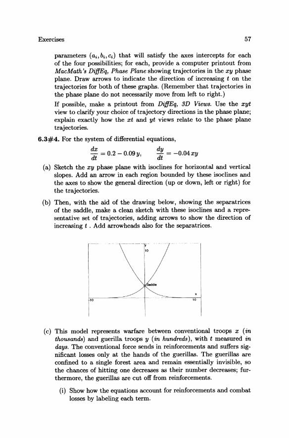
Exercises 57
parameters (ai, bi , Ci) that will satisfy the axes intercepts for each of the four possibilities; for each, provide a computer printout from MacMath's DiffEq, Phase Plane showing trajectories in the xy phase plane. Draw arrows to indicate the direction of increasing t on the trajectories for both of these graphs. (Remember that trajectories in the phase plane do not necessarily move from left to right.)
If possible, make a printout from DiffEq, 3D Views. Use the xyt view to clarify your choice of trajectory directions in the phase plane; explain exactly how the xt and yt views relate to the phase plane trajectories.
6.3#4. For the system of differential equations,
dx dy dt = 0.2 - 0.09 y, dt = -0.04 xy
(a) Sketch the xy phase plane with isoclines for horizontal and vertical slopes. Add an arrow in each region bounded by these isoclines and the axes to show the general direction (up or down, left or right) for the trajectories.
(b) Then, with the aid of the drawing below, showing the separatrices of the saddle, make a clean sketch with these isoclines and a representative set of trajectories, adding arrows to show the direction of increasing t . Add arrowheads also for the separatrices.
10
I.
r.c10;;----~-=- .-. -----10
( c ) This model represents warfare between conventional troops x (in thousands) and guerilla troops y (in hundreds), with t measured in days. The conventional force sends in reinforcements and suffers significant losses only at the hands of the guerillas. The guerillas are confined to a single forest area and remain essentially invisible, so the chances of hitting one decreases as their number decreases; furthermore, the guerillas are cut off from reinforcements.
(i) Show how the equations account for reinforcements and combat losses by labeling each term.

58 6. Systems of Differential Equations
(ii) Tell how many men per day are sent as reinforcements to the conventional force.
(iii) If at the beginning of the campaign the conventional force numbers 2000 and the guerilla force 600, use the graph to tell which side wins and why (mathematically!).
Exercises 6.4 Higher Order Equations
6.4#1. Express each of the following differential equations as a system of first order differential equations:
(a) x" + 3x' + 5x = 0
(b) x" + 3tx' = t
(c) XIII - tx" + x' - 5x + t2 = 0
(d) x" - xx' = o. 6.4#2°. A classical method for solving second order differential equations with either the dependent or independent variable missing [Le., either x or t is missing from I(x",x',x,t) = 0] is to make a substitution y = dx/dt which results in the original equation being expressable as a first order equation in either
y and t, if I(x",x',t) = I(y',y,t) = 0,
or
y and x, if I(x",x',x) = 0, using
" dy dx dy x = dx dt =Ydx'
so you end up with I(dy/dx,y,x) = o. In either case, this new equation is a first order equation in y j once it is
solved for y (as a function of t in the first case, of x in the second), you can get to x = u(t) by solving another first order equation, dx/dt = y, which comes from the original substitution.
You can apply this method to actually solve parts (a), (b), and (d) of Exercise 6.4#1. Take note of the difference in character for each equation. That of part (a) is autonomous (no explicit dependence on t) and linear, with constant coefficients, and will be solved by the general algebraic methods of Chapter 7. If you make the substitution y = dx/dt, you find a first order equation that can be separated in the variables (x, v) if you set y = xv, so that dy/dx = xdv/dx + v (see Part I, Exercise 2 misc#2 about "homogeneous" first order equations).

Exercises 59
The equation of part (b) is a second order nonhomogeneous linear equation, with nonconstant coefficients. The methods of Chapter 7 do not quite apply, but the substitution y = dx / dt makes it a first order nonhomogeneous linear equation that is solvable (by the methods of Chapter 2, Sections 3 and 4).
The equation of part (d) is not linear, so it would not be solvable by the methods of Chapter 7; thus, this classical substitution can be a helpful trick.
6.4#3. For the system dx/dt = 3x - Y dy/dt = x+ 2y
(a) Replace by a second order equation in x.
(b) Replace by a second order equation in y. Does the result surprise you?
(c) Prove that for any system of linear first order equations with constant coefficients,
dx/dt = ax + by dy/dt = ex + dy
the second order equations in x and y are always exactly the same.
(d) Show that, despite the results of (c), the solutions to (a) and (b) are not exactly the same. Explain. Hint: Show what happens with initial conditions x(O) = 0, y(O) = 1.
6.4#4. Replace, where possible, the following systems of first order differential equations by a single equation of higher order.
(a) dx/dt = 3x - y2 dy/dt = x+2y
(b) dx/dt = 3x - y2 dy/dt = x 2 + 2y
(c) dx/dt = y + cos(x + y) dy/dt = x - y sinx
dx/dt = x (d) dy/dt = y sinx

60 6. Systems of Differential Equations
Exercises 6.5 Mechanical Systems with One Degree of Freedom
6.5#1. Consider a particle with mass 1 moving on a line under the potential V(x) = x4 - 1.
(a) Show that the particle obeys the differential equation
x" = -4x3 ,
and write this second order equation as a system of two first order differential equations.
(b) Write down the energy function and show that the energy is constant along solutions.
(c) Sketch some level curves of the energy function. One nice way is to use MacMath's Analyzer program to sketch the two y functions (one positive, one negative) for each value of E.
6.5#2. Consider a particle of mass m moving on a line under the potential V(x) = 2x3 - 3x2 •
(a) Show that the particle obeys the differential equation
mx" = -6x2 + 6x,
and write this second order equation as a system of two first order differential equations.
(b) Sketch the level curves of the energy function in the phase plane; find and describe the equilibria of the motion.
6.5#30 • Consider a particle with mass m = 1, which moves with one degree of freedom under the potential
V(x) = X4 - x2 •
(a) From a sketch of the graph of V(x) [or of 2V(x)], sketch in the phase plane different level curves for the total energy. Find the equilibria. Mark at least three different level curves corresponding to E(x, y) = C, where C is negative, 0, and positive, respectively. Put arrows on the curves to indicate in which direction the particle follows them. (To make it clearer, use different colors for different trajectories). Describe the various types of motion for the particle.
(b) What happens if a small friction term is added on, proportional to the velocity? Sketch the corresponding drawing in the phase plane and describe the equilibria and the motions.

Exercises 61
6.5#4. For a spring with no friction, the potential energy is
k > o.
Find the differential equation describing the motions of a bob of mass m at the end of such a spring and draw the trajectories in phase space. Explain why the trajectories look the way they do.
6.5#5. A mass m is suspended from a spring with spring constant k, as shown.
IIIIIIII
I JJ -,"""m_~ ;:: ~·i J stretched position
Show that if we measure the position of the mass relative to the stretched equilibrium position, we can rewrite the downward force,
F = mg - kx = mx",
without the mg term and thus the force is dependent on position alone.
6.5#6. The force exerted by a spring on a frictionless cart at its end is often modeled by F = -k x where x is the displacement of the cart.
!~ ~ m ;: ....... -....... . .. _-_._- .
I -~
Suppose that a better model is F = -k(x) x, where k(x) = eX'. Let the mass of the cart be m.
(a) Sketch the phase portrait of this system.
(b) If the cart is held still at a displacement of l > ! and then released, what will its velocity be the first time its displacement is !?
6.5#70 • Find a function V(x, y) that is constant along solutions for the system
dx ( 2 dt = - 1- x ),

62 6. Systems of Differential Equations
(Warning: This is truly an exercise in integration!)
6.5#8. Figures 6.5.3 and 6.5.4 show a saddle point at (rr,O). Use an approximation of sin 0 to show that this is indeed a saddle point of E y2/2 - k cos O. Draw the graph of the trajectories near (rr, 0).
6.5#9. Consider the differential equation
x" = ax - x 3 .
( a) '!Urn this equation into a system of two first order equations
dx/dt = I(x, y)
dy/dt = g(x, y)
and state precisely what the relation is between the two.
(b) Find a function E(x, y) which is constant on the trajectories.
(c) What do the level curves of E look like for a > 0, a = 0, a < O?
(d) Classify the solutions of the original second order equation in the three cases of part (c).
6.5#10°. Consider the dynamical system with one degree of freedom
" dV x =--, dx
where Vex) = sin x + ax2 with a > 0 a parameter.
(a) '!Urn the equation into a system of first order equations.
(b) Find a conserved quantity for this system. Plot approximately the level curves of this conserved quantity, for a = 0.01, a = 0.1, a = 0.5, a=l.
(c) Describe the equilibria of the system as functions of a.
6.5#11. Confirm that the mathematical total energy function (18),
y2 E(O,y) = 2 - K cos 0, (18)
is within a constant multiple of the physical total energy, kinetic energy plus potential energy.
6.5#12. Consider the case of a bead constrained to move along a semicircular wire.

Exercises 63
(a) Show that if the bead is a distance s along the wire (from the bottom), with x-coordinate x{s), the force ms" is
V'{x(s» -m -Vr=l =+=7.:{V~,:;={ x~{ s=:=::) ):::=;0)2
(20)
(b) Confirm all the steps of the derivation in Example 6.5.5 to show that
s" = - sin(sj.e).
(c) Confirm that in this case, with s = .eO, that
dv ds
!'(O) implies !(O) = -K \1'1- (20j7r)2. \1'1 + U'(O»2
6.5#13. Consider the final remark of Section 6.5, that one may wonder whether, given a function V(x), there is some other function W(x) such that the motion on the wire with the shape of the graph of W, that is with equation
" W'(x(s» s = , \1'1 + (W'(x(S)))2
is precisely the same as motion under x" = -dVjdx. Clearly, one requirement is I dVjdx I < 1. Show that this is the only requirement.
Exercises 6.6 Essential Size, Conservation Laws
6.6#1. Find the essential size of the following systems:
(a) x' = x, y' = 2y + x 2
(b) x' = xz,y' = 2y + x2 ,z' = Y
(c) x' = x,y' = 2y,z' = x2
6.6#2°.
(a) In Example 6.6.8, fill in all the steps (there are several) that lead from equations (26) to (27).
(b) In Example 6.6.8, verify the statement that r will never leave the plane spanned by r(to) and r'(to).
(c) In Example 6.6.9, verify the statement that the magnitude of r x r' = M, which is conserved, is in fact the angular momentum.

64 6. Systems of Differential Equations
Exercises 6.7 Two-Body Problem
6.7#1. For two bodies moving under Newton's Universal Law of Gravitation,
" amI (Xl - X2)
X2 = IlxI - x211 3
(a) Show that linear momentum is a preserved quantity.
(b) Using ml = 1 x 10⁵ , m2 = 2 x 10⁵ and the initial conditions
x,(to) ~ U] , x,(to) ~ [=!] ,
show that the position vector
x(to) ~ [ =~] , x,'(to) ~ m ' to ~ 1,
X = mlXI + m2x 2
ml+m2
(33)
for the center of mass can be written as X(t) = a+t b, hence showing that the center of mass moves at constant velocity in a straight line.
(c) After translation to the center of mass, X, show that r = Xl - X satisfies
" r r = -K IIr1l3 .
(d) We could set rl = Xl - X and r2 = X2 - X. Show that then
-m2 rl = (X2 - Xl)
ml+m2 ml
r2 = (X2 - Xl). ml+m2
6.7#20 • For three bodies we would have three second order differential equations in Xl, X2, X3 . The center of mass is defined by
X = mlXI + m2X 2 + m3x 3 .
ml +m2+ m3

Exercises 65
(a) Show the conservation of linear momentum for three bodies:
(b) How does the center of mass move?
6.7#3. Show that in the two-body problem the level curves of the total energy E look like Figure 6.7.3, using the graph of the "potential" W{r) given in Figure 6.7.2.
6.7#4.
(a)O Study the motion under a central force
k r - r3 r'
instead of the gravitational force
k r - r2 r
of the two-body problem of Section 6.7.
Write down the equations similar to (35) through (39) in Section 6.7. Make the drawings similar to Figures 6.7.2 and 6.7.3. Explain why there is no bounded motion.
(b) More generally, if the central force is
k r - rQ r'
for which a can we have bounded motions?
6.7#5.
(a) Prove that Kepler's Second Law is equivalent to conservation of angular momentum. Note that both of these statements are valid in any central force field, not just one with an inverse square law such as the gravitational field.
(b) Use MacMath's Planets program to illustrate your examples.
6.7#6.
(a) Confirm equation (41) in the derivation of Kepler's First Law by integration of
dJ) M = (41)

66 6. Systems of Differential Equations
(b) Confirm by integration of (41) that
(Mlr-KIM) O=arccos .
J2E + K2/M2 (42)
6.7#7. Show that r= p
1+ecost is the equation of an ellipse, as claimed in the proof of Kepler's First Law. Recall that an ellipse is the set of points such that the sum of the distances to the foci is constant (= 2a).
6.7#8. The constant of gravity G is (6.673 ± 0.003) x 1O-8cm3/(gsec2 ).
Note, incidentally, that it is not known with great precision.
(a) If a body with small mass ml rotates around one with large mass m2
with period T and semi-major axis a, give a formula for m2 in terms of G, T, and a. How sensitive is this formula to the assumption that one mass is negligible? For instance, how wrong is it if ml = m2/4?
(b) Assume that the mass of the earth is negligible with respect to the mass of the sun. Given that the distance from the earth to the sun is approximately 1.496 x 1013cm, and that the earth revolves around the sun in 1 year (1 year = 3.156 x 10⁷ sec), what is the mass of the sun?
(c) Assume that the mass of the moon is negligible with respect to that of the earth. Knowing that the distance of the moon to the earth is approximately 3.85 x 1OlOcm, roughly what is the mass of the earth?
6.7#9. A recent practical application of the two-body problem was calculation of the mass of Pluto, from the 1978 discovery that Pluto has a moon:
(a) Pluto was discovered in 1930, as a result of perturbations in the orbit of Neptune. In 1978, astronomers J. Christy and R. Harrington discovered that Pluto has a satellite, which they called Charon. Charon appears, from the earth, to have an orbit with a radius of about 20,000 kilometers about Pluto, and a period of about 6 days and 10 hours. If the orbit is circular, what is the mass of Pluto?
Remark. We have asked some astronomers why the orbit is assumed to be circular. They answer that a very eccentric orbit leads to large tidal effects, which would presumably either break up the satellite, or at least absorb enough energy to bring it to a more circular orbit.

Exercises 67
(b) The number found in part (a) is about 100 times too small to ~xplain the irregularities in the orbit of Neptune. Assume rather that the orbit of Charon is very elliptical, with the long axis pointed toward the earth. How eccentric would the orbit need to be in order to bring the mass up to the level required to explain the irregularities?
6.7#10. We are collecting exercises derived from playing with MacMath's Planets program and welcome more examples.
Exercises 6.8 Flows
6.8#1. Use a phase portrait program like MacMath's DiffEq Phase Plane to explore the flow of different rectangles for equations A of Example 6.8.2. For example, some possibilities are shown in the following diagram for various positions of a rectangle like the original one (darkest) of the example:
3.0
IT] m w 0 1IIIIIIIIIilmi
-5.0 5.0
CO W
(i) Show the flow for the solid rectangles symmetric to the original rectangle.
(ii) Explain the similarities and differences in the results.
(iii) Predict what will happen to the dotted rectangles and verify with the computer.
(iv) Conjecture and explain what happens geometrically to the flow in general, globally, for this differential equation. One way to do this is to imagine the phase plane filled with little squares and think about what will happen to them all as you take a step in t.
6.8#2. Repeat Exercise 6.8#1 for equations B of Example 6.8.2.
6.8#3. Repeat Exercise 6.8#1 for equations C of Example 6.8.2. Note that the behavior of this flow is far less obviously predictable than those of equations A and B; this is because the dependence on initial condition

68 6. Systems of Differential Equations
really rules this flow! You should find several different behaviors to explain in this example. This system C is equivalent to the famous one-dimensional equation dx/dt = x 2 - t of Part I of this text. Does that help to explain your results?
6.8#4. For each of the cases A, B,and C of Example 6.8.2, draw or compute and print the direction field with a number of trajectories. Then explain what additional information you get from the flow that you do not get from the direction field.
6.8#5. Verify that the formula and the domain in Example 6.8.4 are correct.
6.8#6°. Give a formula and the appropriate domain for the flow of the following equations:
X' = x3 , x' = x3 - x.
6.8#7. For the following differential equation, an explicit formula for the flow cannot be given in elementary terms. Sketch the domain of the flow, and give a formula for the domain using definite integrals.
x' = x2 - sin(x).
6.8#8. This exercise is quite a bit more challenging than the previous ones. Try to sketch, in 1R3 , the domain of the flow from equations C of Example 6.8.1. In particular, describe how this domain is related to the exceptional solution of the equation. How does this domain intersect the plane x = a for a small (say a = -5), or for a large (say a = 5)?

7
Systems of Differential Equations The only large and important class of systems of differential equations that has been extensively analyzed is that of linear differential equations, which we begin to study in this chapter. We will give examples in Section 7.1 and the formal (simple) side of the theory in Section 7.2. The more substantive theoretical results (for linear equations with varying coefficients) are deferred to Chapter 12 in Part III.
The class of linear differential equations for which we can in general find explicit solutions is restricted to those with constant coefficients. The remainder of this chapter will be devoted to these: how to compute and analyze their solutions. Chapters 8 and 9 deal with important facts that extend from linear to nonlinear differential equationsj Chapters 10 and 11 (in Part III) will work out interesting classes of examples.
As we will see, the theory for constant coefficients is largely linear algebra. When you need to review basic linear algebra operations, consult Appendix L, Sections L1-L6. The related computer programs for finding eigenvalues and eigenvectors are elaborated in Appendices L7 and L8.
7.1 Linear Differential Equations in General
A linear differential equation for a vector function x{t) is one that can be written as
X' = A{t)x (I)
or, more generally, X' = A{t)x + get), (2)
where A is a matrix and g is a vector, both of which can be filled with functions of t. The word "linear" means with respect to the dependent variable Xj the entries of the matrix function A{t) and the vector function get) need not be linear functions of the independent variable t.
Example 7.1.1. The system
X' =y
y'=-X,

70 7. Systems of Linear Differential Equations
which was introduced in Examples 6.1.2, 6.1.3, and 6.2.5 and is one of the basic linear equation examples that you will see often, can be written
X' = A x.
Example 7.1.2. The system
x' =t2x-y
y' = (lnt)x + et
is also linear in x and y and can be written
[X]' [t2 Y = lnt
x' = A(t) x + get).
where the matrix A as well as the vector g depends on t, but their entries are in fact not linear functions of t. •
Example 7.1.3. The system of equations
is not linear. It can be written
x' = y+xy
Y'=X+y2
or as
[:J' [~ (l;X)] [:]
[:],=[i !] [:], but however you write it, the matrix A must contain entries in the depen-dent variables x and y. •
The case of linear differential equations where x is one-dimensional has been extensively treated in Chapter 2. We present here two archetypal examples in two dimensions:
Example 7.1.4. The damped harmonic oscillator. Suppose a mass m is suspended from a spring with restoring force F and damping constant k, as shown in Figure 7.1.1. If x denotes the displacement of the mass

7.1. Linear Differential Equations in General 71
from equilibrium and y its velocity, then it obeys the system of differential equations
x' =y my' = -Fx - ky,
(3)
which can be written alternatively as
(4)
FIGURE 7.1.1. Mass on spring.
You may be more familiar with the same problem in the form of a single second order differential equation,
mx" + kx' + Fx = 0, (5)
which you can obtain by differentiating the first equation of system (3) and substituting x" = y' and x' = y into the second equation of the system .
• Exercise 7.1-7.2#5 elaborates on Example 7.1.4 for the case of varying
rather than constant mass (a water bucket that leaks).
Example 7.1.5. The driven RLe circuit. Consider the electrical circuit of Figure 7.1.2, consisting of a resistor with resistance R, a capacitor with capacitance C, an inductor with inductance L, and a generator which furnishes a potential drop f ( t).
resistor
~ capacitor
FIGURE 7.1.2. Electric circuit.

72 7. Systems of Linear Differential Equations
Then, as you have probably seen in physics or engineering courses (and as we shall show in Chapter 10 of Part III), the voltage drop V(t) across the capacitor and the current I(t) through the inductor satisfy the system of equations
CV'=I LI' = -V - RI + f(t),
which can be written alternatively as
(6)
Again, you may be more familiar with the equation in second order form:
LQ" + RQ' + (l/C)Q = f(t), (7)
where Q = CV is the charge on the capacitor. A
Notice that the two equations (5) and (7) of Examples 7.1.4 and 7.1.5 are almost the same; in fact the equation describing a forced damped harmonic oscillator would be precisely the same as the equation describing the driven RLC circuit. These models will be greatly expanded in Chapters 11 and 10 of Part III, respectively.
Equations like (5) and (7) appear constantly in physics and engineering, both in their own right and as approximations to other more complicated equations.
NONLINEAR EQUATIONS
Certainly not all systems of differential equations are linear. Nearly every example of such a system that was discussed in Chapter 6, such as
i. the predator-prey model:
ii. the simple pendulum:
x' = ax - bxy y' = -cy + dxy,
0" = -K sinO,
iii. the derivation of Kepler's First Law: r" = - K /r + M2 /r3 ,
is not linear, because terms like xy, sinO, and rm (for m =f:. 1) are not linear in the variables
respectively, that underlie each of these examples.

7.1. Linear Differential Equations in General 73
HIGHER ORDER DIFFERENTIAL EQUATIONS
Very often those systems of differential equations that are linear appear in the form of higher order linear differential equations [as defined in the Introduction, equation (5)], like this section's equations (5) and (7), rather than as systems of first order differential equations. However, the method of Section 6.4, translated into the language of matrices, easily changes a higher order equation into a system of first order equations.
Example 7.1.6. The equation x'" - 3x" + tx' - x + t2 = 0, of Example 6.1.6 in Section 6.4, can be written as
x' = [~ ~~] x + [ ~ ] , 1 -t 3 -t2
where the desired solution is x = u(t) = Xl(t). [Recall that X2(t) = u'(t) and X3(t) = u"(t).] .A
Example 7.1.6 illustrates the following procedure for converting an nth order linear differential equation to a system of first order linear differential equations in matrix form:
(1) Solve the original nth order equation for x( n) •
(2) The bottom line of the matrix A(t) is formed by the coefficients of x, x', x", . .. ,x(n-l), in that order, the bottom entry in the vector g(t) is the extra function of t.
(3) Above the bottom line of the matrix, all entries are zeroes except in positions just above the main diagonal, where they are ones.
If you have already run into higher order linear differential equations such as (5) and (7), then you are probably also familiar with the cookbook method for their solution:
Recipe 7.1.7. To solve the equation
ax" + {3x' + '"(x = 0, (8)
substitute u(t) = emt into equation (8), giving (am2 + 13m + '"()emt = o. Since emt does not vanish, we get the characteristic equation
am2 + 13m + '"( = o. (9)
There are three cases to consider:

74 7. Systems of Linear Differential Equations
(a) (32 - 40:, > 0, so the quadratic equation (9) has two real roots ml and m2. Then the general solution is
(b) (32 - 40:, < 0, so the quadratic equation (9) has two complex roots J.L ± ia. Then the general solution is
(c) (32 - 40:, = 0, so the quadratic equation (9) has a single double root m. Then the general solution is
Most of the remainder of this chapter is devoted to understanding this recipe and its generalizations beyond two-dimensional systems of linear differential equations.
7.2 Linearity and Superposition Principles
In exact analogy with the one-dimensional linear differential equations that we studied in Sections 2.2 and 2.3 in Part I, a linear equation of the form
X' = A(t)x + g(t)
is called homogeneous if g(t) = 0 and nonhomogeneous if g(t) =1= O. In the latter case, the equation x' = A(t)x is called the associated homogeneous equation.
There are a certain number of important algebraic properties of linear differential equations, concerning sums of solutions and so forth. They take a bit of time to state, but they are very easy (which does not mean they are not important).
These properties may remind you of similar statements about linear (nondifferential) equations and their associated homogeneous equations. This is not surprising: they are somehow the essence of linearity. At the end of this section, we will give the general framework, which includes both.
Let A(t) be an n x n matrix with entries continuous functions of t.
Theorem 7.2.1 (Superposition of solutions for homogeneous equations). If Ul(t) and U2(t) are two solutions of the homogeneous linear differential equation x' = A(t)x, then any linear combination of those solutions

7.2. Linearity and Superposition Principles 75
for any two numbers 0 1 and O2, is also a solution.
Proof. Just plug u(t) = 01U1(t) + 02U2(t) into x' = A(t)x and rearrange terms. 0
Example 7.2.2. Consider x" + 3x' + 2x = o. You can obtain from Recipe 7.1.7 that two solutions are x = U1(t) = e-t and x = U2(t) = e-2t and that
(10)
is also a solution, or, if you prefer to work with a system of first order equations, by the algorithm of Section 6.4,
[:r=[-~ -!] [:]. Two solutions are U1(t) = [ ::':~t] and U2(t) = [_~:~2t]' as you can
confirm by substitution, and so also is
Note that the top line of the vector solution matches the expression you got for x = u(t) in (10). But it is not obvious that this includes all of the solutions. &
In order to show that indeed we have all solutions for a linear differential equation like Example 7.2.2, we shall wait until Theorem 7.4.12 when we will have a formula showing the existence of solutions. You can show in Exercise 7.2#6 that linear differential equations with constant coefficients automatically satisfy a Lipschitz condition, so from the Fundamental Inequality 6.2.2 you will also have uniqueness.
Theorem 7.2.3 (General solution of nonhomogeneous equations). If up(t) is any (particular) solution of a nonhomogeneous differential equation
x' = A(t)x + g(t), (11)
then a vector function u(t) is a solution of (11) if and only if u(t) can be written
u(t) = up(t) + Uh(t),
where Uh(t) is a solution of the associated homogeneous equation
x' = A(t)x.

76 7. Systems of Linear Differential Equations
Proof. We show that u(t) = up(t) + Uh(t) is a solution by plugging in:
Then we show that the solution must be of form u(t) = up(t) + Uh(t) by proving that u(t) - up(t) satisfies the homogeneous equation A(t)x = 0:
(U(t) - up(t»' = u'(t) - u~(t)
= A(t)u(t) + g(t) - (A(t)up(t) + g(t»
= A(t)(u(t) - up(t». 0
As with the linear equations in one dimension discussed in Sections 2.2 and 2.3 in Part I, the usual ways of finding a particular solution Up(t) to a nonhomogeneous equation are the methods of undetermined coefficients (an educated guess) and variation of parameters. We shall use the first of these here and discuss the second for higher dimensional systems of linear equations later, in Section 7.7.
Example 7.2.4. Consider
A particular solution to the entire nonhomogeneous equation is
(t) _ [0.1 sint - 0.3 cost] Up - 0.1 cos t + 0.3 sin t
as you can confirm, and a solution to the associated homogeneous equation was found in Example 7.2.2. Therefore,
[ 0.1 sint - 0.3 cost] [ e- t ] [ e-2t ] u(t) = 0.1 cos t + 0.3 sin t + C1 _e- t + C2 _2e-2t
for any C1 and C2 is a solution to the original equation. A
Example 7.2.4 is the system that represents x" + 3x' + 2x = sin t, so, as in Example 7.2.2, you can confirm that a solution to this second order equation is read from the top line of the vector equation:
Theorems 7.2.1 and 7.2.3 are both special cases of a more inclusive theorem:

7.2. Linearity and Superposition Principles 77
Theorem 7.2.5 (Superposition of solutions for nonhomogeneous equations). Iful(t) andu2(t) are solutions of two nonhomogeneous linear differential equations
X' = A(t)x + gl (t) and x' = A(t)x + g2(t),
respectively, with the same associated homogeneous equation x' = A(t)x, then
u(t) = Ul(t) + U2(t)
is a solution of the equation x' = A(t)x + gl(t) + g2(t).
Proof. Just plug in. 0
Example 7.2.6. Consider
A particular solution to the nonhomogeneous equation
[:r=[-~ -!] [:]+[~] is, as you can confirm, U2(t) = [t::] j in Example 7.2.4, we found that
the solution to the nonhomogeneous equation
is (t) _ [0.1 sin t - 0.3 cos t]
up - 0.1 cost + 0.3 sint .
Therefore,
[ 0.1 sin t - 0.3 cos t + (1/6)et ] [ e-t ] [ e-2t ] u(t)= 0.1 cost +0.3 sint+ (1/6)et +C1 -e-t +C2 -2e-2t
is, for any C1 and C2 , a solution to the whole thing. A
In the language of linear algebra, the above results may be restated as follows:
Theorem 7.2.1 says that the set of solutions of a homogeneous linear differential equation forms a vector space.

78 7. Systems of Linear Differential Equations
Theorem 7.2.3 says that the set of solutions of a nonhomogeneous linear differential equation is an affine space, i.e., the translate of the vector space of solutions of the associated homogeneous equation by any solution of the nonhomogeneous one.
Now we will relate these statements to the more standard statements from linear algebraic equations. Even if you have never seen these statements exactly, they should be clear.
Let M be a matrix (not necessarily square).
Statement A. Any linear combination of solutions of M x = 0 is a solution.
Statement B. If xp is a solution of Mx = a, then a vector x is another solution if and only if x = xp + Xc with Xc a solution of the associated homogeneous equation Mx = O.
Statement C. If Xl is a solution of Mx = al and X2 is a solution of Mx = a2, then Xl + X2 is a solution of Mx = al + a2'
Clearly these statements are parallel to Theorems 7.2.1, 7.2.3, and 7.2.5. The explanation of this fact is linearity.
Let V and W be vector spaces and T: V -> W a linear transformation. Then we have the following three linearity statements:
Statement 1. Any linear combination of solutions of Tv = 0 is a solution.
Statement 2. If vp is a solution of Tv = a, then a vector v is another solution if and only if v = vp + Vc with Vc a solution of the associated homogeneous equation Tv = O.
Statement 3. If Vi is a solution of Tv = al and V2 is a solution of Tv = a2, then Vi + V2 is a solution of Tv = al + a2'
Statements A, B, and C about systems of linear algebraic equations are the special case of the linearity statements 1, 2, and 3, where T is the linear transformation IRn -> IRm represented by the matrix M.
How about the differential equations of Theorems 7.2.1,7.2.3, and 7.2.5? What are the vector spaces and the linear transformation in that case? Well, the answer is a bit more unpleasant.
The space V is the vector space of continuously differentiable vector functions f(t) defined for tEl, where I is the interval on which A(t) and all the g(t) are defined.
W is the space of continuous vector functions on the same interval I.

7.3. Eigenvectors and Decoupling 79
The transformation T: f 1---+ f'(t) - Af.
Of course, the spaces V and W are infinite dimensional, and so are a bit unfamiliar, but all the results above are so formal that the nature of the vector space involved is irrelevant.
Such a linear transformation T: f 1---+ f'(t) - Af is called a differential operator (more accurately, a vector first order differential operator). Of course, the granddaddy of all differential operators is the derivative D, and it has close relatives D2, D3, ... (the second, third, ... derivatives). Another way of writing the differential equation
ax" + bx' + ex = 0
is (aD2 + bD + c)x = O.
Following this method of notation, all of the theory of linear differential equations can be rewritten in terms of differential operators. We will not do this, although we will use the language when it seems convenient.
7.3 Linear Differential Equations with Constant Coefficients; Eigenvectors and Decoupling
There is no formula for solving linear differential equations if the coefficients are not constant. In fact, it can be proved that the innocent looking equation x" - tx = 0 has no solutions, other than the zero solution, that can be written in terms of the elementary functions, or their indefinite integrals ad infinitum. (Reference: Theorem 6.6, p. 43 of Kaplansky's sixty-seven page book on Differential Algebra.)
In fact, the only substantial class of systems of equations that can be solved in elementary terms is the class of linear differential equations with constant coefficients. As a result, and also because of their intrinsic importance, these equations have traditionally been the bread and butter of differential equation courses. Ours will not be different; they will play a central part in our development.
The following theorem is really the most important result about linear differential equations with constant coefficients. It says that the component of a solution in the direction of an eigenvector evolves independently of everything else and obeys a linear differential equation in one variable, about which we know just about everything from Chapter 2 in Part I. This phenomenon of being able to look at components independently is called decoupling.
Accordingly, the theory of linear differential equations reduces (almost) to the algebraic theory of eigenvalues and eigenvectors. This theory is fairly simple, but when it comes to actually computing eigenvalues, the going

80 7. Systems of Linear Differential Equations
gets stickier. You can review the essentials of eigenvalues and eigenvectors in Appendix L6j actually finding them will most conveniently be done by the computer using the QR method described in Appendix L7 or Jacobi's method, described in Appendix L8.
Theorem 7.3.1 (Evolution in the direction of an eigenvector). Let A be an n x n matrix, and suppose v is an eigenvector 0/ A, with Av = AV.
Then u(t) = ae,X(t-to)v (12)
is the solution o/x' = Ax with initial condition u(to) = av.
Proof. As always, when an explicit solution of a differential equation is proposed, it is a straightforward matter of differentiating it and plugging the derivative into the equation to check whether or not it is correct. Let us compute
d -(u(t)) = Aae,X(t-to)v = a e'x(t-to)(AV) = ae'x(t-to)Av dt
= A(ae,X(t-to)v) = Au(t).
It is easy to verify that the initial condition is satisfied. 0
Do not be fooled by the extreme simplicity of the above derivation. It does not have to be hard to be important. That easy computation is an important service of mathematics to applied science.
Theorem 7.3.2. Let A be an n x n matrix 0/ constants, and suppose v}, ..• , Vm are eigenvectors 0/ A, with AVi = AiVi. Then/or the differential equation x' = Ax, i/ the initial condition is a linear combination 0/ these Vi'S,
m
u(to) = L aiVi, i=l
the solution is m
u(t) = L ai e,X·(t-to)Vi. (13) i=l
Proof. This follows from Theorems 7.2.1 and 7.3.1. 0
Theorem 7.3.2 is of particular interest when the Vi'S form a basis of Rn
or en, for in that case formula (13) gives all solutions to x' = Ax, since any initial condition can be stated as a linear combination of eigenvectors. In real life, this is the typical situation: in general, an n x n matrix will have n distinct eigenvalues and therefore provide an eigenbasis (a basis of eigenvectors) of Rn.

7.3. Eigenvectors and Decoupling 81
Theorem 7.3.3. Let A be an n x n matrix, and suppose Vb .•• , Vn form an eigenbasis of lRn , with AVi = AiVi. Then for the differential elJ.uation x' = Ax, the initial condition can be written
n
u(to) = L aiVi,
i=l
and the solution is n
u(t) = L ai eoX,(t-to)Vi. (14) i=l
The proof has been covered in the paragraph preceding the theorem.
CHANGE OF BASIS
Theorem 7.3.3 permits another point of view. Its key point is that
in a basis of eigenvectors, the coordinates evolve independently.
This statement is equivalent, in the language of change of basis, to the statement that
in a basis of eigenvectors, a system of linear differential equations with constant coefficients will decouple.
We shall now restate and rederive Theorem 7.3.3 in this language of change of basis.
Suppose that Vb .•• , vn is a basis of lRn (or Cn ) made up of eigenvectors of A with corresponding eigenvalues Ab ... , An, as above. Let P be the change of basis matrix, as described in Appendix L2, so that
p~ [++···+l· and p-1AP~ [: 0 l' An
the diagonal matrix with the eigenvalues Ai along the diagonal. This is why, when the eigenvectors of A form a basis for lRn , the matrix is said to be diagonalizable.
Theorem 7.3.4 (Decoupling x' = Ax by change of basis). Consider the differential equation x' = Ax in lRn. If Vb ••. ,Vn are eigenvectors of A forming a basis, with P as the change of basis matrix composed of the Vi as columns, and x == p-1x, then
i. each entry Xi of x satisfies the scalar differential equation

82 7. Systems of Linear Differential Equations
ii. the solution x = u(t) to the original differential equation can be written in terms of the initial condition x(to) as follows:
[
e>.l(t-tO)
x(t) = Px(t) = P o (15)
Proof. If we define x == p-1x, then the entries of x are the coordinates of x with respect to the basis VI,"" Vn (see Theorem L2.22 in Appendix L2). Now we are ready to prove the theorem:
i. Multiply the equation x' = Ax by p-l on the left and introduce a factor of pp-l = I between A and x, giving
or x' = (p-l AP)x.
Since p-l AP is diagonal, this last equation breaks up into
(16)
a completely decoupled set of ordinary first order linear differential equations.
ii. Each of the set (16) of decoupled equations can be explicitly solved as in Section 2.2 in Part I, giving
Xi(t) = e>.·(t-to)Xi(tO)'
Since x(t) = P-1x(t), then x(to) = P-1x(to), and putting all these solutions together in vector form gives equation (15). 0
Remember that Theorem 7.3.4 is simply a restatement of the message of Theorem 7.3.3. We shall solve a sample linear differential equation using both theorems.
Example 7.3.5.
To solve this equation, we first find eigenvalues and eigenvectors. The characteristic polynomial is

7.3. Eigenvectors and Decoupling 83
so the eigenvalues are 1 and ±v'5, and corresponding eigenvectors are
i. Solution by straight eigenvectors. The general solution, by Theorem 7.3.3, is
(17)
SUPP""" we know the initial condition"" x(O) ~ [~]. Then in oroe< to
find a, b, and c in solution (17), we must solve the system of linear algebraic equations
(18)
ii. Solution by change of basis. Theorem 7.3.4 gives the following, in terms of equation (15):
ret
x(t) = P ~ ~ 1 p-l [~] , e-v5t "I
(19)
which you can confirm (Exercise 7.3#9) gives the same result as equations (17) and (18). •
It is interesting to compare the amount of work necessary to solve Example 7.3.5 by the two theorems. In both cases, almost all the work is the same--you have to find all the eigenvalues and eigenvectors. But at the end, the first method, with equation (17), requires solving a (nondifferential) system of equations (18); the second method given by equation (19) requires computing the matrix inverse of P.
The first method is easier if you are solving just for a single set of initial conditions. But if you are going to be solving the problem for a number of different values of 0:, fl, and "I, the alternative second method gives an actual formula which will save a great deal of computation.
COMPLEX EIGENVALUES AND EIGENVECTORS
Up to this point, we have been working as if everything were in real numbers. Actually, there is no difference if the eigenvalues are complex:

84 7. Systems of Linear Differential Equations
Example 7.3.6. We shall solve the basic equation of Example 7.1.1,
[~r [~-~] [~], with initial condition [~~] at t = o.
First we find the eigenvalues and eigenvectors. The characteristic polynomial is >.2 + 1, so the eigenvalues are ±i and corresponding eigenvectors are
The matrices P and p-l are
p = [ ~ ~], -z z
and we can observe that indeed
the diagonal matrix of eigenvalues.
p-l = [1/2 i/2] 1/2 -i/2 '
By the change of basis solution (12) of Theorem 7.3.4, we get
[x(t)] [1 1] [eit 0] [1/2 i/2] [xo] y(t) = -i i 0 e- it 1/2 -i/2 Yo
Thus, Example 7.3.6 shows that computations with complex eigenvalues will yield, if painfully, terms with trigonometric functions in them.
FINDING EIGENVALUES AND EIGENVECTORS
The method we have just explained in this section is the most important for solving x' = Ax; the main task is to find the eigenvectors and eigenvalues of A. In principle, you could try to do this by computing the characteristic polynomial of A, finding the eigenvalues as its roots, and solving for the eigenvectors by solving linear equations.
It turns out that as soon as the matrix A is at all large, this method is quite impractical. First, computing the characteristic polynomial is quite laborious, even if something smarter than the formula for the determinant is used. Above, we spoke rather glibly about "finding the roots" of the polynomial, but it is not obvious how to do this (and in fact it is quite hard).
So we turn to the computer, but if we were to work directly with finding the roots of the characteristic polynomial, we would find that in the

7.4. Exponentials of Matrices 85
computation all precision is lost, and the coefficients of the characteristic polynomials are known only approximately. In addition, the errors in the coefficients may lead to much larger errors in the roots. (See Exercise 7.3#10.)
We have two other computer approaches, the QR method and Jacobi's method, that alleviate some of these problems (although finding eigenvectors and eigenvalues really is hard, and nothing will make it quite simple). Appendices L 7 and L8 respectively describe the QR method (and its simpler cousin, the power method), and Jacobi's method (which only works for symmetric matrices).
7.4 Linear Differential Equations with Constant Coefficients; Exponentials of Matrices
The eigenvector method of Section 7.3 has some limitations. If there are not enough eigenvectors to form a basis of an or en, then there is an alternative approach.
Just as, from Section 2.2 in Part I, the solution of x' = ax with u(O) = Xo is
we shall see (in Theorem 7.4.12) that the general solution to x' = Ax with u(O) = Xo is
u(t) = etAXo. (20)
This requires the exponentials of matrices, to which we now proceed. However, the reader should not think this is a panacea-it just shifts the problem from solving differential equations to computing exponentials.
Definition 7.4.1 (Exponentials of matrices). If A is a square n x n matrix, we define
A2 A3 00 Am eA =:1+A+-, +-, + ... = L -,'
2. 3. m=O m. (21)
First let us give a few examples.
Example 7.4.2.
t212 t313 etI = 1 + tI + -- + -- + ... = et 1,
2! 3! (22)
since 1 = 12 = 13 = .... In particular, if t = 0,
e(O)I = 1 = e(O)A. (23)

86 7. Systems of Linear Differential Equations
Example 7.4.2 is a special case of Example 7.4.3:
Example 7.4.3. If A is a diagonal matrix with diagonal entries '\1. ... ,'\n, then etA is also diagonal, with entries et~l , ... ,et~n along the diagonal. •
Example 7.4.3 is important, because it shows the main way in which exponentials are actually computed, as we shall see in Theorem 7.4.13.
The next example is less familiar but actually easier. It illustrates a phenomenon that occurs for exponentials of matrices but not for exponentials of numbers; that is, if there exist polynomials in the exponent, then etA may have polynomial terms and the series may be finite.
Example 7.4.4.
J~ ~L[~ ~]+[~ ~]+H~ ~]+ ... ~[~ :] because, as you can confirm, [~ ~ ] m = [~ ~ ] , for m ~ 2. •
When real matrices have complex eigenvalues, sines and cosines make their way into the exponential. This is hardly surprising, since ei9 = cos 9 + i sin 9, but please observe that complex numbers are never mentioned in the next example:
Example 7.4.5.
:[~ -~L[~ ~]+t[~ -~]+:",[-~ -~]+~t"[-~ ~]+ ... = [c~st -sint]
smt cost
from the power series for sine and cosine. Note that this calculation indeed gives the solution for the differential equation of Example 7.3.6 that you could expect from equation (20). •
Remark. Since etA is a matrix, the order of multiplication must be (etA)(xo), i.e., (matrix) (vector); the opposite order makes no sense. Moreover, since etA is a matrix function of t, it can be differentiated with respect to t: the derivative of a matrix function M(t} of t is another matrix M'(t} of the same size, where each element M'(t}ij is the derivative of the corresponding element M(t}ij.

7.4. Exponentials of Matrices 87
PROPERTIES OF eA
Formula (21) defining eA for an n x n matrix A is exactly the same as the power series for the exponential of a number; we may hope it will have similar properties. This is true up to a point, as we shall show in the following properties:
Property 7.4.6 (Convergence). The series defining eA converges for every A.
Proof. If SUPi,j IAi, jl :::; k and the matrix A is n x n, then it is can be shown by induction that
because from the formula for multiplication of matrices, each multiplication is the sum of n terms. Therefore,
I 00 (Amkj I <..!:. 00 (nk)m = enk
L m! -n L m! n' m=O m=O
and we see that the series does converge by the comparison test. 0
The fundamental property of the exponential function is ea+b = eaeb . So we might hope that for any two n x n matrices A and B, we would have eA+B = eAeB. Unfortunately, this is false in general, and this is the reason why systems are more difficult than scalar equations. If the two matrices commute, which means that the order of multiplication does not matter, then the hoped-for result is true:
Property 7.4.7 (Addition formula). If A and B are two n x n matrices that commute, so that AB = BA, then
(24)
Proof. Let us look at the two series developments, carefully keeping track of the order of multiplication (not just using the binomial expansion formulas):
i. e(A+B) = I + (A + B) + ~(A + B)2 + ~(A + B)3 + ... 2 6 1
= I + (A + B) + 2(A2 + AB + BA + B2)
1 + "6(A3 + A2B + ABA + AB2 + BA2 + BAB+ B2A+ B 3)
+ ...

88 7. Systems of Linear Differential Equations
ii. eAeB = (I + A + ~A2 + ~A3 + .. -) (I + B + ~B2 + ~B3 + .. -) 1
= I + (A + B) + 2(A2 + 2AB + B2)
1 + - (A3 + 3A 2 B + 3AB2 + B 3) + ... 6 .
Proceed until it is clear that if AB = BA, the series are equal. 0
The most important thing to remember about Property 7.4.7 is the necessity, which you see in the proof, that the matrices commute. In general (when AB =f:. BA),
[0 -1] [0 0] Example 7.4.8. Let A = too and B = t 1 0 . You can confirm
that AB =f:. BA and that A2 = B2 = O. We shall show here that eAeB =f:. eA +B :
,A,B ~:[g ~11:[~ gL (Ht [g -m· (1 +t [~ m = I + t [~ - ~] + t2 [ - ~ ~] = [1 ~ t 2 -n.
From Example 7.4.5,
[0 -1] eA+B = et 1 0 = [C?st -sint].
smt cost
(25)
(26)
Clearly, these results, (25) and (26), do not match (although we do get the same first terms in the power series!), so eAeB =f:. eA+B in this case, where AB=f:.BA. ~
Property 7.4.9 (Differentiation). We have the following formula for the derivative of etA:
d dt (etA) = AetA .
Proof. By the definition of derivative,
!!..etA = lim (!) (e(t+h)A _ etA). dt h--+O h
Certainly tA and hA commute, so e(t+h)A = ehAetA , and we see that
!!..etA = lim (!) (ehA - I)etA . dt h--+O h
(27)

7.4. Exponentials of Matrices
Now ehA - J = hA + !h2 A2 +"', so limh-+o(1jh)(ehA - J) = A and
!!..etA = A etA. dt
89
o
Remarks. For any square matrix A, the matrices A and etA commute, so in the previous formula, the factor A can be written on the right or the left.
In Exercise 7.4#4 you can show that the product and chain rules for differentiation also hold for expressions involving exponentials of matrices.
Example 1.4.10.
t[O d 1 -e dt
as you might have expected from differentiating both sides of the last line of Examples 7.4.5 and 7.4.8. •
Property 1.4.11 (Change of basis). If M is an invertible matrix, then
(28)
Proof. This follows from the power series (21),
M- 1 AM _ 1M- l AM (M- 1 AM)2 (M- 1 AM)3 e = + + + + ...
2! 3! M- 1A2M M- 1A3M
== I + M- 1 AM + 2! + 3! + ...
term by term, by observing that
(M-1AM)ffl = (M-1AM)(M- 1 AM) ... (M-1AM) = M-1AfflM. 0 '-v--'
I
all pairs in the middle cancel by M M- 1 = I
We are now ready to talk about differential equations again; Property 7.4.9 is precisely what it takes to prove the following major theorem:
Theorem 1.4.12 (Solving x' = Ax by exponentiation). The solution u(t) of x' = Ax with u(to) = Xo is
(29)

90 7. Systems of Linear Differential Equations
Proof. Just differentiate (using Property 7.4.9) and check. 0
So, we have a "formula" for the solution to a homogeneous linear differential equation. Unfortunately, Theorem 7.4.12 suffers from the standard defect of formulas: it says very little by itself. We want to know the answers to such questions as whether solutions go to 0 or to 00, and it is unclear that formula (29) says anything about this. We have just shifted the problem from solving the differential equation to computing the exponential.
However, if we have a basis of eigenvectors, the exponential reduces to something familiar. Property 7.4.11 implies that an eigenbasis for A is also an eigenbasis for eA.
Theorem 7.4.13 (Computing etA by eigenvectors). Let A be an n x n matrix and let Vb ... , vn be an eigenbasis for A with corresponding eigenvalues AI, ... , An. Let P be the change of basis matrix (i.e., the Vi are the columns of P); then the exponential etA can be computed as follows:
Proof. This is just a restatement of Property 7.4.11 and Example 7.3.4, as you can show in Exercise 7.4#5. 0
So, in the diagonalizable case where you do have a basis of eigenvectors, Theorems 7.4.12 and 7.4.13 give the same result as Theorem 7.3.4, the eigenvalue/eigenvector method that leads quickly to an easy-to-interpret answer. Note, however, that the method of exponentiating matrices is in a different basis and usually does not lead to anything recognizable as the same thing. (See Exercise 7.4#6.)
Even if there is no basis of eigenvectors, you can fall back on the exponential approach, working directly from the power series using Theorem 7.4.12 and Definition 7.4.1. Only sometimes will this result in anything you can calculate. Calculating the exponential of a matrix can be quite complicated, requiring generalized eigenvectors or Jordan Canonical Form if you want explicit formulas. Although, compared to nonlinear problems, this is still "simple," if you try to put this into practice, you will come to understand the expletive that "hell is undiagonalizable matrices."
Before leaving this subsection, we will make one more algebraic point. We go back and note that Example 7.4.5 is also an example of the following result:
Theorem 7.4.14. If A is an antisymmetric real matrix (or more generally an anti-Hermitian matrix), then etA is orthogonal (or, more generally, unitary).

7.5. Two by Two Matrices and the Bifurcation Diagram 91
Proof. As defined in Appendix L4, antisymmetric means that AT = -A; orthogonal means that the column vectors of the matrix are orthonormal, which in turn means that AT = A-I. We will treat the real case; the complex case is Exercise 7.4#7. Let us differentiate:
Thus, (etA)(etA)T is constant, and at time t = 0 it is the identity, so it is always the identity. Hence, etA is indeed orthogonal. 0
Notice that all of the theory of Section 7.4, as well as that of Section 7.3, is perfectly true with complex numbers as eigenvalues or entries in eigenvectors or the matrix A itself. In particular, the power series of Definition 7.4.1 makes sense for complex-valued matrices; we shall need this fact.
We shall examine in Section 7.5 the case of 2 x 2 matrices, where the mathematics can, surprisingly enough, be done directly from the power series of the exponentials.
7.5 Two by Two Matrices and the Bifurcation Diagram
Garrett Birkhoff says that according to his father, George Birkhoff, the most famous American scholar of differential equations:
If you understand linear equations, you almost understand differential equations;
If you understand linear equations of degree 2, you almost understand all linear equations;
Finally, you almost understand linear equations of degree 2 if you understand those with constant coefficients.
We find the first of these claims overoptimistic; the second and third, on the other hand, are certainly true. Second order linear differential equations with constant coefficients are ubiquitous. For that reason, we devote this section to them.
Second order linear equations with constant coefficients lead to the simplest system of the form x' = Ax, with 2 x 2 matrices A:

92 7. Systems of Linear Differential Equations
In this section, we will consider what the trajectories for this differential equation look like in the xy-plane, when A is a real matrix. In principle, we already could figure out the answer from Sections 7.3 or 7.4, at least if the eigenvalues of A are distinct, but we want to look at what those sections say in more detail in this particular case.
Note that the only equilibrium point is at (0,0). There are three cases of possible eigenvalues for a, b, c, and d real:
(1) real and distinct eigenvalues,
(2) complex eigenvalues (necessarily distinct since they are complex conjugate),
(3) a double eigenvalue (necessarily real).
You can confirm in Exercise 7.5#5 that with tr A = a + d and det A = ad - be the characteristic equation is A2 - (tr A)A + (det A) = 0, with discriminant
~ = (trA)2 -4detA,
and that cases (1), (2), and (3) correspond respectively to ~ > 0, ~ < 0, and ~ = 0.
1. Real (nonzero, distinct) eigenvalues. If ~ > 0, there are two real distinct eigenvalues Al and A2 and the corresponding eigenvectors Vl and V2 form a basis of ]R2. The general solution of x' = Ax can in that case be written, by Theorem 7.3.4, as
and the behavior depends on the signs of Al and A2. We discuss here the results for distinct and nonzero real eigenvalues; those for the case with a double eigenvalue are discussed below in subsection 3, and those for the case where an eigenvalue is zero are discussed in subsection 4.
i. Node source. If ° < Al < A2, then all trajectories tend to 00 as t --+ 00
and to ° as t --+ -00. (See Figure 7.5.1.) Moreover, all trajectories leave (0,0) tangentially to Vl except those that are multiples of V2 (Exercise 7.5#6a).
Y,
Y,
FIGURE 7.5.1. Node source.

7.5. Two by Two Matrices and the Bifurcation Diagram 93
ii. Saddle. IT Al < 0 < A2, then the trajectories with 0 1 = 0 go from o to 00 on the line in the direction of positive and negative multiples of V2, and those with O2 = 0 go from 00 to 0 on the line in the direction of multiples of VI; other trajectories are superpositions of these motions (Exercise 7.5#6b). (See Figure 7.5.2.) ....
v,
FIGURE 7.5.2. Saddle.
iii. Node sink. IT Al < A2 < 0, then all trajectories tend to 0 as t -+ 00 and to 00 as t -+ -00. (See Figure 7.5.3.) Moreover, all trajectories approach (0,0) tangentially to V2 except those that are multiples of VI (Exercise 7.5#6c).
FIGURE 7.5.3. Node sink.
Remark. A node sink is exactly the same thing as a node source with time going backward.
2. Complex eigenvalues. Suppose the two eigenvalues of A are a ± i{3, with {3 > o. Of course, there exists a basis VI, V2 of eigenvectors, but the vectors are in (:2, and it is not quite clear how to use them to describe the behavior of trajectories in the real phase plane. The following trick gives a way:
Observe first that if V is an eigenvector for Al = a + i{3, then v is an eigenvector for A2 = Xl = a - i{3. Let us write V = WI - iW2, where WI and W2 are real. Neither WI or W2 are eigenvectors, but they are linearly independent (Exercise 7.5#7) form a basis of R2; it turns out that in that basis A has a rather pleasant form. Indeed,
AWl + iAw2 = A(WI - iW2) = Av = AlV = (a + i(3)(Wl - iW2)
= (awl + (3w2) + i(aw2 - (3w1),
and identifying real and imaginary parts, we find
AWl = aWl + {3w2
AW2 = {3wl - aW2,

94 7. Systems of Linear Differential Equations
i.e., in the basis WI, W2, the linear transformation A has the matrix
[ 0: -j3] Al = j3 0: .
Alternately, let P = [WI, W2], with Al = p-1 AP. It is easy to compute etAl , because
[0 -1] Al = 0:1 + j3 1 0'
and the two matrices in this sum commute since the identity I commutes with everything. By Property 7.4.7 and a calculation as in Example 7.3.6, we see that
tAl _ tOt [cos j3t - sin j3t] e - e sinj3t cosj3t'
Now it is quite easy to see what the trajectory of a point looks like. It simultaneously turns at speed j3 radians per unit time, under the influence of the rotation matrix above, and approaches or leaves 0, under the influence of etOt , depending on whether 0: < 0 or 0: > O. This leads to the following classification:
i. Spiral sink. If 0: < 0, the trajectories spiral in to (0,0). (See Figure 7.5.4.)
FIGURE 7.5.4. Spiral sink.
ii. Center. If 0: = 0, the trajectories turn periodically on an ellipse and are called "centers," because each ellipse is centered at (0,0). (See Figure 7.5.5.)
FIGURE 7.5.5. Center.

7.5. Two by Two Matrices and the Bifurcation Diagram 95
iii. Spiral source. If a > 0, the trajectories spiral out to 00. (See Figure 7.5.6.)
FIGURE 7.5.6. Spiral source.
The direction of rotation of the spiral trajectories depends on the sign of c, the lower left entry of the matrix A: if c > 0, the rotation is counterclockwise; if c < 0, the rotation is clockwise. (You will prove this fact in Exercise 7.5#8.)
Centers are exceptional, but they turn up often in differential equations describing conservative mechanical systems as discussed in Chapter 6.5. Exercises 7.5#9, and especially 8.1#12, explain why this will occur.
THE TRACE/DETERMINANT PLANE; BIFURCATION DIAGRAM
The information we have assembled for the behavior of trajectories under real or complex eigenvalues leads us to begin Figure 7.5.7, a picture of
the plane determined by tr A and det A.
This plane (which is not an xy phase plane) merely helps us study how tr A and det A and the relationship between them determines the behavior of trajectories to x' = Ax.
The (tr A, det A)-plane is divided by the axes det A = 0 and tr A = 0 and by the parabola
(tr A)2 /4 = det A,
the dividing locus between the cases ~ > 0 and ~ < o. We shall examine more closely all of these divisions.
The sketches in each region of the (tr A, det A)-plane of Figure 7.5.7 are just insets showing a typical drawing (in the xy phase plane) for the trajectories to x' = Ax, for values of A corresponding to that region. The conventional labels for each type of behavior accompany each of these insets.
We still need to understand the remaining possibilities; i.e., what occurs along boundaries of the regions already discussed:
3. along the parabola where ~ = 0,

96 7. Systems of Linear Differential Equations
FIGURE 7.5.7. Bifurcation diagram in (tr A, det A)-plane for the two-dimensional equation x' = Ax.
and the division within the case of real eigenvalues between nodes and saddles:
4. along the horizontal axis det A = O.
3. Double eigenvalue. Along the parabola, ~ = O. If there is only one
(double) eigenvalue A, let VI = [~] be an eigenvector, and let V2 be any
vector linearly independent of VI. Then VI and V2 form a basis, and in that basis the linear transformation A has matrix
for some appropriate number a. You can see this by noting that the first column is correct since AVl = AVl and that, regardless of the entries in the

7.5. Two by Two Matrices and the Bifurcation Diagram 97
second column, the matrix Al will be upper triangular. By Theorem L6.8, A has the eigenvalues (Le., the two A's) along the diagonal.
It is easy to compute etAI , since Al = >"1 + a [~ ~ ], and the two
matrices commute. So by Property 7.4.7 of the exponential and Example 7.4.4, we see that
tAl _ t~ [1 at] e -e 0 1 '
and there are two quite different cases: a =f: 0 and a = O. Note that the first corresponds to there being only one eigenvector, and the second to all vectors being eigenvectors. Both of these possibilities are allowed, since there is one (double) root of the characteristic polynomial. However, the first possibility is usual, and the second exceptional. Indeed, the space of 2 x 2 matrices is four-dimensional, and those whose characteristic polynomial has a double root are defined by the one equation (tr A)2 = 4 det A, so they form a three-dimensional locus. However, if there is a single eigenvalue and two linearly independent eigenvectors, the matrix is simply a multiple of the identity, and the set of such is one-dimensional (given by the multiple in question).
L In the (exceptional) case of infinitely many eigenvectors, the drawing in the phase plane looks like Figure 7.5.8, as should be clear.
FIGURE 7.5.8. Phase plane behavior with double eigenvalue at zero.
iL In the (usual) case of only one eigenvector, the motion of a point under etAI is a superposition of the part due to the exponential, Le., exponential attraction or repulsion depending on whether >.. < 0 or >.. > 0, and motion under the matrix, which is simply motion at constant speed a along the horizontal line through the initial condition. Note that if you go back to the initial variables, this part becomes motion at constant speed along the line parallel to the eigenvector VI and through the initial point.
So if >.. = 0, we find a "shearing" motion, and the drawing in the phase plane appears as in Figure 7.5.9.

98 7. Systems of Linear Differential Equations
FIGURE 7.5.9. Phase plane behavior with single eigenvector and zero eigenvalue.
If A =f. 0, then the exponential term superposes its effect on the above linear motion, leading to Figure 7.5.10.
FIGURE 7.5.1O.Phase plane behavior with single eigenvector and nonzero eigenvalue.
4. A zero eigenvalue. The remaining boundary between regions we have studied in the (tr A, det A)-plane is along the horizontal axis, where det A = 0; the origin has been included in the preceding discussion of the parabola; elsewhere along this axis one of the eigenvalues must be zero (as a result of Theorems L5.2 and L6.8). These are the degenerate cases, because x, = Ax vanishes on some line, which becomes a line of equilibria. The trajectories appear as in Figure 7.5.11.
FIGURE 7.5.11. Phase plane behavior with zero eigenvalue.
But with the slightest perturbation, this whole line of equilibria disappears, and you get either saddles, sinks, centers, or nodes (depending on tr A and the perturbation).
We have now described phase plane behavior for every region on the bifurcation diagram of Figure 7.5.7, in the (tr A,detA)-plane.

7.5. Two by Two Matrices and the Bifurcation Diagram 99
It may be difficult to imagine how to continuously go from the motions with eigenvectors (nodes) across the parabola to the spiraling motions; what happens in general is that the eigenvectors make a smaller and smaller angle, until they coincide and disappear. The sequence of drawings in Figure 7.5.12 illustrates the change.
FIGURE 7.5.12. How a spiral becomes a node as the matrix changes to cross the parabola in the trace/determinant plane for x' = ax - y, y' = X + y.
Example 7.5.1. Consider the system
[: r = [-~ ~] [:]. and observe how the choice of a affects the trajectories. Even before finding the eigenvalues, we can observe the following:
(0,0) is the only equilibrium; trA = a; detA = 1; 1l. = a 2 - 4 = 0 for a = -2 or 2; c is negative, so spirals are clockwise.
Therefore, we can list how the phase plane behavior depends on a:
a < -2, node sink, - 2 < a < 0 spiral sink, a=O 0<a<2 a>2
center, spiral source, node source.
For a = ±2, A is not a multiple of the identity, so the trajectories appear respectively as in Figure 7.5.13.

100 7. Systems of Linear Differential Equations
FIGURE 7.5.13.
As a increases from -00 to +00, the trajectories change as you cross the (tr A, det A)-plane from left to right, along the line det A = 1, as shown in Figure 7.5.14.
detA
: >---+--+----+-+-- trA
a=-2 a=2
FIGURE 7.5.14.
Some insight into the role of a and the way the eigenvectors fit into the diagram can be gained from solving the characteristic equation
,x2 - O',x + 1 = 0, O'±v'O'2 -4
,xl,2 = 2 .
Because of the fortuitous form of the matrix in this example, we can read the eigenvectors directly from the definition of eigenvalue and eigenvector: Av = ,xv.
so the first equation of the multiplication tells us that the eigenvectors have form y = AX, and we have
y = [(a ± J 0'2 - 4)/2]x.
You can show in Exercise 7.5#12 that this eigenvector equation is equivalent to

7.6. Eigenvalues and Global Behavior 101
which is the equation of a surface in a xy-space, a third degree equation in x, y, and a.
This surface is called the Whitney umbrella (after Hassler Whitney, a contemporary mathematician at the Institute for Advanced Study), and it looks like Figure 7.5.15.
direction of eigenvectors for this value of a (> 2)
~~~'"'--
a-2 (single eigenvector) _--_no real eigenvectors
laI<2 1-------1
I I •• I ..... ..
u- -2...-!' .. • .... .. (single eigenvectoC~ ::: ••
.r •••• . .. .. " .. " eigenvectors for a < 2
FIGURE 7.5.15. Whitney umbrella, showing the position of the eigenvectors in the xy phase plane according to the value of the parameter Q. •
7.6 Eigenvalues and Global Behavior
The most important thing to observe about the bifurcation diagram of Section 7.5, which is perhaps a surprising observation, is that
the behavior of solutions is controlled by the signs of the real parts of the eigenvalues (in particular, by the eigenvalues themselves if they are real).
You can easily check, from looking at the diagram, that the origin is

102 7. Systems of Linear Differential Equations
a sink if both eigenvalues have negative real part;
a source if both eigenvalues have positive real part;
a saddle if the eigenvalues have opposite sign
(in which case they are necessarily real).
In this section we will generalize this classification to arbitrary dimension.
SINKS AND SOURCES
The following theorem provides a criterion under which all solutions of a linear differential equation with constant coefficients will tend to O. Typically, this is the kind of equation we will meet when describing dynamical systems with friction, or electrical systems with resistance. In many real systems, such as the electrical distribution system of a geographical region, it is essential to make sure that the conditions of this theorem are satisfied, to guarantee stability of the system.
Theorem 7.6.1. If A is an n x n matrix and all the eigenvalues of A have negative real parts, then all solutions x( t) of X' = Ax satisfy
lim x(t) -+ O. t-+oo
Remarks.
i. The origin is called a sink when Theorem 7.6.1 holds.
ii. There is an exactly analogous statement when all eigenvalues have a positive real part, turning time backward; then the origin is called a source, and limt-+oo x(t) -+ O.
iii. The converse of Theorem 7.6.1 is also correct (Exercise 7.6#2).
Proof. The theorem is easy to prove if the matrix A is diagonalizable over C: just switch to a basis of eigenvectors, and all coefficients decrease exponentially. The (exceptional) case where A is not diagonalizable is, unfortunately, a good deal harder. However, the following argument works in general:
Look at all the eigenvalues and take - A to be the largest real part of an eigenvalue; that is, let
A = - sup{Re Ai I Ai is an eigenvalue of A}.
From Appendix L, we know

7.6. Eigenvalues and Global Behavior 103
Theorem L6.19. For any c, we can find a complex basis Vl, ... , Vn such that in that basis, the matrix of the linear transformation A is uppertriangular, with the eigenvalues along the diagonal, and all off-diagonal terms of absolute value less than c.
That is, let P be the change of basis matrix [Vl, ... , vnl; then Al = p- l AP is upper-triangular as described.
Write Al = B + C, where B is the diagonal part, and C is the strictly upper-triangular part. Please note that A l , B, and C are usually complex matrices, and so we must use complex inner products (Appendices L3 and L4).
Lemma. For y E IRn , and the c of Theorem L6.9, we have the inequalities
Re(By· y) :::; _AIIYI12 and IRe(Cy· y)1 :::; nc1iY112.
Proof of Lemma. For the first inequality, since B is diagonal with the eigenvalues Ai along the diagonal, we see
Re(By· y) = Re (EAiYiY'i) = ERe(Ai)IYiI2 :::; _AIlYI12.
For the second, observe that IICII :::; nc, so using Schwarz's inequality (Theorem L3.3) and then Exercise 7.1-7.2#7, we find
IRe(Cy· y)1 :::; ICy· yl :::; IICylillyll :::; IIClillyl12 :::; nc1lY112. 0
Remark. In Exercise 7.6#3 you show the sharper inequality IIGlI < In(n -1)/2c.
Proof of Theorem, continued. Set y = Px. Then y obeys the differential equation y' = Aly, so
d dt (lIy(t)1I2) = 2 Re(y' . y) = 2 Re(A1Y· y) = 2(Re(By· y) + Re(Cy· y))
:::; 2(-A+nc)IIYIl2.
This means that Ily(t)112 is a lower fence for the differential equation
u' = 2( -A + nc)u,
with solution u(t) = e2(-A+ne)tu (O). If c is chosen so small that nE: - A is negative, then since
lIy(t)1I2 :::; e2(-A+ne)tlly (O)11 2,
we see that y(t) ~ 0 as t ~ 00. 0
Theorem 7.6.1 describes solutions of the differential equation x' = Ax if all the eigenvalues of A have a negative real part. Two points should be noted:

104 7. Systems of Linear Differential Equations
(i) All solutions decrease exponentially, but the basis with respect to which lengths must be measured in order for this to occur may be pretty distorted.
(ii) The exponential rate at which solutions decrease may not be exactly the largest real part of an eigenvalue.
Example 7.6.2. illustrates both (i) and (ii). It shows a distorted basis, and its solutions decrease like C te-t , although this does go to zero as t -4 00
since the decreasing exponential wins over the increasing polynomial; still, it does not decrease quite as fast as e-t . This explains why the rate of decrease we will get is only et(ne-A).
Example 7.6.2. Consider the differential equation
X' = -x+ 100y
y' = -yo
From Section 7.5 we know all about the solutions to this equation; its solution with x(O) = 0, y(O) = 1 is
x(t) = 100te-t
y(t) = e-t .
At time 0, it has length 1 (with respect to the standard basis), and at time 1, it has length JlOOOl/e = 36.789 .... The length of the solution certainly does not appear to be decreasing, and it is not if it is measured with respect to the standard basis. If, however, you measure lengths with respect to a new basis
you will find that all solutions decrease if lei ::; 2 (Exercise 7.6#4). Such a new basis is quite distorted: one basis vector is at least 50 times
longer than the other. •
SADDLES
What happens if the real parts of eigenvalues are both positive and negative? Well, if no eigenvalues have a real part 0, then the space ]Rn breaks up into two subspaces, V+ and V_, with the property that A(V+) = V+ and A(V_) = V_, so that in each of these subspaces Theorem 7.6.1. applies. In the usual case where A is diagonalizable, just take V+ to be the span of the eigenvectors with eigenvalues having a positive real part, and V_ the span of the eigenvectors corresponding to eigenvalues with a negative real part. The general case is, as usual, harder and follows almost immediately from Theorem L6.12.

7.6. Eigenvalues and Global Behavior 105
Theorem 7.6.3. Let A be an nxn matrix, with no eigenvalues havirg a real part O. Let PA be the characteristic polynomial of A, and write PA = P-P+, where the roots of p_ are all the roots of PA that have a negative real part, and the roots of p+ are all the roots of PA that have a positive real part.
Let V± = ker(p±(A». Then for the differential equation x' = Ax ,
(a) Any solution x(t) can be written x(t) = x_(t)+x+(t) with x_(t) and x+(t) in V_ and V+, respectively;
(b) x_(t) tends to 0 as t -+ +00 and x+(t) tends to 0 as t -+ -00.
Proof. By Theorem L6.12, any vector x E lR.n can be written uniquely as
This follows from the fact that p_ and p+ are relatively prime since they have no common roots, hence no common factors.
Suppose that the initial value x(O) = x_(O) + x+(O) of a solution is decomposed as above. Since A(V±) c V±, the solution x±(t) with initial condition x±(O) stays in V± for all t, and in this subspace obeys a differential equation with constant coefficients and all eigenvalues negative or positive respectively. This follows from the fact that the characteristic polynomial of A restricted to V± is p±. Finally, we use the fact that x(t) = x_(t) + x+(t) is just the superposition of solutions, Theorem 7.2.l. D
The technique used in the proof of Theorem 7.6.3 can be extended considerably to isolate the behavior coming from any particular eigenvalue or from other groupings besides the one into roots with positive and negative real parts.
A ZOOLOGICAL DESCRIPTION OF LINEAR DIFFERENTIAL EQUATIONS IN ~a
According to the development so far, we see that linear differential equations with constant coefficients in lR.3 will fall into the following main classes:
(i) those where all three eigenvalues a have negative real part (sinks);
(ii) those with two eigenvalues having a negative real part and one positive eigenvalue (saddles of type 2,1);
(iii) those with one negative eigenvalue and two eigenvalues having a positive real part (saddles of type 1,2);
(iv) those where all three eigenvalues have a positive real part (sources).

106 7. Systems of Linear Differential Equations
In the first case, all solutions tend to 0 as t ~ 00 and to infinity as t ~ -00;
in the second case, there is a plane of solutions tending to 0 as t ~ +00
and a line of solutions tending to 0 as t ~ -00, with all other solutions superpositions of these; the third and fourth cases are like the second and first, respectively, with time running backward.
There are various exceptional equations that do not fit into the description above, namely,
(v) those with a pair of purely imaginary eigenvalues (centers),
(vi) those with a zero eigenvalue.
7.7 Nonhomogeneous Linear Equations
Very frequently, the linear differential equations to be solved are not simply
x' = Ax,
which correspond to free physical systems, but rather
x' = Ax + g(t),
which correspond to driven physical systems. The question of finding a particular solution up(t) for the nonhomoge
neous equation of the driven system can be attacked again as in the one dimensional case of Sections 2.2 and 2.3 of Part I.
There is a formula for solving such systems: the variation of pammeters formula, which we will see in the second part of this section. Although of great importance, variation of parameters generally leads to unpleasant computations in practical cases. For special cases of the "driving function" g(t), there is an alternative method for finding a particular solution up(t) which is usually much simpler: the method of undetermined coefficients. This method really comes into its own when the driving function g( t) is given as an infinite superposition of such special driving functions; this occurs, in particular, if the function is given as a Fourier series, a Fourier transform, or a Laplace transform (see the third subsection below, on Limitations and Extensions of the Method of Undetermined Coefficients).
METHOD OF UNDETERMINED COEFFICIENTS
The special cases for which the method of undetermined coefficients is appropriate occur when the entries of g(t) are linear combinations of functions of the form t k eat; these include polynomials (the case a = 0), plain exponentials (the case k = 0), and functions such as tk sin wt and t k cos wt, because of the formulas
1 "t"t 1 Ott sinwt=--(etw _e- tW ) coswt=-2(etW +e-tW ). (2i) ,

7.7. Nonhomogeneous Linear Equations 107
Using the superposition principle, Theorem 7.2.5, we see that we may consider also the case where g(t) is of the form p(t)eat , where p(t) is a vector of polynomial functions. In that case, try setting
x(t) = q(t) eat,
where q (t) is an unknown vector of polynomial functions of the same degree as p(t). Substituting into the equation and equating like terms, you will be led to a system of linear (nondifferential) equations for the coefficients of q that will in fact have the same number of equations as variables. If the vector g(t) contains terms in sine and cosine, it may be simpler to stick to sines and cosines rather than passing to complex exponentials.
Example 7.7.1. Solve the differential equation
There are two steps to solving this differential equation:
(i) Solve the associated homogeneous equation
(30)
Using the techniques discussed in Sections 7.2 and 7.3, that solution is
(31)
(ii) Solve the nonhomogeneous equation (30) with
That is, try substituting
[~] = q(t)e2t with q(t) = [~] .
By solving the resulting linear equations for the coefficients a and b, you will find a = k, b = -~. The final solution is
Example 7.7.2. Solve the differential equation
(32)

108 7. Systems of Linear Differential Equations
(i) Solve the associated homogeneous equation as in Example 7.7.1; the solution is equation (31).
(ii) Using undetermined coefficients, solve the nonhomogeneous equation (32) with
g(t) = [I1t]et and X(t)=[:::~]et. Using this equation for x, you can substitute into the original equation, which yields a = !. b = !. c = -1, and d = -l The final solution is
RESONANCE
Even with the nonhomogeneous term g( t) of the proper form, the method of undetermined coefficients does not always work. Let us see why, in the simplest case: assume the driving term g( t) is of the form G eat, where G is a constant vector. Then, if we substitute x(t) = Q eat, we find
x'(t) = aQeat = AQeat + Geat,
which leads to (al -A)Q = G.
This is the system of linear equations mentioned above, which can usually be solved only if the matrix (al - A) is invertible:
(33)
The inverse (al - A) -1 only exists if a is not an eigenvalue of A. In general, you can expect trouble with undetermined coefficients if the driving term is an exponential term with the coefficient of the exponent equal to one of the eigenvalues.
The way around this problem is fairly simple, just as in Part I, Chapter 2: it can be shown that if instead of trying for a solution of the form Q eat, you had given yourself a bit more leeway and tried a solution of the form P(t)eat , with P a vector of polynomials of degree equal to the multiplicity of a as a root of the characteristic polynomial of A, then the undetermined coefficients procedure does work.
Example 7.7.3. Solve the differential equation
(34)

7.7. Nonhomogeneous Linear Equations 109
This will not work as well as Examples 7.7.1 and 7.7.2, because -1 is an
[-2 -1] eigenvalue of 5 4· To solve the nonhomogeneous equation (34), try
[x] = [a + bt] e-t . y c+dt
Substitution yields a = -c - i, b = i, c = c, d = -i· Combining these results with the solution (31) to the homogeneous equa
tion, the final solution to equation (34) is
] [] [] [ -c - I + Itl
[; = C1 e3t _~ + C2 e- t _! + e- t c _4 it 4 •
It looks as if this solution depends on three arbitrary constants, but in fact c and C2 play the same role: the freedom in the solution to the inhomogeneous equation is a solution to the associated homogeneous equation. ~
This comment about degrees of freedom is not special to this example: if undetermined coefficients lead to a family of solutions depending on a parameter, then this freedom will always correspond to adding a solution of the associated homogeneous equation, since the difference of two solutions of the inhomogeneous equation is a solution of the associated homogeneous equation.
The phenomenon in which the driving term includes eAt for some eigenvalue >. of the matrix A is called resonance, and it is very important in applications, either because resonance is wanted (for instance, to amplify a radio signal at a particular frequency) or to be avoided (for instance, in a building buffeted by winds or earthquakes).
In many cases of practical importance, such as conservative mechanical systems without friction or electrical systems without resistors, all the eigenvalues of the corresponding matrices describing the system are purely imaginary. If the system is driven with a harmonically oscillating term eiwt
(or sin wt) and if iw is not one of the eigenvalues of A, then you can expect a response that is also harmonically oscillating, i.e., bounded. But if the frequency w of the driving term is an eigenvalue of A, then the response will be a polynomial times an oscillating term and will grow without bound.
This makes it sound as if there is a dichotomy: resonance or no resonance. But if you drive a system near resonance, the response becomes large. For instance, the equation
x" + x = sinwt
with general solution
x(t) = _1_2 sinwt + asint + bcost 1-w

110 7. Systems of Linear Differential Equations
has no periodic solution when w = ±1, and when w is close to ±1, the solutions all exhibit large oscillations. Note that the first order system associated to this equation is
with eigenvalues ±i, which corresponds to w = ±1. Exploration of the behavior of this system is the topic of Exercise 7.7#8.
LIMITATIONS AND EXTENSIONS OF THE METHOD OF UNDETERMINED COEFFICIENTS
A more serious limitation of the method of undetermined coefficients is that the driving terms are restricted; if the driving term were
the method simply does not seem to work. Actually, it is so convenient that people have tried really hard to make it work anyway, and they have succeeded. The key point is that the driving term does not have to be one term of the form pet) eat; it can be a sum of such terms. When you start looking at sums of such terms, it is amazing how many functions you can approximate.
In fact, if you are willing to allow infinite superpositions, i.e., to consider driving terms of the form
(Fourier series),
or continuous superpositions, for instance,
get) = J a(s) eistds (Fourier transforms)
or
get) = J a(s) e-stds (Laplace transforms),
you can get practically any function g at all. The first form is suitable for periodic driving forces, the second for functions that decrease at both +00 and -00, and the third for functions that decrease at +00 but are not controlled near -00.
Example 7.7.4. Suppose you want to solve
(35)

7.7. Nonhomogeneous Linear Equations 111
A priori, this seems like something that cannot be solved by undetermined coefficients. But observe that
sin(t) = ! 11 eistds, t 2_1
as you can check by computing the integral. If we try to solve this equation by undetermined coefficients, i.e., if we set
x(t) = 11 a(s)eistds, -1
yet) = 11 b(s) eistds, -1
and substitute into the equation, we find
11 is a(s) eistds = 11 -2a(s) eistds -11 b(s) eistds, -1 -1 -1 11 isb(s) eistds = 11 5a(s) eistds + 11 4b(s) eistds + ! 11 eistds. -1 -1 -1 2 -1
Combining integrands and factoring out eist , you end up with the system of linear algebraic equations
(is + 2)a(s) + b(s) = 0, -5a(s) + (is - 4)b(s) = ~.
This system of equations can be straightforwardly solved, to yield
1 a(s) = 2(S2 + 2is + 3)'
-is -2 b( s) = -:-:--::-------,:-:-
2(S2 + 2is + 3)
We now know a particular solution in the form
() 111 1 istd x t = -2 2 2· 3 e s,
-1 s + zs + () 1 11 -is - 2 istd
y t = -2 2 2· 3e s. -1 S + zs +
These are not integrals that can be computed in elementary form, but that they are still easy to evaluate numerically, and their properties are easy to understand. The final solution is

112 7. Systems of Linear Differential Equations
Exercises 7.7#9 and 7.7#10 will give further examples of this kind of solution.
METHOD OF VARIATION OF PARAMETERS
There is also an explicit formula for solving nonhomogeneous equations: the formula that goes under the name of variation of parameters. The name comes from one possible derivation, which we do not find particularly enlightening and will not repeat. Most students are repelled by its apparent complication, and one must admit that the integrals that it leads to do tend to be unpleasant.
Theorem 7.7.5. The solution u(t) to x' = Ax + g(t) with u(to) = Xo is
u(t) = e(t-to)Axo + it e(t-8)Ag(s)ds. to
We have already, in Section 2 of Part I, given an explanation of what the various terms in this formula mean in one dimension, to which the reader should return: it makes the formula obvious. A brief statement appears in Appendix T.
We will come back to Theorem 7.7.5 in Chapter 12 in Part III (it turns out that the formula is not restricted to the case of constant coefficients). Here, we will simply prove by an easy but unmotivated computation that it is correct.
Proof. Clearly, u(to) = Xo. Differentiating u(t), we find
d it -u(t) = Ae(t-to)AXo + g(t) + A e(t-s)Ag(s)ds = Au(t) + g(t), dt to
where the g(t) is the derivative of the integral with respect to the upper limit of integration, and the integral term is the derivative with respect to the term t which appears in the exponent. 0
Example 7.7.6. Solve the differential equation
[: r = [~ =~ ] [:] + [i] . Using variation of parameters, the solution is
u(t) = e(t-to)AXo + 1: e(t-8)A [i] ds
and you can confirm that

Exercises 113
so
u(t) = [ et ~e;tet et-!~tet] Xo + 1: [~~~-88] ds.
The last term is a result of exceedingly good fortune in the matrix multiplication, which you can confirm in Exercises 7.7#11. The resulting final solution, after integrating this last term is
_ [et + 2tet -4tet ] [2et- to - 2] u(t) - t t t 2t t Xo + t-to 1 . e e - e e-
The reader is invited to check that this agrees with the solution you could find by undetermined coefficients. ~
Chapter 7 Exercises
Exercises 7.1-7.2 Introduction to Linear Systems
1.1-1.2#1. In order to become more familiar with matrix notation:
(i) Find A(t) and g(t) in order to write each of the following systems in the form x' = A(t)x + g(t):
(a)O x' = ty + t y'=x+y
x'=ty+t+z (b)O y'=x+y
z' = 2x
(ii) Turn the following second order equations into a system of first order differential equations, by finding A(t) and g(t) as above:
(c)O x" - 3x' + 5x = t2
1.1-1.2#20 • Solve the following differential equations by the cookbook method 7.1.7:
(a) x" - 4x' + x = o. (b) x" - 4x' + 8x = o. (c) x" + 12x' + 36x = 0, with x(O) = -2 and x'(O) = -3.
(d) x" - x' - x = 0, with x(O) = x'(O) = 1.
1.1-1.2#30 • Solve the following differential equations by turning each into a system of first order differential equations (setting y = x'). Initial conditions are given.

114 7. Systems of Linear Differential Equations
(a) 3X" - 6x' + 4x = 0 with [:~~n = [~]. (b) 2X" - 2x' + x = 0 with [:?~n = [~l
7.1-7.2#4°. The following equations are of a class called Euler equations, which are discussed in detail in Chapter 12 (in Part III) . For now it suffices to say that there exist solutions of the form x = to., so you can substitute that expression in the differential equations, as in the cookbook method, Recipe 7.1.7, and evaluate the resulting expression in a:
(a) Solve t 2x" + 4tx' + 2x = O.
(b) Determine the domain of definition for the equation in part (a).
(c) Solve t 2x" - x = O.
(d) Discuss the domain of definition for the equation in part (c); give a basis for the solutions with positive t and a basis for the solutions with negative t.
7.1-7.2#5. Consider a mass m(t), depending on t, suspended from a spring as in Example 7.1.1.
(a) Write a system of differential equations describing the motion of the mass.
(b) Now suppose that the mass is a bucket filled with water and that it is punctured, leaking at some rate independent of the motion. Verify as in Example 4.1.1, the leaky bucket, that for a cylindrical bucket with radius r, the height h of the water varies as (t - te) 2, for 0 :::; t :::; te = the time at which the bucket empties, so that
m(t) = prrr2h + mo = Q(t - te)2 + mo,
with Q representing an appropriate constant expression and mo representing the mass of the empty bucket.
(c) Show that in case (b), the matrix system becomes, for 0 :::; t :::; t e ,

Exercises 115
[ 0
= F Q(t-te)2+mo
which is still a linear differential equation in [:], regardless of the
exceedingly nonlinear appearance of t's within the matrix.
7.1-7.2#6. Consider again the leaky bucket suspended by a spring as in Exercise 7.1-7.2 #5, but now assume that the leaking depends on the velocity y. Show that in this case the matrix equation becomes
which is not linear in [:].
7.1-7.2#7°. This is an exercise in the use of Schwarz's inequality, Theorem L3.3, in order to get uniqueness of solutions to linear equations. Given a square matrix A, denote
II All = L lai,jI2. i,j
(a) Show that for any square matrix A and any vector x,
IIAxll:::; IIAllllxll·
(b) What does it mean to say that x' = Ax satisfies a Lipschitz condition on lR x lRn?
(c) Show that every linear differential equation with constant coefficients does satisfy a Lipschitz condition on lR x lRn.
(d) Find a Lipschitz constant for
I [0 1] x = 1 2 x.
Exercises 7.3 Eigenvectors and Decoupling
7.3#1.
(i)O Find the eigenvalues and eigenvectors of the following matrices:
[5 -6] (a) 3 -4 (e) [i j !J

116 7. Systems of Linear Differential Equations
[~ -~] U 4
~] (b) (f) 2 -3
[-2 1] LJ 4
~] (c) -1 -2 (g) 2 -3
H 0
~] [0 2 ~] (d) 2 (h) 0 0 0 1 0
(ii) Write the general solution in cases (a) and (c) to the differential equation x' = Ax and give the vectors x(O) which tend to 0 as t ---t 00
(initial condition).
7.3#2. Solve the following differential equations and draw in both cases the trajectory in the xy plane:
(a) [: r = [~ n [:] with initial condition [:~~n = [n, (b) [: r = [~ !] [:] with initial conditions [:~~n = [~].
7.3#3°. Solve the differential equation
(a) with initial condition [:~~~] = [~] ,
(b) with initial condition [:~~n = [~] . (c) Draw the two trajectories from parts (a) and (b) in the xy phase
plane. Write down the complete solution to the equation.
( a) Solve the differential equation
[X(O)]
with y(O) z(O)

Exercises 117
(b) Solve the differential equation
7.3#5°. For the following differential equations, find a basis for R2 such that vectors expressed with respect to that basis decouple the differential equations:
x' =y (a) y' = X + y
(b) x' = 2x - Y y' = 3y
7.3#6°. Consider the differential equation x' = Ax, where
A = [-~ ~ -~l. 2 -1 0
(a) Find the eigenvalues of A. Find a basis of C3 made of eigenvectors of A.
(b) Write the general solution.
(c) Wh .... the solution ifx(O) ~ [~l? (d) Describe the solutions geometrically.
7.3#7. Find a 2 x 2 matrix with eigenvalues 1 and 3, and corresponding eigenvectors
7.3#8°. For what values of a, b, and c are the following matrices diagonalizable?
(b) [~ ~ !] (c) [! Hl (d) [~ ~ ~ 1

118 7. Systems of Linear Differential Equations
7.3#9. Confirm in Example 7.3.5 that equation (19) gives the same result as equations (17) and (18).
7.3#10. This exercise illustrates how a small error or change in the coefficients of the characteristic polynomial can lead to surprisingly larger errors in its roots. In each case, compare the roots of the first polynomial with the roots of the second:
(a) >..2 - 2), + 1; ).2 - 2), + 0.99.
(b) ).4; ).4 - 0.01
(c) ).4; ).4 - 0.01>. - 0.01.
Exercises 7.4 Exponentials of Matrices
7.4#1. Compute
t [1 4] (a) e -2 3
t[ 2 (d) e -1 ~]
[ 0 1 0] t[2 n t 0 o 0
(b) e 1 (e) e -4 4 1
t[2 1] (c) e 1 4
7.4#2. Compute the exponentials of the following matrices:
[5 -6] H 0
~] (a) 3 -4
(d) 2 0
[~ -~] [~ 2
~] (b) (e) 0 0
(c) [-2 1] -1 -2
U 1 n 7.4#3. Let A = 0 4
[~ 0
~l (a) Find a matrix P such that p-l AP = ).2
0 ).3

Exercises 119
(b) Compute etA.
(c) Solve [~r d m with IDitiai condition
[X(O)] [1] y(O) = 1 . z(O) 1
(d) It is easy to show that x(t) satisfies a third order differential equation with constant coefficients. Find it, and solve it by the cookbook Recipe 7.1.7.
7.4#4. Show that the ordinary product and chain rules for differentiation also hold for expressions involving exponentials of matrices.
7.4#5. Prove Theorem 7.4.13.
7.4#6°. Apply the method of exponentiating matrices to x" +3x' +2x = 0, the equation of Example 7.2.2. You will observe that, in the standard basis in which this method operates, the answer will be quite unrecognizable as being the same as that found in the basis of eigenvectors. The moral should be obvious: use eigenvectors whenever you can! That is, use eigenvectors whenever you have a basis of them.
7.4#7. Prove the complex case of Proposition 7.4.14.
7.4#8. Verify Examples 7.4.2,3,4.
7.4#9. Verify Examples 7.4.8 and 7.4.10. For each one, tell what initial conditions lead to solutions that tend to 0 as t -+ 00.
7.4#10. For the following second order differential equations:
(i) Translate the problem into a system of equations.
(ii) Write the system in the form x' = Ax.
(iii) Find the solution of x' = Ax by calculating etA.
(iv) State the answer to the original problem.
(a) x" + 12x' + 36x = 0, with x(O) = -2 and x'(O) = -3.
(b) x" - 4x' + x = o. (c) x" - 4x' + 8x = o.
You can compare your results with Exercises 7.1-7.2#2a,b,c.
7.4#11°. Let A be a 2 x 2 matrix, with tr A = o.

120 7. Systems of Linear Differential Equations
(a) Show that A2 = -(detA)I.
(b) Write the power series for etA as
etA = a(t)I + .B(t)A,
where a(t) and .B(t) are scalar power series.
(c) Express a(t) and .B(t) as known functions of t.
Remark: You will need to separate the case det A > 0, which leads to hyperbolic functions, and det A < 0, which leads to trigonometric functions.
7.4#12. Let A be any 2 x 2 matrix, and let B = A - t~ A I.
(a) Show that tr B = o. (b) Compute det B in terms of det A and tr A.
(c) Using that A = B + t~ A I, and that B and I commute, write etA in terms of det B and tr A.
Exercises 7.5 Two by Two Matrices and the Bifurcation Diagram
7.5#1. Solve each of the following differential equations and, in each case, draw the track of the solution in the xy-plane.
(a) [: r = [-~ :] [:] with [:~gn = [n (b) [: r = [~ n [:] with [:~g?] = [~]
(c) [: r = [~ !] [:] with [:~g?] = [~]. 7.5#2. Consider the linear system of differential equations x' = Ax given by
x'=x-2y y'=x+y.
(a) Compute etA (by Theorem 7.4.13).
(i)
(b) Find the solution with initial condition (x, y) = (-6,0). Make a drawing (by hand or computer).

Exercises 121
( c ) Consider the related single differential equation
dy x+y =
dx x - 2y
Explain the similarities and differences between studying (i) and (ii).
7.5#3°. Show that if tr A = 0, the equation
dy dy/dt =
dx dx/dt
is exact and can be solved analytically.
7.5#4. Consider the linear system of differential equations
x' = Ax, where A = [=! ~].
(ii)
(a) Determine the eigenvalues and eigenvectors of the matrix A, and write down the general solution in terms of the eigenvalues and eigenvectors. Explain the behavior of the solutions when t ~ -00.
(b) Determine the solution with initial condition x(O) = [~].
7.5#5. Show that for a 2 x 2 matrix, A = [: ~], the characteristic
polynomial can be written A2 - (tr A)A + (det A), with discriminant a = (tr A)2 - 4(det A). Show that a > 0 leads to real, distinct eigenvalues, a < 0 leads to complex eigenvalues, and that a = 0 means a double eigenvalue.
7.5#6. Confirm the text statements about the phase plane behavior with real distinct nonzero eigenvalues as follows:
(a) If both eigenvalues are positive, show that all trajectories leave 0 tangentially to the eigenvector associated with the smaller eigenvalue, except for those leaving along a multiple of the eigenvector associated with the larger eigenvalue; hence the phase plane portrait is a node source.
(b) If the eigenvalues are of opposite sign, show that the trajectories move away from 0 along the eigenvector associated with the positive eigenvalue and toward 0 along the eigenvector associated with the negative eigenvalue; hence the phase plane portrait is a saddle.
(c) If both eigenvalues are negative, show that all trajectories approach o tangentially to the eigenvector associated with the smaller (in absolute value) eigenvalue, except for those approaching along a multiple of the eigenvector associated with the larger (in absolute value) eigenvalue; hence the phase plane portrait is a node sink.

122 7. Systems of Linear Differential Equations
1.5#1°. If for a real matrix A, A is a nonreal eigenvalue, and v = WI +iW2,
where WI and W2 are real, is a corresponding eigenvector, then show that Wl and W2 are linearly independent.
1.5#8°. Consider the differential equation x' = Ax, where A = [~ ~] is
a real matrix. Suppose that the trajectories spiral; show that the direction of spiral trajectories depends on the sign of c. Show that if c > 0, the rotation is counterclockwise; if c < 0, the rotation is clockwise.
1.5#9. Suppose that x(t) describes the position of a particle moving in one dimension, under the potential V(x). If V(x) = ax2, show that the differential equation that x(t) obeys is linear. If a > 0, show that it has a center at 0, and if a < 0, show that it has a saddle.
1.5#10. If you look at solutions of the system x' = 0.2x - 0.04y, y' = x + 0.2y on the computer, they spiral completely around one or two times before leaving the screen. Computer drawn solutions of x' = 0.96x - 0.04y, y' = x + y, on the other hand, seem to twist a little and then travel out along almost straight lines. Will they ever make one revolution? If not, what is the boundary between spiral sources whose solutions make one or more revolutions and those whose solutions do not?
1.5#11. Show with computer and hand drawings how one can move smoothly from saddles to having one zero eigenvalue [i.e., det(A) = 0] to node sources. Show how one can move smoothly from saddles to centers without going through the zero matrix.
1.5#12. In Example 7.5.1 verify the calculations leading from the eigenvector equation to the equation of a surface in xya-space. That is, show that
a±~ y= x
2
implies that y2 - axy + x2 = O.
1.5#13. Consider the linear system of differential equations
where the matrix AQ depends on the parameter a.
(a) Each matrix determines a point (tr AQ , det AQ ) in the (tr A) - (det A)plane. Draw the curve in the (tr A) - (det A)-plane made up of these points when a increases from -00 to +00.
(b) For what values of a (if any) is (0,0) a saddle, a node sink, a spiral sink, a center, a spiral source, or a node source?

Exercises 123
(c) Make computer drawings of trajectories in the phase plane for a = -15, -10, -7, -3,0,3,15. Show directions on trajectories by arrows. Draw directions for real eigenvectors (in color) whenever possible.
(d) Draw in the (x, y, z)-space the set of all real eigenvectors, i.e., in the plane at height a draw the real eigenvectors of AQ (if any).
7.5#14. Consider the system of differential equations
depending on the parameter a.
(a) Classify the differential equation according to values of a.
(b) Draw the phase plane for a = -2, -1, -l, 0, l, 5.
(c) Draw, in the xyz-space, the set of all eigenvectors (i.e., in the plane
at height a, draw the eigenvectors of [ _ ~ 1! a ] ).
7.5#15. Investigate the system
X Y 4 2 4x -2x [ ]' [] [3] y = -4x3 + 2x + (x - x - a) y .
Draw the phase plane for a = -l, -!, -1,0, l. Can you understand why the solutions look the way they do?
7.5#16. Show how the variable a affects the trajectories for different values of a for
7.5#17. Consider the Euler equation
a f3 x" + -x' + -x = 0
t t 2
defined for 0 < t < 00.
(a) Find the general solution.
(b) For what values of (a, f3) is the space of solutions that tend to 0 as t -+ 0 of dimension zero, one, and two, respectively?
(c) For what values of (a, f3) are there any solutions at all that tend to a limit other than zero or infinity as t -+ O?

124 7. Systems of Linear Differential Equations
Exercises 7.6 Eigenvalues and Global Behavior
7.6#1.
(a) Consider the differential equations x' = Ax, where A is the matrices
[0 1 0] (i) 0 0 1 a -1 1 (li) [! j ~ r]
and a is a parameter. For what values of a does the type of the eigenvalues change, for instance, from real to complex, or from positive to negative?
(b) For each of the intervals where the type does not change, describe the solutions of the differential equation. (You may need Analyzer, or Eigenfinder, or both.)
7.6#2. Prove the converse of Theorem 7.6.1. That is, prove the following:
Theorem 7.6.1*. Consider x' = Ax where A is an n x n matrix. If all solutions x(t) satisfy
lim x(t) -+ 0, t-+oo
then all the eigenvalues of A have negative real parts.
7.6#3. In the proof of Theorem 7.6.1 we proved a lemma showing that IICII ~ ne. Prove the sharper limit that IICII ~ In(n -1)/2e.
7.6#4. Consider the differential equation of Example 7.6.2:
x' = -x+ 100y y'=_y.
Show that if you measure lengths with respect to a new basis
then all solutions decrease if lei ~ 2.
7.6#50 • Consider the linear system of differential equations
[: r = [-~ ~] [:]
depending on the parameter a E R..
(a) Explain why' (x, y) = (0,0) is a singular point for the differential equation for any a. For what values of a (if any) is (0,0) a saddle point, a node sink, a spiral sink, a center, a spiral source, or a node source?

Exercises 125
(b) Determine the eigenvalues and eigenvectors of A" for a = 1, and sketch the trajectories in the phase plane.
7.6#6. Consider the differential equation
(a) Find all values of a where the behavior of the differential equation bifurcates.
(b) For each of these values of a, and for one value of a in each of the intervals that they bound, describe and sketch the solutions of the differential equation.
7.6#7. Consider the differential equation
1 o
-(a + 1)
(a) Find the characteristic polynomial of the matrix and find its roots (as functions of a).
(b) At what values of a does the behavior of the trajectories change completely?
(c) In each of the intervals of the a-line bounded by the bifurcation values, what is the dimension of the space of initial conditions Xo such that the solution with that initial condition gives a solution that tends to 0 as t -+ +00 and as t -+ -oo?
(d) Sketch, up to linear change of variables, the solutions of the differential equation in each of the intervals above.
7.6#8. Consider the system of differential equations
[x]' = [v'3cosa sina] [x] y -v'3 0 y'
o ::; a ::; 211'.
(a) Find the values of a for which the equation above bifurcates and classify the equation in the intervals bounded by these values.
(b) Solve the equation for a = 0, 11'/6, 11'/2, 311'/2.
7.6#9. Consider the differential equation
1 o
( -a + ,B + a,B)
depending on two parameters, a and ,B.

126 7. Systems of Linear Differential Equations
(a) Find the eigenvalues of this matrix. (It is easier than you might think.)
(b) For the four values (±1, ±1) of (0:, (3), describe the solutions of the differential equation.
(c) Describe how the dimensions of the spaces of initial conditions leading to solutions that tend to 0 as t -. ±oo depend on (0:,{3).
(d) For what values of (0:, (3) does the matrix admit a basis of eigenvectors? (Try to compute the dimension of the space of eigenvectors associated to any eigenvalue.)
7.5#17. Consider the Euler equation
x" + ~x' + {3 x = 0 t t2
defined for 0 < t < 00.
(a) Find the general solution.
(b) For what values of (0:, (3) is the space of solutions that tend to 0 as t -+ 0 of dimension zero, one, and two, respectively?
(c) For what values of (0:, (3) are there any solutions at all that tend to a limit other than zero or infinity as t -. O?
Exercises 7.7 Nonhomogeneous Linear Equations
7.7#1. Solve the following differential equations by the method of undetermined coefficients:
(.)r~[~ ~ ~lx+[~tl (b) x' = [~ :] x + [~::]
(c) x' = [! -~] x+ [et 6e3t ]
(d) x' = [~ :] x+ [t~t]

Exercises 127
7.7#2°.
(a) Show that trying [~::] et as a solution of
I [2 1] [tet] x = -5 -4 x+ 0
will not work.
(b) Try setting Q(t) as a quadratic instead of a linear function and solve the equation.
7.7#3. Find the general solutions for the following differential equations.
(a) x" + 2X' + X = e-t
(b) x" + 3X' + 2x = e-t
7.7#4°.
(a) Find the general solutions of the differential equations
x" + x' + x = sinwt and x" + 2x = sinwt,
using the method of undetermined coefficients.
(b) Among the solutions for the first equation, which one is the steadystate solution? What is its amplitude as a function of w?
(c) For the second equation, there should be a value Wo of w for which you could not solve by the method of undetermined coefficients. Solve the equation by variation of parameters for that value woo
7.7#5. Show that u(t) = t + 1 is a solution to x" - 4X' + X = t - 3. Find the complete solution to the equation.
7.7#6. Use variation of parameters to solve the differential equation
with x(O) = yeO) = O.
7.7#7.
(a) Write down the general solution to the second order system of differential equations
X = Ax where A = 1 " [_w 2
, 0 O2 ]. -w2

128 7. Systems of Linear Differential Equations
(b) Let (t) = [C?swt] g smwt and assume w =f. Wi, i = 1, 2. Determine Cl, C2 E
C, such that
and Reh(t) = g(t).
(c) Use the method of undetermined coefficients to find a solution
[ 6 eiwt ] x(t) = 6eiwt
to the differential equation x" = Ax+h(t). Determine a real solution to the differential equation x" = Ax + g(t).
7.7#8. Explore with MacMath's DiffEq Phase Plane or DiffEq 3D Views the driven harmonic oscillator x" + x = sin wt. Try values of w near but on either side of the natural frequency (w = 1). Print or sketch your results.
What aspects of the phase plane behavior change? How do they change? Describe what these changes imply for a physical pendulum.
7.7#9°. The square wave g( t), which is periodic of period 271", and which on (-71",71"] is given by
g(t)={+l -1
if t ~ 0 if t < 0,
is given by the Fourier series
1 ( . 1. 1 . ) 1 ~ sin(2n - l)t g( t) =;;: sm t + 3 sm 3t + "5 sm 5t + .. . =;;: ~ 2n _ 1 .
This is something you may already know, or can take on faith (if your faith needs bolstering, try plotting the sum of the first five terms).
Solve the differential equation x" + w2x = g(t) by "undetermined coefficients", by setting x(t) = L an sin nt and considering the an as coefficients to be determined.
For what values of w does this scheme work? Can you solve the equation in the other cases also.
7.7#10. Observe that
Find a solution of
100 1 e-stds = -.
o t
1 x"+x=
t

Exercises 129
by "undetermined coefficients," by writing
x(t) = 1000 I(s)e-stds,
where I(s) is the undetermined coefficient, and plugging into the equation.
7.7#11. Confirm the calculations of the solution to Example 7.7.6.

8
Systems of Nonlinear Differential Equations The general autonomous differential equation on IRn is
X' = f(x) = [ft~X)] , fn(x)
(1)
where f should be thought of as a vector field on an open subset of IRn. It describes the evolution of innumerable actual systems, and even the twodimensional case
has a great many applications.
X' = f(x,y) y' = g(x,y) (2)
In Chapter 7 we studied the case where fis linear; in this chapter, we will concentrate on nonlinear equations. Of course, even when n = 2, we cannot expect the sort of detailed description that we found in the linear case. After all, the linear case depends on only four parameters, whereas the nonlinear case depends on infinitely many, since f and 9 are both arbitrary functions, elements of an infinite-dimensional vector space. [Actually, f and 9 are not quite arbitrary; they must satisfy a Lipschitz condition for equation (1) to have unique solutions through every point and, in practice, will usually be required to be twice continuously differentiable.]
Still, we will get a surprising amount of information about nonlinear vector fields from our analysis of the linear case (and also from iteration in one dimension, in Part I, Chapter 5).
We will see in Sections 8.1-8.3 that near the zeroes of the vector field [the points Xo where f(xo) = 0], the behavior of the differential equation is usually controlled by the linear approximation to the vector field at that point. The linearized problem is precisely what we studied in Chapter 7. Then in Sections 8.4-8.6 we will stand back from the zeroes and see what we can say about the global behavior of nonlinear systems in dimension two.
The two-dimensional system (2) in 1R2 is most amenable to analysis. The functions f and 9 do not depend explicitly on time, thus making system (2) autonomous. We know from Section 6.2 that it makes sense to examine the trajectories of the solutions in the xy phase plane, because for an autonomous system, these trajectories will usually not cross (except where the Existence and Uniqueness Theorem 6.2.3 fails).

132 8. Systems of Nonlinear Differential Equations
Curves in the plane which cannot intersect are so strongly constrained that "chaos" cannot appear. In dimension three, however, trajectories have every opportunity to knot, link, and tangle. This is discussed informally in Sections 8.7 and 8.8, but actual proofs are difficult and are reserved for Chapter 8*, where we can take sufficient detours to explain the difficult points. Chapter 8* consists of many discussions extending the topics introduced here in Chapter 8.
One more topic that belongs here in the introduction to nonlinear differential equations in ]Rn is that of symmetries and volume-preserving equations, which appears as Section 8.6 (but does not have a companion section in Chapter 8*).
Chapter 8 can be extended by various alternative routes:
• After reading Sections 8.7 and 8.8, you may go directly to Chapter 9.
• After reading Sections 8.7 and 8.8, you may read Chapter 8* and then go on to Chapter 9.
• You can alternate sections of Chapters 8 and 8* as follows: 8.1, 8*.1, 8.2, 8*.2, and so on through 8.5, 8*.5, and finally 8*.6. In this case you will find it enlightening to read 8.7 and 8.8 before 8*.5 and 8*.6.
A flowchart is given in the Preface to clarify these suggestions. In this chapter, we shall consider mainly nonlinear autonomous systems
in ]R2, the xy-plane. Occasionally, both statements and proofs are no harder in ]Rn, and there we will do things in more generality.
8.1 Zeroes of Vector Fields and Their Linearization
LOCAL AND GLOBAL BEHAVIOR OF A VECTOR FIELD IN THE PLANE
Example 8.1.1. Consider the differential equation
x'=x- y2+ a +bxy y' = O.2y - x + x3
(3)
for the values a = 1.28 and b = 1.4. The drawing in the phase plane is shown in Figure 8.1.1. ...
We see in Example 8.1.1 that the trajectories just form systems of curves in the plane, more or less parallel on a small scale, except at the six points (and there are only six) where both x' and y' are zero. At these points the vector field vanishes, so they are called the zeroes of the vector field

8.1. Zeroes of Vector Fields and their Linearization 133
(sometimes singular points or singularities). Because the zeroes are the points where the system is at equilibrium, they are also sometimes called equilibria, especially for physical systems.
FIGURE 8.1.1. The phase plane for equation (3). Observe the six points where the vector field vanishes, all within the indicated rectangle.
Definition 8.1.2. Let x' = f(x) be a differential equation, defined in some region U of IRn. Then a point Xo where f(Xo) = 0 is called a zero or equilibrium point of the differential equation.
In particular, when n = 2, a point (xo, Yo) is a zero of the differential equation
if f(xo, Yo) = g(xo, Yo) = O.
x' = f(x,y) y' = g(x,y)
Near the zeroes, the solutions form patterns that should be familiar: they look like the drawings we obtained in the linear case.
More precisely, point A looks like a node source, C looks like a spiral source, E looks like a spiral sink, and B, D, and F look like saddles. We shall now give a rough idea of why this is true by showing how to construct a linearized equation at each zero.
LINEARIZATION: LOCAL BEHAVIOR NEAR SINGULARITIES
If f and g are twice continuously differentiable near a zero (xo, Yo), it is natural to expand them in a Taylor polynomial around this point:
8fl 8fl f(x,y) = 8x (x - xo) + 8y (y - Yo) + P(x - Xo,y - Yo) (XO,YO) (xo,Yo)

134 8. Systems of Nonlinear Differential Equations
Ogl Ogl g(x, y) = ox (x - xo) + oy (y - Yo) + Q(x - Xo, Y - Yo) (XO,YO) (XO,YO)
where P(x - xo, y - Yo) and Q(x - Xo, Y - Yo) start with terms that are at least quadratic in (x-xo) and (y-yo). One may expect that near a zero of the vector field, P and Q will be negligible compared with the linear terms of the Taylor series; of course, this cannot be true if the linear terms vanish identically, and we will see that there are other exceptions.
In order to study the behavior of a system near its zeroes, change the coordinates to indicate displacement from equilibrium:
e = x - Xo, TJ = y - Yo,
and take only the first order terms of the Taylor polynomials. The original nonlinear differential equation
[x] I = [f(X, y)] y g(x, y)
(2)
is approximated by
[ ~]' = [~II(XO'YO) ax (xo,Yo)
(4)
which is called the linearization of the system (2) near (xo, Yo) .
Example 8.1.3. For the differential equation of the damped pendulum,
x' = Y y' = -sinx - y,
(5)
the points (0,0) and (11",0) are zeroes of the vector field. The linearization at (0,0) is
(6)
with parameters ( -1, 1) in the trace-determinant plane. Thus, the linearization at (0,0) is a spiral sink, as shown in Figure 8.1.2.
The linearization at (11", 0) is
(7)
with parameters (-1, -1) in the trace-determinant plane. Thus, the linearization at (11",0) is a saddle, as also shown in Figure 8.1.2.

8.1. Zeroes of Vector Fields and their Linearization 135
FIGURE 8.1.2. The phase plane for equation (5). The zero at (0,0) is a spiral sink; the zeroes at (±1I',0) are saddles. •
Example 8.1.4. We return to our opening Example 8.1.1.
x'=x- y2+ a +bxy y' = O.2y - x + x3
for the values a = 1.28 and b = 1.4.
(3)
For the four zeroes at A, B, C, and E we have numerically computed the linearization, and Figure 8.1.3 on the next page shows side-by-side blowups of the phase plane for the nonlinear equation (3) and the associated linearizations. •
Let us now formalize these notions of what is happening at the zeroes or equilibria of a nonlinear differential equation.
Definition 8.1.5. Let
f(x) = [!1 ~X) 1 fn(x)
be a twice-differentiable vector field on an open subset U of IRn , and let Xo be a zero of f. The linearization of the differential equation x' = f(x) at Xo is the linear differential equation
F.'=AF., (8)
where F.=x-Xo

136 8. Systems of Nonlinear Differential Equations
The differential equation in a neighborhood of point A
The differential equation. in a neighborhood of point B
The differential equation in a neighborhood of point C
The differential equation in a neighborhood of point E
The linearized equation
1; '= 3.6547 1; - 2.9054 11
11 \: .2043 1; + .2 11
The linearized equation
1; '= 3.1713 1; - 2.6051 11
11 '= .6221 1; + .2 11
The linearized equation
1; '= 1.2326 1; - 1.7548 11
11'= 2.098 !; + .2 11
The linearized equation
!; '= -.69IO!; +2.053211
11'= -.7988!; + .211
FIGURE 8.1.3. Blowups from Figure 8.1.1, with associated linearizations.

8.1. Zeroes of Vector Fields and their Linearization 137
and
A= [~:,xo ~IXo
By Taylor's Theorem, we can write
f(x) = A(x - Xo) + h(x - xo),
where h(E) starts with quadratic terms, so E(t) "should" resemble x(t) -Xo.
Principle 8.1.6. In general, near a zero or equilibrium point (xo, Yo), the solutions 01 a nonlinear system 01 differential equations x' = f(x) look like those 01 its linearization
~I ~L. 8z1 xo e' = e·
~I 8z1 Xo ~I 8z" Xo
We call this a principle, rather than a theorem, because the term "look like" is undefined. It will remain undefined, because it means rather different things depending on whether the linearized equation has a saddle or a source or whatever. What we will do in Sections 8.1 and 8.2 is to pick out from the linearized equation the properties of particular interest and show that they go over to the nonlinear setting.
Furthermore, let us elaborate on the caveat "in general":
Principle 8.1.6 is lalse when the matrix A has any purely imaginary eigenvalues or, in particular, il any eigenvalues are O.
In the plane, this corresponds to the two following cases:
(i) II tr A = 0 and det A > 0 (implying "centers" for the linearization), we shall show by example that almost anything can happen. For differential equations with the same linearization, we get very different results in the nonlinear cases.
Example 8.1.7. Consider the differential equation
(9)

138 8. Systems of Nonlinear Differential Equations
About (0,0) the linearized equation is simply
(10)
so tr A = 0 , and the trajectories of solutions to the linearized equation (10) are circles. However, the solutions of the nonlinear system (9) spiral out if e > 0 and spiral in if e < 0 . •
We can make far more complicated examples; for instance, see Example 8.4.3, which has infinitely many periodic solutions.
(ii) If det A = 0 , the linearization is degenerate and the linearized vector field vanishes identically on a line (or even all ofR2). Adding on an arbitrarily small perturbing term can destroy this feature, so again the appearance of the perturbed vector field can differ essentially from the appearance of the linearization.
Example 8.1.8. Consider the system of equations
x' = x2
y' = -yo (11)
Exercise 8.1#4 asks you to find the linearization, to show that an eigenvalue of the linearized equation is 0, and to show that the equation does not behave like its linearization. •
Remark. In Chapter 9, we shall examine general cases and show that Example 8.1.7 leads to "Hopf bifurcation," and Example 8.1.8 leads to "saddle-node bifurcation."
In the plane, if all eigenvalues have a nonzero real part, Principle 8.1.6 means what it says. There is a unified way of making this statement: By making a smooth (nonlinear) change of variables near the equilibrium point you can make the equation into its linearization; you can even require that the derivative of the change of variables be the identity at the zero. A graphic way of saying this is that if the space of trajectories were drawn on a piece of rubber paper, then you could stretch and distort the rubber sheet so that the trajectories of the original equation will fit precisely on those of the linearization; you can even keep your thumb down on the equilibrium point, thereby fixing the point and the tangent vectors, and prevent the rubber sheet from moving or turning around that point.
The proof of the result in that form is quite delicate, so we will take a different approach. We will try to isolate the salient features of each type of zero of a vector field and show that these features carry over to the nonlinear equation near the zero.

8.1. Zeroes of Vector Fields and their Linearization 139
GLOBAL BEHAVIOR OF SOLUTIONS
Look back at Figure 8.1.1. Solutions tend either to the sink E or to 00, except for the zeroes and the exceptional solutions which tend to the saddles. Since such solutions separate generic forms of behavior, they are called separatrices; their existence and basic properties are covered in Section 8.3. In R.2, it will be true that almost all solutions have a generic form of behavior and that the classes with a given behavior are separated by exceptional solutions. Figure 8.1.4 shows all the zeroes of the vector field, but only the trajectories that are the separatrices of the saddles; consider how these separatrices divide Figure 8.1.4 into regions of generic behavior.
FIGURE 8.1.4. The zeroes and separatrices for Examples 8.1.1 and 8.1.4. Point E is a sink and points A and C are sources.
Figure 8.1.5 shows how the separatrices of the saddles divide the plane respectively into the basin of the sink (the points that tend to the sink as t -+ 00) and the points that tend to 00 as t -+ 00. The second picture gives the "basins," called cobasins, of the sources (the points that tend to the sources as t -+ -00) .
FIGURE 8.1.5. Basins and cobasins for Examples 8.1.1 and 8.1.4.

140 B. Systems of Nonlinear Differential Equations
Figures B.1.1-B.1.5 illustrating sinks, sources, and saddles show the generic local forms of behavior. For nonlinear differential equations in JR2, there is also a global generic form of behavior: limit cycles, which do not appear in the linear case. Solutions can be attracted to stable limit cycles as well as to sinksj classes of solutions can be separated by unstable limit cycles as well as separatrices.
Example 8.1.9. Consider the differential equation
[:J' = [y(2-x2)y-x],
which will be discussed in more detail in Example 8.4.2. As is shown in Figure 8.1.6, this example has an attractive and stable
limit cycle, with a node source in the center.
FIGURE 8.1.6. A limit cycle is attracting all solutions except the constant solution at the origin. ~
An unstable limit cycle is repelling, looking like Figure 8.1.6 with all the arrows reversed and a sink at the center. From the forward point of view, an unstable limit cycle acts as a separatrixj if time runs backward, it acts as an attractor.
There is a theorem that allows you to locate limit cycles, whether stable or unstable, if you can guess where they ought to be. This result is called the Poincare-Bendixson Theorem, and will be discussed in Section 8.5. We will also see in that section how hard it can be to actually prove that there is only one limit cycle.
SUMMARY
The general strategy for understanding an autonomous system in the plane will be to
(1) Locate the zeroes of the vector field and analyze them.

8.2. Sources Are Sources and Sinks Are Sinks 141
(2) Draw the separatrices with arrows by starting at each saddle in the direction of the eigenvectors and then "follow your nose" through the vector field.
(3) Locate the stable and unstable limit cycles if you can. (Using a phase plane computer program is the best bet; see MacMath.)
(4) Figure out from the separatrices and limit cycles the boundaries of the basins and cobasins of the sinks, sources, and limit cycles.
If you are able to do all this, you can claim to understand the differential equation. In reality, locating the zeroes is hard: it involves solving a system of nonlinear (nondifferential) equations, and there is no very good way to do that. The DiffEq Phase Plane computer program in MacMath will zoom in on zeroes (singularities) one at a time if you give it a good enough initial guess, but it gives no guarantee that you have found them all.
Once you have located a zero, analyzing it is routine. (The computer, however, had to be taught to differentiate):
(1) Set new coordinates (e, 1/) to indicate displacement from that particular equilibrium.
(2) Replace each term in the original nonlinear differential equation by the linear term in its Taylor polynomial (expanded about the equilibrium point).
(3) Calculate the trace and determinant of the linearization to determine the behavior of trajectories at that equilibrium. (See Figure 7.5.7, the bifurcation diagram.)
Locating limit cycles is even more difficult, and impossible without a computer. However, with computer graphics phase portraits, you can, in fact, usually locate and analyze limit cycles.
We shall now proceed to discuss in detail each of the possible types of zeroes of the vector field (Sections 8.2 and 8.3) and limit cycles (Section 8.4).
8.2 Sources Are Sources and Sinks Are Sinks
The object of this section is well described by the title: we wish to show that if a differential equation has a singularity, and if the linearization there is a sink, then the nonlinear differential equation also has a sink. In this case, it is not much easier to deal with the two-dimensional case than the general case, so we will begin work in IRn.
First we need to know what a nonlinear sink is (and its opposite, a source).

142 8. Systems of Nonlinear Differential Equations
Definition 8.2.1. Let x' = f(x) be an autonomous differential equation in Rn and let Xo be a zero of the vector field.
Then Xo is a sink if there is a neighborhood U of Xo such that any solution u(t) with u(to) E U remains in U for t ~ to, and limt-+oo u(t) = Xo.
The point Xo is a source if there is a neighborhood U of Xo such that any solution u(t) with u(to) E U was in U for all t ~ to and limt-+-oo u(t) = Xo.
Remark. The limit condition is needed to exclude centers.
Theorem 8.2.2. II at a zero 01 an autonomous differential equation the linearization is a sink or a source, then the zero is itsell a sink or a source. Furthermore, all solutions sufficiently close to the zero tend to it exponentially last as t -. 00 lor a sink or as t -. -00 lor a source.
Proof. We will treat only the case of sinks; the source case is similar. We may change coordinates so that the zero under consideration is at the origin and the differential equation can be written
x' = Ax + q(x), (12)
where q starts with at least quadratic terms, so that for some constants C and R, we have
IIq(x)1I ~ Cllxll 2 for IIxll < R. (13)
The proof will consist of Lemma 8.2.3 and Lemma 8.2.4. The idea is straightforward: we already know that the linearization is a sink, and we need to know that the nonlinear term q is sufficiently small near the zero of the differential equation and negligible by comparison with the linear term.
To deal with the linear term, we cannot quite use the argument of Theorem 7.6.1. In Chapter 7, we used Theorem L6.9, which provided us with a complex basis with respect to which solutions have decreasing norm. Of course, a real matrix can always be considered as a complex matrix, so the use of a complex basis was justified so long as we were only using linear equations.
In our present case, the function q(x) may not be defined for complex values of x, and although we could extend it in some way, we prefer to stick to real bases.
Lemma 8.2.3. Let A be a real n x n matrix whose eigenvalues have a negative real part, so that il
-A = sup{ReAIA is an eigenvalue of A},

8.2. Sources Are Sources and Sinks Are Sinks 143
then A > o. Then for any C with 0 < C < A, there exists a basis of Rn in which Ax . x < -Cllxll2 for every x E Rn.
Proof. Theorem L6.19 asserts: If A has k pairs of conjugate nonreal eigenvalues, then there exists a basis wl, ... , Wn of Rn such that for any e, in that basis, A is k-pseudo-upper-triangular with terms of absolute value < e above the pseudo-diagonal. Exercise 8.2-8.3#3 asks you to prove that
where -A is the largest real part of an eigenvalue. Choose e < (A - C)/n, and the lemma follows. 0
1m A.
A eigenvalues :
.~ j i~ ---_+_-...... ---4----1---- Re A.
• -A
t
FIGURE 8.2.1. Relative positions of various constants.
Now we can deal with the nonlinear case, referring to Figure 8.2.1.
Lemma 8.2.4. Let A be a real matrix satisfying Ax· x :5 -C1 I1xIl 2 , and let q(x) satisfy IIq(x)1I :5 C2 11xll2 for IIxll :5 R. Let p = min(R,CI/2C2).
Then any solution of x' = Ax + q(x) with IIx(O)1I :5 p satisfies
for t ~ o.
Proof. This is a "fence" result, as illustrated in Figure 8.2.2: If x(t) is a solution to x' = Ax + q(x) , then
d/dt(lIx(t)1I2) = 2X'(t) . x(t) = 2(Ax(t» . x(t) + 2q(x(t» . x(t) :5 -2CIIIx(t)1I2 + 2C2 IIx(t)113
(14)
whenever IIx(t)1I < R. Our definition of p then gives, when IIx(t)1I :5 p :5 C1/(2C2 ),
(15)

144 8. Systems of Nonlinear Differential Equations
IIx(t)li
slope lines of u' = - C1U
to
FIGURE 8.2.2. The fence described in the proof of Lemma 8.2.4.
Equation (15) says that IIx(t)112 is a lower fence for the differential equation u' = -Cl U, so
if Ilx{O)1I ~ p. Hence, IIxll ~ p for all t > 0, which justifies the use of (15). 0
This completes the proof of Theorem 8.2.2. 0
Remark. Unlike the case of linear equations, it is quite possible for a zero to be a sink without the linearization being a sink, as shown by the following:
Example 8.2.5. Consider the differential equation
(16)
whose linearization at (O,O) is a center, but whose phase portrait looks like Figure 8.2.3.
FIGURE 8,2.3. Phase plane for equation (16).

8.2. Sources Are Sources and Sinks Are Sinks
Let u(t) = x(t)2 + y(t)2j then
u'(t) = 2x(t)x'(t) + 2y(t)y'(t) = 2x( -y - ux) + 2y(x - uy) = -2U(X(t)2 + y(t)2) = -2(u(t))2,
145
and u(t) = 1/(2t - C) is the general solution of this new differential equation in u, representing distance from the origin of a solution to equation (16). In particular, this information about u tells us that solutions to the original system (16) go to (0,0) as t --+ 00, although much more slowly than exponentially. •
Sinks like that in Example 8.2.5 will be called weak sinks. They will be major actors in Chapter 9, under Hopf bifurcations.
LIAPUNOV FUNCTIONS
There is a way to deal simultaneously with zeroes of vector fields for which the linearization is a sink, and at least some of those for which the linearization is not a sink but which are nevertheless (weak) sinks.
Observe that in Example 8.2.5, the quantity d/dtllx(t)1I2 is strictly negative when x(t) =1= O. The proof of Theorem 8.2.4 used the same principle: the equation
(15)
says that with respect to an appropriate basis, the function IIx(t)1I2 decreases with time (and at a particular rate). In both cases, it is handy to define a Liapunov function. Then the fact that the origin is a sink will follow from Theorem 8.2.7.
This special type of function is named for Aleksandr Mikhailovich Liapunov, a Russian mathematician from the late nineteenth and early twentieth centuries, who specialized in the stability of systems, particularly those due to rotating heavy fluids.
Definition 8.2.6. A continuously differentiable function F(x) defined in a neighborhood U of a zero Xo of the vector field f is a Liapunov function for the differential equation x' = f(x) on U if
(1) F has its unique minimum in U at xo,
(2) V F(x) . f(x) < 0 when x(t) E U and x(t) =1= Xo.
Note that you do not need to solve the differential equation x' = f(x) to check that a function is a Liapunov function. The second condition above, by the chain rule, can be written as -9tF(x(t)) < 0, which means that F decreases along solutions.

146 8. Systems of Nonlinear Differential Equations
In the plane, this condition means that all solutions of the differential equation cross the level curves of F from the outside to the inside, as in Figure 8.2.4.
F(x)· F(xo) = c > 0
F(x) • F(xo) = 2c
~ I' vector field crossing level curves of F
FIGURE 8.2.4. Two level curves of a Liapunov function in a direction field for a differential equation.
Theorem 8.2.7. If a zero of a differential equation admits a Liapunov /unction, then the point is a sink.
The proof we will give for Theorem 8.2.7 is rather nonconstructive, and this cannot be avoided unless we make some assumption about how fast f is decreasing along solutions. In Exercise 8.2-8.3#8, we will propose some alternative proofs under stronger hypotheses (of course, the proof of Theorem 8.2.2 or Lemma 8.2.4 is already such an alternative proof). We will write the proof in the plane; it is not really harder in higher dimensions, but the geometric language of "level curves of F" becomes more intimidating.
Proof of Theorem 8.2.7. Suppose F(Xo) = O. [If not, use F(x) - F(Xo) instead of F throughout this proof.)
Choose a circle C in U centered at Xo; the function F must assume a minimum M > 0 on this circle C. Let V be the region inside C where F < M; this is a new neighborhood of xo, smaller than U, and we will show that every solution which enters V is attracted to Xo.
Suppose that u(to) E V. Since the function F(u(t» is decreasing, it can never increase to M for t > to. Hence, the solution will stay in V for all t > to.
Remark. What makes this proof unpleasant is that we cannot speak of limt-+oo(u(t» without some precautions: u(t) might accumulate on a limit cycle or some more complicated object and not have a limiting value. We can say that for any sequence ti ..... 00, there is a subsequence tij such that
.lim u(td ,&--+(X) 3

8.2. Sources Are Sources and Sinks Are Sinks 147
exists. This is simply the statement "any sequence in a compact set has a convergent subsequence," which you should take on faith if you do not know it already. However, you should also be a little wary-this is where the nonconstructivity is hidden. The "simple" statement above gives no hint how to find the subsequence.
Proof, continued. Take any well-spaced sequence of times tending to 00, for instance, the integers. Since the sequence F(u(n)) has a limit, the sequence of differences
F(u(n + 1)) - F(u(n))
tends to O. By the Mean Value Theorem, there exists some number Sn E [n,n + 1] such that
d dtF(U(Sn)) = F(u(n + 1)) - F(u(n)) (17)
tends to O. Extracting a subsequence of Sn, we may suppose that u(sn) converges
to some point u oo . But if U oo =J. XQ,
This contradicts equation (17), so u(sn) tends to Xo as n -+ 00.
This is not quite enough to prove the theorem; it just shows that there is a sequence of times at which the solution tends to Xo. It does show, however, that limt-+oo F(u(t)) = 0, since the function F(u(t)) is decreasing and certainly has a limit. And this is good enough. If u( t) does not converge to XQ, then there is a sequence ti tending to 00 such that U(ti) does converge in V to some point Voo =J. XQ. Then F(u(td) tends to F(voo ) =J. 0, and this is a contradiction. 0
Example 8.2.8. Consider the second order equation
x" + f(x)x' + g(x) = 0, (18)
with f(x) > 0 and x, g(x) of the same sign for x =J. O. This equation is called Lienard's equation and should make you think of the damped harmonic oscillator; the condition f(x) > 0 says that the friction is positive, and the condition xg(x) > 0 says that the force really restores. Of course, the ordinary damped harmonic oscillator equation is a special case of Lienard's equation, but in general the equation is nonlinear, with the friction and the restoring force depending on the position.
It is not really surprising, in view of the signs, that the origin should be a sink, and it is.

148 8. Systems of Nonlinear Differential Equations
Replace the second order equation (18) by the equivalent system
Set G(x) = J: g(u)du and consider
y2 F(x,y) = "2 + G(x).
Note first that F does have an absolute minimum at (0,0), since G has an absolute minimum at 0 [that is why we assumed xg(x) > OJ, and, second, that
VF(x,y) ·f(x,y) = -y2f(x) < 0
when (x, y) :f: (0,0). If we make the stronger assumption that G(x) --+ 00 as x --+ 00, we get
the stronger statement that (0,0) attracts the entire plane. Actually, this is already proved in the proof of Theorem 8.2.7. In that proof, there is at the beginning a seemingly fussy argument to get a compact region V which the vector field always enters; we then showed that all solutions that enter such a region are attracted to the minimum of F.
For this example, every point (Xl. yd is in the region F(x, y) ::; C if C > F(xl, yt}; the hypothesis on G is exactly what is needed to see that this region is compact.
Exercise 8.2-8.3#7 provides an example to show what can go wrong if the hypothesis is removed. •
SINKS AND SOURCES IN THE PLANE
We now know that if the linearization of a vector field f at a zero Xo of f is a sink or a source, then the differential equation x' = f(x) also has a sink or a source at Xo. One might like more precise information, at least for vector fields in the plane, where the linear equations are completely classified. For instance, if the linearization spirals, then do the solutions of the nonlinear differential equation spiral also? This is indeed true, as we will now show.

8.2. Sources Are Sources and Sinks Are Sinks 149
The case of spiral sinks. A typical spiral sink is shown in Figure 8.2.5.
FIGURE 8.2.5. The nonlinear sink E from Figure 8.1.1.
Definition 8.2.9. If f is a vector field in 1R2 and Xo is a zero of f at which the linearization of x' = f(x) is a spiral sink, we will say that Xo is a spiral sink of the differential equation x, = f(x).
This definition is justified by the following result.
Theorem 8.2.10. If Xo is a spiral sink for x' = f(x), then the solutions starting sufficiently close to Xo spiral around Xo·
Proof. We may change coordinates to put Xo at the origin, and if we use the real and imaginary parts of an eigenvector as a basis, then we saw in Section 7.5 that the differential equation will be of the form
[ a -b] x' = b a x+q(x). (19)
We would like to know that the solutions spiral. Let (}(t) be the polar angle of a solution (x(t),y(t)). Since () = arctan(y/x), we have
()' = xy' - x'y = x(bx + ay + Q(x, y)) - y(ax - by + P(x, y)) X 2 +y2 X 2 +y2
= b + xQ(x, y) - yP(x, y), x2 +y2
where P and Q are the coordinate functions of q.
(20)
We saw in Theorem 8.2.2 that if (x(O), y(O)) is sufficiently small, then /I(x(t), y(t))/I will be (exponentially) small as t --+ 00. Furthermore, since in expression (20) for ()' the terms other than b are at least cubic in the numerator and quadratic in the denominator, they give something arbitrarily small for (x, y) near (0,0). We see that for any c, if (x(O), y(O))

150 8. Systems of Nonlinear Differential Equations
is chosen sufficiently small, then 0' ( t) has constant sign for t > 0 , and IO'(t)1 > Ibl - e: for t > O. It immediately follows that the solution turns infinitely many times around O. 0
In Exercises 8.2-8.3#9 and #10, we will show that Theorem 8.2.10 is in some sense the best possible: if the linearization of a differential equation at a zero of the vector field is a sink with equal eigenvalues, then the solutions do not spiral.
The case of node sinks. A typical node sink is shown in Figure 8.2.6.
"-------------~ - --------==~~=== FIGURE 8.2.6. A nonlinear node sink. (This is the opposite of the node source A in Figure 8.1.1.)
Theorem 8.2.11. A differential equation in ]R2 has a node sink at a singular point if its linearization at that point has a node sink. This means that:
(i) All solutions which start sufficiently close to the sink approach the sink tangentially to an eigendirection as t -+ 00.
(ii) Precisely two tmjectories approach tangentially to the eigendirection corresponding to the eigenvalue having smaller absolute value, from opposite sides; all others approach tangentially to the eigendirection with eigenvalue having larger absolute value.
Proof. We have already seen in Theorem 8.2.2 that the singular point is a sink if the linearization is a sink, so we only need to show the statements about directions of trajectories. In the case of node sinks, the linearization has two linearly independent eigenvectors. The proof of Theorem 8.2.11 is much easier if we begin our analysis
• using coordinates that place the node equilibrium (xo, Yo) at the origin, so that ~ = x and 1] = y,
• using the eigenvectors as a basis, which places them along the axes.

8.2. Sources Are Sources and Sinks Are Sinks 151
In that case the differential equation is, for P and Q starting with quadratic terms,
x' = -J.Lx + P(x, y) y' = -vy + Q(x, y)
(21)
where -J.L and -v are the distinct negative eigenvalues, and we will assume that -J.L < -v < 0, so the picture looks like Figure 8.2.8; that is, for every trajectory not on the x-axis, the x-coordinate approaches 0 faster than the y-coordinate; thus, such a trajectory ends up tangent to the y-axis.
eigenvector for A =-u
-----f----- eigenvector for A =.I-l
FIGURE 8.2.7. Phase portrait for x' = -JJX,y' = -vy with -JJ < -v < o.
For the linearized equation, all solutions approach the origin tangentially to the y-axis except those whose trajectory is on the x-axis. We would like to know that for the nonlinear equation there is also a single trajectory tangent to the x-axis and that all the other solutions tend to the sink tangentially to the y-axis. This kind of statement should remind you of the funnels and anti funnels of Part I; indeed, the proofs are just clever choices of fences so that the funnel and antifunnel theorems (with minor modifications) apply (See Appendix T concerning Chapters 1 and 4 in Part I).
Funnels and antifunnels apply to differential equations in one variable, not to systems; however, the trajectories of solutions to the system lie along graphs of solutions to
dy = vy - Q(x, y) = t/J(x y) dx J.Lx - P(x,y) ,
(22)
thinking of y as a function of x, and of
dx = J.Lx - P(x,y) = r/>(x, ) dy vy - Q(x,y) y
(23)
thinking of x as a function of y.

152 8. Systems of Nonlinear Differential Equations
You do need to worry about the curves along which the denominators vanish, as in equations (22) and (23) there is no differential equation there and, in particular, none of the theorems about funnels or antifunnels are true.
However, the curve of the equation /-LX = P(x, y) where equation (22) fails to be defined is a twice-differentiable curve tangent to the y-axis, and similarly the curve of the equation vy = Q(x, y) where equation (23) fails to be defined is a twice-differentiable curve tangent to the x-axis. As we will see, our choice of antifunnels will always exclude the curves along which the differential equations fail to be defined.
To prove Theorem 8.2.11, we will define three regions in the xy-plane, called U, V, and W, bounded by curves as shown in Figure 8.2.8, so that
(a) The differential equation (23) is defined in U , and U is a funnel for (23), so that all solutions that enter it stay in it as y increases to 0; in particular, they approach (0,0) tangentially to the y-axis.
(b) The differential equation (22) is defined in V, and V is an antifunnel for (22) with the uniqueness condition, so there exists a unique trajectory staying in V as X increases to o.
(c) W is also an anti funnel for (22), so the unique trajectory specified in (b) approaches (0,0) tangentially to the x-axis.
y
x
FIGURE 8.2.8. Funnels and antifunnels for system (21).
The most delicate part of the proof is the uniqueness in (b), because the solutions in this antifunnel are in fact converging, but not quite fast enough to stay between the fences.
It should be clear that similar statements will hold if x and y are positive; we chose the regions above because it is easier to think of x and y increasing.
Proof of (a). The region U is a funnel, forcing solutions to approach 0 tangentially to the y-axis.

8.2. Sources Are Sources and Sinks Are Sinks 153
Choose c with 1 < c < 2 and c < J-L/v and let x = u(y) = Iylc. Since c > 1, this curve does indeed approach (0,0) tangentially to the
y-axis. However, since c < 2, it approaches the y-axis more slowly than any twice-differentiable curve that is tangent to the y-axis. In particular, equation (22) is defined in the region V. Of course, equation (23) is defined in U, since </J is infinite only on a curve tangent to the x-axis.
Because y is negative in the region considered, we have u'(y) = _clyIC-l and Iyl/y = -1. This means that by factoring vy out of the denominator (Reference: Part I, Appendix A on Asymptotic Development), we can write
and the leading term in y is -(J-L/v)lyIC-l. Note that this used the requirement c < 2, since p(l~r'Y) might contain linear terms in y, contributed by
terms in y2 of P. Since c < J-L/v, we have
u'(y) = _clyIC-l > </J(u(y),y)
for y < 0 and Iyl sufficiently small. Thus, part (a) is proved.
A similar computation with Ul(y) = -u(y) shows that U is a funnel and, at the same time, that V is an antifunnel, which is the first part of the next step, (b).
Proof of (b). There is a unique trajectory in the antifunnel V.
We first need to find a function K (x) such that in V we have
a1/J ay (x,y) ~ K(x);
i.e., K gives a lower bound for the rate at which solutions can converge in V.
We compute from (22), using the fact that (aP/ay) (0, 0) = 0, that
a1/J ( v aQ/ay ) ( 1 ) ay (x, y) = J-LX - ----;;- 1 - P(x, y)/ J-Lx
= (~_ aQ/ay ) (1 + P(x,y) + ... ) . J-Lx J-Lx MX

154 8. Systems of Nonlinear Differential Equations
Since Iyl:::; Ixl 1/ c in V, 1///1X is the leading term, and we can take
K(x) = 1///1+e x
with an arbitrarily small e if we choose Ixol sufficiently small. Note how far we are from being able to apply the easy uniqueness criterion K(x) > OJ our K(x) goes to -00 as x increases to O. However, the harder antifunnel Theorem 4.7.4 still applies.
Let us repeat the argument: If 'Y1(x) and 1'2(X) are solutions in the antifunnel with 1'1 > 1'2, let 'TJ(x) = 1'1 (x) - 1'2 (x). Then 'TJ'(x) ~ K(x)'TJ(x), so that
1'" K(s)ds / x /(v//-L)+c 'TJ(x) ~ 'TJ(xo) e "'0 = 'TJ(xo) Xo
How does Ixl(v//-L)+c compare to IxI 1/ c ? Since, from the beginning of (i), c < /1/1/, then l/e > 1///1, and if e is chosen sufficiently small, we have l/e> I//J.L + e.
The smaller the power of lxi, the higher the graph of the function near 0, and we see that the function 'TJ(x) is larger than the distance 21x1 1/ C
between the top and the bottom of the antifunnel, so only one solution can pass through the origin. This proves uniqueness.
Proof of (c). The exceptional solution is tangent to the x-axis.
Let v(x) = Ixl 6 for any 8 with 1 < 8 < 2. Then, since x is negative, v'(x) = -8IxI 6- 1, and
.,p(x,v(x» = I/Ixl6 - Q(x, Ix1 6 )
/1X - P(x, Ix1 6 )
( 1/ 6-1 Q(x, Ix16) 1 = -~Ixl - /1X (1 + P(x, IxI6)//1x)
= (_~lxI6-1 _ Q(x, Ix16) (1- P(x,lxI6 ) + ... ) . /1 /1x /1X
The leading term is -(I///1)lxI6- 1, and since 1///1 < 1 < 8, we have
v'(x) < .,p(x, v(x».
A similar argument about V1 = -v shows that W is an antifunnel. The unique solution in the antifunnel V must also lie in W, which forces it to be tangent to the x-axis.
The proof of Theorem 8.2.11 is now complete. 0
The following example will explain why noninteger exponents were necessary in the proof of the preceding theorem.

8.3. Saddles
Example 8.2.12. Consider the system
x' = -2x +y2 y' = -yo
155
The associated linear system has solutions whose trajectories lie on parabolas x = Cy2j we will see that the nonlinear equation is different in a small but annoying way.
This particular nonlinear system can easily be solved: the second equation alone yields
y(t) = Cle-t ,
and then the first equation becomes
which can be solved by variation of parameters, giving
x(t) = e-2t (It e28C~e-28ds + C2)
= e-2t (C~t + C2).
To find the trajectories in the xy phase plane, we need to eliminate t from the equations for x(t) and y(t). From the equation for y(t), we get
t= -logly/CII,
which if inserted in the equation for x(t) gives
x = -y2 1og Iyl + Cay2,
where Ca = (C2/C~ + log ICII). The important thing to realize about these trajectories for the nonlinear
system is that they do not approach the y-axis as fast as the parabolas that we found for the linear equation. Any attempt to fence in the solutions approaching (0,0) tangentially to the y-axis by parabolas is going to fail, and we will have to use a funnel with a wider mouth. ~
8.3 Saddles
Definition 8.3.1. An autonomous differential equation x' = f(x) in ]R2
has a saddle at a zero Xo of f if its linearization there has a saddle.
Theorem 8.3.2. If an autonomous differential equation x' = f(x) has a saddle at xo, then there are precisely

156 8. Systems of Nonlinear Differential Equations
two trajectories that tend to Xo as t -+ 00, that together with Xo form a smooth curve tangent at Xo to the line of eigenvectors with negative eigenvalue (the stable direction),
and precisely
two trajectories that tend to Xo as t -+ -00, that together with Xo form a smooth curve tangent at Xo to the line of eigenvectors with positive eigenvalue (the unstable direction).
As we have seen in Figures 8.1.4 and 8.1.5, the trajectories of Theorem 8.3.2, called separatrices, typically separate the regions of generic behavior, and are, as such, the most important objects to understand about a vector field in the plane. A typical saddle is shown with its separatrices in Figure 8.3.1.
FIGURE 8.3.1. A saddle with eigenvectors and separatrices.
Proof of Theorem 8.3.2. The proof is similar to that for Theorem 8.2.11. Here also we
(i) use coordinates that place the saddle equilibrium (xo, Yo) at the origin, so that e = x and 'TJ = y,
(ii) use the eigenvectors as a basis, which places them along the axes.
or
In that case, the nonlinear differential equation is
[x] = [-JL 0] [x] + [P(X,y)] y 0 v y Q(x,y)
x' = -JLX + P(x, y) y' = vy + Q(x, y),
(24)
with - JL and v the negative and positive eigenvalues, respectively, and P and Q starting with quadratic terms.

8.3. Saddles 157
The fact that the separatrices of a saddle divide the vector field into regions of generic behavior should remind you of anti funnels, and indeed antifunnels are used in the proof. As before, recall that funnels and antifunnels apply to differential equations in one variable, not to systems; however, the trajectories of solutions to system (24) follow the graphs of solutions to the first order differential equation
dy vy+Q(x,y) =
dx -/-LX + P(x, y)' (25)
Equation (25) is less satisfactory than equation (24): it is not a differential equation wherever /-LX = P(x, y), so that the denominator vanishes, and in particular, none of the theorems about funnels and antifunnels are true when this happens. However, the curve /-LX = P(x, y) is an (implicitly defined) twice-differentiable curve tangent to the y-axis (Exercise 8.2-8.3#11), and our choice of antifunnels will completely avoid curves tangent to the y-axis at the origin.
Consider in the left half of the (x, y)-plane the shaded region U, bounded above and below by curves of equation
y = ±,x2 for some Xo < X < 0 and , > 0,
and the lighter region V for which Iyl < lxi, as shown in Figure 8.3.2.
y
r&l1B1IJI----+ x
y = ·Ixl
FIGURE 8.3.2.
Lemma 8.3.3. For, sufficiently large and Xo sufficiently small, the regions U and V described above are both anti funnels for equation (25); therefore, these regions contain a unique solution defined for -Xo < x < 0, and this unique solution is tangent to the x-axis.
Proof of Lemma. (i) U is an anti funnel: first we show that y(x) = ,x2 is a lower fence. If y(x) = ,x2, then y'(x) = 2,x < O. On the other hand,

158 8. Systems of Nonlinear Differential Equations
the solutions to the differential equation (25) have slope 1/J(x,y(x»
1/J(x,y(x»=vy + Q(x,y) ( 1 ) -J.LX 1 _ P(x,y)
/l-X
= (_v'Yx2 _ Q(x,y») (1 + P(x,y) + (P(X,y»)2 + ... ) J.LX J.LX J.LX J.LX
(26) (Reference: Part I, Appendix A on Asymptotic Development) and we need to locate the leading terms. If Q has a term in x 2 , then both terms in the first parentheses are linear in x. Otherwise, the first term dominates the second for sufficiently small Xo when -Xo < x < O. But if Q has such a term in x 2 , then there are no y's in that term and its coefficient is independent of 'Y. So by taking 'Y sufficiently large and a correspondingly small xo, we can guarantee that the first term dominates and, in particular, that 1/J(x,y(x» > O. Therefore, y = 'YX2 is a lower fence. Similarly, y = -'Yx2 is an upper fence, so U is an antifunnel.
(ii) V is an antifunnel: This proof is left as Exercise 8.2-8.3#12. (iii) Unique solution in the antifunnel: In order to use the Antifunnel
Theorem 1.4.5 that promises a unique solution in V, we need first that V is a narrowing antifunnel, which it is as x increases to 0, and second that 81/J18y> 0 in V. If you differentiate the quotient (25) for 1/J(x, y), you get
81/J = (_~ _ 8Q18Y) (1 + ~ + ... ) _ (vy + Q)(8PI8y). (27) 8y J.LX J.LX J.LX (J.LX - P)2
As x 1 0, the only term of (27) that approaches infinity is - v I (J.Lx) , and this leading term is positive in V. [( 8Q 18y starts with a linear term, so (8QI8y)/(J.Lx) is at most a constant; P starts with a quadratic term, so PI J.Lx starts with at most a linear term that approaches zero.] So if (x, y) E V and (x, y) is sufficiently close to the origin, 81/J 18y > O.
Therefore, in this narrowing antifunnel V, as we approach the origin, there is a unique solution to the differential equation (25). The origin is the equilibrium point for the nonlinear system whose trajectories lie along the solutions to that differential equation; therefore, the unique solution is a separatrix of the nonlinear system.
(iv) Tangency of sepamtrix: This separatrix is tangent to the x-axis, the eigenvector with the negative eigenvalue: The unique solution in V is also the unique solution in U, by the same arguments given in part (iii), so it is squeezed in between two parabolas tangent to the axis at the origin.
Thus, the lemma is proved. 0
Proof of Theorem 8.3.2, continued. All the statements about saddles follow from Lemma 8.3.2, applied four times, with the necessary changes

8.4. Limit Cycles 159
of variables for the four directions in which the saddle can be approached. We need the first antifunnel U to control the direction of the separatrixj we need the second antifunnel V, which is broader, to capture all solutions approaching the equilibrium point from the left diagonal quadrant, so as to avoid in the final argument any ''no man's land" between the four rotated versions of U, shown in Figure 8.3.3, where we would not know how the solutions behave.
FIGURE 8.3.3. Four versions of U with four approaches to Xo, yo.
We have now proved the theorem. 0
8.4 Limit Cycles
The simplest thing a solution to a differential equation can do is to be attracted to an equilibrium. In the preceding three sections we have examined equilibria in some detail. The next simplest is for the system to undergo periodic motion, or for the phase plane trajectory to be a cycle. This behavior cannot occur for autonomous systems in ]Rl, since a circle cannot be embedded in a line.
In the plane, cycles exist and are relatively commonj for instance, the solutions of the harmonic oscillator equation
(28)
are cycles. For nonlinear equations, cycles usually behave quite differently from
those associated to linear equations: they are usually isolated and control the behavior of nearby solutions in the same sense that equilibria control the behavior of nearby solutions. This is perhaps the main way in which nonlinear equations differ from linear equations, at least in the plane.

160 8. Systems of Nonlinear Differential Equations
Example 8.4.1. Consider the system of differential equations
(29)
In the phase plane, this differential equation produces Figure 8.4.1.
·2 ~--~--~-------
FIGURE 8.4.1. Trajectories for equation (29) with a = 1.
Certainly it appears that all solutions other than the constant solution at the origin are attracted to a solution whose trajectory is the unit circle. This is, in fact, quite easy to prove. This differential equation has been carefully cooked up to be easy to translate (Exercise 8.4#la) into polar coordinates, as follows:
y o = arctan -, x
so
so
2rr' = 2xx' + 2yy';
xy' - yx' 0' - ----=:.,=----=--::- x2 +y2·
Now substituting x' and y' from (29) gives (Exercise 8.4#lb)
r' = 0(1 - r2)r 0' = -1. (39)
It is fairly easy to solve the first equation of (30), but even easier to analyze it from fields of slopes in the rt-plane (Exercise 8.4#lb): For 0> 0, all solutions for r > 0 are attracted to the constant solution r = 1; for 0 < 0, the solution r = 1 is repelling, and if 0 ~ r(O) < 1, the solution tends to 0, whereas if 1 < r(O), then the solution tends to infinity. •
Example 8.4.1 shows a stable (or attracting) limit cycle when Q > 0 and an unstable (or repelling) limit cycle when 0 < O. Stability means that the cycle attracts nearby solutions as t --+ +00; instability means that the cycle attracts nearby solutions as t --+ -00.

8.4. Limit Cycles 161
In the plane, these are the only kinds of limit cycles that appear "generically" (there are other "exceptional ones," which we will examine in Section 9.4). In higher dimensions, there are many other generic possibilities, which we will consider briefly in Chapter 13 in Part III.
Considering that the existence of limit cycles is a perfectly common form of behavior for a differential equation in the plane, it is amazing how rarely they come up when differential equations are entered at random. Limit cycles do come up rather often, however, in differential equations describing real phenomena. Moreover, as we will see in Chapter 9, limit cycles are essential to understanding how phase plane drawings change their qualitative appearance as a parameter changes.
Here are a few further examples of limit cycles:
Example 8.4.2. Van der Pol's equation,
x" + (x2 -1)x' +x = 0, (31)
describes a nonlinear electrical circuit that we will study further in Chapter 10 in Part III. It can be turned into a system in the standard way:
x' =y y' = (1 - x2 )y - x,
(32)
and the associated phase plane drawing appears as in Figure 8.4.2.
FIGURE 8.4.2. Trajectories for Van der Pol's equation.
There certainly seems to be a limit cycle in Figure 8.4.2, and this phenomenon can be understood as follows. We can think of the differential equation (31) as describing a damped harmonic oscillator, with friction x2 - 1. But x 2 - 1 is only positive for Ixl > 1; in other words, the oscillator is being driven if the displacement x is small, and damped or slowed if it is large. It is not so surprising that it settles down to some particular oscillation. •

162 8. Systems of Nonlinear Differential Equations
It is quite possible to produce differential equations with several limit cycles. The following is an example:
Example 8.4.3. Consider the equation
[X]'=[Y]+(X2+y2)2Sin 1 [x] y -x x2 + y2 Y ,
which yields Figure 8.4.3.
FIGURE 8.4.3. Several limit cycles for Example 8.4.3.
In Exercises 8.4#3, you can prove that this equation has infinitely many periodic solutions, with different trajectories. A
There are many open problems about limit cycles. For instance, it is unknown how many limit cycles a differential equation
x' = P(x, y)
y' = Q(x, y)
with quadratic polynomials P and Q can have, or in what configurations such cycles can lie.
There is one major theorem, the Poincare-Bendixson theorem, that guarantees the existence of limit cycles. This is the subject of the next section.
8.5 The Poincare-Bendixson Theorem
A major theorem that guarantees the existence of limit cycles is due to Henri Poincare (French) and 1. Bendixson (Swedish), in the early twentieth century. To see a statement and a proof, you should read Section 8*.5, which does not require the previous sections of Chapter 8*. Here we will give a useful and simpler special case of the Poincare-Bendixson Theorem that can be stated as follows:

8.5. The Poincare-Bendixson Theorem 163
Theorem 8.5.1 (Poincare-Bendixson Theorem, Annulus Form). Let 0 < a(O) < (3(0) be two periodic functions of period 271", continuous and piecewise differentiable. Let U be the "annular" region in the plane given in polar coordinates by
and let
U = ((r,O) I a(O) ~ r ~ (3(0)}
f(x,y) = [!I(x,y)] h(x,y)
(33)
be a vector field on U , pointing into U along both components of the boundary. If
f(x, y) . [ ~y] ;;t= 0 (34)
in U, then U must contain a limit cycle of x' = f(x,y).
FIGURE 8.5.1. Annulus for Poincare-Bendixson Theorem.
The hypothesis (34) means that the vector field curls around the origin, never pointing in the radial direction. Since the scalar product does not vanish, it must be positive or negative, according to whether the vector field turns counterclockwise or clockwise. Without loss of generality, we will assume that the scalar product (34) is positive.
Proof of Theorem 8.5.1. We will consider U first as a wraparound funnel, and it is easy to associate to U a genuine funnel: consider the region
v = ((r,O) I a(O) ~ r ~ (3(0)}

164 8. Systems of Nonlinear Differential Equations
in the (e, r )-plane, as shown in Figure 8.5.2.
r 1 (e)
r2 ( e)
~~~~~~-+~~~~~~~~~~~ e
1t FIGURE 8.5.2. Unwrapping the annulus in the Or-plane.
The differential equation can be written in polar coordinates
r' = 91(r, e) ()' = 92(r, e),
as in Example 8.4.1, by writing
r2 = x2 + y2, so rr' = xx' + yy'
() = arctan~, so ()' = (y'x - yx')x/r2.
Substituting x = r cos e, y = r sin e leads to
r' = cos elI (r cos (), r sin (}) + sin (}h(rcos (), r sin(}) = 91(r,(})
e' _ cos eh(rcose, r sin e) - sin elI (r cose, r sine) _ ( ()) - -~~
r
(35)
and our hypothesis (34) implies that 92(r, (}) > 0 in the region V. Then the trajectories will coincide, in the ((), r )-plane, with the solutions of the equation
dr = 91(r,e) = G(r,(}). d(} 92(r,e)
(36)
Our hypothesis imply that V is a funnel for equation (36) . Moreover, the function G is periodic of period 211" with respect to (), so this sort of equation is just what was discussed at length in Part I, Section 5.5, including the period mapping P : J -+ JR, which associates to r E J the value of the solution to equation (36) which passes through (0, r) at () = 211". The interval J is the maximal interval on which P is defined; in our case, J = [0(0), ,6(0)] since V is a funnel, and P maps J into itself.

8.5. The Poincare-Bendixson Theorem 165
Any continuous mapping from a closed and bounded interval into itself must have a fixed point (Exercise 8.5#1). The solution through this fixed point is, of course, periodic as a function of 0, and the solution to x' = f(x, y) [as given by Equation (33)] with corresponding trajectory is clearly a cycle. D
There is a fairly obvious condition which implies that the cycle in U is unique: the region V is a funnel for equation (36), but it is also a backward antifunnel. Suppose now that, in addition, dG / dr < 0, so that since G is periodic, the derivative dG/dr < -C for some constant C > O. Then the region V, viewed as a backward antifunnel, satisfies the uniqueness condition of Theorem 4.7.5, so that the periodic solution to (36) is unique, and correspondingly, the equation (33) has a unique cycle in U.
The condition dG / dr < 0 is usually quite difficult to verify, since G is usually a complicated function, but there is a more natural condition which leads to the same conclusion: if the divergence
div f = 8ft + 8h 8x 8y
is strictly negative throughout U, then there is a unique cycle in U that attracts every solution in U. This follows from the fact that the divergence of a vector field f in the plane measures the extent to which its flow ¢f contracts or dilates areas. If there were two limit cycles, the region between them would have an area preserved by the flow, which contradicts negative divergence. This will be covered in Section 8.6, and the uniqueness criterion when the divergence is negative is the object of Exercise 8.6#7.
For examples to illustrate the Poincare-Bendixson Theorem, we go back to the limit cycles we have just discovered in Section 8.4.
Example 8.5.2. Consider the system of differential equations from Example 8.4.1:
(29)
We return to the case when Q = 1, where we already know the unit circle is a limit cycle; we see that an annulus formed by a circle of radius r ~ 1 and a circle of radius r :::; 1 will satisfy the conditions of the Poincare-Bendixson Theorem 8.5.1, as shown in Figure 8.5.3.

166 8. Systems of Nonlinear Differential Equations
-2
FIGURE 8.5.3. A PoincRrfr-.Bendixson annulus for the limit cycle of x' = y + x{l - x2 - y2), y' = -x + y(l - x2 - y2). A
However, the sad fact about the Poincare-Bendixson Theorem 8.5.1 is that it does not tell us how to find a suitable annulus in order to know where to look for a limit cycle. That is often quite difficult, even in a case where we already can see a limit cycle.
Example 8.5.3. Returning to the Van der Pol equation (31) or (32) of Example 8.4.2, it is far less clear how to define an annulus around the limit cycle-give it a try before you read on!
A helpful approach to defining an appropriate annulus is to use a dense grid of slope marks (an option in the MacMath program DiJJEq, Phase Plane). Figure 8.5.4 shows one graphical effort to successfully wander through the morass, always crossing the vectors in the proper direction.
Figure 8.5.4 is a more organized annulus for the same problem, for which actual equations can be written. We leave the writing of the equations as Exercise 8.5#4, giving the hint that the nonstraight curves drawn on the figure are the isoclines for zero slope in the vector field.

8.5. The Poincare-Bendixson Theorem 167
I I I I
I I Window Info
I I low H:
I I 1-6.42000
I I high H: I I
16 .42000 I I
\ ,
, \ lowy:
1-5.04000
high y: 15.04000
OK
'2l (cancel)
FIGURE 8.5.4. A sketched Poincare-Bendixson annulus for the limit cycle of x" + (x2 - l)x' + x = o.
7 t
FIGURE 8.5.5. A well-defined Poincare-Bendixson annulus for the limit cycle of x" + (x2 - l)x' + x = o. •

168 8. Systems of Nonlinear Differential Equations
8.6 Symmetries and Volume-Preserving Equations
As you can see in Section 8* .6, for a "general" vector field
• the zeroes are isolated;
• the zeroes are sinks, saddles or sources;
• all solutions are attracted forward by sinks and attractive limit cycles, and backwards by sources and repelling limit cycles, except for separatrices and limit cycles themselves.
However, differential equations that you study will often not be "general" in this sense and will display quite different behavior. This is usually for one or both of the two following reasons:
(i) The vector field may have symmetries. See Example 8.6.1.
(ii) The vector field may be area-preserving. See Example 8.6.2.
Example 8.6.1. Consider the system
x' = y+x2 +xy
y' = -X+xy+y2.
The computer shows the picture in Figure 8.6.1 for the phase plane.
FIGURE 8.6.1. Phase plane for x' = y + x 2 + xy, y' = -x + xy + y2.
It appears in Figure 8.6.1 that there is a continuous family of closed curves surrounding the origin. Why should they be there? A careful look at the picture appears to show that the diagram is symmetric around the line x + y = O. This is, in fact, true and easy to show, as follows:
The symmetry around the line x + y = 0 is given by (x, y) ...... (-y, -x). One way of expressing the symmetry is to say that if (u(t), v(t» is a solution

8.6. Symmetries and Volume-Preserving Equations 169
of the differential equation, then (-v{ -t), -u{ -t)) is also a solution, as you can verify. This solution follows the symmetric trajectory, but with time reversed.
The symmetry explains the observed behavior as follows: if a solution (x{t),y{t)) crosses the line x + y = 0 at some time to - h, and again at some time to, then between time to and time to + h we will have
(x{to + s), y{to + s)) = (-y{to - s), -x{to - s)),
since this is a solution of the differential equation with the correct initial condition. But this solution returns to the point where we started, giving rise to a periodic solution. Thus, there will be a continuous family of periodic solutions for this equation. A
Example 8.6.2. Consider the system of differential equations
x' = 2cos{x + 2y) - xsin{xy)
y' = - cos{x + 2y) + ysin{xy).
The computer shows the picture in Figure 8.6.2 for the phase plane.
FIGURE 8.6.2. Phase plane for x' = 2cos(x + 2y) - xsin(xy), y' = -cos(x + 2y) + ysin(xy).
In Figure 8.6.2, we see lots of things that are not expected: families of periodic solutions and separatrices of saddles leading to other saddles. Yet, there does not seem to be any symmetry to explain these unusual phenomena as in the previous example. A

170 8. Systems of Nonlinear Differential Equations
The differential equation of Example 8.6.2 is special because it is areapreserving. This is an important notion in itself, which we now explain, using the notion of flows from Section 6.8.
Definition 8.6.3. The differential equation x' = f(x) in ]Rn, with flow ¢r is volume-preserving (area-preserving if n = 2) if for any subset U of ]Rn and any t, the n-dimensional volume
n-volume(¢r(t, U» = n-volume(U).
This is obviously an important property that a differential equation might have, but it is not obvious that there is any easy way to check whether the equation has the property or not. As Corollary 8.6.6 will show, nothing could be simpler. Recall from calculus, or simply define,
. aft afn dlV f = -a + ... + -a .
Xl Xn
Example 8.6.4. The divergence of the vector field in Example 8.6.1 is
a a ax (y + x2 + xY) + ay (-X + xy + y2) = 2x + y + x + 2y = 3(x + y).
The divergence of the vector field in Example 8.6.1 is
! (2cos(x + 2y) - xsin(xy» + ~ (-cos(x + 2y) + ysin(xy» = O. •
The role of the divergence is largely explained by the following theorem:
Theorem 8.6.5. Given a differential equation x' = f(x), the divergence of f measures the rate of change of volumes under the flow ¢r; i.e., for any U C ]Rn, we have
ddvol(¢r(t,U»1 =/ ... { divfdxI ... dxn · t t=o lu
Proof. Using the notation of asymptotic expansion (Part I, Appendix A), we will write
[ UI(~'X) 1 [UI(t, (Xl, .... ,Xn» 1 ¢r(t,x) = : = : '
un(t,x) un(t,(XI, ... ,Xn» where Ui(t, x) = Xi + tfi(t, x) + o(ltl) as t -t 0, since it is a coordinate of a solution to the differential equation. Note: The notation o(ltl) means, since t -t 0, terms of strictly higher order than Itl.

8.6. Symmetries and Volume-Preserving Equations
We start with a formula from Appendix L5:
! r [8Ul/8Xl vol(4)r(t, U» = ... ir, det
u 8un / 8x l
This gives
d ! r d [8Ul/8Xl dt vol(¢r(t, U» = ... ir, dt det
u 8un / 8x l
We can also use the fact that
8Ui (t x) = {t8fi /8Xj(t,x) + o(ltl) 8xj' 1 + t8fd8xi(t,x) + o(ltl)
which gives, for the determinant above,
ifi=lj if i = j,
... aul/8Xn]
... = 1 + tdiv f + o(ltl) .
... 8un /8Xn
171
Differentiating this result with respect to t and evaluating at t = 0 yields the desired result. 0
Corollary 8.6.6. The differential equation x' = f(x) is volume-preserving if and only if div f = o.
Proof. This is immediate from Theorem 8.6.5; the only problem is that the theorem only computes the derivative at t = O. But the following formula repairs this difficulty:
! vol(¢r(t, V»lt=s = ! (vol(¢r(t, ¢f(s, V»»lt=o· Since the theorem holds for any domain V, in particular, V = ¢r(s, U), this proves the derivative of the volume is zero, so it is constant if the divergence of the vector field vanishes. 0
Of course, a volume-preserving vector field cannot have any sources or sinks, since a neighborhood of a sink would be mapped strictly inside itself under the flow, or a neighborhood of a source would be mapped strictly outside itself-in either case, its volume would not be preserved.
This can also be seen from the linearization: if u ' = Au is the linearization of the differential equation x' = f(x) at a zero Xo, then Exercise 8.6#3 asks you to show
div f(Xo) = tr A.
If the vector field is volume-preserving, we must have tr A = 0; in dimension n = 2, this implies that all zeroes must be centers or (rather special) saddles. In fact, from Theorem 8.6.5 we see that

172 8. Systems of Nonlinear Differential Equations
• the flow is volume-expanding if tr A > 0;
• the flow is volume-shrinking if tr A < O.
This goes a long way toward explaining why sources satisfy tr A > 0 and sinks satisfy tr A < O.
If all this volume-preserving stuff seems a little mysterious, it may come as a surprise that in the two-dimensional C8.'3e, the subject was essentially covered way back in Part I, Chapter 2.6. More specifically, the system of equations
X' = I(x, y) y' = g(x, y)
is area-preserving if and only if the associated equation
dy 9 =
dx I
(37)
(38)
is exact. We saw in Section 2.6 in Part I on exact differential equations how to construct on any rectangle where both I and 9 are defined a function F(x, y) which is constant on the solutions of (38), i.e., on the trajectories of (37). This means you can get actual equations for the trajectories, relating x and y (usually implicitly).
Example 8.6.7. In Example 8.6.2, the function F{x,y) = sin{x + 2y) + cos{xy) is constant on the trajectories.
This essentially completely explains the observed behavior. Such a function F will have maxima, minima, saddle points, and, perhaps, more complicated extrema. In any case, near a maximum or a minimum the trajectories form families of closed curves, and a trajectory through a saddle point has no choice but to go to another at the same level, or come back to itself, or go off to infinity. &
This (almost) completely demystifies area-preserving differential equations in JR2 : they are all obtained by taking a function F{x, y) and setting
I of x =-ay
I of y = - ax'
Such equations are called Hamiltonian; in two dimensions their theory is simple: the function F is constant on trajectories, which completely determines them. These Hamiltonian equations are central in physics. In higher dimensions, one function alone does not determine a curve, and 8.'3 we will see in Chapter 11 (in Part III), Hamiltonian equations are very elaborate in higher dimensions.

8.6. Symmetries and Volume-Preserving Equations 173
For an area-preserving differential equation, we can reduce its solution to integrating and inverting functions, at least in principle:
X' = f(x,y)
y' = g(X, y).
(1) First find (as explained in Section 2.6 in Part I on exact differential equations) the function F such that
of ox = -g.
(This function F will be called the Hamiltonian function in Chapter 11 in Part III.)
(2) Next consider the equation F(x, y) = C1 as expressing y implicitly as a function of x, say y = ¢(x). Note: Seeing or understanding the curve y = ¢(x) may be difficult in practice.
(3) Now the first equation becomes separable, dx/(f(x,¢(x» = dt, and if it is possible to integrate dx/(f(x, ¢(x», you can find an expression G(x) = t+C2 • The function G will still need to be inverted to express x as a function of t.
The "almost" inserted in the sentence about demystification comes from the fact that if the equation is defined on a domain with holes, the function F may fail to be defined in the entire domain. This difficulty is important, but we will not discuss it here.
Example 8.6.8. Consider the differential equation from Section 6.5,
x' =y
y' = -sinx,
describing the pendulum, or, more generally,
x' = Y
I oV(x,y) y =- ax .
These equations often had continuous families of closed trajectories, and saddle connections. We can now clearly see why:
(i) They are symmetric with respect to the y-axis, which you can see either directly or from the obvious symmetry of the Hamiltonian function when V(x) is symmetric.
(ii) They are area-preserving, and, in fact, the Hamiltonian function is
F(x, y) = y2/2 + V(x),

174 8. Systems of Nonlinear Differential Equations
also called the total energy. Note the very important fact that conservation of energy and conservation of area are the same thing in this case! •
You might wonder if just by looking at the phase plane of a differential equation, you can tell whether the equation is volume-preserving. In the large (globally), you may get hints that this is so from the phase plane presence of continuous families of periodic solutions and of centers. In the small, if you see sinks or sources, you can be sure it is not area-preserving. But locally, and away from zeroes, you cannot: in the absence of equilibria, any pattern of trajectories is locally compatible with the property of being area-preserving.
More specifically, given any vector field f on a region of the plane with no holes, which furthermore does not vanish in that region, then there is a function f(x, y) > 0 such that the vector field ff is area-preserving. This means that locally (away from zeroes) you can adjust the length of the vectors forming the vector field to make it area-preserving.
Such a function, which acts as a multiplier on the vectors, is classically called an integrating factor and is a standard fixture of elementary courses on differential equations. In most cases, it is just as hard to find an integrating factor as to solve the equation, so we will not expand on this topic.
8.7 Chaos in Higher Dimensions
The theory throughout Chapter 8, especially in Sections 8.5 and 8.6, is quite specific to the plane. Although there are generalizations to higher dimensions, they are much weaker, either because the hypotheses are seldom satisfied or because the conclusions do not describe the flow with any precision. In this section, we want to give some examples that bring out the difficulties.
Example 8.7.1. We already encountered the Lorenz equation in Example 6.1.6. Recall it as the following rather innocent looking autonomous system in JR3:
x' = O'(y - x) y' =px -y - xz z' = -[3z + xy.
(17)
Lorenz produced these equations as a reduction to three dimensions of a set of partial differential equations describing fluid convection; in this case, the parameters 0', p, and [3 are all positive. We will only consider the equation in this range.

8.7. Chaos in Higher Dimensions 175
Solutions of the Lorenz equation for the "traditional parameter values" (1 = 10,,8 = 8/3, and p = 28 are represented in Figure 8.7.1. It is much easier to get a feel for this figure by seeing it move on a computer screen (or a video) than by looking at static pictures.
-25.000 < x < 35.000 -30.000 < Y < 35.000 -10.000 < z < 70.000
dx/dt dy/dt dz/dt
= 10*(y-x) = 2S*x-y-x*z = -(S/3)*z+x*y
FIGURE 8.7.1. The Lorenz attractor. ~

176 8. Systems of Nonlinear Differential Equations
In Example 8.7.1, the reduction to three dimensions is drastic, and there does not appear to be any close relation between the solutions of (17) and the original meteorological problem. Despite this, the literature about the Lorenz equations is very large, with at least one entire book [C. Sparrow, The Lorenz Equations: Bifurcations, Chaos, and Strange Attractors] and many papers devoted to its solutions, but without any complete description in sight. We will largely follow the description in Guckenheimer and Holmes [Nonlinear Oscillations, Dynamical Systems, and Bifurcations of Vector Fields].
We will now give a way of thinking about these solutions by a geometric picture of the Lorenz attractor proposed by R. F. Williams in The Structure of Lorenz Attractors.
Cut out three semi-circles of cardboard, marked as in Figure 8.7.2, and glue them according to the pattern of Figure 8.7.3 .
. ~ .. ~" a a ~
FIGURE 8.7.2. Pattern for cutouts.
FIGURE 8.7.3. How to glue together cutouts of Figure 8.7.2.
You can now draw curves on this model by following the marked curves around; they can be followed (forward) forever unless they end at p. They

8.7. Chaos in Higher Dimensions 177
turn a certain number of times around hole A, then around hole B, etc. The details of the behavior depend in a very sensitive way on the lengths a, b, and c.
The actual behaviors of the solutions to the Lorenz equations (17) behave much the same way: they turn around the zero A for a while, then around B, then around A again, etc.
No one has managed to prove that the behavior of this cardboard model really reflects the differential equation, but extensive computer experimentation backs up the view that this is how the solutions behave.
We will discuss one other phenomenon that appears in three dimensions. Although it is rather easier to understand than the Lorenz equation, it has perplexing properties. The discussion will necessarily be a bit vague: a precise definition of a section mapping is given in Section 8*.4, but we hope we can convey the idea here without the technicalities.
CYCLES AND THE SECTION MAPPING IDEA
Take a cycle and choose a transversal to the cycle (see Figure 8.7.4): in the plane, this transversal will be a line segment; in space, it will be a piece of a plane. If you start in the transversal sufficiently close to the cycle and solve the differential equation, you will stay close to the cycle and hence will come around and intersect the transversal again. This defines a mapping from the transversal to itself, called the section mapping, which has a fixed point at the intersection of the cycle with the transversal. To be accurate about things, you need to worry about the domain, etc., but we will leave all that to Chapter 8*.
x, H
--~-----~--------~--~X,
)-----~x,
r a section H In IRl
a section H In 111: 2
FIGURE 8.7.4. Transversals to cycles used for section mapping.
In the plane, cycles are usually attracting or repelling. This means that the section mapping will usually have an attractive or a repelling fixed point. This is not surprising; after all, the derivative of the section mapping

178 8. Systems of Nonlinear Differential Equations
at the fixed point is some number, and it is usually either bigger or smaller than one.
This sort of fixed point for one-dimensional iteration has been discussed in Part I, Chapter 5, and will be thoroughly discussed for two dimensions in Part III, Chapter 13. For now an informal introduction should suffice.
In three dimensions, there is another generic possibility, beyond being attracting or repelling. The derivative of the section mapping is now a 2 x 2 matrix and will usually have two eigenvalues. It seems intuitively likely that if they both have absolute values smaller than 1, the fixed point will be attracting, and if they both have absolute values great err than 1, the fixed point will be repelling. But what if one is bigger than 1 and the other smaller?
When this happens, we will see in Chapter 13 (Part III) that the mapping has a saddle: there is a curve through the origin (in the section) that is attracted to the origin under the section mapping, and another that is attracted under the inverse of the section mapping as shown in Figure 8.7.5. The situation is very similar to that of Section 8.3. As before, we will call these curves the stable and unstable separatrices of the origin (for the section mapping).
FIGURE 8.7.5. Stable and unstable separatrices in section mapping, and the surfaces they generate.
These "section mapping separatrices" are not solutions of the differential equation: they are contained in a transverse section. A solution through a point of the stable separatrix spirals toward the cycle in forward time; a solution through the unstable separatrix spirals toward the cycle in backward time. The solutions through the stable separatrix form a surface, which deserves to be called the stable separatrix of the cycle, and, similarly, the solutions through the unstable separatrix form a surface called the unstable separatrix of the cycle. An idea of these surfaces is sketched in Figure 8.7.6.

8.7. Chaos in Higher Dimensions 179
FIGURE 8.7.6. If the separatrices are extended, they may intersect.
Exercise 8.7#5 asks you to compute these separatrices explicitly in some simple cases.
Amazing things happen when the stable and unstable separatrices intersect. You can alternately think of the curves intersecting in the section, or the solution through such an intersection point, which spirals toward the cycle both backward and forward. These two ways of seeing the intersection are pictured in Figure 8.7.7.
FIGURE 8.7.7. Intersections and tangling of stable and unstable separatrices in the section plane.
As Figure 8.7.7 shows, such a solution is now forced to spiral away from the cycle, wander around for awhile, and then spiral back toward the solutions. It may sound as if this gives great opportunities for tangling, and it does. In fact, it is not easy to believe quite how much complication must occur any time such a homoclinic tmjectory exists.
Once one point Po is on both curves, all the forward and backward images
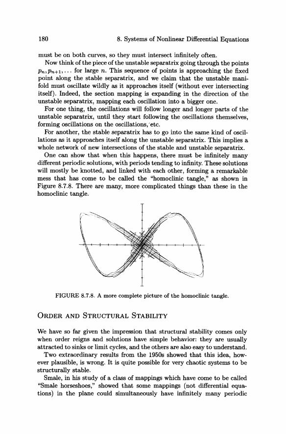
180 8. Systems of Nonlinear Differential Equations
must be on both curves, so they must intersect infinitely often. Now think of the piece of the unstable separatrix going through the points
Pn,Pn+b ... for large n. This sequence of points is approaching the fixed point along the stable separatrix, and we claim that the unstable manifold must oscillate wildly as it approaches itself (without ever intersecting itself). Indeed, the section mapping is expanding in the direction of the unstable separatrix, mapping each oscillation into a bigger one.
For one thing, the oscillations will follow longer and longer parts of the unstable separatrix, until they start following the oscillations themselves, forming oscillations on the oscillations,·etc.
For another, the stable separatrix has to go into the same kind of oscillations as it approaches itself along the unstable separatrix. This implies a whole network of new intersections of the stable and unstable separatrix.
One can show that when this happens, there must be infinitely many different periodic solutions, with periods tending to infinity. These solutions will mostly be knotted, and linked with each other, forming a remarkable mess that has come to be called the "homoclinic tangle," as shown in Figure 8.7.8. There are many, more complicated things than these in the homo clinic tangle.
FIGURE 8.7.8. A more complete picture of the homoclinic tangle.
ORDER AND STRUCTURAL STABILITY
We have so far given the impression that structural stability comes only when order reigns and solutions have simple behavior: they are usually attracted to sinks or limit cycles, and the others are also easy to understand.
Two extraordinary results from the 1950s showed that this idea, however plausible, is wrong. It is quite possible for very chaotic systems to be structurally stable.
Smale, in his study of a class of mappings which have come to be called "Smale horseshoes," showed that some mappings (not differential equations) in the plane could simultaneously have infinitely many periodic

8.8 Structural Stability 181
points, orbits that are dense in a Cantor set, and be structurally stable. Moreover, he showed that if a mapping of the plane has a periodic point, the stable and unstable separatrices of which intersect transversally, then inevitably horseshoe behavior will occur. It is because of his results that we know that if a differential equation in R3 has a cycle, with stable and unstable separatrices which intersect transversally, then there must be infinitely many cycles and all sorts of other complications. But this does not contradict structural stability. Neither does it imply it, of course. We will describe and discuss the Smale horseshoe in Chapter 13 (Part III).
Anosov, in his study of the geodesic flow on closed surfaces of negative curvature, discovered that these are also structurally stable.
The geodesic flow is the differential equation, whose solutions are the geodesics on the surface, parametrized by arclength. To specify a solution, you give a point and a direction, and the point starts out in that direction and goes as straight as it can, at constant speed. Since we needed an initial velocity (the direction) as well as an initial position, we see that this is a second order differential equation on the surface, which can be turned in the standard way into a first order differential equation on the space of unit tangent vectors to the surface. This space of unit tangent vectors is three dimensional: there is a surface's worth of points at which to attach them, and a circle's worth of directions for each point.
A surface of positive curvature focuses geodesics, whereas negative curvature makes them spread out and diverge. It is hard to imagine anything more chaotic than geodesic flow on manifolds of negative curvature; for instance, there are infinitely many closed geodesics, each of which is a cycle in the space of unit vectors, which has stable and unstable separatrices that intersect transversally. In this case, it is fairly easy to imagine what these stable and unstable separatrices are: they are the geodesics that spiral toward the closed geodesic forward and backward.
Moreover, these separatrices intersect transversely: there are geodesics which spiral towards the closed geodesics both forwards and backwards. So there are infinitely many Smale horseshoes, all interrelated in some complicated way. Somehow, the whole geodesic flow is maximally disordered and tangled. But precisely this maximal disorder leads to structural stability. We will discuss geodesics in Chapter 11 (Part III), but will not be able to approach Anosov's theorem.
8.8 Structural Stability
A reader who plays with the phase plane program will observe that, in general, the phase portrait of a differential equation x' = f(x) in the plane changes only slightly when the vector field f is slightly modified:

182 8. Systems of Nonlinear Differential Equations
The zeroes of the modified equation are close to the zeroes of the original equation; they are still sinks, sources, and saddles as they were for the original equation; the basins of the sinks are bounded by the same separatrices, and so forth.
Example 8.8.1.
(a) [:J' = [;=:::~:!]
(b) [: J' = [; = :: : ~:~ ] (c) [: r = [y -xx~;2 5~93~~n x]
--- j
- --------
a)
-,
c)
FIGURE 8.8.1. Perturbed phase planes, showing how the key structures persevere. ...
In Chapter 8*, we will state and give a complete proof of two theorems which make this precise. However, these results are quite difficult and technical, and the content of the main statements (not the proofs) can be

8.8 Structural Stability 183
conveyed without the heavy apparatus introduced in Section 8*.1. In this section, we will try to say enough to allow the reader to go directly to Chapter 9, which is considerably easier than Chapter 8*; bypassing Chapter 8* is probably the right course to follow in a first reading.
Let us pin down more precisely what we expect the reader exploring phase planes to observe. We claim that, in general, in 1R.2,
(1) all zeroes of f are sinks, sources or saddles;
(2) all cycles are attracting or repelling;
(3) all solutions tend as t -+ +00 to sinks or to attractive limit cycles, except the saddles, their stable separatrices, and the unstable limit cycles;
(4) all solutions tend as t -+ -00 to sources or to repelling limit cycles, except the saddles, their unstable separatrices, and the stable limit cycles.
With some minor technical caveats (linearly attracting, etc.), we will call a vector field in the plane which satisfies conditions (1)-(4) structurally stable.
Let us try to see what must happen in order for one of these conditions to fail. At least one fact is clear: there can be a zero of f at which the linearization is neither a sink, a source, or a saddle. This can happen in two rather different ways: one eigenvalue of the linearization can be 0 or there can be a pair of purely imaginary eigenvalues. We discussed this in Section 7.5.
There is, of course, something worse that might happen: both eigenvalues might be zero. The reader should see that this is "more exceptional" than the previous two possibilities, as we shall elaborate by considering the "co dimension" of a bifurcation.
THE CODIMENSION OF A BIFURCATION
If you take a 2 x 2 matrix "at random" (for instance, the linearization of f at some zero), you do not expect any eigenvalues to be 0 or purely imaginary. But if you have a one-parameter family of 2 x 2 matrices, the determinant is a continuous function of the parameter, and if it takes on both positive and negative values, it will have to vanish somewhere. Thus, we expect to see the eigenvalue 0 in one-parameter families. Similarly, the trace will have to vanish somewhere, which leads to purely imaginary eigenvalues.
Both a zero eigenvalue and a pair of purely imaginary eigenvalues are accidents which occur generically in one-parameter families: we say these are bifurcations of codimension 1.

184 8. Systems of Nonlinear Differential Equations
On the other hand, we would not expect both the determinant and the trace to vanish for the same value of the parameter. But if we have a matrix that depends on two parameters, it is hard to see how we could avoid some point mapping to (0,0) in the trace-determinant plane.
A double zero eigenvalue is an accident that occurs generically in twopammeter families but not in one-parameter families: we say this is a codimension 2 bifurcation.
This sort of analysis can be continued: we might look not just at the linearization at a zero but at higher terms of the Taylor polynomial and see how many of these vanish, finding more and more degenerate zeroes of vector fields, which occur generically in higher dimensional families, and near which the differential equation behaves more and more bizarrely. There is a small industry of investigating more and more degenerate zeroes of vector fields, which we will only touch on in Chapter 9.
But the fact that "accidents" can be more or less exceptional, according to the number of parameters needed to make them occur generically, is a very important idea. Without some assumption about differential equations being "general," or belonging to "general" one-parameter and twoparameter families, all kinds of exceptional behavior can occur, and there do not appear to be any straightforward results.
Another accident that might occur is that a limit cycle might fail to be attracting or repelling: it might, for instance, be attracting on one side and repelling on the other as shown in Figure 8.8.2.
FIGURE 8.8.2. A semi-stable limit cycle.
There is actually only one other accident that can occur: the unstable separatrix of a saddle may also be the stable separatrix of another saddle, or even of the same saddle. The first case is called a heteroclinic saddle connection, the second a homoclinic saddle connection. See Figure 8.8.3.

8.8 Structural Stability 185
FIGURE 8.8.3. A heteroclinic and a homoclinic saddle connection.
Again, one can imagine more complicated things, such as the simultaneous saddle connections shown in Figure 8.8.4.
FIGURE 8.4.4. Two simultaneous saddle connections.
The reader should convince herself or himself that both of the accidents seen in Figure 8.8.3 occur generically in one-parameter families, but that the accident in Figure 8.8.4 occurs generically only in two-dimensional families; it is "more exceptional."
Example 8.8.2. Consider a one-parameter family of vector fields fa with a saddle, such that for two values of the parameters, the separatrices intersect a line segment I as shown in Figure 8.8.5.
Consider the (signed) distance d(a) from the intersection As of the stable separatrix with I to the intersection Au of I with the unstable separatrix. The distance d(a) is a real-valued continuous function of a, which is positive for one value of the parameter and negative for another, so it must vanish somewhere.

186 8. Systems of Nonlinear Differential Equations
FIGURE 8.8.5. How separatrices intersect a transverse line segment.
It is hard to see how we could avoid such things in one-parameter families; on the other hand, near a vector field as shown in Figure 8.8.4, there are two analogous distances, and in a one-parameter family one would not expect them to vanish simultaneously. A
There is not any really obvious way to see that this is the end of the list of accidents, yet it is, and the result can be summarized as follows, to be proved and elaborated in Chapter 8*:
Proposition 8.8.3. If all zeroes are sinks, sources, or saddles, all cycles are attmcting or repelling, and there are no saddle connections, then the vector field is structumlly stable.
The reader who wants to see a proof will have to look at Section 8*.5 (which can be read without reading the earlier sections of Chapter 8*), and Section 8*.6 (which requires everything which comes before). But it is rather hard to imagine how Proposition 8.8.3 could be wrong, and so we ask you temporarily to take it on faith.
You can move directly to Chapter 9 on bifurcations without loss of any prerequisites. But we encourage you to at least come back to Chapter 8* later.

Exercises
Chapter 8 Exercises
Exercises 8.1 Zeroes; Linearization
8.1#1. For each of the following differential equations
(a)O [:]' = [ _ sin(~) _ 3Y]
(b) [: r = [X2 ~ ~ ~ 2 ]
(c) [:]' = [X2~~~25]
(d) [x]' = [sin(1r(X-Y))] Y xy-1
187
(i) Locate the singularities and write out the linearization about each of them.
(ii) Find the eigenvalues and eigenvectors of the linearization matrix for each of the singularities. This can be done by hand or with EigenFinder in MacMath.
(iii) With MacMath's DiJJEq, Phase Plane or other phase plane computer software, make a phase portrait for the equation, locating all the singularities. Print three copies.
(iv) On the first phase portrait, draw the eigenvectors at each singularity where they are appropriate, marking the direction of motion by arrows according to the sign of the corresponding eigenvalues. You should be able to see exactly how the phase portrait trajectories are related to these eigenvalues and eigenvectors.
(v) On the second phase portrait, shade in all the basins of the sinks.
(vi) On the third phase portrait, shade in all the cobasins of the sources.
8.1#2. For each of the following differential equations
(i) Locate the singularities and write out the linearization about each of them.
(ii) Find the eigenvalues and eigenvectors of the linearization matrix for each of the singularities. This can be done very quickly with EigenFinder in MacMath.

188 8. Systems of Nonlinear Differential Equations
(iii) Using MacMath's DiffEq, 3D Views, draw a phase portrait for the equation, locating all the singularities. The xyz view will look like spaghetti, but you may find more "order" in the xy, yz, and xz views. Print out a copy of these graphs.
(iv) On each of the two-dimensional graphs printed in (iii), draw the eigenvectors at each singularity where they are appropriate, marking the direction of motion by arrows according to the sign of the corresponding eigenvalues. (That is, draw the appropriate projection of each eigenvector, which means ignoring the relevant third component.) You should gain some insight as to how the phase portrait trajectories are related to these eigenvalues and eigenvectors.
8.1#3. For each of the following differential equations
(a) [:]' = [x3/2~!+XY]
(b)O [:]' = [X4 +4X3 -;;Y-4X+Y)/8]
(i) Find the zeroes of the system, and by linearizing, tell what they are.
(ii) Make a picture of any saddles with their separatrices and proper arrows on each. This can be done in MacMath using DiffEq, Phase Plane, with no slope marks. When a saddle is located, the separatrices are drawn automatically, the first two pointing out from the saddle and the last two pointing inwards toward the saddle. Print the picture and draw arrows on the separatrices.
(ii*) An alternate way of examining the saddles is to find their eigenvalues and eigenvectors, by hand or with MacMath's EigenFinder. If you do not have a computer program that draws separatrices, you may want to locate the other singularities and find their eigenvalues and eigenvectors.
(iii) From this picture of only the saddles and separatrices, with arrows, locate other zeroes and tell what they are. Sketch in some other trajectories, with arrows, in order to fit with the separatrices and their arrows. Show how separatrices determine regions of behavior near the saddle.
(iv) Verify your expectations for the phase portrait with another computer drawing, using slope marks and drawing by computer some trajectories between the separatrices.

Exercises
8.1#4. For the differential equation of Example 8.1.8,
(a) Find the linearization.
(b) Show that an eigenvalue of the linearized equation is zero.
(c) Show that the equation does not behave like its linearization.
8.1#5. For the pretty complicated differential equation
[x]' _ [ 2x+siny-4x(x2+y2) ] y - siny - 3xsin(x - 2y) - 2y(x2 + y2)
189
(i)O Find the linearization near (0,0) to show that the linearization is far simpler than the original equation.
(ii) Compare phase portraits of the nonlinear and linearized systems and estimate how far from the origin the linearization will give a good approximation. (You should not expect the accuracy to be the same in all directions.)
8.1#6. For the following nonlinear systems of differential equations, make sketches by hand to answer the questions:
(a) [:]' = [:y-_x1 ] (d) [:]' = [COS(x;y+ y2)]
(b) [:]' = [x2+::-1] (e) [x]' = [sin(x - y) ] y cos(x + y)
(c) [x]' = [x2+ y2 -2] y y2 _ X4 (f) [x]' = [X(l-y-X)] Y y(2 - x)
(i) Sketch in the phase plane the locus where the vector field is vertical and indicate where it is pointing left and where right. Furthermore, sketch the locus where the vector field is horizontal and indicate where it is pointing up and where down. Combine this information in each region bounded by the isoclines to show the resultant direction of the vector field.
(ii) Find all the singularities of the system. Write down the linearization in each case and describe the type of singularity. Find the eigenvector directions for real eigenvalues of the linearization.

190 8. Systems of Nonlinear Differential Equations
(iii) Sketch some trajectories in the phase plane, among them the separatrices, and color the basins of each sink.
8.1#7. Consider the system of differential equations
x ax-y [ ]' [ ] y = y-x2+x
where a is a parameter.
(a) On what curves is the vector field horizontal? Vertical?
(b) In each region bounded by these curves, tell whether the vector field points up or down, left or right. (The description is a bit different when a > -1 and a < -1 , so consider these cases separately).
(c) Find the zeroes of the vector fields and their linearizations. Classify them.
(d) Sketch the trajectories of the solutions, indicating, in particular, the basins of the sinks and cobasins of the sources, for a = -2, 0, 1.
8.1#8. Find, by hand or computer, the singularities, linearizations, trajectories near the zeroes, and basins of the sinks for
(a) [:r = [~:!] (d) [: r = [(x2 - r)y - x]
(b) [ x r = [x2 + y2 - 25 ] y xy -12
(e) [: r = [x sin~x_+x~) - x]
(c) x 2xy-x [r [ ] y = _y2 + 2xy2 .
Note: You might get answers in (d) for the type of singularity depending on where you click the mouse. How can you explain this uncertainty?
8.1#9. Consider the nonlinear system of differential equations
(a) Locate the singularities of the system. In each case, write down the linearization and the type of singularity for the linearized system. What can you conclude about the singularities for the nonlinear system from the linearizations?

Exercises 191
(b) Draw in the phase plane the curves where the vector field is horizontal and where it is vertical, and indicate where it is pointing up, down, left, and right. Furthermore, indicate the vector field along the line
Why is this line interesting?
(c) Let (x, y) = (u(t), v(t)) be a solution to the nonlinear system. Show that (x,y) = (u(-t),-v(-t)) is also a solution. What is the geometrical meaning of this? In particular, let the solution be such that (u(O), v(O)) is a point in the first quadrant on the curve where the vector field is horizontal. Explain why such a solution has to be periodic.
(d) Finally, sketch the trajectories for the nonlinear system.
8.1#10. Find the linearization of
[ x-xy ] -y+xy
near all its singularities and in each case identify its type. Confirm with a phase portrait, drawn by hand or computer, the behavior of trajectories for the nonlinear system.
8.1#11. For the equations of the pendulum with friction (Example 6.5.4),
(a) Use MacMath's DiJJEq Phase Plane to make computer pictures for different integer values of c: > 0 in order to show at what value(s) of c: the trajectories cease to spiral.
(b) Confirm by algebraic calculation the value of c: at which you expect the spirals to cease.
8.1#12. Suppose that x(t) describes the position of a particle moving in one dimension, under the potential V(x). Show that the vector field in the plane corresponding to this system, as described in Section 6.5, has a zero at (xo,Yo) if and only if dVjdx(xo) = 0 and Yo = O. Show that at such a zero, the linearization is a center if d2Vjdx2 (xo) > 0, i.e., if the potential has a nondegenerate minimum. Show that if the potential has a nondegenerate maximum, the linearization has a saddle.

192 8. Systems of Nonlinear Differential Equations
Exercises 8.2-8.3 Saddles, Sinks, Sources
8.2-8.3#1. For [ : r = [X2 1~ ~ ~ 25] , locate any sinks and sources.
8.2-8.3#2°. Consider the system of differential equations
(i)
and the related single differential equation
dy y - x2
dx -x -xy (ii)
(a) Show that one of three singular points for (i) is a saddle point. Find the eigenvector directions.
(b) We have shown that the shaded region U in Figure 8.3.2,
U = {(x, y)1 - 1 < x < 0, _x2 ~ Y ~ x2 },
defines an antifunnel for (ii) satisfying
~ (!x-_X;y) ~ O.
Show that the symmetric shaded region W,
W = {(x,y)IO < x < 1,-x2 ~ Y ~ x 2 },
defines a funnel for (ii) and, when you reverse "time" (x in this case), W defines an antifunnel satisfying the uniqueness criterion.
(c) What does part (b) tell you about the system (i)?
8.2-8.3#3°. Consider an n x n matrix A with k pairs of conjugate nonreal eigenvalues, so that for any c > 0, by Theorem L6.18, there exists a basis Wl, ... , Wn of IRn such that in that basis A is k-pseudo-upper-triangular with terms of absolute value < c above the pseudo-diagonal. Let -A equal the largest real part of an eigenvalue. For the proof of Proposition 8.2.3, prove that
8.2-8.3#4. For the differential equation

Exercises 193
(a) Show that at (0,0) the linearization gives a center, so we need further analysis to determine the nonlinear behavior.
(b) Show that F(x,y) = x2 + y2 serves as a Liapunov function and use it to analyze the singularity at (0,0) of the differential equation.
(c) Describe all solutions of this equation.
8.2-8.3#5. Consider the differential equation
X = 2Y • [ ]' [ ] Y -e-x (x+y)
(a) Show that every solution that enters the region Iyl ~ e-x2 / 2 is attracted to the origin. Hint: use Example 8.2.8 to find an appropriate Liapunov function.
(b) Show that any solution entering the region x > 0, y > l/x stays in it forever (in particular, is defined for all positive time). Hint: Consider the curve y = l/x as a fence for the associated equation
dy _x2X +y -=-e --. dx y
(c) Use an antifunnel and the symmetries of the equation to describe the basin of the origin with precision.
8.2-8.3#6. Repeat Exercise 8.2-8.3#5 for the equation
this time finding the appropriate regions yourself.
8.2-8.3#7. The equation
behaves quite differently from that of Exercise 8.2-8.3#6 (though the picture looks very similar). How and why?
8.2-8.3#8. Give a proof using fences of the following variant of Liapunov's Theorem: If x' = f(x) is a differential equation, f(xo) = 0 and F is a function such that F(:xo) = 0, the point Xo is an isolated minimum of F, and
VF(x)· f(x) ~ -CF(x)

194 8. Systems of Nonlinear Differential Equations
for some constant C > 0, then Xo is a sink for the differential equation.
8.2-8.3#9°. Consider the differential equation
x' = -ax + P(x, y)
y' = -ay + Q(x, y),
where a > 0, and P and Q start with quadratic terms. Show that the solutions attracted to the sink (0,0) do not spiral around the origin.
Hint: Pass to polar coordinates, and write ()' as in equation (20) in the proof of Theorem 8.2.10. Use the fact that the solutions are attracted exponentially fast to the origin to show that
100 ()' dt < 00.
8.2-8.3#10. Consider the differential equation
x' = -ax - y + P(x,y)
y' = -ay + Q(x, y),
where a > 0, and P and Q start with quadratic terms. Show that the solutions attracted to the sink (0,0) do not spiral around the origin.
Hint: Consider the associated differential equation
dy -ay + Q(x, y) dx -ax-y+P{x,y)
and show that it is well defined in the region _X3/ 2 :::; Y :::; X 3/ 2 , 0 < x < €
for € > 0 sufficiently small. Then show that this region is a backward antifunnel.
8.2-8.3#11°. If
[:J' = [-~x++~~~~)] with P and Q of quadratic or higher order forms, show that the curve ILX = P(x, y) is twice differentiable and tangent to the y-axis.
8.2-8.3#12. In the proof of Lemma 8.2.3, prove that V is an antifunnel.
8.2-8.3#13. For the Lorenz attractor of Example 6.1.6,
[X]' [lO(Y-X)] y = 28x -y-xz z -2.66z + xy

Exercises 195
find the singularities and draw pictures to show how each works.
8.2-8.3#14. For the following second order equations, express each as a system of first order equations by setting x' = y. Then, for 0: = -1,0,1, use MacMath's program DiJJEq, Phase Plane to find the singularities and show the behaviors of the trajectories in the xy phase plane. Use arrows to show the directions of the trajectories in forward time and indicate where there seem to be stable solutions. In Exercises 9.1#9 for (a) and 9.5#6 for (b), we shall come back to these particular systems and explore exactly how and when the behaviors change as 0: changes.
(a) x" - o:x + x3 = o. (b) x" = -dVjdx, where V = sin x + o:x2 , as in Exercise 6.5#10.
8.2-8.3#15. The system
is easy to understand because the z variable and the variables (x, y) evolve independently of each other.
(a) Locate all the zeroes of the system, and give the linearizations at each.
(b) Show that the origin is a saddle, with one positive and two negative eigenvalues.
(c) Use MacMath's program DiJJEq, 3D Views to draw some sample trajectories, adding arrows, that illustrate the three-dimensional behavior around the saddle.
(d) Describe the solutions that are attracted to the origin when t -+ ±oo.
8.2-8.3#16. For the equation of Exercise 8.1#1(c) and Exercise 8.2-8.3#1, [: r = [x2 ~ ~ ~ 25] ,
prove that a separatrix of the upper saddle must enter the basin of the sink at lower left. That is, find a region surrounding the sink for which the vector field of the equation everywhere crosses the boundary going into the region; then show that the separatrix of the saddle must enter this region.

196 8. Systems of Nonlinear Differential Equations
Exercises 8.4 Limit Cycles
8.4#1.
(a) Confirm equations (30) for transforming Example 8.4.1
into polar coordinates
r' = a(1 - r2)r (J' = -1.
(29)
(30)
(b) Make drawings of the rt-plane to confirm that solutions to equation (30) follow the conclusions of Example 8.4.1: For a > 0, all solutions for r > 0 are attracted to the constant solution r = 1; for a < 0, the solution r = 1 is repelling, and if 0 ~ r(O) < 1, the solution tends to 0, whereas if 1 < r(O), the solution tends to infinity.
8.4#2. Show that
gives an example of an unusual limit cycle that is stable on one side, unstable on the other.
8.4#30 • For the equation of Example 8.4.3,
[x]' = [ Y ] + (x2 +y2)2sin 1 [x], Y -x x2 + y2 Y
prove the equation has infinitely many periodic solutions, with different trajectories.
Exercises 8.5 Poincare-Bendixson Theorem
8.5#10 • Let I = [a, b] be a closed and bounded interval. Show that any continuous mapping f : I -+ I has a fixed point. Hint: Use the intermediate value theorem, applied to the function f(x) - x.
8.5#2. Consider the equation of Example 8.4.3 and Figure 8.4.3,
[X]'=[y]+(X2+y2)2Sin 1 [x]. y -x x2 + y2 Y

Exercises 197
(a) Draw a phase portrait and make a Poincare-Bendixson annulus around one of the largest limit cycles.
(b) Find equations for an annulus like you found in part (a).
8.5#3. For the differential equation
[X]' = [Sin(X + y)] y cos(xy)'
print a phase portrait and try to draw Poincare-Bendixson annuli around each limit cycle.
8.5#40 • Consider the Van der Pol equation of Examples 8.4.2 and 8.5.3. Find equations for the annulus as shown in Figure 8.5.5. Hint: It is composed of straight lines plus key portions of the isoclines of zero slope.
8.5#5. Show that the equation
has a limit cycle. (Hint: use appropriate solutions of
as boundaries of an annular region.)
Exercises 8.6 Symmetries; Area-Preserving Equations
8.6#10 • Consider the system of differential equations
(a) Sketch (perhaps using an appropriate computer program) some typical solutions for this equation.
(b) Locate and analyze the singularities.
(c) In part (a), you should have found a region apparently filled by cycles. Show that this is in fact the case.

198 8. Systems of Nonlinear Differential Equations
(d) The saddle apparently has a homoclinic separatrix (an unstable separatrix that curves around and reenters the saddle as a stable separatrix). Show that this is the case, and, for this problem, that you can find an equation for the separatrix!
8.6#2. Consider the system of differential equations
(a) Sketch (perhaps using an appropriate computer program) some typical solutions for this equation.
(b) Locate and analyze the singularities.
(c) In part (a), you should have found a region apparently filled by cycles. Show that this is in fact the case.
The remainder of the exercise attempts to locate this region with greater precision.
(d) Consider the corresponding system of equations for dy/dx. Show that the region x + 1/2 - 1/x ::; Y ::; x + 1/2, t > to, is an antifunnel for an appropriate to. Show that this antifunnel satisfies the uniqueness property.
(e) Sketch the solution in this antifunnel.
(f) Show that all solutions in the part of the plane bounded by this solution are cycles.
8.6#3°. If u' = Au is the linearization of the differential equation x' = f(x) at a zero XQ, show that
div f(:xo) = tr A,
in order to support the statement that a volume-preserving vector field cannot have any sources or sinks.
8.6#4. Show that a linear differential equation x' = Ax is area-preserving if and only if tr A = o.
8.6#5. Draw a phase portrait for each of the following differential equations. Tell (and prove) whether it exhibits properties of symmetries or an area-preserving map.
(a) x" + sin xx' + x = 0

Exercises 199
(b) [x]' = [ y ] + (X2 +y2)2sin 1 [1] y -x x 2 + y2 1
8.6#6.Show that if the differential equation
[x]' = [!(X,y)] y g(x,y)
is area-preserving (see Exercise 6.6#3), then its zeroes cannot be sinks or sources (and therefore must be centers or saddles).
8.6#7. Let f be a vector field defined in a region U C R2. Show that the differential equation x' = f(x) cannot have two cycles, which together bound a region V C U in which div f < o.
Exercises 8.7 Chaos in Higher Dimensions
8.7#1. Show that the divergence of the vector field
[=]' = [p:~; ~~z] z -{3z +xy
(iii)
is -(u + 1 + (3). Why is the Lorenz equation said to be dissipative?
8.7#2°. Consider the function !(x, y, z) = px2 + uy2 + u(z - 2p)2. The object of this exercise is to show that there is a bounded region (in fact, an ellipsoid) which solutions to the Lorenz equations (iii) enter and never leave.
(a) Show that the region! < a is bounded for any a.
(b) Show that the derivative of ! along a solution is
_2u(px2 + y2 + (3z2 - 2p{3z).
(c) Find a number a such that all solutions to the Lorenz equations (iii) enter the region ! ~ a and never leave it.
8.7#3.
(a) Show that the origin is a zero of the differential equation (iii) and that it is a sink when p < 1, but has two real negative eigenvalues and one positive eigenvalue for p > 1.

200 8. Systems of Nonlinear Differential Equations
(b) Show that the function x 2 / u + y2 + z2 is a monotone decreasing function of time when 0 < p < 1, so that all solutions to the Lorenz equations (iii) are attracted to O.
8.7#4.
(a) Show that the origin is the only zero of the vector field for (iii) for p ~ 1, but that there are two other zeroes for p > 1, and give their coordinates.
(b) Show that these new zeroes are sinks for
( 1 U(U+,8+3)) pE 'u-,8-1
and that they have one negative eigenvalue and two complex conjugate eigenvalues with positive real parts for
8.7#5.
u(u +,8 + 3) p> u-,8-1 .
(a) Show that the system of differential equations
has the circle x 2 + y2 = 1, z = 0 as a cycle.
(b) Compute the section mapping P, using the section y = 0, x > 0, and show that at the fixed point of P corresponding to the cycle, the derivative of P has two eigenvalues, one greater than 1 and one less than 1.
(c) Find the separatrices of this fixed point in the section.
(d) Describe the separatrices of the cycle. What behaviors in R2 do these separatrices separate?
Exercises 8.8. Structural Stability
8.8#10 • Consider the system of differential equations
[x]' [ y-x2 ] Y - ax-2-y .

Exercises 201
(a) With MacMath's DiffEq Phase Plane make and print phase pnrtraits for a = 3.5, 0, -3.5, -6, 10. To capture all you need to see, set bounds as -20:$ x :$ 15, -10 :$ y :$ 100.
(b) Describe each phase plane in words, and try to understand what happens between one and the next. That is, explain the qualitative differences between these pictures.
(c) Experiment by trial and error on the computer to find intermediate values of a where the behavior changes.
A generalization of this exercise will be explored a great deal further in Example 9.6.1.

8*
Structural Stability In Chapter 8, we mentioned that one of our main goals is to understand how solutions behave "in general." Another goal is to understand when the solutions of two differential equations behave "the same way." Our main result in this direction is in Section 8*.6, but preliminary results occur in Sections 8* .2-8* .5, and they require a bit of terminology. We begin with the groundwork in Section 8*.1, building up to Definition 8*.1.9 for "structural stability" .
Section 8*.6 contains two major theorems: the first due to Andronov and Pontryagin, and the second to Peixoto. These results give a real handle on structural stability of differential equations in the plane; the whole chapter builds up to them. Their proofs are an order of magnitude longer and more difficult than anything else in this book so far. We work up to Section 8*.6 with a series of sections, 8*.1-8*.5, each of which can be considered as a Structural Stability Appendix at the end of the corresponding section in the previous Chapter 8. We give preparatory definitions in 8*.1 and prove an essential preliminary result in each of the next four sections. Each of these results, Theorems 8*.2.1,8*.3.1,8*.4.1, and 8*.5.6, is important in its own right; Theorem 8*.5.6 is a strong form of the famous Poincare-Bendixson Theorem 8.5.1.
Finally, Section 8*.7 illustrates why the Poincare-Bendixson-Pontryagin-Peixoto program fails in dimension three. Some examples will show that any general analysis of a system in an is likely to be extremely complicated, if not impossible. Indeed, as soon as n ~ 3, "chaos" has a tendency to set in. There is no universally accepted definition of this term, but some features that should appear in chaotic systems are:
• the presence of infinitely many periodic cycles, which in a3 will usually be knotted and linked in complicated ways;
• the appearance of fractal attractors and basin boundaries, with complicated structure at all scales;
• sensitive dependence on the initial point: within a bounded attractor, the distance separating two solutions that start nearby grows exponentially with time, until they are uncorrelated.

204 8*. Structural Stability
8*.1. Preliminaries for Structural Stability
Let us begin with some necessary terminology.
Definition 8*.1.1. (Homeomorphisms). Let X and Y be metric spaces. If you do not know what this means, it does not matter: just think that they are two subsets of IRn , that is the only case we will use. A mapping I : X -+ Y is a homeomorphism if
(1) the mapping I is continuous;
(2) the mapping I is one-to-one and onto, so that 1-1 exists;
(3) the mapping 1-1 is continuous.
Saying that two spaces are homeomorphic is saying that they "look alike topologically": to a topologist, they are identical. An old joke says that a topologist is someone who cannot tell the difference between a doughnut and a coffee cup: do you see why? See Figure 8*.1.1.
, o ',,----,,"
FIGURE 8*.1.1. Topological equivalence of a doughnut and a coffee cup.
Exercise 8*.1#2, with Examples 8*.1.3 and 8*.1.4, give more examples of homeomorphisms.
Definition 8*.1.2 (Topological equivalence). Suppose that fl and f2 are vector fields defined on regions U1 and U2 of Rn for some n. We will say that a homeomorphism h : U1 -+ U2 is a topological equivalence of fl and f2 if h sends oriented trajectories of x' = fl (x) to oriented trajectories of x' = f2(X).
Remark. Imagine drawing both vector fields fl and f2 on rubber sheets. Then they are topologically equivalent if one rubber sheet can be stretched and put onto the other so that the trajectories of one equation coincide with the trajectories of the other, as oriented curves.

8*.1. Preliminaries for Structural Stability 205
We are not requiring that the parametrization of these curves by time coincide. We are also not requiring that the homeomorphism be differentiable, so it can perfectly well send curves that intersect tangentially to curves that intersect transversely, as illustrated by Examples 8*.1.3 and 8*.1.4, illustrated in Figures 8*.1.2 and 8*.1.3.
Example 8*.1.3. Consider the homeomorphism h defined by
FIGURE 8*.1.2. A homeomorphism h not differentiable at the origin. •
Example 8*.1.4. Another homeomorphism h that is not differentiable at the origin is
FIGURE 8*.1.3. Another homeomorphism not differentiable at the origin. •

206 8*. Structural Stability
Algebraic exploration of these examples are provided in Exercise 8*.1#1; however, we usually do not write actual equations for homeomorphisms.
It is not obvious that topological equivalence is a useful equivalence relation. There are at least two others that should be mentioned: topological conjugacy and differentiable conjugacy.
Definition 8 .... 1.5 (Topological conjugacy of flows). The homeomorphism h is a topological conjugacy of the Hows 4Jfl (t, x) and 4Jf2 (t, x) if
(I)
See Figure 8*.1.4.
Flows 4Jf{t,X) are defined and discussed in Section 6.8.
FIGURE 8*.1.4. Topologically conjugating the flows.
Two vector fields have conjugate flows if, when drawn on rubber sheets, one sheet can be stretched and superposed on the other so that the trajectories coincide with their time parametrization.
Deflnition 8 .... 1.6 (Differentiable conjugacy of vector fields). The homeomorphism h is a differentiable conjugacy of the vector fields f1{x) and f2{x) if hand h-1 are differentiable, and
(2)
See Figure 8* .1.5.

8*.1. Preliminaries for Structural Stability 207
h
-vectors at x vectors at h(x)
FIGURE 8*.1.5. Differentiable conjugacy of vector fields.
Condition (2) for differentiable conjugacy may look quite complicated, but it is actually exactly what is called "change of variables in differentiable equations." For the authors, it really explains the meaning of such changes of variables. Let us work out explicitly how this works, in the case of Bernoulli equations (Chapter 2 of Part I, Exercises 2.2-2.3#9 and lOa, page 101).
Example 8*.1.7. A Bernoulli equation is one that can be written x' = -P(t)x + Q(t)xn (where the minus sign is there to be consistent with the notation in Part I). The change of variables suggested in the exercise is z = x 1- n , so that
z' = (l-n)x-nx' = (l-n)x-n(-P(t)x+Q(t)xn) = (n-l)(P(t)z-Q(t»,
which is indeed linear. To interpret this change of variables in terms of vector fields, let us turn
the Bernoulli equation into the system
[! r = [ -P(t)x ~ Q(t)xn ]
and let
Then equation (2) becomes
[~ (1 - ~)x-n ] [ -P(t)x ~ Q(t)xn ] = [(n - 1)(P(~)z - Q(t»]
and the differential equation corresponding to the new vector field is

208 8*. Structural Stability
[!] I = [(n _ 1)(P(!)Z _ Q(t))] .
In this example, h is not really a homeomorphism, and this comes back to haunt you when you try to go back from the variable z to the variable x. &
You are asked in Exercise 8*.1#3 to check that condition (2) for differentiable conjugacy implies (1) for topological conjugacy, and that (1) implies topological equivalence.
Both conditions (2) and (1) are a bit too fine for our purposes: we want to know that "in general," when two differential equations are "close," they are equivalent. This is not the case for (2), since the eigenvalues at corresponding zeroes would have to coincide (Exercise 8*.1#4a). Condition (1) would require that the periods of corresponding cycles should be equal, which is also unreasonable (Exercise 8*.1#4b).
PERTURBATIONS
This brings us to saying precisely when two differential equations x' = fl (x) and x' = f2(xff) are close or, equivalently, when g = fl - f2 is small.
There are serious difficulties if you try to define perturbations on unbounded domains; we will stick to bounded domains. Suppose that g is defined on the closure tJ of a bounded open subset U c an. A first guess is simply to require that
sup IIg(x)1I XEU
be small, but this is not good enough. Indeed, two vector fields that are close in this sense can have zeroes that differ radically.
Example 8*.1.8. Compare the following functions and their derivatives, as shown in Figure 8*.1.6.
h(x) = x 1 2
h(x) = x + We-X sin5x.

8*.1. Preliminaries for Structural Stability 209
12
f,(x)
Df,(x)
Df,(x)
-1 -1
-1 -10
functions derivative functions
FIGURE 8*.1.6. Functions that are close may have derivatives and fixed points that are not. Note the differences in vertical scale between the two graphs! A
The Implicit Function Theorem at the center of multi variable calculus guarantees that if two vector fields f1 and f2 are close, and their derivatives are close, then the zeroes are as well behaved as can be expected. Let g be continuous on U, continuously differentiable on U, with derivative extending continuously to U. Then g is small in the C 1 topology if
is small. The Implicit Function Theorem 13.6.4 (Appendix T) says that if the
zeroes of f1 have no zero eigenvalues and if g is sufficiently small in the C1 topology, then there is exactly one zero of f2 = f1 + g close to every zero of fl. This is one possible correct notion of perturbation for our problem, and our main theorems are true with this definition.
However, the version of the Implicit Function Theorem we will prove in Chapter 13 (in Part III) is stronger than the standard statement and correspondingly requires a stronger hypothesis. Because the stronger hypothesis simplifies some proofs, we will make the following definition. Let
be a twice-differentiable vector field on U as above. Define the C2-norm of this vector field to be

210 8*. Structural Stability
In other words, we will require that "close" means not only that the two functions be close but that their first and second derivatives be close.
We can now state the central definition of Chapter 8*.
Definition 8*.1.9 (Structural stability). We will say that a vector field f defined on a subset U c IRn is structurally stable if there exists c > 0 such that any perturbation g of f with Ilg - fll < c is topologically equivalent to f.
Actually, this definition is a bit loose. We will require that U be a closed and bounded subset of IRn , bounded by a smooth (n - 1 )-dimensional surface, and in practice n will be two, so U will be a closed and bounded region in the plane bounded by smooth curves. Our vector fields will be required to have all partial derivatives up to order two continuous on U.
THE DIFFERENTIABILITY OF THE FLOW
Let f(x) be a smooth vector field on a subset U c IRn , and denote by ¢f(t, xff) : IR x U --+ IRn the associated flow, as described in Section 6.8. In this section, we will see that the flow is a differentiable mapping, and we will derive some consequences. Just knowing that the flow is differentiable is nice but not very exciting. What makes the result important is the formula for the derivative, which is itself a solution of a linear differential equation. This links up the "wild" theory of nonlinear equations with the "tame" theory of linear equations, and the link has proved enormously useful.
In fact, we have already seen at least two instances of the usefulness of this link.
One is the linearization of a differential equation near a zero of the vector field: in that case, the linearization is a linear differential equation with constant coefficients, and linear algebra (eigenvectors and eigenvalues) can be brought to bear; Chapter 8 is filled with the consequences.
The other occurs in Example 5.4.6, where we analyzed the difficulties that "stiffness" introduces to numerical methods. We first studied linear equations, and then saw that by linearizing a nonlinear equation near a given solution, we could transpose the results to an arbitrary equation.
The linearized equation. We first recall the definition of the linearization of x' = f(x). Suppose u(t) is a solution of x' = f(x), defined for 0 ::; t ::; to and that v(t) is a small increment to u(t), so that x(t) = u(t) +v(t) is still a solution. Then
u'(t) + v'(t) = (u + v)'(t) = f(u(t) + v(t» rv f(u(t» + (du(t)f)(v(t». (3)
Remembering that u' = f(u), this says that v approximately satisfies the linearized equation
W' = (du(t)f) w. (4)

8*.1. Preliminaries for Structural Stability 211
You should think of u as known, so that this equation is of the form Wi = A(t)w for some (usually time dependent) matrix A(t).
Example 8*.1.10. Consider the equation x' = x 2 - 1. The constant functions Ul(t) = 1 and U2(t) = -1 are solutions, where the linearizations are respectively
Wi = 2w and Wi = -2w,
correctly reflecting that solutions pull away from Ul and tend toward U2. The function U3 (t) = - tanh t is also a solution, where the linearization is
Wi = -2(tanh t)w.
This time the linearization is time dependent, since the solution is nonconstant, and solutions pull away from the zero solution when t < 0, i.e., when U3(t) rv Ul(t), and are attracted to it when t > 0, i.e., when U3(t) rv U2(t). A
Example 8*.1.11. We invite the reader to show that the function
u(t) = [cost:-cos2t] smt
is a solution of the system
[X]' = [y-2xy - y3 ]. y x-I + y2
The linearized equation along this solution is
,_ [-2sint 1-2(Cost+cos2t)-3Sin3t] w - 1 2sint w.
Let us interpret u, Y, and w above in terms of flows. Suppose that at time 0, we have
u(O) = Xo, yeO) = Yo = w(O);
i.e., we start both the equation and the linearized equation with the same increment from no.
Then equation (3) says that at time t, the increment vet) to u is approximately wet), i.e.,
<Pf(t, Xo + Yo) rv <Pf(t, Xo) + wet).

212 8*. Structural Stability
This suggests that w is somehow the derivative of ¢ f' and this is true. To state it precisely, we want to speak of the flow of the linearized equation. This is not quite well defined, since (4) is time dependent, but let us call ¢u(t, v) : IRn ~ IRn the linear transformation that associates to v the value at time t of the solution of (4) with initial condition vat time O.
Theorem 8*.1.12. The derivative of the flow of a nonlinear equation is the flow of its associated linear equation. That is,
We will actually prove a little more: the error in the linear approximation is quadratic. More precisely, there exist constants C and 8 > 0 such that
II¢f(t, Xo + v) - ¢r(t, Xo) - ¢u(t, v)11 ::; Cllvl12
when IIvll < 8.
Proof. Note that
d dt (¢r(t, Xo + v) - ¢r(t, xo)) = f(¢r(t, Xo + v)) - f(¢r(t, xo)),
whereas
and the curves Ul (t, v) = ¢r(t, Xo + v) - ¢r(t, xo)
and
are solutions of the differential equations
v' = F(t, v) and w' = G(t, w),
respectively, where
F(t, v) = f(u(t) + v) - f(u(t)) and G(t, w) = (du(t)f) (w).
The vector fields F and G are close near the origin in IRn , so the task is to say that two solutions of close differential equations are close. This is just what the Fundamental Inequality 4.4.1 (Appendix T) will do for us.
Once we have seen this, the result is straightforward, but you have to be careful to choose the constants in the right order. The first thing is to decide which we will consider as the real solution and which the perturbed equation. It does not make a lot of difference, but let us say that the

8*.1. Preliminaries for Structural Stability 213
linearized equation is the "real" equation, so that U2 is a real solution, and UI(t) is an approximate solution of the linearized equation.
Next, choose T, the time at which we will differentiate the flow. Choose R, C, and K so that in IIxll :5 R, 0 :5 t :5 T, both equations are Lipschitz with Lipschitz constant K, and so that for IIxll < Rand 0 :5 t :5 T, we have
IIF(t,x) - G(t, x) II = IIf(u(t) + x) - f(u(t» - (du(t)f) (x) II :5 Cllxll2.
If IIvoll < Re-KT, the functions UI(t) [and U2(t)] will satisfy
IluI(t)1I :5 eKtllvoll
for 0 :5 t :5 T, by the "6"-term of the FUndamental Inequality bounding how far they stay from the zero solution. Hence, UI will satisfy
Now the FUndamental Inequality 4.4.1 says that
o
Two USES OF THE IMPLICIT FUNCTION THEOREM
Later in this chapter, we will require two results, both of which are immediate from the Implicit FUnction Theorem 13.6.4 (see Appendix T). The first will be used to assert that the zeroes of a vector field depend continuously on the vector field under appropriate circumstances, but the statement does not require you to think of f as a vector field. Let U be an open subset of an, and f : U -+ an a twice continuously differentiable function. Suppose that f(Xo) = 0 and that dxof is invertible. Then by Taylor's Theorem, there exists R such that IIf(x)1I f. 0 is 0 < IIx - Xoll :5 R (the linear term does not vanish, and the remainder is too small to cancel it).
Proposition 8*.1.13. For all e > 0, there exists D > 0 such that if IIgfll < 6, then the equation g(x) = 0 has a unique solution Xo(g) satisfying IIxo(g) - Xoll < R.
Proposition 8* .1.5 is essentially the Inverse FUnction Theorem; a corollary in Appendix T, of the Implicit FUnction Theorem 13.6.4.
For our second application of the Implicit FUnction Theorem, suppose Scan is a hypersurface, defined implicitly by the equation h(x) = 0, that x! = f(x) is a differential equation with flow f/Jr(t, x), and that Xl = f/J(ro,Xo) E S.

214 8*. Structural Stability
Theorem 8*.1.14. If (dx1h)(f(XI)) =f 0, then there exists a unique continuously differentiable function T(X) defined in a neighborhood of Xo such that 4>r(T(X) , x) E Sand T(XO) = TO·
T.
Figure 8*.1. 7 illustrates all of this, in particular, the graph of the function
The shaded surface is the graph of 1(X)
~~- - -
the flow is transverse to S • expressed by the formula
( dX1h)(f (Xt )) 1= 0
S=(h=O}
FIGURE 8*.1.7. Graph of T as a function of (x, y) E U, giving the time at which the solution starting at (x,y) hits S.
Proof. The equation h( 4>r( t, x) = 0, which represents n differentiable equations in the n + 1 variables Xl> ... ,Xn , t. Proposition 8*.1.14 asserts that these equations implicitly define t as a function of Xl, ... , xn . According to the Implicit Function Theorem, this will be the case near (TO, Xo) if
() at h(4)r(t,x) I(TO .XO)=f O.
The chain rule says that
() d at h(4)r(t, x) I(TO,XO)= dx1 h dt 4>r I(TO.XO)= (dx1 h)(f(XI)),
so the result is true. 0
An exercise in Chapter 13 (Part III) will pin down the use of the Implicit Function Theorem.
What Proposition 8*.1.14 says is that the time it takes for a solution to intersect a hypersurface is a continuously differentiable function of the initial condition if the solution intersects the hypersurface transversely. Note

8* .2. Structural Stability of Sinks and Sources 215
that the condition <Pf(T(X),X) E S can be rewritten U(<pf(T(X),X)) = 0, which is one equation in the n + 1 unknowns t, Xl, ... , Xn; it is not surprising that under appropriate conditions, this defines one of the unknowns (namely, t) implicitly as a function of the others.
8*.2 Structural Stability of Sinks and Sources
This subsection shows the structural stability of sinks and sources: it is one building block for the Structural Stability Theorem of Section 8*.6 (besides being of interest in itself). Theorem 8.2.2 says that if a linear differential equation with a sink is perturbed by higher order terms, the new equation still has a sink. In this subsection, we will pin down more accurately the extent to which the trajectories of a differential equation "do not change" near a sink when the differential equation is perturbed.
Theorem 8*.2.1. (Structural Stability of Sinks). Let f be a vector field on an open subset U of ]Rn, such that f(xo) = 0 and such that the linearization of f at Xo is a sink. Then there exists a basis of]Rn, p > 0 and 8 > 0 such that if
(i) V is the ball around Xo of radius p (with respect to that basis) and av is the boundary of V,
(ii) Ilg - fll < 8 (think of g as a small perturbation of f),
(iii) h: av ---+ av is any homeomorphism,
then the homeomorphism h extends to a homeomorphism "it : V ---+ V which sends trajectories of f to trajectories of g.
Remark. We will actually do better: the map "it will conjugate the flows. However, even if h is very smooth, "it will generally not be differentiable, and the differential equations will not be differentiably conjugate.
To prove Theorem 8*.2.1, we will use a construction popularized by the physicists under the name scattering theory, which is of central importance throughout dynamical systems as the basic way to construct conjugacies.
SCATTERING THEORY
We will denote the flow of the differential equation x' = f(x) by <Pf(t, x). The idea of scattering theory is to choose a small number p and to define
"it(X) = <pg(T(x),h(<Pf(-T(X),X)), (3)
where T(X) is the smallest time so that II<pf(-T(X),x)11 = p.

216 8*. Structural Stability
In other words, as shown in Figure 8*.2.1:
Flow out to av, the boundary of V, under the unperturbed equation x' = f(x) and back in by the perturbed equation .
• (T. h (<p '('T • x)))
FIGURE 8*.2.1. The idea of scattering theory.
Example 8*.2.2. Let us compute what formula (1) gives when
are the two differential equations, V is the unit disc, and h is the identity. Flowing out from x E V to the unit circle leads to the point x/llxll at time -7 = -log Ilxll, and flowing in from there for time 7 under the second differential equation leads to
h(x, y) = (x, yv'x2 + y2).
This mapping is a homeomorphism of the unit disc to itself, but it is not differentiable at the origin. You are asked in Exercises 8 * . 2# 1-3 to calculate several more examples. A
BACK TO THE PROOF OF THE THEOREM
Proof of Theorem 8*.2.1. We have to prove three things to justify the scattering construction suggested by Figure 8*.2.1:
(i) that 7(X) exists (except when x = :xo) and is continuously differentiable (this will be shown by Lemma 8*.2.3);
(ii) that the mapping h(x), constructed by the scattering argument, extends continuously to Xo (but note: there will be no differentiability here!);
(iii) that the mapping h(x) is bijective (one-t~one and onto).

8*.2. Structural Stability of Sinks and Sources 217
Proof of (i). We begin by normalizing our differential equation as in Theorem 8.2.2j i.e., we will suppose that coordinates on JRn and R can be chosen so that
(1) Xo = 0, so that f(x) = Ax + q(x)j
(2) dxof = A satisfies Ax . x ~ -C1 1lx1l2 for some constant C1 > OJ
(3) Ilq(x)1I ~ C2 11xll2 for x ~ R.
- - 1 --Let C1 = CI/2 and C2 = 2C2 j set p = 2" min{R, CI/2C2 ) and p = p/2. In order for formula (3) to make sense, we need to know that the time
T(X) existsj clearly, it does not if x = xo, but that is the only exception. We saw in Theorem 8.2.2 that the norm of a nonzero solution decreases faster than an exponential as t increases, or equivalently it increases faster than an exponential as t decreases until it reaches p, so it must eventually reach p.
To show that h is continuous, we need to know that T(X) is a continuous function of x for x =I- O. This follows from Proposition 8*.1.14.
Lemma 8* .2.3. The function T(X) is a continuously differentiable function of x for IIxll ~ p, x =I- o.
Proof of Lemma. Let u(x) = X· x. According to Proposition 8*.1.14, all we need is dxu(f(x» =I- 0 when Ilxll = pj this follows from equation (3) from Section 8.2 in the proof of Proposition 8.2.4. 0
So for V the ball of radius p, formula (3) makes sense and is continuous for x =I- O. To prove the theorem, we need to show that the mapping h extends continuously to x = Xo and that the extended h is a homeomorphism.
Lemma 8* .2.4. There exists 01 so that the vector field g has a unique zero xo(g) in V, which depends differentiably on g for Ilf - gil < 01.
Proof of Lemma. This follows from Proposition 8* .1.13. We need to check that dxof is invertible, but our hypothesis is that Xo is a sink, so all the eigenvalues have negative real part, and none are zero. 0
Proof of Theorem 8* .2.1, continued.
Proof of (ii). Set y = x - xo(g) and write the differential equation x' = g(x) in the new coordinates:
y' = Agy + qg(y) (4)
since the new origin is always a zero of the vector field. Both Ag and qg depend continuously on g.
By continuity, there will exist 02 satisfying 0 < 02 < 01 such that

218 8*. Structural Stability
(1) Ilxo(g)11 < p,
(2) Agy. y ::; -6111Y112
(3) IIQg(y)ll::; 6211yl12 for y ::; p
if Ilf - gil < 02· Note that the third condition above would presumably be false if we had failed to include second derivatives in our norm on perturbations.
Then the proof of Theorem 8.2.2 now carries over to show that if Ily(t)11 is a solution of (11) with lIy(O)1I ::; p, then y(t) -+ 0 as t -+ 00.
The set V is the ball of radius p around Xo and is contained in the balls of radius p around both Xo and XQ(g). For x close to Xo, 7(X) is very large, and formula (1) shows that h(x) is obtained by solving x' = g(x) for a long time, starting at a point in BV, so h(x) is very close to xo(g). This shows that setting h(xo) = xo(g) provides a continuous extension of h : V -+ IRn.
Proof of (iii). We still need to show that h is a homeomorphism. It is not difficult to see how to do this: set
(5)
where 71 (x) is the smallest time so that II cpg ( -71 (x), x) II = p. This involves a slightly subtle point: is 71 continuous? This requires, according to Proposition 8*.1.9, that BV, the boundary of V, be transverse to g. We know that g is transverse to spheres of radius smaller than p* centered at xo(g), but BV is centered at XQ. But if a vector field is transverse to a closed surface, then so is every sufficiently small perturbation. So we must further restrict g: there exists 0 with 0 < 0 ::; 02 such that if IIg - fll < 0, then g is transverse to BV, and 71(X) is a continuous function of x for x E V, x#- xo(g). Then formula (3) extends to XQ(g) exactly as above, so that h is the required homeomorphism. This finishes the proof of Theorem 8* .2.1. o
8*.3 Time to Pass by a Saddle
In this section we prove a more delicate result that will be essential in Section 8*.6. It will be the technical result that makes the PontryaginPeixoto scheme work. The proof was contributed by A. Douady.
Let f(x) be a vector field in the plane and Xo E 1R2 be a saddle for f. We would like to work in the "first quadrant," so we shall orient the saddle as shown in Figure 8*.3.1, with the stable separatrix on the "horizontal" axis and the unstable separatrix on the "vertical" axis.

8*.3. Time to Pass by a Saddle
saddle
Xo ................................
FIGURE 8*.3.1. Labeling saddle for first quadrant.
Choose sections (or transversals)
and
219
at Xl on the right branch of the stable separatrix and at X2 on the upper branch of the unstable separatrix, respectively. Also choose a diagonal section"( : J -+ a2 at XQ, i.e., a parametrized curve with nonvanishing derivative, with "(0) = Xo and "('(0) transverse to both separatrices, as shown in Figure 8*.3.2. We will require that "('(0) point into the first quadrant. We will call r the parameter on J; it will be the main indedendent variable throughout this subsection.
FIGURE 8*.3.2. Transverse sections 11 and ,,(2; diagonal section 'Y.
We will start solutions at the point "(r) on the "diagonal section" and study the time these solutions take to cross the sections "(i, as a function of r. More precisely, there exists e > 0 such that the flow times
Tl(r) = inf{t > 0 I ¢f(-t,"(r» E "(1 (Ii)}

220 8*. Structural Stability
and T2(r) = inf{t > 0 I ¢Jr(t,'Y(r)) E 'Y2(I2)}
are well defined and continuously differentiable for 0 < r < e.
Remark. After leaving the neighborhood of Xo under consideration, a solution might reenter it and intersect the sections Ii again. The infima in the formulas above specify that the intersection we are describing is the first.
As r '\. 0, the trajectory through 'Y(r) passes closer and closer to Xo, so it must go more and more slowly, and we expect Ti(r) to tend to infinity as r \. 0, as shown in Example 8*.3.1 and Figure 8*.3.3.
Example 8*.3.1. Consider [:] I = [ ;: ]. Its solution is
[x] I [Cle-t ] [re-t] y = C2e2t = re2t ,
since at t = 0 we want x = y = r. For the second section, we want re2T2 = 1, so T2 = -(1ogr)/2.
FIGURE 8*.3.3. How T varies as T. A
Theorem 8* .3.2 makes all of this more precise.
Theorem 8*.3.2. There exist sections 'Yi : Ii -+ ]R2, a diagonal section 'Y : J -+ ]R2, and c as above such that the functions Ti (r) are monotone decreasing on (O,c), tending to 00 as r \. 0, and their derivatives tend to -00.
Proof. We can suppose that the differential equation is the system studied earlier in the proof of Theorem 8.3.2:
x' = -lLx + P(x,y) = F(x,y) y' = vy + Q(x, y) = G(x, y),
(6)

8*.3. Time to Pass by a Saddle 221
and we will take as our sections 'Yi segments of the lines {x = a} and {y = a} with a > 0 to be chosen below, and a segment of the diagonal as our "diagonal section," parametrized by 'Y(r) = (r, r). Also, as in Theorem 8.3.2, we will concentrate on the related equation
dy = vy + Q(x,y) = H(x y) dx -J.Lx + P(x,y) ,
(7)
in the region {(x,y) Ilyl < x} in which (7) is defined. This means we will be studying 71; the proof for 72 is similar.
For 0 < r < a, let u( r, x) be the solution to (7) passing through the point 'Y( r) = (r, r) on the diagonal. Figure 8* .3.4 shows the picture on which the proof will be based.
FIGURE 8* .3.4. Central idea for "how long does it take to pass a saddle along a solution?"
The following lemma gives the main tool to prove Theorem 8*.3.2; this is one of Douady's central ideas.
Theorem 8* .3.3. Let r ::; Xl ::; X2 ::; a. Then the time T(r, XI. X2) required to flow from u(r,xd to u(r,x2) is
Remark. The integrand can be thought of as a.:jdt = dt, so it is not surprising that the integral ends up being in units of time.
Proof of Lemma. Differentiating the formula above with respect to X2,
we need to check that
h T(r,x,x + h) = IF(x,u(r,x))1 + o(h).

222 8*. Structural Stability
Clearly,
1 + (~(r'X)r + o(h)
=h 1 + (G(X, u(r, X))) 2 + o(h). F(x,u(r,x))
On the other hand, the speed of the flow at (x, u(r, x)) is
y'F(x, u(r, x))2 + G(x, u(r, X))2,
and along the graph of u from u(r, x) to u(r, x + h), the speed will vary at most by terms of order h.
Recall from Part I, Appendix A, Asymptotic Development, that little o(h) means smaller than h (for instance, h2)j big O(h) means terms of order at most h.
According to the principle that time = distance/speed, this leads to
hy'1 + G2 / F2 + o(h) 1 (h + o(h) ) h T(r,x,x+h)= VF2+G2+0(h) =IFI 1+0(h) =IFI+o(h),
which proves the lemma. o
Proof of Theorem 8*.3.2, continued. Now let us see that T(r, a) tends to 00 as r -+ 0 for fixed x = a. The function P(x, y)/x is defined and bounded in the region Iyl ~ x ~ a, so that we see (Exercise 8*.3#la) that
La dx La dx r IF(x,u(r,x))l- r J.LX-P(x,u(r,x))
logr . = - -- + {somethmg bounded as r -+ O}
J.L
(8)
and does tend to infinity. The dominant term is determined by r, which measures how close you are passing to the saddle.
To see that the derivative tends to -00 as r -+ 0, we differentiate under the integral sign to find
8T(r,r,a) = _ 1 -La aIF(x,u(r,x))I/Or dx. Or F(r,u(r,r» r IF(x,u(r,x))12
The first term is equivalent to -1/ J.Lrj we will show that the absolute value of the second is bounded by -C log r for an appropriate constant C so is negligible before the first term.

8* .3. Time to Pass by a Saddle 223
Computing the partial derivative above, still considering x fixed, we find (Exercise 8*.3#1b)
ILa aWl/Or I = La lap/ay(x,u(x,r))llau/~(r,x)ldx. (9) r IFI2 r lJ.tx - P(x,u(r,x))1
The first factor in the numerator is bounded above by 01X in the region Iyl s: x s: a for some constant 0 1•
Formula (9) from the proof of Lemma 8.3.3 and the computation following it show that the solutions approach each other in the region {Iyl < x < a} for a sufficiently small; i.e., the function u(rb x) -u(r2' x) is a decreasing function of x for r2 < rl s: x < a, so the second factor in the numerator is a decreasing function of x for any fixed r.
Figure 8* .3.5 may help with the final steps of the proof.
,{(r)
(1-5) Ar
-sAr
FIGURE 8* .3.5. The final steps of proving Theorem 8* .3.2.
Thus, (Exercise 8*.3#1c) you can see from Figure 8*.3.5 that
au au G(r,r) Os: Or (r,x) ~ Or (r,r) = 1- F(r,r) ' (10)
which is a continuous function of r for 0 < r < a and tends to the limit 1 + v / J.t as r -+ 0; as such, it is bounded, for instance, by 2 + v / J.t for a sufficiently small. The denominator is bounded below by J.t2x2/2 for a sufficiently small, so the whole integral is bounded by
La _20....;.1;..!.(2_+_v:...:./J.t....:...) dx ~ -O(logr -loga) s: -Ologr, r J.t X
setting 0 = 201 (2 + v/J.t)/J.t2 and assuming a < 1. 0
Remark. The proof above makes Theorem 8*.3.2 a rather delicate result, depending on the comparison of the rates at which two functions tend to infinity. The authors do not know of anything simpler.

224 8*. Structural Stability
8*.4 Structural Stability of Limit Cycles
The main business of this section is to prove the Structural Stability Theorem 8*.4.10, which is the analog of Theorem 8*.2.1 for linearly attracting or repelling limit cycles: such cycles are structurally stable. For the purposes of Section 8*.6, we will require a more precise statement. The proofs are very similar in spirit to that for Theorem 8*.2.1; more precisely, the key Lemma 8*.4.2 is by itself an analog of Theorem 8* .2.1 for one-dimensional mappings, as opposed to two-dimensional vector fields.
Before we state and prove the main theorem, however, we must lay some more groundwork.
THE SECTION MAPPING
In Part I, Chapter 5, we encountered the period mapping of a periodic differential equation. The section mapping introduced in Figure 8.7.4 and described below is closely analogous, and the period mapping is a special case of a section mapping. See Figure 8*.4.1.
Let f(x) be a vector field on a subset of JRn, with flow <Pf(t, x). Let r be a cycle of the differential equation x' = f(x), Xc Era point,
and H c JRn an (n - I)-dimensional space transverse to r through Xc. In a first reading, the reader may think that n = 2, so that r is a curve in
the plane as in Examples 8.4.1 and 8.4.2, and that H is a line transverse to r at Xc. This case does not quite convey the full complexity ofthe situation, but very little is lost if we imagine n = 3, so that r is a curve in space and H is a plane transverse to r at Xc .
Solutions near the cycle
FIGURE 8*.4.1. Section mappings in R? and JR3.
For a sufficiently small neighborhood N of Xc in H, we can define a mapping P : N --+ H by starting a solution at x EN and setting P(x) to be the next intersection of this solution with H. Figure 8*.4.2 shows this construction. The domain of such a mapping is a bit delicate to define,

8*4. Structural Stability of Limit Cycles 225
as the figure suggests. Sometimes solutions close to r will return close to Xo sooner than the "correct" return, and the domain of P must be chosen sufficiently small that the first return is the correct return.
FIGURE 8*.4.2. The inner trajectory crosses H too soon, so the domain for P must be a smaller subset of H, as indicated by the thicker line for N.
Definition 8*.4.1 (Section mapping). P : N -t H is defined as follows. Let T be the period of Xo, i.e., the time it takes for a solution to go around r. Choose a neighborhood U of Xo in H, sufficiently small that the vector field is transverse to H in U and that U n r = Xo. Choose c < T /2; let We IRn be the set of {cPr(t,x)} for x E U and It I < c. We will assume that c is chosen sufficiently small so that if x E U and Itll, It21 < c, then cPr(tl'X) i= cPr(t2, x) only when tl = t2·
Now consider the set N c U defined by
N = {x E U I cPr(T,x) E W}.
Since cPr(T, xo) = Xo E W and cPr(T, x depends continuously on x, we see that N contains a neighborhood of Xo in H. Define P(x) = cPr(s(x) +T, x), where s(x) is the unique time satisfying Is(x)1 < e and cPr(s(x)+T,x) E H.
In summary, Figure 8*.4.3 shows for n = 2 and n = 3 the following:
H = section
U = portion of H where trajectories intersect transversely (are not tangent) to H
N = subset of U in which P is well defined (trajectories always come back)
W = tube of forward and backward trajectories of points in U.

226 8*.4. Structural Stability
FIGURE 8* .4.3. Regions used in defining section mapping P : N -+ H in ]R2
(above) and ]R3 (below).
Example 8* .4.2. Let us compute explicitly the mapping P for the equation from Example 8.4.1.
(11)
In polar coordinates, the radial equation can be rewritten (Exercise 8.4#2a) as
dr ( )( ) = adt, (12) r l-r l+r
which gives a direction field like Figure 8*.4.4. Equation (12) can be integrated (Exercise 8* .4#2b) to yield
r(O)etl<t r(t) = vr(O)2(e2tl<t _ 1) + 1 (13)

8*4. Structural Stability of Limit Cycles 227
1.5 1---------;;;----, 1.5 f-~;::----------,
o o negative a posHive a
FIGURE 8*.4.4. Solutions for equation (12); 0 = -0.1 (left) and 0 = 0.1 (right).
Take H to be the x-axis, in which case N can be chosen to be the positive x-axis. From the equation (J' = 1, we deduce that the time required to go from the positive x-axis back to itself is 211", so the mapping P is given by
(14)
Graphs of such functions are represented in Figure 8*.4.5 for e2,..", = 2 and e2,..", = 0.8. If a = 0, the P map is the identity.
PIx) PIx)
x x
FIGURE 8*.4.5. The section mappings for equation (12) in Example 8*.4.2, with fixed points at x = 1: attracting on the left (0 = 0.1) and repelling on the right (0 = -0.1). ...

228 8* .4. Structural Stability
Proposition 8*.4.3. The section mapping P is differentiable and one-toone. If P(N) = N' is the image, then p-1 : N' --+ N is also differentiable.
Proof. The fact that P is one-to-one comes from the choice of e in the construction of P above. More precisely, if you flow a time -T from P(x), you will be in W, and then x is the unique point of N which you can flow to H in time less than e. This makes it clear that P is one-to-one and that in fact, p-1 is a section mapping for the differential equation x' = -f(x).
Theorem 8*.1.14 asserts that there is a differentiable function T(X), defined in a neighborhood of xo, such that ¢>f(T(X) , x) E H and T(Xo) = T. Then P is simply the restriction of
x ....... ¢>f(T(X) , x)
to N, which is a composition of two differentiable maps. 0
THE SECTION MAPPING AS A DYNAMICAL SYSTEM
The essential property of P is that iterating P is equivalent to solving the differential equation. More precisely, define the return time T(x) = s(x)+T: this is the function which measures how long it takes for a point of N to return to N. In particular, T(Xo) = T.
Choose yEN and set Yi = poi (y). Of course, this sequence may not be defined for all i because some Yi may not lie in N, so that Y i+ 1 is not defined.
Proposition 8*.4.4. Iterates of P and solutions of the differential equation are related by
Proof. By definition, we have ¢>f(Yi, T(Yi)) = Yi+l. Now the formula follows from the fundamental property (refer to Section 6.8 on flows):
In particular, if Yi is defined for all i > 0, then the times T(yo) + ... + T(Yi-l) tend to infinity, and understanding the orbit of Y under P allows us to say something (in fact, a lot) about solutions for arbitrarily large times.
Proposition 8*.4.4. makes it clear that the mapping P should be viewed as a dynamical system on N, i.e., that it should be iterated. Unfortunately, the mapping P depends not only on f and r, but also on the choice of section. We want to say that it is really independent of the section: more precisely, we will show that different sections lead to conjugate section mappings.

8*4. Structural Stability of Limit Cycles 229
Proposition 8* .4.5. Let Xo and x~ be two points on r; choose subspaces H and H' transverse to r at Xo and x~ and construct section maps P : N -4 H and pI : N ' -4 H' as above. Then there exist subsets Nl and N~ and a differentiable mapping h : Nl -4 N{ with differentiable inverse such that pI = h-1 0 Po h.
In other words, the section maps for two different H's are conjugate, as shown in Figure 8*.4.6, which means that P and pI are essentially the same dynamical system.
FIGURE 8*.4.6. The mapping h which conjugates P to p'.
Proof. Define h by "flowing" from N to N ' ; all the extra words in the statement above are just to restrict to a subset on which this is well defined. The details are very similar to Definition 8*.4.1 and will be left to the reader. D
DERIVATIVE OF THE SECTION MAPPING
For the remainder of this section, we will assume that we are in the plane, so that H is a line and N is an interval. The higher-dimensional case is quite a bit more elaborate, and the plane case will be complicated enough.
In the plane, a section mapping P like the one in Example 8* .4.2 is completely typical and just the sort of mapping studied in Chapter 5 (Part I). The mapping P : N -4 H is always monotone increasing, and in fact pI > O. The point xo is a fixed point of P, which is linearly attracting if PI(XO) < 1 and linearly repelling if PI(xo) > 1.
Note that if Xo is linearly attracting, then it really does attract a neighborhood of itself: choose a neighborhood I of Xo in which pI < 1 - c for some c > 0, then by the mean value theorem, IP(xo)-P(x)1 = PI(y)lxo-xl for some y E [xo,x] C I, so that IP(xo) - P(x)1 < (1- c)lx - xol. Thus, applying P to a point in I moves you closer to XO by a definite amount.

230 8*.4. Structural Stability
If P'(xo) < 1, not only is Xo an attractive fixed point of P, but r attracts a neighborhood of itself. The following result further emphasizes the relation between iterations of P and solutions of the differential equation.
Proposition 8*.4.6. If P'(xo) < 1, there is a neighborhood ofr such that every solution starting in that neighborhood converges to r as t ----+ 00.
Proof. First assume that the solution starts at Yo E I, where I is the neighborhood proved above to be attracted to Xo. Let Yi = pOi(yo). Note that since Yi exists for all i, the solution starting at Yo is defined for all t ~ O. Moreover, since Yi ----+ xo, the times Ty , tend to the period T of Xo. Thus, for large t, the solution is always obtained by flowing from a point near Xo for a time less than 2T, so it stays close to r.
If Yo is close to r but not on I, then the trajectory through Yo will pass close to Xo and hence will cross I at some point Yl. You now continue as above. 0
Definition 8*.4.7 (Linearly attracting or repelling cycles). If P'(xo) < 1, we will say that the cycle r is linearly attracting; if P'(xo) > 1, we will say that r is linearly repelling.
The fact that this depends only on the cycle and not on the section follows from Proposition 8*.4.5. The case where P'(Xo) = 1 will be studied further in Chapter 9.
CHOOSING A NEIGHBORHOOD OF A LIMIT CYCLE
In this subsection, we will construct a nice neighborhood of a limit cycle in the plane which is linearly attracting or repelling. A corresponding neighborhood in the case of a linear sink was found by choosing a basis with respect to which the square length is a Liapunov function, then choosing the region where this Liapunov function is smaller than some small positive constant.
There does not seem to be an analogous construction for cycles, and the result is harder than it appears. We have used a different proof inspired by the Cornell Ph.D. thesis of Salvador Malo, based on the notion of turning a vector field. Because this construction is harder to carry over to lRn for n > 2, we still restrict ourselves to the plane.
TURNING A VECTOR FIELD
To "turn" or "rotate" a vector field f through an angle () means to create a new vector field
£ = [c~() -Sin()] f. 8 sm() cos()
Examples for positive and negative rotation are shown in Figure 8*.4.7.

8*4. Structural Stability of Limit Cycles
\ \ \ \ \
\ \ \ \ \ \ \
\ \ \ \ \ \
\ \ \ \ \ \ \
\ \ \ \ \ \ \
\ \ \ \ \ \ \
\ \ \ \ \ \ \
\ \ \ \ \ \. "
\ \ \ \
\ \ \
\ , \ \
\ \ \ \
\ \ \ \ \
--
6'
\ \
..... \ \ \ \ \ \ \
,\\\\\\\
,\\\\\\\
" \ \ \ \ \ \ \
" \. \ \ \ \ \ \
I I
I
I I
, / /
I I I I I
I I I I
231
«=0
I I I I
I I
I I
I I
I
I I I
I , I I IX / /
I 6
I \ I I
I I
FIGURE 8*.4.7. A vector field is given in the center; turned vector fields are shown for a = 0.1 (above), and for a = -0.1 (below). •

232 8* .4. Structural Stability
Example 8*.4.8. Consider the Van der Pol oscillator of Example 8.4.2:
x" + (x2 - l)x' + X = 0
or
x' =y
y' = (1 - x 2 )y - x,
88 shown in the center of Figure 8*.4.7. The results of rotating this vector field through angles of 0.1 and -0.1, are shown on the left and right, respectively. The angle is easy to observe in the long trajectory coming in at the top of each picture. •
Proposition 8*.4.9. Let r be a linearly attracting cycle of x' = f(x). Then there exists a neighborhood W of r bounded by two smooth simple closed curves, transverse to f, such that every point in W is attracted to r.
Proof. Consider the one-parameter family f9 of vector fields obtained by turning f by an angle O.
A turned vector field is transverse to f if 0 is not a multiple of 7r. So for small positive 0, it points into or out of the region bounded by r; let us suppose it points out (if not, turn the vector field in the other direction). Choose a segment I = [Yo, zol transverse to r at Xo, attracted to Xo under P : I -+ I, 88 above, where Yo is the endpoint outside the region bounded by r.
FIGURE 8*.4.8. A suitable neighborhood W of a limit cycle r.
The solution to x' = f(x) through Yo next intersects I at a point Yl between Yo and Xo, and for sufficiently small 0 > 0, the solution to x, = f8(X) will next intersect I at a point Yl(O) between Yo and Yl. This solution

8*4. Structural Stability of Limit Cycles 233
will be one boundary curve of W; we need to round the two cor'lers, as suggested in Figure 8* .4.8, to make it smooth.
The other boundary curve is constructed by turning the vector field in the opposite direction and starting at zo. 0
SRUCTURAL STABILITY OF CYCLES
Let f be a vector field on an open subset U of ]R2, and r a linearly attracting cycle of x' = f(x) . Let W, I, and P be as above:
W is an annular neighborhood of r such that every point of W is attracted to r, and the vector field f enters W transversely along its entire boundary; I is a segment transverse to f joining one boundary
curve of W to the other; P : I -+ I the corresponding section mapping,
with a single linearly attracting fixed point at XQ, which attracts all of I.
Theorem 8*.4.10 (Structural stability of limit cycles). There exists I) > 0 such that for any homeomorphism h : oW -+ oW which maps each boundary curve to itself, preserving the direction, and any g vector field on a neighborhood of W with IIf - gil < I), there exists a homeomorphism h : W -+ W extending h which maps oriented tmjectories of x' = f(x) to oriented tmjectories of x' = g( x).
Proof. Call Yo and Zo the endpoints of I. We ask the reader to believe that there exists a curve It c W transverse to f joining h(yo) to h(zo). Figure 8*.4.9 suggests how to construct a system of coordinates on W in which It can be taken as a segment of straight line, at least if W is so small that its boundary curves are "close parallels" to r and f has solution curves that are also almost parallel to r. Writing the details would distract from the main argument.
FIGURE 8* .4.9. How to draw in h.

234 8*.4. Structural Stability
Consider the graphs Go = aWUI and G1 = aWUI1 , as shown in Figure 8*.4.10. We can extend h to W.
FIGURE 8*.4.10. The graphs Go and Gt.
Since every solution in W is attracted to r under the flow ¢f of the differential equation x' = f(x), every solution leaving a will intersect a again and, more specifically, I. Let us call this mapping Pf: G --. I.
The same is true of the graph Gt, and, more significantly, it is still true for the flow tPg if IIf - gil is sufficiently small. Let us call the corresponding mapping Pg : a1 --. 11'
The following result is the first step toward the construction of h.
Lemma 8*.4.11. (a) For any g sufficiently close to f, Pg has a unique linearly attractive fixed point on 11.
(b) If g is su1Jjciently close to f for part (a) to hold, then there is a homeomorphism h : Go --. G1 extending h and conjugating Pf to Pg .
Remark. The reader should observe that this statement is not quite obvious even if f = g.
Proof of Lemma. For part (a), observe that f induces a section mapping PI : II --. II which is differentiably conjugate to the section mapping Pf : 10 --. 10 by Proposition 8*.4.5. Thus, the point II n r is a linearly attractive fixed point of Pl. For g close to f (in the technical sense we imposed in Section 8*.1), the mapping Pg will be close to PI together with its derivative. In particular, it will have a unique attractive fixed point Xl.
For part (b), the key idea is as follows: We will construct h by a scattering construction, as usual, but we will need to do it in stages. For any point in 10 , we can solve x' = f(x) backward starting at that point. The solution will cross 10 some number of times (possibly 0) before it escapes W, and we will extend h successively to the subsets where this solution intersects

8*4. Structural Stability of Limit Cycles 235
0,1,2, ... times. This will still leave the point Xo = r n fo, which never escapes and has to be dealt with separately.
_ For the dedicated reader, we now provide greater detail: On 8W eGo, h is already defined (in fact, on the boundary, 8W, it is h). On Pr(8W), define
h(x) = Pg h(Pr- 1(x)).
We invite the reade! to think about why this is continuous at the endpoints of f o. Now extend h to Pi(8W) by
this is well defined because Pr- 1 (x) is in the locus where h was defined in the pre_vious step. Proceeding similarly for Pt(8W), pt(8W), ... , we will define ~ on all of Go except Xo.
Set h(xo) = Xl; we must check that this is continuous. A point in fo very close to Xo will have a backward trajectory unde~ x' = f(x) which intersects fo a great many times. It will be mapped by h to a point whose backward trajectory under x' = g(x) intersects h the same number of times before leaving W. Such a point must be close to Xl. 0
Proof of Theorem 8* .~10, continued. Again, we first state the key idea: Now we must extend h to all of W. The idea for this is not difficult,
though the formulas are a little awesome. Every point of pEW - Go is on a unique arc of trajectory of x' = f(x) going_from a point of q1 E Go to a point q2. The points q1 and q2 are taken by h to the points h(qd, h(q2) E G1 which are two endpoints of a segment of trajectory under x' = g(x). We will map p to the point on this trajectory that is proportionally as far along as p was on its segment of trajectory.
To fill out the proof more precisely: Define the functions To, So: W -Go ~ JR, which give the time it takes for
a point to reach Go under x' = f(x) forward and backward, respectively. Similarly, define T!, Sl : W - G1 using x' = g(x). We extend T1 to G1
so that it measures the time it takes to reach the next intersection with G1 (we could have extended To too, but it is not necessary). Moreover, to lighten the notation (which badly needs it), define the origin of p to be
O(p) = <l>r( -So(p), p),
i.e., the place where the trajectory through p last intersected Go before

236 8* .4. Structural Stability
reaching p. The construction is illustrated in Figure 8*.4.11.
FIGURE 8*.4.11. The key idea o~ the proof of Theorem 8*.4.10. For pone-fifth of the way along the trajectory, h(p) will also be one-fifth of the way along its trajectory.
Now define h : W - Go --+ W - G 1
- (So(P) = = ) h(p) = <pg So(p) + To(p) Sl(h(O(p», h(O(p)) .
We leave to the reader to check that this ghastly formula really does reflect the geometric construction defined above; once he or she has ~one this, they will have no trouble convincing themselves that h extends h.
That h is a homeomorphism follows from the fact that f and g can be exchanged. 0
Note that in this case the map h is not a conjugacy of the flows and that in fact there cannot be a conjugacy if the periods of I' = I' f and the cycle I' g for g, which we have shown to exist, are different. This is why the equivalence condition requiring topological conjugacy of the flows is too strong.
8*.5 Why Poincare-Bendixson Rules Out "Chaos" in the Plane
Differential equations in the plane do not exhibit "chaos." You cannot find in 1R2 the sort of complication associated with infinitely many periodic orbits, invariant Cantor sets, and other exotic phenomena which are such a common feature of iteration (even in one dimension) and of differential equations in three dimensions or more.
The reason for this simplicity is rooted in the Poincare-Bendixson Theorem, in its more general form (soon to be stated as Theorem 8*.5.5), which

8* .5. Why Poincare-Bendixson Rules Out "Chaos" in the Plane 237
asserts that away from the singularities the most complicated sort of orbit a differential equation in the plane can have is a closed orbit.
To prepare for the classical statement of the Poincare-Bendixson Theorem 8*.5.5, we must first define the concept of "limit set."
THE LIMIT SETS OF A POINT
A limit set of a point xp under a differential equation is the set of accumulation points, in the forward or backward direction, of a solution u(xp ).
More formally, let x' = f(x) be a differential equation in ]Rn, with flow ¢r(t, x).
Definition 8*.5.1 (Limit set). The w-limit set of a point x is the set of points to which you come arbitrarily close along the trajectory ¢r(t, x) as t -+ +00:
Lw(x) = {.lim ¢r(ti, xp ) I ti -+ 00 and the sequence is convergent} . 0--+00
There is a corresponding definition of the a-limit set:
La(x) = {.lim ¢r(ti, x) I ti -+ -00 and the sequence is convergent} . 0--+00
Some limit sets are illustrated in Figure 8*.5.1.
FIGURE 8*.5.1. Some possible limit sets: a point, a simple closed orbit, and a more complicated cycle, formed by two homoclinic orbits of a single saddle.
Alternate definitions of limit sets are explored in Exercise 8*.5#1.
Remark. The names for these limit sets come from the first and last letters of the Greek alphabet: a is the beginning, whence solutions come; w is the last, whither solutions go.
Clearly, the limit sets of points on the same trajectory coincide, so we can speak of the limit set of a trajectory.

238 8*. Structural Stability
With this definition, the w-limit set Lw (x) is empty if the solution through x is not defined for all t ?: 0 or tends to 00 with t. Similarly, the a-limit set is empty if the solution is not defined for t :5 O. Furthermore, the limit set has odd properties if the solution does not remain bounded.
Example 8*.5.2. For the differential equation x' = x and the solution u(t) = et , the w-limit set is empty and the a-limit set is O. In fact, all solutions of this equation have the same limit sets, except the constant solution 0 for which both limit sets are the point O. See Figure 8*.5.2.
FIGURE 8*.5.2. Solutions for x' = x. L",(u) = {0}, L,.(u) = O. •
Example 8*.5.3. For the equation of Figure 8.4.1,
the w-limit set of any solution except the constant solution 0 is the unit circle.
·2
FIGURE 8*.5.3. For any x =F 0, the L",(x) is the unit circle. •

8*.5. Why Poincare-Bendixson Rules Out "Chaos" in the Plane 239
In proving the strong Poincare-Bendixson Theorem 8*.5.6, we shall need to know that both limit sets of a point in a limit set are a subset of the limit set. This may not be so surprising for Lw, but it is certainly not so clear for La. Thus, we prove the following proposition:
Proposition 8*.5.4. Ify E Lw(x), then the trajectory through Y is also a subset of Lw(x). In particular, Lw(y) c Lw(x) and La(Y) C Lw(x).
Proof. Let z = <Pr( T, y). Then for any c > 0 there exists 8 > 0 so that for any Yl with IIYl - YII < 8, we have <Pr(Yl,T) is defined and Ilz<Pr(Yb T)II < c. By (the second) definition of the limit set, there exists a sequence ti E JR such that ti -+ 00, and <Pr(ti, x) -+ y. For i sufficiently large, II<pf(ti, xp) - yll < 8, so we see that
Thus, points of the forward trajectory through x will converge to any point of the orbit of Y, whether forward or backward. But Lw(x) is closed, so it will also contain both limit sets. 0
STATEMENT OF THE THEOREMS
The classical statement of the Poincare-Bendixson Theorem is the following:
Theorem 8*.5.5 (Poincare-Bendixson). Let u(t) be a solution to the differential equation x' = f(x) in JR2 as above, defined and bounded for t ~ to. Then if Lw (u) contains no zero of f, it is a cycle.
Remark. Our original Poincare-Bendixson Theorem 8.5.1 concerns a vector field in an annulus, which enters along the entire boundary, and such that the annulus contains no zeroes of f. Theorem 8*.5.5 says that the w-limit set of every point must be a cycle.
We will prove a stronger result.
Theorem 8*.5.6 Stronger Poincare-Bendixson). Let x be a point such that the solution <Pr(t, x) of the differential equation x' = f(x) in JR2 is defined and bounded for t > O. Then either Lw(x) is a cycle or, for any Y E Lw(x), f vanishes identically on Lw(Y) and La(Y)·
Remark. Of course, one possibility is that Y itself is a zero of f. Reasonable vector fields have isolated zeroes, so that usually Lw (y) and La (y) will be single points, but it can happen that the limit sets of points Y as above are

240 8*. Structural Stability
actually subsets of the plane which are not single points (but on which the vector field vanishes identically, as the theorem says).
LABYRINTHS IN THE PLANE
Theorem 8* .5.6. is hard to understand if you cannot imagine what a counterexample might look like. The reader should run the Lorenz equation, Example 6.1.6, on a computer program such as DiffEq, 3DViews in the MacMath package, and consider carefully the resulting Lorenz attractor, pictured for instance in Figure 6.1.8.
It might seem "obvious" that nothing like the Lorenz attractor can exist in the plane, but this is just a failure of the imagination. We will show in Example 8*.5.7 that such things, called labyrinths, do exist. Nevertheless, the Poincare-Bendixson Theorem asserts that in ]R2 a solution cannot wind around such a labyrinth, accumulating on something like the Lorenz attractor.
Example 8*.5.7 (Labyrinth). Consider the region U c 1R.2 bounded by three semi-circles as represented in Figure 8*.5.4. Fill each semi-circle by concentric semi-circles, and imagine the "differential equation" whose flow curves are precisely these arcs. These curves can obviously be continued forever unless they run into one of the centers of the circles or the point o.
FIGURE 8* .5.4. A labyrinth with an unending orbit, unless you land on a singtIlarity. Part of a typical orbit is drawn as a thicker path, starting and ending near the center. .to
Example 8*.5.7 becomes especially interesting if 0, the meeting point of the two semi-circles on one side, is irrational. Consider the following two

8* .5. Why Poincare-Bendixson Rules Out "Chaos" in the Plane 241
lemmas and their implications.
Lemma 8*.5.8. If () is irrational, then for all but countably many x E [-1,1]' the trajectory through x has limit set equal to U.
Proof. Consider the two mappings UI, U2 : [-1, 1] --+ [-1, 1], which give, for any x E [-1,1], the other endpoint of the top or bottom semi-circle, one endpoint of which is x. The bottom map is simply Ul : x 1--+ -x, and the top map is
{ -x - 1 + () if x < () U2(X) = -x + 1 + () if x > () ,
so we see that U2 0 Ul(X) = x + 1 + () mod2. Exercise 8*.5.2 asks you to prove the result from here. D
Remark. You can use the MacMath program Analyzer to iterate this function, even though it is discontinuous. Enter the function
0.5 * «sgn(x - ()) + 1) * (-x + () + 1) + (sgn«() - x) + 1) * (-x + () - 1)),
say with () = 11"/11, and then with () = 3/11, and see the difference, as shown in Figure 8*.5.5.
2.0
e=Yf~o.707
FIGURE 8*.5.5. Different iteration behaviors, to illustrate Lemma 8*.5.8; (J is irrational on the left, mtionalon the right.
The labyrinth of Example 8*.5.7 is not quite a counterexample to the Poincare-Bendixson Theorem, because U contains singularities. In order to remove the singularities, try Example 8*.5.9.
Example 8*.5.9. Start with the idea of Example 8*.5.7, but open up the exceptional trajectories to a union of tadpole-shaped regions V, with narrowing infinitely long tails, as indicated in Figure 8* .5.6, and fill in the opened region, also as indicated. Now a trajectory in U - V has limit set

242 8*. Structural Stability
u - V and, in particular, contains no singularities. See Exercise 8*.5.3 for further exploration of this example. •
FIGURE 8*.5.6. A labyrinth without singularities, to illustrate Example 8*.5.9.
Why is the labyrinth of Example 8*.5.9 still not a counterexample to the Poincare-Bendixson Theorem 8* .5.6? Because there is no direction to these flow curves, you cannot put arrows on the curves in a coherent way! So the Poincare-Bendixson Theorem has met the labyrinth challenge in R,2. Another labyrinth example is given in Exercise 8* .5#4 which especially shows how wrong the Poincare-Bendixson Theorem must be for differential equations in R,3.
Remark. There is a great similarity between this labyrinth "counterexample" and the cardboard model for the Lorenz equations of Example 8.7.l. Nothing like Lemma 8*.5.10, which excludes the labyrinth, holds in R,3,
and "chaos" can therefore rear its ugly head in the Lorenz attractor.
PROOF OF THE POINCARE-BENDIX80N THEOREM
The first step in proving the Poincare-Bendixson Theorem 8*.5.6 is Lemma 8*.5.10, the key result that avoids chaos in the plane.
Lemma 8*.5.10 (Monotonicity). If I is a segment in R,2 transverse to f, which a solution u of X' = f(x) crosses at three points Ai = U(ti) with tl < t2 < t3, then A2 is between Al and A3 on I.
Proof of Lemma. The construction is shown in Figure 8*.5.7. The set u[h, t2J U [AI, A2J forms a simple closed curve, which bounds a region U. The vector field either enters or leaves U. Changing the sign of the vector field if necessary, we can suppose it enters.
Then U(t2' 00) is contained in the interior of U, but the part of I - A2 containing Al is in the boundary of U or outside. Hence, A3 is in the

8* .5. Why Poincare-Bendixson Rules Out "Chaos" in the Plane 243
component of I - A2 E u( t2, 00) belonging to the component of I - A2 not containing AI. 0
FIGURE 8*.5.7. Section crossed by u at three points.
Remark. As said at the beginning of Chapter 8, we are assuming Lipschitz vector fields. So even if the boundary of a region is a solution rather than being crossed by the vector field, it nevertheless prevents any solutions from escaping.
Proof of Theorem 8* .5.6. Let x be a point with bounded forward trajectory, Y E Lw(x), and Z E Lw(Y) or Z E La(Y). We shall illustrate the steps of the proof with Figure 8*.5.8.
If z is not a zero of f, there exists a section Iz through z. The essential thing to see is that cPr([O, 00), y) n Iz = {z}, i.e., the trajectory through Y cannot intersect Iz in more than one point.
Indeed, suppose cPr([O,oo),y) n Iz has two points Yl and Y2 . By Proposition 8*.5.4, both Yl and Y2 belong to Lw(x), so there exist sequences ti ---- 00 and Si ---- 00 such that cPr(ti, x» ---- Yl and cPr(Si, x) ---- Y2. There is a neighborhood V of Iz such that any point in it can be moved onto Iz by flowing a time < c j so there exist sequences t~ ---- 00 and s~ ---- 00 with cPr(t~,x», cPr(s~,x) E I and still ux(tD ---- Yl and ux(sD ---- Y2· IfYI and Y2 are distinct, this is incompatible with the Monotonicity Lemma 8*.5.10.
Now there exist t 1 and t2 such that cPr( t 1 , y) and cPr( t2 , y) are both in V and, in fact, on the arc of trajectory through z in Vj moreover, we may assume t2 - tl > 2c.
Then by modifying t 1 and t2 by less than c, you can find t~ and t~ such that cPr( t~ , y) = cPr( t~, y) = z, and t~ 1= t~. This shows that cPr( t~ - t~ , y) = y, which implies that the trajectory through y is a cycle.
We still need to show that if the trajectory through y is a cycle, then this cycle is the whole w-limit set of x. Choose a section I at Y and let ti be the times for which cPr(ti, x) E Ij the cPr(ti, x) form a sequence on I

244 8*. Structural Stability
cp,(t.x)
I Y,-The trajectory of x ""'" accumulates on the point y .
__ --~ .k'" The trajectory of y accumulates on the point z .
y
These lines are part of the trajectory of x • • ~ ~
+ t these lines are part of the trajectory through y
FIGURE 8*.5.8. Illustration of the proof of Theorem 8*.5.6.

8* .6. Structurally Stable Equations in the Plane 245
converging monotonically to y. Since the solution through y is a cycle of some period T > 0, we have cP,(T,y) = y, so that cP,(ti + T,X) is close to y for large i and, in particular, ti+l is close to ti +T. But this means that the trajectory through x is close to the trajectory through y for all sufficiently large times. 0
8*.6 Structurally Stable Equations in the Plane
MORSE-SMALE VECTOR FIELDS IN THE PLANE
In this section we will attempt to pin down the fact that vector fields in the plane do not exhibit "chaos." More specifically, we will define the set of "nice" (Morse-Smale) vector fields by a few negative properties. Then we will show that these vector fields are structurally stable and dense.
The first of these properties means that
If you perturb a nice vector field a little bit, for instance by adding on a small vector field, then the essential structure of the phase plane does not change: the perturbed differential equation is topologically equivalent to the original one.
The second property means that
Any vector field, however nasty, for instance the zero vector field, can be perturbed an arbitrarily small amount and become nice.
Definition 8*.6.1 (Morse-Smale vector field). A vector field f on a region U C ]R2 is Morse-Smale (abbreviated M-S) if:
(1) the linearizations of f at the zeroes are sinks, saddles, or sources;
(2) the limit cycles are all linearly attracting or repelling;
(3) there are no saddle connections.
Historical Remark. In the West, after the momumental work of Poincare at the turn of the century, the study of differential equations more or less dried up (with the notable exception of George Birkhoff, and some very deep work in celestial mechanics by Carl Ludwig Siegel). In the Soviet Union, work on differential equations never slowed, spearheaded by such mathematicians as A. A. Andronov and L. Pontryagin.
To the authors of this book, these names are historical. Not so the names of Marston Morse, Stephen Smale, Raoul Bott, and John Milnor, who have been at the heart of current developments. Morse's main contribution is not in differential equations, but in a topic called the calculus of variations

246 8*. Structural Stability
in the large, now usually called Morse theory. In the 1930s, he proposed to take something like a surface with a function f and try to understand the topology of the surface by flowing down the gradient curves of the function, eventually deforming the surface into the unstable separatrices of the gradient flow. Even if one is not centrally interested in differential equations, thinking about surfaces forces one to think about gradient flows.
This program was spectacularly applied by Bott in the early 1950s to understand the topology of the space of loops on groups like 80(3). This brought the subject to the forefront of mathematical research. In particular, Milnor wrote a book called Morse theory, which was extremely influential. Smale, who had been a student of Bott in the 1950s, used Morse theory to prove the Poincare conjecture in dimensions at least five. This earned him a Fields medal, the mathematical equivalent of the Nobel prize. After this, his work centered on dynamical systems, and he started a whole school, of which the authors are in some sense a part. He is still very active in the subject, and it is clear that he was much influenced by gradient flows in his more general investigations.
Such gradient flows have very nice properties, and Morse-Smale vector fields are those that share these properties.
For differential equations in the plane, the long-term behavior of trajectories of x' = f(x) is quite easy to understand. We have suggested that to study a differential equation in the plane, the main objective is to locate the basins of the sinks and attracting limit cycles (usually bounded by stable separatrices and repelling limit cycles), and the "antibasins" of the sources and repelling limit cycles (usually bounded by unstable separatrices and attracting limit cycles). Theorem 8*.6.2 justifies this philosophy when the vector field is M-S.
Theorem 8*.6.2. Let U be a bounded region of the plane, bounded by smooth curves, and f be a M-S vector field in U transverse to its boundary, aU. Then as t -+ 00, every solution of x' = f(x) either
(1) leave U, or
(2) tends to a sink or an attracting limit cycle, or
(3) is a stable separatrix of a saddle or a repelling limit cycle.
Similarly, as t -+ -00, every solution either
(1) leaves U, or
(2) emanates from a source or a repelling limit cycle, or
(3) is an unstable separatrix of a saddle or an attracting limit cycle.

8*.6. Structurally Stable Equations in the Plane 247
Proof. This is a corollary of the Poincare-Bendixson theorem (in its strong form Theorem 8*.5.6). Suppose the trajectory 4>f{t,X) does not leave U as t ---+ 00, that Lw{x) is not a cycle, and let y E Lw{x). We wish to show that y is a zero of f (clearly either a sink or a saddle unless x was itself a source). Suppose that f{y) =/: O. The vector field f vanishes identically on L",{y) and on Lw{y) by Theorem 8*.5.6. But both L",{y) and Lw{y) must be saddles: clearly, Lw (y) cannot be a source; if it is a sink, then that sink is also Lw{x). Similarly, L",{y) cannot be a source or a sink. So the trajectory through y is a saddle connection. A similar argument can be made for L",{x). 0
Remark. The notion of a Morse-Smale vector field is not restricted to the plane. However, Theorem 8*.6.2 does not follow from the definition we have given of Morse-Smale in higher dimensions; and the appropriate modification of the conclusion of Theorem 8*.6.2 simply becomes part of the definition of M-S. With this modified definition, structural stability is still true, and the proof we give almost carries over. On the other hand, the density result fails drastically, so the notion of M-S is much less useful: a "general" vector field in an is not M-S when n > 2.
THE STRUCTURAL STABILITY THEOREM
Theorem 8* .6.3 is due to Andronov and Pontryagin. It had a deep influence on the whole theory of dynamical systems, and for quite a while, the hope was that something similar would be true in higher dimensions: that structurally stable vector fields would be open and dense in general. Although this hope was dashed [Smale, 1966,Amer. J. Math], the underlying philosophy is still a central part of the way people think about dynamical systems.
Theorem 8* .6.3 (Structural Stability Theorem). Let U be a bounded region of the plane, bounded by smooth curves, and f be a Morse-Smale vector field on U transverse to the boundary curves. Then f is structurally stable.
Proof. Without being enormously difficult, the proof is quite long and an order of magnitude more elaborate than anything encountered in this book so far. There are four preliminary lemmas, so hang on for a long ride!
For each sink or source Xi, choose a small neighborhood Wx ; and 8x ; > 0 as given by Theorem 8*.2.1. For each limit cycle r j , choose a neighborhood Wrj and 8r j as given by Theorem 8*.4.10. We will take all these neighborhoods disjoint. Let Y be U with the interiors of these neighborhoods deleted. Then the boundary aY of Y is a finite union of simple closed curves, and naturally breaks up into aY = aY' U aY", where aY' is the part of the boundary where solutions enter and aY" is the part where they leave.

248 8*. Structural Stability
Lemma 8* .6.4. Every trajectory enters and leaves V, except the constant solutions at the saddles and their separatrices. The stable separatrices enter V transversely to BV' and the unstable separatrices leave V transversely to BV".
Proof of Lemma. By Theorem 8*.6.2, any solution that does not leave is the stable separatrix of a saddle, and any solution that does not enter is the unstable separatrix of a saddle; all other behaviors were excluded by removing neighborhoods of the sinks, sources, and cycles. Moreover, no trajectory can be both a stable and an unstable separatrix, since there are no saddle connections. 0
So we see that we can define the arrival time, departure time, and the transit time respectively as Arr, Dep, Trans: V -+ IR U 00 by setting
Arr(x) = sup{t I ¢>r([-t, OJ, x) C V}, Dep(x) =sup{t I ¢>r([O,tj,x) C V},
Trans(x) = Arr(x) + Dep(x).
Let a stable separatrix of a saddle Xo intersect BV' at x; let I be a neighborhood of x in BV homeomorphic to an interval; 1- {x} will consist of two intervals 1+ and 1- .
Lemma 8* .6.5. If I is sufficiently short, the function Trans(y) is a monotone function on each of 1+ and 1-, tending to 00 as y -+ x.
Proof of Lemma. Choose a neighborhood of Xo, two sections Ii : It -+
V and 12 : 12 -+ V at points of the stable and unstable separatrices, respectively, and a diagonal segment IJ : J -+ V at Xo, all sufficiently small so that Proposition 8* .3.2 holds. The construction is shown in Figure 8*.6.1. We will call Sl and S2 the variables of Ii and 12 , and s the variable of J, so that the Si live in a neighborhood of 0, whereas ° < s < c. Again, as in Proposition 8* .3.2, the key to success is to write everything in terms of s.
If necessary, making the intervals Ii short, and the J shorter yet, the flow ¢>r defines injective maps G:i : J -+ Ii and positive functions Ti : J -+ IR and Ui : Ii -+ IR such that
and ¢>r (( -l)iui(si), li(Si» E BY.
In words, Ti is the time it takes to flow from the diagonal to the transverse sections li(Ii ), and Ui is the time it takes to flow from these to the entering and exiting boundary.

8*.6. Structurally Stable Equations in the Plane
1 measures the 't2 measures the time it takes to get time it takes to get
av' from 11 to J from J to 12
01 measures the time it takes to get from av' to 11
~::::::=::::::::
02 measures the time it takes to get from 12 to av"
FIGURE 8*.6.1.
With this description, clearly
Trans(-yJ(8)) = L Ti(8) + O"i(O:i(8)). i=1,2
249
Proposition 8* .3.2 tells us that Ti (8) tends to infinity as 8 "" 0, with derivative tending to -00, and that O:i has a bounded derivative. On the other hand, O"i is defined and differentiable in a neighborhood of 0, so it certainly has a bounded derivative in a neighborhood of 0. By the chain rule,
is the sum of a function tending to -00 and of a bounded function, and hence tends to -00. Thus, Trans(-yJ(s)) is a monotone function tending to infinity on J if J is chosen sufficiently short.
This proves the lemma, since the flow defines a homeomorphism from J to a one-sided neighborhood of x in av. 0
Choose, for each intersection x of a separatrix of a saddle and av, a neighborhood Ix C av of x homeomorphic to an interval, and such that these neighborhoods are disjoint.
We can now state precisely what perturbations g = f + k of f we will allow. They will be required to satisfy five conditions:
(1) g is transverse to av, entering on av' and leaving on av";
(2) for each sink or source Xi, the perturbation is smaller on the neighborhood W x ; than ox; > 0, so that Theorem 8*.2.1 applies to the restriction of g to W x; ;

250 8*. Structural Stability
(3) for each limit cycle r j, the perturbation is smaller on the neighborhood Wrj than {jrjl so that Theorem 8*.4.1 applies to the restriction of g to Wrj ;
(4) for each saddle Xo of f, there exists a saddle x" of g, with separatrices intersecting av in exactly the same four ~gments Ix as the separatrices of Xo;
(5) there are no other zeroes of g in V.
Let g be a perturbation of f satisfying the conditions ab(),ve. We will denote by Transr, etc., the constructions above as applied to f.
Lemma 8*.6.6. There exists a homeomorphism h : av' -+ 8V' which is the identity on av' - Ulx and such that, for each intersection x of a separatrix with 8V, there exist subintervals K x , K; c Ix on which transit times are preserved, i.e.,
Transr(Y) = Transg(h(y» (15)
for all y E Kx· h is designed to take points of
Kx to points of K' X with the same transit times
transit time
xy x h{y) '---' ~
K. x and x· are on separatrices. K; and have infinite trans~ times
FIGURE 8*.6.2. Choosing h so that corresponding points have equal transit times.
Proof of Lemma. Lemma 8* .6.5 also applies to x". So for M sufficiently large, there exist Kx and Kx' neighborhoods of x and x" respectively, such that Transr maps each component of Kx - {x} bijectively to (M,oo), and similarly for Kx' and g. Taking M larger if necessary, we may assume K x , Kx' C Ix. Equation (15) and the fact that h should preserve the orientation of av now impose h: Kx -+ Kx" It can now easily be extended to Ix, for instance as suggested by Figure 8*.6.2. 0
We can now extend h: av' ....... av' to a homeomorphism It: V ....... V. To make the formula more readable, we define
Entr(x) = ¢x( -Arr(x), x) and Exit(x) = ¢r(Dep(x), x),

8* .6. Structurally Stable Equations in the Plane 251
so that Entr(x) is the point of BV where the trajectory through x enters V and Exit(x) is the point where it leaves. The point Entr(x) is defined except at the saddles and their unstable separatrices, and the point Exit(x) is defined except at the saddles and their stable separatrices.
Now our extension is given by the following formula:
hex) = <pg ( :::~7~) Transg(h(Entr(x))), h (Entr(X») . (16)
This formula is not well defined on the separatrices, since the times Arr(x) and Trans(x) are not well defined on the separatrices. Let us denote by S(f) the union of the saddles of f and of their separatrices, and similarly for S(g).
Lemma 8*.6.7. Formula (16) defines a homeomorphism h : V - S(f) -+
V - S(g}, which extends continuously to a homeomorphism V -+ V.
Proof of Lemma. Clearly, h is defined and continuous on V - S(f) and maps V - S(f) to V - S(g). The first part of the statement simply comes from observing that the roles of f and g can be interchanged, leading to an inverse of h.
For the second part, first choose p E Ss(xo), a point on astable separatrix entering V at x. Then for y in a sufficiently small neighborhood of Xo, the point Entr(y) will be in K x , so that Transf(Entr(y) = 'fraDSg(h(Entr(y». In this neighborhood, formula (17) becomes
hey) = <pg(Arrf(Y), h (Entr(y))),
which is a continuous function of y. To see the result for points on the unstable separatrices, we must write
formula (17) in terms of the leaving point Exit(x) rather than the entering point. First observe that the homeomorphism h : BV' -+ BV' induces a homeomorphism k : BV" -+ BV" of the leaving boundary by the formula
key) = Exit(h(Entr(y))).
This is obviously well defined and continuous except at the intersections of the unstable separatrices with the boundary. There is a unique such point in each interval Ix C BV" for both f and gj the first must be sent to the second.
Now we leave to the reader the verification that
hex) = <pg ( .::::~~) Transg (k (Exit (x))) , k (Exit (x) ») j
with this formula, the proof works as above for points on the unstable separatrices.

252 8*. Structural Stability
This leaves the saddles. If a sequence of points Xi approaches a saddle xo, and these points are not on the separatrices, then the Xi have entering and leaving points that must approach the intersections of the separatrices with BV; moreover, their arrival and departure times tend to infinity. The sequence h(Xi) must then have the same property, and this shows that it also converges to the saddle X* of g corresponding to Xo. If the sequence Xi is contained in the separatrices of the saddle Xo and converges to xo, then the image sequence is contained in the separatrices of x*, and since the times tend to infinity, such a sequence must must also converge to X* •
Any sequence converging to Xo is formed of two subsequences, one of each of the types above, and since the images of both converge to x*, the image sequence converges. 0
Finally, the homeomorphisms h and k can be extended to the interiors of the Vi and Wj by Theorems 8*.2.1 and 8*.4.1. Denote still by h the homeomorphism U - U obtained in this way; it is a homeomorphism sending oriented trajectories of f to trajectories of g. This ends the proof of the Structural Stability Theorem 8* .6.3. 0
THE DENSITY THEOREM
We next want to claim that any vector field can be approximated by a structurally stable one. The next theorem is attributed to M. M. Peixoto, a contemporary Brazilian mathematician.
Theorem 8*.6.8 (Peixoto's Density Theorem). For any twice-differentiable vector field f in a region U of the plane, there exists a M-S vector field g for IIf - gil arbitrarily small.
Proof. We will proceed in several steps:
(i) First perturb the vector field so that the zeroes are isolated and are sinks, sources, and saddles.
(ii) Then destroy the saddle connections.
(iii) Finally, adjust the cycles so that they are linearly attracting or repelling.
Each of these steps is rather delicate, because we must be sure that we have not undone the steps already accomplished.
Proof of (i). Approximate f by a vector field with isolated zeroes. We will outline in Exercise 8*.6.#2 a proof that any function defined and k times continuously differentiable on a closed subset of an can be approximated on that subset together with its first k derivatives by a polynomial function.

8* .6. Structurally Stable Equations in the Plane 253
For our purposes, approximate both components h and h of the vector field together with their first two derivatives by polynomials PI and P2.
Remark. It is not really any easier, but it is more standard to show that functions can be approximated by trigonometric polynomials. For our purposes, this would do just as well. Exercise 8* .6#3 outlines this proof.
Polynomials vanish on algebraic curves, and algebraic curves, if they do not have whole components in common, intersect at finitely many points. If PI and P2 have an algebraic curve Z of zeroes in common, take any polynomial P that does not vanish identically on Z; then PI and P2 + lOp will have finitely many common zeroes for arbitrarily small e.
Essentially the same argument shows that the zeroes can be taken to be sinks, saddles, or sources. We will take them one at a time, each time taking a much smaller perturbation than before, so as not to disturb the work already done. So suppose Xo is a common zero of PI and P2; by translation, we can assume Xo = O. If we modify PI and P2 by adding on an arbitrarily small linear vector field, for instance choose pi(x,y) = PI(X,y) +elX and pi(x, y) = P2(x, y) + e2Y, then 101 and 102 can be chosen arbitrarily small so that neither the trace nor the determinant of the linearization vanish.
Proof of (ii). We next deal with the saddle connections, which are discussed at length in Section 9.3. Some pictures of saddle connections are shown in Figures 9.3.1 and 9.3.2 in Figure 8*.6.3; note that a saddle connection may connect a saddle to another saddle (heteroclinic) or to itself (homoclinic) .
FIGURE 8*.6.3. A heteroclinic saddle connection (on the left), slightly perturbed in the shaded region (as shown on the right).
Note in Figure 8*.6.3 that this break creates a global change in the behavior of solutions that were near the saddle connection.
There are only finitely many saddle connections; choose a point Xo on one of them, and a neighborhood V of xo, obtained by choosing a section

254 8*. Structural Stability
"I : h ---. lR2 and considering the image of the map h x I2 given by (s, t) t-+
c/>r( t, "I ( s)). We will make infinitely many modifications to f but will keep the same V's throughout.
Lemma 8* .6.9. There exists g with Ilg - fll arbitrarily small such that the vector field g has no saddle connection intersecting V.
It seems obvious that you can break saddle connections by locally modifying the vector field near a saddle connection as suggested by Figure 8*.6.4.
FIGURE 8*.6.4. A small perturbation of a vector field breaks a homo clinic saddle connection. Note that a limit cycle is created in the homoclinic case.
Example 8* .6.10. The vector field of Figure 8* .6.5 illustrates the difficulties that may arise in when carrying out this construction: if a separatrix of a saddle has a saddle connection as w-limit set, as in Figure 8* .6.5, then an arbitrarily small perturbation of the vector field in V may cut the original saddle connection, but create a new one at the same time.
A small break of this saddle connection mightcauset~ and this one to connect
FIGURE 8*.6.5. A bad saddle connection where a break creates another saddle connection. ...

8*.6. Structurally Stable Equations in the Plane 255
Proof of Lemma. The following argument, suggested by John Guckenheimer, will show two statements:
(a) For any integer k and any perturbation fk of f that coincides with f outside V and such that every saddle connection crossing V crosses V at least k times, there exists an arbitrarily small perturbation of fk+1 such that every saddle connection for f k+ 1 crossing V crosses V at least k + 1 times.
(b) For any k and any fk of f that coincides with f outside V and such that every saddle connection crossing V crosses V at least k times, there exists € > 0 such that any perturbation g of fk with Ilg - fkll < €, any saddle connection for g crossing V crosses at least k times.
Using these two statements, we prove Lemma 8*.6.10 as follows: Given 0 > 0, find a sequence of perturbations f2 of f1 = f, then f2 of f1,
then f3 of f2, and so on, and a sequence of numbers 01 = 0,02,03, ... , such that
(1) IIfk - fk - 111 < ok-I/2, k = 2,3, ... ,
(2) every saddle connection for fk crosses V at least k times,
(3) for any g with Ilfk - gil < Ok, all saddle connections for g crossing V cross V at least k times,
(4) Ok < ok-I/2.
You can choose fk satisfying (1) and (2) by property (a), and you can choose Ok satisfying (3) and (4) by property (b).
Properties (1) and (4) guarantee that the fk converge to a vector field g with IIg - fll < 0, and properties (3) and (4) guarantee that g has no saddle connections crossing V. This reduces the proof of Lemma 8* .6.10 to proving (a) and (b).
Remark. In this proof, we made separatrices cross V more and more times. In the limit, they must cross V infinitely many times. This implies that their w-limit sets are cycles.
The proof of (a) goes as follows: Mark on the boundary of V the points where separatrices enter and leave V on their first k crossings (if they occur): this is a finite set of points Z = Z' u Z", where Z' is the subset of Z on saddle connections crossing V in exactly k crosses and Z" = Z - Z'. Next, choose a neighborhood W C V of all k crossings of all the saddle connections crossing V in exactly k segments and intersecting no trajectory segment through a point of Z".
Now perturb the vector field in W so little that the trajectories first entering V at points of Z' cross V k times in W, but after k crosses they do not connect points of Z' to points of Z'.

256 8*. Structural Stability
This perturbation satisfies our requirement: any saddle connection crossing V must enter at some point of Z j if it entered at a point of Z", its trajectory has not been modified for the first k crossings of V (if they occur), and after k such crossings, it does not connect with another point Z. If it enters at a point of Z', then after k crossings it does not connect with a point of Z, so again it must take more than k crossings to connect to a saddle. This proves (a).
Part (b) is much easier. Mark on the boundary of V the points where stable separatrices depart to go to saddles without reentering V, and the first k exit points of unstable separatrices. Our hypothesis says that these two finite sets of points are disjoint, but both move continuously with the vector field, so they will still be disjoint after a sufficiently small perturbation. o
Using Lemma 8*.6.10, it is easy to make an arbitrarily small perturbation of the vector field so that it will have no saddle connections. By the Poincare-Bendixson Theorem (in its strong form, Theorem 8*.5.6), we see that all separatrices must now either go to sinks or sources, accumulate on cycles, or leave the region U.
Now we need to make the cycles linearly attracting or repelling. There may well be infinitely many limit cycles, but they can be classified into finitely many classes as follows:
Declare two cycles to be equivalent ("homotopic in the complement of the zeroes of f" is the standard expression) if they separate the same zeroes of f. Then there are only finitely many classes, since the (finite) set of zeroes of f can be partitioned in only finitely many ways. Moreover, for each equivalence class r, we can consider VI' the union of the annular regions bounded by cycles 'Y E r.
Lemma 8*.6.11. Either the class r contains a single cycle, or VI' is an annular region bounded by two elements of r (the innermost and the outermost cycles in r ).
Remark. For this to be true, it is essential that we first eliminate the saddle connections, for otherwise the boundaries of such regions VI' might well be made up of saddle connections on which cycles in r accumulate. That would make the next argument much more delicate.
Proof of Lemma. Suppose Xi E 'Yi are points of 'Yi E r converging to x E aVI'. Now apply the Poincare-Bendixson theorem to x: both the LQ(x) and Lw(x) must either be cycles or contain a zero of f.
Suppose first that Lw(x) is a cycle 6, so that there exists a sequence ti -t 00 such that 4>f( ti, x) converges to a point y E 6, so 4>f( ti, Xi) also converges to y. Call Yi = 4>f( ti, xd·

8* .6. Structurally Stable Equations in the Plane 257
Next observe that the periods Ti of 'Yi converge to the the period T6 of 8 (and not to 00, as one might fear). Indeed, take a transversal J to 8, which we may assume will contain the Yi. Note that by monotonicity, a cycle can intersect J in at most one point. Then ¢>r(T6, y) = y, so ¢>r(T6,yi) is close to y and will intersect J again within a time which goes to 0 as i -+ 00; since the next intersection is also Yi, this shows that the periods converge.
We may then assume that the ti are bounded and in fact a convergent sequence, converging to some to. Then
and this shows that if Lw(x) is a cycle, then every point of 8Vr is on a cycle. The same argument applies if L",(x) is a cycle.
If neither is a cycle, then both limit sets must contain zeroes of f. In fact, both limit sets must be just one point, which is a saddle of f. Indeed, by Theorem 8* .5.6, f will vanish on both limit sets of any nontrivial trajectory contained in Lw(x), and that would make such a trajectory a saddle connection. But this means that the trajectory through x is itself a saddle connection unless x is itself a saddle of f.
If this is the case, then 'Yi must accumulate not only on x, but also on at least two of the separatrices emanating from x; we just saw that that means that these are saddle connections, which contradicts our hypothesis. o
Proof of (iii). Now we will modify the flow by a small perturbation near each Yr. Choose a section 'Y : I -+ JR2 to the flow which goes from inside the inner boundary to outside the outer boundary of Yr. There is a subinterval lIe I also crossing Vr such that the Poincare section mapping P : II -+ I is well defined. Note that the cycles of r, and in particular the boundary of Vr, intersect h in fixed points of P. Let us approximate P by a Coo mapping p. : II -+ I which agrees with P outside a small neighborhood of VrnII, with all fixed points transverse and having at least one fixed point.
Remark. This last condition is to avoid creating new saddle connections when we eliminate cycles; in Section 9.3 we will see that this is a real possibility.
Lemma 8*.6.12. There exists a vector field which agrees with f outside a small neighborhood of V, which is close to f when p. is close to P, and with section mapping p •.
Proof of Lemma. Embed the rectangle h x [0, a] into V by (s, t) 1-+
¢>r( t, 'Y( s); we will modify the vector field only in this rectangle. There are two flows from the right side to the left side of this rectangle: backward through the inside of the rectangle, and forward through the outside. We

258 8*. Structural Stability
will use the outside identification to identify the right edge with a subinterval of J c I, so that the flow through the rectangle connects s E I to P(s) E J.
We may think of the trajectory through (0, s) as the graph of a function as(t). We will replace this trajectory by the graph of the function (1 -1J(t»as (t) + 1J(t)P*(s), where 1J(t) ~ 0 is a Coo function defined on [O,a] which is identically 0 near 0 and identically 1 near a. We leave it to the reader that these graphs are indeed trajectories of a vector field f*, which is an arbitrarily small perturbation of f when P* is sufficiently close to P. Moreover, the Poincare map for this new vector field is P*, so all cycles of f* in Vr are linearly attracting or repelling. 0
No new saddle connections were created by this construction. The vector field was not modified outside a small neighborhood of the Vr, so there can be no saddle connection there. Moreover, each boundary of Vr is attracting or repelling, according to whether the graph of P is above or beneath the diagonal on It - Vr . We did not modify P near the edges of It, so even after modification, a separatrix that enters V H on one side can never leave it on the same side. And it can not leave VH on the other side, since there is a cycle in Vr separating the two boundary components for the modified equation. This proves the Density Theorem 8* .6.8. 0
Chapter 8* Exercises
Exercises 8*.1 Preliminaries of Structural Stability
8*.1#1.
(a) Find formulas for the inverse of the mappings hA and hB in Examples 8*.1.3 and 8*.1.4.
(b) Verify that hA does indeed map the curve of equation y = x 3 to the diagonal. Verify that hB does map a half-line () = ()o to a curve which spirals infinitely many times around the origin.
8*.1#2. Write a formula for a homeomorphism J:R2 --> R2 which will map
(a) every ring to a spiral of finite length.
(b) every ring to a spiral of infinite length.
(c) circles centered at the origin to squares.

Exercises 259
8*.1#3. With reference to Definitions 8*.1.2, 5 and 6,
(a) Show that differentiable conjugacy of vector fields implies topological conjugacy of the flows.
(b) Show that topological conjugacy of flow implies topological equivalence.
8*.1#4.
(a) Show that if h is a differentiable conjugacy between the vector fields f and g, with f(xo) = 0, then
(i) g(h(Xo)) = 0, and
(ii) the eigenvalues of the linearizations of fat Xo and of gat h(xo) coincide. Hint: Show that
dxohdxof = dh(xo)gdxoh
by differentiating equation (2) in Definition 8.1.6.
(b) Show that if h is a homeomorphism conjugating the flows of the vector fields f and g, and if 'Y is a cycle for f of period T, then hC'Y) is a cycle for g of the same period T.
Exercises 8*.2 Structural Stability of Sinks and Sources
8*.2#1.
(a) Find a homeomorphism ha : lit -+ lit that conjugates the flows of x' = -x and x' = -ax for a > O. That is, flow out the first equation to some point like x = 1, then flow back in by the second equation.
(b) When is ha differentiable? When is h;;l differentiable? When are both differentiable? How do these results relate to Exercise 8*.1#4?
8* .2#2. Find a homeomorphism h : lit -+ lit which conjugates the flows of x' = -x and x' = _x3 for a > O. Show that this function is even less differentiable than the ones found in Exercise 8*.2#1, in the sense that h(x)jx tends to infinity faster.

260 8*. Structural Stability
8*.2#3.
(a) Find a homeomorphism hOI : I ~ JR, where I is an appropriate neighborhood of the origin, which conjugates the flows of x' = -ax and x, = - sin x for a > O. You might try flowing out the first equation to x = 7r /3, then flowing back in by the second equation. If you do this, the formula you obtain will contain an arccos, and you have to be careful about which branch of the arccos you are using.
(b) Draw graphs of hOI for 0: = 1/2,1,2. What is the largest interval I on which hOI is defined? What is the image of hOI? Why can hOI not be extended to a larger interval?
(c) Are hOI and h;;l differentiable? How do these results relate to Exercise 8*.1#4?
If we set fQ(x) = -x and g(x) = - sin x (thought of as vector fields on the line), we might also try to find such a homeomorphism by computing
lim <Pf",(-t,<Pg(t,x)). t-co
(d) Say carefully what the difference is between this formula and the hint in part (a).
(e) Show that the limit above exists only for one value of 0:. Compute it in that case, and relate your formula to the one found in a.
8* .2#4. In this exercise, we will explore the difference between differentiable conjugacy of vector fields and topological conjugacy of the flows. Let the reader be warned that this exercise is quite difficult, and that both the computations and the concepts involved are pretty deep.
(a) Write explicitly the flows <Pr, <Pg, <Pk, of the differential equations
and
[: J' = [ ~~], [: J' = [ -2;: x3 ] ,
[:J' = [-2;:x2 ].
Note the difference that arises from the fact that undetermined coefficients do not work for the last equation.
(b) Show that the first two vector fields are differentiably conjugate, by computing
h(x) = lim cpr( -t, cpg(x, t)). t-co
Verify that h JR2 ~ JR2 is a differentiable homeomorphism with differentiable inverse, and provides a change of variables which turns the second equation into the first.

Exercises 261
(c) Try to do the same for the first and the third equation, and show that the corresponding limit does not exist. Try to explain this as follows: the trajectories of the first equation are the curves y = Cx2 •
What is the equation for the trajectories of the third equation? Can a differentiable homeomorphism with differentiable inverse map the first family of curves to the second?
\
(d) Show that the flows of the first and third equation are none the less conjugate by a homeomorphism, by
i. showing that each trajectory crosses the curve C of equation x4 + y2 in a single pointj
ii. finding the time T(x) such that <l>r(T(x), x) E Cj iii. writing the formula for tPJ.(-T(x), <l>r(T(x), x)).
iv. showing that this formula is a homeomorphism h : IR2 - lR.2.
(e) How differentiable is h at the origin?
Exercises 8*.3 Time to Pass by a Saddle
8*.3#1. In the proof of Theorem 8*.3.2:
8* .3#2. Let D be the unit disc, and f be the linear differential equation
x' =ax y' =-by
for a, b > O. Find the entering and leaving parts of the boundary, and compute the arrival, departure and transit time.
8* .3#3. Repeat Exercise 8* .3#2 for the differential equation
x' = ax y' = _by+x2
for a, b > O. Find the entering and leaving parts of the boundary, and compute the arrival, departure and transit time.
Exercises 8*.4 Structural Stability of Limit Cycles
8*.4#1. Consider the system of differential equations
I sin(x2 + y2) x =y+ 2 2 X
X +y I sin(x2 + y2)
Y = -x + x2 + y2 y

262 8*. Structural Stability
(a) Show that the positive x-axis is transverse to the flow, and compute the section mapping P{x). Hint: pass to polar coordinates.
(b) What are the fixed points of P, and what are the derivatives of P at these fixed points?
(c) Relate the results of (b) to the limit cycles of the differential equation.
8* .4#2. Confirm the calculations for Example 8*.4.2, the radial equation and its solution.
(a) First confirm the radial equation (12). Hint: to translate into polar coordinates, see equation (18) in Example 8.4.1.
(b) Second, confirm the solution (13). Hint: use partial fractions.
Exercises 8*.5 Poincare-Bendixson Rules Out Chaos in the Plane
8*.5#1. There is another way of defining L..,(xp ):
and similarly
8* .5#2. Complete the proof of Lemma 8* .5.8.
8*.5#3. For Example 8*.5.9, show that the white regions crossing the axis form a Cantor set.
8*.5#4. For a labyrinth in 1R3 , make a can X out of lined paper, so that the lines are vertical on the sides and let 211'Ct be the angle between the lines on the top and the bottom. The space X is topologically a sphere, and there are trajectories on it gotten by following the lines. Which four of theoe '"jectorieo are exceptional? III Exercises 8*.6 Structural Stability in the Plane
8* .6#1. The object of this exercise is to prove a strong form of the Weierstrass approximation theorem, which is an important and rather difficult result.

Exercises 263
Theorem (Strong Weierstrass). If f is a k-times continuously differentiable function on ]Rn, then given any bound R > 0, the function f can be approximated on Ilxll ~ R by a polynomial, and further, the derivatives of this polynomial up to order k approximate the derivatives of f.
(a) Show that given such a function f and R > 0, there exists a k-times continuously differentiable function /1 such that
f ( ) - {f(X) if IIxil ~ R/2 I x - ° if IIxil ;::: R.
Try this first in dimension one, and then think of polar coordinates in dimension two.
We will assume from here on that f = /1, so that f(x) = ° when IIxl;::: R.
(b) Let f be a continuous function of one variable and p( x) a polynomial. Show that the function
g(x) = i: p(x - y)f(y)dy
is a polynomial.
(c) Do the same if f is a function of x = (Xl, ... , xn) vanishing when IIxil ;::: R and p is a polynomial in (XI, •.. , xn).
Thus the idea is to find polynomials p«x) such that
ge(x) = i:··· i: p«x - y)f(y)dYI ... dYn
satisfies Ige(x) - f(x) ~ € for any x with IIxil ~ R. One way to do this is to try to make a polynomial bump function, with graph something like a tower in the middle of a plain. With polynomials this is impossible, since polynomials always tend to 00 at 00; but if our tower is surrounded by a big enough plain, then the surrounding mountains will not influence g(x) when x ~ R.
(d) Let p(x) = 1- X2. Show that for any € > 0, there exist N,p and C such that the function
PN(X) = C(p(pX»N
satisfies
j2R pN(x)dx = 1,
-2R IpN(x)1 < € when € < Ixl < 2R.

264 8*. Structural Stability
(e) Show the n-dimensional analog of (d) for the polynomial
qN(Xlo' .. xn) = PN(Xt} ..... PN(Xn).
(f) Show that
is a polynomial which approximates I for IIxll :5 R.
(g) Show that the derivatives of gN of order at most K approximate the derivatives of I for IIxll :5 R. by differentiating under the integral sign.
8* .6#2. The object of this exercise is to outline a proof of the following theorem.
Theorem. II I is a k times continuously differentiable function on an, then lor any R > 0 there exists a trigonometric polynomial which approximates I on 11/11 :5 R together with its first k derivatives.
This should remind you of Dirichlet's theorem giving the convergence of Fourier series, and the proof is closely related. However, it is a bit fussy to go directly from Dirichlet's theorem to this result, and we will sketch a different method, very similar to the proof above. The first step (a), to replace I by a function which vanishes when IIxll > R, is identical.
(b) Show that for any 0 < r < R and c > 0, there exists N and C such that the function
satisfies
r PN,p(x)dx1 ... dXn = 1, JBR where BR = {x E an I IIxll < R}, and PN,p(X) < c when r :5 IIxll < R. Can you compute C exactly when n = I?
(c) Show that the function gN defined by
gN(X) = r l(x)pN(Y - X)dXl ... dxn JRft converges to I as N - 00, together with its first k derivatives.
(d) Show that gN(X) is a trigonometric polynomial.

9
Bifurcations Consider an autonomous differential equation in ]R2, with a parameter a:
dx dt = !(x, y, a)
dy dt = g(x, y, a),
or, more generally, several parameters:
dx dt = !(x, y, al, a2,·· .)
dy dt = g(x,y,al,a2, .. . ).
In general, the phase portrait changes gradually as the parameters vary. But there will usually be values of the parameter for which the phase portrait changes drastically, "revolutionary" values where the entire social order is changed in an instant. For instance, if a sink becomes a source, the solutions starting at initial values in the basin of the sink will have to change their minds and decide to do something else. These abrupt changes in the phase portrait due to a changing parameter are called bifurcations.
Before going further, we must insist on the distinction between the dynamical variables x and y, and the pammeters al,a2, .... The number of dynamic variables is here restricted to two. It makes perfectly good sense to try to understand bifurcations for differential equations in any number of dimensions, and we have seen it in one dimension as in the hunting Example 2.5.2 in Part I. However, we do not understand bifurcations in more than two dimensions: there is no classification of the bifurcations in even three dimensions, and no clear indication that there ever will be such a classification. The number of parameters is much less critical; essentially for reasons of convenience, we will consider only one- and two-parameter families, but similar techniques would go through (with greater effort) for families depending on more parameters.
In order for a parameter value to be revolutionary, at least one of the following four exceptional behaviors must occur:
(1) a zero has linearization with a zero eigenvalue;
(2) a zero has linearization with a pair of purely imaginary eigenvalues;
(3) there is a saddle connection;

266 9. Bifurcations
(4) there is a cycle that is: not linearly attracting or repelling.
In Chapter 8.8 we explained why, when none of these occur, flow of the vector field is stable, and we proved the results in Chapter 8*.{),.
We will see that corresponding to each of the four events listed, there is a bifurcation that can occur "in general" in one-parameter families. They are, respectively,
(1) saddle-node bifurcations: Section 9.1
(2) Andronov-Hopf bifurcations: Section 9.2
(3) saddle connection: Section 9.3
( 4) semi-stable limit cycles: Section 9.4
The first two local bifurcations were already mentioned as exceptions to Principle 8.1.6 and studied in Examples 8.1.7 and 8.1.8. Saddle connections and degenerate limit cycles are harder to study, because they are global bifurcations of the equation; they concern the global behavior of the equation, not just the behavior near a zero of the equation.
Figures 9.0.1 and 9.0.2 illustrate how the presence of a saddle connection or a degenerate limit cycle can cause revolutionary change in the phase plane portrait of a differential equation.
A stable separatrix spirals backward to a source,
then saddle connects (solutions accumulate on the saddle connection),
--+ varying parameter --+
then an unstable separatrix accumulates on a newly created attracting limit cycle
attracting limit cycle
FIGURE 9.0.1. A saddle connection before, during, and after bifurcation. The "revolutionary" value of the parameter that creates the center picture separates different behaviors "before" and "after" the bifurcation.

9. Bifurcations 267
Two limit cycles that collide and disappear.
--+ varying parameter --+
FIGURE 9.0.2. Two limit cycles that collide and disappear, causing a degenerate limit cycle at the "revolutionary" value of the parameter, shown in the center picture.
You will see that limit cycles often occur in bifurcations; therefore, wherever you find a limit cycle is a good place to look for bifurcation behavior.
BIFURCATION DIAGRAMS
The main object of this chapter is not so much to study the individual bifurcations for their own sake but to understand families of differential equations that depend on pammeters. In practice, this means drawing the bifurcation diagmm for such a parametrized family of differential equations: finding the locus of "revolutionary values."
We have already studied one bifurcation diagram: the one corresponding to linear differential equations
which was analyzed in detail in Section 7.5. This really forms a four-parameter family (the parameters are a, b, c, and
d), and even here, trying to imagine the locus in ]R4 where the determinant vanishes (i.e., given in ]R4 by the equation ad - be = 0) is quite a mindstretcher, so we will study a two-parameter family instead, which displays most of the features of the general case [since the behavior of the linear equation is almost always controlled by the trace (a) and the determinant (/3) of A, as you can recall from Section 7.5 and Figure 7.5.7, the bifurcation diagram for two-dimensional linear systems].

268 9. Bifurcations
Example 9.0.1. Consider the two-parameter family of differential equa-tions
(1)
cooked up so that the trace is T and the determinant is o. Many different phase portraits occur for this family, depending on the value of the parameters T and OJ a few are shown in Figure 9.0.3. The picture in the (T, 0) parameter plane comes from Figure 7.5.7 and is shown in Figure 9.0.4.
T = 1,8= 1 T = 1,8 = 0 T = 3, 8 = 1
T =-1, 8 =-1 T = 0, 8 = 0 T = 0,8 = 1
FIGURE 9.0.3. Different phase plane behaviors for x' = TX + by, y' = x, for different values of the parameters T and b.
saddle-node bifurcation
detA
airj(· roe bifu on
Sinks Sources F ·A·C
trace A
FIGURE 9.0.4. The bifurcation diagram for equation (1). The six labeled points give values of the parameters corresponding to the phase portraits in Figure 9.0.3 .
•

9. Bifurcations 269
For nonlinear systems,
dx dt = !(x, y, 0:1> 0:2, ... ,O:n)
dy dt = g(x, y, 0:1> 0:2,· .. ,O:n),
the bifurcations will usually occur on hyperspaces in the n-dimensional parameter space (points if n = 1, curves if n = 2, surfaces if n = 3, etc.). Suppose n = 2; then we will be interested in finding, in the 0:10:2-parameter plane, the bifurcation curves along which the differential equation changes abruptly. These curves define regions in the parameter space in each of which all the corresponding differential equations have roughly the same behavior (shown earlier, for example, in Figure 8.8.1, where we discussed structural stability). That is:
In each region defined by bifurcation curves in parameter space, the corresponding differential equations have the same numbers o! sinks, sources, saddles, limit cycles, and basins, related to each other in the same ways.
OVERVIEW
We will devote each of Sections 9.1-9.4 to one of the four bifurcations. Then we summarize and put them all together in Section 9.5, where we will study several equations depending on a single parameter, and show how and where the phase diagrams bifurcate. In Section 9.6, we will introduce twoparameter families, which have more degenerate bifurcations, and construct global bifurcation diagrams for these situations. We close with a grand example in Section 9.7.
Our goal with Chapter 9 is to show that for a general two-dimensional system of differential equations depending on parameters, there is in the parameter space a bifurcation drawing, somewhat similar to Figure 9.0.4, when there are two parameters. Finding this bifurcation diagram for a given family is tantamount to "understanding the family of differential equations."
PREVIEW SUMMARY
For easy reference we have created here a summary chart of the bifurcations that will be discussed in each of the next four sections. Do not expect to understand this summary all at once! But as you read each of the sections that are devoted to explaining one of the bifurcations, you will be able to use this chart to get some perspective and keep track of what is going on.

Sum
mar
y of
Bifu
rcat
ions
Sa
dd
le-N
od
e
sadd
le a
nd n
ode
coal
esce
and
dis
ap
pe
ar
Ho
pf
sink
bec
omes
sou
rce
(or v
ice
vers
a)
limit
cycl
e cr
eate
d
Sad
dle
Co
nn
ecti
on
.
hete
rocl
inic
(b
etw
een
two
sadd
les)
hom
oclin
ic
(one
sad
dle)
lim
it cy
cle
crea
ted
Sem
i-st
able
Lim
it C
ycle
tw
o ne
sted
lim
it cy
cles
, on
e st
able
, on
e un
stab
le,
coal
esce
and
dis
appe
ar
1B~H~@)
~ ~~~
"-
~~k
"\
I" ,,
",re
i 0.."
",,,,
~ ~
insi
de,
repe
lling
~~ ~
=If)
@o
utS
ide
~
t r
~~!~ c
ycle
, "\
.-...
..;;
sink
has
(but
rem
ains
on
limit
cycl
e si
nk r
emai
ns a
sin
k,
(but
has
cha
nged
sour
ce a
t ce
nter
sta
ys
cons
tant
thr
ough
out
sam
e "a
rm"
of
sadd
le
if a
sadd
le is
inv
olve
d)
det
= 0
at
tr =
0,
det
> 0
"
"arm
s" o
lth
e s
addl
e)
./
"sin
gu
larit
y
at s
ingu
larit
y /
" ba
sins
cha
nge
com
plet
ely
./
Fin
d th
ese
loca
l bifu
rcat
ions
by
solv
ing
alge
brai
c eq
uatio
ns
x' =
0, y'
= 0,
cond
ition
s on
tra
ce a
nd
/or
dete
rmin
ant.
(Com
pute
r p
rog
ram
can
do
it w
ith N
ewto
n's
Met
hod)
To
fin
d th
ese
glob
al b
ifurc
atio
ns y
ou h
ave
to s
olve
(by
com
pute
r)
the
diffe
rent
ial e
quat
ion
and
exam
ine
the
phas
e po
rtra
its.
FIG
UR
E 9
.0.5
.
I\:)
~
~
t:C ~
8 ~
~.

9.1. Saddle-Node Bifurcation 271
9.1 Saddle-Node Bifurcation
The saddle-node bifurcation is the most important of all: it is the bifurcation in which zeroes of vector fields are created and destroyed.
Definition 9.1.1 (Saddle-node bifurcation). A saddle-node bifurcation is what occurs, in general, when a zero of a vector field has a linearization with zero determinant.
A zero determinant implies that at least one of the eigenvalues is zero. Later in this section, the definition's phrase "in general" will be amplified by specific Nondegeneracy Conditions 9.1.6 and 9.1.7. Meanwhile, we shall explain the generic saddle-node, where we can assume one eigenvalue is zero and the other is not:
Suppose a vector field depends on some parameter a, and (x( a), y( a)) is a zero of the vector field. Then there is a corresponding linearization with coefficient matrix A(a), which in turn defines a point
(tr A(a), det A(a))
which moves along a curve in the (trace, determinant)-plane as a varies. You might think from the bifurcation diagram for linear differential equations in JR2 (as in Example 9.0.1) that if this curve hits the line det A = 0 for some value ao of the parameter, the zero of the vector field just changes from being a saddle to being a node, but this is infinitely exceptional. Usually, the zero under consideration collides with some other zero of the vector field, and the two destroy each other like a particle and an antiparticle, disappearing into thin air.
More precisely, in the most usual case:
(i) For a to one side of ao, there are two zeroes of the vector field; a node and a saddle both exist.
(ii) At a = ao there is only one zero; the node and saddle coalesce.
(iii) For a to the other side of ao, these zeroes of the vector field no longer exist; the node and saddle simply disappear.
Example 9.1.2. Consider the differential equation
dx dt
=y
~; =x2 -y+a,
which undergoes bifurcation for ao = 0, as shown in Figure 9.1.1.

272 9. Bifurcations
Before bifurcation: a = -0.266 < ao = o. Sink and saddle. (A spiral sink for this value of aj it would be a node sink for a closer to 0.)
At bifurcation: a = ao = o. "Pony tail" drawing. (Sink saddle have coalescedj one positive eigenvalue, one zero eigenvalue.)
After bifurcation: a = 0.266 > ao = o. Both zeroes of vector field have disappearedj no separatrices.
FIGURE 9.1.1. Saddle-node bifurcation for x' = y, y' = x 2 - Y + a.
You are asked in Exercise 9.1.#3 to check that the zeroes of the vector field are of the type described and to explore the "pony tail" behavior, which you may recall from Part I, Section 2.7. A
Figure 9.1.2 reproduces the middle picture of Figure 9.1.1. for closer examination of the actual saddle-node: The original stable separatrix from the saddle remains as a stable separatrix of the saddle-node, tangent to

9.1. Saddle-Node Bifurcation 273
the eigendirection for the nonzero eigenvalue. But the original unstable separatrix from the saddle exists only on one side, and we call that the exceptional saddle node trajectory. On the other side is the so-called pony tail of undistinguished trajectories.
Pony Toll
FIGURE 9.1.2. Anatomy of a saddle-node.
All solutions in the pony tail are tangent to the eigendirection with eigenvalue zero, as is the exceptional trajectory.
In Figure 9.1.2, this tangency to the horizontal axis may be hard to see; Exercise 9.1.#3c asks you to blow up further the equations of the example. Look ahead to Figure 9.1.8 for the generic saddle-node picture; Figure 9.1.2 shows how it can be twisted.
In this case, there is no distinguished solution in the ponytail:
No solution in the pony tail naturally continues the exceptional solution,
in the sense that it is given by the same convergent power series. [For this example, this was proved in Chapter 2 (in Part I), as you can show in Exercise 9.1.#d]. Such behavior is usually but not always the case. For instance, Exercise 9.1#5 gives an example of a saddle-node in which one solution in the pony tail and the exceptional solution are given by a single formula.
Note that there are two kinds of saddle-nodes. Figure 9.1.2 is an example where the unstable separatrix of the saddle (corresponding to a positive nonzero eigenvalue) becomes the exceptional trajectory. Reversing all the arrows will give the opposite type, where it is the stable separatrix of the saddle (corresponding to a negative nonzero eigenvalue) that becomes the exceptional trajectory.

274 9. Bifurcations
FINDING SADDLE-NoDES
It is quite easy to understand how two singularities can coalesce and disappear if you consider the isoclines along which the vector field is horizontal and vertical. The zeroes of a vector field are the points where these isoclines intersect; possibilities are shown in Figure 9.1.3. If the isoclines for two different slopes (e.g., horizontal and vertical) are smooth curves depending on a parameter a, the number of intersections remains constant unless the parameter passes through a value ao where the curves are tangent. At such a point of tangency, in general, two intersection points coalesce and disappear, as in the last picture of Figure 9.1.1.
FIGURE 9.1.3. Possible interactions of isoclines of horizontal and vertical slopes: intersection, tangency, nonintersection.
In Figure 9.1.3 the phase plane for the left-hand possibility has five different incline regions (see Section 6.1); then as you move through the middle possibility, which defines four regions, to the right-hand possibility, which defines only three regions, the phase plane pictures become simpler, until there is no singularity at all.
Example 9.1.3. For the differential equation of Example 9.1.2, with values of a before, at, and after saddle-node bifurcation, the isoclines of horizontal and vertical slopes in the phase plane look like Figure 9.1.4.
you can expect a saddle-node bifurcation any time the isoclines for horizontal and vertical slopes have an ordinary tangency.
More elaborate tangencies, for instance tangencies where the curves cross, lead to different bifurcations, which do not, in general, appear in oneparameter families. They will occur, however, if the equation has symmetries or satisfies other restrictions. See the subsection below on degenerate saddle nodes, and Section 9.6, with Exercises 9.1#8-10, 9.1#12, and 9.6#6.

9.1. Saddle-Node Bifurcation
Before bifurcation: 01<010·
275
The isoclines intersect in two points, one sink and one saddle.
At bifurcation: 01=010.
The isoclines are tangent; "pony tail" drawing.
After bifurcation: a> 010.
The isoclines no longer intersect; no zeroes of vector field.
FIGURE 9.1.4. How saddle-node bifurcation occurs for x' = y, y' = x 2 - Y + a.
SADDLE-NoDES IN ONE DIMENSION
Saddle-nodes are not restricted to dimension two; they occur in all dimensions, and the simplest is dimension one. We have not emphasized sinks and sources in dimension one, largely because they are so simple; they are covered as a special case in Section 8.3. A zero of x' = f(x) is, of course,

276 9. Bifurcations
a value Xo of x such that f(xo) = 0; it will be a sink if f'(xo) < ° and a source if f'(XO) > 0. In the tx-plane, for any c > 0, the lines x = Xo + c and x = Xo - c will then delimit a funnel (in the case of a sink) or an antifunnel (in the case of a source), as shown in Figure 9.1.5. Furthermore, the antifunnel will have the uniqueness property of Theorem 1.4.5.
solutions phase line solutions phase line
:":~~ 'l -~~ " I )
-~~
sink source
FIGURE 9.1.5. One-dimensional sinks and sources, with phase lines (on the right in each case).
To a one-dimensional autonomous equation x' = f(x) there corresponds a (pretty dull) drawing in the phase line, with sinks and sources appearing as in the vertical lines at the right of each solutions drawing in Figure 9.1.5. (In dimension one, there is no phase plane, just a phase line, parametrized by the dependent variable x.)
In one dimension, it would be more reasonable to talk of sink-source bifurcation, instead of a saddle-node: In one dimension, there are no saddles, and the bifurcation occurs when a sink and a source collide and annihilate each other.
Example 9.1.4. The simplest family of equations for which saddle-node bifurcation occurs is
x' = Q - x2 •
Clearly, this equation has no equilibria if Q < 0, and two if Q > 0, at ±y'{i; +y'{i is a sink and -y'{i is a source. Computer drawings in the txplane for Q = -0.5,0,0.5 look like Figure 9.1.6, with phase lines shown to the right of each solutions picture.
It is clear from these pictures, and not much harder to verify by explicitly calculating solutions, that when Q decreases to 0, the source and the sink coalesce, forming an equilibrium at x = ° which is semi-stable, in the sense that solutions that start at a positive initial value are attracted to it and those that start at a negative initial value are repelled.

9.1. Saddle-Node Bifurcation
solutions drawing phase line
-7
Before bifurcation: a = -0.5.
At bifurcation: a=O.
After bifurcation: a = +0.5
FIGURE 9.1.6. Sink-source bifurcation, for x' = a - x 2 . •
277

278 9. Bifurcations
GENERIC VERSUS DEGENERATE SADDLE-NoDES
In this section, we will discuss what "in general" means. We will not give a precise definition of the term, but it should be fairly easy to get an intuitive grasp of the notion, and the discussion below should help.
Genericity is easiest in one dimension. If we have a differential equation
X' = la(x)
depending on the parameter a, then the equilibria or zeroes for any value of a are the solutions of la(x) = O.
It should be clear to the reader that, in general, these zeroes will be nondegenerate; i.e., when la(xo) = 0, then I~(xo) =1= o. But sometimes, as a varies, the graph of la will become tangent to the x-axis and I~(xo) = 0; this is unavoidable in one-parameter families, where a graph cannot deform or move from a position where it intersects the x-axis to a position where it does not without going through a position where they are tangent, as shown in Figure 9.1.7.
FIGURE 9.1.7. As fa(x) moves from crossing the x-axis twice to not crossing it at all, it must go through a position where it is tangent to the x-axis.
However, when la(xo) = I~(xo) = 0 occurs at Xo for some parameter value ao, we would expect 1::0 (xo) =1= 0 in general. When this is the case, the differential equation x' = la(x) undergoes a saddle-node bifurcation, exactly as in Example 9.1.4.
Of course, in an exceptional family, at some zero the second derivative might vanish when the first derivative vanishes; for instance, la(x) = x3 -
ax has, when a = 0, 10(0) = I~(O) = 1{f(0) = O. The geometric significance is that three zeroes for a > 0 coalesce at 0 when a = 0, leaving just one root for a < o. Thus, the differential equation
x' = x3 - ax

9.1. Saddle-Node Bifurcation 279
has a more complicated bifurcation than a saddle-node: three zeroes coalesce rather than two. This is a degenerate bifurcation (in fact, a pitchfork bifurcation, such as will be shown in Exercises 9.1#8-10). But such degenerate or unusual behavior will not happen in a generic family depending on one parameter.
In two dimensions, genericity is a bit more complicated. It is possible to define degeneracy in terms of appropriate first and second derivatives, but this will be easier if we first put the equation into a standard form. We may assume, by a translation and linear change of variables, that
• the equilibrium point is at 0;
• the x-axis is the eigendirection for the eigenvalue 0;
• the y-axis is the eigendirection for the eigenvalue ,x.
Then the system of differential equations can be written
x' = 0 + P(x,y) (2)
y' = >..y + Q(x, y),
where P(x, y) and Q(x, y) both start with at least quadratic terms. In particular ,
P(x, y) = P2,OX2 + PI,IXY + PO,2y2 + (higher order terms).
Generic will mean that two numbers, >.. and P2,O, do not vanish.
9.1.5 First Nondegeneracy Condition: The value 0 is a simple eigenvalue of the linearization, the other eigenvalue>.. is nonzero.
9.1.6 Second Nondegeneracy Condition: The coefficient P2,O of x 2 in the Taylor expansion of x' is nonzero.
There are two basic configurations for a saddle-node bifurcation, depending on the sign of ,x, as you can show in Exercise 9.1#6. Reflection about the y-axis (i.e., changing to the variables Xl = -x, YI = y) will change the sign of P2,o, and reversing the direction of time changes the sign of >... For convenience, we shall assume >.. < 0 and P2,O > 0, as pictured in Figure 9.1.8. System (2) is based on this configuration, but you can adapt to one of the others by reversing t or reversing x.
Removing the nondegeneracy conditions opens a Pandora's box of possibilities. Practically anything might happen, but some behaviors are more common than others; these are discussed in Section 9.6 on two-parameter families. Here we will just give a brief comment about each.

280 9. Bifurcations
><L_ .;:: a;
I exee tional trajectory
FIGURE 9.1.8. Generic saddle-node for .A < 0, P2,O > O.
If the First Nondegeneracy Condition 9.1.5 fails, both eigenvalues are zero. The linearization is then usually not diagonalizable, so the form (2) is not a reasonable normal form. The example
X' = y
y' = X2 +xy
is quite typical, and the corresponding phase plane is represented in the first drawing in Figure 9.1.9.
first nondegeneracy condition fails
.. second nondegeneracy
condition fails
FIGURE 9.1.9. Degenerate saddle-nodes: some examples.
If the Second Nondegeneracy Condition 9.1.6 fails, then the locus where the vector field is vertical will have equation
2 - 0 Pl,lXY + PO,2Y + ... - ,
which will, when Pl,l # 0, consist of two curves Cr and cy, through the origin, with Cr having slope 0 at the origin and the other not. The

9.1. Saddle-Node Bifurcation 281
locus where the vector field is horizontal is a smooth curve C H through the origin when>. i= 0, usually having an ordinary tangency with Cr. See Figure 9.1.10 and Exercise 9.1#7.
FIGURE 9.1.10. Isocline of horizontal slope C R intersecting isoclines of vertical slope Cr nd Cr.
Then it is clear that a small perturbation of the vector field, for instance adding a small constant to y', will create three zeroes, so that this cannot be a standard saddle-node. The second and third drawings of Figure 9.1.9 give typical pictures: they look like a node sink or a saddle, with greatly flattened tangencies. Exercise 9.1.#12 shows that which picture to expect depends on the sign of q2,OPl,1 + P3,O' Warning: Exercise 9.1#12 is designed to check your understanding of the serious explanation of saddle node behavior that follows, going through similar computations in a more difficult setting. Exercise 9.6#6 gives a different proof of the same result.
SERIOUS EXPLANATION OF SADDLE-NoDE BEHAVIOR
Theorem 9.1.7. Under the two nondegeneracy assumptions 9.1.5 and 9.1.6, with>' < ° and P2,O > 0, there exist unique trajectories which tend to ° tangentially to the y-axis from both sides.
(i) These trajectories, together with the origin, form a smooth curve called the separatrix of the saddle node.
(ii) All trajectories to the left of this separatrix tend to ° tangentially to the x-axis, forming the pony tail.
(iii) There is a unique exceptional trajectory to the right which emanates from the origin, also tangential to the x-axis.
In other words, Theorem 9.1. 7 gives the generic saddle-node of Figure 9.1.8.
Proof. The proof of Theorem 9.1. 7 is essentially a replay of that for Theorem 8.3.2 about saddles; we repeatedly use funnels and antifunnels. Rather

282 9. Bifurcations
than prove everything, we will sketch the main points; the details are left as exercises, corresponding to the similar proof of Theorem 8.3.2.
First, we turn the system of equations (2) into two first order equations, the first for y as a function of x, and the second for x as a function of y.
dy .>..y + Q(x, y) dx P(x,y)
(3)
dx P(x,y) dy .>..y + Q(x, y)'
(4)
Of course, we need to see where these equations are defined, since the denominators can vanish. For any 'T/, 13 > 0, let S be the square lxi, Iyl :::; 'T/, and let the curves y = ±J3x2 subdivide S into regions U1 , U2, U3 , and U4
as indicated in Figure 9.1.11.
FIGURE 9.1.11. Regions defined by y = ±(3x2 •
We proceed to prove the theorem in stages, with three lemmas. Lemma 9.1.8 tells where everything is defined.
Lemma 9.1.8. There exists f30 > 0 such that if 13 > 130, then there exists 'T/o (13) such that if'T/ < 'T/o (f3), then
(i) the function P(x, y) does not vanish in U1 or in U2 except at the origin;
(ii) the function .>..y + Q(x, y) does not vanish in U3 or U4 except at the origin.
Proof of Lemma. By Taylor's Theorem we can write
P(x, y) = P2,OX2 + Pl,lXY + PO,2y2 + h(x, y),
where h(x, y) satisfies the following property:

9.1. Saddle-Node Bifurcation 283
For all c > 0, there exists 'T}1 > 0 such that if lxi, Iyl < 'T}1, then
For any c and 13, you can choose 'T}1 (c, 13) such that for the corresponding U1 and U2, we have Ih(x, y)1 :::: c(1 + f3)x2 on U1 U U2. Clearly, there exists 'T}2(c,f3) such that Ip1,lxy + po,2y21 :::: eX2 in U1 U U2. Thus,
P(x, y) = P2,OX2 + P1,lXY + PO,2y2 + h(x, y) 2': (P2,0 - e(2 + f3))x2 2': 0, (5)
which equals zero only when x = o. Similarly, in U3 and U4 we have that Ixl :::: Vly/f3l. Write
Q(x, y) = q2,Ox2 + q1,lXY + qO,2y2 + higher order terms.
The term Q2,Ox2 contributes to the sum something of order at most y, and this term together with the term >..y comprises the dominant terms of >..y + Q(x, y). So we have
I>"y + Q2,ox21 2': (I>"yl - IQ~~YI.
Choose 130 sufficiently large that (1)''1 - IQ2,01/f33) > 0; for any 13 > 130, there exists e(f3) > 0 such that
P2,0 - e(f3)(2 + 13) > 0 and 1>"1 - IQ2,0! 131 - e(f3) > O.
By Taylor's Theorem, there exists 'T}3(f3) such that for the corresponding U3 and U4 ,
I>"y + Q(x, y)1 2': (1)''1-IQ2,0/f3l- c(f3))IYI· (6)
Finally, set 'T}o (13) to be the smaller of 'T}1 (e, 13), 'T}2 (e, 13), and 'T}3 (13). Thus, inequality (5) proves part (i); inequality (6) proves part (ii). 0
Thus, Lemma 9.1.8 has shown that equation (3) is well defined in U1 and U2 , and equation (4) is well defined in U3 and U4 .
Next we need to show, by Lemma 9.1.9, that each of these regions is an appropriate funnel or antifunnel, forward or backward, as shown in Figure 9.1.12.
Lemma 9.1.9. For 13 > 0 sufficiently large and 'T} < 'T}o(f3) sufficiently small, we have
(i) the region U1 is a funnel for (3), and all trajectories entering U1 approach 0 tangentially;

284 9. Bifurcations
(ii) the region U2 is a backward anti funnel for (3) satisfying the (first) uniqueness condition of Theorem 4.7.4. Hence, there is exactly one tmjectory leaving the origin in U2, and it leaves tangent to the x-axis at the origin;
(iii) the regions U3 and U4 are an antifunnel and a backward anti funnel, respectively, satisfying the (secontl) uniqueness property of Theorem 4.7.5.
FIGURE 9.1.12. Funnels and antifunnels for saddle-node bifurcation.
Proof of Lemma. Parts (i) and (ii) are relatively easy (Exercise 9.1#11), but the uniqueness claim in (iii) requires a bit of work. The cases of U3 and U4 are similar; we will deal with U3. A careful look at Theorem 4.7.5 will show that we need to find a function W(y) defined for -T] < y < 0, such that
8 ( P(x, y) ) W() 8x )..y+Q(x,y) > y
[0" W(y)dy > -00.
The partial derivative yields
~ ( P(x,y) ) = ()..y+Q(x,y))8P/8x-P8Q/8x 8x )..y + Q(x, y) ()..y + Q(x, y))2 .
In U3, the denominator is bounded below by C1y2 for some C1 > 0, as shown in inequality (6), and the leading terms of the numerator are of order lyI3/2, satisfying an inequality

9.1. Saddle-Node Bifurcation 285
for some C2 > 0, since Ixl :::; (y / (3) 1/2. Thus, the partial derivative is bounded below by -C2 /(C1 v'!YT), and this function has a finite integral over (-1/,0). D
Remark. We could not use the first uniqueness theorem for antifunnels, since the leading terms above do not have signs that we can control.
Lemma 9.1.9 proves all the uniqueness required by the theorem; that is, everything except that the solutions leading to the origin in U3 and U4 do so tangentially to the y-axis. To see this, in Lemma 9.1.10 we essentially turn Figure 9.1.12 by 90° and consider the regions V3 and V4 , defined by Ixl :::; "Iy2 with lxi, Iyl :::; 1/, as shown in Figure 9.1.13.
FIGURE 9.1.13. More funnels and antifunnels for saddle-node bifurcation.
Lemma 9.1.10. For "I sufficiently larye, regions V3 and V4 are a narrowing anti funnel and a narrowing backward anti funnel, respectively, for equation (4).
Proof of Lemma. This is again a little delicate. The leading term of
is (PO,2 / >.)y (or higher degree terms in y if PO,2 = 0), and we know nothing about its sign. But it does not matter: the slope of the bounding curve is ±2"1Y, and if we choose "I so that 2"1 > IPo,2/>'I , the required inequalities will be satisfied for 1/ sufficiently small.
Thus, the unique solution in U3 and U4 must in fact be in V3 and V4 ,
respectively. This forces them to be tangent to the y-axis. D

286 9. Bifurcations
Proof of Theorem 9.1.7, continued. The proof is completed by Lemmas 9.1.8, 9.1.9, and 9.1.10, giving where things are defined, where there is uniqueness, and where there are tangencies, respectively. 0
See Exercises 9.1.#12 and 9.6#6 to work through what happens to this proof when degeneracies occur.
HOMOCLINIC SADDLE-NoDES
When Nondegeneracy Conditions 9.1.5 and 9.1.6 are satisfied, saddle-nodes will have, in the eigendirection of eigenvalue zero, a pony tail of solutions tending to the singularity on one side and a single trajectory leaving on the other side. Something peculiar happens when that exceptional trajectory leads back into the pony tail: for nearby values of the parameter for which there are no zeroes of the vector field, there will be limit cycles.
Example 9.1.11. Consider the system of differential equations
x'=a+x2 _ y3
y' = _y+x3 •
For a 9.1.14.
0, a computer drawing of the phase plane looks like Figure
2.5
FIGURE 9.1.14. Homoclinic saddle node.
The origin is a saddle-node, satisfying both nondegeneracy hypotheses, and the drawing shows that the trajectory leaving the saddle-node goes back into the pony tail.

9.1. Saddle-Node Bifurcation 287
If (xo, Yo) is a zero of the vector field, then Xo is a solution of the equation
a+x~ -xg = 0,
for which there are three solutions when a is small and negative, and only one when a is positive, as shown in Figure 9.1.15.
FIGURE 9.1.15. The three possibilities for the roots of 0: + x~ - xg = o.
So the zero of the vector field has bifurcated out of existence for a > 0, in particular when a = 0.2, and the phase plane now looks like Figure 9.1.16. A limit cycle has appeared.
·1.5 a=O.2 ""--=-~ ..... --_.
FIGURE 9.1.16. Limit cycle created by homoclinic saddle-node bifurcation. Note the source in the center of both phase portraits. •

288 9. Bifurcations
It is quite easy to see why the limit cycle of Example 9.1.11 must be there, as will be shown with Figure 9.1.17. Choose coordinates near the saddle-node so that the differential equation is written in "generic form" as system (2).
Take a small rectangle around the saddle-node, so that the vector field points into it on all sides except the right side, and the exceptional trajectory enters it on the left.
If the points A and B are chosen along the top and bottom of the rectangle, sufficiently close to the trajectory approaching the origin tangent to the eigenvector with eigenvalue). < 0, then the trajectories starting at A and B will also reenter the rectangle on the left, as shown.
If we now perturb the equation slightly to make the saddle-node zero of the vector field disappear, the shaded region, bounded by the rectangle and the new solutions through A and B, satisfies the conditions of the Poincare-Bendixson Theorem 8.5.1; thus, a limit cycle within that shaded region is guaranteed.
FIGURE 9.1.17. Poincare-Bendixson region just "after" saddle-node bifurcation, when saddle and node singularities have disappeared.
In conclusion of our discussion of saddle-node behavior, we add yet another possibility of degenerate behavior. Under symmetry, saddle nodes may also exhibit degeneracies. An example is the pitchfork bifurcation, which is explored in Exercises 9.1#8-10.
9.2 Andronov-Hopf Bifurcations
The Hopf bifurcation is a bit more exotic than the saddle-node bifurcation: it is really a phenomenon that requires at least two dimensions and has no analog in dimension one. Its discovery and analysis are usually attributed in the West to Eberhardt Hopf, a Dutch mathematician. We will follow the customary terminology, although apparently A.A. Andronov, a Russian mathematician, has a better claim to its discovery in the 1930s, when Hopf

9.2. Andronov-Hopf Bifurcations 289
and Andronov were both active. In any case, Poincare apparently knew all about it 40 years earlier.
Definition 9.2.1. (Andronov-Hopf bifurcation) An Andronov-Hopf bifurcation occurs in general when a zero of a vector field has a linearization with zero trace and positive determinant.
Thus, Hopf bifurcation occurs in general if an equilibrium is a "center." Of course, a linear center is surrounded by periodic solutions. In Section 8.7, we saw that if a vector field is area-preserving, the zeroes will often be surrounded by periodic solutions, but this is not what happens in general. In general, a zero of a vector field whose linearization is a center will be a "weak" source or sink, in the sense that the nonlinear center attracts or repels nearby points, but at a slower rate than the exponential rate associated with linear sinks and sources.
Associated with Hopf bifurcations are limit cycles. It is easy to see why. Suppose that a nonlinear center is a weak sink: nearby solutions are attracted to it; the solutions with the same initial condition will still come back inside itself after a sufficiently small perturbation. If this perturbation makes the center a source, then such a solution is trapped: it must head toward the zero of the vector field, but it cannot get there. This is just the kind of situation to which the Poincare-Bendixson Theorem 8.5.1 applies, and implies the existence of a limit cycle, as shown in Figure 9.2.1.
before perturbation after perturbation
FIGURE 9.2.1. Existence of the limit cycle created by Hopf bifurcation, as indicated by the Poincare-Bendixson Theorem.
The typical scenario is that as a parameter a approaches a bifurcation value ao, a sink (or source) becomes a weak sink (or source) and then, after bifurcation, changes to a source (or sink). At the same time, a limit cycle grows out of the equilibrium point, as the following example shows.
Example 9.2.2. Consider the differential equation
x'=y
y' = (a - x 2 )y - x.

290
·2
i.2
Before bifurcation: n = -0.5 < no = O.
9. Bifurcations
The origin is a linear sink to which everything is attracted. (Several trajectories.)
At bifurcation: n=no = O. The linearization at the origin is a center, but the origin is a weak sink, very slowly attracting all solutions. [All this is one trajectory, still heading toward (0,0).)
After bifurcation: n = 0.5 > no = O. The origin is now a source. However, the small modification of the equation has not much modified its behavior far from the origin. Solutions from afar still head inward and are attracted to a limit cycle. (Two trajectories shown-Qne inside, one outside limit cycle.)
FIGURE 9.2.2. Hopf bifurcation for Example 9.2.2.
For n = -1, this is the Van der Pol equation studied in Example 8.5.2. There is clearly a unique zero of the vector field, at (0,0), where the linearization has coefficient matrix
A=[O 1]. -1 a
Since det A = 1 and tr A = a, the equation has a Hopf bifurcation at a = o. The computer gives for a = -0.5, 0, 0.5 the phase plane pictures shown
in Figure 9.2.2.

9.2. Andronov-Hopf Bifurcations 291
The following computation shows that for a = 0, the zero is a wel\k sink: If (x(t),y(t)) is a solution, then
d dt (X(t)2 + y(t)2) = 2xx' + 2yy' = _2x2y2 ~ O.
Thus, X(t)2 +y(t)2 is a decreasing positive function of t, which must have a limit as t -t 00. Theorem 9.2.3 will give a way to improve on this function by adding cubic and fourth degree terms to avoid unpleasant places where this derivative vanishes.
Thus, all solutions are attracted to 0 for a ~ O. &
SERIOUS EXPLANATION OF HOPF BIFURCATION BEHAVIOR
Justifying our description of the Hopf bifurcation is really quite complicated. The main task is to show that when the linearization of a vector field at a zero is a center, then the zero in question is usually a weak source or a weak sink. As we saw in Example 8.7.1, an equilibrium point where the linearization is a center may be far more complicated than that; for instance it may have infinitely many limit cycles in every neighborhood of the equilibrium. But we shall see that this is exceptional rather than ordinary.
Suppose x' = fa(x) is a one-parameter family of differential equations in the plane, that Xo is a zero of fa, and that the linearization of x' = faD (X) at Xo is a center. By a translation, we may assume that Xo = (0,0), and by a linear change of variables we may assume that the linearization has coefficient matrix
A = [~1 ~]. In Exercise 9.2.#6, you will see how to make a linear change of variables in x and y, and also in t, to bring the equation to this form; Exercise 9.2.#7 works out an example (which is a harder computation than one might expect). Thus, we assume that at a = ao our differential equation can be written as a perturbation of the equation that gives centers,
x' = F(x, y) = y + F2(x, y) + F3 (x, y) + ... y' = G(x, y) = -x + G2(x, y) + G3 (x, y) +"', (7)
where F2, F3 , G2, and G3 are the second and third degree terms of F and G, and so on. In Theorem 9.2.3, we will use the coefficients of the Fi and G i and will write
i
Fi(x,y) = LP.j,(i_j)x1yi- j j=O
i
Gi(x, y) = L Vj,(i_j)xjyi- j . j=O

292 9. Bifurcations
Theorem 9.2.3. (Liapunov test for weak sink or source in Hopf bifurcation) Ifx' = flAx) is a one-parameter family of differential equations in the plane such that for Q = Qo the equation can be written
, 2 2 3 2 2 X = Y + /-L2,OX + /-Ll,lXY + /-LO,2Y + /-La,ox + /-L2,lX Y + /-Ll,2 XY
+/-Lo,aya + ... , , 2 2 a 2 2
Y = -x + V2,OX + Vl,lXY + VO,2Y + V3,OX + V2,lX y + Vl,2 X Y
+vo,aya + ... ,
as described directly above, then define the Liapunov coefficient
L == 3/-L3,O + /-Ll,2 + V2,1 + 3vo,a - /-L2,O/-Ll,1 + Vl,lVO,2 -2/-LO,2VO,2 - /-LO,2/-Ll,1 + 2/-L2,OV2,O + Vl,lV2,O'
(8)
(i) If L is positive, the origin is a weak source for Q = Qo, and if L is negative, then the origin is a weak sink; if L is zero, you cannot tell.
(ii) If L > 0, the differential equation will have an unstable limit cycle for all values of Q near Qo for which the zero is a sink, and if L < 0, it will have a stable limit cycle for all values of Q near Qo for which the zero is a source.
Note: Formula (8) for L is pretty awful, but it may help to think of it as (a weighted average of coefficients of cubic terms) minus (a weighted average of coefficients of quadratic terms).
It is important to realize that when a real system undergoes a Hopf bifurcation, then weak sinks or weak sources correspond to very different behaviors. Suppose a "real" system has a "control" parameter a (a knob), and for some value ao undergoes a Hopf bifurcation; we will imagine that there is a sink for a < ao, and that the parameter is increased. Then if there is a weak sink for a = ao, there will be a small limit cycle for a slightly larger than ao, and the system simply changes from rest at the sink to small oscillations.
But if there is a weak source for a = ao, the behavior is quite different: There will be nothing near the source to "catch" the system, which will presumably crash or blow up as soon as a hits ao.
In the literature, Hopf bifurcations are often called by the ghastly names "subcritical" in the case of a weak source and "supercritical" in the case of a weak sink: we will not use this exceptionally obscure and unsuggestive terminology.
Example 9.2.4. In Example 9.2.2, at Q = 0, all the /-Li,j and Vi,j are ° except V2,1 = -1; hence, the Liapunov coefficient L = -1 and the zero at (0,0) is a weak sink, as it should be. &

9.2. Andronov-Hopf Bifurcations 293
Proof of Theorem 9.2.3. (i) Since we are perturbing a center, we will seek a Liapunov function (Definition 8.2.6) of a form to give a perturbation of circles,
(9)
with h and 14 homogeneous of degrees three and four, respectively; i.e., we will try to choose a function that is strictly increasing or decreasing along trajectories near (0,0). Note that we have chosen these quadratic terms because the linear terms of the differential equation were selected to make the solutions turn on round circles. Since any such function 1 has an isolated minimum at (0,0), if it is decreasing along trajectories, this will imply that the origin will be a sink, as indicated in Figure 9.2.3.
FIGURE 9.2.3. The surface is the graph of !(x, y) in JR3; the curve on the surface is the unique projection from the plane up onto the surface, where each point on the curve has the form (x(t), y(t), f(x(t), y(t))). This figure illustrates a weak sink; if the singularity were a weak source, the arrows would be reversed.
Incidentally, there is no good a priori reason to limit oneself to homogeneous polynomials of degree four; it just seems to be what works, and the proof naturally leads to consideration of such a function.
By the chain rule, if (x(t), y(t)) is a solution of the differential equation, we see that along this path, on the surface I(x, y) described by equation (9),

294 9. Bifurcations
! (J(x(t), yet))) = (~~) F + (~) G
= (x+ a;: + ':::) (y+F2(x,y)+F3(x,y»
+ (y+: + a::) (-x+G2(X,y)+G3 (x,y»
+ higher order terms
= [xy - xy] (2nd order terms)
+ [XF2 + yG2 + y a;: -x:] (3rd order terms)
+ [XF3 + yG3 + F2 a h + G2 a h + y o!4 _ x a f4] ox 8y ox 8y
(4th order terms)
+ higher order terms. (10)
In (10), the terms of degree two cancel; this was the point of the original changes of variables (7). If we want df /dt to be of constant sign, we must make the terms of degree three disappear; we will show that h can be chosen uniquely so that the terms of degree three vanish. However, f4 cannot be chosen so as to make the terms of degree four vanish in general.
This is really a problem in linear algebra: solving linear equations. Let Pk be the space of homogenous polynomials of degree k in two variables; it is a vector space of dimension k + 1 and can be identified with ]Rk+l by identifying
[Z [ to "ox' + a,x'-'y + ... + au/'·
Now consider the linear transformation Tk: Pk - Pk given by
Op Op Tk(P) = y ox - x oy'
where the polynomials Tk(P), Op/ox, and op/oy are all evaluated at (x, y).
Lemma 9.2.5. If k is odd, Tk is an isomorphism. If k is even, Tk has kernel of dimension one, with basis (x2 + y2)k/2, and its image has dimension k.
Proof of Lemma. It is quite possible to give a conceptual proof of this lemma; such a proof is sketched in Exercise 9.2.#8. We will only need the result for k = 3 and 4, and it is easier to simply write down the matrix of T3 and T4 and check.

9.2. Andronov-Hopf Bifurcations 295
With the identification of Pk with lRk+l given above, the matrices are the following:
[
0 -1
T3 has matrix ~ ~ o 0
o 0 1 -2 0 o -3 ' 1 0
[
0 -1 0 0 0 ] 4 0 -2 0 0
T4 has matrix 0 3 0 -3 0 . o 0 2 0 -4 o 0 0 1 0
The first is invertible: it has nonzero determinant. The second is not invertible: it has determinant zero. But it has rank 4, since the 4 x 4 submatrix in the upper right corner has determinant =1= 0, and the vector
corresponding to the polynomial (x2 + y2)2, is in the kernel.
Remark. The function 3ao + a2 + 3a4 vanishes on each column vector, hence on the image. D
Proof of Theorem 9.2.3, continued. Using Lemma 9.2.5, we see that we can choose 13 uniquely so as to make the cubic term of equation (10) vanish. Further, we can choose 14 so that if we write
G D ah G ah 4 3 2 2 3 4 xF3 + Y 3 + £2 ax + 2 ay = aox + alx Y + a2x Y + a3 xy + a4Y
and set L = 3ao + a2 + 3a4, then
ah ah al4 al4 L 2 2 2 XF3 +yG3 +F2- +G2- +y- -x- = -(x +y) , ax ay ax ay 8
since ah ah L 2 22
xF3 + yG3 + F2 ax + G2 ay - 8(X + y )
is in the image of T4 •
Clearly, with this choice of function I, the quantity
dd (f(x(t), y(t))) = !:(X(t)2 + y(t)2)2 + higher order terms t 8

296 9. Bifurcations
has the same sign as L for (x(t), y(t)) sufficiently small. This proves the first part of the theorem.
(ii) This second part is almost an immediate consequence of the Poincare-Bendixson Theorem 8.5.1. Suppose the linearization of x' = f",o(x) at Xo is a center; we will give the proof when the number L above is negative. A similar argument takes care of the case when L is positive. Construct the function f(x, y) as in part (a) and choose a level curve of f sufficiently close to the origin so that the vector field points strictly inside it.
The vector field will still point in along that curve for nearby values of a: a small perturbation cannot change the direction in which a vector field crosses a curve if it cuts the curve tmnsversely.
Now consider a value 0.1 very close to 0.0 for which Xo is a source. There is then a much smaller curve around Xo such that the vector field f "'1 points out along that curve, as a result of Theorem 8.2.2. The two curves above bound an annular region to which the Poincare-Bendixson Theorem 8.5.1 can be applied and that will contain a limit cycle. This completes the proof for the second part of the theorem. 0
Theorem 9.2.3 has shown that if a vector field undergoes a Hopf bifurcation that is a weak sink, then the differential equation will have a limit cycle for nearby values of the parameter for which the zero of the vector field has become a source. If it is a weak source, then the limit cycles will exist for parameter values for which the zero is a sink.
The following examples demonstrate some of the possibilities for nonlinear systems where linearization at a zero produces a center.
Example 9.2.6. Consider the differential equation
x'=y+x2
y'=-x.
Then the Liapunov number L of Theorem 9.2.4 is zero. The origin is a zero at which the linearization is a center. In fact, the computer quite likely will tell you that the origin is also a center for the nonlinear system; i.e., that all solutions close to the origin are periodic. Exercise 9.2#5 asks you to prove this.

9.2. Andronov-Hopf Bifurcations
FIGURE 9.2.4. Phase plane for Example 9.2.6. A
Example 9.2.7. Consider the family of differential equations
x' = y + ax + x2 + x3
y' = -x.
297
For a = 0, the origin is a zero at which the linearization is a center. The number L is 3 in this case, so the origin is a weak source.
If a < 0, the origin is a sink, so there should be limit cycles for a very small and negative.
Again you are asked to verify these facts by computer in Exercise 9.2.#3, showing that Hopf bifurcation occurs in this family.
'0,"'\ i" \
, I,",' ~, "\ / II
,\ . I' \ ," r
, :
: ' i,fin'
FIGURE 9.2.5. Phase plane for Example 9.2.7 for Q = -0.1, 0, and 0.1 from left to right. A

298
Example 9.2.8. Consider the system
x'=y+ xy2
y' = -x + xy _ y2.
9. Bifurcations
In this case again, L = 0, so you cannot tell, but Figure 9.2.6 shows that the origin is a very weak source. Proving this will wait until later; see Exercise 9.6#3.
Exercise 9.2#4 asks you to show that a small perturbation of this equation can be made to have two limit cycles, thus showing that something else is going on, which we will meet in Section 9.4.
, .
FIGURE 9.2.6. Phase plane for Example 9.2.8. •
9.3 Saddle Connections
We now turn our attention to saddle connection bifurcations. Unlike saddlenode or Hopf bifurcations, these are global bifurcations, and they cannot be detected by studying the zeroes of the vector field.
Saddle connections are harder to locate than saddle-nodes or Hopf bifurcations (Sections 9.1 and 9.2, respectively), for which you must solve some algebraic (nondifferential) equations. You must actually solve the differential equation in order to know that a saddle connection occurs. That is, to draw the pictures and see what is happening, you (or the computer) must be able to draw the separatrices of the saddles.
In general, the stable separatrix of a saddle is not the unstable separatrix of the same or any other saddle. However, this does usually occur for some parameter value in a one-parameter family, and when it does, the phase portrait tends to undergo big changes: we will give some examples below, and there are many more in the exercises. Figure 9.3.1 shows a heteroclinic saddle connection between two saddles.

9.3. Saddle Connections 299
before bifurcation at bifurcation after bifurcation
-----t varying parameter -----t
FIGURE 9.3.1. Heteroclinic saddle connection at bifurcation.
When a stable and an unstable separatrix of one saddle coincide, the saddle is called homoclinic, as shown in Figure 9.3.2.
before bifurcation at bifurcation after bifurcation
-----t varying parameter -----t
FIGURE 9.3.2. Homoclinic saddle connection at bifurcation. Note that the sink remains a sink throughout, so a limit cycle is created.
Quite often, the homoclinic loop of a homoclinic saddle connection encloses a unique zero of the vector field. This zero will be a source or a sink, unless a Hopf or a saddle-node bifurcation occurs for the same value of the parameter. Suppose this zero is a source; it will then still be a source for nearby values of any parameters. But the overall spiral behavior "changes arms" -if a stable separatrix goes "in" before bifurcation, then an unstable one does after bifurcation. The stable separatrix will usually emanate from the source, but the unstable one cannot go to a source and must do something else. Most often it will be attracted to a limit cycle, which is created in the homoclinic saddle connection.
In this case of a homoclinic saddle connection with a limit cycle, there often is a Hopf bifurcation nearby in the parameter space, where the limit cycle dies; this comment will be examined in Section 9.5.
An important aspect of both heteroclinic and homo clinic saddle connections is that this bifurcation drastically changes the basins as shown in Figures 9.3.3 and 9.3.4, elaborations of Figures 9.3.1 and 9.3.2.

300 9. Bifurcations
before bifurcation at bifurcation after bifurcation
~ varying parameter ~
FIGURE 9.3.3. Heteroclinic saddle connection, showing change of basins.
- -~
before bifurcation at bifurcation after bifurcation
~ varying parameter ~
FIGURE 9.3.4. Homoclinic saddle connection, showing change of basins.
Example 9.3.1. Consider the family of differential equations
x' =y
y' = x 3 - X + QX2 - O.ly
depending on the parameter Q. The computer shows in Figure 9.3.5 the phase planes for Q = 0.1 and Q = 0.2, on either side of a saddle connection.
We shall concentrate henceforth on these "before" and "after" pictures, since that is what you look for when you are trying to locate a saddle connection.
As Exercise 9.3.#1, you should experiment with a computer to find to two or three significant figures the value of Qo, for 0.1 < Qo < 0.2, where this saddle connection occurs.
In Figure 9.3.5, note that the region A from the first picture, which is in the basin of the sink at the origin, has no corresponding region in the second picture.

9.3. Saddle Connections 301
0=0.1 0=0.2
FIGURE 9.3.5. Before and after a heteroclinic saddle connection for Example 9.3.1, showing the change of basins of the spiral sink.
The system of differential equations of this example is fairly easy to understand from mechanics, as discussed in Section 6.5: it corresponds to a particle moving in the potential
x 2 x 3 x4 Vo«x) ="2 -a"3 - 4'
with a little bit of friction. The graph of such a function looks like Figure 9.3.6.
.50
a = 0.2 a=O
-2.0 2.0
FIGURE 9.3.6. Potential Va(x) for Example 9.3.1. The parameter 0 controls the difference in height of the two peaks and the x-coordinate of the two corresponding saddles. The solid curve is for 0 = 0.2, dashed for 0 = 0.1, dotted for 0=0.

302 9. Bifurcations
The potential energy Va(x) has two maxima, with the left-hand one higher than the right-hand one for a > o. As a increases, the bump on the left gets higher and the one on the right gets lower. Before the saddle connection, a particle falling from rest at the top of the left bump loses too much energy due to friction to make it over the right bump and gets caught by the sink. After the saddle connection, the same initial position leads to a motion which goes over the right-hand bump and escapes. Now the solutions starting in A, correspond to initial position far to the left and initial velocity positive, slightly larger than what is required to make it over the left-hand maximum. For a = 0, such a solution is captured by the sink; for a = 0.3, it bounces over the right-hand maximum and escapes. •
Example 9.3.2. Consider the system of equations
x' =y
y' = X3 - X + 0.2X2 + ({3x2 - 0.2)y.
------y 115
- --L l~_
f3 = 1.4 The unstable separatrix from the right-hand saddle near (1,0) is attracted to the sink at (0,0).
f3 = 1.5 The basin of the sink is now bounded by a repelling limit cycle.
FIGURE 9.3.7. Before and after a homoclinic saddle connection (on the righthand saddle) for Example 9.3.2. •
As Exercise 9.3#2a, you should experiment with a computer to find to two or three significant figures the value of {3o, for 1.4 < {3o < 1.5, where this homoclinic saddle connection occurs, and to confirm that it is indeed a sink at the origin for all values of {3 in this interval. As Exercise 9.3#2b, you can experiment further with the computer to make the left-hand saddle of Figure 9.3.7 connect, either to itself or to the right-hand saddle.

9.3. Saddle Connections
SERIOUS MATHEMATICAL EXPLANATION OF A HOMOCLINIC SADDLE CONNECTION
303
We will now show that in a homo clinic saddle connection bifurcation, the appearance of limit cycles is unavoidable. This requires a bit of terminology, illustrated by Figures 9.3.8 and 9.3.9. A homoclinic saddle connection is a loop bounding a region (shaded) of the plane. A perturbation fa of the equation x' = fa(x) at bifurcation (that is, for a near ao) will be called inward if the unstable separatrix which at bifurcation led back to the zero now goes into the loop region, outward otherwise, as shown in Figure 9.3.8.
The saddle connection will be called attracting if solutions just inside it spiral toward the homoclinic loop, repelling otherwise, as shown in Figure 9.3.9 on the next page.
Theorem 9.3.3. Let x' = fa(x) be a family of differential equations depending on a parameter a, and suppose that for some value ao of the parameter, the vector field has a zero Xo which is a saddle with a homoclinic saddle connection. Let u' = Au be the linearization of x' = fao(x) at Xo.
(i) If tr A > 0, the saddle connection is repelling. If tr A < 0, the saddle connection is attracting. If tr A = 0, you cannot tell.
(ii) If the saddle connection is repelling, and a is close to ao with the perturbation outward, there will be for that value of a a repelling limit cycle.
(iii) If the saddle connection is attracting, and a is close to ao with the perturbation inward, there will be for that value of a an attracting limit cycle.
FIGURE 9.3.8. Inward and outward perturbations of a homoclinic orbit, as shown on the right saddle of each picture in Figure 9.3.2.

304 9. Bifurcations
attracting repelling
FIGURE 9.3.9. Attracting and repelling homoclinic loops.
Example 9.3.4. Go back to the equations of Example 9.3.2,
x' = y
y' = x3 - X + 0.2X2 + ({3x2 - 0.2)y.
For (3 ~ 1.4, for which there is a homoclinic saddle connection, we find that the saddle point to the right is the point (xo,O), where Xo is the positive solution of the equation x2 + 0.2x - 1 = 0, i.e., Xo = -0.1 + V1.01 ~ 0.9. The linearization matrix
A = [3X~ - O.4xo ~ 1 + 2{3xoY {3x~ ~ 0.2 ]
has tr(A) = {3x~ - 0.2 ~ (1.4)(0.9)2 - 0.2 > O. Thus, the saddle connection is repelling, and repelling limit cycles appear for the outward perturbations, which occur for {3 > {3o, as was shown on the right of Figure 9.3.7. •
Proof of Theorem 9.3.3. The hard part is part (i)j parts (ii) and (iii) then follow by an easy application of the Poincare-Bendixson Theorem 8.5.1.
We will deal with the case tr(A) < OJ the proof for tr(A) > 0 is similar. Consider a solution inside the attracting saddle connection and break it
up into the part near the saddle and the remainder, as indicated in Figure 9.3.10.
We claim that part I of the solution, the part near the saddle, is important, and controlled by tr(A), and part II, away from the saddle, is benign.
To be more precise, we need to introduce some notation. First, let Al > 0, A2 < 0 be the two eigenvalues at the saddle, so that the trace being negative gives A == IA2/ All > 1. Choose transversals Ts and Tu to the homoclinic loop near the saddle, as indicated in Figure 9.3.11, parametrized by u and v, respectively, so that u = 0 and v = 0 are the intersections with the separatrices.
Suppose a solution starts on Ts at u = 80, then intersects Tu at v = 81,
and then intersects Ts at u = 82 ,

9.3. Saddle Connections 305
FIGURE 9.3.10. Homoclinic saddle connection; inner solution near (I) and away (II) from saddle.
FIGURE 9.3.11. Defining transversals and deltas for a typical attracting homoclinic saddle connection.
Then part I is essential in the sense that
81 '" C 18G for some C l #- 0,
and part II is benign in the sense that
Raising to the power>. dominates multiplication by a constant,
82 '" C28l '" Cl C2 8G < 80 ,
when 80 > 0 is sufficiently small, so the loop is attracting.

306 9. Bifurcations
Armed with this notation, we return to proving the theorem, which consists of three parts-looking at region I first with the linear approximation to the saddle, then as a nonlinear saddle, and then meandering through region II. We will actually prove inequalities rather than equivalences, which is enough for our purposes.
Swinging by the Saddle, Part I: the Linear Approximation. To see why the passage near the saddle has the dominant effect, let us study how the linear equation behaves; i.e., let us consider
in some region lui, Ivl ::5 TJ, centered at Xo. The solutions when Al = 1 and A2 = -2 appear in Figure 9.3.12.
FIGURE 9.3.12. A linear saddle when Al = 1, A2 = -2. Note that 61 '" 6~.
The solution (u(t), v(t)) , with (u(O), v(O» = (b, TJ) is given explicitly by
u(t) = be>'!t
y(t) = TJe).2 t .
This solution crosses the line u = TJ when t = 1/Allog(TJ/6)j the corresponding value of v is
b1 = TJ e).2/).1 iog('1/6) = TJ1-).) 6)..
So we see that passage near a linear saddle does indeed raise the distance to the homoclinic loop by a power > 1.

9.3. Saddle Connections 307
FIGURE 9.3.13. A nonlinear saddle when Al = 1, A2 = -2. Note that 61 rv 63.
Swinging by the Saddle, Part II: the Nonlinear Case. Now we must see that passage near a nonlinear saddle leads to the same behavior, as shown in Figure 9.3.13. This requires a lemma.
Lemma 9.3.5. There exist variables (u, v) centered at Xo such that in these variables the equation becomes
U' = AIU(l + gl(U,V))
v' = A2v(1 + g2(U, v»,
where gi (0,0) = g2(0, 0) = 0, so both begin with at least linear terms.
Remark. In these coordinates, the stable separatrix is the v-axis and the unstable separatrix is the u-axis.
Proof of Lemma. By a linear change of variables, it is easy to find coordinates (UI' VI) centered at Xo in which the differential equation has the form
U~ = AIUI + hduI' vI)
v~ = A2VI + h2(UI, VI),
where both hI and h2 start with quadratic terms. The unstable separatrix is then a curve tangent to the ul-axis, and the stable separatrix is a curve tangent to the vI-axis, by Theorem 8.3.2. The first is then the graph of a function VI = a(uI) and the second is the graph of a function UI = ,B(vI), where both a and ,B start with terms that are at least quadratic.
Now set U = UI - ,B(vI) and v = VI - a(uI). It requires the Inverse Function Theorem to see that these form coordinates near Xo: the Jacobian matrix at (Ub vI) is
-8,B/8vI ]
1 '

308 9. Bifurcations
which is the identity, hence, the matrix is invertible at {UbVt} = (O,O). It should be clear that in these coordinates, the stable and unstable
manifolds become exactly the v- and u-axes, respectively, and this implies that the differential equation has the required form. 0
In these coordinates, we can compare the nonlinear equation to a linear system by a fence argument rather similar to several we have seen in Chapter 8 and in Section 9.2. Choose J.tl and J.t2 so that
and J.tl + J.t2 < 0, so that J.t = 1J.t2/ J.tll > 1. Next, switch to the equation for vasa function of u:
dv A2{v{1 + 92{U,V)) = ~~--~~~7 du AIU{l + 91{U,V»
(11)
and compare it to the equation coming from the linear system
(12)
The first (and, of course, the second) is well defined near the origin if U > 0; Le., Al u( 1 + 91 (u, v)) :I 0 if U :I 0 and both U and v are sufficiently small, since 91 vanishes at the origin.
Next, we claim that the solutions of (12) are upper fences for (11) sufficiently close to the origin; Le.,
I A2v(1 + 92(U, v)) I > I J.t2V I AIU(l + 91(U,V)) - J.tlU '
again because 91 and 92 vanish at the origin.
(13)
We can now complete our analysis of passing near a nonlinear sink. Choose a neighborhood U of Xo in which (u, v) form coordinates, and a number "I > 0 so small that the fence property (13) holds in the region 21ul,21vl ::; "I. Let X6o{t) be the solution of the differential equation with initial condition X60 (0) as the point with coordinates U = "I, v = 60 , and suppose this solution crosses the line U = "I at {TJ,6t}. Since the solution to equation (12) with the same initial condition is
v = TJ6~u-J.'
with value TJI-J.'6~ at u = "I, we see that
61 ::; TJI-J.'6~. (14)
Meandering away from the saddle. Going back to the notation at the beginning of this proof, let Ts and Tu be the transversals v = "I and u = "I,

9.4. Semi-Stable Limit Cycles 309
respectively [in the coordinates (u, v) above]. Note that the coordinates u and v do parametrize these transversals, as required.
The homoclinic loop itself is a perfectly nice solution leading from Tu to Ts. The same proof as in Section 8*.4.3 says that the mapping Tu - Ts defined near the point v = 0 of Tu, which consists of starting a solution at a point of Tu and following it until it intersects Ts , is a differentiable mapping with differentiable inverse.
Lemma 9.3.6. There exists a constant 0 such that the solution starting at the point (u, v) = (1], 61 ) next intersects the line Ts at the point (62 , 1]), where 62 :5 061 •
Formula (14) and Lemma 9.3.6 together prove part (i) of Theorem 9.3.3. The main message is that passing by the saddle of an attracting homoclinic saddle connection squeezes the solution much closer to the unstable separatrix.
For parts (ii) and (iii), find a solution inside the saddle connection for which the solution returns closer to the saddle connection than it started. Then this will still be true for a small perturbation; if the saddle connection is inward, a segment of the unstable separatrix and of the solution above bound an annular region such that the vector field points into it everywhere and which must contain a limit cycle. 0
9.4 Semi-Stable Limit Cycles
Another bifurcation that cannot be understood locally, by studying the zeroes of the vector field, is the coalescence of limit cycles. Again, you must solve the differential equation in order to know that this bifurcation occurs.
Example 9.4.1. A simple but rather artificial example of such a bifurcation is given by the family of equations
, (x2 + y2)2 x2 + y2 ) X = -y + 4 - 2 + 0: X
,_ (x2+y2)2 X2 +y2 ) Y -x+ 4 - 2 +0: Y
The computer pictures for this family are shown in Figure 9.4.1, on the next page.
This equation is actually rather easy to understand: in polar coordinates the equation becomes
r' = (r4 /4 - r2 /2 + o:)r ()' = 1.

310
Before bifurcation: 0: < 1/4.
9. Bifurcations
Two nested limit cycles, with arrows showing direction of flow inside, outside, and between them.
At bifurcation: 0: = 1/4. The limit cycles coalesce, with flow directions as marked.
After bifurcation: 0: > 1/4. The coalesced or "semi-stable" limit cycle has become a spiral source.
FIGURE 9.4.1. Semi-stable limit cycle bifurcation for Example 9.4.1.
Since the zeroes of the polynomial r 4 /4-r2 /2+0: occur at r2 = 1±J1 - 4a, we see that there are two zeroes of r' for 0 < a < 1/4, one degenerate zero for a = 1/4, and none for a > 1/4. Thus, there are two cycles when 0< a < 1/4, one when a = 1/4, and none when a > 1/4.
For 0 < a < 1/4, r' is negative between the zeroes and positive elsewhere, so solutions spiral toward the inner limit cycle from both sides and away from the outer one from both sides. For a = 1/4, r' ~ 0 everywhere, vanishing only when r = 1; consequently, the unit circle r = 1 is a semi-stable limit cycle, attracting solutions inside it and repelling solutions outside it.

9.4. Semi-Stable Limit Cycles 311
For a> 1/4, r' > 0 whenever r > 0, so all solutions, except the equilibrium at the origin, spiral to infinity.
This analysis completely explains the observed behavior. A
It is not so very easy to come up with examples of semi-stable limit cycle bifurcations: even though they occur in many families, they tend to occur for rather restricted values of the parameter. We will show in Exercises 9.4#1 and 9.4#2 that near the indeterminate cases of both Theorem 9.2.3, where the Liapunov coefficient L = 0, and Theorem 9.3.3, where a homoclinic saddle connection occurs and the trace of the linearization at the saddle vanishes, this bifurcation usually can be found.
It is also possible to perturb area-preserving vector fields so as to create limit cycles, and examples are given in Exercise 9.4.#2. The next example is of this form, since it can be thought of as a perturbation of
x' = y
y' = -x.
Since many differential equations of practical importance can be thought of as conservative mechanical systems, slightly perturbed by friction and slightly perturbed by a driving force, such examples show up quite frequently in applications.
Example 9.4.2. Consider the family of differential equations
x' =y
y' = -x + (a + /3 cos x)y.
Figure 9.4.2 is the computer result for a = 0 and /3 = 0.5.
FIGURE 9.4.2. Four, of the infinitely many, limit cycles for Example 9.4.2.

312 9. Bifurcations
Before bifurcation: Q = 0.063. Three limit cycles: one irrelevant inner one, and two very close outside. Two trajectories shown.
At bifurcation: Q = 0.065. Too outer cycles appear to have coalesced; too close to call. Drawn as two trajectories, one on the outside, one on the inside.
After birfucation: Q = 0.07. Although solutions take a while getting through the region where the limit cycles were, there certainly are not any there anymore; this is all a single trajectory.
FIGURE 9.4.3. One semi-stable limit cycle bifurcation for Example 9.4.2.
It seems that there are infinitely many cycles as you zoom out. This was proved by Zhang Zhi-fen in 1980; the reader can find a proof and a discussion of the literature in The Theory of Limit Cycles (Ye Yan-Qian, AMS, 1984, pp. 166, 172).

9.4. Semi-Stable Limit Cycles 313
More precisely, Zhang proves that there are precisely n limit cycles in the vertical strip Ixl < (n + 1)7r. Note that Figure 9.4.2 corresponds to the region Ixl < 15.71 '" 57r, and that there are four limit cycles, as there should be. Observe that the limit cycles are alternately attracting and repelling, with the innermost one attracting.
Suppose we keep {3 = 0.5 and increase o. Exercise 9.4#5a asks you to show that the origin is a source for all ° > 0 and that r' > 0 when ° > {3, so that there can then be no limit cycles. What happens to the cycles?
Figure 9.4.3 shows what happens: the attracting limit cycles move out and the repelling limit cycles move in, until they merge and disappear in pairs.
Exercise 9.4#5e asks you to prove that this description is correct. It seems likely that the outer ones disappear first and that the innermost pair disappears last, though the authors have not proved this. A
Another natural way to find coalescing limit cycles is to consider periodic differential equations in one variable. In fact, we have already seen in Chapter 2 (Part I) an example of such a thing.
Example 9.4.3. Example 2.5.2 was the population problem that incorporated both competition and hunting:
x' = (2 + cos t)x - 0.5x2 - o.
When we changed the values of the "hunting" parameter 0, our pictures looked like Figure 9.4.4.
0=1 0=2
FIGURE 9.4.4. Results of changing hunting parameter in Example 9.4.3. A

314 9. Bifurcations
If we now wrap these pictures around a cylinder of circumference equal to one period, we realize that they are the first and third stages of a semistable limit cycle bifurcation, as shown in Figure 9.4.5.
Before bifurcation: Two limit cycles, with arrows showing direction of flow inside, outside, and between them.
At bifurcation: The limit cycles coalesce, with flow directions as marked.
After bifurcation: All solutions simply go downward.
FIGURE 9.4.5. Illustration of Example 9.4.3 as semi-stable limit cycle bifurcation.
9.5 Bifurcation in One-Parameter Families
In preparation for this section, you might review the summary presented in Figure 9.0.5, of the four types of bifurcations described in the four earlier sections. We now proceed to give some examples of how you find the various possible bifurcations in a family of differential equations with one parameter. In the process, we will explain what understanding a differential equation that depends on a parameter means.
Example 9.5.1. Consider the system of differential equations
x' = x 2 - y2 + 1 y' = y _ x2 _ Q.
In this case, it is quite easy to understand the isocline picture. The curve where the vector field is vertical is the hyperbola of equation x 2 - y2 = -1, and the curve where the vector field is horizontal is the parabola of equation y = x2 + Q, which moves up and down with Q.
It is clear that these two curves are tangent exactly when Q = ±1, at the points (0,1) and (0, -1), respectively. It should also be clear that the vector field has no zeroes for Q > 1, two zeroes for -1 < Q < 1, and four if Q <-1.
At a zero (xo, Yo) of the vector field, the linearization matrix A is
A = [ 2xo - 2Yo] . -2xo 1

9.5. Bifurcation in One-Parameter Families
Sample positions of parabola for horizontal slopes
/ fixed
hyperbola x2 _y2=_1
Y= x2 + 0::.
~~~
315
FIGURE 9.5.1. Isoclines of horizontal and vertical slope for x' = x 2 - y2 + 1, I 2 Y = Y -x - O.
From Figure 9.5.1 it is clear that saddle nodes occur only when the (moving) parabola is tangent to the (fixed) hyperbola at the points (0, -1) and (0,1); you can check this by noting that detA vanishes only when Xo = 0 and when Yo = 1/2; this latter line does not intersect the hyperbola x 2 - y2 + 1 = 0, hence it contributes no tangencies. Computer drawings confirming saddle nodes at 0= -1 and a = +1 are in Figure 9.5.2.
Similarly, we can look for Hopf bifurcations by looking at tr A = 1 + 2xo, which vanishes when Xo = -1/2. There are two points on the hyperbola with x-coordinate -1/2; they are (-1/2,±J5/2). If (-1/2,+J5/2) is a zero of the vector field for some a, then det A = J5 - 1 > 0, so at such a value of a, a Hopf bifurcation will indeed occur. It is easy to show that this happens for the unique value ao = J5/2 - 1/4 ~ 0.868. With a computer, you can confirm that this Hopfbifurcation lies just to the right of a = 0.868, for which the phase plane is shown in Figure 9.5.2.
A similar analysis shows that if (-1/2, -J5/2) is a zero of the vector field, then it will be a saddle, so it contributes no bifurcation.
There are two more bifurcations, which you cannot find by analyzing the isocline picture or the linearization matrix, but which can be found by computer exploration: a homoclinic saddle connection for some value a1 ~ 0.722, and a heteroclinic saddle connection for a2 ~ -1.513, as shown in Figure 9.5.2. Both the Hopf bifurcation and the homoclinic saddle connection are associated with limit cycles; indeed, this equation has such a cycle for a = 0.868, as shown in Figure 9.5.2. Apparently, limit cycles exist for no values of a outside the small interval (0.722, 0.86803 ... ) (though we do not quite know how to prove that). A clue to how and where to search for global bifurcations will be provided by closer examination of the numbers and types of singularities and limit cycles in each region of the parameter space defined by the bifurcation diagram.

316
0=-2.0 0=-1.6
0=-1.0 0=0
0=0.868 0=1.0
c: .2
j § " ~
~ .11 c:
~ .!!
" ~ J! • +
·2 -1
number of singularities ~ 4 ~I~(------
9. Bifurcations
0= -1-4
0=+0.72
0=2.0
c: .2 j 8 .!!
~ B ~~~ j i1 •• + ) ex
0 U1 limn cycle
2 ) I f- none -7
FIGURE 9.5.2. Representative dynamic plane pictures for Example 9.5.1, with parameter line bifurcation diagram. The equations are x' = x2 - y2 + 1, y' = Y - x 2 - o.

9.5. Bifurcation in One-Parameter Families 317
Pictures of the phase plane for this equation, for some representative values of the parameter, are shown (arranged in order of increasing a) in Figure 9.5.2. The accompanying bifurcation diagram on the parameter line is shown at the bottom of the same page. A
CAPSULES FOR NUMERICAL INVARIANTS
It is helpful to label the parameter line in a more informative way. The parameter line of Example 9.5.1 is broken up by the five bifurcation points into six regions, and within each of these regions, the numbers of sinks, sources, saddles, and attracting and repelling limit cycles does not change, as we saw in Section 8.8 and more formally in the Structural Stability Theorem 8* .6.3. We call these numbers the numerical invariants of the region, and we will write them as the following "capsules":
[ # sinks
# attr lim cycles
# sources 1 # saddles
# repel lim cycles
The numerical symbols for adjacent regions are related to each other in quite specific ways, depending on the bifurcation that separates them. In Exercise 9.5#7, you are asked to summarize Sections 9.1-9.4 by making a complete list of these possible changes.
Thus, the parameter line in Figure 9.5.2 should be labeled as in Figure 9.5.3; the reader should check that the capsules of adjacent regions are related as Exercise 9.5#7 prescribes. For example, with blowups, you can see that the limit cycle between the homo clinic saddle connection and Hopf bifurcation is repelling, or you can deduce that from the fact that inside the limit cycle the zero is a sink, as identified from the trace of the determinant of the linearization.
(path) (loop)
S.C sr I S.C .S,N )
-2
FIGURE 9.5.3. Repeat of the bifurcation diagram for Figure 9.5.2, with capsules describing numerical invariants in each of the six intervals defined by the bifurcation values of Q.

318 9. Bifurcations
Note that a heteroclinic saddle connection does not change the numbers in a capsule.
Example 9.5.1 brings out a very common phenomenon: saddle connections are often related to Hopf bifurcations in the sense that a limit cycle is born in one bifurcation and dies in the other; moreover, the relevant values of the parameter are often very close, and you often find parameters for which limit cycles exist only after trying to come up with a consistent capsule labeling of the parameter space.
Example 9.5.2. Consider the differential equation
x' = y - x + (x - a)2
y' = y - x3 + 3x.
For a = 2, the point (2,2) is an equilibrium point whose linearization is a center. However, the nonlinear behavior of this equilibrium makes it a weak source; you will note in Figure 9.5.4 when a = 2 how slowly the solution converges backward to the equilibrium point. For a > 2, the equilibrium point is an ordinary sink; after Hopf bifurcation, the equilibrium point is an ordinary source, with solutions spiralling out from it toward a limit cycle. The limit cycle disappears with a homoclinic saddle connection at a:::::: 1.77. &
As explained in Section 8.7, symmetries in differential equations can lead to other, nongeneric, behaviors that will be discussed further in Section 9.6. An example is provided in Exercise 9.5#2, where a double saddle connection appears.
9.6 Bifurcation in Two-Parameter Families
In this section, we will present examples of bifurcation behavior for twoparameter systems of the form
x' = f(x, y, a, (3)
y' = g(x,y,a,{3).
That is, we will break up the a{3 pammeter plane according to the dynamical behavior of the corresponding differential equation. A detailed treatment of this topic is really beyond the scope of this book; there is a large variety of possible behaviors that can occur, and we will not provide an exhaustive list. But we can provide a good introduction, and you can go to the References for more detail.

9.6. Bifurcation in Two-Parameter Families
f-
I Source
a = 1.7 spiral source
Source
a = 1.85 source; limit cvcle
a = 1. 7611050 ... source; homoclinic loop
a=2.0
a = 2.1 spiral sink
saddle conneclion HopI bifurcallOn
• I + ) ex
"7
J I:' '.' i )' \2.,
'ri~' I
[: 1:] [: 1 :] [: 1 :]
319
FIGURE 9.5.4. Representative dynamic plane pictures for Example 9.5.2. At the bottom is the parameter line bifurcation diagram, with capsules describing numerical invariants. The equations are x' = y - x + (x - a?, y' = y - x3 + 3x.

320 9. Bifurcations
The main thing to realize is that each of the four bifurcations presented in Sections 9.1-9.4 will now occur along a curve in the u{3-parameter plane. These curves cut up the parameter plane into regions in which all phase planes "look the same," in particular, have the same "capsule," as defined in Section 9.5.
These bifurcation curves can intersect and meld in various ways; the object of this section is to describe some of the ways in which this can happen. One very innocent way in which they can intersect occurs simply when two bifurcations occur independently in different parts of the xy phase plane, even though they collide in the parameter plane. Things are much more complicated when two bifurcations collide in the phase plane, as well as in the parameter plane. These are called degenerate bifurcations; we will be concerned with bifurcations of codimension two, meaning that they will inevitably occur in systems with two parameters and cannot be eliminated or simplified by small modifications of the equations. Our examples in this section will explore some of the possibilities.
What would we expect of degenerate bifurcations? One answer lies in the fact that each of the codimension one bifurcations-saddle-nodes, Hopf bifurcations and homo clinic saddle connections, and semi-stable limit cycleshad a nondegeneracy hypothesis: some number had to be nonzero in order for the description to be correct. Along the curve corresponding to that bifurcation, the number in question might change sign, going from positive to negative. You must expect something strange to happen at such values.
This leads to the following degenerate bifurcations (Figures 9.6.1-9.6.5):
Case (a): A saddle-node with both eigenvalues zero at the zero of the vector field, creating failure of the First Nondegeneracy Condition 9.1.6 and simultaneous Hopf bifurcation (Example 9.6.1).
FIGURE 9.6.1.

9.6. Bifurcation in Two-Parameter Families
Case (b): A saddle-node with one eigenvalue zero at the zero of the vector field, the other nonzero, and Failure of the Second Nondegeneracy Condition 9.1.7, resulting in a double pony tail (Example 9.6.5).
FIGURE 9.6.2.
Case (c): A Hopf bifurcation for which the first Liapunov coefficient L (Theorem 9.2.3) vanishes, resulting in a weak weak sink or source; we will see that there are arbitrarily small perturbations with two limit cycles near the zero of the vector field (Example 9.6.2 and Exercise 9.2#4).
FIGURE 9.6.3.
Case (d): A homoclinic saddle connection for a saddle with linearization having trace 0 at the zero of the vector field; we will see that when this happens there are arbitrarily small perturbations with two nested limit cycles near the homoclinic saddle connection (Example 9.6.2 and Exercise 9.4#1).
FIGURE 9.6.4.
321
\ o.141~ ,

322
Case (e): Three limit cycles coalescing into one. (Example 9.6.6, which has a great deal of discussion, and Exercise 9.6#13).
FIGURE 9.6.5.
9. Bifurcations
A bit of thought will show that there are many other degenerate possibilities (Figures 9.6.6-9.6.8):
Case (f) : A sort of double saddle connection in which a stable separatrix leading from one ~ saddle to another may occur at the same time as a stable separatrix from the second leads back to the first (Exercise 9.5#2).
FIGURE 9.6.6.
Case (g): Another sort of double saddle connection involving a single saddle with two homoclinic loops (Exercise 9.6#1).
FIGURE 9.6.7.

9.6. Bifurcation in Two-Parameter Families
Case (h): An exceptional homoclinic saddle-node where the exceptional solution comes back not in the pony tail but as one of the separatrices of the saddle (Exercises 9.6#6 and 9.6#12).
FIGURE 9.6.8.
323
This is not the end of the list of possible degenerate bifurcations: Exercise 9.6#15 suggests several more. Space does not allow us to look at all of these carefully, but we will examine a few.
Degenerate case (a) is perhaps the most entertaining. Note that it is a degenerate case of both a Hopf bifurcation and a saddle-node bifurcation, so we would expect it to occur where the curves of saddle-node bifurcations and Hopf bifurcations meet. It turns out that a curve of saddle connections comes to the same point of the parameter plane! The following example represents what happens in general.
Example 9.6.1. X' =y_x2
y' = ax + f3 - y. (15)
The bifurcation diagram is represented with relevant phase plane figures in Figure 9.6.9. This is one rather exceptional case in which most of it can be calculated by hand.
The first thing to do is to find the zeroes and to see when their linearizations have a zero or purely imaginary eigenvalue. This is quite easy: the zeroes of the vector field are the intersections of the parabola y = x2 and the line y = ax + {3, which have coordinates
a±Ja2 +4{3 Xo = 2 '
The linearization at (xo, Yo) is given by
(i) The saddle-node locus
[ -2XO 1]. a -1
_ 2 Yo - xo· (16)
Saddle-nodes occur when one eigenvalue of the linearization is zero or, alternately, when the determinant of the linarization is zero. In our case, this gives
2xo - a = (a ± J a 2 + 4(3) - Q = 0,

324 9. Bifurcations
Le., along the curve in the parameter plane of equation a 2 + 4/3 = O. The reader should see that
(17)
precisely when the line of equation y = ax + /3 is tangent to the parabola y = x2 • So we see that at least for this example, along the saddle-node locus, zeroes of the vector field are created or annihilated.
parameter plane dynamical plane
FIGURE 9.6.9. Saddle-node bifurcation locus (in parameter plane).
In summary, as shown in Figure 9.6.9,
The saddle-node locus is the parabola of equation a 2 + 4/3 = 0 in the parameter plane; inside the parabola, the vector field has no zeroes; outside the parabola, the vector field has two zeroes.
We will now analyze the types of these zeroes.
(ii) The Hopf bifurcation locus
Hopf bifurcation occurs if there is a zero of the vector field whose linearization (2) has a pair of purely imaginary eigenvalues or, equivalently, for a 2 x 2 matrix, if the determinant is positive and the trace is zero.
In our case, these conditions read
2xo = -1, 2xo - a> O. (18)

9.6. Bifurcation in Two-Parameter Families 325
The first equation of (18) is satisfied if 0 2 +4{3 = (0+ 1)2, which reduces to the equation of the line
o 1 {3=-+-2 4' (19)
Substituting the second equation of (18) into the first gives 0 < -1, which describes part of the line (19).
At the point (0,{3) = (-1, -1/4), the Hopf bifurcation curve meets tangentially with the saddle-node curve, as shown in Figure 9.6.10. The corresponding zero of the vector field is at (xo, Yo) = (-1/2, 1/4).
- -parameter plane dynamical plane
FIGURE 9.6.10. Hopf bifurcation locus added to parameter plane.
In Exercise 9.6#2b you are asked to show that in this example the Hopf bifurcations are always weak sources, so that case (c) bifurcations do not occur.
(iii) Saddle connections
Figure 9.6.10 is not the complete description of the parameter plane: if we attempt to put capsules in the various regions, we will find

326 9. Bifurcations
just above the line of Hopf bifurcations and just to the right of the parabola, respectively. Something must happen to make the limit cycle disappear, and it is quite easy to see what.
If we try the values a = -2, {3 = -0.7 and a = -2, {3 = -0.5, we find the pictures of Figure 9.6.11 in the dynamical plane. A careful look at the handedness of the separatrices shows that a homoclinic saddle connection must occur between these two values.
-parameter plane
, \ ~
dynamical plane
FIGURE 9.6.11. Saddle connection bifurcation locus added to parameter plane.
The curves of Hopf bifurcations and saddle-nodes could be computed explicitly in this case. It is much harder to understand the curve of saddle connections, since this requires solving the differential equation. But this bifurcation locus can be found approximately with a bit of computer experimentation, and the program Planar Systems will draw it. It turns out to be another curve tangent to the previous two at their point of contact (a,{3) = (-1, -1/4), as is also shown in Figure 9.6.1l.
Exercise 9.6#2a asks you to extend the locus for saddle connections by computer experiment, such as by fixing a at -3, then -4, then -5, and so on, in each case varying {3 to locate where the saddle connection occurs for that value of a. The results are shown, with capsules, in Figure 9.6.12.
We claim to have now found the complete bifurcation diagram. We have not actually proved it, but the labeling by capsules is now coherent.

9.6. Bifurcation in Two-Parameter Families 327
FIGURE 9.6.12. Parameter plane for Example 9.6.1, with "matrix" notation added for numbers of sources, sinks, saddles, and attracting and repelling limit cycles. •
Example 9.6.1 has demonstrated what usually happens under degenerate possibility (a):
If a vector field depends on two parameters and for some value (00,.80) of these parameters a zero has linearization with both eigenvalues zero, then a smooth curve of saddle nodes goes through (00,.80); furthermore, both a curve of Hopf bifurcations and a curve of saddle connections touch this saddle-node curve tangentially at the same point and die there. There are limit cycles for parameter values between these two curves.
When for a parametrized family of differential equations we have produced a picture like Figure 9.6.12, we think we can fairly say that we understand that family. It may still be quite a task to prove the figure complete, but in our experience, the compatibility test is a good indication that it is. In any case, that is our objective in this chapter.
You know that in passing from one structurally stable region to another, these numerical invariants can vary only in quite restricted ways (Exercise 9.5#7), and it often occurs that a first attempt at labeling does not satisfy these rules, indicating that some bifurcation curves have not been found.
The next example explores degenerate possibilities (c) and (e):

328 9. Bifurcations
Example 9.6.2. Consider the system
x' = /3x + y + a(x2 + xy) + X3 y' = -x + y2.
(20)
In Exercise 9.7#11, you are asked to explore the bifurcation diagram in the large for this system of equations, but one feature is clear: the origin is a zero of the vector field for all values of (a, /3), and the line /3 = ° is a line of Hopf bifurcations. Moreover, the first Liapunov coefficient (defined in Theorem 9.2.3) is L = 3 - a 2 , which vanishes at a = ±.J3; we will examine the bifurcation diagram near a = -.J3.
An easy computer experiment, or, more rigorously, a difficult computation (better done using a computer algebra system such as Maple or Mathematica) will show that this point is a weak weak sink. This means that for (a,/3) = (-.J3, 0) you can find a unique function
(21)
with Ii homogeneous of degree i, and a unique number B such that
! (f(x(t), y(t))) = B(x2 + y2)3 + higher order terms.
The number B is called the second Liapunov coefficient, it is only defined if the first one vanishes. Clearly, if B f. 0, the function I is a Liapunov function, making the origin a weak weak sink or source depending on whether B is negative or positive.
This statement about the second Liapunov coefficient is fairly easy to prove using Lemma 9.2.5. Finding such a function I really comes down to making the cubic, quartic, and quintic terms of
d d/(x(t), y(t))
vanish, which involves solving three systems of linear equations for the coefficients of 13, 14, and 15. The system of equations to find 14 is singular but has a solution anyway: that is precisely what the vanishing of the first Liapunov exponent means. Then there is an "obstruction" to making the terms of degree six vanish, and this obstruction is the number B.
Using Maple for equation (21) on system (20) (with many thanks to Allen Back), we find
x 2 y2 (2 .J3) 3 (;; 2 2 2.J3 3 l(x'Y)="2+"2+ -3"+3" x -v3x y-xy --3-y
+ (2 v'3 - 2) x 3y + (~ + v'3) x 2y2 + 2 v'3xy3 + (~ + 3 ~) y4

9.6. Bifurcation in Two-Parameter Families 329
and
( 64 34v3) 5 (ln3 2) 4 (5 11 v3) 3 2 + ---- x + V')- xy+ ---- xy 15 15 3 3
( 35 In) 2 3 ( In) 4 (88 12 \1'3) 5 + -"3 + 3 v 3 x y + -1 - 3 v 3 xy + -15 + -5 - Y
( 407 167 \1'3) 5 (8 11 \1'3) 4 2 (574 97 \1'3) 3 3 + ----- xy+ --- xy + ---- xy 12 8 3 9 3
( 151 5\1'3) 2 4 (353 299\1'3) 5 (181 71\1'3) 6 + 12-~ xy + 12---U- xy + 36"-36 y
1 11 B = 12 - 24 v3·
Now we will see that near the point (-\1'3,0) in the (a,,B)-plane, there must be parameter values for which the system has two limit cycles. We have seen examples of this sort of thing in Exercise 9.4#2. Indeed, since the origin is a weak weak sink, we can find a solution which comes back inside itself; then we perturb the parameters along the Hopf bifurcation curve, very slightly so that the origin is now a weak source, but the solution we were considering still comes back inside itself. Now since the origin is a weak source, we can find a solution closer to the origin which comes back outside itself, and these two solutions bound a region to which the PoincareBendixson Theorem 8.5.1 can be applied, guaranteeing the existence of one limit cycle.
Now we further perturb the parameters, off the Hopf bifurcation curve, so the origin becomes a linear sink, but we perturb it sufficiently little that the two solutions considered above still come back inside or outside themselves as before. We can now find another solution, much closer to the origin yet, which comes back inside itself, and this third solution, together with the second, bounds a new region to which the Poincare-Bendixson Theorem 8.5.1 can also be applied. Hence, the existence of a second limit cycle is also guaranteed.
Figure 9.6.13 illustrates the construction described in this example; note, however, that the phenomena described are often rather hard to observe, because a weak weak sink is so nearly a center that it is rather hard to see the solution coming back clearly inside itself, as opposed to on itself. The effect being observed is so small that the skeptic would be well justified in wondering whether he is really observing a phenomenon connected with the weak weak sink or whether the numerical method introduces errors larger than the effect under study.

330 9. Bifurcations
weak weak sink weak source plus sink plus limit cycle two limit cycles
FIGURE 9.6.13. Three steps for going from a weak weak sink to two limit cycles .
• Note also the word "small" as applied to the perturbations of Example
9.6.2. These pairs of limit cycles only exist in a very small region of the parameter space, and if the trace at the linear sink is further decreased, the limit cycles collide and disappear. Thus, as shown in Figure 9.6.14:
Near a degenerate Hopf bifurcation, you can expect to see a smooth curve of Hopf bifurcations and a curve of semi-stable limit cycles, which touches the curve of Hopf bifurcations tangentially and dies.
__ ---- Hopi bifurcation
semi·stable limit cycle
FIGURE 9.6.14. Locus of semi-stable limit cycle bifurcation ending tangentially at Hopf bifurcation locus.
Exactly the same argument as the last can be applied to a homoclinic saddle connection if the trace of the linearization at the saddle vanishes. The saddle loop will then usually be weakly attracting or repelling; two perturbations-the first keeping the saddle connection but making it of the opposite type, as it was for the degenerate value of the parameter, will create one limit cycle, and the second to vary it in or out will create another. Thus, as shown in Figure 9.6.15:
near a degenerate saddle connection, you also expect a smooth curve of saddle connections and a curve of semi-stable limit cycles touching the saddle connection curve tangentially and dying there.

9.6. Bifurcation in Two-Parameter Families 331
---saddle connection
FIGURE 9.6.15. Locus of semi-stable limit cycle bifurcation ending tangentially at saddle connection bifurcation locus.
The two events above often occur together. We have seen that a curve of Hopf bifurcations often has a companion curve of saddle connections, together bounding a region of the parameter plane in which the differential equation has a limit cycle. If the Hopf bifurcation becomes degenerate, its companion curve must move to the other side but will not, in general, cross the curve of Hopf bifurcations exactly at the degenerate Hopf bifurcation, but somewhere nearby. Until you understand the discussion above, this would appear to lead to inconsistencies as to the sides of the curves of Hopf bifurcations and saddle connections on which limiit cycles appear. These inconsistencies are resolved by Figure 9.6.16.
saddle connection
limit cycles occur in shaded areas, in number indicated
FIGURE 9.6.16. Typical fitting together of Hopf, saddle connection, and semistable limit cycle bifurcation loci.
All three bifurcation curves together as described is precisely what happens in our last example; let us return to it.
Example 9.6.3. For the equation of Example 9.6.2,
x' = f3x + y + a(x2 + xy) + x3
y' = _x+y2,
Figure 9.6.17 represents the parameter space near (a,f3) = (-y'3,0). The a-axis of Figure 9.6.17 is a curve of Hopf bifurcations, degenerate
when a = -y'3; the computer also calculated a curve of saddle connections, which becomes degenerate near (-1.265, -0.0465). The computer, furthermore, calculated a curve of semi-stable limit cycles, which connects the two degenerate bifurcations. This curve, together with the curves of

332 9. Bifurcations
Hopf bifurcations and saddle connections, delimits a tiny region in the parameter plane in which the equation has two limit cycles. This sort of figure in parameter space is quite common, but a look at its size will tell you why you seldom see it.
Saddle C onnection
one limit cycle S
degenerate Hopf Sifu rcation at (-1.732,0)
no limit cycle
no limit cycle
Hopf Bifurcation
one limit cycle
degenerate Saddle Connection at (-1.265, -0.465)
FIGURE 9.6.17. A tiny piece of parameter space, near two degenerate bifurcations, for x' = (3x + y + a(x2 + xy) + x 3, y' = -x + y2.
Figure 9.6.17 is a blowup of just a small part of the parameter space for Example 9.6.3. Exercise 9.6#12 gives you the larger picture and asks you to determine the capsule labels for each region. This is an excellent way to test your understanding of bifurcations. .t
In order to examine cases (b) and (d), we shall need the following lemma, which is proved in Exercise 9.6#14.
Lemma 9.6.4. The discriminant of the polynomial P( x) = x3 + ax + f3 is fl = 4a3 + 27 f32. Then P has
three real roots if fl < 0,
one real root if fl > 0, and
two real roots, of which one is double, if fl = o.
The curve fl = 0 in the parameter plane is represented in Figure 9.6.18; note that it has a cusp at the origin.
The following example shows one of the two possible generic possibilities when degenerate possibility (b) occurs, the other is explored in Exercise 9.6#10.

9.6. Bifurcation in Two-Parameter Families
a
FIGURE 9.6.18. Parameter plane for Examples 9.6.5 and 9.6.6.
Example 9.6.5. Consider the system of differential equations
x' = y - X 3
y' = Y - ax + {3.
333
At (a, (3) = (0,0), there are two pony tails tangent to the x-axis, and, in addition, there are unique trajectories approaching the origin tangent to the other eigendirectionj in the example, these are the upper and lower parts of the y-axis.
Nearby differential equations depend on the value of Aj inside the cusp of Figure 9.6.18, there are three zeroes, and the differential equation looks like Figure 9.6.19. Outside the cusp, there is a single zero, which is near the origin a node sink. Along the curve A = 0, there are saddle-nodes.
In the parameter space, we see that degenerate possibility (b) simply means that the curve of saddle nodes has a cusp.
FIGURE 9.6.19. On the way to a double pony tail; phase plane for (0:, (3) (-1,0), in the ~ cusp of Example 9.6.5. •

334 9. Bifurcations
Degenerate possibility (d), where three limit cycles coalesce, is rather similar to degenerate possibility (b). Consider the following example, which also looks rather artificial.
Example 9.6.6. Let r2 = x2 + y2 and consider the system of differential equations
This equation has limit cycles r2 = C at those numbers C such that
(C - 1)3 + a(C - 1) +,6 = o.
By Lemma 9.6.4 we know C-1 has three real roots if ~ = 4a3+27,82 < O. Figure 9.6.18 serves as parameter plane for this example also. We find
that inside the cusp there are three limit cycles, outside there is just one, and on the curve ~ = 0, there is a semi-stable limit cycle plus one other limit cycle.
Phase plane pictures are shown in Figure 9.6.20. The calculations comprise Exercise 9.6#8.
FIGURE 9.6.20. Creation of three limit cycles for Example 9.6.6. &
Thus, we see in the parameter space that the curve of semi-stable limit cycles may also have cusps, under degenerate possibility (d).
9.7 Grand Example
If you wish to understand a system of differential equations depending on two (or for that matter any number of) parameters, the basic idea is to

9.7. Grand Example
locate in parameter space the curves (hypersurfaces in parameter space of higher dimensions) along which bifurcations occur,
335
more particularly, the places where these curves meet. Then attempt to
label the components of your drawing by the numbers of sources, sinks, saddles, and attracting or repelling limit cycles.
We shall use the capsules described in Section 9.5, telling how many of each type of feature a differential equation has for parameter values located within a given region of the parameter plane:
[sinks
attracting cycles
sources 1 saddles
repelling cycles
This section is devoted to the following example, which shows some of the complications even simple systems can display. The authors learned a lot from its study, and we have tried to recapture the spirit of exploration in the text.
Example 9.7.1. Consider the system of differential equations
x' = (y - a) cosO - (y - x 3 + 3x)sinO
y' = (y - a)sinO + (y - x 3 + 3x)cosO,
for which a few phase portraits are shown in Figure 9.7.1-enough to show that we will definitely find some interesting bifurcations.
0=-2.2 0= -0.13
, I I I I
" i
0=0 0= -0.18
0=2.2 0=-0.05
FIGURE 9.7.1. Very different phase planes for three different (0,0) values.

336 9. Bifurcations
TURNING A VECTOR FIELD
Example 9.7.1 is an instance of an interesting general construction: turning or rotating a vector field, already encountered in Section 8* .4. Various properties of turned vector fields are explored in Exercise 9.7#1. If
X' = I(x,y), y' = g(X,y)
is any vector field, the turned vector field is the one-parameter family
X' = I(x, y) cosO - g(x, y) sinO
y' = I(x, y) sinO + g(x, y) cosO.
It can easily be imagined by simply rotating, at every point (x, y), the vector at that point by O. A nice illustration was given by Figure 8*.4.7.
In particular, the zeroes of a rotated vector field do not move, and if u' = Au is the linearization of the old vector field at such a zero, then the turned vector field has linearization (Exercise 9.7.#lb)
I _ [COSO -SinO] A U - sin 0 cos 0 u.
Since the rotation matrix has determinant one, we see that the determinant is not changed, so that: saddles stay saddles, saddle-nodes stay saddle-nodes, sources can become sinks, and vice versa.
More specifically, you are asked in Exercise 9.7#le to show that for any zero of the original vector field that is a sink, source, or center, there are precisely two values of 0 E [-11",11") for which a Hopf bifurcation occurs and that these differ by 11".
In Exercise 9.7#1£, you are asked to show that if the zero of the vector field is a nondegenerate saddle-node, then there are precisely two values of () in [-11", 11") for which both eigenvalues of the linearization vanish and that these differ by 11".
LOCAL BIFURCATIONS OF EXAMPLE 9.7.1
It is quite easy to see (in Exercise 9.7#5), when () = 0 or 2n1l", what the zeroes of
x' = y-a, (22)
look like: there are three zeroes for -2 < a < 2, two of which collide at a = ±2 in a saddle-node, leaving only one for lal > 2. Figure 9.7.2

9.7. Grand Example 337
illustrates this basically geometric argument. Thus, the two lines 0: = ±2 are the saddle-node locus in parameter space.
y=,'-3, !
I Y=Cl
\) y=a=-2
FIGURE 9.7.2. Isoclines of horizontal and vertical slope for x' = y - 0, y' = y - x 3 + 3x.
A little computation or experimentation will show that when there is only one zero, it is a sink or a source, and when there are three (necessarily aligned on the line y = 0:), the middle one is a saddle and the two others are sinks or sources.
To find the parameter space locus for Hopf bifurcation, we must find zeros of the vector field where the trace of the linearization is zero. This means we must solve the system (22) in conjunction with the equation for zero trace:
3x2 sin 0 = 2 sin 0 - cos O. (23)
It is easy to eliminate x and y from equations (22) and (23) to get
_ ./2 - cot 0 (7 + coto) 0: - ±y 3 3·
In Exercises 9.7#6 and 9.7#7, you are asked to fill in the details. The graph of this curve for 0: = f(O) looks like Figure 9.7.3.
o
( ---T,··· --..., FIGURE 9.7.3.0 = ±J2 - cot 8)/3(7 + cot 8)/3. The solid parts of these curves give the locus for Hopf bifurcation.

338 9. Bifurcations
The points marked PI and P2 in Figure 9.7.3 have coordinates (a,O) = (±2, -1'(/4): they are two of the points where the saddle-node becomes degenerate with a double eigenvalue zero [the others are (±2, 31'(/4)]. (Recall Exercise 9.7#1£.) The part of the curve above PI and P2 (i.e., -1'(/4 < o < 0) corresponds to a node having trace zero; in other words, they are Hopf bifurcations; the remainder of the curve (dotted) concerns saddles and hence is not a bifurcation curve.
All this information about local bifurcations is displayed in Figure 9.7.4.
THE GLOBAL BIFURCATIONS OF EXAMPLE 9.7.1
So far, we know where the saddle nodes and Hopf bifurcations occur; it remains to find the saddle connections and semi-stable limit cycles. These can no longer be computed by hand; finding the global bifurcations requires an entirely different approach.
However, even without further computer work, note that we do know something: the points of tangency of the curve of saddle nodes and Hopf bifurcations, at (±2, -1'( /4), are places where degenerate bifurcation possibility (a), the double zero eigenvalue, occurs (Section 9.6). You can confirm this in Exercises 9.7#8,9.
In particular, there should be a curve of saddle connections emanating from these points, and there should be a region in the parameter plane between these curves and the Hopf bifurcation curves for which the corresponding dynamical plane pictures show limit cycles surrounding the appropriate nodes.
If you have a program like Planar Systems from Extensions of MacMath draw these curves, you will see that they cross on the line a = 0, at a point Q where 0 is very close to -0.19, and where there are two homo clinic saddle connections simultaneously, creating degenerate bifurcation possibility (f). It is a good bit harder to figure out what they do after that, and the authors only found out after considerable experimentation. It turns out that the curve of saddle connections starting at (2, -1'(/4) approaches the line a = -2, at a critical homoclinic saddle-node where 0 E [-0.139, -0.1385]' as shown in Figure 9.7.5.
The typical behavior near such a parameter value was studied in Exercise 9.6#6. Such a point must be at one end of a segment in the curve of saddlenodes in which the saddle-node is homoclinic. By computer, we can attempt to find the other end of the segment, and find that there is another critical homoclinic saddle node with 0 E [-0.1405, -0.14]' and that between these two values the saddle-node is homoclinic. Notice that this range (less than 0.002, tiny compared to the natural 0 range of 21'() is so small that we never would have found it if we had not been looking for a place for the curve of saddle connections to go.
But this leads to another question: what happens at the other end of this interval? A bit of thought and experimentation will show that there is

9.7. Grand Example 339
0.=-2 0.=2
[1 0] [1 0]
[2 1] Truncated "capsule" notation for number of features:
~ of sinks # of sourc~ L # of saddles J
First, showing loci for saddle node bifurcations at a = ± 2 showing total numbers for sinks and sources, ignoring numbers of saddles or limit cycles
0.=2
Hopf bifurcation
Hopf bifurcation
Second, adding loci for Hopf bifurcation showing number of sinks, sources, and saddles, ignoring numbers of limit cycles
All the "action' for other bifurcations occurs in a region like that shaded, which is blown up in the remaining figures of Section 9.7.
6=0
6=-\
6=-2
6=-3
FIGURE 9.7.4. Summarizing the bifurcation loci for local bifurcations.

340
a=-2
9=-lt/4 ~ - 0.785
Saddle node
9. Bifurcations
a=2 9 =-0.0783
Hopf bifurcation
ddle connection
9 =- 0.8 Saddle node
FIGURE 9.7.5. Adding first saddle connection curves to the bifurcation diagram for saddle-node and Hopf bifurcation. The region illustrated is a blowup shown by the shaded region of Figure 9.7.3.
yet another curve of saddle connections emanating from this point! Again, this possibility only occurred to the authors as they tried to understand the question above. Now we must follow this new curve of saddle connections: where does it go? The answer is that it goes right back to the point Q, where the original saddle connection curves met, as shown in Figure 9.7.6.
a=-2
9=-Xf4 - - 0.785
Saddl node
a=2 9 = -0.0783
Hopf bifurcation
9 =- 0.8 Saddle node
FIGURE 9.7.6. Adding yet another curve for saddle connections to the bifurcation diagram.

9.7. Grand Example 341
In fact, if two for some value of the parameters a saddle has two homoclinic loops [degenerate possibility (g)), there will usually be in the parameter space two curves of homo clinic saddle-nodes which intersect transversely, and two half-curves corresponding to "funny" saddle connections. Typical phase plane pictures are shown in Figure 9.7.7.
IX=-0.4918428 Il = - 0.1880326
IX = 0.0000000 Il = - 0.1859830
IX = 0.5802880 13 = - 0.1864141
FIGURE 9.7.7. Phase planes for degenerate and "funny" saddle connections in Example 9.7.1.
SEMI-STABLE LIMIT CYCLES IN EXAMPLE 9.7.1
When attempting to label components of the drawing so far by the number of limit cycles, we discover inconsistencies. For instance, if you draw the phase diagram for 0: = 2.1, () = -0.13, you will find two limit cycles, both surrounding the unique sink that exists for this value. On the other hand, if you try 0: = 2.1, () = -0.2, you will find no limit cycles. Something must have happened, and a bit of experimentation will show that there is a semi-stable limit cycle for some () E [-0.155, -0.15). Of course, this is just one point of a curve, and we need to find out where the curve goes. Such a curve could meld with a curve of saddle connections, but only at a point where the trace of the corresponding saddle is zero, and we have seen that there are none. It could also meld with a curve of Hopf bifurcations at a point where the first Liapunov coefficient vanishes, and as far as we know, this may happen for some large values of 0:; in principle, the Liapunov coefficient can be computed, but the algebra is daunting. The program Planar Systems in Extensions of MacMath will draw this curve of semi-

342 9. Bifurcations
stable limit cycles, if properly coached, as shown in Figure 9.7.8. It turns out to be a nearly horizontal curve that crosses the entire picture without interacting with any other bifurcation curve.
a=-2
9=-0.1
a=2
HopI bifurcation
Saddle connection Saddle connection
Semi·stable limn cycle
9=-0.0783
9=-0.8
FIGURE 9.7.8. Adding the curves for semi-stable limit cycles to the bifurcation diagram.
Figure 9.7.9 collects all the bifurcation curves we have found in this grand example, complete with capsules showing the number of singularities and limit cycles in each region found by the bifurcation curves.
CYCLES AT INFINITY IN EXAMPLE 9.7.1
There is one more curve of "bifurcations" that must be understood in order to have a coherent bifurcation diagram, and as far as we know, this one cannot be understood in terms of the theory developed so far. There are values of (B,a) such that when you approach them, a limit cycle surrounding everything appears to grow without bounds. We have not succeeded in analyzing this phenomenon theoretically, but the computer indicates that there is a curve close to the line B = 0 along which this occurs.

9.7. Grand Example 343
THE FINAL BIFURCATION DIAGRAM FOR EXAMPLE 9.7.1
Adding the global bifurcation curves to a blow-up of the shaded region in Figure 9.7.4. stretched vertically:
a=-2 a=2
Hopf bifurcation Hopf bifurcation
Saddle connections
Semi-stable limit cycle
&' en II>
0. 0. 0. 0. iii" iii" ::l ::J
8. 0 0.
II> II>
And finally. adding the 'capsules' showing the number of features:
6=-0.0783
6 = - 0.2823
FIGURE 9.7.9. The complete bifurcation diagram for Example 9.7.1.

344 9. Bifurcations
Chapter 9 Exercises
Exercises 9.1 Saddle-Node Bifurcation
9.1#1. Each curve in the following pairs represents an isocline of horizontal or vertical slope and its associated phase plane influence. Put each pair together in the three possible ways (intersecting twice, tangent, or nonintersecting) and sketch the resulting phase plane trajectories (as in Example 6.1.5) to illustrate the saddle-node bifurcation.
(a) / ~-l~ _,
(d)~~ ~ 9.1#2. The examples in Section 9.1 all emphasize what happens geometrically for saddle-node bifurcation to occur; here we focus on the algebraic approach, which may be useful when it gives solvable equations. For each of the following systems of differential equations, find algebraically the values of a for which the system undergoes a saddle-node bifurcation. For each segment of the a-axis in the complement of these points, say how many saddles and how many sinks or sources there are.
x'=y (a), 2 (Example 9.1.2)
y =x -y+a
(b) x'=y-x3
y'=x-y+a
(c)O x' = y - x 3 + xy y'=4x-y-a
x'=x2 +a- y3 (d) y' = _y + x3 (Example 9.1.12)
Hint: you will need to write three equations in x, y, and a, stating the locations of the singularities as well as the condition for the bifurcation. It is then quite easy to eliminate x and y in parts (a) and (b), but for parts (c) and (d), you will probably want a computer to solve a cubic equation (unless you happen to know Cardano's formulas).

Exercises 345
9.1#3. For the system of Example 9.1.2,
X' = Y y' = X 2 - Y + a.
(a) Confirm algebraically that for a = -0.266,0, and +0.266, the zeroes are of the type described in Figure 9.1.1.
(b) Find, by computer experiment and algebraic calculation, a negative value of a closer to zero that gives a node sink rather than a spiral sink.
(c) Blow up a computer picture for a = 0, further than in Figure 9.1.2, to show the tangencies of solutions near the origin. Identify the separatrix of the saddle-node, the exceptional solution, and the pony tail.
(d) Show that when a = 0 there is no curve y = f(x) given by a power series near zero, with f(O) = 1'(0) = 0, that contains the exceptional solution in its graph. Hint: Look at Part I, Example 2.7.4.
9.1#4. For each of the following systems, find a value of a for which the system undergoes saddle-node bifurcation. Explain what happens for values of a close to ao (bifurcation value). Verify your answers with the computer. Make a set of "before, at, after" pictures to use in the next two exercises.
X' = a - x 2
(a) y' =_y
(b) X' = cos x - y + a y' = x4 - Y
9.1#5°. In Exercise 9.1#4a, the differential equation can be solved explicitly. Do so in order to provide equations for the various curves occurring in your pictures. Show how (in this case as opposed to Example 9.1.2) the exceptional solution has a special hair in the pony tail, because one analytic formula holds all across the domain.
9.1#6. Show that in the system of equations (2)
X' = 0 + P(x, y) y' =)..y + Q(x,y).
if ).. > 0, solutions on the exceptional trajectory leave the origin, and if ).. < 0, solutions on the exceptional trajectory approach the origin. Hint: Read Theorem 9.1.7.

346
9.1#7. For each of the four systems described by
X' = xy±y2
y' = _y ± X 2 ,
9. Bifurcations
draw the loci where the vector field is horizontal and where it is vertical. In all cases find arbitrarily small perturbations where the differential equation has three zeroes near the origin.
9.1#8. Suppose V(x) is an even potential, so V(x) = V( -x), and dVjdx(O) = o. Consider the differential equation
" I dV X +ax + dx = O.
(a) For a > 0, show that the origin is a sink if ~ > 0, and a saddle if d 2 V dx'I" < o. The question we will explore is what happens when ~ = O. Note
that ~ = 0 (why?). We shall suppose that ~ > o. (b) Make a phase portrait for the equation if V (x) = X4.
(c) Show that for V,B(x) = V(x) + {3x2, when {3 > 0, the differential equation has a single zero in the neighborhood of the origin, and when {3 < 0, it has three zeroes.
(d) Make phase portraits to show the effects of (c).
(e) Draw a graph of ((x,{3) I V,B(x) = O}. This should explain why this bifurcation is called a "pitchfork."
9.1#9. Return to the second order equation of Exercise B.2-B.3#14a,
x" - ax + x 3 = 0,
and treat it as a system of first order equations with x' = y. At what values of a does the behavior of the trajectories change? Explain these changes.
9.1#10. A pendulum in ]R3, rotating around a vertical axis at a constant speed w with friction coefficient a > 0, satisfies the equation
()" + a()' + [1 - w2 cos ()j sin () = O.

Exercises 347
(a) Write this equation as a system of two first order equations.
(b) Show that this is analogous to the scenario of Exercise 9.1#8 for a potential Vf3(8). Find Vf3(8).
(c) Find the value Wo of w for which this system has a pitchfork bifurcation. Explain physically the meaning of the two new zeroes that arise after bifurcation.
(d) Make phase plane drawings for w < Wo and for w > Wo. Explain the difference in the motions.
9.1#11. Verify parts (i) and (ii) of Lemma 9.1.10.
9.1#12°. (A serious exercise!) In order to see what happens when the Second Nondegeneracy Condition 9.1.6 fails, consider the differential equation
x' = !(x, y) = Pl,lXY + PO,2y2 + P3,OX3 + higher order terms,
y' = g(x, y) = -y + q2,OX2 + ql,lXY + higher order terms.
Suppose that Q2,OPI,1 + P3,O =F O. Consider also the associated differential equation
dy g(x,y) -y+Q20X2+QllXY+··· = = ' , = G(x, y). dx !(x, y) Pl,lXY + PO,2Y2 + P3,OX3 + ...
(a) Show that for any Al < A2 , there exists an c > 0 such that in the set U AloA2 = {(x, y)1 Q2,Ox2 + AIX3 < y < Q2,Ox2 + A2x3, 0 < x < c}, G(x, y) is defined [i.e., !(x, y) =F OJ.
(b) Show that such numbers Ab A2 can be chosen so that U Al ,A2 is a backward antifunnel if C = Q2,OPl,1 +P3,O > 0, and a backward funnel if C < o.
(c) Show that if C < 0, there is a unique solution in the antifunnel.
(d) Formulate and prove analogies of (a), (b), and (c) for -c < x < O.
(e) Show that if C > 0, the origin is a sink, and that all trajectories approach the origin in the funnels of parts (b) and (d), except for two trajectories that approach the origin tangent to the y-axis, from above and below, respectively.
(f) Show that if C < 0, there are two exceptional trajectories that emanate from the origin tangent to the y-axis and two trajectories that approach the origin tangent to the y-axis; all others leave a neighborhood of the origin both backward and forward.
Another approach to this problem is given in Exercise 9.6#6.

348 9. Bifurcations
Exercises 9.2 Hopf Bifurcation
9.2#1. Often a Hopf bifurcation will occur near a saddle. Start with this phase plane picture, assuming that the spiral singularity is a sink.
(a) Draw appropriate arrows on all the separatrices of the saddle and add a few trajectories, with arrows.
(b) Make two more drawings, with arrows, showing how this sink will Hopf bifurcate into a source, showing both what happens at the bifurcation value of parameter and what will happen on the other side of the bifurcation value.
9.2#2°. Consider the equation of Exercise 9.1#2c,
x'=y-x3 +xy
y' =4x - y - a.
(a) Using the algebraic approach, find where Hopf bifurcation occurs.
(b) Explain how the saddle-node and Hopf bifurcations fit together as a varies. Use the computer to make a picture of each of the possible types of phase planes that occur.
9.2#3. Verify the facts of Example 9.2.7 for
x' = y + ax + x2 + x3
y' = -x.
By computer experiment, verify that Hopf bifurcation occurs for a small and negative. Find a sufficiently small perturbation of a to produce a single limit cycle.

Exercises 349
9.2#4. Consider the equations of Example 9.2.9,
X'=y+ xy2
y' = -x + xy _ y2.
Find a computer perturbation such that the phase plane shows two limit cycles (a phenomenon that will be further explored in Exercise 9.4#2). There is a strategy to this exercise, and an interactive graphics program is most advisable.
First, check that the first Liapunov coefficient L indeed vanishes, and use the computer to see that the origin is a weak weak source.
Next you will have to introduce new terms, with a parameter, for each of the following two steps. There are many possible ways to do this, but your choices should accommodate the following stipulations:
(a) First, a limit cycle can be made to occur by creating a Hop! bifurcation. Add a nonlinear term so that the origin remains a center, but so that the first Liapunov coefficient L changes. (For example, add to the x' equation the term ax3 .) Vary the parameter a as you look at the phase portraits until the origin becomes a weak sink. If a is sufficiently small, you will find a limit cycle.
(b) Then you want to change the linearization to make the origin become a source again. That is, add a linear term, such as {jx to x'. Show that if the origin becomes a source, and if (j is sufficiently small, there will be a second limit cycle.
Save your results, which you will use in Exercise 9.4#2.
9.2#5. For the differential equation of Example 9.2.6,
x'=y+x2
y'=-x,
(a) Show that the Liapunov coefficient at the origin is zero, by using Theorem 9.2.4.
(b) Show that all solutions starting near the origin are periodic. Hint: Consider the symmetries of the differential equation.
(c) What is the relation between parts (a) and (b)?
Analysis of a similar problem will be extended in Exercise 9.6#4.
9.2#6. Suppose that a differential equation
x' = !(x, y)
y' = g(x,y)

350 9. Bifurcations
has a zero at the origin and that the linearization there is a center. Show that by a linear change in x, y, and t, the differential equation can be brought to the form
x' = y + P(x,y)
y' = -x + Q(x, y),
where P and Q start with quadratic terms. Hint: In Appendix L6, you will find how to bring the linear part to the form
A = [0 (3] -(3 0
for an appropriate (3, by making a linear change of coordinates in x, y. Then you should rescale time.
9.2#7°. As illustration of Theorem 9.2.3, consider the system of differential equations
x' = (1 + o:)x - 2y + x 2
y' =x-y.
(a) Verify that for 0: = 0, the linearization at the origin is a center.
(b) Compute the Liapunov coefficient at the origin, in order to know whether the nonlinear singularity is a weak sink or a weak source. Hint: to use Theorem 9.2.3, you will need to make a linear change of variables to bring the linear terms to
[ ~ r = [~1 ~] [~] . The trick to do this is described in Exercise 9.2#6.
(c) Would you expect to find limit cycles for small positive or negative values of o:? Check your prediction on a computer.
9.2#8.
(a) Show that if f is a differentiable function on ]R2 satisfying
of of y--x-=o, ax oy
then f is constant on all circles x 2 + y2 = r2, so f depends only on the radius.
(b) Show that if p is a homogeneous polynomial of odd degree satisfying y~ - x~ = 0, then p vanishes identically.

Exercises 351
(c) Show that if p is a homogeneous polynomial of even degree 2n, satis-fying y!!2. - x!!2. = 0 then 8x 8y ,
(d) Prove Lemma 9.2.5 for all k.
Exercises 9.3 Saddle Connections
9.3#1. For the family of differential equations in Example 9.3.1,
x'=y
y' = x3 - X + o:x2 - O.ly,
experiment with a computer to find to two or three significant figures the value of 0:0, for 0.1 < 0:0 < 0.2 where a (heteroclinic) saddle connection occurs.
9.3#2. For the family of differential equations in Example 9.3.1,
x'=y
y' = x3 - X + 0.2X2 + (f3x2 - 0.2)y
(a) Experiment with a computer to find to two or three significant figures the value of {30, for 1.4 < f30 < 1.5 where a homoclinic saddle connection occurs.
(b) Experiment further with the computer to make the left-hand saddle connect, either to itself or to the right-hand saddle. This is harder than Exercise 9.2#4, where you had conditions on the linearization matrix to guide you. But we will tell you that at the very least you can find a value of f3 in the current equation that will indeed cause a saddle connection.
9.3#3. Consider the system of equations
Set 0: = -5.
x' = x 2 - xy + x - O.4y + f3
y' = y2 + xy - y + 0:.
(a) For sequence of f3 = -0.1, 0, +0.1, +0.2, +0.3, ... make enough computer drawings to locate the f3 interval in which a saddle connection occurs.

352 9. Bifurcations
(b) Show on your drawings the difference this bifurcation makes in global behavior of solutions. Also sketch by hand the saddles and separatrices before and after bifurcation, exaggerating, if you like, to show how the changes in global behavior have occurred.
(c) Using blow-ups, try to locate the actual saddle connection to at least one more decimal place.
9.3#4°. Consider the system of equations
x'=y-x+axy+(3 y' = 0.8y - x3 + 3x.
Set (3 = -.0.4.
(a) For a = -0.24, -0.26, ... , -0.34 make enough computer drawings to locate the a interval in which a homoclinic saddle connection occurs. You should blow up the area of interest in the first picture and keep that new window for this exploration.
(b) Explain with hand drawings the global behavior of solutions before, at, and after bifurcation.
9.3#5. For the differential equation
x" = (1 - x2 )x' - X + ax3
(a) Turn the second order equation into a system of first order equations.
(b) Find to at least two decimal places the value of a between 0 and 1 where a heteroclinic saddle connection occurs.
(c) Print out phase portraits for a set of "before," "at," and "after" values of a and color in the cobasins of the source in each of the three views to demonstrate how the global behavior changes. Show also any other places that the behavior changes.
(d) Explain the various possible behaviors as a Van der Pol oscillator (Example 8.4.2) to which a term -ax4 /4 has been added to the potential.
9.3#6. With an asymmetric potential equation, you can get a system of equations
x' = y+ax2
y' = (1 - x2 )y - x
similar to those of Exercise 9.3#5.

Exercises 353
(a) Show that a bifurcation again occurs for a value of a between 0 and 1, but that this one gives a homoclinic saddle connection.
(b) Print out phase portraits for a set of "before," "at," and "after" values of a and color in the cobasins of the source in each of the three views to demonstrate how the global behavior changes. Show also any other places that the behavior changes.
Exercises 9.4 Semi-stable Limit Cycles
9.4#10 • Consider the system of equations
x' = y + [3(x2 + y2)
y' = X + y2 + y3.
(a) Show that the origin is a critical saddle for all values of the parameter [3.
(b) Show that the separatrices for this saddle have a homoclinic saddle connection for a value [30 satisfying 1.2 < [30 < 1.21. Find another decimal of [30. Show (using a computer) that this critical saddle connection is weakly attracting.
Now introduce another parameter a: consider the system of differential equations
x' = ax + y + [3(x2 + y2)
y' = X + y2 + y3.
(c) For values of (a, [3) for which there is still a saddle connection, show that the homoclinic loop is attracting or repelling, depending on the sign of a. For which sign would one expect limit cycles?
(d) Experiment on the computer with lal = 0.3 and of the appropriate sign until you find a good approximation to a saddle connection. Observe the homoclinic loop. Is it attracting or repelling?
(e) Now perturb a and break the saddle connection so as to create two limit cycles. Is the new limit cycle attracting or repelling?
( f) Vary the parameter [3 so as to make the cycles merge and disappear.
9.4#20 • Return to the equations of Exercise 9.2#4 and Example 9.2.9,
x' = y + xy2
y' = -x + xy _ y2.

354 9. Bifurcations
There you found with a computer some perturbation of the equations such that the phase plane showed two limit cycles. Vary your equations further and use the computer to find a semi-stable limit cycle.
9.4#3. Consider the following differential equation (which is a turned vector field, as discussed in Example 8* .4.8 and at the beginning of Section 9.7):
X' = ycosf3 - (-x + ycosx) sinf3
y' = ysinf3 + (-x + y cos x) cosf3.
(a) Make a phase portrait for f3 = 0.01, with bounds -20::; x ::; 20, -20 ::; y ::; 20, to show that there exist four limit cycles.
(b) Make another phase portrait for f3 = 0.02 to show now that there exist only two limit cycles.
(c) Find to two significant figures where the semi-stable limit cycle bifurcation occurs.
(d) Find to two significant figures where another semi-stable limit cycle bifurcation will occur, eliminating the last two limit cycles.
(e) Estimate, and support with computer experimentation, a value of f3 above which the phase portrait will show six limit cycles.
9.4#4. For the equations of Exercise 9.4#3, conjecture and prove how many limit cycles can exist for this equation. Hint: You might try something to make the original solutions become inward and outward fences. For example, you might turn the vector field by an angle that is alternately positive and negative.
9.4#5. Consider the family of equations
x' =y
y' = -x + (a + f3cosx)y.
(a) Show that the origin is a source if f3 > 0 and a sink if f3 < O.
(b) Show that if a < f3 < 0, then r2 is a Liapunov function on all of lR? Deduce that there can be no cycles when lal > 1f31.
(c) Suppose that / is a cycle for some value (a, (3) of the parameter. Show that if al > a, then solutions for the parameter value (aI, (3) cross / from the inside to the outside.
(d) Suppose now that /1 and /2 are two distinct cycles for some value (a > 0, f3 > 0) of the parameter. Suppose /1 attracting, /2 repelling, and /1 inside /2. Show that if al > a and al - a is sufficiently small, then the equation for (aI, (3) has at least two limit cycles in the region bounded by /1 and /2.

Exercises 355
(e) Fix (3 = 0.5 (for instance) and let fa be a cycle for the parameter value ((3,0:), defined and linearly attracting for 0 :::; 0: < 0:0, and that 0:0 is maximal for this property. Show that limajao fa exists and is not linearly attracting or repelling.
Exercises 9.5 Bifurcation in One-Parameter Families
9.5#1. Consider the system of differential equations
x' = y + o:x2
y' = (1 - x2)y - X,
which we will study for 0: > O.
(a) Analyze the zero at (0,0) for all 0:.
(b) Show that the differential equation has exactly one other zero for all 0: > O.
(c) Find and analyze the extra zero for 0: = 1/24 and 0: = 1/6.
(d) You should find in (c) that it is a saddle for both values. Show that this is true for all 0: > O. (Hint: this can be done either by computing the determinant of the linearization or by an antifunnel argument).
(e) Use the computer to sketch the separatrices of this saddle for 0: = 1/6 and 0: = 1/24, and deduce that there is a number 0:0 with 1/24 < 0:0 < 1/6 for which there is a saddle connection.
(f) By successive attempts, find 0:0 to three significant digits.
(g) Show that the change of variables Xl = -X, YI = -y changes the differential equation above into itself, except that 0: becomes -0:.
(h) For what values of 0:, -00 < 0: < 00, does the equation admit a limit cycle?
9.5#2. Consider the system of differential equations
X' =y
y' = (1 - x2)y - X + o:x3,
which we will study for 0: > O.
(a) Analyze the zero at (0,0) for all 0:.
(b) Show that the system has exactly two other zeroes for all 0: > O.

356 9. Bifurcations
(c) Show that these two extra zeroes are saddles for all a > O.
( d) You should find in (c) that the two extra zeroes have precisely the same behavior. This can be better expressed by saying that the change of variables Xl = -X, YI = -y preserves the differential equation. What does this say about the solutions?
(e) Use the computer to sketch the separatrices of these saddles for a = 0.1 and a = 0.3 and deduce from this and the symmetry that there is a number ao with 0.1 < ao < 0.3 for which there are two saddle connections.
(f) By successive attempts, find ao to three significant digits.
9.5#3°. For each of the following differential equations,
X' = y - x3 + 3x (a) y' = X + a _ y2
X' =x+a _y2 (b) y' = y _ x3 + 3x
(c) x' = (x - a)2 + y2 - 4 y' =y - x 3 +4x
(i) Sketch the phase plane, showing the isoclines of horizontal and vert iC8.1 slope. One of these isoclines is fixed in each case; the other depends on a. Show the possible different arrangements of the two isoclines and how many zeroes are produced by each.
(ii) Find any saddle-node bifurcations. From the pictures in (i), you can tell where on the a parameter line to look. Calculate (from the determinant of the linearization, from the isocline intersections, or from computer experimentation) the values of a at which saddle-node bifurcations occur, and use the program DiJJEq to make computer pictures to verify each result.
(iii) Find any saddle connections. You can use the computer pictures from (ii) to locate and explore possibilities for saddle connections; in two of the three cases, you should find some. Hint: The easiest way to look closely for saddle connections is to clear slope marks and draw saddles with separatrices.
(iv) Find any Hopf bifurcations. You can use the linearization matrix at the singularities, the pictures, or any information from the previous parts.

Exercises 357
Note: Parts (a) and (b) exhibit a common phenomenon: switching the functions for x' and y' leads to a picture of entirely different character.
9.5#4. Investigate the following system:
[x]' [ y ] 4 2 [4X3 -2X] y = -4x3 + 2x + (x - x - a) y .
Draw the phase plane for a = -1/2, -1/4, -l/B, 0, 1/2. Can you explain why the solutions look the way they do?
9.5#5. Consider the nonlinear system of differential equations
x' = y
y' = -sinx - ey,
from Example 6.5.4, describing a pendulum with constant e 2: ° depending on friction.
(a) For a given e, locate the singularities of the system. Show that there are two types of singularities for each e.
(b) For a given e, find the linearization of the system at the singular point (xo, Yo) = (0,0). Call the relevant matrix Ae and draw in the (tr A, detA)-plane the curve made up of the points (tr Ae, detAe) for varying e 2: 0.
(c) Use the principle that near (xo, Yo) = (0,0) the solutions to the nonlinear system look like those of
to describe near (0,0) the different qualitative behaviors of the pendulum due to different friction.
( d) For a given e, find the linearization of the system at the singular point (xo, Yo) = (11",0). Call the relevant matrix Be and draw in the (trA, detA)-plane the curve made up of the points (trBe, detBe) for varying e 2: 0.
(e) What can you say about different qualitative behaviors near (11", o)?
9.5#6. Return to the second order equation of Exercises 6.5#10 and B.2-B.3#14b,
x" = - :' where V = sin x + ax2 ,
and treat it as a system of first order equations with x' = y. You can predict at which values of a the trajectories will change behavior using the following geometric method.

358 9. Bifurcations
(a) Show that the zeroes of the system occur when the graph of cosx intersects the graph of 2ax and sketch the different possibilities within -10 < x < 10.
(b) With the help of MacMath's Analyzer, or another graphing program, find, using the computer, the exact values a* of a where the number of intersections changes. Then, for each a", use DifJEq to make a series of careful drawings before, at, and after bifurcation to confirm these results. Mark all separatrices with arrows showing the direction of the trajectories in forward time. Explain exactly which type of bifurcation occurs each time and discuss the stability of the equilibria.
9.5#7. Consider a one-parameter family of differential equations
x' = fa(x,y)
y' = 9a(X, y).
(a) Suppose that the system undergoes a saddle-node bifurcation at ao. If the capsule of the equation is
[: c :]
on the side of ao with the fewer zeroes, show that on the other side it must be one of
[: c+1 b:1 [a + 1 b]
c+ 1 , d e
[a + 1 c + 1 b], [a + 1 c + 1 b] , d-1 e d e-1
where the latter two correspond to homoclinic saddle nodes.
(b) Now suppose that at ao the system undergoes a Hopf bifurcation. If the capsule of the equation is
[: c :]
on the side of ao where the bifurcating zero is a sink, show that on the other side the capsule must be either
b+ 1] c ,
e-1

Exercises 359
depending on whether the zero is for a = ao a weak sink or a weak source.
(c) Now suppose that at ao the system undergoes a homoclinic saddle connection. If the capsule of the equation is
[: c :]
on the side of ao where there is no limit cycle near the homoclinic loop, then show that on the other side of ao, the capsule is either
depending on whether the trace of the linearization of the relevant saddle is negative or positive.
(d) Show that heteroclinic saddle connections do not change the capsule.
(e) Finally, suppose that at ao the system undergoes a semi-stable limit cycle. If the capsule of the equation is
[: c :]
on the side of ao where there are no limit cycles near the semi-stable limit cycle, show that the capsule must be
on the other side of ao.
Exercises 9.6 Bifurcation in Two-Parameter Families
9.6#1. Consider the two-parameter family of differential equations
x' = y + /3x3
y' = X - x3 + ay.
(a) Set a = -0.1 and make phase portraits for j3 = 0.03,0.05, showing the behavior at all the singularities.

360 9. Bifurcations
(b) Find by computer experiment a value of {3 that gives a double saddle connection. Hint: Think ahead about what information about the singularities will be your sign that such a connection has occurred.
(c) Continue the computer experiment to find some of the bifurcation locus for saddle connections, e.g., by fixing (3 above the bifurcation value found in (b) and varying aj repeat for {3 below the bifurcation value.
9.6#2. For Example 9.6.1,
x'=y-x2
y' = ax + {3 - y,
(a) Extend the locus for saddle connections by computer experiment, such as by fixing a at -3, then -4, then -5, and so on, in each case varying (3 to locate where the saddle connection occurs for that value ofa.
(b) Show that the Hopf bifurcations are always weak sources and that therefore degenerate bifurcations type (c) can never happen.
9.6#3. Consider again the system of equations studied in Exercise 9.2#5,
x' = x 2 - a - {3y3 + 0.015x4
y' = -y + (3x3 •
What does part (b) of that exercise say about the second Liapunov coefficient? Compute this coefficient directly and confirm.
9.6#4. For the system of equations
X'=y+ xy2
y' = -x + xy _ y2,
show that the first Liapunov coefficient vanishes but the second does not. Predict whether the origin is a very weak source or very weak sink. Confirm with a computer picture.
9.6#5. Carry out the calculations to confirm the statements in Example 9.6.7.
9.6#6. Consider the system of differential equations
x' = x 2 - a - {3y3 + 0.015x4
y' = -y + {3x3.

Exercises 361
(a) Show that for a = 0 this equation has a saddle-node at the origin, which is nondegenerate for all values of /3. Further, show that if a > 0, there are no zeroes of the vector field near the origin, and if a < 0, there are two.
(b) Draw the dynamical plane by computer for /3 = -2.5 and /3 = -1.5, when a = O. For which of these is the saddle-node homoclinic? For which is there a limit cycle?
(c) Find, still by computer, a value /30 of /3 that separates homoclinic saddle-nodes from nonhomoclinic ones. State exactly what happens to the exceptional trajectory and the separatrices of the saddle-node for that value.
(d) Show that for /31 slightly smaller than /30 (for instance, /31 = -2.3), there is a value of a negative but close to zero for which there is a saddle connection. Follow the curve of saddle connections and "show" that it approaches the line a = 0 tangentially at /3 = /30,
9.6#7. For the following two-parameter families of equations, investigate where bifurcations can occur and confirm them with computer drawings.
X' = ax - /3y2 (a) y' = a(x _ y) _ y2
(b) x' = x 2 - xy + x + a y' = y2 + xy - y + /3
9.6#8°. For the differential equation of Example 9.6.6,
x' = y + ((r2 - 1)3 + a(r2 - 1) + (3)x
y' = -x + ((r2 - 1)3 + a(r2 - 1) + (3)y,
(a) Show that the equation decouples in polar coordinates.
(b) Show that the limit cycles correspond to the circles of radius r, where
(r2 - 1)3 + a(r2 - 1) + /3 = o.
(c) Find the locus of Hopf bifurcation.
(d) Compute the first Liapunov number along this locus. Where does it vanish?
(e) Find the semi-stable limit cycle locus, using parts (a) and (b), and Lemma 9.6.4. Show that it is tangent, at the point found in part (d), to the locus found in part (c). What exactly happens at that point?

362
9.6#9. Consider the system of differential equations
x' = x - ay - x(x2 + y2)
y' = ax + y - y(x2 + y2) - {3,
9. Bifurcations
the subject of pp. 70-73 in J. Guckenheimer and P. Holmes, Nonlinear Oscillations, Dynamical Systems, and Bifurcations of Vector Fields (SpringerVerlag, 1983). Use the computer program Planar Systems (or MacMath's DifJEq, Phase Plane to draw actual pictures for trajectories with (a, {3) chosen from various different regions in the a{3-parameter plane.
9.6#10. Explore the family of equations
x' = x 3 + ax + {3
y' = y,
which is very similar to Example 9.6.5 but shows the other possibility for degenerate possibility (b).
9.6#11. This problem is devoted to another way to understand the behavior of saddle nodes when the Second Nondegeneracy Hypothesis (9.1.6) fails. This question was first considered as Exercise 9.1#12.
Consider the system of equations
123 X = Pl,lXY + PO,2Y + P3,OX + ...
I 2 Y = -y + q2,OX + ....
We will show that if the number P3,O + Pl,lq2,O, is positive, the trajectories behave like the trajectories of a saddle, whereas if P3,O + Pl,lQ2,o < 0, the trajectories behave like those of a node sink.
(a) Show that if you make the change of variable U = x, v = y + Q2,OX2, the differential equation becomes
u' = Pl,lUV + PO,2V2 + (P3,O + Pl,lQ2,O)X3 + ... = P1(u,v)
v' = -v + Ql,luV + QO,2v2 + ... = -v + Ql(U, v),
where Ql (u, v) has no term in u2 .
(b) Show that for sufficiently small € and b, (-v + Ql(U,V»/P1(u,v) is well defined in the region {lxi, IYI ::::: €; Iyl ::::: bx2} and P1(u, v)/(-v + Ql (u, v) is well defined in the region {lxi, Iyl ::::: €; IYI ~ bx2 }. Why is

Exercises 363
the preliminary change of variables (a) necessary?
First Region
~"''''Qr·t'\n,n Region
(c) If P3,O + Pl,lQ2,O < 0, show that the first region of (b) is the union of a funnel and a backward funnel for the differential equation
dv -v + Ql (u, v) du P1(u, v)
and that the second region of (b) is the union of an antifunnel and a backward anti funnel for the differential equation
du P1(u, v) dv -v + Ql(U, v)'
to which the uniqueness criteria of Section 4.7 of Part I apply.
(d) If P3,O + Pl,lQ2,o > 0, show in a manner like part (c) that each of the regions of (b) are formed by a forward and backward anti funnel for an appropriate differential equation, to which a uniqueness criterion applies.
(e) Use the computer to draw the trajectories for a differential equation
x' = 2xy + x3
y' = _y±x2 ,
and relate the results to the analysis above.
9.6#12°.
(a) Given the full bifurcation diagram for Example 9.6.3, add labels for the capsules showing the numbers of sinks, sources, saddles, and cy-

364
des in each region defined by the bifurcation curves.
Saddle Connections
Hopf Bifurcations s; 3 \
il", tnlS1cib itC),Cle
semistable f3 umit cles
a
9. Bifurcations
(b) Analyze the points where the curve of saddle-nodes meets the curves of saddle connections; show that these are examples of degenerate possibility (h).
9.6#13. Find the saddle-node locus for the family of equations
x' = y - x 3
y' = Y - ax - b,
and show that it has a cusp at the origin. Show what this implies for the phase plane behavior.
9.6#14. In this exercise, we will prove Lemma 9.6.4. Consider the function f(x) = x3 + ax +,8.
(a) Show that the equation f(x) = 0 will have three real roots if and only if f has a positive maximum and a negative minimum.
(b) Show that there are no maxima or minima if a > 0, and that if a ::::; 0, there is a maximum at - J -a/3 and a minimum at J -a/3.
(c) Show that the maximum is positive and the minimum is negative if
(d) Show that these conditions together are equivalent to 4a3 + 27,82 < o.
(e) The trigonometric solution of the cubic gives an entertaining way of computing the three real roots when they exist. Make the change of variables x = cy, where c = 2J-a/3, and set A = 3/(ca) to find
3,8 (3 A(x3 + ax +,8) = A((cy)3 + acy +,8) = 4y3 - 3y - 2a V --;; = o.

Exercises 365
Show that
when the discriminant is negative, so that there exists an angle () with
cos(} = 3{3 J -~. 20: 0:
Use the formula cos 3<1> = 4 cos3 <I> - 3 cos <I> to find
() Yl = cos 3'
() + 271" Y2 = cos --3-'
() + 471" Y3 = cos --3-·
(f) When the discriminant is positive, it is easy to find a formula for the unique positive root. Make the substitution x = Y - o:j(3y) to obtain a quadratic equation for y3, with real solutions when the discriminant is positive. Use the quadratic formula to find y, then x.
9.6#15. There are many ways in which the exceptional curve and the separatrices of a saddle-node can interact with the separatrices of a saddle or lead into the pony tail of another saddle-node.
(a) Make a list of such possibilities, which occur in codimension two. The authors found six distinct ones, and are not sure that the list is complete.
(b) For each, find a two-parameter family of differential equations in which it occurs generically. What curves of codimension one bifurcations lead to this parameter value?
Exercises 9.7 Grand Example
9.7#1. Let
be a vector field, and set £9 to be £ turned by (), i.e.,
f. = [C?S(} -Sin(}] [ft]. 9 sm(} cos(} h
(a) Show that if Xo is a zero of f, then it is a zero of f9 for all (). (This is obvious; it is included for completeness.)

366 9. Bifurcations
(b) Show that if u' = Au is the linearization of x' = f(x) at a zero xo, then the vector field turned by 0 has linearization
I [COSO -sinO] A u = sinO cosO U;
Le., the linearization of the turned vector field is the turn of the linearization.
(c) If A = [~ ~ ] , then find a formula for the trace of the linearization
of f9 at Xo.
(d) Show that if Xo is a zero of a vector field that is a saddle-node, then Xo is still a saddle node for the vector field turned by any angle.
(e) Show that if Xo is a linear sink or a linear source, then as you turn the vector field, there will be two opposite angles for which the linearization at Xo is a center (usually these values are Hopf bifurcations).
(f) Show that if Xo is a zero of a vector field that is a saddle-node, then as you turn the vector field, there will be two opposite angles for which the linearization at Xo has a double eigenvalue O.
9.7#2. Let
X' =x2 _ y2
y' = X + 2y + x 2 •
(a) Imagine turning this vector field through an angle O. Find the trace of the linearization of f9 at the origin.
(b) For what values of 0 is the origin a sink, a source, or a center?
(c) For the values of 0 for which the origin is a center for the linearization, is it a weak sink or a weak source in the original nonlinear equation?
(d) On which side of these values does the equation have a limit cycle?
9.7#3. Let f be a vector field with a linearly attracting limit cycle "I.
(a) Show that the vector field f9 that has been turned through an angle o still has a limit cycle "19 for 101 < c, where c is sufficiently small.
(b) Show that "I does not intersect "19 if 0 i:- o. (c) Show that "191 and "192 are on opposite sides of "I if
-c < 01 < 0 < O2 < c.
Hint: Think of the Poincare-Bendixson Theorem 8.5.1.

Exercises
9.7#4. For Example 9.7.1,
x' = (y - a) cos B - (y - x3 + 3x) sin B
y' = (y - a) sinB + (y - x 3 + 3x) cosB,
367
show that there will always be values of B for which the zero becomes a spiral source or a spiral sink. Will there always be values for which it becomes a node source or node sink?
9.7#5. For Example 9.7.1, locate and demonstrate the saddle-node bifurcation for any B.
9.7#6. For a = 0 in Example 9.7.1, show that the zero at (y'3, 0) undergoes Hopf bifurcation at angles B where tan B = -1/7. This locates precisely those points where the Hopf bifurcation locus (Exercise 9.7#7) crosses itself, as shown in Figure 9.7.3.
9.7#7.
(a) Show that Example 9.7.1 has a zero at which the trace of the linearization vanishes precisely if
= ±J2 -cotanB 7 + cotanB. a 3 3
(b) Draw a graph of the curve above, which gives the locus of Hopf bifurcation for Example 9.7.1.
(c) Identify the part of this curve where the zero in question is a saddle.
9.7#8. For Example 9.7.1, show that if the zero of the vector field is a nondegenerate saddle-node, then there are precisely two values of B in [-11',11') for which both eigenvalues of the linearization vanish [degenerate behavior (a)]. Show also that these differ by 11'.
9.7#9. Show that for a = 2 in Example 9.7.1, the double zero eigenvalue occurs for angles B such that tan B = -1. This shows exactly where you can begin to look for the locus of saddle connections.
9.7#10. Consider the two-parameter family of vector fields obtained by turning the system of equations
x' = y - x2 , y' = y-a.
(a) Find the locus where the equation has a saddle node.
(b) When is the saddle node degenerate?
(c) Find the locus where the equation has a Hopf bifurcation.

368 9. Bifurcations
(d) Find a value of the parameters where the equation ha a limit cycle.
(e) Find an approximate value where the equation has a saddle connection.
9.7#11. Explore the system
x' = fix + y + a(x2 + xy) + x 3
y'=_X+y2,
as discussed in Example 9.6.2 as a general problem, using the sort of analysis illustrated in the Grand Example of Section 9.7.

Appendix L
Linear Algebra Linear algebra is a language and a collection of results used throughout mathematics and in a great many applications. Elementary linea,r algebra is not very difficult; in fact, mathematicians tend to consider a problem solved when they can say: "and now it's just linear algebra." For all that, the field involves a number of ideas that are typical of modern mathematics and rather foreign to students whose background is strictly calculus.
Furthermore, although basic linear algebra is rather simple, the problem for the beginner is that it takes so many words to describe the simple procedures and results that the subject may seem tedious and deadly. So let us try to put it in a lighter perspective to keep you going while we lay out the essential tools.
Linear algebra is a bit like a classical symphony, with three main movements and a minuet thrown in for diversion. The main movements are:
I. the theory of linear equations (Iento ponderoso);
II. the geometry of inner product spaces (andante grazioso);
III. the theory of eigenvalues and eigenvectors (allegro).
The minuet is the theory of determinants (allegretto) and is played between the second and third movements.
Only the third part is really a branch of the theory of dynamical systems, which includes differential equations, but the others are necessary there as well as in practically every other aspect of mathematics.
Each of the parts above has its key words and themes: for the first,
vector space, linear independence, span, dimension, basis;
for the second,
orthonormal basis, quadratic form;
finally, for the third,
eigenvalue, eigenvector, diagonalizability, invariant subspace.
The key words above all relate to the theoretical aspect of linear algebra, but there is a different way of looking at the field. Especially in these days of computers, linear algebra is an essential computational tool, and one can also organize linear algebra around the algorithms used in computations. The main algorithm of the first part (and perhaps of all of linear mathematics) is

370
row reduction.
The key algorithm for the second part is the
Gram-Schmidt orthogonalization process.
Appendix L
Finally, the third part depends on a variety of more recent algorithms. The decision as to which ones are key is perhaps not yet final; however, the
QR algorithm
is emerging as central for arbitrary matrices, and
Jacobi's method
appears to be an excellent way to approach symmetric matrices. The remainder of this appendix on linear algebra is arranged in the
following eight sections:
Ll The theory of linear equations: in practice first movement L2 The theory of linear equations: in theory
L3 Vector spaces with inner product spaces second movement L4 Linear transformations and inner products
L5 The theory of determinants minuet
L6 The theory of eigenvalues and eigenvectors third movement L 7 Finding eigenvalues: the QR method L8 Finding eigenvalues: Jacobi's method
The first movement is so "ponderous" as to require splitting into two sections. Nevertheless, they share the common theme of "existence and uniqueness of solutions to systems of linear equations." The second movement and the algorithms of the third movement are also lengthy enough that they are better as separate sections.
After L8 we return to the overall Appendix L to give a very brief summary of all eight subsections and some exercises. You can use the summaries for a quick reference or review, then refer to the specified sections for details.
L 1 Theory of Linear Equations: In Practice
All readers of this book will have solved systems of simultaneous linear (nondifferential) equations. Such problems keep arising allover mathematics and its applications, so a thorough understanding of the problem is essential. What most people encounter in high school is systems of n equations in n unknowns, where n might be general or restricted to n $ 3. Such a system usually has a unique solution, but sometimes something goes

Appendix Ll 371
wrong and some equations are "consequences of others" or "incompatible with others," and in these cases there will be infinitely many solutions or no solutions, respectively. This section is largely concerned with making these notions systematic.
A language has evolved to deal with these concepts, using the words "linear transformation," "linear combination," "linear independence," "kernel," "span," "basis," and "dimension." These words may sound unfriendly, but they correspond to notions that are unavoidable and actually quite transparent if thought of in terms of linear equations. They are needed to answer questions like: "How many equations are consequences of the others?"
The relationship of all these words with linear equations goes further. Throughout this section and the next, there is just one method of proof:
Reduce the statement to a statement about linear equations, row-reduce the resulting matrix, and see whether the statement becomes obvious.
If so, the statement is true, and otherwise it is likely false. This is not the only way to do these proofs; some people might prefer
abstract induction proofs. But we use this method in order to hook into what most students more readily understand.
L1.1. INTRODUCING THE ACTORS: VECTORS AND
MATRICES
Much of linear algebra takes place within JRn or en. These are the spaces of ordered n-tuples of numbers, real for IRn and complex for en.
Such ordered n-tuples, or vectors, occur everywhere, from grades on a transcript to prices on the stock exchange. But the most important examples of vector spaces are also the most familiar, namely IR2 and IR3, which everyone has encountered when studying analytic geometry.
These spaces are important because they have a geometric interpretation, as the plane and space, for which almost everyone has some intuitive feel. Much of linear algebra consists of trying to extend this geometric feel to higher-dimensional spaces; the results and the language of linear algebra are largely extrapolated from these cases. We will often speak of things like "three-dimensional subspaces of IR5." In case these words sound scary, you should realize that even the experts understand such objects only by "educated analogy" to objects in JR2 or JR3; the authors cannot actually "visualize IR4" and they believe that no one really can.
We will write our n-tuples, the vectors, as columns. Some people (especially typists) are bothered by writing vectors as columns rather than rows. But there really are reasons for doing it as columns, such as in expressing systems of linear equations (this section) and in interpreting determinants

372 Appendix L
(Section L4). So if you stick to columns religiously you will avoid endless confusion later.
As you know from basic calculus, an important operation unique to vectors is the scalar or dot product, formally defined as follows:
The dot product is a special case of the inner product, to be studied in Section L3.
The other concrete objects that occur in linear algebra are matrices. An m X n matrix is simply a rectangular array, m high and n wide. A vector v E am is also an m x 1 matrix. Usually our matrices will be arrays of numbers, real or complex, but sometimes one might wish to consider matrices of polynomials or of more general functions. Clearly, the space of m x n real or complex matrices is just amn (or cmn). Putting the entries into a rectangular array allows another operation to be performed with matrices: matrix multiplication.
You cannot multiply just any two matrices A and Bj for the product AB to be defined, the length of A must be equal to the height of B, and then the resulting matrix has height A and length B.
The formal definition is as follows: if A = (ai,j) is an m x n matrix, and B = (bi,i) is an n X p matrix, then C = AB is the m x p matrix with entries
There is a nice way of remembering this formula, which the authors recommend using whenever multiplying matrices: write B above and to the right of A, then C will fit in the space to the right of A and below B, and each entry is the dot product of the row of A and the column of B that it is on.
Example L!.!. To compute AB = C, write
[! 4 o
Observe that this method applies equally well to repeated multiplications. An "explanation" of what makes matrix multiplication a "natural"

Appendix L1 373
operation to perform appears in Theorem L2.20. Exercise L1#1 provides practice on matrix multiplication if you need it.
Once you have matrix multiplication, you can write a system of linear equations much more succinctly, as follows:
is the same as
[I I] [J] [I] , ,
which can be written far more simply as
Ax=b.
The m x n matrix A is comprised of the coefficients on the left of the equations; the vector x in lRn represents the unknowns, the operation between A and x is matrix multiplication, and the vector b in lRm represents the constants on the right of the equations.
L1.2. THE MAIN ALGORITHMS: Row REDUCTION
Given a matrix A, a row opemtion on A is one of the following three operations:
(1) multiplying a row by a nonzero number;
(2) adding a multiple of a row onto another row;
(3) exchanging two rows.
There are two good reasons why these operations are so important. The first is that they only involve arithmetic, i.e., addition, subtraction, multiplication, and division. That is just what computers do well; in some sense, it is all they can do. And they spend a lot of their time doing it: row operations are fundamental to most other mathematical algorithms.
The other reason is that row operations are closely connected to linear equations. Suppose Ax = b represents a system of m linear equations in n

374 Appendix L
unknowns. Then the m x (n + 1) matrix [A, b] composed of the coefficients on the left and the constants on the right,
al,n bl] : : = [A, b],
am,n bm
sums up all the crucial numerical information in each equation. Now the key property is the following:
Theorem Ll.2. If the matrix [A', b'] is obtained from [A, b] by a sequence of row operations, then the set of solutions of Ax = b and of A'x = b' coincide.
Proof. This fact is not hard to see: the row operations correspond to multiplying one equation through by a nonzero number, adding a multiple of one equation onto another, and exchanging two equations. Thus, any solution of Ax = b is also a solution of A'x = b'. On the other hand, any row operation can be undone by another row operation (Exercise L1#2), so any solution A'x = b' is also a solution of Ax = b. 0
Theorem L1.2 suggests trying to solve Ax = b by using row operations on [A, b] to bring it to the most convenient form. The following example shows this idea in action.
Example L1.3. Let us solve (we shall explain how over the next two pages)
2x+y+3z = 1
x-y+z=l
x+y+2z = 1.
By row operations, the matrix
[2 1 3 1] 1 -1 1 1 1 1 2 1
can be brought to
[* ~ ~ =~], 001 2
(1)
so [:: n .. the unique solution of the equation, boca .... the matrix (1) ..
equivalent to the system

Appendix L1
X= -2
y= -1
z=2 .•
375
Most people agree that the "echelon" form (1) at the center of Example L1.3 is best for solving systems of linear equations (though there are many variants, and the echelon form is not actually best for all purposes).
A matrix is in echelon form if
( a) for every row, the first nonzero entry is 1, called a leading 1;
(b) the leading 1 of a lower row is always further to the right then the leading 1 of a higher row;
(c) for every column containing a leading 1, all other entries are O.
Examples L1.4 and L1.5 show matrices that respectively are and are not in echelon form.
Example L1.4. The following matrices are in echelon form; the leading l's are underlined:
[1 0 0 2] o 1 0 -1 , o 0 1 1
[1 1 0 0] o 010 , o 0 0 1
[0 1 2 0 0 3 0 -3] o 0 0 1 -1 1 0 1 o 0 0 0 001 2
••
Examples L1.5. The following matrices are not in echelon form:
[1 0 0 2] o 0 1 -1 , o 1 0 1
[1 1 0 1] o 0 2 0 , 000 1
[0 1 2 0 0 3 0 -3] o 0 0 1 -1 1 1 1 o 0 0 0 001 2
The first matrix violates rule (b); the second violates rules (a) and (c); the third violates rule (c). Exercise L1#3 asks you to find row operations that will bring them to echelon form. •
The following result is absolutely fundamental:
Theorem L1.6. Given any matrix A, there exists a unique matrix A in echelon form which can be obtained from A by row opemtions.
The proof of Theorem L1.6 is more important than the result: it is an explicit algorithm to compute A. This algorithm, called row-reduction, or Gaussian elimination (or several other names), is the main tool in linear equations.
Row-reduction algorithm. To bring a matrix to echelon form:

376 Appendix L
(1) Look down the first column until you find a nonzero entry (called a pivot). If you do not find one, then look in the second column, etc.
(2) Move the row containing the pivot to the first row position, and then divide that row by the pivot to make that entry a leading 1, as defined above.
(3) Add appropriate mUltiples of this row onto the other rows to cancel the entries in the first column of each of the other rows.
Now look down the next column over (and then the next column if necessary, etc.), starting beneath the row you just worked with, and look for a nonzero entry (the next pivot). As above, exchange its row with the second row, divide through, etc.
This proves existence of a matrix in echelon form which can be obtained from a given matrix. Uniqueness is more subtle (and less important) and will have to wait. D
Example L1.7. The following row operations row-reduce the original ma-trix:
[ ~I 2 3 I] [1 2 3 1] [1 2 3
:] 1 0 2 --+ Rl + R2 0 3 3 3 --+ R 2/3 0 1 1 0 1 2 R3 - Rl 0 -2 -2 1 0 -2 -2
RI - 2R, [1 0 1 Tl [~
0 1 -I] --+ 011 --+ 1 1 1 . R3 +2R2 0 0 0 R 3/3 0 0 1
The row operations are labelled with R; 's, which refer in each case only to the rows of the immediately preceding matrix.
Note that after the fourth matrix, we were unable to find a nonzero entry in the third column and below the second, so we had to look in the next column over, where there is a 3. A
A word about practical implementation of the row-reduction algorithm: real matrices as generated by computer operations often have very small entries, which are really zero entries but round-off error has made them nonzero (perhaps 10-5°). Such an entry would be a poor choice for a pivot, because you will need to divide its row through by it, and the row will then contain very large entries. When you then add multiples of that row onto another row, you will be commiting the basic sin of computation: adding numbers of very different sizes, which leads to loss of precision. So, what do you do? You skip over that amost-zero entry and choose another pivot (that is, you set a tolerance below which the computer will treat the entry as an actual zero).

Appendix L1 377
Example L1.8. If you are computing to 10 significant digits, then 1 + 10-10 = 1.0000000001 = 1. So consider the system of equations
lO- lOx + 2y = 1
x+ Y = 1,
the solution of which is x = 1/(2 - 10-10 ), y = (1 - 10-10)/(2 - 10-1°). If you are computing to 10 significant digits, this is x = Y = 0.5. If you actually use 10-10 as a pivot, the row reduction, to 10 significant digits, goes as follows:
[10-10 2
1 1 2.1010
1
f .~]. The "solution" shown by the last matrix reads x = 0, which is very
wrong: x is supposed to be .5. If instead we treat 10-10 as zero and use the second entry of the first column as a first pivot, we find
2 1
1] [1 1 1 ~ 0 2
1] [1 0 .5] 1 ~ 0 1 .5 '
which is right. In Exercise Ll#5, you are asked to analyze precisely where the troublesome errors occurred. All computations have been carried out to 10 significant digits only. A
There is no reason to choose the first nonzero entry in a given column; in practice, one always chooses the largest.
L1.3. SOLVING EQUATIONS USING Row REDUCTION
If you want to solve the system of linear equations Ax = b, form the matrix [A, bj and row-reduce it to echelon form, giving [A, bj. The solutions can then be read right off, as already shown in Example L1.3.
To be more precise, we can state the following, showing what Theorem L1.6 does for us:
Theorem L1.9. Consider the system of linear equations Ax = b, where A is an m x n matrix, x is a vector in IRn , b is a vector in IRm , and the matrix [A, bj row-reduces to echelon form [A, bj. Then one of the following must occur:
(a) If b contains a leading 1, then there are no solutions.
(b) If b does not contain a leading 1, and if every column of A contains a leading 1, then there is exactly one solution.

378 Appendix L
(c) If b does not contain a leading 1, and if some column of A contains no leading 1, then there are infinitely many solutions. They form a family that depends on as many parameters as the number of columns of A not containing leading 1 'so
Before discussing details of this theorem, let us consider the instance where the results are most intuitive, where n = m. Case (b) of Theorem L1.9 has been illustrated by Example L1.3; Examples L1.lO and L1.11 illustrate cases (a) and (c), respectively.
Example L1.10. Let us solve
The matrix
row-reduces to
2x+y+3z = 1
x-y=1
x + y + 2z = 1.
[: ' 3 '] -1 0 1 121
[~ 0 1
1] 1 1 0 0
so the equations are incompatible and there are no solutions. &
Example L1.11. Let us solve
The matrix
row-reduces to
2x + y +3z = 1
x-y=1
x + y + 2z = 1/3.
[: 1 3
'~3] -1 0 1 2
[~ 0 , 2/3] 1 1 -1/3 0 o 0
and there are infinitely many solutions. You can choose z arbitrarily, and then the vector
[ 2/3 - z ] -1/~ - z

Appendix Ll 379
is a solution, the only one with that value of z. A
For instances where n i= m, examples for Theorem Ll.9 are provided in Exercises Ll#4 and Ll#6e.
These examples have a geometric interpretation. As the reader surely knows, and can verify in Exercise Ll#7, two equations in two unknowns
a1X + b1y = C1
a2X + b2y = C2
are incompatible if and only if the lines £1 and £2 in 1R2 with equations a1x+b1Y = C1 and a2x+b2Y = C2 are parallel. The equations have infinitely many equations if and only if (1 = (2'
The case of three equations in three unknowns is a bit more complicated. The three equations each describe a plane in 1R3 .
There are two ways for the equations in 1R3 to be incompatible, which means that the planes never meet in a single point. One way is that two of the planes are parallel, but this is not the only, or even the usual way: they will also be incompatible if no two are parallel, but the line of intersection of any two is parallel to the third, as in Figure Ll.IA. This latter possibility occurs in Example Ll.lO.
There are also two ways for equations in 1R3 to have infinitely many solutions. The three planes may coincide, but again this is not necessary or usual. The equations will also have infinitely many solutions if the planes intersect in a common line, as shown in Figure Ll.IB. This second possibility occurs in Example Ll.ll.
A. No points where all three planes meet
B. A whole line of points where three planes meet
FIGURE L1.l.

380 Appendix L
The phrase in part (c) of Theorem L1.9 concerning the number of parameters is actually a statement about the "dimension of the solution space," a concept that will be explained in Subsections L2.1 and L2.2.
Theorem L1.9 has additional spin-offs, such as the following:
Remark: If you want to solve several systems of n linear equations in n unknowns with the same matrix, e.g., AXl = bI. ... , AXk = bk, you can deal with them all at once using row reduction. Form the matrix
and row-reduce it to get
Various cases can occur:
(a) If A is the identity, then hi is the solution to the ith system Axi = bi'
(b) If hi has a nonzero entry in a row and all the entries of A in that row are zero, then the ith equation has no solutions.
(c) If hi has only zeroes in the rows in which A has only zeroes, then the ith equation has infinitely many solutions, depending on as many parameters as the number of columns of A not containing leading 1 'so
This remark will be very useful when we come to computing inverses of matrices, in the next subsection.
L1.4. INVERSE AND TRANSPOSE OF A MATRIX
The identity matrix In is the n x n-matrix with 1's along the diagonal and O's elsewhere:
I, = [~ ~ 1 and 13 = [~ ! ~]. It is called an identity matrix because multiplication by it does not change the matrix being multiplied: If A is an n x m matrix, then
The columns el, ... , en of In, i.e., the vectors with just one 1 and all other entries 0, will play an important role, particularly in Appendix L2.
For any matrix A, its matrix inverse is another matrix A-I such that
AA-I = A-I A = I, the identity matrix.
The existence of a matrix inverse gives another possible tock to solving equations. That is because A-I Ax = x, so the solution of Ax = b is then

Appendix Ll 381
x = A-lb. In practice, computing matrix inverses is not often a good way of solving linear equations, but it is nevertheless a very important construction.
Only square matrices can have inverses: Exercise Ll#8 asks you
(a) to derive this from Theorem L1.9, and
(b) to show an example where AB = I, but BA :F I. Such a B would be only a "one-sided inverse" for A; a "one-sided inverse" can give uniqueness or existence of solutions to Ax = b, but not both.
Example L1.12. The inverse of a 2 x 2 matrix
as Exercise Ll#9 asks you to confirm by matrix multiplication of AA-I and A-IA. ~
Notice that this 2 x 2 matrix A has an inverse if and only if ad - be :F 0; we will see much more about this sort of thing in the section about determinants. There are analogous formulas for larger matrices, but they rapidly get out of hand.
The effective way of computing matrix inverses for larger matrices is by row reduction:
Theorem L1.13. If A is a square n x n matrix, and if you construct the n x 2n matrix [A I I] and row-reduce it, then there are two possibilities:
(1) the first n columns row-reduce to the identity; in that case the last n columns are the inverse of A;
(2) the first n columns do not row-reduce to the identity, in which case A does not have an inverse.
Proof. (1) Suppose [A I I] row-reduces to [I I B]. Then, since the columns (n + 1, ... , 2n) behave independently, the ith column of B is the solution Xi to the equation AXi = ei. Putting the columns together, this shows A[XI,X2,""Xn ] =AB=I.
In order to show BA = I, start with the matrix [B I I]. Undoing the row operations that led from [A I I] to [I I B] will lead from [B I I] to [I I AJ, so BA= I.
(2) If row-reducing [A I I] does not reduce to [I I B] but to [A' I A"], with the bottom row of A' all zeroes, then there are two possibilities. If the bottom row of A" is also all zeroes, there are infinitely many solutions; if there is a nonzero element in the bottom row of A", then there is no solution. In either case, A is noninvertible. 0

382 Appendix L
Remark. The careful reader will observe that we have shown that if [A I f] row-reduces to [f I BJ, then AB = f. We have not shown that BA = f, although this also is true.
Example L1.14.
A ~ [: -: [] has inverse A- 1 = [ ~ =~ =i] -2 1 3
because
[: 1 3·1 0
~] -1 1·0 1 1 2·0 0
row-reduces to [1 0 O· 3 -1 -4] o 1 o· 1 -1 -1 .
o 0 1· -2 1 3
You can confirm in Exercise LI#9 that AA-l = A-l A = f and that you can use this inverse matrix to solve the system of Example L1.3. •
Example L1.15.
[: 1
~] A= -1 1
has no inverse A -1 because
[ 2~ 1 3· 1 0 0] -1 0·0 1 0
1 2·0 0 1
row-reduces to
[1 0 1· 1 0 -1] o 1 1· -1 0 2. o 0 O· -2 1 3
This is the matrix of Examples L1.lO and L1.l1, for two systems of linear equations, neither of which has a unique solution. •
Note: Examples L1.14 and L1.15 are unusually "simple" in the sense that the row reduction involved no fractions; this is the exception rather than the rule (as you might guess from Example L1.12). So do not be alarmed when your calculations look a lot messier.
Finally, to complete our list of matrix definitions, we note that one more matrix related to a matrix A is its transpose AT, the matrix that interchanges all the rows and columns of A.

Appendix L2 383
[ 1 4 -2] T [1 3] Example L1.16. If B = 3 0 2' then B = _~ ~. A
A frequently used result involving the transpose is the following:
Theorem L1.17. The tmnspose of a product is the product of the tmnsposes in reverse order:
The proof of Theorem L 1.1 7 is straightforward and is left as Exercise L1#11.
The importance of the transpose will be discussed in Section L3.3.
L2 Theory of Linear Equations: Vocabulary
We now come to the most unpleasant chore of linear algebra: defining a fairly large number of essential concepts. These concepts have been isolated by generations of mathematicians as the right way to speak about the phenomena involved in linear equations. For all that, their usefulness, or for that matter meaningfulness, may not be apparent at first.
The most unpleasant of all is the notion of vector space. This is the arena in which "linear phenomena" occur; that is, the structure imposed by a vector space is the bare minimum needed for such phenomena to occur.
L2.1. VECTOR SPACES
A vector space is a set V, the elements of which can be added and multiplied by numbers, and satisfying all the rules which you probably consider "obvious." Being specific about what this means will probably seem both pedantic and mysterious, and it is. In practice, one rapidly gets an intuitive feeling for what a vector space is, and never verifies the axioms explicitly.
A vector space is a set endowed with two operations, addition and multiplication by scalars. A scalar is a number, and in this book the scalars will always be either the real numbers or the complex numbers.
For a vector space V, these two operations must satisfy the following ten rules:
(1) Closure under addition. For all v, w E V, we have v + w E V.
(2) Closure under multiplication by scalars. For any v E V and any scalar a, we have av E V.
(3) Additive identity. There exists a vector 0 E V such that for any v E V, 0 + v = v.

384 Appendix L
(4) Additive inverse. For any v E V, there exists a vector -v E V such that v + (-v) = O.
(5) Commutative law for addition. For all v, W E V, we have v + W = W + v.
(6) Associative law for addition. For all Vb V2, v3 E V, we have VI + (V2 + V3) = (VI + V2) + V3'
(7) Multiplicative identity. For all v E V, we have Iv = v.
(8) Associative law for multiplication. For all scalars a, f3 and all v E V, we have o.(f3v) = (o.f3)v.
(9) Distributive law for scalar addition. For all scalars a, f3 and all v E V, we have (a + f3)v = o.v + f3v.
(10) Distributive law for vector addition. For all scalars a and v, WE V, we have o.(v + w) = o.v + o.w.
We shall now give four examples of vector spaces, which with their variants will be the main examples used in this book.
Example L2.1. The basic example of a vector space is IRn, with the obvious componentwise addition and multiplication by scalars. Actually, you should think of the ten rules as some sort of "essence of IRn ," abstracting from IRn
all its most important properties. &
Example L2.2. The more restricted set of vectors
[ ~ 1 E R3 ,uch that 2x - 3. + z ~ 0
(or any similar homogeneous linear relation on the variables of IRn) forms another vector space, because all ten rules are satisfied by such x, y, z triples (Exercise L2#1). These are important examples also, since they are sub-spaces of the vector space IRn. &
A subspace of a vector space is a subset that is also a vector space under the same operations as the original vector space. Exercise L2#2 asks you to show that all requirements for a vector space are automatically satisfied if just the following two statements are true for any elements Wi, Wj of a subset W of V and any scalar a:
i) Wi +Wj E W; ii) o.Wi E W;
The "vectors" in our third example will probably seem more exotic.

Appendix L2 385
Example L2.3. Consider the space C([O, 1]), which denotes the space of continuous real-valued functions f(x) defined for 0 :5 x :5 1, with addition and multiplication by scalars the usual operations. That is, the "vectors" are now functions f(x), so addition means f(x) + g(x) and multiplication means 0: f(x). Although these functions are not geometric vectors in the sense of our previous example, this space also satisfies all ten requirements for a vector space. •
Example L2.4. Consider the space of twice-differentiable functions f(x) defined for all x E IR such that rP f / dx2 = O. This is a subspace of the vector space of the preceding example and is a vector space itself. But since a function has a vanishing second derivative if and only if it is a polynomial of degree 1, we see that this space is the set of functions
fa.b(X) = a + bx.
In some sense, this space "is" 1R2 , by identifying fa.b with [:] E 1R2 j this
was not obvious from the definition. •
L2.2. LINEAR COMBINATIONS, LINEAR INDEPENDENCE AND
SPAN
If Vb •.• , Vk is a collection of vectors in some vector space V, then a linear combination of the viis a vector v of the form
k
v = Laivi. i=i
The span of Vi, ••• , Vk is the set of linear combinations of the Vi.
Examples L2.5. The standard unit vectors i and j span the plane, because any vector in the plane is a linear combination
The vectors u and V also span the plane, as illustrated in Figure L2.1.
FIGURE L2.1. Any vector can be expressed as the sum of components in the directions u and v.

386 Appendix L
A set of vectors VI,"" Vk spans a vector space V if every element of V is in the span. For instance, i and j span ]R2 but not ]R3.
The vectors V}, ... , Vk are linearly independent if there is only one way of writing a given linear combination, i.e., if
k k
L aiVi = L biVi implies al = b}, a2 = ~, ... , ak = bk'
i=1 i=1
Many books use the following as the definition of linear independence, then prove the equivalence of our definition: A set of vectors VI, ... ,Vk is linearly independent if and only if the only solution to
Another equivalent statement is to say that none of the viis a linear combination of the others (Exercise L2#3). If one of the Vi is a linear combination of the others, they are called linearly dependent.
Remark. Geometrically, linear independence means the following:
(1) One vector is linearly independent if it is not the zero vector.
(2) Two vectors are linearly independent if they do not lie on a line, i.e., if they are not collinear.
(3) Three vectors are linearly independent if they do not lie in a plane, i.e., if they are not coplanar.
The following theorem is basic to the entire theory.
Theorem L2.6. In ]Rn, n + 1 vectors are never linearly independent, and n - 1 vectors never span.
Proof. The idea is to reduce both statements in the theorem to linear equations.
For the first part, let the n + 1 vectors in ]Rn be
[VII] [VI 2] [VI n+l] VI = :' , V2 = :' , ... ,Vn+l = ':
Vn,1 Vn ,2 Vn,n+l
Linear independence for n + 1 vectors can be written as the vector equation alVI + a2V2 + ... + an+lvn+l = 0 or as a system of linear equations

Appendix L2 387
which is n equations in n + 1 unknowns al, ... , an+! , with Vl,l, ... - Vn,n+l
as coefficients (exactly the reverse of the usual interpretation of such a system). These equations are certainly compatible, since al = ... = an+! = o is a solution, but this solution cannot be the only solution: that would mean that fewer equations than unknowns determined the values of the unknowns.
To see this rigorously, row reduce the matrix [Vl, ... ,vn +1. 01. At least one of the n + 1 columns must not contain a leading 1, since there is at most one per row and there are fewer rows than columns. By Theorem L1.9, there cannot be a unique solution to the system of equations.
For the second part, let Vt. ... , Vn-l be vectors in ]Rn. To say they do not span is to say that there exists a vector b such that the equation
has no solutions. Again write this out in full, to get
= :'
i.e., n equations in the n-l unknowns al, ... , an-t. with Vl,l, ... , Vn,n-l as coefficients. We must see that the bi's can be chosen so that the equations are incompatible. Write the matrix
[Vt. ... , Vn-t. I,
temporarily leaving the last column blank. Row-reduce it, at least the first n - 1 columns. There must then be a row starting with n - 1 zeroes, since any row must either begin with a leading one or be all zeroes; furthermore, there is at most one leading 1 per column. Now put a 1 in the nth, or last, position of that row and fill up the nth column by making all the other entries O. By Theorem L1.9, case (b), such an echelon form of the matrix represents a system with no solution. Since any row operation can be undone, we can bring the echelon matrix back to where it started, with the matrix A on the left; the last column will then be a vector b, making the system incompatible. 0
In a vector space, an ordered set of vectors Vl, ... ,Vn is called a basis if it satisfies one of the three following equivalent conditions (We will see below that they are indeed equivalent):
(1) The set is a maximal linearly independent set.
(2) The set is a minimal spanning set.
(3) The set is a linearly independent spanning set.

388 Appendix L
Example L2.7. The most fundamental example of basis is the standard basis of ]Rn:
Clearly, every vector is in the span of el, ... , en:
it is equally clear that el, ... ,en are linearly independent (Exercise L2#4) .
• Example L2.S. The standard basis is not in any sense the only one. Quite the contrary: in general, any old n vectors in ]Rn form a basis. For instance,
We need to show that the three conditions for a basis are indeed equivalent:
If a set Vl,"" Vn is a maximal linearly independent set, then for any other vector w, the set {Vl, ... , Vn, w} is linearly dependent, and there exists a nontrivial relation
al Vl + ... + an Vn + bw = O.
The coeffcient b is not zero, because the relation would then involve only the v's, which are linearly independent by hypothesis; so w can be expressed as a linear combination of the v's and we see that the v's do span.
But {Vl,"" vn} is a minimal spanning set: if one of the Vi'S is omitted, the set no longer spans, since the omitted Vi is linearly independent of the others and hence cannot be in the span of the others. This shows that (1) and (2) are equivalent; the other equivalences are similar and left as Exercise L2#6.
Now Theorem L2.6 above can be restated:
Theorem L2.9. Every basis of]Rn has exactly n elements.
Indeed, a set of vectors never spans if it has fewer than n elements, and is never linearly independent when it has more than n elements.

Appendix L2 389
A vector space is finite-dimensional if it is spanned by finitely many elements. It then has a basis (in fact, many bases): find any finite spanning set and discard elements of it until what is left still spans, but if another vector is discarded, it no longer does.
Theorem L2.10. Any two bases of a finite-dimensional vector space have the same number of elements.
Proof. Let Vb ... , vn be the first basis and W1, .•• , Wm be the second. Then we can write
n
Wj = L ai,jVi· i=1
Now any vector V can be written uniquely v = E~1 biVi = Ej:1 CjWj, so
n m m n n m
LbiVi = LCjWj = LCj Lai,jVi = LLCjai,jVi, i=1 j=1 j=1 i=1 i=1 j=1
so that bi = Ej:1 Cjai,j. Consider the bi's known and this expression a system of n linear equations for the m unknowns C1, •.. , em. The statement that there exist such Ci'S and that they are unique is precisely the statement that this system of equations has a unique solution. We have seen in Theorem Ll.9 that this requires that there be as many unknowns as equations, i.e., that n = m. 0
If a vector space is finite-dimensional, then the number of elements in a basis is called the dimension of the vector space. The dimension of a space is the same as the number of parameters used to describe it. Therefore, we can now more clearly state Theorem Ll.9, case (c): the dimension of the solution space to a system of linear equations with infinitely many solutions is the same as the number of columns of A not containing a leading l.
Theorem L2.10 says precisely that an has dimension n. Therefore, we have
Principle L2.11. An n-dimensional vector space with a basis is essentially the same as an.
More precisely, if Vb .•. , vn is a basis of a vector space V, then V can be identified to an by identifying v with its coefficients with respect to the basis:
a ~ [] can be identilied with a,v,+··· + .. v. ~ v.
One way to understand the proof of Theorem L2.10 is to think that we identified V with an, via the basis Vb ... , vn; then in that identification,

390 Appendix L
Wl, ... , Wm became m vectors of ]Rn, namely the columns of the matrix (ai,j)' (Think about this, as Exercises L2#1O, 11.) The identification preserves all "linear features"; in particular, these m vectors are a basis of]Rn, hence there are n of them. We shall use this fact in Section L2.4.
Remark. Not every vector space comes with an outstanding basis like ]Rn does.
Example L2.12. Consider the subspace V c ]R3 given by
This V does not (in the authors' opinion) have any obvious basis, but, of course, it does have lots of bases; for instance,
U] U] m U] [-1] Each of these bases induces an identification of ]R2 with V as above. For instance, the first pair of basis vectors induces the identification of
Exercise L2#8 asks you to write the identification corresponding to the second pair of basis vectors. •
More generally, any theorem about ]Rn is also a statement about every ndimensional vector space, and any question about finite-dimensional vector spaces can be replaced by a question about ]Rn. We will see many instances of this sort of thinking, both in these appendices and in the body of the book.
Remark. Once you have understood and absorbed the philosophy above, another question naturally comes up: if all vector spaces (at least finite dimensional) are just like]Rn, then why study abstract vector spaces? Why not just stick to ]Rn? The answer is a bit subtle: ]Rn has more structure than just any old vector space-it has a distinguished basis. When you prove something about ]Rn, you then need to check that your proof was "basis independent" before you can extend it to an arbitrary vector space. Even this answer is not really honest; proving things basis independent is usually quite easy. But mathematicians do not really like such proofs: if

Appendix L2 391
you can prove something by adding some structure and then showing you did not need it, it should be possible to prove the same thing without ever mentioning the extra structure. This aesthetic-philosophical consideration is also part of why abstract vector spaces are studied.
Let us turn briefly to the idea of a vector space that is infinite-dimensional.
Example L2.13. The vector space e[O, 1] of continuous functions on [0,1], as in Example L2.3, is not finite-dimensional. This may be seen as follows:
Suppose functions It, ... , / n were a basis and pick n + 1 distinct points xb ... ,Xn+I in [0,1]. Then given any values CI, ... ,Cn+b there certainly exists a continuous function /(x) with /(Xi) = Ci, for instance, the piecewise linear one whose graph consists of the line segments joining up the points (Xi, Ci).
We can write / = E ak/k and, evaluating at the Xi, we get
i = 1, ... ,n + 1.
This, for given Ci'S, is a system of n + 1 equations for the n unknowns ab ... , an; we know by Theorem L1.9 that for appropriate c/s the equations will be incompatible. This is a contradiction to the hypothesis that /b ... , /n spanned. •
Remark. In infinite-dimensional vector spaces, bases still make sense but tend to be useless. The interesting notion is not finite linear combinations but infinite linear combinations, i.e., infinite series E:'o aiVi. This introduces questions of convergence, which are very interesting indeed, but a bit foreign to the spirit of linear algebra. We will examine such questions, however, when dealing with Fourier series.
L2.3. LINEAR TRANSFORMATIONS AND MATRICES
In "concrete" linear algebra, the central actors were "column vectors," inhabiting ]Rn; these became ''vectors'' inhabiting ''vector spaces" in "abstract" linear algegra. The other major actors of "concrete" linear algebra are "matrices"; these correspond to "linear transformations" in the abstract language.
If V and W are vector spaces, a linear trans/ormation T: V -+ W is a mapping satisfying
for all scalars a, b and all VI, V2 E V.
Example L2.14. Matrices give linear transformations: let A = (ai,i) be an m x n matrix (that means m high and n wide). Then A defines a linear

392
transformation T: IRn _ IRm by matrix multiplication:
T(v) = Av.
Such mappings are indeed linear, because A(v + w) A(cv) = cAY. A
Appendix L
Av + Aw and
Remark. In practice, a matrix and its associated linear transformation are usually identified, and the linear transformation T : IRn _ IRm is denoted simply by its matrix A.
For an infinite-dimensional V, a linear transformation T is often given as a differential opemtor on the functions that comprise V:
Example L2.15. Let V be the vector space P2 of polynomials p(x) of degree at most 2; then an example of a linear transformation T is given by the formula
T(p)(x) = (x2 + l)p"(x) - xp'(x) + 2p(x).
The notation T(p)(x) emphasizes that T acts on the polynomials p that comprise the vector space P2 , never on a number p(x) that might describe p for a particular x.
We leave it to the reader as Exercise L2# 13 to verify linearity. A
Example L2.16. A differential operator like that in Example L2.15 can be used on a more general function f ( x) to define a linear transformation such as
T(f)(x) = (x2 + 1)!"(x) - xJ'(x) + 2f(x), T: C2 [0, 1] - C[O, 1]
from the space of twice continuously differentiable functions on [0,1] to the space of continuous functions on [0,1]. A
Alternatively, for an infinite-dimensional V, a linear transformation T is sometimes given by an integml involving the functions of V, corresponding to the matrix A of the finite-dimensional case.
Example L2.17. There are analogs of matrices in C[O, 1]. Let K(x,y) be a continuous function of x and y defined for 0 ::; x, y ::; 1, and consider the mapping
T:C[O, 1]- C[O, 1]
given by
T(f)(x) = fa1 K(x,y)f(y)dy.

Appendix L2
This is analogous to Example L2.14, which could be written
n
T(V)i = Lai,jVj, j=l
393
but here the discrete indices i, j have become "continuous indices" x, y. A
For finite-dimensional matrices, the following result is crucial:
Theorem L2.1S. Every linear transformation T:]Rn -+ ]Rm is given by an m x n matrix MT , the ith column of which is T(ei).
This means that Example L2.14 is "the general" linear transformation in finite-dimensional vector spaces.
Proof. Start with the linear transformation T of Example L2.14 and manufacture the matrix A according to the given rule. Then given any v E ]Rn,
we may write
then, by linearity,
which is precisely the column vector Av. 0
Example L2.19. Consider Sf}, the rotation about the origin by an angle () in the plane, as shown in Figure L2.2. Since
Sf} [~] = [:~::] , S [0] _ [-sin(}] f} 1 - cos(} ,
• [ -sin 9] '.. COsS ...
... 9
[~]
[ COS 9] sin9 __ •
.' .•.•.. 9 ---
FIGURE L2.2.
Theorem L2.18 tells us that Sf} is given by the matrix
[ COS(} -Sin(}] sin () cos () .

394 Appendix L
y
[ XCOSO-YSinO]_ rCOs(a+o)] xsinO+ycosO -lxILsin(a+O)
FIGURE L2.3.
Exercise L2#7a,b asks you to confirm the geometric picture shown in Figure L2.3 and compute some examples of rotations by matrices. A
Remark. In order for a rotation to be a linear transformation, it must be about the origin, which remains fixed. Rotation about any point other than the origin is not linear. (See Exercise L2#7c.)
Example L2.20. Consider Example L2.15. We will identify the polynomials of degree at most 2 with ]R3 by identifying
We can find the matrix A that describes this linear transformation by the following observations:
T{p){x) = (x2 + l)p"{x) - xp'{x) + 2p{x).
if p{x) = 1,
if p{x) = x, if p{x) = x2,
T(l) = 2;
T(x) = x; T(x2) = 2x2 + 2.
From this, you can show (Exercise L2#13) that T is given by the matrix
Exercise L2#13 also asks you to compute the matrices of the same differential operator, operating on polynomials of degree at most 3, 4, n. A

Appendix L2 395
If Vi! V2, and V3 are vector spaces and if S: Vl - V2 and T: V2 - V3 are linear transformations, then the composition To S: Vl - V3 is again a linear transformation. In particular, if Vl = anI, V2 = an2 , and Va = an3 ,
then the matrix MTos should be computable in terms of Ms and MT.
Theorem L2.21. Composition corresponds to matrix multiplication:
MTos =MTMS.
Proof. Take ei E anI, then S(ei) E an2 is the ith column of Ms, and T(S(ei» = MTS(ei) E an3 is the ith column of MTMS. 0
Remark. Many mathematicians would claim that this proposition "explains and justifies" the definition of matrix multiplication. This may seem odd to the novice, who probably feels that composition of linear mappings is far more baroque than matrix multiplication.
One immediate consequence of Theorem L2.21 is:
Corollary L2.22. Matrix multiplication is associative: if A, B, and C are matrices such that the matrix multiplication (AB)C is allowed, then so is A(BC), and they are equal.
Proof. Composition of mappings is associative. 0
L2.4. MATRICES OF LINEAR TRANSFORMATIONS WITH
RESPECT TO A BASIS
So far, matrices have corresponded to linear transformations an _ an or en _ en. What about linear transformations defined on more general vector spaces?
In accordance with Principle L2.11 that a vector space with a basis is an, we will not be surprised to hear that if vector spaces V and W have bases {Vl, ... , vn } and {Wi! ... , w m }, respectively, then any linear transformation T: V - W has a matrix (ti,j) with respect to the bases. One way to see this is to say that the bases allow us to identify V and W to an and am, respectively, via the coefficients of the basis vectors. Then the coefficients ofT(v) with respect to the Wi must depend linearly on the coefficients ofv with respect to the Vi. What this boils down to, in practice, is the following formula:
T(Vi) = Ltj,iWj,
which can be taken as the definition of the matrix. Note the order of the indices: the ith column of ti,j is the vector of coefficients of T(Vi) with respect to {Wi! ... , wm }. A look at Theorem L2.18 will show that this is indeed the correct definition.

396 Appendix L
In practical applications, the vector spaces V and W are often !R.n and !R.m themselves, but the bases {Vl,"" v n } and {Wl,"" w m } are not the standard bases. Is it possible to find the matrix of a linear transformation in terms of the new bases in terms of the old matrix? Of course, it is possible, and the important change of basis theorem is the answer:
Theorem L2.23. If {Vb ... , v n } and {Wb"" wm } are bases of!R.n and !R.m respectively, and if we form the matrices
P = [Vb' .. ,vnJ and Q = [Wb' .. ,wmJ,
then the linear transformation T:!R.n -+ !R.m having matrix A with respect to the standard basis has matrix Q-l AP with respect to the new bases.
The matrices P and Q are called the change of basis matrices, and Q-l AP is the change of basis formula.
Before proving Theorem L2.23 formally, let us see exactly what the change of basis matrices actually do.
If a E !R.n , then Pa = alVl + ... + anvn , so that P takes a column of numbers and uses them as coefficients of the Vi:
[z]
Thus, p- l must do the opposite; it takes vectors in !R.n and gives you their coordinates with respect to the Vi. You might think of P as synthesis and p- l as analysis.
Proof of Theorem L2.23. The ith column of a matrix is the result of applying the matrix to ei' So let us compute Q-l AP(ei). Well, P(ei) = Vi,
so AP(ei) = A(Vi)' Finally, Q-l takes a vector and gives its coordinates with respect to the basis {Wb ... , w m }. So the ith column of Q-l AP is formed of the coordinates of Vi with respect to {Wl, ... , w m }; this is precisely what was to be proved. 0
Of particular importance will be the case where n = m, and the bases in the domain and the range coincide. In that case, there is only one change of basis matrix P, and the matrix of the linear transformation with respect to the new basis is p- 1 AP. The matrices A and p- l AP are said to be conjugate: they are different descriptions of the same linear transformation.

Appendix L2 397
They will share many properties: determinants, characteristic polynomials, eigenvalues, dimensions of eigenspaces, etc. Over and over, we will say that some property of linear transformations is "basis independenf'; this means that if a matrix has the property, then all its conjugates do too. (See Appendix L5, Theorems L5.6, L5.8, and L5.1O.)
Note: Any invertible matrix is a change of basis matrix if you use its columns for the basis.
L2.5. KERNELS AND IMAGES
The kernel and the image of a linear transformation are the "abstract" notions that allow a precise treatment of uniqueness and existence of solutions to linear equations.
If V and W are vector spaces and T: V -+ W is a linear transformation, then the kernel of T is the subspace ker(T) C V given by
ker(T) = {v E V I T(v) = o}.
For more or less obvious reasons, this space is also often called the null space of T.
The image of T is the set of vectors w such that there is a vector v with T(v) = w. That is,
Im(T) = {w E W I there exists v E V such that T(v) = w}.
(Sometimes the image is also called the "range": this usage is a source of confusion since most authors, including ourselves, call the whole vector space W the range of T; consequently, we shall not use the word "range" to refer to the image.)
If V and W are finite-dimensional, we may choose bases for V and W; i.e., we may assume that V = IRn, W = IRm and that T has an m x n matrix A. If we row-reduce A to echelon form A, we can read off a basis for the kernel and the image by the following two neat tricks:
(i) The image is a subspace of W = IRm. Hence any basis will consist of m-vectors. Such a basis is provided by those columns of the original matrix A that after row-reduction will contain a leading 1; the row-reduced matrix A shows that these columns of A are linearly independent.
(ii) The kernel is a subspace of V = IRn. Hence, any basis will consist of n-vectors. We will find one such basis vector for each column of A that does not contain a leading 1, as follows:

398 Appendix L
If the jth column of..4 does not contain a leading 1, then it is a linear combination of those that do, giving a vector
Cj = Cjj ,
such that ..4Cj = OJ hence, ACj = o. The vectors Cj found this way are linearly independent, since
exactly one has a 0 sitting in each position corresponding to a column without leading 1 'so
Example L2.24. Consider the matrix
[-: 2 3 7
~l 1 0 -1 A= 1 -1 0 1 0 2 2 4
which row-reduces to
[1 0 1 3 0] ..4= 0 1 1 2 0
o 0 0 0 1 o 0 000
and describes a linear transformation from ]R5 to ]R4. According to the prescription above, we find bases for the image and for the kernel as follows:
(i) The leading l's of the row-reduced matrix..4 are in columns 1, 2, and 5, so columns 1, 2, and 5 of the original matrix A are a basis for the image:
(ii) A basis for the kernel is provided by the columns not containing leading 1 'so We have in ..4
col 3 = col 1 + col 2j col 4 = 3 colI + 2 col 2. (1)
The second equation of (1) can be rewritten as
3(coll) + 2(col 2) + O(col 3) - l(col 4) + O(col 5) = Ax = O.

Appendix L2 399
A solution for Ax = 0, and hence for Ax = 0, is found from the coefficients of the columns in the last line:
In like manner, the first equation of (1) can be rewritten and you can find another 5-vector, linearly independent of the one from the fourth column (just looking at the third and fourth entries shows that one is not a multiple of the other) and we now have a basis for the kernel:
Hl' [-rl· · Many students find kernels and images difficult concepts to absorb and
use comfortably. These important but rather abstract concepts are best understood in terms of linear equations, where the linear transformation T is represented by a matrix A:
The kernel of T is the set of solutions of the homogeneous equation Ax = O.
The image of T is the set of vectors b for which there exists a solution of Ax = b.
Kernels are related to uniqueness of solutions of linear equations, and images are related to their existence. The latter fact is stated directly above, and the former fact results from the following statement, which is easy to prove:
Vectors Xl and X2 are both solutions of Ax = b if and only if Xl -x2 E ker(A)j in particular, solutions are unique if and only if ker(A) = {O}.
Much of the power of linear algebra comes from the following theorem, known as the dimension formula. It says that there is a conservation law concerning the kernel and the image, and that saying something about uniqueness ipso facto says something about existence.
Theorem L2.2S. Let V and W be finite-dimensional vector spaces, of dimensions nand m, respectively, and let T: V -+ W be a linear transformation. Then
dim(ker(T)) + dim(Im(T)) = dim V.

400 Appendix L
Proof. This is clear from tricks (i) and (ii) above. We find one basis vector for the kernel for each column of A containing a leading 1, and one basis vector for the kernel for each column of A containing a leading 1, so in all we find
dim(ker(T)) + dim(Im(T)) = number of columns of A = dim V.
o
The most important case of Theorem L2.25 is when the dimensions of V and W are equal.
Corollary L2.26. If V and W are finite-dimensional vector spaces with the same dimension, and T: V -+ W is a linear transformation, then
the equation T(x) = b has a solution for any b
if and only if
the equation T(x) = 0 has only the solution x = O.
Proof. Let n be the dimension of V and W. The first statement above is that W is the image of T, so dim(Im(T)) = nj hence, dim(ker(T)) = 0, which is the second statement. 0
The power oflinear algebra comes from Corollary L2.26. See the following example and Exercises L2#16 and L2#17.
Example L2.27. Partial fractions. This example is rather extensive but gives a good idea of the power of Corollary L2.26. Let
P(x) = (x - xt}nl ... (x - Xk)nk
be a polynomial of degree n = nl + ... +nk, with the Xi distinct. The claim of partial fractions is that for any polynomial q of degree < n, the rational function q(x)/p(x) can be written uniquely as
q(x) ql(X) + ... + qk(X) (2) p(x) (x - Xl)n1 (x - Xk)nk '
with each qi a polynomial of degree < ni. The space V of all such ''vectors of polynomials" (ql (x), ... , qk (x)) is
of dimension n, since the ith polynomial has ni coefficients, and similarly the space W of polynomials q of degree < n has dimension n. The process of multiplying out the right-hand side of (2) to get the left-hand side is a linear transformation T: V -+ W, which can be written "explicitly" as
T(ql, . .. , qk) = ql (x)(x - X2)n2 ••• (x - Xk)n k + ... + qk(X)(X - xt}nl ... (x - Xk_l)n k - 1 •

Appendix L2 401
Except in the simplest cases, however, computing the matrix of T would be a big job.
Saying that q/p can be decomposed into partial fractions is precisely saying that W is the image of T, i.e., the first condition of Corollary L2.26. Since it is equivalent to the second alternative, we see that "partial fractions 'Vork" if and only if
the only solution of T( qb ... ,qk) = 0 is ql = ... = qk = O.
Lemma L2.2S. If qi =1= 0 is a polynomial of degree < ni, then
Proof. By making the change of variables u = x - Xi, we can suppose Xi = O. Since qi =1= 0, qi(X) = amxm+ higher terms, with am =1= 0 and m < ni' By Taylor's theorem, for any c there exists 6 such that
if Ixi < 6. So
which tends to 00 as X tends to O. It follows from this that T(qt, . .. , qk) =1= 0 if some qi =1= 0, since for all
j =1= i, the rational functions
have the finite limits qj(Xi)/(X, - Xj)n; as X -+ Xi, and therefore the sum
has infinite limit as X -+ Xi and therefore q cannot vanish identically. 0
Examine Example L2.27 carefully. It really put linear algebra to work. Even after translating the problem into linear algebra, via the linear transformation T, the answer was not clear, and only after using dimensions and the dimension formula is the result apparent. Still, all of this is nothing more than the intuitively obvious statement that either n equations in n unknowns are independent, the good case, or everything goes wrong at once.

402 Appendix L
L3 Vector Spaces and Inner Products
An inner product on a vector space is that extra structure that makes metric statements meaningful: such notions as angles, orthogonality, and length are only meaningful in inner product spaces. The archetypal examples are the dot product on JRn and en. Just as in the case of vector spaces, we will see that these examples are not just the most obvious ones, but that all others are just like them.
However, also just as for vector spaces, there are frequent occasions where stripping away the extra structure of JRn and en is helpful, and we will begin with the general definition.
In this appendix, we will describe spaces with inner products; then in Appendix L4 we will deal with the relations between linear transformations and inner products.
L3.1. REAL INNER PRODUCTS
An inner product on a real vector space V is a rule that takes two vectors a and b and gives a number (a, b) E JR, satisfying the following three rules:
(i) (a, b) = (b, a)
(ii) (aal + f3a2, b) = a(at, b) + f3(a2, b)
(iii) (a, a) > 0 if a =F 0
symmetric
linear
positive definite.
The norm of a vector a with respect to an inner product is
lIall = ../(a,a).
Example L3.!. The standard inner product or dot product on JRn,
n
a·b= Laibi =aTb, i=l
satisfies all these properties. Furthermore,
lIall = va:a: = Ja~ +a~ + ... +a~
gives the standard, or Euclidean norm. &
Example L3.2. On JR2, consider the function

Appendix L3 403
This function easily satisfies properties (i) and (ii). For property (iii), observe that
(a, a) = 2a~ + 2a~ + 2ala2 = (al + a2)2 + a~ + a~ is a sum of squares and is certainly strictly positive unless a = O. Hence, (a, b) is also an inner product. &
The next example will probably be less familiar; it is, however, of great importance, particularly in trying to understand what Fourier series are all about.
Example L3.3. Consider V the vector space of continuous functions on an interval [a, b], and p(x) a positive continuous function on [a, b]. Then the integml
(/,g) = lb p(x)f(x)g(x)dx
defines an inner product on V. The case p = 1 is the continuous analog of the standard inner product. &
L3.2. COMPLEX INNER PRODUCTS
A complex inner product (also called a Hermitian inner product) on a complex vector space V is a complex-valued function on two vectors a and b giving a number (a, b) E e, satisfying the following three rules:
(i) (a, b) = (b, a)
(ii)
(iii) (a, a) > 0 if a ;of 0
conjugate-symmetric
linear with respect to first argument
positive definite.
where the bar denotes the complex conjugate. Note that property (ii) is unchanged from the real case, but, in combination with (i), it says that the complex inner product is linear with respect to the first variable but not the second. Note also that property (iii) makes sense because, from (i), (a, a) is real.
Example L3.4. In en, the standard inner product is (a, b) = Li aibi, and the norm is lIall = V(a,a). &
Example L3.5. Let V be the vector space of complex-valued continuous functions on [-11", 11"]. Then the formula
(/,9) = i: f(x)g(x)dx

404 Appendix L
defines an inner product on V [where g(x) is the complex conjugate of g(x)]. •
L3.3. BASIC THEOREMS AND DEFINITIONS USING INNER
PRODUCTS
The following rather surprising theorem concerning the transpose of a matrix (defined at the end of Section L1.4) is very useful in manipulating and proving other theorems throughout the rest of linear algebra.
Theorem L3.6. For any two vectors v and w in a real or complex inner product space and any real or complex-valued matrix A,
T -(A v, w) = (v, Aw).
The proof of Theorem L3.6 is straightforward and is left as Exercise L3#1.
Remark. Theorem L3.6 says that the transpose depends on the inner product, not the basis; this is why it is important.
Suppose V and W are vector spaces with inner products (but without chosen bases). If T: V - W is a linear transformation, then there is an abstract transposed linear transformation TT: W - V, often called the adjoint, defined by the formula
(TT w, v) = (w,Tv).
If V = an and W = am, with inner products the standard dot product, the matrix for TT is (MT ) T.
Another fact we shall want to have handy is the following:
Theorem L3. 7. The derivative of an inner product follows the ordinary product rule for derivatives: (v(t) , w(t)}' = (v/(t), w(t) + (v(t), w/(t).
The proof of Theorem L3.7 is straightforward and is left as Exercise L3#2.
In the case of a complex vector space, Theorem L3.7, in conjunction with the definition of inner product, leads to interesting results like the following:
Example L3.S. If a vector v E en,
! IIvll2 = (v', v) + (v, v') = (v', v) + (VI, v) = 2Re (v', v),

Appendix L3 405
where Re refers to the "real part" of the complex inner product (Vi, v) .
• Another result, absolutely fundamental, about inner products is the fol
lowing:
Theorem L3.9 (Schwarz's Inequality). For any two vectors a and b in a real or complex inner product space, the inequality
I(a, b)1 :::; IIail IIbil (1)
holds, and equality holds if and only if one of a and b is a multiple of the other by a scalar.
Proof. This proof is not simply crank-turning and really requires some thought. The inequality is no easier to prove for the standard dot product than it is in the general case. We will prove the real case only; the complex case is in Exercise L3#3.
For the first part, consider the function IIa + kbll 2 as a function of k. It is a second degree polynomial, in fact
and it also only takes on values ~ O. But if the discriminant
of the polynomial were positive, the polynomial would have two distinct roots and certainly would change sign. So the discriminant is nonpositive, as we wanted to show.
For the second part, assume b = ca with c > 0; equality now drops out of inequality (1) when the discriminant is zero. Moreover, if a and b are linearly independent, the polynomial Iia + kbll 2 never vanishes; so the discriminant is strictly negative, and equality cannot occur. 0
Having Schwarz's inequality, we can make the following definition: The angle between two vectors v and w of an inner product space V is
that angle 0 satisfying 0 :::; 0 :::; 7r such that
(v,w) coso = IIvil IIwil'
Schwarz's inequality was needed to make sure that there is such an angle, since cosines always have absolute value at most 1.

406 Appendix L
L3.4. ORTHOGONAL SETS AND BASES
Two vectors are called orthogonal (with respect to an inner product) if their inner product is zero; this means that the angle between them (just defined) is a right angle, as it should be. A set of vectors is orthogonal if each pair is orthogonal. A set of vectors is further said to be orthonormal if all the vectors are of unit length.
In general, you cannot say whether a set of vectors is independent just by looking at pairs, but if they are orthogonal, you can.
Theorem L3.10. If a set of nonzero vectors is orthogonal, then the vectors are linearly independent.
Proof. Let al, ... ,lin be an orthogonal set of nonzero vectors and suppose L ki 8.i = O. Then
0= lIL:ki8.i1l2 = L:kikj (8.i,aj) = L:k;I!8.i1!2,
i,j
and the only way this can occur is for all the ki to be zero. D
Orthogonal bases have a remarkable property. In general, if you wish to express a vector with respect to a basis, you must write it as a linear combination of the basis vectors, using unknowns as coefficients, and expand. You then obtain a system of linear equations, with as many equations and unknowns as the dimension of the space. Solving such a system is cumbersome when there are many equations. But if the basis is orthogonal, each coefficient can be computed with one inner product; this result is essential to motivating the definition of Fourier coefficients.
Theorem L3.11. If Ut, U2,··., Un is an orthogonal basis of V, then for any a E V, we have
a = t (a, Ui) Ui'
i=l (Ui' Ui)
Proof. Certainly, we can write a = LajUj, since the Uj form a basis. Take the inner product of both sides with Ui, to get (a, Ui) = ai(ui, Ui), which can be solved for ai' D
Remark. The formula of Theorem L3.11 will find its main use in calculating the coefficients of Fourier series. In that case, the basis in use is often orthogonal but not orthonormal.
Theorem L3.12. If Wt, ... , Wn is an orthonormal basis of a real vector space V, and if

Appendix L3 407
then (a, b) = I: aibi'
Proof. Just plug in: (a, b) = L:i,j aibj(wi, Wj) = L:i aibi' 0
Simple though the proof might be, this result is important; it says that if you identify an inner product space V with IRn using an orthonormal basis of V, then the inner product becomes the ordinary dot product on the coordinates. This says that vector spaces with inner products have no individuality; they all look just like IRn with the ordinary dot product, at least if they have orthonormal bases, which they do, as we will see below.
L3.5. THE GRAM-SCHMIDT ALGORITHM
The Gram-Schmidt algorithm is one of the fundamental tools of linear algebra, used in innumerable settings.
Theorem L3.13 (Gram-Schmidt Orthogonalization). Let V be a vector space with an inner product and Ul, U2, ... , Urn be m linearly independent vectors of V. Then the algorithm below constructs an orthonormal set of vectors WI,"" Wrn having the same span.
Proof. Define new vectors a; and Wi inductively as follows:
al = Ul, a2 = U2 - (U2' Wl)Wb a3 = U3 - (U3, Wl)Wl - (U3, W2)W2,
WI = a1/lIall1, W2 = a2/lla211, W3 = a3/lIa311,
Wm = 3m/1I3m1l·
The WI, ... , Wk are clearly unit vectors, so the normal aspect is covered; showing algebraically that they are orthogonal is left as Exercise L3-4#6a.
To finish proving the theorem, assume by induction that the span of Wb ... , Wk-l is the same as the span of Ul,"" Uk-I. Writing ak = 0 is precisely writing Uk as a linear combination of Wb"" Wk-b which is impossible, so ak i- 0 and the division by Ilak II is possible. Then in the kth line above, Uk is a linear combination of WI,"" Wk, and that Wk is a linear combination of Uk, Wk-l, ... , Wb verifying the inductive hypothesis for k. 0
Example L3.14. Figure L3.1 shows the Gram-Schmidt algorithm in action in 1R2 .

408 Appendix L
'a-u 29 U '2- 2-25 1 , , , , ,
W1 = t[~]
, ,
FIGURE L3.1. Gram-Schmidt orthogonalization.
al 1 [4] [0.8] WI = IIal II = 5 3 = 0.6 '
a2 1 [-2.64] [-0.6] W2 = lIa211 = 4.4 3.52 0.8'
= [~] - {~[~]. [~]} ~ [~] [2] 29 [4] [-2.64]
= 7 - 25 3 = 3.52 . A
Theorem L3.15. Any finite-dimensional vector space with an inner product has an orthonormal basis.
Proof. Apply Gram-Schmidt to any basis. 0
L3.6. ORTHOGONAL COMPLEMENTS AND PROJECTIONS
Let V be an inner product space and W be a subspace of V. Then the orthogonal projection 1i"w(v) ofv onto W is the unique vector in W closest to V. If W is finite dimensional, there is a formula for 1i"w (v) in terms of an orthonormal basis for W.
Theorem L3.16. If V is an inner product space and W a finite-dimensional subspace with an orthonormal basis W17 W2, ••. , Wk, then
(2)
Proof. We can express 1i"w(v) as Ei aiwi, and then the job is to find the ai's. Since we want to minimize the distance from v to 1i"w(v), this means

Appendix L3 409
we want to minimize
which can be rewritten
= IIvll2 + ~) (v, Wi) - ai)2 - L (v, Wi)2.
i i
In this final form, the first and last terms do not depend at all on the ai's, so the only term that can be adjusted by the ai's is the middle term. When
the middle term is zero, producing a minimum of the distance from 7rw{v) to V. This proves uniqueness and existence of expression (2) representing 7rw (v) in terms of the orthonormal basis of W. 0
Example L3.I7. Consider in 1R3 a vector x and a subspace S that is a plane through the origin. Then 7rs{x) is the vector lying in S obtained by dropping perpendiculars from the ends of the vector x to the plane S, as shown in Figure L3.2.
FIGURE L3.2. Orthogonal projection.
Remark. If W is infinite-dimensional, you can still try to use the argument of Theorem L3.16. The finite sum Li aiWi now becomes a series; you need to worry about its convergence. We will see, when dealing with Fourier series, that such questions can be quite complicated. In particular, it is quite possible, when W is infinite dimensional, that the orthogonal projection does not exist: sometimes there will not be a vector in W closest to v.

410 Appendix L
There is now one more term to define: The orthogonal complement of W is the subspace
W.L = {v E V I (v, w) = 0 for all w E W}.
Example L3.18. The orthogonal complement of the plane S in Example L3.17 is S.l., the line through the origin that is perpendicular to S, as shown in Figure L3.3. The projection 7rs.!. (x) is the vector obtained by dropping perpendiculars from the ends of x to the line S.L.
FIGURE L3.3. Orthogonal complement S.!. and projection 7rs.!. (x).
We can now decompose the vector x into the two components shown in Figures L3.3 and L3.4j that is, we can write x as the sum of its orthogonal projection and its projection on the orthogonal complement:
FIGURE L3.4. Decomposition: x = 7rs(x) + 7rs.!.(x). ..
Example L3.18 illustrates the following important theorem.
Theorem L3.19. Any vector v E V can be written uniquely as
v = 7rw{v) + 7rw.!.{v).
Furthermore, IIvll2 = l17rw(v)1I2 + l17rw.!.(v)1I2j in particular, IIvll2 > l17rw{v)1I2, with equality if and only if v E W.

Appendix L4 411
Proof. Let W = ll'WV and w = V-ll'WV. First, let us check that wE W.L. It is enough to show that w is orthogonal to all vectors WI, ••• , Wk of some orthonormal basis of W. We see this as follows:
= (v, wi) - I)v, Wi) (Wi, Wi) = (v, wi) - (v, wi) = O. i
Next observe that
Remark. If we had been in a complex vector space, the cross-term above would have been replaced by (w, w) + (w, w) = 2 Re{w, w).
Finally, we need to show that w = ll'w.L(v), i.e., that if u E W.L, then the minimum of IIv - ull is realized by u = w. We see this as
which is clearly minimal when w = u. 0
L4 Linear Transformations and Inner Products
We shall explain in this section the three kinds of linear transformations that are intimately linked to real inner products: the orthogonal transformations, the antisymmetric ones, and the symmetric ones. All these are special cases of the corresponding complex linear transformations: unitary, anti-Hermitian, and Hermitian, respectively. We will deal here with the real case; the complex case will largely be left as exercises but will appear in Appendix L6 for characterization of eigenvalues.
L4.1. ORTHOGONAL TRANSFORMATIONS
A linear transformation TQ: V - V from an inner product space to itself is called orthogonal (for that inner product) iffor any vectors VI and V2 of V and matrix Q for T, we have (QVI, QV2) = (VI, V2). That is, an orthogonal transformation preserves inner products.
Remark. The name orthogonal is a bit unfortunate; it would be much better to call such linear transformations orthonormal.
Theorem L4.1. The three following conditions are equivalent:

412 Appendix L
(1) A trons/ormation TQ: Rn --+ Rn is orthogonal/or the dot product.
(2) The column vectors 0/ the matrix Q 0/ an orthogonal linear trons/ormation form an orthonormal basis.
(3) The inverse 0/ the matrix Q 0/ a linear trons/ormation is its trons-pose; i.e., QT = Q-l.
Proof. (1) implies (2) follows from the fact that the columns of WI, ... , Wn
of Q are the vectors TQ(ei); from the definition of an orthogonal transformation, we see that
Wi' Wj = TQ(ei)' TQ(ej) = ei' ej.
The equivalence of (2) and (3) follows from the following computations: To see the equivalence, suppose that the columns of Q are WI..'" W n • Then writing QT Q = I, i.e.,
we see that the dot product of each column with itself is 1 (the normal part) and with another is 0 (the orthogonal part) because the Wi form an orthonormal basis.
Finally, (3) implies (1) is seen as follows: pick any vectors v, W ERn. Then, by the definition of dot product and Theorem Ll.17 about trans-poses,
TQ(v), TQ(w) = (Qv)T(Qw) = V T QT Qw = V· w,
because we are now back to the definition of orthogonal transformation. o
It follows immediately from the definition and Theorem L4.1 that the orthogonal trons/ormations form a group, denoted O(n). This means that the orthogonal transformations that compose the group must and do satisfy the following properties:
(i) the product of two orthogonal transformations is orthogonal (this was clear right from the definition);
(ii) an orthogonal transformation is invertible;
(iii) its inverse is orthogonal.

Appendix L4 413
Example L4.2. As we saw in Example L2.19, the orthogonal matrix giving rotation in JR.2 by angle 0 is
Q( 0) = [ cc:s 0 sin 0] . - smO cosO
You can confirm that the columns of Q(O) form an orthonormal basis. The inverse of Q(O) is rotation by -0, and since sin( -0) = - sin 0, we see that
(1)
the transpose, as it should. These are not the only elements of 0(2); the matrix
is also orthogonal; geometrically, it represents reflection with respect to the x-axis. More generally, the product
[COS 0 - sin 0] [1 0] [cos 0 sin 0] sinO cosO 0 -1 = sinO - cosO
is an element of 0(2), and in Exercise L3-4#16 you are asked to show that these and the matrices Q(O) are all elements of 0(2). A
There is a way of expressing the Gram-Schmidt orthogonalization process in terms of orthogonal matrices; this formulation will be used twice in the remainder of these notes, once in the section on determinants and once in the section on the QR method.
Theorem L4.3. Any matrix M can be written as the product M = QR, where Q is orthogonal and R is upper-triangular.
Proof. This is just a way of condensing the Gram-Schmidt process. Let the columns of M be UI,"" Un. First, we will assume that the Ui are linearly independent. Then we can apply Gram-Schmidt to them, and using the notation of Theorem L3.13 we see that all the Gram-Schmidt formulas can be condensed into the following matrix multiplication:
[IT U2 'WI U3 'WI
lIa211 U3 'W2
0
Un' WI] Un 'W2
II~II [WI ... W n ] [ UI U2
which is precisely what we need, since the matrix [WI,"" wnl is orthogonal (Theorem L4.1, part 2). 0

414 Appendix L
L4.2. ANTISYMMETRIC TRANSFORMATIONS
A linear transformation T from a vector space V to itself is called antisymmetric with respect to an inner product if for any vectors VI and V2 we have
(antisymmetric T).
The appropriate definition for the complex case is an anti-Hermitian transformation, which takes the complex conjugate of the right-hand side:
(anti-Hermitian T).
The reason why antisymmetry is an important property is that
A ntisymmetric linear transformations are infinitesimal orthogonal transformations.
More precisely,
Theorem L4.4. Let Q(t) be a family of orthogonal matrices depending on the parameter t. Then Q-l(t)Q'(t) is antisymmetric.
Proof. Start with the definition of orthogonal matrices
and differentiate with respect to t to get
Since Q is orthogonal, we can apply Q-l to both terms in each inner product, so the equation can be rewritten
Theorem L4.4 will have the consequence that if T is antisymmetric with matrix A, then a solution x( t) of x' = Ax will have constant length; i.e., the vector x(t) will move on a sphere of constant radius. Such examples will occur and be of central importance in classical mechanics.
The reason for the word "antisymmetric" is the following.
Theorem L4.5. If V = IRn with the standard inner product, then a linear transformation is antisymmetric if and only if its matrix A is antisymmetric, that is, if AT = -A.
The proof is easy and left to the reader.

Appendix L4 415
L4.3. SYMMETRIC LINEAR TRANSFORMATIONS
A linear transformation T: V -+ V is symmetric with respect to an inner product if for any vectors Vl, v2 E V we have
(symmetric T).
The appropriate definition for the complex case is a Hermitian transformation, which takes the complex conjugate of the right-hand side:
(Hermitian T).
Remark. Linear transformations symmetric with respect to an inner product are often called self-adjoint (and antisymmetric ones are called antiself-adjoint) .
The matrix interpretation is as follows, and the easy proof is left to the reader:
Theorem L4.6. If V = lRn with the standard inner product, then a linear tmnsformation T: V -+ V is symmetric if and only if its matrix A is symmetric, that is, if AT = A. Similarly, if V = en and T is Hermitian, then the matrix A ofT is Hermitian; i.e., it satisfies A = AT.
Orthogonal linear transformations are more or less obviously important. Antisymmetric and anti-Hermitian transformations are important because of their intimate relation with orthogonal and unitary transformations. Symmetric and Hermitian transformations are rather harder to motivate, even though they are studied far more frequently than the anti-Hermitian ones.
Remark. One might look for motivation in quantum mechanics, where Hermitian matrices show up constantly. For instance, finding the energy levels of atoms or molecules boils down to computing the eigenvalues of a Hermitian matrix. Actually, anti-Hermitian matrices are the ones important to quantum mechanics, and the presence of Hermitian matrices is due to the following trick: If H is a Hermitian matrix, then iH is anti-Hermitian.
Indeed, the basic equation of quantum mechanics is the Schrodinger equation
o'l/J h h dt = 27ri(~'l/J+ V'l/J) = 27ri H ('l/J),
where h is Planck's constant. As we will see in Example L4.7 for a onedimensional case, the Laplace operator ~ (in that case, just the second derivative) is a symmetric operator, if appropriate boundary conditions are imposed, and so is the multiplication operator V. Thus, H is symmetric, and it is usually H, the Hamiltonian opemtor, which is studied.

416 Appendix L
But a glance at the equation shows that the really fundamental operator is (h/27ri)H, which is anti-Hermitian. One consequence of the principle "anti-Hermitian operators are infinitesimal unitary operators" is that 111P112 is constant in time; physically, this just says that the probability of finding the system in some state is always 1.
Symmetric matrices show up in their own right when studying quadratic forms; in fact, they correspond precisely to quadratic forms. Our treatment will emphasize this relationship, which will be elaborated in Subsection L4.5 of this appendix and in Appendix L8.
There is not really much point in writing down finite-dimensional examples of Theorem L4.6; they are simply given by symmetric matrices.
The next example is the real reason for Fourier series. It is a bit less straightforward but well worth poring over a bit.
Example L4. 7. Let V be the space of twice continuously differentiable functions on [0,7r] which vanish at ° and 7r, and W the space of continuous functions on [0,7r]. Both spaces are endowed with the inner product
(f, g) = 101< f(x)g(x)dx.
Consider the second derivative operator D2: V -+ W. We claim that D2 is symmetric.
Remark. The attentive reader may well complain: since V and W are different vector spaces, how can such an operator be symmetric? But V is a subspace of W, so the equation (D2 f, g) = (f, D2g) makes perfectly good sense.
The proof that this is so is an exercise in integration by parts:
(D2 f, g) = 101< J"(x)g(x)dx = [f'(x)g(x)]o -101< f'(x)g'(x)dx = (f, D2g).
The second equality is integration by parts; the third comes from the fact that the boundary term drops out since g(O) = g(7r) = 0, and only the integral, which is obviously symmetric in f and 9 (in the ordinary sense of the word), is left. A
Several more examples of a similar style are given in Exercise L3-4#17.
L4.4. THE INNER PRODUCTS ON Rn
We can finally come full circle and describe all inner products on IRn.
Theorem L4.8. Let ( , ) be an inner product on IRn, and let G be the symmetric matrix with entries

Appendix L4 417
Then the given inner product can be written in terms of the standard dot product as
(a, b) = a· Gb. (2)
Conversely, if G is a symmetric matrix and a· Ga =I- 0 for all a =I- 0, then (2) defines an inner product on ]Rn.
Remark. We shall see in Section L4.5 that the property a· Ga =I- 0 for all a =I- 0 makes G a "positive definite" or "negative definite" matrix.
Example L4.9. G = the identity matrix gives the standard inner product .
• But Theorem L4.8 holds true for an arbitrary inner product, not just the
standard one, as we show in the following:
Example L4.1O. In Example L3.1, (a, b) == 2a1b1 + 2a2b2 + a1b2 + a2b1 is
given by the matrix [i ~] because
(a, b) = [:~] . [i ~] [~~]. • Proof of Proposition L4.S. The first part follows from the fact that if you know an inner product on all pairs of basis vectors, then you know it on any pair of vectors by writing the vectors in terms of the basis and multiplying them out.
The second part, the converse, is easy to prove by referring to the symmetric, linear, and positive definite properties listed for an inner product in Section L3.1j this is left to the reader. 0
L4.5. QUADRATIC FORMS
After linear functions, the next simplest to study are the quadratics, and they are important in any mathematician's vocabulary. We often want to know the character of a surface at a critical point, for instance.
Consider the function f(x) that describes the surface in ]Rn+1 for a vector x in ]Rn. Expanding about a critical point a by Taylor series gives

418 Appendix L
The second (linear) term is zero at a critical point, so the shape of the surface near the critical point is dominated by the quadratic term (unless the quadratic terms have rank < n; see below). This quadratic term is a homogeneous quadratic function (meaning there are no nonquadratic terms).
What becomes important is to be able to tell whether at a critical point a given quadratic function represents a maximum, a minimum, or a saddle. The wonderful news is that we shall be able to use a correspondence between quadratic functions and symmetric linear transformations to answer this question easily for any example, using only the high school algebra technique of "completing the square." So let us begin.
A quadratic form on]Rn is a function q(v):]Rn ---+ ]R that is a homogeneous quadratic function of the coordinates Xl,' .. ,Xn comprising the vector v. That is, a quadratic form is a sum of terms of the form aiix~ or aijXiXj'
Examples L4.11.
(i) (4X2 + xy - y2) and xy are quadratic forms on ]R2. As you can see from the graphs of these functions in Figure L4.1, at the origin both these examples represent saddles.
z
FIGURE L4.1. On the left: q(x) = 4x2 + xy - y2j on the right: q(x) = xy.
(ii) (X2 + xz - yz - Z2) and (xy + xz + yz) are quadratic forms on ]R3.
(iii) q(v) = (v, v) = IIvll 2 is one outstanding quadratic form on ]Rn. ~
More generally, a quadratic form on a finite-dimensional vector space V is a function q: V ---+ ]R that is a homogeneous quadratic function in the coordinate functions of V with respect to any basis. Note: the authors do not know why quadratic forms are not simply called quadratic functions.
A very important aspect of quadratic forms is the following:
Any quadratic form can be represented by a symmetric linear transformation Lq , in the following way:

Appendix L4
.(v) ~ Ix" ,xnlL, [] .
Example L4.12.
X2 + xz - yz - z2 = [x, y, z] [ ~ 1/2
o o
-1/2
419
The recipe is to use the coefficients of x~ for the diagonal terms aii and half the coefficients of XiXj for the off-diagonal terms aij. This procedure justifies the following statements:
Theorem L4.13. Let V be a finite-dimensional vector space with an inner product. Then, for any quadratic form q there exists a unique symmetric linear transformation Lq : V -> V such that for any v E V,
q(v) = (v, Lq(v)).
Something useful to do with quadratic forms is a process called decomposition as a sum of squares of linear functions of the variables; these will turn out, by Theorem L4.15, to form a linearly independent set.
Example L4.14. The quadradic form shown in Figure L4.2 can be decomposed as follows:
FIGURE L4.2. q(x) = x 2 + xy. •

420 Appendix L
Theorem L4.15. Given a quadratic form q(x) on]Rn, there exist linearly independent linear functions 01 (x), ... , Om (x) such that
Theorem L4.15 can be proved by "completing squares"; an eXaIllple will show how this can be done, working from left to right on one variable at a time.
Example L4.16. Consider the quadratic form
q(x) = x 2 + 2xy - 4xz + 2yz - 4z2.
Taking all terms in which x appears and completing the square yields
q(x) = [(x + y - 2z)2 - (y2 + 4z2 - 4yz)] + 2yz - 4z2.
Collecting all remaining terms in which y appears and completing the square gives:
q(x) = (x + y - 2z)2 - (y - 3z)2 + z2.
The linear functions that appear in the decomposition,
01 (x, y, z) = x + y - 2z, 02(X, y, z) = y - 3z, 03(X, y, z) = z,
are cert.linly independent since x appears only in Ot, y only in 02, and z only in 03' You can also, of course, check by considering Ax = 0: and showing det A ¥- O.
The decomposition just derived is not unique. For eXaIllple, Exercise L3-4#18 asks you to start with the terms in z first and derive the following alternative decomposition:
q(x) = x 2 + 2xy - 4xz + 2yz - 4Z2 = x 2 + (x + y/2)2 - (x - y/2 + 2Z)2. A
The algorithm for completing the squares should be pretty clear: as long as the square of some coordinate function actually figures in the expression, every appearance of that variable can be incorporated into a perfect square; by subtracting off that perfect square, you are left with a quadratic form in fewer variables. This works as long as there is at least one square, but what should you do with something like the following?
Example L4.17. Consider the quadratic form
q(x) = xy - xz + yz.

Appendix L4 421
One possibility is to trade x for the new variable u = x - y, Le., x = u + y, to give
(u + y)y - uz = y2 + uy - uz
= (y + U/2)2 - u2 /4 - uz - z2 + Z2
= (y + U/2)2 - (u/2 + Z)2 + z2
= (x/2 + y/2)2 - (x/2 - y/2 + z)2 + z2.
There was not anything magical about the choice of Uj almost anything would have done.
We leave it as Exercise L3-4#20 to verify that the linear functions found in this way are indeed linearly independent. A
One more example elaborates on the crucial hypothesis of Theorem L4.15:
EXaIIlple L4.1S. Consider the quadratic form from Example L3.2:
q(x) = (x, x) = 2x~ + 2x~ + 2XIX2.
We can write
q(x) = 2x~ + 2x~ + 2XIX2 = (2x~ + 2XIX2 + xV2) + 2x~ - x~/2
= (V2Xl +x2/V2)2 + (y'372x2)2.
So the quadratic form shown in Figure L4.3 has been decomposed into the sum of two squared linear functions.
FIGURE L4.3. q(x) = 2x~ + 2x~ + 2XIX2.
But, how about writing q(x) = x~ +x~ + (Xl +X2)2, as we did in Example L3.2, with three squared linear functions? This alternative "decomposition"

422 Appendix L
does not reflect Theorem L4.15 because the three linear functions Xl, X2,
and Xl + X2 are not linearly independent. &
There are many ways of decomposing a quadratic form as a sum of linearly independent squares. We will see in Theorem L4.19 that the number m of squares which appear does not depend on the decomposition.
In order to use decomposition of a quadratic form to identify the character of a quadric surface, we must introduce a few more terms.
The number m of linearly independent squares in a representation as above is called the rank of the quadratic form; if m = n, then the form is called nondegenerate. The examples in this section are all nondegenerate; some degenerate cases are illustrated in Exercise L3-4#21.
If there are k plus signs appearing and f minus signs, then the form has signature (k, f); a form of signature (n, 0) is called positive definite, and one of signature (0, n) is called negative definite; the others are called indefinite. The symmetric matrices corresponding to the forms are also called positive or negative definite. Note: Without loss of generality we may assume that the first k have plus signs and the last f have minus signs.
According to these definitions, the form of Example L4.14 has signature (1,1) and rank 2; Examples L4.16 and L4.17 both have signature (2,1) and rank 3; Example L4.18 is positive definite with rank 2; all four examples are nondegenerate.
Now we are ready for the following:
Theorem L4.19. In any two representations of a quadratic form as the sums of squares of linearly independent linear functions
q(x) = 0::1 (x)2 + ... + O::k(x)2 - O::k+1 (x)2 - ... - O::k+l(x)2,
the number (k) of plus and the number (f) of minus signs appearing will be the same; i.e., the signature (k, f) is the same in every representation of a given quadratic form.
There will usually be many ways of representing a quadratic form as a sum of squares of linearly independent linear functions; why should the signs be independent of the representation? In the case of definite matrices, this is clear, as follows:
A quadratic form is positive (resp. negative) definite if and only if it takes positive (resp. negative) values on all nonzero vectors.
This second characterization of positive definiteness says nothing about any decomposition. Similarly, the following statement describes the signature in a third way, also independently of any decomposition:
The numbers (k,f) of the signature are respectively the largest dimensions of the subspaces on which a quadratic form is positive and negative definite.

Appendix L4 423
Proof of Theorem L4.19. Let us make vectors 0i from the coefficients of the variables in the Qi; e.g., for
Q1 = x+2y - z, Q2 = -x + z,
then 01 = (1,2, -I); 02 = (-1,0,1).
Next add to the k + i vectors formed this way 0i independent vectors Ok+l+ 1, ... ,an to make a basis for IRn.
If we now define the positive definite subspace
P = {x I Qk+1(X) = ... = Qn(X) = O},
then P is a k-dimensional subspace of vectors in IRn, by the dimension formula of Theorem L2.9. Likewise, we can define the negative definite subspace which has dimension i
omitting the i terms from k + 1 to k + i + 1. If We IRn is a subspace with dim(W) = k+ 1, then there must be x =I- 0
in W such that Q1(X) = ... = Qk(X) = 0,
again by the dimension formula. On such a vector the quadratic form must take a nonpositive value, so the form is not positive definite on W. This proves that the number k of positive Qi cannot change; likewise, we can show that the number i of negative Qi cannot change. A
Remark. The number n - m is not the dimension of a maximal subspace on which q vanishes. For instance, the form xy = ((x+y)/2)2 - ((x-y)/2)2 has signature (1,1) and is nondegenerate, but it vanishes on the x-axis and on the y-axis.
The following example shows the use of the quadratic form representation in terms of the Xi'S to determine whether a function has a maximum, minimum, or neither.
Example L4.20. Consider the function
f(x, y, z) = 3 + (x2 + 2xy - 4yz + 5z2) + terms of order three or higher.
This function has a critical point at (x, y, z) = (0,0,0) since af lax, af lay, and af laz are all zero there. We want to see whether it is a maximum, a minimum, or neither.

424 Appendix L
For small x, y, and z the quadratic terms are larger than the higher order terms, so we look at
x2 + 2xy - 4yz + 5z2 = (x + y? - (y + 2Z)2 + (3Z)2. ~ ____ '-v-'
Since the signature is (k, £) = (2, 1), I( x, y, z) has neither a maximum nor a minimum.
If you move away from (0,0,0) in a direction where y = -2z (Le., where a2 = 0), then the function will increase.
Try 1(0, -2, 1) > 3 = 1(0,0,0).
If you move away from (0,0,0) in a direction where x = -y and z = ° (Le., al = a3 = 0), then the function will decrease.
Try 1(1, -1,0) < 3 = 1(0,0,0).
This illustrates how the ai give you planar directions along which the function increases (if the a is preceded by a +) or decreases (if the a is preceded by a -). Different planes can be chosen (by the ai), but in every case, the number of linearly independent planes along which the function increases/decreases stays the same. A
L5 Determinants and Volumes
The determinant is a function of square matrices. It is given by various formulas, all of which are far too messy for hand computation once the matrix gets larger than 3 x 3. It can also be computed (much more reasonably) by row reduction. The determinant has a geometric interpretation as a signed volume, and this really makes it important.
In order not to favor anyone of the formulas and to obtain the volume interpretation most easily, we shall define the determinant by three properties that characterize it. We will think of the determinant as a function of n vectors rather than as a function of a matrix; this is a minor point, since whenever you have n vectors in IRn , you can always place them side by side to make an n x n matrix.
L5.1. DEFINITION, EXISTENCE, AND UNIQUENESS OF
DETERMINANT FUNCTION
The determinant
detA = det [+ + ... , +] = det(a"8,, ... , .... )

Appendix L5 425
is the unique real-valued function of n vectors in R.n such that
(1) det A is linear with respect to each of its arguments, Le., (multilinearity)
det(aI, ... , Iii-I, (au + /3w), 8i+l, ... , an)
= a det( a1, ... , Iii-1, u, 1ii+1, ... , an)
+/3 det(a1, ... , Iii-l, w, Iii+I,· .. , an).
(2) det A is antisymmetric, Le., ( antisymmetry )
(3) det I of the identity is 1, Le., (scaling, or normalization)
det(el, e2,"" en) = 1, where ei is the ith standard unit basis vector.
In order to see that this definition of determinant is reasonable, we will want the following theorem:
Theorem L5.1. There indeed exists a function satisfying the three properties of determinant, det A, and it is unique.
The proofs of these two parts are quite different, with a somewhat lengthy but necessary construction for each. The outline for the next several pages is as follows:
First, we shall use a computer program to construct a function D(A) by a process called "development according to the first row." Of course, this could be developed differently, e.g., according to the first column, but you can show in Exercise L5#4 that the result is equivalent to this definition.
Then, we shall prove that D(A) satisfies the properties of det A, thus establishing existence of a function appropriate to the definition of determinant.
Finally, we shall proceed by "column operations" to evaluate this function D(A) and show that it is unique, which will prove uniqueness of the determinant function.
Development according to the first row. Consider the function
n
D(A) = L( -l)1+ial,idet Al,i, i=l
(1)
where Al,i is the (n - 1) x (n - 1) matrix obtained from A by erasing the first line and the ith column.

426 Appendix L
Example L5.2. If
[011 3~ 4~1 A = , then A 1,3 = [rTil so equation (1) corresponds to
D(A) = 1det [~ ~] - 3det [~ ~] + 4det [~ ~] =1(-2)-3(-1)+4(-1)=-3. ~
Of course, the definition (1) is recursive, and to start it out we must say that the determinant of a 1 x 1 matrix, Le., a number, is the number itself. The following Pascal program implements this definition and will compute D(A) for any square matrix of side at most 10; this program will actually run on a personal computer and compute a determinant of the maximum size in about an hour.
Program determinant;
Canst maxsize = 10;
Tupe matrix = record
end;
submatrix = record
Var M:Matrix; S:submatrix; d:real;
end;
size:integer; array[l .. maxsize.l .. maxsizel of real;
size:integer; rows.cols:array[l .. maxsize.l .. maxsizel of boolean;
function det(S:submatrix):real; Var tempdet:real;
i.sign:integer; 51 :submatrix;
Procedure erase(S,SubMatrix, I,jdnteger, liar SIISubMatrix), Var kllnteger, begin {erase)
5 l.slze 1= S.size-l, for k = S.slze-l downto I do S1.cols(k) 1= S.cols[k+ 1 h for k = 1-1 downto 1 do Sl.cols(k) 1= S.cols(k), for k = S.slze-l downto J do 5 1.rows(k) 1= S.rows[k+ 1 h for k = J-l downto 1 do Sl.rows[k) 1= S.rows(k+ 1 h
end,

Appendix L5
begin (function deU If S.slze = 1 then det .= M.coeffs[row[ 11,coll1]] else begin tempdet.= 0, sign .= I,
for I .= 1 to S.slze do begin
erase(S,I, I,S 0,
427
tempdet .= tempdet .. slgn*M.coeffs[S.rows[ 1),S.colsllll*det(S I), sl gn .= -sl gn,
end, det .= tempdet
end,
Procedure InltSubMatrlx(Var S.SubMatrlx}, Var kll nteger, begin
S.slze .= M.slze, for k .= 1 to S.slze do begin S.rows[k) .= k, S.cols[k) .= k end,
end,
Procedure InltMatrlx, begin {define M.slze and M.coeffs any way you like} end,
eegln {main program} Inl tMatrl x, InltSubMatrl x(S}, d .= det(S}, wrlteln('determlnant = 'd},
end.
This program embodies the recursive nature of the determinant as defined above: the key point is that the function det calls itself. It would be quite a bit more difficult to write this program in a language like Basic, which does not allow that sort of thing.
Please note that this program is very time-consuming. This can be seen as follows: suppose that the function det takes time T(k) to compute the determinant of a k x k matrix. Then, since it makes k "calls" of det for a (k - 1) x (k - 1) matrix, as well as k multiplications, k - 1 additions, and k calls of the subroutine erase, we see that
T(k) > kT(k - 1),
so that T(k) > k!T(I). On a personal computer one call or operation takes about 10-6 seconds; on a large mainframe computer that would take more like 10-8 seconds. The time to compute determinants by this method is at least the factorial of the size of the matrix; if you were to try for a larger matrix, say 15 x 15, this would take 15! ~ 1.3 x 10¹² calls or operations, which translates into several minutes on a large mainframe. So if this

428 Appendix L
program were the only way to actually compute determinants, they would be of theoretical interest only. But as we shall soon show, determinants can also be computed by row or column reduction, and this is much more efficient as soon as the matrix is even moderately large.
However, the construction of the function D(A) is most convenient for establishing the following:
Proof of existence for Theorem LS.l. We shall verify that the function D(A), the development along the first row, does indeed satisfy properties (1), (2); and (3) for the determinant det A. This is a messy and uninspiring exercise in the use of induction:
(1) First, let us check multilinearity: Let a1, .. ' ,a.. be n vectors in lRn ,
and write Si = (3b + 'Yc. Let
A = [ab'" ,Si,··· ,a..j, B = [ab"" b, ... ,a..j, C = [a1,'" ,c, ... ,a..j.
We need to check D(A) = (3D(B) + 'YD(C). Just write n
D(A) = ~)-I)j+1a1,jD(A1,j) j=l
0+1 '"' 0+1 = (-1)' ((3b1,i + 'YC1,i)D(A1,i) + L) -I}' a1,jD(A1,j) #i
°+1 °+1 = (3( -I}' b1,iD(A1,i) + 'Y( -I)' C1,iD(A1,i)
+ (3 L( -1)j+1b1,jD(B1,j) + 'Y L( -1)j+1C1 ,jD(C1,j) #i #i
= (3D(B) + 'YD(C).
The third and fourth terms on the third line are by induction, using the fact that all the A 1 ,i are of size n -1, whereas one passes from the third to the fourth line by observing that, except for the ith column, the matrices A, B, and C coincide. This gives property (1).
(2) Next we come to antisymmetry: Let A = [ab"" Si, ... , aj," ., a..l with j > i, and let A' be the same matrix with the ith and jth columns exchanged. Then
n
D(A) = L(-I)k+1a1,kD(A1,k) k=l
°+1 °+1 = (-I)' a1,iD(A1,i) + (-I)' a1,jD(A1,j)
+ L (-I)k+1 a1 ,kD(A1,k). k#i,j

Appendix L5 429
The last term above can be dealt with by induction; if k 1= i,j, then ALk is obtained from Al,k by exchanging the ith and jth columns, and since these matrices are of size n-I, we can assume by induction that D{ALk) = -D{Al,k), so
L (-I)k+1 al,kD {Al ,k) = - L (-I)k+1a~,kD{A~,k)· ki-i,j ki-i,j
We will be done if we can show that
(-I)ial,iD{Al,i) = -(-l)ja~,jD{A~,j)'
(-I)ial,jD{Al,j) = -(-I)ja~,iD{A~,i)·
We will show the first; the second is identical. First, al,i = a~,j. The relation between Al,i and A~,j is as follows: A~,j is obtained from Al,i by moving the jth column over into the ith position. This can be done by exchanging it with its neighbor j - i-I times. Again using induction, since these matrices are of size n - 1, each of these exchanges changes the sign of D, so
(-l)ial ,iD {Al ,i) = (_I)i{ -l)j-i-la~,jD{A~,j)
= -(-l)ja~,jD{A~,j).
This proves property (2).
(3) The normalization condition is much simpler: If A = [eb ... ,en], then only the first entry al,l on the top row is nonzero, and Al,l is the identity matrix one size smaller, so that D of it is 1 by induction. So
D{A) = al,lD{Al,l) = 1,
and we have also proved property (3). 0
Now we know there is at least one function of a matrix A satisfying properties (I), (2), and (3), namely D{A). Of course, there might be others; but we will now show that in the course of row-reducing (or rather column-reducing) a matrix, we simultaneously compute the determinant. Our discussion will use only properties (I), (2) and (3), without the function D{A). We will get out of it an effective method of computing determinants, and at the same time a proof of uniqueness.
The effect of column operations on the determinant. We will use column operations (defined just like the row operations of Appendix L1) rather than row operations in our construction, because we defined the determinant as a function of the n column vectors. This convention will make the interpretation in terms of volumes simpler, and in any case, you

430 Appendix L
will be able to show in Exercise L5#4 that row operations could have been used just as well.
Let us check how each of the three column operations affects the determinant. It turns out that each multiplies the determinant by an appropriate factor fJ-:
(a) Multiply a column through by a number m. Clearly, by property (1), this will have the effect of multiplying the determinant by the same number, so
fJ-=m.
(b) Exchange two columns. By property (2), this changes the sign of the determinant, so
fJ- =-1.
(c) Add a multiple of one column onto another. By property (1), this does not change the determinant, because
det(al,.··, aj, ... , aj + /3a;, ... , a..) = det(al, ... ,a;, ... ,aj, ... ,a..)
+ /3det(at, ... , a;, ... , a;, ... , s.n)
and the last term is zero (since two columns are equal, so exchanging them both changes the sign of the determinant and leaves it unchanged). Therefore,
fJ-=1.
Now any square matrix can be column-reduced until, at the end, you either get the identity or you get a matrix with a column of zeroes (by a corollary of Theorem L1.13). A sequence of matrices resulting from column operations can be denoted as follows, with the multipliers fJ-i atop arrows for each operation:
1-'2 ~ A 1-'3 I-'n-l A
2 ~ ••. ~ n-l
Then, working backward by property (1),
detAn _ 1 = (:n) detAn, det A n- 2 = ( 1 ) det An,
/-Ln-lfJ-n
!
I-'n ~
det A = det An. ( 1) fJ-lfJ-2 ... fJ-n-lfJ-n
(2a)
(2b)
(2c)

Appendix L5
Therefore, from equation (2c),
if An = I, det An = 1 by property (3)
1 detA = ;
J1.1J1.2 ... J1.n-lJ1.n
if An =I- I, det An = 0 by property (1)
detA = O.
431
(3)
(4)
Proof of uniqueness of determinant. Suppose that the function Dl (A) obeys properties (1), (2), and (3). Then for any matrix A,
Dl (A) = ( 1 ) det(An) = D(A); J1.1J1.2··· J1.n
i.e., Dl = D. You may object that a different sequence of row operations might lead to a different sequence of J1.i'S. If that were the case, it would show that the axioms for the determinant were inconsistent; we know they are consistent because of Theorem L5.1.
We have finally finished proving Theorem L5.1. 0
L5.2. THEOREMS RELATING MATRICES AND
DETERMINANTS
There are some matrices whose determinant is easy to compute: the triangular matrices, both upper and lower.
Theorem L5.3. If a matrix is triangular, then its determinant is the product of the entries along the diagonal.
Proof. Suppose the matrix is upper-triangular. If the entries along the diagonal are nonzero, then by adding multiples of the first columns to the others, the first row can be cleared beyond the diagonal, then adding multiples of the second to the third and later columns, the second row can be cleared, etc. We are left (Exercise L5#2) with a diagonal matrix with the same diagonal entries as the original matrix; such a matrix can be turned into the identity by dividing each column through by its entry on the diagonal.
If any of the diagonal entries are zero, then the same clearing operation as above, carried out until you come to such a column, leaves a matrix with a column of zeroes and, hence, has determinant 0 (like the product of the diagonal entries).
If the original matrix had been lower-triangular, the same argument would work, only starting with the last column, and first clearing the bottom row. 0

432 Appendix L
Remark. It is fairly easy to prove Theorem L5.3 from the recursive definition of D, at least if the matrix is lower-triangular. Exercise L5#3 asks you to do so and to adapt the proof to the upper-triangular case.
Appendix L2.5 gives several characterizations of invertible matrices; here are some more:
Theorem L5.4. A matrix A is invertible if and only if its determinant is not zero.
Proof. This follows immediately from the column-reduction algorithm and the uniqueness proof, since along the way we showed, in equations (3) and (4), that a matrix has a nonzero determinant if and only if it can be columnreduced to the identity. (See Section L1.4.) 0
A key property of the determinant, for which we will see a geometric interpretation later, is
Theorem L5.5. If A and B are n x n matrices, then
det(A) det(B) = det(AB).
Proof. If A is invertible, consider the function det(AB)/det(A), as a function of the matrix B. As the reader will easily check, it has properties (1), (2), and (3), which characterize the determinant function. If A is not invertible, the left-hand side of the theorem is zero; the right-hand side must be zero also, because
Image(AB) C Image(A).
Therefore, dimImage(AB) ~ dimImage(A) < n, so AB is not invertible either. 0
Theorem L5.6. If a matrix A is invertible, then detA- 1 = l/detA.
Proof. This is a simple consequence of Theorem L5.5. 0
Theorem L5. 7. The determinant function is basis independent, that is,
det A = det(p- 1 AP).
Again this follows immediately from Theorem L5.5. 0
These facts will be very important in Appendix L6 on eigenvalues and eigenvectors, as will be the next theorem and the next section.
Theorem L5.8. If A is an n x n matrix and B is an m x m matrix, then for the (n + m) x (n + m) matrix formed with these as diagonal elements,

Appendix L5
det [ :I~] = det A det B.
The proof of Theorem L5.8 is left to the reader.
L5.3. THE CHARACTERISTIC POLYNOMIAL OF A MATRIX
AND ITS COEFFICIENTS
433
The characteristic polynomial of a square n x n matrix A is the polynomial det(AI - A). Such A's will playa crucial role in the next Appendix, L6.
Example L5.9. Computing characteristic polynomials is usually just a grind:
is
The characteristic polynomial of
[A+ 1
det ~ o
A-I 1
[-1 0 -2 1 o -1 -~l -1
-;1 1 = (A + 1)2(A - 1) - 2 - 2(A + 1) A+l
= A3 + A2 - 3A - 5. &
Remark. You may encounter elsewhere the definition of the characteristic polynomial as det(A-AI), but you will still get essentially the same results. These expressions match exactly if n is even, and are of opposite sign if n is odd.
The characteristic polynomial is an important application of the determinant, which will really come into its own when we deal with eigenvectors and eigenvalues. However, in this section, we want to define and prove some of the properties of the trace, another important function of a matrix, and finding the characteristic polynomial is an easy way of going about it.
Until now, we have behaved as if all the matrices we had were matrices of numbers. But AI - A is a matrix of polynomials; does our theory of determinants still apply? Certainly, the development according to the first row defined in Section L5.1 makes perfectly good sense even for a matrix of polynomials. Actually, the entire development works for matrices whose entries are any rational function. The only thing we use in row-reduction is the ability to do arithmetic, i.e., to add, subtract, multiply, and divide by everything except 0, and these operations do hold for rational functions.

434 Appendix L
Theorem L5.10. The characteristic polynomial is basis independent.
Proof. Since M - p- l AP = P-l(M - A)P, by Theorem L5.7 we see that
det(M - A) = det(M - p- l AP)
for any invertible matrix P. 0
Theorem L5.1O has some interesting consequences:
Theorem L5.11. The characteristic polynomial of an n x n matrix is a polynomial of degree n, with leading term >.n, negative trace as coefficient of >.n-l, and (-l)n detA as constant term, i.e.,
det(M - A) = >.n - (tr A)>.n-l + ... + (-ltdet A.
FUrthermore, each coefficient of the powers of >. is individually basis independent.
Proof. The fact that the constant term is det ( - A) = (-1) ndet A is seen by setting>. = 0 in the formula for the characteristic polynomial.
The coefficient of >. n-l is actually minus the sum of the diagonal entries: we use this fact to define the trace of a matrix as
tr A = Lai,i.
Directly from this definition it is not at all clear that tr A = tr p- l AP, i.e., that the trace is basis independent. In fact, it is not true that tr AB = tr A tr B. But the basis independence does follow from the description of the trace in terms of the characteristic polynomial, using Theorem L5.1O.
The other coefficients of the characteristic polynomial are important also but do not seem to have names. They are all basis-independent functions of the matrix, and it can be shown conversely that any basis-independent function of matrices is a function of these coefficients. All of this again comes from Theorem L5.1O. 0
Example L5.12. A very useful example for constructing exercises is the companion matrix. Given any polynomial
p(>.) = >.n + an_l>.n + ... + ao,
there is a way of manufacturing a matrix with precisely p(>.) as its characteristic polynomial:
o o o
1 o o
o 1 o
o o
o o

Appendix L5 435
The computation showing that this is true is Exercise L5#6. An illustrative case is the polynomial p( A) = A 3 + 2A 2 + 3A + 4, which is the characteristic polynomial of
[0 1 0] o 0 1, -4 -3 -2
because
det(M - A) = det [~~1 ~1] 4 +3 A+2
= A2(A + 2) + 4 + 3A = A3 + 2A2 + 3A + 4. •
For some matrices, the characteristic polynomial is easy to compute:
Theorem L5.13. The characteristic polynomial of a triangular matrix A = (ai,j) is the product n(A - ai,i)'
Proof. If A is triangular, then so is AI - A; hence, the characteristic polynomial is the product of the diagonal terms. 0
Generally speaking, the characteristic polynomial cannot effectively be computed for large matrices. Using the explicit formula as in Example L5.9, it is already time-consuming for a 10 x 10 matrix, even on a large computer. There are other ways of computing it (for instance, by row-reduction); but we will not go into them as there are more effective ways (like the QR method and Jacobi's method, described in some detail in Appendices L7 and LB, respectively) of dealing with the prime goal of the characteristic polynomial: eigenvalues and eigenvectors.
L5.4. VOLUMES
Determinants have a geometric interpretation (to be further detailed in Section L5.5) that really makes them important:
Determinants measure n-dimensional volumes.
This requires a definition of "volume." Here we will only deal with volumes of k-dimensional parallelepipeds in JRn, and leave more arbitrary shapes to a course in multiple integrals.
Let Vb"" vk be k vectors in JRn; the k-dimensional parallelepiped which they span is the space of points

436 Appendix L
Example L5.14.
------------7
I I
I
I
I I
I
FIGURE L5.1. Right-handed systems of vectors in lR? and lR.3 with the "volumes" they span. •
The k-dimensional volume of PV1 ""Vk is defined by induction:
if k = 1, then the volume is simply the length, voh (Pv ) = IIvll;
if k > 1, then
where Vk-I is the subspace spanned by VI,"" vk-I, and 7rv:-L is the k-l
projection on the orthogonal complement, as defined in Subsection L3.6.
Note that this last formula is precisely "volume = base· height." Before this definition is of much use, we will need to know a few of its
properties. The first and hardest is
Theorem L5.15. The volume of pv" ... ,Vk does not depend on the order ofvl, ... ,vk.
Proof. The heart of the proof is the case k = 2; i.e., the statement that the area of a parallelogram is given by base·height, and that you can choose either side as the base. You are asked in Exercise L5#8 to prove this for vectors in the plane, by classical geometric methods; even this is not absolutely obvious. The notation gets messy, but we are just "algebraicizing" high school plane geometry.
Let us verify by computation:
This last expression is symmetric in VI and V2.

Appendix L5 437
Now let us try the case k > 2. It is enough to show that the volume is unchanged if the last two vectors are exchanged. Indeed, by induction, we may assume that the volume is unchanged if the first k - 1 vectors are permuted (that is, written in a different order), and an arbitrary permutation (or ordering) which moves the kth vector can be achieved by first permuting the first k - 1 so as to bring into the k - 1 position whatever is supposed to go in the kth position, then exchanging the last two, then permuting the first k - 1 again to achieve whatever permutation is desired.
Using the definition of volume twice, we see that
For instance, if you have a line contained in a plane in ]R3, then if you project first onto the plane and then onto the line, or directly onto the line, you get the same thing.
The last two factors in (5) above can therefore be rewritten
which is the volume (area, really, since voh = area) of the parallelogram spanned by
By the case for two vectors above, this does not depend on the order of Vk-l and Vk. Hence, the theorem is proved for all k. 0
The next proposition is easier and intuitive.
Theorem L5.16. [fvb ... ,Vk are orthogonal, then the volume of PV"""Vk is the product of the lengths of Vb ... ,Vk:
Proof. This is proved by induction. It is certainly true if k = 1; from the definition and by induction,
VOlk(PV" ... ,Vk) = VOlk-l(PV" ... ,vk_J ·llll'y.L (vk)11 k-l
= (1Ivlll···· ·llvk-I!D ·llvkll·
The first factor in the last expression above is equal to the first term in the next to last by induction, and the last terms are equal since Vk is already orthogonal to Vk-l, so ll'y.L (Vk) = Vk. 0
k-l

438 Appendix L
One more intuitively desirable property of volumes:
Theorem L5.17. If Q is an orthogonal matrix, then the image under Q of a parallelepiped has the same volume as the original parallelepiped:
Proof. Again, this is proved by induction on k. For k = 1, it is immediate since orthogonal transformations preserve length. By the definition of volume,
and we may assume by induction that
VOlk-l (PV1 , ... ,Vk-l) = VOlk_l (PQ(Vl), ... ,Q(Vk-d)j
the proposition will follow if we know Q(1rVk-:'l (Vk)) = '7rQ(Vk_d.L(Q(Vk)).
This formula should be clear. 0
L5.5. THE RELATION BETWEEN DETERMINANTS AND
VOLUMES
Theorem L5.18. The determinant measures volume, in the sense that its absolute value
Idet[al, ... , an] 1 = vol(Palo ... ,a,,).
Proof. Let us see how Idetl is affected by column operations.
(i) Multiplying a column through by I-' multiplies Idetl by 11-'1.
(ii) Exchanging two columns leaves Idetl unchanged.
(iii) Adding a multiple of one column onto another leaves Idetl unchanged.
Moreover,
(iv) Idet(I)/ = 1, Idet(A)/ = 0 if a column of A is 0,
and exactly as in Section L5.1, these four properties characterize Idetl, since any matrix can be column-reduced.
However, these four properties are also true of the function that takes a matrix and gives the volume of the parallelepiped spanned by the column vectors.

Appendix L5 439
Property (i) is clear, from the definition of volume, if the vector chosen is the last and is therefore true for any column by Theorem L5.15. Property (ii) is Theorem L5.15. Finally, Property (iii) is clear if the column being added to is the last, since if w is obtained by adding an arbitrary linear combination of VI, ... ,Vk-l to Vk, then 7rv.L w = 7rv.L (Vk). That is, (iii)
k-l k-l
is true of any column by (ii). As for (iv), the first part follows from the definition of volume, and the second part is obvious if the column is the last, hence once more is true for any column by (ii). 0
Corollary L5.19. The determinant of an orthogonal matrix is ±1.
Proof. The columns of an orthogonal matrix form an orthnormal basis, so the parallelepiped which they span has volume 1, by either Theorem L5.15 or Theorem L5.17. 0
We are finally in a position to prove the following result. It is surprising how hard it is to prove; we will be using just about everything developed up to now.
Theorem L5.20. For any n x n matrix A, we have det(A) = det(AT ).
Proof. By Theorem L4.3, any matrix can be written A = QR with Q orthogonal and R upper-triangular. Thus, AT = RTQT and det(AT ) = det(RT)det(QT). By Theorem L5.3, det(RT ) = det(R), since both are the product of their diagonal entries. Moreover, det(QT) = det(Q), since they are both of absolute value 1 and their product is 1. 0
One important consequence of Theorem L5.20 is that throughout this text, whenever we were speaking of column operations, we could just as well have spoken of row operations.
Now for the promised geometric explanation of Theorem L5.5,that
det(AB) = det(A)det(B).
As we have just seen, det(A) is the volume of the image under A of the unit cube, i.e., the image of the parallelepiped spanned by el, ... , en, which, of course, has volume 1. Actually, for any "body" X in IRn , det(A) measures the ratio of the volume of the image A(X) to the volume of X; that is, det(A) measures the expansion factor on volumes.
This fact can be heuristically seen as follows: Fill X up with little disjoint cubes whose faces are aligned with the coordinate axes; it seems reasonable to define the volume of X to be the maximum of the sum of the volumes of such little cubes. Then the images of these little cubes under A will fill up A(X), but the volume of each of the image cubes is precisely the volume of the original little cube multiplied by Idet(A)I.

440 Appendix L
Now it should be clear that Idet(AB)1 = Idet(A)det(B)I, since under AB the unit cube is first taken to B(unit cube) with volume Idet(B)I, and then to A(B(unit cube», with volume Idet(A)1 Idet(B)I.
In particular, if A is not invertible, then the column vectors are linearly dependent, and hence A squashes the unit cube down onto a space of lower dimension, by making one or more sides the zero vector. Of course, the volume of the image of the unit cube is then zero.
Signed volumes. As anybody who has integrated functions knows, the area under the curve has to be taken negative when the curve is beneath the x-axis. In integration theory, it is usually much easier to deal with signed areas, volumes, etc., than with unsigned ones. The first step in doing this in n dimensions is the following definition:
The signed volume of the parallelepiped P A spanned by the column vectors of A is given by det A.
Of course, the signed volume does depend on the order of the spanning vectors. The meaning of signed volume is best explained by the following two examples.
Example LS.21. In 1R2, two vectors 81 and 82 in that order span a parallelogram of positive area if and only if the smallest angle from 81 to 82
is counterclockwise, as shown in Example L5.14. A
Example LS.22. In 1R3 , three vectors 8}, 82, and Sa in that order span a parallelepiped of positive signed volume if and only if they form a righthanded coordinate system, as shown in Example L5.14. A
L6 Eigenvalues and Eigenvectors
L6.1. EIGENVALUES AND EIGENVECTORS
Let V be a complex vector space and T: V -+ V be a linear transformation with matrix A. IT for some number A E C and some vector v E V, v =f 0,
AV=AV,
then the number A is called an eigenvalue of A, and every nonzero vector v for which Av = AV is called a corresponding eigenvector of A.
Note that eigenvectors corresponding to a given eigenvalue are never unique: nonzero multiples of an eigenvector are eigenvectors. Note also that the zero vector is never, by definition, an eigenvector. However, nothing prevents zero from being an eigenvalue; in fact, the eigenvectors for the eigenvalue 0 form the kernel of A, and 0 is an eigenvalue if and only if ker A =f {O}.

Appendix L6 441
Example L6.1. If A = [~ -~], the number -i is an eigenvalue and
v = [~] is a corresponding eigenvector of A, since
The next example is the real reason for Fourier series. It is a bit less straightforward but well worth poring over a bit.
Example L6.2. Recalling Example L4.7, let V be the space of infinitely differentiable functions on [0,71"] which vanish at 0 and at 71". Consider the second derivative operator D2: V -+ V. We will describe the eigenvectors (often called eigenfunctions, since they live in a function space) of D2.
The functions !k (x) = sin kx are eigenvectors of D2, with eigenvalue -k2 •
This is nothing more or less than the fact that d2 / dx2 (sin kx) = - k2 sin kx, which everyone learned in elementary calculus. &
L6.2. EIGENVALUES AND THE CHARACTERISTIC
POLYNOMIAL
From a theoretical point of view, the characteristic polynomial is the main actor in the theory of eigenvectors and eigenvalues, at least in finite-dimensional vector spaces.
Theorem L6.3. The eigenvalues of a square matrix A are the roots of its characteristic polynomial.
Proof. From Appendix L2.5 and Theorem L5.4, we can state (Exercise L6#1) that the following four conditions are equivalent:
(a) A has no inverse.
(b) There exists a vector x =I- 0 such that Ax = o.
(c) There exists a vector y that cannot be written as Ax.
(d) detA = o.
By part (b) of these conditions for noninvertibility, det(>.I - A) = 0 if and only if there exists v =I- 0 with (>.1 - A)v = 0, i.e., Av = >.v. D
Theorem L6.3 has many corollaries:

442 Appendix L
Corollary L6.4. An n x n matrix has at most n eigenvalues, and at least one.
Proof. The first part is immediate from Theorem L6.3; the second part is the fundamental theorem of algebra (see below). D
The fundamental theorem of algebra is the following statement:
Every polynomial of degree > 0 with complex coefficients has at least one complex root.
This theorem is what guarantees that an nth degree polynomial equation Pn(x) = 0 has n roots, although some of them may coincide. Naming the root promised as rI, you divide the polynomial Pn by (x - rl) and reapply the theorem to the resulting new polynomial of degree n - 1. As you might guess from the name, the fundamental theorem of algebra is an important theorem. It is also hard to prove, and, more seriously, the proofs tend not to be constructive: they do not give an algorithm for finding the root. We need the statement now in this section and not before, because the subject of eigenvectors and eigenvalues is the first time we must solve polynomial equations, which are not linear; nonlinear equations cannot be treated using row reduction or anything else which uses only arithmetic (addition, subtraction, multiplication, division).
Corollary L6.5. The trace of a matrix is the sum of the eigenvalues and the determinant is their product, each one being taken with its multiplicity.
Proof. This follows directly from Theorem L5.11. D
Remark. It is perfectly common for real polynomials to have complex roots, so there is no reason to expect that real matrices will have real eigenvalues. If the eigenvalues of a real matrix are complex, then so are the corresponding eigenvectors, and the vector space we are dealing with is en rather than ]Rn. Furthermore, we see that an n x n matrix has at most n distinct eigenvalues, and "in general" will have exactly that many, since a polynomial will "in general" have distinct roots.
[0 -1] Example L6.6. If A = 1 0' then the eigenvalues are the roots of
det [_~ ~], or >,2 + 1, so the eigenvalues are ±i. Since
we can write the following system of linear equations:
>'x + y = 0,
-x + >,y = 0,

Appendix L6 443
which is linearly dependent. The eigenvectors are the solutions to this system, but they are determined only up to a multiplicative constant. Solving the system for each value of A, we find that
[x] [1].. . h· val . VI = Y = -i IS an eIgenvector WIt elgen ue Zj
V2 = [:] = [:] is an eigenvector with eigenvalue -i. •
We need one more theorem to complete the general theory:
Theorem L6.7. If A is a square matrix and VI, ... , vm are eigenvectors with distinct eigenvalues, then Vb ... , Vm are linearly independent.
Proof. This result is a good deal harder to prove than the earlier results. We shall do it by contradiction. If Vb ... , Vm are not linearly independent, then there is a first vector Vj which is a linear combination of the earlier linearly independent ones. Thus, we can write
where at least one of the ai is different from zero. Apply AjI - A to both sides to get
Since the A'S are all different, the coefficients ai (Ai - Aj) cannot all be zero. Move the ith such term to the other side of the equality and divide out by the (nonzero) coefficient. This expresses an even earlier Vi with i < j as a linear combination of the Vb ... , Vj-I, which is a contradiction of the assumption that v j is the earliest. 0
Putting TheorelllS L6.3 and L6.7 together yields the following result:
Theorem L6.8. If A is a square n x n matrix whose characteristic polynomial has n distinct roots, then en has a basis Vb ... , vn made of eigenvectors of A.
If all the roots of the characteristic polynomial are real, then the basis vectors in Theorem L6.8 can also be chosen to be real, providing a basis of ]Rn, but if any eigenvalues are not real, then there definitely will not be a basis of]Rn made up of eigenvectors of A.
Theorem L6.8 describes the nicest linear transformations, which are also the most common ones (except in textbooks). Bases of eigenvectors are very important, so we invent a new word to describe them.

444 Appendix L
Definition L6.9. Let T: V -t V be a linear transformation. A basis VI, ... , Vn will be called an eigenbasis for T if each vector Vi is an eigenvector ofT.
Note that Theorem L6.8 does not say that if the characteristic polynomial of a matrix A has multiple roots, then there is no eigenbasis for A. For instance, the identity has only 1 as an eigenvalue, but every basis is an eigenbasis. The correct statement, of which Theorem L6.8 is a special case, is the following:
Theorem L6.10. If A is a square n x n-matrix whose characteristic polynomial has m ~ n distinct roots, then en has an eigenbasis for A if and only if, for each root A of the characteristic polynomial, the dimension of the eigenspace E),. for A,
E),. = {v E en I Av = AV},
is equal to the multiplicity of A as a root of the characteristic polynomial.
Proof: The proof is very similar to that of Theorem L6.8 and is left to the reader. 0
L6.3. DIAGONALIZATION
There is another way of saying that a vector space has an eigenbasis for a matrix:
Theorem L6.1I. Suppose that VI, ... ,Vn is an eigenbasis of en for a linear transformation with matrix Ai let Ai be the eigenvalue of Vi· Let P be the matrix whose ith column is Vi, i.e., the change of basis matrix. Then
The result of Theorem L6.11 is the reason for which the theory of eigenvalues and eigenvectors is frequently called diagonalization of matrices. A matrix A is diagonalizable if and only if there is an eigenbasis for A.
Proof of Theorem L6.11. Let us see what p-I AP does to a standard basis vector ei. Well, P(ei) = Vi; so AP(ei) = AiVi, by definition of eigenvector and eigenvalue. Finally, p-IAP(ei) = Aiei, by undoing the first step. However, the diagonal matrix with Ai in the ith place on the diagonal is precisely the matrix that sends ei to Aiei. 0

Appendix L6 445
Definition L6.l2 A matrix P such that p-1 AP is diagonal will be said to diagonalize A.
Most square matrices can be diagonalized; the one place where this is not true is in the exercise sections of textbooks. More precisely, among all n x n matrices, those that cannot be diagonalized form a subset of a locus defined by a polynomial equation in the entries.
The 2 x 2 case can be worked out explicitly. A matrix A = [~ :] is
definitely diagonalizable if its characteristic polynomial has distinct roots, which happens except when its discriminant vanishes, Le., except if
tr2 A = 4det A or (a + d)2 = 4(ad - be).
It may happen that tr2 A = 4 det A and A is diagonalizable anyway; this occurs precisely if A is a multiple of the identity. If A satisfies tr2 A = 4 det A and if A is not already diagonal, then A is not diagonalizable, as you can prove in Exercise L6#2 So the set of nondiagonalizable 2 x 2 matrices is precisely those whose entries satisfy (a + d)2 = 4(ad - be) but for which b and c do not both vanish.
Example L6.l3. The matrix A = [~ ~] is not diagonalizable. •
The 3 x 3 case has a similar but messier analysis, which you are invited to provide in Exercise L6#3.
PSEUDO-DIAGONAL MATRICES
All the above applies to complex matrices, and even if A is real, it can usually not be diagonalized over the reals. There are bases WI, ... , wn of an such that if P = [WI."" wnl is the change of basis matrix, then p- l AP has many of the pleasant features of diagonal matrices.
Theorem L6.l4. Let A be the matrix of a real linear transformation with eigenvalues
with the first 2k eigenvalues not real and the last n - 2k real. Let
be a corresponding eigenbasis of en, and we may assume that the vectors W2k+l, ... , Wn are real. For j = 1, ... , k set
W2j-l = ReV2j-l and W2j = 1m V2j-l.

446 Appendix L
Let P be the matrix whose ith column is Wi, i.e., the change of basis matrix. Then
el -"'1 "'1 6 0
P-1AP= ele -"'Ie "'Ie ele
0 A21e+l
An Again we leave the proof to the reader. We shall say that a matrix as
above is k-pseudo-diagonal. More specifically, a matrix will be k-pseudodiagonal if it is the sum of a diagonal matrix and of antisymmetric matrices in the k leading 2 x 2 blocks along the diagonal.
L6.4. TRIANGULARIZATION
We have seen in the last section that most, but not all, square matrices are diagonalizable. That is, some matrices do not have enough eigenvectors to make a basis; this fact is the main nuisance of linear algebra. There are many ways of dealing with this nuisance, all more or less unsatisfactory. Most use words like "generalized eigenvector" and "Jordan canonical form" (commonly abbreviated as JCF).
We have two related reasons for omitting Jordan canonical form (usually the centerpiece of a course in linear algebra). First, the JCF is not constructive; if you know a matrix only up to a certain precision, then you never know that it is not diagonalizable. Thus, the JCF is not computable.
The second reason is actually more important. JCF is useful for studying one matrix at a time, especially exceptional nondiagonalizable matrices. It tends to put the spotlight on the behavior of these matrices for their own sake. We view these matrices as mainly important because you have to go through them to get from one generic sort to another (most often when going from a matrix with real eigenvalues to one with complex eigenvalues). We want to see these exceptional nondiagonalizable matrices in context; this is just what JCF does not encourage.
We shall take a different approach, perhaps "truer to life," certainly a good deal easier, and correspondingly less precise: triangularization.
Definition L6.15. A basis VI, ... , vn of a vector space V triangularizes a linear transformation T: V -+ V if T(Vi) is a linear combination of Vb ... ,Vi (but not Vi+b ... ,vn ) for all i with 1 ::; i ::; n.
If V = lRn or en, and T has matrix A, then T is triangularizable if there exists a matrix P such that p-1 AP is upper-triangular; indeed, simply

Appendix L6 447
take the vectors Vi as the columns of P, i.e., take P as the appropriate change of basis matrix. We will say that P triangularizes A.
Triangularization is similar to diagonalization. In particular, recall from Theorem L5.13 and Exercise L6#4 or L6#5 that the diagonal terms of a triangular matrix are the eigenvalues. Therefore, triangularizing a matrix is at least as hard as finding the eigenvalues.
The following theorem is our main tool:
Theorem L6.16. Given any complex matrix A, there exists a unitary matrix M such that M-I AM is upper-triangular.
Equivalently, given any complex n-dimensional vector space V with an inner product and any linear transformation T: V ---t V, there exists an orthonormal basis VI, V2, ... , Vn of V such that for any i, 1 ::; i ::; n, the vector T(Vi) is a linear combination of Vb' .. , Vi and not the further vectors.
The proof we will give is fairly simple but not very constructive: it depends on the fact that any linear transformation from a vector space to itself has at least one (perhaps complex) eigenvector (Theorem L6.4). Recall that this requires the fundamental theorem of algebra, as applied to the characteristic polynomial; both are rather hard to compute. Moreover, the fundamental theorem of algebra is a result about complex numbers, which explains why unitary matrices, the complex analog of orthogonal matrices, as defined in Section L4.1, make their way into the statement. The corresponding statement to Theorem L6.16 with "complex" replaced by "real" and "unitary" replaced by "orthogonal" is simply false; we will see in Theorem L6.17 what replaces it.
The QR method (Appendix L7) gives precisely the orthonormal basis promised by Theorem L6.16, when it converges; so, in fact, exhibiting such a basis is usually possible in practice.
Proof. The equivalence of the two statements is simply the matrix characterization of trianguiarizabilityj we will prove the second statement. The proof is by induction on n; so assume that the theorem is true for all vector spaces of dimension n - 1.
Choose VI a unit eigenvector of T, let VI be the space orthogonal to VI,
and let 11": V ---t VI be the orthogonal projection. Now let TI : VI ---t VI be given by TI(V) = 1I"(T(v)). Since VI has dimension n -1, we can apply the inductive hypothesis and find an orthonormal basis V2,"" Vn of VI such that TI (Vi) is a linear combination of V2, ... ,Vi for all i = 2, ... , n.
We claim that the vectors VI,"" vn do the trick. It is an orthonormal set, with n elements, hence a basis. For 2 ::; i ::; n, the vector T(Vi) differs from TI (Vi) only by some multiple of VI. so it is a linear combination of Vb"" Vi. Finally, VI is an eigenvector. 0

448 Appendix L
When we must work with real matrices, Theorem L6.17 is often an adequate substitute. Let us call a matrix k-pseudo-upper-triangular if it is the sum of a pseudo-diagonal matrix and a matrix with nonzero entries only above the k-pseudo-diagonal. In Exercise L6#6, you are asked to show that the characteristic polynomial of a real k-pseudo-upper-triangular matrix has at most k conjugate pairs of nonreal eigenvalues.
Theorem L6.17 If A is a real n x n matrix with k conjugate pairs of nonreal eigenvalues, there exists a real invertible matrix M such that M-1 AM is k-pseudo-upper-triangular.
Equivalently, given a real vector space V with an inner product and a linear transformation T: V -t V with k conjugate pairs of nonreal eigenvalues, there exists a basis Wl, W2, .•. ,Wn of V such that in that basis the matrix of T is k-pseudo-upper-triangular.
Proof. The proof is similar to that of Theorem L6.16. Suppose the statement is true for all vector spaces of dimension less than nj we may also suppose k > 0: if all the eigenvalues are real the proof of Theorem L6.16 actually shows that there is a real orthonormal basis in which the matrix of T is upper-triangular.
So let A = e +i1J be a nonreal eigenvalue, and v a corresponding eigenvector (necessarily complex). Let Wl and W2 be the real and imaginary parts of Vj note that Wl and W2 are linearly independent, since their complex span is the space spanned by v and v, which are linearly independent since they are eigenvectors for the distinct eigenvalues A and X. This is where we use that A is not real.
Let W be the orthogonal of the plane spanned of Wl and W2, and consider, as above, Tl = 7rw 0 Tlw. By induction, we can assume that there exists a basis W3," . , Wn of W such that the matrix of Tl in that basis is lpseudo-upper-triangular for some l. The proof that in the basis Wl,"" Wn
the matrix of T is (l + 1 )-pseudo-upper-triangular is the same as in Theorem L6.16
Since the determinant of a pseudo-upper-triangular matrix is the same as the determinant of the pseudo-diagonal part, we see that the eigenvalues of T are exactly those of Tl and A, with multiplicity. Thus, l = k - 1. 0
As we have seen, the eigenvalues of A are precisely the diagonal entries of the triangular matrix. One consequence of this result is that, as we have been claiming all along, any matrix can be perturbed arbitrarily little so that its eigenvalues become distinct. Indeed, write any matrix A as MDM-l with D triangular, and let Dl be a slight perturbation of D, where only the diagonal entries have been modified to make the entries distinct. Then M D1M-1 is close to A and has distinct eigenvalues.
Unfortunately, triangular matrices are not diagonal. But, as we shall see in Chapter 8, if we go beyond Theorem L6.16 and add a little trick

Appendix L6 449
of allowing bases that are not orthonormal, the triangular matrix can be further modified to make the off-diagonal terms as small (but not zero) as one wishes.
It is easy to see how to do this. Let us look at the 2 x 2 case: suppose that with respect to some basis VI, V2, a linear transformation T has an upper-triangular matrix. This means that
so that the matrix for T is
T(vt} = ).IVI + aVI, T(V2) = ).2V2
(1)
Note that V2 is an eigenvector and a is the off-diagonal term of the matrix.
Now replace VI by WI = CVI. Equations (1) can now be written
so that
T(vt} = ).IWI + caV2 (we haven't touched V2) and
T(V2) = ).2V2·
T [ :: ] [~l~;] [::] . In the basis WI, V2, the matrix of T has as its only off-diagonal term ca,
which by taking c small can be made as small as you like. (Yes, that also makes WI very small, but we care only about its direction, not its size.)
Theorem L6.18. Given any n x n complex matrix A and any c > 0, there exists an orthogonal basis WI, W2, ... , Wn of en such that if P = [WI, W2, ... , Wn], then p- I AP is upper-triangular, with off-diagonal terms of absolute value smaller than c.
Proof. First find an orthonormal basis Vb ... , vn such that if P = [VI, ... , vnl then p- I AP is upper-triangular, as above. Next let Wk = ckVk. Since
we find
AWk = ck(al,kvI + ... + ak,kvk)
= al,kck-lwl + a2,kck- 2w2 + ... + ak,kwk·
We see that in the basis WI, ... , Wn all the off-diagonal terms are multiplied by a positive power of c and hence can be made as small as one wishes by taking c sufficiently small. D
450 Appendix L
There is a real variant of this result.
Theorem L6.19. Given any n x n real matrix A with k pairs of nonreal eigenvalues and any IE> 0, there exists a basis WI, W2,"" Wn ofRn such that if P = [WI, W2, ... ,Wn ], then p- l AP is k-pseudo-upper-triangular, with off-pseudo-diagonal terms of absolute value smaller than IE.
The proof is analogous to the proof of L6.18 and is left to the reader (Exercise L6#7).
L6.5. EIGENVALUES AND INNER PRODUCTS
The three classes (symmetric, antisymmetric, and orthogonal) of linear transformations that are closely related to inner products (Sections L4.1, L4.2, and L4.3) have rather special eigenvalues and eigenvectors.
We have strived so far to treat the real and the complex cases separately; at this point it becomes misleading to do so; so please remember that real antisymmetric is a special case of complex anti-Hermitian and that orthogonal is the real case of unitary.
Theorem L6.20.
( a) If A is a real symmetric or Hermitian linear transformation, then the eigenvalues of A are real.
(b) If A is a real antisymmetric or anti-Hermitian linear transformation, then the eigenvalues of A are purely imaginary.
(c) If A is an orthogonal or unitary linear transformation, then the eigenvalues of A are of absolute value 1.
In all three cases, any two eigenvectors of A with distinct eigenvalues are orthogonal.
Note that (c) says in particular that the only real eigenvalues an orthogonal matrix can have are ± 1.
Proof. Theorem L6.20 is an easy computation, outlined in the exercises. The proof of Theorem L6.22 in any case will also prove Theorem L6.20 in the finite-dimensional case. 0
Example L6.21. One consequence of Examples L4.7, and L6.2 and Exercise L3-4#17 is that if n =f. m, then i: sin nx sin mx dx = i: cos nx sin mx dx
= i: cosnxcosmxdx = O.

Appendix L6 451
Indeed, the functions sin nx, sin mx, cos nx, and cos mx are eigenvectors of the second derivative operator with distinct eigenvalues _n2 and _m2
as appropriate, so they are hereby shown to be orthogonal. You will meet these integrals when Fourier series are introduced in partial
differential equations. We do not want to claim that the proof given here of their being zero is especially simple, but it is more revealing than just computing the integrals using trigonometric formulas. A
The next result is really of very great importance. It is central to classical mechanics and to quantum mechanics; it is surely the most important mathematical contribution to chemistry, and probably to the engineering of structures as well. The proof we will give here, essentially a corollary of Theorem L6.16, is short but suffers from being nonconstructive, since it relies on the characteristic polynomial and the fundamental theorem of algebra. In application, one needs not only to know that an eigenvector exists but also how to compute it. Jacobi's method (Appendix L8) provides such a method, as well as a constructive proof of the theorem.
Theorem L6.22 (Spectral Theorem).
(a) If A is a Hermitian, anti-Hermitian, or unitary matrix, then en has an orthonormal eigenbasis Vb V2, ... , Vn for A.
(b) If A is real symmetric, then the eigenvalues are real and the basis vectors can be chosen real so that IRn has an orthonormal eigenbasis for A.
Proof. By Theorem L6.16, there exists a unitary matrix P such that p-1 AP is upper-triangular. However, since P is unitary, p-1 AP is still Hermitian, anti-Hermitian, or unitary. Clearly, for a Hermitian matrix to be upper-triangular, it must be diagonal with real entries on the diagonal; for an anti-Hermitian matrix to be upper-triangular, it must be diagonal with purely imaginary entries on the diagonal. Furthermore, since the inverse of an upper-triangular matrix is also upper-triangular, if p- 1 AP is unitary, then it must be diagonal, this time with entries of absolute value 1 on the diagonal (Exercise L6#8).
Since in all three cases p-1 AP turned out to be diagonal, the column vectors of P form an eigenbasis for A, which is orthonormal since P is unitary. The italicized statements, together with the fact that P is unitary, prove Theorem L6.22, part (a).
Part (b) follows from the fact, just proved, that the eigenvalues of a Hermitian matrix, hence of a real symmetric matrix, are real; hence, the eigenvectors can be chosen real. 0
In Exercise L6#9 we will define and prove appropriate properties of normal linear transformations. These include all three of the classes above-

452 Appendix L
unitary, Hermitian, and anti-Hermitian-and allow a unified proof of Theorem L6.22.
L6.6. FACTORING THE CHARACTERISTIC POLYNOMIAL
The characteristic polynomial has already had many uses in this section. The next ones are rather deeper, and techniques along these lines are the most powerful that linear algebra has at its disposal. On the other hand, the characteristic polynomial is more or less uncomputable, and so the results are mainly of theoretical interest.
A first statement is the following:
Theorem L6.23. Any matrix A satisfies its characteristic polynomial PA, i.e., PA(A) = O.
Example L6.24. The characteristic polynomial of the matrix
[ 1 0 2] A = -1 0 1
010
is PA(.~) = A3 - A2 - A + 3. If we compute PA(A) = A3 - A2 - A + 31, we find
[!1 ~ ~] + [~ ~ ~] o 1 0 0 0 3
A + 31
=0. &
Proof of Theorem L6.23. The method of proof is typical of a large class of proofs in this part of linear algebra. First, do it for the diagonal matrices, then the diagonalizable matrices, then the others by approximation.
(i) Suppose A is diagonal, with the eigenvalues Ai along the diagonal. Then all Ak are also diagonal, with powers of the eigenvalues on the diagonal, so PA(A) is diagonal, with PA(Ai) in the ith spot on the diagonal. Since the eigenvalues are the roots of the characteristic polynomial, the result is true.
(ii) Now suppose A is diagonalizable; say, p- I AP = Al is diagonal. Since by Theorem L5.1O PAl = PA, we have

Appendix L6 453
(iii) Now suppose A is anything. In any case, there exists a sequence of matrices Ai converging to A with all the Ai diagonalizable. Since A ....... PA(A) is a continuous function, PA(A) = limi-+OO PA; (Ai) = O. 0
Now we come to the main idea of this section: factorizations of the characteristic polynomial. We will be mainly concerned with factorizations into relatively prime factors, i.e., factors that have no common roots. Such a factorization corresponds to a grouping of the roots of the characteristic polynomial. This will allow the astute reader to isolate the part of the behavior coming from various kinds of eigenvalues.
Theorem L6.25. Let A be an n x n matrix, with characteristic polynomial PA, and suppose that PA is factored: PA = PI112, with PI and 112 relatively prime with leading coefficient 1. Let VI = kerpl(A) and V2 = ker112(A). Then
(i) Any vector x E R." can be written uniquely as x = Xl + X2, with Xl E VI and X2 E Vi.
(ii) For any vector X E Vi we have A(x) E Vi.
(iii) The eigenvectors of A with corresponding eigenvalues roots of Pi are in Vi.
(iv) The characteristic polynomial of A: Vi - Vi is Pi.
Before proceeding to the proof of this result, we make a few comments, insert an example, and prove a lemma.
What does (iv) mean? After all, A: Vi - Vi is not a matrix, at least not until a basis has been chosen for Vi. But recall that characteristic polynomials do not depend on the basis, all they require is a linear transformation mapping a vector space to itself; (ii) says that A: Vi - Vi is such a thing.
Let's move to the example:
Example L6.26. The characteristic polynomial of the matrix
is PA(.~) = >.3 - 2>.2 + >. - 2 = (>.2 + 1)(>' - 2).
So we want to examine VI = ker( A - 2/) and V2 = ker( A 2 + I). The space VI: ker(A - 21) contains all vectors X E R.3 such that (A - 2I)x = 0;

454
i.e.,
Appendix L
-2XI +X2 = 0 =:} -2X2 + X3 = 0
2XI - X2 = 0
The result for the vector x shows that with eigenvalue 2, we have but one parameter, a one-dimensional space of eigenvectors of A. We have shown that VI is a line.
V2: ker(A2 + f) contains all vectors u E IR3 such that (A2 + f)u = 0; i.e.,
the only condition, so vectors in V2 are of the form
The fact that we have two arbitrary constants a, b for the vector u shows that with eigenvalue ±i we have a two-dimensional space of eigenvectors of A. We have shown that V2 is a plane, described, for example, by vectors
Of course, there are other ways to derive these results; the above method was chosen to most clearly show what is happening; a more efficient purely matrix method uses row reduction and the dimension Theorem L2.25 (see Exercise L6#lOa).
Now we are ready to illustrate the conclusions of Theorem L6.25:
(i) Any vecto, [~] in JR' can be wdtten uniquely as

Appendix L6 455
with a correct choice of a, b, and c (from three equations in these three unknowns).
(ii)
A [2~] [~ ~~] [2~] [!~] = [2~:] , 4c 2 -1 2 4c 8c 4c*
where c* = 2c; hence, the resulting vector belongs to ker(A - 21), i.e., A maps Vl --t Vl.
A [ !] = [~ ~~] [!] [-:] = [ !:], -b 2 -1 2 -b -a -b*
where b* = a, and a* = -b; hence, the resulting vector belongs to ker(A2 + I), i.e., A maps lt2 --t V2 •
Exercise L6#lOb asks you to verify properties (iii), and (iv) in similar fashion. &
The lemma we need is the following, which appears to have nothing to do with linear algebra at all. It is known as Bezout's theorem and is an important result in its own right. Another proof appears as Exercise L2#17.
Lemma L6.27 (Bezout's Theorem). Two polynomials Pl and P2 are relatively prime if and only if there exist polynomials ql and q2 such that Plql + P2q2 = 1.
Proof. In one direction, this is clear: if q divides both Pl and P2, then it will also divide Plql + P2q2 for any ql and q2; so q must divide 1, which implies that q must be a constant. This exactly means that Pl and P2 are relatively prime.
The converse is more interesting and involves an algorithm that is important in itself: the Euclidean Algorithm. Let deg(pl) ~ deg(P2), and define a finite sequence of polynomials P3, P4,'" ,Pk by division with remainder as follows:
Pl = q2P2 + P3 with deg(p3) < deg(P2),
P2 = qaPa + P4 with deg(p4) < deg(Pa),
Since the degrees of the Pi are strictly decreasing, this process must end, in fact, in at most deg(PI) steps. The only way in which it can end is with Pk+1 = 0 for some k, since 0 is the only polynomial by which you cannot divide.

456 Appendix L
Consider Pkj it divides Pk-l! and hence Pk-2, etc., and finally both PI and P2. As such, it must be a constant. On the other hand, all the Pi can be written in the form 8lPl + 82P2 for appropriate 81 and 82:
P3 = PI - q2P2,
P4 = P2 - q3P3 = P2 - q3(Pl - q2P2) = -q3Pl + (1 + q2q3)P2,
This ends the proof: Pk is a constant c which can be written c = 8lPl + 82P2j set q2 = 82/C, q2 = 82/C to find 1 = qlPl + Q2P2. 0
Remark. Note that the proof of Lemma L6.27 actually gave a recipe for computing Ql and Q2 (as well as the greatest common divisor of two polynomials). It can also be used to compute greatest common divisors of integers in precisely the same way.
Proof of Theorem L6.25. (i) Suppose Ql('x) and Q2('x) are two polynomials such that PlQl + P2Q2 = 1. Then since PI (A)Ql (A) + P2{A)Q2{A) = I, we have for any vector x that
x = P2{A)Q2{A)x + PI (A)Ql{A)x.
Now P2(A)Q2{A)x E VI since PI (A)P2(A)Q2(A) = PA(A)Q2(A) = 0 by Theorem L6.23 and, similarly, Pl{A)Ql{A)x E V2. This shows that there is a decomposition as in x = Xl + X2 with Xl E VI and X2 E Viz.
For uniqueness of the decomposition, it is enough to show VI n Viz = {O}j indeed, if
X = Xl + X2 = Yl + Y2
with Xl,Yl E VI and X2,Y2 E V2 , then Xl-Yl = Y2 -X2 is in both VI and in V2 • Therefore, if the intersection is 0, we have Xl = Yl and X2 = Y2. If X E VI n Viz, then
so X = O. This proves (i). (ii) If X E VI, then PI (A)x = 0 and PI (A) Ax = ApI (A)x = o. (iii) Suppose Pl{'x) = 0, and Av = 'xv. Then Pl(A)v = Pl('x)V = 0, so
vE VI. (iv) This part is a bit more unpleasant. If you choose a basis of VI and a
basis of Viz, then together these form a basis of V, and since A sends each of these spaces into itself, in this basis A has a matrix of the form

Appendix L7 457
By Theorem L5.8, the characteristic polynomial PA can be written qlq2, where ql and q2 are the characteristic polynomials of Al and A 2, respectively, which in turn are simply the matrices of A: Vi - Vi with respect to the chosen bases of these subspaces. So we have PA = qlq2 = PlP2, and we need to show Pl = ql, P2 = q2. If we show that no root of ql is also a root of P2 and no root of q2 is also a root of Pl, we will be done. But any root A of ql is an eigenvalue of A: Vl - Vi. On the other hand, any eigenvalue of A with corresponding eigenvector in Vi is a root of Pl, hence not a root ofP2. 0
L 7 Finding Eigenvalues: The QR Method
As indicated in Chapter 7 and subsequent chapters, the main task in solving linear differential equations with constant coefficients,
x' = Ax,
is to find the eigenvectors and eigenvalues of A. At the end of Section 7.3, we remarked that computing the characteristic
polynomial of A, finding the eigenvalues as its roots, and solving for the eigenvectors by solving linear equations turns out to be impractical as soon as the matrix A is at all large. The QR method (and its variants) is a different algorithm, and it is probably the one most often used in applications, at least for nonsymmetric matrices. Although it is much more practical than the characteristic polynomial approach, it still has its problems. For one thing, the explanation and proof are especially lengthy and complicated. Finding eigenvectors and eigenvalues really is hard, and nothing will make it quite simple. Our presentation was inspired by a lecture by Michael Shub.
We will begin by a description of the power method, which is a simpler cousin of the QR method.
L 7 .1. THE "POWER" METHOD
Suppose an n x n real matrix A has eigenvalues Al, ... ,An with distinct absolute values, and suppose IAll > IAil, i = 2, ... ,no We then call Al the dominant eigenvalue.
Take from an any vector x "I 0, and consider the sequence of unit vectors
x Axo Axk Xo = /lxII' Xl = IIAxoll'··· ,Xk+1 = IIAxk ll·
It is trivial (for a computer) to compute the sequence Xk. The main point of the "power" method is the following result.
Theorem L7.1. In general, the sequence of vectors X2k converges to a unit eigenvector of A with dominant eigenvalue Al.

458 Appendix L
Proof. We might as well work in a basis Vb"" Vn of unit eigenvectors of A. Suppose that x = ClVl + ... + CnVn , with Cl =1= 0. (This last condition is what "in general" means.) Then
and the various terms have very different magnitudes. In fact, if we divide through by ClA~, we get
AkX CnA~ --k = VI + ... + --k V n , ClAl ClAl
and all the coefficients except the first tend to zero as k -t 00.
Now Xk is a multiple of AkX, so for k large, Xk is close to one of the vectors +Vl or -VI' If Al > 0, then Xk+l is close to the same vector and the sequence Xk converges. If Al < 0, then Xk or Xk+1 is close to the opposite vector; in any case, the even terms X2k converge. 0
You may wonder why we normalized Xi at each step rather than computing Akx directly. The proof of Theorem L7.1 shows that the entries of Akx grow like A~ and will rapidly get out of hand.
The QR method is essentially a way of teasing the other eigenvectors away from the voracious attraction of VI.
Remark. It may seem strange to find the eigenvectors first and then the eigenvalues, but we shall see in Theorem L7.4 how it works.
L7.2. A DESCRIPTION OF THE QR METHOD
Begin with an invertible matrix A.
(i) Find Ql and Rl so that A = QlRb where Ql is orthogonal; Rl is upper-triangular; this is done by the Gram-Schmidt algorithm, Theorem L3.13.
(ii) Now, reverse the orner of the factors and write Al repeat step (i) using Al instead of A.
Note: A = QlRl implies QJ A = Rb which implies Al = QJ AQI = Q1l AQb so Al and A have the same eigenvalues, by Theorem L5.7. We continue, with
Ak- l = QkRk, Ak == RkQk'
As we will see in Section L7.7, the matrices Ak miraculously converge under appropriate circumstances to an upper-triangular matrix with the eigenvalues on the diagonal.

Appendix L7 459
Furthermore, a computer program like MacMath's Eigenfinder will automatically perform the iterations, so the actual process can be rather painless. The following example illustrates how it works; the iterations continue until all the entries below the diagonal are zero, to within whatever tolerance you choose.
Example L7.2. Fb, the matrix [-~ ~ ~], the itemtions of the QR
method are shown in Figure L 7.1.
Matrix after 1 iterations: Matrix after 5 iterations:
-3.6000 -1.2294 0.16903 -3.4912 -1.6154 -0.1448
0.37416 0.74285 -0.8583 0.00098 0.82984 -0.6142
O.OOOOC -0.2258 -0.1428 0.00000 -0.0090 -0.3386
Matrix after 2 iterations: Matrix after 6 iterations:
-3.4656 1.6526C 0.3363Ji -3.4907 1.6149§ 0.1624:3
0.06741 0.8630e -0.4648 0.00023 0.83608 -0.6014
O.OOOOC 0.146n -0.3974 0.00000 0.00378 -0.3453
Matrix after 3 iterations: Matrix after 7 iterations:
-3.4974 -1.6029 -0.0871 -3.4908 -1.6153
0.01764 0.81133 -0.6563 0.00005 0.83346
0.00000 -0.0514 -0.3138 O.OOOOC -0.0015
Matrix after 4 iterations: Eigenvalues:
-3.4893
0.00405
0.0000_0
1.61600 0.1875:1
0.84385 -0.5826
0.02271 -0.3545
-3.4909
0.8343
-0.3434
FIGURE L7.1. QR iteration of a matrix.
-0.1551
-0.6067
-0.3425

460 Appendix L
The program stops after eight iterations because the subdiagonal elements are all less than the chosen tolerance of 0.000l.
The eigenvalues have been boxed on the main diagonal and have rounded values (using more decimal places than shown on the diagonal) of -3.4909, 0.8343, and -0.3434. ~
L7.3. THE MAIN CONVERGENCE RESULT
Theorem L7.3. Suppose A has n real eigenvalues, with distinct absolute values. Then the matrices Ak converge as k --+ 00 to an upper-triangular matrix with the eigenvalues of A on the diagonal.
The proof of Theorem L 7.3 requires laying quite a bit of groundwork, to which we shall shortly proceed. We will be able to explain why this result is true in Section L7.7. Meanwhile, we shall first make some observations.
There is more to be said than Theorem L7.3 gives. First, the requirement that the eigenvalues, or for that matter the matrix A, be real is unnecessary. If A is complex, then Q should be chosen unitary, and Gram-Schmidt works exactly the same way; the reference is Appendix L3.
Unfortunately, if A is real and has complex eigenvalues, then they never have distinct absolute values since they come in conjugate pairs. It turns out that all is still not lost: a pair of complex conjugate eigenvectors leads to matrices Ak with a 2 x 2 submatrix M along the diagonal. The entries in M do not converge as the algorithm proceeds; however, the pair of complex eigenvalues are then the roots of the characteristic polynomial of M. It turns out that this characteristic polynomial does converge even though the entries of the submatrix do not, and characteristic polynomials for 2 x 2 matrices are easy to compute: they always have the form
)..2 _ (tr M» .. + (det M), (1)
as discussed in Chapter 7, Section 5. We do not here prove these results for the complex case, but for completeness we state the theorem that explains how the QR algorithm extends to complex eigenvalues.
Theorem L7.4. Suppose A has n complex (including real) eigenvalues, with distinct absolute values, except for complex conjugate pairs. Then the matrices Ak tend as k --+ 00 to almost upper-triangular matrices. The exceptions are 2 x 2 submatrices along the diagonal, which yield the nonreal complex eigenvalues of A in conjugate pairs, as solutions to the characteristic polynomials of these 2 x 2 submatrices. The real eigenvalues of A lie on the diagonal.

Appendix L7
Example L7.5. Find the eigenvalues for the matrix
o 1 o 0 o 0 o 0 o 0 1 1
o 1 o o o
4.25
o o 1 o o 4
o o o 1 o
.75
corresponding to the characteristic polynomial
o o o o 1 o
461
The results of the computer program Eigenfinder are shown in Figure L7.2.
Original matrix: Matrix alter 20 iteralions:
0.0000 1.00000 0.00000 0.0000 o.ooooc o.ooooc 1.9996 -0.9375 2.89401 -1.352C 1.2815 3.5409
0.0000 0.0000 1.0000C 0.0000 O.ooooc 0.0000 0.0055 -0.0794 -1.6945 0.48031 -0.6236 -1.3997
0.0000 o.ooooc o.OOOOC 1.0000 O.OOO~C O.ooo~ 0.0000 1.133n -0.9200 0.4226 -0.3620 -1.0748
0.0000 o.ooooc O.OOOOC 0.0000 1.0000C 0.0000 0.0000 O.OOOOC 0.0014 -1.0001 0.4981 0.4148
0.0000 O.OOOOC O.OOO~c 0.0000 0.0000 1.0000 O.OOOOC O.OOOOC O.OOOOC 0.0000 -0.0715 -1.3578
1.0000 1.0000 .2500 4.0000 0.7500 0.0000 O.OOOOC O.OOOOC O.OOOOC 0.0000 O. t878 0.07151
Matrix alter 10 Iterations: Matrix alter 30 Ilerations: (almost done)
2.0499 -2.1280 2.3169 -1.2635 -1.3134 -3.6190 1.9999 1o.1377! 3.0334 -1.3534 -1.2800 -3.5373 O. t504E -0.1326 1. t t63 0.t121 0.3036 0.5465E 0.0001 0.3892 1.9079 b.6033E 0.7141 1.6964 0.00000 1.5506! -0.9219 0.5118 0.5798 1.5051 0.0000 10.92801 0.630E b.22650 0.1186 0.5124'1 O.OOOOC 0.0000 ~.0411 -0.9960 -0.4967 -0.4104 0.0000 0.0000 0.0000 1.0000 -0.4978 0.4144 O.OOOOC 0.0000 ~.OOOOC 0.00201 0.0705 -1.3571 0.0000 0.0000 0.0000 10.0000 -0.0715 1.357E 0.0000 0.0000 ~.OOOO 0.0000 0.18771 0.0712E 0.0000 0.0000 0.0000 0.00000 0.1878 10.07151
FIGURE L7.2.
Working down the boxes of Eigenfinder's final matrix, we see, with the help of the trace and determinant expression (1), that the matrix A has
a real eigenvalue 1.9999 ~ 2; complex eigenvalues satisfying >.2 + 0.9998>' + 2.0000 ~ >.2 + >. + 2 = 0; a real eigenvalue -0.9999 ~ -1; complex eigenvalues satisfying >.2 - 0>' + .2499 ~ >.2 + 1 = O.
Therefore, the eigenvalues are 2, -l~v7i, -1, ±!i. These calculations, in fact, match Eigenfinder's numerical listing:
2, -0.5 ± 1.3229i, -1, ±0.5i.

462 Appendix L
L7.4. FLAGS
Unfortunately, although the QR method is quite easy to implement, it is fairly complicated to understand why it works. The key notion is the following:
A flag of R.n is an ascending sequence of subspaces
with each subspace Ui of dimension i, and therefore Un = R.n. A flag may appear to be a nebulous notion, but it is quite easy to work
with in practice. For instance, if the columns a1 ••• ,an of a matrix A are linearly independent, they form a basis of R.nj we may consider the flag FA defined as above with the subspaces defined as follows: each Ui is spanned by a1. ... ,8ij this flag is called the flag associated to the basis.
Of course, many bases have the same associated flag.
Examp~ L7.6. Conmd& A ~ 0 ~ n and B ~ 0 : can write
31) 73 . We
115
The first and last entries in each flag are the samej if we can show that the middle entries each span the same plane, we will have shown that the flags are the same. That is, can we find numbers a and b such that
Yes: a = 2, b = 4. Therefore, FA = FB . •
In fact, if A is the matrix with ith column 8i, then B has the same flag associated to its columns as A if and only if B = AR, with R an invertible upper-triangular matrix. The proof of this fact involves a straightforward calculation in Exercise L7#2, which you should consider compulsory and central to getting a feel for the heart of the QR method. An essential

Appendix L7 463
implication is the following: If you apply Gram-Schmidt to any basis, the vectors of the new orthonormal basis in the same order produce the same flag.
We will need the following special cases of flags:
(1) The flag associated to the standard basis is called the base flag FQ •
(2) Let A be a square diagonalizable n x n matrix and let VI,"" vn be an eigenbasis of IRn for A. Then the flag associated to Vb' .. , Vn is called an eigenflag of A. There are lots (n!) of eigenflags, depending on the order in which the eigenvectors are arranged.
(3) If the eigenvalues Ab"" An corresponding to VI,"" vn have distinct absolute values and are ordered from largest to smallest, i.e.,
then the associated flag AA is called the dominant eigenflag of A. If they are ordered from smallest to largest, we get the recessive eigenflag A:4. of A.
L7.5. OPERATIONS OF LINEAR TRANSFORMATIONS ON
FLAGS
If F = (UI C ... C Un) is a flag of IRn and A is an invertible matrix, then A(Ui ) is the subspace generated by the vectors AVl, AV2,"" AVi, and
is another flag, which we will write AF. Although it does not look as if it has anything to do with it, the following
statement really explains the QR method.
Theorem L7.7. Let A be an invertible diagonalizable matrix whose eigenvalues have distinct absolute values. If
is any flag, then, in general, Ak F converges to AA as k ---- 00.
Remarks. The phrase "in general" means that if
A:4. = (W; C W; C ... )
is the recessive flag, then Ui n W.'::_i = 0 for all i = 1, ... , n. If any flag is jiggled slightly, it will satisfy this "general" requirement. Example L 7.8 shows the geometric significance of the phrase "in general" if n = 3.

464 Appendix L
Example L7.8. For a 3 x 3 invertible diagonalizable matrix with distinct eigenvalues, the geometry of the "general" requirement is illustrated in Figure L7.3.
FIGURE L7.3.
In the case n = 3, the "general" requirement amounts to only two sentences:
u1nw; =0,
which means that the line U1 intersects the plane Wi only at the point 0; similarly,
u2 nw; =0
means that the plane U2 can only intersect Wi at the point O. That is, the plane U2 can only intersect Wi in a line =f. Wi.
Although we will not show this, as long as the eigenvalues of A have distinct absolute values, then for any flag F, even without the "general" requirement, A k F will still converge. However, the limit will not be the dominant eigenflag if F fails to satisfy the condition above.
Proof of Theorem L7.7. We might as well work in a basis Vii ... , Vn of eigenvectors ordered so as to give the dominant eigenflag. Choose a basis Xii ... ,Xn whose associated flag is F; in coordinates,
[Xl 'J
X< ~ x~:: . The "in general" requirement says that Xi,i =f. 0, i = 1, ... ,n. In the basis
of eigenvectors, it is easy to see what Ak F is: it is the flag associated to

Appendix L7 465
the basis
[ ~i::::l ' [~::::l , ... , [~i::::l' >'~Xn,1 >'~Xn,2 >'~xn,n
The coordinates of the vectors above have very different magnitudes; in order to see this more clearly, divide the ith vector by >.fXi,i' These new vectors give the same flag, but this time they look like
where * represents an entry that becomes arbitrarily small as k - 00,
and # represents an entry that is probably very large but its magnitude is irrelevant.
The flag associated to these vectors is very nearly the dominant eigenflag of A. The first vector nearly points in the direction of VI' The second vector is a large multiple of VI plus a vector which nearly points in the direction of V2, so the first and second vectors nearly span the subspace spanned by VI and V2, and so forth. 0
We shall see in Section L 7.7 that while Theorem L 7.7 is true theoretically, numerically it does not lead to a productive algorithm unless the vectors are orthogonal. Without orthogonality, the vectors can get too wild; e.g., if the first # above the diagonal is huge, you could divide the second vector by that number and it would be very close to the first vector.
L7.6. THE RELATION BETWEEN EIGENFLAGS AND
EIGENVALUES
There is a good reason for wanting to find an eigenflag for a matrix A.
Theorem L7.9. If WI, ... , Wn is a basis ofJRn with the associated flag an eigenflag of A, then the matrix of A in that basis is upper-triangular with the eigenvalues on the diagonal.
Proof. Let VI, ... , Vn be eigenvectors such that Wi is a linear combination of VI,"" Vi, say
(2)
Then

466 Appendix L
from equation (2) for the ith term ..
In this last expression, all the terms except the last are linear combinations of V1, ... , Vi-l, Le., of wl, ... , Wi-1, so the ith coefficient of AVi is Ai and the jth coefficient is zero for j > i. Therefore,
i i ]-1 [i ~i A ~1
i ... +]
. 0
OOOOAn
L7.7. THE QR METHOD
The strategy of the QR method is as follows: For a matrix A, take the base flag Fo, and define Fk == Ak Fo.
For example,
Fo = {sp{et} C sp{e1,e2} c··· c sp{el,e2, ... ,en}},
F1 = {sp{Aet} c SP{Ae1, Ae2} c ... c Sp{Ael, Ae2, ... , Aen }} (3)
= {sp{at} C sp{al,a2} c··· c sp{al,a2, . .. ,an}}.
This means that Fo and F1 both serve as flags for A, but with different bases. By Theorem L7.7, Fk converges to the dominant eigenflag in general.
There is an obvious way to find the eigenflag: Fk is the flag associated to the columns of Ak. Unfortunately, this approach (from Theorem L7.7) does not work numerically, because, as we saw in Section L7.1, the entries of Ak get out of hand. Even if we scale the columns to be of unit length (this still has the same associated flag), it still does not work. All columns tend to multiples of the dominant eigenvector, so that although it is true that the plane spanned by the first two columns does tend to the plane of the dominant eigenflag, the spanning vectors are separated by a smaller and smaller angle, and it becomes difficult to tell them apart with finite precision.
A more reasonable idea is to take the base flag Fo, compute

Appendix L7 467
and then describe F1 by an orthogonal basis (from Gram-Schmidt). Continue this way, each time computing Fk by applying A to an orthonormal basis whose associated flag is Fk- 1 and reencoding Fk by an orthonormal basis. This is exactly what the QR method does, but we have to prove it:
Theorem L1.1O. Let A = QIRI, Al = R IQ1, Al = Q2R2, .... The flag associated to the orthogonal matrix
is Fk = Ak Fo, and Ak = Pk- I APk is the linear transformation A written in the basis formed by the columns of Pk . In particular, this means that Ak has the same eigenvalues as A.
Proof. The proof is by induction on k. The base step is for k = 1 with PI = Ql' By Gram-Schmidt, we can write A = Q1R1, and then we see that
Al = RlQl = Q1l AQI
is actually A in a new orthonormal basis. We showed in (3) that the flags Fo and AFo = FI both serve as flags (by different bases) for A. The matrices A and Q1 have the same flag, by Exercise L7#2d. Therefore, AFo indeed is a flag in the orthonormal basis of Q1.
Next suppose that the theorem is true for k - 1, that the flag for Qk-l is Ak-l Fo, and A k- l = Pk.!l APk-I' Writing, by the definition of Qk and Rk ,
A k- 1 = QkRk
means that Qk has the same associated flag as A k- 1 ; by expressions similar to (3), we can show that the flags Fk and A(Fk-1) both serve (by different bases) for Ak • On the other hand,
Ak = RkQk = Qkl Ak-1Qk
shows that Ak is Ak-l written in the orthonormal basis of columns of Qk, so for k we indeed have that the flag Fk = Ak Fo. So when we get done, by Theorem L7.9,
o
OOOOAn
The combination of Theorems L7.1O and L7.9 proves Theorem L7.3 at least if Fo satisfies the "general" condition about the recessive eigenflag of A, the general case.

468 Appendix L
L7.8. ACTUAL COMPUTATIONS WITH QR
We have proved in Section L7.7 that the QR method will find the eigenvalues of A, at least for the usual case of distinct eigenvalues. The flags, which are essential for the proofs, are not used in the actual calculations. The computational algorithm simply is as follows:
(i) Find Qk by Gram-Schmidt on Ak- b so that Ak- 1 = QkRk.
(ii) Find Ak = QJ Ak-lQk, because Ak = RkQk = Qkl Ak-lQk = QJAk-lQk.
(iii) Repeat steps (i) and (ii) until Ak is sufficiently upper-triangular.
The phrase "sufficiently upper-triangular" means the following: First, "zero" in practice means below a preset tolerance (like 0.001), and we are aiming at that for all elements below the diagonal. But we must also allow for the possibility of complex eigenvalues, which leave 2 x 2 submatrices on the diagonal rather than in strictly upper-triangular form. In those cases, as we have already noted in Section L7.3 and Example L7.5, it is simple to compute the eigenvalues of a submatrix from its characteristic polynomial; we note here the same truth even if the eigenvalues are real. So, in practice, we simply continue QR until the subdiagonal of Ak has no two consecutive nonzero elements. Then for each 2 x 2 submatrix, we form the characteristic polynomial from the trace and the determinant and find its eigenvalues; any remaining eigenvalues will be real and already lying on the diagonal of the overall matrix.
There are matrices for which QR does not work. Some examples are given in Exercise L7#8. One is the case of repeated eigenvalues (which need more eigenvectors than the method can find). Another possibility is a matrix with distinct eigenvalues that nevertheless have the same absolute value (which has the effect that none can dominate).
Nevertheless, "in general," the QR method does its job well. Moreover, there is yet an extra twist that enormously improves the computational efficiency of the QR algorithm-the use of Hessenberg matrices. This is what the program Eigenfinder actually does, and the remaining sections of this appendix will explain it.
L7.9. HESSENBERG MATRICES IN QR
Each iteration of the QR method involves doing Gram-Schmidt to the columns of a square n x n matrix, and multiplying two n x n matrices. A bit of checking will show that each of these computations takes Cn3 operations, where C is a constant not depending on n (and actually only well defined after a unit has been chosen). In this section, we will describe a trick to reduce each of these operations to be of order n2 • The underlying

Appendix L7 469
mathematics is not actually very different, but the efficiency of the calculation is so much greater that many numerical analysts would say this is the heart of the QR method.
As we described the QR method, we started with an invertible matrix A and the standard flag Fo, and considered the images FI = A(Fo), F2 = A(Fd, ... , claiming that it converged in general to the dominant eigenflag. The idea behind the Hessenberg calculation is to start with a flag HA better adapted to the situation.
A Hessenberg matrix is a matrix that has nonzero entries only on or above the subdiagonal, the diagonal line beneath the main diagonal.
The neat thing is that a Hessenberg matrix can be reduced to an uppertriangular matrix R efficiently. You can remove the sub diagonal elements one at a time by carefully chosen rotations; the product of these rotations gives the Q in Q R.
Furthermore, everything we do with a Hessenberg matrix will remain Hessenberg: QR and RQ, so if we can just get HA to start, we can continue to find all Qk by the simple product-of-rotations process just mentioned.
Product-Rotation Algorithm
Given a Hessenberg matrix H on which to perform the QR method, we can focus on R = Q-I H = QT H and find QT by a product of rotations that gradually lead to the required upper-triangular form for R. We shall find that
where
Q T H = 8(n - 1, On-I) ..... 8(1, OdH,
1 0 o 1
o 0 o 0
o 0
i i + 1
0 0 0 0
cosO -sinO sinO cosO
0 0
0 0
1
0
0 0 0 0 i 0 i+1 0
1
That is 8(i,Oi) represents the rotation by Oi in the (i,i + 1) plane. In particular, 8(i,Oi) is orthogonal, and (8(i,Oi))-1 = (8(i,Oi))T = 8(i, -Oi).
The product-rotation algorithm begins with i = 1 and proceeds through i = n - 1, at which point all the sub diagonal elements will have been cleared.
The idea is to use 8( i, Oi) to cancel the ith term on the subdiagonal, after the first i-I terms on the sub diagonal of H have vanished. You can accomplish this by solving for Oi whatever equation results from the

470 Appendix L
multiplication for that particular ith entry on the subdiagonal (and you can choose either of the two solutions that occur), or by more formally setting
-b· . cos () = ---r=="=' ==
A careful look at Figure L7.4 should convince the reader that the product 8(i, (}i)H is indeed one step closer to upper-triangular form, with the first i terms on the subdiagonal vanishing.
c=cose
s = sin e
H , 'l -,
diagonal # /I: /I subdiagonal 0 # #
#
e is carefully chosen to ZUQ the l th subdiagonal entry
o ,-,0;.+-#,:-+..."...; o 0 0
o 0: 0 ~+::+...::~
l l +,
o 0, 0 , S (i. 9,) H : , ,
1 0 0 0 0 0 # #:# #:# # o 1 0 0 0 0 0 #'# #'# # o 0 1 0 0 0 0 0:# #:# #
-6-0--0--6"--8--0- -5-o-'-0-#-'·:f-i--
-Ot! - -00- _00- _SO- - 50- -1Q. - _Q - _O_:_Q. li::L#_ -~-o 0'0 0,# # , , , ,
FIGURE L7.4. A step in the middle of QR for a Hessenberg matrix H.
Theorem L 7 .11. Given H an n x n matrix in H essenberg form, there exists a sequence of rotations QT = 8(n - 1, (}n-I) .... ·8(1, (}I) as defined above such that QT H is an upper-triangular matrix R and the matrix H = RQ = QT HQ is also Hessenberg.
Proof. The first half of the theorem is proven by the construction of the rotations 8(i, (}i) as described above; the second half is left to the reader. See Exercises L7#5 and L7#7. 0
Note that we never actually find Q; we keep the 8(i, (}i). It is faster to multiply by all the 8( i, (}i) than it is to multiply them together.
Thus, once we start with a Hessenberg matrix, the entire QR method gives a sequence H k of Hessenberg matrices, for which it is very much easier to find Q's. The product-rotation algorithm is far more efficient than GramSchmidt, which we have already noted will take an order of n3 calculations to compute for each Qk.

Appendix L7 471
Theorem L7.12. Multiplying an n x n matrix by a matrix of the form 8(i,Oi), on the right or on the left, requires 4n multiplications.
The proof is left to the reader. Note how much smaller 4n is than n 3 •
Theorem L7.13. Given H an n x n matrix in Hessenberg form, the sequence of rotations 8(n - 1, On-l) .... ·8(1, OI) as defined above such that QT H is an upper-triangular matrix R can be found using on the order of n2 operations.
We leave the proof as Exercise L7#6. The final thing we need to do is to get a Hessenberg matrix to start.
Hessenberg Algorithm
We must find a basis hl, ... ,hn such that A(hi ) is in the span of hl, ... , hi+l for all i = 1, ... , n. We will, in fact, find an orthonormal basis with this property. The Hessenberg algorithm to do this is very similar to the Gram-Schmidt process, Theorem L3.13.
(1) Start with any unit vector hl, for instance the standard basis vector
U2 = A(hd - (A(hd . hl)hl, U3 = A(h2) - (A(h2) . hl)hl - (A(h2) . h2)h2'
h2 = u2/llu21i, h3 = U3/li u31i,
until either you have a basis, which will usually be the case, or until some Ui = O. If this happens, actually something rather nice has happened, namely, the subspace spanned by hl, ... , h i - l is sent into itself by A and that part, which has lower dimension, can be studied separately. In any case, we then get to freely choose another vector, say e2, which we must then make orthogonal to all those chosen so far. If this leads to 0 again (Le., if e2 was also in the span of h l , .. . , hi-d, then try e3, and so forth. You will certainly find a vector not in this span eventually, since any i vectors in the span of hl, ... ,hi - l are linearly dependent, and the standard basis vectors are linearly independent.
(2) Let P be the change-of-basis matrix with the hi as columns and set
HA = P-lAP.
You now have a Hessenberg matrix H A , which has the same eigenvalues as A. Performing QR on HA is efficient. The summary of Section L7.8 becomes (in Eigenfinder) as follows:
(i) Find HA by the Hessenberg algorithm giving P = (hl' h 2, ... ,hn ),
HA = P-lAP.

472 Appendix L
(ii) Find Ql = Sen - 1,6n - 1 ) ••••• S(I, ( 1) by the product-rotation algorithm; this makes an upper-triangular Rk = Ql Hk- b so that Hk-l = QkRk. (Start with Rl = Qi HA.)
(iii) Find Hk = Ql Hk-lQk = RkQk,
(iv) Repeat steps (ii) and (iii) until Hk is sufficiently upper-triangular.
L8 Finding Eigenvalues: Jacobi's Method
Jacobi's method is a reasonably efficient algorithm for finding eigenvalues for a symmetric matrix, it is not as hard to understand as the QR algorithm, and it provides a constructive proof of the Spectral Theorem L6.22. We restate it here for the case we shall discuss.
Theorem LS.1 (Spectral Theorem). If A is a real symmetric matrix, the eigenvalues are real. Furthermore, R.n has an orthonormal basis Vb V2, ••• , Vn of eigenvectors of A.
The algorithm is not everybody else's method of choice at present. We choose it because it is fairly easy to analyze, and it corresponds to operations that can be geometrically motivated. We suspect also that with the advent of parallel computation, it will regain favor in large-scale computations and may become the method of choice in the not too distant future.
LB.l. JACOBI'S METHOD: THE 2 X 2 CASE
Lemma LS.2. If A is the symmetric 2 x 2 matrix [: :] and
then
2b tan 26 = --d'
a-
Q(-6)AQ(6) = [~1 ~2]' that is, a diagonal matrix, with the eigenvalues >'1, >'2 along the diagonal.
The proof of Lemma LB.2 consists of carrying out the multiplication Q( -6)AQ( 6) and observing that if 6 satisfies the condition of the theorem, the off-diagonal terms of the product vanish. Exercise LB#1 shows how the computer deals with this calculation.

Appendix L8 473
L8.2. JACOBI'S METHOD: THE n X n CASE
1. l'he basic step.
Lemma L8.3. Let A be now any n x n symmetric matrix, with entries ai,j, and let Q( i, Bi ) =
i j
1 0 0 0 0 0 0 0 0 1 0 0 0 0 0 0
0 0 0 0 0 0 0 0 1 0 0 0 0 0 0 0 0 cos B 0 - sinB 0 0 ... i
0 0 0 0 0 0 0 0 0 1 0 0 0
0 0 0 0 0 0 sin B 0 0 0 cosB 0 0 ... j
0 0 0 0 0 0 0 0 1 0
0 0 0 0 0 0 0 0 0 0 1
be the matrix of rotation by angle B in the plane containing the ith and jth standard basis vectors.
Choose any i, j with i < j, and choose B so that tan 2B = 2ai,j / (ai,i -aj,j). If
B = Q. ·(-B)AQ· ·(B) 'I.,J t,J'
then
( a) B is symmetric;
(b) if bk,l is the (k, f) -entry of B, then bi,j = bj,i = 0;
(c) the sum of the squares of the off-diagonal terms of B is the sum of the squares of the off-diagonal terms of A, decreased by the squares of the terms just killed; i. e.,
L b%,l = L a%,l - 2a~,j' k# k-f-l
Proof.
(a) For this part, Qi,j(B) could be any orthogonal matrix Q:
BT = (QT AQ)T = QT AT Q = QT AQ = B.

474 Appendix L
(b) This is exactly the computation in the 2 x 2 case of Lemma LS.2. You can show as Exercise LS#2 that for n > 2 the resulting relevant computations involve just the ith and jth rows and columns, which is just like the 2 x 2 case.
(c) This is where the real content of Jacobi's method is. Let ek be the standard basis vectors and Wk be the orthonormal basis vectors forming the columns of Qi,j((J)j in particular, ek = Wk if k =f i,j. Note that
and
Aet ~
lth column of A , '" kth component of lth column of A
bk,t = ek . Bet = ek . Q-l AQel = Wk . AWL.
This restates that B is the matrix of A in the basis of the Wi'S.
Now we will look at 2:k;ll b~,l and 2:k;ll a~,l' considering the three different possibilities for k and l:
(i) If neither index is an i or a j, then bk,l = ak,l, so the corresponding squares are certainly equal (k =f i,jj l =f i,jj k =f l).
ii) On the other hand, if exactly one index is an i or a j, we will handle the entries in pairs (k =f i,j): The quantity
a~,i + a~,j = (Aek . ei)2 + (Aek . ej)2
is the squared length of the projection of Aek onto the plane spanned by ei and ej. Since the same plane is spanned by Wi and Wj, we see that
bk2 • + b2k • ,'l ,3
is also the squared length of the projection of AWk = Aek onto that plane, so that
a~,i + aL = b~,i + bL·
The same argument applies to indices (i, k) and (j, k) with k =f i, j.
(iii) Lastly, if both indices are from the off-diagonal term i, j or j, i, then
b~ . + b~ . = 2b~ . = 0 '&,3 3,1. '&,3 '
though a~ . + a2 . = 2a~ . ...J. O. '&,3 3," 'I.,) -;-
Summing up the contributions from (i), (ii), and (iii), we have
L: btl = L: b~,l + 2 L: (bL + b~,j) + 0 k# k;li,j;l;li,j;k# k;li,j

Appendix LS 475
= L atl + 2 L (a%,i + a%,j) kt-i,j,Ut-i,j kt-i,j
= ~ ak2 • - (a~ . + a~.) 0 L.-J ,-t. ',3 J,'t
k,l
2. Completion of Jacobi's method. In conjunction with Lemmas LS.2 and LS.3, the following argument completes the proof of the Spectral Theorem.
Proof of Theorem 8.1, continued. Let A be a symmetric matrix. Choose i, j with i =F j so that lai,j I is maximal, and () so that if
Al = Qi,j( -(})AQi,j«(}),
then the (i,j)th term of Al is O. Define PI = Qi,j«(})' Continue this way, killing on the next move the largest off-diagonal term
of Al by conjugating Al by Qil,jl «(}l), setting
A2 = Qit.i1 (-(}1)A1Qil,i1 «(}l) and P2 = PI Qit.i1 «(}t},
and so on. Note that the (i,j) term, which had been killed in AI. may come back to life in A 2 • However, at each stage, the sum of the squares of the off-diagonal terms is decreased by the square of the largest off-diagonal term; in that sense, the An are becoming more and more diagonal.
At this point, a rather unpleasant point needs to be brought up. In general, the sequence of An and the sequence of Pn will converge; in fact, we have never seen a case where they do not. But there is trouble in showing that this is so. However, it is easy to show that a subsequence of the Pn
converges, because these form a sequence in the orthogonal group, which is compact. Let Qm be such a subsequence, so that the sequence
Am = Q;;'; AQm
converges also. Then Q = limm ..... oo Qm is orthogonal and Q-l AQ is diagonal. 0
L8.3. GEOMETRIC SIGNIFICANCE OF JACOBI'S METHOD IN ]R3
A symmetric 3 x 3 matrix A represents a quadratic form (or quadratic function) x TAx on IR3, as described in Appendix L4.5. The equation x TAx = O!
represents a quadric surface. We shall be particularly interested in the cases where O! = 1 or O! = -1. Some are illustrated in Examples LS.4 for the cases where the axes of the surface coincide with the coordinate axes. In IR2, the basic types are ellipses or hyperbolas; in IR3 , the basic types are ellipsoids or hyperboloids (of one or two sheets); in both cases, there are also degenerate examples.

476 Appendix L
Examples LS.4. In ]R2 we see conic sections such as in Figure L8.1.
-2.0
1I'.4v'·1 ~-[!~ ellipse
2.0
1I'-4V'·1 ~-[!..:] hyperbola
FIGURE LB.1. Conic sections in ]R2.
In ]R3 we see quadric surfaces such as in Figure L8.2.
1I'.y'.z'.1 ellipsoid
[ 1 00] L.- 0 1 0 001
1I'.y'-Z'.1 hyperboloid of
on[~ s~ee~] L.- 0 1 0
00-1
1I'-II'-z'.1 hyperboloid of
two[r:et~] L.- 0 -1 0
o 0-1
FIGURE LB.2. Quadric surfaces in ]R3. A
Notice that all the matrices of Examples LS.4 are diagonal matrices; this is no coincidence, as you can tell from the equations. If a symmetric matrix is not diagonal, there will be cross-terms in the equation, and the quadric surface it represents will be rotated, with respect to the x, y, and z axes. A
Example LS.5. For 3x2 + 2y2 + 5z2 - 2xy + 4xz - 4yz = 1, or
-1 2] [X] 2 -2 Y -2 5 z
= 1,

Appendix L8 477
the quadric surface is an ellipsoid. Figure L8.3 shows it by the elliptical intersections of each coordinate plane with the surface; admittedly, this picture is not so easy to interpret.
FIGURE LS.3.
Figure L8.4 shows the same ellipsoid, in the same position, but with the coordinate axes rotated to lie along the axes of the ellipsoid; now you can see it more easily.
FIGURE LS.4.
Remark. Without the arrows on the axes it can be hard to interpret what is in front and what is behind. However, if you remember that we draw right-handed systems, you can see that the arrow on the z-axis is in the front of the picture (but high). &
The question now is "how do we get from a drawing like Figure L8.3 to one like Figure L8.4?" The answer is, by Jacobi's method! Each step of Jacobi's method represents a rotation of the axes in one coordinate plane. The program JacobiDraw does this for you.
Example L8.6. The sequence of pictures from JacobiDraw in Figure L8.5 shows all the steps used in going from Figure L8.3 to Figure L8.4:

478
1[·" 70: .~:: .::::] 2.000 -2000 5.000
Itenllon I Rotation of -31" dlgrees In the Xl plane
1['- 0'00 00 ] 0200 2000 -2.227
00 -2.221 6.236
n.ratlon2 Rot,tlonol 2JJ dlgra.s In the VZ plen,
1[ '7.' 0.' •• -0079]
0.1114 1044 00
-0079 00 7191
. !
ItlAtlon J RotatIonal Il6d1grl" In lhe XV pI.",
pnlClss'ng
Jacobi 's dOn.I Hwnblr of HtrlUons 6
Appendix L
1['000 00
00 1000
-0.077 0018
1['·' 0000
0000 1000
-0.0 0016
-.. 077] 00'8
7191
00 ] 0.016
7192
1[ ~:07 '000 -:: ]
00 -00 7192
FIGURE L8.5. Action of Jacob's method on a quadratic form representing an ellipsoid.
The matrix at the right of each picture represents the start of each step (and therefore the end of the last step), highlighting the off-diagonal element to be zeroed in the current step.
The tolerance for this series of iterations was set at 0.0001 for determining whether an off-diagonal entry has become zero; you can change that tolerance.

Appendix L8 479
The eigenvalues are 1.807, 1.000, and 7.192.
[ .882]
The eigenvectors are .210, -.420
[ 0 ] [.470] .894 ,and - .394 , .447 .789
as can be read off the eigenvector matrix displayed by JacobiDmw. In Exercise L8#5 you can confirm that the eigenvectors form an orthonormal basis as stated in the Spectral Theorem L8.1. ~
A line through the origin is a principal axis for a quadratic form if it intersects the level surfaces for that quadratic form orthogonally. When a symmetric matrix A becomes diagonal in an orthonormal basis, then the lines through the basis vectors appear to be principal axes for the quadratic form. This is, in fact, true in general and explains the alternate name Principal Axis Theorem for the Spectrol Theorem L6.22. Jacobi's method tries to approximate the basis of principal axes by successively rotating in one plane at a time toward the principal axis in that plane.
Example L8.7 shows JacobiDmw in action for a hyperboloid of one sheet.
Example L8.7. For the matrix
H -1 2] o -2 -2 5
Jacobi's method is illustrated geometrically as shown in Figure L8.6.
The eigenvalues are 1.777, -0.728, and 6.950.
[ .886]
The eigenvectors are .069, -.494
[.094] [.490] .949 ,and -.305 . .298 .816

480
[
3.000 ., 000 2 .••• )
-1.000 00 -2000
2.000 -2.000 5.000
[
"63
0200
00
0200 00 ) 00 -2.221
-2.227 6236
Appendix L
1[ 1.763 •. , ••• 006')
0.19l -0.713 -00
-0061 00 6.949
I[ ~:: .:: .:: ) 00 00 6950
FIGURE L8.6. Jacobi's method on a hyperboloid. A
We show in Example LS.S what happens in a degenerate case, where one of the eigenvalues is zero.
Example L8.8. The matrix [~~ ~l represents a degenerate case of 3 0 -1
a quadric surface, because, as you can see, one of the eigenvalues is zero. JacobiDraw gives the representation of the resulting hyperbolic cylinder in Figure LS.7.

Appendix L8
1[::00:: ::00) 3.000 00 -,000
)
1[30.4 00 -00 ) 0,0 00 0.0
-00 00 -2854
It .... tlan I Rotatlonof 318dlgre ... nlh,lIlplenl Jacobi II don,1 Number of tteratlon, I
FIGURE L8.7. Jacobi's method on a degenerate case, a hyperbolic cylinder.
The eigenvalues are 3.854,0, -2.854.
[ .850] [0] [-.525] The eigenvectors are ° , 1, ° . . 525 0 .850
L8.4. RELATIONSHIP BETWEEN EIGENVALUES AND
SIGNATURES
481
Finally, we close this appendix with a reprise of another aspect of quadratic forms-their signatures, as discussed in Theorem L4.19. If a symmetric matrix A has a signature (k, i), then its quadratic form x TAx can be written as the sum of the squares of linearly independent linear expressions, k of them with plus signs and i of them with minus signs.
Geometrically the signature tells whether a form is elliptic (all plus signs, so i = 0) , hyperbolic (a mixture of plus and minus signs, so k "# 0, i "# 0), or not graphable at all (all negative signs, so k = 0). For 1R3 ,
signature (3,0) represents an ellipsoid; signature (2,1) represents an hyperboloid of one sheet; signature (1,2) represents an hyperboloid of two sheets; signature (0,3) has no graph at all.
Theorem L8.9. If a symmetric matrix A has signature (k, i), then k eigenvalues are positive, and i eigenvalues are negative.
Proof. A diagonal matrix represents a quadratic form for which the simplest decomposition is Al x~ + A2X~ + ... + AnX~, making the eigenvalues the coefficients of the squared terms. Furthermore, Theorem L4.19 says that for any decomposition of a quadratic form into a sum of squares of linearly independent linear functions, k and i remain unchanged. So the numbers k

482 Appendix L
and i of the signature correspond to the numbers of positive and negative eigenvalues, respectively. 0
Recall that a positive definite quadratic form is one for which the signature is (n, 0); we now see that this corresponds to all the eigenvalues of the associated matrix being positive.
Appendix L Exercises
Exercises Ll Theory of Linear Equations: In Practice
Ll#l. Perform the following matrix multiplications:
(a) [1 2 3J [7 8] 4 5 6 9 0 I 2
(b) [~ ~] [-! :] [-~ !] [~: -1
~] H 1 ~~] (c) 0 1 -1 1 0 -2
(d) H i] [~:J Ll#2. Show that any row operation can be undone by another row operation. Note the importance of the word "nonzero" in the algorithm for row reduction.
Ll#3. For each of the three matrices in Examples L1.5, find (and label) row operations that will bring them to echelon form.
Ll#4. For each of the following matrices, find (and label) row operations that will bring them to echelon form:

Exercises 483
[1 2 3] [!
3 -1
~l (a) 456 (d) 2 1 7 1
[-: -1
~l [~ 1 1
~l (b) 0 (e) -3 3 -1 1 -4 2
[1 2 3 -!l (c) 2 3 0 o 1 2
Ll#5. For Example L1.7, analyze precisely where the troublesome errors occur.
Ll#6. Solve the following systems of equations using row operations:
2x + 13y - 3z = -7 (a) x + y = 1
x+ 7z = 22
x - 2y - 12z = 12 (b) 2x + 2y + 2z = 4
2x+3y+4z = 3
x+y+z=5 (c) x-y-z=4
2X6Y + 6z = 12
(d)
(e)
x+3y+z=4 -x-y+z =-1 2x+4y = 0
x + 2y + z - 4w + v = 0 x + 2y - z + 2w - v = 0 2x + 4y + z - 5w + v = 0 x + 2y + 3z - lOw + 2v = 0
Ll#7. Draw a sketch to verify each of the following geometric interpretations of systems of linear equations. Then for each of the parts (a)-(d) of Exercise Ll#6, give the geometric interpretation of the solutions.
i. An equation ax + by = d represents a line in ]R2 (and a vertical plane in ]R3).
An equation ax + InJ + cz = d represents a plane in ]R3.
11. A system of two linear equations in ]R2 represents the intersection of two lines, aix + biy = di , for i = 1,2.
The equations are incompatible if and only if one line is parallel (but not equal) to the other.
The equations have infinitely many solutions if and only if the lines coincide.

484 Appendix L
iii. A system of three linear equations in 1R3 represents the intersection of three planes, aiX + biy + CiZ = d i , for i = 1,2,3.
Ll#8.
The equations are incompatible if either at least two of the planes are parallel, or the line of intersection of any two planes is parallel to the third.
The equations have infinitely many solutions if either at least two of the planes coincide and the third is not parallel, or all three planes intersect in a common line.
(a) Derive from Theorem L1.3 the fact that only square matrices can have inverses.
(b) Construct an example where AB = I, but BA:f:. I.
Ll#9. For Example L1.12:
(a) Confirm by matrix multiplication that A-I A = AA-I = I. (b) Use A-I to solve the system of Example L1.3.
Ll#10. Find the inverse, or show it does not exist, for each of the following matrices:
[~ -~] [~ 2
-i] (a) (d) 1 3
[! ~] [1 0 -:] (b) (e) 1 1 -1
(e) U H] Ll#l1. Prove Theorem L1.17, that (AB)T = BT AT.
Exercises L2 Theory of Linear Equations: Vocabulary
L2#1. Fo, Example L2.2, ""'iCy that the 'estrieted set of veeto", [~] such that 2x - 3y + 2z = 0 satisfies all ten of the rules for a vector space.

Exercises 485
L2#2. Show that a subset W of a vector space V is a subspace if the following two statements are true for any elements Wi, Wi of W:
Wi + Wi E Wj aWi E W for any real number a.
That is, show that this short two rule checklist automatically invokes the longer list of ten rules for a vector space when you know W is a subset of a vector space.
L2#3. Show that the following two statements are equivalent to saying that a set of vectors Vl, ... ,Vk is linearly independent:
i. The only way to write the zero vector 0 as a linear combination of the viis to use only zero coefficients.
ii. None of the Vi is a linear combination of the others.
L2#4. Show that the standard basis vectors el, ... ,ek E IRk are linearly independent.
L2#5. ~nmder the fullowffig vreOOrn' m. [~]. and [!]. (a) For what values of a are these three vectors linearly dependent?
(b) Show that for each such a the three vectors lie in the same plane and give an equation of the plane.
L2#6. Let {Vb ... , Vk} be a set of vectors of a vector space V. Show that the following three conditions are equivalent:
i. The set is a maximal linearly independent set.
ii. The set is a minimal spanning set.
iii. The set is a linearly independent spanning set.
L2#7.
(a) For Figure L2.3 in Example L2.19, confirm both geometrically and trigonometrically the vector expressions for the higher point.
(b) Take the triangle with vertices at (1,1), (2,4), and (5,3) and find the new vertices when the triangle is rotated by 30° about the origin.
(c) Confirm the necessity of rotating about the origin in order to make a linear transformation. Hint: look at what would happen to the origin.

486 Appendix L
L2#8. In Example L2.12, write the identification with JR2 induced by the -= Ul and Hl as a baffis oflhe plane x+y+z ~ o.
L2#9. Let VI = [~] and V2 = [!]. Let x and y be the coordinates with
respect to the standard basis {ell e2} and let u and v be the coordinates with respect to {Vb V2}. Write the equations to translate from (x, y) to
(u, v) and back. Use these equations to write the vector [ _:] in terms of
VI and V2.
L2#10. Let Vb ... , V n be vectors of a vector space V and let p[vJ: JRn ~ V be given by
(a) Show that VI, ... , Vn are linearly independent if and only if the map P[v] is one-to-one.
(b) Show that Vb ... , Vn span V if and only if P[v] is onto.
(c) Show that Vb ... , vn is a basis of V if and only if p[vJ is one-to-one and onto.
L2#11. Suppose Vb ... ,Vn is a basis of V and that Wb ... , Wm is another basis of V. Using the quantity p[vJ defined in Exercise L2#1D, show that p[~JI(WI)' ... ' P[~{(Wn) is then a basis of JRn. Use this to show that n = m.
L2#12. Show that the mapping from JRn to JRm described by the product Av (multiplying a vector V in JRn by an m x n matrix A, as in Example L2.9) is indeed linear.
L2# 13. For the mapping from the vector space P2 of polynomials of degree at most two, given by Example L2.15,
T(p)(x) = (x2 + l)p"(x) - xp'(x) + 2p(x)
(a) Verify linearity.
(b) Show that in the basis [! 1 ' the matrix [~ ~ ~l gives T. x 2 0 0 2
(c) Compute the matrices of the same differential operator, on P3 , P4 , ••• ,
Pn (polynomials of degree at most 3, 4, and n).

Exercises 487
L2#14. Confirm that in general the procedure suggested in Section L2.5 for finding a basis of the kernel from n linearly dependent columns of an m x n matrix A leads to n automatically linearly independent m-vectors.
L2#15. For each of the following matrices, find a basis for the kernel and a basis for the image, using Theorem L2.9:
(a) [~ ~ !] (b) [-~ ~ ~]
-1 4 5
(c) [~ ~ !] 234
L2#16. Decompose the following into partial fractions, as requested, being explicit in each case about the system of linear equations involved and showing that its matrix is invertible:
(a) Write
(b) Write
x+x2
(x + 1)(x + 2)(x + 3) as
ABC --+--+--. x+l x+2 x+3
(x + 1)2(x - 1)3 Ax + B Cx2 + Dx + F
as (x + 1)2 + (x _ 1)3
L2#17. Given PI and P2 polynomials of degree kl and k2 respectively, consider the mapping
T: (qt, q2) -+ Plql + P2q2,
where ql and q2 are polynomials of degrees k2 - 1 and kl - 1, respectively, so that
PI ql + P2q2 is of degree ~ kl + k2 - 1.
Note that the space of such (ql, q2) is of dimension kl + k2' and the space of polynomials of degree kl + k2 - 1 is also of dimension kl + k 2.
(a) Show that ker T = {O} if and only if PI and P2 are relatively prime.
(b) Use Theorem L2.1O to show that if PI and P2 are relatively prime, then there exist unique ql and q2 as above such that
Plql + P2q2 = 1.
This procedure gives a proof of Bezout's Theorem, which you will see as Theorem L6.14.

488 Appendix L
Exercises L3-4 The Inner Product
L3-4#1. Prove Theorem L3.1 and its extension to en, to show that
ATy·w=y·Aw.
L3-4#2. Prove Theorem L3.2.
L3-4#3.
(a) Prove Schwarz's inequality, Theorem L3.3, in ]R2 for the standard inner product by direct computation, i.e., show that for any numbers Xl, X2, Ylo and Y2, we have
(b) Prove Schwarz's inequality for Hermitian inner products. (Hint: the proof for real inner products almost goes over to the complex case.)
L3-4#4. Calculate the angles between the following pairs of vectors:
L3-4#5.
(a) Show that [ll Hl U 1 m an orthogonal - of R'.
(h) Use Themem L3.11 to express [i las a linear comhinat;on of theoe
vectors.

Exercises 489
L3-4#6.
(a) Prove algebraically that the Gram-Schmidt construction gives orthogonal vectors, to complete the proof of Theorem L3.13.
(b) Describe geometrically what the Gram-Schmidt algorithm does. Hint: Use Example L3.14 to begin.
L3-4#7.
(a) Apply Gram-Schmidt to the vectors
Wl= [~], W2= [~] where (x,y) =xTKy for K= U ~]. (b) Let {u!, U2} be the resulting orthonormal basis. Let T be defined by
T(x) = K-l Hx for
H=[!~]. Show that the matrix of T with respect to {u!, U2} is symmetric.
L3-4#8. Using the Gram-Schmidt process, obtain an orthonormal basis for 1R3 with the standard inner product from the vectors
L3-4#9. Let V be the space of polynomials of degree at most three. Let
(f,g) = 11 f(t)g(t)dt.
Apply the Gram-Schmidt process to the basis {I, t, t2 , t3}.
L3-4#1O. For the inner product (p, q) = Jooo p(t)q(t) ctdt
(a) Find an orthonormal basis of the space P3 of polynomials degree at most three, that is, with elements Po(t), Pl(t), P2(t), and P3(t), by applying Gram-Schmidt to {I, X, x 2 , x3 }.
(b) Write t2 + t3 as a linear combination of Po ( t), ... , P3 ( t ), using Lemma L3.11.
L3-4#1l.
( a) What is the angle between the vectors [:~] and [:~] for the inner
product (a, b) = albl + 2a2b2?

490 Appendix L
(b) Find a geometric construction that will change the angle to a standard one.
L3-4#12. Show that the projection operator 1Tw gives a decomposition of]Rn into the kernel and image of 1Tw. That is, show that
Wl. = ker1Tw
and that
L3-4#13. Prove Theorem L3.9 for the complex case. That is, for vectors v E en, with vectors WI, W2, ... , Wn forming a basis, show that
and then finish the proof.
L3-4#14. For each of the following matrices, determine whether it is Hermitian, anti-Hermitian, unitary, or none of these:
(a) [ Ii] -i 0 (d) [ cosO
sinO sin 0] cosO
(b) (e) [ e~l e~2 ]
[~61 0 0
161 ] -sto
cos O2 - sin O2
sin O2 cos O2
0 0 COS Ol
(c) [ i 1] -1 2i (f)
L3-4#15. Write each of the following matrices in the form QR, where Q is orthogonal and R is upper-triangular (Theorem L4.3):
(a) [~ i] L3-4#16. Show that the matrices of Example L4.2 are exactly the vertices forming 0(2), the orthogonal group in two dimensions.
L3-4#17. Consider Example L4.7.
(a) Show that the derivative operater D operating on the space CJ [a, bj of continuously differentiable functions on [a, bj, vanishing at a and b, is antisymmetric or anti-Hermitian, as a result of the fact that the eigenvalues are purely imaginary. Find the eigenvectors. Then show that D2 is symmetric.

Exercises 491
(b) Do the same for the space of functions satisfying I (a) = I (b), I' (a) = /,(b).
(c) Show that D2 is symmetric, operating on the space of functions which vanish at a and whose derivatives vanish at b.
(d) Do the same as in part (c) for the space of functions such that I(a) = I'(a) and I(b) = /,(b).
(e) For any numbers 0: and (3 not both zero, and any numbers 'Y and 6 not both zero, do the same as in part (c) for the space of functions I such that
0:/(0) + (3/'(0) = 0
'YI(7r) + 6/,(7r) = o.
L3-4#18. For the quadratic form of Example L4.16,
x 2 + 2xy - 4xz + 2yz - 4Z2
(a) Show that completing the square starting with the z terms, then the y term, and finally the x terms leads to x 2+(x+y/2)2 - (x-y/2+2z)2, as stated in the example.
(b) Find the decomposition by completing the square if you start with the y terms, then do the x terms, and finally the z terms.
L3-4#19. Decompose each of the following quadratic forms by completing squares, and determine its signature.
(a) x 2 + xy _ y2
(b) x 2 + 2xy _ y2
(c) x 2 +xy+yz
(d) xy+yz
L3-L4#20. Consider Example L4.17
q(x) = xy - xz + yz.
(a) Verify that the decomposition
(x/2 + y/2)2 - (x/2 - y/2 + Z)2 + Z2
is indeed composed of linearly independent functions.
(b) Decompose q(x) with a different choice of u, to support the statement that u = x - y was not a magical choice.

492 Appendix L
L3-4#21. Check that the following quadratic forms are degenerate.
(a) x2 + 4xy + 4y2 on ]R2.
(b) x2 + 2xy + 2y2 + 2yz + z2 on ]R3.
(c) 2x2 + 2y2 + z2 + w2 + 4xy + 2xz - 2xw - 2yw on ]R4.
L3-4#22. On R4 88 described by M = [: ~ ], consider the quadratic
form q(M) = det M. What is its signature?
L3-4#23. On W 88 described by H = [b ~ ic b ~ ic ], the space of
Hermitian 2 x 2 matrices, consider the quadratic form q(H) = det H. What is its signature?
L3-4#24. For any real n x n matrix M
(a) Show that M can be written uniquely 88 a sum of a symmetric matrix and an antisymmetric matrix. (Hint: M + MT is symmetric.)
(b) Consider the quadratic form on the vector space of symmetric matrices Ms given by qs(Ms) = tr(M~). Show that qs is positive definite.
(c) Consider the quadratic form on the vector space of antisymmetric matrices MA given by qA(MA) = tr(Ml). Show that qA is negative definite.
(d) Find the signature of q, defined by q(M) = tr(M2).
L3-4#25. For any complex n x n matrix M, find the signature of q, the Hermitian quadratic form defined by q(M) = tr(M M).
L3-4#26. Consider again q( M) = tr{ M2), operating on the space of upper
triangular matrices described by M = [~ : ] .
(a) What kind of surface in ]R3 do you get by setting q(M2) = 1?
(b) What kind of surface in]R3 do you get by setting q(MMT) = 1?
L3-4#27.
(a) Show that the function
([:~], [:~]) = 11(a1 +a2x)(b1 +b2x)dx
defines an inner product on ]R2, and compute its matrix.

Exercises 493
(b) There is an obvious generalization of part a to IR3 , using second degree polynomials. Do the corresponding problem.
L3-4#28. Show that a 2 x 2 matrix G = [: ~] represents an inner
product on IR2 if and only if G is symmetric, det G > 0, and tr G > O.
Exercises L5 Determinants and Volumes
L5#1. Compute the determinants of the following matrices according to development by the first row:
[1 23] (a) 4 01 5 -12
[1 -12]
(b) 0 34 2 10
[1 2 3 4] o 1-1 2
(c) 3 0 1-1 1-1 2 0
L5#2. In the proof of Theorem L5.3, show that the specified row operations give a diagonal matrix with the same diagonal entries as the original matrix.
L5#3. For Theorem L5.3,
(a) Give an alternate proof direct from the recursive definition of D for the case where the matrix is lower triangular.
(b) Adapt the proof in part (a) to the case where the matrix is uppertriangular .
L5#4. For a matrix A, we defined the determinant D(A) recursively by development according to the first row. Show that it could have equally well been defined, with the same result, as development according to the first column.
L5#5. For the matrix A = [! ~ ] (a) Compute the characteristic polynomial and find its roots.
(b) With the change of basis matrix P = [~ ! ] , compute the charac
teristic polynomial of p-1 AP and find its roots, thus confirming the basis independence of the characteristic polynomial.
L5#6. As stated in Example L5.12, prove that given a polynomial p(A), you can easily construct a matrix that has p(A) as its characteristic polynomial. You simply need to show that the stated general "companion" matrix M (or its transpose) indeed has the stated p(A) as detlAI - MI.

494 Appendix L
L5#7. Referring to change-of-basis as introduced in Section L2.4, prove the part of Theorem L5.15 that states the trace is also basis independent.
L5#8. Using classical geometry, show that for a parallelogram you can use either side as a base and still get the same area, confirming Theorem L5.15 for k = 2.
L5#9. To get a better feeling for the relation between volumes and determinants, make a drawing in the plane illustrating that property (iii) of Theorem L5.18 is true for areas of parallelograms. That is, show that the "before" and "after" parallelograms have the same area = base x height. (Hint: use a dissection argument.)
Remark: The general case is analogous, using volume = base x height.
L5#10. Find and identify geometrically the volumes of the solids spanned by the following sets of vectors:
(a) [~], [=~]
(b) [~], [~]
(c) [j], [=:] , [~] (d) m, [~~], m
Exercises L6 Eigenvalues and Eigenvectors
L6#1. Show that for a square matrix A the following four statements are equivalent, thus confirming the proof of Theorem L6.1:
i. A has no inverse.
ii. There exists a vector x =I 0 such that Ax = O.
iii. There exists a vector y that cannot be written as Ax.
IV. detA = O.
L6#2. Prove that if a 2 x 2 matrix A has only one eigenvalue and is not already diagonal, then A is not diagonalizable.
L6#3. For a 3 x 3 matrix A, derive the more complicated conditions and results for diagonalizability. You might refer to Exercise 9.6#14.
L6#4. Prove that if A is a triangular matrix, the eigenvalues of A are the diagonal entries, by applying Theorem L5.3 to >"1 - A.

Exercises 495
L6#5. Prove that if A is a triangular matrix with entries aij, the eigenvalues of A are the diagonal entries, by showing that there exists a nontrivial solution to the equation Av = .xv if and only if .x = aii for some i = 1,2, ... ,no
L6#6. Show that the characteristic polynomial of a real k-pseudo-uppertriangular matrix has at most k/2 conjugate pairs of nonreal eigenvalues.
L6#7. Prove Theorem L6.19. This may be done analogously to the proof given for Theorem L6.18.
L6#8. Show that an upper-triangular orthogonal (or unitary) matrix must be diagonal.
L6#9. A normal linear transformation is one for which AA T = AT A.
(a) Show that Hermitian, anti-Hermitian, and unitary matrices are all normal.
(b) Show that if P is a unitary matrix and A is a normal matrix, then p-l AP = B is a normal matrix.
(c) Show by Theorem L6.16 that there exists (for A normal) a P such that B = p- l AP is normal and upper-triangular.
(d) Show that if a matrix B is normal and upper-triangular, then B is diagonal.
L6#10. Consider Example L6.26 where the matrix A = 0 0 1 ,and [0 1 0] 2 -1 2
we want to examine VI = ker(A - 2J) and V2 = ker(A2 + I). An alternative and faster way to find the Vi is by row reduction as follows:
A-2I=
2-dimensional image .u.
I-dimensional kernel by Theorem L2.25
'" V, i, one-dimensional and x E V, 100,", Illre [~]. (a) By a similar analysis, find V2 •

496 Appendix L
(b) Verify properties (iii) and (iv) of Theorem L6.25 to finish Example L6.26.
L6#11. Apply the Euclidean algorithm to the following pairs of relatively prime numbers PI and 1'2 to verify Bezout's Theorem L6.27. That is, find a pair of numbers a and b such that PIa + P2b = 1:
(a) 21,16. (b) 537,791.
Exercises L 7 Finding Eigenvalues, Eigenvectors: QR Method
:f7t:l~~~:: [1genfinl(O'T::::~ha7nh::~n~:h:h:=~: 6 -11 6
polynomial, its roots are indeed the eigenvalues found by QR.
L1#2. For the heart of the QR method, you should provide the following proofs and examples:
(a) Verify the following lemma: For any n x n matrix
A = [~I ~2 . .. ~ 1 ' !! !
where we label the ith column as a vector a;, and any n x n uppertriangular matrix R, the product AR is given by
[
iii
Tl,la1 (Tl,2al + T2,2a2) (Tl,3al + T2,3a2 + T3,383) ...
111
(t t ,<,j.,) ]. 3=1 ,=1
1
(b) Use the lemma in part (a) to prove the following theorem:
Invertible matrices B and A have the same flag if and only if there exists an R such that B = AR.
(c) Use the theorem in part (b) to show the core statement:
If you apply Gmm-Schmidt to any basis, the vectors of the new orthonormal basis in the same order produce the same flag.

Exercises
(d) As an example, consider
[1 1
A= 0 0 o 1
497
-1] [1 2 3] 2 and R = 0 4 5 . o 006
For B = AR, show that the flag FA associated with the column vectors of A as a basis is the same flag FE associated with the column vectors of B as a basis.
L7#3. Confirm the second step of the induction proof for Theorem L7.1O by showing explicitly that A 2 Fo is a flag associated with Ql Q2'
L7#4. Explain the reasons for each step in the proof of Theorem L7.12.
L7#5. For Figure L7.4 in the Product-Rotation Algorithm (Section L7.4)
(a) Verify that each zero is indeed zero.
(b) Show that this procedure works if you begin with [~ -g] in the
upper left corner and end with [~ -g] in the lower right corner,
but not if you try to cancel nonzero entries by working up the matrix starting at the lower right. In other words, the order is important.
L7#6. Show that the count of operations in Theorem L7.13 is indeed of order n2 .
L7#7. Prove Theorem L7.11 using a manner similar to Figure L7.4. That is, show that RQ; = R8(1, 01 ) T 8(2,02 ) T ... 8(n - 1, On-I) T works to fill the sub diagonal with nonzero terms, from the top down but leaves all zeroes below the subdiagonal.
L7#8. Confirm that for the following matrices, QR gets hung up. The reason is that the eigenvalues do not have distinct absolute values (for different reasons, which you should explain).
(b) [~ j !] Exercises L8 Finding Eigenvalues, Eigenvectors: Jacobi's Method
L8#1. Let A be the symmetric 2 x 2 matrix [~ ~ ] . Then Jacobi's method
will multiply by a rotation matrix Q(O), where tan20 = 2b/(a - d), in

498 Appendix L
order to eliminate the off-diagonal terms. Find formulas for cos () and sin () directly from a, b, and d, so as not to have to calculate (). Note that there are four choices for () (two for 2(), and from each of those, two for ()); take the smallest.
L8#2. Show that for n > 2, the multiplication Q~AQij involves just the ith and jth rows and columns.
L8#3. Sketch the quadric surfaces for the quadratic forms x T Ax repre-sented by the following matrices:
[-~ ~] [~ 0
~] (a) (e) 2 0
[~ ~] [~ 0 J] (b) (f) 0 0
[~ 0
~] [~ 0
~] (c) -1 (g) 2 0 0
[-~ 0 J] [-I 0 J] (d) 1 (h) o 0 0 o 0
L8#4. Either by hand or with the computer program Eigenfinder, find the eigenvalues for the following matrices, then the eigenvectors. Use these to sketch the quadric surfaces for the quadratic forms x T Ax represented by the following matrices. Use the program JacobiDraw to confirm your sketches, and label the axes in the computer printout.
(a) [-.! -.~ =:!] -.3 -.4 3 (c) U! =~]
(b) [-~ j -~] (d) [-~ =~ -~] -3 0 0
L8#5. For the following examples, confirm that the eigenvectors found by the program JacobiDraw do indeed form an orthonormal basis of JR3: (a) Example L8.2j (b) Example L8.3j (c) Example L8.4.
L8#6. Identify and sketch the conic sections and quadric surfaces represented by the quadratic forms defined by the following matrices:

Summary 499
[i ;] [! 1 !l (a) (d) 2 1
[-~ ~] [ 2 4 -~] (b) (e) 4 1 -3 3 -1
[~ !] [~ 0 j] (c) (f) 0 0
L8#7. Determine the signature of each of the following quadratic forms. Where possible, sketch the curve or surface represented by the equation.
(a) x 2 + xy - y2 = 1 (c) x2 + xy + yz = 1
(d) xy+yz=1
Compare results with Exercise L3-4#19.
L8#8. Show that the property of being a principal axis is equivalent to being an eigenvector of the original matrix A.
Appendix L Summary
Ll Summary: Basic Tools for Solving Systems of Linear Equations
Given vectors, as columns, and matrices, with multiplication, we can write
as
Given a matrix A, a row operation on A is one of the following three operations:

500 Appendix L
(I) multiplying a row by a nonzero mumber;
(2) adding a multiple of a row onto another row;
(3) exchanging two rows.
A matrix is in echelon form if
(a) for every row, the first nonzero entry is a 1; called a leading 1;
(b) the leading 1 of a lower row is always to the right of that of a higher row;
(c) for every column containing a leading 1, all other entries are O.
Given any matrix A, there exists a unique matrix A * in echelon form which can be obtained from A by row operations. (Th. L 1.6)
Row Reduction. The algorithm for bringing a matrix to echelon form is as follows:
(I) Look down the first column until you find a nonzero entry (called a pivot). If you don't find one, then look in the second column, etc.
(2) Move the row containing the pivot to the first row, divide that row by the pivot to make the leading entry 1.
(3) Add appropriate multiples of this row onto the other rows to cancel the entries in the first column of each of the other rows.
For a system of linear equations Ax = b, with the matrix [A, b]:
If the matrix [A', b'] is obtained fom [A, b] by row operations, then the set of solutions of a'x' = b' coincides with the set of solutions of Ax = b. (Th. L 1.2)
If [A, b] row reduces to echelon form [A*, b*], then (Th. L 1.9)
(a) If A* is the identity matrix, then x = b* is the unique solution.
(b) If b* contains a leading 1, then there are no solutions.
(c) If b* does not contain a leading 1, and if A* is not the identity, then there are infinitely many solutions.
A matrix A may have an inverse A-l such that AA-l = A-l A = I; this inverse, if there is one, may be found by row-reducing (A I I) to (I I A -1). Ax = b # x = A-lb. (Th. L 1.13)
The transpose AT of a matrix A interchanges the rows and the columns. {AB)T = BT AT. (Th. L 1.17)

Summary
L2 Summary: Vocabulary for Theory of Linear Equations
501
One of the "hard" facts for the novice about linear algebra is simply that there are so many different ways to say anyone thing. In the text of the Appendix, we've tried to mention a lot of them; here we try to be brief rather than comprehensive in that sense.
A vector space V is a set with two operations, addition and multiplication by scalars, satisfying ten basic axioms regarding identities, inverses, and algebraic laws.
For vectors VI, V2, ••• , Vn E V, a linear combination V = E:=l aiVi;
the span is the set of linear combinations, SP{Vb V2, •.. , Vk};
the Vi are linearly independent if no Vi can be written in terms of the others.
A basis is a set of Vi that spans and is linearly independent.
In an, n + 1 vectors are never linearly independent;
n linearly independent vectors always span;
(Th. L 2.6)
n - 1 vectors never span, even if they are linearly independent;
every basis has exactly n elements; (Th. L 2.9)
the standard basis is el, e2, ... , en, where ei is an n-dimensional vector with 1 in the ith place and zeros elsewhere.
Any V with finite dimension n has n elements in any basis; (Th. L 2.10)
can be identified to an. (Princ. L 2.11)
Infinite-dimensional V's also exist (e.g., spaces of functions, as in Examples L 2.13, 2.15, 2.16).
A linear transformation T : V - W is a mapping satisfying T(avI + bv2 } = aT(vI} + bT(v2}.
For a finite-dimensional V, there is a matrix A corresponding to T. (Ex. L 2.14)
T : an _ am is given by an m x n matrix A, with ith column T( ei}: T(v} = Av. (Th. L 2.18)

502 Appendix L
Rotation by a counterclockwise angle 0 in the x, y-plane is given by matrix (Ex. L 2.19)
8 = (COSO -SinO) 9 sin 0 cos 0
Change of basis: (Th. L 2.23)
If P = matrix whose columns are n basis vectors of an, Q = matrix whose columns are m basis vectors of am, A = matrix giving T with respect to the old basis, then
Q-l AP = matrix giving T with respect to the new basis.
Trace, determinant, and characteristic poynomial are all basisindependent. (See Appendix L5, Theorems L 5.7, 5.10, 5.11)
Composition T(S(v» corresponds to matrix multiplication: MT(s) = MTMS' (Th. L 2.21)
Matrix multiplication is associative: (AB)C = A(BC). (Th. L 2.22)
For an infinite-dimensional V, some of the different possibilities for T(f)(x) are as follows:
or
or
a differential operator acting on the functions f (x) E V; (Ex. L 2.15)
an integral, analogous to a matrix; (Ex. L 2.17)
if a function can be expressed with a finite number of parameters, a finite-dimensional V. (Ex. L 2.15, 2.20)
For T: V --+ W,

Summary
the kernel ker(T) = {v I T(v) = O}j
the image Im(T) = {w I T(v) = w}.
For linear equations:
ker(T) is a set of solutions x to T(x) = OJ
503
Im(T) is a set of vectors b for which a solution exists to T(x) = b.
For finite-dimensional V, any W, and linear transformation T : V ~ W, then
dim(ker(T)) + dim(Im(T)) = dim(V) (Th. L 2.25)
If V and W have the same dimension, then
equation T(x) = b has solution for any b if and only if T(x) = 0
has only the solution x = o. (Th. L 2.26)
L3-4 Summary: Inner Products
An inner product on a vector space V takes two vectors a and b and gives a number (a, b), satisfying the following rules (with bar for complex conjugate):
(i) (a, b) = (b, a)
(ii) (aal + f3a2, b) = a(aI, b) + f3(a2, b)
(iii) (a, a) > 0 if a =I- o. (ATv,w) = (v,Aw)
(v, W)' = (v', w) + (v, w')
symmetric
linear
positive definite
(Th. L 3.6)
(Th. L 3.7)
standard inner product or dot product on ]Rn, a· b = L~=l aibi
norm of a vector a with respect to an inner product is lIall = v(a, a).
Schwarz's inequality: I (a, b) I ~ lIalillbll, with equality iff a = cb, for some number c. (Th. L 3.9)
The angle a between two vectors v and w satisfies cos a = (II~~I'I~II)' for
0~a~1r.
Two vectors v and w are orthogonal if (v, w) = OJ orthonormal if also IIvll = IIwll = 1.

504 Appendix L
A set of nonzero orthogonal vectors is linearly independent. (Th. L 3.10)
With an orthogonal basis Ul. U2, ... , Un of V, then any
a = t (a, Ui) Ui. (Th. L 3.11) i=1 (lli, lli)
For an orthonormal basis W1,"" Wn of V with a = E aiwi; b = E biWi, then (a, b) = E aibi' (Th. L 3.12)
Gram-Schmidt orthogonalization: For Ul. U2,"" Um linearly independent vectors of V with inner product, this algorithm constructs an orthonormal set Wl. ... ,Wm with the same span: (Th. L 3.13)
a1 =U1 a2 = U2 - (U2 - W1}W1 83 = U3 - (U3, W1}W1 - (U3, W2}W2
W1 = a1//la1/1 W2 = a2//la2/1 W3 = 83//183/1
8m = U1 - E 1:S;j<n-1 (Urn, Wj}Wj
Gram-Schmidt implies:
Any finite-dimensional V with inner product has an orthonormal ba-sis.
(Th. L 3.15)
Any matrix A can be written as Q R, with
Q orthogonal transformation, (defined below)
R upper-triangular. (Th. L 4.3, App. L 7)
For W a finite-dimensional subspace of an inner product space V:
orthogonal projection 71'w (v) = unique vector W in W that is closest to v.
If Wi form an orthonormal basis of W, 71'w(v) = Ei(V, Wi}Wi (Th. L 3.16)
orthogonal complement Wl. = {v E V I (v, w) = 0 for all W E W}.
Any vector v E V can be written uniquely v = 71'w(v) +7I'w.l. (v) and /lv/l2 = /l7I'W(v)/l2 + /l7I'w.l.(v)/l 2 • (Th. L 3.19)
For linear transformations T : V --+ V with matrix A and any vectors Vi, V2 of V, (L 4)
for real A for complex A if (AVI, AV2) = (VI, V2), transformation is orthogonal unitary if (AVI, V2) = -(VI, AV2)' transformation is antisymmetric anti-Hermitian if (AVI, V2) = (v!, AV2), transformation is symmetric Hermitian

Summary 505
A linear transformation T : JR.n --+ JR.n with standard inner product is orthogonal if and only if for matrix Q of T
the column vectors of Q form an orthonormal basis;
Q satisfies QT Q = I, so QT = Q-l and is orthogonal also.
(These last two lines are equivalent; the inner product is preserved.) (Th. L 4.1)
A linear transformation T : JR.n --+ JR.n with standard inner product is antisymmetric if and only if the matrix A of T is antisymmetric; that is, AT = -A. (Th. L 4.5)
A linear transformation T : JR.n --+ JR.n with standard inner product is symmetric if and only if the matrix A of T is symmetric; that is, AT = A.
(Th. L 4.6)
Antisymmetric linear transformations are infinitesimal orthogonal transformations. For Q(t), a family of orthogonal matrices Q-l(t)Q'(t) is antisymmetric. (Th. L 4.4)
Orthogonal transformations form a group.
A quadratic form on a finite-dimensional vector-space V is a quadratic function q : V --+ JR., homogeneous in the coordinates of V, with respect to any basis.
Symmetric linear transformations and quadratic forms correspond bijectively:
For any quadratic form q, there exists a unique symmetric linear transformation Lq : V --+ V such that for any v E V, q( v} = (v, Lq(v}). (Th. L 4.13)
Any quadratic form q(x} : JR.n --+ JR. can be decomposed into a sum of squares of linearly independent linear functions,
q(x} = ±a~(x} ± a~(x} ± ... ± a~(x},
and the number of plus and minus signs appearing will be the same for any two such decompositions of q(x). (Th. L 4.15, 4.19)
m = rank; if m = n, q(x} is nondegenerate.
If n signs are +, q(x) and its symmetric matrix are positive definite.
If n signs are -, q(x} and its symmetric matrix are negative definite.

506 Appendix L
If k signs are + and £ signs are -, q(x) has signature (k, f).
An often quicker way to determine the signature of a symmetric matrix is by the signs of its eigenvalues (Appendix L 6). In Appendix L 8.3 we discuss that, for a positive definite matrix, all the eigenvalues are positive, and, more generally, that a matrix of signature (k, £) will have k positive eigenvalues and i negative eigenvalues.
For ( , ) an inner product on ]Rn, and G, the symmetric matrix with entries
Gi,j = (ei,ej),
the given inner product can be written in terms of the standard dot product:
(a, b) = a· Gb.
Conversely, if G is a positive definite symmetric matrix, then (*) defines an inner product on ]Rn. (Th. L 4.8)
L5 Summary: Determinants
The determinant function det A satisfies three properties, exists, and is unique: (Th. L 5.1)
(1) det(ab ... , 8i-b (au + ,Bw), 8i+l, ... , 8n) = adet(al, ... ,8i-l,U,8i+l, ... ,8n)
+ ,Bdet(al, ... ,8i-l, W,8i+l, ... ,8n). (multilinearity)
(2) det(al, ... , 8i, ... , aj, ... , 8n) = -det(al, ... ,aj, ... ,8i, ... ,8n) ( antisymmetry)
(3) detI = det(el,e2, ... ,en) = 1, where ei is the ith standard unit basis vector. ( normalization)
Construction of the determinant function can be done either by
(i) development according to the first row: D(A) given by computer program;
(ii) column operations: Each of the three column operations multiplies the determinant by an appropriate factor /-l:
(a) Multiply a column through by a number m. (b) Exchange two columns.
(c) Add a multiple of one column onto another.
Any square matrix can be column-reduced until
/-l=m. /-l =-l.
/-l=l.

Summary
where either An = I, and det A = 1-'11-'2 .. . l-'n-1I-'n; or An = 0, and detA = O.
Theorems:
507
If A is triangular, det A = product of diagonal entries; (Th. L 5.3)
characteristic polynomial: det(AI - A) = n('x - au). (Th. L 5.13)
For A,B both n x n, detAdetB = detAB. (Th. L 5.5)
For A, B both square matrices, det [ :I~] = det A det B.
(Th. L 5.8)
A is invertible {=::} det A -:f:. 0, and then det A -1 = (1/ det A). (Th. L 5.6)
The following are all basis independent:
determinant, det A because det A = det p-1 AP (Th. L 5.7)
trace, tr A == sum of diagonal entries, but tr A tr B -:f:. tr AB (Th. L 5.11)
characteristic polynomial, det(AI - A) (Th. L 5.10)
The k-dimensional volume of PV1 , ... ,v/c is defined by induction:
if k = 1, then the volume is simply the length: voh(Pv = IIvlI;
if k > 1, then volk{Pvt, ... ,v/e) = VOlk-I{Pvt, ... ,v/e_J . 117rv:.L (Vk) II, /c-1 where Vk-I is the subspace spanned by Vb"" Vk-1.
The volume of PV1 , ... ,v/c does not depend on the order of Vb"" Vk. (Th. L 5.15)
IfVb···,Vk are orthogonal, then volk{Pvt, ... ,v,,) = IIVIII· ... ·IIVkll. (Th. L 5.16)
If Q is an orthogonal matrix, then the image under Q of a parallelepiped has the same volume as the original parallelepiped: (Th. L 5.17)
VOlk(PQ(v1), ... ,Q(v,,») = VOlk{Pv1 , ... ,v/c).
The volume of PV1 , ... ,v/c is measured by det{vb"" Vk).
The determinant of an orthogonal matrix is ± 1.
For any n x n matrix A, detA = detAT.
(Th. L 5.18)
(Cor. L 5.19)
(Th. L 5.20)

508 Appendix L
L6 Summary: Eigenvalues and Eigenvectors
For an n x n matrix A, if there exist A E e and nonzero v E en such that AV = Av, then A is an eigenvalue of A and v is its associated eigenvector.
A is an eigenvalue if and only if it is a root of the chamcteristic polynomial:
or,
det(.>.I - A) = 0, (Th. L 6.3)
(Th. L 5.11)
The characteristic polynomial, and hence the set of eigenvalues, is independent of change of basis. Thus A and p-1 AP have the same eigenvalues. (Th. L 6.10)
The matrix A has at least one and at most n eigenvalues. (Th. L 6.4)
( dtr tAA= sum d t} of eigenvalues, each taken with its multiplicity. e = pro uc
(Th. L 6.5)
Eigenvectors with distinct eigenvalues are linearly independent. (Th. L 6.7)
If n Ns are distinct, then en has an eigenbasis (basis of eigenvectors). (Th. L 6.8)
If m A'S are distinct, for m ::; n, then en has an eigenbasis for A if and only if dim (eigenspace E>. of eigenvectors) = multiplicity of A in the characteristic polynomial. (Th. L 6.10)
If P is an invertible matrix whose columns are eigenvectors, then we can diagonalize:
(AI
P-1AP = 0 ... 0), An
with all eigenvalues of A along the diagonal. (Th. L 6.11)
Most matrices can be diagonalizedj all can be triangularizedj the eigenvalues of a triangular matrix will be along the diagonal.
There exists unitary matrix M such that M- 1 AM is upper-triangular. (Th. L 6.16)
For any A and any c > 0, there exists a matrix M with orthogonal columns (but not normalized) such that M- 1 AM is upper-triangular with off-diagonal terms of absolute value < c.
(Th. L 6.17,6.18,6.19)

Summary 509
For a linear transformation with n x n matrix A: (Th. L 6.20)
(a) if A is real symmetric or Hermitian, then the eigenvalues of A are real;
(b) if A is real antisymmetric or anti-Hermitian, then the eigennvalues of A are purely imaginary;
(c) if A is real orthogonal or unitary, then the eigenvalues of A are of absolute value 1;
In all three cases, any two eigenvectors of A with distinct eigenvalues are orthogonal.
Spectral Theorem: (Th. L 6.22)
For A Hermitian, anti-Hermitian, or unitary, en has an orthonormal eigenbasis for A;
If A is real symmetric, the eigenvalues are real, and the basis vectors can be chosen real (meaning that p-l AP is diagonal and the entries are the eigenvalues.)
Appendix L 8, Jacobi's method, gives a constructive proof and discusses for quadratic forms (Appendix L 4.4) the fact that the signature (k, i) is given by the signs of the eigenvalues of the symmetric matrix associated with the quadratic form: the matrix will have k positive eigenvalues and i negative eigenvalues; a positive definite matrix has all positive eigenvalues.
Factoring the characteristic polynomial PA for an n x n matrix A:
PA(A) = o. (Th. L 6.23)
If PA = PIP2, where PI and P2 are relatively prime with leading coefficient 1, and Vi = ker Pi(A), then (Th. L 6.25)
(i) any vector x E lRn can be written uniquely as Xl + X2, where Xi E Vi;
(ii) for any vector Xi E Vi, AXi E Vi; (iii) if an eigenvalue Ai is a root of Pi, its corresponding eigenvectors
E Vi; (iv) the characteristic polynomial of A: Vi --+ Vi is Pi'
This is proved using Bezout's Theorem: (Th. L 6.27)
Two polynomials PI and P2 are relatively prime if and only if there exist polynomials ql and q2 such that PI ql + P2q2 = 1.
Appendices L 7 and L8 each elaborate on a single result, and so are not summarized here.

Appendix T
Key Theorems and Definitions from Parts I and III FOR A FIRST ORDER DIFFERENTIAL EQUATION
x' = f(t,x).
Definition 1.3.1 (Lower fence). For the differential equation x' = f (t, x), we call a continuous and continuously differentiable function a(t) a lower fence if a/(t) :5 f(t, a(t» for all tEl.
lower fence
Definition 1.3.2 (Upper fence). For the differential equation x' = f(t, x), we call a continuous and continuously differentiable function f3(t) an upper fence if f(t,f3(t» :5 f3'(t) for all tEl.
upper fence
An intuitive idea is that a lower fence pushes solutions up, an upper fence pushes solutions down.
Definition 1.4.1 (Funnel). If for the differential equation x' = f(t, x), over some t-interval I, a(t) is a lower fence and f3(t) an upper fence, and if a(t) < f3(t), then the set of points (t,x) for tEl with a(t) :5 x :5 f3(t) is called a funnel.
funnel
Once a solution enters a funnel, it stays there. (See Theorem 4.7.2.)

512 Appendix T
Definition 1.4.3 (Antifunnel). Iffor the differential equation x, = I(t, x), over some t-interval I, aCt) is a lower lence and f3(t) a upper lence, and if aCt) > f3(t), then the set of points (t, x) for tEl with aCt) ~ x ~ f3(t) is called an anti funnel.
Solutions are, in general, leaving an antifunnel. But at least one solution is trapped inside the anti funnel, as is guaranteed by Theorems 4.7.3, 4.7.4, and 4.7.5.
antifunnel
SHARPENING THE THEORY
Definition 4.3.1 (Lipschitz Constant). A number K is a Lipschitz constant with respect to x for a function I(t,x) defined on a region A of R.2
(the t, x-plane) if
(9)
for all (t, xt), (t, X2) in A. We call this inequality a Lipschitz condition in x.
A differential equation x' = I(t, x) admits a Lipschitz condition if the function I admits a Lipschitz condition. What makes a Lipschitz condition important is that
the Lipschitz constant K bounds the rate at which solutions can pull apart,
as the following computation shows. If in the region A, Ul(t) and U2(t) are two solutions to the differential equation x' = I(t, x), then they pull apart at a rate
So in practice we will want the smallest possible value for K. As we will see, such a number K also controls for numerical solutions of
a differential equation the rate at which errors compound. The existence of a Lipschitz condition is often very easy to ascertain, if
the function in question is continuously differentiable.

Appendix T 513
Theorem 4.3.2. If on a rectangle R = [a, b] x [e, dJ a function f(t, x) is differentiable in x with continuous derivative of lax, then f(t, x) satisfies a Lipschitz condition in x with the best possible Lipschitz constant equal to the maximum value of laf laxl achieved in R. That is,
x
K == sup 1 of I. (t,z)ER ax
I
{ I (tl. X2)
I • (tl. X·) I
y(h.XI)
I I
FIGURE 4.3.1. (From Part I.)
Theorem 4.4.1 (Fundamental Inequality). If, on a rectangle R = [a, b] x [c, dJ, the differential equation x' = f(t, x) satisfies a Lipschitz condition with respect to x, with Lipschitz constant K =F 0, and if Ul (t) and U2 ( t) are two approximate solutions, piecewise differentiable, satisfying
lu~(t) - f(t,ul(t))1 ~ Cl
lu~(t) - f(t, U2(t)) I ~ C2
for all t E [a, b] at which Ul (t) and U2 (t) are differentiable; and if for some to E [a,b]
then for all t E [a, b],
where g = Cl + C2. See Figure 4.4.1 on the next page.

514 Appendix T
d '- / I
/ / / /
------ ---- t / / / / / --- ~ / / / / /
I U1 (I). with slopes -- --+- ~ / /' / I wilhin £1 of f(l.x)
J- -- --- ~ ~ I I
-,!>{;-
-L I -- --- """"- "- ~ I
r-- "- "- ~ "" I
--- --l--.. ~ "" '" '\ I I
"" '" \ \ --- ------- 1---- U2(1). with slopes I wilhin £2 of f(l.x)
/' "- \ \ \ c a 10 b
FIGURE 4.4.1. Slope field for x' = f(t,x). (From Part I.)
Theorem 4.5.1 (Uniqueness). Consider the differential equation x' = f(t, x), where f is a function satisfying a Lipschitz condition with respect to x on a rectangle R = [a, bj x [c, d] in the tx-plane. Then for any given initial condition (to, xo), if there exists a solution, there is exactly one solution u( t) with u(to) = Xo.
Theorem 4.7.2 (Funnel Theorem). Let a(t) and (3(t), a(t) :::; (3(t) be two fences defined for t E [a, b), where b might be infinite, defining a funnel for the differential equation x' = f(t,x). Jilurthermore, let f(t, x) satisfy a Lipschitz condition in the funnel.
Then any solution x = u(t) that starts in the funnel at t = a remains in the funnel for all t E [a, b).

Appendix T
___ __"",_"-<: _-- 13 (t) = upper fence ~ -.:...,. --'-.--,,"-"'--..... - -"<. --......... -""
J_-r-~ ,/_-r
~--/--__ r
--r-~--- a (t) = lower fence _-/ __ /--r
FIGURE 4.7.2. Funnel. (From Part I.)
515
Theorem 4.7.3 (Antifunnel Theorem; Existence). Let a(t) and f3(t) , f3(t) ~ a(t), be two fences defined for t E [a, b), where b might be infinite, that bound an antifunnel for the differential equation x' = f( t, x). FUrthermore, let f (t, x) satisfy a Lipschitz condition in the anti funnel.
Then there exists a solution x = u(t) that remains in the antifunnel for all t E [a, b) where u(t) is defined.
---;;.0<' -~--.r--/--r--7"'--~--/--/--r-~--- a (t) = lower fence
FIGURE 4.7.3. Antifunnel. (From Part I).
The really interesting results about antifunnels are the ones which give properties which ensure that the solutions which stay in them are unique. We will give two such properties; the first is a special case of the second, but is so much easier to prove that it seems worthwhile to isolate it.
Theorem 4.7.4 (First uniqueness criterion for antifunnels). Let a(t) and f3(t), f3(t) ~ a(t), be two fences defined for t E [a, b) that bound an antifunnel for the differential equation x' = f(t,x). Let f(t,x) satisfy a Lipschitz condition in the antifunnel. FUrthermore, let the antifunnel be narrowing, with
lim(a(t) - f3(t» = o. t-+b
If of / ax 2: 0 in the antifunnel, then there is a unique solution that stays in the antifunnel.

516 Appendix T
Theorem 4.7.5 (Second uniqueness criterion for antifunnels). Let aCt) and (J(t), (J(t) ~ aCt), be two fences defined for t E [a, b) that bound an antifunnel for the differential equation x' = f(t,x). Let f(t,x) satisfy a Lipschitz condition in the antifunnel. FUrthermore, let the antifunnel be narrowing, with
lim(a(t) - (J(t» = O. t-+b
If (8f/8x)(t, x) ~ wet) in the antifunnel, where wet) is a function satisfying
lb w(s)ds > -00,
then there is a unique solution which stays in the antifunnel.
Note that the first uniqueness criterion is a special case of the second,
with wet) = 0, since J: Ods = 0> -00.
NUMERICAL METHODS
Our numerical methods for solving a differential equation x' = f(t,x) are based on the same idea as Euler's method, in that using intervals of step size h,
ti+l = ti + h and Xi+! = Xi + hm, where m = slope.
1. Euler. For Euler's method we simply use the slope, f(ti, Xi), available at the point where we begin to "follow our noses," the left endpoint of the interval.
(I, ,X, ) X, ________________ *_ /1
// 1
// 1 / 1
/7If' 1 h f (to ,xo ) // 1
// 1 / 1
// 1 Xo ----~-----------::;I--
to I 10+ h h
FIGURE 3.1.1. Euler's method. Single step, starting at (to, xo). (From Part I.)

Appendix T 517
For fancier methods we "sniff ahead," and then can do a better job of "following."
2. Midpoint Euler. For the midpoint Euler method (also called modified Euler) we use the slope mM at the midpoint of the segment we would have obtained with Euler's method, as shown in Figure 3.2.1.
x
(li+1 .xi+1) I midpoinl Euler
I _ -t (I 1+1.x l+1)
--- I Euler
I I I
FIGURE 3.2.1. Midpoint slope = mM = f(ti +~, Xi + ~f(ti'Xi»' (From Part I.)
3. Runge-Kutta. For the Runge-Kutta method we use slope mRK, a weighted average of beginning, midpoint, and ending slopes. The result is a much better convergence with fewer steps.
x line wilh slope m,
-------Xi----~~_~_=-----------+--------------+----~
1 i - - _ 1 i + h/2 1 i +h ........................ line with ---_...,:;Iope m3 --- slope m4
(li+1. Xi+1)
FIGURE 3.2.2. Runge--Kutta makes a linear combination of these four slopes
using mRK = U) (ml + 2m2 + 2m3 + m4)' (From Part I.)

518 Appendix T
slope at beginning of interval
slope at midpoint of a segment with slope ml
slope at midpoint of a segment with slope m2
slope at end of a segment with slope m3
Theorem 4.5.2 (Bound on slope error, Euler's method). Consider the differential equation x' = I(t,x), where I is a continuous function on a rectangle R = [a, bJ x [c, d] in the tx-plane. Let Uh be the Euler approximate solution with step h. Then
(i) lor every h there is an Ch such that Uh satisfies
at any point where Uh is differentiable (and the inequality holds for lejt- and right-hand derivatives elsewhere);
(ii) Ch --+ as h --+ 0;
(iii) if furthermore I is a function on R with continuous derivatives with respect to x and t, with the following bounds over R:
then there is a specific bound on Ch:
lu~(t) - f(t, uh(t»1 ~ h(P + KM).
Theorem 4.6.1 (Bound on slope error, midpoint Euler method). Consider the differential equation x' = f(t,x), where I is a continuously differentiable function on a rectangle R = [a, bJ x [c, d] in the tx-plane. Consider also the midpoint Euler approximate solution Uh, with step h. Then there is an Ch such that Uh satisfies
at any point where Uh is differentiable (or has lejt- and right-hand derivatives elsewhere), and Ch --+ 0 as h --+ o.

Appendix T 519
Furthermore, if f is a function on R with continuous derivatives up to order two with respect to x and t, then there is a constant BM such that
lu;'(t) - f(t, uh(t»1 ::; BMh2 .
This computation is not too difficult if you don't insist on knowing B M, which is a fairly elaborate combination of sup's of the second order partial derivatives.
FROM MULTIVARIABLE CALCULUS
Theorem 13.6.4 (Implicit Function Theorem). Let U = V x W be an open set in IRn x 1R7n , f: U ---- 1R7n a differentiable mapping, and (xo, Yo) a point in U such that f(xo, Yo) = o. If the square m x m matrix of partial derivatives 8f/8y(xo,yo) is invertible, and if 8f/8y satisfies the Lipschitz condition
118f/8y(x,yt} - 8f/8y(X,Y2)11 ::; KYI - Y211
on U for some K, then the equation f(x, y) = 0 expresses Y locally as an implicit function of x near Xo.
More precisely, there exists a neighborhood VI of Xo in IRn and a differentiable function g: VI ---- 1R7n with g(xo) = Yo and f(x,g(x» = o. This function can be computed as follows: Choose x and solve the equation f(x, y) = 0 for Y by Newton's method, starting at Yo, i.e., set
Yn+1 = Yn - [Of/8y(x,Yn)-ljf(x,Yn).
Then if x is chosen sufficiently close to xo, this sequence will converge to a limit which depends of course on x; if you set g(x) equal to this limit, then g will be the required implicit function.
Moreover, the function g computed this way is differentiable at Xo, with derivative
Corollary 13.6.5 (Inverse Function Theorem). Let U C 1R7n be an open neighborhood of 0, and f: U ---- 1R7n a continuously differentiable function, with dxf satisfying a Lipschitz condition
Idx1 f - dX1 fl ::; Klxl - x21
for some constant K. If dof is invertible, there exist neighborhoods U1 C U and VI of 0 in 1R7n and a continuously differentiable mapping g: VI ---- U1
such that g 0 f is the identity of U1 and fog is the identity of VI. The derivative of g at the origin is given by
dog = (dof)-l.

References
Arnold, V.I., Ordinary Differential Equations, M.LT. Press, 1973 (Russian original, Moscow, 1971).
Artigue, Michele and Gautheron, Veronique, Systemes Differentiels: Etude Graphique, CEDIC, Paris, 1983.
Birkhoff, G. and Rota, G. C., Ordinary Differential Equations, Ginn, 1962.
Borrelli, R., Boyce, W. E., and Coleman, c., Differential Equations Laboratory Workbook, John Wiley, 1992.
Borrelli, R. and Coleman, C., Differential Equations: A Modeling Approach, Prentice-Hall 1987.
Boyce, W. E. and DiPrima, R. C., Elementary Differential Equations, John Wiley, 1969, 1994.
Dieudonne, Jean, Calcul Infinitesimal, Hermann, Paris, 1968.
Guckenheimer, J. and Holmes, P., Nonlinear Oscillations, Dynamical Systems, and Bifurcations of Vector Fields, Springer-Verlag, Applied Mathematical Sciences 42, 1983.
Hale, Jack, Ordinary Differential Equations, Wiley-Interscience, 1969.
Hale, Jack and Ko<;ak, Huseyn, Dynamics and Bifurcations, Springer-Verlag, 1991.
Hirsch, M.W. and Smale, S., Differential Equations, Dynamical Systems, and Linear Algebra, Academic Press, 1974.
Kaplansky, I., Differential Algebra.
LaSalle, J.P. and Lefschetz, S., Stability by Liapunov's Direct Method with Applications, Academic Press, 1961.
Lorenz, E.N., "Deterministic Nonperiodic Flow," J. Atmos. Sci. 20, 130, 1963.
Marsden, Jerrold, and McCracken, M., The Hopf Bifurcation and Its Applications, Springer-Verlag, New York 1976.
Peixoto, M.M., Dynamical Systems, Proceedings of 1971 Bahia conference, Academic Press, 1973.
Peixoto, M.M., "Structural Stability on Two Dimensional Manifolds," Topology 1, 101, 1962.
Roessler, O.E., "Continuous Chaos - Four Prototype Equations," Bifurcation Theory and Applications in Scientific Disciplines, edited by O. Gurel and O.E. Rossler, Ann. N. Y. Acad. Sci. 316, 376, 1979.
Sanchez, David A., Allen, Richard C., Jr., and Kyner, Walter T., Differential Equations, An Introduction, Addison-Wesley, 1983.
Simmons, George F., Differential Equations, with Applications and Historical Notes, McGraw-Hill, 1972.

522 References
Smale, Stephen, "Structurally Stable Systems Are Not Dense," American Journal of Mathematics 88, 491, 1966.
Sparrow, C., The Lorenz Equations: Bifurcations, Chaos, and Strange Attractors, Springer-Verlag, Applied Mathematical Sciences 41, 1982.
Strogatz, Steven H., Nonlinear Dynamics and Chaos, with Applictions to Physics, Biology, Chemistry, and Engineering, Addison-Wesley, 1994.
Williams, R.F., "The Structure of Lorenz Attractors," Publ. Math. IHES 50, 101, 1979.
Ye Yan-Qian, The Theory of Limit Cycles, American Mathematical Society, 1984.
Software
Hubbard, J.H. and West, B.H., MacMath 9.2, A Dynamical Systems Software Package, Springer-Verlag, 1994.
Hubbard, J.H., Hinkle, B. and West, B.H., Extensions of MacMath, SpringerVerlag (to appear).
Gollwitzer, Herman, Differential Systems, U'Betcha Publications, 1991.
Khibnik, Alexander and Levitin, V.V., TraX: Analysis of Dynamical Systems, Exeter Software, 1992.
Ko<;ak, Huseyn, Phaser, Springer-Verlag, 1989.

Answers to Selected Problems
Solutions for Exercises 6.1
6.1#2. (b)
dx -=x+2-y dt dy 2 - =X -yo dt
Vertical isocline: line y = x+2. Horizontal isocline: parabola y = x 2 • Notice that in Example 6.1.5 the only difference is the sign of x'; however, the two phase planes do not look at all alike.
x
7
Note: This drawing captures most of the vital character of the phase plane for this system, which is all we can expect without the further study provided in Section 8.6. If you make a computer drawing, you will see that the "spirals" actually close up into ellipses. But without knowing about

524 Answers to Selected Problems
area-preserving systems, you could not predict that fine point in a hand sketch.
6.1#2. (g)
Vertical isoclines: x = 0 and y = 1 - ~x. Horizontal isoclines: y = 0 and y = 2 - x.
y
4
isocline of horizontal slope
x
6
isocline of vertical slope
6.1#4. (c) The vertical isoclines are the 2 circles: (x - 2)2 + y2 = 1 and x2 + y2 = 9. The horizontal isocline is the circle (x - 1)2 + y2 = 4.

Answers to Selected Problems 525
Solutions for Exercises 6.2
6.2#1. To prove the Fundamental Inequality, let
Then
and differentiation with respect to t gives
2-y(th'(t) = 2(UI(t) - U2(t), u~(t) - u~(t»)
therefore, by the Schwarz Inequality,
l-y(th'(t)I $IIUI(t) - u2(t)lIlIu~(t) - u~(t)1I
-y(t)I-y'(t)1 $ -y(t)lIu~(t) - u~(t)lI, since -y(t) ~ 0 for all t.
If -y(t) = 0, on some t-interval, then UI(t) = U2(t) and hence ui = ua in that interval. Where -y(t) i 0, the above equation says
l-y'(t)I $lIu~(t) - u~(t)1I = IIf(t, UI(t» + el - f(t, U2(t» - e211
$lIf(t, UI(t» - f(t, U2(t» II + e
$ kllul(t) - U2(t) II + e, by the Lipschitz condition.
Therefore, -y'(t) $ k-y(t) + e, and the proof in Part I applies. Suppose
[2t_+t 1], UI and U2 are piecewise linear functions, for example UI(t) =
IIUI (t) - u2(t)1I = II [ -0·~~1~ 0.1] II = J(-O.lt + 0.1)2 + (O.lt)2 = JO.02t2 - 0.02t + 0.01
is not a linear function, but the proof still works because of the Schwarz Inequality.
6.2#8. (a) The rate of change of the function F along a solution curve is
dF aF dx aF dy - = - - + - - =2x(y)+2y(-x) =0. dt ax dt 8y dt
Therefore, the trajectories of the solutions in the phase plane are circles x2 +y2 =c.

526 Answers to Selected Problems
(b) Solving the system by Euler's method is equivalent to iterating the equations
In matrix form,
X n+l =xn+hx~ =xn+hYn
Yn+1 = Yn + hy~ = Yn - hxn·
If the initial conditions are x = Xo, Y = Yo, Euler's method will produce
the sequence of points H ( :~ ), H2 (:~) , ... ,Hn (:~ ). The matrix
v'1~h2) =v'I+h2 ( c~O SinO) _1_ -smO cosO ' ~
where () = sin-1 (v'I~h2)' and (~~::O ~::) is rotation by an angle ()
in the clockwise direction. Hence the nth power of H is
Hn = (I + h2)n/2 (c~{n()) sin{n()) ) . - sm{ n()) cos{ n())
Thus, at each step the vector (::) is rotated by a fixed angle, but also
multiplied by VI + h2 > 1, so the Euler solution will spiral as shown below:

Answers to Selected Problems 527
Solutions for Exercises 6.3
6.3#2. (a) For x and y both positive, F(x, y) = Ixlblylae-(fo:+cy) is continuous and differentiable. Any maximum must occur either on the boundary (positive x or y axes) or at an interior point where ~; = ~~ = O. With a, b, c and f all positive, F -+ 0 as x -+ 0 or y -+ 0, and the exponential approaches 0 if either x or y -+ 00. Since F is positive in the interior of the positive quadrant, its maximum must occur where
That is, x = b/ f and y = a/c. (b) If a level curve of F comes very close to the origin, it will also have
to travel very far away. This would mean that if a population became very swall, at some point in the cycle it would have to become very large. When the populations get away from their equilibrium value, they tend to oscillate wildly.
Solutions for Exercises 6.4
6.4#2. Equation (a) is x" + 3x' + 5x = 0, which has solution
as you will see, using the methods of Chapter 7. If you let y = :' y' = y~, then
x" = -3x' - 5x dy
y dx = -3y - 5x
can be solved by letting v = ~ or y = xv and ~ = x: + v. Then
dy = x dv + v = -3 _ ~ dx dx v
and you need to solve
v2 + 3v + 5 dv vdv dx v = -x dx or v2 + 3v + 5 = x

528 Answers to Selected Problems
for v = ~, then solve the resulting equation with y replaced by ~. This is definitely the hard way-you can forget it.
For equation (b), x" +3tx' = t, letting y = x' and y' = x", then y' +3ty = t and ¥t = t(1 - 3y). Therefore, J l~~Y = J tdt by separation of variables, and
In 11 - 3YI _ t 2 C -3 - 2 +
lIt2 1- 3y = ae- 2
1 ,_lIt2 dx or y = - - a e 2" ==-.
3 dt
This leads to x(t) = ~t + Cl J; e-!s2 ds + C2, which is about as good a solution as you can get by any method.
For equation (c), x"-xx' = 0, replacing x' by y and x" by y*, y*-xy =
o => either y = 0 so that x(t) = Ct, or * -x = 0 so y = ;2 + C2, or
~~ = "'; + C3, which can be solved by separation of variables ",1~c = dt.
ifc>O: ~tan-l(Jc) =t+k=>x=yCtan(~ +k1)
if c < 0: let c = _a2 • Then J 22dx 2 = dt x -a
1 1 => - In Ix - al - -In Ix + al = t + kl
a a
and therefore
In -- =at+k2 • Ix-al x+a
Solving this for x{t) gives
if c = 0: ~ = "'22 can be solved by writing ~ = ~dt
1 1 --=-t+k
x 2 2
X=---. t+2k

Answers to Selected Problems 529
Solutions for Exercises 6.5
6.5#3. The graph shows the potential function V(x) = x4_X2 = x 2(x2-1) and below it the phase plane of the system
x' = y
I aV 3 y = -- = -4x + 2x ax
EO= - 0.2
E = ~y2 + x4 - x2 = constant Eo, so y = ±J2(x2 - x4 + Eo) gives curves in the phase plane.
Minimum of V (x) occurs when
4x3 - 2x = 2x(2x2 - 1) = 0
~ x=±/I.

530 Answers to Selected Problems
Maximum of V(x) is at x = 0.
Therefore the equilibria are at (0,0), (±4,0). If Eo < 0, the particle oscillates back and forth about one of the two
equilibrium points (±4, 0). If Eo = 0, the particle either sits at (0,0), or moves on a trajectory which
takes infinite time to go between -1 and ° or ° and 1. If Eo > 0, the particle oscillates infinitely between ±xmax, where Ixmaxl >
1. To get a good idea of the motion, imagine moving along a wire shaped like the function V(x), rolling down to the first minimum, over the maximum (hump) at x = 0, back to the minimum and up the other side, and repeating infinitely often.
(b) The phase plane for x' = y, y' = -4x3 + 2x - 0.2y shows that any trajectory spirals in and eventually ends up at one of the two points
( ±4, 0). The origin is still a saddle point, so if the particle starts at (0,0) it will remain there.
-------- -5
--- -------'
6.5#7. To have V(x, y) constant along solutions of x' = x 2 - 1, y' = x 2 (3 - 2y), we need
dV BV dx BV dy 2 2 dt = dx . dt + By . dt = Vx(x - 1) + VyX (3 - 2y) == o.
There is no unique way to find v from this equation, so try letting
V(x, y) = F(x) + G(y).
Then Vx = F' (x) and Vy = G' (y) are ordinary derivatives of functions of a single variable. Therefore,
(x2 - I)F'(x) + x2(3 - 2y)G'(y) = ° (x2X: 1) F'(x) = -(3 - 2y)G'(y)
implies that both sides must be equal to the same constant, since each side depends on a different variable.

Answers to Selected Problems 531
Therefore, assume ( x:; 1 ) F'(x) = 2 = (2y - 3)G'(y). F'(x) = X~~1 can be
integrated to give F(x) = 2x+ln 1 :+~ I· G'(y) = 2Y~3 ~ G(y) = In 12y-31·
Then V(x, y) = 2x + In 1 :+~ 1 + In 12y - 31 is constant along trajectories of
the system. (It goes to 00 on the lines y = ~ and x = ±1.)
6.5#10. (a) The equation is equivalent to the system
x'=y
y' = -cosx - 2ax
(b) The conserved quantity is
E = ~(X')2 + V(x) = ~y2 + sin x + ax2 = const .
Phase planes are given for a = 0.01,0.1,0.5 and 1.0.
a=1.0 a=O.5
••
a=O.1 a=O.01

532 Answers to Selected Problems
(c) The easiest way to describe the equilibria as functions of 0 is to look at the zeros of y' = - cos x - 20x. The equilibria consist of all intersections of f(x) = cos x with g(x) = -20x.
-2ax
~~~~1=~~~b±~~~x 41t a = 0.02
For 0 = 1 and 0.5 there is only one equilibrium at (xo,O) with Xo small and negative. That will be true for any 0 < it where it is the value of 0
such that y = - 20x is tangeTlt to the graph of cos x at a value ~ < x < 11".
cos X
At x, - 20 = d~ (cos x) = - sin x (slope of line and curve are equal) and - 20x = cos x (two curves intersect).
cos X . _ 1 =} -- = -SIllX or tan x = --. x x
Using Newton's method, x ~ 2.798 and it = c~J:) ~ 0.168. Notice that for 0 = 0.1 there are 3 equilibria, and for 0 = 0.01 there are a lot. Using methods you will learn in Chapter 7, it can be shown that when there is more than one equilibrium, they will be alternately stable and unstable (as in Fig. 6.5.4).

Answers to Selected Problems 533
Solutions for Exercises 6.6
6.6.#2. (a)
r x r' = (xi + yj + zk) x (x'i + y'j + z'k)
== (yz' - zy')i + (zx' - xz')j + (xy' - yx')k (def. of cross product)
!!..(r x r') = (yz" + y'z' - z'y' - zy")i + (zx" + z'x' - x'z' - xz")j dt
+(xy" + x' y' - y' x' - yx")k)
(product rule for differentiation)
= (yz" - zy")i + (zx" - xz")j + (xy" - yx")k
== r x r" (def. of cross product).
Using equation (26), r" = IIr(r)II r states that r" is a constant multiple of mr
r, hence parallel to r. Therefore, r x r" = 0 (Cross product of parallel vectors is 0).
(b) Let n = r(to) x r'(to), the normal vector to the plane spanned by r(to) and r'(to). From part (a), since !t(r(t) x r'(t)) = 0, the cross product of ret) and r'(t) at any point along the trajectory will also be n. That is, ret) always lies in the plane with normal n, the plane spanned by r(to) and r'(to).
. (X(t)) (r(t)COSO(t)) (c) In polar coordmates, r = yet) = r(t)sinO(t) and
r' = (r'(t) cos OCt) - r(t)O'(t) sin O(t)) . r'(t) sinO(t) + r(t)O'(t) cosO(t)
r x r' = (rc~t rs1nt ~O) r' cos 0 - rO' sin 0 r' sin 0 + rO' cos 0
= i(O) - j(O) + k[rr' cos 0 sin 0 + r20' cos2 0
- r sin 0 r' cos 0 + r 20' sin2 OJ
= r 20' (cos2 0 + sin2 O)k
and IIr x r'lI = IIr20'kll = Ir20'1 == the angular momentum M.
Solutions for Exercises 6.7
6.7#2. Using Newton's law F = rna, the differential equations for Xl, X2,
and X3 are:

534 Answers to Selected Problems
The center of gravity X = m 1Xl±m2X2±maXa. Therefore ml±m2±ma '
1 X" = (m x" + m x" + m x") + + I I 2 2 3 3 ml m2 m3
= 1 [Gmlm2(X2 - Xl) + Gmlm3(x3 - xt) ml + m2 + m3 IX2 - xl13 IX3 - xl13
Gmlm2(xl - X2) Gm2m3(x3 - X2) + +_--c'-----'-':........:...-=-----'-IXI - x213 IX3 - x213
Gmlm3(xl - X3) Gm2m3(x2 - X3)] - 0 + IXI-X313 + IX2 -x313 =.
Since X"(t) == 0, X'(t) = b, a constant vector.
Therefore X(t) = a + bt,
which says X moves in a straight line.
6.7#4. (a) The equations for a central force field (in polar coordinates) are:
{ r" - r(O')2 = f(r) 2r' 0' + rO" = 0
and using the fact that (r20')' = 2rr'O' +r20" = r(2r'O' +rO") = 0, so that M = r20' is constant, the first equation in (*) becomes
"M2 ( ) r --=fr. r3
The force f(r) was defined as the multiplier of r/r in the equation
x" = f(r) [~~::], so for this problem 1 f(r) == -~ I·
(36) becomes " M2 k r --
r3 r
(37) becomes " M2 k dW
r =---r3 r dr
so that
(38) becomes W(r) = - ! (~-~) dr = _ (M~~-2 - klnr)
M2 W(r) = 2r2 + k lnr

Answers to Selected Problems 535
The necessary condition for bounded solutions is that W(r) have a local maximum or minimum for r > O.
But dd~ = ~ - ~ = 0 has one solution M2r - kr3 = r(M2 - kr2) = 0, so that r = 0c is a minimum. (M and k are both assumed to be positive constants.) Ex: If M = k = 1, the graph of W(r) has a minimum at r = 1.
-1 .0
I W(r)
v = r'
Solutions for Exercises 6.8
r
6.8#6. (a) x' = x3 = I(x). The solution, by separation of variables, is
x(t) = V 1 2 , c- t
1 1 x(O) = y'C ::::} c = (x(O) )2'
Therefore x(t) = xo/../1- 2tx~. The flow is cPf(t,x) = x/'J1- 2tx2 , with the condition tx2 < ~. Domain of 4> f:

536 Answers to Selected Problems
t
1 x=---
{2t
(b) x' = x3 - X = f(x).
J ~=J(-.!.+ 1/2 + 1/2 )dX=Jdt x3 - x X x-I x + 1
1 1 -In Ixl + "2 In Ix - 11 + "2 In Ix + 11 = t + c
-21n Ixl + In Ix2 - 11 = 2t + c'
CX2x~ 11) = a 2e2t (a> 0)
Ix2 - 11 = a 2e2t x 2
x(O) = 1 => a = Jlx5 - 11 VI - a 2 Xo
x u ~ </>f(t,x) = , with the condition e < Ix2 -11·
Jx2 - (x2 - l)e2t
For -1 ~ x ~ 1, solutions are defined for all t (x == ±1 are constant
solutions). If Ixl > 1, the requirement is that e2t < X:~l' Le., Ixl < v'e~:-l·

Answers to Selected Problems
Solutions for Exercises 7.1-7.2
7.1-7.2#1. (i)
(a) A(t) = (~ ~), g(t) = (~).
(b) A(t) ~ Gin, g(t) ~ m (ii)
(c) (:,~t2»)' = (~5 !) (:,w») + (t~ ). (d) (;W»)' = (c!t ~) (;W») + (~).
7.1-7.2#2.
(a) x(t) = cle(2+v'3)t + C2e(2-v'3)t.
(b) x(t) = e 2t (cl cos(2t) + C2 sin(2t».
(c) x(t) = e-6t ( -2 - 15t).
(d) x(t) = (~ __ 1_) e(!-~)t + (~+ _1_) e(!+~)t. 2 2J5 2 2J5
537
t

538 Answers to Selected Problems
7.1-7.2#3.
(a) x{t)=J3etsin(~).
7.1-7.2#4.
(a) x{ t) = CI/t + C2/t2.
(b) Solutions are defined for t > 0 or for t < 0, depending on where the initial conditions are given.
• 1+2V5 1-V5 (c) The cookbook method produces the solutlOn x{t) = CIt +C2t---r-.
(d) The solution in (c) is defined for t > O. For t < 0, x{t) = CI (-t) 1+2V5 + C2{-t)¥ is a solution of the differential equation. Therefore, the
most general solution is x{t) = cIltI 1\V5 + c2ItI 1- 2V5 , which holds for t ¥= o.
7.1-7.2#7. Schwarz's Inequality says: Given vectors x and y, l(x,y)1 ~ IIxlillyll·
A ~)(~)' ::~ V(l:::r)':: 0: ~:~::: :~:t ~, a,. (a,., x)
IIAxll2 = (al,x)2 + (a2,x)2 + ... + (a,.,x)2
= ~)a;,x)2 ~ L 1Ia;1I211x1l2 (by Schwarz Inequality)
= IIxl1 2 L IlBill2 = IIxll211AI12 i
(if IIAII is defined by Vr..i,; lai;12).
Therefore II Ax II ~ IIxliliAIl by taking the square root. (b) x' = Ax satisfies a Lipschitz condition on a x an if there exists a
real number k such that IIA(x - y)11 ~ kllx - yll for all X,y E an. (c) From part (a), IIA{x-y)1I ~ IIAllllx-yll, where IIAII = Jr-r..-i,-;(-a'-"j)-2 ~
k, since the elements of A are bounded. Therefore, the linear system always satisfies a Lipschitz condition.

Answers to Selected Problems
(d) For x = [~ ;] x, the constant k could be taken to be
v'02 + 12 + 12 + 22 = v'6.
539
Note: other norms for A can be defined. The one used here does not give the "best" Lipschitz constant k.
Solutions for Exercises 7.3
7.3#1. (i)
(a) Al = -1, U1 = C (~) A2 = 2, U2 = C (~).
(b) A = 2, U = C ( ~ ).
(c) A1,2 = -2 ± i, eigenvectors (!), (2i).
(d) A, ~ 1, u, ~ UJ A, ~ 2 with 2 line.dy mdependent eigenvecto'" G) and G)-
(e) A, ~ -1, u, ~ c ( ~1 ); A, ~ 1, u, ~ c UJ Aa ~ 5, Ua ~ em·
(f) Al = 3, U1 = C ( ~ ) j A2 = 1 - 2V2j U2 = C ( -~ ) j -5 -2 + V2
A3 = 1 + 2V2, U3 = C ( ~ ) •
-2 - V2
(g) A, ~ -3, u, ~ c ( ~1 }
A2,3 = 4 ± v7 i, U2,3 = ( ~ ) ± i ( J.r ) . -13 5v7

540 Answers to Selected Problems
(b) The 3 eigenveclo," Me (~) corresponding 10 ~ ~ ?'ii, - W±,='.
7.3#3.
y
-2.0
7.3#4.
(a) G1:D ~ e-' ( ~1 ) +e-" ( ~2 ) + e" m (b) G1lD ~ c,e' UJ He-' ( ~2 ) he" ( ~2 )

Answers to Selected Problems
7.3#5.
(a) A basis for ]R2 is VI = ( 1~; ), V2 = ( H~y'5 ).
(b) A basis for ]R2 is Vl = (~), V2 = ( ! 1 ) .
7.3#6. (a) The eigenvalues and eigenvectors in C3 are
'>'1 = 0, Ul = (~) j '>'2 = 3i, U2 = (-1 ~ 3~) j
2 -1- 3~
'>'3 = -3i, U3 = (-1 ~ 3i) -1 +3i
Ul! U2, U3 form a basis for C3 •
541
(b) To get real solutions, use e 3it (-1 ~ 3i) and take real and imagi-1-3i
nary parts.
e3" (=:~=) ~ [amat+i&n~l [( ;:) +i (!a)]
U ..
~ .(=~) [ ;:]- (~n~) [ ~J
+i!~at (;:) :cm~ Ua}). Therefore, the general solution is
(X(t») (1) ( 4cos3t ) ( 4sin3t ) y(t) =CleOt 2 +C2 -cos3t-3sin3t +C3 -sin3t+ 3cos3t . z(t) 2 -cos3t + 3sin3t -sin3t-3cos3t

542 Answers to Selected Problems
Therefore, the solution with x(O) ~ 0) is
x(t) = ~ (~) + ~ (-cos~~~~tsin3t) + ~ (_sin!:i~;tCOS3t) 3 2 6 _ cos 3t + 3 sin 3t - sin 3t - 3 cos 3t
= t + t(coS3t - 2sin3t) . [! + ~ (cos 3t + sin 3t) ]
3 + 3( -2 cos 3t + sin3t)
(d) The solutions cycle periodically (period 2;) about the fixed point
7.3#8. If A has n distinct eigenvalues, then it has a basis of eigenvectors and hence is diagonalizable.
DeC: A is diagonalizable when the eigenvectors of A form a basis for IRn
(or en).
(a) For [~1 ;],
det [=~ 2 ~ >.] = ->'(2 - >.) + a = >.2 - 2>' + a = °
>. = 2 ± v'4=4li = 1 ± vT=a 2 .
Case (i). Suppose a :f:. 1. Then there are two unequal eigenvalues. Therefore, the matrix is diagonalizable.
Case (ii). Suppose a = 1, so >. = 1.
[0-1 1 ][U]=[-l l][U]=[O]=>{-U+v:o -1 2 -1 v -1 1 v ° v - U
Then there is only one eigenvector c ( ! ). Therefore, the matrix is not
diagonalizable for a = 1.

Answers to Selected Problems
(b)
[1- A
det ~ o
I-A o
~ 1 = (1 - A)(1 - A)(b - A) = OJ b-A
so the eigenvalues are 1, 1 and b.
543
Case (i): Suppose b 1: 1. Then there are distinct eigenvectors for A = 1 and A = bj what about the number of eigenvectors for A = I? If A = 1,
(0 0 0) (U) (0) { u+w=O ~ ~ b ~ 1 : = ~ =? (b - l)w = 0
The<efo"', w ~ 0 and • ~ O. So v ~ G) ;" the only eigenvector £0, the
double eigenvalue. Hence if b 1: 1, the matrix is not diagonalizable. Case (ii): If b = 1, then
So the", Me only two line.dy "'dependent e;genvee_, given by c, (!) and c, ( i 1) , hence th"", ;" no bas .. of e;gen"",torn.
Conclusion: A is n[o~ d~ago;lalizable for any value of b.
(c) For the matrix 1 0 c c 1 0
[-A COl
det 1 -A C
C 1 -A
Roots are equal only if (-2)2/4 + (-2c)3 /27 = c3(c3/4 - 8/27) = 0, i.e., if C = 0 or 25/ 3 /3.
Case (i). If C = 0, A = 0, and

544 Answers to Selected Problems
"" there ;" only one e\genvecto, (~), Case (ii). If c = 25/ 3 /3, then ,\ = 2c/~, -c/~, -c/~. For the
double root, ,\ = -c/ ~ = _24/ 3 /3.
(2r 25 / 3 -3-
2 5 / 3 -3-24 / 3 -3-
1
"" ( ~F) ;" the only eigenvect",,
::~::~: m(ar ; dt)g~naHZahle except when c ~ ° 0' 25
/3/3,
c02
det (1 ~,\ 2 ~ ,\ ~) = (2 _ ,\)[,\2 - 3'\ + 2 - ac] = O. c 0 2-,\
Therefore, the eigenvalues are ,\ = 2, 3±~. If either a or c is 0, ,\ = 2 is a double eigenvalue. If 4ac = -1, ,\ = ~ is a double eigenvalue. Case (i): a = 0, ,\ = 2.
01 ~ ~)(n ~ (~) If bolO, the'e ;" only one eigenvecto, (!), If b ~ 0, m and m are both ~genvecto~, Similarly, for c = 0, ,\ = 2. Case (ii): If 4ac = -1, so ,\ = 3/2 is a double eigenvalue:
C{a i i)(~)~Cf:.:~:)~m=>{::~a2~ and ( ~b) is the only eigenvectm, Therefore, the matdx ;" not diago
nalizable.

Answers to Selected Problems 545
Conclusion: This matrix is diagonalizable unless a = 0 (with b =I- 0), c = 0 (with b =I- 0) or 4ac = -1 (arbitrary b).
Solutions for Exercises 7.4
7.4#6. Write x" + 3x' + 2x = 0 as a system
{X' =y y' = -2x - 3y.
Then (~)' = (~2 !3) (~) and we need to find eAt where A =
(~2 !3). The eigenvalues and eigenvectors of A are Al = -1, Ul =
( !1) and A2 = -2, U2 = ( !2)· Therefore,
At (1 1) (e- t 0) (1 1)-1 e = -1 -2 0 e-2t -1-2
( 2e-t _ e-2t e-t _ e-2t )
= -2e-t + 2e-2t _e-t + 2e-2t .
The solution of the differential equation with initial condition (~g~?) =
Xo is given by u(t) = eA(t-to)xo. If you let t = to and (~) = x(O), then
( -t) (-2t) can be put in the form Cl ~e-t + C2 ;:-2t by letting Cl = 20 + {3
and C2 = 0 + {3.
7.4#11. (a) Any 2 x 2 matrix with trace = 0 can be written as
A = (a b), det A = _(a2 + bc) C -a
A2 = (a b) (a b) e -a c-a
( a2 + be 0) 2 = 0 a2+be =(a + be) I = (-detA)I.

546 Answers to Selected Problems
(b)
tA t2 2 t3 3 t 4 4 e = 1+ tA + - A + -A + -A + ... 2! 3! 4!
= I + tA - C; det A ) I - (~~ det A ) A + ~ (det A)2 I + ...
= 1[1- ~~ detA + ~~ (detA)2 - ~~ (detA)3 + ... J
+ A [t - t~ det A + t~ (detA)2 - ... J = a(t)I + ,B(t)A. 3. 5.
(c) If detA > 0, then
If det A < 0, then
{ a(t) = cos(JdetA· t)
,B(t) = ~sin(v'detA.t) detA
{ a(t) = cosh( vi det AI t)
,B(t) = 1 sinh( vi det AI . t). vldetAI
Solutions for Exercises 7.5
7.5#3. Given x' = Ax with trace A = 0, let
x' = (a b) x. c -a
Then ~~ = ax + by and !fit = ex - ay. To see that the equation
dy ex - ay
dx ax+by
is exact, write it in the form P(x, y)dx + Q(x, y)dy = 0 and check that oP/oy = oQ/ox. From (*), (ex - ay)dx - (ax + by)dy = ° = Pdx + Qdy
OP oQ -=-a=-oy ax'
Integrating P and Q partially with respect to x and y gives
ex2 by2 V(x, y) = 2 - axy - 2 = const.

Answers to Selected Problems 547
(To check: ~~ = ex - ay = P and t = -ax - by = Q.) The level curves of V are trajectories in the phase plane.
7.5#7. If A is real and A is a complex eigenvalue, then X is also an eigenvalue. Furthermore, if
Aw = AW (w is the complex eigenvector corresponding to A),
then taking complex conjugates:
Aw = AW.
Since A is real (A = ..4), this says Aw = Xw. That is, w is the eigenvector corresponding to X.
Since A and X are distinct eigenvalues, W and w are linearly independent. Now suppose W = W1 + iW2 and W1 and W2 are not linearly independent. Then W1 = c· W2 for some scalar c. But this implies that
W1+iW2=CW2+iW2=(C+i)W2} . (C+i) . ~ W1 + ZW2 = --. (W1 - ZW2)
WI - iW2 = CW2 - iW2 = (c - i)W2 C - Z
which contradicts the linear independence of W and w. Therefore, W1 and W2 must be linearly independent.
7.5.#8. If x' = (: :) x, and the trajectories spiral, then detA = ad
be> 0 and trace A = a + d satisfies (trace A)2 < 4(detA), i.e.,
(a + d)2 < 4(ad - bc).
The polar angle O( t) = tan -1 (~), and the direction of the trajectories
will be clockwise if dO / dt < 0 and counterclockwise if dO / dt > O.

548 Answers to Selected Problems
y
x
dJ} d ( -1 Y) xy' - yx' dt = dt tan ;; = X2 + y2 •
Therefore sign(~n = sign(xy' - yx'). But
xy' - yx' = x(cx + dy) - y(ax + by) = cx2 + (d - a)xy _ by2
Therefore, sign(~n = sign(xy' - yx') = sign(c).
Solutions for Exercises 7.6
7.6#5. (a) The origin (0, 0) is always a singular point of the linear equation x' = Ax since AO = 0 implies x' = O. With
A= (-1 1) o 0 '
traceA=:T= -1+0
detA =: D = -20.
Solving for D as a function of T:
D = -20 = -2(T + 1).

Answers to Selected Problems
In the (trace, det) plane, this line can be plotted.
T
-5.83 .................... 1
t node sinks ___ ---'t saddles
Points of intersection are where -2(T + 1) = ~2
(b) For a = 1,
T 2 +8T+8=0 T = -4 ± 2V2 ~ -6.83, -1.17
a = T + 1 ~ -5.83, -0.17.
det(,\l- A) = det (A + 1 -1) = A2 - 2 = O. -1 A-I
A = ±J2 are eigenvalues.
For A = J2, eigenvector is (1 +1 V2 ) .
For A = -v'2, eigenvector is (1 _1 J2). (Note that A is symmetric, so the eigenvectors are orthogonal.)
549

550 Answers to Selected Problems
x
Phase plane for x' = ( ~ 1 ~ ) x.
Solutions for Exercises 7.7
and
,= t(a+ct)+ t(c)= t[(a+c)+ct] x e b + dt e d e (b + d) + dt
x+ e =e 1 ) (t) t t [2(a+ct)+(b+dt)+t] -4 0 -5(a + ct) - 4(b + dt)
t [ (2a+b)+(2c+d+l)t ] = e ( -5a - 4b) + ( -5c - 4d)t .
The equations for a, b, c and d are
a+c=2a+b
c= 2c+d+ 1

Answers to Selected Problems
In matrix form:
b+d= -5a- 4b d= -5c- 4d.
551
Adding 5 times equation 2 to equation 4 shows that these equations are
inconsistent. Instead, let x = (;::: ~ 1t: ) et • Then
, t(a+bt+ct2+b+2ct) x = e d + et + ft2 + e + 2ft
== [( _~ !4) (;:::: 1t: ) + ( ~ ) ] et .
Therefore
[ (a+b)+t(b+2C)+ct2 ] _ [ (2a+d)+t(2b+e+1)+t2(2c+J) ] (d+e)+t(e+2J)+ft2 = (-5a-4d)+t(-5b-4e)+t2(-5c-4J) .
The resulting six equations in a, b, ... , f can be solved to get:
1 b=--
16 5
c= -8 5
e = 16 5
f=--8 1
a+d= -16'
Therefore, a possible solution is
7.7#4. In both equations we can let
{ x(t) = Cl sinwt + C2 coswt
x'(t) = ClwcosWt - c2wsinwt x"(t) = -CIW2 sinwt - C2W2 coswt

552 Answers to Selected Problems
For x" + x' + x = sin(wt):
(Cl sinwt + C2 coswt) + (CIW coswt - C2W sinwt)
+ (-Cl w2 sin wt - C2W2 cos wt)
= sinwt(cl - C2W - Clw2) + coswt(C2 + CIW - C2w2)
1· sinwt + O· coswt
which says
This gives
( 1-W2 ) ( w ) x(t) = (1 _ w2)2 + w2 sinwt - (1 _ W2)2 + w2 coswt
= sinwt 1 [1 -w2
J(l - w2)2 + w2 J(l- w2)2 + w2
- coswt W ] J(l- w2)2 + w2
= R(w)[coscpsinwt - sin cp coswt]
where
(b) Adding the homogeneous solution,
R(w) sin(wt - cp) , ' ...
x(t) = e-!t (ACOS ~t + Bsin ~t) +
steady state solution with amplitude R(w) = 1jJ(1-w2)2 +w2
(Note: R(w) is called the gain.)
, ~
'" transient solution --+ 0 as t --+ 00
(c) For x" + 2x = sinwt
(-CIW2 sinwt - C2w2 coswt) + 2(Cl sinwt + C2 coswt)
= 1 - sin wt + 0 . cos wt
Therefore, (2 - W2)Cl = 1, (2 - W2)C2 = 0 =? C2
(w =I- v'2). o and Cl 1
2-w2

Answers to Selected Problems 553
The full solution is x(t) = A cos J2t + Bsin J2t+ 2!w2 sinwt if w =F J2. For w = J2, write the equation in the form
{X' =y y'=-2x+sinJ2t j
that is, (:)' = (~2 ~) (:) + (sin~t) = Ax+ g(t).
A2 = (~2 ~) (~2 ~) = (~2 ~2) = -21
At t2 2 t3 3 e = 1 + tA + -A + -A + ... 2! 3! t2 t3 t4 t5
= 1 + tA + -(-21) + -(-2A) + -(41) + -(4A) + ... 2! 3! 4! 5!
= 1 (1- (J2t)2 + (J2t)4 _ ... ) 2! 4!
+ ~ (J2t _ (J2t)3 + (J2t)5 _ ... ) J2 3! 5!
= cos(v2t)1 + sin(J2t) A = ( cosJ2t J2 -J2 sin J2t
The variation of parameters formula gives:
u(t) = etAx(O) + lot e<t-s)Ag(s)ds
= ----v"2. x(O) ( cosJ2t ~) - J2 sin J2t cos J2t
~). cosJ2t
ft ( cos(J2(t - s» Sin(~-S») ( 0 ) + 10 -J2sin(J2(t-s» cos(J2(~-s» sinJ2s ds
= v'2 x(O) (COS J2t sin VZt )
-J2 sin J2t cos J2t
+ ft ( ~ sin( J2s) sin( J2(t - S») ds. 10 sin( J2s) cos( J2(t - s»
Finally, we get (noting that the integration is very messy)
u(t) = x(O) ( -~st::nt ) + x'(O) ( c:~t ) + (! sin(J2t) _ tco;~t») .
tsin(v'2t) 2

554 Answers to Selected Problems
7.7#9. To solve x" + w2x = g(t) = 1. ",,00_ sin«2n-l)t) let 11" wn-l 2n-l '
00
x(t) = 2: an sin(nt) n=l
00
x'(t) = 2: nan cos(nt) n=l
00
x"(t) = - 2: n 2an sin(nt) n=l
then - Z=:=l n 2a n sin(nt) + w2 Z=:=l an sin(nt) 1 sin(3t) + ... ). Therefore,
~(sint + 0 . sin(2t) +
n positive odd integer n positive even integer
Therefore an = n11"(wLn2) if n is odd, and 0 if n is even. This works if, and only if, w is not an odd integer. It gives the solution
1 2:00 sin((2n - l)t) x t --( ) - 7r n=l (2n - 1)[w2 - (2n - 1)2]
which obviously converges as n -+ 00.
If w is an odd integer, there is a zero in the denominator, and the solution above is not well defined. Suppose w = 2m - 1 for some integer m > O. Then we need to solve separately the equation
and the equations
"( )2 1 sin(2m - l)t x + 2m -1 x = ---'----'-7r 2m-l
" ( _)2 _.!. sin(2n - l)t x + 2m 1 x - 2 1 ' 7r n-
for n -I- m.
The second set of equations are solved as above, but the first is the resonant case, and to solve it by undetermined coefficients, one must try a solution of the form
x(t) = Atsin(2m -1)t+ Btcos(2m-l)t+C sin(2m -1)t+ Dcos(2m -1)t.
Differentiating twice and substituting in the equation leads to
A=O, 1
B = ---, C,D arbitrary. 2m7r
Thus in that case the general solution of the equation is

Answers to Selected Problems 555
1 "" sin((2n - l)t) x(t) =:;r ~ (2n _ 1)[(2m - 1)2 - (2n - 1)2]
n#m
- tCOS~;":-l)t + Csin((2m - l)t + Dcos((2m - l)t)
where C, D are arbitrary constants, to be determined by the initial conditions.
x
10
Solutions for Exercises 8.1
8.1#1. (a) (i) Singularities of {x; = y. 3 are at (k7r,O), k any y = -smx - y
integer.
~
J=(t 8x
~) (0 1 ) ~~ = 3 with trace J = -3, det J = cos x. =- -cosx-8y
If k is even, J = (~1 !3)' which shows a node sink and if k is odd,
J = (~ !3)' which shows a saddle, as you can see in the figure.

556 Answers to Selected Problems
(ii)
Singularity Eigenvalues Eigenvectors
(2k1r,0) -3 + v'5 (0.934, -0.357)
2
-3 - v'5 (-0.357,0.934)
2
((2k + 1)11",0) .303 (0.957,0.290) -3.303 (-0.290,0.957)
Phase plane with trajectories y
Separatrices and eigenvectors at one sink and one saddle y
Basin of the sink at the origin

Answers to Selected Problems 557
{Xi =y
8.1#3. (b) To find the zeros of I (4 + 4 3 2 4 + )/8' we have y = X X -x - x y that y = 0, and x is a zero of x{x3 + 4x2 - X - 4) = x{x -l){x + l){x + 4).
Therefore, the zeros are at (O,O), (1,0), (-I, 0) and (-4, 0).
J-( ° - {2x3 + 6x2 - X - 2)/4 -1 ) (O,O) and (-4,0) are saddles 1/8 =? (-1,0) and (1,0) are spiral sources.
(ii") Singularity Eigenvalues
(O,O) -0.647 0.772
(1,0) 0.625 ± 1.116i
(-1,0) 0.625 ± 0.864
(-4,0) -2.677 2.802
dxlctt(x,y,a,b)=-y dy/dt(x,y ,a,b )=(x"4+4xA3-xA2-4x+y)/8
a=O.OOOOOOO
b=O.OOOOOOO
Eigenvectors
( -0.839, -0.543) (0.839, -0.648)
(-0.05 ± 0.893i, 1)
(-0.08 ± 1.152i, 1)
( -0.350, -0.937) (0.336, -0.942)
x
4

558 Answers to Selected Problems
8.1#5. (i) The Jacobian matrix J is
( 2 - 12x2 - 4y2 -3sin(x - 2y) - 3xcos(x - 2y) - 4xy
cosy - 8xy ) cosy + 6xcos(x - 2y) - 2X2 - 6y2 .
At the singular point (0,0), J = (~ ~), with eigenvalue .A = 1,2.
Therefore (0,0) is a node source.
The differential equation in the range
-4 < x < 4 2
-4 < Y <4
The same differential equation in the range
-.1 < x < .1 0.1
-.I < Y <.I
The linearization of the differential equation near (0,0)
y
2
·0.1'
0.1

Answers to Selected Problems 559
8.1#9. (a) The singularities of {x; = Y 2 2 1 are at (1,0) and (-1,0). y = -x +y +
( 0 1) (0 1). J = -2x 2y . Therefore, J(l,O) = -2 0 IS a center.
J( -1,0) = (~ ~), so (-1,0) is a saddle, with Al = y'2, Ul = ( ~);
A2 = -y'2, U2 = (_~). We can conclude that (-1,0) is a saddle of the nonlinear system, but we
cannot tell from this linearization what happens at (1,0). (b) The only vertical isocline is y = 0, i.e., the x-axis. The horizontal
isoclines are the two branches of the hyperbola x 2 - y2 = 1. The line
(:) = ( ~1 ) + T ( ~) is the line through the saddle point (-1,0), in
the direction of the unstable manifold.
3
y
3
-3
.. -(u(O),-v(O))
x
3
~" /

560 Answers to Selected Problems
Along this line x' =y = Y2r,y' = _X2+y2+1 = -(-1+r)2+{Y2r)2+1 = r{r + 2). Therefore, ~ = {r + 2)/Y2.
(c) If (x, y) = (u(t), v(t)) is a solution, then u'{t) = v{t), v'{t) = -u2(t)+ v2{t) + 1. Let (e,.,,) = (u{ -t), -v{ -t)). Then ~ = - du~~t) = -v{ -t) = ." ~d .
d." = _ (_ dV) = -u2{-t) +v2(-t) + 1 = -e +.,,2 = 1 dt dt
so (e,.,,) is also a solution. Using this symmetry, it is clear that the trajectory through (u{O), v{O» in the first quadr~t has a symmetric part through (u{O), -v{O)) ~d these two pieces form a periodic tmjectory, with vertical slope on the x-axis.
(d)
, ,
3 3
, , ,
~----------------------~--~------------.----~-
dxldt(x,y ,a,b )=y a=O.OOOOOOO dy/dt(x,y ,a,b )=-x"2+Y"2+ 1 b=O.OOOOOOO
Solutions for Exercises 8.2-8.3
( x)' (-x-Xy) dy y-x2 8.2-8.3#2. Let = 2 ~d dx = = f{x, y). y y-x -x-xy
( -1- y -x) 2 (a) J = -2x 1 . Critical points are where y = x ~d -x -
x(x2) = 0 or -x{1 + x2) = O. Therefore, (0,0) is the only equilibrium.

Answers to Selected Problems 561
J(O,O) = (~1 ~), so (0,0) is a saddle. The eigenvectors are along the
x- and y-axes.
1 Y
x 1
To show that W defines a funnel for dy/dx = (y - x2)/( -x - xy), we need to show that the vector field for the differential equation enters W along y = ±x2 • On the curve y = x 2 ,
dy x 2 - x 2 = == o.
dx -x - x 3
For uniqueness, we need a narrowing antifunnel with ~ > 0 inside the antifunnel.
Certainly, y = x2 and y = _x2, for x > 0, narrow to 0 as x -t 0 (starting from x > 0).
~(f(x, y» = ~ ( y - x2 ) = (-x - xy)(I) - (y - x 2)( -x) 8y 8y -x - xy (x + xy)2
-x - x 3 -(x + x 3 ) = -;------;:-:;-
(x + xy)2 (x + xy)2 .
Since we are reversing x (the time variable) this will make ~ (x, y) > 0 inside the antifunnel.
(c) From part (b), one can conclude that there exist exactly two bounded solutions of the system (i), which both approach 0 as t -t OJ all other solutions must tend to ±oo.

562 Answers to Selected Problems
8.2-8.3#3. There exists a basis WI,"" wn of IRn such that
al -bl 1::13
b l al 1::23
a2
b 2
A=
0
where
[a, bl
D=
and
1::14
1::24 -b2
a2
-bl
al
0
I:: In
-bn =D+E
an
bn an
>'2k+1
An
:1 pseudo-diagonal
upper triangular, every term having absolute value < 1::.
Then Ax·x = (D+ E)x· x = Dx· x+ Ex ·x.
alXI - b l X 2 Xl
blXl + alx2 X2
a2x3 - b2X 4 X3
b2X3 + a2 X 4 X4
Dx·x=
A2k+I X 2n+1 X2k+l
AnXn Xn
= (alX~ - blXIX2 + blXlX2 + aIX~) + (a2X~ - b2X3X4 + b2X3X4 + a2X~) + ... + A2k+1X~k+1 + ... + AnX~
= al(X~ + X~) + a2(X~ + X~) + ... + >'2k+1X~k+1 + ... + AnX~ ::; Allxl1 2 where A = max (Real part of eigenvalues of A)

Answers to Selected Problems
II Ell = ~ e~. < v'n2e2 = ne. ~ ']-
Therefore, Ax· x:5 (A + ne)lIxIl2.
8.2-8.3#9. If
{X' = -ax + P(x,y) y' = -ay + Q(x, y)
563
with a > 0 then (0,0) is a node sink and we know that for IIxli < p, IIx(t)1I2 :5 IIx(0)1I 2e-c1t for some constant Cl > O.
In polar coordinates, x = rcos8, y = rsin8, 8 = tan-1(y/x) and
d8 xy'-x'y x(-ay + Q(x,y» -y(-ax+P(x,y)) = =
dt x2 +y2 x2 +y2 r cos 8Q(r cos 8, r sin 8) - r sin 8(P(r cos 8, r sin 8»
= r2 cos 8Q(r cos 8, r sin 8) - sin 8P(r cos 8, r sin 8)
=--~~--~----~----~--~~--~ r
Since P and Q start with quadratic terms, for r small enough
P(rcos 8, r sin 8) < r2(Mt + el(r» } Q(r cos 8, r sin 8) < r2(M2 +e2(r))
where ei(r) --t 0 as r --t 0 if i = 1,2.
Therefore, I ~~ I :5 k;2 = kr :5 kllxolle-c1t/ 2 for small enough r, where k is a constant.
Thus the solutions do not spiral infinitely as (x, y) --t (0,0).
8.2-8.3#11. Let JLX = P(x,y), where P is a quadratic or higher-order form. Then the Implicit Function Theorem shows that this defines a curve x = x(y) passing through x = 0 at y = O. The derivative ~ can be obtained by implicit differentiation with respect to y:
dx d fJp dx fJP JL dy = dy (P(x, y» = fJx dy + fJy
dx fJP/fJy dy = JL - (fJP/fJx)'

564 Answers to Selected Problems
Since P(x, y) = ax2 + f3xy + 'Yy2 + ... oP ox = 2ax + f3y + ...
is 0 at x = y = O. Similarly, ~~ 1(0,0) = O. Therefore,
dxl = _0_ =0. dy (0,0) J1- - 0
This says the function x(y) is tangent to the y-axis. To show x(y) is twice differentiable at (0,0):
d2x d (dX ) J1- dy2 = dy Px dy + Py
d2x dx d d = Px dy2 + dy . dy (Px) + dy (Py)
d2x dx (dY dX) (dY dX) = Px dy2 + dy Pxy dy + Pxx dy + Pyy dy + Pyx dy
d2x Pyy + 2Pyx~ + Pxx(~)2 dy2 '" - Px
which is also defined since J1- - Px(x, y) = J1- =1= 0 at (0,0).
Solutions for Exercises 8.4
8.4#3. Changing to polar coordinates:
{ r:: ~(xx' +yy') ~ ~(x' +y')r',;" (:,) ~ hin (:,) ~ i(r)
() --1.

Answers to Selected Problems
The equation in r(t) has equilibria at ~ = mr, n any positive integer.
J'(r) = 5r4 sin (:2) + r5 . cos (r12 ) . ~;
= r2 [5r2 sin (r12 ) - 2 cos (r12 ) ] .
At the points ~ = mr, sin ~ = 0 and
J'( ) 2 2 ( ) {Positive if n odd r = - r cos n7!" = .. negative If n even
565
Therefore, 'Y = vk:, vh-, ... are stable equilibrium points and J:;r, .An:, ... are unstable.
The system of equations will have infinitely many limit cycles which are circles of radius h, where those with n even will be stable limit cycles,
v n ". those with n odd will be unstable.
Solutions for Exercises 8.5
8.5#1. Assume J: [a, b] --+ [a, b] is continuous. Let g(x) = J(x) - x. If J(a) = a we are done, otherwise J(a) > a. If J(b) = b we are done, otherwise J(b) < b.
Assuming J(a) > a and J(b) < b, the function g(x) is continuous on [a, b] and satisfies g(a) = J(a) - a > 0 and g(b) = J(b) - b < O. Therefore, by the Intermediate Value Theorem, 9 must take on the value 0 at some x*, a < x* < b. That is, g(x*) = J(x*) - x* = 0 which proves that x* is a fixed point for J.

566
y
b
f(a)
a
a
Answers to Selected Problems
x* b x
8.5#4. Let the vector field be given by
dy = -x + (1 - x 2 )y = (1 _ x 2 ) _ ::.
dx y y
Since there is symmetry, we can consider one half of the annulus as shown in the drawing.
Around the circle, the vector field will point into the region if (x, y) .
(~~, ~) ~ 0.
( ) ( dx dy ) ( 2 2 2 x,Y· dt'dt =xy+y(-x- x -l)y)=-(x -l)y.
If Ixl < 1, this is positive except where y = 0. Let Cc be the circle of radius 1- c. At (1 - 10,0) and (-1 + 10,0) the vector field is vertical, but it does point into the annulus. Let a1 (t) be y = 2x + 2i, - ~ S; x S; 1. Along this line the slope of the vector field is 1 - x 2 - 2x+(~1/5) < 2 for - ~ S; x S; l. Along the horizontal line from x = 1 to x = 2, the vector field points in the negative y-direction.
Let a2 be a line of slope -3. Then a2: Y = -3x + 651, and for 2 < x < 4.0666, the slope of the vector field along a2 is < -3, and tends to -00 as y --+ 0.
Then if a3 is a line with very large negative slope from (4.066 ... ,0) to a point on the O-isocline y = 1~x2' the vector field will be entering on 0:3
and also on the O-isocline (which has positive slope). The annulus can then be completed by symmetry.

Answers to Selected Problems 567
y=2Xf-21/5
y=-3x+61/5
m=O
-7

568 Answers to Selected Problems
Solutions to Exercises 8.6
8.6#1. (a)
x' = x - y
y' = X 2 _ Y
y = x is the vertical isocline
y = x 2 is the horizontal isocline
J = (2~ =~) (b) The equilibria are (0,0) and (1,1).
At (0,0), J = (~ =~) shows a saddle with eigenvalues and vectors
A=l A=-l
At (1,1), J = (; =~). with trace J = 0 and detJ = 1 (a center for
the linear system).

Answers to Selected Problems 569
The equation is exact:
V'" VII dy x2 -y
= dx x-y ~ ------so _(X2 - y) dx + (x - y) dy = 0,
which integrates to V(x,y) = xy-f-"'; = C. This can be solved explicitly
by writing as a quadratic in y: f - xy + (C + "';) = 0
y = x ± J x 2 - 2(c + ~)
y~x (l± x' - !~'-2C ~ x (l± V1 - ~X-2:,) (*)
For C = 0, y = x (1 ± Jl - ~x) describes both the stable and unstable
manifolds for the saddle point (0,0). (c) Level curves of (*) with 0 < c < 1 define the cycles about (1,1),
within the homoclinic separatrix.
8.6#3. Let u' = Au be the linearization of x' = f(x) at a zero Xo. Then the matrix
~ ... ~) !lh. 8"'2
!!b. 8"'n (X=Xo)
is the Jacobian evaluated at the singularity Xo. Therefore, trace(A) = L:~=l ~ IXo = div f(Xo).
Suppose a vector field x' = f(x) has a source or sink at Xo. Then it has been shown that the eigenvalues of A must have all positive real parts (or all negative real parts). Trace(A) = L:~=l Ai = L:~=l R(Ad (since complex Ai come in conjugate pairs). Therefore, trace(A) will be strictly positive (or strictly negative) at Xo. But this would say div f(Xo) =1= 0, and therefore the differential equation is not area preserving. If the field is area preserving, div f(x) = 0 at every point x. Thus any singularities cannot be sinks or sources.

570 Answers to Selected Problems
Solutions for Exercises 8.7
8.7#2. The function f(x,y,z) = px2 + ay2 + a(z - 2p)2 = a defines a family of concentric ellipsoids with center at (0,0, 2p).
(O,..JaiG,O)
(a) The region is clearly bounded by -If, ~ x ~ If" -~ ~ y ~ ~ and 2p - ~ ~ z ~ 2p + ~.
(b) Along a trajectory of
Therefore
{X' = a(y - x) df of dx of dy of dz y' = px - y - xz , dt = ox dt + {)y dt + oz dt· z' = -(3z+xy
df dt = 2pax(y - x) + 2ay(px - y - xz) + 2a(z - 2p)( -(3z + xy)
= -2a[px2 + y2 + (3z2 - 2p{3z].
(c) If there exists a number a such that everywhere, outside of the surface f(x, y, z) = a, i < 0, then all trajectories must enter the ellipsoid. No trajectory can exit it, since this would imply f was increasing at the point of exit, i.e., * > o.
To make * < 0, we need px2+y2+{3z2_2p{3z > O. This defines another ellipsoid E: px2 + y2 + {3(z - p)2 = (3p2. If a can be chosen so E is interior to f(x, y, z) = a, we are done.
Since E is centered at (0,0, p), it is only necessary to choose a so that the cross-section of E at z = p is inside the cross-section of f = a at z = p, and 2p - ~ < 0 (on the ellipse E, 0 < z < 2p).

Answers to Selected Problems 571
!(X.Y." = a
x
At z = p, f(x, y, p) = px2 + uy2 + up2 = a is the two-dimensional ellipse px2 +uy2 = a-up2. Therefore, a must satisfy {3p2 < a_;p2 and {3p < a_;p2 and a > 4up2, i.e., a> max(u({3 + 1)p2, ({3 + u)p2, 4up2) will satisfy all of the requirements.

572 Answers to Selected Problems
Solutions for Exercises 8.8
8.8#1. (a) The phase portraits show the following:
a critical points det trace
-6 -0.3542 5.2916 -0.2916 spiral sink -5.6457 -5.2916 10.2916 saddle
-4.5 -0.5 3.5 0 center -4 -3.5 7 saddle
-3.5 -0.7192 2.0616 0.4384 spiral source -2.7808 -2.0616 4.5616 saddle
0 no critical points
3.5 2.7808 2.0616 -6.5616 node sink +0.7192 -2.0616 -2.4384 saddle
10 9.7958 9.5917 -20.5917 node sink 0.2042 -9.5917 -1.4083 saddle
x
10
·10 saddle
spiral sinks 10 a
·10

Answers to Selected Problems 573
dx/dt = y-xA2 - - - -
dy/dt = a*x-2-y -20 < X < 15 -10 < Y < 100
a=-3.5
a=-6
a=3.5 a=10

574 Answers to Selected Problems
Solutions for Exercises 9.1
9.1#2. (c) To find saddle-node bifurcations, write equations (i) and (ii) for the equilibria and (iii), which says det J = O.
(i) y - x 3 + xy = 0
(ii) 4x - y - a = 0
(iii) 3x2 - y - 4 - 4x = 0
J _ (-3x2 + y 1 + x) - 4 -1
From (iii), y = 3x2 - 4x - 4. Inserting this into (i) gives
(iv) 2x3 - x 2 - 8x - 4 = 0, which gives x-values of the equilibria.
There are three real roots of (iv), x = 2.45819, -0.59828, and -1.35991. The following table gives the corresponding bifurcation values of a.
x y = 3x2 - 4x - 4 a = 4x - y 2.458 4.295 5.537
-0.598 -0.533 -1.860 -1.360 6.988 -12.427
Using intermediate values a = 10, 0, -10, -20, the equilibria for each of these values of a are found from the equation (ii), which becomes x3 -
4x2 + (a - 4)x + a = O.
equilibria 3x2 - y - 4 - 4a y - 3x2 -1 a x y=4x-a detJ trace J
10 -0.940 -13.76 16.17 -17.41 sink
-0.828 -3.314 4.686 -6.373 sink 0 0 0 -4 -1 saddle
4.828 19.314 27.314 -51.628 sink
-10 6.422 35.69 58.36 -89.05 sink
-2.456 10.175 13.747 -8.922 sink -20 -1.080 15.678 -11.854 11.176 saddle
7.537 50.146 86.107 -121.25 sink

Answers to Selected Problems 575
For each value of a, the equilibrium points are the intersection of the two curves (i) y = lx:.z and (ii) y = 4x - a. Note that each bifurcation value
of a produces a line y = 4x - a that is tangent to the curve y = lx:.z at a different point.
{X' = a - x2 (-2X 0) 9.1#5. Let y' = _y . J = ° -1' and the system undergoes
a saddle-node bifurcation when a = 0, at (x,y) = (0,0). For a = 0, the equations can be solved:
J dx 1 Xo _X2 = dt => x(t) = t + (l/xo) = 1 + xot
and

576 Answers to Selected Problems
4
y=o exceptional solution
y
-4
x
4
a=O
These curves give a classical picture of the ponytail, with y == 0 defining both the exceptional solution and the special hair in the ponytail.
{X' = 1- x2
For a = 1, the equations I can also be solved analytically. y =-y
Let y = yoe-t , and solve for et = ~ as follows: f 1~~2 = f dt gives
In (I !tl. I) = 2t + C or 1!tl.1 = ae2t = a~. 1-", , 1-", tr
Co FI-xi 11+xol y(t) = yoyay I~I where a = 1- Xo .

Answers to Selected Problems 577
There is a saddle at (-1,0), with J(-I,O) = (~ ~1) and a node sink
at (1,0). For Xo == ±1, x' = 0 and y decreases if Yo > 0 and increases if Yo < O. If Yo = 0, the trajectory moves along the x-axis as shown by the arrows. All other trajectories are given by (*).
For 0: = -1, tan- 1 x = -t + C, so t = tan-1 Xo - tan-1 x and
(**)
x
4
There are no equilibria; y == 0 is still a solution; the other trajectories all lie along the curves (**).
9.1#12. Let
dy -y + q20x2 + ql1XY + ... - = G(x, y) = -----:::--~dx Pl1XY + P02y2 + P30X3 + ...
and assume q20Pl1 + P30 =J O.
g(x,y)
I(x,y)
(a) If UAt.A2 = {(x,y) I q20x2 +AIX3 < y < q20x2 +A2x3}, for Al < A2, then in U Ai ,A2 :
I(x, y) = Pl1X(q20x2 + Ax3) + P02(Q2ox2 + AX3)2 + P30x3 + ... = (PllQ20 + P30)X3 + O(X4) Al :s; A :s; A2
so for x small enough, I(x, y) = (Pl1Q20 + P30 + c(x))x3 =J O. (b) Along any curve of the form y = ,(x) = Q20x2 + Ax3,
G(x ,(x)) _ -(Q20x2 + Ax3) + Q20x2 + Ql1 X(Q2ox2 + Ax3) + ... , - Pl1X(Q2ox2 + Ax3) + P02(Q2ox2 + Ax3)2 + P30x3 + O(x4)
= X3(Ql1Q20 - A) + O(x4) = Q1lQ20 - A + O(x) X3(pUQ20 + P30) + O(X4) PllQ20 + P30 .

578 Answers to Selected Problems
Therefore for small enough x, G{x,'Y{x» has the sign of Ql1920;A • Pl1Q20 P30
Assume C = q20Pll + P30 > o. If Al < Qllq20 < A2 and a{x) = Q20x2 + AlX3 and {3{x) = Q20x2 + A2x3,
then for x small enough, G{x, a{x)) > 0, G{x, {3{x)) < 0 and a' and {3' can be made as close to 0 as necessary by taking x small. This defines a backward anti funnel.
If C < 0, it is a backward funnel.
(c) To show a unique solution in the antifunnel, note first that it narrows to o.
f2{X, y) . : = (puxy + P02y2 + P30x3 + ... )( -1 + Qux)
- {-y + Q20x2 + QllXY + .. ·)(pux + 2po2y + 3P30x2 + ... ) = -(p30 + Q20PU)X3 + O{x4).
Therefore, if C < 0 and x is small enough, 8G / 8y ~ O. This proves there exists a unique solution staying in the antifunnel as x -+ o.

Answers to Selected Problems 579
Solutions for Exercises 9.2
9.2#2. (a) There will be a Hopf bifurcation for the system
{X,=y-x3 +xy
y'=4x-y-a
at values of a where:
(i) y - x3 - xy = 0 } ==> (x, y) is an equilibrium point
(ii) 4x - y - a = 0
(iii) -3x2 + y - 1 = 0 ==> trace(J) = O.
Solving (i) for y = x 3 /(1 + x) and substituting into (iii) gives a cubic equation for x:
2x3 +3x2 +x+ 1 = 0
which has only one root x = -1.39816. For this value of x, y = x3 / (1 +x) = 6.86456 and a = 4x - Y = -12.457. Therefore, there is only one Hopf bifurcation, at a = -12.457.
(b) Putting this together with the results of Exercise 9.1#2(c) gives the following bifurcation diagram:
Hopi saddle-node saddle-node saddle-node
sink sink sink
saddle saddle ~ sink t
..... source sink (l
-12.457 -12.427 -1.86 5.537
{ X' = (1 + a)x - 2y + x2 9.2#1. (a) The system , has Jacobian matrix y =x-y
J ( 1 + a + 2x - 2 ) Th ... ·l·b . J: I f = 1 -1· e OrIgm IS an eqUl 1 rlUm lor any va ue 0 a.
(1 -2) If a = 0, J(O, 0) = 1 -1 has trace 0, so (0,0) is a center.
(b) To bring the matrix to the desired form, we need to find the eigenvalues and eigenvectors of A where
( x)' = (1 -2) (x) + (X2) = Ax+ (f(X,y)). y 1 -1 Y 0 g(x,y)

580 Answers to Selected Problems
( 1- A det(A - AI) = det 1 -2) 2 . -I-A =A +1=O~A=±z.
The eigenvector for i is w = (1 ~ i) = (~) + i (~). So let P
(~ ~), with p-l = (~ !1)' Make the linear change of variables
( :) = p ( ~ ), (~) = p-l (:) = (x ~ y). Then
u' = y' = X - Y = v
Vi = x' - y' = (x - 2y + x 2) - (x - y) = -y + x 2 = -u + (u + V)2
( U ) I (0 1) (u) + ( 0 ) . { u' = V V = -1 0 v (u + v)2 j l.e., Vi = -u + u 2 + 2uv + v 2
V20 = 1, Vll = 2, V02 = 1, all other coefficients = O. Therefore, the Liapunov coefficient is
L = VllV02 + VllV20 = 2(1) + 2(1) = 4> O.
By Theorem 9.2.3, if L > 0 the equation will have an unstable limit cycle for all values of Q near Q = 0 for which the zero is a sink. If Q = ~,
_ (3/2 -2) ( ) ( ). f _ 1 ( )_ J - 1 -1 at 0, 0 ,so 0, 0 IS a source. I Q - - 2' J 0, 0 -
(1{2 =~) so (0,0) is a sink. Therefore, you would expect to find unstable
limit cycles for small negative values of Q.

Answers to Selected Problems 581
Solutions for Exercises 9.3
9.3#4.
=-0.24
=-0.28
x' = y - x + axy - 0.4
y' = 0.8y - X 3 + 3x
4.
a=-0.26
a=-O.30
(a) The homoclinic saddle connection occurs between a =- 0.26 and a = -0.28.
4.

582 Answers to Selected Problems
(b) The global behavior illustrated by the computer pictures follows this pattern:
a =- 0.26 a* at bifurcation
The limit cycle is for the a-value < a*.
Solutions for Exercises 9.4
9.4#1. (c) For
x' = ax + y + (3(x2 + y2)
y'=X+y2+ y3
a = - 0.28
we find the following phase plane and parameter picture.
0448

Answers to Selected Problems
dxIdt(x,y,a,b)=ax+y+b(xI\2+yI\2) dy/dt(x,y ,a,b )=x+yI\2+Y"3
a=0.2954417
b=1.4124448
.54631
583
x
-1.2064
Inside the dark band between two limit cycles is a spiral source at (-0.145, -0.721), as can be confirmed by evaluating the trace (::::i .00298) and determinant (::::i 1.023) of the Jacobian matrix there.
9.4#2. One possible way to perturb the equations is
x' = y + xy2 + a + fix y' = -x + xy _ y2.
The phase plane shows a dark annulus composed of a trajectory between two limit cycles-the outer one is attracting, the inner one is repelling (toward a spiral sink at the center).

584 Answers to Selected Problems
b 1
2 limit cycles 1 limit cycle
•
The accompanying figure shows the location of the parameter point (a, {3) = (0.0657, -0.1391) in the parameter plane, along with various bifurcation loci. In this case, we found the proper place to look for the semi-stable limit cycle locus after finding a limit cycle on the ''wrong'' side of the Hopf bifurcation.
trajectory spiralling out
trajectory spiraling In (to sink)
-2.7_7

Answers to Selected Problems
Solutions for Exercises 9.5
9.5#3. (a)
{X1 =Y-X3 +3X
y' =x+o _ y2
585
has singularities where the vertical isocline y = x3 - 3x and the horizontal isocline x = y2 - 0 intersect.
(i) The graph of y = x3 - 3x is independent of o. The parabola x = y2 - 0
is shown for several values of o.
5.0
y
-5.0
y = x3-3x
a =5
a = 2
a =0
a = -2
a = -1
a = 1
a=3

586 Answers to Selected Problems
a number of zeros -2 0
-J3 1 -1 2 0 3 1 4
J3 5 2 6 3 5 4 4 5 3 6 2
(ii) Saddle node bifurcations occur where the two isoclines have a point of tangency, i.e., at a = -J3, 0, J3, 3 and 5.
(iii) No saddle connections occur.
(iv) For a Hopf bifurcation to occur, the trace (-3X2 + 3 1) = 1 -2y
3(1 - x2) - 2y must be 0, and det J = 2y(3x2 - 3) - 1 > 0 at a critical point (xo, Yo). Using the above equations for Xo and Yo, Xo would have to be a root of x 3 + ~X2 - 3x - ~ = o. At each of the three roots, det J < O. Therefore, no Hopf bifurcations occur.
(b) If the formulas for x' and y' are interchanged, so that
{X' =x+a _ y2 y'=y-x3 +3x
(i), (ii) the intersection of the horizontal and vertical isoclines are exactly the same as in #3(a), so number of zeros and saddle node bifurcations do not change. However, the phase portrait does change. The trace and
determinant of J = (3 _13x2 -;y) are entirely different. Det J = 1 + 2y(3 - 3x2) and trace J = 2.
(iii) Saddle connections occur at a = 2.37765,3.02866,0.4527. (iv) Because the tr J == 2, there can be no Hopf bifurcations.
Solutions for Exercises 9.6
9.6#8. (a) The Euler equation x" + TX' + .g.x = 0, t > 0, can be solved analytically by making the change of independent variable eU = t. Letting y(u) = x(t), the equation becomes
y"(u) + (a - l)y'(u) + (3y(u) = O.

Answers to Selected Problems 587
The characteristic polynomial for this constant coefficient equation is r2 + (0: - 1)r + (3 = 0, which has roots
(1 - 0:) ± V(1 - 0:)2 - 4(3 r= 2 .
The general solutions for the three cases, in terms of x(t) are:
(i) x(t) = cltr1 + C2tr2
(ii) x(t) = Cltr + C2tr In t
(iii) x(t) = tA(Cl cos (J.dn t) + C2 sin(JL In t))
(the complex roots r = A ± JLi).
if 4(3 < (0: - 1)2
if 4(3 = (0: - 1)2
if 4(3 > (0: - 1)2.
(b) Using this information and the fact that (3 = product of roots, 0: - 1 = sum of roots and A = 12"", the following bifurcation diagram can be drawn to show the dimension of the space of solutions that tend to 0 as t --+ 0:
(c) If (3 = 0, there will be a one-parameter family of constant solutions. (If 0: = 1 and (3 > 0, the solutions will oscillate infinitely as t --+ 0.)

588 Answers to Selected Problems
9.6#12.
~2:J ~':J ~';J r ' ~ .. ~I. Connections ,',
1 0
~2:J ~':J

Index
A Abato, Michael ix acceleration 23 addition
of matrix exponentials 87 of vectors 501
adjoint linear transformation 404 affine space 78 algorithm 369
Gram-Schmidt 407 Hessenberg 471 Jacobi's 473 product rotation 469 QR 471-472
Allen, Richard C., Jr. 521 Andronov, A.A. 203, 245, 247, 288 Andronov-Hopfbifurcation 266,270,
288-298, 315, 319 angular momentum 38-40, 43, 44,
46,47,63 annihilation of equilibria 271, 324 annulus form ofPoincare-Bendixson
Theorem 162-167, 197 use of 309
Anosov's theorem 181 antifunnel theorem 515 antifunnels 151-155,157-159,192-
194, 198, 284, 285, 347, 355, 363, 512
anti-Hermitian matrices 90 anti-Hermitian operator 416 anti-Hermitian transformation 414,
415,450,451,504,509 antisymmetric matrices 90-91 antisymmetric transformation 414,
450, 504, 505, 509 antisymmetry for determinant 425,
428, 506 approximation 12-14, 54-55 arclength 181
area dilation and contraction 165, 170-172
area-preserving 168, 170-174, 197-199
Arnold, V.I. 521 Artigue, Michele ix, 521 associated homogeneous equations
74,76 associativity
for vector space 384 of matrix multiplication 395
astronomy 41 asymptotic development 222 attracting cycles 177 attracting fixed point 177 attracting limit cycle 160-161 attracting saddle connection 303,
304 Australia 22 autonomous 2, 7, 15, 49, 131, 142
B Back, Allen ix, 328-329 Bailey, Graeme x Baranova, Yelena ix Barber, Frederick ix basin 139, 141, 187, 190, 195
boundary 203 basis 80, 104, 117, 369, 387, 388,
406, 486, 501 for image 398-400 for kernel 399-400 for linear transformations 395 independence 397,433-434,502,
507 bead on wire 34-35, 62-63 behavior vii Bekele, Fassil ix Bendixson, I. 162

590 Index
Bernoulli equation 207 Bezout's theorem 455-456,487,496,
509 bifurcation vii, 125-126, 265
summary 270 bifurcation diagram 267-269, 327 bijective correspondence 505 Birkhoff, Garrett 91 Birkhoff, George 91, 245, 521 Blanchard, Paul ix Borrelli, Robert 521 Bott, Raoul 245, 246 boundary conditions 15-17 bounds, on slope error 518 Boyce, William E. 521 Brahe, Tycho 41 Branner, Bodil ix Brown, Daniel ix
C calculus of variations 245 Campbell, Douglas ix Cantor set 181,236, 262 capacitance 71-72 capsule 317-319,327,339,343,358-
359 cardboard model of Lorenz equa-
tion 176-177 cat flow 48 center of mass 42, 47 centers 94-95, 106, 142, 144, 191,
193, 199 central force 38-40, 65 change of basis 80-83, 396, 502
in matrix exponentials 89 matrix for 446
change of variables 138 chaos 132, 199-200, 203, 236-237
in higher dimensions 174-181 characteristic equation 73, 100 characteristic polynomial 84-85, 118,
121, 433-435, 443, 452-457, 493, 495
in summary 502, 507, 508, 509
chemistry 451 Christensen, Marc ix circuit, electrical 71-72 classical mechanics 451 coalescence
of three limit cycles 322, 334 of two limit cycles 309-314
cobasin 139, 141, 187, 190 codimension 183-184, 320, 365 Coleman, Courtney 521 column operations 425-427, 429-
431,506 combat model 57-58 commutativity for vector space 384 companion matrix 434-435,493 competition 56-57 complement, orthogonal 409-411,
504 complex basis 142 complex eigenvalues 93-95, 200
and eigenvectors 83-84, 442 complex inner product 403 composition of linear transforma
tions 395, 502 computation 369 computer program for determinant
425-427 configuration space 23 conic sections 476 conjugacy of flows 206, 229, 259 conjugate-symmetric property for
inner products 403 conservation laws 37-40, 42, 43,
47, 63-65, 529-531 constant coefficients 69-129 continuous functions for vector space
385, 391, 403, 416 continuously differentiable function
512 contraction 165, 170-172 control parameter 292, 301 convergence of matrix exponen-
tials 87 cookbook method 73, 114, 119 Copernicus 41

creation of equilibria 324 curvature 181 cusp in parameter plane 332-334 cycle 22-23, 159, 177-180, 200
at infinity 342 cylinder
D
for labyrinth 262-263 for mapping differential equa
tion 314
d'Ancona, Umberto 17-23 damped harmonic oscillator 147 damped oscillator 161 damped pendulum 134-135 damping 70-71 DDT 22 decomposition
of]Rn 490 of quadratic forms 419-422,
505 decoupling 79-83, 115-118, 361 definitions, from Parts I and III
511-519 degenerate bifurcation 320-334 degenerate cases 98, 106, 138, 183-
184 of Jacobi's method 480-481
degenerate limit cycle 266, 267 degenerate saddle connections 341 degenerate saddle-node 288,367 degrees of freedom 29, 109 density theorem 252-258 determinant 369, 424-440, 493, 502,
506-508 as product of eigenvalues 442 development according to first
row 425-427 diagonal matrix 86 diagonal section 219 diagonalizability 369, 453 diagonalizable matrices 102, 104,
542-545 diagonalization 444, 508
Index 591
Dieudonne, Jean 521 differentiability of flow 210-213 differentiable conjugacy 206-207,
259-260 differentiable functions for vector
space 385, 416, 441 differential operator 79, 392, 441,
486 for vector space 502
differentiation of matrix exponentials 88-89
dilation 165, 170-172 dimension 25-26,369,503
formula 399-400 of vector space 389, 391
DiPrima, R.C. 521 discriminant 332, 365
for inner product 405 dissipative 199 distributivity for vector space 384 divergence 165, 171, 198 dot product 372 Douady, Adrien ix, 218, 221 Douady, proof of theorem 220-223 double eigenvalue 96-98 double pony tail 321, 333 double saddle connection 322 driven oscillator 161 driving force 161 driving functions 106-110 dynamical plane 6 dynamical systems 369
section mapping 228-229
E Earle, Clifford ix echelon form 375-376, 482, 500 eigenbasis 80-81, 117, 156, 444 eigendirections 150 Eigenfinder program 459, 461, 468 eigenflag 465-466 eigenfunctions 441 eigenvalue
double 96-98

592 Index
zero 98, 106, 320, 321 eigenvalues vii, 79, 187-189, 369,
370, 440-482 and eigenvectors 494-499,508-
509 and global behavior 101-106,
124-126 and signatures 481-482, 505 by Jacobi's method 472-482 by QR 457-472 complex 83-84, 93-95, 200 finding 84-85 imaginary 106, 137-138 real 92
eigenvector, generalized 446 eigenvectors vii, 79-83, 187-189,
369, 370, 440-481 and decoupling 79-83,115-118 computing matrix exponen-
tials 90 electrical circuit 71-72 ellipsoid 476-480 elliptical orbits 45-47 energy 46,47, 529-531 engineering 451 entomology 22 equations of motion 1 equilibrium 8, 19-21,31, 133, 137,
141 error 13
slope 518 essential size 36-40, 63 Euclidean norm 402 Euler equation 586 Euler's method 12-13, 54-55, 516,
518,526 evolution 80 exact differential equation 172 exceptional cases 95-98, 106 exceptional equations 183-185 exceptional solution 139, 154 exceptional trajectories 347 existence vii, 2, 14, 131 exponentials of matrices 85-91, 118-
120
F families of differential equations
183-186, 267 one-parameter 314-318 two-parameter 318-343
Felsager, BjlZlrn ix fence 144, 155, 511 fence argument 308 Fields medal 246 finite-dimensional vector space 389,
399-400, 501-504 first nondegeneracy condition 279-
280,320 first order, one-dimensional differ
ential equation 511-519 fishing 21-22 fixed point, attracting or repelling
177 flag 462-466, 496 flow times 219-223 flow
differentiability 210-213 geodesic 181 scattering theory 215-216
flows 47-51, 67-68, 165, 170, 210 conjugate 206 continuity 51
force 26 central 38-40, 65 gravitational 27 restoring 147
Fourier coefficients 406 Fourier series 106, 110, 128, 406,
416,451 Fourier transform 106, 110-111 fractal attractor 203 friction 31, 147, 191 fundamental inequality 2, 14, 75,
212-213, 513, 525 fundamental theorem of algebra
442 funnel 151-155, 163-165, 192,284,
285, 347, 363, 511 funnel theorem 514

G gain 552 Galileo 41 Gautheron, Veronique ix, 521 general solution 74-75, 127 generalized eigenvector 446 generator 71-72 generic behavior 156, 178 geodesic 181 global behavior 139-140
and eigenvalues 101-106, 124-126
global bifurcations 266, 298-314, 315, 325-339
Gollwitzer, Herman 522 Gram-Schmidt orthogonalization
370, 407, 413, 458, 467, 468, 489, 496, 504
grand example for bifurcation 334-343
graphical representation 3-11 gravitation 42 gravitational force 27 group of orthogonal transforma
tions 412, 505 Guckenheimer, John ix, 176, 255,
362,521 guerilla troops 58
H Hale, Jack 521 Hamiltonian equations 172-173 Hamiltonian function 172-173 Hamiltonian operator 415 harmonic oscillation 70-71, 109-
110, 128, 147 Hermitian inner product 403 Hermitian transformation 415, 450,
451, 504, 509 Hessenberg algorithm 471 Hessenberg matrices 468-472 heteroclinic saddle connection 184-
185, 299, 300, 318
Index 593
higher dimensional Hamiltonian equations 172
higher dimensions, and chaos 174-181, 199-200
higher order differential equations 23-26, 73-74
higher terms of Taylor polynomial 184
Hill, Linda x Hinkle, Ben ix, 522 Hirsch, Morris W. 521 Holmes, Philip 176, 362, 521 homeomorphism 204-206, 258-261 homoclinic loop or trajectory 179,
302, 304, 305, 353, 361 double 322
homoclinic saddle connection 184-185, 299, 300, 311, 320, 321, 325-326, 330-332
serious explanation 303-309 homoclinic saddle-node 286-288,
323, 338 homoclinic separatrix 198 homoclinic tangle 180 homogeneous function 418,505 homogeneous linear equation 74,
76,399 homogeneous polynomial 294 Hopfbifurcation 138,145,320,321,
323-325,330-332,348-351 hunting example 313-314 in grand example 337
horseshoes, Smale 181-182 Hubbard, Alexander ix Hubbard, John H. 522 hyperbolic cylinder 481 hyperbolic functions 120 hyperboloid 479-480
I Icerya purchasi 22 identities for vector space 383-384,
501 identity matrix 380

594 Index
image 294,397-400,487,490,495, 503
imaginary eigenvalues 106,137-138, 183
implicit function theorem 26, 209, 213-214, 519, 563
indefinite quadratic form 422 inductance 71-72 infinite-dimensional vector space
391, 501, 502 infinitesimal unitary operator 416 initial conditions 14, 15, 17, 49 inner product 402-424, 488-493,
503-506 inner product space 369,402-411 integral
for vector space 502 in linear transformations 392
intersection of planes 484 invariant subspace 369 invariants, in capsules 236, 317,
327 inverse
for vector space 384 of a matrix 380-382, 484, 500,
507 of orthogonal transformation
412 inverse function theorem 213,307,
519 inverse square law 42 invertible matrices 108, 397, 432 irrational variables, effects of 241 isoclines 8, 189, 315 isomorphism 294 iteration 236, 241
of period mapping 227
J Jacobian or linearization matrix
137, 307 Jacobi's Method 85, 370, 451, 472-
482, 497-499, 509 jaggies 13-
Jones, Trey ix Jordan canonical form 446
K Kaplansky, Irving 79, 521 Kepler's Laws 44-47, 65-66, 72 Kepler, Johannes 41 kernel 294, 397-400, 440, 487,490,
495,502 Khibnik, Alexander 522 kinetic energy 29 K~ak, Huseyn 521, 522 Kyner, Walter T. 521
L labyrinth 240-242, 262 ladybird beetles 22 Laplace operator 415 Laplace transform 106, 110, 128-
129 LaSalle, J.P. 521 leading one 375-378, 500 leaky bucket 114-115 Lefschetz, Solomon 521 Levitin, V.V. 522 Liapunov, Aleksandr Mikhailovich
145 Liapunov coefficient 292, 311, 321,
328, 341, 349, 350, 360, 580
second 328-329 Liapunov function 145-146, 193,
230,293 Liapunov test, in Hopf bifurcation
292 Lienard's equation 147 limit 147 limit cycle
in homoclinic saddle connection 299
in Hopf bifurcation 289-290 in saddle-node bifurcation 286-
288 stable or attracting 160-161

unstable or repelling 160-161 limit cycles 140, 141, 146, 159-
162, 165, 266 attracting and repelling 230 neighborhood 230-233 semi-stable 184 196 266 270 , , , ,
309-314, 341 structural stability of 182-183,
224-236 structural stability theorem
233-236 three coalescing 322, 334 two 329
limit sets 237-239, 241, 243, 262 linear algebra 369-511
summary 501-511 linear approximation 131, 306 linear attraction 183 linear combination 78, 371 linear differential equations vii, 69-
129 linear equations 369-401 linear independence 150, 369, 371,
386, 387, 443, 484-487, 501
linear transformations 397-400 of orthogonal vectors 504
linear momentum 42,47,64-65 linear property for inner products
402, 403, 504 linear transformation 78-79 294 , ,
371, 391-401, 501, 504 inner product 411-424
linearity 74, 78 linearization vii, 132, 133-138, 187-
191 Jacobean matrix 137 of turned vector field 366
linearly attracting limit cycle 366 linearly independent vectors 406 Lipschitz 213, 243 Lipschitz condition 15 51 75 115 , , , ,
512-516, 519, 538 Lipschitz constant 512 , 539 Livesay, G.R. ix
Index 595
local behavior 133-138 local bifurcations 266 Lorenz attractor 10, 11, 194, 240,
242 Lorenz equation 174-177, 199-200 Lorenz, Edward N. 10, 11, 521 lower-triangular matrix 431 Luo, Jaiqi ix
M MacMath 459 Malo, Salvador 230 Maple, use of CAS 328-329 Marcham, Anne x Marsden, Jerrold 521 matrices 73, 372
diagonalizable 102, 104 exponentiating 85-91, 118-120 upper-triangular 103
matrix function 69 matrix multiplication 372, 395, 502 matrix, invertible 108 McCracken, M. 521 mechanical system 26-36, 60-63 midpoint Euler method 13 516
518 " Milnor, John 245-246 minuet 369 Monotonicity Lemma 242, 243 Morrison, Kristi x Morse theory 245-246 Morse, Marston 245-246 Morse-Smale vector field 245-247 multilinearity for determinant 425
428,506 multiplication
of matrices 499, 502 of vectors by scalar 501
multivariable calculus 519
N negative definite matrix 417 negative definite quadratic form
422, 505
,

596 Index
negative real parts 102-106, 124-126, 142
neighborhood of limit cycle 230-233 of sink 171
Newton, Isaac 41, 42, 46 node sinks and sources 92-93, 150-
155 nonautonomous 2,7 nondegeneracy 191 nondegeneracy conditions 347 nondegeneracy hypothesis 320 nondegenerate quadratic forms 505 nonhomogeneous linear differen-
tial equations 74-78, 106-113, 126-129
nonlinear differential equations vii, 72, 131-201
Noonburg, Anne ix, x Noonburg, Derek ix norm of vector 402, 504 normal linear transformation 495 normalization for determinant 425,
429, 506 null space 397-400 nullcline 8, 189 numerical approximation 2,12-14,
54-55 numerical methods 516-518
o Oberste-Vorth, Ralph ix one-parameter families 314-319 operator, differential 79 orbit 22-23, 181 orbits, planetary 45 order 1, 2, 23, 73-74 order (as opposed to chaos) 180-
181 orthogonal basis 406 orthogonal complement 409-411,
504 orthogonal matrices 90-91, 495, 507
determinant 439
in QR method 458 orthogonal projection 408-411,504 orthogonal transformation 411-413,
414, 450, 504, 505, 509 orthogonal vectors 406, 504
volume 437 orthogonalization, Gram-Schmidt
370 orthonormal basis 369, 406 orthonormal matrices 91,472 orthonormal transformations 411 orthonormal vectors 406,407,504 oscillation 31, 180
harmonic 109-110, 128 oscillator
p
damped harmonic 70-71,147 Van der Pol 161
Palmer, Thomas ix Papadopol, Peter ix parallelepiped 507 parameter 265 parameter line 316, 317, 319 parameter plane 327 parameter: one-parameter families
314-319 parameter: two-parameter families
318-335 Park, Heather x Parmet, Marc ix partial fractions 400-401, 487 particular solution 75-76 Peixoto, M.M. vii, 203, 521 Peixoto, M.M., density theorem
252-258 pendulum 26-32, 72, 128, 191,357
nonlinear damped 134-135 rotating 346
period mapping 164, 224, 227 periodic cycle 542 periodic differential equations 313-
314 periodic orbit 22-23, 236

periodic points 180-181 perturbation 31, 138,208,303-305,
321,329 in exercises 349, 351, 353 of limit cycles 224-236, 298,
311 of matrix 448-449 of saddles 247-252 of sinks and sources 215-218
phase plane 6-9, 131, 132, 141 phase space 10-11, 23 pitchfork bifurcation 288, 346 pivot 376, 500 planar system 6-9 planar systems program 338, 342,
362 Planck's constant 415 planets 41, 66-67 Poincare, Henri 162, 245 Poincare...Bendixson theorem vii,
140, 162-167, 196-197, 203, 236-237, 288, 289, 296, 309, 329, 366
corollary 247 statements 163, 239 why it rules out chaos in the
plane 236-245, 262 Poincare section 224, see also sec
tion mapping polar coordinates 361 polynomial, characteristic 452-457,
493, 495, 502, 507, 508, 509
polynomial equations 442 polynomials 294, 295, 401, 509
relatively prime 455-456 vector space 486,487,489
Pontryagin, L. vii, 203, 245, 247 pony tail 272, 273, 275, 281, 286,
345,576 double 321, 333
population interacting 17-23, 56-58, 72 single 313-314
Porter, Dawn x
Index 597
positive definite matrix 417 positive definite property for in
ner products 402, 403, 504 positive definite quadratic forms
422, 505 positive real parts 102-106, 124-
126,200 potential, electrical 71-72 potential energy 27-29, 301 potential function 27, 191, 346,
357, 529-530 power method 457-458 power series 120 predator-prey 17-23, 56, 72 principal axis 479, 499 principal axis theorem 479 product-rotation algorithm 469, 497 product rule for inner products
404 projection 6
orthogonal 408-411, 504 projection operator 490 proof 371 properties of matrix exponentials
87-89 pseudo-diagonal 143, 192,445-446,
562 pseudo-upper-triangular matrix 143,
192,448
Q QR method vii, 85, 370, 457-472,
496-497, 504 quadratic forms 369, 417-424, 475,
492, 498-499, 505 quadric surface 476, 498 quantum mechanics 415, 451
R rank, for quadratic forms 422, 505 real eigenvalues 92 repelling cycles 177 repelling fixed point 177 repelling limit cycle 160-161

598 Index
repelling saddle connection 303, 304
resistance 71-72 resonance 108-110 restoring force 147 resultant 8 RLC circuit 71-72 Rodolia cardinalis 22 Roessler, O.E. 53, 521 Rota, G.C. 521 rotated vector field 230-232, 336,
365-366, 367 rotation
in Jacobi's method 473 in QR method 13
rotation matrix 497,502 rotation transformations 393-394,
413 row operations 482-483, 499-500 row reduction 370, 371, 373-380,
500 algorithm 375-376 and linear independence 387 for inverse 381
Runge-Kutta 13, 517
S saddle connection 173,184-185,266,
270,298-309,315-319,338, 340-341, 351-353
heteroclinic 184-185, 299, 300, 315, 318
homoclinic 184-185, 299, 300, 311, 315, 320, 321, 325-326, 330-332
serious explanation of homoclinic 303-309
saddle-node 138, 266, 270, 271-288, 314, 320, 323-324, 333, 336-337, 344-347
degenerate 367 homoclinic 286-288, 323, 338
saddles 31, 93, 155-159, 192-195, 199
and eigenvalues 104-106,124-126
structural stability of 182-183 Sanchez, David A. 521 sardines 17-23, 56 scalar product 374 scale insects 22 scaling for determinant 425 scattering theory 215-216, 229, 234-
236 Schleicher, Dierk ix Schrodinger equation 415 Schwarz's inequality 115, 405, 504,
525,538 second nondegeneracy condition
321 section mapping 177-180, 200, 224-
230 derivative 229-230
semi-stable limit cycle 184, 196, 266, 270, 309-314, 320, 330-332, 334, 339, 343, 353-355
sensitive dependence on initial condition 203
separatrices 31, 139, 141, 156, 178-181, 189, 195, 200, 347, 348, 355, 365
series 120 Fourier 106, 110, 128,406, 416,
451 sharks 17-23, 56 Siegel, Carl Ludwig 245 signature
and eigenvalues 481-482 for quadratic forms 422-424,
491, 492, 499, 505 signed volume 440 Simmons, George F. 521 singular point 8, 133 singularities 133 sink 142, 146, 148-155, 192-195,
199 structural stability of 182-183,
215-218, 259-260

weak, in Hopf bifurcation 292-297
sinks and sources and eigenvalues 102-106, 124-
126 node 92-93 spiral 94-95
Sisson, Peter ix slope 516 slope error 518 Smale horseshoes 181-182 Smale, Stephen ix, 181-182, 245,
247, 521, 522 solving linear equations 294, 377-
380 source 142, 148-155, 192-195, 199
structural stability of 182-183, 215-280, 259-260
weak, in Hopf bifurcation 292-297
span 369, 386, 387, 486, 501 of vectors forming parallelepiped
435-436,438,440 Sparrow, C. 176, 522 spectral theorem 451, 509
proof 472-482 spiral 122 spiral sinks and sources 94-95,148-
150 spring 70-71 spurious solution 13 square matrices 507 square wave 128 stability vii, see also structural sta-
bility stable equilibrium 31 stable limit cycle 141, 160-161 stable separatrix 178-181 standard basis 388, 501 standard dot product 417 standard inner product 402, 403,
504 standard norm 402 state space 6, 23 steady state solution 127, 552
Index 599
stepsize 13, 516 Strogatz, Steven H. 522 structural stability 180-186, 200-
202, 203-263 definition 210 of limit cycles 224-236, 262 of saddles 247-252 of sinks and sources 215-218,
259-260 structural stability theorem 247-
252,317 subcritical bifurcation 292 subdiagonal469 subspace 384 supercritical bifurcation 292 superposition 74, 77, 78, 107, 110 symmetric linear transformation
418,419 symmetric matrix 472, 475
signature 481-482 symmetric property for inner prod
ucts 402, 504 symmetric saddle node 288 symmetric transformation 415,450,
451,504,505, 509 symmetries 39, 168-169, 173, 193,
197-199 symphony 369 system 1, 2
T tadpoles 241, 262 tangent bifurcation loci 327, 330-
331 tangent isoclines 315 tangential approach 151-155, 156-
159 Taylor polynomial 133-134, 137 Terrell, Robert ix theorems, from Parts I and III 511-
519 Thorn, Rene ix Thomas, Katrina x three limit cycles coalesce 322,334

600 Index
time for computer calculation 427 time-dependence 7 topological conjugacy 206, 208, 260 topological equivalence 204 total energy 29-31, 60, 62, 63 trace 171, 198, 502, 507, 508
as sum of eigenvalues 442 trace/determinant plane 95-100,
121-122, 134, 184 track 6 trajectories 132 trajectory 6, 8, 9 transformation, linear 78-79, 501 transient solution 552 transpose
of a matrix 383, 484, 500 of orthogonal transformation
412 transversal 177, 304 triangular matrix 431, 435, 446,
506-508 trigonometric functions 120 trigonometric solution of cubic 364 turned vector field 230-232, 336,
365-366, 367 two body problem 41-47 two-parameter families 318-323
U undetermined coefficients 76, 106-
111, 127-129 uniqueness
in antifunnel 165, 192, 198, 363, 515-516
of solutions vii, 2, 14, 131, 514
unitary matrices 90,447,495 unitary operator 416 unitary transformation 450, 451,
504, 509 unstable equilibrium 31 unstable limit cycle 141, 160-161 unstable separatrix 178-181
upper-triangular matrices 103, 413, 431, 447, 451, 492, 495, 508
V
in QR method 458, 460, 468, 470-472
Van der Pol equation 161, 166-167, 197
Van der Pol oscillator 232, 290 variation of parameters 76, 106,
112-113, 127, 312, 522 vector 1, 12, 14, 371 vector field 132, 141, 170, 186
rotating or turning 230-232, 336
vector function 69, 78 vector inverse 501 vector space 77-78, 131,369,371,
383-385,484-487,501-503 and inner product 402-411 of differential operators 486 of polynomials 486,487,489
voltage 71-72 Volterra, Vito 17-23 volume 435-440,494,507
dilation and contraction 165, 170-172
volume-preserving 168, 170-174
W Wang, John ix warfare model 58 weak sink or source 145, 292-297 weak weak sink 328-330 weather 10, 11 Weierstrass approximation theo-
rem 263 West, Beverly H. 522 West, James E. ix Whitney umbrella 101 Whitney, Hassler 101 Williams, R.F. 176, 522 Wittner, Ben ix

World War I 17-23 World War II 22
y Van, Anthony ix Yan, Thomas ix Ye, Yan-Qian 312, 522
Z zero eigenvalue 98, 106, 183, 320,
321 double 183-184
zeroes 8, 131, 132, 137, 140, 146, 187-191, 199
structural stability of 182-183 Zhang, Zhi-fen 312-313
Index 601

Texts in Applied Mathematics
(continued from page ii)
33. Thomas: Numerical Partial Differential Equations: Conservation Laws and Elliptic Equations.
34. Chicone: Ordinary Differential Equations with Applications.
35. Kevorkian: Partial Differential Equations: Analytical Solution Techniques, 2nd ed. 36. DullerudlPaganini: A Course in Robust Control Theory: A Convex Approach. 37. QuarteronilSaccolSaleri: Numerical Mathematics.