Ordinary Differential Equations - David M. McClendon
340
Ordinary Differential Equations David M. McClendon Department of Mathematics Ferris State University 2019 edition 1
-
Upload
khangminh22 -
Category
Documents
-
view
0 -
download
0
Transcript of Ordinary Differential Equations - David M. McClendon
Ordinary DifferentialEquations
David M. McClendon
Department of MathematicsFerris State University
2019 edition
1

Contents
Contents 2
1 First-order equations: theory 41.1 What is a differential equation? . . . . . . . . . . . . . . . . . . . . . . 41.2 Linear versus nonlinear . . . . . . . . . . . . . . . . . . . . . . . . . . . 101.3 A first example: exponential growth and decay . . . . . . . . . . . . . 201.4 Qualitative analysis of first-order ODEs (slope fields) . . . . . . . . . 231.5 Numerical techniques: Euler’s method . . . . . . . . . . . . . . . . . . 291.6 Existence and uniqueness of solutions . . . . . . . . . . . . . . . . . . 381.7 Autonomous equations; equilibria and phase lines . . . . . . . . . . . 411.8 Bifurcations . . . . . . . . . . . . . . . . . . . . . . . . . . . . . . . . . 511.9 Summary of Chapter 1 . . . . . . . . . . . . . . . . . . . . . . . . . . . 58
2 First-order equations: solution techniques 602.1 Solution of first-order homogeneous linear equations . . . . . . . . . 602.2 Solution of first-order linear equations by integrating factors . . . . . 652.3 Solution of first-order linear equations by undetermined coefficients 702.4 Separation of variables . . . . . . . . . . . . . . . . . . . . . . . . . . . 762.5 Exact equations . . . . . . . . . . . . . . . . . . . . . . . . . . . . . . . 822.6 Applications of first-order equations . . . . . . . . . . . . . . . . . . . 872.7 Summary of Chapter 2 . . . . . . . . . . . . . . . . . . . . . . . . . . . 982.8 Exam 1 Review . . . . . . . . . . . . . . . . . . . . . . . . . . . . . . . 100
3 First-order linear systems 1083.1 Language for systems of ODEs . . . . . . . . . . . . . . . . . . . . . . 1083.2 Euler’s method for systems . . . . . . . . . . . . . . . . . . . . . . . . 1123.3 Existence and uniqueness of solutions . . . . . . . . . . . . . . . . . . 1163.4 Matrices and matrix operations . . . . . . . . . . . . . . . . . . . . . . 1173.5 Matrix operations on Mathematica . . . . . . . . . . . . . . . . . . . . . 129
2

Contents
3.6 First-order linear systems of ODEs . . . . . . . . . . . . . . . . . . . . 1313.7 The structure of the solution set of a linear system . . . . . . . . . . . 1333.8 Autonomous systems; slope fields and phase planes . . . . . . . . . . 1443.9 First-order, constant-coefficient homogeneous systems . . . . . . . . . 1513.10 A crash course in complex numbers . . . . . . . . . . . . . . . . . . . 1723.11 Complex eigenvalues . . . . . . . . . . . . . . . . . . . . . . . . . . . . 1803.12 Repeated eigenvalues . . . . . . . . . . . . . . . . . . . . . . . . . . . . 1873.13 Summary of linear, const.-coeff., homogeneous linear systems . . . . 1913.14 Non-homogeneous systems . . . . . . . . . . . . . . . . . . . . . . . . 1963.15 Classification of equilibria . . . . . . . . . . . . . . . . . . . . . . . . . 1983.16 The trace-determinant plane . . . . . . . . . . . . . . . . . . . . . . . . 2043.17 Applications of first-order systems . . . . . . . . . . . . . . . . . . . . 2073.18 Exam 2 Review . . . . . . . . . . . . . . . . . . . . . . . . . . . . . . . 213
4 Higher-order linear equations 2214.1 Reduction of order . . . . . . . . . . . . . . . . . . . . . . . . . . . . . 2214.2 nth-order, linear, constant-coefficient equations . . . . . . . . . . . . . 2254.3 Variation of parameters . . . . . . . . . . . . . . . . . . . . . . . . . . . 2324.4 Applications of higher-order equations and systems . . . . . . . . . . 2364.5 Final Exam Review . . . . . . . . . . . . . . . . . . . . . . . . . . . . . 250
A Homework 258A.1 Problems from Chapter 1 . . . . . . . . . . . . . . . . . . . . . . . . . . 261A.2 Problems from Chapter 2 . . . . . . . . . . . . . . . . . . . . . . . . . . 271A.3 Problems from Chapter 3 . . . . . . . . . . . . . . . . . . . . . . . . . . 279A.4 Problems from Chapter 4 . . . . . . . . . . . . . . . . . . . . . . . . . . 297A.5 Selected answers to the homework problems . . . . . . . . . . . . . . 301A.6 Extra credit problems . . . . . . . . . . . . . . . . . . . . . . . . . . . . 308
B Mathematica information 310B.1 General Mathematica principles . . . . . . . . . . . . . . . . . . . . . . 310B.2 Mathematica quick reference guides . . . . . . . . . . . . . . . . . . . . 313B.3 Graphing functions with Mathematica . . . . . . . . . . . . . . . . . . . 317B.4 Solving equations with Mathematica . . . . . . . . . . . . . . . . . . . . 323B.5 Matrix operations on Mathematica . . . . . . . . . . . . . . . . . . . . . 324B.6 Complex numbers in Mathematica . . . . . . . . . . . . . . . . . . . . . 326B.7 Slope fields for first-order equations . . . . . . . . . . . . . . . . . . . 327B.8 Euler’s method for first-order equations . . . . . . . . . . . . . . . . . 328B.9 Picard’s method for first-order equations . . . . . . . . . . . . . . . . 330B.10 Euler’s method for first-order 2× 2 and 3× 3 systems . . . . . . . . . 330B.11 Slope fields for first-order 2× 2 systems . . . . . . . . . . . . . . . . . 333
Index 335
3

Chapter 1
First-order equations: theory
1.1 What is a differential equation?Consider an object of mass 20 kg, that is falling through the Earth’s atmosphere
(gravitational constant is 9.8 m/sec2, drag coefficient 3 N sec/m), near sea level.Let’s try to formulate an equation which describes the velocity of the object.
4

1.1. What is a differential equation?
The setup on the previous page is an example of an ordinary differential equation.More precisely:
Definition 1.1 An ordinary differential equation (ODE) is an equation involv-ing an independent variable t and a function y = y(t), together with the derivatives ofy with respect to t.
Every such equation can be written as
Φ(t, y, y′, y′′, y′′′...) = 0
where Φ is some function of t, y and the derivatives of y with respect to t.
The point of this course is to learn how to solve as many ODEs (and systems ofODEs) as possible, and learn how to analyze ODEs that are “too complicated” tosolve.
Notation: Throughout this course, the independent variable will be called t.This is because in real-world applications of differential equations, the indepen-dent variable usually represents time. Letters such as x, y or z are almost alwaystaken to be functions of t, i.e. most of the time x means x(t); y means y(t); etc.
Examples of ODEs
Example 1: y′ + ty = 3t (i.e. y′ + ty − 3t = 0)
Unwritten assumption: y is a function of t, i.e. y = y(t).
Goal: find explicit equation relating y and t (containing no derivatives), i.e.find y = y(t).
This equation can also be written as
y′(t) + ty(t) = 3tor
dydt
+ ty = 3tor
y + ty = 3tetc.
Question: Is y(t) = e−t a solution of the ODE in Example 1?
5

1.1. What is a differential equation?
Question: Is y(t) = 3 + e−t2/2 a solution of the ODE in Example 1 (the ODE
was y′ + ty = 3t)?
Example 2: cos y(7) − y(4)ety′′−3t2 + 2y′′(y′)3 − 4t2y′′′ + (t2 − 3ty)y′′ + 2y′y = 3ty′ − 4
Example 3: x′′ + c1x′ + c0x = 0 (describes motion of damped oscillator)
Assumption: x = x(t) is a function of t
Ambiguity: c1 and c0: are they constants, or functions of t? In general, lettersnear the beginning of the alphabet connote constants (and in this example, c1 andc0 are constants). However, in the grand scheme of things, letters like this could beconstants or could be functions of t (c1(t) and c0(t)).
This equation can also be written as x+ c1x+ c0x = 0
Example 4: dydt
= 3y
Assumption: y = y(t)
In Example 4,
• y = e3t is a solution because dydt
= ddt
(e3t) = 3e3t = 3y
• y = 2e3t is a solution because dydt
= ddt
(2e3t) = 6e3t = 3 · 2e3t = 3y
• y = Ce3t is a solution for any constant C because dydt
= ddt
(Ce3t) = 3Ce3t = 3y
• y = t2 is not a solution because dydt
= 2t but 3y = 3t2.
6

1.1. What is a differential equation?
Question: Are there any solutions to Example 4 other than y = Ce3t?
Some ODEs are particularly easy to solve. Suppose dydt
= g(t) (i.e. there’s only at on the right-hand side). Then
y = y(t) =∫g(t) dt
by the Fundamental Theorem of Calculus (in particular, notice that there will beinfinitely many solutions, parameterized by a single constant C).
Example 5:dy
dt= 6t2
Example 6:y′′ = cos 2t
These constants (the C in Example 4, the C in Example 5, and the C and Din Example 6) are typical of solutions to ODEs, because solving an ODE is akinto performing indefinite integration. For a general ODE (not just one of the formdydt
= g(t)), we expect arbitrary constants in the description of the solution. Wewill prove in this course that for the most common class of ODEs, the number ofconstants in the solution is equal to the highest order of derivative occurring inthe equation, i.e.
7

1.1. What is a differential equation?
y′′′ − 3y = t2 + 3⇒ there will be 3 arbitrary constants in the answer
y + td6y
dt6= t3 − d2y
dt2⇒ there will be 6 arbitrary constants in the answer
y(5) + 3 = t⇒ there will be 5 arbitrary constants in the answer
With that in mind, we make the following definition:
Definition 1.2 The order of a differential equation is the highest order of derivativethat appears in the equation. An ODE whose order is n is called nth order.
So in an ODE of order n, we expect n arbitrary constants in the answer.
Sometimes you know additional information which allows you to solve for theconstant(s):
Example 7: Suppose a bug travels along a line with velocity at time t given byv(t) = 2t− 4. If at time 0, the bug is at position 7, what is the bug’s position at timet?
In many real-world applications of ODEs, you are given a point (t0, y(t0)) thatthe solution of the ODE is to pass through (for example, in Example 7, you aregiven t0 = 0, y0 = y(t0) = 7).
Definition 1.3 A point (t0, y0) through which a solution to an ODE must pass iscalled an initial value. (In this context y0 = y(t0).) An ODE, together with aninitial value, is called an initial value problem (IVP). A solution of an initial valueproblem is called a particular solution of the ODE; the set of all particular solutionsof the ODE is called the general solution of the ODE.
Example: y′ = 2t is a first-order ODE, whose general solution is y = t2 + C.
8

1.1. What is a differential equation?
Example: y′ = 2ty(0) = 1
is an initial value problem, whose only particular solution is y = t2 + 1.
General rule of thumb: If you have an initial value problem, start by solvingthe ODE (i.e. find the general solution). Then plug in the initial value(s) to solvefor the constant(s), and write the particular solution.
Why do we call these equations “ordinary”?
Notice that in Definition 1.1 above, there is one independent variable t. In multi-variable calculus (Math 320), you learn about functions of more than one variable,like
f(s, t) = s2 − 2s2t+ 5t3.
The natural kind of differentiation you do with these functions is to compute partialderivatives fs = ∂f
∂sand ft = ∂f
∂t(see Section 2.5 for more on these). Differential
equations involving partial derivatives are called partial differential equations(PDEs). An example of a PDE would be something like
∂f
∂s− ∂f
∂t= s2 − st or
12∂2f
∂s2 + 12∂2f
∂t2= 1;
in this case the assumption is that f is some function of two independent variabless and t (i.e. f = f(s, t).
PDEs are much harder to study than ODEs, in general. Your professor, for ex-ample, knows next to nothing about PDEs.
We call differential equations “ordinary” to make clear that they are not PDEs,i.e. that there is one independent variable and that there are therefore no partialderivatives being taken.
9

1.2. Linear versus nonlinear
1.2 Linear versus nonlinearNumerical equations can be classified into different types:
EQUATION CLASS5x+ 2 = 7(x− 1) linear
2x2 + 4x− 3 = x(x− 1) quadraticx4 − 3x2 + x− 4 = 0 polynomial
3x+1 + x
x−2 = 2x
rational2 sin x+ 1 = 0 trigonometric
5ex−2 = 3 exponentialln x+ ln(x+ 2) = 1 logarithmic
......
Each class of equation is studied with its own techniques. (For example, tosolve a quadratic you set one side equal to zero and factor or use the quadraticformula; to solve a rational function, you find a common denominator; etc.)
Question: What is the most important class of numerical equations to learn howto solve?
Question: Why is this class particularly important to study? There are three rea-sons:
1. Ubiquity:
2. Simplicity:
3. “Approximability”:
Similarly, ODEs can be classified into various types; the most important distinc-tion to make when classifying an ODE is to determine whether or not that ODE is “linear”.
Whether or not a differential equation is “linear” has a lot to do with the subjectof linear algebra. In fact, linear algebra is essentially concerned with studying whatis meant by the word “linear” in a very general sense.
10

1.2. Linear versus nonlinear
First, remember what we know about lines from high school: they all (otherthan vertical lines) have an equation of the form
y = mx+ b
What operations are required to describe (the right-hand side of) this equation?
1.
2.
Based on this observation, if we are going to define “linear” in a general sense,we probably need to assume that there is some notion of each of the two operationsabove.
Vector spaces
A general setting in which we can add objects and multiply objects by real numbersis called a vector space; elements of a vector space are called vectors. More precisely:
Definition 1.4 Informally, a (real) vector space V is a set of objects called vectorssuch that:
1. you can add two vectors in V , and the sum is always a vector in V ;
2. you can multiply a vector in V by a real number (in this context the real numberis called a scalar), and the result is always a vector in V ;
3. these methods of addition and scalar multiplication obey a bunch of reasonable“laws” (like the commutative property, the associative property, the distributiveproperty, the fact that multiplying a vector by 1 gives the same vector, etc.)
Exactly what laws need to be obeyed in condition (3) of this definition arespelled out in Chapter 1 of my Linear Algebra (Math 322) Lecture Notes.
Examples of vector spaces
Pretty much any set of objects where you can (a) add the objects to one another,and (b) multiply the objects by real numbers, is a vector space. Here are someprototypical examples:
1. Real numbers: R is a real vector space (where the addition and scalar multi-plication are the usual numerical operations).
11

1.2. Linear versus nonlinear
2. Ordered pairs: R2 is the set of ordered pairs (x, y) of real numbers. To add twoordered pairs, add them coordinate-wise. For example,
(2, 5) + (−3, 2) = (2 + (−3), 5 + 2) = (−1, 7).
Similarly, to multiply an ordered pair by a scalar, multiply coordinate-wise(i.e. multiply each coordinate by the scalar). For example,
3(−1, 7) = (−3, 21).
3. Ordered n-tuples (“traditional” vectors): For any n ∈ N, Rn = (x1, ..., xn) : xj ∈R for all j is a real vector space, where the addition and scalar multiplicationare defined coordinate-wise.
4. Matrices: The set of m× n matrices (this means m rows and n columns) withelements in R, denoted Mmn(R), is a real vector space where the additionand scalar multiplication are defined entry-wise. (Notation: the set of squaren×nmatrices with entries in R is denotedMn(R) rather thanMnn(R).) Matrixspaces are discussed in more detail later in this course and in Chapter 2 of myMath 322 lecture notes.
So among the things that can be thought of as vectors are numbers, orderedpairs, ordered n-tuples (these are “traditional” vectors), and matrices. In thiscourse, we are most concerned with a different vector space, where the vectorsare functions:
Definition 1.5 Let C∞(R,R) denote the set of functions from R to R which are in-finitely differentiable, i.e. functions f for which the nth derivative of f exists for alln. Define the following operations on C∞(R,R):
Addition: Given f, g ∈ C∞(R,R), define f+g ∈ C∞(R,R) by setting (f+g)(t) =f(t) + g(t);
Scalar multiplication: Given f ∈ C∞(R,R) and c ∈ R, define cf ∈ C∞(R,R) bysetting (cf)(t) = c f(t).
These are the usual definitions of addition and scalar multiplication of func-tions that you already know. For example, if f(t) = sin t and g(t) = 4 sin 2t, then
(f + g)(t) = sin t+ 4 sin 2t (3f)(t) = 3 sin t (2f − 5g)(t) = 2 sin t− 20 sin 2t
Theorem 1.6 C∞(R,R), with the operations defined above, is a vector space.
12
1.2. Linear versus nonlinear
Linear operators
Definition 1.7 Let V be a vector space. A function T : V → V is called an operator(on V ). A function T : V → V is called a linear operator (on V ) (or just linear) ifit preserves the vector space operations on V , i.e.
T preserves addition: T (v + w) = T (v) + T (w) for any v,w ∈ V ; and
T preserves scalar multiplication: T (cv) = c T (v) for any c ∈ R and any v ∈ V .
Notation: “f : A → B” means f is a function whose inputs are in set A andwhose outputs are in set B.
Note: In linear algebra, you learn about functions called linear transformations.A linear operator is the same thing as a linear transformation, except that for anoperator, the domain and range are the same vector space.
Motivating Example: What are the linear operators on the vector space R?
• T , defined by T (t) = 5t, is a linear operator:
• More generally, multiplication by any fixed constant a is linear. Let T : R→ Rbe defined by T (t) = at:
T preserves addition: T (s+ t) = a(s+ t) = as+ at = T (s) + T (t);
T preserves scalar multiplication: T (ct) = a(ct) = c(at) = cT (t).
Since T preserves addition and scalar multiplication, it is a linear operator.
• T , defined by T (t) =√t, is not linear:
• T , defined by T (t) = 32t+ 5
2 , is not linear.
13
1.2. Linear versus nonlinear
Theorem 1.8 The only linear operators on R are multiplication by constants. Inother words, if T : R→ R is linear, then T (t) = at for some constant a ∈ R.
PROOF Suppose T : R→ R is linear. Let a = T (1). Then for any t ∈ R,
T (t) = T (t1) = tT (1) = ta = at.
Question: How do you decide whether a numerical equation is linear?
Definition 1.9 A numerical equation is called linear if there is a linear operator Ton R and a real number b ∈ R such that the equation can be written in the form
T (t) = b.
(The goal here is to solve for t.) Equivalently, this means that there are real numbers aand b so that the equation can be rewritten as
at = b.
The first line of this definition will generalize to ODEs, but we need to start with adifferent vector space (other than R).
Question: Let V = C∞(R,R). What operators on this vector space are linear?
Example 1: operator T on C∞(R,R) defined by T (y) = t2y.
14

1.2. Linear versus nonlinear
Example 1, generalized: Let f : R → R be any function. Then the operator T onC∞(R,R) defined by T (y) = f(t)y is linear:
T (x+ y) = T (x(t) + y(t)) = f(t)(x(t) + y(t)) = f(t)x(t) + f(t)y(t)= T (x(t)) + T (y(t))= T (x) + T (y).
T (cy) = T (cy(t)) = f(t)cy(t) = c[f(t)y(t)] = cT (y(t)) = cT (y).
Since T preserves addition and scalar multiplication, it is a linear operator.
So multiplication by any function is a linear operator on C∞(R,R). This isanalogous to multiplication by any fixed constant being a linear operator onR (see Theorem 1.8). But there are other linear operators on C∞(R,R) (seeExample 3 below).
Example 2: operator T defined by T (y) = y2 is not linear:
T (x+ y) = (x+ y)2 6= x2 + y2 = T (x) + T (y).
Example 3: operator D (D is for differentiation) defined by D(y) = y′ is linear:
D(x+ y) = (x+ y)′ = x′ + y′ = D(x) +D(y);
D(cy) = (cy)′ = c y′ = cD(y).
15

1.2. Linear versus nonlinear
You can make more complicated linear operators out of simpler ones by addingthem, multiplying by scalars, and composing them:
Lemma 1.10 Suppose T1 and T2 are linear operators on vector space V . Then:
Sums of linear operators are linear: T1+T2 is a linear operator on V (where (T1+T2)(v) = T1(v) + T2(v));
Scalar multiples of linear operators are linear: for any constant c ∈ R, cT1 is alinear operator on V (where (cT1)(v) = c T1(v));
Compositions of linear operators are linear: T2 T1 is a linear operator on V(where T2 T1(v) = T2(T1(v))).
PROOF See Section 5.4 of my Math 322 lecture notes.
Example: Suppose D : C∞(R,R) → C∞(R,R) is differentiation (D(y) = y′),and T : C∞(R,R)→ C∞(R,R) is multiplication by t2 (T (y) = t2y).
16
1.2. Linear versus nonlinear
Lemma 1.10 has the following important consequence:
Theorem 1.11 For any collection of n + 1 functions p0, p1, p2, ..., pn : R → R, thefunction T : C∞(R,R)→ C∞(R,R) defined by
T (y) =n∑j=0
pj(t)y(j)(t) = p0y + p1y′ + p2y
′′ + p3y′′′ + ...+ pny
(n)
is a linear operator.
Recall: for a function y : R→ R, y(j) denotes the jth derivative of y; in particu-lar y(0) = y and y(1) = y′.
PROOF From Example 3 earlier in this section, the differentiation operator D de-fined by D(y) = y′ is linear, and from Example 1 (generalized) of this section,multiplication by a fixed function is linear. T is made up of a sum of compositionsof these types of operators, so T is linear by Lemma 1.10.
Definition 1.12 An operator T on C∞(R,R) is called a linear differential opera-tor (or just a differential operator) if it can be written as
T (y) =n∑j=0
pjy(j) = p0y + p1y
′ + p2y′′ + p3y
′′′ + ...+ pny(n)
for functions p0, p1, p2, ..., pn : R → R. We say the linear differential operator is nth
order if pn 6= 0 but pj = 0 for all j > n.
Example: Consider the third-order linear differential operator T defined bysetting p0(t) = cos t, p1(t) = t3, p2(t) = 0 and p3(t) = t. Write the formula for T (y)and compute T (y) where y = t4.
We are now in position to define what it means for a differential equation to belinear:
17

1.2. Linear versus nonlinear
Definition 1.13 An ODE is called linear if there is a linear differential operator Tand a function q ∈ C∞(R,R) such that the equation can be written as
T (y) = q.
In other words, an ODE is linear if there are functions p0, p1, p2, ..., pn : R → R andan infinitely differentiable function q : R → R such that the equation can be writtenas
p0y + p1y′ + p2y
′′ + p3y′′′ + ...+ pny
(n) = q
i.e. the equation is of the form
p0(t)y(t) + p1(t)y′(t) + p2(t)y′′(t) + p3(t)y′′′(t) + ...+ pn(t)y(n)(t) = q(t).
An ODE is called nonlinear if it is not linear.
(Compare the first line of this definition with the first line of Definition 1.9. In gen-eral, a linear equation is any equation of the form T (x) = b where T is a lineartransformation, and b is given.)
Note: A linear ODE is nth-order if and only if the corresponding differentialoperator has order n.
More vocabulary
Definition 1.14 A linear ODE is called homogeneous if the equation can be writtenas T (y) = 0 for some linear differential operator T . Equivalently, this means thefunction q as in Definition 1.13 is zero and the equation looks like
p0y + p1y′ + p2y
′′ + p3y′′′ + ...+ pny
(n) = 0
for functions p0, p1, p2, ..., pn : R→ R.A linear ODE is called constant-coefficient if the functions pj as in Definition
1.13 are all constants (the function q need not be constant).
Example: Classify each of the following equations as linear or nonlinear; it it islinear, give its order, determine whether or not it is homogeneous, and determinewhether or not it is constant-coefficient:
(a) y′ + t2y = t3
18

1.2. Linear versus nonlinear
(b) y′′′ + t2y′′′ = y′′
(c) y′′ − 3y′ + 5y = 6t
(d) y′ = y2 + t
Generally speaking:
• linear equations are easier to work with/solve than nonlinear equations;
• the smaller the order, the easier the equation is to solve;
• homogeneous equations are easier to solve than non-homogeneous equa-tions;
• constant-coefficient equations are easier than those which do not have con-stant coefficients.
19

1.3. A first example: exponential growth and decay
1.3 A first example: exponential growth and decaySuppose that you have an ODE which is “as easy as possible”. It should there-
fore be linear, first-order, homogeneous, and constant-coefficient.
Since it is linear and first-order, it must look like
Since it is homogeneous,
Since it is constant-coefficient,
This is the world’s most common class of ODEs, because this class representssituations where the rate of change of quantity y is proportional to y itself. Exam-ples from the real-world include:
• the amount of money in an account which earns interest compounded con-tinually;
• the population of bacteria in a petri dish;
• the amount of radioactive isotopes of a substance like U-238;
• the processing power of the world’s most powerful computer, expressed as afunction of time.
The ODE y′ = ry is easy to solve:
20

1.3. A first example: exponential growth and decay
Because this particular ODE occurs so often, we don’t repeat this method ofsolution over and over. We just memorize the answer:
Theorem 1.15 (Exponential growth/decay) Every linear, first-order, homogeneous,constant-coefficient ODE can be written in the form
y′ = ry a.k.a.dy
dt= ry
where r ∈ R is a nonzero constant. The general solution of this ODE is
y = y0ert
where y0 = y(0), the value of y when t = 0. In this setting, r is called the rate orproportionality constant.
If you graph the solution curve y = y(t), there are two possibilities (really three,but we’ll ignore the r = 0 situation: in that case, since y′ = 0, y is constant):
1. When r > 0, this model is called exponential growth. The graph of thesolution y(t) = y0e
rt looks like this (assuming y0 > 0):
y0
2. When r < 0, this model is called exponential decay. The graph of the solu-tion y(t) = y0e
rt looks like this (assuming y0 > 0):
y0
21

1.3. A first example: exponential growth and decay
Example: Experiments have shown that the rate at which a radioactive elementdecays is directly proportional to the amount present. (Radioactive elements arechemically unstable elements that decay, or decompose, into stable elements astime passes.) Suppose that if you start with 40 grams of a radioactive substance, in12 years you will have 20 grams of radioactive substance left.
1. Write down the initial value problem which models the situation.
2. What is the rate of the model?
3. How much radioactive substance will you have after 7 years?
4. How long will it take for you to only have 5 grams of radioactive substanceleft?
22

1.4. Qualitative analysis of first-order ODEs (slope fields)
1.4 Qualitative analysis of first-order ODEs (slope fields)Let’s consider the initial value problem
y′ = 14y
y(0) = 3
From the previous section on exponential growth, we know the particular solutionof this IVP is
and the graph of this solution is given below:
-8 -6 -4 -2 0 2 4 6 8
1
2
3
4
6
8
10
Suppose we draw “mini-tangent lines” to this curve at various points on thecurve, and measure the slopes of these mini-tangent lines.
23

1.4. Qualitative analysis of first-order ODEs (slope fields)
The observation that that the slope of any mini-tangent line to a solution of anODE must be equal to y′ suggests a graphical method of looking at any first-orderODE which can be rewritten as y′ = φ(t, y).
Definition 1.16 Consider a first-order ODE which is written in the form y′ = φ(t, y)for some function φ. At each point (t, y) in the plane, imagine a “mini-tangent line”passing through the point (t, y) with slope φ(t, y). The collection of all these “mini-tangent lines” is called the slope field or vector field associated to the ODE.
Example: y′ = t
-3 -
5
2-2
-
3
2-1
-
1
2
1
21 3
22 5
23
-3
-2
-1
1
2
3
.
The slope field suggests what the graphs of solutions of the first-order ODEy′ = φ(t, y) look like. If y = y(t) is a solution, then the graph of y(t) must betangent to all of the mini-tangents at all the points (t, y) on the graph. Put anotherway,
“the solutions have to have graphs which flow with the mini-tangents of the vector field”
In the example y′ = t, it appears that the solutions are parabolas. That is thecase, because
24

1.4. Qualitative analysis of first-order ODEs (slope fields)
Example: y′ = y − t
-3 -
5
2-2
-
3
2-1
-
1
2
1
21 3
22 5
23
-3
-2
-1
1
2
3
Observations:
• there appear to be infinitely many different solutions to this ODE,
• but given any one initial value (t0, y0), there is one and only one particularsolution which passes through that point.
25

1.4. Qualitative analysis of first-order ODEs (slope fields)
Using Mathematica to draw slope fields
The computer algebra system Mathematica is an extremely useful tool for drawingslope fields. To sketch the slope field associated to ODE y′ = φ(t, y), use the follow-ing code (which is explained below). The code is to be typed in one Mathematicacell and executed all at once.
phi[t_,y_] := 3y;VectorPlot[1,phi[t,y], t, -3, 3, y, -3, 3,VectorPoints -> 20, Axes -> True,VectorScale -> Automatic, Automatic, None,VectorStyle -> Orange]
An explanation of the code (and things you can change):
1. The first line defines φ(t, y). For example, this code will produce the vectorfield for y′ = 3y.
2. The second line controls the range of the picture; for example, this will sketchthe vector field for t ranging from −3 to 3 and y ranging from −3 to 3.
3. The third line tells Mathematica how many arrows to draw in each direction,and to include the t− and y−axes in the picture.
4. The fourth line controls the size of the arrows and is optional, but I thinkthese choices make for a nice picture.
5. The last line tells Mathematica what color to draw the arrows.
Note: In principle, you don’t type this code over and over. You can get this codefrom the file slopefields.nb (available on my webpage) and you simply copy andpaste the cells into your Mathematica notebooks, editing the formula for φ(t, y), thenumber of vectors you want to draw, and the plot range as necessary.
The code above produces this picture:
-3 -2 -1 0 1 2 3
-3
-2
-1
0
1
2
3
26

1.4. Qualitative analysis of first-order ODEs (slope fields)
Reading pictures of slope fields
As mentioned earlier, solutions to an ODE must “flow with” the slope field of theODE. This allows you to qualitatively study solutions to ODEs by examining a pic-ture of the slope field associated to the ODE.
Example: Below is a picture of the vector field associated to some first-orderODE y′ = φ(t, y):
-6 -4 -2 0 2 4 6
-6
-4
-2
0
2
4
6
1. Write the equations of two explicit solutions to this ODE:
2. On the above picture, sketch the graph of the solution satisfying y(−2) = 1.
3. Suppose y(−2) = 0. Estimate y(2).
4. Suppose y(−2) = 3. Find limt→∞
y(t).
5. Suppose y(2) = 0. Find limt→−∞
y(t).
27

1.4. Qualitative analysis of first-order ODEs (slope fields)
More Mathematica code
All this code can be found in the file slopefields.nb, downloadable from mywebsite:
mcclendonmath.com/330.html
Code to sketch the slope field and several solution curves
The following code will sketch a slope field and also sketch several solutioncurves (passing through randomly chosen points). Execute all this in a single Math-ematica cell:
phi[t_,y_] := 3y;VectorPlot[1,phi[t,y], t, -3, 3, y, -3, 3,VectorPoints -> 20, Axes -> True,VectorScale -> Automatic, Automatic, None,VectorStyle -> Orange,StreamPoints -> 35,StreamScale -> Full,StreamStyle -> Blue, Thick]
The first five lines are the same as the command described earlier; the sixth linedirects Mathematica to sketch 35 solution curves at random locations on the picture.The last line tells Mathematica what color to draw the solution curves.
Code to sketch the slope field and a solution curve passing through a specificpoint
The following code (executed in a single cell) will sketch a slope field and sketcha single solution curve passing through a given point (t0, y0). In this case the initialvalue is (−1, 2):
phi[t_,y_] := 3y;VectorPlot[1,phi[t,y], t, -3, 3, y, -3, 3,VectorPoints -> 20, Axes -> True,VectorScale -> Automatic, Automatic, None,VectorStyle -> Orange,StreamPoints -> -1,2,StreamScale -> Full,StreamStyle -> Blue, Thick]
28

1.5. Numerical techniques: Euler’s method
1.5 Numerical techniques: Euler’s methodIn the previous section we saw that the solution to an initial value problem of
the form y′ = φ(t, y)y(t0) = y0
can be estimated by sketching a slope field for the ODE, and drawing a curvethrough the point (t0, y0) so that the “flows with” the slope field.
Example: y′ = t+ y; (t0, y0) = (−1, 1.5).
-4 -2 0 2 4
-2
0
2
4
6
8
You can see from the picture that for the solution y = y(t) to this IVP, y(.5) ≈ 5.
But, what is y(2)?
29

1.5. Numerical techniques: Euler’s method
Suppose you wanted to know what y(2) was, and tried to used Mathematica todraw a picture with an appropriate scale on the y-axis. You’d get something likethis:
-15 -10 -5 0 5 10 15
-10
0
10
20
30
40
50
60
Based on this picture, a reasonable person might estimate that y(2) is anythingfrom 20 to 30.
Question: How could you estimate what y(2) was without solving the ODE orrelying on reading a picture of the slope field?
What we want is what is called a “numerical method” to approximate informa-tion about the ODE. In general, a numerical method is any computational method(by “computational”, I mean a method that usually can be implemented on a com-puter by writing some appropriate code) which will approximate the solution tosome problem. The study of numerical methods is called numerical analysis.
30
1.5. Numerical techniques: Euler’s method
Euler’s method
Goal: Given initial value problem of formy′ = φ(t, y)y(t0) = y0
estimate y(tn) for some value tn.
-10 -5 5 10
-10
-5
5
10
How the method works: first, you pick a positive integer n and divide the inter-val [t0, tn] into n equal subintervals. Then let ∆t be the length of each subinterval.
Next, start at (t0, y0). Use tangent line approximation to estimate the change iny as t changes from t0 to t1 = t0 + ∆t:
This gives you a point (t1, y1) which probably isn’t on the solution curve y(t),but is pretty close to being on that curve.
Next, repeat the process as if you started at (t1, y1): use tangent line approxima-tion to estimate the change in y as t changes from t1 to t2 = t1 + ∆t:
31

1.5. Numerical techniques: Euler’s method
Repeat this over and over. In general, you obtain the point (tj+1, yj+1) from thepoint (tj, yj) by the equations
tj+1 = tj + ∆tyj+1 = yj + φ(tj, yj)∆t
Keep going until you get to tn, the value at which you wanted to approximate they−coordinate of the solution curve. To summarize:
Definition 1.17 Given a first-order initial value problem of the formy′ = φ(t, y)y(t0) = y0
,
given a number tn 6= t0, and given a natural number n, set ∆t = tn−t0n
. Define asequence of points (tj, yj) recursively by setting
tj+1 = tj + ∆tyj+1 = yj + φ(tj, yj)∆t
The yn obtained by this method is called the approximation to y(tn) obtained byEuler’s method with n steps. n is called the number of steps and ∆t is called thestep size.
Example: Let y(t) be the solution to the IVP y′ = t + y; (t0, y0) = (−1, 1.5). UseEuler’s method with three steps to approximate y(2).
32

1.5. Numerical techniques: Euler’s method
Having computed (t2, y2) = (1, 4), repeat the procedure again to find (t3, y3):
φ(t2, y2) = φ(1, 4) = 1 + 4 = 5;t3 = t2 + ∆t = 1 + 1 = 2y3 = y2 + φ(t2, y2)∆t = 4 + 5(1) = 9
Therefore (t3, y3) = (2, 9) so from execution of Euler’s method with 3 steps, y(2) ≈9.
-4 -2 0 2 4
-2
0
2
4
6
8
10
-6 -4 -2 0 2 4 6
0
5
10
15
20
25
30
Why was our approximation so far off?
How might this approximation improve?
33

1.5. Numerical techniques: Euler’s method
Suppose we repeated the same problem (y′ = t+ y; (t0, y0) = (−1, 1.5); y(2) =?)with 100 steps. That means
∆t = 2− (−1)100 = 3
100 = .03,
so we obtain t1 = t0 + ∆t = −1 + .03 = −.97y1 = y0 + φ(t0, y0)∆t = 1.5 + (.5) (.03) = 1.515
t2 = t1 + ∆t = −.97 + .03 = −.94y2 = y1 + φ(t1, y1)∆t = 1.515 + (−.97 + 1.515)(.03) = 1.53135
...
...t100 = t99 + ∆t = 1.97 + .03 = 2y100 = y99 + φ(t99, y99)∆t = 25.8279
Therefore y(2) ≈ 25.8279.
Plots of points obtained by Euler’s method for this example
3 steps 10 steps 100 steps
-6 -4 -2 0 2 4 6
0
5
10
15
20
25
30
-6 -4 -2 0 2 4 6
0
5
10
15
20
25
30
-6 -4 -2 0 2 4 6
0
5
10
15
20
25
30
So if your step size ∆t is small enough (i.e. if you use enough steps), Euler’smethod does a really good job of producing a sequence of points which will ap-proximate the solution curve y(t).
Bad news: Doing this by hand would take too long.
Good news: We have computers that will perform Euler’s method quickly andeasily.
34

1.5. Numerical techniques: Euler’s method
Mathematica code to implement Euler’s method
I have written some Mathematica code which will implement Euler’s method quickly.Using this code requires two steps. First, you need to type exactly this code (orcopy and paste it from the eulermethod.nb file on my web page); this code definesa program called “euler”:
euler[f_, t_, t0_, tn_, y_, y0_, steps_] :=Block[told = t0, yold = y0, thelist = t0, y0, t, y, h,h = N[(tn - t0)/steps];Do[tnew = told + h;ynew = yold + h *(f /.t -> told, y -> yold);thelist = Append[thelist, tnew, ynew];told = tnew;yold = ynew, steps];
Return[thelist];]
The above code has to be run once each time you restart Mathematica (to define“euler”). Once it is executed, you can then implement Euler’s method with thefollowing type of command:
euler[3y, t,1,3, y,-1, 2]
This command performs Euler’s method for the differential equation y′ = 3ywhere the initial point is (t0, y0) = (1,−1). The procedure stops when t = 3 anduses 2 steps. If you are given a different ODE of the form y′ = φ(t, y), you changethe “3y” to whatever φ(t, y) is. If you are given a different initial value, you changethe 1 and −1 to the coordinates of your initial value. You change the 3 to whereveryou want Euler’s method to stop, and you change the 2 to the number of steps youwant.
35

1.5. Numerical techniques: Euler’s method
The output you get in this situation is
1,-1,2,-4,3,-16
which means that the points coming from Euler’s method are
(t0, y0) = (1,−1) (t1, y1) = (2,−4) (t2, y2) = (3,−16).
The great thing about Mathematica is that you can quickly perform Euler’smethod with a very large number of steps. If you run the command
euler[3y, t,1,3, y,-1, 400]
this will perform Euler’s method with 400 steps. The bad news is that youroutput will be an enormous list (of 401 points). To get only the last point in the list(which is usually what you are most interested in), tweak this command as follows:
euler[3y, t,1,3, y,-1, 400][[401]]
The number in the double brackets should always be one more than the num-ber of steps.
If you only care about a picture of the points you would get by implementingEuler’s method, you can use a command like the one below. It plots all the points(tn, yn) obtained by running Euler’s method using the same parameters as in theprevious commands. If you use a large number of points, it will often appear asthough they make a curve (since the points are really close together):
ListPlot[euler[3y, t, 1,3, y, -1, 400]]
36

1.5. Numerical techniques: Euler’s method
A potential pitfall with Euler’s method
Example: y′ = −ty
.
The solution to this ODE passing through (3, 4) is t2 + y2 = 25. The graph ofthis solution is a...
Note that for this solution, y is not a function of t, because its graph does notpass the Vertical Line Test.
Suppose you tried Euler’s method for this solution (starting at (3, 4) with ∆t =.01). You would get a sequence of points graphed here:
-6 -4 -2 0 2 4 6 8
-6
-4
-2
0
2
4
6
Suppose you wanted to estimate y(tn) where y is a solution of the IVPy′ = φ(t, y)y(t0) = y0
.
You can use Euler’s method to get an answer, but to know if the Euler’s methodcomputation is valid, you would have to know whether or not the solution evenexists at t = tn (more generally, whether it exists for all t ∈ [t0, tn]), and you wouldhave to know that the solution can be written where y is a function of t. We addressthis problem in the next section.
37

1.6. Existence and uniqueness of solutions
1.6 Existence and uniqueness of solutionsRecall that in the last section we were concerned about whether an IVP of the
form y′ = φ(t, y), y(t0) = y0 had a solution where y could be written as a functionof t. More generally, we might be interested in how many solutions of this formmight exist. Questions of this type in mathematics are called existence/uniquenessquestions:
Existence:
Uniqueness:
Here is a very important theoretical result (used in many settings outside ofODEs) which settles these questions in the context we have been discussing. Recallfrom Math 320 (or look ahead to Section 2.5) that ∂φ
∂yis the partial derivative of φ
with respect to y (this is obtained from function φ(t, y) by treating t as a constantand differentating φ with respect to y, i.e.
φ(t, y) = t2 + 3ty3 + ty5 ⇒ ∂φ
∂y=
Theorem 1.18 (Existence/Uniqueness Theorem for first-order ODEs) Supposeφ : R2 → R is a function such that both φ and ∂φ
∂yare continuous for all (t, y) is some
rectangle in R2 containing (t0, y0). Then for some interval I of values of t containingt0, the initial value problem
y′ = φ(t, y)y(t0) = y0
has one and only one solution which is of the form y = f(t) for some function f : R→R.
PROOF First, without loss of generality, we can assume that the initial value isy(0) = 0 (otherwise translate the axes so that the initial condition is at the origin).
Next, we rephrase the IVP of this theorem in a different way: suppose (for now)that there is some function y = f(t) which solves this IVP. Then the function φ(t, y)can be rewritten as φ(t, f(t)). This gives the equation
f ′(t) = φ(t, f(t)) a.k.a. f ′(s) = φ(s, f(s))
38

1.6. Existence and uniqueness of solutions
Integrate both sides of this equation from s = 0 to s = t to get∫ t
0f ′(s) ds =
∫ t
0φ(s, f(s)) ds
f(t)− f(0) =∫ t
0φ(s, f(s)) ds
f(t) =∫ t
0φ(s, f(s)) ds
The last line above is called the integral equation associated to the IVP; it is equiv-alent to the original IVP (in that it has exactly the same set of solutions as theoriginal IVP). We solve this integral equation by a scheme somewhat like Euler’smethod; this scheme is called Picard’s method (of successive approximations):
Picard’s method
Recall that our goal is to solve the integral equation
f(t) =∫ t
0φ(s, f(s)) ds.
Start by guessing what the solution is. Call this guess f0. (If you aren’t a goodguesser, choose any function f , like the constant function f0(t) = 0; the methodwill still work, but might take longer to get an accurate approximation.)
Now substitute this f0 into the right-hand side of the integral equation andevaluate the right-hand side to obtain a function. Call this function f1:
f1(t) =∫ t
0φ(s, f0(s)) ds
Repeat this procedure to obtain a sequence of functions f0, f1, f2, ...
f1(t) =∫ t
0φ(s, f0(s)) ds
f2(t) =∫ t
0φ(s, f1(s)) ds
f3(t) =∫ t
0φ(s, f2(s)) ds
......
fj+1(t) =∫ t
0φ(s, fj(s)) ds
......
39

1.6. Existence and uniqueness of solutions
Definition 1.19 The sequence f0, f1, f2, ... of functions so obtained are called thesuccessive approximations or Picard approximations to the solution y = f(t) ofthe original IVP.
You can show that under the assumptions of this theorem,
f(t) = limj→∞
fj(t)
exists for all t in some interval containing the initial value, and that the functionf so obtained is the only solution of the IVP on that interval. (This is a technicalargument using some difficult concepts from higher mathematics, and is omitted.)
An example
Consider the initial value problem y′ = 2(1 + y), y(0) = 0. Find the solution of thisIVP using Picard’s method of successive approximations.
Picard approximations can also be computed using Mathematica; the relevantcode is in Appendix A.9.
40

1.7. Autonomous equations; equilibria and phase lines
1.7 Autonomous equations; equilibria and phase linesAnother view of exponential growth/decay
Recall that the ODE y′ = ry has as its solutions y = y0ert.
Suppose we were only interested in determining (or estimating) the value ofy(t) for large t. In other words, we want to know
This is pretty easy to figure out in the context of exponential models:
Observe: There is a “special” solution to y′ = ry which is constant (i.e. its graphis a horizontal line).
This behavior generalizes to a large class of ODEs called autonomous equations:the “special” solutions of an autonomous ODE are called equilibria of that ODE;in general (but not always) each equilibrium solution of an ODE either “attracts”other solutions as t→∞, or “repels” them as t→∞.
Analysis of autonomous equations
Definition 1.20 A first-order ODE is called autonomous if it is of the form
y′ = φ(y)
for some function φ : R→ R.An IVP is called autonomous if its differential equation is autonomous.
Example: The exponential growth/decay equation y′ = ry is autonomous withφ(y) = ry.
41

1.7. Autonomous equations; equilibria and phase lines
Example: y′ = 2y cos y
Non-example: y′ = y2t
Consider an autonomous IVP:y′ = φ(y)y(t0) = y0
. (1.1)
Let’s suppose that what we are really interested in is the long-term behavior of thesolutions, i.e. we want to know
limt→∞
y(t).
Since there is no t in the formula for φ, and based on our discussion of exponentialgrowth and decay, we expect that the answer to this question depends on what y0is.
First observation: Suppose y0 is some number such that φ(y0) = 0. Then theconstant function y(t) = y0 is a solution of the autonomous IVP (1.1).
Definition 1.21 Let y′ = φ(y) be an autonomous ODE. A constant function which isa solution of this ODE is called an equilibrium (solution) of the ODE. (The pluralof equilibrium is equilibria.)
Based on the discussion above, we can find equilibria by solving a numericalequation:
Theorem 1.22 The constant function y = y0 is an equilibrium solution of the au-tonomous ODE y′ = φ(y) if and only if φ(y0) = 0.
Once you find the equilibria of an autonomous ODE, you can conclude that theslope field associated to the autonomous ODE must look like this:
42

1.7. Autonomous equations; equilibria and phase lines
In fact, you know even more about the slope field associated to an autonomousODE y′ = φ(y):
Key observation: Since the slope of the mini-tangent line depends only on y(and not on t), that means
In other words, for an ODE of the form y′ = φ(y), the slope field can be de-scribed by another picture which “ignores” the t:
The picture above is called a phase line for the autonomous ODE y′ = φ(y). Itis a picture of a y-axis, with the equilibria indicated by dots or dashes, and arrowsdrawn between the equilibria which indicate the behavior of the solutions as t →∞.
43

1.7. Autonomous equations; equilibria and phase lines
Example: Suppose this is a phase line for an autonomous ODE:
-2 1 3 7
y
(a) Write the equation of four explicit equations of this ODE.
(b) Sketch the slope field associated to this ODE.
-10 -5 5 10
-4
-2
2
4
6
8
10
(c) Suppose y(0) = 4. Find limt→∞
y(t).
(d) Suppose y(5) = 0. Find limt→−∞
y(t).
(e) Suppose y(1) = 8. Is y(t) an increasing function, a decreasing function, or aconstant function?
(f) Suppose y(0) = y0. For what values of y0 is limt→∞
y(t) = 3?
44

1.7. Autonomous equations; equilibria and phase lines
Classification of equilibria
Definition 1.23 An equilibrium solution y = y0 of an autonomous ODE is calledstable (or asymptotically stable or attracting or a sink) if there is an open intervalI of initial values containing y0 such that if y(t0) ∈ I ,
limt→∞
y(t) = y0.
Example: In the preceding example, y = −2 and y = 7 are stable equilibria.
General pictures of stable equilibria (sinks):
-4 -2 0 2 4
-4
-2
0
2
4
y0
Definition 1.24 An equilibrium solution y = y0 of an autonomous ODE is calledunstable (or asymptotically unstable or repelling or a source) if there is an openinterval I of initial values containing y0 such that if y(t0) ∈ I but y(t0) 6= y0,
limt→∞
y(t) 6= y0.
Example: In the preceding example, y = 1 is an unstable equilibrium.
General pictures of unstable equilibria (sources):
-4 -2 0 2 4
-4
-2
0
2
4
y0
45

1.7. Autonomous equations; equilibria and phase lines
Definition 1.25 An equilibrium solution y = y0 of an autonomous ODE is calledsemistable (or neutral) if it is neither stable nor unstable.
Example: In the preceding example, y = 3 is a semistable equilibrium.
Example picture of semistable equilibria: In general, any equilibrium withpictures unlike either of the previous two cases is semistable. Here is an exampleof the kind of pictures you might see:
-4 -2 0 2 4
-4
-2
0
2
4
y0
To find the equilibria of an autonomous ODE y′ = φ(y), you set φ(y) = 0 andsolve for y (using Theorem 3.38). To classify the equilibria as stable, unstable orsemistable, we use calculus:
Theorem 1.26 (Classification of equilibria) Suppose y = y0 is an equilibrium so-lution of autonomous ODE y′ = φ(y), where φ is differentiable at y0. Then:
1. φ(y0) = 0;
2. If φ′(y0) < 0, then y0 is stable.
3. If φ′(y0) > 0, then y0 is unstable.
4. If φ′(y0) = 0 and φ′′(y0) 6= 0, then y0 is semistable.
5. If φ′(y0) = φ′′(y0) = 0, then you need to analyze the graph of φ near y0 toclassify y0.
PROOF Suppose y0 is an equilibrium. Then φ(y0) = 0 by Theorem 1.22.
46

1.7. Autonomous equations; equilibria and phase lines
Case 1: Suppose the function φ is decreasing at y0 (this occurs if φ′(y0) < 0).Then the graph of φ looks like
so the phase line looks like
and therefore y0 is stable. This proves statement (2) of the theorem.
Case 2: Suppose the function φ is increasing at y0 (this occurs if φ′(y0) > 0).Then the graph of φ looks like
so the phase line looks like
and therefore y0 is unstable. This proves statement (3) of the theorem.
Case 3: Suppose the function φ has a local maximum or a local minimum at y0(this occurs if φ′(y0) = 0 but φ′′(y0) 6= 0). Then the graph of φ looks like
so the phase line looks like
and therefore y0 is semistable. This proves statement (4) and finishes the proof ofthe theorem.
47

1.7. Autonomous equations; equilibria and phase lines
Example: For each autonomous ODE, find the equilibrium solutions and clas-sify them as stable, unstable or semistable. Then sketch the phase line associatedto the ODE.
(a) y′ = y − 3
(b) y′ = y2 − 4y + 3
48

1.7. Autonomous equations; equilibria and phase lines
(c) y′ = sin y
(d) y′ = y(y − 2)2
49

1.7. Autonomous equations; equilibria and phase lines
Logistic models
Population biology models seek to determine or estimate the population y of aspecies in terms of the time t. Suppose the species reproduces at rate r > 0. Thismeans that the rate of change in y should be something like r times y. This makessense if the population is small. But if the population gets too big (say greaterthan some constant L > 0), there is not enough food in the ecosystem to supportall of the organisms, so the population won’t grow despite reproduction, becausethe organisms starve. A differential equation representing this type of situation iscalled a logistic equation and has the following form:
y′ = r y (L− y)
In a logistic equation, r is a constant called the rate of reproduction and L is aconstant called the carrying capacity or limiting capacity of the system.
Often L is set equal to 1, in which case y measures not the raw population ofthe species, but the fraction of the largest possible population of the species.
Note that r and L are always positive.
Let’s analyze the logistic equation by finding and classifying its equilibria:
50

1.8. Bifurcations
1.8 BifurcationsIdea: In many applications of ODEs, you obtain a model which has some con-
stants in it:
Ex. 1: Exponential models: y′ = ry
Ex. 2: Logistic models: y′ = ry(L− y)
These constants are often determined experimentally. For example, if a biologiststudying the population of bacteria in a petri dish observes that at t = 0 thereare 200 bacteria and that at time t = 3 there are 420 bacteria, the biologist wouldestimate the r as follows (see Section 1.3):
y(t) = y0ert
y(t) = 200ert
⇒ 420 = 200er(3)
⇒ 2.1 = e3r
⇒ r = 13 ln 2.1 ≈ .2473.
Potential problem(s):
For instance, if there were actually 445 bacteria at time t = 2.95, then the value of r(by the same calculation as above) would be r ≈ .2711.
To get around this, scientists take lots of readings and compile the data to es-timate r using what is called “least-squares” approximation. But this is still error-prone. Because of this error, it is good to sometimes think of the r (or the r and Lin a logistic equation) as only being determined up to a small error.
Suppose you are interested in the long-term behavior of your model, i.e. whathappens as t→∞. For an exponential model, suppose you estimate r ≈ 3. Then
and even if your r is a little off, the same limit statement holds, so you can say withcertainty that y(t) will increase without bound as t → ∞. So qualitatively, yourestimates can be assured of accuracy.
51

1.8. Bifurcations
BUT... if you estimate r ≈ .001 and you figure that your r value might be off byas much as .004, then r might be positive or negative! Then (assuming y0 > 0)
limt→∞
y(t) = limt→∞
y0ert =
so you cannot predict even the qualitative behavior of y(t) for large t with any cer-tainty.
In this section we are interested in studying families of autonomous ODEs thathave an experimental constant (like r) in them (the constant is called a parame-ter). We want to determine whether or not small changes in the parameter wildlychange the behavior of y(t) for t large; equivalently, we want to find the values ofthe parameter for which the behavior of the family “qualitatively changes”. Thesequalitative changes in the system are called bifurcations.
Remark on notation: In general, we describe an ODE with a parameter by writing
y′ = φ(y; r) or y′ = φr(y)
The semicolon or subscript tells you that the letter that follows is a parameter, andnot the independent variable (i.e. y = y(t), not y = y(r)).
Bifurcations of ODEs of the form y′ = φ(y; r) can be classified into four types:
Saddle-node bifurcations (as r changes, a pair of equilibria appear/disappear -one equilibrium attracts and the other repels)
Pitchfork bifurcations (as r changes, one equilibrium changes behavior and turnsinto three equilibria - one on either side)
Transcritical bifurcations (as r changes, two equilibria “cross” and change behav-ior
Degenerate bifurcations anything that isn’t in the other three classes (these arerare)
52

1.8. Bifurcations
Saddle-node bifurcations
Example: y′ = y2 − r
53

1.8. Bifurcations
Pitchfork bifurcations
Example: y′ = y3 − ry
Equilibria:
Stability/instability of equilibria: first, φ′(y) = ddyφ(y) = 3y2 − r.
• y = 0 (all r):
φ′(0) = −r ⇒
0 is stable if r > 00 is neutral if r = 00 is unstable if r < 0
• y =√r (r > 0):
φ′(√r) = 3(
√r)2 − r = 3r − r = 2r > 0 ⇒
√r is unstable if r > 0
• y = −√r (r > 0):
φ′(−√r) = 3(−
√r)2 − r = 3r − r = 2r > 0 ⇒ −
√r is unstable if r > 0
Bifurcation diagram:
-6 -4 -2 2 4 6
-4
-2
2
4
54

1.8. Bifurcations
Transcritical bifurcations
Example: y′ = y2 − ry
Equilibria: y2 − ry = 0 ⇒ y(y − r) = 0 ⇒ y = 0, y = r
Stability/instability of equilibria: first, φ′(y) = ddyφ(y) = 2y − r.
• y = 0 (all r):
φ′(0) = −r ⇒
0 is stable if r > 00 is neutral if r = 00 is unstable if r < 0
• y = r (all r):
φ′(r) = r ⇒
r is unstable if r > 0r is neutral if r = 0r is stable if r < 0
Bifurcation diagram:
-6 -4 -2 2 4 6
-4
-2
2
4
A second example: y′ = ry
Equilibria: y = 0 (for all r); all y (if r = 0)Stability/instability: y = 0 is stable if r < 0 and unstable if r > 0Bifurcation diagram:
-6 -4 -2 2 4 6
-4
-2
2
4
55
1.8. Bifurcations
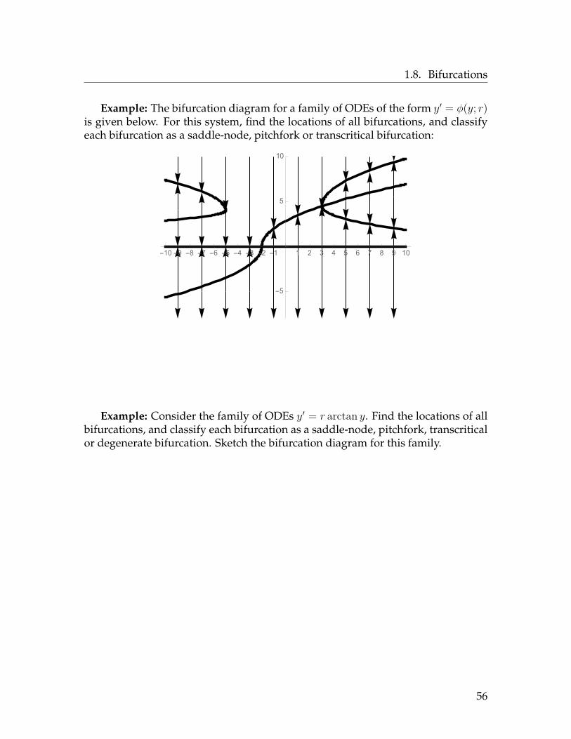
Example: The bifurcation diagram for a family of ODEs of the form y′ = φ(y; r)is given below. For this system, find the locations of all bifurcations, and classifyeach bifurcation as a saddle-node, pitchfork or transcritical bifurcation:
-10 -9 -8 -7 -6 -5 -4 -3 -2 -1 1 2 3 4 5 6 7 8 9 10
-5
5
10
Example: Consider the family of ODEs y′ = r arctan y. Find the locations of allbifurcations, and classify each bifurcation as a saddle-node, pitchfork, transcriticalor degenerate bifurcation. Sketch the bifurcation diagram for this family.
56

1.8. Bifurcations
Procedure to find bifurcations in family y′ = φ(y; r):
1. Find the equilibria in terms of r (by solving φ(y; r) = 0), keeping track ofthe values of r for which equilibrium exists.
2. For each equilibrium y0 found in Step 1, classify the equilibrium bycomputing d
dyφ(y0; r). Keep in mind that in general, this classification
will depend on the value of r.
3. Sketch the bifurcation diagram (start by graphing the formulas for yin terms of r obtained in Step 1; then fill in with vertical arrows basedon the classification in Step 2).
Example: Consider the family of ODEs y′ = ey − r. Find the locations of allbifurcations, and classify each bifurcation as a saddle-node, pitchfork, transcriticalor degenerate bifurcation. Sketch the bifurcation diagram for this family.
57

1.9. Summary of Chapter 1
1.9 Summary of Chapter 1Background and vocabulary
An ordinary differential equation (ODE) is an equation involving an independentvariable t and a function y = y(t), together with derivatives of y with respect to t.The order of an ODE is the highest order of derivative that occurs in the equation.The goal is to solve for an equation relating y and t that has no derivatives in it, i.e.to find y = y(t).
A point (t0, y0) through which an ODE must pass is called an initial value. AnODE together with an initial value is called an initial value problem (IVP). A so-lution of an IVP is called a particular solution; the set of all particular solutions ofan ODE is called the general solution of the ODE.
Generally, to solve an IVP you start by solving the ODE to obtain the generalsolution (which should have one or more arbitrary constants in it... you expect thatthe number of constants equals the order of the equation). Then you plug in theinitial value(s) to solve for the constant(s).
An ODE is called linear if there are functions p0, p1, ..., pn : R → R and a func-tion q : R→ R such that the equation can be written as
p0y + p1y′ + p2y
′′ + ...+ pny(n) = q.
A linear equation is called homogeneous if q = 0.
Qualitative and numerical approaches to first-order ODEs
To study a first-order ODE qualitatively, sketch a picture of its slope field by draw-ing “mini-tangent lines” at every point in the plane (in practice, one does this witha computer). Solutions to the ODE must “flow with” the slope field.
To numerically approximate a solution to an ODE, use Euler’s method: givenIVP y′ = φ(t, y); y(t0) = y0, to approximate y(tn), set ∆t = tn−t0
nand define points
recursively by tj+1 = tj + ∆tyj+1 = yj + φ(tj, yj)∆t
;
the yn obtained by this method (usually implemented on a computer) is an approx-imation to y(tn). The larger n is, the better the approximation.
The existence/uniqueness theorem for first-order ODEs gives conditions un-der which an IVP y′ = φ(t, y); y(t0) = y0 has one and only one solution. This the-
58

1.9. Summary of Chapter 1
orem is proved using Picard’s method of successive approximations, which comefrom the formula
fj+1(t) =∫ t
0φ(s, fj(s)) ds.
The fj converge to the solution y = f(t) as j →∞.
Autonomous ODEs and bifurcations
A first-order ODE is called autonomous if it is of the form y′ = φ(y). A constantfunction which is a solution of this ODE is called an equilibrium of the ODE; tofind the equilibia, set φ(y) = 0 and solve for y. We classify equilibria y0 of anautonomous system as follows:
• If φ′(y0) < 0, then y0 is stable (it attracts on both sides as t→∞);
• If φ′(y0) > 0, y0 is unstable (it repels on both sides as t→∞);
• If φ′(y0) = 0 but φ′′(y0) 6= 0, y0 is semistable (or neutral).
Having classified the equilibria of an autonomous ODE, we draw a phase linewhich describes the behavior of the solutions as t→∞.
Given a parameterized family of autonomous ODEs y′ = φ(y; r), values of rat which qualitative changes of the solutions to the ODE occur are called bifurca-tions. There are three main types of bifurcations:
Saddle-node bifurcations: two equilibria appear or disappearPitchfork bifurcations: one equilibria turns into three (and reverses behavior)Transcritical bifurcations: two equilibria cross each other and reverse behavior
59

Chapter 2
First-order equations: solutiontechniques
2.1 Solution of first-order homogeneous linear equationsRecall: A first-order ODE is linear if it of the form
p1(t)y′ + p0(t)y = q(t)
for functions p1, p0 and q, where p1 6= 0. The equation is called homogeneous ifq = 0 and is called constant-coefficient if p1 and p0 are constants.
Recall also: In Section 1.3, we studied the simplest ODE (first-order linear,constant-coefficient and homogeneous): the exponential growth/decay model:
y′ = ry a.k.a. y′ − ry = 0 ⇒ y = y0ert
Example: Find the particular solution of the IVP
4y′ + y = 0y(0) = 6 .
60

2.1. Solution of first-order homogeneous linear equations
Solution of first-order homogeneous linear equations
Any homogeneous first-order linear equation can be written in the form
p1(t)y′ + p0(t)y = 0.
To solve an equation of this type, first divide through by p1(t) to make the equationhave the form
y′ + p(t)y = 0.
Then, write the y′ in Leibniz notation, “separate the variables” and integrate bothsides (more on this technique later in Chapter 2):
STEPS GENERAL SITUATION EXAMPLE
p1(t)y′(t) + p0(t)y(t) = 0 t3y′ + t5y = 0Divide through by p1
y′ + p(t)y = 0Move py term to other side
y′ = −p(t)yWrite y′ in Leibniz notation
dydt
= −p(t)yMove y to left, dt to right
(i.e. “separate the variables”)1ydy = −p(t) dt
Integrate both sides ∫ 1ydy =
∫−p(t) dt
ln y =∫−p(t) dt
Solve for yy = e−
∫p(t) dt
61

2.1. Solution of first-order homogeneous linear equations
Theorem 2.1 (Solution of a first-order homogeneous linear equation) The gen-eral solution of the first-order, homogeneous linear equation
y′ + p(t)y = 0
isy = exp
(−∫p(t) dt
)= e−
∫p(t) dt.
Note: general solutions of first-order equations should (and do) have arbitraryconstants in them. The arbitrary constant in this general solution is the “+C” thatappears when you calculate
∫p(t) dt. This constant manifests itself as follows:
Therefore the general solution of a homogeneous, first-order linear equation isalways a constant times one particular solution of that equation. More generally:
Theorem 2.2 (Solution of a homogeneous, first-order linear equation) Let yh(t)be any nonzero solution of a homogeneous, first-order linear ODE
p1(t)y′ + p0(t)y = 0.
Then:
1. the only solutions of that equation are of the form Cyh(t) for some constant C.
2. for any constant C, the function Cyh(t) is a solution of the same equation; and
PROOF By the preceding discussion, the set of solutions is the setKe−P (t) whereKis an arbitrary constant and P is an antiderivative of p(t) = p0(t)
p1(t) . The result follows.
62
2.1. Solution of first-order homogeneous linear equations
How this theorem is applied: Suppose you have some homogeneous, linearfirst-order ODE and somehow, someway, you know that
yh(t) = sin t+ e−t
is a solution. Then you know
Subspaces
The theorem of the previous section can be rephrased in the language of linearalgebra. Recall that a vector space is a set of objects which can be added to oneanother and multiplied by constants. If one vector space is a subset of another, wesay that the first space is a subspace of the second. More precisely:
Definition 2.3 Let V be a vector space and let W ⊆ V . We say W is a subspace (ofV ) if
1. W is closed under addition, i.e. for any two vectors w1 and w2 inW , w1 +w2 ∈W ; and
2. W is closed under scalar multiplication, i.e. for any vector w ∈ W and anyscalar r, rw ∈ W .
The most important example of a subspace is the set of multiples of a singlevector.
Definition 2.4 Let V be a vector space and let v ∈ V be a vector. The span of v,denoted Span(v), is the set of linear multiples of v:
Span(v) = cv : c ∈ R
If W ⊆ V is such that W = Span(v), we say W is spanned by v.
63

2.1. Solution of first-order homogeneous linear equations
Examples of spans of a single vector:
• V = R2; v = (3, 2)
• V = R4; v = (1, 1, 1, 1)
• V = C∞(R,R); y = sin t
Lemma 2.5 (Spans are subspaces) The span of any vector is a subspace.
PROOF Essentially, this is because the sum of two multiples of a vector is also amultiple of that vector, and because any constant times a multiple of a vector isalso a multiple of that vector. For a precise proof, see Theorem 3.5 of my Math 322lecture notes.
Lemma 2.6 If W is spanned by v, then W is also spanned by cv for any nonzeroconstant c.
PROOF The set of multiples of v is the same as the set of multiples of cv, so longas c 6= 0.
We can restate Theorem 2.2 as follows:
Theorem 2.7 The set of solutions of a homogeneous, first-order linear ODE form asubspace of C∞(R,R) which is spanned by any one nonzero solution of the equation.
Consequence: If you know one nonzero solution yh = yh(t) of a homogeneous,first-order linear ODE, then you know them all. They are all of the form
A preview: The set of solutions to a homogeneous, nth-order linear ODE willalso be a subspace of C∞(R,R); this subspace will be spanned by n linearly inde-pendent functions rather than just one.
64

2.2. Solution of first-order linear equations by integrating factors
A last remark: Suppose p(t) is constant. Then the first-order homogeneouslinear equation is
2.2 Solution of first-order linear equations by integrating factorsTo solve a general first-order linear equation, first write it in the form
p1(t)y′ + p0(t)y = q(t)
and divide through by p1(t) to get
y′ + p0(t)p1(t)y = q(t)
p1(t) .
After doing this, any first-order linear equation has the following standardform:
y′ + p(t)y = q(t).
From this point, there are two methods of solution:
1. integrating factors (§2.2)
2. undetermined coefficients (§2.3)
Much of the time, either method works, but you should know both.
65
2.2. Solution of first-order linear equations by integrating factors
Integrating factors
Definition 2.8 Given an ODE, an integrating factor for that equation is some ex-pression µ (which may have a t and/or y in it) such that if you multiply through theequation by µ, the equation becomes “easier”.
Consider the first-order linear ODE
y′(t) + p(t)y(t) = q(t).
Now we look for an integrating factor of the form µ(t). After multiplying throughby this function, the equation would be
µ(t)y′(t) + p(t)µ(t)y(t) = µ(t)q(t). (2.1)
Note that if µ(t) were some function such that
µ′(t) = p(t)µ(t),
then equation (2.1) would look like
µ(t)y′(t) + µ′(t)y(t) = µ(t)q(t). (2.2)
This works if µ′(t) = p(t)µ(t), i.e. if µ satisfies the differential equation
µ′ − p(t)µ = 0.
But this is a first-order, homogeneous linear equation, so we know from the previ-ous section that the general solution is given by
µ = exp(−∫−p(t) dt
)= e
∫p(t) dt
Since in this context, we don’t need all the µs that work (we only need one µ), wecan ignore the +C in this integral.
66

2.2. Solution of first-order linear equations by integrating factors
This works! Here is the procedure we just went through:
Procedure to solve first-order linear ODEs via integrating factors
1. Rewrite the equation in the form y′(t) + p(t)y(t) = q(t).
2. Multiply through both sides by the integrating factor µ(t) = e[∫p(t) dt]
(ignore the +C in the integral). This yields the equation
µ(t)y′(t) + µ′(t)y(t) = µ(t)q(t).
3. The left-hand side of the equation you get in Step 2 is always a deriva-tive coming from the Product Rule. This makes the equation
d
dt[µ(t)y(t)] = µ(t)q(t).
4. Integrate both sides with respect to t to get µ(t)y(t) =∫µ(t)q(t) dt.
(You need the +C when doing this integral to get the general solu-tion.)
5. Divide through by µ(t) to solve for y: y(t) = 1µ(t) [
∫µ(t)q(t) dt].
You can solve any first-order linear ODE by this procedure (theoretically). Theonly drawback is that the integrals∫
p(t) dt and∫µ(t)q(t) dt
have to be doable (and you don’t always know if they are doable when you start).
Example 1: Find the general solution of ty′ + 2y = 4t2.
67

2.2. Solution of first-order linear equations by integrating factors
Example 2: Find the particular solution of the IVPy′ + (cos t)y = cos ty(π) = 0 .
68

2.2. Solution of first-order linear equations by integrating factors
Example 3: Find the general solution of y′ + y = 6t.
69

2.3. Solution of first-order linear equations by undetermined coefficients
2.3 Solution of first-order linear equations by undetermined coef-ficients
It turns out that the structure of the solutions of a non-homogeneous linearequation has a lot to do with an associated homogeneous equation:
Definition 2.9 Given a first-order linear ODE p1(t)y′ + p0(t)y = q(t), the ODE
p1(t)y′ + p0(t)y = 0
is called the corresponding homogeneous equation.
Theorem 2.10 Suppose y and y are two solutions of the first-order linear ODE p1(t)y′+p0(t)y = q(t). Then the function y− y is a solution of the corresponding homogeneousequation p1(t)y′ + p0(t)y = 0.
PROOF The corresponding homogeneous equation is
p1(t)y′ + p0(t)y = 0.
Plug the function y − y into the left-hand side:
70

2.3. Solution of first-order linear equations by undetermined coefficients
As a consequence, suppose yp is any one particular solution of the ODE
p1(t)y′ + p0(t)y = q(t).
If y(t) is any solution of that ODE, then y − yp is a solution of the correspondinghomogeneous equation, i.e.
y − yp = Cyh
where yh is any nonzero solution of the corresponding homogeneous equation.Therefore
y(t) = yp(t) + Cyh(t)
where yp is any solution of the original ODE, and yh is any nonzero solution of thecorresponding homogeneous equation. We have proven:
Theorem 2.11 (Solution of the non-homogeneous first-order linear equation)Let yp(t) be any particular solution of the first-order, linear ODE
p1(t)y′ + p0(t)y = q(t).
Let yh(t) be any nonzero solution of the corresponding homogeneous equation
p1(t)y′ + p0(t)y = 0
Then y(t) is a solution of the original ODE if and only if
y(t) = yp(t) + Cyh(t),
where C is an arbitrary constant.
Restated in linear algebra language: This theorem says that the solution set ofa first-order, linear ODE is an affine subspace of C∞(R,R) whose dimension is 1.
How this is applied: Suppose you have some first-order linear ODE and youknow that yp(t) = t2− t is a solution of this ODE. Furthermore, suppose you knowthat yh(t) = e3t is a solution of the corresponding homogeneous equation. Thenthe general solution of the ODE is
71

2.3. Solution of first-order linear equations by undetermined coefficients
How does this theorem fit with the method of solution obtained via integrat-ing factors? Recall from the previous section that the solution to first-order linearODE
y′(t) + p0(t)y(t) = q(t)
is given by
y(t) = 1µ(t)
[∫µ(t)q(t) dt
]where µ(t) = exp
(∫ t0 p0(s) ds
)is the integrating factor.
Method of undetermined coefficients
Theorem 2.11 motivates an alternate way to solve first-order, linear ODEs. Afterwriting the equation in the form
y′ + p(t)y = q(t) (2.3)
if you can find a solution yh of the corresponding homogeneous equation y′ +p(t)y = 0 (which we can do by the methods described in Section 2.1), and if youcan find any one solution yp of (2.3) (which we can sometimes do by “guessing”),then the general solution of (2.3) is
y = yp + Cyh.
This method of solving an ODE is called the method of undetermined coefficients.
72
2.3. Solution of first-order linear equations by undetermined coefficients
Example: Find the general solution of the ODE y′ − 3y = et (without usingintegrating factors).
73

2.3. Solution of first-order linear equations by undetermined coefficients
Example: Find the general solution of the ODE y′ + 2y = 8 cos t (without usingintegrating factors).
74
2.3. Solution of first-order linear equations by undetermined coefficients
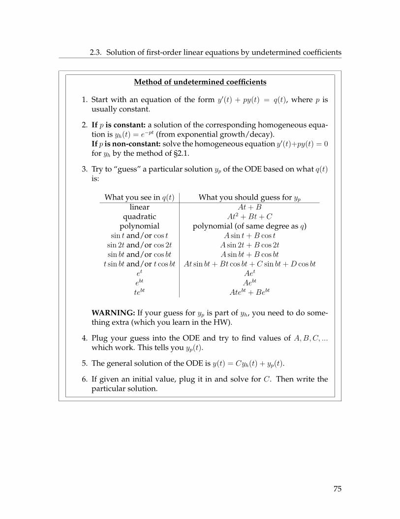
Method of undetermined coefficients
1. Start with an equation of the form y′(t) + py(t) = q(t), where p isusually constant.
2. If p is constant: a solution of the corresponding homogeneous equa-tion is yh(t) = e−pt (from exponential growth/decay).If p is non-constant: solve the homogeneous equation y′(t)+py(t) = 0for yh by the method of §2.1.
3. Try to “guess” a particular solution yp of the ODE based on what q(t)is:
What you see in q(t) What you should guess for yplinear At+B
quadratic At2 +Bt+ Cpolynomial polynomial (of same degree as q)
sin t and/or cos t A sin t+B cos tsin 2t and/or cos 2t A sin 2t+B cos 2tsin bt and/or cos bt A sin bt+B cos btt sin bt and/or t cos bt At sin bt+Bt cos bt+ C sin bt+D cos bt
et Aet
ebt Aebt
tebt Atebt +Bebt
WARNING: If your guess for yp is part of yh, you need to do some-thing extra (which you learn in the HW).
4. Plug your guess into the ODE and try to find values of A,B,C, ...which work. This tells you yp(t).
5. The general solution of the ODE is y(t) = Cyh(t) + yp(t).
6. If given an initial value, plug it in and solve for C. Then write theparticular solution.
75

2.4. Separation of variables
2.4 Separation of variables
Question: Can you explicitly solve a first-order ODE y′ = φ(t, y) for the solu-tions y(t)?
Answer:
Definition 2.12 A first-order ODE is called separable if it can be rewritten in theform f(y)y′ = h(t) for functions f of y and h of t.
In other words, an ODE is separable if one can separate the variables, i.e. putall the y on one side and all the t on the other side.
Theoretical solution of separable, first-order ODEs
Suppose you have a separable, first-order ODE. Then, by replacing the y′ with dydt
,it can be rewritten as
f(y) dydt
= h(t).
Integrate both sides with respect to t to get
∫f(y) dy
dtdt =
∫h(t) dt
On the left-hand side, perform the u−substitution u = y(t), du = dydtdt to get∫
f(u) du =∫h(t) dt
Assuming F and H are antiderivatives of f and h, respectively, we get
F (u) = H(t) + C
which, since u = y = y(t), is equivalent to the solution
F (y) = H(t) + C.
Note: We only need a constant on one side of the equation, because the constantson the two sides can be combined into one.
76

2.4. Separation of variables
A shortcut:
The following method involves the writing of things that are technically incorrect,but always works. Again start with a separable, first-order ODE. Again, replacethe y′ with dy
dtto get
f(y) dydt
= h(t).
Now, pretend that the dydt
is a fraction (it isn’t) and “multiply” through by dt to get
f(y) dy = h(t) dt.
Now, integrate both sides: ∫f(y) dy =
∫h(t) dt
This gives the same solution as before:
F (y) = H(t) + C.
The shortcut above suggests the following method to solve separable ODEs:
Procedure to solve separable ODEs
1. Write the derivative y′ in Leibniz notation as dydt
.
2. Separate the variables, i.e. put all the y (with the dy) on one side ofthe equation, and all the t (with the dt) on the other side of the equa-tion.
WARNING: The equation has to end up in the form f(y) dy = h(t) dt.(For example, you don’t want something like f(y) dy + y = h(t) dt.)
3. Integrate both sides, putting the arbitrary constant on one side.
4. If given an initial value, plug it in and solve for C. Then write theparticular solution.
5. If the problem asks for a solution of the form y = y(t) or y = f(t),solve the solution for y.
77
2.4. Separation of variables
Example 1: Find the general solution of the ODE y′ = ty.
Example 2: Find the particular solution of this initial value problem:y′ = 2t− 2tyy(1) = −2
78
2.4. Separation of variables
Example 3: Find the particular solution of this initial value problem:y′ = y cos t
1+2y2
y(0) = 1
Example 4: Find the particular solution of this initial value problem:y′ = 2−et
3+2yy(0) = 0
Find the value of t for which the solution of this IVP is maximized.
79

2.4. Separation of variables
Example 5: Find the general solution of the logistic equation:
y′ = ry(L− y)
We have proven:
Theorem 2.13 (Solution of the logistic equation) The general solution of the lo-gistic equation y′ = ry(L− y) is
y = L
1 + Ce−rLt.
80

2.4. Separation of variables
Example 6: Find the general solution of this ODE.
y′ = ty3(1 + t2)−1/2
Write your answer in the form y = f(t).
81
2.5. Exact equations
2.5 Exact equationsQuestion: Suppose you are given a first-order ODE which is neither linear nor
separable. Is there any hope of solving it?
Answer:
A review of some multivariable calculus
In multivariable calculus, you study (among other things) functions of two vari-ables z = ψ(s, t). For such a function, the natural method of differentiation is partialdifferentiation. Without going into much detail, here are some informal definitions:
Definition 2.14 Let ψ : R2 → R be a function of two variables, i.e. z = ψ(s, t).
1. The partial derivative of ψ with respect to s, denoted ψs or ∂ψ∂s
, is the expres-sion obtained by treating t as a constant and differentiating the formula definingψ(s, t) with respect to s.
2. The partial derivative of ψ with respect to t, denoted ψt or ∂ψ∂t
, is the expres-sion obtained by treating s as a constant and differentiating the formula definingψ(s, t) with respect to t.
Example: Let ψ(s, t) = 2t3 cos s+ et sin s− 4t.
ψs = ∂ψ
∂s=
ψt = ∂ψ
∂t=
Example: Suppose ψ(s, t) is some function such that ∂ψ∂t
= 12s2t3 +6t. What canyou say about ψ(s, t)?
The following theorem (or a more general version of it) is proven in multivari-able calculus (Math 320):
82

2.5. Exact equations
Theorem 2.15 (Chain Rule) Suppose ψ : R2 → R is a differentiable function ofvariables t and y. Suppose further that both t and y are functions of a third variable s.Then
dψ
ds= ∂ψ
∂t
dt
ds+ ∂ψ
∂y
dy
ds.
Suppose we let s = t in this theorem. Then dtds
= dtdt
= 1 so the formula in theChain Rule becomes
dψ
dt= ∂ψ
∂t+ ∂ψ
∂y
dy
dta.k.a.
∂ψ
∂t+ ∂ψ
∂yy′ = dψ
dt.
What does this have to do with ODEs?
Example: Find the general solution of 2t+ y2 + 2tyy′ = 0.
Bad news: This is not a separable equation.
Good news: This looks a bit like the equation at the above right.
Definition 2.16 A first-order ODE is called exact if there is a function ψ : R2 → Rsuch that the equation has the form
∂ψ
∂t(t, y) + ∂ψ
∂y(t, y)y′ = 0.
Theorem 2.17 (Characterization of exact equations) A first order ODE of the form
M(t, y) +N(t, y)y′ = 0
is exact if and only if ∂M∂y
= ∂N∂t
.
PROOF (⇒) Suppose the equation is exact. Then there is a function ψ = ψ(t, y) :R2 → R so that M = ∂ψ
∂tand N = ∂ψ
∂y. Then
∂M
∂y= ∂2ψ
∂y∂tand
∂N
∂t= ∂2ψ
∂t∂y;
83

2.5. Exact equations
by a theorem from multivariable calculus (called the “Equality of Mixed Partials”),these two quantities are equal (because it doesn’t matter the order in which youcompute a mixed second-order partial derivative).
(⇐) Now we assume ∂M∂y
= ∂N∂t
. Define
ψ(t, y) =∫M(t, y) dt+
∫ [N(t, y)−
∫ ∂
∂yM(t, y) dt
]dy.
Observe that for this ψ,
∂ψ
∂t= ∂
∂t
(∫M(t, y) dt+
∫ [N(t, y)−
∫ ∂
∂yM(t, y) dt
]dy
)
= ∂
∂t
∫M(t, y) dt +
∫ [∂
∂tN(t, y)− ∂
∂t
∫ ∂
∂yM(t, y) dt
]dy
= M(t, y) +∫ [
∂
∂tN(t, y)− ∂
∂yM(t, y)
]dy
= M(t, y) +∫
0 dy (by the hypothesis∂M
∂y= ∂N
∂t)
= M(t, y)
and
∂ψ
∂y= ∂
∂y
(∫M(t, y) dt+
∫ [N(t, y)−
∫ ∂
∂yM(t, y) dt
]dy
)
=∫ ∂
∂yM(t, y) dt+N(t, y)−
∫ ∂
∂yM(t, y) dt
= N(t, y)
as desired.
Remark: To find the ψ for a given exact equation, don’t use the formula in thepreceding theorem. Use the method outlined in forthcoming examples.
Theorem 2.18 (Solution of an exact equation) The exact ODE
∂ψ
∂t(t, y) + ∂ψ
∂y(t, y)y′ = 0
has general solutionψ(t, y) = C
where C is an arbitrary constant.
84

2.5. Exact equations
PROOF By the preceding discussion, we know that the left-hand side of an exactequation can be rewritten as dψ
dt, and since this is equal to zero, ψ must be a con-
stant.
Back to the example: 2t+ y2 + 2tyy′ = 0.
New example: 2ty3 − 2y2 + 4t2 + (3t2y2 − 4ty + 8y)y′ = 0
85

2.5. Exact equations
How to solve an exact equation
1. Write the equation in the form M(t, y) +N(t, y)y′ = 0.
2. Check that the equation is exact by verifying that ∂M∂y
= ∂N∂t
.
3. If the equation is exact, the solution is ψ(t, y) = C where
ψ(t, y) =∫M(t, y) dt =
∫N(t, y) dy.
Keep in mind that when integratingM with respect to t, your answerincludes a “+A(y)”, and when you integrateN with respect to y, youranswer includes a “+B(t)”.
4. Choose A(y) and B(t) to reconcile two versions of ψ obtained by in-tegration.
5. If given an initial value, plug it in and solve for C. Then write theparticular solution.
6. If the problem asks for a solution of the form y = y(t) or y = f(t),solve the solution for y.
Example: y′ = 1−2tey
t2
86

2.6. Applications of first-order equations
2.6 Applications of first-order equationsCompartmental models
Many mathematical models involve processes that can be divided into “compart-ments” or “stages”. You build the model by listing the compartments, and thendescribing the interactions between the compartments. These are called compart-mental models and generate ODEs (or systems of ODEs) which can be analyzedwith the methods of this course.
General setup:
Example 1: Malthusian population model
Let y(t) = population at time t; assume the birth and death rates are proportionalto the population.
Example 2: Logistic population model
Let y(t) = population at time t; assume the birth rate is proportional to the popula-tion; assume the death rate is proportional to the number of interactions betweentwo living beings.
87

2.6. Applications of first-order equations
Examples 1 and 2 are models with one compartment. A population model withmore than one compartment might look like this:
In this context, you would get a system of two ODEsx′(t) = birth rate - aging rate - death rate of youngy′(t) = aging rate - death rate of old
Under reasonable assumptions, you might get something likex′(t) = λy − ax− µxy′(t) = ax− µy
We don’t know how to solve systems yet, but we’ll return to these in Chapter 3.
88

2.6. Applications of first-order equations
Example 3: Mixing problems
Consider a large tank containing 1000 L of pure water, into which a brine solutionof salt water (whose concentration is .1 kg / L) is poured at a constant rate of 6 L/ min. The solution inside the tank is kept well mixed, and is flowing out of thetank at a rate of 6 L / min. Find the concentration of salt in the tank at time t.
89

2.6. Applications of first-order equations
Newtonian mechanics
Recall from physics the three Newtonian laws of motion:
1. When an object is subject to no external force, it continues with constant ve-locity.
2. When a body is subject to external forces, the time rate of change of the ob-ject’s momentum (i.e. the mass times acceleration) is equal to the sum of theforces acting on it.
3. When one body interacts with a second, the force of the first body on thesecond is equal in magnitude, but opposite in direction to the force of thesecond body on the first.
Newton’s Second Law is of particular use in modeling the motion of objectsusing ODEs: let v = v(t) be the velocity of an object at time t. Then
Example: (from page 4 of these lecture notes) Consider an object of mass 20 kg,that is falling through the Earth’s atmosphere (gravitational constant is 9.8 m/sec2;drag coefficient 3 N sec/m), near sea level. Formulate an ODE which describes thevelocity of the object, and solve it.
90

2.6. Applications of first-order equations
Heating and cooling
Goal: formulate (and solve) an ODE which models the temperature inside a build-ing as a function of time.
Assumptions:
• The temperature T (t) inside the building at time t will depend on the follow-ing things (and nothing else):
–
–
–
• Newton’s Law of Cooling (or Heating): the rate of change in temperatureinside the building, absent other forces, is proportional to the temperaturedifference between the outside and the inside
Let T (t) be the temperature inside the building at time t. We obtain the followingODE:
This equation is first-order, and linear. Let’s solve it:
91

2.6. Applications of first-order equations
Theorem 2.19 (Heating and cooling model) Suppose T (t) is the temperature of acompartment at time t. If the outside temperature is given by M(t), the compartmentitself generates heat H(t), and a furnace/air conditioner generates heat U(t) (U ispositive if you’re heating and negative if you’re cooling), then the temperature satisfiesthe ODE
dT
dt= K [M(t)− T (t)] +H(t) + U(t)
where K is a constant. The solution of this ODE (obtained via integrating factors) is
T (t) = e−Kt(∫
eKt [KM(t) +H(t) + U(t)] dt).
Example 1: Suppose we have the simplest possible situation: no one in thebuilding (so H(t) = 0), no A/C or furnace (so U(t) = 0), and a constant outsidetemperature M(t) = M0. Find T (t).
92

2.6. Applications of first-order equations
Example 2: Suppose the outside temperature t hours after midnight is
M(t) = 70− 10 cos(π
12t).
Assuming there is no air conditioning or heating and that the constant from New-ton’s Law is K = 1
4 , find the temperature of the house at time t, if the temperatureinside the house at midnight is 65.
0 6 12 18 24
60
65
70
75
80
93

2.6. Applications of first-order equations
In: M[t_] = 70 - 10 Cos[Pi t / 12];
K = 1/4;
f[t_] = Integrate[E^(K t) K M[t] , t]
Out: −10et/4
(−7(9 + π2) + 9 cos
(πt12
)+ 3π sin
(πt12
))9 + π2
Therefore the solution is 1µ(t) = e−Kt times the previous output which is
T (t) = e−t/4 (f(t) + C) .
To find C, plug in the initial value t0 = 0, T0 = 65 and solve for C. We do this withMathematica:
In: Solve[65 == E^(-0/4) (f[0] + C), C]
Out: C = −5(−9 + π2)9 + π2
Now we know what the temperature T (t) is:
T (t) = e−t/4(f(t) + C)
= e−t/4
−10et/4[−7(9 + π2) + 9 cos
(πt12
)+ 3π sin
(πt12
)]9 + π2 − 5(−9 + π2)
9 + π2
.Below, the interior temperature is graphed with the dashed curve (the exterior
temperature is the solid curve):
0 6 12 18 24
60
65
70
75
80
94

2.6. Applications of first-order equations
Electrical circuits
Kirchoff’s laws govern the physics of electrical circuits. They are:
Current law: The sum of the current flowing into any junction point is zero.
Voltage law: The sum of the instantaneous changes in potential (i.e. the sum ofthe voltage drops) around any closed loop is zero.
Things that can be hooked up to form electrical circuits:
HO
WIT
ISH
OW
TOFIN
DU
NIT
OF
DR
AW
NIN
THE
VO
LTAG
EO
BJECT
LETTERM
EASU
REM
ENT
AD
IAG
RA
MD
RO
Pvoltage
sourceE
voltV
ES
=usually
(batteryor
given/generator)
controlled
resistorR
ohmΩ
Ohm
’sLaw
:(reduces
currentflow)
ER
=RIR
inductorL
henryH
Faraday’sLaw
:(coil)
EL
=LdIdt
capacitorC
faradF
EC
=1Cq
(storesenergy)
(q=
charge)
Also:voltage/
currentrelationshipIC (t)=
CdE
Cdt
95
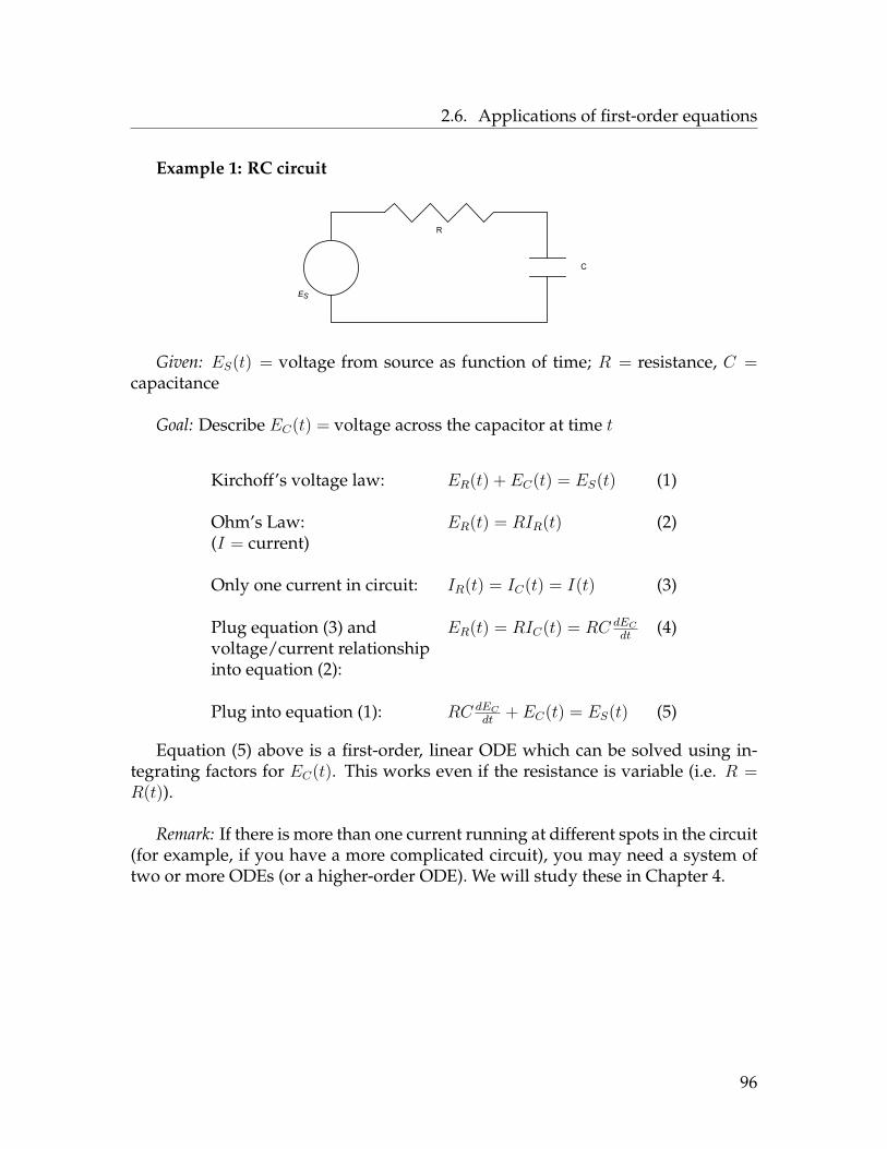
2.6. Applications of first-order equations
Example 1: RC circuit
ES
R
C
Given: ES(t) = voltage from source as function of time; R = resistance, C =capacitance
Goal: Describe EC(t) = voltage across the capacitor at time t
Kirchoff’s voltage law: ER(t) + EC(t) = ES(t) (1)
Ohm’s Law: ER(t) = RIR(t) (2)(I = current)
Only one current in circuit: IR(t) = IC(t) = I(t) (3)
Plug equation (3) and ER(t) = RIC(t) = RC dEC
dt(4)
voltage/current relationshipinto equation (2):
Plug into equation (1): RC dEC
dt+ EC(t) = ES(t) (5)
Equation (5) above is a first-order, linear ODE which can be solved using in-tegrating factors for EC(t). This works even if the resistance is variable (i.e. R =R(t)).
Remark: If there is more than one current running at different spots in the circuit(for example, if you have a more complicated circuit), you may need a system oftwo or more ODEs (or a higher-order ODE). We will study these in Chapter 4.
96

2.6. Applications of first-order equations
Example 2: RL circuit
ES
R
L
Given: ES(t) = voltage from source as function of time; R = resistance, L =inductance
Goal: Describe I(t) = current at time t
Kirchoff’s voltage law: ER(t) + EL(t) = ES(t) (1)
Ohm’s Law: ER(t) = RIR(t) (2)
Faraday’s Law: EL(t) = LdIdt
(3)
Only one current in circuit: IR(t) = IL(t) = I(t) (4)
Plug into equation (1): LdIdt
+RI(t) = ES(t) (5)
Equation (5) above is a first-order, linear ODE which can be solved using inte-grating factors for I(t). (If you need to know the voltage across the resistor, applyOhm’s Law to the answer: ER(t) = RI(t).)
97

2.7. Summary of Chapter 2
2.7 Summary of Chapter 2Theory of first-order linear ODEs
The general solution of any first-order, homogeneous linear equation
p1(t)y′(t) + p0(t)y(t) = 0
is a subspace spanned by one nonzero solution, i.e. is of the form Cyh(t) for anynonzero solution yh. The general solution of any first-order (not necessarily homo-geneous) linear equation
p1(t)y′(t) + p0(t)y(t) = q(t)
is the solution of the corresponding homogeneous equation plus any one particu-lar solution of the original equation, i.e. has the form yp(t) + Cyh(t).
Solution techniques
• Every linear, first-order, homogeneous, constant-coefficient ODE is of theform y′ = ry; the solution of such an equation is y = y0e
rt where y0 = y(0).This is the exponential growth/decay model.
• To solve a linear, first-order equation
p1(t)y′(t) + p0(t)y(t) = q(t),
first divide through by p1, to rewrite the equation as
y′ + p(t)y = q(t).
Then use one of these two methods:
Integrating factors: multiply through both sides of the equation by the inte-grating factor µ(t) = exp (
∫p(t) dt) and then identify the left-hand side
as ddt
(µ(t)y(t)); the general solution is eventually
y(t) = 1µ(t)
[∫µ(t)q(t) dt
].
Undetermined coefficients: first, solve the corresponding homogeneous equa-tion
y′ + p(t)y = 0and call the solution yh. Then, to a particular solution of the originalequation, “guess” what yp is based on what the function q is. Substitute
98

2.7. Summary of Chapter 2
your guess for yp into the ODE and use that equation to solve for theconstant(s) in your guess. The general solution of the equation is then
y = yp + Cyh.
• To solve a first-order equation which is not linear, try one of two methods:
Separation of variables: a first-order ODE is called separable if it can berewritten as f(y)y′ = h(t). To solve a separable ODE, separate the vari-ables and integrate both sides.Note: homogeneous linear equations are also separable and can be solvedvia separation of variables.
Exact equations: a first-order ODE is exact if it is of the form
M(t, y) +N(t, y)y′ = 0.
where ∂M∂y
= ∂N∂t
. The solution of an exact equation is ψ(t, y) = C where
ψ(t, y) =∫M(t, y) dt =
∫N(t, y) dy.
Applications
Applications of first-order models include compartmental models, population dy-namics, mixing problems, Newtonian mechanics, heating and cooling, and electri-cal circuits.
99

2.8. Exam 1 Review
2.8 Exam 1 ReviewWhat should you expect on the exam:
Solve first-order ODEs/IVPs: separable equations, exact equations, first-order lin-ear equations
Solve second-order ODEs that either have no y or no t in them (HW # 79-82)
Verifying whether or not a given equation is or is not a solution of an ODE or IVP
Sketch and/or analyze pictures of slope fields and/or phase lines
Euler’s method: perform a couple of steps for a simple equation
Applications: heating & cooling, population models, circuits, etc. You will begiven formulas (the heating/cooling equation, the RL equation, the RC equa-tion, etc.) if necessary.
Question(s) on vocabulary
Some practice questions:
1. a) What is the difference between a “general solution” and a “particularsolution”?
b) What is meant by the “order” of an ODE?
c) What does it mean for an ODE to be “linear”?
d) What is meant by “existence/uniqueness” (in the context of ODEs)?
e) What is the general form of the general solution of a first-order linearODE?
2. Consider the initial value problemy′ = 2y − ty(0) = 1
Suppose you wanted to estimate y(30) by performing Euler’s method with15 steps. Find the points (t1, y1) and (t2, y2) that would be obtained by thismethod.
3. Here is the picture of a slope field associated to an ODE of the form y′ =φ(t, y):
100

2.8. Exam 1 Review
-5 0 5
-5
0
5
a) Estimate the value of y′ when t = 5 and y = −2.
b) Suppose y(−2) = 4. Estimate y(2).
c) Suppose y(−2) = 4. Estimate y′(2).
d) Suppose y(0) = −2. Find limt→∞
y(t).
e) Sketch the solution of this ODE satisfying y(0) = 3 on the slope field.
f) Find the equation of one particular solution of this ODE.
g) Is the equation which generates this slope field autonomous? Why orwhy not?
4. Here is the picture of the phase line associated to an ODE of the form y′ =φ(y):
-6 -1 2 5
a) Suppose y(1) = 3. Find limt→∞
y(t).
b) Suppose y(−4) = 3. Find limt→−∞
y(t).
c) Find the equilibria of this system, and classify them as stable, unstableor semistable.
d) Suppose y(0) = y0. Find all values of y0 for which limt→∞
y(t) = 5.
5. Sketch the phase lines for each ODE. Find the equilibria and classify them asstable, unstable or semistable:
101

2.8. Exam 1 Review
a) y′ = y2 − 7y + 12b) y′ = y4 − 8y3
c) y′ = sin y + 1
6. Solve each given differential equation or initial value problem. In questions(a), (c) and (i), your answer must be written in the form y = f(t).
a) dydt
= ty2
b)
dydt
= t2
y3
y(0) = −1
c)
dydt
= (y2 + 1)ty(0) = 1
d) y′ = y7
e) y′ = t1+t2
f) y′ = y1+y2
g) 3t3y2 dydt
+ 3t2y3 = 5t4
h) t2y3 + t(1 + y2)y′ = 0
i) y′ = −2ty + 4e−t2
j) tdydt
+ 2y = t2 − t
k)
dydt
= −yt
+ 2y(1) = 3
l) y′′ − 4y′ = e2t
m) y′ − 2y = 4 sin t− 7 cos t
n) yy′′ = (y′)3
7. A 5% sulfuric acid solution is pumped into a 24 L tank at a rate of 3 L / min.The tank initially contains 10% sulfuric acid, and is kept well-stirred at alltimes. If the tank drains at a rate of 4 L / min, find the amount of sulfuricacid in the tank at time t = 3.
Solutions
WARNING: I did these by hand. There might be errors.
1. a) Given an ODE, the set of all solutions of that ODE is called the generalsolution of the ODE. This solution will have one or more arbitrary con-stants in it. If you are given an initial value, you can plug that initialvalue into the general solution, solving for the constant in the generalsolution. This produces a solution of the ODE with no arbitrary con-stants, which is called a particular solution of the ODE.
b) The order of an ODE is the highest-order of derivative appearing in theequation; it is also equal to the number of arbitrary constants in the gen-eral solution.
c) An ODE is linear if it is of the form q(t) = p0(t)y+p1(t)y′+p2(t)y′′+ ...+pn(t)y(n) where q, p0, p1, ..., pn are functions of t. Equivalently, an ODE islinear if it is of the form T (y) = q where T is a linear differential operatoron C∞(R,R).
102

2.8. Exam 1 Review
d) A first-order initial value problem of the form y′ = φ(t, y); y(t0) = y0 hasone and only one solution, which is of the form y = f(t), so long as thefunction φ is “nice” (i.e. φ and ∂φ
∂yare both continuous).
e) The general solution of a first-order linear ODE always has the form y =yp + Cyh, where yp = yp(t) is any one particular solution of the equationand yh = yh(t) is any nonzero solution of the associated homogeneousequation.
2. To use Euler’s method, first compute ∆t = tn−t0n
= 30−015 = 2.
(t0, y0) = (0, 1) so φ(t0, y0) = 2(1)− 0 = 2. Therefore
t1 = t0 + ∆t = 0 + 2 = 2 and y1 = y0 + φ(t0, y0)∆t = 1 + 2(2) = 5
so (t1, y1) = (2, 5). Now φ(t1, y1) = 2(5)− 2 = 8. Therefore
t2 = t1 + ∆t = 2 + 2 = 4 and y2 = y1 + φ(t1, y1)∆t = 5 + 8(2) = 21
so (t2, y2) = (4, 21).
3. a) At (5,−2), the slope y′ appears to be about −1b) Follow the slope field from (−2, 4) until t = 2 and read off the y value to
get y(2) ≈ 1.5.
c) Follow the slope field from (−2, 4) until t = 2 and read off the slope at 2to get y′(2) ≈ 0.
d) As the solution through (0,−2) goes to the right, its y-value approacheslimt→∞
y(t) = −4.
e) -5 0 5
-5
0
5
f) y = −4, y = 0 and y = 6 all appear to be solutions.
g) Notice that the slope at (0, 2) is different from the slope at (5, 2). There-fore the slope y′ cannot depend only on y, so this equation cannot beautonomous.
4. a) limt→∞
y(t) = 5 (follow the arrow forward from y = 3).
b) limt→−∞
y(t) = 2 (follow the arrow backward from y = 3).
103

2.8. Exam 1 Review
c) y = −6 is stable; y = −1 is semistable; y = 2 is unstable; y = 5 is stable.d) If y(0) > 2, then lim
t→∞y(t) = 5. (Equivalent answer: (2,∞).)
5. a) Set φ(y) = y2−7y+12 equal to zero and solve for y to get y = 3 and y = 4(those are the equilibria). To classify them, note that φ′(y) = 2y − 7. Soφ′(3) = −1 < 0 so 3 is stable; φ′(4) = 1 > 0 so 4 is unstable. (So the phaseline has arrows going from −∞ toward 3, 4 towards 3, and 4 towards∞.)
b) Set φ(y) = y4 − 8y3 = y3(y − 8) equal to zero to get y = 0 and y = 8(those are the equilibria). To classify them, compute φ′(y) = 4y3 − 24y2.φ′(8) = 512 > 0 so 8 is unstable. As for y = 0, φ′(0) = 0 so computeφ′′(y) = 12y2 − 48y. That means φ′′(0) = 0. Now compute φ′′′(y) =24y − 48; φ′′′(0) = −24 < 0. Since the first nonzero derivative at 0 is odd(it was the third derivative) and negative, it is as if the first derivativewas negative, so the function φ is decreasing at zero, which makes y = 0a stable equilibria. (So the phase line has arrows going from−∞ toward0, from 8 toward 0 and from 8 toward∞).
c) Set φ(y) = sin y + 1 = 0 and solve for y to get y = 3π2 + 2πN where N
is an integer. To classify these, compute φ′(y) = cos y and observe thatcos(3π
2 +2πN) = 0. Therefore, go to the second derivative: φ′′(y) = − sin yso φ′′(3π
2 + 2πN) = −1 < 0. That makes all these equilibria semistable(all the arrows in the phase line go from left to right since φ(y) ≥ 0 forall y).
6. a) This is a separable equation. Write it as y2 dy = t dt and integrate bothsides to get 1
3y3 = 1
2t2 + C; then solve for y to get y = 3
√32t
2 + 3C which
could also be written as y = 3√
32t
2 + C.
b) This equation is separable: write it as y3 dy = t2 dt and integrate bothsides to get 1
4y4 = 1
3t3+C. Then plug in the initial condition (0,−1) to get
14 = 0 + C, i.e. C = 1
4 . Therefore the particular solution is 14y
4 = 13t
3 + 14 .
c) This equation is separable: write it as 1y2+1 dy = t dt and integrate both
sides to get arctan y = 12t
2 + C. Plug in the initial condition (0, 1) to getπ4 = 0 + C, i.e. C = π
4 . Thus the particular solution is arctan y = 12t
2 + π4 ,
i.e. y = tan(
12t
2 + π4
).
d) This is an exponential growth model whose solution is y = y0e(1/7)t.
e) This equation is already separated: integrate both sides to get y = 12 ln(1+
t2) + C. (The t-integral needs the u-substitution u = 1 + t2.)
f) This equation is separable: write it as y2+1ydy = 1 dt and integrate both
sides to get 12y
2 + ln y = t + C. (To integrate the left-hand side, rewritey2+1y
as y2
y+ 1
y= y + 1
y.)
104

2.8. Exam 1 Review
g) First, rewrite this equation as 3t3y2 dydt
+(3t2y3−5t4) = 0. This equation isexact since ∂
∂t(3t3y2) = 9t2y2 = ∂
∂y(3t2y3 − 5t4). Therefore, the solution
is ψ(t, y) = C where ψ can be found by integrating:
ψ(t, y) =∫
3t3y2 dy = t3y3 + C(t)
ψ(t, y) =∫
(3t2y3 − 5t4) dt = t3y3 − t5 +D(y)
These integrals can be rectified by choosing C(t) = −t5 and D(y) = 0, soψ(t, y) = t3y3 − t5 so the general solution is t3y3 − t5 = C.
h) This equation is separable; rewrite using algebra to get 1+y2
y3 dy = −t dt,i.e.
(y−3 + 1
y
)dy = −t dt. Integrate both sides to obtain −1
2 y−2 + ln y =
−12 t
2 + C.
i) Write this as y′ + 2ty = 4e−t2 . This is first-order linear, so multiplythrough by the integrating factor
exp[∫ t
0p0(s) ds
]= exp
[∫ t
02s ds
]= et
2.
This produces the equation written below, which is solved by usualmethods:
et2y′ + 2tet2y = 4e−t2et2
d
dt
(yet
2) = 4
yet2 = 4t+ C
y = 4te−t2 + Ce−t2.
j) This is first-order linear, so divide through by t to write the equationin the standard form dy
dt+ 2
ty = t − 1. Now multiply through by the
integrating factor
exp[∫ t
0p0(s) ds
]= exp
[∫ t
0
2sds]
= e2 ln t = t2.
This produces the equation written below, which is solved by usualmethods:
t2y′ + 2ty = t3 − t2
d
dt
(t2y)
= t3 − t2
t2y = 14t
4 − 13t
3 + C
y = 14t
2 − 13t+ Ct−2.
105

2.8. Exam 1 Review
k) Rewrite this first-order linear equation as dydt
+ 1ty = 2. Then multiply
through by the integrating factor
exp[∫ t
0p0(s) ds
]= exp
[∫ t
0
1sds]
= eln t = t.
This produces the equation written below, which is solved by usualmethods:
tdy
dt+ y = 2t
d
dt(ty) = 2t
ty = t2 + C
y = t+ C
t.
Now plug in the initial condition (1, 3) to get 3 = 1 + C1 , so C = 2. Thus
the particular solution is y = t+ 2t.
l) This is a second-order equation with no y: start with the substitutionv = y′ to rewrite the equation as v′ − 4v = e2t. This is first-order linearwith constant coefficients. The corresponding homogeneous equationis v′ − 4v = 0 which has nonzero solution vh = e4t. Find a particularsolution by undetermined coefficients: guess vp = Ae2t and plug intothe left-hand side to get v′p − 4vp = 2Ae2t − 4e2t = (2A− 4)e2t. Since theright-hand side should be e2t, we have 2A−4 = 1, i.e. a = 5
2 so vp = 52e
2t.That means the general solution is
v(t) = yp + Cyh = 52e
2t + Ce4t.
Last, integrate this to obtain y =∫v(t) dt = 5
4e2t + Ce4t +D.
m) This is first-order linear with constant coefficients. The correspondinghomogeneous equation is y′ − 2y = 0 which has nonzero solution yh =e2t. Find a particular solution via undetermined coefficients: guess yp =A sin t+B cos t and plug into the left-hand side to get
y′p−2yp = A cos t−B sin t−2A sin t−2B cos t = (−B−2A) sin t+(A−2B) cos t.
Therefore we know that −B − 2A = 4 and A − 2B = 7. Solve theseequations to get A = −1
5 , B = −185 . Thus the particular solution is yp =
−15 sin t− 18
5 cos t so the general solution is
y(t) = yp + Cyh = −15 sin t− 18
5 cos t+ Ce2t.
106

2.8. Exam 1 Review
n) This is a second-order equation with no t: start with the substitutionv = y′ = dy
dtand rewrite the equation as yv dv
dy= v3. Divide through by
v, then separate variables to get v−2 dv = y−1 dy. Integrate both sidesto obtain −1
v= ln y + C, i.e. v = −1
ln y+C . Now, since v = dydt
, we havethe equation dy
dt= −1
ln y+C . This equation is also separable: rewrite it as(ln y + C) dy = −dt and integrate both sides (you need parts on the left-hand side) to get y ln y − y + Cy = −t+D.
7. Let y(t) be the amount of sulfuric acid in the tank at time t; we have y(0) =(10%)(24) = 2.4. Since 5% sulfuric acid is pumped into the tank at a rate of3 L/min, the “rate in” is (.05)(3) = .15. Since the tank drains at 4 L/min, the“rate out” is 4y, so we have the initial value problem
y′ = .15− 4yy(0) = 2.4
Solving this either with integrating factors or undetermined coefficients, weobtain the general solution y = .15
4 +Ce−4t. The particular solution is obtainedby setting t = 0 and y = 2.4 and solving for C to get C = 2.4 − .15
4 , makingthe particular solution y = .15
4 +(2.4− .15
4
)e−4t. Therefore at time t = 3, the
amount of sulfuric acid in the tank is y(3) = .154 +
(2.4− .15
4
)e−12.
107

Chapter 3
First-order linear systems
3.1 Language for systems of ODEsExample: Consider an ecosystem with two species: predators (think wolves or
lynx) and prey (think rabbits). Letx(t) = prey population at time ty(t) = predator population at time t
Each of these quantities can be modeled by a compartmental diagram:
108

3.1. Language for systems of ODEs
This chapter is about first-order systems of ODEs. This means that instead ofhaving one function of t, we have several (say x = x(t) and y = y(t), or y1, y2, ..., yd)which satisfy a collection of equations of the form
x′(t) = φ1(t, x, y)y′(t) = φ2(t, x, y) Ex:
x′ = 2tx+ y − 4t2y′ = xy + 4y cos t− 2etx
or y′1(t) = φ1(t, y1, y2, ..., yd)y′2(t) = φ2(t, y1, y2, ..., yd)
...y′d(t) = φd(t, y1, y2, ..., yd)
Ex:
y′1 = 2y1 − y2 + y3y′2 = y1 + 4y3 + et
y′3 = 5y1 + y2 − 3y3 − 6t− 1
A solution of a system is a collection of functions (x(t), y(t)) or (y1(t), ..., yd(t))which satisfy all the equations in the system. For example, for the system
x′ = −yy′ = x
one solution would be x = cos t, y = sin t:
To establish notation for systems, we borrow language from parametric equa-tions (discussed in Math 230 and/or 320). Recall that if an object is moving in aplane so that the x- and y-coordinates of its position at time t are given by functionsx = x(t) and y = y(t), then we combine these into a single function:
p(t) = −→p (t) = (x(t), y(t)) (or just p = −→p = (x, y))
We do the same thing here: given two functions of t, say x and y, we combine theseinto a single object and write
y = y(t) = (x(t), y(t)) =(x(t)y(t)
)
and given d functions of t, say y1, ..., yd, we combine these into a single object andwrite
y = y(t) = (y1(t), ..., yd(t)) =
y1(t)y2(t)
...yd(t)
.
109

3.1. Language for systems of ODEs
In either case y can be thought of in two (equivalent) ways:
1. as a vector, whose entries are functions of t; or
2. as a “d× 1 column matrix”, where the entries are listed one above the other.
The reason for writing the entries in a column matrix (as opposed to a row matrix)will become apparent later when we discuss matrix multiplication.
The graph of a set of parametric equations is a curve (which lives in a plane ifd = 2 and in 3D space if d = 3):
Example: y = (3− t2, t+ 2) i.e.x(t) = 3− t2y(t) = t+ 2
t x y (x, y)−2 −1 0 (−1, 0)−1 2 1 (2, 1)0 3 2 (3, 2)1 2 3 (2, 3)2 −1 4 (−1, 4)
t=-2 t=-1
t=0
t=1
t=2
-6 -5 -4 -3 -2 -1 1 2 3 4 5 6x
-2
-1
1
2
3
4
5
6y
Notation: a first-order system of ODEs has the formy′1(t) = φ1(t, y1, y2, ..., yd)y′2(t) = φ2(t, y1, y2, ..., yd)
...y′d(t) = φd(t, y1, y2, ..., yd)
;
we shorthand this entire system by writing
y′ = Φ(t,y) or −→y ′ = Φ(t,−→y ).
In this context,
y means
y1(t)y2(t)
...yd(t)
; y′ means
y′1(t)y′2(t)
...y′d(t)
; and Φ(t,y) means
φ1(t, y1, ..., yd)φ2(t, y1, ..., yd)
...φd(t, y1, ..., yd)
.
In Math 330, the number of equations in the system (which we will denote byd) is always the same as the number of functions we are solving for (also d).
110

3.1. Language for systems of ODEs
FIRST-ORDERFIRST-ORDER ODE d× d SYSTEM
y′ = φ(t, y) y′ = Φ(t,y)METHOD OF Euler’s method:
APPROXIMATING tj+1 = tj + ∆tSOLUTION yj+1 = yj + φ(tj, yj)∆t
EXISTENCE/ If φ and ∂φ∂y
are ctsUNIQUENESS in a rectangle containing
THEOREM (t0, y0), then the IVP hasa unique solution
WHAT DOES IT MEAN y′ + p(t)y = q(t)TO BE “LINEAR”? (homogeneous if q = 0)
STRUCTURE OF Solution of homogeneous:GENERAL SOLUTION Cyh
OF LINEAR CLASS (subspace of C∞(R) spannedby any one nonzero solution)
Solution of general eqn:yp + Cyh
where yp is any one solution
SIMPLEST exponential growth/decayMODEL y′ = ry ⇒ y(t) = y0e
rt
AUTONOMOUS y′ = φ(y)EQUATIONS equilibrium solutions:(SYSTEMS) y = y0 where φ(y0) = 0
(stable if φ′(y0) < 0;unstable if φ′(y0) > 0)
METHODS OF separation of variablesSOLUTION methods for exact equations
integrating factorsundetermined coefficients
APPLICATIONS compartmental modelsNewtonian mechanics
heating and coolingelectrical circuits
111

3.2. Euler’s method for systems
3.2 Euler’s method for systemsRecall from Chapter 1: Given a first-order IVP
y′ = φ(t, y)y0 = y(t0)
we can define (t1, y1), (t2, y2), ... recursively by the formulatj+1 = tj + ∆tyj+1 = yj + φ(tj, yj)∆t
where ∆t 6= 0. The sequence of points obtained by this process approximates thesolution y = y(t), and in particular the yn obtained by this method is an approx-imation to y(tn). (The smaller ∆t is, or the larger n is, the better the approximation.)
In Chapter 3 we have a system of ODEs, which together with an initial valuey0 = y(t0) gives:
y′ = Φ(t,y)y0 = y(t0)
Euler’s method adapts in a straight-forward way:
Definition 3.1 Given a first-order system of IVPs of the formy′ = Φ(t, y)y(t0) = y0
,
given a number tn 6= t0, and given a natural number n, set ∆t = tn−t0n
. Define asequence of points (tj,yj) recursively by setting
tj+1 = tj + ∆tyj+1 = yj + Φ(tj,yj)∆t
The yn obtained by this method is called the approximation to y(tn) obtained byEuler’s method with n steps. n is called the number of steps and ∆t is called thestep size.
As with single IVPs, the smaller ∆t is, the better the approximation.
112

3.2. Euler’s method for systems
Example: Consider the systemx′ = y − xy′ = x+ yx(0) = 2y(0) = 0
Estimate (x, y) when t = 3 using 3 steps.
Solution: First, the step size is ∆t = tn−t0n
= 3−03 = 1.
Now we use the formula of Euler’s method to find (y1 and t1) from (y0 and t0):
Having found y1 = (x1, y1) = (0, 2) and t1 = 1, use the formula again:t2 = t1 + ∆t = 1 + 1 = 2y2 = y1 + Φ(t1,y1)∆t = (0, 2) + Φ(1, (0, 2)) · 1 = (0, 2) + (2− 0, 0 + 2)
= (0, 2) + (2, 2)= (2, 4).
Therefore y2 = (2, 4) and t2 = 2. Use the formula one more time:t3 = t2 + ∆t = 2 + 1 = 3y3 = y2 + Φ(t2,y2)∆t = (2, 4) + Φ(2, (2, 4)) · 1 = (2, 4) + (4− 2, 2 + 4)
= (2, 4) + (2, 6)= (4, 10).
We conclude that y(3) ≈ (4, 10).
113
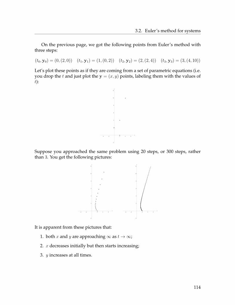
3.2. Euler’s method for systems
On the previous page, we got the following points from Euler’s method withthree steps:
(t0,y0) = (0, (2, 0)) (t1,y1) = (1, (0, 2)) (t2,y2) = (2, (2, 4)) (t3,y3) = (3, (4, 10))
Let’s plot these points as if they are coming from a set of parametric equations (i.e.you drop the t and just plot the y = (x, y) points, labeling them with the values oft):
-4 -2 2 4 6x
-2
2
4
6
8
10
12y
Suppose you approached the same problem using 20 steps, or 300 steps, ratherthan 3. You get the following pictures:
-4 -2 2 4 6x
-2
2
4
6
8
10
12y
-4 -2 2 4 6x
-2
2
4
6
8
10
12y
It is apparent from these pictures that:
1. both x and y are approaching∞ as t→∞;
2. x decreases initially but then starts increasing;
3. y increases at all times.
114

3.2. Euler’s method for systems
Euler’s method for systems on Mathematica
As with Euler’s method for single equations, we don’t usually do Euler’s methodfor systems by hand. The Mathematica notebook eulermethodsystems.nb (avail-able on my web page) has the requisite code for implementing Euler’s method forsystems of 2 or 3 ODEs. Details of the commands are in this file (as with singleequations, you need to run commands once to create modules called “euler2D”and “euler3D” when you start Mathematica), but the Euler’s method command forsystems of 2 ODEs is this:
euler2D[y-x, x+y, t, 1, 7, x, 3, y, -1, 100]
For systems of 3 ODEs, run something like this:
euler3D[y, x t-2, 3x y^2 z, t, 1, 7, x, 3, y, -1, z, 2, 300]
The file eulermethodsystems.nb also contains commands to produce plots com-ing from Euler’s method.
115

3.3. Existence and uniqueness of solutions
3.3 Existence and uniqueness of solutionsRecall from Chapter 1: An IVP
y′ = φ(t, y)y0 = y(t0)
is guaranteed to have a unique solution y = f(t) in some interval containing t0 ifthe functions φ and ∂φ
∂yare both continuous in some rectangle containing (t0, y0).
The proof of this statement comes from converting the IVP into an integralequation
f(t) =∫ t
0φ(s, f(s)) ds
and then solving this using Picard approximations: let f0 be any function satisfyingthe initial condition and define
fj+1(t) =∫ t
0φ(s, fj(s)) ds
for each j; the functions fj converge to a solution f as t→∞.
Picard’s method for systems
All the material above translates directly to systems of ODEs. Consider the IVPy′ = Φ(t,y)y0 = y(t0)
This can be converted into a system of integral equations by assuming y = f(t):f1(t) =
∫ t0 φ1(s, f(s)) ds
......
fd(t) =∫ t
0 φd(s, f(s)) ds
Choose any d functions satisfying the initial conditions; put them into a vectorand call them f0 = (f0,1, f0,2, ..., f0,d). Then, the Picard approximations are givenrecursively by defining
fj+1 = (fj+1,1, fj+1,2, ..., fj+1,d)
in terms of fj as follows: fj+1,1(t) =
∫ t0 φ1(s, fj(s)) ds
fj+1,2(t) =∫ t
0 φ2(s, fj(s)) ds...
...fj+1,d(t) =
∫ t0 φd(s, fj(s)) ds
116

3.4. Matrices and matrix operations
Under certain reasonable hypotheses, you can show that each fj,k convergesas j → ∞ to a function fk. The limit f = (f1, f2, ..., fd) is a solution to the system,and this f is the only solution of the system. We won’t actually do this procedure inthis class, but you should be aware of the conclusion of all this due to its theoreticalimportance. That conclusion is:
Theorem 3.2 (Existence/uniqueness for first-order systems) Suppose that Φ =(φ1, φ2, ..., φd) is a function from Rd+1 to Rd such that for all i and j, both φj and ∂φj
∂yi
are continuous in some rectangular box in Rd+1 containing (t0,y0). Then for someinterval I of values of t containing t0, the system of initial value problems
y′ = Φ(t,y)y0 = y(t0)
has one and only one solution, which is of the form y = f(t) = (f1(t), f2(t), ..., fd(t))for functions f1, ..., fd : R→ R.
3.4 Matrices and matrix operationsIn linear algebra, you consider linear systems of numerical equations. These
look like 2x− y + 4z = 4x+ 3y − 2z = −25x− 2y + z = 0
(with maybe a different number of variables and/or equations).
To study these systems, you rely heavily on the theory of matrices and lineartransformations. The same theory works to describe linear systems of ODEs, so weneed to cover some linear algebra machinery here.
117

3.4. Matrices and matrix operations
Definition 3.3 Given positive integers m and n, an m × n matrix is an array ofnumbers (or functions) aij where 1 ≤ i ≤ m and 1 ≤ j ≤ n. We arrange the entriesof the matrix in a rectangle as follows:
A =
a11 a12 a13 · · · a1na21 a22 a23 · · · a2n
a31 a32. . . ...
...... . . . ...
am1 am2 · · · · · · amn
The set of m × n matrices with entries in R is denoted Mmn(R). The set of m × nmatrices with entries that are functions of some variable t is denoted Mmn(C∞). Twomatrices are equal if they are the same size and if all their entries coincide, i.e. A = Bif they are both m× n and if aij = bij for all i, j.
In particular, aij is the entry of A in the ith row and jth column. m is the number ofrows of A; n is the number of columns of A.
In Math 330, for the most part we only care about matrices which have the samenumber of rows as columns:
Definition 3.4 A matrix is called square if it has the same number of rows as columns.The set of square n × n matrices with entries in R is denoted Mn(R) (as opposed toMnn(R)).
Example:
A =(
1 6−4 5
)is square B =
(1 5 7
)is not square
Definition 3.5 Given a matrixA, the diagonal entries ofA are the numbers a11, a22,a33, ...ann. A matrix A is called diagonal if it is square and all of its nondiagonal en-tries are zero.
Example:
A =
2 0 0 00 −1 0 00 0 0 00 0 0 4
is diagonal; the diagonal entries are 2, −1, 0 and 4
118

3.4. Matrices and matrix operations
Definition 3.6 A square matrix is called upper triangular (abbreviated upper ∆)if all its entries below its diagonal are zero. A matrix is called lower triangular(abbreviated lower ∆) if all the entries above its diagonal are zero. A matrix is calledtriangular if it is either lower triangular or upper triangular.
Example:
A =(
2 30 −4
)B =
−7 0 03 −2 01 −3 4
Note: diagonal matrices are both upper and lower triangular.
Definition 3.7 The trace of a matrix, denoted tr(A), is the sum of the diagonal en-tries of A.
Example:
A =
7et cos t 4t1 −2t2 sin 3t0 −t −e−t
tr(A) = 7et − 2t2 − e−t.
Definition 3.8 The n × n identity matrix, denoted I or In, is the diagonal n × nmatrix with all diagonal entries equal to 1.
I =
1 0 0 · · · 00 1 0 · · · 00 0 1 ......
... . . . 00 0 · · · 0 1
=
11
1. . .
1
In general, a blank entry in a matrix means that entry is zero.
119

3.4. Matrices and matrix operations
Example: For the matrix
A =
1 2 30 −5 −60 0 4
1. Give the size of the matrix.
2. Write down the (3, 2)−entry of the matrix.
3. Write down the diagonal entries of the matrix.
4. What is the trace of the matrix?
5. Is the matrix diagonal? upper triangular? lower triangular?
Addition, scalar multiplication and differentiation of matrices
You can add two matrices of the same size and multiply a matrix by a real number,by performing these operations entry-by-entry.
Note: You can only add two matrices of the same size.
Example: Let
A =(
2 −1 −33 0 −2
)B =
(0 2 23 1 −1
)C =
(2 0−1 −5
)
120
3.4. Matrices and matrix operations
You also differentiate matrices (whose entries are functions) term-by-term:
Definition 3.9 Given A ∈Mmn(C∞), we define the derivative of A, denoted
dA
dt= d
dt(A) = A′(t) = A = A′,
to be the m× n matrix obtained from A by differentiating its entries term-by-term.
Example: A =(
et cos t4e2t sin t
)
Example: y = y(t) =(y1y2
)=(y1(t)y2(t)
)
Matrix multiplication
There is another operation one can perform on matrices. The importance of thisoperation will be seen later; for now we simply define it.
Definition 3.10 Given matrices A ∈ Mmn(F ) and B ∈ Mpq(F ), if n = p then wecan define the productAB, which is anm×q matrixAB defined entrywise by setting
(ab)ij =n(=p)∑k=1
aikbkj = ai1b1j + ai2b2j + ...+ ainbnj.
(If n 6= p, AB is undefined.)
Note:
• If A is a square matrix, we write A2 for AA, A3 for AAA, etc.
• If A isn’t square, then A2 is undefined.
• In general matrix multiplication is not commutative: AB 6= BA most of thetime, even if both products are defined.
121

3.4. Matrices and matrix operations
Example: Let
A =(
1 −1 02 1 −3
); B =
(−2 11 3
); C =
5 −11 20 1
; v =(xy
).
Compute each of the following quantities, or state that they are undefined (withjustification).
(a) AB
(b) BA
(c) A2
(d) B2
(e) Bv
122

3.4. Matrices and matrix operations
Theorem 3.11 (Properties of elementary matrix operations) LetA,B,C be ma-trices, let I be the identity matrix of the appropriate size and let k ∈ R. Then,so long as everything is defined, we have:
1. IA = A and BI = B;
2. A(BC) = (AB)C;
3. k(AB) = (kA)B = A(kB);
4. A(B + C) = AB + AC and (A+B)C = AC +BC.
A useful fact we will need later is the following:
Theorem 3.12 (Powers of a diagonal matrix) If A ∈Mn(R) is a diagonal matrix,then Ar is also diagonal for each r, and the (j, j)−entry of Ar is (aj,j)r.
Example: Let A =
−2 0 00 3 00 0 −1
.
Then A2 =
(−2)2 0 00 32 00 0 (−1)2
=
4 0 00 9 00 0 1
.
WARNING: Computing the powers of a non-diagonal matrix is much harder(see the example of B2 on the previous page).
123

3.4. Matrices and matrix operations
Reasons that matrix multiplication is defined the way that it is (and why vec-tors are thought of as columns rather than rows): Consider this system of threeequations in three variables:
4x− 2y + z = 78x+ 3y + 7z = 12x+ y − 4z = −4
More generally, given any system of d numerical equations in d variables, youcan write down an d× d matrix A, a d× 1 matrix b, so that the equation, in matrixmultiplication language, is
Ax = b
(the goal being to solve for x = (x1, x2, ..., xd) =
x1x2...xd
).
Recall from Chapter 1: a function T : V → V is a linear operator if T (v + w) =T (v) + T (w) and T (rv) = rT (v) for all v,w ∈ V , all r ∈ R.
Another reason for the definition of matrix multiplication is that every linearoperator on Rd is multiplication by a d× d square matrix:
124

3.4. Matrices and matrix operations
Theorem 3.13 (Characterization of linear operators on Rd) For any matrixA ∈Md(R), the function T : Rd → Rd described by
T (v) = Av
is a linear operator on Rd.Conversely, given any linear operator T : Rd → Rd, there is a matrix A ∈ Md(R)
such thatT (v) = Av
for all v ∈ Rd.
PROOF To show that every function of the form T (x) = Ax is linear is pretty easy:
T (v + w) = A(v + w) = Av + Aw = T (v) + T (w)⇒ T preserves addition;
T (rv) = A(rv) = rAv = rT (v)⇒ T preserves scalar multiplication.
Since T preserves addition and scalar multiplication, it is linear.Conversely, to show that every linear operator on Rd is matrix multiplication is
given by matrix multiplication is harder. See Theorem 5.5 of my Math 322 lecturenotes.
Recall that a “linear” equation is one of the form T (x) = b where T is a linearoperator. In light of the previous theorem, we now know:
Theorem 3.14 (Characterization of linear numerical systems) Every linear sys-tem of d numerical equations in d variables is of the form
Ax = b
where A is an d× d matrix and b is a vector in Rd.
How would you solve such a system?
125

3.4. Matrices and matrix operations
Inverses and determinants
We know what it means to add, subtract, and/or multiply two matrices. Whatdoes it mean to divide one matrix by another?
For real numbers, two things are true about division:
1.
2.
So to define “division” of matrices, we really only need to define the “reciprocal”of a matrix. However, with matrices we use the word “inverse” rather than “recip-rocal”:
Definition 3.15 A matrix A ∈Mn(R) is called invertible if there is another matrixA−1 ∈Mn(R) and called an inverse (matrix) of A, such that
AA−1 = I and A−1A = I.
Remark: Non-square matrices are never invertible.
Theorem 3.16 (Properties of inverses) Let A,B ∈Mn(R) be invertible. Then
1. A has only one inverse.
2. (A−1)−1 = A.
3. (AB)−1 = B−1A−1.
In linear algebra, you learn a lot about inverses (including how to computethem in general). In Math 330, you need to memorize these two formulas for in-verses of 1× 1 and 2× 2 matrices:
Theorem 3.17 (1 × 1 inverses) Let A = (a). Then A is invertible if and only ifa 6= 0, in which case
A−1 =(1a
).
PROOF AA−1 = (a)(
1a
)= (1) = I and A−1A =
(1a
)(a) = (1) = I .
126

3.4. Matrices and matrix operations
Theorem 3.18 (2 × 2 inverses) Let A =(a bc d
). Then A is invertible if and
only if ad− bc 6= 0, in which case
A−1 = 1ad− bc
(d −b−c a
)=(
dad−bc
−bad−bc
−cad−bc
aad−bc
).
PROOF If you actually matrix multiply A and A−1 in either order, you will get I .Details are in Theorem 5.32 of my linear algebra notes.
Example: Find A−1 if A =(
3 7−2 1
).
To compute the inverse of a 3 × 3 or larger (square) matrix, use a computer(there is a way to do it by hand that you learn in linear algebra, but you don’t needthat in Math 330). See the next section for the appropriate Mathematica commands.
We saw above that in order for a 1× 1 or 2× 2 matrix to be invertible, there is aformula in terms of its entries that has to be nonzero:
what has to be nonzeroSize of matrix Matrix for A to be invertible
1× 1 A = (a) a
2× 2 A =(a bc d
)ad− bc
3× 3 A =
a b cd e fg h i
?
n× n ?
In linear algebra, you learn that for any square matrix A, there is a magic num-ber, defined as a formula of the terms of the entries of that matrix. This magicnumber is called the determinant of A, is denoted detA or det(A), and tells youwhether or not A is invertible:
Theorem 3.19 A square matrix is A is invertible if and only if detA 6= 0.
127
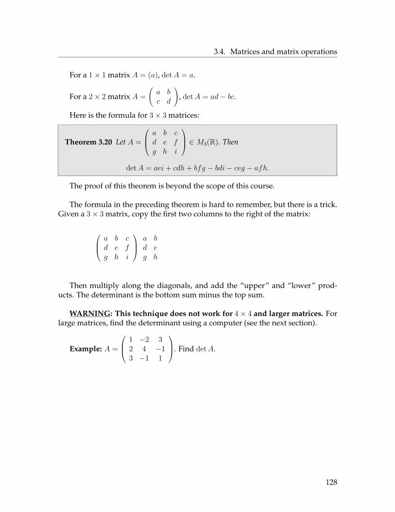
3.4. Matrices and matrix operations
For a 1× 1 matrix A = (a), detA = a.
For a 2× 2 matrix A =(a bc d
), detA = ad− bc.
Here is the formula for 3× 3 matrices:
Theorem 3.20 Let A =
a b cd e fg h i
∈M3(R). Then
detA = aei+ cdh+ bfg − bdi− ceg − afh.
The proof of this theorem is beyond the scope of this course.
The formula in the preceding theorem is hard to remember, but there is a trick.Given a 3× 3 matrix, copy the first two columns to the right of the matrix:
a b cd e fg h i
a bd eg h
Then multiply along the diagonals, and add the “upper” and “lower” prod-ucts. The determinant is the bottom sum minus the top sum.
WARNING: This technique does not work for 4× 4 and larger matrices. Forlarge matrices, find the determinant using a computer (see the next section).
Example: A =
1 −2 32 4 −13 −1 1
. Find detA.
128

3.5. Matrix operations on Mathematica
A major reason why we care about determinants in Math 330 is that an ap-propriate determinant tells us whether or not a system of linear equations has aunique solution:
Theorem 3.21 The system of d linear, numerical equations in d variables
Ax = b ⇔
a11x1 + a12x2 + ...+ a1dxd = b1a21x1 + a22x2 + ...+ a2dxd = b2
......
...ad1x1 + ad2x2 + ...+ addxd = bd
has a unique solution if and only if detA 6= 0, in which case the unique solution isx = A−1b.
PROOF If detA 6= 0, then A is invertible, i.e. A−1 exists. Start with the matrixequation
Ax = b⇔ A−1Ax = A−1b⇔ Ix = A−1b⇔ x = A−1b.
3.5 Matrix operations on MathematicaDefining a matrix: To store a matrix whose entries are numbers as a variable, there
are two methods.
1. Type in the matrix (carefully) using braces to separate the entries. Forexample, to save the matrix (
2 4 7−5 3 1
)
as A, executeA = 2,4,7, -5,3,1Note that the entries are separated by commas, every row of the matrixneeds braces around it, and the entire matrix needs braces around it.
129

3.5. Matrix operations on Mathematica
To type in a column vector, you need only one set of braces, so if you
execute b = 1,2,3 this defines the column vector
123
.
2. Use the Basic Math Assistant Pallette. Click “Pallettes” and “Basic MathAssistant”, then on the Basic Math Assistant click the fourth tab under“Basic Commands” that looks like a matrix. In the Mathematica note-book, type A=, then click the large button that looks like a matrix, thenclick “AddRow” or “AddColumn” until the matrix is the appropriatesize. Click in each box of the matrix and type in the appropriate num-bers. For example, your command to define theA above would look like
A =(
2 4 7-5 3 1
)
To define a matrix whose entries are functions, you must define the matrix asa function: type A[t_] = , then type the matrix and execute. For example:
A[t_] = Cos[t], Sin[t], E^t, E^(-t)
defines the matrix A = A(t) =(
cos t sin tet e−t
). To call this matrix later, type
A[t] (no underscore).
Matrix multiplication: To multiply two matrices in Mathematica, you need a pe-riod between the matrices. For example, after defining matrices A and B,you can compute the matrix product by
A.B
The output you will get won’t look like a matrix; to make it look like a matrixyou can type
A.B //MatrixForm
For matrix powers, you will need to type A.A rather than A^2 (the commandA^2 just squares each entry of A). For a larger matrix power (say A100), runthe following: MatrixPower[A,100] //MatrixForm
Other matrix operations: Once you have saved a matrix as a letter or string, youcan perform standard operations on it as follows (add //MatrixForm to theend of the command to make the output look like a matrix):
1. For the trace of A, execute Tr[A].
2. To multiply A by a scalar (say 5), execute 5 A.
3. To add two matrices (say A and B), execute A + B.
130

3.6. First-order linear systems of ODEs
4. To get the i, j entry of a matrix, use double braces: execute A[[2,3]] (toget the 2, 3−entry).
5. To call the n×n identity matrix, use a command like IdentityMatrix[4](this generates the 4× 4 identity matrix).
6. For the inverse of a matrix, type Inverse[A].
7. For the determinant of a matrix, type Det[A].
8. To take the derivative of a matrix of functions, execute A’[t].
3.6 First-order linear systems of ODEsWe can adapt our definition of “linear” from Chapter 1 from this setting. Recall
that an ODE is called linear if there are functions p0, p1, ..., pn (with pn 6= 0) and qsuch that the equation has the form
Let’s generalize this to systems. The key idea is that instead of multiplying eachderivative of y by a single function (like p0, p1 or pn), we have to multiply a vectorof functions (like y′ = (y′1, y′2, ..., y′d)) by an object that will produce another vectorof functions. The most general object that does this is a
This means we can describe linear systems of ODEs as follows:
Definition 3.22 An nth order, linear d× d system of ODEs is any equation of theform
Any(n) + An−1y(n−1) + ...+ A1y′ + A0y = q
where An, An−1, ..., A1, A0 ∈ Md(C∞) are n d × d matrices of functions with Aninvertible for all t, where q = q(t) = (q1, q2, ..., qd) is a list of d functions of t, andwhere y = (y1, ..., yd) is a list of d functions of t (the goal is to find y).
If all the entries of theAj are constants, we say the system is constant-coefficient.If every entry of q is 0 (i.e. q = 0), we say the system is homogeneous.
131

3.6. First-order linear systems of ODEs
Example: t3x′ + (sin t)y′ +3x− ety = cos 2t
5tx′ − 2y′ +4t2x = e−t
Example:4x′′ − 3y′′ + z′′ +2x′ + 3y′ − 8z′ −x+ y − 3z = 0−2x′′ + 5y′′ − z′′ −3x′ + 7y′ +y − 4z = 0
x′′ −6y′ +3x− y − 2z = 0
132

3.7. The structure of the solution set of a linear system
3.7 The structure of the solution set of a linear systemDefinition 3.23 Given the d× d linear system
Any(n) + An−1y(n−1) + ...+ A1y′ + A0y = q,
the corresponding homogeneous system is the system
Any(n) + An−1y(n−1) + ...+ A1y′ + A0y = 0.
Theorem 3.24 Suppose y and y are two solutions of the d× d linear system
Any(n) + An−1y(n−1) + ...+ A1y′ + A0y = q.
Then y− y is a solution of the corresponding homogeneous system
Any(n) + An−1y(n−1) + ...+ A1y′ + A0y = 0.
(Compare this result with Theorem 2.10.)
PROOF This is a direct calculation:
An(y− y)(n) + An−1(y− y)(n−1) + ...+ A1(y− y)′ + A0(y− y)=[Any(n) + An−1y(n−1) + ...+ A1y′ + A0y
]−[Any(n) + An−1y(n−1) + ...+ A1y′ + A0y
]= q − q= 0.
Consequence: if yp is any one solution of the d× d system, then for any solution yof the system, we have
133

3.7. The structure of the solution set of a linear system
Example: Suppose some 2× 2 system of (non-homogeneous) equations has thefollowing solution of its corresponding homogeneous system:
yh(t) = C1et
(12
)+ C2e
4t sin t(
13
)
=(
C1et + C2e
4t sin t2C1e
t + 3C2e4t sin t
)
i.e.xh(t) = C1e
t + C2e4t sin t
yh(t) = 2C1et + 3C2e
4t sin t .
If one particular solution of the system is
yp(t) =(
sin 2t3 cos 2t
)i.e.
xp(t) = sin 2typ(t) = 3 cos 2t ,
describe all solutions of the system.
The solution set of the homogeneous equation
Recall from Chapter 2 the idea of a subspace:
Definition 3.25 Let V be a vector space and let W ⊆ V . We say W is a subspace(of V ) if
1. W is closed under addition, i.e. for any two vectors w1 and w2 inW , w1 +w2 ∈W ; and
2. W is closed under scalar multiplication, i.e. for any vector w ∈ W and anyscalar r, rw ∈ W .
134

3.7. The structure of the solution set of a linear system
In Chapter 2, we showed that the solution to any first-order linear, homoge-neous ODE is a subspace of C∞(R), spanned by a single nonzero solution:
Definition 3.26 Let V be a vector space and let v ∈ V be a vector. The span of v,denoted Span(v), is the set of linear multiples of v:
Span(v) = cv : c ∈ R
If W ⊆ V is such that W = Span(v), we say W is spanned by v.
We now show the analogous property for first-order linear, homogeneous sys-tems. (The difference is that the solution will be a subspace spanned by d solu-tions.) First, a definition:
Definition 3.27 Let V be a vector space and let v1,v2, ...,vd ∈ V be vectors. Thespan of v1, ...,vd, denoted Span(v1, ...,vd), is the set of linear combinations of the vj :
Span(v1, ...,vd) =
d∑j=1
cjvj : cj ∈ R
= c1v1 + ...+ cdvd : cj ∈ R
If W ⊆ V is such that W = Span(v1, ...,vd), we say W is spanned by v1, ...,vd.
In Math 330, we care about spans where the vectors are functions:
Example 1: V = C∞(R); f1(t) = sin t; f2(t) = cos t.
Example 2: V = C∞(R); f1(t) = t2; f2(t) = 3t2.
Example 3: V = C∞(R); f1(t) = sin2 t; f2(t) = cos2 t; f3(t) = 1.
135

3.7. The structure of the solution set of a linear system
Example 4: V = (C∞(R))2 (i.e. V is the set of ordered pairs of differentiablefunctions);
f1(t) =(
2 sin tsin t+ cos t
); f2(t) =
(2 sin t− cos t
cos t
)
Notice that in Examples 2 and 3, you could drop one of the functions f1, f2, f3without changing the span. This is essentially because
Question: Under what circumstances can you do this in general? In otherwords, given a list of d functions f1, ..., fd, is there an identity relating the func-tions?
136
3.7. The structure of the solution set of a linear system
Definition 3.28 Given vectors v1, ...vd in vector space V , we say the set of vectors islinearly independent if the only constants c1, ..., cd which make
c1v1 + c2v2 + ...+ cdvd = 0
are c1 = c2 = ... = cd = 0.We say the set of vectors is linearly dependent if there are constants c1, ..., cd,
not all zero, which make
c1v1 + c2v2 + ...+ cdvd = 0.
In linear algebra, you learn a lot about what makes vectors linearly indepen-dent or linearly dependent in general. Among other things, you learn:
Theorem 3.29 Given a list of vectors v1, ...vd in vector space V :
1. If the vectors are linearly independent, then you cannot remove any of the vectorsfrom the list without changing the span of the list.
2. If the vectors are linearly dependent, then there is at least one vector which canbe removed from the list without changing the span.
So in some sense, a list of linearly independent vectors is a “minimal” list ofvectors which span a particular subspace. With that in mind, we make the follow-ing definition:
Definition 3.30 If W is a subspace of V spanned by d linearly independent vectors,then we say W is a subspace of dimension d, and we write dimW = dim(W ) = d.In this situation, any collection of d linearly independent vectors in d is called a basisof W .
A reasonable question is to ask whether a vector space or subspace can be oftwo different dimensions: more precisely, can a space W be spanned by 3 linearlyindependent vectors, and also be spanned by 4 linearly independent vectors? Lin-ear algebra theory tells us that the answer is NO:
Theorem 3.31 If V is a vector space or subspace with dim V = d, then
1. Any collection of d linearly independent vectors must also span V , and hence bea basis of V .
2. Any collection of d vectors which span V must also be linearly independent,hence must be a basis of V .
137

3.7. The structure of the solution set of a linear system
So if v1, ...,vd are linearly independent vectors in a d-dimensional subspace W ,then
W = Span(v1, ...,vd) = C1v1 + ...+ Cdvd : Cj ∈ R for all j.
The Wronskian
In Math 330, we only care about whether a set of functions (as opposed to a set ofmore general vectors) is linearly independent or not, and there is an easy test forthat:
Definition 3.32 Given d functions f1, ..., fd ∈ C∞(R), the Wronskian of the func-tions is the function
W = W (t) = W (f1, ..., fd)(t) = det
f1(t) f2(t) · · · fd(t)f ′1(t) f ′2(t) · · · f ′d(t)f ′′1 (t) f ′′2 (t) · · · f ′′d (t)
...... . . . ...
f(d−1)1 (t) f
(d−1)2 (t) · · · f
(d−1)d (t)
.
Given d elements of (C∞(R))d, namely f1 = (f11, f12, ..., f1d), f2 = (f21, ..., fd2), ...,fd = (fd1, ..., fdd), the Wronskian of these functions is the function
W = W (t) = W (f1, ..., fd)(t) = det
f11(t) f21(t) · · · fd1(t)f12(t) f22(t) · · · fd2(t)f13(t) f23(t) · · · fd3(t)
...... . . . ...
f1d(t) f2d(t) · · · fdd(t)
.
Example: Find the Wronskian of f1(t) = sin t and f2(t) = cos t.
138

3.7. The structure of the solution set of a linear system
Example: Find the Wronskian of f1(t) = sin2 t, f2(t) = cos2 t and f3(t) = 1.
Example: Find the Wronskian of f1(t) = (et, e2t) and f2(t) = (2et, 4e2t + et).
Example: Find the Wronskian of f1(t) = (2 sin t, cos t) and f2(t) = (4 sin t, 2 cos t).
The importance of the Wronskian is seen in the following theorem:
139

3.7. The structure of the solution set of a linear system
Theorem 3.33 Given functions f1, ..., fd ∈ C∞(R), if the Wronskian of the functionsW (f1, ..., fd)(t) 6= 0 for at least one value of t, the functions are linearly independent.
Given functions f1, ..., fd ∈ (C∞(R))d, the Wronskian W (f1, ..., fd)(t) 6= 0 for atleast one value of t, then f1, ..., fd are linearly independent.
PROOF Suppose that there are constants c1, ..., cd such that
c1f1(t) + c2f2(t) + ...+ cdfd(t) = 0.
Repeatedly differentiating both sides of this equation, we obtain the system
c1f1(t) + c2f2(t) + ...+ cdfd(t) = 0c1f′1(t) + c2f
′2(t) + ...+ cdf
′d(t) = 0
c1f′′1 (t) + c2f
′′2 (t) + ...+ cdf
′′d (t) = 0
...c1f
(d)1 (t) + c2f
(d)2 (t) + ...+ cdf
(d)d (t) = 0
This system of linear equations has at least one solution: (c1, c2..., cd) = (0, 0, ..., 0).By Theorem 3.21, this is the only solution (i.e. the functions are linearly indepen-dent) if W (t) 6= 0. This proves the first statement; the second statement has asimilar proof.
Theorem 3.34 Given any linear, homogeneous d× d system of ODEs
Any(n) + An−1y(n−1) + ...+ A1y′ + A0y = 0,
the set of solutions of this ODE is a subspace of (C∞(R))d.
PROOF First, we show the solution set is closed under addition. Let y and y besolutions. Then, plugging y + y into the system, we get
An(y + y)(n) + An−1(y + y)(n−1) + ...+ A1(y + y)′ + A0(y + y)=[Any(n) + An−1y(n−1) + ...+ A1y′ + A0y
]+[Any(n) + An−1y(n−1) + ...+ A1y′ + A0y
]= 0 + 0= 0.
Therefore the solution set is closed under addition.
140

3.7. The structure of the solution set of a linear system
Next, we show the solution set is closed under scalar multiplication: let y be asolution and let r ∈ R. Then, by plugging in ry to the system, we get
An(ry)(n) + An−1(ry)(n−1) + ...+ A1(ry)′ + A0(ry)= r
[Any(n) + An−1y(n−1) + ...+ A1y′ + A0y
]= r0= 0.
Therefore the solution set is closed under scalar multiplication, so it is a subspace.
Knowing that the solution set of the homogeneous is a subspace, it is natural toask what its dimension is:
Theorem 3.35 Given any linear, first-order, homogeneous d× d system of ODEs
A1y′ + A0y = 0,
the set of solutions of this system is a d-dimensional subspace of (C∞(R))d.
PROOF Let
e1 =
100...0
, e2 =
010...0
, ..., ed =
00...01
.
For j ∈ 1, ..., d, let y[j] be the unique solution of the system satisfying the initialvalue y[j](0) = ej .
Claim 1: y[1],y[2], ...,y[d] are linearly independent.Proof of Claim 1:
W (y[1],y[2], ...,y[d])(0) = det
y
[1]1 (0) y
[2]1 (0) · · · y
[d]1 (0)
y[1]2 (0) y
[2]2 (0) · · · y
[d]2 (0)
...... . . . ...
y[1]d (0) y
[2]d (0) · · · y
[d]d (0)
= det
1 0 0 · · · 00 1 0 · · · 00 0 1 · · · 0...
...... . . . ...
0 0 0 0 1
= 1.
141

3.7. The structure of the solution set of a linear system
Since the Wronskian is nonzero at t = 0, it is everywhere nonzero, so the solutionsy[1],y[2], ...,y[d] are linearly independent, proving the claim.
Claim 2: y[1],y[2], ...,y[d] span the solution set.Proof of Claim 2: Let y be any solution of the system. To prove the claim, it is
sufficient to prove that there are constants c1, ..., cd so that
c1y[1] + c2y[2] + ...+ cdy[d] = y.
Writing this coordinate-wise, this means we need to solve the system
(∗)
c1y
[1]1 + c2y
[2]1 + ...+ cdy
[d]1 = y1
c1y[1]2 + c2y
[2]2 + ...+ cdy
[d]2 = y2
...c1y
[1]d + c2y
[2]d + ...+ cdy
[d]d = yd
for c1, ..., cd. But since the Wronskian W (y[1],y[2], ...,y[d]) is everywhere nonzero,by Theorem 3.21 we see that the system (∗) can always be solved. This proves theclaim.
Since we have a set of d functions (namely y[1],y[2], ...,y[d]) which are linearlyindependent and span the solution set, by Definition 3.30 the dimension of thesolution set is d, and the set y[1],y[2], ...,y[d] is a basis of the solution set.
142

3.7. The structure of the solution set of a linear system
Putting this all together
Solution of first-order linear, homogeneous systems
Given the d× d linear, first-order homogeneous system
A1y′ + A0y = 0,
the solution set is a d-dimensional subspace. Therefore for any d linearlyindependent solutions y1,y2, ...,yd of the system, the general solution ofthe homogeneous equation is
y = yh = C1y1 + C2y2 + ...+ Cdyd
where C1, C2, ..., Cd are arbitrary constants.
(To verify that the functions y1,y2, ...,yd are linearly independent, computetheir Wronskian and show that the Wronskian is nonzero for at least onevalue of t.)
Solution of general linear systems
Given the d× d linear nth-order system
Any(n) + An−1y(n−1) + ...+ A1y′ + A0y = q,
the general solution is any one particular solution yp plus the solution ofthe corresponding homogeneous system, i.e. the general solution is
y = yp + yh
If the equation is first-order, this means the general solution has the form
y = yp + C1y1 + C2y2 + ...+ Cdyd
where C1, C2, ..., Cd are arbitrary constants and y1,y2, ...,yd are linearly in-dependent solutions of the corresponding homogeneous system.
143
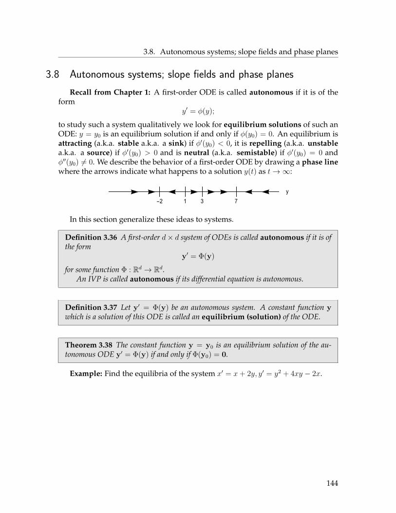
3.8. Autonomous systems; slope fields and phase planes
3.8 Autonomous systems; slope fields and phase planesRecall from Chapter 1: A first-order ODE is called autonomous if it is of the
formy′ = φ(y);
to study such a system qualitatively we look for equilibrium solutions of such anODE: y = y0 is an equilibrium solution if and only if φ(y0) = 0. An equilibrium isattracting (a.k.a. stable a.k.a. a sink) if φ′(y0) < 0, it is repelling (a.k.a. unstablea.k.a. a source) if φ′(y0) > 0 and is neutral (a.k.a. semistable) if φ′(y0) = 0 andφ′′(y0) 6= 0. We describe the behavior of a first-order ODE by drawing a phase linewhere the arrows indicate what happens to a solution y(t) as t→∞:
-2 1 3 7
y
In this section generalize these ideas to systems.
Definition 3.36 A first-order d× d system of ODEs is called autonomous if it is ofthe form
y′ = Φ(y)
for some function Φ : Rd → Rd.An IVP is called autonomous if its differential equation is autonomous.
Definition 3.37 Let y′ = Φ(y) be an autonomous system. A constant function ywhich is a solution of this ODE is called an equilibrium (solution) of the ODE.
Theorem 3.38 The constant function y = y0 is an equilibrium solution of the au-tonomous ODE y′ = Φ(y) if and only if Φ(y0) = 0.
Example: Find the equilibria of the system x′ = x+ 2y, y′ = y2 + 4xy − 2x.
144

3.8. Autonomous systems; slope fields and phase planes
Example: Find the equilibria of the system y′ = (xy + x2, x− 2y + 1).
Slope fields for autonomous 2× 2 systems
Recall that for a first-order ODE y′ = φ(t, y), we drew pictures called slope fieldswhich describe, at each point (t, y), a “mini-tangent” of slope φ(t, y).
Now, let’s consider a first-order 2× 2 system:
y′ = Φ(t,y) ⇔x′ = φ1(t, x, y)y′ = φ2(t, x, y)
In order to draw a slope field that incorporates the t, you would need a 3-dimensional picture (because you need a dimension for each variable t, x and y).You can do this theoretically, but such a picture is usually really hard to read (be-cause you can’t interpret the perspective). Here is an example:
145

3.8. Autonomous systems; slope fields and phase planes
However, if the system is autonomous:
y′ = Φ(y) ⇔x′ = dx
dt= φ1(x, y)
y′ = dydt
= φ2(x, y)
then you don’t have to account for the t. You can draw a picture which includes“mini-tangents” at each point (x, y). The slope of the mini-tangent at (x, y) is
dy
dx=
dydtdxdt
= φ2(x, y)φ1(x, y) .
Example:x′ = −2yy′ = x
x 0 0 1 1 2 2 −1 −1 −1y 1 2 1 −1 1 2 1 −1 0
(x, y) (0, 1) (0, 2) (1, 1) (1,−1) (2, 1) (2, 2) (−1, 1) (−1,−1) (−1,−3)dxdt = φ1(x, y) −2 −4 −2 2 −2 −4 −2 2 0dydt = φ2(x, y) 0 0 1 1 2 2 −1 −1 −1
dydx 0 0 − 1
212 −1 − 1
212 − 1
2 DNE
-3 -2 -1 1 2 3
-3
-2
-1
1
2
3
Here is a computer-generated picture of the slope field of the system;
-3 -2 -1 0 1 2 3
-3
-2
-1
0
1
2
3
146

3.8. Autonomous systems; slope fields and phase planes
As with single equations, the graph of a set of parametric equations which com-prise a solution of the system must “flow with” the slope field. In this case, itappears that the solutions are ellipses centered at the origin:
-3 -2 -1 0 1 2 3
-3
-2
-1
0
1
2
3
-3 -2 -1 0 1 2 3
-3
-2
-1
0
1
2
3
We can verify that the solutions are ellipses by actually solving the system; we’lllearn how to do this in the forthcoming sections.
Phase plane analysis
If you take a slope field (as described above), and you sketch many solution curveson that slope field, you obtain a picture called a phase plane for the system. Often,you “erase” the mini-tangents from this picture and draw only the solution curves.Here is the phase plane for the above example (x′ = −2y, y′ = −x):
-3 -2 -1 0 1 2 3
-3
-2
-1
0
1
2
3
Phase planes are the analogue of phase lines for autonomous equations: theytell you how the solutions of a system behave as t changes.
147

3.8. Autonomous systems; slope fields and phase planes
Example: Below is the phase plane for some first-order 2× 2 autonomous sys-tem y′ = φ(y):
-2 0 2 4 6
-2
0
2
4
6
1. Consider the solution to this system satisfying x(0) = 1, y(0) = 4.
a) Sketch the graph of this solution on the phase plane.
b) Find limt→∞
x(t) for this solution.
c) Find limt→∞
y(t) for this solution.
d) Find limt→−∞
x(t) for this solution.
2. Consider the solution to this system with initial condition y(0) = (5, 3). Forthis solution, does x increase or decrease as t increases? Does y increase ordecrease as t increases?
3. Find all constant functions which solve the system.
148

3.8. Autonomous systems; slope fields and phase planes
Mathematica commands for slope fields and phase planes forsystems
These commands can be found in the file phaseplanes.nb, available on my web-site.
Code to sketch the slope field
The following code will sketch a slope field and also sketch several solutioncurves (passing through randomly chosen points). Execute all this in a single Math-ematica cell:
phi1[x_,y_] := x - y;phi2[x_,y_] := x + 2y;VectorPlot[phi1[x,y], phi2[x,y], x, -3, 3, y, -3, 3,VectorPoints -> 20, Axes -> True,VectorScale -> Automatic, Automatic, None,VectorStyle -> Orange]
Code to sketch the slope field and several solution curves
The following code will sketch a slope field and also sketch several solutioncurves (passing through randomly chosen points). Execute all this in a single Math-ematica cell:
phi1[x_,y_] := x - y;phi2[x_,y_] := x + 2y;VectorPlot[phi1[x,y], phi2[x,y], x, -3, 3, y, -3, 3,VectorPoints -> 20, Axes -> True,VectorScale -> Automatic, Automatic, None,VectorStyle -> Orange,StreamPoints -> 35,StreamScale -> Full,StreamStyle -> Blue]
The first six lines are the same as the command above; the seventh line directsMathematica to sketch 35 solution curves at random locations on the picture. Thelast line tells Mathematica what color to draw the solution curves.
149

3.8. Autonomous systems; slope fields and phase planes
Code to sketch the slope field and a solution curve passing through a specificpoint
The following code (executed in a single cell) will sketch a slope field and sketcha single solution curve passing through a given point (x0, y0). In this case the initialvalue is (−1, 2):
phi1[x_,y_] := x - y;phi2[x_,y_] := x + 2y;VectorPlot[phi1[x,y], phi2[x,y], x, -3, 3, y, -3, 3,VectorPoints -> 20, Axes -> True,VectorScale -> Automatic, Automatic, None,VectorStyle -> Orange,StreamPoints -> -1,2,StreamScale -> Full,StreamStyle -> Blue]
Code to sketch phase planes (solution curves only; no mini-tangent lines)
phi1[x_,y_] := x - y;phi2[x_,y_] := x + 2y;StreamPlot[phi1[x,y], phi2[x,y], x, -4, 4, y, -4, 4,StreamPoints -> 100,StreamStyle -> Black,StreamScale -> Full]
Code to sketch a single solution curve (no mini-tangent lines)
phi1[x_,y_] := x - y;phi2[x_,y_] := x + 2y;StreamPlot[phi1[x,y], phi2[x,y], x, -4, 4, y, -4, 4,StreamPoints -> -1,2,StreamStyle -> Black,StreamScale -> Full]
150

3.9. First-order, constant-coefficient homogeneous systems
3.9 First-order, constant-coefficient homogeneous systemsPreliminaries
Since we assume A1 is invertible, given any first-order, linear system
A1y′ + A0y = q,
we can multiply through by A−11 , rearrange and redefine terms:
We have proven:
Theorem 3.39 Every first-order, linear d× d system of ODEs can be rewritten as
y′ = Ay + q
for some d × d matrix of functions A and some list of functions q = (q1, ..., qd). Thesystem is homogenous if and only if q = 0, and constant-coefficient if and only if theentries of A are constants.
Example: x′ = 3x− y + sin ty′ = x+ 2y − cos t
Example: x′ = etx+ 2e3ty − e−tzy′ = e3tx− ety + 4e−tzz′ = e−tx+ etz
151

3.9. First-order, constant-coefficient homogeneous systems
Recall from Chapters 1 & 2: the most simple first-order ODE is linear, homo-geneous and constant-coefficient:
Now let’s think about the most simple first-order system.
Since it is linear and first order, it must look like
Since it is homogeneous,
Since it is constant-coefficient,
Theorem 3.40 Every first-order, linear, homogeneous, constant-coefficient of dODEscan be written as
y′ = Ay
where y = y(t) = (y1(t), y2(t), ..., yd(t)) and A is an d × d matrix whose entries arenumbers.
Note that any such system is autonomous, and its only equilibrium is y = 0.
What should the solution of such a system be? In light of the answer for singleequations
y′ = ry ⇒
the solution of y′ = Ay is probably something like
152

3.9. First-order, constant-coefficient homogeneous systems
Matrix exponentials
Question: Given a square matrix A, what is eA = exp(A)? What is eAt = exp(At)?
To answer this question, recall from Calculus II the Taylor series of et:
Lemma 3.41 Let t be a real number. Then
et =∞∑n=0
tn
n! = 1 + t+ t2
2 + t3
3! + t4
4! + ...
(this series converges absolutely for all t).
Notice that the Taylor series formula for et involves only nonnegative integerpowers of t, and addition. These are operations that are well-defined for squarematrices, so we can define the exponential of a square matrix as follows:
Definition 3.42 Let A ∈ Md(R). The (matrix) exponential of A, denoted eA orexp(A), is
eA = exp(A) =∞∑n=0
1n!A
n = I + A+ 12A
2 + 13!A
3 + 14!A
4 + ...
Remarks:• If A is not square, then A2, A3, ... do not exist, so eA does not exist.• If A is d× d, then A2, A3, A4, ... are all d× d so eA is also d× d.• It is not clear that this series converges (or what the word “converges” even
means in this sense). Fact: this series converges for all square matrices A.• You cannot compute matrix exponentials entry-by-entry:
exp(a bc d
)6=(ea eb
ec ed
).
• For any constant t,
exp(tA) = exp(At) =∞∑n=0
1n! (At)
n =∞∑n=0
1n!A
ntn
= I + At+ 12A
2t2 + 13!A
3t3 + ...
• If A = 0, the zero matrix, then eA = I + 0 + 0 + ... = I . So e0 = I .• It is not always the case that
eA+B = eAeB.
This holds only if AB = BA (which as we know is false, in general).
153
3.9. First-order, constant-coefficient homogeneous systems
Theorem 3.43 Let A ∈ Mn(R) be a matrix whose entries are numbers. The onlysolution y = y(t) to the first-order system
y′ = Ayy(0) = y0
isy(t) = eAty0.
PROOF First, let’s check that the equation y′ = Ay is satisfied. Let y(t) = eAty0.
Next, let’s check the initial condition. If y(t) = eAty0, then when t = 0 we have
y(0) = eA0y0 = e0y0 = Iy0 = y0
as desired.
Since both the ODE and initial value are satisfied by y, y is a solution of the sys-tem. By the existence/uniqueness theorem, such a system has only one solution,so y = eAty0 is the only solution.
154
3.9. First-order, constant-coefficient homogeneous systems
Computing matrix exponentials
Example: Consider the first-order systemx′ = x+ 3yy′ = 2x+ 2y
with initial condition x(0) = 1, y(0) = −3. Find the solution of this system.
Theoretical solution:
Problem: How do you compute eAt?
Easier Example: Consider the first-order systemx′ = 7xy′ = −3y
with initial condition x(0) = 1, y(0) = −3. Find the solution of this system.
Theoretical solution 1: WriteA =(
7 00 −3
)and y0 =
(1−3
). Then the solution
is
y(t) =(x(t)y(t)
)= eAty0 = exp
(7t 00 −3t
)(1−3
)
Theoretical solution 2: This system is “uncoupled” (the x and y have nothingto do with one another); from our study of exponential models in Chapter 1, thesolution is
155

3.9. First-order, constant-coefficient homogeneous systems
In fact, what we saw in the previous example is more general:
Theorem 3.44 (Exponentiation of diagonal matrices) If Λ is diagonal with diag-onal entries λ1, λ2, ..., λn, then
exp(Λ) =
eλ1
eλ2
. . .eλn
and exp(Λt) =
eλ1t
eλ2t
. . .eλnt
.
PROOF Let Λ be as in the theorem. It is sufficient to prove the second statement,because by letting t = 1 in the second statement you get the first statement. ByTheorem 3.12, for any k
(Λt)k =
(λ1t)k
(λ2t)k. . .
(λnt)k
so
eΛt =∞∑k=0
1k! (Λt)
k =
∞∑k=0
1k!(λ1t)k
∞∑k=0
1k!(λ2t)k
. . .∞∑k=0
1k!(λnt)
k
=
eλ1t
eλ2t
. . .eλnt
as desired.
Example: If Λ =
1 0 00 0 00 0 −2
, then eΛt =
et 0 00 1 00 0 e−2t
.
Question: What do you do if the matrix is not diagonal?
156

3.9. First-order, constant-coefficient homogeneous systems
Suppose A ∈ Mn(R) can be “factored” into a product of three matrices as fol-lows:
A = SΛS−1.
Then for any k,
Ak = (SΛS−1)k =
so
eA =∞∑k=0
1k!A
k =
We have proven:
Theorem 3.45 Let S be any invertible n× n matrix, and let Λ be any n× n matrix.Then if A = SΛS−1, we have
eA = exp(SΛS−1) = SeΛS−1 and eAt = exp(S(Λt)S−1) = SeΛtS−1.
These ideas lead to the following definition:
Definition 3.46 A square n × n matrix A is called diagonalizable (a.k.a. similarto a diagonal matrix) if there is an invertible matrix S ∈ Mn(R) and a diagonalmatrix Λ ∈Mn(R) such that A = SΛS−1.
Application: Suppose A =(
5 27 3
)(2 00 −3
)(5 27 3
)−1
.
157

3.9. First-order, constant-coefficient homogeneous systems
At this point we have reduced the problem of computing the matrix exponen-tials of a diagonalizable matrix A to figuring out what the diagonal matrix Λ is andwhat the invertible matrix S is:
The following theory is derived in linear algebra (see Chapter 8 of my Math 322notes):
Definition 3.47 Let A ∈ Mn(R). A number λ is called an eigenvalue of A if andonly if one of the two equivalent conditions hold:
1. λ is a solution of the equation det(A− λI) = 0;
2. there is a nonzero vector v (called an eigenvector (of A corresponding to λ))such that Av = λv.
Note: eigenvectors, by definition, are never the zero vector.
Note: an eigenvector corresponding to an eigenvalue λ is never unique: if v isan eigenvector corresponding to λ, then so is cv for any nonzero constant c.
Recall our example from the beginning of this section:
A =(
1 32 2
)
Find the eigenvalues and eigenvectors of this matrix A.
158

3.9. First-order, constant-coefficient homogeneous systems
Note that in this example, the eigenvalues sum to 4 + (−1) = 3 = tr(A) and theeigenvalues multiply to (4)(−1) = −4 = 1(2)−2(3) = detA. This is true in general:
Theorem 3.48 Assume the eigenvalues of a matrix A are listed according to theirmultiplicities. Then:
1. The sum of the eigenvalues is tr(A).
2. The product of the eigenvalues is det(A).
The phrase “according to their multiplicities” means, for instance, that if det(A−λI) ends up being (λ − 2)(λ + 3)(λ + 3), then λ = −3 should be listed twice (i.e.λ = −3 is an “eigenvalue of multiplicity 2”).
The importance of eigenvalues and eigenvectors is seen in the following theo-rem:
Theorem 3.49 Let A ∈Mn(R) be a square matrix. If A has n different real eigenval-ues, then A is diagonalizable, in which case A = SΛS−1 where Λ is a diagonal matrixwhose entries are the eigenvalues of A, and S is a matrix whose columns are the cor-responding eigenvectors (written in the same order as the eigenvalues are written inΛ).
Example: Diagonalize the matrix A =(
1 32 2
).
159

3.9. First-order, constant-coefficient homogeneous systems
Using diagonalization to solve a system
Here was the example from the beginning of this section:
Consider the first-order systemx′ = x+ 3yy′ = 2x+ 2y
with initial condition x(0) = 1, y(0) = −3. Find the solution of this system.
160

3.9. First-order, constant-coefficient homogeneous systems
How to compute matrix exponentials
1. Given a d × d square matrix A, find the eigenvalues of A by solvingthe equation det(A − λI) = 0 for λ. Hopefully, you get d distinct λs,and hopefully all the λ are real numbers. This would guarantee thatA is diagonalizable.
(We’ll talk about what to do if you don’t get distinct, real λs later.)
2. For each λ, find an eigenvalue corresponding to λ by finding a nonzerov which satisfies the vector equation Av = λv.
3. Let Λ be a diagonal matrices whose entries are the eigenvalues of A;let S be a matrix whose entries are the eigenvectors of A (written inthe same order as the eigenvalues). Then
A = SΛS−1.
(Find the inverse of S by methods from earlier in this chapter.)
4. exp(Λt) is diagonal, whose entries are eλts. Then
exp(At) = S exp(Λt)S−1
(multiply these matrices back together to get the exponential).
What do the eigenvalues and eigenvectors “mean”?
Simple Example 1: x′ = −2xy′ = −6y ↔ y′ =
(−2 00 −6
)y
Here is the vector field for this system:
-10 -5 0 5 10
-10
-5
0
5
10
161

3.9. First-order, constant-coefficient homogeneous systems
This isn’t a very interesting system, because it is “uncoupled” (the x equationhas all the xs and the y equation has all the ys. Since both equations representexponential decay, we know the general solution is
x = x0e−2t
y = y0e−6t
Suppose we were interested in the solution to this system with initial value y0 =y(0) = (5, 4). We know that its parametric equations are
x = 5e−2t
y = 4e−6t
and its graph is
-10 -5 0 5 10
-10
-5
0
5
10
Question: What is the Cartesian equation of this curve?
More generally, given any initial value y0 = (x0, y0) with x0 6= 0 and y0 6= 0, thesolution of this system is
x = x0e−2t
y = y0e−6t ↔ y = Kx3 for some constant K.
So most of the solution curves are cubic. This matches the following picture of thephase plane for this system:
-4 -2 0 2 4
-4
-2
0
2
4
162

3.9. First-order, constant-coefficient homogeneous systems
However: there are some “special” solutions of the system which are not cubic:
• Suppose y0 = 0, x0 6= 0:
• Suppose x0 = 0, y0 6= 0:
• Suppose x0 = y0 = 0: Then x(t) = 0, y(t) = 0 for all t. This is a constantsolution y = 0.
These straight-line solutions have a lot to do with the behavior of the other solu-tions. Think of the straight-line solutions as representing “forces” acting on a pointin the xy-plane, where the coefficient on the exponential term of the correspond-ing variable is the “magnitude” of the force. The curve another point will travelreflects the sum effect of these “forces”.
Simple Example 2:x′ = −xy′ = y
↔ y′ =(−1 00 1
)y ⇒
x = x0e
−t
y = y0et ⇒ y = K
x
y = 0 is again a constant solution; the straight-line solutions are again x = 0 andy = 0.
-4 -2 0 2 4
-4
-2
0
2
4
-4 -2 0 2 4
-4
-2
0
2
4
163

3.9. First-order, constant-coefficient homogeneous systems
Harder Example (studied earlier in this section):x′ = x+ 3yy′ = 2x+ 2y ↔ y′ = Ay where A =
(1 32 2
)
Eigenvalues and eigenvectors of A:
λ = −1↔ (3,−2) λ = 4↔ (1, 1)
General solution of the system:
y = eAty0 =(
35e−t + 2
5e4t −3
5 e−t + 3
5e4t
−25 e−t + 2
5e4t 2
5e−t + 3
5e4t
)(x0y0
).
= (
35x0 − 3
5y0)e−t +
(25x0 + 3
5y0)e4t(
−25 x0 + 2
5y0)e−t +
(25x0 + 3
5y0)e4t
Let’s suppose we wanted to see if there are any straight-line solutions which solvethis system. To do this, let’s try to choose the initial condition (x0, y0) so that eitherthe e−t terms or the e4t terms drop out of the general solution:
• To make the e−t terms drop out: we need
So if x0 = y0 = 1, we get the solution
y =(e4t
e4t
)= e4t
(11
)
which has Cartesian equation y = x.
• To make the e4t terms drop out: we need
25x0 + 3
5y0 = 0,
in which case y0 = −23 x0 and the solution when x0 = 3, y0 = −2 reduces to
y =(
3e−t−2e−t
)= e−t
(3−2
)
which has Cartesian equation y = −23 x.
164

3.9. First-order, constant-coefficient homogeneous systems
Summary: For the 2× 2 linear, constant-coefficient systemx′ = x+ 3yy′ = 2x+ 2y ↔ y′ = Ay where A =
(1 32 2
),
we have found two solutions:
y1 = e4t(
11
)=(e4t
e4t
)and y2 = e−t
(3−2
)=(
3e−t−2e−t
).
From the theory, we know that the solution set is 2 dimensional (since there are2 equations), so any two linearly independent solutions will span the solution set.Let’s verify that y1 and y2 are linearly independent by computing their Wronskian:
W (y1,y2) = det(e4t 3e−te4t −2e−t
)= −5e3t 6= 0
so y1 and y2 are linearly independent, so the general solution of the system is
y = C1y1 + C2y2 = C1e4t(
11
)+ C2e
−t(
3−2
).
Slope field and phase plane of this system:
-4 -2 0 2 4
-4
-2
0
2
4
-4 -2 0 2 4
-4
-2
0
2
4
165
3.9. First-order, constant-coefficient homogeneous systems
The behavior in this example is not a coincidence: suppose you have anystraight-line solution of any d × d linear, constant-coefficient system y′ = Ay.Choose a vector v which goes along that straight line; then parameterize the straightline by the equations y = eλtv, where λ ∈ R is some constant. That meansy′ = λeλtv so by plugging in to the equation y′ = Ay, we get
In other words, v is an eigenvector of A with eigenvalue λ.
Assuming there are d different λs, there will be d different straight-line solu-tions which can be shown to be linearly independent using the Wronskian. There-fore we can conclude:
Theorem 3.50 (General sol’n of const.-coeff. system with distinct eigenvalues)Let A ∈Md(R) be a matrix with d distinct, real eigenvalues λ1, λ2, ..., λd whose corre-sponding eigenvectors are v1, ...,vd. Then if y = (y1, y2, ..., yd), the general solutionof the d× d system of ODEs
y′ = Ay
isy = C1e
λ1tv1 + C2eλ2tv2 + ...+ Cde
λdtvd.
Example: Find the general solution of
dxdt
= 8x− ydydt
= 11x− 4y .
166

3.9. First-order, constant-coefficient homogeneous systems
Example: (same system from previous pages)dxdt
= 8x− ydydt
= 11x− 4y
What is the particular solution if you have an initial value given to you, like x(0) =2, y(0) = 14?
First, find the general solution (previous page):
Let A =(
8 −111 −4
); eigenvalues and eigenvectors of A are
λ = −3↔ (1, 11) λ = 7↔ (1, 1)
so the general solution is
y = C1e−3t
(111
)+ C2e
7t(
11
)=(
C1e−3t + C2e
7t
11C1e−3t + C2e
7t
).
i.e. x(t) = C1e
−3t + C2e7t
y(t) = 11C1e−3t + C2e
7t
Now, for the particular solution:
Plug in the known initial values and solve for C1 and C2.
167

3.9. First-order, constant-coefficient homogeneous systems
Putting all this together
Example:
1. Find the general solution of the systemx′ = x+ 3yy′ = −4x− 6y
2. Find the particular solution of this system satisfying x(0) = 2, y(0) = −1.
3. Find a basis of the solution set and verify that the functions in this basis arelinearly independent.
4. For the particular solution found in # 2, find (x, y) when t = 3, and findlimt→∞
x(t) and limt→∞
y(t).
Solution:
168

3.9. First-order, constant-coefficient homogeneous systems
Mathematica code for eigenvalues, eigenvectors and matrixexponentials
It is unreasonable to solve (by hand) first-order linear, constant-coefficient systemsof ODEs if there are three or more equations / variables in the system. Even com-puting the eigenvalues requires you to factor a cubic (or higher-degree) polynomialin λ, which is hard. Therefore, we use computers.
Example: Use Mathematica to find the general solution of the system of ODEsx′ = 3x+ 2zy′ = 3y − 2zz′ = 2x− 2y + z
Solution: First, define the matrix A:
A = 3,0,2, 0,3,-2, 2,-2,1
Now, find the eigenvalues and eigenvectors of A: execute
Eigensystem[A] // MatrixForm
which produces output(5 3 -1
1, -1, 1 1, 1, 0 -1, 1, 2
)This means the eigenvalues and eigenvectors of A are
λ = 5↔
1−11
λ = 3↔
110
λ = −1↔
−112
so the general solution is
y = C1e5t
1−11
+ C2e3t
110
+ C3e−t
−112
.i.e.
x(t) = C1e5t + C2e
3t − C3e−t
y(t) = −C1e5t + C2e
3t + C3e−t
z(t) = C1e5t + 2C3e
−t
169

3.9. First-order, constant-coefficient homogeneous systems
Example: Use Mathematica to find the particular solution of the preceding sys-tem with initial value x(0) = 2, y(0) = −1, z(0) = 3.
Solution # 1: Find the general solution as on the previous page. Then, plug in theinitial condition (since t = 0, all the exponential terms are 1) and solve for the con-stants with a command like this (I’ll call the constants K, L, M rather than C1, C2, C3):
Solve[2 == K + L - M, -1 == -K + L + M, 3 == K + 2M, K,L,M]
You get outputK→ 2, L→ 1
2 , M→12
which means that C1 = 2, C2 = 1
2 , C3 = 12 . Plug these into the general solution to
get x(t) = 2e5t + 1
2e3t − 1
2e−t
y(t) = −2e5t + 12e
3t + 12e−t
z(t) = 2e5t + 2 · 12e−t
⇒
x(t) = 2e5t + 1
2e3t − 1
2e−t
y(t) = −2e5t + 12e
3t + 12e−t
z(t) = 2e5t + e−t
Solution # 2: We know the theoretical solution is y = eAty0, so define A and y0and compute the matrix exponential directly:
A = 3,0,2, 0,3,-2, 2,-2,1y0 = 2,-1,3y[t_] = MatrixExp[A t].y0
This gives the answer which, after expanding with the Expand[%] command, inMathematica output looks like
−e−t
2 + e3t
2 + 2e5t,e−t
2 + e3t
2 − 2e5t, e−t + 2e5t
and hand-written, this answer isx(t) = −1
2 e−t + 1
2e3t + 2e5t
y(t) = 12e−t + 1
2e3t − 2e5t
z(t) = e−t + 2e5t,
the same as what was found in Solution # 1.
170

3.9. First-order, constant-coefficient homogeneous systems
Useful Mathematica commands in this context:
• MatrixExp[A] computes eA;
• Eigensystem[A] gives the eigenvalues of A, together with their eigenvectors.If you get output that looks like
-5, 0, -1, 2, -3, 1
that means the eigenvalues and eigenvectors are
λ = −5↔ (−1, 2) λ = 0↔ (−3, 1);
the output looks better if you run Eigensystem[A] // MatrixForm
• Eigenvalues[A] gives just the eigenvalues of A;
• Eigenvectors[A] gives just the eigenvectors of A (in the same order as theeigenvalues were given with the preceding command);
• CharacteristicPolynomial[A,x] gives a formula for det(A− λI) (with x in-stead of λ);
• DiagonalizableMatrixQ[A] asks whether or not A is a diagonalizable matrix(it returns True if it is, and False if it isn’t).
171

3.10. A crash course in complex numbers
3.10 A crash course in complex numbersExample: Solve the system, with the given initial value:
x′ = −yy′ = x
x(0) = 1y(0) = 0
Slope field and phase plane:
-4 -2 0 2 4
-4
-2
0
2
4
-4 -2 0 2 4
-4
-2
0
2
4
Notice that there are no straight line solutions (which makes sense, given that thematrix had no eigenvalues). The solutions appear to be circles.
Question: where do the circles come from?
172

3.10. A crash course in complex numbers
A brief history of complex numbers
Recall: Quadratic formula (method of solution known 1600 BC, written down in628 AD by Brahmagupta):
ax2 + bx+ c = 0 ⇒ x = −b±√b2 − 4ac
2a
Potential dilemma: what if b2 − 4ac < 0?
History: up to the 1500s, people were happy to say that ax2 + bx + c = 0 hasno solution (because they believed you “can’t” take the square root of a negativenumber).
What about a “cubic formula”?
ax3 + bx2 + cx+ d = 0 ⇒ x = ?
Such a formula exists! (discovered by Cardano in 1545) Here it is:
x = − b
3a + 3
√√√√√( −b3
27a3 + bc
6a2 −d
2a
)+
√√√√( −b3
27a3 + bc
6a2 −d
2a
)2
+(c
3a −b2
9a2
)3
+ 3
√√√√√( −b3
27a3 + bc
6a2 −d
2a
)−
√√√√( −b3
27a3 + bc
6a2 −d
2a
)2
+(c
3a −b2
9a2
)3
.
Bad news: there are two square roots in this formula, and often the numberunder these square roots is negative.
Cardano’s fix: he “pretended” that square roots of these negative numbers ex-isted and found that in the cubic formula, eventually these “pretend” numbersdrop out and x ends up being a real number which solves the cubic equation.
Bombelli in 1572 called Cardano’s pretend numbers “imaginary numbers”. Hedecided to see what kinds of arithmetic one could do with these “imaginary” num-bers, and showed that you could make sense of addition, multiplication, division,powers and roots of them.
Imaginary numbers were controversial until 1742, when Euler proved the Fun-damental Theorem of Algebra, which states that any polynomial whose coeffi-cients are real numbers has a root, if you allow imaginary numbers as solutions. Inother words, if you write down the equation
anxn + an−1x
n−1 + ...+ a1x+ a0 = 0,
173

3.10. A crash course in complex numbers
then there is a solution x if you allow for the possibility that x is imaginary (thetheorem is true even if the aj are allowed to be imaginary).
Today: we have discovered that square roots of negative numbers are not re-ally “imaginary”. They describe physical quantities in fluid dynamics, electromag-netism, signal and image processing, quantum mechanics, and special and generalrelativity. As such, we don’t call these numbers “imaginary”; we call them complexnumbers.
The basics of complex numbers
Definition 3.51 A complex number is any number of the form z = x+ iy where xand y are real numbers (for now, i is just a symbol... this symbol will be given meaninglater). The set of complex numbers is denoted C.
Given a complex number z = x+ iy, the real part of z, denoted <(z) or Re(z), isx, and the imaginary part of z, denoted =(z) or Im(z), is y.
A complex number z is called pure imaginary if <(z) = 0; a complex number zis real if =(z) = 0.
The set ofm×nmatrices with entries in C is denotedMmn(C), and the set of squaren× n matrices with entries in C is denoted Mn(C). Operations on these matrices aredefined the same way they are for other types of matrices. The real part and imaginarypart of a complex vector or matrix are computed term-by-term.
Note: for z ∈ C, <(z) and =(z) are real numbers. For example:
<(2 + 5i) = 2 =(−1− 4i) = −4
Comments on notation: Usually a complex number is denoted by z, w, or a Greekletter like ζ (zeta) or ξ (xi) or ω (omega). The letters s, t, u, v, x and y should notbe used to denote complex numbers; they connote real numbers. In particular itis always understood with complex numbers that “z” means the complex numberz = x+ iy.
Remark: in general you want to avoid immediately thinking of a complex numberas x+ iy. Just think of it as z.
Definition 3.52 The (complex) conjugate of z = x + iy ∈ C is z = x − iy. The(complex) conjugate of a matrix or vector whose entries are complex numbers isobtained by taking the conjugate of each entry of the matrix/vector.
Example: If z = 2− 7i, then z = 2 + 7i.
174

3.10. A crash course in complex numbers
Example: Find <(v) and v, if v = (3− 2i, 7 + i,−i).
Arithmetic in CAddition and subtraction in C are defined by combining like terms. For example,
(2− 3i) + (1 + i) = 3− 2i and (−3 + i)− (2 + 7i) = −5− 6i.
Multiplication is defined by distributing terms, together with the law that i2 = −1(this is the first time we need the idea that i =
√−1). For example:
(2 + 5i)(−1− 2i) = −2− 5i− 4i− 10i2 = −2− 9i+ 10 = 8− 9i.
Division is trickier; to divide one complex number by a nonzero complex number,what you do is multiply through the numerator and denominator of the fractionby the conjugate of the denominator. An example:
(1 + i)÷ (3− 4i) = 1 + i
3− 4i = (1 + i)(3 + 4i)(3− 4i)(3 + 4i) = −1 + 7i
25 = −125 + 7
25i.
The operations thus defined satisfy all the elementary arithmetic properties: addi-tion and multiplication are commutative and associative, addition and multiplica-tion have identity elements (0 = 0 + 0i and 1 = 1 + 0i respectively); every elementhas an additive inverse; every nonzero element has a reciprocal; the distributiveproperty holds. Also:
Lemma 3.53 Let z1, z2 ∈ C. Then z1 + z2 = z1 + z2 and z1z2 = z1 z2.
PROOF Write z = x+ iy. If you worked out both sides of the equations in terms ofx and y, you would see the left- and right- hand sides of the equations are equal.
Lemma 3.54 Let z ∈ C. Then z + z = 2<(z) and z − z = 2i=(z).
PROOF Write z = x + iy; then z + z = x + iy + (x − iy) = 2x = 2<(z). Also,z − z = (x+ iy)− (x− iy) = 2iy = 2i=(z).
175

3.10. A crash course in complex numbers
Geometric interpretation of CWe think of the complex number z = x + iy as if it is the vector (x, y) (which liesin a plane). Thus C is a plane (in the same way that R is a line). The “x−axis”of this plane is called the real axis and the “y−axis” of this plane is called theimaginary axis. Addition of complex numbers corresponds to “head-to-tail” or“parallelogram” addition of vectors, i.e.
(3 + 2i) + (1− 3i) = 4− i
is essentially the same as
(3, 2) + (1,−3) = (4,−1).
Observe that if we think of z as a vector, then z is the vector obtained by reflect-ing z through the real axis (note that z = z if and only if z is real):
z = 3 + 2 i
w = -4
q = 2i
-4 -2 2 4
-3
-2
-1
1
2
3
Question: How is multiplication of complex numbers interpreted geometri-cally?
Answer:
Lemma 3.55 Let z ∈ C. Then zz is real, and zz ≥ 0.
PROOF Let z = x+iy, then zz = (x+iy)(x−iy) = x2 +iyx−iyx−i2y2 = x2 +y2 ≥ 0.
Definition 3.56 The absolute value a.k.a. norm a.k.a. modulus of a complexnumber z = x+ iy is |z| =
√zz =
√x2 + y2.
z = x+iy
x
y
176

3.10. A crash course in complex numbers
The norm of a complex number is its distance from zero, so the “norm of a com-plex number” generalizes the notion of “absolute value of a real number”.
Another view of division in C: given z1, z2 ∈ C, we have
z1 ÷ z2 = z1
z2= z1z2
z2z2= z1z2
|z2|2.
Special case (reciprocals): If z 6= 0, then
z−1 = 1z
= z
zz= z
|z|2.
In particular, if |z| = 1, then z−1 = z (useful special case: 1i
= i−1 = i = −i).
Lemma 3.57 Let z1, z2 ∈ C. Then |z1z2| = |z1||z2|.
PROOF Write z1 = x1 + iy1 (same for z2), if you work out both sides in terms of thexs and ys you would see that they are equal.
Definition 3.58 Let z = x + iy ∈ C. The argument of z, denoted arg(z), is anyangle θ (in radians) such that x = |z| cos θ and y = |z| sin θ.
z = x+iy
x
y
Given z, you can solve for θ = arg z by setting θ = arctan(yx
)if x 6= 0; if x = 0
then θ = π/2 if y > 0 and θ = −π/2 if y < 0. Notice that arguments are onlydefined up to multiples of 2π.
Definition 3.59 The polar coordinates of a complex number z are (r, θ) where r =|z| and θ = arg z. If the polar coordinates of z are (r, θ), we write
z = r cos θ + ir sin θ = r(cos θ + i sin θ)
or z = r cis θ.
177

3.10. A crash course in complex numbers
z = x+iy= r cis θ r = |z|
θ = arg(z)
x
y
Euler’s formula
To define functions like exponentials and trig functions of complex numbers, weuse power series (because power series are made up only of addition, subtraction,multiplication and division, and all these operations are already defined for com-plex numbers).
There is an issue regarding what it means for a series of complex numbers toconverge, but it turns out that any power series which converges for all real num-bers also converges for all complex numbers.
Definition 3.60 For any complex number z ∈ C, define
ez = exp(z) =∞∑n=0
zn
n!
cos z =∞∑n=0
(−1)nz2n
(2n)!
sin z =∞∑n=0
(−1)nz2n+1
(2n+ 1)! .
From this, you can show that all the usual trigonometric and exponential identitiesthat hold for real numbers also hold for complex numbers. Additionally, theseoperations preserve conjugation:
Lemma 3.61 Let z ∈ C. Then
ez = ez; cos z = cos z; sin z = sin z.
PROOF Conjugation is preserved under multiplication and addition, and thesethree operations are made up of only multiplication and addition.
More importantly, we have the following amazing identity which links expo-nential and trigonometric functions:
178
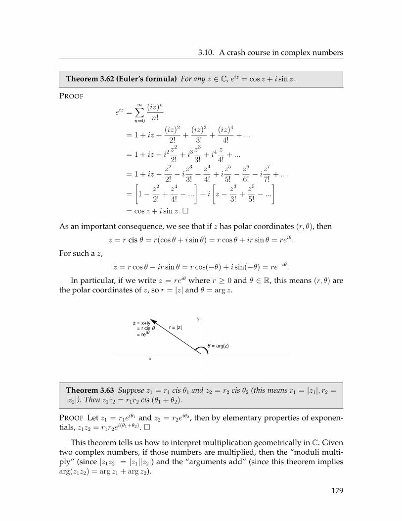
3.10. A crash course in complex numbers
Theorem 3.62 (Euler’s formula) For any z ∈ C, eiz = cos z + i sin z.
PROOF
eiz =∞∑n=0
(iz)nn!
= 1 + iz + (iz)2
2! + (iz)3
3! + (iz)4
4! + ...
= 1 + iz + i2z2
2! + i3z3
3! + i4z
4! + ...
= 1 + iz − z2
2! − iz3
3! + z4
4! + iz5
5! −z6
6! − iz7
7! + ...
=[1− z2
2! + z4
4! − ...]
+ i
[z − z3
3! + z5
5! − ...]
= cos z + i sin z.
As an important consequence, we see that if z has polar coordinates (r, θ), then
z = r cis θ = r(cos θ + i sin θ) = r cos θ + ir sin θ = reiθ.
For such a z,
z = r cos θ − ir sin θ = r cos(−θ) + i sin(−θ) = re−iθ.
In particular, if we write z = reiθ where r ≥ 0 and θ ∈ R, this means (r, θ) arethe polar coordinates of z, so r = |z| and θ = arg z.
z = x+iy= r cis θ= reiθ
r = |z|
θ = arg(z)
x
y
Theorem 3.63 Suppose z1 = r1 cis θ1 and z2 = r2 cis θ2 (this means r1 = |z1|, r2 =|z2|). Then z1z2 = r1r2 cis (θ1 + θ2).
PROOF Let z1 = r1eiθ1 and z2 = r2e
iθ2 , then by elementary properties of exponen-tials, z1z2 = r1r2e
i(θ1+θ2).
This theorem tells us how to interpret multiplication geometrically in C. Giventwo complex numbers, if those numbers are multiplied, then the “moduli multi-ply” (since |z1z2| = |z1||z2|) and the “arguments add” (since this theorem impliesarg(z1z2) = arg z1 + arg z2).
179

3.11. Complex eigenvalues
3.11 Complex eigenvaluesRecall the example at the start of the previous section that led us to complex
numbers: x′ = −yy′ = x
x(0) = 1y(0) = 0
To solve this, remember that we let A =(
0 −11 0
)and let y =
(xy
)so that the
system became y′ = Ay. We then tried to find the eigenvalues of A:
det(A− λI) = 0
det(−λ −11 −λ
)= 0
λ2 + 1 = 0
180

3.11. Complex eigenvalues
From the previous page, we have(0 −11 0
)= A = SΛS−1 =
(i −i1 1
)(i 00 −i
)12i
(1 i−1 i
)
Therefore the solution of the system is
eAty0 = S eΛt S−1(
10
)
=(i −i1 1
) (eit 00 e−it
)12i
(1 i−1 i
)(10
)
= 12i
(i −i1 1
)(cos t+ i sin t 0
0 cos(−t) + i sin(−t)
)(1 i−1 i
)(10
)(using Euler’s formula)
= 12i
(i −i1 1
)(cos t+ i sin t 0
0 cos t− i sin t
)(1−1
)(using identities cos(−t) = cos t; sin(−t) = − sin t)
= 12i
(i −i1 1
)(cos t+ i sin t− cos t+ i sin t
)
= 12i
(i cos t− sin t+ i cos t+ sin tcos t+ i sin t− cos t+ i sin t
)
Just as in Cardano’s cubic formula, the complex numbers are a means to an end:they drop out once Euler’s formula is applied and everything is multiplied out.
To summarize, we have found that the solution to the systemx′ = −yy′ = x
x(0) = 1y(0) = 0
is x = cos ty = sin t .
The Cartesian equation of this set of parametric equations is x2 + y2 = 1, whosegraph is a circle of radius 1 centered at the origin. This matches the slope field westarted with.
181

3.11. Complex eigenvalues
The general situation
Theorem 3.64 (Complex Roots Theorem) Suppose f is a polynomial with real co-efficients, i.e. f(x) = a0 + a1x + a2x
2 + ... + anxn. Then if z is any root of f (i.e.
f(z) = 0), then the conjugate z is also a root of f .
PROOF Suppose f(z) = 0. Then (using Lemma 2.39) we see f(z) = f(z) = 0 = 0as well.
Recall that to find eigenvalues of a matrix with real entries, we find roots of thepolynomial det(A − λI). The Complex Roots Theorem implies, therefore, that fora real matrix, whenever a complex number is an eigenvalue of that matrix, so is itsconjugate. More generally:
Theorem 3.65 Let A ∈Mn(R) be a matrix whose entries are real. If λ = a+ ib ∈ Cis an eigenvalue of matrix A with eigenvector v (v may have complex entries), thenthe conjugate λ = a− ib is also an eigenvalue, whose eigenvector is v.
PROOF We are given that Av = λv. Take the conjugate of both sides:
To summarize:
Theorem 3.66 If A ∈ Mn(R) has n distinct (real or complex) eigenvalues, then A isdiagonalizable over the complex numbers, i.e. A = SΛS−1 where S,Λ ∈ Mn(C) aresuch that Λ is a diagonal matrix whose entries are the eigenvalues of A, and S is amatrix whose columns are the corresponding eigenvectors (written in the same orderas the eigenvalues are written in Λ).
Moreover, any non-real eigenvalues and eigenvectors of A come in complex conju-gate pairs.
182

3.11. Complex eigenvalues
A shortcut in the complex case
Suppose you have a 2× 2 system
y′ = Ay
where the eigenvalues of A are not real. In light of Theorem 3.50, the solution ofthe system is
y = C1eλ1tv1 + C2e
λ2tv2
Since the eigenvalues and eigenvectors are complex-conjugate pairs, this solutioncan be rewritten as
y = C1eλtv + C2e
λtv.
In other words, a basis of the solution space is given by the two functions
y1 = eλtv; y2 = eλtv.
Notice that since t is real, t = t so λt = λ t = λt. Since exponentiation preservesconjugation, we have
y2 = eλtv = eλtv = eλt v = eλtv = y1.
Therefore a basis of the solution space is given by y1,y1. The problem is thatthese solutions have complex numbers in them.
Goal: Find a basis of the solution space which has only real numbers in it.
Idea: Since the solution space is a subspace, the sum of the two basis elementsis also a solution:
y1 + y1 = 2<(y1)
Multiplying this sum by 12 doesn’t change whether or not it is a solution, so we
now know <(y1) is a solution. This solution is real!
Similarly, since the solution space is a subspace, the difference of the two basiselements is also a solution:
y1 − y1 = 2i=(y1)
Multiplying this sum by 12i doesn’t change whether or not it is a solution, so we
now know =(y1) is a solution. This solution is also real!
183

3.11. Complex eigenvalues
What are these real and imaginary parts? Well, y1 = eλtv. Write λ = α+ iβ andwrite v = a + ib to get
y1 = e(α+iβ)t(a + ib)= eαteiβt(a + ib)= eαt(cos(βt) + i sin(βt))(a + ib)= eαt cos(βt) a + ieαt cos(βt) b + ieαt sin(βt) a − eαt sin(βt) b
=[eαt cos(βt) a − eαt sin(βt) b
]+ i
[eαt cos(βt) b + eαt sin(βt) a
]
Claim: The two solutions
eαt cos vt a − eαt sin vtb and eαt cos vtb + eαt sin vt a
are linearly independent.
Proof of claim: Compute their Wronskian:
W (t) = det(a1e
αt cos(βt)− b1eαt sin(βt) b1e
αt cos(βt) + a1eαt sin(βt)
a2eαt cos(βt)− b2e
αt sin(βt) b2eαt cos(βt) + a2e
αt sin(βt)
)...
(lots of work with algebra and trig identities that I am omitting)...
= e2αt(a1b2 − a2b1)
= e2αt det(a1 b1a2 b2
)= e2αt det
(a b
).
Because a and b are the real and imaginary parts coming from non-real eigenvectorv, they must be linearly independent (if they weren’t, then the eigenvector couldbe taken to be real, in which case v = v, in which case v would be an eigenvectorcorresponding to eigenvalues λ and λ 6= λ. But this is impossible, since Av cannotbe both λv and λv, since λ is not real.)
Therefore the determinant det(
a b)
is never zero, so W (t) 6= 0, so the twosolutions are linearly independent, proving the claim.
At this point, we have two linearly independent real solutions (namely <(v1)and =(v1)), which must form a basis of the solution space since the solution spaceis two-dimensional. To summarize:
184
3.11. Complex eigenvalues
Theorem 3.67 (Solution of 2 × 2 system with complex eigenvalues) Suppose
y′ = Ay
is a 2×2 linear, constant-coefficient system of ODEs whereA has non-real eigenvaluesλ = α + iβ and λ = α − iβ. Let the corresponding eigenvectors be v = a + ib andv = a − ib. Then the solution of the ODE is
y = C1[eαt cos(βt) a − eαt sin(βt) b] + C2[eαt cos(βt) b + eαt sin(βt) a].= C1<(eλtv) + C2=(eλtv).
Example 1: Find the general solution ofx′ = 4x+ yy′ = −5x+ 2y
Solution: Let A =(
4 1−5 2
)and y =
(xy
), so that the system becomes y′ = Ay.
First, find the eigenvalues:
0 = det(A− λI) = det(
4− λ 1−5 2− λ
)= (4− λ)(2− λ) + 5 = λ2 − 6λ+ 13
Next, find the corresponding eigenvectors:
Apply Theorem 3.67:
185

3.11. Complex eigenvalues
Example 2: Suppose x′(t) = −11x(t) + 4y(t) and y′(t) = −8x(t) − 3y(t). Ifx(0) = 2 and y(0) = −3, find x(t) and y(t).
Below are the phase planes for Examples 1 and 2:
Example 1: λ = 3± 2i Example 2: λ = −7± 4i(soln’s have e3t cos 2t, e3t sin 2t) (soln’s have e−7t cos 4t, e−7t sin 4t)
-10 -5 0 5 10
-10
-5
0
5
10
-10 -5 0 5 10
-10
-5
0
5
10
186

3.12. Repeated eigenvalues
3.12 Repeated eigenvaluesExample:
x′ = 3x+ 2yy′ = 3y
Let’s try this the same way as our previous examples: let A =(
3 20 3
)and
let y = (x, y) so that the system is y′ = Ay. Then the solution is y = eAty0. Let’scompute this as usual:
Eigenvalues and eigenvectors of A:
det(A− λI) = det(
3− λ 20 3− λ
)= (3− λ)2 ⇒ λ = 3
This suggests that maybe the solution should look like
y = C1e3t(
10
)i.e.
x = C1e
3t
y = 0
However: our theory tells us that the solution space should be two-dimensional,so it should be spanned by two linearly independent functions (and have two ar-bitrary constants). We only have one such function in the solution space: e3t (andonly one constant). So this can’t be right.
187

3.12. Repeated eigenvalues
Actually, this system is fairly easy to solve, because it is uncoupled (“uncou-pled” means the y′ equation has only y in it, so you can solve the equation for ywhile ignoring x).
x′ = 3x+ 2yy′ = 3y
From the second equation, y = C1e3t (exponential growth). Substituting this into
the first equation, we get
x′ = 3x+ 2C1e3t ⇒ x′ − 3x = 2C1e
3t
This equation is first-order, linear (but not homogeneous) and can therefore besolved with integrating factors:
Question: What does this solution have to do with eigenvalues and eigenvec-tors?
188

3.12. Repeated eigenvalues
Suppose you have a 2 × 2 system y′ = Ay where A has a repeated eigenvalueλ, whose eigenvector is v. We know one nonzero solution is
y1 = eλtv;
we need to find a second linearly independent solution.
First try: y2 = teλtw.Plug this into the system y′ = Ay and see what happens:
Second try: y2 = teλtw1 + eλtw2.Plug this into the system y′ = Ay:
189

3.12. Repeated eigenvalues
Theorem 3.68 Suppose A ∈M2(R) is not a scalar multiple of the identity. If A has arepeated eigenvalue λ of multiplicity 2, then the general solution of the system of twoODEs given by y′ = Ay is
y(t) = C1eλtv + C2
[eλtw + teλtv
]where v is an eigenvector of A corresponding to eigenvalue λ, and w is some othernonzero vector satisfying (A− λI)w = v; w is called a generalized eigenvector ofA corresponding to λ.
Example: Find (x, y) when t = 3, if x′(t) = 12x(t) + 4y(t) and y′(t) = −x(t) +16y(t), and if (x, y) = (2,−1) when t = 0.
190

3.13. Summary of linear, const.-coeff., homogeneous linear systems
3.13 Summary of linear, const.-coeff., homogeneous linear systems2× 2 systems
SupposeA ∈M2(R) and consider the system y′ = Ay where y = (x, y). The uniquesolution to such a system with initial value y(0) = y0 is always y(t) = eAty0; thegeneral solution of the system is given by y = C1y1 + C2y2, where y1 and y2 areany two linearly independent solutions of the system. There are four cases whichdescribe all possible solutions:
Case 1:A has two distinct, realeigenvalues λ1 and λ2,whose eigenvectors are
v1 and v2
⇒The general solution is
y = C1eλ1tv1 + C2e
λ2tv2
Case 2:A has a pair of complexconjugate eigenvaluesλ = α + iβ, λ = α− iβwhose eigenvectors arev = a + ib, v = a − ib
⇒
The general solution is
y = C1 [eαt cos(βt) a − eαt sin(βt) b] +C2 [eαt cos(βt) b + eαt sin(βt) a]
= C1<(eλtv) + C2=(eλtv)
Case 3:A is not a scalar multipleof the identity, but A hasa repeated eigenvalue λwith one eigenvector v
⇒
The general solution is
y = C1eλtv + C2
[eλtw + teλtv
]where w satisfies (A− λI)w = v
Case 4:A = λI
(i.e. A is a scalar multipleof the identity matrix)
⇒
The system is uncoupled;the equations can be solved
separately to obtainthe general solution
x = C1e
λt
y = C2eλt
191

3.13. Summary of linear, const.-coeff., homogeneous linear systems
Systems of more than two ODEsSuppose A ∈ Mn(R) and consider the system y′ = Ay where y = (y1, ..., yn). The uniquesolution to such a system with initial value y(0) = y0 is always y(t) = eAty0; the generalsolution of the system is given by y = C1y1 + C2y2 + ...Cdyd, where y1,y2, ...,yd are anyd linearly independent solutions of the system. To describe the solutions, you need to findthe eigenvalues of A. In general:
• You might get some real eigenvalues of multiplicity one, say λ1, λ2, ..., λk, with re-spective eigenvectors v1, ...,vk.
Each real eigenvalue λj of this type generates a solution of the form eλjtvj .
• You might get some complex eigenvalues (coming in pairs of complex conjugates),say
λ1, λ1 = α1 ± iβ1; λ2, λ2 = α2 ± iβ2; ...; λk, λk = αk ± iβk,whose corresponding eigenvectors are
v1,v1 = a1 ± ib1; v2,v2 = a2 ± ib2; ...; vk,vk = ak ± ibk.Each pair of eigenvalues αj ± iβj of this type generates a pair of solutions
<(eλjtvj) = eαjt cosβjtaj − eαjt sin βjtbj and =(eλjtvj) = eαjt cosβjtbj + eαjt sin βjtaj .
• You might get some repeated real eigenvalues of multiplicity greater than one, say
λ1(multiplicity m1), λ2(multiplicity m1), ..., λl(multiplicity ml),
where each eigenvalue λj has exactly one linearly independent eigenvector vj . Eachsuch eigenvalue λj of multiplicity mj generates a list of mj solutions of the form
eλjtvj , eλjtw1 + teλjtvj , eλjtw2 + teλjtw1 + t2eλjtvj , ...,
eλtwm−1 + teλjtwm−2 + t2eλjtwm−3 + ...tmj−1eλjtw1 + tmj−1eλjtvj .where wi satisfies (A− λI)iwi = vj .
• You might get repeated real eigenvalues which have more than one linearly inde-pendent eigenvector. This is beyond the scope of Math 330, but for each such eigen-value λj of multiplicitymj , there aremj solutions generated by this eigenvalue; eachof these is a polynomial in t multiplied by eλjt.
• You might get some repeated complex eigenvalues (coming in pairs of complex con-jugates), say
α1 ± iβ1(multiplicity n1), α2 ± iβ2(multiplicity n1), ..., αm ± iβm(multiplicity nm).
This too is beyond the scope of Math 330, but for each pair of eigenvalues of multi-plicity mj , there are 2mj solutions generated by this eigenvalue; each of these solu-tions is a polynomial in t multiplied by something like the solutions in the secondbullet point above.
Each solution of y′ = Ay is a linear combination of the n total functions generated bythe eigenvalues of the n× n matrix A.
192

3.13. Summary of linear, const.-coeff., homogeneous linear systems
Example: Suppose A is some 9×9 matrix whose eigenvalues are 2,−1, 5, 3±2i,and ±6i, where 5 has multiplicity 3 and all others have multiplicity 1. Assumingthat there is one linearly independent eigenvector corresponding to each eigen-value, this tells you that the general solution of y′ = Ay is
y(t) = C1e2tv
+ C2e−tv
+ C3e5tv + C4(e5tw1 + te5tv) + C5(e5tw2 + te5tw1 + t2e5tv)
+ C6(e3t cos 2t a − e3t cos 2tb) + C7(e3t cos 2tb + e3t cos 2t a)
+ C8(cos 6t a − sin 6tb) + C9(cos 6tb + sin 6t a).
Note: The vs, as and bs in different lines of this solution are not the samevectors. If the letters appear in the same horizontal line, they are the same vector.
193

3.13. Summary of linear, const.-coeff., homogeneous linear systems
An example with Mathematica
Solve y = Ay, y(0) = y0 where
A =
4 −6 6 0 −6 66 −8 6 0 −5 56 −6 4 0 −5 55 −5 0 3 −4 32 −2 0 2 −4 52 −2 0 2 −2 3
; y0 =
12−1−314
.
Step 1: Type in the matrices and save them as something like A and y0.
Step 2: Find the eigenvalues of A:
In: Eigenvalues[A]
Out: 4, 2+i, 2-i, -2, -2, -2
This tells you that the solutions yj should each be of the form
C1e4t + C2e
2t cos t+ C3e2t sin t+ C4e
−2t + C5te−2t + C6t
2e−2t.
Step 3: Compute the solution y(t) = eAty0:
In: y[t_] = MatrixExp[A t].y0
Out: some stuff
In: Expand[y[t]] // MatrixForm
Out:
e4t
e−2t + e4t − 3e−2tt−2e−2t + e4t − 3e−2tt
−2e−2t −(
12 + 5i
2
)e(2−i)t −
(12 −
5i2
)e(2+i)t − 3e−2tt
−3e−2t + (2− 3i)e(2−i)t + (2 + 3i)e(2+i)t
(2− 3i)e(2−i)t + (2 + 3i)e(2+i)t
To simplify this, we need a bit more theory of complex numbers:
194

3.13. Summary of linear, const.-coeff., homogeneous linear systems
Theorem 3.69 For any real numbers a, b, u and v,
(a+ ib)e(u+iv)t + (a− ib)e(u−iv)t = 2aeut cos vt− 2beut sin vt.
PROOF First, notice that for any complex number z = x+ iy,
z + z = (x+ iy) + (x− iy) = 2x = 2<(z).
Now, let w = u+ iv and c = a+ ib. Then the left-hand side of the theorem is
cewt + cewt = cewt + cewt = 2<(cewt).
Finally,
<(cwt) = Re((a+ ib)(eut cos vt+ ieut sin vt)) = aeut cos vt− beut sin vt.
Put these equations together to prove the theorem.
Using this theorem, the solution Mathematica produced on the previous page:
y(t) =
e4t
e−2t + e4t − 3e−2tt−2e−2t + e4t − 3e−2tt
−2e−2t −(
12 + 5i
2
)e(2−i)t −
(12 −
5i2
)e(2+i)t − 3e−2tt
−3e−2t + (2− 3i)e(2−i)t + (2 + 3i)e(2+i)t
(2− 3i)e(2−i)t + (2 + 3i)e(2+i)t
can (and should) be rewritten as
y(t) =
e4t
e−2t + e4t − 3te−2t
−2e−2t + e4t − 3te−2t
−2e−2t − e2t cos t− 5e2t sin t− 3te−2t
−3e−2t + 4e2t cos t− 6e2t sin t4e2t cos t− 6e2t sin t
.
195

3.14. Non-homogeneous systems
3.14 Non-homogeneous systemsRecall from Chapter 2 that to solve a first-order, linear, constant-coefficient ODE
that is not homogeneous, you use the method of undetermined coefficients:
Example: y′ + 4y = et
Solution: First, the corresponding homogeneous is y′ + 4y = 0, i.e. y′ = −4ywhich has solution yh = Ce−4t.
Now, “guess” a particular solution. Let’s try yp = Aet. Plugging this into theleft-hand side of the original equation, we have
(Aet)′ + 4(Aet) = et
⇒ 5Aet = et
⇒ A = 15
Therefore yp = 15et, so the general solution is y(t) = yp + yh = 1
5et + Ce−4t.
This same technique works for systems of the form y′ = Ay + q where A hasconstant coefficients. First, solve the corresponding homogeneous system y′ = Ayusing the techniques of the previous sections; then find a particular solution ypusing the method of undetermined coefficients.
Example: Find the general solution of the systemx′ = x− 3y + e2t
y′ = 4x− 6y
Solution: First, establish notation: define
A =(
1 −34 −6
)q =
(e2t
0
)y =
(xy
)
This means we are trying to solve the system
y′ = Ay + q
so we start with the corresponding homogeneous system
y′ = Ay
196

3.14. Non-homogeneous systems
Eigenvalues of A:
0 = det(A− λI) = det(
1− λ −34 −6− λ
)= (1− λ)(−6− λ) + 12
= λ2 + 5λ+ 6= (λ+ 2)(λ+ 3)⇒ λ = −2, λ = −3
Eigenvectors:
λ = −2 : Ax = −2x⇒x− 3y = −2x4x− 6y = −2y ⇒ x = y ⇒
(11
)
λ = −3 : Ax = −3x⇒x− 3y = −3x4x− 6y = −3y ⇒ 4x = 3y ⇒
(34
)Therefore the solution of the homogeneous is
yh = C1e−2t
(11
)+ C2e
−3t(
34
).
Undetermined coefficients: Now we find yp. Since
q =(e2t
0
), let’s try yp =
(Ae2t
Be2t
).
We have
y′p =(
2Ae2t
2Be2t
);
this should equal
Ayp + q =(
1 −34 −6
)(Ae2t
Be2t
)+(e2t
0
)=(
(A− 3B + 1)e2t
(4A− 6B)e2t
).
Equating terms of y′p with those of Ayp + q, we get2A = A− 3B + 12B = 4A− 6B
From the second equation, A = 2B, and from the first equation, we get 5B = 1 soB = 1
5 (and therefore A = 2B = 25 ).
Therefore
yp =(
25e
2t
15e
2t
)
197

3.15. Classification of equilibria
and the general solution of the original system is
y = yh + yp =(
25e
2t + C1e−2t + 3C2e
−3t
15e
2t + C1e−2t + 4C2e
−3t
),
i.e. x(t) = 2
5e2t + C1e
−2t + 3C2e−3t
y(t) = 15e
2t + C1e−2t + 4C2e
−3t .
3.15 Classification of equilibriaRecall from Chapter 1 that to classify an equilibrium y0 of a single first-order au-tonomous equation y′ = φ(y), you find the sign of the derivative φ′(y0):
φ′(y0) > 0⇔ y0 is unstableφ′(y0) < 0⇔ y0 is stable
φ′(y0) = 0 and φ′′(y0) 6= 0⇔ y0 is semistable
So classifying the equilibria of a system y′ = Φ(y) should have something todo with the “derivative” of Φ. But Φ is a function of several variables, which hasseveral components. What is the “derivative” of Φ?
Definition 3.70 Let Φ : Rd → Rd be a function of the form
Φ(x1, ...xd) = (φ1(x1, ...xd), φ2(x1, ...xd), ..., φd(x1, ...xd)).
The total derivative of Φ is the d× d matrix
DΦ = DΦ(x1, ..., xd) =
∂φ1∂x1
∂φ1∂x2
· · · ∂φ1∂xd
∂φ2∂x1
∂φ2∂x2
· · · ∂φ2∂xd...
... . . . ...∂φd
∂x1
∂φd
∂x2· · · ∂φd
∂xd
.
Example: Find the total derivative of Φ, where Φ : R2 → R2 is defined by
Φ(x, y) = (3x2 + 2xy, 4xy3 − 2x2y).
198

3.15. Classification of equilibria
Example: Find DΦ(π, 0, π2 ) of Φ = (φ1, φ2, φ3), if
φ1(x, y, z) = 2 sin x+ cos y;φ2(x, y, z) = 3 cosx− 2 sin z;
φ3(x, y, z) = 3 cosx− 2 sin y + 5 cos z.
Example: Suppose Φ(y) = Ay, where A ∈Md(R). Find DΦ.
For a system, you classify an equilibrium y0 of a system of first-order autonomoussystems by finding the signs of the eigenvalues of the total derivative DΦ(y0):
Definition 3.71 An equilibrium solution y = y0 of an autonomous system is calledstable (or asymptotically stable or attracting or a sink) if there is an open disk E(an open disk is the set of points inside a circle) of initial values, centered at y0, suchthat if y(t0) ∈ E,
limt→∞
y(t) = y0.
An equilibrium solution y = y0 of an autonomous system is called semistable (orneutral) if it is not stable, but there is an open disk E (an open disk is the set ofpoints inside a circle) of initial values, centered at y0, such that if y(t0) ∈ E, then y(t)stays close to y0 for all t ≥ 0.
An equilibrium solution y = y0 of an autonomous system is called unstable (orasymptotically unstable) if it is neither stable nor semistable.
199
3.15. Classification of equilibria
To classify equilibria, we look at the signs of the (real parts of the) eigenvaluesof DΦ(y0) (these play the same role as the signs of φ′(y0) for single equations):
Theorem 3.72 (Classification of equilibria) Suppose y = y0 is an equilibriumsolution of autonomous ODE y′ = Φ(y). Then:
1. Φ(y0) = 0;
2. If the real part of every eigenvalue of DΦ is negative, then y0 is stable.
3. If the real part of any eigenvalue of DΦ is positive, then y0 is unstable.
4. If DΦ has only eigenvalues with nonpositive real parts, and has at least oneeigenvalue with zero real part, then y0 is semistable.
Example: Consider the autonomous (but not linear) 2× 2 system of ODEsx′(t) = x2 − 2xy′(t) = 4− (x+ 2)(y − 1)
Find the equilibria of this system and classify them as stable, unstable or semistable.
200

3.15. Classification of equilibria
Note that in the previous problem, the eigenvalues of DΦ(y0) could be read offfrom the matrix. This is because the matrix is triangular:
Theorem 3.73 If A is a triangular matrix, then the eigenvalues of A are its diagonalentries.
PROOF See Chapter 8 of my Math 322 lecture notes.
Example: Find and classify all the equilibria of the 2× 2 systemx′ = x− y + 1y′ = y(x− 2)
201

3.15. Classification of equilibria
CLASSES OF STABLE EQUILIBRIA:
Stable node (two negative, real eigenvalues)
λ1 = λ2 < 0 λ1 = λ2 < 0w/ 2 lin. indep. w/ 1 eigenvector v
eigenvectors v1,v2 λ1 < λ2 < 0 and 1 gen. eigenvec. w
-2 -1 0 1 2
-2
-1
0
1
2
-2 -1 0 1 2
-2
-1
0
1
2
-2 -1 0 1 2
-2
-1
0
1
2
Stable spiral (two non-real eigenvalues with negative real part)
λ = α± iβ, α < 0 λ = α± iβ, α < 0
-2 -1 0 1 2
-2
-1
0
1
2
-2 -1 0 1 2
-2
-1
0
1
2
CLASSES OF UNSTABLE EQUILIBRIA:
Unstable node (two positive, real eigenvalues)
λ1 = λ2 > 0 λ1 = λ2 > 0w/ 2 lin. indep. w/ 1 eigenvector v
eigenvectors v1,v2 λ1 > λ2 < 0 and 1 gen. eigenvec. w
-2 -1 0 1 2
-2
-1
0
1
2
-2 -1 0 1 2
-2
-1
0
1
2
-2 -1 0 1 2
-2
-1
0
1
2
202

3.15. Classification of equilibria
Unstable spiral (two non-real eigenvalues with positive real part)
λ = α± iβ, α > 0 λ = α± iβ, α > 0
-2 -1 0 1 2
-2
-1
0
1
2
-2 -1 0 1 2
-2
-1
0
1
2
Saddle (one positive, real eigenvalue and one negative, real eigenvalue)
λ1 > 0, λ2 < 0 λ1 > 0, λ2 < 0λ1 ↔ v1, λ2 ↔ v2 λ1 ↔ v1, λ2 ↔ v2
-2 -1 0 1 2
-2
-1
0
1
2
-2 -1 0 1 2
-2
-1
0
1
2
CLASSES OF SEMISTABLE EQUILIBRIA:
Center (two non-real eigenvalues with zero real part)
λ = ±iβ λ = ±iβ
-2 -1 0 1 2
-2
-1
0
1
2
-2 -1 0 1 2
-2
-1
0
1
2
203
3.16. The trace-determinant plane
3.16 The trace-determinant planeRecall that an equilibrium y0 of an autonomous equation y′ = Φ(y) can be clas-
sified by looking at the eigenvalues of its determinant.
Suppose y′ = Φ(y) is a 2×2 system and that y0 is an equilibrium of this system.It turns out that you can classify this equilibrium without finding the eigenvaluesof DΦ(y0): you only need to compute the trace and determinant of DΦ(y0).
Suppose DΦ(y0) =(a bc d
). Then the eigenvalues of D(Φ(y0)) can be com-
puted as usual, in terms of a, b, c and d:
0 = det(DΦ(y0)− λI) = det(a− λ bc d− λ
)= (a− λ)(d− λ)− bc= ad− aλ− dλ+ λ2 − bc= λ2 − (a+ d)λ+ (ad− bc)= λ2 − (trA)λ+ detA.
Solve for λ using the quadratic formula to get
λ =trA±
√(trA)2 − 4 detA
2 = t±√t2 − 4d2
where t = trA and d = detA.
Suppose the equilibrium is a saddle. That means one of the eigenvalues ispositive and one is negative, i.e.
In this case, the product of the eigenvalues is(t+√t2 − 4d2
)(t−√t2 − 4d2
)= t2 − (t2 − 4d)
4 = d.
This shows that the equilibrum is a saddle if and only if d < 0.
204

3.16. The trace-determinant plane
From the previous page,
λ =trA±
√(trA)2 − 4 detA
2 = t±√t2 − 4d2
where t = trA and d = detA.
Next, recall that the eigenvalues of a matrix sum to the trace t. So if the eigen-values have the same sign, their sign will coincide with the sign of the trace.
Last, take a look at the expression under the square root:
1. if d > 14t
2, then the number under the square root is negative. This meansthe eigenvalues are (non-real) complex numbers with real part trA
2 , so theequilibrium is
2. if d = 14t
2, then the number under the square root is zero. This means theeigenvalue trA
2 is real and repeated, so the equilibrium is a
3. if 0 < d < 14t
2, then the number under the square root is positive. This meansthere are two real eigenvalues which must have the same sign since theirproduct is d (which is positive). This makes the equilibrium a node.
To summarize, we have proven this statement:
Theorem 3.74 (Trace-determinant plane) Suppose y0 is an equilibrium of a 2× 2autonomous system y′ = Φ(y). Let t = trDΦ(y0) and let d = detDΦ(y0).
1. If d < 0, then y0 is a saddle.
2. If 0 < d ≤ t2
4 , then y0 is a node. The node is stable if t < 0 and unstable if t > 0.
3. If d > t2
4 , then y0 is a spiral or center. y0 is a stable spiral if t < 0, a center ift = 0, and an unstable spiral if t > 0.
205

3.16. The trace-determinant plane
The previous theorem is sometimes described with the following picture, calledthe trace-determinant plane:
saddle
unstable spiralstable spiral
stable node unstable nodet = tr DΦ
d = det DΦ
Example: Suppose y0 is an equilibrium of some 2 × 2 system y′ = Φ(y) and
DΦ(y0) =(
5 72 3
). Classify this equilibrium.
Example: Suppose y0 is an equilibrium of some 2 × 2 system y′ = Φ(y) suchthat trDΦ(y0) = 3 and detDΦ(y0) = 11. Classify this equilibrium.
Example: Suppose y0 is an equilibrium of some 2 × 2 system y′ = Φ(y) suchthat trDΦ(y0) = 0 and detDΦ(y0) = −2. Classify this equilibrium.
206

3.17. Applications of first-order systems
3.17 Applications of first-order systemsCompartmental models
Example: Consider two tanks (say A and B) connected by two pipes which pumpfluid between the tanks. Each tank holds 24 liters of a brine solution. Fresh waterflows into tank A at a rate of 6 L/min, and fluid is drained out of tank B at thesame rate. Suppose that 8 L of fluid per minute is being pumped from tank A totank B, and 2 L/min of fluid per minute is pumped from tank B to tank A. If thetanks are kept well-stirred, and if tank A initially contains 3 kg of salt, and tank Binitially contains 1 kg of salt, find the amount of salt in each tank at time t > 0.
This yields the following linear, constant-coefficient system of ODEs:
A′(t) = −1
3 A+ 112B
B′(t) = 13A−
13B
⇔ y′ =(−13
112
13
−13
)y initial value y(0) =
(31
)
207

3.17. Applications of first-order systems
From the previous page:A′(t) = −1
3 A+ 112B
B′(t) = 13A−
13B
⇔ y′ =(−13
112
13
−13
)y; y(0) =
(31
)
Eigenvalues:
0 = det(−13 − λ
112
13
−13 − λ
)= λ2+ 2
3λ+ 112 =
(λ+ 1
2
)(λ+ 1
6
)⇒ λ = −1
2 , λ = −16
Eigenvectors:
λ = −12 ↔
(−12
)λ = −1
6 ↔(
12
)General solution:
y = C1e(−1/2)t
(−12
)+ C2e
(−1/6)t(
12
)i.e.
A(t) = −C1e
−t/2 + C2e−t/6
B(t) = 2C1e−t/2 + 2C2e
−t/6
Find the particular solution using the initial condition:
y0 =(−C1 + C22C1 + 2C2
)=(
31
)⇒ C1 = −1.25
C2 = 1.75 ⇒A(t) = 1.25e−t/2 + 1.75e−t/6B(t) = −2.5e−t/2 + 3.5e−t/6
-4 -2 0 2 4
-4
-2
0
2
4
5 10 15 20
0.5
1.0
1.5
2.0
2.5
3.0
208

3.17. Applications of first-order systems
Predator-prey population dynamics
We started this chapter with an example taken from the population dynamics ofinteracting species. Here is a more formal version of this setup:
Let
R(t) = rabbit population at time t (i.e. prey)L(t) = lynx population at time t (i.e. predators)
From the discussion at the beginning of the chapter, we saw that the compartmentsbehaved as follows:
R
aR bRL
L
cRL dL
where a, b, c and d are positive constants. Thus we have the following system ofODEs, called the Lotka-Volterra equations:
R′ = aR− bRLL′ = cRL− dL
This system is not linear, but it is autonomous, so we can study it via phase planesand equilibria analysis.
Equilibria:
Classification of equilibria: First, find the total derivative:
Φ(R,L) = (aR− bRL, cRL− dL)⇒ DΦ =(
∂φ1∂R
∂φ1∂L
∂φ2∂R
∂φ1∂L
)=(a− bL −bRcL cR− d
).
209

3.17. Applications of first-order systems
Equilibrium (0, 0):
DΦ(0, 0) =(a 00 −d
)⇒ Eigensystem λ = a↔
(10
);λ = −d↔
(01
)
Therefore (0, 0) is a saddle (one positive eigenvalue, one negative eigenvalue).
Equilibrium(dc, ab
):
DΦ(d
c,a
b
)=(a− b(a/b) −b(d/c)c(a/b) c(d/c)− d
)=(
0 −bd/cca/b 0
)
⇒ Eigenvalues λ = ±i√ad
Therefore(dc, ab
)is a center.
Phase plane analysis:
d/c
a/b
210

3.17. Applications of first-order systems
SIR model of disease spread
The study of how diseases spread across a population is called epidemiology.Let’s consider an example which shows how systems of ODEs are used in thiscontext.
Setup: Consider a contagious disease (think chicken pox) where once peopleget the disease, they recover; if they recover, they build up an immunity to thedisease and can’t get the disease again. This divides the population into threeclasses:
S(t) = fraction of susceptible individuals at time tI(t) = fraction of infective individuals at time tR(t) = fraction of recovered (or dead) individuals at time t
We assume that the disease acts more quickly than the population can reproduce,so the total population S(t)+I(t)+R(t) is constant, and always equal to 1 (thereforethe birth rate is assumed to be zero). That means that there are really only twounknown functions (S(t) and I(t)), because you can always find R(t) by taking1 − S(t) − I(t). This leads to the following compartmental model, called the SIRmodel:
S I RrI IS rR I
In this model:
rI = rate of infectionrR = rate at which infected individuals recover (or die)
This model translates into the following system of ODEs:dSdt
= −rIISdIdt
= rIIS − rRI
(We also know that dRdt
= rRI , but we don’t need this since S + I +R = 1.)
211

3.17. Applications of first-order systems
From the previous page: dSdt
= −rIISdIdt
= rIIS − rRI
This system is not linear, but it is autonomous.
Equilibria: 0 = −rIIS0 = I(rIS − rR) ⇒ I = 0 or S = rR
rI
So every point with I = 0 is an equilibrium of his system.
Example phase planes:
rI = .3; rR = .05 rI = .3; rR = .2 rI = .3; rR = .8
0.0 0.2 0.4 0.6 0.8 1.0
0.0
0.2
0.4
0.6
0.8
1.0
0.0 0.2 0.4 0.6 0.8 1.0
0.0
0.2
0.4
0.6
0.8
1.0
0.0 0.2 0.4 0.6 0.8 1.0
0.0
0.2
0.4
0.6
0.8
1.0
SIR models can be adapted to account for diseases that take longer to act (inwhich case there are births and deaths in the population). This is done in thehomework exercises.
212

3.18. Exam 2 Review
3.18 Exam 2 ReviewOn this exam, you may use: one 4” × 6” note card with whatever you want onboth sides.
What should you expect to be asked on the exam:• Solve 2× 2 constant-coefficient, linear ODEs and/or IVPs• Find and classify equilibria of 2×2 autonomous systems (using trace-determinant
plane if necessary)• Analyze pictures of phase planes• Perform one or two steps of Euler’s method for systems, given a simple equa-
tion• Applications / story problems (interconnected tanks, population models,
etc.)• Answer question(s) on theory and/or vocabulary
NOT on the exam:• Eigenvalues of 3× 3 or larger matrices• Computing matrix exponentials (unless you choose to use them)• Matrix operations (unless you choose to use them)• Spans / subspaces / linear independence / basis / Wronskian / other linear
algebra issues• Picard’s method for systems / integral equation for systems• Questions that require you to know any Mathematica code
Some practice questions:
1. a) What does it mean for a d× d system of ODEs to be “linear”?
b) What is the form of the general solution of a d × d first-order, linearsystem of ODEs?
c) What is Euler’s formula? (Note: this is not Euler’s method) What is theimportance of Euler’s formula in differential equations?
2. Consider the initial value problemy′ = (y + t, 2y − x)y(0) = (2, 1)
where y = (x, y). Estimate y(4) by using Euler’s method with two steps.
3. Find and classify the equilibria of the autonomous systemx′ = 2x− xyy′ = xy − 3y + 4x− 12 .
213

3.18. Exam 2 Review
4. Suppose y0 and y1 are the two equilibria of some 2 × 2 system y′ = Φ(y). IfDΦ(y0) has trace 8 and determinant 12, and if DΦ(y0) has trace 8 and deter-minant 18, classify the equilibria y0 and y1.
5. Find the general solution of each system. In addition:
• In parts (a) and (c), write your answer coordinate-wise, i.e. asx(t) = somethingy(t) = something .
• In part (b), give a rough sketch of the phase plane of the system.
• In parts (b), (c) and (e), classify the equilibrium 0 as a node, spiral, sad-dle or center.
a)x′ = −4x+ 9yy′ = −4x− 16y
b)x′ = 7x+ 8yy′ = 16x− y
c)x′ = 3x− 8yy′ = 4x− 5y
d)x′ = −x+ 3y + 12e−ty′ = 3x− y
e)x′ = −3x+ 13yy′ = −10x+ 3y
f) y′ = Ay where A is a 3 × 3 matrix with eigenvalues λ = 2, λ = −3 andλ = 5 and respective eigenvectors (1, 2,−3), (1,−1, 5) and (0,−2, 1).
6. Find the particular solution of this initial value problem:
y′ = (−13x+ 2y, 3x− 8y)y(0) = (5, 2)
7. Here is the phase plane corresponding to some 2 × 2 autonomous system ofODEs y′ = Φ(y):
-10 -5 5 10
-10
-5
5
10
a) Sketch the graph of the solution of this system satisfying y(0) = (−6,−4).
214
3.18. Exam 2 Review
b) Suppose y = (x, y) is the solution of this system satisfying y(0) = (6, 2).Find lim
t→−∞y(t).
c) Suppose y = f(t) is the solution of this system satisfying f(0) = (4, 8).Find r such that (8, r) is on the graph of f .
d) Find all saddles of this system (if any). Classify each saddle as stable orunstable.
e) Find all nodes of this system (if any). Classify each node as stable orunstable.
f) Find all spirals of this system (if any). Classify each spiral as stable orunstable.
8. Two large tanks (call them X and Y) each hold 240 L of liquid. They areinterconnected by a pipe which pumps liquid from tank X to tank Y at a rateof 8 L/min. A brine solution of concentration 0.1 kg/L of salt flows into tankX at a rate of 10 L/min; the solution flows out of the system of tanks via twopipes (one pipe allows flow out of tank X at 2 L/min and another pipe allowsflow out of tank Y at 8 L/min). Suppose that initially, tank Y contains purewater but tank X contains 60 kg of salt; assume that at all times the liquids ineach tank are kept mixed.
a) Draw a compartmental diagram that models this situation.
b) Write down the initial value problem which models this situation, clearlydefining your variables.
c) Solve the initial value problem you wrote down in part (a).
d) Find the amount of salt in tank Y at time 240.
Solutions
WARNING: as always, these might have errors.
1. a) A d× d system of ODEs is linear if it can be written in the form
Any(n) + An−1y(n−1) + ...+ A1y′ + A0y = q
where the Aj are d × d matrices whose entries are functions of t, and qis a vector whose entries are functions of t.
b) The general solution of a d × d, first-order linear system y′ = Ay + q isof the form
y = yp + yh= yp + (C1y1 + C2y2 + ...Cdyd)
215
3.18. Exam 2 Review
where yp is any one particular solution of the system, and y1, ....,yd arelinearly independent solutions of the corresponding homogeneous sys-tem y′ = Ay.
c) Euler’s formula says that for any complex number θ, eiθ = cos θ+ i sin θ.This formula explains why a system of differential equations y′ = Ayhas solutions with cosines and sines in them whenever A has non-realeigenvalues.
2. Think of the system as y′ = Φ(t,y); y0 = y(t0). First, ∆t = tn−t0n
= 4−02 = 2.
Now Φ(t0,y0) = Φ(0, (2, 1)) = (1 + 0, 2(1)− 2) = (1, 0) sot1 = t0 + ∆t = 0 + 2 = 2y1 = y0 + Φ(y0)∆t = (2, 1) + (1, 0)2 = (4, 1).
Next, Φ(t1,y1) = Φ(2, (4, 1)) = (2 + 1, 2(1)− 4) = (3,−2) sot2 = t1 + ∆t = 2 + 2 = 4y2 = y1 + Φ(y1)∆t = (4, 1) + (3,−2)2 = (10,−3).
Thus y(4) ≈ (10,−3).
3. Thinking of the system as y′ = Φ(y), we set Φ(y) = 0 and solve for y. Startwith the first equation:
0 = 2x− xy = x(2− y)⇒ x = 0 or y = 2.
If x = 0, plugging in the second equation gives −3y − 12 = 0, i.e. y = −4,so one equilibrium is (0,−4). If y = 2, plugging in the second equation gives2x − 6 + 4x − 12 = 0, i.e. x = 3, so the other equilibrium is (3, 2). To classifythe equilibria, find the eigenvalues of DΦ:
DΦ =(
2− y −xy + 4 x− 3
);
DΦ(0,−4) =(
6 00 −3
); this matrix has negative determinant, so (0,−4) is
an unstable saddle.
DΦ(3, 2) =(
0 −36 0
); this matrix has trace 0 and positive determinant, so
(3, 2) is a center.
4. Let t = tr(DΦ(y0)) and d = det(DΦ(y0)); we have t = 8 and d = 12. Sinced < t2
4 and t > 0, y0 is an unstable node.
Now, let t = tr(DΦ(y1)) and d = det(DΦ(y1)); we have t = 8 and d = 18.Since d > t2
4 and t > 0, y0 is an unstable spiral.
216

3.18. Exam 2 Review
5. Answers may vary in this problem, due to different choices of eigenvectors.All of these problems are approached by first finding eigenvalues via theequation det(A−λI) = 0 and then finding eigenvectors by the equationAv =λv.
a) Eigenvalue λ = −10 (repeated twice).Eigenvector v (found by setting Av = λv): v = (−3, 2).Then, solve (A − λI)w = v to find a generalized eigenvector: w =(1,−1).
So the general solution is y = C1e−10t
(−32
)+C2
[e−10t
(1−1
)+ te−10t
(−32
)].
Written coordinate-wise:x(t) = (−3C1 + C2)e−10t − 3C2te
−10t
y(t) = (2C1 − C2)e−10t + 2C2te−10t .
b) The general solution, coming from eigenvalues and eigenvectors, is
y = C1e15t(
11
)+ C2e
−9t(
1−2
);
0 is an unstable saddle since it has one positive and one negative eigen-value (alternatively, because the matrix has negative determinant). Thestraight-line solutions are y = x (which goes away from the origin sinceits eigenvalue is positive) and y = −2x (which goes toward the origin(since its eigenvalue is negative), so the phase plane looks roughly likethis:
-10 -5 0 5 10
-10
-5
0
5
10
c) Eigenvalues: λ = −1± 4i; eigenvectors: (1± i, 1).Since the eigenvalues are non-real with negative real part (alternatively,since the matrix has negative trace t and determinant d satisfying d >t2
4 ), 0 is a stable spiral.The general solution is
y = C1
[e−t cos 4t
(11
)− e−t sin 4t
(10
)]+ C2
[e−t cos 4t
(10
)+ e−t sin 4t
(11
)].
Written coordinate-wise:x(t) = (C1 + C2)e−t cos 4t+ (C2 − C1)e−t sin 4ty(t) = C1e
−t cos 4t+ C2e−t sin 4t .
217

3.18. Exam 2 Review
d) Start by solving the homogeneous system y′ = Ay whereA =(−1 33 −1
).
By usual methods, this solution is yh = C1e−4t
(1−1
)+ C2e
2t(
11
).
Next, find a particular solution by guessing yp =(Ae−t
Be−t
). Plugging in
the original system, we get−A = −A+ 3B + 12−B = 3A−B which has solution
A = 0, B = −4. Therefore yp =(
0−4e−t
)so the solution of the original
system is
y = yp + yh =(
0−4e−t
)+ C1e
−4t(
1−1
)+ C2e
2t(
11
).
e) Eigenvalues: λ = ±11i; eigenvectors: (3∓ 11i, 10)Since the eigenvalues are pure imaginary (alternatively, since the matrixA has zero trace and positive determinant), 0 is a center.The general solution is
y = C1
[cos 11t
(310
)− sin 11t
(−11
0
)]+ C2
[cos 11t
(−11
0
)+ sin 11t
(310
)]
=(
(3C1 − 11C2) cos 11t+ (11C1 + 3C2) sin 11t10C1 cos 11t+ 10C2 sin 11t
).
f) y = C1e2t
12−3
+ C2e−3t
1−15
+ C3e5t
0−21
.
6. Eigensystem: λ = −14↔(
2−1
); λ = −7↔
(13
).
General solution: y = C1e−14t
(2−1
)+ C2e
−7t(
13
).
Plug in y(0) = (5, 2) to get
5 = 2C1 + C22 = −C1 + 3C2
Solve for C1 and C2 to get
C1 = 137 , C2 = 9
7 . Thus the particular solution is
y = 137 e−14t
(2−1
)+ 9
7e−7t
(13
)
=(
267 e−14t + 9
7e−7t
−137 e−14t + 27
7 e−7t
).
218

3.18. Exam 2 Review
7. a)
-10 -5 5 10
-10
-5
5
10
b) limt→−∞
y(t) = −5.
c) r = 7.
d) This system has an unstable saddle at (0, 6) (saddles are always unsta-ble).
e) This system has no nodes.
f) This system has an unstable spiral at (−1,−5).
8. a)x(t) y(t)
1 y/30x/30
x/120
b) Let x(t) = the amount of salt in tank X at time t, and let y(t) = theamount of salt in tank Y at time t. Then we have the initial value prob-lem
x′(t) = − x30 −
x120 + 1
y′(t) = x30 −
y30
x(0) = 60y(0) = 0
c) We can rewrite the system as y′ = Ay + q where y = (x, y), q = (1, 0)
and A =(−124 0130
−130
). To solve this, first solve the homogeneous sys-
tem using eigenvalues and eigenvectors (notice that since this matrix istriangular, you can read off the eigenvalues as the diagonal entries):
det(A− λI) = (−124 − λ)(−1
30 − λ)⇒ λ = −124 ,−130
The corresponding eigenvectors (letting v = (x, y) and solvingAv = λv)are:
λ = −124 :
−124 x = −1
24 x130x−
130y = −1
24 y⇒ x− y = −5
4 y ⇒ x = −14 y ⇒ v = (1,−4)
λ = −130 :
−124 x = −1
30 x130x−
130y = −1
30 y⇒ x = 0⇒ v = (0, 1)
So the general solution of the homogeneous is
yh = C1e−t/24
(1−4
)+ C2e
−t/30(
01
).
219

3.18. Exam 2 Review
Now for the particular solution. Since q has constant entries, guess yp =(AB
). Then, by plugging in the original system we have
0 = −A
24 + 10 = A
30 −B30
Therefore A = B = 24, so yp = (24, 24). Therefore
y = yp + yh =(
2424
)+ C1e
−t/24(
1−4
)+ C2e
−t/30(
01
).
i.e. x(t) = C1e
−t/24 + 24y(t) = −4C1e
−t/24 + C2e−t/30 + 24
Plugging in the initial conditions x(0) = 60, y(0) = 0, we get 60 = C1 +24(i.e. C1 = 26) and 0 = −4C1 + C2 + 24 (i.e. C2 = 80). Therefore theparticular solution is
x(t) = 26e−t/24 + 24y(t) = −104e−t/24 + 80e−t/30 + 24
d) y(240) = −104e−240/24 + 80e−240/30 + 24 = −104e−10 + 80e−8 + 24.
220

Chapter 4
Higher-order linear equations
4.1 Reduction of orderRecall that a nth order, linear ODE has the form
We know from Chapters 1-3 how to approach first-order equations and sys-tems. On the face of things, it seems like we would have to invent entirely newtheory to study nth-order equations and systems. However, there is a trick calledreduction of order. Here’s how this trick works for linear systems:
Start with the nth-order linear equation
pny(n) + pn−1y
(n−1) + ...+ p2y′′ + p1y
′ + p0 = q
and rewrite this equation (renaming the coefficient functions pj if necessary) bysolving for y(n) to get
y(n) = p0y + p1y′ + p2y
′′ + ...+ pn−1y(n−1) + q (4.1)
Here comes the trick. We turn the nth-order equation (4.1) into a first-order sys-tem as follows: first, define for j ∈ 0, ..., n− 1,
yj(t) = y(j)(t)
and arrange these yj into a vector:
y(t) =
y0(t)y1(t)y2(t)
...yn−1(t)
=
y(t)y′(t)y′′(t)
...y(n−1)(t)
.
221

4.1. Reduction of order
Now,
y′ = d
dt
y0(t)y1(t)y2(t)
...yn−2(t)yn−1(t)
= d
dt
y(t)y′(t)y′′(t)
...y(n−2)(t)y(n−1)(t)
=
y′(t)y′′(t)y′′′(t)
...y(n−1)(t)y(n)(t)
=
y1(t)y2(t)y3(t)
...yn−1(t)y(n)(t)
Substituting in the formula from Equation (4.1) (previous page), we get
y′ =
y1(t)y2(t)
...yn−1(t)
p0y0(t) + p1y1(t) + ...+ pn−2yn−2(t) + pn−1yn−1(t) + q(t)
=
11
. . .1
1p0 p1 p2 · · · · · · pn−1
y0(t)y1(t)y2(t)
...yn−2(t)yn−1(t)
+
000...0q(t)
= Ay + q
where
A =
11
. . .1
1p0 p1 p2 · · · · · · pn−1
and q =
000...0q(t)
.
Note that if we can solve the first-order system
y′ = Ay + q,
then by reading the first row off this solution, we have solved the original nth-orderequation!
In general, an nth-order ODE can be turned into a linear n × n system of first-order ODEs using this procedure, and a d × d system of nth-order ODEs can beconverted into a dn× dn system of first-order ODEs using similar techniques.
222
4.1. Reduction of order
Example: Convert the following second-order equation to a first-order systemof the form y′ = Ay + q:
y′′ + 4e−3ty′ − 3ety = 7e2t
Example: Convert the following third-order system to a first-order system ofthe form y′ = Ay + q:
x′′′ −4x′′ + 2y′′ −3x′ + 5y′ −x+ 7y = 0x′′′ + y′′′ +3y′′ −2x′ +3x− 4y = et
223

4.1. Reduction of order
Since solving a nth-order system is equivalent to solving a first-order systemwith more variables and more equations, the existence/uniqueness theory we de-veloped for first-order systems lifts to this setting. The only issue is what consti-tutes an initial value.
When solving a first-order system y′ = Φ(t,y), an initial value is some y(t0) =y0, which is really a list of values of all the components of y at t = t0. In this setting,since the components of y are the zeroth to (n− 1)th derivatives of y, to specify aninitial value for an nth-order equation means to specify the values of
at some value t0.
Definition 4.1 Given an nth-order ODE, an initial value of the ODE is a num-ber t0, together with the values y(t0), y′(t0), ..., y(n−1)(t0) of y and its first (n − 1)derivatives at t0. We write such an initial value as
(t0, y(t0), y′(t0), ..., y(n−1)(t0)) or (t0, y0, y′0, y′′0 , ..., y
(n−1)0 ).
An nth-order ODE together with an initial value of this type is called a initial valueproblem.
Theorem 4.2 (Existence/uniqueness for nth-order equations) Suppose
φ = φ(t, y, y′, ..., y(n−1)) : Rn+1 → R
is a function such that φ, ∂φ∂y, ∂φ∂y′, ..., ∂φ
∂y(n−1) are each continuous for all (t, y, y′, ..., yn−1)in some box in Rn+1 containing (t0, y0, y
′0, ..., y
(n−1)0 ). Then for some interval of t val-
ues containing t0, the initial value problemy(n) = φ(t, y, y′, ..., y(n−1))y(t0) = y0, y
′(t0) = y′0, ..., y(n−1)(t0) = yn−1
0
has one and only one solution which is of the form y = f(t) for some function f : R→R.
224

4.2. nth-order, linear, constant-coefficient equations
Theorem 4.3 (Existence/uniqueness for nth-order systems) Suppose
Φ = (φ1, φ2, ..., φn) : Rn+1 → Rn
is a function whose components are
φj = φj(t, y, y′, ..., y(n−1)) : Rn+1 → R.
If for every j, φj,∂φj
∂y, ∂φj
∂y′, ..., ∂φj
∂y(n−1) are continuous at all (t, y, y′, ..., yn−1) in some box
in Rn+1 containing (t0, y0, y′0, ..., y
(n−1)0 ), then for some interval of t values containing
t0, the initial value problemy(n) = Φ(t,y,y′, ...,y(n−1))y(t0) = y0,y′(t0) = y′0, ...,y(n−1)(t0) = yn−1
0
has one and only one solution which is of the form y = f(t) for some function f : R→Rn.
4.2 nth-order, linear, constant-coefficient equationsThe homogeneous case
Recall from Chapter 1 that an nth-order, linear, homogeneous constant-coefficientODE looks like
pny(n) + pn−1y
(n−1) + ...+ p2y′′ + p1y
′ + p0y = 0
where p0, ..., pn are constants, and pn 6= 0.
Motivating Example: 2y′′′ − 3y′′ − 9y′ + 10y = 0
Method of Solution: Convert this to a first-order system, and solve the system.From the preceding discussion, we start by solving the equation for y′′′:
Then let
y =
yy′
y′′
225

4.2. nth-order, linear, constant-coefficient equations
so that the equation is converted to the first order system
y′ = Ay =
0 1 00 0 1−5 9
232
y.
The solution of the original equation, which was
2y′′′ − 3y′′ − 9y′ + 10y = 0,
is the top row of y(t) = eAty0.
To compute this solution, we’d start by finding eigenvalues:
0 = det(A− λI) = det
−λ 1 00 −λ 1−5 9
232 − λ
=
−λ 1 00 −λ 1−5 9
232 − λ
−λ 10 −λ−5 9
2
This generalizes: starting with an nth-order, constant-coefficient ODE, you canalways read off the formula for det(A − λI) by looking at the constants in theoriginal equation.
226

4.2. nth-order, linear, constant-coefficient equations
Definition 4.4 Given an nth-order linear, constant-coefficient ODE
pny(n) + pn−1y
(n−1) + ...+ p2y′′ + p1y
′ + p0y = q,
the nth degree polynomial equation
pnλn + pn−1λ
n−1 + ...+ p2λ2 + p1λ+ p0 = 0
is called the characteristic equation of the ODE.
When you perform reduction of order on a constant-coefficient, nth-order equa-tion to obtain a first-order system
y′ = Ay,
it turns out that the eigenvalues of A are exactly the roots of the characteristicequation (to prove this in general, you would need to know how to compute de-terminants of matrices via “minors”; you learn this technique in linear algebra).
Therefore, if the characteristic equation has distinct real roots, then the solutionof the system is
y = C1eλ1tv1 + C2e
λ2tv2 + ...+ Cneλntvn.
If we choose eigenvectors where the first component of each eigenvector is 1, andthen read off the top row of this solution to find y, we can conclude:
Theorem 4.5 Suppose that the characteristic equation of an nth-order linear, homoge-neous constant-coefficient ODE has n distinct, real roots λ1, ..., λn. Then, the generalsolution of the ODE is
y = y(t) = C1eλ1t + C2e
λ2t + ...+ Cneλnt.
Example: Find the particular solution of the ODE
y′′ − 7y′ + 10y = 0
satisfying y(0) = 2 and y′(0) = 17.
227

4.2. nth-order, linear, constant-coefficient equations
What about complex roots of the characteristic equation?
Suppose the characteristic equation has complex eigenvalues α ± iβ with corre-sponding eigenvectors a ± ib. That means (in the 2 × 2 case) that the solution ofthe system is
y = C1[eαt cos(βt) a − eαt sin(βt) b
]+ C2
[eαt cos(βt) b + eαt sin(βt) a
].
As before, you can choose an eigenvector whose top entry is 1; reading off thetop row of this solution and combining the like terms, we get (after renaming theconstants)
y = C1eαt cos(βt) + C2e
αt sin(βt).
This generalizes:
Theorem 4.6 Whenever the characteristic equation of an nth-order linear, homoge-neous constant-coefficient ODE has a pair of complex conjugate roots α ± iβ, thegeneral solution of the ODE contains terms of the form
C1eαt cos(βt) and C2e
αt sin(βt).
Example: Find the general solution of the ODE y′′′ + 2y′′ + 5y′ = 0.
228

4.2. nth-order, linear, constant-coefficient equations
What about repeated real roots?
Recall that if you have a repeated eigenvalue in a system y′ = Ay, you get solutionswhich contain eλt, teλt, etc. This translates into our setting as follows:
Theorem 4.7 Whenever the characteristic equation of an nth-order linear, homoge-neous constant-coefficient ODE has a repeated root λ of multiplicity m, the generalsolution of the ODE contains terms of the form
C1eλt, C2te
λt, C3t2eλt, ..., and Cmtm−1eλt.
Example: Find the general solution of the ODE y′′ − 6y′ + 9y = 0.
Summary
To solve a constant-coefficient homogeneous ODE, find the roots of the charac-teristic equation:
• each real root λ of multiplicity 1 generates a solution of the form eλt;
• each pair of non-real roots α± iβ of multiplicity 1 generates two solutions ofthe form eαt cos(βt) and eαt sin(βt);
• each repeated real root λ of multiplicity m > 1 generates m solutions of theform eλt, teλt, t2eλt, ..., tm−1eλt;
• (not assessed in Math 330) each repeated pair of non-real roots α ± iβ ofmultiplicity m > 1 generates 2m solutions of the form
eαt cos(βt), eαt sin(βt), teαt cos(βt), teαt sin(βt), ..., tm−1eαt cos(βt), tm−1eαt sin(βt).
Multiply each solution generated by a root of the characteristic equation by an ar-bitrary constant, and add them up to get the general solution of the homogeneousnth-order equation.
229

4.2. nth-order, linear, constant-coefficient equations
What about non-homogeneous equations?
We already know from Chapters 1 and 2 that for linear nth-order equations, if yh isthe solution of the corresponding homogeneous equation, then for any particularsolution yp of the original equation, the solution set of the original equation is
y = yp + yh.
So to solve an nth-order, constant-coefficient non-homogeneous system, we firstsolve the corresponding homogeneous and then find a particular solution yp usingundetermined coefficients.
Example: Solve the ODE y′′′ − 3y′′ + 3y′ − y = 4e2t.
Solution: The characteristic equation is
λ3 − 3λ2 + 3λ− 1 = 0(λ− 1)3 = 0 (use Mathematica to factor if necessary)⇒ λ = 1 (repeated three times)
(The Mathematica command to factor is Factor[x^3 - 3x^2 + 3x - 1].)
Therefore the solution of the homogeneous is
yh = C1et + C2te
t + C3t2et.
230

4.2. nth-order, linear, constant-coefficient equations
Example: Solve the ODE y′′′ − 3y′′ + 3y′ − y = et.
Solution: This has the same homogeneous equation as the example on the pre-vious page, so
yh = C1et + C2te
t + C2t2et.
We might try yp = Aet, but this is already part of the homogeneous solution yh, sowe need to try something else.
231

4.3. Variation of parameters
4.3 Variation of parametersRecall that to solve a second-order, linear, non-homogeneous ODE like
y′′ + p1(t)y′ + p0(t)y = q(t),
you first solve the corresponding homogeneous equation
y′′ + p1(t)y′ + p0(t)y = 0.
The solution to the homogeneous is the span of two linearly independent solutions(say y1 and y2):
Then the solution to the original non-homogeneous equation is
Question: How do you find yp?
Answer # 1: Undetermined coefficients: guess yp (with some unknown constants),and try to figure out what the constants have to be.
Upside of this method: It’s pretty easy to implement, if your guessed yp is correct.
Drawback of this method: You have to “guess” the class of yp correctly to getstarted, and if the q(t) in the ODE is weird, you have no way to guess yp correctly,so this method only works if q(t) is “nice”.
Answer # 2:
232
4.3. Variation of parameters
How the method works
Goal: Find particular solution yp of
y′′ + p1(t)y′ + p0(t)y = q(t) (4.2)
given that the solution of the corresponding homogeneous is
yh(t) = C1y1(t) + C2y2(t).
Idea: replace the constants C1 and C2 in the above expression with functions c1(t)and c2(t), and try to find functions that work in the original equation.
Suppose yp = c1(t)y1(t) + c2(t)y2(t). Differentiate both sides of this equationtwice (using the Product Rule) to get
y′p = c′1(t)y1(t) + c1(t)y′1(t) + c′2(t)y2(t) + c2(t)y′2(t)
y′′p = [c′1(t)y1(t) + c′2(t)y2(t)]′ + c′1(t)y′1(t) + c1(t)y′′1(t) + c′2(t)y′2(t) + c2(t)y′′2(t)
Trick: to simplify this, let’s assume that c′1(t)y1(t) + c′2(t)y2(t) = 0. Then the deriva-tives become
yp = c1(t)y1(t) + c2(t)y2(t) (4.3)y′p = c1(t)y′1(t) + c2(t)y′2(t) (4.4)
y′′p = c′1(t)y′1(t) + c1(t)y′′1(t) + c′2(t)y′2(t) + c2(t)y′′2(t) (4.5)
and by plugging in to the left-hand side of the original equation (4.2), we get
y′′p + p1y′p + p0yp = [c′1y′1 + c1y
′′1 + c′2y
′2 + c2y
′′2 ] + p1 [c1y
′1 + c2y
′2] + p0 [c1y1 + c2y2]
= c1(y′1 + p1y′1 + p0y1) + c2(y′′2 + p1y
′2 + p0y2) + c′1y
′1 + c′2y
′2
= c′1y′1 + c′2y
′2.
233

4.3. Variation of parameters
To summarize, we have shown:
Theorem 4.8 (Variation of parameters for second-order equations) If y1 and y2are two linearly independent solutions of the second-order, linear, homogeneous equa-tion y′′(t) + p1(t)y′(t) + p0(t)y(t) = 0, then for any functions c1 and c2 which solvethe system of equations
c′1y1 + c′2y2 = 0c′1y′1 + c2y
′2 = q(t) ,
the function yp = c1(t)y1(t) + c2(t)y2(t) is a particular solution of the second-orderlinear equation y′′(t) + p1(t)y′(t) + p0(t)y(t) = q(t).
Good news: The system in the above theorem can always be solved (uniquely)for c′1 and c′2 by addition-elimination.
This is the advantage of variation of parameters (as opposed to undetermined coeffi-cients): you can always do it, no matter the function q(t), and you don’t need to make anyguesses.
Bad news: The functions you get for c′1 and c′2 need to be integrated to get backto c1 and c2; this integration is not always “doable”.
Example: y′′ − 2y′ + y = et
t.
234

4.3. Variation of parameters
Example: y′′ + 4y = 6 csc t.
235

4.4. Applications of higher-order equations and systems
4.4 Applications of higher-order equations and systemsMass-spring systems
Consider a mass attached to a fixed point by a spring:
m
Let x(t) be the horizontal position of the mass at time t, and scale the x-axis so thatx = 0 is the position of the mass when the spring is at rest.
Our goal is to determine the position of the mass at time t (i.e. find x(t)). To dothis, we will determine the forces acting on the mass:
1. the spring exerts a force on the mass, which by Hooke’s Law is proportionalto the distance the spring is stretched/compressed. Since the force acts in theopposite direction to where the object moves, we have
Fspring(x) = −kx
The larger k is, the stiffer the spring.
2. as the object moves, it encounters friction from the surface it rolls/slidesacross. This force is proportional to the velocity of the object, and acts inthe opposite direction that the object is moving:
Ffriction(x) = −bx′
The larger b is, the greater the friction.
3. there may be other external forces (magnetic or electrical fields, gravity, etc.)Call these Fexternal.
From Newton’s laws of motion, we know that the sum of these forces on the objectmust equal ma = mx′′(t). This gives the equation
which can be rewritten as follows:
236

4.4. Applications of higher-order equations and systems
Definition 4.9 The second-order ODE
mx′′(t) + bx′(t) + kx(t) = Fext(t)
where m and k are positive constants and b is a nonnegative constant, is called theoscillator equation (or just an oscillator). b is called the damping coefficient; ifb > 0 the oscillator is called damped; if b = 0 the oscillator is called undamped. IfFext is nonzero, the oscillator is called driven. An oscillator that is undamped, butnot driven is called a simple oscillator.
Solution of the simple oscillator
The simple oscillator is the second-order, constant-coefficient homogeneousequation
mx′′(t) + kx(t) = 0.To solve it, consider the characteristic equation
mλ2 + k = 0
which has solution λ = ±i√
km
. Thus the general solution is
x(t) = C1 cos√ k
mt
+ C2 sin√ k
mt
.This can be rewritten. Set
ψ = − arctan C2
C1and A =
√C2
1 + C22
Then notice that
A cos√ k
mt+ ψ
= A cos√ k
mt
cosψ − A sin√ k
mt
sinψ
= (A cosψ) cos√ k
mt
− (A sinψ) sin√ k
mt
= C1 cos
√ k
mt
− (−C2) sin√ k
mt
.which is the same as the original solution. We have proven:
237

4.4. Applications of higher-order equations and systems
Theorem 4.10 (Solution of the simple oscillator) The simple oscillator
mx′′(t) + kx(t) = 0
has as its general solution
x(t) = A cos√ k
mt+ ψ
where A and ψ are the two arbitrary constants. A is called the amplitude and ψ iscalled the phase shift.
The graph of a simple oscillator is something like this:
5 10 15 20
-2
-1
1
2
238

4.4. Applications of higher-order equations and systems
Solution of the damped, but undriven, oscillator
The damped, undriven oscillator is the second-order, constant-coefficient ho-mogeneous equation
mx′′(t) + bx′(t) + kx(t) = 0.To solve it, consider the characteristic equation
mλ2 + bλ+ k = 0which by the quadratic formula, has solution λ = −b±
√b2−4mk
2m . Thus there are threecases:
• If b is small (more precisely, if b2 − 4mk < 0), the oscillator is called under-damped (the effects of the spring outweigh the friction). In this case, thereare two complex conjugate solutions λ1 and λ2 of the characteristic equation,so the general solution is
x(t) = C1eαt cos(βt) + C2e
αt sin(βt).In particular, you can show α must be negative (HW), so the solutions havegraphs which look like
5 10 15 20
-4
-2
2
4
• If b is large (more precisely, if b2 − 4mk > 0), the oscillator is called over-damped (the frictional force outweighs the harmonics coming from the spring).In this case, there are two real solutions λ1 and λ2 of the characteristic equa-tion, both of which must be negative (HW). Thus the general solution is
x(t) = C1eλ1t + C2e
λ2t
and the graph of x looks something like
5 10 15 20
-2
-1
1
2
3
4
239

4.4. Applications of higher-order equations and systems
• If b is such that b2−4mk = 0, then you get a repeated root in the characteristicequation λ = −b
2m . Thus the general solution is
x(t) = C1e(− b
2m)t + C2te
(− b2m
)t
and the graph of x looks like
5 10 15 20
-4
-2
2
4
so we again consider the oscillator to be overdamped (but the damping takeslonger to occur).
An example of a driven oscillator
Example: A mass-spring system is driven by an external force of 5 sin t. Themass equals 1, the spring constant equals 3, and the damping coefficient is 4. If themass is initially located at x(0) = 1
2 and at rest, find its equation of motion.
240

4.4. Applications of higher-order equations and systems
.
Here is the graph of x(t) = −12 e−3t + 2e−t + 1
2 sin t− cos t:
5 10 15 20 25 30
-1.0
-0.5
0.5
1.0
241

4.4. Applications of higher-order equations and systems
Coupled mass-spring systems(A fancy way of saying “more than one mass hooked up by springs”)
m1 m2
k1 k2
242

4.4. Applications of higher-order equations and systems
Recall: For the coupled mass-spring system
m1 m2
k1 k2
we obtained the second-order system of ODEsm1x
′′1 + (k1 + k2)x1 − k2x2 = 0
m2x′′2 + k2x2 − k2x1 = 0
which is reduced in order to the first-order system
x′ =
0 0 1 00 0 0 1
−(k1+k2)m1
k2m1
0 0k2m2
−k2m2
0 0
x
The eigenvalues of this matrix can be computed with Mathematica. Suppose wehave an example with m1 = 2, m2 = 1, k1 = 4 and k2 = 2. If both objects aredisplaced 4 units to the right of their equilibrium positions and then released, thenthe initial condition of the system is
x(0) = 4; y(0) = 4; x′(0) = 0; y′(0) = 0 i.e. x0 =
4400
.
So the solution is
x(t) = eAtx0 =
83 cos t+ 4
3 cos 2t163 cos t− 4
3 cos 2t−83 sin t− 8
3 sin 2t−16
3 sin t+ 83 sin 2t
(computed with Mathematica). We need only the top two rows of this solution, so
x1(t) = 83 cos t+ 4
3 cos 2tx2(t) = 16
3 cos t− 43 cos 2t
Here are the graphs of x1(t) and x2(t) (x1 is the solid line):
243

4.4. Applications of higher-order equations and systems
5 10 15 20 25 30
-6
-4
-2
2
4
Keep in mind, however, that the vertical axis on the above picture measureseach object’s displacement from when the respective springs are at rest. If you want apicture that tracks the position of the two objects on the same scale, you need toadd the length of spring # 2 when it is at rest to x2, the position of mass # 2. Thisyields the following picture, if that length is, for example, 10 units:
5 10 15 20 25 30
5
10
Pendulums
We start by considering a single pendulum where a mass m is at the end of a beamof length l; the other end of the beam has fixed position.
We assume for simplicity that the pendulum is contained in a plane (so themass only moves back and forth, not in a circle or ellipse). We also suppose thatthe only force acting on the pendulum is gravity (no friction or air resistance). ByNewton’s Second Law (in the context of rotational forces),
244

4.4. Applications of higher-order equations and systems
Definition 4.11 The undamped pendulum equation which gives the angle θ atwhich the mass hangs as a function of t is
θ′′ + g
lsin θ = 0.
This is NOT a linear equation. However, if θ is small, then we can use a Taylorpolynomial (of order 1 to approximate sin θ:
-3 -2 -1 1 2 3
-1.0
-0.5
0.5
1.0
-0.4 -0.2 0.2 0.4
-0.4
-0.2
0.2
0.4
Thus the pendulum equation, when θ is small, can be rewritten as
θ′′ + g
lθ = 0.
This IS linear (and homogeneous and constant-coefficient).
Remark: This equation is called the linearization of the pendulum equation. Ingeneral, to study a nonlinear ODE one starts by constructing a “linearization” ofthat differential equation, then applying the methods of this course. If only therewas a Math 331: Differential Equations 2.....
In fact, we’ve seen the linearized equation before:
The solution isθ(t) = A cos
(√g
lt+ ψ
)
245
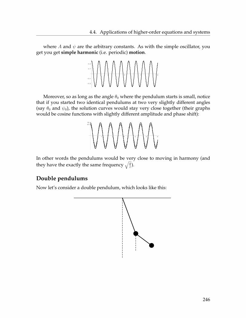
4.4. Applications of higher-order equations and systems
where A and ψ are the arbitrary constants. As with the simple oscillator, youget you get simple harmonic (i.e. periodic) motion.
2 4 6 8
-0.2
-0.1
0.1
0.2
Moreover, so as long as the angle θ0 where the pendulum starts is small, noticethat if you started two identical pendulums at two very slightly different angles(say θ0 and ψ0), the solution curves would stay very close together (their graphswould be cosine functions with slightly different amplitude and phase shift):
1 2 3 4 5 6
θ0ψ0
In other words the pendulums would be very close to moving in harmony (andthey have the exactly the same frequency
√gl).
Double pendulums
Now let’s consider a double pendulum, which looks like this:
246

4.4. Applications of higher-order equations and systems
The double pendulum satisfies the second-order (non-linear) system of ODEs(trust me on this):
(m1 +m2)l1θ′′1 +m2l2 cos(θ1 − θ2)θ′′2 −m2l2 sin(θ1 − θ2)(θ′2)2 + g(m1 +m2) sin θ1 = 0m2l2θ
′′2 +m2l1 cos(θ1 − θ2)θ′′1 −m2l1 sin(θ1 − θ2)θ2
1 +m2g sin θ2 = 0
In this system, g ≈ 9.8 is the gravitational constant, m1 and m2 are the masses atthe ends of the pendulums, and l1 and l2 are the lengths of the pendulums.
Again, this is non-linear, but assuming θ1 and θ2 are small, we can assumesin θj ≈ θj , cos(θ1−θ2) ≈ 1 and sin(θ1−θ2) ≈ 0. This yields the linearized equations
(m1 +m2)l1θ′′1 +m2l2θ′′2 + (m1 +m2)gθ1 = 0 (1)
m2l2θ′′2 +m2l1θ
′′1 +m2gθ2 = 0 (2)
which can be solved via reduction of order, followed by eigentheory/etc. (HW)
It is hopeless to solve the double pendulum equation analytically, so we ap-proximate solutions numerically (using Euler’s method or another method) on acomputer. See the file doublependulum.nb on my webpage for Mathematica codethat will do this.
What’s significant about the double pendulum is that very similar initial valueslead to wildly different behavior.
Trajectories of the double pendulum with m1 = m2 = 1, l1 =√
2, l2 = 1:
θ1(0) = π4 , θ2(0) = π θ1(0) = π
4 , θ2(0) = π − .02 θ1(0) = π4 , θ2(0) = π − .05
-2 -1 1 2
-2.5
-2.0
-1.5
-1.0
-0.5
-2 -1 1 2
-2.5
-2.0
-1.5
-1.0
-0.5
-2 -1 1 2
-2.5
-2.0
-1.5
-1.0
-0.5
The idea of similar initial values leading to wildly different future behavior isthe subject of a branch of mathematics called chaos theory.
247
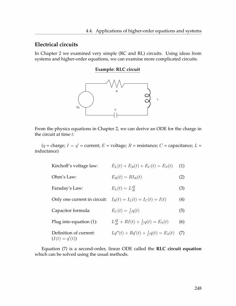
4.4. Applications of higher-order equations and systems
Electrical circuits
In Chapter 2 we examined very simple (RC and RL) circuits. Using ideas fromsystems and higher-order equations, we can examine more complicated circuits.
Example: RLC circuit
ES
R
C
L
From the physics equations in Chapter 2, we can derive an ODE for the charge inthe circuit at time t:
(q = charge; I = q′ = current; E = voltage; R = resistance; C = capacitance; L =inductance)
Kirchoff’s voltage law: EL(t) + ER(t) + EC(t) = ES(t) (1)
Ohm’s Law: ER(t) = RIR(t) (2)
Faraday’s Law: EL(t) = LdIdt
(3)
Only one current in circuit: IR(t) = IL(t) = IC(t) = I(t) (4)
Capacitor formula: EC(t) = 1Cq(t) (5)
Plug into equation (1): LdIdt
+RI(t) + 1Cq(t) = ES(t) (6)
Definition of current: Lq′′(t) +Rq′(t) + 1Cq(t) = ES(t) (7)
(I(t) = q′(t))
Equation (7) is a second-order, linear ODE called the RLC circuit equationwhich can be solved using the usual methods.
248

4.4. Applications of higher-order equations and systems
Note the analogies between this equation and the damped oscillator. Theseconnections reveal some initial parallels between gravitational mechanics and elec-tromagnetism, two of the four fundamental mechanisms in physics (the other twobeing the weak and strong nuclear forces).
Mass-spring system RLC electricalwith damping series circuit
EQUATION mx′′ + bx′ + kx = Fext(t) Lq′′ +Rq′ + 1Cq = ES(t)
SOLVING FOR displacement x charge q
OTHER velocity x′ current I = q′
ANALOGOUS (I = q′)QUANTITIES
mass m inductance L
damping constant b resistance R(from friction)
spring constant k (capacitance)−1 1C
external force Fext(t) voltage source ES(t)
The analogies between these systems are really only seen when you build themathematical models for them. This exemplifies what (higher-level) math is reallyabout: math is really about placing physical (or economic or biological) modelsinto a sufficiently abstract framework so that we can see the similarities (and/ordistinctions) between seemingly different things.
THE END
249

4.5. Final Exam Review
4.5 Final Exam ReviewOn the final exam, you may use: one sheet of paper (max size 8.5” × 11”) withwhatever you want on both sides.
What you should expect to be asked on the final exam: Essentially everything:Theory: Answer questions on course vocabulary and/or concepts (existence/uniqueness,
general vs. particular solution, linear vs. nonlinear, etc.)Qualitiative: Create and/or analyze pictures of vector fields, phase lines, phase
planes, etc.; compute and classify equilibria for equations and/or systemsNumerical: Euler’s method for single equations and/or systemsAnalytic: Solve ODEs and/or systems of ODEs, using the various methods dis-
cussed during the semesterApplications: Set up and/or solve story problems involving ODEs and/or sys-
tems of ODEsIncluding: population models, heating and cooling problems, tank problems, predator-prey models, SIR models, mass-spring systems, pendulums, RC, RL and RLC elec-trical circuits
Practice questions on the material of Chapter 4:
1. a) Why did I say “there is no such thing as a higher-order linear ODE” inclass?
b) What is meant by an “initial value” of a nth-order ODE (or system ofODEs)?
c) What is meant by the phrase “characteristic equation” (in the context ofODEs)?
2. Convert each equation or system to a first-order system of the form y′ =Ay + q. Be sure to clearly define what y, A and q are.
a) y′′′ + 5ty′′ − 2t2y′ = 7et
b)x′′ + x′ − 2y′ + 5x− 6y = 0x′′ − y′′ − x′ + 3x− y = 0
3. Find the general solution of each system:
a) y′′ − 3y′ − 40y = 0b) y(4) + 9y(3) + 18y′′ = 0c) y′′ − 4y′ + 10 = 0d) 2y′′ + 32y′ + 128y = 5e−2t
e) y′′ − 7y′ − 44y = 1037 sin t
250
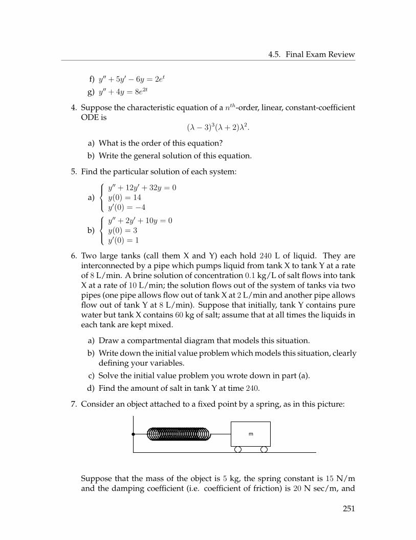
4.5. Final Exam Review
f) y′′ + 5y′ − 6y = 2et
g) y′′ + 4y = 8e2t
4. Suppose the characteristic equation of a nth-order, linear, constant-coefficientODE is
(λ− 3)3(λ+ 2)λ2.
a) What is the order of this equation?
b) Write the general solution of this equation.
5. Find the particular solution of each system:
a)
y′′ + 12y′ + 32y = 0y(0) = 14y′(0) = −4
b)
y′′ + 2y′ + 10y = 0y(0) = 3y′(0) = 1
6. Two large tanks (call them X and Y) each hold 240 L of liquid. They areinterconnected by a pipe which pumps liquid from tank X to tank Y at a rateof 8 L/min. A brine solution of concentration 0.1 kg/L of salt flows into tankX at a rate of 10 L/min; the solution flows out of the system of tanks via twopipes (one pipe allows flow out of tank X at 2 L/min and another pipe allowsflow out of tank Y at 8 L/min). Suppose that initially, tank Y contains purewater but tank X contains 60 kg of salt; assume that at all times the liquids ineach tank are kept mixed.
a) Draw a compartmental diagram that models this situation.
b) Write down the initial value problem which models this situation, clearlydefining your variables.
c) Solve the initial value problem you wrote down in part (a).
d) Find the amount of salt in tank Y at time 240.
7. Consider an object attached to a fixed point by a spring, as in this picture:
m
Suppose that the mass of the object is 5 kg, the spring constant is 15 N/mand the damping coefficient (i.e. coefficient of friction) is 20 N sec/m, and
251
4.5. Final Exam Review
the entire system (at time t) is subject to no external force. If at time 0, themass has initial velocity 1 m/sec to the right but is 2 m to the left of whereit would be at rest, find the equation of motion of the object. Is this systemoverdamped or underdamped (explain your answer)? Which is the moresignificant part of the system, the frictional force or the harmonics from thespring?
8. Consider an undamped pendulum of length 4.9 m and mass 15 kg.
a) Write the (nonlinear) undamped pendulum equation which governs thismotion.
b) Write the linearization of this undamped pendulum equation.
c) Find the general solution of the linearized equation you wrote in part(b).
9. A series RLC circuit has a constant voltage source of ES(t) = 20 volts, aresistor of 80 Ω, an inductor of 4 H, and a capacitor of 1
1000 F. If the initialcurrent is zero and the initial charge on the capacitor is 4 coulombs:
a) Find the charge in the circuit as a function of time t.
b) Find the current in the circuit as a function of time t.
Solutions
WARNING: as always, these might have errors.
1. a) Every higher-order linear ODE can be converted to a first-order systemof ODEs, so we really only need to know how to solve first-order linearODEs and systems to solve higher-order ODEs.
b) An initial value is a list of values of y, y′, y′′, y′′′, ..., y(n−1) at the same t0.
c) The characteristic equation of the higher-order, constant-coefficient ODEpny
(n)+pn−1y(n−1)+...+p2y
′′+p1y′+p0y = q(t) is the polynomial equation
pnλn + ...+ p2λ
2 + p1λ+ p0 = 0.
2. a) First, rewrite the equation as y′′′ = 2t2y′ − 5ty′′. Then we can let y =
(y, y′, y′′); let q = (0, 0, 7et) and let A =
0 1 00 0 10 2t2 −5t
. Then y′ =
Ay + q as wanted.
b) From the first equation, we know x′′ = −5x + 6y − x′ + 2y′. Next, bymultiplying the second equation by −1 and then adding it to the firstequation, we get y′′ + 2x′ − 2y′ + 2x − 5y = 0, i.e. y′′ = −2x + 5y −
252

4.5. Final Exam Review
2x′ + 2y′. Therefore, we can let y = (x, y, x′, y′); let q = 0 and let A =0 0 1 00 0 0 1−5 6 −1 2−2 5 −2 2
. Then y′ = Ay + q as wanted.
3. a) The characteristic equation is λ2 − 3λ− 40 = (λ− 8)(λ+ 5) so λ = 8 andλ = −5. Thus the general solution is y = C1e
8t + C2e−5t.
b) The characteristic equation is λ4 + 9λ3 + 18λ2 = λ2(λ+ 6)(λ+ 3) so λ = 0(repeated twice), λ = −6 and λ = −3. Thus the general solution isy = C1 + C2t+ C3e
−6t + C4e−3t.
c) The characteristic equation is λ2 − 4λ + 10 so λ = 4±√
16−402 = 4±i2
√6
2 =2±√
6 i. Thus the general solution is y = C1e2t cos(
√6 t)+C2e
2t sin(√
6 t).
d) First, solve the homogeneous equation; the characteristic equation is2λ2 + 32λ + 128 = 2(λ + 8)2 so λ = −8 (repeated twice). Thereforeyh = C1e
−8t + C2te−8t.
Next, find a particular solution using undetermined coefficients: guessyp = Ae−2t and plug in to obtain 8Ae−2t − 64Ae−2t + 128Ae−2t = 5e−2t,i.e. 72A = 5, i.e. A = 5
72 so yp = 572e−2t.
Finally, y = yp + yh = 572e−2t + C1e
−8t + C2te−8t.
e) First, solve the homogeneous equation; the characteristic equation isλ2 − 7λ − 44 = (λ − 11)(λ + 4) so λ = −11 and λ = 4 Thereforeyh = C1e
−11t + C2e4t.
Next, find a particular solution using undetermined coefficients: guessyp = A sin t+B cos t and plug in to obtain (−A sin t−B cos t)−7(A cos t−B sin t)− 44(A sin t+B cos t) = 13 sin t, i.e.
−A+ 7B − 44A = 1037−B − 7A− 44B = 0
so A = −452 , B = 7
2 . Thus yp = −452 sin t+ 7
2 cos t.Finally, y = yp + yh = −45
2 sin t+ 72 cos t+ C1e
−11t + C2e4t.
f) First, solve the homogeneous equation; the characteristic equation isλ2 + 5λ − 6 = (λ + 6)(λ − 1) so λ = −6 and l = 1. Therefore yh =C1e
−6t + C2et.
Next, find a particular solution using undetermined coefficients: guessyp = Atet and plug in to obtain (2Aet+Atet)+5(Aet+Atet)−6Atet = 2et,i.e. 7A = 2, i.e. A = 2
7 . Therefore yp = 27te
t.Finally, y = yp + yh = 2
7tet + C1e
−6t + C2et.
253

4.5. Final Exam Review
g) First, solve the homogeneous equation; the characteristic equation isλ2 + 4 = (λ− 2i)(λ+ 2i) so λ = ±2i. Therefore yh = C1 cos 2t+ C2 sin 2t.Next, find a particular solution using undetermined coefficients: guessyp = Ae2t and plug in to obtain 4Ae2t+4Ae2t = 8e2t, i.e. 8A = 8 so A = 1.Therefore yp = e2t.Finally, y = yp + yh = e2t + C1 cos 2t+ C2 sin 2t.
4. a) Since the characteristic equation has degree 3 + 1 + 2 = 6, this equationhas order 6.
b) y = C1e3t + C2te
3t + C3t2e3t + C4e
−2t + C5 + C6t.
5. a) First, solve the system; the characteristic equation is λ2 + 12λ + 32 =(λ + 8)(λ + 4) so the general solution is y = C1e
−8t + C2e−4t. Now, plug
in the initial values to get14 = C1 + C2−4 = −8C1 − 4C2
and solve to get C1 = −13, C2 = 27. Therefore the particular solution isy = −13e−8t + 27e−4t.
b) First, solve the system; the characteristic equation is λ2 + 2λ + 10 = 0which has solution λ = −2±
√4−40
2 = −2±6i2 = −1 ± 3i. Therefore the
general solution is y = C1e−t cos 3t+C2e
−t sin 3t. Plug in the initial valuesto get
3 = C11 = −C1 + 3C2
so C1 = 3, C2 = 43 . Therefore the particular solution is y = 3e−t cos 3t +
43e−t sin 3t.
6. a)x(t) y(t)
1 y/30x/30
x/120
b) Let x(t) = the amount of salt in tank X at time t, and let y(t) = theamount of salt in tank Y at time t. Then we have the initial value prob-lem
x′(t) = − x30 −
x120 + 1
y′(t) = x30 −
y30
x(0) = 60y(0) = 0
c) We can rewrite the system as y′ = Ay + q where y = (x, y), q = (1, 0)
and A =(−124 0130
−130
). To solve this, first solve the homogeneous system
using eigenvalues and eigenvectors:
det(A− λI) = (−124 − λ)(−1
30 − λ)⇒ λ = −124 ,−130
254

4.5. Final Exam Review
The corresponding eigenvectors (letting v = (x, y) and solvingAv = λv)are:
λ = −124 :
−124 x = −1
24 x130x−
130y = −1
24 y⇒ x− y = −5
4 y ⇒ x = −14 yv = (1,−4)
λ = −130 :
−124 x = −1
30 x130x−
130y = −1
30 y⇒ x = 0⇒ v = (0, 1)
So the general solution of the homogeneous is
yh = C1e−t/24
(1−4
)+ C2e
−t/30(
01
).
Now for the particular solution. Since q has constant entries, guess yp =(AB
). Then, by plugging in the original system we have
0 = −A
24 + 10 = A
30 −B30
Therefore A = B = 24, so yp = (24, 24). Therefore
y = yp + yh =(
2424
)+ C1e
−t/24(
1−4
)+ C2e
−t/30(
01
).
i.e. x(t) = C1e
−t/24 + 24y(t) = −4C1e
−t/24 + C2e−t/30 + 24
Plugging in the initial conditions x(0) = 60, y(0) = 0, we get 60 = C1 +24(i.e. C1 = 26) and 0 = −4C1 + C2 + 24 (i.e. C2 = 80). Therefore theparticular solution is
x(t) = 26e−t/24 + 24y(t) = −104e−t/24 + 80e−t/30 + 24
d) y(240) = −104e−240/24 + 80e−240/30 + 24 = −104e−10 + 80e−8 + 24.
7. Use the oscillator equation:
mx′′(t) + bx′(t) + kx(t) = Fext(t)⇒ 5x′′ + 20x′ + 15x = 0⇒ x′′ + 4x′ + 3x = 0
255
4.5. Final Exam Review
Now solve this; the characteristic equation is λ2 + 4λ + 3 = (λ + 3)(λ + 1)so the general solution is y = C1e
−3t + C2e−t. Plugging in the initial values
x(0) = −2, x′(0) = 1, we get−2 = C1 + C21 = −3C1 − C2
Therefore C1 = 12 and C2 = −5
2 so the particular solution is y = 12e−3t − 5
2e−t.
Last, this system is overdamped since the eigenvalues coming from the char-acteristic equation are real. Since the system is overdamped, the frictionalforce outweighs the harmonics coming from the spring.
8. a) θ′′ + 9.84.9 sin θ = 0
b) θ′′ + 9.84.9θ = 0, i.e. θ′′ + 2θ = 0.
c) The characteristic equation is λ2 + 2 = 0, which has roots λ = ±i√
2.Therefore the general solution is θ = C1 cos(t
√2) + C2 sin(t
√2).
9. a) Start with the RLC circuit equation (q is the charge, and I = q′ is thecurrent):
Lq′′ +Rq′ + 1Cq = ES(t)
4q′′ + 80q′ + 1000q = 20q′′ + 20q′ + 250q = 5
To solve this, start with the characteristic equation λ2 + 20λ + 250 = 0,which has solutions λ = −10 ± i5
√6. Thus the general solution of the
homogeneous is
qh = C1e−10t cos(5
√6 t) + C2e
−10t sin(5√
6 t).
Now we can find the particular solution by guessing qp = A: we get0 + 0 + 250A = 5 so A = 1
50 . That makes the general solution
q(t) = qp + qh = 150 + C1e
−10t cos(5√
6 t) + C2e−10t sin(5
√6 t).
To find the particular solution, plug in the given values q′(0) = 0 andq(0) = 4 to get
4 = 150 + C1
0 = −10C1 + 5√
6C2⇒ C1 = 199
50 , C2 = 19925√
6.
Thus the particular solution, which gives the charge at time t, is
q(t) = 150 + 199
50 e−10t cos(5
√6 t) + 199
25√
6sin(5
√6 t).
256

4.5. Final Exam Review
b) The current is the derivative of the charge:
I(t) = q′(t) = −199√
610 e−10t cos(5
√6 t) + 199
√6
15 e−10t sin(5√
6 t).
257

Appendix A
Homework
Algebra and calculus review
1. Solve for y in terms of t:
a) 1√y+1 = 3t2 + 2
b) 1y
= 2t− 3c) 1
y2 = 1t
+ 2d) arctan y = 5t− 4
2. Solve for y in terms of t:
a) y2 − 2y = t+ 4b) sin 3y = 4 cos t
c) t2 + 2y2 = 8d) ln(y + 1) = ln(t+ 1)− 2
3. Solve for y in terms of t; simplifying your answer as much as possible.
a)√ty = t
b) ln y = 4 ln t+ 3c) ey−2 = 3et−1
d) e3y = et + 1
4. Compute the following limits:
a) limt→∞
et
b) limt→∞
e−2t
c) limt→∞
32+et
d) limt→∞
32+e−t
5. Compute the following limits:
a) limt→∞
(e−3t + 2e−t)
b) limt→∞
sin 2t
c) limt→∞
et sin t
d) limt→∞
e−2t cos t
258

6. Find the derivative of each function:
a) f(t) = 3t2 − 7t+ 5b) f(t) = (t2 + 3)8
c) f(t) = t2e2t + 4te2t
d) f(t) = 4te−t
7. Find the derivative of each function:
a) f(t) = sin 4t b) f(t) = e−t sin 2t
8. Find the derivative of each function:
a) f(t) = sin3(4t2) b) f(t) = e3t cos 4t− 2e3t sin 4t
9. Find the first, second and third derivative of each function:
a) f(t) = e−2t
b) f(t) = sin 4t+ cos 4tc) f(t) = t cos td) f(t) = −te3t + 2e3t
10. Compute the following integrals:
a)∫t dt
b)∫
(3t4 − 2t7) dtc)∫t−1 dt
d)∫t−2 dt
11. Compute the following integrals:
a)∫ 4tdt
b)∫ 1tdt
c)∫ 6t2dt
d)∫ 1√
tdt
12. Compute the following integrals:
a)∫
12√t dt
b)∫ 3√t dt
c)∫
(√t+ 1) dt
d)∫ √
t+ 1 dt
13. Compute the following integrals:
a)∫
2 sin t dtb)
∫(sin 3t+ cos t) dt
c)∫ 1t2+1 dt
d)∫
(11e2t − 18e−3t + 7e−t) dt
14. Compute the following integrals. Your answer will have a t in it.
259

a)∫ t0(2s+ 1) ds
b)∫ t1 2s−1/2 ds
c)∫ t
0 e−s ds
d)∫ t
14sds
15. Compute the following integrals (using integration by parts):
a)∫te−3t dt b)
∫t ln t dt
16. Compute the following integrals:
a)∫ 2t2−4 dt b)
∫sin t cos t dt
17. Compute the following integrals:
a)∫ et
et+1 dt b)∫ et+1
et dt
18. Compute the following integrals:
a)∫ t2+2
(t−1)2 dt b)∫ (t−2)2
tdt
19. Some sequences in mathematics are defined by a method called recursion:this means that each term in the sequence is given by a formula which de-pends on previous terms. For example, suppose you are given
x0 = 3 and xn+1 = 2xn.
Then you can find x1, x2, x3, ... by repeatedly plugging in to the second equa-tion as follows:
x1 = 2x0 = 2(3) = 6x2 = 2x1 = 2(6) = 12x3 = 2x2 = 2(12) = 24
......
In each part of this problem, you are given a recursive formula and a valueof x0. Based on this formula, write down x1, x2, x3, and x4.
a) x0 = 1;xn+1 = −xnb) x0 = 18;xn+1 = 1
3xn + 3c) x0 = 1;xn+1 = 2xn
d) x0 = 3;xn+1 = 2− 12xn
20. Suppose x0 = 0, x1 = 1 and xn+2 = xn+1 + 2xn. Find x7.
260

A.1. Problems from Chapter 1
A.1 Problems from Chapter 1Problems from Section 1.1
21. In each part, you are given an ODE and a possible solution of that ODE.Determine whether or not the possible solution is actually a solution of theODE.
Hint: Plug the possible solution in to both sides of the ODE and see if theyare equal.
a) ODE: dydt
= y2−1t2+2t
Possible solution: y = 2t+ 1b) ODE: y′′ + y = t2 + 2
Possible solution: y = sin t+ t2
c) ODE: d2ydt2− dy
dt= 2y
Possible solution: y = e2t − 3e−t
22. In each part, you are given an ODE and a possible solution of that ODE.Determine whether or not the possible solution is actually a solution of theODE
Hint: To compute derivatives of the possible solutions, differentiate implic-itly.
a) ODE: dydt
= ty
Possible solution: t2 + y2 = 9b) ODE: dy
dt= 2ty
y−1
Possible solution: y − ln y − 1 = t2
23. In each part, you are given an initial value problem and a possible solution ofthat IVP. Determine whether or not the possible solution is actually a solutionof the IVP:
a) IVP:y′ = 6yy(0) = 2
Possible solution: y = 2e6t
b) IVP:y′ = 6yy(0) = −1
Possible solution: y = 2e6t +−3
24. In each part, you are given an initial value problem and a possible solution ofthat IVP. Determine whether or not the possible solution is actually a solutionof the IVP:
a) IVP:y′ = −t
y
y(4) = 3Possible solution: t2 + y2 = 20
b) IVP:y′ = −t
y
y(4) = 3Possible solution: t2 + y2 = 25
261

A.1. Problems from Chapter 1
Problems from Section 1.2
25. Determine whether each of the formulas T given below defines a linear op-erator on C∞(R,R) (no proof is required, just write “linear” or “not linear”):
a) T (y) = y + t
b) T (y) = 4y(7)
c) T (y) = y′′ + ty′ − (3 sin t)yd) T (y) = (y′)2 + 2y − 4y′′
26. Suppose T is the linear differential operator defined by
T (y) = ety′′′ − e−ty′′ + e4ty′ − 2y.
a) What is the order of this opera-tor?
b) Find T (2et).
c) Find T (e2t).
d) Find T (4).
27. Suppose T is the fourth-order linear differential operator defined by settingp0(t) = 2t2, p1(t) = t3, p2(t) = 8t4, p3(t) = 0 and p4(t) = 2t6 and using theformula given in Definition 1.12 of the lecture notes.
a) Write the formula for T (y).b) Find T (2t6).
In each part of Problems 28-31 you are given an ODE. For each equation:(i) give the order of the equation;
(ii) give the number of arbitrary constants you would expect in the general solu-tion;
(iii) classify the equation as linear or nonlinear;(iv) if the equation is linear, determine whether or not it is homogeneous;(v) if the equation is linear, determine whether or not it is constant-coefficient.
28. a) dydt
+ 5tdydt− 3y2 = y7 sin t
b) 4y−cos y3 +y′′′′− t2y′′ = ety′′−y2c) et+y d
2ydt2
+ cos tdydt
= 0
29. a) t2 dydt
+ t4y = 3tdydt− 2t
b) y8 + y′ = e3tc) y(8) + y′ = e3t
30. a) 2y d2ydt2− y2 dy
dt= 0
b) et d2ydt2
+ cos tdydt
= 0c) 2d3y
dt3+ 4d2y
dt2− 8dy
dt+ 6y = 0
262

A.1. Problems from Chapter 1
31. a) 8y′′ − 5y′ + 3y = 6ty′′
b) y(4) + y′′′ + y′′ + y′ + y = etc) y′
y= 2
Problems from Section 1.3
32. Suppose that some quantity is changing as time passes so that the rate ofincrease of the quantity is equal to 4.7 times the size of the quantity.
a) Write the ODE represented by this model.
b) Write the general solution of this ODE.
c) Write the particular solution of this ODE corresponding to the situationwhere you start with 5 units of the quantity.
d) Write the particular solution of this ODE corresponding to the situationwhere at time 3, you have 12 units of the quantity.
33. Suppose that y(t) is some quantity which grows at a rate proportional to itssize.
a) Suppose that initially, I have exactly twice as much of the quantity asyou do. After 50 years, will I have more than twice as much as you, ex-actly twice as much as you, or less than twice as much as you? Explain.
b) Suppose that initially, I have exactly one more unit of the quantity thanyou do (we both have a positive amount). After 50 years, will the dif-ference between our holdings be greater than one, equal to one, or lessthan one? Explain.
34. The amount of money in a retirement account grows proportionally to theamount of money in the account. Suppose initially that there is $100 in theaccount, and that five years later, there is $118 in the account.
a) Find a formula for the amount of money y = y(t) in the account t yearsafter the account is opened.
b) Find the (exponential) rate of growth of the account, expressed as anannual percentage rate.
c) Find the amount of money in the account thirty-five years after it isopened.
35. The half-life of a substance which decays exponentially is the amount of timeit takes for the substance to decay to half of its original amount. Carbon-14has a half-life of 5730 years.
a) Find the (exponential) rate of decay of carbon-14.
263

A.1. Problems from Chapter 1
b) If you have 25 grams of carbon-14 now, how much will you have 20000years from now? (A decimal approximation is OK.)
c) If you wanted to have 5 g of carbon-14 10000 years from now, how muchshould you start with now? (A decimal approximation is OK.)
Problems from Section 1.4
36. Consider the ODE y′ = t− 2y.
a) Find four points (t, y) where y′ = 0.
b) Find y′ at the points (2, 3), (0, 3), (0,−2), (2, 2), (−2, 0), (−1, 0), and (−2, 1).
c) Sketch the mini-tangent lines corresponding to the points used in parts(a) and (b). (There should be one picture with all the mini-tangents onit.)
37. Consider the ODE y′ = 135 (y4 + y3 − 20y2).
a) Use Mathematica to draw a picture of the slope field associated to thisODE, in the viewing window [−8, 8] × [−8, 8]. Attach a printout of thispicture; please label the picture “37”.
b) Find the equation of three explicit solutions to this ODE.
c) Let g(t) be the solution to this ODE passing through (−2,−3).
i. Find limt→∞
g(t).
ii. Find limt→−∞
g(t).
d) Sketch (by hand) the graph of the solution to this ODE satisfying y(2) =4 on the picture you printed in part (a).
38. Consider the ODE y′ = 110 (y3 − ty2 + 2y2 − 9y + 9t− 18), and let h(t) be the
solution to this ODE satisfying h(0) = 1.
a) Use Mathematica to draw a picture of the slope field associated to thisODE, in the viewing window [−6, 10] × [−8, 8], with the stream line forh shown. Attach a printout of this picture; please label the picture “38”.
b) Estimate h(3) and h(5).
c) Estimate h′(2).
d) Estimate all t > 0 (if any) for which h(t) = 2.
e) Estimate all t > 0 (if any) for which h(t) = 6.
f) Find limt→∞
h(t).
g) Find limt→−∞
h(t).
264
A.1. Problems from Chapter 1
39. Consider the initial value problemy′ = y − arctan ty(0) = y0
where y0 is a constant.
a) Use Mathematica to draw a picture of the slope field associated to thisODE, in the viewing window [0, 10] × [−5, 5], with several stream linesshown. Attach a printout of this picture; please label the picture “39”.
b) Suppose you knew that y0 was between 1.5 and 2.5. Is this informationsufficient to describe the qualitative behavior of y for large t (i.e. to findlimt→∞
y(t))? Explain.
c) Suppose you knew that y0 was between 0 and 1. Is this informationsufficient to describe the qualitative behavior of y for large t (i.e. to findlimt→∞
y(t))? Explain.
Problems from Section 1.5
40. Consider the initial value problemy′ = 5 + 2t− 3yy(0) = 5 .
Perform Euler’s method by hand (show your work) to compute (t1, y1), (t2, y2),(t3, y3) and (t4, y4) for ∆t = 1.
41. Consider the initial value problemy′ = 1
2 − t+ 2yy(0) = 2 .
Perform Euler’s method by hand (show your work) to estimate y(2), usingfour steps.
42. Consider the initial value problemy′ = 5− 3√yy(0) = 2 .
a) Use Mathematica to implement Euler’s method to estimate y(3), using∆t = .01.
b) Attach a printout of the graph of the points obtained from Euler’s methodin part (a). Label the picture “42”.
265

A.1. Problems from Chapter 1
43. Consider the initial value problemy′ = 4−ty
1+y2
y(0) = 3 .
a) Use Mathematica to implement Euler’s method to estimate y(60) using300 steps.
b) Attach a printout of the graph of the points obtained from Euler’s methodin part (a). Please label the picture “43 (b)”.
c) Based on the picture you get in part (b), do you trust your answer frompart (a)? Why or why not?
d) Use Mathematica to implement Euler’s method to estimate y(60) using3000 steps.
e) Attach a printout of the graph of the points obtained from Euler’s methodin part (d). Please label the picture “43 (e)”.
f) Based on the picture you get in part (e), do you trust your answer frompart (d)? Why or why not?
g) (Optional; extra credit) Explain thoroughly why you got the picture youdid in part (b). (Saying “I didn’t use enough steps” is insufficient; youneed to describe the particular properties of the vector field of this ODEthat lead to the specific picture you get in part (b).)
Problems from Section 1.6
44. Consider the initial value problemy′ = 1− y3
y(0) = 0 .
a) Use Picard’s method of successive approximations, with f0(t) = 0, tofind f1(t), f2(t), and f3(t).
b) Graph f3 (for t ≥ 0 only) as obtained in part (a). If you use a Mathematicagraph, label it as “44 (b)”.
c) Plot the vector field associated to this ODE (viewing window [0, 4] ×[0, 4]) with the stream line passing through the given initial value; labelthe picture “44 (c)”.
d) Based on your pictures, would you say that the function f3 obtained inpart (a) is, or is not, a good approximation of the solution y = f(t) of theIVP?
e) Would it be reasonable to estimate y(4) by computing f3(4)? Why orwhy not?
266

A.1. Problems from Chapter 1
45. Consider the initial value problemy′ = −y − 1y(0) = 0 .
a) Use Picard’s method of successive approximations, with f0(t) = 0, tofind f1(t), f2(t), f3(t) and f4(t).
b) Based on your answers to part (a), write f(t) = limj→∞
fj(t) as an infinite
series.
c) Recognize the infinite series from part (b) as being related to a “com-mon” one, and find a formula for f(t).Hint: the series you get will probably have initial index 1, not 0. Takethis into account.
Problems from Section 1.7
In problems 46-50, assume that this is the phase line of some autonomous ODEy′ = φ(y):
-7 -2 3 6
46. a) Write the equation of one explicit solution of this ODE.
b) Find all sinks of this ODE (if there aren’t any, say so).
c) Find all unstable equilibria of this ODE (if there aren’t any, say so).
d) Find all semistable equilibria of this ODE (if there aren’t any, say so).
47. a) Suppose y(0) = 0. Find limt→∞
y(t).
b) Suppose y(0) = −10. Find limt→∞
y(t).
c) Suppose y(2) = 5. Find limt→−∞
y(t).
d) Suppose y(−1) = 6. Find limt→−∞
y(t).
48. a) Suppose y(0) = 4. Is y(t) an increasing function or decreasing function?
b) Suppose y(0) = y0. For what values of y0 is limt→∞
y(t) = −2?
c) Suppose y(0) = y0. For what values of y0 is limt→∞
y(t) > 0?
49. a) Sketch a (possible) graph of the function φ.
b) Sketch a (possible) slope field for this ODE.
267

A.1. Problems from Chapter 1
c) Sketch a graph of the particular solution of this ODE whose initial con-dition is y(1) = 0.
d) (Optional; extra credit) Write down a formula for φ which would pro-duce the phase line shown before Problem 46.
50. For each quantity, determine whether the quantity is positive, negative orzero:
Hint: Your answer to Problem 49 (a) may be helpful.
a) φ(−7)b) φ(0)
c) φ(4)d) φ′(−2)
e) φ′(3)f) φ′(6)
In each part of Problems 51-54, you are given an autonomous equation. For eachequation:
(i) find all equilibria of the equation;(ii) classify each equilibrium as stable, unstable or semistable;
(iii) sketch the phase line of the equation.
51. a) y′ = y2 − 9 b) dydt
= 2 cos y
52. a) y′ = ey − 1 b) y′ = e−2y − 1
53. a) dydt
= 2y ln(6/y) b) y′ = y3(y − 2)2(y + 3)(y − 5)
Hint: In part (b) of Problem 53, graph the function, and estimate the valuesof its derivative at the equilibria by looking at the graph.
54. y′ = φ(y), where φ is a function whose graph is as follows:
-4 -3 -2 -1 1 2 3 4y
-6
-5
-4
-3
-2
-1
1
2
3
4
5
6
7
8ϕ(y)
55. Suppose that the population y of a certain species of fish in a given area ofthe ocean (i.e. in a “fishery”) would be described by a logistic equation, ifthere was no fishing. Since fish are delicious, we want to catch some of thesefish so we can eat them. But if we catch too many fish, the population may be
268

A.1. Problems from Chapter 1
driven to extinction. That would be bad. This question deals with a modelfor managing the fishery (which is actually used in the real world, by theway).
Let E be a constant which denotes the level of effort being put into fishing(the greater E is, the harder people work at catching fish). It is reasonable toassume that the rate at which they catch fish depends on the fish populationy (because the more fish there are, the easier to catch them). So a simpleexpression which can be used to describe the rate at which fish are caughtis E times y. To model the fish population including this effect, you adaptthe logistic equation by subtracting the rate at which fish are caught, leadingto what is called the Schaefer model, used in biology and environmentalscience. Here is that model:
dy
dt= ry(L− y)− Ey.
a) Find the two equilibria of this equation (in terms of the constants r, Land E).
b) Suppose E < Lr. What will the fish population be in the long run?Explain.Hint: This has something to do with whether or not the equilibria youfound in part (a) are stable or unstable.
c) Suppose E > Lr. What will the fish population be in the long run?Explain.
d) A sustainable yield Y of the fishery is a quantity of fish that can becaught indefinitely. It is the product of the effort E and the stable equi-librium fish population corresponding to effort E. Find Y as a functionof E (this is called the yield-effort curve).
e) Determine the value of E which maximizes Y (and thereby producesthe maximum sustainable yield).Hint: Maximize the function Y (E) using the method you learn in Calcu-lus 1.
Problems from Section 1.8
In Questions 56 and 57, use the following bifurcation diagram for a parameterizedfamily of ODEs y′ = φ(y; r):
269

A.1. Problems from Chapter 1
-10 -9 -8 -7 -6 -5 -4 -3 -2 -1 1 2 3 4 5 6 7 8 9 10
-10
-9
-8
-7
-6
-5
-4
-3
-2
-1
1
2
3
4
5
6
7
8
9
10
56. a) Find all values of r (if any) at which the family has a saddle-node bifur-cation.
b) Find all values of r (if any) at which the family has a transcritical bifur-cation.
c) Find all values of r (if any) at which the family has a pitchfork bifurca-tion.
d) Sketch the phase line corresponding to the equation where r = 2.e) Find all equilibria corresponding to the situation where r = 6, and clas-
sify them as stable, unstable or semistable.f) Suppose r = −2 and y(0) = 1. Find lim
t→∞y(t).
57. a) Suppose you know that r is somewhere between 5 and 7 and that y(0) >0. Can you accurately predict the long-term behavior of y(t)? If so, whatis this behavior? If not, why not?
b) Suppose you know that r is somewhere between −7 and −6 and thaty(0) is somewhere between 1 and 5. Can you accurately predict the long-term behavior of y(t)? If so, what is this behavior? If not, why not?
c) Suppose you know that r is somewhere between 5 and 7 and that y(0) =−5. Can you accurately predict the long-term behavior of y(t)? If so,what is this behavior? If not, why not?
In each part of Problems 58-61 you are given a parameterized family of ODEs (r isthe parameter). For each parameterized family of ODEs:
(i) find all value(s) of r at which bifurcations occur;(ii) classify each bifurcation as saddle-node, pitchfork, transcritical or degener-
ate;(iii) sketch a bifurcation diagram for the family.
270

A.2. Problems from Chapter 2
58. a) y′ = y2 + 6y + r b) y′ = y2 − r2
59. a) y′ = y + ry1+y2 b) y′ = (y2 − r)(y2 − 16)
60. (Optional; extra credit) y′ = ry + y3 − y5
61. y′ = f(y) + r, where f has the graph given below:
-4 -3 -2 -1 1 2 3 4y
-4
-3
-2
-1
1
2
3
4f(y)
Hint: As r changes, how does the graph of f(y) + r change? What changes inthis graph “cause” a bifurcation?
A.2 Problems from Chapter 2Problems from Section 2.1
62. Find the general solution of each ODE:
a) y′ − 2y = 0 b) 7y′ = y
63. Find the general solution of each ODE:
a) y′ = y√t b) dy
dt= y cos t
64. Find the particular solution of each IVP:
a)y′ ln t = y
t
y(e) = 3 b)y′et + y′ = yet
y(0) = 4
65. Suppose you know that y = 6e4t sin 2t is a solution to some homogeneous,linear, first-order ODE.
271
A.2. Problems from Chapter 2
a) Is y = 9e4t sin 2t also a solution of this ODE? Why or why not?
b) Is y = 6e3t sin 2t also a solution of this ODE? Why or why not?
Problems from Section 2.2
66. Solve each given differential equation or initial value problem, using themethod of integrating factors:
a)y′ − 2y = 3ety(0) = 4
b) dydt
= te−t + 1− y
67. Solve each given differential equation or initial value problem, using themethod of integrating factors:
a) ty′ − y = t2e−t b)t3y′ + 4t2y = e−t
y(−1) = 0
68. Solve each given differential equation or initial value problem:
a)y′ = cos t−2ty
t2
y(π) = 0b) tdy
dt+ 2y = sin t
Problems from Section 2.3
69. Suppose you have a first-order linear ODE, where y = 3e2t sin 2t is a solutionof the equation and y = 2e4t sin 2t is a solution of the corresponding homoge-neous equation. Write the general solution of the ODE.
70. Solve each given differential equation or initial value problem, using themethod of undetermined coefficients:
a) y′ + 3y = e−2tb)
y′ − 4y = 2 cos 2ty(0) = −3
71. Solve each given differential equation or initial value problem, using themethod of undetermined coefficients:
a)y′ + y = te2t
y(0) = 24b) y′ − 4y = 2t2 + 8t
72. Consider the ODE y′ + 7y = 20e−7t.
a) Find a nonzero solution of the corresponding homogeneous equation.
272

A.2. Problems from Chapter 2
b) Try the method of undetermined coefficients with guess yp = Ae−7t.Does this work? Explain.
c) Try the method of undetermined coefficients with guess yp = Ate−7t.Does this work? Explain.
d) Solve the ODE y′ − 3y = 9e3t, by first solving the corresponding homo-geneous equation and then using the method of undetermined coeffi-cients. To find the appropriate formula to guess for yp, use the previousexample in this question as a guide.
e) For each given ODE:(i) find the solution yh of the corresponding homogeneous equation;
and(ii) write down what you would need to guess for yp to utilize the method
of undetermined coefficients.You do not need to solve the equation.
i. y′ + 6y = e4t
ii. y′ + 6y = e−6tiii. y′ + 6y = e2t
iv. y′ − 2y = e2t
f) Write down a general rule which tells you when your “normal” guesswon’t work (when attempting the method of undetermined coefficients),and how to adapt your guess so that it will work.You are responsible for implementing this rule on Exam 1.
Problems from Section 2.4
73. Find the general solution of each ODE:
a) y′ =√y(t+ 1) b) dy
dt= sec y sin t
74. Find the general solution of each ODE:
a) y′ = t2
y(4+t3) b) ty′ = 1− y2
75. Find the general solution of each ODE; write your answer as a function y =f(t).
a) eyy′ = 4 b) dydt
= (y sec t)2
76. Find the particular solution of each initial value problem; write your answeras a function y = f(t):
273

A.2. Problems from Chapter 2
a)
dydt
= 1−2ty
y(1) = −2b)
yy′ = 4ty(1) = −3
77. a) Solve the following initial value problem:
2(y − 1)y′ = et
y(0) = 2b) (Optional; extra credit) Write your answer to part (a) as a function y =
f(t), simplified as much as possible.
78. Let y = f(t) be the solution of the initial value problemy′ = ty2 − 2y2
y(0) = 1 .
Find f(4).
Problems 79-82 introduce some methods to solve second-order ODEs. A second-order ODE always has the form
φ(t, y, y′, y′′) = 0 a.k.a. φ(t, y,
dy
dt,d2y
dt2
)= 0.
I haven’t said anything in class about how to solve second-order ODEs, but in twospecial cases you can use a trick, together with our techniques for solving first-order ODEs, to solve a second-order equation. You should be able to solve thesetypes of second-order equations on Exam 1.
• Case 1: The equation has no y in it, i.e. the equation is of the form
φ(t, y′, y′′) = 0.
To solve this, let v(t) = y′. Then y′′ = v′(t) so by substituting v for y′ and v′
for y′′, the equation can be rewritten as φ(t, v, v′) = 0. This rewritten equationis first-order! Solve it for v, then integrate v to get the solution y(t) =
∫v(t) dt
of the original second-order equation.
• Case 2: The equation has no t in it, i.e. the equation is of the form
φ(y, y′, y′′) = 0 a.k.a. φ(y,dy
dt,d2y
dt2
)= 0.
To solve this, pretend y is an independent variable and let v = v(y) = dydt
.Then
d2y
dt2= d
dt
(dy
dt
)= d
dt(v(y)) = dv
dy· dydt
= dv
dyv.
This means you can replace dydt
with v and d2ydt2
with dvdyv in the original equation
to get
φ
(y, v,
dv
dyv
)= 0.
274

A.2. Problems from Chapter 2
This is a first-order equation in v, which can be solved by usual methods tofind v = v(y). Then solve the equation dy
dt= v(y) (this equation is usually
separable) to find y in terms of t.
In Problems 79-82, solve the given second-order ODE or IVP. Write your final an-swer in the form y = f(t).
79. a) td2ydt2
= 2dydt
+ 2 b) ty′′ey′ = ey′ − 1
80. a)
d2ydt2
+ 2(dydt
)2tan y = 0
y(0) = 0y′(0) = 1
b) y′′ = −2t(y′)2
81. a) y′′ = −y b) (y2 + 1)y′′ = 2y(y′)2
Hint: In part (a), you will need the following integration rule, which you canuse without proof: ∫ 1√
C − y2 dy = arcsin(
y√C
)+D.
82. a) y′′ − 2y′ = 12 sin t b) y′′ + 4y′ = 10e3t
Hint: Combine this new technique with the method of undetermined coeffi-cients.
Problems from Section 2.5
83. Determine whether or not each of the given differential equations is exact. Ifthe equation is exact, find its solution.
a) (2t+ 3) + (2y − 2)dydt
= 0b) (2t+ 4y) + (2t− 2y)y′ = 0c) (et cos y + 2 cos t)dy
dt+ et sin y − 2y sin t = 0
d) y′ = et sin y+3y3t−et sin y
84. Find the solution of each initial value problem:
a)
2t− y + 2yy′ − ty′ = 0y(1) = 3
b)
yt
+ 6t+ (ln t)y′ = 0y(1) = 7
Note: this IVP could also be written as yt
+ 6t+ (ln t)y′ = 0, y(1) = 7.
275

A.2. Problems from Chapter 2
85. Consider the differential equation y + (2t− ey)y′ = 0.
a) Show this equation is not exact.
b) Show that after you multiply through the entire equation by y, the equa-tion becomes exact.
c) Solve the equation.
86. (Optional; extra credit) Find the general solution of the differential equation
(t+ 2) sin y + t cos ydydt
= 0.
Hint: You have to figure out something to multiply the equation through byto make the equation become exact.
Problems from Section 2.6
In Problems 87-92, use the following setup: A nitric acid solution flows at a con-stant rate of 6 L/min into a large tank that initially holds 200 L of a 0.5% nitric acidsolution. The solution inside the tank is kept well stirred, and flows out of the tankat a rate of 8 L/min. The solution entering the tank is 20% nitric acid. Let y(t) bethe amount (i.e. volume) of nitric acid in the tank at time t (where t is in minutes).
87. a) Determine the volume of solution in the tank as a function of t.Hint: The tank starts with 200 L of solution; 6 L of solution flows in perminute and 8 L of solution flows out per minute.
b) Draw a compartmental diagram (with boxes and arrows) representingthis situation (the compartment should be y(t)).WARNING: The “rate out” is tricky. To get this, you have to multiplythe rate at which fluid flows out of the tank by the concentration of fluidin the tank; the concentration of fluid in the tank has to take into accountthe fact that the volume of fluid in the tank is not constant.
c) Write an initial value problem which models this setup.
d) Using the initial value problem you wrote in part (c), use Euler’s methodwith ∆t = 1 to estimate the amount of fluid in the tank at time 60.
e) Using the initial value problem you wrote in part (c), use Euler’s methodwith ∆t = .001 to estimate the amount of fluid in the tank at time 60.
88. a) Use Mathematica to sketch the slope field for this differential equation,with the stream line corresponding to y(t) included. Use the viewingwindow [−5, 100] × [−5, 50]. Attach a printout of your slope field, la-belled as “88 (a)”.
276
A.2. Problems from Chapter 2
b) Based on your slope field, estimate the amount of nitric acid in the tankat time 20.
c) Based on your slope field, estimate all times t where there is exactly 10L of nitric acid in the tank.
d) Based on your slope field, estimate the maximum amount of nitric acidthat is in the tank at any one instant.
e) Based on your slope field, estimate the time when the amount of nitricacid in the tank is maximized.
89. Solve the IVP of Problem 87 (c), writing your answer in the form y = f(t).
Hint: Use integrating factors.
90. a) Have Mathematica sketch the graph of the solution you obtain in Prob-lem 89 (where 0 ≤ t ≤ 100). Attach a printout of this graph, labelledas “90 (a)”. (Check that the graph you get is consistent with the pictureyou obtained in Problem 88 (a); if it isn’t, something is wrong.)
b) Use your answer to Problem 89 to find the exact value of y(60).c) Find a decimal value of the value of y(60), and compare it to what you
got in parts (d) and (e) of Problem 87. Were those estimates accurate?d) (Optional; extra credit) Find the exact answers (not decimal approxima-
tions) to the questions asked in parts (d) and (e) of Problem 87.
91. a) Find a formula for the concentration of nitric acid at time t.Hint: This is tricky, because you have to divide the amount of nitric acidin the tank by the volume, and unlike the example in class, the volumeof solution in the tank is not a constant.
b) Have Mathematica sketch the graph of the function you obtain in part (a)(where 0 ≤ t ≤ 100). Attach a printout of this graph, labelled as “91 (b)”.
c) From the graph produced in part (b), estimate the first time t when thesolution in the tank is 10% nitric acid.
d) (Optional; extra credit) Find the exact value of the first time at whichthe solution in the tank is 10% nitric acid.
92. Suppose you wanted to know how much nitric acid was in the tank at time150. I claim that this is not computable by figuring y(150). Why not? What isthe amount of nitric acid in the tank at time 150? What is the concentrationof nitric acid in the tank at time 150? Explain your answers.
In Problems 93-96, use the following setup: A parachutist has mass 75 kg. Shejumps out of a helicopter (assume her initial velocity is 0) which is 2000 m abovethe ground, and falls toward the ground under the influence of two forces: gravity(which is 9.8 m/sec2) and air resistance (drag coefficient 30 N sec/m).
277

A.2. Problems from Chapter 2
93. a) Draw a free body diagram representing this situation.b) Write an initial value problem which models this situation. Set the prob-
lem up so that v > 0 corresponds to downward motion.c) Sketch the phase line for the equation you wrote in part (b).d) What is the terminal velocity of the parachutist (assuming she never
pulls her rip cord)?e) Use Mathematica to sketch the slope field for this differential equation,
with the stream line corresponding to v(t) included (use the viewingwindow [−5, 50]×[−5, 50]). Attach a printout of your slope field, labelledas “93 (d)”.
94. a) Solve the IVP you wrote down in Question 93 (b).b) Use Mathematica to sketch the graph of v(t) (use the viewing window
[−5, 50] × [−5, 50]). Attach a printout of this graph, labelled as “94 (b)”.(Check that this graph is consistent with the slope field obtained in Prob-lem 93 (e); if it isn’t, something is wrong.)
95. a) Find a formula which gives the parachutist’s height above the groundat time t.Hint: In Problem 94 (a), you found the parachutist’s velocity at time t.You know what the parachutist’s height at time 0 is (that is given in thesetup). How do you get from an object’s velocity back to its position(the parachutists’ height is like her position)?WARNING: Keep in mind that v > 0 corresponds to the parachutistfalling, given how we have set this problem up.
b) Her parachute is set to open automatically when her velocity reaches 20m/sec. How many seconds after she jumps out of the helicopter willher parachute open? (A decimal answer is OK; it might be useful tohave Mathematica solve an equation here.)
c) How high above the ground will she be when her parachute opens?(Again, a decimal answer is OK.)
96. (Optional; extra credit)
a) After the parachutist’s chute opens, assume that the forces affecting hervelocity are gravity (still 9.8 m/sec2) and air resistance (but now, thedrag coefficient is 90 N sec/m rather than 30 because the chute providesgreater air resistance).How many seconds after her parachute opens will she hit the ground?(A decimal answer is OK.)Hint: To solve this question, you need to write an appropriate initialvalue problem, and then solve it.
278

A.3. Problems from Chapter 3
b) What will her velocity be when she hits the ground? (A decimal answeris OK.)
c) Graph the parachutist’s velocity against elapsed time, starting at t = 0(when she jumps out of the helicopter) and ending when she hits theground.
97. A bottle of champagne is originally at room temperature (70). It is chilledin ice (32). Suppose that it takes 15 minutes for the champagne to chill to60. How long (including the original 15 minutes) will it take for the wineto reach 46? (A decimal answer is OK, but you need to actually solve theequation... don’t rely on pictures or Euler’s method.)
Hint: This is a heating and cooling problem with U(t) = H(t) = 0, so this isclosely related to Example 1 on page 92 of the lecture notes.
98. Choose one of problems (a), (b):
a) An RC electrical circuit (see page 96 of the lecture notes) with a 1 Ω re-sistor and a 10−4 F capacitor is driven by a voltage ES(t) = sin 2t V. If theinitial capacitor voltage is zero, find:
i. the voltage across the capacitor at time t;ii. the voltage across the resistor at time t (to get this, apply Kirchoff’s
voltage law to the answer to (i); andiii. the current at time t (to get this, apply Ohm’s law to the answer to
part (ii).b) An RL electrical circuit (see page 97 of the lecture notes) with a 1 Ω resis-
tor and a .01 H inductor is driven by a generator whose voltage at timet is ES(t) = sin 2t V. If the initial current across the inductor is 0, find:
i. the current at time t;ii. the voltage across the resistor at time t (to get this, apply Ohm’s Law
to the answer to (i); andiii. the voltage across the inductor at time t.
A.3 Problems from Chapter 3Problems from Section 3.1
99. In each part, you are given a system of first-order ODEs and a possible solu-tion of that system. Determine whether or not the possible solution is actually
279

A.3. Problems from Chapter 3
a solution of the system.
a)x′(t) = 3x− 2yy′(t) = 2x− 2y POSSIBLE SOL’N:
x(t) = 8e2t + e−t
y(t) = 4e2t + 2e−t
b)x′(t) = x+ 3yy′(t) = −4x− y POSSIBLE SOL’N:
x(t) = 2 cos 11t+ 2 sin 11ty(t) = −8 sin 11t
100. In each part, you are given an IVP, together with a possible solution. Deter-mine whether or not the possible solution is actually a solution of the IVP.
a) IVP:
x′(t) = 2yy′(t) = x− y
y(0) = (2,−3)POSSIBLE SOL’N:
x(t) = 2
3e−2t − 2
3et
y(t) = −23 e−2t − 1
3et
b) IVP:
x′(t) = 2yy′(t) = x− y
y(0) = (2,−3)POSSIBLE SOL’N:
x(t) = 8
3e−2t − 2
3et
y(t) = −83 e−2t − 1
3et
101. In each part, you are given a set of parametric equations y(t). For each set ofparametric equations:
(i) Write the set of parametric equations out, coordinate by coordinate (seethe answers if you don’t understand what this means).
(ii) Find the values of y(0), y(1) and y(2).
a) y(t) = (t2 − 2, t+ 3) b) y(t) = (2t, 5t,−7t)
In each part of Problems 102-104, you are given a set of two parametric equationsof the form y(t) = (x(t), y(t)). For each set of parametric equations:
(i) Use the following command in Mathematica to sketch the graph of these para-metric equations in the xy-plane:
ParametricPlot[formula for x(t), formula for y(t),t, -100, 100, PlotRange -> xmin, xmax, ymin, ymax]
This command plots the graph of the parametric equations in the viewingwindow [xmin, xmax] × [ymin, ymax]. You are responsible for choosing anappropriate viewing window for each set of equations (I’d start with [−10, 10]×[−10, 10] and then zoom in or out as necessary).
(ii) Print the graph you get in Mathematica (labelling it with the problem num-ber/letter).
(iii) On the graph you print, draw (by hand) an arrow on the curve indicating thedirection of motion.
280

A.3. Problems from Chapter 3
(iv) Indicate (by hand) the point on the graph corresponding to t = 0 by drawinga thick point and labelling that point “t = 0”.
102. a) y(t) = (cos t, sin t) b) y(t) = (et, 3e−t)
Hint: In Mathematica, e is E, not e.
103. a) y(t) = (et cos 2t, et sin 2t) b) y(t) = (−2 sin 3t, cos 3t)
104. a) y(t) = (3et, e2t) b) y(t) =(
4et+e−t
10 , 2et−5e−t
10
)Problems from Section 3.2
105. Consider the initial value problemx′ = x− yy′ = 2x+ y
y(0) = (2, 1).
Perform Euler’s method by hand (show your work), to compute the points(t1,y1), (t2,y2) and (t3,y3) when ∆t = 1.
106. Consider the initial value problemx′ = −yy′ = x
y(0) = (3, 0).
Perform Euler’s method by hand (show your work) to estimate y(2), usingfour steps.
107. Consider the initial value problemx′ = x+ 2yy′ = −3x+ y
y(0) = (−2, 1).
Use Mathematica to implement Euler’s method to estimate y(4), using 1000steps.
108. Consider the initial value problemx′ = −4x− 8yy′ = 8x+ 4y
y(0) = (1, 1).
281

A.3. Problems from Chapter 3
a) Use Mathematica to implement Euler’s method to estimate y(30), using10000 steps.
b) Attach a printout of the graph of the points obtained from Euler’s methodin part (a) (use the viewing window [−10, 10] × [−10, 10]). Label thegraph “108 (b)”.
c) Based on the picture you get in part (b), describe (in your own words)the qualitative behavior of the solutions as t increases.
109. Consider the initial value problemx′ = −3x− 6yy′ = 6x− 3y
y(0) = (−8, 7).
a) Use Mathematica to implement Euler’s method to estimate y(50), using1000 steps.
b) Attach a printout of the graph of the points obtained from Euler’s methodin part (a) (use the viewing window [−10, 10] × [−10, 10]). Label thegraph “109 (b)”.
c) Based on the picture you get in part (b), describe (in your own words)the qualitative behavior of the solutions as t increases.
110. Consider the initial value problemx′ = −y − zy′ = xz′ = x− z
y(0) = (1, 2,−1)
.
a) Use Mathematica to implement Euler’s method to estimate y(5), using 5steps.
b) Use Mathematica to implement Euler’s method to estimate y(5), using100 steps.
c) Based on what you get in part (b), would you say your answer to (a) isaccurate? Why or why not?
d) Use Mathematica to implement Euler’s method to estimate y(5), using1000 steps.
e) Based on what you get in part (d), would you say your answer to (b) isaccurate? Why or why not?
f) Use Mathematica to implement Euler’s method to estimate y(5), using10000 steps.
282

A.3. Problems from Chapter 3
g) Use Mathematica to implement Euler’s method to estimate y(5), using100000 steps. (This took my computer 34 seconds to run.)
h) Suppose you needed an approximation of y(5) correct to two decimalplaces. Based on what you have done in this problem, is it sufficient touse Euler’s method with 10000 steps? Explain.
i) If you needed an approximation of y(5) correct to three decimal places.Based on what you have done in this problem, is it sufficient to useEuler’s method with 10000 steps? Explain.
Problems from Section 3.4
In Problems 111-117, use the following matrices and vectors to compute the indi-cated quantities. If the quantity does not exist, just write “does not exist”.
A =(
5 −21 3
)B =
(−3 −10 4
)C =
(4 2−8 −4
)D =
(2 00 −1
)
G =
1 −3 02 2 −54 1 −2
H =
4 0 00 1
2 00 0 −2
J =
1 0 00 −1 00 0 −1
K =
(cos 2t sin 3t
4 sin 2t − sin 3t
)x = x(t) = (et cos t, et sin t) z = z(t) = (sin t, 2 cos 3t, 4e7t)
111. a) the trace of C
b) the trace of G
c) 3Ad) 2A−B + C
e) A− 2I (Hint: I is not given above. You should know what I is.)
f) C−λI (your answer should be in terms of λ, the Greek letter “lambda”.)
112. a) K ′
b) z′(t)c) AB
d) G2
e) Axf) BCx
113. a) AK b) D8 c) J20 d) H3
114. a) Hn (your answer should be in terms of n).
b) (Dt)n (your answer should be in terms of n and t).
283

A.3. Problems from Chapter 3
115. a) A−1 b) C−1 c) AB−1A
116. a) detA b) detD c) detG
117. a) det(A− λI) b) det(B − λI)
Hint: Your answers should be in terms of λ.
118. a) Is the matrix A given before Problem 111 a diagonal matrix?
b) Is the matrix H given before Problem 111 a diagonal matrix?
Problems from Section 3.7
119. For each given set of functions, compute the Wronskian. Then, determinewhether or not the functions are linearly independent.
a) f1(t) = t2 + 5t, f2(t) = t2 − 5tb) f1(t) = e3t, f2(t) = e3(t−1)
c) f1(t) = 1, f2(t) = t, f3(t) = t2
d) f1(t) = sin x, f2(x) = cos x, f3(x) = sin 2x, f4(x) = cos 2xHint: To compute a 4 × 4 determinant, use Mathematica (there’s also acommand which computes the Wronskian of a set of functions directly).
120. Show that the Wronskian of the functions f1(t) = (et, 2et − e−t, 3et), f2(t) =(4et, e−t, 0) and f3(t) = (−2et, 4et − 3e−t, 6et) is zero. Then show these func-tions are linearly dependent by finding constants c1, c2 and c3 (not all zero)such that c1f1 + c2f2 + c3f3 = 0.
121. a) Prove that if a and b are different constants, then eat and ebt are linearlyindependent.Hint: Compute the Wronskian of the two functions in terms of a and b.
b) Prove that if a, b and c are three different constants, then eat, ebt, ect isa linearly independent set.Hint: Compute the Wronskian of the functions, and then use Mathemat-ica to factor the Wronskian using the Factor[ ] command. This willexplain why the Wronskian is not equal to zero.
Note: the facts proved in this problem generalize: if a1, ..., ad are differentconstants, then ea1t, ea2t, ..., eadt is a linearly independent set. (You shouldremember this fact, so you don’t have to re-verify it over and over.)
122. (Optional; extra credit) Prove that for any constants a and b (with b 6= 0), thefunctions eat sin bt and eat cos bt are linearly independent.
284

A.3. Problems from Chapter 3
123. Suppose that yp(t) = (2e5t,−3e5t, e5t) is a solution of some linear systemA1y′ + A0y = q, and suppose that the solution of the corresponding ho-mogeneous system A1y′ + A0y = 0 is
yh(t) = C1e4t
2−30
+ C2e−2t
1−14
+ C3et
510
.a) How many equations comprise this system?
b) Write the general solution of this system in vector form.
c) Write the general solution coordinate-wise.
d) Write the particular solution corresponding to C1 = 3, C2 = −2 andC3 = 2.
e) Find the value of y(3) for the solution found in part (d).
f) Find the value of x(2) for the solution found in part (d).
g) Find the particular solution satisfying y(0) = (−1, 4, 2).
Problems from Section 3.8
124. Consider the system of ODEs x′ = x+ 4yy′ = x− 2y .
For each point (x, y) below, compute the value of dydx
at that point. Then sketchthe mini-tangents corresponding to those points (there should be one picture,with all the vectors on it; each mini-tangent should have an arrowhead on it,drawn in the manner of the example on page 110 of the Fall 2017 lecturenotes).
(1, 0) (0, 2) (0,−2) (−3, 0)(1, 3) (−2,−3) (3,−1) (−3, 2)(−2, 2) (−1, 1) (1,−1) (2,−2)
125. For each given initial value problem, use Mathematica to sketch the slope fieldof the system and the graph of the solution of the IVP (the intent here is foryou to use Command 3 from the file phaseplanes.nb). Label your pictureswith the problem number/letter:
a)
x′ = 3yy′ = xx(0) = −2y(0) = 3
285
A.3. Problems from Chapter 3
Note: this system of IVPs could also be written y′ = (3y, x); y(0) =(−2, 3).
b) y′ = (x− xy, x+ 2y2 − x2y); y(0) = (1, 0)
126. Same directions as the previous problem:
a) y′ = (y sin(x+ y), xe−x−y); y(0) = (1,−1)b) y′ = (2xy, x− 2y + x2y3); y(2) =
(−1, 5
4
)127. Find all equilibria of each autonomous system of ODEs:
a) y′ = (y2 − 3y − 4, 2x+ 3y) b) y′ = (y − x, y2 + xy − 4)
128. Find all equilibria of each autonomous system of ODEs:
a)x′ = 4x2 − yy′ = 1− y2 b)
x′ = (x− 2)(y + 3)y′ = (y − 1)(x+ 4)
129. Consider the system of two ODEs:x′ = x− 3y′ = 2− 2y
a) Use Mathematica to draw the phase plane (not the slope field) for thissystem (use the viewing window [−8, 8] × [−8, 8] and ask Mathematicato draw at least 200 solution curves). Print this picture, labelling it as“129”.
b) On your picture, sketch the graph of the solution to this system satisfy-ing y(0) = (0, 4).
c) Either by looking at your picture or by doing some algebra, find all con-stant functions which solve the system.
d) Suppose y(0) = (0,−5). In this situation:
i. Is x(t) an increasing function, a decreasing function, or a constantfunction of t?
ii. Is y(t) an increasing function, a decreasing function, or a constantfunction of t?
iii. What is limt→∞
x(t)?
iv. What is limt→∞
y(t)?
e) Suppose y(1) = (5, 5). Answer the same questions (i)-(iv) as in part (d).
f) Suppose y(0) = (3,−2). Answer the same questions (i)-(iv) as in part(d).
286

A.3. Problems from Chapter 3
130. Consider the system of two ODEs:x′ = 4y − xy − x+ 4y′ = 2x− xy − y + 2
a) Use Mathematica to draw the phase plane (not the slope field) for thissystem (use the viewing window [−10, 10]× [−8, 8] and ask Mathematicato draw at least 200 solution curves). Print this picture, labelling it as“130”.
b) Either by looking at your picture or by doing some (nontrivial) algebra,find all constant functions which solve the system.
c) Suppose y(0) = (7,−7).
i. Which of these statements best describes the behavior of x(t) in thissituation?A. x(t) increases for all tB. x(t) decreases for all tC. initially, x(t) is increasing, but then it becomes decreasingD. initially, x(t) is decreasing, but then it becomes increasing
ii. Which of these statements best describes the behavior of y(t) in thissituation?A. y(t) increases for all tB. y(t) decreases for all tC. initially, y(t) is increasing, but then it becomes decreasingD. initially, y(t) is decreasing, but then it becomes increasing
d) Suppose y(1) = (1,−6). Answer the same questions (i) and (ii) as in part(c).
e) Suppose y(0) = (8, 9). Answer the same questions (i) and (ii) as in part(c).
f) Let E be the set of points (x0, y0) such that limt→∞
x(t) = 4 if y(0) ∈ E. Onthe picture you obtained in part (a), shade the set of points which belongto E.
131. A biologist is studying the population of two species, X and Y. He lets x(t)and y(t) represent the population of these species at time t, and based on hisbiology research, he comes up with a system of ODEs modeling this situation.He asks Mathematica to sketch a picture of the phase plane for this system,and Mathematica produces this:
287

A.3. Problems from Chapter 3
0 200 400 600 800 1000
0
200
400
600
800
1000
a) Suppose that the current population of species X is somewhere between700 and 800, and that the current population of species Y is somewherebetween 800 and 900. Based on this model, can the biologist say whatwill happen to the population of these species in the long run? If so,what will happen? If not, why can’t he tell?
b) Suppose that the current population of species X is somewhere between400 and 500, and that the current population of species Y is somewherebetween 200 and 250. Based on this model, can the biologist say whatwill happen to the population of these species in the long run? If so,what will happen? If not, why can’t he tell?
c) Suppose that the current population of species X is somewhere between600 and 700, and that the current population of species Y is somewherebetween 400 and 600. Based on this model, can the biologist say whatwill happen to the population of these species in the long run? If so,what will happen? If not, why can’t he tell?
132. (Optional; extra credit) The observed growth of tumors can be explained bythe following mathematical model. Let N(t) be the number of cells in thetumor at time t (so the bigger N is, the worse the tumor is). Some of thecells in the tumor “proliferate” (i.e. they split to make more cancerous cells,growing the tumor); let P (t) be the number of proliferating cells in the tumorat time t. The functions P and N are modeled by the following system ofODEs:
P ′ = cP − r(N)PN ′ = cP
where c is a positive constant and r : R → R is an increasing function whichrepresents the rate at which proliferating cells become non-proliferating (cand r depend on things like the type of cancer, the patient’s age, weight,height, sex, etc.). Suppose that a patient starts with a tumor consisting of oneproliferating cancerous cell (so that the initial condition is P (0) = 1, N(0) = 1)and suppose that c = 30.
288

A.3. Problems from Chapter 3
For each of the following functions r(N), determine the long-term size of thetumor, i.e. the number of cancerous cells the patient will end up with in thelong run.
a) r(N) = N2
b) r(N) = N
c) r(N) =√N lnN
d) r(N) = lnN
Based on what you observe in parts (a)-(d), describe (in English) some prop-erty (or properties) of the function r and the long-term size of the tumor.
Hint: in parts (a)-(d), have Mathematica sketch the phase line starting at thepoint (1, 1) for the appropriate system(s), and figure out where each solutioncurve ends.
Problems from Section 3.9
Note: In Problems 133-136, you can (and probably should) use Mathematica tocheck your answers, but I want to see all the steps worked out by hand.
133. Compute the exponential of the following matrix:(1 −23 −4
)
134. Find the general solution of this system of ODEs:x′ = x+ yy′ = 4x+ y
135. Find the particular solution of the systemy′ = (2x− y, 3x− 2y)y(0) = (−6, 4)
136. Find the general solution of this system of ODEs:x′ = 4x− 3yy′ = 8x− 6y
137. Consider the 2× 2 system of ODEs y′ = Ay where
A =(−7 1−6 −2
).
289

A.3. Problems from Chapter 3
a) Find the eigenvalues and eigenvectors of A.
b) Find a basis of the solution set, and verify that the functions in this basisare linearly independent by computing their Wronskian.
c) Find the general solution of the system y′ = Ay.
d) If y = (x, y) is any solution of the system y′ = Ay, find limt→∞
x(t) andlimt→∞
y(t).
e) Find the Cartesian equation(s) of all straight-line solutions of the system.
f) Find the particular solution of y′ = Ay satisfying y(0) = (2,−1).
g) For the solution found in part (f), find (the exact values of) y(2) andy(−2).
138. Consider the 3× 3 initial value problem
y′ = Ayy(0) = (1, 3,−2) where
A =
3 0 −1−2 2 18 0 −3
.a) Use Mathematica to find the particular solution of this system (recall that
the command MatrixExp[ ] computes matrix exponentials).
b) Based on the solution you got in part (a), what are the eigenvalues ofthe matrix A? Explain how you answered this question by looking atthe solution to part (a).
139. Use Mathematica to find the general solution of each following system ofODEs:
a) x′ = 3x+ 2y + 4zy′ = 2x + 2zz′ = 4x+ 2y + 3z
b) x′ = x+ y + zy′ = 2x+ y − zz′ = −8x− 5y − 3z
c) w′ = 20w − 101x− 80y − 5zx′ = 7w − 7x− 28y − 28zy′ = −14w − 49x+ 56y − 7zz′ = 3w − 75x− 12y + 36z
290

A.3. Problems from Chapter 3
Problems from Sections 3.11 to 3.14
140. Find the general solution of this system of ODEs:x′ = 3x− 2yy′ = 4x− y
141. Find the particular solution of this initial value problem:y′ = (x− 5y, x− 3y)y(0) = (1, 1)
142. a) Find the general solution of this system of ODEs:x′ = 3x− 4yy′ = x− y
b) Write the Cartesian equation(s) of any straight-line solutions of this sys-tem.
143. Find the particular solution of this initial value problem:y′ = (x− 4y, 4x− 7y)y(0) = (3, 2)
144. Find the general solution of this system of ODEs:x′ = 2x− y + 8e2t
y′ = 3x− 2y + 20e2t
Write your answer coordinate-wise, i.e. asx(t) = somethingy(t) = something .
145. Find the particular solution of this initial value problem:y′ = (−3x+ 2y, x− 2y + 3)y(0) = (1, 2)
146. Find the general solution of this system of ODEs:x′ = 2x− 5y − cos 3ty′ = x− 2y + sin 3t
Write your answer coordinate-wise.
291

A.3. Problems from Chapter 3
147. Suppose you are given a system of ODEs y′ = Ay where A has the indi-cated properties. Write the general solution of the system (write each answercoordinate-wise):
a) A is a 4× 4 matrix with the following eigenvalues and eigenvectors:
λ = −3↔
3014
λ = 2↔
21−31
λ = 4↔
0001
λ = −6↔
0351
.
b) A is a 3 × 3 matrix with eigenvalues λ = 2 and λ = 4 (λ = 4 is repeatedtwice). An eigenvector corresponding to λ = 2 is (1, 5, 0) and an eigen-vector corresponding to λ = 4 is (1, 2,−1). A generalized eigenvectorfor λ = 4 is (0, 3,−4).
c) A is a 4×4 matrix with eigenvalues λ = 3±2i and λ = 0 (λ = 0 is repeatedtwice). An eigenvector corresponding to λ = 3 + 2i is (1 − i, 1 + 2i, i, 0)and an eigenvector corresponding to λ = 0 is (1, 3,−2, 4). A generalizedeigenvector corresponding to λ = 0 is (0, 1, 4,−2).
148. Find the solution of each system (using Mathematica to compute quantities asnecessary). Write the answers coordinate-wise, and simplify them as muchas possible. In particular, your answers should not contain i.
a)
x′ = y + zy′ = x+ zz′ = x+ y
b)
y′ = (−45x− 90y − 45z, 16x− 116y − 4z, 76x− 191y − 244z)y(0) = (1, 3,−2)
c)
y′ = (y1 − y2 + y3, 2y1 − 2y2 + 3y3,43y1 − y2 + 2
3y4, 3y1 − y2 − 2y3 + y4)y(0) = (2, 0, 1,−1)
Hint: use the ExpToTrig[ ] command, then the Simplify[ ] commandto get rid of the imaginary numbers in part (c).
Problems from Section 3.15
In Problems 149-151, find and classify the equilibria of each autonomous system.Your classification should be specific (i.e. your answer should be “saddle”, “stablenode”, “unstable node”, “stable spiral”, “unstable spiral” or “center”).
292
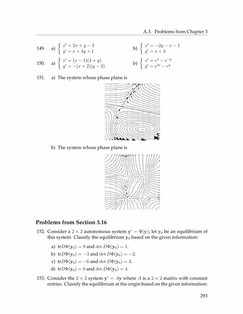
A.3. Problems from Chapter 3
149. a)x′ = 2x+ y − 3y′ = x+ 4y + 1 b)
x′ = −2y − x− 1y′ = x+ 3
150. a)x′ = (x− 1)(4 + y)y′ = −(x+ 2)(y − 3) b)
x′ = ex − e−yy′ = e2x − ey
151. a) The system whose phase plane is
-2 2 4 6 8
-4
-2
2
4
b) The system whose phase plane is
-2 2 4 6 8
-2
2
4
6
8
Problems from Section 3.16
152. Consider a 2 × 2 autonomous system y′ = Φ(y); let y0 be an equilibrium ofthis system. Classify the equilibrium y0 based on the given information:
a) trDΦ(y0) = 8 and detDΦ(y0) = 1.
b) trDΦ(y0) = −3 and detDΦ(y0) = −2.
c) trDΦ(y0) = −6 and detDΦ(y0) = 3.
d) trDΦ(y0) = 0 and detDΦ(y0) = 4.
153. Consider the 2 × 2 system y′ = Ay where A is a 2 × 2 matrix with constantentries. Classify the equilibrium at the origin based on the given information:
293

A.3. Problems from Chapter 3
a) trA = −1 and detA = 7.
b) trA = 5 and detA = −1.
c) trA = 2 and detA = 3.
d) trA = 0 and detA = −6.
Problems from Section 3.17
154. Two large tanks (call them X and Y) each hold 100 L of liquid. They areinterconnected by pipes which pump liquid from tank X to tank Y at 3 L/minand from tank Y to tank X at 1 L/min. A brine solution of concentration 0.2kg/L of salt flows into tank X at a rate of 5 L/min; the solution flows out ofthe system of tanks via two pipes (one pipe allows flow out of tank X at 2L/min and another pipe allows flow out of tank Y at 2 L/min). Suppose thatinitially, tank Y contains pure water but tank X contains 40 kg of salt; assumethat at all times the liquids in each tank are kept mixed.
a) Draw a compartmental diagram which models this situation.
b) Write an initial value problem modeling the situation, where x(t) andy(t) represent the amount of salt in tanks X and Y respectively, at time t,and y = (x, y).
c) Use Mathematica to draw a picture of the vector field for your system,with the solution curve to your initial value problem indicated. Use theviewing window [0, 60]×[0, 60]; attach a printout of this picture, labelledas “154 (c)”.
d) Based on your picture from part (c), estimate the amount of salt in tankX at the instant when tank Y has 10 kg of salt in it.
e) Estimate the amount of salt in each tank 8 minutes after the initial situa-tion by having Mathematica implement Euler’s method with 10000 steps.
f) Solve the initial value problem you wrote down in part (b). Write youranswer coordinate-wise.
g) Have Mathematica graph the functions x(t) and y(t) on the same axes(in the viewing window [0, 100] × [0, 60]). The appropriate Mathematicacommands arex[t_] = whatever formula you get for x(t)y[t_] = whatever formula you get for y(t)Plot[x[t],y[t], t, 0, 100, PlotRange -> 0,60]Attach a printout of these graphs (labelled as “154 (g)”). Make sure youindicate which graph is x(t) and which is y(t).
294

A.3. Problems from Chapter 3
h) Find the amount of salt in each tank at time 8 (I want both the exactamount and a decimal approximation). Compare your answer to part(e); how accurate was your estimate in part (e)?
i) Find the concentration of salt in tank X at time 8.
155. In this problem, we explore a model (called the Gause competitive exclusionmodel) which describes how the populations of two species behave, whenthe species are in competition for the same resource. Let X and Y be twospecies whose populations at time t are x(t) and y(t), respectively, where xand y satisfy the system of differential equations
y′ = Φ(y) a.k.a.x′ = rXx(LX − x− αy)y′ = rY y(LY − y − βx) .
In this setting, α is a nonnegative number called the competition coefficientof Y on X ; it measures the degree to which increased numbers of species Ynegatively impact the ability of species X to survive. Similarly, β ≥ 0 is thecompetition coefficient of X on Y .
a) If α = β = 0 (i.e. the species are not in competition), the populations ofX and Y change according to what model? In light of this, what do theconstants rX , Lx, rY and LY represent?
b) This system of ODEs has four equilibria: three of them are (0, 0) (i.e.both species are extinct), (0, LY ) (species X is extinct), and (LX , 0) (speciesY is extinct).
i. Find the fourth equilibrium.ii. Explain why this fourth equilibrium is called the coexistence equi-
librium.
c) FindDΦ(0, 0). Compute the eigenvalues ofDΦ(0, 0) and show that (0, 0)is an unstable equilibrium.Hint: a matrix is called triangular if all the entries below its diagonal arezero, or if all the entries above its diagonal are zero. The eigenvalues ofa triangular matrix are always its diagonal entries.
d) Find DΦ(0, LY ). Compute the eigenvalues of DΦ(0, LY ) (the hint of part(c) is useful).
e) Based on your computations in part (d), show that (0, LY ) is a stableequilibrium if and only if α > LX
LY.
f) Find DΦ(LX , 0). Compute the eigenvalues of DΦ(LX , 0).
g) Based on your computations in part (f), show that (LX , 0) is a stableequilibrium if and only if β > LY
LX.
295

A.3. Problems from Chapter 3
h) Suppose that neither (0, LY ) nor (LX , 0) are stable.
i. Show that the following three inequalities hold:
LX − αLY > 0 βLX − LY < 0 αβ − 1 < 0
ii. Compute DΦ at the coexistence equilibrium.iii. Compute and simplify detDΦ and tr DΦ at the coexistence equilib-
rium using Mathematica.iv. Use the inequalities described in part (i) to show that the coexistence
equilibrium must be stable.
i) If the two species occupy the same ecological niche (i.e. they eat thesame food, live in the same places, etc.), then it is reasonable to assumethat β = 1
α. For example, if X and Y are species of beetles where each Y
beetle eats twice as much grain as each X beetle, then α would be 2 andβ would be 1
2 . What happens to the coexistence equilibrium in this case?What does that mean about the two species?
156. In the SIR model we studied in class, we assumed that the disease actedquickly (before any births or deaths could occur). Now let’s assume thatthe disease acts more slowly, so that we can account for births and deaths inour model. Let:
S = the population of the susceptible class (as before)I = the population of the infective class (as before)R = the population of the recovered class (as before)b = the birth rate (assume this is constant)d = the death rate due to factors other than the diseasec = the death rate due to the diseaseβ = the rate at which infections take placeγ = the rate at which infected patients recover
This leads to the following compartmental diagram:
IS Rb βIS
cI
dIdS dR
γI
Note that we can no longer assume that S + I + R = 1, because the totalpopulation may change as time passes.
296

A.4. Problems from Chapter 4
a) Write the system of differential equations for S, I and R. (In the rest ofthis problem, we will call this system y′ = Φ(y) where y = (S, I, R).)
b) There is one equilibrium of the system which has the form (S#, 0, 0),where S# 6= 0 (this is called the disease-free equilibrium; it representsthe situation where no one has the disease). Find S# in terms of thevariables listed above.
c) Find DΦ(S#, 0, 0), and have Mathematica compute the eigenvalues ofthis matrix.
d) Show that the disease-free equilibrium is stable if and only if βb < d(c+d+ γ).
e) There is a second equilibrium called the endemic equilibrium (becausein this situation the disease persists), which has the form (S∗, I∗, R∗).Find S∗, I∗ and R∗ in terms of the variables listed above.
f) Find DΦ(S∗, I∗, R∗) and have Mathematica compute the eigenvalues ofthis matrix.
g) Show that the endemic equilibrium is stable if and only if βb > d(γ+ c+d).
h) Explain why your answers to parts (d) and (g) make sense, given whatthe variables in the problem mean.
A.4 Problems from Chapter 4Problems from Section 4.1
157. Rewrite this third-order ODE as a first-order system of the form y′ = Ay + q.Be sure to carefully identify what y, A and q are.
y′′′ − 4y′′ + 7y′ − 8y = cos t
158. Rewrite this second-order system of equations as a first-order system of theform y′ = Ay + q. Be sure to carefully identify what y, A and q are.
x′′ +2x′ −3y′ +4x = 0y′′ −x′ +4y′ −7x +3y = 0
Problems from Section 4.2
159. Find the general solution of each differential equation:
297

A.4. Problems from Chapter 4
a) y′′ − 8y′ + 12y = 0b) y′′ = −7y′ + 18y
c) y′′′ + 11y′′ + 30y′ = 0
160. Find the general solution of each differential equation:
a) y′′ + 4y′ + 11y = 0b) y′′′ + 9y′ = 0
c) y′′ − 12y′ + 36y = 0
161. Find the general solution of each differential equation:
a) y′′ − 4y′ − 21y = e4t
b) y′′ + y = sin 2tc) y′′ − 25y = t
162. Find the particular solution of each initial value problem:
a)
y′′ − 8y′ + 15y = 0y(0) = 3y′(0) = 2
b)
y′′ + 4y′ + 4y = 0y(0) = −6y′(0) = −1
c)
y′′ + 2y′ + 5y = 0y(0) = 1y′(0) = 0
163. Find the particular solution of this initial value problem:y′′ − 16y′ + 63y = et
y(0) = 11y′(0) = −5
164. Find the general solution of this differential equation:
y(5) + y(4) − 4y′′′ − 8y′′ − 32y′ − 48y = 0.
Hint: use Mathematica to factor the characteristic equation.
Problems from Section 4.4
165. a) Explain why the α on page 239 of the lecture notes must be negative.
b) Explain why the λ1 and λ2 on page 239 of the lecture notes must both benegative.
166. Consider a 12 kg mass attached to a fixed point by a spring (like the pictureon the top of page 236 of the notes). If the spring constant is 1
4 N/m andthe damping coefficient (i.e. coefficient of friction) is 7
2 N sec/m, and theentire system (at time t) is subject to an external force of 257 cos 2t N, find theposition of the mass at time t. Assume that at time 0, the mass has no initialvelocity but is 8 m to the right of where it would be at rest.
298

A.4. Problems from Chapter 4
167. Consider a coupled mass-spring system like the one pictured at the top ofpage 243 in the notes. Assume that m1 = 6 kg and m2 = 2 kg, and the springconstants are k1 = 3 N/m and k2 = 2 N/m. If the first mass is displaced 4m left of its equilibrium position and the second mass is displaced 2 m rightof its equilibrium position, and then the masses are released with no initialvelocity:
a) Find the position of each mass at time t.
b) Assuming that the spring between the two masses is 10 m long at rest,have Mathematica sketch a graph showing the positions of the massesat time t in the viewing window [0, 50] × [−5, 20] (attach a printout ofthis graph, labelled as “168”). The vertical axis should be scaled so thatheight 0 corresponds to the first mass being at equilibrium, as in thesecond picture on page 244 in the lecture notes.To graph two functions at once; see Problem 154 (g) for the appropriatecommands.
168. Suppose that three identical springs, each with spring constant k = 3 andtwo identical masses, each of mass 12, are attached in a straight line, with theends of the outside springs fixed. Here is a picture of the system:
12 kg 12 kg
k = 3 k = 3 k = 3
x = 0 y = 0
Suppose that the masses move along a frictionless surface; let x(t) and y(t) bethe displacement of the masses at time t, where x = 0 and y = 0 correspond tothe system being at rest, and positive values of x and y indicate displacementto the right.
a) Write down a second-order system of differential equations describingthe system (coming from Newton’s laws).
b) Convert the system from part (a) to a first-order system of equations.
c) Find the general solution of the system you wrote down in part (a).Hint: Use Mathematica to find eigenvalues and eigenvectors for the sys-tem you obtained in part (b).
299

A.4. Problems from Chapter 4
d) Suppose that initially, the left-hand mass starts at x = 2 and the right-hand mass starts at y = −1, and that both masses have an initial right-ward velocity of 1.
i. Find x(t) and y(t) in this case.ii. Graph x and y on the same axes (see Problem 154 (g) for the ap-
propriate Mathematica commands); attach a printout of this graph,labelled as “168 (d)”. You are responsible for choosing a reasonableviewing window.
iii. Find the positions of the masses (i.e. x and y) when t = 3.
169. Consider an undamped pendulum of length 2 m and mass 45 kg.
a) Write the undamped pendulum equation in this case.b) Write the linearization of the equation you wrote in part (a).c) Find the general solution of the linearized equation you wrote in part
(b).d) Suppose that at time 0, the pendulum is at angle θ = .05 radians and has
angular velocity−.3 radians/second. What is the largest angle obtainedby the pendulum as it swings?Hint: Find the particular solution corresponding to these initial condi-tions; one aspect of this particular solution gives the answer to the ques-tion.
170. (Optional; extra credit) Consider the linearized double pendulum equation(coming from page 247 of the lecture notes; repeated here for convenience):
(m1 +m2)l1θ′′1 +m2l2θ′′2 + (m1 +m2)gθ1 = 0
m2l2θ′′2 +m2l1θ
′′1 +m2gθ2 = 0
a) Rewrite this system of two second-order equations as a first-order sys-tem of four equations y′ = Ay.Hint: To get started, pretend this is a system of two equations in the twovariables θ′′1 and θ′′2 and solve for those two quantities in terms of theother variables.
b) Use Mathematica to find the eigenvalues and eigenvectors of the matrixA, and write the general solution of the equation y′ = Ay you wrote inpart (a).
c) Write the formulas for θ1 and θ2.
171. A series RLC circuit (as in page 248 of these notes) has a voltage source givenby ES(t) = 10 cos 2t volts, a resistor of 2 Ω, an inductor of 1
4 H, and a capacitorof 1
13 F. If the initial current is zero and the initial charge on the capacitor is3.5 coulombs, find the current in the circuit as a function of time t.
300

A.5. Selected answers to the homework problems
A.5 Selected answers to the homework problems
1. (b) y = 12t−3
2. a) y =√t+ 3 + 1
(c) y = ±12
√8− t2
3. (c) y = 2 + ln 3 + t− 1
4. a) ∞b) 0
6. a) f ′(t) = 6t− 7
9. a) f ′(t) = −2e−2t
f ′′(t) = 4e−2t
f ′′′(t) = −8e−2t
10. a) 12t
2 + C
12. (b) 34t
4/3 + C
(c) 23t
3/2 + t+ C
14. a) t2 + t
b) 4√t− 4
15. (b) −14 t
2 + 12t
2 ln t+ C
16. (a) 12 ln(2− x)− 1
2 ln(2 + x) + C
(b) 12 sin2 t+ C
18. a) −3t−1 + (t− 1) + 2 ln(t− 1) + C
19. a) x1 = −1; x2 = 1; x3 = −1;x4 = 1
20. 43
21. a) not a solution
22. a) solution
24. a) not a solution
25. a) not linear
b) linear
28. (b) order 4;4 constants in gen. sol’n;nonlinear
29. a) order 1;1 constant in gen. sol’n;linear;not homogeneous;not constant-coefficient
32. (d) y = 12e14.1 e
4.7t
34. (c) $318.55.
35. (c) 16.7621 grams.
37. (b) y = 4, y = 0, y = −5
38. (a) -5 0 5
-5
0
5
40. (t4, y4) = (4, 61).
41. y(2) ≈ 33.
46. (a) There are four possible an-swers: y = −7, y = −2, y = 3or y = 6.
(b) y = −2 is the only sink.
47. a) −2
50. (a) φ(−7) is negative(c) φ(4) is positive
301

A.5. Selected answers to the homework problems
(d) φ′(−2) is negative
51. (a) y = −3 is stable; y = 3 is un-stable
52. (a) y = 0 is unstable
53. (a) y = 0 is unstable; y = 6 is sta-ble
55. (a) y = 0 and y = rL−er
.
(e) E = 12rL
57. (a) Yes; if 5 ≤ r ≤ 7 and y(0) > 0we know that lim
t→∞y(t) = 0,
so the long-term value of y iszero.
58. (a) There is only one bifurcationat r = 9; it is a saddle-nodebifurcation.
62. (a) y = Ce2t
63. (b) y = Cesin t
64. (a) y = 3 ln t
66. (a) y = 7e2t − 3et
67. (a) y = −te−t + Ct
70. (a) y = Ce−3t + e−2t
71. (b) y = Ce4t − 12t
2 − 94t−
916
72. (a) yh = e−7t
(b) No; on the left-side you get 0which cannot equal 20e−7t.
(d) y = Ce3t + 9te3t
74. a) 12y
2 = 13 ln(4 + t3) + C
b) y = Ct2−1Ct2+1
75. (a) y = ln(4t+ C)
79. (a) y = Ct3 − t+D
80. (a) y = arctan(Ct+D)
81. (a) y = C cos t+D sin t
82. (a) y = Ce2t − 2t3 − 3t2 − t+D
83. a) Exact; solution is y2−2y+t2 +3t = C
b) Not exact
84. a) y2 − ty + t2 = 7
85. (c) y2t− yey + ey = C
87. (a) 200− 2t
(c)y′ = 6
5 −4y
100−ty(0) = 1
(e) 15.0017
88. (d) ymax ≈ 20(e) t ≈ 35
89. y = −25 (t− 100)− 39
108 (t− 100)4.
90. (b) f(60) = 9376625 .
91. (a)−25 (100−t)− 39
108 (100−t)4
200−2t .
(c) t ≈ 20.
93. (b)
dvdt
= 9.8− 3075v
v(0) = 0(d) 24.5
94. v = 492 −
492 e−(2/5)t.
95. (a) h(t) = 82454 −
492 t−
2454 e−(2/5)t.
(b) t = 25 ln 49
9 ≈ 4.2365.
96. t = 15 ln 719
ln 1419≈ 49.0466
99. a) solution
b) not a solution
302

A.5. Selected answers to the homework problems
101. a) (i)x(t) = t2 − 2y(t) = t+ 3
(ii) y(0) = (−2, 3); y(1) = (−1, 4); y(2) = (2, 5).
102. (a) Use this code (all executed in one cell):ParametricPlot[Cos[t], Sin[t], t, -100,100,PlotRange -> -2,2,-2,2]
You will find that the graph is a circle.
105. (t1,y1) = (1, (3, 6)); (t2,y2) = (2, (0, 18)); (t3,y3) = (3, (−18, 36)).
107. The x-coordinate when t = 4 is 92.1414.
109. (a) y(50) ≈ (−6.531 · 10−45, 5.708 · 10−45) ≈ (0, 0).
(b)
-10 -5 5 10x
-10
-5
5
10
y
110. (d) y(5) ≈ (.515676, .362851, .326229).
(e) No, when more steps are used, the coordinates of y(5) change signifi-cantly.
111. a) 0
(c)(
15 −63 9
)
(e)(
3 −21 1
)
(f)(
4− λ 2−8 −4− λ
)
112. a)(−2 sin 2t 3 cos 3t8 cos 2t −3 cos 3t
)
b) (cos t,−6 sin 3t, 28e7t)
c)(−15 −13−3 11
)
113. (b)(
28 00 1
)
(c)
1 0 00 1 00 0 1
115. a)(
317
217
−117
517
)
116. (a) 17(b) −2
117. (a) λ2 − 8λ+ 17
118. a) No
b) Yes
303

A.5. Selected answers to the homework problems
119. a) W (t) = 20t2; the functions are linearly independent (since W (1) 6= 0).
(c) W (t) = 2; the functions are linearly independent (since W (0) 6= 0).
121. a) First, compute the Wronskian:
W (t) = det(
eat ebt
(eat)′ (ebt)′)
= det(
eat ebt
aeat bebt
)= be(a+b)t − ae(a+b)t
= (b− a)e(a+b)t.
Since a 6= b, W (t) 6= 0, so the functions eat and ebt are linearly indepen-dent, as desired.
124. dydx
∣∣∣(1,0)
= 1; dydx
∣∣∣(0,2)
= −12 ; dy
dx
∣∣∣(0,−2)
= −12 ; dy
dx
∣∣∣(−3,0)
= 1. The slope field withthese four mini-tangents is:
-6 -4 -2 0 2 4 6-6
-4
-2
0
2
4
6
125. (a) -4 -2 0 2 4
-4
-2
0
2
4
(b) -3 -2 -1 0 1 2 3
-3
-2
-1
0
1
2
3
127. (a) (−6, 4) and(
32 ,−1
)128. (a)
(12 , 1
)and
(−12 , 1
)129. (c) y(t) = (3, 1).
(d) i. x(t) is decreasingii. y(t) is increasing
iii. limt→∞
x(t) = −∞
304

A.5. Selected answers to the homework problems
iv. limt→∞
y(t) = 1
135. y = C1et(
11
)+ C2e
−t(
13
)137. (c) y = C1e
−4t(
13
)+ C2e
−5t(
12
).
141. y =(e−t cos t−3e−t sin te−t cos t−e−t sin t
)143. y =
(3e−3t+4te−3t
2e−3t+4te−3t
)144.
x(t) = 4e2t + C1e
t + C2e−t
y(t) = 8e2t + C1et + 3C2e
−t
147. a)
y1(t) = 3C1e
−3t + 2C2e2t
y2(t) = 2C2e2t + 3C4e
−6t
y3(t) = C1e−3t − 3C2e
2t + 5C4e−6t
y4(t) = 4C1e−3t + C2e
2t + C3e4t + C4e
−6t
148. a)
x(t) = C1e
2t − C2e−t − C3e
−t
y(t) = C1e2t + C3e
−t
z(t) = C1e2t + C2e
−t
149. a) The only equilibrium is(
137 ,−57
), which is an unstable node.
151. (b) There are four equilibria: (2, 0) (stable node), (5, 0) (unstable saddle), (5, 4)(unstable node) and (2, 4) (unstable saddle).
152. a) Unstable node
b) Unstable saddle
c) Stable node
154. (b)
x′ = −1
20 x+ 1100y + 1
y′ = 3100x−
3100y
y(0) = (40, 0)
155. a) When α = β = 0, the populations of X and Y behave according to logisticmodels.
b) i. The fourth equilibrium is(αLY −LX
αβ−1 , βLX−LY
αβ−1
).
c) DΦ(0, 0) =(rXLX 0
0 rYLY
). The eigenvalues of this matrix are rXLX
and rYLY , both of which are positive, so (0, 0) is unstable.
305

A.5. Selected answers to the homework problems
(d) DΦ(0, LY ) =(rXLX − αrXLY 0−βrYLY −rYLY
). One eigenvalue of this ma-
trix is −rYLY < 0; the other is rX(LX − αLY ).
(e) If α > LX
LY, then LX − αLY < 0 so both eigenvalues of DΦ(0, LY ) are
negative, in which case (0, LY ) is stable.
(i) In this case, there is no coexistence equilibrium (since the denominatorsin the coexistence equilibrium would have to be zero).
156. (b) S# = bd
(c) DΦ( bd, 0, 0) =
−d −β b
d0
00 β b
d− c− d− γ 0
0 γ −d
;
the eigenvalues are −d (repeated twice) and 1d(bβ − d(c+ d+ γ)).
(e) S∗ = c+d+γβ
; I∗ = bβ−d(c+d+γ)β(c+d+γ) ; R∗ = γ(bβ−d(c+d+γ))
βd(c+d+γ) .
157. y =
yy′
y′′
; A =
0 1 00 0 18 −7 4
; q =
00
cos t
.
159. a) y = C1e2t + C2e
6t.
160. a) y = C1e2t cos
(√7t)
+ C2e2t sin
(√7t).
161. a) y = −121 e
4t + C1e7t + C2e
−3t.
162. a) y = 132 e
3t − 72e
5t.
165. a) If you convert the second-order equation mx′′(t) + bx′(t) + kx(t) = 0 toa first-order system via reduction of order, the system becomes
x′ =(
0 1−km
−bm
)x = Ax.
We have tr(A) = −bm< 0 and detA = k
m> 0. Since the trace is negative
and the determinant is positive, the equilibrium 0 is either a stable spiralor stable node, so both of its eigenvalues must have negative real part.
166. x(t) = −764145 cos 2t+ 112
145 sin 2t− 396145e
−t/6 + 16e−t/8.
167. a)
x(t) = −167 cos
(t√
32
)− 12
7 cos(
t√3
)y(t) = 32
7 cos(t√
32
)− 18
7 cos(
t√3
)
306

A.5. Selected answers to the homework problems
168. a)
12x′′ = −3x+ 3(y − x)12y′′ = −3(y − x)− 3y (or something equivalent to this)
(d) i.x(t) = 1
2 cos t2 + 3
2 cos t√
32 + 2 sin t
2y(t) = 1
2 cos t2 −
32 cos t
√3
2 + 2 sin t2
169. a) θ′′ + 9.82 sin θ = 0.
b) θ′′ + 9.82 θ = 0.
(d)√
409140 radians (which is about 0.1444).
171. I(t) = 12 cos 2t− 3
2 sin 2t− 12e−4t cos 6t− 47
2 e−4t sin 6t.
307

A.6. Extra credit problems
A.6 Extra credit problems1. The Snowplow Problem: Suppose that one morning it starts snowing hard,
but at a constant rate. A snowplow sets out at 9 AM to clear a road. At 11AM, it has cleared 15 miles, and at 1 PM, it has cleared an additional 10 miles.When did it start snowing?
To solve this problem, carry out the following steps:
a) Let t be the time, measured in hours, with t = 0 corresponding to 9 AM.Let h = h(t) be the height of the snow at time t. We will assume therate of snowfall is constant, and equal to r. Write down a differentialequation which could be used to solve for h(t), if there was no plowing.
b) Solve the equation from part (a) for h in terms of t (there will be an ar-bitrary constant; let’s call this constant B so everyone is using the samenotation).
c) Let x(t) be the distance the snowplow has travelled at time t. It is rea-sonable to assume that the deeper the snow is, the slower the snowplowhas to travel. A simple mathematical model for this is to assume that thevelocity of the snowplow at time t is inversely proportional to the heighth(t). Use this to write a differential equation satisfied the function x(t)(let’s agree to use the letter k for the proportionality constant).
d) Solve the differential equation of part (c) to obtain a formula for x(t)(let’s agree to call the arbitrary constant that appears here D).
e) Use the initial conditions of this problem (given before part (a)) to solvefor B, D and k.
f) Answer the original question: when did it start snowing? Round youranswer to the nearest minute.
308
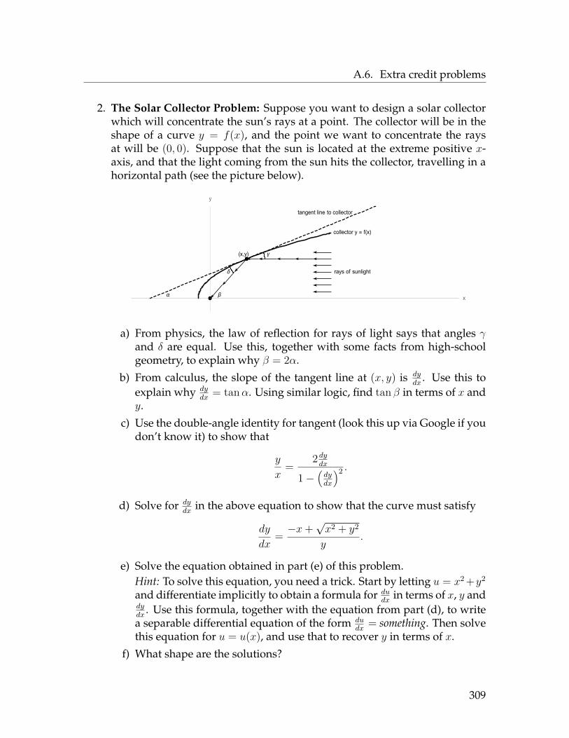
A.6. Extra credit problems
2. The Solar Collector Problem: Suppose you want to design a solar collectorwhich will concentrate the sun’s rays at a point. The collector will be in theshape of a curve y = f(x), and the point we want to concentrate the raysat will be (0, 0). Suppose that the sun is located at the extreme positive x-axis, and that the light coming from the sun hits the collector, travelling in ahorizontal path (see the picture below).
collector y = f(x)
rays of sunlight
tangent line to collector
α β
γ
δ
(x,y)
x
y
a) From physics, the law of reflection for rays of light says that angles γand δ are equal. Use this, together with some facts from high-schoolgeometry, to explain why β = 2α.
b) From calculus, the slope of the tangent line at (x, y) is dydx
. Use this toexplain why dy
dx= tanα. Using similar logic, find tan β in terms of x and
y.
c) Use the double-angle identity for tangent (look this up via Google if youdon’t know it) to show that
y
x=
2 dydx
1−(dydx
)2 .
d) Solve for dydx
in the above equation to show that the curve must satisfy
dy
dx= −x+
√x2 + y2
y.
e) Solve the equation obtained in part (e) of this problem.Hint: To solve this equation, you need a trick. Start by letting u = x2 +y2
and differentiate implicitly to obtain a formula for dudx
in terms of x, y anddydx
. Use this formula, together with the equation from part (d), to writea separable differential equation of the form du
dx= something. Then solve
this equation for u = u(x), and use that to recover y in terms of x.
f) What shape are the solutions?
309

Appendix B
Mathematica information
B.1 General Mathematica principlesMathematica is an extremely useful and powerful software package / program-
ming language invented by a mathematician named Stephen Wolfram. Early ver-sions of Mathematica came out in the late 1980s and early 1990s; the most recentversion (which is loaded onto machines at FSU as of 2016) is Mathematica 10.
Mathematica does symbolic manipulation of mathematical expressions; it solvesall kinds of equations; it has a library of important functions from mathematicswhich it recognizes while doing computations; it does 2- and 3-dimensional graph-ics; it has a built-in word processor tool; it works well with Java and C++; etc. Onething it doesn’t do is prove theorems, so it is less useful for a theoretical mathemati-cian than it is for an engineer or college student.
A bit about how Mathematica works: When you use the Mathematica program,you are actually running two programs. The “front end” of Mathematica is the partthat you type on and the part you see. This part actually resides on the machine atwhich you are seated. The “kernel” is the part of Mathematica that actually does thecalculations. If you type in 2 + 2 and hit [SHIFT]+[ENTER], the front end “sends”that information to the kernel which actually does the computation. The kernelthen “sends” the result back to the front end, which displays the output 4 on thescreen. Essentially, the way one uses Mathematica is by typing some “stuff” in, hit-ting [SHIFT]+[ENTER] to execute that stuff, and getting some output back fromthe program.
About Mathematica notebooks and cells: The actual files that Mathematicaproduces that you can edit and save are called notebooks and carry the file designa-tion *.nb; they take up little space and can easily be saved to Google docs or on a
310

B.1. General Mathematica principles
flash drive, or emailed to yourself if you want them somewhere you can retrievethem. Suggestion: when saving any file, include the date in the file name (so it iseasier to remember which file you are supposed to be open).
A Mathematica notebook is broken into cells. A cell can contain text, input, oroutput. A cell is indicated by a dark blue, right bracket (a “]”) on the right-handside of the notebook. To select a cell, click that bracket. This highlights the “]”in blue. Once selected, you can cut/copy/paste/delete cells as you would high-lighted blocks of text in a Word document.
To change the formatting of a cell, select the cell, then click“Format / Style”and select the style you want. You may want to play around with this to see whatthe various styles look like. There are three particularly important styles:
• input: this is the default style for new cells you type• output: this is the default style for cells the kernel produces from your com-
mands• text: changing a cell to text style allows you to make comments in between
the calculations
Executing mathematical commands: To execute an input cell, put the cursoranywhere in the cell and hit [ENTER]. Well, not any [ENTER]; you have to usethe [ENTER] on the numeric keypad at the far-right edge of the keyboard. The[ENTER] next to the apostrophe key (a.k.a. [RETURN]) gives you only a carriagereturn. You can also hold down the [SHIFT] key and hit either [ENTER] or [RE-TURN] to execute a command.
311

B.1. General Mathematica principles
Important general concepts re: Mathematica syntax
1. Multiplication: use a star or a space: 2 * 3 or 2 3 will multiply numbers;a x means a times x; ax means the variable ax (in Mathematica, variables donot have to be named after one letter; they can be named by words or otherstrings of characters as well).
2. Parentheses: used for grouping and multiplication only. Parentheses mean“times” in Mathematica, and always mean that you intend to multiply whatis in front of the parenthesis by what is inside the parenthesis.
3. Brackets: must be used to surround the input of any function or built-inMathematica command. For example, to evaluate a function f(x), you wouldtype f[x], not f(x). Essentially, square brackets mean “of” in Mathematica.
4. Capitalization: All Mathematica commands and built-in functions begin withcapital letters. For example, to find the sine of π, typing sin(pi) or sin[pi]does you no good (the first version would be the variable “sin” times thevariable “pi”, for instance). The correct syntax is Sin[Pi]. Similarly, e is Eand i is I in Mathematica.
5. Spaces: Mathematica commands do not have spaces in them; for example, theinverse function of sine is ArcSin, not Arc Sin or Arcsin.
6. Pallettes: Lots of useful commands are available on the Basic Math AssistantPallette, which can be brought up by clicking “Pallettes / Basic Math Assis-tant” on the toolbar. If you click on a button in the pallette, what you seeappears in the cell. The tab halfway down this palette marked d
∫Σ has cal-
culus commands, and the tab to the right of the d∫
Σ has matrix commands.
7. Logarithms: Mathematica does not know what Ln is. For natural logarithms(base e), type "Log[ ]". For common logarithms (base 10), type "Log10[ ]".
8. % refers to the last output (like “Ans” on a TI-calculator).
9. Help: To get help on a command, type “?” followed by the command youdon’t understand. If necessary, click the you get at the end of the helpblurb to open a help browser. You can also find out how to do lots of stuff inMathematica by using Google: search for what you want help on.
10. Mathematica gives exact answers (i.e. not decimals) for everything if possible.If you need a decimal approximation, use the command N[ ]. For example,N[Pi] spits out 3.14159...
11. If Mathematica freezes up in the middle of a calculation, click “Evaluation /Abort Evaluation” on the toolbar.
312
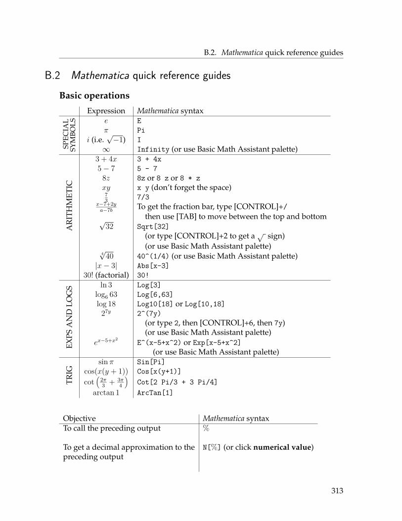
B.2. Mathematica quick reference guides
B.2 Mathematica quick reference guidesBasic operations
Expression Mathematica syntax
SPEC
IAL
SYM
BOLS e E
π Pii (i.e.
√−1) I
∞ Infinity (or use Basic Math Assistant palette)
AR
ITH
MET
IC
3 + 4x 3 + 4x5− 7 5 - 7
8z 8z or 8 z or 8 * zxy x y (don’t forget the space)73 7/3
x−7+2ya−7b To get the fraction bar, type [CONTROL]+/
then use [TAB] to move between the top and bottom√32 Sqrt[32]
(or type [CONTROL]+2 to get a√ sign)(or use Basic Math Assistant palette)
4√
40 40^(1/4) (or use Basic Math Assistant palette)|x− 3| Abs[x-3]
30! (factorial) 30!
EXPS
AN
DLO
GS ln 3 Log[3]
log6 63 Log[6,63]log 18 Log10[18] or Log[10,18]
27y 2^(7y)(or type 2, then [CONTROL]+6, then 7y)(or use Basic Math Assistant palette)
ex−5+x2 E^(x-5+x^2) or Exp[x-5+x^2](or use Basic Math Assistant palette)
TRIG
sin π Sin[Pi]cos(x(y + 1)) Cos[x(y+1)]cot
(2π3 + 3π
4
)Cot[2 Pi/3 + 3 Pi/4]
arctan 1 ArcTan[1]
Objective Mathematica syntaxTo call the preceding output %
To get a decimal approximation to the N[%] (or click numerical value)preceding output
313

B.2. Mathematica quick reference guides
Defining functions
Objective Mathematica syntaxDefine a function f(x) = formula f[x_] = formula
(one equals sign, underscore after x)
Define parametric function f[t_] = f(t),g(t)x = f(t), y = g(t)
Define function of multiple variables f[x_,y_] = formulaz = f(x, y)
Tables and graphs (see also Section B.3)
Objective Mathematica syntaxGenerate table of values for f Table[x,f[x], x,xmin,xmax,step]
(put //TableForm at end of commandto arrange output in a table)
Plot the graph of f(x) = formula Plot[formula, x,xmin,xmax]
Plot multiple graphs at once Plot[formula,formula, ..., formula,x,xmin,xmax]
Plot the graph of f(x) = formula Plot[formula, x,xmin,xmax,with range of y−values specified PlotRange -> ymin,ymax]
Plot the graph of f(x) = formula Plot[formula, x,xmin,xmax,with x- and y-axes on same scale PlotRange -> ymin,ymax,
AspectRatio -> Automatic]
Plot graph of a set of parametric ParametricPlot[f[t], t, -20,20,equations (after defining them PlotRange -> xmin,xmax,as f(t)) ymin,ymax]
314

B.2. Mathematica quick reference guides
Function operations and calculus
Expression Mathematica syntax
f(x+ 3) (if f is a function) f[x+3]xf(2x)− x2f(x) x f[2x] - x^2 f[x]
(spaces important)(f g)(x) f[g[x]]
limx→4
f(x) Limit[f[x], x -> 4]
f ′(3) f’[3]g′′′(x) g’’’[x] or D[g[x],x,3]
partial derivative fx D[f[x,y], x]partial derivative fyy D[f[x,y], y,2]partial derivative fyxy D[f[x,y], y,2, x,1]
∫x2 dx Integrate[x^2,x]
(or use∫
sign on Basic Math Assistant palette)∫ 52 cosx dx Integrate[Cos[x], x, 2, 5]
(or use∫ sign on Basic Math Assistant palette)
(for a decimal approximation, use NIntegrate)
12∑k=1
f(k) Sum[f[k], k, 1, 12]
(or use Basic Math Assistant palette)
∞∑k=1
blah Sum[blah, k, 1, Infinity]
(or use Basic Math Assistant palette)
To find the Taylor polynomial of orderN for function f , centered at point a, execute
Normal[Series[f, variable, a, N]]
For example, to find the eighth Taylor polynomial of f(x) = cos 2x centered at 0,execute
Normal[Series[Cos[2x], x, 0, 8]]
315
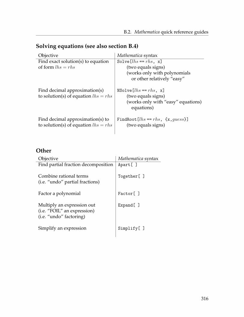
B.2. Mathematica quick reference guides
Solving equations (see also section B.4)
Objective Mathematica syntaxFind exact solution(s) to equation Solve[lhs == rhs, x]of form lhs = rhs (two equals signs)
(works only with polynomialsor other relatively “easy”
Find decimal approximation(s) NSolve[lhs == rhs, x]to solution(s) of equation lhs = rhs (two equals signs)
(works only with “easy” equations)equations)
Find decimal approximation(s) to FindRoot[lhs == rhs, x,guess]to solution(s) of equation lhs = rhs (two equals signs)
OtherObjective Mathematica syntaxFind partial fraction decomposition Apart[ ]
Combine rational terms Together[ ](i.e. “undo” partial fractions)
Factor a polynomial Factor[ ]
Multiply an expression out Expand[ ](i.e. “FOIL” an expression)(i.e. “undo” factoring)
Simplify an expression Simplify[ ]
316
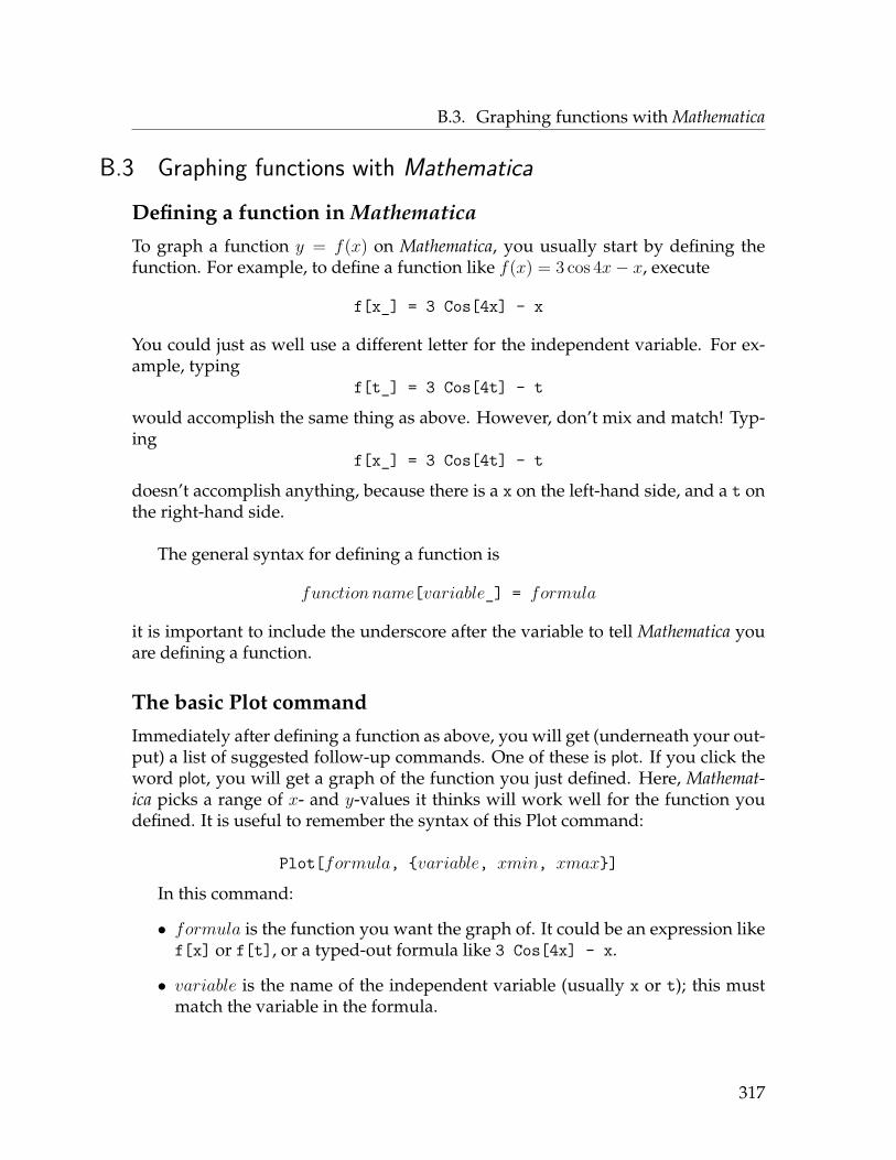
B.3. Graphing functions with Mathematica
B.3 Graphing functions with MathematicaDefining a function in Mathematica
To graph a function y = f(x) on Mathematica, you usually start by defining thefunction. For example, to define a function like f(x) = 3 cos 4x− x, execute
f[x_] = 3 Cos[4x] - x
You could just as well use a different letter for the independent variable. For ex-ample, typing
f[t_] = 3 Cos[4t] - t
would accomplish the same thing as above. However, don’t mix and match! Typ-ing
f[x_] = 3 Cos[4t] - t
doesn’t accomplish anything, because there is a x on the left-hand side, and a t onthe right-hand side.
The general syntax for defining a function is
function name[variable_] = formula
it is important to include the underscore after the variable to tell Mathematica youare defining a function.
The basic Plot command
Immediately after defining a function as above, you will get (underneath your out-put) a list of suggested follow-up commands. One of these is plot. If you click theword plot, you will get a graph of the function you just defined. Here, Mathemat-ica picks a range of x- and y-values it thinks will work well for the function youdefined. It is useful to remember the syntax of this Plot command:
Plot[formula, variable, xmin, xmax]
In this command:
• formula is the function you want the graph of. It could be an expression likef[x] or f[t], or a typed-out formula like 3 Cos[4x] - x.
• variable is the name of the independent variable (usually x or t); this mustmatch the variable in the formula.
317

B.3. Graphing functions with Mathematica
• xmin and xmax are numbers which represent, respectively, the left-most andright-most values of the independent variable shown on the graph. For ex-ample, if your Plot command has x,-3,5 in it, then the graph will go fromx = −3 to x = 5.
Here is an example, which plots f(x) = 3 cos 4x− x from x = −10 to x = 10:
Plot[3 Cos[4x] - x, x, -10,10]
-10 -5 5 10
-10
-5
5
10
Plotting multiple functions at once
Suppose you want to plot more than one function on the same set of axes. To dothis, you tweak the earlier Plot command by replacing the formula with a list offormulas inside squiggly braces, separated by commas. Thus the command youexecute looks something like this:
Plot[formula1, formula2, ..., variable, xmin, xmax]
For example, the following command plots sin 2x, 2 sin x and sin x+ 2 on the sameset of axes:
Plot[Sin[2x], 2 Sin[x], Sin[x] + 2, x, -2 Pi, 2 Pi]
-6 -4 -2 2 4 6
-2
-1
1
2
3
In Mathematica 10, the first graph you type will be blue; the second graph you typewill be orange; the third graph you type is green; other graphs are in other colors.To change the way the graphs look, consult the end of this section.
318

B.3. Graphing functions with Mathematica
Specifying a range of y-values
By default, Mathematica just chooses a range of y-values it thinks will make thegraph look good. If you want to force Mathematica to use a particular range of y-values, then you have to insert a phrase in the Plot command called PlotRange.This goes after the x,xmin,xmax and after another comma, but before the clos-ing square bracket. The general command is
Plot[formulas, var,xmin,xmax, PlotRange -> ymin,ymax]
and an example of the code, which plots sin x on the viewing window [−π, π] ×[−2, 3] is
Plot[Sin[x], x, -Pi, Pi, PlotRange -> -2,3]
-3 -2 -1 1 2 3
-2
-1
1
2
3
Making the x- and y-axes have the same scale on the screen
Here is the graph of f(x) = 3 cos 4x − x that Mathematica produces with the com-mand
Plot[3 Cos[4x] - x, x, -10,10]
-10 -5 5 10
-10
-5
5
10
If you look at this graph, the distance from the origin to (5, 0) looks a lot longerthan the distance from the origin to (0, 5). But in actuality, both these distancesare 5 units. The graph is distorted so that it fits nicely on your screen. To fixthe distortion (you might want to do this if you needed to estimate the slope ofa graph accurately), insert the command AspectRatio -> Automatic into the Plotcommand (similar to how you would insert a PlotRange command). This forces
319

B.3. Graphing functions with Mathematica
the number of pixels on your screen representing one unit in the x direction tobe equal to the number of pixels on your screen representing one unit in the ydirection. Here is the general syntax:
Plot[formulas, var,xmin,xmax, AspectRatio -> Automatic]
This command can also be used with the PlotRange command:
Plot[formulas, var,xmin,xmax, PlotRange -> ymin,ymax,AspectRatio -> Automatic]
Here is an example command:
Plot[3 Cos[4x] - x, x, -10,10, AspectRatio -> Automatic]
-10 -5 5 10
-10
-5
5
10
Changing the appearance of the curves
As mentioned earlier, by default Mathematica graphs all the functions with solidlines, using different colors for different formulas on the same picture. To changethis, insert various directives into the Plot command using PlotStyle. Here aresome examples:
Plot[3 Cos[4x] - x, x, -10,10, PlotStyle -> Thick]
320

B.3. Graphing functions with Mathematica
-10 -5 5 10
-10
-5
5
10
Plot[3 Cos[4x] - x, x, -10,10, PlotStyle -> Dashed]
-10 -5 5 10
-10
-5
5
10
Plot[3 Cos[4x] - x, x, -10,10, PlotStyle -> Dotted]
-10 -5 5 10
-10
-5
5
10
If you are plotting more than one function at once, then after the PlotStyle ->,you can type a list of graphics directives, separated by commas, enclosed by a setof squiggly braces. The directives will be applied to each function you are graph-ing, in the same order as they are typed after the PlotStyle ->. For example, thiscommand plots x, 2x and 3x, where x is thick and black, 2x is red and dotted, and3x is blue and dashed:
Plot[x,2x,3x, x, -3,3,PlotStyle -> Thick, Black, Dotted, Red, Blue, Dashed]
321

B.3. Graphing functions with Mathematica
Parametric equations
To define a set of parametric equations like x = t cos t, y = sin 2t in Mathematica,type the following and execute:
f[t_] = t Cos[t], Sin[2t]
In general, the syntax is
name of function[t_] = formula for x,formula for y
(You don’t have to call the function f , of course.) You don’t need to have only twocoordinates x and y here; you could type more formulas, separated by commas, ifnecessary.
After defining the parametric equations as above, one follow-up command youget in the suggestions bar is parametric plot. Click that, and you will get a graph ofthe parametric equations in the xy-plane. The syntax looks like this:
ParametricPlot[f[t], t, -40, 40]
-40 -20 20 40
(The −40 and 40 are the range of t values considered; they don’t matter exceptthat they should be far apart for the purposes of getting a good graph.) Oftenthe viewing window for such a picture is not very useful. To fix this, tweak thecommand by using PlotRange:
ParametricPlot[f[t], t, -40, 40, PlotRange -> -8,8,-4,6]
-5 5
-4
-2
2
4
6
The PlotRange part of the command specifies the range of x− and y−valuesseen on the graph. For example, in this picture, x will go from −8 to 8 and y willrun from −4 to 6.
You can also use the PlotStyle directives described in earlier labs if you wantto change the appearance of the graph.
322

B.4. Solving equations with Mathematica
B.4 Solving equations with MathematicaThere are three methods to solve an equation using Mathematica. They have
something in common: to solve an equation, the equation must be typed with twoequals signs where the = is. (A single equal sign is used in Mathematica to assignvalues to variables, which doesn’t apply in the context of solving equations.)
The Solve command
To solve an equation of the form lhs = rhs, execute
Solve[lhs == rhs, variable]
where variable is the name of the variable you want to solve for. For example, tosolve x2 − 2x− 7 = 0 for x, execute Solve[x^2 - 2x - 7 == 0, x].
You can solve an equation for one variable in terms of others: for example,Solve[a x + b == c, x] solves for x in terms of a, b and c.
WARNING: The advantage of the Solve command is that it gives exact an-swers (no decimals); this can be a pro or con (as sometimes the exact answers arehorrible to write down). The disadvantage is that it only works on polynomial, ra-tional and other “easy” equations. It won’t work on equations that mix-and-matchtrigonometry and powers of x like x2 = cosx.
The NSolve command
NSolve works exactly like Solve, except that it gives decimal approximations to thesolutions. It has the same drawback as Solve in that it only works on reasonably“easy” equations. The syntax is
NSolve[lhs == rhs, variable]
The FindRoot command
To find decimal approximations to equations that are too hard for the Solve andNSolve commands, use FindRoot. This executes a numerical algorithm to estimatea solution to an equation. The good news is that this command always works; thebad news is that it requires an initial “guess” as to what the solution is (usuallyyou determine the initial guess by graphing both sides of the equation and seeingroughly where the graphs cross). For example, to find a solution to x2 = cosx nearx = 1, execute
FindRoot[x^2 == Cos[x], x, 1]
323
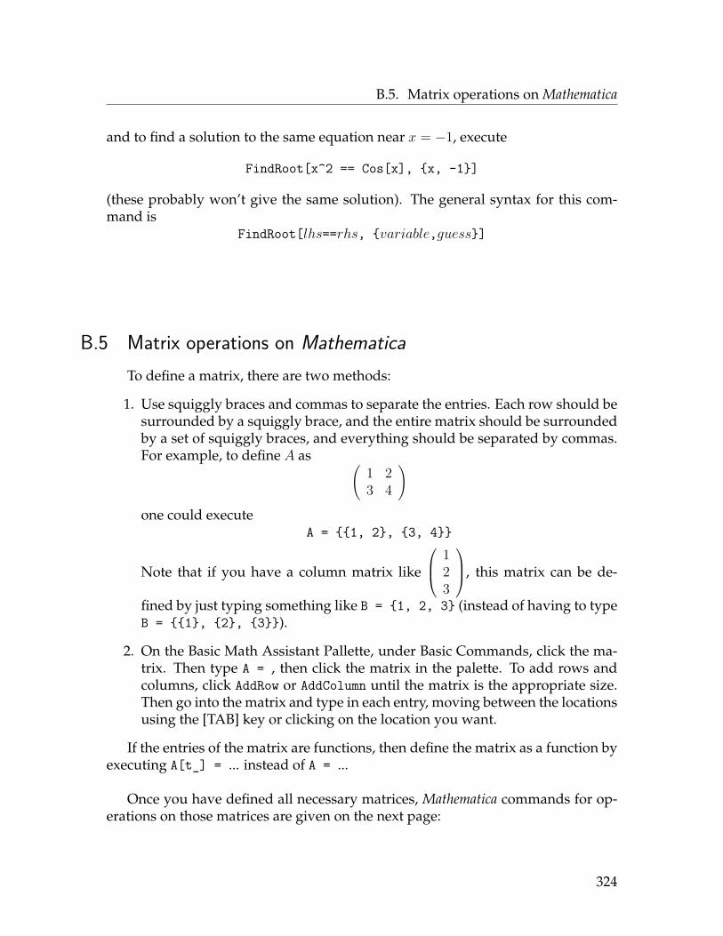
B.5. Matrix operations on Mathematica
and to find a solution to the same equation near x = −1, execute
FindRoot[x^2 == Cos[x], x, -1]
(these probably won’t give the same solution). The general syntax for this com-mand is
FindRoot[lhs==rhs, variable,guess]
B.5 Matrix operations on MathematicaTo define a matrix, there are two methods:
1. Use squiggly braces and commas to separate the entries. Each row should besurrounded by a squiggly brace, and the entire matrix should be surroundedby a set of squiggly braces, and everything should be separated by commas.For example, to define A as (
1 23 4
)one could execute
A = 1, 2, 3, 4
Note that if you have a column matrix like
123
, this matrix can be de-
fined by just typing something like B = 1, 2, 3 (instead of having to typeB = 1, 2, 3).
2. On the Basic Math Assistant Pallette, under Basic Commands, click the ma-trix. Then type A = , then click the matrix in the palette. To add rows andcolumns, click AddRow or AddColumn until the matrix is the appropriate size.Then go into the matrix and type in each entry, moving between the locationsusing the [TAB] key or clicking on the location you want.
If the entries of the matrix are functions, then define the matrix as a function byexecuting A[t_] = ... instead of A = ...
Once you have defined all necessary matrices, Mathematica commands for op-erations on those matrices are given on the next page:
324

B.5. Matrix operations on Mathematica
In this chart, if A is a matrix of functions, replace the A with A[t].
Note: To make Mathematica display an answer as a matrix:
1. follow your command with // MatrixForm, or
2. once you’ve executed the command, choose Display as... matrix from the sug-gestions bar.
EXPRESSION MATHEMATICA SYNTAX
BA
SIC
MA
TR
IXO
PE
RA
TIO
NS
Matrix addition / subtractionA+B A + BA−B A - B
Scalar multiplication3A 3AnA n A (space important)−5A+ 1
2B -5A + (1/2)BMatrix product AB A.B (the period is important)
A2 A.A or MatrixPower[A,2] (not A^2)A7 MatrixPower[A,7] (not A^7)
Trace tr(A) Tr[A]Determinant detA Det[A]Transpose AT Transpose[A]To get the entry of matrix A in the A[[i,j]]
ith row and jth columnTo call the n× n identity matrix I IdentityMatrix[n]Find derivative of a matrix of functions A’[t]
term-by-term
LIN
EA
RSY
STE
MS Matrix inverse A−1 Inverse[A] (not A^-1)
Find the rank of A MatrixRank[A](i.e. # of lin. indep. columns)
Reduced row-echelon form of A RowReduce[A]Find particular solution of Ax = b LinearSolve[A,b]Find basis of null space N(A) NullSpace[A]Find least-squares solution x of Ax = b LeastSquares[A,b]Matrix exponential eA = exp(A) MatrixExp[A]
EIG
EN
TH
EO
RY Eigenvalues and eigenvectors of A Eigensystem[A]
Just the eigenvalues of A Eigenvalues[A]Just the eigenvectors of A Eigenvectors[A]Find det(A− xI) CharacteristicPolynomial[A,x]
Determine if A is diagonalizable DiagonalizableMatrixQ[A]Determine if A is positive definite PositiveDefiniteMatrixQ[A]Determine if A is negative definite NegativeDefiniteMatrixQ[A]
325

B.6. Complex numbers in Mathematica
B.6 Complex numbers in MathematicaTo type in a complex number in Mathematica, type I (capital I) for the imaginary
number i. When Mathematica gets an answer with an i in it, it displays i for the i.
Basically, commands with complex numbers are the same as they are with realnumbers. To multiply (7−5i)(3 + 2i), for example, just execute (7 - 5I)(3 + 2I);to find ei, execute E^I. There are some commands that are unique to complex num-bers; those are given below:
Objective Mathematica syntaxFind real part of complex number Re[ ]
Find imaginary part of complex number Im[ ]
Find norm of complex number Abs[ ]
Find argument of complex number Arg[ ]
Find conjugate of complex number Conjugate[ ]
326

B.7. Slope fields for first-order equations
B.7 Slope fields for first-order equationsAll this code is available in the file slopefields.nb, available on my web page.
Code to sketch the slope field of y′ = φ(t, y):
Execute all this in a single Mathematica cell:
phi[t_,y_] := formula;"VectorPlot[1,phi[t,y], t, -10,10, y, -8, 8,VectorPoints -> 20, Axes -> True,VectorScale -> Automatic, Automatic, None,VectorStyle -> Orange]
Some of the things you can change as necessary:
• formula should be whatever φ(t, y) is equal to; for example, given the ODEy′ = 2t+ y2, the first line of the code would be phi[t_,y_] = 2t + y^2;
• the numbers in the second line set the viewing windows; for example, in theabove code the viewing window is [−10, 10]× [−8, 8];
• the 20 is the number of arrows drawn in each direction.
Code to sketch the slope field and several solution curves
Execute all this in a single Mathematica cell:
phi[t_,y_] := formula;VectorPlot[1,phi[t,y], t, -10, 10, y, -8, 8,VectorPoints -> 20, Axes -> True,VectorScale -> Automatic, Automatic, None,VectorStyle -> Orange,StreamPoints -> 35,StreamScale -> Full,StreamStyle -> Black, Thick]
The first five lines are the same as the command described earlier; the sixth linedirects Mathematica to sketch 35 solution curves at random locations on the picture.The last line tells Mathematica what color to draw the solution curves.
327

B.8. Euler’s method for first-order equations
Code to sketch the slope field and a solution curve passingthrough a specific point
The following code (executed in a single cell) will sketch a slope field and sketcha single solution curve passing through a given point (t0, y0), which is specified inthe sixth line of the code. In this case the initial value is (−1, 2):
phi[t_,y_] := formula;VectorPlot[1,phi[t,y], t, -10, 10, y, -8, 8,VectorPoints -> 20, Axes -> True,VectorScale -> Automatic, Automatic, None,VectorStyle -> Orange,StreamPoints -> -1,2,StreamScale -> Full,StreamStyle -> Black, Thick]
B.8 Euler’s method for first-order equationsAll this code is available in the file eulermethod.nb, available on my web page.
Code to generate the program “euler”
Run this block of code once each time you start Mathematica to define a programcalled euler:
euler[f_, t_, t0_, tn_, y_, y0_, steps_] :=Block[told = t0, yold = y0, thelist = t0, y0, t, y, h,h = N[(tn - t0)/steps];Do[tnew = told + h;ynew = yold + h *(f /.t -> told, y -> yold);thelist = Append[thelist, tnew, ynew];told = tnew;yold = ynew, steps];
Return[thelist];]
328

B.8. Euler’s method for first-order equations
Implementing Euler’s method
Once the above command is executed, you can then implement Euler’s methodwith:
euler[formula, t,t0, tn, y,y0, n]
Here,• (t0, y0) is the initial value;• tn is the value of t where you want to estimate y (i.e. the ending value of t);• n is the number of steps.
To get only the last point in the list (which is usually what you are most interestedin), tweak this command as follows:
euler[3y, t,1,3, y,-1, 400][[401]]
The number in the double brackets should always be one more than the num-ber of steps.
Plotting the points coming from Euler’s method
Surround the euler command with ListPlot[ ]:
ListPlot[euler[3y, t, 1,3, y, -1, 400]]
329

B.9. Picard’s method for first-order equations
B.9 Picard’s method for first-order equationsYou can also implement Picard’s method using Mathematica (although this was
not discussed in Chapter 1). To do this, run the following code in one cell:
f0[t_] = 0;phi[t_,y_] = 2(1+y);n = 12;Do[f0[t_] = Integrate[phi[s,f0[s]], s,0,t], n];f0[t]
In the command above:• the first line contains the initial guess (which is in this case f0(t) = 0);• the second line contains the formula for φ(t, y) (which is in this case φ(t, y) =
2(1 + y);• the third line is the number of steps (i.e. this command will compute f12);• the last two lines should not be changed.
B.10 Euler’s method for first-order 2× 2 and 3× 3 systemsAll this code can be found in the file eulermethodsystems.nb, available on my
website.
Code to generate the program “euler2D”
This creates a program called euler2D which can be executed to implement Euler’smethod for a 2× 2 system:
euler2D[f_, g_, t_, t0_, tn_, x_, x0_, y_, y0_, steps_] :=Block[told = t0, xold = x0, yold = y0, thelist = t0, x0, y0,
t, x, y, h, h = N[(tn - t0)/steps];Do[tnew = told + h;xnew = xold + h*(f /. t -> told, x -> xold, y -> yold);ynew = yold + h*(g /. t -> told, x -> xold, y -> yold);thelist = Append[thelist, tnew, xnew, ynew];told = tnew;xold = xnew;
330

B.10. Euler’s method for first-order 2× 2 and 3× 3 systems
yold = ynew, steps];Return[thelist];]
Implementing Euler’s method for 2× 2 systems
Once the above command is executed, you can then implement Euler’s methodwith:
euler2D[formula for x′, formula for y′, t,t0, tn, x,x0, y,y0, n]
To get only the last point in the list, add [[number]] to the end of the command,where number is one more than n, the number of steps used.
To plot the points obtained, use a command like this:
ListPlot[Transpose[euler2D[y - x, x + y, t, 0, 3, x, 2, y, 0, 3]][[2]],
PlotRange -> -5, 7, -2, 12,AspectRatio -> Automatic]
Code to generate the program “euler3D”
This creates a program called euler3D which can be executed to implement Euler’smethod for a 3× 3 system:
euler3D[f_, g_, k_, t_, t0_, tn_, x_, x0_, y_, y0_, z_, z0_,steps_] :=
Block[told = t0, xold = x0, yold = y0, zold = z0,thelist = t0, x0, y0, z0, t, x, y, z, h,
h = N[(tn - t0)/steps];Do[tnew = told + h;xnew = xold + h*(f /. t -> told, x -> xold, y -> yold, z -> zold);ynew = yold + h*(g /. t -> told, x -> xold, y -> yold, z -> zold);znew = zold + h*(k /. t -> told, x -> xold, y -> yold, z -> zold);thelist = Append[thelist, tnew, xnew, ynew, znew];told = tnew;xold = xnew;zold = znew;yold = ynew, steps];
Return[thelist];]
331

B.10. Euler’s method for first-order 2× 2 and 3× 3 systems
Implementing Euler’s method for 3× 3 systems
Once the above command is executed, you can then implement Euler’s methodwith:
euler3D[formula for x′, formula for y′, formula for z′,t,t0, tn, x,x0, y,y0, z,z0, n ]
To get only the last point in the list, add [[number]] to the end of the command,where number is one more than n, the number of steps used.
To plot the points obtained, use a command like this:
ListPointPlot3D[Transpose[euler3D[x - z, y + x, y - x, t, 0, 3,
x, 2, y, -2, z, 1,40]][[2]],PlotRange -> -6, 6, -16, 2, -10, 4,
AspectRatio -> Automatic]
332

B.11. Slope fields for first-order 2× 2 systems
B.11 Slope fields for first-order 2× 2 systemsAll this code can be found in the file phaseplanes.nb, available on my website.
Throughout this section, the assumption is that we are dealing with an au-tonomous 2× 2 system of the form
x′(t) = φ1(x, y)y′(t) = φ2(x, y)
Otherwise, these commands are edited in a manner similar to how you would editthe commands from Section A.7.
Code to sketch the slope field
Execute in a single Mathematica cell:
phi1[x_,y_] := x - y;phi2[x_,y_] := x + 2y;VectorPlot[phi1[x,y], phi2[x,y], x, -3, 3, y, -3, 3,VectorPoints -> 20, Axes -> True,VectorScale -> Automatic, Automatic, None,VectorStyle -> Orange]
Code to sketch the slope field and several solution curves
Execute in a single Mathematica cell:
phi1[x_,y_] := x - y;phi2[x_,y_] := x + 2y;VectorPlot[phi1[x,y], phi2[x,y], x, -3, 3, y, -3, 3,VectorPoints -> 20, Axes -> True,VectorScale -> Automatic, Automatic, None,VectorStyle -> Orange,StreamPoints -> 35,StreamScale -> Full,StreamStyle -> Black]
333

B.11. Slope fields for first-order 2× 2 systems
Code to sketch the slope field and a solution curve passingthrough a specific point
Execute in a single Mathematica cell:
phi1[x_,y_] := x - y;phi2[x_,y_] := x + 2y;VectorPlot[phi1[x,y], phi2[x,y], x, -3, 3, y, -3, 3,VectorPoints -> 20, Axes -> True,VectorScale -> Automatic, Automatic, None,VectorStyle -> Orange,StreamPoints -> -1,2,StreamScale -> Full,StreamStyle -> Black]
Code to sketch phase planes (solution curves only; nomini-tangent lines)
Execute in a single Mathematica cell:
phi1[x_,y_] := x - y;phi2[x_,y_] := x + 2y;StreamPlot[phi1[x,y], phi2[x,y], x, -4, 4, y, -4, 4,StreamPoints -> 100,StreamStyle -> Black,StreamScale -> Full]
Code to sketch a single solution curve (no mini-tangent lines)
Execute in a single Mathematica cell:
phi1[x_,y_] := x - y;phi2[x_,y_] := x + 2y;StreamPlot[phi1[x,y], phi2[x,y], x, -4, 4, y, -4, 4,StreamPoints -> -1,2,StreamStyle -> Black,StreamScale -> Full]
334

Index
C∞(R,R), 12I , 119Mn(R), 118Mmn(C∞), 118Mmn(R), 118Mmn(C), 174=(z), 174<(z), 174z, 174exp(A), 153C, 174d× d linear system of ODEs, 131et, Taylor series of, 153i, 174nth-order system of ODEs, 131Mathematica cells, 311Mathematica code for Euler’s method,
35, 328Mathematica code for Euler’s method
(systems), 115, 330Mathematica code for Picard’s method,
330Mathematica code for eigenvalues and
eigenvectors, 169, 324Mathematica code for matrix exponen-
tials, 169, 324Mathematica code for matrix operations,
129, 324Mathematica code for phase planes, 149,
333
Mathematica code for slope fields, 26,28, 149, 327, 333
Mathematica notebook, 311Mathematica, calculus commands, 315Mathematica, commands for complex
numbers, 326Mathematica, defining functions in, 314,
317Mathematica, finding Taylor polynomi-
als, 315Mathematica, graphing with, 314, 317Mathematica, solving equations with,
316
absolute value (of a complex number),176
addition (in a vector space), 11addition (of matrices), 120addition in C, 175affine subspace, 71amplitude, 238argument (of a complex number), 177arithmetic in C, 175asymptotically stable (equilibrium), 45,
199asymptotically unstable (equilibrium),
45, 199attracting, 199attracting (equilibrium), 45autonomous (system), 144
335

Index
autonomous ODE, 41
basis, 137bifurcation diagram, 53bifurcation, pitchfork, 54bifurcation, saddle-node, 53bifurcation, transcritical, 55bifurcations, 52Bombelli, 173Brahmagupta, 173
calculus with Mathematica, 315capacitor, 96Cardano, 173carrying capacity, 50cell (Mathematica), 311center, 203Chain Rule, 83chaos theory, 247characteristic equation, 227classification of equilibria, 46classification of equilibria (systems), 198,
200coil, 96compartmental models, 87, 207complex conjugate, 174complex eigenvalues, 180complex number, 174complex numbers in Mathematica, 326complex numbers, arithmetic, 175complex numbers, division, 177complex numbers, geometry of, 176complex numbers, history of, 173complex numbers, multiplication of,
179complex numbers, reciprocals of, 177complex plane, 176complex roots (of characteristic equa-
tion), 228Complex Roots Theorem, 182computing eigenvalues, 158computing matrix exponentials, 155,
161
conjugate (of complex number), 174constant-coefficient (system of ODEs),
131constant-coefficient ODE, 18cooling and heating models, 91, 92corresponding homogeneous equation,
70corresponding homogeneous system,
133cosine (of a complex number), 178coupled mass-spring systems, 242cubic formula, 173current (electrical circuit), 96current law (electrical circuits), 95
damped (oscillator), 237damped oscillator, example, 239damping coefficient, 237derivative of a matrix, 121derivative, partial, 82derivative, total, 198determinant, 127determinant of 1× 1 matrix, 128determinant of 2× 2 matrix, 128determinant of 3times3 matrix, 128diagonal entries (of a matrix), 118diagonal matrix, 118diagonal matrix, exponential of, 156diagonal matrix, powers of, 123diagonalizable (matrix), 157diagonalizing a matrix, 157diagram, bifurcation, 53differential operator, 17differentiation of matrices, 121dimension (of vector space), 137disease spread, model, 211division (in C), 177division in C, 175double pendulum, 246driven (oscillator), 237driven oscillator, example, 240
eigenvalue, 158
336

Index
eigenvalues and eigenvectors, Mathe-matica code for, 169, 324
eigenvalues, complex, 180eigenvalues, repeated, 187eigenvector, 158eigenvector, generalized, 190electrical circuits, 95, 248epidemiology, 211equality (of matrices), 118equation, characteristic, 227equilibria (systems), classification of,
200equilibria, classification of, 46equilibria, classification of (systems),
198equilibrium (of ODE), 42equilibrium (systems), 144Euler, 173Euler’s formula, 179Euler’s method (equations), 31, 32Euler’s method (systems), 112Euler’s method, Mathematica code for,
35, 115, 328, 330Euler’s method, potential pitfall, 37exact equation, 83exact equation, solution of, 84examples of ODEs, 5Existence/Uniqueness Theorem for nth-
order linear equations, 224Existence/Uniqueness Theorem for nth-
order linear systems, 225Existence/Uniqueness Theorem for first-
order ODEs, 38Existence/Uniqueness Theorem for first-
order systems, 117exponential (of a complex number), 178exponential (of a matrix), 153exponential decay, 20, 21exponential growth, 20, 21
Faraday’s Law, 96, 248first-order linear equation, solution of,
71
first-order linear system, solution of,67
functions in Mathematica, 314, 317Fundamental Theorem of Algebra, 173
general solution (of an ODE), 8general solution (of ODE), 8generalized eigenvector, 190graph of parametric equations, 110graphing with Mathematica, 314, 317
heating and cooling models, 91, 92history of complex numbers, 173homogeneous (system of ODEs), 131homogeneous ODE, 18homogeneous, first-order linear equa-
tion, solution of, 62Hooke’s Law, 236
identity matrix, 119imaginary axis, 176imaginary numbers, 173imaginary part (of a complex number),
174inductor, 96infectives (SIR model), 211infinitely differentiable (function), 12initial value, 8initial value (nth-order), 224initial value problem, 8initial value problem (nth-order), 224integral equation, 39integral equation (systems), 116integrating factor, 66inverse (of a matrix), 126inverse of 1× 1 matrix, 126inverse of 2× 2 matrix, 127inverses, properties of, 126invertible (matrix), 126IVP, 8IVP (nth-order), 224
Kirchoff’s Laws, 248Kirchoff’s laws, 95
337

Index
limiting capacity, 50linear differential operator, 17linear numerical systems, characteri-
zation of, 125linear ODE, 18linear operator, 13linear operators on Rd, characteriza-
tion of, 125linear system of numerical equations,
117linear system of ODEs, 131linear systems, structure of solution set,
143linear transformation, 13linearization, 245linearly dependent, 137linearly independent, 137logistic equation, 50logistic equation, solution of, 80logistic population model, 87Lotka-Volterra equations, 209lower triangular, 119
Malthusian population model, 87mass-spring systems, 236mass-spring systems, coupled, 242matrix, 118matrix addition, 120matrix derivative, 121matrix exponential, 153matrix exponential of diagonal matrix,
156matrix exponentials, Mathematica code
for, 169, 324matrix exponentials, computing, 155,
161matrix multiplication, 121matrix operations on Mathematica, 129,
324matrix operations, properties of, 123matrix scalar multiplication, 120matrix, diagonal, 118
method of successive approximations(equations), 39, 116
mini-tangent line, 24mixing problems (one tank), 89mixing problems (two tanks), 207modulus (of a complex number), 176multiplication (in C), 179multiplication in C, 175multiplication of matrices, 121
nth order (ODE), 8nth order differential operator, 17neutral, 199neutral (equilibrium), 46Newton’s Law of Cooling and Heat-
ing, 91Newton’s Second Law (of motion), 90Newtonian mechanics, 90node, stable, 202node, unstable, 202nonlinear ODE, 18norm (of a complex number), 176notation for systems of ODEs, 110notebook (Mathematica), 311numerical analysis, 30numerical method, 30
ODE, definition of, 5ODEs, examples of, 5Ohm’s Law, 96, 248operator, 13operator, differential, 17operator, linear, 13order (of an ODE), 8ordinary differential equation, defini-
tion of, 5oscillator, 237overdamped (oscillator), 239, 240
parameter, 52parametric equations, 109parametric equations, graph of, 110partial derivative, 82
338

Index
partial differential equation, 9particular solution (of an ODE), 8particular solution (of ODE), 8PDE, 9pendulum equation, undamped, 245pendulum, double, 246pendulum, single, 244phase line, 43phase plane, 147phase planes, Mathematica code for, 149,
333phase shift, 238Picard’s method (equations), 39, 116Picard’s method, Mathematica code for,
330pitchfork bifurcation, 54plane, trace-determinant, 205polar coordinates (of a complex num-
ber), 177population model, logistic, 87population model, Malthusian, 87powers of a diagonal matrix, 123predator-prey model, 108predator-prey systems, 209product (of matrices), 121properties of matrix exponentials, 153properties of matrix inverses, 126properties of matrix operations, 123proportionality constant, 21pure imaginary number, 174
quadratic formula, 173
rate (of exponential growth/decay), 21rate of reproduction (logistic equation),
50RC circuit, 96real axis, 176real part (of a complex number), 174real vector space, 11reciprocals (in C), 177recovered (SIR model), 211reduction of order, 221
repeated eigenvalues, 187repeated roots (of characteristic equa-
tion), 229repelling (equilibrium), 45resistor, 96RL circuit, 97RLC circuit, 248
saddle, 203saddle-node bifurcation, 53scalar, 11scalar multiplication, 11scalar multiplication (of matrices), 120semistable (equilibrium), 46, 199separable (ODE), 76separation of variables, 76simple harmonic motion, 246simple oscillator, 237simple oscillator, solution of, 238sine (of a complex number), 178single pendulum, 244sink, 45, 199SIR model, 211slope field, 24slope fields (2× 2 systems), 145slope fields, Mathematica code for, 26,
28, 149, 327, 333slope fields, reading pictures of, 27solution (of a system), 109solution of first-order linear system,
67solution of general first-order linear equa-
tion, 71solution of homogeneous, first-order
linear equation, 62solving equations with Mathematica, 316solving exact equations, 86solving first-order linear ODEs, 67solving separable ODEs, 77source, 45span (of a collection of vectors), 135span (of a single vector), 63span (of a vector), 135
339

Index
spiral, stable, 202spiral, unstable, 203square (matrix), 118stable (equilibrium), 45, 199stable node, 202stable spiral, 202step size, 112step size (in Euler’s method), 32structure of solution set of a linear sys-
tem, 143subspace, 63, 134successive approximations (equations),
39, 116susceptibles (SIR model), 211system of numerical equations, matrix
language, 124system of ODEs, linear, 131systems, notation for, 110
Taylor polynomials, computing withMathematica, 315
Taylor series of et, 153total derivative, 198trace, 119trace-determinant plane, 205transcritical bifurcation, 55transformation, linear, 13triangular, 119
undamped (oscillator), 237undamped pendulum equation, 245underdamped (oscillator), 239undetermined coefficients, 72, 75undetermined coefficients (nth-order equa-
tions), 230undetermined coefficients (systems), 196unstable (equilibrium), 45, 199unstable node, 202unstable spiral, 203upper triangular, 119
variation of parameters, 232, 234vector, 11
vector field, 24vector field with solution curve through
specified initial value, Mathe-matica code, 28, 328
vector field with solution curves, Math-ematica code, 28, 327
vector field, Mathematica code, 26, 327vector field, interpretation of, 27vector space, 11voltage, 96voltage law (electrical circuits), 95
Wronskian, 138
340