Revision: September 4, 2021

David Sagan

2

Overview

Bmad (Otherwise known as “Baby MAD" or “Better MAD" or just plain “Be MAD!") is a subroutinelibrary for relativistic charged–particle and X-Ray simulations in accelerators and storage rings. Bmadhas been developed at Cornell University’s Laboratory for Elementary Particle Physics and has been inuse since 1996.

Prior to the development of Bmad, simulation programs at Cornell were written almost from scratchto perform calculations that were beyond the capability of existing, generally available software. Thispractice was inefficient, leading to much duplication of effort. Since the development of simulationprograms was time consuming, needed calculations where not being done. As a response, the Bmadsubroutine library, using an object oriented approach and written in Fortran 2008, were developed. Theaim of the Bmad project was to:

• Cut down on the time needed to develop programs.• Cut down on programming errors.• Provide a simple mechanism for lattice function calculations from within control system programs.• Provide a flexible and powerful lattice input format.• Standardize sharing of lattice information between programs.

Bmad can be used to study both single and multi–particle beam dynamics as well as X-rays. Over theyears, Bmad modules have been developed for simulating a wide variety of phenomena including intrabeam scattering (IBS), coherent synchrotron radiation (CSR), Wakefields, Touschek scattering, higherorder mode (HOM) resonances, etc., etc. Bmad has various tracking algorithms including Runge–Kuttaand symplectic (Lie algebraic) integration. Wakefields, and radiation excitation and damping can besimulated. Bmad has routines for calculating transfer matrices, emittances, Twiss parameters, dispersion,coupling, etc. The elements that Bmad knows about include quadrupoles, RF cavities (both storage ringand LINAC accelerating types), solenoids, dipole bends, Bragg crystals etc. In addition, elements canbe defined to control the attributes of other elements. This can be used to simulate the “girder” whichphysically support components in the accelerator or to easily simulate the action of control room “knobs”that gang together, say, the current going through a set of quadrupoles.

One current area of development for Bmad is X-ray simulation. To that end, new element classes havebeen defined including a mirror element and a crystal element for simulations of crystal diffraction.The ultimate aim is to develop a environment where Bmad can be used for simulations starting fromelectron generation from a cathode, to X-ray generation in Wigglers and other elements, to X-ray trackingthrough to the experimental end stations.

To be able to extend Bmad easily, Bmad has been developed in a modular, object oriented, fashion tomaximize flexibility. As just one example, each individual element can be assigned a particular trackingmethod in order to maximize speed or accuracy and the tracking methods can be assigned via the latticefile or at run time in a program.

3

Introduction

As a consequence of Bmad being a software library, this manual serves two masters: The programmerwho wants to develop applications and needs to know about the inner workings of Bmad, and the userwho simply needs to know about the Bmad standard input format and about the physics behind thevarious calculations that Bmad performs.

To this end, this manual is divided into three parts. The first two parts are for both the user andprogrammer while the third part is meant just for programmers.

Part IPart I discusses the Bmad lattice input standard. The Bmad lattice input standard was developedusing theMAD [Grote96, Iselin94]. lattice input standard as a starting point but, as Bmad evolved,Bmad’s syntax has evolved with it.

Part IIpart II gives the conventions used by Bmad— coordinate systems, magnetic field expansions, etc.— along with some of the physics behind the calculations. By necessity, the physics documentationis brief and the reader is assumed to be familiar with high energy accelerator physics formalism.

Part IIIPart III gives the nitty–gritty details of the Bmad subroutines and the structures upon which theyare based.

More information, including the most up–to–date version of this manual, can be found at the Bmadweb site[Bmad]. Errors and omissions are a fact of life for any reference work and comments from you,dear reader, are therefore most welcome. Please send any missives (or chocolates, or any other kind ofsustenance) to:David Sagan <dcs16@cornell.edu>

The Bmad manual is organized as reference guide and so does not do a good job of instructing thebeginner as to how to use Bmad. For that there is an introduction and tutorial on Bmad and Tao (§1.2)concepts that can be downloaded from the Bmad web page. Go to either the Bmad or Tao manual pagesand there will be a link for the tutorial.

It is my pleasure to express appreciation to people who have contributed to this effort, and without whom,Bmad would only be a shadow of what it is today: To David Rubin for his support all these years, toÉtienne Forest (aka Patrice Nishikawa) for use of his remarkable PTC/FPP library (not to mentionhis patience in explaining everything to me), to Desmond Barber for very useful discussions on how tosimulate spin, to Mark Palmer, Matt Rendina, and Attilio De Falco for all their work maintaining thebuild system and for porting Bmad to different platforms, to Frank Schmidt and CERN for permissionto use the MAD tracking code. to Hans Grote and CERN for granting permission to adapt figures fromthe MAD manual for use in this one, to Martin Berz for his DA package, and to Dan Abell, Ivan Bazarov,Moritz Beckmann, Scott Berg, Oleksii Beznosov, Joel Brock, Sarah Buchan, Avishek Chatterjee, JingYee Chee, Joseph Choi, Robert Cope, Jim Crittenden, Gerry Dugan, Christie Chiu, Michael Ehrlichman,Jim Ellison, Ken Finkelstein, Mike Forster, Thomas Gläßle, Klaus Heinemann, Richard Helms, GeorgHoffstaetter, Henry Lovelace III, Chris Mayes, Karthik Narayan, Katsunobu Oide, Tia Plautz, MattRandazzo, Michael Saelim, Jim Shanks, Jeff Smith, Jeremy Urban, Suntao Wang, Mark Woodley, andDemin Zhou for their help.

4

Contents

I Language Reference 23

1 Orientation 251.1 What is Bmad? . . . . . . . . . . . . . . . . . . . . . . . . . . . . . . . . . . . . . . . . 251.2 Tao and Bmad Distributions . . . . . . . . . . . . . . . . . . . . . . . . . . . . . . . . . 251.3 Resources: More Documentation, Obtaining Bmad, etc. . . . . . . . . . . . . . . . . . . 261.4 PTC: Polymorphic Tracking Code . . . . . . . . . . . . . . . . . . . . . . . . . . . . . . 27

2 Bmad Concepts and Organization 292.1 Lattice Elements . . . . . . . . . . . . . . . . . . . . . . . . . . . . . . . . . . . . . . . . 292.2 Lattice Branches . . . . . . . . . . . . . . . . . . . . . . . . . . . . . . . . . . . . . . . . 292.3 Lattice . . . . . . . . . . . . . . . . . . . . . . . . . . . . . . . . . . . . . . . . . . . . . 302.4 Lord and Slave Elements . . . . . . . . . . . . . . . . . . . . . . . . . . . . . . . . . . . 30

3 Lattice File Format 353.1 File Example and Syntax . . . . . . . . . . . . . . . . . . . . . . . . . . . . . . . . . . . 353.2 Digested Files . . . . . . . . . . . . . . . . . . . . . . . . . . . . . . . . . . . . . . . . . 363.3 Element Sequence Definition . . . . . . . . . . . . . . . . . . . . . . . . . . . . . . . . . 373.4 Lattice Elements . . . . . . . . . . . . . . . . . . . . . . . . . . . . . . . . . . . . . . . . 373.5 Lattice Element Names . . . . . . . . . . . . . . . . . . . . . . . . . . . . . . . . . . . . 383.6 Matching to Lattice Element Names . . . . . . . . . . . . . . . . . . . . . . . . . . . . . 383.7 Lattice Element Attributes . . . . . . . . . . . . . . . . . . . . . . . . . . . . . . . . . . 413.8 Custom Element Attributes . . . . . . . . . . . . . . . . . . . . . . . . . . . . . . . . . . 423.9 Parameter Types . . . . . . . . . . . . . . . . . . . . . . . . . . . . . . . . . . . . . . . . 443.10 Particle Species Names . . . . . . . . . . . . . . . . . . . . . . . . . . . . . . . . . . . . 443.11 Units and Constants . . . . . . . . . . . . . . . . . . . . . . . . . . . . . . . . . . . . . . 463.12 Arithmetic Expressions . . . . . . . . . . . . . . . . . . . . . . . . . . . . . . . . . . . . 473.13 Intrinsic functions . . . . . . . . . . . . . . . . . . . . . . . . . . . . . . . . . . . . . . . 493.14 Statement Order . . . . . . . . . . . . . . . . . . . . . . . . . . . . . . . . . . . . . . . . 503.15 Print Statement . . . . . . . . . . . . . . . . . . . . . . . . . . . . . . . . . . . . . . . . 513.16 Title Statement . . . . . . . . . . . . . . . . . . . . . . . . . . . . . . . . . . . . . . . . 513.17 Call Statement . . . . . . . . . . . . . . . . . . . . . . . . . . . . . . . . . . . . . . . . . 513.18 Inline Call . . . . . . . . . . . . . . . . . . . . . . . . . . . . . . . . . . . . . . . . . . . 523.19 Use_local_lat_file Statement . . . . . . . . . . . . . . . . . . . . . . . . . . . . . . . . 523.20 Return and End_File Statements . . . . . . . . . . . . . . . . . . . . . . . . . . . . . . 533.21 Expand_Lattice Statement . . . . . . . . . . . . . . . . . . . . . . . . . . . . . . . . . . 533.22 Lattice Expansion . . . . . . . . . . . . . . . . . . . . . . . . . . . . . . . . . . . . . . . 533.23 Calc_Reference_Orbit Statement . . . . . . . . . . . . . . . . . . . . . . . . . . . . . . 543.24 Merge_Elements Statement . . . . . . . . . . . . . . . . . . . . . . . . . . . . . . . . . . 543.25 Combine_Consecutive_Elements Statement . . . . . . . . . . . . . . . . . . . . . . . . 55

5

6 CONTENTS

3.26 Slice_Lattice Statement . . . . . . . . . . . . . . . . . . . . . . . . . . . . . . . . . . . . 553.27 Start_Branch_At Statement . . . . . . . . . . . . . . . . . . . . . . . . . . . . . . . . . 563.28 Debugging Statements . . . . . . . . . . . . . . . . . . . . . . . . . . . . . . . . . . . . . 56

4 Elements 594.1 AB_Multipole . . . . . . . . . . . . . . . . . . . . . . . . . . . . . . . . . . . . . . . . . 604.2 AC_Kicker . . . . . . . . . . . . . . . . . . . . . . . . . . . . . . . . . . . . . . . . . . . 614.3 BeamBeam . . . . . . . . . . . . . . . . . . . . . . . . . . . . . . . . . . . . . . . . . . . 624.4 Beginning_Ele . . . . . . . . . . . . . . . . . . . . . . . . . . . . . . . . . . . . . . . . . 644.5 Bends: Rbend and Sbend . . . . . . . . . . . . . . . . . . . . . . . . . . . . . . . . . . . 654.6 Capillary . . . . . . . . . . . . . . . . . . . . . . . . . . . . . . . . . . . . . . . . . . . . 694.7 Collimators: Ecollimator and Rcollimator . . . . . . . . . . . . . . . . . . . . . . . . . . 704.8 Converter . . . . . . . . . . . . . . . . . . . . . . . . . . . . . . . . . . . . . . . . . . . . 714.9 Crab_Cavity . . . . . . . . . . . . . . . . . . . . . . . . . . . . . . . . . . . . . . . . . . 744.10 Crystal . . . . . . . . . . . . . . . . . . . . . . . . . . . . . . . . . . . . . . . . . . . . . 754.11 Custom . . . . . . . . . . . . . . . . . . . . . . . . . . . . . . . . . . . . . . . . . . . . . 784.12 Detector . . . . . . . . . . . . . . . . . . . . . . . . . . . . . . . . . . . . . . . . . . . . 794.13 Diffraction_Plate . . . . . . . . . . . . . . . . . . . . . . . . . . . . . . . . . . . . . . . 794.14 Drift . . . . . . . . . . . . . . . . . . . . . . . . . . . . . . . . . . . . . . . . . . . . . . . 804.15 E_Gun . . . . . . . . . . . . . . . . . . . . . . . . . . . . . . . . . . . . . . . . . . . . . 814.16 ELseparator . . . . . . . . . . . . . . . . . . . . . . . . . . . . . . . . . . . . . . . . . . 824.17 EM_Field . . . . . . . . . . . . . . . . . . . . . . . . . . . . . . . . . . . . . . . . . . . 834.18 Fiducial . . . . . . . . . . . . . . . . . . . . . . . . . . . . . . . . . . . . . . . . . . . . . 834.19 Floor_Shift . . . . . . . . . . . . . . . . . . . . . . . . . . . . . . . . . . . . . . . . . . . 854.20 Fork and Photon_Fork . . . . . . . . . . . . . . . . . . . . . . . . . . . . . . . . . . . . 864.21 Girder . . . . . . . . . . . . . . . . . . . . . . . . . . . . . . . . . . . . . . . . . . . . . . 894.22 Group . . . . . . . . . . . . . . . . . . . . . . . . . . . . . . . . . . . . . . . . . . . . . . 924.23 Hybrid . . . . . . . . . . . . . . . . . . . . . . . . . . . . . . . . . . . . . . . . . . . . . 944.24 Instrument, Monitor, and Pipe . . . . . . . . . . . . . . . . . . . . . . . . . . . . . . . . 954.25 Kickers: Hkicker and Vkicker . . . . . . . . . . . . . . . . . . . . . . . . . . . . . . . . . 954.26 Kicker . . . . . . . . . . . . . . . . . . . . . . . . . . . . . . . . . . . . . . . . . . . . . . 964.27 Lcavity . . . . . . . . . . . . . . . . . . . . . . . . . . . . . . . . . . . . . . . . . . . . . 964.28 Lens . . . . . . . . . . . . . . . . . . . . . . . . . . . . . . . . . . . . . . . . . . . . . . . 984.29 Marker . . . . . . . . . . . . . . . . . . . . . . . . . . . . . . . . . . . . . . . . . . . . . 984.30 Mask . . . . . . . . . . . . . . . . . . . . . . . . . . . . . . . . . . . . . . . . . . . . . . 994.31 Match . . . . . . . . . . . . . . . . . . . . . . . . . . . . . . . . . . . . . . . . . . . . . . 1004.32 Mirror . . . . . . . . . . . . . . . . . . . . . . . . . . . . . . . . . . . . . . . . . . . . . . 1024.33 Multipole . . . . . . . . . . . . . . . . . . . . . . . . . . . . . . . . . . . . . . . . . . . . 1034.34 Multilayer_mirror . . . . . . . . . . . . . . . . . . . . . . . . . . . . . . . . . . . . . . . 1034.35 Null_Ele . . . . . . . . . . . . . . . . . . . . . . . . . . . . . . . . . . . . . . . . . . . . 1044.36 Octupole . . . . . . . . . . . . . . . . . . . . . . . . . . . . . . . . . . . . . . . . . . . . 1044.37 Overlay . . . . . . . . . . . . . . . . . . . . . . . . . . . . . . . . . . . . . . . . . . . . . 1054.38 Patch . . . . . . . . . . . . . . . . . . . . . . . . . . . . . . . . . . . . . . . . . . . . . . 1064.39 Photon_Init . . . . . . . . . . . . . . . . . . . . . . . . . . . . . . . . . . . . . . . . . . 1094.40 Quadrupole . . . . . . . . . . . . . . . . . . . . . . . . . . . . . . . . . . . . . . . . . . . 1124.41 Ramper . . . . . . . . . . . . . . . . . . . . . . . . . . . . . . . . . . . . . . . . . . . . . 1134.42 RFcavity . . . . . . . . . . . . . . . . . . . . . . . . . . . . . . . . . . . . . . . . . . . . 1144.43 Sad_Mult . . . . . . . . . . . . . . . . . . . . . . . . . . . . . . . . . . . . . . . . . . . . 1164.44 Sample . . . . . . . . . . . . . . . . . . . . . . . . . . . . . . . . . . . . . . . . . . . . . 1174.45 Sextupole . . . . . . . . . . . . . . . . . . . . . . . . . . . . . . . . . . . . . . . . . . . . 1184.46 Solenoid . . . . . . . . . . . . . . . . . . . . . . . . . . . . . . . . . . . . . . . . . . . . . 118

CONTENTS 7

4.47 Sol_Quad . . . . . . . . . . . . . . . . . . . . . . . . . . . . . . . . . . . . . . . . . . . . 1194.48 Taylor . . . . . . . . . . . . . . . . . . . . . . . . . . . . . . . . . . . . . . . . . . . . . . 1204.49 Wiggler and Undulator . . . . . . . . . . . . . . . . . . . . . . . . . . . . . . . . . . . . 123

4.49.1 Periodic Type Wigglers . . . . . . . . . . . . . . . . . . . . . . . . . . . . . . . . 1244.49.2 Map Type Wigglers . . . . . . . . . . . . . . . . . . . . . . . . . . . . . . . . . . 1264.49.3 Old Wiggler Cartesian Map Syntax . . . . . . . . . . . . . . . . . . . . . . . . . 126

5 Element Attributes 1295.1 Dependent and Independent Attributes . . . . . . . . . . . . . . . . . . . . . . . . . . . 1295.2 Field_Master . . . . . . . . . . . . . . . . . . . . . . . . . . . . . . . . . . . . . . . . . . 1305.3 Type, Alias and Descrip Attributes . . . . . . . . . . . . . . . . . . . . . . . . . . . . . 1305.4 Group, Overlay and Ramper Element Syntax . . . . . . . . . . . . . . . . . . . . . . . . 1315.5 Energy and Wavelength Attributes . . . . . . . . . . . . . . . . . . . . . . . . . . . . . . 1345.6 Orientation: Offset, Pitch, Tilt, and Roll Attributes . . . . . . . . . . . . . . . . . . . . 136

5.6.1 Straight Line Element Orientation . . . . . . . . . . . . . . . . . . . . . . . . . . 1365.6.2 Bend Element Orientation . . . . . . . . . . . . . . . . . . . . . . . . . . . . . . 1385.6.3 Photon Reflecting Element Orientation . . . . . . . . . . . . . . . . . . . . . . . 1395.6.4 Reference Orbit Manipulator Element Orientation . . . . . . . . . . . . . . . . . 1395.6.5 Fiducial Element Orientation . . . . . . . . . . . . . . . . . . . . . . . . . . . . . 1405.6.6 Girder Orientation . . . . . . . . . . . . . . . . . . . . . . . . . . . . . . . . . . . 140

5.7 Hkick, Vkick, and Kick Attributes . . . . . . . . . . . . . . . . . . . . . . . . . . . . . . 1405.8 Aperture and Limit Attributes . . . . . . . . . . . . . . . . . . . . . . . . . . . . . . . . 141

5.8.1 Apertures and Element Offsets . . . . . . . . . . . . . . . . . . . . . . . . . . . . 1425.8.2 Aperture Placement . . . . . . . . . . . . . . . . . . . . . . . . . . . . . . . . . . 1435.8.3 Apertures and X-Ray Generation . . . . . . . . . . . . . . . . . . . . . . . . . . 144

5.9 X-Rays Crystal & Compound Materials . . . . . . . . . . . . . . . . . . . . . . . . . . . 1445.10 Surface Properties for X-Ray elements . . . . . . . . . . . . . . . . . . . . . . . . . . . . 147

5.10.1 Surface Grid . . . . . . . . . . . . . . . . . . . . . . . . . . . . . . . . . . . . . . 1485.11 Walls: Vacuum Chamber, Capillary and Mask . . . . . . . . . . . . . . . . . . . . . . . 150

5.11.1 Wall Syntax . . . . . . . . . . . . . . . . . . . . . . . . . . . . . . . . . . . . . . 1505.11.2 Wall Sections . . . . . . . . . . . . . . . . . . . . . . . . . . . . . . . . . . . . . . 1515.11.3 Interpolation Between Sections . . . . . . . . . . . . . . . . . . . . . . . . . . . . 1525.11.4 Capillary Wall . . . . . . . . . . . . . . . . . . . . . . . . . . . . . . . . . . . . . 1545.11.5 Vacuum Chamber Wall . . . . . . . . . . . . . . . . . . . . . . . . . . . . . . . . 1545.11.6 Mask Wall For Diffraction Plate and Mask Elements . . . . . . . . . . . . . . . . 156

5.12 Length Attributes . . . . . . . . . . . . . . . . . . . . . . . . . . . . . . . . . . . . . . . 1575.13 Is_on Attribute . . . . . . . . . . . . . . . . . . . . . . . . . . . . . . . . . . . . . . . . 1585.14 Multipole Attributes: Magnetic and Electric . . . . . . . . . . . . . . . . . . . . . . . . 1585.15 Field Maps . . . . . . . . . . . . . . . . . . . . . . . . . . . . . . . . . . . . . . . . . . . 160

5.15.1 Field Map Common attributes . . . . . . . . . . . . . . . . . . . . . . . . . . . . 1615.15.2 Cartesian_Map Field Map . . . . . . . . . . . . . . . . . . . . . . . . . . . . . . 1635.15.3 Cylindrical_Map Field Map . . . . . . . . . . . . . . . . . . . . . . . . . . . . . 1635.15.4 Grid_Field Field Map . . . . . . . . . . . . . . . . . . . . . . . . . . . . . . . . . 1655.15.5 Taylor_Field Field Map . . . . . . . . . . . . . . . . . . . . . . . . . . . . . . . . 167

5.16 RF Couplers . . . . . . . . . . . . . . . . . . . . . . . . . . . . . . . . . . . . . . . . . . 1695.17 Field Extending Beyond Element Boundary . . . . . . . . . . . . . . . . . . . . . . . . . 1695.18 Automatic Scaling of Accelerating Fields . . . . . . . . . . . . . . . . . . . . . . . . . . 1705.19 Wakefields . . . . . . . . . . . . . . . . . . . . . . . . . . . . . . . . . . . . . . . . . . . 171

5.19.1 Short-Range Wakes . . . . . . . . . . . . . . . . . . . . . . . . . . . . . . . . . . 1715.19.2 Short-Range Wakes — Old Format . . . . . . . . . . . . . . . . . . . . . . . . . 1725.19.3 Long-Range Wakes . . . . . . . . . . . . . . . . . . . . . . . . . . . . . . . . . . 173

8 CONTENTS

5.19.4 Long-Range Wakes – Old Format . . . . . . . . . . . . . . . . . . . . . . . . . . 1755.20 Fringe Fields . . . . . . . . . . . . . . . . . . . . . . . . . . . . . . . . . . . . . . . . . . 175

5.20.1 Turning On/Off Fringe Effects . . . . . . . . . . . . . . . . . . . . . . . . . . . . 1755.20.2 Fringe Types . . . . . . . . . . . . . . . . . . . . . . . . . . . . . . . . . . . . . . 176

5.21 Instrumental Measurement Attributes . . . . . . . . . . . . . . . . . . . . . . . . . . . . 178

6 Tracking, Spin, and Transfer Matrix Calculation Methods 1796.1 Particle Tracking Methods . . . . . . . . . . . . . . . . . . . . . . . . . . . . . . . . . . 1796.2 Linear Transfer Map Methods . . . . . . . . . . . . . . . . . . . . . . . . . . . . . . . . 1836.3 Spin Tracking Methods . . . . . . . . . . . . . . . . . . . . . . . . . . . . . . . . . . . . 1866.4 Integration Methods . . . . . . . . . . . . . . . . . . . . . . . . . . . . . . . . . . . . . . 1886.5 CSR and Space Charge Methods . . . . . . . . . . . . . . . . . . . . . . . . . . . . . . . 188

6.5.1 ds_step and num_steps Parameters . . . . . . . . . . . . . . . . . . . . . . . . . 1896.5.2 Field_calc Parameter . . . . . . . . . . . . . . . . . . . . . . . . . . . . . . . . . 1896.5.3 PTC Integration . . . . . . . . . . . . . . . . . . . . . . . . . . . . . . . . . . . . 190

6.6 Symplectify Attribute . . . . . . . . . . . . . . . . . . . . . . . . . . . . . . . . . . . . . 1916.7 taylor_map_include_offsets Attribute . . . . . . . . . . . . . . . . . . . . . . . . . . . 191

7 Beam Lines and Replacement Lists 1937.1 Branch Construction Overview . . . . . . . . . . . . . . . . . . . . . . . . . . . . . . . . 1937.2 Beam Lines and Lattice Expansion . . . . . . . . . . . . . . . . . . . . . . . . . . . . . . 1937.3 Line Slices . . . . . . . . . . . . . . . . . . . . . . . . . . . . . . . . . . . . . . . . . . . 1957.4 Element Reversal . . . . . . . . . . . . . . . . . . . . . . . . . . . . . . . . . . . . . . . . 1957.5 Beam Lines with Replaceable Arguments . . . . . . . . . . . . . . . . . . . . . . . . . . 1967.6 Lists . . . . . . . . . . . . . . . . . . . . . . . . . . . . . . . . . . . . . . . . . . . . . . . 1967.7 Use Statement . . . . . . . . . . . . . . . . . . . . . . . . . . . . . . . . . . . . . . . . . 1977.8 Tagging Lines and Lists . . . . . . . . . . . . . . . . . . . . . . . . . . . . . . . . . . . . 197

8 Superposition, and Multipass 1998.1 Superposition . . . . . . . . . . . . . . . . . . . . . . . . . . . . . . . . . . . . . . . . . . 199

8.1.1 Superposition Fundamentals . . . . . . . . . . . . . . . . . . . . . . . . . . . . . 1998.1.2 Superposition and Sub-Lines . . . . . . . . . . . . . . . . . . . . . . . . . . . . . 2048.1.3 Jumbo Super_Slaves . . . . . . . . . . . . . . . . . . . . . . . . . . . . . . . . . 2048.1.4 Changing Element Lengths when there is Superposition . . . . . . . . . . . . . . 205

8.2 Multipass . . . . . . . . . . . . . . . . . . . . . . . . . . . . . . . . . . . . . . . . . . . . 2068.2.1 Multipass Fundamentals . . . . . . . . . . . . . . . . . . . . . . . . . . . . . . . 2068.2.2 The Reference Energy in a Multipass Line . . . . . . . . . . . . . . . . . . . . . 208

9 Lattice File Global Parameters 2119.1 Parameter Statements . . . . . . . . . . . . . . . . . . . . . . . . . . . . . . . . . . . . . 2119.2 Particle_Start Statements . . . . . . . . . . . . . . . . . . . . . . . . . . . . . . . . . . 2149.3 Beam Statement . . . . . . . . . . . . . . . . . . . . . . . . . . . . . . . . . . . . . . . . 2159.4 Beginning and Line Parameter Statements . . . . . . . . . . . . . . . . . . . . . . . . . 215

10 Parameter Structures 21710.1 What is a Structure? . . . . . . . . . . . . . . . . . . . . . . . . . . . . . . . . . . . . . 21710.2 Bmad_Common_Struct . . . . . . . . . . . . . . . . . . . . . . . . . . . . . . . . . . . 21810.3 PTC_Common_Struct . . . . . . . . . . . . . . . . . . . . . . . . . . . . . . . . . . . . 22210.4 Bmad_Com and PTC_Com . . . . . . . . . . . . . . . . . . . . . . . . . . . . . . . . . 22210.5 CSR_Parameter_Struct . . . . . . . . . . . . . . . . . . . . . . . . . . . . . . . . . . . 22310.6 Opti_DE_Param_Struct . . . . . . . . . . . . . . . . . . . . . . . . . . . . . . . . . . . 22410.7 Dynamic Aperture Simulations: Aperture_Param_Struct . . . . . . . . . . . . . . . . . 225

CONTENTS 9

11 Beam Initialization 22711.1 Beam_Init_Struct Structure . . . . . . . . . . . . . . . . . . . . . . . . . . . . . . . . . 22711.2 File Based Beam Initialization . . . . . . . . . . . . . . . . . . . . . . . . . . . . . . . . 231

12 Lattice Examples 23512.1 Example: Injection Line . . . . . . . . . . . . . . . . . . . . . . . . . . . . . . . . . . . . 23512.2 Example: Chicane . . . . . . . . . . . . . . . . . . . . . . . . . . . . . . . . . . . . . . . 23612.3 Example: Energy Recovery Linac . . . . . . . . . . . . . . . . . . . . . . . . . . . . . . 23712.4 Example: Colliding Beam Storage Rings . . . . . . . . . . . . . . . . . . . . . . . . . . . 23812.5 Example: Rowland Circle X-Ray Spectrometer . . . . . . . . . . . . . . . . . . . . . . . 24012.6 Example: Backward Tracking Through a Lattice . . . . . . . . . . . . . . . . . . . . . . 242

13 Lattice File Conversion 24313.1 MAD Conversion . . . . . . . . . . . . . . . . . . . . . . . . . . . . . . . . . . . . . . . . 243

13.1.1 Convert MAD to Bmad . . . . . . . . . . . . . . . . . . . . . . . . . . . . . . . . 24313.1.2 Convert Bmad to MAD . . . . . . . . . . . . . . . . . . . . . . . . . . . . . . . . 24313.1.3 Convert to PTC . . . . . . . . . . . . . . . . . . . . . . . . . . . . . . . . . . . . 244

13.2 SAD Conversion . . . . . . . . . . . . . . . . . . . . . . . . . . . . . . . . . . . . . . . . 244

14 List of Element Attributes 24514.1 !PTC_Com Element Attributes . . . . . . . . . . . . . . . . . . . . . . . . . . . . . . . 24514.2 AB_multipole Element Attributes . . . . . . . . . . . . . . . . . . . . . . . . . . . . . . 24514.3 AC_Kicker Element Attributes . . . . . . . . . . . . . . . . . . . . . . . . . . . . . . . . 24614.4 BeamBeam Element Attributes . . . . . . . . . . . . . . . . . . . . . . . . . . . . . . . . 24614.5 Beam_Init Element Attributes . . . . . . . . . . . . . . . . . . . . . . . . . . . . . . . . 24714.6 Beginning Statement Attributes . . . . . . . . . . . . . . . . . . . . . . . . . . . . . . . 24714.7 Bends: Rbend and Sbend Element Attributes . . . . . . . . . . . . . . . . . . . . . . . . 24814.8 Bmad_Com Statement Attributes . . . . . . . . . . . . . . . . . . . . . . . . . . . . . . 24814.9 Capillary Element Attributes . . . . . . . . . . . . . . . . . . . . . . . . . . . . . . . . . 24914.10 Collimators: Ecollimator and Rcollimator Element Attributes . . . . . . . . . . . . . . . 24914.11 Converter Element Attributes . . . . . . . . . . . . . . . . . . . . . . . . . . . . . . . . . 25014.12 Crab_Cavity Element Attributes . . . . . . . . . . . . . . . . . . . . . . . . . . . . . . . 25014.13 Crystal Element Attributes . . . . . . . . . . . . . . . . . . . . . . . . . . . . . . . . . . 25114.14 Custom Element Attributes . . . . . . . . . . . . . . . . . . . . . . . . . . . . . . . . . . 25114.15 Detector Element Attributes . . . . . . . . . . . . . . . . . . . . . . . . . . . . . . . . . 25214.16 Diffraction_Plate Element Attributes . . . . . . . . . . . . . . . . . . . . . . . . . . . . 25214.17 Drift Element Attributes . . . . . . . . . . . . . . . . . . . . . . . . . . . . . . . . . . . 25314.18 ELseparator Element Attributes . . . . . . . . . . . . . . . . . . . . . . . . . . . . . . . 25314.19 EM_Field Element Attributes . . . . . . . . . . . . . . . . . . . . . . . . . . . . . . . . 25414.20 E_Gun Element Attributes . . . . . . . . . . . . . . . . . . . . . . . . . . . . . . . . . . 25414.21 Fiducial Element Attributes . . . . . . . . . . . . . . . . . . . . . . . . . . . . . . . . . 25514.22 Floor_Shift Element Attributes . . . . . . . . . . . . . . . . . . . . . . . . . . . . . . . 25514.23 Fork and Photon_Fork Element Attributes . . . . . . . . . . . . . . . . . . . . . . . . . 25514.24 Girder Element Attributes . . . . . . . . . . . . . . . . . . . . . . . . . . . . . . . . . . 25514.25 Group Element Attributes . . . . . . . . . . . . . . . . . . . . . . . . . . . . . . . . . . 25614.26 Hybrid Element Attributes . . . . . . . . . . . . . . . . . . . . . . . . . . . . . . . . . . 25614.27 Instrument, Monitor, and Pipe Element Attributes . . . . . . . . . . . . . . . . . . . . . 25614.28 Kicker Element Attributes . . . . . . . . . . . . . . . . . . . . . . . . . . . . . . . . . . 25714.29 Kickers: Hkicker and Vkicker Element Attributes . . . . . . . . . . . . . . . . . . . . . . 25714.30 Lcavity Element Attributes . . . . . . . . . . . . . . . . . . . . . . . . . . . . . . . . . . 25814.31 Lens Element Attributes . . . . . . . . . . . . . . . . . . . . . . . . . . . . . . . . . . . 258

10 CONTENTS

14.32 Line Statement Attributes . . . . . . . . . . . . . . . . . . . . . . . . . . . . . . . . . . 25914.33 Marker Element Attributes . . . . . . . . . . . . . . . . . . . . . . . . . . . . . . . . . . 25914.34 Mask Element Attributes . . . . . . . . . . . . . . . . . . . . . . . . . . . . . . . . . . . 25914.35 Match Element Attributes . . . . . . . . . . . . . . . . . . . . . . . . . . . . . . . . . . 26014.36 Mirror Element Attributes . . . . . . . . . . . . . . . . . . . . . . . . . . . . . . . . . . 26014.37 Multilayer_Mirror Element Attributes . . . . . . . . . . . . . . . . . . . . . . . . . . . . 26114.38 Multipole Element Attributes . . . . . . . . . . . . . . . . . . . . . . . . . . . . . . . . . 26114.39 Octupole Element Attributes . . . . . . . . . . . . . . . . . . . . . . . . . . . . . . . . . 26214.40 Overlay Element Attributes . . . . . . . . . . . . . . . . . . . . . . . . . . . . . . . . . . 26214.41 Parameter Statement Attributes . . . . . . . . . . . . . . . . . . . . . . . . . . . . . . . 26214.42 Particle_Start Statement Attributes . . . . . . . . . . . . . . . . . . . . . . . . . . . . . 26314.43 Patch Element Attributes . . . . . . . . . . . . . . . . . . . . . . . . . . . . . . . . . . . 26314.44 Photon_Init Element Attributes . . . . . . . . . . . . . . . . . . . . . . . . . . . . . . . 26314.45 Quadrupole Element Attributes . . . . . . . . . . . . . . . . . . . . . . . . . . . . . . . 26414.46 RFcavity Element Attributes . . . . . . . . . . . . . . . . . . . . . . . . . . . . . . . . . 26514.47 Ramper Element Attributes . . . . . . . . . . . . . . . . . . . . . . . . . . . . . . . . . . 26514.48 Sad_Mult Element Attributes . . . . . . . . . . . . . . . . . . . . . . . . . . . . . . . . 26614.49 Sample Element Attributes . . . . . . . . . . . . . . . . . . . . . . . . . . . . . . . . . . 26614.50 Sextupole Element Attributes . . . . . . . . . . . . . . . . . . . . . . . . . . . . . . . . . 26714.51 Sol_Quad Element Attributes . . . . . . . . . . . . . . . . . . . . . . . . . . . . . . . . 26714.52 Solenoid Element Attributes . . . . . . . . . . . . . . . . . . . . . . . . . . . . . . . . . 26814.53 Taylor Element Attributes . . . . . . . . . . . . . . . . . . . . . . . . . . . . . . . . . . 26814.54 Wiggler and Undulator Element Attributes . . . . . . . . . . . . . . . . . . . . . . . . . 269

II Conventions and Physics 271

15 Coordinates 27315.1 Laboratory Coordinates and Reference Orbit . . . . . . . . . . . . . . . . . . . . . . . . 274

15.1.1 The Reference Orbit . . . . . . . . . . . . . . . . . . . . . . . . . . . . . . . . . . 27415.1.2 Element Entrance and Exit Coordinates . . . . . . . . . . . . . . . . . . . . . . . 27515.1.3 Reference Orbit and Laboratory Coordinates Construction . . . . . . . . . . . . 27515.1.4 Patch Element Local Coordinates . . . . . . . . . . . . . . . . . . . . . . . . . . 277

15.2 Global Coordinates . . . . . . . . . . . . . . . . . . . . . . . . . . . . . . . . . . . . . . 27815.2.1 Lattice Element Positioning . . . . . . . . . . . . . . . . . . . . . . . . . . . . . . 27915.2.2 Position Transformation When Transforming Coordinates . . . . . . . . . . . . . 28115.2.3 Crystal and Mirror Element Coordinate Transformation . . . . . . . . . . . . . . 28215.2.4 Patch and Floor_Shift Elements Entrance to Exit Transformation . . . . . . . . 28215.2.5 Fiducial and Girder Elements Origin Shift Transformation . . . . . . . . . . . . 28315.2.6 Reflection Patch . . . . . . . . . . . . . . . . . . . . . . . . . . . . . . . . . . . . 283

15.3 Transformation Between Laboratory and Element Body Coordinates . . . . . . . . . . . 28315.3.1 Straight Element Misalignment Transformation . . . . . . . . . . . . . . . . . . . 28315.3.2 Bend Element Misalignment Transformation . . . . . . . . . . . . . . . . . . . . 284

15.4 Phase Space Coordinates . . . . . . . . . . . . . . . . . . . . . . . . . . . . . . . . . . . 28515.4.1 Reference Particle, Reference Energy, and Reference Time . . . . . . . . . . . . 28515.4.2 Charged Particle Phase Space Coordinates . . . . . . . . . . . . . . . . . . . . . 28615.4.3 Time-based Phase Space Coordinates . . . . . . . . . . . . . . . . . . . . . . . . 28815.4.4 Photon Phase Space Coordinates . . . . . . . . . . . . . . . . . . . . . . . . . . . 288

CONTENTS 11

16 Electromagnetic Fields 28916.1 Magnetostatic Multipole Fields . . . . . . . . . . . . . . . . . . . . . . . . . . . . . . . . 28916.2 Electrostatic Multipole Fields . . . . . . . . . . . . . . . . . . . . . . . . . . . . . . . . . 29116.3 Exact Multipole Fields in a Bend . . . . . . . . . . . . . . . . . . . . . . . . . . . . . . . 29216.4 Map Decomposition of Magnetic and Electric Fields . . . . . . . . . . . . . . . . . . . . 29416.5 Cartesian Map Field Decomposition . . . . . . . . . . . . . . . . . . . . . . . . . . . . . 29416.6 Cylindrical Map Decomposition . . . . . . . . . . . . . . . . . . . . . . . . . . . . . . . 296

16.6.1 DC Cylindrical Map Decomposition . . . . . . . . . . . . . . . . . . . . . . . . . 29716.6.2 AC Cylindrical Map Decomposition . . . . . . . . . . . . . . . . . . . . . . . . . 298

16.7 Field Modeling Using Taylor Maps . . . . . . . . . . . . . . . . . . . . . . . . . . . . . . 30016.8 RF fields for Field_Calc = Bmad_Standard . . . . . . . . . . . . . . . . . . . . . . . . 301

17 Fringe Fields 30317.1 Dipole Soft Edge Fringe Map for Bends and Sad_Mult . . . . . . . . . . . . . . . . . . 30317.2 Dipole Hard Edge Fringe Map . . . . . . . . . . . . . . . . . . . . . . . . . . . . . . . . 30417.3 Quadrupole Soft Edge Fringe Map . . . . . . . . . . . . . . . . . . . . . . . . . . . . . . 30617.4 Magnetic Multipole Hard Edge Fringe . . . . . . . . . . . . . . . . . . . . . . . . . . . . 30617.5 Electrostatic Multipole Hard Edge Fringe . . . . . . . . . . . . . . . . . . . . . . . . . . 307

18 Wakefields 30918.1 Short–Range Wakes . . . . . . . . . . . . . . . . . . . . . . . . . . . . . . . . . . . . . . 30918.2 Long–Range Wakes . . . . . . . . . . . . . . . . . . . . . . . . . . . . . . . . . . . . . . 310

19 Multiparticle Simulation 31319.1 Bunch Initialization . . . . . . . . . . . . . . . . . . . . . . . . . . . . . . . . . . . . . . 313

19.1.1 Elliptical Phase Space Distribution . . . . . . . . . . . . . . . . . . . . . . . . . 31319.1.2 Kapchinsky-Vladimirsky Phase Space Distribution . . . . . . . . . . . . . . . . . 315

19.2 Touschek Scattering . . . . . . . . . . . . . . . . . . . . . . . . . . . . . . . . . . . . . . 31619.3 Macroparticles . . . . . . . . . . . . . . . . . . . . . . . . . . . . . . . . . . . . . . . . . 31719.4 Space Charge and Coherent Synchrotron Radiation . . . . . . . . . . . . . . . . . . . . 318

19.4.1 1_Dim CSR Calculation . . . . . . . . . . . . . . . . . . . . . . . . . . . . . . . 31919.4.2 Slice Space Charge Calculation . . . . . . . . . . . . . . . . . . . . . . . . . . . . 31919.4.3 FFT_3D Space Charge Calculation . . . . . . . . . . . . . . . . . . . . . . . . . 321

19.5 High Energy Space Charge . . . . . . . . . . . . . . . . . . . . . . . . . . . . . . . . . . 321

20 Synchrotron Radiation 32320.1 Synchrotron Radiation Damping and Excitation . . . . . . . . . . . . . . . . . . . . . . 32320.2 Synchrotron Radiation Integrals . . . . . . . . . . . . . . . . . . . . . . . . . . . . . . . 324

21 Linear Optics 32921.1 Coupling and Normal Modes . . . . . . . . . . . . . . . . . . . . . . . . . . . . . . . . . 32921.2 Tunes From One-Turn Matrix Eigen Analysis . . . . . . . . . . . . . . . . . . . . . . . . 33121.3 Linear Action-Angle Coordinates . . . . . . . . . . . . . . . . . . . . . . . . . . . . . . . 33221.4 Dispersion Calculation . . . . . . . . . . . . . . . . . . . . . . . . . . . . . . . . . . . . . 334

22 Spin Dynamics 33722.1 Equations of Motion . . . . . . . . . . . . . . . . . . . . . . . . . . . . . . . . . . . . . . 33722.2 Quaternion Representation of Spin Rotations . . . . . . . . . . . . . . . . . . . . . . . . 33822.3 Invariant Spin Field . . . . . . . . . . . . . . . . . . . . . . . . . . . . . . . . . . . . . . 33922.4 Linear ∂n/∂δ Calculation . . . . . . . . . . . . . . . . . . . . . . . . . . . . . . . . . . . 34022.5 Linear Single Resonance Analysis . . . . . . . . . . . . . . . . . . . . . . . . . . . . . . 34222.6 SLIM Formalism . . . . . . . . . . . . . . . . . . . . . . . . . . . . . . . . . . . . . . . . 344

12 CONTENTS

22.7 Spinor Notation . . . . . . . . . . . . . . . . . . . . . . . . . . . . . . . . . . . . . . . . 347

23 Taylor Maps 34923.1 Taylor Maps . . . . . . . . . . . . . . . . . . . . . . . . . . . . . . . . . . . . . . . . . . 34923.2 Spin Taylor Map . . . . . . . . . . . . . . . . . . . . . . . . . . . . . . . . . . . . . . . . 35023.3 Symplectification . . . . . . . . . . . . . . . . . . . . . . . . . . . . . . . . . . . . . . . . 35123.4 Map Concatenation and Feed-Down . . . . . . . . . . . . . . . . . . . . . . . . . . . . . 35223.5 Symplectic Integration . . . . . . . . . . . . . . . . . . . . . . . . . . . . . . . . . . . . . 352

24 Tracking of Charged Particles 35524.1 Relative Versus Absolute Time Tracking . . . . . . . . . . . . . . . . . . . . . . . . . . . 35524.2 Element Coordinate System . . . . . . . . . . . . . . . . . . . . . . . . . . . . . . . . . . 35624.3 Hamiltonian . . . . . . . . . . . . . . . . . . . . . . . . . . . . . . . . . . . . . . . . . . 35724.4 Symplectic Integration . . . . . . . . . . . . . . . . . . . . . . . . . . . . . . . . . . . . . 35924.5 BeamBeam Tracking . . . . . . . . . . . . . . . . . . . . . . . . . . . . . . . . . . . . . . 35924.6 Bend: Exact Body Tracking with k1 = 0 . . . . . . . . . . . . . . . . . . . . . . . . . . 36024.7 Bend: Body Tracking with finite k1 . . . . . . . . . . . . . . . . . . . . . . . . . . . . . 36224.8 Converter Tracking . . . . . . . . . . . . . . . . . . . . . . . . . . . . . . . . . . . . . . 36324.9 Drift Tracking . . . . . . . . . . . . . . . . . . . . . . . . . . . . . . . . . . . . . . . . . 36724.10 ElSeparator Tracking . . . . . . . . . . . . . . . . . . . . . . . . . . . . . . . . . . . . . 36724.11 Kicker, Hkicker, and Vkicker, Tracking . . . . . . . . . . . . . . . . . . . . . . . . . . . 36824.12 LCavity Tracking . . . . . . . . . . . . . . . . . . . . . . . . . . . . . . . . . . . . . . . 369

24.12.1 LCavity Bmad_Standard Tracking . . . . . . . . . . . . . . . . . . . . . . . . . 36924.12.2 LCavity Runge Kutta Tracking . . . . . . . . . . . . . . . . . . . . . . . . . . . . 36924.12.3 LCavity Fringe Fields . . . . . . . . . . . . . . . . . . . . . . . . . . . . . . . . . 370

24.13 Octupole Tracking . . . . . . . . . . . . . . . . . . . . . . . . . . . . . . . . . . . . . . . 37124.14 Patch Tracking . . . . . . . . . . . . . . . . . . . . . . . . . . . . . . . . . . . . . . . . . 37124.15 Quadrupole Tracking . . . . . . . . . . . . . . . . . . . . . . . . . . . . . . . . . . . . . 37224.16 RFcavity Tracking . . . . . . . . . . . . . . . . . . . . . . . . . . . . . . . . . . . . . . . 37324.17 Sad_Mult Tracking . . . . . . . . . . . . . . . . . . . . . . . . . . . . . . . . . . . . . . 37324.18 Sextupole Tracking . . . . . . . . . . . . . . . . . . . . . . . . . . . . . . . . . . . . . . . 37424.19 Sol_Quad Tracking . . . . . . . . . . . . . . . . . . . . . . . . . . . . . . . . . . . . . . 37424.20 Solenoid Tracking . . . . . . . . . . . . . . . . . . . . . . . . . . . . . . . . . . . . . . . 37624.21 Symplectic Tracking with Cartesian Modes . . . . . . . . . . . . . . . . . . . . . . . . . 377

25 Tracking of X-Rays 37925.1 Coherent and Incoherent Photon Simulations . . . . . . . . . . . . . . . . . . . . . . . . 379

25.1.1 Incoherent Photon Tracking . . . . . . . . . . . . . . . . . . . . . . . . . . . . . 37925.1.2 Coherent Photon Tracking . . . . . . . . . . . . . . . . . . . . . . . . . . . . . . 38025.1.3 Partially Coherent Photon Simulations . . . . . . . . . . . . . . . . . . . . . . . 382

25.2 Element Coordinate System . . . . . . . . . . . . . . . . . . . . . . . . . . . . . . . . . . 38225.2.1 Transform from Laboratory Entrance to Element Coordinates . . . . . . . . . . 38225.2.2 Transform from Element Exit to Laboratory Coordinate . . . . . . . . . . . . . 383

25.3 Mirror and Crystal Element Transformation . . . . . . . . . . . . . . . . . . . . . . . . 38325.3.1 Transformation from Laboratory to Element Coordinates . . . . . . . . . . . . . 38325.3.2 Transformation from Element to Laboratory Coordinates . . . . . . . . . . . . . 384

25.4 Crystal Element Tracking . . . . . . . . . . . . . . . . . . . . . . . . . . . . . . . . . . . 38625.4.1 Calculation of Entrance and Exit Bragg Angles . . . . . . . . . . . . . . . . . . . 38625.4.2 Crystal Coordinate Transformations . . . . . . . . . . . . . . . . . . . . . . . . . 38825.4.3 Laue Reference Orbit . . . . . . . . . . . . . . . . . . . . . . . . . . . . . . . . . 39025.4.4 Crystal Surface Reflection and Refraction . . . . . . . . . . . . . . . . . . . . . . 391

CONTENTS 13

25.4.5 Bragg Crystal Tracking . . . . . . . . . . . . . . . . . . . . . . . . . . . . . . . . 39225.4.6 Coherent Laue Crystal Tracking . . . . . . . . . . . . . . . . . . . . . . . . . . . 394

25.5 X-ray Targeting . . . . . . . . . . . . . . . . . . . . . . . . . . . . . . . . . . . . . . . . 394

26 Simulation Modules 39726.1 Tune Tracker Simulator . . . . . . . . . . . . . . . . . . . . . . . . . . . . . . . . . . . . 397

26.1.1 Tune Tracker Components. . . . . . . . . . . . . . . . . . . . . . . . . . . . . . . 40026.1.2 Tuning . . . . . . . . . . . . . . . . . . . . . . . . . . . . . . . . . . . . . . . . . 40126.1.3 Programmer Instructions . . . . . . . . . . . . . . . . . . . . . . . . . . . . . . . 40226.1.4 Tune Tracker Module . . . . . . . . . . . . . . . . . . . . . . . . . . . . . . . . . 40226.1.5 Tune Tracker Example Program . . . . . . . . . . . . . . . . . . . . . . . . . . . 40426.1.6 Save States . . . . . . . . . . . . . . . . . . . . . . . . . . . . . . . . . . . . . . . 404

26.2 Instrumental Measurements . . . . . . . . . . . . . . . . . . . . . . . . . . . . . . . . . . 40526.2.1 Orbit Measurement . . . . . . . . . . . . . . . . . . . . . . . . . . . . . . . . . . 40526.2.2 Dispersion Measurement . . . . . . . . . . . . . . . . . . . . . . . . . . . . . . . 40626.2.3 Coupling Measurement . . . . . . . . . . . . . . . . . . . . . . . . . . . . . . . . 40626.2.4 Phase Measurement . . . . . . . . . . . . . . . . . . . . . . . . . . . . . . . . . . 407

27 Using PTC/FPP 40927.1 PTC Tracking Versus Bmad Tracking . . . . . . . . . . . . . . . . . . . . . . . . . . . . 40927.2 PTC / Bmad Interfacing . . . . . . . . . . . . . . . . . . . . . . . . . . . . . . . . . . . 409

III Programmer’s Guide 411

28 Bmad Programming Overview 41328.1 Manual Notation . . . . . . . . . . . . . . . . . . . . . . . . . . . . . . . . . . . . . . . . 41328.2 The Bmad Libraries . . . . . . . . . . . . . . . . . . . . . . . . . . . . . . . . . . . . . . 41328.3 Using getf and listf for Viewing Routine and Structure Documentation . . . . . . . . . 41528.4 Precision of Real Variables . . . . . . . . . . . . . . . . . . . . . . . . . . . . . . . . . . 41728.5 Programming Conventions . . . . . . . . . . . . . . . . . . . . . . . . . . . . . . . . . . 41728.6 Using Modules . . . . . . . . . . . . . . . . . . . . . . . . . . . . . . . . . . . . . . . . . 418

29 An Example Bmad Based Program 42129.1 Programming Setup . . . . . . . . . . . . . . . . . . . . . . . . . . . . . . . . . . . . . . 42129.2 A First Program . . . . . . . . . . . . . . . . . . . . . . . . . . . . . . . . . . . . . . . . 42129.3 Explanation of the Simple_Bmad_Program . . . . . . . . . . . . . . . . . . . . . . . . 423

30 The ele_struct 42730.1 Initialization and Pointers . . . . . . . . . . . . . . . . . . . . . . . . . . . . . . . . . . . 43030.2 Element Attribute Bookkeeping . . . . . . . . . . . . . . . . . . . . . . . . . . . . . . . 43030.3 String Components . . . . . . . . . . . . . . . . . . . . . . . . . . . . . . . . . . . . . . 43030.4 Element Key . . . . . . . . . . . . . . . . . . . . . . . . . . . . . . . . . . . . . . . . . . 43130.5 The %value(:) array . . . . . . . . . . . . . . . . . . . . . . . . . . . . . . . . . . . . . . 43130.6 Connection with the Lat_Struct . . . . . . . . . . . . . . . . . . . . . . . . . . . . . . . 43230.7 Limits . . . . . . . . . . . . . . . . . . . . . . . . . . . . . . . . . . . . . . . . . . . . . . 43230.8 Twiss Parameters, etc. . . . . . . . . . . . . . . . . . . . . . . . . . . . . . . . . . . . . . 43330.9 Element Lords and Element Slaves . . . . . . . . . . . . . . . . . . . . . . . . . . . . . . 43330.10 Group and Overlay Controller Elements . . . . . . . . . . . . . . . . . . . . . . . . . . . 43330.11 Coordinates, Offsets, etc. . . . . . . . . . . . . . . . . . . . . . . . . . . . . . . . . . . . 43430.12 Transfer Maps: Linear and Non-linear (Taylor) . . . . . . . . . . . . . . . . . . . . . . . 43530.13 Reference Energy and Time . . . . . . . . . . . . . . . . . . . . . . . . . . . . . . . . . . 435

14 CONTENTS

30.14 EM Fields . . . . . . . . . . . . . . . . . . . . . . . . . . . . . . . . . . . . . . . . . . . . 43630.15 Wakes . . . . . . . . . . . . . . . . . . . . . . . . . . . . . . . . . . . . . . . . . . . . . . 43630.16 Wiggler Types . . . . . . . . . . . . . . . . . . . . . . . . . . . . . . . . . . . . . . . . . 43730.17 Multipoles . . . . . . . . . . . . . . . . . . . . . . . . . . . . . . . . . . . . . . . . . . . 43830.18 Tracking Methods . . . . . . . . . . . . . . . . . . . . . . . . . . . . . . . . . . . . . . . 43830.19 Custom and General Use Attributes . . . . . . . . . . . . . . . . . . . . . . . . . . . . . 43830.20 Bmad Reserved Variables . . . . . . . . . . . . . . . . . . . . . . . . . . . . . . . . . . . 439

31 The lat_struct 44131.1 Initializing . . . . . . . . . . . . . . . . . . . . . . . . . . . . . . . . . . . . . . . . . . . 44231.2 Pointers . . . . . . . . . . . . . . . . . . . . . . . . . . . . . . . . . . . . . . . . . . . . . 44331.3 Branches in the lat_struct . . . . . . . . . . . . . . . . . . . . . . . . . . . . . . . . . . 44331.4 Param_struct Component . . . . . . . . . . . . . . . . . . . . . . . . . . . . . . . . . . 44431.5 Elements Controlling Other Elements . . . . . . . . . . . . . . . . . . . . . . . . . . . . 44631.6 Lattice Bookkeeping . . . . . . . . . . . . . . . . . . . . . . . . . . . . . . . . . . . . . . 45031.7 particle_start Component . . . . . . . . . . . . . . . . . . . . . . . . . . . . . . . . . . . 45231.8 Custom Parameters . . . . . . . . . . . . . . . . . . . . . . . . . . . . . . . . . . . . . . 453

32 Lattice Element Manipulation 45532.1 Creating Element Slices . . . . . . . . . . . . . . . . . . . . . . . . . . . . . . . . . . . . 45532.2 Adding and Deleting Elements From a Lattice . . . . . . . . . . . . . . . . . . . . . . . 45532.3 Finding Elements . . . . . . . . . . . . . . . . . . . . . . . . . . . . . . . . . . . . . . . 45632.4 Accessing Named Element Attributes . . . . . . . . . . . . . . . . . . . . . . . . . . . . 457

33 Reading and Writing Lattices 45933.1 Reading in Lattices . . . . . . . . . . . . . . . . . . . . . . . . . . . . . . . . . . . . . . 45933.2 Digested Files . . . . . . . . . . . . . . . . . . . . . . . . . . . . . . . . . . . . . . . . . 45933.3 Writing Lattice files . . . . . . . . . . . . . . . . . . . . . . . . . . . . . . . . . . . . . . 460

34 Normal Modes: Twiss Parameters, Coupling, Emittances, Etc. 46134.1 Components in the Ele_struct . . . . . . . . . . . . . . . . . . . . . . . . . . . . . . . . 46134.2 Tune and Twiss Parameter Calculations . . . . . . . . . . . . . . . . . . . . . . . . . . . 46234.3 Tune Setting . . . . . . . . . . . . . . . . . . . . . . . . . . . . . . . . . . . . . . . . . . 46334.4 Emittances & Radiation Integrals . . . . . . . . . . . . . . . . . . . . . . . . . . . . . . 46334.5 Chromaticity Calculation . . . . . . . . . . . . . . . . . . . . . . . . . . . . . . . . . . . 464

35 Tracking and Transfer Maps 46535.1 The coord_struct . . . . . . . . . . . . . . . . . . . . . . . . . . . . . . . . . . . . . . . 46535.2 Tracking Through a Single Element . . . . . . . . . . . . . . . . . . . . . . . . . . . . . 46735.3 Tracking Through a Lattice Branch . . . . . . . . . . . . . . . . . . . . . . . . . . . . . 46835.4 Forking from Branch to Branch . . . . . . . . . . . . . . . . . . . . . . . . . . . . . . . . 47035.5 Multi-turn Tracking . . . . . . . . . . . . . . . . . . . . . . . . . . . . . . . . . . . . . . 47135.6 Closed Orbit Calculation . . . . . . . . . . . . . . . . . . . . . . . . . . . . . . . . . . . 47235.7 Partial Tracking through elements . . . . . . . . . . . . . . . . . . . . . . . . . . . . . . 47235.8 Apertures . . . . . . . . . . . . . . . . . . . . . . . . . . . . . . . . . . . . . . . . . . . . 47235.9 Custom Tracking . . . . . . . . . . . . . . . . . . . . . . . . . . . . . . . . . . . . . . . . 47335.10 Tracking Methods . . . . . . . . . . . . . . . . . . . . . . . . . . . . . . . . . . . . . . . 47335.11 Using Time as the Independent Variable . . . . . . . . . . . . . . . . . . . . . . . . . . . 47435.12 Absolute/Relative Time Tracking . . . . . . . . . . . . . . . . . . . . . . . . . . . . . . 47435.13 Taylor Maps . . . . . . . . . . . . . . . . . . . . . . . . . . . . . . . . . . . . . . . . . . 47435.14 Tracking Backwards . . . . . . . . . . . . . . . . . . . . . . . . . . . . . . . . . . . . . . 47535.15 Reversed Elements and Tracking . . . . . . . . . . . . . . . . . . . . . . . . . . . . . . . 475

CONTENTS 15

35.16 Beam (Particle Distribution) Tracking . . . . . . . . . . . . . . . . . . . . . . . . . . . . 47635.17 Spin Tracking . . . . . . . . . . . . . . . . . . . . . . . . . . . . . . . . . . . . . . . . . . 47735.18 X-ray Targeting . . . . . . . . . . . . . . . . . . . . . . . . . . . . . . . . . . . . . . . . 477

36 Miscellaneous Programming 47936.1 Custom and Hook Routines . . . . . . . . . . . . . . . . . . . . . . . . . . . . . . . . . . 47936.2 Custom Calculations . . . . . . . . . . . . . . . . . . . . . . . . . . . . . . . . . . . . . . 48036.3 Hook Routines . . . . . . . . . . . . . . . . . . . . . . . . . . . . . . . . . . . . . . . . . 48236.4 Physical and Mathematical Constants . . . . . . . . . . . . . . . . . . . . . . . . . . . . 48336.5 Global Coordinates and S-positions . . . . . . . . . . . . . . . . . . . . . . . . . . . . . 48336.6 Reference Energy and Time . . . . . . . . . . . . . . . . . . . . . . . . . . . . . . . . . . 48336.7 Global Common Structures . . . . . . . . . . . . . . . . . . . . . . . . . . . . . . . . . . 48436.8 Parallel Processing . . . . . . . . . . . . . . . . . . . . . . . . . . . . . . . . . . . . . . . 485

37 PTC/FPP Programming 48737.1 Phase Space . . . . . . . . . . . . . . . . . . . . . . . . . . . . . . . . . . . . . . . . . . 48737.2 PTC Initialization . . . . . . . . . . . . . . . . . . . . . . . . . . . . . . . . . . . . . . . 48837.3 PTC Structures Compared to Bmad’s . . . . . . . . . . . . . . . . . . . . . . . . . . . . 48837.4 Variable Initialization and Finalization . . . . . . . . . . . . . . . . . . . . . . . . . . . 48937.5 Correspondence Between Bmad Elements and PTC Fibres . . . . . . . . . . . . . . . . 48937.6 Taylor Maps . . . . . . . . . . . . . . . . . . . . . . . . . . . . . . . . . . . . . . . . . . 49037.7 Patches . . . . . . . . . . . . . . . . . . . . . . . . . . . . . . . . . . . . . . . . . . . . . 49037.8 Number of Integration Steps & Integration Order . . . . . . . . . . . . . . . . . . . . . 49037.9 Creating a PTC layout from a Bmad lattice . . . . . . . . . . . . . . . . . . . . . . . . . 49137.10 Internal_State . . . . . . . . . . . . . . . . . . . . . . . . . . . . . . . . . . . . . . . . . 491

38 OPAL 49338.1 Phase Space . . . . . . . . . . . . . . . . . . . . . . . . . . . . . . . . . . . . . . . . . . 493

39 C++ Interface 49539.1 C++ Classes and Enums . . . . . . . . . . . . . . . . . . . . . . . . . . . . . . . . . . . 49539.2 Conversion Between Fortran and C++ . . . . . . . . . . . . . . . . . . . . . . . . . . . 496

40 Quick_Plot Plotting 49940.1 An Example . . . . . . . . . . . . . . . . . . . . . . . . . . . . . . . . . . . . . . . . . . 50140.2 Plotting Coordinates . . . . . . . . . . . . . . . . . . . . . . . . . . . . . . . . . . . . . . 50240.3 Length and Position Units . . . . . . . . . . . . . . . . . . . . . . . . . . . . . . . . . . 50340.4 Y2 and X2 axes . . . . . . . . . . . . . . . . . . . . . . . . . . . . . . . . . . . . . . . . 50440.5 Text . . . . . . . . . . . . . . . . . . . . . . . . . . . . . . . . . . . . . . . . . . . . . . . 50440.6 Styles . . . . . . . . . . . . . . . . . . . . . . . . . . . . . . . . . . . . . . . . . . . . . . 50440.7 Structures . . . . . . . . . . . . . . . . . . . . . . . . . . . . . . . . . . . . . . . . . . . . 509

41 HDF5 51141.1 HDF5 Particle Beam Data Storage . . . . . . . . . . . . . . . . . . . . . . . . . . . . . . 51141.2 HDF5 Grid_Field Data Storage . . . . . . . . . . . . . . . . . . . . . . . . . . . . . . . 513

42 Helper Routines 51542.1 Nonlinear Optimization . . . . . . . . . . . . . . . . . . . . . . . . . . . . . . . . . . . . 51542.2 Matrix Manipulation . . . . . . . . . . . . . . . . . . . . . . . . . . . . . . . . . . . . . . 515

16 CONTENTS

43 Bmad Library Routine List 51743.1 Beam: Low Level Routines . . . . . . . . . . . . . . . . . . . . . . . . . . . . . . . . . . 51943.2 Beam: Tracking and Manipulation . . . . . . . . . . . . . . . . . . . . . . . . . . . . . . 51943.3 Branch Handling Routines . . . . . . . . . . . . . . . . . . . . . . . . . . . . . . . . . . 52043.4 Coherent Synchrotron Radiation (CSR) . . . . . . . . . . . . . . . . . . . . . . . . . . . 52043.5 Collective Effects . . . . . . . . . . . . . . . . . . . . . . . . . . . . . . . . . . . . . . . . 52043.6 Custom Routines . . . . . . . . . . . . . . . . . . . . . . . . . . . . . . . . . . . . . . . . 52043.7 Electro-Magnetic Fields . . . . . . . . . . . . . . . . . . . . . . . . . . . . . . . . . . . . 52143.8 HDF Read/Write . . . . . . . . . . . . . . . . . . . . . . . . . . . . . . . . . . . . . . . 52243.9 Helper Routines: File, System, and IO . . . . . . . . . . . . . . . . . . . . . . . . . . . . 52343.10 Helper Routines: Math (Except Matrix) . . . . . . . . . . . . . . . . . . . . . . . . . . . 52543.11 Helper Routines: Matrix . . . . . . . . . . . . . . . . . . . . . . . . . . . . . . . . . . . 52643.12 Helper Routines: Miscellaneous . . . . . . . . . . . . . . . . . . . . . . . . . . . . . . . . 52743.13 Helper Routines: String Manipulation . . . . . . . . . . . . . . . . . . . . . . . . . . . . 52743.14 Helper Routines: Switch to Name . . . . . . . . . . . . . . . . . . . . . . . . . . . . . . 53043.15 Inter-Beam Scattering (IBS) . . . . . . . . . . . . . . . . . . . . . . . . . . . . . . . . . 53043.16 Lattice: Element Manipulation . . . . . . . . . . . . . . . . . . . . . . . . . . . . . . . . 53043.17 Lattice: Geometry . . . . . . . . . . . . . . . . . . . . . . . . . . . . . . . . . . . . . . . 53243.18 Lattice: Informational . . . . . . . . . . . . . . . . . . . . . . . . . . . . . . . . . . . . . 53443.19 Lattice: Low Level Stuff . . . . . . . . . . . . . . . . . . . . . . . . . . . . . . . . . . . . 53643.20 Lattice: Manipulation . . . . . . . . . . . . . . . . . . . . . . . . . . . . . . . . . . . . . 53643.21 Lattice: Miscellaneous . . . . . . . . . . . . . . . . . . . . . . . . . . . . . . . . . . . . . 53743.22 Lattice: Nametable . . . . . . . . . . . . . . . . . . . . . . . . . . . . . . . . . . . . . . 53843.23 Lattice: Reading and Writing Files . . . . . . . . . . . . . . . . . . . . . . . . . . . . . . 53843.24 Matrices . . . . . . . . . . . . . . . . . . . . . . . . . . . . . . . . . . . . . . . . . . . . 53943.25 Matrix: Low Level Routines . . . . . . . . . . . . . . . . . . . . . . . . . . . . . . . . . 54043.26 Measurement Simulation Routines . . . . . . . . . . . . . . . . . . . . . . . . . . . . . . 54143.27 Multipass . . . . . . . . . . . . . . . . . . . . . . . . . . . . . . . . . . . . . . . . . . . . 54143.28 Multipoles . . . . . . . . . . . . . . . . . . . . . . . . . . . . . . . . . . . . . . . . . . . 54143.29 Nonlinear Optimizers . . . . . . . . . . . . . . . . . . . . . . . . . . . . . . . . . . . . . 54243.30 Overloading the equal sign . . . . . . . . . . . . . . . . . . . . . . . . . . . . . . . . . . 54243.31 Particle Coordinate Stuff . . . . . . . . . . . . . . . . . . . . . . . . . . . . . . . . . . . 54343.32 Photon Routines . . . . . . . . . . . . . . . . . . . . . . . . . . . . . . . . . . . . . . . . 54343.33 Interface to PTC . . . . . . . . . . . . . . . . . . . . . . . . . . . . . . . . . . . . . . . . 54343.34 Quick Plot Routines . . . . . . . . . . . . . . . . . . . . . . . . . . . . . . . . . . . . . . 544

43.34.1 Quick Plot Page Routines . . . . . . . . . . . . . . . . . . . . . . . . . . . . . . . 54443.34.2 Quick Plot Calculational Routines . . . . . . . . . . . . . . . . . . . . . . . . . . 54543.34.3 Quick Plot Drawing Routines . . . . . . . . . . . . . . . . . . . . . . . . . . . . . 54543.34.4 Quick Plot Set Routines . . . . . . . . . . . . . . . . . . . . . . . . . . . . . . . . 54743.34.5 Informational Routines . . . . . . . . . . . . . . . . . . . . . . . . . . . . . . . . 54843.34.6 Conversion Routines . . . . . . . . . . . . . . . . . . . . . . . . . . . . . . . . . . 54943.34.7 Miscellaneous Routines . . . . . . . . . . . . . . . . . . . . . . . . . . . . . . . . 54943.34.8 Low Level Routines . . . . . . . . . . . . . . . . . . . . . . . . . . . . . . . . . . 549

43.35 Spin Tracking . . . . . . . . . . . . . . . . . . . . . . . . . . . . . . . . . . . . . . . . . . 55143.36 Transfer Maps: Routines Called by make_mat6 . . . . . . . . . . . . . . . . . . . . . . 55143.37 Transfer Maps: Complex Taylor Maps . . . . . . . . . . . . . . . . . . . . . . . . . . . . 55243.38 Transfer Maps: Taylor Maps . . . . . . . . . . . . . . . . . . . . . . . . . . . . . . . . . 55243.39 Transfer Maps: Driving Terms . . . . . . . . . . . . . . . . . . . . . . . . . . . . . . . . 55443.40 Tracking and Closed Orbit . . . . . . . . . . . . . . . . . . . . . . . . . . . . . . . . . . 55443.41 Tracking: Low Level Routines . . . . . . . . . . . . . . . . . . . . . . . . . . . . . . . . 55643.42 Tracking: Mad Routines . . . . . . . . . . . . . . . . . . . . . . . . . . . . . . . . . . . . 557

CONTENTS 17

43.43 Tracking: Routines called by track1 . . . . . . . . . . . . . . . . . . . . . . . . . . . . . 55843.44 Twiss and Other Calculations . . . . . . . . . . . . . . . . . . . . . . . . . . . . . . . . . 55943.45 Twiss: 6 Dimensional . . . . . . . . . . . . . . . . . . . . . . . . . . . . . . . . . . . . . 56043.46 Wakefields . . . . . . . . . . . . . . . . . . . . . . . . . . . . . . . . . . . . . . . . . . . 56043.47 C/C++ Interface . . . . . . . . . . . . . . . . . . . . . . . . . . . . . . . . . . . . . . . . 560

IV Bibliography and Index 563

Bibliography 565

Routine Index 571

Index 579

18 CONTENTS

List of Figures

2.1 Superposition example. . . . . . . . . . . . . . . . . . . . . . . . . . . . . . . . . . . . . 31

4.1 Coordinate systems for rbend and sbend elements. . . . . . . . . . . . . . . . . . . . . . 664.2 Crystal element geometry. . . . . . . . . . . . . . . . . . . . . . . . . . . . . . . . . . . . 754.3 Example with photon_fork elements. . . . . . . . . . . . . . . . . . . . . . . . . . . . . 864.4 Girder example. . . . . . . . . . . . . . . . . . . . . . . . . . . . . . . . . . . . . . . . . 904.5 Patch Element. . . . . . . . . . . . . . . . . . . . . . . . . . . . . . . . . . . . . . . . . . 107

5.1 Geometry of Pitch and Offset attributes . . . . . . . . . . . . . . . . . . . . . . . . . . . 1375.2 Geometry of a Tilt . . . . . . . . . . . . . . . . . . . . . . . . . . . . . . . . . . . . . . . 1375.3 Geometry of a Bend . . . . . . . . . . . . . . . . . . . . . . . . . . . . . . . . . . . . . . 1385.4 Geometry of a photon reflecting element orientation . . . . . . . . . . . . . . . . . . . . 1395.5 Apertures for ecollimator and rcollimator elements. . . . . . . . . . . . . . . . . . . . . 1415.6 Surface curvature geometry. . . . . . . . . . . . . . . . . . . . . . . . . . . . . . . . . . . 1465.7 Capillary or vacuum chamber wall. . . . . . . . . . . . . . . . . . . . . . . . . . . . . . . 1515.8 Convex cross-sections do not guarantee a convex volume. . . . . . . . . . . . . . . . . . 1535.9 vacuum chamber crotch geometry. . . . . . . . . . . . . . . . . . . . . . . . . . . . . . . 1555.10 Example mask wall . . . . . . . . . . . . . . . . . . . . . . . . . . . . . . . . . . . . . . 1565.11 Field mapcoordinates when used with a bend element. . . . . . . . . . . . . . . . . . . 161

6.1 Dark current tracking. . . . . . . . . . . . . . . . . . . . . . . . . . . . . . . . . . . . . . 180

8.1 Superposition example. . . . . . . . . . . . . . . . . . . . . . . . . . . . . . . . . . . . . 1998.2 Superposition Offset. . . . . . . . . . . . . . . . . . . . . . . . . . . . . . . . . . . . . . 200

12.1 Injection line into a dipole magnet. . . . . . . . . . . . . . . . . . . . . . . . . . . . . . . 23512.2 Four bend chicane. . . . . . . . . . . . . . . . . . . . . . . . . . . . . . . . . . . . . . . . 23612.3 Example Energy Recovery Linac. . . . . . . . . . . . . . . . . . . . . . . . . . . . . . . . 23812.4 Dual ring colliding beam machine . . . . . . . . . . . . . . . . . . . . . . . . . . . . . . 23812.5 Rowland circle spectrometer . . . . . . . . . . . . . . . . . . . . . . . . . . . . . . . . . 240

15.1 The three coordinate system used by Bmad. . . . . . . . . . . . . . . . . . . . . . . . . 27315.2 The local Reference System. . . . . . . . . . . . . . . . . . . . . . . . . . . . . . . . . . 27415.3 Lattice elements as LEGO blocks. . . . . . . . . . . . . . . . . . . . . . . . . . . . . . . 27515.4 Laboratory coordinates construction. . . . . . . . . . . . . . . . . . . . . . . . . . . . . 27615.5 The local reference coordinates in a patchelement. . . . . . . . . . . . . . . . . . . . . . 27715.6 The Global Coordinate System . . . . . . . . . . . . . . . . . . . . . . . . . . . . . . . . 27915.7 Orientation of a Bend. . . . . . . . . . . . . . . . . . . . . . . . . . . . . . . . . . . . . . 28015.8 Mirror and crystal geometry . . . . . . . . . . . . . . . . . . . . . . . . . . . . . . . . . 28115.9 Interpreting phase space z at constant velocity. . . . . . . . . . . . . . . . . . . . . . . . 286

19

20 LIST OF FIGURES

19.1 CSR Calculation . . . . . . . . . . . . . . . . . . . . . . . . . . . . . . . . . . . . . . . . 319

21.1 Illustration of a positive tune . . . . . . . . . . . . . . . . . . . . . . . . . . . . . . . . . 331

24.1 Element Coordinate System. . . . . . . . . . . . . . . . . . . . . . . . . . . . . . . . . . 35724.2 Geometry for the exact bend calculation. . . . . . . . . . . . . . . . . . . . . . . . . . . 36024.3 Converter geometry. . . . . . . . . . . . . . . . . . . . . . . . . . . . . . . . . . . . . . . 36424.4 ElSeparator electric field. . . . . . . . . . . . . . . . . . . . . . . . . . . . . . . . . . . . 36724.5 Standard patch transformation. . . . . . . . . . . . . . . . . . . . . . . . . . . . . . . . . 37124.6 Solenoid with a hard edge. . . . . . . . . . . . . . . . . . . . . . . . . . . . . . . . . . . 376

25.1 Crystal, Mirror, and Multilayer_Mirror Element Coordinates. . . . . . . . . . . . . . . 38325.2 Reference trajectory reciprocal space diagram for crystal diffraction. . . . . . . . . . . . 38625.3 Reference energy flow for Laue diffraction . . . . . . . . . . . . . . . . . . . . . . . . . . 390

26.1 General diagram of a phase lock loop. . . . . . . . . . . . . . . . . . . . . . . . . . . . . 39726.2 Flow chart of tune tracker module functions. . . . . . . . . . . . . . . . . . . . . . . . . 39926.3 Plot of VCO response of typical tune tracker setup. . . . . . . . . . . . . . . . . . . . . 403

29.1 Example Bmad program . . . . . . . . . . . . . . . . . . . . . . . . . . . . . . . . . . . . 42229.2 Output from the example program . . . . . . . . . . . . . . . . . . . . . . . . . . . . . . 425

30.1 The ele_struct(part 1). . . . . . . . . . . . . . . . . . . . . . . . . . . . . . . . . . . . 42830.2 The ele_struct(part 2). . . . . . . . . . . . . . . . . . . . . . . . . . . . . . . . . . . . 429

31.1 Definition of the lat_struct. . . . . . . . . . . . . . . . . . . . . . . . . . . . . . . . . . 44231.2 Definition of the param_struct. . . . . . . . . . . . . . . . . . . . . . . . . . . . . . . . 44531.3 Example of multipass combined with superposition . . . . . . . . . . . . . . . . . . . . . 448

35.1 Condensed track_all code. . . . . . . . . . . . . . . . . . . . . . . . . . . . . . . . . . . 470

37.1 PTC structure relationships . . . . . . . . . . . . . . . . . . . . . . . . . . . . . . . . . . 489

39.1 Example Fortran routine calling a C++ routine. . . . . . . . . . . . . . . . . . . . . . . . 49639.2 Example C++ routine callable from a Fortran routine. . . . . . . . . . . . . . . . . . . . 496

40.1 Quick Plot example program. . . . . . . . . . . . . . . . . . . . . . . . . . . . . . . . . . 50040.2 Output of plot_example.f90. . . . . . . . . . . . . . . . . . . . . . . . . . . . . . . . . . 50140.3 A Graph within a Box within a Page. . . . . . . . . . . . . . . . . . . . . . . . . . . . . 50240.4 Continuous colors using the function pg_continuous_colorin PGPlot and PLPlot.

Typical usage: call qp_routine(..., color = pg_continuous_color(0.25_rp), ...)505

List of Tables

3.1 Physical units used by Bmad. . . . . . . . . . . . . . . . . . . . . . . . . . . . . . . . . . 463.2 Physical and mathematical constants recognized by Bmad. . . . . . . . . . . . . . . . . 47

4.1 Table of element types suitable for use with charged particles. . . . . . . . . . . . . . . 594.2 Table of element types suitable for use with photons. . . . . . . . . . . . . . . . . . . . 604.3 Table of controller elements. . . . . . . . . . . . . . . . . . . . . . . . . . . . . . . . . . 60

5.1 Table of dependent variables. . . . . . . . . . . . . . . . . . . . . . . . . . . . . . . . . . 1295.2 Dependent variables that can be set in a primary lattice file. . . . . . . . . . . . . . . . 1305.3 Example normalized and unnormalized field strength attributes. . . . . . . . . . . . . . 130

6.1 Table of available tracking_method switches for charged particle tracking. . . . . . . . 1826.2 Table of available mat6_calc_method switches for charged-particle tracking. . . . . . . 1856.3 Table of available spin_tracking_method switches for charged-particle tracking. . . . . 187

16.1 F and nref for various elements. . . . . . . . . . . . . . . . . . . . . . . . . . . . . . . . 291

26.1 Effect on VCO response of increasing KP , KI , or KD. . . . . . . . . . . . . . . . . . . . 402

31.1 Bounds of the root branch array. . . . . . . . . . . . . . . . . . . . . . . . . . . . . . . . 44431.2 Possible element %lord_status/%slave_status combinations. . . . . . . . . . . . . . . . 447

40.1 Plotting Symbols at Height = 40.0 . . . . . . . . . . . . . . . . . . . . . . . . . . . . . . 50740.2 PGPLOT Escape Sequences. . . . . . . . . . . . . . . . . . . . . . . . . . . . . . . . . . 50840.3 Roman to Greek Character Conversion . . . . . . . . . . . . . . . . . . . . . . . . . . . 508

21

22 LIST OF TABLES

Part I

Language Reference

23

Chapter 1

Orientation

1.1 What is Bmad?

Bmad is an open-source software library (aka toolkit) for simulating charged particles and X-rays. Bmadis not a program itself but is used by programs for doing calculations. The advantage of Bmad overa stand-alone simulation program is that when new types of simulations need to be developed, Bmadcan be used to cut down on the time needed to develop such programs with the added benefit that thenumber of programming errors will be reduced.

Over the years, Bmad has been used for a wide range of charged-particle and X-ray simulations. Thisincludes:Lattice design X-ray simulationsSpin tracking Wakefields and HOMsBeam breakup (BBU) simulations in ERLs Touschek SimulationsIntra-beam scattering (IBS) simulations Dark current trackingCoherent Synchrotron Radiation (CSR) Frequency map analysis

1.2 Tao and Bmad Distributions

The strength of Bmad is that, as a subroutine library, it provides a flexible framework from whichsophisticated simulation programs may easily be developed. The weakness of Bmad comes from itsstrength: Bmad cannot be used straight out of the box. Someone must put the pieces together into aprogram. To remedy this problem, the Tao program[Tao] has been developed. Tao, which uses Bmadas its simulation engine, is a general purpose program for simulating particle beams in accelerators andstorage rings. Thus Bmad combined with Tao represents the best of both worlds: The flexibility of asoftware library with the ease of use of a program.

Besides the Tao program, an ecosystem of Bmad based programs has been developed. These programs,along with Bmad, are bundled together in what is called a Bmad Distribution which can be downloadedfrom the web. The following is a list of some of the more commonly used programs.

bmad_to_mad_and_sadThe bmad_to_mad_and_sad program converts Bmad lattice format files to MAD8, MADX and SADformat.

25

26 CHAPTER 1. ORIENTATION

bbuThe bbu program simulates the beam breakup instability in Energy Recovery Linacs (ERLs).

dynamic_apertureThe dynamic_aperture program finds the dynamic aperture through tracking.

ibs_linacThe ibs_linac program simulates the effect of intra-beam scattering (ibs) for beams in a Linac.

ibs_ringThe ibs_linac program simulates the effect of intra-beam scattering (ibs) for beams in a ring.

long_term_trackingThe long_term_tracking_program is for long term tracking of a particle or beam possibly includ-ing tracking of the spin.

luxThe lux program simulates X-ray beams from generation through to experimental end stations.

mad8_to_bmad.py, madx_to_bmad.pyThese python programs will convert MAD8 and MADX lattice files to to Bmad format.

mogaThe moga (multiobjective genetic algorithms) program does multiobjective optimization.

synradThe synrad program computes the power deposited on the inside of a vacuum chamber wall due tosynchrotron radiation from a particle beam. The calculation is essentially two dimensional but thevertical emittance is used for calculating power densities along the centerline. Crotch geometriescan be handled as well as off axis beam orbits.

synrad3dThe synrad3d program tracks, in three dimensions, photons generated from a beam within thevacuum chamber. Reflections at the chamber wall is included.

taoTao is a general purpose simulation program.

1.3 Resources: More Documentation, Obtaining Bmad, etc.

More information and download instructions are readily available at the Bmad web site:www.classe.cornell.edu/bmad/

Links to the most up-to-date Bmad and Tao manuals can be found there as well as manuals for otherprograms and instructions for downloading and setup.

The Bmad manual is organized as reference guide and so does not do a good job of instructing thebeginner as to how to use Bmad. For that there is an introduction and tutorial on Bmad and Tao (§1.2)concepts that can be downloaded from the Bmad web page. Go to either the Bmad or Tao manual pagesand there will be a link for the tutorial.

1.4. PTC: POLYMORPHIC TRACKING CODE 27

1.4 PTC: Polymorphic Tracking Code

The PTC/FPP library of Étienne Forest handles Taylor maps to any arbitrary order. This is alsoknown as Truncated Power Series Algebra (TPSA). The core Differential Algebra (DA) package used byPTC/FPP was developed by Martin Berz[Berz89]. The PTC/FPP libraries are interfaced to Bmad sothat calculations that involve both Bmad and PTC/FPP can be done in a fairly seamless manner.

Basically, the FPP (“Fully Polymorphic Package”) part of the code handles Taylor map manipulation.This is purely mathematical. FPP has no knowledge of accelerators, magnetic fields, particle trackingetc. PTC (“Polymorphic Tracking Code”) implements the physics and uses FPP to handle the Taylormap manipulation. Since the distinction between FPP and PTC is irrelevant to the non-programmer,“PTC” will be used to refer to the entire package.

PTC is used by Bmad when constructing Taylor maps and when the tracking_method §6.1) is set tosymp_lie_ptc. All Taylor maps above first order are calculated via PTC. No exceptions.

For more discussion of PTC see Chapter §27. For the programmer, also see Chapter §37.

For the purposes of this manual, PTC and FPP are generally considered one package and the combinedPTC/FPP library will be referred to as simply “PTC”.

28 CHAPTER 1. ORIENTATION

Chapter 2

Bmad Concepts and Organization

This chapter is an overview of some of the nomenclature used by Bmad. Presented are the basic concepts,such as element, branch, and lattice, that Bmad uses to describe such things as LINACs, storagerings, X-ray beam lines, etc.

2.1 Lattice Elements

The basic building block Bmad uses to describe a machine is the lattice element. An element can be aphysical thing that particles travel “through” like a bending magnet, a quadrupole or a Bragg crystal, orsomething like a marker element (§4.29) that is used to mark a particular point in the machine. Besidesphysical elements, there are controller elements (Table 4.3) that can be used for parameter control ofother elements.

Chapter §4 lists the complete set of different element types that Bmad knows about.

In a lattice branch (§2.2), The ordered array of elements are assigned a number (the element index)starting from zero. The zeroth beginning_ele (§4.4) element, which is always named BEGINNING,is automatically included in every branch and is used as a marker for the beginning of the branch.Additionally, every branch will, by default, have a final marker element (§4.29) named END.

2.2 Lattice Branches

The next level up from a lattice element is the lattice branch. A lattice branch contains anordered sequence of lattice elements that a particle will travel through. A branch can represent aLINAC, X-Ray beam line, storage ring or anything else that can be represented as a simple ordered listof elements.

Chapter §7 shows how a branch is defined in a lattice file with line, list, and use statements.

A lattice (§2.3), has an array of branches. Each branch in this array is assigned an index startingfrom 0. Additionally, each branch is assigned a name which is the line that defines the branch (§7.7).

29

30 CHAPTER 2. BMAD CONCEPTS AND ORGANIZATION

2.3 Lattice

an array of branches that can be interconnected together to describe an entire machine complex. Alattice can include such things as transfer lines, dump lines, x-ray beam lines, colliding beam storagerings, etc. All of which are connected together to form a coherent whole. In addition, a lattice maycontain controller elements (Table 4.3) which can simulate such things as magnet power suppliesand lattice element mechanical support structures.

Branches can be interconnected using fork and photon_fork elements (§4.20). This is used to simulateforking beam lines such as a connections to a transfer line, dump line, or an X-ray beam line. Thebranch from which other branches fork is called a root branch.

A lattice may contain multiple root branches. For example, a pair of intersecting storage rings willgenerally have two root branches, one for each ring. The use statement (§7.7) in a lattice file will listthe root branches of a lattice. To connect together lattice elements that are physically shared betweenbranches, for example, the interaction region in colliding beam machines, multipass lines (§8.2) can beused.

The root branches of a lattice are defined by the use (§7.7) statement. To further define such thingsas dump lines, x-ray beam lines, transfer lines, etc., that branch off from a root branch, a forkingelement is used. Fork elements can define where the particle beam can branch off, say to a beam dump.photon_fork elements can define the source point for X-ray beams. Example:erl: line = (..., dump, ...) ! Define the root branchuse, erldump: fork, to_line = d_line ! Define the fork pointd_line: line = (..., q3d, ...) ! Define the branch line

Like the root branch Bmad always automatically creates an element with element index 0 at thebeginning of each branch called beginning. The longitudinal s position of an element in a branch isdetermined by the distance from the beginning of the branch.

Branches are named after the line that defines the branch. In the above example, the branch line wouldbe named d_line. The root branch, by default, is called after the name in the use statement (§7.7).

The “branch qualified” name of an element is of the formbranch_name>>element_name

where branch_name is the name of the branch and element_name is the “regular” name of the element.Example:root>>q10wxline>>cryst3

When parsing a lattice file, branches are not formed until the lattice is expanded (§3.22). Therefore, anexpand_lattice statement is required before branch qualified names can be used in statements. See§3.6 for more details.

2.4 Lord and Slave Elements

A real machine is more than a collection of independent lattice elements. For example, the field strengthin a string of elements may be tied together via a common power supply, or the fields of different elementsmay overlap.

Bmad tries to capture these interdependencies using what are referred to as lord and slave elements.The lord elements may be divided into two classes. In one class are the controller elements. These are

2.4. LORD AND SLAVE ELEMENTS 31

A) Physical Layout: B) Bmad Representation:

CLEO

Q1WQ1EIP

s

Lord elements:

Slave elements:

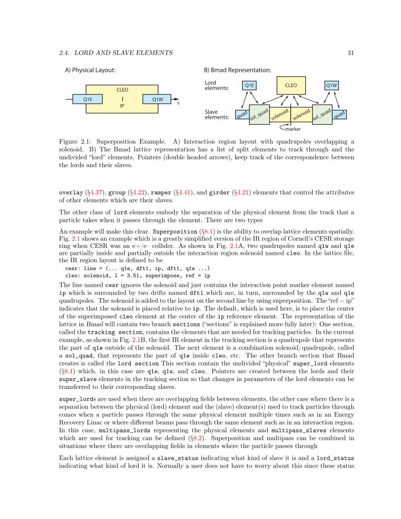
CLEOQ1E Q1W

sol_quadquad

solenoid

marker

quadsol_quad

solenoid

Figure 2.1: Superposition Example. A) Interaction region layout with quadrupoles overlapping asolenoid. B) The Bmad lattice representation has a list of split elements to track through and theundivided “lord” elements. Pointers (double headed arrows), keep track of the correspondence betweenthe lords and their slaves.

overlay (§4.37), group (§4.22), ramper (§4.41), and girder (§4.21) elements that control the attributesof other elements which are their slaves.

The other class of lord elements embody the separation of the physical element from the track that aparticle takes when it passes through the element. There are two types

An example will make this clear. Superposition (§8.1) is the ability to overlap lattice elements spatially.Fig. 2.1 shows an example which is a greatly simplified version of the IR region of Cornell’s CESR storagering when CESR was an e+/e– collider. As shown in Fig. 2.1A, two quadrupoles named q1w and q1eare partially inside and partially outside the interaction region solenoid named cleo. In the lattice file,the IR region layout is defined to be

cesr: line = (... q1e, dft1, ip, dft1, q1w ...)cleo: solenoid, l = 3.51, superimpose, ref = ip

The line named cesr ignores the solenoid and just contains the interaction point marker element namedip which is surrounded by two drifts named dft1 which are, in turn, surrounded by the q1w and q1equadrupoles. The solenoid is added to the layout on the second line by using superposition. The “ref = ip”indicates that the solenoid is placed relative to ip. The default, which is used here, is to place the centerof the superimposed cleo element at the center of the ip reference element. The representation of thelattice in Bmad will contain two branch sections (“sections” is explained more fully later): One section,called the tracking section, contains the elements that are needed for tracking particles. In the currentexample, as shown in Fig. 2.1B, the first IR element in the tracking section is a quadrupole that representsthe part of q1e outside of the solenoid. The next element is a combination solenoid/quadrupole, calleda sol_quad, that represents the part of q1e inside cleo, etc. The other branch section that Bmadcreates is called the lord section This section contain the undivided “physical” super_lord elements(§8.1) which, in this case are q1e, q1w, and cleo. Pointers are created between the lords and theirsuper_slave elements in the tracking section so that changes in parameters of the lord elements can betransferred to their corresponding slaves.

super_lords are used when there are overlapping fields between elements, the other case where there is aseparation between the physical (lord) element and the (slave) element(s) used to track particles throughcomes when a particle passes through the same physical element multiple times such as in an EnergyRecovery Linac or where different beams pass through the same element such as in an interaction region.In this case, multipass_lords representing the physical elements and multipass_slaves elementswhich are used for tracking can be defined (§8.2). Superposition and multipass can be combined insituations where there are overlapping fields in elements where the particle passes through

Each lattice element is assigned a slave_status indicating what kind of slave it is and a lord_statusindicating what kind of lord it is. Normally a user does not have to worry about this since these status

32 CHAPTER 2. BMAD CONCEPTS AND ORGANIZATION

attributes are handled automatically by Bmad. The possible lord_status settings are:

girder_lordA girder_lord element is a girder element (§4.21).

multipass_lordmultipass_lord elements are created when multipass lines are present (§8.2).

overlay_lordAn overlay_lord is an overlay element (§4.37).

group_lordA group_lord is a group element (§4.22).

super_lordA super_lord element is created when elements are superimposed on top of other elements (§8.1).

not_a_lordThis element does not control anything.

Any element whose lord_status is something other than not_a_lord is called a lord element. In thetracking part of the branch, lord_status will always be not_a_lord. In the lord section of thebranch, under normal circumstances, there will never be any not_a_lord elements.

Lord elements are divided into two classes. A major lord represents a physical element which the slaveelements are a part of. super_lords and multipass_lords are major lords. As a consequence, a majorlord is a lord that controls nearly all of the attributes of its slaves. The other lords — girder_lords,group_lords and overlay_lords — are called minor lords. These lords only control some subset of aslaves attributes.

The possible slave_status settings are

multipass_slaveA multipass_slave element is the slave of a multipass_lord (§8.2).

slice_slaveA slice_slave element represents a longitudinal slice of another element. Slice elements are notpart of the lattice but rather are created on-the-fly when, for example, a program needs to trackpart way through an element.

super_slaveA super_slave element is an element in the tracking part of the branch that has one or moresuper_lord lords (§8.1).

minor_slaveminor_slave elements are elements that are not slice_slaves and are only controlled by minorlords (overlay_lords, group_lords, or girder_lords).

freeA free element is an element with no lords.

For historical reasons, each branch in a lattice has a tracking section and a lord section and thetracking section is always the first (lower) part of the element array and the lord section inhabitsthe second (upper) part of the array. All the lord elements are put in the lord section of branch 0and all the other lord sections of all the other branches are empty.

2.4. LORD AND SLAVE ELEMENTS 33

As a side note, Étienne Forest’s PTC code (§1.4) uses separate structures to separate the physical element,which PTC calls an element from the particle track which PTC call a fibre. [Actually, PTC has twostructures for the physical element, element and elementp. The latter being the “polymorph” version.]This element and fibre combination corresponds to Bmad multipass_lord and multipass_slaveelements. PTC does not handle overlapping fields as Bmad does with superposition (§8.1).

34 CHAPTER 2. BMAD CONCEPTS AND ORGANIZATION

Chapter 3

Lattice File Format

A lattice (§2) defines the sequence of elements that a particle will travel through along with the attributes(length, strength, orientation, etc.) of the elements. A lattice file (or files) is a file that is used to describean accelerator or storage ring.

When Bmad was first developed, The Bmad lattice file syntax was modeled upon the format defined forthe MAD program[Grote96]. Since then, the Bmad format has been developed to meet ever increasingsimulation needs so currently there are many differences between the two formats. One difference, whichhas been present from the very start, is that there are no “action” commands (action commands tell theprogram to calculate the Twiss parameters, do tracking, etc.) in a Bmad lattice file. The reason for thisis due to the fact that Bmad is a software library and not a program. That is, interacting with the userto determine what actions a Bmad based program should take is left to the program itself and is notpart of the Bmad standard.

3.1 File Example and Syntax

The following (rather silly) example shows some of the features of a Bmad lattice file:! This is a commentparameter[E_TOT] = 5e9 ! Parameter definitionpa1 = sin(3.47 * pi / c_light) ! Constant definitionbend1: sbend, type = "arc bend", l = 2.3, ! An element definition

g = 2*pa1, tracking_method = bmad_standardbend2: bend1, l = 3.4 ! Another element defbend2[g] = 105 - exp(2.3) / 37.5 ! Redefining an attributeln1: line = (ele1, ele2, ele3) ! A line definitionln2: line = (ln1, ele4, ele5) ! Lines can contain linesarg_ln(a, b): line = (ele1, a, ele2, b) ! A line with arguments.use, ln2 ! Which line to use for the lattice

A Bmad lattice file consists of a sequence of statements. An exclamation mark (!) denotes a commentand the exclamation mark and everything after the exclamation mark on a line are ignored. Bmad isgenerally case insensitive. Most names are converted to uppercase. Exceptions where a name is notconverted include file names and atomic formulas for materials used in crystal diffraction.

Normally a statement occupies a single line in the file. Several statements may be placed on the sameline by inserting a semicolon (“;”) between them. A long statement can occupy multiple lines by putting

35

36 CHAPTER 3. LATTICE FILE FORMAT

an ampersand (“&”) at the end of each line of the statement except for the last line. Additionally, linesthat end with an “implicit end-line continuation character” are automatically continued to the next lineand lines that begin with an “implicit begin-line continuation character are automatically appended tothe previous line. The implicit end-line continuation characters are:, ( [ =

The implicit begin-line continuation characters are:, ) ] =

The following example shows a command extending over four lineswall = ! End-line continuation character.section = s = 0.45 ! Begin-line continuation character.

! Begin-line continuation character.Note: The symbols “+”, “-”, “*”, and “/” are not valid implicit continuation characters. The reason forthis is to avoid confusion when a species name (for example “He++”) comes at the end of a line.

A single line in a lattice file is limited to 500 characters. Commands have no restrictions as to thenumber of lines they may be continued over and there is no limit to the length of a command.

Names of constants, elements, lines, etc. are limited to 40 characters. The first character must be a letter(A — Z). The other characters may be a letter, a digit (0 — 9) or an underscore (_). Other charactersmay appear but should be avoided since they are used by Bmad for various purposes. For example,the backslash (\) character is used to by Bmad when forming the names of superposition slaves (§8.1)and dots (.) are used by Bmad when creating names of tagged elements (§7.8). Also use of specialcharacters may make the lattice files less portable to non-Bmad programs.

The following example constructs a linear lattice with two elements:parameter[geometry] = openparameter[e_tot] =2.7389062E9parameter[particle] = POSITRONbeginning[beta_a] = 14.5011548beginning[alpha_a] = -0.53828197beginning[beta_b] = 31.3178048beginning[alpha_b] = 0.25761815q: quadrupole, l = 0.6, b1_gradient = 9.011d: drift, l = 2.5t: line = (q, d)use, t

here parameter[geometry] (§9.1) is set to open which specifies that the lattice is not circular. In thiscase, the beginning Twiss parameters need to be specified and this is done by the beginning statements(§9.4). A quadrupole named q and a drift element named d are specified and the entire lattice consistsof element q followed by element d.

3.2 Digested Files

Normally the Bmad parser routine will create what is called a “digested file” after it has parsed a latticefile so that when a program is run and the same lattice file is to be read in again, to save time, thedigested file can be used to load in the lattice information. This digested file is in binary format andis not human readable. The digested file will contain the transfer maps for all the elements. Using adigested file can save considerable time if some of the elements in the lattice need to have Taylor mapscomputed. (this occurs typically with map–type wigglers).

3.3. ELEMENT SEQUENCE DEFINITION 37

Bmad creates the digested file in the same area as the lattice file. If Bmad is not able to create adigested file (typically because it does not have write permission in the directory), an error message willbe generated but otherwise program operation will be normal.

Digested files contain the names of the lattice files used to create them. If a lattice file has been modifiedsince the digested file has been created then the lattice files will be reread and a new digested file willbe generated.

Note: If any of the random number functions (§3.13) are used in the process of creating the lattice, thedigested file will be ignored. In this case, each time the lattice is read into a program, different randomnumbers will be generated for expressions that use such random numbers.

Digested files can also be used for easy transport of lattices between programs or between sessions ofa program. For example, using one program you might read in a lattice, make some adjustments (sayto model shifts in magnet positions) and then write out a digested version of the lattice. This adjustedlattice can now be read in by another program.

3.3 Element Sequence Definition

A line defines a sequence of elements. lines may contain other lines and so a hierarchy may beestablished. One line is selected, via a use statement, that defines the lattice. For example:l3: line = (l1, l2) ! Concatenate two linesl1: line = (a, b, c) ! Line with 3 elementsl2: line = (a, z) ! Another lineuse, l3 ! Use l3 as the lattice definition.

In this case the lattice would be(a, b, c, a, z)

Lines can be defined in any order. See Chapter 7 for more details.

The superimpose construct allows elements to be placed in a lattice at a definite longitudinal position.What happens is that after a lattice is expanded, there is a reshuffling of the elements to accommodateany new superimpose elements. See §8.1 for more details.

3.4 Lattice Elements

The syntax for defining a lattice element roughly follows the MAD [Grote96] program:ele_name: keyword [, attributes]

where ele_name is the element name, keyword is the type of element, and attributes is a list of theelements attributes. Chapter 4 gives a list of elements types with their attributes. Overlay and grouptype elements have a slightly different syntax:ele_name: keyword = list , master-attribute [= value] [, attributes]

and Girder elements have the syntaxele_name: keyword = list [, attributes]

For example:q01w: quadrupole, type = "A String", l = 0.6, tilt = pi/4h10e: overlay = b08e, b10e , var = hkick

The keyword specifying the element type can be the name of an element that has already been declared.In this case, the element being defined will inherit the attributes that have been set for the elementassociated with keyword. Example:

38 CHAPTER 3. LATTICE FILE FORMAT

qa, quad, l = 0.6, tilt = pi/4 ! Define QA.qb: qa ! QB Inherits from QA.qa[k1] = 0.12 ! QB unaffected by modifications of QA.

In this example, element QB inherits the attributes of QA which, in this case, are the length and tiltparameters of QA. Once QB is defined, the elements are separate so modifications of the parameters ofQA after QB is defined will not affect QB.

Bmad allows element names to be abbreviations of element types. For example, “Q”, QU”, and “QUADRUPOL”are all valid element names but “QUADRUPOLE”, being an exact match to the corresponding element type,is not. Care must be used when using elements that are abbreviations of element types since Bmadallows element type names to be abbreviated (but element names may not be abbreviated when usinginheritance). For example:q1: quad ! Q1 is a quadrupole since it comes before the next line.quad: sextupole ! QUAD element is defined to be a sextupole.q2: quad ! Q2 is a sextupole as it inherits from QUAD.q3: qua ! Q3 is a quadrupole. Inherit from names cannot be abbreviated.

3.5 Lattice Element Names

A valid element name may be up to 40 characters in length. The first character of the name must be aletter [A-Z]. After that, the rest of the name can contain only letters, digits [0-9], underscore “_”, period“.”, backslash “\”, or a hash mark “#”. A double hash mark “##” is not permitted since this interferswith the notation for finding the N th element with a given name (§3.6). It is best to avoid these lastthree symbols since Bmad uses them to denote “relationships”. Periods are used for tagging (§7.8), andbackslash and hash marks are used for to compose names for superposition (§8.1) and multipass (§8.2)slave elements.

There is a short list of names that cannot be used as an element, line or list name. These reserved namesare:beamparticle_startbeginningdebug_markerendno_digestedparameterparser_debugprintroottitleusewrite_digested

Note: The one exception is if end is used to define a marker. This exception is allowed since Bmad usesthe end name to define a marker in any case.

3.6 Matching to Lattice Element Names

Where appropriate, for example when setting element attributes (§3.7), the wild card characters “*”and “%” can be used to select multiple elements. The “*” character will match any number of characters

3.6. MATCHING TO LATTICE ELEMENT NAMES 39

(including zero) while “%” maches to any single character. Additionally, matching can be restricted toa certain element class using the syntax:class::element_name

where class is a class (EG: sextupole). For example:m* ! Match to all elements whose name begins with "m".a%c ! Match to "abc" but not to "ac" or "azzc".quadrupole::*w ! Match to all quadrupoles whose name ends in "w"

Note: The character “%” can be used in expressions used for setting lattice element parameter values.In this case, the “%” character represents the name of the lattice element whose parameter is being set.This is discussed in section §3.7.

Instead of matching to an element name, matches may be made to type, alias, or descrip attributes(§5.3) using the syntax:attribute_name::string

where attribute_name is one of:typealiasdescrip

and string is a string to match to which can include wild card characters “*” and “%”. If stringcontains blank characters, the string must be enclosed with single or double quotation marks. Note: Anelement attribute that is blank will never match. Also note that while type, alias, or descrip stringsmay have lower case characters (unlike element names, these strings are not converted to upper case),matching is always case insensitive. For Example:type::"det bpm*" ! Match to all elements whose type string starts with "det bpm".alias::* ! Match to all elements whose alias string is not blank.

After lattice expansion (§3.22), the general syntax to specify a set of elements is:branch_id>>class::element_idbranch_id>>element_name##N ! N^th instance of element_name in branch with branch_idbranch_id>>class::element_id##N+M ! M^th element after elementbranch_id>>class::element_id##N-M ! M^th element before element

where ... marks an optional component, class is a class name, branch_id is a branch name orindex (§2.2), element_id is and element name or element index (§7.2), and ##N indicates that the Nthmatching element in a branch is to be used. Examples:x_br>>quad::q* ! All quadrupoles of branch "x_br" whose name begins with "q".2>>45 ! element #45 of branch #2.q01##3 ! The 3rd element named q01 in each branch where there are at

! least three elements named q01.q01-1 ! Elements just before all elements named q01.q01##3+0 ! Same as q01##3.

Note: Group and overlay elements have unique names so using ## is unnecessary.

Note: When using the ## construct, super_lord and girder_lord elements are considered to be situatedwhere their slave elements are situated in the lattice. This is independent of where they actually existwhich is in the lord part of branch 0 (§2.4).

Note: When using +M and -M offsets, no space should be put around the plus or minus signs. Off-sets cannot be used with overlay, group, ramper_lord or multipass_lord elements. If used with asuper_lord or girder element, for a -M offset the element selected is the Mth element before the firstslave element of the lord and for a +M offset the element selected is the Mth element after the last slaveelement of the lord. Also, independent of the geometry of the branch, the element selected will “wrap”around the ends of the branch. For example, if a lattice branch looks like:

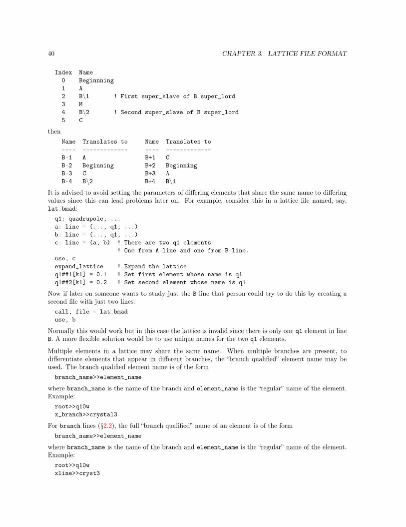
40 CHAPTER 3. LATTICE FILE FORMAT

Index Name0 Beginnning1 A2 B\1 ! First super_slave of B super_lord3 M4 B\2 ! Second super_slave of B super_lord5 C

thenName Translates to Name Translates to---- ------------- ---- -------------B-1 A B+1 CB-2 Beginning B+2 BeginningB-3 C B+3 AB-4 B\2 B+4 B\1

It is advised to avoid setting the parameters of differing elements that share the same name to differingvalues since this can lead problems later on. For example, consider this in a lattice file named, say,lat.bmad:q1: quadrupole, ...a: line = (..., q1, ...)b: line = (..., q1, ...)c: line = (a, b) ! There are two q1 elements.

! One from A-line and one from B-line.use, cexpand_lattice ! Expand the latticeq1##1[k1] = 0.1 ! Set first element whose name is q1q1##2[k1] = 0.2 ! Set second element whose name is q1

Now if later on someone wants to study just the B line that person could try to do this by creating asecond file with just two lines:call, file = lat.bmaduse, b

Normally this would work but in this case the lattice is invalid since there is only one q1 element in lineB. A more flexible solution would be to use unique names for the two q1 elements.

Multiple elements in a lattice may share the same name. When multiple branches are present, todifferentiate elements that appear in different branches, the “branch qualified” element name may beused. The branch qualified element name is of the formbranch_name>>element_name

where branch_name is the name of the branch and element_name is the “regular” name of the element.Example:root>>q10wx_branch>>crystal3

For branch lines (§2.2), the full “branch qualified” name of an element is of the formbranch_name>>element_name

where branch_name is the name of the branch and element_name is the “regular” name of the element.Example:root>>q10wxline>>cryst3

3.7. LATTICE ELEMENT ATTRIBUTES 41

Using the full name is only needed to distinguish elements that have the same regular name in separatebranches. When parsing a lattice file, branches are not formed until the lattice is expanded (§3.22).Therefore an expand_lattice statement is required before full names can be used in statements.

After lattice expansion (§3.22), when setting element attributes (§3.7, a comma delimited list of namescan be used (the commas are actually optional). Each item in a list is either the name of an element oran element range. An element range has the syntax:branch>>class::ele1:ele2

wherebranch ! Optional branch name or index.class ! Optional element class name ("quadrupole", "sbend", etc.)ele1 ! Starting element of the range.ele2 ! Ending element of the range.

For example:3,15:17 ! Elements with index 3, 15, 16, and 17 in branch 0.3 15:17 ! Same as above (commas are optional).2>>45:51 ! Elements 45 through 51 of branch 2.q1:q5 ! Elements between q1 and q5.sbend::q1:q5 ! All sbend elements between q1 and q5 including q1 and q5 if they.

! are sbends. Notice that q1 and q5 do not have to be sbends

With a comma delimited list of names, a tilde prefix can be used to remove elements from the list.Adding and subtracting elements is done left to right. For example:*::*, ~quadrupole::* ! All elements except quadrupolesb*, ~b1*, b13 ! All elements with names beginning with B except

! elements with names beginning with B1. However,! elements named B13 are retained.

With a list of names, an ampersand “&” can be used to form the intersection of two sets.100:200 & sbend::* ! All sbend elements whose index is between 100 and 200.q* & quad::* ! Equivalent to "quadrupole::q*".q* & quad::* b1 ! Equivalent to "quadrupole::q*, b1".

3.7 Lattice Element Attributes

Any lattice element has various attributes like its name, its length, its strength, etc. The values ofelement attributes can be specified when the element is defined. For example:b01w: sbend, l = 6.0, rho = 89.0 ! Define an element with attributes.

After an element’s definition, an individual attribute may be referred to using the syntaxclass::element_name[attribute_name]

Examples:q01[k1] ! K1 attribute of element Q01.sbend::b0%[dg] ! DG attribute of sbend elements whose name

! has three characters starting with "B0"

Element attributes can be set or used in an algebraic expression:b01w[roll] = 6.5 ! Set an attribute value.b01w[L] = 6.5 ! Change an attribute value.b01w[L] = b01w[rho] / 12 ! OK to reset an attribute value.my_const = b01w[rho] / b01w[L] ! Use of attribute values in an expression.

42 CHAPTER 3. LATTICE FILE FORMAT

Notice that there can be no space between the element name and the [ opening bracket.

Chapter Chapter 4 lists the attributes appropriate for each element class.

When setting an attribute value, if more than one element has the element_name then all such elementswill be set. When setting an attribute value, if element_name is the name of a type of element, allelements of that type will be set. For exampleq_arc[k1] = 0.234 ! Set all elements named Q_ARC.rfcavity::*[voltage] = 3.7 ! Set all RFcavity elements.

To set an attribute for multiple element at one time, The wild cards “*”, and “%” can be used in elementnames (§3.6). Examples:*[tracking_method] = bmad_standard ! Matches all elements.quadrupole::Q*[k1] = 0.234 ! Matches all quadrupoles with names beginning with Q.Q%1[k1] = 0.234 ! Matches to "Q01" but not "Q001".

Unlike when there are no wild cards used in a name, it is not an error if a name with wild cards doesnot match to any element. Note: A name with wild cards will never match to the BEGINNING element(§7.7).

The “%” symbol can be used in expression to represent the lattice element whose parameter is being set.For example:s%z[k2] = %[k2] + 0.03 * ran_gauss()

The “s%z” on the left hand side matches to all three letter elements whose name begins with “s” andends with “z”. For each element that is matched, the “%[k2]” in the expression on the right hand sidewill be the k2 value of that element. Thus, if there are three elements, named s0z, saz, and s.z, in thelattice that match s%z, the above command is equivalent to the following three commandss0z[k2] = s0z[k2] + 0.03 * ran_gauss()saz[k2] = saz[k2] + 0.03 * ran_gauss()s.z[k2] = s.z[k2] + 0.03 * ran_gauss()

After lattice expansion (§3.22), the attributes of specific elements may be set using the syntax as discussedin Section §3.6. Example:expand_lattice ! Expand the lattice.97[x_offset] = 0.0023 ! Set x_offset attribute of 97th elementb2>>si_cryst##2[tilt] = 0.1 ! Tilt the 2nd instance of "si_cryst" in branch "b2"5:32[x_limit] = 0.3 ! Sets elements with indexes 5 through 32 in branch 0.

3.8 Custom Element Attributes

Real scalar and vector custom element attributes may be defined for any class of element and real scalerparameters can be defined for the lattice as a whole. Custom element attributes are useful with programsthat need to associate “extra” information with particular lattice elements or the lattice itself and it isdesired that this extra information be settable from within a lattice file. For example, a program mightneed an error tolerance for the strength of quadrupoles.

Adding custom attributes will not disrupt programs that are not designed to use the custom attributes.Currently, up to 40 named custom attributes may be defined for any given element class. The syntaxfor defining custom attributes is:parameter[custom_attributeN] = class_name::attribute_name

Where “N” is an integer between 1 and 40 and "attribute_name" is the name of the attribute. To restrictthe custom attribute to a particular element class, the element class can be prefixed to the attributename. To define a global parameter for the lattice, use parameter” as the class name. Examples:

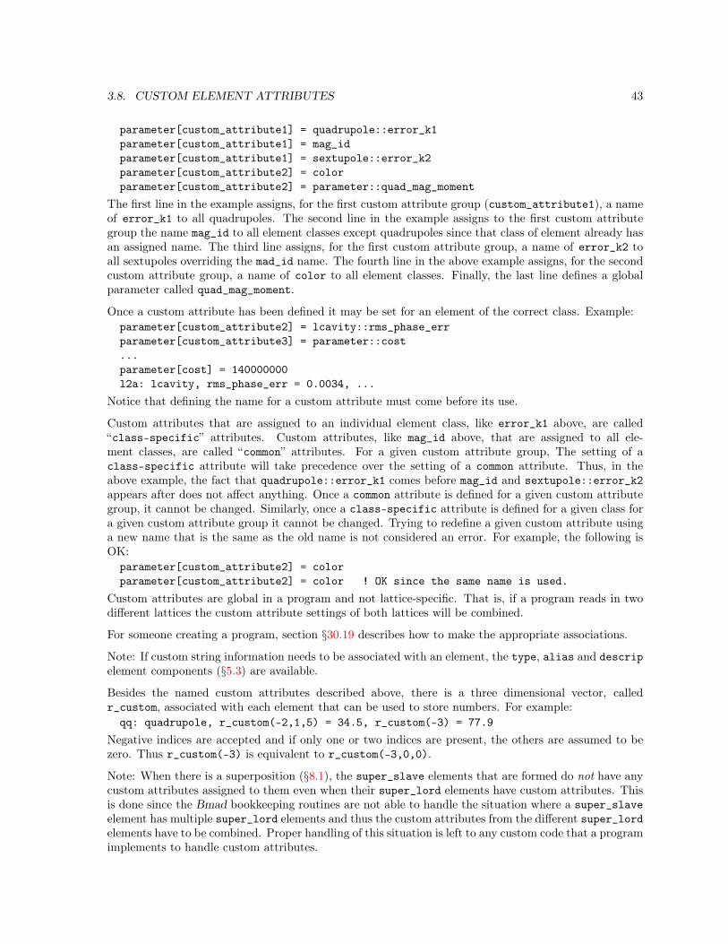
3.8. CUSTOM ELEMENT ATTRIBUTES 43

parameter[custom_attribute1] = quadrupole::error_k1parameter[custom_attribute1] = mag_idparameter[custom_attribute1] = sextupole::error_k2parameter[custom_attribute2] = colorparameter[custom_attribute2] = parameter::quad_mag_moment

The first line in the example assigns, for the first custom attribute group (custom_attribute1), a nameof error_k1 to all quadrupoles. The second line in the example assigns to the first custom attributegroup the name mag_id to all element classes except quadrupoles since that class of element already hasan assigned name. The third line assigns, for the first custom attribute group, a name of error_k2 toall sextupoles overriding the mad_id name. The fourth line in the above example assigns, for the secondcustom attribute group, a name of color to all element classes. Finally, the last line defines a globalparameter called quad_mag_moment.

Once a custom attribute has been defined it may be set for an element of the correct class. Example:parameter[custom_attribute2] = lcavity::rms_phase_errparameter[custom_attribute3] = parameter::cost...parameter[cost] = 140000000l2a: lcavity, rms_phase_err = 0.0034, ...

Notice that defining the name for a custom attribute must come before its use.

Custom attributes that are assigned to an individual element class, like error_k1 above, are called“class-specific” attributes. Custom attributes, like mag_id above, that are assigned to all ele-ment classes, are called “common” attributes. For a given custom attribute group, The setting of aclass-specific attribute will take precedence over the setting of a common attribute. Thus, in theabove example, the fact that quadrupole::error_k1 comes before mag_id and sextupole::error_k2appears after does not affect anything. Once a common attribute is defined for a given custom attributegroup, it cannot be changed. Similarly, once a class-specific attribute is defined for a given class fora given custom attribute group it cannot be changed. Trying to redefine a given custom attribute usinga new name that is the same as the old name is not considered an error. For example, the following isOK:parameter[custom_attribute2] = colorparameter[custom_attribute2] = color ! OK since the same name is used.

Custom attributes are global in a program and not lattice-specific. That is, if a program reads in twodifferent lattices the custom attribute settings of both lattices will be combined.

For someone creating a program, section §30.19 describes how to make the appropriate associations.

Note: If custom string information needs to be associated with an element, the type, alias and descripelement components (§5.3) are available.

Besides the named custom attributes described above, there is a three dimensional vector, calledr_custom, associated with each element that can be used to store numbers. For example:qq: quadrupole, r_custom(-2,1,5) = 34.5, r_custom(-3) = 77.9

Negative indices are accepted and if only one or two indices are present, the others are assumed to bezero. Thus r_custom(-3) is equivalent to r_custom(-3,0,0).

Note: When there is a superposition (§8.1), the super_slave elements that are formed do not have anycustom attributes assigned to them even when their super_lord elements have custom attributes. Thisis done since the Bmad bookkeeping routines are not able to handle the situation where a super_slaveelement has multiple super_lord elements and thus the custom attributes from the different super_lordelements have to be combined. Proper handling of this situation is left to any custom code that a programimplements to handle custom attributes.

44 CHAPTER 3. LATTICE FILE FORMAT

3.9 Parameter Types

There are five types of parameters in Bmad: reals, integers, switches, logicals (booleans), and strings.Acceptable logical values are

true falset f

For examplerf1[is_on] = False

String literals can be quoted using double quotes (") or single quotes (’). If there are no blanks orcommas within a string, the quotes can be omitted. For example:Q00W: Quad, type = "My Type", alias = Who_knows, &

descrip = "Only the shadow knows"

Unlike most everything else, strings are not converted to uppercase.

Switches are parameters that take discrete values. For example:parameter[particle] = positronq01w: quad, tracking_method = bmad_standard

The name “switch” can refer to the parameter (for example, tracking_method) or to a value that it cantake (for example, bmad_standard). The name “method” is used interchangeably with switch.

3.10 Particle Species Names

For the purpose of assigning names to simulated particles, particles are divided into four groups. Onegroup are are fundamental particles. These are:electron, positronmuon, antimuonproton, antiprotonneutron anti_neutrondeuteron anti_deuteronpion+, pion0, pion-photon

For historical reasons, names for the fundamental particles are not case sensitive.

Another group are atoms. The general syntax for atoms is:#nnnAAccc

The curly brackets ... denote optional prefixes and suffixes. AA here is the atomic symbol, #nnn is thenumber of nucleons, and ccc is the charge. Examples:parameter[particle] = #12C+3 ! Triply charged carbon-12parameter[particle] = He-- ! Doubly charged He.

If the number of nucleons is given, the appropriate weight for that isotope is used. If the number ofnucleons is not present, the mass is an average weighted by the isotopic abundances of the element. Thecharge may be given by using the appropriate number of plus (+) or minus (-) signs or by using a plusor minus sign followed by a number. Thus “---” is equivalent to “-3”. Names here are case sensitive.“@M” must be used and not “@m” for specifying the mass.

Another group of particles are the “known” molecules. The syntax for these are:BBB@Mxxxxccc

@Mxxxx is the mass in AMU, ccc is the charge, and BBB is the molecular formula. The mass may tospecified to hundredths of an AMU. The known molecules are:

3.10. PARTICLE SPECIES NAMES 45

CO CO2D2 D2OOH O2H2 H2O HFN2 NH2 NH3CH2 CH3 CH4C2H3 C2H4 C2H5

Like with atoms, if the mass is not specified, the average isotopic mass is used. Examples:C2H3@M28.4+ ! Singly charged C2H3 with mass of 28.4CH2 ! Neutral CH2

Like the atomic formulas, molecular formulas are case sensitive.

The last group of particle are particles where only the mass and charge are specified. The syntax forthese are:@Mxxxxccc

Example:@M37.54++ ! Doubly charged molecule of mass 37.54 AMU.

Note: When setting the value of a variable to be a particle species ID, use the species function asdiscussed in §3.13.

46 CHAPTER 3. LATTICE FILE FORMAT

3.11 Units and Constants

Bmad uses SI (Système International) units as shown in Table 3.1. Note that MAD uses different units.For example, MAD’s unit of Particle Energy is GeV not eV.

Note: For compatibility with MAD, the beam, energy = xxx command (§9.3) uses GeV and the emassand pmass constants (see below this section) also use GeV. It is recommended that the use of theseconstructs be avoided.

Quantity Units

Angles radiansBetatron Phase radiansCurrent AmpsFrequency HzKick radiansLength metersMagnetic Field TeslaParticle Energy eVRF Phase Angles radians/2πVoltage Volts

Table 3.1: Physical units used by Bmad.

Bmad defines commonly used physical and mathematical constants shown in Table 3.2. All symbolsuse straight SI units except for emass and pmass which are provided for compatibility with MAD andshould be avoided.As an alternative, the mass_of, and anomalous_moment_of functions (§3.13) may be used in place ofthe defined constants for mass and anomalous magnetic moment.

Note: The standard definition of the magnetic moment g-factor for spin 1/2 fundamental particles is

µ = gq

2mS (3.1)

where µ is the magnetic moment, q is the particle charge, and m is the mass. The anomalous momenta is then defined to be

a =g − 2

2(3.2)

For nuclei and other composite baryonic particles, it is conventional to define the g-factor using

µ = ge

2mpS (3.3)

wheremp is the mass of the proton. This is inconvenient for calculations since an equation like Eq. (22.2)would not work for all particles. To get around this, the g-factors used by Bmad are always derived fromEq. (3.1) (think of this as an “effective” g-factor).

3.12. ARITHMETIC EXPRESSIONS 47

Symbol Value Units Name

pi 3.141592653589793twopi 2 * pifourpi 4 * pie 2.718281828459045e_log 2.718281828459045sqrt_2 1.414213562373095degrad 180 / pi From rad to degdegrees pi / 180 From deg to radraddeg pi / 180 From deg to radanom_moment_deuteron −0.1425617662 Deuteron anomalous magnetic moment∗anom_moment_electron 0.00115965218128 Electron anomalous magnetic momentanom_moment_muon 0.00116592089 muon anomalous magnetic momentanom_moment_proton 1.792854734463 proton anomalous magnetic momentanom_moment_he3 −4.184153686 He3 anomalous magnetic moment∗fine_struct_const 0.0072973525693 Fine structure constantm_deuteron 1.87561294257 · 109 eV Deuteron massm_electron 0.51099895000 · 106 eV Electron massm_neutron 0.93956542052 · 109 eV Neutron massm_muon 105.6583755 · 106 eV Muon massm_pion_0 134.9766 · 106 eV π0 massm_pion_charged 139.57018 · 106 eV π+, π− massm_proton 0.93827208816d · 109 eV Proton massc_light 2.99792458 · 108 m/sec Speed of lightr_e 2.8179403262 · 10−15 m Electron radiusr_p 1.5346982647 · 10−18 m Proton radiuse_charge 1.602176634 · 10−19 Coul Electron chargeh_planck 4.135667696 · 10−15 eV*sec Planck’s constanth_bar_planck 6.582118990 · 10−16 eV*sec Planck / 2πemass 0.51099895000 · 10−3 GeV Electron mass (please avoid using)pmass 0.93827208816 GeV Proton mass (please avoid using)

∗ Effective anomalous moments. See the discussion after Eq. (3.1).

Table 3.2: Physical and mathematical constants recognized by Bmad.

3.12 Arithmetic Expressions

Arithmetic expressions can be used in a place where a real value is required. The standard operatorsare defined:

a+ b Additiona− b Subtractiona ∗ b Multiplicationa / b Divisiona ∧ b Exponentiation

Bmad also has a set of intrinsic functions. A list of these is given in §3.13.

Literal constants can be entered with or without a decimal point. An exponent is marked with the letterE. For example1, 10.35, 5E3, 314.159E-2

Symbolic constants can be defined using the syntax

48 CHAPTER 3. LATTICE FILE FORMAT

constant_name = expression

Alternatively, to be compatible with MAD, using “:=” instead of “=” is acceptedconstant_name := expression

Examples:my_const = sqrt(10.3) * pi^3abc := my_const * 23

Unlike MAD, Bmad uses immediate substitution so that all constants in an expression must have beenpreviously defined. For example, the following is not valid:abc = my_const * 23 ! No: my_const needs to be defined first.my_const = sqrt(10.3) * pi^3

here the value of my_const is not known when the line “abc = . . .” is parsed. Note: To get the effect ofdelayed evaluation, use overlay (§4.37) or group (§4.22) controller elements.

Once defined, symbolic constants cannot be redefined. For example:my_const = 1my_const = 2 ! No! my_const cannot be redefined.

The restriction against redefining constants was implemented to avoid hard to find problems. On veryrare occasions, it is convenient to be able to redefine constants so if the redefinition has a redef: prefix,a constant can be redefinedmy_const = 1redef: my_const = 2 ! OK!

It is advised not to use redef unless there a very good reason for its use.

group (§4.22) and overlay (§4.37) controller elements are an exception to the immediate evaluationrule. Since controller elements may control elements that do not exist until lattice expansion (§3.22),the arithmetic expressions associated with controller elements are not evaluated until lattice expansion.Example:s_20W: sextupole, l = 0.27sk: overlay = s_20W[a1]:-2*s_20W[L], var = k1, k1 = 0.2s_20W[L] = 0.34s_30E: s_20W...expand_lattice

Here the expression of overlay sk is evaluated, when the lattice is expanded, to be -0.68 = -2*0.34.This uses the length of element s_20W at the point when the lattice is expanded and not at the pointwhen sk was defined. Additionally, the element s_30E, which inherits the attributes of s_20W, inheritsa value of zero for a1 (skew multipole moment) since inheritance uses immediate evaluation just like thesetting of constants.

Element attributes can be used after they have been defined but not before. Example:sa: sextupole, l = 0.3, k2 = 0.01 * sa[L] ! Goodsb: sextupole, k2 = 0.01 * sb[L], l = 0.3 ! BAD SET OF K2. L IS DEFINED AFTER.

In this example, the k2 attribute of element sa is correctly set since k2 is defined after l. On the otherhand, k2 of element sb will have a value of zero since l of sb defaults to zero before it is set.

One potential pitfall with immediate substitution is that when an element attribute changes, it does notaffect prior evaluations. Example:s1: sextupole, k2 = 2.3aa = s1[k2] ! aa = 2.3s1[k2] = 1.7 ! value of aa does not change

3.13. INTRINSIC FUNCTIONS 49

Here the value of constant aa will remain fixed at 2.3 no matter how the value of s1[k2] is altered afteraa is defined.

Another potential pitfall is when using dependent element attributes (§5.1). For example:b01w: sbend, l = 0.5, angle = 0.02a_const = b01w[g] ! No: bend g has not yet been computed!

Here the bend strength g (§4.5) will eventually be computed to be 0.04 (= angle / l) but that computationdoes not happen until lattice expansion (§3.22). In this case, the value of a_const will be the defaultvalue of g which is zero. As a rule of thumb, never rely on dependent attributes having their correctvalue.

3.13 Intrinsic functions

The following intrinsic functions are recognized by Bmad:sqrt(x) Square Rootlog(x) Logarithmexp(x) Exponentialsin(x), cos(x) Sine and cosinetan(x), cot(x) Tangent and cotangentsinc(x) Sin(x)/x Functionasin(x), acos(x) Arc sine and Arc cosineatan(x) Arc Tangentatan2(y, x) Arc Tangent of y/xabs(x) Absolute Valuefactorial(n) Factorialran() Random number between 0 and 1ran_gauss() Gaussian distributed random numberran_gauss(sig_cut) Gaussian distributed random numberint(x) Nearest integer with magnitude less then xnint(x) Nearest integer to xsign(x) 1 if x positive, -1 if negagive, 0 if zerofloor(x) Nearest integer less than xceiling(x) Nearest integer greater than xmass_of(A) Mass of particle Acharge_of(A) Charge, in units of the elementary charge, of particle Aanomalous_moment_of(A) Anomalous magnetic moment of particle Aspecies(A) Species ID of A

ran_gauss is a Gaussian distributed random number with unit RMS. Both ran and ran_gauss use aseeded random number generator. To choose the seed setparameter[ran_seed] = <Integer>

A value of zero will set the seed using the system clock so that different sequences of random numberswill be generated each time a program is run. The default behavior if parameter[ran_seed] is notpresent is to use the system clock for the seed.

The ran_gauss(cut) function with an argument truncates the distribution so that no values are returnedwith an absolute value greater than cut. If cut is non-positive, it is ignored so that, for example,ran_gauss(-1) is equivalent to ran_gauss().

If an element is used multiple times in a lattice, and if ran or gauss_ran is used to set an attributevalue of this element, then to have all instances of the element have different attribute values the settingof the attribute must be after the lattice has been expanded (§3.22). For example:

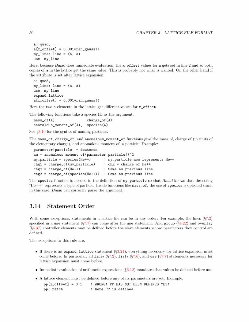
50 CHAPTER 3. LATTICE FILE FORMAT

a: quad, ...a[x_offset] = 0.001*ran_gauss()my_line: line = (a, a)use, my_line

Here, because Bmad does immediate evaluation, the x_offset values for a gets set in line 2 and so bothcopies of a in the lattice get the same value. This is probably not what is wanted. On the other hand ifthe attribute is set after lattice expansion:a: quad, ...my_line: line = (a, a)use, my_lineexpand_latticea[x_offset] = 0.001*ran_gauss()

Here the two a elements in the lattice get different values for x_offset.

The following functions take a species ID as the argument:mass_of(A), charge_of(A)anomalous_moment_of(A), species(A)

See §3.10 for the syntax of naming particles.

The mass_of, charge_of, and anomalous_moment_of functions give the mass of, charge of (in units ofthe elementary charge), and anomalous moment of, a particle. Example:parameter[particle] = deuteronam = anomalous_moment_of(parameter[particle])^2my_particle = species(He++) ! my_particle now represents He++chg1 = charge_of(my_particle) ! chg = charge of He++chg2 = charge_of(He++) ! Same as previous linechg3 = charge_of(species(He++)) ! Same as previous line

The species function is needed in the definition of my_particle so that Bmad knows that the string“He++” represents a type of particle. Inside functions like mass_of, the use of species is optional since,in this case, Bmad can correctly parse the argument.

3.14 Statement Order

With some exceptions, statements in a lattice file can be in any order. For example, the lines (§7.2)specified in a use statement (§7.7) can come after the use statement. And group (§4.22) and overlay(§4.37) controller elements may be defined before the slave elements whose parameters they control aredefined.

The exceptions to this rule are:

• If there is an expand_lattice statement (§3.21), everything necessary for lattice expansion mustcome before. In particular, all lines (§7.2), lists (§7.6), and use (§7.7) statements necessary forlattice expansion must come before.

• Immediate evaluation of arithmetic expressions (§3.12) mandates that values be defined before use.

• A lattice element must be defined before any of its parameters are set. Example:pp[z_offset] = 0.1 ! WRONG! PP HAS NOT BEEN DEFINED YET!pp: patch ! Here PP is defined

3.15. PRINT STATEMENT 51

In this example, the z_offset of the element pp is set before pp has been defined. This is an error.As a corollary to this rule, element parameters that are set using wild card characters will onlyaffect those parameters that have been already defined. For example:crystal::*[b_param] = 0.2c5: crystal

In this example, the b_param of all crystal elements is set to 0.2 except for c5 and all othercrystal elements that are defined after the set.

3.15 Print Statement

The print statement prints a message at the terminal when the lattice file is parsed by a program.Syntax:print <string>

Where <string> is the string to be printed. Variable values can be printed by using back-tick charac-ters. For example:print Remember! Q01 quad strength of `q01[k1]` not yet optimized!print Optimization is as easy as 2 + 2 = `2+2`.

will result in the following being printed:Message in Lattice File: Remember! Q01 quad strength of 0.4526 not yet optimized!Message in Lattice File: Optimization is as easy as 2 + 2 = 4.

The print statement is useful to remind someone using the lattice of important details.

3.16 Title Statement

The title statement sets a title string which can be used by a program. For consistency with MADthere are two possible syntaxestitle, <String>

or the statement can be split into two linestitle<String>

For exampletitle"This is a title"

3.17 Call Statement

It is frequently convenient to separate the lattice definition into several files. Typically there might bea file (or files) that define the layout of the lattice (something that doesn’t change often) and a file (orfiles) that define magnet strengths (something that changes more often). The call is used to read inseparated lattice files. The syntax iscall, filename = <String>

Example:call, filename = "../layout/my_layout.bmad" ! Relative pathnamecall, filename = "/nfs/cesr/lat/my_layout.bmad" ! Absolute pathnamecall, filename = "$LATDIR/my_layout.bmad" ! Absolute pathname

52 CHAPTER 3. LATTICE FILE FORMAT

Bmad will read the called file until a return or end_file statement is encountered or the end of the fileis reached.

For filenames that have a relative pathname, the called file will be searched for relative to the directoryof the calling file. Thus, in the above example, if the file containing the call statements is in the directory/path/to/lat_dir, the first call will open the file:/path/to/lat_dir/../layout/my_layout.bmad

To call a file relative to the current working directory, use the environment variable PWD. Example:call, filename = $PWD/here.bmad

Where a called file is searched for may be modified by using a use_local_lat_file statement. SeeSection §3.19 for more details.

3.18 Inline Call

Any lattice elements will have a set of attributes that need to be defined. As a convenience, it is possibleto segregate an element attribute or attributes into a separate file and then “call” this file using an “inlinecall”. The inline call has three forms. In an element definition, the inline call has the form<ele_name>: <ele_type>, ..., call::<file_name>, ...

or<ele_name>: <ele_type>, ..., <attribute_name> = call::<file_name>, ...

where <attribute_name> is the name of the attribute and <file_name> is the name of the where theattribute structure is given. The third form of the inline call occurs when an element attribute isredefined and has the form<ele_name>[<attribute_name>] = call::<file_name>

Example:c: crystal, call::my_curvature.bmad, surface = call::my_surface.bmad, ...

For grid_fields, which can take some time to parse, a HDF5 binary file can to created and then theHDF5 file, which must have a .h5 or .hdf5 suffix, can be read in with an inline call Example:qq: quadrupole, grid_field = call::my_grid.h5, ...

To create hdf5 files, first create a lattice with the grid_field defined with plain text. Next read thelattice into any program that can create Bmad lattice files (for example, the Tao program (§1.2) can dothis) and have the program then generate a lattice file.

3.19 Use_local_lat_file Statement

It is sometimes convenient to override where Bmad looks for called files (see §3.17). For example, supposeit is desired to temporarily override the settings in a called file without modifying the called file itself.In this case, the use_local_lat_file statement can be used. When this statement is encountered in alattice file, the local directory (that is, the directory from which the program is run) is searched first forthe called file and if a file of the correct name is found, that file is used.

An example will make this clear. Suppose lattice file /A/lat.bmad contains the call:call, filename = "/B/sub.bmad"

Now suppose that you want to use lat.bmad with a modified sub.bmad but you do not want to modify/A/lat.bmad or /B/sub.bmad. The solution is to create two new files. One file, call it new.bmad, whichcan be situated in any directory, has two lines in it:use_local_lat_filecall, filename = "/A/lat.bmad"

The second new file is the modified sub.bmad and it must be in the directory from which the programis run.

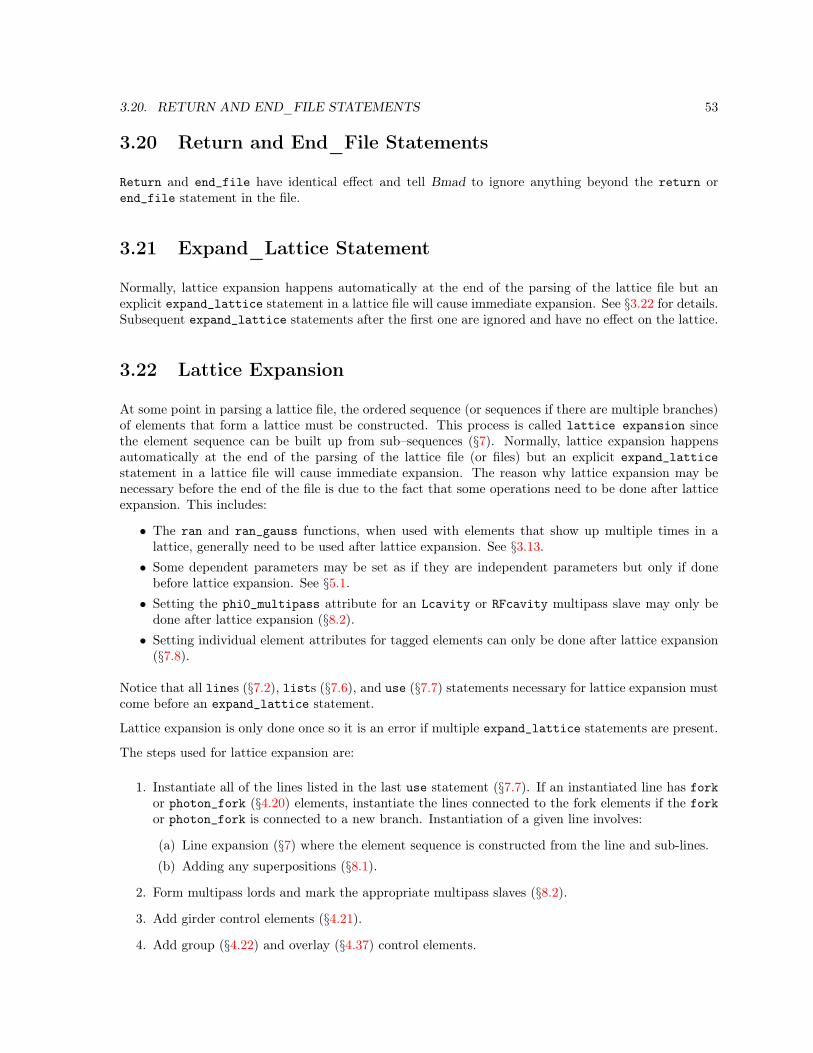
3.20. RETURN AND END_FILE STATEMENTS 53

3.20 Return and End_File Statements

Return and end_file have identical effect and tell Bmad to ignore anything beyond the return orend_file statement in the file.

3.21 Expand_Lattice Statement

Normally, lattice expansion happens automatically at the end of the parsing of the lattice file but anexplicit expand_lattice statement in a lattice file will cause immediate expansion. See §3.22 for details.Subsequent expand_lattice statements after the first one are ignored and have no effect on the lattice.

3.22 Lattice Expansion

At some point in parsing a lattice file, the ordered sequence (or sequences if there are multiple branches)of elements that form a lattice must be constructed. This process is called lattice expansion sincethe element sequence can be built up from sub–sequences (§7). Normally, lattice expansion happensautomatically at the end of the parsing of the lattice file (or files) but an explicit expand_latticestatement in a lattice file will cause immediate expansion. The reason why lattice expansion may benecessary before the end of the file is due to the fact that some operations need to be done after latticeexpansion. This includes:

• The ran and ran_gauss functions, when used with elements that show up multiple times in alattice, generally need to be used after lattice expansion. See §3.13.

• Some dependent parameters may be set as if they are independent parameters but only if donebefore lattice expansion. See §5.1.

• Setting the phi0_multipass attribute for an Lcavity or RFcavity multipass slave may only bedone after lattice expansion (§8.2).

• Setting individual element attributes for tagged elements can only be done after lattice expansion(§7.8).

Notice that all lines (§7.2), lists (§7.6), and use (§7.7) statements necessary for lattice expansion mustcome before an expand_lattice statement.

Lattice expansion is only done once so it is an error if multiple expand_lattice statements are present.

The steps used for lattice expansion are:

1. Instantiate all of the lines listed in the last use statement (§7.7). If an instantiated line has forkor photon_fork (§4.20) elements, instantiate the lines connected to the fork elements if the forkor photon_fork is connected to a new branch. Instantiation of a given line involves:

(a) Line expansion (§7) where the element sequence is constructed from the line and sub-lines.

(b) Adding any superpositions (§8.1).

2. Form multipass lords and mark the appropriate multipass slaves (§8.2).

3. Add girder control elements (§4.21).

4. Add group (§4.22) and overlay (§4.37) control elements.

54 CHAPTER 3. LATTICE FILE FORMAT

A lattice file where all the statements are post lattice expansion valid is called a “secondary latticefile”. To promote flexibility, Bmad has methods for parsing lattices in a two step process: First, a“primary” lattice file that defines the basic lattice is read. After the primary lattice has been parsed andlattice expansion has been done, the second step is to read in one or more secondary lattice files. Suchsecondary lattice files can be used, for example, to set such things as element misalignments. The pointhere is that there are no calls (§3.17) of the secondary files in the primary file so the primary lattice filedoes not have to get modified when different secondary files are to be used.

3.23 Calc_Reference_Orbit Statement

The calc_reference_orbit statement triggers the computation of the “standard” reference orbit whichis defined to be the closed orbit if the geometry (set by parameter[geometry] (§9.1)) is closed andwhich is defined to be the orbit as calculated from the starting position (set by any particle_startstatements (§9.2)) if the geometry is open.

The calc_reference_orbit statement is used before a merge_elements statement (§3.24) to signalthat the maps of the Taylor elements produced by the merge_elements statement are computed fromthe standard reference orbit and not the zero orbit.

The calc_reference_orbit statement must come after an expand_lattice command (§3.22).

The calc_reference_orbit statement can only be used if the standard reference orbit can be computed.For example, for a lattice with closed geometry, the closed orbit must exist.

The calc_reference_orbit statement has no arguments. Example:expand_lattice ! Expand the lattice.calc_reference_orbit ! Compute the reference orbit.

3.24 Merge_Elements Statement

The merge_elements statement is used to merge groups of consecutive elements into single taylor ele-ments (§4.48) for faster tracking. The syntax of this statement ismerge_elements <list>

where <list> is a list of elements that are not to be combined.

Example:call, file = my_ring.bmad ! Read in a latticeparameter[taylor_order] = 3 ! Set the taylor order for the mapsexpand_lattice ! Expand the latticecalc_reference_orbit ! ref orbit calc.merge_elements sbend::*, bb ! Merge everything but sbend elements and

! any elements named BB.In this example, groups of elements that are between bends (with the exception of any elements named“BB”), are replaced by taylor elements. The order of the Taylor maps is set by parameter[taylor_order](§9.1).

The merge_elements statement must come after an expand_lattice command (§3.22).

If there is a calc_reference_orbit statement before the merge_elements statement, the “standard”reference orbit (§3.23) is used for the computation of the Taylor maps. Otherwise the zero orbit is usedas the reference orbit.

3.25. COMBINE_CONSECUTIVE_ELEMENTS STATEMENT 55

3.25 Combine_Consecutive_Elements Statement

The combine_consecutive_elements statement is used to combine consecutive elements with the samename into a single element. If a marker element has been placed in between two element with the samename, the marker element will be discarded. This can be a useful statement to add when given a latticewhere elements have been split into two.1 The combine_consecutive_elements statement must comeafter lattice expansion (§3.22). Example:m: markermyline: line = (q1, m, q1)use, mylineexpand_latticecombine_consecutive_elements

In this case the finished line will will have a single q1 element whose length will be twice the length ofq1

3.26 Slice_Lattice Statement

The slice_lattice statement is used to remove elements from the lattice. The slice_lattice isuseful when analysis of only part of the lattice is desired and the analysis of the entire lattice can takea significant amount of time.

The slice_lattice statement must come after lattice expansion (§3.22). The syntax of the slice_latticestatement isslice_lattice <element-list>

where <element-list> is a list of elements (§3.6). For exampleexpand_lattice ! Lattice expansion must happen firstslice_lattice q1##2:357

In this example, all elements outside of the range from element q1##2 (the second instance of q1 in thelattice) to element with index number 357 are discarded. The exception is that lord elements (§2.4) ofany elements that remain are retained and the beginning element at the start of any branch is alsoretained.

For any lattice branch where elements are removed, the Twiss parameters and reference energy is com-puted, and the Twiss parameters and reference energy at the entrance end of the first element that isnot removed is transferred to the beginning branch element. The branch geometry is also set to open.

For a lattice branch with a closed geometry, the Twiss parameters are computed with the RF on. That is,the reference momentum at the beginning of the sliced lattice branch, which is computed from the closedorbit phase space pz of the unsliced lattice, may be non-zero. This will affect the Twiss calculation. Ifthis is not what is wanted, the RF can be turned off before the slice_lattice command which willensure the reference momentum is zero at the beginning of the lattice branch. Example:expand_latticerfcavity::*[is_on] = False ! Turn RF offslice_lattice q1##2:357 ! Slice the lattice! This shows how to reset the RF and geometry if needed.rfcavity::*[is_on] = True ! Turn RF back onparameter[geometry] = closed ! Change the geometry.... etc ...

Also see the start_branch_at statement (§3.27).1This is common in lattices translated from MAD.

56 CHAPTER 3. LATTICE FILE FORMAT

3.27 Start_Branch_At Statement

The start_branch_at statement is used to shift the starting point of a lattice branch while keepingthe relative order of the elements the same. This shifting only applies to elements in the trackingpart of the lattice (§2.4). The BEGINNING element of the branch (§7.7) and any lord elements areunaffected. The start_branch_at statement must come after lattice expansion (§3.22). The syntax ofthe start_branch_at statement isstart_branch_at <lattice-element>

where <lattice-element> is the name or index of a lattice element to be moved to the start of thebranch the element is in. For exampleexpand_lattice ! Lattice expansion must happen firststart_branch_at Q3

In this example, the elements in the lattice branch containing Q3 would be shifted so that the Q3 elementis the first element in the branch. Thus, if the lattice branch originally consisted of the elementsQ1, Q2, Q3, Q4, Q5, Q6

then the shifted lattice would beQ3, Q4, Q5, Q6, Q1, Q2

Elements that originally come before the new starting point are always wrapped around to the end ofthe branch.

Also see the slice_lattice statement (§3.26).

3.28 Debugging Statements

There are a few statements which can help in debugging the Bmad lattice parser itself. That is, thesestatements are generally only used by programmers. These statements are:debug_markerno_digestedno_superimposeparser_debugwrite_digested

The debug_marker statement is used for marking a place in the lattice file where program execution isto be halted. This only works when running a program in conjunction with a program debugging tool.

The no_digested statement if present, will prevent Bmad from creating a digested file (§3.2. That is,the lattice file will always be parsed when a program is run. The write_digested statement will cancela no_digested statement.

The no_superimpose statement is used to suppress superpositions (§8.1). This is useful for debuggingpurposes.

The parser_debug statement will cause information about the lattice to be printed out at the terminal.The syntax isparser_debug <switches>

Valid <switches> areparticle_start ! Print the particle_start information.const ! Print table of constants defined in the lattice file.ele <n1> <n2> ... ! Print full info on selected elements.lattice ! Print a list of lattice element information.

3.28. DEBUGGING STATEMENTS 57

lord ! Print full information on all lord elements.seq ! Print sequence information.slave ! Print full information on all slave elements.time ! Print timing information.

Here < n1 >, < n2 >, etc. are the index of the selected elements in the lattice. Exampleparser_debug var lat ele 34 78

58 CHAPTER 3. LATTICE FILE FORMAT

Chapter 4

Elements

A lattice is made up of a collection of elements — quadrupoles, bends, etc. This chapter discusses thevarious types of elements available in Bmad.

Element Section Element Section

AB_Multipole 4.1 Match 4.31AC_Kicker 4.2 Monitor 4.24BeamBeam 4.3 Multipole 4.33Beginning_Ele 4.4 Null_Ele 4.35Converter 4.8 Octupole 4.36Crab_Cavity 4.9 Patch 4.38Custom 4.11 Photon_Fork 4.20Drift 4.14 Pipe 4.24E_Gun 4.15 Quadrupole 4.40Ecollimator 4.7 Rbend 4.5ElSeparator 4.16 Rcollimator 4.7EM_Field 4.17 RFcavity 4.42Fiducial 4.18 Sad_Mult 4.43Floor_Shift 4.19 Sbend 4.5Fork 4.20 Sextupole 4.45HKicker 4.25 Sol_Quad 4.47Hybrid 4.23 Solenoid 4.46Instrument 4.24 Taylor 4.48Kicker 4.26 Undulator 4.49Lcavity 4.27 VKicker 4.25Marker 4.29 Wiggler 4.49Mask 4.30

Table 4.1: Table of element types suitable for use with charged particles.

Most element types available in MAD are provided in Bmad. Additionally, Bmad provides a number ofelement types that are not available in MAD. A word of caution: In some cases where both MAD andBmad provide the same element type, there will be an overlap of the attributes available but the twosets of attributes will not be the same. The list of element types known to Bmad is shown in Table 4.1,

59

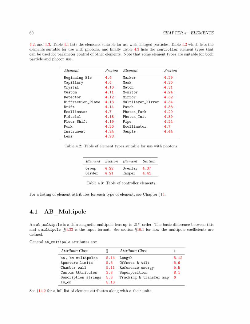
60 CHAPTER 4. ELEMENTS

4.2, and 4.3. Table 4.1 lists the elements suitable for use with charged particles, Table 4.2 which lists theelements suitable for use with photons, and finally Table 4.3 lists the controller element types thatcan be used for parameter control of other elements. Note that some element types are suitable for bothparticle and photon use.

Element Section Element Section

Beginning_Ele 4.4 Marker 4.29Capillary 4.6 Mask 4.30Crystal 4.10 Match 4.31Custom 4.11 Monitor 4.24Detector 4.12 Mirror 4.32Diffraction_Plate 4.13 Multilayer_Mirror 4.34Drift 4.14 Patch 4.38Ecollimator 4.7 Photon_Fork 4.20Fiducial 4.18 Photon_Init 4.39Floor_Shift 4.19 Pipe 4.24Fork 4.20 Rcollimator 4.7Instrument 4.24 Sample 4.44Lens 4.28

Table 4.2: Table of element types suitable for use with photons.

Element Section Element Section

Group 4.22 Overlay 4.37Girder 4.21 Ramper 4.41

Table 4.3: Table of controller elements.

For a listing of element attributes for each type of element, see Chapter §14.

4.1 AB_Multipole

An ab_multipole is a thin magnetic multipole lens up to 21st order. The basic difference between thisand a multipole (§4.33 is the input format. See section §16.1 for how the multipole coefficients aredefined.

General ab_multipole attributes are:

Attribute Class § Attribute Class §an, bn multipoles 5.14 Length 5.12Aperture limits 5.8 Offsets & tilt 5.6Chamber wall 5.11 Reference energy 5.5Custom Attributes 3.8 Superposition 8.1Description strings 5.3 Tracking & transfer map 6Is_on 5.13

See §14.2 for a full list of element attributes along with a their units.

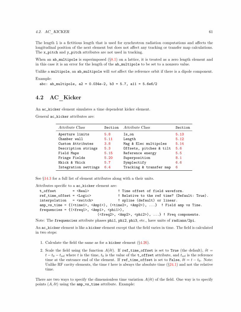
4.2. AC_KICKER 61

The length l is a fictitious length that is used for synchrotron radiation computations and affects thelongitudinal position of the next element but does not affect any tracking or transfer map calculations.The x_pitch and y_pitch attributes are not used in tracking.

When an ab_multipole is superimposed (§8.1) on a lattice, it is treated as a zero length element andin this case it is an error for the length of the ab_multipole to be set to a nonzero value.

Unlike a multipole, an ab_multipole will not affect the reference orbit if there is a dipole component.

Example:abc: ab_multipole, a2 = 0.034e-2, b3 = 5.7, a11 = 5.6e6/2

4.2 AC_Kicker

An ac_kicker element simulates a time dependent kicker element.

General ac_kicker attributes are:

Attribute Class Section Attribute Class Section

Aperture limits 5.8 Is_on 5.13Chamber wall 5.11 Length 5.12Custom Attributes 3.8 Mag & Elec multipoles 5.14Description strings 5.3 Offsets, pitches & tilt 5.6Field Maps 5.15 Reference energy 5.5Fringe Fields 5.20 Superposition 8.1Hkick & Vkick 5.7 Symplectify 6.6Integration settings 6.4 Tracking & transfer map 6

See §14.3 for a full list of element attributes along with a their units.

Attributes specific to a ac_kicker element are:t_offset = <Real> ! Time offset of field waveform.ref_time_offset = <Logic> ! Relative to the ref time? (Default: True).interpolation = <switch> ! spline (default) or linear.amp_vs_time = (<time1>, <Amp1>), (<time2>, <Amp2>), ... ! Field amp vs Time.frequencies = (<freq1>, <Amp1>, <phi1>),

(<freq2>, <Amp2>, <phi2>), ... ! Freq components.

Note: The frequencies attribute phases phi1, phi2, phi3, etc., have units of radians/2pi.

An ac_kicker element is like a kicker element except that the field varies in time. The field is calculatedin two steps:

1. Calculate the field the same as for a kicker element (§4.26).

2. Scale the field using the function A(δt). If ref_time_offset is set to True (the default), δt =t− t0 − tref where t is the time, t0 is the value of the t_offset attribute, and tref is the referencetime at the entrance end of the element. If ref_time_offset is set to False, δt = t − t0. Note:Unlike RF cavity elements, the time t here is always the absolute time (§24.1) and not the relativetime.

There are two ways to specify the dimensionless time variation A(δt) of the field. One way is to specifypoints (A, δt) using the amp_vs_time attribute. Example:

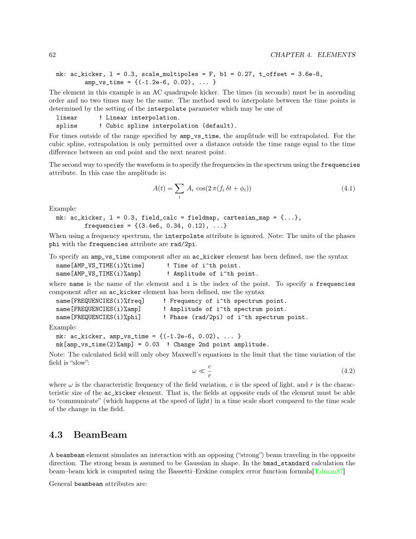
62 CHAPTER 4. ELEMENTS

mk: ac_kicker, l = 0.3, scale_multipoles = F, b1 = 0.27, t_offset = 3.6e-8,amp_vs_time = (-1.2e-6, 0.02), ...

The element in this example is an AC quadrupole kicker. The times (in seconds) must be in ascendingorder and no two times may be the same. The method used to interpolate between the time points isdetermined by the setting of the interpolate parameter which may be one oflinear ! Linear interpolation.spline ! Cubic spline interpolation (default).

For times outside of the range specified by amp_vs_time, the amplitude will be extrapolated. For thecubic spline, extrapolation is only permitted over a distance outside the time range equal to the timedifference between an end point and the next nearest point.

The second way to specify the waveform is to specify the frequencies in the spectrum using the frequenciesattribute. In this case the amplitude is:

A(t) =∑i

Ai cos(2π(fi δt+ φi)) (4.1)

Example:mk: ac_kicker, l = 0.3, field_calc = fieldmap, cartesian_map = ...,

frequencies = (3.4e6, 0.34, 0.12), ...

When using a frequency spectrum, the interpolate attribute is ignored. Note: The units of the phasesphi with the frequencies attribute are rad/2pi.

To specify an amp_vs_time component after an ac_kicker element has been defined, use the syntaxname[AMP_VS_TIME(i)%time] ! Time of i^th point.name[AMP_VS_TIME(i)%amp] ! Amplitude of i^th point.

where name is the name of the element and i is the index of the point. To specify a frequenciescomponent after an ac_kicker element has been defined, use the syntaxname[FREQUENCIES(i)%freq] ! Frequency of i^th spectrum point.name[FREQUENCIES(i)%amp] ! Amplitude of i^th spectrum point.name[FREQUENCIES(i)%phi] ! Phase (rad/2pi) of i^th spectrum point.

Example:mk: ac_kicker, amp_vs_time = (-1.2e-6, 0.02), ... mk[amp_vs_time(2)%amp] = 0.03 ! Change 2nd point amplitude.

Note: The calculated field will only obey Maxwell’s equations in the limit that the time variation of thefield is “slow”:

ω c

r(4.2)

where ω is the characteristic frequency of the field variation, c is the speed of light, and r is the charac-teristic size of the ac_kicker element. That is, the fields at opposite ends of the element must be ableto “communicate” (which happens at the speed of light) in a time scale short compared to the time scaleof the change in the field.

4.3 BeamBeam

A beambeam element simulates an interaction with an opposing (“strong”) beam traveling in the oppositedirection. The strong beam is assumed to be Gaussian in shape. In the bmad_standard calculation thebeam–beam kick is computed using the Bassetti–Erskine complex error function formula[Talman87]

General beambeam attributes are:

4.3. BEAMBEAM 63

Attribute Class Section Attribute Class Section

Aperture limits 5.8 Is_on 5.13Chamber wall 5.11 Offsets, pitches & tilt 5.6Custom Attributes 3.8 Reference energy 5.5Description strings 5.3 Superposition 8.1Is_on 5.13 Tracking & transfer map 6

See §14.4 for a full list of element attributes along with a their units.

Attributes specific to a beambeam element are:sig_x = <Real> ! Horizontal strong beam sigma at the centersig_y = <Real> ! Vertical strong beam sigma at the centersig_z = <Real> ! Strong beam lengthcharge = <Real> ! Strong beam charge. Default = -1n_slice = <Int> ! Number of strong beam slicescrab_x1 = <Real> ! Crabbing linear coefficient.crab_x2 = <Real> ! Crabbing quadratic coefficient.crab_x3 = <Real> ! Crabbing cubic coefficient.crab_tilt = <Real> ! Crabbing tilt.beta_a_strong = <Real> ! Strong beam $a$-mode beta Twiss parameteralpha_a_strong = <Real> ! Strong beam $a$-mode alpha Twiss parameterbeta_b_strong = <Real> ! Strong beam $b$-mode beta Twiss parameteralpha_b_strong = <Real> ! Strong beam $b$-mode alpha Twiss parameterbbi_constant ! See below. Dependent attribute (§5.1).

The number of particles in the strong beam is set bycharge * parameter[n_part]

parameter[n_part] is the nominal number of particles of the strong beam. parameter[n_part] isa global setting (§9.1) and is used for all beambeam elements. To vary the number of particles in anindividual beambeam element, the charge attribute is used. The default is charge = -1 which indicatesthat the strong beam has the opposite charge of the weak beam.

sig_z are the strong beam’s longitudinal sigma. The strong beam is divided up into n_slice equal charge(not equal thickness) slices. Propagation through the strong beam involves a kick at the charge center ofeach slice with drifts in between the kicks. The kicks are calculated using the standard Bassetti–Erskinecomplex error function formula[Talman87]. Even though the strong beam can have a finite sig_z, thelength of the beambeam element is zero. This is achieved by drifting a particle at the beginning andat the end of tracking so that the longitudinal starting point and ending points are at the beambeamelement. For example, with n_slice = 2 the calculation would proceed as follows:0. Start with the particle longitudinally at the beambeam element.1. Offsets, pitches and tilt are applied to convert from laboratory to element

body coordinates (§15.3.2. Propagate (drift) backwards to the center of the first slice.3. Apply the beam--beam kick due to the first slice.4. Propagate (drift) forwards to the center of the second slice.5. Apply the beam--beam kick due to the second slice.6. Propagate (drift) backwards to the body coordinate longitudinal center.7. Offsets, pitches and tilt are applied to convert from element body to

laboratory coordinates.sig_x, sig_y are the transverse sigmas of the strong beam at s0 which is the s-position where thebeambeam element is located. For calculating the sigmas of any given slice, sig_x and sig_y are ex-trapolated using the Twiss parameters at s0. The Twiss parameters at s0 are set by beta_a_strong,

64 CHAPTER 4. ELEMENTS

beta_b_strong, alpha_a_strong, and alpha_b_strong. If beta_a_strong is zero (the default), thea-mode Twiss parameters as calculated from the lattice is used. Similarly, if beta_b_strong is zero (thedefault), the b-mode Twiss parameters as calculated from the lattice is used.

The x_offset, y_offset, and z_offset attributes (§5.6) are used to offset the strong beam. Note thatin MAD the attributes used to offset the strong beam are called xma and yma. x_pitch and y_pitchgives the beam–beam interaction a crossing angle. x_pitch, y_pitch or some combination of the twoshould be set to the crossing angle of the strong beam with respect to the reference orbit of the weakbeam. To curve the strong beam centroid to simulate crabbing, the following parameters can be used:crab_x1, crab_x2crab_x3, crab_tilt

If crab_tilt is zero (the default), the strong beam centroid (xc, yc) will have yc zero and

xc = crab_x1 · z + crab_x2 · z2 + crab_x3 · z3 (4.3)

With a finite crab_tilt, the curvature is rotated around the z axis as shown in figure 5.2.

The bbi_constant is a measure of the beam–beam interaction strength. It is a dependent variable andis calculated from the equation

Cbbi = N me re/(2π γ (σx + σy)) (4.4)

In the linear region, near x = y = 0, the beam–beam kick is approximately

kx = −4π xCbbi/σx

ky = −4π y Cbbi/σy (4.5)

The beam–beam tune shift is

dQx = Cbbi βx/σx

dQy = Cbbi βy/σy

(4.6)

Example:parameter[n_part] = 1.34e10 ! Used for all beambeam elesbbi: beambeam, sig_x = 3e-3, sig_y = 3e-4, x_offset = 0.05

4.4 Beginning_Ele

A beginning_ele element, named “BEGINNING”, is placed at the beginning of every branch (§2.2) ofa lattice to mark the start of the branch. The beginning_ele always has element index 0 (§2). Thecreation of this beginning_ele element is automatic and it is not permitted to define a lattice withbeginning_ele elements at any other position.

The attributes of the beginning_ele element in the root branch are are generally set using beginning(§9.4) statements or line parameter (§9.4) statements. [The attributes of other beginning_ele elementsare set solely with line parameter statements.]

If the first element after the beginning_ele element at the start of a branch is reversed (§7.4), thebeginning_ele element will be marked as reversed so that a reflection patch is not needed in thiscircumstance.

See §14.6 for a full list of element attributes.

4.5. BENDS: RBEND AND SBEND 65

4.5 Bends: Rbend and Sbend

Rbends and sbends are dipole bends. The difference is that rbend elements use a Cartesian (“rectangular”)coordinate system to describe the shape of the magnet while sbend elements use a polar (“sector”)coordinate system.

For any given sbend element it is possible to construct an equivalent rbend element that has the sameshape and vice versa. Given this, and to simplify internal bookkeeping, all rbend elements are convertedto sbend elements when a lattice is read in to a program. In order to preserve the information as towhether a bend element was originally specified as an sbend or an rbend in the lattice file, all bendelements have a sub_key parameter which is appropriately set when the lattice is parsed. This sub_keyparameter does not affect tracking and is only used if a new lattice file is generated by the program.

General rbend and sbend attributes are:

Attribute Class Section Attribute Class Section

Aperture limits 5.8 Mag & Elec multipoles 5.14Chamber wall 5.11 Offsets, pitches & tilt 5.6Custom Attributes 3.8 Overlapping Fields 5.17Description strings 5.3 Reference energy 5.5Fringe Fields 5.20 Superposition 8.1Hkick & Vkick 5.7 Symplectify 6.6Is_on 5.13 Field Maps 5.15Integration settings 6.4 Tracking & transfer map 6Length 5.12

See §14.7 for a full list of element attributes along with a their units.

Attributes specific to rbend and sbend elements are:angle = <Real> ! Design bend angle. A settable dependent var (§5.1).b_field = <Real> ! Design field strength (= P_0 g / q) (§5.1).db_field = <Real> ! Actual - Design bending field difference (§5.1).b1_gradient = <Real> ! Quadrupole field strength (§5.1).b2_gradient = <Real> ! Sextupole field strength (§5.1).e1, e2 = <Real> ! Face angles.exact_multipoles = <Switch> ! Curved coordinate correction? off is default.fint, fintx = <Real> ! Face field integrals.g = <Real> ! Design bend strength (= 1/rho).dg = <Real> ! Actual - Design bend strength difference (§5.1).h1, h2 = <Real> ! Face curvature.hgap, hgapx = <Real> ! Pole half gap.k1 = <Real> ! Quadrupole strength.k2 = <Real> ! Sextupole strength (§5.1).l = <Real> ! "Length" of bend. See below.l_arc = <Real> ! Arc length. For rbends only.l_chord = <Real> ! Chord length. See §5.12.l_sagitta ! Sagittal length. Dependent param (§5.1).ptc_field_geometry = <Switch> ! See below.rho = <Real> ! Design bend radius. A settable dependent param (§5.1).roll = <Real> ! See 5.6.

angle

66 CHAPTER 4. ELEMENTS

e2e1

x1x2

L

s2

ρ

α

ρ

s1

(a) Rbend

e2e1x1

x2

s1

L s2

ρ

α

ρ

(b) Sbend

e2e1

x1 x2

s1

L s2

ρ

α

ρ

(c) Reversed sbend

Figure 4.1: Coordinate systems for (a) normal (non-reversed)rbend, (b) normal sbend, and (c) reversedsbend elements. The bends are viewed from “above” (viewed from positive y). Normal bends have g,angle, and rho all positive. Reversed bends have g, angle, and rho all negative. For (a) and (b), asdrawn, e1 and e2 are both positive. For (c), as drawn, e1 and e2 are both negative. In all cases, Lis positive. Notice that for reversed bends, the x-axis points towards the center of the bend while fornormal bends the x-axis points towards the outside.

The total design bend angle. A positive angle represents a bend towards negative x values (seeFig. 15.2).

B_field, dB_fieldThe B_field parameter is the design magnetic bending field which determines the reference orbitand the placement of lattice elements downstream from the bend. The dB_field parameter is thedifference between the actual (“total”) field and the design field. Thus:Actual B-field = B_field + dB_field

See the discussion of g and dg below for more details.

e1, e2The rotation angle of the entrance pole face is e1 and at the exit face it is e2. Zero e1 and e2for an rbend gives a rectangular magnet (Fig. 4.1a). Zero e1 and e2 for an sbend gives a wedgeshaped magnet (Fig. 4.1b). An sbend with an e1 = e2 = angle/2 is equivalent to an rbend withe1 = e2 = 0 (see above). This formula holds for both positive and negative angles.

Note: The correspondence between e1 and e2 and the corresponding parameters used in the SADprogram [SAD] is:e1(Bmad) = e1(SAD) * angle + ae1(SAD)e2(Bmad) = e2(SAD) * angle + ae2(SAD)

exact_multipolesThe exact_multipoles switch can be set to one of:off ! Defaultvertically_purehorizontally_pure

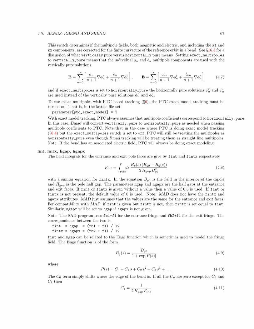
4.5. BENDS: RBEND AND SBEND 67

This switch determines if the multipole fields, both magnetic and electric, and including the k1 andk2 components, are corrected for the finite curvature of the reference orbit in a bend. See §16.3 for adiscussion of what vertically pure versus horizontally pure means. Setting exact_multipolesto vertically_pure means that the individual an and bn multipole components are used with thevertically pure solutions

B =

∞∑n=0

ïann+ 1

∇φrn +bn

n+ 1∇φin

ò, E =

∞∑n=0

ïaenn+ 1

∇φin +benn+ 1

∇φrnò

(4.7)

and if exact_multipoles is set to horizontally_pure the horizontally pure solutions ψrn and ψinare used instead of the vertically pure solutions φrn and φin.

To use exact multipoles with PTC based tracking (§6), the PTC exact model tracking must beturned on. That is, in the lattice file set:parameter[ptc_exact_model] = T

With exact model tracking, PTC always assumes that multipole coefficients correspond to horizontally_pure.In this case, Bmad will convert vertically_pure to horizontally_pure as needed when passingmultipole coefficients to PTC. Note that in the case where PTC is doing exact model tracking(§6.4) but the exact_multipoles switch is set to off, PTC will still be treating the multipoles ashorizontally_pure even though Bmad tracking will be treating them as straight line multipoles.Note: If the bend has an associated electric field, PTC will always be doing exact modeling.

fint, fintx, hgap, hgapxThe field integrals for the entrance and exit pole faces are give by fint and fintx respectively

Fint =

∫pole

dsBy(s) (By0 −By(s))

2HgapB2y0

(4.8)

with a similar equation for fintx. In the equation By0 is the field in the interior of the dipoleand Hgap is the pole half gap. The parameters hgap and hgapx are the half gaps at the entranceand exit faces. If fint or fintx is given without a value then a value of 0.5 is used. If fint orfintx is not present, the default value of 0 is used. Note: MAD does not have the fintx andhgapx attributes. MAD just assumes that the values are the same for the entrance and exit faces.For compatibility with MAD, if fint is given but fintx is not, then fintx is set equal to fint.Similarly, hgapx will be set to hgap if hgapx is not given.

Note: The SAD program uses fb1+f1 for the entrance fringe and fb2+f1 for the exit fringe. Thecorrespondence between the two isfint * hgap = (fb1 + f1) / 12fintx * hgapx = (fb2 + f1) / 12

fint and hgap can be related to the Enge function which is sometimes used to model the fringefield. The Enge function is of the form

By(s) =By0

1 + exp[P (s)](4.9)

whereP (s) = C0 + C1 s+ C2 s

2 + C3 s3 + . . . (4.10)

The C0 term simply shifts where the edge of the bend is. If all the Cn are zero except for C0 andC1 then

C1 =1

2Hgap Fint(4.11)

68 CHAPTER 4. ELEMENTS

g, dg, rhoThe design bending radius which determines the reference coordinate system is rho (see §15.1.1).g = 1/rho is the curvature function and is proportional to the design dipole magnetic field. g isrelated to the design magnetic field B_field via

g =q

p0B_field (4.12)

where q is the charge of the reference particle and p0 is the reference momentum. It is important tokeep in mind that changing g will change the design orbit (§15) and hence will move all downstreamlattice elements in space.

The parameter dg is the difference between the actual and the design bending strengths. Therelationship between dg and dB_field is analogous to the relationship between g and B_field inEq. (4.12). The actual (“total”) field strength is given by the sum:Actual g = g + dg

Changing dg leaves the design orbit and the positions of all downstream lattice elements unchangedbut will vary a particle’s orbit. One common mistake when designing lattices is to vary g and notdg which results in downstream elements moving around. See Sec. §12.2 for an example.

h1, h2The attributes h1 and h2 are the curvature of the entrance and exit pole faces. They are present forcompatibility with MAD but are not yet implemented in terms of tracking and other calculations.

k1, b1_gradientThe normalized and unnormalized quadrupole strength.

k2, b2_gradientThe normalized and unnormalized sextupole strength.

l, l_arc, l_chord, l_sagittaFor compatibility with MAD, for an rbend, l is the chord length and not the arc length as it is foran sbend. After reading in a lattice, Bmad will internally convert all rbends into sbends, and thel_chord attribute of the created sbend will be set to the input l. The l of the the created sbendwill be set to the true path length (see above). Alternatively for an rbend, instead of setting l,the l_arc attribute can be used to set the true arc length.

For sbend elements, l_chord will be set to the calculated chord length. For both types of bends,the l_sagitta parameter will be set to the sagitta length (The sagitta is the distance from themidpoint of the arc to the midpoint of the chord). l_sagitta can be negative and will have thesame sign as the g parameter.

ref_tiltThe ref_tilt attribute rotates a bend about the longitudinal axis at the entrance face of the bend.A bend with ref_tilt of π/2 and positive g bends the element in the −y direction (“downward”).See Fig. 15.7. It is important to understand that ref_tilt, unlike the tilt attribute of otherelements, bends both the reference orbit along with the physical element. Note that the MADtilt attribute for bends is equivalent to the Bmad ref_tilt. Bends in Bmad do not have a tiltattribute.

The difference between rbend and sbend elements is the way the l, e1, and e2 attributes are interpreted.To ease the bookkeeping burden, after reading in a lattice, Bmad will internally convert all rbends intosbends. This is done using the following transformation on rbends:

4.6. CAPILLARY 69

l_chord(internal) = l(input)l(internal) = 2 * asin(l_chord * g / 2) / ge1(internal) = e1(input) + theta / 2e2(internal) = e2(input) + theta / 2

The attributes g, angle, and l are mutually dependent. If any two are specified for an element Bmad willcalculate the appropriate value for the third. After reading in a lattice, angle is considered a dependentvariable (§5.1).

Since internally all rbends are converted to sbends, if one wants to vary the g attribute of a bend andstill keep the bend rectangular, an overlay (§4.37) can be constructed to maintain the proper face angles.For example:l_ch = 0.54g_in = 1.52l_coef = asin(l_ch * g_in / 2) / g_inmy_bend: rbend, l = l_ch, g = g_inmy_overlay: overlay = my_bend, my_bend[e1]:l_coef, my_bend[e2]:l_coef,

var = g, g = g_in

Notice that l_coef is just arc_length/2.

In the local coordinate system (§15.1.1), looking from “above” (bend viewed from positive y), and withref_tilt = 0, a positive angle represents a particle rotating clockwise. In this case. g will also bepositive. For counterclockwise rotation, both angle and g will be negative but the length l is alwayspositive. Also, looking from above, a positive e1 represents a clockwise rotation of the entrance face anda positive e2 represents a counterclockwise rotation of the exit face. This is true irregardless of the signof angle and g. Also it is always the case that the pole faces will be parallel whene1 + e2 = angle

Example bend specification:b03w: sbend, l = 0.6, k1 = 0.003, fint ! gives fint = fintx = 0.5

ptc_field_geometry determines what coordinates PTC uses within a bend for calculating fields. Thisonly affects tracking if PTC is being used and if ptc_com[exact_model] is set to True (§10.4). Possiblevalues for ptc_field_geometry are:sector ! Defaultstraight

For sector reference coordinates, the field coordinate reference frame is with respect to the arc ofthe reference trajectory. For straight coordinates the coordinate reference frame is with respect to thechord line. For a bend where there are no other fields besides the basic dipole field, tracking is essentiallyuneffected.1 When there are quadrupole or higher order fields, the fields are centered about the referenceframe set by ptc_field_geometry. Since Bmad based tracking does not implement straight geometrytracking, Bmad and PTC tracking will show marked differences when ptc_field_geometry is set tostraight.

4.6 Capillary

A capillary element is a glass tube that is used to focus x-ray beams.

General capillary attributes are:1There will be a small difference due to the fact that with a straight geometry tracking uses a coordinate system with

the z-axis along the chord and with a sector geometry an integration step uses the curvilinear coordinate system with thez-axis along the arc of the bend. If the length of an integration step is made small, this difference will go to zero.

70 CHAPTER 4. ELEMENTS

Attribute Class Section Attribute Class Section

Aperture limits 5.8 Offsets, Pitches & Tilt 5.6Capillary Wall 5.11 Reference energy 5.5Custom Attributes 3.8 Tracking & transfer map 6Description strings 5.3

See §14.9 for a full list of element attributes along with a their units.

Attributes specific to a capillary element are:critical_angle_factor = <Real> ! Critical angle * Energy (rad * eV)

The critical angle above which photons striking the capillary surface are refracted into the capillary mate-rial scales as 1/Energy. The constant of critical angle * energy is given by the critical_angle_factor.

The inside wall of a capillary is defined using the same syntax used to define the chamber wall for otherelements (§5.11).

The length of the capillary is a dependent variable and is given by the value of s of the last wallcross-section (§5.11.4).

4.7 Collimators: Ecollimator and Rcollimator

An ecollimator is a drift with elliptic collimation. An rcollimator is a drift with rectangular colli-mation.

Alternatively, for defining a collimator with an arbitrary shape, a mask element (§4.30) may be used.

General ecollimator and rcollimator attributes are:

Attribute Class Section Attribute Class Section

Aperture limits 5.8 Offsets, Pitches & Tilt 5.6Chamber wall 5.11 Overlapping Fields 5.17Custom Attributes 3.8 Reference energy 5.5Description strings 5.3 Superposition 8.1Hkick & Vkick 5.7 Symplectify 6.6Integration settings 6.4 Field Maps 5.15Length 5.12 Tracking & transfer map 6

Attributes specific to a capillary element are:px_aperture_width2 = <real> ! px aperture half widthpx_aperture_center = <real> ! px aperture centerpy_aperture_width2 = <real> ! py aperture half widthpy_aperture_center = <real> ! py aperture centerz_aperture_width2 = <real> ! z aperture half widthz_aperture_center = <real> ! z aperture centerpz_aperture_width2 = <real> ! pz aperture half widthpz_aperture_center = <real> ! pz aperture center

Note: Collimators are the exception to the rule that the aperture is independent of any tilts. See §5.8for more details. Additionally, the default setting of offset_moves_aperture is True for collimators(§5.8.1).

4.8. CONVERTER 71

Besides the standard aperture settings 5.8 that can be used to limit x and y phase space coordinates,collimators can be used to limit the other four phase space coordinates as well. For rcollimatorelements, particles are collimated if px_aperture_width2 is greater than zero andpx < px_aperture_center - px_aperture_width2 orpx > px_aperture_center + px_aperture_width2

with similar equations for py, z, and pz. For ecollimators, if px_aperture_width2 and py_aperture_width2are both nonzero, particles are collimated if((px - px_aperture_center) / px_aperture_width2)^2 +

((py - py_aperture_center) / py_aperture_width2)^2 < 1

If one or both of px_aperture_width2 or py_aperture_width2 are zero, the computation is the sameas for an rcollimator. A similar situation occurs for z and pz.

Example:d21: ecollimator, l = 4.5, x_limit = 0.09, y_limit = 0.05,

px_aperture_width2 = 0.3, py_aperture_width = 0.1

4.8 Converter

A converter element represents a target (plate) onto which particles are slammed in order to generateparticles of a different type. For example, a tungsten plate which is bombarded with electrons to generatepositrons.

General custom attributes are:

Attribute Class Section Attribute Class Section

Aperture limits 5.8 Is_on 5.13Chamber wall 5.11 Length 5.12Custom Attributes 3.8 Offsets, pitches & tilt 5.6Description strings 5.3 Reference energy 5.5Integration settings 6.4 Superposition 8.1

Tracking & transfer map 6

The attributes specific to an converter aredistribution = <Struct> ! Outgoing particle distribution.pc_out_min = <Real> ! Minimum outgoing particle momentum (eV).pc_out_max = <Real> ! Maximum outgoing particle momentum (eV).angle_out_max = <Real> ! Maximum outgoing angle.species_out = <SpeciesID> ! Output species.p0c = <Real> ! Output reference momentum.E_tot = <Real> ! Output reference energy. A settable dependent var (§5.1).

The species of the outgoing particles is specified by the species_out parameter (§3.10).

The converter must be the last element in a lattice branch (§2.2) except for possible fork, photon_forkor marker elements. A fork or photon_fork element (§4.20) after the converter is used to connect tothe line containing the elements that come after the converter Example:parameter[particle] = electronparameter[geometry] = opento_after: fork, to_line = after_cvtercvter, species_out = positron, p0c = 3e6, distribution = ...

72 CHAPTER 4. ELEMENTS

pre_linac: line = (..., cvter, to_after)after_cvter: line = (...) ! Everything after the converter.after_cvter[beta_a] = 27; after_cvter[beta_b] = 32use, pre_linac

The line up to the fork element, pre_linac, has the converter just before the fork element. The forkelement, called to_after, connects to the line named after_cvter which contains all the elementsafter the converter. The reference particle and reference momentum for the after_cvter line is set topositron and 3e6 respectively to agree with the setting of species_out and p0c set in the converterelement.

Since Bmad cannot calculate the appropriate Twiss and dispersion values after the converter, valuesmust be set in the lattice file. Thus, in the above example, the starting beta function at the beginningof the after_cvter line is set to be βa = 27 m and βb = 32 m.

The p0c and E_tot attributes of the converter set the reference momentum or energy at the exit end ofthe converter. At least one of these attributes must be set. If both are set, E_tot is calculated to beconsistent with p0c.

The distribution parameter of a converter element specifies the distribution of outgoing particlesfor a given converter thickness. Multiple distribution instances with differing thicknesses may bepresent in an element. The actual thickness of the converter will be taken to be the element’s, length Lparameter. During tracking, the outgoing distribution will be computed by interpolating between the twodistributions that bracket the actual thickness. The exception is when there is only onedistributionpresent. In this case, the calculation will just use that distribution for the calculation independent ofthe element length. Example:cvter: converter, ..., distribution =

material = tungsten, ! Optional. Not used in tracking.thickness = 0.003, ! Converter thickness for this distribution.sub_distribution = ..., ! Distribution at one incoming momentum.sub_distribution = ..., ! Distribution at another incoming momentum.... ! etc.

The material component is optional and is only for recording the converter material. Each distributionis made up of a number of sub_distribution components. Each one specified the outgoing distributionfor a given incoming particle momentum. During tracking, interpolation is used to compute the distri-bution appropriate for an incoming particle with a given momentum. It is an error in the momentumof the incoming particle is outside the range of the momentums specified in the sub_distributions. Agiven sub_distribution will look like:sub_distribution = pc_in = 3e8, ! Incoming momentum*c (eV)>prob_pc_r = ..., ! Momentum and radius probability tabledirection_out = ..., ! Momentum orientation probability coefs

A sub_distribution has three components: The pc_in component specifies the incoming particlemomentum appropriate for the sub_distribution, the prob_pc_r component holds a two-dimensionaltable of the probability P (pout, r) (Eq. (24.48)), and direction_out holds the coefficients for calculatingthe outgoing particle direction. prob_pc_r look like:prob_pc_r = r_values = [0.0, 4.9e-5, 1.25e-4, ...],row = pc_out = 1.55e6, prob = [0.0, 6.1e-6, 1.23e-5, ...],row = pc_out = 3.96e6, prob = [0.0, 1.1e-5, ...],... ! More rows

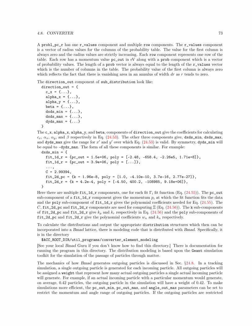
4.8. CONVERTER 73

A probl_pc_r has one r_values component and multiple row components. The r_values componentis a vector of radius values for the columns of the probability table. The value for the first column isalways zero and the radius values are strictly increasing. Each row component represents one row of thetable. Each row has a momentum value pc_out in eV along with a prob component which is a vectorof probability values. The length of a prob vector is always equal to the length of the r_values vectorwhich is the number of columns in the table. The probability value of the first column is always zerowhich reflects the fact that there is vanishing area in an annulus of width dr as r tends to zero.

The direction_out component of sub_distribution look like:direction_out = c_x = ...,alpha_x = ...,alpha_y = ...,beta = ...,dxds_min = ...,dxds_max = ...,dyds_max = ...

The c_x, alpha_x, alpha_y, and beta, components of direction_out give the coefficients for calculatingcx, αx, αy, and β respectively in Eq. (24.53). The other three components give, dxds_min, dxds_max,and dyds_max give the range for x′ and y′ over which Eq. (24.53) is valid. By symmetry, dyds_min willbe equal to -dydx_max. The form of all these components is similar. For example:dxds_min = fit_1d_r = pc_out = 1.5e+06, poly = [-2.48, -658.4, -2.26e5, 1.71e+8],fit_1d_r = pc_out = 3.9e+06, poly = [...],...,C = 2.99394,fit_2d_pc = k = 1.96e-8, poly = [1.0, -4.10e-10, 3.7e-16, 2.77e-27],fit_2d_r = k = 4.2e-4, poly = [-4.50, 400.2, -108985, 9.18e+06],

Here there are multiple fit_1d_r components, one for each fit Γi fit function (Eq. (24.55)). The pc_outsub-component of a fit_1d_r component gives the momentum pi at which the fit function fits the dataand the poly sub-component of fit_1d_r gives the polynomial coefficients needed for Eq. (24.55). TheC, fit_2d_pc and fit_2d_r components are used for computing Ξ (Eq. (24.56)). The k sub-componentsof fit_2d_pc and fit_2d_r give kp and kr respectively in Eq. (24.56) and the poly sub-components offit_2d_pc and fit_2d_r give the polynomial coefficients wn and kn respectively.

To calculate the distributions and output the appropriate distribution structures which then can beincorporated into a Bmad lattice, there is modeling code that is distributed with Bmad. Specifically, itis in the directory$ACC_ROOT_DIR/util_programs/converter_element_modeling

[See your local Bmad Guru if you don’t know how to find this directory.] There is documentation forrunning the program in this directory. The distribution modeling is based upon the Geant simulationtoolkit for the simulation of the passage of particles through matter.

The mechanics of how Bmad generates outgoing particles is discussed in Sec. §24.8. In a trackingsimulation, a single outgoing particle is generated for each incoming particle. All outgoing particles willbe assigned a weight that represent how many actual outgoing particles a single actual incoming particlewill generate. For example, if an actual incoming particle with a particular momentum would generate,on average, 0.42 particles, the outgoing particle in the simulation will have a weight of 0.42. To makesimulations more efficient, the pc_out_min, pc_out_max, and angle_out_max parameters can be set torestrict the momentum and angle range of outgoing particles. If the outgoing particles are restricted

74 CHAPTER 4. ELEMENTS

in momentum or angle, the weight of the outgoing particles will be appropriately adjusted such thatthe weighted distribution of outgoing particles within the momentum and/or angle restricted range isindependent of the whether or not there is are restrictions. A value of zero (the default) for any one ofthese parameters means that that parameter is ignored.

4.9 Crab_Cavity

A crab_cavity is an RF cavity that gives a z-dependent kick. This is useful in colliding beam machines,where there is a finite crossing angle at the interaction point, to rotate the beams near the IP.

General crab_cavity attributes are:

Attribute Class Section Attribute Class Section

Aperture limits 5.8 Length 5.12Chamber wall 5.11 Offsets, pitches & tilt 5.6Custom Attributes 3.8 Reference energy 5.5Description strings 5.3 Superposition 8.1Hkick & Vkick 5.7 Symplectify 6.6Integration settings 6.4 Field Maps 5.15Is_on 5.13 Tracking & transfer map 6

See §14.12 for a full list of element attributes along with a their units.

The attributes specific to an crab_cavity aregradient = <Real> ! Accelerating gradient (V/m).phi0 = <Real> ! Phase (rad/2π) of the reference particle with

! respect to the RF. phi0 = 0 is on crest.phi0_multipass = <Real> ! Phase with respect to a multipass lord (rad/2π).rf_frequency = <Real> ! RF frequency (Hz).voltage ! Cavity voltage. Dependent attribute (§5.1).

The Hamiltonian Hcrab for a thin crab cavity is[Sun10]:

Hcrab = −qrel V xcP0

sin(k z + 2π φ0) (4.13)

where x and z are particle coordinates, qrel is the charge relative to the reference particle, V is the“effective” cavity voltage, P0 is the reference energy, φ0 is a user settable phase, and k is the wavenumber

k =2π frfc

(4.14)

Which give kicks

∆px = −∂Hcrab

∂x=qrel V

cP0sin(k z + 2π φ0)

∆pz = −∂Hcrab

∂z=qrel V k x

cP0cos(k z + 2π φ0) (4.15)

Note: The sign of Hcrab used by Authors in the literature is not standardized. Bmad uses the conventionsuch that a particle with the charge of the reference particle and with z and V positive will have a positive∆px.

4.10. CRYSTAL 75

The equations of motion can also be derived from analysis of a TM110 cavity mode for particles near thecenterline[Kim11]. With this mode, the transverse kick is due to the magnetic field and the longitudinalkick is due to the electric field. Using this, the integrated electric and magnetic fields needed for spintracking are: ∫

By =−Vc

sin(k z + 2π φ0)∫Es = β V k x cos(k z + 2π φ0) (4.16)

where β = v/c is the normalized speed of the particle.

4.10 Crystal

A crystal element represents a crystal used for photon diffraction.

General crystal attributes are:

Attribute Class Section Attribute Class Section

Aperture limits 5.8 Surface Properties 5.10Custom Attributes 3.8 Symplectify 6.6Description strings 5.3 Offsets, Pitches & Tilt 5.6Reference energy 5.5 Tracking & transfer map 6

See §14.13 for a full list of element attributes along with a their units.

Attributes specific to a crystal element are:b_param = <Real> ! b parametercrystal_type = <String> ! Crystal material (§5.9) and reflection plane.psi_angle = <Real> ! Rotation of H-vector about the surface normal.thickness = <Real> ! Thickness of crystal for Laue diffraction.

Ref Orb InRef Orb Out

Hns^

xx

xz

θB,in θB,out

αH

ψ

ElementRef Frame

A) Bragg B) Laue UndiffractedBeam

Bragg DiffractedBeam

Forward DiffractedBeam

Ref Orb In

θB,in θB,out

x z

zz

x

z

z

z

z

x

x

x

H

ElementRef Frame

Figure 4.2: Crystal element geometry. A) Geometry for Bragg diffraction. The geometry shown is forref_tilt = 0 (reference trajectory in the x-z plane). The angle αH (alpha_angle) is the angle of the Hvector with respect to the surface normal n. For ψ (psi_angle) zero, the incoming reference orbit, theoutgoing reference orbit, n, and H are all coplanar. B) Geometry for Laue diffraction. In this case thereare three outgoing beams: The Bragg diffracted beam, the forward diffracted beam, and the undiffractedbeam.

76 CHAPTER 4. ELEMENTS

ref_orbit_follows = <which_beam> ! Reference orbit aligned with what outgoing beam?graze_angle_in = <Real> ! Angle between incoming ref orbit and surface.graze_angle_out = <Real> ! Angle between outgoing ref orbit and surface.

Dependent variables (§5.1) specific to a crystal element are:alpha_angle ! Angle of H-vector with respect to the surface normal.bragg_angle ! Nominal Bragg angle at the reference wave length.bragg_angle_in ! Incoming grazing angle for Bragg diffraction.bragg_angle_out ! Outgoing grazing angle for Bragg diffraction.d_spacing ! Lattice plane spacing.darwin_width_pi ! Darwin width for pi polarized light (radians).darwin_width_sigma ! Darwin width for sigma polarized light (radians).dbragg_angle_de ! Variation of the Bragg angle with energy (radians/eV).l ! Length of reference orbit.pendellosung_period_pi ! Pendellosung period for pi polarized light.pendellosung_period_sigma ! Pendellosung period for sigma polarized light.ref_wavelength ! Reference wavelength (§5.5). Dependent attribute (§5.1).ref_cap_gamma ! Γ at the reference wavelength.tilt_corr ! Tilt correction due to a finite psi_angle.v_unitcell ! Unit cell volume.

The crystal_type attribute defines the crystal material and diffraction lattice plane. The syntax is"ZZZ(ijk)" where ZZZ is the material name and ijk are the Miller indices for the diffraction plane. Forexample,b_cryst1: crystal, crystal_type = "Si(111)", b_param = -1, ...

The atomic formula is case sensitive so, for example, "SI(111)" is not acceptable. The list of known crys-tal materials is given in §5.9. Given the crystal_type, the spacing between lattice planes (d_spacing),the unit cell volume (v_unitcell), and the structure factor[Bater64] values can be computed.

The b_param is the standard b asymmetry factor

b =sin(αH + θB)

sin(αH − θB)(4.17)

where θB is the Bragg angle (bragg_angle)

θB = sin−1

Åλ

2 d

ã(4.18)

and αH (alpha_angle) is the angle of the reciprocal lattice H vector with respect to the surface normalas shown in Fig. 4.2A. If b_param is set to -1 then there is Bragg reflection and alpha_H is zero. Ifb_param is set to 1 then there is Laue diffraction again with alpha_H zero. With the orientation shownin Fig. 4.2A, alpha_H is positive.

The ref_orbit_follows parameter sets how the outgoing reference orbit is constructed. This is onlyrelevant with Laue diffraction. The possible settings of this parameter are:bragg_diffracted ! Defaultforward_diffractedundiffracted

The geometry of this situation is shown in Fig. 4.2B. The reference orbit for the undiffracted beamis just a straight line extension of the incoming reference trajectory. This trajectory is that trajectorythat photons whose energy is far from the Bragg condition (that is, far from the reference energy) willfollow. The forward_diffracted reference orbit is parallel to the undiffracted trajectory and is thetrajectory of the forward diffracted photons whose energy is the reference energy and whose incoming

4.10. CRYSTAL 77

orbit is on the incoming reference trajectory. Finally, the bragg_diffracted reference orbit (the default)is the backward diffracted orbit.

Note: Changing the setting of ref_orbit_follows will change the reference orbit downstream of thecrystal which, in turn, will change the placement all downstream elements.

The value of the element reference orbit length l is calculated by Bmad. L will be zero for Bragg diffrac-tion. For Laue diffraction, l will depend upon the crystal thickness and the setting of ref_orbit_follows.

If psi_angle is zero, the incoming reference orbit, the outgoing reference orbit, n and H are all coplanar.A non-zero psi_angle Rotates the H vector around the +x axis of the Element Reference Frame (SeeFig. 4.2A).

To keep the outgoing reference trajectory independent of the value of psi_angle, the crystal will beautomatically tilted by the appropriate “tilt correction” tilt_corr. The calculation of tilt_corr isoutlined in §25.4.2. tilt_corr will be zero if psi_angle is zero.

The reference trajectory for a Bragg crystal is that of a zero length bend (§15.2.3) and hence the length(l) parameter of a crystal is fixed at zero. If the graze_angle_in and graze_angle_out angles are zero(the default), the orientation of the reference trajectory with respect to the crystal surface is specified bythe incoming Bragg angle bragg_angle_in (θg,in) and outgoing Bragg angle bragg_angle_out (θg,out)as shown in Fig. 4.2A. These angles are computed from the photon reference energy and the other crystalparameters such that a photon with the reference energy traveling along the reference trajectory will bein the center of the Darwin curve (§25.4). It is sometimes convenient to be able to specify the anglesthat the reference trajectory makes with respect to the crystal independent of the Bragg angles. To dothis, set graze_angle_in and graze_angle_out to the desired angles.

Notice that due to refraction at the surface, the computed bragg_angle from Eq. (4.18) will deviateslightly from the average of bragg_angle_in and bragg_angle_out.

The reference trajectory in the global coordinate system (§15.2) is determined by the value of theref_tilt parameter along with the value of bragg_angle_in + bragg_angle_out. These bragg anglestake into account refraction so that the reference trajectory downstream of the crystal will be properlycentered with respect to the reference photon. A positive bragg_angle_in + bragg_angle_out bendsthe reference trajectory in the same direction as a positive g for a bend element. The

A crystal may be offset and pitched (5.6). The incoming local reference coordinates are used for thesemisalignments.

When a crystal is bent (§5.10), the H vector is assumed follow the surface curvature. That is, it isassumed that the lattice planes are curved by the bending.

Example:crystal_ele: crystal, crystal_type = "Si(111)", b_param = -1

The darwin_width_sigma and darwin_width_pi parameters are the computed Darwin width, in radi-ans, for sigma and pi polarized light respectively. Here the Darwin width dθD is defined as the width atthe η = ±1 points (cf. Batterman[Bater64] Eq (32))

dθD =2 Γ |P |Re

([FH FH ]1/2

)|b|1/2 sin θtot

(4.19)

whereθtot = bragg_angle_in + bragg_angle_out

The pendellosung_period_sigma and pendellosung_period_pi are the pendellosung periods for Lauediffraction. If the crystal is set up for Bragg diffraction then the values for these parameters will be setto zero.

78 CHAPTER 4. ELEMENTS

The dbragg_angle_de parameter is the variation in Bragg angle with respect to the photon energy andis given by the formula

dθBdE

= − λ

2 dE cos(θB)(4.20)

See Section §12.5 for an example lattice that can be used to simulate a Rowland circle spectrometer.

4.11 Custom

A custom element is an element whose properties are defined outside of the standard Bmad subroutinelibrary. That is, to use a custom element, some programmer must write the appropriate custom routineswhich are then linked with the Bmad subroutines into a program. Bmad will call the custom routines atthe appropriate time to do tracking, transfer matrix calculations, etc. See the programmer who wrotethe custom routines for more details! See §36.2 on how to write custom routines.

General custom attributes are:

Attribute Class Section Attribute Class Section

Aperture limits 5.8 Is_on 5.13Chamber wall 5.11 Length 5.12Custom Attributes 3.8 Offsets, pitches & tilt 5.6Description strings 5.3 Reference energy 5.5Field Maps 5.15 Superposition 8.1Fringe fields 5.20 Symplectify 6.6Integration settings 6.4 Tracking & transfer map 6

See §14.14 for a full list of element attributes along with a their units.

As an alternative to defining a custom element, standard elements can be “customized” by setting oneor more of the following attributes to custom:

tracking_method §6.1mat6_calc_method §6.2field_calc §6.4aperture_type §5.8

As with a custom element, setting one of these attributes to custom necessitates the use of custom codeto implement the corresponding calculation.

Attributes specific to a custom element are

val1, ..., val12 = <Real> ! Custom valuesdelta_e_ref = <Real> ! Change in energy.

delta_e_ref is the energy gain of the reference particle between the starting edge of the element andthe ending edge.

Example:

c1: custom, l = 3, val4 = 5.6, val12 = 0.9, descrip = "params.dat"

In this example the descrip string is being used to specify a file that contains parameters for the element.

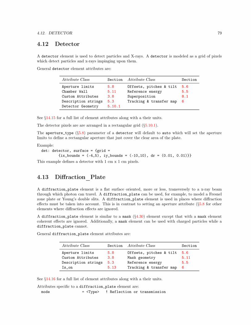
4.12. DETECTOR 79

4.12 Detector

A detector element is used to detect particles and X-rays. A detector is modeled as a grid of pixelswhich detect particles and x-rays impinging upon them.

General detector element attributes are:

Attribute Class Section Attribute Class Section

Aperture limits 5.8 Offsets, pitches & tilt 5.6Chamber Wall 5.11 Reference energy 5.5Custom Attributes 3.8 Superposition 8.1Description strings 5.3 Tracking & transfer map 6Detector Geometry 5.10.1

See §14.15 for a full list of element attributes along with a their units.

The detector pixels are are arranged in a rectangular grid (§5.10.1).

The aperture_type (§5.8) parameter of a detector will default to auto which will set the aperturelimits to define a rectangular aperture that just cover the clear area of the plate.

Example:det: detector, surface = grid =

ix_bounds = (-4,5), iy_bounds = (-10,10), dr = (0.01, 0.01)This example defines a detector with 1 cm x 1 cm pixels.

4.13 Diffraction_Plate

A diffraction_plate element is a flat surface oriented, more or less, transversely to a x-ray beamthrough which photon can travel. A diffraction_plate can be used, for example, to model a Fresnelzone plate or Young’s double slits. A diffraction_plate element is used in places where diffractioneffects must be taken into account. This is in contrast to setting an aperture attribute (§5.8 for otherelements where diffraction effects are ignored.

A diffraction_plate element is similar to a mask (§4.30) element except that with a mask elementcoherent effects are ignored. Additionally, a mask element can be used with charged particles while adiffraction_plate cannot.

General diffraction_plate element attributes are:

Attribute Class Section Attribute Class Section

Aperture limits 5.8 Offsets, pitches & tilt 5.6Custom Attributes 3.8 Mask geometry 5.11Description strings 5.3 Reference energy 5.5Is_on 5.13 Tracking & transfer map 6

See §14.16 for a full list of element attributes along with a their units.

Attributes specific to a diffraction_plate element are:mode = <Type> ! Reflection or transmission

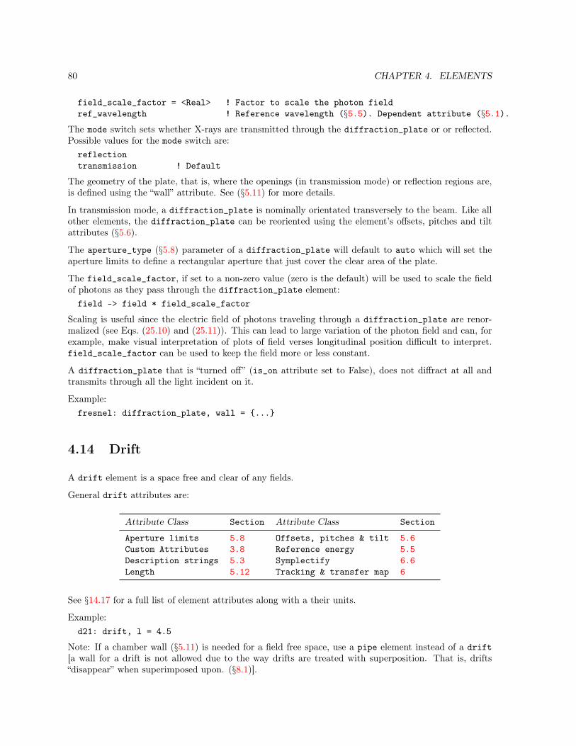
80 CHAPTER 4. ELEMENTS

field_scale_factor = <Real> ! Factor to scale the photon fieldref_wavelength ! Reference wavelength (§5.5). Dependent attribute (§5.1).

The mode switch sets whether X-rays are transmitted through the diffraction_plate or or reflected.Possible values for the mode switch are:reflectiontransmission ! Default

The geometry of the plate, that is, where the openings (in transmission mode) or reflection regions are,is defined using the “wall” attribute. See (§5.11) for more details.

In transmission mode, a diffraction_plate is nominally orientated transversely to the beam. Like allother elements, the diffraction_plate can be reoriented using the element’s offsets, pitches and tiltattributes (§5.6).

The aperture_type (§5.8) parameter of a diffraction_plate will default to auto which will set theaperture limits to define a rectangular aperture that just cover the clear area of the plate.

The field_scale_factor, if set to a non-zero value (zero is the default) will be used to scale the fieldof photons as they pass through the diffraction_plate element:field -> field * field_scale_factor

Scaling is useful since the electric field of photons traveling through a diffraction_plate are renor-malized (see Eqs. (25.10) and (25.11)). This can lead to large variation of the photon field and can, forexample, make visual interpretation of plots of field verses longitudinal position difficult to interpret.field_scale_factor can be used to keep the field more or less constant.

A diffraction_plate that is “turned off” (is_on attribute set to False), does not diffract at all andtransmits through all the light incident on it.

Example:fresnel: diffraction_plate, wall = ...

4.14 Drift

A drift element is a space free and clear of any fields.

General drift attributes are:

Attribute Class Section Attribute Class Section

Aperture limits 5.8 Offsets, pitches & tilt 5.6Custom Attributes 3.8 Reference energy 5.5Description strings 5.3 Symplectify 6.6Length 5.12 Tracking & transfer map 6

See §14.17 for a full list of element attributes along with a their units.

Example:d21: drift, l = 4.5

Note: If a chamber wall (§5.11) is needed for a field free space, use a pipe element instead of a drift[a wall for a drift is not allowed due to the way drifts are treated with superposition. That is, drifts“disappear” when superimposed upon. (§8.1)].

4.15. E_GUN 81

4.15 E_Gun

An e_gun element represents an electron gun and encompasses a region starting from the cathode werethe electrons are generated. General e_gun attributes are:

Attribute Class Section Attribute Class Section

Aperture limits 5.8 Length 5.12Chamber wall 5.11 Mag & Elec multipoles 5.14Custom attributes 3.8 Offsets, pitches & tilt 5.6Description strings 5.3 Overlapping Fields 5.17Field autoscaling 5.18 Reference energy 5.5Hkick & Vkick 5.7 Symplectify 6.6Integration settings 6.4 Field Maps 5.15Is_on 5.13 Tracking & transfer map 6

See §14.20 for a full list of element attributes along with a their units.

The attributes specific to an e_gun aregradient = <Real> ! Gradient.gradient_err = <Real> ! Gradient error.phi0 = <Real> ! Phase (rad/2π) of the reference particle with

! respect to the RF. phi0 = 0 is on crest.phi0_err = <Real> ! Phase error (rad/2π)rf_frequency = <Real> ! Frequency of the RF field.voltage = <Real> ! Voltage. Dependent attribute (§5.1).voltage_err = <Real> ! Voltage error. Dependent attribute (§5.1).

The voltage is simply related to the gradient via the element length l:voltage = gradient * l

If the voltage is set to a non-zero value, the length l must also be non-zero to keep the gradient finite.A particle with the charge as the reference particle will have a positive energy gain if the voltage andgradient are positive and vice versa.

field_autoscale The voltage and gradient are scaled by field_autoscale and, if there is a finiterf_frequency, the phase of the frequency is shifted by phi0_autoscale as discussed in Section §5.18.Autoscaling can be toggled on/off by using the autoscale_phase and autoscale_amplitude toggles.

An e_gun may either be DC if the rf_frequency component is zero of AC if not. For an AC e_gun, thephase of the e_gun, The phase φref isφref = phi0 + phi0_err + phi0_autoscale

Electrons generated at the cathode can have zero initial momentum and this presents a special problem(§5.5). As a result, the use of e_gun elements are restricted and they can only be used in a “linear”(non-recirculating) lattice branch. Only one e_gun can be present in a lattice branch and, if it is present,it must be, except for possibly marker or null_ele elements, the first element in any branch.

Note: In order to be able to avoid problems with a zero reference momentum at the beginning of thee_gun, the reference momentum and energy associated with an e_gun element is calculated as outlinedin Section §5.5. Additionally, the reference momentum at the exit end of the e_gun, that is p0c, mustbe non-zero. Thus, for example, if p0c is zero at the start of the lattice, the e_gun voltage must benon-zero.

82 CHAPTER 4. ELEMENTS

Additionally, in order to be able to avoid problems with a zero reference momentum at the beginning ofthe e_gun, absolute time tracking (§24.1) is always used in an e_gun element independent of the settingof parameter[absolute_time_tracking] (§9.1).

Note: The default tracking_method (§6.1) setting for an e_gun is time_runge_kutta and the defaultmat6_calc_method is tracking.

In this example the field of an e_gun is given by a grid of field values (§5.15.4):apex: e_gun, l = 0.23, field_calc = fieldmap, rf_frequency = 187e6,

grid_field = call::apex_gun_grid.bmadwith the file apex_gun_grid.bmad being:m = 0, harmonic = 1,master_scale = voltage,geometry = rotationally_symmetric_rz,r0 = (0, 0),dr = (0.001, 0.001),pt(0,0) = ( (0, 0), (0, 0), (1, 0), (0, 0), (0, 0), (0, 0)),pt(0,1) = ( (0, 0), (0, 0), (0.99, 0), (0, 0), (0, 0), (0, 0)),...

4.16 ELseparator

An elseparator is an electrostatic separator.

General elseparator attributes are:

Attribute Class Section Attribute Class Section

Aperture limits 5.8 Mag & Elec multipoles 5.14Chamber wall 5.11 Offsets, pitches & tilt 5.6Custom Attributes 3.8 Overlapping Fields 5.17Description strings 5.3 Reference energy 5.5Fringe Fields 5.20 Superposition 8.1Hkick & Vkick 5.7 Symplectify 6.6Integration settings 6.4 Field Maps 5.15Is_on 5.13 Tracking & transfer map 6Length 5.12

See §14.18 for a full list of element attributes along with a their units.

Attributes specific to an elseparator element are:gap = <Real> ! Distance between electrodesvoltage ! Voltage between electrodes. This is a settable dependent variable (§5.1).e_field ! Electric field. This is a settable dependent variable (§5.1).

For an elseparator, the kick for a positively charged particle, with the magnitude of the charge that isthe same as that of the reference particle (set by parameter[particle] §9.1), is determined by hkickand vkick. The kick for a negatively charged particle is opposite this. The gap for an Elseparator isused to compute the voltage for a given kicke_field (V/m) = sqrt(hkick^2 + vkick^2) * P0 * c_light / Lvoltage (V) = e_field * gap

4.17. EM_FIELD 83

Specifying a e_field or voltage with no tilt results in a vertical kick.

Examples:h_sep1: elsep, l = 4.5, hkick = 0.003, gap = 0.11h_sep2: elsep, l = 4.5, e_field = 1e5, tilt = pi/2

4.17 EM_Field

An em_field element can contain general electro-magnetic (EM) fields. Both AC and DC fields areaccommodated. General em_field attributes are:

Attribute Class Section Attribute Class Section

Aperture limits 5.8 Is_on 5.13Chamber wall 5.11 Length 5.12Custom Attributes 3.8 Offsets, pitches & tilt 5.6Description strings 5.3 Reference energy 5.5Field Maps 5.15 Superposition 8.1Hkick & Vkick 5.7 Symplectify 6.6Integration settings 6.4 Tracking & transfer map 6

See §14.19 for a full list of element attributes along with a their units.

Attributes specific to an em_field element are:constant_ref_energy = <Logical> ! Does the element have a constant reference energy? Default = True.

If the constant_ref_energy logical is set to True (the default), the reference energy (§15.4.1) at theexit end of the element is set equal to the entrance end reference energy. This is the same behavior formost other elements. If the constant_ref_energy logical is set to False, the reference energy at theexit end is calculated like it is in a lcavity or e_gun element.

Note: em_field elements will be created when elements are superimposed (§8.1) and there is no othersuitable element class.

4.18 Fiducial

A fiducial element is used to fix the position and orientation of the reference orbit within the globalcoordinate system at the location of the fiducial element. A fiducial element will affect the globalfloor coordinates (§15.2) of elements both upstream and downstream of the fiducial element.

Other elements that are used to shift the lattice in the global coordinate frame are floor_shift (§4.19)and patch (§4.38).

General fiducial element attributes are:

Attribute Class Section Attribute Class Section

Aperture limits 5.8 Reference energy 5.5Custom Attributes 3.8 Superposition 8.1Description strings 5.3 Tracking & transfer map 6

84 CHAPTER 4. ELEMENTS

See §14.21 for a full list of element attributes along with a their units.

Attributes specific to a fiducial elements are:origin_ele = <Name> ! Reference element.origin_ele_ref_pt = <location> ! Reference pt on reference ele.dx_origin = <Real> ! x-position offsetdy_origin = <Real> ! y-position offsetdz_origin = <Real> ! z-position offsetdtheta_origin = <Real> ! orientation angle offset.dphi_origin = <Real> ! orientation angle offset.dpsi_origin = <Real> ! orientation angle offset.

For tracking purposes, the fiducial element is considered to be a zero length marker. That is, thetransfer map through a fiducial element is the unit map.

A fiducial element sets the global floor coordinates (§15.2) of itself and of the elements, both upstreamand downstream, around it. This can be thought of as a two step process. The first step is to determinethe global coordinates of the fiducial element itself, and the second step is to shift the coordinates ofthe elements around it. That is, shifting the position of a fiducial element shifts the lattice elementsaround it as one solid body.

The floor coordinates of the fiducial element are determined starting with an origin_ele element. Iforigin_ele is not specified, the origin of the global coordinates (§15.2 is used. If the origin_ele has afinite length, the reference point may be chosen using the origin_ele_ref_pt attribute which may beset to one ofentrance_endcenter ! Defaultexit_end

Once the origin reference position is determined, the reference position of the fiducial element iscalculated using the offset attributes[dx_origin, dy_origin, dz_origin][dtheta_origin, dphi_origin, dpsi_origin]

The transformation between origin and fiducial positions is given in §15.2.4.

Once the position of the fiducial element is calculated, all elements of the lattice branch the fiducialelement is contained in, both the upstream and downstream elements, are shifted so that everythingis consistent. That is, the fiducial element orients the entire lattice branch. The exception here isthat if there are flexible patch elements (§4.38) in the lattice branch, the fiducial element will onlydetermine the positions up to the flexible patch element.

Example: A lattice branch with elements 0 through 103 has a fiducial element at position 34 and aflexible patch at position 67. In this case the fiducial element will determine the reference orbit forelements 0 through 66.

Rules:

• If an origin_ele is specified, the position of this element must to calculated before the positionof the fiducial element is calculated (§15.1.1). This means, the origin_ele must be in a priorlattice branch from the branch the fiducial element is in or the origin_ele in the same branchas the fiducial element but is positioned upstream from the fiducial element and there is aflexible patch in between the two elements.

• If a fiducial element affects the position of element 0 in the lattice branch (that is, there areno flexible patch elements in between), any positioning of element 0 via beginning or lineparameter statements (§9.4) are ignored.

4.19. FLOOR_SHIFT 85

• Fiducial elements must not over constrain the lattice geometry. For example, two fiducialelements may not appear in the same lattice branch unless separated by a flexible patch.

Another example is that if there are no flexible patch elements in the lattice, and if branch A hasa branch element connecting to branch B, the geometry of branch A will be calculated first andthe geometry of branch B can then be calculated from the known coordinates of the fork element.If branch B contains a fiducial element then this is an error since the coordinate calculationnever backtracks to recalculate the coordinates of the elements of a branch once the calculationhas finished with that branch.

Example:f1: fiducial, origin_ele = mark1, x_offset = 0.04

See §12.4 for an example where a fiducial element is used to position the second ring in a dual ringcolliding beam machine.

4.19 Floor_Shift

A floor_shift element shifts the reference orbit in the global coordinate system without affectingparticle tracking. That is, in terms of tracking, a floor_shift element is equivalent to a marker (§4.29)element.

Also see patch (§4.38) and fiducial (§4.18) elements.

General floor_shift element attributes are:

Attribute Class Section Attribute Class Section

Aperture limits 5.8 Reference energy 5.5Custom Attributes 3.8 Superposition 8.1Description strings 5.3 Tracking & transfer map 6Length 5.12

See §14.22 for a full list of element attributes along with a their units.

Attributes specific to a floor_shift elements are:l = <Real> ! Lengthx_offset = <Real> ! x offset from origin point.y_offset = <Real> ! y offset from origin point.z_offset = <Real> ! z offset from origin point.x_pitch = <Real> ! rotation of the reference coords.y_pitch = <Real> ! rotation of the reference coords.tilt = <Real> ! rotation of the reference coords.origin_ele = <Name> ! Reference element.origin_ele_ref_pt = <location> ! Reference pt on the reference ele.

The floor_shift element sets the reference orbit at the exit end of the floor_shift element as follows:Start with the reference orbit at the origin_ele reference point (see below). This coordinate system isshifted using the offset, pitch and tilt parameters of the floor_shift element. The shifted coordinatesystem is used as the coordinate system at the exit end of the floor_shift element. The referenceposition transformation through a floor_shift element is given in Section §15.2.4. In this respect,the floor_shift element is similar to the fiducial element. The difference being that the fiducial

86 CHAPTER 4. ELEMENTS

element affects the global floor coordinates of elements both upstream and downstream of the fiducialelement while a floor_shift element only affects the floor position of elements downstream from it.

Like a fiducial element, the transfer map through a floor_shift element will be the unit map. Thatis, the phase space coordinates of a particle will not change when tracking through a floor_shiftelement.

The l attribute can be used to adjust the longitudinal s position.

The floor_shift element can be used, for example, to restore the correct global geometry when asection of the lattice is represented by, say, a taylor type element.

If an origin_ele is not specified, the default origin_ele is the lattice element before the floor_shiftelement. If an origin_ele is specified, Bmad needs to be able to calculate the position of this elementbefore the position of the fiducial element is calculated. See the discussion of the origin_ele forfiducial elements (§4.18). Notice that if the origin_ele is specified, and is different from the elementupstream from the floor_shift element, the coordinates at the exit end of the floor_shift elementis independent of the coordinates of the upstream element.

If the origin_ele has a finite length, the reference point may be chosen using the origin_ele_ref_ptattribute which may be set to one ofentrance_endcenterexit_end ! Default

PTC does not have an analogous element for the Floor_shift element. When converting to PTC, afloor_shift element will be treated as a marker element.

Example:floor: floor_shift, z_offset = 3.2

This offsets the element after the floor_shift 3.2 meters from the previous element.

4.20 Fork and Photon_Fork

A fork or photon_fork element marks the start of an alternative branch for the beam (or X-rays orother particles generated by the beam) to follow.

Collectively fork and photon_fork elements are called forking elements. An example geometry is shownin Fig. 4.3. The branch containing a forking element is called the “base branch”. The branch that theforking element points to is called the “target branch”.

x-ray lines

Figure 4.3: Example use of photon_fork elements showing four X-ray lines (branches) attached to amachine.

4.20. FORK AND PHOTON_FORK 87

The only difference between fork and photon_fork is that the default particle type for the target branchforked from a fork element is the same particle type as the base branch. The default particle type forthe target branch from a photon_fork element is a photon. The actual particle associated with a branchcan be set by setting the particle attribute of the forking element.

General fork and photon_fork attributes are:

Attribute Class Section Attribute Class Section

Aperture limits 5.8 Length 5.12Chamber wall 5.11 Reference energy 5.5Custom Attributes 3.8 Superposition 8.1Description strings 5.3 Tracking & transfer map 6Is_on 5.13

See §14.23 for a full list of element attributes along with a their units.

Attributes specific to fork and photon_fork elements are:direction = <+/- 1> ! Particles are entering or leaving?to_line = <LineName> ! What line to fork to.to_element = <ElementID> ! What element to attach to in the line being forked to.new_branch = <T/F> ! Make a new branch from the to_line? Default = True.

Branch lines can themselves have forking elements. A branch line always starts out tangential to theline it is branching from. A patch element (§4.38) can be used to reorient the reference orbit as needed.Example:from_line: line = (... A, PB, B, ...) ! Defines base branchpb: photon_fork, to_line = x_linex_line: line = (X_PATCH, X1, X2, ...) ! Defines target branchx_line[p0c] = 1e3 ! Photon reference momentumx_patch: patch, x_offset = 0.01use, from_line

In this example, a photon generated at the fork element PB with x = 0 with respect to the from_linereference orbit through PB will, when transferred to the x_line, and propagated through X_PATCH, havean initial value for x of −0.01.

Forking elements have zero length and, like marker elements, the position of a particle tracked througha forking element does not change.

Forking elements do not have orientational attributes like x_pitch and tilt (5.6). If the orientation ofthe target branch needs to be modified, this can be accomplished using a patch element at the beginningof the line.

The is_on attribute, while provided for use by a program, is ignored by Bmad proper.

If the reference orbit needs to be shifted when forking from one ring to another ring, a patch can beplaced in a separate “transfer” line to isolate it from the branches defining the rings. Example:ring1: line = (... A, F1, B, ...) ! First ringx_line: line = (X_F1, X_PATCH, X_F2) ! "Transfer" linering2: line = (... C, F2, D, ...) ! Second ringuse, ring1

f1: fork, to_line = x_linef2: fork, to_line = x_line, direction = -1

88 CHAPTER 4. ELEMENTS

x_patch: patch, x_offset = ...x_f1: fork, to_line = ring1, to_element = f1, direction = -1x_f2: fork, to_line = ring2, to_element = f2

Here the fork F1 in ring1 forks to x_line which in turn forks to ring2.

The above example also illustrates how to connect machines for particles going in the reverse direction.In this case, rather than using a single fork element to connect lines, pairs of fork elements are used.Ring2 has a fork element f2 that points back through x_line and then to ring1 via the x_f1 fork.Notice that both f2 and x_f2 have their direction attribute set to -1 to indicate that the fork isappropriate for particles propagating in the -s direction. Additionally, since f2 has direction set to -1,it will, by default, connect to the downstream end of the x_line. The default setting of direction is 1.

It is important to note that the setting of direction does not change the placement of elements in theforked line. That is, the global position (§15.2) of any element is unaffected by the setting of direction.To shift the global position of a forked line, patch elements must be used. In fact, the directionparameter is merely an indicator to a program on how to treat particle propagation. The directionparameter is not used in any calculation done by Bmad.

The to_element attribute for a forking element is used to designate the element of the target branchthat the forking element connects to. To keep things conceptually simple, the to_element must be a“marker-like” element which has zero length and unit transfer matrix. Possible to_element types are:beginning_elefiducialfork and photon_forkmarker

When the to_element is not specified, the default is to connect to the beginning of the target branchif direction is 1 and to connect to the end of the target branch if direction is -1. In this case,there is never a problem connecting to the beginning of the target branch since all branches have abeginning_ele element at the beginning. When connecting to the end of the target branch the lastelement in the target branch must be a marker-like element. Note that, by default, a marker element isplaced at the end of all branches (§7.1)

The default reference particle type of a branch line will be a photon is using a photon_fork or will be thesame type of particle as the base branch if a fork element is used. If the reference particle of a branch lineis different from the reference particle in the base branch, the reference energy (or reference momentum)of a target branch line needs to be set using line parameter statements (§9.4). If the reference particleof a branch line is the same as the reference particle in the base branch, the reference energy will defaultto the reference energy of the base branch if the reference energy is not set for the branch.

Example showing an injection line branching to a ring which, in turn, branches to two x-ray lines:inj: line = (..., br_ele, ...) ! Define the injection lineuse, inj ! Injection line is the rootbr_ele: fork, to_line = ring ! Fork element to ringring: line = (..., x_br, ..., x_br, ...) ! Define the ringring[E_tot] = 1.7e9 ! Ring ref energy.x_br: photon_fork, to_line = x_line ! Fork element to x-ray linex_line: line = (...) ! Define the x-ray linex_line[E_tot] = 1e3

The new_branch attribute is, by default, True which means that the lattice branch created out of theto_line line is distinct from other lattice branches of the same name. Thus, in the above example, thetwo lattice branches made from the x_line will be distinct. If new_branch is set to False, a new latticebranch will not be created if a lattice branch created from the same line already exists. This is useful,for example, when a chicane line branches off from the main line and then branches back to it.

4.21. GIRDER 89

When a lattice is expanded (§3.22), the branches defined by the use statement (§7.7) are searched forfork elements that branch to new target branches. If found, the appropriate branches are instantiatedand the process repeated until there are no more branches to be instantiated. This process does not goin reverse. That is the lines defined in a lattice file are not searched for fork elements that have targetinstantiated branches. For example, if, in the above example, the use statement was:use, x_line

then only the x_line would be instantiated and the lines inj and ring would be ignored.

If the target branch and base branch both have the same reference particle, and if the element forkedinto is the beginning element, the reference energy and momentum of the target branch will be set tothe reference energy and momentum at the fork element. In this case, neither the reference energynor reference momentum of the target branch should be set. If it is desired to have the referenceenergy/momentum of the target branch different from what is inherited from the fork element, a patchelement (§4.38) can be used at the beginning of the target branch. In all other cases, where eitherthe two branches have different reference particles or the fork connects to something other than thebeginning element, there is no energy/momentum inheritance and either the reference energy or referencemomentum of the target branch must be set.

How to analyze a lattice with multiple branches can be somewhat complex and will vary from program toprogram. For example, some programs will simply ignore everything except the root branch. Hopefullyany program documentation will clarify the matter.

4.21 Girder

A girder is a support structure that orients the elements that are attached to it in space. A girder canbe used to simulate any rigid support structure and there are no restrictions on how the lattice elementsthat are supported are oriented with respect to one another. Thus, for example, optical tables can besimulated.

General girder attributes are:

Attribute Class Section Attribute Class Section

Custom Attributes 3.8 Length 5.12Description strings 5.3 Offsets, pitches & tilt 5.6Is_on 5.13

See §14.24 for a full list of element attributes along with a their units.

Attributes specific to a girder are: Attributes specific to girder elements are:girder = <List> ! List of elements on the Girderorigin_ele = <Name> ! Reference element.origin_ele_ref_pt = <location> ! Reference pt on reference ele.dx_origin = <Real> ! x-position offsetdy_origin = <Real> ! y-position offsetdz_origin = <Real> ! z-position offsetdtheta_origin = <Real> ! orientation angle offset.dphi_origin = <Real> ! orientation angle offset.dpsi_origin = <Real> ! orientation angle offset.l ! Girder "Length" (5.12). Dependent attribute (§5.1).

90 CHAPTER 4. ELEMENTS

x

zx

z

C

xz

S

BA

OG

OC

OA

rCA

Figure 4.4: Girder supporting three elements labeled A, B, and C. OA is the reference frame at theupstream end of element A (§15.1.3), OC is the reference frame at the downstream end of element C, andOG is the default origin reference frame of the girder. rCA is the vector from OA to OC . The length lof the girder is the difference in s between points OC and OA.

A simple example of a girder is shown in Fig. 4.4. Here a girder supports three elements labeled A, B,and C where B is a bend so the geometry is nonlinear. Such a girder may specified in the lattice file like:

g1: girder = A, B, C

The girder statement can take one of two forms:<element_name>: GIRDER = <ele1>, <ele2>, ..., <eleN>, ...

or<element_name>: GIRDER = <ele_start>:<ele_end>, ...

With the first form, a girder element will be created for each section of the lattice where there isa “consecutive” sequence of “slave” elements <ele1> through <eleN>. This section of the lattice from<ele1> through <eleN> is called the “girder support region”. “Consecutive” here means there are no otherelements in the girder support region except for possibly drift and/or marker elements. Drift elementscannot be controlled by a girder2 but may appear in the girder slave list. If a drift does appear in theslave list, drift elements will not be ignored when determining if elements are consecutive. Note: If adrift-like element is desired to be supported by a girder, use a pipe element instead. Marker elementspresent in a girder support region, but not mentioned in the girder slave list, are simply ignored.

The second form of a girder statement specifies the first and last elements in the sequence of elementsto be supported. Everything in between except drift elements will be supported by the girder.

Wild card characters (§3.7) can be used in any element name in the girder slave list. Additionally, beamline names (§7.2) can be used. In this case, any drift elements within a beam line will be ignored.

A lattice element may have at most one girder supporting it. However, a girder can be supportedby another girder which in turn can be supported by a third girder, etc. Girders that support othergirders must be defined in the lattice file after the supported girders are defined. Example:g1: girder = A, B, Cg2: girder = g1 ! g2 must come after g1!2This policy was created to avoid the problem where the superposition of marker elements on top of drifts would prevent

girder formation.

4.21. GIRDER 91

A girder may not directly support multipass_slave (§8.2) or super_slave (§8.1) elements. Rather,a girder may support the corresponding lord elements.

The reference frame from which the girder’s offset, pitch, and tilt attributes (§5.6) are measured isconstructed as follows: A reference frame, called the “origin” reference frame may be defined usingthe attributes origin_ele and origin_ele_ref_pt which constructs the girder’s origin frame to becoincident with the reference frame of another element. Example:g2: girder = ..., origin_ele = Q, origin_ele_ref_pt = entrance_end

In this example, girder g2 has an origin reference frame coincident with the entrance end frame of anelement named Q. Valid values for origin_ele_ref_pt areentrance_endcenter ! Defaultexit_end

For crystal, mirror, and multilayer_mirror elements, setting origin_ele_ref_pt to center resultsin the reference frame being the frame of the surface (cf. Fig. 5.6).

To specify that the global coordinates (§15.2) are to be used for a girder set origin_ele to global_coordinates.Typically this is the same as using the beginning element (§4.4) as the origin_ele except when thebeginning element is offset or reoriented (§9.4).

If origin_ele is not given, the default origin frame is used. The default origin frame is constructed asfollows: Let OA be the reference frame of the upstream end of the first element in the list of supportedelements. In this example it is the upstream end of element A as shown in the figure. Let OC bethe downstream end of the last element in the list of supported elements. In this example this is thedownstream end of element C. The origin of the girder’s reference frame, marked OG in the figure, willbe half way along the vector rCA from the origin of OA to the origin of OB . The orientation of OG isconstructed by rotating the OA coordinate system along an axis in OA’s x-y plane such that OA’s z axisends up parallel with rCA. In the example above, the rotation axis will be along OA’s y-axis.

Once the origin reference frame is established, the reference frame of the girder can be offset from theorigin frame using the parametersdx_origin dtheta_origindy_origin dphi_origindz_origin dpsi_origin

The orientation of the girder’s reference frame from the origin frame is given in §15.2.4. Example:g3: girder = ... , dx_origin = 0.03

This offsets girder g3’s reference frame 3 cm horizontally from the default origin frame. If no offsetsare given, the origin frame is the same as the girder’s reference frame.

The length l of a girder, which is not used in any calculations, is a dependent attribute computed byBmad and set equal to the s path length between points OC and OA.

The physical orientation of the girder with respect to it’s reference frame is, like other elements, deter-mined by the offset, pitch and tilt orientation attributes as outlined in §5.6 and §15.2.4. When a girderis shifted in space, the elements it supports are also shifted. In this case, the orientation attributes(x_offset, y_pitch, etc.) give the orientation of the element with respect to the girder. The orienta-tion with respect to the local reference coordinates is given by x_offset_tot, which are computed fromthe orientation attributes of the element and the girder. An example will make this clear:q1: quad, l = 2q2: quad, l = 4, x_offset = 0.02, x_pitch = 0.01d: drift, l = 8g4: girder = q1, q2, x_pitch = 0.002, x_offset = 0.03this_line: line = (q1, d, q2)use, this_line

92 CHAPTER 4. ELEMENTS

In this example, g4 supports quadrupoles q1 and q2. Since the supported elements are colinear, thecomputation is greatly simplified. The reference frame of g4, which is the default origin frame, is ats = 7 meters which is half way between the start of q1 at at s = 0 meters and the end of q2) which is ats = 14. The reference frames of q1 and q2 are at their centers so the s positions of the reference framesisElement S_ref dS_from_g4q1 1.0 -6.0g4 7.0 0.0q2 12.0 5.0

Using a small angle approximation to simplify the calculation, the x_pitch of g4 produces an offset atthe center of q2 of 0.01 = 0.002 ∗ 5. This, added to the offsets of g4 and q2, give the total x_offset,denoted x_offset_tot of q2 is 0.06 = 0.01 + 0.03 + 0.02. The total x_pitch, denoted x_pitch_tot, ofq2 is 0.022 = 0.02 + 0.001.

A girder that has its is_on attribute set to False is considered to be unsifted with respect to it’sreference frame.

4.22 Group

Group elements are a type of control element (§2.4) used to make variations in the attributes of otherelements (called “slave” attributes) during execution of a program. For example, to simulate the actionof a control room knob that changes the beam tune in a storage ring, a group element can be usedto vary the strength of selected quads in a specified manner. Also see overlay (§4.37) The differencebetween group and overlay elements is that overlay elements set the values of the attributes directlywhile group elements make delta changes to attribute values.

General group attributes are:

Attribute Class Section Attribute Class Section

Custom Attributes 3.8 Description strings 5.3

See §14.25 for a full list of element attributes along with a their units.

There are two types of group elements: Expression based and knot based. The general syntax for aexpression based group element isname: GROUP = ele1[attrib1]:exp1, ele2[attrib2]:exp2, ...,

VAR = var1, var2, ..., var1 = init_val1, old_var1 = init_val_old1, ...

where ele1[attrib1], ele2[attrib2], etc. specify the slave attributes and exp1, exp2, etc. are thearithmetical expressions, that are functions of var1, var2, etc., and are used to determine a value forthe slave attributes.

The general syntax for a knot based group element isname: GROUP = ele1[attrib1]:y_knot_points1, ele2[attrib2]:y_knot_points2, ...,

VAR = var1, X_KNOT = x_knot_points, INTERPOLATION = type,var1 = init_val1, old_var1 = init_val_old1, ...

When using knot points, the group may only have one variable parameter.

See Section §5.4 for a detailed description of this syntax.

Example of a expression based group element:

4.22. GROUP 93

gr1: group = q[k1]:a+b^2, var = a, b, a = 1, old_a = 2gr1[old_b] = 2

There are two numbers associated with each variable in a group: One number is the value of the variable(also called the “present” value) and the other number is the “old” value. To refer to these old valuesprepend the string “old_” to the variable name. Thus, in the above example, the old variable valueshave names old_a and old_b and these old values can be set in the same manner as the present values.

Example of a knot based group element:gr2: group = beginning[E_tot]]:4e6,...,

var = time, x_knot = ..., interpolate = spline

Here the function used to translate from the group’s variables to the slave attribute values is a cubicspline interpolation based upon the knot points specified (§5.4).

A group element is like an overlay element in that a group element controls the attribute values ofother “slave” elements. The difference is that the value of a slave attribute that is controlled by (one ormore) overlay elements is uniquely determined by the controlling overlay elements. A group element,on the other hand, is used to make changes in value. An example will make this clear:gr: group = q1[k1]:0.1*a^2, var = a, a = 2, old_a = 1q, quad, k1 = 0.5

When a program reads the lattice file, initially the value of q[k1] will be 0.5 as set in the definition ofq. Later, during lattice expansion (§3.22), the group elements are added to the lattice. When the groupelement gr is added, the fact that old_a and a are different causes the value of q[k1] to be modified.The delta value isdelta = 0.1*a^2 - 0.1*old_a^2

= 0.3

And this is added to the existing value of 0.5 so that the value of q[k1] becomes 0.8. After the valueof q[k1] has been updated, the value of old_a is automatically update to be the present value of a sothat the value of q[k1] will not be further modified.

In general, deltas used to modify slave attributes are computed as the difference between the arithmeticexpression evaluated with the present variable values and the arithmetic expression evaluated with theold variable values.

Notice that in a lattice file the value of a slave attribute after the lattice is read in is independent ofwhether the group is defined before or after elements whose attributes are controlled by the group. Thisis true since the effect of a group element happens when the lattice is expanded, not when parser readsthe group definition. On the other hand, after the lattice has been read in, if a program varies both agroup variable and a slave attribute, the value of the slave attribute will be dependent upon the orderof which is modified first. For example, consider a lattice containing:gr: group = q[k1]:a^2, var = aq, quad

Now if a program first sets gr[a] to 0.3 and then sets q[k1] to 0.5, the result is that q[k1] will havea value of 0.5. That is, the value of q[k1] will be independent of gr[a]. If the setting is reversed sothat q[k1] is set first, the value of q[k1] will be 0.59. Since the result is order dependent, trying to“simultaneously” vary the attributes of both group variables and slave attributes can lead to unpredictableresults. For example, consider lattice “optimization” where a program varies a set of lattice parametersto achieve certain goals (for example, minimum beta at some point in the lattice, etc.). If the list ofparameters to be varied contains both group variables and slave attributes, the actual changes to slaveattributes may be different from what the user expects when the program varies its list of parameters.

Different group elements may control the same slave attribute and a group element may control othergroup, overlay or girder element attributes. However, It does not make sense, and it is not permitted,

94 CHAPTER 4. ELEMENTS

for a group element to control the same attribute as an overlay element or for a group element tocontrol a dependent attribute (§5.1). To setup a group element to control the same slave attribute asan overlay, define an intermediate overlay. For example:ov: overlay = qk1 q2[k1], ..., var = aq, quadgr: group = ov_q[k1]:a^2, var = a ! Newov_q: overlay = q, var = k1 ! New

In this example, the overlay ov controls the attribute q[k1] so it is not permitted for q[k1] to be aslave of a group element. To have group control of q[k1], two elements are introduced: the group gris setup controlling ov_q[k1] and overlay ov_q is an overlay that controls q[k1]. Notice that trying tocontrol ov directly by a group element will not work since ov controls multiple elements.

A group can be used to control an elements position and length using one of the following attributes:accordion_edge ! Element grows or shrinks symmetricallystart_edge ! Varies element’s upstream edge s-positionend_edge ! Varies element’s downstream edge s-positions_position ! Varies element’s overall s-position. Constant length.

With accordion_edge, start_edge, end_edge, and symmetric_edge the longitudinal position of anelements edges are varied. This is done by appropriate control of the element’s length and the lengthsof the elements to either side. In all cases the total length of the lattice is kept invariant.

As an example, consider accordion_edge which varies the edges of an element so that the center of theelement is fixed but the length varies:gr: group = Z[accordion_edge], var = offset

A change of, say, 0.1 gr’s offset variable moves both edges of element Z by 0.1 meters so that the lengthof Z changes by 0.2 meters but the center of Z is constant. To keep the total lattice length invariant,the lengths of the elements to either side are decreased by 0.1 meters to keep the total lattice lengthconstant.q10: quad, l = ...q11: quad, l = ...d1: drift, l = ...d2: drift, l = ...this_line: line = (... d1, q10, d2, q11, ...)gr2: group = q10[start_edge], var = a, a = 0.1

The effect of gr2[a] will be to lengthen the length of q10 and shorten the length of d1.

A lattice file may contain lines and lattice elements that are not part of the actual finished lattice whenthe lattice is constructed. Group elements where none of its slave elements are part of the finishedlattice are ignored and are also not part of the finished lattice. When a group element has some slaveelements that are part of the finished lattice and some slave elements that are not, the group element asimplemented in the finished lattice will only control slave elements that actually exist in the finished. Inany case, a slave element that a group element references must be defined (but not necessarily be usedin the finished lattice) in the lattice file. This rule is enforced in order to catch spelling mistakes.

If the arithmetical expression used for an group contains an element attribute, care must be taken ifthat element attribute is changed. This is discussed in §3.12 and §5.4.

4.23 Hybrid

A hybrid element is an element that is formed by a program by concatenating other element together.Hybrid elements are used to reduce the number of elements in a lattice to speed up a simulation. Interms of tracking a hybrid element is essentially the same as a taylor element.

4.24. INSTRUMENT, MONITOR, AND PIPE 95

4.24 Instrument, Monitor, and Pipe

Essentially Bmad treats instrument, monitor, and pipe elements like a drift. There is a difference,however, when superimposing elements (§8.1). For example, a quadrupole superimposed on top of adrift results in a free quadrupole element in the tracking part of the lattice and no lord elements arecreated. On the other hand, a quadrupole superimposed on top of a monitor results in a quadrupoleelement in the tracking part of the lattice and this quadrupole element will have two lords: A quadrupolesuperposition lord and a monitor superposition lord.

General instrument, monitor, and pipe attributes are:

Attribute Class Section Attribute Class Section

Aperture limits 5.8 Is_on 5.13Chamber wall 5.11 Length 5.12Custom Attributes 3.8 Offsets, pitches & tilt 5.6Description strings 5.3 Reference energy 5.5Hkick & Vkick 5.7 Superposition 8.1Instrumental variables 5.21 Symplectify 6.6Integration settings 6.4 Tracking & transfer map 6

See §14.27 for a full list of element attributes along with a their units.

The offset, pitch, and tilt attributes are not used by any Bmad routines. If these attributes areused by a program they are typically used to simulate such things as measurement offsets. The is_onattribute is also not used by Bmad proper. Example:d21: instrum, l = 4.5

4.25 Kickers: Hkicker and Vkicker

An hkicker gives a beam a horizontal kick and a vkicker gives a beam a vertical kick. Also see thekicker (§4.26) element.

General hkicker vkicker attributes are:

Attribute Class Section Attribute Class Section

Aperture limits 5.8 Is_on 5.13Chamber wall 5.11 Length 5.12Custom Attributes 3.8 Mag & Elec multipoles 5.14Description strings 5.3 Offsets, pitches & tilt 5.6Field Maps 5.15 Reference energy 5.5Fringe Fields 5.20 Superposition 8.1Hkick & Vkick 5.7 Symplectify 6.6Integration settings 6.4 Tracking & transfer map 6

See §14.29 for a full list of element attributes along with a their units.

Note that hkicker and vkicker elements use the kick attribute while a kicker uses the hkick andvkick attributes. Example:h_kick: hkicker, l = 4.5, kick = 0.003

96 CHAPTER 4. ELEMENTS

4.26 Kicker

A kicker can deflect a beam in both planes. Note that a kicker uses the hkick and vkick attributeswhile hkicker and vkicker elements use the kick attribute. In addition, a kicker can apply a dis-placement to a particle using the h_displace and v_displace attributes.

General kicker attributes are:

Attribute Class Section Attribute Class Section

Mag & Elec multipoles 5.14 Length 5.12Aperture limits 5.8 Offsets, pitches & tilt 5.6Chamber wall 5.11 Overlapping Fields 5.17Custom Attributes 3.8 Reference energy 5.5Description strings 5.3 Superposition 8.1Fringe Fields 5.20 Symplectify 6.6Hkick & Vkick 5.7 Field Maps 5.15Integration settings 6.4 Tracking & transfer map 6Is_on 5.13

See §14.28 for a full list of element attributes along with a their units.

Example:a_kick: kicker, l = 4.5, hkick = 0.003

4.27 Lcavity

An lcavity is a LINAC accelerating cavity. The main difference between an rfcavity and an lcavityis that, unlike an rfcavity, the reference energy (§15.4.2) through an lcavity is not constant.

General lcavity attributes are:

Attribute Class Section Attribute Class Section

Aperture limits 5.8 Offsets, pitches & tilt 5.6Chamber wall 5.11 Overlapping Fields 5.17Custom Attributes 3.8 Reference energy 5.5Description strings 5.3 RF Couplers 5.16Field autoscaling 5.18 Superposition 8.1Fringe Fields 5.20 Symplectify 6.6Hkick & Vkick 5.7 Field Maps 5.15Integration settings 6.4 Tracking & transfer map 6Is_on 5.13 Wakes 5.19Length 5.12

See §14.30 for a full list of element attributes along with a their units.

The attributes specific to an lcavity arecavity_type = <Switch> ! Type of cavity.gradient = <Real> ! Accelerating gradient (V/m).gradient_err = <Real> ! Accelerating gradient error (V/m).

4.27. LCAVITY 97

phi0 = <Real> ! Phase (rad/2π) of the reference particle with! respect to the RF. phi0 = 0 is on crest.

phi0_multipass = <Real> ! Phase with respect to a multipass lord (rad/2π).phi0_err = <Real> ! Phase error (rad/2π)e_loss = <Real> ! Loss parameter for short range wakefields (V/Coul).rf_frequency = <Real> ! RF frequency (Hz).voltage ! Cavity voltage. Dependent attribute (§5.1).l_active = <Real> ! Active region length. Dependent attribute (§5.1).n_cell = <Int> ! Number of cavity cells. Default is 1.longitudinal_mode = <Int> ! Longitudinal mode. Default is 1. May be 0 or 1.

The dependent variable voltage attribute can be used in place of gradient as discussed in §5.1. voltageis a dependent attribute and is defined to bevoltage = gradient * L

The energy kick felt by a particle, assuming no phase slippage, isdE = q_rel * gradient_tot * L * cos(2π * (φt + φref))

where qrel is the charge of the particle relative to the charge of the reference particle. where the totalgradient isgradient_tot = (gradient + gradient_err) * field_autoscale

φt is the part of the phase due to when the particle arrives at the cavity and depends upon whetherabsolute time tracking or relative time tracking is being used as discussed in §24.1. The phaseφref isφref = phi0 + phi0_multipass + phi0_err + phi0_autoscale

phi0_multipass is only to be used with multipass to shift the phase of the cavity from pass to pass.See §8.2.

phi0_autoscale and field_autoscale are calculated by Bmad’s auto-scale module. See Section §5.18for more details. Autoscaling can be toggled on/off by using the autoscale_phase and autoscale_amplitudetoggles.

The energy change of the reference particle is just the energy change for a particle with z = 0 and nophase or gradient errors. ThusdE(reference) = gradient * L * cos(2π * φref)

The energy kick for a Bmad lcavity is consistent with MAD. Note: The MAD8 documentation for anlcavity has a wrong sign. Essentially the MAD8 documentation givesdE = gradient * L * cos(2π * (φref - phi(z))) ! WRONG

This is incorrect.

When short-range wakefields are being simulated, with bmad_com%sr_wakes_on = True (§10.4), thee_loss attribute can be used to modify the gradient in order to maintain a constant average energygain. That is, e_loss can be used to simulate the effect of a feedback circuit that attempts to maintainthe average energy of the bunch after the element constant. The energy kick is thendE(with wake) = dE + e_loss * n_part * e_charge

n_part is set using the parameter statement (§9.1) and represents the number of particles in a bunch.e_charge is the charge on an electron (Table 3.2). Notice that the e_loss term is independent of thesign of the charge of the particle.

The cavity_type is the type of cavity being simulated. Possible settings are:ptc_standardstanding_wave ! Defaulttraveling_wave

98 CHAPTER 4. ELEMENTS

The cavity_type switch is ignored if a field map is used. With the standing_wave setting, thetransverse trajectory through an lcavity is modeled using equations developed by Rosenzweig andSerafini[Rosen94] modified to give the correct phase-space area at non ultra-relativistic energies. SeeSection §24.12 for more details. Note: The transfer matrix for an lcavity with finite gradient is neversymplectic. See §15.4.2. In addition, couplers (§5.16) and HOM wakes (§5.19) can be modeled.

When an element’s tracking_method is set to runge_kutta, the fields used with field_calc set tobmad_standard are described in Section (§16.8). With cavity_type set to standing_wave, the longitu-dinal mode is set by the longitudinal_mode parameter. The possible values are 0 or 1 and the defaultsetting is 1.

If an element’s cavity_type parameter is set to standing_wave, and if the field_calc parameter isset to bmad_standard, and if an element’s tracking_method is set to runge_kutta (§6.1), the “activeregion” over which there is a finite field is n_cell half-wave pillbox resonators where each pillbox haslength λ/2 (§16.8). The default setting for n_cell is 1. The dependent parameter l_active is set to thelength of the active region. The active region should have a length less than the length of the element.If the length of the element is not equal to the active region, the active region is centered in the elementand the regions to either side are treated as field free.

Note: When an element’s tracking_method is set to bmad_standard, settings for the parameters n_cell,and longitudinal_mode are ignored.

Example:lwf: lcavity, l = 2.3, rf_frequency = 500e6, voltage = 20e6,

tracking_method = runge_kutta, n_cell = 3, longitudinal_mode = 1Note: The default bmad_standard tracking for lcavity elements when the velocity β is significantlydifferent from 1 can only be considered as a rough approximation. Indeed, the only accurate way tosimulate a cavity in this situation is by integrating through the actual field [Cf. Runge Kutta tracking(§6.1)]

4.28 Lens

A lens is an element for concentrating or dispersing light rays.

This element is under development...

4.29 Marker

A marker is a zero length element meant to mark a position.

General marker attributes are:

Attribute Class Section Attribute Class Section

Aperture limits 5.8 Is_on 5.13Chamber wall 5.11 Offsets & tilt 5.6Custom Attributes 3.8 Reference energy 5.5Description strings 5.3 Superposition 8.1Instrumental variables 5.21 Tracking & transfer map 6

See §14.33 for a full list of element attributes along with a their units.

4.30. MASK 99

The x_offset, y_offset and tilt attributes are not used by any Bmad routines. Typically, if theseattributes are used by a program, they are used to simulate things like BPM offsets. The is_on attributeis also not used by Bmad proper.

Example:mm: mark, type = "BPM"

4.30 Mask

A mask element defines an aperture where the mask area can essentially have an arbitrary shape.

For X-ray tracking, a mask element is similar to a diffraction_plate (§4.13) element except that with adiffraction_plate element, coherent effects are taken into account while, with a mask element, coherenteffects are ignored. Also a mask element can be used with charged particles while a diffraction_platecannot.

General mask element attributes are:

Attribute Class Section Attribute Class Section

Aperture limits 5.8 Offsets, pitches & tilt 5.6Custom Attributes 3.8 Reference energy 5.5Description strings 5.3 Superposition 8.1Is_on 5.13 Tracking & transfer map 6

See §14.34 for a full list of element attributes along with a their units.

Notice that, unlike a rcollimator or a ecollimator, a mask element has zero length.

Attributes specific to a mask element are:mode = <Type> ! Reflection or transmission (photon tracking only).field_scale_factor = <Real> ! Factor to scale the photon field.ref_wavelength ! Reference wavelength (§5.5). Dependent attrib (§5.1).wall = ... ! Defines mask geometry (5.11, 5.11.6).

Note: These attributes are only pertinent for photon tracking. Charged particle tracking assumestransmission mode and does not use field_scale_factor and ref_wavelength attributes.

The mode switch, which is only used for photon tracking, sets whether X-rays are transmitted throughthe mask or or reflected. Possible values for the mode switch are:reflectiontransmission ! Default

The geometry of the mask, that is, where the openings (in transmission mode) or reflection regions are,is defined using the “wall” attribute. See §5.11 and 5.11.6 for more details.

In transmission mode, a mask is nominally orientated transversely to the beam. Like all other elements,the mask can be reoriented using the element’s offsets, pitches and tilt attributes (§5.6).

The aperture_type (§5.8) parameter of a mask will default to auto which will set the aperture limitsto define a rectangular aperture that just cover the clear area of the mask.

The field_scale_factor, if set to a non-zero value (zero is the default) will be used to scale the fieldof photons as they pass through the mask element:field -> field * field_scale_factor

100 CHAPTER 4. ELEMENTS

Scaling is useful since the electric field of photons traveling through a mask are renormalized (seeEqs. (25.10) and (25.11)). This can lead to large variation of the photon field and can, for example, makevisual interpretation of plots of field verses longitudinal position difficult to interpret. field_scale_factorcan be used to keep the field more or less constant.

A mask that is “turned off” (is_on attribute set to False), does not mask at all and transmits everything.

Example:scrapper: mask, mode = transmission, wall =

section = type = clear, v(1) = 0.9, 0.5,section = type = opaque, r0 = (0, 0.4), v(1) = 0.1, 0.1

4.31 Match

A match element is used to match the Twiss parameters between two points.

General match attributes are:

Attribute Class Section Attribute Class Section

Aperture limits 5.8 Length 5.12Custom Attributes 3.8 Reference energy 5.5Description strings 5.3 Superposition 8.1Is_on 5.13

See §14.35 for a full list of element attributes along with a their units.

Attributes specific to a match element are:beta_a0, beta_b0 = <Real> ! Beginning betasbeta_a1, beta_b1 = <Real> ! Ending betasalpha_a0, alpha_b0 = <Real> ! Beginning alphasalpha_a1, alpha_b1 = <Real> ! Ending alphaseta_x0, eta_y0 = <Real> ! Beginning etaseta_x1, eta_y1 = <Real> ! Ending etasetap_x0, etap_y0 = <Real> ! Beginning eta’etap_x1, etap_y1 = <Real> ! Ending eta’c11_mat0, c12_mat0, c21_mat0, c22_mat0 = <Real> ! Beginning coupling.c11_mat1, c12_mat1, c21_mat1, c22_mat1 = <Real> ! Ending coupling.dphi_a, dphi_b = <Real> ! Phase advancesx0, px0, y0, py0, z0, pz0 = <Real> ! Beginning coordinatesx1, px1, y1, py1, z1, pz1 = <Real> ! Ending coordinatesdelta_time = <Real> ! Change in time.match_end = <Logic> ! See below. Default is False.match_end_orbit = <Logic> ! See below. Default is False.match_end_input ! See below. Set by Bmad.match_end_orbit_input ! See below. Set by Bmad.

The transfer map for a match element is a linear transformation with a “kick”:

r1 = M r0 + V (4.21)

where r1 is the output coordinates, and r0 are the input coordinates. The matrix M is the linear partof the map and the vector V is the zeroth order part of the map.

4.31. MATCH 101

Nomenclature: The parameters beta_a0, alpha_a0, etc. of the match element are called the begin-ning (upstream) “design” Twiss parameters. The parameters beta_a1, alpha_a1, etc. of the matchelement are called the ending (downstream) “design” Twiss parameters. Similarly, c11_mat0, etc. arethe beginning components of the C coupling matrix (§21.1).

The matrix M is calculated such that if (and only if) the actual (computed) Twiss coupling parametersat the beginning match element are equal to the beginning design Twiss and coupling parameters, thenthe computed Twiss and coupling parameters at the end of the match element will be the end designTwiss and coupling parameters and the phase advances (in radians) will be dphi_a and dphi_b (§21.1).

Note: If all beginning and ending betas and alphas (beta_a0, beta_a1, etc.) are zero, and M will bethe appropriate matrix such that the phase advance through the element for the a and b modes will bedphi_a and dphi_b respectively, and the ending Twiss parameters will be equal to the beginning Twissparameters.

The kick term V is constructed so that if a particle has coordinates (x0, px0, y0, py0, z0, pz0)before the match element, the coordinates just after the element will be (x1, px1, y1, py1, z1, pz1).With this, V will be:

V =

x1px1y1py1z1pz1

−M

x0px0y0py0z0pz0

(4.22)

The delta_time parameter adds a constant to the particle’s time. This will also affect the z phase spacecoordinate through Eq. (15.28) and the transfer map though the element. If delta_time is zero, thetransfer map through the element will be the M matrix as discussed above. With a finite delta_time, thetransfer map will be different from M. The order of operations, is the effect of delta_time is applied firstand the linear transformation above is applied afterwards. Since using match_end or match_end_orbitwith a finite delta_time can be confusing, such a situation is not allowed. Use two separate patchelements if needed.

The length attribute l is not used in the transfer matrix calculation. The length l is used to computethe time it takes to go through a match element.

Example:mm: match, beta_a0 = 12.5, beta_b0 = 3.4, eta_x0 = 1.0, ...

match_end, match_end_inputThe default value of match_end is False. The match_end attribute is used for appropriately settingthe beginning design Twiss parameters from within a program. If the match_end attribute is setto True, the beginning design Twiss parameters are set to be equal to the actual Twiss parametersfrom the exit end of the previous element. In this case, the actual Twiss parameters at the endof the match element will be the design Twiss parameters. The match_end attribute may only beset to True with open lattices (§9.1) since, for a closed lattice, it is not possible to calculate theTwiss parameters at the previous element independently of the design end Twiss parameters at thematch element.

When running a program, if a match element initially has it’s match_end attribute set to True, theBmad bookkeeping routines will ensure that the match element’s beginning design Twiss parametersare appropriately set as explained above. If match_end is now toggled to False by the program,the beginning Twiss attribute values, and hence the transfer matrix for the match element, willbe frozen. Thereafter, variation of any parameter in the lattice that affects the calculated Twiss

102 CHAPTER 4. ELEMENTS

parameters at the beginning of the match element will not affect the match element’s transfermatrix.When a lattice is read in, the match_end_input attribute is set by Bmad to be equal to match_end.This attribute does not affect any computations and is not settable by the user. It is simply presentto tell the user (and Bmad) what the setting of match_end was in the lattice file.

match_end_orbit, match_end_orbit_inputThe match_end_orbit attribute is similar in operation to the match_end attribute. The defaultvalue of match_end_orbit is False. When running a program, if match_end_orbit is set to True,when any particle is tracked through the match element, the match element’s starting coordinateparameters, (x0, px0, y0, py0, z0, pz0), will be set to the particle’s coordinates at the exitend of the previous element. That is, the particle will always have coordinates equal to (x1, px1,y1, py1, z1, pz1) at the end of the match element. If match_end_orbit is now toggled to Falseby the program, the ending coordinate parameters, and hence the V vector, will become fixed.As with the match_end attribute, the match_end_orbit attribute may only be used with openlattices (§9.1).When a lattice is read in, the match_end_orbit_input attribute is set by Bmad to be equal tomatch_end_orbit. This attribute does not affect any computations and is not settable by theuser. It is simply present to tell the user (and Bmad) what the setting of match_end_orbit wasin the lattice file.

A match element that is “turned off” (is_on attribute set to False), is considered to be like a markerelement. That is, the orbit and Twiss parameters are unchanged when tracking through a match elementthat is turned off.

4.32 Mirror

A mirror reflects photons.

General mirror attributes are:

Attribute Class Section Attribute Class Section

Aperture limits 5.8 Reference energy 5.5Custom Attributes 3.8 Superposition 8.1Description strings 5.3 Surface Properties 5.10Offsets, pitches & tilt 5.6 Tracking & transfer map 6

See §14.36 for a full list of element attributes along with a their units.

Attributes specific to a mirror element are:graze_angle = <Real> ! Angle between incoming beam and mirror surface.critical_angle = <Real> ! Critical angle.ref_wavelength ! Reference wavelength (§5.5). Dependent attribute (§5.1).

The reference trajectory for a mirror is that of a zero length bend (§15.2.3) and hence the length (l)parameter of a mirror is fixed at zero. The reference trajectory is determined by the values of thegraze_angle and ref_tilt parameters. A positive graze_angle bends the reference trajectory in thesame direction as a positive g for a bend element.

A mirror may be offset and pitched (5.6). The incoming local reference coordinates are used for thesemisalignments.

4.33. MULTIPOLE 103

4.33 Multipole

A multipole is a thin magnetic multipole lens up to 21st order. The basic difference between this andan ab_multipole is the input format. See section §16.1 for how the multipole coefficients are defined.

General multipole attributes are:

Attribute Class Section Attribute Class Section

Aperture limits 5.8 Reference energy 5.5Custom Attributes 3.8 Is_on 5.13Chamber wall 5.11 Offsets, pitches & tilt 5.6Description strings 5.3 Tracking & transfer map 6KnL, KnSL, Tn multipoles 5.14

See §14.38 for a full list of element attributes along with a their units.

The length l is a fictitious length that is used for synchrotron radiation computations and affects thelongitudinal position of the next element but does not affect any tracking or transfer map calculations.

When an multipole is superimposed (§8.1) on a lattice, it is treated as a zero length element and inthis case it is an error for the length of the multipole to be set to a nonzero value.

Like a MAD multipole, a Bmad multipole will affect the reference orbit if there is a dipole component.Example:m1: multipole, k1l = 0.034e-2, t1, k3sl = 4.5, t3 = 0.31*pi

4.34 Multilayer_mirror

A multilayer_mirror is a substrate upon which multiple layers of alternating substances have been de-posited. The idea is similar to crystal diffraction: light reflected at each interface constructively interfereswith light reflected from other interfaces. The amplified reflection offsets losses due to absorption.

General crystal attributes are:

Attribute Class Section Attribute Class Section

Aperture limits 5.8 Symplectify 6.6Custom Attributes 3.8 Offsets, pitches & tilt 5.6Description strings 5.3 Superposition 8.1Reference energy 5.5 Tracking & transfer map 6Surface Properties 5.10

The attributes specific to a multilayer_mirror arematerial_type = <String> ! Materials in each layer.d1_thickness = <Real> ! Thickness of layer 1d2_thickness = <Real> ! Thickness of layer 2n_cell = <Integer> ! Number of cells (= Number of layers / 2)ref_wavelength ! Reference wavelength (§5.5). Dependent attribute (§5.1).

See §14.37 for a full list of element attributes along with a their units.

Dependent attributes (§5.1) are

104 CHAPTER 4. ELEMENTS

graze_angle ! Angle between incoming beam and mirror surface.v1_unitcell ! Unit cell volume for layer 1v2_unitcell ! Unit cell volume for layer 2

A multilayer_mirror is constructed of a number of “cells”. The number of cells is set by n_cell. Eachcell consists of two layers of dielectric material. The materials used is given by the material_typeattribute. The format for this ismaterial_type = "<material_1>:<material_2>"

where <material_1> and <material_2> are the material names for the first and second layers of thecell respectively. The first layer is the bottom layer and the second layer is the top layer of the cell.Material names are case sensitive. So “FE” cannot be used in place of “Fe” A list of materials is given in§5.9 and can include crystal materials or elemental materials.

Example:mm: multilayer_mirror, material_type = "W:BORON_CARBIDE", n_cell = 100, &

d1_thickness = 1e-9, d2_thickness = 1.5e-9m2: multi ! This is a multipole element!!!

Note: Due to the fact that multilayer_mirrors where introduced much later than multipole elements,if there is an ambiguity in the name as shown in the above example, an element will be considered tobe of type multipole.

4.35 Null_Ele

A null_ele is a special type of element. It is like a marker but it has the property that when the latticeis expanded (§7.2) all null_ele elements are removed. The primary use of a null_ele is in computergenerated lattices where it can be used to serve as a reference point for element superpositions (§8.1).Another use is to split an element using superposition while avoiding having to add a marker elementto the lattice. Example:N: null_ele, superimpose, ref = quadrupole::*

This will split all quadrupoles in the lattice in two.

Null_ele elements are not generally useful otherwise.

4.36 Octupole

An octupole is a magnetic element with a cubic field dependence with transverse offset (§16.1). Thebmad_standard calculation treats an octupole using a kick–drift–kick model.

General octupole attributes are:

Attribute Class Section Attribute Class Section

Aperture limits 5.8 Mag & Elec multipoles 5.14Chamber wall 5.11 Offsets, pitches & tilt 5.6Custom Attributes 3.8 Overlapping Fields 5.17Description strings 5.3 Reference energy 5.5Fringe Fields 5.20 Superposition 8.1Hkick & Vkick 5.7 Symplectify 6.6Integration settings 6.4 Field Maps 5.15Is_on 5.13 Tracking & transfer map 6Length 5.12

4.37. OVERLAY 105

See §14.39 for a full list of element attributes along with a their units.

Attributes specific to an octupole element are:k3 = <Real> ! Octupole strength.b3_gradient = <Real> ! Field strength. (§5.1).

If the tilt attribute is present without a value then a value of π/8 is used. Example:oct1: octupole, l = 4.5, k3 = 0.003, tilt ! same as tilt = pi/8

4.37 Overlay

Overlay elements are a type of control element (§2.4) used to make variations in the attributes of otherelements (called “slave” attributes) while a program is running. For example, to simulate the action of amagnet power supply that controls a string of magnets. Also see group (§4.22) The difference betweengroup and overlay elements is that overlay elements set the values of the attributes directly whilegroup elements make delta changes to attribute values.

General overlay attributes are:

Attribute Class Section Attribute Class Section

Custom Attributes 3.8 Is_on 5.13Description strings 5.3

See §14.40 for a full list of element attributes along with a their units.

There are two types of overlay elements: Expression based and knot based. The general syntax for aexpression based overlay element isname: OVERLAY = ele1[attrib1]:coef1, ele2[attrib2]:coef2, ...,

default_attrib = init_valuewhere ele1[attrib1], ele2[attrib2], etc. specify the slave attributes and exp1, exp2, etc. are thearithmetical expressions, that are functions of var1, var2, etc., and are used to determine a value forthe slave attributes.

The general syntax for a knot based overlay element isname: OVERLAY = ele1[attrib1]:y_knot_points1, ele2[attrib2]:y_knot_points2, ...,

VAR = var1, X_KNOT = x_knot_points, INTERPOLATION = type,var1 = init_val1, ...

See Section §5.4 for a detailed description of this syntax.

An overlay element is used to control the attributes of other elements. If multiple overlays control thesame slave parameter, the parameter value will be the sum of the values set by the individual overlays.For example:over1: overlay = a_ele, b_ele:2.0, var = hkick, hkick = 0.003over2: overlay = b_ele, var = hkickover2[hkick] = 0.9a_ele: quad, hkick = 0.05 ! NO: Cannot control slave attributes of overlaysb_ele: rbend, ...this_line: line = (... a_ele, ... b_ele, ...)use, this_line

In the example the overlay over1 controls the hkick attribute of the "slave" elements a_ele and b_ele.over2 controls the hkick attribute of just b_ele. over1[hick] has a value of 0.003 and over2[hkick]has been assigned a value of 0.9. Thus:

106 CHAPTER 4. ELEMENTS

a_ele[hkick] = over1[hkick]= 0.003

b_ele[hkick] = over2[hkick] + 2 * over1[hkick]= 0.906

Overlays completely determine the value of the attributes that are controlled by the overlay. in the aboveexample, the hkick of 0.05 assigned directly to a_ele is overwritten by the overlay action of over1.

The default value for an overlay is 0 so for exampleover3: overlay = c_ele, var = k1

will make c_ele[k1] = 0.

As illustrated above, different overlay elements may control the same element attribute. And anoverlay element may control other overlay, group or girder elements. However, It does not makesense for an overlay element to control the same attribute as a group element or for an overlay elementto control a dependent attribute (§5.1).

The is_on parameter may be set for an overlay. If set to False, the overlay will be ignored. If all theoverlays controlling a given attribute are turned off, the attribute can be set directly just like if therewere no controlling overlays to begin with. Example:abc: overlay = ... , ...abc[is_on] = F

Note: group elements do not have an is_on parameter since this is unnecessary.

A lattice file may contain lines and lattice elements that are not part of the actual finished lattice whenthe lattice is constructed. Group elements where none of its slave elements are part of the finishedlattice are ignored and are also not part of the finished lattice. When a group element has some slaveelements that are part of the finished lattice and some slave elements that are not, the group element asimplemented in the finished lattice will only control slave elements that actually exist in the finished. Inany case, a slave element that a group element references must be defined (but not necessarily be usedin the finished lattice) in the lattice file. This rule is enforced in order to catch spelling mistakes.

If the arithmetical expression used for an overlay contains an element attribute, care must be taken ifthat element attribute is changed. This is discussed in §3.12 and §5.4.

4.38 Patch

A patch element shifts the reference orbit and time. Also see floor_shift (§4.19) and fiducial (§4.18)elements.

General patch element attributes are:

Attribute Class Section Attribute Class Section

Aperture limits 5.8 Offsets, pitches & tilt 5.6Chamber wall 5.11 Reference energy 5.5Custom Attributes 3.8 Superposition 8.1Description strings 5.3 Tracking & transfer map 6Length 5.12

See §14.43 for a full list of element attributes along with a their units.

Attributes specific to a patch elements are:

4.38. PATCH 107

z

z

Entrance Exit

Entrance

Exitz

z

L

A) B)z_off

set

Figure 4.5: A) A patch element can align its exit face arbitrarily with respect to its entrance face. Thered arrow illustrates a possible particle trajectory form entrance face to exit face. B) The referencelength of a patch element, if ref_coords is set to the default value of exit_end, is the longitudinaldistance from the entrance origin to the exit origin using the reference coordinates at the exit end asshown. If ref_coords is set to entrance_end, the length of the patch will be equal to the z_offset.

x_offset = <Real> ! Exit face offset from Entrance.y_offset = <Real> ! Exit face offset from Entrance.z_offset = <Real> ! Exit face offset from Entrance.t_offset = <Real> ! Reference time offset.x_pitch = <Real> ! Exit face orientation from Entrance.y_pitch = <Real> ! Exit face orientation from Entrance.tilt = <Real> ! Exit face orientation from Entrance.E_tot_offset = <Real> ! Reference energy offset (eV).E_tot_set = <Real> ! Reference energy at exit end (eV).flexible = <Logic> ! Default: False.p0c_set = <Real> ! Reference momentum at exit end (eV).ref_coords = <Switch> ! Coordinate system defining the length.l = <Real> ! Reference length. Dependent attribute (§5.1).

A straight line element like a drift or a quadrupole has the exit face parallel to the entrance face. Witha patch element, the entrance and exit faces can be arbitrarily oriented with respect to one another asshown in Fig. 4.5A. The length l of a patch is a dependent (§5.1) parameter and is the longitudinal (zcomponent) distance from the entrance origin to the exit origin using the exit end reference coordinatesas shown in Fig. 4.5B. See §15.1.4 for a further discussion on the coordinate system of a patch. Noticethat while the length of the patch is defined with respect to the exit coordinates, the offsets that definethe position of the exit end coordinates are defined with respect to the entrance coordinates.

There are two different ways the orientation of the exit face is determined. Which way is used isdetermined by the setting of the flexible attribute. With the flexible attribute set to False, thedefault, The exit face of the patch will be determined from the offset, tilt and pitch attributes asdescribed in §15.2.4. This type of patch is called “rigid” or “inflexible” since the geometry of the patchis solely determined by the patch’s attributes as set in the lattice file and is independent of everythingelse. Example:pt: patch, z_offset = 3.2 ! Equivalent to a drift

With flexible set to True, the exit face is taken to be the reference frame of the entrance face of thenext element in the lattice. In this case, it must be possible to compute the reference coordinates ofthe next element before the reference coordinates of the patch are computed. A flexible patch willhave its offsets, pitches, and tilt as dependent parameters (§5.1) and these parameters will be computedappropriately. Here the patch is called “flexible” since the geometry of the patch will depend upon thegeometry of the rest of the lattice and, therefore, if the geometry of the rest of the lattice is modified (is“flexed”), the geometry of the patch will vary as well. See Section §12.3 for an example.

108 CHAPTER 4. ELEMENTS

The coordinates of the lattice element downstream of a flexible patch can be computed if there is afiducial element (§4.18) somewhere downstream or if there is a multipass_slave (§8.2) element whichis just downstream of the patch or at most separated by zero length elements from the patch. In thislatter case, the multipass_slave must represent an N th pass slave with N greater than 1. This workssince the first pass slave will be upstream of the patch and so the first pass slave will have its coordinatesalready computed and the position of the downstream slave will be taken to be the same as the firstpass slave. Notice that, without the patch, the position of multipass slave elements are independent ofeach other.

With bmad_standard tracking (§6.1) A particle, starting at the upstream face of the patch, is propagatedin a straight line to the downstream face and the suitable coordinate transformation is made to translatethe particle’s coordinates from the upstream coordinate frame to the downstream coordinate frame(§24.14). In this case the patch element can be thought of as a generalized drift element.

If there are magnetic or electric fields within the patch, the tracking method through the patch mustbe set to either runge_kutta or custom. Example:pa2: patch, tracking_method = runge_kutta, field_calc = custom,

mat6_calc_method = tracking, ...

In order to supply a custom field when runge_kutta tracking is used, field_calc (§6.4) needs to be setto custom. In this case, custom code must be supplied for calculating the fields as a function of position(§36.2).

The E_tot_offset attribute offsets the reference energy:E_tot_ref(exit) = E_tot_ref(entrance) + E_tot_offset (eV)

Setting the E_tot_offset attribute will affect a particle’s px, py and pz coordinates via Eqs. (15.27) and(15.31). Notice that E_tot_offset does not affect a particle’s actual energy, it just affects the differencebetween the particle energy and the reference energy.

Alternatively, to set the reference energy, the E_tot_set or p0c_set attributes can be used to setthe reference energy/momentum at the exit end. It is is an error if more than one of E_tot_offset,E_tot_set and p0c_set is nonzero.

Important: Bmad may apply the energy transformation either before or after the coordinate transfor-mation. This matters when the speed of the reference particle is less than c. For this reason, and due tocomplications involving PTC, it is recommended to use two patches in a row when both the orbit andenergy are to be patched.

Unfortunately, there is no intuitive way to define the “length” L of a patch. This is important sincethe transit time of the reference particle is the element length divided by the reference velocity. Andthe reference transit time will affect how the phase space z coordinate changes through the patch viaEq. (15.28). To provide flexibility, a patch has a ref_coords parameter which can be set which willaffect how the length is calculated. Possible settings of ref_coords are:entrance_end ! Results in L = z_offsetno_end ! Results in L = 0exit_end ! Default

The default setting of ref_coords is exit_end and with this, the length is calculated as the perpen-dicular distance between the origin of the patch’s entrance coordinate system and the exit face of thepatch using as shown in Fig. 4.5. If ref_coords is set to entrance_end, the length is calculated as theperpendicular distance between the entrance face and the origin of the exit coordinate system. In thiscase, the length has the same value as z_offset. Finally, if ref_coords is set to no_end, the length istaken to be zero. Example:p1: patch, x_offset = 1, x_pitch = 0.4 ! L = 0.289418p2: p1, ref_coords = entrance_end ! L = 0

4.39. PHOTON_INIT 109

Here p1 has ref_coords set to exit_end (the default). p2 inherits the parameters of p1 and setsref_coords to entrance_end.

It is important to keep in mind that if there are multiple patches in a row, while two different config-urations may be the same in a geometrical sense the total length may not be the same. For example:

pA: patch, x_offset = 1 ! L = 0pB: patch, x_pitch = 0.4 ! L = 0sum: line = (pA, pB)

The configuration of pA followed by pB is equivalent geometrically to the p1 patch above but the totallength of the (pA, pB) line is zero which is different from the length of p1.

The t_offset attribute offsets the reference time so that the reference time at the exit end of the patcht_ref(exit) is related to the reference time at the beginning of the patch t_ref(entrance) viat_ref(exit) = t_ref(entrance) + t_offset + dt_travel_ref

where dt_travel_ref is the time for the reference particle to travel through the patch. dt_travel_refis defined to be:dt_travel_ref = L / beta_ref

Where L is the length of the patch and beta_ref is the reference velocity/c at the exit end of theelement. That is, the reference energy offset is applied before the reference particle is tracked throughthe patch. Since this point can be confusing, it is recommended that a patch element be split into twoconsecutive patches if the patch has finite l and E_tot_offset values.

While a finite t_offset will affect the reference time at the end of a patch, a finite t_offset will notaffect the time that is calculated for a particle to reach the end of the patch. On the other hand, a finitet_offset will affect a particle’s z coordinate via Eqs. (15.28). The change in z, δz will be

δz = β · c · t_offset (4.23)

where β is the normalized particle speed (which is independent of any energy patch). Another way oflooking at this is to note that In a drift, if the particle is on-axis and on-energy, t and t_ref change butz does not change. In a time patch (a patch with only t_offset finite), t_ref and z change but t doesnot.

When a lattice branch contains both normally oriented and reversed elements (§15.1.3), a patch, or seriesof patches, which reflects the z direction must be placed in between. Such a patch, (or patches) iscalled a reflection patch. See Section §15.2.6 for more details on how a reflection patch is defined. Inorder to avoid some confusing conceptual problems involving the coordinate system through a reflectionpatch, Runge-Kutta type tracking is prohibited with a reflection patch.3

Since the geometry of a patch element is complicated, interpolation of the chamber wall in the regionof a patch follows special rules. See section §5.11.5 for more details.

4.39 Photon_Init

A photon_init element is used as a starting element for x-ray tracking. A photon_init element can beused to define such things as the initial energy spectrum and angular orientation. As explained below, aphoton_init element can be a “stand alone” photon source or it can have an associated “physical source”element.

General photon_init attributes are:3In general, Runge-Kutta type tracking through a patch is a waste of time unless electric or magnetic fields are present.

110 CHAPTER 4. ELEMENTS

Attribute Class Section Attribute Class Section

Aperture limits 5.8 Length 5.12Chamber wall 5.11 Offsets, pitches & tilt 5.6Custom Attributes 3.8 Reference energy 5.5Description strings 5.3 Tracking & transfer map 6

See §14.44 for a full list of element attributes along with a their units.

Attributes specific to an photon_init element are:ds_slice = <Real>E_center = <Real> ! Average init photon energy of 1st mode (eV).E2_center = <Real> ! Average init photon energy of 2nd mode (eV).E2_probability = <Real> ! Probability of 2nd mode.E_center_relative_to_ref = <Logic> ! E_center relative to reference E?e_field_x = <Real> ! Polarization. x & y = 0 -> randome_field_y = <Real>energy_distribution = <Switch> ! Gaussian or uniformphysical_source = <String> ! physical source of x-raysref_wavelength ! Reference wavelength (§5.5). Dependent attribute (§5.1).sig_x = <Real>sig_y = <Real>sig_z = <Real>sig_vx = <Real>sig_vy = <Real>sig_E = <Real> ! Init photon energy width of 1st mode (eV).sig_E2 = <Real> ! Init photon energy width of 2nd mode (eV).spatial_distribution = <Switch> ! Gaussian or uniform.transverse_sigma_cut = <Real>velocity_distribution = <Switch> ! Gaussian, spherical, or uniform.

The distribution of photons is bimodal. The first mode is characterized by the parameters E_center,and sig_E, the second mode is characterized by the parameters E2_center and sig_E2. The probabilityof emitting a photon in the second mode is given by E2_probability.

ds_sliceUsed when there is an associated physical source element. The physical source element is sliced intopieces of thickness ds_slice and each slice is tested to see if photons from the slice can possiblypass through the first aperture. When photons are generated, photons will only be generated fromslices where they have a hope of passing through the first aperture. This makes the simulationmore efficient. The default value of ds_slice is 0.01 meter.

E_center, E2_centerAverage initial photon energy in eV. If E_center_relative_to_ref is set to True, E_center andE2_center will be relative to the reference energy.

E_center_relative_to_refWith a setting of True (the default), E_center and E2_center are taken to be with respect to thereference energy (§15.4.1). That is, if True, the center energy <E> is<E-1st-mode> = E1_center + Reference_Energy<E-2nd-mode> = E2_center + Reference_Energy

If E_center_relative_to_ref is set to False, E_center and E2_center are taken to be the centerenergy values independent of the reference energy.

4.39. PHOTON_INIT 111

E2_probabilityProbability of emitting a photon from the 2nd mode. A value of 0 (the default) will mean thatall photons will be emitted from the 1st mode and a value of 1 will mean that all photons will beemitted from the 2nd mode.

e_field_x, e_field_yElectric field component of initial photons in the x and y planes. If both are set to 0 then a randomfield is chosen with unit intensity E2

x + E2y = 1.

energy_distributionSets the type of energy spectrum for emitted photons. If there is an associated physical elementthen this parameter is ignored and the energy distribution is calculated from the properties of thephysical element. Possible settings are:gaussian ! Defaultuniform

The gaussian setting gives Gaussian distributions for the two modes with width set by sig_E andsig_E2. The uniform setting gives a flat distribution in the range:[-sig_E, sig_E] ! For the 1st mode[-sig_E2, sig_E2] ! For the 2nd mode

physical_sourceUsed to specify the “physical” source of the photons. See below for more details

sig_E, sig_E2Energy width of the two modes in eV. See energy_distribution for more details.

sig_vx, sig_vyWidth of emitted photons in vx/c and vy/c directions. See velocity_distribution for moredetails.

sig_x, sig_y, sig_zWidth of emitted photons in x, y and z directions. See spatial_distribution for more details.

spatial_distributionSets spacial (x, y, z) spectrum of emitted photons. If there is an associated physical element thenthis parameter is ignored and the energy distribution is calculated from the properties of thephysical element. Possible settings are:gaussian ! Defaultuniform

The gaussian setting gives a Gaussian distribution with width σ where sigma issig_x ! for x distributionsig_y ! for y distributionsig_z ! for z distribution

The uniform setting gives a flat distribution in the range: [−σ, σ].

velocity_distributionSets the transverse (vx/c, vy/c) velocity spectrum of emitted photons. If there is an associatedphysical element then this parameter is ignored and the energy distribution is calculated fromthe properties of the physical element. The longitudinal velocity is always computed to makev2x + v2

y + v2z = c2 Possible settings are:

gaussian ! Defaultsphericaluniform

The gaussian setting gives a Gaussian distribution with width σ where sigma is

112 CHAPTER 4. ELEMENTS

sig_vx for vx/c distributionsig_vy for vy/c distribution

The uniform setting gives a flat distribution in the range: [−σ, σ]. The spherical setting givesflat distribution in all directions. With the spherical setting is used, and the next downstreamelement excluding drifts and markers is an element with aperture limits (§5.8), Bmad can optimizephoton emission to only emitting photons that are very likely to be within the aperture when theyhit the downstream element. This cuts down on computation time.

For the purposes of positioning the elements in the lattice around it, a photon_init element is consideredto have zero length.

photon_init elements are used in one of two modes: With or without an associated physical sourceelement specified by the physical_source attribute. Without an associated physical source, thephoton_init element completely specifies the initial photon distribution. With an associated physi-cal source element, the photon distribution is determined by the properties of the physical source butthe shape of the energy spectrum can be modified by setting attributes in the photon_init element.Example:

b05w: sbend, l = 3.2, angle = 0.1pfork: photon_fork, to_line = c_line, superimpose, ref = b05w, offset = 0.4bend_line: line = (..., b05w, ...)use bend_line

c_line: line = (pinit, ...)c_line[E_tot] = 15e3pinit: photon_init, physical_source = "b05w", sig_E = 2.1

In this example, the bend b05w is a bend producing photons. It is part of the line bend_line. bend_linealso contains a photon_fork element named pfork which branches to the line c_line. c_line containsthe photon_init element pinit which references b03w as the associated physical source element. Whenphotons are tracked, they are generated in b05w and then propagated to the pfork fork. After thisthey are propagated through c_line. The pinit element acts like a zero length marker element whenphotons propagate through it. That is, the pinit element essentially serves to associate c_line withb03w for the purposes of photon tracking. Also, in this example, pinit modifies the photon energyspectrum so that only photons whose energy is within 2.1 eV are generated

It is important to note that in the above example, with the photon_init element having an associatedphysical source, the setting of things like the spatial shape sig_z, etc. in the photon_init element willbe ignored.

See Section §12.5 for an example lattice that can be used to simulate a Rowland circle spectrometerusing a photon_init element.

4.40 Quadrupole

A quadrupole is a magnetic element with a linear field dependence with transverse offset (§16.1).

General quadrupole attributes are:

4.41. RAMPER 113

Attribute Class Section Attribute Class Section

Aperture limits 5.8 Mag & Elec multipoles 5.14Chamber wall 5.11 Offsets, pitches & tilt 5.6Description strings 5.3 Overlapping Fields 5.17Fringe Fields 5.20 Reference energy 5.5Hkick & Vkick 5.7 Superposition 8.1Integration settings 6.4 Symplectify 6.6Is_on 5.13 Field Maps 5.15Length 5.12 Tracking & transfer map 6

See §14.45 for a full list of element attributes along with a their units.

Attributes specific to a quadrupole element are:

b1_gradient = <Real> ! Field strength. (§5.1).k1 = <Real> ! Quadrupole strength.fq1 = <Real> ! Soft edge fringe parameter.fq2 = <Real> ! Soft edge fringe parameter.

If the tilt attribute is present without a value then a value of π/4 is used.

For a quadrupole with zero tilt and a positive k1, the quadrupole is horizontally focusing and verticallydefocusing (§16.1).

The fq1 and fq2 parameters are used to specify the quadrupolar “soft” edge fringe. See §17.3 for moredetails. The fringe_at and fringe_type settings (§5.20) determine if the fringe field is used in tracking(§5.20).

Example:

q03w: quad, l = 0.6, k1 = 0.003, tilt ! same as tilt = pi/4

4.41 Ramper

A ramper element is a type of control element (§2.4). That is, a ramper element can be used tomake variations in the attributes of other elements while a program is running. The ramper element issimilar to an overlay element except that ramper elements are designed to efficiently control large setsof elements. Also ramper elements can be used to smoothly vary parameters as particle are propagatedthrough a lattice. Ramper elements where implemented to solve the problem of simulating machineramping where the strength of many elements in a machine are varied continuously as a function oftime. The drawback of ramper elements is that they can be only be used with programs that that aredesigned to handle them.4 Ramper elements will be ignored in programs that are not designed to handlethem.

Parameters that ramper elements control must not be controlled by any overlay.

Note: ac_kicker elements can also be used for simulating a time dependent element.

General ramper attributes are:

4In particular, the long_term_tracking program that is bundled with the Bmad software (§1.2) can handle ramperelements.

114 CHAPTER 4. ELEMENTS

Attribute Class Section Attribute Class Section

Custom Attributes 3.8 Is_on 5.13Description strings 5.3

See §14.47 for a full list of element attributes.

The syntax for ramper elements is exactly the same as for overlay (§4.37) elements except that ramperelements do not have a gang attribute.

Like overlays, There are two types of ramper elements: Expression based and knot based. The generalsyntax for a expression based ramper element isname: RAMPER = ele1[attrib1]:coef1, ele2[attrib2]:coef2, ...,

default_attrib = init_valuewhere ele1[attrib1], ele2[attrib2], etc. specify the slave attributes and exp1, exp2, etc. are thearithmetical expressions, that are functions of var1, var2, etc., and are used to determine a value forthe slave attributes.

The general syntax for a knot based ramper element isname: RAMPER = ele1[attrib1]:y_knot_points1, ele2[attrib2]:y_knot_points2, ...,

VAR = var1, X_KNOT = x_knot_points, INTERPOLATION = type,var1 = init_val1, ...

See Section §5.4 for a detailed description of this syntax.

Examples:ramp_e: ramper = *[e_tot]:4e+08, 4.00532e+08, 4.01982e+08, ...,

var = time, x_knot = 0, 0.001, 0.002, ..., interpolation = splineamp = 1e9; omega = 0.167; t0 = 0.053ramp_rf: ramper = rfcavity::*[voltage]:amp*sin(omega *(t + t0)),

rfcavity::*[phi0]:0.00158*t^2 + 3*q, var = t, qRamp_e uses a cubic spline fit to interpolate between the knot points specified in the element definition.The “*[e_tot]” construct in the definition of ramp_e means that the ramper will be applied to thee_tot attribute (§5.5) of all elements (since the wild card character “*” (§3.6) will match to all elementnames).

The ramp_rf ramper in the above example varies the voltage and phase (phi0) attributes of all elementsthat match to rfcavity::*. That is, all rfcavity elements. Here mathematical expressions are usedinstead of knot points.

Ramper elements can control the variables of other controller element but in this case it is not permittedto use wild card characters. That is, in the above example, “*” will not match to any controller elements.

Unlike group or overlay elements, it is not permitted for different ramper elements to control the sameparameter of a given slave element.

Note: There is a program to plot controller response curves bundled with the Bmad software (§1.2)called controller_function_plot. Documentation on this can be found at:util_programs/controller_function_plot

4.42 RFcavity

An rfcavity is an RF cavity without acceleration generally used in a storage ring. The main differencebetween an rfcavity and an lcavity is that, unlike an lcavity, the reference energy (§15.4.2) throughan rfcavity is constant.

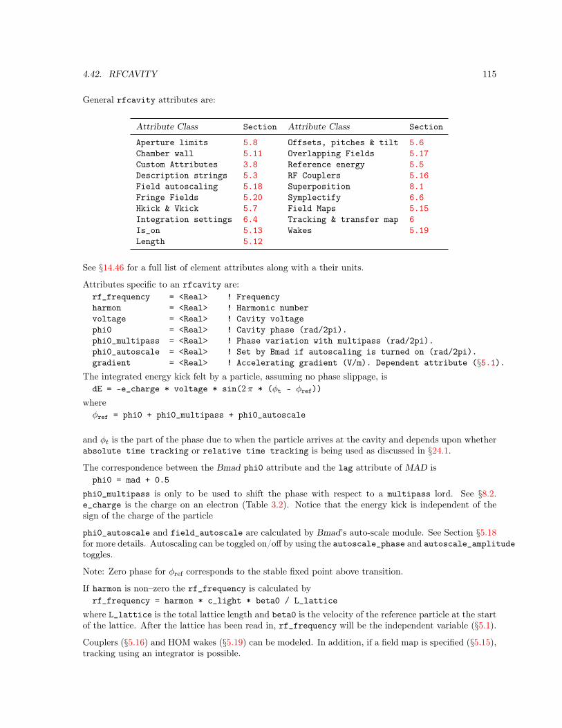
4.42. RFCAVITY 115

General rfcavity attributes are:

Attribute Class Section Attribute Class Section

Aperture limits 5.8 Offsets, pitches & tilt 5.6Chamber wall 5.11 Overlapping Fields 5.17Custom Attributes 3.8 Reference energy 5.5Description strings 5.3 RF Couplers 5.16Field autoscaling 5.18 Superposition 8.1Fringe Fields 5.20 Symplectify 6.6Hkick & Vkick 5.7 Field Maps 5.15Integration settings 6.4 Tracking & transfer map 6Is_on 5.13 Wakes 5.19Length 5.12

See §14.46 for a full list of element attributes along with a their units.

Attributes specific to an rfcavity are:rf_frequency = <Real> ! Frequencyharmon = <Real> ! Harmonic numbervoltage = <Real> ! Cavity voltagephi0 = <Real> ! Cavity phase (rad/2pi).phi0_multipass = <Real> ! Phase variation with multipass (rad/2pi).phi0_autoscale = <Real> ! Set by Bmad if autoscaling is turned on (rad/2pi).gradient = <Real> ! Accelerating gradient (V/m). Dependent attribute (§5.1).

The integrated energy kick felt by a particle, assuming no phase slippage, isdE = -e_charge * voltage * sin(2π * (φt - φref))

whereφref = phi0 + phi0_multipass + phi0_autoscale

and φt is the part of the phase due to when the particle arrives at the cavity and depends upon whetherabsolute time tracking or relative time tracking is being used as discussed in §24.1.

The correspondence between the Bmad phi0 attribute and the lag attribute of MAD isphi0 = mad + 0.5

phi0_multipass is only to be used to shift the phase with respect to a multipass lord. See §8.2.e_charge is the charge on an electron (Table 3.2). Notice that the energy kick is independent of thesign of the charge of the particle

phi0_autoscale and field_autoscale are calculated by Bmad’s auto-scale module. See Section §5.18for more details. Autoscaling can be toggled on/off by using the autoscale_phase and autoscale_amplitudetoggles.

Note: Zero phase for φref corresponds to the stable fixed point above transition.

If harmon is non–zero the rf_frequency is calculated byrf_frequency = harmon * c_light * beta0 / L_lattice

where L_lattice is the total lattice length and beta0 is the velocity of the reference particle at the startof the lattice. After the lattice has been read in, rf_frequency will be the independent variable (§5.1).

Couplers (§5.16) and HOM wakes (§5.19) can be modeled. In addition, if a field map is specified (§5.15),tracking using an integrator is possible.

116 CHAPTER 4. ELEMENTS

If a field map is specified (§5.15), tracking using an integrator is possible. A field map is only used forrunge_kutta, fixed_step_runge_kutta, and symp_lie_bmad tracking (§6.1). Only the fundamentalmode has an analytical formula for the symplectic tracking. In the future, the other modes could beused with symp_lie_bmad tracking using a field expansion about the centerline.

The cavity_type is the type of cavity being simulated. Possible settings are:ptc_standardstanding_wave ! Defaulttraveling_wave

The cavity_type switch is ignored if a field map is used.

Example:rf1: rfcav, l = 4.5, harmon = 1281, voltage = 5e6

4.43 Sad_Mult

A sad_mult element is equivalent to a SAD[SAD] mult element. This element is a combination solenoid,multipole, bend, and RF cavity.

General sample attributes are:

Attribute Class Section Attribute Class Section

an, bn multipoles 5.14 Length 5.12Aperture limits 5.8 Offsets, pitches & tilt 5.6Chamber wall 5.11 Reference energy 5.5Custom Attributes 3.8 Superposition 8.1Description strings 5.3 Tracking & transfer map 6Fringe Fields 5.20

See §14.48 for a full list of element attributes along with a their units.

Attributes specific to an sextupole element are:bs_field = <Real> ! Solenoid field. SAD equivalent: BZ.e1, e2 = <Real> ! Bend face angles.eps_step_scale = <Real> ! Step size scale. Default = 1. SAD equivalent: EPS.fq1, fq2 = <Real> ! Quadrupole fringe integral. SAD equivalents: F1, F2.ks = <Real> ! Solenoid strength.x_offset_mult = <Real> ! Mult component offset. SAD equivalent: DX.y_offset_mult = <Real> ! Mult component offset. SAD equivalent: DY.x_pitch_mult = <Real> ! Mult component pitch. SAD equivalent: DPX or CHI1.y_pitch_mult = <Real> ! Mult component pitch. SAD equivalent: DPY or CHI2.fringe_type = <Switch> ! Type of fringe. SAD equivalent: DISFRIN.fringe_at = <Switch> ! Where fringe is applied. SAD equivalent: FRINGE.

One difference between SAD and Bmad is that SAD defines the solenoid field by what are essentially aset of marker elements so that the solenoid field at a SAD mult element is not explicitly declared in themult element definition. Bmad, on the other hand, requires a sad_mult element to explicitly declarethe solenoid parameters.

Another difference between SAD and Bmad is that, within a solenoid, the reference trajectory is alignedwith the solenoid axis (and not aligned with the axis of the elements within the solenoid region).

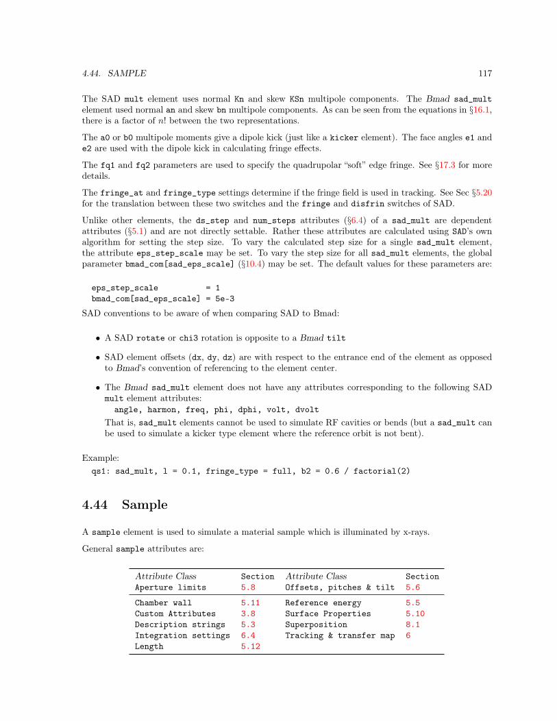
4.44. SAMPLE 117

The SAD mult element uses normal Kn and skew KSn multipole components. The Bmad sad_multelement used normal an and skew bn multipole components. As can be seen from the equations in §16.1,there is a factor of n! between the two representations.

The a0 or b0 multipole moments give a dipole kick (just like a kicker element). The face angles e1 ande2 are used with the dipole kick in calculating fringe effects.

The fq1 and fq2 parameters are used to specify the quadrupolar “soft” edge fringe. See §17.3 for moredetails.

The fringe_at and fringe_type settings determine if the fringe field is used in tracking. See Sec §5.20for the translation between these two switches and the fringe and disfrin switches of SAD.

Unlike other elements, the ds_step and num_steps attributes (§6.4) of a sad_mult are dependentattributes (§5.1) and are not directly settable. Rather these attributes are calculated using SAD’s ownalgorithm for setting the step size. To vary the calculated step size for a single sad_mult element,the attribute eps_step_scale may be set. To vary the step size for all sad_mult elements, the globalparameter bmad_com[sad_eps_scale] (§10.4) may be set. The default values for these parameters are:

eps_step_scale = 1bmad_com[sad_eps_scale] = 5e-3

SAD conventions to be aware of when comparing SAD to Bmad:

• A SAD rotate or chi3 rotation is opposite to a Bmad tilt

• SAD element offsets (dx, dy, dz) are with respect to the entrance end of the element as opposedto Bmad’s convention of referencing to the element center.

• The Bmad sad_mult element does not have any attributes corresponding to the following SADmult element attributes:angle, harmon, freq, phi, dphi, volt, dvolt

That is, sad_mult elements cannot be used to simulate RF cavities or bends (but a sad_mult canbe used to simulate a kicker type element where the reference orbit is not bent).

Example:qs1: sad_mult, l = 0.1, fringe_type = full, b2 = 0.6 / factorial(2)

4.44 Sample

A sample element is used to simulate a material sample which is illuminated by x-rays.

General sample attributes are:

Attribute Class Section Attribute Class SectionAperture limits 5.8 Offsets, pitches & tilt 5.6

Chamber wall 5.11 Reference energy 5.5Custom Attributes 3.8 Surface Properties 5.10Description strings 5.3 Superposition 8.1Integration settings 6.4 Tracking & transfer map 6Length 5.12

118 CHAPTER 4. ELEMENTS

See §14.49 for a full list of element attributes along with a their units.

This element is in development.

Attributes specific to an solenoid element are:mode = <Switch> ! Reflection or transmission.material = <type> ! Type of material. §5.9

The mode parameter can be set to:reflectiontransmission

With mode set to reflection, photons will be back scattered from the sample surface isotropically. Inthis case the material properties will not matter. Additionally, a patch (§4.38) element will be neededafter the sample element to properly reorient the reference orbit.

With mode set to transmission, photons will be transmitted through the sample. In this case materialwill be used to determine the attenuation and phase shift of the photons.

Example:formula409: sample, x_limit = 10e-3, y_limit = 20e-3, mode = reflection

4.45 Sextupole

A sextupole is a magnetic element with a quadratic field dependence with transverse offset (§16.1).

General sextupole attributes are:

Attribute Class Section Attribute Class Section

Aperture limits 5.8 Mag & Elec multipoles 5.14Chamber wall 5.11 Offsets, pitches & tilt 5.6Custom Attributes 3.8 Overlapping Fields 5.17Description strings 5.3 Reference energy 5.5Fringe Fields 5.20 Superposition 8.1Hkick & Vkick 5.7 Symplectify 6.6Integration settings 6.4 Field Maps 5.15Is_on 5.13 Tracking & transfer map 6Length 5.12

See §14.50 for a full list of element attributes along with a their units.

Attributes specific to an sextupole element are:k2 = <Real> ! Sextupole strength.b2_gradient = <Real> ! Field strength. (§5.1).

The bmad_standard calculation treats a sextupole using a kick–drift–kick model.

If the tilt attribute is present without a value then a value of π/6 is used. Example:q03w: sext, l = 0.6, k2 = 0.3, tilt ! same as tilt = pi/6

4.46 Solenoid

A solenoid is an element with a longitudinal magnetic field.

General solenoid attributes are:

4.47. SOL_QUAD 119

Attribute Class Section Attribute Class Section

Aperture limits 5.8 Mag & Elec multipoles 5.14Chamber wall 5.11 Offsets, pitches & tilt 5.6Custom Attributes 3.8 Overlapping Fields 5.17Description strings 5.3 Reference energy 5.5Fringe Fields 5.20 Superposition 8.1Hkick & Vkick 5.7 Symplectify 6.6Integration settings 6.4 Field Maps 5.15Is_on 5.13 Tracking & transfer map 6Length 5.12

See §14.52 for a full list of element attributes along with a their units.

Attributes specific to an solenoid element are:

ks = <Real> ! Solenoid strength.bs_field = <Real> ! Field strength. (§5.1).l_soft_edge = <Real> ! For modeling a ‘‘soft" fringe.r_solenoid = <Real> ! Solenoid radius.

The bmad_standard tracking model (§6.1) uses a “hard edge” model where the field goes from zero tofull strength. Example:

cleo_sol: solenoid, l = 2.6, ks = 1.5e-9 * parameter[p0c]

“Soft edge” end fields may be simulated by using Runge-Kutta tracking and setting the field_calcparameter of the element to soft_edge. Example:

soft_sol: solenoid, l = 1.0, field_calc = soft_edge, l_soft_edge = 0.5,r_solenoid = 0.1, tracking_method = runge_kutta, mat6_calc_method = tracking

Here the solenoid is modeled as a perfect current carrying cylinder with a length of 0.5 meters and acylinder radius of 0.1 meters. The length of the element, 1.0 meters, must be greater than l_soft_edgesince particles need to be tracked through the non-zero fringe field that extends outside of the cylinder.In fact, since the field is always finite everywhere, to the extent that the field is nonzero at the edgesof the element places a bound on the accuracy of the simulation. Note that bmad_standard trackingwill always ignore the setting of field_calc. That is, with bmad_standard tracking the field alwaysextends to the edges of the element and the value of l_soft_edge is ignored.

4.47 Sol_Quad

A sol_quad is a combination solenoid/quadrupole. Alternatively, the sad_mult element can also beused. The advantage of the sad_mult element is that it can simulate a quadrupole field that is cantedwith respect to the solenoid field.

General sol_quad attributes are:

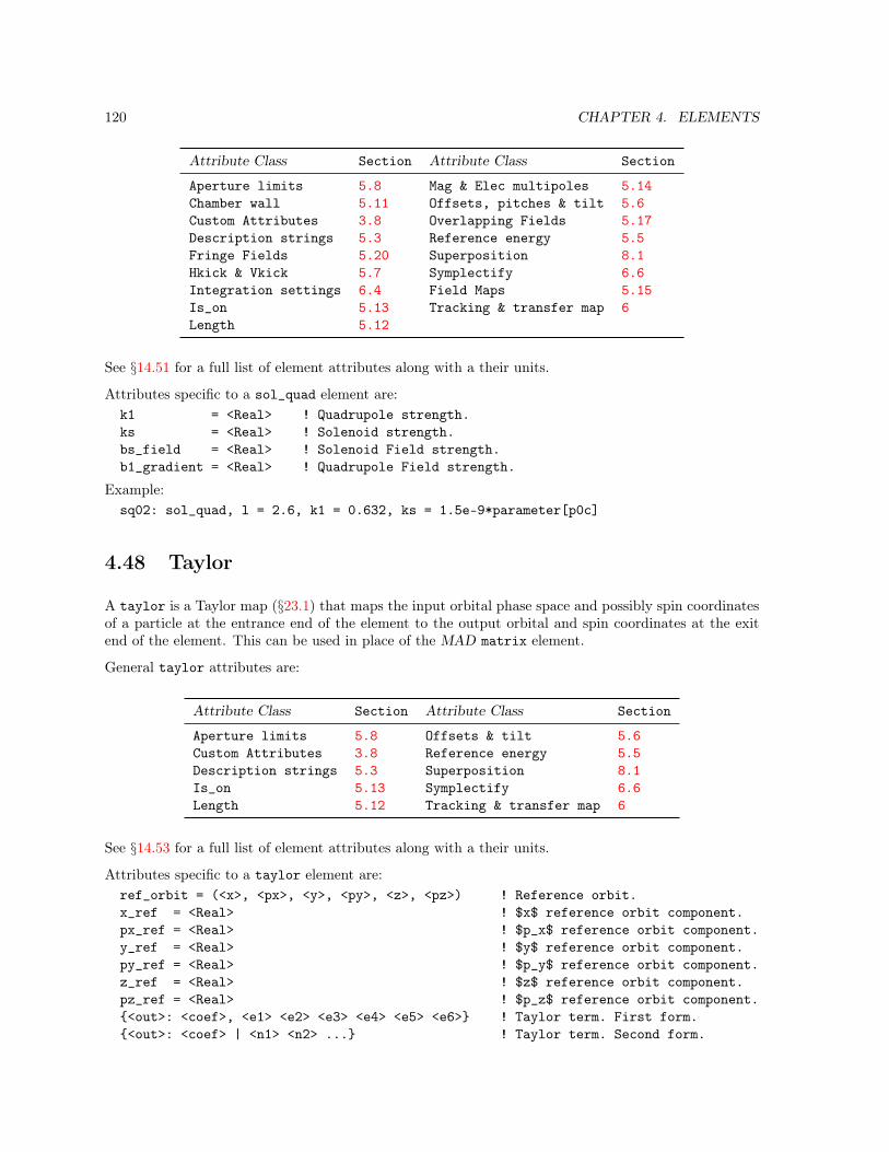
120 CHAPTER 4. ELEMENTS

Attribute Class Section Attribute Class Section

Aperture limits 5.8 Mag & Elec multipoles 5.14Chamber wall 5.11 Offsets, pitches & tilt 5.6Custom Attributes 3.8 Overlapping Fields 5.17Description strings 5.3 Reference energy 5.5Fringe Fields 5.20 Superposition 8.1Hkick & Vkick 5.7 Symplectify 6.6Integration settings 6.4 Field Maps 5.15Is_on 5.13 Tracking & transfer map 6Length 5.12

See §14.51 for a full list of element attributes along with a their units.

Attributes specific to a sol_quad element are:k1 = <Real> ! Quadrupole strength.ks = <Real> ! Solenoid strength.bs_field = <Real> ! Solenoid Field strength.b1_gradient = <Real> ! Quadrupole Field strength.

Example:sq02: sol_quad, l = 2.6, k1 = 0.632, ks = 1.5e-9*parameter[p0c]

4.48 Taylor

A taylor is a Taylor map (§23.1) that maps the input orbital phase space and possibly spin coordinatesof a particle at the entrance end of the element to the output orbital and spin coordinates at the exitend of the element. This can be used in place of the MAD matrix element.

General taylor attributes are:

Attribute Class Section Attribute Class Section

Aperture limits 5.8 Offsets & tilt 5.6Custom Attributes 3.8 Reference energy 5.5Description strings 5.3 Superposition 8.1Is_on 5.13 Symplectify 6.6Length 5.12 Tracking & transfer map 6

See §14.53 for a full list of element attributes along with a their units.

Attributes specific to a taylor element are:ref_orbit = (<x>, <px>, <y>, <py>, <z>, <pz>) ! Reference orbit.x_ref = <Real> ! $x$ reference orbit component.px_ref = <Real> ! $p_x$ reference orbit component.y_ref = <Real> ! $y$ reference orbit component.py_ref = <Real> ! $p_y$ reference orbit component.z_ref = <Real> ! $z$ reference orbit component.pz_ref = <Real> ! $p_z$ reference orbit component.<out>: <coef>, <e1> <e2> <e3> <e4> <e5> <e6> ! Taylor term. First form.<out>: <coef> | <n1> <n2> ... ! Taylor term. Second form.

4.48. TAYLOR 121

tt<out><n1><n2>... = <Coef> ! Taylor term. Third form.delta_ref_time = <Real> ! Change in the reference time.delta_e_ref = <Real> ! Change in the reference energy.

For historical reasons, there are three different forms that can be used to specify a taylor term. Noticethat the first form (above) uses a comma “,” to separate the <coef> from <e1>, while the second formuses a vertical bar “|” to separate <coef> from <n1>.

The orbital (x, px, y, py, z, pz) part of the Taylor map, M, maps input orbital coordinates r(in) to theoutput orbital coordinates r(out)

r(out) =M(r(in)) (4.24)

Notice that Stern-Gerlach effects are ignored so that the output coordinates are independent of the spin.M has six componentsMj one for each output coordinate rj(out)

rj(out) =Mj(r(in)) (4.25)

EachMj is made up of a number of terms

Mj =

Nj∑k=1

Mjk (4.26)

and each term Mjk is a polynomial in the input orbital coordinates with respect to the reference orbit.

Mjk(r(in)) = Cjk ·Π6i=1 δr

eijki (4.27)

where Cjk is the coefficient for the term, the eijk are integer exponents, and δr = r(in) − rref with rrefwith being the reference orbit.

A term in a Taylor map can be specified by one of three forms as shown above. The first form is<out>: <coef>, <e1> <e2> <e3> <e4> <e5> <e6>

<Out> is an integer in the range 1 to 6 corresponding to the index j in Eq. (4.27) (<out> = 1 for x,etc.). <coef> corresponds to Cjk in Eq. (4.27), and <e1>, <e2>, <e3>, <e4>, <e5>, and <e6> correspondto eijk, i = 1 . . . 6. For example, the Taylor map

py(out) = 0.9 · δx+ 2.73 · δy2(in) δpz(in) + . . . (4.28)

would be written as4: 0.9, 1 0 0 0 0 0, 4: 2.73, 0 0 2 0 0 1, ...

The second form for specifying a Taylor term uses the syntax:<out>: <coef> | <n1> <n2> ...

The set of integers <n1>, <n2> each must be between 1 and 6 inclusive. The value of the ith exponenteijk in Eq. (4.27) is equal to the number of integers that are equal to i. For example, the above Taylormap would be written using the second form as4: 0.9 | 1, 4: 2.73 | 336, ...

Notice that with the second form, spaces between exponent integers is optional.

The third form is like the second form and has the syntax:tt<out><n1><n2>... = <Coef> ! Taylor term. Third form.

For example, the Taylor map above would be written using the third form as:tt41 = 0.9, tt4336 = 2.73, ...

122 CHAPTER 4. ELEMENTS

The spin (§22.1) part of the transport map Q (§23.2) gives the spin rotation quaternion q (§22.2) as afunction of input orbital coordinates (the form of the T-BMT equation assures that Q cannot dependupon the spin coordinates):

q =Q(r(in)) (4.29)

q has four components and in analogy to Eq. (4.25) one writes

qj = Qj(r(in)) (4.30)

Each Qj is made up of a number of terms

Qj =

Nj∑k=1

Qjk (4.31)

and each term Qjk is a polynomial in the input orbital coordinates with respect to the reference orbit.

Qjk(r(in)) = Cjk ·Π6i=1 δr

eijki (4.32)

Rather than using an integer index, the four components of a quaternion are labeled (S1, Sx, Sy, Sz).The syntax for the spin part uses the first or second forms as described above. For exampleSx: 0.43 | 13

is equivalent to the termSx = 0.43 · δx(in) δy(in) (4.33)

By default, a taylor element starts out with the unit phase space map. That is, a taylor elementstarts with the following 6 terms1: 1.0, 1 0 0 0 0 0, 2: 1.0, 0 1 0 0 0 0,3: 1.0, 0 0 1 0 0 0, 4: 1.0, 0 0 0 1 0 05: 1.0, 0 0 0 0 1 0, 6: 1.0, 0 0 0 0 0 1

Which is equivalent to1: 1.0 | 1, 2: 1.0 | 2, 3: 1.0 | 34: 1.0 | 4, 5: 1.0 | 5, 6: 1.0 | 6

If there are no Sx spin terms are present, the Sx quaternion component will always evaluate to zero.This is equivalent to a single term Sx: 0.0 |. Similarly for the Sy and Sz components. If no S1 termis present, it is considered an error if any Sx, Sy, or Sz term is present. If no S1, Sx, Sy, nor Sz spinterms are present, S1 component will be given a default term of S1: 1.0 |. Thus, if no spin terms arepresent at all, the spin map will be the unit map.

The ref_orbit attribute specifies the phase space (x, px, y, py, z, pz) reference orbit at the start of theelement used to construct the Taylor map. Alternatively, the individual components of the referenceorbit may be specified by using the attributes x_ref, px_ref, y_ref, py_ref, z_ref, or pz_ref.

Note: when converting the map from Bmad to PTC (§27), the Bmad/PTC interface code will convertfrom Bmad phase space coordinates to PTC phase space coordinates and will convert the map to usingthe reference orbit as the map zero orbit. This does not affect tracking but will affect map analysis.

A term in a taylor element will override any previous term with the same out and e1 through e6indexes. For example the term:tt: Taylor, 1: 4.5, 1 0 0 0 0 0

will override the default 1: 1.0, 1 0 0 0 0 0 term.

The l length attribute of a taylor element does not affect phase space coordinates but will affect thelongitudinal s position of succeeding elements and will affect the time it takes a particle to track through

4.49. WIGGLER AND UNDULATOR 123

the element The calculation involves first calculating the change in reference time which is the time aparticle with the reference energy would take to transverse the element. Next, Eq. (15.28) is used withthe change in the phase space z coordinate to calculate the time a particle takes to traverse the element.

The time a particle takes to track through a taylor element can also be controlled by setting thedelta_ref_time attribute which sets the travel time for the reference particle. delta_ref_time is adependent attribute so that if both l and delta_ref_time are set, the value of delta_ref_time willbe modified by Bmad to correspond to the setting of l.

The delta_e_ref attribute can be used to modify the reference energy at the exit end of the taylorelement. The phase space transport is completely determined by the Taylor map and is independent ofdelta_e_ref. For example, with a unit Taylor map, the phase space coordinates px and py constantthrough the element independent of delta_e_ref. However, a finite delta_e_ref will modify thereference momentum P0 and hence through Eq. (15.27) will affect the transport downstream of theTaylor element. This behavior is in contrast to how delta_e_ref is handled in a patch element. In apatch element, the transformation used when delta_e_ref is non-zero is to hold as constant the actualtransverse momenta Px and Py and then px and py are modified using Eq. (15.27).

A taylor element that is “turned off” (is_on attribute set to False), is considered to be like a markerelement. That is, the orbit and Twiss parameters are unchanged when tracking through a taylor elementthat is turned off.

Example taylor element definitions:

tt: Taylor, 4: 2.7, 0 0 2 0 0 1, 2: 1.9 | 1 1 2,S1: 0.43 | 2 , ...,ref_orbit = (0.01, 0.003, 0.002, 0.001, 0.0, 0.2)

t_unit: taylor s1: 1 | ! This is the identity spin/orbital map.

And

Note: When tracking a particle’s spin through a map, the quaternion used to rotate the spin is alwaysnormalized to one so that the magnitude of the spin will be invariant.

Note: Tracking through a taylor elements using symp_lie_ptc is the same as tracking with the taylortracking method. That is, the Taylor map is simply evaluated and no effort at symplectification is done.Furthermore, evaluating the Taylor map of a taylor element using the taylor method is faster thanevaluation using symp_lie_ptc. Thus the taylor tracking method should always be used with taylorelements.

4.49 Wiggler and Undulator

A wiggler or undulator element is basically a periodic array of alternating bends. The differencebetween wigglers and undulators is in the x-ray emission spectrum. Charged particle tracking will bethe same.

Henceforth, the term “wiggler” will denote either a wiggler or undulator

General wiggler attributes are:

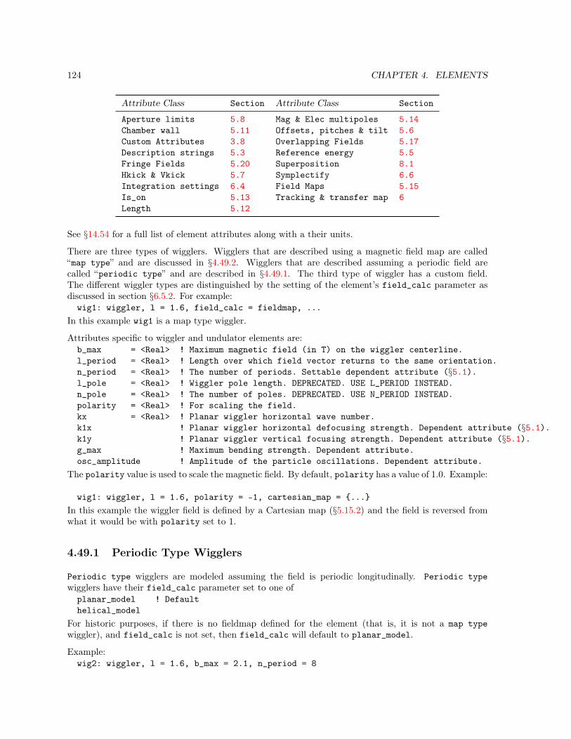
124 CHAPTER 4. ELEMENTS

Attribute Class Section Attribute Class Section

Aperture limits 5.8 Mag & Elec multipoles 5.14Chamber wall 5.11 Offsets, pitches & tilt 5.6Custom Attributes 3.8 Overlapping Fields 5.17Description strings 5.3 Reference energy 5.5Fringe Fields 5.20 Superposition 8.1Hkick & Vkick 5.7 Symplectify 6.6Integration settings 6.4 Field Maps 5.15Is_on 5.13 Tracking & transfer map 6Length 5.12

See §14.54 for a full list of element attributes along with a their units.

There are three types of wigglers. Wigglers that are described using a magnetic field map are called“map type” and are discussed in §4.49.2. Wigglers that are described assuming a periodic field arecalled “periodic type” and are described in §4.49.1. The third type of wiggler has a custom field.The different wiggler types are distinguished by the setting of the element’s field_calc parameter asdiscussed in section §6.5.2. For example:wig1: wiggler, l = 1.6, field_calc = fieldmap, ...

In this example wig1 is a map type wiggler.

Attributes specific to wiggler and undulator elements are:b_max = <Real> ! Maximum magnetic field (in T) on the wiggler centerline.l_period = <Real> ! Length over which field vector returns to the same orientation.n_period = <Real> ! The number of periods. Settable dependent attribute (§5.1).l_pole = <Real> ! Wiggler pole length. DEPRECATED. USE L_PERIOD INSTEAD.n_pole = <Real> ! The number of poles. DEPRECATED. USE N_PERIOD INSTEAD.polarity = <Real> ! For scaling the field.kx = <Real> ! Planar wiggler horizontal wave number.k1x ! Planar wiggler horizontal defocusing strength. Dependent attribute (§5.1).k1y ! Planar wiggler vertical focusing strength. Dependent attribute (§5.1).g_max ! Maximum bending strength. Dependent attribute.osc_amplitude ! Amplitude of the particle oscillations. Dependent attribute.

The polarity value is used to scale the magnetic field. By default, polarity has a value of 1.0. Example:

wig1: wiggler, l = 1.6, polarity = -1, cartesian_map = ...In this example the wiggler field is defined by a Cartesian map (§5.15.2) and the field is reversed fromwhat it would be with polarity set to 1.

4.49.1 Periodic Type Wigglers

Periodic type wigglers are modeled assuming the field is periodic longitudinally. Periodic typewigglers have their field_calc parameter set to one ofplanar_model ! Defaulthelical_model

For historic purposes, if there is no fieldmap defined for the element (that is, it is not a map typewiggler), and field_calc is not set, then field_calc will default to planar_model.

Example:wig2: wiggler, l = 1.6, b_max = 2.1, n_period = 8

4.49. WIGGLER AND UNDULATOR 125

This defines a periodic type wiggler with field_type defaulting to planar_model.

For the planar_model, wigglers use a simplified model where the wiggler has field components

Bx = −b_maxkxky

sin(kx x) sinh(ky y) cos(kz z + φz)

By = b_max cos(kx x) cosh(ky y) cos(kz z + φz) (4.34)

Bz = −b_maxkzky

cos(kx x) sinh(ky y) sin(kz z + φz)

with k2y = k2

x + k2z . Here z is the distance from the beginning of the wiggler, the input parameter b_max

is the maximum field on the centerline, and kz is given in terms of the period length (l_period) by

kz =2π

lperiod(4.35)

The phase φz is chosen so that By is symmetric about the center of the wiggler

φz =−kz L

2(4.36)

Note: Originally kz was calculated using l_pole — the length of a pole — with the period length beingtwice the pole length. When the helical model option was introduced this became problematical sincethe period of a helical wiggler could be either 2 or 4 times the pole length depending upon the geometry.As a result, using the pole length was deprecated and instead the period length or number should beused.

The helical_model for the field is

Bx = −b_max cosh(kz x) sin(kz z + φz) (4.37)By = b_max cosh(kz y) cos(kz z + φz)

Bz = −b_max [sinh(kz x) cos(kz z + φz) + sinh(kz y) sin(kz z + φz)]

With field_calc set to planar_model, and with bmad_standard tracking (§6), the horizontal andvertical focusing is assumed small. The vertical motion is modeled as a combination focusing quadrupoleand focusing octupole giving a kick (modified from [Corbett99])

dpydz

= k1y

Åy +

2

3k2y y

3

ã(4.38)

where

gmax =eBmax

P0 (1 + pz)(4.39)

k1y =−k2

y

2 k2z

g2max (4.40)

with k1y (a dependent element attribute) being the linear focusing constant.

The averaged horizontal motion isdpxdz

= k1x x (4.41)

with

k1x =k2x

2 k2z

g2max (4.42)

126 CHAPTER 4. ELEMENTS

With field_calc set to helical_model, and with bmad_standard tracking, the transport in the ver-tical and horizontal planes is the same as with the transport in the vertical plane with planar_model(Eq. (4.38)).

While bmad_standard tracking uses an averaged trajectory, the actual trajectory has oscillations thatlook like

x = A cos(kz z) (4.43)

with the amplitude A given byA =

gmax

k2z

(4.44)

The value of A, computed for an on-energy (pz = 0) particle, is calculated and stored in the dependentparameter osc_amplitude.

With field_calc set to planar_model and bmad_standard tracking, the phase φz in Eqs. (4.36) isirrelevant. When the tracking involves Taylor maps and symplectic integration, the choice of phase issuch that, with an integer number of periods, a particle that enters the wiggler on-axis will leave thewiggler on-axis provided there is an integer number of periods. Notice that with field_calc set tohelical_model it is not possible to set the phase so that a particle that enters the wiggler on-axis willleave the wiggler on-axis.

When using a tracking through a periodic wiggler with a tracking method that integrates through themagnetic field (§6.4), The magnetic field is approximated using a single wiggler term as if the wigglerwere a map type wiggler. This wiggler model has unphysical end effects and will give results that aredifferent from the results obtained when using the bmad_standard tracking method.

Tracking a particle through a wiggler is always done so that if the particle starts on-axis with nomomentum offsets, there is no change in the z coordinate even though the actual trajectory through thewiggler does not follow the straight line reference trajectory.

4.49.2 Map Type Wigglers

Map type wigglers are modeled using a field map as described in section §5.15. Map type wigglers havetheir field_calc parameter set to fieldmap. Note: For historic reasons, unlike other types of elements,field_calc will default to fieldmap if there is a field map present in a wiggler.

Unlike periodic type wigglers, the b_max attribute for a map type wiggler is a dependent attributeand is set by Bmad to be the maximum field on-axis computed for polarity = 1.

Note: There is no bmad_standard tracking for a map_type wiggler.

4.49.3 Old Wiggler Cartesian Map Syntax

When the wiggler model was first developed, the only type of map that could be used for map typewigglers was a Cartesian map (§5.15). The syntax for specifying this Cartesian map was different fromwhat it is currently. The old syntax for a Cartesian map term was:

term(i) = C, kx, ky, kz, φz (4.45)

Example:wig1: wiggler, l = 1.6,

term(1) = 0.03, 3.00, 4.00, 5.00, 0.63,term(2) = ...

4.49. WIGGLER AND UNDULATOR 127

The old syntax was limited to using the cartesian_map y family (§16.5) with x0 = y0 = 0. There wasalso a different normalization convention. The old style hyper-y form was

Bx = −C kxky

sin(kxx) sinh(kyy) cos(kzz + φz)

By = C cos(kxx) cosh(kyy) cos(kzz + φz) ! Old style

Bs = −C kzky

cos(kxx) sinh(kyy) sin(kzz + φz) (4.46)

with k2y = k2

x + k2z .

The old style hyper-xy form was

Bx = Ckxky

sinh(kxx) sinh(kyy) cos(kzz + φz)

By = C cosh(kxx) cosh(kyy) cos(kzz + φz) ! Old style

Bs = −C kzky

cosh(kxx) sinh(kyy) sin(kzz + φz) (4.47)

with k2y = k2

z − k2x ,

The old style hyper_x form was

Bx = Ckxky

sinh(kxx) sin(kyy) cos(kzz + φz)

By = C cosh(kxx) cos(kyy) cos(kzz + φz) ! Old style

Bs = −C kzky

cosh(kxx) sin(kyy) sin(kzz + φz) (4.48)

with k2y = k2

x − k2z .

The correspondence between C in the above equations and A in the new equations is given by comparingEqs. (4.46), (4.47), and (4.48) with Eqs. (16.35).

When the cartesian_map construct was being developed, an intermediate hybrid syntax was used de-fined:

term(i) = A, kx, ky, kz, x0, y0, φz, family (4.49)

The parameters here directly correspond to the cartesian_map forms (see Eqs. (16.32) through (16.37)).

For example, the old style syntax:term(1) = 0.03*4/5, 3.00, 4.00, 5.00, 0.63 ! Old style

is equivalent to the hybrid syntax:term(2) = 0.03, 3.00, 4.00, 5.00, 0, 0, 0.63, y ! Hybrid style

Note: When converting from the old or hybrid styles to the new syntax, the field_calc parametermust be set to fieldmap.

128 CHAPTER 4. ELEMENTS

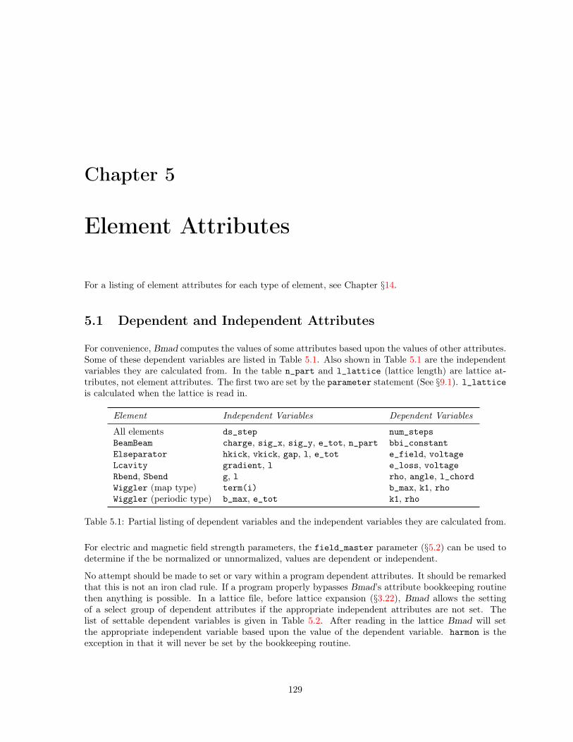
Chapter 5

Element Attributes

For a listing of element attributes for each type of element, see Chapter §14.

5.1 Dependent and Independent Attributes

For convenience, Bmad computes the values of some attributes based upon the values of other attributes.Some of these dependent variables are listed in Table 5.1. Also shown in Table 5.1 are the independentvariables they are calculated from. In the table n_part and l_lattice (lattice length) are lattice at-tributes, not element attributes. The first two are set by the parameter statement (See §9.1). l_latticeis calculated when the lattice is read in.

Element Independent Variables Dependent Variables

All elements ds_step num_stepsBeamBeam charge, sig_x, sig_y, e_tot, n_part bbi_constantElseparator hkick, vkick, gap, l, e_tot e_field, voltageLcavity gradient, l e_loss, voltageRbend, Sbend g, l rho, angle, l_chordWiggler (map type) term(i) b_max, k1, rhoWiggler (periodic type) b_max, e_tot k1, rho

Table 5.1: Partial listing of dependent variables and the independent variables they are calculated from.

For electric and magnetic field strength parameters, the field_master parameter (§5.2) can be used todetermine if the be normalized or unnormalized, values are dependent or independent.

No attempt should be made to set or vary within a program dependent attributes. It should be remarkedthat this is not an iron clad rule. If a program properly bypasses Bmad’s attribute bookkeeping routinethen anything is possible. In a lattice file, before lattice expansion (§3.22), Bmad allows the settingof a select group of dependent attributes if the appropriate independent attributes are not set. Thelist of settable dependent variables is given in Table 5.2. After reading in the lattice Bmad will setthe appropriate independent variable based upon the value of the dependent variable. harmon is theexception in that it will never be set by the bookkeeping routine.

129

130 CHAPTER 5. ELEMENT ATTRIBUTES

Element Dependent Variable Set Independent Variables Not Set

Lcavity voltage gradientRbend, Sbend rho gRbend, Sbend angle g, or lRFcavity rf_frequency harmonWiggler (periodic type) n_pole l_pole

Table 5.2: Dependent variables that can be set in a primary lattice file.

5.2 Field_Master

The field_master attribute of an element sets whether the element’s normalized (normalized by thereference energy) field strengths or the unnormalized strengths are the independent variables (§5.1). Thesetting of field_master also sets whether an element’s magnetic multipoles (§5.14) are interpreted asnormalized or unnormalized (electric multipoles are always treated as unnormalized).

Table 5.3 shows some normalized and unnormalized field strength attributes. The default value offield_master for an element is False if there are no field values set in the lattice file for that element.If normalized field values are present then the default is also False and if there are unnormalized fieldvalues present then the default is True.

For example:Q1: quadrupole, b1_gradient = 0 ! Field strengths are the independent variablesQ1: quadrupole, field_master = T ! Same as aboveQ2: quadrupole ! Define Q2.Q2[b1_gradient] = 0 ! Field strengths now the independent variables.Q2[field_master] = T ! Same as above.

Specifying both normalized and unnormalized strengths for a given element is not permitted. Forexample:Q3: quadrupole, k1 = 0.6, bl_hkick = 37.5 ! NO. Not VALID.

Element Normalized Unnormalized

Sbend, Rbend g b_fieldSbend, Rbend dg db_fieldSolenoid, Sol_quad ks bs_fieldQuadrupole, Sol_quad, Sbend, Rbend k1 b1_gradientSextupole, Sbend, Rbend k2 b2_gradientOctupole k3 b3_gradientHKicker, VKicker kick bl_kickMost hkick bl_hkickMost vkick bl_vkick

Table 5.3: Example normalized and unnormalized field strength attributes.

5.3 Type, Alias and Descrip Attributes

There are three string labels associated with any element:

5.4. GROUP, OVERLAY AND RAMPER ELEMENT SYNTAX 131

type = "<String>"alias = "<String>"descrip = "<String>"

The type and alias attributes can be up to 40 characters in length and descrip can be up to 200characters. If the attribute string does not contain a blank, comma, or a semicolon, the quotation marksmay be omitted.

Bmad routines do not use these labels directly. Rather these labels have a number of purposes. Forexample, a Bmad based program that is used as an online machine model could associate a label stringwith a machine database element to facilitate machine control.

Example:Q00W: Quad, type = "My Type", alias = Who_knows, &

descrip = "Only the shadow knows"

5.4 Group, Overlay and Ramper Element Syntax

The syntax for specifying group (§4.22), overlay (§4.37), or ramper (§4.41) elements are virtuallyidentical and is discussed below. The name “controller” will be used to denote either a group, overlay,or ramper element.

Controller elements have a set of one or more “variables” that are used to control the values of attributesof other elements (called “slave” attributes).

There are two types of controllers in terms of how slave attribute values are computed — Expressionbased controllers and knot based controllers. Expression based controllers use mathematical expres-sions (§3.12) to define how slave attribute values are calculated based upon the values of the controllervariables. Knot based controllers use an array of points (called “knots”) with either linear or cubic splineinterpolation (in particular, the cubic non-smoothing Akima spline[Akima70]) to determine the relation-ship between variables and slave attributes. With a knot based controller, the number of controllervariables is restricted to be one.

The general syntax for an expression based group element isname: GROUP = ele1[attrib1]:exp1, ele2[attrib2]:exp2, ...,

VAR = var1, var2, ..., var1 = init_val1,old_var1 = old_init_val1, ..., GANG = logical, ...

For an expression based overlay element, the syntax is identical except OVERLAY is substituted forGROUP and there are no old values to set:name: OVERLAY = ele1[attrib1]:exp1, ele2[attrib2]:exp2, ...,

VAR = var1, var2, ..., var1 = init_val1, GANG = logical, ...

For an expression based ramper element, the syntax is identical to the overlay element except RAMPERis used in place of OVERLAY and there is no GANG attribute.

In the above, Name is the name of the controller element, ele1, ele2, ... are the elements whose attributesare to be controlled, attrib1, attrib2, etc. are the controlled attributes (called “slave” attributes), var1,var2, etc. are the control variables, and exp1, exp2, etc. are the arithmetical expressions that definethe relationship between the variables and the slave attributes. Example:gr1: group = q1[k1]:-tan(a)*b, q2[tilt]:b^2, var = a, b

To define an expression based controller element, two lists are needed: One list defines the slaveattributes along with the arithmetic expressions used for computing the value of the slave attributes.The other list defines the variables within the controller element that can be varied. In the above

132 CHAPTER 5. ELEMENT ATTRIBUTES

example, the variables are a and b, and the slave attributes are the k1 attribute of element q1 and thetilt attribute of element q2. The arithmetic expressions used for the control are -tan(a)*b and bˆ2.

The general syntax for For a knot based group element is:name: GROUP = ele1[attrib1]:y_knot_points1, ele2[attrib2]:y_knot_points2, ...,

VAR = var1, X_KNOT = x_knot_points, INTERPOLATION = type,var1 = init_val1, old_var1 = init_val_old1, ..., GANG = logical, ...

and the general syntax for a knot based overlay element is similar:name: OVERLAY = ele1[attrib1]:y_knot_points1, ele2[attrib2]:y_knot_points2, ...,

VAR = var1, X_KNOT = x_knot_points, var1 = init_val1, ...,GANG = logical, INTERPOLATION = type, ...

For ramper elements, the syntax is similar to the overlay syntax except that OVERLAY is replaced byRAMPER and there is no GANG attribute. The x_knot array is combined with a given y_knot array to givea series of N knot points where N is the size of the x_knot and y_knot arrays. As such, the size of allknot arrays must be the same with the additional restriction that the x_knot array must have valuesthat are strictly ascending. Example:ov: overlay = q1[k1]:-0.12, 0.23, 0.53, q2[k1], q3[k1], q4[k1]:0.37, 0.12, 0.92,

var = time, x_knot = 0.0, 0.7, 1.0

K In this example there are three knot points for each slave parameter. For the slave parameter q4[k1]the knot points are (0.0, 0.37), (0.7, 0.12), and (1.0, 0.92). If a y_knot_points array is not present fora particular slave attribute, the knot array of the previous slave attribute is used. Thus, in the aboveexample, the y_knot array used for q2[k1] and q3[k1] are the same as the y_knot array for q1[k1].

The method used to interpolate between the knot points is determined by the setting of the interpolateparameter which may be one oflinear ! Linear interpolation.spline ! Cubic spline interpolation (default).

For variable values outside of the range specified by x_knot, the slave parameter value will be ex-trapolated using the interpolation function calculated from the three points nearest the end. That is,extrapolation will be linear if interpolate is set to linear and will be cubic if interpolate is set tospline. For the cubic spline, extrapolation is only permitted over a distance outside the x_knot rangeequal to the difference between the value of the x_knot end point and its neighbor point. Thus in theabove example, extrapolation will be allowed in the intervals [−0.7, 0.0] and [1.0, 1.7].

After a controller has been defined, the individual knot points may be referenced using the syntaxname[x_knot(i)] ! I^th x_knot pointname[slave(j)%y_knot(i)] ! I^th y_knot point of j^th slave.

For example:ov: overlay = q1[k1]:-0.12, 0.23, 0.53, q2[tilt]:0.37, 0.12, 0.92,

var = time, x_knot = 0.0, 0.7, 1.0ov[x_knot(3)] = 2.0 ! Changes from 1.0 to 2.0ov[slave(2)%y_knot(2) = 0.2 ! Changes q2[tilt] y_knot(2) from 0.12 to 0.2

If the gang attribute is True (which is the default) a controller will control all elements of a givenname. Thus, in the above example, if there are multiple elements named q1 then gr1 will control thek1 attribute of all of them. If gang is set to False, a separate controller is created for each element inthe lattice of a given name. For example:gr1: group = q1[k1]:-tan(a)*b, q2[tilt]:b^2, var = a, b, gang = False

In this example, suppose there are five q1 and five q2 elements in the lattice. In this case, there will befive gr1 group elements created. The first gr1 will control the first q1 and q2 to appear in the lattice,etc. With gang set to False, it is an error if the number of instances in the lattice for a given slave

5.4. GROUP, OVERLAY AND RAMPER ELEMENT SYNTAX 133

name is different from any other slave name. In this example, it would be an error if the number of q1elements in the lattice is different from the number of q2 elements in the lattice.

To vary coefficients in expressions, use variables in place of the coefficients and then variables can bevaried. For example:gr1: group = s1[k2]: 0.03+1.07*vv, var = vv ! Instead of this...gr2: group = s1[k2]: a+b*vv, var = vv, a, b, a = 0.03, b = 1.07 ! Use this.

Wild card characters can be used in element names. Example:rf_control: overlay = rfcavity::*[voltage]:v, var = v

The syntax for specifying an attribute attrib of element ele to be controlled is ele[attrib]. Theattribute part [attrib] may be omitted and in this case the name of the attribute will be taken to bethe name of the first variable. Example:ov1: overlay = sex1:-tan(k2)^b, var = k2, b

In this example, the controlled attribute of element sex1 is k2. Except in cases where this defaultattribute syntax is used, the names of the variables are arbitrary and do not have to correspond to thename of any actual attribute.

The arithmetic expressions used to evaluate controlled attribute value changes may be a constant. Inthis case, the actual expression used is this constant times the first variable. If the expression is omittedentirely, along with the separating “:”, the constant will be taken to be unity. Example:gr1: group = b1, b3:-pi, var = angle

This is equivalent togr1: group = b1[angle]:angle, b3[angle]:-pi*angle, var = angle

Arithmetic expressions may themselves contain element attributes. Example:sk_q20W: overlay = sex_20W[a1]:-sex_20W[L], k1

Here the sk_q20w overlay controls the a1 multipole attribute of element sex_20w and the length ofsex_20w is used as a scale factor between the overlay’s variable k1 and the controlled attribute a1. Thepotential problem here is that, to keep the internal bookkeeping simple, the value of sex_20w[L] isevaluated once during parsing of the lattice file and never reevaluated (§3.12). If it is desired to use avariable element attribute in an expression, this may be effectively done by defining a control variableto take its place. Thus the above overlay may be recast as:sk_q20W: overlay = sex_20W[L]:ll, sex_20W[a1]:ll*k1, var = k1, ll

Initial values can be assigned to the variables from within the definition of the controller element.Example:ov1: overlay = ..., var = a, b, a = 7, b = 2

Here the initial values 7 and 2 are assigned to a and b respectively. Alternatively, variables can be setafter a controller element has been defined. Example:ov1: overlay = ..., var = a, bov1[a] = 7gr1[b] = 2

Note: There is an old deprecated syntax. For group elements the syntax was:name: GROUP = ele1[attrib1]:coef1, ele2[attrib2]:coef2, ...,

attrib = init_value ! DO NOT USE THIS SYNTAX!

and for overlay elements the old syntax was identical except that GROUP was replaced by OVERLAY:name: OVERLAY = ele1[attrib1]:coef1, ele2[attrib2]:coef2, ...,

attrib = init_value ! DO NOT USE THIS SYNTAX!

With this old syntax, there is only one variable. Additionally, there are no arithmetic expressions.Rather, attribute changes are linear in the command variable with the constant of proportionality givenby a specified coefficient. For example with the old syntax

134 CHAPTER 5. ELEMENT ATTRIBUTES

ov1: overlay = sq1:3.7, sq2[tilt], k0 = 2 ! DO NOT USE THIS SYNTAX!

is equivalent, in the present syntax, to:ov1: overlay = sq[k0]:3.7, sq2[tilt], var = k0, k0 = 2

Note: In this old syntax the colon “:” separating the controlled attribute from the linear coefficient maybe replaced by a slash “/”. For group elements, there was an added wrinkle that, with the old syntax,the variable’s name is fixed to be command. For example, with the old syntaxgr1: group = sq1:3.7, sq2[tilt], k0 = 2 ! DO NOT USE THIS SYNTAX!

is equivalent, in the present syntax, to:gr1: group = sq[k0]:3.7, sq2[tilt], var = command, command = 2

5.5 Energy and Wavelength Attributes: E_tot, P0C, andRef_Wavelength

The attributes that define the reference energy and momentum at an element are:e_tot = <Real> ! Total energy in eV.p0c = <Real> ! Momentum in eV.

The energy and momentum are defined at the exit end of the element. For ultra–relativistic particles,and for photons, these two values are the same (§15.4.2). Except for multipass elements (§8.2), e_totand p0c are dependent attributes and, except for multipass elements, any setting of e_tot and p0c inthe lattice input file is an error. The value of e_tot and p0c for an element is calculated by Bmad to bethe same as the previous element except for e_gun, lcavity, converter, and patch elements. To setthe e_tot or p0c at the start of the lattice use the beginning or parameter statements. See §9.1. Sincethe reference energy changes from the start to the end of an lcavity, converter or em_field element,these elements have the dependent attributese_tot_start andp0c_start

which are just the reference energy and momentum at the start of the element.

The beginning_ele element (§4.4) also has associated e_tot_start and p0c_start attributes as wellas e_tot and p0c. Generally, for a beginning_ele, p0c_start and p0c are the same and e_tot_startand e_tot are the same and the values for these attributes are set in the lattice file with the appropriateparameter (§9.1) or beginning (§9.4) statement. The exception occurs when there is an e_gun elementin the lattice (§4.15). In this case, the p0c_start and e_tot_start attributes of the beginning_eleare set to the values as set in the lattice file and e_tot is set toe_tot = e_tot_start + voltage

and p0c is calculated from e_tot and the mass of the particle being tracked. For example, if the latticefile contained:beginning[p0c] = 0gun: e_gun, voltage = 0.5e6injector: line = (gun, ...)

Then the following energy values will be set for the beginning beginning_ele element:p0c_start = 0e_tot_start = mc2e_tot = mc2 + 0.5e6p0c = Sqrt(e_tot - mc2^2)

5.5. ENERGY AND WAVELENGTH ATTRIBUTES 135

where mc2 is the particle rest mass. The reason for using this convoluted convention is to allow thesetting, in the lattice file, of a zero reference momentum at the start of the lattice, while avoiding thecalculational problems that would occur if the e_gun element truly had a starting reference momentumof zero. Specifically, the problem with zero reference momentum is that the phase space momentumwould be infinity as can be seen from Eqs. (15.27).

For lattice branches other than the root branch, the reference energy or momentum is set using the linename of the branch (§9.4). For example:ff: fork, to_line = line_2nd, ...line_2nd: line = (...)line_2nd[particle] = He+line_2nd[p0c] = 1e9

For multipass elements, the reference energy may be set by specifying one of e_tot, p0c, as describedin §8.2.

For photons, the reference wavelength, ref_wavelength is also a dependent attribute calculated fromthe reference energy.

136 CHAPTER 5. ELEMENT ATTRIBUTES

5.6 Orientation: Offset, Pitch, Tilt, and Roll Attributes

By default, an element, like a quadrupole, is aligned in space coincident with the reference orbit runningthrough it (§15.1.3). A quadrupole can be displaced in space using the quadrupole’s “orientational”attributes. For a quadrupole, the orientational attributes only affect the physical element and not thereference orbit. However, the orientational attributes of some other elements, like the fiducial element,do affect the reference orbit. To sort all this out, lattice elements can be divided into seven classes:

1. Straight line elements (§5.6.1)Straight line elements are elements where the reference orbit is a straight line. Examples includequadrupoles, and sextupoles as well as zero length elements like markers.

2. Dipole bends (§5.6.2)Dipole bends are:sbend & rbend

3. Photon reflecting elements (§5.6.3)The reflecting elements arecrystalmirrormultilayer_mirror

These elements have a kink in the reference orbit at the nominal element surface.

4. Reference orbit manipulator elements (§5.6.4)Elements that are used to manipulate the reference orbit arefork & photon_forkfloor_shiftpatch

5. Fiducial Element (§5.6.5)

6. Girder Elements (§5.6.6)

7. Control ElementsControl elements are elements that control attributes of other elements. The control elements are:

groupoverlay

These elements do not have orientational attributes.

5.6.1 Straight Line Element Orientation

The straight line elements have the following orientational attributes:x_offset = <Real>y_offset = <Real>z_offset = <Real>x_pitch = <Real>y_pitch = <Real>tilt = <Real>

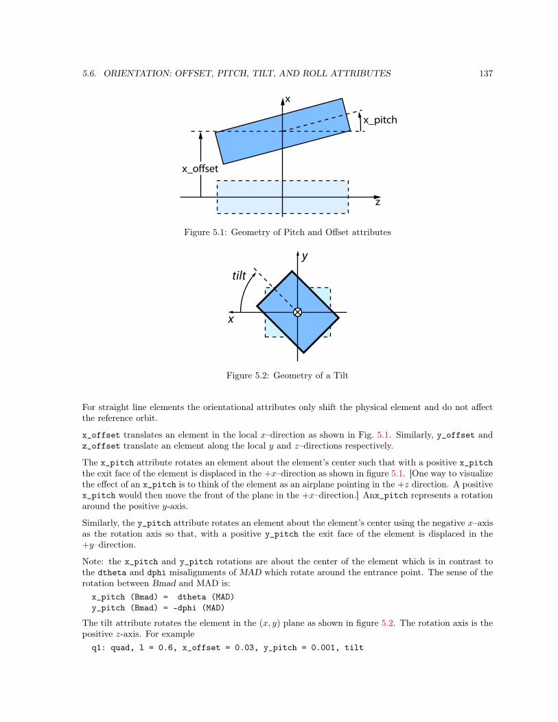
5.6. ORIENTATION: OFFSET, PITCH, TILT, AND ROLL ATTRIBUTES 137

x_offset

x_pitch

z

x

Figure 5.1: Geometry of Pitch and Offset attributes

x

y

tilt

Figure 5.2: Geometry of a Tilt

For straight line elements the orientational attributes only shift the physical element and do not affectthe reference orbit.

x_offset translates an element in the local x–direction as shown in Fig. 5.1. Similarly, y_offset andz_offset translate an element along the local y and z–directions respectively.

The x_pitch attribute rotates an element about the element’s center such that with a positive x_pitchthe exit face of the element is displaced in the +x–direction as shown in figure 5.1. [One way to visualizethe effect of an x_pitch is to think of the element as an airplane pointing in the +z direction. A positivex_pitch would then move the front of the plane in the +x–direction.] Anx_pitch represents a rotationaround the positive y-axis.

Similarly, the y_pitch attribute rotates an element about the element’s center using the negative x–axisas the rotation axis so that, with a positive y_pitch the exit face of the element is displaced in the+y–direction.

Note: the x_pitch and y_pitch rotations are about the center of the element which is in contrast tothe dtheta and dphi misalignments of MAD which rotate around the entrance point. The sense of therotation between Bmad and MAD is:x_pitch (Bmad) = dtheta (MAD)y_pitch (Bmad) = -dphi (MAD)

The tilt attribute rotates the element in the (x, y) plane as shown in figure 5.2. The rotation axis is thepositive z-axis. For exampleq1: quad, l = 0.6, x_offset = 0.03, y_pitch = 0.001, tilt

138 CHAPTER 5. ELEMENT ATTRIBUTES

Like MAD, Bmad allows the use of the tilt attribute without a value to designate a skew element. Thedefault tilt is π/(2(n+ 1)) where n is the order of the element:sol_quad n = 1quadrupole n = 1sextupole n = 2octupole n = 3

Note that hkick and vkick attributes are not affected by tilt except for kicker and elseparatorelements.

5.6.2 Bend Element Orientation

roll

z

x

ref_tilt

Figure 5.3: Geometry of a Bend. Like straight line elements, offsets and pitches are calculated withrespect to the coordinates at the center of the bend. The exception is the roll attribute which is arotation around the axis passing through the entrance and exit points. Shown here is the geometry fora bend with ref_tilt = 0. That is, the bend is in the x− z plane.

The orientation attributes for sbend and rbend elements isx_offset = <Real>y_offset = <Real>z_offset = <Real>x_pitch = <Real>y_pitch = <Real>ref_tilt = <Real> ! Shifts and reference orbit rotation axis.roll = <Real>

The geometry for orienting a bend is shown in Fig. 5.3. Like straight line elements, the offset and pitchattributes are evaluated with respect to the center of the element.

Unlike the straight line elements, bends do not have a tilt attribute. Rather they have a ref_tiltand a roll attribute. The roll attribute rotates the bend along an axis that runs through the entrancepoint and exit point as shown in figure 5.3. A roll attribute, like the offset and pitch attributes doesnot affect the reference orbit. The major effect of a roll is to give a vertical kick to the beam. Fora bend with positive bend angle, a positive roll will move the outside portion (+x side) of the bendupward and the inside portion (-x side) downward. Much like car racetracks which are typically slantedtowards the inside of a turn.

The ref_tilt attribute of a bend rotates the bend about the z axis at the upstream end of the bend asshown in Fig. 5.3. Unlike rolls and tilts, ref_tilt also shifts the rotation axis of the reference orbitalong with the physical element. A bend with a ref_tilt of π/2 will bend a beam vertically downward(§15.2). Note that the ref_tilt attribute of Bmad is the same as the MAD tilt attribute.

5.6. ORIENTATION: OFFSET, PITCH, TILT, AND ROLL ATTRIBUTES 139

5.6.3 Photon Reflecting Element Orientation

Ref Orb In Ref Orb Out

x

z

O

Figure 5.4: Geometry of a photon reflecting element orientation. The reference coordinates used fordefining the orientational attribute is the entrance reference coordinates.

Photon reflecting elements have the following orientational attributes:

x_offset = <Real>y_offset = <Real>z_offset = <Real>x_pitch = <Real>y_pitch = <Real>ref_tilt = <Real> ! Shifts both element and reference orbit.tilt = <Real>

Roughly, these elements can be viewed as zero length bends except, since there is no center position, theorientational attributes are defined with respect to the entrance coordinates as shown in Fig. 5.4. Likebend elements, the ref_tilt attribute rotates both the physical element and the reference coordinates.The tilt attribute rotates just the physical element. Thus the total rotation of the physical elementabout the entrance z axis is the sum tilt + ref_tilt.

Frequently, it is desired to orient reflecting elements with respect to the element’s surface. This canbe done using a girder element (§4.21) which supports the reflecting element and with the girder’sorigin_ele_ref_pt attribute set to center.

5.6.4 Reference Orbit Manipulator Element Orientation

The fork, photon_fork, floor_shift, and patch elements use the following attributes to orient theirexit edge with respect to their entrance edge:

x_offset = <Real>y_offset = <Real>z_offset = <Real>x_pitch = <Real>y_pitch = <Real>tilt = <Real>

Here "exit" edge for fork and photon_fork elements is defined to be the start of the line being branchedto. [Within the line containing the fork, the fork element is considered to have zero length so the exitface in the line containing the fork is coincident with the entrance face.] The placement of the exitedge for these elements defines the reference orbit. Thus, unlike the corresponding attributes for otherelements, the orientational attributes here directly control the reference orbit.

140 CHAPTER 5. ELEMENT ATTRIBUTES

5.6.5 Fiducial Element Orientation

The fiducial element (§4.21) uses the following attributes to define its position:origin_ele = <Name> ! Reference element.origin_ele_ref_pt = <location> ! Reference pt on reference ele.dx_origin = <Real> ! x-position offsetdy_origin = <Real> ! y-position offsetdz_origin = <Real> ! z-position offsetdtheta_origin = <Real> ! orientation angle offset.dphi_origin = <Real> ! orientation angle offset.dpsi_origin = <Real> ! orientation angle offset.

See Section §4.18 for more details.

5.6.6 Girder Orientation

A girder (§4.21) element uses the same attributes as a fiducial element (§4.18) to orient the referencegirder position. In addition, the following attributes are used to move the girder physically from thereference position:x_offset = <Real>y_offset = <Real>z_offset = <Real>x_pitch = <Real>y_pitch = <Real>tilt = <Real>

Shifting the girder from its reference position shifts all the elements that are supported by the girder.See Section §4.21 for more details.

If an element is supported by a girder element (§4.21), the orientational attributes of the element arewith respect to the orientation of the girder. The computed offsets, pitches and tilt with respect to thelocal reference coordinates are stored in the dependent attributesx_offset_toty_offset_totz_offset_totx_pitch_toty_pitch_tottilt_totroll_tot

A *_tot attribute will only be present if the corresponding non *_tot attribute is present. For exam-ple, only sbend and rbend elements have a roll_tot attribute since only these elements have a rollattribute.

If an element is not supported by a girder, the values of the *_tot attributes will be the same value asthe values of the corresponding non *_tot attributes.

5.7 Hkick, Vkick, and Kick Attributes

The kick attributes that an element may have are:kick, bl_kick = <Real> ! Used only with a Hkicker or Vkickerhkick, bl_hkick = <Real>vkick, bl_vkick = <Real>

5.8. APERTURE AND LIMIT ATTRIBUTES 141

kick, hkick, and vkick attributes are the integrated kick of an element in radians. kick is only usedfor hkicker and vkicker elements. All other elements that can kick use hkick and vkick. The tiltattribute will only rotate a kick for hkicker, vkicker, elseparator and kicker elements. This rulewas implemented so that, for example, the hkick attribute for a skew quadrupole would represent ahorizontal steering. The bl_kick, bl_hkick, and bl_vkick attributes are the integrated field kick inmeters-Tesla. Normally these are dependent attributes except if they appear in the lattice file (§5.1).

For an elseparator element, the hkick and vkick are appropriate for a positively charged particle.The kick for a negatively charged particle is opposite this.

5.8 Aperture and Limit Attributes

ecollimator

rcollimator and all

other elements x

y

x2_limitx1_limit

y1_limit

y2_limit

Figure 5.5: Apertures for ecollimator and rcollimator elements. [note: positive z points up, out of thepage.] As drawn, all limits x1_limit, x2_limit, y1_limit, y2_limit are positive.

The aperture attributes are:x1_limit = <Real> ! Horizontal, negative side, aperture limitx2_limit = <Real> ! Horizontal, positive side, aperture limity1_limit = <Real> ! Vertical, negative side, aperture limity2_limit = <Real> ! Vertical, positive side, aperture limitx_limit = <Real> ! Alternative to specifying x1_limit and x2_limity_limit = <Real> ! Alternative to specifying y1_limit and y2_limitaperture = <Real> ! Alternative to specifying x_limit and y_limitaperture_at = <Switch> ! What end aperture is at. (§5.8.2)aperture_type = <Switch> ! What type of aperture it isoffset_moves_aperture = <Logical> ! Element offsets affect aperture position (§5.8.1)

x1_limit, x2_limit, y1_limit, and y2_limit specify the half–width of the aperture of an element asshown in figure 5.5. Note: Normally all of these will be zero or positive. A zero x1_limit, x2_limit,y1_limit, or y2_limit is interpreted as no aperture in the appropriate plane.

For convenience, x_limit can be used to set x1_limit and x2_limit to a common value. Example:s: sextupole, x1_limit = 0.09, x2_limit = 0.09s: sextupole, x_limit = 0.09 ! Same as above

Similarly, y_limit can be used to set y1_limit and y2_limit. The aperture attribute can be use toset all four x1_limit, x2_limit, y1_limit and y2_limit to a common value. Internally, the Bmad codedoes not store x_limit, y_limit, or aperture. This means that using x_limit, y_limit or aperturein arithmetic expressions is an error:

142 CHAPTER 5. ELEMENT ATTRIBUTES

q1: quad, aperture = 0.09q2: quad, aperture = q1[aperture] ! THIS IS AN ERROR!q2: quad, aperture = q1[x1_limit] ! Correct

By default, apertures are assumed to be rectangular except that an ecollimator has a elliptical aperture.This can be changed by setting the aperture_type attribute. The possible values of this attribute are:auto ! Default for detector, mask and diffraction_plate elementscustomelliptical ! Default for ecollimator elements.rectangular ! Default for most elements.wall3d ! Vacuum chamber wall (§5.11).

The custom setting is used in the case where programs have been compiled with custom, non-Bmad, codeto handle the aperture calculation. The auto setting is used for automatic calculation of a rectangularaperture. For diffraction_plate and mask elements, the auto setting causes the four aperture limitsto be set to just cover the clear area of element (§5.11.6). For all other elements, the auto setting is onlyto be used when there is an associated surface grid (§5.10.1) for the element and, in this case, Bmad toset the four limits to just cover the surface grid.

The wall3d setting uses the vacuum chamber wall as specified by a wall attribute (§5.11). Usingthe wall construct allows for complex apertures to be constructed. Note that The wall thickness andmaterial type are not used when calculating if a particle has hit the wall. That is, the wall is consideredto be infinitely thin. Also note that a wall must cover the entire length of the element longitudinally.This is done in order to be able to spot errors in specifying the wall geometry.

For elliptical apertures, all four x1_limit, x2_limit, y1_limit, and y2_limit must be non-zero.

For rectangular apertures, the limits x1_limit, x2_limit, y1_limit, or y2_limit may be negative. Forexample:s: sextupole, x1_limit = -0.02, x2_limit = 0.09

In this case, particles will hit the aperture if their x-coordinate is outside the interval [0.02, 0.09]. Thatis, particles at the origin will be lost.

To avoid numerical overflow and other errors in tracking, a particle will be considered to have hit anaperture in an element, even if there are no apertures set for that element, if its orbit exceeds 1000meters. Additionally, there are other situations where a particle will be considered lost. For example, ifa particle’s trajectory does not intersect the output face in a bend.

Examples:q1, quadrupole, y1_limit = 0.03q1[y2_limit] = 0.03q1[y_limit] = 0.03 ! equivalent to the proceeding 2 lines.q1[aperture_at] = both_ends

5.8.1 Apertures and Element Offsets

Normally, whether a particle hits an aperture or not is evaluated independent of any element offsets(§5.6). This is equivalent to the situation where a beam pipe containing an aperture is independent ofthe placement of the physical element the beam pipe passes through. That is, the beam pipe does not“touch” the physical element. This can be changed by setting the offset_moves_aperture attribute toTrue. In this case any offsets or pitches will be considered to have shifted the aperture boundary. Theexceptions here is that the default for the following elements is for offset_moves_aperture to be True:

rcollimator,

5.8. APERTURE AND LIMIT ATTRIBUTES 143

ecollimator,multilayer_mirror,mirror, andcrystal

Even with offset_moves_aperture set to True, tilts will not affect the aperture calculation. This isdone, for example, so that the tilt of a skew quadrupole does not affect the aperture. The exceptionhere is that tilting an rcollimator or ecollimator element will tilt the aperture. Additionally, whenthe aperture is at the surface (see below), any tilt will be used in the calculation.

Example:q1: quad, l = 0.6, x1_limit = 0.045, offset_moves_aperture = T

5.8.2 Aperture Placement

By default, for most elements, the aperture is evaluated at the exit face of the element. This can bechanged by setting the aperture_at attribute. Possible settings for aperture_at are:both_endscontinuousentrance_endexit_end ! Default for most elementsno_aperturesurfacewall_transition

The exit_end setting is the default for most elements except for the following elements who have adefault of surface:crystaldiffraction_platemaskmirrormultilayer_mirrorsample

In fact, for the following elements:mirror,multilayer_mirrorcrystal

The surface setting for aperture_at must be used. Additionally, due to the complicated geometry ofthese elements, to keep things conceptionally simple, the rule is imposed that, for an aperture at thesurface, the offset_moves_aperture setting must be left in its default state of True. Additionally, Forentrance_end or exit_end apertures, offset_moves_aperture must be set to False.

Note: The entrance and exit ends of an element are independent of which direction particles are trackedthrough an element. Thus if a particle is tracked backwards it enters an element at the “exit end” andexits at the “entrance end”. The continuous setting indicates that the aperture is continuous along thelength of the element. This only matters when particle tracking involves stepping through an elementa little bit at a time. For example, as in Runge-Kutta tracking (§6.1). For tracking where a formulais used to transform the particle coordinates at the entrance of an element to the coordinates at theexit end, the aperture is only checked at the end points so, in this situation, a continuous aperture isequivalent to the both_ends setting.

The wall_transition setting is like the continuous setting in that the aperture boundary is consid-ered to be continuous along the element’s length. However, unlike the continuous setting, with the

144 CHAPTER 5. ELEMENT ATTRIBUTES

wall_transition setting a particle outside the wall is considered alive and it is only when a particlemoves through the wall that it is lost. The wall_transition setting is used for things like septummagnets where a particle may be safely outside or inside the wall. Note to programmers: By supplyinga custom wall_hit_handler_custom routine, scattering of particles through a wall may be simulated.

Examples:q2: quad, aperture_type = elliptical, aperture_at = continuousq1: quad, l = 0.6, x1_limit = 0.045, offset_moves_aperture = T

5.8.3 Apertures and X-Ray Generation

With X-ray simulation apertures can be used by Bmad to limit the directions in which photons aregenerated. This can greatly decrease simulation times. For example, a photon passing through adiffraction_plate element will diffract in an arbitrary direction. If a downstream element has anaperture set, Bmad can restrict the velocity directions so that the photons will fill the downstreamaperture and the amount of time wasted tracking photons that ultimately would be collimated is minimal.

5.9 X-Rays Crystal & Compound Materials

For basic crystallographic and X-ray matter interaction cross-sections, Bmad uses the XRAYLIB[Schoon11]library. Crystal structure parameters in XRAYLIB are mainly from R. W. G. Wyckoff[Wyckoff65] withsome structure parameters coming from NIST. The list of available structures is:

AlphaAlumina GaP KCl PlatinumAlphaQuartz GaSb KTP RbAPAluminum Ge LaB6 SapphireBe Gold LaB6_NIST SiBeryl Graphite LiF Si_NISTCopper InAs LiNbO3 Si2CsCl InP Muscovite SiCCsF InSb NaCl TitaniumDiamond Iron PET TlAPGaAs KAP

These names are case sensitive

Besides the above crystal list, Bmad can calculate structure factors for all the elements and the followinglist of materials. Material properties are from NIST. These names are case sensitive. That is, the NISTmaterials all use upper case. As noted in the table, several of the materials may be specified using theappropriate chemical formula. For example, liquid water may be referenced using the name H2O.

A_150_TISSUE_EQUIVALENT_PLASTIC LITHIUM_TETRABORATEACETONE LUNG_ICRPACETYLENE M3_WAXADENINE MAGNESIUM_CARBONATEADIPOSE_TISSUE_ICRP MAGNESIUM_FLUORIDEAIR_DRY_NEAR_SEA_LEVEL MAGNESIUM_OXIDEALANINE MAGNESIUM_TETRABORATEALUMINUM_OXIDE, Al2O3 MERCURIC_IODIDEAMBER METHANE

Continued on next page

5.9. X-RAYS CRYSTAL & COMPOUND MATERIALS 145

AMMONIA, NH3 METHANOLANILINE MIX_D_WAXANTHRACENE MS20_TISSUE_SUBSTITUTEB_100_BONE_EQUIVALENT_PLASTIC MUSCLE_SKELETALBAKELITE MUSCLE_STRIATEDBARIUM_FLUORIDE MUSCLE_EQUIVALENT_LIQUID_WITH_SUCROSEBARIUM_SULFATE MUSCLE_EQUIVALENT_LIQUID_WITHOUT_SUCROSEBENZENE, C6H6 NAPHTHALENEBERYLLIUM_OXIDE NITROBENZENEBISMUTH_GERMANIUM_OXIDE NITROUS_OXIDEBLOOD_ICRP NYLON_DU_PONT_ELVAMIDE_8062BONE_COMPACT_ICRU NYLON_TYPE_6_AND_TYPE_6_6BONE_CORTICAL_ICRP NYLON_TYPE_6_10BORON_CARBIDE, B4C NYLON_TYPE_11_RILSANBORON_OXIDE, B2O3 OCTANE_LIQUIDBRAIN_ICRP PARAFFIN_WAXBUTANE N_PENTANEN_BUTYL_ALCOHOL PHOTOGRAPHIC_EMULSIONC_552_AIR_EQUIVALENT_PLASTIC PLASTIC_SCINTILLATOR_VINYLTOLUENE_BASEDCADMIUM_TELLURIDE PLUTONIUM_DIOXIDECADMIUM_TUNGSTATE POLYACRYLONITRILECALCIUM_CARBONATE POLYCARBONATE_MAKROLON_LEXANCALCIUM_FLUORIDE POLYCHLOROSTYRENECALCIUM_OXIDE POLYETHYLENECALCIUM_SULFATE POLYETHYLENE_TEREPHTHALATE_MYLARCALCIUM_TUNGSTATE POLYMETHYL_METHACRALATE_LUCITE_PERSPEXCARBON_DIOXIDE POLYOXYMETHYLENECARBON_TETRACHLORIDE POLYPROPYLENECELLULOSE_ACETATE_CELLOPHANE POLYSTYRENECELLULOSE_ACETATE_BUTYRATE POLYTETRAFLUOROETHYLENE_TEFLONCELLULOSE_NITRATE POLYTRIFLUOROCHLOROETHYLENECERIC_SULFATE_DOSIMETER_SOLUTION POLYVINYL_ACETATECESIUM_FLUORIDE POLYVINYL_ALCOHOLCESIUM_IODIDE POLYVINYL_BUTYRALCHLOROBENZENE POLYVINYL_CHLORIDECHLOROFORM POLYVINYLIDENE_CHLORIDE_SARANCONCRETE_PORTLAND POLYVINYLIDENE_FLUORIDECYCLOHEXANE POLYVINYL_PYRROLIDONE12_DDIHLOROBENZENE POTASSIUM_IODIDEDICHLORODIETHYL_ETHER POTASSIUM_OXIDE12_DICHLOROETHANE PROPANEDIETHYL_ETHER PROPANE_LIQUIDNN_DIMETHYL_FORMAMIDE N_PROPYL_ALCOHOLDIMETHYL_SULFOXIDE PYRIDINEETHANE RUBBER_BUTYLETHYL_ALCOHOL RUBBER_NATURALETHYL_CELLULOSE RUBBER_NEOPRENEETHYLENE SILICON_DIOXIDEEYE_LENS_ICRP SILVER_BROMIDEFERRIC_OXIDE SILVER_CHLORIDEFERROBORIDE SILVER_HALIDES_IN_PHOTOGRAPHIC_EMULSIONFERROUS_OXIDE SILVER_IODIDEFERROUS_SULFATE_DOSIMETER_SOLUTION SKIN_ICRPFREON_12 SODIUM_CARBONATEFREON_12B2 SODIUM_IODIDEFREON_13 SODIUM_MONOXIDEFREON_13B1 SODIUM_NITRATEFREON_13I1 STILBENEGADOLINIUM_OXYSULFIDE SUCROSEGALLIUM_ARSENIDE TERPHENYLGEL_IN_PHOTOGRAPHIC_EMULSION TESTES_ICRPGLASS_PYREX TETRACHLOROETHYLENEGLASS_LEAD THALLIUM_CHLORIDE

Continued on next page

146 CHAPTER 5. ELEMENT ATTRIBUTES

GLASS_PLATE TISSUE_SOFT_ICRPGLUCOSE TISSUE_SOFT_ICRU_FOUR_COMPONENTGLUTAMINE TISSUE_EQUIVALENT_GAS_METHANE_BASEDGLYCEROL TISSUE_EQUIVALENT_GAS_PROPANE_BASEDGUANINE TITANIUM_DIOXIDEGYPSUM_PLASTER_OF_PARIS TOLUENEN_HEPTANE TRICHLOROETHYLENEN_HEXANE TRIETHYL_PHOSPHATEKAPTON_POLYIMIDE_FILM TUNGSTEN_HEXAFLUORIDELANTHANUM_OXYBROMIDE URANIUM_DICARBIDELANTHANUM_OXYSULFIDE URANIUM_MONOCARBIDELEAD_OXIDE URANIUM_OXIDELITHIUM_AMIDE UREALITHIUM_CARBONATE VALINELITHIUM_FLUORIDE VITON_FLUOROELASTOMERLITHIUM_HYDRIDE WATER_LIQUID, H2OLITHIUM_IODIDE WATER_VAPORLITHIUM_OXIDE XYLENE

Ref Orb InRef Orb Out

xz

θB,in θB,out

pq

Element Reference Frame

source

detector

Figure 5.6: Surface curvature geometry. The element reference frame used to describe surface curvaturehas the z axis pointing towards the interior of the element, and the x axis in the plane defined by theentrance and exit reference orbit.

5.10. SURFACE PROPERTIES FOR X-RAY ELEMENTS 147

5.10 Surface Properties for X-Ray elements

The following X-ray elements have a surface which X-rays impinge upon:crystal §4.10detector §4.12diffraction_plate §4.13mask §4.30mirror, and §4.32multilayer_mirror §4.34sample §4.44

[There is also the capillary element but this element specifies its surface differently.]

The coordinate system used for characterizing the curvature of a surface is the element reference frameas shown in Fig. 5.6). This coordinate system has the z axis pointing towards the interior of the element,and the x axis in the plane defined by the entrance and exit reference orbit. In this coordinate system, thesurface is an ellipsoid plus a fourth order polynomial in x and y plus a possible “figure error” contributionzoff defined by a surface grid:

−z =1

gz

[1−

»1− (gx x)2 − (gy y)2

]+ (5.1)

1

gsp

[1−

»1− (gsp x)2 − (gsp y)2

]+

∑2≤i+j≤6

cij xi yj − zoff

zoff is discussed in section §5.10.1 and is only present when the surface grid type is set to Displacement.In Eq. (5.1) the cij coefficients parameterize the fourth order polynomial, gsp parameterize the sphericalcurvature, and gx, gy, and gz parameterize ellipsoid curvature. [In principle, the spherical curvatureis not needed since the elliptical curvature is more general. In practice, it is sometimes convenient tobe able to specify spherical curvature.] If gz is zero, the elliptical curvature is ignored. If gz or gsp ispositive, the curvature is concave towards the incoming photon. If negative, the curvature is convex.The spherical and ellipsoid parameters are set for an element by setting the element parametersspherical_curvature = <Real> ! gspelliptical_curvature_x = <Real> ! gxelliptical_curvature_y = <Real> ! gyelliptical_curvature_z = <Real> ! gz

The polynomial coefficients cij are set in the lattice file by setting the element attributescurvature_xM_yN = <Real>

where M and N are integers in the range 0 through 6 with the restriction2 ≤ M + N ≤ 6

Example:c2: crystal, spherical_curvature = 1/4.7, curvature_x2_y0 = 0.37, ...

in this example, curvature_x2_y0 corresponds to the c20 term in Eq. (5.1). To get the effect of anonzero x0 y0, x1 y0, or x0 y1 terms (since corresponding curvature_xN_yM are not permitted), elementoffsets and pitches can be used (§5.6).

Some useful formulas: Series expansion for a sphere of radius R:

−z =x2

2R+

x4

8R3+

x6

16R5+

y2

2R+

y4

8R3+

y6

16R5+x2 y2

4R3+

3x4 y2

16R5+

3x2 y4

16R5(5.2)

For a torus with equation (»x2 + (z + r +R)2 −R

)2

+ y2 = r2 (5.3)

148 CHAPTER 5. ELEMENT ATTRIBUTES

The series expansion is:

−z =x2

2 (r +R)+

x4

8 (r +R)3+

x6

16 (r +R)5+y2

2 r+

y4

8 r3+ (5.4)

y6

16 r5+

x2 y2

4 r (r +R)2+

3x4 y2

16 r (r +R)4+

(3 r +R)x2 y4

16 r3 (r +R)3

For a curved crystal, if p is the distance from the source to the crystal, and q is the distance fromthe crystal to the detector, the needed radius of curvature Rs in the sagittal (transverse) plane to givefocusing is [Rio98]:

1

p+

1

q=

sin θg,in + sin θg,outRs

(5.5)

where θg,in and θg,out are the entrance and exit graze angles. In the tangential (meridional) plane, theradius Rt needed for focusing is

sin2 θg,inp

+sin2 θg,out

q=

sin θg,in + sin θg,outRt

(5.6)

The above formulas assume that the crystal is constructed so that the orientation of the Bragg planesfollows the orientation of the surface. Mirrors have similar formulas with θg,in = θg,out = θ.

Example:t_bragg = 1.3950647rt = 1 ! Crystal transverse radiusrs = rt*(sin(t_bragg))^2c: crystal, crystal_type = "Si(553)", b_param = -1,

curvature_x0_y2 = 1 / (2 * rs), curvature_x0_y4 = 1 / (8 * rs^3),curvature_x2_y0 = 1 / (2 * rt), curvature_x4_y0 = 1 / (8 * rt^3),

5.10.1 Surface Grid

A surface can be broken up into a grid of rectangles. This is useful, for example, in breaking up adetector element into pixel photo receptors or in simulating a rough surface for crystals and otherelements. The general syntax is:surface = grid = active = <T/F> ! Turn on/off effect of grid. Default = Truetype = <type_name>, ! Segmented, Displacement, or H_Misalignix_bounds = (<ix_min>, <ix_max>), ! Min/max index bounds in x-directioniy_bounds = (<iy_min>, <iy_max>), ! Min/max index bounds in y-directionr0 = (<x0>, <y0>), ! (x,y) coordinates at grid origindr = (<dx>, <dy>), ! width and height of pixels.! Grid points used with type = H_Misalign:pt(<i>,<j>) = (<dz/dx>, <dz/dy>, <dz/dx_rms>, <dz/dy_rms>),! Grid points used with type = Displacement:pt(<i>,<j>) = (<z>), ! orpt(<i>,<j>) = (<z>, <dz/dx>, <dz/dy>), ! orpt(<i>,<j>) = (<z>, <dz/dx>, <dz/dy>, <d2z/dxdy>),

Example:

5.10. SURFACE PROPERTIES FOR X-RAY ELEMENTS 149

ccd: crystal, surface = grid = type = h_misalign,r0 = (0.0, 0.01), dr = (0.005, 0.005),ix_bounds = (1, 57), iy_bounds = (-30, 10),pt(1,-30) = (0.001, -0.002, 0, 0),pt(1,-29) = ...,

The grid is a two dimensional with bounds given by the ix_bounds and iy_bounds components. Thesetwo components must be present. In the above example the grid is 57 pixels in x and 41 pixels in y.

The physical placement of the grid on the element is determined by the r0 and dr components. r0 isoptional and gives the (x, y) coordinates of the center of the pixel with index (0, 0). The dr component,which must be present, gives the pixel width and height. Thus the center of the (i, j) pixel is:(x,y) = (r0(1), r0(2)) + (i*dr(1), j*dr(2))

There are several types of grids. What type of grid is determined by the type component Possible typevalues are:Displacement ! Mesh defines an offset from the nominal surface.H_Misalign ! Misalignment of crystal H vectorSegmented ! Surface is a matrix of flat rectangles

Note: The type must be set before specifying any pt.

DisplacementWith the type parameter set to Displacement, an offset zoff is added to the surface positiondefined in Eq. (5.1). The z offset at a given (x, y) position is determined by a spline interpolationof the z values of the grid of points defined by pt(<i>,<j>). For each point pt(<i>,<j>), thez value along with the dz/dx, dz/dy, d2z/dxdy slopes can be specified or only the z value needsto be specified. With the later option the slopes will be computed by taking finite differences ofnearest neighbors.

H_MisalignA setting of the type attribute to H_Misalign is used with crystals only. With H_Misalign, thegrid defines misalignment of the H vector which is the normal to the diffracting planes of thecrystal (§25.4). When using H_Misalign, each pt(i,j) component gives the misalignment of Hfor the corresponding pixel. For an individual photon, the misalignment of H will bedz/dx_tot = <dz/dx> + r1 * <dz/dx_rms>dz/dy_tot = <dz/dy> + r2 * <dz/dy_rms>

where dz/dx_tot and dz/dy_tot are the rotational misalignment (§5.6) used in the calculation,the quantities in brackets <...> are components of pt, and r1 and r2 are Gaussian distributedrandom numbers with unit rms. These random numbers are regenerated for each photon.

SegmentedWhen the type component is set to Segmented, the crystal surface is modeled as a grid of flat“rectangles” (the actual shape is very close but not quite rectangular). Using a segmented surfaceonly makes sense when the surface is curved (see Eq. (5.1)). There is one rectangle for eachpixel. Each rectangle has an extent in the (x, y) transverse dimensions equal to the extent ofthe corresponding pixel. Eq. (5.1) is used to calculate the z coordinate of the vertices of a givenrectangle and then these z values are adjusted so that1) The rectangle is flat (the vertices all lie on a plane).2) The rectangle contacts the unsegmented surface (Eq. (5.1)) at two

diagonally opposite vertices.3) The other two diagonally opposite vertices will be as close as possible

in the least squares sense from the unsegmented surface.Note: The pt component is not used here.

150 CHAPTER 5. ELEMENT ATTRIBUTES

5.11 Walls: Vacuum Chamber, Capillary and Mask

The wall attribute for an element is used to define:vacuum chamber wallcapillary element (§4.6) inside walldiffraction_plate (§4.13) geometry

The topics of the following subsections are:§5.11.1 General wall syntax.§5.11.2 Cross-section construction.§5.11.3 Capillary and vacuum chamber wall interpolation.§5.11.4 Capillary wall.§5.11.5 Vacuum chamber wall.§5.11.6 Diffraction_plate and mask element geometries.

5.11.1 Wall Syntax

The syntax of the wall attribute is:wall = superimpose = <T/F>, ! Chamber wall onlythickness = <real> ! Default thickness.opaque_material = <material_type> ! Default opaque material.clear_material = <material_type> ! Default clear material.section = type = <section_type>, ! Chamber Mask, and Diffraction_plate onlys = <longitudinal_position>, ! Relative to beginning of element.

! Not used for mask or diffraction_plate.r0 = (<x0>, <y0>), ! section (x,y) origin. Default = (0, 0).absolute_vertices = <T/F>, ! Vertex relative to r0? Default = F.material = <material_type>, ! Mask and Diffraction_plate only.thickness = <real>, ! Mask and Diffraction_plate only.dr_ds = <value>, ! Capillary and Chamber onlyv(1) = <x>, <y>, <radius_x>, <radius_y>, <tilt>,v(2) = ... ,...,

section = s = <longitudinal_position>,v(1) = ... ,... ,

... A wall begins with “wall = ” and ends with a “”. In between are a number of individual cross-section structures. Each individual cross-section begins with “section = ” and ends with a “”. Thes parameter of a cross-section gives the longitudinal position of the cross-section. Example:this_cap: capillary,wall = section = ! cross-section with top/bottom symmetrys = 0, v(1) = 0.02, 0.00,v(2) = 0.00, 0.02, 0.02, v(3) = -0.01, 0.01 ,

section = ! Cross-section that is a tilted ellipse.s = 0.34,v(1) = 0.003, -0.001, 0.015, 0.008, 0.2*pi

In this example an element called this_cap is a capillary whose wall is defined by two cross-sections.

5.11. WALLS: VACUUM CHAMBER, CAPILLARY AND MASK 151

s x

yV(1)

V(5)V(4)

V(3)

V(2)A) B)

(x0, y0)

Figure 5.7: A) The inside wall of a capillary or the vacuum chamber wall of a non-capillary element isdefined by a number of cross-sectional slices. B) Each cross-section is made up of a number of vertices.The segments between the vertices can be either a line segment, the arc of a circle, or a section of anellipse.

5.11.2 Wall Sections

The wall is defined by a number of cross-sectional slices. For Fig. 5.7A shows the geometry for capillaryor vacuum chamber walls. Each cross-section is defined by a longitudinal position s relative to thebeginning of the element and a number of vertices. The arc between each vertex may be either a straightline, an arc of a circle, or a section of an ellipse. For a capillary it is mandatory that a cross-section beconvex. That is, given any two points within the cross-section, all points on the line segment connectingthem must be within the cross-section.

The v(<j>) within a cross-section define the vertices for each cross-section. The vertices are defined withrespect to the section origin given by r0. Each v(<j>) has five parameters. It is mandatory to specifythe first two parameters <x> and <y>. Specifying the rest, <radius_x>, <radius_y>, and <tilt>, isoptional. The default values, if not specified, is zero. The point (<x>, <y>) defines the position of thevertex. The parameters <radius_x>, <radius_y>, and <tilt> define the shape of the segment of thecross-section between the given vertex and the preceding one.<radius_x> = 0, <radius_y> = 0 --> Straight line segment.<radius_x> != 0, <radius_y> = 0 --> Circular arc with radius = radius_x<radius_x> = 0, <radius_y> != 0 --> Illegal!<radius_x> != 0, <radius_y> != 0 --> Ellipse section.

When an ellipse is specified, <radius_x>, and <radius_y> are the half width and half height of thesemi-major axes and the <tilt> parameter gives the tilt of the ellipse. <radius_x> and <radius_y>must not be negative.

In the example above, for the first cross-section, v(2) specifies a non-zero <radius_x> and, by default,<radius_y> is zero. Thus the segment of the cross-section between v(1) and v(2) is circular in naturewith a radius of 0.02. Since v(3) does not specify <radius_x> nor <radius_y>, the cross-section betweenv(2) and v(3) is a straight line segment.

The vertex points must be arranged in a “counter clockwise manner”. For vertices <v(i)> and <v(i+1)>connected by a line segment this translates to

0 < θi+1 − θi (mod 2π) < π (5.7)

where (rn, θn) are the polar coordinates of the nth vertex with respect to the point r0. For verticesconnected by an arc, “counter clockwise manner” means that the line segment with one end at the center

152 CHAPTER 5. ELEMENT ATTRIBUTES

of the arc and the other end traversing the arc from <v(i)> to <v(i+1)> rotates in counter clockwise asshown in Fig. 5.7B.

The red line segment with one end at the center of the arc and the other end traversing the arc from,in this case, V (2) to V (3), rotates in counter clockwise manner. In general, there are two solutions forconstructing such an arc. For positive radii, the solution chosen is the one whose center is closest tothe section origin (x0, y0). If the radii are negative, the center point will be the point farthest from theorigin (the dashed line between V (2) and V (3) in the figure).

A restriction on cross-sections is that the section origin (x0, y0) must be in the interior of any cross-section and that for any cross-section a line drawn from the origin at any given angle θ will intersect thecross-section at exactly one point as shown in Fig. 5.7B. This is an important point in the constructionof the wall between cross-sections as explained below.

The last vertex specified, call it <v(n)>, should not have the same <x>, <y> values as the first vertex<v(1)>. That is, there will be a segment of the cross-section connecting <v(n)> to <v(1)>. The geometryof this segment is determined by the parameters of <v(1)>.

If there is mirror symmetry about the x or y axis for a cross-section, the “mirrored” vertices, on the“negative” side of the mirror plane, do not have to be specified. Thus if all the vertex points of a cross-section are in the first quadrant, that is, all <x> and <y> are zero or positive, mirror symmetry aboutboth the x and y axes is assumed. If all the <y> values are zero or positive and some <x> values arepositive and some are negative, mirror symmetry about the x axis is assumed. Finally, if all the <x>values are zero or positive but some <y> values are positive and some are negative, symmetry aboutthe y axis is assumed. For example, for the first in the above example, since all the <y> values arenon-negative and there are positive and negative <x> values, symmetry about the x axis is assumed.

The one exception to the above rule that (<x>, <y>) is the vertex center is when a single vertex v(1)is specified for a cross-section with a non-zero <radius_x>. In this case, (<x>, <y>) are taken to be thecenter of the circle or ellipse. For example, if a single vertex is specified for a cross-section as:section = s = 0.3, v(1) = 0.03, -0.01, 0.15, 0.08, 0.2

the cross-section will be an ellipse with center at (0.03,−0.01) with a tilt of 0.2 and axes radii of 0.15and 0.08. If a cross-section has a single vertex and <radius_x> is not specified, the cross-section is arectangle. For examplesection = s = 0.3, v(1) = 0.03, 0.01

The vertices are defined with respect to the local sector origin r0 except if absolute_vertices is setto True in which case the vertex numbers are taken as absolute. For example, the following two cross-sections are identical and describe a rectangle with edges at x = 1 and 5 and y = −6 and 6section = absolute_vertices = T, r0 = (4, 0),

v(1) = 5, 6, v(2) = 1, 6, v(3) = 1, -6, v(4) = 5, -6section = r0 = (4, 0), v(1) = 2, 6

Notice that while r0 is not needed in the first section for positioning of the vertices, it is needed in thefirst section to make Eq. (5.7) true.

5.11.3 Interpolation Between Sections

For capillary and vacuum chamber walls, the wall between cross-sections, is defined by interpolation.At a given s position, the r, θ coordinate system in the transverse x, y plane is defined with respect toan origin rO(s) given by a linear interpolation of the origins of the cross-sections to either side of thegiven s position. Let s1 denote the position of the cross-section just before s and s2 denote the positionof the cross-section just after s. Let r01 be the (x0, y0) origin defined for the cross section at s1 and r02

5.11. WALLS: VACUUM CHAMBER, CAPILLARY AND MASK 153

xxx

y

y

yA)

B)

C)

s = 0

s = 0.5

s = 1

Figure 5.8: Example where convex cross-sections do not produce a convex volume. Cross-sections (A)and (C) are ellipses with a 5 to 1 aspect ratio. Half way in between, linear interpolation produces aconvex cross-section as shown in (B).

be the (x0, y0) origin defined for the cross section at s2. Then

rO(s) = (1− s) r01 + s r02 (5.8)

wheres ≡ s− s1

s2 − s1(5.9)

Let rc1(θ) and rc2(θ) be the radius of the wall as a function of θ for the cross-sections at s = s1 ands = s2 respectively. The wall rc(θ, s) at any point s between s1 and s2 is then defined by the equation

rc(θ, s) = p1(s) rc1(θ) + p2(s) rc2(θ) (5.10)

where p1 and p2 are cubic polynomials parameterized by

p1 = 1− s+ a1 s+ a2 s2 + a3 s

3

p2 = s+ b1 s+ b2 s2 + b3 s

3 (5.11)

If ai = bi = 0 for all i = 1, 2, 3, the interpolation is linear and this is the default if either of the parametersdr_ds1 and dr_ds2 are not given in the wall definition. These parameters are the slopes of the wall withrespect to s at the end points

dr_ds1 ≡ dr

ds

∣∣∣∣s=s1

, dr_ds2 ≡ dr

ds

∣∣∣∣s=s2

(5.12)

where r is the average r averaged over all θ. When both dr_ds1 and dr_ds2 are specified, the ai andbi are calculated so that the slopes of the wall match the values of dr_ds1 and dr_ds2 along with theconstraints.

p1(0) = 1 , p1(1) = 0

p2(0) = 0 , p2(1) = 1 (5.13)

M ≡ a21 + a2

2 + a23 + b21 + b22 + b23 is a minimum

The last constraint ensures a “smooth” transition between the two cross-sections.

To refer to a cross-section parameters after an element has been defined, the following syntax is used:ele_name[wall%section(n)%v(j)%x] ! x value of j^th vertex of n^th cross-section

154 CHAPTER 5. ELEMENT ATTRIBUTES

5.11.4 Capillary Wall

For a capillary, s must be zero for the first cross-section and the length of the capillary is given bythe value of s of the last cross-section.

For a capillary, in order for Bmad to quickly track photons, Bmad assumes that the volume betweenthe cross-sections is convex. The volume will be convex if each cross-section rc(θ, s) at any given s isconvex. Note that it is not sufficient for rc(θ, s) to be convex at the specified cross-sections as shown inFig. 5.8. Also note that it is perfectly fine for the total capillary volume to not be convex.

5.11.5 Vacuum Chamber Wall

The vacuum chamber wall is independent of the element apertures (§5.8). Unless a program is specificallyconstructed, the presence of a vacuum chamber wall will not affect particle tracking.

The vacuum chamber wall defined for an element may be shorter or longer than the element. Thevacuum chamber wall for a particular lattice branch is the sum of all the chamber walls of the individualelements. That is, the chamber wall at any given point is determined by interpolation of the nearestsections upstream and downstream to the point. Thus a given lattice element need not contain a wallcomponent for the chamber wall to be well defined at the element.

The exception to the above rule is when a section has its type component set to either:wall_startwall_end

wall_start and wall_end sections must come in pairs. The next section after a wall_end section (ifthis section is not the last section in the lattice) must be a wall_start section. If a section has a typeof wall_start, the region between that section and the previous section (which must be a wall_endsection) will be considered to have no wall. If the wall_start section is the first section of the latticebranch, the region of no wall will start at the beginning of the branch. Similarly, if a section has a typeof wall_end, the region between that section and the next section (or the end of the lattice branch ifthere is no next section) will not have a wall.

The chamber walls of any two elements may not overlap. The exception is when the superimposeattribute for a wall of an element is set to True. In this case, any other wall cross-sections from anyother elements that overlap the superimposed wall are discarded. Superposition of a wall is useful, forexample, in introducing mask regions into the wall.

If a branch has a closed geometry (§9.1), wall sections that extend beyond the ends of the branch are“wrapped” around.

If a particle is past the last wall cross-section or before the first wall cross-section, The following rulesare used: If the branch has a closed geometry, the wall will be interpolated between the last and firstcross-sections. If the branch has an open geometry, the wall is taken to have a constant cross-section inthese regions.

The chamber wall is defined with respect to the local coordinate system (§15.1.1). That is, in a bend awall that has a constant cross section is a section of a torus.

Patch elements (§4.38) complicate the wall geometry since the coordinate system at the end of thepatch may be arbitrarily located relative to the beginning of the patch. To avoid confusion as to whatcoordinate system a wall section belongs to, patch elements are not allowed to define a wall. The wallthrough a patch is determined by the closest wall sections of neighboring elements.

Each section has a type attribute. This attribute is not used for capillary elements. For a vacuum

5.11. WALLS: VACUUM CHAMBER, CAPILLARY AND MASK 155

A) B)

leg1

leg2

trunk1

trunk2

trunk

trunk1 trunk2

trunk

O1 O2O x

y

s

C)

OL OT

WTWL

P

Figure 5.9: A) Crotch geometry: Two pipes labeled “leg1” and “leg2” merge into a single pipe calledthe “trunk” pipe. Five wall sections are used to define the crotch geometry (solid lines). Dashed linesrepresent sections not involved in defining the crotch. For purposes of illustration, the three trunksections are displaced longitudinally but in reality must have the same longitudinal coordinate. B)Example layout of the trunk1, trunk2 and trunk wall sections. O1, O2 and O are the x0, y0 origins ofthe sections.

chamber wall, the type attribute is used to describe a “crotch” geometry where two pipes merge intoone pipe. The possible values for the type attribute are:

normal ! defaultleg1leg2trunk1trunk2trunk

The geometry of a crotch is shown in Fig. 5.9A. Two pipes, called “leg1” and “leg2”, merge into one pipecalled the “trunk” pipe. The trunk pipe can be either upstream or downstream of the leg pipes. Todescribe this situation, five sections are needed: One section in each leg pipe which need to have theirtype attribute set to leg1 and leg2, and three sections in the trunk with one having a a type attributeof trunk1, another having a type attribute of trunk2 and the third having a type attribute of trunk.There can be no sections between the leg sections and the trunk sections.

All three trunk sections must be associated with the same element and have the same s value. In thelist of sections of the element containing the trunk elements, the trunk1 and trunk2 sections must belisted first if the leg pipes are upstream of the trunk pipe (the situation shown in the figure) and mustbe listed last if the leg pipes are downstream. That is, the trunk1 and trunk2 sections are “between”the leg sections and the trunk section. It does not matter if trunk1 is before or after trunk2.

The trunk1 and trunk2 sections must not overlap and the trunk section must be constructed so thatits area is the union of the areas of trunk1 and trunk2. An example is illustrated in Fig. 5.9B. Herethe trunk1 and trunk2 sections are squares with origins labeled O1 and O2 in the figure. By necessity,these origins must be different since each must lie within the boundaries of their respective areas. Thetrunk section is a rectangle encompassing the two squares and has an origin labeled O.

Between leg1 and trunk1 sections the wall is interpolated using these two section. Similarly for theregion between leg2 and trunk2 sections. Away from these regions interpolation is done as outlined in§5.11.3. However, these two regions need a different interpolation scheme since, leg1 and trunk1, aswell as leg2 and trunk2 sections do not have to be parallel to each other.

156 CHAPTER 5. ELEMENT ATTRIBUTES

x

y

A) B)

o

po’

s1

s4

s2 s

3

s5

Figure 5.10: A) The surface of a diffraction_plate or mask element is divided into “clear” (white)and “opaque” (black) areas. As explained in the text, these areas are defined by five sections labeleds1 through s5. B) All wall sections must be star shaped with respect to the section’s origin. In thisexample, The section is not star shaped since a line drawn from the origin point o to the point p on theboundary intersects the boundary twice in between. In this case the section can be made star shapedby moving the origin to o′.

5.11.6 Mask Wall For Diffraction Plate and Mask Elements

The wall attribute (§5.11) of a diffraction_plate or mask element specifies what areas of the elementwill transmit or reflect particle and what areas will not. Here the “wall” defines a 2-dimensional areawhere particles (or X-rays) impinge upon and not a 3-dimensional surface. As such, the s longitudinalposition parameter of wall sections is not used with mask and diffraction_plate elements.

The algorithm used to decide if a particle hitting a given point will be transmitted or not is as follows.A wall is comprised a a ordered list of sections as discussed in §5.11.2. Sections will be labeleds1, s2, s3, . . . with si being the ith section defined in the wall structure. Each section of the wall musthave its type attribute set to one of:clearopaque

A section is called “clear” or “opaque” depending upon the setting of its type attribute. The first sections1 must be labeled clear. Each clear section has zero or more associated opaque sections. An opaquesection sj is associated with clear section si if and only if i is less than j, and all the sections k betweeni and j (that is, i < k < j) are opaque sections. For example, if the wall defines 6 sections:$s_1$ Clear$s_2$ Clear$s_3$ Opaque$s_4$ Opaque$s_5$ Clear$s_6$ Opaque

Then clear section s1 does not have any associated opaque sections, clear section s2 has two associatedopaque section s3 and s4, and clear section s5 has one associated opaque section s6.

Each section covers an area specified by the vertex list associated with the section. To decide ifa particle is transmitted, each clear section, starting from s1, is tested to see if the particle’s (x, y)coordinates is within the section. If the particle position is not within any clear section, the particleis considered to have hit an opaque region. If a particle is within one or more clear regions, let si bethe clear region with the smallest index i that the particle is within. The particle is transmitted if theparticle is outside of all associated opaque region of si.

5.12. LENGTH ATTRIBUTES 157

When tracking photons, any clear section can be given a material and thickness. Available materialsare listed in §5.9. A photon transversing a clear area with a defined material will be attenuated and havea phase shift. Note that material and thickness properties are not to be assigned to opaque sections.

To enable Bmad to quickly calculate whether a particle has landed on a clear or opaque section, Allsections, both clear and opaque, must be “star shaped” with respect to the (x0, y0) origin used by thesection. That is, a line drawn from the section origin to any point on the section boundary must notpass through any boundary points of the section in between. This is illustrated in Fig. 5.10B where thesection is not star shaped since a line drawn from the origin o to the point p on the boundary passesthrough two boundary points in between. In this case the section can trivially be made star shaped bymoving the origin to point o′. If it is not possible to make a section star shaped by moving the origin,the section must be divided into multiple sections.

An example geometry is shown in Fig. 5.10A. A wall that constructs this geometry is:z_plate: diffraction_plate, wall = section = ! $s_1$type = clear,v(1) = 0, 0, 0.03, 0.013,

section = ! $s_2$type = opaque,v(1) = 0, 0, 0.005,

section = ! $s_3$type = opaque,r0 = (0.02, 0.00),v(1) = 0, 0, 0.005

section = ! $s_4$type = clear,v(1) = 0.04, 0, v(2) = 0.04, 0.022,v(3) = 0, 0.03,

section = ! $s_5$type = opaque,v(1) = 0.032, 0.016,

There are two clear sections s1 and s4. Clear section s1 has an oval shape and has two associated circularopaque sections s2 and s3. Clear section s4 has a hexagonal shape and has one associated rectangularopaque section s5. Notice that because opaque section s5 is associated with clear section s4, and sinceclear section s4 comes after clear section s1, opaque section s5 does not affect clear section s1 eventhough s5 (completely) overlaps s1. This shows that the ordering of the clear sections is important butthe ordering of the opaque sections associated with a given clear section is not important.

5.12 Length Attributes

The length attributes arel = <Real> !l_chord = <Real> ! Chord length of a bend. Dependent attribute.

The length l is the path length of the reference particle. The one exception is for an rbend, the lengthl set in the lattice file is the chord length (§4.5). internally, Bmad converts all rbends to sbends andstores the chord length under the l_chord attribute. Example:b: rbend, l = 0.6 ! For rbends, l will be converted to l_chord

For a girder element the length l is a dependent attribute and is set by Bmad to be the difference inlongitudinal position s of the downstream end of the last element supported relative to the upstreamend of the first element.

158 CHAPTER 5. ELEMENT ATTRIBUTES

For wigglers, the length l is not the same as the path length for a particle with the reference energystarting on the reference orbit. See §15.1.1.

For patch elements the l length is, by definition, equal to z_offset. For patch elements, l is adependent attribute and will be automatically set to z_offset by Bmad.

The length of a capillary element is a dependent variable and is given by the value of s of the lastwall cross-section (§5.11.4).

The length of a crystal is zero for Bragg diffraction and is a dependent attribute dependent upon thecrystal thickness for Laue diffraction. See §4.10 for more details.

5.13 Is_on Attribute

The is_on attributeis_on = <Logical>

is used to turn an element off. Turning an element off essentially converts it into a drift. Exampleq1: quad, l = 0.6, k1 = 0.95q1[is_on] = False

is_on does not affect any apertures that are set. Additionally, is_on does not affect the reference orbit.Therefore, turning off an lcavity will not affect the reference energy.

The following elements cannot be “turned off:”beginning_elecapillarycrystaldriftfiducialfloor_shiftpatchgroupnull_eleoverlayhybridmirrormultilayer_mirrorphoton_initsample

A related is multipoles_on (§5.14.

5.14 Multipole Attributes: Magnetic and Electric

Multipole formulas for are given in §16.1 and §16.2. Note that the setting of field_master (§5.2) willdetermine if multipoles are interpreted as normalized or unnormalized.

A multipole (§4.33) element specifies its magnetic multipole components using normal and skew com-ponents with a tiltKnL = <Real> ! Normal component. n = Integer.KnSL = <Real> ! Skew component. n = Integer.Tn = <Real> ! Tilt. n = Integer. Default is $pi$/(2n + 2)

5.14. MULTIPOLE ATTRIBUTES: MAGNETIC AND ELECTRIC 159

Where n is an integer in the range from 0 (dipole component) through 21. If Tn is given without a value,a default of pi/(2n + 2) will be used producing a skew field. Example:m: multipole, k1l = 0.32, t1 ! Skew quadrupole of strength 0.32

Following MAD, a non-zero dipole (K0L component will affect the reference orbit (just like a normal dipolewill). This is not true for any other element.

An ab_multipole (§4.1) specifies magnetic multipoles using normal (Bn) and skew (An) components:An = <Real>Bn = <Real>

Here n ranges from 0 (dipole component) through 21. Example:q1: ab_multipole, b2 = 0.12, a20 = 1e7, field_master = T

Note that there is a factor of n-factorial difference between An, Bn and KnL, KnSL multipoles §16.1.

Elements like quadrupoles and sextupoles can have assigned to them both magnetic and electric multi-pole fields. In this case, the magnetic fields are specified using the same convention as the ab_multipole.For such non-multipole elements, the magnetic multipole strength is scaled via (Eq. (16.17))

an(actual) = Frnref0

rn0an(input), bn(actual) = F

rnref0

rn0bn(input) (5.14)

where “input” denotes the input value set in the lattice file, “actual” denotes the value that is usedto compute the field, F is the strength of the element (for example F is K1 · L for a quadrupole),and r0 is the “measurement radius” and is set by the r0_mag attribute. The default value of r0 is 0 inwhich case the factor of rnref

0 /rn0 is omitted. The scaling may be turned off altogether by setting thescale_multipoles attribute. Example:q1: quadrupole, b2 = 0.12, a20 = 1e7, scale_multipoles = F

Electric multipoles are specified using normal (Bn_elec) and skew (An_elec) components.An_elec = <Real>Bn_elec = <Real>

Here n ranges from 0 (dipole component) through 21. Like the magnetic multipoles, a measurementradius r0_elec can be used to scale the multipoles as explained in §16.2. Example:q1: quadrupole, l = 1.2, b2_elec = 1e6, r0_elec = 0.034

See §16.2 for how electric multipoles are defined. Notice that Electric multipoles are never scaled bythe element’s field strength as they are with magnetic multipoles. If the value of r0_elec is zero (thedefault) the multipoles will not be scaled.

Unlike magnetic multipoles, there are no factors of the reference momentum nor the element length inthe definition for electric multipoles. That is, electric multipole values represent the field and not thenormalized integrated field. Thus an electric multipole associated with a zero length element will haveno effect on tracking. This being the case, Bmad does not allow electric multipole values to be specifiedfor multipole and ab_multipole elements. Indeed, in the limit of zero element length at constantintegrated electric field strength, the equations of motion are singular since, unlike the magnetic case,the infinite fringe fields give rise to infinite energy shifts.

The magnetic and electric multipole kick can be toggled on or off using the multipoles_on attribute.Example:call, file = "lattice.bmad" ! Read in a lattice filequadrupole::*[multipoles_on] = False ! But I want the multipoles off.q1[k1] = 0.3 ! k1 attribute not affected.

multipoles_on only effect multipoles specified by An, Bn, An_elec, or Bn_elec. Other multipoles, likethe k2 multipole of a sextupole, are not affected. The exception is multipole and ab_multipoleelements do not have the multipoles_on attribute. Rather they can be toggles on/off using the is_onattribute.

160 CHAPTER 5. ELEMENT ATTRIBUTES

5.15 Field Maps

There are two general ways to specify complicated electro-magnetic field configurations that cannot besimply modeled using multipoles. One way is to use custom fields. Specifying a custom field is done byusing custom code and linking this code with Bmad into a program. That is, custom fields are definedoutside of the Bmad software (§6.4).

The other way to specify a complicated field is to use a “field map”. There are four types of field maps:

cartesian_map ! §5.15.2cylindrical_map ! §5.15.3grid_field ! §5.15.4taylor_field ! §5.15.5

Essentially, cylindrical_map and cartesian_map define fields using a set of functions with user definedcoefficients with the functions formulated to obey Maxwell’s equations. The grid_field type definesthe field on a grid of points and interpolation is used to evaluate the field in between the points. Finally,the taylor_field type defines a set of Taylor maps. Each map defines the field in the transverse (x, y)plane at constant z. Interpolation is used to evaluate the field in between the planes.

The cylindrical_map and grid_field types can be used with both RF and DC fields. The other twotypes can only be used with DC fields. RF fields may only be used with the following element classes:

e_gun ! §4.15em_field ! §4.17lcavity ! §4.27rfcavity ! §4.42

An element may specify multiple fields of a given type and/or may define multiple fields of differenttypes. In both these cases, the field in the element is taken to be the sum of the individual fields. Forexample:

sb: sbend, field_calc = fieldmap, cylindrical_map = ..., cylindrical_map = ...

In this example an element has two cylindrical_map fields and the total field is the sum of the fields ofeach one. Separating fields like this can be useful, for example, to decouple the specification of electricfrom magnetic fields, or to decouple the specification of AC and DC fields.

The field of one element can overlap onto other elements. This is explained in Sec. §5.17.

Field maps are used with integration type tracking methods (§6.4). It is important to note that fieldmaps are ignored by bmad_standard tracking. Additionally, grid_field field maps cannot be used withsymp_lie_ptc.

Field maps may extend longitudinally beyond the ends of an element. See Sec (§5.17) for more details.

In a lattice file, once a field map is defined for an element, components of the field map may be redefinedusing the notation

ele_name[field_map_name(index)%component_name] = value

where ele_name is the name of the element, field_map_name is the name of the type of field map,index is the index of the field map which is “1” for the first field map defined for an element, etc.,component_name is the name of the component, and value is the value to set to. Example:

qq, quadrupole, grid_field = field_scale = 0.5, ..., ...qq[grid_field(1)%field_scale] = 0.7 ! Change field_scale value

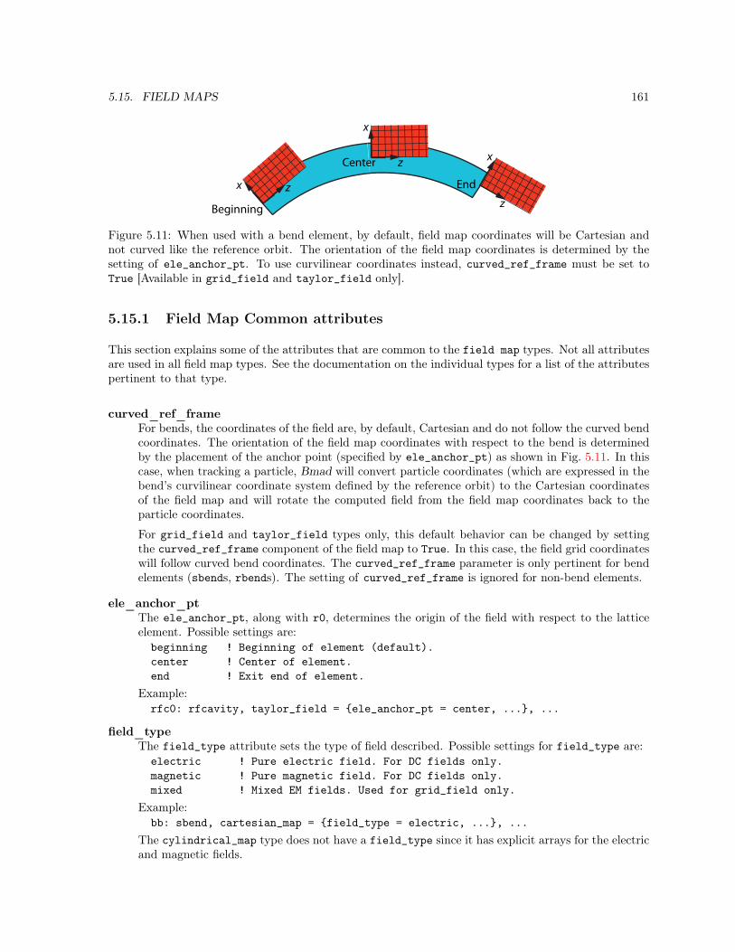
5.15. FIELD MAPS 161

x

zBeginning

Endx z

Center

x

z

Figure 5.11: When used with a bend element, by default, field map coordinates will be Cartesian andnot curved like the reference orbit. The orientation of the field map coordinates is determined by thesetting of ele_anchor_pt. To use curvilinear coordinates instead, curved_ref_frame must be set toTrue [Available in grid_field and taylor_field only].

5.15.1 Field Map Common attributes

This section explains some of the attributes that are common to the field map types. Not all attributesare used in all field map types. See the documentation on the individual types for a list of the attributespertinent to that type.

curved_ref_frameFor bends, the coordinates of the field are, by default, Cartesian and do not follow the curved bendcoordinates. The orientation of the field map coordinates with respect to the bend is determinedby the placement of the anchor point (specified by ele_anchor_pt) as shown in Fig. 5.11. In thiscase, when tracking a particle, Bmad will convert particle coordinates (which are expressed in thebend’s curvilinear coordinate system defined by the reference orbit) to the Cartesian coordinatesof the field map and will rotate the computed field from the field map coordinates back to theparticle coordinates.

For grid_field and taylor_field types only, this default behavior can be changed by settingthe curved_ref_frame component of the field map to True. In this case, the field grid coordinateswill follow curved bend coordinates. The curved_ref_frame parameter is only pertinent for bendelements (sbends, rbends). The setting of curved_ref_frame is ignored for non-bend elements.

ele_anchor_ptThe ele_anchor_pt, along with r0, determines the origin of the field with respect to the latticeelement. Possible settings are:beginning ! Beginning of element (default).center ! Center of element.end ! Exit end of element.

Example:rfc0: rfcavity, taylor_field = ele_anchor_pt = center, ..., ...

field_typeThe field_type attribute sets the type of field described. Possible settings for field_type are:electric ! Pure electric field. For DC fields only.magnetic ! Pure magnetic field. For DC fields only.mixed ! Mixed EM fields. Used for grid_field only.

Example:bb: sbend, cartesian_map = field_type = electric, ..., ...

The cylindrical_map type does not have a field_type since it has explicit arrays for the electricand magnetic fields.

162 CHAPTER 5. ELEMENT ATTRIBUTES

field_scaleThe field_scale attribute is used to scale the overall field magnitude. The default value is 1.A value of -1 will reverse the field. If the master_parameter is defined, it is multiplied with thefield_scale to give the overall scale. Example:qq, quadrupole, grid_field = field_scale = 0.5, ..., ...qq[grid_field(1)%field_scale] = 0.7 ! Change value after element def.qq[grid_field(1)%master_parameter] = k1 ! Change value after element def.

harmonicThe harmonic attribute, along with rf_frequency element attribute, sets the oscillation frequencyof the field map. The harmonic attribute is only used with cylindrical_map and grid_fieldtypes. The default value of harmonic is 0. The harmonic number needs to be 0 for DC fields.Example:lc1: lcavity, rf_frequency = 500e6, grid_field = harmonic = 2, ..., ...

Notice that rf_frequency is set outside of any field map and is common to all field maps.

master_parameterThe master_parameter defines a “master” element attribute for scaling the field. Example:qq: quadrupole, taylor_field = master_parameter = "K1", ..., k1 = ...

This example defines the master_parameter for the taylor_field to be the quadrupole strengthk1. By using the same master parameter for a set of field map instances within a given latticeelement, the sum field of the set can be controlled by a single attribute. The master_parametermust be set to a valid element attribute. If the name is blank (""), no master parameter is used.The master_parameter, if defined, is multiplied with the field_scale to give the value used toscale the fields. The default master_parameter is blank ("") except for wiggler elements where,for historical reasons, the default is polarity.Certain parameters have an associated “error” parameter. If the master_parameter is one of theseparameters, the value used to scale the field is the sum of the master_parameter and the associatederror parameter. The elements that have associated error parameters are:Parameter Assoc. Error Param Element Type--------- ------------------ --------------Voltage Voltage_err E_gun, LCavityGradient Gradient_err E_gun, LCavityPhi0 Phi0_err E_gun, LCavityG dG Sbend, RbendB_field dB_field Sbend, Rbend

phi0_fieldmapFor AC fields, phi0_fieldmap is the phase of the field map field relative to the fundamentalmode. The phase phi0_fieldmap is relative to the fundamental frequency and not the frequencyof the field map mode. That is, the “zero crossing” point of the field map is shifted by a timephi0_fieldmap/f0 where f0 is the fundamental mode frequency.

r0The r0 attribute is the (x0, y0, z0) vector specifying the offset of the origin point that definesthe field relative to the anchor point defined by ele_anchor_pt. The origin position of the field(r_origin) is determined byr_origin = r0 + r_anchor

where r_anchor is determined by the setting of ele_anchor_pt. In the reference coordinates(§15.1.1) with respect to the element r_anchor is:ele_anchor_pt r_anchor------------- ---------beginning (0, 0, 0) ! Defaultcenter (0, 0, L/2)end (0, 0, L)

with L being the length of the element.Example:rfc0: rfcavity, taylor_field = r0 = (-0.23, ...), ..., ...

5.15. FIELD MAPS 163

5.15.2 Cartesian_Map Field Map

The cartesian_map field map is only used for DC fields. Each term of a cartesian_map is a solutionof Laplace’s equation in cartesian coordinates. as described in Sec. §16.5.

The lattice file syntax for the cartesian_map type is:cartesian_map = field_type = <String>, ! Type of field: Default = Magnetic.field_scale = <Real>, ! Scale factor for the E & B fields.master_parameter = <Name>, ! Master scaling parameter for E & B fields.ele_anchor_pt = <Position>, ! Anchor position: Beginning (default), Center, or End.r0 = (<x0>, <y0>, <z0>), ! Anchor offset. Default is 0.term = <A>, <k_x>, <k_y>, <k_z>, <x_0>, <y_0>, <phi_z>, <family>,term = ....

The possible settings of <family> are explained in Sec. §16.5. Example:q01: quadrupole, l = 0.6, field_calc = fieldmap,

cartesian_map = term = 0.03, 3.00, 4.00, 5.00, 0, 0, 0.63, y,term = ..., ...

See Sec. §5.15.1 for an explanation of the attributes that are common with other field map types.

To use with PTC dependent tracking methods (§6.4) there are a number of restrictions:

• There can be only one cartesian_map field map and there cannot be any other field maps of anykind.

• cartesian_map may not be used with a bend.

• Only magnetic fields may be used.

• The transverse terms in r0 must be zero.

5.15.3 Cylindrical_Map Field Map

The cylindrical_map field map is used for both DC and AC fields. Each term of a cylindrical_mapis a solution of Laplace’s equation in cylindrical coordinates. as described in Sec. §16.6.

The lattice file syntax for the cylindrical_map type is:cylindrical_map = field_scale = <Real>, ! Scale factor for the E & B fields.master_parameter = <Name>, ! Master scaling parameter for E & B fields.ele_anchor_pt = <Position>, ! Anchor position: Beginning (default), Center, or End.m = <Integer>, ! Azimuthal mode numberharmonic = <Integer>, ! RF frequency harmonic numberphi0_fieldmap = <Real>, ! Phase of oscillations.theta0_azimuth = <Real>, ! Azimuthal orientation.r0 = (<x0>, <y0>, <z0>), ! Anchor offset. Default is 0.dz = <Real>, ! Distance between sampled field points.e_coef_re = (<Real>, <Real>, ....), ! Real part of E.e_coef_im = (<Real>, <Real>, ....), ! Imaginary part of E.b_coef_re = (<Real>, <Real>, ....), ! Real part of B.b_coef_im = (<Real>, <Real>, ....), ! Imaginary part of B.

164 CHAPTER 5. ELEMENT ATTRIBUTES

See Sec. §5.15.1 for an explanation of the attributes that are common with other field map types.

For DC fields, the e coefficients specify the electric fields and the b coefficients specify the magneticfields. For AC fields, the e coefficients specify modes that have finite longitudinal electric fields whilethe modes associated with the b coefficients do not.

To specify the RF frequency, specify the rf_frequency element attribute along with the harmonicattribute. See the discussion of the harmonic attribute in Sec. §5.15.1.

The basic equations used for the cylindrical_map decomposition of the fields are given in Section §16.6.A lattice element may have multiple cylindrical_map components with each cylindrical_map beingassociated with a particular azimuthal mode m.

e_re and e_im give the real an imaginary part of e and b_re and b_im give the real and imaginary partof b. All of these vectors must be present and have the same length. The exception is with an m = 0mode either the e or b arrays can be omitted and will default to zero. The number of terms N for the eor b vectors must be a power of 2 and all modes must have the same number of terms. The nth elementin the e or b arrays, with n running from 0 to N − 1, is associated with a wavelength kn

kn =

®2π nN dz 0 ≤ n < N

22π (n−N)N dz

N2 ≤ n ≤ N − 1

(5.15)

This convention produces less high frequency components then the convention of using kn = 2π n/Ndz.

The longitudinal length of the field is

Lfield =N − 1

dz(5.16)

this may be different from the length l specified for the element.

For AC fields, the time t in Eq. (16.47) is computed depending upon whether absolute time trackingor relative time tracking is being used as discussed in §24.1. For rfcavity elements, the phasefactor φ0j in Eq. (16.47) is computed byφ0j = harmonic(j) * [0.25 - (phi0 + phi0_multipass + phi0_err +

phi0_autoscale + phi0_fieldmap(j))]where phi0_fieldmap(j) and harmonic(j) are specific to the jth grid field while the other factors areelement parameters and so will be the same for all grid field maps of a given element. For non rfcavityelements the phase isφ0j = harmonic(j) * [phi0 + phi0_multipass + phi0_err +

phi0_autoscale + phi0_fieldmap(j)]where phi0_fieldmap(j) and harmonic(j) are specific to the jth cylindrical field map while the otherfactors are element parameters and so will be the same for all cylindrical field maps of a given element.

Example:m1: lcavity, rf_frequency = 1e6, voltage = 2e6, cylindrical_map = m = 2, harmonic = 3,r0 = (0, 0, 0.001), dz = 0.1,theta0_azimuth = 0.3, field_scale = 0.7,ele_anchor_pt = center, master_parameter = voltage,e_coef_re = (...), e_coef_im = (...),b_coef_re = (...), b_coef_im = (...), field_calc = fieldmap

Note: When using PTC based tracking (§6), the following restrictions apply:

• The fields must be DC.• all the e_coef and b_coef arrays must have the same length.

5.15. FIELD MAPS 165

• r0(1) and r0(2) (the transverse offsets) must be zero.• The element containing the map cannot be an sbend or rbend.• May not be combined with other field map types.

5.15.4 Grid_Field Field Map

A grid_field is grid of field points specified using the syntax:grid_field = geometry = <String>, ! Geometry of the grid.field_type = <String>, ! Type of field: Default = Mixed.field_scale = <Real>, ! Scale factor for the E & B fields.phi0_fieldmap = <Real>, ! Phase of oscillations.harmonic = <Int>, ! RF frequency harmonic numberinterpolation_order = <Int>, ! 1 (default) or 3 interpolation polynomial order.master_parameter = <Name>, ! Master scaling parameter for E & B fields.curved_ref_frame = <Logical>, ! Use a curved reference frame with bends?r0 = (...), ! Grid origin. Syntax is geometry dependent.dr = (...), ! Grid spacing. Syntax is geometry dependent.ele_anchor_pt = <Position> ! BEGINNING, CENTER, or ENDpt(<Integer>, ...) = ( ... ), ! Field points. Syntax is geometry dependent....

See Sec. §5.15.1 for an explanation of the attributes that are common with other field map types.

To specify the RF frequency, specify the rf_frequency element attribute along with the harmonicattribute. See the discussion of the harmonic attribute in Sec. §5.15.1.

For field_type set to electric or magnetic, the field is DC. That is, For field_type set to electricor magnetic, the value of harmonic must be 0. For field_type set to mixed, the field may be DC orAC.

For AC fields, the individual field components are complex. the syntax for specifying a complex numberis:(<Re>, <Im>)

Example:pt(0, 0, -7) = ((0.34, -4.3), (2.37, 9.34), ...) ! Complex fieldpt(0, 0, -7) = (0.12, -0.33, ...) ! Imaginary components are zero

The actual fields E and B are computed from the complex fields Ec and Bc via

E = <[Ec exp (−2π i (φt + φref))

](5.17)

with a similar equation for B. φt is the part of the phase due to when the particle arrives at the cavityand depends upon whether absolute time tracking or relative time tracking is being used asdiscussed in §24.1. The phase φref for the jth grid field in an rfcavity element isφref,j = harmonic(j) * [0.25 - (phi0 + phi0_multipass + phi0_err +

phi0_autoscale + phi0_fieldmap(j))]where phi0_fieldmap(j) and harmonic(j) are specific to the jth grid field while the other factors areelement parameters and so will be the same for all grid field maps of a given element. For non rfcavityelements the phase isφref,j = harmonic(j) * [phi0 + phi0_multipass + phi0_err +

phi0_autoscale + phi0_fieldmap(j)]

166 CHAPTER 5. ELEMENT ATTRIBUTES

The geometry switch sets the type of the grid and must come before any pt is given. The possiblesettings of geometry are:rotationally_symmetric_rzxyz

The rotationally_symmetric_rz setting for geometry is for fields that are rotationally symmetricaround the z axis. The format for this type of grid_field isgrid_field = geometry = rotationally_symmetric_rz,r0 = (<x0>, <y0>, <z0>), ! Grid origindr = (<dr>, <dz>), ! Grid spacingpt(<ir>, <iz>) = (<E_r>, <E_phi>, <E_z>) ! For field_type = Electricpt(<ir>, <iz>) = (<B_r>, <B_phi>, <B_z>) ! For field_type = Magneticpt(<ir>, <iz>) = (<E_r>, <E_phi>, <E_z>, <B_r>, <B_phi>, <B_z>)

! For field_type = Mixed....

where <iz> can be negative but <ir> must be non-negative.

The xyz setting for geometry can be used for all rectangular field grids. The format for this type ofgrid_field isgrid_field = geometry = xyz,r0 = (<x0>, <y0>, <z0>), ! Grid origindr = (<dx>, <dy>, <dz>), ! Grid spacingpt(<ix>, <iy>, <iz>) = (<E_x>, <E_y>, <E_z>), ! For field_type = Electricpt(<ix>, <iy>, <iz>) = (<B_x>, <B_y>, <B_z>), ! For field_type = Magneticpt(<ix>, <iy>, <iz>) = (<E_x>, <E_y>, <E_z>, <B_x>, <B_y>, <B_z>),

! For field_type = Mixed....

where <ix>, <iy>, and <iz> can be negative.

[For clarity sake, the following discusses the xyz case. Extension to other cases is straight forward.]There is no restriction on the bounds of the indexes (ix, iy, iz) of the pt(ix, iy, iz) array. Apoint (ix, iy, iz) corresponds in space to the point (x, y, z):(x, y, z) = dr * (ix, iy, iz) + r0 + r_anchor

where z is measured from the beginning of the element and r_anchor is determined by the setting ofele_anchor_pt:ele_anchor_pt r_anchor------------- ---------beginning (0, 0, 0) ! Defaultcenter (0, 0, L/2)end (0, 0, L)

with L being the length of the element.

Example:apex: e_gun, l = 0.23, field_calc = fieldmap, rf_frequency = 187e6,

grid_field = call::apex_gun_grid.bmad

with the file apex_gun_grid.bmad being:geometry = rotationally_symmetric_rz,harmonic = 1,

5.15. FIELD MAPS 167

master_parameter = voltage,r0 = (0, 0),dr = (0.001, 0.001),pt(0,0) = ( (0, 0), (0, 0), (1, 0), (0, 0), (0, 0), (0, 0)),pt(0,1) = ( (0, 0), (0, 0), (0.99, 0), (0, 0), (0, 0), (0, 0)),...

The order of the polynomials used to interpolate the field is determined by the setting of interpolation_order.The value of this integer may be either 1 or 3. A value of 1 is the default and gives linear interpolation.A value of 3 will give cubic interpolation which will be better if the field values on the grid are smoothand well behaved. However, a cubic interpolation will be slower and will magnify gird field errors so careshould be taken in choosing the interpolation order.

It is considered an error if the field of the grid is evaluated for a point that is transversely outside ofthe grid. That is, a grid must extend transversely to the aperture or at least beyond the trajectoryof any particle. [Actually, to prevent problems when the aperture is set at the grid boundary, if thedistance between the particle and the grid boundary is within 1/2 of the spacing between grid points,no error is generated and the field will be calculated using extrapolation.] On the other hand, it isacceptable to evaluate the grid field at a point that is longitudinally outside of the grid. In this case,the field is assumed to go to zero. This is done by effectively adding to the grid two planes of zero fieldlongitudinally to either side of the grid. So a particle traveling outside of the grid longitudinally will seethe field drop to zero within one longitudinal grid spacing length.

Grid fields may stored in HDF5 binary format which may then be called using an inline call (§3.18).For example:qq: quadrupole, grid_field = call::my_grid.h5, ...

5.15.5 Taylor_Field Field Map

The taylor_field field map is only used for DC fields. A taylor_field is comprised of a set of twodimensional Taylor maps.

The syntax for describing a taylor_field is:taylor_field = field_type = <String>, ! Type of field: Default = Magnetic.field_scale = <Real>, ! Scale factor for the E & B fields.master_parameter = <Name>, ! Master scaling parameter for E & B fields.curved_ref_frame = <Logical>, ! Use curved coords with bends?canonical_tracking = <logical> ! Use (px, py) instead of (x’, y’) when tracking?ele_anchor_pt = <Position>, ! Anchor position: Beginning (default), Center, or End.r0 = (<x0>, <y0>, <z0>), ! Anchor offset. Default is 0.dz = <Real>, ! Distance between sampled field points.plane(<i>) = <term1>, <term2>, <term3>, ...., ! Taylor map at constant z.plane(<j>) = ....

See Sec. §5.15.1 for an explanation of the attributes that are common with other field map types.

Each plane(<i>) component specifies a Taylor map at constant z (§16.7). The index <i> for the differentplanes must be in consecutive order. The plane with <i> = 0 corresponds to the z = 0 origin. Thereis no restriction for the starting <i> index of the first plane. That is, there does not have to be a planewith index <i> = 0 (in this case, the origin needs to be outside of the element).

The individual Taylor series terms follow the same syntax as the Taylor terms in a taylor element(§4.48):

168 CHAPTER 5. ELEMENT ATTRIBUTES

<out>: <coef>, <e1> <e2> ! EM Taylor term. First form.<out>: <coef> | <n1> <n2> ... ! EM Taylor term. Second form.

except that 1) <out> must be one ofBx, By, or Bz

2) there are only two exponents <e1> and <e2> corresponding to x, and y respectively for the first form,and 3) the integers <n1>, <n2>, etc., are restricted to being 1 or 2.

To use with PTC dependent tracking methods (§6.4) there are a number of restrictions:

• There can be only one taylor_field field map and there cannot be any other field maps of anykind.

• The number of planes must be odd. If you want to be able to track with PTC to the center of theelement, the number of planes must be of the form 4n+ 1 where n is an integer.

• Only magnetic fields may be used.

• The plane locations must be symmetric with respect to the center of the element. That is, the firstplane and the last plane must be equidistant from the element center.

• The element may not be superimposed upon (§8.1). [PTC tracks from plane to plane so there isno good way to cut an element at an arbitrary position.]

• In a bend with curved_ref_frame = False, The setting of ele_anchor_pt must be center.

If the edges of the taylor_field, which are defined by the first and last planes, is different than theedges of the element, Bmad and PTC will do tracking differently. With Bmad, the tracking will startat one edge of the element and will end at the other end. That is, Bmad will ignore the field outside ofthe element (but this can be modified using field overlap (§5.17)). PTC, on the other hand, will start atan element end and then track from the element end backwards to the first plane like in a drift. It willthen track to the ending plane and finally track backwards from the ending plane to the ending elementedge line in a drift. That is, PTC does not ignore the field outside of the element.

When using PTC based tracking (§6), the canonical_tracking parameter can be used to select whetherthe transverse phase space coordinates used in tracking is the canonical (x, px, y, py) (§15.4.2) coordinatesor the non-canonical (x, x′, y, y′) coordinates. The default is False. The difference comes at the edgesof element if the field is not zero. With canonical coordinates, there is a kick at the edge while withthe non-canonical there is not. What is best depends upon the problem. For example, with a solenoidmagnet where the field is constant right up to the edge, canonical tracking will be needed since the edgekick is significant. However, the edge kick is not well defined (that is, certain assumptions are built intothe edge kick calculation. For example, with a solenoid, cylindrical symmetry is generally assumed).Thus for some arbitrary field, the assumptions used by PTC may by incorrect for the problem at hand.Thus in many cases, especially for single pass machines, the non-canonical tracking is a better choice.

Example:t1: sbend, k1 = 2, taylor_field = field_type = electric, ele_anchor_pt = end,dz = 1.2, r0 = (0, 0, 2.0),field_scale = 1.3, curved_ref_frame = False,master_parameter = k1,plane(-2) = Bx: 0.3| 1, Bx: 1.3, 1 2, By: 0.7, 3 1, ...,plane(-1) = Bx: 0.6|, By: 0.4|112, By: 0.7, 4 0, ...,... , field_calc = fieldmap

5.16. RF COUPLERS 169

5.16 RF Couplers

For lcavity and rfcavity elements, the attributes that characterize the dipole transverse kick due toa coupler port are:coupler_at = <Switch> ! What end the coupler is atcoupler_strength = <Real> ! Normalized strengthcoupler_angle = <Real> ! Polarization angle (rad/2π)coupler_phase = <Real> ! Phase angle with respect to the RF (rad/2π)

The possible coupler_at settings are:entrance_endexit_end ! defaultboth_ends

The kick due to the coupler isdP_x = amp * cos(phase) * cos(angle)dP_y = amp * cos(phase) * sin(angle)dE = amp * (cos(angle) * x + sin(angle) * y) * sin(phase) * twopi * rf_frequency / c_light

where dP_x and dP_y are the transverse momentum kicks, dE is an energy kick, andamp = gradient * coupler_strengthphase = twopi * (phase_particle + phase_ref + coupler_phase) ! For lcavity §4.27

= pi/2 + twopi * (phase_particle - phase_ref + coupler_phase) ! For rfcavity §4.27angle = twopi * coupler_angle

The energy kick is needed to keep things symplectic.

Example:rf1: lcav, l = 4.5, gradient = 1.2e6, coupler_at = both_ends,

coupler_strength = 0.037

5.17 Field Extending Beyond Element Boundary

The field_overlaps element attribute can be used to indicate that the electric or magnetic fields ofone element overlap another element. The syntax is:<overlapping_ele>: ... field_overlaps = <overlapped_ele1>, <overlapped_ele2>, ...

The braces are optional if there is only one overlapped element.

Example:b1: sbend, l = 2.3, field_overlaps = q1, s2, ...inj_line: line = (..., s2, b1, mark3, q1, ...)

In this example, the field of element b1 extends beyond the ends of b1 and overlaps elements q1 and s2.There is no limit to the number of elements that are overlapped by any given element and overlappedelements do not have to be next to the overlapping element in the line. If there are multiple elementswhose name matches the name of a overlapped element, the element closest to the overlapping elementis chosen. Thus in the above example, if there are multiple elements named q1, the closest q1 to b1 isdesignated as the overlapped element.

There can be multipole field_overlaps = ... constructs for an overlapping element. Thus the fol-lowing is equivalent to the above example:b1: sbend, l = 2.3, field_overlaps = q1, field_overlaps = s2

Note: When the field overlaps elements that are superimposed (§8.1), the overlapped elements must bethe super_lord elements and never the slaved elements.

The field, when field_calc (§6.4) is set to bmad_standard, never extends beyond the element boundaryand so a bmad_standard field will never overlap another element.

170 CHAPTER 5. ELEMENT ATTRIBUTES

5.18 Automatic Scaling of Accelerating Fields

Elements that have accelerating fields are:e_gun ! §4.15em_field ! §4.17lcavity ! §4.27rfcavity ! §4.42

[Notice that rfcavity elements by definition, have a constant reference energy while with all the otherelements the entrance end reference energy will, in general, be different from the exit end referenceenergy.]

The problem that arises with accelerating fields is how to set the overall amplitude (and phase if thefields are oscillating) of the field so that a particle, starting on the reference orbit and starting with thereference energy, has the desired energy gain at the exit end of the element where the “desired” is set bythe voltage or gradient attribute of the element plus a phi0 phase attribute for AC fields.

The scaling problem is not present when bmad_standard tracking (§6.1) is used since bmad_standardtracking uses an integrated formula that is designed to give the proper acceleration. Rather it is aproblem for Runge-Kutta and other methods integration methods.

The problem becomes even more complicated at non-ultra relativistic energies where the particle velocityis not a constant. In this case, the proper amplitude and/or phase settings will depend upon what theincoming energy of the reference particle is.

To help with the scaling problem, Bmad has the capability to automatically scale an accelerating field’samplitude and/or phase. The two lattice element parameters that turn on/off auto scaling are (§9.1):autoscale_phase = <Logical> ! Automatic phase scaling.autoscale_amplitude = <Logical> ! Automatic amplitude scaling.

The default value is True for both parameters. Example:rf2: rfcavity, autoscale_phase = F

Scaling takes place during program execution when a lattice is initially created (that is, when the latticefile is parsed) and when parameters in the lattice that would change the scaling are varied. The elementparameters varied when autoscaling is done are:field_autoscale ! Amplitude scalephi0_autoscale ! phase scale

For an rfcavity element, the field_autoscale parameter is set so that when the phase is adjustedfor maximum acceleration, the voltage gain of a particle on the zero orbit is equal to the value of theelement’s voltage parameter and then phi0_autoscale is shifted by approximately 90 degrees so thatwith phi0 equal to zero a particle on the zero orbit will not see any energy gain through the cavity.

If no autoscaling is done, the default setting of field_autoscale is 1 and the default setting ofphi0_autoscale is 0.

For an rfcavity, the autoscaling is normally done around a phase of phi0 = 0 which is appropriatefor a ring above transition since phi0 = 0 is the stable fixed point. Below transition, the stable fixedpoint is at phi0 = 0.5. In this case, the bmad_com global parameter rf_phase_below_transition_ref(§10.2) should be set to True so that autoscaling is done around phi0 = 0.5. For an ultrarelativisticreference particle with speed very nearly c there is no difference in the autoscaling between phi0 = 0and phi0 = 0.5. However, when there are velocity variations of the particle within the cavity there willbe differences between autoscaling at the two phases.

Notice that if autoscaling is on, the field_autoscale is adjusted so that a particle on the zero orbitwill see a field appropriate for the setting of the element’s voltage setting. If autoscaling is off, the fieldis independent of the element’s voltage setting.

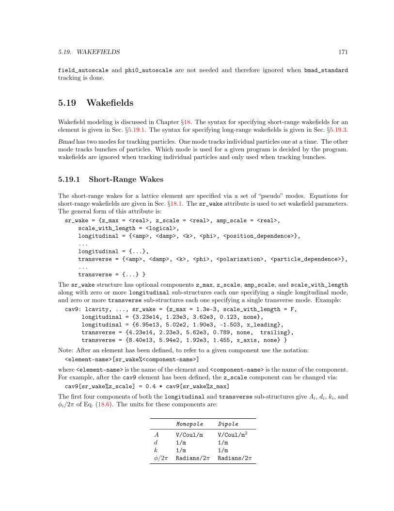
5.19. WAKEFIELDS 171

field_autoscale and phi0_autoscale are not needed and therefore ignored when bmad_standardtracking is done.

5.19 Wakefields

Wakefield modeling is discussed in Chapter §18. The syntax for specifying short-range wakefields for anelement is given in Sec. §5.19.1. The syntax for specifying long-range wakefields is given in Sec. §5.19.3.

Bmad has two modes for tracking particles. One mode tracks individual particles one at a time. The othermode tracks bunches of particles. Which mode is used for a given program is decided by the program.wakefields are ignored when tracking individual particles and only used when tracking bunches.

5.19.1 Short-Range Wakes

The short-range wakes for a lattice element are specified via a set of “pseudo” modes. Equations forshort-range wakefields are given in Sec. §18.1. The sr_wake attribute is used to set wakefield parameters.The general form of this attribute is:sr_wake = z_max = <real>, z_scale = <real>, amp_scale = <real>,

scale_with_length = <logical>,longitudinal = <amp>, <damp>, <k>, <phi>, <position_dependence>,...longitudinal = ...,transverse = <amp>, <damp>, <k>, <phi>, <polarization>, <particle_dependence>,...transverse = ...

The sr_wake structure has optional components z_max, z_scale, amp_scale, and scale_with_lengthalong with zero or more longitudinal sub-structures each one specifying a single longitudinal mode,and zero or more transverse sub-structures each one specifying a single transverse mode. Example:cav9: lcavity, ..., sr_wake = z_max = 1.3e-3, scale_with_length = F,

longitudinal = 3.23e14, 1.23e3, 3.62e3, 0.123, none,longitudinal = 6.95e13, 5.02e2, 1.90e3, -1.503, x_leading,transverse = 4.23e14, 2.23e3, 5.62e3, 0.789, none, trailing,transverse = 8.40e13, 5.94e2, 1.92e3, 1.455, x_axis, none

Note: After an element has been defined, to refer to a given component use the notation:<element-name>[sr_wake%<component-name>]

where <element-name> is the name of the element and <component-name> is the name of the component.For example, after the cav9 element has been defined, the z_scale component can be changed via:cav9[sr_wake%z_scale] = 0.4 * cav9[sr_wake%z_max]

The first four components of both the longitudinal and transverse sub-structures give Ai, di, ki, andφi/2π of Eq. (18.6). The units for these components are:

Monopole Dipole

A V/Coul/m V/Coul/m2

d 1/m 1/mk 1/m 1/mφ/2π Radians/2π Radians/2π

172 CHAPTER 5. ELEMENT ATTRIBUTES

Monopole modes are modes that are independent of transverse position and dipole modes are modesthat are linear in the transverse position.

For the longitudinal sub-structures, there is a 5th component which gives the transverse positiondependence of the wake. Possible values are:none ! No position dependencex_leading ! Linear in the leading particle x-positiony_leading ! Linear in the leading particle y-positionx_trailing ! Linear in the trailing particle x-positiony_trailing ! Linear in the trailing particle y-position

“x_leading”, for example, means that the wake left by a “leading” particle is linear in the x-position ofthe particle while the kick to a “trailing” particle is independent of the the trailing particle’s transvrseposition. “y_trailing”, on the other hand, means that the wake left by a leading particle is independentof the leading particle’s transverse position but that the kick felt by a trailing particle is proportional tothe trailing particle’s y-position.

For the transverse sub-structures, there is a 5th component giving the polarization and a 6th componentspecifying if the kick is dependent upon the leading or trailing particle transverse position. Possible valuesfor the polarization arenone ! Kick in both x and y-planesx_axis ! Kick in only the x-planey_axis ! Kick in only the y-plane

and possible values for the particle dependence are:none ! No transverse dependenceleading ! Depends linearly on the leading particle position.trailing ! Depends linearly on the trailing particle position.

The z_max component of sr_wake specifies the the maximum z value at which the pseudo mode fit isvalid. The z_max component is optional and if present and positive, Bmad will check that the distancebetween particles does not exceed z_max. If it does, Bmad will report an error. If z_max is not positiveit is ignored.

If scale_with_length is False (the default is True), the length factors in Equations like Eqs. (18.1) and(18.4) are dropped. This is convenient for using zero length elements with wake simulations.

The amp_scale component is used to scale the amplitude of the modes. This corresponds to Aamp inEq. (18.6). The default value is 1.0.

The z_scale is used to scale the z distance in the wake equations:z(used in equations) = z_scale * z(actual)

The default value is 1.0.

Note: In a beam chamber with circular symmetry, the linear terms in the longitudinal wake are zeroand the transverse wake has no terms independent of the transverse offsets nor terms that depend uponthe trailing particle offset.

5.19.2 Short-Range Wakes — Old Format

There is an old, deprecated, format for specifying short-range wakes where the wake data is containedin a separate file whose name is given by the lr_wake_file attribute. Example:abc: lcavity, sr_wake_file = "sr.wake", lr_freq_spread = 0.0023, lr_self_wake_on = F

Example file:

5.19. WAKEFIELDS 173

! Pseudo Wake modes:! Amp Damp K Phase Polar- Transverse_! Longitudinal: [V/C/m] [1/m] [1/m] [rad] ization Dependence! Transverse: [V/C/m^2] [1/m] [1/m] [rad]

&short_range_modeslongitudinal(1) = 3.23e14 1.23e3 3.62e3 0.123longitudinal(2) = 6.95e13 5.02e2 1.90e3 -1.503.. etc ..transverse(1) = 4.23e14 2.23e3 5.62e3 0.789 none linear_trailingtransverse(2) = 8.40e13 5.94e2 1.92e3 1.455.. etc ..

z_max = 1.3e-3/

Notice that the old format uses radians and not radians/2π for the phase.

Possible settings for the polarization parameter are: parameter are:none ! Defaultx_axisy_axis

The polarization name may be abbreviated.

The transverse_dependence parameter sets whether the wake kick is linear in the offset of the leadingor trailing particle or is independent of the transverse offset. Possible settings of this parameter are:none ! Default for longitudinal modeslinear_leading ! Default for transverse modeslinear_trailing

The transverse_dependence parameter may be abbreviated. Note: Due to the way the wake fileis parsed, if transverse_dependence is specified for a particular mode, polarization must also bespecified.

For longitudinal modes: If the transverse_dependence is none (the default), the polarization mustalso be none (other combinations do not make sense). If the transverse_dependence is not none for alongitudinal mode, the polarization must be set to x_axis or y_axis.

5.19.3 Long-Range Wakes

The lr_wake attribute is used to set the long-range wakefield parameters for a lattice element. Equationsfor long-range wakes is given in Sec. §18.2. The general form of this attribute is:lr_wake = time_scale = <real>, amp_scale = <real>, freq_spread = <real>,

self_wake_on = <logical>, t_ref = <real>,mode = <freq_in>, <R_over_Q>, <damp>, <phi>, <m_order>, <polar_angle>,

<b_sin>, <b_cos>, <a_sin>, a_cos>,...mode = ...

The lr_wake structure has optional components time_scale, amp_scale, freq_spread, self_wake_on,and t_ref along with one or more mode sub-structures each specifying a single long-range mode. Ex-ample:f1 = 1.65e9; q1 = 7e4cav9: lcavity, ..., lr_wake = time_scale = 1.7, freq_spread = 0.001,

mode = f1, 0.76, f1/(2*q1), 0, 1, unpolarized,mode = -1, 0.57, 3e4, 0, 2, 0.15

174 CHAPTER 5. ELEMENT ATTRIBUTES

The first six components of the mode sub-structure correspond to ω/2π, R/Q, d, φ/2π, m, and θp/2πin §18.2. The units of R/Q are Ω/meter2m. The last four components, which are optional, correspondto bsin, bcos, asin, and acos. These four components can be used as a convenient way to save the state ofthe long-range wakes. These components will typically not be present in a lattice file except for latticefiles generated by a program that does wake simulations.

A negative frequency is used to designate wakes that are part of the fundamental accelerating mode.That is, the frequency of such a mode is set to the value of rf_frequency for the lattice element thewake is associated with. It is an error to have a negative frequency for a mode for elements that do nothave a rf_frequency attribute. Bmad needs to know if a wake is part of the fundamental mode due totiming issues as discussed in §24.1.

The freq_spread component of the lr_wake structure is used to randomly vary the long-range modefrequencies. This can be used to spread out the long-range mode frequencies among different cavities.The default value is zero which means there is no varying the mode frequencies. The fractional differencebetween of the mode frequencies used in a simulation and the input mode frequencies will have a Gaussiandistribution with an RMS given by freq_spread. For example, a value of 0.01 for freq_spread givesa 1% variation in frequency. Note: Wake modes that are locked to the fundamental accelerating mode(§5.19.4), are not shifted.

The self_wake_on component can be used to turn off the long-range self-wake which is the longitudinalkick given a particle due to the wake generated by that same particle. [The transverse self wake is alwayszero.] The default setting of self_wake_on is True. Turning off the self-wake, for example, can be doneto avoid double counting if both long-range and short-range wakes are defined. Also, The standardformulas for the long–range resistive wall wake are not valid over short time scales. In this case, theself-wake should be turned off.

The amp_scale component is used to scale the amplitude of the modes. This corresponds to Aamp inEq. (18.6). The default value is 1.0.

The time_scale component is used to scale the time distance in the wake equations:

t (used in equations) = time_scale * t(actual)

The default value is 1.0.

The t_ref component is the reference time used in computing the wake (Eq. (18.20)). Like the modecomponents b_sin, etc., This component is typically not set when a lattice file is constructed.

After the long–range wake has been defined, components can be referenced or redefined using the notation

lr_wake%mode(n)%freq_in ! Input Frequencylr_wake%mode(n)%freq ! Actual Frequency (set by Bmad)lr_wake%mode(n)%r_over_q ! R/Qlr_wake%mode(n)%damp ! dlr_wake%mode(n)%phi ! Actually phi/2pilr_wake%mode(n)%polar_angle ! Polarization Anglelr_wake%mode(n)%polarized ! Logicallr_wake%freq_spread ! Frequency spreadlr_wake%amp_scale ! Amplitude scalelr_wake%time_scale ! Time scale

freq_in is the input frequency set in the lr_wake structure and freq is the actual frequency set byBmad. Freq will only be different from freq_in if freq_spread is nonzero. Example:

cav9[lr_wake%mode(2)%freq_in] = 1.1 * cav9[lr_wake%mode(2)%freq_in] ! Raise frequency by 10%

5.20. FRINGE FIELDS 175

5.19.4 Long-Range Wakes – Old Format

There is an old, deprecated, format for specifying long-range wakes where the wake data is contained ina separate file whose name is given by the lr_wake_file element attribute. Example:abc: lcavity, lr_wake_file = "lr.wake", lr_freq_spread = 0.0023, lr_self_wake_on = F

The file gives the wake modes by specifying the frequency (ω/2π), R/Q, Q, and m (order number), and,optionally, the polarization angle θp/2π for each cavity mode. The input uses Fortran90 namelist syntax:The data begins with the string &long_range_modes and ends with a slash /. Everything outside thisis ignored. Each mode is labeled lr(i) where i is the mode index. An example input file is:

Freq R/Q Q m Polar b_sin b_cos a_sin a_cos t_ref[Ohm/ Angle

[Hz] m^(2m)] [Rad/2pi]&long_range_modeslr(1) = 1.650e9 0.76 7.0e4 1 "unpol"lr(2) = 1.699e9 11.21 5.0e4 1 "0.15"lr(3) = -1 0.57 1.1e6 0 "unpol"

/[Note: The quotation marks are needed with some compilers and not with others.] If the polarizationangle is set to “unpolarized” the mode is taken to be unpolarized.

Two deprecated element attributes that affect the long-range wake are lr_freq_spread and lr_self_wake_onwhich correspond to lr_wake%freq_spread and lr_wake%self_wake_on (5.19.3

Notice that with the old format it is not possible to specify the phase offset φ.

5.20 Fringe Fields

Lattice elements can have fringe fields at the element edges. Whether Bmad tries to model the fringefields using the models described below first depends upon what kind of tracking is done. Fringe effectsare not applied when an element’s tracking_method is set to:customlinearmad

Additionally, no fringe effects will be used if the tracking_method is runge_kutta or time_runge_kutta,and the element’s field_calc (§6.4) is not bmad_standard. This is done since it is assumed, in thiscase, that the body of the field includes any fringe fields.

5.20.1 Turning On/Off Fringe Effects

Whether fringe fields are ignored or not is determined by the setting of the fringe_at element parameter.The possible settings areno_endboth_ends ! Defaultentrance_endexit_end

This is particularly useful in vetoing the fringe effect in the interior of split elements. If there is no fringeat a particular boundary, the setting of attributes like fringe_type (see below) are ignored.

When a particle’s spin is being tracked through the fringe field at an element’s edge, the spin_fringe_onlogical attribute of the element determines how the tracking is handled. Example:

176 CHAPTER 5. ELEMENT ATTRIBUTES

q: quad, spin_fringe_on = T, fringe_at = exit_end

Here, there is no fringe effect at the entrance of the element and the fringe at the exit end of the elementwill affect the spin. The default setting of spin_fringe_on is True.

5.20.2 Fringe Types

Bmad and PTC have several fringe field models for the magnetic field. Which fringe model is used isset by two element attributes:fringe_typeptc_fringe_geometry

For elements that have a multipole type fringe field (dipole, quadrupole, etc., as opposed to solenoid orRF fringes), the fringe_type switch is used to select how a fringe field is simulated. For everythingexcept for rbend and sbend elements, fringe_type may be set to one of:none ! Defaultsoft_edge_onlyhard_edge_onlyfull

The none setting ignores any fringe fields. The fringe field kick is divided into two pieces. The first pieceis called the hard edge fringe kick and is the kick in the limit that the longitudinal extent of the fringeis zero. The second piece is the soft edge fringe kick which is the fringe kick with the fringe having afinite longitudinal extent minus the hard edge fringe kick. That isfringe kick = hard fringe kick + soft fringe kick

The advantage of separating the fringe kick in this way is that the hard fringe can be used withouthaving to know anything about the longitudinal extent of the fringe. In many cases, this is a goodenough approximation. Note that using the soft fringe without the hard fringe is not physical but canbe useful in understanding how the soft edge component affects tracking. See §17 for details.

For rbend and sbend elements, the possible fringe_type settings are:nonesoft_edge_only ! SAD equivalent: fringe = 1, disfrin = 1hard_edge_only ! SAD equivalent: fringe = 0, disfrin = 0fulllinear_edgebasic_bend ! Default. SAD equivalent: fringe = 0, disfrin = 1sad_full ! SAD equivalent: fringe = 1, disfrin = 0

The basic_bend setting, which is the default, is essentially the basic vertical focusing effect that ispresent when there is a finite e1 or e2 face angle. With bmad_standard tracking, basic_bend alsoincludes second order terms (§17.2). The linear_edge setting ignores these second order terms. Insome cases, for instance in a chicane, basic_bend is not good enough. With fringe_type set to full,higher order effects are taken into account.

PTC does not have a linear_edge fringe model. With PTC tracking, basic_bend tracking is used iflinear_edge is chosen.

Additionally, for use with PTC, the ptc_fringe_geometry switch can be used to define the symmetryof the fringe fields. Possible settings are:x_invariantmultipole_symmetry

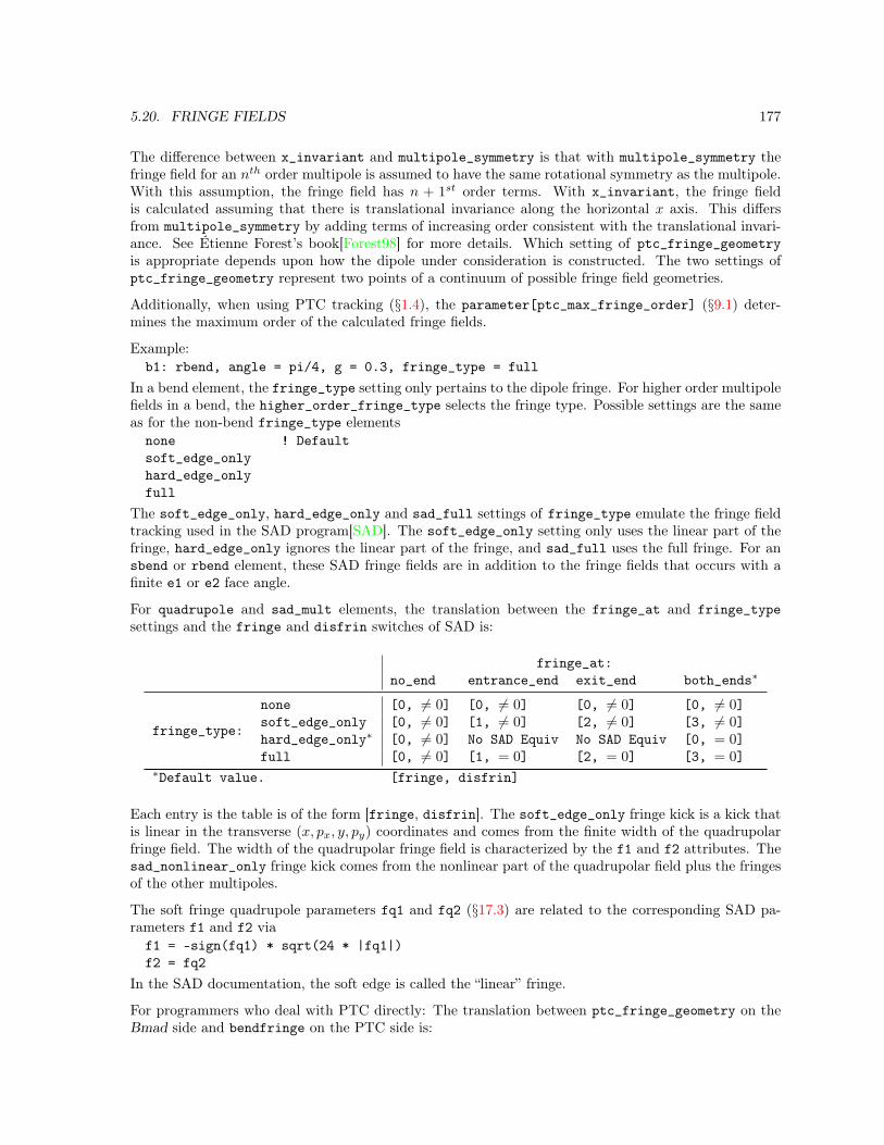
5.20. FRINGE FIELDS 177

The difference between x_invariant and multipole_symmetry is that with multipole_symmetry thefringe field for an nth order multipole is assumed to have the same rotational symmetry as the multipole.With this assumption, the fringe field has n + 1st order terms. With x_invariant, the fringe fieldis calculated assuming that there is translational invariance along the horizontal x axis. This differsfrom multipole_symmetry by adding terms of increasing order consistent with the translational invari-ance. See Étienne Forest’s book[Forest98] for more details. Which setting of ptc_fringe_geometryis appropriate depends upon how the dipole under consideration is constructed. The two settings ofptc_fringe_geometry represent two points of a continuum of possible fringe field geometries.

Additionally, when using PTC tracking (§1.4), the parameter[ptc_max_fringe_order] (§9.1) deter-mines the maximum order of the calculated fringe fields.

Example:b1: rbend, angle = pi/4, g = 0.3, fringe_type = full

In a bend element, the fringe_type setting only pertains to the dipole fringe. For higher order multipolefields in a bend, the higher_order_fringe_type selects the fringe type. Possible settings are the sameas for the non-bend fringe_type elementsnone ! Defaultsoft_edge_onlyhard_edge_onlyfull

The soft_edge_only, hard_edge_only and sad_full settings of fringe_type emulate the fringe fieldtracking used in the SAD program[SAD]. The soft_edge_only setting only uses the linear part of thefringe, hard_edge_only ignores the linear part of the fringe, and sad_full uses the full fringe. For ansbend or rbend element, these SAD fringe fields are in addition to the fringe fields that occurs with afinite e1 or e2 face angle.

For quadrupole and sad_mult elements, the translation between the fringe_at and fringe_typesettings and the fringe and disfrin switches of SAD is:

fringe_at:no_end entrance_end exit_end both_ends∗

fringe_type:

none [0, 6= 0] [0, 6= 0] [0, 6= 0] [0, 6= 0]soft_edge_only [0, 6= 0] [1, 6= 0] [2, 6= 0] [3, 6= 0]hard_edge_only∗ [0, 6= 0] No SAD Equiv No SAD Equiv [0, = 0]full [0, 6= 0] [1, = 0] [2, = 0] [3, = 0]

∗Default value. [fringe, disfrin]

Each entry is the table is of the form [fringe, disfrin]. The soft_edge_only fringe kick is a kick thatis linear in the transverse (x, px, y, py) coordinates and comes from the finite width of the quadrupolarfringe field. The width of the quadrupolar fringe field is characterized by the f1 and f2 attributes. Thesad_nonlinear_only fringe kick comes from the nonlinear part of the quadrupolar field plus the fringesof the other multipoles.

The soft fringe quadrupole parameters fq1 and fq2 (§17.3) are related to the corresponding SAD pa-rameters f1 and f2 viaf1 = -sign(fq1) * sqrt(24 * |fq1|)f2 = fq2

In the SAD documentation, the soft edge is called the “linear” fringe.

For programmers who deal with PTC directly: The translation between ptc_fringe_geometry on theBmad side and bendfringe on the PTC side is:

178 CHAPTER 5. ELEMENT ATTRIBUTES

ptc_fringe_geometry bendfringe

x_invariant Truemultipole_symmetry False

5.21 Instrumental Measurement Attributes

instrument, monitor, detector, and marker elements have special attributes to describe errors associ-ated with orbit, betatron phase, dispersion and coupling measurements. These attributes are:

Attribute Symbol (See: §26.2)tilt θt See §5.6x_offset xoff See §5.6y_offset yoff See §5.6x_gain_err dgx,err Horizontal gain errory_gain_err dgy,err Vertical gain errorcrunch ψerr Crunch angletilt_calib θerr tilt angle calibrationx_offset_calib xcalib Horizontal offset calibrationy_offset_calib ycalib Vertical offset calibrationx_gain_calib dgx,calib Horizontal gain calibrationy_gain_calib dgy,calib Vertical gain calibrationcrunch_calib ψcalib Crunch angle calibrationnoise nf Noise factorde_eta_meas dE/E Percent change in energyx_dispersion_err ηx,err Horizontal dispersion errory_dispersion_err ηy,err Vertical dispersion errorx_dispersion_calib ηx,calib Horizontal dispersion calibrationy_dispersion_calib ηy,calib Vertical dispersion calibrationn_sample Ns Number of sampling pointsosc_amplitude Aosc Oscillation amplitude

A program can use these quantities to calculate “measured” values from the “laboratory” values. Here,“laboratory” means as calculated from some model lattice. See §26.2 for the conversion formulas.

Chapter 6

Tracking, Spin, and Transfer MatrixCalculation Methods

Bmad allows for a number of methods that can be use to “track” a particle through a lattice element.Here “track” can mean one of three things:1) Calculate a particle’s phase space coordinates at the exit

end of the element given the coordinates at the entrance end.2) Calculate the linear transfer map (Jacobian) through an element

about a given reference orbit.3) Calculate the a particle’s spin orientation at the exit end

of the element given the coordinates at the beginning.

The different tracking methods that are available have different advantages and disadvantages in termsof speed, symplecticity, etc. What tracking method is used, is selected on an element–by–element basisusing the attributes:tracking_method = <Switch> ! phase space tracking method.mat6_calc_method = <Switch> ! 6x6 transfer matrix calculation.spin_tracking_method = <Switch> ! Spin tracking method.

Example:q2: quadrupole, tracking_method = symp_lie_ptcq2[tracking_method] = symp_lie_ptcquadrupole::*[tracking_method] = symp_lie_ptc

The first two lines of this example have exactly the same effect in terms of setting the tracking_method.The third line shows how to set the tracking_method for an entire class of elements.

These switches are discussed in more detail in the following sections.

6.1 Particle Tracking Methods

The tracking_method attribute of an element sets the algorithm that is used for single particle trackingthrough that element. Table 6.1 gives which methods are available for each type of element. Note:Table 6.1 pertains to charged-particle tracking only. When tracking photons, only bmad_standard andcustom tracking method are available.

179

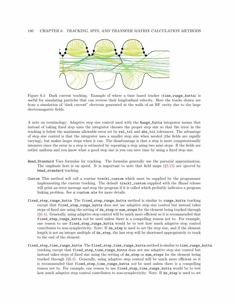
180 CHAPTER 6. TRACKING, SPIN, AND TRANSFER MATRIX CALCULATION METHODS

Figure 6.1: Dark current tracking. Example of where a time based tracker (time_runge_kutta) isuseful for simulating particles that can reverse their longitudinal velocity. Here the tracks drawn arefrom a simulation of “dark current” electrons generated at the walls of an RF cavity due to the largeelectromagnetic fields.

A note on terminology: Adaptive step size control used with the Runge_Kutta integrator means thatinstead of taking fixed step sizes the integrator chooses the proper step size so that the error in thetracking is below the maximum allowable error set by rel_tol and abs_tol tolerances. The advantageof step size control is that the integrator uses a smaller step size when needed (the fields are rapidlyvarying), but makes larger steps when it can. The disadvantage is that a step is more computationallyintensive since the error in a step is estimated by repeating a step using two mini steps. If the fields arerather uniform and you know what a good step size is you can save time by using a fixed step size.

Bmad_Standard Uses formulas for tracking. The formulas generally use the paraxial approximation.The emphasis here is on speed. It is important to note that field maps (§5.15) are ignored bybmad_standard tracking.

Custom This method will call a routine track1_custom which must be supplied by the programmerimplementing the custom tracking. The default track1_custom supplied with the Bmad releasewill print an error message and stop the program if it is called which probably indicates a programlinking problem. See s:custom.ele for more details.

fixed_step_runge_kutta The fixed_step_runge_kutta method is similar to runge_kutta trackingexcept that fixed_step_runge_kutta does not use adaptive step size control but instead takessteps of fixed size using the setting of ds_step or num_steps for the element being tracked through(§6.4). Generally, using adaptive step control will be much more efficient so it is recommended thatfixed_step_runge_kutta not be used unless there is a compelling reason not to. For example,one reason to use fixed_step_runge_kutta would be to test how much adaptive step controlcontributes to non-symplecticity. Note: If ds_step is used to set the step size, and if the elementlength is not an integer multiple of ds_step, the last step will be shortened appropriately to trackto the end of the element.

fixed_step_time_runge_kutta The fixed_step_time_runge_kuttamethod is similar to time_runge_kuttatracking except that fixed_step_time_runge_kutta does not use adaptive step size control butinstead takes steps of fixed size using the setting of ds_step or num_steps for the element beingtracked through (§6.4). Generally, using adaptive step control will be much more efficient so itis recommended that fixed_step_time_runge_kutta not be used unless there is a compellingreason not to. For example, one reason to use fixed_step_time_runge_kutta would be to testhow much adaptive step control contributes to non-symplecticity. Note: If ds_step is used to set

6.1. PARTICLE TRACKING METHODS 181

the step size, and if the element length is not an integer multiple of ds_step, the last step will beshortened appropriately to track to the end of the element.

Linear Linear just uses the 0th order vector with the 1st order 6x6 transfer matrix for an element. Verysimple. Depending upon how the transfer matrix was generated this may or may not be symplectic.Note: a linear tracking method may not be used with mat6_calc_method set to tracking sincethis would give a circular dependency.

MAD This uses the MAD 2nd order transfer map. This method is not able to handle element misalign-ments or kicks, and becomes inaccurate as the particle energy deviates from the reference energy.MAD tracking is generally only used for testing purposes. Note: Thanks to CERN and FrankSchmidt for permission to use the MAD tracking code within Bmad.

runge_kutta This uses a 4th order Runge Kutta integration algorithm with adaptive step size control.This is essentially the ODEINT subroutine from Numerical Recipes[Press92]. This may be slow butit should be accurate. This method is non-symplectic. Warning: When using custom fields, if thefields do not obey Maxwell’s equation, there is the possibility of the runge_kutta tracking haltingmid way through an element. See section §6.4 for more details.

Symp_Lie_Bmad Symplectic tracking using a Hamiltonian with Lie operation techniques. This is similarto Symp_Lie_PTC (see below) except this uses a Bmad routine. By bypassing some of the generalityinherent in PTC (§1.4), Symp_Lie_Bmad achieves about a factor of 10 improvement in speed overSymp_Lie_PTC.

Symp_Lie_PTC Symplectic tracking using a Hamiltonian with Lie operator techniques. This uses ÉtienneForest’s PTC (§1.4) software for the calculation. This method is symplectic but can be slow.Exceptions: The tracking is not symplectic when tracking through and element with an associatedelectric field and when tracking through a taylor element.

Taylor This uses a Taylor map generated from the PTC (§1.4) package. Generating the map may taketime but once you have it it should be very fast. One possible problem with using a Taylor mapis that you have to worry about the accuracy if you do tracking at points that are far from theexpansion point about which the map was made. This method is non-symplectic away from theexpansion point. Whether the Taylor map is generated taking into account the offset an elementhas is governed by the taylor_map_includes_offsets attribute (§6.7).The order of a Taylor map is set by the parameter[taylor_order] parameter (§9.1).

Time_Runge_Kutta This method uses time as the independent variable instead of the longitudinal zposition. The advantage of this method is that it can handle particles which reverse directionlongitudinally. One use for this method is “dark current” tracking where, as illustrated in Fig. 6.1,low energy particles generated at the vacuum chamber walls can be found traveling in all directions.Notice that time_runge_kutta is different from using absolute time tracking as explained in§24.1.

182 CHAPTER 6. TRACKING, SPIN, AND TRANSFER MATRIX CALCULATION METHODS

Element Class Bmad_Standard

Custom

Linear

MAD

Fixed_Step_Runge_Kutta

Runge_Kutta

Symp_Lie_Bmad

Symp_Lie_PTC

Taylor

Fixed_Step_Time_Runge_Kutta

Time_Runge_Kutta

ab_multipole D X X X Xac_kicker D X X X Xbeambeam D X Xconverter D Xcrab_cavity D X Xcustom D X X Xdrift D X X X X X X Xe_gun X Xa Decollimator D X X X X X Xelseparator D X X X X X X Xem_field X D X X Xfiducial D X Xfloor_shift D X Xhkicker D X X X X X Xinstrument D X X X X X Xkicker D X X X X X Xlcavity D X X X X X Xmarker D X X X Xmatch D X Xmonitor D X X X X X Xmultipole D X X X Xoctupole D X X X X X Xpatch D X Xc X Xquadrupole D X X X X X X X Xrbend D X X X X Xrcollimator D X X X X X Xrfcavity D X X X X X X Xsad_mult D X X X Xsbend D X X X X X X Xsextupole D X X X X X X Xsolenoid D X X X X X X X Xsol_quad D X X X X X X Xtaylor X X X Dvkicker D X X X X X Xwiggler (map type) X X X X X X Xwiggler (periodic type) D X X Xb Xb Xb DbaOnly if the beginning energy is non-zero.bSee §4.49.1 for more details.cOnly available for non-reflection patch elements.

Table 6.1: Table of valid tracking_method switches for use charged particle tracking. When trackingphotons, only bmad_standard and custom tracking methods are available. “D” denotes the defaultmethod. “X” denotes a valid method.

6.2. LINEAR TRANSFER MAP METHODS 183

6.2 Linear Transfer Map Methods

The mat6_calc_method attribute sets how the 6x6 Jacobian transfer matrix for a given element iscomputed. Table 6.2 gives which methods are available for each type of element. Note: Table 6.2 is forcharged-particle tracking only. When tracking photons, transfer matrices (which are not very useful) arenot computed.

In addition to the mat6_calc_method switch, two element attributes that can affect the way the transfermatrix is calculated are symplectify and taylor_map_includes_offsets. These are discussed insections §6.6 and §6.7 respectively.

For methods that do not necessarily produce a symplectic matrix the symplectify attribute of anelement can be set to True to solve the problem. See §23.3.

Symplectic integration is like ordinary integration of a function f(x) but what is integrated here is aTaylor map. Truncating the map to 0th order gives the particle trajectory and truncating to 1st ordergives the transfer matrix (Jacobian). The order at which a Taylor series is truncated at is set bytaylor_order (see §9.1. Like ordinary integration there are various formulas that one can use to dosymplectic integration. In Bmad (or more precisely in PTC (§1.4)) you can use one of 3 methods. Thisis set by integrator_order. integrator_order = n where n is allowed by PTC to be 2, 4, or 6. Withan integration order of n the error in an integration step scales as dzn where dz is step size. The step sizedz is set by the length of the element and the value of ds_step. Remember, as in ordinary integration,higher integration order does not necessarily imply higher accuracy.

Bmad_Standard Uses formulas for the calculation. The formulas generally use the paraxial approxima-tion. The emphasis here is on speed.

Custom This method will call a routine make_mat6_custom which must be supplied by the programmerimplementing the custom transfer matrix calculation. The default make_mat6_custom suppliedwith the Bmad release will print an error message and stop the program if it is called whichprobably indicates a program linking problem. See s:custom.ele for more details.

MAD This uses the MAD 2nd transfer map. This method is not able to handle element misalignmentsor kicks, and becomes inaccurate as the particle energy deviates from the reference energy. MADtracking is generally only used for testing purposes. Thanks must be given to CERN and FrankSchmidt for permission to use the MAD tracking code within Bmad.

Static This prevents the transfer matrix from being recomputed. Using Static in the input file isgenerally not a good idea since it prevents the matrix from being computed in the first place.Typically Static is used internally in a program to prevent recomputation.

Symp_Lie_Bmad A symplectic calculation using a Hamiltonian with Lie operator techniques. This issimilar to Symp_Lie_PTC (see below) except this uses a Bmad routine. By bypassing some of thegenerality inherent in PTC, Symp_Lie_Bmad achieves about a factor of 10 improvement in speedover Symp_Lie_PTC. However, Symp_Lie_Bmad cannot generate maps above first order.

Symp_Lie_PTC Symplectic integration using a Hamiltonian and Lie operators. This uses the PTC (§1.4)software for the calculation. This method is symplectic but can be slow. Exceptions: The trackingis not symplectic when tracking through and element with an associated electric field and whentracking through a taylor element.

Taylor This uses a Taylor map generated from Étienne’s PTC package. Generating the map maytake time but once you have it it should be very fast. One possible problem with using a Taylormap is that you have to worry about the accuracy if you do a calculation at points that are far

184 CHAPTER 6. TRACKING, SPIN, AND TRANSFER MATRIX CALCULATION METHODS

from the expansion point about which the map was made. This method is non-symplectic awayfrom the expansion point. Whether the Taylor map is generated taking into account the offset anelement has is governed by the taylor_map_includes_offsets attribute (§6.7). bmad_standardand taylor tracking methods are identical. Note: Taylor maps for match, and patch elements arelimited to first order.

The order of a Taylor map is set by the parameter[taylor_order] parameter (§9.1).

Tracking This uses the tracking method set by tracking_method to track 6 particles around thecentral orbit. This method is susceptible to inaccuracies caused by nonlinearities. Further-more this method is almost surely slow. While non–symplectic, the advantage of this methodis that it is directly related to any tracking results. Note: a linear tracking method maynot be used with mat6_calc_method set to tracking since this would give a circular depen-dency. The two parameters that affect this calculation are bmad_com%d_orb(6) (§10.2) whichsets the six deltas used for displacing the initial particle coordinates from the reference orbit andbmad_com%mat6_track_symmetric which sets whether symmetric or asymmetric differences areused.

6.2. LINEAR TRANSFER MAP METHODS 185

Bmad_Standard

Custom

MAD

Static

Symp_Lie_Bmad

Symp_Lie_PTC

Taylor

Tracking

ab_multipole D X X X X Xac_kicker X X X X Dbeambeam D X X Xconverter D Xcrab_cavity X X Dcustom D X Xdrift D X X X X X Xe_gun X X Decollimator D X X X X Xelseparator D X X X X X Xem_field X X X X Dfiducial D X X X Xfloor_shift D X X X Xhkicker D X X X X Xinstrument D X X X X Xkicker D X X X X Xlcavity D X X X X Xmarker D X X X X Xmatch D X X Xmonitor D X X X X Xmultipole D X X X X Xoctupole D X X X X Xpatch D X X X X Xquadrupole D X X X X X X Xrbend D X X X X X Xrcollimator D X X X X Xrfcavity D X X X X X Xsad_mult D X X X X Xsbend D X X X X X Xsextupole D X X X X X Xsolenoid D X X X X X X Xsol_quad D X X X X X X Xtaylor X X X Dvkicker D X X X X Xwiggler (map type) D X X Xa Xa Xa Xwiggler (periodic type) X X Xa Xa Da XaSee §4.49.1 for more details

Table 6.2: Table of available mat6_calc_method switches for charged-particle tracking. When trackingphotons, transfer matrices are not computed. “D” denotes the default method. “X” denotes an availablemethod.

186 CHAPTER 6. TRACKING, SPIN, AND TRANSFER MATRIX CALCULATION METHODS

6.3 Spin Tracking Methods

The spin_tracking_method attribute of an elements sets the algorithm that is used for tracking aparticle’s spin (§22.1) through that element. Table 6.3 gives which methods are available for each typeof element. Note: This table is only for charged-particle tracking since photons do not have spin.

Possible spin_tracking_method settings are:

CustomThis method will call a routine track1_spin_custom which must be supplied by the programmerimplementing the custom spin tracking calculation. See s:custom.ele for more details.

TrackingHow spin is tracked here will depend also on the setting of tracking_method. If tracking_methodis set to runge_kutta or time_runge_kutta the spin will be tracked along with the phase space par-ticle coordinates using the local fields. For tracking_method set to symp_lie_ptc, the spin track-ing will use PTC. For all other tracking_methods, the spin will be tracked using the “bmad_standard”spin tracking method which involves Romberg integration of the spin rotation matrix.

The runge_kutta and time_runge_kutta spin tracking uses the same fourth order integrator asis used for the orbital coordinates to track the spin rotation vector.

Symp_Lie_PTCSymplectic integration using a Hamiltonian and Lie operators. This uses Étienne’s PTC softwarefor the calculation. This method is symplectic but can be slow.

Since speed may be an issue, Bmad has an global parameter called spin_tracking_on which is part ofthe bmad_com instance (§10.4) that determines whether spin is tracked or not. Note: There is also anotherbmad_com parameter called spin_baier_katkov_flipping_on which can influence spin tracking.

The spin_fringe_on element attribute (§5.20.1) can be used to toggle whether the fringe fields of anelement affect the spin.

Example:q: quadrupole, spin_tracking_method = symp_lie_ptc

6.3. SPIN TRACKING METHODS 187

Custom

Symp_Lie_PTC

Tracking

ab_multipole X Dac_kicker X Dbeambeam X Dconverter X Dcrab_cavity X Dcustom D Xdrift X X De_gun X Decollimator X X Delseparator X X Dem_field X Dfiducial X X Dfloor_shift X X Dhkicker X X Dinstrument X X Dkicker X X Dlcavity X X Dmarker X X Dmatch X Dmonitor X X Dmultipole X X Doctupole X X Dpatch X X Dquadrupole X X Drbend X X Drcollimator X X Drfcavity X X Dsad_mult X Dsbend X X Dsextupole X X Dsolenoid X X Dsol_quad X X Dtaylor Dvkicker X X Dwiggler X X D

Table 6.3: Table of available spin_tracking_method switches for charged-particle tracking (photons donot have spin). “D” denotes the default method. “X” denotes an available method.

188 CHAPTER 6. TRACKING, SPIN, AND TRANSFER MATRIX CALCULATION METHODS

6.4 Integration Methods

“Integration methods” are tracking methods that involve integrating through an element’s magnetic andelectric fields. Integration methods are split into two classes: Those that can track Taylor maps andthose that simply track a particle’s position. The Taylor map methods aresymp_lie_bmad ! Only to first ordersymp_lie_ptc ! Uses PTCtaylor ! Uses PTC

See section §23.1 for more information on Taylor maps and symplectic integration. The latter twomethods involve using the PTC library (§1.4).

The methods that do not involve Taylor maps arefixed_step_runge_kuttafixed_step_time_runge_kuttarunge_kuttatime_runge_kutta

there are a number of element attributes that can affect the calculation. They areds_step = <Real> ! Integration step length (§6.5.1)num_steps = <Integer> ! Number of integration steps. (§6.5.1)integrator_order = <Integer> ! Integrator order (§6.5.3)field_calc = <Switch> ! How the field is calculated (§6.5.2)

Example:q1: quadrupole, l = 0.6, tracking_method = bmad_standard,

mat6_calc_method = symp_lie_ptc, ds_step = 0.2, field_calc = custom

6.5 CSR and Space Charge Methods

When doing beam tracking through an element (§19), Coherent Synchrotron Radiation (CSR) and SpaceCharge (SC) effects can be included by setting the appropriate method switches in that element. Theseswitches are:csr_method = <Switch> ! Coherent Synchrotron Radiationspace_charge_method = <Switch> ! Space charge method

Note: For CSR or SC effects to be included in tracking the bmad_com logical csr_and_space_charge_onmust be set to True (§10.2).

The possible settings for csr_method areoff ! No CSR. Default.1_dim ! One dimensional calculation (§19.4.1).

The possible settings of space_charge_method areoff ! No SC. Default.slice ! SC using slices (§19.4.2).fft_3d ! SC using a 3D grid (§19.4.3).

Example:q1: quadrupole, l = 0.6, csr_method = 1_dim, space_charge_method = slice, ...

Note: There is also high energy space charge calculation that can be used with single particle trackingand is discussed in §19.5.

6.5. CSR AND SPACE CHARGE METHODS 189

6.5.1 ds_step and num_steps Parameters

One way to create a transfer map through an element is to divide the element up into slices andthen to propagate the transfer map slice by slice. There are several ways to do this integration. Therunge_kutta type methods integrate the equations of motion to give the 0th order Taylor map whichjust represents a particle’s orbit. Symplectic integration using Lie algebraic techniques, on the otherhand, can generate Taylor maps to any order. The ds_step attribute determines the slice thickness.Alternatively, num_steps attribute can be used in place of ds_step to specify the number of slices. Thisis applicable to symp_lie_bmad and symp_lie_ptc integration. Example:q: quadrupole, l = 0.6, ds_step = 0.1 ! 10 cm step size.sbend::*[ds_step] = 0.2 ! Set the step_size for all sbend elements.

Since computation time will vary with the number of integration steps, the optimum step size is thelargest length such that the variations of the step size do not significantly affect the calculation. It isimportant to remember that the optimum step size is dependent upon what is to be calculated.

The default value for ds_step for a given element is calculated based upon the element’s field strength.One should consider the default as more of a guesstimate.

The runge_kutta and time_runge_kutta tracking uses adaptive step control independent of ds_step.These methods use three bmad_com parameters §10.4) namely:bmad_com[rel_tol_adaptive_tracking]bmad_com[abs_to_adaptive_tracking]bmad_com[max_num_runge_kutta_step]

The estimated error of the integration is then bounded byerror < abs_tol + |orbit| * rel_tol

lowering the error bounds makes for greater accuracy (as long as round-off doesn’t hurt) but for slowertracking.

6.5.2 Field_calc Parameter

The runge_kutta type tracking methods all use as input the electric and magnetic fields of an element.How the EM fields are calculated is determined by the field_calc attribute for an element. For alllattice elements, except wigglers and undulators, possible values for field_calc are:bmad_standard ! This is the default except for custom elementscustom ! Default for custom elements.fieldmap

For wigglers and undulators, possible values for field_calc are:planar_modelhelical_modelcustomfieldmap

For historical reasons, the default setting for field_calc for wigglers and undulators is planar_modelexcept if there is a field map present (§5.15) in which case the default is fieldmap. Note that withbmad_standard tracking, the setting of field_calc is ignored except in the case of wigglers andundulators where field_calc must be set to either planar_model or helical_model.

Custommeans that the field calculations are done outside of the Bmad software. A program doing customfield calculations will need the appropriate custom routine (§36.2). Elements that set field_calc tofieldmap need to have a field map defined (§5.15).

190 CHAPTER 6. TRACKING, SPIN, AND TRANSFER MATRIX CALCULATION METHODS

Warning: When tracking a particle through a custom field using runge_kutta, it is important that thefield obey Maxwell’s equations. Fields that do not obey Maxwell’s Equations may cause the runge_kuttaadaptive step size control algorithm to take smaller and smaller steps until the step size becomes so smallthe tracking will stop. What happens is that the step size control algorithm takes a step and then takestwo half steps over the same region and from this estimates the error in the calculation. If the error islarger than the allowed tolerance the control algorithm shortens the step and tries again. A field thatdoes not obey Maxwell’s equations can fool the control algorithm into thinking that the error is alwayslarger than the allowed tolerance for any finite step size. A typical situation is where the field has anunphysical step across some boundary.

6.5.3 PTC Integration

The integrator_order element attribute is the order of the integration formula for Symp_Lie_PTC andis used for constructing Taylor maps. Possible values areintegrator_order = 2 (default), 4, or 6

Essentially, an integration order of n means that the error in an integration step scales as dzn+1 wheredz is the slice thickness. For a given number of steps a higher order will give more accurate results buta higher order integrator will take more time per step. It turns out that for wigglers, after adjustingds_step for a given accuracy, the order 2 integrator is the fastest. This is not surprising given the highlynonlinear nature of a wiggler. Note that symp_lie_bmad always uses an order 2 integrator independentof the setting of integrator_order.

When tracking uses the PTC library (§1.4), there are two global parameters that can be set in the latticefile that affect the calculation. These are:ptc_com[exact_model] = <Logical> ! "exact" tracking? Default: Falseptc_com[exact_misalign] = <Logical> ! "exactly" misalign elements? Default: True

The default for exact_model is False and the default for exact_misalign is True.

The exact_model parameter sets whether PTC uses an “exact” model for tracking. Essentially thismeans that the paraxial approximation (§24.3) is made for exact_model set to False and is not madeif set to True. This can be important, for example, for bend tracking when the bend radius is small.

In PTC, exact modeling can be set on an element-by-element basis. Currently Bmad does not supportspecifying element-by-element setting of exact modeling. However, PTC does not have a non-exacttracking option for elements that have an electric field. In this case, PTC tracking will always be exactindependent of the setting of exact_model. Additionally, for elements with an electric field, trackingwill not be symplectic.

The exact_misalign parameter determines whether misalignments are handled exactly or whetherapproximations are made that will speed up the calculation.

In addition to the above parameters, how the Hamiltonian is split when tracking with PTC can be setfor individual elements using the ptc_integration_type parameter. Possible settings of this parameteraredrift_kick ! See Eq. (125) of [Forest06]matrix_kick ! See Eq. (132) of [Forest06]. Defaultripken_kick ! See Eq. (130) of [Forest06]

Example:q2: quad, l = 0.6, k1 = 0.34, ptc_integration_type = drift_kick

A discussion of the different types of integration schemes is given by Forest[Forest06]. The equationthat shows the appropriate splitting of the Hamiltonian for each integration type is referenced in the

6.6. SYMPLECTIFY ATTRIBUTE 191

above list. The ripken_kick type is for benchmarking with the SixTrack program and is not otherwisegenerally useful. The difference between drift_kick and matrix_kick is that with drift_kick thequadrupolar part of the magnetic multipole is is included in the applied kick between drifts while in thematrix_kick method the quadrupolar component is used for the “matrix” tracking between kicks. Withthe matrix_kick method the tune of a machine tends to be insensitive to how many integration steps(set by ds_step or n_steps) are used.

PTC does not implement matrix_kick tracking for elements with an electric field. In this case, thesetting of ptc_integration_type is ignored and tracking will be drift_kick. Thus, if an electric fieldis introduced into an element, more integration steps may be required to get the correct tune.

6.6 Symplectify Attribute

The symplectify attributesymplectify = <Logical>

is used to make the transfer matrix for an element symplectic. The linear transport matrix may be non–symplectic for a number of reasons. For example, the linear matrix that comes from expanding a TaylorMap around any point that is not the origin of the map is generally not symplectic. The transfer matrixfor an element can be symplectified by setting the symplectify attribute to True. See section §23.3for details on how a matrix is symplectified. The default value of symplectify, if it is not present, isFalse. If it is present without a value then it defaults to true. Examples:s1: sextupole, l = 0.34 ! symplectify = Falses1: sextupole, symplectify = True, l = 0.34 ! symplectify = Trues1: sextupole, symplectify, l = 0.34 ! symplectify = True

Note that for elements like an lcavity where the reference momentum at the downstream end ofthe element is different from the upstream end, the transfer matrix is never symplectic. In this case,“symplectification” involves first transforming the transfer matrix so that the reference momentum is thesame upstream and downstream, then performing symplectification, and finally back transforming thereference momentum to their original values.

6.7 taylor_map_include_offsets Attribute

The taylor_map_includes_offsets attribute sets whether the Taylor map generated for an elementincludes the affect due to the elements (mis)orientation in space. That is, the affect of any pitches,offsets or tilt (§5.6). The default is True which means that the Taylor map will include such effects.

How taylor_map_includes_offsets is set will not affect the results of tracking or the Jacobian matrixcalculation. What is affected is the speed of the calculations. With taylor_map_includes_offsets setto True the Taylor map will have to be recalculated each time an element is reoriented in space. Onthe other hand, with taylor_map_includes_offsets set to False each tracking and Jacobian matrixcalculation will include the extra computation involving the effect of the orientation. Thus if an element’sorientation is fixed it is faster to set taylor_map_includes_offsets to True and if the orientation isvarying it is faster to set taylor_map_includes_offsets to False.

If the global parameter bmad_com%conserve_taylor_maps (§10.4) is set to True (the default), then,if an element is offset within a program, and if taylor_map_include_offsets is set to True for thatelement, Bmad will toggle taylor_map_include_offsets to False to conserve the map.

192 CHAPTER 6. TRACKING, SPIN, AND TRANSFER MATRIX CALCULATION METHODS

Chapter 7

Beam Lines and Replacement Lists

This chapter describes how to define the ordered list of elements that make up a lattice branch (§2.2).In a lattice, branches may be connected together using fork or photon fork elements (s:fork), or byusing multipass (§8.2).

7.1 Branch Construction Overview

A lattice branch (§2.2) is defined in a lattice file using what are called beam lines (§7.2) and replacementlists (§7.6). The beam lines are divided into two types - lines with (§7.5) and lines without (§7.2)replacement arguments. This essentially corresponds to the MAD definition of lines and lists. Therecan be multiple beam lines and replacement lists defined in a lattice file and lines and lists can benested inside other lines and lists.

Since lines can be nested within other lines, The same element name may be repeated multiple times ina branch. To distinguish between multiple elements of the same name, lines and lists may be tagged(§7.8) to produce unique element names.

A marker element named END will, by default, be placed at the ends of all the branches unless aparameter[no_end_marker] statement (§9.1) is used to suppress the insertion. Additionally, if anending marker named END is already present in the lattice file, no extra marker will be created.

Branches are ordered in an array (§2.3) and each branch is assigned an index number starting withindex 0. When there are multiple branches in a lattice, the reference orbit (§15.1.1) of a branch mustnot depend upon details of branches later on in the array. Bmad depends upon this and calculates thereference orbits of the branches one at a time starting with the first branch.

7.2 Beam Lines and Lattice Expansion

A beam line without arguments has the formatlabel: line = (member1, member2, ...)

where member1, member2, etc. are either elements, other beam lines or replacement lists, or sublinesenclosed in parentheses. Example:line1: line = (a, b, c)

193

194 CHAPTER 7. BEAM LINES AND REPLACEMENT LISTS

line2: line = (d, line1, e)use, line2

The use statement is explained in Section §7.7. This example shows how a beam line member can referto another beam line. This is helpful if the same sequence of elements appears repeatedly in the lattice.

The process of constructing the ordered sequences of elements that comprise the branches of the latticeis called lattice expansion. In the example above, when line2 is expanded to form the lattice (inthis case there is only one branch so lattice and branch can be considered synonymous), the definitionof line1 will be inserted in to produce the following lattice:beginning, d, a, b, c, e, end

The beginning and end marker elements are automatically inserted at the beginning and end of thelattice. The beginning element will always exist but insertion of the end element can be suppressed byinserting into the lattice:parameter[no_end_marker] = T ! See: §9.1

Lattice expansion occurs either at the end after the lattice file has been parsed, or, during parsing, atthe point where an expand_lattice statement (§3.22) is found.

Each element is assigned an element index number starting from 0 for the beginning element, 1 forthe next element, etc.

In the expanded lattice, any null_Ele type elements (§4.35) will be discarded. For example, if elementb in the above example is a null_Ele then the actual expanded lattice will be:beginning, d, a, c, e, end

A member that is a line or list can be “reflected” (elements taken in reverse order) if a negative sign isput in front of it. For example:line1: line = (a, b, c)line2: line = (d, -line1, e)

line2 when expanded givesd, c, b, a, e

It is important to keep in mind that line reflection is not the same as going backwards through elements.For example, if an sbend or rbend element (§4.5) is reflected, the face angle of the upstream edge(§15.1.3) is still specified by the e1 attribute and not the e2 attribute. True element reversal can beaccomplished as discussed in Sec. §7.4.

Reflecting a subline will also reflect any sublines of the subline. For example:line0: line = (y, z)line1: line = (line0, b, c)line2: line = (d, -line1, e)

line2 when expanded givesd, c, b, z, y, e

A repetition count, which is an integer followed by an asterisk, means that the member is repeated. Forexampleline1: line = (a, b, c)line2: line = (d, 2*line1, e)

line2 when expanded givesd, a, b, c, a, b, c, e

Repetition count can be combined with reflection. For exampleline1: line = (a, b, c)line2: line = (d, -2*line1, e)

line2 when expanded gives

7.3. LINE SLICES 195

d, c, b, a, c, b, a, e

Instead of the name of a line, subline members can also be given as an explicit list using parentheses.For example, the previous example could be rewritten asline2: line = (d, -2*(a, b, c), e)

Lines can be defined in any order in the lattice file so a subline does not have to come before a line thatreferences it. Additionally, element definitions can come before or after any lines that reference them.

A line can have the multipass attribute. This is covered in §8.2.

7.3 Line Slices

A line “slice” is a section of a line from some starting element to some ending element. A line slicecan be used to construct a new line similar to how an unsliced line is used to construct a new line. Anexample will make this clear:line1: line = (a, b, c, d, e)line2: line = (z1, line1[b:d], z2)

The line slice line1[b:d] that is used to construct line2 consists of the elements in line1 from elementb to element d but not elements a or e. When line2 is expanded, it will have the elements:z1, b, c, d, z2

The general form for line slices isline_name[element1:element2]

where line_name is the name of the line and element1 and element2 delimit the beginning and endingpositions of the slice. The beginning and ending element names may be omitted and, if not present,the default is the beginning element and ending element of the line respectively. Thus, for example,“line4[:q1]” represents the list of elements from the start of line4 up to, and including the elementq1.

If there are multiple elements of the same name, the double hash ## symbol (§3.6) can be use to denotethe Nth element of a given name. If double hash is not used, the first instance of a given element nameis assumed. That is, something like “q1” is equivalent to “q1##1”.

Wild card characters and class::element_name syntax (§3.6) are not allowed with slice element names.

Line slicing of a given line occurs after the line has been expanded (all sublines and line slices substitutedin). Thus, the following makes sense:line1: line = (a, b, c, d, e)line2: line = (z1, line1, z2)line3: line = (line2[z1:c])

7.4 Element Reversal

An element is reversed if particles traveling through it enter at the “exit” end and leave at the “entrance”end. Being able to reverse elements is useful, for example, in describing the interaction region of a pairof rings where particles of one ring are going in the opposite direction relative to the particles in theother ring.

Element reversal is indicated by using a double negative sign “−−” prefix. The double negative signprefix can be applied to individual elements or to a line. If it is applied to a line, the line is both reflected(same as if a single negative sign is used) and each element is reflected. For example:

196 CHAPTER 7. BEAM LINES AND REPLACEMENT LISTS

line1: line = (a, b, --c)line2: line = (--line1)line3: line = (c, --b, --a)

In this example, line2 and line3 are identical. Notice that the reversal of a reversed element makesthe element unreversed.

Another example involving element reversal is given in Section §12.6.

Reversed elements, unlike other elements, have their local z-axis pointing in the opposite directionto the local s-axis (§15.1.3). This means that there must be a reflection patch (§15.2.6) betweenreversed and unreversed elements. Since this complicates matters, it is generally only useful to employelement reversal in cases where there are multiple intersecting lines with particle beams going in oppositedirections through some elements (for example, colliding beam interaction regions). In this case, elementreversal is typically used with multipass (§8.2) and the lattice will contain a branch of unreversedelements for simulating particles going in one direction along with a branch of reversed elements tosimulate particle going in the other direction.

Where reversed elements are not needed, it is simple to define elements that are effectively reversed. Forexample:b00: bend, angle = 0.023, e1 = ...b00_rev: b00, angle = -b00[angle], e1 = -b00[e2], e2 = -b00[e1]

and b00_rev serves as a reversed version of b00.

Internally, Bmad associates an orientation attribute with each element. This attribute is set to -1for reversed elements and 1 for unreversed elements. This attribute. If a program can print out theattributes for an element, checking the orientation attribute will show if an element is reversed or not.

7.5 Beam Lines with Replaceable Arguments

Beam lines can have an argument list using the following syntaxline_name(dummy_arg1, dummy_arg2, ...): LINE = (member1, member2, ...)

The dummy arguments are replaced by the actual arguments when the line is used elsewhere. Forexample:line1(DA1, DA2): line = (a, DA2, b, DA1)line2: line = (h, line1(y, z), g)

When line2 is expanded the actual arguments of line1, in this case (y, z), replaces the dummyarguments (DA1, DA2) to give for line2h, a, z, b, y, g

Unlike MAD, beam line actual arguments can only be elements or beam lines. Thus the following isnot allowedline2: line = (h, line1(2*y, z), g) ! NO: 2*y NOT allowed as an argument.

7.6 Lists

When a lattice is expanded, all the lattice members that correspond to a name of a list are replacedsuccessively, by the members in the list. The general syntax islabel: LIST = (member1, member2, ...)

For example:

7.7. USE STATEMENT 197

my_list1 list = (a, b, c)line1: line = (z1, my_list, z2, my_list, z3, my_list, z4, my_list)use, line1

When the lattice is expanded the first instance of my_list in line1 is replaced by a (which is the firstelement of my_list), the second instance of my_list is replaced by b, etc. If there are more instancesof my_list in the lattice then members of my_list, the replacement starts at the beginning of my_listafter the last member of my_list is used. In this case the lattice would be:z1, a, z2, b, z3, c, z4, a

members of a replacement list can only be simple elements and not other lines or lists. For example,the following is not allowed:line1: line = (a, b)my_list: list = (2*line1) ! Lines cannot be list members.

A repetition count is permittedmy_list1: list = (2*a, b)my_list2: list = (a, a, b) ! Equivalent to my_list1

7.7 Use Statement

The particular line or lines that defines the root branches (§2.3) to be used in the lattice is selected bythe use statement. The general syntax isuse, line1, line2 ...

For example, line1 may correspond to one ring and line2 may correspond to the other ring of a dualring colliding beam machine. In this case, multipass (§8.2) will be needed to describe the commonelements of the two rings. Exampleuse, e_ring, p_ring

would pick the lines e_ring and p_ring for analysis. These will be the root branches.

use statements can come anywhere in the lattice, even before the definition of the lines they refer to.Additionally, there can be multiple use statements. The last use statement in the file defines whichline to use.

The total number of branches in the lattice is equal to the number of lines that appear on the usestatement plus the number of fork and photon_fork elements that branch to a new branch.

To set such things as the geometry of a branch, beginning Twiss parameters, etc., see Section s:beginning.

7.8 Tagging Lines and Lists

When a lattice has repeating lines, it can be desirable to differentiate between repeated elements. Thiscan be done by tagging lines with a tag. An example will make this clear:line1: line = (a, b)line2: line = (line1, line1)use, line2

When expanded the lattice would be:a, b, a, b

The first and third elements have the same name “a” and the second and fourth elements have the samename “b”. Using tags the lattice elements can be given unique names. lines or lists are tagged using theat (@) sign. The general syntax is:

198 CHAPTER 7. BEAM LINES AND REPLACEMENT LISTS

tag_name@line_name ! Syntax for linestag_name@list_name ! Syntax for liststag_name@replacement_line(arg1, arg2, ...) ! Syntax for replacement lines.

Thus to differentiate the lattice elements in the above example line2 needs to be modified using tags:line1: line = (a, b)line2: line = (t1@line1, t2@line1)use, line2

In this case the lattice elements will have names of the form:tag_name.element_name

In this particular example, the lattice with tagging will be:t1.a, t1.b, t2.a, t2.b

Of course with this simple example one could have just as easily not used tags:t1.a: a; t2.a: at1.b: b; t2.b: bline1: line = (t1.a, t1.b, t2.a, t2.b)use, line2

But in more complicated situations tagging can make for compact lattice files.

When lines are nested, the name of an element is formed by concatenating the tags together with dotsin between in the form:tag_name1.tag_name2. ... tag_name_n.element_name

An example will make this clear:list1 = (g, h)line1(y, z) = (a, b)line2: line = (t1@line1(a, b))line3: line = (line2, hh@list1)line4: line = (z1@line3, z2@line3)use, line4

The lattice elements in this case are:z1.t1.a, z1.t1.b, z1.hh.g, z2.t1.a, z2.t1.b, z1.hh.h

To modify a particular tagged element the lattice must be expanded first (§3.22). For example:line1: line = (a, b)line2: line = (t1@line1, t2@line1)use, line2expand_latticet1.b[k1] = 1.37b[k1] = 0.63 ! This statement generates an error

After the lattice has been expanded there is no connection between the original a and b elements andthe elements in the lattice like t1.b. Thus the last line in the example where the k1 attribute ofb ismodified generates an error since there are no elements named b in the lattice.

Chapter 8

Superposition, and Multipass

This chapter covers two concepts: superposition (§8.1) and multipass (§8.2) Superposition is usedwhen elements overlap spatially. Multipass is used when an element is “shared” between branches suchas the interaction region shared by two storage rings, or when a beam goes through the same physicalelement in a branch multiple times as in an energy recovery linac.

In both cases, lord and slave elements (§2.4) are constructed by Bmad to hold the necessary informa-tion. In both cases, the lord elements will represent the “physical” element while the slave elementswill embody the “beam path”.

8.1 Superposition

8.1.1 Superposition Fundamentals

In practice the field at a particular point in the lattice may be due to more than one physical element.One example of this is a quadrupole magnet inside a larger solenoid magnet as shown in Fig. 8.1A. Bmadhas a mechanism to handle this using what is called “superposition”. A simple example shows how thisworks (also see section §2.4):

A) Physical layout: B) “Standard” superposition.

SQ

M

Lord elements:

Slave elements:

M

S#1 S#2Q\SQ#1

C) With jumbo super_slaves:

Lord elements:

Slave elements:

M

S#1Q\S

SQSQ

lord_pad1lord_pad2

Figure 8.1: Superposition example. A) The physical layout involves a quadrupole partially inside asolenoid. B) The standard superposition procedure involves creating super_slave elements whose edgesare at the boundaries where the physical elements overlap. C) When jumbo super_slaves are created,the super_slaves span the entire space where elements overlap.

199

200 CHAPTER 8. SUPERPOSITION, AND MULTIPASS

Offset

Reference element Superimposed

element

s

referenceorigin

elementorigin

Figure 8.2: The superposition offset is the distance along the local reference orbit from the origin pointof the reference element to the origin point of the element being superimposed.

Q: quad, l = 4D: drift, l = 12S: solenoid, l = 8, superimpose, ref = Q, ele_origin = beginningM: marker, superimpose, ref = S, offset = 1lat: line = (Q, D)use, lat

The superimpose attribute of element S superimposes S over the lattice (Q, D). The placement of S issuch that the beginning of S is coincident with the center of Q (this is is explained in more detail below).Additionally, a marker M is superimposed at a distance of +1 meter from the center of S. The trackingpart of the lattice (§2.4) looks like:

Element Key Length Total1) Q#1 Quadrupole 2 22) Q\S Sol_quad 2 43) S#1 Solenoid 3 74) M Marker 04) S#2 Solenoid 3 105) D#2 Drift 4 14

What Bmad has done is to split the original elements (Q, D) at the edges of S and then S was splitwhere M is inserted. The first element in the lattice, Q#1, is the part of Q that is outside of S. Since thisis only part of Q, Bmad has put a #1 in the name so that there will be no confusion. (# has no specialmeaning other than the fact that Bmad uses it for mangling names). The next element, Q\S, is the partof Q that is inside S. Q\S is a combination solenoid/quadrupole element as one would expect. S#1 is thepart of S that is outside Q but before M. This element is just a solenoid. Next comes M, S#1, and finallyD#2 is the rest of the drift outside S.

In the above example, Q and S will be super_lord elements (s:lord.slave) and four elements in thetracking part of the lattice will be super_slave elements. This is illustrated in Fig. 8.1B.

Notice that the name chosen for the sol_quad element Q\S is dependent upon what is being superimposedupon what. If Q had been superimposed upon S then the name would have been S\Q.

When Bmad sets the element class for elements created from superpositions, Bmad will set the class ofthe element to something other than an em_field element (§4.17) if possible. If no other possibilitiesexist, Bmad will use em_field. For example, a quadrupole superimposed with a solenoid will producea sol_quad element but a solenoid superimposed with a rfcavity element will produce an em_fieldelement since there is no other class of element that can simultaneously handle solenoid and RF fields.

With the lattice broken up like this Bmad has constructed something that can be easily analyzed.

8.1. SUPERPOSITION 201

However, the original elements Q and S still exist within the lord section of the lattice. Bmad hasbookkeeping routines so that if a change is made to the Q or S elements then these changes can getpropagated to the corresponding slaves. It does not matter which element is superimposed. Thus, inthe above example, S could have been put in the Beam Line (with a drift before it) and Q could thenhave been superimposed on top and the result would have been the same (except that the split elementscould have different names).

If an element has zero length (for example, a marker element), is superimposed, or is superimposedupon, then the element will remain in the tracking part of the lattice and there will be no correspondinglord element. See Fig. 8.1.

Superimpose syntax:Q: quad, superimpose, ... ! Superimpose element Q.Q: quad, superimpose = T, ... ! Same as above.Q: quad, ... ! First define element Q ...Q[superimpose] = T ! ... and then superimpose.Q[superimpose] = F ! Suppress superposition.

Superposition happens at the end of parsing so the last set of the superimpose for an element willoverride previous settings.

It is also possible to superimpose an element using the superimpose command which has the syntax:superimpose, element = <ele-name>, ...

With the same optional superposition parameters (ref, offset, etc.) given below. Example:superimpose, element = Q1, ref = B12, offset = 1.3,

ele_origin = beginning, ref_origin = endNote: Superposition using the superimpose statement allows superimposing the same element with multi-ple reference elements and/or multiple offsets. The drawback is that superposition using the superimposestatement may not be switched off later in the lattice file.

The placement of a superimposed element is illustrated in Fig. 8.2. The placement of a superimposedelement is determined by three factors: An origin point on the superimposed element, an origin pointon the reference element, and an offset between the points. The attributes that determine these threequantities are:create_jumbo_slave = <Logical> ! See §8.1.3wrap_superimpose = <Logical> ! Wrap if element extends past lattice ends?ref = <lattice_element>offset = <length> ! default = 0ele_origin = <origin_location> ! Origin pt on element.ref_origin = <origin_location> ! Origin pt on ref element.

ref sets the reference element. If ref is not present then the start of the lattice is used (more precisely,the start of branch 0 (§2.2)). Wild card characters (§3.6 can be used with ref. If ref matches tomultiple elements (which may also happen without wild card characters if there are multiple elementswith the name given by ref) in the lattice a superposition will be done, one for each match.

The location of the origin points are determined by the setting of ele_origin and ref_origin. Thepossible settings for these parameters arebeginning ! Beginning (upstream) edge of elementcenter ! Center of element. Default.end ! End (downstream) edge of element

center is the default setting. Offset is the longitudinal offset along the local reference orbit (§15.1.1)between the origin points. The default offset is zero.

Note: There is an old syntax, deprecated but still supported for now, where the origin points werespecified by the appearance of:

202 CHAPTER 8. SUPERPOSITION, AND MULTIPASS

ele_beginning ! Old syntax. Do not use.ele_center ! Old syntax. Do not use.ele_end ! Old syntax. Do not use.ref_beginning ! Old syntax. Do not use.ref_center ! Old syntax. Do not use.ref_end ! Old syntax. Do not use.

For example, “ele_origin = beginning” in the old syntax would be “ele_beginning”.

The element begin superimposed may be any type of element except drift, group, overlay, and girdercontrol elements. The reference element used to position a superimposed element may be a group oroverlay element as long as the group or overlay controls the attributes of exactly one element. In thiscase, the controlled element is used as the reference element.

By default, a superimposed element that extends beyond either end of the lattice will be wrapped aroundso part of the element will be at the beginning of the lattice and part of the element will be at the end.For consistency’s sake, this is done even if the geometry is set to open (for example, it is sometimesconvenient to treat a circular lattice as linear). Example:d: drift, l = 10q: quad, l = 4, superimpose, offset = 1machine: line = (d)use, machine

The lattice will have five elements in the tracking section:Element Key Length

0) BEGINNING Beginning_ele 01) Q#2 Quadrupole 3 ! Slave representing beginning of Q element2) D#1 Drift 63) Q#1 Quadrupole 1 ! Slave representing end of Q element4) END Marker 0

And the lord section of the lattice will have the element Q.

To not wrap an element that is being superimposed, set the wrap_superimpose logical to False. Fol-lowing the above example, if the definition ofq is extended by adding wrap_superimpose:q: quad, l = 4, superimpose, offset = 1, wrap_superimpose = F

In this instance there are four elements in the tracking section:Element Key Length

0) BEGINNING Beginning_ele 01) Q Quadrupole 42) D#1 Drift 74) END Marker 0

And the lord section of the lattice will not have any elements.

To superimpose a zero length element “S” next to a zero length element “Z”, and to make sure that Swill be on the correct side of Z, set the ref_origin appropriately. For example:S1: marker, superimpose, ref = Z, ref_origin = beginningS2: marker, superimpose, ref = Z, ref_origin = endZ: marker

The order of the elements in the lattice will beS1, Z, S2

If ref_origin is not present or set to center, the ordering of the elements will be arbitrary.

If a zero length element is being superimposed at a spot where there are other zero length elements, thegeneral rule is that the element will be placed as close as possible to the reference element. For example:

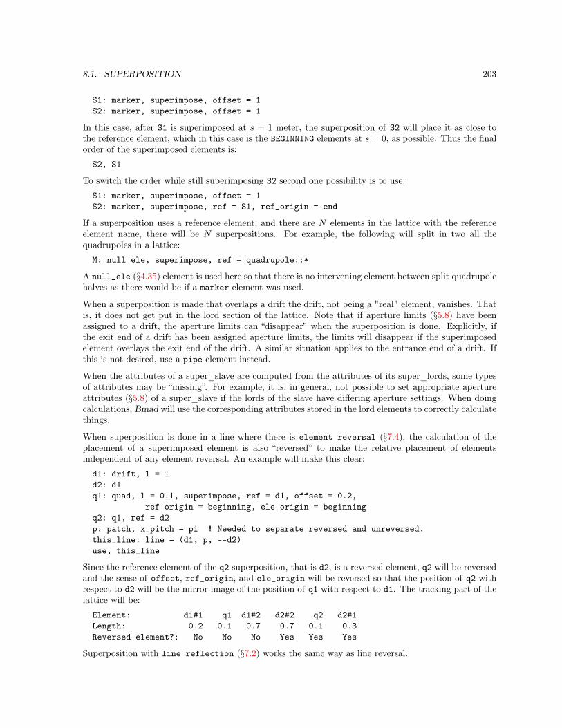
8.1. SUPERPOSITION 203

S1: marker, superimpose, offset = 1S2: marker, superimpose, offset = 1

In this case, after S1 is superimposed at s = 1 meter, the superposition of S2 will place it as close tothe reference element, which in this case is the BEGINNING elements at s = 0, as possible. Thus the finalorder of the superimposed elements is:

S2, S1

To switch the order while still superimposing S2 second one possibility is to use:

S1: marker, superimpose, offset = 1S2: marker, superimpose, ref = S1, ref_origin = end

If a superposition uses a reference element, and there are N elements in the lattice with the referenceelement name, there will be N superpositions. For example, the following will split in two all thequadrupoles in a lattice:

M: null_ele, superimpose, ref = quadrupole::*

A null_ele (§4.35) element is used here so that there is no intervening element between split quadrupolehalves as there would be if a marker element was used.

When a superposition is made that overlaps a drift the drift, not being a "real" element, vanishes. Thatis, it does not get put in the lord section of the lattice. Note that if aperture limits (§5.8) have beenassigned to a drift, the aperture limits can “disappear” when the superposition is done. Explicitly, ifthe exit end of a drift has been assigned aperture limits, the limits will disappear if the superimposedelement overlays the exit end of the drift. A similar situation applies to the entrance end of a drift. Ifthis is not desired, use a pipe element instead.

When the attributes of a super_slave are computed from the attributes of its super_lords, some typesof attributes may be “missing”. For example, it is, in general, not possible to set appropriate apertureattributes (§5.8) of a super_slave if the lords of the slave have differing aperture settings. When doingcalculations, Bmad will use the corresponding attributes stored in the lord elements to correctly calculatethings.

When superposition is done in a line where there is element reversal (§7.4), the calculation of theplacement of a superimposed element is also “reversed” to make the relative placement of elementsindependent of any element reversal. An example will make this clear:

d1: drift, l = 1d2: d1q1: quad, l = 0.1, superimpose, ref = d1, offset = 0.2,

ref_origin = beginning, ele_origin = beginningq2: q1, ref = d2p: patch, x_pitch = pi ! Needed to separate reversed and unreversed.this_line: line = (d1, p, --d2)use, this_line

Since the reference element of the q2 superposition, that is d2, is a reversed element, q2 will be reversedand the sense of offset, ref_origin, and ele_origin will be reversed so that the position of q2 withrespect to d2 will be the mirror image of the position of q1 with respect to d1. The tracking part of thelattice will be:

Element: d1#1 q1 d1#2 d2#2 q2 d2#1Length: 0.2 0.1 0.7 0.7 0.1 0.3Reversed element?: No No No Yes Yes Yes

Superposition with line reflection (§7.2) works the same way as line reversal.

204 CHAPTER 8. SUPERPOSITION, AND MULTIPASS

8.1.2 Superposition and Sub-Lines

Sometimes it is convenient to do simulations with only part of a lattice. The rule for how superpositionsare handled in this case is illustrated in the following example. Consider a lattice file which defines aline called full which is defined by two sublines called sub1 and sub2:sub1: line = ..., ele1, ...sub2: line = ...full: line = sub1, sub2m1: marker, superimpose, ref = ele1, offset = 3.7use, full

Now suppose you want to do a simulation using only the sub2 line. Rather than edit the original file,one way to do this would be to create a second file which overrides the used line:call, file = "full.bmad"use, sub2

where full.bmad is the name of the original file. What happens to the superposition of m1 in this case?Since m1 uses a reference element, ele1, that is not in sub1, Bmad will ignore the superposition. Eventhough Bmad will ignore the superposition of m1 here, Bmad will check that ele1 has been defined.If ele1 has not been defined, Bmad will assume that there is a typographic error and issue an errormessage.

Notice that in this case it is important for the superposition to have an explicit reference element sincewithout an explicit reference element the superposition is referenced to the beginning of the lattice.Thus, in the above example, if the superposition were written like:m1: marker, superimpose, offset = 11.3

then when the full line is used, the superposition of m1 is referenced to the beginning of full (which isthe same as the beginning of sub1) but when the sub2 line is used, the superposition of m1 is referencedto the beginning of sub2 which is not the same as the beginning of full.

8.1.3 Jumbo Super_Slaves

The problem with the way super_slave elements are created as discussed above is that edge effectswill not be dealt with properly when elements with non-zero fields are misaligned. When this is impor-tant, especially at low energy, a possible remedy is to instruct Bmad to construct “jumbo” super_slaveelements. The general idea is to create one large super_slave for any set of overlapping elements.Returning to the superposition example at the start of Section §8.1, If the superposition of solenoid S ismodified to beS: solenoid, l = 8, superimpose, ref = Q, ele_origin = beginning,

create_jumbo_slave = T

The result is shown in Fig. 8.1C. The tracking part of the lattice will beElement Key Length Total

1) Q\S Sol_quad 2 42) M Marker 03) S#2 Solenoid 3 104) D#2 Drift 4 14

Q and part of S have been combined into a jumbo super_slave named Q\S. Since the super_lordelements of a jumbo super_slave may not completely span the slave two attributes of each lord will beset to show the position of the lord within the slave. These two attributes arelord_pad1 ! offset at upstream endlord_pad2 ! offset at downstream end

8.1. SUPERPOSITION 205

lord_pad1 is the distance between the upstream edge of the jumbo super_slave and a super_lord.lord_pad2 is the distance between the downstream edge of a super_lord and the downstream edge ofthe jumbo super_slave. With the present example, the lords have the following padding:

lord_pad1 lord_pad2Q 0 3S 2 0

The following rule holds for all super lords with and without jumbo slaves:Sum of all slave lengths = lord length + lord_pad1 + lord_pad2

One major drawback of jumbo super_slave elements is that the tracking_method (§6.1) will, bynecessity, have to be runge_kutta, or time_runge_kutta and the mat6_calc_method (§6.2) will be setto tracking.

Notice that the problem with edge effects for non-jumbo super_slave elements only occurs when el-ements with nonzero fields are superimposed on top of one another. Thus, for example, one does notneed to use jumbo elements when superimposing a marker element.

Another possible way to handle overlapping fields is to use the field_overlaps element attribute asdiscussed in §5.17.

8.1.4 Changing Element Lengths when there is Superposition

When a program is running, if group (§4.22) or overlay (§4.37) elements are used to vary the length ofelements that are involved in superimposition, the results are different from what would have resultedif instead the lengths of the elements where changed in the lattice file. There are two reasons for this.First, once the lattice file has been parsed, lattices can be “mangled” by adding or removing elementsin a myriad of ways. This means that it is not possible to devise a general algorithm for adjustingsuperimposed element lengths that mirrors what the effect of changing the lengths in the lattice file.

Second, even if a lattice has not been mangled, an algorithm for varying lengths that is based on thesuperimpose information in the lattice file could lead to unexpected results. To see this consider thefirst example in Section §8.1. If the length of S is varied in the lattice file, the upstream edge of S willremain fixed at the center of Q which means that the length of the super_slave element Q#1 will beinvariant. On the other hand, if element S is defined byS: solenoid, l = 8, superimpose, offset = 6

This new definition of S produces exactly the same lattice as before. However, now varying the length ofS will result in the center of S remaining fixed and the length of Q#1 will not be invariant with changesof the length of S. This variation in behavior could be very confusing since, while running a program,one could not tell by inspection of the element positions what should happen if a length were changed.

To avoid confusion, Bmad uses a simple algorithm for varying the lengths of elements involved in su-perposition: The rule is that the length of the most downstream super_slave is varied. With the firstexample in Section §8.1, the group G varying the length of Q defined by:G: group = Q, var = l

would vary the length of Q\S which would result in an equal variation of the length of S. To keep thelength of S invariant while varying Q the individual super_slave lengths can be varied. Example:G2: group = Q#1, S#1:-1, var = l

The definition of G2 must be placed in the lattice file after the superpositions so that the super slavesreferred to by G2 have been created.

In the above example there is another, cleaner, way of achieving the same result by varying the down-stream edge of Q:G3: group = Q, var = end_edge

206 CHAPTER 8. SUPERPOSITION, AND MULTIPASS

8.2 Multipass

8.2.1 Multipass Fundamentals

Multipass lines are a way to handle the bookkeeping when different elements being tracked throughrepresent the same physical element. For example, consider the case where dual ring colliding beammachine is to be simulated. In this case the lattice file might look like:ring1: line = (..., IR_region, ...)ring2: line = (..., --IR_region, ...)IR_region: line = (Q1, ....)use, ring1, ring2

[The “–” construct means go through the line backwards (§7.4)] In this case, the Q1 element in ring1represents the same physical element in ring2. Thus the parameters of both the Q1s should be varied intandem. This can be done automatically using multipass. The use of multipass simplifies lattice andprogram development since the bookkeeping details are left to the Bmad bookkeeping routines.

To illustrate how multipass works, consider the example of an Energy Recovery Linac (ERL) wherethe beam will recirculate back through the LINAC section to recover the energy in the beam before it isdumped. In Bmad, this situation can simulated by designating the LINAC section as multipass. Thelattice file might look like:RF1: lcavitylinac: line[multipass] = (RF1, ...)erl: line = (linac, ..., linac)use, erlexpand_latticeRF1\2[phi0_multipass] = 0.5

The line called linac is designated as multipass. This linac line appears twice in the line erl anderl is the root line for lattice expansion. The lattice constructed from erl will have two RF1 elementsin the tracking part of the lattice:RF1\1, ..., RF1\2, ...

Since the two elements are derived from a multipass line, they are given unique names by addinga \n suffix. These types of elements are known as multipass_slave elements. In addition, to themultipass_slave elements, there is a multipass_lord element (that doesn’t get tracked through)called RF1 in the lord part of the lattice (§2.4). Changes to attributes of the lord RF1 element will bepassed to the slave elements by Bmad’s bookkeeping routines. Assuming that the phase of RF1\1 givesacceleration, to make RF1\2 decelerate the phi0_multipass attribute of RF1\2 is set to 0.5. This isthe one attribute that Bmad’s bookkeeping routines will not touch when transferring attribute valuesfrom RF1 to its slaves. Notice that the phi0_multipass attribute had to be set after expand_lattice(§3.22) is used to expand the lattice. This is true since Bmad does immediate evaluation and RF1\2 doesnot exist before the lattice is expanded. Phi0_multipass is useful with relative time tracking §24.1.However, phi0_multipass is “unphysical” and is just a convenient way to shift the phase pass-to-passthrough a given cavity. To “correctly” simulate the recirculating beam, absolute time tracking should beused and the length of the lattice from a cavity back to itself needs to be properly adjusted to get thedesired phase advance. See the discussion in section §24.1.

Multiple elements of the same name in a multipass line are considered physically distinct. Example:m_line: line[multipass] = (A, A, B)u_line: line = (m_line, m_line)use, u_line

In this example the tracking part of the lattice isA\1, A\1, B\1, A\2, A\2, B\2

8.2. MULTIPASS 207

In the control section of the lattice there will be two multipass lords called A and one called B. [Thatis, Bmad considers the lattice to have three physically distinct elements.] The first A lord controls the1st and 4th elements in the tracking part of the lattice and the second A lord controls the 2nd and 5thelements. If m_line was not marked multipass, the tracking part of the lattice would have four A andtwo B elements and there would be no lord elements.

Sublines contained in a multipass line that are themselves not marked multipass act the same as if theelements of the subline where substituted directly in place of the subline in the containing line. Forexample:a_line: line = (A)m_line: line[multipass] = (a_line, a_line, B)u_line: line = (m_line, m_line)use, u_line

In this example, a_line, which is a subline of the multipass m_line, is not designated multipass andthe result is the same as the previous example where m_line was defined to be (A, A, B). That is,there will be three physical elements represented by three multipass lords.

Multipass lines do not have to be at the same “level” in terms of nesting of lines within lines. Additionally,multipass can be used with line reversal (§7.4). Example:m_line: line[multipass] = (A, B)m2_line: line = (m_line)P: patch, ...arc: line = (..., P)u_line: line = (m_line, arc, --m2_line)use, u_line

Here the tracking part of the lattice isA\1, B\1, ..., B\2 (r), A\2 (r)

The “(r)” here just denotes that the element is reversed and is not part of the name. The lattice will havea multipass lord A that controls the two A\n elements and similarly with B. This lattice represents thecase where a particle goes through the m_line in the “forward” direction, gets turned around in the arcline, and then passes back through m_line in the reverse direction. While it is possible to use reflection“−” (§7.2) instead of reversal “−−” (§7.4), reflection here does not make physical sense. Needed here isa reflection patch P (§4.38) between reversed and unreversed elements.

The procedure for how to group lattice elements into multipass slave groups which represent the samephysical element is as follows. For any given element in the lattice, this element has some line it camefrom. Call this line L0. The L0 line in turn may have been contained in some other line L1, etc. Thechain of lines L0, L1, ..., Ln ends at some point and the last (top) line Ln will be one of the root lineslisted in the use statement (§7.7) in the lattice file. For any given element in the lattice, starting withL0 and proceeding upwards through the chain, let Lm be the first line in the chain that is marked asmultipass. If no such line exists for a given element, that element will not be a multipass slave. Forelements that have an associated Lm multipass line, all elements that have a common Lm line and havethe same element index when Lm is expanded are put into a multipass slave group (for a given line theelement index with respect to that line is 1 for the first element in the expanded line, the second elementhas index 2, etc.). For example, using the example above, the first element of the lattice, A\1, has thechain:

m_line, u_lineThe last element in the lattice, (A\2), has the chainm_line, m2_line, u_line

For both elements the Lm line is m_line and both elements are derived from the element with index 1with respect to m_line. Therefore, the two elements will be slaved together.

As a final example, consider the case where a subline of a multipass line is also marked multipass:

208 CHAPTER 8. SUPERPOSITION, AND MULTIPASS

a_line: line[multipass] = (A)m_line: line[multipass] = (a_line, a_line, B)u_line: line = (m_line, m_line)use, u_line

In this case the tracking part of the lattice will be:A\1, A\2, B\1, A\3, A\4, B\2

There will be two lord elements representing the two physically distinct elements A and B. The A lordelement will will control the four A\n elements in the tracking part of the lattice. The B lord will controlthe two B\n elements in the tracking part of the lattice.

To simplify the constructed lattice, if the set of lattice elements to slave together only contains oneelement, a multipass lord is not constructed. For example:m_line: line[multipass] = (A, A, B)u_line: line = (m_line)use, u_line

In this example no multipass lords are constructed and the lattice is simplyA, A, B

It is important to note that the global coordinates (§15.2) of the slaves of a given multipass lord arenot constrained by Bmad to be the same. It is up to the lattice designer to make sure that the physicalpositions of the slaves makes sense (that is, are the same).

8.2.2 The Reference Energy in a Multipass Line

Consider the lattice where the tracking elements areA\1, C, A\2

where A\1 and A\2 are multipass slaves of element A and C is a lcavity element with some finite voltage.In this case, the reference energy calculation (§5.5) where the reference energy of an element is inheritedfrom the previous element, assigns differing reference energies to A\1 and A\2. In such a situation, whatshould be the assigned reference energy for the multipass lord element A? Bmad calculates the lordreference energy in one of two ways. If, in the lattice file, e_tot or p0c is set for the multipass lordelement, that setting will be used. Exception: For em_field, lcavity, and custom elements where thereference energy may change, set e_tot_start or p0c_start instead of e_tot or p0c. If the referenceenergy (or reference momentum) is not set in the lattice file, the reference energy of the lord is set equalto the reference energy of the first pass slave element.

It is important to keep this convention in mind if the normalized field strength (k1, for a quadrupole,etc.) for the lord element is set in the lattice file. To be physical, the unnormalized strength (the actualfield) has to be the same for all slave elements. Bmad therefore calculates the unnormalized strength forthe lord and sets the slave unnormalized strengths to be equal to the lord unnormalized strength. Afterthis, the normalized strength for the slaves is calculated. Notice that the normalized strengths for theslaves will differ from each other. For sbend and rbend elements the calculation is a bit trickier. Herethe g bending strength must be the same for all slaves since the setting of g determines the referencegeometry. In this case, dg for each slave is adjusted accordingly so that the total normalized field, g +dg, gives the same unnormalized field for all slaves. Note that since the normalized field is calculatedfrom the unnormalized field for the slaves, the setting of field_master (§5.2) is set to True for all theslaves independent of the setting of field_master for the lord.

To keep track of how the reference energy has been calculated for an element, Bmad sets an internalelement switch called multipass_ref_energy which is set to “user_set” if the energy is explicitly set

8.2. MULTIPASS 209

in the lattice file and is set to “first_pass” if the reference energy is calculated from the the standardreference energy calculation of the first pass slave element.

Note: Historically, there was an element parameter n_ref_pass that could be set to control the referenceenergy. This parameter may be seen in old lattice files but will be ignored.

An example of an ERL lattice with multipass can be found in Section §12.3.

210 CHAPTER 8. SUPERPOSITION, AND MULTIPASS

Chapter 9

Lattice File Global Parameters

This chapter deals with statements that can be used to set “global” parameter values. That is, parametervalues that are associated with the lattice as a whole and not simply associated with a single element.

Discussed elsewhere are the global structures (§10.1) bmad_com and ptc_com (§10.4).

9.1 Parameter Statements

Parameter statements are used to set a number of global variables. If multiple branches are present(§2.2), these variables pertain to the root branch. The variables that can be set by parameter areparameter[absolute_time_tracking] = <Logical> ! Absolute time used for RF clock?parameter[custom_attributeN] = <string> ! Defining custom attributes (§3.8).parameter[default_tracking_species] = <Switch> ! Default type of tracked particle.

! Default is ref_particle.parameter[e_tot] = <Real> ! Reference total Energy.

! Default: 1000 * rest_energy.parameter[electric_dipole_moment] = <Real> ! Particle electric dipole moment.parameter[live_branch] = <Logical> ! Is branch fit for tracking?parameter[geometry] = <Switch> ! Open or closedparameter[lattice] = <String> ! Lattice name.parameter[machine] = <String> ! Machine name.parameter[n_part] = <Real> ! Number of particles in a bunch.parameter[no_end_marker] = <Logical> ! Default: False.parameter[p0c] = <Real> ! Reference momentum.parameter[particle] = <speciesID> ! Reference species: positron, proton, etc.parameter[photon_type] = <Switch> ! Incoherent or coherent photons?parameter[ran_seed] = <Integer> ! Random number generator init.parameter[taylor_order] = <Integer> ! Default: 3parameter[high_energy_space_charge_on] = <logical>

Examplesparameter[lattice] = "L9A19C501.FD93S_4S_15KG"parameter[geometry] = closedparameter[taylor_order] = 5parameter[E_tot] = 5.6e9 ! eV

211

212 CHAPTER 9. LATTICE FILE GLOBAL PARAMETERS

parameter[absolute_time_tracking]The absolute_time_tracking switch sets whether the clock for the lcavity and rfcavity ele-ments is tied to the reference particle or to uses the absolute time (§24.1). A value of False (thedefault) mandates relative time and a value of True mandates absolute time. The exception isthat for an e_gun element (§4.15), absolute time tracking is always used in order to be able toavoid problems with a zero reference momentum at the beginning of the element.

parameter[custom_attributeN]Here N is an integer between 1 and 40. For more information on defining custom attributes, see§3.8. Name of the machine the lattice simulates. Example: "LHC".

parameter[live_branch]Setting live_branch to False (default is True) indicates to a program that no tracking or otheranalysis of the root branch should be done. This can be useful if the lattice has multiple branchesand analysis of the root branch is not necessary. Other branches can also be marked as alive/deadusing line parameter statements (§9.4). Note that the Bmad library itself ignores the setting oflive_branch and it is up to the program being run to decide if this parameter is ignored or not.In particular, the Tao program (§1.2) will respect the setting of live_branch.

parameter[default_tracking_species]The parameter[default_tracking_species] switch establishes the default type of particles tobe tracked. See §3.10 for the syntax for naming particle species. In addition, this switch can beset to:ref_particle ! defaultanti_ref_particle

By default, default_tracking_species is set to ref_particle so that the particle being trackedis the same as the reference particle set by param[particle]. In the case, for example, where thereare particles going one way and antiparticles going the another, default_tracking_species canbe used to switch between tracking the particles or antiparticles.

parameter[e_tot], parameter[p0c]The parameter[e_tot] and parameter[p0c] are the reference total energy and momentum at thestart of the lattice. Each element in a lattice has an individual reference e_tot and p0c attributeswhich are dependent parameters. The reference energy and momentum will only change betweenLCavity or Patch elements. The starting reference energy, if not set, will be set to 1000 timethe particle rest energy. Note: beginning[e_tot] and beginning[p0c] (§9.4) are equivalent toparameter[e_tot] and parameter[p0c].

parameter[electric_dipole_moment]The electric_dipole_moment sets the electric dipole moment value η for use when tracking withspin (§22.1).

parameter[geometry]Valid geometry settings areclosed ! Default w/o LCavity element present.open ! Default if LCavity elements present.

A machine with a closed geometry is something like a storage ring where the particle beamrecirculates through the machine. A machine with an open geometry is something like a linac. Inthis case, if the reference particle is not a photon, the initial Twiss parameters need to be specifiedin the lattice file using the beginning statement (§9.4). If the geometry is not specified, closed isthe default. The exception is that if there is an Lcavity element present or the reference particleis a photon, open will be the default.Notice that by specifying a closed geometry it does not mean that the downstream end of thelast element of the lattice has the same global coordinates (§15.2) as the global coordinates at

9.1. PARAMETER STATEMENTS 213

the beginning. Setting the geometry to closed simply signals to a program to compute closedorbits and periodic Twiss parameters as opposed to calculating orbits and Twiss parameters basedupon initial orbit and Twiss parameters at the beginning of the lattice. Indeed, it is sometimesconvenient to treat lattices as closed even though there is no closure in the global coordinate sense.For example, when a machine has a number of repeating “periods”, it may be convenient to onlyuse one period in a simulation. Since Bmad ignores closure in the global coordinate sense, it is upto the lattice designer to ensure that a lattice is truly geometrically closed if that is desired.

high_energy_space_charge_onToggle to turn on or off the ultra-relativistic space charge effect in particle tracking (§19.5). Compu-tationally, this is separate from the lower energy space charge and CSR calculation (§19.4). Defaultis False. Notice that including the high energy space charge can be done on a branch-by-branchbasis (§9.4).

parameter[lattice]Used to set the lattice name. The lattice name is stored by Bmad for use by a program but itdoes not otherwise effect any Bmad routines.

parameter[n_part]The parameter[n_part] is the number of particle in a bunch. it is used with BeamBeam elementsand is used to calculate the change in energy through an Lcavity. See §4.27 for more details.

parameter[no_end_marker]Setting parameter[no_end_marker] to True will suppress the automatic inclusion of a markernamed END at the end of the lattice (§7.1).

parameter[p0c]See parameter[e_tot].

parameter[particle]The parameter[particle] switch sets the reference species. See §3.10 for the syntax for namingparticle species.

The setting of the reference particle is used, for example, to determine the direction of the fieldin a magnet and given the normalized field strength (EG: k1 for a quadrupole). Generally, theparticles that by default are tracked through a lattice are the same as the reference particle. Thisdefault behavior can be altered by setting parameter[default_tracking_species].

parameter[photon_type]The photon_type switch is used to set the type of photons that are used in tracking. Possiblesettings are:incoherent ! Defaultcoherent

The general rule is use incoherent tracking except when there is a diffraction_plate element inthe lattice.

parameter[ptc_exact_model]Deprecated. Replaced by ptc_com[exact_model] (§10.4).The ptc_exact_model and ptc_exact_misalign switches affect tracking using the PTC library.See §6.4 for more details.

parameter[ptc_max_fringe_order]When using PTC tracking (§1.4), the parameter[ptc_max_fringe_order] determines the maxi-mum order of the calculated fringe fields. The default is 2 which means that fringe fields due to aquadrupolar field. These fields are 3rd order in the transverse coordinates.

214 CHAPTER 9. LATTICE FILE GLOBAL PARAMETERS

parameter[ran_seed]For more information on parameter[ran_seed] see §3.13.

parameter[taylor_order]The Taylor order (§23.1) is set by parameter[taylor_order] and is the maximum order for aTaylor map.

9.2 Particle_Start Statements

particle_start statements are used, among other things to set the starting coordinates for particletracking. If multiple branches are present (§2.2), these variables pertain to the root branch.particle_start[x] = <Real> ! Horizontal position.particle_start[px] = <Real> ! Horizontal momentum.particle_start[y] = <Real> ! Vertical position.particle_start[py] = <Real> ! Vertical momentum.particle_start[z] = <Real> ! Longitudinal position.particle_start[pz] = <Real> ! Momentum deviation. Only for non-photons.particle_start[direction] = +/-1 ! Longitudinal direction of travel.particle_start[E_photon] = <Real> ! Energy (eV). Only used for photons.particle_start[emittance_a] = <Real> ! A-mode emittanceparticle_start[emittance_b] = <Real> ! B-mode emittanceparticle_start[emittance_z] = <Real> ! Z-mode emittanceparticle_start[sig_z] = <Real> ! Beam sigma in z-directionparticle_start[sig_pz] = <Real> ! Beam Sigma pzparticle_start[field_x] = <Real> ! Photon beam field along x-axisparticle_start[field_y] = <Real> ! Photon beam field along y-axisparticle_start[phase_x] = <Real> ! Photon beam phase along x-axisparticle_start[phase_y] = <Real> ! Photon beam phase along y-axisparticle_start[t] = <Real> ! Absolute timeparticle_start[spin_x] = <Real> ! Spin polarization x-coordinateparticle_start[spin_y] = <Real> ! Spin polarization y-coordinateparticle_start[spin_z] = <Real> ! Spin polarization z-coordinate

Normally the absolute time, set by particle_start[t], is a dependent parameter set by solvingEq. (15.28) for t. The exception is when the initial velocity is zero. (This can happen if there isan e_gun (§4.15) element in the lattice). In this case, z must be zero and t is an independent parameterthat can be set.

The longitudinal direction of travel is set by particle_start[direction]. This can be set to +1 (travelin the +s direction) or -1 for the reverse. +1 is the default. Generally particle_start[direction]should not be set to -1 since most programs will not be constructed to handle this situation. To track aparticle in the reverse direction see §12.6.

For particles with spin, the spin can be specified using Cartesian coordinates with spin_x, spin_y, andspin_z.

For photons, px, py, and pz are the normalized velocity components (Cf. Eq. (15.38)). For photons pzis a dependent parameter which will be set so that Eq. (15.39) is obeyed.

Note: particle_start used to be called beam_start. Since this was confusing (beam initializationparameters are stored in a separate beam_init_struct structure (§11.1)), the name was changed. Cur-rently the use of the beam_start name is deprecated but still supported for backwards compatibility.

9.3. BEAM STATEMENT 215

Exampleparticle_start[y] = 2 * particle_start[x]

9.3 Beam Statement

The beam statement is provided for compatibility with MAD. The syntax isbeam, energy = GeV, pc = GeV, particle = <Switch>, n_part = <Real>

For examplebeam, energy = 5.6 ! Note: GeV to be compatible with MADbeam, particle = electron, n_part = 1.6e10

Setting the reference energy using the energy attribute is the same as using parameter[e_tot]. Sim-ilarly, setting pc is equivalent to setting parameter[p0c]. Valid particle switches are the same asparameter[particle].

9.4 Beginning and Line Parameter Statements

For non–circular lattices, the beginning statement can be used to set the Twiss parameters and beamenergy at the beginning of the first lattice branch.beginning[alpha_a] = <Real> ! "a" mode alphabeginning[alpha_b] = <Real> ! "b" mode alphabeginning[beta_a] = <Real> ! "a" mode betabeginning[beta_b] = <Real> ! "b" mode betabeginning[cmat_ij] = <Real> ! C coupling matrix. i, j = ‘‘1’’, or ‘‘2’’beginning[e_tot] = <Real> ! Reference total energy in eV.beginning[eta_x] = <Real> ! x-axis dispersionbeginning[eta_y] = <Real> ! y-axis dispersionbeginning[etap_x] = <Real> ! x-axis dispersion derivative.beginning[etap_y] = <Real> ! y-axis dispersion derivative.beginning[p0c] = <Real> ! Reference momentum in eV.beginning[phi_a] = <Real> ! "a" mode phase.beginning[phi_b] = <Real> ! "b" mode phase.beginning[ref_time] = <Real> ! Starting reference time.beginning[s] = <Real> ! Longitudinal starting position.

The gamma_a, gamma_b, and gamma_c (the coupling gamma factor) will be kept consistent with the valuesset. If not set the default values are all zero. beginning[e_tot] and parameter[e_tot] are equivalentand one or the other may be set but not both. Similarly, beginning[p0c] and parameter[p0c] areequivalent.

For any lattice the beginning statement can be used to set the starting floor position of the first latticebranch (see §15.2). The syntax isbeginning[x_position] = <Real> ! X positionbeginning[y_position] = <Real> ! Y positionbeginning[z_position] = <Real> ! Z positionbeginning[theta_position] = <Real> ! Angle on floorbeginning[phi_position] = <Real> ! Angle of attackbeginning[psi_position] = <Real> ! Roll angle

216 CHAPTER 9. LATTICE FILE GLOBAL PARAMETERS

If the floor position is not specified, the default is to place beginning element at the origin with all anglesset to zero.

The beginning statement is useful in situations where only parameters for the first branch need bespecified. If this is not the case, the parameters for any branch can be specified using a statement of theformline_name[parameter] = <Value>

This construct is called a line parameter statement Here line_name is the name of a line and parameteris the name of a parameter. The parameters that can be set here are the same parameters that can beset with the beginning statement with the additional parameters from the parameter statement:default_tracking_speciesgeometryhigh_energy_space_charge_onlive_branchparticleinherit_from_fork

Example:x_ray_fork: fork, to_line = x_rayx_ray: line = (...)x_ray[E_tot] = 100

The inherit_from_fork logical is used to determine if the reference energy and Twiss parameters ascalculated from the fork element defining the branch is used to set the beginning element of the branch.This parameter is ignored if the fork element does not fork to the beginning element of the branch. Thedefault is True. If any reference energy or momentum or any Twiss parameter is set, inherit_from_forkis implicitly set to False.

Rules:

1. The floor position of a line can only be set if the line is used for a root branch.

2. Line parameters statements must come after the associated line. This rule is similar to the rulethat element attribute redefinitions must come after the definition of the element.

Chapter 10

Parameter Structures

10.1 What is a Structure?

A “structure” is a collection of parameters. Bmad has various structures which can be used for varioustasks. For example, the beam_init_struct structure (§11.1) is used to set parameters used to initializeparticle beams.

A given program may give the user access to some of these structures so, in order to allow intelligentparameter setting, this chapter gives an in-depth description of the most common ones.

Each structure has a “structure name” (also called a “type name”) which identifies the list of parame-ters (also called “components”) in the structure. Associated with a structure there will be an “instance”of this structure and this instance will have an “instance name” which is what the user uses to set pa-rameters. It is possible to have multiple instances of a structure. For example, in the situation wherea program is simulating multiple particle beams, there could be multiple beam_init_struct (§11.1)instances with one for each beam.

Bmad defines uses some structures to hold global parameters. That is, parameters that shared by allcode. Each of these structures has a single associated instance. These are:

Structure Instance

bmad_common_stuct bmad_comcsr_parameter_stuct csr_param

All other structures will have instance names that are program specific. That is, see the programdocumentation for the instance name(s) used.

For historical reasons, There are two syntaxes used for setting structure components. The syntax whensetting in a lattice file uses square brackets:instance_name[parameter_name] = value

When setting a component in a program initialization file the syntax uses the percent “%” character:instance_name%parameter_name = value

Examples:bmad_com[max_aperture_limit] = 10 ! Lattice file syntax.bmad_com%max_aperture_limit = 10 ! Program initialization file syntax.

217

218 CHAPTER 10. PARAMETER STRUCTURES

this sets the max_aperture_limit parameter of bmad_com which is an instance name of the bmad_common_struct.Note: A program is free to set the instance name for any structure. This should be documented in theprogram manual.

Note: Thought must be given to setting bmad_com and other global parameters in a lattice file (§10.4)since that will affect every program that uses the lattice.

10.2 Bmad_Common_Struct

The bmad_common_struct structure contains a set of global parameters. There is only one global instance(§10) of this structure and this instance has the name bmad_com. The components of this structure alongwith the default values are:type bmad_common_structreal(rp) max_aperture_limit = 1e3 ! Max Aperture.real(rp) d_orb(6) = 1e-5 ! for the make_mat6_tracking routine.real(rp) default_ds_step = 0.2 ! Integration step size.real(rp) significant_length = 1e-10 ! meterreal(rp) rel_tol_tracking = 1e-8 ! Closed orbit relative tolerance.real(rp) abs_tol_tracking = 1e-11 ! Closed orbit absolute tolerance.real(rp) rel_tol_adaptive_tracking = 1e-8 ! Runge-Kutta tracking relative tolerance.real(rp) abs_tol_adaptive_tracking = 1e-10 ! Runge-Kutta tracking absolute tolerance.real(rp) init_ds_adaptive_tracking = 1e-3 ! Initial step size.real(rp) min_ds_adaptive_tracking = 0 ! Minimum step size to use.real(rp) fatal_ds_adaptive_tracking = 1e-8 ! Threshold for loosing particles.real(rp) autoscale_amp_abs_tol = 0.1_rp ! Autoscale absolute amplitude tolerance (eV).real(rp) autoscale_amp_rel_tol = 1d-6 ! Autoscale relative amplitude tolerancereal(rp) autoscale_phase_tol = 1d-5 ! Autoscale phase tolerance.real(rp) electric_dipole_moment = 0 ! Particle’s EDM. Call set_ptc to transfer value to PTC.real(rp) ptc_cut_factor = 0.006 ! Cut factor for PTC trackingreal(rp) sad_eps_scale = 5.0d-3 ! Used in sad_mult step length calc.real(rp) sad_amp_max = 5.0d-2 ! Used in sad_mult step length calc.integer sad_n_div_max = 1000 ! Used in sad_mult step length calc.integer taylor_order = 3 ! 3rd order is defaultinteger default_integ_order = 2 ! PTC integration orderinteger ptc_max_fringe_order = 2 ! PTC max fringe order (2 => Quadrupole !).integer max_num_runge_kutta_step = 10000 ! Max num RK steps before particle is lost.logical rf_phase_below_transition_ref = F ! Autoscale around phase phi0 = 0.5logical sr_wakes_on = T ! Short range wakefields?logical lr_wakes_on = T ! Long range wakefieldslogical mat6_track_symmetric = T ! symmetric offsetslogical ptc_use_orientation_patches = T ! Ele orientation translated to PTC patches?logical auto_bookkeeper = T ! Automatic bookkeeping?logical csr_and_space_charge_on = F ! CSR and space charge (separate from HE SC).logical spin_tracking_on = F ! spin tracking?logical spin_sokolov_ternov_flipping_on = F ! Spin flipping during radiation emission?logical radiation_damping_on = F ! Radiation damping toggle.logical radiation_fluctuations_on = F ! Radiation fluctuations toggle.logical radiation_zero_average = F ! Shift so that average radiation kick is zero?logical conserve_taylor_maps = T ! Enable bookkeeper to set

! ele%taylor_map_includes_offsets = F?

10.2. BMAD_COMMON_STRUCT 219

logical absolute_time_tracking_default = F ! Default for lat%absolute_time_trackinglogical aperture_limit_on = T ! Use aperture limits in tracking.logical debug = F ! Used for code debugging.

end type

Parameter description:

abs_tol_adaptive_trackingAbsolute tolerance to use in adaptive tracking. This is used in runge-kutta and time_runge_kuttatracking (§6.4).

abs_tol_trackingAbsolute tolerance to use in tracking. Specifically, Tolerance to use when finding the closed orbit.

absolute_time_tracking_defaultDefault setting to be applied to a lattice if absolute_time_tracking (§9.1) is not specifiedin a lattice file. Additionally, if an element that is not associated with a lattice is tracked,absolute_time_tracking_default will be used to determine whether absolute time tracking isused.

To change between absolute and relative time tracking (§24.1) after lattice file parsing, the absolute_time_trackingcomponent of a lat_struct (§35.12) can be appropriately set.

aperture_limit_on]Aperture limits may be set for elements in the lattice (§5.8). Setting aperture_limit_on to Falsewill disable all set apertures. True is the default.

auto_bookkeeperToggles automatic or intelligent bookkeeping. See section §31.6 for more details.

autoscale_amp_abs_tolUsed when Bmad autoscales (§5.18) an elements field amplitude. This parameter sets the absolutetolerance for the autoscale amplitude parameter.

autoscale_amp_rel_tolUsed when Bmad autoscales (§5.18) an elements field amplitude. This parameter sets the relativetolerance for the autoscale amplitude parameter. Used when Bmad autoscales (§5.18) an elementsAC phase. This parameter sets the absolute tolerance for the autoscale parameter.

autoscale_phase_tol

init_ds_adaptive_trackingInitial step to use for adaptive tracking. This is used in runge-kutta and time_runge_kuttatracking (§6.4).

conserve_taylor_mapsToggle to determine if the Taylor map for an element include any element “misalignments”. SeeSection §6.7 for more details.

csr_and_space_charge_onTurn on or off the coherent synchrotron radiation and space charge calculations. (§19.4). Thespace charge calculation here is not to be confused with the high energy space charge calculation(§19.5)

220 CHAPTER 10. PARAMETER STRUCTURES

d_orbSets the orbit displacement used in the routine that calculates the transfer matrix through anelement via tracking. That is, when the mat6_calc_method (§6.2) is set to tracking. d_orb needsto be large enough to avoid significant round-off errors but not so large that nonlinearities willaffect the results. The default value is 10−5. Also see mat6_track_symmetric.

debugUsed for communication between program units for debugging purposes.

default_ds_stepStep size for tracking code §6 that uses a fixed step size. For example, symp_lie_ptc tracking.

default_integ_orderOrder of the integrator used by Étienne Forest’s PTC code (§28.2). The order of the PTC integratoris like the order of a Newton-Cotes method. Higher order means the error term involves a higherorder derivative of the field.

electric_dipole_momentThe electric dipole moment value used in tracking a particle’s spin (§22.1).

fatal_ds_adaptive_trackingThis is used in runge-kutta and time_runge_kutta tracking (§6.4). If the step size falls below thevalue set for fatal_ds_adaptive_tracking, a particle is considered lost. This prevents a programfrom “hanging” due to taking a large number of extremely small steps. The most common causeof small step size is an “unphysical” magnetic or electric field.

lr_wakes_onToggle for turning on or off long-range higher order mode wakefield effects.

mat6_track_symmetricToggle to turn off whether the transfer matrix from tracking routine (twiss_from_tracking) tracks12 particles at both plus and minus d_orb values or only tracks 7 particles to save time but is lessaccurate..

max_aperture_limitSets the maximum amplitude a particle can have during tracking. If this amplitude is exceeded,the particle is lost even if there is no element aperture set. Having a maximum aperture limit helpsprevent numerical overflow in the tracking calculations.

max_num_runge_kutta_stepThe maximum number of steps to take through an element with runge_kutta or time_runge_kuttatracking. The default value is 10,000. If the number of steps reaches this value, the particle beingtracked is marked as lost and a warning message is issued. Under “normal” circumstances, a par-ticle will take far fewer steps to track through an element. If a particle is not through an elementafter 10,000 steps, it generally indicates that there is a problem with how the field is defined. Thatis, the field does not obey Maxwell’s Equations. Especially: discontinuities in the field can causeproblems.

min_ds_adaptive_trackingThis is used in runge-kutta and time_runge_kutta tracking (§6.4). Minimum step size to use foradaptive tracking. If To be useful, min_ds_adaptive_tracking must be set larger than the valueof fatal_ds_adaptive_tracking. In this case, particles are never lost due to taking too small astep.

10.2. BMAD_COMMON_STRUCT 221

ptc_use_orientation_patchesWith Bmad, there is no distinction whether an element’s orientation attributes (offsets, pitches,or tilt (§5.6)) is deliberate (part of the “design” of the machine) or an error (a “misalignment”).With PTC this is not true. If the ptc_use_orientation_patches switch is set to True (thedefault), when a Bmad element is translated to PTC, the element’s orientation attributes are storedas patches. That is, “desgin” values. If set to False, these parameters are stored as misalignments.This will generally not make any difference to a calculation. The exception comes with PTC centricprograms that vary machine parameters.1

ptc_max_fringe_orderMaximum order for computing fringe field effects in PTC.

rf_phase_below_transition_refUsed when Bmad autoscales (§5.18) an rfcavity and when Bmad calculates the reference timethrough a cavity (which affects calculation of phase space z via Eq. (15.28)). If True, the referencephase will be taken to be at phi0 = 0.5 which is appropriate for a ring below transition. Defaultis False in which case autoscaling will be around the phase phi0 = 0.

radiation_damping_onToggle to turn on or off effects due to radiation damping in particle tracking (§20.1). The defaultis False. Note: The standard Bmad emittance calculation, which involves calculating synchrotronradiation integrals (§20.2) can be done without a problem when radiation_damping_on is set toFalse. However, since the closed orbit will be affected by whether radiation_damping_on is setor not, the calculated emittances will depend upon the setting of radiation_damping_on.

radiation_fluctuations_onToggle to turn on or off effects due to radiation fluctuations in particle tracking (§20.1). The defaultis False. Note: The standard Bmad emittance calculation, which involves calculating synchrotronradiation integrals (§20.2) can be done without a problem when radiation_damping_on is set toFalse. And since the calculation of the closed orbit ignores the fluctuating part of the radiation, thesetting of radiation_damping_on, unlike the setting of radiation_damping_on, will not affectthe emittance calculation.

radiation_zero_averageAs discussed in Section §20.1, it is sometimes convenient to shift the emitted radiation spectrum sothat the average energy emitted along the closed orbit is zero. This gets rid of the “sawtooth” effect.To shift the average emitted energy to zero, set radiation_zero_average to True. The defaultis False. Currently, the shifting of the spectrum only works for non PTC dependent tracking.That is, the shifting is not applicable to tracking with Taylor maps and with symp_lie_ptc (§6.1)tracking.

rel_tol_adaptive_trackingRelative tolerance to use in adaptive tracking. This is used in runge_kutta and time_runge_kuttatracking (§6.4).

rel_tol_trackingRelative tolerance to use in tracking. Specifically, Tolerance to use when finding the closed orbit.

significant_lengthSets the scale to decide if two length values are significantly different. For example, The superpo-sition code will not create any super_slave elements that have a length less then this.

1None of the programs that come bundled with Bmad (a Bmad Distribution) are PTC centric.

222 CHAPTER 10. PARAMETER STRUCTURES

sr_wakes_onToggle for turning on or off short-range higher order mode wakefield effects.

spin_sokolov_ternov_flipping_onThis determines if the Sokolov-Ternov effect is included in a simulation. The Sokolov-Ternoveffect[Barber99] is the self-polarization of charged particle beams due to asymmetric flipping of aparticle’s spin when the particle is bent in a magnetic field. Also, spin flipping will not be done ifspin tracking is off or both radiation damping and excitation are off.

spin_tracking_onDetermines if spin tracking is performed or not.

taylor_orderCutoff Taylor order of maps produced by sym_lie_ptc.

10.3 PTC_Common_Struct

The ptc_common_struct structure contains a set of global parameters that effect tracking when PTCis involved. There is only one global instance (§10) of this structure and this instance has the nameptc_com. The components of this structure along with the default values are:

type ptc_common_structtaylor_order_ptc = 3 ! What has been set in PTC. 0 -> not yet settaylor_order_saved = 3 ! Default to use.max_fringe_order = 2 ! 2 => Quadrupole.complex_ptc_used = True ! Complex PTC code in use?use_totalpath = False ! phase space z = time instead of time - ref_time?old_integrator = True ! PTC OLD_INTEGRATOR.exact_model = False ! PTC EXACT_MODEL.exact_misalign = True ! PTC ALWAYS_EXACTMIS.

end type

10.4 Bmad_Com and PTC_Com

The parameters of the bmad_com instance of the bmad_common_struct structure (§10.2) can be set inthe lattice file using the syntax

bmad_com[parm-name] = value

where parm-name is the name of a component of bmad_common_struct. For example:

bmad_com[rel_tol_tracking] = 1e-7

A similar situation holds for the ptc_com instance of the ptc_common_struct structure.

Be aware that setting either a bmad_com or ptc_com parameter value in a lattice file will affect allcomputations of a program even if the program reads in additional lattice files. That is, setting ofbmad_com or ptc_com components is “sticky” and persists even when other lattice files are read in. Thereare two exceptions: A program is always free to override settings of these parameters. Additionally, asecond lattice file can also override the setting made in a prior lattice file.

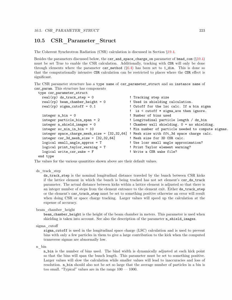
10.5. CSR_PARAMETER_STRUCT 223

10.5 CSR_Parameter_Struct

The Coherent Synchrotron Radiation (CSR) calculation is discussed in Section §19.4.

Besides the parameters discussed below, the csr_and_space_charge_on parameter of bmad_com (§10.4)must be set True to enable the CSR calculation. Additionally, tracking with CSR will only be donethrough elements where the parameter csr_method (§6.4) has been set to 1_dim. This is done sothat the computationally intensive CSR calculation can be restricted to places where the CSR effect issignificant.

The CSR parameter structure has a type name of csr_parameter_struct and an instance name ofcsr_param. This structure has componentstype csr_parameter_structreal(rp) ds_track_step = 0 ! Tracking step sizereal(rp) beam_chamber_height = 0 ! Used in shielding calculation.real(rp) sigma_cutoff = 0.1 ! Cutoff for the lsc calc. If a bin sigma

! is < cutoff * sigma_ave then ignore.integer n_bin = 0 ! Number of bins usedinteger particle_bin_span = 2 ! Longitudinal particle length / dz_bininteger n_shield_images = 0 ! Chamber wall shielding. 0 = no shielding.integer sc_min_in_bin = 10 ! Min number of particle needed to compute sigmas.integer space_charge_mesh_size = [32,32,64] ! Mesh size with fft_3d space charge calc.integer csr_3d_mesh_size = [32,32,64] ! Mesh size for 3D CSR calc.logical small_angle_approx = T ! Use lcsr small angle approximation?logical print_taylor_warning = T ! Print Taylor element warning?logical write_csr_wake = F ! Write a CSR wake file?

end typeThe values for the various quantities shown above are their default values.

ds_track_stepds_track_step is the nominal longitudinal distance traveled by the bunch between CSR kicksif the lattice element in which the bunch is being tracked has not set element’s csr_ds_trackparameter. The actual distance between kicks within a lattice element is adjusted so that there isan integer number of steps from the element entrance to the element exit. Either ds_track_stepor the element’s csr_track_step must be set to something positive otherwise an error will resultwhen doing CSR or space charge tracking. Larger values will speed up the calculation at theexpense of accuracy.

beam_chamber_heightbeam_chamber_height is the height of the beam chamber in meters. This parameter is used whenshielding is taken into account. See also the description of the parameter n_shield_images.

sigma_cutoffsigma_cutoff is used in the longitudinal space charge (LSC) calculation and is used to preventbins with only a few particles in them to give a large contribution to the kick when the computedtransverse sigmas are abnormally low.

n_binn_bin is the number of bins used. The bind width is dynamically adjusted at each kick pointso that the bins will span the bunch length. This parameter must be set to something positive.Larger values will slow the calculation while smaller values will lead to inaccuracies and loss ofresolution. n_bin should also not be set so large that the average number of particles in a bin istoo small. “Typical” values are in the range 100 — 1000.

224 CHAPTER 10. PARAMETER STRUCTURES

particle_bin_spanparticle_bin_span is the width of a particle’s triangular density distribution (cf. §19.4) in mul-tiples of the bin width. A larger span will give better smoothing of the computed particle densitywith an attendant loss in resolution.

%space_charge_mesh_sizeThe %space_charge_mesh_size sets the size of the grid used when an element’s space_charge_methodis set to fft_3d (§6.5). The value of this parameter is a 3-element array (nx, ny, nz) giving themesh size in the x, y, and z directions respectively. Default values are (32, 32, 64).

%csr3d_mesh_sizeThe %csr3d_mesh_size sets the size of the grid used when an element’s csr_method is set tosteady_state_3d (§6.5). The value of this parameter is a 3-element array (nx, ny, nz) giving themesh size in the x, y, and z directions respectively. Default values are (32, 32, 64).

n_shield_imagesn_shield_images is the number of shielding current layers used in the shielding calculation. Avalue of zero results in no shielding. See also the description of the parameter beam_chamber_height.The proper setting of this parameter depends upon how strong the shielding is. Larger values givebetter accuracy at the expense of computation speed. “Typical” values are in the range 0 — 5.

sc_min_in_binthe sc_min_in_bin parameter sets the minimum number of particle in a bin needed to computethe transverse beam sigmas for that bin. If the number of particles is less than this number, thebeam sigmas are taken to be equal to the beam sigmas of a nearby bin where there are enoughparticle to compute the sigma. The beam sigmas are needed for the CS calculation but not needfor the CSR calculation.

write_csr_wakeIf True (default is False), an output file called csr_wake.dat is created that contains a table ofthe CSR wake at each track step (the track step size is set by ds_track_step). If tracking is donethrough multiple lattice elements, the wake tables for the elements are appended to the file. Thisfile is useful for visualization of the wake.

Note: Taylor map elements (§4.48) that have a finite length cannot be subdivided for the CSR calcu-lation. Bmad will ignore any taylor elements present in the lattice but will print a warning that it isdoing so. To suppress the warning, print_taylor_warning should be set to False.

10.6 Opti_DE_Param_Struct

The Differential Evolution (DE) optimizer is used in nonlinear optimization problems. This optimizeris based upon the work of Storn and Price[Storn96]. There are a number of parameters that can bevaried to vary how the optimizer works. These parameters are are contained in a structure namedopti_de_param_struct. the instance name is opti_de_param. This structure has components

Defaulttype opti_de_param_structreal(rp) CR = 0.8 ! Crossover Probability.real(rp) F = 0.8 !real(rp) l_best = 0.0 ! Percentage of best solution used.logical binomial_cross = False ! IE: Default = Exponential.logical use_2nd_diff = False ! use F * (x_4 - x_5) term

10.7. DYNAMIC APERTURE SIMULATIONS: APERTURE_PARAM_STRUCT 225

logical randomize_F = False !logical minimize_merit = True ! F => maximize the Merit func.

end type

The "perturbed vector" is v = x_1 + l_best * (x_best - x_1) + F * (x_2 - x_3) + F * (x_4 - x_5)The last term F * (x_4 - x_5) is only used if use_2nd_diff = T.

The crossover can be either "Exponential" or "Binary". Exponential crossover is what is described in thepaper. With Exponential crossover the crossover parameters from a contiguous block and the averagenumber of crossover parameters is approximately average crossovers ∼ min(D, CR / (1 - CR)) where Dis the total number of parameters. With Binary crossover the probability of crossover of a parameteris uncorrelated with the probability of crossover of any other parameter and the average number ofcrossovers is average crossovers = D * CR

randomize_F = True means that the F that is used for a given generation is randomly chosen to bewithin the range [0, 2*F] with average F.

10.7 Dynamic Aperture Simulations: Aperture_Param_Struct

The dynamic_aperture_struct is used for dynamic aperture calculations. This structure has compo-nents:type aperture_param_structreal(rp) :: min_angle = 0real(rp) :: max_angle = piinteger :: n_angle = 9integer :: n_turn = 100 ! Number of turns a particle must survivereal(rp) :: x_init = 1e-3 ! Initial estimate for horizontal aperturereal(rp) :: y_init = 1e-3 ! Initial estimate for vertical aperturereal(rp) :: accuracy = 1e-5 ! Resolution of bracketed aperture.

end type

226 CHAPTER 10. PARAMETER STRUCTURES

Chapter 11

Beam Initialization

Some Bmad based programs track beams of particles instead of tracking individual particles one-by-one.This can be useful for several reasons. For example, tracking beams is useful when inter-bunch or intra-bunch effects are to be simulated. Also tracking beams can simplify the bookkeeping a program needsto do to calculate such quantities such as the bunch size.

A Bmad based program has two standard ways to specify the initial distribution of a beam. One is usinga beam_init_struct structure (§10.1) which holds parameters (for example, the beam emittances)from which a distribution of particles can be constructed. The beam_init_struct structure is explainedin Section §11.1. The other way is to specify the initial beam distribution via a file that has the individualparticle positions. This is covered in Section §11.2.

11.1 Beam_Init_Struct Structure

The beam_init_struct structure (§10.1) holds parameters which are used to initialize a beam. Theparameters of this structure, shown with their default values, are:type beam_init_structcharacter(200) :: position_file = ’’ ! Initialization file name.character distribution_type(3) ! "ELLIPSE", "KV", "GRID", "" (default).type (ellipse_beam_init_struct) ellipse(3) ! For ellipse beam distributiontype (kv_beam_init_struct) KV ! For KV beam distributiontype (grid_beam_init_struct) grid(3) ! For grid beam distributionlogical use_particle_start_for_center = F ! Use particle_start instead of center?character random_engine ! "pseudo" (default) or "quasi".character random_gauss_converter ! "exact" (default) or "quick".real center(6) = 0 ! Bench center offset.real center_jitter(6) = 0 ! Bunch center rms jitterreal emit_jitter(2) = 0 ! %RMS a and b-mode emittance jitterreal sig_z_jitter = 0 ! bunch length RMS jitterreal sig_pz_jitter = 0 ! pz energy spread RMS jitterreal random_sigma_cutoff = -1 ! -1 => no cutoff used.integer n_particle = 0 ! Number of simulated particles per bunch.logical renorm_center = T ! Renormalize centroid?logical renorm_sigma = T ! Renormalize sigma?real(rp) spin(3) = 0, 0, 0 ! Spin (x, y, z)

227

228 CHAPTER 11. BEAM INITIALIZATION

real a_norm_emit = 0 ! a-mode normalized emittance (= γ ε)real b_norm_emit = 0 ! b-mode normalized emittance (= γ ε)real a_emit = 0 ! a-mode emittance (= γ ε)real b_emit = 0 ! b-mode emittance (= γ ε)real dpz_dz = 0 ! Correlation of pz with longitudinal position.real dt_bunch = 0 ! Time between bunches.real sig_z = 0 ! Z sigma in m.real sig_pz = 0 ! pz sigma.real bunch_charge = 0 ! Charge in a bunch.integer n_bunch = 0 ! Number of bunches.character species = "" ! Species. Default is reference particle.logical full_6D_coupling_calc = F ! Use 6x6 1-turn matrix to match distribution?logical use_t_coords = F ! If true, the distributions will be

! calculated using time coordinates (§15.4.3).logical use_z_as_t = F ! Only used if use_t_coords = T:

! If True, the z coordinate stores the time.! If False, the z coordinate stores the s-position.

end typeNote: The z coordinate value given to particles of a bunch is with respect to the nominal center ofthe bunch. Therefore, if there are multiple bunches, and there is an RF cavity whose frequency is notcommensurate with the spacing between bunches, absolute time tracking (§24.1) must be used.

%position_file%position_file sets the name of the file to be read in containing the particle coordinates. Inputfrom a file is triggered if not-blank. The format of the file is discussed in Section §11.2.

%a_emit, %b_emit, %a_norm_emit, %b_norm_emitNormalized and unnormalized emittances. Either a_norm_emit or a_emit may be set but notboth. similarly, either b_norm_emit or b_emit may be set but not both.

When simulating a ring, if any of these parameters is set negative, and if the Bmad based programbeing run has enabled it, the value of the parameter will be set the value as calculated from thelattice using synchrotron radiation integral formulas (§20.2).

%bunch_chargeThe %bunch_charge paramter sets the charge of a bunch. If reading from a file, the bunch chargewill be set to the value of %bunch_charge except if %bunch_charge has a value of zero in whichcase the bunch charge as specified in the file is used.

%center(6)The %center parameter is used to offset the center position of a bunch when the %use_particle_start_for_centeris set to False. See the description of %use_particle_start_for_center below for more details.

%center_jitter, %emit_jitter, %sig_z_jitter, %sig_pz_jitterThese components can be used to provide a bunch-to-bunch random variation in the emittanceand bunch center. Note: The old, deprecated, name for %sig_pz_jitter is %sig_e_jitter. Thisdeprecated name is currently accepted.

%distribution_type(3)The %distribution_type(:) array determines what algorithms are used to generate the particledistribution for a bunch. Note: If %position_file is not blank, the beam distribution will beread from the appropriate file and %distribution_type will be ignored.

%distributeion_type(1) sets the distribution type for the (x, px) 2D phase space, etc. Possibil-ities for %distributeion_type(:) are:

11.1. BEAM_INIT_STRUCT STRUCTURE 229

"", or "RAN_GAUSS" ! Random distribution (default)."ELLIPSE" ! Ellipse distribution (§19.1.1)"KV" ! Kapchinsky-Vladimirsky distribution (§19.1.2)"GRID" ! Uniform distribution.

Since the Kapchinsky-Vladimirsky distribution is for a 4D phase space, if the Kapchinsky-Vladimirskydistribution is used, "KV" must appear exactly twice in the %distributeion_type(:) array.

Unlike all other distribution types, the GRID distribution is independent of the Twiss parametersat the point of generation. For the non-GRID distributions, the distributions are adjusted if thereis local x-y coupling (§21.1). For lattices with a closed geometry, if full_6D_coupling_calc isset to True, the full 6-dimensional coupling matrix is used. If False, which is the default, The4-dimensional V matrix of Eq. (21.5) is used.

Note: The total number particles generated is the product of the individual distributions. Forexample:type (beam_init_struct) bibi%distribution_type = ELLIPSE", "ELLIPSE", "GRID"bi%ellipse(1)%n_ellipse = 4bi%ellipse(1)%part_per_ellipse = 8bi%ellipse(2)%n_ellipse = 3bi%ellipse(2)%part_per_ellipse = 100bi%grid(3)%n_x = 20bi%grid(3)%n_px = 30

The total number of particles per bunch will be 32 × 300 × 600. The exception is that whenRAN_GAUSS is mixed with other distributions, the random distribution is overlaid with the otherdistributions instead of multiplying. For example:type (beam_init_struct) bibi%distribution_type = RAN_GAUSS", "ELLIPSE", "GRID"bi%ellipse(2)%n_ellipse = 3bi%ellipse(2)%part_per_ellipse = 100bi%grid(3)%n_x = 20bi%grid(3)%n_px = 30

Here the number of particle is 300 × 600. Notice that when RAN_GAUSS is mixed with otherdistributions, the value of beam_init%n_particle is ignored.

%full_6D_coupling_calcIf set True, coupling between the transverse and longitudinal modes is taken into account whencalculating the beam distribution. The default False decouples the transverse and longitudinalcalculations.

%dPz_dzCorrelation between pz and z phase space coordinates.

%dt_bunchTime between bunches

%ellipse(3)The %ellipse(:) array sets the parameters for the ellipse distribution (§19.1.1). Each compo-nent of this array looks liketype ellipse_beam_init_structinteger part_per_ellipse ! number of particles per ellipse.integer n_ellipse ! number of ellipses.real(rp) sigma_cutoff ! sigma cutoff of the representation.

end type

230 CHAPTER 11. BEAM INITIALIZATION

%grid(3)The %grid component of the beam_init_struct sets the parameters for a uniformly spaced gridof particles. The components of %grid are:type grid_beam_init_structinteger n_x ! number of columns.integer n_px ! number of rows.real(rp) x_min ! Lower x limit.real(rp) x_max ! Upper x limit.real(rp) px_min ! Lower px limit.real(rp) px_max ! Upper px limit.

end type

%KVThe %kv component of the beam_init_struct sets the parameters for the Kapchinsky-Vladimirskydistribution (§19.1.2). The components of %KV are:type kv_beam_init_structinteger part_per_phi(2) ! number of particles per angle variable.integer n_I2 ! number of I2real(rp) A ! A = I1/e

end type

%n_bunchThe number of bunches in the beam is set by n_bunch. If reading the distribution from a file,if %n_bunch is zero, the number of bunches created is the number of defined in the file and if%n_bunch is not zero, the number created is %n_bunch. It is an error if %n_bunch is greater thanthe number of bunches defined in the file. If not reading from a file, if %n_bunch is zero, one bunchis created.

%n_particleNumber of particles generated when the %distribution_type is "RAN_GAUSS". Ignored for otherdistribution types. When reading the distribution from a file, if %n_particle is zero, the numberof particles in a bunch will be the number of particles defined in the file. If %n_particle is non-zerowhen reading from a file, the number of particles in a bunch will be %n_particle. It is an error if%n_particle is non-zero and the number of particles defined in the file is less than %n_particle.

%random_engineThis component sets the algorithm to use in generating a uniform distribution of random numbersin the interval [0, 1]. "pseudo" is a pseudo random number generator and "quasi" is a quasi randomgenerator. "quasi random" is a misnomer in that the distribution generated is fairly uniform.

%random_gauss_converter, %random_sigma_cutoffTo generate Gaussian random numbers, a conversion algorithm from the flat distribution generatedaccording to %random_engine is needed. %random_gauss_converter selects the algorithm. The"exact" conversion uses an exact conversion. The "quick" method is somewhat faster than the"exact" method but not as accurate. With either conversion method, if %random_sigma_cutoffis set to a positive number, this limits the maximum sigma generated.

%renorm_center, %renorm_sigmaIf set to True, these components will ensure that the actual beam center and sigmas will correspondto the input values. Otherwise, there will be fluctuations due to the finite number of particlesgenerated.

%sig_pz, %sig_zLongitudinal sigmas. %sig_pz is the fractional energy spread dE/E. This, along with %dPz_dz

11.2. FILE BASED BEAM INITIALIZATION 231

determine the longitudinal profile. Note: The old, deprecated, name for %sig_pz is %sig_e. Thisdeprecated name is currently accepted.

When simulating a ring, if any of these parameters is set negative, and if the Bmad based programbeing run has enabled it, the value of the parameter will be set the value as calculated from thelattice using synchrotron radiation integral formulas (§20.2).

%speciesName of the species tracked. If not set then the default tracking particle type is used.

%spinParticle spin in Cartesian (x, y, z) coordinates.

%use_particle_start_for_centerIf %use_particle_start_for_center is set to True (default is False), the center of the bunchis determined by (particle_start[x], particle_start[px], . . ., particle_start[pz]) (§9.2)setting in the lattice file rather than the setting of %center in the beam_init_struct. In thiscase, %center is a dependent parameter and will be set to the value of particle_start.

%use_t_coords, %use_z_as_tThe problem with handling particle distributions at low energies is that when a particle’s velocityis zero, the phase space z-coordinate is zero. What is needed here is to generate distributions intime and or in longitudinal s-position. To do this, two switches, use_to_coords and use_z_as_t,are used.

If use_t_coords is True (default is False), the values in the distributions are taken as describingparticles using “time coordinates” (§15.4.3).The use_z_as_t parameter is only used if use_t_coords is set to True. When use_t_coords isTrue, if use_z_as_t is also True, the value of the time (in seconds) assigned to a particle will beset equal to the z-coordinate (in meters) and a new z-coordinate will be calculated based uponEq. (15.28). This is useful for describing the situation, for example, where particles may originateat a cathode at the same s-position, but different times. If use_z_as_t is False (the default), the zcoordinate is taken to describe the s-coordinate. This is useful for modeling particles that have thesame time but different s positions. In this case, particles are “born” inside the lattice element atthe location of the particle’s s-coordinate. To properly track the particles, the bunch will need tobe tracked through the element where they are born with a tracking method that can handle insideparticles. Currently the only such tracking method is time_runge_kutta. When the particles getto the end of the element, the particle positions are converted to standard s-coordinates.

Since HDF5 beam files store complete information about a particle, use_to_coords and use_z_as_tare not needed and are ignored.

11.2 File Based Beam Initialization

A beam initialization file specifies the coordinates of all the particles in a beam. If a Bmad based programuses a beam_init_struct (§11.2) for inputting initialization parameters, the file name for file based beaminitialization can be set using the %position_file component of the structure. Also the bunch charge,bunch number, and number of particles per bunch can be set in the beam_init_struct. Additionally,the bunch centroid can be offset by setting beam_init%center and beam_init%center_jitter.

There are two formats for the beam initialization file: ASCII and binary. Currently, the binary fileformat is undergoing revision and will not be discussed here. The ASCII file format is:<ix_ele> ! Lattice element index. This is ignored.

232 CHAPTER 11. BEAM INITIALIZATION

<n_bunch> ! Number of bunches.<n_particle> ! Number of particles per bunch to use[bunch loop: ib = 1 to n_bunch]BEGIN_BUNCH ! Marker to mark the beginning of a bunch specification block.<species_name> ! Species of particle<bunch_charge> ! Charge of bunch. 0 => Use <macro_charge>.<z_center> ! z position at center of bunch.<t_center> ! t position at center of bunch.[particle loop: Stop when END_BUNCH marker found]<x> <px> <y> <py> <z> <pz> <macro_charge> <state> <spin_x> <spin_y> <spin_z>

[end particle loop]END_BUNCH ! Marker to mark the end of the bunch specification block

[end bunch loop]

Example:0 ! ix_ele1 ! n_bunch25000 ! n_particleBEGIN_BUNCHPOSITRON3.2E-9 ! bunch_charge0.0 ! z_center0.0 ! t_center-6.5E-3 9.6E-3 -1.9E-2 8.8E-3 2.2E-2 -2.4E-2 1.2E-13 1 1.0 0.0 0.08.5E-3 5.5E-3 4.0E-2 -1.9E-2 -4.9E-3 2.1E-2 1.2E-13 1 1.0 0.0 0.01.1E-2 -1.9E-2 -2.5E-2 1.0E-2 -1.8E-2 -7.1E-3 1.2E-13 1 1.0 0.0 0.0-3.4E-2 -2.7E-3 -4.1E-3 1.3E-2 1.3E-2 1.0E-2 1.2E-13 1 1.0 0.0 0.06.8E-3 -4.5E-3 2.5E-3 1.4E-2 -2.3E-3 7.3E-2 1.2E-13 1 1.0 0.0 0.01.2E-2 -9.8E-3 1.7E-3 6.4E-3 -9.8E-3 -7.2E-2 1.2E-13 1 1.0 0.0 0.01.1E-2 -3.5E-4 1.2E-2 1.8E-2 5.4E-3 1.4E-2 1.2E-13 1 1.0 0.0 0.0

... etc. ...END_BUNCH

The first line of the file gives <ix_ele>, the index of the lattice element at which the distribution wascreated. This is ignored when the file is Read.

The second line gives <n_bunch>, the number of bunches. This can be overridden by a non-zero settingof beam_init%n_bunch.

The third line gives <n_particle> the number of particles in a bunch. The actual number rows specifyingparticle coordinates may be more then <n_particle>. In this case, particles will be discarded so thatthe beam has <n_particle> particles. The setting of <n_particle> can be overridden by a non-zerosetting of beam_init%n_particle.

After this, there are <n_bunch> blocks of data, one for each bunch. Each one of these blocks startswith a BEGIN_BUNCH line to mark the beginning of the block and ends with a END_BUNCH marker line.In between, the first four lines give the <species_name> name, <bunch_charge>, <z_center>, and<t_center> values. The <species_name> name may be one of:positron ! defaultelectronprotonantiprotonmuonantimuon

11.2. FILE BASED BEAM INITIALIZATION 233

photon

The lines following the <t_center> line specify particle coordinates. One line for each particle. Onlythe first six numbers, which are the phase space coordinates, need to be specified for each particle. Ifthe <macro_charge> column is not present, or is zero, it defaults to <bunch_charge>/<n_particle>.

The <state> parameter indicates whether a particle is alive or dead. Values are1 ! Alive2-7 ! Dead

The particle spin is specified by x, y and z components.

Each particle has an associated <macro_charge>. If <bunch_charge> is set to a non-zero value,the charge of all the particles will be scaled by a factor to make the total macro charge equal to<bunch_charge>. The macro charge is ignored in tracking. The charge of the particle used in trackingis the charge as calculated for the particle species. On the other hand, the macro charge is used tocalculate such things as the total charge in a particular region or the field produced by a particle. Thatis, the macro charge acts as a weighting factor for a particle when the particle’s field or the particle’seffect on other particles is calculated.

When the particle coordinates are read in the centroid will be shifted by the setting of beam_init%center(unless beam_init%use_particle_start_for_center is set True) and beam_init%center_jitter.

234 CHAPTER 11. BEAM INITIALIZATION

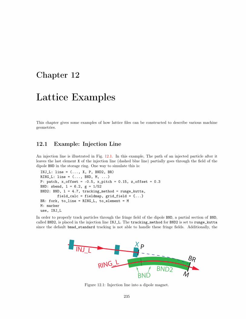
Chapter 12

Lattice Examples

This chapter gives some examples of how lattice files can be constructed to describe various machinegeometries.

12.1 Example: Injection Line

An injection line is illustrated in Fig. 12.1. In this example, The path of an injected particle after itleaves the last element X of the injection line (dashed blue line) partially goes through the field of thedipole BND in the storage ring. One way to simulate this is:INJ_L: line = (..., X, P, BND2, BR)RING_L: line = (..., BND, M, ...)P: patch, x_offset = -0.5, x_pitch = 0.15, z_offset = 0.3BND: sbend, l = 6.2, g = 1/52BND2: BND, l = 4.7, tracking_method = runge_kutta,

field_calc = fieldmap, grid_field = ...BR: fork, to_line = RING_L, to_element = MM: markeruse, INJ_L

In order to properly track particles through the fringe field of the dipole BND, a partial section of BND,called BND2, is placed in the injection line INJ_L. The tracking_method for BND2 is set to runge_kuttasince the default bmad_standard tracking is not able to handle these fringe fields. Additionally, the

INJ_L

BND

BRRING_L

X P

MBND2

Figure 12.1: Injection line into a dipole magnet.

235

236 CHAPTER 12. LATTICE EXAMPLES

field_calc parameter of BND2 is set to field map so that the actual field profile of this particularmagnet can be used in the tracking. The field is specified in the grid_field parameter (§5.15).

After traversing element X in the injection line, the particle goes through the patch P which offsets thereference trajectory so that following element, BND2, is properly positioned. The beginning of BND2 ismarked by a black dashed line in the figure. At the end of BND2 the fork element BR connects INJ_Lwith the marker M in RING_L.

12.2 Example: Chicane

A chicane is a series of bending magnets that shifts the beam trajectory in the transverse plane whilekeeping the starting and ending trajectories constant. Chicanes are useful for doing things like bunchcompression or as a variable bunch time delay. An example four bend chicane is illustrated in Fig. 12.2A.The lattice file for this is:parameter[geometry] = openbeginning[beta_a] = 20beginning[beta_b] = 20parameter[p0c] = 1e7

bnd1: rbend, l = 2bnd2: rbend, l = 2d1: drift, l = 3d2: drift, l = 2

chicane: overlay = bnd1[dg]:-ge, bnd2[dg]:ge, var = ge, ge = 2e-3

c_line: line = (bnd1, d1, bnd2, d2, bnd2, d1, bnd1)use, c_line

The chicane is controlled by an overlay (§4.37) called chicane. This overlay controls the dg attribute ofthe bends (alternatively the hkick or b0 attributes could have been used).

It is important to note that using g instead of dg to control the chicane strength would be a mistake.[Or, alternatively, b_field instead of db_field if controlling the unnormalized field.] This is illustratedin Fig. 12.2B where the chicane overlay was replaced by:chicane: overlay = bnd1[g]:-ge, bnd2[g]:ge, var = ge, ge = 1e-1

The problem here is that g sets the reference orbit so varying g will vary the physical layout of themachine which is not what is wanted. Since the actual normalized field is g + dg, it is dg that should

A) B)

Figure 12.2: Four bend chicane. A) Correctly implemented chicane. The red line is the beam orbitmagnified by a factor of 100. B) Incorrectly implemented chicane where the g parameter of the bends isused to control the chicane strength instead of dg.

12.3. EXAMPLE: ENERGY RECOVERY LINAC 237

be varied. Notice that in the case where g is varied, the bends are no longer rectangular. This is truesince rbend elements, when read in from the lattice file, are converted to sbend elements. In this casethe converted bends have e1 and e2 face angles of zero. When the chicane overlay varies g, the faceangle remain zero. That is, the bends will always be pure sector bends. [In a situation where, indeed, gis to be varied and it is desired to keep bends rectangular, the appropriate variation of the e1 and e2can be put in the controlling overlay.]

12.3 Example: Energy Recovery Linac

An Energy Recovery Linac (ERL) is illustrated in Fig. 12.3A. The ERL starts with an injection line thatfeeds a linac which accelerates the beam to some energy. The beam then transverses a return arc whichreinjects the bunches into the linac. The length of the return arc is such that, on the second pass, thebeam is decelerated giving its energy back to the RF cavities. Finally, the decelerated beam is steeredthrough a dump line where, at the end, an absorber stops the beam.

A lattice file for modeling this ERL:parameter[geometry] = openparameter[absolute_time_tracking] = T

BEND_L1: sbend, angle = -25*pi/180, l = 0.2, ...BEND_L2: BEND_L1

A_PATCH: patch, flexible = TD_PATCH: patch, x_offset = 0.034, x_pitch = asin(0.32)INJECT: line = (...)LINAC: line[multipass] = (BEND_L1, ..., BEND_L2)ARC: line = (..., BEND_A7)DUMP: line = (...)

ERL: line = (INJECT, LINAC, ARC, A_PATCH, LINAC, D_PATCH, DUMP)

Fig. 12.3B shows the injector and arc merging into the beginning of the linac. The first element of thelinac is a bend named BEND_L1. The bending angle for BEND_L1 has been set at the appropriate valuefor injection from the injector. To get the correct geometry for injection from the arc, a patch element,named A_PATCH, is placed in the ERL line between the arc and the linac. A_PATCH is a flexible patchwhich means that the exit edge of A_PATCH will automatically be aligned with the entrance edge of thenext element which is BEND_L1.

Note that this use of a flexible patch works since the orientation of BEND_L1 has been determined beforethe orientation of A_PATCH is determined. The orientation of elements is determined in order startingfrom the first element in the line (the exception to this rule is if there is a floor_position element) andthe orientation of BEND_L1 is thus determined right after the injector section on the first pass throughthe linac.

Fig. 12.3C shows the end of the linac splitting off into the dump and arc sections. The D_PATCH isused to orient the reference trajectory so that the dump is correctly positioned. Here it is not possibleto make the D_PATCH flexible since the position of the dump is unknown when the orientation of theD_PATCH is calculated. However, the D_PATCH could be made flexible if a floor_position element isused in the dump line (Bmad will work both forward and backwards from a floor_position elementso that a floor_position element may be placed anywhere in the dump line).

238 CHAPTER 12. LATTICE EXAMPLES

Linac

Injector

Arc

Dump

BND_A7

A_PATCH

D_PATCH

A)

B)

C)

Injector

LinacBND_L1

Dump

ArcBND_L2

Figure 12.3: Example Energy Recovery Linac. A) The ERL consists of an injection line, acceleratinglinac, return arc, deceleration linac, and finally a beam dump. B) Close up of the section where the endof the injector and the end of the arc inject into the beginning of the linac. C) Close up of the end ofthe linac which injects into the dump and the beginning of the arc.

12.4 Example: Colliding Beam Storage Rings

The idealized layout of a pair of storage rings used for colliding counter rotating beams of electrons andgold is shown in Fig. 12.4. Rings A and B intersect at two interaction regions labeled ir1 and ir2 wherethe beams collide. The basic lattice description is:

IR

AB

z

x

PatchRegions

Figure 12.4: Dual ring colliding beam machine. The beam in the A ring rotates clockwise and in the Bring counterclockwise.

12.4. EXAMPLE: COLLIDING BEAM STORAGE RINGS 239

ir: line[multipass] = (...)pa_in; patch, ... ; pa_out; patch, ...pb_in; patch, ... ; pb_out; patch, ...m: markerfid: fiducial, origin_ele = m...A: line = (arc_a, pa_in, ir, m, pa_out)A[particle] = electronB_rev: line = (arc_b, pb_in, ir, fid, pb_out)B: line = (--B_rev)B[particle] = Au+79use, A, B

Lines ir is the interaction region line which is declared multipass since they are shared by the tworings. Line A represents ring A. In ring A where the electron beam which, by definition, travels in thesame direction as increasing s, rotates clockwise. Line B_rev is a “reversed” line of ring B and, like a,represents a beam rotating clockwise. Line B, which represents ring B, is the reverse of B_rev and herethe gold beam rotates counterclockwise. In this construction, all elements of B are reversed. While thisis not mandatory (only the interaction regions must be reversed in B), having all of B reversed simplifiesthe geometry since this means that the local coordinate systems of both lines A and b will be “aligned”with the x-axis pointing to the outside of the ring and the y-axis pointing up, out of the page. Havingnon-aligned coordinate systems is possible but potentially very confusing.

The two rings are physically aligned using a marker m in A and a fiducial element fid in B that alignswith m. Each ring has two rigid patch elements, pa_in and pa_out for the A ring, and pb_in and bp_outfor the B ring, on either side of the interaction region. The dashed, green rectangles in the figure showthe regions where the patches are.

The finished lattice will have two branches, The first branch (with index 0) will be derived from line A(and hence will be named “A”) and the second branch (with index 1) will be derived from line B (andhence will be named “B”). The multipass lords representing the physical IR elements will be in the “lordsection” of branch 0.

240 CHAPTER 12. LATTICE EXAMPLES

Crystal

φ

Source

Detector

z

x2θ

B,in−φ

2φ

R

Y (m

m)

Y (m

m)

X (mm) X (mm)

A) B) C)

2θB,out

−φ

GlobalCoordinants

Figure 12.5: Rowland circle spectrometer: A) X-rays scattered from a sample (labeled source in thefigure) illuminates a crystal with X-rays. Some of the X-rays are reflected from the crystal onto thedetector. Note: For clarity’s sake the center of the global coordinate system as shown is shifted fromthe true center at the Source element. B) The detector image when the radius of curvature of the bentcrystal is “perfect”. That is, twice the radius of the Rowland circle. C) The detector image when theradius of curvature of the crystal is shifted 1% from perfect.

12.5 Example: Rowland Circle X-Ray Spectrometer

This example shows how Bmad can be used to simulate X-rays. In this case, the present example istaken from a case study where simulations were done in order to understand how imperfections in aRowland circle spectrometer would affect measurements.

A Rowland circle spectrometer is illustrated in Fig. 12.5A. The source was a sample that is illuminatedwith X-rays. Some of the X-rays scatter from the sample and are reflected from the crystal to thedetector. To properly focus the X-rays onto the detector, the source, crystal and detector lie ona circle, called the Rowland circle. The crystal is bent and the radius of curvature of the crystal is 2Rwhere R is the radius of the Rowland circle.

The angle from the source to the Rowland circle center to the crystal is 2θB,in − φ where θB,in is theentrance Bragg angle for photons whose energy matches the given reference energy and φ is an anglethat will be varied when doing an energy scan of the scattered X-ray spectrum. Similarly, the anglefrom the crystal to the Rowland circle center to the detector is 2θB,out − φ where θB,out is the exitBragg angle at the given reference energy.

The lattice for this simulation is:beginning[e_tot] = 8.955e3 ! Reference photon energyparameter[particle] = photon

phi = 0err = 0r_rowland = 0.5 ! Rowland circle radius

source: photon_init, sig_x = 5e-5, sig_y = 5e-5, spatial_distribution = uniform,E_center_relative_to_ref = T, sig_E = 2, energy_distribution = gaussian,velocity_distribution = spherical

12.5. EXAMPLE: ROWLAND CIRCLE X-RAY SPECTROMETER 241

drift1: drift

cryst: crystal, crystal_type = "Si(553)", b_param = -1, aperture = 0.050,spherical_curvature = (1+err) / (2 * r_rowland), aperture_type = elliptical

drift2: drift

det: detector, surface = grid = ix_bounds = (-97, 97),iy_bounds = (-243, 243), dr = (172e-6, 172e-6)

daves_line: line = (source, drift1, cryst, drift2, det)use, daves_line

!------------------

expand_lattice ! Calculates the Bragg angles needed below.

theta_in = cryst[bragg_angle_in] ! 78.2759 * pi / 180theta_out = cryst[bragg_angle_out] ! 78.2759 * pi / 180

cryst[graze_angle_in] = theta_in - phi/2cryst[graze_angle_out] = theta_out - phi/2drift1[L] = 2 * r_rowland * sin(theta_in-phi/2)drift2[L] = 2 * r_rowland * sin(theta_out-phi/2)

beginning[theta_position] = theta_in + phi/2det[x_pitch] = pi/2 - theta_out + phi/2

The reference photon energy is 8.995 KeV and the Rowland circle radius is 0.5 m. The simulation usesa photon_init element (§4.39) for the source having a Gaussian energy spread with a sigma of 2 eV.The initial velocity distribution of the photons, set by the velocity_distribution parameter, is takento be uniform in all directions (“spherical” distribution). Since the element that is downstream fromthe source (which is the crystal element) has a defined aperture, Bmad is able to use this to not generatephotons that will be lost at the crystal. This reduces the simulation time.

The crystal is Silicon 553 crystal which is symmetrically cut (b_param = -1) so that in this examplethe entrance Bragg angle is equal to the exit Bragg angle. The detector has a segmented surface withpixels spaced 172µm apart. Along the x-axis, which is the coordinate along the detector surface in theplane of Fig. 12.5A, the pixel index is in the range [−97, 97]. Along the y-axis, which is the out of planecoordinate, the pixel index is in the range [−243, 243].

The expand_lattice command (§3.21) is used to command Bmad to construct the lattice which includescalculating the Bragg angles. After lattice expansion, the variables theta_in and theta_out are set tothe Bragg angle entrance and exit Bragg angles respectively. The entrance and exit graze angles of thecrystal, which are used to determine the reference trajectory (§15.2.3, can be set to theta_in - phiand theta_out - phi respectively. Note that if these graze angles had not been explicitly set, the grazeangles would be automatically set to the Bragg angles which is not what is wanted when doing an energyscan with finite phi.

In the actual experimental setup that this example is modeled on, the source and Rowland circle werefixed in the global coordinate system (§15.2) while the crystal and detector move with changing phi(see Fig. 12.5A). To mimic this, the beginning[theta_position] (§9.4) is set to give the desired

242 CHAPTER 12. LATTICE EXAMPLES

orientation of the beginning reference trajectory within the global coordinate system. This does notaffect photon tracking since changing the initial orientation of the reference trajectory just shifts all thelattice elements as one rigid body. Additionally, the detector orientation is fixed so that the detectorsurface normal always points towards the Rowland circle center. To get the correct orientation for thedetector, the detector’s x_pitch attribute, which rotates the detector (§5.6), is set appropriately.

The effect of varying the crystal curvature is shown in Fig. 12.5B and Fig. 12.5C. A Bmad basedprogram called Lux was used for the simulation. The Lux program generates a set of photons andrecords the statistics at the detector. In Fig. 12.5B the crystal is correctly bent with the parametererr in the lattice set to zero. This produces a well focused spot on the detector. In Fig. 12.5C thecrystal curvature is shifted by 1% by setting err equal to 0.01. This error degrades the focusing andleads to a spot that is enlarged along the x-axis.

12.6 Example: Backward Tracking Through a Lattice

By creating a reversed lattice, one can track a particles backwards through the lattice. For exam-ple, assume that you have a lattice file called original_lattice.bmad which defines a line calledoriginal_line tracking electrons. To create a reversed lattice, create a new file with the following:

call, file = original_lattice.bmadreversed_line: line = (--original_line)parameter[default_tracking_species] = positronuse, reversed_line

The “−−” reverses the line and reverses the elements (§7.4). Tracking through reversed_line is equiv-alent to tracking backwards through original_line.

The default for the type of particle tracked is set by parameter[default_tracking_species] (§9.1).[A Bmad based program can always override this default but it will be assumed here that this is notthe case.] In this case, the default species to use for tracking is set to the antiparticle of the referenceparticle species. If the original_line lattice had just static magnetic fields and no electric fields, bytracking with the anti-particle in the reversed lattice, the anti-particle will follow the same path (butbackward) as the particle in the original lattice. For this to work, the anti-particle must be startedwith the appropriate phase space coordinates. If (x, px, y, py, z, pz) is the phase space coordinates ofthe particle at the end of the original lattice, the anti-particle must be initialized with phase spacecoordinates of (x,−px, y,−py, immaterial, pz).

It should be keept in mind that tracking backwards in the lattice is not exactly the same as trackingbackwards in time. In particular, the two are different if there are electric fields or if radiation dampingand/or excitation is turned on.

Chapter 13

Lattice File Conversion

A Bmad Distribution (§1.2) contains a number of translation programs between Bmad and other formats.

13.1 MAD Conversion

13.1.1 Convert MAD to Bmad

Python scripts to convert from MAD8 and MADX are available at:util_programs/mad_to_bmad

Due to differences in language definitions, conversions must be done with some care. The followingdifferences should be noted:

• Bmad, unlike MAD, does not have any “action” commands. An action command is a commandthat makes a calculation. Examples include MAD’s SURVEY and TWISS commands.

• In Bmad all variables must be defined before being used (§3.12) while MAD will simply take avariable’s value to be zero if it is not defined.

• Bmad, unlike MAD, does not allow variable values to be redefined.

13.1.2 Convert Bmad to MAD

To convert to MAD8 or MADX, the Tao program can be used. Additionally, the program util_programs/bmad_to_mad_or_sadis available. Since MAD does not have a wiggler or a sol_quad element, this conversion routine makes“equivalent” substitution. For a sol_quad, the equivalent substitution will be a drift-matrix-drift seriesof elements. For a wiggler, a series of bend and drift elements will be used (the program can also use adrift-matrix-drift model here but that is not as accurate). The bends and drifts for the wiggler modelare constructed so that the global geometry of the lattice does not change. Additionally the bends anddrifts are constructed to most nearly match the wiggler’sTransfer matrix$I_2$ and $I_3$ synchrotron radiation integrals (§20.2)

Note that the resulting model will not have the vertical cubic nonlinearity that the actual wiggler has.

243

244 CHAPTER 13. LATTICE FILE CONVERSION

13.1.3 Convert to PTC

A PTC “flatfile” can be constructed using the Tao program with the following commands:Tao> ptc initTao> write ptc

13.2 SAD Conversion

Conversion from SAD[SAD] to Bmad is accomplished using the Python scriptutil_programs/sad_to_bmad/sad_to_bmad.py

Currently, the following restrictions on SAD lattices apply:

• SAD mult elements cannot have an associated RF field

• Misalignments in a sol element with geo = 1 cannot be handled.

Bmad to SAD to conversion can be done with the Tao program or the program util_programs/bmad_to_mad_or_sad.

Chapter 14

List of Element Attributes

Alphabetical list of element attributes for each type of element.

Note for programmers: The program that generates a file of attributes indexed by the internal referencenumber is:util_programs/element_attributes.f90

14.1 !PTC_Com Element Attributes

exact_misalign exact_model max_fringe_order old_integrator

14.2 AB_multipole Element Attributes

a0 - a20, b0 - b20 is_on superimpose x_offset_tot [m]alias l [m] tilt [rad] y1_limit [m]aperture [m] mat6_calc_method tilt_tot [rad] y2_limit [m]aperture_at multipoles_on tracking_method y_limit [m]aperture_type offset [m] type y_offset [m]create_jumbo_slave offset_moves_aperture wall y_offset_tot [m]delta_ref_time [sec] p0c [eV] wrap_superimpose z_offset [m]descrip ptc_integration_type x1_limit [m] z_offset_tot [m]e_tot [eV] ref_origin x2_limit [m]ele_origin reference x_limit [m]field_master spin_tracking_method x_offset [m]

245

246 CHAPTER 14. LIST OF ELEMENT ATTRIBUTES

14.3 AC_Kicker Element Attributes

a0 - a20, b0 - b20 frequencies p0c [eV] typealias fringe_at ptc_integration_type vkickamp_vs_time fringe_type r0_elec [m] wallaperture [m] grid_field r0_mag [m] wrap_superimposeaperture_at hkick ref_origin x1_limit [m]aperture_type integrator_order ref_time_offset x2_limit [m]bl_hkick [T*m] interpolation reference x_limit [m]bl_vkick [T*m] is_on scale_multipoles x_offset [m]cartesian_map l [m] space_charge_method x_offset_tot [m]create_jumbo_slave lord_pad1 [m] spin_fringe_on x_pitchcsr_ds_step [m] lord_pad2 [m] spin_tracking_method x_pitch_totcsr_method lr_freq_spread [Hz] sr_wake y1_limit [m]cylindrical_map lr_self_wake_on sr_wake_file y2_limit [m]delta_ref_time [sec] lr_wake superimpose y_limit [m]descrip lr_wake_file symplectify y_offset [m]ds_step [m] mat6_calc_method t_offset [sec] y_offset_tot [m]e_tot [eV] multipass_ref_energy taylor_field y_pitchele_origin multipoles_on taylor_map_includes_offsets y_pitch_totfield_calc num_steps tilt [rad] z_offset [m]field_master offset [m] tilt_tot [rad] z_offset_tot [m]field_overlaps offset_moves_aperture tracking_method

14.4 BeamBeam Element Attributes

alias crab_x2 [1/m] ref_origin x_limit [m]alpha_a_strong crab_x3 [1/m2] reference x_offset [m]alpha_b_strong create_jumbo_slave sig_x [m] x_offset_tot [m]aperture [m] delta_ref_time [sec] sig_y [m] x_pitchaperture_at descrip sig_z [m] x_pitch_totaperture_type e_tot [eV] spin_tracking_method y1_limit [m]bbi_constant ele_origin superimpose y2_limit [m]beta_a_strong [m] field_calc symplectify y_limit [m]beta_b_strong [m] is_on tilt [rad] y_offset [m]charge l [m] tilt_tot [rad] y_offset_tot [m]cmat_11 mat6_calc_method tracking_method y_pitchcmat_12 n_slice type y_pitch_totcmat_21 offset [m] wall z_offset [m]cmat_22 offset_moves_aperture wrap_superimpose z_offset_tot [m]crab_tilt [rad] p0c [eV] x1_limit [m]crab_x1 ptc_integration_type x2_limit [m]

14.5. BEAM_INIT ELEMENT ATTRIBUTES 247

14.5 Beam_Init Element Attributes

alias fringe_type ptc_integration_type wrap_superimposeaperture [m] hkick ref_origin x1_limit [m]aperture_at integrator_order reference x2_limit [m]aperture_type is_on space_charge_method x_limit [m]bl_hkick [T*m] l [m] spin_fringe_on x_offset [m]bl_vkick [T*m] lord_pad1 [m] spin_tracking_method x_offset_tot [m]create_jumbo_slave lord_pad2 [m] sr_wake x_pitchcsr_ds_step [m] lr_freq_spread [Hz] sr_wake_file x_pitch_totcsr_method lr_self_wake_on superimpose y1_limit [m]delta_ref_time [sec] lr_wake symplectify y2_limit [m]descrip lr_wake_file taylor_map_includes_offsets y_limit [m]ds_step [m] mat6_calc_method tilt [rad] y_offset [m]e_tot [eV] multipass_ref_energy tilt_tot [rad] y_offset_tot [m]ele_origin num_steps tracking_method y_pitchfield_calc offset [m] type y_pitch_totfield_overlaps offset_moves_aperture vkick z_offset [m]fringe_at p0c [eV] wall z_offset_tot [m]

14.6 Beginning Statement Attributes

alpha_a cmat_22 etap_y psi_position [rad]alpha_b e_tot [eV] inherit_from_fork ref_time [sec]beta_a [m] e_tot_start [eV] p0c [eV] s [m]beta_b [m] eta_x [m] p0c_start [eV] theta_position [rad]cmat_11 eta_y [m] phi_a [rad] x_position [m]cmat_12 eta_z [m] phi_b [rad] y_position [m]cmat_21 etap_x phi_position [rad] z_position [m]

248 CHAPTER 14. LIST OF ELEMENT ATTRIBUTES

14.7 Bends: Rbend and Sbend Element Attributes

a0 - a20, b0 - b20 field_master mat6_calc_method symplectifyalias field_overlaps multipass_ref_energy taylor_fieldangle [rad] fint multipoles_on taylor_map_includes_offsetsaperture [m] fintx num_steps tracking_methodaperture_at fringe_at offset [m] typeaperture_type fringe_type offset_moves_aperture vkickb1_gradient [T/m] g [1/m] p0c [eV] wallb2_gradient [T/m2] grid_field ptc_canonical_coords wrap_superimposeb_field [T] h1 [1/m] ptc_field_geometry x1_limit [m]bl_hkick [T*m] h2 [1/m] ptc_fringe_geometry x2_limit [m]bl_vkick [T*m] hgap [m] ptc_integration_type x_limit [m]cartesian_map hgapx [m] r0_elec [m] x_offset [m]create_jumbo_slave higher_order_fringe_type r0_mag [m] x_offset_tot [m]csr_ds_step [m] hkick ref_origin x_pitchcsr_method integrator_order ref_tilt [rad] x_pitch_totcylindrical_map is_on ref_tilt_tot [rad] y1_limit [m]db_field [T] k1 [1/m2] reference y2_limit [m]delta_ref_time [sec] k2 [1/m3] rho [m] y_limit [m]descrip l [m] roll [rad] y_offset [m]dg [1/m] l_chord [m] roll_tot [rad] y_offset_tot [m]ds_step [m] l_sagitta [m] scale_multipoles y_pitche1 [rad] lord_pad1 [m] space_charge_method y_pitch_tote2 [rad] lord_pad2 [m] spin_fringe_on z_offset [m]e_tot [eV] lr_freq_spread [Hz] spin_tracking_method z_offset_tot [m]ele_origin lr_self_wake_on sr_wakeexact_multipoles lr_wake sr_wake_filefield_calc lr_wake_file superimpose

14.8 Bmad_Com Statement Attributes

abs_tol_adaptive_tracking [m] default_ds_step [m] max_aperture_limit [m] rel_tol_adaptive_trackingabs_tol_tracking [m] fatal_ds_adaptive_tracking [m] max_num_runge_kutta_step rel_tol_trackingaperture_limit_on init_ds_adaptive_tracking [m] min_ds_adaptive_tracking [m] significant_length [m]

14.9. CAPILLARY ELEMENT ATTRIBUTES 249

14.9 Capillary Element Attributes

alias mat6_calc_method tilt_tot [rad] x_pitch_totaperture [m] n_slice_spline tracking_method y1_limit [m]aperture_at offset [m] type y2_limit [m]aperture_type offset_moves_aperture wall y_limit [m]create_jumbo_slave p0c [eV] wrap_superimpose y_offset [m]critical_angle_factor [rad*eV] ptc_integration_type x1_limit [m] y_offset_tot [m]delta_ref_time [sec] ref_origin x2_limit [m] y_pitchdescrip reference x_limit [m] y_pitch_tote_tot [eV] spin_tracking_method x_offset [m] z_offset [m]ele_origin superimpose x_offset_tot [m] z_offset_tot [m]l [m] tilt [rad] x_pitch

14.10 Collimators: Ecollimator and Rcollimator Element At-tributes

alias integrator_order py_aperture_width2 wrap_superimposeaperture [m] is_on pz_aperture_center x1_limit [m]aperture_at l [m] pz_aperture_width2 x2_limit [m]aperture_type lord_pad1 [m] ref_origin x_limit [m]bl_hkick [T*m] lord_pad2 [m] reference x_offset [m]bl_vkick [T*m] lr_freq_spread [Hz] space_charge_method x_offset_tot [m]create_jumbo_slave lr_self_wake_on spin_fringe_on x_pitchcsr_ds_step [m] lr_wake spin_tracking_method x_pitch_totcsr_method lr_wake_file sr_wake y1_limit [m]delta_ref_time [sec] mat6_calc_method sr_wake_file y2_limit [m]descrip multipass_ref_energy superimpose y_limit [m]ds_step [m] num_steps symplectify y_offset [m]e_tot [eV] offset [m] taylor_map_includes_offsets y_offset_tot [m]ele_origin offset_moves_aperture tilt [rad] y_pitchfield_calc p0c [eV] tilt_tot [rad] y_pitch_totfield_overlaps ptc_integration_type tracking_method z_aperture_center [m]fringe_at px_aperture_center type z_aperture_width2 [m]fringe_type px_aperture_width2 vkick z_offset [m]hkick py_aperture_center wall z_offset_tot [m]

250 CHAPTER 14. LIST OF ELEMENT ATTRIBUTES

14.11 Converter Element Attributes

alias l [m] superimpose x_pitch_totangle_out_max [rad] mat6_calc_method tilt [rad] y1_limit [m]aperture [m] offset [m] tilt_tot [rad] y2_limit [m]aperture_at offset_moves_aperture tracking_method y_limit [m]aperture_type p0c [eV] type y_offset [m]create_jumbo_slave p0c_start [eV] wall y_offset_tot [m]delta_ref_time [sec] pc_out_max [eV] wrap_superimpose y_pitchdescrip pc_out_min [eV] x1_limit [m] y_pitch_totdistribution ptc_integration_type x2_limit [m] z_offset [m]e_tot [eV] ref_origin x_limit [m] z_offset_tot [m]e_tot_start [eV] reference x_offset [m]ele_origin species_out x_offset_tot [m]is_on spin_tracking_method x_pitch

14.12 Crab_Cavity Element Attributes

alias grid_field ptc_integration_type wrap_superimposeaperture [m] harmon ref_origin x1_limit [m]aperture_at hkick reference x2_limit [m]aperture_type integrator_order rf_frequency [Hz] x_limit [m]bl_hkick [T*m] is_on rf_wavelength [m] x_offset [m]bl_vkick [T*m] l [m] space_charge_method x_offset_tot [m]cartesian_map lord_pad1 [m] spin_tracking_method x_pitchcreate_jumbo_slave lord_pad2 [m] sr_wake x_pitch_totcsr_ds_step [m] lr_freq_spread [Hz] sr_wake_file y1_limit [m]csr_method lr_self_wake_on superimpose y2_limit [m]cylindrical_map lr_wake symplectify y_limit [m]delta_ref_time [sec] lr_wake_file taylor_field y_offset [m]descrip mat6_calc_method taylor_map_includes_offsets y_offset_tot [m]ds_step [m] multipass_ref_energy tilt [rad] y_pitche_tot [eV] num_steps tilt_tot [rad] y_pitch_totele_origin offset [m] tracking_method z_offset [m]field_calc offset_moves_aperture type z_offset_tot [m]field_master p0c [eV] vkickfield_overlaps phi0 [rad/2pi] voltage [Volt]gradient [eV/m] phi0_multipass [rad/2pi] wall

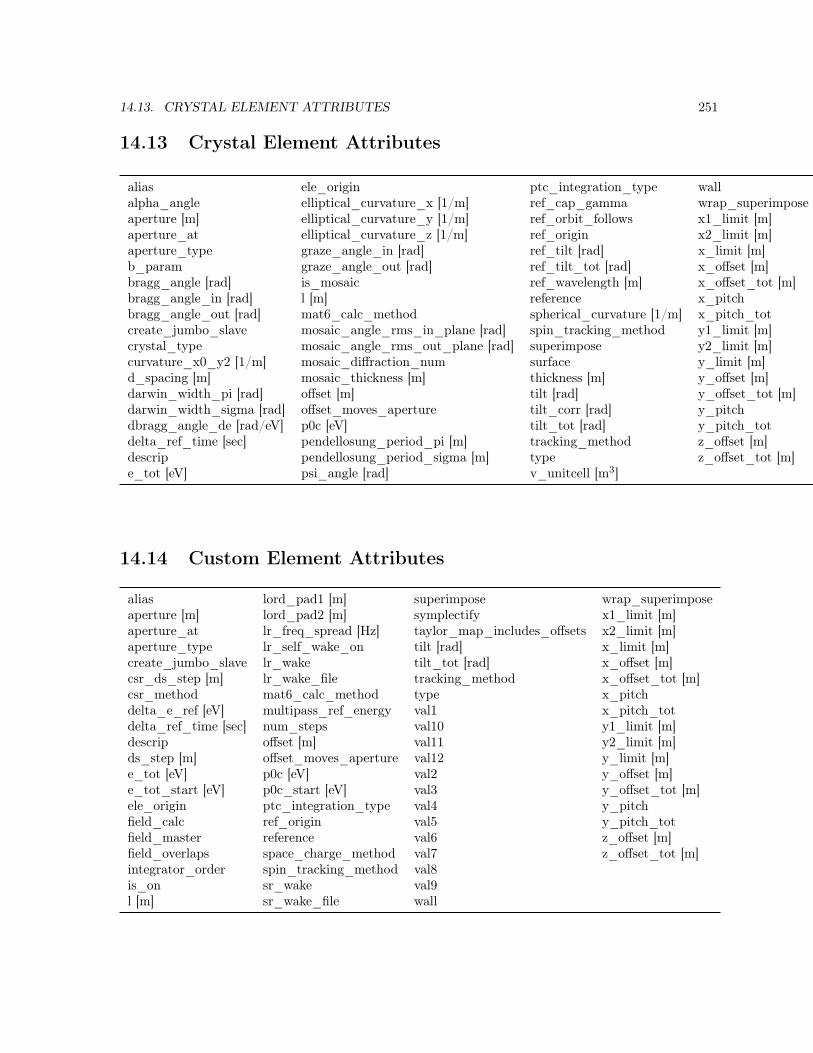
14.13. CRYSTAL ELEMENT ATTRIBUTES 251

14.13 Crystal Element Attributes

alias ele_origin ptc_integration_type wallalpha_angle elliptical_curvature_x [1/m] ref_cap_gamma wrap_superimposeaperture [m] elliptical_curvature_y [1/m] ref_orbit_follows x1_limit [m]aperture_at elliptical_curvature_z [1/m] ref_origin x2_limit [m]aperture_type graze_angle_in [rad] ref_tilt [rad] x_limit [m]b_param graze_angle_out [rad] ref_tilt_tot [rad] x_offset [m]bragg_angle [rad] is_mosaic ref_wavelength [m] x_offset_tot [m]bragg_angle_in [rad] l [m] reference x_pitchbragg_angle_out [rad] mat6_calc_method spherical_curvature [1/m] x_pitch_totcreate_jumbo_slave mosaic_angle_rms_in_plane [rad] spin_tracking_method y1_limit [m]crystal_type mosaic_angle_rms_out_plane [rad] superimpose y2_limit [m]curvature_x0_y2 [1/m] mosaic_diffraction_num surface y_limit [m]d_spacing [m] mosaic_thickness [m] thickness [m] y_offset [m]darwin_width_pi [rad] offset [m] tilt [rad] y_offset_tot [m]darwin_width_sigma [rad] offset_moves_aperture tilt_corr [rad] y_pitchdbragg_angle_de [rad/eV] p0c [eV] tilt_tot [rad] y_pitch_totdelta_ref_time [sec] pendellosung_period_pi [m] tracking_method z_offset [m]descrip pendellosung_period_sigma [m] type z_offset_tot [m]e_tot [eV] psi_angle [rad] v_unitcell [m3]

14.14 Custom Element Attributes

alias lord_pad1 [m] superimpose wrap_superimposeaperture [m] lord_pad2 [m] symplectify x1_limit [m]aperture_at lr_freq_spread [Hz] taylor_map_includes_offsets x2_limit [m]aperture_type lr_self_wake_on tilt [rad] x_limit [m]create_jumbo_slave lr_wake tilt_tot [rad] x_offset [m]csr_ds_step [m] lr_wake_file tracking_method x_offset_tot [m]csr_method mat6_calc_method type x_pitchdelta_e_ref [eV] multipass_ref_energy val1 x_pitch_totdelta_ref_time [sec] num_steps val10 y1_limit [m]descrip offset [m] val11 y2_limit [m]ds_step [m] offset_moves_aperture val12 y_limit [m]e_tot [eV] p0c [eV] val2 y_offset [m]e_tot_start [eV] p0c_start [eV] val3 y_offset_tot [m]ele_origin ptc_integration_type val4 y_pitchfield_calc ref_origin val5 y_pitch_totfield_master reference val6 z_offset [m]field_overlaps space_charge_method val7 z_offset_tot [m]integrator_order spin_tracking_method val8is_on sr_wake val9l [m] sr_wake_file wall

252 CHAPTER 14. LIST OF ELEMENT ATTRIBUTES

14.15 Detector Element Attributes

alias l [m] tilt_tot [rad] y1_limit [m]aperture [m] mat6_calc_method tracking_method y2_limit [m]aperture_at n_sample type y_dispersion_calib [m]aperture_type noise wall y_dispersion_err [m]create_jumbo_slave offset [m] wrap_superimpose y_gain_calib [m]crunch [rad] offset_moves_aperture x1_limit [m] y_gain_err [m]crunch_calib [rad] osc_amplitude [m] x2_limit [m] y_limit [m]curvature_x0_y2 [1/m] p0c [eV] x_dispersion_calib [m] y_offset [m]de_eta_meas ptc_integration_type x_dispersion_err [m] y_offset_calib [m]delta_ref_time [sec] ref_origin x_gain_calib [m] y_offset_tot [m]descrip reference x_gain_err [m] y_pitche_tot [eV] spherical_curvature [1/m] x_limit [m] y_pitch_totele_origin spin_tracking_method x_offset [m] z_offset [m]elliptical_curvature_x [1/m] superimpose x_offset_calib [m] z_offset_tot [m]elliptical_curvature_y [1/m] surface x_offset_tot [m]elliptical_curvature_z [1/m] tilt [rad] x_pitchis_on tilt_calib [rad] x_pitch_tot

14.16 Diffraction_Plate Element Attributes

alias field_scale_factor superimpose x_pitchaperture [m] is_on surface x_pitch_totaperture_at mat6_calc_method tilt [rad] y1_limit [m]aperture_type mode tilt_tot [rad] y2_limit [m]create_jumbo_slave offset [m] tracking_method y_limit [m]curvature_x0_y2 [1/m] offset_moves_aperture type y_offset [m]delta_ref_time [sec] p0c [eV] wall y_offset_tot [m]descrip ptc_integration_type wrap_superimpose y_pitche_tot [eV] ref_origin x1_limit [m] y_pitch_totele_origin ref_wavelength [m] x2_limit [m] z_offset [m]elliptical_curvature_x [1/m] reference x_limit [m] z_offset_tot [m]elliptical_curvature_y [1/m] spherical_curvature [1/m] x_offset [m]elliptical_curvature_z [1/m] spin_tracking_method x_offset_tot [m]

14.17. DRIFT ELEMENT ATTRIBUTES 253

14.17 Drift Element Attributes

alias l [m] superimpose x_pitchaperture [m] lord_pad1 [m] symplectify x_pitch_totaperture_at lord_pad2 [m] taylor_map_includes_offsets y1_limit [m]aperture_type mat6_calc_method tilt [rad] y2_limit [m]create_jumbo_slave multipass_ref_energy tilt_tot [rad] y_limit [m]csr_ds_step [m] num_steps tracking_method y_offset [m]csr_method offset [m] type y_offset_tot [m]delta_ref_time [sec] offset_moves_aperture wall y_pitchdescrip p0c [eV] wrap_superimpose y_pitch_totds_step [m] ptc_integration_type x1_limit [m] z_offset [m]e_tot [eV] ref_origin x2_limit [m] z_offset_tot [m]ele_origin reference x_limit [m]field_calc space_charge_method x_offset [m]integrator_order spin_tracking_method x_offset_tot [m]

14.18 ELseparator Element Attributes

a0 - a20, b0 - b20 fringe_type ptc_canonical_coords vkickalias gap ptc_integration_type voltage [Volt]aperture [m] grid_field r0_elec [m] wallaperture_at hkick r0_mag [m] wrap_superimposeaperture_type integrator_order ref_origin x1_limit [m]cartesian_map is_on reference x2_limit [m]create_jumbo_slave l [m] scale_multipoles x_limit [m]csr_ds_step [m] lord_pad1 [m] space_charge_method x_offset [m]csr_method lord_pad2 [m] spin_fringe_on x_offset_tot [m]cylindrical_map lr_freq_spread [Hz] spin_tracking_method x_pitchdelta_ref_time [sec] lr_self_wake_on sr_wake x_pitch_totdescrip lr_wake sr_wake_file y1_limit [m]ds_step [m] lr_wake_file superimpose y2_limit [m]e_field [V/m] mat6_calc_method symplectify y_limit [m]e_tot [eV] multipass_ref_energy taylor_field y_offset [m]ele_origin multipoles_on taylor_map_includes_offsets y_offset_tot [m]field_calc num_steps tilt [rad] y_pitchfield_master offset [m] tilt_tot [rad] y_pitch_totfield_overlaps offset_moves_aperture tracking_method z_offset [m]fringe_at p0c [eV] type z_offset_tot [m]

254 CHAPTER 14. LIST OF ELEMENT ATTRIBUTES

14.19 EM_Field Element Attributes

alias field_overlaps phi0 [rad/2pi] typeaperture [m] fringe_at phi0_autoscale [rad/2pi] wallaperture_at fringe_type phi0_err [rad/2pi] wrap_superimposeaperture_type grid_field ptc_canonical_coords x1_limit [m]autoscale_amplitude integrator_order ptc_integration_type x2_limit [m]autoscale_phase is_on ref_origin x_limit [m]cartesian_map l [m] reference x_offset [m]constant_ref_energy lord_pad1 [m] rf_frequency [Hz] x_offset_tot [m]create_jumbo_slave lord_pad2 [m] space_charge_method x_pitchcsr_ds_step [m] lr_freq_spread [Hz] spin_fringe_on x_pitch_totcsr_method lr_self_wake_on spin_tracking_method y1_limit [m]cylindrical_map lr_wake sr_wake y2_limit [m]delta_ref_time [sec] lr_wake_file sr_wake_file y_limit [m]descrip mat6_calc_method superimpose y_offset [m]ds_step [m] multipass_ref_energy symplectify y_offset_tot [m]e_tot [eV] num_steps taylor_field y_pitche_tot_start [eV] offset [m] taylor_map_includes_offsets y_pitch_totele_origin offset_moves_aperture tilt [rad] z_offset [m]field_autoscale p0c [eV] tilt_tot [rad] z_offset_tot [m]field_calc p0c_start [eV] tracking_method

14.20 E_Gun Element Attributes

alias fringe_at phi0 [rad/2pi] voltage_err [Volt]aperture [m] fringe_type phi0_autoscale [rad/2pi] wallaperture_at gradient [eV/m] phi0_err [rad/2pi] wrap_superimposeaperture_type gradient_err [eV/m] ptc_integration_type x1_limit [m]autoscale_amplitude grid_field ref_origin x2_limit [m]autoscale_phase integrator_order reference x_limit [m]cartesian_map is_on rf_frequency [Hz] x_offset [m]create_jumbo_slave l [m] space_charge_method x_offset_tot [m]csr_ds_step [m] l_cathode_region [m] spin_fringe_on x_pitchcsr_method lord_pad1 [m] spin_tracking_method x_pitch_totcylindrical_map lord_pad2 [m] sr_wake y1_limit [m]delta_ref_time [sec] lr_freq_spread [Hz] sr_wake_file y2_limit [m]descrip lr_self_wake_on superimpose y_limit [m]ds_step [m] lr_wake symplectify y_offset [m]dt_max [sec] lr_wake_file taylor_field y_offset_tot [m]e_tot [eV] mat6_calc_method taylor_map_includes_offsets y_pitchele_origin multipass_ref_energy tilt [rad] y_pitch_totemit_fraction num_steps tilt_tot [rad] z_offset [m]field_autoscale offset [m] tracking_method z_offset_tot [m]field_calc offset_moves_aperture typefield_overlaps p0c [eV] voltage [Volt]

14.21. FIDUCIAL ELEMENT ATTRIBUTES 255

14.21 Fiducial Element Attributes

alias dy_origin [m] origin_ele superimposedelta_ref_time [sec] dz_origin [m] origin_ele_ref_pt tracking_methoddescrip e_tot [eV] p0c [eV] typedphi_origin [rad] ele_origin ptc_integration_type wrap_superimposedpsi_origin [rad] l [m] ref_origindtheta_origin [rad] mat6_calc_method referencedx_origin [m] offset [m] spin_tracking_method

14.22 Floor_Shift Element Attributes

alias l [m] spin_tracking_method x_limit [m]aperture [m] mat6_calc_method superimpose x_offset [m]aperture_at offset [m] tilt [rad] x_pitchaperture_type offset_moves_aperture tracking_method y1_limit [m]create_jumbo_slave origin_ele type y2_limit [m]delta_ref_time [sec] origin_ele_ref_pt upstream_ele_dir y_limit [m]descrip p0c [eV] wall y_offset [m]downstream_ele_dir ptc_integration_type wrap_superimpose y_pitche_tot [eV] ref_origin x1_limit [m] z_offset [m]ele_origin reference x2_limit [m]

14.23 Fork and Photon_Fork Element Attributes

alias ele_origin p0c [eV] tracking_methodaperture [m] is_on ptc_integration_type typeaperture_at ix_to_branch ref_origin wrap_superimposeaperture_type ix_to_element ref_species x1_limit [m]create_jumbo_slave l [m] reference x2_limit [m]delta_ref_time [sec] mat6_calc_method spin_tracking_method x_limit [m]descrip new_branch superimpose y1_limit [m]direction offset [m] to_element y2_limit [m]e_tot [eV] offset_moves_aperture to_line y_limit [m]

14.24 Girder Element Attributes

alias dz_origin [m] tilt [rad] y_offset [m]descrip is_on tilt_tot [rad] y_offset_tot [m]dphi_origin [rad] l [m] type y_pitchdpsi_origin [rad] origin_ele x_offset [m] y_pitch_totdtheta_origin [rad] origin_ele_ref_pt x_offset_tot [m] z_offset [m]dx_origin [m] ref_tilt [rad] x_pitch z_offset_tot [m]dy_origin [m] ref_tilt_tot [rad] x_pitch_tot

256 CHAPTER 14. LIST OF ELEMENT ATTRIBUTES

14.25 Group Element Attributes

accordion_edge [m] gang start_edge y_knotalias interpolation typedescrip s_position [m] varend_edge [m] slave x_knot

14.26 Hybrid Element Attributes

alias e_tot [eV] ref_origin x2_limit [m]aperture [m] ele_origin reference x_limit [m]aperture_at l [m] spin_tracking_method y1_limit [m]aperture_type mat6_calc_method superimpose y2_limit [m]create_jumbo_slave offset [m] tracking_method y_limit [m]delta_e_ref [eV] offset_moves_aperture typedelta_ref_time [sec] p0c [eV] wrap_superimposedescrip ptc_integration_type x1_limit [m]

14.27 Instrument, Monitor, and Pipe Element Attributes

alias integrator_order spin_fringe_on x_offset [m]aperture [m] is_on spin_tracking_method x_offset_calib [m]aperture_at l [m] sr_wake x_offset_tot [m]aperture_type lord_pad1 [m] sr_wake_file x_pitchbl_hkick [T*m] lord_pad2 [m] superimpose x_pitch_totbl_vkick [T*m] lr_freq_spread [Hz] symplectify y1_limit [m]create_jumbo_slave lr_self_wake_on taylor_map_includes_offsets y2_limit [m]crunch [rad] lr_wake tilt [rad] y_dispersion_calib [m]crunch_calib [rad] lr_wake_file tilt_calib [rad] y_dispersion_err [m]csr_ds_step [m] mat6_calc_method tilt_tot [rad] y_gain_calib [m]csr_method multipass_ref_energy tracking_method y_gain_err [m]de_eta_meas n_sample type y_limit [m]delta_ref_time [sec] noise vkick y_offset [m]descrip num_steps wall y_offset_calib [m]ds_step [m] offset [m] wrap_superimpose y_offset_tot [m]e_tot [eV] offset_moves_aperture x1_limit [m] y_pitchele_origin osc_amplitude [m] x2_limit [m] y_pitch_totfield_calc p0c [eV] x_dispersion_calib [m] z_offset [m]field_overlaps ptc_integration_type x_dispersion_err [m] z_offset_tot [m]fringe_at ref_origin x_gain_calib [m]fringe_type reference x_gain_err [m]hkick space_charge_method x_limit [m]

14.28. KICKER ELEMENT ATTRIBUTES 257

14.28 Kicker Element Attributes

a0 - a20, b0 - b20 fringe_type ptc_integration_type wallalias grid_field r0_elec [m] wrap_superimposeaperture [m] h_displace [m] r0_mag [m] x1_limit [m]aperture_at hkick ref_origin x2_limit [m]aperture_type integrator_order reference x_limit [m]bl_hkick [T*m] is_on scale_multipoles x_offset [m]bl_vkick [T*m] l [m] space_charge_method x_offset_tot [m]cartesian_map lord_pad1 [m] spin_fringe_on x_pitchcreate_jumbo_slave lord_pad2 [m] spin_tracking_method x_pitch_totcsr_ds_step [m] lr_freq_spread [Hz] sr_wake y1_limit [m]csr_method lr_self_wake_on sr_wake_file y2_limit [m]cylindrical_map lr_wake superimpose y_limit [m]delta_ref_time [sec] lr_wake_file symplectify y_offset [m]descrip mat6_calc_method taylor_field y_offset_tot [m]ds_step [m] multipass_ref_energy taylor_map_includes_offsets y_pitche_tot [eV] multipoles_on tilt [rad] y_pitch_totele_origin num_steps tilt_tot [rad] z_offset [m]field_calc offset [m] tracking_method z_offset_tot [m]field_master offset_moves_aperture typefield_overlaps p0c [eV] v_displace [m3]fringe_at ptc_canonical_coords vkick

14.29 Kickers: Hkicker and Vkicker Element Attributes

a0 - a20, b0 - b20 fringe_at p0c [eV] wallalias fringe_type ptc_canonical_coords wrap_superimposeaperture [m] grid_field ptc_integration_type x1_limit [m]aperture_at integrator_order ref_origin x2_limit [m]aperture_type is_on reference x_limit [m]bl_kick [T*m] kick scale_multipoles x_offset [m]cartesian_map l [m] space_charge_method x_offset_tot [m]create_jumbo_slave lord_pad1 [m] spin_fringe_on x_pitchcsr_ds_step [m] lord_pad2 [m] spin_tracking_method x_pitch_totcsr_method lr_freq_spread [Hz] sr_wake y1_limit [m]cylindrical_map lr_self_wake_on sr_wake_file y2_limit [m]delta_ref_time [sec] lr_wake superimpose y_limit [m]descrip lr_wake_file symplectify y_offset [m]ds_step [m] mat6_calc_method taylor_field y_offset_tot [m]e_tot [eV] multipass_ref_energy taylor_map_includes_offsets y_pitchele_origin multipoles_on tilt [rad] y_pitch_totfield_calc num_steps tilt_tot [rad] z_offset [m]field_master offset [m] tracking_method z_offset_tot [m]field_overlaps offset_moves_aperture type

258 CHAPTER 14. LIST OF ELEMENT ATTRIBUTES

14.30 Lcavity Element Attributes

alias field_autoscale offset [m] typeaperture [m] field_calc offset_moves_aperture vkickaperture_at field_master p0c [eV] voltage [Volt]aperture_type field_overlaps p0c_start [eV] voltage_err [Volt]autoscale_amplitude fringe_at phi0 [rad/2pi] wallautoscale_phase fringe_type phi0_autoscale [rad/2pi] wrap_superimposebl_hkick [T*m] gradient [eV/m] phi0_err [rad/2pi] x1_limit [m]bl_vkick [T*m] gradient_err [eV/m] phi0_multipass [rad/2pi] x2_limit [m]cartesian_map grid_field ptc_integration_type x_limit [m]cavity_type hkick ref_origin x_offset [m]coupler_angle [rad] integrator_order reference x_offset_tot [m]coupler_at is_on rf_frequency [Hz] x_pitchcoupler_phase [rad/2pi] l [m] rf_wavelength [m] x_pitch_totcoupler_strength l_active [m] space_charge_method y1_limit [m]create_jumbo_slave longitudinal_mode spin_fringe_on y2_limit [m]csr_ds_step [m] lord_pad1 [m] spin_tracking_method y_limit [m]csr_method lord_pad2 [m] sr_wake y_offset [m]cylindrical_map lr_freq_spread [Hz] sr_wake_file y_offset_tot [m]delta_ref_time [sec] lr_self_wake_on superimpose y_pitchdescrip lr_wake symplectify y_pitch_totds_step [m] lr_wake_file taylor_field z_offset [m]e_loss [eV] mat6_calc_method taylor_map_includes_offsets z_offset_tot [m]e_tot [eV] multipass_ref_energy tilt [rad]e_tot_start [eV] n_cell tilt_tot [rad]ele_origin num_steps tracking_method

14.31 Lens Element Attributes

alias mat6_calc_method tilt_tot [rad] x_pitch_totaperture [m] offset [m] tracking_method y1_limit [m]aperture_at offset_moves_aperture type y2_limit [m]aperture_type p0c [eV] wall y_limit [m]create_jumbo_slave ptc_integration_type wrap_superimpose y_offset [m]delta_ref_time [sec] radius [m] x1_limit [m] y_offset_tot [m]descrip ref_origin x2_limit [m] y_pitche_tot [eV] reference x_limit [m] y_pitch_totele_origin spin_tracking_method x_offset [m] z_offset [m]focal_strength [1/m] superimpose x_offset_tot [m] z_offset_tot [m]l [m] tilt [rad] x_pitch

14.32. LINE STATEMENT ATTRIBUTES 259

14.32 Line Statement Attributes

alpha_a e_tot [eV] inherit_from_fork ref_time [sec]alpha_b e_tot_start [eV] live_branch s [m]beta_a [m] eta_x [m] p0c [eV] theta_position [rad]beta_b [m] eta_y [m] p0c_start [eV] x_position [m]cmat_11 eta_z [m] particle y_position [m]cmat_12 etap_x phi_a [rad] z_position [m]cmat_21 etap_y phi_b [rad]cmat_22 geometry phi_position [rad]default_tracking_species high_energy_space_charge_on psi_position [rad]

14.33 Marker Element Attributes

alias lr_wake_file tilt_calib [rad] x_pitch_totaperture [m] mat6_calc_method tilt_tot [rad] y1_limit [m]aperture_at n_sample tracking_method y2_limit [m]aperture_type noise type y_dispersion_calib [m]create_jumbo_slave offset [m] wall y_dispersion_err [m]crunch [rad] offset_moves_aperture wrap_superimpose y_gain_calib [m]crunch_calib [rad] osc_amplitude [m] x1_limit [m] y_gain_err [m]de_eta_meas p0c [eV] x2_limit [m] y_limit [m]delta_ref_time [sec] ptc_integration_type x_dispersion_calib [m] y_offset [m]descrip ref_origin x_dispersion_err [m] y_offset_calib [m]e_tot [eV] ref_species x_gain_calib [m] y_offset_tot [m]ele_origin reference x_gain_err [m] y_pitchis_on spin_tracking_method x_limit [m] y_pitch_totl [m] sr_wake x_offset [m] z_offset [m]lr_freq_spread [Hz] sr_wake_file x_offset_calib [m] z_offset_tot [m]lr_self_wake_on superimpose x_offset_tot [m]lr_wake tilt [rad] x_pitch

14.34 Mask Element Attributes

alias mat6_calc_method tilt [rad] x_pitchaperture [m] mode tilt_tot [rad] x_pitch_totaperture_at offset [m] tracking_method y1_limit [m]aperture_type offset_moves_aperture type y2_limit [m]create_jumbo_slave p0c [eV] wall y_limit [m]delta_ref_time [sec] ptc_integration_type wrap_superimpose y_offset [m]descrip ref_origin x1_limit [m] y_offset_tot [m]e_tot [eV] ref_wavelength [m] x2_limit [m] y_pitchele_origin reference x_limit [m] y_pitch_totfield_scale_factor spin_tracking_method x_offset [m] z_offset [m]is_on superimpose x_offset_tot [m] z_offset_tot [m]

260 CHAPTER 14. LIST OF ELEMENT ATTRIBUTES

14.35 Match Element Attributes

alias c22_mat0 is_on referencealpha_a0 c22_mat1 l [m] spin_tracking_methodalpha_a1 create_jumbo_slave mat6_calc_method superimposealpha_b0 delta_ref_time [sec] match_end tracking_methodalpha_b1 delta_time [sec] match_end_input typeaperture [m] descrip match_end_orbit wrap_superimposeaperture_at dphi_a [rad] match_end_orbit_input x0 [m]aperture_type dphi_b [rad] offset [m] x1 [m]beta_a0 [m] e_tot [eV] offset_moves_aperture x1_limit [m]beta_a1 [m] ele_origin p0c [eV] x2_limit [m]beta_b0 [m] eta_x0 [m] ptc_integration_type x_limit [m]beta_b1 [m] eta_x1 [m] px0 y0 [m]c11_mat0 eta_y0 [m] px1 y1 [m]c11_mat1 eta_y1 [m] py0 y1_limit [m]c12_mat0 [m] etap_x0 py1 y2_limit [m]c12_mat1 [m] etap_x1 pz0 y_limit [m]c21_mat0 [1/m] etap_y0 pz1 z0 [m]c21_mat1 [1/m] etap_y1 ref_origin z1 [m]

14.36 Mirror Element Attributes

alias elliptical_curvature_z [1/m] spherical_curvature [1/m] x_offset [m]aperture [m] graze_angle [rad] spin_tracking_method x_offset_tot [m]aperture_at l [m] superimpose x_pitchaperture_type mat6_calc_method surface x_pitch_totcreate_jumbo_slave offset [m] tilt [rad] y1_limit [m]critical_angle [rad] offset_moves_aperture tilt_tot [rad] y2_limit [m]curvature_x0_y2 [1/m] p0c [eV] tracking_method y_limit [m]delta_ref_time [sec] ptc_integration_type type y_offset [m]descrip ref_origin wall y_offset_tot [m]e_tot [eV] ref_tilt [rad] wrap_superimpose y_pitchele_origin ref_tilt_tot [rad] x1_limit [m] y_pitch_totelliptical_curvature_x [1/m] ref_wavelength [m] x2_limit [m] z_offset [m]elliptical_curvature_y [1/m] reference x_limit [m] z_offset_tot [m]

14.37. MULTILAYER_MIRROR ELEMENT ATTRIBUTES 261

14.37 Multilayer_Mirror Element Attributes

alias graze_angle [rad] spin_tracking_method x_offset_tot [m]aperture [m] l [m] superimpose x_pitchaperture_at mat6_calc_method surface x_pitch_totaperture_type material_type tilt [rad] y1_limit [m]create_jumbo_slave n_cell tilt_tot [rad] y2_limit [m]curvature_x0_y2 [1/m] offset [m] tracking_method y_limit [m]d1_thickness [m] offset_moves_aperture type y_offset [m]d2_thickness [m] p0c [eV] v1_unitcell [m3] y_offset_tot [m]delta_ref_time [sec] ptc_integration_type v2_unitcell [m3] y_pitchdescrip ref_origin wall y_pitch_tote_tot [eV] ref_tilt [rad] wrap_superimpose z_offset [m]ele_origin ref_tilt_tot [rad] x1_limit [m] z_offset_tot [m]elliptical_curvature_x [1/m] ref_wavelength [m] x2_limit [m]elliptical_curvature_y [1/m] reference x_limit [m]elliptical_curvature_z [1/m] spherical_curvature [1/m] x_offset [m]

14.38 Multipole Element Attributes

alias is_on spin_tracking_method x_limit [m]aperture [m] k0l - k20l, t0 - t20 superimpose x_offset [m]aperture_at l [m] tilt [rad] x_offset_tot [m]aperture_type mat6_calc_method tilt_tot [rad] y1_limit [m]create_jumbo_slave offset [m] tracking_method y2_limit [m]delta_ref_time [sec] offset_moves_aperture type y_limit [m]descrip p0c [eV] wall y_offset [m]e_tot [eV] ptc_integration_type wrap_superimpose y_offset_tot [m]ele_origin ref_origin x1_limit [m] z_offset [m]field_master reference x2_limit [m] z_offset_tot [m]

262 CHAPTER 14. LIST OF ELEMENT ATTRIBUTES

14.39 Octupole Element Attributes

a0 - a20, b0 - b20 fringe_at ptc_canonical_coords wallalias fringe_type ptc_integration_type wrap_superimposeaperture [m] grid_field r0_elec [m] x1_limit [m]aperture_at hkick r0_mag [m] x2_limit [m]aperture_type integrator_order ref_origin x_limit [m]b3_gradient [T/m3] is_on reference x_offset [m]bl_hkick [T*m] k3 [1/m4] scale_multipoles x_offset_tot [m]bl_vkick [T*m] l [m] space_charge_method x_pitchcartesian_map lord_pad1 [m] spin_fringe_on x_pitch_totcreate_jumbo_slave lord_pad2 [m] spin_tracking_method y1_limit [m]csr_ds_step [m] lr_freq_spread [Hz] sr_wake y2_limit [m]csr_method lr_self_wake_on sr_wake_file y_limit [m]cylindrical_map lr_wake superimpose y_offset [m]delta_ref_time [sec] lr_wake_file symplectify y_offset_tot [m]descrip mat6_calc_method taylor_field y_pitchds_step [m] multipass_ref_energy taylor_map_includes_offsets y_pitch_tote_tot [eV] multipoles_on tilt [rad] z_offset [m]ele_origin num_steps tilt_tot [rad] z_offset_tot [m]field_calc offset [m] tracking_methodfield_master offset_moves_aperture typefield_overlaps p0c [eV] vkick

14.40 Overlay Element Attributes

alias interpolation type y_knotdescrip is_on vargang slave x_knot

14.41 Parameter Statement Attributes

absolute_time_tracking high_energy_space_charge_on n_part ptc_exact_misaligndefault_tracking_species lattice no_end_marker ptc_exact_modele_tot [eV] lattice_type p0c [eV] ran_seedelectric_dipole_moment live_branch particle taylor_ordergeometry machine photon_type

14.42. PARTICLE_START STATEMENT ATTRIBUTES 263

14.42 Particle_Start Statement Attributes

direction field_y sig_pz x [m]e_photon [eV] phase_x [rad] sig_z [m] y [m]emittance_a [m*rad] phase_y [rad] spin_x z [m]emittance_b [m*rad] px spin_yemittance_z [m*rad] py spin_zfield_x pz t [sec]

14.43 Patch Element Attributes

alias ele_origin ref_origin x2_limit [m]aperture [m] field_calc reference x_limit [m]aperture_at flexible spin_tracking_method x_offset [m]aperture_type l [m] superimpose x_pitchcreate_jumbo_slave mat6_calc_method t_offset [sec] y1_limit [m]delta_ref_time [sec] offset [m] tilt [rad] y2_limit [m]descrip offset_moves_aperture tracking_method y_limit [m]downstream_ele_dir p0c [eV] type y_offset [m]e_tot [eV] p0c_set [eV] upstream_ele_dir y_pitche_tot_offset [eV] p0c_start [eV] wall z_offset [m]e_tot_set [eV] ptc_integration_type wrap_superimposee_tot_start [eV] ref_coords x1_limit [m]

14.44 Photon_Init Element Attributes

alias energy_distribution sig_x [m] x_limit [m]aperture [m] l [m] sig_y [m] x_offset [m]aperture_at mat6_calc_method sig_z [m] x_offset_tot [m]aperture_type offset [m] spatial_distribution x_pitchcreate_jumbo_slave offset_moves_aperture spin_tracking_method x_pitch_totdelta_ref_time [sec] p0c [eV] superimpose y1_limit [m]descrip physical_source tilt [rad] y2_limit [m]ds_slice [m] ptc_integration_type tilt_tot [rad] y_limit [m]e2_center [eV] ref_origin tracking_method y_offset [m]e2_probability ref_wavelength [m] transverse_sigma_cut y_offset_tot [m]e_center [eV] reference type y_pitche_center_relative_to_ref scale_field_to_one velocity_distribution y_pitch_tote_field_x [V/m] sig_e [eV] wall z_offset [m]e_field_y [V/m] sig_e2 [eV] wrap_superimpose z_offset_tot [m]e_tot [eV] sig_vx x1_limit [m]ele_origin sig_vy x2_limit [m]

264 CHAPTER 14. LIST OF ELEMENT ATTRIBUTES

14.45 Quadrupole Element Attributes

a0 - a20, b0 - b20 fq1 [m] offset_moves_aperture typealias fq2 [m] p0c [eV] vkickaperture [m] fringe_at ptc_canonical_coords wallaperture_at fringe_type ptc_integration_type wrap_superimposeaperture_type grid_field r0_elec [m] x1_limit [m]b1_gradient [T/m] hkick r0_mag [m] x2_limit [m]bl_hkick [T*m] integrator_order ref_origin x_limit [m]bl_vkick [T*m] is_on reference x_offset [m]cartesian_map k1 [1/m2] scale_multipoles x_offset_tot [m]create_jumbo_slave l [m] space_charge_method x_pitchcsr_ds_step [m] lord_pad1 [m] spin_fringe_on x_pitch_totcsr_method lord_pad2 [m] spin_tracking_method y1_limit [m]cylindrical_map lr_freq_spread [Hz] sr_wake y2_limit [m]delta_ref_time [sec] lr_self_wake_on sr_wake_file y_limit [m]descrip lr_wake superimpose y_offset [m]ds_step [m] lr_wake_file symplectify y_offset_tot [m]e_tot [eV] mat6_calc_method taylor_field y_pitchele_origin multipass_ref_energy taylor_map_includes_offsets y_pitch_totfield_calc multipoles_on tilt [rad] z_offset [m]field_master num_steps tilt_tot [rad] z_offset_tot [m]field_overlaps offset [m] tracking_method

14.46. RFCAVITY ELEMENT ATTRIBUTES 265

14.46 RFcavity Element Attributes

alias field_autoscale num_steps tracking_methodaperture [m] field_calc offset [m] typeaperture_at field_overlaps offset_moves_aperture vkickaperture_type fringe_at p0c [eV] voltage [Volt]autoscale_amplitude fringe_type phi0 [rad/2pi] wallautoscale_phase gradient [eV/m] phi0_autoscale [rad/2pi] wrap_superimposebl_hkick [T*m] grid_field phi0_multipass [rad/2pi] x1_limit [m]bl_vkick [T*m] harmon ptc_integration_type x2_limit [m]cartesian_map hkick ref_origin x_limit [m]cavity_type integrator_order reference x_offset [m]coupler_angle [rad] is_on rf_frequency [Hz] x_offset_tot [m]coupler_at l [m] rf_wavelength [m] x_pitchcoupler_phase [rad/2pi] l_active [m] space_charge_method x_pitch_totcoupler_strength longitudinal_mode spin_fringe_on y1_limit [m]create_jumbo_slave lord_pad1 [m] spin_tracking_method y2_limit [m]csr_ds_step [m] lord_pad2 [m] sr_wake y_limit [m]csr_method lr_freq_spread [Hz] sr_wake_file y_offset [m]cylindrical_map lr_self_wake_on superimpose y_offset_tot [m]delta_ref_time [sec] lr_wake symplectify y_pitchdescrip lr_wake_file taylor_field y_pitch_totds_step [m] mat6_calc_method taylor_map_includes_offsets z_offset [m]e_tot [eV] multipass_ref_energy tilt [rad] z_offset_tot [m]ele_origin n_cell tilt_tot [rad]

14.47 Ramper Element Attributes

alias is_on vardescrip slave x_knotinterpolation type y_knot

266 CHAPTER 14. LIST OF ELEMENT ATTRIBUTES

14.48 Sad_Mult Element Attributes

a0 - a20, b0 - b20 fb2 [m] rho [m] x_offset_mult [m]alias fq1 [m] spin_fringe_on x_offset_tot [m]aperture [m] fq2 [m] spin_tracking_method x_pitchaperture_at fringe_at superimpose x_pitch_multaperture_type fringe_type symplectify x_pitch_totbs_field [T] is_on taylor_map_includes_offsets y1_limit [m]create_jumbo_slave ks [1/m] tilt [rad] y2_limit [m]delta_ref_time [sec] l [m] tilt_tot [rad] y_limit [m]descrip mat6_calc_method tracking_method y_offset [m]ds_step [m] num_steps type y_offset_mult [m]e1 [rad] offset [m] wall y_offset_tot [m]e2 [rad] offset_moves_aperture wrap_superimpose y_pitche_tot [eV] p0c [eV] x1_limit [m] y_pitch_multele_origin ptc_integration_type x2_limit [m] y_pitch_toteps_step_scale [m] ref_origin x_limit [m] z_offset [m]fb1 [m] reference x_offset [m] z_offset_tot [m]

14.49 Sample Element Attributes

alias l [m] surface x_pitch_totaperture [m] mat6_calc_method tilt [rad] y1_limit [m]aperture_at material_type tilt_tot [rad] y2_limit [m]aperture_type mode tracking_method y_limit [m]create_jumbo_slave offset [m] type y_offset [m]curvature_x0_y2 [1/m] offset_moves_aperture wall y_offset_tot [m]delta_ref_time [sec] p0c [eV] wrap_superimpose y_pitchdescrip ptc_integration_type x1_limit [m] y_pitch_tote_tot [eV] ref_origin x2_limit [m] z_offset [m]ele_origin reference x_limit [m] z_offset_tot [m]elliptical_curvature_x [1/m] spherical_curvature [1/m] x_offset [m]elliptical_curvature_y [1/m] spin_tracking_method x_offset_tot [m]elliptical_curvature_z [1/m] superimpose x_pitch

14.50. SEXTUPOLE ELEMENT ATTRIBUTES 267

14.50 Sextupole Element Attributes

a0 - a20, b0 - b20 fringe_at ptc_canonical_coords wallalias fringe_type ptc_integration_type wrap_superimposeaperture [m] grid_field r0_elec [m] x1_limit [m]aperture_at hkick r0_mag [m] x2_limit [m]aperture_type integrator_order ref_origin x_limit [m]b2_gradient [T/m2] is_on reference x_offset [m]bl_hkick [T*m] k2 [1/m3] scale_multipoles x_offset_tot [m]bl_vkick [T*m] l [m] space_charge_method x_pitchcartesian_map lord_pad1 [m] spin_fringe_on x_pitch_totcreate_jumbo_slave lord_pad2 [m] spin_tracking_method y1_limit [m]csr_ds_step [m] lr_freq_spread [Hz] sr_wake y2_limit [m]csr_method lr_self_wake_on sr_wake_file y_limit [m]cylindrical_map lr_wake superimpose y_offset [m]delta_ref_time [sec] lr_wake_file symplectify y_offset_tot [m]descrip mat6_calc_method taylor_field y_pitchds_step [m] multipass_ref_energy taylor_map_includes_offsets y_pitch_tote_tot [eV] multipoles_on tilt [rad] z_offset [m]ele_origin num_steps tilt_tot [rad] z_offset_tot [m]field_calc offset [m] tracking_methodfield_master offset_moves_aperture typefield_overlaps p0c [eV] vkick

14.51 Sol_Quad Element Attributes

a0 - a20, b0 - b20 field_overlaps offset_moves_aperture typealias fringe_at p0c [eV] vkickaperture [m] fringe_type ptc_canonical_coords wallaperture_at grid_field ptc_integration_type wrap_superimposeaperture_type hkick r0_elec [m] x1_limit [m]b1_gradient [T/m] integrator_order r0_mag [m] x2_limit [m]bl_hkick [T*m] is_on ref_origin x_limit [m]bl_vkick [T*m] k1 [1/m2] reference x_offset [m]bs_field [T] ks [1/m] scale_multipoles x_offset_tot [m]cartesian_map l [m] space_charge_method x_pitchcreate_jumbo_slave lord_pad1 [m] spin_fringe_on x_pitch_totcsr_ds_step [m] lord_pad2 [m] spin_tracking_method y1_limit [m]csr_method lr_freq_spread [Hz] sr_wake y2_limit [m]cylindrical_map lr_self_wake_on sr_wake_file y_limit [m]delta_ref_time [sec] lr_wake superimpose y_offset [m]descrip lr_wake_file symplectify y_offset_tot [m]ds_step [m] mat6_calc_method taylor_field y_pitche_tot [eV] multipass_ref_energy taylor_map_includes_offsets y_pitch_totele_origin multipoles_on tilt [rad] z_offset [m]field_calc num_steps tilt_tot [rad] z_offset_tot [m]field_master offset [m] tracking_method

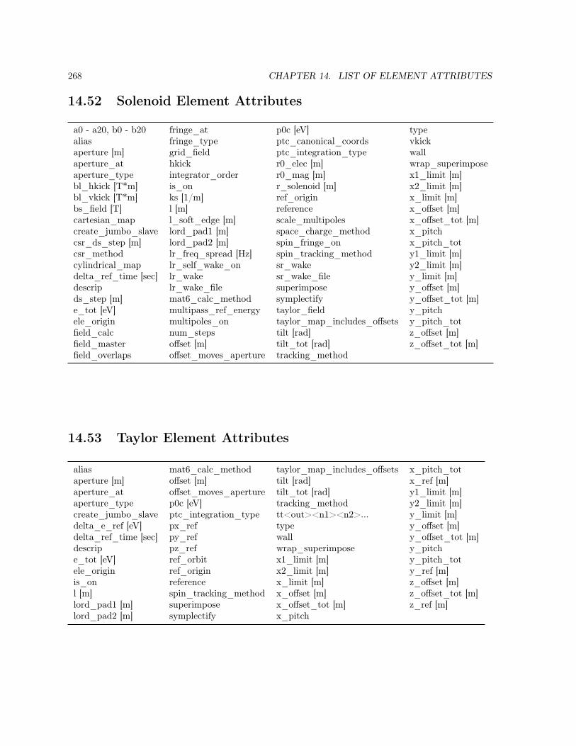
268 CHAPTER 14. LIST OF ELEMENT ATTRIBUTES

14.52 Solenoid Element Attributes

a0 - a20, b0 - b20 fringe_at p0c [eV] typealias fringe_type ptc_canonical_coords vkickaperture [m] grid_field ptc_integration_type wallaperture_at hkick r0_elec [m] wrap_superimposeaperture_type integrator_order r0_mag [m] x1_limit [m]bl_hkick [T*m] is_on r_solenoid [m] x2_limit [m]bl_vkick [T*m] ks [1/m] ref_origin x_limit [m]bs_field [T] l [m] reference x_offset [m]cartesian_map l_soft_edge [m] scale_multipoles x_offset_tot [m]create_jumbo_slave lord_pad1 [m] space_charge_method x_pitchcsr_ds_step [m] lord_pad2 [m] spin_fringe_on x_pitch_totcsr_method lr_freq_spread [Hz] spin_tracking_method y1_limit [m]cylindrical_map lr_self_wake_on sr_wake y2_limit [m]delta_ref_time [sec] lr_wake sr_wake_file y_limit [m]descrip lr_wake_file superimpose y_offset [m]ds_step [m] mat6_calc_method symplectify y_offset_tot [m]e_tot [eV] multipass_ref_energy taylor_field y_pitchele_origin multipoles_on taylor_map_includes_offsets y_pitch_totfield_calc num_steps tilt [rad] z_offset [m]field_master offset [m] tilt_tot [rad] z_offset_tot [m]field_overlaps offset_moves_aperture tracking_method

14.53 Taylor Element Attributes

alias mat6_calc_method taylor_map_includes_offsets x_pitch_totaperture [m] offset [m] tilt [rad] x_ref [m]aperture_at offset_moves_aperture tilt_tot [rad] y1_limit [m]aperture_type p0c [eV] tracking_method y2_limit [m]create_jumbo_slave ptc_integration_type tt<out><n1><n2>... y_limit [m]delta_e_ref [eV] px_ref type y_offset [m]delta_ref_time [sec] py_ref wall y_offset_tot [m]descrip pz_ref wrap_superimpose y_pitche_tot [eV] ref_orbit x1_limit [m] y_pitch_totele_origin ref_origin x2_limit [m] y_ref [m]is_on reference x_limit [m] z_offset [m]l [m] spin_tracking_method x_offset [m] z_offset_tot [m]lord_pad1 [m] superimpose x_offset_tot [m] z_ref [m]lord_pad2 [m] symplectify x_pitch

14.54. WIGGLER AND UNDULATOR ELEMENT ATTRIBUTES 269

14.54 Wiggler and Undulator Element Attributes

a0 - a20, b0 - b20 g_max [1/m] osc_amplitude [m] typealias grid_field p0c [eV] vkickaperture [m] hkick polarity wallaperture_at integrator_order ptc_canonical_coords wrap_superimposeaperture_type is_on ptc_integration_type x1_limit [m]b_max [T] k1x [1/m2] r0_elec [m] x2_limit [m]bl_hkick [T*m] k1y [1/m2] r0_mag [m] x_limit [m]bl_vkick [T*m] kx [1/m] ref_origin x_offset [m]cartesian_map l [m] reference x_offset_tot [m]create_jumbo_slave l_period [m] scale_multipoles x_pitchcsr_ds_step [m] lord_pad1 [m] space_charge_method x_pitch_totcsr_method lord_pad2 [m] spin_fringe_on y1_limit [m]cylindrical_map lr_freq_spread [Hz] spin_tracking_method y2_limit [m]delta_ref_time [sec] lr_self_wake_on sr_wake y_limit [m]descrip lr_wake sr_wake_file y_offset [m]ds_step [m] lr_wake_file superimpose y_offset_tot [m]e_tot [eV] mat6_calc_method symplectify y_pitchele_origin multipass_ref_energy taylor_field y_pitch_totfield_calc multipoles_on taylor_map_includes_offsets z_offset [m]field_master n_period term z_offset_tot [m]field_overlaps num_steps tilt [rad]fringe_at offset [m] tilt_tot [rad]fringe_type offset_moves_aperture tracking_method

270 CHAPTER 14. LIST OF ELEMENT ATTRIBUTES

Part II

Conventions and Physics

271

Chapter 15

CoordinatesBmad uses three coordinate systems as illustrated in Fig. 15.1. First, the global (also called “floor”)coordinates are independent of the accelerator. Thus such things as the building the accelerator is inmay be described using global coordinates.

It is not convenient to describe the position of the beam using the global coordinate system so a “local”coordinate system is used (§15.1). This curvilinear coordinate system defines the nominal position ofthe lattice elements. The relationship between the local and global coordinate systems is describedin §15.2.

The “nominal” position of a lattice element is the position of the element without what are called“misalignments” (that is, position and orientation shifts). Each lattice element has “element body”coordinates which are attached to the physical element. That is, the electric and magnetic fields of anelement are described with respect to element coordinates. If there are no misalignments, the elementcoordinates are aligned with the local coordinates. The transformation between local and elementcoordinates is given in §15.3.

When discussing local vs element coordinates, it can be less confusing to use the name “laboratory”cordinates instead of local coordinates. The x = y = 0 curved line of the laboratory coordinate systemis known as the “reference orbit”.

s

xX

Z

Global (”floor”) coordinates

Local coordinate systema.k.a. The laboratory coords

x

z

Nominal elementposition

Element bodycoordinates

Actual elementposition

Reference orbit

Figure 15.1: The three coordinate systems used by Bmad: The global (or “floor”) coordinate systemis independent of the accelerator. The local curvilinear coordinate system follows the bends of theaccelerator. Each lattice element has element body coordinates which, if the element is not “misaligned”is the same as the local coordinates. The x = y = 0 curved line of the laboratory coordinate system isknown as the “reference orbit”.

273

274 CHAPTER 15. COORDINATES

15.1 Laboratory Coordinates and Reference Orbit

15.1.1 The Reference Orbit

The local reference orbit is the curved path used to define a coordinate system for describing aparticle’s position as shown in Fig. 15.2. The reference orbit is also used for orientating lattice elementsin space. At a given time t, a particle’s position can be described by a point O on the reference orbit adistance s relative to the reference orbit’s zero position plus a transverse (x, y) offset. The point O onthe reference orbit is used as the origin of the local (x, y, z) coordinate system with the z–axis tangentto the reference orbit. The z–axis will generally be pointing in the direction of increasing s (Fig. 15.2A)but, as discussed below, will point counter to s for elements that are reversed (Fig. 15.2B). The x andy–axes are perpendicular to the reference orbit and, by construction, the particle is always at z = 0.The coordinate system so constructed is called the “local coordinate system” or sometimes the“laboratory coordinate system” when there is need to distinguish it from the “element coordinatesystem” (§15) which is attached to the physical element. There is a separate reference orbit for eachbranch (§2.2) of a lattice.

Notice that, in a wiggler, the reference orbit, which is a straight line, does not correspond to the orbitthat any actual particle could travel. Typically the physical element is centered with respect to thereference curve. However, by specifying offsets, pitches or a tilt (See §5.6), the physical element maybe arbitrarily shifted with respect to its reference curve. Shifting a physical magnet with respect to itsreference curve generally means that the reference curve does not correspond to the orbit that any actualparticle could travel.

Do not confuse this reference orbit (which defines the local coordinate system) with the reference orbitabout which the transfer maps are calculated (§34.2). The former is fixed by the lattice while the lattercan be any arbitrary orbit.

ReferenceOrbit

ActualOrbit

Center ofCurvature

x

yz

s

|g| = 1/ρ

s = 0

Particle

ReferenceParticle

A) Normal B) Reversed

ReferenceOrbit

ActualOrbit Center of

Curvature

x

yz

s

|g| = 1/ρ

s = 0

Particle

ReferenceParticle

O O

Figure 15.2: The local reference coordinate system. By construction, a particle’s z coordinate is zero.This is not to be confused with the phase space z coordinate (§15.4.2). The curvature vector g lies inthe x-y plane and has a magnitude of 1/ρ where ρ is the bending radius. A) The z-axis will normallybe parallel to the s-axis. B) For reversed elements it will be antiparallel. In both cases, the particleand reference particle are traveling in the direction of greater s.

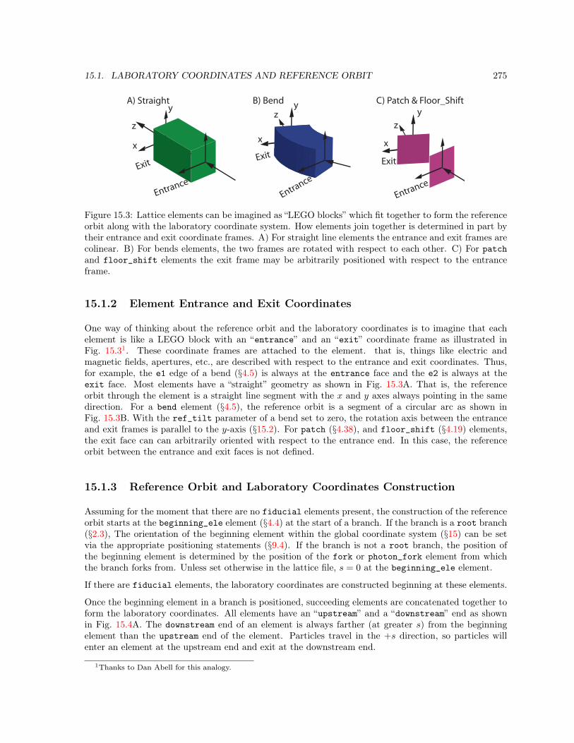
15.1. LABORATORY COORDINATES AND REFERENCE ORBIT 275

Entrance

Exit

Entrance

Exitx

y

zz

y

x

A) Straight B) Bend

Entrance

Exit

x

C) Patch & Floor_Shifty

z

Figure 15.3: Lattice elements can be imagined as “LEGO blocks” which fit together to form the referenceorbit along with the laboratory coordinate system. How elements join together is determined in part bytheir entrance and exit coordinate frames. A) For straight line elements the entrance and exit frames arecolinear. B) For bends elements, the two frames are rotated with respect to each other. C) For patchand floor_shift elements the exit frame may be arbitrarily positioned with respect to the entranceframe.

15.1.2 Element Entrance and Exit Coordinates

One way of thinking about the reference orbit and the laboratory coordinates is to imagine that eachelement is like a LEGO block with an “entrance” and an “exit” coordinate frame as illustrated inFig. 15.31. These coordinate frames are attached to the element. that is, things like electric andmagnetic fields, apertures, etc., are described with respect to the entrance and exit coordinates. Thus,for example, the e1 edge of a bend (§4.5) is always at the entrance face and the e2 is always at theexit face. Most elements have a “straight” geometry as shown in Fig. 15.3A. That is, the referenceorbit through the element is a straight line segment with the x and y axes always pointing in the samedirection. For a bend element (§4.5), the reference orbit is a segment of a circular arc as shown inFig. 15.3B. With the ref_tilt parameter of a bend set to zero, the rotation axis between the entranceand exit frames is parallel to the y-axis (§15.2). For patch (§4.38), and floor_shift (§4.19) elements,the exit face can can arbitrarily oriented with respect to the entrance end. In this case, the referenceorbit between the entrance and exit faces is not defined.

15.1.3 Reference Orbit and Laboratory Coordinates Construction

Assuming for the moment that there are no fiducial elements present, the construction of the referenceorbit starts at the beginning_ele element (§4.4) at the start of a branch. If the branch is a root branch(§2.3), The orientation of the beginning element within the global coordinate system (§15) can be setvia the appropriate positioning statements (§9.4). If the branch is not a root branch, the position ofthe beginning element is determined by the position of the fork or photon_fork element from whichthe branch forks from. Unless set otherwise in the lattice file, s = 0 at the beginning_ele element.

If there are fiducial elements, the laboratory coordinates are constructed beginning at these elements.

Once the beginning element in a branch is positioned, succeeding elements are concatenated together toform the laboratory coordinates. All elements have an “upstream” and a “downstream” end as shownin Fig. 15.4A. The downstream end of an element is always farther (at greater s) from the beginningelement than the upstream end of the element. Particles travel in the +s direction, so particles willenter an element at the upstream end and exit at the downstream end.

1Thanks to Dan Abell for this analogy.

276 CHAPTER 15. COORDINATES

B)

C)

x

zx

z

s - -bnd

dft xz xz

s

dft- -bnd

P

x

y

z

s

Upstream

Downstream

AB

C

A)

D)

xz

xz

sdft bnd

Figure 15.4: A) The laboratory coordinates are constructed by connecting the downstream referenceframe of one element with the upstream reference frame of the next element in the branch. Coordinatesshown is for the mating of element A to element B. B) Example with drift element dft followed by abend bnd. Both elements are unreversed. C) Similar to (B) but in this case element bnd is reversed.D) Similar to (C) but in this case a reflection patch has been added in between dft and bnd. In (B),(C), and (D) the (x, z) coordinates are drawn at the entrance end of the elements. The y coordinate isalways out of the page.

Normally, the upstream end is the element’s entrance end (Fig. 15.3) and the downstream end is theelement’s exit exit. This corresponds to particles entering at the entrance end and exiting the elementat the exit end. However, if an element is reversed (§7.4), the element’s exit end will be upstream endand the element’s entrance end will be the downstream end. That is, for a reversed element, particleswill enter at the element’s exit end and will exit at the entrance end.

The procedure to connect elements together to form the laboratory coordinates is to mate the down-stream reference frame of the element with the upstream reference frame of the next element in thebranch so that, without misalignments, the (x, y, z) axes coincide2. This is illustrated in Fig. 15.4.Fig. 15.4A shows the general situation with the downstream frame of element A mated to the upstreamframe of element B. Figures 15.4B-C show branches constructed from the following lattice file:DFT: drift, l = 2BND: sbend, l = 2, g = pi/12P: patch, x_pitch = pi ! Reflection patch.B_line: line = (DFT, BND) ! No reversal.C_line: line = (DFT, --BND) ! Illegal. Do not use!D_line: line = (DFT, P, --BND) ! Valid.

The (x, z) coordinates are drawn at the entrance end of the elements and z will always point towardsthe element’s exit end. Fig. 15.4B shows the branch constructed from B_line containing an unreverseddrift named dft connected to an unreversed bend named bnd. Fig. 15.4C shows the branch constructedfrom C_line. This is like B_line except here element bnd is reversed. This gives an unphysical situationsince a particle traveling through dft will “fall off” when it gets to the end. Fig. 15.4D shows thebranch constructed from D_line. Here a “reflection” patch P (§15.2.6) has been added to get aplausible geometry. The patch rotates the coordinate system around the y-axis by 180(leaving they-axis invariant). It is always the case that a reflection patch is needed between reversed and unreversedelements

2If there are misalignments, the entrance and exit frames will move with the element. However, the upstream anddownstream frames, along with the reference orbit and laboratory coordinates, will not move.

15.1. LABORATORY COORDINATES AND REFERENCE ORBIT 277

ele_a

x

ss0

s0

s1

ele_b

rb

L

x

s

sa1

α γ

β

patch

sa2

ra

Figure 15.5: The local reference coordinates in a patch element. The patch element, shown schematicallyas an irregular quadrilateral, is sandwiched between elements ele_a and ele_b. L is the length of thepatch. In this example, the patch has a finite x_pitch.

Notes:

• If the first element after the beginning_ele element at the start of a branch is reversed, thebeginning_ele element will be marked as reversed so that a reflection patch is not needed in thiscircumstance.

• Irrespective of whether elements are reversed or not, the laboratory (x, y, z) coordinate system atall s-positions will always be a right-handed coordinate system.

• Care must be take when using reversed elements. For example, if the field of the bnd element inB_line is appropriate for, say, electrons, that is, electrons will be bent in a clockwise fashion goingthrough bnd, then an electron going through D_line will be lost in the bend (the y-axis and hencethe field is in the same direction for both cases so electrons will still be bent in a clockwise fashionbut with D_line a particle needs to be bent counterclockwise to get through the bend). To get aparticle through the bend, positrons must be used.

• A reflection patch that rotated the coordinates, for example, around the x-axis by 180(by settingy_pitch to pi) would also produce a plausible geometry.

15.1.4 Patch Element Local Coordinates

Generally, if a particle is reasonably near the reference orbit, there is a one-to-one mapping betweenthe particle’s position and (x, y, s) coordinates. A patch (§4.38) elements with a non-zero x_pitch ornon-zero y_pitch breaks the one-to-one mapping. This is illustrated in Fig. 15.5. The patch element,shown schematically as an, irregular quadrilateral, is sandwiched between elements ele_a and ele_b.The local coordinate system with origin at α are the coordinates at the end of ele_a. The coordinates atthe end of the patch has its origin labeled γ. By convention, the length of the patch L is taken to be thelongitudinal distance from α to γ with the patch’s exit coordinates defining the longitudinal direction.The “beginning” point of the patch on the reference orbit a distance L from point γ is labeled β in thefigure.

278 CHAPTER 15. COORDINATES

In the local (x, y, s) coordinate system a particle at α will have some value s = s0. A particle at pointβ will have the same value s = s0 and a particle at γ will have s = s1 = s0 + L. A particle at point rain Fig. 15.5 illustrates the problem of assigning (x, y, s) coordinates to a given position. If the particleis considered to be within the region of ele_a, the particle’s s position will be sa2 which is greaterthan the value s0 at the exit end of the element. This contradicts the expectation that particles withinele_a will have s ≤ s0. If, on the other hand, the particle is considered to be within the patch region,the particle’s s position will be sa1 which is less than the value s0 at the entrance to the patch. Thiscontradicts the expectation that a particles within the patch will have s ≥ s0.

To resolve this problem, Bmad considers a particle at position ra to be within the patch region. Thismeans that there is, in theory, no lower limit to the s-position that a particle in the patch region canhave. This also implies that there is a discontinuity in the s-position of a particle crossing the exit faceof ele1. Typically, when particles are translated from the exit face of one element to the exit face of thenext, this patch problem does not appear. It only appears when the track between faces is considered.

Notice that a particle at position rb in Fig. 15.5 can simultaneously be considered to be in either ele_aor the patch. While this creates an ambiguity it does not complicate tracking.

15.2 Global Coordinates

The Cartesian global coordinate system, also called the ‘floor” coordinate system, is the coordinatesystem “attached to the earth” that is used to describe the local coordinate system. Following theMAD convention, the global coordinate axis are labeled (X,Y, Z). Conventionally, Y is the “vertical”coordinate and (X,Z) are the “horizontal” coordinates. To describe how the local coordinate system isoriented within the global coordinate system, each point on the s-axis of the local coordinate systemis characterized by its (X,Y, Z) position and by three angles θ(s), φ(s), and ψ(s) that describe theorientation of the local coordinate axes as shown in Fig. 15.6. These three angles are defined as follows:

θ(s) Azimuth angle: Angle in the (X,Z) plane between the Z–axis and the projection of the z–axisonto the (X,Z) plane. A positive angle of θ = π/2 corresponds to the projected z–axis pointingin the positive X direction.

φ(s) Pitch (elevation) angle: Angle between the z–axis and the (X,Z) plane. A positive angle ofφ = π/2 corresponds to the z–axis pointing in the positive Y direction.

ψ(s) Roll angle: Angle of the x–axis with respect to the line formed by the intersection of the (X,Z)plane with the (x, y) plane. A positive ψ forms a right–handed screw with the z–axis.

By default, at s = 0, the reference orbit’s origin coincides with the (X,Y, Z) origin and the x, y, and zaxes correspond to the X, Y , and Z axes respectively. If the lattice has no vertical bends (the ref_tiltparameter (§4.5) of all bends are zero), the y–axis will always be in the vertical Y direction and thex–axis will lie in the horizontal (X,Z) plane. In this case, θ decreases as one follows the reference orbitwhen going through a horizontal bend with a positive bending angle. This corresponds to x pointingradially outward. Without any vertical bends, the Y and y axes will coincide, and φ and ψ will both bezero. The beginning statement (§9.4) in a lattice file can be use to override these defaults.

Following MAD, the global position of an element is characterized by a vector V

V =

ÑXYZ

é(15.1)

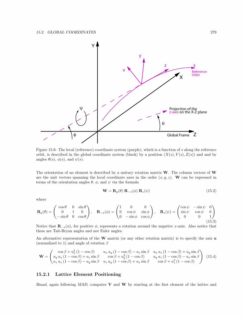
15.2. GLOBAL COORDINATES 279

X

Z

Y

x

y

z

φ

ψ

θ

ReferenceOrbit

Projection of thez-axis on the X-Z plane

Global Frame

s

Figure 15.6: The local (reference) coordinate system (purple), which is a function of s along the referenceorbit, is described in the global coordinate system (black) by a position (X(s), Y (s), Z(s)) and and byangles θ(s), φ(s), and ψ(s).

The orientation of an element is described by a unitary rotation matrix W. The column vectors of Ware the unit vectors spanning the local coordinate axes in the order (x, y, z). W can be expressed interms of the orientation angles θ, φ, and ψ via the formula

W = Ry(θ) R−x(φ) Rz(ψ) (15.2)

where

Ry(θ) =

Ñcos θ 0 sin θ

0 1 0− sin θ 0 cos θ

é, R−x(φ) =

Ñ1 0 00 cosφ sinφ0 − sinφ cosφ

é, Rz(ψ) =

Ñcosψ − sinψ 0sinψ cosψ 0

0 0 1

é(15.3)

Notice that R−x(φ), for positive φ, represents a rotation around the negative x-axis. Also notice thatthese are Tait-Bryan angles and not Euler angles.

An alternative representation of the W matrix (or any other rotation matrix) is to specify the axis u(normalized to 1) and angle of rotation β

W =

Ñcosβ + u2

x (1− cosβ) ux uy (1− cosβ)− uz sinβ ux uz (1− cosβ) + uy sinβuy ux (1− cosβ) + uz sinβ cosβ + u2

y (1− cosβ) uy uz (1− cosβ)− ux sinβuz ux (1− cosβ)− uy sinβ uz uy (1− cosβ) + ux sinβ cosβ + u2

z (1− cosβ)

é(15.4)

15.2.1 Lattice Element Positioning

Bmad, again following MAD, computes V and W by starting at the first element of the lattice and

280 CHAPTER 15. COORDINATES

x0

y0

θt = πz

y

z

z

z

y

x

xθt = -π/2

θt = 0

θt = π/2

A) B)

θt = 0

θt = π/2

θt = π

θt = -π/2

x0

y0

ρ

Figure 15.7: A) Rotation axes (bold arrows) for four different ref_tilt angles of θt = 0, ±π/2, and π.(x0, y0, z0) are the local coordinates at the entrance end of the bend with the z0 axis being directed intothe page. Any rotation axis will be displaced by a distance of the bend radius rho from the origin. B)The (x, y, z) coordinates at the exit end of the bend for the same four ref_tilt angles. In this case thebend angle is taken to be π/2.

iteratively using the equations

Vi = Wi−1 Li + Vi−1, (15.5)Wi = Wi−1 Si (15.6)

Li is the displacement vector for the ith element and matrix Si is the rotation of the local reference systemof the exit end with respect to the entrance end. For clarity, the subscript i in the equations below willbe dripped. For all elements whose reference orbit through them is a straight line, the corresponding Land S are

L =

Ñ00L

é, S =

Ñ1 0 00 1 00 0 1

é, (15.7)

Where L is the length of the element.

For a bend, the axis of rotation is dependent upon the bend’s ref_tilt angle (§5.6) as shown inFig. 15.7A. The axis of rotation points in the negative y0 direction for ref_tilt = 0 and is offset bythe bend radius rho. Here (x0, y0, z0) are the local coordinates at the entrance end of the bend withthe z0 axis being directed into the page in the figure. For a non-zero ref_tilt, the rotation axis isitself rotated about the z0 axis by the value of ref_tilt. Fig. 15.7B shows the exit coordinates for fourdifferent values of ref_tilt and for a bend angle angle of π/2. Notice that for a bend in the horizontalX − Z plane, a positive bend angle will result in a decreasing azimuth angle θ.

For a bend, S is given using Eq. (15.4) with

u = (− sin θt,− cos θt, 0)

β = αb (15.8)

where θt is the ref_tilt angle. The L vector for a bend is given by

L = Rz(θt) L, L =

Ñρ(cosαb − 1)

0ρ sinαb

é(15.9)

where αb is the bend angle (§4.5) and ρ being the bend radius (rho). Notice that since u is perpendicularto z, the curvilinear reference coordinate system has no “torsion”. That is, it is a Frenet-Serret coordinatesystem.

15.2. GLOBAL COORDINATES 281

θb

α

xz

zx

O

In

Out

θb

α

xz

zx

Oin

In

Out

Oout

A) B)

Figure 15.8: Mirror and crystal geometry. The geometry shown here is appropriate for a ref_tilt angleof θt = 0. θg is the bend angle of the incoming (entrance) ray, and αb is the total bend angle of thereference trajectory. A) Geometry for a mirror or a Bragg crystal. Point O is the origin of both the localcoordinates just before and just after the reflection/diffraction. B) Geometry for a Laue crystal. PointOout is the origin of the coordinates just after diffraction is displaced from the origin Oin just beforediffraction due to the finite thickness of the crystal. here the bend angles are measured with respect tothe line that is in the plane of the entrance and exit coordinates and perpendicular to the surface. ForLaue diffraction, the user has the option of using the undiffracted beam (shown in red) as the referencetrajectory.

Note: An alternative equation for S for a bend is

S = Rz(θt) Ry(−αb) Rz(−θt) (15.10)

The bend transformation above is so constructed that the transformation is equivalent to rotating thelocal coordinate system around an axis that is perpendicular to the plane of the bend. This rotationaxis is invariant under the bend transformation. For example, for θt = 0 (or π) the y-axis is the rotationaxis and the y-axis of the local coordinates before the bend will be parallel to the y-axis of the localcoordinates after the bend as shown in Fig. 15.7. That is, a lattice with only bends with θt = 0 or π willlie in the horizontal plane (this assuming that the y-axis starts out pointing along the Y -axis as it doesby default). For θt = ±π/2, the bend axis is the x-axis. A value of θt = +π/2 represents a downwardpointing bend.

15.2.2 Position Transformation When Transforming Coordinates

A point Qg = (X,Y, Z) defined in the global coordinate system, when expressed in the coordinate systemdefined by (V,W) is

QVW = W−1 (Qg −V) (15.11)This is essentially the inverse of Eq. (15.5). That is, vectors propagate inversely to the propagation ofthe coordinate system.

Using Eq. (15.11) with Eqs. (15.5), and (15.6), the transformation of a particle’s position q = (x, y, z)and momentum P = (Px, Py, Pz) when the coordinate frame is transformed from frame (Vi−1,Wi−1)to frame (Vi,Wi) is

qi = S−1i (qi−1 − Li) , (15.12)

Pi = S−1i Pi−1 (15.13)

282 CHAPTER 15. COORDINATES

Notice that since S (and W) is the product of orthogonal rotation matrices, S is itself orthogonal andits inverse is just the transpose

S−1 = ST (15.14)

15.2.3 Crystal and Mirror Element Coordinate Transformation

A crystal element (§4.32) diffracts photons and a mirror element (§4.32) reflects them. For a crystalsetup for Bragg diffraction, and for a mirror, the reference orbit is modeled as a zero length bend withL = (0, 0, 0), as shown in Fig. 15.8A. Shown in the figure is the geometry appropriate for a ref_tiltangle of θt = 0 (the rotation axis is here the y-axis). Since the mirror or crystal element is modeled tobe of zero length, the origin points (marked O in the figure) of the entrance and exit local coordinatesare the same. For Laue diffraction, the only difference is that L is non-zero due to the finite thickness ofthe crystal as shown in Fig. 15.8B. This results in a separation between the entrance coordinate originOin and the exit coordinate origin Oout.

In all cases, the total bending angle is

αb = bragg_angle_in + bragg_angle_out ! Crystal, graze_angle_in = 0

αb = graze_angle_in + graze_angle_out ! Crystal, graze_angle_in 6= 0

αb = 2 graze_angle ! Mirror (15.15)

With a mirror or Bragg diffraction, the bend angles are measured with respect to the surface plane. WithLaue diffraction the bend angles are measured with respect to the line in the bend plane perpendicularto the surface.

For Laue diffraction, the user has the option of using the undiffracted beam (shown in red) as thereference trajectory.

The orientation of the exit coordinates (the local coordinates after the reflection) are only affected bythe element’s ref_tilt and bend angle parameters and is independent of all other parameters such asthe radius of curvature of the surface, etc. The local z-axis of the entrance coordinates along with thez-axis of the exit coordinates define a plane which is called the element’s bend plane. For a mirror,the graze angle is a parameter supplied by the user. For a crystal, the Bragg angles are calculated sothat the reference trajectory is in the middle of the Darwin curve. Calculation of the Bragg angles fora crystal is given in Section §25.4.1.

15.2.4 Patch and Floor_Shift Elements Entrance to Exit Transformation

For patch (§4.38) and floor_shift (§4.19) elements, the shift in the exit end reference coordinates isgiven by Eqs. (15.5) and (15.6) with

L =

Ñx_offsety_offsetz_offset

éS = Ry(x_pitch) R−x(y_pitch) Rz(tilt) (15.16)

The difference here between patch and floor_shift elements is that, with a patch element, the shift isrelative to the exit end of the previous element while, for a floor_shift element, the shift is relative tothe reference point on the origin element specified by the origin_ele parameter of the floor_shift.

15.3. TRANSFORMATION BETWEEN LABORATORYAND ELEMENT BODY COORDINATES283

15.2.5 Fiducial and Girder Elements Origin Shift Transformation

For fiducial and girder elements, the alignment of the reference coordinates with respect to “origin”coordinates is analogous to Eqs. (15.16). Explicitly:

L =

Ñdx_origindy_origindz_origin

éS = Ry(dtheta_origin) R−x(dphi_origin) Rz(dpsi_origin) (15.17)

15.2.6 Reflection Patch

A Patch (or a series of patches) that reflects the direction of the z-axis is called a reflection patch.By “reflected direction” it is meant that the dot product z1 · z2 is negative where z1 is the z-axis vectorat the entrance face and z2 is the z-axis vector at the exit face. This condition is equivalent to thecondition that the associated S matrix (see Eq. (15.16)) satisfy:

S(3, 3) < 0 (15.18)

Using Eq. (15.16) gives, after some simple algebra, this condition is equivalent to

cos(x_pitch) cos(y_pitch) < 0 (15.19)

When there are a series of patches, The transformations of all the patches are concatenated together toform an effective S which can then be used with Eq. (15.18).

15.3 Transformation Between Laboratory and Element Body Co-ordinates

The element body coordinates are the coordinate system attached to an element. Without any misalign-ments, where “misalignments” are here defined to be any offset, pitch or tilt (§5.6), the laboratorycoordinates (§15.1.1) and element body coordinates are the same. With misalignments, the transfor-mation between laboratory and element body coordinates depends upon whether the local coordinatesystem is straight (§15.3.1) or bent (§15.3.2).

When tracking a particle through an element, the particle starts at the nominal (§15) upstream endof the element with the particle’s position expressed in laboratory coordinates. Tracking from the thenominal upstream end to the actual upstream face of the element involves first transforming to elementbody coordinates (with s = 0 in the equations below) and then propagating the particle as in a field freedrift space from the particle’s starting position to the actual element face. Depending upon the element’sorientation, this tracking may involve tracking backwards. Similarly, after a particle has been trackedthrough the physical element to the actual downstream face, the tracking to the nominal downstreamend involves transforming to laboratory coordinates (using s = L in the equations below) and thenpropagating the particle as in a field free drift space to the nominal downstream edge.

15.3.1 Straight Element Misalignment Transformation

For straight line elements, given a laboratory coordinate frame Λs with origin a distance s from thebeginning of the element, misalignments will shift the coordinates to a new reference frame denoted Es.

284 CHAPTER 15. COORDINATES

Since misalignments are defined with respect to the middle of the element, the transformation betweenΛs and Es is a three step process:

Λs −→ Λmid −→ Emid −→ Es (15.20)

where Λmid and Emid are the laboratory and element reference frames at the center of the element.

The first and last transformations from Λs to Λmid and from Emid to Es use Eqs. (15.5), (15.6), and(15.7) with the replacement L → L/2 − s for the first transformation and L → s − L/2 for the thirdtransformation. The middle transformation, by definition of the offset, pitch and tilt parameters is

L =

Ñx_offsety_offsetz_offset

éS = Ry(x_pitch) R−x(y_pitch) Rz(tilt) (15.21)

Notice that with this definition of how elements are misaligned, the position of the center of a non-bendmisaligned element depends only on the offsets, and is independent of the pitches and tilt.

15.3.2 Bend Element Misalignment Transformation

For rbend and sbend elements there is no tilt attribute. Rather, there is the roll attribute and aref_tilt attribute. The latter affects both the reference orbit and the bend position (§5.6.2). Further-more, ref_tilt is calculated with respect to the coordinates at the beginning of the bend while, likestraight elements, roll, offsets, and pitches are calculated with respect to the center of the bend. Thedifferent reference frame used for ref_tilt versus everything else means that five transformations areneeded to get from the laboratory frame to the element body frame (see Eq. (15.20)). Symbolically:

Λs −→ Λmid −→ Ωmid −→ Ω0 −→ E0 −→ Es (15.22)

The first transformation, Λs to Λmid, from laboratory coordinates at a distance s from the beginning ofthe element to laboratory coordinates at the center the bend is a rotation around the center of curvatureof the bend and is given by Eqs. (15.5) and (15.6) with Eqs. (15.8) and (15.9) with the substitutionαb → (L/2− s)/ρ.

The second transformation Λmid to Ωmid at the center of the element adds in the misalignments (Notethat the coordinate frame Ωmid is neither a laboratory frame or an element frame so hence the use of adifferent symbol Ω). Explicitly, the Λmid −→ Ωmid transformation is

L = Loff + [Rz(roll)− 1] Rz(θt) Ry(αb/2) Lc

S = Ry(x_pitch) R−x(y_pitch) Rz(roll) (15.23)

where

Lc =

Ñρ(cos(αb/2)− 1)

0ρ sin(αb/2)

é, Loff =

Ñx_offsety_offsetz_offset

é(15.24)

The reason why L has a different form from straight line elements is due to the fact that the axis ofrotation for a roll is displaced from the z-axis of the coordinate system at the center of the bend (seeFig. 5.3).

The third transformation from Ωmid to Ω0 is like the first transformation and rotates from the center ofthe bend to the beginning. Again Eqs. (15.8) and (15.9) are used with the substitution αb → −L/2ρ.

15.4. PHASE SPACE COORDINATES 285

The fourth transformation Ω0 to E0 tilts the reference frame by an amount ref_tilt:

L = 0, S = Rz(θt) (15.25)

The fifth and final transformation, E0 to Es, like the first and third, rotates around the center of thebend but in this case, since we are dealing with element coordinates, the ref_tilt is ignored. That is,Eqs. (15.8) and (15.9) are used with the substitutions θt → 0 and αb → L/ρ.

Notice that with this definition of how elements are misaligned, the position of the center of a misalignedelement depends only on the offsets and roll, and is independent of the pitches and tilt. Also theorientation of an element depends only on the pitches roll, and ref_tilt, and is independent of theoffsets.

15.4 Phase Space Coordinates

15.4.1 Reference Particle, Reference Energy, and Reference Time

The reference energy and reference time are needed in evaluating the phase space coordinates ofcharged particles (§15.4.2).

All lattice elements, except for controller elements, have an associated reference energy energy. Thereference energy at the start of a lattice’s root branch (§2.2) is set in the lattice file by setting the refer-ence momentum (p0c) or total energy (E_tot) using a parameter (§9.1) or beginning (§9.4) statement.For other branches, the energy at the start of the branch is set using the appropriate line parameter(§9.4) statement.

Note that the reference momentum p0c is actually the reference momentum times the speed of light sothat the reference momentum has the same unit (eV) as the reference energy.

For most elements, the reference energy is the same as the reference energy of the proceeding element.The following elements are exceptions:

customem_fieldhybridlcavitypatch

The reference energy of these elements is determined by tracking a particle (the “reference particle”)through the element with the particle starting on the reference orbit and whose energy is equal to thereference energy. The energy of the particle at the downstream end is the reference energy of the element.

Besides the reference energy, lattice elements have an associated reference time which is computed,for most elements, by the time-of-flight of the reference particle assuming that the reference particleis following the reference orbit. Exceptions are wiggler elements which uses the time-of-flight of theactual undulating trajectory. [Actually what is used in the computation of the z phase space coordinate(Eq. (15.28)) is the sum of reference time deltas of the elements that a particle has passed through. Itis not possible to assign a unique reference time to an element when particles are recirculating throughelements as in a storage ring.]

286 CHAPTER 15. COORDINATES

s

Lp

sReference

Particle

z

A) B)

L0Figure 15.9: Interpreting phase space z at constant velocity: A) The change in z going through anelement of length L0 is L0 − Lp. B) At constant time, z is the longitudinal distance between thereference particle and the particle.

15.4.2 Charged Particle Phase Space Coordinates

For charged particles (more correctly, for everything but photons (§15.4.4)), Bmad uses the canonicalphase space coordinates

r(s) = (x, px, y, py, z, pz) (15.26)

The longitudinal position s is the independent variable instead of the time. x and y, are the transversecoordinates of the particle as shown in Fig. 15.2A. Note that x and y are independent of the position ofthe reference particle.

The phase space momenta px and py are normalized by the reference (sometimes called the design)momentum P0

px =PxP0

py =PyP0

(15.27)

where Px and Py are respectively the x and y momentums.

The phase space z coordinate is

z(s) = −β(s) c (t(s)− t0(s))

≡ −β(s) c∆t(s) (15.28)

t(s) is the time at which the particle is at position s, t0(s) is the time at which the reference particle is atposition s, and β is v/c with v being the particle velocity (and not the reference velocity). The referenceparticle is, by definition, “synchronized” with elements whose fields are oscillating and therefore theactual fields a particle will see when traveling through such an element will depend upon the particle’sphase space z. For example, the energy change of a particle traveling through an lcavity (§4.27) orrfcavity (§4.42) element is z dependent. Exception: With absolute time tracking (§24.1) fields are tiedto the absolute time and not z.

If the particle’s velocity is constant, and is the same as the velocity of the reference particle (for example,at high energy where β = 1 for all particles), then β c t is just the path length. In this case, the changein z going through an element is

∆z = L0 − Lp (15.29)

15.4. PHASE SPACE COORDINATES 287

where, as shown in Fig. 15.9A, L0 is the path length of the reference particle (which is just the lengthof the element) and Lp is the path length of the particle in traversing the element. Another way ofinterpreting phase space z is that, at constant β, and constant time, z is the longitudinal distancebetween the particle and the reference particle as shown in Fig. 15.9B. with positive z indicating thatthe particle is ahead of the reference particle.

Do not confuse the phase space z with the z that is the particle’s longitudinal coordinate in the localreference frame as shown in Fig. 15.2. By construction, this latter z is always zero.

Notice that if a particle gets an instantaneous longitudinal kick so that β is discontinuous then, fromEq. (15.28), phase space z is discontinuous even though the particle itself does not move in space. Ingeneral, from Eq. (15.28), The value of z for a particle at s2 is related to the value of z for the particleat s1 by

z2 =β2

β1z1 − β2 c (∆t2 −∆t1) (15.30)

∆t2 − ∆t1 can be interpreted as the difference in transit time, between the particle and the referenceparticle, in going from s1 to s2.

The longitudinal phase space momentum pz is given by

pz =∆P

P0≡ P − P0

P0(15.31)

where P is the momentum of the particle. For ultra–relativistic particles pz can be approximated by

pz =∆E

E0(15.32)

where E0 is the reference energy (energy here always refers to the total energy) and ∆E = E − E0

is the deviation of the particle’s energy from the reference energy. For an Lcavity element (§4.27) thereference momentum is not constant so the tracking for an Lcavity is not canonical.

MAD uses a different coordinate system where (z, pz) is replaced by (−c∆t, pt) where pt ≡ ∆E/P0c.For highly relativistic particles the two coordinate systems are identical.

The relationship, between the phase space momenta and the slopes x′ ≡ dx/ds and y′ ≡ dy/ds is

x′ =px»

(1 + pz)2 − p2x − p2

y

(1 + gx) (15.33)

y′ =py»

(1 + pz)2 − p2x − p2

y

(1 + gx) (15.34)

g = 1/ρ is the curvature function with ρ being the radius of curvature of the reference orbit and it hasbeen assumed that the bending is in the x–z plane.

With the paraxial approximation, and in the relativistic limit, the change in z with position is

dz

ds= −g x− 1

2(x′2 + y′2) (15.35)

This shows that in a linac, without any bends, the z of a particle always decreases.

A particle can also have a spin. The spin is characterized by the spinor Ψ = (ψ1, ψ2)T where ψ1,2 are

complex numbers (§22.1).

288 CHAPTER 15. COORDINATES

15.4.3 Time-based Phase Space Coordinates

Some specialized routines (for example, time Runge Kutta tracking) use the time t as the independentvariable for charged particle tracking. This is useful when particles can reverse direction since the normalz based tracking cannot handle this. Direction reversal can happen, for example, with low energy “darkcurrent” electrons that are generated at the walls of the vacuum chamber.

When the tracking is time based the phase space coordinates are:

(x, c px, y, c py, z, c ps) (15.36)

The positions x, y, and z are the same as with phase space coordinates (§15.4.2). The momenta aredefined as

cpx ≡ mc2γβxcpy ≡ mc2γβy (15.37)

cps ≡ mc2γβs,

and internally are stored in units of eV.

15.4.4 Photon Phase Space Coordinates

The phase space coordinates discussed above implicitly assume that particles are traveling longitudinallyin only one direction. That is, the sign of the s component of the momentum cannot be determined fromthe phase space coordinates. This is generally fine for tracking high energy beams of charged particlesbut for photon tracking this would oftentimes be problematical. For photons, therefore, a different phasespace is used:

(x, βx, y, βy, z, βz) (15.38)

Here (βx, βy, βz) is the normalized photon velocity with

β2x + β2

y + β2z = 1 (15.39)

and (x, y, z) are the reference orbit coordinates with z being the distance from the start of the latticeelement the photon is in.

In Bmad, the information associated with a photon include its phase space coordinates and time alongwith the photon energy and four parameters Ex, φx, and Ey, φy specifying the intensity and phase ofthe field along the x and y axes transverse to the direction of propagation. the field in the vicinity ofthe photon is

Ex(r, t) ∼ Ex ei(k (z−z0)−ω (t−tref)+φx)

Ey(r, t) ∼ Ey ei(k (z−z0)−ω (t−tref)+φy) (15.40)

where z0 is the photon z position and and tref is the reference time.

The normalization between field and intensity is dependent upon the particular parameters of any givensimulation and so must be determined by the program using Bmad.

Chapter 16

Electromagnetic Fields

16.1 Magnetostatic Multipole Fields

Start with the assumption that the local magnetic field has no longitudinal component (obviously thisassumption does not work with, say, a solenoid). Following MAD, ignoring skew fields for the moment,the vertical magnetic field along the y = 0 axis is expanded in a Taylor series

By(x, 0) =∑n

Bnxn

n!(16.1)

Assuming that the reference orbit is locally straight (there are correction terms if the reference orbit iscurved (§16.3)), the field is

Bx = B1y + B2 xy +1

6B3(3x2y − y3) + . . . (16.2)

By = B0 + B1x+1

2B2(x2 − y2) +

1

6B3(x3 − 3xy2) + . . . (16.3)

For some fields, the normalized integrated multipoleKnL can be used when specifying magnetic multipolecomponents

KnL ≡q LBnP0

(16.4)

where q is the charge of the reference particle (in units of the elementary charge), L is the element length,and P0 is the reference momentum (in units of eV/c). Note that P0/q is sometimes written as Bρ. Thisis just an old notation where ρ is the bending radius of a particle with the reference energy in a field ofstrength B. Notice that P0 is the local reference momentum at the element which may not be the sameas the reference energy at the beginning of the lattice if there are lcavity elements (§4.27) present.

The kicks ∆px and ∆py that a particle experiences going through a multipole field is

∆px =−q LByP0

(16.5)

= −K0L − K1Lx +1

2K2L(y2 − x2) +

1

6K3L(3xy2 − x3) + . . .

∆py =q LBxP0

(16.6)

= K1Ly + K2Lxy +1

6K3L(3x2y − y3) + . . .

289

290 CHAPTER 16. ELECTROMAGNETIC FIELDS

A positive K1L quadrupole component gives horizontal focusing and vertical defocusing. The generalform is

∆px =

∞∑n=0

KnL

n!

bn2 c∑m=0

Ån

2m

ã(−1)m+1 xn−2m y2m (16.7)

∆py =

∞∑n=0

KnL

n!

bn−12 c∑

m=0

Ån

2m+ 1

ã(−1)m xn−2m−1 y2m+1 (16.8)

where bαc means round down to the integer equal to or less than α and(ab

)(“a choose b”) denotes a

binomial coefficient.

The above equations are for fields with a normal component only. If a given multipole field of order nhas normal Bn and skew Sn components and is rotated in the (x, y) plane by an angle Tn, the magneticfield at a point (x, y) can be expressed in complex notation as

By(x, y) + iBx(x, y) =1

n!(Bn + iSn) e−i(n+1)Tn einθ rn (16.9)

where (r, θ) are the polar coordinates of the point (x, y).

Note that, for compatibility with MAD, theK0L component of a Multipole element rotates the referenceorbit essentially acting as a zero length bend. This is not true for multipoles of any other type of element.

Instead of using magnitude Kn and rotation angle θn, Another representation is using normal ‹Kn andskew Sn. The conversion between the two are‹Kn = Kn cos((n+ 1)Tn)

Sn = Kn sin((n+ 1)Tn) (16.10)

Another representation of the magnetic field used by Bmad divides the fields into normal bn and skewan components. In terms of these components the magnetic field for the nth order multipole is

q L

P0(By + iBx) = (bn + ian) (x+ iy)n (16.11)

The an, bn representation of multipole fields can be used in elements such as quadrupoles, sextupoles,etc. to allow “error” fields to be represented. The conversion between (an, bn) and (KnL, SnL, Tn) is

bn + ian =1

n!(KnL+ i SnL) e−i(n+1)Tn (16.12)

In the case where SnL = 0

KnL = n!√a2n + b2n (16.13)

tan[(n+ 1)Tn] =−anbn

(16.14)

To convert a normal magnet (a magnet with no skew component) into a skew magnet (a magnet withno normal component) the magnet should be rotated about its longitudinal axis with a rotation angle of

(n+ 1)Tn =π

2(16.15)

For example, a normal quadrupole rotated by 45 becomes a skew quadrupole.

16.2. ELECTROSTATIC MULTIPOLE FIELDS 291

The multipole fields can be “reference energy” scaled and/or “element strength” scaled. Scalinghere means that the an and bn values used in tracking are scaled from the input values given in thelattice file.

Reference energy scaling is applied if the field_master attribute (§5.2) is True for an element so thatthe multipole values specified in the lattice file are not reference energy normalized[

an, bn]−→

[an, bn

]· qP0

(16.16)

Element strength scaling is applied when the multipoles are associated with a non AB_Multipoleelement and if the scale_multipoles attribute (§5.14) is True. This scaling uses a measurement radiusr0 and a scale factor F : [

an, bn]−→

[an, bn

]· F · r

nref0

rn0(16.17)

r0 is set by the r0_mag attribute of an element. F and nref are set automatically depending upon thetype of element as shown in Table 16.1. The γp term is

Element F nref

Elseparator√Hkick2 + Vkick2 0

Hkicker Kick 0Kicker,AC_Kicker

√Hkick2 + Vkick2 0

Rbend G * L 0Sbend G * L 0Vkicker Kick 0

Wiggler 2 c L_poleBmaxπ p0c 0

Quadrupole K1 * L 1Sol_Quad K1 * L 1Solenoid KS * L 1Sextupole K2 * L 2Octupole K3 * L 3

Table 16.1: F and nref for various elements.

16.2 Electrostatic Multipole Fields

Except for the elseparator element, Bmad specifies DC electric fields using normal ben and skew aencomponents (§5.14. The potential φn for the nth order multipole is

φn = −Re

ïben − iaenn+ 1

(x+ iy)n+1

rn0

ò(16.18)

where r0 is a “measurement radius” set by the r0_elec attribute of an element (§5.14).

The electric field for the nth order multipole is

Ex − iEy = (ben − iaen)(x+ iy)n

rn0(16.19)

Notice that the magnetic multipole components an and bn are normalized by the element length, referencecharge, and reference momentum (Eq. (16.11)) while their electric counterparts are not.

292 CHAPTER 16. ELECTROMAGNETIC FIELDS

Using the paraxial approximation, The kick given a particle due to the electric field is

dpxds

=q Exβ P0 c

,dpyds

=q Eyβ P0 c

(16.20)

Where β is the normalized velocity.

16.3 Exact Multipole Fields in a Bend

For static magnetic and electric multipole fields in a bend, the spacial dependence of the field is differentfrom multipole fields in an element with a straight geometry as given by Eqs. (16.11) and (16.19). Theanalysis of the multipole fields in a bend here follows McMillan[McMill75].

In the rest of this section, normalized coordinates r = r/ρ, x/ = x/ρ, and y = y/ρ will be used whereρ is the bending radius of the reference coordinate system, r is the distance, in the plane of the bend,from the bend center to the observation point, x is the distance in the plane of the from the referencecoordinates to the observation point and y is the distance out-of-plane. With this convention r = 1 + x.

An electric or magnetic multipole can be characterized by a scalar potential φ with the field given by−∇φ. The potential is a solution to Laplace’s equation

1

r

∂

∂ r

År∂ φ

∂ r

ã+∂2φ

∂ y2= 0 (16.21)

As McMillian shows, it is also possible to calculate the magnetic field by constructing the appropriatevector potential. However, from a practical point of view, it is simpler to use the scalar potential forboth the magnetic and electric fields.

Solutions to Laplace’s equation can be found in form

φrn =−1

1 + n

b(n+1)/2c∑p=0

Ån+ 1

2 p

ã(−1)p Fn+1−2p(r) y

2p (16.22)

and in the form

φin =−1

1 + n

bn/2c∑p=0

Ån+ 12p+ 1

ã(−1)p Fn−2p(r) y

2p+1 (16.23)

where(ab

)(“a choose b”) denotes a binomial coefficient, n is the order number which can range from 0

to infinity, bαc means round down to the integer equal to or less than α. [Notice that here n is relatedto m in McMillian’s paper by m = n+ 1. Also note that the φr and φi here have a normalization factorthat is different from McMillian.]

In Eq. (16.23) the Fp(r) are related by

Fp+2 = (p+ 1) (p+ 2)

∫ r

1

dr

r

ñ∫ r

1

dr r Fp

ô(16.24)

with the “boundary condition”:

F0(r) = 1

F1(r) = ln r (16.25)

16.3. EXACT MULTIPOLE FIELDS IN A BEND 293

This condition ensures that the number of terms in the sums in Eqs. (16.22) and (16.23) are finite. Withthis condition, all the Fp can be constructed:

F1 = ln r = x− 1

2x2 +

1

3x3 − . . .

F2 =1

2(r2 − 1)− ln r = x2 − 1

3x3 +

1

4x4 − . . .

F3 =3

2[−(r2 − 1) + (r2 + 1) ln r] = x3 − 1

2x4 +

7

20x5 − . . . (16.26)

F4 = 3[1

8(r4 − 1) +

1

2(r2 − 1)− (r2 +

1

2) ln r] = x4 − 2

5x5 +

3

10x6 − . . .

Etc...

In terms of implementing these functions on a computer, the exact r-dependent functions are problemat-ical due to round off error near x = 0. For example, Evaluating F4(r) at x = 10−4 results in a completeloss of accuracy (no significant digits!) when using double precision numbers. In practice, Bmad uses aPadé approximant for x small enough and then switches to the r-dependent formulas for x away fromzero.

For magnetic fields, the “real” φrn solutions will correspond to skew fields and the “imaginary” φin solutionswill correspond to normal fields

B = − P0

q L

∞∑n=0

ρnîan ‹∇φrn + bn ‹∇φinó (16.27)

where the gradient derivatives of ‹∇ are with respect to the normalized coordinates. In the limit ofinfinite bending radius ρ, the above equations converge to the straight line solution given in Eq. (16.11).

For electric fields, the “real” solutions will correspond to normal fields and the “imaginary” solutions areused for skew fields

E = −∞∑n=0

ρnîaen ‹∇φin + ben ‹∇φrnó (16.28)

And this will converge to Eq. (16.19) in the straight line limit.

In the vertical plane, with x = 0, the solutions φrn and φin have the same variation in y as the multipolefields with a straight geometry. For example, the field strength of an n = 1 (quadrupole) multipolewill be linear in y for x = 0. However, in the horizontal direction, with y = 0, the multipole field willvary like dF2/dx which has terms of all orders in x. In light of this, the solutions φrn and φin are called“vertically pure” solutions.

It is possible to construct “horizontally pure” solutions as well. That is, it is possible to constructsolutions that in the horizontal plane, with y = 0, behave the same as the corresponding multipole fieldswith a straight geometry. A straight forward way to do this, for some given multipole of order n, isto construct the horizontally pure solutions, ψrn and ψin, as linear superpositions of the vertically puresolutions

ψrn =

∞∑k=n

Cnk φrk, ψin =

∞∑k=n

Dnk φik (16.29)

with the normalizations Cnn = Dnn = 1. The Cnk and Dnk are chosen, order by order, so that ψrn andψin are horizontally pure. For the real potentials, the Cnk, are obtained from a matrix M where Mij

is the coefficient of the xj term of (dFi/dx)/i when Fi is expressed as an expansion in x (Eq. (16.26)).Cnk, k = 0, . . . ,∞ are the row vectors of the inverse matrix M−1. For the imaginary potentials, the Dnk

294 CHAPTER 16. ELECTROMAGNETIC FIELDS

are constructed similarly but in this case the rows of M are the coefficients in x for the functions Fi. Toconvert between field strength coefficients, Eqs. (16.27) and (16.28) and Eqs. (16.29) are combined

an =

∞∑k=n

1

ρk−nCnk αk, aen =

∞∑k=n

1

ρk−nDnk αek,

bn =

∞∑k=n

1

ρk−nDnk βk, ben =

∞∑k=n

1

ρk−nDnk βek (16.30)

where αk, βk, αek, and βek are the corresponding coefficients for the horizontally pure solutions.

When expressed as a function of r and y, the vertically pure solutions φn have a finite number of terms(Eqs. (16.22) and (16.23)). On the other hand, the horizontally pure solutions ψn have an infinite numberof terms.

The vertically pure solutions form a complete set. That is, any given field that satisfies Maxwell’sequations and is independent of z can be expressed as a linear combination of φrn and φin. Similarly, thehorizontally pure solutions form a complete set. [It is, of course, possible to construct other completesets in which the basis functions are neither horizontally pure nor vertically pure.]

This brings up an important point. To properly simulate a machine, one must first of all understandwhether the multipole values that have been handed to you are for horizontally pure multipoles, vertically,pure multipoles, or perhaps the values do not correspond to either horizontally pure nor vertically puresolutions! Failure to understand this point can lead to differing results. For example, the chromaticityinduced by a horizontally pure quadrupole field will be different from the chromaticity of a verticallypure quadrupole field of the same strength. With Bmad, the exact_multipoles (§4.5) attribute of abend is used to set whether multipole values are for vertically or horizontally pure solutions. [Note toprogrammers: PTC always assumes coefficients correspond to horizontally pure solutions. The BmadPTC interface will convert coefficients as needed.]

16.4 Map Decomposition of Magnetic and Electric Fields

Electric and magnetic fields can be parameterized as the sum over a number of functions with eachfunction satisfying Maxwell’s equations. These functions are also referred to as “maps”, “modes”, or“terms”. Bmad has two parameterizations:Cartesian_Map ! §16.5.Cylindrical_Map ! §16.6

These parameterizations are two of the four field map parameterizations that Bmad defines §5.15.

The cartesian_map decomposition involves a set of terms, each term a solution the Laplace equationsolved using separation of variables in Cartesian coordinates. This decomposition can be used for DC butnot AC fields. See §16.5. for more details. The syntax for specifying the cartesian_map decompositionis discussed in §5.15.2.

The cylindrical_map decomposition can be used for both DC and AC fields. See §16.6 for more details.The syntax for specifying the cylindrical_map decomposition is discussed in §5.15.3.

16.5 Cartesian Map Field Decomposition

Electric and magnetic fields can be parameterized as the sum over a number of functions with eachfunction satisfying Maxwell’s equations. These functions are also referred to as “maps”, “modes”, or

16.5. CARTESIAN MAP FIELD DECOMPOSITION 295

“terms”. Bmad has two types. The “Cartesian” decomposition is explained here. The other type is thecylindrical decomposition (§16.6).

The Cartesian decomposition implemented by Bmad involves a set of terms, each term a solution theLaplace equation solved using separation of variables in Cartesian coordinates. This decomposition isfor DC electric or magnetic fields. No AC Cartesian Map decomposition is implemented by Bmad. In alattice file, a Cartesian map is specified using the cartesian_map attribute as explained in Sec. §5.15.2.

The Cartesian decomposition is modeled using an extension of the method of Sagan, Crittenden, andRubin[Sagan03]. In this decomposition, the magnetic(or electric field is written as a sum of terms Bi(For concreteness the symbol Bi is used but the equations below pertain equally well to both electricand magnetic fields) with:

B(x, y, z) =∑i

Bi(x, y, z;A, kx, ky, kz, x0, y0, φz, family) (16.31)

Each term Bi is specified using seven numbers (A, kx, ky, kz, x0, y0, φz) and a switch called family whichcan be one of:x, quy, sq

Roughly, taking the offsets x0 and y0 to be zero (see the equations below), the x family gives a fieldon-axis where the y component of the field is zero. that is, the x family is useful for simulating, say,magnetic vertical bend dipoles. The y family has a field that on-axis has no x component. The qufamily has a magnetic quadrupole like (which for electric fields is skew quadrupole like) field on-axisand the sq family has a magnetic skew quadrupole like field on-axis. Additionally, assuming that thex0 and y0 offsets are zero, the sq family, unlike the other three families, has a nonzero on-axis z fieldcomponent.

Each family has three possible forms These are designated as “hyper-y”, “hyper-xy”, and “hyper-x”.

For the x family the hyper-y form is:

Bx = Akxky

cos(kx(x+ x0)) cosh(ky(y + y0)) cos(kzz + φz)

By = A sin(kx(x+ x0)) sinh(ky(y + y0)) cos(kzz + φz)

Bs = −A kzky

sin(kx(x+ x0)) cosh(ky(y + y0)) sin(kzz + φz) (16.32)

with k2y = k2

x + k2z

The x family hyper-xy form is:

Bx = Akxkz

cosh(kx(x+ x0)) cosh(ky(y + y0)) cos(kzz + φz)

By = Akykz

sinh(kx(x+ x0)) sinh(ky(y + y0)) cos(kzz + φz)

Bs = −A sinh(kx(x+ x0)) cosh(ky(y + y0)) sin(kzz + φz) (16.33)

with k2z = k2

x + k2y

And the x family hyper-x form is:

Bx = A cosh(kx(x+ x0)) cos(ky(y + y0)) cos(kzz + φz)

By = −A kykx

sinh(kx(x+ x0)) sin(ky(y + y0)) cos(kzz + φz)

Bs = −A kzkx

sinh(kx(x+ x0)) cos(ky(y + y0)) sin(kzz + φz) (16.34)

with k2x = k2

y + k2z

296 CHAPTER 16. ELECTROMAGNETIC FIELDS

The relationship between kx, ky, and kz ensures that Maxwell’s equations are satisfied. Notice thatwhich form hyper-y, hyper-xy, and hyper-x a particular Bi belongs to can be computed by Bmad bylooking at the values of kx, ky, and kz.

Using a compact notation where Ch ≡ cosh, subscript x is kx(x+ x0), subscript z is kzz + φz, etc., they family of forms is:

Form hyper-y hyper-xy hyper-x

Bx −A kxky

Sx Shy Cz Akxkz

Shx Shy Cz A Shx Sy Cz

By A Cx Chy Cz Akykz

Chx Chy Cz Akykx

Chx Cy Cz (16.35)

Bz −A kzky

Cx Shy Sz −A Chx Shy Sz −A kzkx

Chx Sy Sz

with k2y = k2

x + k2z k2

z = k2x + k2

y k2x = k2

y + k2z

the qu family of forms is:

Form hyper-y hyper-xy hyper-x

Bx Akxky

Cx Shy Cz Akxkz

Chx Shy Cz A Chx Sy Cz

By A Sx Chy Cz Akykz

Shx Chy Cz Akykx

Shx Cy Cz (16.36)

Bz −A kzky

Sx Shy Sz −A Shx Shy Sz −A kzkx

Shx Sy Sz

with k2y = k2

x + k2z k2

z = k2x + k2

y k2x = k2

y + k2z

the sq family of forms is:

Form hyper-y hyper-xy hyper-x

Bx −A kxky

Sx Chy Cz Akxkz

Shx Chy Cz −A Shx Cy Cz

By A Cx Shy Cz Akykz

Chx Shy Cz Akykx

Chx Sy Cz (16.37)

Bz −A kzky

Cx Chy Sz −A Chx Chy Sz Akzkx

Chx Cy Sz

with k2y = k2

x + k2z k2

z = k2x + k2

y k2x = k2

y + k2z

The singular case where kx = ky = kz = 0 is not allowed. If a uniform field is needed, a term withvery small kx, ky, and kz can be used. Notice that since ky must be non-zero for the hyper-y forms(remember, k2

y = k2x + k2

z for these forms and not all k’s can be zero), and kz must be non-zero forthe hyper-xy forms, and kx must be nonzero for the hyper-x forms. The magnetic field is always welldefined even if one of the k’s is zero.

16.6 Cylindrical Map Decomposition

Electric and magnetic fields can be parameterized as the sum over a number of functions with eachfunction satisfying Maxwell’s equations. These functions are also referred to as “maps”, “modes”, or

16.6. CYLINDRICAL MAP DECOMPOSITION 297

“terms”. Bmad has two types. The “cylindrical” decomposition is explained here. The other type isthe Cartesian decomposition (§16.6).

In a lattice file, a cylindrical map is specified using the cylindrical_map attribute as explained inSec. §5.15.3.

The cylindrical decomposition takes one of two forms depending upon whether the fields are timevarying or not. The DC decomposition is explained in Sec. §16.6.1 while the RF decomposition isexplained in Sec. §16.6.2.

16.6.1 DC Cylindrical Map Decomposition

The DC cylindrical parametrization used by Bmad essentially follows Venturini et al.[Venturini98].See Section §5.15 for details on the syntax used to cylindrical maps in Bmad. The electric and magneticfields are both described by a scalar potential

B = −∇ψB , E = −∇ψE (16.38)

The scalar potentials both satisfy the Laplace equation ∇2 ψ = 0. The scalar potentials are decomposedas a sum of modes indexed by an integer m

ψB = Re

[ ∞∑m=0

ψBm

](16.39)

[Here and below, only equations for the magnetic field will be shown. The equations for the electricfields are similar.] The ψBm are decomposed in z using a discrete Fourier sum.1 Expressed in cylindricalcoordinates the decomposition of ψBm is

ψBm =

N/2−1∑n=−N/2

ψBmn =

N/2−1∑n=−N/2

−1

knei kn z cos(mθ − θ0m) bm(n) Im(kn ρ) (16.40)

where Im is a modified Bessel function of the first kind, and the bm(n) are complex coefficients. [Forelectric fields, em(n) is substituted for bm(n)] In Eq. (16.40) kn is given by

kn =2π n

N dz(16.41)

where N is the number of “sample points”, and dz is the longitudinal “distance between points”. Thatis, the above equations will only be accurate over a longitudinal length (N − 1) dz. Note: Typically thesum in Eq. (16.40) and other equations below runs from 0 to N −1. Using a sum from −N/2 to N/2−1gives exactly the same field at the sample points (z = 0, dz, 2 ds, . . .) and has the virtue that the field issmoother in between.

The field associated with ψBm is for m = 0:

Bρ = Re

N/2−1∑n=−N/2

ei kn z b0(n) I1(kn ρ)

Bθ = 0 (16.42)

Bz = Re

N/2−1∑n=−N/2

i ei kn z b0(n) I0(kn ρ)

1Venturini uses a continuous Fourier transformation but Bmad uses a discrete transformation so that only a finite

number of coefficients are needed.

298 CHAPTER 16. ELECTROMAGNETIC FIELDS

And for m 6= 0:

Bρ = Re

N/2−1∑n=−N/2

1

2ei kn z cos(mθ − θ0m) bm(n)

[Im−1(kn ρ) + Im+1(kn ρ)

]Bθ = Re

N/2−1∑n=−N/2

−1

2ei kn z sin(mθ − θ0m) bm(n)

[Im−1(kn ρ)− Im+1(kn ρ)

] (16.43)

Bz = Re

N/2−1∑n=−N/2

i ei kn z cos(mθ − θ0m) bm(n) Im(kn ρ)

While technically ψBm0 is not well defined due to the 1/kn factor that is present, the field itself is wellbehaved. Mathematically, Eq. (16.40) can be corrected if, for n = 0, the term Im(kn ρ)/kn is replacedby

Im(k0 ρ)

k0→

ρ if m = 0

ρ/2 if m = 1

0 otherwise(16.44)

The magnetic vector potential for m = 0 is constructed such that only Aθ is non-zero

Aρ = 0

Aθ = Re

N/2−1∑n=−N/2

i

knei kn z b0(n) I1(kn ρ)

(16.45)

Az = 0

For m 6= 0, the vector potential is chosen so that Aθ is zero.

Aρ = Re

N/2−1∑n=−N/2

−i ρ2m

ei kn z cos(mθ − θ0m) bm(n)[Im−1(kn ρ)− Im+1(kn ρ)

]Aθ = 0 (16.46)

Az = Re

N/2−1∑n=−N/2

−i ρm

ei kn z cos(mθ − θ0m) bm(n) Im(kn ρ)

Note: The description of the field using “generalized gradients”[Newton99] is similar to the aboveequations. The difference is that, with the generalized gradient formalism, terms in θ and ρ are expandedin a Taylor series in x and y.

16.6.2 AC Cylindrical Map Decomposition

For RF fields, the cylindrical mode parametrization used by Bmad essentially follows Abell[Abell06].The electric field is the real part of the complex field

E(r) =

M∑j=1

Ej(r) exp[−2π i (fj t+ φ0j)] (16.47)

16.6. CYLINDRICAL MAP DECOMPOSITION 299

where M is the number of modes. Each mode satisfies the vector Helmholtz equation

∇2Ej + k2tj Ej = 0 (16.48)

where ktj = 2π f/c with fj being the mode frequency.

The individual modes vary azimuthally as cos(mθ − θ0) where m is a non-negative integer. [in thisand in subsequent equations, the mode index j has been dropped.] For the m = 0 modes, there is anaccelerating mode whose electric field is in the form

Eρ(r) =

N/2−1∑n=−N/2

−ei kn z i kn e0(n) I1(κn, ρ)

Eθ(r) = 0 (16.49)

Ez(r) =

N/2−1∑n=−N/2

ei kn z e0(n) I0(κn, ρ)

where Im is

Im(κn, ρ) ≡ Im(κn ρ)

κmn(16.50)

with Im being a modified Bessel function first kind, and κn is given by

κn =»k2n − k2

t =

®√k2n − k2

t |kn| > kt

−i√k2t − k2

n kt > |kn|(16.51)

withkn =

2π n

N dz(16.52)

N is the number of points where Ezc is evaluated, and dz is the distance between points. The length ofthe field region is (N − 1) dz. When κn is imaginary, Im(κn ρ) can be evaluated through the relation

Im(−i x) = i−m Jm(x) (16.53)

where Jm is a Bessel function of the first kind. The e0 coefficients can be obtained given knowledge ofthe field at some radius R via

e0(n) =1

I0(κn, R)

1

N

N−1∑p=0

e−2π i n p/N Ez(R, p dz) (16.54)

The non-accelerating m = 0 mode has an electric field in the form

Eρ(r) = Ez(r) = 0

Eθ(r) =

N/2−1∑n=−N/2

ei kn z b0(n) I1(κn, ρ) (16.55)

where the b0 coefficients can be obtained given knowledge of the field at some radius R via

b0(n) =1

I1(κn, R)

1

N

N−1∑p=0

e−2π i n p/N Eθ(R, p dz) (16.56)

300 CHAPTER 16. ELECTROMAGNETIC FIELDS

For positive m, the electric field is in the form

Eρ(r) =

N/2−1∑n=−N/2

−i ei kn zñkn em(n) Im+1(κn, ρ) + bm(n)

Im(κn, ρ)

ρ

ôcos(mθ − θ0m)

Eθ(r) =

N/2−1∑n=−N/2

−i ei kn zîkn em(n) Im+1(κn, ρ) + (16.57)

bm(n)

ÇIm(κn, ρ)

ρ− 1

mIm−1(κn, ρ)

åôsin(mθ − θ0m)

Ez(r) =

N/2−1∑n=−N/2

ei kn z em(n) Im(κn, ρ) cos(mθ − θ0m)

The e_m and b_m coefficients can be obtained given knowledge of the field at some radius R via

em(n) =1

Im(κn, R)

1

N

N−1∑p=0

e−2π i n p/N Ezc(R, p dz)

bm(n) =R

Im(κn, R)

[1

N

N−1∑p=0

i e−2π i n p/N Eρc(R, p dz)− kn em(n) Im+1(κn, R)

](16.58)

where Eρc, Eθs, and Ezc are defined by

Eρ(R, θ, z) = Eρc(R, z) cos(mθ − θ0m)

Eθ(R, θ, z) = Eθs(R, z) sin(mθ − θ0m) (16.59)Ez(R, θ, z) = Ezc(R, z) cos(mθ − θ0m)

The above mode decomposition was done in the gauge where the scalar potential ψ is zero. The electricand magnetic fields are thus related to the vector potential A via

E = −∂t A, B = ∇×A (16.60)

Using Eq. (16.47), the vector potential can be obtained from the electric field via

Aj =−iEj

2π fj(16.61)

Symplectic tracking through the RF field is discussed in Section §24.4. For the fundamental acceleratingmode, the vector potential can be analytically integrated using the identity∫

dxx I1(a

√x2 + y2)√

x2 + y2=

1

aI0(a

√x2 + y2) (16.62)

16.7 Field Modeling Using Taylor Maps

Bmad has a number of field map models that can be used to model electric or magnetic fields (§5.15).One model involves a set of Taylor maps. This model is restricted to modeling DC fields. In a latticefile, the Taylor field model is specified using the taylor_field attribute as explained in Sec. §5.15.5.

16.8. RF FIELDS FOR FIELD_CALC = BMAD_STANDARD 301

The Taylor field model specifies the field using a set of Taylor maps. Each map defines the field in thetransverse (x, y) plane at constant longitudinal z: That is, each Taylor map is comprised of three Taylorseries, one for each field component, and each Taylor series is a polynomial in x and y:

B = (Bx(x, y; i), By(x, y; i), Bz(x, y; i)) (16.63)

where the Bx, By, Bz on the right hand side represent the tree Taylor series, i denotes the Taylor mapat zi = i · dz where dz is the spacing between maps. The maps are restricted to be equally spacedto enable higher order integration schemes in PTC (See default_integ_order in §10.4). [Note: EachTaylor field model specifies either an electric or magnetic field. In this section, the symbol B can referto either magnetic or electric fields.]

Interpolation of the field in Bmad is done using a cubic spline fit. Given a position (x, y, z), the field Band transverse field derivatives ∂B/∂r, are evaluated at two positions r0 = (x, y, zi0) and r1 = (x, y, zi1)with zi0 being the positions of the maps to either side of z. The longitudinal field derivatives are derivedfrom the transverse ones using Maxwell’s equations:

∂Bx∂z

=∂Bz∂x

,∂By∂z

=∂Bz∂y

,∂Bz∂z

= −Å∂Bx∂x

+∂By∂y

ã(16.64)

Once the field and longitudinal derivatives are known at r0 and r1, a standard cubic spline interpolationis done.

Note: If the Taylor field model uses curved coordinates, There will be inaccuracies in the computedfield to the extent that Maxwell’s equations have to be modified to take into account the coordinatecurvature.

16.8 RF fields for Field_Calc = Bmad_Standard

The following describes the how RF fields are calculated when the the field_calc attribute of an RFelement is set to bmad_standard.

The traveling wave model for RF cavities the field, in cylindrical coordinates is

Es(r, φ, s, t) = G cos(k s− ω t+ 2π φ

)Er(r, φ, s, t) =

1

2Gk r sin

(k s− ω t+ 2π φ

)(16.65)

Bφ(r, φ, s, t) =1

2 cGk r sin

(k s− ω t+ 2π φ

)where G is the accelerating gradient, k = ω/c is the wave number with ω being the RF frequency.

For standing wave cavities, the RF fields are modeled as N half-wave cells, each having a length of λ/2where λ = 2π/k is the wavelength. If the length of the RF element is not equal to the length of N cells,the “active region” is centered in the element and the regions to either side are treated as field free.

The field in the standing wave cell is modeled either with a p = 0 or p = 1 longitudinal mode. The p = 1longitudinal mode (which is the default if the longitudinal mode is not set in the element), models thefields as a pillbox with the transverse wall at infinity as detailed in Chapter 3, Section VI of reference[Lee99]

Es(r, φ, s, t) = 2G cos(k s) cos(ω t+ 2π φ)

Er(r, φ, s, t) = Gk r sin(k s) cos(ω t+ 2π φ) (16.66)

Bφ(r, φ, s, t) =−1

cG k r cos(k s) sin(ω t+ 2π φ)

302 CHAPTER 16. ELECTROMAGNETIC FIELDS

The overall factor of 2 in the equation is present to ensure that an ultra-relativistic particle enteringwith φ = 0 will experience an average gradient equal to G.

For the p = 0 longitudinal mode, a “pseudo TM010” mode is used that has the correct symmetry:

Es(r, φ, s, t) = 2G sin(k s) sin(ω t+ 2π φ)

Er(r, φ, s, t) = −Gk r cos(k s) sin(ω t+ 2π φ) (16.67)

Bφ(r, φ, s, t) =1

cG k r sin(k s) cos(ω t+ 2π φ)

Chapter 17

Fringe Fields

The fringe field kick is divided into two pieces. The first piece is called the hard edge fringe kick andis the kick in the limit that the longitudinal extent of the fringe is zero. The second piece is the softedge fringe kick which is the fringe kick with the fringe having a finite longitudinal extent minus thehard edge fringe kick. That is

fringe kick = hard fringe kick + soft fringe kick

The advantage of separating the fringe kick in this way is that the hard fringe can be used withouthaving to know anything about the longitudinal extent of the fringe field. In many cases, this is a goodenough approximation.

17.1 Dipole Soft Edge Fringe Map for Bends and Sad_Mult

The dipole soft edge fringe model is adapted from SAD[SAD]. For sbend and rbend elements, the fringemap is defined in terms of the field integrals FH1 for the entrance end and FH2 for the exit end givenby (see Eq. (4.8))

FH1 ≡ FintHgap =

∫pole

dsBy(s) (By0 −By(s))

2B2y0

(17.1)

With a similar equation for FH2.

For a sad_mult element the corresponding parameters are fb1 and fb2. the conversion between thebend and sad_mult parameters is

fb1 = 12FH1, fb2 = 12FH2 (17.2)

The soft edge map is

x2 = x1 + c1 pz

py2 = py1 + c2 y1 − c3 y31 (17.3)

z2 = z1 +1

1 + pz1

Åc1 px1 +

1

2c2 y

21 −

1

4c3 y

41

ã303

304 CHAPTER 17. FRINGE FIELDS

For the entrance face:

c1 =gtot fb12

24 (1 + pz)=

6 gtot F2H1

1 + pz, c2 =

g2tot fb1

6 (1 + pz)=

2 g2tot FH1

1 + pz,

c3 =2 g2

tot

3 fb1 (1 + pz)=

g2tot

18FH1 (1 + pz)(17.4)

For a bend, g_tot is the total bending strength

gtot = g + dg (17.5)

g being the reference bend strength and dg being bend the difference between the actual and referencebend strengths (§4.5). For a sad_mult element g_tot is calculated from the equation

gtot =»a2

0 + b20 (17.6)

It might seem strange that c3 diverges to infinity as FH goes to zero since naively one would expect thesoft edge kick to vanish in the hard edge limit where the fringe has no longitudinal extent. However, inthe hard edge limit, the field does not obey Maxwell’s equations. The limiting map, as FH goes to zero,has fields that diverge to infinity and this explains why the full (hard + soft) limiting map is not thesame as the hard edge map at the limit of zero longitudinal extent.

For the exit face, the appropriate equations can be derived using the substitution

FH1 → FH2

gtot → −gtot (17.7)

17.2 Dipole Hard Edge Fringe Map

The bend fringe kick is a combination of the equations developed by Hwang and Lee[Hwang15] modifiedto include quadrupole terms as given in Section 5.3.1 of Iselin[Iselin94]. The Lie map generator ΩMgiven by Hwang and Lee Eqs. (35) and (36) is used under the conditions that

K0h = K1h = K2h = K3h = K4h = K5h = K6h = 0 (17.8)

Here the subscript “h” has been added so as to not confuse these parameters with the magnetic multipolecoefficients K1, K2, etc. Note: Hwang and Lee do not present an equation for the change in z in theirpaper.

The generator used by Bmad for the entrance fringe is:

ΩM1 =(x2 − y2) gtot tan(e1)

2+y2 g2

tot sec3(e1) [1 + sin2(e1)] fint hgap2 (1 + pz)

+x3 [4K1 tan(e1)− g2

tot tan3(e1)]

12 (1 + pz)+x y2 [−4K1 tan(e1) + g2

tot tan(e1) sec2(e1)]

4 (1 + pz)(17.9)

+(x2 px − 2x y py) gtot tan2(e1)

2 (1 + pz)− y2 px gtot [1 + tan2(e1)]

2 (1 + pz)

where gtot is the total bending strength (design + error) and K1 is the quadrupole moment of the bend.

17.2. DIPOLE HARD EDGE FRINGE MAP 305

The generator for the exit fringe is

ΩM2 =(x2 − y2) gtot tan(e2)

2+y2 g2

tot sec3(e2) [1 + sin2(e2)] fint hgap2 (1 + pz)

+x3 [4K1 tan(e2)− g2

tot tan3(e2)]

12 (1 + pz)+x y2 [−4K1 tan(e2) + g2

tot tan(e2) sec2(e2)]

4 (1 + pz)(17.10)

+(−x2 px + 2x y py) gtot tan2(e2)

2 (1 + pz)+y2 px gtot [1 + tan2(e2)]

2 (1 + pz)

The map M is obtained from the equation M = exp[ : ΩM : ]. To second order in the transversecoordinates the map can be obtained by expanding the exponential to second order

M' 1+: ΩM : +1

2: ΩM : : ΩM : (17.11)

The transport for the entrance fringe is then

∆x =gtot

2 (1 + pz)

[−x2 tan2(e1) + y2 sec2(e1)

]∆px = x gtot tan(e1) +

y2 g2tot [tan(e1) + 2 tan3(e1)]

2 (1 + pz)

+(x2 − y2)K1 tan(e1)

1 + pz+

(x px − y py) gtot tan2(e1)

1 + pz

∆y =x y gtot tan2(e1)

1 + pz(17.12)

∆py = y

ñ−gtot tan(e1) +

g2tot [1 + sin2(e1)] sec3(e1)

1 + pzfint hgap

ô− (x py gtot tan2(e1)

1 + pz− y px gtot [1 + tan2(e1)]

1 + pz− 2x yK1 tan(e1)

(1 + pz)

∆z =ΩM1 − (x2 − y2) gtot tan(e1)/2

1 + pz

The transport for the exit fringe is

∆x =gtot

2 (1 + pz)

[x2 tan2(e2)− y2 sec2(e2)

]∆px = x gtot tan(e2)− (x2 + y2) g2

tot tan3(e2)

2 (1 + pz)

+(x2 − y2)K1 tan(e2)

1 + pz+

(−x px + y py) gtot tan2(e2)

1 + pz

∆y = −x y gtot tan2(e2)

1 + pz(17.13)

∆py = y

ñ−gtot tan(e2) +

g2tot [1 + sin2(e2)] sec3(e2)

1 + pzfint hgap

ô+x y g2

tot sec2(e2) tan(e2)

1 + pz

+(x py gtot tan2(e1)

1 + pz+y px gtot [1 + tan2(e1)]

1 + pz− 2x yK1 tan(e2)

(1 + pz)

∆z =ΩM2 − (x2 − y2) gtot tan(e2)/2

1 + pz

306 CHAPTER 17. FRINGE FIELDS

17.3 Quadrupole Soft Edge Fringe Map

The quadrupole soft edge fringe model is adapted from SAD[SAD]. The fringe map is:

x2 = x1 eg1 + g2 px1

px2 = px1e−g1

y2 = y1 e−g1 − g2 py1 (17.14)

py2 = py1eg1

z2 = z1 −[g1 x1 px1 + g2

(1 +

g1

2

)e−g1 p2

x1

]+[g1 y1 py1 + g2

(1− g1

2

)eg1 p2

y1

]where

g1 =K1 fq11 + pz

, g2 =K1 fq21 + pz

(17.15)

K1 is the quadrupole strength, and fq1 and fq2 are the fringe quadrupole parameters. These parametersare related to the field integral In via

fq1 = I1 −1

2I20 , fq2 = I2 −

1

3I30 (17.16)

where In is defined by

In =1

K1

∫ ∞−∞

(K1(s)−H(s− s0)K1) (s− s0)n ds (17.17)

and H(s) is the step function

H(s) =

®1 s > 0

0 s < 0(17.18)

and it is assumed that the quadrupole edge is at s0 and the interior is in the region s > s0.

See Sec. §5.20 for the relation between fq1 / fq2 and the corresponding f1 and f2 parameters of SAD.

17.4 Magnetic Multipole Hard Edge Fringe

The magnetic multipole hard edge fringe field is modeled using the method shown in Forest[Forest98].For the mth order multipole the Lee transform is (Forest Eq. (13.29)):

f± = ∓<ï

(bm + i am) (x+ i y)m+1

4 (m+ 2) (1 + δ)

ßx px + y py + i

m+ 3

m+ 1(x px − y py)

™ò≡ px f

x + py fy

1 + δ(17.19)

The multipole strengths am and bm are given by (16.9) and the second equation defines fx and fy. Onthe right had side of the first equation, the minus sign is appropriate for particles entering the magnetand the plus sign is for particle leaving the magnet. Notice that here the multipole order m is equivalentto n− 1 in Forest’s notation.

17.5. ELECTROSTATIC MULTIPOLE HARD EDGE FRINGE 307

With this, the implicit multipole map is (Forest Eq. (13.31))

xf = x− fx

1 + δ

px = pfx −pfx ∂xf

x + pfy ∂xfy

1 + δ

yf = y − fy1 + δ

(17.20)

py = pfy −pfx ∂yf

x + pfy ∂yfy

1 + δ

δf = δ

zf =pfx f

x + pfy fy

(1 + δ)2

17.5 Electrostatic Multipole Hard Edge Fringe

The electric multipole hard edge fringe field, to lowest order, consists of just a longitudinal field. Theintegrated longitudinal field at constant (x, y) for the nth order multipole is simply obtained by requiringthat the curl of the field is zero. This gives:∫

Es(x, y) ds = φn(x, y) (17.21)

where φn is given in Eq. (16.18). [For a magnetic multipole there is an analogous equation.]

The effect on the spin when tracking through the fringe field of a multipole field tends to be weak. Assuch, this hard edge model is sufficient. and the spin is tracked using the T-BMT equation (Eq. (22.1)).

308 CHAPTER 17. FRINGE FIELDS

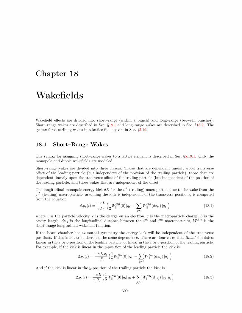
Chapter 18

Wakefields

Wakefield effects are divided into short–range (within a bunch) and long–range (between bunches).Short–range wakes are described in Sec. §18.1 and long–range wakes are described in Sec. §18.2. Thesyntax for describing wakes in a lattice file is given in Sec. §5.19.

18.1 Short–Range Wakes

The syntax for assigning short–range wakes to a lattice element is described in Sec. §5.19.1. Only themonopole and dipole wakefields are modeled.

Short–range wakes are divided into three classes: Those that are dependent linearly upon transverseoffset of the leading particle (but independent of the position of the trailing particle), those that aredependent linearly upon the transverse offset of the trailing particle (but independent of the position ofthe leading particle, and those wakes that are independent of the offset.

The longitudinal monopole energy kick dE for the ith (trailing) macroparticle due to the wake from thejth (leading) macroparticle, assuming the kick is independent of the transverse positions, is computedfrom the equation

∆pz(i) =−eLv P0

(1

2WSR‖ (0) |qi|+

∑j 6=i

WSR‖ (dzij) |qj |

)(18.1)

where v is the particle velocity, e is the charge on an electron, q is the macroparticle charge, L is thecavity length, dzij is the longitudinal distance between the ith and jth macroparticles, WSR

‖ is theshort–range longitudinal wakefield function.

If the beam chamber has azimuthal symmetry the energy kick will be independent of the transversepositions. If this is not true, there can be some dependence. There are four cases that Bmad simulates:Linear in the x or y-position of the leading particle, or linear in the x or y-position of the trailing particle.For example, if the kick is linear in the x-position of the leading particle the kick is

∆pz(i) =−eLxiv P0

(1

2WSR‖ (0) |qi|+

∑j 6=i

WSR‖ (dzij) |qj |

)(18.2)

And if the kick is linear in the y-position of the trailing particle the kick is

∆pz(i) =−eLv P0

(1

2WSR‖ (0) |qi| yi +

∑j 6=i

WSR‖ (dzij) |qj | yj

)(18.3)

309

310 CHAPTER 18. WAKEFIELDS

The kick ∆px(i) due to the transverse wake for the ith particle is modeled with the equation

∆px(i) =−eL

∑j |qj |xWSR

⊥ (dzij)

v P0(18.4)

Where WSR⊥ is the transverse short–range wake function and x is the horizontal displacement of the

leading or trailing particle as appropriate. There is a similar equation for ∆py(i). If the beam chamberhas azimuthal symmetry, the only wakes present are those that are dependent upon the offset of theleading particle. If the transverse wake is modeled as being independent of position the above equationis modified:

∆px(i) =−eL

∑j |qj |WSR

⊥ (dzij)

v P0(18.5)

With either the longitudinal wake WSR‖ or the transverse WSR

⊥ wake, the wake can be approximated asa sum of what are called “pseudo” modes Wi(z), i = 1 . . .M :

W (z) = Aamp

M∑i=1

Wi(z) = Aamp

M∑i=1

Ai ediz sin(ki z + φi) (18.6)

This is similar to approximating any function as a sum of Fourier terms. The parameters (Ai, di, ki, φi)are chosen by the person constructing the lattice to fit the calculated wake potential. Since z is negativefor trailing particles, di should be positive to get the wake to decay exponentially with distance. Thedimensionless overall amplitude scale Aamp is introduced as a convenient way to scale the overall wake.The reason why the pseudo mode approach is used in Bmad is due to the fact that, with pseudo modes,the calculation time scales as the number of particles N while a calculation based upon a table of wakevs z would scale as N2. [The disadvantage is that initially must perform a fit to the wake potential togenerate the mode parameter values.]

18.2 Long–Range Wakes

The lattice syntax for defining long-range wakes is discussed in Sec. §5.19.3.

Following Chao[Chao93] Eq. 2.88, the long–range wakefields are characterized by a set of cavity modes.The wake function Wi for the ith mode is

Wi(t) = −cAampÅR

Q

ãi

exp(−di t) sin(ωi t+ φi) (18.7)

The order of the mode mi does not come into this equation but will appear in equations below. Thedimensionless overall amplitude scale Aamp is introduced as a convenient way to scale the amplitude ofall the wakes with just one parameter. Normally, for a wake that has a well defined mode, The phasefactor φi is zero. Finite φi is used for simulations of such things as the long-range resistive wall wake.In this case, the resistive wall wake needs to be modeled as the sum of a number of modes since theresistive wall wake is not well modeled by a single damped sinusoid.

The mode strength (R/Q)i in the above equation has units of Ohms/meter2mi . Notice that R/Q isdefined so that it includes the cavity length. Thus the long–range wake equations, as opposed to theshort–range ones, do not have any explicit dependence on L. To make life more interesting, differentpeople define R/Q differently. A common practice is to define an R/Q “at the beam pipe radius”. Inthis case the above equations must be modified to include factors of the beam pipe radius. Anotherconvention uses a “linac definition” which makes R/Q twice as large and adds a factor of 2 in Eq. (18.7)to compensate.

18.2. LONG–RANGE WAKES 311

Note: Originally, Bmad characterized the damping factor di using the quality factor Qi via the relation-ship

di =ωi

2Qi(18.8)

This proved to be inconvenient when modeling such things as the resistive wall wake (where it is conve-nient to have modes where ωi = 0) so the lattice file syntax was modified to use di directly.

Assuming that the macroparticle generating the wake is offset a distance rw along the x–axis, a trailingmacroparticle at transverse position (r, θ) will see a kick

∆p⊥ = −C ImW (t)mrm−1Är cosmθ − θ sinmθ

ä(18.9)

= −C ImW (t)mrm−1 (x cos[(m− 1)θ]− y sin[(m− 1)θ])

∆pz = −C ImW ′(t) rm cosmθ (18.10)

where in this, and other equations below, the subscript i has been dropped. C is given by

C =e

c P0(18.11)

andIm = qw r

mw (18.12)

with qw being the magnitude of the charge on the particle. Generalizing the above, a macroparticle at(rw, θw) will generate a wake

−∆px + i∆py = C ImW (t)mrm−1 e−imθw ei(m−1)θ (18.13)∆pz = C ImW

′(t) rm cos[m(θ − θw)] (18.14)

Comparing Eq. (18.13) to (16.9), and using the relationship between kick and field as given by (16.5)and (16.6), shows that the form of the wakefield transverse kick is the same as for a multipole of ordern = m− 1.

The wakefield felt by a particle is due to the wakefields generated by all the particles ahead of it. If thewakefield kicks are computed by summing over all particle pairs, the computation will scale as N2 whereN is the number of particles. This quickly becomes computationally exorbitant. A better solution isto keep track of the wakes in a cavity. When a particle comes through, the wake it generates is simplyadded to the existing wake. This computation scales as N and makes simulations with large number ofparticles practical.

To add wakes together, a wake must be decomposed into its components. Spatially, there are normaland skew components and temporally there are sin and cosine components. This gives 4 componentswhich will be labeled acos, asin, bcos, and bsin. For a mode of order m, a particle passing through at atime tw with respect to the reference particle will produce wake components

δasin ≡ cAamp

ÅR

Q

ãed tw cos(ω tw) Im sin(mθw)

δacos ≡ − cAampÅR

Q

ãed tw sin(ω tw) Im sin(mθw) (18.15)

δbsin ≡ cAamp

ÅR

Q

ãed tw cos(ω tw) Im cos(mθw)

δbcos ≡ −cAampÅR

Q

ãed tw sin(ω tw) Im cos(mθw)

312 CHAPTER 18. WAKEFIELDS

These are added to the existing wake components. The total is

asin =∑

particles

δasin (18.16)

with similar equations for acos etc. Here the sum is over all particles that cross the cavity before thekicked particle. To calculate the kick due to wake, the normal and skew components are added together

atot = e−d t (acos cos(ω t+ φ) + asin sin(ω t+ φ)) (18.17)

btot = e−d t (bcos cos(ω t+ φ) + bsin sin(ω t+ φ))

Here t is the passage time of the particle with respect to the reference particle. In analogy to Eq. (18.13)and (18.14), the kick is

−∆px + i∆py = Cm (btot + iatot) rm−1 ei(m−1)θ (18.18)

∆pz = −C rm((b′tot + ia′tot)e

imθ + (b′tot − ia′tot)e−imθ)

(18.19)

where a′ ≡ da/dt and b′ ≡ db/dt.

When simulating trains of bunches, the exponential factor d tw in Eq. (18.15) can become very large. Toprevent numerical overflow, Bmad uses a reference time zref so that all times t in the above equationsare replaced by

t −→ t− tref (18.20)

The above equations were developed assuming cylindrical symmetry. With cylindrical symmetry, thecavity modes are actually a pair of degenerate modes. When the symmetry is broken, the modes no longerhave the same frequency. In this case, one has to consider a mode’s polarization angle θp. Equations(18.17) and (18.18) are unchanged. In place of Eq. (18.15), the contribution of a particle to a mode is

δasin = cAamp

ÅR

Q

ãed tw cos(ω tw) Im

[sin(mθw) sin2(mθp) + cos(mθw) sin(mθp) cos(mθp)

]δacos = − cAamp

ÅR

Q

ãed tw sin(ω tw) Im

[sin(mθw) sin2(mθp) + cos(mθw) sin(mθp) cos(mθp)

](18.21)

δbsin = cAamp

ÅR

Q

ãed tw cos(ω tw) Im

[cos(mθw) cos2(mθp) + sin(mθw) sin(mθp) cos(mθp)

]δbcos = −cAamp

ÅR

Q

ãed tw sin(ω tw) Im

[cos(mθw) cos2(mθp) + sin(mθw) sin(mθp) cos(mθp)

]Note: Technically an unpolarized mode is actually two polarized modes perpendicular to each other.The axes of these two normal modes can be chosen arbitrary as long as they are at right angles.

Chapter 19

Multiparticle Simulation

Bmad has routines for tracking two types of objects called “particles” and “macroparticles”. Particlesare characterized by a six-vector representing the particle’s phase space coordinates and a pair of com-plex numbers characterizing the particle’s spin. A macroparticle is like a particle with the addition of a6× 6 “sigma” matrix characterizing the size of the macroparticle.

Macroparticle tracking was implemented in Bmad in order to simulate particle bunches. The idea wasthat far fewer macroparticles than particles would be needed to characterize a bunch. In practice, it wasfound that the complexity of handling the macroparticle sigma matrix more than offset the reductionin the number of particles needed. Hence, while the basic macroparticle tracking routines still exist,macroparticle tracking is not currently maintained and the use of this code is discouraged. Howevermacroparticle tracking could be revived in the future if there is a demonstrated need for it.

Particle tracking can be divided into “single particle” tracking and “beam” tracking. Single particletracking is simply tracking a single particle. Beam tracking is tracking an ensemble of particles dividedup into a number of bunches that make up a “beam”.

19.1 Bunch Initialization

[Developed by Michael Saelim]

To better visualize the evolution of a particle beam, it is sometimes convenient to initialize the beamwith the particles regularly spaced. The following two algorithms are implemented in Bmad for such apurpose.

See Chapter c:beam.init for details on the standard input format used by Bmad based programs forreading in bunch initialization parameters.

19.1.1 Elliptical Phase Space Distribution

To observe nonlinear effects on the beam, it is sometimes convenient to initialize a bunch of particlesin a way that puts more particles in the tails of the bunch than one would normally have with thestandard method of seeding particles using a Gaussian distribution. In order to preserve the emittance,a distribution with more particles in the tail needs to decrease the charge per tail particle relative tothe core. This feature, along with a regular distribution, are contained in the following “ellipse”

313

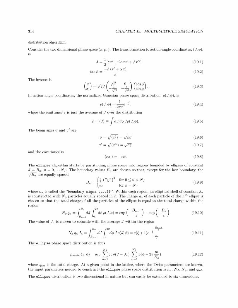
314 CHAPTER 19. MULTIPARTICLE SIMULATION

distribution algorithm.

Consider the two dimensional phase space (x, px). The transformation to action-angle coordinates, (J, φ),is

J =1

2[γx2 + 2αxx′ + βx′2] (19.1)

tanφ =−β (x′ + αx)

x(19.2)

The inverse is Åxx′

ã=√

2J

Ç √β 0

− α√β− 1√

β

åÅcosφsinφ

ã. (19.3)

In action-angle coordinates, the normalized Gaussian phase space distribution, ρ(J, φ), is

ρ(J, φ) =1

2πεe−

Jε . (19.4)

where the emittance ε is just the average of J over the distribution

ε = 〈J〉 ≡∫dJ dφJρ(J, φ). (19.5)

The beam sizes σ and σ′ are

σ =»〈x2〉 =

√εβ (19.6)

σ′ =»〈x′2〉 =

√εγ, (19.7)

and the covariance is〈xx′〉 = −εα. (19.8)

The ellipse algorithm starts by partitioning phase space into regions bounded by ellipses of constantJ = Bn, n = 0, . . . NJ . The boundary values Bn are chosen so that, except for the last boundary, the√Bn are equally spaced

Bn =

®ε2

(nσ nN

)2 for 0 ≤ n < NJ

∞ for n = NJ(19.9)

where nσ is called the “boundary sigma cutoff”. Within each region, an elliptical shell of constant Jnis constructed with Nφ particles equally spaced in φ. The charge qn of each particle of the nth ellipse ischosen so that the total charge of all the particles of the ellipse is equal to the total charge within theregion

Nφ qn =

∫ Bn

Bn−1

dJ

∫ 2π

0

dφ ρ(J, φ) = exp

Å−Bn−1

ε

ã− exp

Å−Bn

ε

ã(19.10)

The value of Jn is chosen to coincide with the average J within the region

Nφ qn Jn =

∫ Bn

Bn−1

dJ

∫ 2π

0

dφ J ρ(J, φ) = ε(ξ + 1)e−ξ∣∣∣∣Bn−1ε

Bnε

(19.11)

The ellipse phase space distribution is thus

ρmodel(J, φ) = qtot

NJ∑n=1

qn δ(J − Jn)

Nφ∑m=1

δ(φ− 2πm

Nφ) (19.12)

where qtot is the total charge. At a given point in the lattice, where the Twiss parameters are known,the input parameters needed to construct the ellipse phase space distribution is nσ, NJ , Nφ, and qtot.

The ellipse distribution is two dimensional in nature but can easily be extended to six dimensions.

19.1. BUNCH INITIALIZATION 315

19.1.2 Kapchinsky-Vladimirsky Phase Space Distribution

The Kapchinsky-Vladimirsky (KV) distribution can be thought of as a four dimensional analog of theellipse distribution with only one elliptical shell. Consider a 4D phase space (x, x′, y, y′). Using thisframework, a 4D Gaussian distribution is

ρ(Jx, φx, Jy, φy) =1

(2π)2εxεyexp(−Jx

εx) exp(−Jy

εy) (19.13)

=1

(2π)2εxεyexp(−I1

ε), (19.14)

where the orthogonal action coordinates are:

I1 =

ÅJxεx

+Jyεy

ãε (19.15)

I2 =

Å−Jxεy

+Jyεx

ãε (19.16)

with ε = ( 1ε2x

+ 1ε2y

)−1/2. The reverse transformation is:

Jx =

ÅI1εx− I2εy

ãε (19.17)

Jy =

ÅI1εy

+I2εx

ãε. (19.18)

The KV distribution isρ(I1, I2, φx, φy) =

1

Aδ(I1 − ξ), (19.19)

where A =εxεyε2 ξ(2π)2 is a constant which normalizes the distribution to 1. By choosing a particular ξ,

and iterating over the domain of the three remaining coordinates, one can populate a 3D subspace ofconstant density.

The range in I2 to be iterated over is constrained by Jx, Jy ≥ 0. Thus I2isintherange[− εxεy I1,εyεxI1].

This range is divided into N regions of equal size, with a ring of particles placed in the middle of eachregion. The angle variables are also constrained to φx, φy ∈ [0, 2π], with each range divided into Mx andMy regions, respectively. Each of these regions will have a particle placed in its center.

The weight of a particle is determined by the total weight of the region of phase space it represents.Because the density ρ is only dependent on I1,

q =

∫ ∞0

dI1

∫ I2+∆I2

I2

dI2

∫ φx+∆φx

φx

dφx

∫ φy+∆φy

φy

dφy1

Aδ(I1 − ξ) (19.20)

=1

A∆I2∆φx∆φy. (19.21)

To represent the distribution with particles of equal weight, we must partition (I2, φx, φy)-space intoregions of equal volume.

The weight of each particle is

q =1

NMxMy=

1

Ntot(19.22)

where Ntot is the total number of particles

316 CHAPTER 19. MULTIPARTICLE SIMULATION

19.2 Touschek Scattering

[Developed by Michael Ehrlichman]

Touschek scattering occurs when a single scattering event between two particles in the same beamtransfers transverse momentum to longitudinal momentum, and the resulting change in longitudinalmomentum results in the loss of one or both particles. In the case of storage rings, these losses impose abeam lifetime. In low-emittance storage rings, Touschek scattering can be the dominant mechanism forparticle loss. In the case of linear accelerators, these losses generate radiation in the accelerator tunnel.When the scattered particles collide with the beam chamber, x-rays are produced which can damageequipment and impose a biohazard. Studies of Touschek scattering typically look at beam lifetime andlocations where scattering occurs and where particles are lost.

A commonly utilized theory for studying Touschek scattering is from Piwinski [Piwin98]. A basic outlineof the derivation is,

1. Scatter two particles from a bunch in their COM frame using the relativistic Moller cross-section.

2. Boost from COM frame to lab frame. Changes to longitudinal momentum end up amplified by afactor of γ.

3. Integrate over 3D Gaussian distribution of particle positions and angles.

During the derivation many approximations are made which lead to a relatively simple formula. Theintegration is set up such that only those collisions which will result in particle loss are counted. Theformula takes the momentum aperture as a parameter. The resulting formula is reproduced here to givethe reader an idea of what influences the scattering rate, and how one might go about evaluating theformula,

R =r2ecβxβyσhN

2p

8√πβ2γ4σ2

xβσ2yβσsσp

∫ ∞τm

(Å2 +

1

τ

ã2 Å τ/τm1 + τ

− 1

ã+ 1−

√1 + τ√τ/τm

− 1

2τ

Å4 +

1

τ

ãlnτ/τm1 + τ

) √τ√

1 + τe−B1τI0 [B2τ ] dτ, (19.23)

where τm = β2δ2m and δm is the momentum aperture. This formula gives the rate at which particles

are scattered out of the bunch. It is assumed that two particles are lost per scattering event, one withtoo much energy and one with too little energy. If a machine with an asymmetric momentum apertureis being studied, then the formula should be evaluated twice, once for each aperture, and the resultsaveraged. Refer to [Piwin98] for definitions of the parameters involved. This formula is implemented inBMAD as part of the touschek_mod module.

Different formulas for calculating the Touschek scattering rate exist elsewhere in the literature. Forexample, Wiedemann [Wiede99], presents a formula with a simpler integrand. This formula, originallyfrom a paper by LeDuff [Duff87], is derived in a fashion similar to Piwinski except that the formula doesnot take dispersion into account and uses a non-relativistic scattering cross-section. Since Piwinski’sformula is the most robust, it is the one used in Bmad.

Particles are lost from Touschek scattering due to two effects. In storage rings, there is a momentumaperture defined by the RF system that is often referred to as the RF bucket. If the δp imparted by aTouschek scattering event exceeds this RF bucket, then the particle will no longer undergo synchrotronoscillations with the rest of the bunch and will coast through the accelerator. Second, if the Touschekscattering event occurs in a dispersive region, the scattered particles will take on a finite J and undergo

19.3. MACROPARTICLES 317

betatron oscillations. These oscillations can be large in amplitude and may cause the particles to collidewith the beam pipe. To first order, the amplitude of J due to a scattering event that imparts a momentumdeviation of ∆p is,

J ≈ γ0H0∆p2

2, (19.24)

where γ0 is relativistic γ and H0 is the dispersion invariant.

19.3 Macroparticles

Note: The macroparticle tracking code is not currently maintained in favor of tracking an ensemble ofparticles where each particle is specified by a position without a sigma matrix. The following is presentfor historical reference only.

A macroparticle[Brown77] is represented by a centroid position r and a 6 × 6 σ matrix which definesthe shape of the macroparticle in phase space. σi =

√σ(i, i) is the RMS sigma for the ith phase space

coordinate. For example σz =√σ(5, 5).

σ is a real, non-negative symmetric matrix. The equation that defines the ellipsoid at a distance ofn–sigma from the centroid is

(r− r)tσ−1(r− r) = n (19.25)

where the t superscript denotes the transpose. Given the sigma matrix at some point s = s1, the sigmamatrix at a different point s2 is

σ2 = M12 σ1 Mt12 (19.26)

where M12 is the Jacobian of the transport map from point s1 to s2.

The Twiss parameters can be calculated from the sigma matrix. The dispersion is given by

σ(1, 6) = ηx σ(6, 6)

σ(2, 6) = η′x σ(6, 6) (19.27)σ(3, 6) = ηy σ(6, 6)

σ(4, 6) = η′y σ(6, 6)

Ignoring coupling for now, the betatron part of the sigma matrix can be obtained from the linearequations of motion. For example, using

x =√

2βx εx cosφx + ηx pz (19.28)

Solving for the first term on the RHS, squaring and averaging over all particles gives

βx εx = σ(1, 1)− σ2(1, 6)

σ(6, 6)(19.29)

It is thus convenient to define the betatron part of the sigma matrix

σβ(i, j) ≡ σ(i, j)− σ(i, 6)σ(j, 6)

σ(6, 6)(19.30)

and in terms of the betatron part the emittance is

ε2x = σβ(1, 1)σβ(2, 2)− σ2β(1, 2) (19.31)

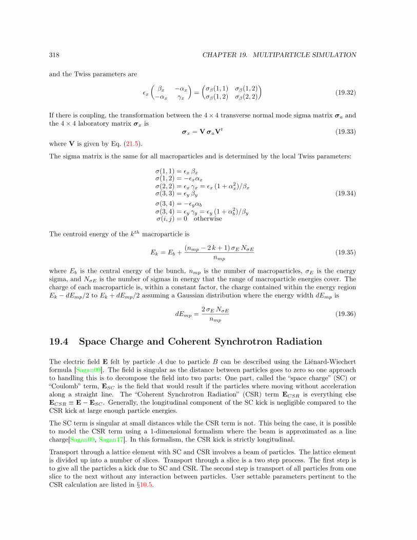
318 CHAPTER 19. MULTIPARTICLE SIMULATION

and the Twiss parameters are

εx

Åβx −αx−αx γx

ã=

Åσβ(1, 1) σβ(1, 2)σβ(1, 2) σβ(2, 2)

ã(19.32)

If there is coupling, the transformation between the 4× 4 transverse normal mode sigma matrix σa andthe 4× 4 laboratory matrix σx is

σx = VσaVt (19.33)

where V is given by Eq. (21.5).

The sigma matrix is the same for all macroparticles and is determined by the local Twiss parameters:

σ(1, 1) = εx βxσ(1, 2) = −εxαxσ(2, 2) = εx γx = εx (1 + α2

x)/βxσ(3, 3) = εy βy (19.34)σ(3, 4) = −εyαbσ(3, 4) = εy γy = εy (1 + α2

b)/βyσ(i, j) = 0 otherwise

The centroid energy of the kth macroparticle is

Ek = Eb +(nmp − 2 k + 1)σE NσE

nmp(19.35)

where Eb is the central energy of the bunch, nmp is the number of macroparticles, σE is the energysigma, and NσE is the number of sigmas in energy that the range of macroparticle energies cover. Thecharge of each macroparticle is, within a constant factor, the charge contained within the energy regionEk − dEmp/2 to Ek + dEmp/2 assuming a Gaussian distribution where the energy width dEmp is

dEmp =2σE NσEnmp

(19.36)

19.4 Space Charge and Coherent Synchrotron Radiation

The electric field E felt by particle A due to particle B can be described using the Liénard-Wiechertformula [Sagan09]. The field is singular as the distance between particles goes to zero so one approachto handling this is to decompose the field into two parts: One part, called the “space charge” (SC) or“Coulomb” term, ESC is the field that would result if the particles where moving without accelerationalong a straight line. The “Coherent Synchrotron Radiation” (CSR) term ECSR is everything elseECSR ≡ E− ESC . Generally, the longitudinal component of the SC kick is negligible compared to theCSR kick at large enough particle energies.

The SC term is singular at small distances while the CSR term is not. This being the case, it is possibleto model the CSR term using a 1-dimensional formalism where the beam is approximated as a linecharge[Sagan09, Sagan17]. In this formalism, the CSR kick is strictly longitudinal.

Transport through a lattice element with SC and CSR involves a beam of particles. The lattice elementis divided up into a number of slices. Transport through a slice is a two step process. The first step isto give all the particles a kick due to SC and CSR. The second step is transport of all particles from oneslice to the next without any interaction between particles. User settable parameters pertinent to theCSR calculation are listed in §10.5.

19.4. SPACE CHARGE AND COHERENT SYNCHROTRON RADIATION 319

19.4.1 1_Dim CSR Calculation

When an element’s csr_method is set to 1_dim (§6.5), The particle-particle CSR kick is calculatedby dividing the bunch longitudinally into a number of bins. To smooth the computed bin densities,each particle of the bunch is considered to have a triangular density distribution as shown in Fig. 19.1.The particle density of a bin is calculated by summing the contribution from all the particles. Thecontribution of a given particle to a given bin is calculated from the overlap of the particle’s triangulardensity distribution with the bin. For the CSR kick, the density is actually calculated for a second setof staggered bins that have been offset by 1/2 the bin width with respect to the first set. This givesthe density at the edges of the original set of bins. The density is considered to vary linearly betweenthe computed density points. For a description of the parameters that affect the CSR calculation seeSection §10.5.

19.4.2 Slice Space Charge Calculation

When an element’s space_charge_method is set to slice (§6.5), the calculation of the SC kick uses,the same particle binning as is used with the 1_dim CSR calculation (§19.4.1). The kick is dividedinto longitudinal and a transverse parts. The transverse part uses the same Bassetti–Erskine complexerror function formula[Talman87] as with the beam-beam interaction (§24.5) except here, since all theparticles are moving in the same direction, the kicks due to the electric and magnetic fields generated

z

ρ

bins

particle

shifted bins

Figure 19.1: The Coherent Synchrotron Radiation kick is calculated by dividing longitudinally a bunchinto a number of bins. To smooth the computed densities, each particle of the bunch is considered tohave a triangular density distribution.

320 CHAPTER 19. MULTIPARTICLE SIMULATION

by a given particle tend to cancel

Ky(CS) + iKx(CS) =re ρ(z)

γ3 e·

2π (σx + σy)

σx − σy(19.37)w

x+ i y»2(σ2

x − σ2y)

− exp

ñ− x2

2σ2x

− y2

2σ2y

ô· w

x σyσx

+ i y σxσy»2(σ2

x − σ2y)

where K(CS) is the CS kick per unit length of travel of the beam, ρ(z) is the density of particles perunit length evaluated at the z position of the kicked particle, e is the charge on the electron, and w isthe complex error function.

The longitudinal SC kick is given by Eq. (31) of Sagan[Sagan09]

dKSC =rcmc

2 sign(ζ)ρ(z′)dz′

σx σy exp[x2

2σ2x

+ y2

2σ2y

]+

σ2x+σ2

y

σx+σyγ|ζ|+ γ2ζ2

, (19.38)

where ζ is the longitudinal distance between the kick point and the slice doing the kicking. There aretwo simulation modes for the longitudinal SC kick. In both these modes, the kick is evaluated at thecenter plane of each slice. The kick is a sum kicks from all the slices. Since the thickness of the slicesis, in general, not negligible, the the integral over a slice is used to calculate the kick. The total kickKSC(j) at slice j is

KSC(j) =∑i

∫ ζij+dzslice/2

ζij−dzslice/2dζ dKSC (19.39)

where the sum is over all slices i, ζij is the distance between slices i and j, and dzslice is the slicethickness. An analytic expression of the above integral is easily calculated assuming that the chargedensity ρ(z) is linearly varying within a given slice. For brevity’s sake, the calculation is not explicitlypresented here. Once the kick at the slice center planes is calculated, the kick given to a particle iscalculated using linear interpolation.

One mode for calculating the transverse SC kick which is computationally fast, ignores the transversedependence of the kick and just evaluates the kick on the beam centerline. The other simulation moderepresents the kick due to a given slice using a Padé approximant of form∫ ζij+dzslice/2

ζij−dzslice/2dζ dKSC '

1

a00 + a20x2 + a40x4 + a02y2 + a04y4 + a22x2 y2(19.40)

the a_mn are calculated from an analytic formula derived from integrating Eq. (19.38). The reason forusing this form is that it is a reasonable approximation even for very large x or y in that the actual andapproximate kick both go to zero in this limit. That this Padé approximant is reasonable is dependentupon the fact that all the amn for a slice are either all positive or all negative. Kicks from different slicescan be combined using standard Differential Algebra techniques to give a summed kick in the same formas above. To avoid divergences, for a given j where the kick is evaluated, all the kicks from slices withnegative coefficients are combined together and all the kicks from slices with positive coefficients arecombined together and the total kick is then the sum of the “positive kick” part and the “negative kick”part. The kick applied to a particle is calculated by first evaluating the kick, at the particle’s x and y,at the neighboring slices and then using linear interpolation.

Note: Match elements (§4.31) can have orbit shifts which are not well handled by the CSR algorithm.For this reason, match elements are ignored in the CSR calculation.

19.5. HIGH ENERGY SPACE CHARGE 321

19.4.3 FFT_3D Space Charge Calculation

When an element’s space_charge_method is set to fft_3d (§6.5), the space charge calculation uses codefrom the OpenSC package developed by Rob Ryne and Chris Mayes [Ryne18]. The method works bycalculating the field due to the particle on a 3D grid and then interpolating the field to the points wherethe particles are. This method will be able to handle lower energy bunches than the slice method(§19.4.2) the disadvantage is that the fft_3d method will be slower. Another point to keep in mind isthat the fft_3d method currently ignores image charge forces due to an emitting cathode and so willnot be accurate for tracking at the very lowest energies near the emitter.

Note: The mesh size is set by the csr_pram parameter space_charge_mesh_size (§10.5).

19.5 High Energy Space Charge

Bmad has a code module for simulating the effect of space charge (SC) at high energies. This is separatefrom the regular space charge calculation of §19.4. Thus it should be noted that turning on of both theregular space charge and the high energy space charge in the same element will result in double countingof the space charge effect.

The advantage of the high energy space charge algorithm is that the kick on a given particle is computedassuming a Gaussian beam with the beam size calculated using emittances supplied by the user. Thusthe high energy space charge calculation can be done in single particle tracking (§19) as opposed to thebeam tracking that must be used for the regular space charge calculation. The other advantage is thatthe high energy space charge calculation is quick since it is assumed that the kick is small enough sothat the kick is only applied once per lattice element. The disadvantage of the high energy space chargecalculation is that there is the assumption that the beam distribution is Gaussian which is generallyacceptable for storage rings at relatively high energy but will not accurate in other situations.

If a Bmad based program has been constructed to use the high energy space charge module (the doc-umentation for the program should indicate if this is true), the high energy space charge force can beturned on or off by setting the parameter[high_energy_space_charge_on] parameter (§9.1, §9.4).

The high energy space charge kick is computed assuming a gaussian bunch shape

Ky + iKx =reN

γ3 σzexp

ïz2

2σz

ò· σx + σyσx − σy

(19.41)w x+ i y»

2(σ2x − σ2

y)

− exp

ñ− x2

2σ2x

− y2

2σ2y

ô· w

x σyσx

+ i y σxσy»2(σ2

x − σ2y)

where N is the number of particles in the bunch. This equation is similar to Eq. (19.37) except thatρ(z) has been replaced assuming that the longitudinal distribution is Gaussian. For particles close tothe bunch core the kick is linear with displacement giving rise to a tune shift [Decking00].

The high energy space charge calculation ignores any CSR effects and ignores any longitudinal kicks andis thus not a good approximation at lower energies. See the discussion in [Sagan09] for more details.

322 CHAPTER 19. MULTIPARTICLE SIMULATION

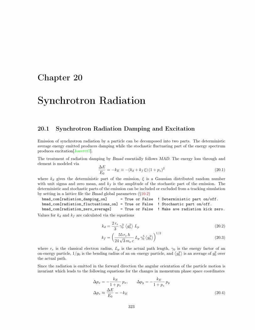
Chapter 20

Synchrotron Radiation

20.1 Synchrotron Radiation Damping and Excitation

Emission of synchrotron radiation by a particle can be decomposed into two parts. The deterministicaverage energy emitted produces damping while the stochastic fluctuating part of the energy spectrumproduces excitation[Jowett87].

The treatment of radiation damping by Bmad essentially follows MAD. The energy loss through andelement is modeled via

∆E

E0= −kE ≡ −(kd + kf ξ) (1 + pz)

2 (20.1)

where kd gives the deterministic part of the emission, ξ is a Gaussian distributed random numberwith unit sigma and zero mean, and kf is the amplitude of the stochastic part of the emission. Thedeterministic and stochastic parts of the emission can be included or excluded from a tracking simulationby setting in a lattice file the Bmad global parameters (§10.2)bmad_com[radiation_damping_on] = True or False ! Deterministic part on/off.bmad_com[radiation_fluctuations_on] = True or False ! Stochastic part on/off.bmad_com[radiation_zero_average] = True or False ! Make ave radiation kick zero.

Values for kd and kf are calculated via the equations

kd =2 re3

γ30

⟨g2

0

⟩Lp (20.2)

kf =

Å55 re ~

24√

3me cLp γ

50

⟨g3

0

⟩ã1/2

(20.3)

where re is the classical electron radius, Lp is the actual path length, γ0 is the energy factor of anon-energy particle, 1/g0 is the bending radius of an on–energy particle, and

⟨g2

0

⟩is an average of g2

0 overthe actual path.

Since the radiation is emitted in the forward direction the angular orientation of the particle motion isinvariant which leads to the following equations for the changes in momentum phase space coordinates

∆px = − kE1 + pz

px, ∆py = − kE1 + pz

py

∆pz ≈∆E

E0= −kE (20.4)

323

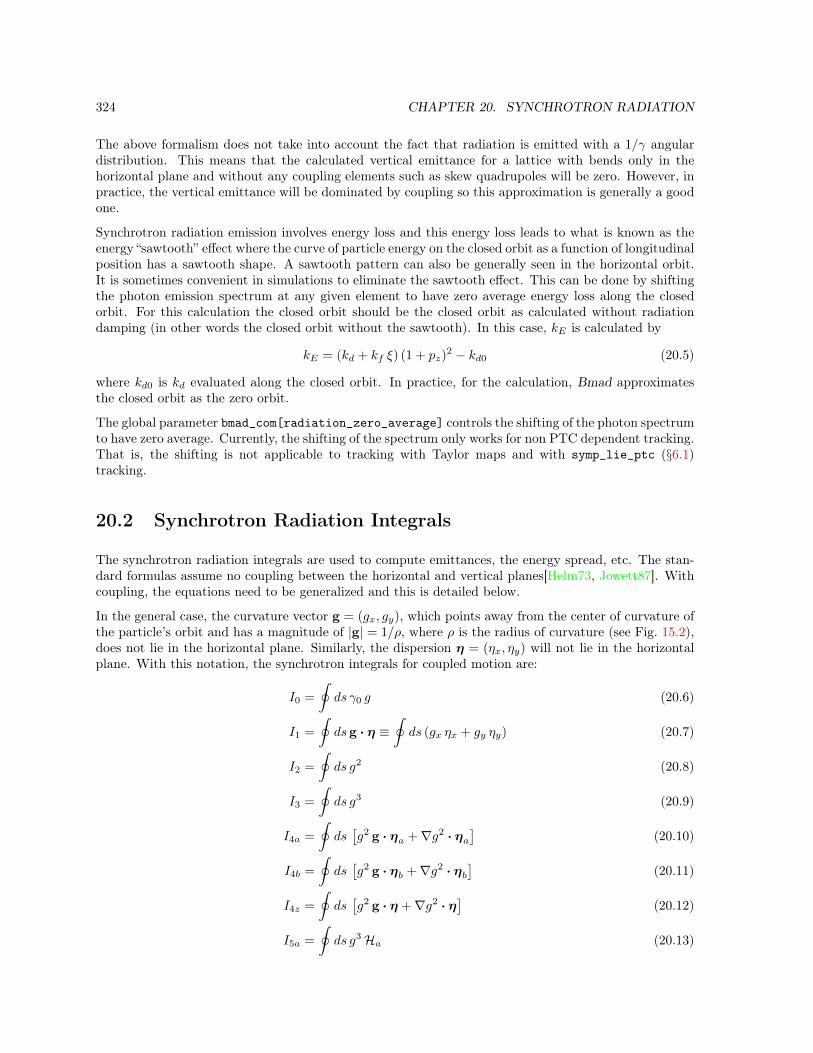
324 CHAPTER 20. SYNCHROTRON RADIATION

The above formalism does not take into account the fact that radiation is emitted with a 1/γ angulardistribution. This means that the calculated vertical emittance for a lattice with bends only in thehorizontal plane and without any coupling elements such as skew quadrupoles will be zero. However, inpractice, the vertical emittance will be dominated by coupling so this approximation is generally a goodone.

Synchrotron radiation emission involves energy loss and this energy loss leads to what is known as theenergy “sawtooth” effect where the curve of particle energy on the closed orbit as a function of longitudinalposition has a sawtooth shape. A sawtooth pattern can also be generally seen in the horizontal orbit.It is sometimes convenient in simulations to eliminate the sawtooth effect. This can be done by shiftingthe photon emission spectrum at any given element to have zero average energy loss along the closedorbit. For this calculation the closed orbit should be the closed orbit as calculated without radiationdamping (in other words the closed orbit without the sawtooth). In this case, kE is calculated by

kE = (kd + kf ξ) (1 + pz)2 − kd0 (20.5)

where kd0 is kd evaluated along the closed orbit. In practice, for the calculation, Bmad approximatesthe closed orbit as the zero orbit.

The global parameter bmad_com[radiation_zero_average] controls the shifting of the photon spectrumto have zero average. Currently, the shifting of the spectrum only works for non PTC dependent tracking.That is, the shifting is not applicable to tracking with Taylor maps and with symp_lie_ptc (§6.1)tracking.

20.2 Synchrotron Radiation Integrals

The synchrotron radiation integrals are used to compute emittances, the energy spread, etc. The stan-dard formulas assume no coupling between the horizontal and vertical planes[Helm73, Jowett87]. Withcoupling, the equations need to be generalized and this is detailed below.

In the general case, the curvature vector g = (gx, gy), which points away from the center of curvature ofthe particle’s orbit and has a magnitude of |g| = 1/ρ, where ρ is the radius of curvature (see Fig. 15.2),does not lie in the horizontal plane. Similarly, the dispersion η = (ηx, ηy) will not lie in the horizontalplane. With this notation, the synchrotron integrals for coupled motion are:

I0 =

∮ds γ0 g (20.6)

I1 =

∮dsg · η ≡

∮ds (gx ηx + gy ηy) (20.7)

I2 =

∮ds g2 (20.8)

I3 =

∮ds g3 (20.9)

I4a =

∮ds[g2 g · ηa +∇g2 · ηa

](20.10)

I4b =

∮ds[g2 g · ηb +∇g2 · ηb

](20.11)

I4z =

∮ds[g2 g · η +∇g2 · η

](20.12)

I5a =

∮ds g3Ha (20.13)

20.2. SYNCHROTRON RADIATION INTEGRALS 325

I5b =

∮ds g3Hb (20.14)

I6b =

∮ds g3 βb (20.15)

where γ0 is that usual relativistic factor and Ha is

Ha = γa η2a + 2αa ηa η

′a + βaη

′2a (20.16)

with a similar equation for Hb. Here ηa = (ηax, ηay), and ηb = (ηbx, ηby) are the dispersion vectors forthe a and b modes respectively in x–y space (these 2–vectors are not to be confused with the dispersion4–vectors used in the previous section). The position dependence of the curvature function is:

gx(x, y) = gx + x k1 + y s1

gy(x, y) = gy + x s1 − y k1 (20.17)

where k1 is the quadrupole moment and s1 is the skew–quadrupole moment. Using this gives on–axis(x = y = 0)

∇g2 = 2 (gxk1 + gys1, gxs1 − gyk1) (20.18)

I0 is not a standard radiation integral. It is useful, though, in calculating the average number of photonsemitted. For electrons:

N =5 rf

2√

3 ~ cI0 (20.19)

where N is the average number of photons emitted by a particle over one turn, and the “classical radiusfactor” rf is

rf =e2

4π ε0(20.20)

rf has a value of 1.4399644 · 10−9 meters-eV for all particles of charge ±1.

In a dipole a non–zero e1 or e2 gives a contribution to I4 via the ∇g2 ·η term. The edge field is modeledas a thin quadrupole of length δ and strength k = −g tan(e)/δ. It is assumed that g rises linearly withinthe edge field from zero on the outside edge of the edge field to its full value on the inside edge of theedge field. Using this in Eq. (20.18) and integrating over the edge field gives the contribution to I4 froma non–zero e1 as

I4z = − tan(e1) g2 (cos(θ) ηx + sin(θ) ηy) (20.21)

With an analogous equation for a finite e2. The extension to I4a and I4b involves using ηa and ηb inplace of η. In Eq. (20.21) θ is the reference tilt angle which is non–zero if the bend is not in thehorizontal plane. Here use of the fact has been made that the g vector rotates as θ and the quadrupoleand skew quadrupole strengths rotate as 2 θ.

The above integrals are invariant under rotation of the (x, y) coordinate system and reduce to thestandard equations when gy = 0 as they should.

There are various parameters that can be expressed in terms of these integrals. The I1 integral can berelated to the momentum compaction αp via

I1 = αp L (20.22)

where L is the storage ring circumference. The energy loss per turn is

U0 =2 reE

40

3 (mc2)3I2 (20.23)

326 CHAPTER 20. SYNCHROTRON RADIATION

where E0 is the nominal energy and re is the classical electron radius (electrons are assumed here butthe formulas are easily generalized).

The damping partition numbers are

Ja = 1− I4aI2

, Jb = 1− I4bI2

, and Jz = 2 +I4zI2

. (20.24)

Sinceηa + ηb = η , (20.25)

Robinson’s theorem, Ja + Jb + Jz = 4, is satisfied. Alternatively, the exponential damping coefficientsper turn are

αa =U0 Ja2E0

, αb =U0 Jb2E0

, and αz =U0 Jz2E0

. (20.26)

The energy spread is given by

σ2pz =

ÅσEE0

ã2

= Cqγ20

I32I2 + I4z

(20.27)

where γ0 is the usual energy factor and

Cq =55

32√

3

~mc

= 3.84× 10−13 meter for electrons (20.28)

If the synchrotron frequency is not too large, the bunch length is given by

σ2z =

I1M(6, 5)

σ2pz (20.29)

where M(6, 5) is the (6, 5) element for the 1–turn transfer matrix of the storage ring. Finally, theemittances are given by

εa =Cq

I2 − I4aγ2

0 I5a

εb =Cq

I2 − I4b

Åγ2

0 I5b +13

55I6b

ã(20.30)

The I6b term come from the finite vertical opening angle of the radiation[Rauben91]. Normally this termis very small compared to the emittance due to coupling or vertical kicks due to magnet misalignment.

For a non-circular machine, radiation integrals are still of interest if there are bends or steering elements.However, in this case, the appropriate energy factors must be included to take account any changes inenergy due to any lcavity elements. For a non-circular machine, the I1 integral is not altered and theI4 integrals are not relevant. The other integrals become

L2 =

∫ds g2 γ4

0 (20.31)

L3 =

∫ds g3 γ7

0 (20.32)

L5a =

∫ds g3Ha γ6

0 (20.33)

L5b =

∫ds g3Hb γ6

0 (20.34)

In terms of these integrals, the energy loss through the lattice is

U0 =2 remc

2

3L2 (20.35)

20.2. SYNCHROTRON RADIATION INTEGRALS 327

The energy spread assuming σE is zero at the start and neglecting any damping is

σ2E =

4

3Cq re

(mc2

)2L3 (20.36)

The above equation is appropriate for a linac. In a storage ring, where there are energy oscillations,the growth of σ2

E due to quantum excitation is half that. One way to explain this is that in a storagering, the longitudinal motion is “shared” between the z and pz coordinates and, to preserve phase spacevolume, this reduces σ2

E by a factor of 2.

Again neglecting any initial beam width, the transverse beam size at the end of the lattice is

εa =2

3Cq re

L5a

γf

εb =2

3Cq re

L5b

γf(20.37)

Where γf is the final gamma.

328 CHAPTER 20. SYNCHROTRON RADIATION

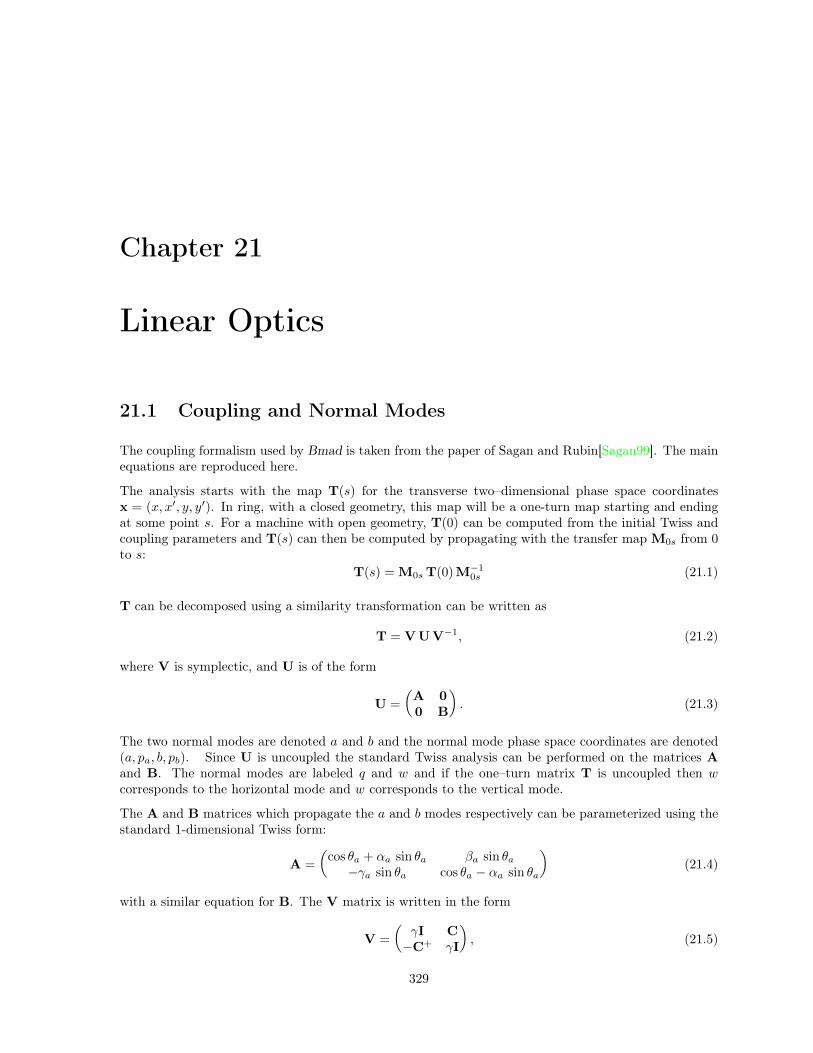
Chapter 21

Linear Optics

21.1 Coupling and Normal Modes

The coupling formalism used by Bmad is taken from the paper of Sagan and Rubin[Sagan99]. The mainequations are reproduced here.

The analysis starts with the map T(s) for the transverse two–dimensional phase space coordinatesx = (x, x′, y, y′). In ring, with a closed geometry, this map will be a one-turn map starting and endingat some point s. For a machine with open geometry, T(0) can be computed from the initial Twiss andcoupling parameters and T(s) can then be computed by propagating with the transfer map M0s from 0to s:

T(s) = M0s T(0) M−10s (21.1)

T can be decomposed using a similarity transformation can be written as

T = V U V−1, (21.2)

where V is symplectic, and U is of the form

U =

ÅA 00 B

ã. (21.3)

The two normal modes are denoted a and b and the normal mode phase space coordinates are denoted(a, pa, b, pb). Since U is uncoupled the standard Twiss analysis can be performed on the matrices Aand B. The normal modes are labeled q and w and if the one–turn matrix T is uncoupled then wcorresponds to the horizontal mode and w corresponds to the vertical mode.

The A and B matrices which propagate the a and b modes respectively can be parameterized using thestandard 1-dimensional Twiss form:

A =

Åcos θa + αa sin θa βa sin θa−γa sin θa cos θa − αa sin θa

ã(21.4)

with a similar equation for B. The V matrix is written in the form

V =

ÅγI C−C+ γI

ã, (21.5)

329

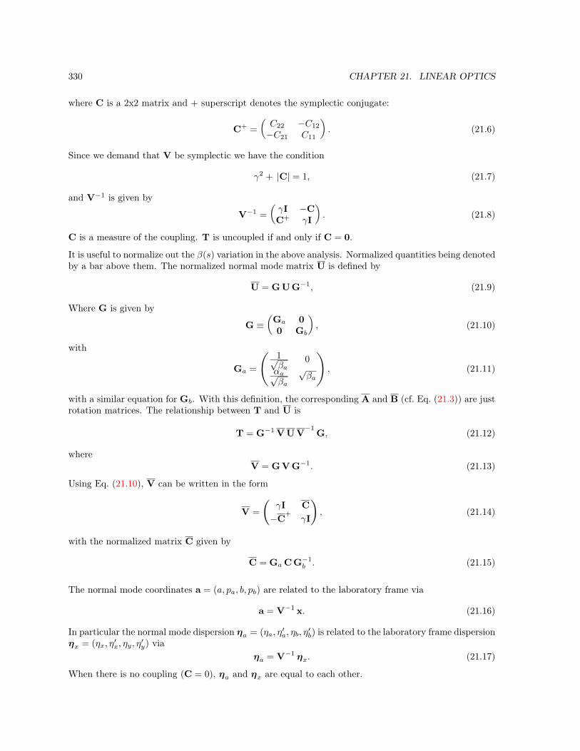
330 CHAPTER 21. LINEAR OPTICS

where C is a 2x2 matrix and + superscript denotes the symplectic conjugate:

C+ =

ÅC22 −C12

−C21 C11

ã. (21.6)

Since we demand that V be symplectic we have the condition

γ2 + |C| = 1, (21.7)

and V−1 is given by

V−1 =

ÅγI −CC+ γI

ã. (21.8)

C is a measure of the coupling. T is uncoupled if and only if C = 0.

It is useful to normalize out the β(s) variation in the above analysis. Normalized quantities being denotedby a bar above them. The normalized normal mode matrix U is defined by

U = G U G−1, (21.9)

Where G is given by

G ≡Å

Ga 00 Gb

ã, (21.10)

with

Ga =

Ñ1√βa

0

αa√βa

√βa

é, (21.11)

with a similar equation for Gb. With this definition, the corresponding A and B (cf. Eq. (21.3)) are justrotation matrices. The relationship between T and U is

T = G−1 V U V−1

G, (21.12)

whereV = G V G−1. (21.13)

Using Eq. (21.10), V can be written in the form

V =

ÇγI C

−C+

γI

å, (21.14)

with the normalized matrix C given by

C = Ga C G−1b . (21.15)

The normal mode coordinates a = (a, pa, b, pb) are related to the laboratory frame via

a = V−1 x. (21.16)

In particular the normal mode dispersion ηa = (ηa, η′a, ηb, η

′b) is related to the laboratory frame dispersion

ηx = (ηx, η′x, ηy, η

′y) via

ηa = V−1 ηx. (21.17)

When there is no coupling (C = 0), ηa and ηx are equal to each other.

21.2. TUNES FROM ONE-TURN MATRIX EIGEN ANALYSIS 331

x

px

+θx

z

pz

+θz ??

A) B)

Figure 21.1: A) The standard accelerator physics convention is that a clockwise rotation in (x, px) or(y, py) space represents a positive tune. B) For longitudinal oscillations, it is sometimes conventional totake counterclockwise rotation as positive if a machine is always running above transition.

21.2 Tunes From One-Turn Matrix Eigen Analysis

Given the 6 × 6 one-turn matrix for a storage ring, one issue is how to extract the tunes. If there isno coupling the analysis is simple but with coupling things get more complicated. In the general case,calculating with eigenvectors and eigenvalues gives, assuming that the lattice is stable, three pairs ofeigenvalues with the two eigenvalues of a given pair being complex conjugates and all eigenvalues havingunit amplitude. That is, the eigenvalues λi, i = 1, . . . 6 can be ordered in pairs:

λ1, λ2 = exp(i θa), exp(−i θa)

λ3, λ4 = exp(i θb), exp(−i θb) (21.18)λ5, λ6 = exp(i θc), exp(−i θc)

where θa, θb, and θc are the three tunes. To associate λ1 and λ2, along with their associated eigenvectorsV1 and V2, with the “horizontal-like” mode, all the eigenvectors are compared to one another and theeigenvector pair with the largest values for the x and px components are used for V1 and V2. Similarly,for the “vertical-like” mode, eigenvector pair with the largest values for the y and py components areassociated with V3 and V4, and finally for the “longitudinal-like” mode the eigenvector pair with thelargest values for the z and pz components are associated with V5 and V6.

It can be useful to arrange the eigenvalues such that the odd numbered eigenvalues (1, 3, and 5) areassociated with the tune and the even numbered eigen values (2, 4, and 6) are associated with thenegative of the tune as arranged in Eq. (21.18). The algorithm for doing this can be deduced by firstconsidering the case where the motion is in one-dimension only. Here taken to be (x, p) as shown inFig. 21.1. Notice that, by the standard accelerator physics convention, a positive tune represents aclockwise rotation in the transverse dimensions. For the longitudinal mode what counts as positive tunecan depend upon whether the machine is above transition or not. To keep the mathematics consistent,positive tune for all modes will be taken to be clockwise.

Assuming that the motion is circular, the one-turn matrix M with tune θ is

M =

Åcos(θ) sin(θ)− sin(θ) cos(θ)

ã(21.19)

332 CHAPTER 21. LINEAR OPTICS

The eignvalues and eigenvectors are

λ1 = exp(i θ), V1 =1√2

(1, i)

λ2 = exp(−i θ), V2 =1√2

(1,−i) (21.20)

Thus, for the eigenvector (1, i)/√

2, were the momentum component is rotated by a factor of π/2 coun-terclockwise from the position coordinate, the rotation angle is the tune. The rotation angle associatedwith the eigenvector (1,−i)/

√2 is associated with the negative of the tune.

In the general case, each Vk, k = 1, . . . 6, is a vector in (x, px, y, py, z, pz) space with each component ofthe vector being a complex number. The criterion that an eigenvector is associated with the tune is thatthe phase of the momentum components are on average rotated clockwise from the position coordinatesis ‹V∗k S Vk = i, k = 1, 3, 5‹V∗k S Vk = −i, k = 2, 4, 6 (21.21)

where the tilde means transpose and S is the matrix

S =

0 1 0 0 0 0−1 0 0 0 0 00 0 0 1 0 00 0 −1 0 0 00 0 0 0 0 10 0 0 0 −1 0

(21.22)

Eq. (21.21), along with the condition

Vk+1 = V ∗k , k = 1, 3, 5 (21.23)

makes sure that the Vk are properly normalized.1

21.3 Linear Action-Angle Coordinates

The transformation from the one-turn 6× 6 matrix T in laboratory coordinates to action-angle coordi-nates uses the similarity transformation

T = N R N−1 (21.24)

where N is a symplectic matrix. NT S N = S with S given in Eq. (21.22) and R is a rotation matrix

R =

ÑR2(θa)

R2(θb)R2(θc)

é(21.25)

with each 2× 2 rotation submatrix R2 being of the form as M in Eq. (21.19). The transformation fromlaboratory coordinates x to normal mode a coordinates is

a = N−1 x (21.26)1Different Authors use different conventions. For example, the S matrix in the paper by Chao[Chao81], is the negative

of the S matrix defined here and in the paper by Ohmi, Hirata, and Oide [Ohmi94] the phases are reversed (positive phaseis counterclockwise rotation) as can be seen from Eqs. (77) and (79) in their paper.

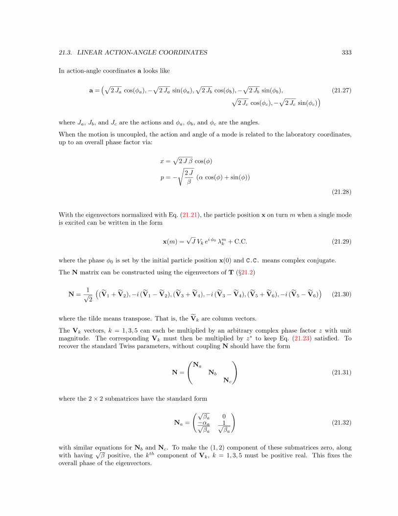
21.3. LINEAR ACTION-ANGLE COORDINATES 333

In action-angle coordinates a looks like

a =Ä√

2 Ja cos(φa),−√

2 Ja sin(φa),√

2 Jb cos(φb),−√

2 Jb sin(φb), (21.27)√2 Jc cos(φc),−

√2 Jc sin(φc)

äwhere Ja, Jb, and Jc are the actions and φa, φb, and φc are the angles.

When the motion is uncoupled, the action and angle of a mode is related to the laboratory coordinates,up to an overall phase factor via:

x =√

2 J β cos(φ)

p = −

2 J

β(α cos(φ) + sin(φ))

(21.28)

With the eigenvectors normalized with Eq. (21.21), the particle position x on turn m when a single modeis excited can be written in the form

x(m) =√J Vk e

i φ0 λmk + C.C. (21.29)

where the phase φ0 is set by the initial particle position x(0) and C.C. means complex conjugate.

The N matrix can be constructed using the eigenvectors of T (§21.2)

N =1√2

Ä(‹V1 + ‹V2),−i (‹V1 − ‹V2), (‹V3 + ‹V4),−i (‹V3 − ‹V4), (‹V5 + ‹V6),−i (‹V5 − ‹V6)

ä(21.30)

where the tilde means transpose. That is, the ‹Vk are column vectors.

The Vk vectors, k = 1, 3, 5 can each be multiplied by an arbitrary complex phase factor z with unitmagnitude. The corresponding Vk must then be multiplied by z∗ to keep Eq. (21.23) satisfied. Torecover the standard Twiss parameters, without coupling N should have the form

N =

ÑNa

Nb

Nc

é(21.31)

where the 2× 2 submatrices have the standard form

Na =

(√βa 0−αa√βa

1√βa

)(21.32)

with similar equations for Nb and Nc. To make the (1, 2) component of these submatrices zero, alongwith having

√β positive, the kth component of Vk, k = 1, 3, 5 must be positive real. This fixes the

overall phase of the eigenvectors.

334 CHAPTER 21. LINEAR OPTICS

21.4 Dispersion Calculation

The dispersion (η) and the dispersion derivative (η′) are defined by the equations

ηx(s) ≡ dx

dpz

∣∣∣∣s

, η′x(s) ≡ dηxds

∣∣∣∣s

=dx′

dpz

∣∣∣∣s

ηy(s) ≡ dy

dpz

∣∣∣∣s

, η′y(s) ≡ dηyds

∣∣∣∣s

=dy′

dpz

∣∣∣∣s

(21.33)

ηz(s) ≡dz

dpz

∣∣∣∣s

Given the dispersion at a given point, the dispersion at some other point is calculated as follows: Letr = (x, px, y, py, z, pz) be the reference orbit, around which the dispersion is to be calculated. Let V andM be the zeroth and first order components of the transfer map between two points labeled 1 and 2:

r2 = M r1 + V (21.34)

Define the dispersion vector η by

η =(ηx, η

′x (1 + pz), ηy, η

′y (1 + pz), ηz, 1

)(21.35)

Differentiating Eq. (21.34) with respect to energy, the dispersion at point 2 in terms of the dispersion atpoint 1 is

η2 =

ïdpz2dpz1

ò−1

[Mη1] + Vη (21.36)

where

Vη =

ïdpz2dpz1

ò−1 1

1 + pz1

M12 px1 +M14 py1

M22 px1 +M24 py1

M32 px1 +M34 py1

M42 px1 +M44 py1

M52 px1 +M54 py1

M62 px1 +M64 py1

−

0px2

1+pz2

0py2

1+pz2

00

(21.37)

The sixth row of the matrix equation gives dpz1/dpz2. Explicitly

dpz2dpz1

=

6∑i=1

M6i η1i +M62 px1 +M64 py1

1 + pz1(21.38)

For everything except RFcavity and Lcavity elements, dpz2/dpz1 is 1.

For a non-circular machine, there are two ways one can imagine defining the dispersion: Either withrespect to changes in energy at the beginning of the machine or with respect to the local change inenergy at the point of measurement. The former definition will be called “non-local dispersion” and thelatter definition will be called “local dispersion”. For a circular machine, local dispersion is always used.The dispersion defined in the above equations, which is what Bmad uses in calculations, is the localdispersion. The non-local dispersion η(s1) at some point s1 is related to the local dispersion η(s1) via

η(s1) =dpz1dpz0

η(s1) (21.39)

where s0 is the beginning of the machine.

21.4. DISPERSION CALCULATION 335

For a non-circular machine, there are advantages and disadvantages to using either local or non-localdispersion. Local dispersion has the problem that dpz2/dpz1 in Eq. (21.36) may go through zero at apoint producing infinite dispersions at that point. The non-local dispersion has the merit of reflectingwhat one would measure if the starting energy of the beam is varied. The local dispersion, on the otherhand, reflects the correlations between the particle energy and particle position within a beam.

336 CHAPTER 21. LINEAR OPTICS

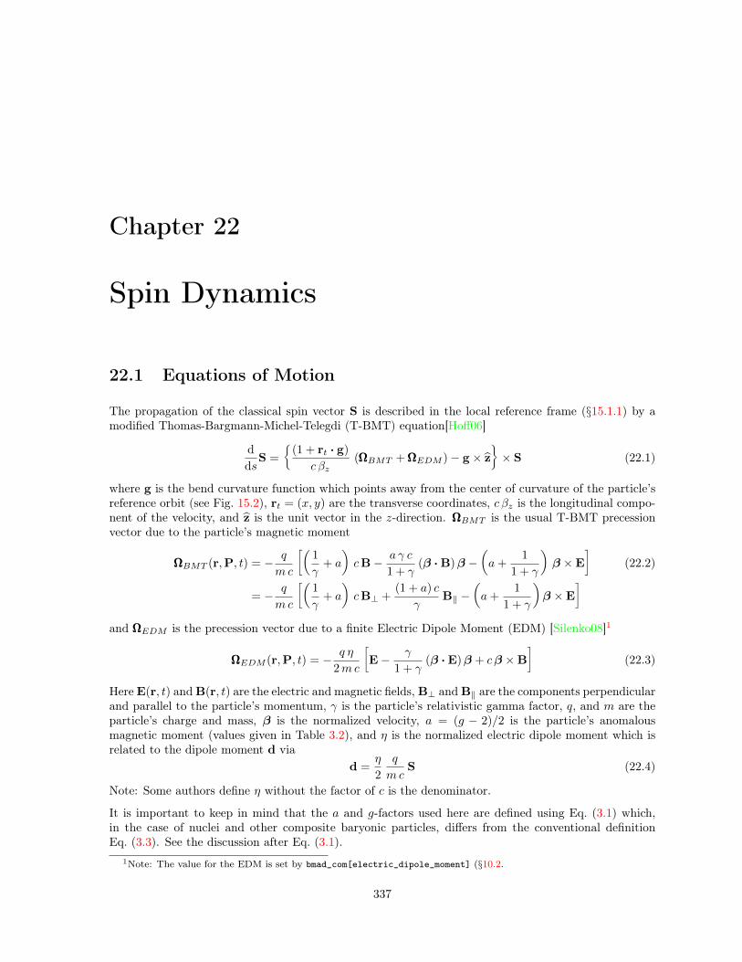
Chapter 22

Spin Dynamics

22.1 Equations of Motion

The propagation of the classical spin vector S is described in the local reference frame (§15.1.1) by amodified Thomas-Bargmann-Michel-Telegdi (T-BMT) equation[Hoff06]

d

dsS =

ß(1 + rt · g)

c βz(ΩΩΩBMT + ΩΩΩEDM )− g × z

™× S (22.1)

where g is the bend curvature function which points away from the center of curvature of the particle’sreference orbit (see Fig. 15.2), rt = (x, y) are the transverse coordinates, c βz is the longitudinal compo-nent of the velocity, and z is the unit vector in the z-direction. ΩΩΩBMT is the usual T-BMT precessionvector due to the particle’s magnetic moment

ΩΩΩBMT (r,P, t) = − q

m c

ïÅ1

γ+ a

ãcB− a γ c

1 + γ(β ·B)β −

Åa+

1

1 + γ

ãβ ×E

ò(22.2)

= − q

m c

ïÅ1

γ+ a

ãcB⊥ +

(1 + a) c

γB‖ −

Åa+

1

1 + γ

ãβ ×E

òand ΩΩΩEDM is the precession vector due to a finite Electric Dipole Moment (EDM) [Silenko08]1

ΩΩΩEDM (r,P, t) = − q η

2mc

ïE− γ

1 + γ(β ·E)β + cβ ×B

ò(22.3)

Here E(r, t) and B(r, t) are the electric and magnetic fields, B⊥ and B‖ are the components perpendicularand parallel to the particle’s momentum, γ is the particle’s relativistic gamma factor, q, and m are theparticle’s charge and mass, β is the normalized velocity, a = (g − 2)/2 is the particle’s anomalousmagnetic moment (values given in Table 3.2), and η is the normalized electric dipole moment which isrelated to the dipole moment d via

d =η

2

q

m cS (22.4)

Note: Some authors define η without the factor of c is the denominator.

It is important to keep in mind that the a and g-factors used here are defined using Eq. (3.1) which,in the case of nuclei and other composite baryonic particles, differs from the conventional definitionEq. (3.3). See the discussion after Eq. (3.1).

1Note: The value for the EDM is set by bmad_com[electric_dipole_moment] (§10.2.

337

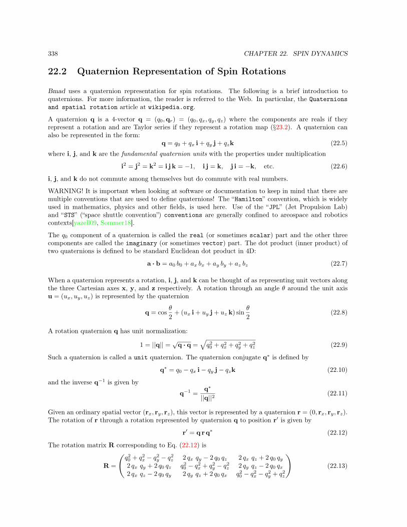
338 CHAPTER 22. SPIN DYNAMICS

22.2 Quaternion Representation of Spin Rotations

Bmad uses a quaternion representation for spin rotations. The following is a brief introduction toquaternions. For more information, the reader is referred to the Web. In particular, the Quaternionsand spatial rotation article at wikipedia.org.

A quaternion q is a 4-vector q = (q0,qr) = (q0, qx, qy, qz) where the components are reals if theyrepresent a rotation and are Taylor series if they represent a rotation map (§23.2). A quaternion canalso be represented in the form:

q = q0 + qx i + qy j + qzk (22.5)

where i, j, and k are the fundamental quaternion units with the properties under multiplication

i2 = j2 = k2 = i j k = −1, i j = k, j i = −k, etc. (22.6)

i, j, and k do not commute among themselves but do commute with real numbers.

WARNING! It is important when looking at software or documentation to keep in mind that there aremultiple conventions that are used to define quaternions! The “Hamilton” convention, which is widelyused in mathematics, physics and other fields, is used here. Use of the “JPL” (Jet Propulsion Lab)and “STS” (“space shuttle convention”) conventions are generally confined to areospace and roboticscontexts[yazell09, Sommer18].

The q0 component of a quaternion is called the real (or sometimes scalar) part and the other threecomponents are called the imaginary (or sometimes vector) part. The dot product (inner product) oftwo quaternions is defined to be standard Euclidean dot product in 4D:

a · b = a0 b0 + ax bx + ay by + az bz (22.7)

When a quaternion represents a rotation, i, j, and k can be thought of as representing unit vectors alongthe three Cartesian axes x, y, and z respectively. A rotation through an angle θ around the unit axisu = (ux, uy, uz) is represented by the quaternion

q = cosθ

2+ (ux i + uy j + uz k) sin

θ

2(22.8)

A rotation quaternion q has unit normalization:

1 = ||q|| =√

q · q =»q20 + q2

x + q2y + q2

z (22.9)

Such a quaternion is called a unit quaternion. The quaternion conjugate q∗ is defined by

q∗ = q0 − qx i− qy j− qzk (22.10)

and the inverse q−1 is given by

q−1 =q∗

||q||2(22.11)

Given an ordinary spatial vector (rx, ry, rz), this vector is represented by a quaternion r = (0, rx, ry, rz).The rotation of r through a rotation represented by quaternion q to position r′ is given by

r′ = q r q∗ (22.12)

The rotation matrix R corresponding to Eq. (22.12) is

R =

Ñq20 + q2

x − q2y − q2

z 2 qx qy − 2 q0 qz 2 qx qz + 2 q0 qy2 qx qy + 2 q0 qz q2

0 − q2x + q2

y − q2z 2 qy qz − 2 q0 qx

2 qx qz − 2 q0 qy 2 qy qz + 2 q0 qx q20 − q2

x − q2y + q2

z

é(22.13)

22.3. INVARIANT SPIN FIELD 339

In quaternion notation, two rotations q1 and q2 are combined into one rotation using the formula

q12 = q2 q1 (22.14)

where q12 is the result of rotation q1 followed by q2. Note that this equation is analogous to how rotationmatrices are combined (for more information see [Quat]).

22.3 Invariant Spin Field

In a storage ring, the invariant spin field n(r, s) = (nx, ny, nz) [Hoff06, Duan15], which is a functionof phase space position r = (x, px, y, py, z, pz) and longitudinal position s, is the continuous function withunit amplitude that satisfies

n(Mrr, s) =Ms(r) n(r, s) (22.15)

where Mr is the orbital part of the 1-turn transfer map and Ms(r), derived from T-BMT equation,is the spin part of the map which is a function of r. That is, the invariant spin field (ISF) obeys theT-BMT equation. Thus, a particle whose spin points in the direction of n(r, s) at some time t will, inthe absence of radiation effects, always have its spin pointing in the direction of n(r, s). When there areno resonances, n(r, s) is unique up to a flip of sign.

In general, it is not straightforward to calculate n. The exceptional case (besides the cases where thereis a resonance) is if the particle is on the closed orbit r0. In this case, sinceMrr0 = r0, and sinceMs(r)is a rotation matrix, Eq. (22.15) can be solved to give the invariant spin field on the closed orbit denotedby n0. Over one turn, a spin on the closed orbit rotates around n0 by the angle 2πν0 where ν0 is theclosed-orbit spin tune.

Once the invariant spin field has been calculated, various quantities of interest can be computed. Forexample, given some initial distribution of spins in a beam, the maximum possible time averaged polar-ization 〈S〉max is

〈S〉max =

∫dr ρ(r) n(r) (22.16)

where the integral is over the beam phase space space density ρ and the longitudinal s-dependence isimplicit. The above equation neglects any single spin polarization or depolarization processes. Noticethat what is calculated is a time averaged quantity. Instantaneously, the beam can be fully polarizedbut the average over many turns, at some given position s, cannot exceed 〈S〉max.

Another quantity that can be computed from knowledge of n is the equilibrium polarization of a beam.The Baier-Katkov-Strakhovenko polarization Pbks (generalized from Sokolov-Ternov to include non-vertical fields) is calculated by ignoring deviations of the beam from the closed orbit[Barber99]

Pbks = ± 8

5√

3

∮ds g3 b · n0∮

ds g3

Å1− 2

9(n0 · s)2

ã (22.17)

where g = 1/ρ is the bending strength (ρ is the bending radius), s is the unit vector in the direction ofmotion, and b is defined to be

b ≡ s× ds/ds

|ds/ds|(22.18)

Notice that b is the direction of the magnetic field when s is perpendicular to the magnetic field andwhen there is no electric field. In the above equation, the plus sign is for positrons (polarized parallel to

340 CHAPTER 22. SPIN DYNAMICS

the field) and the minus sign is for electrons. Since the above equation is only valid when the anomalousmagnetic moment is small[Jackson76], this formula is not valid for protons and anti-protons.

The corresponding BKS polarization build-up rate τ−1bks is

τ−1bks =

5√

3

8

re γ5 ~

m

1

C

∮ds g3

Å1− 2

9(n0 · s)2

ã(22.19)

If the the stochastic excitation of the beam is taken into account, the generalized Sokolov-Ternov polar-ization is called the Derbenev-Kondratenko-Mane formula

Pdk = ± 8

5√

3

∮ds

≠g3 b ·

Ån− ∂n

∂δ

ã∑∮ds

Æg3

Ç1− 2

9(n · s)2 +

11

18

∣∣∣∣∂n

∂δ

∣∣∣∣2å∏ (22.20)

where <> denotes an average over phase space, and δ is the fractional energy deviation which, for ultra-relativistic particles, is the same as phase space pz. Since, away from any resonances, n is very close ton0, and since generally machines are tuned away from any resonances, the n − ∂n/∂δ and n · s termscan be replaced by n0 − ∂n/∂δ and n0 · s when evaluating Pdk.

The time dependence of the polarization is [Barber99])

P(t) = Pdk (1− exp(−t/τdk)) + P0 exp(−t/τdk) (22.21)

where P0 is the initial polarization and the polarization rate τ−1dk is

τ−1dk =

5√

3

8

re γ5 ~

m

1

C

∮ds

Æg3

Ç1− 2

9(n · s)2 +

11

18

∣∣∣∣∂n

∂δ

∣∣∣∣2å∏

(22.22)

τ−1dk can be decomposed into two parts:

τ−1dk = τ−1

pol + τ−1dep (22.23)

τ−1pol is the polarization rate given by the first two terms on the RHS in Eq. (22.22) and the depolarizationrate τ−1

dep is given by the the third term:

τ−1pol =

5√

3

8

re γ5 ~

m

1

C

∮ds

≠g3

Å1− 2

9(n · s)2

ã∑τ−1dep =

5√

3

8

re γ5 ~

m

1

C

∮ds

Æg3 11

18

∣∣∣∣∂n

∂δ

∣∣∣∣2∏

(22.24)

τ−1pol is generally well approximated by the Baier-Katkov-Strakhovenko polarization rate (Eq. (22.19)).The difference being that τ−1

bks is evaluated along the closed orbit while τ−1pol takes into account the size

of the beam.

22.4 Linear ∂n/∂δ Calculation

When evaluating the equations in the previous section, in many situations it is sufficient to just use thevalue of ∂n/∂δ as calculated in the linear regime. In the linear regime, ∂n/∂δ is only dependent upon

22.4. LINEAR ∂N/∂δ CALCULATION 341

the s-position and is independent of the phase space position. The calculation of ∂n/∂δ starts with thelinearized transport equations which are characterized by a 6× 6 orbital 1-turn transfer matrix M alongwith the spin transport which can be written in the form

qs(r) = q0 +−→q · r (22.25)

The quaternion map qs, evaluated at the orbital phase space point r, has a zeroth order part q0 (thespin rotation for a particle on the closed orbit) and the first order part −→q = (q1, . . . ,q6) which is avector of six quaternions and which is evaluated in Eq. (22.25) by taking the dot product with the vectorr.

The closed orbit invariant spin n0 which has unit amplitude satisfies the equation

q0 n0 q∗0 = n0 (22.26)

The solution to this equation, normalized to one, is

n0 =(q0,x, q0,y, q0,z)

‖(q0,x, q0,y, q0,z)‖(22.27)

Since qs is a rotation quaternion, the magnitude of qs(r) must remain one. Using Eq. (22.25) inEq. (22.9), to keep the magnitude equal to one to linear order gives the condition

q0 · qk = 0, k = 1, . . . , 6 (22.28)

for all qk components of −→q .

To calculate ∂n/∂δ, the first step is to compute the eigenvectors vk and eigenvalues λk, k = 1, . . . , 6 ofthe 1-turn orbital matrix. The corresponding spin eigenvectors nk are computed from the equation

qs(vk) (n0 + nk) q∗s(vk) = n0 + λk nk (22.29)

Using Eqs. (22.25) and (22.26), and keeping only linear terms gives

λk nk − q0 nk q∗0 = (−→q · vk) n0 q∗0 + q0 n0 (−→q ∗ · v∗k) (22.30)

This equation is linear in the unknown nk and so may be easily solved using standard linear algebratechniques.

Since the eigenvectors vk span phase space, for any given phase space position r, there exist a set ofcoefficients Ak(r), k = 1, . . . , 6, such that

r =

6∑k=1

Ak(r) vk (22.31)

Define the function n by

n(r) ≡ n0 +

6∑k=1

Ak(r) nk (22.32)

This function obeys the T-BMT equation and is continuous and thus is the solution (up to a flip in signand a normalization constant) for the invariant spin field. From this, ∂n/∂δ, which is computed takingthe derivative at constant x, px, y, py, and z, is obtained via

∂n

∂δ=

6∑k=1

Ak nk (22.33)

342 CHAPTER 22. SPIN DYNAMICS

with the Ak being computed by inverting the equation

(0, 0, 0, 0, 0, 1)t =

6∑k=1

Ak vk (22.34)

where the superscript t means transpose. Notice that for ∂n/∂δ, as well as any other partial derivative,the component in the direction of n0 will be zero since, to first order, the amplitude of n must beconstant (since the equation for n is only valid to first order, the computed amplitude will have non-zerohigher order terms).

A problem arises if the machine that is being simulated does not have any RF cavities or the voltagein the cavities is zero. In this case, there are no synchrotron oscillations which results in degenerateeigenvectors and the eigenvectors will not span all of phase space. The solution here is to reduce thedimensionality of phase space to five by remove the z coordinate. The above equations then can be usedwith the sums over k ranging from 1 to 5.

It is sometimes informative to compute the contribution of ∂n/∂δ due to a single mode of oscillation.That is, to compute ∂n/∂δ with the sum in Eq. (22.33) restricted to be over the two corresponding eigenstates that comprise the oscillation mode of interest. This information can help guide lattice design.

22.5 Linear Single Resonance Analysis

Resonances occur when the spin tune νs is an integer (“imperfection” resonances) and when the spintune νs in combination with the three orbital tunes νx, νy, and νz is an integer (“intrinsic” or “spin-orbit”resonances)

νs +mx νx +my νy +mz νz = m0 (22.35)

where mx, my, mz, and m0 are integers. In the linear approximation (§22.4), resonances only occur ifone and exactly one of the mx, my, or mz has a value of one and the other two are zero.

Generally, in rings where the synchrotron radiation is large (think electrons), the depolarization dueto radiation will tend to dominate (§22.3). For rings where the synchrotron radiation is small (thinkprotons), resonances will be more important. Notice that synchrotron radiation, being a stochasticprocess results in depolarization. Resonances, on the other hand, are not stochastic and even if aresonance tilts the polarization there can be the possibility of recovery.

In order to calculate the effect of a resonance it is helpful to know the resonance strength The resonancestrength calculation can be motivated by considering the Single Resonance Model (SRM)[Hoff06] whereit is assumed that only one orbital mode is excited and that there is a single dominating resonance. Inthis case the spin equation of motion is

ds

dθ= Ω× s, Ω =

Ñεr cos Φεr sin Φν0

é(22.36)

where εr is the resonance strength, ν0 is the closed orbit spin tune and θ is the longitudinal angle withθ = 2π representing one turn in the circular accelerator. In the above equation the phase Φ is relatedto the orbital mode tune Q via

Φ = Qθ + Φ0 (22.37)

with Φ0 being the starting phase. Eq. (22.36) can be solved by transforming to a coordinate systemrotating about the z-axis with a rotational frequency Q. In this frame, the spin vector sR is

sR = qz(−Φ/2) s q∗z(−Φ/2), where qz(φ) ≡ (cos(φ/2), 0, 0, sin(φ/2)) (22.38)

22.5. LINEAR SINGLE RESONANCE ANALYSIS 343

Using Eq. (22.38) in Eq. (22.36) gives

dsRdθ

= ΩR × sR, ΩR =

Ñεr0δ

é, δ = ν0 −Q (22.39)

If a spin is initially aligned along the n0 axis (s = sR = (0, 0, 1)), then at resonance, with δ = 0, the spinwill be rotated by an angle 2π εr. This gives a physical interpretation to εr. Thus, for a resonance tobe small, the resonance strength must satisfy

εr 1 (22.40)

In the rotating coordinate system, a spin oriented parallel to ΩR remains parallel to ΩR so ΩR is in thedirection of the invariant spin field. Transforming back to the laboratory frame and normalizing to one,n is

n(Φ) =sgn(δ)

Λ

Ñεr cos Φεr sin Φ

δ

é, Λ =

√δ2 + ε2r (22.41)

where the sign factor sgn(δ) is chosen so that on the closed orbit with J = 0 the n axis is in the positivez-direction.

Eq. (22.41) shows that resonance is when δ = 0 or ν0 = Q. The use of a sinusoidal perturbation inthe single resonance model results in the suppression of all other resonances which can be of the formν0 = m0 ± Q where m0 is some integer. In an actual machine, the presence of a perturbation at somespecific point in the machine will produce a comb of resonances of the form m0 ±Q.

Restricting discussion to linear resonances, the resonance strength will scale with√J where J is the

action of the orbital oscillations (§21.3)εr =

√J ξr (22.42)

where ξr is the normalized resonance strength. In this case, the criterion for the resonance strengthto be small (Eq. (22.40)) is that

√J ξr is small comapared to one with J being the action for particle

motion at a few beam sigma.

The normalized resonance strength can be related to the first order spin eigenvectors nk (Eq. (22.29)) bycomparing Eq. (22.41) with the equations developed in §22.4. The eigen analysis in §22.4 gives the closedorbit n0 along with the six eigenvectors (vk,nk) and corresponding eigenvalues λk, k = 1, . . . 6 of the1-turn spin-orbital transport. The orbital part of the kth eigenvector, vk, normalized using Eq. (21.21),represents particle motion with unit action Jk for that mode. Considering Eq. (22.33), if only one modeis excited for some particular k and with some amplitude

√J , the invariant spin field on the mth turn is

n(m) =1

Λn

Än0 + Re

Ä2√J nk e

i φ0 λmkää

Λn =

√1 + 4 J

∣∣Re(nk)∣∣2 (22.43)

where φ0 is the initial phase (see Eq. (21.29)). Comparing this to Eqs. (22.41) and (22.42), the constantpart of the n vector in Eq. (22.41) (nz) is associated with n0 in Eq. (22.43) and the time varying part ofn in Eq. (22.41) (nx and ny) is associated with vk in Eq. (22.43). Taking the ratio of constant to timevarying parts in both equations and equating gives

ξr = 2 δ∣∣Re(nk)

∣∣ (22.44)

where k is either one of the two spin eigenvectors of the mode exciting the resonance.

ξr can be related to the G matrix of the SLIM formalism (Eq. (22.50)). The corresponding equationis[Hoff06]

ξr =1

2π

∣∣G · vk∣∣ (22.45)

344 CHAPTER 22. SPIN DYNAMICS

Here k must correspond to the eigenvalue which is the tune of the mode. The k that corresponds to theeigenvalue which is negative the tune cannot be used here (unlike Eq. (22.44)).

While Eqs. (22.44) and (22.45) can be used to calculate ξr within the single resonance model independentof how large δ is, in a real machine, where there are many resonances, Eqs. (22.44) and (22.45) are strictlyonly valid at resonance with δ = 0. In this case Eq. (22.44) is singular since, as δ goes to zero, nk goesto infinity. In practice, Eqs. (22.44) and (22.45) may be used to calculate ξr with reasonable accuracywhen δ is small.

22.6 SLIM Formalism

The SLIM formalism2 [Chao81, Barber99], introduced by Alex Chao, is a way to represent the linearized(that is, first order) orbital and spin transport as an 8× 8 matrix which then can be analyzed usingstandard linear algebra techniques. The idea is to expand the transport map around the closed orbit(r0,n0) where r0 is the orbital closed orbit and n0 is the “spin closed orbit”. Namely the unit-vector,one-turn periodic solution of the Thomas-BMT equation on r0

3. n0 is just the invariant spin field onthe closed orbit. The formalism provides estimates of the equilibrium spin polarization and the rate ofdepolarization in electron storage rings, both under the restriction of the aforementioned linearization.Moreover, a procedure known as spin-matching, for minimizing depolarization driven by the noise in-jected into synchro-betatron motion by synchrotron radiation, and which involves optimizing the layoutof the ring, can be executed in a simple and elegant way via the SLIM formalism. The formalism canalso give insights into proton spin dynamics in regimes where the linearization suffices.

The SLIM formalism expresses spin components using two right-hand coordinate systems: 4(l(s),n0(s),m(s)

)and(

l0(s),n0(s),m0(s))

(22.46)

The axes l0(s) and m0(s) are solutions of the Thomas-BMT equation on the closed orbit and, generally,are not one-turn periodic. The axes l(s) and m(s) are chosen to be one-turn periodic but can have anarbitrary s dependence which can be chosen for convenience otherwise. The axes l0(s) and m0(s) areused for spin-matching and l(s) and m(s) are used for calculating polarization and depolarization. Withrespect to these axes, a unit-length spin S can be written as

S =»

1− α20 − β2

0 n0 + α0 l0 + β0 m0 or

S =√

1− α2 − β2 n0 + α l + βm (22.47)

To linearize the transport, it is assumed that α0, and β0 (and hence α and β) are small compared toone. To first order, the variation from unity of the spin component along the n0 axis will be secondorder and can be ignored:

S ≈ n0 + α0 l0 + β0 m0 orS ≈ n0 + α l + βm (22.48)

2The name references an early computer program that implemented the formalism.3Warning: The symbol n or ~n used in [Chao81, Barber85] and other early literature to denote the periodic solution

of the T–BMT equation on the closed orbit should be replaced by the symbol n0 to conform to the modern convention[Barber99] and thereby avoid confusion with the symbol n which denotes the invariant spin field. In addition, the symbols~m and ~l appearing, for example, in the formulae for the matrix G in [Barber85], should be replaced by the symbols m0 andl0, namely by the modern symbols for the two (normally) non-periodic solutions of the T-BMT equation, which togetherwith n0, form an orthonormal coordinate system.

4Different authors will use different conventions for the ordering of the axes The ordering used here puts n0 secondreflecting the fact that in many rings the n0 axis will point in the vertical y-direction in the arcs.

22.6. SLIM FORMALISM 345

The n0 coordinate is dropped since the spin component along n0 is a constant. With this, the eight-dimensional spin-orbit phase space used in the SLIM formalism is

(x, px, y, py, z, pz, α0, β0) or(x, px, y, py, z, pz, α, β) (22.49)

where the orbital part x, px, etc. is taken with respect to the closed orbit.

The first order map between two any points s1 and s2 is an 8× 8 matrix M which is written in the form

M(s1, s2) =

ÅM6×6 06×2

G2×6 D2×2

ã(22.50)

where M(s1, s2) is the 6× 6 orbital phase space transport matrix, and G(s1, s2) contains the couplingof the spin coordinates (α0, β0) or (α, β) to the orbital motion. The upper right block 06×2 in the Mmatrix is zero since Stern-Gerlach effects are ignored. When G is calculated with respect to the (l0,m0)axes, large spin precessions on the closed orbit due to dipole and solenoid fields are eliminated. Thatleaves small precessions due to synchro-betatron motion. The G matrix then represents the dominatinglinear dependence of the small precessions on the six synchro-betatron coordinates and it then providesa good framework for analysis [Barber85, Barber99]. In Eq. (22.50), D is a 2× 2 rotation matrix for thespin transport of a particle on the closed orbit. In this case, since the l0(s) and m0(s) are solutions tothe T-BMT equation, D is the unit matrix.

To compute M for a section of the ring, the first step is to find the 6× 6 orbital matrix for the section.To calculate n0, l0 and m0, first n0 at some starting point s is calculated (section 18.3) and propagatedaround the ring. This n0 is then available for calculations involving the whole ring. If only part of thering is being analyzed, the orientation of n0 at the start of the section can be an input parameter. Thatis, it can be given by the User and not calculated. However, for spin-matching, it usually only makesphysical sense to use the n0 at the start of the section that corresponds to the n0 calculated for thewhole ring. After n0 is known at some s-position, l0 and m0 at that s-position can be chosen somewhatarbitrarily to form the right handed coordinate system. Sometimes it is possible to make a special choiceof the initial l0 and m0 in order to simplify the G matrices. For example, in a section where there areonly drifts and quadrupoles so that there is no spin rotation for a particle traveling on the centerline,with n0 pointing vertically, a choice of m0 pointing in the longitudinal s-direction results in the first lineof the G matrix for the section being zero. After the initial l0 and m0 axes have been specified at someinitial s, the axes can be transported along the closed orbit of the section.

If the one-turn G were zero everywhere, the spin motion would be completely decoupled from the orbitalmotion (at least to first order) and the depolarization rate τ−1

dep given by Eq. (22.24) would be zero since∂n/∂δ would be zero. Therefore, spin-matching analysis for a section of the ring involves adjustingthe parameters (quadrupole strengths, drift lengths etc) of the section so as to minimize elements inappropriate columns of the G matrix. This decreases the rate of depolarization by minimizing ∂n/∂δat the dipole magnets (where g in Eq. (22.24) is nonzero) [Barber99]. Such adjustments are made whilesimultaneously maintaining acceptable Courant-Snyder parameters and for this the closed orbit shouldbe taken to be the design orbit. This optimization can be carried out using standard facilities in Bmad.The calculation of ∂n/∂δ in the SLIM approximation is described below.

The process for calculating electron polarization and the rate of depolarization in the SLIM formalismis as follows. First, the 8 × 8 matrix M for one-turn is calculated as described above. After this,using the closed-orbit spin tune ν0, a specific version of (l,m) is constructed by rotating the vectors l0and m0 backwards around n0 by the angle 2πν0 in a drift space right at the end of the turn, therebytransforming α0 and β0 into α and β and transforming the G matrix correspondingly5. The original

5Adding a rotation at the end is just for convenience. For some other applications it is useful to choose axes l and mwith respect to which spins precess at the constant rate with a phase advance of 2πν0 per turn.

346 CHAPTER 22. SPIN DYNAMICS

one-turn G matrix is not one-turn periodic but the transformed G matrix is one-turn periodic and thematrix D for one-turn becomes the 2 × 2 rotation matrix with rotation angle 2πν0 [Chao81]. The newmatrix M is then also one-turn periodic and its eigenvectors are used as described after Eq. (22.58)for calculating the derivative ∂n/∂δ used in Eq. (22.24). Note that if the elements in the appropriatecolumns of the non-periodic G matrix for the one-turn map at a dipole have been minimized by spin-matching, the corresponding elements of the periodic one-turn G matrix have been minimized too. Asa consequence it can be seen, via Eqs. (22.59) and (22.60), that ∂n/∂δ has been minimized as required.

In contrast to the approach in [Barber85, Barber99], Bmad calculates the G and D matrices from thequaternion of the spin transport map (which Bmad calculates via PTC (§27)). After the (l0,n0,m0) co-ordinates have been calculated (or set by the User) at some initial point, the spin axes can be transportedusing the q0 quaternion (Eq. (22.25)). When analyzing only a section of a ring, there is no identifiablespin tune so nothing further needs to be done. In this case, the D matrix is just a unit matrix. Whenanalyzing one-turn maps, if the l and m axes are set to be the l0(s) and m0(s) axes except at the end ofthe lattice, the spin phase advance as a function of s will be zero except just before the starting positionwhere there will be a discontinuous jump in phase.

Once the (l0,n0,m0) axes have been calculated, the matrices G and D can be calculated from the spintransport map (which Bmad calculates via PTC (§27)). The first order transport map Eq. (22.25) is used.Let qlnm(s) be the quaternion that transforms from (l0,n0,m0)6 coordinates to (x, y, z) coordinates ata given point s. With this, the spin transport q from s1 to s2 in the (l0,n0,m0) coordinate system is

qs(s1, s2) = qlnm(s2) qs(s1, s2) q−1lnm(s1) (22.51)

The zeroth order part of qs gives:

q0(s1, s2) = qlnm(s2) q0(s1, s2) q−1lnm(s1) (22.52)

represents a rotation around the n0 axis.

To calculate the D matrix, q0 is converted into a 3× 3 rotation matrix R0 via Eq. (22.13)). The secondrow and second column of this rotation matrix corresponds to the n0 axis. Since the component of thespin along this axis does not vary to first order, R0 has the form

R0 =

ÑR0(1, 1) 0 R0(1, 3)

0 1 0R0(3, 1) 0 R0(3, 3)

é(22.53)

That is, the rotation is around the n0 axis. Since the n0 spin component is ignored in the SLIM formalism(Eq. (22.49)), the 2× 2 D matrix is simply R0 with the second row and second column removed.

D(s1, s2) =

ÅR0(1, 1) R0(1, 3)R0(3, 1) R0(3, 3)

ã(22.54)

In particular, when using the (l0,n0,m0) coordinate system, q0 represents the identity (≡ (1, 0, 0, 0))and D is a unit matrix as expected.

The rows of the G matrix encode the first-order dependence of the changes of the angles α0 and β0 (orof the angles α and β). The G matrix can therefore be calculated from qi which is the first order partof qs

qi = qlnm(s2) qi(s1, s2) q−1lnm(s1) (22.55)

Using Eq. (22.25) in Eq. (22.13) and keeping only first order terms gives

G(1, i) = 2(q0,y qi,x − q0,0 qi,z) (22.56)G(2, i) = 2(q0,0 qi,x + q0,y qi,z), i = 1, . . . , 6

6Such a formalism works also with the (l,n0,m)

22.7. SPINOR NOTATION 347

where the fact that q0,x = q0,z = 0 has been used.7 8

The calculation of the derivative ∂n/∂δ within the SLIM formalism is similar to the calculation usingquaternions (§22.4). The following follows Barber[Barber99]. The calculation starts with the one-turnperiodic 8 × 8 matrix M [Here the periodic (l(s),n0(s),m(s)) coordinate system must be used sincethe ending coordinates for M must be the same as the starting coordinates.] The eigenvectors uk andeigenvalues λk (k = 1, . . . 8) of M are of the form

uk =

Åvkwk

ã, k = 1, . . . , 6 (22.58)

uk =

Å06

wk

ã, k = 7, 8

where vk are eigenvectors of the orbital submatrix M, and for the first six eigenvectors the wk arecomputed via (compare with Eqs. (22.30))

wk = [λk I2 −D]−1

G vk, k = 1, . . . , 6 (22.59)

where I2 is the 2× 2 unit matrix. These eigenvectors, computed at the chosen starting point s1 and arethen propagated to other s-positions s2 using M(s1, s2).

The derivative ∂n/∂δ is computed analogously to Eq. (22.60)

∂n

∂δ=

Å∂α

∂δ,∂β

∂δ

ã=

6∑k=1

Ak wk (22.60)

with the Ak being computed from Eq. (22.34).

Alternatively, Chao [Chao79] gives a an analytical formulation where the eigenvectors are normalized inthe form Eq. (21.21). With this, ∂n/∂δ is computed via

∂n

∂δ= i

6∑k=1

v∗k5 wk (22.61)

22.7 Spinor Notation

The following describes the old spinor representation formally used by Bmad to represent spins. Thisdocumentation is kept as an aid for comparison with the spin tracking literature.

In the SU(2) representation, a spin S is written as a spinor Ψ = (ψ1, ψ2)T where ψ1,2 are complex

numbers. The conversion between SU(2) and SO(3) is

S = Ψ†σΨ ←→ Ψ =eiξ√

2 (1 + s3)

Å1 + s3

s1 + is2

ã(22.62)

7Do not be confused by the x, y and z subscripts which refer to the components of q as defined in Eq. (22.5). q rotatesspins in the (l0,n0,m0) coordinate system. Not the (x, y, z) coordinate system.

8Unlike the operation of going from the linearized quaternion transport (Eq. (22.25) to the M matrix, given an Mmatrix, it is not possible to uniquely construct the qi quaternions. qi,x and qi,z can be determined by Eq. (22.56).However, qi,0 and qi,y can only be determined via Eq. (22.26) up to an unknown factor κ:

qi,0 = κ q0,y , qi,y = −κ q0,0 (22.57)

A finite κ represents a variation of the spin tune with a particle’s orbital phase space position. This is, a finite qi,0 andqi,y represent a non-linear effect which will average to zero over many turns as a particle with constant orbital amplitudesamples different points on the phase space torus it is on.

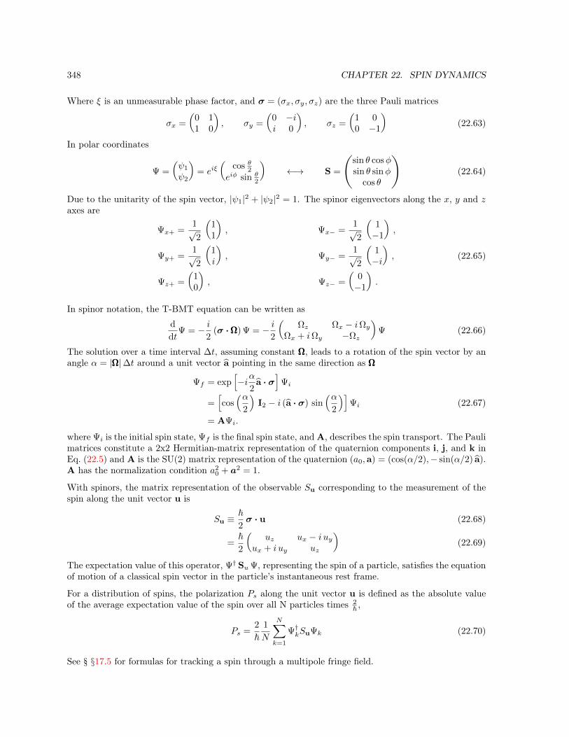
348 CHAPTER 22. SPIN DYNAMICS

Where ξ is an unmeasurable phase factor, and σ = (σx, σy, σz) are the three Pauli matrices

σx =

Å0 11 0

ã, σy =

Å0 −ii 0

ã, σz =

Å1 00 −1

ã(22.63)

In polar coordinates

Ψ =

Åψ1

ψ2

ã= eiξ

Åcos θ2

eiφ sin θ2

ã←→ S =

Ñsin θ cosφsin θ sinφ

cos θ

é(22.64)

Due to the unitarity of the spin vector, |ψ1|2 + |ψ2|2 = 1. The spinor eigenvectors along the x, y and zaxes are

Ψx+ =1√2

Å11

ã, Ψx− =

1√2

Å1−1

ã,

Ψy+ =1√2

Å1i

ã, Ψy− =

1√2

Å1−i

ã, (22.65)

Ψz+ =

Å10

ã, Ψz− =

Å0−1

ã.

In spinor notation, the T-BMT equation can be written as

d

dtΨ = − i

2(σ ·ΩΩΩ) Ψ = − i

2

ÅΩz Ωx − iΩy

Ωx + iΩy −Ωz

ãΨ (22.66)

The solution over a time interval ∆t, assuming constant ΩΩΩ, leads to a rotation of the spin vector by anangle α = |ΩΩΩ|∆t around a unit vector a pointing in the same direction as ΩΩΩ

Ψf = exp[−iα

2a · σ

]Ψi

=[cos(α

2

)I2 − i (a · σ) sin

(α2

)]Ψi (22.67)

= AΨi.

where Ψi is the initial spin state, Ψf is the final spin state, and A, describes the spin transport. The Paulimatrices constitute a 2x2 Hermitian-matrix representation of the quaternion components i, j, and k inEq. (22.5) and A is the SU(2) matrix representation of the quaternion (a0,a) = (cos(α/2),− sin(α/2) a).A has the normalization condition a2

0 + a2 = 1.

With spinors, the matrix representation of the observable Su corresponding to the measurement of thespin along the unit vector u is

Su ≡~2σ · u (22.68)

=~2

Åuz ux − i uy

ux + i uy uz

ã(22.69)

The expectation value of this operator, Ψ† Su Ψ, representing the spin of a particle, satisfies the equationof motion of a classical spin vector in the particle’s instantaneous rest frame.

For a distribution of spins, the polarization Ps along the unit vector u is defined as the absolute valueof the average expectation value of the spin over all N particles times 2

~ ,

Ps =2

~1

N

N∑k=1

Ψ†kSuΨk (22.70)

See § §17.5 for formulas for tracking a spin through a multipole fringe field.

Chapter 23

Taylor Maps

23.1 Taylor Maps

A transport mapM : R6 → R6 through an element or a section of a lattice is a function that maps thestarting phase space coordinates r(in) to the ending coordinates r(out)

r(out) =M (δr) (23.1)

whereδr = r(in)− rref (23.2)

rref is the reference orbit at the start of the map around which the map is made. In many cases thereference orbit is the zero orbit. For a storage ring, the closed orbit is commonly used for the referenceorbit. For a lattice with an open geometry the reference orbit may be the orbit as computed from somegiven initial coordinates.

M in the above equation is made up of six functions Mi : R6 → R. Each of these functions maps toone of the r(out) coordinates. Each of these functions can be expanded in a Taylor series and truncatedat some order. Each Taylor series is in the form

ri(out) =

N∑j=1

Cij

6∏k=1

(δrk)eijk (23.3)

Where the Cij are coefficients and the eijk are integer exponents. The order of a given term associatedwith index i, j is the sum over the exponents

orderij =

6∑k=1

eijk (23.4)

The order of the entire map is the order at which the map is truncated.

The standard Bmad routine for printing a Taylor map might produce something like this:Taylor Terms:Out Coef Exponents Order Reference--------------------------------------------------1: -0.600000000000 0 0 0 0 0 0 0 0.2000000001: 1.000000000000 1 0 0 0 0 0 1

349

350 CHAPTER 23. TAYLOR MAPS

1: 0.145000000000 2 0 0 0 0 0 2--------------------------------------------------2: -0.185000000000 0 0 0 0 0 0 0 0.0000000002: 1.300000000000 0 1 0 0 0 0 12: 3.800000000000 2 0 0 0 0 1 3--------------------------------------------------3: 1.000000000000 0 0 1 0 0 0 1 0.1000000003: 1.600000000000 0 0 0 1 0 0 13: -11.138187077310 1 0 1 0 0 0 2--------------------------------------------------4: 1.000000000000 0 0 0 1 0 0 1 0.000000000--------------------------------------------------5: 0.000000000000 0 0 0 0 0 0 0 0.0000000005: 0.000001480008 0 1 0 0 0 0 15: 1.000000000000 0 0 0 0 1 0 15: 0.000000000003 0 0 0 0 0 1 15: 0.000000000003 2 0 0 0 0 0 2--------------------------------------------------6: 1.000000000000 0 0 0 0 0 1 1 0.000000000

Each line in the example represents a single Taylor term. The Taylor terms are grouped into 6 Taylorseries. There is one series for each of the output phase space coordinate. The first column in theexample, labeled “out”, (corresponding to the i index in Eq. (23.3)) indicates the Taylor series: 1 = x(out),2 = px(out), etc. The 6 exponent columns give the eijk of Eq. (23.3). In this example, the second Taylorseries (out = 2), when expressed as a formula, would read:

px(out) = −0.185 + 1.3 δpx + 3.8 δx2 δpz (23.5)

The reference column in the above example shows the input coordinates around which the Taylor mapis calculated. In this case, the reference coordinates where

(x, px, y, py, z, pz)ref = (0.2, 0, 0.1, 0, 0, 0, 0) (23.6)

The choice of the reference point will affect the values of the coefficients of the Taylor map. As anexample, consider the 1-dimension map

x(out) = A sin(k δx) (23.7)

Then a Taylor map to 1st order isx(out) = c0 + c1 δx (23.8)

where

c1 = Ak cos(k xref) (23.9)c0 = A sin(k xref) (23.10)

23.2 Spin Taylor Map

A Taylor map that fully describes spin (§22.1) and orbital motion, would consist of nine Taylor series(six for the orbital phase space variables and three for the spin components) and each Taylor series wouldbe a polynomial in nine variables.

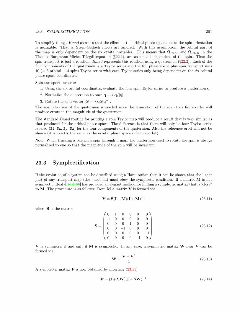
23.3. SYMPLECTIFICATION 351

To simplify things, Bmad assumes that the effect on the orbital phase space due to the spin orientationis negligible. That is, Stern-Gerlach effects are ignored. With this assumption, the orbital part ofthe map is only dependent on the six orbital variables. This means that ΩΩΩBMT and ΩΩΩEDM in theThomas-Bargmann-Michel-Telegdi equation (§22.1), are assumed independent of the spin. Thus thespin transport is just a rotation. Bmad represents this rotation using a quaternion (§22.2). Each of thefour components of the quaternion is a Taylor series and the full phase space plus spin transport uses10 (= 6 orbital + 4 spin) Taylor series with each Taylor series only being dependent on the six orbitalphase space coordinates.

Spin transport involves:1. Using the six orbital coordinates, evaluate the four spin Taylor series to produce a quaternion q.

2. Normalize the quaternion to one: q −→ q/|q|.3. Rotate the spin vector: S −→ q S q−1.

The normalization of the quaternion is needed since the truncation of the map to a finite order willproduce errors in the magnitude of the quaternion.

The standard Bmad routine for printing a spin Taylor map will produce a result that is very similar asthat produced for the orbital phase space. The difference is that there will only be four Taylor serieslabeled (S1, Sx, Sy, Sz) for the four components of the quaternion. Also the reference orbit will not beshown (it is exactly the same as the orbital phase space reference orbit).

Note: When tracking a particle’s spin through a map, the quaternion used to rotate the spin is alwaysnormalized to one so that the magnitude of the spin will be invariant.

23.3 Symplectification

If the evolution of a system can be described using a Hamiltonian then it can be shown that the linearpart of any transport map (the Jacobian) must obey the symplectic condition. If a matrix M is notsymplectic, Healy[Healy86] has provided an elegant method for finding a symplectic matrix that is “close”to M. The procedure is as follows: From M a matrix V is formed via

V = S(I−M)(I + M)−1 (23.11)

where S is the matrix

S =

0 1 0 0 0 0−1 0 0 0 0 00 0 0 1 0 00 0 −1 0 0 00 0 0 0 0 −10 0 0 0 −1 0

(23.12)

V is symmetric if and only if M is symplectic. In any case, a symmetric matrix W near V can beformed via

W =V + Vt

2(23.13)

A symplectic matrix F is now obtained by inverting (23.11)

F = (I + SW)(I− SW)−1 (23.14)

352 CHAPTER 23. TAYLOR MAPS

23.4 Map Concatenation and Feed-Down

Of importance in working with Taylor maps is the concept of feed-down. This is best explained withan example. To keep the example simple, the discussion is limited to one phase space dimension so thatthe Taylor maps are a single Taylor series. Take the map M1 from point 0 to point 1 to be

M1 : x1 = x0 + 2 (23.15)

and the map M2 from point 1 to point 2 to be

M2 : x2 = x21 + 3x1 (23.16)

Then concatenating the maps to form the map M3 from point 0 to point 2 gives

M3 : x2 = (x0 + 2)2 + 3(x0 + 2) = x20 + 7x0 + 10 (23.17)

However if we are evaluating our maps to only 1st order the map M2 becomes

M2 : x2 = 3x1 (23.18)

and concatenating the maps now gives

M3 : x2 = 3(x0 + 2) = 3x0 + 6 (23.19)

Comparing this to Eq. (23.17) shows that by neglecting the 2nd order term in Eq. (23.16) leads to 0thand 1st order errors in Eq. (23.19). These errors can be traced to the finite 0th order term in Eq. (23.15).This is the principal of feed–down: Given M3 which is a map produced from the concatenation of twoother maps, M1, and M2

M3 = M2(M1) (23.20)

Then if M1 and M2 are correct to nth order, M3 will also be correct to nth order as long as M1 has noconstant (0th order) term. [Notice that a constant term in M2 does not affect the argument.] Whathappens if we know there are constant terms in our maps? One possibility is to go to a coordinatesystem where the constant terms vanish. In the above example that would mean using the coordinatex0 at point 0 given by

x0 = x0 + 2 (23.21)

23.5 Symplectic Integration

Symplectic integration, as opposed to concatenation, never has problems with feed–down. The subject ofsymplectic integration is too large to be covered in this guide. The reader is referred to the book “BeamDynamics: A New Attitude and Framework” by Étienne Forest[Forest98]. A brief synopsis: Symplecticintegration uses as input 1) The Hamiltonian that defines the equations of motion, and 2) a Taylor mapM1 from point 0 to point 1. Symplectic integration from point 1 to point 2 produces a Taylor map M3

from point 0 to point 2. Symplectic integration can produce maps to arbitrary order. In any practicalapplication the order n of the final map is specified and in the integration procedure all terms of orderhigher than n are ignored. If one is just interested in knowing the final coordinates of a particle at point2 given the initial coordinates at point 1 then M1 is just the constant map

M1 : x1 = ci (23.22)

23.5. SYMPLECTIC INTEGRATION 353

where ci is the initial starting point. The order of the integration is set to 0 so that all non–constantterms are ignored. The final map is also just a constant map

M3 : x2 = cf (23.23)

If the map from point 1 to point 2 is desired then the map M1 is just set to the identity map

M1 : x1 = x0 (23.24)

In general it is impossible to exactly integrate any non–linear system. In practice, the symplecticintegration is achieved by slicing the interval between point 1 and point 2 into a number of (generallyequally spaced) slices. The integration is performed, slice step by slice step. This is analogous tointegrating a function by evaluating the function at a number of points. Using more slices gives betterresults but slows down the calculation. The speed and accuracy of the calculation is determined by thenumber of slices and the order of the integrator. The concept of integrator order can best be understoodby analogy by considering the trapezoidal rule for integrating a function of one variable:∫ yb

ya

f(y) dy = h

ï1

2f(ya) +

1

2f(yb)

ò+ o(h3 f (2)) (23.25)

In the formula h = yb − ya is the slice width. 0(h3 f (2)) means that the error of the trapezoidal rulescales as the second derivative of f . Since the error scales as f (2) this is an example of a second orderintegrator. To integrate a function between points y1 and yN we slice the interval at points y2 . . . yN−1

and apply the trapezoidal rule to each interval. Examples of higher order integrators can be found, forexample, in Numerical Recipes[Press92]. The concept of integrator order in symplectic integration isanalogous.

The optimum number of slices is determined by the smallest number that gives an acceptable error.The slice size is given by the ds_step attribute of an element (§6.4). Integrators of higher order willgenerally need a smaller number of slices to achieve a given accuracy. However, since integrators ofhigher order take more time per slice step, and since it is computation time and not number of sliceswhich is important, only a measurement of error and calculation time as a function of slice numberand integrator order will unambiguously give the optimum integrator order and slice width. In doing atiming test, it must be remembered that since the magnitude of any non-nonlinearities will depend uponthe starting position, the integration error will be dependent upon the starting map M1. Bmad hasintegrators of order 2, 4, and 6 (§6.4). Timing tests performed for some wiggler elements (which havestrong nonlinearities) showed that, in this case, the 2nd order integrator gave the fastest computationtime for a given accuracy. However, the higher order integrators may give better results for elementswith weaker nonlinearities.

354 CHAPTER 23. TAYLOR MAPS

Chapter 24

Tracking of Charged Particles

Bmad can track both charged particles and X-rays. This chapter deals with charged particles and X-raysare handled in chapter §25.

For tracking and transfer map calculations (here generically called “tracking”), Bmad has various methodsthat can be applied to a given element (Cf. Chapter §6). This chapter discusses the bmad_standardcalculation that is the default for almost all element types and the symp_lie_bmad calculation that doessymplectic integration.

Generally, it will be assumed that tracking is in the forward direction.

24.1 Relative Versus Absolute Time Tracking

Unlike other elements, the kick given a particle going through an lcavity, rfcavity, or possibly anem_field element depends upon the time that the particle enters the element relative to some “RF clock”.Bmad has two modes for calculating this time called “relative time tracking” and “absolute timetracking”. The switch to set the type of tracking for a lattice is parameter[absolute_time_tracking](§9.1).

The phase of the RF, φrf, is determined by

φrf = φt + φref (24.1)

where φt is the part of the phase that depends upon the time t and φref is a fixed phase offset (generallyset in the lattice file) and independent of the particle coordinates. See Eqs. (4.27) and (4.42)

The phase φt isφt = frf teff (24.2)

where frf is the RF frequency, and teff is the effective time. With relative time tracking, whichBmad uses by default, teff is a function of the phase space coordinate z (§15.4.2) via

teff(s) = t0(s)− t0(sent)−z(s)

β c(24.3)

where t0 is the reference time (see Eq. (15.28)) and sent is the s-position at the upstream end of theelement. teff is defined such that a particle entering an element with z = 0 has teff = 0.

355

356 CHAPTER 24. TRACKING OF CHARGED PARTICLES

With absolute time tracking, teff is defined by

teff(s) = t(s)− t0(sent) (24.4)

t0(sent), by definition, equal to the time of the reference particle at the entrance end of the element. Withmultipass §8.2, t0(sent) is set by the time of the reference particle at the entrance end of the element onthe first pass. For absolute time tracking, it is important to keep in mind that t0(sent) is a property ofthe element independent of how tracking is done. Thus, if a particle goes through a particular elementmultiple times, the value of tent will be the same for each transit.

To understand the difference between relative and absolute time tracking, consider a particle travelingon the reference orbit along side the reference particle in a circular ring with one RF cavity. This particlealways has z = 0 and thus, with relative time tracking, teff will always be zero at the entrance tothe cavity. With absolute time tracking, the particle, on the first turn, will have teff equal to zero.However, on subsequent turns (or subsequent passes if using multipass), the time will increase by therevolution time tC on each turn. If the RF frequency frf is some multiple of the revolution harmonic,the RF phase with absolute vs relative time tracking will be some multiple of 2π and thus RF kick giventhe particle will be the same in both cases. However, if the RF frequency is not some multiple of therevolution harmonic, there will be a difference in the RF kicks (except for the kick on the first turn).

There are advantages and disadvantages to using either relative or absolute time tracking. Absolute timetracking is more correct since RF cavities may have frequencies that are not commensurate with therevolution time. The problem with absolute time tracking is that the transfer map through the cavityis now a function of time and therefore is a function of z and the turn number. This complicates latticeanalysis. For example, standard element transfer maps use phase space coordinates so with absolutetime tracking, one has a different map for each turn.

With relative time tracking the transfer map problem is swept under the rug. The penalty for usingrelative time tracking is that results can be unphysical. For example, with relative time tracking, theclosed orbit is essentially independent of the RF frequency. From a different angle this can be viewed asa desirable feature since if one is only interested in, say, calculating the Twiss parameters, it can be anannoyance to have to worry that the ring one has constructed have a length that is exactly commensuratewith the RF frequency. And it is potentially confusing to see non-zero closed orbits when one is notexpecting it due to a mismatch between the ring circumference and the RF frequency or due to RFcavities not being spaced a multiple of the RF wavelength apart.

The above discussion is limited to the cavity fundamental mode. Long-range wakefields, on the otherhand, cannot be synchronized to the z coordinate since, in general, their frequencies are not commen-surate with the fundamental mode frequency. For simulating the long-range wakes, the kick is thus,by necessity, tied to the absolute time. The exception is that a wake associated with the fundamentalmode (that is, has the same frequency as the fundamental mode) will always use relative time if thefundamental is using relative time and vice versa.

Do not confuse absolute time tracking with the time_runge_kutta tracking method (§6.1). Thetime_runge_kutta method uses time as the independent variable instead of z. Absolute time trackingjust means that the RF phase is dependent upon the time instead of z. It is perfectly possible to useabsolute time tracking with code that uses z as the independent variable.

24.2 Element Coordinate System

The general procedure for tracking through an element makes use of element reference coordinates(also called just element coordinates). Without any offsets, pitches or tilt (§5.6), henceforth called

24.3. HAMILTONIAN 357

x

zLaboratoryEntrance Coords

LaboratoryExit Coords

ElementEntrance Coords

ElementExit Coords

x

xx

z

z

z

Figure 24.1: Element coordinates are coordinates attached to the physical element (solid green outline).The laboratory coordinates are fixed at the nominal position of the element (red dashed outline).

.

“misalignments”, the element coordinates are the same as the laboratory reference coordinates (orsimply laboratory coordinates) (§15.1.1). The element coordinates stay fixed relative to the element.Therefore, if the element is misaligned, the element coordinates will follow as the element shifts inthe laboratory frame as shown in Fig. 24.1.

Tracking a particle through an element is a three step process:

1. At the entrance end of the element, transform from the laboratory coordinates to the entranceelement coordinates.

2. Track through the element ignoring any misalignments.

3. At the exit end of the element, transform from the exit element reference frame to the laboratoryreference frame.

The transformation between laboratory and element reference frames is given in §15.3.1 and §15.3.2.

24.3 Hamiltonian

The time dependent HamiltonianHt in the curvilinear coordinate system shown in Fig. 15.2 is ([Ruth87])

Ht = ψ +

ñÅps − as1 + g x

ã2

+ ‹m2 + (px − ax)2 + (py − ay)2

ô1/2

(24.5)

where (px, py, ps/(1 + gx)) are the momentum normalized by P0, ρ being the local radius of curvatureof the reference particle, and ‹m, a and ψ are the normalized mass, vector, and scalar potentials:‹m =

mc2

c P0

Åax, ay,

as1 + g x

ã=qA

P0 cψ(x, y, z) =

q ψ

P0 c(24.6)

In terms of the normalized velocities βx, βy, the canonical momentum are

px =mc2

P0 cβx + ax, py =

mc2

P0 cβy + ay (24.7)

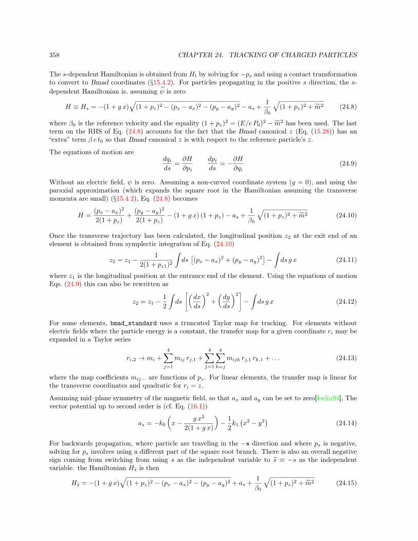
358 CHAPTER 24. TRACKING OF CHARGED PARTICLES

The s-dependent Hamiltonian is obtained from Ht by solving for −ps and using a contact transformationto convert to Bmad coordinates (§15.4.2). For particles propagating in the positive s direction, the s-dependent Hamiltonian is, assuming ψ is zero

H ≡ Hs = −(1 + g x)»

(1 + pz)2 − (px − ax)2 − (py − ay)2 − as +1

β0

»(1 + pz)2 + ‹m2 (24.8)

where β0 is the reference velocity and the equality (1 + pz)2 = (E/cP0)2 − ‹m2 has been used. The last

term on the RHS of Eq. (24.8) accounts for the fact that the Bmad canonical z (Eq. (15.28)) has an“extra” term β c t0 so that Bmad canonical z is with respect to the reference particle’s z.

The equations of motion aredqids

=∂H

∂pi

dpids

= −∂H∂qi

(24.9)

Without an electric field, ψ is zero. Assuming a non-curved coordinate system (g = 0), and using theparaxial approximation (which expands the square root in the Hamiltonian assuming the transversemomenta are small) (§15.4.2), Eq. (24.8) becomes

H =(px − ax)2

2(1 + pz)+

(py − ay)2

2(1 + pz)− (1 + g x) (1 + pz)− as +

1

β0

»(1 + pz)2 + ‹m2 (24.10)

Once the transverse trajectory has been calculated, the longitudinal position z2 at the exit end of anelement is obtained from symplectic integration of Eq. (24.10)

z2 = z1 −1

2(1 + pz1)2

∫ds[(px − ax)2 + (py − ay)2

]−∫ds g x (24.11)

where z1 is the longitudinal position at the entrance end of the element. Using the equations of motionEqs. (24.9) this can also be rewritten as

z2 = z1 −1

2

∫ds

ñÅdx

ds

ã2

+

Ådy

ds

ã2ô−∫ds g x (24.12)

For some elements, bmad_standard uses a truncated Taylor map for tracking. For elements withoutelectric fields where the particle energy is a constant, the transfer map for a given coordinate ri may beexpanded in a Taylor series

ri,2 → mi +

4∑j=1

mij rj,1 +

4∑j=1

4∑k=j

mijk rj,1 rk,1 + . . . (24.13)

where the map coefficients mij··· are functions of pz. For linear elements, the transfer map is linear forthe transverse coordinates and quadratic for ri = z.

Assuming mid–plane symmetry of the magnetic field, so that ax and ay can be set to zero[Iselin94], Thevector potential up to second order is (cf. Eq. (16.1))

as = −k0

Åx− g x2

2(1 + g x)

ã− 1

2k1

(x2 − y2

)(24.14)

For backwards propagation, where particle are traveling in the −s direction and where ps is negative,solving for ps involves using a different part of the square root branch. There is also an overall negativesign coming from switching from using s as the independent variable to s ≡ −s as the independentvariable. the Hamiltonian Hs is then

Hs = −(1 + g x)»

(1 + pz)2 − (px − ax)2 − (py − ay)2 + as +1

β0

»(1 + pz)2 + ‹m2 (24.15)

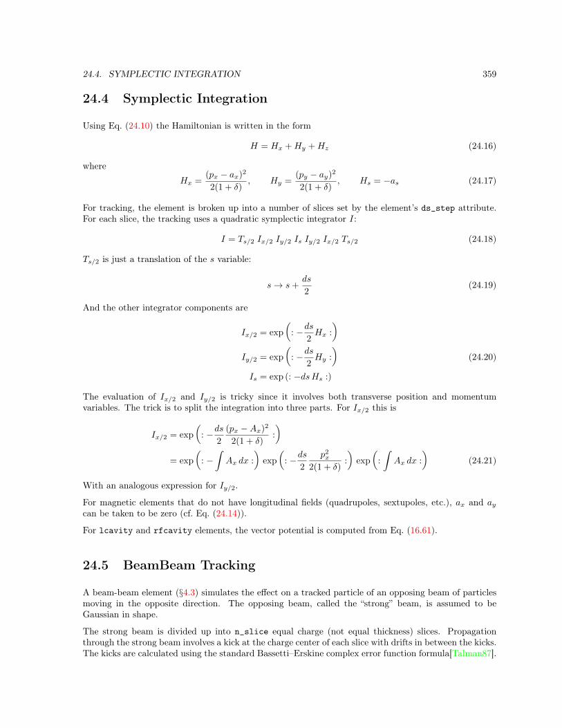
24.4. SYMPLECTIC INTEGRATION 359

24.4 Symplectic Integration

Using Eq. (24.10) the Hamiltonian is written in the form

H = Hx +Hy +Hz (24.16)

where

Hx =(px − ax)2

2(1 + δ), Hy =

(py − ay)2

2(1 + δ), Hs = −as (24.17)

For tracking, the element is broken up into a number of slices set by the element’s ds_step attribute.For each slice, the tracking uses a quadratic symplectic integrator I:

I = Ts/2 Ix/2 Iy/2 Is Iy/2 Ix/2 Ts/2 (24.18)

Ts/2 is just a translation of the s variable:

s→ s+ds

2(24.19)

And the other integrator components are

Ix/2 = exp

Å: −ds

2Hx :

ãIy/2 = exp

Å: −ds

2Hy :

ã(24.20)

Is = exp (: −dsHs :)

The evaluation of Ix/2 and Iy/2 is tricky since it involves both transverse position and momentumvariables. The trick is to split the integration into three parts. For Ix/2 this is

Ix/2 = exp

Å: −ds

2

(px −Ax)2

2(1 + δ):

ã= exp

Å: −∫Ax dx :

ãexp

Å: −ds

2

p2x

2(1 + δ):

ãexp

Å:

∫Ax dx :

ã(24.21)

With an analogous expression for Iy/2.

For magnetic elements that do not have longitudinal fields (quadrupoles, sextupoles, etc.), ax and aycan be taken to be zero (cf. Eq. (24.14)).

For lcavity and rfcavity elements, the vector potential is computed from Eq. (16.61).

24.5 BeamBeam Tracking

A beam-beam element (§4.3) simulates the effect on a tracked particle of an opposing beam of particlesmoving in the opposite direction. The opposing beam, called the “strong” beam, is assumed to beGaussian in shape.

The strong beam is divided up into n_slice equal charge (not equal thickness) slices. Propagationthrough the strong beam involves a kick at the charge center of each slice with drifts in between the kicks.The kicks are calculated using the standard Bassetti–Erskine complex error function formula[Talman87].

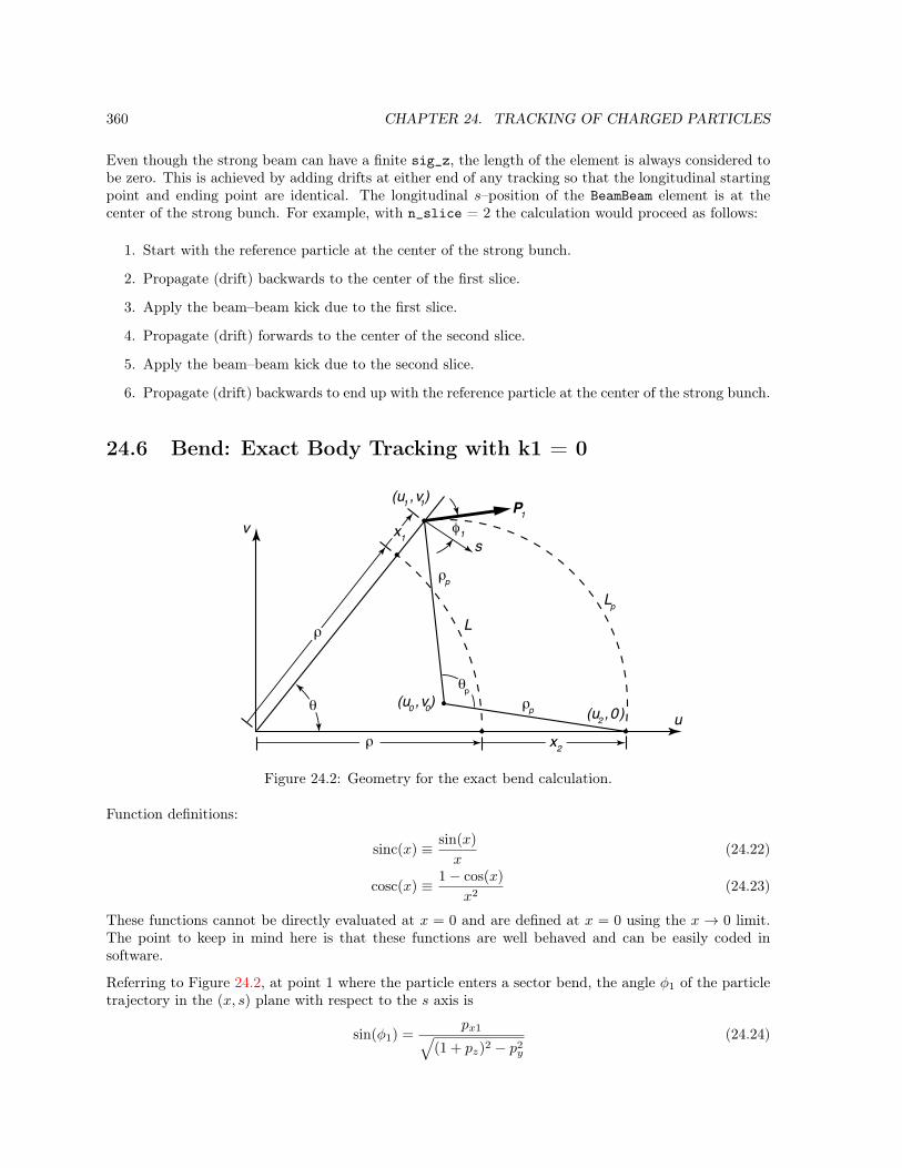
360 CHAPTER 24. TRACKING OF CHARGED PARTICLES

Even though the strong beam can have a finite sig_z, the length of the element is always considered tobe zero. This is achieved by adding drifts at either end of any tracking so that the longitudinal startingpoint and ending point are identical. The longitudinal s–position of the BeamBeam element is at thecenter of the strong bunch. For example, with n_slice = 2 the calculation would proceed as follows:

1. Start with the reference particle at the center of the strong bunch.

2. Propagate (drift) backwards to the center of the first slice.

3. Apply the beam–beam kick due to the first slice.

4. Propagate (drift) forwards to the center of the second slice.

5. Apply the beam–beam kick due to the second slice.

6. Propagate (drift) backwards to end up with the reference particle at the center of the strong bunch.

24.6 Bend: Exact Body Tracking with k1 = 0

v

u

φ1

(u1 ,v1)

(u2 ,0)(u0 ,v0)

x1

ρ

ρ x2

θ ρp

ρp

s

LLp

θp

P1

Figure 24.2: Geometry for the exact bend calculation.

Function definitions:

sinc(x) ≡ sin(x)

x(24.22)

cosc(x) ≡ 1− cos(x)

x2(24.23)

These functions cannot be directly evaluated at x = 0 and are defined at x = 0 using the x → 0 limit.The point to keep in mind here is that these functions are well behaved and can be easily coded insoftware.

Referring to Figure 24.2, at point 1 where the particle enters a sector bend, the angle φ1 of the particletrajectory in the (x, s) plane with respect to the s axis is

sin(φ1) =px1»

(1 + pz)2 − p2y

(24.24)

24.6. BEND: EXACT BODY TRACKING WITH K1 = 0 361

where the subscript “1” for pz and py is dropped since these quantities are invariant.

The (u, v) coordinate system in the plane of the bend is defined with the u-axis along the exit edge ofthe bend and the v-axis is perpendicular to the u-axis. The origin is at the design center of the bend.In this coordinate system the point (u1, v1) where the particle enters the bend is given by

u1 = (ρ+ x1) cos(θ) (24.25)v1 = (ρ+ x1) sin(θ) (24.26)

where ρ is the design radius of curvature, x1 is the offset of the particle from the design at the entrancepoint, and θ is the design bend angle

θ =L

ρ(24.27)

with L being the design arc length.

The coordinates (u0, v0) of the center of curvature of the particle trajectory is

u0 = u1 − ρp cos(θ + φ1) (24.28)v0 = v1 − ρp sin(θ + φ1) (24.29)

where ρp is the radius of curvature of the particle trajectory in the (u, v) plane (see Eq. (24.34)).

The coordinates of the particle at the exit face is (u2, 0) where

u2 = u0 +»ρ2p − v2

0 (24.30)

After some manipulation, the offset of the particle x2 from the design point at the exit face is

x2 = u2 − ρ

= x cos(θ)− L2 g cosc(θ) +α

[cos2(θ + φ1) + gp α]1/2

+ cos(θ + φ1)(24.31)

= x cos(θ)− L2 g cosc(θ) +

[cos2(θ + φ1) + gp α

]1/2 − cos(θ + φ1)

gp(24.32)

where g ≡ 1/ρ and

α = 2 (1 + g x1) sin(θ + φ1)L sinc(θ)− gp (1 + g x1)2 L2 sinc2(θ) (24.33)

gp =1

ρp=

gtot»(1 + pz)2 − p2

y

(24.34)

and gtot is the bending strength of the actual field. Both Eq. (24.31) and Eq. (24.32) are needed sinceEq. (24.31) is singular when α = 0 and θ + φ1 = π (which happens when the particle is bent by 180),and Eq. (24.32) is singular when gp is zero. A simple way to implement the calculation for x2 is to useEq. (24.31) when |θ + φ1| < π/2 and otherwise use Eq. (24.32).

Once x2 is computed, the arc length of the particle Lp is

Lp =|Lc|

sinc(θp/2)(24.35)

where Lc is the vector (chord) from point 1 and point 2

Lc = (Lcu, Lcv) =(x2 + L2 g cosc(θ)− x1 cos(θ),−L sinc(θ)− x1 sin(θ)

)(24.36)

362 CHAPTER 24. TRACKING OF CHARGED PARTICLES

and θp is the angle made by the particle trajectory which is twice the angle between the initial particletrajectory P and the vector Lc

θp = 2(θ + φ1 −

π

2− atan2 (Lcv, Lcu)

)(24.37)

where atan2(y, x) is the standard two argument arctangent function.

Once Lp is computed, px2, y2 and z2 are easily derived from

px2 =»

(1 + pz)2 − p2y sin(θ + φ1 − θp) (24.38)

y2 = y1 +py Lp»

(1 + pz)2 − p2y

(24.39)

z2 = z1 +β L

βref− (1 + pz)Lp»

(1 + pz)2 − p2y

(24.40)

where β is the normalized velocity of the particle and βref if the normalized velocity of the referenceparticle.

Using the above equation, round-off error will give a non-zero final position even if the initial position iszero. Even though the round-off error will be very small, a non-zero result can be confusing. To avoidthis, the standard linear transfer matrix for a bend is used if all the following conditions are satisfied:

|x g|, |px|, |py|, |pz| < 10−9, and, gtot = g (24.41)

The matrix is:

cos(θ) L sinc(θ) 0 0 0 g L2 cosc(θ)−g sin(θ) cos(θ) 0 0 0 g L sinc(θ)

0 0 1 L 0 00 0 0 1 0 0

−g L sinc(θ) −g L2 cosc(θ) 0 0 1 LÄ

1γ2 − g2 L2 sincc(θ)

ä0 0 0 0 0 1

(24.42)

where

sincc(θ) ≡ x− sin(x)

x3(24.43)

24.7 Bend: Body Tracking with finite k1

For a bend with a finite k1, the Hamiltonian for the body of an sbend is

H = (k0 − g)x− g x pz +1

2

((k1 + g k0)x2 − k1 y

2)

+p2x + p2

y

2(1 + pz)(24.44)

24.8. CONVERTER TRACKING 363

This is simply solved

x2 = cx (x− xc) + sxpx1

1 + pz1+ xc

px2 = τx ω2x (1 + pz1) sx (x− xc) + cx px1

y2 = cy y1 + sypy1

1 + pz1

py2 = τy ω2y (1 + pz1) sy y1 + cy py1 (24.45)

z2 = z1 +m5 +m51(x− xc) +m52px1 +m511 (x− xc)2 +

m512 (x− xc) px1 +m522 p2x1 +m533 y

2 +m534 y1 py1 +m544 p2y1

pz2 = pz1

where

kx = k1 + g k0 ωx ≡ |kx|

1 + pz1

xc =g (1 + pz1)− k0

kxωy ≡

|k1|

1 + pz1(24.46)

and

kx > 0 kx < 0 k1 > 0 k1 < 0

cx = cos(ωx L) cosh(ωx L) cy = cosh(ωy L) cos(ωy L)

sx =sin(ωx L)

ωx

sinh(ωx L)

ωxsy =

sinh(ωy L)

ωy

sin(ωy L)

ωy(24.47)

τx = −1 +1 τy = +1 −1

and

m5 = −g xc L

m51 = −g sx m52 =τx g

1 + pz1

1− cxω2x

m511 =τx ω

2x

4(L− cx sx) m533 =

τy ω2y

4(L− cy sy)

m512 =−τx ω2

x

2 (1 + pz1)s2x m534 =

−τy ω2y

2 (1 + pz1)s2y

m522 =−1

4 (1 + pz1)2(L+ cx sx) m544 =

−1

4 (1 + pz1)2(L+ cy sy)

24.8 Converter Tracking

Tracking through a converter element involves generating five random numbers 1 and then using thesenumbers with the outgoing particle distribution to generate the position and orientation of the outgoingparticle. The outgoing particle distribution is pre-computed by a program converter_element_modelingand the distribution parameters are included in the converter element description in the Bmad lattice file

1Since the outgoing particle starts at the exit surface of the converter only five numbers are needed to generate the6-dimensional particle phase space position.

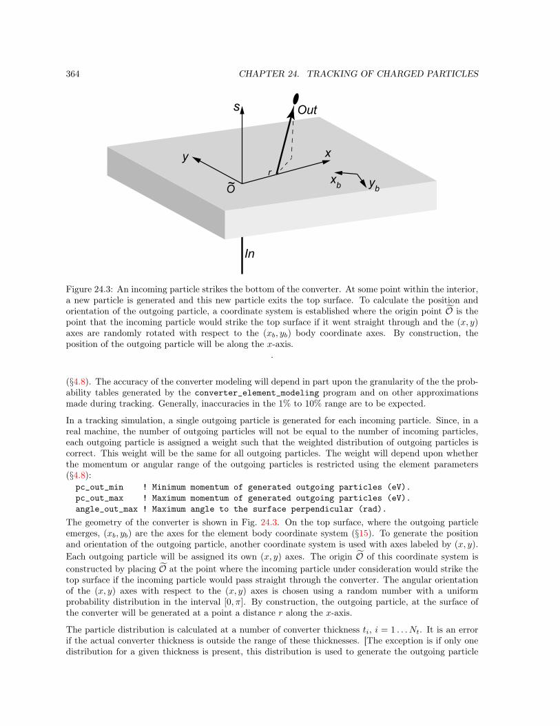
364 CHAPTER 24. TRACKING OF CHARGED PARTICLES

O

x

s

r

In

Out

y

xb yb~

Figure 24.3: An incoming particle strikes the bottom of the converter. At some point within the interior,a new particle is generated and this new particle exits the top surface. To calculate the position andorientation of the outgoing particle, a coordinate system is established where the origin point ‹O is thepoint that the incoming particle would strike the top surface if it went straight through and the (x, y)axes are randomly rotated with respect to the (xb, yb) body coordinate axes. By construction, theposition of the outgoing particle will be along the x-axis.

.

(§4.8). The accuracy of the converter modeling will depend in part upon the granularity of the the prob-ability tables generated by the converter_element_modeling program and on other approximationsmade during tracking. Generally, inaccuracies in the 1% to 10% range are to be expected.

In a tracking simulation, a single outgoing particle is generated for each incoming particle. Since, in areal machine, the number of outgoing particles will not be equal to the number of incoming particles,each outgoing particle is assigned a weight such that the weighted distribution of outgoing particles iscorrect. This weight will be the same for all outgoing particles. The weight will depend upon whetherthe momentum or angular range of the outgoing particles is restricted using the element parameters(§4.8):pc_out_min ! Minimum momentum of generated outgoing particles (eV).pc_out_max ! Maximum momentum of generated outgoing particles (eV).angle_out_max ! Maximum angle to the surface perpendicular (rad).

The geometry of the converter is shown in Fig. 24.3. On the top surface, where the outgoing particleemerges, (xb, yb) are the axes for the element body coordinate system (§15). To generate the positionand orientation of the outgoing particle, another coordinate system is used with axes labeled by (x, y).Each outgoing particle will be assigned its own (x, y) axes. The origin ‹O of this coordinate system isconstructed by placing ‹O at the point where the incoming particle under consideration would strike thetop surface if the incoming particle would pass straight through the converter. The angular orientationof the (x, y) axes with respect to the (x, y) axes is chosen using a random number with a uniformprobability distribution in the interval [0, π]. By construction, the outgoing particle, at the surface ofthe converter will be generated at a point a distance r along the x-axis.

The particle distribution is calculated at a number of converter thickness ti, i = 1 . . . Nt. It is an errorif the actual converter thickness is outside the range of these thicknesses. [The exception is if only onedistribution for a given thickness is present, this distribution is used to generate the outgoing particle

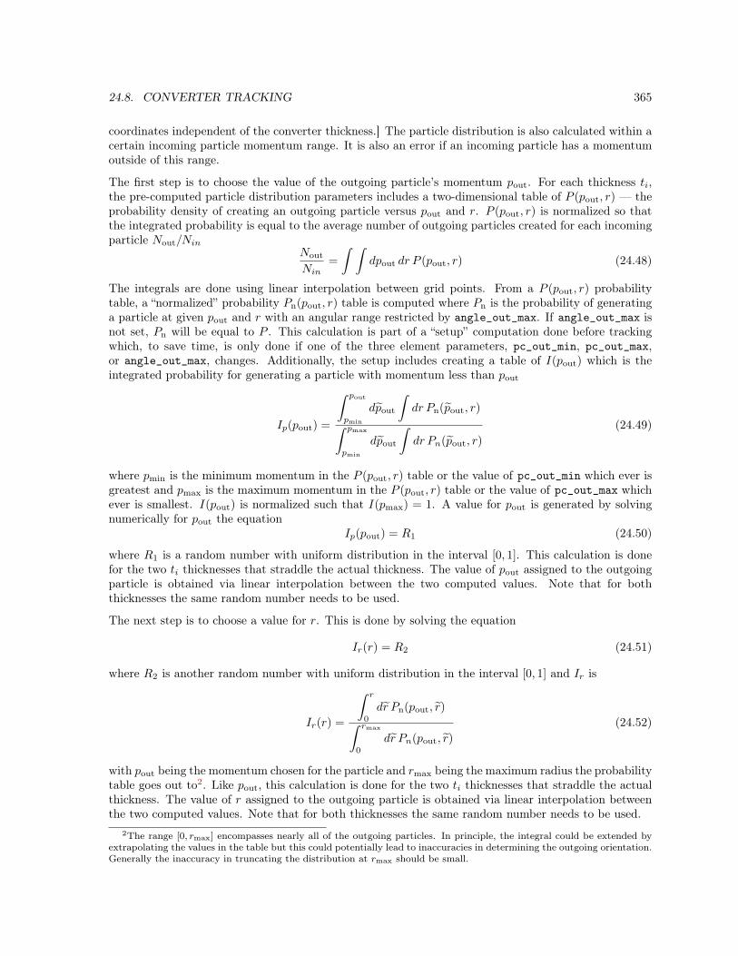
24.8. CONVERTER TRACKING 365

coordinates independent of the converter thickness.] The particle distribution is also calculated within acertain incoming particle momentum range. It is also an error if an incoming particle has a momentumoutside of this range.

The first step is to choose the value of the outgoing particle’s momentum pout. For each thickness ti,the pre-computed particle distribution parameters includes a two-dimensional table of P (pout, r) — theprobability density of creating an outgoing particle versus pout and r. P (pout, r) is normalized so thatthe integrated probability is equal to the average number of outgoing particles created for each incomingparticle Nout/Nin

Nout

Nin=

∫ ∫dpout dr P (pout, r) (24.48)

The integrals are done using linear interpolation between grid points. From a P (pout, r) probabilitytable, a “normalized” probability Pn(pout, r) table is computed where Pn is the probability of generatinga particle at given pout and r with an angular range restricted by angle_out_max. If angle_out_max isnot set, Pn will be equal to P . This calculation is part of a “setup” computation done before trackingwhich, to save time, is only done if one of the three element parameters, pc_out_min, pc_out_max,or angle_out_max, changes. Additionally, the setup includes creating a table of I(pout) which is theintegrated probability for generating a particle with momentum less than pout

Ip(pout) =

∫ pout

pmin

dpout

∫dr Pn(pout, r)∫ pmax

pmin

dpout

∫dr Pn(pout, r)

(24.49)

where pmin is the minimum momentum in the P (pout, r) table or the value of pc_out_min which ever isgreatest and pmax is the maximum momentum in the P (pout, r) table or the value of pc_out_max whichever is smallest. I(pout) is normalized such that I(pmax) = 1. A value for pout is generated by solvingnumerically for pout the equation

Ip(pout) = R1 (24.50)

where R1 is a random number with uniform distribution in the interval [0, 1]. This calculation is donefor the two ti thicknesses that straddle the actual thickness. The value of pout assigned to the outgoingparticle is obtained via linear interpolation between the two computed values. Note that for boththicknesses the same random number needs to be used.

The next step is to choose a value for r. This is done by solving the equation

Ir(r) = R2 (24.51)

where R2 is another random number with uniform distribution in the interval [0, 1] and Ir is

Ir(r) =

∫ r

0

dr Pn(pout, r)∫ rmax

0

dr Pn(pout, r)

(24.52)

with pout being the momentum chosen for the particle and rmax being the maximum radius the probabilitytable goes out to2. Like pout, this calculation is done for the two ti thicknesses that straddle the actualthickness. The value of r assigned to the outgoing particle is obtained via linear interpolation betweenthe two computed values. Note that for both thicknesses the same random number needs to be used.

2The range [0, rmax] encompasses nearly all of the outgoing particles. In principle, the integral could be extended byextrapolating the values in the table but this could potentially lead to inaccuracies in determining the outgoing orientation.Generally the inaccuracy in truncating the distribution at rmax should be small.

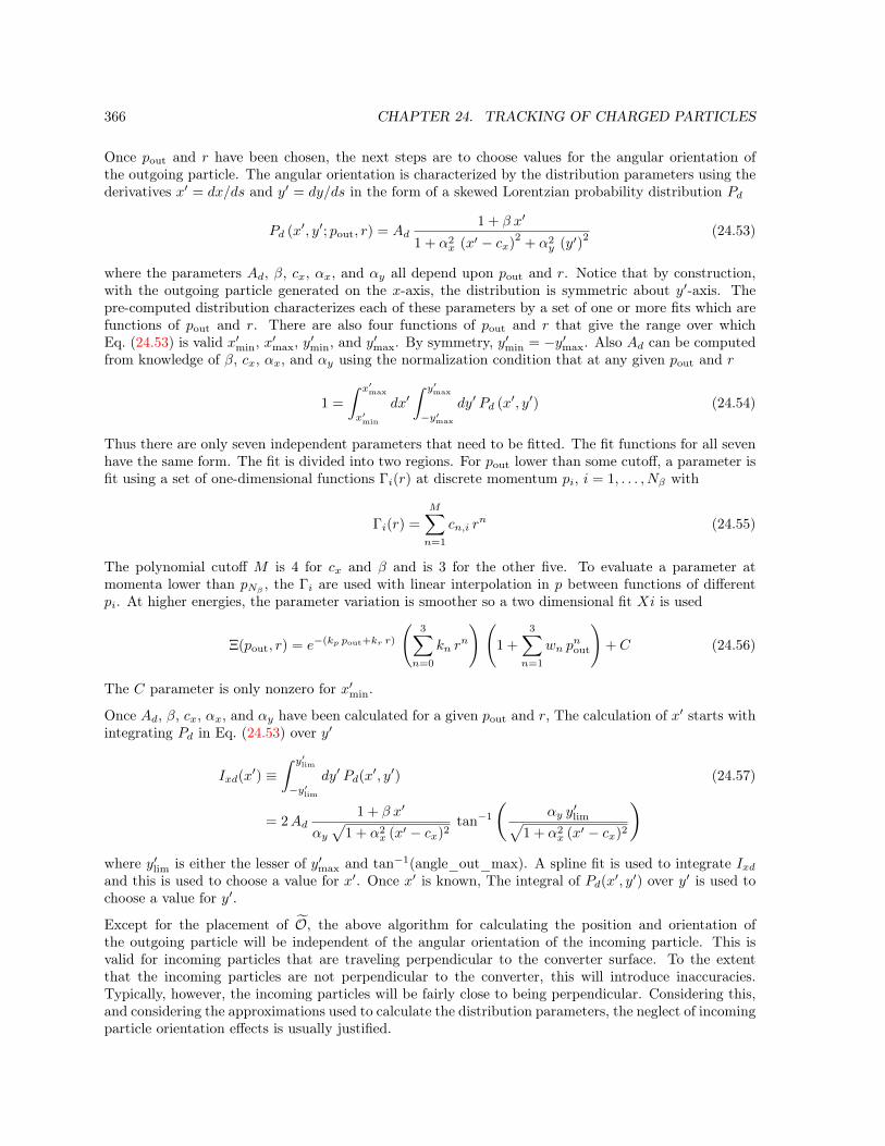
366 CHAPTER 24. TRACKING OF CHARGED PARTICLES

Once pout and r have been chosen, the next steps are to choose values for the angular orientation ofthe outgoing particle. The angular orientation is characterized by the distribution parameters using thederivatives x′ = dx/ds and y′ = dy/ds in the form of a skewed Lorentzian probability distribution Pd

Pd (x′, y′; pout, r) = Ad1 + β x′

1 + α2x (x′ − cx)

2+ α2

y (y′)2 (24.53)

where the parameters Ad, β, cx, αx, and αy all depend upon pout and r. Notice that by construction,with the outgoing particle generated on the x-axis, the distribution is symmetric about y′-axis. Thepre-computed distribution characterizes each of these parameters by a set of one or more fits which arefunctions of pout and r. There are also four functions of pout and r that give the range over whichEq. (24.53) is valid x′min, x

′max, y′min, and y

′max. By symmetry, y′min = −y′max. Also Ad can be computed

from knowledge of β, cx, αx, and αy using the normalization condition that at any given pout and r

1 =

∫ x′max

x′min

dx′∫ y′max

−y′max

dy′ Pd (x′, y′) (24.54)

Thus there are only seven independent parameters that need to be fitted. The fit functions for all sevenhave the same form. The fit is divided into two regions. For pout lower than some cutoff, a parameter isfit using a set of one-dimensional functions Γi(r) at discrete momentum pi, i = 1, . . . , Nβ with

Γi(r) =

M∑n=1

cn,i rn (24.55)

The polynomial cutoff M is 4 for cx and β and is 3 for the other five. To evaluate a parameter atmomenta lower than pNβ , the Γi are used with linear interpolation in p between functions of differentpi. At higher energies, the parameter variation is smoother so a two dimensional fit Xi is used

Ξ(pout, r) = e−(kp pout+kr r)

(3∑

n=0

kn rn

) (1 +

3∑n=1

wn pnout

)+ C (24.56)

The C parameter is only nonzero for x′min.

Once Ad, β, cx, αx, and αy have been calculated for a given pout and r, The calculation of x′ starts withintegrating Pd in Eq. (24.53) over y′

Ixd(x′) ≡

∫ y′lim

−y′limdy′ Pd(x

′, y′) (24.57)

= 2Ad1 + β x′

αy√

1 + α2x (x′ − cx)2

tan−1

Çαy y

′lim√

1 + α2x (x′ − cx)2

åwhere y′lim is either the lesser of y′max and tan−1(angle_out_max). A spline fit is used to integrate Ixdand this is used to choose a value for x′. Once x′ is known, The integral of Pd(x′, y′) over y′ is used tochoose a value for y′.

Except for the placement of ‹O, the above algorithm for calculating the position and orientation ofthe outgoing particle will be independent of the angular orientation of the incoming particle. This isvalid for incoming particles that are traveling perpendicular to the converter surface. To the extentthat the incoming particles are not perpendicular to the converter, this will introduce inaccuracies.Typically, however, the incoming particles will be fairly close to being perpendicular. Considering this,and considering the approximations used to calculate the distribution parameters, the neglect of incomingparticle orientation effects is usually justified.

24.9. DRIFT TRACKING 367

24.9 Drift Tracking

Bmad uses the exact map for a drift This gives the map

x2 = x1 +Lpx1

(1 + pz1) pl

px2 = px1

y2 = y1 +Lpy1

(1 + pz1) pl

py2 = py1 (24.58)

z2 = z1 +

Åβ

βref− 1

pl

ãL

pz2 = pz1

where β is the normalized particle velocity, βref is the reference particle’s normalized velocity, and pl isthe longitudinal momentum

pl =

1−

p2x + p2

y

(1 + pz)2(24.59)

24.10 ElSeparator Tracking

[Thanks to Étienne Forest for the derivation of the elseparator equation of motion.]

The Hamiltonian for an electric separator is

H = −ps = −®Å

1

β0+ δ + kE x

ã2

− ‹m2 − p2x − p2

y

´1/2

(24.60)

Here the canonical coordinates (−c t, δ are being used, ‹m is defined in Eq. (24.6), and ps = −H is justthe longitudinal momentum. In the above equation, kE is the normalized field

kE =q E

P0 c(24.61)

z

x

Figure 24.4: Elseparator Electric field. The fringe field lines break the translational invariance in x..

368 CHAPTER 24. TRACKING OF CHARGED PARTICLES

The field is taken to be pointing along the x-axis with positive kE accelerating a particle in the positivex direction. To solve the equations of motion, a “hard edge” model is used where kE is constant insidethe separator and the field ends abruptly at the separator edges.

Since, as shown in Fig. 24.4, the fringe fields break the translational invariance in x, it is important herethat the x = 0 plane be centered within the separator plates. With this, the canonical momentum δ justoutside the separator assumes its free space form of δ = (E −E0)/E0). This is analogous to the case ofa solenoid where, to ensure that the canonical transverse momenta assume their free space form justoutside the solenoid, the z-axis must be along the centerline of the solenoid.

The solution of the equations of motion is:

x = (x0 − xc) cosh

ÅkE L

ps

ã+px0

kEsinh

ÅkE L

ps

ã+ xc

px = kE (x0 − xc) sinh

ÅkE L

ps

ã+ px0 cosh

ÅkE L

ps

ãy = y0 + L

py0

ps(24.62)

py = py0

c δt =

∫ L

0

−∂H∂δ

= (x0 − xc) sinh

ÅkE L

ps

ã+px0

kE

ïcosh

ÅkE L

ps

ã− 1

òwhere the critical position xc is

xc = −‹EkE

(24.63)

and ‹E ≡ 1

β0+ δ =

E

P0 c(24.64)

Eqs. (24.62) predict that for x < xc and px0 = 0 a particle will, unphysically, accelerate in the negativex direction. In actuality, a particle in this instance will be reflected backwards by the longitudinalcomponent of the edge field. Specifically, the argument of the square root in Eq. (24.60) must benon-negative and a particle will only make it through the separator if

x0 >1

kE

Ä»‹m2 + p2x0 + p2

y0 − ‹Eä (24.65)

24.11 Kicker, Hkicker, and Vkicker, Tracking

The Hamiltonian for a horizontally deflecting kicker or separator is

H =p2x + p2

y

2(1 + pz)− k0 x (24.66)

This gives the map

x2 = x1 +1

1 + pz1

ÅLpx1 +

1

2k0 L

2

ã, px2 = px1 + k0 L,

y2 = y1 +Lpy1

1 + pz1, py2 = py1, (24.67)

z2 = z1 −L

2(1 + pz1)2

Åp2x1 + p2

y1 + px1 k0 L+1

3k2

0 L2

ã, pz2 = pz1

The generalization when the kick is not in the horizontal plane is easily derived.

24.12. LCAVITY TRACKING 369

24.12 LCavity Tracking

24.12.1 LCavity Bmad_Standard Tracking

For bmad_standard tracking, and with cavity_type set to standing_wave, the transverse trajectorythrough an Lcavity is modeled using equations developed by Rosenzweig and Serafini[Rosen94] (R&S)with

b0 = 1, and b−1 = 1 (24.68)and all other bn set to zero.

The transport equations in R&S were developed in the ultra-relativistic limit with β = 1. To extendthese equations, the transport through the cavity body (R&S Eq. (9)) has been modified to give thecorrect phase-space area at non ultra-relativistic energies:Å

xx′

ã2

=

(cos(α)

»8

η(∆φ)β1 γ1γ′ cos(∆φ) sin(α)

−»

η(∆φ)8

γ′

β2 γ2 cos(∆φ) sin(α) β1 γ1β2 γ2

cos(α)

) Åxx′

ã1

(24.69)

The added factors of β give the matrix the correct determinate of β1 γ1/β2 γ2. While the added factors ofβ do correct the phase space area, the above equation can only be considered as a rough approximation forsimulating particles when β is significantly different from 1. Indeed, the only accurate way to simulatesuch particles is by integrating through the actual field [Cf. Runge Kutta tracking (§6.1)].

The change in z going through a cavity is calculated by first calculating the particle transit time ∆t

c∆t =

∫ s2

s1

ds1

β(s)

=

∫ s2

s1

dsE√

E2 − (mc2)2(24.70)

=c Pz2 − c Pz1

G

where it has been assumed that the accelerating gradient G is constant through the cavity. In thisequation β = v/c, E is the energy, and Pz1 and Pz2 are the entrance and exit momenta. Using Eq. (15.28),the change in z is thus

z2 =β2

β1z1 − β2

Çc Pz2 − c Pz1

G− c P z2 − c P z1

G

å(24.71)

where P and G are the momentum and gradient of the reference particle.

Note that the above transport equations are only symplectic on-axis There are second order terms inthe transverse coordinates that are missing. To obtain a proper symplectic matrix, the symplectifyattribute of an lcavity element (§6.6) can be set to True.

24.12.2 LCavity Runge Kutta Tracking

With cavity_type set to standing_wave, and with longitudinal_mode set to 0 (the default), the fieldin a cavity, in cylindrical coordinates, is modeled by

Ez = 2G sin(k s) sin(2π (f t+ φref))

Er = −r Gk cos(k s) sin(2π (f t+ φref)) (24.72)

Bφ =r

cGk sin(k s) cos(2π (f t+ φref))

370 CHAPTER 24. TRACKING OF CHARGED PARTICLES

where G is the voltage gradient, r is the radius, f is the frequency, φref is the reference phase, and k isthe wave number

k =2π f

c(24.73)

With cavity_type set to standing_wave and with longitudinal_mode set to 1, the field is modeled as

Ez = 2G cos(k s) cos(2π (f t+ φref))

Er = r Gk sin(k s) cos(2π (f t+ φref)) (24.74)

Bφ = −rcGk cos(k s) sin(2π (f t+ φref))

With cavity_type set to traveling_wave, the setting of longitudinal_mode is ignored and the fieldis given by

Ez = G cos(θ)

Er = −r2Gk sin(θ) (24.75)

Bφ = − r

2 cGk sin(θ)

θ = 2π (f t+ φref)− k s

24.12.3 LCavity Fringe Fields

Assuming cylindrical symmetry, the radial and azimuthal fields near the axis can be related to thelongitudinal electric field via Maxwell’s equations[Hartman93]

Er = −r2

∂Ez∂z

, Bφ =r

2 c

∂Ez∂t

(24.76)

Assuming the particle velocity is c, these equations can be combined with the force equation

Fr = q (Er − cBφ) (24.77)

to give[Rosen94]

Fr = −q r2

dEzdz

(24.78)

where the total derivative is used here3. From Eq. (24.78), the fringe field kick in the horizontal plane atthe entrance end, valid for both traveling wave and standing wave cavities, is (cf. Rosenzweig[Rosen94]Eq (10))

∆px = − q “Ez2 c P0

x (24.79)

with a similar equation in the vertical. Here “Ez is the longitudinal electric field just inside the fringe,and P0 is the reference momentum. At the exit end, the kick is the negative of Eq. (24.79). This fringekick is built into xxpc.

3Hartman[Hartman93] Eq (16) is not valid for a forward propagating wave component of the field. Thus HartmanEq (17) is only valid for a backward propagating wave component. Eq. (24.78), on the other hand, is valid for all wavecomponents.

24.13. OCTUPOLE TRACKING 371

The integrated fringe fields, needed to calculate the spin precession, are at the entrance end∫Er ds = −r

4“Ez∫

Bφ ds =r

4 c“Ez (24.80)

The integrated fields at the exit end are obtained by negating the RHS of these equations.

24.13 Octupole Tracking

The Hamiltonian for an upright octupole is

H =p2x + p2

y

2(1 + pz)+k3

24(x4 − 6x2 y2 + y4) (24.81)

An octupole is modeled using a kick-drift-kick model.

24.14 Patch Tracking

The transformation of the reference coordinates through a “standard” patch (a patch where custom fieldsare not used) is given by Eqs. (15.5) and (15.6). At the entrance end of the patch, a particle’s positionand momentum in the entrance coordinate system will be

r = (x, y, 0)

P = (Px, Py, Pz) =Äpx, py,±

»(1 + pz)2 − p2

x − p2y

äP0ent (24.82)

where px, py and pz are the phase space momenta, and z, which is coordinate z and not phase space z, isalways zero by construction as shown in Fig. 24.5 [Also see Fig. 15.2 and the discussion in §15.4.2.] Thesign of the longitudinal momentum Pz is determined by whether the particle is traveling in the positives or negative s direction (which will occur when an element is flipped longitudinally).

The transformation between entrance and exit coordinate systems is given by Eqs. (15.12) and (15.13)

r→ S−1 (r− Loff)

P→ S−1 P (24.83)

z

z

Entrance Exit

Entrance

Exitz

z

L

A) B)z_off

set

Figure 24.5: Standard tracking through a patch element. A particle’s starting coordinate at the entranceend of the patch has, by construction, coordinate z = 0. The particle is drifted, as in a field free region,between the entrance z = 0 plane and the exit z = 0 plane.

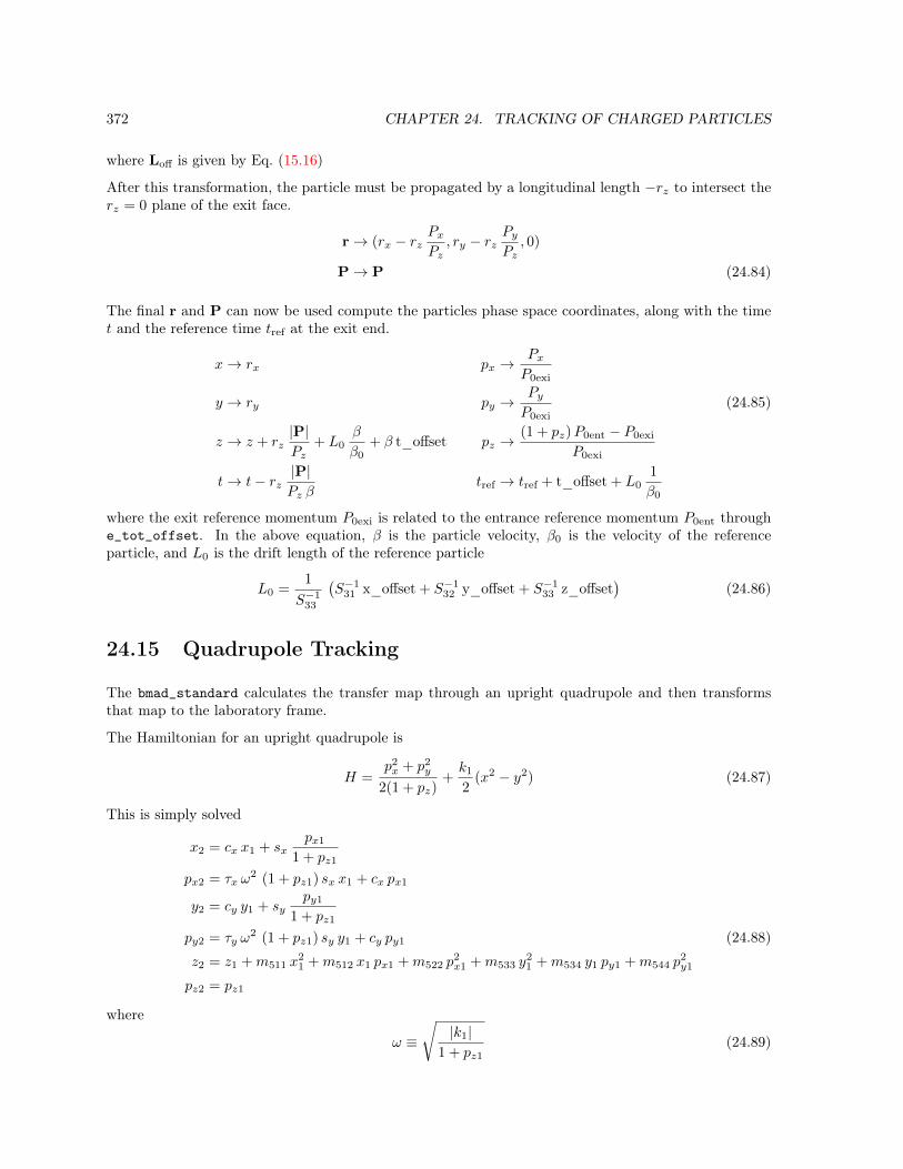
372 CHAPTER 24. TRACKING OF CHARGED PARTICLES

where Loff is given by Eq. (15.16)

After this transformation, the particle must be propagated by a longitudinal length −rz to intersect therz = 0 plane of the exit face.

r→ (rx − rzPxPz, ry − rz

PyPz, 0)

P→ P (24.84)

The final r and P can now be used compute the particles phase space coordinates, along with the timet and the reference time tref at the exit end.

x→ rx px →PxP0exi

y → ry py →PyP0exi

(24.85)

z → z + rz|P|Pz

+ L0β

β0+ β t_offset pz →

(1 + pz)P0ent − P0exi

P0exi

t→ t− rz|P|Pz β

tref → tref + t_offset + L01

β0

where the exit reference momentum P0exi is related to the entrance reference momentum P0ent throughe_tot_offset. In the above equation, β is the particle velocity, β0 is the velocity of the referenceparticle, and L0 is the drift length of the reference particle

L0 =1

S−133

(S−1

31 x_offset + S−132 y_offset + S−1

33 z_offset)

(24.86)

24.15 Quadrupole Tracking

The bmad_standard calculates the transfer map through an upright quadrupole and then transformsthat map to the laboratory frame.

The Hamiltonian for an upright quadrupole is

H =p2x + p2

y

2(1 + pz)+k1

2(x2 − y2) (24.87)

This is simply solved

x2 = cx x1 + sxpx1

1 + pz1

px2 = τx ω2 (1 + pz1) sx x1 + cx px1

y2 = cy y1 + sypy1

1 + pz1

py2 = τy ω2 (1 + pz1) sy y1 + cy py1 (24.88)

z2 = z1 +m511 x21 +m512 x1 px1 +m522 p

2x1 +m533 y

21 +m534 y1 py1 +m544 p

2y1

pz2 = pz1

where

ω ≡ |k1|

1 + pz1(24.89)

24.16. RFCAVITY TRACKING 373

and

k1 > 0 k1 < 0 k1 > 0 k1 < 0

cx = cos(ω L) cosh(ω L) cy = cosh(ω L) cos(ω L)

sx =sin(ω L)

ω

sinh(ω L)

ωsy =

sinh(ω L)

ω

sin(ω L)

ω(24.90)

τx = −1 +1 τy = +1 −1

with this

m511 =τx ω

2

4(L− cx sx) m533 =

τy ω2

4(L− cy sy)

m512 =−τx ω2

2 (1 + pz1)s2x m534 =

−τy ω2

2 (1 + pz1)s2y (24.91)

m522 =−1

4 (1 + pz1)2(L+ cx sx) m544 =

−1

4 (1 + pz1)2(L+ cy sy)

24.16 RFcavity Tracking

Tracking through an rfcavity uses a kick-drift-kick model. The kick is a pure energy kick (see equationsin §4.42) and the phase of the RF is calculated under the assumption that the waveform moves at aphase velocity equal to the velocity of the reference particle.

The transverse forces due to the RF are ignored. This is a reasonable approximation when the ac-celeration is small. Lcavity elements should be used in place of rfcavity elements when this is notso.

24.17 Sad_Mult Tracking

The “hard edge” fringe field kick is taken from Forest[Forest98] Eqs. (13.29) and onward. In the notationof Bmad, and taking into account both normal and skew terms, Eq. (13.29) is for the mþorder multipole(what Forest labels n+ 1)

f± = ∓< (bm + i am) (x+ i y)(m+1)

4 (m+ 2) (1 + pz)

ïx px + y py + i

m+ 3

m+ 1(x py − y px)

ò(24.92)

The “soft edge” dipole fringe for sad_mult elements is a generalization of the soft edge dipole fringe fora SAD bend element. For the entrance kick the equations are:

x2 = x1 +δ1

1 + δ1∆xfx, px2 = px1 +

1

1 + δ1

[∆xfy v −∆xfay v

3]

y2 = y1 −δ1

1 + δ1∆yfy, py2 = py1 +

1

1 + δ1

[∆yfx w −∆yfax w

3]

(24.93)

z2 = z1 +1

(1 + δ1)2

ï∆xfx px1 −∆yfy py1 +

1

2(∆yfx + ∆xfy)w2 − 1

4(∆yfax + ∆xfay)w4

ò

374 CHAPTER 24. TRACKING OF CHARGED PARTICLES

where

∆xfx =K0 F

2B

24L, ∆yfx =

K20 FB

6L2, ∆yfax =

2K20

3FB L2,

∆yfy =SK0 F

2B

24L, ∆xfy =

SK20 FB

6L2, ∆xfay =

2SK20

3FB L2, (24.94)

v = cos θ x1 + sin θ y1, w = − sin θ x1 + cos θ y1, tan θ =−SK0

K0

24.18 Sextupole Tracking

The Hamiltonian for an upright sextupole is

H =p2x + p2

y

2(1 + pz)+k2

6(x3 − 3x y2) (24.95)

Tracking through a sextupole uses a kick-drift-kick model.

24.19 Sol_Quad Tracking

The Hamiltonian is

H =(px + ks

2 y)2

2(1 + pz)+

(py − ks2 x)2

2(1 + pz)+k1

2(x2 − y2) (24.96)

Solving the equations of motion gives

x2 = m11 x1 +m12 px1 +m13 y1 +m14 py1

px2 = m21 x1 +m22 px1 +m23 y1 +m24 py1

y2 = m31 x1 +m32 px1 +m33 y1 +m34 py1

py2 = m41 x1 +m42 px1 +m43 y1 +m44 py1 (24.97)

z2 = z1 +

4∑j=1

4∑k=j

m5jk rj rk

pz2 = pz1

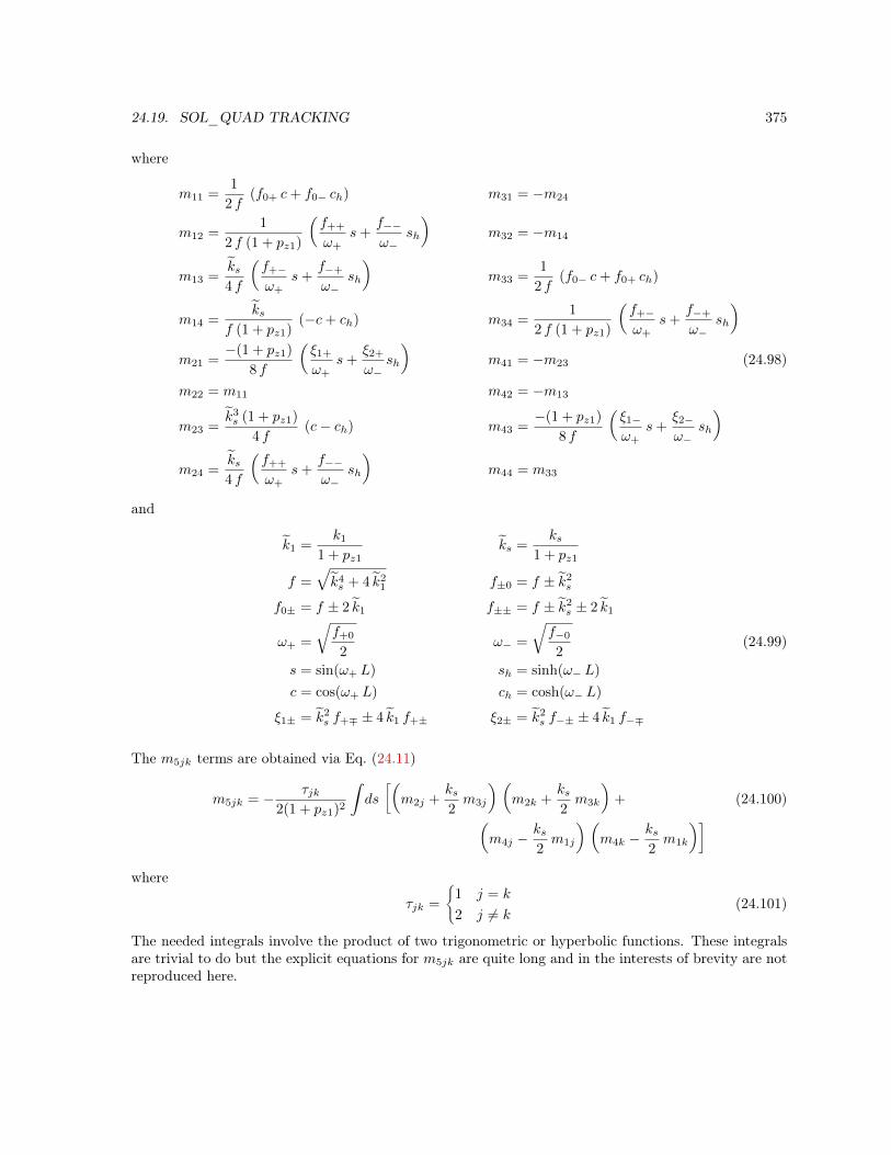
24.19. SOL_QUAD TRACKING 375

where

m11 =1

2 f(f0+ c+ f0− ch) m31 = −m24

m12 =1

2 f (1 + pz1)

Åf++

ω+s+

f−−ω−

sh

ãm32 = −m14

m13 =ks4 f

Åf+−

ω+s+

f−+

ω−sh

ãm33 =

1

2 f(f0− c+ f0+ ch)

m14 =ks

f (1 + pz1)(−c+ ch) m34 =

1

2 f (1 + pz1)

Åf+−

ω+s+

f−+

ω−sh

ãm21 =

−(1 + pz1)

8 f

Åξ1+

ω+s+

ξ2+

ω−sh

ãm41 = −m23 (24.98)

m22 = m11 m42 = −m13

m23 =k3s (1 + pz1)

4 f(c− ch) m43 =

−(1 + pz1)

8 f

Åξ1−ω+

s+ξ2−ω−

sh

ãm24 =

ks4 f

Åf++

ω+s+

f−−ω−

sh

ãm44 = m33

and

k1 =k1

1 + pz1ks =

ks1 + pz1

f =»k4s + 4 k2

1 f±0 = f ± k2s

f0± = f ± 2 k1 f±± = f ± k2s ± 2 k1

ω+ =

…f+0

2ω− =

…f−0

2(24.99)

s = sin(ω+ L) sh = sinh(ω− L)

c = cos(ω+ L) ch = cosh(ω− L)

ξ1± = k2s f+∓ ± 4 k1 f+± ξ2± = k2

s f−± ± 4 k1 f−∓

The m5jk terms are obtained via Eq. (24.11)

m5jk = − τjk2(1 + pz1)2

∫ds

ïÅm2j +

ks2m3j

ã Åm2k +

ks2m3k

ã+ (24.100)Å

m4j −ks2m1j

ã Åm4k −

ks2m1k

ãòwhere

τjk =

®1 j = k

2 j 6= k(24.101)

The needed integrals involve the product of two trigonometric or hyperbolic functions. These integralsare trivial to do but the explicit equations for m5jk are quite long and in the interests of brevity are notreproduced here.

376 CHAPTER 24. TRACKING OF CHARGED PARTICLES

z

Figure 24.6: Solenoid with a hard edge. The field is assumed to end abruptly at the edges of the solenoid.Here, for purposes of illustration, the field lines at the ends are displaced from one another.

.

24.20 Solenoid Tracking

The Hamiltonian for a solenoid is

H =

(px + ks

2 y)2

2 (1 + pz)+

(py − ks

2 x)2

2 (1 + pz)(24.102)

where the normalized field ks is

ks =B

P0(24.103)

The solution to the equations of motion for a constant ks are

x2 =1 + c

2x1 +

s

kspx1 +

s

2y1 +

1− cks

py1

px2 =−ks s

4x1 +

1 + c

2px1 −

ks (1− c)4

y1 +s

2py1

y2 =−s2x1 −

1− cks

px1 +1 + c

2y1 +

s

kspy1 (24.104)

py2 =ks (1− c)

4x1 +

−s2px1 −

ks s

4y1 +

1 + c

2py1

z2 = z1 +L

2 (1 + pz1)2

ñÅpx1 +

ks2y1

ã2

+

Åpy1 −

ks2x1

ã2ô

pz2 = pz1

where

c = cos

Åks2L

ãs = sin

Åks2L

ã(24.105)

To be useful, the canonical momenta px and py in the above equations must be connected to the canonicalmomenta used for other elements (drifts, quadrupoles, etc.) that may be placed to either side of the

24.21. SYMPLECTIC TRACKING WITH CARTESIAN MODES 377

solenoid. These side elements use zero ax and ay (cf. Eq. (24.7)). The vector potential used in thesolenoid canonical momenta may be made zero at the edges of the solenoid if the solenoid fringe fieldis assumed to end abruptly at the edges of the solenoid (as shown in Fig. 24.6), and the reference axisz-axis (at x = y = 0) is placed along the centerline of the solenoid so that there is cylindrical symmetryaround the z-axis.

24.21 Symplectic Tracking with Cartesian Modes

The method for symplectic integration for elements that define the magnetic field using a Cartesian modedecomposition (§5.15.2) is outlined in §24.4. The vector potential is constructed to avoid singularitieswhen one of the wave vectors kx, ky, or kz is zero.

For the x family the vector potential is:

Form hyper-y hyper-xy hyper-x

Ax Akzk2y

Sx Shy Sz A1

kyShx Shy Sz A

kzkx ky

Shx Sy Sz

Ay 0 0 0

Az Akxk2y

Cx Shy Cz Akxky kz

Chx Shy Cz A1

kyChx Sy Cz

For the y family the vector potential is:

Form hyper-y hyper-xy hyper-xAx 0 0 0

Ay −A kzkx ky

Sx Shy Sz −A 1

kxShx Shy Sz −A kz

k2x

Shx Sy Sz

Az −A 1

kxSx Chy Cz −A ky

kx kzShx Chy Cz −A ky

k2x

Shx Cy Cz

For the qu family the vector potential is:

Form hyper-y hyper-xy hyper-x

Ax A1

kzSx Chy Sz A

kyk2z

Shx Chy Sz Akykx kz

Shx Cy Sz

Ay −A kxky kz

Cx Shy Sz −A kxk2z

Chx Shy Sz −A 1

kzChx Sy Sz

Az 0 0 0

For the sq family the vector potential is:

Form hyper-y hyper-xy hyper-x

Ax A1

kzCx Shy Sz A

kyk2z

Chx Shy Sz Akykx kz

Chx Sy Sz

Ay Akxky kz

Sx Chy Sz −A kxk2z

Shx Chy Sz A1

kzShx Cy Sz

Az 0 0 0

378 CHAPTER 24. TRACKING OF CHARGED PARTICLES

Chapter 25

Tracking of X-Rays

Bmad can track both charged particles and X-rays. This chapter deals with X-rays. Charged particlesare handled in chapter §24.

25.1 Coherent and Incoherent Photon Simulations

Bmad can track photons either coherently or incoherently. In both cases, the photon has a transverseelectric field

(Ex, Ey) (25.1)

Ex and Ey are complex and therefore have both amplitude and phase information. When photons aretracked incoherently, the phase information is not used for calculating X-ray intensities.

In addition to coherent and incoherent tracking, partially coherent simulations can be done by usingsets of photons with the photons in any one set treated as coherent and the photons between sets beingtreated as incoherent.

25.1.1 Incoherent Photon Tracking

In a simulation with incoherent photons, some number of photons, N0, will be generated and the ithphoton (i = 1, . . . , N0) will have a initial “electric field” components Ex0(i), Ey0(i) assigned to it. Thefield amplitude E0 will be

»E2x0 + E2

y0.

At some an observation point, the power S per unit area falling on some small area dA due to either xor y component of the electric field is

Sx,y =αp

N0 dA

∑j∈hits

E2x,y(j) (25.2)

where αp is a constant that can be chosen to fit the simulation against experimental results, and the sumis over photons who intersect the area. The factors of N0 and dA in the above equation make, withinstatistical fluctuations, S independent of N0 and, for dA small enough, S will be independent of dA asit should be. The total power is just Sx + Sy.

When traveling through vacuum, the electric field of a photon is a constant. As an example, consider apoint source radiating uniformly in 4π solid angle with each photon having the same initial field E0. An

379

380 CHAPTER 25. TRACKING OF X-RAYS

observation area dA situated a distance R from the source will intercept N0 dA/4π R2 photons which

gives a power of

Sw =αpE

20

4π R2(25.3)

which falls off as 1/R2 as expected.

At some places the light may be split into various “channels”. An example is Laue diffraction whereX-rays can excite the α and β branches of the dispersion surface. Or a partially silvered mirror wheresome of the light is reflected and some is transmitted. In such a case, the probability Pi of a photontraveling down the ith channel is

Pi “E2i =

SiS0

(25.4)

where Si is the power flowing into channel i, S0 is the power flowing into the junction, and “Ei = Ei/E0

is the ratio of the electric field amplitudes of any photon just before and just after being shunted intothe ith channel. The probabilities must be properly normalized∑

Pi = 1 (25.5)

If the ratio of the electric field of any photon just before and just after being shunted into the ith channelis not a constant, than “Ei must be adjusted so that “E2

i is equal to the average of “E2i (j) for all photons

j channeled into channel i.

As long as Eqs. (25.4) and (25.5) are satisfied, the choice of the Pi, and “Ei are arbitrary. This freedomallows simulation to be optimized for efficiency. For example, In an actual experiment much of thelight can be lost never to reach a detector and be counted. To decrease the simulation time, simulatedphotons may be limited to be generated with a direction to be within some solid angle Ω1 if photonswith a direction outside this solid angle will not contribute to the simulation results. In this case, thereare two channels. Channel 1 consists of all photons whose direction is within Ω1 and channel 2 is allthe other photons. To limit the photons to channel 1, P1 is taken to be 1 and P2 is taken to be 0.Additionally, if the light, say, is being generated isotropically from a surface into a Ω0 = 2π solid anglethen “E1 =

Ω1

Ω0(25.6)“E2 is infinite here but since no photons are generated in channel 2 this is not a problem.

25.1.2 Coherent Photon Tracking

In a simulation with coherent photons, some number of photons, N0, will be generated and the ith photon(i = 1, . . . , N0) will have an initial electric field Ex0(i), Ey0(i) assigned to it. These quantities will becomplex.

At some an observation point, the field E at some small area dA due to either x or y component of theelectric field is

E =αp

N0 dA

∑j∈hits

E(j) (25.7)

where αp is a constant that can be chosen to fit the simulation against experimental results, and thesum is over photons who intersect the area. In the above equation E(j) is either the x or y componentof the electric field as is appropriate. The factors of N0 and dA in the above equation make, withinstatistical fluctuations, E independent of N0 and, for dA small enough, E will be independent of dA asit should be.

25.1. COHERENT AND INCOHERENT PHOTON SIMULATIONS 381

When traveling through a a vacuum, the photons travel ballistically in straight lines. This is justified byusing the stationary phase approximation with Kirchhoff’s integral. the electric field of a photon varieswith the propagation length. There is nothing physical in this and is just a way to make the bookkeepingcome out correctly. As an example, consider a point source radiating uniformly in 4π solid angle witheach photon having the same initial field component (either x or y) E1. An observation area dA situateda distance R from the source will intercept N0 dA/4π R

2 photons and each photon will have a field ofE1R exp(i k R) where k is the photon wave number (all photons must have the same k to be coherent).This gives an electric field at the observation point of

E =αpE1 exp(i k R)

4π R(25.8)

which falls off as 1/R as expected.

At a diffraction_plate element where diffraction effects are to be simulated, the following procedureis used:

1. The electric field components are multiplied by the propagation length L:

E → E L (25.9)

The propagation length is reset to zero so that the at the next point where the propagation lengthis factored into the electric field the propagation length will be the length starting at the aperture.

2. Depending upon the program, the photon is is either given a random direction over 2π solidangle or the photon’s direction is restricted to be within some solid angle chosen to increase theprobability that the photon will make it through some downstream aperture.

If the photon is restricted to some aperture dependent solid angle of area Ω, the photon’s electricfield is scaled by

E → EΩ

4π(25.10)

3. The electric field components are scaled by

E → Ek

4π i(cos θ1 + cos θ2) (25.11)

where θ1 and θ2 are the direction cosines of the incoming and outgoing directions of the photonwith respect to the longitudinal reference axis.

This algorithm is designed so that the resulting fields at points downstream from the aperture as com-puted from a simulation will, to within statistical errors, be the same as one would get using Kirchoff’sintegral. That is, the simulation is constructed to be a Monte Carlo integration of Kirchhoff’s integral.

What is, and what is not considered a place where there are diffraction effects is dependent upon theproblem. For example, there are diffraction effects associated with light reflecting from a mirror (or anyother object) of finite size. If these effects are important to the experiment, then a procedure similar tothe one above must be followed.

At places where there are no diffraction effects a simulation can treat the photons ballistically or can usethe aperture procedure outlined above. While in theory it is possible to choose what to do, in practicethe aperture procedure increases the number of photons that must be tracked for a given resolution.Thus, from a practical standpoint the ballistic alternative should always be used.

382 CHAPTER 25. TRACKING OF X-RAYS

As explained in §25.1.1, at some places the light may be split into various “channels”. With coherentphotons, the analog to Eq. (25.4) is

Pi “Ei =EiE0

(25.12)

where here “Ei can be complex to take into account phase shifts. The same considerations about choosingthe Pi and “Ei apply to coherent photons as incoherent photons. In particular, “E1 for the case of isotropicemission from a surface as in the example in §25.1.1 (cf. Eq. (25.6)) is“E1 =

Ω1

Ω0(25.13)

25.1.3 Partially Coherent Photon Simulations

When there is partial coherence the photons must be divided into sets. All of the photons of a given setare considered coherent while the photons of different sets are treated incoherently.

The procedure is to track all the photons of one set coherently and calculate the field using equationEq. (25.7). The fields of different sets are then combined to calculate a power using Eq. (25.2).

25.2 Element Coordinate System

The general procedure for tracking through an element makes use of element reference coordinates(also called just element coordinates). Without any offsets, pitches or tilt (§5.6), henceforth called“misalignments”, the element coordinates are the same as the laboratory reference coordinates (orsimply laboratory coordinates) (§15.1.1). The element coordinates stay fixed relative to the element.Therefore, if the element is misaligned, the element coordinates will follow as the element shifts inthe laboratory frame as shown in Fig. 24.1.

For crystal (§4.10), mirror (§4.32), and multilayer_mirror (§4.34) elements, the “kinked” referencetrajectory through the element complicates the calculation. For these elements, there are three coordinatesystems attached to the element as shown in Fig. 25.1. Besides the element entrance and elementexit coordinates, there are element surface coordinates with z perpendicular to the surface pointinginward.

Tracking a particle through an element is therefore a three step transformation:

1. At the entrance end of the element, transform from the laboratory reference coordinates to theelement’s entrance or surface coordinates.

2. Track through the element ignoring any misalignments.

3. At the exit end of the element, transform from the element coordinates to the laboratory exitcoordinates.

25.2.1 Transform from Laboratory Entrance to Element Coordinates

For elements that have a reference orbit kink (§25.2), the element coordinates here are the surfacecoordinates. Otherwise the element coordinates are the entrance coordinates.

1. Apply offsets, pitches and tilt using the formulas in §15.2.2 along with Eqs. (15.6), and (15.16).

25.3. MIRROR AND CRYSTAL ELEMENT TRANSFORMATION 383

x

z

ElementSurface Coordinates

xz

ElementExit Coordinates

x

zElementEntrance Coordinates

n

O OO

Figure 25.1: The three element coordinate systems for crystal (Bragg configuration), mirror, andmultilayer_mirror elements. The origin O of all three are the same but are shown spread out forclarity. n is the normal to the element surface.

.

2. Apply the tilt to the electric field (Eq. (15.40)).

3. For crystal, mirror, and multilayer_mirror elements rotate to element surface coordinates.

4. Transform the photon’s position as if in a drift by a distance −z where z is the photon’s longitudinalcoordinate. That is, z will be zero at the end of the transform to element coordinates (rememberthat z is the distance from the start of the element (§15.4.4)).

25.2.2 Transform from Element Exit to Laboratory Coordinate

The back transformation from element to laboratory coordinates is accomplished by the transformation

1. For crystal, mirror, and multilayer_mirror elements rotate to element from element surfacecoordinates to element exit coordinates

2. Apply the reverse tilt to the electric field (Eq. (15.40)).

3. Apply reverse offsets, pitches and tilt using the formulas in §15.2.2 along with Eqs. (15.6), and(15.16).

25.3 Transformation for Mirror and Crystal Elements BetweenLaboratory and Element Coordinates

25.3.1 Transformation from Laboratory to Element Coordinates

With photons, the intensities must also be transformed. The transformation from the entrance laboratorycoordinates to the entrance element coordinates is:

1. Track as in a drift a distance z_offset_tot.

2. Apply offsets and pitches: The effective “length” of the element is zero (§15.2.3) so the origin of

384 CHAPTER 25. TRACKING OF X-RAYS

the element coordinates is the same point around which the element is pitched so

x1 = x0 − xoffpx1 = px0 − (1 + pz0)x′pitch

y1 = y0 − yoff (25.14)py1 = px0 − (1 + pz0) y′pitch

z1 = z0 + x′pitch x1 + y′pitch y1

where xoff ≡ x_offset, x′pitch ≡ x_pitch, etc.

3. Apply ref_tilt and tilt: Åx2

y2

ã= R(θtot)

Åx1

y1

ãÅpx2

py2

ã= R(θtot)

Åpx1

py1

ã(25.15)Å

Ex2

Ey2

ã= R(θtot)

ÅEx1

Ey1

ãwhere E is shorthand notation for

E ≡ E ei φ (25.16)

with E being the field intensity and φ being the field phase angle. In the above equations R is therotation matrix

R(θ) =

Åcos θ sin θ− sin θ cos θ

ã(25.17)

with θtot being

θtot =

®ref_tilt + tilt + tilt_corr for crystal elementsref_tilt + tilt for mirror elements

(25.18)

The tilt_corr correction is explained in §25.4.2.

25.3.2 Transformation from Element to Laboratory Coordinates

The back transformation from exit element coordinates to exit laboratory coordinates is accomplishedby the transformation

1. Apply ref_tilt and tilt: ref_tilt rotates the exit laboratory coordinates with respect to theexit element coordinates in the same way ref_tilt rotates the entrance laboratory coordinateswith respect to the entrance element coordinates. The forward and back transformations arethus just inverses of each other. With tilt, this is not true. tilt, unlike ref_tilt, does notrotate the output laboratory coordinates. There is the further complication in that tilt is arotation about the entrance laboratory coordinates. The first step is to express tilt with respectto the exit coordinates. This is done with the help of the S matrix of Eq. (15.8) with αt givenby Eq. (15.15). The effect of the tilt can be modeled as a rotation vector ein in the entrancelaboratory coordinates pointing along the z-axis

ein = (0, 0, tilt) (25.19)

25.3. MIRROR AND CRYSTAL ELEMENT TRANSFORMATION 385

In the exit laboratory coordinates, the vector eout is

eout = S ein (25.20)

The z component of eout combines with ref_tilt to give the transformationÅx2

y2

ã= R(−θt)

Åx1

y1

ãÅpx2

py2

ã= R(−θt)

Åpx1

py1

ã(25.21)Å

Ex2

Ey2

ã= R(−θt)

ÅEx1

Ey1

ãwhere θt is ref_tilt + eout,z. The x and y components of eout give rotations around the x and yaxes

px3 = px2 − eout,y

py3 = py2 + eout,x (25.22)z3 = z2 + x2 eout,y − y2 eout,x (25.23)

2. Apply pitches: Since pitches are defined with respect to the entrance laboratory coordinates, theyhave to be translated to the exit laboratory coordinates

Pout = S Pin (25.24)

where Pin = (x′pitch, y′pitch, 0) is the pitch vector in the entrance laboratory frame and Pout is the

vector in the exit laboratory frame. The transformation is then

px4 = px3 −Pout,y

py4 = py3 + Pout,x (25.25)z4 = z3 + x3 Pout,y − y3 Pout,x (25.26)

3. Apply offsets: Again, offsets are defined with respect to the entrance laboratory coordinates. Likepitches, the translation is

Oout = S Oin (25.27)

where Oin = (xoff, yoff, soff) is the offset in the entrance laboratory frame. The transformation is

x5 = x4 + Oout,x − px4 Oout,z

y5 = y4 + Oout,y − py4 Oout,z (25.28)z5 = z4 + Oout,z (25.29)

386 CHAPTER 25. TRACKING OF X-RAYS

Hn

x

z

αHψΗ

K0

k0

KH

kHθB,in

Q

θ0

H

nx

z

αH

ψΗ

A) B)

K0

k0

KH kH

θB,in

Q

θ0

-x^--

-

--

---

Figure 25.2: Reference trajectory reciprocal space diagram for for A) Bragg diffraction and B) Lauediffraction. The bar over the vectors indicates that they refer to the reference trajectory. The x-zcoordinates shown are the element surface coordinates. All points in the diagram are in the plane of thepaper except for the tip of H. K0, and KH are the wave vectors inside the crystal and k0 and kH arethe wave vectors outside the crystal. The reference photon traveling along the reference trajectory hasK0 and KH originating at the Q point. For Laue diffraction, the crystal faces are assumed parallel. ForBragg diffraction the crystal normal is in the −x direction while for Laue diffraction the crystal normalis in the −z direction

25.4 Crystal Element Tracking

[Crystal tracking developed by Jing Yee Chee, Ken Finkelstein, and David Sagan]Crystal diffraction is modeled using dynamical diffraction theory. The notation here follows Battermanand Cole[Bater64]. The problem can be divided up into two parts. First the reference trajectory must becalculated. This means calculating the incoming grazing angle θB,in and outgoing grazing angle θB,out aswell as calculating the transformations between the various coordinate systems. This is done in §25.4.1,§25.4.2, and §25.4.3. The second part is the actual tracking of the photon and this is covered in §25.4.5§25.4.6 and §??.

25.4.1 Calculation of Entrance and Exit Bragg Angles

Fig. 25.2 shows the geometry of the problem. The bar over the vectors indicates that they refer to thereference trajectory. The reference trajectory is calculated such that the reference photon will be in thecenter of the Darwin curve. That is, the internal wave vectors K0 and KH originate from the Q point(See [Bater64] Figs. 8 and 29).

The external wave vectors k0, and kH and the internal wave vectors have magnitude

|k0| = |kH| =1

λ(25.30)

|K0| = |KH | =1− δλ

(25.31)

where λ is the wavelength, and δ is

δ =λ2re2π V

F ′0 =Γ

2F ′0 =

1

2ΓF ′0 (25.32)

25.4. CRYSTAL ELEMENT TRACKING 387

with re being the classical electron radius, V the unit cell volume, and F ′0 is the real part of the F0

structure factor.

In element surface coordinates (which will be the coordinate system used henceforth), k0 lies in the x-zplane. K0 is related to k0 via Batterman Eq. (25)

K0 = k0 + q0 n (25.33)

where the value of q0 is to be determined. Here, and in equations below, if the equation is true in general,and not just for the reference trajectory, the bar superscript is dropped.

Since n is in the −x direction, K0 is also in the x-z plane. Thus k0 and K0 can be written in the form

k0 =1

λ

Ñ− cos θB,in

0sin θB,in

é, K0 =

1− δλ

Ñ− cos θ0

0sin θ0

é[Bragg]

k0 =1

λ

Ñsin θB,in

0cos θB,in

é, K0 =

1− δλ

Ñsin θ0

0cos θ0

é[Laue] (25.34)

Where, as shown in Fig. 25.2, θB,in, and θ0 are the angles of k0 and K0 with respect to the x-axis forBragg reflections and with respect to the z-axis for Laue reflection.

αH (alpha_angle) is the angle that H makes with respect to the −z axis and ψH (psi_angle) is therotation of H around the −z axis such that for ψH = 0, H is in the x-z plane and oriented as shown inFig. 25.2. Thus

H ≡ 1

d“H =

1

d

Ñ− sinαH cosψHsinαH sinψH− cosαH

é(25.35)

where “H is H normalized to 1. αH is determined via the setting of b_param and via Eq. (4.17).

The vectors K0 and H must add up to the reciprocal lattice vector KH

KH = K0 + H (25.36)

Taking the length of both sides of this equation and using Eqs. (25.31), (25.34), and (25.35) gives for θ0

sin θ0 =

−β “Hz − “Hx

»“H2x + “H2

z − β2“H2x + “H2

z

Bragg

−β “Hx + “Hz

»“H2x + “H2

z − β2“H2x + “H2

z

Laue

(25.37)

whereβ ≡ λ

2 d (1− δ)(25.38)

Once θ0 has been calculated, θB,in can be calculated from Eq. (25.33)

cos θB,in = (1− δ) cos θ0 [Bragg] (25.39)sin θB,in = (1− δ) sin θ0 [Laue] (25.40)

The outgoing reference wave vector kH is computed using the equation

KH = kH + qH n (25.41)

388 CHAPTER 25. TRACKING OF X-RAYS

Using this with Eqs. (25.35) and (25.36) gives

kH,x = KH,z =1

d“Hx + k0,x

kH,y = KH,y =1

d“Hy (25.42)

kH,z =

…1

λ2− k2

H,x − k2

H,y

The total bending angle of the reference trajectory is then

θbend = tan−1

Ç|k0 × kH |k0 · kH

å(25.43)

The outgoing Bragg angle θB,out is then defined to be the difference between the total bend angle andthe entrance Bragg angle.

θB,out ≡ θbend − θB,in (25.44)

25.4.2 Crystal Coordinate Transformations

There are four transformations needed between coordinates denoted by Σ1, Σ2, Σ3, and Σ4

Σ1 Transform from laboratory entrance to element entrance coordinates.Σ2 Transform from element entrance to surface coordinates.Σ3 Transform from surface to element exit coordinates.Σ4 Transform from element exit to laboratory exit coordinates.

The total transformation is just the map represented by S and V of Eqs. (15.5) and (15.6)

[S,V] = Σ4 Σ3 Σ2 Σ1 (25.45)

The transformation Σ1 is given in §25.3.1 and the transformation Σ4 is given in §25.3.2. In general, thetransformation Σ1 needs a “tilt correction” (Eq. (25.18)), as explained below, when ψH is nonzero. [Theexception is when the undiffracted or forward_diffracted beam is tracked with Laue geometry. Inthese cases, no tilt correction is needed.] Since this tilt correction is independent of any misalignments,the tilt correction calculation proceeds assuming here that there are no misalignments. The finite V dueto the finite crystal thickness in Laue diffraction will also be ignored for the moment.

Without misalignments, and with ψH zero, the transformation Σ1 is, as it is for every other type ofelement, just the unit matrix.

Σ1 = I (25.46)

That is, the two coordinate systems are identical. Furthermore, the transformation Σ2 from elemententrance coordinates to surface coordinates is a rotation around the y axis

Σ2 = Ry(θB,in) ≡

Ñcos θB,in 0 sin θB,in

0 1 0− sin θB,in 0 cos θB,in

é[Laue] (25.47)

= Ry(θB,in −π

2) [Bragg]

The transformation from element surface coordinates to element exit coordinates, Σ3, is another rotationaround the y axis

Σ3 = Ry(θB,out) [Laue] (25.48)

= Ry(θB,out +π

2) [Bragg]

25.4. CRYSTAL ELEMENT TRACKING 389

and the transformation from element exit coordinates to laboratory exit coordinates, Σout is the unitymatrix

Σ4 = I (25.49)

Thus, the combined transformation S from laboratory entrance to laboratory exit coordinates is arotation around the y axis of θB,in + θB,out as explained in section §15.2

S = Σ4 Σ3 Σ2 Σ1 = Ry(θB,in + θB,out) (25.50)

When ψH is non-zero, the situation is complicated since, if S as calculated above is used, the vectorkH would be bent out of the x-z plane even though it has been assumed that the ref_tilt θt is zero.But kH points in the same direction as the z axis of the outgoing reference trajectory. Furthermore, bydefinition, the reference trajectory has the form given by Eq. (15.8) with the Rz(θt) matrix dependingonly upon the ref_tilt parameter (which is here taken to be zero). To satisfy Eq. (15.8), the crystalmust be reoriented to keep the kH vector in the x-z plane of the laboratory entrance coordinates. Thereorientation is done by rotating the crystal about the laboratory entrance z axis by an amount θcorr(tilt_corr).

With this tilt correction the transformation Σ1 is a rotation about the z axis

Σ1 =

Ñcos θcorr − sin θcorr 0sin θcorr cos θcorr 0

0 0 1

é(25.51)

To calculate a value for θcorr, note that the transformation Σ2 from element entrance coordinates toelement surface coordinates is not affected by a finite ψH and so Eq. (25.47) is unmodified. The kHvector, expressed in laboratory entrance coordinates, is Σ−1

1 Σ−12 kH where the components of kH are

given by Eq. (25.42). To satisfy Eq. (15.8), this vector must have zero y component

(Σ−1

1 Σ−12 kH

)·

Ñ010

é= 0 (25.52)

Solving gives

θcorr = tan−1 kH,ykH,z sin θB,in − kH,x cos θB,in

(25.53)

The transformation Σ3 from element surface coordinates to element exit coordinates is now obtained byrequiring that the total transformation from laboratory entrance to laboratory exit coordinates be theRy(−αb) matrix given in Eq. (15.8)

Σ3 Σ2 Σ1 =

Ñcos θbend 0 − sin θbend

0 1 0sin θbend 0 cos θbend

é(25.54)

In the above equation, the transformation Σ4 has been dropped since it is the unit matrix independentof ψH .

For Laue diffraction when the non-diffracted beam is tracked, the exit coordinate system corresponds tothe entrance coordinate system. That is, V is the unit matrix. In this case, there is no tilt correctionand Σ3 = Ry(−θB,in) is just the inverse of Σ2.

390 CHAPTER 25. TRACKING OF X-RAYS

Q

H

α β

BA

KH_

K0_

x

z

nT

_k0

Figure 25.3: Energy flow used to determine the reference orbit for Laue diffraction.

25.4.3 Laue Reference Orbit

For Laue diffraction, with the reference orbit following the undiffracted beam, the reference orbit atthe exit surface is just the extension of the reference orbit at the entrance surface. Since the referenceorbit’s direction is k0. the reference orbit displacement vector L (cf. Eq. (15.5)) is given by

L =t2

dk0 · tdk0 [undiffracted] (25.55)

where

t =

Ñ00t

é(25.56)

with t being the crystal thickness and the z-axis pointing into the crystal as illustrated in Fig. 25.3. TheS rotation matrix (Eq. (15.6)) for the undiffracted beam will be the unit matrix.

With the reference orbit following the forward_diffracted or Bragg_diffracted beam, the displace-ment vector L follows the energy flow associated with the tie points labeled A or B in Fig. 25.3. Thesetie points are defined by the intersection of the dispersion surfaces and the vector n originating from thepoint T as shown in the figure. The energy flow is perpendicular to the dispersion surface and it canbe shown that since, by construction, n goes through the Q point, and since the dispersion surfaces arehyperboles, the energy flows from A and B tie points are colinear. The direction of the energy flow isgiven by:

Kf = ξH KH + ξ0 K0 (25.57)

where ξH and ξ0 are given by [Bater64] Eq. (18) (See section §25.4.5 below). L is thus

L =t2

Kf · tKf (25.58)

At the exit surface, if the reference orbit is following the forward_diffracted beam, the orientation ofthe element exit coordinates will be the same as the orientation of the element entrance coordinates.That is, S (Eq. (15.6)) is the unit matrix. If the reference orbit is following the Bragg diffracted beam,S is the same as for Bragg diffraction

S =

Ñcos θbend 0 − sin θbend

0 1 0sin θbend 0 cos θbend

é(25.59)

25.4. CRYSTAL ELEMENT TRACKING 391

25.4.4 Crystal Surface Reflection and Refraction

There are corrections to the field amplitude and phase when a photon reflects or refracts from the surfaceof a crystal. A plane wave is incident on a crystal surface with

E = “E0 exp(ik0 r) (25.60)

An outgoing plane wave has a fieldE = “E1 exp(ik1 r) (25.61)

A simulation of this condition will start with a number of photons with wave vector k0 and electricfield E0. After reflecting from the surface, the photons will have wave vector k1. Now imagine a setof N photons that flow through an planar area dA0, perpendicular to the incoming beam, before beingreflected from the surface.

Since the electric field is “E0, when tracking incoherent photons“E20 =

αpE20 N

dA0(25.62)

where αp is the simulation constant (cf. Eq. (25.2). After the photons are reflected they will have somefield E1 and thus “E2

1 =αpE

21 N

dA1(25.63)

Where dA1 is the area that the photons flow through which is related to dA0 via

dA1

dA0=

k1 · zk0 · z

≡ |b| (25.64)

Combining the above three equations, the change in field for a photon as it reflects from the surface is

E1

E0=“E1“E0

»|b| Incoherent (25.65)

For coherent photon tracking the electric field at dA0 is“E0 =αpE0N

dA0(25.66)

After the photons are reflected they will have some field E1 and thus“E1 =αpE1N

dA1(25.67)

Combining these equations the change in field for a photon as it reflects from the surface is

E1

E0=“E1“E0

|b| Coherent (25.68)

Additionally, for coherent tracking, all photons in a plane wave must have the same phase when passingthrough an area transverse to the wave. Thus the two photons labeled a and b in Fig. ?? must have thesame phase advance in going from dA0 to dA1. The difference in the phase advance for photon b relativeto a from dA0 to the surface is k0 · r where r is the vector between where photon b hits the surfacerelative to photon a. Similarly, the difference in the phase advance for photon b relative to a from the

392 CHAPTER 25. TRACKING OF X-RAYS

surface to dA0 is −k1 · r. Since the total phase advance for both photons is the same from dA0 to dA1

the phase shift dφb of photon b as it is reflected from the surface relative to the phase shift dφa is

dφb = dφa − (k1 − k0) · r (25.69)

This shift in the reflection phase can be related to the lattice diffraction planes. The wave vectordifference can be written

k1 − k0 = H + q n (25.70)

where n is perpendicular to the surface. Combining Eqs. (25.69) and (25.70) and since r is in the planeof the surface

dφb = dφa −H · r (25.71)

This shows that the reflection shift has the same periodicity as the pattern of the lattice planes at thesurface of the crystal. Notice that for a mirror, where one point on the surface is the same as any other,dφb must be equal to dφa. Using this in Eq. (25.69) gives

k1 · r = k0 · r (25.72)

and since |k1| = |k0| this proves that the angle of incidence is equal to the angle of reflection for a mirror.

In practice, the registration of the surface planes with respect to the surface is not specified in a simu-lation. Thus the reflection phase shift can only be calculated up to a constant offset.

25.4.5 Bragg Crystal Tracking

The starting photon coordinates are specified in the laboratory entrance coordinates. The transforma-tion from laboratory entrance coordinates to element entrance coordinates k0 is given in §25.3. Thetransformation to element surface coordinates k0 is

k0 = Σ2 k0 (25.73)

with Σ2 given by Eq. (25.47). The outgoing wave vector kH is related to k0 via

kH = k0 + H + qt n (25.74)

where qt is determined by using Eqs. (25.34) and (25.35) in Eq. (25.30)

kH,x = k0,x +Hx

kH,y = k0,y +Hy (25.75)

kH,z =»λ2 − k2

H,x − k2H,y

To compute the field amplitude of the outgoing photon, the equation to be solved is ([Bater64] Eq. (21))

ξ0 ξH =1

4k2 P 2 Γ2 FH FH (25.76)

where ξ0 and ξH are given by [Bater64] Eq. (18) and P is the polarization factor

P =

®1 σ polarization statecos 2θg π polarization state

(25.77)

2θg is the angle between K0 and KH which is well approximated by θB,in + θB,out.

25.4. CRYSTAL ELEMENT TRACKING 393

The solution to Eq. (25.76) is ([Bater64] Eq. (31))

ξ0 =1

2k |P |Γ [FH FH ]1/2 |b|1/2 [η ± (η2 + sgn(b))1/2]

ξH =1

2k |P |Γ [FH FH ]1/2

1

|b|1/2 [η ± (η2 + sgn(b))1/2](25.78)

where the + part of ± is for the α branch and the − part of ± is for the β branch and sgn is the signfunction

sgn(b) ≡®

1 b > 0

−1 b < 0(25.79)

and η is given by [Blas94] Eq. (5)

η =−b a+ ΓF0 (1− b)2 Γ |P |

√|b|FH FH

(25.80)

with the asymmetry factor b for the photon being tracked being given by [Blas94] Eq. (3)

b ≡ n · k0

n · (◊k0 + H)(25.81)

and the angular deviation variable a is given by [Blas94] Eq. (4)

a ≡ H2 + 2 k0 ·Hk2

0

= −2 ∆θ sin(2θB) (25.82)

Once ξ0 and ξH are determined, the ratio of the incoming and outgoing fields for the α or β branchescan be computed via ([Bater64] Eq. (24))

rE ≡EH

E0=− 2 ξ0

k P ΓFH=− k P ΓFH

2 ξH(25.83)

where the α or β subscript has been suppressed. The total field which is the sum of the fields on thebranches is computed using the boundary conditions

E0 = E0α + E0β , 0 = EHα + EHβ (25.84)

Using the above two equations gives

E0α = E0rEβ

rEβ − rEαEHα = E0

rEα rEβrEβ − rEα

E0β = −E0rEα

rEβ − rEαEHβ = −E0

rEα rEβrEβ − rEα

(25.85)

As can be seen from Battermann and Cole Figs. (8) and (29), the α tie point is excited and the β tiepoint is not if ξ0α < ξ0β and vice versa. Since only one tie point is excited, The external field ratio isequal to the internal field ratio

EeHEi0

=EHjE0j

(25.86)

where j is α or β as appropriate.

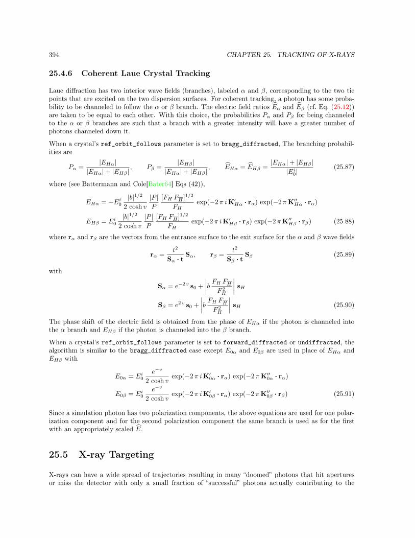
394 CHAPTER 25. TRACKING OF X-RAYS

25.4.6 Coherent Laue Crystal Tracking

Laue diffraction has two interior wave fields (branches), labeled α and β, corresponding to the two tiepoints that are excited on the two dispersion surfaces. For coherent tracking, a photon has some proba-bility to be channeled to follow the α or β branch. The electric field ratios “Eα and “Eβ (cf. Eq. (25.12))are taken to be equal to each other. With this choice, the probabilities Pα and Pβ for being channeledto the α or β branches are such that a branch with a greater intensity will have a greater number ofphotons channeled down it.

When a crystal’s ref_orbit_follows parameter is set to bragg_diffracted, The branching probabil-ities are

Pα =|EHα|

|EHα|+ |EHβ |, Pβ =

|EHβ ||EHα|+ |EHβ |

, “EHα = “EHβ =|EHα|+ |EHβ |

|Ei0|(25.87)

where (see Battermann and Cole[Bater64] Eqs (42)),

EHα = −Ei0|b|1/2

2 cosh v

|P |P

[FH FH ]1/2

FHexp(−2π iK′Hα · rα) exp(−2πK′′Hα · rα)

EHβ = Ei0|b|1/2

2 cosh v

|P |P

[FH FH ]1/2

FHexp(−2π iK′Hβ · rβ) exp(−2πK′′Hβ · rβ) (25.88)

where rα and rβ are the vectors from the entrance surface to the exit surface for the α and β wave fields

rα =t2

Sα · tSα, rβ =

t2

Sβ · tSβ (25.89)

with

Sα = e−2 v s0 +

∣∣∣∣b FH FHF 2H

∣∣∣∣ sH

Sβ = e2 v s0 +

∣∣∣∣b FH FHF 2H

∣∣∣∣ sH (25.90)

The phase shift of the electric field is obtained from the phase of EHα if the photon is channeled intothe α branch and EHβ if the photon is channeled into the β branch.

When a crystal’s ref_orbit_follows parameter is set to forward_diffracted or undiffracted, thealgorithm is similar to the bragg_diffracted case except E0α and E0β are used in place of EHα andEHβ with

E0α = Ei0e−v

2 cosh vexp(−2π iK′0α · rα) exp(−2πK′′0α · rα)

E0β = Ei0e−v

2 cosh vexp(−2π iK′0β · rα) exp(−2πK′′0β · rβ) (25.91)

Since a simulation photon has two polarization components, the above equations are used for one polar-ization component and for the second polarization component the same branch is used as for the firstwith an appropriately scaled “E.

25.5 X-ray Targeting

X-rays can have a wide spread of trajectories resulting in many “doomed” photons that hit aperturesor miss the detector with only a small fraction of “successful” photons actually contributing to the

25.5. X-RAY TARGETING 395

simulation results. The tracking of doomed photons can therefore result in an appreciable lengthening ofthe simulation time. To get around this, Bmad can be setup to use what is called “targeting” to greatlyreduce the number of doomed photons generated.

Photons can be generated either at a source like a wiggler element or at a place where diffraction issimulated like at a diffraction_plate element. To be able to do targeting, an element with aperturesdefined must be present downstream from the generating element. The idea is to only generate photonsthat are going in the general direction of the “target” which is the space within the aperture.

A necessary restriction for targeting to work is that the photon must travel in a straight line throughall elements between the generating element and the element with the apertures. So, for example, acrystal element would not be allowed between the two two elements. A crystal element could bethe aperture element as long as the aperture was defined before photons were diffracted. That is, if theaperture was at the upstream end of the crystal or was defined with respect to the crystal surface.

The target is defined by the four corners of the aperture. In element coordinates, the (x, y, z) values ofthe corners are:(-x1_limit, -y1_limit, z_lim)(-x1_limit, y2_limit, z_lim)( x2_limit, -y1_limit, z_lim)( x2_limit, y2_limit, z_lim)

where x1_limit, etc. are the aperture limits (§5.8) and z_lim will be zero except if the element’saperture_at parameter is set to entrance_end in which case z_lim will be set to -L where L is thelength of the element.

If the aperture is associated with a curved surface (for example with a crystal element), four extracorner points are also used to take into account that the aperture is not planar. These extra points have(x, y, z) values in element coordinates of(-x1_limit, -y1_limit, z_surface(-x1_limit, -y1_limit))(-x1_limit, y2_limit, z_surface(-x1_limit, y2_limit))( x2_limit, -y1_limit, z_surface( x2_limit, -y1_limit))( x2_limit, y2_limit, z_surface( x2_limit, y2_limit))

where z_surface(x,y) is the z value of the surface at the particular (x, y) point being used. Noticethat in this case z_lim is zero.

The coordinates of the four or eight corner points are converted from element coordinates of the apertureelement to element coordinates of the photon generating element. Additionally, the approximate centerof the aperture, which in element coordinates of the aperture element is (0, 0, zlim), is converted toelement coordinates of the photon generating element.

The above calculation only has to be done once at the beginning of a simulation.

When a photon is to be emitted from a given point (xemit, yemit, zemit), the problem is how to restrictthe velocity vector (βx, βy, βz) (which is normalized to 1) to minimize the number of doomed photonsgenerated. The problem is solved by constructing a vector r for each corner point:

r = (xlim, ylim, zlim)− (xemit, yemit, zemit) (25.92)

The direction of each r is characterized in polar coordinates (φ, y) defined by

y =ry|r|

tanφ =rxrz

(25.93)

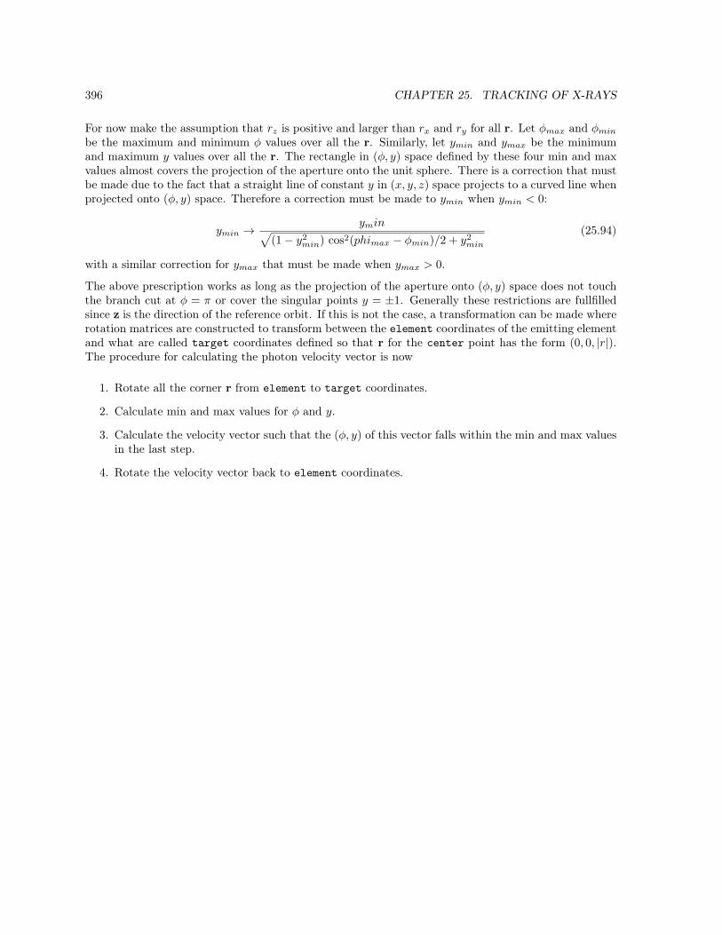
396 CHAPTER 25. TRACKING OF X-RAYS

For now make the assumption that rz is positive and larger than rx and ry for all r. Let φmax and φminbe the maximum and minimum φ values over all the r. Similarly, let ymin and ymax be the minimumand maximum y values over all the r. The rectangle in (φ, y) space defined by these four min and maxvalues almost covers the projection of the aperture onto the unit sphere. There is a correction that mustbe made due to the fact that a straight line of constant y in (x, y, z) space projects to a curved line whenprojected onto (φ, y) space. Therefore a correction must be made to ymin when ymin < 0:

ymin →ymin√

(1− y2min) cos2(phimax − φmin)/2 + y2

min

(25.94)

with a similar correction for ymax that must be made when ymax > 0.

The above prescription works as long as the projection of the aperture onto (φ, y) space does not touchthe branch cut at φ = π or cover the singular points y = ±1. Generally these restrictions are fullfilledsince z is the direction of the reference orbit. If this is not the case, a transformation can be made whererotation matrices are constructed to transform between the element coordinates of the emitting elementand what are called target coordinates defined so that r for the center point has the form (0, 0, |r|).The procedure for calculating the photon velocity vector is now

1. Rotate all the corner r from element to target coordinates.

2. Calculate min and max values for φ and y.

3. Calculate the velocity vector such that the (φ, y) of this vector falls within the min and max valuesin the last step.

4. Rotate the velocity vector back to element coordinates.

Chapter 26

Simulation Modules

In the Bmad “ecosystem”, various modules have been developed to simulate machine hardware. Thischapter provides documentation.

26.1 Tune Tracker Simulator

[Tune tracker simulation developed by Michael Ehrlichman]The digital tune tracker (dTT) is device for determining the fractional tune of a storage ring and excitingresonant beam oscillations. In short, the dTT starts with a beam position monitor (BPM) to detectthe beam oscillations. The signal from the BPM is feed into a phase-locked loop (PLL) circuit whichoscillates at the oscillation frequency the beam. A signal from the PLL is used to modulate a kicker tokeep the beam oscillating at the beam’s oscillation frequency. The tune tracker is capable of excitingboth betatron and synchrotron oscillations.

In general, a PLL is a control system for matching the frequency of a VCO to some incoming periodicreference signal. It does this by adjusting the frequency of the VCO according to the phase differencebetween the VCO output and the reference signal. A general diagram of a PLL is shown in Fig. 26.1.

In Fig. 26.1, the phase detector compares the two incoming signals, and outputs a signal that is propor-tional to the difference in phase. There are various ways to implement a phase detector. The tune trackerphase detector is a mixer followed by low-pass filter, which will be discussed in more detail below. Theloop controller, also known as a loop filter, is usually some combination of (P)roportional, (I)ntegration,and (D)ifferentiation paths. The loop controller sums these paths, and the resulting signal is sent to the

Figure 26.1: General diagram of a phase lock loop. The loop adjusts the speed of a VCO according tothe phase difference between the VCO and an incoming signal.

397

398 CHAPTER 26. SIMULATION MODULES

VCO. The output of the loop controller rises when the VCO is slower than the reference, and drops whenthe VCO is faster. The gains of the three PID paths are adjusted to produce a control loop that is stableand can efficiently lock onto the reference signal from some incorrect initial frequency. A real-world PLLalso needs to track perturbations to the reference frequency.

A diagram of the digital tune tracker is shown in Fig. 26.2. This function takes in one new BPMmeasurement per call, and returns a sinusoidal signal that has the same frequency as the BPM signal.The phase of the returned signal differs from the phase of the BPM signal by φ0, the phase advancefrom position at the BPM to position at the kicker on the next turn.

Comparing this diagram to the PLL in Fig. 26.1, the boxes from Subtract closed orbit offset to the endof the Low Pass Filter comprise the phase detector. After the Low Pass Filter to just before the GainKvco box comprises the loop controller. The Gain Kvco box comprises the VCO. The feedback loopconsists of the update to ω that follows Gain Kvco.

26.1. TUNE TRACKER SIMULATOR 399

Figure26.2:Flow

chartof

tune

trackermod

ulefunction

s.

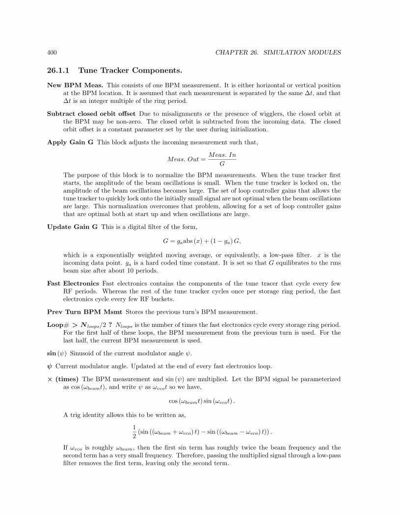
400 CHAPTER 26. SIMULATION MODULES

26.1.1 Tune Tracker Components.

New BPM Meas. This consists of one BPM measurement. It is either horizontal or vertical positionat the BPM location. It is assumed that each measurement is separated by the same ∆t, and that∆t is an integer multiple of the ring period.

Subtract closed orbit offset Due to misalignments or the presence of wigglers, the closed orbit atthe BPM may be non-zero. The closed orbit is subtracted from the incoming data. The closedorbit offset is a constant parameter set by the user during initialization.

Apply Gain G This block adjusts the incoming measurement such that,

Meas. Out =Meas. In

G

The purpose of this block is to normalize the BPM measurements. When the tune tracker firststarts, the amplitude of the beam oscillations is small. When the tune tracker is locked on, theamplitude of the beam oscillations becomes large. The set of loop controller gains that allows thetune tracker to quickly lock onto the initially small signal are not optimal when the beam oscillationsare large. This normalization overcomes that problem, allowing for a set of loop controller gainsthat are optimal both at start up and when oscillations are large.

Update Gain G This is a digital filter of the form,

G = gaabs (x) + (1− ga)G,

which is a exponentially weighted moving average, or equivalently, a low-pass filter. x is theincoming data point. ga is a hard coded time constant. It is set so that G equilibrates to the rmsbeam size after about 10 periods.

Fast Electronics Fast electronics contains the components of the tune tracer that cycle every fewRF periods. Whereas the rest of the tune tracker cycles once per storage ring period, the fastelectronics cycle every few RF buckets.

Prev Turn BPM Msmt Stores the previous turn’s BPM measurement.

Loop# > N loops/2 ? Nloops is the number of times the fast electronics cycle every storage ring period.For the first half of these loops, the BPM measurement from the previous turn is used. For thelast half, the current BPM measurement is used.

sin (ψ) Sinusoid of the current modulator angle ψ.

ψ Current modulator angle. Updated at the end of every fast electronics loop.

× (times) The BPM measurement and sin (ψ) are multiplied. Let the BPM signal be parameterizedas cos (ωbeamt), and write ψ as ωvcot so we have,

cos (ωbeamt) sin (ωvcot) .

A trig identity allows this to be written as,

1

2(sin ((ωbeam + ωvco) t)− sin ((ωbeam − ωvco) t)) .

If ωvco is roughly ωbeam, then the first sin term has roughly twice the beam frequency and thesecond term has a very small frequency. Therefore, passing the multiplied signal through a low-passfilter removes the first term, leaving only the second term.

26.1. TUNE TRACKER SIMULATOR 401

In stable operation, ωvco makes small amplitude oscillations about ωbeam. In this case, the timeintegral of (ωbeam − ωvco) t is small for all t, and a small angle approximation for sine can beapplied, and the output of the low pass filter can be written as,

(ωbeam − ωvco) t, (26.1)

which is proportional to the phase difference between the beam and the VCO. Thus completes thephase detector.

KI

Nloops

∫·dt This is the (I)ntegrated channel of the PID controller. It integrates the output of the

phase detector, providing negative feedback. If the integrated phase is positive, the I channel slowsthe VCO down. If negative, it speeds the VCO up. This channel is expected to equilibrate tosome non-zero value proportional to the difference between the beam frequency and the VCO basefrequency.

Update ψ This increments the modulator phase according to,

ψn+1 = ψn +TringNloops

ωvco. (26.2)

In order to more accurately model things, ωvco is not updated within the fast electronics loop.

Increment Loop# by 1 Loop# counts the number of times the fast electronics has been loopedthrough.

If Loop# > Nloops, exit, else, loop Nloops is the number of times the fast electronics cycle per ringperiod.

Gain KP This is the (P)roportional channel of the PID controller. Is provides negative feedbackproportional to the output of the phase detector. This channel responds faster than the integratedchannel and so helps the tune tracker track sudden changes in the frequency of the beam. Inpractice, it also damps tune tracker oscillations. If KP is too small, the VCO may oscillateindefinitely around the fractional tune of the beam. See section §26.1.2 below for more details.

Gain KD × filtered derivative This is the (D)ifferential channel of the PID controller. Provides afiltered first derivative of the output of the phase detector. The derivative is obtained a polynomialfitted to a history of the phase detector output. This channel can be used to smooth out the VCOresponse and reduce overshoot. See section §26.1.2 below for more details.

+ (sum) This block sums the three output of the PID controller.

Gain Kvco This block represents the response of a voltage controlled oscillator. The frequency of theoutput of a VCO is proportional to the voltage of its input. This block simply multiplies theoutput of the PID controller by a constant. This block updates the VCO frequency.

sin (ψ + ψ0) Calculates kicker amplitude to be returned to the calling program. This is the kickamplitude that should be used during the next turn. ψ0 is the phase advance from position at theBPM to position at next turn’s kicker.

26.1.2 Tuning

Tuning the tune tracker consists of adjusting the four gain parameters KP , KI , KD, and Kvco. The goalis to set the parameters such that the tune tracker quickly locks onto the fractional tune of the beam,and settles quickly. If multiple tunes are being explored, then the size of the convergence region is also

402 CHAPTER 26. SIMULATION MODULES

Parameter Rise Time Overshoot Settling Rate Precision Stability Region

KP slight decrease decrease faster degrade shrinkKI decrease increase slower no change shrinkKD

see note slight increase slight decrease slightly faster degrade grow

Table 26.1: Effect on VCO response of increasing KP , KI , or KD. Note: The effects of the derivativechannel are theoritical and have not been verified extensively.

important. i.e. The set of parameters should work for a wide range of fractional tunes. If jitter is beingexplored, then the ability of the tune tracker to track a varying fractional tune is also important.

A plot of the VCO speed during typical tune tracker operation is shown in Fig. 26.3. A tune tracker witha base period of 0.571 oscillations per ring period tracks a beam with a fractional tune of 0.5691. Markedon this plot are 4 important features. They are the rise time, overshoot, settling rate, and precision. Therise time is how long it takes the tune tracker to approach the fractional tune of the beam. This is thelocation of the first peak after operation begins. The overshoot is the difference between the amplitudeof the first peak and the fractional tune. The settling rate measures the decay rate of the oscillations ofthe VCO about the fractional tune. The precision is the noise in the VCO frequency. The discrete natureof the BPM measurements introduces noise at the phase detector stage. The proportional channel addsthis noise to the VCO frequency Shown in Tab. [26.1] is the effect increasing the PID controller gains.

Stability region refers to the range of fractional tunes that the tune tracker will converge to when startingfrom an initial tune in that range. In practice, if KP and KI are increased to optimize response to aparticular fractional tune, the stability region will shrink. e.g. A large KP and KI could be found thatvery quickly lock on to a fractional tune of 0.569, but are unstable for 0.622. But note that a smallerKP and KI can be found that give acceptible performance at 0.569, and also acceptible performance at0.622 (and even 0.074).

26.1.3 Programmer Instructions

This seciton contains instructions on how to implement the tune tracker module and how to use thetune tracker driver program. The tune tracker is written as an object or class, and so supports multipleinstances.

After setting up the tune tracker in a program, it is best to first verify that the tune tracker is efficientlylocking onto the beam and that the beam oscillations are indeed growing with time. The tune trackershould lock on after about 10,000 turns, and the beam oscillations should reach equilibrium amplitudeafter about 10 damping periods.

See the tune tracker section in the Physics chapter of this manual for an example of how the VCOfrequency should respond with time in a successful implementation. Guidelines for setting the gainparameters are also located in the Physics chapter.

26.1.4 Tune Tracker Module

The tune tracker module has four public functions. They are,

Function id = init_dTT(tt_param_struct) !Constructor, creates new tune tracker!instance, handles initialization.

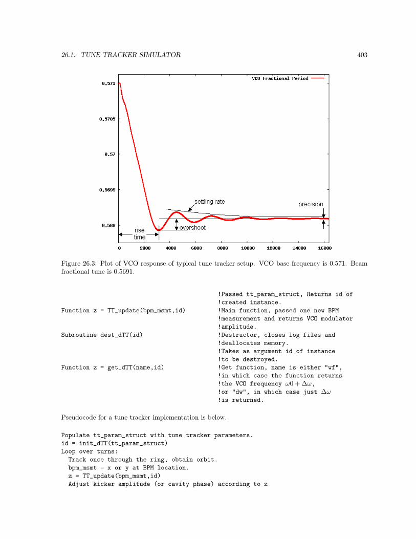
26.1. TUNE TRACKER SIMULATOR 403

Figure 26.3: Plot of VCO response of typical tune tracker setup. VCO base frequency is 0.571. Beamfractional tune is 0.5691.

!Passed tt_param_struct, Returns id of!created instance.

Function z = TT_update(bpm_msmt,id) !Main function, passed one new BPM!measurement and returns VCO modulator!amplitude.

Subroutine dest_dTT(id) !Destructor, closes log files and!deallocates memory.!Takes as argument id of instance!to be destroyed.

Function z = get_dTT(name,id) !Get function, name is either "wf",!in which case the function returns!the VCO frequency ω0 + ∆ω,!or "dw", in which case just ∆ω!is returned.

Pseudocode for a tune tracker implementation is below.

Populate tt_param_struct with tune tracker parameters.id = init_dTT(tt_param_struct)Loop over turns:Track once through the ring, obtain orbit.bpm_msmt = x or y at BPM location.z = TT_update(bpm_msmt,id)Adjust kicker amplitude (or cavity phase) according to z

404 CHAPTER 26. SIMULATION MODULES

dest_dTT(id)

See tune_tracker.f90 for the contents of tt_param_struct.

If a horizontal or vertical tune tracker is to be implemented, the BPM measrements should be the x or ycoordinate at the BPM location, and the kicks should be changes in x′ or y′ at the kicker location. If alongitudinal tune tracker is to be implemented the BPM measurements should be the x coordinate in adispersive region, and the kicks should be changes in phase at an RF cavity. Similarly, if a longitudinaltune tracker is being used in conjunction with a horizontal tune tracker, the BPM of the horizontal tunetracker should be placed in a region of low dispersion. This will prevent the horizontal tune tracker frominadvertantly locking onto the synchrotron tune.

26.1.5 Tune Tracker Example Program

An example program is located in src/examples/tune_tracker. This program contains code for im-plementing simultaneous horizontal, vertical, and longitudinal tune trackers.

For most implementations of the tune tracker module, a good approach would be to either use a modifiedversion of the tune tracker example program, or copy and paste code from the example program. Keepin mind that the example program implements multiple simultaneous tune trackers. An implementationof just one tune tracker would be much simpler.

The example program performs the following steps.

1. Read in file which contains tune tracker parameters such as gains.

2. Parse lattice with twiss3 subroutines. The twiss3 subroutines are needed to obtain the longitu-dinal phase advance when implementing longitudinal tune trackers.

3. Check that the kick attribute of the kicker element is actually free.

4. Calculate phase advance from position at BPM to position at kicker. Note that this is the phaseof the kicker on the next turn.

5. Creates log files which record position at BPM and kicker, the VCO frequency, and slope at thekicker.

6. Loops over turns, passing BPM measurements to TT_update and adjusting kicker amplitudesbased on the returned value. Note that it will take the beam oscillations several damping times toequilibriate. This often means tracking for several 10,000 turns. Use of the save state parametermay shorten simulation times in certain applications.

7. Calculates and FFT of the BPM data and records in log file.

Also located in src/examples/tune_tracker is an example .in file that implements horizontal, vertical,and longitudinal tune trackers. The gains used in the .in file were selected for their large convergenceregion. More agressive tuning may lead to faster lock on. See the Physics section for details.

26.1.6 Save States

If tt_param_struct%useSaveState is set to true, then the destructor dest_dTT will save the tunetracker state variables to a file called tt_state.#. Similarly, the constructor init_dTT will set the state

26.2. INSTRUMENTAL MEASUREMENTS 405

variables according to the save state file. The constructor will also return the beam coordinates to beused at element zero of the ring.

Save states allow you to pick up where you left off, and not have to wait for the beam oscillations toequilibriate. For example, you could have one program that tracks for 100,000 turns, allowing the tunetracker to lock on and the beam excitation to equilibriate with radiation damping. The simulation writesa save state file which can be used as a starting point for other simulations that perform studies on theexcited beam.

26.2 Instrumental Measurements

Bmad has the ability to simulate instrumental measurement errors for orbit, dispersion, betatron phase,and coupling measurements. The appropriate attributes are listed in §5.21 and the conversion formulasare outlined below.

26.2.1 Orbit Measurement

For orbits, the relationship between measured position (x, y)meas and true position (x, y)true isÅxy

ãmeas

= nf

År1

r2

ã+ Mm

ïÅxy

ãtrue

−Åxy

ã0

ò(26.3)

where the Gaussian random numbers r1 and r2 are centered at zero and have unit width and thefactor nf represents the inherent noise in the measurement. In the above equation, (x, y)0 represents ameasurement offset and Mg is a “gain” matrix writen in the form

Mm =

Å(1 + dgx) cos(θ + ψ) (1 + dgx) sin(θ + ψ)−(1 + dgy) sin(θ − ψ) (1 + dgy) cos(θ − ψ)

ã(26.4)

Here dgx and dgy represent gain errors and the angles θ and ψ are tilt and “crunch” errors.

In the above equations, various quantities are writen as a difference between an “error” quantity and a“calibration” quantity:

x0 = xoff − xcaliby0 = yoff − ycalibψ = ψerr − ψcalibθ = θerr − θcalib (26.5)

dgx = dgx,err − dgx,calibdgy = dgy,err − dgy,calib

See §5.21 for the element attribute names that correspond to these quantities.

The calibration component is useful in a simulation where initally the error quantities are set to representthe errors in the monitors. After this, analysis of orbit data with the machine in various states can beused to calculate a best guess as to what the errors are. The calculated error values can then be put inthe calibration quantities. This represents a correction in software of the errors in the monitors. Furthersimulations of orbit measurements will show how well the actual orbit can be deduced from the measuredorbit.

406 CHAPTER 26. SIMULATION MODULES

26.2.2 Dispersion Measurement

A dispersion measurement is considered to be the result of measuring the orbit at two different energies.The measured values are thenÅ

ηxηy

ãmeas

=

√2nf

dE/E

År1

r2

ã+ Mm

ïÅηxηy

ãtrue

−ÅÅ

ηxηy

ãerr

−Åηxηy

ãcalib

ãò(26.6)

The factor of√

2 comes from the fact that there are two measurements. Mm is given in Eq. (26.4).

26.2.3 Coupling Measurement

The coupling measurement is considered to be the result of measuring the beam at a detector over Nsturns while the beam oscillates at a normal mode frequency with some amplitude Aosc. The measuredcoupling is computed as follows. First, consider excitation of the a-mode which can be written in theform: Å

xiyi

ãtrue

= Aosc

Åcosφi

K22a cosφi +K12a sinφi

ãtrue

(26.7)

i is the turn number and φi is the oscillation phase on the ith turn. The coefficients K22a and K12a arerelated to the coupling C via David and Rubin[Sagan99] Eq. 54:

K22a =−√βb

γ√βa

C22

K12a =−√βb

γ√βa

C12 (26.8)

To apply the measurement errors, consider the general case where the beam’s oscillations are split intotwo components: One component being in-phase with some reference oscillator (which is oscillating withthe same frequency as the beam) and a component oscillating out-of-phase:Å

xiyi

ãtrue

=

Åqa1x

qa1y

ãtrue

Aosc cos(φi + dφ) +

Åqa2x

qa2y

ãtrue

Aosc sin(φi + dφ) (26.9)

where dφ is the phase of the reference oscillator with respect to the beam. Comparing Eq. (26.7) withEq. (26.9) gives the relation

K22a =qa1x qa1y + qa2x qa2y

q2a1x + q2

a2x

K12a =qa1x qa2y − qa2x qa1y

q2a1x + q2

a2x

(26.10)

This equation is general and can be applied in either the true or measurement frame of reference.Eq. (26.3) can be used to transform (xi, yi)true in Eq. (26.7) to the measurement frame of reference.Only the oscillating part is of interest. Averaging over many turns givesÅ

qa1x

qa1y

ãmeas

= Mm

Åqa1x

qa1y

ãtrue

,

Åqa2x

qa2y

ãmeas

= Mm

Åqa2x

qa2y

ãtrue

(26.11)

This neglects the measurement noise. A calculation shows that the noise gives a contribution to themeasured K22a and K12a of

K22a → K22a + r1nf

NsAosc, K12a → K12a + r2

nfNsAosc

(26.12)

26.2. INSTRUMENTAL MEASUREMENTS 407

Using the above equations, the transformation from the true coupling to measured coupling is as follows:From a knowledge of the true C and Twiss values, the true K22a and K12a can be calculated viaEq. (26.8). Since the value of dφ does not affect the final answer, dφ in Eq. (26.9) is chosen to be zero.Comparing this to Eq. (26.7) givesÅ

qa1x

qa1y

ãtrue

=

Å1

K22a

ãtrue

,

Åqa2x

qa2y

ãtrue

=

Å0

K12a

ãtrue

(26.13)

Now Eq. (26.11) is used to convert to the measured q’s and Eq. (26.10) then gives the measured K22a

and K12a. Finally, Applying Eq. (26.12) and then Eq. (26.8) gives the measured C22 and C12.

A similar procedure can be applied to b-mode oscillations to calculate values for the measured C11 andC12. K11b and K12b are defined byÅ

xiyi

ãtrue

= Aosc

ÅK11b cosφi +K12b sinφi

cosφi

ãtrue

(26.14)

Comparing this to David and Rubin[Sagan99] Eq. 55 gives

K11b =

√βa

γ√βb

C11

K12b =−√βa

γ√βb

C12 (26.15)

The qx1b, qy1b, qx2b and qy2b are defined by using Eq. (26.9) with the “a” subscript replaced by “b”. Therelationship between K and q is then

K11b =qb1y qb1x + qb2y qb2x

q2b1y + q2

b2y

K12b =qb1y qb2x − qb2y qb1x

q2b1y + q2

b2y

(26.16)

26.2.4 Phase Measurement

Like the coupling measurement, the betatron phase measurement is considered to be the result of mea-suring the beam at a detector over Ns turns while the beam oscillates at a normal mode frequency withsome amplitude Aosc. Following the analysis of the previous subsection, the phase φ isÅ

φaφb

ãmeas

=

Åφaφb

ãtrue

+nf

NsAosc

År1

r2

ã−

(tan−1

Äqa2xqa1x

ätan−1

Äqb2yqb1y

ä)meas

(26.17)

408 CHAPTER 26. SIMULATION MODULES

Chapter 27

Using PTC/FPP

The PTC/FPP library of Étienne Forest handles Taylor maps to any arbitrary order. This is alsoknown as Truncated Power Series Algebra (TPSA). The core Differential Algebra (DA) package used byPTC/FPP was developed by Martin Berz[Berz89]. The PTC/FPP libraries are interfaced to Bmad sothat calculations that involve both Bmad and PTC/FPP can be done in a fairly seamless manner.

The FPP (“Fully Polymorphic Package”) part of the code handles Taylor map manipulation and Liealgebraic operations. This is purely mathematical. FPP has no knowledge of accelerators, magneticfields, particle tracking etc. PTC (“Polymorphic Tracking Code”) implements the physics and uses FPPto handle the Taylor map manipulation. Since the distinction between FPP and PTC is irrelevant to thenon-programmer, “PTC” will be used to refer to the entire package.

PTC is used by Bmad when constructing Taylor maps and when the tracking_method §6.1) is set tosymp_lie_ptc. All Taylor maps above first order are calculated via PTC. No exceptions.

For the programmer, see Chapter §37 for more information.

27.1 PTC Tracking Versus Bmad Tracking

While such things as magnet strengths will be the same, the model that PTC uses when it tracksthrough a lattice element is independent of Bmad. That is, what approximations are made can bedifferent. Generally the agreement between PTC and Bmad tracking is quite good. But there aresituations where there is a noticeable difference. In such cases, one thing to do is to vary parametersthat affect PTC tracking. Two parameters that affect PTC accuracy are the integration step size andthe order of the integrator. The step size is set by each lattice element’s ds_step parameter (§6.5.1).

27.2 PTC / Bmad Interfacing

Bmad interfaces to PTC in two ways: One way, called “single element” mode, uses PTC on a per elementbasis. In this case, the method used for tracking a given element can be selected on an element-by-elementbasis so non-PTC tracking methods can be mixed with PTC tracking methods to optimize speed andaccuracy. [PTC tends to be accurate but slow.] The advantage of single element mode is the flexibility itaffords. The disadvantage is that it precludes using PTC’s analysis tools which rely on the entire lattice

409

410 CHAPTER 27. USING PTC/FPP

being tracked via PTC. Such tools include normal form analysis beam envelope tracking, etc.

The alternative to single element mode is “whole lattice” mode where a series of PTC layouts (equivalentto a Bmad branch) are created from a Bmad lattice. Whether single element or whole lattice mode (orboth) is used is determined by the program being run.

Part III

Programmer’s Guide

411

Chapter 28

Bmad Programming Overview

28.1 Manual Notation

Bmad defines a number of structures and these structures may contain components which are structures,etc. In order to keep the text in this manual succinct when referring to components, the enclosingstructure name may be dropped. For example, the lat_struct structure looks liketype lat_structcharacter(40) nametype (mode_info_struct) a, b, ztype (lat_param_struct) paramtype (ele_struct), pointer :: ele(:)type (branch_struct), allocatable :: branch(:)... etc. ...

end typeIn this example, “%a” could be used to refer to, the a component of the lat_struct. To make it explicitthat this is a component of a lat_struct, “lat_struct%a” is an alternate possibility. Since the vastmajority of structures have the “_struct” suffix, this may be shortened to “lat%a”. A similar notationworks for subcomponents. For example, a branch_struct looks liketype branch_structcharacter(40) nameinteger ix_from_ele ! Index of branching elementinteger, pointer :: n_ele_track ! Number of tracking elementsinteger, pointer :: n_ele_maxtype (ele_struct), pointer :: ele(:) ! Element array... etc. ...

end typeThe ele component of the branch component of the lat_struct can be referred to using “lat%branch%ele”,“%branch%ele”, or “%ele”. Potentially, the last of these could be confused with the “lat%ele” componentso “%ele” would only be used if the meaning is unambiguous in the context.

28.2 The Bmad Libraries

The code that goes into a program based upon Bmad is divided up into a number of libraries. TheBmad libraries are divided into two groups. One group of libraries contains “in-house” developed code.

413

414 CHAPTER 28. BMAD PROGRAMMING OVERVIEW

The other “package” libraries consist of “external” code that Bmad relies upon.

The in-house developed code libraries are:

bmadThe bmad library contains the routines for relativistic charged particle simulation including particletracking, Twiss calculations, symplectic integration, etc., etc.

cpp_bmad_interface The cpp_bmad_interface library is for interfacing Bmad with C++. Thislibrary defines a set of C++ classes corresponding to the major Bmad structures. Along with this,the library contains conversion routines to move information between the C++ classes and thecorresponding Bmad structures.

sim_utilsThe sim_utils library contains a set of miscellaneous helper routines. Included are routinesfor string manipulation, file manipulation, matrix manipulation, spline fitting, Gaussian randomnumber generation, etc.

The package libraries are:

forestThis is the PTC/FPP (Polymorphic Tracking Code / Fully Polymorphic Package) library of ÉtienneForest that handles Taylor maps to any arbitrary order (this is also known as Truncated PowerSeries Algebra (TPSA)). See Chapter 27 for more details. FPP/PTC is a very general package.For more information see the FPP/PTC manual[Forest02]. The core Differential Algebra (DA)package used by PTC was developed by Martin Berz[Berz89].

fftwFFTW is a C subroutine library for computing the discrete Fourier transform in one or moredimensions. FFTW has a Fortran 2003 API.

gsl / fgslThe Gnu Scientific Library (GSL), written in C, provides a wide range of mathematical routinessuch as random number generators, special functions and least-squares fitting. There are over 1000functions in total. The FGSL library provides a Fortran interface to the GSL library.

hdf5hdf5 is a library for for storing and managing data[HDF5]. In particular, Bmad uses this libraryfor storing particle position data and field grid data.

lapack / lapack95lapack is a widely used package of linear algebra routines written in Fortran77. The lapack95library provides a Fortran95 interface to lapack.

mad_tpsamad_tpsa is a subset of the MAD-NG (Next Generation MAD) code[MAD-NG]. Specifically, themad_tpsa library implements TPSA (Truncated Power Series Algebra). This is similar to theFPP code (see above). There are several advantages to using mad_tpsa over FPP. For one, usingmad_tpsa is independent of PTC so mad_tpsa can be used along side PTC. Another reason is thatmad_tpsa is more flexible and better structured.

recipesNumerical Recipes is a set of subroutines for doing scientific computing including Runge–Kuttaintegration, FFTs, interpolation and extrapolation, etc., etc. The documentation for this library

28.3. USING GETF AND LISTF FOR VIEWING ROUTINE AND STRUCTURE DOCUMENTATION415

is the books “Numerical Recipes, in Fortran, The Art of Scientific Computing” and “NumericalRecipes in Fortran90, the Art of Parallel Scientific Computing”[Press92]. The first book explainshow the subroutines work and the second book explains what the argument lists for the Fortran90version of the subroutines are. You do need both books if you want to use Numerical Recipes. ForBmad, this library has been modified to handle double precision reals which is the standard forthe other libraries (See §28.4). Additionally, some routines have been modified so that NumericalRecipes can be built as a shared object library. If you get a compiler complaint about a call toa Numerical Recipes routine missing a required argument, look in the code for that routine fordocumentation.

open_spacechargeThe open_spacecharge library provides low energy tracking with space charge effects.

PGPLOTThe pgplot Graphics Subroutine Library is a Fortran or C-callable, device-independent graphicspackage for making simple scientific graphs. Documentation including a user’s manual may beobtained from the pgplot web site at

www.astro.caltech.edu/~tjp/pgplot.

One disadvantage of pgplot for the programmer is that it is not the most user friendly. To remedythis, there is a set of Fortran90 wrapper subroutines called quick_plot. The quick_plot suite ispart of the sim_utils library and is documented in Chapter 40.

plplotThe plplot library is an updated version of pgplot. The plplot library can be used as a replace-ment for pgplot. The quick_plot suite, which is part of the sim_utils library and is documentedin Chapter 40, provides wrapper routines for plplot to make things more programmer friendly.

xraylibThe xraylib library provides routines for obtaining parameters pertinent to the X-ray interactionwith matter. xraylib is developed by Tom Schoonjans and is hosted on github[Schoon11]

28.3 Using getf and listf for Viewing Routine and Structure Doc-umentation

As can be seen from the program example in Chapter 29 there is a lot going on behind the scenes evenfor this simple program. This shows that programming with Bmad can be both easy and hard. Easy inthe sense that a lot can be done with just a few lines. The hard part comes about since there are manydetails that have to be kept in mind in order to make sure that the subroutines are calculating what youreally want them to calculate.

To help with the details, all Bmad routines have in their source files a comment block that explains thearguments needed by the subroutines and explains what the subroutine does. To help quickly accessthese comments, there are two Python scripts that are supplied with the Bmad distribution that areinvoked with the commands listf (“list function”) and getf (“get function”).

The getf command is used to locate routines and structures, and to type out information on them. Theform of the command is

getf <name>

416 CHAPTER 28. BMAD PROGRAMMING OVERVIEW

This searches for any routine or structure with the name <name>. <name> may contain the wild–cards“*” and “.” where “*” matches to any number of characters and “.” matches to any single character. Forexample:

getf bmad_parsergetf lat_structgetf twiss_at_.

The third line in this example will match to the routine twiss_at_s but not the routine twiss_at_start.You may or may not have to put quotation marks if you use wild card characters. As an example, thecommand getf twiss_struct produces:/home/cesrulib/cesr_libs/devel/cvssrc/bmad/modules/twiss_mod.f90type twiss_structreal(rp) beta, alpha, gamma, phi, eta, etapreal(rp) sigma, emit

end type

The first line shows the file where the structure is located (This is system and user dependent so don’t besurprised if you get a different directory when you use getf). The rest of the output shows the definitionof the twiss_struct structure. The result of issuing the command getf relative_tracking_chargeis:File: ../../bmad/modules/bmad_utils_mod.f90!+! Function relative_tracking_charge (orbit, param) result (rel_charge)!! Routine to determine the relative charge/mass of the particle being! tracked relative to the charge of the reference particle.!! Input:! orbit -- coord_struct: Particle position structure.! param -- lat_param_struct: Structure holding the reference particle id.!! Output:! rel_charge -- real(rp): Relative charge/mass!-function relative_tracking_charge (orbit, param) result (rel_charge)

The first line again shows in what file the subroutine is located. The rest of the output explains whatthe routine does and how it can be called.

The getf command can also be used to search for global integer and real parameter constants. Forexamplegetf c_light

will give the result:File: ../sim_utils/interfaces/physical_constants.f90

real(rp), parameter :: c_light = 2.99792458d8 ! speed of light

[Global constants are constants defined in a module that have global scope (defined before the containsstatement).] For parameters whose name ends with a dollar sign “$” character (§28.5, the dollar signsuffix may be omitted in the search string. For example the searchgetf quadrupole

will give the resultFile: ../../bmad/modules/bmad_struct.f90

integer, parameter :: drift$ = 1, sbend$ = 2, quadrupole$ = 3, group$ = 4, ...

28.4. PRECISION OF REAL VARIABLES 417

Since the dollar sign is a special character for the Python regexp module used by getf, to include adollar sign in the search string the dollar sign must be prefixed by three back slashes. Thus the searchgetf quadrupole\\\$

will also locate the value of quadrupole$.

The listf command is like the getf command except that only the file name where a routine orstructure is found is printed. The listf command is useful if you want to just find out where a routineor structure definition lives. For example, the listf relative* command would produceFile: ../../bmad/code/relative_mode_flip.f90

function relative_mode_flip (ele1, ele2) result (rel_mode)

File: ../../bmad/modules/bmad_utils_mod.f90function relative_tracking_charge (orbit, param) result (rel_charge)

The way getf and listf work is that they search a list of directories to find the bmad, sim_utils, andtao libraries. Currently the libraries in the Bmad distribution that were not developed at Cornell arenot searched. This is primarily due to the fact that, to save time, getf and listf make assumptionsabout how documentation is arranged in a file and the non–Cornell libraries do not follow this format.

28.4 Precision of Real Variables

Historically, Bmad come in two flavors: One version where the real numbers are single precision anda second version with double precision reals. Which version you are working with is controlled by thekind parameter rp (Real Precision) which is defined in the precision_def module. On most platforms,single precision translates to rp = 4 and double precision to rp = 8. The double precision version isused by default since round-off errors can be significant in some calculations. Long–term tracking is anexample where the single precision version is not adequate. Changing the precision means recompilingall the libraries except PTC and pgplot. You cannot mix and match. Either you are using the singleprecision version or you are using the double precision version. Currently, Bmad is always compileddouble precision and it is a near certainty that there would have to be some fixes if there was ever aneed for compiling single precision.

To define floating point variables in Fortran with the correct precision, use the syntax “real(rp)”. Forexample:

real(rp) var1, var2, var3When you want to define a literal constant, for example to pass an argument to a subroutine, add thesuffix _rp to the end of the constant. For example

var1 = 2.0_rp * var2call my_sub (var1, 1.0e6_rp)

Note that 2_rp is different from 2.0_rp. 2_rp is an integer of kind rp, not a real.

Independent of the setting of rp, the parameters sp and dp are defined to give single and double precisionnumbers respectively.

28.5 Programming Conventions

Bmad subroutines follow the following conventions:

A “$” suffix denotes a parameter: A dollar sign “$” at the end of a name denotes an parameter.For example, in the above program, to check whether an element is a quadrupole one would write:

418 CHAPTER 28. BMAD PROGRAMMING OVERVIEW

if (lat%ele(i)%key == quadrupole$) ...

Checking the source code one would find in the module bmad_struct

integer, parameter :: drift$ = 1, sbend$ = 2, quadrupole$ = 3, group$ = 4

One should always use the parameter name instead of the integer it represents. That is, one shouldnever write

if (lat%ele(i)%key == 3) ... ! DO NOT DO THIS!

For one, using the name makes the code clearer. However, more importantly, the integer value ofthe parameters may at times be shuffled for practical internal reasons. The use of the integer valuecould thus lead to disastrous results.

By convention all names ending in “$” are parameters. And most “dollar sign” parameters areintegers but there are exceptions. For example, the parameter real_garbage$ is a real number.To find the value of a dollar sign parameter, the getf or listf (§28.3) commands can be used.

Structure names have a “_struct” suffix: For example: lat_struct, ele_struct, etc. Structureswithout a _struct are usually part of Étienne’s PTC/FPP package.

28.6 Using Modules

When constructing a program unit,1 the appropriate use statement(s) need to appear at the top ofthe unit to import the appropriate modules. This should be a simple matter but, due to historicalreasons, Bmad module dependencies are somewhat convoluted. At some point in the future this will bestraightened out but, for now, the following serves as a guide on how to handle things.

In many cases, a “use bmad” statement is all that is needed. If there is a problem, an error message willbe generated at the program linking stage. The error message might look like:[100%] Linking Fortran executable /home/dcs16/linux_lib/production/bin/testCMakeFiles/test-exe.dir/test.f90.o: In function ‘MAIN__’:test.f90:(.text+0x22e): undefined reference to ‘write_bmad_lattice_file_’gmake[2]: *** [/home/dcs16/linux_lib/production/bin/test] Error 1gmake[1]: *** [CMakeFiles/test-exe.dir/all] Error 2

The “undefined reference” line shows that the subroutine write_bmad_lattice_file was called inthe program (“MAIN”) without the necessary use statement. To find the correct use statement, use thegetf or listf command (§28.3) to find the file that the subroutine is in. Example:> listf write_bmad_lattice_file

File: ../bmad/modules/write_lat_file_mod.f90subroutine write_bmad_lattice_file (bmad_file, lat, err, output_form, orbit0)

This shows that the subroutine lives in the file write_lat_file_mod.f90. The coding rule that Bmadfollows is that the module name is the file name minus the .f90 suffix.2 Thus the needed use statementin this case is:use write_lat_file_mod

Note: if the linking error looks like:1A program unit is a module such as a subroutine, function, or program.2Be aware. PTC code does not follow this logic.

28.6. USING MODULES 419

[100%] Linking Fortran executable /home/dcs16/linux_lib/production/bin/testCMakeFiles/test-exe.dir/test.f90.o: In function ‘MAIN__’:test.f90:(.text+0x230): undefined reference to

‘write_lat_file_mod_mp_write_bmad_lattice_file_’

here the error message referenceswrite_lat_file_mod_mp_write_bmad_lattice_file_

The “write_lat_file_mod_mp” prefix shows that the linker knows to look in the module write_lat_file_modfor the subroutine. Here the problem is not a missing use statement but rather the problem is that thelinker cannot find the module itself. This indicates something like a library is missing in the list oflibraries to link to or the order of libraries to link to is wrong. This kind of problem generally happenswith libraries other than the Bmad library itself. Further documentation on how the list of libraries tolink to is defined is contained on the Bmad web site[Bmad].

420 CHAPTER 28. BMAD PROGRAMMING OVERVIEW

Chapter 29

An Example Bmad Based Program

To get the general feel for how Bmad works before getting into the nitty–gritty details in subsequentchapters, this chapter analyzes an example test program.

29.1 Programming Setup

Information on how to setup your work environment for the compiling and linking of programs can beobtained from the Bmad web site at:

https://www.classe.cornell.edu/bmad In particular, instructions for compiling, linking, andrunning of the example program can be obtained by going to the above web page and clicking on thebutton labeled “Compiling Custom Programs”.

29.2 A First Program

Consider the example program shown in Fig. 29.1. The source code for this program is provided withBmad in the directory:$ACC_ROOT_DIR/examples/simple_bmad_program

[Note: $ACC_ROOT_DIR is the root directory of the Bmad Distribution when you are running “off-site”and is root directory of the Release when you are running “on-site”.]

421

422 CHAPTER 29. AN EXAMPLE BMAD BASED PROGRAM

1 program test23 use bmad ! Define the structures we need to know about.4 implicit none5 type (lat_struct), target :: lat ! This structure holds the lattice info6 type (ele_struct), pointer :: ele, cleo7 type (ele_pointer_struct), allocatable :: eles(:)8 type (all_pointer_struct) a_ptr9 integer i, ix, n_loc

10 logical err1112 ! Programs should always implement "intelligent bookkeeping".13 bmad_com%auto_bookkeeper = .false.1415 ! Read in a lattice, and modify the ks solenoid strength of "cleo_sol".1617 call bmad_parser ("lat.bmad", lat) ! Read in a lattice.1819 call lat_ele_locator (’CLEO_SOL’, lat, eles, n_loc, err) ! Find element20 cleo => eles(1)%ele ! Point to cleo_sol element.21 call pointer_to_attribute (cleo, "KS", .true., a_ptr, err) ! Point to KS attribute.22 a_ptr%r = a_ptr%r + 0.001 ! Modify KS component.23 call set_flags_for_changed_attribute (cleo, a_ptr%r)24 call lattice_bookkeeper (lat)25 call lat_make_mat6 (lat, cleo%ix_ele) ! Remake transfer matrix2627 ! Calculate starting Twiss params if the lattice is closed,28 ! and then propagate the Twiss parameters through the lattice.2930 if (lat%param%geometry == closed$) call twiss_at_start (lat)31 call twiss_propagate_all (lat) ! Propagate Twiss parameters3233 ! Print info on the first 11 elements3435 print *, " Ix Name Ele_type S Beta_a"36 do i = 0, 1037 ele => lat%ele(i)38 print "(i4,2x,a16,2x,a,2f12.4)", i, ele%name, key_name(ele%key), ele%s, ele%a%beta39 enddo4041 ! print information on the CLEO_SOL element.4243 print *44 print *, "!---------------------------------------------------------"45 print *, "! Information on element: CLEO_SOL"46 print *47 call type_ele (cleo, .false., 0, .false., 0, .true., lat)4849 deallocate (eles)5051 end program

Figure 29.1: Example Bmad program

29.3. EXPLANATION OF THE SIMPLE_BMAD_PROGRAM 423

29.3 Explanation of the Simple_Bmad_Program

A line by line explanation of the example program follows. The use bmad statement at line 3 defines theBmad structures and defines the interfaces (argument lists) for the Bmad subroutines. In particular, thelat variable (line 5), which is of type lat_struct (§31.3), holds all of the lattice information: The list ofelements, their attributes, etc. The setting of bmad_com%auto_bookkeeper to False in line 13 enablesthe “intelligent” bookkeeping of lattice attributes as discussed in §31.6). The call to bmad_parser (line17) causes the lattice file lat.bmad to be parsed and the lattice information is stored the lat variable.Note: To get a listing of the lat_struct components or to find out more about bmad_parser use thegetf command as discussed in §28.3.

The routine lat_ele_locator (§32.3) is used in line 19 to find the element in the lattice with the nameCLEO_SOL. Line 20 defines a pointer variable named cleo which is used here as shortcut notation ratherthan having to write eles(1)%ele when refering to this element. The call to pointer_to_attributein line 21 sets up a pointer structure a_ptr%r to point to the KS solenoid strength component of cleo.[a_ptr also has components a_ptr%i and a_ptr%l to point to integrer or logical components if needed.See §32.4.]

Line 22 changes the ks solenoid strength of cleo. Since an element attribute has been changed, the callto set_flags_for_changed_attribute in line 23 is needed for Bmad to inform Bmad that this attributehas changed and the call to lattice_bookkeeper does the necessary lattice bookkeeping (§31.6).

The call to lat_make_mat6 in line 25 recalculates the linear transfer matrix for the CLEO_SOL element.

In line 30, the program checks if the lattice is circular (§9.1) and, if so, uses the routine twiss_at_startto multiply the transfer matrices of the individual elements together to form the 1–turn matrix from thestart of the lat back to the start. From this matrix twiss_at_start calculates the Twiss parametersat the start of the lattice and puts the information into lat%ele(0) (§34.2). The next call, to twiss_-propagate_all, takes the starting Twiss parameters and, using the transfer matrices of the individualelements, calculates the Twiss parameters at all the elements. Notice that if the lattice is not circular,The starting Twiss parameters will need to have been defined in the lattice file.

The program is now ready output some information. Lines 24 through 28 of the program print infor-mation on the first 11 elements in the lattice. The do-loop is over the array lat%ele(:). Each elementof the array holds the information about an individual lattice element as explained in Chapter 31. Thelat%ele(0) element is basically a marker element to denote the beginning of the array (§7). Using thepointer ele to point to the individual elements (line 37) makes for a cleaner syntax and reduces typing.The table that is produced is shown in lines 1 through 12 of Fig. 29.2. The first column is the elementindex i. The second column, ele%name, is the name of the element. The third column, key_name(elethename of the element class. ele%key is an integer denoting what type of element (quadrupole, wiggler,etc.) it is. key_name is an array that translates the integer key of an element to a printable string.The fourth column, ele%s, is the longitudinal position at the exit end of the element. Finally, the lastcolumn, ele%x%beta, is the a–mode (nearly horizontal mode) beta function.

The type_ele routine on line 47 of the program is used to type out the CLEO_SOL’s attributes and otherinformation as shown on lines 14 through 41 of the output (more on this later).

This brings us to the lattice file used for the input to the program. The call to bmad_parser shows thatthis file is called simple_bmad_program/lat.bmad. In this file there is a call to another filecall, file = "layout.bmad"

It is in this second file that the layout of the lattice is defined. In particular, the line used to define theelement order looks likecesr: line = (IP_L0, d001, DET_00W, d002, Q00W, d003, ...)

424 CHAPTER 29. AN EXAMPLE BMAD BASED PROGRAM

use, cesr

If you compare this to the listing of the elements in Fig. 29.2 you will find differences. For example,element #2 in the program listing is named CLEO_SOL\3. From the definition of the cesr line this shouldbe d001 which, if you look up its definition in layout.bmad is a drift. The difference between lattice fileand output is due to the presence the CLEO_SOL element which appears in lat.bmad:ks_solenoid := -1.0e-9 * clight * solenoid_tesla / beam[energy]cleo_sol: solenoid, l = 3.51, ks = ks_solenoid, superimpose

The solenoid is 3.51 meters long and it is superimposed upon the lattice with its center at s = 0 (thisis the default if the position is not specified). When bmad_parser constructs the lattice list of elementsthe superposition of IP_L0, which is a zero–length marker, with the solenoid does not modify IP_L0.The superposition of the d001 drift with the solenoid gives a solenoid with the same length as the drift.Since this is a “new” element, bmad_parser makes up a name that reflects that it is basically a sectionof the solenoid it came from. Next, since the CLEO_SOL element happens to only cover part of the Q00Wquadrupole, bmad_parser breaks the quadrupole into two pieces. The piece that is inside the solenoid isa sol_quad and the piece outside the solenoid is a regular quadrupole. See §8.1 for more details. Sincethe center of the CLEO_SOL is at s = 0, half of it extends to negative s. In this situation, bmad_parserwill wrap this half back and superimpose it on the elements at the end of the lattice list near s = slatwhere slat is the length of the lattice. As explained in Chapter 31, the lattice list that is used for trackingextends from lat%ele(0) through lat%ele(n) where n = lat%n_ele_track. The CLEO_SOL element isput in the section of lat%ele(n) with n > lat%n_ele_track since it is not an element to be trackedthrough. The Q00W quadrupole also gets put in this part of the list. The bookkeeping informationthat the cleo_sol\3 element is derived from the cleo_sol is put in the cleo_sol element as shown inlines 33 through 41 of the output. It is now possible in the program to vary, say, the strength of theks attribute of the CLEO_SOL and have the ks attributes of the dependent (“super_slave”) elementsupdated with one subroutine call. For example, the following code increases the solenoid strength by1% lattice_bookkeeper lat_ele_locatorcall lat_ele_locator (’CLEO_SOL’, lat, eles, n_loc, err)eles(1)%ele(ix)%value(ks$) = eles(1)%ele%value(ks$) * 1.01call lattice_bookkeeper (lat)

Bmad takes care of the bookkeeping. In fact control_bookkeeper is automatically called when transfermatrices are remade so the direct call to control_bookkeeper may not be necessary.

Running the program (§29.1) gives the output as shown in Fig. 29.2.

29.3. EXPLANATION OF THE SIMPLE_BMAD_PROGRAM 425

1 Ix Name Ele_type S Beta_a2 0 BEGINNING BEGINNING_ELE 0.0000 0.93813 1 IP_L0 MARKER 0.0000 0.93814 2 CLEO_SOL#3 SOLENOID 0.6223 1.35005 3 DET_00W MARKER 0.6223 1.35006 4 CLEO_SOL#4 SOLENOID 0.6380 1.37107 5 Q00W\CLEO_SOL SOL_QUAD 1.7550 7.86198 6 Q00W#1 QUADRUPOLE 2.1628 16.23509 7 D003 DRIFT 2.4934 27.4986

10 8 DET_01W MARKER 2.4934 27.498611 9 D004 DRIFT 2.9240 46.601812 10 Q01W QUADRUPOLE 3.8740 68.17711314 !---------------------------------------------------------15 ! Information on element: CLEO_SOL1617 Element # 87118 Element Name: CLEO_SOL19 Key: Solenoid20 S_start, S: 766.671421, 1.75500021 Ref_time: 5.854050E-092223 Attribute values [Only non-zero/non-default values shown]:24 1 L = 3.5100000E+00 m25 5 KS = -8.5023386E-02 1/m26 10 FRINGE_TYPE = None (1)27 11 FRINGE_AT = Both_Ends (3)28 13 SPIN_FRINGE_ON = T (1)29 47 PTC_CANONICAL_COORDS = 1.0000000E+0030 49 BS_FIELD = 1.5000000E+00 T31 50 DELTA_REF_TIME = 1.1708100E-08 sec32 53 P0C = 5.2890000E+09 eV BETA = 0.99999999533 54 E_TOT = 5.2890000E+09 eV GAMMA = 1.0350315E+0434 66 NUM_STEPS = 1835 67 DS_STEP = 2.0000000E-01 m3637 TRACKING_METHOD = Bmad_Standard APERTURE_AT = Exit_End38 MAT6_CALC_METHOD = Bmad_Standard APERTURE_TYPE = Rectangular39 SPIN_TRACKING_METHOD = Tracking OFFSET_MOVES_APERTURE = F40 PTC_INTEGRATION_TYPE = Matrix_Kick SYMPLECTIFY = F41 CSR_METHOD = Off FIELD_MASTER = F42 SPACE_CHARGE_METHOD = Off43 FIELD_CALC = Bmad_Standard4445 Slave_status: Free4647 Lord_status: Super_Lord48 Slaves:49 Index Name Type50 865 Q00E\CLEO_SOL Sol_Quad51 866 CLEO_SOL#1 Solenoid52 868 CLEO_SOL#2 Solenoid53 2 CLEO_SOL#3 Solenoid54 4 CLEO_SOL#4 Solenoid55 5 Q00W\CLEO_SOL Sol_Quad5657 Twiss at end of element:58 A B Cbar C_mat59 Beta (m) 7.73293815 88.01448113 | -0.16691726 0.00910908 -0.05360747 0.2376423660 Alpha -6.94661336 -1.53007417 | 2.24946759 -0.02027746 0.03925732 0.1450678761 Gamma (1/m) 6.36956306 0.03796110 | Gamma_c = 1.00851669 Mode_Flip = F62 Phi (rad) 1.00744612 1.55387058 X Y Z63 Eta (m) -0.08500243 -0.00073095 -0.08600823 -0.00846284 0.0002913464 Etap -0.08439901 -0.00135097 -0.08534249 -0.00922386 1.00000000

Figure 29.2: Output from the example program

426 CHAPTER 29. AN EXAMPLE BMAD BASED PROGRAM

Chapter 30

The ele_struct

This chapter describes the ele_struct which is the structure that holds all the information about anindividual lattice element: quadrupoles, separators, wigglers, etc. The ele_struct structure is shown inFigs. 30.1 and 30.2. This structure is somewhat complicated, however, in practice, a lot of the complexityis generally hidden by the Bmad bookkeeping routines.

As a general rule, for variables like the Twiss parameters that are not constant along the length ofan element, the value stored in the corresponding component in the ele_struct is the value at thedownstream end of the element.

For printing information about an element, the type_ele or type_ele routines can be used (§29.2). Thedifference between the two is that type_ele will print to the terminal window while type_ele will returnan array of strings containing the element information.

427

428 CHAPTER 30. THE ELE_STRUCT

type ele_structcharacter(40) name ! name of element \srefc:ele.string.character(40) type ! type name \srefc:ele.string.character(40) alias ! Another name \srefc:ele.string.character(40) component_name ! Used by overlays, multipass patch, etc.character(200), pointer :: descrip ! Description string.type (twiss_struct) a, b, z ! Twiss parameters at end of element \srefc:normal.modes.type (xy_disp_struct) x, y ! Projected dispersions \srefc:normal.modes.type (ac_kicker_struct), pointer :: ac_kick ! ac_kicker element parameters.type (bookkeeping_state_struct) bookkeeping_state ! Element attribute bookkeepingtype (branch_struct), pointer :: branch ! Pointer to branch containing element.type (controller_struct), pointer :: control ! For group and overlay elements.type (cartesian_map_struct), pointer :: cartesian_map(:) ! Used to define DC fieldstype (cylindrical_map_struct), pointer :: cylindrical_map(:) ! Used to define DC fieldstype (ele_struct), pointer :: lord ! Pointer to a slice lord.type (taylor_field_struct), pointer :: taylor_field(:) ! Used to define DC and AC fields.type (grid_field_struct), pointer :: grid_field(:) ! Used to define DC and AC fields.type (fibre), pointer :: ptc_fibre ! PTC tracking.type (floor_position_struct) floor ! Global floor position.type (mode3_struct), pointer :: mode3 ! Full 6-dimensional normal mode decomposition.type (photon_element_struct), pointer :: photontype (rad_int_ele_cache_struct), pointer :: rad_int_cache

! Radiation integral calc cached valuestype (space_charge_struct), pointer :: space_chargetype (taylor_struct) :: taylor(6) ! Orbital Taylor map.type (taylor_struct) :: spin_taylor(0:3) ! Spin Taylor map.type (wake_struct), pointer :: wake ! Wakes

ele_struct definition continued on next figure...

Figure 30.1: The ele_struct. structure definition. The complete structure is shown in this and thefollowing figure.

429

... ele_struct definition continued from previous figure.type (wall3d_struct) :: wall3d ! Chamber or capillary walltype(coord_struct) map_ref_orb_in ! Transfer map ref orbit at upstream end of element.type(coord_struct) map_ref_orb_out ! Transfer map ref orbit at downstream end of element.type(coord_struct) time_ref_orb_in ! Reference orbit at upstream end for ref_time calc.type(coord_struct) time_ref_orb_out ! Reference orbit at downstream end for ref_time calc.real(rp) value(num_ele_attrib$) ! attribute values.real(rp) old_value(num_ele_attrib$) ! Used to see if %value(:) array has changed.real(rp) vec0(6) ! 0th order transport vector.real(rp) mat6(6,6) ! 1st order transport matrix.real(rp) c_mat(2,2) ! 2x2 C coupling matrixreal(rp) gamma_c ! gamma associated with C matrixreal(rp) s_start ! longitudinal ref position at entrance_endreal(rp) s ! longitudinal position at the downstream end.real(rp) ref_time ! Time ref particle passes downstream end.real(rp), pointer :: r(:,:,:) ! For general use. Not used by Bmad.real(rp), pointer :: a_pole(:) ! multipolereal(rp), pointer :: b_pole(:) ! multipolesreal(rp), pointer :: a_pole_elec(:) ! Electrostatic multipoles.real(rp), pointer :: b_pole_elec(:) ! Electrostatic multipoles.real(rp), pointer :: custom(:) ! Custom attributesinteger key ! key valueinteger sub_key ! Records bend input type (rbend$, sbend$).integer ix_ele ! Index in lat%branch(n)%ele(:) array [n = 0 <==> lat%ele(:)].integer ix_branch ! Index in lat%branch(:) array [0 => In lat%ele(:)].integer lord_status ! overlay_lord$, etc.integer n_slave ! Number of slavesinteger n_slave_field ! Number of field slavesinteger ix1_slave ! Pointer to lat%control arrayinteger slave_status ! super_slave$, etc.integer n_lord ! Number of lordsinteger n_lord_field ! Number of field lordsinteger ic1_lord ! Pointer to lat%ic array.integer ix_pointer ! For general use. Not used by Bmad.integer ixx, iyy ! Index for Bmad internal useinteger mat6_calc_method ! bmad_standard$, taylor$, etc.integer tracking_method ! bmad_standard$, taylor$, etc.integer spin_tracking_method ! bmad_standard$, symp_lie_ptc$, etc.integer ptc_integration_type ! drift_kick$, matrix_kick$, etc.integer field_calc ! Used with Runge-Kutta integrators.integer aperture_at ! Aperture location: exit_end$, ...integer aperture_type ! Type of aperture: rectanular$, elliptical$, or custom$.integer orientation ! -1 -> Element is longitudinally reversed. +1 -> Normal.logical symplectify ! Symplectify mat6 matrices.logical mode_flip ! Have the normal modes traded places?logical multipoles_on ! For turning multipoles on/offlogical scale_multipoles ! multipole components scaled by the strength of element?logical taylor_map_includes_offsets ! Taylor map calculated with element offsets?logical field_master ! Calculate strength from the field value?logical is_on ! For turning element on/off.logical logic ! For general use. Not used by Bmad.logical bmad_logic ! For Bmad internal use only.logical select ! For element selection. Used by make_hybrid_ring, etc.logical csr_method ! Coherent synchrotron radiation calculationlogical space_charge_method ! Space charge method.logical offset_moves_aperture ! element offsets affects aperture?

end type

Figure 30.2: The ele_struct. The complete structure is shown in this and the preceding figure.

430 CHAPTER 30. THE ELE_STRUCT

30.1 Initialization and Pointers

The ele_struct has a number of components and subcomponents that are pointers and this raises adeallocation issue. Generally, most ele_struct elements are part of a lat_struct variable (§31.2) andsuch elements in a lat_struct are handled by the lat_struct allocation/deallocation routines. In thecase where a local ele_struct variable is used within a subroutine or function, the ele_struct variablemust either be defined with the save attributetype (ele_struct), save :: ele ! Use the save attributelogical, save :: init_needed = .false....if (init_needed) thencall init_ele (ele, quadrupole$) ! Initialize element onceinit_needed = .false.

endifor the pointers within the variable must be deallocated with a call to deallocate_ele_pointers:type (ele_struct) ele...call init_ele (ele, sbend$) ! Initialize element each time...call deallocate_ele_pointers (ele) ! And deallocate.

In the “normal” course of events, the pointers of an ele_struct variable should not be pointing to thesame memory locations as the pointers of any other ele_struct variable. To make sure of this, theequal sign in the assignment ele1 = ele2 is overloaded by the routine ele_equal_ele. The exceptionhere are the “Electro-magnetic field component” pointers ele%wig_term, ele%em_field%mode(:)%map,and ele%em_field%mode(:)%grid. Since these components potentially contain large arrays, and sincethe individual sub-components of these components are not likely to be individually modified, The fieldcomponent pointers of ele1 and ele2 after the set ele1 = ele2 will point at the same memory locations.

Note: The assignment ele1 = ele2 will not modify ele1%ix_ele or ele1%ix_branch. If ele1 isassociated with a lattice then ele1%lat will also be unaffected.

30.2 Element Attribute Bookkeeping

When a value of an attribute in an element changes, the values of other attributes may need to bechanged (§5.1). Furthermore, in a lattice, changes to one element may necessitate changes to attributevalues in other elements. For example, changing the accelerating gradient in an lcavity will change thereference energy throughout the lattice.

The attribute bookkeeping for a lattice can be complicated and, if not done intelligently, can causeprograms to be slow if attributes are continually being changed. In order to keep track what bookkeepinghas been done, the ele%status component is used by the appropriate bookkeeping routines for makingsure the bookkeeping overhead is keep to a minimum. However, “intelligent” bookkeeping is only doneif explicitly enabled in a program. See §31.6 for more details.

30.3 String Components

The %name, %type, %alias, and %descrip components of the ele_struct all have a direct correspon-dence with the name, type, alias, and descrip element attributes in an input lattice file (§5.3). On

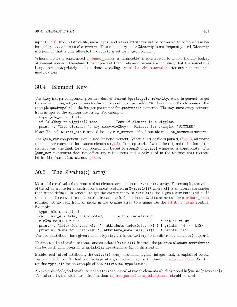
30.4. ELEMENT KEY 431

input (§33.1), from a lattice file, name, type, and alias attributes will be converted to to uppercase be-fore being loaded into an ele_struct. To save memory, since %descrip is not frequently used, %descripis a pointer that is only allocated if descrip is set for a given element.

When a lattice is constructed by bmad_parser, a “nametable” is constructed to enable the fast lookupof element names. Therefore, It is important that if element names are modified, that the nametableis updated appropriately. This is done by calling create_lat_ele_nametable after any element namemodifications.

30.4 Element Key

The %key integer component gives the class of element (quadrupole, rfcavity, etc.). In general, to getthe corresponding integer parameter for an element class, just add a “$” character to the class name. Forexample quadrupole$ is the integer parameter for quadrupole elements. The key_name array convertsfrom integer to the appropriate string. For example:type (ele_struct) eleif (ele%key == wiggler$) then ! Test if element is a wiggler.print *, "This element: ", key_name(ele%key) ! Prints, for example, "WIGGLER"

Note: The call to init_ele is needed for any ele_struct defined outside of a lat_struct structure.

The %sub_key component is only used for bend element. When a lattice file is parsed, (§33.1), all rbendelements are converted into sbend elements (§4.5). To keep track of what the original definition of theelement was, the %sub_key component will be set to sbend$ or rbend$ whatever is appropriate. The%sub_key component does not affect any calculations and is only used in the routines that recreatelattice files from a lat_struct (§33.3).

30.5 The %value(:) array

Most of the real valued attributes of an element are held in the %value(:) array. For example, the valueof the k1 attribute for a quadrupole element is stored in %value(k1$) where k1$ is an integer parameterthat Bmad defines. In general, to get the correct index in %value(:) for a given attribute, add a “$"as a suffix. To convert from an attribute name to its index in the %value array use the attribute_indexroutine. To go back from an index in the %value array to a name use the attribute_name routine.Example:type (ele_struct) elecall init_ele (ele, quadrupole$) ! Initialize elementele%value(k1$) = 0.3 ! Set K1 valueprint *, "Index for Quad K1: ", attribute_index(ele, "K1") ! prints: ‘4’ (= k1$)print *, "Name for Quad k1$: ", attribute_name (ele, k1$) ! prints: ‘K1’

The list of attributes for a given element type is given in the writeup for the different element in Chapter 4.

To obtain a list of attribute names and associated %value(:) indexes, the program element_attributescan be used. This program is included in the standard Bmad distribution.

Besides real valued attributes, the value(:) array also holds logical, integer, and, as explained below,“switch” attributes. To find out the type of a given attribute, use the function attribute_type. See theroutine type_ele for an example of how attribute_type is used.

An example of a logical attribute is the flexible logical of match elements which is stored in %value(flexible$).To evaluate logical attributes, the functions is_true(param) or is_false(param) should be used.

432 CHAPTER 30. THE ELE_STRUCT

Integer attributes stored in the value(:) array include n_slice (stored in %value(n_slice$)). Withinteger attributes, the nint(param) Fortran instrinsic should be used for evaluation.

A switch attribte is an attribute whose value is one of a certain set of integers where each integercorresponds to some “state”. For example, the fringe_at switch which, as explained in §5.20, may haveone of four values. Generally, the integer parameters that correspond to the states of a switch can beconstructed by putting a “$” after the associated name. Thus, with the fringe_at switch, the fourinteger parameters are no_end$, both_ends$, entrance_end$, and exit_end$. For example:if (nint(ele%value(fringe_type$)) == soft_edge_only$) then...

For printing purposes, to convert a switch value to the appropriate string, use the routineswitch_-attrib_value_name can be used.

The %field_master logical within an element sets whether it is the normalized strength or field strengththat is the independent variable. See §5.1 for more details.

The %old_value(:) component of the ele_struct is used by the attribute_bookkeeper routine tocheck for changes for changes in the %value(:) array since the last time the attribute_bookkeeperroutine had been called. If nothing has been changed, the attribute_bookkeeper routine knows notto waste time recalculating dependent values. Essentially what this means is that the %old_value(:)array should not be modified outside of attribute_bookkeeper.

30.6 Connection with the Lat_Struct

If an element is part of a lat_struct (§31), the %ix_ele and %ix_branch components of the ele_structidentify where the element is. Additionally, the %lat component will point to the encomposing lattice.That istype (lat_struct), pointer :: lattype (ele_struct), pointer :: ele2if (ele%ix_ele > -1) thenie = ele%ix_eleib = ele%ix_branchlat => ele%latele2 => lat%branch(ib)%ele(ie)print *, associated(ele2, ele) ! Will print True.

endif

In this example the ele2 pointer is constructed to point to the ele element. The test (ele%ix_ele > -1)is needed since ele_struct elements may exist outside of any lat_struct instance. Such “external”elements always have %ix_ele< 0. A value for %ix_ele of -2 is special in that it prevents the deallocate_-ele_pointers routine from deallocating the pointers of an element which has its %ix_ele set to -2.

An element “slice” is an example of an element that exists external to any lat_struct instance. A sliceis an ele_struct instance that represents some sub-section of a given element. Element slices are usefulwhen tracking particles only part way through an element (§35.7).

30.7 Limits

The aperture limits (§5.8) in the ele_struct are:%value(x1_limit$)

30.8. TWISS PARAMETERS, ETC. 433

%value(x2_limit$)%value(y1_limit$)%value(y2_limit$)

The values of these limits along with the %aperture_at, %aperture_type, and %offset_moves_aperturecomponents are used in tracking to determine if a particle has hit the vacuum chamber wall. See Sec-tion §35.8 for more details.

30.8 Twiss Parameters, etc.

The components %a, %b, %z, %x, %y, %c_mat, %gamma_c, %mode_flip, and mode3 hold information on theTwiss parameters, dispersion, and coupling at the downstream end of the element. See Chapter 34 formore details.

30.9 Element Lords and Element Slaves

In Bmad, elements in a lattice can control other elements. The components that determine this controlare:

%slave_status%n_slave%n_slave_field%ix1_slave%lord_status%n_lord%n_lord_field%ic1_lord%component_name

This is explained fully in the chapter on the lat_struct (§31).

30.10 Group and Overlay Controller Elements

Group and overlay elements use the %control_var(:) array for storing information about the controlvariables. Each element in the array represents a single variable. %control_var(:) is an array ofcontroller_var_struct structures and these structures look like:

type controller_structcharacter(40) :: name = ""real(rp) :: value = 0real(rp) :: old_value = 0

end type

The %old_value component is only used for group elements.

See Section §32.2 for an example of setting up a controller element within a program.

434 CHAPTER 30. THE ELE_STRUCT

30.11 Coordinates, Offsets, etc.

The “upstream” and “downstream” ends of an element are, by definition, where the physical ends of theelement would be if there were no offsets. In particular, if an element has a finite z_offset, the physicalends will be displaced from upstream and downstream ends. See §35.2 for more details.

The %floor component gives the “laboratory” global “floor” coordinates (§15.2) at the downstream endof the element. These coordinates are computed without misalignments. That is, the coordinates arenot “body” coordinates. The components of the %floor structure are

type floor_position_structreal(rp) r(3) ! Offset from originreal(rp) w(3,3) ! Orientation matrix (Eq. (15.2))real(rp) theta, phi, psi ! Angular orientation

end type

The routine ele_geometry will calculate an element’s floor coordinates given the floor coordinates at thebeginning of the element. In a lattice, the lat_geometry routine will calculate the floor coordinates forthe entire lattice using repeated calls to ele_geometry.

The positional offsets (§5.6) for an element from the reference orbit are stored in

%value(x_offset$)%value(y_offset$)%value(z_offset$)%value(x_pitch$)%value(y_pitch$)%value(tilt$)

If the element is supported by a girder element (§4.21) then the girder offsets are added to the elementoffsets and the total offset with respect to the reference coordinate system is stored in:

%value(x_offset_tot$)%value(y_offset_tot$)%value(z_offset_tot$)%value(x_pitch_tot$)%value(y_pitch_tot$)%value(tilt_tot$)

If there is no girder, the values for %value(x_offset_tot$), etc. are set to the corresponding val-ues in %value(x_offset$), etc. Thus, to vary the position of an individual element the values of%value(x_offset$), etc. are changed and to read the position of an element a program should look at%value(x_offset_tot$), etc.

The longitudinal position at the downstream end of an element is stored in %s and the reference timeis stored in %ref_time. This reference time is calculated assuming that the reference time is zeroat the start of the lattice. Also stored in the ele_struct is the reference time at the start of theelement and the differnece in the reference time between the end and the beginning. These are given in%value(ref_time_start$) and %value(delta_ref_time$) respectively.

Notice that the reference time used to calculate the z phase space coordinate (Eq. (15.28)) may bedifferent from %ref_time. For example, with multiple bunches the z phase space coordinate is generallytaken to be with respect to a reference particle at the center of the bunch the particle is in. And, ata given element, the reference time of the different bunch reference particles will be different. Anotherexample happens when a particle is tracked through multiple turns. In this case the reference time at agiven element will depend upon the turn number.

30.12. TRANSFER MAPS: LINEAR AND NON-LINEAR (TAYLOR) 435

30.12 Transfer Maps: Linear and Non-linear (Taylor)

The routine make_mat6 computes the linear transfer matrix (Jacobian) along with the zeroth or-der transfer vector. This matrix is stored in %mat6(6,6) and the zeroth order vector is stored in%vec0(6). The reference orbit at the upstream end of the element about which the transfer matrixis computed is stored in %map_ref_orb_in and the reference orbit at the downstream end is stored in%map_ref_orb_out. In the calculation of the transfer map, the vector %vec0 is set so thatmap_ref_orb_out = %mat6 * map_ref_orbit_in + %vec0

The reason redundant information is stored in the element is to save computation time.

To compute the transfer maps for an entire lattice use the routine lat_make_mat6.

The Taylor map (§6) for an element is stored in %taylor(1:6). Each %taylor(i) is a taylor_structstructure that defines a Taylor series:type taylor_structreal (rp) reftype (taylor_term_struct), pointer :: term(:) => null()

end type

Each Taylor series has an array of taylor_term_struct terms defined astype taylor_term_structreal(rp) :: coefinteger :: expn(6)

end type

The coefficient for a Taylor term is stored in %coef and the six exponents are stored in %exp(6).

To see if there is a Taylor map associated with an element the association status of %taylor(1)%termneeds to be checked. As an example the following finds the order of a Taylor map.type (ele_struct) ele...if (associated(ele%taylor(1)%term) then ! Taylor map existstaylor_order = 0do i = 1, 6do j = 1, size(ele%taylor(i)%term)taylor_order = max(taylor_order, sum(ele%taylor(i)%term(j)%exp)

enddoenddo

else ! Taylor map does not existtaylor_order = -1 ! flag non-existence

endif

The Taylor map is made up around some reference phase space point corresponding to the coordinatesat the upstream of the element. This reference point is saved in %taylor(1:6)%ref. Once a Taylor mapis made, the reference point is not needed in subsequent calculations. However, the Taylor map itselfwill depend upon what reference point is chosen (§23.1).

30.13 Reference Energy and Time

The reference energy and reference time are computed around a reference orbit which is different fromthe reference orbit used for computing transfer maps (§30.12). The energy and time reference orbit foran element is stored in

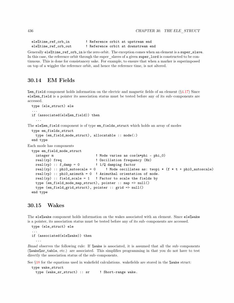
436 CHAPTER 30. THE ELE_STRUCT

ele%time_ref_orb_in ! Reference orbit at upstream endele%time_ref_orb_out ! Reference orbit at downstream end

Generally ele%time_ref_orb_in is the zero orbit. The exception comes when an element is a super_slave.In this case, the reference orbit through the super_slaves of a given super_lord is constructed to be con-tinuous. This is done for consistancey sake. For example, to ensure that when a marker is superimposedon top of a wiggler the reference orbit, and hence the reference time, is not altered.

30.14 EM Fields

%em_field component holds information on the electric and magnetic fields of an element (§4.17) Sinceele%em_field is a pointer its association status must be tested before any of its sub–components areaccessed.type (ele_struct) ele...if (associated(ele%em_field)) then...

The ele%em_field component is of type em_fields_struct which holds an array of modestype em_fields_structtype (em_field_mode_struct), allocatable :: mode(:)

end type

Each mode has componentstype em_field_mode_structinteger m ! Mode varies as cos(m*phi - phi_0)real(rp) freq ! Oscillation frequency (Hz)real(rp) :: f_damp = 0 ! 1/Q damping factorreal(rp) :: phi0_autoscale = 0 ! Mode oscillates as: twopi * (f * t + phi0_autoscale)real(rp) :: phi0_azimuth = 0 ! Azimuthal orientation of mode.real(rp) :: field_scale = 1 ! Factor to scale the fields bytype (em_field_mode_map_struct), pointer :: map => null()type (em_field_grid_struct), pointer :: grid => null()

end type

30.15 Wakes

The ele%wake component holds information on the wakes associated with an element. Since ele%wakeis a pointer, its association status must be tested before any of its sub–components are accessed.type (ele_struct) ele...if (associated(ele%wake)) then...

Bmad observes the following rule: If %wake is associated, it is assumed that all the sub–components(%wake%sr_table, etc.) are associated. This simplifies programming in that you do not have to testdirectly the association status of the sub–components.

See §18 for the equations used in wakefield calculations. wakefields are stored in the %wake struct:type wake_structtype (wake_sr_struct) :: sr ! Short-range wake.

30.16. WIGGLER TYPES 437

type (wake_lr_struct) :: lr ! Long-range wake.real(rp) :: amp_scale = 1 ! Wake amplitude scale factor.real(rp) :: time_scale = 1 ! Wake time scale factor.

end typeThe short–range wake parameterization uses pseudo–modes (§18.1). This parameterization utilizes the%wake%sr%long(:), and %wake%sr%trans(:) arrays for the longitudinal and transverse modes respec-tively. The structure used for the elements of these arrays are:type wake_sr_mode_struct ! Pseudo-mode short-range wake structreal(rp) amp ! Amplitudereal(rp) damp ! Damping factor.real(rp) freq ! Frequency in Hzreal(rp) phi ! Phase in radians/2pireal(rp) b_sin ! non-skew sin-like component of the wakereal(rp) b_cos ! non-skew cos-like component of the wakereal(rp) a_sin ! skew sin-like component of the wakereal(rp) a_cos ! skew cos-like component of the wake

end typeThe wakefield kick is calculated from Eq. (18.6). %amp, %damp, %freq, and %phi are the input parametersfrom the lattice file. the last four components (%norm_sin, etc.) store the accumulated wake: Before thebunch passes through these are set to zero and as each particle passes through the cavity the contributionto the wake due to the particle is calculated and added the components.

%wake%z_sr_mode_max is the maximum z value beyond which the pseudo mode representation is notvalid. This is set in the input lattice file.

The %wake%lr array stores the long–range wake modes. The structure definition is:type wake_lr_struct ! Long-Range Wake structreal(rp) freq ! Actual Frequency in Hzreal(rp) freq_in ! Input frequency in Hzreal(rp) R_over_Q ! Strength in V/C/m^2real(rp) Q ! Quality factorreal(rp) angle ! polarization angle (radians/2pi).integer m ! Order (1 = dipole, 2 = quad, etc.)real(rp) b_sin ! non-skew sin-like component of the wakereal(rp) b_cos ! non-skew cos-like component of the wakereal(rp) a_sin ! skew sin-like component of the wakereal(rp) a_cos ! skew cos-like component of the wakelogical polarized ! Polarized mode?

end typeThis is similar to the sr_mode_wake_struct. %freq_in is the actual frequency in the input file. bmad_-parser will set %freq to %freq_in except when the lr_freq_spread attribute is non-zero in which casebmad_parser will vary %freq as explained in §4.27. %polarized is a logical that indicates whether themode has a polarization angle. If so, then %angle is the polarization angle.

30.16 Wiggler Types

The %sub_key component of the ele_struct is used to distinguish between map type and periodictype wigglers (§30.4):if (ele%key == wiggler$ .and. ele%sub_key == map_type$) ...if (ele%key == wiggler$ .and. ele%sub_key == periodic_type$) ...

438 CHAPTER 30. THE ELE_STRUCT

For a map type wiggler, the wiggler field terms (§4.49.2) are stored in the %wig_term(:) array of theelement_struct. This is an array of wig_term_struct structure. A wig_term_struct looks like:type wig_term_structreal(rp) coefreal(rp) kx, ky, kzreal(rp) phi_zinteger type ! hyper_y$, hyper_xy$, or hyper_x$

end type

A periodic wiggler will have a single %wig_term(:) term that can be used for tracking purposes, etc.The setting for this wig_term element isele%wig_term(1)%ky = pi / ele%value(l_pole$)ele%wig_term(1)%coef = ele%value(b_max$)ele%wig_term(1)%kx = 0ele%wig_term(1)%kz = ele%wig_term(1)%kyele%wig_term(1)%phi_z = (ele%value(l_pole$) - ele%value(l$)) / 2ele%wig_term(1)%type = hyper_y$

30.17 Multipoles

The multipole components of an element (See §16.1) are stored in the pointers %a_pole(:) and%b_pole(:). If %a_pole and %b_pole are allocated they always have a range %a_pole(0:n_pole_maxx)and %b_pole(0:n_pole_maxx). Currently n_pole_maxx= 20. For a Multipole element, the %a_pole(n)array stores the integrated multipole strength KnL, and the %b_pole(n) array stores the tilt Tn.

A list of Bmad routines for manipulating multipoles can be found in §43.28.

30.18 Tracking Methods

A number of ele_struct components control tracking and transfer map calculations. These are:%mat6_calc_method%tracking_method%taylor_order%symplectify%multipoles_on%taylor_map_includes_offsets%is_on%csr_method%space_charge_method%offset_moves_apaerture

See Chapter §35 for more details.

30.19 Custom and General Use Attributes

There are four components of an ele_struct that are guaranteed to never be used by any Bmad routineand so are available for use by someone writing a program. These components are:%r(:,:,:) ! real(rp), pointer.

30.20. BMAD RESERVED VARIABLES 439

%custom(:) ! real(rp), pointer.%ix_pointer ! integer.%logic ! logical.

Values for ele%r and ele%custom can be set in the lattice file (§3.8). If values are set for ele%r orele%custom, these arrays will be expanded in size if needed.

Accessing the ele%custom array should be done using the standard accessor routines (§32.4). Forexample, if the lattice file being used defines a custom attribute called rise_time (§3.8):parameter[custom_attribute1] = "rise_time"

then a program can access the rise_time attribute via:type (ele_struct), poiner :: eletype (all_pointer_struct) a_ptr...ele => ... ! Point ele to some element in the latticecall pointer_to_attribute (ele, "RISE_TIME", .true., a_ptr, err_flag)print *, "RISE_TIME Attribute has value:", a_ptr%r

Note: Even if there are custom attributes associated with a given type of element (say, all quadrupoles),a given element of that type may not have its %custom(:) array allocated. [In this case, none of thecustom values have been set so are zero by definition.] In the above example, the %custom array will beallocated if needed in the call to pointer_to_attribute.

If not defined through a lattice file, custom attributes can also be defined directly from within a programusing the set_custom_attribute_name routine. For example:logical err_flag...call set_custom_attribute_name (’QUADRUPOLE::ERROR_CURRENT’, err_flag)

Note: When there is a superposition (§8.1), the super_slave elements that are formed do not have anycustom attributes assigned to them even when their super_lord elements have custom attributes. Thisis done since the Bmad bookkeeping routines are not able to handle the situation where a super_slaveelement has multiple super_lord elements and thus the custom attributes from the different super_lordelements have to be combined. Proper handling of this situation is left to any custom code that a programimplements to handle custom attributes.

30.20 Bmad Reserved Variables

A number of ele_struct components are reserved for Bmad internal use only. These are:%ixx%iyy%bmad_logic

To avoid conflict with multiple routines trying to use these components simultaneously, these componentsare only used for short term bookkeeping within individual routines.

440 CHAPTER 30. THE ELE_STRUCT

Chapter 31

The lat_struct

The lat_struct is the structure that holds of all the information about a lattice (§2.3). The componentsof a lat_struct are listed in Fig. 31.1.

The %ele_init component within the lat_struct is not used by Bmad and is available for generalprogram use.

441

442 CHAPTER 31. THE LAT_STRUCT

type lat_structcharacter(40) use_name ! Name in USE statementcharacter(40) lattice ! Lattice namecharacter(80) input_file_name ! Lattice input file namecharacter(80) title ! From TITLE statementcharacter(100), allocatable :: print_str(:) ! Saved print statementstype (expression_atom_struct), allocatable :: constant(:) ! Constants defined in the latticetype (mode_info_struct) a, b, z ! Tunes, etc.type (lat_param_struct) param ! Parameterstype (bookkeeping_state_struct) lord_state ! lord bookkeeping status.type (ele_struct) ele_init ! For use by any programtype (ele_struct), pointer :: ele(:) => null() ! Array of elements [=> branch(0)].type (branch_struct), allocatable :: branch(:) ! Branch(0:) arraytype (control_struct), allocatable :: control(:) ! Control listtype (photon_reflect_surface_struct), pointer :: surface(:) => null()type (coord_struct) particle_start ! Starting coordstype (pre_tracker_struct) pre_tracker ! For OPAL/IMPACT-Ttype (nametable_struct) nametable ! For quick searching by element name.real(rp), allocatable :: custom(:) ! Custom attributes.integer version ! Version numberinteger n_ele_track ! Number of lat elements to track through.integer n_ele_max ! Index of last valid element in %ele(:) arrayinteger n_control_max ! Last index used in control_arrayinteger n_ic_max ! Last index used in ic_arrayinteger input_taylor_order ! As set in the input fileinteger, allocatable :: ic(:) ! Index to %control(:)integer :: photon_type = incoherent$ ! Or coherent$. For X-ray simulations.integer :: creation_hash ! Number to determine if lattice is different.logical absolute_time_tracking ! Use absolute time in lcavity and rfcavity tracking?

end type

Figure 31.1: Definition of the lat_struct.

31.1 Initializing

Normally initialization of a lat_struct lattice is done by bmad_parser when a lattice file is parsedand does not have to be done by the programmer. When a programmer needs to initialize a lattice,however, init_lat is used to initialize the lattice with a single branch. After this initial setup, theroutines allocate_branch_array and allocate_lat_ele_array can be used to set up additional branches.Example:

type (lat_struct) lat...call init_lat (lat, 1000) ! Branch(0) has 1001 elements.call allocate_branch_array (lat, 2) ! Allocate Branch(1) and Branch(2).call allocate_lat_ele_array (lat, 20, 1) ! Branch(1) has 21 elementscall allocate_lat_ele_array (lat, 30, 2) ! Branch(2) has 31 elements.

31.2. POINTERS 443

31.2 Pointers

Since the lat_struct has pointers within it, there is an extra burden on the programmer to make surethat allocation and deallocation is done properly. To this end, the equal sign has been overloaded bythe routine lat_equal_lat so that when one writes

type (lat_struct) lattice1, lattice2! ... some calculations ...lattice1 = lattice2

the pointers in the lat_struct structures will be handled properly. The result will be that lattice1 willhold the same information as lattice2 with all the lattice elements in the same place but the pointersin lattice1 will point to different locations in physical memory so that changes to one lattice will notaffect the other.

deallocate_lat_pointers Initial allocation of the pointers in a lat_struct variable is generally handledby the bmad_parser and lat_equal_lat routines. Once allocated, local lat_struct variables must havethe save attribute or the pointers within must be appropriately deallocated before leaving the routine.type (lat_struct), save :: lattice ! Either do this at the start or ......call deallocate_lat_pointers (lattice) ! ... Do this at the end.

Using the save attribute will generally be faster but will use more memory. Typically using the saveattribute will be the best choice.

31.3 Branches in the lat_struct

The lattice is divided up into the “root branch” (§7.7) and, if there are fork or photon_fork elements,a number “forked” branches.

The branches of a lattice is contained in the lat%branch(0:) array. The %branch(0:) array is alwaysindexed from 0 with the 0 branch being a root branch. The definition of the branch_struct structureistype branch_structcharacter(40) nameinteger ix_branch ! Index in lat%branch(:) array.integer ix_from_branch ! -1 => No forking element to this branch.integer ix_from_ele ! Index of forking elementinteger, pointer :: n_ele_track ! Number of tracking elementsinteger, pointer :: n_ele_maxtype (mode_info_struct), pointer :: a, b, ztype (ele_struct), pointer :: ele(:)type (lat_param_struct), pointer :: paramtype (wall3d_struct), pointer :: wall3d(:)type (ptc_branch1_info_struct) ptctype (normal_form_struct) normal_form_with_rf, normal_form_no_rf

end type

The value of the %branch(i)%ix_branch conponent is the branch index and will thus have the value i.This can be useful when passing a branch to a subroutine. The %branch(i)%ix_from_branch componentgives the branch index of the branch that the ith branch branched off from. %branch(i)%ix_from_elegives the index in the %branch(j)%ele(:) array of the fork or photon_fork element that marks thebeginning of the ith branch. Example:

444 CHAPTER 31. THE LAT_STRUCT

Element index

section min max

tracking 0 %n_ele_trackcontrol %n_ele_track+1 %n_ele_max

Table 31.1: Bounds of the tracking and control parts of the root branch (lat%branch(0)%ele(:)) array.

type (lat_struct), target :: lattype (ele_struct), pointer :: ele...ib = lat%branch(3)%ix_from_branchie = lat%branch(3)%ix_from_ele! ele is the fork or photon_fork element for lat%branch(3)ele => lat%branch(ib)%ele(ie)! This is the same as the above.ele => pointer_to_ele(lat%branch(3)%ix_from_branch, lat%branch(3)%ix_from_ele)

The %branch%ele(:) array holds the array of elements in the branch. Historically, the lat_struct wasdeveloped at the start of the Bmad project and branches were implemented well after that. To maintaincompatibility with older code, the following components point to the same memory blockslat%ele(:) <---> lat%branch(0)%ele(:)lat%n_ele_track <---> lat%branch(0)%n_ele_tracklat%n_ele_max <---> lat%branch(0)%n_ele_maxlat%param <---> lat%branch(0)%param

All %branch%ele(:) arrays are allocated with zero as the lower bound. The %ele(0) element of allbranches is an beginning_ele element with its %name component set to “BEGINNING”. %ele(0)%mat6is always the unit matrix. For the root branch, the %branch(0)%ele(0:) array is divided up intotwo parts: The “tracking” part and a “control” part (also called the “lord” part). The tracking part ofthis array holds the elements that are tracked through. The control part holds elements that controlattributes of other elements (§31.5). The bounds of these two parts is given in Table 31.1. Only the rootbranch has a lord section so %branch%n_ele_track and %branch%n_ele_max are the same for all otherbranches. Since the root branch can also be accessed via the lat%ele(:) array, code that deals withthe lord section of the lattice may use lat%ele(:) in place of lat%branch(0)%ele(:).

for a given fork or photon_fork element, the index of the branch that is being forked to and the indexof the element that is being forked to is stored in:ix_branch = nint(branch_ele%value(ix_branch_to$)) ! branch indexix_element = nint(branch_ele%value(ix_element_to$)) ! element indexdirection = nint(branch_ele%value(direction$))

The direction will be +1 for forward forking and -1 for backward forking.

31.4 Param_struct Component

The %param component within each lat%branch(:) is a lat_param_struct structure whose definitionis shown in Fig. 31.2 This structure would be more aptly named branch_param_struct but is namedotherwise for historical reasons.

%param%total_length is the length of the branch that a beam tracks through defined by

31.4. PARAM_STRUCT COMPONENT 445

type lat_param_structreal(rp) n_part ! Particles/bunch (for beambeam elements).real(rp) total_length ! total_length of latticereal(rp) unstable_factor ! closed branch: growth rate/turn.

! all branches: |orbit/limit|real(rp) t1_with_RF(6,6) ! Full 1-turn 6x6 matrixreal(rp) t1_no_RF(6,6) ! Transverse 1-turn 4x4 matrix (RF off).integer particle ! +1 = positrons, -1 = electrons, etc.integer geometry ! open$, etc...integer ixx ! Integer for general uselogical stable ! For closed branch. Is lat stable?type (bookkeeper_status_struct) bookkeeping_state

! Overall status for the branch.end type

Figure 31.2: Definition of the param_struct.

%param%total_length = %ele(n_ele_track)%s - %ele(0)%sNormally %ele(0)%s = 0 so %param%total_length = %ele(n_ele_track)%s but this is not always thecase.

%param%n_part is the number of particles in a bunch and is used by beambeam element to determine thestrength of the beambeam interaction. %param%n_part is also used by lcavity elements for wakefieldcalculations.

For closed branches, %param%t1_with_RF and %param%t1_no_RF are the 1–turn transfer matrices fromthe start of the branch to the end. %param%t1_with_RF is the full transfer matrix with RF on.%param%t1_no_RF is the transverse transfer matrix with RF off. %param%t1_no_RF is used to com-pute the Twiss parameters. When computing the Twiss parameters %param%stable is set according towhether the matrix is stable or not. If the matrix is not stable the Twiss parameters cannot be computed.If unstable, %param%unstable_factor will be set to the growth rate per turn of the unstable mode.

Besides being set when the 1–turn transfer matrix is calculated, %param%unstable_factor will be setif a particle is lost in tracking to:orbit_amplitude / limit - 1

The particle type for a branch is stored in the integer variable %param%particle. The value of this vari-able will encode for a fundamental particle, atom, or molecule. See the file particle_species_mod.f90for more details. If the particle corresponds to a fundamental particle, %param%particle will correspondto one of the following constants:electron$, positron$,muon$, antimuon$,proton$, antiproton$,photon$, pion_0$,pion_minus$, pion_plus$deuteron$ deuteron_0$

To print the name of the particle use the function particle_name. A particles mass and charge canbe obtained from the functions mass_of and charge_of respectively. charge_of returns the particle’scharge in units of e. Example:type (lat_struct) lat...print *, "Beam Particles are: ", particle_name(lat%param%particle)

446 CHAPTER 31. THE LAT_STRUCT

if (lat%param%particle == proton$) print *, "I do not like protons!"print *, "Particle mass (eV): ", mass_of(lat%param%particle)print *, "Particle charge: ", charge_of(lat%param%particle)

31.5 Elements Controlling Other Elements

In the lat_struct structure, certain elements in the %ele(:) array (equivalent to the %branch(0)%ele(:)array), called lord elements, can control the attributes (component values) of other %branch(:)%ele(:)elements. Elements so controlled are called slave elements. The situation is complicated by the factthat a given element may simultaneously be a lord and a slave. For example, an overlay element(§4.37) is a lord since it controls attributes of other elements but an overlay can itself be controlled byother overlay and group elements. In all cases, circular lord/slave chains are not permitted.

The lord and slave elements can be divided up into classes. What type of lord an element is, is setby the value of the element’s ele%lord_status component. Similarly, what type of slave an elementis is set by the value of the element’s ele%slave_status component. Nomenclature note: An elementmay be referred to by it’s %lord_status or %slave_status value. For example, an element withele%lord_status set to super_lord$ can be referred to as a “super_lord” element.

The value of the ele%lord_status component can be one of:

super_lord$A super_lord element is created when elements are superimposed on top of other elements (§8.1).

girder_lord$A girder_lord element is a girder element (§4.21). That is, the element will have ele%key =girder$.

multipass_lord$multipass_lord elements are created when multipass lines are present (§8.2).

overlay_lord$An overlay_lord is an overlay element (§4.37). That is, such an element will have ele%key =overlay$.

ramper_lord$A ramper_lord is a ramper element (§4.41). That is, such an element will have ele%key =ramper$. Note that a ramper_lord will not have any associated slaves.

group_lord$A group_lord is a group element (§4.22). That is, such an element will have ele%key = group$.

not_a_lord$This element does not control anything.

Any element whose %lord_status is something other than not_a_lord$ is called a lord element. In thetracking part of the branch (§31.3), %lord_status will always be not_a_lord$. In the lord sectionof the branch, under normal circumstances, there will never be any not_a_lord elements. However, itis permissible, and sometimes convenient, for programs to set the %lord_status of a lord element tonot_a_lord$.

The possible values for the ele%slave_status component are:

31.5. ELEMENTS CONTROLLING OTHER ELEMENTS 447

ele%lord_status

ele%slave_status not_

a_lo

rd$

grou

p_lo

rd$

gird

er_l

ord$

over

lay_

lord

$

mult

ipas

s_lo

rd$

supe

r_lo

rd$

free$ X X X X X Xminor_slave$ X X X X X Xmultipass_slave$ X Xslice_slave$ Xsuper_slave$ X

(a) Possible ele%lord_status and ele%slave_statuscombinations within an individual element.

lord%lord_status

slave%slave_status not_

a_lo

rd$

grou

p_lo

rd$

gird

er_l

ord$

over

lay_

lord

$

mult

ipas

s_lo

rd$

supe

r_lo

rd$

free$minor_slave$ X X Xmultipass_slave$ X X 1super_slave$ X X X

(b) Possible %lord_status and %slave_status com-binations for any lord/slave pair.

Table 31.2: Possible %lord_status/%slave_status combinations. “X” marks a possible combination. “1”indicates that the slave will have exactly one lord of the type given in the column.

multipass_slave$A multipass_slave element is the slave of a multipass_lord (§8.2).

slice_slave$A slice_slave element represents a longitudinal slice of another element. Slice elements are notpart of the lattice but rather are created on-the-fly when, for example, a program needs to trackpart way through an element.

super_slave$A super_slave element is an element in the tracking part of the branch that has one or moresuper_lord lords (§8.1).

minor_slave$A minor_slave element is an element that is not a slice_slave and does not have a majorlord. Major lords are super_lords and multipass_lords. A minor_slave element will some haveattributes that are controlled by overlay_lords, group_lords, or girder_lords.

free$A free element is one that has no lords. [But there still might be field overlap from other elements.]

super_slave elements always appear in the tracking part of the branch. The other types can be ineither the tracking or control parts of the branch.

Only some combinations of %lord_status values and %slave_status values are permissible for a givenelement. Table 31.2a lists the valid combinations. Thus, for example, it is not possible for an elementto be simultaneously a super_lord and a super_slave.

For lord/slave pairs, Table 31.2b lists the valid combinations of %lord_status values in the lord ele-ment and %slave_status values in the slave element. Thus, for example, a super_slave may only becontrolled by a super_lord. In the example in Section §8.2, element A would be a multipass_lordand A\1 and A\2 would be multipass_slaves. When superposition is combined with multipass, theelements in the tracking part of the branch will be super_slaves. These elements will be controlled bysuper_lords which will also be multipass_slaves and these super_lord/multipass_slave elementswill be controlled by multipass_lords. This is illustrated in Fig. 31.3.

448 CHAPTER 31. THE LAT_STRUCT

s

%lord_status = multipass_lord$

%name = “A”

%name = “A\1”

%slave_status = super_slave$

%slave_status = multipass_slave$

%lord_status = super_lord$

%name = “A\1#1”Tracking Part:

...

...

Figure 31.3: Example of multipass combined with superposition. A multipass_lord element namedA controls a set of multipass_slaves (only one shown). The multipass_slave elements are alsosuper_lord elements and they will control super_slave elements in the tracking part of the branch.

The number of slave elements that a lord controls is given by the value of the lord’s %n_slave component.Additionally, the number of lord elements that the slave has is given by the value of the slave’s. %n_lordcomponent. To find the slaves and lords of a given element, use the routines pointer_to_slave andpointer_to_lord. Example:type (lat_struct), target :: lattype (ele_struct), pointer :: this_ele, lord_ele, slave_ele...this_ele => lat%ele(321) ! this_ele points to a given element in the lattice

do i = 1, this_ele%n_lord ! Loop over all lords of this_ele! lord_ele points to the i^th lord element of this_elelord_ele => pointer_to_lord (this_ele, i)...

enddo

do i = 1, this_ele%n_slave ! Loop over all slaves of this_ele! slave_ele points to the i^th slave element of this_eleslave_ele => pointer_to_slave (this_ele, i)...

enddo

For non-ramper elements, the lord/slave bookkeeping is bidirectional. That is, for any given element,call it this_ele, consider the ith lord:lord_ele_i => pointer_to_lord (this_ele, i)

then there will always be some index j such that the element pointed to bypointer_to_slave(lord_ele_i, j)

is the original element this_ele. The same is true for the slaves of any given element. That is, for theith slaveslave_ele_i => pointer_to_slave (this_ele, i)

there will always be some index j such that the element pointed to by

31.5. ELEMENTS CONTROLLING OTHER ELEMENTS 449

pointer_to_lord(slave_ele_i, j)The following ordering of slaves and lords is observed:

Slaves of a super_lord:The associated super_slave elements of a given super_lord element are ordered from the entranceend of the super_lord to the exit end. That is, in the code snippet above, pointer_to_slave(this_ele, 1) will point to the slave at the start of the super_lord and pointer_to_slave(this_ele, this_ele%n_lord) will point to the slave at the exit end of the super_lord.

Slaves of a multipass_lord:The associated multipass_slave elements of a multipass_lord element are ordered by passnumber. That is, in the code snippet above, pointer_to_slave (this_ele, i) will point to theslave of the ith pass.

Lord of a multipass_slave:A multipass_slave will have exactly one associated multipass_lord and this lord will be thefirst one. That is, pointer_to_lord (this_ele, 1).

The element control information is stored in the lat%control(:) array. Each element of this array isa control_struct structuretype control_structtype (expression_atom_struct), allocatable :: stack(:) ! Evaluation stacktype (lat_ele_loc_struct) slave ! Slave locationtype (lat_ele_loc_struct) lord ! Lord locationinteger ix_attrib ! index of controlled attribute

end typeEach element in the lat%control(:) array holds the information on one lord/slave pair. The %lordcomponent gives the location of the lord element which is always in the root branch — branch 0.The %slave component give the element location of the slave element. The %stack and %ix_attribcomponents are used to store the arithmetic expression and attribute index for overlay and groupcontrol. The appropriate control_struct for a given lord/slave pair can be obtained from the optionalfourth argument of the pointer_to_lord and pointer_to_slave functions. Example: The following printsa list of the slaves, along with the attributes controlled and coefficients, on all group elements in a lattice.

type (lat_struct), target :: lattype (ele_struct), pointer :: lord, slavetype (control_struct), pointer :: con...do i = lat%n_ele_track+1, lat%n_ele_max ! loop over all lordslord => lat%ele(i)if (lord%lord_status = group_lord$) thenprint *, "Slaves for group lord: ", lord%namedo j = 1, lord%n_slaveslave => pointer_to_slave (lord, j, con)attrib_name = attribute_name (slave, con%ix_attrib)print *, i, slave%name, attrib_name, con%coef

enddoendif

enddoThe elements in the lat%control(:) array associated with the slaves of a given lord are in the sameorder as the slaves and the index of the associated lat%control(:) element of the first slave is givenby the %ix1_slave component of the lord Example:

450 CHAPTER 31. THE LAT_STRUCT

type (lat_struct), target :: lattype (ele_struct), pointer :: lord, slavetype (control_struct), pointer :: con1, con2...lord => lat%ele(i) ! Point to some lorddo j = 1, lord%n_slaveslave => pointer_to_slave (lord, j, con1)con2 => lat%control(lord%ix1_slave+j-1) ! con1 and con2 are the same.

enddoExcept for a slice_slave, the %ic1_lord, %n_lord, and %n_lord_field components of a given slaveelement, along with the lat%ic(:) array, can be used to find the lords of the slave. Simplified, the codefor the pointer_to_lord function is:function pointer_to_lord (slave, ix_lord, con, ...) result (lord_ptr)implicit nonetype (lat_struct), target :: lattype (ele_struct) slavetype (ele_struct), pointer :: lord_ptrtype (control_struct), pointer, optional :: controlinteger ix_lord, icon!icon = lat%ic(slave%ic1_lord + ix_lord - 1)lord_ptr => lat%ele(lat%control(icon)%lord%ix_ele)if (present(con)) con => lat%control(icon)

end functionThis method for finding the lords of an element is considered “private”. That is, no code outside of theofficial Bmad library should rely on this.

slice_slave element bookkeeping has is different depending upon whether the element being sliced isa super_slave or not. If the element being sliced is a super_slave, a slice_slave element that iscreated is, for bookkeeping purposes, considered to be a slave of the super_slave’s lords. In this case,the bookkeeping is exactly the same as that of any super_slave, and pointer_to_lord will return apointer to one of the super_slave’s lords.

On the other hand, if a non super_slave element is being sliced, the %lord pointer component of theslice_slave will be set to point to the element being sliced.

31.6 Lattice Bookkeeping

The term “lattice bookkeeping” refers to the updating of the appropriate parameter values when a givenparameter in the lattice is changed. For example, if the accelerating gradient of an lcavity elementis modified, the reference energy parameter of all elements downstream of the lcavity will need to bechanged and this can also alter the transfer maps of the lcavity and downstream elements. Bmaddivides the lattice bookkeeping into “core” part and everything else. The core part itself is divided intofive parts:

Attribute bookkeepingThis refers to intra-element dependent attribute bookkeeping (§5.1).

Control bookkeepingThis refers to Lord/Slave bookkeeping for overlay (§4.37) and group (§4.22)elements, and forsuperposition (§8.1) and multipass (§8.2) lords.

31.6. LATTICE BOOKKEEPING 451

Floor Position bookkeeping This refers to bookkeeping to keep track of an elements global “floor”position stored in the ele%floor structure.

Length bookkeeping This refers to bookkeeping to keep track of the longitudinal s-position of anelement stored in the ele%s component.

Reference Energy bookkeeping This refers to the reference energy assigned to each element (§36.6).ele%value(E_tot$) and ele%value(p0c$)

Historically, as the concept of lattice bookkeeping was being developed, to be back compatible withexisting programs, calls to bookkeeping routines were added to calculational routines such as the trackingroutine track1 and the routine for calculating the linear transfer map make_mat6. This “automatic”bookkeeping system is inefficient since there is no good way to keep track of what element attributes havebeen modified which leads to redundant bookkeeping calculations. Eventually, as Bmad developed andbecame more complicated, it was found that the unnecessary bookkeeping load was generally causinga significant slowdown in program execution time — even in programs where no element attributeswere changed. To avoid this, an “intelligent” bookkeeping system was developed. In order to be backcompatible with existing programs, the automatic bookkeeping system is the default. However, giventhe fact that the automatic bookkeeping system has known deficiencies, and given the overhead withmaintaining two bookkeeping systems, the current plan is to start phasing out the automatic bookkeepingsystem sometime in the not-so-far future. Thus old programs should be converted to the new systemand all new programs should use the new bookkeeping system.

To use intelligent bookkeeping, a program must set the global bmad_com%auto_bookkeepper to false.This is done once at the start of the program. When a set of attributes needs to be modified, theset_flags_for_changed_attribute routine must be called for each element attribute that is set. Afterall the attributes have been set, lattice_bookkeeper is called to do the core bookkeeping. Exampletype (lat_struct) lat...bmad_com%auto_bookkeeper = .false. ! Only needs to be done once....lat%ele(i)%value(gradient$) = 1.05e6 ! Change, say, the gradient of an RFCavitycall set_flags_for_changed_attribute (lat%ele(i), lat%ele(i)%value(gradient$))

... Set attributes of other elements ...

call lattice_bookkeeper (lat) ! Do once after all attribute sets done.

The argument list for set_flags_for_changed_attribute isset_flags_for_changed_attribute (ele, attribute)

The attribute argument may be either real, integer, or logical.

The set_flags_for_changed_attribute routine sets flags in the ele%status structure. This structureis of type bookkeeper_status_struct and looks liketype bookkeeper_status_structinteger attributes ! Intra element dependent attribute statusinteger control ! Lord/slave bookkeeping statusinteger floor_position ! Global (floor) geometry statusinteger length ! Longitudinal position statusinteger ref_energy ! Reference energy statusinteger mat6 ! Linear transfer map statusinteger rad_int ! Radiation integrals cache status

end type

452 CHAPTER 31. THE LAT_STRUCT

All components of this structure give the status of some lattice bookkeeping aspect. The first fivecomponents of this structure correspond to the five core bookkeeping parts discussed above. The othertwo components are discussed below.

Possible values for the status components aresuper_ok$ok$stale$

The set_flags_for_changed_attribute routine sets the appropriate status components of an elementto stale$ which marks that element for the appropriate bookkeeping. When the bookkeeping is done bylattice_bookkeeper, the stale$ status components are set to ok$. The super_ok$ value is reservedfor use by any program that needs to do its own custom bookkeeping. How this works is as follows: TheBmad bookkeeping routines will never convert a status component with value super_ok$ to ok$ withoutfirst doing some needed bookkeeping. Thus if a program sets a status component to super_ok$ and thenlater on finds that the status component is set to ok$, the program knows that bookkeeping has beendone. An example will make this clear. Suppose a program needs to keep track of a collection of highorder transfer maps between various points in a lattice. Suppose that the constant calculation of thesemaps would slow the program done so it is desired to recalculate a given map only when necessary. Toimplement this, the program could set the ele%status%mat6 attribute of all the element to super_ok$when the maps are calculated. If the program subsequently finds a ele%status%mat6 attribute of anelement set to ok$ it knows that it should recalculate any transfer maps that span that element.

It is guaranteed that when lattice_bookkeeper is run, all five core status components will not bestale$. The routines used by lattice_bookkeeper are:attribute_bookkeeper ! Intra-element attributescontrol_bookkeeper ! Lord/slave controls_calc ! Longitudinal element s-positionlat_geometry ! Global (floor) positions.lat_compute_ref_energy_and_time ! Reference energy

In general, these routines should not be called directly since the correct way to do things is not alwaysstraight forward. See the code for lattice_bookkeeper for more details.

After the core bookkeeping is done, a program can call lat_make_mat6 to remake the transfer matrices.lat_make_mat6 will remake the transfer matrices if either the ele%status%mat6 flag is stale$ or thereference orbit around which the existing transfer matrix was computed has shifted. lat_make_mat6will set the ele%status%mat6 flag to ok$ for all elements whose transfer matrices are recomputed.

31.7 particle_start Component

The lat%particle_start component is a coord_struct structure for holding the information obtainedfrom particle_start statements (§9.2) in a Bmad lattice file.

This component is not used in any standard Bmad calculation. It is up to an individual program to useas desired. Use init_coord to initalize a particle position. Example:type (lat_struct) lattype (coord_struct) orbit_start...call bmad_parser("lat.bmad", lat) ! Read in a lattice....! orbit_start is initalized for tracking from the beginning of the latticecall init_coord(orbit_start, lat%particle_start, lat%ele(0), downstream_end$)

31.8. CUSTOM PARAMETERS 453

31.8 Custom Parameters

Custom parameters defined for the lattice as a whole (§3.8 are stored in lat%custom. The followingshows how to print a table of the custom parameterstype (lat_struct) latcharacter(80) aname...if (allocated(lat%custom)) thendo i = 1, size(lat%custom)aname = attribute_name(def_parameter$, i+custom_attribute0$)if (aname(1:1) == "!") cycle ! Ignore non-existant parametersprint "(a, es12.4)", " parameter[" // trim(aname) // "] = ", lat%custom(i)

enddoendif

454 CHAPTER 31. THE LAT_STRUCT

Chapter 32

Lattice Element Manipulation

32.1 Creating Element Slices

It is sometimes convenient to split an element longitudinally into “slices” that represent a part of theelement. This is complicated by the fact that elements are not necessarily uniform. For example, maptype wigglers are nonuniform and bend elements have end effects. Furthermore, attributes like hkickneed to be scaled with the element length.

To create an element slice, the routine create_element_slice can be used. Example:type (ele_struct) ele, sliced_ele...sliced_ele = elesliced_ele%value(l$) = l_slice ! Set the sliced element’s lengthcall create_element_slice (sliced_ele, ele, l_start, param, ...)

See the documentation on create_element_slice for more details (§28.3).

32.2 Adding and Deleting Elements From a Lattice

Modifying the number of elements in a lattice involves a bit of bookkeeping. To help with this there area number of routines.

The routine remove_eles_from_lat is used to delete elements from a lattice.

For adding elements there are three basic routines: To add a lord element, the new_control routine isused. To add a new element to the tracking part of the lattice, use the insert_element routine. Finally, tosplit an element into two pieces, the routine split_lat is used. These basic routines are then used in suchroutines as create_overlay that creates overlay elements, create_group which creates group elements,add_superimpose which superimposes elements, etc. Example:type (lat_struct), target :: lattype (ele_struct), pointer :: g_lord, slave

type (control_struct) con(1)integer ix, nlogical err_flag

455

456 CHAPTER 32. LATTICE ELEMENT MANIPULATION

...call new_control (lat, ix)g_lord => lat%ele(ix)allocate (ele%control_var(1))ele%control_var(1)%name = "A"call reallocate_expression_stack(con(1)%stack, 10))call expression_string_to_stack (’3.2*A^2’, con(1)%stack, n, err_flag)con(1)%ix_attrib = k1$call lat_ele_locator (’Q1W’, lat, eles)con(1)%slave = ele_to_lat_loc(eles(1)%ele)call create_group (g_lord, con, err_flag)

This example constructs a group element with one variable with name A controlling the K1 attribute ofelement Q1W using the expression “3.2 ·A2” where A is the name of the control variable.

For constructing group elements (but not overlay elements), the controlled attribute (set by con(1)%ix_attribin the above example) can be set to, besides the set of element attributes, any one in the following list:accordion_edge$ ! Element grows or shrinks symmetricallystart_edge$ ! Varies element’s upstream edge s-positionend_edge$ ! Varies element’s downstream edge s-positions_position$ ! Varies element’s overall s-position. Constant length.

See Section §4.22 for the meaning of these attributes

32.3 Finding Elements

The routine lat_ele_locator can be used to search for an element in a lattice by name or key type or acombination of both. Example:type (lat_struct) lattype (ele_pointer_struct), allocatable :: eles(:)integer n_loc; logical err...call lat_ele_locator ("quad::skew*", lat, eles, n_loc, err)print *, "Quadrupole elements whose name begins with the string "SKEW":"print *, "Name Branch_index Element_index"do i = 1, n_loc ! Loop over all elements found to match the search string.print *, eles(i)%ele%name, eles(i)%ele%ix_branch, eles(i)%ele%ix_ele

enddo

This example finds all elements where ele%key is quadrupole$ and ele%name starts with “skew”. Seethe documentation on lat_ele_locator for more details on the syntax of the search string.

The ele_pointer_struct array returned by lat_ele_locator is an array of pointers to ele_structelementstype ele_pointer_structtype (ele_struct), pointer :: ele

end type

The n_loc argument is the number of elements found and the err argument is set True on a decodeerror of the search string.

Once an element (or elements) is identified in the lattice, it’s attributes can be altered. However, caremust be taken that an element’s attribute can be modified (§5.1). The function attribute_free willcheck if an attribute is free to vary.

32.4. ACCESSING NAMED ELEMENT ATTRIBUTES 457

type (lat_struct) latinteger ix_ele...call lat_ele_locator (’Q10W’, lat, eles, n_loc, err) ! look for an element "Q10W"free = attribute_free (eles(i)%ele, "K1", lat, .false.)if (.not. free) print *, "Cannot vary k1 attribute of element Q10W"

32.4 Accessing Named Element Attributes

A “named” parameter of the ele_struct structure is a parameter that has an associated name that canbe used in a lattice file. For example, the quadrupole strength is named K1 (§4.40). This parameter isstored in the ele%value(:) array. Specifically at ele%value(k1$).

Historically, named parameters where always accessed directly but this has proved to be somewhatproblematical for a number of reasons. For one, something like ele%value(k1$) will always have avalue even if the associated lattice element does not have an associated K1 parameter (For example,a sextupole does not have a K1 parameter). Another issue involves allocation since components likeele%a_pole(:) are pointers that are not necessarily allocated.

To get around some of these issues, accessor functions have been developed for all non-character basednamed attributes. These accessor functions are:pointer_to_attribute ! pointer_to_attributepointers_to_attribute ! pointers_to_attributeset_ele_attribute ! set_ele_attributevalue_of_attribute ! value_of_attribute

The workhorse is pointer_to_attribute that returns a pointer to the appropriate attribute. Thereturned pointer argument is actually an instance of an all_pointer_struct which looks like:type all_pointer_structreal(rp), pointer :: r => null()integer, pointer :: i => null()logical, pointer :: l => null()

end type

When the all_pointer_struct argument is returned, one (or zero if the attribute name is not recog-nized) of the pointer components will be associated. For example:type (ele_struct) eletype (all_pointer_struct) attrib_ptr...call pointer_to_attribute (ele, "A3_ELEC", .true., attrib_ptr, err)attrib_ptr%r = 0.34call attribute_set_bookkeeping (ele, "A3_ELEC", err_flag, attrib_ptr)call lattice_bookkeeper (lat) ! Bookkeeping needed due to parameter change

Also see the example program in §29.2.

The set_ele_attribute routine is useful when there is user input since this routine can evaluateexpressions. For example:type (lat_struct) lattype (ele_pointer_struct), allocatable :: eles(:)integer n_loc, nlogical err_flag, make_xfer_mat...

458 CHAPTER 32. LATTICE ELEMENT MANIPULATION

call lat_ele_locator (’Q01W’, lat, eles, n_loc, err_flag)do n = 1, n_loccall set_ele_attribute (eles(n)%ele, "K1 = 0.1*c_light", lat, err_flag)

enddo

This example sets the K1 attribute of all elements named Q01W. set_ele_attribute checks whether anelement is actually free to be varied and sets the err_flag logical accordingly. An element’s attributemay not be freely varied if, for example, the attribute is controlled via an Overlay.

Chapter 33

Reading and Writing Lattices

33.1 Reading in Lattices

There are two subroutines in Bmad to read in a Bmad standard lattice file: bmad_parser and bmad_-parser2. bmad_parser is used to initialize a lat_struct (§31) structure from scratch using the informa-tion from a lattice file. Unless told otherwise, after reading in the lattice, bmad_parser will compute the6x6 transfer matrices for each element and this information will be stored in the digested file (§3.2)that is created. Notice that bmad_parser does not compute any Twiss parameters.

bmad_parser2 is typically used after bmad_parser if there is additional information that needs to beadded to the lattice. For example, consider the case where the aperture limits for the elements is storedin a file that is separate from the main lattice definition file and it is undesirable to put a call statementin one file to reference the other. To read in the lattice information along with the aperture limits, thereare two possibilities: One possibility is to create a third file that calls the first two:

! This is a file to be called by bmad_parsercall, file = ""lattice_file""call, file = ""aperture_file""

and then just use bmad_parser to parse this third file. The alternative is to use bmad_parser2 so thatthe program code looks like:

! program code to read in everythingtype (lat_struct) latcall bmad_parser (’lattice_file’, lat) ! read in a lattice.call bmad_parser2 (’aperture_file’, lat) ! read in the aperture limits.

33.2 Digested Files

Since parsing can be slow, once the bmad_parser routine has transferred the information from a latticefile into the lat_struct it will make what is called a digested file. A digested file is an image of thelat_struct in binary form. When bmad_parser is called, it first looks in the same directory as thelattice file for a digested file whose name is of the form:

459

460 CHAPTER 33. READING AND WRITING LATTICES

""digested_"" // LAT_FILE

where LAT_FILE is the lattice file name. If bmad_parser finds the digested file, it checks that the file isnot out–of–date (that is, whether the lattice file(s) have been modified after the digested file is made).bmad_parser can do this since the digested file contains the names and the dates of all the lattice filesthat were involved. Also stored in the digested file is the “Bmad version number”. The Bmad versionnumber is a global parameter that is increased (not too frequently) each time a code change involvesmodifying the structure of the lat_struct or ele_struct. If the Bmad version number in the digestedfile does not agree with the number current when bmad_parser was compiled, or if the digested fileis out–of–date, a warning will be printed, and bmad_parser will reparse the lattice and create a newdigested file.

Since computing Taylor Maps can be very time intensive, bmad_parser tries to reuse Taylor Maps itfinds in the digested file even if the digested file is out–of–date. To make sure that everything is OK,bmad_parser will check that the attribute values of an element needing a Taylor map are the same asthe attribute values of a corresponding element in the digested file before it reuses the map. Elementnames are not a factor in this decision.

This leads to the following trick: If you want to read in a lattice where there is no corresponding digestedfile, and if there is another digested file that has elements with the correct Taylor Maps, then, to saveon the map computation time, simply make a copy of the digested file with the digested file namecorresponding to the first lattice.

read_digested_bmad_file write_digested_bmad_file The digested file is in binary format and is nothuman readable but it can provide a convenient mechanism for transporting lattices between programs.For example, say you have read in a lattice, changed some parameters in the lat_struct, and now youwant to do some analysis on this modified lat_struct using a different program. One possibility is tohave the first program create a digested filecall write_digested_bmad_file (’digested_file_of_mine’, lat)

and then read the digested file in with the second programcall read_digested_bmad_file (’digested_file_of_mine’, lat)

An alternative to writing a digested file is to write a lattice file using write_bmad_lattice_file

33.3 Writing Lattice files

write_bmad_lattice_file To create a Bmad lattice file from a lat_struct instance, use the routinewrite_bmad_lattice_file. MAD–8, MAD–X, or SAD compatible lattice files can be created from alat_struct variable using the routine write_lattice_in_foreign_format:type (lat_struct) lat ! lattice...call bmad_parser (bmad_lat_file, lat) ! Read in a latticecall write_lattice_in_foreign_format ("lat.mad", "MAD-8", lat) ! create MAD file

Information can be lost when creating a MAD or SAD file. For example, neither MAD nor SAD has theconcept of things such as overlays and groups.

Chapter 34

Normal Modes: Twiss Parameters,Coupling, Emittances, Etc.

34.1 Components in the Ele_struct

The ele_struct (§30) has a number of components that hold information on the Twiss parameters,dispersion, and coupling at the exit end of the element. The Twiss parameters of the three normal modes(§21.1) are contained in the ele%a, ele%b, and ele%z components which are of type twiss_struct:type twiss_structreal(rp) beta ! Twiss Beta functionreal(rp) alpha ! Twiss Alpha functionreal(rp) gamma ! Twiss gamma functionreal(rp) phi ! Normal mode Phase advancereal(rp) eta ! Normal mode dispersionreal(rp) etap ! Normal mode dispersion derivativereal(rp) sigma ! Normal mode beam sizereal(rp) sigma_p ! Normal mode beam size derivativereal(rp) emit ! Geometric emittancereal(rp) norm_emit ! Energy normalized emittance (= γ ε)

end typeThe projected horizontal and vertical dispersions in an ele_struct are contained in the ele%x andele%y components. These components are of type xy_disp_struct:type xy_disp_structreal(rp) eta ! Projected dispersionreal(rp) etap ! Projected dispersion derivative.

end typeThe components ele%emit, ele%norm_emit, ele%sigma, ele%sigma_p are not set by the standard Bmadroutines and are present for use by any program.

The relationship between the projected and normal mode dispersions are given by Eq. (21.16). The 2x2coupling matrix C (Eq. (21.5)) is stored in the ele%c_mat(2,2) component of the ele_struct and theγ factor of Eq. (21.5) is stored in the ele%gamma_c component. There are several routines to manipulatethe coupling factors. For example:c_to_cbar(ele, cbar_mat) ! Form Cbar(2,2) matrixmake_v_mats(ele, v_mat, v_inv_mat) ! Form V coupling matrices.

461

462CHAPTER 34. NORMAL MODES: TWISS PARAMETERS, COUPLING, EMITTANCES, ETC.

See §43.24 for a complete listing of such routines.

Since the normal mode and projected dispersions are related, when one is changed within a program theappropriate change must be made to the other. To make sure everything is consistent, the set_flags_-for_changed_attribute routine can be used. Example:type (lat_struct), target :: latreal(rp), pointer :: attrib_ptr...attrib_ptr => lat%ele(ix_ele)%value(k1$) ! Point to some attribute.attrib_ptr = value ! Change the value.call set_flags_for_changed_attribute (lat%ele(ix_ele), attrib_ptr)

The %mode_flip logical component of an ele_struct indicates whether the a and b normal modes havebeen flipped relative to the beginning of the lattice. See Sagan and Rubin[Sagan99] for a discussion ofthis. The convention adopted by Bmad is that the %a component of all the elements in a lattice willall correspond to the same physical normal mode. Similarly, the %b component of all the elements willall correspond to some (other) physical normal mode. That is, at an element where there is a modeflip (with %mode_flip set to True), the %a component actually corresponds to the B matrix element inEq. (21.3) and vice versa. The advantage of this convention is that calculations of mode properties (forexample the emittance), can ignore whether the modes are flipped or not.

The normal mode analysis of Sagan and Rubin, while it has the benefit of simplicity, is strictly onlyapplicable to lattices where the RF cavities are turned off. The full 6-dimensional analysis is summarizedby Wolski[Wolski06]. The normal_mode3_calc routine perform the full analysis. The results are put inthe %mode3 component of the ele_struct which is of type mode3_struct:type mode3_structreal(rp) v(6,6)type (twiss_struct) a, b, ctype (twiss_struct) x, y

end typeThe 6-dimensional mode3%v(6,6) component is the analog of the 4-dimensional V matrix appearing inEq. (21.2).

34.2 Tune and Twiss Parameter Calculations

A calculation of the Twiss parameters starts with the Twiss parameters at the beginning of the lattice.For linear machines, these Twiss parameters are generally set in the input lattice file (§9.4). For circularmachines, the routine twiss_at_start may be used (§9.4)type (lat_struct) lat...if (lat%param%geometry == closed$) call twiss_at_start(lat)

In either case, the initial Twiss parameters are placed in lat%ele(0). The tune is placed in the variableslat%a%tune and lat%b%tune.

To propagate the Twiss, coupling and dispersion parameters from the start of the lattice to the end, theroutine, twiss_propagate_all can be used. This routine works by repeated calls to twiss_propagate1which does a single propagation from one element to another. The Twiss propagation depends uponthe transfer matrices having already computed (§35). twiss_propagate_all also computes the Twissparameters for all the lattice branches.

Before any Twiss parameters can be calculated, the transfer matrices stored in the lattice elements mustbe computed. bmad_parser does this automatically about the zero orbit. If, to see nonlinear effects,

34.3. TUNE SETTING 463

a different orbit needs to be used for the reference, The routine twiss_and_track can be used. Forexample:type (lat_struct) lattype (coord_struct), allocatable :: orbit(:)call bmad_parser (’my_lattice’, lat)call twiss_and_track (lat, orb, ok)

Once the starting Twiss parameters are set, twiss_propagate_all can be used to propagate the Twissparameters to the rest of the elements

The routine twiss_and_track_at_s can be used to calculate the Twiss parameters at any given longitu-dinal location. Alternatively, to propagate the Twiss parameters partially through a given element usethe routine twiss_and_track_intra_ele.

34.3 Tune Setting

The routine set_tune can be used to set the transverse tunes:set_tune (phi_a_set, phi_b_set, dk1, lat, orb_, ok)

set_tune varies quadrupole strengths until the desired tunes are achieved. As input,set_tune takes anargument dk1(:) which is an array that specifies the relative change to be make to the quadrupoles inthe lattice.

To set the longitudinal (synchrotron) tune, the routine set_z_tune can be used. set_z_tune works byvarying rf cavity voltages until the desired tune is achieved.

34.4 Emittances & Radiation Integrals

See Section §20.2 for details on the radiation integral formulas.

The routine radiation_integrals is used to calculate the normal mode emittances along with the radiationintegrals:type (lat_struct) lattype (normal_modes_struct) modestype (rad_int_all_ele_struct) ele_rad_int...call radiation_integrals (lat, orbit, modes, rad_int_by_ele = ele_rad_int)

The modes argument, which is of type normal_modes_struct, holds the radiation integrals integratedover the entire lattice.type normal_modes_structreal(rp) synch_int(0:3) ! Synchrotron integrals I0, I1, I2, and I3real(rp) sigE_E ! SigmaE/Ereal(rp) sig_z ! Sigma_Zreal(rp) e_loss ! Energy loss / turn (eV)real(rp) rf_voltage ! Total rfcavity voltage (eV)real(rp) pz_aperture ! pz aperture limittype (anormal_mode_struct) a, b, ztype (linac_normal_mode_struct) lin

end type

464CHAPTER 34. NORMAL MODES: TWISS PARAMETERS, COUPLING, EMITTANCES, ETC.

In particular, the %a, %b, and %z components, which are of type anormal_mode_struct hold the emittancevalues:type anormal_mode_structreal(rp) emittance ! Beam emittancereal(rp) synch_int(4:6) ! Synchrotron integralsreal(rp) j_damp ! damping partition numberreal(rp) alpha_damp ! damping per turnreal(rp) chrom ! Chromaticityreal(rp) tune ! "Fractional" tune in radians

end type

The ele_rad_int argument, which is is of type rad_int_all_ele_struct, holds the radiation integralson an element-by-element basis.type rad_int_all_ele_structtype (rad_int1_struct), allocatable :: ele(:) ! Array is indexed from 0

end type

34.5 Chromaticity Calculation

For a circular lattice, chrom_calc calculates the chromaticity by calculating the tune change with changein beam energy.

chrom_tune sets the chromaticity by varying the sextupoles. This is a very simple routine that simplydivides the sextupoles into two families based upon the local beta functions at the sextupoles.

Chapter 35

Tracking and Transfer Maps

35.1 The coord_struct

The coord_struct holds the coordinates of a particle The definition of the coord_struct istype coord_structreal(rp) vec(6) ! (x, px, y, py, z, pz)real(rp) s ! Longitudinal position.real(rp) t ! Absolute time (not relative to reference).real(rp) spin(3) ! (x, y, z) Spin vectorreal(rp) field(2) ! Photon (x, y) field intensity.real(rp) phase(2) ! Photon (x, y) phase.real(rp) charge ! charge in a particle (Coul).real(rp) path_len ! path length (used by coherent photons).real(rp) r ! For general use. Not used by Bmad.real(rp) p0c ! For non-photons: Reference momentum. Negative -> going backwards.

! For photons: Photon momentum (not reference).real(rp) beta ! Velocity / c_light.integer ix_ele ! Index of the lattice element the particle is in.

! May be -1 or -2 if element is not associated with a lattice.integer ix_branch ! Index of the lattice branch the particle is in.integer ix_user ! Not used by Bmadinteger state ! alive$, lost$, lost_neg_x_aperture$, etc.integer direction ! Longitudinal direction of motion = +/- 1integer species ! Positron$, proton$, etc.integer location ! upstream_end$, inside$, or downstream_end$

end type

The components of the coord_struct:

%betaThe normalized velocity v/c is stored in %beta.

%directionLongitudinal direction of travel. A setting of +1 is in the forward (downstream) direction and asetting of -1 is in the reverse (upstream) direction (§15.1.3). Notice that the setting of directionis independent of the orientation of the lattice element the particle is traveling through. That is,

465

466 CHAPTER 35. TRACKING AND TRANSFER MAPS

for an element with reversed orientation (ele%orientation = -1), a particle with direction =1 will be traveling towards the entrance end of the element and with direction = -1 the particlewill be traveling towards the exit end (§15.1.3).

%field_x, %field_yThe %field_x and %field_y components are for photon tracking and are in units of field/sqrt(cross-section-area). That is, the square of these units is an intensity. It is up to individual programs todefine an overall scaling factor for the intensity if desired.

%ix_branchThe %ix_branch component gives the index of the lattice branch in the lat%branch(ib) arraythat the particle is in.

%ix_eleThe %ix_ele component gives the index of the element in the lat%branch(ib)%ele(:) arraythat the particle is in. If the element is not associated with a lattice, %ix_ele is set to -1. Wheninitializing a coord_struct (see below), %ix_ele will be initialized to not_set$.

%ix_userThe %ix_user component is for use by code outside of the Bmad library. This component will notbe modified by Bmad.

%locationThe %location component indicates where a particle is longitudinally with respect to the elementbeing tracked. %location will be on of:entrance_end$inside$exit_end$

entrance_end$ indicates that the particle is at the element’s entrance (−s) end and exit_end$indicates that the particle is at the element’s exit (+s) end. inside$ indicates that the particleis in between. If the element has edge fields (for example, the e1 and e2 edge fields of a bend), aparticle at the entrance_end$ or exit_end$ is considered to be just outside the element.

%p0cFor charged-particles, the reference momentum in eV is stored in the %p0c component. For photons,%p0c is the actual (not reference) momentum. For charged-particles, %p0c may be negative if theparticle is traveling backwards longitudinally. For photons, %vec(6) (βz) will be negative if thephoton is going backward.

%rThe %r component is for use by code outside of the Bmad library. Bmad will not modify thiscomponent.

%sThe %s component gives the absolute s-position of the particle. When tracking through an element(say with Runge-Kutta tracking), and when the particle coordinates is expressed in element bodycoordinates (§15.3), the s-position at any point within the element, by definition, is independentof any misalignments the element has as long as the element is not reversed. If the element isreversed, the s-position is reversed as well.

%spin(3)The %spin(3) component gives a particle’s (x, y, z) spin vector (§22.1).

%stateThe %state component will be one of:

35.2. TRACKING THROUGH A SINGLE ELEMENT 467

not_set$alive$lost$lost_neg_x_aperture$lost_pos_x_aperture$lost_neg_y_aperture$lost_pos_y_aperture$lost_z_aperture$

The not_set$ setting indicates that the coord_struct has not yet been used in tracking. Thealive$ setting indicates that the particle is alive. If a particle is “dead”, the %state componentwill be set to one of the other settings. The lost_neg_x_aperture$ setting indicates that theparticle was lost at an aperture on the −x side of the element. The lost_z_aperture$ setting isused to indicate that the particle tried to “turn around”. This can happen, for example, with strongmagnetic fields or when a particle has been decelerated too much. The reason why the particle ismarked lost in this case is due to the fact that s-based tracking algorithms cannot handle particlesthat reverse direction. The exception is that the time_runge_kutta (§6.1) tracking method canhandle particle reversal so in this case, particles will not be declared lost if they reverse direction.

The lost$ setting is used when neither of the other lost_*_aperture$ settings are not appropri-ate. For example, lost$ is used in Runge-Kutta tracking when the adaptive step size becomes toosmall (this may happen if the fields do not obey Maxwell’s equations).

To convert the integer value of %state to a string that can be printed, use the function coord_-state_nametype (coord_struct) orbitprint *, "State of the orbit: ", coord_state_name(orbit%state)

%t%t gives the absolute time.

%vec(:)The %vec(:) array defines the phase space coordinants (§15.4.2). Note that for photons, thedefinition of the phase space coordinates (§15.4.4) is different from that used for charged particles.

To initialize a coord_struct so it can be used as the start of tracking, the init_coord routine can beused:type (coord_struct) start_orbreal(rp) phase_space_start(6)...phase_space_start = [...]call init_coord (start_orb, phase_space_start, lat%ele(i), lat%param%particle)

Here init_coord will initialize start_orb appropriately for tracking through element lat%ele(i) withthe particle species set to the species of the reference particle given by lat%param%particle.

35.2 Tracking Through a Single Element

track1 is the routine used for tracking through a single elementtype (coord_struct), start_orb, end_orbtype (ele_struct) elereal(rp) start_phase_space(6)logical err

468 CHAPTER 35. TRACKING AND TRANSFER MAPS

...start_phase_space = [...]call init_coord (start_orb, start_phase_space, ele, photon$)call track1 (start_orb, ele, end_orb, err_flag = err)if (.not. particle_is_moving_forward(end_orb)) thenprint *, "Particle is lost and gone forever..."

endif

To check if a particle is still traveling in the forward direction, the particle_is_moving_forward routinecan be used as shown in the above example.

The “virtual” entrance and exit ends of a lattice element are, by definition, where the physical ends ofthe element would be if there were no offsets. In particular, if an element has a finite z_offset (§30.11),the physical ends will be displaced from the virtual ends. The position ds of a particle with respect tothe physical entrance end of the element isds = coord%s - (ele%s + ele%value(z_offset_tot$) - ele%value(l$))

When tracking through an element, the starting and ending positions always correspond to the virtualends. If there is a finite z_offset, the tracking of the element will involve tracking through drifts justbefore and just after the tracking of the body of the element so that the particle ends at the propervirtual exit end.

Note: The z phase space component of the orbit (%vec(5)) is independent of the value of ele%ref_timeeven though the reference time is used to define z (See Eq. (15.28)). This is true since the startingreference time that is used for a particle is arbitrary. For example, when tracking multiple bunches, thereference time is typically set so that a particle at the center of a bunch has z = 0. Also, in a ring,ele%ref_time is only the reference time for the first turn through an element. Since Bmad does notkeep track of turn number, there is no way for Bmad to know what the true reference time is other thanto calculate it from the value of z!

35.3 Tracking Through a Lattice Branch

When tracking through a lattice branch, one often defines an array of coord_structs – one for eachelement of the lattice branch. In this case, the ith coord_struct corresponds to the particle coordinatesat the end of the ith element. Since the number of elements in the lattice is not known in advance, thearray must be declared to be allocatable. The lower bound of the array must be set to zero to match alat%branch(i)%ele(:) array. The upper bound should be the upper bound of the %branch(i)%ele(:)array. The routine reallocate_coord will allocate an array of coord_structs:type (coord_struct), allocatable :: orbit(:)type (lat_struct) lat...call reallocate_coord (orbit, lat, ix_branch)

Alternatively, the save attribute can be used so that the array stays around until the next time theroutine is calledtype (coord_struct), allocatable, save :: orb(:)

Saving the coord_stuct is faster but leaves memory tied up. Note that in the main program, the saveattribute is not permitted If a coord_struct array is passed to a routine, the routine must explicitlyset the lower bound to zero if the array is not declared as allocatable:subroutine my_routine (orbit1, orbit2)use bmadimplicit none

35.3. TRACKING THROUGH A LATTICE BRANCH 469

type (coord_struct), allocatable :: orbit1(:) ! OKtype (coord_struct) orbit2(0:) ! Also OK...

Declaring the array allocatable is mandatory if the array is to be resized or the array is passed to aroutine that declares it allocatable.

For an entire lattice, the coord_array_struct can be used to define an array of coord_array arrays:type coord_array_structtype (coord_struct), allocatable :: orb(:)

end type

The routine reallocate_coord_array will allocate an coord_array_struct instancetype (coord_array_struct), allocatable :: all_orbit(:)type (lat_struct) lat...call reallocate_coord_array (all_orbit, lat)...

Once an array of coord_struct elements is defined, the track_all routine can be used to track througha given lattice branchtype (coord_struct), allocatable :: orbit(:)integer ib, track_state...ib = 1 ! Branch to track throughcall init_coord(orbit(0), init_phase_space, lat%branch(ib)%ele(0), proton$)call track_all (lat, orbit, ib, track_state, err_flag)if (track_state /= moving_forward$) thenprint *, "Particle lost at element:", track_stateprint *, "Aperture lost at: ", coord_state_name(orbit(track_state)%state)

After tracking, orbit(i) will correspond to the particles orbit at the end of lat%branch(ib)%ele(i).

For routines like track_all where an array of coord_structs is used, an integer track_state argumentis provided that is set to moving_forward$ if the particle survives to the end, or is set to the index ofthe element at which the particle either hit an aperture or the particle’s longitudinal velocity is reversed.

The reason why the reversal of the particle’s longitudinal velocity stops tracking is due to the fact thatthe standard tracking routines, which are s-based (that is, use longitudinal position s as the independentcoordinate), are not designed to handle particles that reverse direction. To properly handle this situation,time-based tracking needs to be used (§35.11). Notice that this is different from tracking a particle inthe reversed (−s) direction.

Alternatively to track_all, the routine track_many can be used to track through a selected number ofelements or to track backwards (See §35.14).

The track_all routine serves as a good example of how tracking works. A condensed version of thecode is shown in Fig. 35.1. The call to track1 (line 18) tracks through one element from the exit end ofthe n− 1st element to the exit end of the nth element.

470 CHAPTER 35. TRACKING AND TRANSFER MAPS

1 subroutine track_all (lat, orbit, ix_branch, track_state, err_flag)2 use bmad3 implicit none4 type (lat_struct), target :: lat5 type (branch_struct), pointer :: branch6 type (coord_struct), allocatable :: orbit(:)7 integer, optional :: ix_branch, track_state8 logical, optional :: err_flag9 logical err

1011 !1213 branch => lat%param(integer_option(0, ix_branch))14 branch%param%ix_track = moving_forward15 if (present(track_state)) track_state = moving_forward\$1617 do n = 1, branch%n_ele_track18 call track1 (orbit(n-1), branch%ele(n), branch%param, orbit(n), err_flag = err)19 if (.not. particle_is_moving_forward(orbit(n))) then20 if (present(track_state)) track_state = n21 orbit(n+1:)%status = not_set$22 return23 endif24 enddo25 end subroutine

Figure 35.1: Condensed track_all code.

35.4 Forking from Branch to Branch

Tracking from a fork or photon_fork (§4.20) element to the target branch is not “automatic”. That is,since the requirements of how to handle forking can vary greatly from one situation to the next, Bmaddoes not try to track from one branch to the next in any one of its tracking routines.

The discussion here is restricted to the case where the particle being tracked is simply transferred fromthe forking element to the target branch. [Thus the subject of photon generation is not covered here.]

There are two cases discussed here. The first case is when a given branch (called to_branch) has anassociated forking element in the from_branch that forks to the beginning of the to_branch. Appropriatecode is:type (lat_struct), target :: lat ! Latticetype (branch_struct) :: to_branch ! Given target branchtype (branch_struct), pointer :: from_branch ! Base branchtype (ele_struct), pointer :: fork_eletype (coord_struct), allocatable :: from_orbit(:), to_orbit(:)integer ib_from, ie_from

ib_from = to_branch%ix_from_branch

if (ib_from < 0) then! Not forked to ...

else

35.5. MULTI-TURN TRACKING 471

from_branch => lat%branch(ib_from)ie_from = to_branch%ix_from_elefork_ele => from_branch%ele(ie_from)to_orbit(0) = from_orbit(ie_from)call transfer_twiss (fork_ele, to_branch%ele(0))

endif

from_orbit(0:) and to_orbit(0:) are arrays holding the orbits at the exit end of the elements forthe from_branch and to_branch respectively. The call to transfer_twiss transfers the Twiss values tothe to_branch which can then be propagated through the to_branch using twiss_propagate_all.

The second case starts with the fork_ele forking element. This is similar to the first case but is a bitmore general since here the element, called to_ele in the to_branch that is connected to fork_ele neednot be the starting element of to_branch.type (lat_struct), target :: lat ! Latticetype (branch_struct), pointer :: to_branch ! Target branchtype (ele_struct), pointer :: to_eletype (coord_struct), allocatable :: from_orbit(:), to_orbit(:)integer ib_to, ie_to

ib_to = nint(fork_ele%value(ix_to_branch$))ie_to = nint(fork_ele%value(ix_to_element$))

to_branch => lat%branch(ib_to)to_ele => to_branch%ele(ie_to)to_orbit(to_ele%ix_ele) = from_orbit(fork_ele%ix_ele)

Notice that, by convention, the transferred orbit is located at the exit end of the to_ele.

35.5 Multi-turn Tracking

Multi-turn tracking over a branch is simply a matter of setting the coordinates at the beginning zerothelement equal to the last tracked element within a loop:type (lat_struct) lat ! lattice to track throughtype (coord_struct), allocatable :: orbit(:)...call reallocate_coord (orbit, lat, ix_branch = 1)orbit(0)%vec = [0.01, 0.2, 0.3, 0.4, 0.0, 0.0] ! initdo i = 1, n_turnscall track_all (lat, orbit, 1)orbit(0) = orbit(lat%branch(1)%n_ele_track)

end do

Often times it is only the root branch, branch(0), that is to be tracked. In this case, the above reducestotype (lat_struct) lat ! lattice to track throughtype (coord_struct), allocatable :: orbit(:)...call reallocate_coord (orbit, lat%n_ele_max)orbit(0)%vec = [0.01, 0.2, 0.3, 0.4, 0.0, 0.0] ! initdo i = 1, n_turnscall track_all (lat, orbit)

472 CHAPTER 35. TRACKING AND TRANSFER MAPS

orbit(0) = orbit(lat%n_ele_track)end do

35.6 Closed Orbit Calculation

For a circular lattice the closed orbit may be calculated using closed_orbit_calc. By default thisroutine will track in the forward direction which is acceptable unless the particle you are trying tosimulate is traveling in the reverse direction and there is radiation damping on. In this case you musttell closed_orbit_calc to do backward tracking. This routine works by iteratively converging on theclosed orbit using the 1–turn matrix to calculate the next guess. On rare occasions if the nonlinearitiesare strong enough, this can fail to converge. An alternative routine is closed_orbit_from_trackingwhich tries to do things in a more robust way but with a large speed penalty.

35.7 Partial Tracking through elements

There are several routines for tracking partially through an element:twiss_and_track_at_stwiss_and_track_intra_eletrack_from_s_to_stwiss_and_track_from_s_to_smat6_from_s_to_s

These routines make use of element “slices” (§32.1) which are elements that represent some sub-sectionof an element. There are two routines for creating slices:create_element_slicecreate_uniform_element_slice

It is important to note that to slice up a given element, the s_to_s tracking routines will not alwayswork. For example, consider the case where a given element is followed by a zero length multipole. Iftrack_from_s_to_s is called with a value for s2 (the value at the end of the track) which correspondsto the exit end of this element, the result will also include tracking through the zero length multipole.Thus, in the case where a given element is to be sliced, one or the other of the two slice routines givenabove must be first used to create an element slice then this slice can be used for tracking.

35.8 Apertures

The routine check_aperture_limit checks the aperture at a given element. The ele%aperture_typecomponent determines the type of aperture. Possible values for ele%aperture_type arerectangular$elliptical$custom$

With custom$, a program needs to be linked with a custom version of check_aperture_limit_custom.

The logical bmad_com%aperture_limit_on determines if element apertures (See §5.8) are used to deter-mine if a particle has been lost in tracking. The default bmad_com%aperture_limit_on is True. Even ifthis is False there is a “hard” aperture limit set by bmad_com%max_aperture_limit. This hard limit isused to prevent floating point overflows. The default hard aperture limit is 1000 meters. Additionally,

35.9. CUSTOM TRACKING 473

even if a particle is within the hard limit, some routines will mark a particle as lost if the trackingcalculation will result in an overflow.

lat%param%lost is the logical to check to see if a particle has been lost. lat%param%ix_lost is set bytrack_all and gives the index of the element at which a particle is lost. %param%end_lost_at giveswhich end the particle was lost at. The possible values for lat%param%end_lost_at are:entrance_end$exit_end$

When tracking forward, if a particle is lost at the exit end of an element then the place where the orbitwas outside the aperture is at orbit(ix) where ix is the index of the element where the particle is lost(given by lat%param%ix_lost). If the particle is lost at the entrance end then the appropriate index isone less (remember that orbit(i) is the orbit at the exit end of an element).

To tell how a particle is lost, check the lat%param%plane_lost_at parameter. Possible values for thisare:x_plane$y_plane$z_plane$

x_plane$ and y_plane$ indicate that the particle was lost either horizontally, or vertically. z_plane$indicates that the particle was turned around in an lcavity element. That is, the cavity was deceleratingthe particle and the particle did not not have enough energy going into the cavity to make it to the exit.

35.9 Custom Tracking

Custom code can be used for tracking. This is discussed in detail in sections §36.2 and §36.3.

35.10 Tracking Methods

For each element the method of tracking may be set either via the input lattice file (see §6.1) or directlyin the program by setting the %tracking_method attribute of an elementtype (ele_struct) ele...ele%tracking_method = symp_lie_ptc$ ! for symp_lie_ptc, trackingprint *, "Tracking_method: ", calc_method_name(ele%tracking_method)

To form the corresponding parameter to a given tracking method just put “$” after the name. Forexample, the bmad_standard tracking method is specified by the bmad_standard$ parameter. To convertthe integer %tracking_method value to a string suitable for printing, use the tracking_method_namearray.

It should be noted that except for linear tracking, none of the Bmad tracking routines make useof the ele%mat6 transfer matrix. The reverse, however, is not true. The transfer matrix routines(lat_make_mat6, etc.) will do tracking.

For determining what tracking methods are valid for a given element, use valid_tracking_method andvalid_mat6_calc_method functionsprint *, "Method is valid: ", valid_tracking_method(ele, symp_lie_ptc$)

Bmad simulates radiation damping and excitation by applying a kick just before and after each element.

474 CHAPTER 35. TRACKING AND TRANSFER MAPS

35.11 Using Time as the Independent Variable

Time tracking uses time as the independent variable as opposed to the standard s based tracking. Timetracking is useful when a particle’s trajectory can reverse itself longitudinally. For example, low energyparticles generated when a relativistic particle hits the vacuum chamber wall are good candidates fortime tracking.

Currently, the only ele%tracking_method available for time tracking is time_runge_kutta$. Timetracking needs extra bookkeeping due to the fact that the particle may reverse directions. See thedark_current_tracker program as an example.

Note: Using time as the independent variable can be used with both absolute and relative time tracking(§24.1).

35.12 Absolute/Relative Time Tracking

Absolute or relative time tracking (§24.1) can be set after the lattice file is parsed, by setting the%absolute_time_tracking component of the lat_struct. when %absolute_time_tracking is tog-gled, the autoscale_phase_and_amp must be called to reset the appropriate phase offsets and scaleamplitudes.

35.13 Taylor Maps

A list of routines for manipulating Taylor maps is given in §43.38. The order of the Taylor maps is setin the lattice file using the parameter statement (§9.1). In a program this can be overridden using theroutine set_ptc. The routine taylor_coef can be used to get the coefficient of any given term in a Taylormap.type (taylor_struct) t_map(6)...print *, "out(4)=coef * in(1)^2:", taylor_coef(t_map(4), 1, 1)print *, "out(4)=coef * in(1)^2:", taylor_coef(t_map(4), [2,0,0,0,0,0])

Transfer Taylor maps for an element are generated as needed when the ele%tracking_method orele%mat6_calc_method is set to Symp_Lie_Bmad, Symp_Lie_PTC, or Taylor. Since generating a mapcan take an appreciable time, Bmad follows the rule that once generated, these maps are never regener-ated unless an element attribute is changed. To generate a Taylor map within an element irregardlessof the ele%tracking_method or ele%mat6_calc_method settings use the routine ele_to_taylor. Thisroutine will kill any old Taylor map before making any new one. To kill a Taylor map (which frees upthe memory it takes up) use the routine kill_taylor.

To test whether a taylor_struct variable has an associated Taylor map. That is, to test whethermemory has been allocated for the map, use the Fortran associated function:type (bmad_taylor) taylor(6)...if (associated(taylor(1)%term)) then ! If has a map ......

To concatenate the Taylor maps in a set of elements the routine concat_taylor can be usedtype (lat_struct) lat ! latticetype (taylor_struct) taylor(6) ! taylor map

35.14. TRACKING BACKWARDS 475

...call taylor_make_unit (taylor) ! Make a unit mapdo i = i1+1, i2call concat_taylor (taylor, lat%ele(i)%taylor, taylor)

enddo

The above example forms the transfer Taylor map starting at the end of element i1 to the end ofelement i2. Note: This example assumes that all the elements have a Taylor map. The problem withconcatenating maps is that if there is a constant term in the map “feed down” can make the resultinaccurate (§23.1. To get around this one can “track” a taylor map through an element using symplecticintegration.type (lat_struct) lat ! latticetype (taylor_struct) taylor(6) ! taylor map...call taylor_make_unit (taylor) ! Make a unit mapdo i = i1+1, i2call call taylor_propagate1 (taylor, lat%ele(i), lat%param)

enddo

Symplectic integration is typically much slower than concatenation. The width of an integration stepis given by %ele%value(ds_step$. The attribute %ele%value(num_steps$), which gives the numberof integration steps, is a dependent variable (§5.1) and should not be set directly. The order of theintegrator (§23.1) is given by %ele%integrator_order. PTC (§27) currently implements integrators oforder 2, 4, or 6.

35.14 Tracking Backwards

Tracking backwards happens when a particle goes in the direction of decreasing s. This is indicated inthe coord_struct by coord%direction = -1.

The time_runge_kutta tracking_method is able to handle the situation where a particle would reversedirection due to string electric or magnetic fields. All other tracking methods are not able to handle thissince they are position (s) based, instead of time based. With non time_runge_kutta tracking methods,the equations of motion become singular when a particle “tries” to reverse direction. In such a situation,the particle will be marked as lost and the coord_struct will have %status /= alive$.

The “problem” with tracking backwards is that the reference time t0(s) that is used to compute the zphase space coordinate (Eq. (15.28)) is independent of the motion of any particle. That is, a particletraveling backwards will have a large negative z. As an alternative to tracking backwards, reversing thelattice and tracking forwards is possible (§35.15).

One restriction with backwards tracking is that, for simplicity’s sake, Bmad does not compute transfermatrices for propagation in the backwards direction. Tracking with reversed elements does not have thisrestriction.

35.15 Reversed Elements and Tracking

With a lattice element that is reversed (s:ele.reverse), the transfer map and transfer matrix that isstored in the element is, just like for a non-reversed element, appropriate for a particle traveling in the+s direction.

476 CHAPTER 35. TRACKING AND TRANSFER MAPS

35.16 Beam (Particle Distribution) Tracking

Tracking with multiple particles is done with a beam_struct instance:type beam_structtype (bunch_struct), allocatable :: bunch(:)

end type

A beam_struct is composed of an array of bunches of type bunch_struct:type bunch_structtype (coord_struct), allocatable :: particle(:)integer, allocatable :: ix_z(:) ! bunch%ix_z(1) is index of head particle, etc.real(rp) charge_tot ! Total charge in bunch (Coul).real(rp) charge_live ! Total charge of live particles in bunch (Coul).real(rp) z_center ! Longitudinal center of bunch (m). Note: Generally, z_center of

! bunch #1 is 0 and z_center of the other bunches is negative.real(rp) t_center ! Center of bunch creation time relative to head bunch.integer species ! electron$, proton$, etc.integer ix_ele ! Element this bunch is at.integer ix_bunch ! Bunch index. Head bunch = 1, etc.

end type

The bunch_struct has an array of particles of type coord_struct (§35.1).

Initializing a beam_struct to conform to some initial set of Twiss parameters and emittances is doneusing the routine init_beam_distribution:type (lat_struct) lattype (beam_init_struct) beam_inittype (beam_struct) beam...call init_beam_distribution (lat%ele(0), lat%param, beam_init, beam)

The lat%ele(0) argument, which is of type ele_struct, gives the twiss parameters to initialize thebeam to. In this case, we are starting tracking from the beginning of the lattice. The beam_initargument which is of type beam_init gives additional information, like emittances, which is needed toinitialize the beam. See chapter §11 for more details.

Tracking a beam is done using the track_beam routinetype (lat_struct) lattype (beam_struct) beam...call track_beam (lat, beam)

or, for tracking element by element, track1_bunch can be used.

For analyzing a bunch of particles, that is, for computing such things as the sigma matrix from theparticle distribution, the calc_bunch_params routine can be used.

Notice that when a particle bunch is tracked to a given longitudinal position in the lattice, all the particlesof the bunch are at that longitudinal position (this is no different if particles are tracked individuallyindependent of the bunch). Given that the bunch has a non-zero bunch length, the current time t(s)associated with the particles will be different for different particles (See Eq. (15.28)). If it is desired toreconstruct the shape of the bunch at constant time, each particle must be tracked either forward orbackwards by an appropriate amount. Since this tracking generally involves only very short distances,it is usually acceptable to ignore any fields and to propagate the particles as if they were in a field freeregion.

35.17. SPIN TRACKING 477

35.17 Spin Tracking

See Section §6.3 for a list of spin tracking methods available. To turn spin tracking on, use thebmad_com%spin_tracking_on flag. ele%spin_tracking_method sets the method used for spin tracking.After properly initializing the spin in the coord_struct, calls to track1 will track both the particleorbit and the spin.

The Sokolov-Ternov effect[Barber99] is the self-polarization of charged particle beams due to asymmetricflipping of a particle’s spin when the particle is bent in a magnetic field. Whether this effect is includedin a simulation is determined by the setting of bmad_com%spin_sokolov_ternov_flipping_on. Also,spin flipping will not be done if spin tracking is off or both radiation damping and excitation are off.

35.18 X-ray Targeting

X-rays can have a wide spread of trajectories resulting in many “doomed” photons that hit aperturesor miss the detector with only a small fraction of “successful” photons actually contributing to thesimulation results. The tracking of doomed photons can therefore result in an appreciable lengtheningof the simulation time. To get around this, Bmad can be setup to use what is called “targeting” tominimize the number of doomed photons generated.

This is explained in detail in §25.5. The coordinates of the four or eight corner points and the centertarget point are stored in:gen_ele%photon%target%corner(:)%r(1:3)gen_ele%photon%target%center%r(1:3)

where gen_ele is the generating element (not the element with the aperture).

478 CHAPTER 35. TRACKING AND TRANSFER MAPS

Chapter 36

Miscellaneous Programming

36.1 Custom and Hook Routines

Bmad calculations, like particle tracking through a lattice element, can be customized using what arecalled “custom” and “hook” routines. The general idea is that a programmer can implement customcode which is linked into a program and this custom code will be called at the appropriate time byBmad. Thus, for example, custom code can be created for Runge-Kutta tracking that calculates theelectromagnetic field of some complicated electromagnet.

To enable Bmad to be able to call customized code, there are a number of “entry points” defined inthe Bmad code. At each entry point, a “dummy” version of a custom and hook routine is called. Forhook routines, this dummy version does nothing except to keep the linker happy when customized hookroutine is not implemented by a program. For custom routines, the dummy version will issue an errormessage since it should not have been called. That is, the difference between custom and hook routinesis that the hook routine is always called at the appropriate time without regard to the type of latticeelement under consideration or what tracking method is being used. See below for more details.

Note: Custom and Hook entry points are added to Bmad on an as-needed basis. If you have a need thatis not met by the existing set of entry points, please contact a Bmad maintainer.

Customization is done by copying the appropriate dummy routine to the same area where code files forthe program to be customized are, modifying the dummy routine to do what you want it to do, andthen relinking the program.

Important:

• Do not put the non-dummy version of a custom routine into a library that is linked to the program.This will generally result in the non-dummy version not being linked to.

• Do not modify directly any dummy routine in the bmad directory. This is unnecessary and itcomplicates updating your local copy of the Bmad code as the Bmad code is developed over time.

While coding a custom routine, it is important to remember that it is not permissible to modify anyroutine argument that does not appear in the list of output arguments shown in the comment sectionat the top of the file.

Note: Remember to modify the appropriate compile script file (typically named something like “cmake.XXX”)so that any routines that you have added to your program area are compiled and linked.

479

480 CHAPTER 36. MISCELLANEOUS PROGRAMMING

36.2 Custom Calculations

There are essentially two ways to do custom (as opposed to hook) calculations. One way involves usinga custom element (§4.11). The other way involves setting the appropriate method component of anelement to custom. An appropriate method component is one oftracking_method §6.1mat6_calc_method §6.2field_calc §6.4aperture_type §5.8

There are eight routines that implement custom calculations:check_aperture_limit_customem_field_custominit_custommake_mat6_customradiation_integrals_customtrack1_customtrack1_spin_customwall_hit_handler_custom

[Use getf for more details about the argument lists for these routines.]

The dummy versions of these custom routines, if called, will print an error message and stop the program.The exception is the dummy init_custom routine which will simply do nothing when called.

The init_custom routine is called by bmad_parser at the end of parsing for any lattice element thatis a custom element or has set any one of the element components as listed above to custom. Theinit_custom routine can be used to initialize the internals of the element. For example, consider acustom element defined in a lattice file bymy_element: custom, val1 = 1.37, descrip = "field.dat", mat6_calc_method = tracking

In this example, the descrip (§5.3) component is used to specify the name of a file that containsparameters for this element. When init_custom is called for this element (see below), the file can beread and the parameters stored in the element structure. Besides the ele%value array, parameters maybe stored in the general use components given in §30.19.

The make_mat6_custom routine is called by the track1 routine when calculating the transfer matrixthrough an element.

The track1_custom routine is called by the track1 routine when the tracking_method for the elementis set to custom. Further customization can be set by the routines track1_preprocess and track1_-postprocess. See Section §36.3 for more details.

A potential problem with track1_custom is that the calling routine, that is track1, does some work likechecking aperture, etc. (see the track1 code for more details). If this is not desired, the track1_preprocessroutine (§36.3) can be used to do custom tracking and to make sure that track1 does not do any extracalculations. This is accomplished by putting the custom tracking code in track1_preprocess and bysetting the finished argument of track1_preprocess to True.

The check_aperture_limit_custom routine is used to check if a particle has hit an aperture in tracking.It is called by the standard Bmad routine check_aperture_limit when ele%aperture_type is set tocustom$. A custom element has the standard limit attributes (§5.8) so a custom element does not haveto implement custom aperture checking code.

The em_field_custom routine is called by the electro-magnetic field calculating routine em_field_calcwhen ele%field_calc is set to custom$. As an alternative to em_field_custom, a custom element canuse a field map (§5.15) to characterize the element’s electromagnetic fields.

36.2. CUSTOM CALCULATIONS 481

Note: When tracking through a patch element, the first step is to transform the particle’s coordinatesfrom the entrance frame to the exit frame. This is done since it simplifies the tracking. [The criterionfor stopping the propagation of a particle through a patch is that the particle has reached the exitface and the calculation to determine if a particle has reached the exit face is simplified if the particle’scoordinates are expressed in the coordinate frame of the exit face.] Thus for patch elements, unlike allother elements, the particle coordinates passed to em_field_custom are the coordinates with respectto the exit coordinate frame and not the entrance coordinate frame. If field must be calculated in theentrance coordinate frame, a transformation between entrance and exit frames must be done:subroutine em_field_custom (ele, param, s_rel, time, orb, &

local_ref_frame, field, calc_dfield, err_flag)use lat_geometry_mod...real(rp) w_mat(3,3), w_mat_inv(3,3), r_vec(3), r0_vec(3)real(rp), pointer :: v(:)...! Convert particle coordinates from exit to entrance frame.v => ele%value ! v helps makes code compactcall floor_angles_to_w_mat (v(x_pitch$), v(y_pitch$), v(tilt$), w_mat, w_mat_inv)r0_vec = [v(x_offset$), v(y_offset$), v(z_offset$)]r_vec = [orb%vec(1), orb%vec(3), s_rel] ! coords in exit framer_vec = matmul(w_mat, r_vec) + r0_vec ! coords in entrance frame

! Calculate field and possibly field derivative...

! Convert field from entrance to exit framefield%E = matmul(w_mat_inv, field%E)field%B = matmul(w_mat_inv, field%B)if (logic_option(.false., calc_dfield)) thenfield%dE = matmul(w_mat_inv, matmul(field%dE, w_mat))field%dB = matmul(w_mat_inv, matmul(field%dB, w_mat))

endif

The wall_hit_handler_custom routine is called when the Runge-Kutta tracking code odeint_bmaddetects that a particle has hit a wall (§5.11). [This is separate from hitting an aperture that is onlydefined at the beginning or end of an lattice element.] The dummy wall_hit_handler_custom routinedoes nothing. To keep tracking, the particle must be marked as alivesubroutine wall_hit_handler_custom (orb, ele, s, t)...orb%state = alive$ ! To keep on truckin’...

Note: odeint_bmad normally does not check for wall collisions. To change the default behavior, therunge_kutta_com common block must modified. This structure is defined in runge_kutta_mod.f90:type runge_kutta_common_structlogical :: check_wall_aperture = .false.integer :: hit_when = outside_wall$ ! or wall_transition$

end type

type (runge_kutta_common_struct), save :: runge_kutta_com

To check for wall collisions, the %check_wall_aperture component must be set to true. The %hit_whencomponents determines what constitutes a collision. If this is set to outside_wall$ (the default),

482 CHAPTER 36. MISCELLANEOUS PROGRAMMING

then any particle that is outside the wall is considered to have hit the wall. If %hit_when is set towall_transition$, a collision occurs when the particle crosses the wall boundary. The distinctionbetween outside_wall$ and wall_transition$ is important if particles are to be allowed to traveloutside the wall.

36.3 Hook Routines

A hook routine is like a custom routine in that a hook routine can be used for customizing a Bmadcalculation by replacing the dummy version of a hook routine with customized code. The difference isthat the hook routine is always called at the appropriate time without regard to the type of latticeelement under consideration or what tracking method is being used. There are three hook routines thatare available:

apply_element_edge_kick_hookele_geometry_hookele_to_fibre_hooktime_runge_kutta_periodic_kick_hooktrack1_bunch_hooktrack1_preprocesstrack1_postprocesstrack1_wake_hook

The apply_element_edge_kick_hook routine can be used for custom tracking through a fringe field.See the documentation in the file apply_element_edge_kick_hook.f90 for more details.

The ele_geometry_hook routine can be used for custom calculations of the global geometry of anelement. This is useful, for example, for a support table on a kinematic mount since Bmad does nothave the knowledge to calculate the table orientation from the position of the mount points. See thedocumentation in the file ele_geometry_hook.f90 for more details.

The ele_to_fibre_hook routine can be used to customize how the PTC fibre corresponding to a Bmadlattice element is constructed.

The time_runge_kutta_periodic_kick_hook routine can be used to introduce a time dependent kickwhen doing tracking with time_runge_kutta. This routine could be used, for example, to add the kickdue to a passing beam ! on a residual gas ion that is being tracked. See the documentation in the filetime_runge_kutta_periodic_kick_hook.f90 for more details.

The track1_bunch_hook routine can be used for custom bunch tracking through an element.

The track1_preprocess and track1_postprocess routines are called by the track1 routine. [Addi-tionally, if the element being tracked through has its tracking method set to custom, the track1_customroutine is called.] The track1_preprocess and track1_postprocess routines are useful for a numberof things. For example, if the effect of an electron cloud is to be modeled, these two routines can beused to put in half the electron cloud kick at the beginning of an element and half the kick at the end.

The routine track1_preprocess has an additional feature in that it has an argument radiation_includedthat can be set to True if the routine track1_custom will be called and track1_custom will be handlingradiation damping and excitation effects.

The track1_wake_hook can be used to apply custom wakes.

36.4. PHYSICAL AND MATHEMATICAL CONSTANTS 483

36.4 Physical and Mathematical Constants

Common physical and mathematical constants that can be used in any expression are defined in the file:

sim_utils/interfaces/physical_constants.f90The following constants are definedpi = 3.14159265358979d0twopi = 2 * pifourpi = 4 * pisqrt_2 = 1.41421356237310d0sqrt_3 = 1.73205080757d0complex: i_imaginary = (0.0d0, 1.0d0)

e_mass = 0.51099906d-3 ! DO NOT USE! In GeVp_mass = 0.938271998d0 ! DO NOT USE! In GeV

m_electron = 0.51099906d6 ! Mass in eVm_proton = 0.938271998d9 ! Mass in eV

c_light = 2.99792458d8 ! speed of lightr_e = 2.8179380d-15 ! classical electron radiusr_p = r_e * m_electron / m_proton ! proton radiuse_charge = 1.6021892d-19 ! electron charge

h_planck = 4.13566733d-15 ! eV*sec Planck’s constanth_bar_planck = 6.58211899d-16 ! eV*sec h_planck/twopi

mu_0_vac = fourpi * 1e-7 ! Permeability of free spaceeps_0_vac = 1 / (c_light**2 * mu_0_vac) ! Permittivity of free space

classical_radius_factor = r_e * m_electron ! Radiation constant

g_factor_electron = 0.001159652193 ! Anomalous gyro-magnetic momentg_factor_proton = 1.79285 ! Anomalous gyro-magnetic moment

36.5 Global Coordinates and S-positions

The routine lat_geometry will compute the global floor coordinates at the end of every element in alattice. lat_geometry works by repeated calls to ele_geometry which takes the floor coordinates atthe end of one element and calculates the coordinates at the end of the next. For conversion betweenorientation matrix W (§15.2) and the orientation angles θ, φ, ψ, the routines floor_angles_to_w_matand floor_w_mat_to_angles can be used.

The routine s_calc calculates the longitudinal s positions for the elements in a lattice.

36.6 Reference Energy and Time

The reference energy and time for the elements in a lattice is calculated by lat_compute_ref_energy_-and_time. The reference energy associated with a lattice element is stored in

484 CHAPTER 36. MISCELLANEOUS PROGRAMMING

ele%value(E_tot_start$) ! Total energy at upstream end of element (eV)ele%value(p0c_start$) ! Momentum * c_light at upstream end of element (eV)ele%value(E_tot$) ! Total energy at downstream end (eV)ele%value(p0c$) ! Momentum * c_light at downstream end(eV)

Generally, the reference energy is constant throughout an element so that %value(E_tot_start$ =%value(E_tot$ and %value(p0c_start$ = %value(p0c$. Exceptions are elements of type:custom,em_field,hybrid, orlcavity

In any case, the starting %value(E_tot_start$ and %value(p0c_start$ values of a given element willbe the same as the ending %value(E_tot$ and %value(p0c$ energies of the previous element in thelattice.

The reference time and reference transit time is stored inele%ref_time ! Ref time at downstream endele%value(delta_ref_time$)

The reference orbit for computing the reference energy and time is stored inele%time_ref_orb_in ! Reference orbit at upstream endele%time_ref_orb_out ! Reference orbit at downstream end

Generally ele%time_ref_orb_in is the zero orbit. The exception comes when an element is a super_slave.In this case, the reference orbit through the super_slaves of a given super_lord is constructed to be con-tinuous. This is done for consistency sake. For example, to ensure that when a marker is superimposedon top of a wiggler the reference orbit, and hence the reference time, is not altered.

group (§4.22), overlay (§4.37), and super_lord elements inherit the reference from the last slave intheir slave list (§31.5). For super_lord elements this corresponds to inheriting the reference energy ofthe slave at the downstream end of the super_lord. For group and overlay elements a reference energyonly makes sense if all the elements under control have the same reference energy.

Additionally, photonic elements like crystal, capillary, mirror and multilayer_mirror elementshave an associated photon reference wavelengthele%value(ref_wavelength$) ! Meters.

36.7 Global Common Structures

There are two common variables used by Bmad for communication between routines. These arebmad_com, which is a bmad_common_struct structure, and global_com which is a global_common_structstructure. The bmad_com structure is documented in Section §10.4.

The global_common_struct is meant to hold common parameters that should not be modified by theuser.type global_common_structlogical be_thread_safe = F ! Avoid thread unsafe practices?logical exit_on_error = T ! Exit program on error?

end type

A global variable global_com is defined in the sim_utils library:type (global_common_struct), save :: global_com

And various routines use the settings in global_com.

36.8. PARALLEL PROCESSING 485

%be_thread_safeToggle to prevent non thread safe calculational optimizations from being done. See Sec. §36.8 formore details.

%exit_on_errorThe %exit_on_error component tell a routine if it is OK to stop a program on a severe error.Stopping is generally the right thing when a program is simply doing a calculation and getting awrong answer is not productive. In control system programs and in interactive programs like Tao,it is generally better not to stop on an error.

36.8 Parallel Processing

Bmad was initially developed without regard to parallel processing. When a demand for multithreadingcapability arose, Bmad was modified to meet the need. In order to retain some of the speedups that canbe achieved with saved variables, a switch was introduced in the global_common_struct (§36.7) called%be_thread_safe. The default is False. This should be set True in a a multithreaded program:global_com%be_thread_safe = .true.

One rule to follow in multithreaded programs: lat_struct instances must be local.

Another rule is that PTC code (§27) is not thread safe.

486 CHAPTER 36. MISCELLANEOUS PROGRAMMING

Chapter 37

PTC/FPP Programming

The PTC/FPP library of Étienne Forest handles Taylor maps to any arbitrary order. this is alsoknown as Truncated Power Series Algebra (TPSA). The core Differential Algebra (DA) package used byPTC/FPP was developed by Martin Berz[Berz89]. The PTC/FPP code is interfaced to Bmad so thatcalculations that involve both Bmad and PTC/FPP can be done in a fairly seamless manner.

FPPThe “Fully Polymorphic Package” (FPP) library implements Differential Algebra (DA) for the ma-nipulation of Taylor maps. Thus in FPP you can define a Hamiltonian and then generate theTaylor map for this Hamiltonian. FPP is very general. It can work with an arbitrary number ofdimensions. FPP is purely mathematical in nature. It has no knowledge of accelerators, magneticfields, particle tracking, Twiss parameters, etc.

PTCThe “Polymorphic Tracking Code” PTC library is for accelerator simulation. It uses FPP as a backend for calculating such things as one turn maps.

PTC is used by Bmad when constructing Taylor maps and when the tracking_method §6.1) is set tosymp_lie_ptc. All Taylor maps above first order are calculated via PTC. No exceptions.

For information on using PTC within Bmad, see Chapter §27. For more information on PTC/FPP ingeneral the PTC/FPP manual[Forest02].

37.1 Phase Space

PTC uses different longitudinal phase space coordinates compared to Bmad. Bmad’s phase space coor-dinates are (§15.4.2)

(x, px, y, py, z, pz) (37.1)

In PTC one can choose between several different coordinate systems. The one that Bmad uses is

(x, px, y, py, pt, c∆t) (37.2)

wherept =

∆E

P0(37.3)

487

488 CHAPTER 37. PTC/FPP PROGRAMMING

This choice of phase space is set in set_ptc. Specifically, the PTC global variable DEFAULT, which is oftype internal_states, has the %time switch set to True.

vec_bmad_to_ptc and vec_ptc_to_bmad are conversion routines that translate between the two. Actu-ally there are a number of conversion routines that translate between Bmad and PTC structures. See§43.33 for more details.

37.2 PTC Initialization

One important parameter in PTC is the order of the Taylor maps. By default Bmad will set this to 3.The order can be set within a lattice file using the parameter[taylor_order] attribute. In a programthe order can be set using set_ptc. In fact set_ptc must be called by a program before PTC canbe used. bmad_parser will do this when reading in a lattice file. That is, if a program does not usebmad_parser then to use PTC it must call set_ptc. Note that resetting PTC to a different orderreinitializes PTC’s internal memory so one must be careful if one wants to change the order in midprogram.

37.3 PTC Structures Compared to Bmad’s

Bmad uses a lat_struct structure to hold the information on a machine and a lat_struct has anarray of branch_structs (the %branch(:) component) with each branch_struct holding an arrayof ele_structs (the %ele(:) component). The ele_struct holds the information on the individualelements. An ele_struct holds information about both the physical element and the reference orbitthrough it.

PTC has a somewhat different philosophy as illustrated in Fig. 37.1. A PTC mad_universe structureis very roughly equivalent to a Bmad lat_struct. That is, both structures can contain the descriptionfor an entire accelerator complex. Note that it is standard in PTC to use two mad_universe structurescalled m_u and m_t. These two are defined globally. The difference between m_u and m_t is that m_u isused as a bookkeeping device for convenient accessing of all lattice elements. On the other hand, m_tcontains the layouts that can be used for tracking.

equivalent to a Bmad branch_struct. A layout has a pointer to a linked list of fibre structures. Eachfibre has a pointer to a magnet structure which holds the information about the physical element andeach fibre holds information about the reference orbit through the element.

With PTC, The top level structure mad_universe has two components called %first and %last whichare pointers to the ends of an array of layout_array structures. Each layout_array holds a layoutstructure. A layout structure has pointers to the previous and next layouts making a linked listof layouts indicated by the horizontal arrows. Each layout has pointers to a linked list of fibrestructures. The fibre structures represent the reference trajectory through an element. Each fibrestructure has a pointer to a element and an elementp structures which represent the physical element.With Bmad, the lat_struct roughly corresponds to the PTC layout_array(:), the branch_structroughly corresponds to the PTC layout and the element_struct roughly corresponds to the PTCfibre, element and elementp structures.

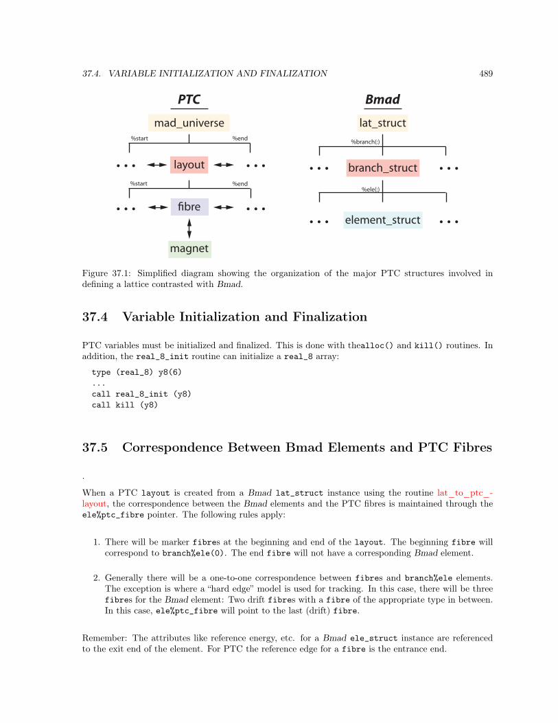
37.4. VARIABLE INITIALIZATION AND FINALIZATION 489

mad_universe

magnet

lat_struct

BmadPTC

fibre

layout branch_struct

element_struct

%start %end

%end%start

%branch(:)

%ele(:)

Figure 37.1: Simplified diagram showing the organization of the major PTC structures involved indefining a lattice contrasted with Bmad.

37.4 Variable Initialization and Finalization

PTC variables must be initialized and finalized. This is done with thealloc() and kill() routines. Inaddition, the real_8_init routine can initialize a real_8 array:

type (real_8) y8(6)...call real_8_init (y8)call kill (y8)

37.5 Correspondence Between Bmad Elements and PTC Fibres

.

When a PTC layout is created from a Bmad lat_struct instance using the routine lat_to_ptc_-layout, the correspondence between the Bmad elements and the PTC fibres is maintained through theele%ptc_fibre pointer. The following rules apply:

1. There will be marker fibres at the beginning and end of the layout. The beginning fibre willcorrespond to branch%ele(0). The end fibre will not have a corresponding Bmad element.

2. Generally there will be a one-to-one correspondence between fibres and branch%ele elements.The exception is where a “hard edge” model is used for tracking. In this case, there will be threefibres for the Bmad element: Two drift fibres with a fibre of the appropriate type in between.In this case, ele%ptc_fibre will point to the last (drift) fibre.

Remember: The attributes like reference energy, etc. for a Bmad ele_struct instance are referencedto the exit end of the element. For PTC the reference edge for a fibre is the entrance end.

490 CHAPTER 37. PTC/FPP PROGRAMMING

37.6 Taylor Maps

FPP stores its real_8 Taylor maps in such a way that it is not easy to access them directly to look atthe particular terms. To simplify life, Étienne has implemented the universal_taylorstructure:type universal_taylorinteger, pointer :: n ! Number of coefficientsinteger, pointer :: nv ! Number of variablesreal(dp), pointer :: c(:) ! Coefficients C(N)integer, pointer :: j(:,:) ! Exponents of each coefficients J(N,NV)

end type

Bmad always sets nv = 6. Bmad overloads the equal sign to call routines to convert between Étienne’sreal_8 Taylor maps and universal_taylor:type (real_8) tlr(6) ! Taylor maptype (universal_taylor) ut(6) ! Taylor map...tlr = ut ! Convert universal_taylor -> real_8ut = tlr ! Convert real_8 -> universal_taylor

37.7 Patches

There is a significant difference between how patches are treated in PTC and Bmad. In PTC, a patchis just though of as a coordinate transformation for propagating a particle from one fibre to the next.As such, the patch is part of a fibre. That is, any fibre representing tracking through quadrupoles,bends, etc. will have patches for the entrance and exit ends of the fibre.

With Bmad, on the other hand, a patch is a “first class” element on par with all other elements be theyquadrupoles, bends, etc. When translating a patch from Bmad to PTC, the patch is represented inPTC as a marker element with a patch at the exit end.

37.8 Number of Integration Steps & Integration Order

“Drift like” elements in PTC will use, by default, only one integration step. Bmad uses the default whentranslating from Bmad lattice elements to PTC fibres. The Bmad lattice elements that are drift like are:

driftecollimatorinstrumentmonitorpipercollimator

When tracking, there is a trade-off between step size and integrator order. Higher order means fewersteps are needed to get the same accuracy. But one higher order step is computationally more intensivethen one lower order step so what is the optimum order and number of steps is dependent upon variousfactors like magnet strength and how fast the field is varying. Generally, when the field is varying, suchas in a wiggler, lower order and more steps are favored. Also spin tracking is always 2nd order in PTC.So going to higher order for the orbital tracking with less steps will cause the spin tracking to be lessaccurate.

37.9. CREATING A PTC LAYOUT FROM A BMAD LATTICE 491

The way PTC “resplitting” routines work is that, for a given element, they start by assuming that thetracking will be done using a 2nd order integrator, They then compute the number of steps needed basedupon the electric and magnetic field strengths. This number is compared to a crossover limit point herenamed C1. If the number of steps is less than or equal to C1 then the resplitting routine stops andtracking will thereafter be done with a 2nd order integrator with the calculated number of steps. On theother hand, if the number of steps is greater than C1, the resplitting routine will redo the calculationassuming 4th order integration. With 4th order integration, the number of calculated steps will comparedto a different crossover limit point here called C2. Again, if the number of steps is less than or equalto C2, the routine will assign 4th order tracking to the element. Otherwise, the routine will assign 6thorder tracking to the element with an appropriate number of steps.

The default crossover limit points are

[C1, C2] = [30, 60] For wiggler type elements.[C1, C2] = [4, 18] For all other elements.

The greater number for wigglers is a reflection of the fact that the wiggler field is not constant.

37.9 Creating a PTC layout from a Bmad lattice

For a programmer, it is sometimes useful to feed a Bmad lattice into PTC and then use PTC for all thecalculations. As an example of how to do this, the following minimal program creates a PTC layoutfrom a Bmad lattice:use pointer_lattice, dummy => latuse ptc_layout_mod, dum1 => dpimplicit nonetype (lat_struct), target :: lattype(layout), pointer:: als!call bmad_parser (’lat.bmad’, lat)call lat_to_ptc_layout (lat, .true.)als => lat%branch(0)%ptc%m_t_layout

37.10 Internal_State

The internal_state structure looks like:type internal_state

integer totalpath ! total time or path length is usedlogical(lp) time ! Time is used instead of path lengthlogical(lp) radiation ! Radiation damping (but not excitation) is turned onlogical(lp) nocavity ! Cavity is turned into a driftlogical(lp) fringe ! fringe fields are turned on (mainly for quadrupoles)logical(lp) stochastic ! Random Stochastic kicks to x(5)logical(lp) envelope ! Stochastic envelope terms tracked in probe_8logical(lp) para_in ! If true, parameters in the map are includedlogical(lp) only_4d ! REAL_8 Taylor in (x,p_x,y,p_y)logical(lp) delta ! REAL_8 Taylor in (x,p_x,y,p_y,delta)logical(lp) spin ! Spin is trackedlogical(lp) modulation ! One modulated family tracked by probe

492 CHAPTER 37. PTC/FPP PROGRAMMING

logical(lp) only_2d ! REAL_8 Taylor in (x,p_x)logical(lp) full_way !

end type internal_state

Chapter 38

OPAL

OPAL (Object Oriented Parallel Accelerator Library) is a tool for charged-particle optic calculations inlarge accelerator structures and beam lines including 3D space charge. OPAL is built from first principlesas a parallel application, OPAL admits simulations of any scale: on the laptop and up to the largest HighPerformance Computing (HPC) clusters available today. Simulations, in particular HPC simulations,form the third pillar of science, complementing theory and experiment.

OPAL includes various beam line element descriptions and methods for single particle optics, namelymaps up to arbitrary order, symplectic integration schemes and lastly time integration. OPAL is basedon IPPL (Independent Parallel Particle Layer) which adds parallel capabilities. Main functions inheritedfrom IPPL are: structured rectangular grids, fields and parallel FFT and particles with the respectiveinterpolation operators. Other features are, expression templates and massive parallelism (up to 8000processors) which makes is possible to tackle the largest problems in the field.

The manual can be obtained atamas.web.psi.ch/docs/opal/

38.1 Phase Space

OPAL uses different longitudinal phase space coordinates compared to Bmad. Bmad’s phase spacecoordinates are

(x, px/p0, y, py/p0,−βc(t− t0), (p− p0)/p0) (38.1)

OPAL uses(x, γβx, y, γβy, z, γβz) (38.2)

convert_particle_coordinates_s_to_t and convert_particle_coordinates_s_to_t are conversionroutines . . .

493

494 CHAPTER 38. OPAL

Chapter 39

C++ Interface

To ease the task of using C++ routines with Bmad, there is a library called cpp_bmad_interface whichimplements a set of C++ classes in one–to–one correspondence with the major Bmad structures. Inaddition to the C++ classes, the Bmad library defines a set of conversion routines to transfer data valuesbetween the Bmad Fortran structures and the corresponding C++ classes.

The list of all classes is given in the filecpp_bmad_interface/include/cpp_bmad_classes.h

The general rule is that the equivalent class to a Bmad structure named xxx_struct will be namedCPP_xxx. Additionally, for each Bmad structure, there is a opaque class named Bmad_xxx_classfor use in the translation code discussed below. The names of these opaque classes have the formBmad_xxx_class and are used to define pointer instances in routine argument lists.

39.1 C++ Classes and Enums

Generally, The C++ classes have been set up to simply mirror the corresponding Bmad structures.For example, the CPP_lat class has a string component named .version that mirrors the %versioncomponent of the lat_struct structure. There are some exceptions. For example, structure componentsthat are part of PTC (§1.4) are not present in the classes.

While generally the same component name is used for both the Bmad structures and the C++ classes,in the case where there is a C++ reserved word conflict, the C++ component name will be different.

A header file bmad_enums.h defines corresponding Bmad parameters for all C++ routine. The Bmadparameters are in a namespace called Bmad. The convention is that the name of a corresponding C++ parameter is obtained by dropping the ending $ (if there is one) and converting to uppercase. Forexample, electron$ on the Fortran side converts to Bmad::ELECTRON in C++.

All of the C++ class components that are arrays or matrices are zero based so that, for example, theindex of the .vec[i] array in a CPP_coord runs from 0 through 5 and not 1 through 6 as on theFortran side. Notice that for a lat_struct the %ele(0:) component has a starting index of zeroso there is no off–by–one problem here. The exception to this rule is the %value(:) array of theele_struct which has a span from 1 to num_ele_attrib$. In this case, To keep the conversion of theof constructs like ele%value(k1$) consistant, the corresponding ele.value[] array has goes from 0 toBmad::NUM_ELE_ATTRIB with the 0th element being unused.

495

496 CHAPTER 39. C++ INTERFACE

1 subroutine f_test2 use bmad_cpp_convert_mod3 implicit none45 interface6 subroutine cpp_routine (f_lat, c_coord) bind(c)7 import f_lat, c_ptr8 type (lat_struct) :: f_lat9 type (c_ptr), value :: c_coord

10 end subroutine11 end interface1213 type (lat_struct), target :: lattice // lattice on Fortran side14 type (coord_struct), target :: orbit15 type (c_ptr), value :: c_lat16 ! ...17 call lat_to_c (c_loc(lattice), c_lat) ! Fortran side convert18 call cpp_routine (c_lat, c_loc(orbit)) ! Call C++ routine19 call lat_to_f (c_lat, c_loc(lattice)) ! And convert back20 end subroutine

Figure 39.1: Example Fortran routine calling a C++ routine.

1 #include "cpp_bmad_classes.h"23 using namespace Bmad;45 extern "C" cpp_routine (CPP_lat& c_lat, Bmad_coord_class* f_coord, f_lat) 6 CPP_coord c_coord;7 coord_to_c (f_coord, c_coord); // C++ side convert8 // ... do calculations ...9 cout << c_lat.name << " " << c_lat.ele[1].value[K1] << endl;

10 coord_to_f (c_coord, f_coord); // And convert back11

Figure 39.2: Example C++ routine callable from a Fortran routine.

39.2 Conversion Between Fortran and C++

A simple example of a Fortran routine calling a C++ routine is shown in Figs. 39.1 and 39.2. Conversionbetween structure and classes can happen on either the Fortran side or the C++ side. In this example,the lat_struct / CPP_lat conversion is on the Fortran side and the coord_struct / CPP_coord is onthe C++ side.

On the Fortran side, the interface block defines the argument list of the C++ routine being called.

On the C++ side, f_coord is an instance of the Bmad_coord_class opaque class.

A C++ routine calling a Fortran routine has a similar structure to the above example. The interfaceblock in Fig. 39.1 can be used as a prototype. For additional examples of conversion between Fortranand C++, look at the test code in the directory

39.2. CONVERSION BETWEEN FORTRAN AND C++ 497

cpp_bmad_interface/interface_test

498 CHAPTER 39. C++ INTERFACE

Chapter 40

Quick_Plot Plotting

Quick Plot is an interface layer to either the PGPLOT[PGPLOT] or PLPLOT[PLPLOT] plotting libraries.Whether PGPLOT or PLPLOT is used depends upon an environmental switch set when the Bmad libraryand other associated libraries are compiled (§28.2). [Note: Quick Plot lives in the sim_utils librarywhich comes with the Bmad distribution.] A quick reference guide can be seen online by using thecommand getf quick_plot. For identification in a program, all Quick Plot subroutines start with aqp_ prefix. Also, by convention, all PGPLOT subroutines start with a pg prefix.

499

500 CHAPTER 40. QUICK_PLOT PLOTTING

1 program example_plot2 use quick_plot3 integer id4 character(1) ans56 ! Generate PS and X-windows plots.7 call qp_open_page ("PS-L") ! Tell \quickplot to generate a PS file.8 call plot_it ! Generate the plot9 call qp_close_page ! quick_plot.ps is the file name

10 call qp_open_page ("X", id, 600.0_rp, 470.0_rp, "POINTS")11 call plot_it12 write (*, "(a)", advance = "NO") " Hit any class to end program: "13 accept "(a)", ans1415 !----------------------------------------------------------------------16 contains17 subroutine plot_it ! This generates the plot18 real(rp), allocatable :: x(:), y(:), z(:), t(:)19 real(rp) x_axis_min, x_axis_max, y_axis_min, y_axis_max20 integer x_places, x_divisions, y_places, y_divisions21 character(80) title22 logical err_flag23 namelist / parameters / title2425 ! Read in the data26 open (1, file = "plot.dat", status = "old")27 read (1, nml = parameters) ! read in the parameters.28 call qp_read_data (1, err_flag, x, 1, y, 3, z, 4, t, 5) ! read in the data.29 close (1)3031 ! Setup the margins and page border and draw the title32 call qp_set_page_border (0.01_rp, 0.02_rp, 0.2_rp, 0.2_rp, "%PAGE")33 call qp_set_margin (0.07_rp, 0.05_rp, 0.05_rp, 0.05_rp, "%PAGE")34 call qp_draw_text (title, 0.5_rp, 0.85_rp, "%PAGE", "CT")3536 ! draw the left graph37 call qp_set_box (1, 1, 2, 1)38 call qp_calc_and_set_axis ("X", minval(x), maxval(x), 4, 8, "ZERO_AT_END")39 call qp_calc_and_set_axis ("Y", minval(z), maxval(z), 4, 8, "GENERAL")40 call qp_draw_axes ("X\dlab\u", "\gb(\A)")41 call qp_draw_data (x, y, symbol_every = 0)4243 call qp_save_state (.true.)44 call qp_set_symbol_attrib (’times’, color = "blue", height = 20.0_rp)45 call qp_set_line_attrib ("PLOT", color = "blue", style = "dashed")46 call qp_draw_data (x, z, symbol_every = 5)47 call qp_restore_state4849 ! draw the right graph. "star5_filled" is a five pointed star.50 call qp_save_state (.true.)51 call qp_set_box (2, 1, 2, 1)52 call qp_set_graph_attrib (draw_grid = .false.)53 call qp_set_symbol_attrib (’star5_filled’, height = 10.0_rp)54 call qp_set_axis ("Y", -0.1_rp, 0.1_rp, 4, 2)55 call qp_set_axis (’Y2’, 1.0_rp, 100.0_rp, label = "Y2 axis", &56 draw_numbers = .true., ax_type = "LOG")57 call qp_draw_axes ("\m1 \m2 \m3 \m4 \m5 \m6 \m7", "\fsLY\fn", title = "That Darn Graph")58 call qp_draw_data (x, t, draw_line = .false., symbol_every = 4)59 call qp_restore_state60 end subroutine61 end program

Figure 40.1: Quick Plot example program.

40.1. AN EXAMPLE 501

Figure 40.2: Output of plot_example.f90.

40.1 An Example

An example of how Quick Plot can be used in a program is shown in Fig. 40.1. In the Bmad distributiona copy of this program is in the filesim_utils/plot_example/plot_example.f90

The plot_example.f90 program generates the figure shown in Fig. 40.2 from the input file namedplot.dat. The first few lines of the data file are&parameterstitle = "A Tale of Two Graphs"

/

Any junk here...

Col1 Col2 Col3 Col4 Col50 0.0000 0.1000 0.0000 -0.01251 0.0001 0.0995 0.0101 -0.01272 0.0004 0.0980 0.0203 -0.01303 0.0009 0.0955 0.0304 -0.0132...

The program first creates a PostScript file for printing on lines 7 through 9 and then makes an X–windows plot on lines 10 and 11. The write/accept lines 12 and 13 are to pause the program to preventthe X-window from immediately closing upon termination of the program.

The heart of the plotting is in the subroutine plot_it beginning on line 17. The namelist read on line27 shows how both parameters and data can be stored in the same file so that a plotting program canbe automatically told what the appropriate plot labels are. The qp_draw_text call on line 34 drawsthe title above the two graphs.

The qp_read_data call on line 28 will skip any “header” lines (lines that do not begin with somethingthat looks like a number) in the data file. In this instance qp_read_data will read the first, third forthand fifth data columns and put them into the x, y, z, and t arrays.

502 CHAPTER 40. QUICK_PLOT PLOTTING

qp_set_page_border, qp_set_box, and qp_set_margin sets where the graph is going to be placed.qp_set_box(1, 1, 2, 1) on line 37 tells Quick Plot to put the first graph in the left box of a 2 boxgrid. The qp_set_margin on line 33 sets the margins between the box and the graph axes.

qp_calc_and_set_axis on lines 38 and 39 are used to scale the axes. "ZERO_AT_END" ensures that thex–axis starts (or stops) at zero. qp_calc_and_set_axis is told to restrict the number of major divisionsto be between 4 and 8. For the horizontal axis, as can be seen in Fig. 40.2, it chooses 5 divisions.

After drawing the first data curve (the solid curve) in the left graph, the routines qp_set_symbol_attriband qp_set_line_attrib are called on lines 44 and 45 to plot the next data curve in blue with a dashedline style. By default, this curve goes where the last one did: in the left graph. To keep the setting of theline and symbol attributes from affecting other plots the routines qp_save_state and qp_restore_stateon lines 43 and 47 are used. qp_save_state saves the current attributes in an attribute stack. qp_-restore_state restores the saved attributes from the attribute stack. qp_draw_axes is called on line 40to draw the x and y-axes along, and qp_draw_data is called on lines 41 and 46 to draw the two datacurves.

Lines 50 through 60 draw the third curve in the right hand graph. The qp_set_axis call on lines 55/56sets a log scale for the y2 (right hand) axis. The syntax of the string arguments of qp_draw_axes in lines40 and 57/58 comes from PGPLOT and allows special symbols along with subscripts and superscripts.

40.2 Plotting Coordinates

Quick Plot uses the following concepts as shown in Fig. 40.3PAGE -- The entire drawing surface.BOX -- The area of the page that a graph is placed into.GRAPH -- The actual plotting area within the bounds of the axes.

In case you need to refer to the PGPLOT routines the correspondence between this and PGPLOT is:QUICK_PLOT PGPLOT---------- ------PAGE VIEW SURFACEBOX No corresponding entity.

x-axis

Page

Box

Box

Box

Graphy-axis

Figure 40.3: A Graph within a Box within a Page.

40.3. LENGTH AND POSITION UNITS 503

GRAPH VIEWPORT and WINDOWEssentially the VIEWPORT is the region outside of which lines and symbols will be clipped (if clippingis turned on) and the WINDOW defines the plot area. I’m not sure why PGPLOT makes a distinction,but VIEWPORT and WINDOW are always the same region.

qp_open_page determines the size of the page if it is settable (like for X–windows). The page is dividedup into a grid of boxes. For example, in Fig. 40.3, the grid is 1 box wide by 3 boxes tall. The borderbetween the grid of boxes and the edges of the page are set by qp_set_page_border. The box thatthe graph falls into is set by qp_set_box. The default is to have no margins with 1 box covering theentire page. The qp_set_margin routine sets the distance between the box edges and the axes (See thePGPLOT manual for more details).

40.3 Length and Position Units

Typically there is an optional units argument for Quick Plot routines that have length and/or positionarguments. For example, using getf one can see that the arguments for qp_draw_rectangle areSubroutine qp_draw_rectangle (x1, x2, y1, y2, units, color, width, style, clip)

The units argument is a character string which is divided into three parts. The syntax of the unitsargument isunit_type/ref_object/corner

The first part unit_type gives the type of units"%" -- Percent."DATA" -- Data units. (Draw default)"MM" -- millimeters."INCH" -- Inches. (Set default)"POINTS" -- Printers points. NOT PIXELS. (72 points = 1 inch).

Note: For displays with a resolution of 72 pixels / inch, POINTS corresponds to pixels but many displayshave a higher resolution. The second and third parts give the reference point for a position. The secondpart specifies the reference object

"PAGE" -- Relative to the page (Set default)."BOX" -- Relative to the box."GRAPH" -- Relative to the graph (Draw default).

The third part gives corner of the reference object that is the reference point"LB" -- Left Bottom (Set and Draw default)."LT" -- Left Top."RB" -- Right Bottom."RT" -- Right Top.

Notes:

• The DATA unit type, by definition, always uses the lower left corner of the GRAPH as a referencepoint.

• For the % unit_type the / between unit_type and ref_object can be omitted.

• If the corner is specified then the ref_object must appear also.

• Everything must be in upper case.

• For some routines (qp_set_margin, etc.) only a relative distance is needed. In this case theref_object/corner part, if present, is ignored.

504 CHAPTER 40. QUICK_PLOT PLOTTING

• The units argument is typically an optional argument. If not present the default units will beused. There are actually two defaults: The draw default is used for drawing text, symbols, orwhatever. The set default is used for setting margins, and other lengths. Initially the draw defaultis DATA/GRAPH/LB and the set default is INCH/PAGE/LB. Use qp_set_parameters to change this.

Examples:"DATA" -- This is the draw default."DATA/GRAPH/LB" -- Same as above."DATA/BOX/RT" -- ILLEGAL: DATA must always go with GRAPH/LB."%PAGE/LT" -- Percentage of page so (0.0, 1.0) = RT of page."%BOX" -- Percentage of box so (1.0, 1.0) = RT of box."INCH/PAGE" -- Inches from LB of page.

40.4 Y2 and X2 axes

The top and right axes of a graph are known as X2 and Y2 respectively as shown in Fig. 40.3. Normallythe X2 axis mirrors the X axis and the Y2 axis mirrors the Y axis in that the tick marks and axis numberingfor the X2 and Y2 axes are the same as the X and Y axes respectively. qp_set_axis can be used to disablemirroring. For example:call qp_set_axis ("Y2", mirror = .false.) ! y2-axis now independent of y.

qp_set_axis can also be used to set Y2 axis parameters (axis minimum, maximum, etc.) and settingthe Y2 or X2 axis minimum or maximum will, by default, turn off mirroring.

Note that the default is for the X2 and Y2 axis numbering not to be shown. To enable or disable axisnumbering again use qp_set_axis. For example:call qp_set_axis ("Y2", draw_numbers = .true.) ! draw y2 axis numbers

To plot data using the X2 or Y2 scale use the qp_use_axis routine. For example:call qp_save_state (.true.)call qp_use_axis (y = "Y2")! ... Do some data plotting here ...call qp_restore_state

40.5 Text

PGPLOT defines certain escape sequences that can be used in text strings to draw Greek letters, etc.These escape sequences are given in Table 40.2.

PGPLOT defines a text background index:-1 - Transparent background.0 - Erase underlying graphics before drawing text.

1 to 255 - Opaque with the number specifying the color index.

40.6 Styles

Symbolic constants have been defined for Quick Plot subroutine arguments that are used to choosevarious styles. As an example of this is in lines 44 and 45 of Fig. 40.1. The numbers in the following arethe PGPLOT equivalents.

The Quick Plot line styles are:

40.6. STYLES 505

PGPlot

PLPlot

Figure 40.4: Continuous colors using the function pg_continuous_color in PGPlot and PLPlot. Typicalusage: call qp_routine(..., color = pg_continuous_color(0.25_rp), ...)

1 -- solid$ Solid2 -- dashed$ Dashed3 -- dash_dot$ Dash--dot4 -- dotted$ Dotted5 -- dash_dot3$ Dash--dot--dot--dot

The color styles in Quick Plot are:0 -- White$ (actually the background color)1 -- Black$ (actually the foreground color)2 -- Red$3 -- Green$4 -- Blue$5 -- Cyan$6 -- Magenta$7 -- Yellow$8 -- Orange$9 -- Yellow_Green$10 -- Light_Green$11 -- Navy_Blue$12 -- Purple$13 -- Reddish_Purple$14 -- Dark_Grey$15 -- Light_Grey$

Integers from [17, (largest integer)] represent continuous colors. The function pq_continuous_colormaps [0.0, 1.0] to these integers. See Fig. 40.4.

The fill styles are:1 -- solid_fill$2 -- no_fill$3 -- hatched$4 -- cross_hatched$

The symbol types are:0 -- square_sym$1 -- dot_sym$2 -- plus_sym$3 -- times_sym$4 -- circle_sym$5 -- x_sym$7 -- triangle_sym$8 -- circle_plus_sym$

506 CHAPTER 40. QUICK_PLOT PLOTTING

9 -- circle_dot_sym$10 -- square_concave_sym$11 -- diamond_sym$12 -- star5_sym$13 -- triangle_filled_sym$14 -- red_cross_sym$15 -- star_of_david_sym$16 -- square_filled_sym$17 -- circle_filled_sym$18 -- star5_filled_sym$

Beside this list, PGPLOT maps other numbers onto symbol types. The PGPLOT list of symbols is:-3 ... -31 - a regular polygon with abs(type) edges.

-2 - Same as -1.-1 - Dot with diameter = current line width.

0 ... 31 - Standard marker symbols.32 ... 127 - ASCII characters (in the current font).

E.G. to use letter F as a marker, set type = ICHAR("F").> 127 - A Hershey symbol number.

Table 40.1 shows some of the symbols and there associated numbers. Note: At constant height PGPLOTgives symbols of different size. To partially overcome this, Quick Plot scales some of the symbols to givea more uniform appearance. Table 40.1 was generated using a height of 40 via the callcall qp_draw_symbol (0.5_rp, 0.5_rp, "%BOX", k, height = 40.0_rp)

Table 40.3 shows how the character string "\g<r>", where "<r>" is a Roman letter, map onto the Greekcharacter set.

40.6. STYLES 507

Table 40.1: Plotting Symbols at Height = 40.0

508 CHAPTER 40. QUICK_PLOT PLOTTING

\u Start a superscript or end a subscript\d Start a subscript or end a superscript. \u and \d must always be used in pairs\b Backspace (i.e., do not advance text pointer after plotting the previous character)\fn Switch to Normal font (1)\fr Switch to Roman font (2)\fi Switch to Italic font (3)\fs Switch to Script font (4)\\ Backslash character (\)\x Multiplication sign (×)\. Centered dot (·)\A Angstrom symbol (Å)\gx Greek letter corresponding to roman letter x\mn \mnn Graph marker number n or nn (1-31)

\(nnnn)Character number nnnn (1 to 4 decimal digits) from the Hershey character set;the closing parenthesis may be omitted if the next character is neither a digitnor “)”. This makes a number of special characters (e.g., mathematical, musical,astronomical, and cartographical symbols) available.

Table 40.2: PGPLOT Escape Sequences.

Roman

Greek

Roman

Greek

Roman

Greek

Roman

Greek

Table 40.3: Conversion for the string "\g<r>" where "<r>" is a Roman character to the correspondingGreek character.

40.7. STRUCTURES 509

40.7 Structures

Quick Plot uses several structures to hold data. The structure that defines a line is a qp_line_structtype qp_line_structinteger width ! Line width. Default = 1character(16) color ! Line color. Default = "black"character(16) style ! Line style. Default = "solid"

end type

The qp_symbol_struct defines how symbols are drawntype qp_symbol_structcharacter(16) type ! Default = "circle_dot"real(rp) height ! Default = 6.0 (points)character(16) color ! Default = "black"character(16) fill ! Default = "solid_fill"integer line_width ! Default = 1

end type

The qp_axis_struct defines how axes are drawntype qp_axis_structcharacter(80) label ! Axis label.real(rp) min ! Axis range left/bottom number.real(rp) max ! Axis range right/top number.real(rp) number_offset ! Offset in inches of numbering from the axis line.

! Default = 0.05real(rp) label_offset ! Offset in inches of the label from the numbering.

! Default = 0.05character(16) label_color ! Default = "black"real(rp) major_tick_len ! Length of the major ticks in inches. Def = 0.10real(rp) minor_tick_len ! Length of the minor ticks in inches. Def = 0.06integer major_div ! Number of major divisions. Default = 5integer major_div_nominal ! Nominal value. Def = 5.integer minor_div ! Number of minor divisions. 0 = auto-choose. Default = 0integer minor_div_max ! Maximum number for auto choose. Default = 5integer places ! Places after the decimal point. Default = 0character(16) type ! "LINEAR" (default), "LOG", or "CUSTOM".character(16) bounds ! "GENERAL" (default), "ZERO_AT_END", etc.integer tick_side ! +1 = draw to the inside (def), 0 = both, -1 = outside.integer number_side ! +1 = draw to the inside, -1 = outside (default).logical draw_label ! Draw the label? Default = True.logical draw_numbers ! Draw the numbering? Default = True.

end type

The %bounds parameter sets how axis min and max values are calculated. Possible settings are:"ZERO_AT_END" ! Min or max value is set to zero."ZERO_SYMMETRIC" ! Min and max chosen so that max = -min."GENERAL" ! No restrictions."EXACT" ! The inputted data min/max is used.

Finally, the qp_plot_struct is a container for the axis that make up a plottype qp_plot_structcharacter(80) :: title = " "type (qp_axis_struct) x, y, x2, y2

510 CHAPTER 40. QUICK_PLOT PLOTTING

type (qp_axis_struct), pointer :: xx, yy ! Pointer to axes used for plotting.logical :: draw_box = .true.logical :: draw_title = .true.logical :: draw_grid = .true.logical :: x2_mirrors_x = .true.logical :: y2_mirrors_y = .true.logical :: xx_points_to_xlogical :: yy_points_to_y

end type

Chapter 41

HDF5

HDF5, which stands for “Hierarchical Data Format” version 5[HDF5], is a set of file formats designed tostore and organize large amounts of data. HDF5 has been developed by scientists from a number ofinstitutions including the National Center for Supercomputing Applications, the University of Illinoisat Urbana-Champaign, and Sandia National Laboratories. Tools for viewing and editing HDF5 files areavailable from the HDF Group[HDF5]. Programs include h5dump and HDFView which can be used todirectly view files. Interfaces so that HDF5 files can accessed via Java or Python also exist.

Bmad uses HDF5 for storing beam particle (positions, spin, etc.) and grid_field (§5.15.4 data. Storagedetails are given in sections §41.1 and §41.2 respectively. While HDF5 defines how data is formatted, HDF5does not define the syntax for how data is to be stored. For that, Bmad uses the syntax defined by theBeam Physics extension to the openPMD standard[openPMD]. To understand the rest of this chapter,the reader should familiarize themselves with the openPMD and Beam Physics standards.

41.1 HDF5 Particle Beam Data Storage

The code for reading and writing beam data to/from HDF5 files is contained in the routines hdf5_-read_beam and hdf5_write_beam.

As per the openPMD/Beam Physics standard, particle beam data is stored in a tree structure within adata file. The root “group” (tree node) for each bunch of the beam has the path within the file:/data/%T/particles/

where %T is an integer.

For any bunch, parameters (“attributes”) stored in the bunch root group are:speciesType ! The name of the particle species using the SpeciesType syntax.totalCharge ! Total bunch charge.chargeLive ! Charge of live particles.numParticles ! Number of particles.

The SpeciesType syntax defined by the SpeciesType extension to the openPMD standard is similar tothe Bmad standard (§9.1) but there are differences. For one, the SpeciesType standard does not havean encoding for the charge state of atoms and molecules. Another difference is that for fundamentalparticles the names are case sensitive while for Bmad they are not (Note that atom and molecule namesin Bmad are case sensitive).

511

512 CHAPTER 41. HDF5

What per-particle data is stored is determined by whether the bunch particles are photons or not. Thefollowing particle parameters are common for both types:

Beam Physics Parameter Bmad Equivalent Notes

time -%vec(5) / (c %beta) time - ref_time. See Eq. (15.28)timeOffset %t - time reference timetotalMomentumOffset %p0csPosition %s See Fig. 15.2weight %charge Macro bunch chargebranchIndex %ix_branchelementIndex %ix_elelocationInElement %location See belowparticleStatus %state See the %state table in §35.1

The Bmad Equivalent column gives the conversion between the Beam Physics parameters and thecoord_struct (§35.1) structure components (the coord_struct structure contains the particle positioninformation). Parameters with a “%” suffix are coord_struct components and %vec(5) corresponds tothe phase space z coordinate. The particleState is an integer which corresponds to the coord_struct%state component. A value of 1 indicates that the particle is alive (corresponding to the value ofalive$) and any other value indicates that the particle is dead.

The locationInElement Beam Physics parameter is related to the coord_struct %location parametervia the following transformation:

locationInElement Value %location Value

-1 upstream_end$0 inside$1 downstream_end$

For photons, additional per-particle data is:

Beam Physics Parameter Bmad Equivalent

velocity/x, y, z (%vx, %vy, %vz)position/x, y, z (%x, %y, %z)pathLength %path_lenphotonPolarizationAmplitude/x, y %fieldphotonPolarizationPhase/x, y %phase

For clarity’s sake, the %vec(1) through %vec(6) phase space coordinate components in the coord_structhave been replaced by %x, %vx, . . ., %z, %vz in the above table

For non-photons, additional per-particle data is:

Beam Physics Parameter Bmad Equivalent

momentum/x, y, z %p0c×(%px, %py, sqrt((1 + %pz)2 - %px2 - %py2))totalMomentum %p0c×%pzposition/x, y, z (%x, %y, 0)spin/x, y, z %spinchargeState Derived from %species

41.2. HDF5 GRID_FIELD DATA STORAGE 513

For clarity’s sake, the %vec(1) through %vec(6) phase space coordinate components in the coord_structhave been replaced by %x, %px, . . ., %z, %pz in the above table. Notice that the Beam Physics z position(not to be confused with phase space z) is always zero by construction as shown in Fig. 15.2.

41.2 HDF5 Grid_Field Data Storage

The code for reading and writing grid_field data to/from HDF5 files is contained in the routineshdf5_read_grid_field and hdf5_write_grid_field.

As per the openPMD/Beam Physics standard, grid_field (§5.15.4 data is stored in a tree structurewithin a data file. The root “group” (tree node) for each grid_field has the path within the file:/ExernalFieldmesh/%T/

where %T is an integer.

For any grid_field, parameters stored in the grid_field root group are:

Parameter in File Bmad Equivalent

gridGeometry %geometrymasterParameter %master_parametercomponentFieldScale %field_scale

fieldScaleß

%field_scale×master param value If master parameter set.%field_scale Otherwise.

harmonic %harmonic

RFphaseß

%harmonic×%phi0_fieldmap For lcavity elements%harmonic×(0.25 - %phi0_fieldmap) For all others.

eleAnchorPt %ele_anchor_ptgridOriginOffset %r0gridSpacing %drinterpolationOrder %interpolation_ordergridLowerBound %ptr%pt lower boundgridSize %ptr%pt sizefundamentalFrequency elegridCurvatureRadius ele

The Bmad Equivalent column gives the conversion between the Beam Physics parameters and thegrid_field_struct structure components (that have a “%” prefix). The value for gridCurvatureRadiusis set to the value of rho of the associated lattice element if %curved_ref_frame is True.

Notice that the masterParameter attribute is not part of the standard. If not present, which couldhappen if a file is created by non-Bmad code, the default is a blank string indicating no master parameter.If masterParameter is set in the data file, there is a potential problem in that it may not be possibleto calculate %field_scale if the value of the master parameter is not equal to the value when the datawas written. To get around this, if the non-standard masterParameter is present, the value of the non-standard componentFieldScale (which has a default value of one) will be used to set %field_scale andthe fieldScale parameter will be ignored. If masterParameter is not present, componentFieldScaleis ignored and %field_scale is set from the value of fieldScale.

When reading a data file, the setting of grid_field%field_type is determined by what data is storedin the file. If both electric and magnetic field data is present, %field_type is set to mixed$. Otherwise,%field_type is set to magnetic$ if magnetic field data is present or electric$ if electric field data ispresent.

514 CHAPTER 41. HDF5

The correspondence between the gridGeometry parameter and the grid_field%geometry componentis

gridGeometry Value %geometry Value

"rectangular" xyz$"cylindrical" rotationally_symmetric_rz$

Chapter 42

Helper Routines

This chapter gives an overview of various computational helper routines.

42.1 Nonlinear Optimization

Nonlinear optimization is the process of finding a minimum (or maximum) of a nonlinear function (the"merit" function). Nonlinear optimization is frequently used for lattice design or matching of data to amodel. For more information on this see the Tao manual.

In terms of routines for implementing nonlinear optimization the Numerical Recipes library (§28.2 thatis distributed along with Bmad contains several. In particular, the routine super_mrqmin which im-plements the Levenberg–Marquardt is an excellent routine for finding local minimum when the meritfunction can be expressed as the sum of quadratic terms. Another routine, frprmn, which is an imple-mentation of the Fletcher–Reeves algorithm, is also good at finding local minimum and has the advantagethat as input it does not need a derivative matrix as does Levenberg–Marquardt. The disadvantage ofFletcher–Reeves is that it is slower than Levenberg–Marquardt.

A second implementation of Levenberg–Marquardt available with Bmad is opti_lmdif which is Fortran90version of the popular lmdif routine. Also available is opti_de which implements the DifferentialEvolution algorithm of Storn and Price[Storn96]. This routine is good for finding global minima but canbe slow.

Another routine that should be mentioned is the amoeba routine from Numerical Recipes that implementsthe downhill simplex method of Neider and Mead. This routine is robust but slow but is easily parallelizedso it is a good routine for parallel processing.

42.2 Matrix Manipulation

There are a number of Bmad routines for matrix manipulation as listed in §43.24. In fact, Fortran90 hasa number of intrinsic matrix routines as well but this is outside the scope of this manual. The followingexample shows some of the Bmad matrix routines mat_inverse and mat_make_unit.real(rp) mat(6,6), mat_inv(6,6)call mat_make_unit (mat) ! make a unit matrixcall mat_inverse (mat, mat_inv) ! Compute the inverse matrix.

515

516 CHAPTER 42. HELPER ROUTINES

Chapter 43

Bmad Library Routine List

Below are a list of Bmad and sim_utils routines sorted by their functionality. Use the getf and listf(§28.3) scripts for more information on individual routines. This list includes low level routines thatare not generally used in writing code for a program but may be useful in certain unique situations.Excluded from the list are very low level routines that are solely meant for Bmad internal use.

517

518 CHAPTER 43. BMAD LIBRARY ROUTINE LIST

Routine Type Section

Beam: Low Level Routines 43.1Beam: Tracking and Manipulation 43.2Branch Handling 43.3Coherent Synchrotron Radiation (CSR) 43.4Collective Effects 43.5Custom and Hook Routines 43.6Electro-Magnetic Fields 43.7HDF Read/Write 43.8Helper Routines: File, System, and IO 43.9Helper Routines: Math (Except Matrix) 43.10Helper Routines: Matrix 43.11Helper Routines: Miscellaneous 43.12Helper Routines: String Manipulation 43.13Helper Routines: Switch to Name 43.14Inter-Beam Scattering (IBS) 43.15Lattice: Informational 43.18Lattice: Element Manipulation 43.16Lattice: Geometry 43.17Lattice: Low Level Stuff 43.19Lattice: Manipulation 43.20Lattice: Miscellaneous 43.21Lattice: Nametable 43.22Lattice: Reading and Writing Files 43.23Matrices 43.24Matrix: Low Level Routines 43.25Measurement Simulation Routines 43.26Multipass 43.27Multipoles 43.28Optimizers (Nonlinear) 43.29Overload Equal Sign 43.30Particle Coordinate Stuff 43.31Photon Routines 43.32PTC Interface 43.33Quick Plot 43.34Spin 43.35Transfer Maps: Routines Called by make_mat6 43.36Transfer Maps: Complex Taylor Maps 43.37Transfer Maps: Taylor Maps 43.38Transfer Maps: Driving Terms 43.39Tracking: Tracking and Closed Orbit 43.40Tracking: Low Level Routines 43.41Tracking: Mad Routines 43.42Tracking: Routines Called by track1 43.40Twiss and Other Calculations 43.44Twiss: 6-Dimensional 43.45Wakefields 43.46C/C++ Interface 43.47

43.1. BEAM: LOW LEVEL ROUTINES 519

43.1 Beam: Low Level Routines

The following helper routines are generally not useful for general use.

bend_edge_kick (ele, param, particle_at, orb, mat6, make_matrix, track_spin)Subroutine to track through the edge field of an sbend. Reverse tracking starts with the particlejust outside the bend and

init_spin_distribution (beam_init, bunch)Initializes a spin distribution according to init_beam%spin

order_particles_in_z (bunch)Routine to order the particles longitudinally in terms of decreasing %vec(5). That is from large z(head of bunch) to small z.

track1_bunch (bunch_start, lat, ele, bunch_end, err, centroid, direction)Routine to track a bunch of particles through an element.

track1_bunch_hom (bunch_start, ele, param, bunch_end, direction)Routine to track a bunch of particles through an element.

43.2 Beam: Tracking and Manipulation

See §35.16 for a discussion of using a collection of particles to simulate a bunch.

bbi_kick (x_norm, y_norm, r, kx, ky)Routine to compute the normalized kick due to the beam-beam interaction using the normalizedposition for input.

calc_bunch_params (bunch, bunch_params, error, print_err)Finds all bunch parameters defined in bunch_params_struct, both normal-mode and projected

calc_bunch_params (bunch, bunch_params, plane, slice_center,slice_spread, err, print_err)

Finds all bunch parameters for a slice through the beam distribution.

init_beam_distribution (ele, param, beam_init, beam, err_flag, modes)Routine to initialize a distribution of particles matched to the Twiss parameters, centroid position,and Energy - z correlation

init_bunch_distribution (ele, param, beam_init, ix_bunch, bunch, err_flag, modes)Routine to initialize either a random or tail-weighted distribution of particles.

reallocate_beam (beam, n_bunch, n_particle, save)Routine to reallocate memory within a beam_struct.

reallocate_bunch (bunch, n_particle)Subroutine to reallocate particles within a bunch_struct.

track_beam (lat, beam, ele1, ele2, err, centroid, direction)Routine to track a beam of particles from the end of lat%ele(ix1) Through to the end of lat%ele(ix2).

520 CHAPTER 43. BMAD LIBRARY ROUTINE LIST

43.3 Branch Handling Routines

allocate_branch_array (lat, upper_bound)Routine to allocate or re-allocate an branch array. The old information is saved.

transfer_branch (branch1, branch2)Routine to set branch2 = branch1. This is a plain transfer of information not using the overloadedequal.

transfer_branches (branch1, branch2)Routine to set branch2 = branch1. This is a plain transfer of information not using the overloadedequal.

43.4 Coherent Synchrotron Radiation (CSR)

csr_bin_particles (ele, particle, bin)Routine to bin the particles longitudinally in s.

csr_bin_kicks (lat, ele, s_travel, bin, small_angle_approx)Routine to cache intermediate values needed for the csr calculations.

csr_kick_calc (ele, bin, particle)Routine to calculate the longitudinal coherent synchrotron radiation kick.

i_csr (kick1, i_bin, k_factor, bin) result (i_this)Routine to calculate the CSR kick integral.

z_calc_csr (d, k_factor, bin, small_angle_approx, dz_dd) result (z_this)Routine to calculate the distance between the source particle and the kicked particle.

d_calc_csr (dz_particles, k_factor, bin, small_angle_approx) result (d_this)Routine to calculate the distance between source and kick points.

43.5 Collective Effects

touschek_lifetime (mode, Tl, lat)Routine to calculate the Touschek lifetime for a lat.

43.6 Custom Routines

apply_element_edge_kick_hook (orb, fringe_info, track_ele, param,finished, mat6, make_matrix, rf_time)

Routine that can be customized to track through the edge field of an element. This routine isalways called by apply_element_edge_kick.

check_aperture_limit_custom (orb, ele, particle_at, param, err_flag)Routine to check if an orbit is outside an element’s aperture. Used when ele%aperture_type isset to custom$

43.7. ELECTRO-MAGNETIC FIELDS 521

ele_geometry_hook (floor0, ele, floor, finished, len_scale)Routine that can be customized to calculate the floor position of an element.

ele_to_fibre_hook (ele, ptc_fibre, param)Routine that can be customized for creating a PTC fibre from a Bmad element. This routine isalways called by ele_to_fibre.

em_field_custom(ele, param, s_rel, orbit, local_ref_frame, field,calc_dfield, err_flag, calc_potential, use_overlap,grid_allow_s_out_of_bounds, rf_time, used_eles)

Custom routine for calculating fields.

init_custom (ele, err_flag)Routine for initializing custom elements or elements that do custom calculations.

make_mat6_custom (ele, param, start_orb, end_orb, err_flag)Routine for custom calculations of the 6x6 transfer matrices.

radiation_integrals_custom (lat, ir, orb, rad_int1, err_flag)User supplied routine to calculate the synchrotron radiation integrals for a custom element.

time_runge_kutta_periodic_kick_hook (orbit, dt_ref, ele, param, stop_time, init_needed)

Custom routine to add a kick to a particle at periodic times.

track1_bunch_hook (bunch_start, lat, ele, bunch_end, err, centroid, direction, finished)

Routine that can be customized for tracking a bunch through a single element.

track1_custom (start_orb, ele, param, end_orb, err_flag, finished, track)Dummy routine for custom tracking.

track1_postprocess (start_orb, ele, param, end_orb)Dummy routine for post processing after the track1 routine is done.

track1_preprocess (start_orb, ele, param, err_flag, finished, radiation_included, track)Dummy routine for pre processing at the start of the track1 routine.

track1_spin_custom (start, ele, param, end, err_flag, make_quaternion)Dummy routine for custom spin tracking. This routine needs to be replaced for a custom calcula-tion.

track1_wake_hook (bunch, ele, finished)Routine that can be customized for tracking through a wake.

wall_hit_handler_custom (orb, ele, s)This routine is called by the Runge-Kutta integrator odeint_bmad when a particle hits a wall.

43.7 Electro-Magnetic Fields

em_field_calc (ele, param, s_pos, orbit, local_ref_frame, field, calc_dfield, err_flag,calc_potential, use_overlap, grid_allow_s_out_of_bounds, rf_time,

used_eles,err_print_out_of_bounds)

Routine to calculate the E and B fields for an element.

522 CHAPTER 43. BMAD LIBRARY ROUTINE LIST

em_field_custom(orbit, ele, param, s1_body, s2_body, err_flag, track, mat6, make_-matrix)

Custom routine for calculating fields.

43.8 HDF Read/Write

hdf5_write_attribute_string(root_id, attrib_name, string, error)Routine to create an HDF5 attribute whose value is a string.

hdf5_open_file (file_name, action, file_id, error)Routine to open an HDF5 file.

hdf5_open_object(root_id, object_name, info, error, print_error) result (obj_id)Routine to open an existing group or dataset.

hdf5_close_object(obj_id, info)Routine to close a group or dataset.

hdf5_exists (root_id, object_name, error, print_error) result (exists)Routine to check if a object with object_name exists relative to root_id.

hdf5_open_group (root_id, group_name, error, print_error) result (g_id)Routine to open an existing group.

hdf5_open_dataset(root_id, dataset_name, error, print_error) result (obj_id)Routine to open an existing group or dataset.

hdf5_num_attributes(root_id) result (num)Routine to return the number of attributes associated with a group or dataset.

hdf5_get_attribute_by_index(root_id, attrib_indx, attrib_id, attrib_name)Routine to return the ID and name of an attribute given the attribute’s index number. This routineis useful for looping over all the attributes in a group or dataset.

hdf5_attribute_info(root_id, attrib_name, error, print_error) result (info)Routine to return information on an attribute given the attribute name and encompassing group.

hdf5_object_info (root_id, obj_name, error, print_error) result (info)Routine to get information on an object (group or dataset).

hdf5_read_attribute_int(root_id, attrib_name, attrib_value, error, print_error, dflt_value)

Routine to read a integer attribute value or array.

hdf5_read_attribute_real(root_id, attrib_name, attrib_value, error, print_error, dflt_value)

Routine to read a real attribute value or array.

hdf5_read_attribute_alloc_string(root_id, attrib_name, string, error, print_error)Routine to read a string attribute. Also see: hdf5_read_attribute_string

hdf5_read_attribute_string(root_id, attrib_name, string, error, print_error)Routine to read a string attribute. Also see: hdf5_read_attribute_alloc_string

43.9. HELPER ROUTINES: FILE, SYSTEM, AND IO 523

hdf5_write_dataset_real(root_id, dataset_name, value, error)Routine to create a dataset of reals.

hdf5_write_dataset_int(root_id, dataset_name, value, error)Routine to create a dataset of integers.

hdf5_read_beam (file_name, beam, error, ele, pmd_header)Routine to read a beam data file.

hdf5_write_grid_field (file_name, ele, g_field, err_flag)Routine to create an hdf5 file encoding an array of grid_field structures. Note: Conventionally,the file name should have an ".h5" suffix.

pmd_write_int_to_dataset (root_id, dataset_name, bmad_name, unit, array, error)

pmd_write_int_to_pseudo_dataset(root_id, dataset_name, bmad_name, unit, value, v_shape, error)

pmd_write_real_to_dataset (root_id, dataset_name, bmad_name, unit, array, error)

pmd_write_real_to_pseudo_dataset (root_id, dataset_name, bmad_name, unit, value, v_shape, error)

pmd_write_complex_to_dataset (root_id, dataset_name, bmad_name, unit, array, error)

pmd_write_units_to_dataset (root_id, dataset_name, bmad_name, unit, error)

pmd_read_int_dataset (root_id, name, conversion_factor, array, error)

pmd_read_real_dataset (root_id, name, conversion_factor, array, error)

pmd_read_complex_dataset (root_id, name, conversion_factor, array, error)

hdf5_read_grid_field (file_name, ele, g_field, err_flag, pmd_header, combine)Routine to read an hdf5 file that encodes an array of grid_field structures.

hdf5_write_beam (file_name, bunches, append, error, lat)Routine to write particle positions of a beam to an HDF5 binary file.

43.9 Helper Routines: File, System, and IO

append_subdirectory (dir, sub_dir, dir_out, err)Routine to combine a directory specification with a subdirectory specification to form a completedirectory

524 CHAPTER 43. BMAD LIBRARY ROUTINE LIST

cesr_iargc ()Platform independent function to return the number of command line arguments. Use this withcesr_getarg.

cesr_getarg (i_arg, arg)Platform independent function to return the i’th command line argument. Use this with cesr_iargc.

dir_close ()Routine to close a directory that was opened with dir_open. Also see dir_read.

dir_open (dir_name) result (opened)Routine to open a directory to obtain a list of its files. Use this routine with dir_read and dir_close.

dir_read (file_name) result (valid)Routine to get the names of the files in a directory. Use this routine with dir_open and dir_close.

file_suffixer (in_file_name, out_file_name, suffix, add_switch)Routine to add/replace a suffix to a file name.

get_tty_char (this_char, wait, flush)Routine for getting a single character from the terminal. Also see: get_a_char

get_a_char (this_char, wait, ignore_this)Routine for getting a single character from the terminal. Also see: get_tty_char

get_file_time_stamp (file, time_stamp)Routine to get the "last modified" time stamp for a file.

lunget()Function to return a free file unit number to be used with an open statement.

milli_sleep (milli_sec)Routine to pause the program for a given number of milli-seconds.

out_io (...)Routine to print to the terminal for command line type programs. The idea is that for programswith a gui this routine can be easily replaced with another routine.

out_io_called (level, routine_name)Dummy routine for linker. See out_io for more details.

out_io_end ()Dummy routine for linker. See out_io for more details.

out_io_line (line)Dummy routine for linker. See out_io for more details.

output_direct (file_unit, print_and_capture, min_level, max_level, set, get)Routine to set where the output goes when out_io is called. Output may be sent to the terminalscreen, written to a file, or both. Also can be used to restrict output verbosity.

read_a_line (prompt, line_out, trim_prompt, prompt_color, prompt_bold, history_file)

Routine to read a line of input from the terminal. The line is also add to the history bufferso that the up-arrow

43.10. HELPER ROUTINES: MATH (EXCEPT MATRIX) 525

skip_header (ix_unit, error_flag)Routine to find the first line of data in a file.

splitfilename(filename, path, basename, is_relative) result (ix_char)Routine to take filename and splits it into its constituent parts, the directory path and the basefile name.

system_command (line, err_flag)Routine to execute an operating system command from within the program.

type_this_file (filename)Routine to type out a file to the screen.

43.10 Helper Routines: Math (Except Matrix)

complex_error_function (wr, wi, zr, zi)This routine evaluates the function w(z) in the first quadrant of the complex plane.

cross_product (a, b)Returns the cross product of a x b

find_indexx0 (name, var_str_index, ix_match, ix2_match, add_to_list, n_match, has_been_added)

Subroutine to find a matching name in a list of names. This name is overloaded by find_indexx.

find_indexx1 (name, nametable, ix_match, ix2_match, add_to_list, n_match, has_been_added)

Subroutine to find a matching name in a list of names. This name is overloaded by find_indexx.

find_indexx2 (name, names, an_indexx, n_max, ix_match, ix2_match, add_to_list, n_match, has_been_added)

Subroutine to find a matching name in a list of names. This name is overloaded by find_indexx.

find_indexx3 (name, names, n_min, an_indexx, n_max, ix_match, ix2_match, add_to_list, n_match, has_been_added)

Subroutine to find a matching name in a list of names. This name is overloaded by find_indexx.

indexx_str (str_arr, indx_arr)Subroutine to sort a character array. This subroutine is used to overload the generic name indexx.

indexx_var_str (str_arr, indx_arr)Subroutine to sort a character array. This subroutine is used to overload the generic name indexx.

init_str_indexx_struct(var_str_indexx, n_min)Routine to initialize a str_indexx_struct instance.

linear_fit (x, y, n_data, a, b, sig_a, sig_b)Routine to fit to y = A + B x

modulo2 (x, amp)Function to return y = x + 2 * n * amp, n is an integer, such that y is in the interval [-amp, amp].

ran_engine (set, get, ran_state)Routine to set what random number generator algorithm is used. If this routine is never calledthen pseudo_random$ is used.

526 CHAPTER 43. BMAD LIBRARY ROUTINE LIST

ran_gauss (harvest)Routine to return a Gaussian distributed random number with unit sigma.

ran_gauss_converter (set, set_sigma_cut, get, get_sigma_cut, ran_state)Routine to set what conversion routine is used for converting uniformly distributed random num-bers to Gaussian distributed random numbers.

ran_seed_put (seed, ran_state)Routine to seed the random number generator.

ran_seed_get (seed, ran_state)Routine to return the seed used for the random number generator.

ran_uniform (harvest)Routine to return a random number uniformly distributed in the interval [0, 1]. This routine usesthe same algorithm as ran from

spline_akima (spline, ok)Given a set of (x,y) points we want to interpolate between the points. This routine computes thesemi-hermite cubic spline developed by akima

spline_evaluate (spline, x, ok, y, dy)Routine to evaluate a spline at a set of points.

super_ludcmp (a,indx,d, err)This routine is essentially ludcmp from Numerical Recipes with the added feature that an errorflag is set instead of bombing the program when there is a problem.

43.11 Helper Routines: Matrix

mat_eigen (mat, eigen_val, eigen_vec, error, print_err)Routine for determining the eigen vectors and eigen values of a matrix.

mat_inverse (mat, mat_inv, ok, print_err)Routine to take the inverse of a square matrix.

mat_make_unit (mat)routine to create a unit matrix.

mat_rotation (mat, angle, bet_1, bet_2, alph_1, alph_2)Routine to construct a 2x2 rotation matrix for translation from point 1 to point 2.

mat_symplectify (mat_in, mat_symp, p0_ratio, r_root)Routine to form a symplectic matrix that is approximately equal to the input matrix.

mat_symp_error (mat, p0_ratio, err_mat) result (error)Routine to check the symplecticity of a square matrix

mat_symp_conj (mat) result (mat_conj)Routine to take the symplectic conjugate of a square matrix.

mat_symp_decouple (t0, stat, u, v,ubar, vbar, g, twiss1, twiss2, gamma, type_out)

Routine to find the symplectic eigen–modes of the one turn 4x4 coupled transfer matrix T0.

mat_type (mat, nunit, header, num_form, lines, n_lines)Routine to output matrices to the terminal or to a file

43.12. HELPER ROUTINES: MISCELLANEOUS 527

43.12 Helper Routines: Miscellaneous

date_and_time_stamp (string, numeric_month, include_zone)Routine to return the current date and time in a character string.

err_exit()Routine to first show the stack call list before exiting. This routine is typically used when aprogram detects an error condition.

integer_option (integer_default, opt_integer)Function to return True or False depending upon the state of an optional integer.

is_false (param) result (this_false)Routine to translate from a real number to a boolian True or False. Translation: 0 = False, nonzero= True.

is_true (param) result (this_true)Routine to translate from a real number to a boolian True or False. Translation: 0 = False, nonzero= True.

logic_option (logic_default, opt_logic)Function to return True or False depending upon the state of an optional logical.

re_allocate (ptr_to_array, n, exact)Function to reallocate a pointer to an array of strings, integers, reals, or logicals.

re_associate (array, n)Function to reassociate an allocatable array of strings, integers, reals, or logicals.

real_option (real_default, opt_real)Function to return True or False depending upon the state of an optional real.

string_option (string_default, opt_string)Routine to return True or False depending upon the state of an optional string.

43.13 Helper Routines: String Manipulation

all_pointer_to_string (a_ptr, err) result (str)Routine to turn the value pointed to by an all_pointer_struct into a string for printing.

downcase (str_in) result (str_out)Routine to convert a string to lower case.

downcase_string (string)Routine to convert a string to lowercase:

index_nocase (string, match_str) result (indx)Function to look for a sub-string of string that matches match_str. This routine is similar to thefortran INDEX function

indexx_str (str_arr, indx_arr)Subroutine to sort a character array. This subroutine is used to overload the generic name indexx.

528 CHAPTER 43. BMAD LIBRARY ROUTINE LIST

int_str(int, width) result (str)Routine to return a string representation of an integer.

is_alphabetic (string, valid_chars) result (is_alpha)Function to tell if a string has all alphabetical characters. Spaces are counted as not alphabetic

is_integer (string, int)Function to tell if the first word in a string is a valid integer.

is_logical (string, ignore) result (good)Function to test if a string represents a logical. Accepted possibilities are (individual characterscan be either case):

is_real (string, ignore, real_num) result (good)Function to test if a string represents a real number.

location_decode (string, array, ix_min, num, names, exact_case, print_err)Subroutine to set a list of locations in a logical array to True.

location_encode1 (string, loc, exists, ix_min, names, separator, err_flag)Routine to encode a list of locations. This routine is overloaded by the routine: location_encode.

logic_str(logic) result (str)Routine to return a string representation (T/F) of a logical.

match_reg (str, pat)Function for matching with regular expressions. Note: strings are trimmed before comparison.

match_wild (string, template) result (this_match)Function to do wild card matches. Note: trailing blanks will be discarded before any matching isdone.

match_word (string, names, ix, exact_case, can_abbreviate, matched_name)Routine to match the first word in a string against a list of names. Abbreviations are accepted.

on_off_logic (logic, true_str, false_str) result (name)Function to return the string "ON" or "OFF".

ordinal_str(n) result (str)Routine to return a string representing the ordinal position of n. EG n = 1 -> "1st", n = 2 ->"2nd", etc.

parse_fortran_format (format_str, multiplyer, power, code, width, digits)Routine to parse a Fortran edit descriptor. This routine assumes that format_str will be a editdescriptor for a single entity like ’3f10.6’.

quote(str) result (q_str)Function to put double quote marks (") around a string. The string will not be modified if thereare already quote marks of either kind.

quoten(str, delim) result (q_str)Function to put double quote marks (") around each string in an array and return the concatenatedstring with a delimitor between the strings.

real_num_fortran_format (number, width, n_blanks) result (fmt_str)Routine to find a "nice" edit descriptor format for a real number. The format will either be "es"for numbers that are very small or very large or "f".

43.13. HELPER ROUTINES: STRING MANIPULATION 529

real_str(r_num, n_signif) result (str)Routine to return a string representing a real number. Trailing zeros will be supressed.

real_to_string (real_num, width, n_signif, n_decimal) result (str)Routine to turn a real number into a string for printing. Printing the number without an explicitexponent is preferred.

reals_to_string (real_arr, width, n_blank, n_signif, n_decimal) result (str)Routine to turn a n array of reals into a string for printing.

reals_to_table_row (real_arr, width, n_decimal, n_blank) result (str)Routine to turn an array of real numbers into a string for printing tables. Fixed format is preferredand floating format will only be used if necessary.

str_find_first_in_set (line, set)Function to locate the first character in "line" that matches a character in "set". If no match isfound, function returns 0.

str_find_first_not_in_set (line, set)Function to locate the first character in "line" that does not match a character in "set". If allcharacters match,

str_find_last_in_set (line, set)Function to locate the last character in "line" that matches a character in "set". If no match isfound, function returns 0.

str_find_last_not_in_set (line, set)Function to locate the last character in "line" that does not match a character in "set". If allcharacters match,

str_match_wild(str, pat) result (a_match)Function to match a character string against a regular expression pattern.

str_set(str_out, str_in)Routine to set a variable length string. Trailing blanks will be trimmed.

string_to_int (line, default, err_flag, err_print_flag)Routine to convert a string to an integer.

string_to_real (line, default, err_flag, err_print_flag)Routine to convert a string to an real.

string_trim(in_string, out_string, word_len)Routine to trim a string of leading blanks and/or tabs and also to return the length of the firstword.

string_trim2 (in_str, delimitors, out_str, ix_word, delim, ix_next)Routine to trim a string of leading delimiters and also to return the length of the first word.

str_downcase (dst, src)Routine to convert a string to down case.

str_substitute (string, str_match, str_replace, do_trim)Routine to substitute all instances of one sub-string for another in a string

to_str(num, max_signif) result (string)Routine to return the string representation of a number.

530 CHAPTER 43. BMAD LIBRARY ROUTINE LIST

unquote (str_in) result (str_out)Routine to remove quotation marks at the ends of a string. Quotation marks will only be removedif they match at both ends.

upcase (str_in) result (str_out)Routine to convert a string to upper case.

upcase_string (string)Routine to convert a string to uppercase:

43.14 Helper Routines: Switch to Name

coord_state_name (coord_state) result (state_str)Routine to return the string representation of a coord%state state.

43.15 Inter-Beam Scattering (IBS)

bane1(ele, coulomb_log, rates, n_part)This is an implementation of equations 10-15 from "Intrabeam scattering formulas for high energybeams" Kubo,Mtingwa,Wolski.

bjmt1(ele, coulomb_log, rates, n_part)This is an implementation of equations 1-9 from "Intrabeam scattering formulas for high energybeams" Kubo,Mtingwa,Wolski.

cimp1(ele, coulomb_log, rates, n_part)This is an implementation of equations 34,38-40 from "Intrabeam scattering formulas for highenergy beams" Kubo,Mtingwa,Wolski.

ibs_lifetime(lat,ibs_sim_params,maxratio,lifetime,granularity)This module computes the beam lifetime due to the diffusion process.

mpxx1(ele, coulomb_log, rates, n_part)Modified Piwinski, further modified to treat Coulomb Log in the same manner as Bjorken-Mtingwa,CIMP, Bane, Kubo & Oide, etc.

mpzt1(ele, coulomb_log, rates, n_part)Modified Piwinski with Zotter’s integral. This is Piwinski’s original derivation, generalized to takethe derivatives of the optics functions.

43.16 Lattice: Element Manipulation

These routine are for adding elements, moving elements, etc.

add_lattice_control_structs (ele, n_add_slave, n_add_lord, n_add_slave_field,n_add_lord_field, add_at_end)

Routine to adjust the control structure of a lat so that extra control elements can be added.

43.16. LATTICE: ELEMENT MANIPULATION 531

add_superimpose (lat, super_ele_in, ix_branch, err_flag, super_ele_out,save_null_drift, create_jumbo_slave, ix_insert, mangle_slave_-

names)Routine to make a superimposed element.

attribute_bookkeeper (ele, force_bookkeeping)Routine to make sure the attributes of an element are self-consistent.

autoscale_phase_and_amp(ele, param, err_flag, scale_phase,scale_amp, call_bookkeeper)

Routine to set the phase offset and amplitude scale of the accelerating field. This routine workson lcavity, rfcavity and e_gun elements.

create_element_slice (sliced_ele, ele_in, l_slice, offset, param,include_upstream_end, include_downstream_end, err_flag, old_slice)

Routine to transfer the %value, %wig_term, and %wake%lr information from a superposition lordto a slave when the slave has only one lord.

create_field_overlap (lat, lord_name, slave_name, err_flag)Subroutine to add the bookkeeping information to a lattice for an element’s field overlappinganother element.

create_group (lord, contrl, err)Routine to create a group control element.

create_girder (lat, ix_girder, contrl, girder_info, err_flag)Routine to add the controller information to slave elements of an girder_lord.

create_overlay (lord, contrl, err)Routine to add the controller information to slave elements of an overlay_lord.

create_wiggler_model (wiggler_in, lat)Routine to create series of bend and drift elements to serve as a model for a wiggler. This routineuses the mrqmin nonlinear optimizer to vary the parameters in the wiggler

insert_element (lat, insert_ele, ix_ele, ix_branch, orbit)Routine to Insert a new element into the tracking part of the lat structure.

make_hybrid_lat (lat_in, lat_out, use_taylor, orb0_arr)Routine to concatenate together elements to make a hybrid lat

new_control (lat, ix_ele, ele_name)Routine to create a new control element.

pointer_to_attribute (ele, attrib_name, do_allocation,a_ptr, err_flag, err_print_flag, ix_attrib)

Returns a pointer to an attribute of an element with name attrib_name.

pointers_to_attribute (lat, ele_name, attrib_name, do_allocation,ptr_array, err_flag, err_print_flag, eles, ix_attrib)

Returns an array of pointers to an attribute with name attrib_name within elements with nameele_name.

pointer_to_branchRoutine to return a pointer to a lattice branch.

pointer_to_next_ele (this_ele, offset, skip_beginning, follow_fork) result (next_ele)Function to return a pointer to the Nth element relative to this_ele in the array of elements in alattice branch.

532 CHAPTER 43. BMAD LIBRARY ROUTINE LIST

pointer_to_ele (lat, ix_ele, ix_branch) result (ele_ptr)pointer_to_ele (lat, ele_loc_id) result (ele_ptr)

Routine to point to a given element.

pointer_to_ele_multipole (ele, a_pole, b_pole, ksl_pole, pole_type)Routine to point to the appropriate magnetic or electric poles in an element.

pointer_to_element_at_s (branch, s, choose_max, err_flag, s_eff, position) result (ele)

Function to return a pointer to the element at position s.

remove_eles_from_lat (lat, check_sanity)Routine to remove an elements from the lattice.

set_ele_attribute (ele, set_string, err_flag, err_print_flag)Routine to set an element’s attribute.

set_ele_status_stale (ele, status_group, set_slaves)Routine to set a status flags to stale in an element and the corresponding ones for any slaves theelement has.

set_status_flags (bookkeeping_state, stat)Routine to set the bookkeeping status block.

split_lat (lat, s_split, ix_branch, ix_split, split_done,add_suffix, check_sanity, save_null_drift, err_flag, choose_max, ix_-

insert)Routine to split a lat at a point.

value_of_attribute (ele, attrib_name, err_flag, err_print_flag, err_value) result (value)

Returns the value of an element attribute.

43.17 Lattice: Geometry

bend_shift(position1, g, delta_s, w_mat, ref_tilt) result(position2)Function to shift a particle’s coordinates from one coordinate frame of reference to another withina bend with curvature g and reference tilt ref_tilt.

coords_curvilinear_to_floor (xys, branch, err_flag) result (global)Routine to find the global position of a local lab (x, y, s) position. s = position from beginning oflattice branch.

coords_element_frame_to_local (body_position, ele, w_mat, calculate_angles) result (local_position)

Returns Cartesian coordinates relative to the exit end lab frame floor coordinates (which isele%floor if ele%orientation == 1).

coords_floor_to_curvilinear (floor_coords, ele0, ele1, status, w_mat) result (local_coords)

Given a position in global "floor" coordinates, return local curvilinear (ie element) coordinatesfor an appropriate element, ele1, near ele0. That is, the s-position of local_coords will be within

43.17. LATTICE: GEOMETRY 533

coords_floor_to_relative (floor0, global_position,calculate_angles, is_delta_position) result (local_position)

Returns local floor position relative to floor0 given a global floor position. This is an essentiallyan inverse of routine coords_relative_to_floor.

coords_relative_to_floor (floor0, dr, theta, phi, psi) result (floor1)Starting from a given reference frame and given a shift in position, return the resulting referenceframe.

coords_local_curvilinear_to_floor (local_position, ele, in_ele_frame,w_mat, calculate_angles, use_patch_entrance) result (global_posi-

tion)Given a position local to ele, return global floor coordinates.

coords_floor_to_local_curvilinear (global_position, ele, status, w_mat, use_-patch_entrance)

result(local_position)Given a position in global coordinates, return local curvilinear coordinates in ele relative to floor0

ele_geometry (floor_start, ele, floor_end, len_scale, ignore_patch_err)Routine to calculate the physical (floor) placement of an element given the placement of thepreceding element. This is the same as the MAD convention.

ele_geometry_with_misalignments (ele, len_scale) result (floor)Routine to calculate the element body coordinates (that is, coordinates with misalignments) foran element at some distance s_offset from the upstream end.

ele_misalignment_l_s_calc (ele, l_mis, s_mis)Calculates transformation vector L_mis and matrix S_mis due to misalignments for an ele Usedto transform coordinates and vectors relative to the center of the element

floor_angles_to_w_mat (theta, phi, psi, w_mat, w_mat_inv)Routine to construct the W matrix that specifies the orientation of an element in the global "floor"coordinates. See the Bmad manual for more details.

floor_w_mat_to_angles (w_mat, theta, phi, psi, floor0)Routine to construct the angles that define the orientation of an element in the global "floor"coordinates from the W matrix. See the Bmad manual for more details.

lat_geometry (lat)Routine to calculate the physical placement of all the elements in a lattice. That is, the physicalmachine layout on the floor.

orbit_to_local_curvilinear (orbit, ele) result (local_position)Routine to return the local curvilinear position and orientation of a particle.

patch_flips_propagation_direction (x_pitch, y_pitch) result (is_flip)Routine to determine if the propagation direction is flipped in a patch. This is true if the tranfor-mation matrix element S(3,3) = cos(x_pitch) * cos(y_pitch)

s_calc (lat)Routine to calculate the longitudinal distance S for the elements in a lat.

update_floor_angles (floor, floor0)Routine to calculate floor angles from its W matrix.

534 CHAPTER 43. BMAD LIBRARY ROUTINE LIST

w_mat_for_bend_angle (angle, ref_tilt, r_vec) result (w_mat)Routine to compute the W matrix for the angle transformation in a bend. Using the notation inthe Bmad manual:

w_mat_for_x_pitch (x_pitch, return_inverse)Routine to return the transformation matrix for an x_pitch.

w_mat_for_y_pitch (y_pitch, return_inverse)Routine to return the transformation matrix for an y_pitch.

w_mat_for_tilt (tilt, return_inverse)Routine to return the transformation matrix for an tilt.

43.18 Lattice: Informational

attribute_free (ix_ele, attrib_name, lat, err_print_flag, except_overlay) result (free)attribute_free (ele, attrib_name, lat, err_print_flag, except_overlay) result (free)attribute_free (ix_ele, ix_branch, attrib_name, lat, err_print_flag, except_overlay)result (free)

Overloaded function to check if an attribute is free to vary.

attribute_index (ele, name, full_name)Function to return the index of an attribute for a given element type and the name of the attribute

attribute_name (ele, ix_att)Function to return the name of an attribute for a particular type of element.

attribute_type (attrib_name, ele) result (attrib_type)Routine to return the type (logical, integer, real, or named) of an attribute.

branch_name(branch) result (name)Routine to return a string with the lattice branch name encoded. This routine is useful for errormessages.

check_if_s_in_bounds (branch, s, err_flag, translated_s)Routine to check if a given longitudinal position s is within the bounds of a given branch of alattice.

element_at_s (lat, s, choose_max, ix_branch, err_flag, s_eff, position) result (ix_ele)Routine to return the index of the element at position s.

ele_has_offset (ele) result (has_offset)Function to tell if an element has a non-zero offset, pitch or tilt.

ele_loc_to_string (ele, show_branch0, parens) result (str)Routine to encode an element’s location into a string.

equivalent_taylor_attributes (ele_taylor, ele2) result (equiv)Routine to see if two elements are equivalent in terms of their attributes so that their Taylor Maps,if they existed, would be the same.

find_element_ends (ele, ele1, ele2, ix_multipass)Routine to find the end points of an element.

43.18. LATTICE: INFORMATIONAL 535

get_slave_list (lord, slaves, n_slave)Routine to get the list of slaves for an element.

key_name (key_index)Translate an element key index (EG: quadrupole$, etc.) to a character string.

key_name_to_key_index (key_str, abbrev_allowed) result (key_index)Function to convert a character string (eg: "drift") to an index (eg: drift$).

lat_ele_locator (loc_str, lat, eles, n_loc, err, above_ubound_is_err, ix_dflt_branch, order_by_index)

Routine to locate all the elements in a lattice that corresponds to loc_str.

lat_sanity_check (lat, err_flag)Routine to check the control links in a lat structure, etc.

n_attrib_string_max_len () result (max_len)Routine to return the maximum number of characters in any attribute name known to bmad.

name_to_list (lat, ele_names)Routine to make a list of the elements in a lat whose name matches the names in the ele_nameslist.

num_lords (slave, lord_type) result (num)Routine to return the number of lords of a given type for a given lattice element.

num_lords (slave, lord_type) result (num)Routine to return the number of lords of a lattice element of a certain type.

pointer_to_indexed_attribute (ele, ix_attrib, do_allocation,a_ptr, err_flag, err_print_flag)

Returns a pointer to an attribute of an element ele with attribute index ix_attrib.

pointer_to_lord (slave, ix_lord, control, ix_slave_back, field_overlap_ptr, ix_control, ix_ic) result (lord_ptr)

Function to point to a lord of a slave.

pointer_to_multipass_lord (ele, ix_pass, super_lord) result (multi_lord)Routine to find the multipass lord of a lattice element. A multi_lord will be found for:

pointer_to_slave (lord, ix_slave, control, field_overlap_ptr) result (slave_ptr)Function to point to a slave of a lord.

rf_is_on (branch) result (is_on)Routine to check if any rfcavity is powered in a branch.

switch_attrib_value_name (attrib_name, attrib_value, ele, is_default,name_list) result (val_name)

Routine to return the name corresponding to the value of a given switch attribute.

type_ele (ele, type_zero_attrib, type_mat6, type_taylor,twiss_out, type_control, type_wake, type_floor_coords,type_field, type_wall, lines, n_lines)

Subroutine to print or put in a string array information on a lattice element.

type_twiss (ele, frequency_units, compact_format, lines, n_lines)Subroutine to print or put in a string array Twiss information from an element.

536 CHAPTER 43. BMAD LIBRARY ROUTINE LIST

valid_tracking_method (ele, species, tracking_method) result (is_valid)Routine to return whether a given tracking method is valid for a given element.

valid_mat6_calc_method (ele, species, mat6_calc_method) result (is_valid)Routine to return whether a given mat6_calc method is valid for a given element.

43.19 Lattice: Low Level Stuff

bracket_index (s, s_arr, i_min, dr, restrict)Routine to find the index ix so that s(ix) ≤ s < s(ix+1). If s < s(1) then ix = 0

check_controller_controls (ele_key, contrl, name, err)Routine to check for problems when setting up group or overlay controllers.

deallocate_ele_pointers (ele, nullify_only, nullify_branch, dealloc_poles)Routine to deallocate the pointers in an element.

re_allocate_eles (eles, n, save_old, exact)Routine to allocate an array of ele_pointer_structs.

twiss1_propagate (twiss1, mat2, ele_key, length, twiss2, err)Routine to propagate the twiss parameters of a single mode.

43.20 Lattice: Manipulation

allocate_element_array (ele, upper_bound)Routine to allocate or re-allocate an element array.

allocate_lat_ele_array (lat, upper_bound, ix_branch)Routine to allocate or re-allocate an element array.

control_bookkeeper (lat, ele, err_flag)Routine to calculate the combined strength of the attributes for controlled elements.

deallocate_ele_array_pointers (eles)Routine to deallocate the pointers of all the elements in an element array and the array itself.

deallocate_lat_pointers (lat)Routine to deallocate the pointers in a lat.

init_ele (ele, key, sub_key, ix_ele, branch)Routine to initialize an element.

init_lat (lat, n)Routine to initialize a Bmad lat.

lattice_bookkeeper (lat, err_flag)Routine to do bookkeeping for the entire lattice.

reallocate_coord (coord, n_coord)Routine to reallocate an allocatable coord_struct array to at least: coord(0:n_coord).

43.21. LATTICE: MISCELLANEOUS 537

reallocate_coord_array (coord_array, lat)Routine to allocate an allocatable coord_array_struct array to the proper size for a lattice.

set_custom_attribute_name (custom_name, err_flag, custom_index)Routine to add custom element attributes to the element attribute name table.

set_ele_defaults (ele, do_allocate)Subroutine to set the defaults for an element of a given type.

set_on_off (key, lat, switch, orb, use_ref_orb, ix_branch, saved_values, attribute)Routine to turn on or off a set of elements (quadrupoles, RF cavities, etc.) in a lat.

transfer_ele (ele1, ele2, nullify_pointers)Routine to set ele2 = ele1. This is a plain transfer of information not using the overloaded equal.

transfer_eles (ele1, ele2)Routine to set ele2(:) = ele1(:). This is a plain transfer of information not using the overloadedequal.

transfer_ele_taylor (ele_in, ele_out, taylor_order)Routine to transfer a Taylor map from one element to another.

transfer_lat (lat1, lat2)Routine to set lat2 = lat1. This is a plain transfer of information not using the overloaded equal.

transfer_lat_parameters (lat_in, lat_out)Routine to transfer the lat parameters (such as lat%name, lat%param, etc.) from one lat toanother.

zero_ele_kicks (ele)Subroutine to zero any kick attributes like hkick, blvkick, etc. See also: ele_has_kick, ele_has_-offset, zero_ele_offsets.

zero_ele_offsets (ele)Routine to zero the offsets, pitches and tilt of an element.

43.21 Lattice: Miscellaneous

c_multi (n, m, no_n_fact, c_full)Routine to compute multipole factors: c_multi(n, m) = +/- ("n choose m")/n!

ele_compute_ref_energy_and_time (ele0, ele, param, err_flag)Routine to compute the reference energy and reference time at the end of an element given thereference enegy and reference time at the start of the element.

lat_compute_ref_energy_and_time (lat, err_flag)Routine to compute the reference energy for each element in a lattice.

field_interpolate_3d (position, field_mesh, deltas, position0)Function to interpolate a 3d field.

order_super_lord_slaves (lat, ix_lord)Routine to make the slave elements of a super_lord in order.

538 CHAPTER 43. BMAD LIBRARY ROUTINE LIST

release_rad_int_cache (ix_cache)Routine to release the memory associated with caching wiggler values.

set_flags_for_changed_attribute (ele, attrib)Routine to mark an element as modified for use with "intelligent" bookkeeping.

43.22 Lattice: Nametable

create_lat_ele_nametable (lat, nametable)Routine to create a sorted nametable of element names for a lattice.

ele_nametable_index(ele) result(ix_nt)Routine to return the index in the nametable corresponding to ele. The reverse routine is:pointer_to_ele.

nametable_add (nametable, name, ix_name)Routine to add a name to the nametable at index ix_name.

nametable_bracket_indexx (nametable, name, n_match) result (ix_max)Routine to find the index ix_max such that: nametable%name(nametable%indexx(ix_max)) <=name < nametable%name(nametable%indexx(ix_max+1))

nametable_change1 (nametable, name, ix_name)Routine to change one entry in a nametable.

find_indexx1 (name, nametable, ix_match, ix2_match, add_to_list, n_match, has_been_added)

Subroutine to find a matching name in a list of names. This name is overloaded by find_indexx.

nametable_init(nametable, n_min, n_max)Routine to initialize a nametable_struct instance.

nametable_remove (nametable, ix_name)Routine to remove a name from the nametable at index ix_name.

43.23 Lattice: Reading and Writing Files

bmad_parser (lat_file, lat, make_mats6, digested_read_ok, use_line, err_flag)Routine to parse (read in) a Bmad input file.

bmad_parser2 (lat_file, lat, orbit, make_mats6, err_flag, in_lat)Routine to parse (read in) a Bmad input file to modify an existing lattice.

write_lattice_in_foreign_format (out_type, out_file_name, lat, ref_orbit,use_matrix_model, include_apertures, dr12_drift_max,ix_start, ix_end, ix_branch, converted_lat, err)

Routine to write a mad or sad lattice file.

combine_consecutive_elements (lat)Routine to combine consecutive elements in the lattice that have the same name. This allowssimplification, for example, of lattices where elements have been split to compute the beta functionat the center.

43.24. MATRICES 539

create_sol_quad_model (sol_quad, lat)Routine to create series of solenoid and quadrupole elements to serve as a replacement model fora sol_quad element.

create_unique_ele_names (lat, key, suffix)Routine to give elements in a lattice unique names.

read_digested_bmad_file (digested_file, lat, inc_version,err_flag, parser_calling, lat_files)

Routine to read in a digested file.

write_bmad_lattice_file (bmad_file, lat, err, output_form, orbit0)Routine to write a Bmad lattice file using the information in a lat_struct.

write_digested_bmad_file (digested_name, lat, n_files, file_names, extra, err_flag)Routine to write a digested file.

43.24 Matrices

c_to_cbar (ele, cbar_mat)Routine to compute Cbar from the C matrix and the Twiss parameters.

cbar_to_c (cbar_mat, a, b, c_mat)Routine to compute C coupling matrix from the Cbar matrix and the Twiss parameters.

clear_lat_1turn_mats (lat)Clear the 1-turn matrices in the lat structure.

concat_transfer_mat (mat_1, vec_1, mat_0, vec_0, mat_out, vec_out)Routine to concatinate two linear maps

determinant (mat) result (det)Routine to take the determinant of a square matrix This routine is adapted from Numerical Recipes.

do_mode_flip (ele, err_flag)Routine to mode flip the Twiss parameters of an element

make_g2_mats (twiss, g2_mat, g2_inv_mat)Routine to make the matrices needed to go from normal mode coords to coordinates with the betafunction removed.

make_g_mats (ele, g_mat, g_inv_mat)Routine to make the matrices needed to go from normal mode coords to coordinates with the betafunction removed.

make_mat6 (ele, param, start_orb, end_orb, err_flag)Routine to make the 6x6 transfer matrix for an element.

make_v_mats (ele, v_mat, v_inv_mat)Routine to make the matrices needed to go from normal mode coords to X-Y coords and vice versa.

mat6_from_s_to_s (lat, mat6, vec0, s1, s2, orbit, ix_branch, one_turn,unit_start, err_flag, ele_save)

Subroutine to calculate the transfer map between longitudinal positions s1 to s2.

540 CHAPTER 43. BMAD LIBRARY ROUTINE LIST

mat6_to_taylor (vec0, mat6, bmad_taylor)Routine to form a first order Taylor map from the 6x6 transfer matrix and the 0th order transfervector.

match_ele_to_mat6 (ele, start_orb, mat6, vec0, err_flag, twiss_ele, include_delta_time)

Routine to make the 6 x 6 transfer matrix from the twiss parameters.

multi_turn_tracking_to_mat (track, i_dim, map1, map0, track0, chi)Routine to analyze 1-turn tracking data to find the 1-turn transfer matrix and the closed orbitoffset.

transfer_matrix_calc (lat, xfer_mat, xfer_vec, ix1, ix2, ix_branch, one_turn)Routine to calculate the transfer matrix between two elements. If ix1 and ix2 are not present thefull 1–turn matrix is calculated.

one_turn_mat_at_ele (ele, phi_a, phi_b, mat4)Routine to form the 4x4 1-turn coupled matrix with the reference point at the end of an element.

lat_make_mat6 (lat, ix_ele, ref_orb, ix_branch, err_flag)Routine to make the 6x6 linear transfer matrix for an element

taylor_to_mat6 (a_taylor, r_in, vec0, mat6, r_out)Routine to calculate the linear (Jacobian) matrix about some trajectory from a Taylor map.

transfer_mat2_from_twiss (twiss1, twiss2, mat)Routine to make a 2 x 2 transfer matrix from the Twiss parameters at the end points.

transfer_mat_from_twiss (ele1, ele2, orb1, orb2, m)Routine to make a 6 x 6 transfer matrix from the twiss parameters at the beginning and end ofthe element.

twiss_from_mat2 (mat_in, twiss, stat, type_out)Routine to extract the Twiss parameters from the one-turn 2x2 matrix

twiss_from_mat6 (mat6, orb0, ele, stable, growth_rate, status, type_out)Routine to extract the Twiss parameters from the one-turn 6x6 matrix

twiss_to_1_turn_mat (twiss, phi, mat2)Routine to form the 2x2 1-turn transfer matrix from the Twiss parameters.

43.25 Matrix: Low Level Routines

Listed below are helper routines that are not meant for general use.

sol_quad_mat6_calc (ks_in, k1_in, length, ele, orbit, mat6, make_matrix)Routine to calculate the transfer matrix for a combination solenoid/quadrupole element.

tilt_mat6 (mat6, tilt)Routine to transform a 6x6 transfer matrix to a new reference frame that is tilted in (x, Px, y, Py)with respect to the old reference frame.

43.26. MEASUREMENT SIMULATION ROUTINES 541

43.26 Measurement Simulation Routines

Routines to simulate errors in orbit, dispersion, betatron phase, and coupling measurements

to_eta_reading (eta_actual, ele, axis, add_noise, reading, err)Compute the measured dispersion reading given the true dispersion and the monitor offsets, noise,etc.

to_orbit_reading (orb, ele, axis, add_noise, reading, err)Calculate the measured reading on a bpm given the actual orbit and the BPM’s offsets, noise, etc.

to_phase_and_coupling_reading (ele, add_noise, reading, err)Find the measured coupling values given the actual ones

43.27 Multipass

multipass_all_info (lat, info)Routine to put multipass to a multipass_all_info_struct structure.

multipass_chain (ele, ix_pass, n_links, chain_ele, use_super_lord)Routine to return the chain of elements that represent the same physical element when there ismultipass.

pointer_to_multipass_lord (ele, lat, ix_pass, super_lord) result (multi_lord)Routine to find the multipass lord of a lattice element. A multi_lord will be found for:

43.28 Multipoles

ab_multipole_kick (a, b, n, ref_species, ele_orientation, coord, kx, ky, dk, pole_type, scale)

Routine to put in the kick due to an ab_multipole.

multipole_kicks (knl, tilt, ref_species, ele, orbit, pole_type, ref_orb_offset)Routine to put in the kick due to a multipole.

mexp (x, m) result (this_exp)Returns x**m with 0**0 = 0.

multipole_ab_to_kt (an, bn, knl, tn)Routine to convert ab type multipoles to kt (MAD standard) multipoles.

multipole_ele_to_ab (ele, use_ele_tilt, ix_pole_max, a, b, pole_type, include_kicks, b1)

Routine to put the scaled element multipole components (normal and skew) into 2 vectors.

multipole_ele_to_kt (ele, use_ele_tilt, ix_pole_max, knl, tilt, pole_type, include_kicks)

Routine to put the scaled element multipole components (strength and tilt) into 2 vectors.

multipole_init(ele, who, zero)Routine to initialize the multipole arrays within an element.

542 CHAPTER 43. BMAD LIBRARY ROUTINE LIST

multipole_kick (knl, tilt, n, ref_species, ele_orientation, coord, pole_type, ref_orb_offset)

Routine to put in the kick due to a multipole.

multipole_kt_to_ab (knl, knsl, tn, an, bn)Routine to convert kt (MAD standard) multipoles to ab type multipoles.

43.29 Nonlinear Optimizers

opti_lmdif (vec, n, merit, eps) result(this_opti)Function which tries to get the merit function(s) as close to zero as possible by changing the valuesin vec. Multiple merit functions can be used.

initial_lmdif()Routine that clears out previous saved values of the optimizer.

suggest_lmdif (XV, FV, EPS, ITERMX, at_end, reset_flag)Reverse communication routine.

super_mrqmin (y, weight, a,chisq, funcs, storage, alamda, status, maska)

Routine to do non-linear optimizations. This routine is essentially mrqmin from Numerical Recipeswith some added features.

opti_de (v_best, generations, population, merit_func, v_del, status)Differential Evolution for Optimal Control Problems. This optimizer is based upon the work ofStorn and Price.

43.30 Overloading the equal sign

These routines are overloaded by the equal sign so should not be called explicitly.

branch_equal_branch (branch1, branch2)Routine that is used to set one branch equal to another.

bunch_equal_bunch (bunch1, bunch2)Routine that is used to set one macroparticle bunch to another. This routine takes care of thepointers in bunch1.

coord_equal_coord (coord1, coord2)Routine that is used to set one coord_struct equal to another.

ele_equal_ele (ele_out, ele_in)Routine that is used to set one element equal to another. This routine takes care of the pointersin ele1.

lat_equal_lat (lat_out, lat_in)Routine that is used to set one lat equal to another. This routine takes care of the pointers in lat1.

lat_vec_equal_lat_vec (lat1, lat2)Routine that is used to set one lat array equal to another. This routine takes care of the pointersin lat1(:).

43.31. PARTICLE COORDINATE STUFF 543

universal_equal_universal (ut1, ut2)Routine that is used to set one PTC universal_taylor structure equal to another.

43.31 Particle Coordinate Stuff

angle_to_canonical_coords (orbit, coord_type)Routine to convert from angle (x, x’, y, y’, z, z’) coordinates to canonical (x, px, y, py, z, pz)coordinates.

convert_coords (in_type_str, coord_in, ele, out_type_str, coord_out, err_flag)Routine to convert between lab frame, normal mode, normalized normal mode, and action-anglecoordinates.

convert_pc_to (pc, particle, E_tot, gamma, kinetic, beta, brho, beta1, err_flag)Routine to calculate the energy, etc. from a particle’s momentum.

convert_total_energy_to (E_tot, particle, gamma, kinetic, beta, pc, brho,beta1, err_flag)

Routine to calculate the momentum, etc. from a particle’s total energy.

init_coord (orb, vec, ele, element_end, particle, direction, E_photon,t_offset, shift_vec6, spin)

Routine to initialize a coord_struct.

type_coord (coord)Routine to type out a coordinate.

43.32 Photon Routines

bend_photon_init (g_bend_x, g_bend_y, gamma, orbit, E_min, E_max, E_in-teg_prob,

vert_angle_min, vert_angle_max, vert_angle_symmetric, emit_-probability)

Routine to initialize a photon generated by a charged particle in a bend.

bend_photon_vert_angle_init (E_rel, gamma, r_in, invert) result (r_in)Routine to convert a "random" number in the interval [0,1] to a photon vertical emission angle fora simple bend.

43.33 Interface to PTC

concat_real_8 (y1, y2, y3, r2_ref, keep_y1_const_terms)Routine to concatenate two real_8 taylor series.

ele_to_fibre (ele, ptc_fibre, param, use_offsets, integ_order, steps,for_layout, track_particle)

Routine to convert a Bmad element to a PTC fibre element.

map_coef (y, i, j, k, l)Function to return the coefficient of the map y(:) up to 3rd order.

544 CHAPTER 43. BMAD LIBRARY ROUTINE LIST

kill_ptc_layouts (lat)Routine to kill the layouts associated with a Bmad lattice.

kind_name (this_kind)Function to return the name of a PTC kind.

normal_form_rd_terms(one_turn_map, normal_form, rf_on, order)Calculates driving terms à la [Bengt97] from the one-turn map.

remove_constant_taylor (taylor_in, taylor_out, c0, remove_higher_order_terms)Routine to remove the constant part of a taylor series.

lat_to_ptc_layout (lat)Routine to create a PTC layout from a Bmad lat.

set_ptc (e_tot, particle, taylor_order, integ_order, n_step, no_cavity,init_complex, force_init)

Routine to initialize PTC.

sort_universal_terms (ut_in, ut_sorted)Routine to sort the taylor terms from "lowest" to "highest".

taylor_to_real_8 (bmad_taylor, beta0, beta1, ptc_re8, ref_orb_ptc, exi_orb_ptc)Routine to convert from a taylor map in Bmad to a real_8 taylor map in Étienne’s PTC.

type_layout (lay)Routine to print the global information in a PTC layout.

type_map1 (y, type0, n_dim)Routine to type the transfer map up to first order.

type_fibre (ptc_fibre, print_coords, lines, n_lines)Routine to print the global information in a fibre.

type_map (y)Routine to type the transfer maps of a real_8 array.

type_real_8_taylors (y)Routine to type out the taylor series from a real_8 array.

taylor_to_genfield (bmad_taylor, ptc_genfield, c0)Routine to construct a genfield (partially inverted map) from a taylor map.

universal_to_bmad_taylor (u_taylor, bmad_taylor)Routine to convert from a universal_taylor map in Étienne’s PTC to a taylor map in Bmad.

43.34 Quick Plot Routines

43.34.1 Quick Plot Page Routines

qp_open_page (page_type, i_chan, x_len, y_len, units, plot_file, scale)Routine to Initialize a page (window) for plotting.

qp_select_page (iw)Routine to switch to a particular page for drawing graphics.

43.34. QUICK PLOT ROUTINES 545

qp_close_page()Routine to finish plotting on a page.

43.34.2 Quick Plot Calculational Routines

qp_axis_niceness (imin, imax, divisions) result (score)Routine to calculate how “nicely” an axis will look. The higher the score the nicer.

qp_calc_and_set_axis (axis_str, data_min, data_max, div_min, div_max,bounds, axis_type, slop_factor)

Routine to calculate a "nice" plot scale given the minimum and maximum of the data.

qp_calc_axis_params (data_min, data_max, div_min,div_max, axis)

Routine to calculate a "nice" plot scale given the minimum and maximum of the data. This issimilar to calc_axis_scale.

qp_calc_axis_places (axis)Routine to calculate the number of decimal places needed to display the axis numbers.

qp_calc_axis_scale (data_min, data_max, axis, niceness_score)Routine to calculate a "nice" plot scale given the minimum and maximum of the data.

qp_calc_minor_div (delta, div_max, divisions)Routine to calculate the number of minor divisions an axis should have.

qp_convert_rectangle_rel (rect1, rect2)Routine to convert a "rectangle" (structure of 4 points) from one set of relative units to another

43.34.3 Quick Plot Drawing Routines

qp_clear_box()Routine to clear the current box on the page.

qp_clear_page()Routine to clear all drawing from the page.

qp_draw_circle (x0, y0, r, angle0, del_angle,units, width, color, line_pattern, clip)

Routine to plot a section of an ellipse.

qp_draw_ellipse (x0, y0, r_x, r_y, theta_xy,angle0, del_angle, units, width, color, line_pattern, clip)

Routine to plot a section of an ellipse.

qp_draw_axes(x_lab, y_lab, title, draw_grid)Routine to plot the axes, title, etc. of a plot.

qp_draw_data (x_dat, y_dat, draw_line, symbol_every, clip)Routine to plot data, axes with labels, a grid, and a title.

qp_draw_graph (x_dat, y_dat, x_lab, y_lab, title,draw_line, symbol_every, clip)

Routine to plot data, axes with labels, a grid, and a title.

546 CHAPTER 43. BMAD LIBRARY ROUTINE LIST

qp_draw_graph_title (title)Routine to draw the title for a graph.

qp_draw_grid()Routine to draw a grid on the current graph.

qp_draw_histogram (x_dat, y_dat, fill_color, fill_pattern, line_color, clip)Routine to plot data, axes with labels, a grid, and a title.

qp_draw_curve_legend (x_origin, y_origin, units, line, line_length,symbol, text, text_offset, draw_line, draw_symbol, draw_text)

Routine to draw a legend with each line in the legend having a line, a symbol, some text.

qp_draw_text_legend (text, x_origin, y_origin, units)Routine to draw a legend of lines of text.

qp_draw_main_title (lines, justify)Routine to plot the main title at the top of the page.

qp_draw_polyline (x, y, units, width, color, line_pattern, clip, style)Routine to draw a polyline.

qp_draw_polyline_no_set (x, y, units)Routine to draw a polyline. This is similar to qp_draw_polyline except qp_set_line_attrib isnot called.

qp_draw_polyline_basic (x, y)Routine to draw a polyline. See also qp_draw_polyline

qp_draw_line (x1, x2, y1, y2, units, width, color, line_pattern, clip, style)Routine to draw a line.

qp_draw_rectangle (x1, x2, y1, y2, units, color, width, line_pattern, clip, style)Routine to draw a rectangular box.

qp_draw_symbol (x, y, units, type, height, color, fill_pattern, line_width, clip)Draws a symbol at (x, y)

qp_draw_symbols (x, y, units, type, height, color,fill_pattern, line_width, clip, symbol_every)

Draws a symbol at the (x, y) points.

qp_draw_text (text, x, y, units, justify, height, color, angle,background, uniform_spacing, spacing_factor)

Routine to draw text.

qp_draw_text_no_set (text, x, y, units, justify, angle)Routine to display on a plot a character string. See also: qp_draw_text.

qp_draw_text_basic (text, len_text, x0, y0, angle, justify)Routine to display on a plot a character string. See also: qp_draw_text.

qp_draw_x_axis (who, y_pos)Routine to draw a horizontal axis.

qp_draw_y_axis (who, x_pos)Routine to draw a horizontal axis.

43.34. QUICK PLOT ROUTINES 547

qp_paint_rectangle (x1, x2, y1, y2, units, color, fill_pattern)Routine to paint a rectangular region a specified color. The default color is the background color(white$).

qp_to_axis_number_text (axis, ix_n, text)Routine to form the text string for an axis number.

43.34.4 Quick Plot Set Routines

qp_calc_and_set_axis (axis, data_min, data_max,div_min, div_max, bounds, axis_type, slop_factor)

Routine to calculate a "nice" plot scale given the minimum and maximum of the data.

qp_eliminate_xy_distortion(axis_to_scale)This routine will increase the x or y margins so that the conversion between data units and pageunits is the same for the x and y axes.

qp_set_axis (axis_str, a_min, a_max, div, places, label, draw_label,draw_numbers, minor_div, minor_div_max, mirror, number_offset,label_offset, major_tick_len, minor_tick_len, ax_type,tick_min, tick_max, dtick, set_ticks, axis)

Routine to set (but not plot) the min, max and divisions for the axes of the graph.

qp_set_box (ix, iy, ix_tot, iy_tot)Routine to set the box on the physical page. This routine divides the page into a grid of boxes.

qp_set_graph (title)Routine to set certain graph attributes.

qp_set_graph_limits()Routine to calculate the offsets for the graph. This routine also sets the PGPLOT window sizeequal to the graph size.

qp_set_graph_placement (x1_marg, x_graph_len, y1_marg, y_graph_len, units)Routine to set the placement of the current graph inside the box. This routine can be used inplace of qp_set_margin.

qp_set_layout (x_axis, y_axis, x2_axis, y2_axis,x2_mirrors_x, y2_mirrors_y, box, margin, page_border)

Routine to set various attributes. This routine can be used in place of other qp_set_* routines.

qp_set_line (who, line)Routine to set the default line attributes.

qp_set_margin (x1_marg, x2_marg, y1_marg, y2_marg, units)Routine to set up the margins from the sides of the box (see QP_SET_BOX) to the edges of theactual graph.

qp_set_page_border (x1_b, x2_b, y1_b, y2_b, units)Routine to set the border around the physical page.

qp_set_page_border_to_box ()Routine to set the page border to correspond to the region of the current box. This allows qp_-set_box to subdivide the current box.

548 CHAPTER 43. BMAD LIBRARY ROUTINE LIST

qp_set_clip (clip)Routine to set the default clipping state.

qp_set_parameters (text_scale, default_draw_units, default_set_units,default_axis_slop_factor)

Routine to set various quick plot parameters.

qp_subset_box (ix, iy, ix_tot, iy_tot, x_marg, y_marg)Routine to set the box for a graph. This is the same as qp_set_box but the boundaries of thepage are taken to be the box boundaries.

qp_set_symbol (symbol)Routine to set the type and size of the symbols used in plotting data. See the pgplot documentationfor more details.

qp_set_symbol_attrib (type, height, color, fill_pattern, line_width, clip)Routine to set the type and size of the symbols used in plotting data.

qp_set_line_attrib (style, width, color, pattern, clip)Routine to set the default line attributes.

qp_set_graph_attrib (draw_grid, draw_title)Routine to set attributes of the current graph.

qp_set_text_attrib (who, height, color,background, uniform_spacing, spacing_factor)

Routine to set the default text attributes.

qp_use_axis (x, y)Routine to set what axis to use: X or X2, Y or Y2.

43.34.5 Informational Routines

qp_get_axis_attrib (axis_str, a_min, a_max, div, places, label,draw_label, draw_numbers, minor_div, mirror, number_offset,label_offset, major_tick_len, minor_tick_len, ax_type,tick_min, tick_max, dtick)

Routine to get the min, max, divisions etc. for the X and Y axes.

qp_get_layout_attrib (who, x1, x2, y1, y2, units)Routine to get the attributes of the layout.

qp_get_line (style, line)Routine to get the default line attributes.

qp_get_parameters (text_scale, default_draw_units, default_set_units,default_axis_slop_factor)

Routine to get various quick_plot parameters.

qp_get_symbol (symbol)Routine to get the symbol parameters used in plotting data. Use qp_set_symbol or qp_set_-symbol_attrib to set symbol attributes.

qp_text_len (text)Function to find the length of a text string.

43.34. QUICK PLOT ROUTINES 549

43.34.6 Conversion Routines

qp_from_inch_rel (x_inch, y_inch, x, y, units)Routine to convert from a relative position (an offset) in inches to other units.

qp_from_inch_abs (x_inch, y_inch, x, y, units)Routine to convert to absolute position (x, y) from inches referenced to the Left Bottom corner ofthe page

qp_text_height_to_inches(height_pt) result (height_inch)Function to convert from a text height in points to a text height in inches taking into account thetext_scale.

qp_to_inch_rel (x, y, x_inch, y_inch, units)Routine to convert a relative (x, y) into inches.

qp_to_inch_abs (x, y, x_inch, y_inch, units)Routine to convert an absolute position (x, y) into inches referenced to the Left Bottom corner ofthe page.

qp_to_inches_rel (x, y, x_inch, y_inch, units)Routine to convert a relative (x, y) into inches.

qp_to_inches_abs (x, y, x_inch, y_inch, units)Routine to convert an absolute position (x, y) into inches referenced to the left bottom corner ofthe page.

43.34.7 Miscellaneous Routines

qp_read_data (iu, err_flag, x, ix_col, y, iy_col, z, iz_col, t, it_col)Routine to read columns of data.

43.34.8 Low Level Routines

qp_clear_box_basic (x1, x2, y1, y2)Routine to clear all drawing from a box. That is, white out the box region.

qp_clear_page_basic()Routine to clear all drawing from the page.

qp_close_page_basic()Routine to finish plotting on a page. For X this closes the window.

qp_convert_point_rel (x_in, y_in, units_in, x_out, y_out, units_out)Routine to convert a (x, y) point from from one set of relative units to another.

qp_convert_point_abs (x_in, y_in, units_in, x_out, y_out, units_out)Routine to convert a (x, y) point from from one set of absolute units to another.

qp_draw_symbol_basic (x, y, symbol)Routine to draw a symbol.

qp_init_com_struct ()Routine to initialize the common block qp_state_struct. This routine is not for general use.

550 CHAPTER 43. BMAD LIBRARY ROUTINE LIST

qp_join_units_string (u_type, region, corner, units)Routine to form a units from its components.

qp_justify (justify)Function to convert a justify character string to a real value representing the horizontal justification.

qp_open_page_basic (page_type, x_len, y_len, plot_file,x_page, y_page, i_chan, page_scale)

Routine to Initialize a page (window) for plotting.

qp_paint_rectangle_basic (x1, x2, y1, y2, color, fill_pattern)Routine to fill a rectangle with a given color. A color of white essentially erases the rectangle.

qp_pointer_to_axis (axis_str, axis_ptr)Routine to return a pointer to an common block axis.

qp_restore_state()Routine to restore saved attributes. Use qp_save_state to restore the saved state.

qp_restore_state_basic (buffer_basic)Routine to restore the print state.

qp_save_state (buffer_basic)Routine to save the current attributes. Use qp_restore_state to restore the saved state.

qp_save_state_basic ()Routine to save the print state.

qp_select_page_basic (iw)Routine to switch to a particular page for drawing graphics.

qp_set_char_size_basic (height)Routine to set the character size.

qp_set_clip_basic (clip)Routine to set the clipping state. Note: This affects both lines and symbols.

qp_set_color_basic (ix_color)Routine to set the color taking into account that GIF inverts the black for white.

qp_set_graph_position_basic (x1, x2, y1, y2)Routine to set the position of a graph. Units are inches from lower left of page.

qp_set_line_width_basic (line_width)Routine to set the line width.

qp_set_symbol_fill_basic (fill)Routine to set the symbol fill style.

qp_set_symbol_size_basic (height, symbol_type, uniform_size)Routine to set the symbol_size

qp_set_text_background_color_basic (color)Routine to set the character text background color.

qp_split_units_string (u_type, region, corner, units)Routine to split a units string into its components.

qp_text_len_basic (text)Function to find the length of a text string.

43.35. SPIN TRACKING 551

43.35 Spin Tracking

spinor_to_polar (spinor) result (polar)Routine to convert a spinor into polar coordinates.

polar_to_vec (polar) result (vec)Routine to convert a spin vector from polar coordinates to Cartesian coordinates.

polar_to_spinor (polar) result (coord)Routine to convert a spin vector in polar coordinates to a spinor.

vec_to_polar (vec, phase) result (polar)Routine to convert a spin vector from Cartesian coordinates to polar coordinates preserving thecomplex phase.

spinor_to_vec (spinor) result (vec)Routine to convert a spinor to a spin vector in Cartesian coordinates.

vec_to_spinor (vec, phase) result (coord)Routine to convert a spin vector in Cartesian coordinates to a spinor using the specified complexphase.

angle_between_polars (polar1, polar2)Function to return the angle between two spin vectors in polar coordinates.

spin_omega (field, orbit, sign_z_vel, phase_space_coords), result (omega)Return the modified T-BMT spin omega vector.

track1_spin (start_orb, ele, param, end_orb, make_quaternion)Routine to track the particle spin through one element.

43.36 Transfer Maps: Routines Called by make_mat6

Make_mat6 is the routine for calculating the transfer matrix (Jacobin) through an element. The routineslisted below are used by make_mat6. In general a program should call make_mat6 rather than using theseroutines directly.

make_mat6_bmad (ele, param, start_orb, end_orb, err)Routine to make the 6x6 transfer matrix for an element using closed formulas.

make_mat6_custom (ele, param, c0, c1, err_flag)Routine for custom calculations of the 6x6 transfer matrices.

make_mat6_symp_lie_ptc (ele, param, start_orb, end_orb)Routine to make the 6x6 transfer matrix for an element using the PTC symplectic integrator.

make_mat6_taylor (ele, param, start_orb, end_orb, err_flag)Routine to make the 6x6 transfer matrix for an element from a Taylor map.

make_mat6_tracking (ele, param, start_orb, end_orb, err_flag)Routine to make the 6x6 transfer matrix for an element by tracking 7 particle with different startingconditions.

552 CHAPTER 43. BMAD LIBRARY ROUTINE LIST

43.37 Transfer Maps: Complex Taylor Maps

complex_taylor_coef (bmad_taylor, expn)Function complex_taylor_coef (bmad_complex_taylor, i1, i2, i3, i4, i5, i6, i7, i8, i9) Function toreturn the coefficient for a particular complex_taylor term from a complex_taylor Series.

complex_taylor_equal_complex_taylor (complex_taylor1, complex_taylor2)Subroutine that is used to set one complex_taylor equal to another. This routine takes care of thepointers in complex_taylor1.

complex_taylor_make_unit (complex_taylor)Subroutine to make the unit complex_taylor map: r(out) = Map * r(in) = r(in)

complex_taylor_exponent_index(expn) result(index)Function to associate a unique number with a complex_taylor exponent.

complex_taylor_to_mat6 (a_complex_taylor, r_in, vec0, mat6, r_out)Subroutine to calculate, from a complex_taylor map and about some trajectory: The 1st order(Jacobian) transfer matrix.

complex_taylors_equal_complex_taylors (complex_taylor1, complex_taylor2)Subroutine to transfer the values from one complex_taylor map to another: complex_taylor1 <=complex_taylor2

init_complex_taylor_series (complex_taylor, n_term, save)Subroutine to initialize a Bmad complex_taylor series (6 of these series make a complex_taylormap). Note: This routine does not zero the structure. The calling

kill_complex_taylor (complex_taylor)Subroutine to deallocate a Bmad complex_taylor map.

mat6_to_complex_taylor (vec0, mat6, complex_taylor)Subroutine to form a first order complex_taylor map from the 6x6 transfer matrix and the 0thorder transfer vector.

sort_complex_taylor_terms (complex_taylor_in, complex_taylor_sorted)Subroutine to sort the complex_taylor terms from "lowest" to "highest" of a complex_taylorseries.

track_complex_taylor (start_orb, complex_taylor, end_orb)Subroutine to track using a complex_taylor map.

truncate_complex_taylor_to_order (complex_taylor_in, order, complex_taylor_out)Subroutine to throw out all terms in a complex_taylor map that are above a certain order.

type_complex_taylors (complex_taylor, max_order, lines, n_lines, file_id, out_type, clean)

Subroutine to output a Bmad complex_taylor map.

43.38 Transfer Maps: Taylor Maps

add_taylor_term (bmad_taylor, coef, expn, replace)add_taylor_term (bmad_taylor, coef, i1, i2, i3, i4, i5, i6, i7, i8, i9, replace)

Overloaded routine to add a Taylor term to a Taylor series.

43.38. TRANSFER MAPS: TAYLOR MAPS 553

concat_ele_taylor (taylor1, ele, taylor3)Routine to concatenate two taylor maps.

concat_taylor (taylor1, taylor2, taylor3)Routine to concatenate two taylor series: taylor3(x) = taylor2(taylor1(x))

ele_to_taylor (ele, param, orb0, taylor_map_includes_offsets, orbital_taylor, spin_taylor)

Routine to make a Taylor map for an element. The order of the map is set by set_ptc.

equivalent_taylor_attributes (ele1, ele2) result (equiv)Routine to see if to elements are equivalent in terms of attributes so that their Taylor Maps wouldbe the same.

init_taylor_series (bmad_taylor, n_term, save_old)Routine to initialize a Bmad Taylor series.

kill_taylor (bmad_taylor)Routine to deallocate a Bmad Taylor map.

mat6_to_taylor (mat6, vec0, bmad_taylor)Routine to form a first order Taylor map from the 6x6 transfer matrix and the 0th order transfervector.

sort_taylor_terms (taylor_in, taylor_sorted, min_val)Routine to sort the taylor terms from "lowest" to "highest" of a Taylor series.

taylor_coef (bmad_taylor, expn)Function to return the coefficient for a particular taylor term from a Taylor Series.

taylor_equal_taylor (taylor1, taylor2)Routine to transfer the values from one taylor map to another: Taylor1 ≤ Taylor2

transfer_map_calc (lat, t_map, err_flag, ix1, ix2, ref_orb, ix_branch,one_turn, unit_start, concat_if_possible)

Routine to calculate the transfer map between two elements.

transfer_map_from_s_to_s (lat, t_map, s1, s2, ref_orb, ix_branch,one_turn, unit_start, err_flag, concat_if_possible)

Subroutine to calculate the transfer map between longitudinal positions s1 to s2.

taylor_minus_taylor (taylor1, taylor2) result (taylor3)Routine to add two taylor maps.

taylor_plus_taylor (taylor1, taylor2) result (taylor3)Routine to add two taylor maps.

taylors_equal_taylors (taylor1, taylor2)Routine to transfer the values from one taylor map to another.

taylor_make_unit (bmad_taylor, ref_orbit)Routine to make the unit Taylor map

taylor_to_mat6 (a_taylor, c0, mat6, c1)Routine to calculate the linear (Jacobian) matrix about some trajectory from a Taylor map.

taylor_inverse (taylor_in, taylor_inv, err)Routine to invert a taylor map.

554 CHAPTER 43. BMAD LIBRARY ROUTINE LIST

taylor_propagate1 (bmad_taylor, ele, param, track_particle)Routine to track a real_8 taylor map through an element. The alternative routine, if ele has ataylor series, is concat_taylor.

track_taylor (start_orb, bmad_taylor, ref_orb)Routine to track using a Taylor map.

transfer_ele_taylor (ele_in, ele_out, taylor_order)Routine to transfer a Taylor map from one element to another.

truncate_taylor_to_order (taylor_in, order, taylor_out)Routine to throw out all terms in a taylor map that are above a certain order.

type_taylors (bmad_taylor, max_order, lines, n_lines, file_id, out_style, clean)Routine to output a Bmad taylor map.

43.39 Transfer Maps: Driving Terms

srdt_calc (lat, srdt_sums, order, n_slices_gen_opt, n_slices_sxt_opt, per_ele_out)Calculates driving terms using summations over sextupole moments like those in [Bengt97] and[Wang12]. Often called resonance driving terms (RDTs), though strictly speaking not all termsdrive resonances. Terms that are first and second order in sextupole moment are included. Seesrdt_mod for a list of available driving terms.

make_srdt_cache(lat, n_slices_gen, n_slices_sxt, eles, cache)Used to speed up calculation of the 2nd order driving terms. Makes an Nk2 ×Nk2 × 11 array thatcontains the precomputed cross-products of the linear optics at each sextupole moment.

srdt_calc_with_cache(lat, srdt_sums, order, n_slices_gen_opt, n_slices_sxt_opt,cache, per_ele_out)

Same as 43.39, but makes use of a cache precomputed by 43.39 to speed up the calculations.

srdt_lsq_solution(lat, var_indexes, var_names, ls_soln, n_slices_gen_opt, n_-slices_sxt_opt,chrom_set_x_opt, chrom_set_y_opt)

Given a lattice and the indices of the sextupole moments to use as variables, finds the least squaressolution to the sextupole moments that minimize the 1st order driving terms. If there are morevariables than driving terms, then the solution sets the driving terms to zero and minimizes thesum of the squares of the variables. If there are fewer variables than driving terms, then thesolution is that which minimizes the sum of the squares of the driving terms.

43.40 Tracking and Closed Orbit

The following routines perform tracking and closed orbit calculations.

check_aperture_limit (orb, ele, particle_at, param, old_orb, check_momentum)Routine to check if an orbit is outside an element’s aperture.

check_aperture_limit_custom (orb, ele, particle_at, param, err_flag)Routine to check if an orbit is outside an element’s aperture. Used when ele%aperture_type isset to custom$

43.40. TRACKING AND CLOSED ORBIT 555

closed_orbit_calc (lat, closed_orb, i_dim, direction, ix_branch, err_flag, print_err)Routine to calculate the closed orbit at the beginning of the lat.

closed_orbit_from_tracking (lat, closed_orb, i_dim, eps_rel, eps_abs,init_guess, err_flag)

Routine to find the closed orbit via tracking.

dynamic_aperture1 (branch, orb0, theta_xy, S_xy, aperture_param, aperture, check_xy_init)

Routine to determine the dynamic aperture of a lattice via tracking.

multi_turn_tracking_analysis (track, i_dim, track0, ele, stable, growth_rate,chi, err_flag)

Routine to analyze multi-turn tracking data to get the Twiss parameters etc.

multi_turn_tracking_to_mat (track, i_dim, mat1, track0, chi)Routine to analyze 1-turn tracking data to find the 1-turn transfer matrix and the closed orbitoffset.

offset_particle (ele, param, set, orbit, set_tilt, set_hvkicks,drift_to_edge, s_pos, s_out, set_spin, mat6, make_matrix)

Routine to effectively offset an element by instead offsetting the particle position to correspond tothe local element coordinates.

offset_photon (ele, orbit, set, offset_position_only, rot_mat)Routine to effectively offset an element by instead offsetting the photon position to correspond tothe local crystal or mirror coordinates.

orbit_amplitude_calc (ele, orb, amp_a, amp_b, amp_na, amp_nb)Routine to calculate the "invariant" amplitude of a particle at a particular point in its orbit.

particle_is_moving_backwards (orbit) result (is_moving_backward)Routine to determine if a particle is moving in the backward -s direction. If not moving backwardit is dead or is moving backward.

particle_is_moving_forward (orbit) result (is_moving_forward)Routine to determine if a particle is moving in the forward +s direction. If not moving forward itis dead or is moving backward.

tilt_coords (tilt_val, coord, mat6, make_matrix)Routine to effectively tilt (rotate in the x-y plane) an element by instead rotating the particleposition with negative the angle.

track1 (start_orb, ele, param, end_orb, track, err_flag, ignore_radiation,mat6, make_matrix, init_to_edge)

Routine to track through a single element.

track1_bunch_csr (bunch_start, ele, centroid, bunch_end, err, s_start, s_end)Routine to track a bunch of particles through the element lat%ele(ix_ele) with csr radiation effects.

track1_spin_custom (start, ele, param, end, err_flag, track, make_quaternion)Dummy routine for custom spin tracking. This routine needs to be replaced for a custom calcula-tion.

track_all (lat, orbit, ix_branch, track_state, err_flag, orbit0)Routine to track through the lat.

556 CHAPTER 43. BMAD LIBRARY ROUTINE LIST

track_from_s_to_s (lat, s_start, s_end, orbit_start, orbit_end, all_orb,ix_branch, track_state)

Routine to track a particle between two s-positions.

track_many (lat, orbit, ix_start, ix_end, direction, ix_branch, track_state)Routine to track from one element in the lat to another.

twiss_and_track (lat, orb, ok)twiss_and_track (lat, orb_array, ok)

Routine to calculate the twiss parameters, transport matrices and orbit.

twiss_and_track_at_s (lat, s, ele_at_s, orb, orb_at_s, ix_branch, err,use_last, compute_floor_coords)

Routine to calculate the Twiss parameters and orbit at a particular longitudinal position.

twiss_and_track_from_s_to_s (branch, orbit_start, s_end, orbit_end,ele_start, ele_end, err, compute_floor_coords)

Routine to track a particle from one location to another.

twiss_and_track_intra_ele (ele, param, l_start, l_end, track_upstream_end,track_downstream_end, orbit_start, orbit_end, ele_start, ele_end,

err, compute_floor_coords, reuse_ele_end)Routine to track a particle within an element.

twiss_from_tracking (lat, ref_orb0, symp_err, err_flag, d_orb)Routine to compute from tracking the Twiss parameters and the transfer matrices for every elementin the lat.

wall_hit_handler_custom (orb, ele, s)This routine is called by the Runge-Kutta integrator odeint_bmad when a particle hits a wall.

43.41 Tracking: Low Level Routines

absolute_time_tracking (ele) result (is_abs_time)Routine to return a logical indicating whether the tracking through an element should use absolutetime or time relative to the reference particle.

odeint_bmad (orbit, ele, param, s1_body, s2_body, err_flag, track, mat6, make_-matrix)

Routine to do Runge Kutta tracking.

create_uniform_element_slice (ele, param, i_slice,n_slice_tot, sliced_ele, s_start, s_end)

Routine to create an element that represents a slice of another element. This routine can be usedfor detailed tracking through an element.

track_a_drift (orb, length, mat6, make_matrix, include_ref_motion)Routine to track through a drift.

track_a_bend (orbit, ele, param, mat6, make_matrix)Particle tracking through a bend element.

43.42. TRACKING: MAD ROUTINES 557

43.42 Tracking: Mad Routines

make_mat6_mad (ele, param, c0, c1)Routine to make the 6x6 transfer matrix for an element from the 2nd order MAD transport map.The map is stored in ele%taylor.

make_mad_map (ele, param, energy, map)Routine to make a 2nd order transport map a la MAD.

mad_add_offsets_and_multipoles (ele, map)Routine to add in the effect of element offsets and/or multipoles on the 2nd order transport mapfor the element.

mad_drift (ele, energy, map)Routine to make a transport map for a drift space. The equivalent MAD-8 routine is: TMDRF

mad_elsep (ele, energy, map)Routine to make a transport map for an electric separator. The equivalent MAD-8 routine is:TMSEP

mad_sextupole (ele, energy, map)Routine to make a transport map for an sextupole. The equivalent MAD-8 routine is: TMSEXT

mad_sbend (ele, energy, map)Routine to make a transport map for a sector bend element. The equivalent MAD-8 routine is:TMBEND

mad_sbend_fringe (ele, energy, into, map)Routine to make a transport map for the fringe field of a dipole. The equivalent MAD-8 routineis: TMFRNG

mad_sbend_body (ele, energy, map)Routine to make a transport map for the body of a sector dipole. The equivalent MAD-8 routineis: TMSECT

mad_tmfoc (el, sk1, c, s, d, f)Routine to compute the linear focusing functions. The equivalent MAD-8 routine is: TMFOC

mad_quadrupole (ele, energy, map)Routine to make a transport map for an quadrupole element. The equivalent MAD-8 routine is:TMSEXT

mad_rfcavity (ele, energy, map)Routine to make a transport map for an rfcavity element. The equivalent MAD-8 routine is:TMRF

mad_solenoid (ele, energy, map)Routine to make a transport map for an solenoid. The equivalent MAD-8 routine is: TMSEXT

mad_tmsymm (te)routine to symmetrize the 2nd order map t. The equivalent MAD-8 routine is: tmsymm

mad_tmtilt (map, tilt)Routine to apply a tilt to a transport map. The equivalent MAD-8 routine is: TMTILT

558 CHAPTER 43. BMAD LIBRARY ROUTINE LIST

mad_concat_map2 (map1, map2, map3)Routine to concatenate two 2nd order transport maps.

mad_track1 (c0, map, c1)Routine to track through a 2nd order transfer map. The equivalent MAD-8 routine is: TMTRAK

track1_mad (start_orb, ele, param, end_orb)Routine to track through an element using a 2nd order transfer map. Note: If map does not existthen one will be created.

mad_map_to_taylor (map, energy, taylor)Routine to convert a mad order 2 map to a taylor map.

taylor_to_mad_map (taylor, energy, map)Routine to convert a Taylor map to a mad order 2 map. If any of the Taylor terms have ordergreater than 2 they are ignored.

make_unit_mad_map (map)Routine to initialize a 2nd order transport map to unity.

43.43 Tracking: Routines called by track1

Note: Unless you know what you are doing do not call these routines directly. Rather use track1.

symp_lie_bmad (ele, param, start_orb, end_orb, track, mat6, make_matrix, offset_ele)

Symplectic integration through an element to 0th or 1st order.

track1_bmad (start_orb, ele, param, end_orb, err_flag, mat6, make_matrix)Particle tracking through a single element BMAD_standard style.

track1_custom (start_orb, ele, param, end_orb, err_flag, finished, track)Dummy routine for custom tracking.

track1_linear (start_orb, ele, param, end_orb)Particle tracking through a single element using the transfer matrix..

track1_postprocess (start_orb, ele, param, end_orb)Dummy routine for post processing after the track1 routine is done.

track1_preprocess (start_orb, ele, param, err_flag, finished, radiation_included, track)Dummy routine for pre processing at the start of the track1 routine.

track1_radiation (orbit, ele, param, edge)Routine to put in radiation damping and/or fluctuations.

track1_runge_kutta (start_orb, ele, param, end_orb, err_flag, track, mat6, make_matrix)

Routine to do tracking using Runge-Kutta integration.

track1_symp_lie_ptc (start_orb, ele, param, end_orb, track)Particle tracking through a single element using a Hamiltonian and a symplectic integrator.

track1_taylor (start_orb, ele, param, end_orb, taylor, mat6, make_matrix)Routine to track through an element using the elements taylor series.

43.44. TWISS AND OTHER CALCULATIONS 559

track1_time_runge_kutta(start_orb, ele, param, end_orb, err_flag, track, t_end, dt_step)

Routine to track a particle through an element using Runge-Kutta time-based tracking.

43.44 Twiss and Other Calculations

calc_z_tune (lat, ix_branch)Routine to calculate the synchrotron tune from the full 6X6 1 turn matrix.

chrom_calc (lat, delta_e, chrom_x, chrom_y, err_flag, pz,low_E_lat, high_E_lat, low_E_orb, high_E_orb, ix_branch)

Routine to calculate the chromaticities by computing the tune change when then energy is changed.

chrom_tune (lat, delta_e, target_x, target_y, err_tol, err_flag)Routine to set the sextupole strengths so that the lat has the desired chromaticities.

quad_beta_ave (ele, beta_a_ave, beta_b_ave)Routine to compute the average betas in a quad.

radiation_integrals (lat, orbit, mode, ix_cache, ix_branch, rad_int_by_ele)Routine to calculate the synchrotron radiation integrals, the emittance, and energy spread.

radiation_integrals_custom (lat, ir, orb, err_flag)User supplied routine to calculate the synchrotron radiation integrals for a custom element.

relative_mode_flip (ele1, ele2)Function to see if the modes of ELE1 are flipped relative to ELE2.

set_tune (phi_a_set, phi_b_set, dk1, lat, orb, ok)Routine to Q_tune a lat. This routine will set the tunes to within 0.001 radian (0.06 deg).

set_z_tune (lat, z_tune, ok)Routine to set the longitudinal tune by setting the RF voltages in the RF cavities.

transfer_twiss (ele_in, ele_out, reverse)Routine to transfer the twiss parameters from one element to another.

twiss_and_track (lat, orb)Routine to calculate the Twiss and orbit parameters. This is not necessarily the fastest routine.

twiss_at_element (ele, start, end, average)Routine to return the Twiss parameters at the beginning, end, or the average of an element.

twiss_and_track_at_s (lat, s, ele, orb_, here)Routine to calculate the Twiss parameters and orbit at a particular longitudinal position.

twiss_at_start (lat, status, ix_branch, type_out)Routine to calculate the Twiss parameters at the start of the lat.

twiss_from_tracking (lat, closed_orb_, d_orb, error)Routine to compute from tracking, for every element in the lat, the Twiss parameters and thetransfer matrices.

twiss_propagate1 (ele1, ele2, err_flag)Routine to propagate the Twiss parameters from the end of ELE1 to the end of ELE2.

560 CHAPTER 43. BMAD LIBRARY ROUTINE LIST

twiss_propagate_all (lat, ix_branch, err_flag, ie_start, ie_end, zero_uncalculated)Routine to propagate the Twiss parameters from the start to the end.

twiss_to_1_turn_mat (twiss, phi, mat2)Routine to form the 2x2 1-turn transfer matrix from the Twiss parameters.

43.45 Twiss: 6 Dimensional

normal_mode3_calc (t6, tune, B, HV, above_transition)Decompose a 2n x 2n symplectic matrix into normal modes. For more details see:

twiss3_propagate_all (lat, ix_branch)Routine to propagate the twiss parameters using all three normal modes.

twiss3_propagate1 (ele1, ele2, err_flag)Routine to propagate the twiss parameters using all three normal modes.

twiss3_at_start (lat, err_flag, ix_branch, tune3)Routine to propagate the twiss parameters using all three normal modes.

43.46 Wakefields

init_wake (wake, n_sr_long, n_sr_trans, n_lr_mode, always_allocate)Routine to initialize a wake struct.

randomize_lr_wake_frequencies (ele, set_done)Routine to randomize the frequencies of the lr wake HOMs.

track1_sr_wake (bunch, ele)Routine to apply the short range wakefields to a bunch.

track1_lr_wake (bunch, ele)Routine to put in the long-range wakes for particle tracking.

zero_lr_wakes_in_lat (lat)Routine to zero the long range wake amplitudes for the elements that have long range wakes in alattice.

43.47 C/C++ Interface

fscalar2scalar (f_scalar, n) result (c_scalar)Function to translate a scalar from Fortran form to C form.

fvec2vec (f_vec, n) result (c_vec)Function to translate a vector from Fortran form to C form.

mat2vec (mat, n) result (vec)Function to take a matrix and turn it into an array in C standard row-major order.

43.47. C/C++ INTERFACE 561

tensor2vec (tensor, n) result (vec)Function to take a tensor and turn it into an array in C standard row-major order::

vec2mat (vec, mat)Routine to take a an array in C standard row-major order and turn it into a matrix.

vec2tensor (vec, tensor)Routine to take a an array in C standard row-major order and turn it into a tensor.

remove_null_in_string (str_in, str_outRoutine to convert a null character in a string to a blank.

f_logic (logic) result (f_log)Function to convert from a C logical to a Fortran logical.

f_logic_int (logic) result (f_log)Function to convert from a C logical to a Fortran logical. This function is overloaded by f_logic.

f_logic_bool (logic) result (f_log)Function to convert from a C logical to a Fortran logical. This function is overloaded by f_logic.

remove_null_in_string_arr (str_in, str_out)This routine overloaded by: remove_null_in_string

remove_null_in_string_char (str_in, str_out)This routine overloaded by: remove_null_in_string

to_c_str (f_str, c_str)Subroutine to append a null (0) character at the end of a string (trimmed of trailing blanks) so itwill look like a C character array.

to_f_str (c_str, f_str)Subroutine to append a null (0) character at the end of a string (trimmed of trailing blanks) so itwill look like a C character array.

562 CHAPTER 43. BMAD LIBRARY ROUTINE LIST

Part IV

Bibliography and Index

563

Bibliography

[Abell06] Dan Abell, “Numerical computation of high-order transfer maps for rf cavities”, Phys.Rev. ST Accel. Beams, 9, pp. 052001, (2006).

[Akima70] H. Akima, “A New Method of Interpolation and Smooth Curve Fitting Based on LocalProcedures,” J. Assoc. Comp. Mach., 17 pp. 589-602 (1970).

[Alianelli04] L. Alianeli, M. Sanchez del Rio, R. Fe1ici, “I. A Monte Carlo algorithm for the simula-tion of Bragg scattering by imperfect crystals; and II. Application to mosaic copper,”Proc. SPIE 5536, Advances in Computational Methods for X-Ray and Neutron Optics,(2004).

[Barber85] D. P. Barber, J. Kewisch, G. Ripken, R. Rossmanith, and R. Schmidt, “A solenoid spinrotator for large electron storage rings,” Particle Accelerators, 17 243–262 (1985).

[Barber99] D. P. Barber and G. Ripken, “Computer Algorithms and Spin Matching,” Handbook ofAccelerator Physics and Engineering, 1st Edition, 3rd printing, World Scientific Pub.Co. Inc. (1999). Note: 1st edition has more detail than the 2nd edition.

[Bater64] B. Batterman, and H. Cole, “Dynamical Diffraction of X Rays by Perfect Crystals”,Rev. Mod. Phys.,36, 3, pp. 681–717, (1964).

[Berz89] M. Berz, “Differential Algebraic Description of Beam Dynamics to Very High Orders,”Particle Accelerators, Vol. 24, pp. 109-124, (1989).

[Bengt97] J. Bengtsson, “The Sextupole Scheme for the Swiss Light Source (SLS): An AnalyticApproach,” SLS Note 9/97, Paul Scherrer Institut, (1997).

[Blas94] R. C. Blasdell and A. T. Macrander, “Modifications to the 1989 SHADOW ray-tracingcode for general asymmetric perfect-crystal optics,” Nuc. Instr. & Meth. A 347, 320(1994).

[Bmad] The Bmad web site:https://www.classe.cornell.edu/bmad

[Brown77] K. L. Brown, F. Rothacker, D. C. Carey, and Ch. Iselin, “TRANSPORT Appendix,”Fermilab, unpublished, (December 1977).

[Chao79] Alexander W. Chao, “Evaluation of beam distribution parameters in an electron storagering,” Journal of Applied Physics 50, 595 (1979).

[Chao81] Alexander W. Chao, “Evaluation of Radiative Spin Polarization in an Electron StorageRing,” Nucl. Instrum. & Meth. 180, 29, (1981).

565

566 BIBLIOGRAPHY

[Chao93] Alexander Chao, Physics of Collective Beam Instabilities in High Energy Accelerators,Wiley, New York (1993).

[Corbett99] J. Corbett and Y. Nosochkov, “Effect of Insertion Devices in SPEAR–3,” Proc. 1999Part. Acc. Conf., p. 238, (1999).

[Decking00] W. Decking, R. Brinkmann, “Space Charge Problems in the TESLA Damping Ring”,Europ. Accel. Phys. Conf., Vienna, (2000).

[Duff87] J. Le Duff, Single and Multiple Touschek Effects. Proc. CAS Berlin 1987, CERN 89-01,(1987).

[Duan15] Zhe Duan, Mei Bai, Desmond P. Barber, Qing Qin, “A Monte-Carlo simulation of theequilibrium beam polarization in ultra-high energy electron (positron) storage rings,”Nuc. Instrum. and methods in Phys. Research A 793, pp 81-91, (2015).

[Forest02] É. Forest, F. Schmidt, E. McIntosh, Introduction to the Polymorphic Tracking Code,CERN-SL-2002-044 (AP), and KEK-Report 2002-3 (2002). Can be obtained at:

https://frs.web.cern.ch/frs/report/sl-2002-044.pdf

[Forest06] Étienne Forest, ‘Geometric integration for particle accelerators,” J. Phys. A: Math. Gen.39 (2006) 5321–5377.

[Forest88] É. Forest, J. Milutinovic, “Leading Order Hard Edge Fringe Fields Effects Exact in (1+δ)and Consistent with Maxwell’s Equations for Rectilinear Magnets,” Nuc. Instrum. andMethods in Phys. Research A 269, pp 474-482, (1988).

[Forest98] É. Forest, Beam Dynamics: A New Attitude and Framework, Harwood Academic Pub-lishers, Amsterdam (1998).

[Grote96] H. Grote, F. C. Iselin, The MAD Program User’s Reference Manual, Version 8.19,CERN/SL/90-13 (AP) (REV. 5) (1996). Can be obtained at:

https://mad.web.cern.ch/mad

[Hartman93] S. C. Hartman and J. B. Rosenzweig, “Ponderomotive focusing in axisymmetric rflinacs”, Phys. Rev. E 47, 2031 (1993).

[Jackson76] J. D. Jackson, “On understanding spin-flip synchrotron radiation and the transversepolarization of electrons in storage rings”, Rev. Modern Phys., 48, 3, 1976.

[Ohmi94] K.Ohmi, K.Hirata, and K.Oide, “From the Beam-Envelope Matrix to Synchrotron-Radiation Integrals”, Phys. Rev. E 49, 751 (1994).

[HDF5] Hierarchical Data Format Version 5. Web page:https://www.hdfgroup.org/

[Healy86] L. M. Healy, Lie Algebraic Methods for Treating Lattice Parameter Errors in ParticleAccelerators. Doctoral thesis, University of Maryland, unpublished, (1986).

[Helm73] R. H. Helm, M. J. Lee, P. L. Morton, and M. Sands, “Evaluation of Synchrotron Radi-ation Integrals,” IEEE Trans. Nucl. Sci. NS-20, 900 (1973).

[Hoff06] G. Hoffstaetter, Hight-Energy Polarized Proton Beams, A Modern View, Springer.Springer Tracks in Modern Physics Vol 218, (2006).

[Hwang15] Hwang and S. Y. Lee, “Dipole Fringe Field Thin Map for Compact Synchrotrons”, Phys.Rev. ST Accel. Beams, 12, 122401, (2015).

BIBLIOGRAPHY 567

[Iselin94] F. C. Iselin, The MAD program Physical Methods Manual, unpublished, (1994). Can beobtained at:

https://mad.home.cern.ch/mad

[Jowett87] J. M. Jowett, “Introductory Statistical Mechanics for Electron Storage Rings,” AIPConf. Proc. 153, Physics of Part. Acc., M. Month and M. Dienes Eds., pp. 864, (1987).

[Kim11] Hung Jin Kim, “Symplectic map of crab cavity” Unpublished, FERMILAB-TM-2523-APC.

[Kohn95] V. G. Kohn, “On the Thcory of Reflectivitlby an X-Ray Multilaler Mirror” physicastatus solidi (b), 187, 61, (1995).

[Lee99] S. Y. Lee, Accelerator Physics, World Scientific, Singapore, (1999).

[MAD-NG] Next Generation MAD program at:https://github.com/MethodicalAcceleratorDesign/MAD

[McMill75] E. M. McMillan, “Multipoles in Cylindrical Coordinates,” Nucl. Instrum. Meth. 127,471 (1975).

[Newton99] D. Newton and A. Wolski, “Fast, Accurate Calculation of Dynamical Maps from Mag-netic Field Data Using Generalised Gradients,” Proc. PAC09 (2009).

[openPMD] openPMD: Open standard for particle-mesh data files. Documentation at:https://github.com/openPMD/openPMD-standard

[PGPLOT] PGPLOT graphics library developed by Tim Pearson. Documentation at:http://www.astro.caltech.edu/~tjp/pgplot/

[PLPLOT] PLPLOT graphics library developed primarily by Maurice J. LeBrun and GeoffreyFurnish. Documentation at:

http://plplot.sourceforge.net/

[Piwin98] Anton Piwinski, The Touschek Effect in Strong Focusing Storage Rings. DESY Report98-179, 1998.

[Press92] W. Press, B. Flannery, S. Teukolsky, and W. Wetterling, Numerical Recipes in Fortran,the Art of Scientific Computing, Second Edition, Cambridge University Press, NewYork, (1992).W. Press, B. Flannery, S. Teukolsky, and W. Wetterling, Numerical Recipes in For-tran90, the Art of Parallel Scientific Computing, Cambridge University Press, NewYork, (1996).

[Quat] Wikipedia article, “Quaternions and spatial rotation”,https://en.wikipedia.org/wiki/Quaternions_and_spatial_rotation.

[Rauben91] T. Raubenheimer, “Tolerances to Limit the Vertical Emittance in Future Storage Rings”,Particle Accelerators, 1991, 36, pp.75-119. SLAC-PUB-4937 Rev., (1991).

[Rio98] Manuel Sanchez del Rio, “Ray tracing simulations for crystal optics,” Proc. SPIE 3448,Crystal and Multilayer Optics, 230 (1998).

[Rosen94] J. Rosenzweig and L. Serafini, “Transverse Particle Motion in Radio–Frequency LinearAccelerators,” Phys Rev E, Vol. 49, p. 1599, (1994).

568 BIBLIOGRAPHY

[Ruth87] R. D. Ruth, “Single-Particle Dynamics in Circular Accelerators,” in AIP ConferenceProceedings 153, Physics of Particle Accelerators, pp. 152–235, M. Month and M.Dienes editors, American Institute of Physics, New York (1987).

[Ryne18] C. E. Mayes, R. D. Ryne, D. C. Sagan, “3D SPACE CHARGE IN BMAD”, 9th Int.Part. Accel. Conf., Vancouver, pp. 3428–3430, (2018). Software available at: https://github.com/RobertRyne/OpenSpaceCharge.

[SAD] D. Zhou and K. Oide, “Maps Used in SAD” (unpublished). Also see:https://acc-physics.kek.jp/SAD/

[Sagan03] D. Sagan, J. Crittenden, and D. Rubin. “A Symplectic Model for Wigglers,” Part. Acc.Conf. (2003).

[Sagan99] D. Sagan and D. Rubin “Linear Analysis of Coupled Lattices,” Phys. Rev. ST Accel.Beams 2, 074001 (1999).

https://link.aps.org/doi/10.1103/PhysRevSTAB.2.074001

[Sagan09] D. Sagan, G. Hoffstaetter, C. mayes, and U. Sae-Ueng, “Extended one-dimensionalmethod for coherent synchrotron radiation including shielding,” Phys. Rev. Accel. &Beams 12, 040703 (2009).

[Sagan17] D. Sagan and C. Mayes, “Coherent Synchrotron Radiation Simulations for Off-AxisBeams Using the Bmad Toolkit”, Proc. Europ. Part. Accel. Conf. p. 2829 — 31 (2006).

[Silenko08] Alexander Silenko, “Equation of Spin Motion in Storage Rings in a Cylindrical Coordi-nate System,” Phys. Rev. ST Accel. Beams, 9 pp. 034003, (2006).

[Storn96] R. Storn, and K. V. Price, “Minimizing the real function of the ICEC’96 contest bydifferential evolution” IEEE conf. on Evolutionary Computation, 842-844 (1996).

[Sun10] Yi-Peng Sun, Ralph Assmann, Rogelio Tomás, and Frank Zimmermann, “Crab Disper-sion and its Impact on the CERN Large Hadron Collider Collimation”, Phys. Rev. STAccel. Beams, 13, pp. 031001, (2010).

[Sommer18] Hannes Sommer, Igor Gilitschenski, Michael Bloesch, Stephan Weiss, Roland Sieg-wart, and Juan Nieto, “Why and How to Avoid the Flipped Quaternion Multiplication”,Aerospace 5, 72, (2018),

https://doi.org/10.3390/aerospace5030072

[Talman87] R. Talman, “Multiparticle Phenomena and Landau Damping,” in AIP Conf. Proc. 153,Physics of Particle Accelerators, pp. 789–834, M. Month and M. Dienes editors, Amer-ican Institute of Physics, New York (1987).

[Tao] D. Sagan, J. Smith, The Tao Manual. Can be obtained at:https://www.classe.cornell.edu/bmad/tao_entry_point.html

[Venturini98] M Venturini, D Abell, A Dragt, “Map Computation from Magnetic Field Data andApplication to the LHC High-Gradient Quadrupoles,” Proc. 1998 International Comp.Accel. Phys. Conf. (ICAP ’98), 980914, 184 (1998).

[Wang12] C. Wang, “Explicit formulas for 2nd-order driving terms due to sextupoles and chromaticeffects of quadrupoles,” ANL/APS/LS-330, Argonne National Laboratory, (2012).

[Wiede99] H. Wiedemann, Particle Accelerator Physics, Springer, New York, 3rd Edition (2007).

BIBLIOGRAPHY 569

[Wolski06] A. Wolski, “Alternative approach to general coupled linear optics,” Phys. Rev. ST Accel.Beams 9, 024001 (2006).

[Wyckoff65] R. W. G. Wyckoff, Crystal Structures, Interscience Publ. (1965).

[Schoon11] T. Schoonjans et al. “The xraylib library for X-ray-matter interactions. Recent devel-opments,” Spectrochimica Acta Part B: Atomic Spectroscopy 66, pp. 776-784 (2011).Code for xraylib is at:

https://github.com/tschoonj/xraylib

[yazell09] Douglas J. Yazell, “Origins of the Unusual Space Shuttle Quaternion Definition”, 47thAIAA Aerospace Sciences Meeting, January, Orlando, Florida (2009).

570 BIBLIOGRAPHY

Routine Index

ab_multipole_kick, 541absolute_time_tracking, 556add_lattice_control_structs, 530add_superimpose, 455, 530add_taylor_term, 552all_pointer_to_string, 527allocate_branch_array, 442, 520allocate_element_array, 536allocate_lat_ele_array, 442, 536angle_between_polars, 551angle_to_canonical_coords, 543append_subdirectory, 523apply_element_edge_kick_hook, 482, 520attribute_bookkeeper, 432, 452, 531attribute_free, 534attribute_index, 431, 534attribute_name, 431, 534attribute_type, 431, 534autoscale_phase_and_amp, 474, 531

bane1, 530bbi_kick, 519bend_edge_kick, 519bend_photon_init, 543bend_photon_vert_angle_init, 543bend_shift, 532bjmt1, 530bmad_parser, 422, 423, 431, 437, 442, 443, 459,

462, 480, 538bmad_parser2, 459, 538bracket_index, 536branch_equal_branch, 542branch_name, 534bunch_equal_bunch, 542

c_multi, 537c_to_cbar, 461, 539calc_bunch_params, 476, 519calc_bunch_params_slice, 519calc_z_tune, 559cbar_to_c, 539

cesr_getarg, 524cesr_iargc, 523check_aperture_limit, 472, 480, 554check_aperture_limit_custom, 472, 480, 520,

554check_controller_controls, 536check_if_s_in_bounds, 534chrom_calc, 464, 559chrom_tune, 464, 559cimp1, 530clear_lat_1turn_mats, 539closed_orbit_calc, 554closed_orbit_from_tracking, 555combine_consecutive_elements, 538complex_error_function, 525complex_taylor_coef, 552complex_taylor_equal_complex_taylor, 552complex_taylor_exponent_index, 552complex_taylor_make_unit, 552complex_taylor_to_mat6, 552complex_taylors_equal_complex_taylors, 552concat_ele_taylor, 552concat_real_8, 543concat_taylor, 474, 553concat_transfer_mat, 539control_bookkeeper, 452, 536convert_coords, 543convert_pc_to, 543convert_total_energy_to, 543coord_equal_coord, 542coord_state_name, 467, 530coords_curvilinear_to_floor, 532coords_element_frame_to_local, 532coords_floor_to_curvilinear, 532coords_floor_to_local_curvilinear, 533coords_floor_to_relative, 532coords_local_curvilinear_to_floor, 533coords_relative_to_floor, 533create_element_slice, 455, 472, 531create_field_overlap, 531create_girder, 531

571

572 ROUTINE INDEX

create_group, 455, 531create_lat_ele_nametable, 431, 538create_overlay, 455, 531create_planar_wiggler_model, 531create_sol_quad_model, 538create_uniform_element_slice, 472, 556create_unique_ele_names, 539cross_product, 525csr_bin_kicks, 520csr_bin_particles, 520csr_kick_calc, 520

d_calc_csr, 520date_and_time_stamp, 527deallocate_ele_array_pointers, 536deallocate_ele_pointers, 430, 432, 536deallocate_lat_pointers, 443, 536determinant, 539dir_close, 524dir_open, 524dir_read, 524do_mode_flip, 539downcase, 527downcase_string, 527dynamic_aperture1, 555

ele_compute_ref_energy_and_time, 537ele_equal_ele, 430, 542ele_geometry, 434, 483, 533ele_geometry_hook, 482, 520ele_geometry_with_misalignments, 533ele_has_offset, 534ele_loc_name, 534ele_misalignment_l_s_calc, 533ele_nametable_index, 538ele_to_fibre, 543ele_to_fibre_hook, 482, 521ele_to_taylor, 474, 553element_at_s, 534em_field_calc, 480, 521em_field_custom, 480, 481, 521equivalent_taylor_attributes, 534, 553err_exit, 527

f_logic, 561f_logic_bool, 561f_logic_int, 561field_interpolate_3d, 537file_suffixer, 524find_element_ends, 534find_indexx0, 525find_indexx1, 525, 538

find_indexx2, 525find_indexx3, 525floor_angles_to_w_mat, 483, 533floor_w_mat_to_angles, 483, 533fscalar2scalar, 560fvec2vec, 560

get_a_char, 524get_file_time_stamp, 524get_slave_list, 534get_tty_char, 524

hdf5_attribute_info, 522hdf5_close_object, 522hdf5_exists, 522hdf5_get_attribute_by_index, 522hdf5_num_attributes, 522hdf5_object_info, 522hdf5_open_dataset, 522hdf5_open_file, 522hdf5_open_group, 522hdf5_open_object, 522hdf5_read_attribute_alloc_string, 522hdf5_read_attribute_int, 522hdf5_read_attribute_real, 522hdf5_read_attribute_string, 522hdf5_read_beam, 511, 523hdf5_read_grid_field, 513, 523hdf5_write_attribute_string, 522hdf5_write_beam, 511, 523hdf5_write_dataset_int, 523hdf5_write_dataset_real, 522hdf5_write_grid_field, 513, 523

i_csr, 520ibs_lifetime, 530index_nocase, 527indexx_str, 525, 527indexx_var_str, 525init_beam_distribution, 476, 519init_bunch_distribution, 519init_complex_taylor_series, 552init_coord, 452, 467, 543init_custom, 480, 521init_ele, 536init_lat, 442, 536init_spin_distribution, 519init_str_indexx_struct, 525init_taylor_series, 553init_wake, 560initial_lmdif, 542insert_element, 455, 531

ROUTINE INDEX 573

int_str, 527integer_option, 527is_alphabetic, 528is_false, 527is_false(param), 431is_integer, 528is_logical, 528is_real, 528is_true, 527is_true(param), 431

key_name, 535key_name_to_key_index, 535kill_complex_taylor, 552kill_ptc_layouts, 543kill_taylor, 474, 553kind_name, 544

lat_compute_ref_energy_and_time, 452, 483,537

lat_ele_locator, 422–424, 456, 535lat_equal_lat, 443, 542lat_geometry, 434, 452, 483, 533lat_make_mat6, 423, 435, 452, 540lat_sanity_check, 535lat_to_ptc_layout, 489, 544lat_vec_equal_lat_vec, 542lattice_bookkeeper, 423, 424, 451, 536linear_fit, 525location_decode, 528location_encode1, 528logic_option, 527logic_str, 528lunget, 524

mad_add_offsets_and_multipoles, 557mad_concat_map2, 557mad_drift, 557mad_elsep, 557mad_map_to_taylor, 558mad_quadrupole, 557mad_rfcavity, 557mad_sbend, 557mad_sbend_body, 557mad_sbend_fringe, 557mad_sextupole, 557mad_solenoid, 557mad_tmfoc, 557mad_tmsymm, 557mad_tmtilt, 557mad_track1, 558make_g2_mats, 539

make_g_mats, 539make_hybrid_lat, 531make_mad_map, 557make_mat6, 435, 451, 539make_mat6_bmad, 551make_mat6_custom, 480, 521, 551make_mat6_mad, 557make_mat6_symp_lie_ptc, 551make_mat6_taylor, 551make_mat6_tracking, 551make_srdt_cache, 554make_unit_mad_map, 558make_v_mats, 461, 539map_coef, 543mat2vec, 560mat6_from_s_to_s, 472, 539mat6_to_complex_taylor, 552mat6_to_taylor, 539, 553mat_eigen, 526mat_inverse, 515, 526mat_make_unit, 515, 526mat_rotation, 526mat_symp_conj, 526mat_symp_decouple, 526mat_symp_error, 526mat_symplectify, 526mat_type, 526match_ele_to_mat6, 540match_reg, 528match_wild, 528match_word, 528mexp, 541milli_sleep, 524modulo2, 525mpxx1, 530mpzt1, 530multi_turn_tracking_analysis, 555multi_turn_tracking_to_mat, 540, 555multipass_all_info, 541multipass_chain, 541multipole_ab_to_kt, 541multipole_ele_to_ab, 541multipole_ele_to_kt, 541multipole_init, 541multipole_kick, 541multipole_kicks, 541multipole_kt_to_ab, 542

n_attrib_string_max_len, 535name_to_list, 535nametable_add, 538

574 ROUTINE INDEX

nametable_bracket_indexx, 538nametable_change1, 538nametable_init, 538nametable_remove, 538new_control, 455, 531normal_form_rd_terms, 544normal_mode3_calc, 462, 560num_lords, 535

odeint_bmad, 481, 556offset_particle, 555offset_photon, 555on_off_logic, 528one_turn_mat_at_ele, 540opti_de, 515, 542opti_lmdif, 515, 542orbit_amplitude_calc, 555orbit_to_local_curvilinear, 533order_particles_in_z, 519order_super_lord_slaves, 537ordinal_str, 528out_io, 524out_io_called, 524out_io_end, 524out_io_line, 524output_direct, 524

parse_fortran_format, 528particle_is_moving_backwards, 555particle_is_moving_forward, 468, 555patch_flips_propagation_direction, 533pmd_read_complex_dataset, 523pmd_read_int_dataset, 523pmd_read_real_dataset, 523pmd_write_complex_to_dataset, 523pmd_write_int_to_dataset, 523pmd_write_int_to_pseudo_dataset, 523pmd_write_real_to_dataset, 523pmd_write_real_to_pseudo_dataset, 523pmd_write_units_to_dataset, 523pointer_to_attribute, 457, 531pointer_to_branch, 531pointer_to_ele, 531pointer_to_ele_multipole, 532pointer_to_element_at_s, 532pointer_to_indexed_attribute, 535pointer_to_lord, 448–450, 535pointer_to_multipass_lord, 535, 541pointer_to_next_ele, 531pointer_to_slave, 448, 449, 535pointers_to_attribute, 457, 531

polar_to_spinor, 551polar_to_vec, 551

qp_axis_niceness, 545qp_calc_and_set_axis, 500, 502, 545, 547qp_calc_axis_params, 545qp_calc_axis_places, 545qp_calc_axis_scale, 545qp_calc_minor_div, 545qp_clear_box, 545qp_clear_box_basic, 549qp_clear_page, 545qp_clear_page_basic, 549qp_close_page, 500, 544qp_close_page_basic, 549qp_convert_point_abs, 549qp_convert_point_rel, 549qp_convert_rectangle_rel, 545qp_draw_axes, 500, 502, 545qp_draw_circle, 545qp_draw_curve_legend, 546qp_draw_data, 500, 545qp_draw_ellipse, 545qp_draw_graph, 545qp_draw_graph_title, 545qp_draw_grid, 546qp_draw_histogram, 546qp_draw_line, 546qp_draw_main_title, 546qp_draw_polyline, 546qp_draw_polyline_basic, 546qp_draw_polyline_no_set, 546qp_draw_rectangle, 503, 546qp_draw_symbol, 546qp_draw_symbol_basic, 549qp_draw_symbols, 546qp_draw_text, 500, 501, 546qp_draw_text_basic, 546qp_draw_text_legend, 546qp_draw_text_no_set, 546qp_draw_x_axis, 546qp_draw_y_axis, 546qp_eliminate_xy_distortion, 547qp_from_inch_abs, 549qp_from_inch_rel, 549qp_get_axis_attrib, 548qp_get_layout_attrib, 548qp_get_line_attrib, 548qp_get_parameters, 548qp_get_symbol_attrib, 548qp_init_com_struct, 549

ROUTINE INDEX 575

qp_join_units_string, 549qp_justify, 550qp_open_page, 500, 503, 544qp_open_page_basic, 550qp_paint_rectangle, 546qp_paint_rectangle_basic, 550qp_pointer_to_axis, 550qp_read_data, 500, 501, 549qp_restore_state, 500, 502, 550qp_restore_state_basic, 550qp_save_state, 500, 502, 550qp_save_state_basic, 550qp_select_page, 544qp_select_page_basic, 550qp_set_axis, 500, 504, 547qp_set_box, 500, 502, 503, 547qp_set_char_size_basic, 550qp_set_clip, 547qp_set_clip_basic, 550qp_set_color_basic, 550qp_set_graph, 547qp_set_graph_attrib, 500, 548qp_set_graph_limits, 547qp_set_graph_placement, 547qp_set_graph_position_basic, 550qp_set_layout, 547qp_set_line, 547qp_set_line_attrib, 500, 502, 548qp_set_line_width_basic, 550qp_set_margin, 500, 502, 503, 547qp_set_page_border, 500, 501, 503, 547qp_set_page_border_to_box, 547qp_set_parameters, 504, 548qp_set_symbol, 548qp_set_symbol_attrib, 500, 502, 548qp_set_symbol_fill_basic, 550qp_set_symbol_size_basic, 550qp_set_text_attrib, 548qp_set_text_background_color_basic, 550qp_split_units_string, 550qp_subset_box, 548qp_text_height_to_inches, 549qp_text_len, 548qp_text_len_basic, 550qp_to_axis_number_text, 547qp_to_inch_abs, 549qp_to_inch_rel, 549qp_to_inches_abs, 549qp_to_inches_rel, 549qp_use_axis, 504, 548quad_beta_ave, 559

quote, 528quoten, 528

radiation_integrals, 463, 559radiation_integrals_custom, 480, 521, 559ran_engine, 525ran_gauss, 525ran_gauss_converter, 526ran_seed_get, 526ran_seed_put, 526ran_uniform, 526randomize_lr_wake_frequencies, 560re_allocate, 527re_allocate_eles, 536re_associate, 527read_a_line, 524read_digested_bmad_file, 460, 539real_num_fortran_format, 528real_option, 527real_str, 528real_to_string, 529reallocate_beam, 519reallocate_bunch, 519reallocate_coord, 468, 536reallocate_coord_array, 469, 536reals_to_string, 529reals_to_table_row, 529relative_mode_flip, 559release_rad_int_cache, 537remove_constant_taylor, 544remove_eles_from_lat, 455, 532remove_null_in_string, 561remove_null_in_string_arr, 561remove_null_in_string_char, 561rf_is_on, 535

s_calc, 452, 483, 533set_custom_attribute_name, 439, 537set_ele_attribute, 457, 532set_ele_defaults, 537set_ele_status_stale, 532set_flags_for_changed_attribute, 423, 451, 462,

538set_on_off, 537set_ptc, 474, 488, 544set_status_flags, 532set_tune, 463, 559set_z_tune, 463, 559skip_header, 524sol_quad_mat6_calc, 540sort_complex_taylor_terms, 552

576 ROUTINE INDEX

sort_taylor_terms, 553sort_universal_terms, 544spin_omega, 551spinor_to_polar, 551spinor_to_vec, 551spline_akima, 526spline_evaluate, 526split_lat, 455, 532splitfilename, 525srdt_calc, 554srdt_calc_with_cache, 554srdt_lsq_solution, 554str_downcase, 529str_find_first_in_set, 529str_find_first_not_in_set, 529str_find_last_in_set, 529str_find_last_not_in_set, 529str_match_wild, 529str_set, 529str_substitute, 529string_option, 527string_to_int, 529string_to_real, 529string_trim, 529string_trim2, 529suggest_lmdif, 542super_ludcmp, 526super_mrqmin, 515, 542switch_attrib_value_name, 432, 535symp_lie_bmad, 558system_command, 525

taylor_coef, 474, 553taylor_equal_taylor, 553taylor_inverse, 553taylor_make_unit, 553taylor_minus_taylor, 553taylor_plus_taylor, 553taylor_propagate1, 553taylor_to_genfield, 544taylor_to_mad_map, 558taylor_to_mat6, 540, 553taylor_to_real_8, 544taylors_equal_taylors, 553tensor2vec, 560tilt_coords, 555tilt_mat6, 540time_runge_kutta_periodic_kick_hook, 482, 521to_c_str, 561to_eta_reading, 541to_f_str, 561

to_orbit_reading, 541to_phase_and_coupling_reading, 541to_str, 529touschek_lifetime, 520track1, 451, 467, 480, 482, 555track1_bmad, 558track1_bunch, 476, 519track1_bunch_csr, 555track1_bunch_hom, 519track1_bunch_hook, 482, 521track1_custom, 480, 521, 558track1_linear, 558track1_lr_wake, 560track1_mad, 558track1_postprocess, 480, 482, 521, 558track1_preprocess, 480, 482, 521, 558track1_radiation, 558track1_runge_kutta, 558track1_spin, 551track1_spin_custom, 480, 521, 555track1_sr_wake, 560track1_symp_lie_ptc, 558track1_taylor, 558track1_time_runge_kutta, 558track1_wake_hook, 482, 521track_a_bend, 556track_a_drift, 556track_all, 469, 555track_beam, 476, 519track_complex_taylor, 552track_from_s_to_s, 472, 555track_many, 469, 556track_taylor, 554transfer_branch, 520transfer_branches, 520transfer_ele, 537transfer_ele_taylor, 537, 554transfer_eles, 537transfer_lat, 537transfer_lat_parameters, 537transfer_map_calc, 553transfer_map_from_s_to_s, 553transfer_mat2_from_twiss, 540transfer_mat_from_twiss, 540transfer_matrix_calc, 540transfer_twiss, 471, 559truncate_complex_taylor_to_order, 552truncate_taylor_to_order, 554twiss1_propagate, 536twiss3_at_start, 560twiss3_propagate1, 560

ROUTINE INDEX 577

twiss3_propagate_all, 560twiss_and_track, 463, 556, 559twiss_and_track_at_s, 463, 472, 556, 559twiss_and_track_from_s_to_s, 472, 556twiss_and_track_intra_ele, 463, 472, 556twiss_at_element, 559twiss_at_start, 422, 423, 462, 559twiss_from_mat2, 540twiss_from_mat6, 540twiss_from_tracking, 220, 556, 559twiss_propagate1, 462, 559twiss_propagate_all, 422, 423, 462, 463, 559twiss_to_1_turn_mat, 540, 560type_complex_taylors, 552type_coord, 543type_ele, 422, 423, 427, 535type_map, 544type_map1, 544type_ptc_fibre, 544type_ptc_layout, 544type_real_8_taylors, 544type_taylors, 554type_this_file, 525type_twiss, 535

universal_equal_universal, 542universal_to_bmad_taylor, 544unquote, 529upcase, 530upcase_string, 530update_floor_angles, 533

valid_mat6_calc_method, 473, 536valid_tracking_method, 473, 535value_of_attribute, 457, 532vec2mat, 561vec2tensor, 561vec_to_polar, 551vec_to_spinor, 551

w_mat_for_bend_angle, 533w_mat_for_tilt, 534w_mat_for_x_pitch, 534w_mat_for_y_pitch, 534wall_hit_handler_custom, 480, 481, 521, 556write_bmad_lattice_file, 460, 539write_digested_bmad_file, 460, 539write_lattice_in_foreign_format, 460, 538

z_calc_csr, 520zero_ele_kicks, 537zero_ele_offsets, 537zero_lr_wakes_in_lat, 560

578 ROUTINE INDEX

Index

! comment symbol, 35$

character to denote a parameter, 417& continuation symbol, 35

ab_kicker, 61ab_multipole, 60, 159, 181, 184, 186abs, 49abs_tol_adaptive_tracking, 189, 218abs_tol_tracking, 218absolute time tracking, 355, 474absolute_time_tracking, 211absolute_time_tracking_default, 218ac_kicker, 291accordion_edge, 94acos, 49action-angle, 332alias, 130alpha_a, 63, 215alpha_a_strong, 63alpha_angle, 76alpha_b, 63, 215alpha_b_strong, 63an, see multipole, anangle, 65, 116, 129, 280anomalous_moment_of, 46, 49antimuon, 44antimuon$, 445antiproton, 44antiproton$, 445aperture, 141, 158, 432aperture_at, 141, 143aperture_limit_on, 219aperture_type, 79, 80, 99, 141apply_element_edge_kick_hook, 482arithmetic expressions, 47

constants, 47intrinsic functions, see intrinsic functions

asin, 49atan, 49auto_bookkeeper, 218

automatic field scaling, 170

b1_gradient, 68, 113, 120, 130b2_gradient, 68, 118, 130b3_gradient, 105, 130b_field, 65, 66, 130b_max, 124, 129b_param, 75bbi_constant, 63, 129be_thread_safe, 218beam, 38, 313beam initialization parameters, 227, 231beam line, see linebeam statement, 215beam tracking

list of routines, 519beam_init, 233beam_init_struct, 227beambeam, 62, 129, 181, 184, 186, 213, 359, 445beginning, 38beginning element, 29, 42beginning statement, 36, 215, 278beginning_ele, 64, 88, 134bendfringe, 177beta_a, 63, 215beta_a0, 100beta_a1, 100beta_a_strong, 63beta_b, 63, 215beta_b0, 100beta_b1, 100beta_b_strong, 63bl_hkick, 130, 140bl_kick, 130, 140bl_vkick, 130, 140Bmad, 2

distribution, 413error reporting, 3general parameters, 218information, 3lattice file format, 35

579

580 INDEX

lattice format, see lattice file formatstatement syntax, 35

bmad version number, 459bmad_com, 222, 484bmad_common_struct, 218

aperture_limit_on, 472auto_bookkeeper, 451max_aperture_limit, 472

bmad_parser, 459bmad_standard

mat6_calc_method, 183tracking method, 287tracking_method, 180

bn, see multipole, bnbookkeeper_status_struct, 451bookkeeping

automatic, 451intelligent, 451

both_ends, 143bragg_angle, 75bragg_angle_in, 76bragg_angle_out, 76branch, 29, 30, 193, 216

root, 443branch_struct, 443bs_field, 116, 120, 130bs_gradient, 119bunch, 313bunch initialization, 313

C++ interface, 495classes, 495Fortran calling C++, 496

C/C++ interfacelist of routines, 560

callinline, 52

call statement, 51canonical coordinates, see phase space coordi-

natescapillary, 69, 158, 181, 184, 186

wall, 154cartesian_map, 160, 163, 294cavity_type, 74, 96ccylindrical map, 163change, 233charge, 63, 129charge_of, 49chromaticity, 464closed, 212closed orbit, 472

cmat_ij, 215coherent synchrotron radiation, see CSRcoherent tracking, 379comment symbol (!), 35complex taylor map

list of routines, 552constant_ref_energy, 83constants, 46, 483continuation symbol (&), 35continuous, 143control_struct, 449controller element, 29conversion to other lattice formats, 243converter, 71, 363coord_array_struct, 469coord_struct, 465coordinates, 273

global, see global coordinateslist of routines, 543phase space, see phase space coordinatesreference, see reference orbit

cos, 49coupler_angle, 169coupler_at, 169coupler_phase, 169coupler_strength, 169coupling, see normal modecrab_cavity, 74critical_angle_factor, 70crotch chamber geometry, 154crunch, 178crunch_calib, 178crystal, 75, 142, 143, 158, 184, 186, 275, 282,

382, 383tilt correction, 388

crystal_type, 75CSR, 318, 321csr and space charge methods, 188csr parameters, 223csr_and_space_charge_on, 218csr_method, 188custom, 78, 181, 184, 186, 189, 479, 480

mat6_calc_method, 183reference energy, 285, 483spin_tracking_method, 186tracking_method, 180

custom_attributeN, 212cylindrical map, 296cylindrical_map, 160

d1_thickness, 103

INDEX 581

d2_thickness, 103d_orb(6), 218d_spacing, 76db_field, 65, 66, 130dbragg_angle_de, 76de optimizer parameters, 224de_eta_meas, 178debug_marker statement, 56default_ds_step, 218default_integ_order, 218default_tracking_species, 212, 216delta_e, 129delta_e_ref, 78dependent attribute, 129descrip, 130, 480detector, 79, 178dg, 65, 67, 130diffraction_plate, 79, 143digested files, 36, 459dispersion, 317, 324, 334downstream element end, 275dphi_a, 100dphi_b, 100drift, 80, 181, 184, 186, 202, 367

superposition, 203driving terms

list of routines, 554ds_slice, 110ds_step, 129, 188–190, 475dynamic_aperture_struct, 225

e1, 65, 66, 116e2, 65, 66, 116E2_center, 110E2_probability, 110E_center, 110E_center_relative_to_ref, 110e_field, 82, 129e_field_x, 111e_field_y, 111e_gun, 81, 134, 170, 214e_loss, 74, 96, 129e_tot, 129, 134, 208, 211, 212, 215e_tot_offset, 106e_tot_set, 106e_tot_start, 134ecollimator, 70, 141, 142, 181, 184, 186ele

%status, 451ele_geometry_hook, 482ele_origin, 201

ele_pointer_struct, 422ele_struct, 422, 427

%a, 433, 461%a_pole(:), 438%alias, 430%aperture_type, 472%b, 433, 461%b_pole(:), 438%bmad_logic, 439%c, 461%c_mat, 433, 461%component_name, 433%descrip, 430%em_field, 436%emit, 461%field_master, 432%floor, 434%gamma_c, 433, 461%ic1_lord, 433, 450%ix1_slave, 433%ix_branch, 432%ix_ele, 432, 456%ix_pointer, 438%ixx, 439%iyy, 439%key, 423, 431%lat, 432%logic, 438%lord_status, 433, 446, 447%map_ref_orb_in, 435%map_ref_orb_out, 435%mat6, 435, 473%mode3, 433, 462%mode_flip, 433%n_lord, 433, 447, 450%n_lord_field, 433, 450%n_slave, 433, 447%n_slave_field, 433%name, 430%norm_emit, 461%old_value(:), 432%r, 438%ref_time, 434%s, 423, 434%sigma, 461%sigma_p, 461%slave_status, 433, 446, 447%sub_key, 431%tracking_method, 473%type, 430%value(:), 431

582 INDEX

%vec0, 435%wake, 436%x, 423%z, 433, 461attribute values, 431components not used by Bmad, 438in lat_struct, 444initialization, 430multipoles, 438pointer components, 430Taylor maps, 435transfer maps, 435

ele_to_fibre_hook, 482electric fields, 291

map decomposition, 294electric_dipole_moment, 212electron, 44electron$, 445element, 29, 59

class, 179matching to names, 38name, 38names, 38table of class types, 181

element attribute, 129dependent and independent, 129

Element attribute bookkeeping, 430element attributes, 41

defining custom attributes, 42element body coordinates, 283element coordinates, 275, 356, 382element reversal, 195elliptical_curvature_x, 147elliptical_curvature_y, 147elliptical_curvature_z, 147elseparator, 82, 129, 140, 181, 184, 186, 291,

367, 368em_field, 83, 134, 170, 355

reference energy, 285emittance_a, 214emittance_b, 214emittance_z, 214end, 38end element, 29, 213end_edge, 94end_file statement, 53energy, 215energy_distribution, 111Enge function, 67entrance element end, 275entrance_end, 143, 275, 473

eps_step_scale, 116eta_x, 215eta_x0, 100eta_y, 215eta_y0, 100etap_x, 215etap_x0, 100etap_y, 215etap_y0, 100exact_misalign, 190, 213exact_model, 190exact_multipoles, 65, 66, 294exit element end, 275exit_end, 143, 275, 473exp, 49expand_lattice, 49, 53, 198, 206

F (multipole scale factor), 291f1, 113, 116f2, 113, 116factorial, 49fftw

library, 414fgsl

library, 414fibre, 489fiducial, 83, 88, 283field maps, 160field_calc, 78, 188, 189field_master, 130field_overlaps, 169, 205field_scale, 161field_scale_factor, 79, 80, 99field_type, 161field_x, 214field_y, 214fint, 65, 67fintx, 65, 67fixed_step_runge_kutta

tracking_method, 180fixed_step_time_runge_kutta

tracking_method, 180flexible, 106flexible patch, 84, 107floor coordinates, see global coordinatesfloor_position_struct, 434floor_shift, 85, 275

coordinate transformation, 282follow_diffracted_beam, 75Forest, Étienne, see PTC/FPPfork, 86, 88, 443, 470

INDEX 583

FPP, see PTC/FPPfree$, 446fringe fields, 175fringe_at, 175fringe_type, 116, 176functions, see intrinsic functions

g, 65, 67, 116, 129, 130g_max, 124gang, 131gap, 82, 129geometry, 202, 211, 212, 216, 422getf, 415girder, 89, 93, 106, 157, 202, 283, 434, 444, 449girder_lord, 31girder_lord$, 446global coordinates, 278, 483

in ele_struct, 434list of routines, 532reference orbit origin, 278

global_com, 484parallel processing, 485

global_common_struct, 484parallel processing, 485

grad_loss_sr_wake, 218gradient, 74, 81, 96, 129gradient_err, 81graze_angle, 103grid field, 165grid_field, 160group, 48, 92, 106, 202, 433, 444, 449

reference energy, 484syntax, 131

group_lord, 31, 446gsl

library, 414

h1, 65, 68h2, 65, 68h_displace, 96harmon, 115, 116, 129, 432hdf5, 511

library, 414hdf5 and grid_field data, 513hdf5 and particle beam data, 511hgap, 65hgapx, 65, 67high_energy_space_charge_on, 211hkick, 82, 95, 96, 129, 130, 140hkicker, 95, 140, 181, 184, 186, 291, 368hybrid, 94

reference energy, 285, 483

incoherent tracking, 379inflexible patch, 107instrument, 95, 178, 181, 184, 186integration methods, 188integrator_order, 188, 190, 475intrinsic functions, 49is_on, 87, 98, 158

k1, 65, 68, 113, 120, 129, 130k1x, 124k1y, 124k2, 68, 118, 130k3, 105, 130kick, 95, 130, 140kicker, 96, 140, 181, 184, 186, 291, 368kill_fringe, 116knl, see multipole, knlks, 116, 119, 120, 130

l, 68, 76, 85, 101, 103, 129, 157l_arc, 65, 68l_chord, 65, 68, 129, 157l_period, 124l_pole, 124l_sagitta, 65, 68laboratory coordinates, 274, 283lapack

library, 414lapack95

library, 414lat_param_struct, 444

%n_part, 445%stable, 445%t1_no_RF, 445%t1_with_RF, 445%total_length, 444end_lost_at, 473ix_lost, 473ix_track, 469lost, 473

lat_struct, 422, 433, 441%branch(:), 443%control, 449%ele(:), 423, 444%ele_init, 441%ic, 450%ix1_slave, 449%n_ele_max, 444%n_ele_track, 444%n_slave, 449

584 INDEX

%n_slave_field, 449%param, see lat_param_struct%particle_start, 452absolute_time_tracking, 474example use of, 423initializing, 442parallel processing, 485pointers, 443

lattice, 30, 211, 213expansion, 53, 129

lattice element, 29lattice expansion, 48lattice files, 35

MAD files, 460name syntax, 36parser debugging, 56reading, 459reading and writing routines, 538

lcavity, 96, 129, 134, 169, 170, 181, 184, 186,208, 211–213, 286, 287, 355, 359, 369,373, 436

and geometry, 212and param%n_part, 445reference energy, 285, 483

length of elements, 157lens, 98limit, 141line, 37, 193, 423

with arguments, 196line slice, 195linear, 473

tracking_method, 181linear_leading, 173linear_trailing, 173list, 193, 196listf, 415live_branch, 211, 212log, 49logicals, 44lord, 446lord_pad1, 204lord_pad2, 204lord_status, 31lords

ordering, 449lr_freq_spread, 437lr_wakes_on, 218

machine, 212macroparticles, 317

tracking, 313

MAD, 3, 59, 196, 215, 278, 279, 289, 460beam statement, 215conversion, 243delayed substitution, 48element rotation origin, 137MAD-8, 460mat6_calc_method, 183phase space convention, 287radiation, 323syntax compatibility with BMAD, 48tracking_method, 181units, 46

mad_tpsalibrary, 414

magnetic fields, 289map decomposition, 294

map, see transfer mapmarker, 81, 88, 98, 178, 181, 184, 186mask, 99mass_of, 46, 49master_parameter, 161mat6_calc_method, 78, 179, 183mat6_track_symmetric, 218match, 100, 181, 184, 186match_end, 101match_end_input, 101match_end_orbit, 102match_end_orbit_input, 102material_type, 103matrix

list of routines, 539matrix manipulation, 515max_aperture_limit, 218measurement, 405measurement simulations

list of routines, 541minor_slave$, 446mirror, 102, 142, 143, 275, 282, 382, 383mode, 79, 99mode3_struct, 462modules, 418monitor, 95, 178, 181, 184, 186multilayer_mirror, 103, 142, 143, 382multipass, 38, 53, 97, 115, 199, 206

list of routines, 541multipass_lord, 31, 206, 449multipass_lord$, 446multipass_ref_energy, 208multipass_slave, 31, 206, 449multipass_slave$, 446multipole, 103, 158, 181, 184, 186, 290

INDEX 585

%scale_multipoles, 438an, bn, 159, 290

in ele_struct, 438KnL, Tn, 289, 290

in ele_struct, 438knl, tn, 158list of routines, 541

multipoles_on, 159muon, 44muon$, 445

n_cell, 74, 96, 103n_part, 129, 211, 213, 215

in BeamBeam element, 63n_pole, 124n_sample, 178n_slice, 63no_aperture, 143no_digested statement, 56no_end_marker, 211, 213no_major_lord, 31no_superimpose statement, 56noise, 178none, 173normal mode

a–mode, 329b–mode, 329Coupling, 329

not_a_lord, 31not_a_lord$, 446null_ele, 81, 104num_steps, 129, 188, 189numerical recipes

library, 414, 515

octupole, 104, 130, 181, 184, 186, 291, 371tilt default, 137

offset, 201offset_moves_aperture, 141OPAL, 493

phase space, 493open, 101, 202, 212open_spacecharge

library, 415opti_de_param_struct, 224optimizers, 515orbit

measurement, 405origin_ele, 84, 85, 89origin_ele_ref_pt, 84, 85, 89osc_amplitude, 178

overlay, 48, 92, 93, 202, 433, 444, 449, 458reference energy, 484syntax, 131

overlay_lord, 31ovlerlay, 105, 113

p0c, 134, 208, 211, 212, 215p0c_set, 106p0c_start, 134parameter, 38parameter statement, 35, 36, 129, 134, 211parameter types, 44paraxial approximation, 287parser_debug statement, 56particle, 213, 215, 216particle species name, 44particle_start, 38, 452particle_start statement, 214patch, 84, 87, 106, 134, 158, 181, 184, 186, 212,

275, 277, 371, 449and chamber wall, 154coordinate transformation, 282example, 237reference energy, 285reflection, 283

pendellosung_period_pi, 76pendellosung_period_sigma, 76permfringe, 177pgplot

and Quick_Plot, 499library, 415

phase space coordinates, 285, 286, 465MAD convention, 287

phase_x, 214phase_y, 214phi0, 74, 96, 115, 116phi0_autoscale, 81phi0_multipass, 74, 96, 115phi_a, 215phi_b, 215phi_origin, 84, 89phi_position, 215photon, 44

phase space coordinates, 288photon_fork, 86, 88, 443, 470photon_init, 109photon_type, 211, 213photons

list of routines, 543physical_source, 111pion+, 44

586 INDEX

pion-, 44pion0, 44pion_0$, 445pion_minus$, 445pion_plus$, 445pipe, 95

superposition, 203plplot

library, 415polarity, 124positron, 44positron$, 445print statement, 51programming

conventions, 417example program, 421precision (rp), 417

proton, 44proton$, 445psi_angle, 75, 389psi_origin, 84, 89psi_position, 215PTC, 27

single element mode, 409whole lattice mode, 410

PTC integration, 190PTC/FPP, 409, 487

initialization, 488library, 414list of routines, 543patch, 490phase space, 487real_8, 490Taylor Maps, 490universal_taylor, 490

PTC/FPP variableinitialization, 489

ptc_exact_misalign, 211ptc_exact_model, 211, 213ptc_max_fringe_order, 177, 213px, 214px0, 101px1, 101py, 214py0, 101py1, 101pz, 214pz0, 101pz1, 101

qp_axis_struct, 509

qp_line_struct, 509qp_symbol_struct, 509quadrupole, 112, 130, 181, 184, 186, 291, 359,

372tilt default, 137

quick plotlist of routines, 544

quick_plot, 499axes, 504color styles, 505fill styles, 505line styles, 504position units, 503structures, 509symbol styles, 505symbol table, 506

r0_mag, 159, 291r_custom, 43radiation damping and excitation, see

synchrotron radiationradiation_damping_on, 218radiation_fluctuations_on, 218radiation_zero_average, 218ramper, 444ran, 37, 49, 53ran_gauss, 37, 49, 53ran_seed, 49, 211, 213rbend, 65, 129, 130, 140, 157, 177, 181, 184, 186,

194, 275, 280, 291, 431, 455coordinate transformation, 284

rcollimator, 70, 141, 142, 181, 184, 186ref, 201ref_origin, 201ref_tilt, 68, 282, 384, 389ref_time, 215ref_wave_length, 76, 134reference energy, 158, 285, 450, 483reference orbit, 158, 274

construction, 275origin in global coordinates, 278

reference particle, 285reference time, 285reflection of elements, 194rel_tol_adaptive_tracking, 189, 218rel_tol_tracking, 218relative time tracking, 355replacement list, see listreserved names, 38return statement, 53reversed elements, 475

INDEX 587

RF field map, 115RF fields, 301rf fields, 298rf_frequency, 74, 96, 115, 116, 129rfcavity, 114, 129, 169, 170, 181, 184, 186, 211,

286, 355, 359, 373, 436rho, 67, 116, 129, 280rigid patch, 107roll, 65, 136

coordinate transformation, 284roll_tot, 140root, 38root branch, 30, 216, 275rp, 417runge_kutta, 189

and field maps, 115and Taylor maps, 188tracking_method, 181

s-positions, 483SAD, 244sad, 177sad_mult, 116, 373sample, 117, 143sbend, 65, 129, 130, 140, 157, 177, 181, 184, 186,

194, 275, 280, 291, 360, 362, 431, 455coordinate transformation, 284

scale_multipoles, 159secondary lattice file, 54sextupole, 118, 130, 181, 184, 186, 291, 359, 374

tilt default, 137sig_E, 111sig_E2, 111sig_vx, 111sig_vy, 111sig_x, 63, 111, 129sig_y, 63, 111, 129sig_z, 63, 111sim_utils library, 414sin, 49slave, 446

ordering, 449slave_status, 31slice_slave, 31slice_slave$, 446sol_quad, 119, 130, 181, 184, 186, 291, 374

conversion to MAD, 243tilt default, 137

solenoid, 118, 130, 181, 184, 186, 291, 368, 376space_charge_mesh_size, 223space_charge_method, 188

spatial_distribution, 111species, 49spherical_curvature, 147spin, 337, 465spin taylor map, 350spin tracking

list of routines, 551methods, 186

spin_fringe_on, 175, 186spin_sokolov_ternov_flipping_on, 218spin_tracking_method, 179, 186spin_tracking_on, 218spin_x, 214spin_y, 214spin_z, 214sqrt, 49sr_wakes_on, 218ss:coher, 380start_edge, 94statement order, 50static

mat6_calc_method, 183strings, 44structure, 217structures, 418super_lord, 31, 449super_lord$, 446super_slave, 31, 449super_slave$, 446superimpose, 37, 38, 199

example, 424superposition, 199

reference energy, 484surface, 143surface curveture, 147surface grid, 148switches, 44symmetric_edge, 94symp_lie_Bmad, 474

tracking_method, 181symp_lie_bmad, 189, 190

and field maps, 115and Taylor maps, 188mat6_calc_method, 183

symp_lie_PTC, 474symp_lie_ptc, 189

and Taylor maps, 188mat6_calc_method, 183spin_tracking_method, 186tracking_method, 181

symplectic

588 INDEX

conjugate, 330integration, 189

symplectic integration, 349, 352, 359symplectification, 351symplectify, 191sympliectify, 183synchrotron radiation

calculating, 473damping and excitation, 323integrals, 324

t_offset, 106tags for Lines and Lists, 53tags for lines and lists, 197tan, 49Tao, 25tao, 515taylor, 120, 181, 184, 186, 189, 474

and Taylor maps, 188deallocating, 474mat6_calc_method, 183tracking_method, 181

taylor field, 167taylor field modeling, 300taylor Map, 474taylor map, 349

feed-down, 352list of routines, 552reference coordinates, 350structure in ele_struct, 435with digested files, 460

taylor_field, 160taylor_map_includes_offsets, 183, 191taylor_order, 211, 214, 218theta_origin, 84, 89theta_position, 215thickness, 75tilt, 64, 85, 91, 95, 98, 105, 106, 113, 136, 142,

178, 280, 384, 434coordinate transformation, 284

tilt_calib, 178tilt_corr, 76, 384, 388tilt_err_tot, 140tilt_tot, 140, 434time

phase space coordinates, 288time_runge_kutta, 189

tracking_method, 181title statement, 51tn, see multipole, tnto_element, 88

Touschek Scattering, 316track1_postprocess, 482track1_preprocess, 482tracking, 465

apertures, 472backwards, 475list of routines, 554Macroparticles, 313mat6_calc_method, 184, 186partial, 472particle distributions, 476spin, 477

tracking methods, 179tracking_method, 78, 179transfer map

in ele_struct, 435mat6_calc_method, see mat6_calc_methodTaylor map, see Taylor map

tunecalculation, 462setting, 463

tune tracker simulation, 397twiss

list of routines, 559, 560twiss parameters, 462

calculation, 462twiss_struct, 461type, 130

undulator, 123units

with MAD, 46upstream element end, 275use statement, 35, 37, 197use_local_lat_file_statement, 52

v1_unitcell, 103v2_unitcell, 103v_displace, 96v_unitcell, 76val1, ..., Val12, 78variables, see lattice file format, variablesvelocity_distribution, 111vkick, 82, 95, 96, 129, 130, 140vkicker, 95, 140, 181, 184, 186, 291, 368voltage, 74, 81, 82, 96, 115, 116, 129voltage_err, 81

wake_lr_struct, 437wake_sr_mode_struct, 437wakefields, 309

in ele_struct, 436

INDEX 589

list of routines, 560long-range, 310short-range, 309

wakesshort-range, 171

wall, 109, 150wall_transition, 143wig_term_struct, 438wiggler, 123, 129, 157, 181, 184, 186, 274, 359,

431, 455conversion to MAD, 243reference time, 285tracking, 377types, 437

write_digested statement, 56

x, 214x0, 101x1, 101x1_limit, 141, 432x2_limit, 141, 432x_axis, 173x_gain_calib, 178x_gain_err, 178x_half_length, 110x_limit, 141, 432x_offset, 64, 85, 91, 95, 98, 106, 107, 136, 141,

142, 178, 274, 383, 434x_offset_calib, 178x_offset_mult, 116x_offset_tot, 140, 434x_origin, 84, 89x_pitch, 60, 64, 85, 91, 95, 106, 136, 142, 274,

383, 434x_pitch_mult, 116x_pitch_tot, 140, 434x_position, 215xraylib

library, 415xy_disp_struct, 461

y, 214y0, 101y1, 101y1_limit, 141y2_limit, 141y_axis, 173y_gain_calib, 178y_gain_err, 178y_half_length, 110y_limit, 141

y_offset, 64, 85, 91, 95, 98, 106, 136, 142, 178,274, 383, 434

y_offset_calib, 178y_offset_mult, 116y_offset_tot, 140, 434y_origin, 84, 89y_pitch, 60, 64, 85, 91, 95, 106, 136, 142, 274,

383, 434y_pitch_mult, 116y_pitch_tot, 140, 434y_position, 215

z, 214z0, 101z1, 101z_offset, 64, 85, 94, 106, 136z_offset_tot, 140, 383z_origin, 84, 89z_position, 215