David Bühler
307
ANNÉE 2017 THÈSE / UNIVERSITÉ DE RENNES 1 sous le sceau de l’Université Bretagne Loire pour le grade de DOCTEUR DE L’UNIVERSITÉ DE RENNES 1 Mention : Informatique Ecole doctorale Matisse présentée par David Bühler préparée à l’Unité Mixte de Recherche 6074 – IRISA Institut de recherche en informatique et systèmes aléatoires UFR Informatique Electronique (ISTIC) Structuring an Abstract Interpreter through Value and State Abstractions : EVA, an Evolved Value Analysis for Frama-C Thèse soutenue à Rennes le 15 mars 2017 devant le jury composé de : Antoine Miné Professeur des universités – Université Pierre et Ma- rie Curie / rapporteur Mihaela Sighireanu Maître de conférences – Université Paris Diderot / rapporteur Thomas Jensen Directeur de recherche – INRIA / examinateur Yann Régis-Gianas Maître de conférences – Université Paris Diderot / examinateur Sandrine Blazy Professeur des universités – Université de Rennes 1 / directrice de thèse Boris Yakobowski Ingénieur Chercheur – CEA LIST / co-directeur de thèse
-
Upload
khangminh22 -
Category
Documents
-
view
0 -
download
0
Transcript of David Bühler

ANNÉE 2017
THÈSE / UNIVERSITÉ DE RENNES 1sous le sceau de l’Université Bretagne Loire
pour le grade de
DOCTEUR DE L’UNIVERSITÉ DE RENNES 1
Mention : Informatique
Ecole doctorale Matisse
présentée par
David Bühler
préparée à l’Unité Mixte de Recherche 6074 – IRISA
Institut de recherche en informatique et systèmes aléatoiresUFR Informatique Electronique (ISTIC)
Structuring
an Abstract Interpreter
through Value and State
Abstractions :
EVA, an
Evolved Value Analysis
for Frama-C
Thèse soutenue à Rennes
le 15 mars 2017
devant le jury composé de :
Antoine MinéProfesseur des universités – Université Pierre et Ma-rie Curie / rapporteur
Mihaela SighireanuMaître de conférences – Université Paris Diderot /rapporteur
Thomas JensenDirecteur de recherche – INRIA/examinateur
Yann Régis-GianasMaître de conférences – Université Paris Diderot /examinateur
Sandrine BlazyProfesseur des universités – Université de Rennes 1 /directrice de thèse
Boris YakobowskiIngénieur Chercheur – CEA LIST /co-directeur de thèse


C O N T E N T S
Résumé étendu en français 1
i context 5
1 introduction 7
2 abstract interpretation 17
2.1 Semantics of a Programming Language . . . . . . . . . 17
2.1.1 Control-flow Graph and Denotational Semantics 17
2.1.2 A toy language . . . . . . . . . . . . . . . . . . . 19
2.1.3 Syntax Simplifications . . . . . . . . . . . . . . . 22
2.1.4 Collecting Semantics . . . . . . . . . . . . . . . . 23
2.2 Abstract Interpretation Principles . . . . . . . . . . . . . 26
2.2.1 Main Concepts . . . . . . . . . . . . . . . . . . . 26
2.2.2 Formalization . . . . . . . . . . . . . . . . . . . . 27
2.2.3 Lattices . . . . . . . . . . . . . . . . . . . . . . . . 28
2.2.4 Fixpoint Computation . . . . . . . . . . . . . . . 30
2.2.5 Widening . . . . . . . . . . . . . . . . . . . . . . 32
2.2.6 Abstract Domains: Summary . . . . . . . . . . . 33
2.3 Combination of Abstractions . . . . . . . . . . . . . . . 34
2.3.1 Abstract Domains of the Literature . . . . . . . 35
2.3.2 Direct Product . . . . . . . . . . . . . . . . . . . . 37
2.3.3 Reduced Product . . . . . . . . . . . . . . . . . . 38
2.3.4 Open Product . . . . . . . . . . . . . . . . . . . . 42
2.3.5 Communication through a Shared Language . . 42
2.3.6 Communication by Messages . . . . . . . . . . . 43
2.3.7 Abstract Interpretation Based Analyzers . . . . 45
ii eva : a modular analyzer for c 49
3 architecture of the analyzer 51
3.1 Overview of the EVA Structure . . . . . . . . . . . . . . 51
3.1.1 The Frama-C Platform . . . . . . . . . . . . . . . 51
3.1.2 The Abstract Interpreter . . . . . . . . . . . . . . 53
3.1.3 Abstractions . . . . . . . . . . . . . . . . . . . . . 53
3.2 A Modular Abstract Interpreter . . . . . . . . . . . . . . 55
3.2.1 Inner Workings of the Abstract Interpreter . . . 55
3.2.2 Combination of Abstractions . . . . . . . . . . . 58
3.2.3 Instantiating the Abstractions . . . . . . . . . . . 60
3.3 Structuring a Combination of Datatypes . . . . . . . . . 60
3.3.1 Context and Motivation . . . . . . . . . . . . . . 60
3.3.2 Interface of a Combination . . . . . . . . . . . . 61
3.3.3 Polymorphic Keys . . . . . . . . . . . . . . . . . 62
3.3.4 Naive Implementation . . . . . . . . . . . . . . . 64
3.3.5 GADT Structure of a Datatype . . . . . . . . . . 64
iii

iv contents
3.3.6 Automatic Generation of the Accessors . . . . . 67
3.4 Development and Contributions . . . . . . . . . . . . . 69
3.4.1 Evolution of the Abstract Interpreter . . . . . . 69
3.4.2 Contributions . . . . . . . . . . . . . . . . . . . . 70
3.4.3 Development . . . . . . . . . . . . . . . . . . . . 71
4 syntax and semantics of the language 73
4.1 The C Language . . . . . . . . . . . . . . . . . . . . . . . 73
4.1.1 The C Standard . . . . . . . . . . . . . . . . . . . 74
4.1.2 C Intermediate Language . . . . . . . . . . . . . 74
4.1.3 The C Spirit . . . . . . . . . . . . . . . . . . . . . 75
4.2 A C-like Language . . . . . . . . . . . . . . . . . . . . . 79
4.2.1 Syntax . . . . . . . . . . . . . . . . . . . . . . . . 80
4.2.2 Representation of Values in Memory . . . . . . 83
4.2.3 Validity of Pointers and Locations, Memories . 86
4.2.4 Evaluation of Expressions in a Memory . . . . . 87
4.3 A Concrete Semantics for Clike . . . . . . . . . . . . . . 89
4.3.1 Pointer Arithmetic and Memory Layout . . . . . 89
4.3.2 Concrete States Independent of the Memory Lay-out . . . . . . . . . . . . . . . . . . . . . . . . . . 91
4.3.3 Concrete Semantics of Expressions . . . . . . . . 93
4.3.4 Concrete Semantics of Statements . . . . . . . . 95
iii abstract semantics of expressions 99
5 value abstractions 101
5.1 Alarms . . . . . . . . . . . . . . . . . . . . . . . . . . . . 101
5.1.1 Reporting Undesirable Behaviors . . . . . . . . . 101
5.1.2 Alarms as ACSL Assertions for the End User . 102
5.1.3 Set of Possible Alarms . . . . . . . . . . . . . . . 103
5.1.4 Maps of Alarms . . . . . . . . . . . . . . . . . . . 106
5.1.5 Propagating Alarms and Bottom Elements . . . 109
5.2 Abstractions of Concrete Values . . . . . . . . . . . . . 111
5.2.1 Concretization and Soundness of Value Abstrac-tions . . . . . . . . . . . . . . . . . . . . . . . . . 111
5.2.2 Lattice Structure . . . . . . . . . . . . . . . . . . 113
5.2.3 Semantics of Values and Alarms . . . . . . . . . 114
5.2.4 Abstraction of Constants . . . . . . . . . . . . . 115
5.2.5 Abstraction of Operators . . . . . . . . . . . . . 115
5.2.6 Abstractions of Memory Locations . . . . . . . . 118
5.3 The Cvalue Implementation . . . . . . . . . . . . . . . . 120
5.3.1 Basic Representation of Constant Values . . . . 121
5.3.2 Garbled Mix: a Representation of Not ConstantValues . . . . . . . . . . . . . . . . . . . . . . . . 124
5.3.3 Forward Abstract Semantics of Cvalues . . . . . 129
5.3.4 Meet of Garbled Mixes . . . . . . . . . . . . . . . 132
5.3.5 Backward Propagators . . . . . . . . . . . . . . . 136
6 evaluation of expressions 141

contents v
6.1 Evaluation and Valuation . . . . . . . . . . . . . . . . . 141
6.1.1 A Generic Functor . . . . . . . . . . . . . . . . . 142
6.1.2 Abstract Domain Requirement . . . . . . . . . . 142
6.1.3 Valuations . . . . . . . . . . . . . . . . . . . . . . 144
6.1.4 Forward and Backward Evaluations . . . . . . . 146
6.1.5 Atomic Updates of a Valuation . . . . . . . . . . 149
6.1.6 Complete Evaluations . . . . . . . . . . . . . . . 153
6.1.7 Simplified Implementation . . . . . . . . . . . . 155
6.2 Forward and Backward Evaluation Strategies . . . . . . 157
6.2.1 Backward Propagation of Reductions . . . . . . 158
6.2.2 Forward Propagation of Reductions . . . . . . . 163
6.2.3 Interweaving Forward and Backward Propaga-tions . . . . . . . . . . . . . . . . . . . . . . . . . 166
6.2.4 Evaluation Subdivision . . . . . . . . . . . . . . 173
iv abstract semantics of statements 177
7 state abstractions 179
7.1 Collaboration for the Evaluation: Domain Queries . . . 180
7.1.1 Semantics of Dereference . . . . . . . . . . . . . 180
7.1.2 Additional Query on any Expressions . . . . . . 184
7.1.3 Interaction through an Oracle . . . . . . . . . . . 186
7.2 Backward Propagators . . . . . . . . . . . . . . . . . . . 191
7.2.1 Backward Semantics of Dereference . . . . . . . 191
7.2.2 Triggering New Reductions . . . . . . . . . . . . 194
7.3 Abstract Semantics of Statements . . . . . . . . . . . . . 197
7.3.1 Abstract Semantics of Statements . . . . . . . . 198
7.3.2 Domain Product . . . . . . . . . . . . . . . . . . 201
7.3.3 Tracking Reductions . . . . . . . . . . . . . . . . 201
7.3.4 Related Works and Limitations . . . . . . . . . . 203
8 domains and experimental results in eva 209
8.1 The Cvalue Domain . . . . . . . . . . . . . . . . . . . . . 209
8.1.1 Description . . . . . . . . . . . . . . . . . . . . . 209
8.1.2 Integration in the EVA Framework . . . . . . . . 210
8.1.3 Performance Compared to VALUE . . . . . . . . 212
8.2 The Equality Domain . . . . . . . . . . . . . . . . . . . . 216
8.2.1 Dependences of an Expression . . . . . . . . . . 216
8.2.2 The Equality Abstract States and Queries . . . . 218
8.2.3 Interpretation of Assignments . . . . . . . . . . 221
8.2.4 Interpretation of Other Statements . . . . . . . . 227
8.2.5 Implementation . . . . . . . . . . . . . . . . . . 228
8.2.6 Experimental Results . . . . . . . . . . . . . . . . 229
8.3 Other New Domains in EVA . . . . . . . . . . . . . . . 230
8.3.1 Binding to the APRON domains . . . . . . . . . 230
8.3.2 The Symbolic Locations Domain . . . . . . . . . 231
8.3.3 The Gauges Domain . . . . . . . . . . . . . . . . 231
8.3.4 Bitwise Abstractions . . . . . . . . . . . . . . . . 231

vi contents
8.3.5 Experimental Results . . . . . . . . . . . . . . . . 231
8.3.6 Conclusion . . . . . . . . . . . . . . . . . . . . . . 232
v abstract semantics of traces 235
9 predicated analyses 237
9.1 Motivation . . . . . . . . . . . . . . . . . . . . . . . . . . 237
9.2 A Generic Abstract Interpretation Based Framework . 239
9.3 The Predicated Domain . . . . . . . . . . . . . . . . . . 241
9.3.1 Predicated Elements . . . . . . . . . . . . . . . . 241
9.3.2 Predicated Lattice . . . . . . . . . . . . . . . . . . 243
9.3.3 A Weaker Join . . . . . . . . . . . . . . . . . . . . 245
9.4 A Predicated Analysis . . . . . . . . . . . . . . . . . . . 248
9.4.1 The Abstract Transfer Functions . . . . . . . . . 248
9.4.2 Improving the Analysis: Avoiding RedundantValues . . . . . . . . . . . . . . . . . . . . . . . . 250
9.4.3 Propagating Unreachable States . . . . . . . . . 253
9.4.4 Convergence of the Analysis . . . . . . . . . . . 254
9.5 A Verified Soundness Proof . . . . . . . . . . . . . . . . 254
9.5.1 Prerequisites . . . . . . . . . . . . . . . . . . . . . 254
9.5.2 Lattice Structure . . . . . . . . . . . . . . . . . . 255
9.5.3 Weak-Join . . . . . . . . . . . . . . . . . . . . . . 255
9.5.4 Analysis . . . . . . . . . . . . . . . . . . . . . . . 256
9.6 Related Work . . . . . . . . . . . . . . . . . . . . . . . . 257
9.7 Experimental Results . . . . . . . . . . . . . . . . . . . . 260
9.7.1 Scope of the Current Implementation . . . . . . 260
9.7.2 Application on two Simple Domains . . . . . . . 261
9.7.3 Results on Variables Initialization . . . . . . . . 262
9.7.4 Validation of the Optimizations . . . . . . . . . 264
9.7.5 Experiments on Examples from the Literature . 266
9.8 Conlusion . . . . . . . . . . . . . . . . . . . . . . . . . . 267
vi conclusion 269
10 perspectives 271
10.1 Summary . . . . . . . . . . . . . . . . . . . . . . . . . . . 271
10.2 Future Works in EVA . . . . . . . . . . . . . . . . . . . . 272
10.3 Long-Term Perspectives . . . . . . . . . . . . . . . . . . 274
vii appendix 277
a notations summary 279
b proofs 281
c development files 285
bibliography 290

R É S U M É É T E N D U E N F R A N Ç A I S
contexte
Il aura fallu moins de 80 années à l’informatique pour devenir uncomposant essentiel de nos sociétés. En 1936, Alan Turing pose lesbases de l’informatique théorique ; dans les années qui suivent sontconstruites les premières machines précurseurs des ordinateurs mo-dernes, désormais omniprésents dans nos vies quotidiennes. Nousnous sommes habitués à leurs avantages, et avons appris à gérer leursoccasionnels désagréments : les bugs, ou erreurs logicielles. Dans lemême temps, les systèmes informatiques se sont également répan-dus dans l’industrie, et se retrouvent dans les appareils ménagers,les systèmes de transports, les équipements médicaux, les contrô-leurs d’usine, les programmes spatiaux. . . Dans des systèmes cri-tiques en particulier (tels que les robots médicaux, les voitures auto-nomes, l’aviation ou les centrales nucléaires), les conséquences d’uneerreur logicielle peuvent se révéler dramatiques, en termes de vieshumaines, d’impact environnemental ou de destructions matérielles.Cette observation met en évidence le besoin impérieux de méthodesfiables pour la détection des erreurs d’un programme, ou mieux en-core, pour la preuve de leur absence.
Un moyen simple de découvrir les fautes d’un programme est dele tester, c’est-à-dire de l’exécuter en vérifiant si son comportementest bien conforme à ce qui en est attendu. Les tests sont courammentutilisés dans l’industrie, mais atteignent rapidement leur limites : lesprogrammes informatiques dépendent généralement de leur contexted’exécution et d’actions de l’utilisateur qui ne peuvent être exhaus-tivement essayés. Les méthodes de tests, aussi efficaces soient-ellespour détecter les erreurs, ne peuvent jamais en garantir l’absence.
C’est pour obtenir de telles garanties qu’ont été développées desméthodes formelles de raisonnement sur les programmes informa-tiques, fondées sur les mathématiques. Elles visent à établir une spéci-fication logique des programmes, et à prouver que cette spécificationest effectivement vérifiée par leurs implémentations. Elles reposentsur une sémantique formelle des langages de programmation, quidéfinit dans le monde mathématique la signification de chacun deleurs éléments syntaxiques. Un programme peut alors être vu et ma-nipulé comme un objet mathématique sur lequel différentes proprié-tés peuvent être formulées et prouvées. Mais de nos jours, les pro-grammes peuvent être composés de millions de lignes de code, et leurreprésentation mathématique est alors démesurément complexe. . . etne peut être efficacement manipulée qu’au travers de l’informatique.
1

2 contents
Cette approche connait elle-même ses limitations : le théorème deRice établit que toute propriété non triviale d’un langage de program-mation est indécidable. Une conséquence directe de cet énoncé estl’impossibilité de développer un programme capable de déterminerautomatiquement si un programme quelconque est erroné. Les ou-tils de vérification formelle contournent cet obstacle en sacrifiant lacomplétude, se limitant à une certaine catégorie de programmes, ourequièrent une intervention humaine pour compléter leurs actions.
interprétation abstraite
Parmi les méthodes formelles, l’interprétation abstraite est une théo-rie générale d’approximation des sémantiques des langages de pro-grammation. Elle découle de l’idée qu’il n’existe pas une sémantiqueuniverselle et idéale, mais de nombreuses façons de caractériser unlangage. Puisqu’une sémantique concrète exacte se révèle générale-ment non calculable, l’interprétation abstraite propose de raisonnersur des sémantique abstraites, moins précises mais plus aisées à ma-nipuler. De telles sémantiques permettent de calculer automatique-ment une sur-approximation des comportements possibles d’un pro-gramme. Une propriété prouvée par la sémantique abstraite est alorsvérifiée par toute exécution du programme. Les analyses fondées surl’interprétation abstraite sont particulièrement efficaces pour démon-trer l’absence d’opérations illégales menant à des échecs (divisionspar zéro, accès invalides à la mémoire. . . ). Néanmoins, les approxi-mations opérées par une sémantique abstraite peuvent contrecarrerla vérification d’un programme.
La conception d’une sémantique abstraite —ou domaine abstrait—est délicate : celle-ci doit être suffisamment précise pour permettrela preuve des propriétés désirées, et suffisamment simple pour per-mettre l’analyse de larges programmes. Depuis l’introduction de l’in-terprétation abstraite par Patrick et Radhia Cousot à la fin des an-nées 70, une large variété de domaines abstraits a été proposée dansla littérature. Chaque domaine possède ses avantages et ses incon-vénients, offre un certain compromis entre précision et efficacité, etrépond à différentes problématiques. L’une des forces de l’interpréta-tion abstraite est la possibilité de composer plusieurs domaines abs-traits en une seule analyse. En effet, la vérification d’un programmeréel nécessite bien souvent la combinaison de différents domaines. Deplus, les informations inférées par un domaine peuvent être utiles àun autre domaine dans son interprétation du programme. Pour at-teindre une meilleure précision, un interpréteur abstrait doit doncmettre en œuvre une communication entre les différents domainesdurant l’analyse d’un programme. Enfin, chaque domaine se montreplus ou moins efficace selon le programme considéré. Un analyseur

contents 3
dispose d’un champ d’action d’autant plus large qu’il est modulaire,favorisant l’ajout, le retrait ou le remplacement de domaines abstraits.
contributions
Cette thèse propose un nouveau cadre pour la composition de do-maines abstraits. L’idée principale en est l’organisation d’une séman-tique abstraite suivant la distinction usuelle entre expressions et ins-tructions, en cours dans la plupart des langages impératifs. Une ex-pression exprime le calcul d’une valeur, alors qu’une instruction re-présente une action à exécuter. Un programme est alors une listed’instructions à réaliser, définies au moyen d’expressions. La défi-nition d’une sémantique abstraite peut se diviser entre abstractionsde valeurs et abstractions d’états. Les abstractions de valeurs repré-sentent les valeurs possibles d’une expression en un point donné, etassurent l’interprétation de la sémantique des expressions. Les abs-tractions d’états représentent les états machines qui peuvent se pro-duire lors de l’exécution d’un programme, et permettent d’interpréterla sémantique des instructions.
De ce choix de conception découle naturellement un élégant sys-tème de communication entre abstractions. Lors de l’interprétationd’une instruction, les abstractions d’états peuvent échanger des infor-mations au moyen d’abstractions de valeurs, qui expriment des pro-priétés à propos des expressions. Les valeurs forment donc une inter-face de communication entre états abstraits, mais sont également deséléments canoniques de l’interprétation abstraite. Ils peuvent donceux-même être combinés par les moyens existants de compositiond’abstractions, permettant encore davantage d’interactions entre lescomposants des sémantiques abstraites.
Cette thèse explore les possibilités offertes par cette nouvelle archi-tecture des sémantiques abstraites. Nous décrivons en particulier desstratégies efficaces pour le calcul d’abstractions de valeurs précises àpartir des propriétés inférées par les domaines, et nous illustrons lesdifférentes possibilités d’interactions que ce système offre. L’architec-ture que nous proposons inclue également une collaboration directedes abstractions pour l’émission des alarmes qui signalent les erreurspossibles du programme analysé.
Nous proposons également un mécanisme permettant d’interagiravec les composants d’une combinaison générique de types OCaml.Nous utilisons des GADT pour encoder la structure interne d’unecombinaison, et construisons automatiquement les fonctions d’injec-tion et de projection entre le produit et ses composants. Cette fonc-tionnalité permet d’établir une communication directe entre les diffé-rentes abstractions d’un interpréteur abstrait.
Enfin, une dernière contribution de cette thèse est l’extension au-tomatique de domaines abstraits à l’aide de prédicats logiques qui

4 contents
évitent les pertes d’information aux points de jonction. De fait, lorsqueplusieurs chemins d’exécution se rejoignent, un domaine abstrait doitreprésenter les comportements possibles de chacun des chemins, cequi engendre souvent des pertes de précision. Pour remédier à cettelimitation, nous proposons de propager un ensemble d’états abstraits,munis chacun d’un prédicat qui indique sous quelle condition l’étatest valable. Contrairement à d’autres approches, notre analyse nemaintient pas une stricte partition des états abstraits, car les prédi-cats utilisés ne sont pas mutuellement exclusifs. Cette particularitérend possible des optimisations cruciales pour le passage à l’échellede cette technique, confirmée par nos résultats expérimentaux sur unprogramme industriel généré.
mise en œuvre au sein de frama-c
Frama-C est une plateforme logicielle extensible et collaborative dé-diée à l’analyse de programme C. Elle fournit un large éventail defonctionnalités à travers plusieurs analyseurs qui exploitent différentestechnologies pour vérifier des propriétés logiques sur des programmes C.Ces propriétés peuvent être spécifiées par des annotations écritesdans un langage de spécification dédié. Depuis ses origines, Frama-Cinclut un interpréteur abstrait nommé Value Analysis (ou simplementVALUE). Il calcule une sur-approximation des valeurs de chaque va-riable d’un programme, et émet une alarme en chaque point dontil échoue à prouver l’absence d’erreur à l’exécution. Cet analyseurest capable de traiter le sous-ensemble de C99 utilisé dans l’informa-tique embarquée, et a déjà été appliqué avec succès sur des codesindustriels critiques. Néanmoins, VALUE ne bénéficie pas d’une ar-chitecture modulaire : il a été écrit autour de son domaine d’origine,et le fort couplage entre l’analyseur et ses abstractions rend difficilel’implémentation de nouveaux domaines abstraits.
L’ensemble du système de composition des abstractions proposédans cette thèse a été mis en œuvre dans EVA, la nouvelle version del’interpréteur abstrait de Frama-C. EVA est une évolution majeure deVALUE, et a été spécifiquement conçue pour faciliter l’introduction denouvelles abstractions et permettre des interactions riches entre cesabstractions. Grâce à son architecture modulaire et extensible, cinqnouveaux domaines abstraits ont pu être introduit dans l’analyseuren moins d’un an, améliorant ainsi tant ses capacités que sa précision.Des efforts considérables ont également été consacrés à préserver lesbonnes performances de l’analyseur. En particulier, le mécanisme deGADT décrit plus haut a été déployé pour maintenir certaines optimi-sations cruciales qui dépendent du domaine originel de VALUE. Enfin,l’extension automatique de domaines abstraits à l’aide de prédicatsdisjonctifs a été implémentée en tant que plugin indépendant dans laplateforme Frama-C.

Part I
C O N T E X T


1I N T R O D U C T I O N
In the last decades, computer systems have become more and morepervasive in our everyday lives. We are now accustomed to use com-puters and smartphones everywhere, and also to face the occasionalbugs in their operating systems, software components or online plat-forms. They may be a real annoyance for the users, but their resolu-tion goes rarely beyond “rebooting the damn thing” in the worst casescenario. At the same time, but perhaps less visibly, computer sys-tems also made inroads in the industry. “Embedded system“ refersto a computer system integrated as part of a larger device, whose pri-mary function is not computing. They are now widespread and essen-tial in household appliance, transportation systems, medical equip-ments, factory controllers, space programs. . . This includes safetycritical systems such as operating room machines, autonomous cars,flight-control systems in avionics and nuclear power plants manage-ments. In such systems, a bug can lead to catastrophic outcomesin terms of human lives, environmental disasters or property dam-ages. Most often, bugs cannot be easily circumvented in this context.This raises the need for efficient methodologies to detect bugs in com-puter programs beforehand, and even more importantly, to prove theabsence of bugs in computer programs.
The execution of a program usually depends on some inputs thatcome from its context or from users actions. In order to hunt bugs, aprogram can be tested, by running it multiple times on various inputs,and by checking the behavior of each execution in compliance withsome requirements. Testing methods are commonly used in industry,as they can be very effective for quickly discovering bugs in programs,especially at the earlier stages of their development. However, mostprograms accept an infinite set of possible inputs, and thus cannotbe tested exhaustively in every possible configuration. Testing canthen miss some bugs, and can never ensure the absence of bugs in aprogram.
To obtain stronger guarantees on program behaviors, we need toturn towards formal methods, that gather the techniques for reason-ing about computer programs based on mathematical foundations.Formal methods aim at establishing a logical specification of pro-grams, and at verifying that programs satisfy their specification. Theyrely on a formal semantics of the programming language used towrite programs. The semantics gives a mathematical characterizationof the meaning of each syntactic element of the language. Then, aprogram, which is a composition of these elements, can be seen as a
7
8 introduction
mathematical object on which properties can be formally stated andproved. The semantics is meant to describe precisely the possible be-haviors of a program execution, according to its inputs. Various kindsof logical properties can be expressed about program behaviors. Thisthesis focuses on the safety property that the execution of a programcan never cause a runtime error. A runtime error is a failure at theexecution of an illegal operation (forbidden by the semantics of theprogramming language), such as a division by zero, a buffer overflowor an invalid memory access. The absence of runtime error does notensure that the program behaves as expected by the programmer orby the user, but only that its execution does not crash. Other inter-esting properties include the termination of a program computation,or its functional correctness —that is proving that the output of theprogram meets some logical specification. However, establishing anexact specification of large and complex programs is often particu-larly challenging.
Even the mathematical representation of a program is generallyhuge and cumbersome: modern programs often consist of millionsof lines of code, divided into various, nested and intricate compo-nents interacting with each other. This complexity prevents the proofof programs to be manageable manually. Instead, much efforts havebeen devoted to the mechanization of formal methods, and manytools have been developed to assist or even automatically achieve theverification of programs. However, this approach faces the barrierof the algorithmical undecidability of any non-trivial property aboutprogram semantics, stated by Rice’s theorem [Ric53]. A non-trivialproperty is neither true or false for every program. A semantic prop-erty is related to the formal semantics of the programming language(and not to its syntax). For such a non-trivial semantic property, thereexists no algorithm (and thus no program) that decides for all pro-gram P whether P satisfies the property. A direct consequence ofthe Rice’s theorem is the impossibility of a universal machine able tocheck in a finite time whether any program contains bugs. To circum-vent this impossibility, formal verification tools may either sacrificecompleteness, by being limited to a specific class of programs, oreventually resort to human interventions in order to overcome theirinherent limitations.
The formal verification of programs has been an active researcharea from the early days of computer science, and various sets oftechniques have sprung up since them. The current techniques in-clude deductive methods, model checking and abstract interpretation,which is the subject of this thesis.
deductive verification establishes the compliance of a programto its specifications as a collection of mathematical proof obliga-tions, and discharges these obligations using SMT solvers (suchas Alt-Ergo, Z3 or CVC4) or interactive theorem provers (such

introduction 9
as Coq or Isabelle). In this context, the specification of a pro-gram often consists of preconditions and postconditions for eachof its functions. While deductive verification techniques relievethe user from the burden of most intermediate steps of a pro-gram proof, they cannot infer in general the inductive argu-ments required to handle loops. They thus rely on loop invari-ants that the user must provide.
model checking works on the model of a program, expressedgenerally as a finite-state automaton. The automaton is ex-plored exhaustively to determine if all its possible sequencesof states satisfy a given property. The property to be verified isgenerally expressed in temporal logic, and thus can be relatedto the execution traces of the program. Model checking has theadvantage of being completely automatic, and can exhibit anerroneous execution trace when the program does not satisfy aproperty. However, designing a practical model of the programcan be difficult, and the size of the model is critical: scalabil-ity issues prevent the use of model checking for large realisticprograms.
abstract interpretation is a general theory for the analysis ofcomputer programs by sound approximations of their seman-tics. A language semantics, defined as the most precise mathe-matical characterization of program behaviors, describes closelythe execution of programs, but is generally not computable. Thegist of abstract interpretation is to reason on relaxed abstract se-mantics, less precise but more easier to handle. Analyses can bederived from a computable abstract semantics; they compute anover-approximation of the possible behaviors of a program, byinterpreting it according to the given semantics.
Once given an abstract semantics, an abstract interpretation basedanalysis is completely automatic and can be applied to any program.However, the approximations made by the semantics may preventthe proof of the property to be verified. An analysis either proves theproperty despite its approximations, or does not state anything aboutit —due to overly wide approximations, or because the property isfalse. In other words, abstract interpretation may fail to prove the cor-rectness of correct programs, but always detects incorrect programs.
The design of an abstract semantics —also called abstract domain—is always a delicate matter. Above all, an abstract semantics must besound, by capturing all the possible behaviors of a program execution.This ensures the correctness of abstract interpretation based analyses:if a property can be proved within the abstract semantics, then theproperty is satisfied for every possible execution of the program. Thesoundness of an abstract semantics is usually guaranteed by relatingit to a more precise concrete semantics. Furthermore, an abstract se-

10 introduction
mantics seeks to strike a balance between precision and efficiency, inorder to enable the practical analysis of large and complex programs.It needs to be sufficiently subtle to prove the property to be verified,and tractable enough to scale on large codes. The abstract interpre-tation framework provides mathematical tools and methodologies toensure the soundness of an abstract semantics, and the terminationof the derived analyses.
The abstract interpretation has been introduced and developed byPatrick and Radhia Cousot in the late 1970s. Since then, much workhas been conducted to design abstract domains suitable for the anal-ysis of different classes of programs and for the proof of various fam-ilies of properties. A wide variety of abstract domains have alreadybeen described in the literature; each one features different reasoningand approximations, and offers a different trade-off between accuracyand efficiency. A major asset of the abstract interpretation frameworkis the possibility to compose several abstract domains within a singleanalysis. Indeed, the verification of complex programs often requiresjoining the strengths of multiples abstract domains.
The principles of abstract interpretation have been applied to imple-ment static analyzers that have already shown their industrial appli-cability to prove safety properties on critical codes. One of the mostsignificant achievements of abstract interpretation remains the com-pletely automatic proof of absence of runtime errors in the primaryflight control software in the Airbus A340 and A380 airplanes by theAstrée analyzer [Ber+10]. Nevertheless, designing sound but preciseabstract interpreters remains difficult. To enable accurate analyseson large classes of programs and properties, most analyzers imple-ment a way of combining abstract domains where abstractions canbe added, removed or replaced as needed. However, the combinationof abstract domains is a challenge in itself. On the one hand, thedomains must remain relatively independent: adding one domainshould not require modifying the existing ones. On the other hand,they must also be able to cooperate by exchanging information, inorder to achieve a better interpretation of the programs.
1.0.0.1 The C Language
In this thesis, we focus more specifically on the analysis of programswritten in C. The C language, created by Thompson and Ritchie inthe early 1970s as the development language of the Unix operatingsystem, has become over the years one of the foremost programminglanguages in computer science. It remains nowadays among the mostwidely used programming language in the world, especially for em-bedded, safety-critical programs. The C Programming Language [KR78],written by Kernighan and Rithchie in 1978, was formerly regarded asthe authoritative reference on C. Since 1989, the semantics of C isofficially specified by the successive versions of the C standard, pub-

introduction 11
lished by the American National Standards Institute (ANSI) and theInternational Organization for Standardization (ISO); its current ver-sion is the C11 standard [C11]. However, these documents are allwritten in a natural language prose, without any mathematical for-malization, and can only provide an informal description, with itsinevitable share of ambiguities. This situation leads to some misun-derstandings of the standard, and different visions (with subtle vari-ations) of the C semantics coexist among programmers and compilerwriters.
Moreover, the C language is oriented towards efficiency and porta-bility. These features probably explain the success of the language,that offers strong performances on almost any existing hardware.They also make the language more bug-prone, by sacrificing the math-ematical rigour and clarity needed to avoid errors. In particular, thelanguage achieves its goals by underspecifications, and by exposingboth low-level and high-level views of the memory.
underspecification The C standard contains hundreds of under-specifications, where the exact behavior of a specific construct isnot precisely defined. In particular, the execution of any illegaloperation (as a division by zero) may behave arbitrarily. Thissupports an efficient portability, as the compiler can choose themost practical way to handle these operations. This also makesbugs harder to detect and to understand, as their effects mayvary and are generally unpredictable. This aspect of the C stan-dard is often overlooked: some programmers rely on the com-mon implementation of unspecified behaviors by current com-pilers, without any guarantee that their implementation choiceswill persist.
dual views of the memory The C language features both low-level and high-level accesses to the memory (respectively viabit manipulations and typed expressions), and exposes the bi-nary representation of high-level memory structures. Thosedual views of the memory give more leeway to the program-mers for implementing efficient programs, letting them choosethe most convenient approach to address different algorithms.However, the interactions (and their restrictions) between thetwo models can be subtle and must be well understood. In par-ticular, a commonly held view is that variable addresses andpointer values are simply integers, and can be handled accord-ingly. Even though the standard does not strictly legitimate thisidea, a formal verication tool may choose to embrace it, in orderto be able to verify the real-world programs that rely on thisassumption.

12 introduction
While these features of the C language drive even more the need forthe formal verification of C programs, they also are challenging toaddress precisely in sound and scalable analyzers.
1.0.0.2 Frama-C
The Frama-C platform is an extensible and collaborative frameworkdedicated to the analysis of C programs [Kir+15]. It provides a collec-tion of interoperable analyzers, organized as plugins around a com-mon kernel that centralizes information. Through its modular pluginarchitecture, Frama-C features a wide range of functionalities, andenables the user to exploit different techniques to prove propertieson a program. The properties to be verified can be specified in theprogram as C annotation comments, written in a dedicated specifi-cation language. This formal language supports a wide variety ofproperties, and allows the user to write partial or complete specifica-tions of functions.
Frama-C currently includes analyses based on abstract interpre-tation, deductive verification and dynamic checking. The work pre-sented in this thesis is built upon the Value Analysis plugin (abbrevi-ated as VALUE), that uses abstract interpretation techniques to over-approximate the values of the variables of a program. During itsanalysis, VALUE emits an alarm at each program point where it failsto prove the absence of an undefined behavior according to the Cstandard. It handles the subset of C99 commonly used in embeddedsoftwares, and has already been successfully applied to verify safety-critical code. One of its key features is an intricate memory abstrac-tion, able to represent efficiently and precisely both low-level andhigh-level concepts of the C memory model. However, the VALUEanalyzer was written around a single abstract domain, resulting ina very tight coupling. So far, adding new abstract domains was notpossible.
1.0.0.3 Contributions
This thesis presents the guiding principles, the design and the im-plementation of EVA [BBY17], the new abstract interpreter of theFrama-C platform. EVA stands for Evolved Value Analysis, and isa major evolution of the former VALUE analyzer. EVA overcomesthe limitations of VALUE and features a modular and extensible ar-chitecture, designed to facilitate the implementation of new abstractsemantics. Its main principle is to organize the internal abstractionsby following the distinction between expressions and statements usedin most imperative languages. An expression expresses the computa-tion of a value (for instance, an integer) from a combination of con-stants, variables and operators. A statement represents an action tobe carried out, such as the modification of a variable, or a jump in

introduction 13
another part of the code. Then, a program consists of a sequenceof statements, which usually uses expressions to define their actions.The cornerstone of EVA’s architecture is the division of the abstractsemantics between value and state abstractions. A value abstractionapproximates the possible values of an expression, while a state ab-straction represents the machine states that can occur at a programpoint during an execution. Value abstractions interpret the seman-tics of expressions, while state abstractions interpret the semantics ofstatements —whose actions are modeled on the abstract states.
This design of such an abstract interpreter leads quite naturally to anew communication system between abstractions. When interpretinga statement that contains some expressions, different state abstrac-tions can exchange information through value abstractions of theseexpressions. This interaction system is elegant, as it is completelyembedded in the abstract semantics of the analyzer: while the valueabstractions act as a communication interface between state abstrac-tions, they also are standard elements of the abstract interpretationframework. Thus, they can also be composed through the existingcombination methods, enabling even more interactions between thecomponents of the abstract semantics. In EVA, both value and stateabstractions are extensible.
The main contributions of this thesis are:
• a new framework for the combination and the interaction ofmultiple abstractions in the abstract interpretation theory. Wedefine in this document the modular interfaces and the formalrequirements that the abstractions must fulfill. We detail theirmeans of communication, and prove that they do not contra-vene the soundness of the analysis. We also formalize a seman-tics and a cooperative emission mechanism for the alarms thatreport the possible bugs of a program.
• the implementation of this architecture within EVA, the newopen-source abstract interpreter of Frama-C. It has been usedon various industrial case studies, and features a better preci-sion and similar performances than the former abstract inter-preter of Frama-C. Our design has also been validated by in-troducing different new abstractions in the analyzer.
• a mechanism to enable interacting with the components of amodular combination of OCaml types. We use GADT to encodethe inner shape of a combination, and automatically build in-jection and projection functions between a product of datatypesand its components. This mechanism has allowed us to main-tain some crucial optimizations of the former VALUE analyzerthat heavily rely on some specific abstraction within a modularcombination.

14 introduction
• orthogonally, the automatic extension of abstract domains totrack sets of disjunctive abstract states, each one being qualifiedwith a predicate for which the state holds. This enhances theprecision of an abstract semantics at join points, when severalpossible paths of a program execution meet. At these points,predicates preserve the information lost by the merge of abstractstates. Unlike other approaches, the analysis does not main-tain a strict partition of the abstract states, as the predicateswe use are not mutually exclusive. This design enables someoptimizations that are crucial for scalability, as confirmed byour experimental results on an industrial, generated Safety Crit-ical Application Development Environment (SCADE) program.This mechanism has not been implemented within EVA, but asa new dedicated plugin of Frama-C that exploit the results ofEVA. This work has been published in [BBY14] and [BBY16].
1.0.0.4 Overview of this Manuscript
This thesis is structured as follows.Chapter 2 presents the mathematical foundations of our works: it
formalizes the semantics of a programming language, and introducesthe abstract interpretation framework. Special attention is devoted tothe standard approaches for the combination of abstract semanticsproposed in the literature.
Chapter 3 outlines the architecture and the core principles of EVA.It presents the hierarchy of abstractions, the inner working of the ab-stract interpreter, and the structuring of a modular product of OCamltypes through GADT. These features do not depend on the analyzedlanguage, and could be easily reused in another analyzer. This chap-ter also underlines the differences between VALUE and EVA.
Chapter 4 introduces the semantics of the C language, with a spe-cial focus on its underspecifications and its dual views of the memory.For the sake of simplicity, we formalize our works on a simplified lan-guage, smaller than C but with the same distinctive features. In par-ticular, its pointer values are standard integers. This chapter definesthis language and its semantics.
Chapter 5 is dedicated to the abstractions of expressions: the valueabstractions, but also the alarms that report the possibly illegal opera-tions on expressions. This chapter formalizes their interfaces and thesoundness requirements of their semantics. It also presents the valueabstractions currently available in EVA, focusing on their handling ofpointer values as integers.
Chapter 6 shows how the abstract semantics of values and alarmsenables the precise and complete evaluation of expressions, i.e. thecomputation of abstractions for an expression from abstractions of itssubterms, and conversely. This chapter also presents the evaluationstrategies implemented within EVA.

introduction 15
Chapter 7 is dedicated to the state abstractions —or abstract do-mains. It formalizes their interface and their formal specification, andproposes different examples to illustrate the opportunities for interac-tions between abstract domains using the evaluation of expressionsinto value abstractions. Finally, this chapter compares our communi-cation system with the most relevant related works of the literature.
Chapter 8 describes the abstract domains that have been imple-mented within EVA so far, and presents the results of the experimentsconducted to validate our works.
Chapter 9 presents the extension of an arbitrary abstract domainwith conditional predicates to postpone the loss of information at joinpoints. It formalizes the “predicated domains” and their semantics,and shows how to conduct efficient analyses over them. It is impor-tant to note that this last work has not been integrated into EVA, butas a new plugin of Frama-C.
Chapter 10 concludes this thesis. It summarizes the results achievedin this thesis, and proposes some ideas of future works, to further im-prove the EVA analyzer.


2A B S T R A C T I N T E R P R E TAT I O N
This thesis is based on abstract interpretation, a general theory forthe sound approximation of the semantics of computer programs. Itscore concept is that there is no innate, universal or ideal semanticsto characterize program behaviors. Instead, a wide variety of formalsemantics can be designed to this end, and one should choose care-fully the most appropriate one to prove a specific property on a givenprogram. Abstract interpretation links a very precise, but generallyundecidable, concrete semantics to abstract ones – the abstract seman-tics being sound approximations of the concrete one. The abstractsemantics are thus conservative: the absence of errors in an abstractsemantics ensures the absence of errors in the concrete semantics.
This chapter describes our mathematical representation of com-puter programs, and formalizes more specifically the collecting se-mantics of a simplistic programming language. Then, it introducesthe mathematical foundations of abstract interpretation, and definesthe concepts and the notations used in this thesis. It finally presentssome well-known abstract semantics of the literature, and the differ-ent ways to compose them in the abstract interpretation framework.
2.1 semantics of a programming language
In computer science, the formal methods gather the techniques basedon logic and mathematics for the specification, the development andthe verification of algorithms and computer programs. In this context,a formal verification is a mathematical proof of the correspondencebetween a program and a logical specification. The first step towardsthe formal verification of programs is the mathematical characteriza-tion of the programming language used to write them. A program-ming language is a formal notation designed to express algorithmsby encoding sequences of instructions that a machine (a computer)can execute. It is described by its syntax —the definition of the validsequences of characters of the language— and by its semantics —themeaning of its syntactic entities, i.e. their effect when they are exe-cuted by the machine.
2.1.1 Control-flow Graph and Denotational Semantics
The behavior of a program (of its execution by a machine) can be for-mally described as a sequence of machine states. We call statements
the smallest syntactic elements of the language that express an action
17

18 abstract interpretation
to be carried out. The execution of a statement can alter the currentstate: for instance, assignments can modify the value of a variable.We call control structures the syntactic parts of the language thatspecify the order of statements execution. In this thesis, programsare represented as control-flow graphs that explicitely encode the con-trol structure of a program; the edges are labeled by statements.
The statement semantics of a language can be defined using threemain kinds of formal semantics. An operational semantics closely de-scribes the behavior of a construct execution through a transition sys-tem between the program states. A transition is inductively definedas a sequence of computational steps. An axiomatic semantics estab-lishes logical implications between assertions valid before a statementand assertions valid after it. The assertions are logical predicates de-scribing the program states, closely related to Hoare logic. A programand the property to be verified can be translated into a logic formula,and proving that the program satisfies the property is reduced toproving the formula. Finally, a denotational semantics formalizes themeaning of the language syntax through mathematical objects (calleddenotations). This is the most abstract definition of a language seman-tics, independent of its concrete implementation. This thesis uses de-notational semantics as they are easier to manipulate in mathematicalproofs. For instance, we define the semantics of statements as func-tions on the program states.
Definition 1 (Control-flow graph). A control-flow graph is a directedlabeled graph G = (N, init ,final ,Σ, I,Ω, T ) where:
• the finite set of nodes N is the set of program points. Amongthem, init ∈ N and final ∈ N are respectively the initial and theending node of the program.
• Σ is a set of states. Among them, I ⊆ Σ is the set of possibleinitial states and Ω ⊆ Σ is a set of erroneous states.
• T is a set of labeled edges, namely transitions (n, f,m) betweentwo nodes n ∈ N and m ∈ N with a function f such that:
f : Σ\Ω → Σ ∅
f is the denotation of a language statement, modeling its effecton a non-erroneous program state. It computes a new (possiblyerroneous) state as the result of the execution of the statement,or the special value ∅ if the statement cannot be executed fromthe argument state.
By convention, program points (nodes) are represented by natural in-tegers N ⊆ N and the initial node is always 0.The erroneous states are states that a correct program should neverreach. They can correspond to bugs or crashes of a program execu-tion.

2.1 semantics of a programming language 19
Henceforth, we identify programs and control-flow graphs. A control-flow graph describes the possible executions of a program as se-quences of pairs of a state in Σ and a node in N . An executionstarts by an initial state in I at the node init , and then follows thetransitions given by the edges of the graph. It is worth noting thatthe graph structure can encode non–determinism, if multiple transi-tions can be chosen for a state at a point. An execution stops withsuccess when reaching the final node final , and stops by failure ifreaching an erroneous state. An execution may also never end, eitherthrough an infinite sequence of states, or by reaching a node withoutany transition to apply.
The representation of a program execution as a sequence of statesand nodes is called a trace.
Definition 2 (Traces). Let G = (N, init ,final ,Σ, I,Ω, T ) be a control-flow graph. For K = N or K = 0, . . . , n, the sequence (Sk, pck)k∈K ∈
(Σ ×N )K is a trace of G if:
S0 ∈ I ∧ n0 = init
∀k ∈ K\0, ∃(nk−1, f, nk) ∈ T, Sk = f(Sk−1)
The finite sequence (Sk, pck)k∈0,. . . ,n is a complete execution of Gif, on top of that, pcn = final .
The sequence (Sk, pck)k∈0,. . . ,n is an erroneous execution of G ifSn ∈ Ω.
The set of the possible behaviors of a program execution is thendescribed by all its traces. This is the trace semantics of a program.
Definition 3 (Trace semantics). The trace semantics of a program G
is the set of its traces, denoted TG.
2.1.2 A toy language
This chapter is based on a simplified language that we call Toy. AToy program operates on a finite set X of integer variables, whosevalue can change during the execution. It is thus natural to definethe states of a program as the set of environments ρ : X → N thatlink each program variable to an integer, augmented with a singleerroneous state Ω —as there is only one erroneous state, we identifythe set of erroneous states with this state.
Σ = (X → N) Ω
Figure 2.1 presents the syntax of Toy, divided into statements andexpressions. Expressions are either integer constants, variables orarithmetic operations and comparisons between subexpressions. Theirmathematical meaning should be clear. Statements are:

20 abstract interpretation
Variables: x, y, z ∈ X
Expressions: e ::= n n ∈ Z integers
| x x ∈ X variables
| e+ e | e− e | e× e | e÷ e arithmetic
| e = e | e = e | e < e | e ≤ e comparisons
Statements: stmt ::= x := e assignment
| e==0? test
| skip identity
Figure 2.1: Syntax of the Toy language
• assignments x := e, whose effect is to change the value of thegiven variable x into the value of the expression e in the currentenvironment.
• test filters e==0? that enable the transition only if the expres-sion e has the value 0. In other words, it blocks the executionfor the environments in which e is not zero.
• skip statements, which have no effect on the program states.
Again, their semantics is really standard. Figure 2.2 formally de-fines the semantics of statements and expressions as mathematicalfunctions.
The evaluation of an expression e is a function e from environ-ments to integers or to the erroneous state.
e : (X → N) → (N Ω)
The evaluation of a variable is its value in the environment; the eval-uation of arithmetic operations follows the integer arithmetics; theevaluation of a comparison is 1 if the comparison holds, and 0 other-wise. The evaluation of a division fails if the evaluation of the divisoris 0.
According to the definition 1 of control-flow graph, the semanticsof a statement s is a function:
|s| : (X → N) → Σ ∅
Given an environment ρ, we denote byρ[x ← v] the environment ρ inwhich x has the image v.
ρ[x ← v](y) =
v if y = x
ρ(y) otherwise

2.1 semantics of a programming language 21
n(ρ) n
x(ρ) ρ(x)
e1 ♦ e2(ρ) e1(ρ)♦ e2(ρ) ∀♦ ∈ +,−,×
e1
♦
e2(ρ)
1 if e1(ρ)
♦ e2(ρ)
0 otherwise∀
♦
∈ =, =, <,≤
e1 ÷ e2(ρ)
e1(ρ)/e2(ρ) if e2(ρ) = 0
Ω otherwise
|x := e| (ρ)
Ω if e(ρ) = Ω
ρ[x ← e(ρ)] otherwise
|e==0?| (ρ)
Ω if e(ρ) = Ω
ρ if e(ρ) = 0
∅ otherwise
|skip| (ρ) ρ
Figure 2.2: Denotational semantics of Toy

22 abstract interpretation
The semantics of an assignment x := e changes an environment ρ
into the environment ρ[x ← v], where v is the result of the evaluationof e in ρ. The semantics of a test e==0? in an environment ρ is theidentity if e evaluates to 0, and blocks otherwise. Both semantics leadto the error state if the evaluation of e is the error state. Finally, thesemantics of the skip statement is the identity function.
We henceforth use the statements to denote their semantics in pro-gram graphs: a transition is (n, stmt,m) where n and m are twoprogram points, and stmt a language statement.
2.1.3 Syntax Simplifications
Encoding the control structures by control-flow graphs allows us tofocus only on the statement semantics, and greatly simplifies the for-malization of the language. However, graphs are not a very conve-nient way for humans to write algorithms or programs. We use in-stead the standard control structures of imperative programming lan-guages —sequences of statements, conditional branches through if in-structions and loops— as syntactic sugar for the control-flow graphsthat they represent. The connection between those syntactic struc-tures and control-flow graphs is given below. In this thesis, mostcode examples are written using this C-like syntax.
sequences :
1: x1 := e1;
2: x2 := e2;
3: ...
1
2
3
x1 := e1
x2 := e2
conditional branches : the condition e = 0 induced by an if(e)
statement is translated into the test filter (e = 0)==0?, which isequivalent.
1: if (e)
2: [A]
3: else
4: [B]
5:
6: ...
1
A B
2 4
3 5
6
(e = 0)==0? e==0?
skip skip
loop :
1: while (e)
2: [A]
3:
4: ...
1
A
2
3
4
(e = 0)==0?
skip
e==0?

2.1 semantics of a programming language 23
variables: a b t
while (b = 0)
t := b;
b := a− (a÷ b)× b;
a := t;
0
1
2
3
4
5
(b = 0)==0?
t := b
b := a− (a÷ b)× b
a := t
skip
b==0?
Figure 2.3: Euclidean algorithm
Example 1. Figure 2.3 presents an implementation of the oldest knownnon-trivial algorithm: the Euclidean algorithm. It operates on threevariables a, b and t; the initial node is 0 and the final node is 5. Asthe modulo operation a mod b does not exists in the language, it istranslated into a− (a÷ b)× b. When an execution reaches this finalnode, the variable a has the value of the greatest common divisor(gcd) of the initial values of a and b.
2.1.4 Collecting Semantics
The definition 1 of a program includes a set of erroneous states. Theydescribe undesirable behaviors that should not happen during a pro-gram execution and that we aim to prevent. In the Toy language forinstance, a program reaches the erroneous state when a division byzero occurs, which is mathematically undefined. In this thesis, weare interested in formally proving the property that a given programis free of undesirable behaviors. This means that an execution ofthe program cannot reach an erroneous state. This property can beseen as a global invariant of all possible program executions. In thetrace semantics, a program satisfies this invariant if none of its tracesreaches an erroneous state. We then say that the program is correct.
(Sk, pck)k∈0,. . . ,n ∈ TG, Sn ∈ Ω
However, we do not need the full expressivity of the trace semanticsto formalize this property. We are only interested in the states that aprogram execution can reach, but not to the connection between thesuccessive states. We thus can overlook the exact traces of a programand reason only on the set of reachable states. This is the collecting
semantics of a program, that connects each program point to the setof possible states at this point.

24 abstract interpretation
Definition 4 (Collecting semantics). The collecting semantics of a pro-gram G = (N, init ,final ,Σ, I,Ω, T ), denoted CG, is the function fromnodes N to states Σ defined as:
CG : N → Σ
CG(n) S ∈ Σ | ∃t ∈ TG, (S, n) ∈ t
The collecting semantics is strictly less expressive than the tracesemantics. The trace semantics can be used to ensure the terminationof a program G (if all traces of TG are finite), or to express propertiesthat relate the final state of an execution with its initial state. In theprogram G of example 1, the correction of the Euclidian algorithmcan be stated by the following property:
∀(ρk, pck)k∈0,. . . ,n ∈ TG, pcn = final ⇒ ρn(a) = gcd(ρ0(a), ρ0(b))
The simpler collecting semantics, although unable to express suchproperties, allows however a straightforward definition of the correct-ness of programs.
Definition 5. A program G is correct if ∀n ∈ N, CG(n) ∩ Ω = ∅.
While the collecting semantics is really convenient to our needs, itis built upon the trace semantics. Let us rather define the collectingsemantics as the solution of equations between the sets of reachablestates at each node of a program, using the transition system of thegraph. To simplify the equations, we assume that no transition endsat the initial node. This property ensures that CG(init) is exactly theset of initial states of the program G. Any program can be turnedinto a graph that satisfies this property by adding a new initial nodeand a skip statement from it to the previous initial node.
Theorem 1. Let G = (N, init ,final ,Σ, I,Ω, T ) be a program such that
(n, f, init) ∈ T . The collecting semantics CG is the smallest solution of
the following system of equations:
C(init) = I
∀n∈N\init, C(n) =
(m,stmt,n)∈T
|stmt| (S) | S ∈ C(m) (2.1)
Proof. Let us prove first that CG is a solution of this equation system.By definition 4 of the collecting semantics:
S ∈ CG(n) ⇔ ∃(ti)i∈K ∈ TG ∧ ∃k ∈ K, tk = (S, n)
By definition 2 of traces:
k = 0 ⇒ (S, n) = t0 ⇒ S ∈ I ∧ n = init
k > 0 ⇒
S ∈ CG(n)
∃(n, stmt, n) ∈ T, S = |stmt| (S)with (S, n) = tk−1

2.1 semantics of a programming language 25
As (n, f, init) ∈ T , if k > 0 then n = init . Thus, CG(init) ⊆ I and asI is defined as the initial states at the program point init , we naturallyobtain CG(init) = I .Conversely to the k > 0 case, we assume a state S ∈ CG(n) and atransition (n, stmt, n) ∈ T such that S = |stmt| (S). Then:
∃(ti)i∈K ∈ TG ∧ ∃k ∈ K, tk = (S, n)
We define a new sequence (ti) as:
∀i ∈ 0, . . . , k ti = ti
tk+1 = (S, n)
This sequence is a trace of G, as (ti) is a trace of G and by hypothesisS = |stmt| (S) for the transition (n, stmt, n). Thus, S ∈ CG(n).
S ∈ CG(n) ⇔ ∃S ∈ CG(n) ∧ ∃(n, stmt, n) ∈ T, S = |stmt| (S)
This ensures finally:
∀n ∈ N\init, CG(n) =
(m,stmt,n)∈T
|stmt| (S) | S ∈ CG(m)
Let us now prove that CG is the smallest solution of the equationsystem via the following stronger lemma.
Lemma 1. Let G = (N, init ,final ,Σ, I,Ω, T ) be a program such that
(n, f, init) ∈ T . The collecting semantics CG is the smallest solution of
the following system of equations:
C(init) ⊇ I
∀n∈N\init, C(n) ⊇
(m,stmt,n)∈T
|stmt| (S) | S ∈ C(m) (2.2)
In other words, if X : N → P(Σ) is a solution of this system of equations,
then ∀n ∈ N, CG(n) ⊆ X(n).
Proof. Let X be a solution of 2.2. Then X(init) ⊇ I . Let n ∈ N
different from init . We need to prove that CG(n) ⊆ X(n). Let S be astate of CG(n).
∃(Si, ni)i∈K ∈ TG ∧ ∃k ∈ K, S = Sk ∧ n = nk
By definition 2 of traces:
S0 ∈ I ∧ n0 = init
∀k ∈ K\0, ∃(nk−1, stmt, nk) ∈ T, Sk = |stmt| (Sk−1)
We can easily prove by induction that ∀k ∈ K, Sk ∈ X(nk). The basecase is immediate: S0 ∈ I ⊆ X(n0). We assume Sk−1 ∈ X(nk−1).There exists a transition (nk−1, stmt, nk) ∈ T such that nk = init andSk = |stmt| (Sk−1). Equation 2.1 ensures that Sk ∈ X(nk).In particular, (S, n) ∈ (Si, ni)i∈K and thus S ∈ X(n).We have thus proved CG(n) ⊆ X(n).

26 abstract interpretation
Although suitable for expressing the property we aim at proving,the collecting semantics is usually not computable. The semanticsof the Toy language manipulates infinite sets of states, and even thesemantics of the Euclidian algorithm given in Figure 2.3 would not beeasy to formalize. On a real machine, the number of possible statesis finite but remains far too oversized to be used directly as means ofproof. We now need to work on more practical approximations of thisprecise semantics.
2.2 abstract interpretation principles
The abstract interpretation [CC77a; CC79b; CC92a; Cou81; Cou78] isa fundamental theory and a practical framework for the realistic ap-proximation of the semantics of programs. This section presents andformalizes its principles. It explains how to ensure that an approxi-mated semantics is correct according to the collecting semantics, andhow to guarantee the termination of an abstract interpretation basedanalysis.
2.2.1 Main Concepts
A language semantics, defined as a precise mathematical characteri-zation of program executions, is generally not computable. Such se-mantics —the collecting semantics, for instance— are called concrete
semantics. The gist of abstract interpretation is to reason on a relaxedabstract semantics, designed to be easier to handle. An abstract se-mantics is an approximated characterization of programs executions.
The states used to define a concrete semantics are called concretestates. The collecting semantics links each program point to the set ofreachable states. On the other hand, an abstract semantics operateson abstract states. An abstract state represents a set of concrete states,and an abstract collecting semantics links each program point to oneabstract state. The abstract interpration theory provides a method-ology to ensure that an abstract semantics is computable and sound.An abstract semantics is sound if it captures all the possible behaviors(all the executions) of a program. This means that the abstract stateat a program point must represent at least all the reachable states ofthe collecting semantics. In a sound abstract semantics, an abstractstate expresses a property (an invariant) that holds in all reachablestates. In particular, if the abstract states of all program points ex-clude the erroneous states, the soundness of the abstract semanticsguarantees that no erroneous state is a reachable state: the programis then proved correct.
However, the abstract semantics is only an over-approximation ofthe concrete semantics. If the representation of an abstract state in-cludes an erroneous state, we cannot conclude that this is actually a

2.2 abstract interpretation principles 27
reachable state. Designing an abstract semantics always involves acontinuing trade-off between accuracy and efficiency: it must be pre-cise enough to exclude the erroneous states on correct programs, butits computation must be tractable and scale on large programs.
2.2.2 Formalization
The collection of abstract states over which operates an abstract se-mantics is called an abstract domain. The function that links eachabstract state to the set of concrete states it represents is called theconcretization of the domain.
Definition 6 (Abstract domain). An abstract domain is a set D ofabstractions and a concretization function γ from elements of the do-main to sets of concrete states.
γ : D → P(Σ)
We said that an abstract state d ∈ D abstracts or represents the con-crete states of γ(d).
Traditionnally, the elements e of an abstract semantics are denotedwith a sharp note e. In this thesis, we prefer the octothorpe e#.
Definition 7 (Abstract semantics). Let G = (N, init ,final ,Σ, I,Ω, T )
be a program, and D be an abstract domain. A sound abstract seman-tics of G is a function CG
# : N → D such that:
∀n ∈ N, CG(n) ⊆ γ(CG#(n))
An abstract semantics on an abstract domain can be defined throughfunctions that over-approximate the concrete semantics of the lan-guage statements. Such functions —one for each statement kind—are called transfer functions. An abstract domain must also be equippedwith an over-approximation of the union of concrete states.
Definition 8 (Transfer function). A sound transfer function for a state-ment stmt is a function |stmt| #:
|stmt| # : D → D
∀S# ∈ D, |stmt| (γ(S#)) ⊆ γ( |stmt| #(S#))
Definition 9 (Inclusion and join). A sound approximation of the in-clusion of concrete states is a relation between abstract states suchthat:
∀(S1#, S2
#) ∈ D, S1# S2
# ⇒ γ(S1#) ⊆ γ(S2
#)
A sound approximation of the union of concrete states is a join oper-ation between abstract states such that:
∀(S1#, S2
#) ∈ D, γ(S1#) ∪ γ(S2
#) ⊆ γ(S1# S2
#))

28 abstract interpretation
Theorem 2. Let G = (N, init ,final ,Σ, I,Ω, T ) be a program such that
(n, f, init) ∈ T , and D be an abstract domain. Any solution of the follow-
ing system of equations is a sound abstract semantics of G:
γ(X(init)) ⊇ I
∀n∈N\init, X(n)
(m,stmt,n)∈T
( |stmt| #(X(m)) ) (2.3)
Proof. Let X : N → D be a solution of 2.3. Let C : X → P(Σ) definedas ∀n ∈ N, C(n) = γ(X(n)). Then we have:
C(init) ⊇ I
∀n∈N\init, X(n)
(m,stmt,n)∈T
( |stmt| #(X(m)) )
⇒ C(n) ⊇ γ(
(m,stmt,n)∈T
( |stmt| #(X(m)) ))
⇒ C(n) ⊇
(m,stmt,n)∈T
( γ( |stmt| #(X(m))) )
⇒ C(n) ⊇
(m,stmt,n)∈T
( |stmt| (γ(X(m))) )
⇒ C(n) ⊇
(m,stmt,n)∈T
( |stmt| (C(m)) )
C is thus a solution of the system of equation 2.2, and by lemma 1:
∀n ∈ N, CG(n) ⊆ C(n) = γ(X(n))
Any solution of 2.3 is a sound abstract semantics of G, according todefinition 7.
We will focus now on the conditions ensuring that the system ofequations has a solution, and how to efficiently compute it.
2.2.3 Lattices
The abstractions used in abstract interpretation have generally a lat-tice structure. We introduce here the standard notions of lattices inorder theory and as algebraic structure.
Definition 10 (Partially ordered set). A partial order over a set E is abinary relation that is reflexive, antisymmetrical and transitive:
• ∀x ∈ E, x x (reflexivity)
• ∀(x, y) ∈ E2, (x y ∧ y x) ⇒ x = y (antisymmetry)
• ∀(x, y) ∈ E2, (x y ∧ y z) ⇒ x z (transitivity)
A set with a partial order (E,) is called a partially ordered set (orposet).

2.2 abstract interpretation principles 29
Definition 11 (Lower and upper bounds). Let (E,) be a partiallyordered set, and S ⊆ E a subset of it. An upper bound of S is anelement u ∈ E such that ∀x ∈ S, x u. An upper bound b of S is itsleast upper bound if b b for each upper bound b of S. A lower bound
of S is an element l ∈ E such that ∀x ∈ S, l x. A lower bound l
of S is its greatest lower bound if l l for each lower bound l of S.
Definition 12 (Lattice). A lattice (L,,,) is a partially orderedset (L,) where each pair (x, y) ∈ L2 has a least upper bound, de-noted by x y, and a greatest lower bound, denoted by x y. Thebinary operators and are respectively called the join and the meet
of L.
A lattice can also be defined as an algebraic structure. Both defini-tions 12 and 13 are equivalent.
Definition 13 (Algebraic lattice). A lattice is a set L with two commu-tative and associative binary operations and such that
∀(x, y) ∈ L2, x (x y) = x = x (x y)
We can define a partial order over such a structure as:
∀(x, y) ∈ L2, x y ⇔ x y = y
And for this partial order, x y is the greatest lower bound of x, y,and x y is its least upper bound. Conversely, the join and meet ofdefinition 12 satisfy the properties of definition 13.
Definition 14 (Semilattice). A join-semilattice is a partially orderedset where any pair has a least upper bound (called join). A meet-semilattice is a partially ordered set where any pair has a greatestlower bound (called meet).
Definition 15 (Bounded lattice). A bounded lattice is a lattice (L,
,,) that has a greatest element , called top, and a least element ⊥,called bottom. For the algebraic structure, this is equivalent to:
∀x ∈ L, x⊥ = x ∧ x = x
Definition 16 (Complete lattice). A complete lattice is a partially or-dered set in which every subset S has a least upper bound, denotedS. This is equivalent to state that every subset S has a greatest lowerbound, denoted S.
A complete lattice L is bounded: ⊥ = ∅ and = L.
We have defined the basic notions of lattice structure as a mathe-matical object. However, we must not lose sight that the lattices usedin abstract interpretation are composed of abstractions of a concretesemantics, and that a concretization function gives meaning to theseabstractions by relating them to sets of concrete elements. The latticestructure of abstractions must be consistent with their concretization.

30 abstract interpretation
γ : X# → P(X)
γ () = X
γ (⊥) = ∅
x1 x2 ⇒ γ (x1) ⊆ γ (x2)
γ (x1) ∪ γ (x2) ⊆ γ (x1 x2)
γ (x1) ∩ γ (x2) ⊆ γ (x1 x2)
Figure 2.4: Lattices
Definition 17. Let (X#, γ) be a set of abstractions of concrete ele-ments in X. The lattice structure (X#,,,,,⊥) of X# must sat-isfy the properties stated in Figure 2.4:
• the partial order over abstractions is equivalent to the inclusionof their concretizations;
• the concretization of is the set of all concrete elements; theconcretization of ⊥ is the empty set;
• the join is an over-approximation of the union of concrete sets;
• the meet is an over-approximation of the intersection of concretesets.
2.2.4 Fixpoint Computation
Resolving the system of equations 2.3 can be reduced to the compu-tation of a function fixpoint. Let (X,) be a partially ordered set,and f : X → X a function. A fixpoint of f is an element x ∈ X
such that f(x) = x. A pre-fixpoint of f (respectively a post-fixpoint)is an element x ∈ X such that x f(x) (respectively f(x) x).If it exists, the least fixpoint of a function f is denoted lfp(f), andits greatest fixpoint is denoted gfp(f). An important result for theabstract interpretation of programs is the fundamental theorem ofKnaster-Tarski [Tar55]:
Theorem 3 (Knaster-Tarski fixpoint theorem). Let L be a complete lattice
and let f : L → L be a monotonic function. Then the set of fixpoints of f
is also a complete lattice. In particular, f has a least and a greatest fixpoint,
and:
lfp(f) = x ∈ L | x f(x) = x ∈ L | x = f(x)
gfp(f) = x ∈ L | f(x) x = x ∈ L | x = f(x)
This theorem proves the existence of a solution of the equations 2.3when the abstract domain is a complete lattice and the transfer func-tions are monotonic.
Let G = (N, init ,final ,Σ, I,Ω, T ) be a program and let the abstractdomain (D,,,,,⊥) be a complete lattice of abstractions of con-crete states Σ. We write X the set of functions X : N → D from
2.2 abstract interpretation principles 31
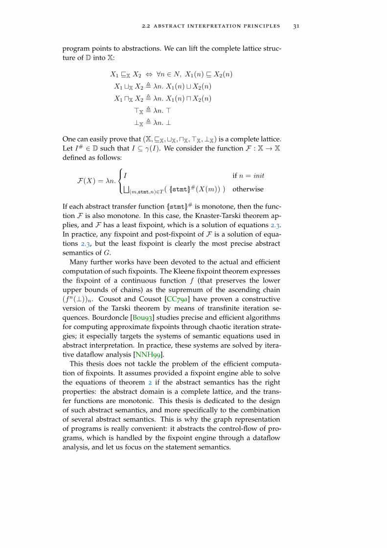
program points to abstractions. We can lift the complete lattice struc-ture of D into X:
X1 X X2 ⇔ ∀n ∈ N, X1(n) X2(n)
X1 X X2 λn. X1(n) X2(n)
X1 X X2 λn. X1(n) X2(n)
X λn.
⊥X λn. ⊥
One can easily prove that (X,X,X,X,X,⊥X) is a complete lattice.Let I# ∈ D such that I ⊆ γ(I). We consider the function F : X → X
defined as follows:
F(X) = λn.
I if n = init
(m,stmt,n)∈T ( |stmt| #(X(m)) ) otherwise
If each abstract transfer function |stmt|# is monotone, then the func-tion F is also monotone. In this case, the Knaster-Tarski theorem ap-plies, and F has a least fixpoint, which is a solution of equations 2.3.In practice, any fixpoint and post-fixpoint of F is a solution of equa-tions 2.3, but the least fixpoint is clearly the most precise abstractsemantics of G.
Many further works have been devoted to the actual and efficientcomputation of such fixpoints. The Kleene fixpoint theorem expressesthe fixpoint of a continuous function f (that preserves the lowerupper bounds of chains) as the supremum of the ascending chain(fn(⊥))n. Cousot and Cousot [CC79a] have proven a constructiveversion of the Tarski theorem by means of transfinite iteration se-quences. Bourdoncle [Bou93] studies precise and efficient algorithmsfor computing approximate fixpoints through chaotic iteration strate-gies; it especially targets the systems of semantic equations used inabstract interpretation. In practice, these systems are solved by itera-tive dataflow analysis [NNH99].
This thesis does not tackle the problem of the efficient computa-tion of fixpoints. It assumes provided a fixpoint engine able to solvethe equations of theorem 2 if the abstract semantics has the rightproperties: the abstract domain is a complete lattice, and the trans-fer functions are monotonic. This thesis is dedicated to the designof such abstract semantics, and more specifically to the combinationof several abstract semantics. This is why the graph representationof programs is really convenient: it abstracts the control-flow of pro-grams, which is handled by the fixpoint engine through a dataflowanalysis, and let us focus on the statement semantics.

32 abstract interpretation
2.2.5 Widening
We have seen that the abstract interpretation theory expresses an ab-stract semantics of programs as a system of equations (theorem 2).These systems are solved by applying iteratively the equations un-til reaching a post-fixpoint. However, these equations may require alarge number of iterations to be solved. Especially when the abstractdomain is infinite or simply disproportionate, the convergence maybe extremely slow. Moreover, some abstract domains used in real-world analyzers do not have a complete lattice structure. To acceleratethe convergence, the abstract interpretation relies on an extrapolationoperator called widening [CC92b; Cor08], and usually denoted by ∇.The idea behind widening is to study the differences between the ab-stractions computed by two successive iterations and to extrapolatethe effect of the next iterations by predicting a possible fixpoint. Inthe dataflow analysis of a program, this consists in generalizing thebehaviors of a loop from the properties of the first iterations.
Definition 18 (Widening). Let (L,) be a partially ordered set. Awidening operator is a function ∇ : L×L → L such that:
• For all pairs of elements x, y ∈ L2, we have x x∇ y andy x∇ y.
• for all increasing chains x0 x1 . . . xn . . . , the increas-ing chain defined as:
y0 x0
yn+1 yn ∇ xn+1
(2.4)
is ultimately stationary, i.e. ∃k ∈ N, ∀j ≥ k, yj = yk.
The first property of the definition ensures the soundness of the op-erator, that acts like the join of two abstractions. The second propertyallows a fast convergence of the iterative resolving of equations. Weconsider the monotone function F : X → X defined in Section 2.2.4,whose post-fixpoints are solutions of the equations 2.3. We now de-fine the increasing chain yn as:
y0 ⊥
yn+1 yn ∇F(yn)
The chain (yn) is increasing as yn yn ∇F(yn). By definition of thewidening, this chain is stationary starting from a k ∈ N. We thenhave:
F(yk) yk ∇F(yk) = yk+1 = yk
and yk is thus a post–fixpoint of F .

2.2 abstract interpretation principles 33
While ensuring a fast convergence of the fixpoint computation,the extrapolations made by a widening operator may be very im-precise and lose crucial information, thus leading to a post-fixpointmuch greater than the least fixpoint. Several techniques can be imple-mented to mitigate this loss of precision.
A worthwhile observation is that all iterations do not need to ap-ply the widening operator. It can be safely replaced by the standardjoin of abstractions at some iterations, as long as the widening is ap-plied often enough to guarantee the convergence. The join ensuresthat the chain (yn) is increasing, and the widening ensures the chain(yφ(n)) is ultimately stationary, with φ(n) being the steps where theextrapolations are done. How often to extrapolate the next iterationby widening is a trade-off between precision and efficiency. Differentheuristics can be used to choose when to widen [Cou+09]. A com-mon strategy is to delay the widening [Bla+07; Bag+05], replacingthe extrapolation operator by the standard join of abstractions for thefirst n iterations. This allows the computed abstractions to accumu-late more constraints that can be used for a better extrapolation of aloop behavior. Two extrapolation steps can also be separated by m
iterations without widening.A widening with thresholds [LJG11; Lea+08; Hal93] can also be used
to limit the extrapolations made by standard widenings. It consists indefining a finite set C of threshold constraints that express candidateproperties that may hold in the concrete semantics of the analyzedprogram, and that we enforce in the widening. The widening be-tween yn and yn+1 is then reduced by the constraints that are stillsatisfied in yn+1. The constraints can be expressed as a set of thresh-old abstract states TH . The widening by thresholds is then built uponthe standard widening as follows:
x∇TH y = min(z ∈ TH ∪ x∇ y | y z)
The widening by thresholds x∇TH y is the least threshold state greaterthan y, or the standard wideninng x∇ y. The precision and the effi-ciency of this approach depends on the choice and the number of thethresholds.
Finally, the over-approximations made for the computation of apost-fixpoint can be corrected afterwards, by decreasing iteration se-quence [Cou99]. Dually to the widening operator, a narrowing oper-ator ∆ can be defined to accelerate the decreasing iterations [CC92b].
2.2.6 Abstract Domains: Summary
The abstract interpretation theory approximates the collecting seman-tics of a program through an abstract semantics expressed as equa-tions over an abstract domain. An abstract domain is a collection of

34 abstract interpretation
abstract states, related to sets of concrete states through a concretiza-tion function γ. An abstract domain provides:
• an inclusion and a join operations that over-approximate theinclusion and the union of sets of concrete states, according to γ.
• a set of transfer functions, or abstract transformers, that over-approximate the concrete semantics of statements in the collect-ing semantics.
As shown by Section 2.2.2, these are the only requirements that anabstract domain must fulfill to ensure the soundness of an abstract in-terpretation based analysis. Guaranteeing the termination of the anal-ysis also requires the abstract domain to have a complete lattice struc-ture, and its transfer functions to be monotone. In practice however,the fast convergence of the analysis is usually achieved through theextrapolations made by a widening operator. This technique makesunnecessary the other restrictions on abstract domains. Most abstractinterpreters use relaxed hypothesis on their abstract domains and relyonly on widenings to limit their analysis time. Several domains pro-posed in the literature do not have a complete lattice structure. Gangeet al. [Gan+13] explore the abstract interpretation over domains thatdo not have a lattice structure. The Astrée static analyzer includes do-mains without a lattice structure, without even a preorder, and whosetransfer functions are not monotonic [Cou+06].
However, the lattice structure of abstractions brings good proper-ties to an abstract interpretation based analysis, even if it is not strictlyneeded for its termination or its soundness. In particular, the commu-tativity and the associativity of the join and meet operators ensurethat the iterations order does not affect the result (and thus the preci-sion) of the analysis. If we do not enforce complete lattices or mono-tonic transfer functions, we assume henceforth that the abstractionswe use have a bounded lattice structure —or at least a semilatticestructure.
2.3 combination of abstractions
Over the years, many abstract domains have been designed to addressvarious problems on different classes of programs. The complete ver-ification of a program often requires properties inferred by differentdomains. The abstract interpretation framework provides some stan-dard ways to create new abstractions from existing ones, especiallyby combining abstract domains and their abstract semantics. Mostof them allow abstract domains to interact with each other duringthe analysis, exchanging information in order to reach more preciseabstractions of the program semantics. Cortesi et al. [CCF13] offersa good survey of the product operators on abstract domains in theliterature. In this section, we first give an overview of the existing

2.3 combination of abstractions 35
Domain Reference Properties
Signs [CC77b] x ∈ ±
Intervals [CC77b] x ∈ [a..b]
Boxes [GC10a] x ∈n
i=1[ai..bi]
Congruences [Gra89; Gra97] x ≡ c mod m
Linear congruences [Gra91]n
i=1(ai · xi) ≡ c mod m
Linear equalities [Kar76]n
i=1(ai · xi) = n
Polyhedra [CH78]n
i=1(ai · xi) ≤ n
Octagons [Min06c] ±x± y ≤ c
Ellipsoids [Fer04] ax2 + by2 + cxy ≤ n
a, b, c, n,m ∈ N
x, y ∈ X
Table 2.1: Numerical abstract domains in the literature
abstract domains; we then present different approaches to combineabstract domains.
2.3.1 Abstract Domains of the Literature
A wide variety of abstract domains have already been proposed inthe literature, and the design of new abstract domains remains a veryactive field of reseach. Each domain has its strengths and weaknesses.They provide different expressiveness and computational complexity.They infer different families of properties, handle precisely variouskinds of code patterns and offer different balances between precisionand efficiency. Relational domains encode properties that involve mul-tiple variables. Some relational domains limit the number of variablesthat can be related through the properties they infer. Non-relational
domain abstracts each variable independently.Table 2.1 presents some of the well-known numerical abstract do-
mains in the literature. The family of properties that each domainmay infer is given to the right. An abstract state represents the set ofconcrete states in which the properties hold.
signs The sign domain [CC77b] is one of the simplest abstractionsknown in abstract interpretation: it only infers the sign of eachvariable of the program.

36 abstract interpretation
intervals The interval domain [CC77b] represents the range ofvariables by maintaining an upper bound and a lower boundfor their possible values. It relies on the well-known intervalarithmetics [Moo66]. The interval domain is very popular asit is able to infer crucial information for program verificationdespite its low complexity.
boxes Boxes [GC10a] are a refinements of the interval domain: theyrepresent the possible values of each variable as a disjunctionof intervals, encoded by a propositional formula over intervalconstraints and represented by Linear Decision Diagrams, anextension of Binary Decision Diagrams.
congruences The arithmetical congruence domain [Gra89; Gra97]infers a congruence constraints for each variable independently.This domain is especially useful for variables used as array in-dices, that are most of the time congruent to the size of the arrayelements.
linear equalities A linear equality domain [Kar76] detects affinerelationships among program variables.
linear congruences A linear congruences domain [Gra91] dis-covers system of linear congruence equations satisfied by theinteger variables of a program. It generalizes the domain ofarithmetical congruences into a fully relational domain.
polyhedra A convex polyhedra domain [CH78] manipulates sys-tems of linear inequalities between program variables. It canexpress complex invariants at the cost of a very high complex-ity.
zones & octagons Zones (or DBM) [Min07] and octagons [Min06c]aim to find an happy medium between the expressiveness andthe cost of the polyhedron and the interval domains. They useDifferent-Bound Matrices [Yov96; Lar+97] to efficiently encodebounds on the sum and the difference of pairs of variables.
ellipsoids Ellipsoids [Fer04] are a specialized domain dedicated tothe analysis of digital filters.
These are only numerical domains on arithmetical variables, but theabstract interpretation framework has also been successfully appliedto prove various properties on memory. Abstract domains have beennotably designed to infer information about pointer aliasing [Hin01;RL12], large or complex memory structures [VB04; Min06a] or heap-allocated storage [BR06; SRW02; TCR13].

2.3 combination of abstractions 37
2.3.2 Direct Product
We now study the composition of abstract domains within the ab-stract interpretation framework. Henceforth, we assume given twoabstract domains A# and B# and their respective concretizations,join-semilattice structures with widenings and transfer functions.
γA : A → P(Σ) (A#,A,A,∇A) |stmt| A# : A → A
γB : B → P(Σ) (B#,B,B,∇B) |stmt| B# : B → B
The direct product of two abstract domains is simply the set ofpairs of elements of each domain. A pair (a, b) from A×B abstractsthe concrete states represented by both abstract states a and b. Theoperators are defined by the pointwise application of the operatorof each underlying domain. This trivially preserves the soundnessproperties of the domains, as well as their (possibly complete) latticestructure, the monotony of the transfer functions and the definition 18
of widening.
γA×B : A×B → P(Σ)
γA×B(a, b) γA(a) ∩ γB(b)
(a, b) A×B (a, b) ⇔ a A a ∧ b B b
(a, b) A×B (a, b) (aA a, bB b)
(a, b)∇A×B (a, b) (a∇A a, b∇B b)
|stmt| A×B#(a, b) ( |stmt| A
#(a), |stmt| B#(b))
The direct product allows an automatic parallelization of analyzesbased on different abstract domains, but it is not more precise thanthe sequence of these analyzes. It discovers in one analysis the invari-ants inferred by its underlying domains in separate analyzes. Whilethe direct product adds no intrinsic complexity to the abstract se-mantics of the domains, more accurate analyzes can be obtained bymutually refining the underlying abstract domains.
Example 2. Let us consider the program of Figure 2.5 that operateson variables i, x and y. The assumption of line 2 constrains the setof initial states of the program: they are environments in which thevariable i has a value between 0 and 10. Such an assumption can alsobe translated as a test filter of the toy language, as in the graph rep-resentation given at the right of the figure. In this case, the programaccepts any initial state, but those that do not satisfy the conditionare stuck in the initial node. Both representations are equivalent.
On this program, the interval domain infers that i ∈ [0..3] initially,that x ∈ [0..12] at line 1, that x ∈ [1..12] at line 3 and finally thatx− i ∈ [−2..12]. This does not exclude the division by zero at line 3.The arithmetic congruence domain infers that x ≡ 0 mod 4, but has

38 abstract interpretation
-2 vars: i, x, y.
-1 /* assume 0 <= i <= 3; */
0
1 x := 4*i;
2 if (x > 0)
3 y := 10/(x-i);
4
0
1
2
3
4
((0 ≤ i) + (i ≤ 3))==0?
x := 4× i
(x ≤ 0)==0?
y := 10÷ (x− i)
(x > 0)==0?
Figure 2.5: Need for interactions between abstract domains
no information about the expression x− i at line 3. Therefore, thedirect product between an interval domain and an arithmetic cannotprove that the division by zero never occurs on this program. Nev-ertheless, the product of abstract states inferred at line 3 contains allinformation needed to prove this property:
i → [0..3]
x → [1..12]
y →
x ≡ 0 mod 4 (2.5)
The two constraints on variable x ensures that the value of x belongsto the interval [4..12], and thus that the expression x− i belongs tothe interval [1..12], excluding the division by zero. Here, provingthe correctness of the program requires an inter-reduction betweenthe properties inferred by each abstract domain. This is exactly thepurpose of a reduced product.
2.3.3 Reduced Product
The reduced product [CC79b] is a refinement of the direct productthat overcomes its limitations by mutually refining the underlying ab-stract states. Intuitively, it reduces the abstract state of each domainby exploiting the properties inferred by the other. These reductionsimprove the information known by each component without affect-ing the meaning (the concretization) of the pair. This allows eachdomain to approximate more precisely the program without compro-mising the soundness of the analysis. Formally, the reduced productconsiders the equivalence classes of the direct products that have thesame concretization. Practically, it works on the smallest representa-tives of each class, by reducing maximally the result of each operationthrough a reduction operator. reduce(a, b) computes the smallest el-ement of A × B that has the same concretization as (a, b). If both

2.3 combination of abstractions 39
underlying domains have a complete lattice structure, it can be de-fined as the meet of the equivalence class of (a, b).
reduce(a, b) = minA×B((a, b) | γA×B(a
, b) = γA×B(a, b))
=
(a, b) | γA×B(a, b) = γA×B(a, b)
The reduced product A ∗B is then defined as the set A×B with thefollowing operators. The concretization is the same as for the directproduct. The lattice operators and the transfer functions use the re-duction operator to minimize their output in the direct product. Asits concretization remains unchanged, this does not affect the sound-ness of the product domain. On the other hand, the result of thewidening cannot be reduced without breaking the properties statedin definition 18. A widened state is thus not necessarily the smallestelement of its equivalence class. This is why the reduced productcannot be defined as reduce(a, b) | (a, b) ∈ A×B.
γA∗B(a, b) γA(a) ∩ γB(b)
(a, b) A∗B (a, b) ⇔ a A a ∧ b B b
(a, b) A∗B (a, b) reduce(aA a, bB b)
|stmt| A∗B#(a, b) reduce( |stmt| A
#(a), |stmt| B#(b))
(a, b)∇A∗B (a, b) (a∇A a, b∇B b)
Example 3. On the program of Figure 2.5, the direct product stateinferred at line 3 was given by equation 2.5. Its reduction in thereduced product is:
i → [0..3]
x → [4..12]
y →
x ≡ 0 mod 4
The interval component is then able to prove the absence of a divisionby zero in the program.
Although the mathematical definition of the reduced product en-joys ideal theoretical properties, the maximal reduction between ar-bitrary domains is not computable in general. The implementationsof domains composition usually fall back to an approximate reducedproduct, through a relaxed version of the reduction operator. Such arelaxed operator partially reduces a pair of abstract states, satisfyingthe following properties:
reduce : A×B → A×B
∀(a, b) ∈ A×B,
reduce(a, b) A×B (a, b)
γA×B(reduce(a, b)) = γA×B(a, b)

40 abstract interpretation
The choice of the reductions performed within an approximate re-duced product must reach a balance between precision and efficiency.A standard (and trivial) reduction is the normalization of a canonicalbottom element: any pair (⊥A, b) or (a,⊥B) has an empty concretiza-tion and can be replaced by (⊥A,⊥B). The specification and the com-plexity of the stronger reductions depend entirely on the involvedabstract domains.
2.3.3.1 Granger Product
Granger [Gra92] proposes a convenient approach to compute an ap-proximation of the reduce function. It simplifies its implementationby separating the reduction of each component of the pair. Thereductions are split up into two operations A : A × B → A andB : A×B → B such that:
∀(a, b) ∈ A×B,
γ(a, b) = γ(A(a, b), b) = γ(a, B(a, b))
A(a, b) A a ∧ B(a, b) B b
Each operator refines the state of a domain with the information ofthe other state. Both operators can then be used iteratively until reach-ing a fixpoint. The Granger product of a pair (a, b) is defined as thefixpoint of the decreasing sequence:
(a0, b0) (a, b)
(an+1, bn+1) (A(an, bn), B(an, bn))
2.3.3.2 Limitations of the Reduced Product
Approximate reduced products are well suited on some specific ab-stract domains, as proved by the well-known product of interval andcongruence domains [Gra89]. Nevertheless, the reduced product isnot the panacea of domain composition. Two main impediments hin-der the spread of its use for arbitrary abstract domains.
1. Reduced products are not modular: the reduction operator isspecific to the domains it refines. It can be hard to define on richdomains, and is even more intricate to apply on a high numberof domains. Adding a new abstract domain to a Granger prod-uct of n domains may require the implementation of 2n reduc-tion functions, and each one may involve different alternativesto approximate the maximal reduced product.
2. The reduced product performs the inter-reduction of domainson the result of the transfer functions. There is no interaction be-tween abstract domains during their interpretation of the state-ment semantics. However, an abstract domain could exploit theproperties inferred by other domains to approximate more accu-rately the semantics of a statement. The shared properties could

2.3 combination of abstractions 41
-5 vars: x, y, z.
/* assume 0 < x < 10
&& 0 < y < 10
&& 0 < z < 10; */
0 if (z > 5)
y := x + 3
z := 100 / (x - y + z)
0
1
2
3
(z ≤ 5)==0?
y := x+ 3
z := 100÷ (x− y + z)
(z > 5)==0?
Figure 2.6: Need for interactions during statements interpretation
be lost or pointless after the statement, preventing the reducedproduct from recovering the same precision.
Example 4. The program of Figure 2.6 operates on three variables x, y,z. The assumption constrains the initial states. We study the analysiswith the domains of intervals and linear equalities. An interval anal-ysis infers the initial range [1..9] of each variable, and the propertiesz ∈ [6..9] at line 1 and y ∈ [4..12] at line 2. The interval arithmeticsleads to x− y + z ∈ [−6..11] at line 2. The linear equalities domaincannot express a constraint over z, and only infers y = x+ 3 at line 2.None of the two domains can exclude the possibility of a divisonby zero. The states of each domain cannot be mutually refined here:their product is already minimal. The state computed by the reducedproduct at line 2 is:
x ∈ [1..9]
y ∈ [6..12]
z ∈ [6..9]
× y = x+ 3
Therefore, the reduced product of intervals and linear equalities can-not prove the correctness of the program. However, the equalityy = x + 3 implies that x − y ∈ [−3]. As the interval domain en-sures that z ∈ [6..9], this proves that x− y + z ∈ [3..6]. The programcan thus be proved correct by a combination of the interval and theequality domain, provided that both domains can collaborate duringthe approximation of a statement semantics.
Example 5. A more classic example of this limitation of reduced prod-ucts is the abstract interpretation of programming language includingarrays. A precise approximation of an array access t[i] often requiresat the same time some bounds and a congruence information aboutthe possible values of i. This requires some interaction between aninterval and a congruence domain within the transfer functions. Oth-erwise, the loss of precision can be too big to be recovered afterwards,especially on large arrays.

42 abstract interpretation
2.3.4 Open Product
The open product [CCH00] is a framework to easily implement inter-actions between abstract domains during their abstract operations. Itbases their inter-reductions on queries and open operations. A query isa boolean function that expresses a property inferred by an abstractstate. An open operation is a transfer function that additionaly re-ceives a set of queries describing some properties that are known tohold. The transfer functions over an abstract domain can use thequeries provided by other domains to improve their precision. Infor-mation thus flows between abstract domains through queries. In thiscontext, an open interpretation is an abstract domain that implementsa set of queries Q, and open operations with respect to the same setof queries Q. The open product of several open interpretations overthe same queries Q is defined as:
• the cartesian product of domain;
• queries as the disjunction of the queries of each domain (astrue ≤ false is used as the order on booleans, λx. qA(x)∨ qB(x)
is the most precise query logically implied by qA and qB);
• the component-wise application of the open operations on eachdomain, with the queries defined above.
While the open product has been specifically designed to let domainsinteract during a statement interpretation, a reduce operator can alsobe used to refine the result of the open operations. In particular,the open product is orthogonal and complementary to the Grangerproduct.
The main drawback of the open product is the restriction to booleanfunctions, that lack expressivity. Moreover, the communication byqueries is used only for the open operations, while the join of abstractdomains can also be an important source of imprecision. Finally, de-signing an open product requires to properly identify beforehand theset of properties that need to be exchanged by abstract domains.
2.3.5 Communication through a Shared Language
We have seen that the reduced product is highly non modular andthus cumbersome to apply on a wide variety of domains. A naturalsolution to this issue is the use of an independant language of con-straints L as intermediary between abstract domains [Cou+06]. Sucha language is for instance defined in [TCR13] for the inter-reductionbetween shape abstract domains. Following the Granger productidea, one can interface an abstract domain D with the language L
by extending it with two functions:

2.3 combination of abstractions 43
• extract : D → L , that expresses the constraints guaranteed tohold by an abstract state;
• refine : D× L → D, that refines an abstract state according tosome constraints.
If we assume the constraints L equipped with a concretization func-tion γL : L → P(Σ), the two functions must satisfy the followingproperties (the two first are soundness properties, and the third statesthat the refinement of an abstract state d cannot be less precise than d):
γ(d) ⊆ γL (extract(d))
γ(d) ∩ γL (l) ⊆ γL (refine(d, l))
refine(d, l) d
An approximate reduced product can then be implemented by suc-cessive iterations of extracting constraints from states and refiningstates with these constraints. The constraint language should be de-signed in advance with utmost care, as it is the fixed interface be-tween all abstract domains. Unlike the order product, this extensionof domains does not allow interactions during the interpretation ofstatements.
2.3.6 Communication by Messages
The most advanced collaboration between abstract domains is un-questionably the communication by messages introduced and imple-mented in Astrée [Cou+06]. This design has been followed later inother analyzers such as Canal [Dup13] and Verasco [Jou+15]. Its mainidea is to use as shared interface between domains an extensible setof atomic messages. The messages can be of various kinds; each onecarries a different type of information. For instance, Verasco [Jou16]uses different messages to express the interval of a variable, the arith-metical congruence of a variable, the exact value of a variable, theequality between a variable and an expression, or the equality be-tween an expression and a quasi-linear expression. Communicationchannels relay a list of messages from domains to domains. Each do-main can use some of the messages from a channel, and emit somenew messages of its own. A domain is always free to ignore themessages it does not understand. This allows adding a new kind ofmessage without having to modify all the existing domains.
A domain creates messages and is reduced according to messagesthrough the two functions extract and refine presented in the abovesubsection. Following the concepts of the open product, the transferfunctions can also exploit the information conveyed by channels. Sev-eral channels can enable various forms of communication betweenabstract domains. Astrée uses channels of two types:

44 abstract interpretation
• input channel for a domain to request more information. Aninput channel is implemented as a list of functions, each onecomputing messages of a fixed kind.
• output channel for a domain to emit a message intended forother domains. An output channel can be implemented as a listof messages to be processed.
2.3.6.1 Input Channels
An input channel works as the set of queries in the open product. Thecommunication model of Astrée actually extends the open product intwo different ways:
• the functions of an input channel produce messages and notsimply booleans;
• two input channels are provided: a pre and a post channels, thatcontain messages describing properties known to hold respec-tively before and after the given statement.
The new signature of transfer functions is given below. The trans-fer function |stmt| #((d, pre), post) over-approximates the semanticsof stmt on the concrete states represented by d and satisfying pre ,knowing that the resulting states satisfy post .
|stmt| # : (D×L ) → L → D
|stmt| (γ(d) ∩ γ(pre)) ∩ γ(post) ⊆ γ( |stmt| #((d, pre), post))
The pre channel is collaboratively built by the product of abstractstates inferred at the program point before the statement —this statesproduct is the argument of the transfer function. The post channelmust be built from the abstract states inferred after the statement—this states product is the result of the transfer function. The post
channel is thus incrementally filled by each abstract state computedby the transfer function of one of the domains. The evaluation orderof abstract domains thereby affects the communication between them.The first domain to be processed has always an empty post channel.The nth domain to be processed benefits from the messages createdby the previous domains, and can add some new messages for thenext ones.
2.3.6.2 Output Channels
While an input channel allows a domain to request information, anoutput channel allows a domain to send information on its own ini-tiative. Input and output channels are used in parallel by the transferfunctions. Astrée uses two output channels:

2.3 combination of abstractions 45
• an oriented output channel, that allows a domain to send amessage to the next domains to be processed;
• a broadcast output channel, that allows a domain to send a mes-sage to all domains (including those that have already performtheir computation).
At the beginning of the interpretation of a statement, both outputchannels are empty. Messages are incrementally provided by eachdomain when interpreting the statement (through the transfer func-tions). The contents of the oriented channel can directly be used bythe transfer function of a domain to be more accurate. The use of thebroadcast channel is postponed to the end of the interpretation of thestatement. The content of the broacast channel is only then sent to alldomains, that finally have the opportunity to use its information.
2.3.6.3 Summary
The communication by messages resolves the two main issues of thereduced product. It is modular, as a domain can be freely added orremoved from a product without directly impacting the others. It isextensible, as adding a new kind of message does not require the com-munication system or all existing domains to be modified. Finally,it enables various powerful interactions between abstract domains.However, this extensive leeway for domain collaboration comes atthe price of some complexity. The communication system can be in-vasive in the implementation of the abstract interpreter. It has to bemaintained in parallel of the abstract semantics implemented by thedomains. It features four different channels of two different types thatmust be handled by the abstract domains and their transfer functions.The product of domains is ordered, and the order impacts the pos-sible interactions. Moreover, each domain needs to choose carefullyhow to exchange each atomic information, as each channel reachesdifferent domains at different costs.
2.3.7 Abstract Interpretation Based Analyzers
Over the years, the fundamental principles of the abstract interpre-tation theory have been applied to develop static analyzers, that aresoftwares that aim at proving automatically the absence of some un-desirable behaviors in real-world programs. The undesirable behav-iors tracked by an analyzer are generally the runtime errors of a pro-gramming language, modeled by the error states Ω in our concrete se-mantics. Static analysis has already shown its industrial applicabilityto prove safety properties on critical or embedded code, and abstractinterpretation has known considerable progress in recent years, interms of both research breakthrough and industrial-strength imple-mentations. However, although most abstract interpreters use mul-

46 abstract interpretation
tiple domains internally, few explain how the different domains ex-change information. We present here some of the worthwhile toolsbased on abstract interpretation.
ikos [Bra+14] is an open-source framework that supports the devel-opment of static analysis based on abstract interpretation. Itprovides a front-end for C/C++ programs based on llvm [LA04],some optimized fixpoint algorithms and several numerical ab-stract domains including octagons, discrete symbolic domains,and a reduced product between intervals and congruences. It isused for instance by the verification software SeaHorn [Gur+15].
apron [JM09] is an open-source library providing numerical abstractdomains of the literature under a unified interface. It currentlycontains an implementation of intervals, octagons, linear equali-ties, convex polyhedra, linear congruences, and a reduced prod-uct between polyhedra and linear congruences. The Interprocanalyzer [Ja] has been designed to demonstrate the features ofthe apron library.
astrée [Bla+02; Bla+07; Cou+05; Cou+09] is an abstract interpretertailored towards the verification of safety-critical embedded real-time softwares written in C. It contains many numerical abstractdomains able to handle heterogeneous kinds of abstract prop-erties and to prove complex numerical invariants. Astrée en-joys a modular architecture that organizes a hierarchy of do-mains, and features the advanced communication by messagesbetween them described above. It has been successfully appliedto prove the absence of runtime error in the flight control codesof the Airbus fly-by-wire systems.
verasco [Jou+15] is an abstract interpreter that is itself formallyproved using the Coq proof assistant. Verasco is integrated intoCompCert [Ler09], a formally-verified compiler for C, in sucha way that the safety properties established by Verasco carryover the compiled code. The design of Verasco follows closelythat of Astrée, especially for the interactions between abstractdomains.
clousot [FL10] checks the absence of runtime errors, but also ver-ifies the contract specifications of functions. It analyzes eachfunction of a program in isolation, using its pre- and post-conditions.It works at the bytecode level and is thus language independent.It organizes several domains in a hierarchy inspired by thatof Astrée, and enables some communications between them.Clousot relies on an abstract interpretation engine, but also em-bodies other techniques such as goal-directed backward propa-gations or the inference of pre- and post-conditions.

2.3 combination of abstractions 47
frama-c/value Frama-C [Kir+15] is an extensible and collabora-tive platform dedicated to the specification and the verificationof C programs. For this purpose, Frama-C provides several plu-gins based on different techniques. Among them, the VALUEplugin uses abstract interpretation to compute a variation do-main for the variables of a program. Unlike other analyzers, theVALUE architecture is not modular: it contains only one abstractdomain and does not allow the introduction of new abstractions.The work presented in the next chapter and developed in theremaining of this thesis extends the VALUE plugin to overcomethis limitation. The Frama-C platform is introduced in moredetails in Section 3.1.1, and the differences between the formerVALUE analyzer and our work are emphasized in Section 3.4.


Part II
E VA : A M O D U L A R A N A LY Z E R F O R C


3A R C H I T E C T U R E O F T H E A N A LY Z E R
This chapter outlines the main ideas that have guided the develop-ment of EVA, and that still underlie its architecture. Each of the up-coming chapters focuses on a specific component of EVA, while thischapter explains how these components fit together and interact witheach other to form a complete abstract interpreter. Thus, it does notdwell on the details or the formalization of the analyzer, but intro-duces its main features.
EVA being a plugin of the Frama-C plateform, we start by brieflypresenting this framework. We then describe the modular architec-ture of EVA, which relies on a particular hierarchy of different ab-stractions. We explain the role of these abstractions in the generic ab-stract interpreter, and sketch the communication between them. Wealso propose an implementation mechanism that enables some inter-action between the components of a generic combination of datatypes.This has been successfully implemented to improve the product of ab-stractions in EVA. We finally discuss the software development of theanalyzer, which is based on VALUE, the previous abstract interpreterof Frama-C.
3.1 overview of the eva structure
Figure 3.1 sketches the different layers of our analyzer architecture.The services each layer provides are given on the left, and the syn-tax fragments on which they operate are on the right. This sectionfollows the internal organization of the analyzer. We first introduceFrama-C, the platform that EVA is part of. Then, we describe theabstract interpreter itself, and the hierarchy of abstractions it uses torepresent program semantics.
3.1.1 The Frama-C Platform
The EVA abstract interpreter is a plugin of the Frama-C [Kir+15] plat-form: an extensible and collaborative framework dedicated to theanalysis of the source code of C programs. It is structured around akernel providing shared functionalities, and a set of plugins that im-plement various types of verification. The plugins may interact witheach other, and a plugin may build upon the properties proved by another analysis. In particular, the results inferred by EVA are availableto the other plugins of Frama-C.
51

52 architecture of the analyzer
Frama-C Kernel
Abstract Interpreter
Abstract Domains
Values and Alarms
QueriesLattice Transfer
C and Logic AST
Function CFG
Statements
Expressions
Parsing
Forward Analysis
State Abstraction
C Values and Memory
Locations Abstraction
Figure 3.1: Overall layers of EVA
Available analyses in Frama-C include abstract interpretation (EVAplugin), deductive verification (WP plugin), generation of temporal an-notations (aorai plugin), runtime assertion checking (E-ACSL plugin),etc. A more exhaustive list can be found at http://frama-c.com/
plugins.html. Note that EVA is not a new plugin of Frama-C, but amajor evolution of its former abstract interpreter, the Value Analysisplugin (often abbreviated as VALUE).
Among the main features provided by the kernel are:
• the parsing and the type-checking of the C files supplied asinput. A symbolic linker then produces a program equivalent tothe input files. The resulting AST is expressed in the augmentedFrama-C version of the C Intermediate Language [Nec+02].
• the possibility to specify C functions, using a first-order logiccalled ANSI/ISO C Specification Language (ACSL). Logical an-notations may range from basic assertions (e.g. expressing thatan operation does not overflow), to full-fledged functional spec-ification of the function behavior.
• the tracking and automatic consolidation of the logical statuses(true, false or unknown) set by the plugins on the ACSL annota-tions present in the program [CS12].
The verification of a program generally starts by proving that it doesnot contain runtime errors, i.e. undefined behaviors according to the Cstandard. This is often a prerequisite to more complex verificationssuch as functional correctness. Within Frama-C, safety assertions(that exclude undefined behaviors) can be generated in a systematicway by two plugins: RTE and EVA. Afterwards, all plugins may at-tempt to prove these assertions. EVA is somewhat special, in that itintermingles the generation of safety assertions and their verification.EVA is also able to emit logical statuses on simple user-written ACSLassertions.

3.1 overview of the eva structure 53
Frama-C — and thus EVA — is written in OCaml [Cuo+09], andis an open source, free software. Its source code is available at http://frama-c.com/download.html. The first version of EVA was publiclyreleased in Frama-C Aluminium in June 2016. This thesis is basedon this work.
3.1.2 The Abstract Interpreter
The generic abstract interpreter works on the AST provided by theFrama-C kernel. It iterates an interprocedural forward dataflow anal-ysis over the CFG of the functions of a given program. The analysispropagates the states of an abstract domain through the CFG, accordingto an abstract semantics soundly modeling the effect of statements.Statements are visited following a chaotic iteration strategy [Bou93].Widening steps are performed to ensure convergence. The analysisof a whole program is fully context-sensitive: function calls are sym-bolically inlined. Recursive functions are not handled.
Once a fixpoint has been reached, the computed abstract statesinfer valid properties at each program point. During the analysis,EVA emits an alarm for each operation where the abstract semanticsfails to prove the absence of an undesirable behavior. Alarms areexpressed as ACSL assertions that may be proved later by anotherplugin of Frama-C. Each alarm may report a real error if the re-ported undesirable behavior indeed occurs at runtime for at least onepossible execution. Otherwise, the alarm is a false alarm, due to theover-approximation made by the abstract semantics. Importantly, thesoundness of the abstract semantics ensures that an alarm is issuedfor each operation that may fail. If the analysis raises no alarm for agiven program, then this program is free of the undesirable behaviorthat EVA detects.
The abstract interpreter is generic: it does not depend on a par-ticular abstraction. The architecture and the inner working of thisinterpreter are further developed in Section 3.2.1. But before delvinginto the details of the interpreter, we need to present the hierarchy ofabstractions on which it relies.
3.1.3 Abstractions
The design of EVA relies on the separation between state abstractions
and value abstractions. As the name implies, a state abstraction repre-sents some concrete states at a point of a program execution. A valueabstraction represents the C values an expression can have in someconcrete states. A state abstraction handles the semantics of state-ments, while a value abstraction operates at the level of expressions.This distinction between value and state abstractions was already pro-posed by Cousot [Cou99] to design an abstract interpreter, but was

54 architecture of the analyzer
not used to structure or reduce a product of different abstractions. Onthe other hand, EVA uses the value abstractions as a shared commu-nication interface that allows different state abstractions to interactwith each other.
Value abstractions and state abstractions are fully formalized inChapter 5 and in Chapter 7 respectively. The main value abstractionused by EVA is described in Section 5.3. The state abstractions cur-rently available in EVA are listed in Chapter 8. The following is anoutline of the role of both kinds of abstractions in the abstract inter-preter.
3.1.3.1 State Abstractions
An abstract domain — or a state abstraction — is a collection of abstract
states which are abstractions of the sets of possible concrete states thatmay occur at a program point. An abstract domain must provide:
• a join-semilattice structure, fulfilling the properties establishedin Figure 2.4. The inclusion relation reflects the precision of theabstract states. The join computes an upper bound of two states,and is used when two branches of the CFG merge. A wideningoperator is also mandatory, to ensure a fast convergence of thefixpoint computation.
• sound transformers — or transfer functions — for statements,that infer properties by modeling the effect of a statement onan abstract state. They are the abstract semantics of the domain,and are used to propagate abstract states through the CFG.Theymust satisfy the property of definition 8.
• queries, which extract information from abstract states by as-signing a value to some expressions, or a location to some ad-dresses. They are detailed in Chapter 7.
The abstract domains do not interact directly with each other, butachieve some communications and inter-reductions through valueand locations abstractions expressed by the queries.
3.1.3.2 Value and Locations Abstractions
Value and locations abstractions are non-relational abstractions aboutexpressions and addresses in some given concrete states. A value ab-straction is an approximation of the set of possible concrete valuesthat an expression may have in these states. As expressions includedereferences of a program variable, a value abstraction may be an ap-proximation of the concrete value of a variable in some states. A lo-cation abstraction is an approximation of the set of possible memorylocations that an address may have. Both abstractions serve similarpurposes, and must fulfill the same requirements. Although they are

3.2 a modular abstract interpreter 55
internally two different entities, the value and location abstractionsin EVA are very close, and share a large part of their implementation.Therefore, we usually do not distinguish between value and locationabstractions, and often write “value abstraction” for both kinds ofabstractions.
Value (and location) abstractions are used to cooperatively evalu-ate addresses and expressions in a product of abstract states comingfrom several abstract domains. Value (respectively location) abstrac-tions encode an abstract semantics of the operators on expressions(respectively addresses). According to the properties it has inferred,an abstract state may express the possible concrete value of a vari-able, expression or address by providing such abstractions. Theseabstractions are then made available to the transformers of all do-mains, which can use them to approximate more precisely the effectof a statement.
Value and location abstractions must have a meet-semilattice struc-ture. Similarly to state abstractions, the order relation reflects the pre-cision of the abstractions. The meet is used to combine abstractionsprovided by different domains. Value and location abstractions alsoprovide sound transformers over-approximating the effect of arith-metic operators on expressions and addresses. As the concrete oper-ators may cause undefined behavior at execution time, their abstractcounterparts also produce alarms, which report the error cases.
Alarms are essential: they are the final result of an analysis, andhighlight all the possible undesirable behaviors that may happen dur-ing the execution of a given program. In return, the absence of alarmguarantees the absence of undesirable behavior. An abstract inter-preter aims at emitting as few alarms as possible — while remainingsound. It is thus natural to also involve the state abstraction in theircomputation, allowing them to avoid some alarms thanks to their in-ferred properties.
Values, locations and alarms form the complete communication in-terface between the abstract domains and the generic abstract inter-preter. They are formally described in Chapter 5.
3.2 a modular abstract interpreter
This section offers a more detailed view of the inner workings of anabstract interpreter based on the separation between value and stateabstractions. We also briefly explain the combination of abstractions,as well as the principles that underlie their inter-reduction.
3.2.1 Inner Workings of the Abstract Interpreter
Figure 3.2 presents the internal architecture of EVA. We commenton the diagram from bottom to top. Note that the three layers of

56 architecture of the analyzer
ValuesAlarms
Memory Locations
Communication Interface
Queries Transfer Lattice
Domain
Evaluation
PartitioningInterpretation
DataflowMemExec
Computation Initialization
providesuses
back
war
dre
fere
nce
Expressions
Statements
Functions
Programs
Functor
Generic module
Figure 3.2: Architecture of the analyzer

3.2 a modular abstract interpreter 57
Figure 3.1 are still shown, and that the figure focuses on the structureof the abstract interpreter. As described above, it relies on differentabstractions to model the semantics of the C language.
The alarms are abstractions of the possible undesirable behaviorsof a program. They are listed in a fixed module that defines thescope of the verification made by the abstract interpreter. On theother hand, the value, location and state abstractions are parametersof an analysis. The abstract interpreter is made of a hierarchy of func-tors built upon these abstractions. In the diagram, yellow boxes aregeneric OCaml functors, and the plain arrows point out the modulearguments of each functor.
The evaluator depends on the value (and location) abstractions, andthe queries of an abstract domain. It is able to evaluate any expres-sion into a value abstraction, or any address into a location abstrac-tion, based on the abstract semantics provided by both value andlocation modules. It queries the abstract domain for initial value ab-stractions to work on, especially for abstractions of the possible valueof variables. The evaluator also gathers the alarms produced duringthe evaluation of an expression.
The interpretation functor depends on an evaluator and the abstracttransformers of the domain. It implements the generic transfer func-tions for C statements. It evaluates all the expressions involved in agiven statement, emits the alarms issued by the evaluations, and thencalls the abstract transformers of the domain. These transformers mayuse all the abstractions computed by the evaluations. For an assign-ment, this includes a value abstraction for the right expression, anda location abstraction for the lvalue being assigned. These abstrac-tions have been computed cooperatively, using information comingfrom any abstract domain. Thus, if the analyzer is instantiated on aproduct of abstract domain, information may flow from a domain toanother.
The partitioning functor expands an abstract domain into its pow-erset extension. Such an extension refines a domain by inferring adisjunction of abstract states at each program point, instead of onlyone abstract state. Most domains of abstract interpretation are con-vex: they can only represent convex sets of concrete elements. Theconvexity of domains leads to more scalable analysis, but preventsthe verification of non-convex properties. Disjunctions may signifi-cantly improve the precision of an analysis: they overcome convexitylimitations, and also mitigate the need for relational abstractions. Inorder to limit the cost of processing multiple abstract states in paral-lel, the number of disjuncts is bounded by a parameter of the analysis.The dataflow functor implements a forward dataflow analysis propa-gating a disjunctive set of states over a function body. It relies on apowerset domain, and on the generic transfer functions for one ab-

58 architecture of the analyzer
stract state. It computes a fixpoint on the CFG of a function for theabstract semantics defined by the transfer functions.
A backward reference links the interpretation functor to the upper-most one. Indeed, the interpreter has to handle all the C statements,including function calls. The analysis of EVA is context-sensitive: thefunction calls are all symbolically inlined. On a function call, a newdataflow analysis is instantiated over the body of the called function,starting at its entry point with the abstract state from the call site.When the inner dataflow reaches a fixpoint, the analysis of the call-ing function continues with the abstract state computed at the returnstatement of the called function. The memexec functor serves as acache for the entire analysis of a function. It stores the abstract stateinferred at the end of a function body, according to the entry abstractstate of the dataflow analysis. It is used to avoid performing severalanalysis of a same function body with equivalent abstract states.
In addition to the dataflow and to memexec, the computation func-tor also relies on an initialization functor. This last component pro-duces the initial abstract state of the analysis, according to the globalvariables of the program, and to the arguments of its main function.
3.2.2 Combination of Abstractions
The abstract interpreter of EVA is modular: it can be instantiated overany compatible abstractions. Moreover, the abstractions it relies onmay be a product of several datatypes. Indeed, the shared evalua-tion through value abstractions has been designed to let informationflow between different abstract domains. The value and location ab-stractions may also be extended to enable new forms of communi-cation. To this end, we provide generic combiners for state, valueand locations abstractions. These three combiners are OCaml func-tors, from two abstraction modules to a new one, whose elements arepairs of both incoming abstractions. They preserve all the require-ments needed to guarantee the soundness of the analyzer. Successiveapplications of these functors allow the combination of any numberof abstractions.
The value and the location combiners make a standard partial re-duced product. An inter-reduction function can be provided, to nar-row the approximations made by each component using the otherone. Otherwise, the new abstract semantics is simply the pointwiseapplication of the semantics of each component.
The state combiner takes two abstract domains operating on thesame value (and location) abstractions, and produces a new domainstill operating on the same value (and location) abstractions. A queryto a combination of abstract states returns the meet of the value ab-stractions extracted from the query to each state. The abstract trans-formers are carried out pointwise on each abstract state, but each one

3.2 a modular abstract interpreter 59
may use value (and location) abstractions computed with the resultsprovided by the other abstract state. Thus, there is no explicit reduc-tion function for the product of states. Instead, their inter-reduction isachieved through the value (and location) abstractions, cooperativelycomputed by the evaluation of the expression and lvalues involved inthe program statements.
The state combiner is limited to abstract domains understandingthe same value abstractions. In order to link abstract domains builtover different value abstractions, we also provide a generic converter:a functor that lifts an abstract domain over an abstraction V to anequivalent domain over an abstraction W , according to injection andprojection functions between V and W .
More precisely, let D be an abstract domain working on a valueabstraction V , and E be an abstract domain working on a value ab-straction W . We can combine them by:
1. combining the two value abstractions into the product V ×W .Conversion functions between the initial abstractions and theproduct are straightforward — the injection completes an ab-stract value with the top abstraction of the other module:
inj V : V → V ×W proj V : V ×W → V
v → v,W (v, w) → v
2. lifting separately each domain D and E to equivalent new do-mains D and E working on the value abstraction V ×W . Thisoperation uses the conversion functions between value abstrac-tions.
3. combining the domains D and E into the product D ×E.
The communication mechanism of EVA uses the value abstractionsas implicit interface between abstract domains. This naturally limitsthe communication between abstract domains understanding differ-ent value abstractions. If the value abstractions are combined througha simple cartesian product, no information may flow between thetwo abstract domains. However, an inter-reduction function betweenvalue abstractions can be provided to the value combiner, and thismay also achieve an inter-reduction of the domains. Indeed, a valuecomponent provided by the query of the first domain may reduce theother component used by the transformer of the second domain. Thefollowing example illustrates this.
Example 6. We consider two non-relational memory domains D and E
storing information about the possible C values of integer variables.D abstracts the value of a variable as an interval, while E abstracts itwith a congruence. D and E naturally use respectively intervals andcongruences as value abstractions.

60 architecture of the analyzer
Assuming a condition x > 3, where D and E provide respectivelythe interval abstraction [0..12] and the congruence 0[3] for x:
• the standard arithmetic semantics of intervals and congruencesleads to the abstractions [4..12] and 0[3] for the variable x afterthe condition;
• the congruence information allows reducing the interval [4..12]into [6..12]. This is the natural inter-reduction between intervaland congruence.
• the domain transformers use the computed value abstractionsto reduce their current states. The interval domain binds x tothe new interval [6..12].
To a certain extent, the architecture of EVA transfers the need ofa reduced product to the lower layer of value abstractions, ratherthan to the more complicated layer of state abstractions. Finally, notethat both abstraction combiners may be specialized, to enable further(direct) communication between specific modules.
3.2.3 Instantiating the Abstractions
The abstractions used for an analysis are parameters of a run of theabstract interpreter, provided on the command-line, or set throughthe graphical interface. The different abstractions are thus instanti-ated and combined at runtime, as well as the set of functors thatforms the abstract interpreter.
3.3 structuring a combination of datatypes
In this section, we present a mechanism to enable interacting withthe components of a generic combination of OCaml types. We de-scribe the constant inner shape of the datatype combination througha GADT, and automatically build injection and projection functionsbetween compound values (from the combination) and leaf values(at the root of the combination). We use such a structuring for thedifferent abstractions of EVA.
3.3.1 Context and Motivation
EVA is a modular analyzer, and can be instantiated with any abstrac-tion fulfilling the requirements described in the next sections. Severalabstractions are already provided, as well as generic combiners. Byconstruction, the abstractions used during an execution of the ana-lyzer are unknown, and are often a product of several underlyingabstractions. However, there are real advantages in being able to ex-tract a particular component from within these abstractions.

3.3 structuring a combination of datatypes 61
Listing 3.1: Combination of Datatypes
1 module type Abstraction = sig type t [...] end
module A1 : Abstraction = sig [...] end (* leaf abstraction *)
module A2 : Abstraction = sig [...] end (* leaf abstraction *)
[...]
5
(* Abstraction combiner *)
module Combiner (Left: Abstraction) (Right: Abstraction)
: Abstraction with type t = Left.t * Right.t = struct
type t = Left.t * Right.t
10 [...]
end
• Some optimizations of EVA rely on a particular abstraction, bothfor precision and performance. For instance, the evaluator canproceed by disjunction on some specific value abstractions. Thepartitioning strategy can also be chosen according to the repre-sentation of the main abstract domain.
• Although the design of EVA enables some communication be-tween abstractions, further collaboration may require a directaccess to each other. This is typically the case when two linkedstate domains want to exchange information without using anew kind of abstract values.
• Tracking a particular abstraction during an analysis may easeits debugging.
Listing 3.1 presents the general situation we tackle. A generic moduleinterface is defined, including an abstract type t; in our case, this isthe signature of the abstractions used by the analyzer. Several leafmodules implement this interface. One or several functors are able tocreate new modules satisfying the signature from existing ones. Sucha combiner builds a new datatype upon the types of its arguments.The objective is to automatically equip any abstraction module withfunctions enabling a direct interaction with its components — theleaf modules that are part of its composition. For a leaf module, thisincludes only itself.
3.3.2 Interface of a Combination
Listing 3.2 presents the External signature we seek. The keys arepolymorphic OCaml values identifying the type of the abstractionsthat may be part of the combination. Such a leaf abstraction, whoseelements are of type t, must export a key carrying its type t, i.e. akey of type t Key.k.

62 architecture of the analyzer
Listing 3.2: Keys and interface
1 type (_,_) eq = Eq : (’a,’a) eq | Neq
module type Key = sig
type ’a k
5 val create : string -> ’a k
val eq_type : ’a k -> ’b k -> (’a, ’b) eq
end
module type External = sig
10 type t
val get : ’a Key.k -> (t -> ’a) option
val set : ’a Key.k -> ’a -> t -> t
end
Listing 3.3: Implementing keys with GADT
1 type ’a gadt_key =
| A1 : A1.t gadt_key
| A2 : A2.t gadt_key
The Key module provides two functions: create and eq_type. Thefirst one creates a new key from a string describing the abstractionto which the key will be linked. The second one compares two keysof respective types a Key.k and b Key.k. It they are the same, theneq_type returns an equality witness of the types a and b.
The External interface exports the type t, and two access func-tions get and set. If the type t is a combination of several datatypes,these functions allow interacting with its components, identified bytheir keys.
• get takes a key of type a Key.k, and returns a new functionthat takes a value v of type t, and returns the component of vcorresponding to the key if it exists — i.e. if the type t is acombination of several datatypes including the type a carriedby the key. Otherwise, get returns None.
• set takes a key of type a Key.k and a matching value of type a,and inserts it in a value of type t, if possible — i.e. if the type t
is a combination of several datatypes including the type a. Oth-erwise, set is the identity function.
3.3.3 Polymorphic Keys
If the leaf modules are all statically known, the keys can easily be im-plemented as a GADT (see Listing 3.3). However, this choice prevents

3.3 structuring a combination of datatypes 63
Listing 3.4: Using extensible types to implement polymorphic keys
1 module Key : Key = struct
type _ key = ..
module type K = sig
5 type t
type _ key += Key : t key
end
type ’a k = (module K with type t = ’a)
10
let create (type a) () =
let module M = struct
type t = a
type _ key += Key : t key
15 end in
(module M : K with type t = a)
let eq_type (type a) (type b) (x : a k) (y : b k) : (a, b) eq =
let module A = (val x : K with type t = a) in
20 let module B = (val y : K with type t = b) in
match A.Key with
| B.Key -> Eq
| _ -> Neq
end
creating keys for new abstractions dynamically. The architecture ofEVA is intended to ease the introduction of new abstractions. We ul-timately want to enable new abstractions to be implemented as otherplugins of Frama-C, without modifying the analyzer itself.
This is why we use an extensible phantom type for keys. As weneed to dynamically extend this type, we define each new constructorinto a new module, allowing us to use the same constructor nameeach time. The keys are the first class modules, each embeddinga fresh constructor of the extensible type. Listing 3.4 exhibits theirimplementation. The idea comes from the module Type_equal.Id ofthe Core kernel library1, which uses the same mechanism.
In practice, a key is a record gathering not only the first class mod-ule, but also an integer and a string. The string is the name of the key;it must be provided to the create function, and can then be printedfor debugging purpose. A different integer is chosen for each key (bysuccessive increment of a static counter). It serves as a hash of thekey.
And now that we have polymorphic keys, a leaf abstraction modulemay export a key that identifies it, as in Listing 3.5.
1 https://ocaml.janestreet.com/ocaml-core/latest/doc/core_kernel/Core_
kernel/Type_equal.mod/

64 architecture of the analyzer
Listing 3.5: Exporting keys
1 module A1 : Abstraction = sig type t = [...] end
let a1_key : A1.t = Key.create "A1"module A2 : Abstraction = sig type t = [...] end
let a2_key : A2.t = Key.create "A2"
3.3.4 Naive Implementation
The polymorphic key allows a first straightforward implementationof the External signature, shown by Listing 3.6. For a leaf module,an access function compares the given key with the internal key of thedomain, and behaves accordingly. The combiner requires that bothargument modules also implement the External signature. Then, theaccess function of a combination simply calls that of the components.
Although simple, this implementation has several drawbacks:
• the code of the get and set functions is quite odd, and must beidentically duplicated in each leaf module of abstractions;
• adding a new function based on the keys to the External sig-nature requires modifying all existing domains.
• the functions are inefficient on a large combination of abstrac-tions, as they systematically process all the underlying modules.
To address these issues, we only require the abstraction modules (leafand combination) to provide a formal description of the internal struc-ture of their datatype. More efficient implementation of the get andset functions for a particular module can then be deduced from itsdatatype structure.
3.3.5 GADT Structure of a Datatype
Listing 3.7 presents the structure type used to describe the internalshape of a datatype. A value of type t structure defines the struc-ture of the datatype t. This definition can be directly the type t
(the Leaf constructor, for a leaf module), or a pair of two datatypesdescribed by structures (the Node constructor, for a combination ofmodules). The Void constructor is a valid structure for any type, butdoes not allow interacting with its components. It can be used forthe components of a combination that do not need the functionalitiesprovided by the External signature. New constructors may also beadded to describe other datatype layouts.
Then, any abstraction module has to fulfill the signature Internal
of Listing 3.7, which simply adds to the signature of abstractions avalue of type t structure, where t is the type of the abstractions. The

3.3 structuring a combination of datatypes 65
Listing 3.6: Naïve implementation of the External signature
1 module External_A1 : External with type t = A1.t = struct
type t = A1.t
let key : t key = Key.create ()
5 let get : type a. a key -> (t -> a) option = fun k =
match Key.eq_type key k with
| Eq -> Some (fun t -> t)
| Neq -> None
10 let set : type a. a key -> t -> a -> t = fun k t new_t ->
match Key.eq_type key k with
| Eq -> new_t
| Neq -> t
end
15
module External_Combiner (Left : External) (Right : External)
: External = struct
include Combiner (Left) (Right)
20 let get key =
match Left.get key left with
| Some g -> Some (fun t -> g (fst t))
| None -> match Right.get key with
| Some g -> Some (fun t -> g (snd t))
25 | None -> None
let set key (left, right) new_d =
Left.set key left new_d, Right.set key right new_d
end

66 architecture of the analyzer
Listing 3.7: Structure of a Datatype
1 type ’a structure =
| Void : ’a structure
| Leaf : ’a key -> ’a structure
| Node : ’a structure * ’b structure -> (’a * ’b) structure
5
module type Internal = sig
include Abstraction
val structure : t structure
end
10
module A1 = struct
include A1
let key : t key = Key.create "A1"let structure = Leaf key
15 end
module A2 = struct
include A2
let structure = Void
20 end
module Combiner (Left: Internal) (Right: Internal)
: Internal = struct
include Combiner (Left) (Right)
25 let structure = Node (Left.structure) (Right.structure)
end

3.3 structuring a combination of datatypes 67
Listing 3.8: Dependent Maps
1 type map =
| Empty : map
| Node : map * ’a key * ’a data * map -> map
5 let rec find : type a. a Key.k -> map -> a Data.t option
= fun key -> function
| Empty -> None
| Node (left, k, d, right, _) ->
match Key.eq_type key k with
10 | Eq -> Some d
| Neq ->
find key (if Key.compare key k <= 0 then left else right)
structure of some leaf modules and of the combiner are also given inthe listing.
For a leaf type t identified by a key k and a module M implement-ing the External interface, we call accessors for t in M the applicationof the get and set functions of a module to the key k. This builds thefunctions allowing the interaction with the component of type t fromthe module M , if it exists. The structure value of a module M allowsthe automatic generation of the relevant accessors for the datatypesthat the module M indeed contains. These are the relevant accessorsfor the module, the others being dummy constant functions: for thetypes not included in a module, get always returns None and set isthe identity function. Thanks to the structure, the relevant accessorscan even be built once and for all, when the module is created (atcompile-time for the leaf module, or at the application of the com-biner functor). After their generation, we need to store the accessorsand to make them available for use. As the type of an accessor de-pends on the type of the key, we use maps from keys to dependentdata. Their implementation follows the one for usual maps, exceptthat find needs the equality witness of keys (see Listing 3.8).
3.3.6 Automatic Generation of the Accessors
Finally, Listing 3.9 presents the generation of the relevant accessorsof a module, based on the structure that it provides. The Open func-tor transforms a generic internal module, including a structure valuethat matches its internal type, into an external one. All relevant acces-sors are computed at the application of this functor, and stored in adependent map. Then, we can pick up the accessor for a specific key;if the key is not in the map, the dummy accessor is returned instead.In both cases, the obtained accessor is efficient, as it knows staticallythe path to the requested leaf abstraction in the compound datatype.

68 architecture of the analyzer
Listing 3.9: Accessors generation
1 module Open (M : Internal) = struct
(* Getters *)
type (’a, ’b) get = ’b key * (’a -> ’b)
5 type ’a getter = Get : (’a, ’b) get -> ’a getter
let lift_get f (Get (key, get)) = Get (key, fun t -> get (f t))
let rec compute_getters :
type a. a structure -> (a getter) KMap.t = function
10 | Void -> KMap.empty
| Leaf key -> KMap.singleton key (Get (key, fun (t : a) -> t))
| Node (left, right) ->
let l = compute_getters left and r = compute_getters right in
let l = KMap.map (lift_get fst) l
15 and r = KMap.map (lift_get snd) r in
KMap.merge l r
let getters = compute_getters M.structure
let get (type a) (key: a key) : (M.t -> a) option =
20 match KMap.find key getters with
| None -> None
| Some (Get (k, get)) -> match Key.eq_type key k with
| None -> None
| Some Eq -> Some get
25
(* Setters *)
type (’a, ’b) set = ’b key * (’b -> ’a -> ’a)
type ’a setter = Set : (’a, ’b) set -> ’a setter
30 let lift_set f (Set (key, set)) =
Set (key, fun v b -> f (fun a -> set v a) b)
let rec compute_setters:
type a. a structure -> (a setter) KMap.t = function
| Void -> KMap.empty
35 | Leaf key -> KMap.singleton key (Set (key, fun v _t -> v))
| Node (left, right) ->
let l = compute_setters left and r = compute_setters right in
let l = KMap.map (lift_set (fun set (l, r) -> set l, r)) l
and r = KMap.map (lift_set (fun set (l, r) -> l, set r)) r in
40 KMap.merge l r
let setters = compute_setters M.structure
let set (type a) (key: a key) : (a -> M.t -> M.t) =
match KMap.find key setters with
45 | None -> fun _ t -> t
| Some (Set (k, set)) -> match Key.eq_type key k with
| None -> fun _ t -> t
| Some Eq -> set

3.4 development and contributions 69
We detail the generation for the get function; the principles are thesame for the set function.
The (a, b) get type denotes pairs of a key of type b and the get
accessor for this key in the type a. The compute_getters functionrecursively gathers all the get pairs for a type a described by ana structure, using a map from keys to these pairs (KMap). For avoid structure, no accessor can be recovered. For a leaf structure,the only relevant accessor is the identity function for the key of theleaf. For a node structure, we compute recursively the accessorsfor both branches of the node; they are accessors for the sub-typeof each branch, and we lift them on the new type denoted by thestructure: pairs of elements from each branch. We then merge bothaccessor maps. getters is the map resulting from the applicationof compute_getters to the structure of the module argument of thefunctor. Then, the final get function amounts to search the corre-sponding accessor in the map. Note that we need again the typeequality witness given by Key.eq_type for the correct typing of thefunction.
3.4 development and contributions
EVA is not a completely new abstract interpreter: it is a major evo-lution of a pre-existing plugin of Frama-C called Value Analysis,and simply abbreviated as VALUE. In this section, we briefly presentthis former abstract interpreter, emphasize the main innovations in-troduced with EVA, and comment on its development.
3.4.1 Evolution of the Abstract Interpreter
Since its inception, Frama-C has contained an abstract interpreter,the VALUE plugin. This analyzer handles the subset of C99 com-monly used in embedded software, and already gets precise resultson such codes. It has also been considerably optimized for years toachieve scalability on large programs, and has indeed been success-fully used to verify safety-critical industrial codes [Cuo+12]. VALUEfeatures an intricate memory abstraction [Kir+15, §4] , able to repre-sent efficiently and precisely both low-level concepts such as unionsand bitfields, or high-level ones, such as arrays. This abstract domainis rich, but cannot infer relational properties. Interestingly, aggressivestate partitioning is often sufficient to alleviate this limitation: the re-lation information is instead carried out by the disjunction encodedby the multiple states.
More problematic was the fact that VALUE has been written aroundits abstract domain, resulting in a very tight coupling. The abstractdomain was hard-wired in the analyzer, and adding new abstractions— relational or not — was not really possible. The primary objective
70 architecture of the analyzer
of this work was to make the abstract interpreter adequately modular,in order to ultimately be able to complete the initial abstract domainwith new abstractions, including (but not limited to) relational ones.Such a goal could only be achieved by a deep reorganization of theanalyzer. This has required to specify the functions ascribed to theabstractions, and to design clear interfaces for them. Then we haverewritten the analyzer to comply with the new architecture, separat-ing the existing code between a generic abstract interpreter and ab-stractions implementing the abstract semantics of VALUE. Thus, inthe new EVA interpreter, the legacy abstract domain, inherited fromVALUE, is only one of many abstractions.
However, a major challenge was also to preserve the already goodperformances of the VALUE analyzer, in terms of both precision andscalability. Yet, some optimizations and heuristics of the analyzer,which were crucial for its efficiency, relied on its internal representa-tion of a program semantics, which is now the internal type of oneabstract domain among others. These mechanisms could only be keptin EVA only thanks to the structuration of abstractions described inSection 3.3. Indeed, this allows the generic abstract interpreter to ex-tract from an abstract domain the component corresponding to thelegacy VALUE, and to apply the algorithms accordingly. Such opti-mizations or heuristics, that need a specific abstraction to work, aresimply disabled when the given abstraction is not available for ananalysis. This may impact the results precision or analysis time, butnot the soundness of the analysis. In particular, such optimizationsand heuristics support the instance of trace partitioning and the cacheof a function dataflow that was used by VALUE, and that have beenported for EVA.
In the end, EVA is a modular and extensible abstract interpreter.When instantiated with the legacy abstract domain inherited fromVALUE, it provides the same functionnalities, with equivalent perfor-mances, as VALUE did.
3.4.2 Contributions
The evolution of the abstract interpreter is not just about modularity;EVA also features a combination of abstractions and an implicit meansof communication between them that achieve a new form of partialreduced products. Compared to the former abstract interpreter, themain novelties of EVA are:
• a modular architecture, enabling the instantiation of the ana-lyzer on generic abstractions. It has also been designed to facil-itate the introduction and the combination of new abstractions.
• a generic combination of abstractions that enables some directinteraction with the components of a product of datatypes.

3.4 development and contributions 71
• the direct cooperation of all abstractions to the emission of thealarms, that report the undesirable behaviors of a program. InVALUE, alarms were directly emitted as a side effect of the appli-cation of any abstract semantics, which would have preventedan abstraction to reduce the alarms stemming from another one.
• the communication between state abstractions, through non re-lational abstractions of the possible C values of expressions —or of the possible locations of addresses.
• a shared evaluation of expressions in a product of abstract states,featuring a complete and efficient backward propagation phase,that depends on the produced alarms and on the reductionsperformed by the abstract domains. More systematic backwardpropagators have been written accordingly.
• the introduction of several new abstractions, including:
– a binding for the numerical abstract domains provided bythe APRON library;
– an abstract domain of symbolic equalities;
– bitwise value and state abstractions, a domain of symboliclocations and a gauge domain, all contributed by BorisYakobowski.
From the diagram of Figure 3.2, the dataflow, partitioning, memexecand initialization functors are mostly inherited from the former VALUEinterpreter. We have only modified them to turn them into genericfunctors, without modifying their algorithms. The other parts of theabstract interpreter are essentially new.
3.4.3 Development
The OCaml implementation of the work presented in this manuscriptis available as the EVA plugin of the silicon version of Frama-C2. Thesource files can be found in the directory src/plugins/value/. Thetable of Appendix C presents the division in sub-directories, as wellas the main files of the development, with a brief description of thefeatures that each implements, and references to the sections of thisthesis that expound their role.
conclusion
Within the EVA abstract interpreter, the internal hierarchy of abstrac-tions follows the usual distinction between the expressions and thestatements of imperative programming languages. Value abstractions
2 Available at http://frama-c.com/download-all-versions.html

72 architecture of the analyzer
approximate the semantics of expressions, while state abstractions—or abstract domains— approximate the semantics of statements.Multiple value abstractions are combined in a standard reduced prod-uct. Multiple abstract domains exchange information using the valueabstractions as a shared communication interface. Furthermore, anOCaml GADT encodes the inner shape of the combination of abstrac-tions, enabling direct interactions with its components.
The architecture and the features described in this chapter seemsuitable for the development of the abstract interpreter of any imper-ative language. As a plugin of Frama-C, EVA is dedicated to theanalysis of C programs. The next chapter introduces the C program-ming language, and formalizes the concrete semantics used to definethe soundness of our analysis.

4S Y N TA X A N D S E M A N T I C S O F T H E L A N G U A G E
The C programming language [KR78], created by Thompson andRitchie around 1970, is nowadays one of the most used in the world.It remains the choice language for embedded and safety-critical pro-grams. Yet, some of the distinctive features that explain its successalso make it difficult to analyze. To cope with some of these imped-iments, Frama-C is built on an extended version of the C Interme-diate Language (CIL) [Nec+02], an open-source front-end for the Cprogramming language that facilitates program analysis and trans-formation. Basically, CIL is a simplified subset of C featuring a fewcore constructs with a clean semantics.
However, CIL is still huge and overly complicated for our needs.This thesis is not intended to present the exhaustive interpretationof the C semantics by EVA, but only some of its most interestingconcepts. While EVA works directly on the CIL AST, we formalizeits analysis on a simplified language named clike. We design clike
as a toy language, but close enough to C for the features we wantto focus on. On the one hand, clike enables the encoding of allthe pointer arithmetic allowed in C. It is even more permissive thana strict interpretation of the C standard: its pointer values can behandled as standard integers. This allows the analysis of more real-world programs. On the other hand, it does not include the mostcomplex memory structures, such as unions or bitfields. They arehowever supported by EVA, in particular by the main abstract domaininherited from the VALUE plugin.
The remainder of this chapter presents the C language throughsome important facets of its spirit, its underlying principles. It alsooutlines the simplifications offered by CIL. It then describes the syn-tax and the principles of our own language, and finally formalizes itsconcrete semantics, emphasizing the processing of the pointer arith-metic.
4.1 the c language
This section provides an overview of the C language, as described inthe standard, and of the CIL front-end. It especially focuses on somekey features of the language that are crucial for programmers, andthat a static analyzer cannot overlook.
73

74 syntax and semantics of the language
4.1.1 The C Standard
The current official specification of the syntax and the semantics ofthe C language is the C11 standard [C11], issued by the ISO. This doc-ument is written in natural language and does not use a mathemati-cal formalization to characterize the C semantics. Although intendedto be well defined, this natural language text can only provide aninformal semantics description, that may be ambiguous for the read-ers and sometimes leads to misinterpretation. This is all the morea serious drawback that the C standard is a contract between com-piler implementors and program writers. Misunderstanding aboutthe standard meaning often results in programming bugs, when theexecution of a program does not behave as its author planned to.
Another difficulty of formally analyzing the C semantics lies in thelarge number of constructs included in the C language. For instance,it supports many control flow patterns, some of them being redun-dant: for iterations in addition to the while loops, switch disjunctionsin addition to if conditionals, and several jump statements, either re-stricted (break and continue) or unrestricted (goto). It also provides alarge choice of data types, including recursively defined types, enu-merations, variable length arrays, unions, bitfields. . . Moreover, anyexpression may embed side-effects, which change the state of the exe-cution environment when evaluating the expression. The unspecifiedevaluation order even leads to non-determinism. All this diversity offunctionalities is a blessing for the programmers, but also a curse foranalyzers.
To handle more easily the breadth of the C semantics, Frama-Crelies on the CIL framework.
4.1.2 C Intermediate Language
CIL [Nec+02; Cil] is the Abstract Syntax Tree (AST) of Frama-C. Itwas originally a front-end for the C programming language aimingat facilitating program analysis and transformation. It consists in ahighly-structured subset of C, provided with a cleaner semantics. Itsimplifies C programs by clarifying ambiguous constructs and remov-ing redundant ones. It parses, type-checks and transforms any validC program into a structured and typed AST that the Frama-C plu-gins — including EVA — can analyze. Among the most importantsimplifications performed by CIL are the following:
• All forms of loop constructs are transformed into an infiniteloop while(1) with an explicit break statement for termination.
• Shortcut evaluations of boolean expressions and the ?: operatorare also compiled into explicit conditionals.
• All functions bodies are given a single return statement.

4.1 the c language 75
• Explicit casts are inserted for all necessary promotions and con-versions of types.
• The side-effects of expressions are moved into separate state-ments. Non-determinism is handled by specific unspecified se-
quence of statements, whose order of execution is not specified.
• Declarations of unused entities are removed.
All these transformations help the analyzer, both by reducing thenumber of constructs to deal with, and by making explicit some intri-cate behaviors of the C standard (like side-effects). The CIL version ofFrama-C also supports the logical annotation of a program throughthe ANSI/ISO C Specification Langage (ACSL) [ACSL]. It is a be-havioral formal language for C programs, inspired by JML [Lea+08].ACSL can express a wide range of functional properties through as-sertions attached to a statement or function contracts, either partialor complete.
Despite the efforts made toward a clearer semantics, CIL remains alarge piece of work. Although the EVA analyzer handles most part ofCIL, the scope of this thesis does not include the exhaustive interpre-tation of the C semantics. This is why this thesis is based on a smaller,simplified language. However, some key features of the C languageare too important to be overlooked by our simplications. We detailthese features and their consequences before defining our language.
4.1.3 The C Spirit
The complexity of analyzing C programs is not only due to the lackof mathematical formalization of the semantics, or to the wide rangeof program constructs provided by the language. Some difficultiesalso arise directly from some of the goals pursued by the language,and thus cannot be avoided by simplifying it, or by considering onlya subset of its semantics, without depreciating the relevance of theanalysis.
The main principles that have guided the standard committee areunderlined in the introduction of the C99 Rationale [C99]. In par-ticular, the committee states that a major goal was to preserve thetraditional spirit of C, which essence lies in the underlying principles
upon which the C language is based. This spirit is summarized by a fewsentences, including:
• Trust the programmer.
• Don’t prevent the programmer from doing what needs to bedone.
• Make it fast, even if it is not guaranteed to be portable.

76 syntax and semantics of the language
The C standard mostly achieves these objectives by underspecifyingthe language, and by providing both a low and a high level view ofthe memory. These design choices probably explain a part of the pop-ularity of the C language, but are a burden for an abstract interpreterthat has to cope with them.
4.1.3.1 Underspecified Behaviors
In order not to restrict compilers implementation, the C standardunder-specifies the semantics of the language. It distinguishes threekinds of underspecifications:
• an implementation-defined behavior depends on the compiler im-plementation. Their precise specification is thus left to the com-piler, which must document these behaviors. An example ofsuch behavior is the size of integers in memory, even if the stan-dard imposes a lower bound.
• an unspecified behavior is a choice between several fixed behav-iors on some program constructs, defined by the standard. Acompiler does not need to document its choices, that may de-pend on the context. For instance, the arguments of a functioncan be evaluated in any order at each call site.
• an undefined behavior occurs on non-portable or illegal programconstructs, and on use of erroneous data, for which the standardimposes no requirements. In case of undefined behaviors, theexecution of a program can do literally anything, including ter-mination, crash or unforeseeable results. Undefined behaviorsinclude dereferencing a null pointer, signed integer overflowsand divisions by zero.
The underspecification of the C standard gives a compiler more lee-way to efficiently compile C programs. Implementation-defined be-haviors have been used to ease the support of various hardware archi-tectures, and nowadays C runs on almost any computer in the world.Unspecified behaviors let the compiler choose freely the most conve-nient way to process some constructs. Undefined behaviors spare thecompiler to check for error cases, and thus allow the generation ofmore efficient code.
However, underspecification is also a burden for program writers.To be portable, a program must not depend on some specific behav-iors defined by a compiler, or on the choice of unspecified behaviorsmade by the compiler. Moreover, a program is correct only if it isfree of undefined behaviors. However, such behaviors can be hard todetect at runtime, as their actual effect during the execution is unpre-dictable. Sometimes, the implementation of undefined behaviors bya compiler does not raise any error, and behaves exactly as expectedby the programmer. But a compiler may change its implementation

4.1 the c language 77
Listing 4.1: Detection of undefined behaviors
1 int main ()
int a, b, c;
b = 1;
*((int *)&a + 1) = 0;
5 c = 1 / b;
return c;
choices at any time without notice. A program involving such behav-iors is not correct, even if its execution reveals nothing wrong.
Example 7. Let us consider the program of listing 4.1. At line 4, theaddition between the pointer (int*)&a and the integer 1 is well de-fined: the pointer behaves the same as a pointer to the first elementof an array of length one with int type, and the expression(int*)&a+1points one past the last element of this array [C11, Section 6.5.6]. How-ever, the use of the result of an addition that points just beyond anarray object as the operand of the * operator is an undefined behav-ior [C11, Annex J.2]. The standard allows the computation of suchpointers that cannot be dereferenced because of their conveniencewhen looping through arrays. Still, according to the C standard, theprogram of listing 4.1 exhibits an undefined behavior, and thus its ex-ecution behaves arbitrarily: for instance, it can run a flight simulator.
Sadly, most compilers do not embed a flight simulator, but insteaddereference the address resulting from the addition without furthercheck. The location that is assigned at line 4 thus depends on thememory layout between the program variables, that can differ at eachexecution. If the variable c is adjacent to a in memory, then the vari-able c is written at line 4, which does not impact the remainder ofthe program. If the variable b is adjacent to a in memory, then thevariable b has the value 0 at line 5, which may cause a crash whendividing by b (or a flight simulator to launch). If the memory loca-tion adjacent to a is invalid, then the program will probably fail fromline 4.
Writing correct C programs requires an extensive knowledge of theunderspecifications, which are pervasive in the language: the C11
version of the standard includes no less than 203 kinds of undefinedbehaviors [C11, Annex J.2]. In this regard, automatic analyzers able toensure the absence of undefined behavior in a program can providea valuable assistance.
These analyzers have to handle the three kinds of underspecifi-cations used by the standard. The concrete semantics of EVA fol-lows the solutions commonly used in abstract interpretation. Theimplementation-defined behaviors are mostly parameters of the anal-

78 syntax and semantics of the language
ysis: a program is then verified with respect to a given target architec-ture and a specific compiler. The unspecified behaviors are modeledby non-determinism: all possible implementation choices are consid-ered by the analysis. Finally, the undefined behaviors are consideredas errors that abort program executions. The undefined behaviorsthat EVA currently detects are listed in Section 5.1.
4.1.3.2 Low-level and High-level View of the Memory
The desire of providing the programmers with all the tools they mayneed explains the duality of the C memory model. The C standardexposes both a low-level and a high-level view to the memory:
• a high-level view by means of the effective types of structuredobjects, including arrays, structs and unions [C11, Section 6.2.5];
• a low-level view by means of the untyped byte representationsof values [C11, Section 6.2.6].
Any value of a type τ is represented as a sequence of bytes, andcan be interpreted as an array of n unsigned single-byte characters,where n is the size in bytes of an object of type τ . This byte inter-pretation is called the object representation of the value. An object canbe read and written either though typed expressions or through bytemanipulations of their object representation. The definition of the ob-ject representations of values is partly imposed by the standard, andpartly left to the compiler. A formal analysis of C programs requiresto reconcile the low-level and the high-level world. Greater difficul-ties arise when these two worlds conflict, i.e. when a typed value andits object representation are inconsistent.
Some object representations do not match a typed value, and arecalled trap representations [C11, 6.2.6.1 §5]. They can be manipu-lated byte to byte, but their access through a typed lvalue is unde-fined. A value may have also several object representations, and thusthe equality between two values x and y of type τ does not implythe equivalence of their byte interpretations, that can be checked bymemcmp(&x, &y, sizeof(τ)). The standard states that the equality x ==
y does not necessarily imply that x and y have the same value; otheroperations may distinguish between them [C11, 6.2.6.1 §8].
Even more unsettling, it appears that the equivalence of the objectrepresentation may not guarantee the equality between values. Theprogram of listing 4.2 may exhibit such a behavior. If the variable y
is adjacent to x in memory, then the two pointers p and q point tothe same memory address &y. Therefore, they may have the sameobject representation (unless the compiler stores additional informa-tion in the pointer representation, such as the origin of the pointer).However, as seen at example 7, the dereference of p is an undefinedbehavior and may behave arbitrarily, unlike the dereference of q. In

4.2 a c-like language 79
Listing 4.2: Object representation of pointers
1 int main ()
int y = 1, x = 0;
int *p = &x + 1, *q = &y;
if (memcmp(&p, &q, sizeof(p)) == 0)
5 printf("%d %d %d\n", *p, *q, p == q);
6
practice, the program is compiled without warning by gcc 6.2.1 withthe options -O1 -Wall, and it prints ’1 1 0’ for *p, *q and p==q, mean-ing that the pointers have the same object representation, differentvalues, and that they point to the same variable.
In practice, such examples are corner cases that can be forbid-den without a significant loss of expressiveness: a program behaviorshould not depend on the variable layout in memory. However, bothkinds of memory accesses offered by the C standard are important toprogrammers, and a realistic analyzer cannot omit the features thatsupport the low-level world, such as the pointer arithmetic or theconnection between pointers and arrays. Therefore, the concrete se-mantics that we use in EVA forbids any discrepancy between typedvalues and their objects representations, but provides:
• both consistent low-level and high-level views of the memory,linked by bijective interpretation functions that are parametersof the analysis. This is described in Section 4.2.2.
• pointer arithmetic where pointer values are just integer addresses,and can be manipulated as such. However, the language pre-vents jumping from a variable to another, establishing a separa-tion of the variables in memory. This is described in Section 4.3.
4.2 a c-like language
Although EVA works on CIL and thus supports a large part of the Clanguage, this thesis does not aim at detailing its interpretation of thewhole C semantics. It rather intends to present and formalize the gen-eral concepts that underlie the abstract interpreter architecture. Webelieve that these concepts are worthwhile regardless of the analyzedlanguage, but they also take into account the specificities of the Cstandard described by the above section. We thus base our work on asimplified language, close enough to CIL, provided with a clearer se-mantics, and that still complies with the principles of the C standardstated before. This language is inspired by that of Miné [Min06b]. Wename it clike.

80 syntax and semantics of the language
4.2.1 Syntax
Figure 4.1 introduces the syntax of clike.A program operates over a fixed, finite set of variables x ∈ X in
memory. Each variable has a type, and can hold only a value of itstype. The type of a variable x is given by a builtin function typeof(x).Our language manipulates values and objects of different types:
• arithmetic types denote values in different subsets of Q, includ-ing signed or unsigned integers types, real floating-point types,and the basic type char.
• a τ -pointer type describes a reference to an entity of type τ inthe memory. A pointer value is either the null pointer or apair (&x, i) of a variable x and an integer, byte-expressed, off-set i such that 0 ≤ i ≤ sizeof(x).
• Arithmetic and pointer types are collectively called scalar types.We denote by Vτ the set of values ranged by a scalar type τ , andby V the set of all scalar values.
• Finally, inhabitants of aggregate types can be constructed fromobjects of different types, through arrays of fixed size and struc-tures:
– τ [n] is the type of an array of n objects of type τ , adjacentin memory.
– field1 : τ1; . . . ;fieldk : τk is the type of a structure made ofk adjacent boxes in memory, such that the nth box has thename fieldn and contains an object of type τn.
Definition 19 (pointer value). A not null pointer value is a pair ofa variable x and an integer i such that 0 ≤ i ≤ sizeof(x). It iswritten (&x, i).
The expressions of clike are typed. An expression of our language iseither:
• a constant, namely a scalar value. Among them, the address ofa variable x is (&x, 0), but we often write it &x for readability.
• the application of an n-ary operator ♦ on expressions. Opera-tors in OP include arithmetic operations, equality and relationalcomparisons, left and right shifts, bitwise operators and castsinto a scalar type. They follow the same syntax as in C but arespecialized according to their type. For instance, the addition isderived into several operators +τ carrying the type τ of scalarvalues on which it can be applied.
• the dereference ∗τa of an address a. It reads a value of a scalar
type τ at the memory location denoted by a.

4.2 a c-like language 81
Types:
integer ::= char | short | int | long | long long
float ::= float | double | long double
arith ::= char | (signed | unsigned) integer | float
scalar ::= arith | type ptr
τ ∈ type ::= scalar | τ [n] | fieldi : τii≤n
Variables: x ∈ X
Values:
Vint ⊂ Z
Vfloat ⊂ Q
Vptr (&x, i) | x ∈ X , 0 ≤ i ≤ sizeof(x)∪ null
V
τ∈scalar Vτ
Expressions and addresses:
e ∈ expr ::= cst cst ∈ V scalar constant
| ♦ (en) ♦ ∈ OP operators
| ∗τa dereference
a ∈ addr ::= e | a.field | a[e]
Statements:
stmt ::= ∗τa := e assignment
| ∗τa ← ∗τa copy
| e==0? test
| enter_scope(x)
| exit_scope(x)
Figure 4.1: Syntax of the clike language

82 syntax and semantics of the language
The dereference ∗τa of the address a is called a lvalue. An address iseither:
• a direct expression of pointer type;
• an address a plus an offset fi for a field in a structure: a.fi ;
• an address a plus an integer expression i for the offset of a cellin an array: a[i].
In clike, an access to the memory is always an explicit dereference ofan address. This design provides a clear separation between the com-putation of a memory location from an address, and the reading ofthe memory at this location. This leads to a unified formal definitionof the semantics of any memory access. In this semantics, readingthe value of a variable x of type τ is achieved by the dereference ofits address ∗τ (&x). Similarly, the access to the nth cell of an array t
is the dereference ∗τ (&t[n]). It is important to remember that in thegeneral case where e is an arbitrary expression of pointer type, e[n]is an address, and the access to the cell is made by ∗τ (e[n]). For read-ability however, we write most of our examples using the C syntax:we simply write x for the dereference ∗τ (&x), and t[n] for an accessto an array cell.
As in CIL, the expressions have no side-effects. All modificationof the environment or observable behaviors are carried out by state-ments. A statement is either:
• an assignment from the value of an expression to a lvalue;
• the direct copy of the content of a lvalue location into another;
• a test that halts the execution when a condition is not satisfied;
• the entry in scope or the exit from scope of a variable.
Following our mathematical representation of programs defined inSection 2.1, a program is a graph whose nodes are integer-numberedprogram points and whose edges are labeled by statements. A pro-gram has a single entry point, which by convention is the node 0, anda single ending point. Such a graph is a CFG and is represented bya set of triples (source node, statement, destination node). However,for clarity, we write code using a C-like syntax.
As explained in Section 2.1, the graph structure of clike clearly en-codes the various control-flow constructs of the C language, as condi-tional branchs, switch disjunctions, loops or goto statements. In thisway, they are directly managed by the fixpoint engine of Frama-C.Figure 4.2 gives an example of C code, its conversion in a clike
graph structure, and the exact translation of each statement in theclike syntax. The side-effect ++i of the conditional expression atline 3 is converted into the assignment statement between nodes 2

4.2 a c-like language 83
int i = -1;
while (i < 10)
if (t[++i] > 0)
break;
int x = t[i];
(a) C code
0
1
2
3
4
5
i=-1
if(i<10)
i=i+1
if(t[i]<=0)
if(i>=10)
if(t[i]>0)
x=t[i]
(b) clike graph
i = -1 : ∗τ (&i) := −1
if(i<10) : (∗τ (&i) ≥ 10)==0?
if(i>=10) : (∗τ (&i) < 10)==0?
i = i+1 : ∗τ (&i) := ∗τ (&i) + 1
if(t[i]<=0) : (∗τ (&t[∗τ (&i)]) > 0)==0?
if(t[i]>0) : (∗τ (&t[∗τ (&i)]) ≤ 0)==0?
x = t[i] : ∗τ (&x) := ∗τ (&t[∗τ (&i)])
(with τ = int)
(c) Translation of the statements
Figure 4.2: From C to clike
and 3, before the translation of the conditional statement. The while
loop becomes simply the graph loop between nodes 1 (the loop entrypoint) to 3. The natural loop exit is the edge between nodes 1 and 4,and the break exit is the edge between nodes 3 and 4.
The remaining of this section gives meaning to the values and ex-pressions of clike, but the concrete semantics that we will actuallyuse is formally defined in the next section.
4.2.2 Representation of Values in Memory
The semantics of clike is designed to allow the dereference ∗τa of avalue of any scalar type τ at any address a, provided that a is a valid
address for this type (the validity of a pointer is defined later). Inparticular, the value of any variable can be read as an array of char, asin the C language. However, defining such a semantics firstly requiresto formalize the connections between values of different types. Thissection defines the representation of the values in memory, and theirinterpretation as a scalar type.

84 syntax and semantics of the language
4.2.2.1 Interpretation of Values
The execution of a program is described by a sequence of concretememories. A memory represents the contents of each program vari-able in X as an array of single-byte characters in Vbytes = 0, 1, . . . , 255.Concrete memories are kept untyped to allow casts between scalartypes: an integer variable may store a pointer, and conversely. How-ever, this requires some conversions between scalar values and se-quences of bytes.
Indeed, the C values Vτ of a scalar type τ may be encoded onsuccessive bytes, whose number and meaning depend on the hard-ware architecture, which we assume fixed. We assume given, foreach scalar type τ :
• its size in bytes sizeof(τ ). This function is naturally extendedto variables and expressions, whose size is that of their type.
• a bijective interpretation function φτ defining the memory rep-resentation of its values. This function interprets a sequenceof sizeof(τ ) bytes as a value of type τ , and conversely for itsinverse.
Definition 20 (Interpretation function). For a scalar type τ , an inter-pretation function is a bijective function φτ in:
φτ : (Vbytes)sizeof(τ ) → Vτ
The interpretation functions of arithmetic values in Q are completelydetermined by the hardware architecture. However, the interpreta-tion of pointer values depends on the memory layout. Each execu-tion of a program induces a map θ from the variables to integers-numbered memory addresses. Such a map always fulfills some re-quirements.
Definition 21 (Memory layout). For a program P , a valid memorylayout is an injective function θ : X → N from variables to integersaddresses such that:
• the integer memory address of a variable is strictly positive (theinteger 0 is used for the representation of the null pointer):∀x ∈ X , θ(x) > 0
• the contents of different variables do not overlap in memory :∀x, y ∈ X , θ(y) > θ(x) ⇒ θ(y)− θ(x) > sizeof(x)
• the content of the variables fits in memory:∀x ∈ X , θ(x) + sizeof(x) < 2sizeof(ptr)
Notation 1. For a program P , the set of valid memory layouts is writ-ten ΘP .

4.2 a c-like language 85
Note that the requirements for the valid memory layouts limit thenumber and the size of the variables a program can use, according tothe size of the pointer type.
The interpretation of pointers is then the combination of the mem-ory layout θ and an interpretation φaddress of integer memory ad-dresses. The null pointer is always interpreted as the integer 0. Apointer (&x, i) made of a variable x and an offset i is interpreted asthe integer address θ(x) + i.
Definition 22 (Pointer interpretation). The interpretation φptr of pointervalues is defined as:
φptr(null) = 0
φptr(&x, i) = φaddress(θ(x) + i)
Note that the second requirement of Definition 21 ensures that twodifferent pointer values have different integer addresses.
Lemma 2. In any memory layout θ and for any two pointer values (&x, i)
and (&y, j) in Vptr, we have:
θ(x) + i = θ(y) + j ⇒ x = y ∧ i = j
Proof. We suppose that the two pointer values (&x, i) and (&y, j) aredifferent. As a memory layout is injective, θ(x) = θ(y). We assumeθ(y) > θ(x) (the other case is symmetrical). According to the secondcondition of Definition 21: θ(y) > θ(x) + sizeof(x). We also knowfrom the definition 19 of Vptr that 0 ≤ i ≤ sizeof(x) and 0 ≤ j ≤
sizeof(y). Finally, we get:
θ(y)+j > θ(x) + sizeof(x) ≥ θ(x) + i
Thus, the function f(&x, i) = θ(x) + i is injective. As we requirethe interpretation functions to be bijective, φaddress is also bijective.The interpretation φptr is then injective, and its inverse can be definedon the image φptr(Vptr). Outside this image, the inverse fails.
Definition 23 (Inverse of the pointer interpretation). The interpreta-tion of sizeof(ptr) bytes as a pointer value is defined as:
g(n) =
(&x, i) if θ(x) + i = n
∅ if ∀(&x, i) ∈ Vptr, θ(x) + i = n
φ−1ptr = g φ−1
address

86 syntax and semantics of the language
4.2.2.2 Indeterminate Values
During the execution of a program, the value of a variable is notalways well defined in memory. On the one hand, the program vari-ables have a scope, i.e. a part of the program where they can be re-ferred to. Out of its scope, a variable has no content in memory, andany reference to it results in an error. On the other hand, at its entryin scope, the content of a variable is unspecified, until an assignmentsets a first value to the variable.
To report these two indeterminate states of a variable in the mem-ories, the bytes are enriched with two special values: uninit for theuninitialized variables and none for the out-of-scope variables. Wedistinguish these values to properly report the related undefined be-haviors when they occur.
4.2.3 Validity of Pointers and Locations, Memories
We define here the validity of a pointer and the notion of memorylocation as a consecutive sequence of byte addresses. We then defineconcrete memories, on which the semantics of clike is based.
4.2.3.1 Pointer and Memory Locations
Definition 24 (Validity of a pointer). A pointer value (&x, i) is valid
when it points inside the content of x: 0 ≤ i < sizeof(x).
Definition 25 (Memory location). A memory location is a pointer value (&x, i)
together with a type τ . We write it locτ (&x, i). It represents the con-secutive addresses of the sizeof(τ ) bytes in memory starting at thepointer value. Those are bytes whose contents in memory form avalue of type τ .
locτ (&x, i) (&x, i+ n) | 0 ≤ n < sizeof(τ )
We denote by τ -location a location of type τ .
Definition 26 (Validity of a memory location). A location of type τ
is valid when all the pointer values it represents are valid. In otherwords, a τ -location is valid when its pointer value is valid and whenthe offset plus the size being read (i.e. the size of τ ) is smaller thanthe size of the variable.
Notation 2 (Valid τ -pointers). A pointer value is a valid τ -pointerwhen it defines a valid τ -location. The set of valid τ -pointers is writ-ten Lτ . By extension, Lbytes is the set of valid pointer values.
Lτ (&x, i) | x ∈ X , 0 ≤ i ≤ sizeof(x)− sizeof(τ )
Lbytes (&x, i) | x ∈ X , 0 ≤ i < sizeof(x)

4.2 a c-like language 87
4.2.3.2 Concrete Memories
Finally, memories bind valid byte locations to byte values, enrichedwith the special values for uninitialized and out-of-scope variables.
Definition 27 (Concrete memories). A concrete memory m is a mapfrom valid pointer values to the set of values Vbytes ∪ uninit, none.
Notation 3. For a program P , the set of all concrete memories is writ-ten M.
M : Lbytes → (Vbytes ∪ uninit, none)
The set of concrete memories depends on the program through itsvariables, that define the set of valid pointer values. For readability,we choose to omit this dependency in the notation.
4.2.4 Evaluation of Expressions in a Memory
Figure 4.3 details the evaluation em
of an expression e of scalar typein a memory m. It produces either a value in V or an error Ω, in caseof an illegal operation.
Constants are already values in V, and so require no treatment.The application of an operator ♦en relies on the semantics [(♦)] of theoperator. It computes the resulting value or fails, according to thevalues of the arguments, and does not involve the memory. For themost part, our operator semantics follow that of the C as defined inits standard. The undesirable behaviors that may occur in the C se-mantics are here failures leading to the error value. This includes forinstance divisions by zero, integer overflows or invalid pointer ma-nipulations. An exhaustive list of the undesirable behaviors trackedby EVA is available in Section 5.1.
The next rules of Figure 4.3 describe the computation of addressesand their dereference. The evaluation of the address of an array cellt [e] shifts the address of t by the value of e, using pointer arithmetic.Assuming that t evaluates to the pointer value (&x, i) and e evalu-ates to the integer j, the address of t[e] is (&x, i+ sizeof(t[0]) · j).Computing the address of a structure field is similar, but relies on theoffsetof() C macro to obtain the offset of the field in the structuretype. This macro gives the offset (in bytes) of a given member withina structure type.
The dereference of an address fails if it is not valid for the readtype τ : the address must evaluate to a valid τ -pointer (&x, i) in Lτ .The dereference also fails if the memory contains some indeterminatevalue at any byte of the location locτ (&x, i). Otherwise, the derefer-ence reads the sizeof(τ ) bytes starting at the address in memory,and interprets them as a value of type τ .
In order to simplify the writing of the dereference semantics, weintroduce here a new notation about memories. We write mτ [(b, i)]

88 syntax and semantics of the language
[(♦)] : Vn→ V+ Ω
vm v ∀v ∈ V
♦(e1, . . . , en)m [(♦)]
e1m, . . . , enm
t[e]m
(&x, i+ sizeof(t[0]) · j)
if
tm= (&x, i) ∈ Vptr
em= j ∈ N
Ω otherwise
s.fieldm
(&x, i+ offsetof(field))
if sm= (&x, i) ∈ Vptr
Ω otherwise
∗τam
φτ (m(&x, i), . . . ,m(&x, i+ sizeof(τ )− 1))
if
am= (&x, i) ∈ Lτ
∀l ∈ locτ (&x, i), m(l) /∈ uninit, none
Ω otherwise
Figure 4.3: Evaluation of expressions and addresses

4.3 a concrete semantics for clike 89
the interpretation of the bytes of locτ (&b, i) — i.e. the contents ofthese byte addresses in memory — as a value of type τ . If v is nota valid τ -pointer, then mτ [v] is the error value. If for a byte l oflocτ (&b, i, ), m(b) is uninitialized or out-of-scope, then mτ [v] is theerror value. The value of the dereference ∗τa is then the τ -valuestored in memory at the address a, namely mτ [am].
Definition 28 (Load in memory and dereference).
φτ (v1, . . . , vn)
φτ (v1, . . . , vn) if ∀i, vi /∈ uninit, none
Ω otherwise
mτ [v]
φτ (m(locτ (&x, i)) if v = (&x, i) ∈ Lτ
Ω otherwise
∗τam = mτ [am]
The next section uses these definition of values and expressions todevelop a concrete semantics that remains consistent when pointervalues can be handled as standard integers.
4.3 a concrete semantics for clike
In the clike language as in the C spirit, pointer values can be seen asinteger addresses, and can be converted into any scalar types throughthe interpretation functions. This tight connection between pointervalues and integer addresses makes the evaluation of expressions de-pendent of the address of variables —that is, dependent of the mem-ory layout of program variables. This section illustrates this behav-ior, explains why it is undesirable, and formalizes a concrete seman-tics for clike that is independent of memory layouts. Following theguideline of Section 2.1, this concrete semantics is defined throughthe denotational characterization of expressions and statements.
4.3.1 Pointer Arithmetic and Memory Layout
Let us formally define the semantics of some operations about point-ers, as they reveal interesting connections between our semantics ofexpressions and the memory layout of a program execution.
According to the C standard, arithmetic operations over pointersmay only create nearly valid pointer values, namely pointers that pointinside a variable or one byte past it. Reflecting this, a pointer value ofclike is always nearly valid (definition 19). For instance, the additionof an integer to a τ pointer value adds to its offset the integer, multi-plied by the size in bytes of the type τ of the pointed value. However,if the resulting pointer value is not nearly valid, the operation is un-defined, and degenerates into the error value in our semantics. As we

90 syntax and semantics of the language
specifically banned overlapping between (even nearly) valid pointersvalues, this behavior prevents pointer arithmetic to jump from a vari-able to another. This is less general than in the C semantics, thatstate that two pointers compare equal if “one is a pointer to one past the
end of an object and the other is a pointer to the start of another object that
immediately follows the first object in the address space” [C11, 6.5.9 §6].
[(+τ ptr)]((&x, i), n)
(&x, i+ sizeof(τ ) · n)
if i+ sizeof(τ ) · n ≤ sizeof(b)
Ω otherwise
However, the conversions between pointer and integer values areallowed, as long as they are consistent with the memory layout θ ofthe program execution. This is slightly more permissive that the Cstandard, in which such conversions are implementation defined, ex-cept for the null pointer that is equivalent to the integer constant 0.However, as stated in a footnote, “the mapping functions [for conver-sions between pointers and integers] are intended to be consistent with
the addressing structure of the execution environment” [C11, 6.3.2.3 §5].
Definition 29 (Conversions between integer and pointer types).
∀n ∈ Vint, ∀(&x, i) ∈ Vptr, ∀τ ∈ integer ,
[((τ ))](&x, i)
θ(x) + i if θ(x) + i ∈ Vτ
Ω otherwise
[((τ ptr))](n)
null if n = 0
(&x, i) if n = θ(x) + i and (&x, i) ∈ Vptr
Ω otherwise
Note that Lemma 2 ensures that the conversion from an integer toa pointer is well defined.
Moreover, integer arithmetic does not have the same constraintsas pointer arithmetic. Thus, integer arithmetic on converted pointervalues may lead to jumps between variables, according to a memorylayout θ. The program on Figure 4.4 illustrates this possibility, on anarchitecture where unsigned integers can encode all pointer values.In a memory layout θ such that θ(b) = θ(a) + 5, this program is “cor-rect” and assigns the value 42 to the variable b. In all other memorylayouts, the value of addr cannot be cast into a (nearly) valid pointervalue at line 5, and the program is incorrect.
Thus, through the conversions between pointer values and integers,the concrete evaluation of expressions leads to program semanticsthat depend on the memory layout of a particular environment.

4.3 a concrete semantics for clike 91
1 void main()
int a, b;
unsigned int addr = (unsigned int) &a;
addr = addr + 5;
5 int *ptr = (int *) addr;
*ptr = 42;
Figure 4.4: Jump between variables via integer arithmetic
4.3.2 Concrete States Independent of the Memory Layout
An important asset of the C language is to feature both high-level andlow-level access to the memory. While typed variables, structures andarrays provide a high-level view of the memory, the objects stored inthat memory can also be seen as an untyped contiguous sequenceof bytes. Any values can then be read or written byte to byte. Thislow-level management can even be used for addresses and pointervalues. As an example, on a standard architecture, the union struc-ture of Figure 4.5 allows easy accesses to the low and high bytes ofa pointer. Although programs seeking for portability should not in-clude such constructs, they are perfectly legitimate in other contexts.This duality between low-level and high-level view of the memoryneeds to be reflected in our concrete semantics. Hence its dependen-cies to the interpretation functions, which link typed values to theirbyte representations.
However, a programmer should never assume anything about thememory layout of a program execution. A program based on anexpected memory layout (as the one of Figure 4.4) must not be con-sidered correct. Thus, the concrete semantics of our language shouldnot depend on the addressing structure given by the θ function. Yetconcrete memories have to depend on it: pointer values cannot befully abstracted as long as they may be cut into bytes or convertedinto an integer.
The code snippet of Figure 4.6 illustrates this dependency througha quite strange but nevertheless legitimate way for writing a value in avariable x. The unsigned integer half _addr can not be represented asan abstract pointer value (&x, i). First, its integer offset would itselfdepend on the integer address of x. Moreover, the multiplication atline 4 has no meaning for a pointer value. However, the integershalf _addr and mod2_addr are still related to the address of x, as thepointer x_ptr , computed from them, is a valid pointer to x.
Since memories are perforce related to the variable layout, our con-crete semantics involve memories attached with the correspondingmemory layouts. We remind the reader that for a program P , we de-note by ΘP the set of possible memory layouts for its execution; they

92 syntax and semantics of the language
1 union ptr
struct ptr_s
low: short;
high: short;
5 ;
void * ptr_p;
Figure 4.5: Pointer union
1 int x;
unsigned half_addr = (unsigned)&x / 2;
unsigned mod2_addr = (unsigned)&x % 2;
int *x_ptr = (int *) (half_addr * 2 + mod2_addr);
5 *x_ptr = 42;
Figure 4.6: Pointer arithmetic through integers
are the maps from the program variables to integer addresses satis-fying the conditions stated in Section 4.2.2. Then, a concrete state ofour semantics is a function from memory layouts to concrete memo-ries. Such functions give the memory that occurs at a program point,according to the addressing structure of the program variables.
Definition 30 (Concrete State). For a program P , a concrete state S isa function from the memory layouts in ΘP to concrete memories inM. The set of concrete states is:
S : ΘP → M
Thus, the value of some variables at a program point may alsodepend on the addressing structure. However, the behavior of theprogram should not. For instance, in the code of Figure 4.6, the inte-ger variables half _addr and mod2_addr depend on the address of thevariable x, but the final assignment at line 5 does not. The concretestate after this assignment would then be:
S = λθ.
x → 42
half_addr → θ(x)/2
mod2_addr → θ(x) mod 2
x_ptr → &x
In contrast, in the code of Figure 4.4, the location of the final assign-ment at line 6 depends on the memory placement of the variables a
and b. This later behavior should be strictly forbidden by the concretesemantics. We now formalize a concrete semantics of the languagethat meets those demands.

4.3 a concrete semantics for clike 93
4.3.3 Concrete Semantics of Expressions
The concrete states of our semantics are functions from memory lay-outs to memories. As the value of expressions depends on the ad-dressing structure, the concrete values are also indexed by the mem-ory layouts. For a program P , they are functions from its correctmemory layouts ΘP to C values in V.
Definition 31 (Concrete value). For a program P , a concrete value V
is a function from the memory layouts in ΘP to C values in V. Theset of concrete values is:
V : ΘP → V
The semantics of an expression in a concrete state S is its evalua-tion in each memory bound to a possible layout in S. If any of theseevaluations fails, the semantics leads to the error value Ω. Otherwise,the semantics of an expression computes a value in V for each mem-ory layout —and the computed value may be different in each layout.However, some expressions not only affect the computation of values,but also impact the memory behavior of the program. This is the casefor the addresses being dereferenced (for a read or a write operation),and for the conditions of if statements. We want such expressionsto have the same value in a concrete state, regardless of the memorylayout. We thus chose to enforce this rule in the concrete semanticsof clike.
Figure 4.7 formalizes the concrete semantics of expressions and ad-dresses on concrete values. It operates on concrete values in V . It is
denoted by ·Θ , and derived from the expression evaluation in onememory ·. Concrete states S are functions of type λθ. mθ, such asS(θ) is the memory mθ in the layout θ. Concrete values V are func-tions of type λθ. v such as V (θ) is the C value v in the layout θ. Thesemantics of an expression e take a concrete state and produce eithera concrete value or the error case Ω.
eΘ : S → (V+Ω)
The concrete semantics of a constant v is the constant function λ_.v.The concrete semantics of an operator application ♦(−→ei ) is the point-wise application of the evaluation ♦(−→ei )S(θ) for all layouts θ, pro-vided that non of them fails. The concrete semantics of addressesare defined likewise: they also fail if the evaluation fails in one ofthe memory layouts. A dereference also requires the address to beindependent of the memory layout: for a dereference ∗τa, the ad-dress a must evaluate to the same valid τ -location l in all the possiblememory layouts of the program. All the memories of the state mustalso contain no indeterminate byte value at this location, allowingthe dereference of the location to succeed in all layouts. Then, in the

94 syntax and semantics of the language
eΘ : S → (V+Ω)
vΘ(S) λθ. v ∀v ∈ V
♦(−→ei )Θ(S)
λθ. ♦(−→ei )S(θ) if ∀θ ∈ ΘP , ♦(−→ei )S(θ) = Ω
Ω otherwise
t[e]Θ(S)
λθ. t[e]S(θ) if ∀θ ∈ ΘP , t[e]S(θ) = Ω
Ω otherwise
s.fieldΘ(S)
λθ. s.fieldS(θ) if ∀θ ∈ ΘP , s.fieldS(θ) = Ω
Ω otherwise
∗τaΘ(S)
λθ. (S(θ))τ [l] if ∀θ ∈ ΘP ,
aS(θ) = l ∈ Lτ
S(θ)τ [l] = Ω
Ω otherwise
Figure 4.7: Concrete semantics of expressions and addresses
concrete state S, for each layout θ, the value of the dereference is theτ -value stored in the memory S(θ) at this location l. This value maydepend on the memory layout.
The semantics of operators can also be lifted from C values in V
to functions in V . Their concrete semantics become their pointwiseapplication on the C value for each memory layout. A failure in onelayout causes the error to be the result of the operation in all layouts.
Definition 32 (Concrete semantics of operators). The concrete seman-
tics of operators [(♦)]Θ
is defined from their previous semantics [(♦)]
as follows:
[(♦)]Θ
: (V)n → (V+Ω)
[(♦)]Θ(V )
Ω if ∃θ ∈ ΘP , [(♦)](V (θ)) = Ω
λθ. [(♦)](V (θ)) otherwise
The concrete semantics of operator application ♦(−→ei ) can be equiv-alently redefined as the application of the concrete semantics of theoperator ♦ on the concrete values V1 to Vn stemming from the seman-tics of the expressions e1 to en, provided that none of them fails.

4.3 a concrete semantics for clike 95
Lemma 3.
♦(e1, . . . , en)Θ(S) =
[(♦)]Θ(V1, . . . , Vn) if
e1Θ(S) = V1 ∈ V
. . .
enΘ(S) = Vn ∈ V
Ω otherwise
Proof. Immediate from the above definition.
4.3.4 Concrete Semantics of Statements
Figure 4.8 presents the concrete semantics of statements, which ismuch more standard than the semantics of expressions. It operateson S ∪ Ω, ∅, where:
• S is the set of concrete states;
• Ω is a special state denoting an error —when the execution ofa statement fails and the program aborts;
• ∅ represents a blocking state: an assumption statement blocksthe execution if the condition does not hold.
Figure 4.8 presents the equivalent operational and denotational se-mantics of statements. The operational semantics defines rules S
i ⇓ S that links an initial state S and a statement i to the result of theexecution of i in S. The rules leading to the error state Ω are omittedin the figure. The denotational semantics of a statement i is a transferfunction |i| :
|i| : S → S ∪ Ω, ∅
Again, a concrete state S is a function of type λθ. mθ, such as S(θ)
is the memory mθ in the layout θ. A sequence of concrete statesthroughout the statements describes an execution of the program foreach possible memory layout.
assignment For an assignment ∗τa := e in the concrete state S:
• the address a must evaluate to the same valid τ -location l ∈ Lτ
in the memory S(θ), for all memory layout θ;
• the evaluation of the expression e must not fail in any memory
S(θ), but produce a valid value vθ ∈ V: eΘ(S) = λθ.vθ (V inthe figure).
Then, the concrete state after the assignment is the function S suchas for each layout θ, the memory S(θ) is the previous memory S(θ)
where the sizeof(τ ) bytes of the location l are bound to the interpre-tation in bytes of the value vθ. The sizeof(τ ) bytes of the location l

96 syntax and semantics of the language
loc(&x) loctypeof(x)(&x, 0)
∀θ ∈ ΘP , aS(θ) = l ∈ Lτ eΘ(S) = V ∈ V
S ∗τa := e ⇓ λθ. S(θ)
locτ (l) → φ−1τ (V (θ))
∀θ ∈ ΘP , aS(θ) = l ∈ Lτ ∀θ ∈ ΘP , aS(θ) = l ∈ Lτ
S ∗τa ← ∗τa ⇓ λθ. S(θ)
locτ (l) → S(θ)(locτ (l))
∀θ ∈ ΘP , eS(θ) = 0
S e==0? ⇓ S
∀θ ∈ ΘP , eS(θ) /∈ 0,Ω
S e==0? ⇓ ∅
S enter_scope(x) ⇓ λθ. S(θ)
loc(&x) → uninit
S exit_scope(x) ⇓ λθ. S(θ)
loc(&x) → none
(a) Operational semantics
| ∗τ a := e| (S)
λθ. S(θ)
locτ (l) → φ−1τ (V (θ))
if
∀θ ∈ ΘP , aS(θ) = l ∈ Lτ
eΘ(S) = V ∈ V
Ω otherwise
| ∗τ a ← ∗τa| (S)
λθ. S(θ)
locτ (l) → S(θ)(locτ (l))
if
∀θ ∈ ΘP , aS(θ) = l ∈ Lτ
∀θ ∈ ΘP , aS(θ) = l ∈ Lτ
Ω otherwise
|e==0?| (S)
S if ∀θ ∈ ΘP , eS(θ) = 0
∅ if ∀θ ∈ ΘP , eS(θ) /∈ 0,Ω
Ω otherwise
|enter_scope(x)| (S) λθ. S(θ)
loc(&x) → uninit
|exit_scope(x)| (S) λθ. S(θ)
loc(&x) → none
(b) Denotational semantics
Figure 4.8: Concrete semantics of statements

4.3 a concrete semantics for clike 97
are denoted by locτ (l), and the interpretation in bytes of a value v oftype τ is φ−1
τ (v). In each memory layout θ, the resulting memory isthus S(θ)
locτ (l) → φ−1τ (vθ)
.Otherwise, the assignment fails.
copy For a copy of lvalues ∗τa ← ∗τa in the concrete state S,
both addresses — the one being copied and the one being assigned— should be independent of the memory layout. They must evaluaterespectively to the same valid τ -locations l and l in the memory S(θ),for all memory layout θ. Then, the concrete state after the assignmentis the function S such as for each layout θ, the memory S(θ) is theprevious memory S(θ) where the sizeof(τ ) bytes of the location l
are bound to the content of the sizeof(τ ) bytes of the location l
in S(θ). Thus, in each memory layout θ, the resulting memory isS(θ)
locτ (l) → S(θ)(locτ (l))
. Otherwise, the copy of lvalues fails.
assumption The truth value of the condition of a test should notdepend on the memory layout. For a test e==0? in a concrete stateS:
• if for all layout θ, the condition e evaluates without error toa non-zero value in the memory S(θ), then the state S passesthrough the test unchanged;
• if for all layout θ, the condition e evaluates without error to thezero value in the memory S(θ), then the state S does not passthrough the test, and the execution blocks —but does not fail;
• otherwise, the assumption fails, and the execution aborts. Thishappens when the evaluation of e fails for some layouts, orwhen it yields a zero value for some layouts, and a non-zerovalue for some others.
entry in scope and exit from scope These two statementsnever fail. They change all the content of the involved variable in allthe memories carried by the state. We write loc(&x) for the set ofthe valid byte locations of the variable x, which are loctypeof(x)(&x, 0).All those bytes becomes uninit at the entry in scope of x, and none
at its exit from scope. From a previous state S, the new state is thenλθ. S(θ)
loc(&x) → vsizeof(x)
, where v ∈ uninit, none.
conclusion
Following the principles given in Section 2.1, the denotational seman-tics of the expressions and statements of clike defines naturally thecollecting semantics of its programs. As in the common vision of theC language, this semantics allows addresses and pointer values to

98 syntax and semantics of the language
be handled as standard integers. However, the semantics also pro-hibits the behavior of a program to depend on the specific integervalue of a variable address. This collecting semantics can then besoundly approximated in accordance with the abstract interpretationtheory. The remaining of this thesis describes how this semantics canbe practically handled by the hierarchy of abstractions implementedin EVA.
Part iii is dedicated to the abstract semantics of expressions:
• Chapter 5 formalizes the abstractions used for this purpose: thealarms, that report the illegal operations in expressions, and thevalue abstractions, that approximate the result of the evaluationof an expression in a concrete state.
• Chapter 6 presents some efficient strategies to compute preciseabstractions for complete expressions from partial information.
Part iv is dedicated to the abstract semantics of statements:
• Chapter 7 formalizes the state abstractions, on which are mod-eled the action expressed by a statement. It illustrates how thecooperative computation of alarms and value abstractions canassist a domain to precisely interpret the effect of statements.
• Chapter 8 describes the abstract domains that have been imple-mented within EVA, and the results of some experiments con-ducted to validate the design of the analyzer.
Finally, Part v is dedicated to the abstract semantics of traces. Chap-ter 9 presents a generic framework to improve the precision of stan-dard abstract domains when two control-flow paths meet. At thesepoints, domains are extended with conditional predicates that retaininformation coming from each path.

Part III
A B S T R A C T S E M A N T I C S O F E X P R E S S I O N S


5VA L U E A B S T R A C T I O N S
The abstract domains of EVA interact by exchanging properties aboutthe expressions and the addresses involved in a program statement.These properties are expressed through specific abstractions of valuesand locations. A value abstraction (respectively a location abstraction)represents the possible values of an expression (resp. the possible lo-cations pointed to an address) in the set of concrete states representedby the abstract domains. They implement an abstract semantics ofthe operations on expressions and addresses, except for dereferencesthat involve concrete states. To support further interactions betweendomains, value and location abstractions are extensible and can becombined into a standard reduced product. A typical example is thereduced product of intervals and congruences.
In clike, the evaluation of an expression or address either pro-duces a concrete value, or fails when it exhibits an undefined behav-ior according to the C standard. The eventuality of such failures arerepresented by alarms, emitted by the abstract interpreter to reportthe undesirable behaviors of a program. They are collaboratively pro-duced by all abstractions of values, locations or states.
Alarms, value and location abstractions are the communication in-terface between abstract domains. This chapter formalizes the alarmsused by EVA, and defines the requirements that the value (and loca-tion) abstractions must fulfil. It finally presents the value abstractionscurrently available in EVA, and focuses on their representation andtheir abstract semantics of concrete values depending on the memorylayouts (through integer arithmetic on variable addresses).
5.1 alarms
5.1.1 Reporting Undesirable Behaviors
Although abstract interpretation is a generic framework for inferringproperties about programs, most static analyzers focus on proving theabsence of undesirable behaviors. These behaviors are usually thosethat may lead to an error during a program execution, or to an unex-pected result due to undefined behaviors in the C standard. EVA is noexception, and currently detects the following undefined behaviors:
• for lvalue dereferences: invalid memory accesses (null pointerdereferencing or out-of-bounds accesses); reading uninitializedmemory or dangling pointers (i.e. to out of scope variables);writing in const memory;
101

102 value abstractions
• for arithmetic operations: divisions by zero, integer overflows,undefined bit shifts;
• for floating-point operations: infinite values or NaN results1;overflows in the conversion from floating-point to integer;
• for pointer-related operations: subtractions between pointersranging over different objects; function calls through a pointerwith an incompatible type; invalid pointer comparisons;
• multiple side-effects on the same variable without a sequencepoint; assignments of an aggregate where the left- and right-hand-side overlap.
One of the main purposes of EVA is to emit an alarm at each programpoint where it fails to prove the absence of one of these undesirablebehaviors. Each alarm may either reveal a real bug in the program,or be due to the over-approximations made through the abstractionsused for the analysis. The latter alarms are false alarms. On theother hand, the soundness of the analysis guarantees that each un-
safe statement, where an undesirable behavior may occur, is indeedannotated by an alarm. Thus, the alarms are themselves a soundover-approximation of the undesirable behaviors of the program. Ifan analysis raises no alarm on a program, then this program is freeof the undesirable behaviors that EVA detects.
By pointing out all the potential runtime errors of a program, thealarms are the main result of the analyzer for the end user. We nat-urally aim at producing as few alarms as possible while remainingsound – ideally none on a program without any undesirable behavior.It is thus essential that the different abstractions used for the analysismay directly influence which alarms are generated. Therefore, alarmsare part of the communication interface between the abstract domainsand the analyzer.
5.1.2 Alarms as ACSL Assertions for the End User
The alarms that EVA emits are standard ACSL assertions, handled bythe Frama-C kernel. Each one is a guard against an undesirable be-havior that EVA has failed to exclude. If such an assertion is satisfiedfor all possible executions of the program, then the corresponding un-desirable behavior never occurs, meaning that the alarm was a falsealarm. Otherwise, there is at least one execution that violates the as-sertion, and this execution triggers the reported undesirable behavior.
To each assertion is associated a logical status, ranging over true,false and unknown. A true status is naturally given to the assertions
1 These are not undefined behaviors w.r.t. the ISO C99 or IEEE 754 specifications, butwe choose to report them as undesirable errors.

5.1 alarms 103
that have been proven correct, which excludes the undesirable behav-ior. Otherwise, the undesirable behavior may occur (unknown status)or definitely happens if the program point is reachable in at least oneconcrete execution (false status). Thus, an assertion with a false
status is not a false alarm. The assertions are inserted into the sourcecode, and are searchable in the GUI. In order not to overload the in-terface, EVA does not emit assertions it has already proven correct (i.e.with a true status): it does not report on the undesirable behaviors ithas been able to exclude. However, it is possible to run the analysiswith no abstract domain at all, to force the emission of the alarms forall possible undesirable behaviors our analyzer handles, and comparethe outcome with the normal analysis.
At the end of an analysis, the conjunction of all emitted assertionsis a sufficient condition for the code to be correct. An alarm with afalse status precludes this, unless the code it concerns is dead. Oth-erwise, the assertions with an unknown status remain to be proven.If one can prove, one way or another, that they hold for all possibleexecutions of the program, then they were all false alarms: the pro-gram is free of undesirable behaviors, even if our analyzer alone wasunable to ensure it. To spare the burden of the manual proof of theseassertions, the other plugins of Frama-C can also be used to provethem. The Frama-C kernel then ensures the automatic consolidationof the logical statuses set by different plugins on an assertion. Thus,a true status may eventually be set on all alarms issued by EVA.
5.1.3 Set of Possible Alarms
Alarms stem from illegal operations on expressions. They are pro-duced by the abstract operators on values, accumulated during ex-pression evaluation, and ultimately raised by the analyzer. In themeantime, the abstract domains may exclude some of them, thanksto the properties they have inferred. We define here the set of possiblealarms that may be raised for a given expression.
5.1.3.1 Alarms from Operators
In the concrete semantics, the operators on expressions may returneither a scalar value in V in case of success, or an error Ω whichdenotes the undesirable behaviors that we track. For each operator,there is a finite set of logical conditions on its input values that arenecessary and sufficient to exclude the error cases. To each one cor-responds an ACSL assertion, whose free variables are the argumentsof the operator. We denote by alarms(♦) the set of these assertions:they are the possible alarms for the operator ♦. As a reminder, [(♦)](v)
denotes the application of the operator ♦ on a vector v of C values.This operation fails if and only if at least one assertion of alarms(♦)
is not satisfied for the values v of the arguments.

104 value abstractions
Definition 33. For a n-ary operator ♦, alarms(♦) is a set of assertionsin V
n→ true, false such that:
[(♦)](v) = Ω ⇔ ∃A ∈ alarms(♦), ¬A(v)
As an example, the possible alarms for a signed integer addition arethe arithmetic conditions avoiding integer overflows, which are on a32-bits hardware:
alarms(·+ ·)(x, y) =
−2147483648 ≤ x+ y
x+ y ≤ 2147483647
And the possible alarms for a division prevent the divisor from beingzero, and the quotient from overflowing, which can happen for x =
−231 and y = −1 on the same hardware.
alarms(·/·)(x, y) =
y = 0
x/y ≤ 2147483647
Section 4.3.3 defined the concrete values as functions from memory
layouts to C values. Also, the semantics [(♦)]Θ
of an operator on con-crete values V are its pointwise application on the C values V (θ) foreach memory layout θ. Such semantics fail if and only if there existsone memory layout θ in which the operation on the C values fails,that is if an alarm is not satisfied for V (θ).
∀V ∈ Vn,
[(♦)]Θ(V ) = Ω ⇔ ∀A ∈ alarms(♦), ∀θ ∈ ΘP , A(V (θ))
Then, in a concrete state S, an operation ♦(e1, . . . , en) succeeds ifand only if for all layout θ, all the alarms for ♦ hold for the values of e1to en in the memory S(θ). For an alarm A, we write A(e1, . . . , en)(S)for the truth value of A applied to the values of e1 to en in the mem-ories S(θ) for all layouts θ.
Definition 34. Let ♦ be an n-ary operator and A : Vn→ true, false
an alarm of alarms(♦). For any expressions e1 to en, we defineA(e1, . . . , en) as the assertion in S → true, false such that:
A(e1, . . . , en)(S) ∀θ ∈ ΘP , A(e1S(θ), . . . , e1S(θ))
Lemma 4. For any n-ary operator ♦ and expressions e1 to en, the operation
♦(e1, . . . , en) succeeds in the concrete state S if and only if for any alarm A
of alarms(♦), the assertion A(e1. . . , en) holds in S.
♦(e1, . . . , en)Θ(S) = Ω ⇔
∀A ∈ alarms(♦), A(e1, . . . , en)(S)
∀i ∈ 1, . . . , n, eiΘ(S) = Ω
Proof. This directly results from the semantics ♦(−→ei )Θ(S) as stated
in lemma 3.

5.1 alarms 105
5.1.3.2 Alarms from Dereferences
For a dereference, three alarms ensure respectively the validity of thememory read, and that the pointed value in memory is initializedand not a dangling address. Their validity depends on the memoriesof a state, and is thus defined through the layout-wise semantics ofexpressions, in a given concrete state S:
• \valid_read(a)(S) holds whenever the address a evaluates tothe same valid τ -location l in every memory of S;
• \initialized(a)(S) holds whenever no memory of S containsthe uninitialized value at a byte of the τ -location of a;
• ¬\dangling(a)(S) holds whenever no memory of S containsthe out-of-scope value at a byte of the τ -location of a.
alarms(∗τ ·)(a) \valid_read(a);
\initialized(a);¬\dangling(a)
∗τaΘ(S) = Ω ⇔
\valid_read(a)(S)
∧ \initialized(a)(S)
∧ ¬\dangling(a)(S)
5.1.3.3 Alarms on Complete Expressions
The set of possible alarms is easily extended to any expression e, bygathering the union of all possible alarms of its operators and deref-erences. Then, the evaluation of e in a concrete state S succeeds ifand only if the assertions of alarms(e) are satisfied for the values ofthe variables of e in all memories of the state.
Definition 35. For any expression e, the set alarms(e) of possiblealarms for this expression is the set of assertions in S → true, false
defined as:
alarms(♦(e1, . . . , en)) alarms(♦)(e1, . . . , en) ∪ (
1≤i≤n
alarms(ei))
alarms(∗τa) alarms(∗τ )(a) ∪ alarms(a)
Lemma 5. The evaluation of an expression e succeeds in a concrete state S
if and only if all the assertions in alarms(e) hold in S.
eΘ(S) = Ω ⇔ ∀A ∈ alarms(e), A(S)
Proof. Immediate from the definition of the expression semantics fromFigure 4.7: an expression fails if one of its operation fails (includingdereferences).

106 value abstractions
inconsistency
true false
unknown
kind = closed | open
A = (assertion → status)× kind
∀A ∈ A,
default(A) =
true if A is closed
unknown if A is open
A(a) =
A(a) if a ∈ A
default(A) otherwise
Figure 5.1: Statuses and alarms
These possible alarms are syntactically deduced from the expres-sions involved in the program statements. In the absence of abstractdomains able to infer properties about the program behaviors, theanalyzer would emit all of them. Otherwise, the abstractions usedby the analyzer should be able to express a precise status for at leastsome of these alarms.
5.1.4 Maps of Alarms
EVA aims at establishing whether undesirable behaviors may occur ina program execution. Proving the absence of undesirable behaviorsamounts to prove the assertions of alarms(e), for each expression e ofthe program. On the other hand, if an assertion is unsatisfied, then itsundesirable behavior occurs in some execution. Thus, EVA strives togive a precise logical status to these assertions, during the evaluationof expressions.
5.1.4.1 Definition
Formally, the alarms propagated by EVA are partial maps from logicalassertions to property statuses (Figure 5.1). An alarm map for theexpression e must give a status to each assertion in alarms(e), butdoes not necessarily contain explicitly all of these assertions. Themissing assertions are implicitly bound to a default status. EVA usestwo different kinds of alarm maps, closed or open, with a differentdefault status:
• closed maps bind missing assertions to true, excluding the un-desirable behaviors they stand for. Thus, a closed map reportsall the alarms that may occur for the given expression.
• open maps bind missing assertions to unknown. An open mapgives a precise status to some alarms, but without guaranteeingcompleteness: all other alarms may occur. However, open maps

5.1 alarms 107
are useful to assert the absence of some particular behaviors,without a complete knowledge of the evaluation.
Definition 36. An alarm map is a map from assertions to logical sta-tuses. A closed alarm map implicitly binds missing assertions totrue, while an open alarm map implicitly binds missing assertionsto false.
Notation 4. The set of (open and closed) alarm maps is denoted A.
As all the possible alarms for an expression are syntactically known,these partial maps are not absolutely necessary. In particular, anopen map A about an expression e can always be completed intoa closed map by binding all its missing assertions from alarms(e)
to the unknown status. However, they make simpler the use of alarmmaps as means of communication between abstractions. Value andstate abstractions are thus simpler to write, because they can focus onthe alarms they are able to understand. Also, adding new alarms canbe done in a transparent way.
5.1.4.2 Semantics of Alarm Maps
Notation 5. We denote by A |=A [(♦)](V ) the fact that an alarm map A
is a sound abstraction of the undesirable behaviors that arise from theapplication of a n-ary operator ♦ to a vector V of concrete values.
Firstly, this requires that the assertions carried by the alarm mapsindeed prevent undesirable behaviors of the operation, i.e. that theybelong to alarms(♦). An alarm map cannot contain any assertionunrelated to the given operation. Secondly, it also requires that theprecise statuses assigned to assertions in A are correct in all memorylayouts: the assertions bound to true (resp. false) in A are satisfied(resp. their negation is satisfied) on the C values V (θ), for any layout θ.This condition is extended to the omitted assertions of closed maps,that are implicitly bound to true. (As the default status of open mapis imprecise, the condition does not apply to the missing assertionsof open maps.)
Definition 37. An alarm map A is a sound abstraction of an operation[(♦)](V ) if and only if:
• all alarms of A are alarms of alarms(♦);
• the precise statuses assigned by A to the alarms in alarms(♦)
are correct for the values V .
∀V ∈ Vn, ∀A ∈ A,
A |=A [(♦)] (V ) ⇔
∀A ∈ A, A ∈ alarms(♦)
∀A ∈ alarms(♦), A(A) = true ⇒ ∀θ ∈ ΘP , A(V (θ))
∀A ∈ alarms(♦), A(A) = false ⇒ ∀θ ∈ ΘP ,¬A(V (θ))

108 value abstractions
For a closed map, as the missing assertions are bound to true, theconjunction of all these assertions ensures the absence of undesirablebehavior: if all the assertions are satisfied for the values V (θ) in all
memory layouts θ, then the computation of ♦
V
succeeds.
Lemma 6. If a closed map A is a sound abstraction of the operation
[(♦)]Θ(V ), then the assertions in A ensure that the computation succeeds.
A |=A [(♦)] (V )
A closed⇒ ∀θ ∈ ΘP , ∀A ∈ A, A(V (θ)) ⇒ [(♦)](V ) = Ω
Proof. Let A be such a map. By definition of closed map, for anyalarm A ∈ alarms(♦), either A ∈ A or A(A) = true. If for all alarmsA ∈ A, we have ∀θ ∈ ΘP , A(V (θ)), then we have this propertyfor all alarms of alarms(♦), as A(A) = true also implies it. Thus,definition 33 ensures [(♦)](V ) = Ω.
The soundness definition of alarm maps is similarly extended tothe evaluation of any expression e in a concrete state S. The evalu-ation of an expression fails if one of the involved operators fails. A
map of alarms A is a sound abstraction of the evaluation eΘ(S) ifeach assertion of A belongs to alarms(e), and if the statuses of A arecorrect in the state S. Once again, this latter condition also appliesto the assertion of alarms(e) implicitly bound to the default status ofthe map. If the map is closed, then the evaluation of e succeeds inthis state if all its assertions are satisfied.
Notation 6. We denode by A |=A eΘ(S) the fact that the alarmmap A is a sound abstraction of the undesirable behaviors of theevaluation of an expression e in S.
Definition 38. An alarm map A is a sound abstraction of the evalua-tion of an expression e in a concrete state S if and only if:
• the alarms of A are alarms of alarms(e);
• the precise statuses assigned by A to the alarms in alarms(e)
are correct in the state S.
∀e ∈ expr , ∀S ∈ S, ∀A ∈ A,
A |=A eΘ(S) ⇔
∀A ∈ A, A ∈ alarms(e)
∀A ∈ alarms(e), A(A) = true ⇒ A(S)
∀A ∈ alarms(e), A(A) = false ⇒ ¬A(S)
Lemma 7. If a closed map A is a sound abstraction of the evaluation eΘ(S),then the assertions in A ensure that the computation succeeds.
A |=A eΘ(S)A closed
⇒ ∀θ ∈ ΘP , ∀A ∈ A, A(S) ⇒ eΘ(S) = Ω

5.1 alarms 109
Proof. Same reasonning than for lemma 6, by using lemma 5.
As a consequence, if the empty closed map is a sound abstractionof an evaluation, then the evaluation always succeeds.
5.1.4.3 Lattice Structure of Alarm Maps
The alarms are also equipped with a bounded lattice structure. Thejoin A and meet A are defined pointwise. The domains of the twomaps are equalized by adding in each map the assertions presentonly in the other, bound to the default status of the map. Then, thejoin or meet of the statuses lattice (Figure 5.1) is applied pointwise onthe maps, as well as on their default status. Thus, the join or meetof two maps of the same kind returns a map of this kind; the joinwith an open map returns an open map, while the meet with a closed
map returns a closed map. The meet may discover an inconsistencybetween statuses, which stops the analysis as it means the analysisis incorrect. The bottom of the alarms lattice is the closed emptymap, denoting an absence of undesirable behavior. Its top is the open
empty map: any undesirable behavior may happen, and no assertionhas a precise status.
Lemma 8. If A1 and A2 are both sound abstractions of the evaluation eΘ(S),then the meet A1 A A2 is a sound abstraction of the evaluation eΘ(S).
A1 |=A eΘ(S)A2 |=A eΘ(S)
⇒ (A1 A A2) |=A eΘ(S)
Proof. Let e be an expression, S a concrete state, and A1 and A2 two
sound abstractions of the evaluation eΘ(S). The alarms carried byA1 or A2 are in alarms(e); an alarm of the meet is an alarm from A1
or A2, and thus is in alarms(e). The status assigned by each map tothe alarm is correct, and thus the meet of theses statuses —which isthe status of the meet of the maps— is also correct.
5.1.5 Propagating Alarms and Bottom Elements
Each operator on expression yields a value or raises an undesirablebehavior. The abstract semantics take into account both possibilities.Thus, each abstract operator produces an abstraction of the possibleresulting value and an alarm map. During the evaluation of an ex-pression e, the intermediate value abstractions are directly consumedby further operators, until finally reaching a value abstraction for e.On the other hand, the alarm maps produced at each step of an eval-uation are joined together. Indeed, the final alarm map must over-approximate the possible undesirable behaviors of all the operators

110 value abstractions
involved in the evaluation of e. Thus, a sound abstraction of the un-desirable behavior of the evaluation of the expression ♦(e1, . . . , en) isthe join of:
• the alarm maps for the complete evaluation of each operand ei
• the alarm maps for the application of the operator ♦ to thevalues of its operands.
Lemma 9. Let ♦ be n-ary operator, e1 to en be n expressions and S be a con-
crete state. Let n alarm maps A1 to An be respectively sound abstractions
of the evaluation of the expressions e1 to en in S. Let an alarm map A♦ be a
sound abstraction of the operation [(♦)](V ), where V is the vector of concrete
values of the expressions e1 to en in S. The join between A1, . . . , An and
A♦ is a sound abstraction of the evaluation of the expression ♦(e1, . . . , en)
in the state S.
∀i ∈ 1, . . . , n, Ai |=A eiΘ(S)
∧ ∀θ ∈ ΘP , A♦ |=A [(♦)](e1S(θ), . . . , enS(θ))⇓
(
1≤i≤n
Ai) A A♦ |=A ♦(e1, . . . , en)Θ(S)
Lemma 10. Let a be an address, and S be a concrete state. If the alarm
map A is a sound abstraction of the evaluation of the address a and A∗ is
a sound abstraction of the dereference ∗(aΘ(S)), then the join between A
and A∗ is a sound abstraction of the evaluation ∗τaΘ(S) .
A |=A aΘ(S)
A∗ |=A ∗aΘ(S)Θ
(S)
⇒ AA A∗ |=A ∗τaΘ(S)
Proof. Both lemmas stem directly from definition 35 of the set of pos-sible alarms for an arbitrary expression.
An alarm gets a false status when the analysis guarantees that its un-desirable behavior always occurs, meaning that the evaluation of thegiven expression always fails. An alarm with a false status shouldalways be issued with the special value abstraction ⊥, which meansthat no value can be produced. This canonical value is used to com-plement the lattice structure of each abstraction used by our analyzer.It denotes an abstraction without any concretization, i.e. an unreach-able state, and is shared between all abstractions. When this bottomvalue ⊥ arises for the evaluation of a subterm, then the completeevaluation fails and returns ⊥ as well.
Figure 5.2 presents the OCaml type related to the alarms and thebottom element. The bottom case is implemented via a polymorphicvariant, to simplify its use through the analyzer. The types or_bottom

5.2 abstractions of concrete values 111
1 type ’a or_bottom = [ ‘Value of ’a | ‘Bottom ]
type ’t with_alarms = ’t * Alarmset.t
type ’t evaluated = ’t or_bottom with_alarms
5 let (>>=) (t, a) f =
match t with
| ‘Bottom -> ‘Bottom, a
| ‘Value t -> let t’, a’ = f t in t’, Alarmset.union a a’
Figure 5.2: OCaml types for the alarms and the bottom case
and with_alarms complement any existing type respectively with thebottom case and with a map of alarms. The type evaluated is thecombination of both, and is pervasive in the implementation of theforward abstract semantics of expression. During an evaluation, weuse the >>= monad to join the alarms produced at each step, and topropagate the bottom case when it arises.
5.2 abstractions of concrete values
The alarms over-approximate the undesirable behaviors of a program.The other abstractions over-approximate the correct behaviors of theprogram, excluding these erroneous cases that are taken into accountthrough the alarms. These other abstractions are divided into severallayers, each operating at a different level of the program semantics.The bottom layer is made of over-approximations of the C scalar valuean expression may have at a given program point. Those approxima-tions are abstractions of values of integer types, real floating-pointtypes or pointer type. They model the semantics of expressions, andare part of the communication interface between the different abstrac-tions of the top layer, which models the semantics of statements.
This section first defines the soundness of such value abstractions.It then presents their lattice structure and their abstraction of the se-mantics of constants and operators. It finally outlines the conceptof location abstractions, that similarly abstract the semantics of ad-dresses.
5.2.1 Concretization and Soundness of Value Abstractions
Values in V# are abstractions of sets of concrete values of scalar types.They implement an abstract semantics of expressions. The soundnessof these abstract semantics is defined through a concretization func-tion γV, that connects each value to the set of concrete values it repre-sents. As explained in Section 4.3, while the C value of an expressionmay depend on the memory layout, our concrete semantics shouldnot. Let us remind that in this semantics, a concrete value is a C
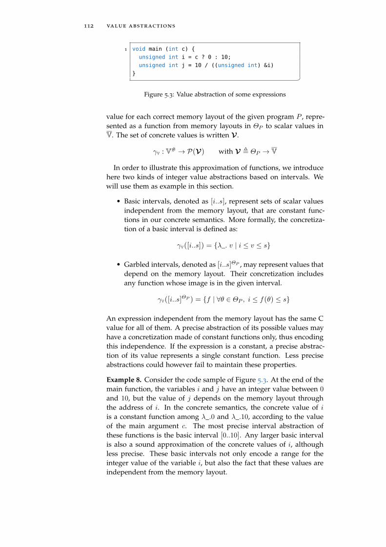
112 value abstractions
1 void main (int c)
unsigned int i = c ? 0 : 10;
unsigned int j = 10 / ((unsigned int) &i)
Figure 5.3: Value abstraction of some expressions
value for each correct memory layout of the given program P , repre-sented as a function from memory layouts in ΘP to scalar values inV. The set of concrete values is written V .
γV : V# → P(V) with V ΘP → V
In order to illustrate this approximation of functions, we introducehere two kinds of integer value abstractions based on intervals. Wewill use them as example in this section.
• Basic intervals, denoted as [i..s], represent sets of scalar valuesindependent from the memory layout, that are constant func-tions in our concrete semantics. More formally, the concretiza-tion of a basic interval is defined as:
γV([i..s]) = λ_. v | i ≤ v ≤ s
• Garbled intervals, denoted as [i..s]ΘP , may represent values thatdepend on the memory layout. Their concretization includesany function whose image is in the given interval.
γV([i..s]ΘP ) = f | ∀θ ∈ ΘP , i ≤ f(θ) ≤ s
An expression independent from the memory layout has the same Cvalue for all of them. A precise abstraction of its possible values mayhave a concretization made of constant functions only, thus encodingthis independence. If the expression is a constant, a precise abstrac-tion of its value represents a single constant function. Less preciseabstractions could however fail to maintain these properties.
Example 8. Consider the code sample of Figure 5.3. At the end of themain function, the variables i and j have an integer value between 0
and 10, but the value of j depends on the memory layout throughthe address of i. In the concrete semantics, the concrete value of i
is a constant function among λ_.0 and λ_.10, according to the valueof the main argument c. The most precise interval abstraction ofthese functions is the basic interval [0..10]. Any larger basic intervalis also a sound approximation of the concrete values of i, althoughless precise. These basic intervals not only encode a range for theinteger value of the variable i, but also the fact that these values areindependent from the memory layout.

5.2 abstractions of concrete values 113
On the other hand, the garbled interval [0..10]ΘP (or any largergarbled interval) is also a sound approximation of the concrete valuesof i, but fails to encode this fact. This garbled interval is also a soundapproximation of the set of possible concrete values of j, that cannotbe represented by a basic interval.
In a given memory layout θ, the set of the possible values denotedby an abstraction v# is the union of the image of θ by all functionsof the concretization of v#. We denote this set by γV(v#)(θ), even ifγV(v#) is a set of functions.
γV(v#)(θ) = f(θ) | f ∈ γV(v
#)
This view of a value abstraction yields a set of C values in eachmemory layout of ΘP , but leaves out some information given by theset of functions. For instance, an abstraction can encode that the valueof an expression is independent of the memory layout, even withoutany information about its precise value. This is the case of the basicinterval [−∞..∞]. Its concretization is then the set of constant func-tions λ_.k in V , much more precise than the set of all these functions.However, for all memory layouts, the set γV([−∞..∞])(θ) is the set ofall values V, and the property carried by the abstraction is lost. Yet,this property may be important if the expression is used as a condi-tional in an if statement, as the control flow of a program should notdepend on the memory layout.
Still, in a memory layout θ, an abstraction v# is a sound approxi-mation of the value of an expression e in a given concrete memory m
when e evaluates in the memory m into a C value that belongs to theconcretization γV(v#)(θ):
∃f ∈ γV(v#), e
m= f(θ) ⇔ e
m∈ γV(v
#)(θ)
However, according to a concrete state, the soundness of a valueabstraction is not defined for each memory layout independently. Theconcrete states of our language semantics are functions from correctmemory layouts to memories. The evaluation of a scalar expressionin a concrete state is then a function from memory layouts to scalarvalues. The soundness of value abstraction is defined accordingly.
Definition 39. An abstraction v# is a sound approximation of thevalue of an expression e in a given concrete state S when the eval-uation of e in S is in the concretization of v#.
e(S) ∈ γV(v#)
5.2.2 Lattice Structure
A value abstraction V# must be equipped with a lattice structure(V#,V,V,V,V) that satisfies the properties specified in Figure 2.4,

114 value abstractions
according to the value concretization γV. The join and the meet over-approximate respectively the union and the intersection of sets ofconcrete values. Value abstractions are partially ordered according tothe inclusion of their concretization. The top element represents allpossible C values of scalar type.
During the analysis, two values are met when they are both soundabstractions of the possible values of the same lvalue or expression.Then, the meet produces the most precise value abstraction for thisexpression. In particular, each abstract domain supplies the analyzerwith value abstractions during the evaluation of an expression. Thegeneric evaluator performs naturally the meet of these values, to ben-efit from the information inferred by all domains.
By contrast with the lattice structure required for state abstractions,the join between value abstractions is not really crucial. In abstractinterpretation, the join of abstract states is used at a merge point inthe CFG, to over-approximate the concrete states coming from eachbranch. But there is not such thing in expressions. In EVA, the join onvalues is only used when the evaluation of an expression is separatedinto several cases, to rejoin the abstractions computed for each case.The process of subdividing an evaluation is explained in Section 6.2.4.
The state abstractions and the generic analyzer naturally resort tothe top element of the value lattice whenever they have no informa-tion about a variable or an expression.
5.2.3 Semantics of Values and Alarms
An alarm map models the undesirable behaviors that may occur whenthe evaluation of an expression fails into the error value Ω. If theassertions carried by such a map are satisfied at runtime, then theevaluation cannot fail. A value abstraction approximates the concretevalue an expression may have when its evaluation does not fail. Apair of a value abstraction and an alarm map can thus exhaustivelyrepresent the evaluation of an expression.
Definition 40 (Semantics of pairs of values and alarms). A pair of avalue abstraction v and an alarm map A is a sound abstraction of theevaluation of an expression e in a concrete state S when A is a soundapproximation of the undesirable behaviors of the evaluation, and v
is a sound approximation of its resulting value. We denote that by
(v,A) |=V×A eΘ(S).
(v,A) |=V×A eΘ(S) ⇔
A |=A eΘ(S)eΘ(S) ⊆ γV (v) ∪ Ω
We also define the lattice structure of such pairs, by the pointwiseapplication of the lattice structure of value abstrations and alarmmaps.

5.2 abstractions of concrete values 115
Definition 41 (Lattice structure of pairs of values and alarms).
∀(v1, v2) ∈ (V#)2, ∀(A1,A2) ∈ A2,
(v1,A1) V×A(v2,A2) ⇔ v1 V v2 ∧ A1 A A2
(v1,A1) V×A(v2,A2) (v1 V v2,A1 A A2)
(v1,A1) V×A(v2,A2) (v1 V v2,A1 A A2)
V×A
(V,A)
Lemma 11. If two pairs of value abstractions and alarm maps (v1,A1)
and (v2,A2) are sound abstractions of the evaluation of an expression e
in a concrete state S, then their meet is also a sound abstraction of this
evaluation eΘ(S).
(v1,A1) |=V×A eΘ(S)(v2,A2) |=V×A eΘ(S)
⇒ (v1,A1) V×A(v2,A2) |=V×A eΘ(S)
Proof. This lemma is a direct consequence of the properties of Fig-ure 2.4 and of lemma 8.
5.2.4 Abstraction of Constants
Some lifting functions embed concrete values into abstract ones. Theyare used to translate the constants into the abstracted world. For aconstant c of the language, we write c# its injection in the value ab-straction V#: c# is simply the smallest abstract element v of V# suchthat c ∈ γV(v). Let us recall that the constants of our language includeinteger, floating-point and pointer values. For a value abstraction un-able to represent some types, c# could be V for some constants c.
5.2.5 Abstraction of Operators
The main feature of value abstractions is to implement an abstractsemantics for the C operators on expressions. For each n-ary oper-ation ♦ on C expressions, the value abstraction provides a forwardand a backward abstract counterpart F#♦ and B
#♦ . Their correctness
is defined through the concretization γv. As the concretization of avalue abstraction is a set of concrete values, we silently lift the seman-tics of operators from elements to sets. By convenience, we also writeγV(v) for the concretization of a vector v of value abstractions.
Notation 7 (Concretization of a vector of abstractions, and concretesemantics on sets).
∀v = (v1, . . . , vn) ∈ (V#)n,
γV(v) γV(v1), . . . , γV(vn)
[(♦)]Θ(γV (v)) [(♦)]
Θ(V ) | V ∈ γV (v)

116 value abstractions
5.2.5.1 Forward Abstract Semantics
Given abstractions v of the operands, the forward function F#♦ pro-
duces a sound abstraction of the output of the operation, when ap-plied to concrete values in the concretization of v. The resulting ab-straction of F#♦ consists of:
• an alarm map that is a sound abstraction of the undesirable
behaviors of the evaluation of [(♦)]Θ(γV (v)).
• a value that is an over-approximation of the set of the possible
concrete values resulting from [(♦)]Θ(γV (v)), when no undesir-
able behavior occurs. This value may be ⊥, if the operation iscompletely illegal (i.e. if it always fails with the error Ω).
Definition 42. A forward abstract semantics of an n-ary operator ♦
is a function F#♦ from a vector v of n value abstractions to a pair of
a value abstraction and an alarm map that are sound abstractions ofthe possible output of the operator, when applied to concrete valuesin the concretization of v.
F#♦ : (V#)n → (V# +⊥)×A
∀v ∈ (V#)n, F#♦ (v) = (r,A) ⇒
A |=A [(♦)]Θ(γV(v))
[(♦)]Θ(γV (v)) ⊆ γV (r) ∪ Ω
5.2.5.2 Backward Abstract Semantics
Conversely, the backward function B#♦ produces abstractions of the
operands from an abstraction of the result. However, such a back-ward propagation of abstractions cannot be precise for operators withseveral operands, as multiple abstractions should be deduced fromonly one. Indeed, knowing that x ≤ y or that x + y ∈ [0..10] inall layouts is not enough to infer any information about the valueof x and y. Instead, a backward operator B
#♦ takes the value ab-
stractions of the operands, and tries to reduce them according to theabstraction of the result. The reduced abstractions must still over-approximate all the possible concrete values for the arguments lead-ing to a value included in the result abstraction through the operator.For instance, the backward operation on interval abstractions for thecomparison ≤ [0..10] with result [1] reduces the first argumentvalue to [−∞..10], and lets the second argument value unchanged.The backward addition + [−10..−∞] with a result in [0..10] leadsto the same result.
Definition 43. A backward abstract semantics of an n-ary operator ♦is a function B
#♦ that takes an abstraction r and a vector v of n abstrac-
tions, and that produces a vector of value abstractions that are sound

5.2 abstractions of concrete values 117
abstractions of the possible inputs in v for which the operator leadsto a result in the concretization of r.
B#♦ : (V#)n ×V# → (V# +⊥)n
∀v, r ∈ (V#)n+1, x ∈ γV (v) |[(♦)]Θ(x) ∈ γV (r) ⊆ γV(B
#♦ (v, r))
The backward operators handle only value abstractions, and do notproduce or reduce alarms. Indeed, while the value of ♦(e) dependsdirectly on the value of the expressions e, the alarms issued for theoperation are independent from those issued for its operands. Also,the backward operators can assume that the operation succeeds, sincethe alarms produced by the forward abstract semantics report theerror cases. This may achieve some reductions of the operands, ifsome values lead necessarily to an undesirable behavior. However,backward operators may also reveal a contradiction, leading to theempty value abstraction ⊥ for one of the operand, and so for thewhole expression. This happens typically when the condition of anif statement is unsatisfied.
5.2.5.3 Implementation Signature
Figure 5.4 presents the OCaml interface of the abstract operators ofvalue abstractions in EVA. The type t is the one of the value abstrac-tion. Operators are grouped by arity; unop and binop are the unaryand binary operators of the CIL AST. The type on which this oper-ator is applied is also explicitly given, as the CIL operators are notspecialized by their type. The context argument gathers the expres-sions of the operands; they are only needed to create the proper mapof alarms for this particular application of the operator. Indeed, therelevant alarms are assertions whose free variables are these expres-sions. Finally, an abstract operator takes the value abstractions ofthe operands, and returns an abstraction of the result — value andalarms — through the t evaluated type introduced in Section 5.1.5.
Likewise, a backward operator takes a value abstraction for eachoperand and for the result, and returns either bottom — in case ofcontradiction — or a value abstraction for each operand. In manycases, the abstraction of the result is too imprecise to achieve a reduc-tion of the operands. The backward operator could then return theoperand abstractions unchanged, but it may be useful to notify explic-itly the absence of reduction. To this end, the results of the backwardoperators are OCaml option types, None meaning that no reductionhas been performed.
Similar functions are provided for conversions, which are not stan-dard unary operators in CIL, and for which the source and destinationtypes are given explicitly.

118 value abstractions
1 type t (* type of value abstraction *)
val forward_unop :
context:unop_context -> typ -> unop -> t -> t evaluated
5 val forward_binop :
context:binop_context -> typ -> binop -> t -> t -> t evaluated
val forward_cast :
context:exp -> src_typ:typ -> dst_typ: typ -> t -> t evaluated
10 val backward_unop :
typ -> unop -> arg:t -> res:t -> t option or_bottom
val backward_binop :
typ -> binop -> left:t -> right:t -> result:t ->
(t option * t option) or_bottom
15 val backward_cast:
src_typ: typ -> dst_typ: typ -> src_val: t -> dst_val: t ->
t option or_bottom
Figure 5.4: Interface of the abstract operators on values
5.2.6 Abstractions of Memory Locations
Values are abstractions of C values of scalar types only. Copies ofaggregate types such as arrays and structures must be handled by thestate abstractions – although the content of their fields and cells canbe represented as values. However, in a language with pointers suchas C, scalar variables may contain addresses. Hence, values are alsoabstractions of pointer values, and thus of memory addresses. Theabstract (forward and backward) transformers on value abstractionsencompass all expression operations involving pointers: addition ofan integer to a pointer, subtraction of two pointers, comparison ofpointers, conversion between integer types and pointers.
However, the abstract value operators do not include the addressoperations — array subscripting and structure fields. Instead, the ad-dress semantics is abstracted by specific representations of memorylocations. They are abstractions of the set of the possible memorylocations pointed to by an address in some concrete states. They im-plement an abstract semantics of addresses, and are used to processdereferencing through the state abstractions of the memory. Theseabstractions of address locations are closely tied to the abstractionsof the expression values. Indeed, an address is an expression (eval-uating to a pointer value, thus a location), plus certain offsets forfields in structures and cells in arrays, the latter being also denotedby expressions (evaluating to integers). In fact, the abstractions for lo-cations could be exactly the same as for the pointer values. However,the distinction between the two allows for some more precision andsome subtleties in the handling of addresses. In particular, EVA han-

5.2 abstractions of concrete values 119
dles bitfields through the location abstractions only (although clike
does not include bitfield).It is worth remembering that in clike, addresses appear only in
dereferences and assignments. In a given concrete state, the derefer-ence and assignment semantics both require their address to evaluateto the same valid τ -location in all possible memory layouts. Thus,the location abstractions approximate sets of constant locations, iden-tified as valid pointer values for the considered type. If the value ofan address depends on the memory layout, an alarm is emitted.
A set of such location abstractions is denoted L#. A concretizationγL links each location abstraction to the set of memory locations itrepresents.
γL : L# → P(L)
As usual, location abstractions are equipped with a lattice structure(L#,L,L,L,L). Finally, location abstractions provide the ab-stract address semantics:
• F#addr converts a value abstraction v into a location abstraction
(as an expression with pointer type is also an address): the re-sult only abstracts the constant valid pointer values of γV(v).
• F#
[]abstracts array subscripting a[e], from a location abstraction
of the address a and a value abstraction of the expression e.
• F#.f abstracts the location of the field f in the structures repre-
sented by the given location abstraction.
F#addr : V# → (L#+⊥)×A
F#
[]: L# → V# → (L#+⊥)×A
F#.f : L# → (L#+⊥)×A
These forward functions also have their backward counterparts. Asfor value operator ♦, these operations do not depend on memories.Their abstract forward and backward semantics are guided by thesame principles and the same soundness requirements as the seman-tics of expression. We do not detail them here, and refer the readerto Section 5.2.5.
5.2.6.1 Reductions on Addresses
As mentioned earlier, the dereference of an address forces some re-quirements about the value of the address, regardless of the concretestate and the resulting concrete value. In the absence of dynamicallocation, the validity of an address can be checked without anyknowledge of the memory. A dereferenced address must have thesame valid pointer value in all memory layout, i.e. a value such as

120 value abstractions
Listing 5.1: Reducing abstract location
1 void main (int i)
int t[2] = 1,2;
int x = t[i];
int *p = i ? &x : NULL;
5 int y = *p;
λ_.(&x, i) with x a variable of the program, and i an integer between 0
and sizeof(x)− 1. Otherwise, the dereference raises an error.In EVA, the location semantics reflects this:
• if an abstract location does not guarantee the validity of theaddress, an alarm is emitted;
• if possible, abstract locations are shrunk to their valid parts for adereference. This includes reducing the abstraction of an arrayindex to a positive integer value, strictly less than the size of thearray.
Example 9. The code of listing 5.1 includes two dereferences thatfails for some initial value of the argument i. At line 3, the abstractsemantics F#
[]can reduce the value abstraction of i to a representation
of 0; 1, the only possible integer offset for the array t. At line 5, theabstract semantics F
#addr can reduce the value abstraction of p to a
representation of &x, as null is never a valid pointer value. Inboth cases, the location abstraction of the address represents only thevalid memory locations for the dereference.
5.3 the cvalue implementation
EVA provides abstractions of integer, floating–point and pointer val-ues called cvalue. These abstractions are inherited from VALUE, theformer abstract interpreter of Frama-C. They handle the whole se-mantics of expressions, and always produce closed maps of alarmsto report undesirable behaviors. As the default value abstractions,they are the privileged means of communication between abstractdomains in our analyzer. They are able to express precise alias in-formation between variables, which is very convenient for purely nu-merical domains.
In this section, we first describe formally the representation ofconcrete values chosen in the cvalue abstractions. We then give anoverview of their semantics, focusing on the addition between point-ers and integers. We finally address the backward propagators forthe same operation.

5.3 the cvalue implementation 121
5.3.1 Basic Representation of Constant Values
As explained in Section 4.3.3, the concrete values of our semanticsare functions from memory layouts to C values. In practice, mostof the values manipulated by a program are independent from thememory layout — and are thus constant functions in our semantics.Other concrete values only arise when performing integer arithmeticon variable addresses. The cvalue module provides specific and pre-cise abstractions of sets of concrete values that are independent ofthe memory layout, and another coarser representation for arbitraryconcrete values.
The basic arithmetic and pointer abstractions stand only for C val-ues independent of the memory layout. They simply describe a setof C values, and their concretization is the set of constant functions,from any memory layouts to a C value in the set they describe. Theirrepresentation of sets of C values and their abstract semantics arequite precise.
On the other hand, values depending on the memory layout arecaptured by an imprecise abstraction called garbled mix, whose se-mantics is postponed to the next subsection.
5.3.1.1 Basic Integer Abstractions
The basic integer abstractions represent sets of integer values. Theyare a reduced product of sets of discrete integers and integer intervalswith congruence.
discrete sets The sets of integers are not real abstractions: theyrepresent exactly their elements. However, for performance reasons,their cardinal is kept small: above a certain limit, they are automati-cally converted into integer intervals. Their maximal cardinal is user-configurable2, and is 8 by default. These sets are ordered, and areimplemented with arrays.
i1, i2, . . . , in ∀k, ik ∈ Z k < l ⇒ ik < il
integer intervals These abstract values are themselves a re-duced product between intervals and congruence. An integer inter-val is a pair of two values min and max in Z∪ +∞;−∞, such thatmin ≤ max . A congruence information is encoded with two naturalintegers rem and mod of N, such that 0 < mod and 0 ≤ rem < mod .Such an interval and a congruence represent the set of integers be-tween min and max and congruent to rem modulo mod . We writethis abstraction as:
[min..max ]rem%mod
2 Through the parameter -val-ilevel

122 value abstractions
A canonical representation of these abstractions is maintained. Thelower (respectively upper) bound of the interval is always refined up(resp. down) to the nearest integer validating the congruence. A valuecarrying no congruence information has mod = 1 and rem = 0. Anyvalue representing less than 8 integers (by default) is automaticallyconverted into the set of these integers.
concretization These abstractions represent only integer val-ues that do not depend on the memory layout. Formally, their con-cretizations are the following:
γCVal(X) λ_. i | i ∈ Z ∧ i ∈ X
γCVal([min..max ]r%m) λ_. i | i ∈ Z ∧ min ≤ i ≤ max
∧ i ≡ r mod m
These concretizations go into mathematical numbers. They de-scribe sets of concrete values in any integer type. The set of concretevalues of type τ depicted by an abstraction a is then the intersection(Vτ )ΘP ∩ γCVal(a).
By a slight abuse of notation, as a basic arithmetic abstraction a
describes only constant functions to integer i, we write i ∈ a forλ_.i ∈ γCVal(a).
canonization Maintaining a canonical representation of theseabstractions requires conversions between discrete sets and intervals.The conversions have to be sound through the concretization. The op-erator continuous expands a set i1, . . . , in into the smallest intervaland congruence abstraction whose concretization contains the con-stants i1 to in. As the integers of the set are ordered, the intervalbounds are i1 and in. The modulo m is the greatest common divisorof the subtractions ik − i1. Indeed, we have:
∃r, ∀k, ik ≡ r mod m ⇔ ∀k, m | (ik − i1)
And the remainder r can be deduced from the modulo m and any ik.Conversely, the operator discrete breaks an interval [i..s]r%m into theset of all integers it describes. As the bounds of the interval satisfythe congruence, both are in the set, as well as all integers i1 + k ·m
between i1 and in.
continuous(i1, . . . , in) = [i1..in]r%m
with
m = pgcd(i2 − i1, . . . , in − i1)
r = i1 mod m
discrete([i..s]r%m) = i, i+m, i+ 2m, . . . , s
Note that the discrete operation is exact, while the continuous canlose much precision. For instance, continuous(1, 100) = [1..100]0%1.

5.3 the cvalue implementation 123
Finally, the canonize operator maintains a canonical representation ofthe basic integer abstractions.
canonize(i1, . . . , in) =
i1, . . . , in if n ≤ 8
continuous(i1, . . . , in) otherwise
canonize([i..s]r%m) =
discrete([i..s]r%m) if (s − i)/m < 8
[i..s]r%m otherwise
with
i = minj(j ≥ i ∧ j ≡ r mod m)
s = maxt(t ≤ s ∧ t ≡ r mod m)
5.3.1.2 Basic Floating-point Abstractions
Sets of floating-point values are represented by a floating–point inter-val, that is a pair of two double floating–point numbers. It representsthe set of all floating-point numbers between them, excluding infiniteand NaNs. We write them as:
[min..max ]
And the concretization of such an interval is:
γCVal([min..max ]) λ_. f | f ∈ Q ∧ min ≤ f ≤ max
5.3.1.3 Basic Pointer Abstractions
Concrete pointer values are pairs of a program variable and an integeroffset, expressed in bytes. The basic pointer abstractions are mapsfrom variables to basic integer abstractions. Such a map, binding thevariables xk to the abstractions ok, is written as follows:
&xk+ok k
These maps represent pointer values independent of the memory lay-out, i.e. pointing to the same memory position in all layouts. Thus,the concretization of a map L contains the set of all constant functionsto a pointer value (&x, i) such that the variable x is in the map, andthe integer offset i is in the concretization of L(x).
Furthermore, such a map is also used to depict the integer inter-pretation of a pointer value. Indeed, the basic arithmetic abstractionsare unable to capture the dependence between an integer and a mem-ory location, and cannot represent the integer conversion of a pointer.Instead, we use the maps to represent a set of pointer values, or theinteger conversion of these pointer values. Thus, they can representinteger values that are dependent of the memory layout, but whoseconversion into a pointer value is independent of the memory layout.

124 value abstractions
Listing 5.2: Basic pointer abstraction representing integers
1 #include <stdint.h>
int x = 1;
uintptr_t y = (uintptr_t)&x + 42;
5 int z = (int *)(y - 42);
Thus, the maps may denote the possible values of an expression ofpointer or integer type. Formally, their concretization is:
γCVal( &x+o ) λ_. (&x, i) | λ_.i ∈ γCVal(o)
∪ λθ. (θ(x) + i) | λ_.i ∈ γCVal(o))
γCVal( &xk+ok k∈K)
k∈K
γCVal( &xk+ok )
As for the integer abstractions, this concretization must be intersectedwith the set of concrete values V . In particular, some of the pointervalues (&xk, i) may be invalid and not exist in Vptr. The concretiza-tion of a basic pointer abstraction may even contains no pointer val-ues but only integers. For instance, at line 4 of listing 5.2, a sound ab-straction of the variable y is the map &x+[42] ; its concretizationis the singleton λθ. (θ(x) + 42), whose conversion into a pointervalue would fail. At line 5, the abstraction of the integer y-42 and ofthe pointer (int *)y-42 is the same map &x+[0] .
In the implementation, the numerical abstractions are embeddedinto pointers abstractions as maps from the null base to the arith-metic abstraction. For the sake of clarity, we keep separate theseabstractions in this manuscript.
5.3.2 Garbled Mix: a Representation of Not Constant Values
The basic pointer abstractions are able to precisely handle the wholesemantics of pointers. They also represent the integer conversion ofpointers, but are unable to interpret all the integer arithmetic on thoseconcrete values. For instance, the result of an integer multiplicationbetween two variable addresses cannot be represented as a map froma variable to a basic integer representation.
After arithmetic operations that are meaningless on variable ad-dresses, the precise maps for pointer values degenerate into impre-cise abstractions in which the offset information is discarded. Thesenew abstractions store only the variable addresses from which thenew concrete value has been computed. These abstractions are calledgarbled mix.

5.3 the cvalue implementation 125
5.3.2.1 Definition
Let X be a set of program variables. A garbled mix GM(X) mod-els all the concrete values whose byte interpretation according to thememory layout depends only on the integer addresses of the vari-ables of X . Such a concrete value has the same byte interpretationin two memory layouts where the variables of X have the same ad-dresses. We consider the byte interpretation of the value to make thesymbolic representation of pointer values (&x, i) dependent of theaddress of x.
Definition 44. A concrete value V of type τ depends only on theinteger addresses of variables in X when for any layouts θ and θ thatcoincide on X , the byte interpretations of the C values V (θ) and V (θ)
are equal.
∀θ, θ ∈ (ΘP )2, θ|X = θ|X ⇒ φτ (V (θ)) = φτ (V (θ))
We denote this property by V ≡ V |X .
Definition 45 (Concretization of garbled mixes). The concretizationof a garbled mix is then defined as:
γCVal(GM(X)) = V ∈ V | V ≡ V |X
Finally, the widest abstraction is the special garbled mix GM(X ) —X being the set of the program variables.
Lemma 12. The concretization of GM(X ) is the set of all concrete values.
γCVal(GM(X )) = V
Proof. As memory layouts are functions from X to N:
∀θ, θ ∈ (ΘP )2, θ|X = θ|X ⇒ θ = θ
⇒ ∀V ∈ V , φτ (V (θ)) = φτ (V (θ))
And thus ∀V ∈ V , V ≡ V |X ⇒ ∀V ∈ V , V ∈ γCVal(GM(X )).
It is worth noting that a garbled mix for an expression expressesnothing on the C values this expression may have, but only specifiesthe variable addresses on which its values may depend. Thus, a gar-bled mix may depict the possible values of any expression, regardlessof its type.
5.3.2.2 Assumption About Memory Layouts
The semantics of the cvalue abstractions makes an assumption overthe possible memory layouts of a program. It requires that the integeraddress of a variable x cannot be deduced from the address of theother program variables. If this invariant is not guaranteed for aparticular program P , then the semantics of the cvalue abstractions isunsound for the analysis of P .

126 value abstractions
Axiom 1. Let P be a program, X the set of variables of this program, and
Θ the set of possible memory layouts for these variables. Let x be a variable
of X . The address of x is not determined by the address of all other variables
from X : there is no function f : N(|X |−1) → N such that in all layout of Θ,
the memory address of x is f(θ(X\x)).
∀x ∈ X , f : N(|X |−1) → N, ∀θ ∈ ΘP , θ(x) = f(θ(X\x))
In other words, for each variable x of the program P , there exists two
memory layout θ and θ such that:
• the addresses of x in θ and in θ are different;
• but the addresses of all other variables are the same in θ and in θ.
∀x ∈ X , ∃(θ, θ) ∈ (ΘP )2,
θ(x) = θ(x)
∀y ∈ X , y = x ⇒ θ(y) = θ(y)
The immediate consequence of this axiom is that a pointer value (&x, i)
belongs to the concretization of a garbled mix GM(X) if and only if xbelongs to X .
Theorem 4. Let X be a set of variables, x be a variable, and i be an integer.
λ_.(&x, i) ∈ γCVal(GM(X)) ⇔ x ∈ X
λθ.(θ(x) + i) ∈ γCVal(GM(X)) ⇔ x ∈ X
Proof. Let us remind definition 22 of pointer interpretation:
φptr(&x, i) = φaddress(θ(x) + i) (5.1)
We assume first that x ∈ X . Let θ and θ be two memory layouts suchthat θ|X = θ|X . In particular, θ(x) = θ(x).Let V = (λ_.(&x, i))(θ). Equation 5.1 ensures:
φptr(V (θ)) = φaddress(θ(x) + i)
= φaddress(θ(x) + i) = φptr(V (θ))
Let V = λθ.(θ(x) + i), we also have:
φint(V (θ)) = φint(θ(x) + i) = φint(θ(x) + i) = φint(V (θ))
In conclusion, V and V belong to γCVal(GM(X)).Conversely, let y be a variable such that λ_.(&y, i) ∈ γCVal(GM(X)).
Axiom 1 ensures the existence of two memory layouts θ and θ suchthat:
θ(y) = θ(y)
∀x ∈ X , x = y ⇒ θ(x) = θ(x)

5.3 the cvalue implementation 127
GM(X )
GM(xii)
xi+oi i
[i..s]r%m
ik
[i..s]
⊥
includes
may include
GM(X) GM(Y ) ⇔ X ⊆ Y
xi+oi i GM(X) ⇔ ∀i, xi ∈ X
xi+oi i yj+pj j ⇔ ∀i, ∃j, yj = xi ∧ oi pj
[i..s]r%m [i..s]r%m ⇔
i ≥ i ∧ s ≤ s
m ≡ 0[m] ∧ r ≡ r[m]
jl [i..s]r%m ⇔ ∀l, i ≤ jl ≤ s ∧ jl ≡ r[m]
ik jl ⇔ ik ⊆ jl
Figure 5.5: Lattice structure of the cvalue abstractions
And thus y /∈ X ⇔ θ|X = θ|X .By definition 45 of garbled mixes, equation 5.1 and the bijectivity ofinterpretation functions (stated in definition 20):
θ|X = θ|X ⇔ φptr(V (θ)) = φptr(V (θ))
⇔ φaddress(θ(y) + i) = φaddress(θ(y) + i)
⇔ θ(y) + i = θ(y) + i
⇔ θ(y) = θ(y)
Finally, y /∈ X ⇔ θ(y) = θ(y) and θ(y) = θ(y) by hypothesis, whichimplies y ∈ X .The proof is exactly the same for the concrete value λθ.θ(x) + i.
This proposition allows us to define the lattice structure of cvalueabstractions.
5.3.2.3 Lattice Structure of the Cvalue Abstractions
The diagram of Figure 5.5 defines the lattice structure of the cvalueabstractions. The top element GM(X ) includes all other abstractions.The inclusion of garbled mixes is the inclusion of their variable sets.All garbled mixes include all basic arithmetic abstractions; a garbledmix includes a pointer map if all variables of the map belong alsoto the garbled mix. A map M is more precise than another M iffor all variable, the abstraction of its offset is more precise in M than

128 value abstractions
in M — considering that the missing variables of a map are boundto ⊥. Finally, the lattice structure of the arithmetic cvalue abstractionsfollows the standard rules of intervals and congruences.
We prove the structure lattice for operations involving garbled mixes—the other abstractions being more standard.
Lemma 13. The order relation defined at Figure 5.5 is sound according to
the concretization γCVal. For all cvalue abstractions C and C :
C C ⇔ γCVal(C) ⊆ γCVal(C)
Proof. We prove the case C = GM(X), according to the cvalue C.
Case 1. if C is a basic integer or float abstraction:
γCVal(C) ⊆ λ_.r | r ∈ Q
Let V = λ_.r with r ∈ Q. The byte interpretation of r doesnot depend on the memory layout:
∀θ, θ ∈ (ΘP )2, φτ (V (θ)) = φτ (r) = φτ (V (θ))
And by definition 45, for all set X , V ∈ γCVal(GM(X)).Thus, for all basic integer or float abstraction C and allset X ,
γCVal(C) ⊆ γCVal(GM(X))
Case 2. If C is a map abstraction: C = xi + oi i.Let V be a concrete value in γCVal(C). It has the form V =
λ_.(&xi, j) or V = λθ.θ(xi) + j.By theorem 4, such a concrete value belongs to γCVal(GM(X))
if and only if xi ∈ X .Thus:
γCVal( xi + oi i) ⊆ γCVal(GM(X)) ⇔ ∀i, xi ∈ X
Case 3. If C is a garbled mix: C = GM(Y ).Let V be a concrete value of type τ that belongs to γCVal(GM(Y )).
∀θ, θ ∈ (ΘP )2, θ|Y = θ|Y ⇒ φτ (V (θ)) = φτ (V (θ))
If Y ⊆ X , then θ|X = θ|X ⇒ θ|Y = θ|Y , and:
∀θ, θ ∈ (ΘP )2, θ|X = θ|X ⇒ φτ (V (θ)) = φτ (V (θ))
This implies that V also belongs to γCVal(GM(X)).
Y ⊆ X ⇒ γCVal(GM(Y )) ⊆ γCVal(GM(X))
Conversely, we assume that γCVal(GM(Y )) ⊆ γCVal(GM(X)).By theorem 4:
y ∈ Y ⇒ (λ .(&y, 0)) ∈ γCVal(GM(Y ))
⇒ (λ .(&y, 0)) ∈ γCVal(GM(X)) ⇒ y ∈ X
And thus Y ⊆ X . We have finally:
Y ⊆ X ⇔ γCVal(GM(Y )) ⊆ γCVal(GM(X))

5.3 the cvalue implementation 129
5.3.3 Forward Abstract Semantics of Cvalues
The cvalue semantics of the C operators is divided into the approx-imation of the corresponding mathematical operation, and the em-bedding of its result into the type of the concrete operator. In whatfollows, we omit the emission of alarms and focus on the abstrac-tion of the correct behaviors of the operators. Without detailing thecomplete cvalue semantics, we use the integer addition as runningexample.
5.3.3.1 Mathematical Arithmetic
arithmetic on basic arithmetic abstractions The basicarithmetic abstractions represent only constant functions from mem-ory layout to C values. The semantics of an operator ♦ is its pointwiseapplication on C values under each memory layout independently.As long as the operator on C values does not depend itself on the lay-outs, its semantics on constant functions lead to a constant function.This is the case for all operators, except for the casts between integerand pointer values.
∀i, Vi = λ_. vi ⇒ [(♦)]Θ(V1, . . . , Vn) = λθ. [(♦)](V1(θ), . . . , Vn(θ))
= λ_. [(♦)](v1, . . . , vn)
Thus, the abstract semantics of basic arithmetic abstractions forthese operators produce only basic arithmetic abstractions. The se-mantics of discrete sets amount to performing the concrete operationon each element of the sets. The semantics of the other abstractionsfollow the standard arithmetic on intervals and congruences [Moo66;Gra89]. If an operation involves a discrete set and an interval withcongruence, the set is treated as an interval abstraction. In any case,the resulting abstraction is revised into its canonical representation.
The abstract semantics for the integer addition is given as exam-ple. We use the infix notation +CVal for the cvalue semantics of themathematical addition.
xk0≤k≤i +CVal yl0≤l≤j = canonize(xk + yl0≤k≤i ∧ 0≤l≤j)
[ix..sx]rx%mx +CVal [iy..sy]ry%my = canonize([i..s]r%m)
where
i = ix + iy
s = sy + sy
m = pgcd(mx,my)
r = (rx + ry) mod m
[i..s]r%m +CVal yl0≤l≤j = [i..s]r%m +CVal continuous(yl0≤l≤j)

130 value abstractions
integer arithmetic on pointers abstractions As vari-able addresses can be manipulated through integer arithmetic, thepointer abstractions end up describing integer values. As far as possi-ble, maps from variable to integer offsets are used as a precise repre-sentation of the integer interpretation of valid pointer values. But forthe operations that are meaningless on pointers, the maps degenerateinto garbled mix.
We use again the integer addition as an example of the abstractsemantics on cvalues. The addition between the integer view of apointer and an integer is naturally defined as:
[(+int)]Θ(λθ. θ(x) + i , λ_. j) = λθ. θ(x) + (i+ j)
This output can be soundly described by a map from the variable x
to an abstraction of (i+ j). Let M be a basic pointer abstraction anda be a basic arithmetic abstraction, both representing a set of concreteinteger values. We want a map R such that:
M +CVal a = R
⇒ ∀x ∈ γCVal(M ), ∀y ∈ γCVal(a), [(+int)]Θ(x, y) ∈ γCVal(R)
Note that, as the operator +int is typed, the concrete values x and y
must be of integer type. By using the notation j ∈ a for λ_.j ∈
γCVal(a), this condition can be rewritten as:
∀x ∈ M, ∀i ∈ M(x), ∀j ∈ a, (λθ. θ(x) + (i+ j)) ∈ γCVal(R)
Thus, the map R binds each variable x in M to a basic integer ab-straction of λ_.(i+ j), for all integers i and j in the abstractions M(x)
and a. A precise abstraction for it is M(x) +CVal a. The result of theabstract addition is then a precise map:
&xi+oi +CVal a = &xi+(oi +CVal a) i
However, the map abstractions can only approximate concrete inte-gers that point to the same memory position, regardless of the mem-ory layouts. Yet, most integer operations on variable addresses donot keep this property. For instance, the result of the addition of theaddress of two variables x and y cannot be represented as a mapfrom a variable to a basic arithmetic abstraction. Indeed, the abstrac-tion bound to x should stand for the address of y, which obviouslydepends on the memory layout.
[(+int)]Θ(λθ. θ(x), λθ. θ(y)) = λθ. θ(x) + θ(y)
However, the resulting concrete value λθ. θ(x) + θ(y) belongs tothe concretization of the garbled mix GM(x, y), as a function from theinteger address of the variables x and y. More generally, in the ab-stract semantics of cvalues, the integer addition of two abstractions

5.3 the cvalue implementation 131
containing variable addresses degenerates into garbled mix, only re-taining the addresses from which the new value has been computed.The complete abstract addition on pointer maps and garbled mix isgiven by:
&xi+oi i +CVal a = &xi+(oi +CVal a) i
&xi+oi i +CVal &yj+pj j = GM(xii ∪ yjj)
&xi+oi i +CVal GM(yjj) = GM(xii ∪ yjj)
GM(xii) +CVal GM(yjj) = GM(xii ∪ yjj)
5.3.3.2 Embedding into the Machine World
The cvalue abstractions describe sets of mathematical values, but theactual operators of our language operate on machine values, encodedby a fixed and finite number of bytes. Some operations have thesame semantics in the mathematical and the machine worlds. This istypically the case for all comparison operators, whose result is alwaysa boolean in 0, 1. For the other operators, we need to shrink theabstract cvalue resulting from their mathematical semantics, in orderfor it to fit inside the operator type. This last step also handles thealarms about integer overflows.
5.3.3.3 Memory Locations of Addresses and Dereference
The cvalue abstractions of the possible memory locations of an ad-dress are roughly the same as the basic pointer abstractions of ex-pressions: maps from variables to offset abstractions, except that theoffsets are expressed in bits, and not in bytes. This allows the maps tomodel accurately the location of bitfields. The arithmetic abstractionsare ineffective to account for address values, but are used for theirinteger offsets.
The semantics of the variable maps are the same as before. Com-posing an address expression and its offset amounts to the additionof a pointer abstraction and an integer abstraction. The abstractionof the address locations is reduced to its valid part. The valid offsetsfor a variable x, expressed in bit, are [0..8 · (sizeof(x)− 1)]0%8, ex-cept for a bitfield, on which case no assumption can be made on thealignment of the offset. We omit the bitfield case in the following.The reduction of a map amounts to the reduction of all its offsets.The reduction of a garbled mix coming from an expression allows itsconversion into a map, from the variables it contains to all possibleoffsets for them. Indeed, a dereference requires that the pointed loca-

132 value abstractions
tion is the same in all memory layouts, which is exactly expressed bysuch a map.
offset(x) = [0..8 · (sizeof(xi)− 1)]0%8
valid( &xi+oi i) = &xx+(oi offset(x)) i
valid(GM(xii)) = xi+ offset(ii) i
This forward reduction can be crucial for the precision of the analy-sis. As we have seen above, a garbled mix tends to propagate to all ab-stractions, as the composition through any operator of a garbled mixand any other abstraction leads to another garbled mix. However, byrequiring the address to be independent of the memory layout, deref-erences allow reducing a garbed mix to a precise map representation.
5.3.4 Meet of Garbled Mixes
5.3.4.1 Motivation and General Considerations
Backward propagators on the basic cvalue abstractions can be imple-mented by following the standard rules of interval, congruence andpointer arithmetic. The next section is dedicated to an abstract back-ward semantics involving garbled mixes. As garbled mixes are veryloose approximations, their reduction is of particular importance forthe analysis precision. However, most reductions on garbled mixesare only possible if the variable addresses are adequately indepen-dent from each other in the possible memory layouts of a program.Ideally, we want the guarantee that if a concrete value depends onlyon the variable addresses in X on one hand, and on the variableaddresses in Y in the other, then it depends only on the variable ad-dresses in X ∩ Y . This would allows us to define the meet betweengarbled mixes as:
GM(X) CVal GM(Y ) = GM(X ∩ Y )
This definition is correct if and only if:
γCVal(GM(X)) ∩ γCVal(GM(Y )) ⊆ γCVal(GM(X ∩ Y ))
If any function from program variables X to integers N were amemory layout, this would definitely be the case.
Proof. Let V be a concrete value in both concretizations of GM(X)
and GM(Y ), and let θ and θ be two functions from X to N such thatθ|X∩Y = θ|X∩Y . We define a third function θ” by:
θ”(x) =
θ(x) if x ∈ X
θ(x) otherwise
5.3 the cvalue implementation 133
As θ|X∩Y = θ|X∩Y , we have θ|X = θ”|X and θ|Y = θ”|Y .By definition 45, φτ (V (θ)) = φτ (V (θ”)) = φτ (V (θ)).Thus, for all functions θ and θ:
θ|X∩Y = θ|X∩Y ⇒ φτ (V (θ)) = φτ (V (θ))
Which implies that V is in γCVal(GM(X ∩ Y )).
However, definition 21 imposes some restriction over memory lay-outs, and the intermediate function used in the proof could not be amemory layout.
5.3.4.2 Difficulties
Variable addresses cannot be completely independent from each oth-ers, as definition 21 precludes overlapping between variables. There-fore, if x and y are different variables, then their addresses cannot bethe same in a valid memory layout. Axiom 1 excludes the address of avariable to be certainly determined by the addresses of the other vari-ables. This is equivalent to state that the addressing space is strictlylarger than the set of program variables. The size of the addressingspace is determined by the number of possible pointer values, namely2sizeof(ptr), and a variable x takes sizeof(x) bytes in memory, plusone byte after that must not overlap with an other variable either (seedefinition 21). Finally, the address 0 is reserved to the null pointer.
x∈X
(sizeof(x) + 1) + 1 < 2sizeof(ptr)
However, this is not sufficient for our needs, as illustrated by thefollowing exemple.
Example 10. We consider a set X of variables, and assume the ad-dressing space to be only one more than
x∈X (sizeof(x) + 1) + 1.Let x be a variable of X , and θ be any valid memory layout for X .Then we have:
θ(x) < 3 ⇔ ∀y ∈ X\x, θ(y) > 2
Thus, the concrete value V = λθ.(θ(x) < 3) can be computed in eachlayout from θ(x) or from the set of θ(y) for all other variables y. Thismeans that V belongs to GM(x) and to GM(X\x).Thus, GM(x) CVal GM(X\x) = GM(∅).
5.3.4.3 New Restrictions on the Addressing Space
As axiom 1 is not strong enough, we reinforce it by axiom 2: it re-quires that the difference between the size of the addressing spaceand the size of all program variables is bigger than the size of thebiggest program variable.

134 value abstractions
Axiom 2.
x∈X
(sizeof(x) + 1) + 1+maxx∈X
(sizeof(x)) < 2sizeof(ptr)
Lemma 14. Given a program P with a set X of variables and two memory
layouts θ and θ in ΘP , axiom 2 ensures the existence of a series of valid
memory layouts θ0, . . . , θn such that θ0 = θ, θn = θ and:
∀i ∈ 1, . . . , n, ∃x ∈ X , ∀y ∈ X , y = x ⇒ θi(y) = θi−1(y)
Proof. The complete proof is given in Annex B. The idea is to shift onevariable at a time in θ and θ until all variables are adjacent, starting ataddress 1. Then, axiom 2 ensures that it remains enough addressingspace to move any variable at the end of the space. The same variableis put at the same address at the end of the addressing space in thetwo series, and the process can be repeated on the remaining vari-ables (shifting the variables to fill the gap left by the previous move,and chosing a shared variable to move at the released space).
Lemma 14 allows us to define the meet of two garbled mixes ofdisjoint sets of variables.
Lemma 15. Let X and Y be two sets of program variables. Then:
X ∩ Y = ∅ ⇒ GM(X) CVal GM(Y ) = GM(∅)
The concretization of GM(∅) is the set of concrete values V that are constant
according to the layout: ∀(θ, θ), φ(V (θ)) = φ(V (θ)).
Proof. Let X and Y be two sets of program variables such that X ∩
Y = ∅. Let V ∈ V be a concrete value of type τ that belongs toγCVal(GM(X)) and γCVal(GM(Y )). We want to prove that V also be-longs to γCVal(GM(X ∩ Y )). Let θ and θ be two memory layouts. Bylemma 14, there exists a series of layouts (θi)0≤i≤n from θ to θ suchthat:
∀i ∈ 1, . . . , n, ∃x ∈ X , ∀y ∈ X , y = x ⇒ θi(y) = θi−1(y)
Let i ∈ 1, . . . , n. Let x such that y = x ⇒ θi(y) = θi−1(y).
• Either x /∈ X , and thus θi−1|X = θi|X . As V ∈ γCVal(GM(X)), wehave φτ (V (θi)) = φτ (V (θi−1));
• Or x ∈ X , and thus x /∈ Y . By the same reasoning applied to Y ,φτ (V (θi)) = φτ (V (θi−1)).
For each i ∈ 1, . . . , n, φτ (V (θi)) = φτ (V (θi−1)).Finally, φτ (V (θ)) = φτ (V (θ0)) = φτ (V (θn)) = φτ (V (θ)),and V ∈ γCVal(GM(∅)).

5.3 the cvalue implementation 135
However, axiom 2 is still not sufficient to allow the general defini-tion of garbled mixes. To extend the preceding proof to the generalcase where X ∩ Y = ∅, we need the existence of a series of layoutsfrom θ to θ such that two successive layouts differ only on one vari-able x such that θ(x) = θ(x). This means that the series of layoutsfrom θ to θ remains constant on the variables such that θ(x) = θ(x).
Axiom 3.
(
x∈X
(sizeof(x) + 1)) + 1+ (|X |+ 2)(maxx∈X
(sizeof(x))) < 2sizeof(ptr)
Conjecture 1. Given a set X ⊆ X of variables and two memory layouts θ
and θ such that θ|X = θ|X , axiom 3 ensures the existence of a series of
valid memory layouts θ0, . . . , θn such that θ0 = θ, θn = θ and:
∀i ∈ 1, . . . , n, ∃x ∈ X\X, ∀y ∈ X , y = x ⇒ θi(y) = θi−1(y)
Proof. We only give a general idea of a proof of this conjecture byinduction on the number of variables x such that θ(x) = θ(x). Theresult is trival if there is no such variable. Otherwise, we choose sucha variable x, and simply move it in θ by defining θ(x) θ(x). If thenew function is a layout (i.e. if there is no aliasing conflict), then weare in the inductive case. Otherwise, there is a variable y such thatθ(y) and θ(x) are in conflict. In this case, axiom 3 gives us enoughaddressing space to move y in θ before moving x.
Lemma 16. Let X and Y be two sets of program variables,
GM(X) CVal GM(Y ) = GM(X ∩ Y )
Proof. Let V ∈ V a concrete value that belongs to γCVal(GM(X)) andγCVal(GM(Y )). Let θ and θ be two memory layouts such that θ|X∩Y =
θ|X∩Y . By conjecture 1, there exists a series of layouts (θi)0≤i≤n
from θ to θ such that:
∀i ∈ 1, . . . , n, ∃x ∈ X\(X ∩ Y ), ∀y ∈ X , y = x ⇒ θi(y) = θi−1(y)
Let i ∈ 1, . . . , n. Let x ∈ X\(X ∩ Y ) such that y = x ⇒ θi(y) =
θi−1(y).
• Either x /∈ X , and θi−1|X = θi|X ⇒ φτ (V (θi)) = φτ (V (θi−1))
• Or x /∈ Y , and θi−1|Y = θi|Y ⇒ φτ (V (θi)) = φτ (V (θi−1))
For each i ∈ 1, . . . , n, φτ (V (θi)) = φτ (V (θi−1)).Thus, φτ (V (θ)) = φτ (V (θ0)) = φτ (V (θn)) = φτ (V (θ))
and V ∈ γCVal(GM(∅)).

136 value abstractions
5.3.4.4 Discussion on the Address Space Restrictions
In order to define some relevant reductions on garbled mixes, we havemade some restrictions on the address space offered by the range ofpointer values. We require the address space to be large enough (com-pared to the space required by the variables of a program), so that nobit of information about the integer addresses of some variables canbe inferred from the integer addresses of other variables. Axiom 1
ensures that the integer address of a variable x cannot be computedfrom the integer addresses of other variables. Axiom 2 ensures thatany concrete value that can be computed from the integer addressesof two disjoint sets of variables is a constant functions: it does notdepend on the memory layout. In particular, this is the case for theinteger address of x, which is not a constant function, and thus cannotbe computed from the addresses of other variables. Axiom 3 ensuresthat a concrete value that can be computed from the integer addressesof two sets X and Y of variables is a function that depends only onthe integer addresses of the variables in X ∩ Y : it has the same Cvalue in two memory layouts in which the variables of X ∩ Y havethe same addresses. It can thus be computed from these addressesonly. It is worth noting that axiom 3 entails axiom 2, which in turnentails axiom 1.
These restrictions on the range of pointer values may seem toostrong. However, on modern architectures, the limitation of the ad-dress space comes from the hardware rather than from the range ofpointer values. When pointers are stored on 64 bits, 16 exabits ofstorage are required to exhaust the address space. Thus, axiom 3 isa sensible assumption on 64 bit systems: it holds for any programthat does not require several exabits of memory to be executed. Inmore constrained architectures, our backward propagators on gar-bled mixes remain sound on programs that do not take advantage ofthe limited address space to compute a same information about thememory layout from the addresses of different variables. This alsoseems to be a sensible request.
A last observation can also mitigate the severity of our axioms. Indefinition 21 of memory layouts, the non-aliasing condition applies si-multaneously to all the variables of a program. This choice was madefor the sake of simplicity. In practice, variables have a scope, and theydo not exist in memory outside their scope. The non-aliasing condi-tion could thus be weakened: at each program point, it must be validfor all the variables in scope at this point. Then, the axioms need tohold only for the set of variables in scope at a program point.
5.3.5 Backward Propagators
We prove here the two lemmas that ensure the soundness of a back-ward propagation of the garbled mixes involved on an addition. Ax-

5.3 the cvalue implementation 137
iom 2 allows a backward propagation in the specific case of two gar-bled mixes that do not intersect. Axiom 3 leads to a general backwardpropagation.
Lemma 17. Let X = xi, Y = yi and Z = zi three sets of variables
such that X ∩ Y = ∅. Let M be a basic pointer maps such that dom(M ) =
Z. Assuming axiom 2, if
x + y = z
∈ ∈ ∈
GM(X) GM(Y ) M
then
x ∈ xi + | xi ∈ Z ∪ null+
y ∈ yi + | yi ∈ Z ∪ null+
Proof. Let VX , VY and VZ be three concrete values of arithmetic type τ
such that VX + VY = VZ and
VX ∈ γCVal(GM(X)) VY ∈ γCVal(GM(Y )) VZ ∈ γCVal(M )
There exists z ∈ Z and i ∈ N such that VZ = λθ.θ(z) + i.We assume z /∈ Y (otherwise, z /∈ X as X ∩ Y = ∅, and the proof issymmetric). Let θ and θ two memory layouts. By lemma 14, thereexists a series of layouts θ0, . . . , θn such that θ0 = θ, θn = θ and
∀i ∈ 1, . . . , n, ∃xi ∈ X , ∀y ∈ X , y = xi ⇒ θi(y) = θi−1(y)
Let i ∈ 1, . . . , n.
• If xi /∈ X , then VX(θi) = VX(θi−1).
• Otherwise, x /∈ Y and VY (θi) = VY (θi−1).
– If x = z, VZ(θi) = VZ(θi−1). As VX = VZ − VY , we alsohave VX(θi) = VX(θi−1).
– Otherwise, VX(θi)− VX(θi−1) = θi(z)− θi−1(z).
In all cases, VX(θi)− VX(θi−1) = θi(z)− θi−1(z).Thus, VX(θ)− VX(θ) = θ(z)− θ(z).This equation holds for any layouts θ and θ. We can conclude that itexists k ∈ N such that for any layout θ:
VX(θ) = θ(z) + k
VY (θ) = i− k
And thus VX ∈ γCVal( z+ ) and VY ∈ γCVal( null+ ).This is true for any z ∈ X ∩Z, and symmetrically for any z ∈ Y ∩Z.In the general case, we have:
VX ∈ γCVal( xi + | xi ∈ Z ∪ null+ )
VY ∈ γCVal( yi + | yi ∈ Z ∪ null+ )

138 value abstractions
As the addition is inversible, the general backward propagator cansimply be define using the forward semantics and the meet operator.
Lemma 18. Let X = xi, Y = yi and Z = zi three sets of variables.
Let MX , MY and MZ be three basic pointer maps such that dom(MX) = X ,
dom(MY ) = Y and dom(MZ) = Z. Assuming axiom 3, if
x + y = z
∈ ∈ ∈GM(X) GM(Y ) GM(Z)
or MX or MY or MZ
then
x ∈ GM(X ∩ (Y ∪Z))
y ∈ GM(Y ∩ (Y ∪Z))
Proof. Let VX , VY and VZ be three concrete values of arithmetic type τ
such that VX + VY = VZ and
VX ∈ γCVal(GM(X)) VY ∈ γCVal(GM(Y )) VZ ∈ γCVal(GM(Z))
Then VX = VZ − VY and VZ − VY ∈ γCVal(Y ∪Z).Thus:
VX ∈ γCVal(GM(X))∩γCVal(GM(Y ∪Z)) ⊆ γCVal(GM(X)CVal GM(Y ∪Z))
and by lemma 16:
γCVal(GM(X) CVal GM(Y ∪Z)) ⊆ γCVal(GM(X ∩ (Y ∪Z)))
Finally, VX ∈ γCVal(GM(X ∩ (Y ∪Z)). The proof is identical for VY .As MX CVal GM(X):
V ∈ γCVal(MX) ⇒ V ∈ γCVal(GM(X))
Likewise for MY and MZ , and the proof holds for VX ∈ γCVal(MX),or VY ∈ γCVal(MY ), or VZ ∈ γCVal(MZ). Naturally, if VX ∈ γCVal(MX)
and VY ∈ γCVal(MY ), there is a more precise backward propagationusing pointer arithmetic.
conclusion
An abstract semantics of expression is implemented through alarmmaps and value abstractions. An alarm map reports the undesir-able behaviors that may arise when the evaluation of an expressionreaches an illegal operation. A value abstractions represents the validresults of the evaluation of an expression. Forward and backwardfunctions over-approximate the semantics of each operator ♦ of the

5.3 the cvalue implementation 139
programming language, linking abstractions of the operands and ab-stractions of the result. In a language with pointers, the value abstrac-tions can also represent variable addresses and pointer values. On alanguage where the addresses of variables can be handled as stan-dard integers, the abstract semantics of values must also be able tosoundly interpret the integer arithmetic on pointer values. To remainscalable, EVA uses coarse abstractions, named garbled mixes, to rep-resent the integer computations on addresses that cannot be easilyrepresented as standard pointer values. Backward propagators arethen important to regain precision on garbled mixes, but they requirefurther assumptions about the address space provided by the rangeof possible pointer values.
The next chapter describes how a generic engine to compute soundabstractions of complete expressions can be derived from the abstractsemantics of operators.


6E VA L U AT I O N O F E X P R E S S I O N S
A value abstraction implements a full abstract semantics for all theoperators of our language. These semantics issue alarms to reportundesirable behaviors; otherwise, they over-approximate their effectsby producing abstractions for the result, or for the operands. Like-wise, a location abstraction represents the meaning of addresses, bymodeling the offset of fields in structures and cells of arrays.
Thus, value and location abstractions allow the evaluation of allexpression fragments, except for dereferences. Indeed, dereferencesdepend on the concrete state in which they occur, more precisely onthe content of memories at the location pointed out by the address.This chapter assumes given an abstract semantics for the dereference:a forward and a backward function that link an (abstract) location tothe (abstract) value at this location.
F#∗τ (S#) : L# → V#
B#∗ (S#) : V# → L#
This is actually the main feature required from a state abstraction.Unlike the semantics of other operators, these functions depend onthe current abstract state S#, representing a set of concrete states.Equipped with such functions, a value abstraction and a location ab-straction are sufficient to evaluate any expression, by successive ap-plications of the appropriate abstract semantics.
This chapter is dedicated to the inner workings of the EVA evalua-tor and the strategies it uses, regardless of the underlying abstractionsit relies on. We especially focus on the trade-off reached for the inter-weaving of forward and backward evaluations. We also mention thepartitioning of evaluations, to mitigate the need for relational infor-mation.
6.1 evaluation and valuation
This section presents the generic evaluator of EVA, that can be instanti-ated above any compatible value and state abstractions. The previouschapter was dedicated to the value abstractions of EVA. This sectionfirst explains the requirements that the state abstraction must fulfill,and then presents the operating principles of the evaluator, that actsby atomic update of maps from expressions to value abstractions,named valuations.
141

142 evaluation of expressions
1 module Make
(Value : Abstract_value.S)
(Loc : Abstract_location.S with type value = Value.t)
(Domain : Abstract_domain.S with type value = Value.t
5 and type location = Loc.location)
Figure 6.1: The evaluation functor
6.1.1 A Generic Functor
In EVA, the generic evaluator is an OCaml functor from a module ofvalue abstractions, a module of location abstractions and a moduleof state abstractions. These abstractions have to be compatible witheach other. The location semantics use the value abstractions of theexpressions appearing in addresses. Conversely, on expressions suchas addrof(a) and startof(a), the abstract location of the address a
must be converted into an abstract value for the expression. Finally,the abstract semantics of dereferences, provided by the state abstrac-tion, are functions mapping a location to a value abstraction.
6.1.2 Abstract Domain Requirement
We present here the features required from an abstract domain inorder to enable the evaluation of expressions. Chapter 7 is fully ded-icated to abstract domains, and expounds their formalization withmore details and examples. An abstract domain D is a collectionof state abstractions: each abstract state represents a set of concretestates. As usual, we assume the existence of a concretization func-tion γD that links abstract states to concrete states.
γD : D → P(S)
The evaluation of an expression depends on an abstract state, describ-ing the possible concrete states in which the evaluation occurs. Thedomain implements different queries that supplies the evaluator withvalue abstractions.
6.1.2.1 Abstract Semantics of Dereferences
The first query of an abstract domain is the abstract semantics ofdereference, mandatory to complete the evaluation of expressions.This semantics takes place in an abstract state D. The forward seman-tics F
#∗τ (D) receives an abstraction of the possible memory locations
of the lvalue being dereferenced; it computes a sound value abstrac-tion of the concrete values that may be stored in these locations in allthe state represented by the abstract state D. The alarms that may beproduced here ensure the validity of the location, and that the con-

6.1 evaluation and valuation 143
tents of the read memory slice are proper (i.e. not indeterminate in Cparlance, and in particular initialized).
Thus, in an abstract state D, from an abstract location l, the valueabstraction and the alarm map produced by F
#∗τ (D) must be a sound
approximation of ∗τ cΘ(S), for all concrete state S in γD(D) and all
constant c in γV(l).
F#∗τ : D → L# → V# ×A
∀c ∈ γL(l), ∀S ∈ γD(D), F#∗τ (D, l) |=V×A ∗τ cΘ(S)
See definition 40 for the formalization of |=V×A. It is worth notingthat this forward semantics only abstracts the dereference of constantlocations c in γL(l), which must be valid locations to avoid undesir-able behaviors. It does not handle the evaluation of an address intoa memory location, whose abstract semantics is provided by locationabstractions.
The backward counterpart B#∗τ (D, l, v) of this abstract semantics
tries to reduce the abstract location l, knowing a value abstraction v ofits dereference. The concretization of the new abstract location mustcontain all the concrete locations that lead to a concrete value in γV(v)
in the concrete states in γD(D).
B#∗τ : D → L# → V# → L#
γL(B#∗τ (D, l, v)) ⊇ c ∈ γL(l) | ∃S ∈ γD(D), ∗τ c
Θ(S) ∈ γV(v)
The forward and backward semantics of dereferences providedby an abstract domain are respectively illustrated in Sections 7.1.1and 7.2.1.
6.1.2.2 Additional Queries
As abstraction of the concrete states, the abstract domain is naturallyable to provide an abstract semantics for dereference. However, anabstract domain may infer some relevant properties on other expres-sions than dereferences. Thus, an abstract domain also supplies theevaluator with alarm maps and value abstractions for arbitrary ex-pressions. This is the query F
#
D (D, e), which computes sound ab-stractions of the concrete evaluation of an expression e in an abstractstate D
F#
D: D → expr → V# ×A
∀S ∈ γD (D) , F#D (D, e) |=V×A eΘ(S)
This additional query is detailed in Section 7.1.2.

144 evaluation of expressions
6.1.3 Valuations
The generic evaluator manipulates partial maps from expressions tovalue abstractions. Such a map stores the results of all computationsdone during an evaluation, including all intermediate steps. Theymake available the value abstraction computed for each expressionfragment processed by the evaluator. These maps are called valua-tions, ranged over by E . They are abstractions of sets of concretestates.
6.1.3.1 Formalization
Definition 46 (Valuations). A valuation is a partial function from ex-pressions to value abstractions. A valuation E represents all the con-crete states S for which the abstraction E(e) is a sound approximation
of the concrete evaluation eΘ(S), for all expressions e in the valua-tion.
γE(E) S | ∀e ∈ dom(E), eΘ(S) ∈ γV(E(e))
Notation 8. The set of valuations is denoted E.
E : expr V#
By extension, we consider that any missing expression in a valua-tion is implicitly bound to the special top abstraction V+Ω, whoseconcretization is the set of concrete values plus the error value. Then,a valuation E abstracts the set of concrete states S such that for all
expression e, eΘ(S) ∈ γV(E(e)). However, notice that a valuationonly contains explicitly value abstraction for some expressions, with-out any error abstraction. Thus, a valuation only abstracts the statesin which the concrete evaluation of these expressions succeeds. Toexclude the potential error cases — and the states leading to them —,the evaluator also produces alarms, separately from valuations.
In order to store evenly all computations of an evaluation, a valua-tion is actually a pair of a two maps, one from expressions to valueabstractions and the other from addresses to locations abstractions.Both maps work in the same way, so we omit the second map in theformalization for the sake of simplicity. Also, the two maps are alsoused to record some other information provided or used by the evalu-ator. However, these additional data impact neither the concretizationnor the soundness of the valuation, and may safely be omitted fromtheir formalization.
6.1.3.2 Lattice Structure
The valuations naturally get a lattice structure. A valuation E1 ismore precise than another valuation E2 whenever E1 contains at leastall expressions constrained by E2, and that their abstractions in E1

6.1 evaluation and valuation 145
are more precise than those in E2. The top valuation is the emptyvaluation, that constrains the value of no expression. The join and themeet are defined by the pointwise application of the correspondingoperations in the underlying abstractions. Finally, would a valuationbind an expression to the bottom abstraction, then the valuation isitself ⊥.
Definition 47 (Lattice of valuations). The lattice of valuations is de-fined as:
E E E ⇔ ∀e ∈ dom(E ), e ∈ dom(E) ∧ E(e) V E (e)
dom(E E E ) dom(E) ∩ dom(E )
dom(E E E ) dom(E) ∪ dom(E )
E E E λe. E(e) V E(e) if e ∈ dom(E E E )
E E E λe.
E(e) V E(e) if e ∈ dom(E) ∩ dom(E )
E(e) if e ∈ dom(E)\ dom(E )
E (e) if e ∈ dom(E )\ dom(E)
Lemma 19. The valuation order is consistent with the concretization:
E E E ⇒ γE (E) ⊆ γE (E)
Proof. This lemma relies on the same soundness property of the un-derlying value lattice: v V v ⇒ γV(v) ⊆ γV(v). Thus, we canrewrite:
E E E ⇒ dom(E ) ⊆ dom(E) ∧ ∀e ∈ dom(E ), γV(E(e)) ⊆ γV(E(e))
We assume E E E . Then, for any concrete state S ∈ S, we have:
∀e ∈ dom(E), eΘ(S) ∈ γv (E (e))
⇒ ∀e ∈ dom(E ), eΘ(S) ∈ γv (E (e))
⇒ ∀e ∈ dom(E ), eΘ(S) ∈ γv (E (e))
Thus, by definition 46, γE (E) ⊆ γE (E).
Lemma 20. The valuation join is an over-approximation of the union of
concrete states.
γE(E) ∪ γE(E) ⊆ γE(E E E )
Proof. Let E” = E E E , and let S ∈ γE(E)∪ γE(E). We need to prove
that S ∈ γE(E”).Let e ∈D dom(E”). By definition of the join, e ∈ dom(E) ∩ dom(E ).By definition of the concretization of valuations:
eΘ(S) ∈ γV(E(e)) ∨ eΘ(S) ∈ γV(E(e))

146 evaluation of expressions
By soundness property of the join of value abstractions:
eΘ(S) ∈ γV(E(e) V E(e))
As E”(e) = E(e) V E(e), we finally have:
∀e ∈ dom(E”), eΘ(S) ∈ γV(E”(e))
Which implies S ∈ γE(E”).
Lemma 21. The valuation meet is an over-approximation of the intersection
of concrete states.
γE(E) ∩ γE(E) ⊆ γE(E E E )
Proof. Let E” = E E E , and let S ∈ γE(E)∩ γE(E). We need to prove
that S ∈ γE(E”).Let e ∈D dom(E”). By definition of the meet, e ∈ dom(E) ∪ dom(E ).
Case 1. e ∈ dom(E) ∩ dom(E )
By definition of the concretization,
eΘ(S) ∈ γV(E(e)) ∧ eΘ(S) ∈ γV(E(e))
By soundness property of the meet of value abstractions:
eΘ(S) ∈ γV(E(e) V E(e)) = γE(E”)
Case 2. e ∈ dom(E)\ dom(E )
By definition of the concretization,
eΘ(S) ∈ γV(E(e)) = γE(E”)
Case 3. e ∈ dom(E )\ dom(E): symmetric case.
In all three cases, ∀e ∈ dom(E”), eΘ(S) ∈ γE(E”).Thus, S ∈ γE(E”).
6.1.4 Forward and Backward Evaluations
6.1.4.1 Definitions
A forward evaluation of an expression is an abstract transposition ofits concrete evaluation, through the complete semantics induced bythe value, location and state abstractions. It is a bottom-up propa-gation of value (and location) abstractions, from the leaves (the con-stants) to the root of the expression. The constants are first convertedinto value abstractions, including the integer addresses of the vari-ables appearing in the expression. Then, the forward evaluation re-lies on the abstract forward semantics of operators and dereference

6.1 evaluation and valuation 147
to approximate the value of each subterm, until it reaches the root ex-pression. It also accumulates the alarms issued by these semantics ateach step. The alarms ensuring the absence of undesirable behaviorduring the concrete evaluation of the expression are the union of allthose alarms.
Conversely, a backward evaluation is a top-down propagation thataims at reducing the value (and location) abstractions computed forthe subterms of an expression, knowing an abstraction of the valueof the expression. It relies on the abstract backward semantics foroperators and dereference, which learn information from the resultof an operation – possibly enabling reductions on the arguments.
Both evaluations operate on a valuation. At the beginning, the valu-ation is empty by default, but an evaluation can also be initiated witha valuation that already constrains the value of some expressions. Ateach step, the forward or the backward evaluation fills this valuationwith the computed abstractions. At the end, the valuation is the mainresult of the evaluation: it contains all the computed abstractions, in-cluding one for the root expression. Thus, forward and backwardevaluations are functions from an initial valuation to an updated val-uation. In addition, the forward evaluation produces a map of alarms,and the backward evaluation takes as argument a value abstractionfor the root expression.
Notation 9 (Forward and backward evaluation). For an abstract state D,we write respectively e#D and ←−e #D the forward and the backwardevaluation of the expression e.
· #D : E → E×A
←−· #D : E×V# → E
Forward and backward evaluations over-approximate the concreteevaluation of e in all the concrete states in the concretization of D.Their soundness, defined below, relies on the concretization of theabstract state D.
6.1.4.2 Soundness and Precision Requirements
Basically, both abstract evaluations must preserve the soundness ofthe valuation. An evaluation plays out in an abstract state, and startswith an initial valuation. Both the abstract state and the valuationare abstractions of a set of concrete states. An abstract evaluation ap-proximates the possible concrete value of expressions in the concretestates represented by both abstractions.
Notation 10. Let D be an abstract state and E be a valuation. We de-note by γDE(D, E) the intersection of the concretization of an abstractstate A and the concretization of a valuation E .
γDE(D, E) γD (D) ∩ γE (E)

148 evaluation of expressions
Proposition 1 (Soundness of a forward evaluation). A sound forward
evaluation e#D(E) produces an alarm map A and a valuation E such that,
for any state S in γDE(D, E):
• A is a sound abstraction of the undesirable behaviors of eΘ(S);
• if the expression e evaluates without error in S, the valuation E is
still a sound abstraction of S. Otherwise, this state is excluded by
some assertions of the alarm map.
e #D(E) = E ,A ⇒ ∀S ∈ γDE(D, E),
A |=A eΘ(S)eΘ(S) = Ω ⇒ S ∈ γE(E
)
A backward evaluation ignores the undesirable behaviors and dealsonly with value (and location) abstractions. It takes a value abstrac-tion v for the expression e, and updates a valuation accordingly.
Proposition 2 (Soundness of a backward evaluation). A sound back-
ward evaluation ←−e #D(E , v) produces a valuation E which is a sound ab-
straction of all concrete states of γDE(D, E) in which e evaluates to a con-
crete value in γV(v).
←−e #D(E , v) = E ⇒ ∀S ∈ γDE(D, E), eΘ(S) ∈ γV(v) ⇒ S ∈ γE(E)
In both cases, the condition on the produced valuation E impliesthat the abstractions bound in E to any expression is a correct ap-proximation of its possible concrete value in some states of γDE(D, E).For a forward evaluation, these are the states in which the concreteevaluation succeeds. For a backward evaluation, these are the statesfor which the given value abstraction represents the resulting valueof the concrete evaluation. However, in both cases, there is no guar-antee that the new valuation actually contains an abstraction for therequested expression. In fact, according to the soundness require-ment, the empty valuation is always sound as the result of a forwardor a backward evaluation. Thus, we also impose some precision re-quirements to an abstract evaluation.
Proposition 3 (Precision of forward and backward evaluations). A
precise forward evaluation e #D(E) or backward evaluation ←−e #D(E , v)produces a valuation E such that:
• the updated valuation E is more precise than the initial valuation E ;
• the updated valuation E contains an abstraction of the requested ex-
pression e;
• in the case of the backward evaluation ←−e #D(E , v), the value abstrac-
tion bound to e in the new valuation E is at least as precise as the
given value v.

6.1 evaluation and valuation 149
e #D(E) = E ,A ⇒ E E E ∧ e ∈ dom(E )
←−e #D(E , v) = E ⇒ E E E ∧ e ∈ dom(E ) ∧ E (e) v
In practice, all subterms of the requested expression appear inthe valuation produced by our evaluator. However, the abstractionsbound to some subterms or to the requested expression itself may bevery imprecise, and may even be the top value abstraction.
6.1.5 Atomic Updates of a Valuation
An evaluation is implemented as a series of atomic updates of a val-uation, following the abstract semantics applied to the abstractions italready contains. Definition 48 formally defines the atomic forward
and backward steps at the level of an expression e, which may bethe root expression to be evaluated, or any of its subterms. Let E
be the current valuation and D the current abstract state. If the ex-pression e is an operation ♦(e1, . . . , en), the forward step binds e tothe meet of the value abstractions given by the semantics F
#♦ applied
to E(e1) to E(en), and by the query F#
D(D,♦(−→ei )) of the abstract do-
main. The backward step binds sequentially the expressions e1 to en
to the abstractions given by the semantics B#♦ applied to E(e1), . . . ,
E(en) and E(e). If one of the expressions is not bound in the map,the top value abstraction V is used instead. The same principlesapply to the dereference, with the abstract semantics F#∗τ and B
#∗τ pro-
vided by the abstract domain. We omit the computation of addresses,which follows likewise the abstract semantics of location abstractions,with the same requirements as for the value abstractions. Finally, ifthe expression e is a constant c, the forward step binds e to the ab-stract embedding c# of the constant, while the backward step is theidentity.
Also, the update of a valuation is conservative: when a new ab-straction v is computed for an expression e at any step, the update
operation of valuations meets the new abstraction v with the previ-ous abstraction bound at e in the valuation.

150 evaluation of expressions
Definition 48 (Atomic update of a valuation). In an abstract state D
and the valuation E , the forward and backward atomic updates of avaluation are defined as:
E(e)
E(e) if e ∈ dom(E)
v otherwise
update(E , e, v) E [e → E(e) V v]
F♦#(♦(−→ei )) fst(F#♦(
−−−→E(ei))) V fst(F
#
D(D,♦(−→ei )))
forward(E , e)
update(E , e,F♦#(♦(−→ei ))) if e = ♦(−→ei )
update(E , e, fst(F#∗τ (E(a)))) if e = ∗τa
update(E , e, c#) if e = c ∈ V
backward(E , e)
update(E ,−→ei , B#♦(
−−−→E(ei), E(e))) if e = ♦(−→ei )
update(E , a, B#∗τ (E(a), E(e))) if e = ∗τa
E if e = c ∈ V
For the backward step, we wrote update(E ,−→e ,−→v ) for the multipleupdates of a vector of expressions −→e to a vector of abstractions −→v inthe valuation E .
Any atomic step preserves the following invariants on the valua-tion:
• the updated valuation is at least as precise as the previous valu-ation;
• the updated valuation is an abstraction of the same concretestates as the previous valuation when the concrete evaluationsucceeds.
Lemma 22. In an abstract state D and an initial valuation E , a forward or
backward atomic step only performs updates of the valuation update(E , e, v)
such that the value v is a sound approximation of the concrete evaluation of
the expression e when it does not fail:
∀S ∈ γDE(D, E), eΘ(S) ∈ γV(v) ∪ Ω
Proof. This lemma stems from the soundness of the abstract semanticsused to compute the value abstraction v. The proof is similar for eachcase of the definition of the forward or backward functions. We proveit for the forward evaluation of the application of a value operation.Let −→ei = e1, . . . , en be n expressions and ♦ a n-ary operator. We needto prove that either the evaluation of ♦(−→ei ) raises the error value, or:
♦(−→ei )Θ(S) ∈ γV(fst(F
#♦(
−−−→E(ei))) V F
#
D(D,♦(−→ei )))

6.1 evaluation and valuation 151
From definition 52 of the query F#
D(see also Section 6.1.2), we have:
♦(−→ei )Θ(S) ∈ γV(F
#
D(D,♦(−→ei ))) ∪ Ω (6.1)
And from definition 42 of the semantics of value:
∀v ∈ (V#)n, [(♦)]Θ(γv(v)) ⊆ γV(fst(F
#♦(
−→v ))) (6.2)
And from the definition 46 of valuation soundness:
∀e ∈ dom(E), ∀S ∈ γE(E), eΘ(S) ∈ γv(E(e)) (6.3)
Finally, the definition of concrete evaluations given by Figure 4.7 is:
∀S ∈ S, (∀i, eiΘ(S) = Vi = Ω) ⇒ ♦(−→ei )
Θ(S) [(♦)]
Θ(−→Vi) (6.4)
If the evaluation of ♦(−→ei ) does not fail, then the evaluation of eachexpression ei does not fail either. By 6.3 and by defining E(e) = V
for all expressions e outside the domain of E , we have
∀S ∈ γE(E), eiΘ(S) ∈ γv(E(ei)) (6.5)
And then:
∀S ∈ γDE(D, E), ♦(−→ei )Θ(S) = [(♦)]
Θ(−−−−−−→ei
Θ(S)) by 6.4
∈ [(♦)]Θ(γV(
−−−→E(ei))) by 6.5
⊆ γV(fst(F#♦(
−−−→E(ei))) by 6.2
Finally, by 6.1, this result and the soundness of the meet of valueabstractions ensure that, if the concrete evaluation does not fail, then:
∀S ∈ γDE(D, E), ♦(−→ei )Θ(S) ⊆ γV(fst(F
#♦(
−−−→E(ei))) ∩ γV(F
#
D(D,♦(−→ei )))
⊆ γV(fst(F#♦(
−−−→E(ei))) V F
#
D(D,♦(−→ei )))
⊆ γV(F♦#(♦(−→ei )))
Therefore, the value abstraction F♦#(♦(−→ei )) used to update the val-
uation in the case of the forward evaluation of ♦(−→ei ) is a sound ap-proximation of the concrete evaluation of the expression e, if it doesnot fail.
Theorem 5 (Soundness of atomic updates). In an abstract state D, an
atomic step forward(E , e) or backward(E , e) produces a valuation E such
that:
E E E
∀S ∈ S such that eΘ(S) = Ω, S ∈ γDE(D, E) ⇔ S ∈ γDE(D, E )

152 evaluation of expressions
Proof. Let E be an initial valuation, D an abstract state, e an expres-sion and v a value abstraction. The first condition of Theorem 5 isguaranteed by the update function:
∀e = e, update(E , e, v)(e) = E(e)
e ∈ dom(E) ⇒ update(E , e, v)(e) = E(e) V v V E(e)
We write E = update(E , e, v), and we have:
∀e ∈ dom(E), e ∈ dom(E ) ∧ E (e) V E(e) ⇒ E E E
By lemma 19, this ensures that γE(E) ⊆ γE(E), and thus that
γDE(D, E ) ⊆ γDE(D, E), which implies the left-to-right implicationof the second condition.
The converse stems from lemma 22. We assume eΘ(S) = Ω. LetS be a concrete state in γDE(D, E). As v is the value used to update theabstraction of the expression e in the valuation E , the lemma ensuresthat:
eΘ(S) ∈ γV(v) (6.6)
By definition 46, we have:
∀e ∈ dom(E), eΘ(S) ∈ γv (E (e)) (6.7)
As ∀e = e, E (e) = E(e), we deduce:
∀e ∈ dom(E), e = e ⇒ eΘ(S) ∈ γv (E (e))
For the expression e itself, E (e) = E(e) V v. Then:
• either e ∈ dom(E), and by 6.7: eΘ(S) ∈ γV(E (e)). Thus:
eΘ(S) ∈ γV(v) ∩ γV(E (e)) ⊆ γV(v V E (e)) = γV(E(e))
• or e /∈ dom(E), and E (e) = v V = v eΘ(S).
In both cases, as dom(E ) = dom(E) ∪ e, we finally have
∀e ∈ dom(E ), eΘ(S) ∈ γv (E (e))
which implies S ∈ γE(E).
We have proved that for all concrete state S such that the evaluationof e succeeds,
S ∈ γDE(D, E) ⇒ S ∈ γDE(D, E )

6.1 evaluation and valuation 153
6.1.6 Complete Evaluations
Complete evaluations of an expression e can now be defined by seriesof atomic steps. Thanks to the invariant of theorem 5, any sequenceof the atomic steps on some subterms of e leads to a valuation moreprecise than the initial one, and which is a sound abstraction of theconsidered concrete states. But in order for the evaluation to be mean-ingful, these atomic updates must also be properly ordered. As de-fined previously, a forward evaluation is a bottom-up propagation,and performs the forward steps from the constants to the root ex-pression, going up the operations. In particular, this ensures that theabstractions needed at one step have already been computed at a pre-vious step, and are thus available in the valuation. On the other hand,the backward semantics of an operator need abstractions of its resultand of its operands at the same time. Thus, a backward evaluationshould follow a forward evaluation that gives a first value abstrac-tion to each subterm of the root expression. Then, the valuation isupdated with the new value for the expression, which is propagatedthrough a sequence of backward steps, going down the operators un-til reaching constants.
Definition 49 (Forward evaluation). A possible definition of the for-ward evaluation e #D(E) for an expression e in an abstract state D
is:
c #D(E) ⊥A, forward(E , e)
∗τa #D(E) snd(F#∗τ (E(a))) A A
, forward(E , e)
where a#D(E) = A, E
♦−→ei #D(E) snd(F#D(D,♦−→ei )) A (snd(F
#♦(
−−−→E (ei))) A A
),
forward(E , e)
where
e1#D(E) = A1, E1
e2#D(E1) = A2, E2
. . .
en#D(En−1) = An, E
A = A1 A A2. . . A An
Theorem 6. The above definition of forward evaluation satisfies the sound-
ness and precision properties stated in propositions 1 and 3.
Proof. Let e be an expression, E an initial valuation and D an abstractstate. Let S be a state in the concretization γDE(D, E). We writee#D(E) = A, E . The soundness and precision requirements on thevaluation E is a direct consequence of theorem 5: as the result ofapplications of atomic steps, E satisfies:
E E E
eΘ(S) = Ω ⇒ S ∈ γE(E)

154 evaluation of expressions
E also contains a value abstraction for e and for each subterm of e,as a forward step has been applied to each.
Finally, we can prove that A |=A eΘ(S) by an inductive reasoningon expressions. Let us assume that e = ♦−→ei —the same proof appliesfor a dereference—, and that the alarm maps A1 to An produced bye1#D(E) to en#D(E) are sound abstraction of the concrete evaluationof e1 to en. By definition 42, the alarm map A produced by theforward semantics F
#♦ is a sound abstraction of the operation. By
lemma 9, the join of A1, . . . , An and A is a sound abstraction of theevaluation of ♦−→ei . By soundness of the domain query F
#
D, the alarm
map snd(F#D(D,♦−→ei )) is also a sound abstraction of the evaluation
of ♦−→ei . By lemma 8, the meet of both alarm maps is still a soundabstraction of this evaluation.
Definition 50 (Backward evaluation). A possible definition of thebackward evaluation ←−e #D(E , v) of an expression e to a value ab-straction v in an abstract state D is:
←−c #D (E) E
←−∗τa#D (E) ←−a #D(backward(E , ∗τa))
←−−♦−→ei #D (E) (←−en#D ←−−en−1#D . . . ←−e1#D)(backward(E ,♦−→ei ))
←−e #D(E , v) ←−e #D (update(E , e, v))
Theorem 7. The above definition of backward evaluation satisfies the sound-
ness and precision properties stated in propositions 2 and 3.
Proof. This theorem results from theorem 5. Let e be an expression, va value abstraction, E a valuation and D an abstract state. We write:
E = update(E , e, v)
E” = ←−e #D (E ) = ←−e #D(E , v)
Let S be a concrete state in γDE(D, E) such that eΘ(S) ∈ γV(v).
Then eΘ(S) ∈ γV(v) ∩ γV(E(e)) since S ∈ γE(E). We have:
eΘ(S) ∈ γV(v) ∩ γV(E(e)) ⊆ γV(v V E(e)) = γV(E(e))
∀e = e, eΘ(S) ∈ γE(E(e)) = γ(E (e))
And thus, S ∈ γE(E).
We have S ∈ γDE(D, E ) and eΘ(S) = Ω. As E” results from a se-ries of backward steps from E , theorem 5 implies that S ∈ γDE(D, E”).Thus:
∀S ∈ γDE(D, E), eΘ(S) ∈ γV(v) ⇒ S ∈ γDE(D, E”)
Moreover, we have E” E E E E , and E”(e) V E (e) V v. Theconditions of proposition 3 are satisfied too.

6.1 evaluation and valuation 155
6.1.7 Simplified Implementation
Figure 6.1 is a short OCaml implementation of a simple evaluator,following the foundations laid previously. Monads, introduced inSection 5.1.5, are widely used to handle both the bottom case and thealarms. The gradually updated valuation is an imperative reference.It is initially the empty map, unless otherwise specified.
6.1.7.1 Forward Evaluator
The forward evaluation naturally uses the valuation as a cache: if thevaluation already contains a value abstraction for the requested ex-pression, this abstraction is returned. Otherwise, a value abstractionis internally computed for the expression, added into the valuation,and then returned. As the forward evaluation also produces alarms,the valuation also caches the alarm maps gathered at each level of theevaluation of an expression. Note that the computation is done onlyif the given expression is missing in the valuation, so we can simplyadd the new abstractions in the valuation.
As explained in Section 6.1.2.2, an abstract domain may infer rel-evant information about arbitrary expressions. Thus, the coopera-tive forward evaluation involves the abstract domain systematically,which supplies it with sound abstractions (value and alarms) for thecurrent expression. In parallel, the internal forward evaluation is theapplication of the abstract semantics corresponding to the expression.It uses the result of the main forward evaluation for the subterms.The propagation of the bottom case and the join of all alarms is hid-den in the monad. Finally, the cooperative evaluation meets the ab-stractions given by the domain and those computed by the abstractsemantics, as both are sound approximations of the evaluation.
In practice, the EVA evaluator only involves the abstract domainon some expressions: dereferences, cast, operators. These are the ex-pressions on which a state abstraction may provide further precisionthan the internal evaluation. The constants and some particular con-structs of the C language (as sizeof) are only internally processedby the value semantics. Also, the semantics of dereferences and theadditional query on arbitrary expressions are kept separate in theinterface of abstract domains.
6.1.7.2 Backward Evaluator
The backward evaluation starts with a new value abstraction for agiven expression, and compares it with the value abstraction com-puted by a forward evaluation. If the new abstraction brings moreprecision, the meet between the former and the new value abstractionis stored in the valuation, and is then backward propagated to thesubterm of the expression. If the former value abstraction is included

156 evaluation of expressions
Listing 6.1: Implementation of a simplified evaluator
1 let (>>-) t f = match t with
| ‘Bottom -> Bottom
| ‘Value t -> f t
5 let (>>=) (t, a) f = match t with
| ‘Bottom -> ‘Bottom, a
| ‘Value t -> let t’, a’ = f t in t’, Alarmset.union a a’
let valuation = ref Valuation.empty
10
let rec forward_eval state expr =
try Valuation.find !valuation expr
with Not_found ->
let r = coop_forward_eval state expr in
15 Valuation.add !valuation expr r; r
and coop_forward_eval state expr =
let v, a = internal_forward_eval state expr in
let v’, a’ = Domain.extract_expr state expr in
20 Value.meet v v’, Alarms.meet a a’
and internal_forward_eval state = function
| BinOp (op, e1, e2) ->
forward_eval state e1 >>= fun v1 ->
25 forward_eval state e2 >>= fun v2 ->
Value.forward_binop (e1, e2) op v1 v2
| Const c -> Value.constant c
| [...]
30 let rec backward_eval state expr new_value =
let old_value, alarms = forward_eval state expr in
if Value.is_included old_value new_value then ‘Value ()
else
Value.meet new_value old_value >>- fun result ->
35 Valuation.add !valuation expr (result, alarms);
internal_backward_state state result
and internal_backward state result = function
| BinOp (op, e1, e2) ->
40 fst (forward_eval state e1) >>- fun left ->
fst (forward_eval state e2) >>- fun right ->
Value.backward_binop binop ~left ~right ~result
>>- fun (v1, v2) ->
backward_eval fuel state e1 v1 >>- fun () ->
45 backward_eval fuel state e2 v2
| Const c -> ‘Value ()
| [...]

6.2 forward and backward evaluation strategies 157
in the new abstraction or if the expression is a constant, the backwardevaluation stops. Remember that the multiple calls to forward_eval
amount to searching in the valuation, once the first forward evalua-tion has been done.
The backward evaluation directly updates the valuation. It returnsthe bottom case if it discovers a contradiction, or unit at the end ofthe propagation.
6.1.7.3 Effective Implementation
The implementation that Figure 6.1 presents is pleasantly simple, butalso relatively naive. A real implementation would likely be moreintricate; as an example, the generic evaluator of EVA now exceeds1000 lines of code. Especially, Figure 6.1 omits the high-level evalua-tion functions that trigger each evaluation pass. Carefully choosingwhen to propagate information is a crucial matter in order to imple-ment an efficient evaluation strategy. The next section presents thestrategies used in EVA for the interweaving of forward and backwardpropagations.
6.2 forward and backward evaluation strategies
The last section presented the evaluation as a series of atomic updatesof a valuation, following the abstract semantics provided by bothvalue and state abstractions. Such updates preserve the required in-variants of soundness and precision of the valuation. It now remainsto determine an effective strategy for ordering these atomic opera-tions that achieves a precise evaluation of a complete expression. Asusual in abstract interpretation, this involves seeking a good trade-offbetween accuracy and efficiency. In particular, we will see in exam-ple 16 that applying an unbounded number of atomic updates maylead to a slow convergence before the valuation reaches a fixpoint.
As we have seen, starting from an empty valuation, the first stepneeds to be a forward propagation step from the constants of theexpressions, as the backward semantics need value abstractions forthe result of some operations. Also, applying successively the samesemantics on the same subterm is pointless. Apart from that, anyinterweaving of forward and backward semantics could work.
However, there are a number of scenarios in which some propaga-tions cannot bring new information in a valuation. In this section, wefirst focus on the conditions where a forward or a backward propaga-tion step is useful, i.e. may improve further the precision of the cur-rent valuation. We then present the interweaving strategy betweenforward and backward propagations used in EVA.

158 evaluation of expressions
6.2.1 Backward Propagation of Reductions
We detail here the situations where an atomic propagation of thebackward semantics is relevant, i.e. may compute more precise ab-stractions than a previous forward evaluation did. This is the casewhen alarms have been issued by the corresponding forward evalu-ation step, when an abstract domain improved the value abstractiongiven by the forward semantics, or for the conditional expression ofan if statement.
6.2.1.1 Reduction on Alarms
Let us consider the application of a binary C operator ♦. The samereasoning would apply for an operator of any arity. At the level of anexpression e = ♦(e1, e2), the forward atomic step applies the forwardsemantics F
#♦ to some value abstractions v1 and v2 of e1 and e2. It
produces an alarm map A and a value abstraction v of the result.
F#♦(v1, v2) = (A, v)
Then, a backward atomic step may try to reduce the abstractions v1
and v2 by the new abstractions v1 and v2 given by the backward se-mantics B#♦ .
B#♦(v1, v2, v) = (v1, v
2)
The soundness of the abstract semantics B#♦ (definition 43) ensures
that any concrete values V1 and V2 in the respective concretizations
of v1 and v2 such that [(♦)]Θ(V1, V2) ∈ γV(v) are also in the respective
concretizations of v1 and v2.
∀(V1, V2) ∈ γV(v1, v2), [(♦)]Θ(V1, V2) ∈ γV(v) ⇒ (V1, V2) ∈ γV(v
1, v
2)
Moreover, the soundness of the forward semantics F#♦ (definition 42)ensures that for such concrete values V1 ∈ γV(v1) and V2 ∈ γV(v2), the
concrete value [(♦)]Θ(V1, V2) is indeed in γV(v), unless the operation
fails with the error case. Thus, we have:
∀(V1, V2) ∈ γV(v1, v2), [(♦)]Θ(V1, V2) = Ω ⇒ (V1, V2) ∈ γV(v
1, v
2)
Finally, if the alarm map A is the empty closed map (the bottomelement representing the empty set of undesirable behavior), then theerror case never happens.
A = none ⇒ γV(v1, v2) ⊆ γV(v1, v
2)
In this case, the new abstractions v1 and v2 computed by the back-ward abstract semantics cannot be more precise than the former ab-stractions v1 and v2. The backward step is then pointless on the ex-pression fragment e.

6.2 forward and backward evaluation strategies 159
1 void f(char a, char b)
char w = 0;
if (a > 49 && b > 49)
w = a + b;
5
1 extern int t[10];
void g(int n) int w = t[n]
Figure 6.2: Backward propagation after alarm emission
Otherwise, if the alarm map A is not empty, the application ofthe operator ♦ may fail for some concrete values V1 and V2 in therespective concretizations of v1 and v2. Remember that an alarm mapis only an over-approximation of undesirable behaviors, and it canbe non empty even if no error occurs. Nevertheless, if the operationreally fails for some concrete values, the backward semantics B#♦ maysuccessfully reduce the initial value abstractions v1 and v2 to removesuch concrete values from their concretizations.
Example 11. Let us consider the first code of Figure 6.2, and morespecifically the evaluation of the expression a+ b at line 4. All com-putations are done on the signed integer type of 1 byte. As the valuesof the variables a and b are unbounded to the right, the result of theiraddition may exceed the signed integer range, which is an undefinedbehavior. At this point, the forward semantics F
#+ of any value ab-
straction must produce a non empty alarm map, with at least thealarm a+b < 127 bound to an unknown status.
An interval analysis easily infers the interval [50..127] as value ab-straction for the variables a and b at line 4, and the interval arithmeticleads to the interval [100..127] for a+b (together with the alarm men-tioned above). This resulting interval excludes some values for a andfor b, those such a+b ≥ 128. Indeed, as a ≥ 50 and b ≥ 50, we candeduce that both variables must be between 50 and 77. Thus, thebackward propagation on intervals for this addition reduces the in-terval for a and b to [50..77]. Note that this interval would still not besufficient to exclude the error case.
Example 12. On the second code of Figure 6.2, the dereference of t[n]at line 5 raises an alarm, as the index n is unbounded. Then, withthe cvalue representation of memory locations, the abstraction of thepossible memory address of t[n] is the map &t+[0..9] . Thebackward propagation of this abstraction allows reducing the possi-ble value of n to the interval [0..9].
Note that the same reductions could be achieved from the alarmmap, which carries the same information about the inconsistent val-

160 evaluation of expressions
ues of the operands of an operation. However, some backward prop-agations may also be relevant in the absence of alarms, when a valueabstraction computed for an expression is directly reduced, as ex-plained below.
6.2.1.2 Value Reduction on Conditional Statements
We have seen that on operations producing no alarms, a backwardpropagation of the value computed by the forward semantics is point-less: a sound backward semantics cannot achieve a better precision.However, the value abstraction computed by a forward evaluationcan sometimes be reduced, and such a reduction may lead to furtherreductions downstream.
A natural place for a value reduction is on the condition of if state-ments, translated into e==0? filters in our language syntax. A e==0?filter halts the concrete states in which the expression e has not a zerovalue. Through a dataflow analysis, when an abstract state D reachesa filter e==0?, its processing depends on the value abstraction com-puted by the forward evaluation of e:
• if the abstraction represents only a zero value, then the abstractstate goes through the filter statement unchanged;
• if it is an abstraction of non-zero value only, the abstract state isnot propagated through the filter statement;
• otherwise, the expression e may evaluate to zero and non-zerovalues. The abstract state must be propagated through the filterstatement, but from this point forward, we can assume that theexpression e evaluates to zero.
In the latter case, the valuation resulting from the forward evaluationof e is inaccurate. In this valuation, the value abstraction for the con-dition e can be replaced by an abstraction of the concrete zero value.Then, this more precise value for e can be backward propagated tothe subterms of e, to make the valuation even more precise.
Example 13. Figure 6.3 illustrates the forward and backward evalu-ations of the condition of an if statement. The C code we consideris on top, next to its representation as a control-flow graph with ourlanguage syntax. The node 0 is the entry point of the function f , andthe conditional construct is separated into two filter statements onthe boolean expressions x+y < 0 and x+y ≥ 0. The latter leads tothe first branch, and the former to the second branch. The table be-low shows the valuations produced by the evaluations of each filtercondition, with interval abstractions. The precondition of function f
ensures that the variable x is between −10 and 10, and the variable y
is between 5 and 20. The forward evaluation of the expression x+ y
leads to the interval [−5..30] in each edge, the constant 0 is evidently

6.2 forward and backward evaluation strategies 161
1 /*@ requires -10 <= x <= 10
&& 5 <= y <= 20; */
void f(int x, int y)
if (x + y >= 0)
5 [Branch 1]
else
[Branch 2]
0
1
2
(x+y < 0)==0?
(x+y ≥ 0)==0?
Valuation after: forward backward
branch 1
x →
y →
x+y →
0 →
x+y < 0 →
[−10..10]
[5..20]
[−5..30]
[0]
[0..1]
[−5..10]
[5..20]
[0..30]
[0]
[0]
branch 2
x →
y →
x+y →
0 →
x+y ≥ 0 →
[−10..10]
[5..20]
[−5..30]
[0]
[0..1]
[−10..− 6]
[5..9]
[−5..− 1]
[0]
[0]
Figure 6.3: Backward propagation on a conditional statement

162 evaluation of expressions
bound to the singleton interval [0], and the truth value of each condi-tion is unknown, represented by the interval [0..1].
Then, in each edge, the value abstraction of the condition is re-duced to the interval [0], which is then backward propagated to thesubterms. Note that in the table of Figure 6.3, the expressions are or-dered following the forward evaluation; the backward one operatesin the reverse order. The interval for constants cannot be reduced. Inthe first branch, x+y < 0 is equal to 0, so x+y ≥ 0, and the intervalfor x+y is reduced to [0..30]. This interval is again backward propa-gated, reducing x to [−5..10] and leaving y unchanged. Conversely,in the valuation for second branch, x+y is reduced to [−5..− 1], andthen x is reduced to [−10..− 6] and y to [5..9].
6.2.1.3 Value Reduction from the Abstract Domain
If the reductions on the conditionals of a program are especially natu-ral, an abstract domain may also induce some reductions of the valueabstractions computed during a forward evaluation of arbitrary ex-pressions. Indeed, as explained in Section 6.1.2.2, a state abstractionprovides not only the abstract semantics of dereferences, but also sup-plies the forward evaluator with value abstractions for arbitrary ex-pressions. These value abstractions are based on the properties in-ferred by the domain, and may bring additional precision to the eval-uation. In that case, it may also be beneficial to backward propagatethem. Figure 6.4 presents an example where such a propagation maybe useful.
Example 14. We focus on the last assignment of the left code of Fig-ure 6.4, and more specifically on the evaluation of the expression y-x.We assume that this evaluation involves an interval domain and a re-lational domain, whose inferred properties at line 5 are shown at theright table of the figure. The interval bounds for x and y come directlyfrom the assertion, and the inequality between them follows from theconditional. The evaluation uses intervals as value abstractions. Theinternal forward evaluation uses the interval provided by the intervaldomain for the dereferences of the variables and computes [−15..5]
for the expression y − x. However, the relational domain can use itsinequality to supply the interval [1..+∞] as a sound abstraction forthis same expression. The meet of both intervals gives [1..5], which isstrictly more precise. Through the usual interval arithmetic, the back-ward propagation of this new value allows reducing the respectiveinterval for x and y to [0..4] and [1..5], and thus makes the resultingvaluation more accurate.
Ultimately, this backward propagation allows the interval domainto reduce the value abstraction it has inferred for the variables x and y.In practice, the reduction of the interval domain could also be doneat the evaluation of the conditional, at line 4. However, when using

6.2 forward and backward evaluation strategies 163
1 /*@ assert 0 ≤ x ≤ 10
2 && -5 ≤ y ≤ 5; */
3 b = x < y;
if (b)
5 w = y - x;
Intervals Relational
x → [0..10]
y → [−5..5]
b = (x < y)
x < y
Figure 6.4: Backward propagation from an abstract domain
deeply relational abstractions, achieving a maximal inter-reductionbetween abstract domains can be overly costly on intricate condition-als. In some cases, a better strategy is to postpone some reductions tothe program points where the involved variables are actually used.
6.2.2 Forward Propagation of Reductions
A backward propagation aims at reducing some value abstractions ofthe valuation, increasing its precision. The same objective can alsomotivate a forward propagation. After a reduction achieved by abackward propagation, may a forward propagation improve the pre-cision further?
6.2.2.1 Exact Forward Operator
We say that an abstract forward semantics F#♦ is exact when they do
not introduce irrelevant concrete values in the concretization of theresulting abstraction. This means that:
∀(v1, v2) ∈ (V#)2,
∀V ∈ γV(F#♦(v1, v2)), ∃(V1, V2) ∈ γV(v1, v2), V = [(♦)]
Θ(V1, V2)
For instance, this is the case for the interval arithmetic of the integeraddition and subtraction. Indeed, the abstract addition of intervalabstractions is:
[i1, s1] +# [i2, s2] [i1 + i2, s1 + s2]
and we have indeed:
∀n ∈ [i1 + i2, s1 + s2], ∃n1 ∈ [i1, s1] ∧ n2 ∈ [i2, s2], n = n1 + n2
However, the abstract multiplication of intervals is not exact. Asa simple example, [0..4] ∗ #[3] = [0..12], but there is no integer n
between 0 and 4 such that 3 ∗ n = 1. Note that the abstract semanticsof integer interval with congruence, used in the cvalue abstraction ofEVA and described at Section 5.3, is exact on the multiplication witha constant, but not on any arbitrary multiplication.

164 evaluation of expressions
6.2.2.2 Forward Propagation after a Backward Evaluation Step
We consider again the application of a binary operator ♦, throughthe forward and backward evaluation steps of an expression e =
♦(e1, e2). We denote respectively by v1 and v2 the initial value ab-stractions of the operands e1 and e2 — and by v the value abstractiongiven by the forward abstract operator F#♦ for the expression e.
F#♦(v1, v2) = v
We then assume that a reduction has soundly narrowed this value ab-straction v to v. The former abstraction v has to be at least as preciseas the latter one v, but they may also be equal. Then, a backward stephas reduced the value abstractions of the operands e1 and e2 to v1and v2. We thus have:
v V v v1 V v1 v2 V v2
∀(V1, V2) ∈ γV(v1, v2), [(♦)]Θ(V1, V2) ∈ γV(v
) ⇒ (V1, V2) ∈ γV(v1, v
2)
Using these reduced abstractions, a forward step leads to a newvalue abstraction v” for the expression e. We now have:
∀(V1, V2) ∈ γV(v1, v
2), [(♦)]
Θ(V1, V2) ∈ γV(v”) + Ω
If the forward abstract semantics for this operator are exact, thenwe also have:
∀V ∈ γV(v), ∃(V1, V2) ∈ γV(v1, v2), V = [(♦)]Θ(V1, V2)
As v V v, and from the soundness requirement of the backwardstep, we can deduce that:
∀V ∈ γV(v), ∃(V1, V2) ∈ γV(v1, v2),
V = [(♦)]Θ(V1, V2)
(V1, V2) ∈ γV(v1, v2)
The second assertion implies that [(♦)]Θ(V1, V2) ∈ γV(v”), and thus
V ∈ γV(v”). Finally, we have that all concrete values of γV(v) arealso in γV(v”), and thus the value abstraction v” recomputed by theforward semantics cannot be more precise than the already reducedvalue abstraction v for the expression e = ♦(e1, e2).
On the other hand, if the forward abstract semantics are not exact,the forward semantics may compute a more precise abstraction aftera standard backward propagation. We give an example of such asituation, using the interval semantics of the multiplication.
Example 15. We consider the evaluation of the conditional (3 ∗ x) <12 of a filter statement, where the values of the variable x may rangefrom 0 to 4. This corresponds to the evaluation of the conditional at
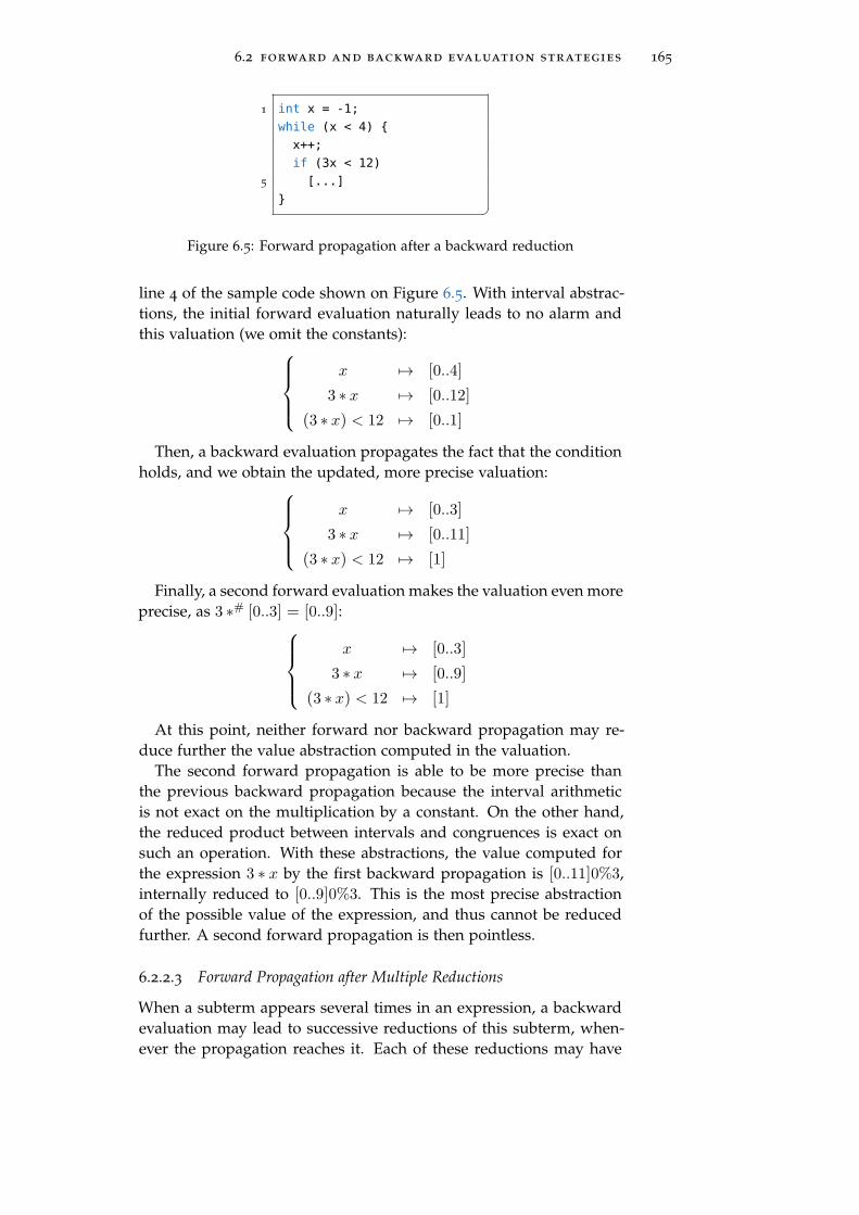
6.2 forward and backward evaluation strategies 165
1 int x = -1;
while (x < 4)
x++;
if (3x < 12)
5 [...]
Figure 6.5: Forward propagation after a backward reduction
line 4 of the sample code shown on Figure 6.5. With interval abstrac-tions, the initial forward evaluation naturally leads to no alarm andthis valuation (we omit the constants):
x → [0..4]
3 ∗ x → [0..12]
(3 ∗ x) < 12 → [0..1]
Then, a backward evaluation propagates the fact that the conditionholds, and we obtain the updated, more precise valuation:
x → [0..3]
3 ∗ x → [0..11]
(3 ∗ x) < 12 → [1]
Finally, a second forward evaluation makes the valuation even moreprecise, as 3 ∗# [0..3] = [0..9]:
x → [0..3]
3 ∗ x → [0..9]
(3 ∗ x) < 12 → [1]
At this point, neither forward nor backward propagation may re-duce further the value abstraction computed in the valuation.
The second forward propagation is able to be more precise thanthe previous backward propagation because the interval arithmeticis not exact on the multiplication by a constant. On the other hand,the reduced product between intervals and congruences is exact onsuch an operation. With these abstractions, the value computed forthe expression 3 ∗ x by the first backward propagation is [0..11]0%3,internally reduced to [0..9]0%3. This is the most precise abstractionof the possible value of the expression, and thus cannot be reducedfurther. A second forward propagation is then pointless.
6.2.2.3 Forward Propagation after Multiple Reductions
When a subterm appears several times in an expression, a backwardevaluation may lead to successive reductions of this subterm, when-ever the propagation reaches it. Each of these reductions may have

166 evaluation of expressions
1 /*@ assert 0 <= x <= 100; */
if (x == x+1)
[...]
forward backward forward backward
x →
x+1 →
x==x+1 →
[0..100]
[1..101]
[0..1]
[1..99]
[1..100]
[1]
[1..99]
[2..100]
[0..1]
[2..98]
[2..99]
[1]
. . .
Figure 6.6: Slow convergence of interval propagations
a different reason. In this case, a forward propagation may achievefurther precision, even if the abstract semantics are exact.
Example 16. The processing of the unsatisfiable conditional (x == x
+1) is a classical example of a slow convergence through the propa-gation of intervals. If the interval representing the possible values ofthe variable x is not a singleton, then the forward abstract semanticsof interval are unable to prove that the condition does not hold. Inthe code of Figure 6.6, for example, the value of the variable x rangesfrom 0 to 100. Thus, the value of x+1 ranges from 1 to 101, andthe interval abstractions cannot disprove the equality between bothexpressions. The backward propagation of this equality reduces theinterval for each expression (including x) to the meet of both intervals,which is [1..100]. And the backward propagation of this new intervalfor x+1 reduces a second time the interval for the variable x, down tothe interval [1..99]. Then, the cycle recurs: the forward propagation ofthese new intervals is still unable to disprove the equality, but reducesthe value of x+1, and the backward propagation of the equality rulesout the bounds of the interval for x. Ultimately, alternating forwardand backward propagations leads to the empty interval, raising thebottom case. The table of Figure 6.6 shows the successive valuationsproduced by the first steps of this process. Here, proving the condi-tion to not hold requires 50 iterations of a forward and a backwardpropagation of intervals.
6.2.3 Interweaving Forward and Backward Propagations
The two previous sections detail the cases where a forward or abackward propagation is relevant, i.e. may achieve further precisionthrough the produced valuation. However, the last presented exam-ple points out that an unrestricted application of forward and back-ward propagation may lead to a slow convergence of the evaluationof an expression. Rather than always seeking for the most precisevaluation for the given expression, a better balance between precisionand efficiency has to be found in the use of both propagations.

6.2 forward and backward evaluation strategies 167
This section expounds the evaluation strategies implemented inEVA for the interweaving of the forward and the backward propa-gations.
6.2.3.1 Complete Propagations Strategy
Section 6.1.5 presented the atomic steps of a forward or backwardpropagation. Each of these steps soundly updates the valuation, andthey may thus be intertwined in any way that leads to the completeevaluation of a given expression. However, we choose to avoid mixingthese forward and backward steps.
Instead, EVA always performs a complete propagation through anexpression in a given direction: from the constants to the root ex-pression for a forward evaluation, and conversely for a backwardone. While opposite full propagations may follow one after another,there is no alternating during a complete propagation, and thus nodirect interaction between forward and backward phases. This choicemakes the implementation much simpler, as in the code presented inFigure 6.1. The forward and the backward mechanisms are kept sep-arate, rather than being all mutually recursive functionalities. Thisdesign allows a better control of the evaluation convergence, as weseek for a single global fixpoint of the computed valuation. It alsoavoids successive reductions of the same subterm where the last onesupersedes the others. The following example illustrates this.
Example 17. Let us consider the evaluation of the expression 2x− 1,where the value of the variable x is unknown. We assume that thecomputations are done in the signed integer type of 1 byte, whosevalues range from −128 to 127. As signed integer overflows are pro-hibited, the multiplication 2 ∗ x requires the value of x to be in theinterval [−64..63]. Furthermore, the next subtraction 2x− 1 requires2x to be in the interval [−127..127], and thus x to be in [−63..63].
If each atomic step that produces some alarms triggers a backwardpropagation of its resulting value, the value abstraction of variable x
would be reduced twice in the valuation. Actually, the first backwardpropagation of the value [−128..126] for the subterm 2x is useless, asthe upcoming backward propagation of the value [−128..125] for theexpression 2x− 1 is strictly stronger. We can also notice that if thevariable x is replaced by a more complex expression, each backwardpropagation may be overly costly.
Thus, instead of performing a backward propagation wheneverpossible, the evaluator first completes the forward propagation, andonly then starts a backward propagation of the computed value forthe root expression 2x− 1. On this example, this leads to the sameprecise valuation as the other strategy, but minimizes the number ofbackward steps done.

168 evaluation of expressions
This strategy of complete propagations is always as precise as trig-gering opposite propagations as soon as possible. We call this latterstrategy the greedy algorithm. Remember that during these propaga-tions, the valuation contains the value abstractions previously com-puted for all the subterms of the evaluated expression. The atomicpropagation steps always meet the new value abstraction they inferfor some subterm with the one stored in the valuation. Thus, the val-uation can only become more and more precise through the propaga-tions. An atomic step always uses the value abstractions stored in thevaluation. Now, during a (forward or backward) propagation, whenan opposite atomic step is relevant on a subterm t, it is postponeduntil the end of the current propagation. Afterwards, the completeopposite (backward or forward) propagation reaches this subterm t,and makes the postponed step using the abstractions of the currentvaluation. These value abstractions are at least as precise as the onesthat were in the valuation during the previous propagation phase.Thus, the postponed atomic step is at least as precise as the initialstep would have been.
However, in some specific cases, the strategy of complete propaga-tions may require more computations to achieve the same precision asthe alternate strategy. Indeed, during a (forward or backward) prop-agation A, an opposite propagation B may reduce some abstractionsthat will be used by the current propagation A. Then, the A propaga-tion leads to less precise results due to the lack of reductions, whichthe B propagations will make later. After the B propagation, anothercomplete propagation A will however lead to the same precision asthe greedy algorithm. The following example illustrates this.
Example 18. Consider now the evaluation of the quite contrived ex-pression (1/x)+x, with the variable x having a value in 0; 1. Thedivision by x requires x to have a non-zero value. A backward stepat the subterm 1/x will reduce the value of x to 1. Note that weuse here integer sets as value abstractions.
If the expression is evaluated from left to right, the greedy algo-rithm produces the following successive valuations at each step:
valuation after 1 2 3 4
x →
1/x →
(1/x)+x →
0; 1
0; 1
1
1
1
1
1
2
1. forward evaluation of the variable x
2. forward evaluation of 1/x
3. backward propagation of the value 1 for 1/x
4. forward evaluation of (1/x)+x

6.2 forward and backward evaluation strategies 169
On the other hand, our strategy of complete propagations post-pones any backward step after the first forward evaluation, whichdoes not benefit from the reduction of the variable x. Thus, the pro-duced valuation are the following:
valuation after 1 2 3
x →
1/x →
(1/x)+x →
0; 1
1
1; 2
1
1
1; 2
1
1
2
1. first complete forward propagation
2. complete backward propagation
3. second complete forward propagation
Both strategies lead ultimately to the same valuation, but here, ourstrategy requires more computations. However, note that the numberof steps for the greedy algorithm depends on the evaluation orderof the subterm. If the right operand of the addition is processedbefore the left operand, an additional forward propagation is neededanyway to take into account the reduction of x.
6.2.3.2 Triggering Relevant Propagation Steps
The propagations are done globally on entire expressions. However,as explained in both previous sections, the atomic steps of a prop-agation are not all relevant: some are unable to improve the pre-cision of the valuation resulting from a previous computation. Wenaturally want the propagations to avoid performing pointless opera-tions, without forgetting any effective reduction. This requires keep-ing track of the subterms where a new propagation may be useful.
At each level of a complete (forward or backward) propagation,EVA checks whether an opposite propagation step may improve theprecision further, according to the criteria listed in Sections 6.2.1 and 6.2.2.Through a forward propagation, these are the steps where alarmsare produced, or where an abstract domain reduces the abstractioninternally computed by the value semantics. Through a backwardpropagation, this only requires the reduction of the value abstractionstored in the valuation. The information is internally stored in thevaluation —this information is not exported in its interface. Then, a(forward or backward) propagation goes through the entire expres-sion, but uses this information to only perform the relevant atomicsteps. A propagation always needs to cross the whole expression, toensure not to neglect some possible reductions. Through the propa-gation, an atomic step of the abstract semantics is performed if andonly if:
• this propagation is marked as relevant in the valuation;

170 evaluation of expressions
• the current propagation has reduced some value abstractions onwhich this semantics step is based (compared to the abstractionspreviously computed and stored in the valuation).
Example 19. Let us consider the expression ((3x+5)/4)− 1, where x
is a signed integer of 1 byte. We assume known that the variable x
ranges from 0 to 42. With the interval abstractions, a complete for-ward propagation leads to the following valuation. The exclamationmark indicates the relevance of a backward propagation for a subterm(here because of the alarm preventing the addition to overflow).
x → [0..42]
3x → [0..126]
3x+5 → [5..127] !
(3x+5)/4 → [1..31]
((3x+5)/4)− 1 → [0..30]
Then, a backward propagation omits the subtraction and the divi-sion step, but propagates backward the interval [0..127] through theaddition to its operands, using the backward semantics of interval.This reduces the interval for 3x to [0..122]. Thus, this new interval isagain backward propagated through the multiplication. This reducesthe interval for x to [0..40]. The resulting valuation is the following,where this time, the exclamation mark indicates the relevance of aforward propagation.
x → [0..40] !
3x → [0..122] !
3x+5 → [5..127]
(3x+5)/4 → [1..31]
((3x+5)/4)− 1 → [0..30]
Then, a forward propagation may start again. As the interval ab-straction of x has been reduced by the previous backward propaga-tion, it is now forward propagated. The forward semantics of multi-plication reduces the interval for 3x to [0..120], which is in turn usedby the forward semantics of addition and leads to the reduction ofthe interval for 3x+1 to [5..125], which is in turn used by the for-ward semantics of division, but leads to the same interval as beforefor (3x+5)/4. Thus, the propagation avoids the following step, andreturns the valuation:
x → [0..40]
3x → [0..120]
3x+5 → [5..125]
(3x+5)/2 → [1..31]
((3x+5)/4)− 1 → [0..30]

6.2 forward and backward evaluation strategies 171
There was no alarm during this last forward propagation, andno domain was involved either. Thus, there is no place for a back-ward propagation, and the evaluation should stop here: this is themost precise valuation we can obtain for the evaluation of the expres-sion ((3x+5)/4)− 1, knowing that the variable x has a value in theinterval [0..42].
6.2.3.3 The Interweaving Strategy
This section finally explains how the complete forward and back-ward propagations are intertwined. As shown by example 16, theunbounded alternating of both kinds of propagation may take a largenumber of iterations until reaching a fixed point, namely a valuationthat cannot be improved by any new propagation. Instead, we use afixed number of iterations: an initial forward evaluation, then a com-plete backward propagation, and finally a second forward propaga-tion for conditional expressions only. This strategy spares the evalua-tor from dealing with slow convergence issues, and has little impacton the precision of the resulting valuations, as shown by our experi-ments related in Section 8.1.3.1.
initial forward evaluation In any context, the evaluation ofan expression starts necessarily by a complete forward propagation.This fills the valuation with a value abstraction for each subterm ofthe expression, and gathers the alarms needed to exclude the undesir-able behaviors that the evaluation may cause. If the starting valuationis non-empty, the evaluation uses it to avoid the computation of theexpressions it contains.
backward propagation Then, a complete backward propaga-tion tries to improve the precision of the valuation on the subtermsof the expression. For the conditional expression of a test statement,if the computed abstraction for the expression represents non-zeroconcrete values, it is reduced to the zero abstraction and marked asrelevant for the backward propagation. If the computed abstractionrepresents only non-zero values, the condition is unsatisfied, and theevaluation raises the bottom case.
For arbitrary expressions, this backward propagation only aims atreducing some subterms according to the emitted alarms or to thecontributions of the abstract domain. It is especially useful to reducethe value abstraction of variables, as the main abstract domain ofEVA is a memory model of variables: it will learn only from theabstractions computed for variables. Backward reductions may alsoavoid the emission of successive redundant alarms, as in the nextexample.
Example 20. On the code of Listing 6.2, an alarm has to be emitted atline 2 to prevent the addition from overflowing. Without any reduc-

172 evaluation of expressions
tion of the variable i, the same alarm would be emitted at line 3 aswell. The backward propagation of the value abstraction computedfor i+1 to the operand i may solve this issue.
Listing 6.2: Avoiding redundant alarms
1 void main (char i)
int a = i+1;
int b = i+1;
second forward evaluation for conditionals For arbi-trary expressions involved in assignments, EVA does only the initialforward evaluation and one complete backward propagation. How-ever, on the conditional expression of a test statement, EVA performsa second forward propagation. Indeed, the backward propagationof conditions is especially important, as it reflects that the conditionholds after the test statement. Moreover, this second forward prop-agation aims not only at reducing even more the value abstractionscomputed by both previous passes, but also:
• determines whether the backward propagation has fully reducedthe subterms according to the truth value of the condition;
• reveals the inconsistency of the condition in some rare cases.
If the second forward propagation evaluates the condition as true,then no other reduction is needed to take into account that the condi-tion holds. We then say that the backward propagation has fully re-duced the subterms of the condition. Otherwise, an imprecise valueabstraction for the condition means that one backward pass was notenough to fully propagate the truth value of the condition on its sub-terms (and especially its variables). As in Example 16, more prop-agations may solve the issue, at the expense of the efficiency of theevaluation. Instead, EVA stops the propagations here, but enables an-other mechanism to recover some precision: the partitioning of theevaluation, described in the following subsection.
Finally, the second forward evaluation may also discover an incon-sistency. The following example presents such a case.
Example 21. In any execution of the code presented on the Listing 6.3,the condition at line 4 does not hold. However, the semantics of in-tervals is unable to prove this fact on a single forward propagation:as the precise value of the variable i is unknown, t[i] and t[i+1] arerespectively depicted by the intervals [0..2] and [1..3], whose intersec-tion is not empty. Then, a backward propagation assumes that theconditional expression evaluates to true, and reduces the interval forboth expressions to the meet [1..2]. To the left, this allows reducing

6.2 forward and backward evaluation strategies 173
Listing 6.3: Second forward propagation on conditional expression
1 int t[3] = 0, 1, 2, 3;
/*@ requires 0 <= i <= 2; */
void main (int i)
if (t[i] == t[i+1])
5 [...]
Listing 6.4: Subdivision of evaluation
1 int t[5] = 0, 1, 2, 3, 4;
/*@ assert 0 <= i <= 4; */
if (t[i] == i)
[...]
5
the variable i to [1..2]; to the right, this allows reducing i to [0..1].At the end of the backward propagation, i is bound to the singletoninterval [1] in the valuation.
Stopping the evaluation here would lead to a quite odd valuation,where the variable i has the precise value [1] for which the conditionis clearly false, while the condition is still considered as true. Thesecond forward propagation solves this issue, raising the bottom casewhen reaching the equality.
6.2.4 Evaluation Subdivision
6.2.4.1 General Considerations
An evaluation can be split according to the possible values of a sub-term. Let us consider the evaluation of an expression e, and a sub-term t of e. Given a partition v1, . . . , vn of the possible values of t,the evaluation is done independently for each vi, assuming t has avalue in vi. The result (alarm map and valuation) of each evalua-tion are then joined. This mechanism was introduced to mitigate theabsence of relational information in the former VALUE abstract inter-preter. It has been maintained in EVA with some improvements. Thefollowing example illustrates how subdividing an evaluation may im-prove its precision.
Example 22. This example uses the standard interval arithmetic asabstract value semantics. We first consider the evaluation of the ex-pression x*x where x has a value between −10 and 10. The evaluationof x*x naturally leads to the interval [−100..100]. However, when

174 evaluation of expressions
x ∈ [−10..0] or when x ∈ [0..10], the evaluation leads to the interval[0..100]. We can conclude that [0..100] is a sound approximation ofx*x when x ∈ [−10..10].
Listing 6.4 presents another example of useful subdivision. Whenevaluating the condition at line 3, both expressions t[i] and i havea value in the interval [0..4], but the interval semantics cannot guar-antee that they have the same value in this interval. Dividing theevaluation according to each possible value of i proves the equalityin each case.
6.2.4.2 Formalization
The soundness of subdividing an evaluation is stated by the followingtheorem.
Theorem 8 (Subdivision of a forward evaluation). Let e be an expres-
sion, E be a valuation, and D be an abstract state. If E1, E2, . . . , En is a set
of valuations such that
∀i ∈ 1, . . . , n, Ei E E
γE(E) = γE(E1) ∪ γE(E2) ∪ . . . ∪ γE(En)
then the subdivision of an evaluation according to the sets Ei, defined as:
e #D(E) =
i∈1. . .n
( e #D(Ei))
satisfies the properties 1 and 3 of a forward evaluation in E .
(Here,
is the join of pairs of valuations and alarm maps.)
It is worth noting that the theorem condition γE(E) = ∪i(γE(Ei)) isstronger than the condition E = i(Ei), which only guarantees thatγE(E) ⊇ ∪i(γE(Ei)).
Proof. We use the same notations as the theorem. Let S be a concretestate in γDE(D, E). As γE(E) = ∪i(γE(Ei)), there exists i such thatS ∈ γDE(D, Ei).Let E ,A = e #D(Ei). By proposition 1:
A |=A eΘ(S)eΘ(S) = Ω ⇒ S ∈ γE(E
)
Let E”,A” =
i∈1. . .n( e #D(Ei)). We have E E E” and A A A”,which implies:
A” |=A eΘ(S)eΘ(S) = Ω ⇒ S ∈ γE(E”)
This holds for any concrete state S in γDE(D, E), validating proposi-tion 1.

6.2 forward and backward evaluation strategies 175
Let (E i,Ai) = e #D(Ei). Proposition 3 ensures that E
i E Ei ande ∈ dom(E
i) . By hypothesis, Ei E E . Finally:
∀i ∈ 1, . . . , n,
e ∈ dom(E i)
E i E E
⇒
e ∈ dom(
i(Ei))
i(Ei) E E
This validates proposition 3 for
i(Ei).
6.2.4.3 Heuristics and Implementation
Theorem 8 provides a sound and general context for subdividing anevaluation. However, repeating an evaluation in n different valua-tions has a high cost —it basically multiplies the evaluation time by n.The use of the valuation as a cache alleviates lightly the cost of a sub-division: only the computations that actually depend on the splitsubterm have to be performed again.
Example 23. We consider the expression ((x+y)*(x+y)+ e). If the signof x+y is not known, subdividing the evaluation according to this sub-term is useful, as shown by the previous example. However, thereis no need to repeat the computation of the addition x+y or the eval-uation of e. In fact, the subdivision can be limited to the subterm(x+y)*(x+y). The resulting valuations are then joined, and the evalua-tion of the complete expression can continue.
While theorem 8 is proved for any “partition” of a valuation, theevaluation subdivision in EVA is limited to the partitioning of the ab-stract value of only one subterm of the considered expression. Froma current valuation E and for a subterm t, we assume given a set ofabstract value v1, . . . , vn such that:
∀i ∈ 1, . . . , n, vi E E(t)
γV(E(t)) = γV(v1) ∪ γV(v2) ∪ . . . ∪ γV(vn)(6.8)
Then, the set of valuations Ei = E [t → vi] satisfies the conditionof theorem 8, and the evaluation subdivision according to them issound.
From an arbitrary abstract value E(t), there is not always a set ofvalues satisfying equation 6.8. As example, a garbled mix (see Sec-tion 5.3.2) cannot be divided into a partition of smaller abstractions.On the other hand, an interval can be divided into many differentpartitions. In EVA, the subdivision is done only on the intervals andthe integer sets of the cvalue abstraction (see Section 5.3.1). The valuecombination structuring, described in Section 3.3, is used to work onthe cvalue component of an arbitrary value abstraction (if this com-ponent exists).
Finally, the evaluation engine of EVA triggers such a subdivisionwhen:

176 evaluation of expressions
• on the condition of an if statement, the second forward evalua-tion proves that the backward propagation failed to fully prop-agate the truth value of the condition on its subterms (see Sec-tion 6.2.3).In this case, a subdivision is applied on any integer variable:
– appearing in the address of a dereference (in an array offsetor in the computation of a pointer);
– whose possible values are represented by an integer set.
The subdivision is done by considering separately all integersin the set. As the cardinal of integer sets are kept small by theanalyzer, this does not overly impact the analysis time. This isexactly the instance described in listing 6.4.
• on the right expression e of an assignment that contains severaloccurrences of the same syntactic subterm t, if the possible val-ues of t are approximated by a basic integer or floating cvalue.The subdivided evaluation is limited to the smaller subterm of ethat contains all occurrences of t, as already illustrated in exam-ple 23. The number of divisions of an interval is specified by aparameter of the abstract interpreter.
Although a subdivision is limited to one subterm, successive subdivi-sions of different subterms can be performed on the evaluation of anexpression. On the expression (x*x + y*y), EVA executes two subdi-visions:
• one of the subterm of x*x, according to the value of x;
• one of the subterm of y*y, according to the value of y.

Part IV
A B S T R A C T S E M A N T I C S O F S TAT E M E N T S


7S TAT E A B S T R A C T I O N S
An abstract domain D is a collection of state abstractions carryinginformation about program variables. Each abstract state D repre-sents a set of concrete states S at a program point. A concretizationfunction γD links abstract states to the concrete states they represent.
γD : D → P(S)
A domain can be a combination of several domains D1, D2, . . . , Dn.Its abstract states are then tuples (d1, d2, . . . , dn) representing the in-tersection of the concretization of each subdomain:
γD(d1, d2, . . . , dn) = γD(d1) ∩ γD(d2) ∩ . . . ∩ γD(dn)
This section expounds how the subdomains of a combination interactwith each other in our architecture.
Abstract domains provide transformers implementing an abstractsemantics of statements. Each transformer models the effect of a state-ment on abstract states, inferring properties about how a program ex-ecution may behave at this point. The abstract interpreter uses themto propagate abstract states through the CFG of a program. At a nodeof the CFG, the computed abstract state is an over-approximation ofthe possible concrete states given by the concrete semantics of thelanguage.
The above description of abstract domains is absolutely standard inabstract interpretation. This chapter does not develop the general no-tion of abstract domains further, but only focuses on the interactionsbetween them. The previous chapter was dedicated to the evaluationof an expression into alarms and value abstractions. This evaluationis collaborative: it involves all available domains, extracting informa-tion from each abstract state and pooling them. This informationis expressed with alarm maps and value abstractions. The abstractdomains provide the mandatory abstract semantics for the derefer-ence of lvalues, but they can also supply the evaluator with someabstractions of other expressions. To compute precise abstractions,an abstract domain may request additional information from otherdomains. Finally, an abstract domain can trigger the backward prop-agation of value abstractions for some expressions.
When processing a statement, the abstract interpreter evaluates theexpressions involved in the statement. At the end of these evalua-tions, a valuation (see Section 6.1.3) stores all the produced alarmsand value abstractions. They have been cooperatively computed us-ing the properties inferred by each abstract domain at the program
179

180 state abstractions
Listing 7.1: Signature of domain queries
1 type ’a or_bottom = ‘Bottom | ‘Value of ’a
type ’a evaluated = ’a or_bottom * alarms
val extract_lval : (* F#∗τ *)
5 oracle:(exp -> value evaluated) ->
state -> lval -> typ -> location -> (value * origin) evaluated
val extract_expr : (* F#D *)
9 oracle:(exp -> value evaluated) ->
10 state -> exp -> (value * origin) evaluated
point before the statement. Then, these abstractions are available forthe abstract domain transformers to model the semantics of the state-ment as precisely as possible. Thus, information may flow from adomain to another, through the shared evaluation of expressions.
7.1 collaboration for the evaluation : domain queries
A state abstract domain D provides two query functions, on whichthe generic evaluator relies. Those functions translate AST fragmentsinto alarm maps and value abstractions. If the domain is a product ofseveral domains, all their answers to a query are intersected thanksto the meet operator of the alarm and value lattices. Thereby, eachdomain may contribute to reduce the abstract value computed for anexpression, or decrease the number of emitted alarms.
These queries have been briefly presented through Section 6.1.2,but this section illustrates them in examples. Listing 7.1 shows theirOCaml signature. The explanation of the oracle argument is post-poned to Subsection 7.1.3.
7.1.1 Semantics of Dereference
The first query is a forward abstract semantics F#∗τ for dereferences,
mandatory to perform the evaluation of expressions.
Definition 51 (Semantics of dereference). In an abstract state D, asound abstract semantics F
#∗τ of dereferences is a function from a lo-
cation abstraction l to a value abstraction v and a map of alarms A
such that:
• v is a sound approximation of the concrete values that may bestored at any concrete address of γL(l) in any concrete state ofγD(D);

7.1 collaboration for the evaluation : domain queries 181
• A is a sound abstraction of the possible failure of the derefer-ence of any concrete address in γL(l). Therefore, the assertionsof A ensure that the dereference succeeds.
F#∗τ : D → L# → V# ×A
∀a ∈ γv (l) , ∀S ∈ γD (D) , F#∗τ (D, l) |=V×A ∗τaΘ(S)
The alarms produced by F#∗τ ensure the validity of the location,
and that the contents of the read memory slice are proper (i.e. notindeterminate in C parlance, and in particular initialized). They havebeen described in Section 5.1.3.2.
Proposition 4. For a product of domains D = D1 × . . . × Dn, a sound
abstract semantics F#∗τ can be defined by:
F#∗τ ((d1, d2, . . . , dn), l) = F#∗τ (d1, l)V×AF#∗τ (d2, l)V×A
. . . V×A
F#∗τ (dn, l)
Proof. Let l be a location abstraction and D = (d1, d2, . . . , dn) be aproduct of n abstract states from domains D1, D2, . . . , Dn. For eachdomain Di, we have:
∀S ∈ γD(di), F#∗τ (di, l) |=V×A ∗τa
Θ(S)
We thus have:
S ∈ γD(d1, . . . , dn) ⇒ ∀i ∈ 1, . . . , n, S ∈ γD(di)
⇒ ∀i ∈ 1, . . . , n, F#∗τ (d, l) |=V×A ∗τaΘ(S)
⇒ F#∗τ ((d1, d2, . . . , dn), l) |=V×A ∗τaΘ(S)
The last deduction is the application of lemma 11.
Example 24. Figure 7.1 illustrates the collaboration between state ab-stractions through their semantics of dereference. The objective is toanalyze the C code at the top, where the value of i ranges between0 and 4 at the first line. This code features basic integer arithmeticand the access to an array. We focus on the evaluation of the rightexpression at line 3, which is written ∗int (&t[i+1]) in our language(see Chapter 4). We omit the alarms: as the analyzed code does notinclude C undefined behaviors, there may be none with sufficientlyprecise abstractions.
As all the C values of the target code are constant in any memorylayout, we do not need abstractions of values dependent on the layout.We thus use only some of the basic value abstractions presented inSection 5.3 for the evaluation of expressions:
• integer intervals with congruences [i..j]r%m represent sets ofinteger values; an interval without congruence information iswritten [i..j], and a singleton interval is written [i].

182 state abstractions
1 int t[5] = 1, 2, 3, 4, 5;
if (0 <= i && i < 2)
• r = t[i + 1];
Env Array
States Di → [0..1]
r → ⊥t : [1; 2; 3; 4; 5]
F#∗int (D,&i → [0]) [0..1]
F#∗int (D,&r → [0]) ⊥
F#∗int (D,&t → [4..8]0%4) [2..3]
F#∗int (D,&t → [0..16]0%4) [1..5]
&i#(D) = (&i)# = &i → [0] (1)
i#(D) = ∗int(&i)#(D)
= F#∗int (D, &i → [0] )
= [0..1] v v = [0..1] (2)
1#(D) = 1# = [1] (3)
i+1#(D) = i#(D) +# 1#(D)
= [0..1] +# [1] = [1..2] (4)
&t#(D) = (&t)# = &t → [0] (5)
&t [i+ 1]#(D) = &t#(D) +# sizeof(int) ×# i+1#(S)= &t → [0] +# [4] ×# [1..2]
= &t → [0] +# [4..8]0%4
= &t → [4..8]0%4 (6)
∗int (&t [i])#(D) = F#∗int(D, &t → [4..8]0%4 )
= v v [2..3] = [2..3] (7)
Figure 7.1: Forward collaboration between domains

7.1 collaboration for the evaluation : domain queries 183
• maps &x → [i..j]r%m from variables to intervals-expressedbyte offsets represent sets of pointer values.
We assume given two abstract domains that cooperate:
• an environment mapping integer variables to intervals repre-senting their possible values at a statement;
• an array domain, able to represent precisely the value of eachcell of an array, but also to model an imprecise access to anarray;
We are not interested in their implementation or their interpretationof statements, but only in their semantics of dereferences. A repre-sentation of the state D of each domain at the bullet point is givenin the first line of the table. The following lines show their answersto some queries, i.e. the value abstraction computed by their derefer-ence semantics for some location abstractions. In this example, eachdomain has information about different expressions, and returns V
for the others.Finally, the equations of Figure 7.1 detail each step of the forward
evaluation of the expression ∗int (&t[i+1]) in the state D. It proceedsbottom-up, using the domains semantics of dereference and the nat-ural semantics of value abstractions. Note that we write the abstractvalue semantics F#♦ with an infix notation ♦#.
1. The read of the variable i is a dereference of the address &i.First, the address &i is converted into its abstract representationin the value abstractions, here the map &i → [0] .
2. The abstract semantics of dereferences is provided by the do-mains. The environment provides the interval [0..1] for the vari-able i. The array domain cannot interpret a non-array lvalue,and returns v. The meet of those two values is [0..1].
3. The constant 1 is directly converted into its abstract representa-tion in the value abstractions, here the interval [1].
4. The evaluation of the expression i+1 relies on the abstract se-mantics of intervals and congruences, leading to the abstrac-tion [1..2].
5. The constant &t is converted into the map &t → [0] .
6. The evaluation of the address &t[i+1] relies on the abstract se-mantics of pointer abstractions — array subscripting is equiv-alent to the addition of a pointer and an integer. The inter-val [1..2] computed for the offset is multiplied by the size inbytes of the type of the array elements. Here we assumed
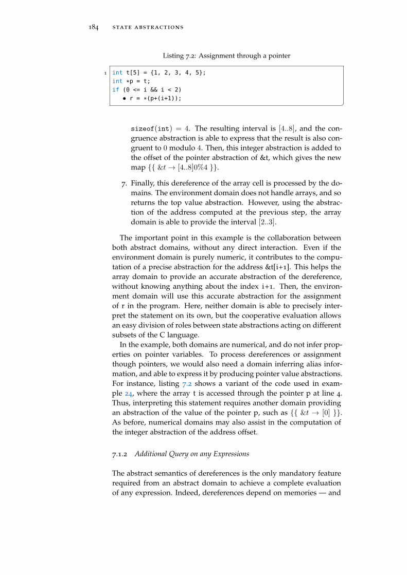
184 state abstractions
Listing 7.2: Assignment through a pointer
1 int t[5] = 1, 2, 3, 4, 5;
int *p = t;
if (0 <= i && i < 2)
• r = *(p+(i+1));
sizeof(int) = 4. The resulting interval is [4..8], and the con-gruence abstraction is able to express that the result is also con-gruent to 0 modulo 4. Then, this integer abstraction is added tothe offset of the pointer abstraction of &t, which gives the newmap &t → [4..8]0%4 .
7. Finally, this dereference of the array cell is processed by the do-mains. The environment domain does not handle arrays, and soreturns the top value abstraction. However, using the abstrac-tion of the address computed at the previous step, the arraydomain is able to provide the interval [2..3].
The important point in this example is the collaboration betweenboth abstract domains, without any direct interaction. Even if theenvironment domain is purely numeric, it contributes to the compu-tation of a precise abstraction for the address &t[i+1]. This helps thearray domain to provide an accurate abstraction of the dereference,without knowing anything about the index i+1. Then, the environ-ment domain will use this accurate abstraction for the assignmentof r in the program. Here, neither domain is able to precisely inter-pret the statement on its own, but the cooperative evaluation allowsan easy division of roles between state abstractions acting on differentsubsets of the C language.
In the example, both domains are numerical, and do not infer prop-erties on pointer variables. To process dereferences or assignmentthough pointers, we would also need a domain inferring alias infor-mation, and able to express it by producing pointer value abstractions.For instance, listing 7.2 shows a variant of the code used in exam-ple 24, where the array t is accessed through the pointer p at line 4.Thus, interpreting this statement requires another domain providingan abstraction of the value of the pointer p, such as &t → [0] .As before, numerical domains may also assist in the computation ofthe integer abstraction of the address offset.
7.1.2 Additional Query on any Expressions
The abstract semantics of dereferences is the only mandatory featurerequired from an abstract domain to achieve a complete evaluationof any expression. Indeed, dereferences depend on memories — and

7.1 collaboration for the evaluation : domain queries 185
thus on concrete states, and must be approximated by state abstrac-tions. All other operations on expressions can be safely handled byvalue (and location) abstractions. Yet, an abstract domain may inferrelevant properties about any expressions, and not only dereferences.For instance, a domain tracking inequalities in a program may ex-press that e1 − e2 is positive when it has inferred e1 ≥ e2, regardlessof the value of e1 and e2. To take advantage of all inferences madeby the domains, the evaluation also involves the abstract states onarbitrary expressions.
The second query provided by an abstract domain supplies addi-tional information about arbitrary C expressions. It computes soundabstractions for their complete evaluations in all the concrete statesin the concretization of the abstract state.
Definition 52 (Arbitrary domain query). In an abstract state D, asound query F
#
D (D, e) for an expression e computes:
• a sound value abstraction v of the concrete values that the ex-pression e may have in a concrete state of γD(D);
• an alarm map A which is a sound abstraction of the evaluationof e in any concrete state of γD(D).
F#
D: D → expr → V# ×A
∀S ∈ γD (D) , F#D (D, e) |=V×A eΘ(S)
Proposition 5. For a product of domains D = D1 × . . . × Dn, a sound
abstract semantics F#D
can be defined by:
F#
D((d1, d2, . . . , dn), l) = F
#
D(d1, l)V×A
F#
D(d2, l)V×A
. . . V×A
F#
D(dn, l)
Proof. The same reasoning as for proposition 4 applies here.
In EVA, the evaluation of an expression queries the state domainson each non-constant expression, using F
#∗τ for dereferences and F
#
D
for other expressions. In the second case, the meet V×A
is used to in-tersect the abstractions computed by the abstract semantics of valuesand by the query of domains.
Example 25. The analysis of the code shown at Figure 7.2 illustratesthe utility of the query on arbitrary expressions. We use integer inter-vals as value abstractions, and two state abstractions: an environmentmapping variables to intervals, and a relational domain inferringsymbolic inequalities between C expressions. The two assertions con-strain the possible values of the variables a and b between 0 and 10,which are stored as intervals in the environment domain. The condi-tion at line 3 does not allow reducing these intervals, but the symbolicdomain retains that the inequality a+b>9 holds. The table shows theabstract states inferred at line 4, and their answers to queries on someexpressions, including but not limited to dereferences. The evaluationof the expression 2*(a+b) is as follow:

186 state abstractions
1 /*@ assert 0 <= a <= 10; */
/*@ assert 0 <= b <= 10; */
if (a + b >= 10)
• r = 2 * (a + b);
Environment Inequalities
States D
a → [0..10]
b → [0..10]
r → ⊥
a+ b > 9
a [0..10]
b [0..10]
a+ b [10..+∞]
2 ∗ (a+ b)
Figure 7.2: Collaboration between domains on arbitrary expressions
• the environment provides the interval [0..10] for the variables aand b;
• the interval abstract semantics of addition computes [0..20] for a+b, while the relational domain supplies the interval [10..+∞].The meet of both intervals gives [10..20];
• the interval abstract semantics of multiplication computes [20..40]for 2*(a+b), and no domain can reduce this value.
Here, the relational domain cannot avail its inferred inequality with-out the query on arbitrary expressions, which would have led to asignificant loss of precision when interpreting the assignment.
7.1.3 Interaction through an Oracle
To compute a precise value abstraction for an expression, a domain—and especially a relational one— may need additional informationabout other expressions. Thus, a domain can request the evaluationof new expressions, through an oracle given in argument of the queryfunctions. The oracle triggers the requested evaluation using all avail-able domains, and returns the cooperatively computed abstractionsto the initial domain. The oracle has the same specification as theevaluation: it provides an alarm map and a value that are soundapproximations of the concrete evaluation of the expression in thecurrent state D. A domain can thus rely on it to make its own answerto a query.

7.1 collaboration for the evaluation : domain queries 187
Definition 53 (Oracle). An oracle is a function from expressions topairs of a value abstraction and an alarm map.
oracle : expr → V# ×A
Definition 54 (Oracle concretization). For an oracle oracle, we defineγo(oracle) as the set of concrete states S for which the answer of theoracle for any expression e is a sound approximation of its evaluationin S:
γo(oracle) S ∈ S | ∀e ∈ expr , oracle(e) |=V×A eΘ(S)
Definition 55 (Sound oracle). In an abstract state D and a valuation E ,an oracle is sound if it produces sound approximations of the evalua-tions in the concrete state of γDE(D, E).
∀S ∈ γDE(D, E), ∀e ∈ expr , oracleD,E (e) |=V×A eΘ(S)
This is equivalent to γDE(D, E) ⊆ γo(oracle).
Definition 56. The domain queries F#∗τ and F
#
Dof an abstract state D
take as additional argument an oracle. The queries produce soundalarm maps and value abstractions for the concrete states in γD(D) ∩
γo(oracle).
F#∗τ : (expr → V# ×A) → D → expr → L# → V# ×A
F#
D: (expr → V# ×A) → D → expr → V# ×A
∀D ∈ D, ∀e ∈ expr , ∀l ∈ L, ∀a ∈ γv (l) , ∀S ∈ γD(D) ∩ γo(oracle),
F#∗τ (oracle, D, ∗τa, l) |=V×A ∗τa
Θ(S)
F#
D (oracle, D, e) |=V×A eΘ(S)
Theorem 9. If the oracle given to a domain is sound in the current abstract
state and valuation, then the requirement of the queries of definition 56 still
guarantees the soundness of the forward evaluation stated by proposition 1
and proved by theorem 6.
Proof. According to proposition 1, a sound forward evaluation in anabstract state D and a valuation E produces abstractions (a new valu-ation and an alarm map) that are over-approximations of the concreteevaluation in any concrete states in γDE(D, E). By definition 55, if anoracle is sound for D and E , then:
γDE(D, E) ⊆ γo(oracle) (7.1)
We can informally see that refining the query of a state D to an ap-proximation of the concrete states in γD(D) ∩ γo(oracle) instead ofjust γD(D) does not impact the soundness of the evaluation.

188 state abstractions
Listing 7.3: Implementation of an oracle in the evaluator
1 let rec forward_eval fuel state expr =
try Valuation.find !valuation expr
with Not_found ->
Valuation.add !valuation expr (Value.top, Alarmset.all);
5 let r = coop_forward_eval fuel state expr in
Valuation.add !valuation expr r; r
and coop_forward_eval fuel state expr =
let oracle =
10 if fuel > 0
then forward_eval (pred fuel) state
else (Value.top, Alarmset.all)
in
let v, a = internal_forward_eval fuel state expr in
15 let v’, a’ = Domain.extract_expr oracle state expr in
Value.meet v v’, Alarms.meet a a’
and internal_forward_eval fuel state expr =
[...]
In order to formally verify this fact, we would need to redo theproof of theorem 6. This proof relies on the invariant of the atomicupdates of the valuation, stated by theorem 5, which itself relies onlemma 22. This lemma asserts that the forward semantics used foran atomic update produces sound value abstractions of the concreteevaluation of the expression being processed. In other words, for anexpression e, the forward abstract semantics must compute a value v
such that:∀S ∈ γDE(D, E), eΘ(S) ∈ γV(v) ∪ Ω
By inclusion 7.1, a concrete state in γDE(D, E) is also in γo(oracle),and thus the queries of the domain produce value abstractions thatsatisfy this equation. The same reasoning applies for the alarm maps.
A forward evaluation satisfying the properties of propositions 1
and 3 is a sound oracle. As the forward evaluation returns a valuation,the oracle just needs to extract the expected value abstraction from thevaluation.
Proposition 6. In an abstract state D and a valuation E , a sound oracle
can be defined by:
oracleD,E (e) (E (e),A) where (E ,A) = e#D(E)

7.1 collaboration for the evaluation : domain queries 189
Proof. Let S be a concrete state in γDE(D, E). Proposition 1 ensuresthat:
A |=A eΘ(S)
eΘ(S) = Ω ⇒ S ∈ γE(E)
By definition 46, S ∈ γE(E) ⇒ eΘ(S) ∈ γv(E (e)) —proposition 3
ensures that e ∈ dom(E ). We thus have eΘ(S) ∈ γv(E (e)) ∪ Ω inall cases, and then:
(E (e),A) |=V×A eΘ(S)
As the oracle triggers new evaluations, an uncontrolled use of theoracle may lead to (1) a loop in the evaluation, or to (2) an infinitechain of evaluations of different expressions. To prevent (1) fromhappening, the oracle can return on re-occurrences of the sameexpression. The number of recursive uses of the oracle should alsobe limited by a parameter of the analysis, to avoid (2).
Listing 7.3 contains an improvement of the simplified evaluator pre-sented in Section 6.1.7, that shows the implementation of the oracleused in EVA. The extract_expr query of the domain takes as argumentthe oracle, which calls the main forward evaluation. The evaluationuses a valuation as a cache. Before any computation on an expres-sion e, it also binds the top value and alarm abstractions to e in thevaluation. This prevents any loop in the evaluation: if a domain re-quests the re-evaluation of e, the main function returns directly thistop abstractions. This imprecise value is replaced by the computedone at the end of the evaluation. Moreover, an integer fuel is used toavoid an infinite sequence of evaluations: a call of the oracle decre-ments it, and the oracle returns the top abstractions when the fuelreaches zero.
Thanks to the oracle, the abstract domains may share informationthrough alarms and value abstractions during the evaluation, withoutresorting to a direct communication between domains. Especially,the oracle allows a relational domain to fully avail the relations ithas inferred, and lets the other domains collaborate in leveragingthese relations. The following example illustrates this with a symbolicequality domain.
Example 26. In this example, we study the analysis of the code snip-pet shown in figure 7.3, which is quite similar to the code of exam-ple 24: at line 5, the assignment of the variable r depends on thevalue of t[i], under the condition i < 2. However, the access to thearray cell t[i] is done through the tmp variable, which has been com-puted before the condition. Accurately interpreting the assignment

190 state abstractions
1 /*@ assert 0 <= i <= 4; */
int t[5] = 1, 2, 3, 4, 5;
int tmp = t[i] + 1;
if (i < 2)
5 • r = 2 * tmp;
Env Array Equality
States D
i → [0..1]
tmp → [2..6]
r → ⊥
t :
[1; 2; 3; 4; 5]tmp = t[i] + 1
2 ∗ tmp
tmp [2..6] oracleD(t[i] + 1)
i [0..1]
t[i] [1..2]
t[i] + 1 oracleD(tmp)
r ⊥
Figure 7.3: Interaction through the oracle
thus requires to take into account the reduction of tmp implied by thecondition i < 2.
We use the same value abstractions as in the previous example:intervals and congruences for integers, and maps from variables tointeger abstractions for pointers. We assume given three abstract do-mains — the first two being those already used in the example 24.Their abstract states before the interpretation of the assignment ofline 5 is given in the first line of the figure table. The following linesshow their answers to some queries about various expressions. Thesedomains are:
• an environment mapping integer variables to intervals. Afterthe initial assertion 0 ≤ i and the condition i < 2, the variablei is known to be in [0..1]. The set of possible values of tmp
has been cooperatively computed at line 3, but has not beenreduced by the condition, since this domain is unable to link i
and tmp.
• the array domain that represents the values of each cell of t
• a relational domain inferring symbolic equalities between ex-pressions. At line 3, it has inferred tmp = t[i] + 1, which is stillvalid at line 5.
Without the oracle mechanism, the evaluation of 2 ∗ tmp in thesestates leads simply to the abstraction [2] ∗# [2..6] = [4..12]0%2. The

7.2 backward propagators 191
Listing 7.4: Signature of domain backward propagators
1 type ’a or_bottom = ‘Bottom | ‘Value of ’a
val backward_location : (* B#∗τ *)
4 state -> location -> value -> location or_bottom
5
val reduce_further : (* B#D *)
7 state -> exp -> value -> (exp * value) list
equality domain cannot supply a value abstraction for tmp by itself,despite the relation it has inferred. But it can use the oracle to geta value abstraction of t[i]+1, and then returns it as a sound valueabstraction of tmp. The oracle calls the complete evaluation of t[i]+1
in the full state, which proceeds as shown previously in example 24:by intertwining the value semantics and the semantics of dereferenceprovided by the environment and the array domain, it computes theprecise interval [2..3] for t[i]+1. Indeed, the standard evaluation oft[i]+1 takes into account the reduction of i stemming from the condi-tion at line 4. Then, the equality domain returns the interval [2..3] fortmp, and the evaluation of 2 ∗ tmp becomes [2] ∗# [2..3] = [4..6]0%2.
Note that when evaluating t[i]+1, the equality domain can requestthe evaluation of tmp through the oracle, for the same reason as be-fore. Here, the oracle returns the top abstraction directly, to preventthe evaluation to loop endlessly between tmp and t[i]+1.
7.2 backward propagators
Within value abstractions, forward and backward propagators aredual. Likewise, state abstractions can provide the backward coun-terparts of queries. Listing 7.4 presents their signature.
7.2.1 Backward Semantics of Dereference
When an abstraction of the possible values of an lvalue is reduced, theabstraction of the memory location of the lvalue might be reducedas well. This is typically the case for memory accesses through animprecise pointer or in an array. This reduction requires knowledgeof the memory state, and thus involves the state abstractions.
Definition 57 (Backward semantics of dereference). In an abstractstate D, a sound backward semantics B
#∗τ of dereference is a func-
tion from a location abstraction l and a value abstraction v to a newlocation abstraction l such that l over-approximates all concrete ad-

192 state abstractions
1 /*@ assert 0 <= i <= 3; */
int t[5] = 1, 2, 3, 4, 5;
•
4 if (t[i+1] < 4)
5 r = 2 * i;
Env Array
States Di → [0..3]
r → ⊥t : [1; 2; 3; 4; 5]
Figure 7.4: Backward propagation on an array access
dresses in γV(l) whose dereference is in γV(v) for at least one concretestate of γD(D).
B#∗τ : D → L# → V# → L#
a ∈ γL(l) | ∃S ∈ γD(D), ∗τaΘ(S) ∈ γV(v) ⊆ γL(B
#∗τ (D, l, v))
As usual for backward propagators, it is always sound to returnthe previous location unreduced.
Proposition 7. For a product of domains D = D1 × . . . × Dn, a sound
abstract semantics B#∗τ can be defined by:
B#∗τ ((d1, . . . , dn), l, v) B#∗τ (d1, l, v) V . . . V B#∗τ (dn, l, v)
Proof. Let D = (d1, . . . , dn) be a product of abstract states of a domainD = D1 × . . . ×Dn. Let l be a location abstraction and v be a valueabstraction. Let a be a constant pointer value such that:
a ∈ γL(l) ∧ ∗τaΘ(S) ∈ γV(v)
We need to prove that a ∈ γL(B#∗τ (D, l, v)). Let S be a state in γD(D)
such that ∗τaΘ(S) ∈ γV(v). For each i between 1 and n, we have
γD(D) ⊆ γD(di) and thus S ∈ γD(di). This implies:
a ∈ γL(l) ∧ ∀i ∈ 1, . . . , n, ∃S ∈ γD(di), ∗τaΘ(S) ∈ γV(v)
By definition 57:
∀i ∈ 1, . . . , n, a ∈ γL(B#∗τ (di, l, v))
By soundness of the meet of value abstractions, we can deduce:
a ∈ B#∗τ (d1, l, v) V . . . V B#∗τ (dn, l, v) = γL(B
#∗τ (D, l, v))

7.2 backward propagators 193
Example 27. The analysis of the code snippet of Figure 7.4 illustratesthe need for a backward propagator for dereferences. We use theenvironment domain and the array domain already used in the pre-vious examples. Their abstract states at line 3 are represented in thefigure table. In these states, a forward evaluation of the condition ofline 4 computes:
• the interval [1..4] for the expression i+1, according to the ab-stract semantics of addition.
• the map &t → [4..16]0%4 for the address &t[i+1], accord-ing to the abstract semantics of array subscripting.
• the interval [2..5] for the expression t [ i+1], through the derefer-ence semantics of the array domain.
• the interval [0..1] for the condition t [ i+1] < 4, according to theabstract semantics of comparison.
Then, the analysis of the if branch assumes the condition to be trueby backward propagating the singleton interval [1] through the ex-pression t [ i]<4. This backward evaluation reduces:
• the interval for t [ i ] to [2..3], according to the backward propa-gator of intervals on comparisons.
• the map for the address &t[i+1] to &t → [4..8]0%4 , thanksto the backward propagation provided by the array domain. In-deed, this map represents the only locations of the previousabstraction of the address for which the dereference has a valuein [2..3].
• the interval for the expression i+1 to [1..2], through the back-ward semantics of array subscripting.
• the interval for the variable i to [0..1], according to the backwardsemantics of addition.
The backward semantics of dereference allows reducing the value ab-straction of i according to the value abstraction t [ i ]. If the variable iis used later in the branch, this reduction can be significant for theprecision of the analysis.
Example 28. The previous example exhibits a reduction of an arrayindex according to the value of the array cell. The code of Figure 7.5presents a reduction of a pointer according to the pointed value. Weuse here the environment domain for integer variables, along witha domain performing an alias analysis and inferring pointer abstrac-tions (maps from variables to integer offsets). The table presents theirstates at line 5. When evaluating the expression at line 6, the aliasing

194 state abstractions
1 int a = 42;
int b = 0;
int v = rand();
int *p = v ? &a : &b;
5 •
6 int r = 100 / *p;
Environment Alias analysis
States Da → [42]
b → [0]
v →
r → ⊥p → &a, &b
Figure 7.5: Backward propagation on a pointer dereference
domain provides the abstraction &a → [0], &b → [0] for thepointer p. Using it, the environment domain abstracts the result ofthe dereference *p into the interval [0..42], by joining the intervals itstores at each location &a → [0] and &b → [0] . Then, theforward evaluation of 100 / *p raises an alarm about the potentialdivision by zero.
We have seen in Section 6.2.1 that an alarm makes a backward prop-agation relevant. Here, the interval backward semantics on divisionreduces the abstraction of the divisor *p to [1..42]. Then, the environ-ment domain can reduce the abstraction of the dereference location:as b is equal to 0, &a → [0] is the only possible location for thisdereference. This reduces the abstraction of p for the alias analysis.
7.2.2 Triggering New Reductions
On a backward propagation, the relations inferred by a domain mayinduce further interesting reductions. For instance, if a ≤ b holds,then any reduction of the infimum of the possible values of a im-plies the same reduction for b. Hence, when performing a reduction,the generic evaluator notifies the domains through the function B
#
D,
which returns a list of new reductions to be backward propagatedby the evaluator. The new reductions, deduced from the prior oneand from the inferences made by the domain, must be correct in theconcrete states for which the initial reductions are valid. To avoiddiverging, the generic evaluator limits the number of successive re-ductions made through B
#
D. In the signature of Listing 7.4, B
#
Dis
named reduce_further, and we call it the reducer.
Definition 58. In an abstract state D, a reduction of an expression e toa value abstraction v soundly implies a reduction of an expression e
to a value abstraction v when for all concrete state S in γD(D) inwhich the evaluation of e is in γV(v), the evaluation of e is in γV(v).

7.2 backward propagators 195
The query B#
D(D, e, v) returns a list of pairs (e, v) such that the
reduction of e to v soundly implies the reduction of e to v.
B#
D: D → expr → V# → (expr ×V#)n
∀(e, v) ∈ B#
D(D, e, v), ∀S ∈ γD(D),
eΘ(S) ∈ γV(v) ⇒ eΘ(S) ∈ γV(v)
Proposition 8. For a product of domains D = D1 × . . . × Dn, a sound
abstract semantics F#
Dcan be defined as the concatenation of all the new
reductions proposed by each domain Di.
Proof. Let D = (d1, . . . , dn) be a product of abstract states of domainsD1, . . . , Dn. Let e and e be two expressions, and v and v two valueabstractions, and let i ∈ 1, . . . , n. If (e, v) is a new reduction pro-posed by the domain Di as a sound consequence of the reduction ofe to v, then:
∀S ∈ γD(di), eΘ(S) ∈ γV(v) ⇒ eΘ(S) ∈ γV(v)
As γD(D) ⊆ γD(di), this implies:
∀S ∈ γD(D), eΘ(S) ∈ γV(v) ⇒ eΘ(S) ∈ γV(v)
and thus (e, v) is also a valid new reduction in the state D.
Theorem 10. The backward propagations of the reductions proposed by a
domain through B#
D(D, e, v) do not impact the soundness of the backward
evaluation stated by proposition 2 and proved by theorem 6.
Proof. Let D be an abstract state, E be a valuation, e be an expres-sion and v be a value abstraction. Proposition 2 states that a soundbackward propagation ←−e #D(E , v) produces a valuation E such that:
∀S ∈ γDE(D, E), eΘ(S) ∈ γV(v) ⇒ S ∈ γE(E)
We consider a new reduction proposed by the domain:
(e, v) ∈ B#
D(D, e, v)
Then we have:
∀S ∈ γD(D), eΘ(S) ∈ γV(v) ⇒ eΘ(S) ∈ γV(v)
As γDE(D, E) ⊆ γD(D), we also have:
∀S ∈ γDE(D, E), eΘ(S) ∈ γV(v) ⇒ eΘ(S) ∈ γV(v) (7.2)
By proposition 2 again, we know that the backward propagation
←−e #D(E , v) produces a valuation E” that satisfies:
∀S ∈ γDE(D, E), eΘ(S) ∈ γV(v) ⇒ S ∈ γE(E”) (7.3)
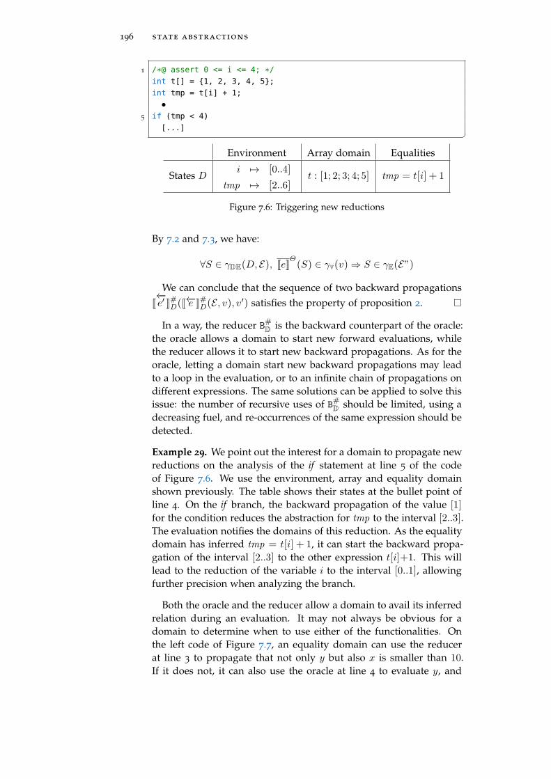
196 state abstractions
1 /*@ assert 0 <= i <= 4; */
int t[] = 1, 2, 3, 4, 5;
int tmp = t[i] + 1;
•
5 if (tmp < 4)
[...]
Environment Array domain Equalities
States Di → [0..4]
tmp → [2..6]t : [1; 2; 3; 4; 5] tmp = t[i] + 1
Figure 7.6: Triggering new reductions
By 7.2 and 7.3, we have:
∀S ∈ γDE(D, E), eΘ(S) ∈ γV(v) ⇒ S ∈ γE(E”)
We can conclude that the sequence of two backward propagations
←−e #D(←−e #D(E , v), v) satisfies the property of proposition 2.
In a way, the reducer B#D
is the backward counterpart of the oracle:the oracle allows a domain to start new forward evaluations, whilethe reducer allows it to start new backward propagations. As for theoracle, letting a domain start new backward propagations may leadto a loop in the evaluation, or to an infinite chain of propagations ondifferent expressions. The same solutions can be applied to solve thisissue: the number of recursive uses of B#
Dshould be limited, using a
decreasing fuel, and re-occurrences of the same expression should bedetected.
Example 29. We point out the interest for a domain to propagate newreductions on the analysis of the if statement at line 5 of the codeof Figure 7.6. We use the environment, array and equality domainshown previously. The table shows their states at the bullet point ofline 4. On the if branch, the backward propagation of the value [1]
for the condition reduces the abstraction for tmp to the interval [2..3].The evaluation notifies the domains of this reduction. As the equalitydomain has inferred tmp = t[i] + 1, it can start the backward propa-gation of the interval [2..3] to the other expression t[i]+1. This willlead to the reduction of the variable i to the interval [0..1], allowingfurther precision when analyzing the branch.
Both the oracle and the reducer allow a domain to avail its inferredrelation during an evaluation. It may not always be obvious for adomain to determine when to use either of the functionalities. Onthe left code of Figure 7.7, an equality domain can use the reducerat line 3 to propagate that not only y but also x is smaller than 10.If it does not, it can also use the oracle at line 4 to evaluate y, and

7.3 abstract semantics of statements 197
1 /*@ assert 0 <= x <= 20; */
int y = x;
if (y < 10)
r = x;
1 /*@ assert 0 <= x <= 20; */
int y = x;
if (y < 10)
y = 0;
5 r = x;
Figure 7.7: Using the oracle or the reducer
return the result for x. In both cases, the equality domain assistsin interpreting the assignment, leading the abstraction of r to reflectthat the variable is smaller than 10. Using the reducer narrows theabstraction of x as soon as possible, even if it is not read in the branch.On the other hand, relying on the oracle postpones the reduction ofthe abstraction of x to when it becomes useful (i.e. when x is read).However, if y is written in the branch before the assignment of r,then the equality does not hold anymore, and x cannot be reducedaccording to the condition y < 10. On the right code of Figure 7.7,using the reducer when backward propagating the condition is theonly way to allow a precise interpretation of the assignment at line 5.
On some code patterns, only one of the oracle or reducer can beof some help. On the code of Figure 7.6, the equality tmp = t[i] + 1
allows a reduction of the abstraction of i through the reducer. Butthe equality domain has inferred no equality about i itself, and thuscannot use the oracle to narrow the abstraction of i. With the oracle,the domain can only narrow the abstraction of t[i]+1 in the branch.It is possible to deduce the value of i from the value of t[i]+1 bya backward propagation, but the oracle does not provide this fea-ture. On the other hand, on the code of Figure 7.3, the same equalitytmp = t[i] + 1 does not allow reducing the abstraction of tmp fromthe reduction of i. This would need a forward evaluation of t[i]+1
first, and the reducer does not provide this feature.This restriction of the oracle and the reducer —the oracle does only
forward evaluation, and the reducer only backward propagation—helps limiting their cost. It also makes their implementation mucheasier, by keeping separate the forward and the backward propaga-tions.
7.3 abstract semantics of statements
An abstract domains implements an abstract semantics of statementsthrough abstract transformers (or transfer functions). Such transform-ers over-approximate the effects of a statement on an element of thedomain. These transformers are used to propagate abstract statesthrough the CFG, inferring properties about the possible behaviorsthat may occur at a program point during its concrete execution.

198 state abstractions
Until now, we have focused on the cooperative evaluation of ex-pressions to alarms and value abstractions. We will now see how thisevaluation assists the domain transformers to accurately interpret astatement, using information provided by all abstract domains.
7.3.1 Abstract Semantics of Statements
When interpreting a statement, EVA starts by evaluating cooperativelyall involved addresses and expressions into value and location ab-stractions. It follows the strategy described in Chapter 6, and involvesthe abstract domains as explained above. The evaluations producean alarm map that over-approximates the undesirable behaviors thatmay occur at this statement, according to the current abstract state.Using the internal features of the Frama-C kernel, EVA emits the un-proven alarms (with a non-true status) as ACSL assertions that reportthe potential undesirable behaviors to the final user.
Then, EVA interprets the statement semantics in the case where noundesirable behavior happens: it considers only the concrete statesin which the concrete evaluations succeed, which are the concretestates that satisfy the emitted assertions. The valuation produced bythe evaluations is a sound abstraction of these concrete states: thisis guaranteed by the invariant of the atomic updates of a valuation,proved in theorem 5. The abstract transformers of a domain can safelyuse this valuation to model the effect of the statement on their abstractstates.
Definition 59 (Domain transformers). A domain transformer is afunction from a statement, a valuation and an abstract state to anew abstract state that is a sound over-approximation of the non-erroneous concrete states after the statement.
TD : stmt → E → D → D
∀stmt ∈ stmt, ∀E ∈ E, ∀D ∈ D,
γD(TD(stmt , E , D)) ⊇ S ∈ S\Ω |
∃S ∈ γDE(D, E), S = |stmt| (S)
The content of the valuation E given to a domain transformer de-pends on the interpreted statement. The valuation is the result of:
• for an assignment a := e, the evaluation of the expression e to avalue abstraction and of the address a to a location abstraction;
• for a copy ∗τa ← ∗τa, the evaluation of both addresses a and a;
• for an assumption e==0?, the evaluation of the expression e
and the backward propagation of the value abstraction 0# forthis expression;

7.3 abstract semantics of statements 199
• for the entry in scope or exit from scope of variables, the valua-tion is empty as the statement does not involve any expressionor address. Actually, the domain transformers for these state-ments take no valuation.
The soundness properties of the evaluation functions have been statedin Chapter 6. They ensure that the use of the domain transformersdescribed by definition 59 on these valuations leads to sound transferfunctions over-approximating the concrete semantics of statements.This is formally proved by the following theorems for assignments,copies and assumptions. Since the entry in scope and exit from scopecannot fail and do not involve valuations, their abstract transformersfulfill directly the requirement of definition 8.
Theorem 11. Let stmt be the assignment ∗τa := e, and let D be an abstract
state of the domain D. If e#D : E → E × A is an evaluation function
satisfying the properties of proposition 1, then the function |stmt|# defined
as follows is a sound transfer function on non erroneous states, according to
definition 8.
|stmt| #(D) = TD(stmt , E , D) where E ,A = a#D(E )
and E ,A = e#D(E)
Moreover, if it exists a concrete state S in γD(D) for which the execution of
stmt fails (i.e. such that |stmt| (S) = Ω), then A or A is a non-bottom
alarm map, and an alarm is thus emitted by the analyzer.
Proof. Let S be a concrete state of γD(D). The semantics of assign-
ment, given in Figure 4.8, defines |stmt| (S) = Ω only if eΘ(S) = Ω
or aΘ(S) = Ω. Otherwise, the execution of stmt in S succeeds.
Case 1. eΘ(S) = Ω. By lemma 5, ∃A ∈ alarms(e), ¬A(S).As S ∈ γDE(D,E), the soundness of the evaluation (propo-
sition 1) ensures that A |=A eΘ(S). By definition 38,A(A) = true. Therefore, A is not the bottom alarm map,and the alarm A is emitted by the analyzer.
Case 2. eΘ(S) = Ω but aΘ(S) = Ω.
As S ∈ γDE(D,E) and eΘ(S) = Ω, proposition 1 en-sures that S ∈ γE(E
). Thus, S ∈ γDE(D, E ) and the samereasoning as before applies: ∃A ∈ alarms(a), ¬A(S), and
A |=A eΘ(S), and finally A(A) = true. The alarm A isemitted by the analyzer.
Case 3. eΘ(S) = Ω and aΘ(S) = Ω.By proposition 1, we have S ∈ γE(E
).Thus S ∈ γDE(D, E ), and we also have S ∈ γE(E).Finally, S ∈ γDE(D, E) and definition 59 ensures that:
|stmt| (S) ∈ γD(TD(stmt , E , D))

200 state abstractions
Finally, TD(stmt , E , D) is an sound over-approximation of the non-erroneous concrete states in |stmt| (γD(D)). Moreover, an alarm isemitted if Ω ∈ |stmt| (γD(D)).
Theorem 12. Let stmt be a copy ∗τa1 := a2, and let D be an abstract
state of the domain D. If e#D : E → E × A is an evaluation function
satisfying the properties of proposition 1, then the function |stmt|# defined
as follows is a sound transfer function on non erroneous states, according to
definition 8.
|stmt| #(D) = TD(stmt , E , D) where E ,A = a1#D(E )
and E ,A = a2#D(E)
Moreover, if it exists a concrete state S in γD(D) for which the execution of
stmt fails (i.e. such that |stmt| (S) = Ω), then A or A is a non-bottom
alarm map, and an alarm is thus emitted by the analyzer.
Proof. The same reasoning as for theorem 11 applies.
Theorem 13. Let stmt be an assumption e==0?, and let D be an abstract
state of the domain D. If e#D : E → E×A and ←−e #D : E → V# → E
are a forward and a backward evaluation functions satisfying the properties
of propositions 1 and 2, then the function |stmt| # defined as follows is a
sound transfer function on non erroneous states, according to definition 8.
|stmt| #(D) = TD(stmt , E , D) where E = ←−e #D(E , 0#)
and E ,A = e#D(E)
Moreover, if it exists a concrete state S in γD(D) for which the execution of
stmt fails (i.e. such that |stmt| (S) = Ω), then A is a non-bottom alarm
map, and an alarm is thus emitted by the analyzer.
Proof. Let S be a concrete state of γD(D). The semantics of assign-
ment, given in Figure 4.8, defines |stmt| (S) = Ω only if eΘ(S) = Ω.Otherwise, the execution of stmt in S succeeds or blocks.
Case 1. eΘ(S) = Ω. By lemma 5, ∃A ∈ alarms(e), ¬A(S).As S ∈ γDE(D,E), the soundness of the evaluation (propo-
sition 1) ensures that A |=A eΘ(S). By definition 38,A(A) = true. Therefore, A is not the bottom alarm map,and the alarm A is emitted by the analyzer.
Case 2. eΘ(S) = Ω but eΘ(S) = 0.Then |stmt| (S) = ∅ ⊆ γD(TD(stmt , E , D)).
Case 3. eΘ(S) = 0
By proposition 1, we have S ∈ γE(E).
By proposition 2, we also have S ∈ γE(E).Finally, S ∈ γDE(D, E) and definition 59 ensures that:
|stmt| (S) ∈ γD(TD(stmt , E , D))

7.3 abstract semantics of statements 201
Finally, TD(stmt , E , D) is an sound over-approximation of the non-erroneous concrete states in |stmt| (γD(D)). Moreover, an alarm isemitted if Ω ∈ |stmt| (γD(D)).
7.3.2 Domain Product
The product of several abstract domains D1 to Dn is straightforward.An abstract state is a tuple (D1, . . . , Dn) ∈ D1 × . . . ×Dn. The latticestructure is that of the direct product (see Section 2.3.2). In particular,the product maintains the properties of the underlying lattices. If thedomains D1 to Dn are complete lattices, then their product is a com-plete lattice as well. The forward and backward queries of the prod-uct perform the meet of the abstractions produced by each domain.They have been formally defined and proved correct all through thedefinition of queries, in section 7.1 and 7.2. Finally, the abstract trans-formers of the product are the component-wise applications of theabstract transformers of each underlying domain.
TD1×. . .×Dn(stmt , E , (D1, . . . , Dn)) (TD1
(stmt , E , D1),
. . . ,
TDn(stmt , E , Dn))
The monotonicity of the transfer functions requires the monotonicityof the computation of the valuation. This requires the monotonicityof the abstract semantics of value and location abstractions, as well asthe monotonicity of all domain queries. However, as most analyzers(see Section 2.2.6), EVA relies mainly on widening operators to en-sure a fast convergence of its analysis. The monotonicity of transferfunctions, as a complete lattice structure of domains, are ancillary.
The interactions between domains are entirely embedded in thecollaborative computation of the valuation. The same valuation isthen used separately by each domain for interpreting the statementas precisely as possible. The examples of this chapter are intended toillustrate how domains contribute cooperatively to the computationof a precise valuation, but also how this valuation supports their in-terpretation of statements. Chapter 8 presents the domains currentlyavailable in EVA, and their different uses of the valuation. Finally,the next section identifies the relevance of some elements of a valu-ation owing to the reductions that have been performed during theevaluation.
7.3.3 Tracking Reductions
Some abstractions included in the valuation given to a domain trans-former are especially relevant to assist the interpretation of a state-ment. This is for instance the case for the value abstraction of the

202 state abstractions
1 int main (int i)
int x = 17;
int t[] = 1, 2, 3, 4, 5;
•
5 int r = t[i] + x;
if (r + i >= 20)
[...]
Environment Array domain
States D
i →
x → [17]
r → ⊥
t : [1; 2; 3; 4; 5]
Figure 7.8: Interpreting a statement
right expression of an assignment, and for the location abstractionof the address being assigned. However, the valuation also containssound approximations of the values or locations of all subterms ofthe evaluated expressions and addresses, and these abstractions mayalso help a domain to be more accurate. To process a conditional test,the abstractions computed for the subterms of the condition can beespecially important, as the backward propagation of the truth valueof the condition could have reduced them.
Example 30. Let us consider the analysis of the code of Figure 7.8,with the previously introduced environment and array domain. Thetable represents their abstract states at line 4. The interpretation ofthe statement at line 5 starts by evaluating the expression t[i]+x, thatleads to the interval [18..22]. This interval can be directly used bythe environment domain as an abstraction of the possible values ofr after the assignment. Furthermore, the evaluation of t[i] raises analarm asserting that the success of the dereference requires i to bebetween 0 and 4. And the backward propagation on t[i] reduces theabstraction of i to the interval [0..4].
This new interval is a sound abstraction of the possible values ofi after the assignment, as any other concrete value leads to the errorvalue for the dereference t[i] at line 5 —and thus aborts the pro-gram execution in our semantics, or exhibits an undefined behavioraccording to the C standard. The environment domain can use theabstractions of t[i]+x and i to compute the abstract state:
i → [0..4]
x → [17]
r → [18..22]
which is a sound and precise abstraction of the concrete states afterthe assignment of line 5.

7.3 abstract semantics of statements 203
Afterwards, the interpretation of the conditional statement at line 6
propagates the value 1# to the condition r+i>=20. The backward prop-agators of the interval semantics reduce the abstraction of r to [20..22],and cannot reduce the abstraction [0..4] of i. Without interpreting thecomparison, the environment domain can use again the resulting val-uation to compute the abstract state:
i → [0..4]
x → [17]
r → [20..22]
which is a sound and precise abstraction of the concrete states at thebeginning of the if branch at line 5.
Although some abstractions of the valuation may assist a domaintransformer, some others are already known by the abstract state. Forinstance, at line 5 of the previous example, the value abstraction ofx in the valuation is the interval [17] provided by the environmentdomain. Thus, the domain transformer cannot learn anything newfrom this abstraction. Similarly, the value abstraction of i is not re-duced by the backward propagation of line 6, and the abstract statealready contains it. Generally, browsing all the valuation seekingnew or more precise abstractions to refine an abstract state can beexpensive, especially when complex expressions are involved in astatement. Updating the state for each abstraction of the valuation isobviously too costly, and determining which abstractions can refinethe state requires a read of the state and a comparison for each storedabstraction.
To address this issue, the generic evaluator of EVA tracks the reduc-tion of the value abstractions supplied by the abstract domains duringthe backward propagation, and highlights the abstractions that haveactually been reduced. In practice, the valuation stores abstractionsalong with a boolean flag indicating whether the abstraction is moreprecise than the one supplied by the domain for the given expres-sion. This boolean is false by default, and is updated only when areduction is achieved.
7.3.4 Related Works and Limitations
The communication through value abstractions shares some objec-tives and aspects of an open product (see Section 2.3.4). The queriesof both designs fulfill the same role: they express the properties in-ferred by a domain in a form that another domain can use. Moreover,the mutual refinement of abstract domains is not postponed to theend of transfer functions: the information stemming from queries isavailable to the domains during their interpretation of a statement.However, the open product limits queries to boolean functions, with-out further restrictions. Our design both extends the type and defines

204 state abstractions
more clearly the scope of the queries: they abstract the possible valuesof addresses and expressions through specific abstractions (values, lo-cations and alarms). Furthermore, the transfer functions do not inter-act directly with the queries, but with the result of complete evalua-tions of addresses and expressions. The evaluation engine, describedin Chapter 6, exploits all queries and includes various mechanisms toachieve a better precision. This allows for further and easier interac-tions between domains. In particular, a forward propagation allowsa query about a subterm to refine the abstraction of an expression; abackward propagation allows a query about an expression to refinethe abstractions of the subterms. In this way, a domain may take ad-vantage of a property about an expression that have been computedfrom queries on other expressions. Finally, the oracle (Section 7.1.3)and the reducer (Section 7.2.2) provides access to the complete for-ward and backward evaluations, that cannot be implemented as aquery by a single domain.
We now focus more specifically to the comparison between ourmodel of domains interactions and the communication by messagesintroduced by the Astrée analyzer (see Section 2.3.6).
7.3.4.1 Architecture
The Astrée design requires the communication system to be main-tained in parallel of an abstract semantics implementation. The mul-tiple channels conveying messages can be invasive in the analyzerarchitecture. In EVA, the interface between abstract domains consistsof alarm, value and location abstractions, that are part of the abstractsemantics implemented by the analyzer. We believe that separatingvalue and state abstractions is a very convenient way to structurean abstract interpreter. It naturally allows for the implementation ofsmaller modules connected by clear interfaces. Moreover, while someof the communication channels of Astrée are oriented, our product ofdomains is unordered: the combination order does not impact theprecision of the analysis.
7.3.4.2 Expressiveness
The communication by messages is unquestionably more expressivethan the interactions through values and locations. The set of mes-sages is extensible, and any property can be as expressed as a newkind of message. On the other hand, the abstract domains of EVA onlyinteract through abstractions of address locations and expression val-ues. Nevertheless, we claim that our design enables the informationexchanges that have been actually implemented via messages in As-trée and Verasco. Since the messages of Astrée [Cou+06] are not asthoroughly detailed as those of Verasco [Jou+15; Jou16], we focus on

7.3 abstract semantics of statements 205
the latter analyzer. For each kind of message, we describe how toachieve the same interactions between the domains of EVA:
• the messages expressing an interval, a congruence relation orthe exact value of a variable are naturally supported by ourvalue abstractions, which include intervals, arithmetical congru-ence and small sets of exact values.
• the messages expressing the equality between two expressionscan be replaced by the use of the oracle or the reducer, to statethat two expressions evaluates to the same value. This has beenillustrated by examples 26 and 29.
Finally, the emission of the alarms in EVA involves directly all theabstractions of our analyzer. Some abstractions can thus be dedicatedto removing specific alarms without having to propagate informationtowards existing domains. This cannot be achieved by a standardcommunication by messages.
7.3.4.3 Ease of Use
We believe that the design we propose facilitates the introduction ofnew domains —and new interactions between them— in the analyzer.
First, it seems natural to build an abstract domain upon value andlocation abstractions. In Astrée, the intervals are the main actor ofthe communication between abstract domains. In EVA, numerical do-mains use the location abstractions to interpret precisely dereferencesand assignments through pointers, without embedding an alias anal-ysis. In general, we have shown how our design allows the precisecombination of domains that handle different subsets of the languagesemantics and of the undesirable behaviors tracked by the analyzer.Provided that the union of domains covers the whole semantics, theevaluation engine makes the connection between them and even en-ables relevant mutual refinements between them (see examples 24
and 27).Second, the value and location abstractions are natural candidates
for a reduced product. This enables interactions even between do-mains understanding different components of the product, as demon-strated by example 6. By mutually refining the components of thevalue or location abstractions, new communications can be estab-lished between existing domains without having to modifying them.Moreover, domains need not be adapted when a new kind of value isadded. The idea is already exploited in EVA, where the values are areduced product between interval and arithmetical congruence.
Third, the oracle and the reducer allow a relational domain to fullyexploit its inferred relations with the seamless support of all othersdomains, without resorting to an explicit communication channel. Arelation between expressions is expressed as a comparison between

206 state abstractions
the result of their evaluations, and the evaluation engine harnessesautomatically the information known by all domains. This sparesnon-relational domains to process relational properties, while takingadvantage from them.
7.3.4.4 Limitations
The interactions between EVA’s domains are currently limited to thetransfer functions. The inclusion, join and widening operations donot embed any communication mechanism. A simple and suitablesolution in our architecture would be to provide the domains with theoracle and the reducer when performing these operations. A domaincould then request the value of an expression to be more accurate, orstate the value of an expression to refine the other domains. However,this would make the signature of these functions much more complex:as binary operations, they would require two oracles (one for eachincoming state) and one reducer (for the resulting state). As we seeka clear interface to ease the implementation of new abstract domains,we chose to limit the interactions to the transfer functions, where therelevant evaluations to perform are more obvious.
The use of a single valuation as means of communication can alsobe seen as a limitation. Astrée and Verasco embed in parallel channelsfor preconditions (whose messages are emitted by the states beforethe transfer function) channels for postconditions (whose messagesare incrementally emitted by the states resulting from the transferfunction). Although there is no such distinction in our design, themeaning of the valuation received by a transfer function stands in be-tween preconditions and postconditions. The valuation results fromevaluations. While these evaluations are performed in the abstractstates before the considered statement, the resulting valuation is com-puted assuming that the concrete evaluations succeed (thanks to thealarm maps reporting the error cases). For instance, the location ab-straction of an assignment address has been reduced to its valid partsfor a write operation. The value abstractions of variables can havebeen reduced according to emitted alarms (see examples 11 and 12).Furthermore, the valuation for a test statement has been reduced byassuming the condition of the test. Therefore, the valuation also con-tains postconditions of the statement.
Finally, value and location abstractions remain less expressive andless extensible than arbitrary messages. The structuring of datatypecombinations, described in Section 3.3, could help to overcome thelimitations of our communication system. It allows interacting di-rectly with the components of a generic product. Two specific do-mains can thus be interconnected, should they require a novel formof communication that cannot be encoded through abstractions ofexpressions. While the evaluation to values and locations organizesseamless interactions between domains, the structure of the domains

7.3 abstract semantics of statements 207
product enables explicit communications between them. However,this comes down to an approximate reduced product, specific to thedomains it involves. Until now, we had not experiencing any problemrequiring such a radical workaround to our analyzer design.


8D O M A I N S A N D E X P E R I M E N TA L R E S U LT S I N E VA
This chapter presents the different abstract domains that have beensuccessfully implemented within EVA. None of them is a novelty per
se. The main domain is an adaptation of the abstract semantics im-plemented by the former abstract interpreter of Frama-C, the VALUEplugin. The others are well-known abstractions of the existing liter-ature. Nevertheless, their diversity is worth noticing: some are nu-merical, some are symbolic, some are relational; some abstract thememory and others do not. They also includes a binding to the ex-isting domains provided by the apron library. Being able to embedsuch different abstractions easily into EVA —five new domains havebeen introduced in less than a year— seems a good validation of ourdesign choices.
This chapter does not provide a detailed, formal or exhaustive de-scription of the implemented domains. It mainly underlines howthese domains fit into the EVA architecture. It also compares the per-formance and the precision between VALUE and EVA, when the latteris instanciated with abstractions that are equivalent to the semanticsimplemented by the former. If finally presents some experimentalresults obtained with the newer abstractions.
8.1 the cvalue domain
The most important abstract domain of EVA is the cvalue domain —the name is historical. It is inherited from VALUE, and was retrofittedfor EVA. It is a non-relational domain describing whole memories asmaps from variables to sequences of sliced abstract values.
8.1.1 Description
cvalue embeds directly the standard value abstractions of EVA, de-scribed in Section 5.3. Its state domain is quite involved, and werefer the reader to [Kir+15, §4] for a more complete explanation. Thememory is represented as a map from the variables of the program tooffsetmaps [BC11]. Offsetmaps are basically maps from bits-expressedintervals of offsets to abstract values. A struct with two int fieldscontaining the abstract values v1 and v2 respectively is represented,on a 32-bit architecture, by
0− 31→v1 32− 63→v2 (8.1)
209

210 domains and experimental results in eva
The abstract values are the cvalue abstractions of Section 5.3, plus twoadditional booleans that abstract the possibility that the value may beuninitialized, or a dangling pointer. Most ocaml datastructures arehash-consed for efficiency [CD08].
The memory is untyped, and it is possible to write an abstract valueof any type anywhere in the memory. This makes the domain ableto represent efficiently and precisely both low-level concepts such asunions and bitfields, or high-level ones, such as arrays. Thus, theoffsetmap 8.1 can also be the representation of an array of two cellscontaining respectively the abstract values v1 and v2; or the repre-sentation of a 64-bits variable accessed as an array of two 32-bitscells. Assignments overlapping existing bindings are automaticallyhandled, and remain precise. Assignments to a very large numberof non-contiguous locations are automatically approximated. Thisdomain shares some similarities with Miné’s [Min06a]. However, as-signments with partial overlap to existing bindings are handled quitedifferently, as Miné’s methodology may store multiple bindings atthe same offset.
As the cvalue abstractions embed some precise representations ofpointer values, the cvalue domain is able to infer accurate alias infor-mation. This drastically simplifies the writing of other domains, thatdo not need to track information about pointers. Currently, cvalue
is the only domain featuring an alias analysis, and the other domainsrelies on it to interpret the assignments involving pointers.
Let us add that the abstractions of cvalue (the offsetmaps, as wellas the maps from variables) are written using generic ocaml func-tors, which are also functors in the abstract interpretation sense. Wehave reused these abstractions when writing some of the new EVAdomains.
8.1.2 Integration in the EVA Framework
8.1.2.1 Participation to the Cooperative Evaluation
A cvalue state is able to represent all objects in memory, from scalarvariables to arrays, unions and structures of any types. During thecooperative evaluation of an expression, the cvalue domain providesa forward and backward abstract semantics of dereference for thecvalue abstractions. To the other queries F
#
Dconcerning arbitrary ex-
pressions, the domain always returns the top value and alarm abstrac-tions. It does not use the oracle nor trigger new reductions.
8.1.2.2 Interpretation of Statements
The cvalue domain uses the valuation produced on any statement torefine its internal state. It browses the valuation to collect the deref-erences: as the domain gathers information on variables only, the

8.1 the cvalue domain 211
abstractions computed for other expressions cannot directly help toreduce its state. More specifically, the domain searches the derefer-ences such that:
• the value abstraction is flagged as reduced compared to thevalue provided by the dereference semantics of the current cvalue
state. Otherwise, the cvalue abstraction stored in the state is al-ready as precise as the one in the valuation.
• the location abstraction of the address represent only one con-crete location (this location abstraction is also stored in the val-uation). Otherwise, the cvalue abstraction cannot be soundlywritten in the state, since its exact location remains unknown.
For such dereferences ∗τa, the value abstraction stored in the valua-tion is written at the single possible location of the address a.
On a conditional statement if (c), the produced valuation is an ab-straction of the set of concrete states before the statement in whichthe evaluation of the condition c succeeds and returns a non-zerovalue. Thanks to the backward propagation achieved by the coop-erative evaluation, updating the state from the valuation allows thedomain to take into account that the condition holds without havingto understand it.
On an assignment, the produced valuation is a sound abstractionof the concrete states before the statement in which the evaluationsof the left address and of the right expression succeed. As the ab-stract transformer has to interpret the statement only for those states,it starts by updating the state from the valuation. This allows the do-main to gain some precision, by rejecting some concrete states leadingto an error at this program point. Then, the transformer still has to in-terpret the assignment. It uses the location abstractions cooperativelycomputed for the addresses. This allows it to interpret in the sameprecise way the assignments from both low-level and high–level viewof the memory. The interpretation of an assignment ∗τa := e amountsto write the cvalue abstraction computed for e at the concrete loca-tions represented by the location abstraction computed for a. If thelocation abstraction represents a single concrete location, this opera-tion overwrites the previous value stored by the state at this location.Otherwise, the assignment can write at any of the concrete locationsdescribed by the address abstraction, and let the others unmodified.For each of these possible locations, the cvalue domain stores thejoin between the cvalue abstraction of e and the previous cvalue ab-straction stored at this location. The offsetmap data structure handlesautomatically the write operation in both cases.
On a copy, the cvalue domain uses the location abstractions com-puted for both left and right addresses. It copies and pastes the off-setmap slice from the right locations to the left locations, performing

212 domains and experimental results in eva
joins if necessary (i.e. if the location abstractions have non-singletonconcretizations).
8.1.3 Performance Compared to VALUE
As the cvalue domain has the same abstract semantics as the onewhich was implemented by the former abstract interpreter VALUE, itis especially worthwhile to compare the performance between VALUEand EVA, when the latter is instanciated with this domain alone.Structuring the abstract interpreter into multiple separate layers in-teracting through minimal interfaces was mandatory to achieve ageneric analyzer, but also entails some slowdown of the analysis.Many optimizations of the VALUE analyzer relied on the tight con-nection between the analyzer and the implemented semantics. Somehad to be abandoned within EVA for the sake of genericity and ex-tensibility; others have been kept thanks to the GADT structure of thedomain combination: this mechanism, detailed in Section 3.3, allowsthe generic abstract interpreter to extract the cvalue component froman arbitrary product of abstraction and to perform the optimizationsaccordingly. If the product of combination does not include a cvaluecomponent, then these optimizations are disabled.
Furthermore, the evaluation strategy has been entirely revised inEVA. In particular, the complete and systematic backward propaga-tion made by EVA on every evaluated expression is new; formerly,VALUE relied mainly on syntactic patterns to perform some backwardpropagations. Even if all backward propagators have not been imple-mented yet in the cvalue abstractions —backward propagators formultiplication and division are especially lacking—, the new prop-agators are strictly stronger than before, and the generic evaluatorresorts to them more aggressively. This has improved the precisionof EVA with respect to VALUE.
Table 8.1 presents the results of the experiments we conducted tocompare the performance between VALUE and EVA. During the de-velopment of the EVA interpreter, we continuously validated it onthe pre-existing test suite of VALUE. These tests can be found inthe tests/value directory of Frama-C. They are C code snippets in-tended for verifying the soundness or the accuracy of the analyzer onparticular constructs. We used them to ensure that the new analyzerhad no regression, whether in terms of soundness or precision. Ta-ble 8.1a shows the number of files that bring out differences betweenthe two interpreters. We have omitted two tests that focus on recur-sion and downcasts. On the one hand, VALUE features a preliminarysupport for recursive functions, which has not been ported on EVAyet. On the other hand, EVA emits alarms about unsafe downcasts,and VALUE does not. On all other tests, not only EVA exhibits noregression with respect to the former analyzer, but it also obtains a

8.1 the cvalue domain 213
tests/value files 389
Precision loss in EVA 0
Less emitted alarms in EVA 7 (1.8%)
Reduced final state in EVA 22 (5.6%)
Precision gain with EVA 27 (6.9%)
(a) Improved precision on the test suite of Frama-C
loc statements VALUE EVA
idct 342 586 (94%)1.5s 1.4s time
56 56 alarms
tweetnacl 799 658 (99%)9.8s 11.9s time
2 2 alarms
hiredis 3935 982 (83%)10.3s 13.2s time
212 208 alarms
papabench 3199 1845 (55%)1.1s 1.3s time
31 31 alarms
debie 5326 2872 (98%)9.3s 10.9s time
62 55 alarms
gzip 5196 4170 (94%)81s 94s time
1928 1865 alarms
polarssl 24k 2758 (49%)227s 236s time
159 158 alarms
indus1 99k 30955 (81%)408s 430s time
228 228 alarms
indus2 125k 36782 (80%)758s 715s time
244 244 alarms
(b) Performance comparison on case studies
Table 8.1: Comparisons between VALUE and EVA

214 domains and experimental results in eva
better result on 27 of the 389 test files of Frama-C. A better resultmeans either less alarms (for 7 files) or a more precise abstract stateat the end of the main function (for 22 files). Note that these testshave been designed for the legacy interpreter, and not for the newfeatures of EVA. It is thus quite positive to register improvementswithin this test suite, without even introducing new abstractions.
Table 8.1b compares the performance of both analyzers on casestudies. For each case study, the table indicates the number of lines ofcode (without blanks, comments and headers), the number of state-ments visited by the analysis (with the coverage percentage for thewhole program), and the analysis time and number of alarms emit-ted for each analyzer. The first line concerns the biggest file of the testsuite of Frama-C, which is not in the previously tested tests/value
directory, but in tests/idct. The six following lines present vari-ous case studies on open-source codes, mainly used to benchmarkthe analyzer. The analysis is more or less well configured betweenthose codes, which leads to a large disparity in the number of emit-ted alarms (but both analyzers always run with the same parametersfor a given case study). The last two lines are about proprietary soft-wares. They are safety-critical embedded programs on which EVA iscurrently deployed in industry.
EVA shows improvements in 4 of these 9 case studies, emitting lessalarms than VALUE did. However, these improvements remain small,except for the debie program, where the number of emitted alarmsfalls from 62 to 55 (a decrease of 11%). At the same time, EVA isgenerally slower than VALUE by 5 to 20%, which remains satisfactory.The biggest time increase happens on tweetnacl and hiredis, wherethe analyzes are respectively 21% and 28% slower. However, theseanalyzes take about 10 seconds only. On polarssl and indus1 where theanalyzes take several minutes, EVA is only 5% slower. On our biggestbenchmark, EVA is even faster than VALUE from 6%. This may bedue to more precise abstract states, leading to a faster convergence.
8.1.3.1 Efficiency of Possible Evaluation Strategies
Chapter 6 was dedicated to the evaluation of expression in EVA. Inparticular, Section 6.2.3 presented the strategy of intertwining prop-agations used in EVA, and discussed some alternatives. Table 8.2presents the experimental results obtained for different strategies:
• EVA: the current strategy used in EVA, described in Section 6.2.3,consists in a single complete backward propagation after anyforward evaluation.
• (-): expressions and addresses of assignments are only forwardevaluated, without any backward propagation. It is worth not-ing that the reduction of a dereferenced location to its valid partis done during the forward evaluation, and thus still achieved
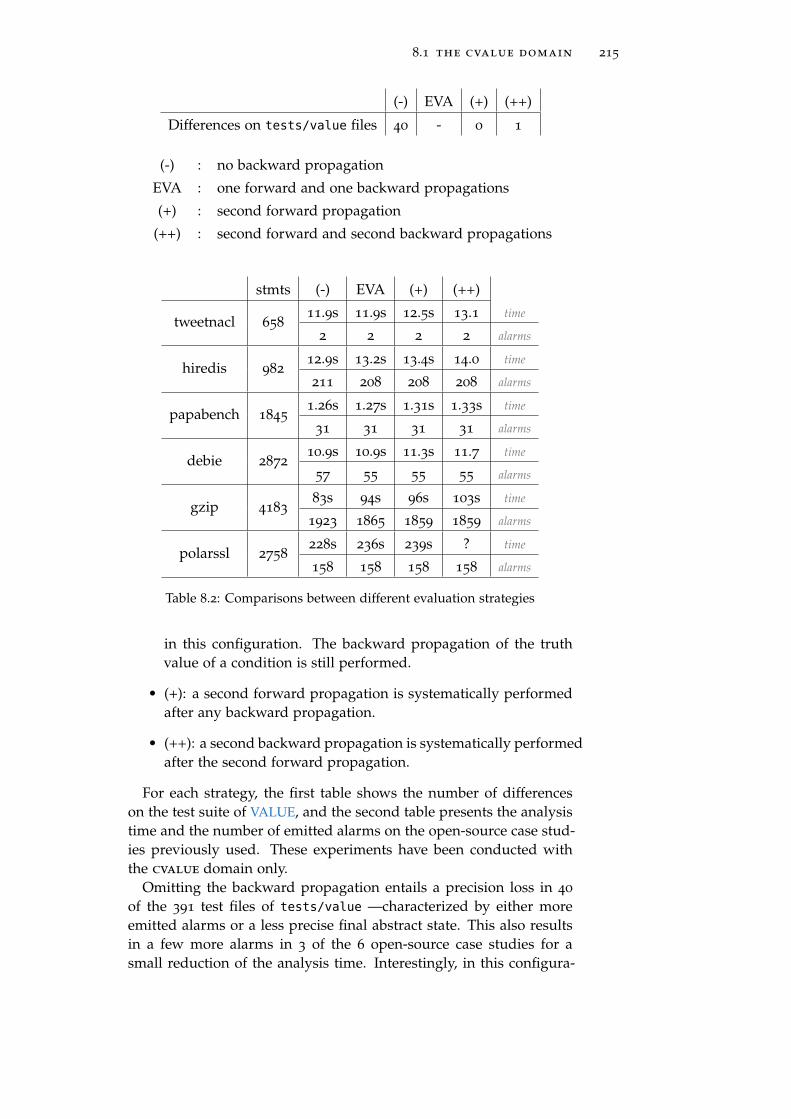
8.1 the cvalue domain 215
(-) EVA (+) (++)
Differences on tests/value files 40 - 0 1
(-) : no backward propagation
EVA : one forward and one backward propagations
(+) : second forward propagation
(++) : second forward and second backward propagations
stmts (-) EVA (+) (++)
tweetnacl 65811.9s 11.9s 12.5s 13.1 time
2 2 2 2 alarms
hiredis 98212.9s 13.2s 13.4s 14.0 time
211 208 208 208 alarms
papabench 18451.26s 1.27s 1.31s 1.33s time
31 31 31 31 alarms
debie 287210.9s 10.9s 11.3s 11.7 time
57 55 55 55 alarms
gzip 418383s 94s 96s 103s time
1923 1865 1859 1859 alarms
polarssl 2758228s 236s 239s ? time
158 158 158 158 alarms
Table 8.2: Comparisons between different evaluation strategies
in this configuration. The backward propagation of the truthvalue of a condition is still performed.
• (+): a second forward propagation is systematically performedafter any backward propagation.
• (++): a second backward propagation is systematically performedafter the second forward propagation.
For each strategy, the first table shows the number of differenceson the test suite of VALUE, and the second table presents the analysistime and the number of emitted alarms on the open-source case stud-ies previously used. These experiments have been conducted withthe cvalue domain only.
Omitting the backward propagation entails a precision loss in 40
of the 391 test files of tests/value —characterized by either moreemitted alarms or a less precise final abstract state. This also resultsin a few more alarms in 3 of the 6 open-source case studies for asmall reduction of the analysis time. Interestingly, in this configura-

216 domains and experimental results in eva
tion, EVA obtains approximately the same results and analysis timesthan VALUE on the biggest open-source case studies, gzip and polarssl.It is still slightly more precise thanks to the stronger backward prop-agation on conditionals.
On the other hand, the second forward propagation and the secondbackward propagation show nearly no difference in the test suite orin the open-source case studies. The only difference in the test suitecomes from a non-idempotent backward propagator, which gain pre-cision by being applied twice. The only difference in the case studiesoccurs on gzip, where the second forward propagation avoids theemission of 6 alarms out of 1865. Even if the cost of these additionalpropagations is insignificant, their low impact on the analysis preci-sion seems to make them unnecessary.
8.2 the equality domain
The cvalue domain provides a precise representation of memories,but is unable to infer relations between variables. The first relationalabstraction introduced in EVA has been a symbolic domain track-ing Herbrand equalities between C expressions. Our intentions wassomewhat similar to those of Miné [Min06b], in particular abstract-ing over temporary variables resulting from code normalization. Ourequality domain is especially interesting because of its use of the ora-cle and the reducer during the cooperative evaluation. The equalitiesare deduced from equality conditions and from assignments that donot read the memory locations being modified. They are then usedto trigger new forward evaluations or backward propagations. Asound interpretation of a statement also requires to remove from theabstract state the equalities which hold no longer afterwards. This isonly needed on assignments, for the equalities between expressionsthat depend on the written location. To do so, the equality domainneeds an abstraction of the byte locations on which an expressiondepends.
This section first defines the dependences of expressions and ad-dresses, as well as abstractions of these dependences. It then for-malizes the abstract states of the domain, its queries and its abstracttransformers. Finally, it presents some details about the implementa-tion and the experimental results obtained with this new domain.
8.2.1 Dependences of an Expression
We first define the dependence of an expression as an operator deps
computing sets of bytes in P(Lbytes): deps(e, S) is the set of the mem-ory bytes on which the evaluation of e depends in the concrete state S.We remind the reader of the definition 25 of memory locations: for

8.2 the equality domain 217
a pointer value l, locτ (l) is the set of sizeof(τ ) bytes in memorystarting at l.
locτ (&x, i) (&x, i+ n) | 0 ≤ n < sizeof(τ )
Definition 60 (Dependences). If the evaluation of an expression e
succeeds in a concrete state S, the dependence of e in S is inductivelydefined as:
deps(∗τa, S) locτ (l) ∪ deps(a, S)
where ∀θ ∈ ΘP , aS(θ) = l ∈ Lτ
deps(♦(e1, . . . , en), S) ∪i∈1,. . . ,ndeps(ei, S)
deps(cst , S) ∅
deps(t[i], S) deps(t, S) ∪ deps(i, S)
deps(e.field , S) deps(e, S)
Let us recall that if the evaluation of a dereference ∗τa, then the con-crete semantics guarantees the existence of a valid location l such thatin all layouts θ, aS(θ) = l.
Lemma 23. Let e be an expression and S a concrete state such that the
evaluation of e in S succeeds: eΘ(S) = V . The resulting concrete value V
only depends on the bytes of deps(e, S). If S is another concrete state that
coincide with S on these bytes, then eΘ(S) = V .
∀S, S ∈ S, ∀e ∈ expr , eΘ(S) = Ω,
(∀θ ∈ ΘP , ∀l ∈ deps(e, S), S(θ)(l) = S(θ)(l))
⇒ eΘ(S) = eΘ(S) ∧ deps(e, S) = deps(e, S)
Proof. The concrete semantics of expressions involves the concretestates only on dereferences, where the bytes of the address are read.On two states coinciding on these bytes, the concrete semantics leadsto the same concrete values as result of the evaluation.
The dependence of an expression e in a concrete state dependsonly on the evaluation of the addresses a dereferenced in the expres-sion. The evaluation of such an address a depends on the bytes ofdeps(a, S), and deps(a, S) ⊆ deps(e, S). Thus, the evaluation of a isthe same on two states coinciding on these bytes, and thus the depen-dences of e is the same on such states.
Definition 61 (Zone abstraction). An abstraction of arbitrary sets ofbytes (i.e. dependences), called zone, is a collection of abstractions Z#
equipped with:
• a concretization γZ
: Z# → P(Lbytes). A zone abstraction z is asound approximation of the dependence of an expression e in aconcrete state S if and only if deps(e, S) ⊆ γ
Z(z).

218 domains and experimental results in eva
• a standard lattice structure (Z#,Z,
Z,
Z,
Z) fulfilling the prop-
erties specified in Figure 2.4 according to the concretization.
• an injection zone : L# → type → Z# from location abstractions,such that for a location abstraction l and a type τ , all bytes oflocτ (γL(l)) are in the concretization of zone(l, τ ).
∀l ∈ L#, ∀τ, (λ_.L) ∈ γL(l) ⇒ locτ (L) ⊆ γZ(zone(l, τ ))
We assume given a zone abstraction Z#. In the EVA equality do-main, the zone abstractions are the maps from variables to integeroffset abstractions presented in Section 5.3.1.3. However, the formal-ization below does not depend on the chosen zone abstraction.
8.2.2 The Equality Abstract States and Queries
We can now define the states and the semantics of the equality do-main. An abstract state of this domain is a set of equalities betweensyntactic expressions, and represents all the concrete states in whichthe equalities hold. An abstraction of the dependence of each expres-sion involved in an equality is also computed by the domain.
Definition 62 (Equality domain). The domain stores expressions alongwith an abstraction of their dependences. An equality in E is denotedas a set of expressions. An abstract state in D
eqis a set of equalities.
The concretization of such an abstract state is the set of concrete statesin which, for each equality:
• all the expressions evaluate to the same concrete value;
• the zone stored for each expression is a sound approximationof its dependences.
E P(expr ×Z#)
Deq P(E)
γeq
: Deq→ S
S ∈ γeq(D) ⇔ ∀E ∈ D, ∃V ∈ V , ∀(e, z) ∈ E,
eΘ(S) = V
deps(e, S) ⊆ γZ(z)
The equality domain should also maintain some invariants to makethe handling of abstract states easier. The equalities should be disjointsets of expressions, and no equality should be a singleton, as a sin-gleton equality brings no information whatsoever. These conditionsdo not impact the concretization of an abstract state, and thus do notimpact the soundness of the domain and its semantics. However, ne-glecting these invariants leads to performance issues. Singleton equal-ities enlarge needlessly the abstract states. Multiple equalities about

8.2 the equality domain 219
the same syntactic expression e make harder to find all expressionsguaranteed to be equal to e by the abstract state. As these invariantsare easy to maintain, we assume that they hold, and define the find
operation accordingly.
Definition 63. We define a find operation of an expression e in anequality state D: it retrieves all the expressions that are guaranteedto evaluate to the same concrete value as e.
find(e,D)
E if ∃z ∈ Z, (e, z) ∈ E ∧ E ∈ D
∅ otherwise
The find operator allows us to define the forward and backwardqueries F
#
Deqand B
#
Deq, by simply using the oracle or the reducer on
the expressions that evaluate to the same concrete value as the re-quested expression. The forward query F
#∗τ on dereferences is imple-
mented exactly as the query on arbitrary expressions F#
Deq, without
using the location abstraction computed for the address. The back-ward query B
#∗τ on dereferences is the identity. Obviously, on an
expression implying an equality or an inequality, the forward queryof the domain may also answer directly, if the involved equality isknown by the abstract state.
Definition 64 (Queries of the equality domain). Let
be the concate-nation of lists. Let D be an abstract state of the equality domain, ebe an expression, l be a location abstraction, v be a value abstraction.The queries of the equality domain are defined as:
F#eq(oracle, D, e)
V,A if find(e,D) = ∅
V
(e,_)∈find(e,D)
(fst(oracle(e))),⊥A otherwise
F#∗τ (oracle, D, e, l) F#eq(oracle, D, e)
F#
Deq(oracle, D, e)
1# if e = (e1 ♦= e2) ∧ e2 ∈ find(e1, D)
0# if e = (e1 ♦ = e2) ∧ e2 ∈ find(e1, D)
F#eq(oracle, D, e) otherwise
B#∗τ (D, l, v) l
B#
Deq(D, e, v)
(e,_)∈find(e,D)
[(e, v)]
With ♦= ∈ =,≤,≥ and ♦ = ∈ =, <,>.
Theorem 14. The queries of the equality domain defined above satisfy the
requirements stated in definitions 56, 57 and 58.
Proof.

220 domains and experimental results in eva
forward queries We prove here the soundness of F#Deq
; the proof
for F#∗τ is exactly the same. Let D be an abstract state of the equalitydomain, e be an expression and oracle be an oracle.Let S be a concrete state in γ
eq(D) ∩ γo(oracle). We need to prove:
F#
Deq(oracle, D, e) |=V×A eΘ(S)
The first two cases for F#
Deqstem directly from the definition of the
abstract states. As S ∈ γ(D), we have:
e2 ∈ find(e1, D) ⇒ e1Θ(S) = e2
Θ(S)
⇒
e1 ♦= e2Θ(S) = 1
e1 ♦ = e2Θ(S) = 0
We now consider the general case. Let E = find(e,D). If E isempty, then F
#
Deq(oracle, D, e) is the top abstraction, which is sound
by definition. Otherwise, ∃z, (e, z) ∈ E and definition 62 of theconcretization of the domain ensures that:
∃V ∈ V , ∀(e, z) ∈ E, eΘ(S) = V
This ensures that eΘ(S) succeeds, and thus ⊥A |=A eΘ(S).Moreover, for all (e, z) ∈ E, we have eΘ(S) = eΘ(S).As S ∈ γo(oracle), the definition 54 of the oracle concretization en-sures that:
∀e ∈ expr , eΘ(S) ∈ γV(fst(oracle(e)))
Thus:∀(e, z) ∈ E, eΘ(S) ∈ γV(fst(oracle(e
)))
And by the soundness property of the meet operation,
∀(e, z) ∈ E, eΘ(S) ∈ γV(
(e,z)∈find(e,D)
(fst(oracle(e))))
Finally, we have
(
(e,z)∈find(e,D)
(fst(oracle(e))),⊥A) |=V×A
eΘ(S)
qed.
backward queries B#∗τ being the identity function, its sound-
ness is immediate. Let us prove the soundness of B#Deq
. Let D be anabstract state of the equality domain, let e be an expression and v

8.2 the equality domain 221
be a value abstraction. Let S be a concrete state in γeq(S) such that
eΘ(S) ∈ γV(v). We need to prove:
∀(e, v) ∈ B#
Deq(S, e, v), eΘ(S) ∈ γV(v
)
⇔ ∀(e, z) ∈ find(e,D), eΘ(S) ∈ γV(v)
From the definition 63 of find and the definition 62 of the concretiza-tion of the equality domain, we know that:
∀(e, z) ∈ find(e,D), eΘ(S) = eΘ(S)
and we already have eΘ(S) ∈ γV(v).
8.2.3 Interpretation of Assignments
On an assignment ∗τa := e, the equality transformer needs to:
1. remove from the abstract state the equalities involving syntacticexpressions whose value could be modified by the assignment;
2. computes an abstraction of the dependences of e and a.
3. adds the new equality ∗τa == e if it holds after the assignment,i.e. if the assignment does not modifies the value of a or e.
The second point requires some abstractions of the addresses deref-erenced in expressions or assigned by assignment. As mentionnedin Section 6.1.3, the valuations of EVA are made of a map from ex-pressions to value abstractions, and a map from addresses to locationabstractions. The latter map was omitted in the formalization of theevaluation, but it fulfills the same purpose and requirements as theexpression map. The concretization of valuations is extended accord-ingly.
Definition 65 (Concretization of extended valuations). The concretiza-tion of valuation is extended to:
γE(E) S | ∀e ∈ dom(E), eΘ(S) ∈ γV(E(e))
∧ ∀a ∈ dom(E), aΘ(S) ∈ γL(E(a))
Thus, the valuation makes available the location abstractions neededby the equality domain to interpret assignments.
8.2.3.1 Removing Equalities
We first define a kill function that removes from the equalities of anabstract state each expression whose dependence intersects a givenmemory location.

222 domains and experimental results in eva
Definition 66. Let l be a location abstraction. We define the functionkill as:
killE : Z# → E → E
killeq
: L# → type → Deq→ D
eq
killE(z, E) (e, z) | (e, z) ∈ E ∧ z Zz = ⊥
killeq(l, τ, D) killE(zone(l, τ ), E) | E ∈ D
Lemma 24. Let ∗τa := e be an assignment, l a location abstraction and D
an abstract state of the equality domain. If D is a sound approximation of
the concrete states before the statement and if l is a sound approximation of
the address a in these concrete states, then killeq(l, τ, D) is a sound approxi-
mation of the concrete states after the execution of the assignment.
∀S ∈ γeq(D), aΘ(S) ∈ γL(l) ⇒ | ∗τ a := e| (S) ∈ γ
eq(kill
eq(l, τ, D))
Proof. Let ∗τa := e be an assignment and let l be a sound approx-imation of the value of a. Let D be an abstract state of the equal-ity domain and let D = killeq(l, τ, D). Let S a concrete state inγeq(D) for which the interpretation of the assignment succeeds, and
let S = | ∗τ a := e| (S). We want to prove that S ∈ γeq(D). This
requires that:
∀E ∈ D, ∃V ∈ V , ∀(e, z) ∈ E,
eΘ(S) = V
deps(e, S) ∈ γZ(z)
Let E be an equality of D. By the definition of kill, we have:
∃E ∈ D, E = killE(zone(l, τ ), E)
⇔ ∃E ∈ D, E = (e, z) | (e, z) ∈ E ∧ z Zzone(l, τ ) = ⊥ (8.2)
As E ∈ D and S ∈ γeq(D), definition 62 states that it exists a concrete
value V such that:
∀(e, z) ∈ E,
eΘ(S) = V
deps(e, S) ∈ γZ(z)
(8.3)
We also have S = | ∗τ a := e| (S).Let L ∈ Lτ such that ∀θ ∈ ΘP , aS(θ) = L. Such a concrete loca-tion exists, as the execution of the assignment succeeds in S, and wehave λ_.L ∈ γL(l), since l is a sound approximation of the address a.The state S can then be rewritten:
S = λθ. S(θ)
locτ (L) → φ−1τ (V (θ))
This implies that:
∀θ ∈ ΘP , ∀l /∈ locτ (L), S(θ)(l) = S(θ)(l) (8.4)

8.2 the equality domain 223
Now, let (e, z) ∈ E. By 8.2:
(e, z) ∈ E ∧ z Zzone(l, τ ) = ⊥ (8.5)
By the concretization 62 of the equality domain: deps(e, S) ⊆ γZ(z)
As λ_.L ∈ γL(l), by definition 61: locτ (L) ⊆ γZ(zone(l, τ ))
As z Zzone(l, τ ) = ⊥, we have γ
Z(z) ∩ γ
Z(zone(l, τ )) ⊆ γ
Z(⊥
Z) = ∅
And thus deps(e, S) ∩ locτ (l) ⊆ γZ(z) ∩ γ
Z(zone(l, τ )) = ∅
And by 8.4 and 8.5:
(e, z) ∈ E ∧ ∀θ ∈ ΘP , ∀l ∈ deps(e, S), S(θ)(l) = S(θ)(l) (8.6)
By equation 8.3:
eΘ(S) = V
deps(e, S) ∈ γZ(z)
Finally, lemma 23 and equation 8.6 ensures that:
eΘ(S) = eΘ(S) ∧ deps(e, S) = deps(e, S)
This means that
∀(e, z) ∈ E,
eΘ(S) = V
deps(e, S) ∈ γZ(z)
qed.
8.2.3.2 Computing Dependences
We now presents the computation of an abstraction of the depen-dences of expressions in the concrete states represented by a valua-tion.
Definition 67 (Computation of dependences abstractions). We definedeps# : expr → E → Z# inductively as:
deps#(∗τa, E) zone(E(a), τ ) Zdeps#(a, E)
deps#(♦(e1, . . . , en), E) i∈1,. . . ,ndeps#(ei, E)
deps#(cst , E) ⊥Z
deps#(t[i], E) deps#(t, E) Zdeps#(i, E)
deps#(e.field , E) deps#(e, E)
Lemma 25. Let E be a valuation, e be an expression and a be an address.
The zone abstractions deps#(e, E) and deps#(a, E) are respectively sound
approximations of deps(e, S) and deps(a, S) for all states S in γE(E).
∀E ∈ E, ∀e ∈ expr , ∀a ∈ addr ,
∀S ∈ γE(E),
deps(e, S) ⊆ γZ(deps#(e, E))
deps(a, S) ⊆ γZ(deps#(a, E))

224 domains and experimental results in eva
Proof. By induction of the expression e and the address a, using thatthe join
Zis an overapproximation of the union of sets ∪ (depen-
dences are sets of bytes). The base case, for constants cst , is trivial:γZ(⊥
Z) = ∅ by definition. We prove the case of dereferences, assum-
ing the induction hypothesis. Let E be a valuation, τ a scalar typeand a an address. Let S be a concrete state in γE(E).
deps(a, S) ⊆ γZ(deps#(a, E)) ⇒ deps(∗τa, S) ⊆ γ
Z(deps#(∗τa, E))
We recall the definition of the concrete and abstract dependences ofthe dereference:
deps(∗τa, S) = locτ (L) ∪ deps(a, S)
where ∀θ ∈ ΘP , aS(θ) = L ∈ Lτ
deps#(∗τa, E) = zone(E(a), τ ) Zdeps#(a, E)
We have S ∈ γE(E) and aΘ(S) = λ_.LBy definition 65: (λ_.L) ∈ γL(E(a))
By definition 61: locτ (L) ⊆ γZ(zone(l, τ ))
By induction hypothesis: deps(a, E) ⊆ γZ(deps#(a, E))
By these equations and the soundness of the join:
locτ (L) ∪ deps(a, S) ⊆ γZ(zone(l, τ )) ∪ γ
Z(deps#(a, E)
⊆ γZ(zone(E(a), τ )
Zdeps#(a, E))
qed.
8.2.3.3 Adding New Equalities
After an assignment ∗τa := e, the equality between ∗τa and e holds,unless if the assignment modifies the value of the expression e or ofthe value of the address a.
Example 31. An example of the first case is the assignment ∗τ (&x, 0) =
∗τ (&x, 0) +τ 1 where τ is a scalar type. This assignment is written x
= x+1 in the C syntax. Obviously, the equality x = x+ 1 does nothold after the assignment —in fact, this equality never holds.
Example 32. Figure 8.1 presents two code snippets where the exe-cution of the final assignment ∗τa := e modifies the value of thesyntactic address a. At line 2 on the left code, t[t[0]] refers to t[0],the first cell of the array t, which is thus modified by the assignment.Afterwards, t[0] contains the value 2 and t[t[0]] refers to t[2], thethird cell of the array. The equality t[t[0]]==2 is false, as t[2] hasvalue 0.
At line 3 on the right code, *(p+i) refers to &i, and the assignmentmodifies the value of the variable i. Afterwards, the pointer *(p+i)
refers to &(i+1), which is not even a valid address to read at: theequality *(p+i)==1 does not hold.

8.2 the equality domain 225
int t[5] = 0; 0; 0; 0; 0
int t[t[0]] = 2;
int i = 0;
int *p = &i;
*(p+i) = 1;
Figure 8.1: Assignment modifying the address
Lemma 26. Let ∗τa := e be an assignment. Let S be a concrete state in
which the execution of the assignment succeeds. Let a location abstraction l
be a sound approximation of the value of a in S. Let two zone abstractions zaand ze be sound approximations of the dependences of respectively a and e
in S. If zone(l, τ ) Zza and zone(l, τ )
Zze are bottom, then the syntactic
equality ∗τa = e holds after the assignment, i.e. in the state | ∗τ a := e| (S).
Moreover, the zone abstractions za and ze are still sound approximations of
the dependences of e and a in this post state.
If we write S = | ∗τ a := e| (S):
aΘ(S) ∈ γL(l)
deps(a, S) ⊆ za
deps(e, S) ⊆ ze
zone(l, τ ) Zze = ⊥
Z
zone(l, τ ) Zza = ⊥
Z
⇒
∗τaΘ(S) = eΘ(S)
deps(a, S) ⊆ za
deps(e, S) ⊆ ze
Proof. This proof uses the same notations as the lemma. As the exe-
cution of the assignment succeeds in the concrete state S, aΘ(S) isa constant location (independent of the memory location). We thenwrite:
(λ_.L) = aΘ(S) V = eΘ(S) S = | ∗τ a := e| (S)
As l is a sound approximation of the value of a in S: (λ_.L) ∈ γL(l)
By definition 61, locτ (L) ⊆ zone(l, τ )
By soundness of zones: deps(a, S) ⊆ γZ(za) ∧ deps(e, S) ⊆ γ
Z(ze)
By the soundness property of the meet:
zone(l, τ ) Zza = ⊥
Z⇒ locτ (L) ∩ deps(a, S) = ∅
zone(l, τ ) Zze = ⊥
Z⇒ locτ (L) ∩ deps(e, S) = ∅
Thanks to the concrete semantics of assignment (Figure 4.8), the poststate S can be written as:
S = λθ. S(θ)
locτ (L) → φ−1τ (V (θ))] (8.7)
The concrete states S and S coincide on all bytes but locτ (L). As theintersection between locτ (L) and the dependences of e and a in S isempty, lemma 23 applies, and we have:
eΘ(S) = eΘ(S) ∧ deps(e, S) = deps(e, S)
aΘ(S) = aΘ(S) ∧ deps(a, S) = deps(a, S)

226 domains and experimental results in eva
This already ensures that deps(a, S) ⊆ γZ(za) ∧ deps(e, S) ⊆ γ
Z(ze).
The zone abstractions za and ze are still sound approximations of thedependences of a and e in the post state S.Moreover, we have:
eΘ(S) = eΘ(S) = V
aΘ(S) = aΘ(S) = λ_.L
By the concrete semantics of expressions (Figure 4.7) and 8.7:
∗τaΘ(S) = λθ. (S(θ))τ [l]
= λθ. φτ (S
(θ)(locτ (L))
= λθ. φτ (φ
−1τ (V (θ)))
= λθ. V (θ)
= V = eΘ(S)
The equality ∗τa = e holds in the post state S.
The last requirement to finally define the transfer function on as-signments is the addition of a new equality into an abstract state. Weassume given an operator ⊕
eqthat adds a new equality between two
expressions (and their dependences) to an abstract state. It must sat-isfies the following lemma.
Proposition 9. Let D be an abstract state of the equality domain, e1 and
e2 be two expressions, and z1 and z2 be two zone abstractions. We write
D = (e1, z1), (e2, z2)⊕eqD. Then:
∀S ∈ γeq(D),
e1Θ(S) = e2
Θ(S)
deps(e1, S) ⊆ z1
deps(e2, S) ⊆ z2
⇒ S ∈ γeq(D)
8.2.3.4 Complete Interpretation of Assignments
Definition 68. Let ∗τa := e be an assignment, D be an abstract stateof the equality domain, E be a valuation containing an abstraction foreach subterm of a and e.
T eq(∗τa := e, E , D)
E ⊕eq
D if za Zz = ze Z
z = ⊥Z
D otherwise
where
za = deps#(a, E)
ze = deps#(e, E)
z = zone(E(a), τ )
E = (∗τa, za), (e, ze)
D = kill(E(a), D)

8.2 the equality domain 227
Theorem 15. Let ∗τa := e be an assignment, D be an abstract state of
the equality domain, E be a valuation. For all the concrete states S in
γeqE(D, E) for which the execution of the statement succeeds, the concrete
state | ∗τ a := e| (S) is in γeq(T eq(∗τa := e, E , D)).
In other words, T eq satisfies a sound abstract transformer of assignments
that satisfies the property of definition 59.
Proof. Let ∗τa := e be an assignment, D be an abstract state of theequality domain, E be a valuation containing an abstraction for eachsubterm of a and e.Let S be a concrete state in γ
eqE(D, E). We write S = | ∗τ a := e| (S),D” = T eq(∗τa := e, E , D) and want to prove that S ∈ γ
eq(D”).
As S ∈ γE(E), by definition 65: aΘ(S) ∈ γL(E(a)).By lemma 24: S ∈ γ
eq(kill
eq(E(a), τ, D))
In the second case of the definition, D” = killeq(E(a), τ, D), and the
proof is completed. We now consider the first case only.Lemma 25 ensures that the zones za = deps#(a, E) and ze = deps#(e, E)
are sound approximations of the dependences of a and e in the con-crete states of γE(E):
deps(e, S) ⊆ γZ(ze)
deps(a, S) ⊆ γZ(za)
And we already know aΘ(S) ∈ γL(E(a)).Thus, lemma 26 ensures that:
zone(E(a), τ ) Zze = ⊥
Z
zone(E(a), τ ) Zza = ⊥
Z
⇒
∗τaΘ(S) = eΘ(S)
deps(e, S) ⊆ γZ(ze)
deps(a, S) ⊆ γZ(za)
The new equality holds in the concrete state S, and the depen-dences are still correct. Proposition 9 ensures that the new abstractstate (∗τa, za), (e, ze)⊕eq
S is a sound abstraction of S. In all cases:
S ∈ γeq(D”)
8.2.4 Interpretation of Other Statements
The interpretation of other statements than assignments is straight-forward.
On an test filter (e1 = e2)==0?, the equality e1 = e2 is added tothe abstract state. In the C syntax, this corresponds to the if branchof if(e1==e2) or the else branch of if(e1!=e2). Otherwise, the equalitydomain cannot learn anything from a test filter, and the abstract stateafter the statement is the same as the abstract state before.

228 domains and experimental results in eva
Finally, the abstract transformer for the entry in scope of variablesis the identity; the abstract transformer for the exit of scope of vari-ables removes from the state the expressions that depends on thesevariables.
8.2.5 Implementation
An equality is encoded as a set of at least two expressions. A setof equalities is encoded as a map from expressions to equalities: itbinds each involved expression to the equality containing it. This rep-resentation makes efficient the find operation, used for every queryduring the evaluation. On the other hand, the addition or removal ofan equality can be costly, as the modification of an existing equality E
requires to update the binding of each expression in E. In an abstractstate where e1 and e2 belong respectively to the disjoint equalities E1
and E2, adding the equality e1 = e2 amounts to merge E1 and E2,and requires |E1|+ |E2| binding updates. In an abstract state where e
belongs to E, removing e —when e can be modified by an assign-ment— requires |E| binding updates. In practice, the cardinal of theequalities propagated by the domain remains small enough to notoverly imped the analysis.
Two last optimizations limit the number of equalities created bythe domain. Firstly, if the removal of e makes E a singleton, then E
is totally removed instead. Secondly, the addition of a new equalitye1 = e2 is avoided if the two abstractions for e1 and e2 in the valuationare singleton —if they represent only one concrete value. (For theequality stemming from the assignment ∗τa := e, this means that theabstractions for a and e are singleton.) In this case, the equality is de
facto already known by the abstract states of the other domains.The join of two abstract states must keep only the equalities carried
by both states. It is simply a merge of both maps, by intersectinngpointwise the equalities bound to the same expressions. Expressionsbelonging to only one map are simply removed. The maps used bythe domain are patricia trees [OG98], where the placement of a data isfixed by the bits of its key. This allows efficient merges, by traversingthe two maps at the same time.
As shown in the previous sections, the abstract domain relies ondependence abstractions to remove from the states the expressionswhose value may be modified by assignments. These dependence ab-stractions are built upon the location abstractions cooperatively com-puted by the evaluation, and made available by the valuation. To ef-ficiently retrieve the expressions to be removed at an assignment, thedomain also maintains a dependency table —implemented throughthe generic datastructures of cvalue— that links a location to theexpressions that depends on it.

8.2 the equality domain 229
loc statements EVA EVA+EQ
idct 342 586 (94%)1.4s 1.7 time
56 56 alarms
tweetnacl 799 658 (99%)12s 15s time
2 2 alarms
papabench 3199 1845 (55%)1.3s 1.4s time
31 31 alarms
debie 5326 2872 (98%)13s 13s time
55 42 alarms
gzip 5196 4170 (94%)42s 53s time
1505 1501 alarms
polarssl 24k 2758 (49%)230s 294s time
158 149 alarms
indus1 99k 30955 (81%)430s 686s time
228 222 alarms
indus2 125k 36782 (80%)715s 1343s time
244 238 alarms
Table 8.3: Experimental results of the equality domain
Finally, the domain only relies on the oracle and the reducer toavail the relations it infers. It is thus independent of the chosen valueabstraction, and is implemented as a functor from value to state ab-straction.
8.2.6 Experimental Results
In practice, the equality domain of EVA behaves exactly as explainedin examples 26 and 29.
Table 8.3 presents the experimental results obtained with the equal-ity domain on the programs already used in Section 8.1.3. It comparesthe analysis time and the number of emitted alarms by EVA’s analysisinstantiated with only the cvalue domain, or with the product of thecvalue domain and the equality domain. In 5 out of 8 programs (allthose with a significant number of alarms), less alarms are emitted.The slowdown introduced by the equality domain does not exceed30%, except on the two industrial case studies, on which the analy-sis 60% and 88% slower. Still, gaining 6 alarms there (on analysesthat use loop unrolling and disjunctive completion very aggressivelyfor maximum precision) is already a very positive result, given thelimited relationality of the equality domain.

230 domains and experimental results in eva
8.3 other new domains in eva
In addition to the equality domain, four other new abstract domainshave been introduced in EVA during the last year: a binding to thenumerical abstract domains provided by the apron library, a domainof symbolic locations, a gauges domain and a bitwise domain. Thefirst three domains are purely numerical. They process the assign-ments through pointers in the same way as the equality domain: theyrely on the location abstractions computed by the cvalue domain toremove the properties invalidated by the assignment. The bitwise do-main is built upon the same memory model than the cvalue domain,reusing the generic OCaml functors of its data structures.
This section briefly describes these new domains, and presentstheir performances on the same case studies used before in this chap-ter. It should be remembered that the implementation of these do-mains remain mostly experimental.
8.3.1 Binding to the APRON domains
We have implemented a minimal binding to the numerical abstractdomains available in apron [JM09]. The resulting domains (boxes, oc-tagons, strict or loose convex polyhedra, linear equalities) are proofsof concept to demonstrate that preexisting relational domains fit withinthe communication model of EVA, and are easy to introduce. Ourapron binding has currently less than 1000 lines of code. The abstractstate is an apron state. A (static) mapping between the apron dimen-sions and the scalar variables present in the program is created by thebinding, and used as a correspondence table to translate the memory lo-cations inferred by the cvalue domain. Indeed, the apron domainsbring no information about which variable a pointer may point to;instead, they entirely rely on the other domains for aliasing informa-tion. The domain answers queries for arithmetic expressions, thatare translated into the apron internal langage. Sub-expressions thatcannot be handled by apron are linearized on-the-fly into intervals,using the cooperatively computed value. Currently, the binding islimited to variables with integer types.
We plan to add support for variables with floating-point types.Tracking information for structs or arrays is also easy, and simply re-quires extending the correspondence table. However, the most impor-tant improvement would consist in using variable packing [Cou+09].Analyzing large problems in which all variables are in relation isknown to be unfeasible, due to the high algorithmic complexity ofrelational domains. The domain should instead infer subsets of “re-lated” variables, and only track relations within those sets. The dif-ficulty lies in finding good heuristics, which should then be imple-mented on the EVA side of the domain.
8.3 other new domains in eva 231
8.3.2 The Symbolic Locations Domain
The symbolic locations domain tracks accesses to arrays or throughpointers in a symbolic way. Its intent is to analyze code such as ifif (t[i]<=e)v=t[i]; in a precise way. Indeed, when i is imprecise, do-mains that represent arrays in extenso cannot learn information fromthe condition (because any cell may be involved). The domain sharessome similarities with the recency abstraction [BR06]. Its state is amap from symbolic locations (such as t[i], *p or p->v) to an abstractvalue. Strong reductions may be performed on those values whenanalyzing conditions, to be shared with the other domains when thelocation is encountered again later.
8.3.3 The Gauges Domain
Gauges [Ven12] are a weakly relational domain, able to efficiently in-fer general linear inequality invariants within loops. Technically, thevariables involved in the invariants are all related to loop counters,that model the current number of iterations in each loop. Gaugesare especially useful to infer invariants for pointer offsets, as pointerarithmetic introduces +4 or +8 increments (for 32- and 64-bits architec-ture respectively), that cannot be directly handled by domains suchas octagons . The gauges domain communicates integer and pointervalues through the standard values of EVA.
8.3.4 Bitwise Abstractions
The bitwise domain aims at adding bitvector-like reasoning to EVA(including on floating-point values and pointers), without resortingto a dedicated implementation. Instead, we reuse the expressivity ofthe offsetmaps, that represent sequences of bits in the cvalue domain.Indeed, this abstraction is already able to extract the possible valuesof some bits in a memory range. This bitwise domain works on anew kind of value abstractions, namely a sequence of bits of knownlength. Only the forward and backward abstract semantics for thebitwise C operators, as well as integer casts and multiplication/divi-sion by a power of 2, have been implemented. All other operationsdegenerate to V. The reduced product between the standard valuesand those new bitwise values performs a conversion between the tworepresentations when possible.
8.3.5 Experimental Results
Figure 8.2 presents the results of some experiments conducted on thenew abstract domains of our analyzer. We compare the precision andthe analysis time of:

232 domains and experimental results in eva
loc stmts EVA Eqs Loc Gau All
tweetnacl 799 65812s 15s 14s 15s 19s time
2 2 2 2 2 alarms
papabench 3199 18451.3s 1.4s 1.3s 1.3s 1.6s time
31 31 31 31 31 alarms
debie 5326 287211s 13s 14s 13s 16s time
55 42 55 53 40 alarms
gzip 5196 417042s 53s — 60s — time
1505 1501 — 1500 — alarms
polarssl 24k 2758230s 294s 266s 382s 432s time
158 149 156 152 140 alarms
indus 125k 37k850s 1090s 1390s 1120s 1930s time
153 136 150 153 134 alarms
Figure 8.2: Experimental results on the new abstract domains
• EVA with the default cvalue domain (EVA);
• EVA with the cvalue domain, augmented respectively with:
– the equality domain (Eqs);
– the symbolic locations domain (Loc);
– the gauges domain (Gau);
– all these three domains (All).
We observe some improvements on two case studies, debie and po-larssl, where the introduction of the new domains allows the analyzerto rule out a few more alarms. The slowdown introduced by eachdomain basically ranges between 15 to 66% from case to case. On po-larssl, the largest open-source case study, the analysis with all thesedomains is twice as slow than the analysis with the cvalue domainonly, and proves 11% of the alarms emitted by the cvalue domain.
These results are quite encouraging, given that the new domainsremain experimental and mostly unoptimized. However, much workremains to be done to bring the new domain to the same level ofmaturity than the cvalue domain.
8.3.6 Conclusion
This concludes our presentation of the EVA analyzer. The alarmsand the value abstractions used by the analyzer have been formal-ized in Chapter 5. The strategies for the cooperative computation

8.3 other new domains in eva 233
of these abstractions of expressions has been detailled in Chapter 6.Chapter 7 illustrated how this cooperative computation can assist ab-stract domains to precisely interpret the statement semantics. Finally,this chapter described the new abstract domains that have been im-plemented within EVA, and how they fit into its architecture. Eventhough the new abstractions are not as efficient as the legacy cvalue
domain yet, they fit properly in the architecture of our analyzer. Inour experience, the communication through value abstractions doesnot restrain the expressivity of the product of abstract domains, andthe cooperative evaluation of expressions effectively assists the imple-mentation of new domains. We believe that the variety of abstractionsintroduced within EVA in less than a year validates its core conceptsand its design.


Part V
A B S T R A C T S E M A N T I C S O F T R A C E S


9P R E D I C AT E D A N A LY S E S
This chapter differs slightly from the other parts of this thesis. Whilethe preceding chapters are mostly dedicated to the structuring of ahierachy of abstractions, and to the organization of interactions be-tween them, this chapter presents a generic framework to improvethe precision of any abstract domain at join points. Moreover, thiswork has not been implemented in EVA, but as a standalone newplugin of Frama-C.
Abstract semantics often perform wide approximations when twocontrol-flow paths meet, by merging the states from each path. Thisjoin of abstract states ensures the soundness of the abstract semantics,but is also a common source of imprecision: the properties inferredin only one path are generally lost. This chapter presents how tomechanically augment any standard domain with conditional predi-cates to circumvent this imprecision. The predicates are derived fromconditional statements, and postpone the loss of information. Theresulting domain is called a predicated domain, and analyses oversuch a domain are called predicated analyses. This work has beenpublished in [BBY16].
After detailing our motivations, this chapter formalizes the seman-tics of a predicated domain, and explains how to build an efficientpredicated analysis. It also outlines the coq proof of the soundness ofa predicated analysis, exposes some related works, and describes theexperimental evaluation of our practical implementation.
9.1 motivation
Seeking to strike the best balance between precision and efficiency isalways a challenge in abstract interpretation. Flow-sensitivity, whichallows to infer static properties that depend on program points, isoften considered as a prerequisite to obtain a precise program anal-ysis. More aggressive analyses are path-sensitive: the analysis of aprogram statement depends on the control-flow path followed toreach this statement. Nevertheless, most analyses sacrifice full path-sensitivity and perform approximations when two control-flow pathsmeet. Those approximations may lead to a significant loss of preci-sion, and may preclude inferring some interesting properties of theprogram.
Consider as an example the code fragment of Figure 9.1, whichis a simplified version of a real-life program that opens and closesfile descriptors. Proving that the three calls to the close function
237

238 predicated analyses
1 i f ( f l a g 1 ) fd1 = open ( path1 ) ;
i f ( fd1 == −1) e x i t ( ) ; [ . . . ] // code 1
5 i f ( f l a g 2 ) fd2 = open ( path2 ) ;
i f ( fd2 == −1) i f ( f l a g 1 ) c l o s e ( fd1 ) ;e x i t ( ) ;
10 [ . . . ] // code 2
i f ( f l a g 1 ) c l o s e ( fd1 ) ;i f ( f l a g 2 ) c l o s e ( fd2 ) ;
Figure 9.1: Example of interleaved conditionals
are correct, i.e. that the corresponding fd variable has been properlycreated following the calls to the open function, heavily relies on thepossible values for the flag1 and flag2 variables. An analysis thatdoes not keep track of the relation between flag1 and fd1 on the onehand, and flag2 and fd2 on the other hand, will not be able to provethat the program is correct.
In this chapter, we define an analysis in which information aboutthe conditionals that have been encountered so far is retained usingboolean predicates. These predicates guard the values inferred aboutthe program. Our analysis is parameterized by a pre-existing analy-sis domain, which we use to derive a new predicated analysis. Moreprecisely, we propagate two kinds of information that are not presentin the original domain: a context and an implication map.
1. A context is a boolean predicate synthesized from the guardsof the conditionals that have been reached so far, and that isguaranteed to hold at the current program point. In our exam-ple, at the beginning of line 8, the context would be flag2 ∧
(fd2 = −1).
2. An implication map is a set of facts from the original analysis do-main, guarded by boolean predicates. Each fact is guaranteed tohold when its guard holds. In this example, we suppose that theanalysis domain keeps track of whether open returned a validfile descriptor, or −1 in case of error. Here are the implicationswe would like to infer after line 6:
flag1 → valid_fd(fd1) true → valid_fd(fd2) ∨ (fd2 = −1)
The first implication results from the analysis of the condition-als at lines 1–3; it precisely models the information we needbetween flag1 and fd1. The second implication is simply thepostcondition of the open function, which holds uncondition-ally.

9.2 a generic abstract interpretation based framework 239
e ∈ expr ::= x x ∈ X
| v v ∈ V
| e♦e
c, p ∈ C ::= e |¬c | c∧c | c∨c | true | false
stmt ::= x := e
| c ?
Figure 9.2: Syntax of our language
Based on abstract interpretation, our framework is generic: it enablesmechanically augmenting any standard dataflow analysis with pred-icates, regardless of its specific properties. The results stated in thischapter have been formally verified with Coq, an interactive proofmanagement system. We also integrated it into Frama-C as a stan-dalone plugin, designed to complement EVA. Our experiments showthat predicated analyses over more focused – hence simpler to imple-ment – domains may significantly enhance the precision of the resultsof EVA, while remaining scalable.
9.2 a generic abstract interpretation based framework
Predicated analyzes are mostly independent of the target language,even though our implementation handles C programs. For the sakeof brevity, we formalizes the predicated domains and analyses overa simplified version of clike, without pointer values. Thus, the con-crete values and the concrete states of its semantics do not involvememory layouts. We still identify the programs and their control-flow graphs, and use a collecting semantics to characterize them. Webriefly present the simplified language hereafter.
syntax Figure 9.2 presents the syntax of our language. Programsoperate over a fixed, finite set of variables X whose values belongto an unspecified set V. Expressions are either variables, constants,or the application of a binary operator ♦ to expressions. We strat-ify expressions e in expr and conditions c in C, the truth value ofan element of V being given by a mapping T from V to booleans.Statements are either assignments such as x := e, or tests c ? that haltexecution when the condition does not hold.
concrete semantics A concrete state of the program at a node
n of its control-flow graph is described by a memory m ∈ VX
assign-ing a value to each variable. The semantics e
m(resp. c
m) of an
expression e (resp. a condition c) is its evaluation in the memory m,and implicitly depends on the semantics of the operators ♦.

240 predicated analyses
(a) Concrete semantics
|x := e| (S)
m[x → em] |m ∈ S
|c ?| (S)
m |m ∈ S ∧T(cm) = true
(b) Abstract semantics
γL(L) = VX
γL(l1) ∪ γL(l2) ⊆ γL(l1 L l2)
|i| (γL(l)) ⊆ γL( |i|#L (l))
Figure 9.3: Concrete and abstract semantics
The semantics |stmt| of a statement stmt is a transfer functionover a set of memories, described by the first equalities of Figure 9.3a.After an assignment x := e, the variable x is bound (in the new states)to the value of the expression e. A test blocks execution, only allowingstates in which the condition holds.
abstract semantics A predicated analysis relies on a standardabstract domain L, equipped with the classic operations of the ab-stract interpretation framework presented in Section 2.2.2:
• a partial order L over abstract states,
• a monotone concretization function γL from L to P(VX), linking
the abstract states to the concrete ones,
• greatest and smallest elements L and ⊥L, such that γL(L) =
VX
and γL(⊥L) = ∅,
• sound over-approximations join L and meet L of the unionand intersection of concrete states,
• sound abstract transfer functions |stmt| L# from L to L that
over-approximate the concrete semantics.
entailment and equivalence of conditions In the follow-ing, we will need to compare some conditions, in particular to decidewhether one condition logically implies another. To do so, we choosea coarse interpretation, that treats the expressions present inside con-ditions as uninterpreted terms. Let ∆ be the set exprtrue,false
of functions from expressions to booleans. Given such a functionδ ∈ ∆, we lift it to a valuation on conditions in the obvious way,e.g. δ(c1∧c2) = δ(c1) ∧ δ(c2) where in the r.h.s., the symbol ∧ is theusual conjunction operator. We say that a condition c1 entails anothercondition c2, written c1 c2 when the evaluation of c1 implies the

9.3 the predicated domain 241
evaluation of c2 for all valuations. Similarly, we define the equivalence
of two conditions as their mutual entailment.
c1 c2 ∀δ ∈ ∆, δ(c1) ⇒ δ(c2)
c1 c2 ∀δ ∈ ∆, δ(c1) ⇔ δ(c2)
For example, ((x > y)∧(z = 0))∧(h = 2) (h = 2)∧(x > y)
holds.As a partial preorder, this entailment remains quite weak. Since
it does not give a meaning to the operators inside expressions, therelation between e.g. c > 3 and c ≥ 1 is not captured, and c >
3 c ≥ 1 does not hold. This is by design, so that implication andequivalence may be decided efficiently. The real entailment relationmay be arbitrarily stronger: any decidable pre-order compatible withT(c
m) is also suitable.
9.3 the predicated domain
This section shows how to augment a generic abstract domain withconditional predicates. We first define our predicated domain, equipit with a lattice structure, and then define operations suitable for anefficient analysis.
9.3.1 Predicated Elements
Our analysis builds a predicated domain on top of any abstract do-main L; we refer to L as the underlying domain. The information wepropagate in this new domain is two-fold:
1. A mapping I from predicates in C to elements of L, called a map.Maps stand for implications from guards to (abstract) values.Hence they contain conditional information: if I maps p to l,then l is a correct approximation of the state as soon as p holds.
2. A boolean predicate c ∈ C, called the context, standing for aset of facts that we know to hold at the current program point.Contexts are used to preserve information when performing ajoin operation. In particular, the join defined in Section 9.3.3uses the context to form new interesting guards.1
We use the syntax λp.l to denote the map from p to l. We writep → l ∈ I to mean that I guards l by p, and I(p) for l. We say thatp → l is trivial when l = L, as the value L brings no informationwhatsoever. In order to have a decidable semantics, we restrict our-selves to finite maps in which all but a finite number of implications
1 In our analysis, presented in Section 9.4, contexts are always derived from the guardsof the test statements present in the program.

242 predicated analyses
are trivial. This restriction is also important because we often performseemingly infinite intersections
p∈C I(p). In fact, those intersections
always involve a finite number of guards p bound to a value differentfrom L.
We also require the guard false, which corresponds to a contradic-tion, to be bound to ⊥L. In the following, we only mention non-trivialguards, and omit the guard for false.2
We call a context and a map that satisfy these properties a context-
implication-map pair, ranged over by Φ and abbreviated as CI-pair. Wedefine Lpred, the predicated domain over L, as the set of such CI-pairs.CI-pairs will represent the abstract state of our predicated analysis.
The concretization of a CI-pair is defined as follows. We say that animplication p → l holds in a concrete state m when, if p holds in theconcrete state m, then m belongs to the concretization of l. Formally,p
m⇒ m ∈ γL (l). The concretization γpred (c, I) of a CI-pair is the
set of states wherein c is true and all implications of I hold.
γpred (c, I)
m | cm= true∧ ∀p ∈ C, p
m⇒ m ∈ γL (I(p))
Notice that the concretization is consistent with our convention fortrivial implications, which hold by definition in any concrete state.Therefore, only the non-trivial implications impact the concretizationof a CI-pair.
9.3.1.1 Rewriting Guards
For the sake of clarity, we use a special notation λ to denote the ap-plication of a rewriting operator on the guards of a map. Given anoperator O from guards to guards, applying it naively on an implica-tion map I would lead to “collisions”: distinct guards p1, . . . , pn maybe rewritten by O into a single guard p. In this case, O(I) shouldbind p to the meet of all the values previously mapped to p1, . . . , pn,i.e. to I(p1) [L] · · · [L]I(pn). Our notation λ makes implicit thismeet. Formally, given f : Cn → C and l : Cn → L:
λx (f(x)) . l (x) means λp.
[
][x ∈ Cn] l (x) | p f (x)
f(x) should be seen as a pattern, that involves the variables boundby x, but may also mention other variables bound elsewhere. Forinstance, to add by a conjunction a predicate c to the guard of each im-plication of a map I , we will write the new map as I = λ
p (p∧ c) . I (p).
Here, the notation stands for λp.
[ L] I (q) | ∀q ∈ C, q p∧ c. Forany predicate p such that p c, the new map binds the predicate p∧ c
to the meet of both previous values I (p) and I (p∧ c). On the con-trary, p is now bound to L (the meet of the empty set) since nopredicate q verify p q ∧ c.
2 By a slight abuse of notation, we also omit the guard for false when defining mapsthrough the notation λp.l.

9.3 the predicated domain 243
9.3.2 Predicated Lattice
Assuming that (L,L,L) is a lattice, we can equip the set of CI-pairswith a derived lattice structure. For convenience, given a CI-pairΦ = (c, I), we use Φ(p) for I(p). First and foremost, note that for agiven CI-pair Φ and a predicate p, not only does Φ (p) approximatesthe concrete states whenever p holds, but so do all the L-states boundin Φ to weaker guards p. We can therefore define an even more pre-cise abstraction of the states implied by p by gathering all the abstractstates guarded by such a guard p, and over-approximating their in-tersection. We call this abstraction consequence.
Definition 69. Given Φ = (c, I), the consequence Φ ↓ p of p in Φ isdefined as:
Φ ↓ p
p∈L
I(p) | p∧c p
It is immediate that Φ ↓ p L Φ(p) indeed holds for all Φ and p.Also, guards that contradict the context have ⊥L as a consequence,since I maps false to ⊥L.
Example 33. In the following examples, L is a basic interval domain.Consider a CI-pair Φ with the trivial context true and two non-trivialimplications, p → x ∈ [2; 6] and q → x ∈ [1; 3]. Then Φ also carriessome information for p∧q, since Φ ↓ (p∧q) = x ∈ [2; 3]. Supposenow that the context of Φ is p∧r. Then Φ ↓ true = x ∈ [2; 6], sincep∧r p.
Using the consequence operator, we can define a preorder on CI-pairs,as well as join and meet operations. This will induce a lattice struc-ture on the set CI-pairs. A CI-pair Φ1 = (c1, I1) is more precise thanΦ2 = (c2, I2), which we write Φ1 ↓
pred Φ2, when c1 is stronger thanc2 and all the consequences of Φ1 are more precise than those of Φ2.The join Φ1
↓pred Φ2 has a context equal to the disjunction of c1 and
c2, and associates each predicate to the join of its consequences in Φ1
and Φ2. Conversely, the meet Φ1 ↓pred Φ2 has a context equal to the
conjunction of c1 and c2, and a map obtained by lifting L pointwise.Finally, ↓
pred establishes naturally an equivalence relation ∼↓pred on
the set of CI-pairs.
Definition 70. Let Φ1 = (c1, I1) and Φ2 = (c2, I2).
Φ1 ↓pred Φ2 c1 c2 ∧ ∀p ∈ C, Φ1 ↓ p L Φ2 ↓ p
Φ1 ∼↓pred Φ2 c1 c2 ∧ ∀p ∈ C, Φ1 ↓ p = Φ2 ↓ p
Φ1 ↓pred Φ2 c1∨c2 , λp. (Φ1 ↓ pL Φ2 ↓ p)
Φ1 ↓pred Φ2 c1∧c2 , λp. (Φ1(p) L Φ2(p))
We write Lpred∼ the set of CI-pairs quotiented by the relation ∼↓pred.
By construction, two CI-pairs that are equivalent w.r.t this relation

244 predicated analyses
contain exactly the same information. In fact, their concretizationsare identical, as stated below:
Lemma 27. Given two CI-pairs Φ1 and Φ2, Φ1 ∼ Φ2 implies γpred (Φ1) =
γpred (Φ2).
Equiped with the operators defined above, Lpred∼ is itself a lattice,as stated by the following three results.
Lemma 28. The relation ↓pred is a partial order on Lpred∼.
We write sup (resp. inf) the least upper bound (resp. greatest lowerbound) of two elements of Lpred∼. Then ↓
pred and sup coincide, ↓pred
and inf coincide, and ↓pred induces a lattice structure over Lpred∼.
Lemma 29. (Lpred∼,↓pred) is a lattice, in which
Φ1 ↓pred Φ2 = sup (Φ1,Φ2)
Φ1 ↓pred Φ2 = inf (Φ1,Φ2)
Finally, the predicated join and meet of CI-pairs are respectivelyover-approximations of the union and intersection of concrete states(with respect to the concretization function).
Lemma 30. ↓pred and ↓
pred are sound:
γpred(Φ1) ∪ γpred(Φ2) ⊆ γL(Φ1 ↓pred Φ2)
γpred(Φ1) ∩ γpred(Φ2) ⊆ γL(Φ1 ↓pred Φ2)
We write pred and ⊥pred for the most general and most restrictiveCI-pairs, respectively. Both pred and ⊥pred contain trivial implica-tions only (except for false).
Definition 71. The greatest and least element of (Lpred∼,↓pred) are
respectively
pred (true,λp.L)
⊥pred (false,λp.L)
The definition of ⊥pred might seem strange, as it would be temptingto bind all predicates to ⊥L instead. However, such a map would notbe finite. Furthermore, since the context is false, the contents of themap are actually irrelevant. Indeed, given any map I and predicatep, (false, I) ↓ p = I(false) = ⊥L.
9.3.2.1 Computing joins
The definition we have given for ↓pred does not easily lend itself to
an implementation. Indeed, our definition uses an universal quan-tification on all predicates, and the result of a join may contain an

9.3 the predicated domain 245
unbounded number of non-trivial implications. (Trivial implicationsdo not contribute to the result of ↓, as their bound is L.) However,if the two inputs are finite CI-pairs, then there is a finite CI-pair in theequivalence class of the join.
Example 34. Consider two CI-pairs Φ1 and Φ2 with the same trivialcontext true and these respective non-trivial implications:
p → x ∈ [0]
q → x ∈ [1]r → x ∈ [42]
Then their join Φ has context true, and contains at least theseimplications:
p∧r → x ∈ [0; 42] q∧r → x ∈ [1; 42] p∧q∧r → x ∈ [42]
All weaker or unrelated predicates are bound to L, as either Φ1 orΦ2 (or both) has no information about them. The three implicationsabove immediately arise from the definitions of ↓
pred. Finally, andthis is the key to having a finite join, there exist maps representingΦ in which all the other (stronger) implications are trivial ones. Con-sider, for instance, a predicate s stronger than p∧q∧r. By definitionof ↓
pred, it should be bound in Φ to (Φ1 ↓ s) L (Φ2 ↓ s), which isequal to x ∈ [42]. However, since Φ(p∧q∧r) L Φ ↓ s by def-inition, binding s to x ∈ [42] is redundant, and it can instead bebound to L.
However, notice that we had to consider all combinations of con-junctions of predicates from Φ1 and Φ2 to compute Φ. In the generalcase, computing a join is exponential in the number of implicationspresent in its inputs. We let |Φ| be the number of non-trivial andnon-false implications in the CI-pair Φ. There exist CI-pairs Φ1 andΦ2 such that Φ1
↓pred Φ2 requires at least 2|Φ1|+|Φ2| implications to be
represented.
9.3.3 A Weaker Join
The high complexity of the algebraic lattice structure of CI-pairs wouldbe a serious hindrance to an efficient practical analysis. We constructinstead a relaxed join operation. In essence, we define a weak-join
pred which is an upper bound of its arguments, but not the least
[San+06a]. Said otherwise, pred is an over-approximation of ↓pred.

246 predicated analyses
Definition 72. Let Φ1 = (c1, I1) and Φ2 = (c2, I2) be two CI-pairs.The weak-join Φ1 pred Φ2 between them is defined as:
(c1, I1) pred (c2, I2) = (c1∨c2, λp. (l∪ (p) L l1 (p) L l2 (p)))
where
l∪ = λ(p1,p2) (p1∧p2) . I1(p1) L I2(p2)
l1 = λp1 (¬c2∧p1) . I1(p1)
l2 = λp2 (¬c1∧p2) . I2(p2)
The context of the weak-join remains the disjunction of the priorcontexts. Within the implication map, the operator l∪ combines impli-cations of the two previous maps: the L-join of values present underguards p1 and p2 respectively in Φ1 and Φ2 is kept under the newguard p1∧p2. Conversely, the operators l1 and l2 preserve the valuesonly present in Φ1 or Φ2 respectively. A value l valid in Φ1 under aguard p1 may be present in the weak-join under a guard q, providedthat the two following conditions hold. First, q must imply p1, so thatits consequence in Φ1 is smaller than l. Second, q must contradict c2,so that its consequence in Φ2 is ⊥L. Thus, the consequences of q inΦ1 and Φ2 are both included in the value l, which can be bound toq in the weak-join. We naturally choose q = ¬c2∧p1. Symetrically,values present in Φ2 are present under guards that negate c1. Notethat this additional information from Φi is useless if all guards p∧¬cj
contradict the new context, i.e. whenever ci cj .
Example 35. Let us continue Example 34. Operator l∪ creates onlythe first two implications stemming from the “full” join operator, thusavoiding the potential blow-up of processing all the combinations ofconjunctions of predicates from Φ1 and Φ2. Also, the operators l1 andl2 do nothing here, as the negation of the contexts of the CI-pairs isfalse. Notice that the loss of precision regarding p∧q∧r is irrecover-able: knowing p∧r → x ∈ [0; 42] and q∧r → x ∈ [1; 42], we can onlydeduce that p∧q∧r → x ∈ [1; 42]. This is strictly less precise than thevalue x ∈ [42] obtained with the “strong” join operator.
This is actually a general property of pred. The implications “miss-ing” in the weak join always contain a conjunction of several guardsfrom the same map. These are for example the guards of the form(
i pi)∧(
j pj) with |i| > 1 or |j| > 1, where the pi come from onemap, and the pj from the other.
Example 36. Consider now Figure 9.4, that introduces the result of apredicated analysis with the interval domain on the sample code onits left. We write Φi for the state at the end of line i, its context andnon-trivial implications being shown in the two rightmost columns.We have Φ4 = Φ2pred Φ3 by definition. The value implied by true inΦ4 comes from the operator l∪, and is equal to I2(true) L I3(true).Conversely, the value implied by c comes from the operator l1, which

9.3 the predicated domain 247
1 x = 0 ; y = 0 ; v = 1 ;i f ( c ) x = v ; e l s e y = v ;
5 w = 0 ;i f ( c )
c = 2 ;
. . .
lineΦline: state after the statement
context implications
1 true true → v ∈ [1], x ∈ [0], y ∈ [0]
2 c true → v ∈ [1], x ∈ [1], y ∈ [0]
3 ¬c true → v ∈ [1], x ∈ [0], y ∈ [1]
4c∨¬c
≡ true
true → v ∈ [1], x ∈ [0, 1], y ∈ [0, 1]
c → v ∈ [1], x ∈ [1], y ∈ [0]
¬c → v ∈ [1], x ∈ [0], y ∈ [1]
5 true
true → v ∈ [1], w ∈ [0], x ∈ [0, 1], y ∈ [0, 1]
c → v ∈ [1], w ∈ [0], x ∈ [1], y ∈ [0]
¬c → v ∈ [1], w ∈ [0], x ∈ [0], y ∈ [1]
6 c true → v ∈ [1], w ∈ [0], x ∈ [1], y ∈ [0]
7 true true → v ∈ [1], w ∈ [0], x ∈ [1], y ∈ [0], c ∈ [2]
8 truetrue → v ∈ [1], w ∈ [0], x ∈ [0, 1], y ∈ [0, 1]
c → v ∈ [1], w ∈ [0], x ∈ [1], y ∈ [0], c ∈ [2]
Figure 9.4: Example of an analysis using a predicated interval analysis
negates the context of Φ3; furthermore, the value is exactly Φ2(true).Note that the intervals inferred in Φ2 and Φ3 are entirely retained,guarded by the negations of the converse contexts; no information isactually lost.
The following result states that our weak-join pred is weaker than↓pred. Since ↓
pred is the least upper bound, pred is an upper bound,hence correct.
Lemma 31. : If Φ1 and Φ2 are two CI-pairs, then
Φ1 ↓pred Φ2
↓pred (Φ1 pred Φ2)
9.3.3.1 Efficient implementation of the weak-join operation
Consider the definition of Φ1 pred Φ2. The operators l1 and l2 arelinear on the size of the corresponding map. On the other hand, l∪requires |Φ1| × |Φ2| operations. Thus, the total complexity is a priori
in |Φ1| × |Φ2|.

248 predicated analyses
lift(i, (c, I))
c,λp. |i| #L(I (p))
kill(x, (c, I))
kill+C(x, c) , λp
kill−C(x, p)
. I (p)
assume(e, (c, I)) (c∧e , λp (p [e ← true]) . I (p))
|x := e| #pred(Φ) lift(x := e, kill(x,Φ))
|c ?| #pred(Φ) lift(c ?, assume(c,Φ))
Figure 9.5: Definition of the abstract semantics | · |#pred
We can however refine this bound. Any implication p → l presentin both Φ1 and Φ2 will exist in the join. Thus, any implication of theform p∧p → l L l is redundant with p → l and does not needto be considered. An optimized implementation of the weak-joinshould thus consider only the subparts of the maps that are distinct.The practical complexity is now in
Φdiff1
×
Φdiff2
, where
Φdiffi
is themap that contains the implications of Φi not present in the other map.This is of particular interest when performing a dataflow analysis:the two maps at a join point share all implications collected beforethe control-flow split and not modified in-between.
9.4 a predicated analysis
This section presents the transfer functions used for a dataflow anal-ysis on predicated domains, explains how to avoid the computationof redundant guarded values, and details some strategies to decreasethe practical complexity of our analysis.
9.4.1 The Abstract Transfer Functions
As the symbolic equality domain presented in Section 8.2, predicatedanalyses rely on an operator that computes the dependence of ex-pressions (see Section 8.2.1): deps(e) is the set of variables on whichthe evaluation of e depends. On our toy language, this is the set ofvariables syntactically present in e. However, due to pointer values,deps(e) usually depends on the current program point in the C lan-guage.
Figure 9.5 defines our abstract semantics for statements in Lpred.The gist of the analysis is to apply the transfer functions of L to eachof its elements in the map, which is carried out by the lift function.However, to remain sound, we also need to modify predicates (eitherin the context or in a guard) whose truth values are possibly modifiedby a statement. Following standard dataflow terminology, we definea kill operator, that removes within predicates the expressions that de-

9.4 a predicated analysis 249
assume(¬e, (c, I)) (c∧¬e , λp (p [e ← false]) . I (p))
assume(p1∧p2,Φ) assume(p1,Φ) ↓pred assume(p2,Φ)
assume(p1∨p2,Φ) assume(p1,Φ) ↓pred assume(p2,Φ)
Figure 9.6: Extended assume to predicates in disjunctive normal form.
pend on a certain variable x. This operator is used for an assignmentsuch as x := e, as this instruction modifies the value of x. It relies ontwo killC functions on predicates, whose action depend on whetherthe predicate occurs in a positive or a negative position. kill+
C(x, p)
(resp. kill−C(x, p)) replaces by true (resp. false) the sub-expressions
of p that depend on x, alternating with the other operator when theyencounter the operator ¬.3
While kill and lift used in conjunction are sufficient to define asound abstract semantics for Lpred, they never use the existing impli-cations or enrich the context. The join operation retains some of thespecific information of each branch (by creating new implications),but only when the branches have different non-true contexts. Thus,we define an operator assume that enriches the context by a new ex-pression e ∈ C, supposed to be satisfied, and replaces by true theoccurrences of e in the guards of the map. As a side-effect, thevalue under a guard implied by e gets merged with the value un-der the guard true, refining it. This assume operator is extended inFigure 9.6 to predicates in disjunctive normal form: assuming a dis-junction amounts to joining the assume of each conjunctive clauses,which are themselves the meet of the assume of the literals. Assum-ing the negation of an expression consists in replacing it by false inthe guards.
Within our abstract semantics | · | #pred, it is natural to use assume
after a test c ?, where the predicate c holds by definition. This isexactly what we did in the examples of Section 9.3, to keep track ofwhich branch of a conditional we were in.
Example 37. After line 2 in Figure 9.4, in the branches of the con-ditional, the operator assume enriches the context according to thecondition. After the conditional, the context reverts to true dueto the join between Φ2 and Φ3. At line 6, on a conditional withthe same condition c, the assume operator maps the true guard toI5(true) L I5(c), as c is now true. We have re-learnt the informa-tion known about x and y at line 5. Notice that assume removes theguards that are redundant or incompatible with the context, keepingonly the facts relevant at the current program point. On line 7, c isoverwritten. Hence, the context c is reset to true by the kill oper-
3 Those operators are formally defined as function kill_pred in the Coq proofs.

250 predicated analyses
ator. Finally, upon exiting the conditional, we lose the information¬c → v ∈ [1], w ∈ [0], x ∈ [0], y ∈ [1] coming from the “else” branch,as negating the context true results in an implication that never holds.But the information coming from the “then” branch is preserved un-der the guard ¬¬c, equivalent to c.
As an optimization not presented in Figure 9.5, it is sometimes use-ful to skip the application of assume. Typically, if a preliminary analy-sis has detected that no part of condition c will never be tested again,there is no point in tracking it. Conversely, since any application ofassume(p, ·) is sound – provided p actually holds – it is sometimesuseful to use assume after some well-suited assignments.
Consider for example b := p where b is a boolean variable and p apredicate not dependent on b, a common pattern in generated code.We may assume (b ∨ ¬p) ∧ (¬b∨ p) after such a statement. Then, ona test b ?, the analysis will be able to re-learn p. Using the assume
function more or less aggressively can be seen as a trade-off betweenprecision and complexity — in particular because contexts are usedby our weak-join operation to create new implications.
9.4.1.1 Soundness of the Analysis
The analysis we have defined above correctly approximates the con-crete semantics of the program.
Lemma 32. Our predicated analysis over Lpred is sound.
γpred (Φ1) ∪ sγpred (Φ2) ⊆ γpred (Φ1 pred Φ2)
|i| (γpred (Φ)) ⊆ γpred
|i| #pred(Φ)
Moreover, we can state a stronger result, that links, at a programpoint n, the abstract semantics of L with its counterpart on Lpred.
Lemma 33. If the underlying transfer functions are monotonic, our predi-
cated analysis is as precise as the non-predicated one.
Of course, the predicated analysis can be more precise. As an ex-ample, on line 6 of the program of Figure 9.4, the non-predicatedanalysis would have inferred the value I5(true). Our own result—namely I6(true)— is much more precise.
9.4.2 Improving the Analysis: Avoiding Redundant Values
Amongst the values guarded in the implications of a map I , the valueunder the true guard plays a special role. I (true) always holds bydefinition, and represents the broadest, less precise knowledge wehave on the state. All other values can be used to refine this value,under some hypothesis. Indeed, whenever a predicate p is satisfied,

9.4 a predicated analysis 251
the meet between I (true) and I (p) is a correct abstraction of thestate, more precise than I(true).
Based on this reasoning, all information carried by I (true) can beremoved from the other values without any loss of precision. Further-more, the guarded values may be seen as complementing I (true),and can be handled differently. In particular, the transfer functions ofthe underlying domain may be expensive – even more so if they areprecise. Applying them under each guard is likely to be costly, andmay uselessly duplicate some information in each implication of themap.
Reducing the size of the guarded values, as well as the cost of treat-ing them, is essential to decrease the practical complexity of the pred-icated analysis. For this purpose, we require two additional featuresfrom the underlying domain L.
1. A transfer function |i, p| #L×Cover statements i, parameterized
by the predicate p that guards the processed value. This way,the analysis can be more precise on the true guard only andavoid the duplication of new information. Thus, |i, true| #L×C
may be defined as |i| #L , while |i, ·| #L×Capplied to a non-true
guard should be defined as a very imprecise operation, thatonly guarantees the soundness of the analysis on L. Formally,we only require |i, ·| #L×C
to be an over-approximation of |i| #L .The lift operator is then redefined as
lift(i, (c, I))
c,λp. |i, p| #L×C(I(p))
2. A difference operation \L that discards information already con-tained in another element of L, that we use to simplify impli-cation maps. Ideally, a\Lb should be as large as possible (w.r.t.L), while retaining all the information of a not already presentin b. To be sound, we require a L a\Lb. We define an operatorreduce, that simplifies each implication w.r.t. the value mappedin the true guard. It can be used at any time, but it is most use-ful whenever the shape of the map has changed significantlyand redundancies may have been introduced (i.e. after a join oran assumption).
reduce(I) λp. I (p) \LI (true)
These two operators may discard a lot of information; ideally, theywould just keep the values that the non-predicated analysis fails tocompute. In fact, provided that \L is such that no information isirrecoverably lost by its application, then reduce actually preservesthe information contained in the map: only its actual contents arealtered.
Lemma 34. Suppose that (a\Lb) L b = a holds for all a, b ∈ L. Then we
have (c, I) ∼↓pred (c, reduce(I)).
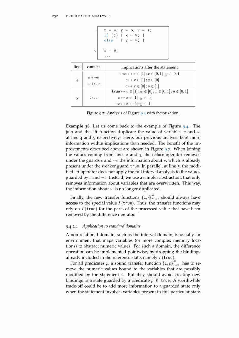
252 predicated analyses
1 x = 0 ; y = 0 ; v = 1 ;i f ( c ) x = v ; e l s e y = v ;
5 w = 0 ;. . .
line context implications after the statement
4c∨¬c
≡ true
true → v ∈ [1] ;x ∈ [0, 1] ; y ∈ [0, 1]
c → x ∈ [1] ; y ∈ [0]
¬c → x ∈ [0] ; y ∈ [1]
5 true
true → v ∈ [1] ;w ∈ [0] ;x ∈ [0, 1] ; y ∈ [0, 1]
c → x ∈ [1] ; y ∈ [0]
¬c → x ∈ [0] ; y ∈ [1]
Figure 9.7: Analysis of Figure 9.4 with factorization.
Example 38. Let us come back to the example of Figure 9.4. Thejoin and the lift function duplicate the value of variables v and w
at line 4 and 5 respectively. Here, our previous analysis kept moreinformation within implications than needed. The benefit of the im-provements described above are shown in Figure 9.7. When joiningthe values coming from lines 2 and 3, the reduce operator removesunder the guards c and ¬c the information about v, which is alreadypresent under the weaker guard true. In parallel, at line 5, the modi-fied lift operator does not apply the full interval analysis to the valuesguarded by c and ¬c. Instead, we use a simpler abstraction, that onlyremoves information about variables that are overwritten. This way,the information about w is no longer duplicated.
Finally, the new transfer functions |i, ·| #L×Cshould always have
access to the special value I (true). Thus, the transfer functions mayrely on I (true) for the parts of the processed value that have beenremoved by the difference operator.
9.4.2.1 Application to standard domains
A non-relational domain, such as the interval domain, is usually anenvironment that maps variables (or more complex memory loca-tions) to abstract numeric values. For such a domain, the differenceoperation can be implemented pointwise, by dropping the bindingsalready included in the reference state, namely I (true).
For all predicates p, a sound transfer function |i, p| #L×Chas to re-
move the numeric values bound to the variables that are possiblymodified by the statement i. But they should avoid creating newbindings in a state guarded by a predicate p true. A worthwhiletrade-off could be to add more information to a guarded state onlywhen the statement involves variables present in this particular state.

9.4 a predicated analysis 253
Indeed, thanks to the application of reduce, if such a state contains amapping for a given variable, then its numeric value is more precisethan the one bound in the state I (true). Thus, the evaluation of thestatement may really be more precise in the guarded state. Note thatthis last refinement is not implemented in the domains used for ourexperimental evaluation.
These two optimizations have another advantage. Indeed, they de-crease the size of the guarded values and postpone their alterationuntil it becomes necessary. Thus, the implications collected beforea split of the control-flow graph are more likely not to be modifiedin the branches. This maximises the shared subparts of the CI-pairspropagated through parallel branches. Since our efficient join onlyconsiders the distinct subparts of maps to create new implications,maximizing the shared subparts prevents an unnecessary increase inthe size of the predicated maps.
For a relational domain, the principles of those improvements wouldbe the same, but the difference operation may be more difficult to im-plement. However, it does not have to be complete: it is always soundto retain some redundancy.
9.4.3 Propagating Unreachable States
Whenever the lifted transfer function of the underlying domain re-turns the abstract state ⊥L for a value kept under a guard p, there isby definition no concrete state where p holds. We can thus refine theCI-pair by assuming the predicate ¬p. The former and latter maps arenot equivalent, as their context differ. However, their concretizationis exactly the same, as stated by the result below.
Lemma 35. Given Φ and p such that either Φ(p) =⊥L or Φ ↓ p = ⊥L,
then γpred (Φ) = γpred (assume(¬p,Φ))
Through this mechanism, information can flow from the underly-ing domain to the predicated one, by means of the contrapositive ofthe collected implications.
This also means we could embed the context of our abstract statesdirectly in the implication map. A domain mathematically isomor-phic to ours is obtained simply by mapping the negation of the con-text to bottom. However, we chose a formalisation that keeps separatethe context and the implication map. For the sake of clarity firstly, asthese two components play very different roles in the analysis. Sec-ondly, this design provides more leeway in the implementation, inparticular to select finely the predicates of the context.

254 predicated analyses
9.4.4 Convergence of the Analysis
Throughout the analysis of a given program, all guards of non trivialimplications present in a map are derived from the conditionals of theprogram, so their number remains finite. In practice, this number canbe high; we discuss a possible way of limiting it in Section 9.7. Thepredicated analysis essentially amounts to performing the underly-ing analysis over the values under each guard (except for the assume
operations, which allow us to be more precise). Thus, if the underly-ing domain provides (or requires) a widening operator to effectivelycompute the fixpoint, then it can (and should) be lifted as well. Fi-nally, if the underlying transfer functions are monotonic, so are thepredicated ones, which ensures the termination of our analysis.
9.5 a verified soundness proof
The lattice structure of the predicated domain, the relation betweenthe join and the weak-join and the soundness of the analysis havebeen formalized and proven in Coq [Coq], an interactive theoremprover. The proofs scripts are mechanically checked by the Coq ker-nel, ensuring their correctness. This increases very significantly theconfidence in our formalization. In particular, the soudness of theweak-join operator, and of its optimized version, was a non-trivialresult.
This section gives a brief outline of this development. A correspon-dance between the notations of this manuscript and the Coq ones isavailable at the beginning of the script.
9.5.1 Prerequisites
Our Coq development is parameterized by the following elements,that are kept abstract.
expressions and environments . We require three sets, stand-ing for numeric values Value, variables Var, and expressionsExp. Concrete states are environments in Env := Var → Value.Given an environment, the evaluation function eval_expr as-sesses the value of an expression. The update function modelsthe assignment of a single variable in an environment, and thedeps function verifies that if an expression exp does not dependon a variable var, then no update of var can affect the evalua-tion of exp.
lattice . We require a lattice (L,,,) – the underlying abstractdomain – plus the correctness of its operations. The Coq de-velopment requires a complete lattice. Indeed, the join and meetare infinitary, and have type (L → Prop) → L; the first argument

9.5 a verified soundness proof 255
denotes the set of elements of L that are being joined or met.4
This was done to simplifiy the proofs, as using a binary join ormeet would have required to reason on the order in which theoperations are performed.
analysis over L . We require a monotonic concretization functionconcr from L to Env, and monotonic transfer functions assign
and assume with the properties of definition 8.
9.5.2 Lattice Structure
We define the predicates as an inductive structure over the expres-sions, and extend the evaluation on expressions to predicates. Theentailment and equivalence between predicates are defined us-ing this evaluation. We then show that the constructors LAnd, LOrand LNot for predicates are morphisms of the relations induced by
and, and register those lemmas in the type classes mechanism ofCoq [SO08]. Then, given p q, we can prove (p ∧ r) (q ∧ r)
directly by a rewriting step. This mechanism is used extensivelythroughout the proofs.
CI-pairs are records of a predicate (the context) and a function frompredicates to L (the map). To simplify some definitions, we do notrequire false to be always bound to ⊥L. Instead, we prove that allabstract operations preserve this property, called false_bottom in thedevelopment.
The intermediate function in_map ci P gathers the values of L boundto guards of ci that satisfy the proposition (on predicates) P. The def-inition of the consequence ci ↓ p is then:
(in_map ci (fun p ⇒ p∧ (context ci) p))
The inclusion CI_incl, equivalence CI_equiv, join CI_join andmeet CI_meet of CI-pairs are then defined as specified in Section 9.3,together with the proofs of their correctness: CI_incl is an orderrelation, CI_equiv an equivalence relation, CI_join the least upperbound and CI_meet the greatest lower bound of two CI-pairs. Theseproofs heavily rely on intermediate lemmas about consequences.
9.5.3 Weak-Join
Proving the correctness of the weak-join – and of its optimization – isthe more involved part of the development.
The weak-join of CI-pairs is defined as the meet of three CI-pairs,which correspond to the three operators l∪, l1 and l2 of Definition 72.The first one is created by the function CI_conj_join, and the lat-ter two are symmetrically created by the same function CI_neg_join.
4 Readers unfamiliar with Coq can simply see Prop as the set of booleans.

256 predicated analyses
Given Φ1 and Φ2, their weak-join is the meet of CI_conj_join Φ1 Φ2,CI_neg_join Φ1 Φ2 and CI_neg_join Φ2 Φ1. We prove that the re-sults of CI_conj_join and CI_neg_join are greater (less precise) thanthe original join. Therefore, so is their meet, and the weak-join is in-deed greater than the join.
We then validate the final optimization of the weak-join.CI_shared ci1 ci2 contains only implications that belong to both ci1
and ci2; other predicates are bound to . Conversely, CI_diff ci1 ci2
contains only the elements of ci1 mapped to different values in ci2;other predicates are bound to . The efficient weak-join is the meetbetween the shared CI-pair and the previous weak-join of the rests.The last lemma asserts the equality between the former and the effi-cient weak-join.
9.5.4 Analysis
The concretization CI_concr links CI-pairs to concrete environments.We prove that this concretization is monotonic, and consistent withthe join and meet operations. The deps function is also extended topredicates. We then define a function kill_pred that implements thetwo operators kill+
Cand kill−
C, defined respectively as weaken_pred and
strengthen_pred.Then we define the transfer function CI_assign and CI_assume
such as specified in Section 9.4.1. Finally, we ensure the soundness oftheir definition:
• If the environment env is a concretization of ci, and if the ex-pression exp evaluates to val in env, then update var val env
is a concretization of CI_assign var exp ci;
• If the environment env is a concretization of ci, and if the ex-pression exp evaluates to a positive value in env, then env is aconcretization of CI_assume exp ci.
The soundness of CI_assign does not depend on the exact definitionsof the functions weaken_pred and strengthen_pred on predicates.We actually prove that more involved operators killC are also sound.For example, we could use two operators that invert assignmentsof the form x := x + k in the guards, instead of removing all theoccurrences of x.
Those generalized operators are called weaken and strengthen inthe formalization, and take as additional argument the expression towhich the variable is being assigned. Let us recall that the operator

9.6 related work 257
T(·) injects values of V into booleans. The properties that must besatisfied by weaken and strengthen are as follows:
∀c ∈ C,m ∈ M, x ∈ X , e ∈ exp,
T(cm) ⇒ T(weaken (c, x, e)
m[x→em])
T(strenghten (c, x, e)m[x→e
m]) ⇒ T(c
m)
Given the assignment x := x+ 3, taking for weaken the functionthat replaces occurrences of x by x− 3 is obviously correct here. Thedrawback of this approach is that a potentially infinite number of newpredicates may be created, which might lead to a non-terminatinganalysis. Performing widening steps on the context and the guardsmight be required.
9.6 related work
Convex numeric domains, such as intervals, polyhedra, octagons andlinear equalities, are widely used in abstract interpretation. Theirconvexity enables scalable analysis but impedes the representation ofdisjunctive invariants, causing overly wide imprecisions. Therefore,a large body of work has been devoted to remedy this shortcoming.Disjunctive completion [CC79b; GR98] of abstract domains avoids thecomputation of joins by propagating multiple abstract states in par-allel along the analysis. One downside is that the code may needto be fully analyzed for each separate state, whereas our frameworkstrives to minimize the unnecessary computations by getting rid ofredundancy. On the other side, disjunctive completion can be usedto unroll loop symbolically, something our approach does not han-dle. However, as widening is notably hard to perform properly ondisjunctive sets [BHZ04], most of these analyses operate on a before-hand bounded number of disjunct states. Then, some join must even-tually be performed, and a distance between abstract states [San+06b;PC06] can be used to first rejoin the most related states. This is linkedto our difference operator, since nearby states (according to this dis-tance metrics) should have small differences.
Additional information can be attached to the disjunct components.In practice, such disjunctive domains are often stored by binary deci-sion–diagram (bdd) [Bry86] where the nodes contain some predicatesand the leaves are numeric abstract states.
Boolean partitioning [Ber+10] distinguishes the numerical values ofsmall sets of variables with respect to the truth values of some booleanvariables. Such a partitioning may include several boolean trees work-ing on different sets of variables, chosen by heuristics. By comparison,our predicated domain is built on entire states of the underlying do-main. Indeed, we do not restrict the variables that may appear inour abstract states. This could be an interesting extension to further

258 predicated analyses
improve scalability. Under a guard p, we could choose to keep in-formation only on the variables that are read or written inside an if
whose condition involves p. The Binary Decision Tree Abstract Domain,proposed by Chen and Cousot [CC15], uses the conditionals of theprogram as nodes for the tree, as in our analysis. In their work, theshape of the tree is mostly static, making the join operation simplerto implement. The function transfer for assignments preserves allnodes, unlike in our approach where some guards are weakened orremoved. On the other hand, the whole tree must be rebuilt, whichmay be very costly.
Trace partitioning [HT98; MR05] associates each component withsome set of execution paths, and involves heuristics on the control-flow to choose a partition of the traces that guides the disjunction.Also, traces should be merged when it is no longer useful to keepthem separate; syntactic criteria are used to detect such merge points.Property simulation [DLS02] avoids the cost of full path-sensitivity forproving a single fixed property: it groups the abstractions of execu-tion states wherein the given property has the same state. The boxes
domain [GC10a] implements a specific disjunctive refinement of in-tervals with decision diagrams extended over linear arithmetic, whileour framework is parametrized by the underlying domain under con-sideration. Closer to our approach, although focusing on terminationproof through backward analysis, [UM14] designs a decision tree ab-stract domain from linear constraints to generic values. Some effort isalso made to maintain a canonical representation of the trees. How-ever, unlike our setup, the ordering and the join are point-to-pointoperations relying on unification of trees. Also, widening must beused, as the height of the trees height is not bounded a priori.
While binary decision trees make choices on the truth values ofboolean predicates, the Segmented Decision Tree Abstract Domain [CCM10]can express properties depending on the range of values of arithmeticvariables. Each node is a disjunction over exclusive value intervals fora variable, specified by a symbolic segmentation, and the number ofpossible choices is not bounded a priori. Since the number of seg-ments may grow indefinetely, the widening operator must act on theshape of the tree.
As disjunctive completions, all these domains make a strict parti-tion of their abstract states. Each component of the disjunction isthe only abstraction of the concrete states for some cases, and thejoin between them are postponed as much as possible. Therefore, theanalysis can not be relaxed on some disjunct without losing precisionfor the cases it represents. In contrast, our framework performs thejoin immediately, but preserves the lost information in abstract valuesguarded in implications. Then, these separate values provide someadditional information to the join, but are not intended to be inter-preted alone. This design allows the optimizations proposed in Sec-

9.6 related work 259
tion 9.4.2, where the treatment of these ancillary values is lightened.This would be impossible to implement on a disjunctive domain with-out leading to arbitrary precision loss.
Predicate abstraction [GS96] would infer a single fact along all execu-tion paths, but this fact may be arbitrarily complex and thus can ex-press disjunctive properties. CEGAR [Cla+00] improves predicate ab-straction by refining the invariants inferred using counter-examples.Different approaches have been proposed to combine numeric do-mains with predicates [GC10b; BHT08; FJM05]. In particular, Fischeret al. show how to build analyses that propagate a map from a de-terminate set of predicates to the numerical elements of any existingdataflow analysis [FJM05]. As usual in counter-examples based tech-niques, the predicates are incrementally found by successive refine-ment iterations of the analysis, that prune out unverified invariants.Still, finding the proper predicate may be arbitrarily complex, result-ing in hard to predict analysis times. Also, the refinement phaserequires decidable theories and powerful decision procedures to findthe counter-examples from which the predicate is deduced. We in-stead chose to limit ourselves to uninterpreted predicates relating theconditionals present in the program, for simplicity and predictability.Furthermore, predicate abstraction is mostly goal-driven, and usedby model-checkers to prove that a certain property is valid. Our pred-icated framework uses predicates to postpone the loss of precisioninherent to joins in abstract interpretation, but it is not goal-driven. In-stead, the same analysis will be done for e.g. all the potential runtimeerrors of the program (which is why the analysis needs to be run onlyonce). In particular, improving an unsufficiently precise analysis re-quires designing more fine-grained analysis domains. This contrastswith the automatic refinement available with predicate abstraction.
Otherwise, Mihaila and Simon present in [MS14] another way tosynthesize predicates by observing losses in abstract domain. Theypropagate a single numeric state augmented with sets of implicationsbetween predicates, specifically generated by the numerical abstractdomain at join points. For the domain of intervals, the join betweenthe two states where x ∈ [0; 5] and x ∈ [10; 15] would typically pro-duce the implication x > 5 ⇒ x > 10. At conditionals in the control-flow graph, implications are fed to the underlying domain to recoverthe numeric loss. The transfer functions follow the same general con-siderations than ours, but the predicates stem from the numeric do-main and are not restricted to the conditionals of the program. Thusthey also heed to avoid generating redundant implications, althoughthis makes the full recovery more intricate than in our construction.
Finally, combining abstract domains is a standard way to enhancethe abilities of static analysis based on abstract interpretation. Theseanalyses were introduced in the founding papers [CC79b] and widelystudied since [CCF13]. In particular, our predicated domain is a re-

260 predicated analyses
duced product between contexts and maps, and the maps can be seenas instances of a reduced cardinal power [CC79b], where the base isthe chosen underlying abstract domain and the exponent is the set ofconditional predicates.
9.7 experimental results
We have integrated our predicated analyses framework as a new plu-gin of the Frama-C platform. This plugin complements the resultsof the Value Analysis. We used it on two simple domains presentedin the previous section; the obtained results are presented in this sec-tion.
9.7.1 Scope of the Current Implementation
To limit the imprecisions caused by the junctions of convex abstrac-tions, EVA already embeds an instance of trace partitioning: it post-pones the joins of abstract states by propagating multiple ones sep-arately. As dissociating every feasible execution path leads to in-tractable analyses, the maximum number of parallel states maintainedby EVA is limited by a parameter called slevel. Once this threshold isreached, all new states are joined and propagated without trace par-titioning. Still, high slevel values may lead to high analysis time.
For performance reasons, this partitioning is directly integrated onthe dataflow analysis. It is systematically applied on top of all thedomains on which is instanciated the analysis. of the value and stateabstractions, this trace abstractions is thus not extensible for the timebeing. Instead, we have integrated our predicated analyses frame-work as a new plugin of the Frama-C platform. This plugin comple-ments the EVA analysis by validating a posteriori some of the alarmsit has emitted. By construction, our plugin mainly improves EVA’sresults on successive test statements with identical conditions5. Al-though such pattern is relatively unusual in idiomatic C code, it ismuch more frequent in generated programs, for which our method iswell adapted.
This predicated analyses plugin has been designed to be modular.It is parameterized by the underlying abstract domain, and builds adataflow analysis with predicates for this domain. This plugin runsafter EVA, which it mainly uses to get aliasing information on point-ers. This information is needed to ensure the soundness of the deps
operator. For convenience, we also chose to reuse some data struc-tures of EVA. In particular, the maps from predicates to abstract val-ues are patricia trees with hash-consing. Finally, all the predicates are
5 Modulo conjunction, disjunction and negation, but only over uninterpreted expres-sions.

9.7 experimental results 261
normalized into a disjunctive normal form. This way, a CI-pair nevermanages different equivalent predicates.
Generated programs can include a very large number of nested con-ditional branches and loops, leading to overly wide contexts in ourown analysis. To avoid a complexity explosion, we limit the numberof literals in the predicates used in contexts and guards (thereby de-creasing the precision of our results), according to a parameter clevel.The join removes any implications whose guard exceeds this limit; inthe context, we try to keep the most recent predicates.
The analysis is modular: it processes once and separately each func-tion of a program, retains a summary of their effect regardless of theircall context and still benefit from it at each function call. The kill op-erator, applied to the set of variables potentially modified by the call,guarantees the soundness of our analysis, and the meet of the pred-icated domain put together the abstract states before the call and atthe return statement of the called function.The plugin is available at http://yakobowski.org/predicated.html.
9.7.2 Application on two Simple Domains
This subsection describes the two abstract domains on which we haveinstantiated our predicated analysis plugin. Of course, our frame-work could also be applied to other domains, e.g. intervals or the“valid file descriptors” domain used for Figure 9.1.
9.7.2.1 Tracking Initialized Variables
Our experiments relied on a domain retaining, at each program point,the set of variables that were properly initialized. This domain canbe used to prove that no unitialized variables are read at executiontime. We used it successfully on generated C programs. In this kindof code, variable initialization may happen inside conditionals, andfar away from the points where the variable is used.
In the semantics of our simplified language, we introduce a defaultvalue uninit in V, to which all variables are equal at program entry.The execution of a statement is correct when all the involved variablesare initialized.
γinit (V ) = m | ∀x ∈ V,m (x) = uninit
|x := e| #init(V ) =
V ∪ x if deps(e) ⊆ V
V \ x otherwise
|c ?| #init(V ) = V

262 predicated analyses
|c ?, p|#eq×C
(E)
E ∪ e1 = e2 if p ≡ true and c = (e1 = e2)
E otherwise
|x := e, p|#eq×C
(E)
killeq(x,E) ∪ x = e if p ≡ true and x /∈ deps(e)
killeq(x,E) otherwise
killeq(v, E) (a = b) ∈ E | v /∈ deps(a) ∧ v /∈ deps(b)
E\eqF (a = b) ∈ E | (a = b) /∈ F
γeq (E)
m | (a = b) ∈ E ⇒ am= b
m
Figure 9.8: Abstract semantics for the equality domain
9.7.2.2 A Second Abstract Domain: Herbrand Equalities
We also reused for our experiments the symbolic domain trackingHerbrand equalities between C expressions, presented at Section 8.2.This equality domain boils down to retaining equalities stemmingfrom assignments or equality conditions. Its formal definition is re-called in Figure 9.8, where the set E of equalities increases on testsinvolving an equality, and on assignments that do not refer to thevariable being modified. To be sound, the transfer function on assign-ments must also remove equalities that involve the overwritten vari-able, through the killeq operator. Following Section 9.4.2, we presentsimplified transfer functions, for which only the true guard is en-riched, and in which the operator \eq can be used to remove redun-dant equalities.
This domain lends itself to a natural extension of our analysis,namely the strengthening of the context and the guards by backward-propagating information from L. For example, we can quotient allthe predicates of the CI-pairs by the congruence relation induced bythe equalities stored in the map. Furthermore, when applying the op-erator kill (following an assignment, say to x) on an expression e thatinvolves x, we may instead substitute e by another equal expression.This is more precise than removing the occurrences of x in the guardsand the context.
9.7.3 Results on Variables Initialization
We tested our plugin on a C program of 5800 lines generated by theindustrial environment SCADE, devoted to real-time software. Asoften with such codes, multiple conditionals are heavily used — typ-ically to test automata states or clocks. In fact, this program has anextremely high ratio of conditionals w.r.t. the total number of state-ments: 819 out of 2830. Furthermore, many conditionals are complex,with multiple conjunctions and disjunctions. If the operators && and

9.7 experimental results 263
0
100
200
300
400
500
0 1 2 3 4 5 6 7init
ializ
atio
nas
sert
ions
tobe
valid
ated
clevel: size of predicates (context and guards)
slevel = 1slevel = 100
slevel = 1000
slevelassertions tobe validated
initializationassertions
remaining assertions/clevel
1 2 3 4 5 6
1 632 439 188 167 131 130 130 126
100 488 297 150 144 110 109 109 106
1000 430 239 113 102 71 70 70 67
2000 409 218 100 96 65 64 64 61
time of the Value Analysis
slevel time
1 1.4s
100 6.7s
1000 175s
2000 400s
time of the predicated analysis
clevel time
1 0.7s
2 0.73s
3 0.8s
4 1.0s
5 1.9s
6 10s
7 85s
Figure 9.9: Experimental results

264 predicated analyses
|| are desugared into multiple if, the resulting program has 9576
statements, and 3428 conditionals. Thus, this program is a very goodbenchmark for an analysis.
Our results are presented in Figure 9.9. We first applied EVA, whichemitted various assertions it could not validate (column 2). As ex-pected, a higher slevel results in fewer alarms. Between 55% and 70%of those are assertions requiring variables to be properly initialized(column 3), which are those the domain of Section 9.7.2.1 understands.We then ran our predicated analysis, instantiated by this domain,with different limits for the size of predicates. For the values of clevel
we used, the number of initialization assertions still unproven afterthe predicated analysis are shown in the five corresponding columns.Hence, lower figures are better. The analysis time for the EVA and forthe predicated analysis are also given, according to their parameter;they are independent from each other. Remember that EVA must berun (at least with slevel 1) before our analysis can run. So the twotimings should be added to compare the total analysis time.
While EVA produces significantly less alarms with a higher slevel,its analysis time also increases drastically. This is unsurprising, asfully partitioning for k successive conditionals may require as muchas 2k distinct states. On the other hand, our plugin is effective toquickly validate numerous assertions left unproven by EVA, even withstrongly limited predicates. The precision of our analysis increasesrapidly with the clevel parameter, while the analysis time remainsreasonable. More generally, it turns out that small contexts are suf-ficient to retain most of the relevant information: fewer assertionsremain to be validated with clevel = 1 (2.1s) and slevel = 1 than withclevel = 0 and slevel = 2000 (400s). Intuitively, even inside deeplynested conditionals (which generates complex contexts), the more re-cent guards are often the more useful. In general, our results showthat it is much more cost efficient to increase the clevel parameter thanthe slevel parameter. Those results are extremely encouraging, giventhe difference in maturity between our plugin and EVA. Indeed, theabstract domains of EVA have been considerably optimized for speedfor many years.
9.7.4 Validation of the Optimizations
The relevance of the improvements developed in Section 9.4.2 havebeen validated through some experiments on the same code as above.We compared the efficiency of the optimized predicated analysis (namedOpt in the results) with two modified versions of our framework:
• one without any difference operation, where each relevant valueis kept unreduced in the join (Diffless);

9.7 experimental results 265
Initialization Equalities
clevel Opt Diffless OrigTF Opt Diffless OrigTF
1
0.7s
10
22
0.7s
10
22
0.9s
10
22
2.2s
187
304
11s
1751
3895
28s
1786
4320
time
average
max
2
0.73s
25
44
0.74s
26
45
2.9s
97
302
3.7s
391
680
58s
6983
18653
timeout
time
average
max
3
0.8s
89
157
1.0s
101
172
30s
777
2732
8.4s
1015
2269
240s
23616
73518
timeout
time
average
max
4
1.1s
279
552
1.6s
382
601
timeout
26s
3195
9258
timeout timeout
time
average
max
5
1.9s
847
1132
4.8s
1255
1764
timeout
160s
9004
46386
timeout timeout
time
average
max
Opt : Optimized analysis as described in the manuscript
Diffless : Analysis without the difference operation
OrigTF : Analysis with the original transfer functions applied
in each implication
Figure 9.10: Effectiveness of the optimizations
• one in which the original transfer function of the underlyingabstract domain is applied to each abstract value in the implica-tions (OrigTF).
We used as underlying domains the two domains presented in Sec-tion 9.7.2. For each configuration and for different size limits forpredicates, the Figure 9.10 shows the analysis time and some mea-sure of the amount of information propagated during the analysis.With the domain of initialized variables, we give the average and themaximum numbers of implications kept during the analysis at eachprogram point. For the equality domain, we give the average and themaximum numbers of equalities (in implications) propagated by theanalysis at each program point. A timeout denotes an analysis timethat exceeds 10 minutes.
The introduction of the difference operation has little impact onthe performance analysis for the initialization domain. In contrast, itgreatly improves the equality analysis, as it removes many equalitiesfrom the implications, and all the operations on equality sets depend

266 predicated analyses
1 i f ( i >= 0 && i < 10 )x = 1 ;
e l s ex = 0 ;
5 [ . . . ]i f ( x== 1 )
/*@ assert 0 <= i < 10; */
a [ i ] = 4 2 ;
1p = &x ;while ( n > 0 )
/*@ assert p != 0; */
x = *p + x ;5n−−;
i f ( ! ( n > 0 ) )p = 0 ;
Figure 9.11: Examples of disjunctions in the literature
on their size. Not surprisingly, the benefits of the difference operationdepend on the underlying abstract domain, as its aim is to reduce thesize of the abstract values.
The application of a lighter transfer function for the implicationsspeeds up substantially the analysis for both domains. Not only thisnew function is itself faster than the original one, but it also leadsto a large diminution of superfluous implications. Indeed, the orig-inal transfer function alters systematically all implications, and thusthe shared subparts of two CI-pairs are minimized after a disjunction.With the lighter transfer function, most of the implications collectedbefore a split in the control-flow are propagated in the branches with-out any change, and are kept unchanged in the join. The combinationof these implications is then avoided, thanks to the optimization ofthe join presented at the end of Section 9.3.3.
9.7.5 Experiments on Examples from the Literature
We have successfully applied our predicated analyses, instantiatedwith the domain of equalities, to various codes of the literature [FJM05;San+06b; MS14; HHP13] — starting with the motivating example in-troduced in Figure 9.1. To analyze it, we simply modeled the open
function as a random assignment to 1 or −1 (corresponding to a suc-cessful or failed call, respectively), and replaced the calls to close byan assertion requiring the file descriptor to be 1. The implicationsgathered along the analysis link flag1 and flag2 to the value of fd1and fd2, and the close assertions are directly proved.
Two other interesting examples are presented in Figure 9.11. Theproperties required for the program to be correct are given as acsl as-sertions. The left one requires the variable i to be within the boundsof the array a at line 8, which is effectively ensured by the conditionx == 1. This pattern — storing a predicate within a boolean, whichis tested later — is actually quite frequent. Disjunctive domains han-dle this code naturally, since they propagate two complete separatestates after the disjunction, while our analysis is guided by the mean-ing of the implications. At line 6, we have no implication of the formx = c → _; however, we have ¬ (0 ≤ i < 10) → x = 0, which be-comes ¬ (0 ≤ i < 10) → ⊥ at line 7. The predicate 0 ≤ i < 10 can
9.8 conlusion 267
then be added to the context, as stated in Section 9.4.3. This is suffi-cient to validate the assertion.
Finally, disjunctive domains may distinguish loop iterations, bypropagating one abstract state for each iteration. Without specificpredicates able to label each iteration, our framework cannot offer thesame expressiveness. Still, we can sometimes convey relevant infor-mation through a loop. The example on the right of Figure 9.11 showsa loop in which a pointer p is dereferenced and then freed (set to 0) inits last iteration. Our predicated analyses infer ¬ (n > 0) → p = 0
and n > 0 → p = &x, thus ensuring the validity of dereferencing p
in the loop, where the context is n > 0.
9.8 conlusion
We have described a generic framework to enhance the precision ofstandard dataflow analyses. This framework constructs a derivedpredicated analysis able to mitigate information loss at junction pointsof the control-flow graph, by retaining the conditional values abouteach branch. Our analysis strives to minimize redundant informationprocessing due to these disjunctions. Experimental tests led througha dedicated plugin of Frama-C, applied to generated C code, showedthat a predicated analysis over simple domains can significantly im-prove the results of prior analyses.
9.8.0.1 Future works
The literals of our predicates are expressions that we currently con-sider as uninterpreted. In order to improve our analysis, we intendto give some meaning to the operators in these expressions and toextend the logical implication between guards accordingly. In partic-ular, we could handle successive conditions on distinct but relatedexpressions, such as (x ≥ 0) ? and (x ≥ 2) ?. The difficulty lies infinding an equational theory for that would be expressive enough,but not too costly.
Another interesting extension would be to preserve more informa-tion when encountering invertible assignments such as x := x + 1.Currently, all information about x is lost in the context and the guardsafterwards. This requires some care to avoid producing an infinitenumber of new predicates, which would endanger the convergenceof the analysis.
Moreover, prior syntactic analyses or heuristics could help to se-lect relevant predicates for the contexts, which would no longer beextended at each test statement. This would avoid maintaining im-plication guards that will never be useful again later in the program.Likewise, we could use heuristics to define variable packing strate-gies, in order to limit the abstract states themselves. The booleanpartitioning used in Astrée [Ber+10] keeps information only for some

268 predicated analyses
syntactically well-chosen variables. We could do the same, by keep-ing in the state under a guard p only the variables that are related top in the program.
Finally, it would be worthwhile to apply our predicated analysisover more complex abstract domains.

Part VI
C O N C L U S I O N


10P E R S P E C T I V E S
10.1 summary
In this thesis, we have proposed a new framework for the combina-tion of multiple domains in the abstract interpretation theory. Its coreconcept is the structuring of the abstract semantics by following theusual distinction between expressions and statements. This can beachieved by a convenient architecture where abstractions are sepa-rated in two layers: value abstractions, in charge of the expressionsemantics, and state abstractions —or abstract domains—, in chargeof the statement semantics. This design leads to a natural communi-cation system where the abstract domains, when interpreting a state-ment, interact and exchange information through value abstractions,that express properties about expressions. While the values form thecommunication interface between domains, they are also standard el-ements of the abstract interpretation framework. The communicationsystem is thus embedded in the abstract semantics, and the usualtools of abstract interpretation apply naturally to value abstractions.For instance, different kinds of value abstractions can be composedthrough the existing methods of combination of abstractions. Thisthesis has explored the possibilities offered by this framework, andwe have described strategies to compute precise value abstractionsfrom the information inferred by abstract domains. The architecturealso features a direct collaboration for the emission of alarms thatreport the possible errors of a program.
This design has been implemented within EVA, the new versionof the abstract interpreter provided by the Frama-C platform. EVAis a major evolution of the former abstract interpreter of Frama-C,named VALUE. Unlike VALUE, EVA enjoys a modular and extensiblearchitecture designed to ease the introduction of new abstractions.Thanks to this work, five new domains from the literature have beenimplemented in the last year, enhancing the scope of the analyzer.Considerable efforts have also been devoted to preserve the efficiencyof the analyzer. To maintain some crucial optimizations relying ona specific abstraction, we have developed a GADT structure allow-ing direct and efficient interactions with the components of a genericproduct of OCaml data types (Section 3.3). We have also defined aformal semantics for the value abstractions called garbled mixes, thatsoundly represent the results of integer arithmetic applied to pointervalues (Section 5.3). In the end, EVA is now an accomplished project:
271

272 perspectives
it is already used in industrial case studies, and has definitely super-seded VALUE in the Frama-C framework.
10.2 future works in eva
This section outlines diverse developments that are planned to im-prove EVA in the short to medium term. They derive from the workdone in this thesis or from the state of the art, and aim mainly tofacilitate the implementation of even more domains.
simplify the api The foremost motivation for the developmentof EVA was to enable and to ease the introduction of new abstractionsin the analyzer. The modular architecture and the communicationsystem of EVA meet these goals. Nonetheless, the programming in-terface of abstract domains is still relatively complicated; some partsare a remnant of the former analyzer, such as the functions for theinitialization of the initial state of the analysis —that have not beenmentioned in this thesis. Much work remains to be done towards thesimplification, the standardization and the documentation of the APIof EVA. Moreover, we would like to provide support tools to buildcomplete domains from simpler abstractions —such as domains thatdo not interact with others, or simple observers that do not partici-pate in the computations. We also intend to develop a simpler functorto automatically manage the memory for purely numerical domains(the memory model of the cvalue domain is far too complex to playthis role). This functor could follow the preliminary work undertakenwith the binding of the apron domains.
extend the value abstractions All means of communica-tion between abstract domains involve value abstractions. Even ifthe reduced product of value abstractions currently available in EVAalready establishes a rich and expressive interface, new value abstrac-tions may enable further interactions. We draw here a few avenuesworth exploring to extend value abstractions.
• In general, intervals cannot precisely represent the possible val-ues of an unsigned integer variable in case of arithmetic over-flow (which is not an undefined behavior for unsigned integersin the C standard). At the end of Listing 10.1, the variable x
can be 0 or 2n − 1 (where n is the size in bits of an integer). Themost precise interval that contains these two values is [0..2n− 1],which is overly imprecise. A dedicated value abstraction maycircumvent this loss of precision.
• The disjunctive union of intervals is a well-known refinementof intervals [GC10a] that enables the precise approximation of

10.2 future works in eva 273
Listing 10.1: Unsigned integer overflow in C
1 unsigned int x = 0;
if (c) x--;
non-convex sets of values. To remain scalable, some strategiesmust be found to bound the number of disjuncts.
• Some relational domains rely on the linear approximation ofexpressions [Min06b], that is the simplification of arbitrary ex-pressions into affine forms with interval coefficients. The lin-earization of an expression could be easily encoded as a valueabstraction, in a reduced product with intervals to extract thecoefficients that approximate nonlinear expressions.
cooperatively evaluate logical assertions The Frama-Cplatform embeds the ACSL language for the formal specification of aprogram through logical annotations. These annotations can be un-derstood by its diverse plugins —and by the abstract domains of EVA.ACSL annotations can be written by the user or by another plugin.Then, the domains of EVA can prove some annotations (if they arelogically implied by the inferred abstract state), or use them to re-duce their states (and rely on other plugins to prove them). For thetime being, only the main cvalue domain understands and processesthe logical assertions. The cooperation between the domains of EVAis currently limited to the interpretation of C statements —throughthe shared evaluation of C expressions. The same collaborative mech-anism should also be applied to the interpretation of ACSL assertions,by a shared evaluation of the logical terms. However, this requiressome weighty works, as the ACSL AST is much larger than the C AST.
improve the state partitioning To achieve further precision,EVA uses an automatic partitioning of abstract domains and infers adisjunction of states at each point of a program. To remain scalable,the maximal number of disjuncts is bounded by a parameter of theanalysis. Apart from this parameter, the strategy for the choice ofthe state partitioning is naive, cannot be adjusted for specific needs,and rests upon optimization heuristics tailored to the main cvalue
domain. Further development should allow the user to specify crite-ria and directives for both the disjunction and the junction of statesduring the analysis. Moreover, trace partitioning [MR05] is a tech-nique that relates each state with a trace abstraction of the executionpaths it represents. Then, choosing a partition of the traces (throughheuristics or user commands) can guide the disjunction of states. Aform of trace partitioning could greatly improve the precision and theuser-friendliness of EVA.

274 perspectives
develop and hone new abstractions within eva Finally,we should carry on reaping the rewards of this thesis, by developingand improving even further the domains of EVA. On the one hand,the new abstract domains that have been implemented last year re-main mostly experimental; they need to be strengthened to reach thesame level of maturity as the inherited cvalue domain. On the otherhand, new classes of worthwhile domains can be contemplated tofurther enrich the abstract interpreter. For instance, abstract domainsfor shape may be required to precisely analyze programs includinglinked and dynamically allocated data structures. Moreover, it is dif-ficult to exactly foresee the specific needs of new domains before try-ing to implement them. Confronting our framework to a wide rangeof abstract domains will bring its strengths and weaknesses to light.Such experiments should guide our further developments of the EVAinternal architecture.
10.3 long-term perspectives
This section presents some ideas of future research directions thatwe deem worthwhile and promising, to go along with or beyond theconcepts proposed in this thesis.
extension of the communication system Our successfulexperiments on various abstract domains have convinced us of thesuitability and the merits of a communication through value abstrac-tions. Nonetheless, this communication system could be extended tocreate further opportunities for domains to interact, leading to moreaccurate analyses. We sketch here some ideas for further improve-ments.
Firstly, the interactions are for now limited to the interpretation ofstatements. The domains could also benefit from interactions duringjoin operations, where some precision is usually lost. At join points,there are no natural expressions to evaluate. Nevertheless, any ex-pression can still be evaluated (or reduced by backward propagation)at the request of domains that want to acquire (or send) informationthrough value abstractions. This would enable nearly the same re-ductions between abstract states at the merge points of the CFG asthose on regular statements. More generally, we could extend thepossibilities of interactions by providing the domains with a greateraccess to the evaluation functionalities. In our design, a domain cansend information to the others by asserting a value for an expres-sion —the value is then backward propagated through the expression.Currently, a domain can initiate a backward propagation only whena value abstraction is reduced (the new backward propagation mustthen be a consequence of the reduction). However, some domains

10.3 long-term perspectives 275
may want to initiate backward propagations on other circumstancesthat need to be identified.
Secondly, when answering a query, a domain is unaware of the con-text of the operation, such as the program point, the expression beingevaluated, or the abstractions computed so far by other domains. Thisinformation may assist a costly domain to choose the right trade-offbetween precision and efficiency on a case-by-case basis. For instance,a domain could choose to perform more complex but more accuratecomputation at some specific points of interest, or when the abstrac-tions provided by other domains remain overly imprecise, or wherean alarm can be avoided.
Finally, value abstractions can only express properties about theexpressions of the language. While this expressivity seems perfectlysuitable for a cooperative interpretation of statements one by one, amore advanced communication system may involve properties aboutthe effect of a block of statements, a loop, or a whole function. How-ever, this would require the design of brand new kinds of interactionsaltogether.
efficient combination of different domains Regardlessof the interactions established between abstractions, the combinationof very different domains may cause serious efficiency issues. First,the high complexity of some domains impedes their scalability onlarge programs, while the reasoning they conduct can be highly valu-able in some settings. A modular abstract interpreter should enablethe activation of such domains on only parts of the analyzed pro-gram, according to automatic heuristics or to criteria specified by theuser. Secondly, different domains may have different convergencespeeds, depending on their lattice structure and the implementationof the widening operator. Even without any inter-reduction betweenabstract states, the convergence speed of a domain product is that ofthe slowest domain. This implies that the faster domains perform un-necessary computations through the last iterations needed to reachthe fixpoint of the slowest domain. Interplay between domains mayalso slow down the convergence, and makes the optimizations of thefixpoint computation even harder, since the states of a domain maybe reduced after reaching a first fixpoint. While this thesis has tackledthe challenge of designing a modular and practical communication sys-tem between various abstractions, progress needs to be strengthenedtoward the efficient combination of arbitrary domains.
summary of function analyses The strong efficiency of thecvalue domain, inherited from the VALUE plugin, is partly due to anautomatic summarization mechanism that speeds up analyses [Yak15].This cache mechanism has been specifically tailored to this domain,and its soundness relies on the absence of relational properties. It

276 perspectives
now needs to be extended to arbitrary domains while remaining cost-efficient. In particular, the use of relational properties significantlycomplicates the computation of a concise summary, as the set of vari-ables that serves for the analysis of a function cannot be easily deter-mined.
other formal verification techniques This thesis was ded-icated to the formal verification of programs through abstract inter-pretation, by uniting the strengths of manifold abstract domains. Anambitious research direction would be to unite the strengths of dif-ferent techniques of formal verification. Frama-C is a platform thatalready gathers a set of interoperable tools based on various verifica-tion technologies. Although these different tools can be applied to thesame program, each one works mostly independently from the oth-ers. However, they could certainly benefit from closer interactions. Inparticular, abstract interpretation and weakest precondition calculuscan be intertwined to achieve the automation of a program proof or abetter precision. On the one hand, abstract interpretation has alreadybeen successfully applied to infer the loop invariants required to thecomputation of weakest preconditions [Bar+05]. On the other hand,abstract interpretation based analyses can be improved by resortingto decision procedures and SMT solvers [HMM12].

Part VII
A P P E N D I X


AN O TAT I O N S S U M M A RY
Color notation: Concrete vs Abstract.
var
iable
variables x ∈ X 4.2.1
memory layouts θ ∈ ΘP 4.2.2
Cva
lu
es
C values of τ type c ∈ Vτ 4.2.1
. . . including pointer values (&x, i) ∈ Vptr 4.2.1
all scalar C values c ∈ V 4.2.1
byte values V 0, . . . , 255 4.2.2
undeterminate values uninit, none 4.2.2.2
interpretation functions φτ : (Vbytes)sizeof(τ ) → Vτ 4.2.2
valu
es
concrete values as functions
from layouts to C valuesV ∈ V : ΘP → V 4.3.3
error value Ω 4.2.4
value abstraction v ∈ V# 5.2.1
value concretization γV : V# → P(V) 5.2.1
value lattice structure γV : V# → P(V) 5.2.2
lo
ca
tio
ns valid location of type τ
1 Lτ 4.2.3.1
abstract location L# 5.2.6
location concretization γL : L# → P(L) 5.2.6
location lattice structure L, L, L, L 5.2.6
ala
rm
s
possible alarms for an expression alarms(e) 5.1.3
alarm map A ∈ A 5.1.4
alarm map soundness |=A 5.1.4
alarm map lattice A, A, A, A 5.1.4
1 always independent of memory layouts
279

280 notations summary
oper
ato
rs
n-ary operator ♦ 4.2.1
application of ♦ [(♦)] : Vn→ V 4.2.4
concrete semantics of ♦ [(♦)]Θ
: (V)n → V 4.3.3
forward abstract semantics F#♦ 5.2.5
backward abstract semantics B#♦ 5.2.5
sta
tes
memories m ∈ M 4.2.3.1
concrete states S ∈ S = MΘP 4.3.2
state abstractions
(abstract domain)D ∈ D 7
domain concretization γD : D → P(S) 7
domain lattice D, D, D, D 7
forward dereference semantics F#∗τ 7.1.1
backward dereference semantics B#∗τ 7.2.1
forward query on arbitrary
expressionF#
D7.1.2
backward query on arbitrary
expressionB#
D7.2.2
valu
atio
ns
valuations E ∈ E 6.1.3
valuation concretization γE : E → P(S) 6.1.3
valuation lattice E, E, E, E 6.1.3

BP R O O F S
lemma 14
Lemma. Given a program P with a set X of variables and two memory
layouts θ and θ in ΘP , axiom 2 ensures the existence of a series of valid
memory layouts θ0, . . . , θn such that θ0 = θ, θn = θ and for all i, θi−1 and
θi differ on at most one variable.
∀i ∈ 1, . . . , n, ∃x ∈ X , ∀y ∈ X , y = x ⇒ θi−1(y) = θi(y)
Proof. By induction on the number of variables. For one variable,the result is trivial. We assume the lemma true for any set of n− 1
variables, and we consider a set X of n variables.We fix a special memory layout θ and we prove the existence of a
series of adequate layouts from any layout θ to θ —adequate meaningthat two succesive layouts differ on at most one variable. Then, forany layouts θ and θ”, two series of adequate layouts from θ to θ andfrom θ” to θ can be combined into a series of adequate layouts from θ
to θ”. We name the variables of X = y1, . . . , yn, and fix θ as:
θ(yk) = 2sizeof(ptr) − 1−
j∈k,. . . ,n
(sizeof(yj) + 1)
This function from ΘP to N is a memory layout according to defi-nition 21:
1. Strictly positive addresses by axiom 2:
∀k, θ(yk) = 2sizeof(ptr) − 1−
j∈k,. . . ,n
(sizeof(yj) + 1)
≥ 2sizeof(ptr) − 1−
j∈1,. . . ,n
(sizeof(yj) + 1)
> maxx∈X
(sizeof(y)) > 0
2. Non-aliasing:
∀k > k, θ(yk)− θ(yk) =
j∈k,. . . ,k−1
(sizeof(yj) + 1)
≥ sizeof(yk) + 1 > sizeof(yk)
3. Fits in memory:
∀k, θ(yk) = 2sizeof(ptr) − 1−
j∈k,. . . ,n
(sizeof(yj) + 1)
< 2sizeof(ptr) − sizeof(yk)
281

282 proofs
We now consider an arbitrary memory layouts θ. We construct theseries of layouts θ0 to θk. The idea is to shift one variable at a time inθ until all variables are adjacent. Then, axiom 2 ensures that
We rename the variables of X as x1, . . . , xn such that
j ≤ k ⇒ θ(xj) ≤ θ(xk)
We then define the functions θ0 to θn as follows:
θ0 = θ
∀i ∈ 1, . . . , n,
∀k = i, θi(xk) = θi−1(xk)
θi(xi) =
j∈1,. . . ,i−1(sizeof(xj) + 1) + 1
Let us prove inductively that for all i ∈ 0, . . . , n, θi is a valid layout,and that the variables x1 to xn are still ordered in θi.
j ≤ k ⇒ θi(xi) ≤ θi(xk)
It is true for θ0 by hypothesis. We assume it is also true for θi−1, andprove it for θi. As θi is equal to θi−1 except on xi, we only have toconsider this variable.
1. Strictly positive address: θi(xi) > 0.
2. Non-aliasing with “smaller” variables xk with k < i:
θi(xi−1) = θi−1(xi−1) =
j∈1,. . . ,i−2
(sizeof(xj) + 1) + 1
⇒ θi(xi)− θi(xi−1) = sizeof(xi−1) + 1 > sizeof(xi−1)
And for any variable xk with k < i− 1, as θi−1 is valid:θi−1(xi−1)− θi−1(xk) > sizeof(xk)
And:
θi(xi)− θi(xk) = θi(xi)− θi−1(xk)
= (θi(xi)− θi−1(xi−1)) + (θi−1(xi−1)− θi−1(xk))
> sizeof(xi−1) + sizeof(xk)
> sizeof(xk)
3. Non-aliasing with “greater” variables xk with k > i:By inductive hypothesis, θi−1(xi−1) ≤ θi−1(xi).As θi−1 is a memory layout according to definition 21:
θi−1(xi)− θi−1(xi−1) ≥ sizeof(xi−1) + 1
⇒ θi−1(xi) ≥ θi−1(xi−1) + sizeof(xi−1) + 1
≥
j∈1,. . . ,i−1
(sizeof(xj) + 1) + 1
≥ θi(xi)

proofs 283
For k > i, θi(xk) = θi−1(xk) and:
θi(xk)− θi(xi) ≥ θi−1(xk)− θi−1(xi)
≥ sizeof(xk)
(Still by definition 21)
4. The address fits in memory thanks to axiom 2:
θi(xi) =
j∈1,. . . ,i−1
(sizeof(xj) + 1) + 1
≤
x∈X
(sizeof(x) + 1) + 1
< 2sizeof(ptr) −maxx∈X
(sizeof(x)) ≤ 2sizeof(ptr) − sizeof(xi)
5. Point 2 and 3 have also proved the invariant
k < i ⇒ θi(xi) < θi(xk)
k > i ⇒ θi(xi) > θi(xk)
Thus, the series of functions θ0 to θn are memory layouts, accordingto definition 21. By definition, for any i ∈ 1, . . . , n, θi and θi−1 areequal except on xi.
We finally consider the function θn+1 defined as:
θn+1(x) =
θn(x) if x = yn
2sizeof(ptr) − (sizeof(yn) + 1) if x = yn
We can note that θn+1(yn) = θ(yn). Let us prove that this lastfunction θn+1 is also a memory layout. As θn is a memory layout, weonly consider the variable yn on which θn+1 differs.As θn+1(yn) = θ(yn) or by axiom 2, we directly have:
0 < θn+1(yn) < 2sizeof(ptr) − sizeof(yn)
Let xi be a variable different from yn. Then:
θn(xi) =
j∈1,. . . ,i−1
(sizeof(xj) + 1) + 1
≤
j =i
(sizeof(xj) + 1) + 1
< 2sizeof(ptr) −maxy∈X
(sizeof(y)) + sizeof(xi)
θn+1(yn)− θn+1(xi) = 2sizeof(ptr) − sizeof(yn)− θn(xi)
≥ 2sizeof(ptr) −maxy∈X
(sizeof(y))− θn(xi)
> sizeof(xi)

284 proofs
summary : We have a series of memory layouts θ0 to θn+1 suchthat θ0 = θ, θn+1(yn) = θ(yn) and for all i ∈ 0, . . . , n, θi and θi+1
differ on at most one variable (this is immediate by their definitions).Let M = 2sizeof(ptr) − sizeof(yn)− 1. We now consider the restric-
tion of θn+1 and θ from the set of variables X\yn = y1, . . . , yn−1
to the integer addresses strictly between 0 and M . They are validmemory layouts on a set of n− 1 variables in a space addressing ver-ifying axiom 2. Indeed, we have:
M = 2sizeof(ptr) − sizeof(yn)− 1
>
y∈X
(sizeof(y) + 1) + 1+maxy∈X
(sizeof(y))− sizeof(yn)− 1
>
y∈X\yn
(sizeof(y) + 1) + 1+ maxy∈X\yn
(sizeof(y))
Thus, the inductive hypothesis applies: there exists a series of ade-quate memory layouts from θn+1 to θ, restricted to the variables X\yn
and the addressing space 1, . . . ,M − 1. We can complete each mem-ory layout θ? of this series by θ?(yn) = M , and obtain a series ofadequate memory layouts from θn+1 to θ without restriction.
We have finally constructed a series of adequate memory layoutsfrom an arbitrary layout θ to the fixed memory layout θ.

CD E V E L O P M E N T F I L E S
File Main functionalities Ref
alarmset.mli Maps of alarms, embodying the undesirable
behaviors tracked down by EVA5.1
eval.mli Types heavily used in EVA (including bottom
and alarm monads, the valuations and some
types about assignments and function calls)
5.1.5
6.1.3
value_parameters Options of the analyzer
engine/ Generic abstract interpreter 3.2.1
evaluation Evaluation of expressions 6
non_linear_evaluation Subdivision of an evaluation 6.2.4
transfer_stmt Interpretation of statements
transfer_logic Interpretation of logical assertion — incomplete
partitioning Disjunctive powerset of an abstract domain v
partitioned_dataflow Dataflow on a disjunctive powerset domain
mem_exec2 Cache for the dataflow of a function body
initialization Generation of the abstract state at the entry
point of a program
abstractions Instantiation of the abstractions (according to the
options of the analyzer)
compute_functions Analysis of an entire function and beginning of
the analysis (Computation functor on Figure 3.2)
values/ Abstractions of values 5
abstract_value Signature of value abstractions 5.2
abstract_locations Signature of location abstractions 5.2.6
cvalue_forward Forward abstract transformers of cvalues1 5.3.3
cvalue_backward Backward abstract transformers of cvalues 5.3.4
1 The implementation of cvalues is in src/plugins/value_types/cvalue.ml
285

286 development files
offsm_values Bitwise value abstractions
main_values Value abstractions currently provided by EVA
(including cvalues)
main_locations Location abstractions currently provided by EVA
value_product Reduced product of value abstractions 3.2.2
domains/ Abstract domains iv
abstract_domain Signature of abstract domains
domain_builder Automatic generation of some domain features
domain_lift Lifts a domain to another value abstraction 3.2.2
domain_product Combines two domains working on the same
value abstractions
3.2.2
cvalue/ Legacy memory domain
apron/ Binding with the numerical abstract domains of
the APRON library
equality/ Symbolic equality domain
gauges/ Gauges domain
offsm_domain Bitwise abstract domain
symbolic_locs Symbolic location domain
utils/ Utilitary files shared between VALUE and EVA
structure Structure of a datatype
legacy/ The legacy abstract interpreter VALUE
gui_files/ The graphical user interface of VALUE/EVA

L I S T O F F I G U R E S
Figure 2.1 Syntax of the Toy language . . . . . . . . . . . . 20
Figure 2.2 Denotational semantics of Toy . . . . . . . . . . 21
Figure 2.3 Euclidean algorithm . . . . . . . . . . . . . . . 23
Figure 2.4 Lattices . . . . . . . . . . . . . . . . . . . . . . . 30
Figure 2.5 Need for interactions between abstract domains 38
Figure 2.6 Need for interactions during statements inter-pretation . . . . . . . . . . . . . . . . . . . . . . 41
Figure 3.1 Overall layers of EVA . . . . . . . . . . . . . . . 52
Figure 3.2 Architecture of the analyzer . . . . . . . . . . . 56
Figure 4.1 Syntax of the clike language . . . . . . . . . . 81
Figure 4.2 From C to clike . . . . . . . . . . . . . . . . . . 83
Figure 4.3 Evaluation of expressions and addresses . . . . 88
Figure 4.4 Jump between variables via integer arithmetic 91
Figure 4.5 Pointer union . . . . . . . . . . . . . . . . . . . 92
Figure 4.6 Pointer arithmetic through integers . . . . . . . 92
Figure 4.7 Concrete semantics of expressions and addresses 94
Figure 4.8 Concrete semantics of statements . . . . . . . . 96
Figure 5.1 Statuses and alarms . . . . . . . . . . . . . . . . 106
Figure 5.2 OCaml types for the alarms and the bottom case111
Figure 5.3 Value abstraction of some expressions . . . . . 112
Figure 5.4 Interface of the abstract operators on values . . 118
Figure 5.5 Lattice structure of the cvalue abstractions . . 127
Figure 6.1 The evaluation functor . . . . . . . . . . . . . . 142
Figure 6.2 Backward propagation after alarm emission . . 159
Figure 6.3 Backward propagation on a conditional state-ment . . . . . . . . . . . . . . . . . . . . . . . . . 161
Figure 6.4 Backward propagation from an abstract domain 163
Figure 6.5 Forward propagation after a backward reduction165
Figure 6.6 Slow convergence of interval propagations . . 166
Figure 7.1 Forward collaboration between domains . . . . 182
Figure 7.2 Collaboration between domains on arbitraryexpressions . . . . . . . . . . . . . . . . . . . . . 186
Figure 7.3 Interaction through the oracle . . . . . . . . . . 190
Figure 7.4 Backward propagation on an array access . . . 192
Figure 7.5 Backward propagation on a pointer dereference 194
Figure 7.6 Triggering new reductions . . . . . . . . . . . . 196
Figure 7.7 Using the oracle or the reducer . . . . . . . . . 197
Figure 7.8 Interpreting a statement . . . . . . . . . . . . . 202
Figure 8.1 Assignment modifying the address . . . . . . . 225
Figure 8.2 Experimental results on the new abstract do-mains . . . . . . . . . . . . . . . . . . . . . . . . 232
287

Figure 9.1 Example of interleaved conditionals . . . . . . 238
Figure 9.2 Syntax of our language . . . . . . . . . . . . . . 239
Figure 9.3 Concrete and abstract semantics . . . . . . . . 240
Figure 9.4 Example of an analysis using a predicated in-terval analysis . . . . . . . . . . . . . . . . . . . 247
Figure 9.5 Definition of the abstract semantics | · |#pred . . 248
Figure 9.6 Extended assume to predicates in disjunctivenormal form. . . . . . . . . . . . . . . . . . . . . 249
Figure 9.7 Analysis of Figure 9.4 with factorization. . . . 252
Figure 9.8 Abstract semantics for the equality domain . . 262
Figure 9.9 Experimental results . . . . . . . . . . . . . . . 263
Figure 9.10 Effectiveness of the optimizations . . . . . . . . 265
Figure 9.11 Examples of disjunctions in the literature . . . 266
L I S T O F TA B L E S
Table 2.1 Numerical abstract domains in the literature . 35
Table 8.1 Comparisons between VALUE and EVA . . . . 213
Table 8.2 Comparisons between different evaluation strate-gies . . . . . . . . . . . . . . . . . . . . . . . . . 215
Table 8.3 Experimental results of the equality domain . 229
L I S T I N G S
Listing 3.1 Combination of Datatypes . . . . . . . . . . . . 61
Listing 3.2 Keys and interface . . . . . . . . . . . . . . . . . 62
Listing 3.3 Implementing keys with GADT . . . . . . . . . 62
Listing 3.4 Using extensible types to implement polymor-phic keys . . . . . . . . . . . . . . . . . . . . . . 63
Listing 3.5 Exporting keys . . . . . . . . . . . . . . . . . . . 64
Listing 3.6 Naïve implementation of the External signature 65
Listing 3.7 Structure of a Datatype . . . . . . . . . . . . . . 66
Listing 3.8 Dependent Maps . . . . . . . . . . . . . . . . . 67
Listing 3.9 Accessors generation . . . . . . . . . . . . . . . 68
Listing 4.1 Detection of undefined behaviors . . . . . . . . 77
Listing 4.2 Object representation of pointers . . . . . . . . 79
Listing 5.1 Reducing abstract location . . . . . . . . . . . . 120
Listing 5.2 Basic pointer abstraction representing integers 124
Listing 6.1 Implementation of a simplified evaluator . . . 156
288

Listing 6.2 Avoiding redundant alarms . . . . . . . . . . . 172
Listing 6.3 Second forward propagation on conditional ex-pression . . . . . . . . . . . . . . . . . . . . . . . 173
Listing 6.4 Subdivision of evaluation . . . . . . . . . . . . 173
Listing 7.1 Signature of domain queries . . . . . . . . . . . 180
Listing 7.2 Assignment through a pointer . . . . . . . . . . 184
Listing 7.3 Implementation of an oracle in the evaluator . 188
Listing 7.4 Signature of domain backward propagators . . 191
Listing 10.1 Unsigned integer overflow in C . . . . . . . . . 273
A C R O N Y M S
ACSL ANSI/ISO C Specification Language
ANSI American National Standards Institute
API Application Programming Interface
AST Abstract Syntax Tree
CIL C Intermediate Language
CFG Control-Flow Graph
GADT Generalized Algebraic Data Type
GUI Graphical User Interface
ISO International Organization for Standardization
SCADE Safety Critical Application Development Environment
SMT Satisfiability Modulo Theories
EVA Evolved Value Analysis
VALUE the legacy Value Analysis of Frama-C
CI Context and Implication map
289


B I B L I O G R A P H Y
[ACSL] Patrick Baudin, Pascal Cuoq, Jean-Christophe Filliâtre,Claude Marché, Benjamin Monate, Yannick Moy, and Vir-gile Prevosto. ACSL: ANSI/ISO C Specification Language,
Version 1.12. Tech. rep. http://frama-c.com/download/acsl.pdf. CEA LIST and INRIA, 2016 (cit. on p. 75).
[Bag+05] Roberto Bagnara, Patricia M. Hill, Elisa Ricci, and EneaZaffanella. “Precise widening operators for convex poly-hedra”. In: Sci. Comput. Program. 58.1-2 (2005), pp. 28–56
(cit. on p. 33).
[Bar+05] Michael Barnett, Bor-Yuh Evan Chang, Robert DeLine,Bart Jacobs, and K. Rustan M. Leino. “Boogie: A ModularReusable Verifier for Object-Oriented Programs”. In: For-
mal Methods for Components and Objects, 4th International
Symposium, FMCO 2005, Amsterdam, The Netherlands, Novem-
ber 1-4, 2005, Revised Lectures. Ed. by Frank S. de Boer,Marcello M. Bonsangue, Susanne Graf, and Willem P. deRoever. Vol. 4111. Lecture Notes in Computer Science.Springer, 2005, pp. 364–387 (cit. on p. 276).
[BBY14] Sandrine Blazy, David Bühler, and Boris Yakobowski. “Im-proving Static Analyses of C Programs with ConditionalPredicates”. In: Formal Methods for Industrial Critical Sys-
tems - 19th International Conference, FMICS 2014, Florence,
Italy, September 11-12, 2014. Proceedings. Ed. by FrédéricLang and Francesco Flammini. Vol. 8718. Lecture Notesin Computer Science. Springer, 2014, pp. 140–154 (cit. onp. 14).
[BBY16] Sandrine Blazy, David Bühler, and Boris Yakobowski. “Im-proving static analyses of C programs with conditionalpredicates”. In: Sci. Comput. Program. 118 (2016), pp. 77–95 (cit. on pp. 14, 237).
[BBY17] Sandrine Blazy, David Bühler, and Boris Yakobowski. “Struc-turing Abstract Interpreters through State and Value Ab-stractions”. In: 18th International Conference on Verification,
Model Checking, and Abstract Interpretation VMCAI 2017.2017 (cit. on p. 12).
[BC11] Richard Bonichon and Pascal Cuoq. “A Mergeable Inter-val Map”. In: Stud. Inform. Univ. 9.1 (2011), pp. 5–37 (cit.on p. 209).
291

292 Bibliography
[Ber+10] J. Bertrane, P. Cousot, R. Cousot, J. Feret, L. Mauborgne,A. Miné, and X. Rival. “Static analysis and verification ofaerospace software by abstract interpretation”. In: Proc. of
AIAA Infotech@Aerospace. AIAA-2010-3385. 2010, p. 38 (cit.on pp. 10, 257, 267).
[BHT08] Dirk Beyer, Thomas A. Henzinger, and Grégory Théodu-loz. “Program Analysis with Dynamic Precision Adjust-ment”. In: 23rd IEEE/ACM International Conference on Au-
tomated Software Engineering ASE. 2008, pp. 29–38 (cit. onp. 259).
[BHZ04] Roberto Bagnara, Patricia M. Hill, and Enea Zaffanella.“Widening Operators for Powerset Domains”. In: Verifi-
cation, Model Checking, and Abstract Interpretation, 5th In-
ternational Conference, VMCAI. 2004, pp. 135–148 (cit. onp. 257).
[Bla+02] Bruno Blanchet, Patrick Cousot, Radhia Cousot, JérômeFeret, Laurent Mauborgne, Antoine Miné, David Mon-niaux, and Xavier Rival. “Design and Implementationof a Special-Purpose Static Program Analyzer for Safety-Critical Real-Time Embedded Software”. In: The Essence
of Computation, Complexity, Analysis, Transformation. Essays
Dedicated to Neil D. Jones [on occasion of his 60th birthday].2002, pp. 85–108 (cit. on p. 46).
[Bla+07] Bruno Blanchet, Patrick Cousot, Radhia Cousot, JérômeFeret, Laurent Mauborgne, Antoine Miné, David Mon-niaux, and Xavier Rival. “A Static Analyzer for LargeSafety-Critical Software”. In: CoRR abs/cs/0701193 (2007)(cit. on pp. 33, 46).
[Bou93] François Bourdoncle. “Efficient chaotic iteration strate-gies with widenings”. English. In: Formal Methods in Pro-
gramming and Their Applications. Ed. by Dines Bjørner,Manfred Broy, and IgorV. Pottosin. Vol. 735. Lecture Notesin Computer Science. Springer Berlin Heidelberg, 1993,pp. 128–141 (cit. on pp. 31, 53).
[BR06] Gogul Balakrishnan and Thomas W. Reps. “Recency-Abstractionfor Heap-Allocated Storage”. In: Static Analysis, 13th Inter-
national Symposium, SAS 2006, Seoul, Korea, August 29-31,
2006, Proceedings. Ed. by Kwangkeun Yi. Vol. 4134. Lec-ture Notes in Computer Science. Springer, 2006, pp. 221–239 (cit. on pp. 36, 231).
[Bra+14] Guillaume Brat, Jorge A. Navas, Nija Shi, and ArnaudVenet. “IKOS: A Framework for Static Analysis Basedon Abstract Interpretation”. In: Software Engineering and
Formal Methods - 12th International Conference, SEFM 2014,

Bibliography 293
Grenoble, France, September 1-5, 2014. Proceedings. 2014, pp. 271–277 (cit. on p. 46).
[Bry86] Randal E. Bryant. “Graph-Based Algorithms for BooleanFunction Manipulation”. In: IEEE Trans. Computers 35.8(1986), pp. 677–691 (cit. on p. 257).
[C11] ISO Working Group 14. Programming languages – C. Stan-dard. ISO/IEC 9899:2011. International Organization forStandardization, 2011 (cit. on pp. 11, 74, 77, 78, 90).
[C99] Rationale for International Standard – Programming Languages
– C. Standard. Revision 5.10. International Organizationfor Standardization, 2003 (cit. on p. 75).
[CC15] Junjie Chen and Patrick Cousot. “A Binary Decision TreeAbstract Domain Functor”. In: Static Analysis - 22nd Inter-
national Symposium, SAS 2015, Saint-Malo, France, Septem-
ber 9-11, 2015, Proceedings. 2015, pp. 36–53 (cit. on p. 258).
[CC77a] Patrick Cousot and Radhia Cousot. “Abstract Interpreta-tion: A Unified Lattice Model for Static Analysis of Pro-grams by Construction or Approximation of Fixpoints”.In: Conference Record of the Fourth ACM Symposium on Prin-
ciples of Programming Languages, Los Angeles, California, USA,
January 1977. 1977, pp. 238–252 (cit. on p. 26).
[CC77b] Patrick Cousot and Radhia Cousot. “Static Determinationof Dynamic Properties of Generalized Type Unions”. In:Language Design for Reliable Software. 1977, pp. 77–94 (cit.on pp. 35, 36).
[CC79a] P. Cousot and R. Cousot. “Constructive Versions of Tarski’sFixed Point Theorems”. In: Pacific Journal of Mathematics
81.1 (1979), pp. 43–57 (cit. on p. 31).
[CC79b] Patrick Cousot and Radhia Cousot. “Systematic Designof Program Analysis Frameworks”. In: Conference Record
of the Sixth Annual ACM Symposium on Principles of Pro-
gramming Languages, San Antonio, Texas, USA, January 1979.1979, pp. 269–282 (cit. on pp. 26, 38, 257, 259, 260).
[CC92a] Patrick Cousot and Radhia Cousot. “Abstract Interpreta-tion Frameworks”. In: J. Log. Comput. 2.4 (1992), pp. 511–547 (cit. on p. 26).
[CC92b] Patrick Cousot and Radhia Cousot. “Comparing the Ga-lois Connection and Widening/Narrowing Approachesto Abstract Interpretation”. In: Programming Language Im-
plementation and Logic Programming, 4th International Sym-
posium, PLILP’92, Leuven, Belgium, August 26-28, 1992, Pro-
ceedings. 1992, pp. 269–295 (cit. on pp. 32, 33).

294 Bibliography
[CCF13] Agostino Cortesi, Giulia Costantini, and Pietro Ferrara.“A Survey on Product Operators in Abstract Interpreta-tion”. In: Semantics, Abstract Interpretation, and Reasoning
about Programs: Essays Dedicated to David A. Schmidt on the
Occasion of his Sixtieth Birthday, Manhattan, Kansas, USA,
19-20th September 2013. 2013, pp. 325–336 (cit. on pp. 34,259).
[CCH00] Agostino Cortesi, Baudouin Le Charlier, and Pascal VanHentenryck. “Combinations of abstract domains for logicprogramming: open product and generic pattern construc-tion”. In: Sci. Comput. Program. 38.1-3 (2000), pp. 27–71
(cit. on p. 42).
[CCM10] Patrick Cousot, Radhia Cousot, and Laurent Mauborgne.“A Scalable Segmented Decision Tree Abstract Domain”.In: Time for Verification, Essays in Memory of Amir Pnueli.2010, pp. 72–95 (cit. on p. 258).
[CD08] Pascal Cuoq and Damien Doligez. “Hashconsing in anincrementally garbage-collected system: a story of weakpointers and hashconsing in ocaml 3.10.2”. In: Proceedings
of the ACM Workshop on ML, 2008, Victoria, BC, Canada,
September 21, 2008. 2008, pp. 13–22 (cit. on p. 210).
[CH78] Patrick Cousot and Nicolas Halbwachs. “Automatic Dis-covery of Linear Restraints Among Variables of a Pro-gram”. In: Conference Record of the Fifth Annual ACM Sym-
posium on Principles of Programming Languages, Tucson, Ari-
zona, USA, January 1978. 1978, pp. 84–96 (cit. on pp. 35,36).
[Cil] CIL: Infrastructure for C Program Analysis and Transforma-
tion. https://people.eecs.berkeley.edu/~necula/cil/.2009 (cit. on p. 74).
[Cla+00] Edmund M. Clarke, Orna Grumberg, Somesh Jha, YuanLu, and Helmut Veith. “Counterexample-Guided Abstrac-tion Refinement”. In: Computer Aided Verification, 12th In-
ternational Conference, CAV. 2000, pp. 154–169 (cit. on p. 259).
[Coq] The Coq development team. The Coq proof assistant refer-
ence manual. http://coq.inria.fr. LogiCal Project. 2015
(cit. on p. 254).
[Cor08] Agostino Cortesi. “Widening Operators for Abstract In-terpretation”. In: Sixth IEEE International Conference on
Software Engineering and Formal Methods, SEFM 2008, Cape
Town, South Africa, 10-14 November 2008. 2008, pp. 31–40
(cit. on p. 32).

Bibliography 295
[Cou+05] Patrick Cousot, Radhia Cousot, Jérôme Feret, Laurent Mauborgne,Antoine Miné, David Monniaux, and Xavier Rival. “TheASTRÉE Analyzer”. In: Programming Languages and Sys-
tems, 14th European Symposium on Programming,ESOP 2005,
Held as Part of the Joint European Conferences on Theory and
Practice of Software, ETAPS 2005, Edinburgh, UK, April 4-8,
2005, Proceedings. 2005, pp. 21–30 (cit. on p. 46).
[Cou+06] Patrick Cousot, Radhia Cousot, Jérôme Feret, Laurent Mauborgne,Antoine Miné, David Monniaux, and Xavier Rival. “Com-bination of Abstractions in the ASTRÉE Static Analyzer”.In: Advances in Computer Science - ASIAN 2006. Secure Soft-
ware and Related Issues, 11th Asian Computing Science Con-
ference, Tokyo, Japan, December 6-8, 2006, Revised Selected
Papers. 2006, pp. 272–300 (cit. on pp. 34, 42, 43, 204).
[Cou+09] Patrick Cousot, Radhia Cousot, Jérôme Feret, Laurent Mauborgne,Antoine Miné, and Xavier Rival. “Why does Astrée scaleup?” In: Formal Methods in System Design 35.3 (2009), pp. 229–264 (cit. on pp. 33, 46, 230).
[Cou78] P. Cousot. “Méthodes itératives de construction et d’ap-proximation de points fixes d’opérateurs monotones surun treillis, analyse sémantique de programmes (in French)”.Thèse d’État ès sciences mathématiques. Grenoble, Fran-ce: Université Joseph Fourier, 21 March 1978 (cit. on p. 26).
[Cou81] P. Cousot. “Semantic Foundations of Program Analysis”.In: Program Flow Analysis: Theory and Applications. Ed. byS.S. Muchnick and N.D. Jones. Prentice-Hall, Inc., Engle-wood Cliffs, New Jersey, 1981. Chap. 10, pp. 303–342 (cit.on p. 26).
[Cou99] Patrick Cousot. “The Calculational Design of a GenericAbstract Interpreter”. In: Calculational System Design. NATOASI Series F. IOS Press, 1999 (cit. on pp. 33, 53).
[CS12] Loïc Correnson and Julien Signoles. “Combining Analy-ses for C Program Verification”. In: Formal Methods for In-
dustrial Critical Systems - 17th International Workshop, FMICS
2012, Paris, France, August 27-28, 2012. Proceedings. 2012,pp. 108–130 (cit. on p. 52).
[Cuo+09] Pascal Cuoq, Julien Signoles, Patrick Baudin, Richard Boni-chon, Géraud Canet, Loïc Correnson, Benjamin Monate,Virgile Prevosto, and Armand Puccetti. “Experience re-port: OCaml for an industrial-strength static analysis frame-work”. In: Proceeding of the 14th ACM SIGPLAN interna-
tional conference on Functional programming, ICFP 2009, Ed-
inburgh, Scotland, UK, August 31 - September 2, 2009. 2009,pp. 281–286 (cit. on p. 53).

296 Bibliography
[Cuo+12] Pascal Cuoq, Philippe Hilsenkopf, Florent Kirchner, SébastienLabbé, Nguyen Thuy, and Boris Yakobowski. “Formalverification of software important to safety using the Frama-C tool suite”. In: NPIC & HMIT. 2012 (cit. on p. 69).
[DLS02] Manuvir Das, Sorin Lerner, and Mark Seigle. “ESP: Path-Sensitive Program Verification in Polynomial Time”. In:Proceedings of the 2002 ACM SIGPLAN Conference on Pro-
gramming Language Design and Implementation (PLDI), 2002.2002, pp. 57–68 (cit. on p. 258).
[Dup13] Jan Dupal. “Reduced Product of Abstract Domains”. PhDthesis. Masarykova univerzita, Fakulta informatiky, 2013
(cit. on p. 43).
[Fer04] Jérôme Feret. “Static Analysis of Digital Filters”. In: Pro-
gramming Languages and Systems, 13th European Symposium
on Programming, ESOP 2004, Held as Part of the Joint Euro-
pean Conferences on Theory and Practice of Software, ETAPS
2004, Barcelona, Spain, March 29 - April 2, 2004, Proceedings.2004, pp. 33–48 (cit. on pp. 35, 36).
[FJM05] Jeffrey Fischer, Ranjit Jhala, and Rupak Majumdar. “Join-ing dataflow with predicates”. In: Proceedings of the 10th
European Software Engineering Conference held jointly with
13th ACM SIGSOFT International Symposium on Founda-
tions of Software Engineering, 2005, Lisbon, Portugal, Septem-
ber 5-9, 2005. 2005, pp. 227–236 (cit. on pp. 259, 266).
[FL10] Manuel Fähndrich and Francesco Logozzo. “Static Con-tract Checking with Abstract Interpretation”. In: Formal
Verification of Object-Oriented Software - International Con-
ference, FoVeOOS 2010, Paris, France, June 28-30, 2010, Re-
vised Selected Papers. 2010, pp. 10–30 (cit. on p. 46).
[Gan+13] Graeme Gange, Jorge A. Navas, Peter Schachte, HaraldSøndergaard, and Peter J. Stuckey. “Abstract Interpreta-tion over Non-lattice Abstract Domains”. In: Static Anal-
ysis - 20th International Symposium, SAS 2013, Seattle, WA,
USA, June 20-22, 2013. Proceedings. 2013, pp. 6–24 (cit. onp. 34).
[GC10a] Arie Gurfinkel and Sagar Chaki. “Boxes: A Symbolic Ab-stract Domain of Boxes”. In: Static Analysis - 17th Interna-
tional Symposium, SAS 2010, Perpignan, France, September
14-16, 2010. Proceedings. 2010, pp. 287–303 (cit. on pp. 35,36, 258, 272).
[GC10b] Arie Gurfinkel and Sagar Chaki. “Combining predicateand numeric abstraction for software model checking”.In: STTT 12.6 (2010), pp. 409–427 (cit. on p. 259).

Bibliography 297
[GR98] Roberto Giacobazzi and Francesco Ranzato. “Optimal Do-mains for Disjunctive Abstract Intepretation”. In: Sci. Com-
put. Program. 32.1-3 (1998), pp. 177–210 (cit. on p. 257).
[Gra89] Philippe Granger. “Static analysis of arithmetical congru-ences”. In: International Journal of Computer Mathematics
30.3-4 (1989), pp. 165–190 (cit. on pp. 35, 36, 40, 129).
[Gra91] Philippe Granger. “Static Analysis of Linear CongruenceEqualities among Variables of a Program”. In: TAPSOFT’91:
Proceedings of the International Joint Conference on Theory
and Practice of Software Development, Brighton, UK, April
8-12, 1991, Volume 1: Colloquium on Trees in Algebra and
Programming (CAAP’91). 1991, pp. 169–192 (cit. on pp. 35,36).
[Gra92] Philippe Granger. “Improving the Results of Static Anal-yses Programs by Local Decreasing Iteration”. In: Foun-
dations of Software Technology and Theoretical Computer Sci-
ence, 12th Conference, New Delhi, India, December 18-20, 1992,
Proceedings. 1992, pp. 68–79 (cit. on p. 40).
[Gra97] Philippe Granger. “Static Analyses of Congruence Prop-erties on Rational Numbers (Extended Abstract)”. In: Static
Analysis, 4th International Symposium, SAS ’97, Paris, France,
September 8-10, 1997, Proceedings. 1997, pp. 278–292 (cit.on pp. 35, 36).
[GS96] Susanne Graf and Hassen Saïdi. “Verifying Invariants Us-ing theorem Proving”. In: CAV. Vol. 1102. LNCS. 1996,pp. 196–207 (cit. on p. 259).
[Gur+15] Arie Gurfinkel, Temesghen Kahsai, Anvesh Komuravelli,and Jorge A. Navas. “The SeaHorn Verification Frame-work”. In: Computer Aided Verification - 27th International
Conference, CAV 2015, San Francisco, CA, USA, July 18-24,
2015, Proceedings, Part I. 2015, pp. 343–361 (cit. on p. 46).
[Hal93] Nicolas Halbwachs. “Delay Analysis in Synchronous Pro-grams”. In: Computer Aided Verification, 5th International
Conference, CAV ’93, Elounda, Greece, June 28 - July 1, 1993,
Proceedings. 1993, pp. 333–346 (cit. on p. 33).
[HHP13] Matthias Heizmann, Jochen Hoenicke, and Andreas Podel-ski. “Software Model Checking for People Who Love Au-tomata”. In: Computer Aided Verification - 25th International
Conference, CAV 2013, Saint Petersburg, Russia, July 13-19,
2013. Proceedings. 2013, pp. 36–52 (cit. on p. 266).
[Hin01] Michael Hind. “Pointer analysis: haven’t we solved thisproblem yet?” In: Proceedings of the 2001 ACM SIGPLAN-
SIGSOFT Workshop on Program Analysis For Software Tools

298 Bibliography
and Engineering, PASTE’01, Snowbird, Utah, USA, June 18-
19, 2001. Ed. by John Field and Gregor Snelting. ACM,2001, pp. 54–61 (cit. on p. 36).
[HMM12] Julien Henry, David Monniaux, and Matthieu Moy. “PA-GAI: a path sensitive static analyzer”. In: CoRR abs/1207.3937
(2012) (cit. on p. 276).
[HT98] Maria Handjieva and Stanislav Tzolovski. “Refining StaticAnalyses by Trace-Based Partitioning Using Control Flow”.In: Static Analysis, 5th International Symposium, SAS. 1998,pp. 200–214 (cit. on p. 258).
[Ja] B. Jeannet and al. The Interproc Analyzer. url: http://pop-art.inrialpes.fr/people/bjeannet/bjeannet-forge/
interproc/index.html (cit. on p. 46).
[JM09] Bertrand Jeannet and Antoine Miné. “Apron: A Libraryof Numerical Abstract Domains for Static Analysis”. In:Computer Aided Verification, 21st International Conference,
CAV 2009, Grenoble, France, June 26 - July 2, 2009. Proceed-
ings. 2009, pp. 661–667 (cit. on pp. 46, 230).
[Jou+15] Jacques-Henri Jourdan, Vincent Laporte, Sandrine Blazy,Xavier Leroy, and David Pichardie. “A Formally-VerifiedC Static Analyzer”. In: Proceedings of the 42nd Annual ACM
SIGPLAN-SIGACT Symposium on Principles of Programming
Languages, POPL 2015, Mumbai, India, January 15-17, 2015.2015, pp. 247–259 (cit. on pp. 43, 46, 204).
[Jou16] Jacques-Henri Jourdan. “Verasco: a Formally Verified CStatic Analyzer. (Verasco: un analyseur statique pour Cformellement vérifié)”. PhD thesis. Paris Diderot Univer-sity, France, 2016 (cit. on pp. 43, 204).
[Kar76] Michael Karr. “Affine Relationships Among Variables ofa Program”. In: Acta Inf. 6 (1976), pp. 133–151 (cit. onpp. 35, 36).
[Kir+15] Florent Kirchner, Nikolai Kosmatov, Virgile Prevosto, JulienSignoles, and Boris Yakobowski. “Frama-C: A softwareanalysis perspective”. In: Formal Asp. Comput. 27.3 (2015),pp. 573–609 (cit. on pp. 12, 47, 51, 69, 209).
[KR78] Brian W. Kernighan and Dennis Ritchie. The C Program-
ming Language. Prentice-Hall, 1978 (cit. on pp. 10, 73).
[LA04] Chris Lattner and Vikram S. Adve. “LLVM: A Compila-tion Framework for Lifelong Program Analysis & Trans-formation”. In: 2nd IEEE / ACM International Symposium
on Code Generation and Optimization (CGO 2004), 20-24
March 2004, San Jose, CA, USA. 2004, pp. 75–88 (cit. onp. 46).

Bibliography 299
[Lar+97] Kim Guldstrand Larsen, Fredrik Larsson, Paul Petters-son, and Wang Yi. “Efficient verification of real-time sys-tems: compact data structure and state-space reduction”.In: Proceedings of the 18th IEEE Real-Time Systems Sympo-
sium (RTSS ’97), December 3-5, 1997, San Francisco, CA,
USA. 1997, pp. 14–24 (cit. on p. 36).
[Lea+08] Gary T. Leavens, Erik Poll, Curtis Clifton, Yoonsik Cheon,Clyde Ruby, David Cok, Peter Müller, Joseph Kiniry, andPatrice Chalin. JML Reference Manual. 2008 (cit. on pp. 33,75).
[Ler09] Xavier Leroy. “Formal verification of a realistic compiler”.In: Commun. ACM 52.7 (2009), pp. 107–115 (cit. on p. 46).
[LJG11] Lies Lakhdar-Chaouch, Bertrand Jeannet, and Alain Gi-rault. “Widening with Thresholds for Programs with Com-plex Control Graphs”. In: Automated Technology for Ver-
ification and Analysis, 9th International Symposium, ATVA
2011, Taipei, Taiwan, October 11-14, 2011. Proceedings. 2011,pp. 492–502 (cit. on p. 33).
[Min06a] Antoine Miné. “Field-sensitive value analysis of embed-ded C programs with union types and pointer arithmetics”.In: Proceedings of the 2006 ACM SIGPLAN/SIGBED Confer-
ence on Languages, Compilers, and Tools for Embedded Sys-
tems (LCTES’06), Ottawa, Ontario, Canada, June 14-16, 2006.2006, pp. 54–63 (cit. on pp. 36, 210).
[Min06b] Antoine Miné. “Symbolic Methods to Enhance the Pre-cision of Numerical Abstract Domains”. In: Verification,
Model Checking, and Abstract Interpretation, 7th International
Conference, VMCAI 2006, Charleston, SC, USA, January 8-
10, 2006, Proceedings. 2006, pp. 348–363 (cit. on pp. 79, 216,273).
[Min06c] Antoine Miné. “The octagon abstract domain”. In: Higher-
Order and Symbolic Computation 19.1 (2006), pp. 31–100
(cit. on pp. 35, 36).
[Min07] Antoine Miné. “A New Numerical Abstract Domain Basedon Difference-Bound Matrices”. In: CoRR abs/cs/0703073
(2007) (cit. on p. 36).
[Moo66] Ramon E Moore. Interval analysis. Vol. 4. Prentice-Hall En-glewood Cliffs, 1966 (cit. on pp. 36, 129).
[MR05] Laurent Mauborgne and Xavier Rival. “Trace Partition-ing in Abstract Interpretation Based Static Analyzers”. In:Programming Languages and Systems, 14th European Sympo-
sium on Programming, ESOP. 2005, pp. 5–20 (cit. on pp. 258,273).

300 Bibliography
[MS14] Bogdan Mihaila and Axel Simon. “Synthesizing Predi-cates from Abstract Domain Losses”. In: NASA Formal
Methods - 6th International Symposium, NFM 2014, Hous-
ton, TX, USA, April 29 - May 1, 2014. Proceedings. 2014,pp. 328–342 (cit. on pp. 259, 266).
[Nec+02] George C. Necula, Scott McPeak, Shree Prakash Rahul,and Westley Weimer. “CIL: Intermediate Language andTools for Analysis and Transformation of C Programs”.In: Compiler Construction, 11th International Conference, CC
2002, Held as Part of the Joint European Conferences on The-
ory and Practice of Software, ETAPS 2002, Grenoble, France,
April 8-12, 2002, Proceedings. 2002, pp. 213–228 (cit. onpp. 52, 73, 74).
[NNH99] Flemming Nielson, Hanne Riis Nielson, and Chris Han-kin. Principles of program analysis. Springer, 1999 (cit. onp. 31).
[OG98] Chris Okasaki and Andrew Gill. “Fast Mergeable IntegerMaps”. In: In Workshop on ML. 1998, pp. 77–86 (cit. onp. 228).
[PC06] Corneliu Popeea and Wei-Ngan Chin. “Inferring Disjunc-tive Postconditions”. In: Advances in Computer Science -
ASIAN 2006. Secure Software and Related Issues, 11th Asian
Computing Science Conference. 2006, pp. 331–345 (cit. onp. 257).
[Ric53] Henry Gordon Rice. “Classes of recursively enumerablesets and their decision problems”. In: Transactions of the
American Mathematical Society 74.2 (1953), pp. 358–366 (cit.on p. 8).
[RL12] Valentin Robert and Xavier Leroy. “A Formally-VerifiedAlias Analysis”. In: Certified Programs and Proofs - Sec-
ond International Conference, CPP 2012, Kyoto, Japan, De-
cember 13-15, 2012. Proceedings. Ed. by Chris Hawblitzeland Dale Miller. Vol. 7679. Lecture Notes in ComputerScience. Springer, 2012, pp. 11–26 (cit. on p. 36).
[San+06a] Sriram Sankaranarayanan, Michael Colón, Henny B. Sipma,and Zohar Manna. “Efficient Strongly Relational Polyhe-dral Analysis”. In: Verification, Model Checking, and Ab-
stract Interpretation, 7th International Conference, VMCAI
2006, Charleston, SC, USA, January 8-10, 2006, Proceedings.2006, pp. 111–125 (cit. on p. 245).
[San+06b] Sriram Sankaranarayanan, Franjo Ivancic, Ilya Shlyakhter,and Aarti Gupta. “Static Analysis in Disjunctive Numeri-cal Domains”. In: Static Analysis, 13th International Sympo-

Bibliography 301
sium, SAS 2006, Seoul, Korea, August 29-31, 2006, Proceed-
ings. 2006, pp. 3–17 (cit. on pp. 257, 266).
[SO08] Matthieu Sozeau and Nicolas Oury. “First-Class TypeClasses”. In: Theorem Proving in Higher Order Logics, 21st
International Conference, TPHOLs 2008, Montreal, Canada,
August 18-21, 2008. Proceedings. 2008, pp. 278–293 (cit. onp. 255).
[SRW02] Shmuel Sagiv, Thomas W. Reps, and Reinhard Wilhelm.“Parametric shape analysis via 3-valued logic”. In: ACM
Trans. Program. Lang. Syst. 24.3 (2002), pp. 217–298 (cit. onp. 36).
[Tar55] Alfred Tarski. “A lattice-theoretical fixpoint theorem andits applications.” In: Pacific J. Math. 5.2 (1955), pp. 285–309 (cit. on p. 30).
[TCR13] Antoine Toubhans, Bor-Yuh Evan Chang, and Xavier Ri-val. “Reduced Product Combination of Abstract Domainsfor Shapes”. In: Verification, Model Checking, and Abstract
Interpretation, 14th International Conference, VMCAI 2013,
Rome, Italy, January 20-22, 2013. Proceedings. 2013, pp. 375–395 (cit. on pp. 36, 42).
[UM14] Caterina Urban and Antoine Miné. “A Decision Tree Ab-stract Domain for Proving Conditional Termination”. In:Static Analysis - 21st International Symposium, SAS. 2014,pp. 302–318 (cit. on p. 258).
[VB04] Arnaud Venet and Guillaume P. Brat. “Precise and ef-ficient static array bound checking for large embeddedC programs”. In: Proceedings of the ACM SIGPLAN 2004
Conference on Programming Language Design and Implemen-
tation 2004, Washington, DC, USA, June 9-11, 2004. Ed. byWilliam Pugh and Craig Chambers. ACM, 2004, pp. 231–242 (cit. on p. 36).
[Ven12] Arnaud Venet. “The Gauge Domain: Scalable Analysis ofLinear Inequality Invariants”. In: Computer Aided Verifica-
tion - 24th International Conference, CAV 2012, Berkeley, CA,
USA, July 7-13, 2012 Proceedings. Ed. by P. Madhusudanand Sanjit A. Seshia. Vol. 7358. Lecture Notes in Com-puter Science. Springer, 2012, pp. 139–154 (cit. on p. 231).
[Yak15] Boris Yakobowski. “Fast Whole-program Verification Us-ing On-the-fly Summarization.” In: Workshop on Tools for
Automatic Program Analysis. 2015 (cit. on p. 275).
[Yov96] Sergio Yovine. “Model Checking Timed Automata”. In:Lectures on Embedded Systems, European Educational Forum,
School on Embedded Systems, Veldhoven, The Netherlands,
November 25-29, 1996. 1996, pp. 114–152 (cit. on p. 36).