Symmetries, integrals and solutions of ordinary differential equations of maximal symmetry

Proc. Indian Acad. Sci. (Math. Sci.) Vol. 120, No. 1, February 2010, pp. 113–130.© Indian Academy of Sciences

Symmetries, integrals and solutions of ordinary differentialequations of maximal symmetry

P G L LEACH, R R WARNE, N CAISTER, V NAICKERand N EULER∗

School of Mathematical Sciences, University of KwaZulu-Natal, P.O. Box X54001Durban 4000, Republic of South Africa∗School of Mathematics, Lulea University of Technology, SE-971 87 Lulea, SwedenE-mail: [email protected]; [email protected]

MS received 2 January 2008; revised 17 September 2009

Abstract. Second- and third-order scalar ordinary differential equations of maximalsymmetry in the traditional sense of point, respectively contact, symmetry are examinedfor the mappings they produce in solutions and fundamental first integrals. The pro-perties of the ‘exceptional symmetries’, i.e. those not considered to be generic to scalarequations of maximal symmetry, can be recast into a form which is applicable to all suchequations of maximal symmetry. Some properties of these symmetries are demonstrated.

Keywords. Lie symmetry; exceptional symmetries; mapping of integrals andsolutions.

1. Introduction

The relationships between the symmetries, integrals and solutions of ordinary differentialequations have received some detailed attention in recent years to elaborate the propertiesalready reported by Lie such as the maximal number of point symmetries of a scalarequation and the mapping of solutions into solutions by the transformations generated bythe symmetries. The algebras of integrals of scalar ordinary differential equations of loworder were considered in [15, 16, 7, 14]. The results of Lie on the maximal number ofsymmetries for a scalar ordinary differential equation were expanded in [11] and [17].

More recently an alternate representation of the standard categories of the symme-tries of scalar second-order ordinary differential equations and third-order ordinary dif-ferential equations of maximal symmetry was provided [19] by breaking away from theusual representation in terms of point and contact symmetries. We recall that the stan-dard categories for these equations are homogeneity, solution, sl(2, R) and noncartan [10]for second-order ordinary differential equations and homogeneity, solution, sl(2, R) andintrinsically contact [14] for third-order ordinary differential equations.

The present work is motivated by two observations of Euler and Euler [5] in a workdevoted to the use of generalized Sundman symmetries and their associated transformations[26, 4], which may be regarded as an example of the use of nonlocal symmetries. Thefirst observation was of the transformation of one first integral of the nonlinear ordinarydifferential equation under investigation to another first integral. The second observationwas of the generation of the general solution of the source ordinary differential equation

113

114 P G L Leach et al

under a mapping of a particular solution of the corresponding target equation. Here weexplore the mapping of solutions and integrals of elementary scalar ordinary differentialequations of maximal symmetry to delineate the properties to be expected without thecomplexities of the real application considered by Euler and Euler [5].

Since we are dealing with equations of maximal symmetry, we may consider the repre-sentative equations, videlicet y′′ = 0 and y′′′ = 0, to make our investigations even moretransparent. In §2 we give the results for y′′ = 0 and in §3 for y′′′ = 0. The propertiesobserved lead to further considerations of the structures of symmetries which are exploredin §§4 and 5. A well-known feature of second- and third-order ordinary differential equa-tions of maximal symmetry is the possession of exceptional symmetries, two noncartansymmetries for second-order ordinary differential equations and three intrinsically con-tact symmetries for third-order ordinary differential equations, by comparison with scalarordinary differential equations of higher order of maximal symmetry. Examination of thesymmetry – integral relations for second- and third-order ordinary differential equationsleads to an hypothesis for an additional class of symmetries for nth-order ordinary dif-ferential equations of maximal symmetry. The number of symmetries in this class equalsthe order of equation and so we can associate 2n + 4 symmetries with a scalar nth-orderordinary differential equation of maximal symmetry thereby removing the exceptionalcharacter from second- and third-order ordinary differential equations.

The outstanding question is whether these results extend to linear nth-order ordinarydifferential equations of less than maximal symmetry. In considering this question we cantake consolation in a preliminary result. A linear scalar third-order ordinary differentialequation can have 4, 5 or, the maximal, 7 (point; 10 contact) symmetries. In generala linear scalar nth-order ordinary differential equation has n + 1, n + 2 or n + 4 Liepoint symmetries [17]. Govinder and Leach [9] have shown the equivalence of all threeclasses of linear nth-order ordinary differential equations under nonlocal transformations.Consequently all linear (æq linearizable by any form of transformation) scalar nth-orderordinary differential equations are equally categorized. Thus the properties which wediscuss below are applicable to a very wide class of ordinary differential equations withmany subclasses which are generally treated as separate, but which in fact are revealed byour analysis in terms of more general symmetries and transformations to be identical.

In the Conclusion we summarize the salient results and point to further possible avenuesof research. In Appendix A we present a point critical for the unification of the discussionof essential oneness of scalar linear nth-order ordinary differential equations which wasnot considered in [9].

2. The equation y ′′ = 0y ′′ = 0y ′′ = 0

The representative second-order ordinary differential equation of maximal point symmetry,videlicet

y′′ = 0, (2.1)

has the solution

y = A0 + A1x, (2.2)

the first integrals, termed fundamental [14],

I1 = y − xy′ and I2 = y′ (2.3)

Ordinary differential equations of maximal symmetry 115

and eight Lie point symmetries, being a representation of the algebra sl(3, R), videlicet

�h = y∂y

]homogeneity; 1A1

�s1 = 1∂y

�s2 = x∂y

]solution; 2A1

�sl1 = ∂x

�sl2 = x∂x + 12y∂y

�sl3 = x2∂x + xy∂y

⎤

⎥⎦ special linear; A3,8 (sl(2, R))

�nc1 = y∂x

�nc2 = xy∂x + y2∂y

]

noncartan; 2A1,

(2.4)

in which the subalgebras of the algebra of the Lie point symmetries, sl(3, R), are listed withtheir usual descriptors. They are the subalgebras of the homogeneity symmetry, �h, thesolution symmetries1, �sj , j = 1, 2, the sl(2, R) subalgebra central to all scalar ordinarydifferential equations of maximal Lie point symmetry and �ncj , j = i, 2, the so-callednoncartan symmetries which are the generators of transformations which are not fibre-preserving [10]. The notation for the subalgebras listed in (2.4) follows the Mubarakzyanovclassification scheme [18, 21–23] with sl(2, R) being the common name for A3,8.

The actions of the eight Lie point symmetries, once extended, of (2.1) on the firstintegrals given in (2.3) are

�[1]h I1 = I1 �

[1]h I2 = I2

�[1]s1 I1 = 1 �

[1]s1 I2 = 0

�[1]s2 I1 = 0 �

[1]s2 I2 = 1

�[1]sl1I1 = −I2 �

[1]sl1I2 = 0

�[1]sl2I1 = 1

2I1 �[1]sl2I2 = − 1

2I2

�[1]sl3I1 = 0 �

[1]sl3I2 = I1

�[1]nc1I1 = −I1I2 �

[1]nc1I2 = −I 2

2

�[1]nc2I1 = I 2

1 �[1]nc2I2 = I1I2

(2.5)

in which we see that the actions of the different classes of symmetry have noticeablydifferent results2.

1Note that we have written the solution, 1, explicitly in the expression for �s1 to emphasise its presence. Thesame usage is followed in (3.4).2There is always some ambiguity with the homogeneity symmetry and �sl2. Here we adopt the standard formfor �sl2 as presented by Mahomed and Leach [17]; see also Moyo and Leach [20]. The ambiguity of the form of�sl2 is highlighted by the differing forms found for nth-order ordinary differential equations of different orders[17] and their fundamental first integrals [6].


The finite transformations corresponding to each symmetry are given by

�h : x = x y = yea

�s1 : x = x y = y + a

�s2 : x = x y = y + ax

�sl1 : x = x + a y = y

�sl2 : x = xea y = yea/2

�sl3 : x = x

1 − axy = y

1 − ax

�nc1 : x = x + ay y = y

�nc2 : x = x

1 − ayy = y

1 − ay,

(2.6)

where a is the parameter of the finite transformation so chosen that a = 0 corresponds tothe identity. Under these finite transformation the solution (2.2) becomes

�h : y = ea (A0 + A1x)

�s1 : y = A0 + a + A1x

�s2 : y = A0 + (A1 + a) x

�sl1 : y = A0 − aA1 + A1x

�sl2 : y = A0ea/2 + A1xe−a/2

�sl3 : y = A0 + (A0a + A1) x

�nc1 : y = 1

1 + aA1[A0(1 − aA1) + A1x]

�nc2 : y = 1

1 + aA1(A0 + A1x)

(2.7)

in which we note that in the cases of �s1, �s2, �sl1 and �sl3 a one-parameter solution ismapped into a two-parameter solution. In the instances of �s1 and �sl1 the constant A0may be taken as a specific number including zero, i.e., a particular solution be used, and thetransformed solution is a general solution. For �s2 and �sl3 the constant A1 may be taken asa specific number including zero and again the transformed solution is a general solution.Geometrically one pictures the transformation as being out of the surface specified dueto one of the parameters being fixed. We see that the observation of this property in thecase of a particular ordinary differential equation by Euler and Euler [5] is not peculiarbut something to be expected in the case of second-order ordinary differential equationsof maximal symmetry. This enhances the possibility of useful application to nonlinearequations arising in applications.

The fundamental first integrals transform as

�h : I1 = I1ea I2 = I2ea

�s1 : I1 = I1 + a I2 = I2

�s2 : I1 = I1 I2 = I2 + a

�sl1 : I1 = I1 − aI2 I2 = I2

�sl2 : I1 = I1ea/2 I2 = I2e−a/2

�sl3 : I1 = I1 I2 = I2 + aI1

�nc1 : I1 = I1

1 + aI2I2 = I2

1 + aI2

�nc2 : I1 = I1

1 − aI1I2 = I2

1 − aI1,

(2.8)


where once again a is the parameter of the finite transformation with a = 0 being theidentity, and all other integrals transform in terms of their decompositions as functions ofthe fundamental first integrals [6].

We note that, unlike the example reported by Euler and Euler [5] for a nonlinear equation,not one of the fundamental first integrals is transformed into a function which does notcontain the original integral. However, we do see that one integral can be transformed intoa combination of the two original fundamental first integrals. We can make use of thisfeature to see a transformation similar to that reported by Euler and Euler [5]3. If we take

�sl1 then �sl3 in turn with a = −1, for instance, in both cases, ¯I 2 = I1, and we have aninstance of the result observed by Euler and Euler.

3. The equation y ′′′ = 0y ′′′ = 0y ′′′ = 0

We list in the same order as in §2 for (2.1) the equivalent features of the equation

y′′ = 0, (3.1)

which are

y = A0 + A1x + 1

2A2x

2, (3.2)

I1 = y − xy′ + 1

2x2y′′,

I2 = y′ − xy′′,

I3 = y′′, (3.3)

(the justification for the ordering is the same as for (2.1))

�h = y∂y

]homogeneity; 1A1

�s1 = 1∂y

�s2 = x∂y

�s3 = 12x2∂y

⎤

⎥⎦ solution; 3A1

�sl1 = ∂x

�sl2 = x∂x + y∂y

�sl3 = x2∂x + 2xy∂y

⎤

⎥⎦ special linear; A3,8 (sl(2, R))

�ic1 = y′∂x + 12y′2∂y

�ic2 = (xy′ − y)∂x + 12xy′2∂y

�ic3 =(

12xy′ − y

) [x∂x +

(12xy′ + y

)∂y

]

⎤

⎥⎥⎥⎦

intrinsically contact; 3A1,

(3.4)

3That we take two transformations to obtain a result similar to the one obtained by Euler and Euler in onetransformation has no serious meaning. The symmetry of (2.1) is an eight-parameter symmetry and we choose aparticular basis for its representation in terms of eight one-parameter symmetries. The infinitesimal representationof the transformation of Euler and Euler comes from a representation which is not diagonal in the representationpresented here.


with the intrinsically contact symmetries, �icj , j = 1, 3, replacing the noncartan pointsymmetries of (2.1) and the subalgebras of the representation of the ten-element of thealgebra sp(4) [1] indicated in the same fashion as for (2.4),

�[1]h I1 = I1 �

[1]h I2 = I2 �

[1]h I3 = I3

�[1]s1 I1 = 1 �

[1]s1 I2 = 0 �

[1]s1 I3 = 0

�[1]s2 I1 = 0 �

[1]s2 I2 = 1 �

[1]s2 I3 = 0

�[1]s3 I1 = 0 �

[1]s3 I2 = 0 �

[1]s3 I3 = 1

�[1]sl1I1 = −I2 �

[1]sl1I2 = −I3 �

[1]sl1I3 = 0

�[1]sl2I1 = I1 �

[1]sl2I2 = 0 �

[1]sl2I3 = −I3

�[1]sl3I1 = 0 �

[1]sl3I2 = 2I1 �

[1]sl3I3 = 2I2

�[1]ic1I1 = − 1

2I 22 �

[1]ic1I2 = −I2I3 �

[1]ic1I3 = −I 2

3

�[1]ic2I1 = I1I2 �

[1]ic2I2 = 1

2I 22 + I1I3 �

[1]ic2I3 = I2I3

�[1]ic3I1 = −I 2

1 �[1]ic3I2 = −I1I2 �

[1]ic3I3 = − 1

2I 22

(3.5)

and we see that the pattern with the exceptional symmetries, �icj , j = 1, 3, does nothave the simplicity of that shown by the �ncj , j = 1, 2, of (2.1) in (2.5). The finitetransformations corresponding to each symmetry are given in (3.6).

�h : x = x y = yea

�s1 : x = x y = y + a

�s2 : x = x y = y + ax

�s3 : x = x y = y + 12ax2

�sl1 : x = x + a y = y

�sl2 : x = xea y = yea

�sl3 : x = x

1 − axy = y

(1 − ax)2

�ic1 : x = x + ay′ y = y + 12ay′2 y′ = y′

�ic2 : x = x − a(y − 12xy′)

1 − 12ay′ y =

y − ay′(y − 1

2xy′)

(1 − 1

2ay′)2

y′ = y′

1 − 12ay′

�ic3 : x = x

1 + a(y − 1

2xy′) y =

y + a(y − 1

2xy′)2

[1 + a

(y − 1

2xy′)]2

y′ = y′

1 + a(y − 1

2xy′) ,

(3.6)


where in the case of the intrinsically contact symmetries we present the transformationsof the first derivatives to emphasize that they follow from the transformations engenderedin the basic variables, x and y,

�h : y = ea(A0 + A1x + 1

2A2x2)

�s1 : y = A0 + a + A1x + 12A2x

2

�s2 : y = A0 + (A1 + a) x + 12A2x

2

�s3 : y = A0 + A1x + 12 (A2 + a) x2

�sl1 : y = A0 − aA1 + 12A2a

2 + (A1 − aA2) x + 12A2x

2

�sl2 : y = A0ea + A1x + 12A2x

2e−a

�sl3 : y = A0 + (2A0a + A1) x +(a2A0 + aA1 + 1

2A2

)x2

�ic1 : y = 1

1 + aA2

[A0(1 + aA2) − 1

2aA21 + A1x + 1

2A2x2]

�ic2 : y =A0

(1 − 1

2aA1

) (1 − 1

2aA1 − 12aA0

)

[(1 − 1

2aA1

)2 − 12a2A0A2

]2

+x[A1(1 − 1

2aA1) + 12aA0A2

]+ 1

2A2x2

(1 − 1

2aA1

)2 − 12a2A0A2

�ic3 : y = A0 + A1x

1 + aA0+ 1

2 x2

[

A2 − a2A21

1 + aA0

]

(3.7)

and finally the integrals transform as

I1 I2 I3�h : I1ea I2ea I3ea

�s1 : I1 + a I2 I3�s2 : I1 I2 + a I3�s3 : I1 I2 I3 + a

�sl1 : = I1 − aI2 + 12a2I3 I2 − aI3 I3

�sl2 : I1ea I2 I3e−a

�sl3 : I1 I2 = I2 + 2aI1 I3 + 2aI2 + 2a2I1

�ic1 : I1 − 12

a

1 + aI3I 2

2I2

1 + aI3

I3

1 + aI3

�ic2 :I1

(1 − 1

2aI2

)2 − 12I1I3a2

I2 − 12a(I 2

2 − 2I1I3)

(1 − 1

2aI2

)2 − 12a2I1I3

I3(

1 − 12aI2

)2 − 12a2I1I3

�ic3 :I1

1 + aI1

I2

1 + aI1

I3 − 12a(I 2

2 − 2I1I3)

1 + aI1.

(3.8)


We observe that the possibilities for the transformation of particular solutions to generalsolutions exist for all of the listed symmetries. In some cases one of the elements of thesolution set,

{1, x, 1

2x2}, can be missing, i.e., its arbitrary multiplying constant is zero,

and the transformation, by its introduction of the missing element of the solution setmultiplied by the parameter of the transformation, i.e. a third arbitrary constant, leads tothe general solution. In other cases all elements of the solution set must be present, butone of what would normally be an arbitrary constant takes a specific nonzero value. Thenthe transformation leads to the general solution since the parameter of the transformationbecomes the necessary arbitrary constant. If one thinks of the solution as an arbitraryvector in the three-dimensional space of the solution set, the former transformation mapsa solution from one in the plane of just two of the solutions to the general vector whereasthe latter transformation maps a solution from a plane not of two of the solutions to thegeneral solution.

In terms of a single mapping we have the following results for the mapping of a particularsolution to the general solution. We list the parameter of interest. The others must bearbitrary.

�h : any one of A0, A1 or A3 fixed nonzero

�s1 : A0 fixed

�s2 : A1 fixed

�s3 : A1 fixed

�sl1 : A0 or A1 fixed



�is1 : A0 fixed; A1 or A2 fixed nonzero

�is2 : A0, A1 or A2 fixed nonzero

�is3 : A0 or A1 fixed nonzero; A2 fixed.

Since all integrals can be expressed in terms of the fundamental integrals, the transfor-mation rules for the integrals can be computed from the rules given in (3.8). For examplethe autonomous integral J , (= yy′′ − 1

2y′2) is I1I3 − 12I 2

2 and under the finite transforma-tion corresponding to �ic1,

J = I1I3 − 12 I 2

2

= J

1 + aI3.

Naturally a succession of transformations can map a solution from the origin to thegeneral solution, for example the application of the three solution symmetries – obviouslywith different transformation parameters! – in turn.

4. A standardized form for the exceptional symmetries

The exceptional symmetries, the noncartan, �ncj , of (2.1) and the intrinsically contact,�icj , of (3.1) have a generally quadratic effect on the fundamental first integrals, but thereis hot insufficient evidence to support a postulate of a general formula. For the cartan


symmetries the situation is clear-cut for the homogeneity and solution symmetries andsuggestive for the sl(2, R) symmetries. We propose a set of symmetries to replace theexceptional symmetry for (2.1) and (3.1) to produce simpler actions than those listed in(2.5) and (3.5). We propose that the symmetries have the property

�eiIj = IiIj , (4.1)

where �ei is the ith exceptional symmetry and Ij is the j th fundamental first integral.We take these exceptional symmetries to have the form

�ei = ξi∂x + ηi∂y, i = 1, n, (4.2)

in which the variable dependence in the coefficient functions, ξi and ηi , is not yet specified.The required dependence is established in the subsequent treatment.

We commence with the archetypal second-order ordinary differential equation (2.1).The symmetry (4.2) is required to have the properties4

η′′1 − y′ξ ′′

1 = 0

η1 − ξ1y′ − (η′

1 − y′ξ ′1)x = (y − xy′)2 (4.3)

η′1 − y′ξ ′

1 = y′(y − xy′)

in the case of �e1 and

η′′2 − y′ξ ′′

2 = 0

η2 − ξ2y′ − (η′

2 − y′ξ ′2)x = y′(y − xy′) (4.4)

η′2 − y′ξ ′

2 = y′2

in the case of �e2, where (4.3a) and (4.4a) are the requirements that the �ei , i = 1, 2,be symmetries of (2.1). We note that both are differential consequences of (4.3c) and(4.4c), equally (4.3b) and (4.4b). If we substitute (4.3c) and (4.4c) into (4.3b) and (4.4b)respectively, we obtain

η1 − y′ξ1 = y(y − xy′) = yI1 (4.5)

η2 − y′ξ2 = yy′ = yI2 (4.6)

which in each case gives an explicit relationship between the coefficient functions of thesymmetries and the first integrals. The explicitness of the relationship is reminiscent of thatof Noether’s theorem [24] even though the noncartan symmetries of (2.1) are not normallycounted amongst the Noether’s symmetries of the action integral usually associated with(2.1)5.

In (4.5) and (4.6) we note that the noncartan symmetries are recovered by the choicesη1 = y2, ξ1 = xy (�nc2) and η2 = 0, ξ2 = −y (�nc1) respectively. The generality of therequirement (4.1) does not impinge upon the functional forms of the coefficient functionsof the symmetries in their standard representation as point symmetries.

4A prime indicates total differentiation with respect to the independent variable, x.5Some association has been made, see for example Moyo et al [19], but the resulting integral presents problemsof interpretation as a meaningful construct (see also Govinder et al [8]).


In the case of (3.1) we obtain three sets of equations which are similar in structure tothose in (4.3) and (4.4). By the same process, this time a twofold substitution, we find that

η1 − y′ξ1 = y(y − xy′ + 1

2x2y′′)

= yI1

η2 − y′ξ2 = y(y′ − xy′′) = yI2 (4.7)

η3 − y′ξ3 = yy′′ = yI3

in which we find a repetition of the structures given in (4.5) and (4.6). The detail of thereduction is given in Appendix B.

In the case of the third-order ordinary differential equation, (3.1), the connection withNoether’s theorem becomes less than somewhat tenuous since the relationship betweenthe symmetry and integral requires that the Lagrangian be regular [25] and (3.1) cannotbe a consequence of the variational principle applied to a regular Lagrangian.

The symmetries in (4.7) must necessarily be generalized symmetries rather than contactsymmetries due to the presence of the second derivatives in ηi − y′ξi . The actions of theintrinsically contact symmetries of (3.1) on the fundamental first integrals do not fit thesimplicity of the posited (4.1). One pays a price for simplicity!

In the case of the third-order ordinary differential equation, (3.1), a set of symmetriesequivalent to the intrinsically contact symmetries but expressed in terms of a generalizedWronskian structure has been reported by Moyo et al [19]. Specifically they are

�icej = [(w′j y − wjy

′)′y − (w′j y − wjy

′)y′]∂y (4.8)

in which for (3.1) {wj , j = 1, 3} ⇔ {1, x, 1

2x2}, i.e. the solution set of (3.1) used above.

With this specific solution set from (4.8) we obtain the symmetries

�ice1 = (y′2 − yy′′)∂y

�ice2 = (x(y′2 − yy′′) − yy′)∂y (4.9)

�ice3 =[

12x2(y′2 − yy′′) + y(y − xy′)

]∂y.

The symmetries are neither the �icj of (3.4) nor the symmetries of (4.7) which give theproperty (4.1).

5. Higher-order equations

In §§2 and 3 we treated the properties of the symmetries, in particular the ‘exceptionalsymmetries’, in considerable detail. We now enunciate some propositions for the excep-tional symmetries, which have now become nonexceptional, for higher-order equations ofmaximal symmetry.

PROPOSITION I

The differential operator

�ej = ξj ∂x + ηj ∂y ⇔ (ηj − y′ξj )∂y = yIj ∂y, j = 1, n, (5.1)

where Ij , j = 1, n, is a fundamental first integral of the nth-order ordinary differentialequation of maximal order, i.e. belonging to the equivalence class of y(n) = 0 undertransformation, is a Lie symmetry of that equation.


Proof. The nth extension of �ej is

�[n]ej = Ij

n∑

i=0

y(i)∂y(i) , (5.2)

whence the result follows by the application of (5.2) to the differential equation.

Remark. We observe that

�[k]ej = Ii�

[k]h , (5.3)

where �h is the homogeneity symmetry.

PROPOSITION II

The set of n symmetries of the form (5.1) constitutes an abelian algebra.

Proof. Since the symmetries are generalized, the (n − 1)th extension is required for thecalculation of the Lie Bracket. The Lie Bracket of �ei and �ej is found as follows:

[�ei, �ej ]LB = [�[n−1]ei , �

[n−1]ej ]LB

= [Ii�[n−1]h , Ij�

[n−1]h ]LB

= Ii(�[n−1]h Ij )�

[n−1]h − Ij (�

[n−1]h Ii)�

[n−1]h

= IiIj�[n−1]h − Ij Ii�

[n−1]h

= 0. (5.4)

PROPOSITION III

The action of �ei on Ij is

�[n−1]ei Ij = IiIj . (5.5)

Proof. We have

�[n−1]ei Ij = Ii�

[n−1]h Ij

= IiIj . (5.6)

We note that there are general results for the standard homogeneity, solution and speciallinear symmetries. In the case of the first the results are somewhat obvious, but we statethem for the purposes of completion.

PROPOSITION IV

The representative nth-order ordinary differential equation, y(n) = 0, possesses the homo-geneity symmetry, �h = y∂y , with the property that

�[n−1]h Ij = Ij , (5.7)

where Ij is a fundamental first integral.


Proof. The proof is evident.

PROPOSITION V

The representative nth-order ordinary differential equation, y(n) = 0, possesses n solutionsymmetries of the form �si = si∂y , i = 1, n, where s

(n)i = 0, with the property that

�[n−1]si Ij = δij , i, j = 1, n. (5.8)

Proof. Again the proof is trivial.

PROPOSITION VI

The representative nth-order ordinary differential equation, y(n) = 0, possesses the three-element algebra sl(2, R) in the representation

�sl1 = ∂x

�sl2 = x∂x + 12 (n − 1)y∂y (5.9)

�sl3 = x2∂x + (n − 1)xy∂y

with actions on the fundamental first integrals of

�[n−1]sl1 Ij = −Ij+1, In+1 = 0

�[n−1]sl2 Ij = 1

2 (n + 1 − 2j)Ij (5.10)

�[n−1]sl3 Ij = (j − 1)(n + 1 − j)Ij−1, I0 = 0.

Proof. The proof follows from direct computation.

Finally we present the general structures based upon a symmetry of the form � =ξ∂x + η∂y which follows from the requirements (5.4), (5.6), (5.8) and (5.10).

PROPOSITION VII

The general forms of a symmetry � = ξ∂x + η∂y possessing the characteristic propertiesof the homogeneity symmetry, the solution symmetries, the special linear symmetries andthe exceptional symmetries are

�h = ξh∂x + ηh∂y : ηh − y′ξh = y

�si = ξsi∂x + ηsi∂y : ηsi − y′ξsi = si, i = 1, n,

�sli = ξsli∂x + ηsli∂y : ηsli − y′ξsli =

⎧⎪⎨

⎪⎩

−y′, i = 112 (n − 1)y − xy′, i = 2

(n − 1)xy − x2yi, i = 3

�ei = ξei∂x + ηei∂y : ηei − y′ξei = yIi, i = 1, n,


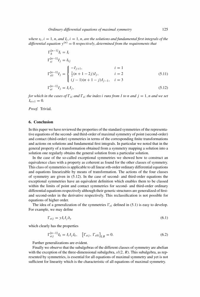
where si , i = 1, n, and Ii , i = 1, n, are the solutions and fundamental first integrals of thedifferential equation y(n) = 0 respectively, determined from the requirements that

�[n−1]h Ii = Ii

�[n−1]si Ij = δij

�[n−1]sli Ij =

⎧⎪⎨

⎪⎩

−Ij+1, i = 112 (n + 1 − 2j)Ij , i = 2

(j − 1)(n + 1 − j)Ij−1, i = 3

(5.11)

�[n−1]ei Ij = IiIj , (5.12)

for which in the cases of �si and �ei the index i runs from 1 to n and j = 1, n and we setIn+1 = 0.

Proof. Trivial.

6. Conclusion

In this paper we have reviewed the properties of the standard symmetries of the representa-tive equations of the second- and third-order of maximal symmetry of point (second-order)and contact (third-order) symmetries in terms of the corresponding finite transformationsand actions on solutions and fundamental first integrals. In particular we noted that in thegeneral property of a transformation obtained from a symmetry mapping a solution into asolution one regularly obtains the general solution from a particular solution.

In the case of the so-called exceptional symmetries we showed how to construct anequivalence class with a property as coherent as found for the other classes of symmetry.This class of symmetries is applicable to all linear nth-order ordinary differential equationsand equations linearizable by means of transformation. The actions of the four classesof symmetry are given in (5.12). In the case of second- and third-order equations theexceptional symmetries have an equivalent definition which enables them to be classedwithin the limits of point and contact symmetries for second- and third-order ordinarydifferential equations respectively although their generic structures are generalized of first-and second-order in the derivative respectively. This reclassification is not possible forequations of higher order.

The idea of a generalization of the symmetries �ei defined in (5.1) is easy to develop.For example, we may define

�eij = yIiIj ∂y (6.1)

which clearly has the properties

�[n−1]eij Ik = IiIj Ik,

[�eij , �elk

]LB

= 0. (6.2)

Further generalizations are evident.Finally we observe that the subalgebras of the different classes of symmetry are abelian

with the exception of the three-dimensional subalgebra, sl(2, R). This subalgebra, as rep-resented by symmetries, is essential for all equations of maximal symmetry and yet is notsufficient for linearity which is the characteristic of all equations of maximal symmetry.


Appendix

Appendix A: Complete symmetry group of a scalar linear nth-order ordinarydifferential equation

The equivalence of all linear nth-order ordinary differential equations under nonlocaltransformation, be the number of Lie point symmetries n + 4, n + 2 or n + 1, whichextends the results obtained here for linear equations of maximal point symmetry to alllinear equations relies upon any linear equation with the number of symmetries beingrepresentative of the class of linear equations with that number of symmetries. This pointis not made explicit in [9]. The result relies on the representation of complete symmetrygroup of the class of differential equations being automatically included in the given sevensymmetries for that class. We recall that the complete symmetry group of a differentialequation is represented by the algebra of minimal dimension which specifies completelydifferential equation [12, 13, 2, 3]. In the case of nth-order linear differential equations6

the Lie point symmetries are

number of n + 4 n + 2 n + 1symmetries

homogeneity y∂y y∂y y∂y

symmetry

solution si(x)∂y si(x)∂y si(x)∂y

special linear/ wi(x)∂x ∂x

autonomy +1

2(n − 1)w′

I (x)y∂y

algebra {sl(2, R) ⊕s A1} ⊕s nA1 A1 ⊕s {A1 ⊕s nA1} A1 ⊕s nA1,

(A.1)

where the n linearly independent functions, si(x), are solutions of the nth-order lineardifferential equation and the three functions, wi(x), are the three linearly independentsolutions of the third-order equation [17]

(n + 1)!

(n − 2)!4!w′′′ + Bn−2w

′ + 12B ′

n−2w = 0 (A.2)

for an equation written in normal form and with the coefficient of y(n−2) being Bn−2. Theequation with n + 2 Lie point symmetries is assumed to be written in autonomous form.The equivalence is a consequence of the following proposition.

PROPOSITION

The complete symmetry group of a scalar nth-order linear ordinary differential equationis represented by the algebra A1 ⊕s nA1, where the one-element subalgebra, A1, is rep-resented by �h and the n-element subalgebra, nA1, is represented by �si , i = 1, n, ofsolution synergies.

6As always the equation is taken to be homogeneous. The dependent variable of a nonhomogeneous linearequation is related to the dependent variable of the corresponding homogeneous linear equation by means of atranslation involving a function of the independent variable.


Proof. The proof is constructive. We apply the n solution symmetries in turn to the equation

y(n) = f (x, y, y′, . . . , y(n−1)) (A.3)

to obtain a nonhomogeneous equation which is linear in y and its derivatives. The appli-cation of the homogeneity symmetry removes the nonhomogeneous term and gives thedesired result.

We illustrate the first few steps. The application of �[n]s1 to (A.3) gives

s(n)1 = s

(j)

1∂f

∂y(j)(A.4)

in which summation over the repeated index is implied7. The associated Lagrange’ssystem is

dx

0= dy(j)

s(j)

1

= df

s(n)1

, (A.5)

where the middle term implies a succession of equalities, with the characteristics x,

uj = y(j)

s(j)

1

= y

s1, j = 1, n − 1, (A.6)

and

w1 = f

s(n)1

− y

s1(A.7)

so that (A.3) may now be written as

y(n) = s(n)1

s1y + s

(n)1 F1(x, uj ). (A.8)

The application of �[n]s2 to (A.8) leads to

s(n)2

s(n)1

− s2

s1=(

s(j)

2

s(j)

1

− s2

s1

)∂F1

∂uj

(A.9)

and this in turn to the new form of (A.8) as

y(n) =(

s(n)2

s(n)1

− s2

s1

)

⎧⎪⎪⎪⎪⎨

⎪⎪⎪⎪⎩

u1

s(1)2

s(1)1

− s2

s1

+ F2(x, vj )

⎫⎪⎪⎪⎪⎬

⎪⎪⎪⎪⎭

, (A.10)

7Note that we are assuming that the equation is linear, homogeneous and of the nth-order. Otherwise it can bequite general in form. For a general equation at least one solution must be such that s[n] is not zero. We take thatto be s1.


for which the new characteristic is

vj = uj

s(j)

2

s(j)

1

− s2

s1

− u1

s(1)2

s(1)1

− s2

s1

, j = 2, n − 1. (A.11)

The process is continued for all of the symmetries, �si . On the application of the n-th ofthe symmetries of the equation corresponding to (A.9) contains only one derivative and sothe integration is elementary. The current function F(x, w), in which w is the penultimatecharacteristic, is an affine function of w which is linear in y and its first n − 1 derivatives.The application of the homogeneity symmetry removes the arbitrary function of x andwe are left with an homogeneous equation of precisely determined coefficients. In factthe equation has the standard form of a linear homogeneous equation of known solution,videlicet

∣∣∣∣∣∣∣∣∣∣∣∣∣∣∣

s1 s2 s3 . . . sn y

s(1)1 s

(1)2 s

(1)3 . . . s

(1)n y(1)

s(2)1 s

(2)2 s

(2)3 . . . s

(2)n y(2)

......

.... . .

......

s(n)1 s

(n)2 s

(n)3 . . . s

(n)n y(n)

∣∣∣∣∣∣∣∣∣∣∣∣∣∣∣

= 0. (A.12)

With this demonstration of the equivalence of all linear equations within a class ofgiven number of Lie point symmetries the completeness of the results of [9] is established.A fortiori the results presented in this paper for linear equations of maximal symmetryare extended to all linear equations and to all equations which can be reduced to linearequations by means of transformation.

Appendix B: A demonstration of the derivation of one of (4.7)

We illustrate the manner of derivation of the set of equations (4.7) using �1 and the integralI1. The symmetry, �1, is a symmetry of (3.1) and is required to satisfy (4.1). Consequentlywe have the set of four equations

η′′′1 − 3y′′ξ ′′

1 − y′ξ ′′′1 = 0, (B.1)

ξ1(xy′′ − y′) + η1 − x(η′1 − y′ξ ′

1) + 1

2x2(η′′

1 − 2y′′ξ ′1 − y′ξ ′′

1 )

=(

1

2x2y′′ − xy′ + y

)2

, (B.2)

ξ1y′′ + x(η′′

1 − 2y′′ξ ′1 − y′ξ ′′

1 ) − (η′1 − y′ξ ′

1)

=(

1

2x2y′′ − xy′ + y

)(xy′′ − y′), (B.3)

η′′1 − 2y′′ξ ′

1 − y′ξ ′′1 =

(1

2x2y′′ − xy′ + y

)y′′, (B.4)

where once again the prime denotes total differentiation with respect to the independentvariable, x.


We use (B.4) to eliminate η′′1 − 2y′′ξ ′

1 − y′ξ ′′1 from (B.2) and (B.3) to obtain

ξ1(xy′′ − y′) + η1 − x(η′1 − y′ξ ′) + 1

2x2y′′

(1

2x2y′′ − xy′ + y

)

=(

1

2x2y′′ − xy′ + y

)2

, (B.5)

ξ1y′′ − (η′

1 − y′ξ ′1) = −

(1

2x2y′′ − xy′ + y

)y′. (B.6)

We substitute for η′1 − y′ξ ′

1 from (B.6) into (B.5) and are left with

η1 − ξ1y′ =

(1

2x2y′′ − xy′ + y

)y (B.7)

as required. The satisfaction of (B.1) is automatic.

Acknowledgements

The referee is thanked for a very careful reading of the text and the consequent usefulcomments. RRW and VN thank the National Research Foundation of South Africa for itssupport. PGLL and RRW thank the University of KwaZulu-Natal for its support.

References

[1] Abraham-Shrauner B, Leach P G L, Govinder K S and Ratcliff G, Hidden and contactsymmetries of ordinary differential equations, J. Phys. A28 (1995) 6707–6716

[2] Andriopoulos K, Leach P G L and Flessas G P, Complete symmetry groups of ordinarydifferential equations and their integrals: Some basic considerations, J. Math. Anal. Appl.262 (2001) 256–273

[3] Andriopoulos K and Leach P G L, The economy of complete symmetry groups for linearhigher-dimensional systems, J. Nonlinear Math. Phys. 9(II Suppl.) (2002) 10–23

[4] Euler N, Wolf T, Leach P G L and Euler M, Linearisable third-order ordinary differentialequations and generalised Sundman transformations, Acta Appl. Math. 76 (2003) 89–115

[5] Euler Norbert and Euler Marianna, Sundman Symmetries of Nonlinear Second-Orderand Third-Order Ordinary Differential Equaions (preprint: Department of Mathematics,Lulea University of Technology, SE-971 87 Lulea, Sweden) (2004)

[6] Flessas G P, Govinder K S and Leach P G L, Characterisation of the algebraic propertiesof first integrals of scalar ordinary differential equations of maximal symmetry, J. Math.Anal. Appl. 212 (1997) 349–374

[7] Govinder K S and Leach P G L, The algebraic structure of the first integrals of third-orderlinear equations, J. Math. Anal. Appl. 193 (1995) 114–133

[8] Govinder K S and Leach P G L, Noetherian integrals via nonlocal transformation, Phys.Lett. A201 (1995) 91–94

[9] Govinder K S and Leach P G L, On the equivalence of linear third-order differentialequations under nonlocal transformations, J. Math. Anal. Appl. 287 (2003) 399–404

[10] Hsu L and Kamran N, Symmetries of second-order ordinary differential equations andElie Cartan’s method of equivalence, Lett. Math. Phys. 15 (1988) 91–99

[11] Krause J and Michel L, Equations differentielles lineaires d’ordre n ≥ 2 ayant uneAlgebre de Lie de symetrie de dimension n+4, Compte Rendus du Academie des Sciencesde Paris Serie I 307 (1988) 905–910


[12] Krause J, On the complete symmetry group of the classical Kepler system, J. Math. Phys.35 (1994) 5734–5748

[13] Krause J, On the complete symmetry group of the Kepler problem in Arima A ed, Pro-ceedings of the XXth International Colloquium on Group Theoretical Methods in Physics(World Scientific, Singapore) (1995) 286–290

[14] Leach P G L, Govinder K S and Abraham-Shrauner B, Symmetries of first integrals andtheir associated differential equations, J. Math. Anal. Appl. 235 (1999) 58–83

[15] Mahomed F M and Leach P G L, The linear symmetries of a nonlinear differentialequation, Quæstiones Mathematicæ 8 (1985) 241–274

[16] Mahomed F M and Leach P G L, Lie algebras associated with scalar second-orderordinary differential equations, J. Math. Phys. 30 (1989) 2770–2777

[17] Mahomed F M and Leach P G L, Symmetry Lie algebras of nth-order ordinary differen-tial equations, J. Math. Anal. Appl. 151 (1990) 80–107

[18] Morozov V V, Classification of six-dimensional nilpotent Lie algebras, Izvestia VysshikhUchebn Zavendeniı Matematika 5 (1958) 161–171

[19] Moyo S, Verstraete J B A and Leach P G L, Non-Noetherian Lie symmetries areNoetherian Symmetries, Advances in Systems, Signals, Control and Computers,Bajic VB ed (IAAMSAD & ANS (South Africa), Durban) Vol II (1998) 72–76

[20] Moyo S and Leach P G L, Exceptional properties of second- and third-order ordinarydifferential equations of maximal symmetry, J. Math. Anal. Appl. 252 (2000) 840–863

[21] Mubarakzyanov G M, On solvable Lie algebras, Izvestia Vysshikh Uchebn ZavendeniıMatematika 32 (1963) 114–123

[22] Mubarakzyanov G M, Classification of real structures of five-dimensional Lie algebras,Izvestia Vysshikh Uchebn Zavendeniı Matematika 34 (1963) 99–106

[23] Mubarakzyanov G M, Classification of solvable six-dimensional Lie algebras with onenilpotent base element, Izvestia Vysshikh Uchebn Zavendeniı Matematika 35 (1963)104–116

[24] Noether Emmy, Invariante Variationsprobleme, Koniglich Gesellschaft der Wissens-chaften Gottingen Nachrichten Mathematik-physik Klasse 2 (1918) 235–267

[25] Sarlet Willy and Cantrijn Frans, Generalizations of Noether’s theorem in classicalmechanics, SIAM Rev. 23 (1981) 467–494

[26] Sundman K F, Memoire sur le problem des trois corps, Acta Mathematica 36 (1912–1913) 105–179

Symmetries, integrals and solutions of ordinary differential equations of maximal symmetry

Documents

Transcript of Symmetries, integrals and solutions of ordinary differential equations of maximal symmetry