12 Multiple Integrals
294
12 M ultiple Integrals
-
Upload
khangminh22 -
Category
Documents
-
view
1 -
download
0
Transcript of 12 Multiple Integrals

12 Multiple Integrals

Double Integrals over Rectangles � � � � � � � � � � �
In much the same way that our attempt to solve the area problem led to the definitionof a definite integral, we now seek to find the volume of a solid and in the process wearrive at the definition of a double integral.
Review of the Definite Integral
First let’s recall the basic facts concerning definite integrals of functions of a singlevariable. If is defined for , we start by dividing the interval inton subintervals of equal width and we choose sample points
in these subintervals. Then we form the Riemann sum
and take the limit of such sums as to obtain the definite integral of from to :
In the special case where , the Riemann sum can be interpreted as the sum ofthe areas of the approximating rectangles in Figure 1, and represents thearea under the curve from to .
FIGURE 1
0
y
xa b⁄ ¤ ‹ xi-1 xi xn-1
x¡* x™* x£* x i* xn*
Îx
f(x i*)
bay � f �x�x
ba f �x� dx
f �x� � 0
yb
a f �x� dx � lim
n l � �
n
i�1 f �xi*� �x2
bafn l �
�n
i�1 f �xi*� �x1
xi*�x � �b � a��n�xi�1, xi�
�a, b�a � x � bf �x�
12.1
839
In this chapter we extend the idea of a definite integralto double and triple integrals of functions of two orthree variables. These ideas are then used to computevolumes, surface areas, masses, and centroids of more
general regions than we were able to consider inChapter 6. We also use double integrals to calcu-late probabilities when two random variables areinvolved.

Volumes and Double Integrals
In a similar manner we consider a function of two variables defined on a closed rect-angle
and we first suppose that . The graph of f is a surface with equation. Let S be the solid that lies above R and under the graph of f, that is,
(See Figure 2.) Our goal is to find the volume of S.The first step is to divide the rectangle into subrectangles. We do this by divid-
ing the interval into m subintervals of equal width and dividing into n subintervals of equal width . Bydrawing lines parallel to the coordinate axes through the endpoints of these subinter-vals as in Figure 3, we form the subrectangles
each with area .
If we choose a sample point in each , then we can approximate the partof S that lies above each by a thin rectangular box (or “column”) with base andheight as shown in Figure 4. (Compare with Figure 1.) The volume of thisbox is the height of the box times the area of the base rectangle:
If we follow this procedure for all the rectangles and add the volumes of the corre-sponding boxes, we get an approximation to the total volume of S:
(See Figure 5.) This double sum means that for each subrectangle we evaluate at thechosen point and multiply by the area of the subrectangle, and then we add the results.
f
V � �m
i�1 �
n
j�1 f �xij*, yij*� �A3
f �xij*, yij*� �A
f �xij*, yij*�RijRij
Rij�xij*, yij*�
FIGURE 3Dividing R into subrectangles
(x*£™, y*£™)
yj_1
yj
xixi_1
y
x
d
c
›
0 ⁄ ¤
Rij
a b
(x*ij, y*
ij)
(xi, yj)
Îx
Îy
�A � �x �y
Rij � �xi�1, xi � � �yj�1, yj� � ��x, y� xi�1 � x � xi, yj�1 � y � yj
�y � �d � c��n�yj�1, yj ��c, d ��x � �b � a��m�xi�1, xi��a, b�
R
S � ��x, y, z� � � 3 0 � z � f �x, y�, �x, y� � R
z � f �x, y�f �x, y� � 0
R � �a, b� � �c, d � � ��x, y� � � 2 a � x � b, c � y � d
f
840 � CHAPTER 12 MULTIPLE INTEGRALS
FIGURE 2
0c
d
R
a
bx
z=f(x, y)z
y
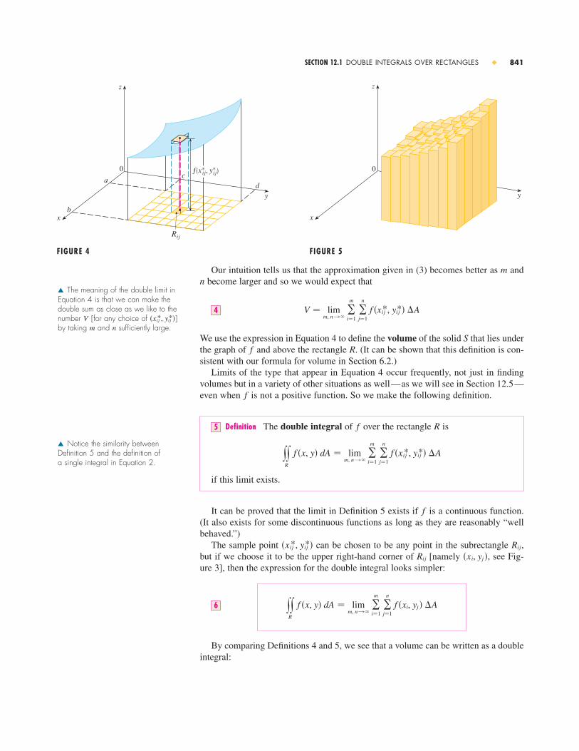
Our intuition tells us that the approximation given in (3) becomes better as m andn become larger and so we would expect that
We use the expression in Equation 4 to define the volume of the solid that lies underthe graph of and above the rectangle . (It can be shown that this definition is con-sistent with our formula for volume in Section 6.2.)
Limits of the type that appear in Equation 4 occur frequently, not just in findingvolumes but in a variety of other situations as well—as we will see in Section 12.5—even when is not a positive function. So we make the following definition.
Definition The double integral of over the rectangle is
if this limit exists.
It can be proved that the limit in Definition 5 exists if is a continuous function.(It also exists for some discontinuous functions as long as they are reasonably “wellbehaved.”)
The sample point can be chosen to be any point in the subrectangle but if we choose it to be the upper right-hand corner of [namely , see Fig-ure 3], then the expression for the double integral looks simpler:
By comparing Definitions 4 and 5, we see that a volume can be written as a doubleintegral:
yyR
f �x, y� dA � lim m, n l �
�m
i�1 �
n
j�1 f �xi, yj� �A6
�xi, yj�Rij
Rij,�xij*, yij*�
f
yyR
f �x, y� dA � lim m, n l �
�m
i�1 �
n
j�1 f �xij*, yij*� �A
Rf5
f
RfS
V � lim m, n l �
�m
i�1 �
n
j�1 f �xij*, yij*� �A4
x
y
0
zz
y
0c
d
Rij
a
bx
f(x*ij, y*
ij)
FIGURE 4 FIGURE 5
SECTION 12.1 DOUBLE INTEGRALS OVER RECTANGLES � 841
� The meaning of the double limit inEquation 4 is that we can make the double sum as close as we like to thenumber [for any choice of ] by taking and sufficiently large.nm
�xij*, yij*�V
� Notice the similarity between Definition 5 and the definition of a single integral in Equation 2.

If , then the volume of the solid that lies above the rectangle and below the surface is
The sum in Definition 5,
is called a double Riemann sum and is used as an approximation to the value of the double integral. [Notice how similar it is to the Riemann sum in (1) for a function ofa single variable.] If happens to be a positive function, then the double Riemann sum represents the sum of volumes of columns, as in Figure 5, and is an approximation tothe volume under the graph of .
EXAMPLE 1 Estimate the volume of the solid that lies above the squareand below the elliptic paraboloid . Divide
into four equal squares and choose the sample point to be the upper right corner ofeach square . Sketch the solid and the approximating rectangular boxes.
SOLUTION The squares are shown in Figure 6. The paraboloid is the graph ofand the area of each square is 1. Approximating the
volume by the Riemann sum with , we have
This is the volume of the approximating rectangular boxes shown in Figure 7.
We get better approximations to the volume in Example 1 if we increase the num-ber of squares. Figure 8 shows how the columns start to look more like the actual solid
FIGURE 7 x
y
z
16
2
2
z=16-≈-2¥
� 13�1� � 7�1� � 10�1� � 4�1� � 34
� f �1, 1� �A � f �1, 2� �A � f �2, 1� �A � f �2, 2� �A
V � �2
i�1 �
2
j�1 f �xi, yj� �A
m � n � 2f �x, y� � 16 � x 2 � 2y 2
Rij
Rz � 16 � x 2 � 2y 2R � �0, 2� � �0, 2�
f
f
�m
i�1 �
n
j�1 f �xij*, yij*� �A
V � yyR
f �x, y� dA
z � f �x, y�RVf �x, y� � 0
842 � CHAPTER 12 MULTIPLE INTEGRALS
0
y
1
2
x1 2
(2, 2)
R¡™ R™™
R¡¡ R™¡
(2, 1)(1, 1)
(1, 2)
FIGURE 6

and the corresponding approximations become more accurate when we use 16, 64, and256 squares. In the next section we will be able to show that the exact volume is 48.
EXAMPLE 2 If , evaluate the integral
SOLUTION It would be very difficult to evaluate this integral directly from Definition 5but, because , we can compute the integral by interpreting it as a vol-ume. If , then and , so the given double integralrepresents the volume of the solid S that lies below the circular cylinder and above the rectangle R. (See Figure 9.) The volume of S is the area of a semicirclewith radius 1 times the length of the cylinder. Thus
The Midpoint Rule
The methods that we used for approximating single integrals (the Midpoint Rule, theTrapezoidal Rule, Simpson’s Rule) all have counterparts for double integrals. Here weconsider only the Midpoint Rule for double integrals. This means that we use a doubleRiemann sum to approximate the double integral, where the sample point in
is chosen to be the center of . In other words, is the midpoint of and is the midpoint of .
Midpoint Rule for Double Integrals
where is the midpoint of and is the midpoint of .�yj�1, yj�yj�xi�1, xi�xi
yyR
f �x, y� dA � �m
i�1 �
n
j�1 f �xi, yj� �A
�yj�1, yj �yj
�xi�1, xi�xiRij�xi, yj�Rij
�xij*, yij*�
yyR
s1 � x 2 dA � 12 � �1�2 � 4 � 2�
x 2 � z2 � 1z � 0x 2 � z2 � 1z � s1 � x 2
s1 � x 2 � 0
yyR
s1 � x 2 dA
R � ��x, y� �1 � x � 1, �2 � y � 2
(a) m=n=4, VÅ41.5 (b) m=n=8, VÅ44.875 (c) m=n=16, VÅ46.46875
FIGURE 8 The Riemann sum approximations to the volume under z=16-≈-2¥ become more accurate as m and n increase.
SECTION 12.1 DOUBLE INTEGRALS OVER RECTANGLES � 843
FIGURE 9
x y
S
z
(0, 0, 1)
(1, 0, 0) (0, 2, 0)
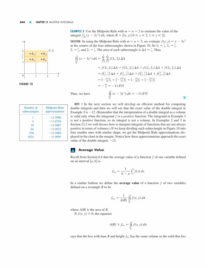
EXAMPLE 3 Use the Midpoint Rule with to estimate the value of theintegral , where , .
SOLUTION In using the Midpoint Rule with , we evaluate at the centers of the four subrectangles shown in Figure 10. So , ,
, and . The area of each subrectangle is . Thus
Thus, we have
NOTE � In the next section we will develop an efficient method for computing double integrals and then we will see that the exact value of the double integral inExample 3 is . (Remember that the interpretation of a double integral as a volumeis valid only when the integrand is a positive function. The integrand in Example 3is not a positive function, so its integral is not a volume. In Examples 2 and 3 inSection 12.2 we will discuss how to interpret integrals of functions that are not alwayspositive in terms of volumes.) If we keep dividing each subrectangle in Figure 10 intofour smaller ones with similar shape, we get the Midpoint Rule approximations dis-played in the chart in the margin. Notice how these approximations approach the exactvalue of the double integral, .
Average Value
Recall from Section 6.4 that the average value of a function of one variable definedon an interval is
In a similar fashion we define the average value of a function of two variablesdefined on a rectangle R to be
where is the area of R.If , the equation
says that the box with base and height has the same volume as the solid that lies faveR
A�R� � fave � yyR
f �x, y� dA
f �x, y� � 0A�R�
fave �1
A�R� yy
R
f �x, y� dA
f
fave �1
b � a y
b
a f �x� dx
�a, b�f
�12
f�12
yyR
�x � 3y 2 � dA � �11.875
� �958 � �11.875
� (� 6716 ) 1
2 � (� 13916 ) 1
2 � (� 5116) 1
2 � (� 12316 ) 1
2
� f ( 12, 54 ) �A � f ( 1
2, 74 ) �A � f ( 32, 54 ) �A � f ( 3
2, 74 ) �A
� f �x1, y1� �A � f �x1, y2 � �A � f �x2, y1 � �A � f �x2, y2 � �A
yyR
�x � 3y 2 � dA � �2
i�1 �
2
j�1 f �xi, yj� �A
�A � 12y2 � 7
4y1 � 54
x2 � 32x1 � 1
2
f �x, y� � x � 3y 2m � n � 2
1 � y � 2R � ��x, y� 0 � x � 2xxR �x � 3y 2 � dAm � n � 2
844 � CHAPTER 12 MULTIPLE INTEGRALS
0
y
1
2
x1 2
32
(2, 2)R¡™ R™™
R¡¡ R™¡
FIGURE 10
Number of Midpoint Rulesubrectangles approximations
1 �11.50004 �11.8750
16 �11.968764 �11.9922
256 �11.99801024 �11.9995

under the graph of . [If describes a mountainous region and you chop offthe tops of the mountains at height , then you can use them to fill in the valleys sothat the region becomes completely flat. See Figure 11.]
EXAMPLE 4 The contour map in Figure 12 shows the snowfall, in inches, that fell onthe state of Colorado on December 24, 1982. (The state is in the shape of a rect-angle that measures 388 mi west to east and 276 mi south to north.) Use the contourmap to estimate the average snowfall for Colorado as a whole on December 24.
SOLUTION Let’s place the origin at the southwest corner of the state. Then , and is the snowfall, in inches, at a location x miles to the east
and y miles to the north of the origin. If R is the rectangle that represents Colorado,then the average snowfall for Colorado on December 24 was
fave �1
A�R� yy
R
f �x, y� dA
f �x, y�0 � y � 2760 � x � 388,
FIGURE 12
02
4
6
8
10121416
1820
2224
FIGURE 11
fave
z � f �x, y�f
SECTION 12.1 DOUBLE INTEGRALS OVER RECTANGLES � 845

where . To estimate the value of this double integral let’s use theMidpoint Rule with . In other words, we divide R into 16 subrectanglesof equal size, as in Figure 13. The area of each subrectangle is
Using the contour map to estimate the value of at the center of each subrect-angle, we get
Therefore
On December 24, 1982, Colorado received an average of approximately inches ofsnow.
512
fave ��6693��88.6��388��276�
� 5.5
� �6693��88.6�
� 0.1 � 6.1 � 16.5 � 8.8 � 1.8 � 8.0 � 16.2 � 9.4�
� �A�0.4 � 1.2 � 1.8 � 3.9 � 0 � 3.9 � 4.0 � 6.5
yyR
f �x, y� dA � �4
i�1 �
4
j�1 f �xi, yj� �A
f
FIGURE 13
02
4
6
8
10 121416
1820
2224
0
y
x388
276
�A � 116�388��276� � 6693 mi2
m � n � 4A�R� � 388 � 276
846 � CHAPTER 12 MULTIPLE INTEGRALS

Properties of Double Integrals
We list here three properties of double integrals that can be proved in the same man-ner as in Section 5.2. We assume that all of the integrals exist. Properties 7 and 8 arereferred to as the linearity of the integral.
where c is a constant
If for all in , then
yyR
f �x, y� dA � yyR
t�x, y� dA9
R�x, y�f �x, y� � t�x, y�
yyR
c f �x, y� dA � c yyR
f �x, y� dA8
yyR
� f �x, y� � t�x, y�� dA � yyR
f �x, y� dA � yyR
t�x, y� dA7
SECTION 12.1 DOUBLE INTEGRALS OVER RECTANGLES � 847
6. A 20-ft-by-30-ft swimming pool is filled with water. Thedepth is measured at 5-ft intervals, starting at one corner ofthe pool, and the values are recorded in the table. Estimatethe volume of water in the pool.
7. Let be the volume of the solid that lies under the graph ofand above the rectangle given by
, . We use the lines and y � 4x � 32 � y � 62 � x � 4f �x, y� � s52 � x 2 � y 2
V
2
3
4
5
7
0
1
3
5
8
�3
�4
0
3
6
�6
�8
�5
�1
3
�5
�6
�8
�4
0
xy 0 1 2 3 4
1.0
1.5
2.0
2.5
3.0
1. Find approximations to using the samesubrectangles as in Example 3 but choosing the samplepoint to be the (a) upper left corner, (b) upper right corner,(c) lower left corner, (d) lower right corner of each sub-rectangle.
2. Find the approximation to the volume in Example 1 if the Midpoint Rule is used.
3. (a) Estimate the volume of the solid that lies below the surface and above the rectangle
, . Use a Riemann sum with , , and take the sample point to be the upper right corner of each subrectangle.
(b) Use the Midpoint Rule to estimate the volume of the solid in part (a).
4. If , use a Riemann sum with ,to estimate the value of . Take
the sample points to be the upper left corners of the subrectangles.
5. A table of values is given for a function defined on.
(a) Estimate using the Midpoint Rule with.
(b) Estimate the double integral with by choos-ing the sample points to be the points farthest from theorigin.
m � n � 4m � n � 2
xxR f �x, y� dAR � �1, 3� � �0, 4�
f �x, y�
xxR �y 2 � 2x 2� dAn � 2m � 4R � ��1, 3� � �0, 2�
n � 2m � 30 � y � 4R � ��x, y� 0 � x � 6
z � xy
xxR �x � 3y2� dA
Exercises � � � � � � � � � � � � � � � � � � � � � � � � � �12.1
� Double integrals behave this waybecause the double sums that definethem behave this way.
0 5 10 15 20 25 30
0 2 3 4 6 7 8 85 2 3 4 7 8 10 8
10 2 4 6 8 10 12 1015 2 3 4 5 6 8 720 2 2 2 2 3 4 4

11–13 � Evaluate the double integral by first identifying it asthe volume of a solid.
11.
12.
13.� � � � � � � � � � � � �
14. The integral , where ,represents the volume of a solid. Sketch the solid.
15. Use a programmable calculator or computer (or the sum command on a CAS) to estimate
where . Use the Midpoint Rule with the following numbers of squares of equal size: 1, 4, 16, 64,256, and 1024.
16. Repeat Exercise 15 for the integral .
17. If is a constant function, , and , show that
18. If , show that 0 � xxR sin�x � y� dA � 1.R � �0, 1� � �0, 1�
xxR k dA � k�b � a��d � c�.R � �a, b� � �c, d�
f �x, y� � kf
xxR cos�x 4 � y 4 � dA
R � �0, 1� � �0, 1�
yyR
e�x 2�y 2 dA
R � �0, 4� � �0, 2�xxR s9 � y 2 dA
xxR �4 � 2y� dA, R � �0, 1� � �0, 1�
xxR �5 � x� dA, R � ��x, y� 0 � x � 5, 0 � y � 3
xxR 3 dA, R � ��x, y� �2 � x � 2, 1 � y � 6
74
74
7070
7674
74
7070
7674
74
7070
66
62
58
54
76
68
68
to divide into subrectangles. Let and be the Riemannsums computed using lower left corners and upper right corners, respectively. Without calculating the numbers , ,and , arrange them in increasing order and explain yourreasoning.
8. The figure shows level curves of a function in the square. Use them to estimate to
the nearest integer.
9. A contour map is shown for a function on the square.
(a) Use the Midpoint Rule with to estimate thevalue of .
(b) Estimate the average value of .
10. The contour map shows the temperature, in degrees Fahren-heit, at 3:00 P.M. on May 1, 1996, in Colorado. (The statemeasures 388 mi east to west and 276 mi north to south.)Use the Midpoint Rule to estimate the average temperaturein Colorado at that time.
y
0
2
4
2 4 x
10
10
10 20
20
30
300 0
fxxR f �x, y� dA
m � n � 2R � �0, 4� � �0, 4�
f
x0
y
1
1
910
11
1213
14
xxR f �x, y� dAR � �0, 1� � �0, 1�
f
ULV
ULR
848 � CHAPTER 12 MULTIPLE INTEGRALS

Iterated Integrals � � � � � � � � � � � � � � � �
Recall that it is usually difficult to evaluate single integrals directly from the definitionof an integral, but the Evaluation Theorem (Part 2 of the Fundamental Theorem ofCalculus) provides a much easier method. The evaluation of double integrals from firstprinciples is even more difficult, but in this section we see how to express a doubleintegral as an iterated integral, which can then be evaluated by calculating two singleintegrals.
Suppose that is a function of two variables that is continuous on the rectangle. We use the notation to mean that is held fixed and
is integrated with respect to from to . This procedure is calledpartial integration with respect to . (Notice its similarity to partial differentiation.)Now is a number that depends on the value of , so it defines a functionof :
If we now integrate the function with respect to from to , we get
The integral on the right side of Equation 1 is called an iterated integral. Usually thebrackets are omitted. Thus
means that we first integrate with respect to from to and then with respect to from to .
Similarly, the iterated integral
means that we first integrate with respect to (holding fixed) from to and then we integrate the resulting function of with respect to from to Notice that in both Equations 2 and 3 we work from the inside out.
EXAMPLE 1 Evaluate the iterated integrals.
(a) (b)
SOLUTION(a) Regarding as a constant, we obtain
� x 2�22
2 � � x 2�12
2 � � 32 x 2
y2
1 x 2y dy � x 2
y 2
2 �y�1
y�2
x
y2
1 y
3
0 x 2y dx dyy
3
0 y
2
1 x 2y dy dx
y � d.y � cyyx � bx � ayx
yd
c y
b
a f �x, y� dx dy � y
d
c y
b
a f �x, y� dx� dy3
baxdcy
yb
a y
d
c f �x, y� dy dx � y
b
a y
d
c f �x, y� dy� dx2
yb
a A�x� dx � y
b
a y
d
c f �x, y� dy� dx1
x � bx � axA
A�x� � yd
c f �x, y� dy
xxx
dc f �x, y� dy
yy � dy � cyf �x, y�
xxdc f �x, y� dyR � �a, b� � �c, d �
f
12.2
SECTION 12.2 ITERATED INTEGRALS � 849

Thus, the function in the preceding discussion is given by in thisexample. We now integrate this function of from 0 to 3:
(b) Here we first integrate with respect to :
Notice that in Example 1 we obtained the same answer whether we integrated withrespect to or first. In general, it turns out (see Theorem 4) that the two iterated inte-grals in Equations 2 and 3 are always equal; that is, the order of integration does notmatter. (This is similar to Clairaut’s Theorem on the equality of the mixed partialderivatives.)
The following theorem gives a practical method for evaluating a double integral byexpressing it as an iterated integral (in either order).
Fubini’s Theorem If is continuous on the rectangle , , then
More generally, this is true if we assume that is bounded on , is discon-tinuous only on a finite number of smooth curves, and the iterated integralsexist.
The proof of Fubini’s Theorem is too difficult to include in this book, but we canat least give an intuitive indication of why it is true for the case where .Recall that if is positive, then we can interpret the double integral asthe volume of the solid that lies above and under the surface . Butwe have another formula that we used for volume in Chapter 6, namely,
where is the area of a cross-section of in the plane through perpendicular tothe -axis. From Figure 1 you can see that is the area under the curve whoseequation is , where is held constant and . Therefore
and we have
yyR
f �x, y� dA � V � yb
a A�x� dx � y
b
a y
d
c f �x, y� dy dx
A�x� � yd
c f �x, y� dy
c � y � dxz � f �x, y�CA�x�x
xSA�x�
V � yb
a A�x� dx
z � f �x, y�RSVxxR f �x, y� dAf
f �x, y� � 0
fRf
yyR
f �x, y� dA � yb
a y
d
c f �x, y� dy dx � y
d
c y
b
a f �x, y� dx dy
c � y � dR � ��x, y� a � x � bf4
xy
� y2
1 9y dy � 9
y 2
2 �1
2
�27
2
y2
1 y
3
0 x 2 y dx dy � y
2
1 y
3
0 x 2y dx� dy � y
2
1 x 3
3 y�
x�0
x�3
dy
x
� y3
0 32 x 2 dx �
x 3
2 �0
3
�27
2
y3
0 y
2
1 x 2y dy dx � y
3
0 y
2
1 x 2y dy� dx
xA�x� � 3
2 x 2A
850 � CHAPTER 12 MULTIPLE INTEGRALS
FIGURE 1
x
0
z
ax
b
y
A(x)
C
� Theorem 4 is named after the Italian mathematician Guido Fubini(1879–1943), who proved a very gen-eral version of this theorem in 1907. But the version for continuous functionswas known to the French mathematicianAugustin- Louis Cauchy almost a centuryearlier.

A similar argument, using cross-sections perpendicular to the -axis as in Figure 2,shows that
EXAMPLE 2 Evaluate the double integral , where, . (Compare with Example 3 in Section 12.1.)
SOLUTION 1 Fubini’s Theorem gives
SOLUTION 2 Again applying Fubini’s Theorem, but this time integrating with respect tofirst, we have
EXAMPLE 3 Evaluate , where .
SOLUTION 1 If we first integrate with respect to , we get
SOLUTION 2 If we reverse the order of integration, we get
To evaluate the inner integral we use integration by parts with
v � �cos�xy�
x du � dy
dv � sin�xy� dy u � y
yyR
y sin�xy� dA � y2
1 y
�
0 y sin�xy� dy dx
� �12 sin 2y � sin y]0
�� 0
� y�
0 ��cos 2y � cos y� dy
� y�
0 [�cos�xy�]x�1
x�2 dy
yyR
y sin�xy� dA � y�
0 y
2
1 y sin�xy� dx dy
x
R � �1, 2� � �0, ��xxR y sin�xy� dA
� y2
1 �2 � 6y 2 � dy � 2y � 2y 3]1
2� �12
� y2
1
x 2
2� 3xy 2�
x�0
x�2
dy
yyR
�x � 3y 2 � dA � y2
1 y
2
0 �x � 3y 2 � dx dy
x
� y2
0 �x � 7� dx �
x 2
2� 7x�
0
2
� �12
� y2
0
[xy � y 3]y�1y�2
dx
yyR
�x � 3y 2 � dA � y2
0 y
2
1 �x � 3y 2 � dy dx
1 � y � 2R � ��x, y� 0 � x � 2xxR �x � 3y 2 � dA
yyR
f �x, y� dA � yd
c y
b
a f �x, y� dx dy
y
SECTION 12.2 ITERATED INTEGRALS � 851
FIGURE 2
x
0
z
y
ycd
FIGURE 3
R0
_120 0.5 1 1. 2 2
10
yx
z_4
_8 z=x-3¥
FIGURE 4
z=y sin(xy)
10
_1
y10
32 2
1
x
z
� Notice the negative answer inExample 2; nothing is wrong with that.The function in that example is not apositive function, so its integral doesn’trepresent a volume. From Figure 3 wesee that is always negative on , sothe value of the integral is the negativeof the volume that lies above the graphof and below .Rf
Rf
f
� For a function that takes on both positive and negative values,
is a difference of volumes:, where is the volume above
and below the graph of and is the volume below and above the graph. The fact that the integral in Example 3 is means that these two volumes and are equal. (SeeFigure 4.)
V2V1
0
RV2fR
V1V1 � V2
xxR f �x, y� dA
f

and so
If we now integrate the first term by parts with and , weget , , and
Therefore
and so
EXAMPLE 4 Find the volume of the solid that is bounded by the elliptic paraboloid, the planes and , and the three coordinate planes.
SOLUTION We first observe that is the solid that lies under the surfaceand above the square . (See Figure 5.) This
solid was considered in Example 1 in Section 12.1, but we are now in a position toevaluate the double integral using Fubini’s Theorem. Therefore
In the special case where can be factored as the product of a function of only and a function of only, the double integral of can be written in a particularlysimple form. To be specific, suppose that and .Then Fubini’s Theorem gives
In the inner integral is a constant, so is a constant and we can write
� yb
a t�x� dx y
d
c h�y� dy
yd
c y
b
a t�x�h�y� dx� dy � y
d
c h�y��y
b
a t�x� dx�� dy
h�y�y
yyR
f �x, y� dA � yd
c y
b
a t�x�h�y� dx dy � y
d
c y
b
a t�x�h�y� dx� dy
R � �a, b� � �c, d �f �x, y� � t�x�h�y�fy
xf �x, y�
� y2
0 ( 88
3 � 4y 2 ) dy � [ 883 y �
43 y3 ]0
2� 48
� y2
0 [16x �
13 x 3 � 2y 2x]x�0
x�2 dy
V � yyR
�16 � x 2 � 2y 2 � dA � y2
0 y
2
0 �16 � x 2 � 2y 2 � dx dy
R � �0, 2� � �0, 2�z � 16 � x 2 � 2y 2S
y � 2x � 2x 2 � 2y 2 � z � 16S
� �sin 2�
2� sin � � 0
y2
1 y
�
0 y sin�xy� dy dx � �
sin �x
x �1
2
y ��� cos �x
x�
sin �x
x 2 � dx � �sin �x
x
y ��� cos �x
x � dx � �sin�x
x� y
sin �x
x 2 dx
v � sin �xdu � dx�x 2dv � � cos �x dxu � �1�x
� �� cos �x
x�
sin �x
x 2
� �� cos �x
x�
1
x 2 [sin�xy�]y�0y��
y�
0 y sin�xy� dy � �
y cos�xy�x �
y�0
y��
�1
x y
�
0 cos�xy� dy
852 � CHAPTER 12 MULTIPLE INTEGRALS
FIGURE 5
4
0 0.5 1 1.5 2 21
0
yx
z
0.5
16
12
8
1.5
0
� In Example 2, Solutions 1 and 2 areequally straightforward, but in Example 3the first solution is much easier than thesecond one. Therefore, when we eval-uate double integrals it is wise to choosethe order of integration that gives simplerintegrals.
since is a constant. Therefore, in this case, the double integral of can bewritten as the product of two single integrals:
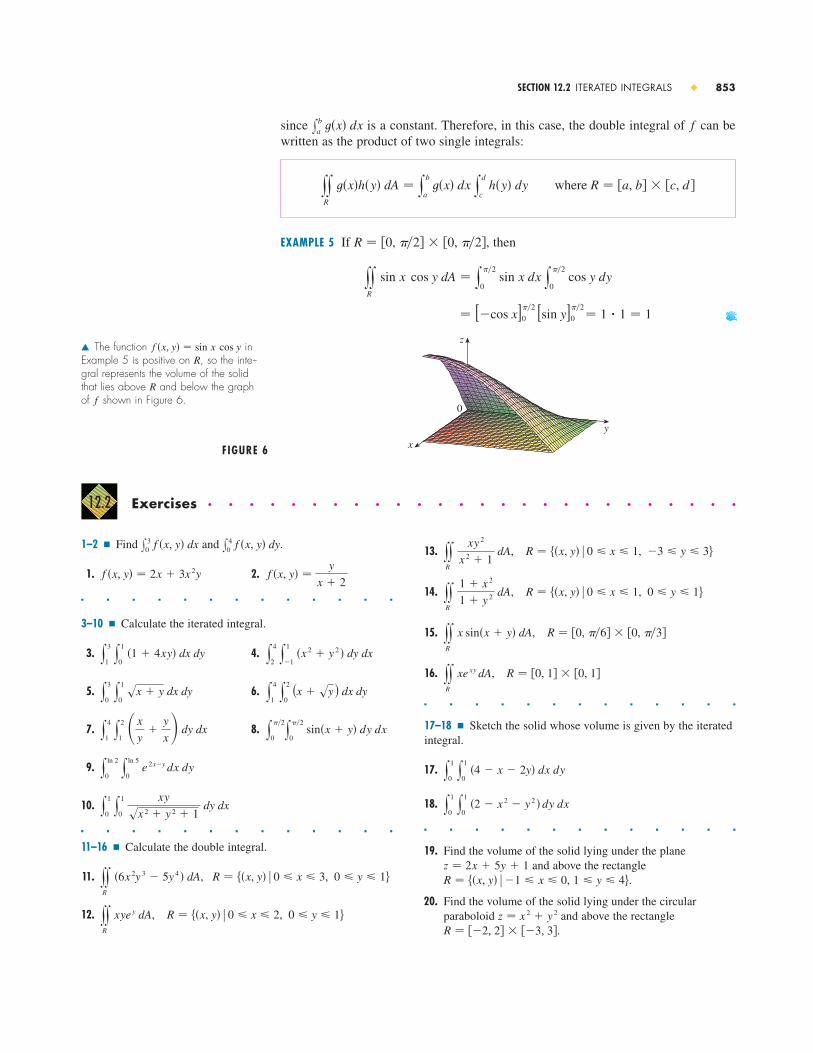
EXAMPLE 5 If , then
FIGURE 6
y
x
z
0
� [�cos x]0
��2 [sin y]0
��2� 1 � 1 � 1
yyR
sin x cos y dA � y��2
0 sin x dx y
��2
0 cos y dy
R � �0, ��2� � �0, ��2�
where R � �a, b� � �c, d �yyR
t�x�h�y� dA � yb
a t�x� dx y
d
c h�y� dy
fxba t�x� dx
SECTION 12.2 ITERATED INTEGRALS � 853
13. ,
14. ,
15. ,
16. ,
� � � � � � � � � � � � �
17–18 � Sketch the solid whose volume is given by the iteratedintegral.
17.
18.
� � � � � � � � � � � � �
19. Find the volume of the solid lying under the planeand above the rectangle
, .
20. Find the volume of the solid lying under the circular paraboloid and above the rectangle
.R � ��2, 2� � ��3, 3�z � x 2 � y 2
1 � y � 4R � ��x, y� �1 � x � 0z � 2x � 5y � 1
y1
0 y
1
0 �2 � x 2 � y 2 � dy dx
y1
0 y
1
0 �4 � x � 2y� dx dy
R � �0, 1� � �0, 1�yyR
xe xy dA
R � �0, ��6� � �0, ��3�yyR
x sin�x � y� dA
R � ��x, y� 0 � x � 1, 0 � y � 1yyR
1 � x 2
1 � y 2 dA
R � ��x, y� 0 � x � 1, �3 � y � 3yyR
xy 2
x 2 � 1 dA
1–2 � Find and .
1. 2.
� � � � � � � � � � � � �
3–10 � Calculate the iterated integral.
3. 4.
5. 6.
7. 8.
9.
10.
� � � � � � � � � � � � �
11–16 � Calculate the double integral.
11. ,
12. , R � ��x, y� 0 � x � 2, 0 � y � 1yyR
xye y dA
R � ��x, y� 0 � x � 3, 0 � y � 1yyR
�6x 2y 3 � 5y 4 � dA
y1
0 y
1
0
xy
sx 2 � y 2 � 1 dy dx
yln
2
0 y
ln 5
0 e 2x�y dx dy
y��2
0y
��2
0 sin�x � y� dy dxy
4
1 y
2
1 � x
y�
y
x� dy dx
y4
1 y
2
0 (x � sy ) dx dyy
3
0 y
1
0 sx � y dx dy
y4
2 y
1
�1 �x 2 � y 2 � dy dxy
3
1 y
1
0 �1 � 4xy� dx dy
f �x, y� �y
x � 2f �x, y� � 2x � 3x 2y
x4
0 f �x, y� dyx3
0 f �x, y� dx
Exercises � � � � � � � � � � � � � � � � � � � � � � � � � �12.2
� The function inExample 5 is positive on , so the inte-gral represents the volume of the solidthat lies above and below the graphof shown in Figure 6.f
R
Rf �x, y� � sin x cos y

28. Graph the solid that lies between the surfacesand for ,
. Use a computer algebra system to approximate thevolume of this solid correct to four decimal places.
29–30 � Find the average value of over the given rectangle.
29. ,has vertices , , ,
30. ,� � � � � � � � � � � � �
31. Use your CAS to compute the iterated integrals
Do the answers contradict Fubini’s Theorem? Explain whatis happening.
32. (a) In what way are the theorems of Fubini and Clairaut similar?
(b) If is continuous on and
for , , show that .txy � tyx � f �x, y�c y da x b
t�x, y� � yx
a y
y
c f �s, t� dt ds
�a, b� � �c, d �f �x, y�
y1
0 y
1
0
x � y
�x � y�3 dx dyandy1
0 y
1
0
x � y
�x � y�3 dy dx
CAS
R � �0, ��2� � �0, 1�f �x, y� � x sin xy
�1, 0��1, 5���1, 5���1, 0�Rf �x, y� � x 2 y
f
y � 1 x � 1z � 2 � x 2 � y 2z � e�x 2
cos �x 2 � y 2 �CAS21. Find the volume of the solid lying under the elliptic
paraboloid and above the square.
22. Find the volume of the solid lying under the hyper-bolic paraboloid and above the square
.
23. Find the volume of the solid bounded by the surfaceand the planes , , , ,
and .
24. Find the volume of the solid bounded by the elliptic parabo-loid , the planes and ,and the coordinate planes.
25. Find the volume of the solid in the first octant bounded bythe cylinder and the plane .
26. (a) Find the volume of the solid bounded by the surfaceand the planes , , ,
, and .
; (b) Use a computer to draw the solid.
27. Use a computer algebra system to find the exact value of theintegral , where . Then usethe CAS to draw the solid whose volume is given by theintegral.
R � �0, 1� � �0, 1�xxR x 5y 3e xy dACAS
z � 0y � 3y � 0x � �2x � 2z � 6 � xy
x � 2z � 9 � y 2
y � 2x � 3z � 1 � �x � 1�2 � 4y 2
z � 0y � 1y � 0x � 1x � 0z � xsx 2 � y
R � ��1, 1� � �1, 3�z � y 2 � x 2
R � ��1, 1� � ��2, 2�x 2�4 � y 2�9 � z � 1
Double Integrals over General Regions � � � � � � � � �
For single integrals, the region over which we integrate is always an interval. But for double integrals, we want to be able to integrate a function not just over rectanglesbut also over regions of more general shape, such as the one illustrated in Figure 1.We suppose that is a bounded region, which means that can be enclosed in a rec-tangular region as in Figure 2. Then we define a new function with domain by
0
y
x
D
y
0 x
D
R
FIGURE 2FIGURE 1
F�x, y� � �0
f �x, y� if
if
�x, y� is in D
�x, y� is in R but not in D1
RFRDD
Df
12.3
854 � CHAPTER 12 MULTIPLE INTEGRALS

If the double integral of F exists over R, then we define the double integral of over D by
Definition 2 makes sense because R is a rectangle and so has beenpreviously defined in Section 12.1. The procedure that we have used is reasonablebecause the values of are 0 when lies outside and so they contributenothing to the integral. This means that it doesn’t matter what rectangle we use aslong as it contains .
In the case where we can still interpret as the volume ofthe solid that lies above and under the surface (the graph of ). You cansee that this is reasonable by comparing the graphs of and in Figures 3 and 4 andremembering that is the volume under the graph of .
Figure 4 also shows that is likely to have discontinuities at the boundary pointsof . Nonetheless, if is continuous on and the boundary curve of is “wellbehaved” (in a sense outside the scope of this book), then it can be shown that
exists and therefore exists. In particular, this is the case forthe following types of regions.
A plane region is said to be of type I if it lies between the graphs of two con-tinuous functions of , that is,
where and are continuous on . Some examples of type I regions are shownin Figure 5.
In order to evaluate when is a region of type I, we choose a rect-angle that contains , as in Figure 6, and we let be the functiongiven by Equation 1; that is, agrees with on and is outside . Then, byFubini’s Theorem,
Observe that if or because then lies outside .Therefore
yd
c F�x, y� dy � y
t2�x�
t1�x� F�x, y� dy � y
t2�x�
t1�x� f �x, y� dy
D�x, y�y t2�x�y t1�x�F�x, y� � 0
yyD
f �x, y� dA � yyR
F�x, y� dA � yb
a y
d
c F�x, y� dy dx
D0FDfFFDR � �a, b� � �c, d �
DxxD f �x, y� dA
0
y
xba
D
y=g™(x)
y=g¡(x)
0
y
xba
D
y=g™(x)
y=g¡(x)
0
y
xba
D
y=g™(x)
y=g¡(x)
FIGURE 5 Some type I regions
�a, b�t2t1
D � ��x, y� a � x � b, t1�x� � y � t2�x�
xD
xxD f �x, y� dAxx
R F�x, y� dA
DDfDF
FxxR F�x, y� dA
Fffz � f �x, y�D
xxD f �x, y� dAf �x, y� � 0D
RD�x, y�F�x, y�
xxR F�x, y� dA
where F is given by Equation 1yyD
f �x, y� dA � yyR
F�x, y� dA2
f
SECTION 12.3 DOUBLE INTEGRALS OVER GENERAL REGIONS � 855
y
0
z
x
D
graph of f
FIGURE 3
FIGURE 6
d
0 x
y
bxa
cy=g¡(x)
D
y=g™(x)
FIGURE 4
y
0
z
x
D
graph of F

because when . Thus, we have the following for-mula that enables us to evaluate the double integral as an iterated integral.
If is continuous on a type I region D such that
then
The integral on the right side of (3) is an iterated integral that is similar to the oneswe considered in the preceding section, except that in the inner integral we regard as being constant not only in but also in the limits of integration, and
We also consider plane regions of type II, which can be expressed as
where and are continuous. Two such regions are illustrated in Figure 7.Using the same methods that were used in establishing (3), we can show that
where D is a type II region given by Equation 4.
EXAMPLE 1 Evaluate , where is the region bounded by the parabolas and .
SOLUTION The parabolas intersect when , that is, , so . We note that the region , sketched in Figure 8, is a type I region but not a type IIregion and we can write
Since the lower boundary is and the upper boundary is , Equa-tion 3 gives
� �3 x 5
5�
x 4
4� 2
x 3
3�
x 2
2� x�
�1
1
�32
15
� y1
�1 ��3x 4 � x 3 � 2x 2 � x � 1� dx
� y1
�1 �x�1 � x 2 � � �1 � x 2 �2 � x�2x 2 � � �2x 2 �2 � dx
� y1
�1 [xy � y 2]y�2x 2
y�1�x 2
dx
yyD
�x � 2y� dA � y1
�1 y
1�x2
2x2 �x � 2y� dy dx
y � 1 � x 2y � 2x 2
D � ��x, y� �1 � x � 1, 2x 2 � y � 1 � x 2
Dx � �1x 2 � 12x 2 � 1 � x 2
y � 1 � x 2y � 2x 2DxxD �x � 2y� dA
yyD
f �x, y� dA � yd
c y
h2� y�
h1� y� f �x, y� dx dy5
h2h1
D � ��x, y� c � y � d, h1�y� � x � h2�y�4
t2�x�.t1�x�f �x, y�x
yyD
f �x, y� dA � yb
a y
t2�x�
t1�x� f �x, y� dy dx
D � ��x, y� a � x � b, t1�x� � y � t2�x�
f3
t1�x� � y � t2�x�F�x, y� � f �x, y�
856 � CHAPTER 12 MULTIPLE INTEGRALS
FIGURE 7Some type II regions
d
0 x
y
c
x=h¡(y)D
x=h™(y)
d
0 x
y
c
x=h¡(y)D x=h™(y)
x1_1
y
(_1, 2) (1, 2)
D
y=2≈
y=1+≈
FIGURE 8

NOTE � When we set up a double integral as in Example 1, it is essential to draw a diagram. Often it is helpful to draw a vertical arrow as in Figure 8. Then the limits of integration for the inner integral can be read from the diagram as follows: The arrow starts at the lower boundary , which gives the lower limit in the integral, and the arrow ends at the upper boundary , which gives the upper limit of inte-gration. For a type II region the arrow is drawn horizontally from the left boundary tothe right boundary.
EXAMPLE 2 Find the volume of the solid that lies under the paraboloid and above the region in the -plane bounded by the line and the parabola
.
SOLUTION 1 From Figure 9 we see that is a type I region and
Therefore, the volume under and above is
SOLUTION 2 From Figure 10 we see that can also be written as a type II region:
Therefore, another expression for is
FIGURE 11 yx
z
z=≈+¥
y=2x
y=≈
� 215 y 5�2 �
27 y 7�2 �
1396 y 4 ]0
4 � 21635
� y4
0
x 3
3� y 2x�
x� 12 y
x�sy
dy � y4
0
� y 3�2
3� y 5�2 �
y 3
24�
y 3
2 � dy
V � yyD
�x 2 � y 2 � dA � y4
0 y
sy
12 y
�x 2 � y 2 � dx dy
V
D � {�x, y� 0 � y � 4, 12
y � x � sy}
D
� y2
0
��x 6
3� x 4 �
14x 3
3 � dx � �x 7
21�
x 5
5�
7x 4
6 �0
2
�216
35
� y2
0
x 2y � y 3
3 �y�x2
y�2x
dx � y2
0 x 2�2x� �
�2x�3
3� x 2x 2 �
�x 2 �3
3 � dx
V � yyD
�x 2 � y 2 � dA � y2
0 y
2x
x2 �x 2 � y 2 � dy dx
Dz � x 2 � y 2
D � ��x, y� 0 � x � 2, x 2 � y � 2x
D
y � x 2y � 2xxyD
z � x 2 � y 2
y � t2�x�y � t1�x�
SECTION 12.3 DOUBLE INTEGRALS OVER GENERAL REGIONS � 857
FIGURE 10D as a type II region
FIGURE 9D as a type I region
y
0 x1 2
(2, 4)
D
y=≈
y=2x
x=œ„y
12
x= y
y
4
0 x
D
(2, 4)
� Figure 11 shows the solid whose volume is calculated in Example 2. It lies above the -plane, below theparaboloid , and betweenthe plane and the paraboliccylinder .y � x 2
y � 2xz � x 2 � y 2
xy

EXAMPLE 3 Evaluate where is the region bounded by the line and the parabola .
SOLUTION The region is shown in Figure 12. Again is both type I and type II,but the description of as a type I region is more complicated because the lowerboundary consists of two parts. Therefore, we prefer to express as a type IIregion:
Then (5) gives
If we had expressed as a type I region using Figure 12(a), then we would haveobtained
but this would have involved more work than the other method.
EXAMPLE 4 Find the volume of the tetrahedron bounded by the planes, , , and .
SOLUTION In a question such as this, it’s wise to draw two diagrams: one of the three-dimensional solid and another of the plane region over which it lies. Figure 13shows the tetrahedron bounded by the coordinate planes , , the verticalplane , and the plane . Since the plane inter-sects the -plane (whose equation is ) in the line , we see that Tx � 2y � 2z � 0xy
x � 2y � z � 2x � 2y � z � 2x � 2yz � 0x � 0T
D
z � 0x � 0x � 2yx � 2y � z � 2
yyD
xy dA � y�1
�3 y
s2x�6
�s2x�6 xy dy dx � y
5
�1 y
s2x�6
x�1 xy dy dx
D
�1
2 �y 6
24� y 4 � 2
y 3
3� 4y 2�
�2
4
� 36
� 12 y
4
�2
��y 5
4� 4y 3 � 2y 2 � 8y� dy
� 12 y
4
�2 y[�y � 1�2 � ( 1
2 y2 � 3)2] dy
yyD
xy dA � y4
�2 y
y�1
12 y2�3
xy dx dy � y
4
�2
x 2
2 y�
x�12 y2�3
x�y�1
dy
FIGURE 12
(5, 4)
0
y
x_3
y=x-1
(_1, _2)
y=_œ„„„„„2x+6
y=œ„„„„„2x+6 (5, 4)
0
y
x
_2
x=y+1
(_1, _2)
x= -3¥2
(a) D as a type I region (b) D as a type II region
D � {(x, y) �2 � y � 4, 12
y2 � 3 � x � y � 1}
DD
DD
y 2 � 2x � 6y � x � 1DxxD xy dA,
858 � CHAPTER 12 MULTIPLE INTEGRALS
FIGURE 13
(0, 1, 0)
(0, 0, 2)
y
x
0
z
x+2y+z=2x=2y
”1, , 0’12
T

lies above the triangular region in the -plane bounded by the lines ,, and . (See Figure 14.)
The plane can be written as , so the requiredvolume lies under the graph of the function and above
Therefore
EXAMPLE 5 Evaluate the iterated integral .
SOLUTION If we try to evaluate the integral as it stands, we are faced with the task of first evaluating . But it’s impossible to do so in finite terms since
is not an elementary function. (See the end of Section 5.8.) So we mustchange the order of integration. This is accomplished by first expressing the giveniterated integral as a double integral. Using (3) backward, we have
where
We sketch this region in Figure 15. Then from Figure 16 we see that an alterna-tive description of is
This enables us to use (5) to express the double integral as an iterated integral in thereverse order:
Properties of Double Integrals
We assume that all of the following integrals exist. The first three properties of doubleintegrals over a region follow immediately from Definition 2 and Properties 7, 8,and 9 in Section 12.1.
D
� 12 �1 � cos 1�
� y1
0 y sin�y 2 � dy � �
12 cos�y 2 �]0
1
� y1
0 y
y
0 sin�y 2 � dx dy � y
1
0 [x sin�y 2 �]x�0
x�y dy
y1
0 y
1
x sin�y 2 � dy dx � yy
D
sin�y 2 � dA
D � ��x, y� 0 � y � 1, 0 � x � y
DD
D � ��x, y� 0 � x � 1, x � y � 1
y1
0 y
1
x sin�y 2 � dy dx � yy
D
sin�y 2 � dA
x sin�y 2 � dyx sin�y 2 � dy
x10 x1
x sin�y 2 � dy dx
� y1
0 �x 2 � 2x � 1� dx �
x 3
3� x 2 � x�
0
1
�1
3
� y1
0
2 � x � x�1 �x
2� � �1 �x
2�2
� x �x 2
2�
x 2
4 � dx
� y1
0 [2y � xy � y 2]y�x�2
y�1�x�2
dx
V � yyD
�2 � x � 2y� dA � y1
0 y
1�x�2
x�2 �2 � x � 2y� dy dx
D � {�x, y� 0 � x � 1, x�2 � y � 1 � x�2}z � 2 � x � 2y
z � 2 � x � 2yx � 2y � z � 2x � 0x � 2y � 2
x � 2yxyD
SECTION 12.3 DOUBLE INTEGRALS OVER GENERAL REGIONS � 859
1 x0
y
D
y=1
y=x
x0
y
1
Dx=0x=y
FIGURE 16D as a type II region
FIGURE 15D as a type I region
FIGURE 14
y= x2
”1, ’12
x+2y=2 ”or y=1- ’x2
D
y
0
1
x1

If for all in , then
The next property of double integrals is similar to the property of single integralsgiven by the equation .
If , where and don’t overlap except perhaps on their bound-aries (see Figure 17), then
Property 9 can be used to evaluate double integrals over regions that are neithertype I nor type II but can be expressed as a union of regions of type I or type II. Fig-ure 18 illustrates this procedure. (See Exercises 41 and 42.)
The next property of integrals says that if we integrate the constant functionover a region , we get the area of :
Figure 19 illustrates why Equation 10 is true: A solid cylinder whose base is andwhose height is 1 has volume , but we know that we can also writeits volume as .
Finally, we can combine Properties 7, 8, and 10 to prove the following property.(See Exercise 45.)
xxD 1 dA
A�D� � 1 � A�D�D
yyD
1 dA � A�D�10
DDf �x, y� � 1
x0
y
D
x0
y
D¡
D™
(a) D is neither type I nor type II. (b) D=D¡ � D™, D¡ is type I, D™ is type II.FIGURE 18
D
yyD
f �x, y� dA � yyD1
f �x, y� dA � yyD2
f �x, y� dA9
D2D1D � D1 � D2
xba f �x� dx � x
ca f �x� dx � x
bc f �x� dx
yyD
f �x, y� dA � yyD
t�x, y� dA8
D�x, y�f �x, y� � t�x, y�
yyD
c f �x, y� dA � c yyD
f �x, y� dA7
yyD
� f �x, y� � t�x, y�� dA � yyD
f �x, y� dA � yyD
t�x, y� dA6
860 � CHAPTER 12 MULTIPLE INTEGRALS
0
y
x
D
D¡ D™
FIGURE 17
FIGURE 19Cylinder with base D and height 1
D y
0
z
x
z=1
If for all in , then
EXAMPLE 6 Use Property 11 to estimate the integral , where is thedisk with center the origin and radius 2.
SOLUTION Since and , we haveand therefore
Thus, using , , and in Property 11, we obtain
4�
e� yy
D
e sin x cos y dA � 4�e
A�D� � ��2�2M � em � e�1 � 1�e
e�1 � e sin x cos y � e 1 � e
�1 � sin x cos y � 1�1 � cos y � 1�1 � sin x � 1
DxxD e sin x cos y dA
mA�D� � yyD
f �x, y� dA � MA�D�
D�x, y�m � f �x, y� � M11
SECTION 12.3 DOUBLE INTEGRALS OVER GENERAL REGIONS � 861
13. ,
is the triangular region with vertices (0, 2), (1, 1), and
14. , is bounded by
15.
is bounded by the circle with center the origin and radius 2
16. , is the triangular region with vertices ,
, and � � � � � � � � � � � � �
17–24 � Find the volume of the given solid.
17. Under the paraboloid and above the regionbounded by and
18. Under the paraboloid and above the regionbounded by and
19. Under the surface and above the triangle withvertices , , and
20. Bounded by the paraboloid and the planes, , ,
21. Bounded by the planes , , , andx � y � z � 1
z � 0y � 0x � 0
x � y � 1z � 0y � 0x � 0z � x 2 � y 2 � 4
�1, 2��4, 1��1, 1�z � xy
x � y 2 � yy � xz � 3x 2 � y 2
x � y 2y � x 2z � x 2 � y 2
�6, 0��2, 4�
�0, 0�DyyD
ye x dA
D
yyD
�2x � y� dA,
y � sx, y � x 2DyyD
�x � y� dA
�3, 2�D
yyD
y 3 dA1–6 � Evaluate the iterated integral.
1. 2.
3. 4.
5. 6.
� � � � � � � � � � � � �
7–16 � Evaluate the double integral.
7.
8.
9.
10.
11. , is bounded by , ,
12. , D � ��x, y� 0 � y � 1, 0 � x � yyyD
xsy 2 � x 2 dA
x � 1y � x 2y � 0DyyD
x cos y dA
yyD
e y2 dA, D � ��x, y� 0 � y � 1, 0 � x � y
yyD
2y
x 2 � 1 dA, D � {�x, y� 0 � x � 1, 0 � y � sx}
yyD
4y
x 3 � 2 dA, D � ��x, y� 1 � x � 2, 0 � y � 2x
yyD
x 3y 2 dA, D � ��x, y� 0 � x � 2, �x � y � x
y1
0 y
v
0 s1 � v 2 du dvy
��2
0 y
cos �
0 e sin � dr d�
y1
0 y
2�x
x �x 2 � y� dy dxy
1
0 y
ey
y sx dx dy
y2
1 y
2
y xy dx dyy
1
0 y
x 2
0 �x � 2y� dy dx
Exercises � � � � � � � � � � � � � � � � � � � � � � � � � �12.3

41–42 � Express as a union of regions of type I or type IIand evaluate the integral.
41.
42.
� � � � � � � � � � � � �
43–44 � Use Property 11 to estimate the value of the integral.
43. ,
44. ,
is the disk with center the origin and radius � � � � � � � � � � � � �
45. Prove Property 11.
46. In evaluating a double integral over a region , a sum of iterated integrals was obtained as follows:
Sketch the region and express the double integral as an iterated integral with reversed order of integration.
47. Evaluate , where
[Hint: Exploit the fact that is symmetric with respect toboth axes.]
48. Use symmetry to evaluate , where is the region bounded by the square with vertices and .
49. Compute , where is the disk, by first identifying the integral as the volume
of a solid.
50. Graph the solid bounded by the plane andthe paraboloid and find its exact volume.(Use your CAS to do the graphing, to find the equations ofthe boundary curves of the region of integration, and toevaluate the double integral.)
z � 4 � x 2 � y 2x � y � z � 1CAS
x 2 � y 2 � 1DxxD s1 � x 2 � y 2 dA
�0, �5���5, 0�
DxxD �2 � 3x � 4y� dA
D
D � ��x, y� x 2 � y 2 � 2.xxD �x 2 tan x � y 3 � 4� dA
D
yyD
f �x, y� dA � y1
0 y
2y
0 f �x, y� dx dy � y
3
1 y
3�y
0 f �x, y� dx dy
D
12D
yyD
e x 2�y 2 dA
D � �0, 1� � �0, 1�yyD
sx 3 � y 3 dA
x0
y
y=_1
x=_1
x=1
x=¥
y=1+≈
D
yyD
xy dA
x0
y
1
_1
_1 1
D(1, 1)
yyD
x 2 dA
D22. Bounded by the cylinder and the planes , in the first octant
23. Bounded by the cylinder and the planes ,, in the first octant
24. Bounded by the cylinders and � � � � � � � � � � � � �
; 25. Use a graphing calculator or computer to estimate the -coordinates of the points of intersection of the curves
and . If is the region bounded bythese curves, estimate .
; 26. Find the approximate volume of the solid in the first octant that is bounded by the planes , , and and the cylinder . (Use a graphing device to estimatethe points of intersection.)
27–28 � Use a computer algebra system to find the exact volume of the solid.
27. Under the surface and above the regionbounded by the curves and for
28. Between the paraboloids andand inside the cylinder
� � � � � � � � � � � � �
29–34 � Sketch the region of integration and change the orderof integration.
29. 30.
31. 32.
33. 34.
� � � � � � � � � � � � �
35–40 � Evaluate the integral by reversing the order of integration.
35.
36.
37.
38.
39.
40.
� � � � � � � � � � � � �
y8
0 y
2
sy3 e x4
dx dy
y1
0 y
��2
arcsin y cos x s1 � cos2x dx dy
y1
0 y
1
x 2 x 3 sin�y 3 � dy dx
y3
0y
9
y 2 y cos�x 2 � dx dy
y1
0 y
1
sy sx 3 � 1 dx dy
y1
0 y
3
3y e x2
dx dy
y1
0 y
��4
arctan x f �x, y� dy dxy
4
0 y
2
y�2 f �x, y� dx dy
y1
0 y
2�y
y 2 f �x, y� dx dyy
2
1 y
ln x
0 f �x, y� dy dx
y��2
0 y
sin x
0 f �x, y� dy dxy
1
0 y
x
0 f �x, y� dy dx
x 2 � y 2 � 1z � 8 � x 2 � 2y 2z � 2x 2 � y 2
x � 0y � x 2 � xy � x 3 � x
z � x 3y 4 � xy 2
CAS
y � cos xz � xz � 0y � x
xxD x dA
Dy � 3x � x 2y � x 4x
y 2 � z2 � r 2x 2 � y 2 � r 2
z � 0x � 0y � zx 2 � y 2 � 1
z � 0x � 0x � 2y,y 2 � z2 � 4
862 � CHAPTER 12 MULTIPLE INTEGRALS

Suppose that we want to evaluate a double integral , where is one ofthe regions shown in Figure 1. In either case the description of in terms of rectan-gular coordinates is rather complicated but is easily described using polar coordinates.
Recall from Figure 2 that the polar coordinates of a point are related to the rec-tangular coordinates by the equations
The regions in Figure 1 are special cases of a polar rectangle
which is shown in Figure 3. In order to compute the double integral ,where is a polar rectangle, we divide the interval into subintervals of equal width and we divide the interval into subintervals
of equal width . Then the circles and the rays divide the polar rectangle R into the small polar rectangles shown in Figure 4.
FIGURE 3Polar rectangle
FIGURE 4Dividing R into polar subrectangles
O
∫å
r=a
¨=å
¨=∫r=b
R
Ψ
¨=¨j¨=¨j_1
(ri*, ¨j
*)
r=ri_1
r=ri
Rij
O
� � � jr � ri�� � � � ���n��j�1, �j�n��, ��r � �b � a��m
�ri�1, ri�m�a, b�RxxR f �x, y� dA
R � ��r, �� a � r � b, � � � �
y � r sin �x � r cos �r 2 � x 2 � y 2
�x, y��r, ��
FIGURE 1
x0
y
R
≈+¥=4
≈+¥=1
x0
y
R
≈+¥=1
(a) R=s(r, ¨) | 0¯r¯1, 0¯¨¯2πd (b) R=s(r, ¨) | 1¯r¯2, 0¯¨¯πd
RR
RxxR f �x, y� dA
SECTION 12.4 DOUBLE INTEGRALS IN POLAR COORDINATES � 863
Double Integrals in Polar Coordinates � � � � � � � � � �12.4
� See Appendix H for information about polar coordinates.
O
y
x
¨
x
yr
P(r, ̈ )=P(x, y)
FIGURE 2

The “center” of the polar subrectangle
has polar coordinates
We compute the area of using the fact that the area of a sector of a circle with radiusand central angle is . Subtracting the areas of two such sectors, each of which
has central angle , we find that the area of is
Although we have defined the double integral in terms of ordinaryrectangles, it can be shown that, for continuous functions , we always obtain thesame answer using polar rectangles. The rectangular coordinates of the center of are , so a typical Riemann sum is
If we write , then the Riemann sum in Equation 1 can bewritten as
which is a Riemann sum for the double integral
Therefore, we have
Change to Polar Coordinates in a Double Integral If is continuous on a polarrectangle given by , , where ,then
yyR
f �x, y� dA � y
� y
b
a f �r cos �, r sin �� r dr d�
0 � � � � 2�� � � � 0 � a � r � bRf2
� y
� y
b
a f �r cos �, r sin �� r dr d�
� lim m, n l �
�m
i�1 �
n
j�1 t�ri*, � j*� �r �� � y
�y
b
a t�r, � � dr d�
yyR
f �x, y� dA � lim m, n l �
�m
i�1 �
n
j�1 f �ri* cos � j*, ri* sin � j*� �Ai
y
� y
b
a t�r, �� dr d�
�m
i�1 �
n
j�1 t�ri*, � j*� �r ��
t�r, �� � rf �r cos �, r sin ��
�m
i�1 �
n
j�1 f �ri* cos � j*, ri* sin � j*� �Ai � �
m
i�1 �
n
j�1 f �ri* cos � j*, ri* sin � j*� ri* �r ��1
�ri* cos � j*, ri* sin � j*�Rij
fxx
R f �x, y� dA
� r i* �r ��
� 12 �ri � ri�1 ��ri � ri�1� ��
� 12
�ri2 � ri
2�1� ��
�Ai � 12 ri
2 �� �12 ri�1
2 ��
Rij�� � � j � � j�1
12 r 2��rRij
� j* � 12 ��j�1 � �j�ri* � 1
2 �ri�1 � ri �
Rij � ��r, �� ri�1 � r � ri, � j�1 � � � � j
864 � CHAPTER 12 MULTIPLE INTEGRALS
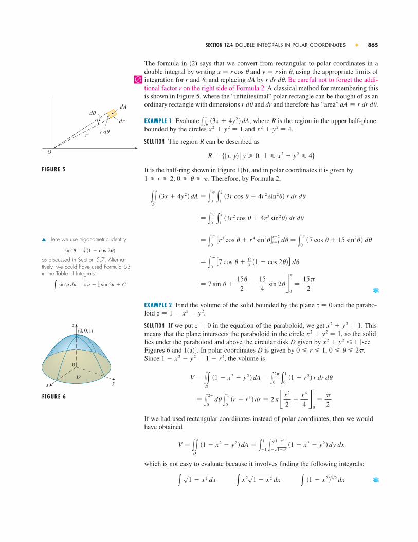
The formula in (2) says that we convert from rectangular to polar coordinates in a double integral by writing and , using the appropriate limits of
| integration for and , and replacing by . Be careful not to forget the addi-tional factor r on the right side of Formula 2. A classical method for remembering thisis shown in Figure 5, where the “infinitesimal” polar rectangle can be thought of as anordinary rectangle with dimensions and and therefore has “area”
EXAMPLE 1 Evaluate , where is the region in the upper half-planebounded by the circles and .
SOLUTION The region can be described as
It is the half-ring shown in Figure 1(b), and in polar coordinates it is given by, . Therefore, by Formula 2,
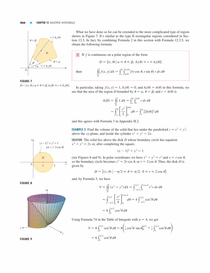
EXAMPLE 2 Find the volume of the solid bounded by the plane and the parabo-loid .
SOLUTION If we put in the equation of the paraboloid, we get . Thismeans that the plane intersects the paraboloid in the circle , so the solidlies under the paraboloid and above the circular disk given by [seeFigures 6 and 1(a)]. In polar coordinates is given by , .Since , the volume is
If we had used rectangular coordinates instead of polar coordinates, then we wouldhave obtained
which is not easy to evaluate because it involves finding the following integrals:
y �1 � x 2 �3�2 dxy x 2s1 � x 2 dxy s1 � x 2 dx
V � yyD
�1 � x 2 � y 2 � dA � y1
�1 y
s1�x2
�s1�x2 �1 � x 2 � y 2 � dy dx
� y2�
0 d� y
1
0 �r � r 3 � dr � 2� r 2
2�
r 4
4 �0
1
��
2
V � yyD
�1 � x 2 � y 2 � dA � y2�
0 y
1
0 �1 � r 2 � r dr d�
1 � x 2 � y 2 � 1 � r 20 � � � 2�0 � r � 1D
x 2 � y 2 � 1Dx 2 � y 2 � 1
x 2 � y 2 � 1z � 0
z � 1 � x 2 � y 2z � 0
� 7 sin � �15�
2�
15
4 sin 2��
0
�
�15�
2
� y�
0 [7 cos � �
152 �1 � cos 2��] d�
� y�
0 [r 3 cos � � r 4 sin2�]r�1
r�2 d� � y
�
0 �7 cos � � 15 sin2� � d�
� y�
0 y
2
1 �3r 2 cos � � 4r 3 sin2�� dr d�
yyR
�3x � 4y 2 � dA � y�
0 y
2
1 �3r cos � � 4r 2 sin2�� r dr d�
0 � � � �1 � r � 2
R � ��x, y� y � 0, 1 � x 2 � y 2 � 4
R
x 2 � y 2 � 4x 2 � y 2 � 1RxxR �3x � 4y 2 � dA
dA � r dr d�.drr d�
r dr d�dA�ry � r sin �x � r cos �
SECTION 12.4 DOUBLE INTEGRALS IN POLAR COORDINATES � 865
O
d¨
r d¨
dr
dA
r
FIGURE 5
� Here we use trigonometric identity
as discussed in Section 5.7. Alterna-tively, we could have used Formula 63in the Table of Integrals:
y sin2u du � 12 u �
14 sin 2u � C
sin2� � 12 �1 � cos 2��
FIGURE 6
y
0
(0, 0, 1)
D
x
z
What we have done so far can be extended to the more complicated type of regionshown in Figure 7. It’s similar to the type II rectangular regions considered in Sec-tion 12.3. In fact, by combining Formula 2 in this section with Formula 12.3.5, weobtain the following formula.
If is continuous on a polar region of the form
then
In particular, taking , , and in this formula, wesee that the area of the region bounded by , , and is
and this agrees with Formula 3 in Appendix H.2.
EXAMPLE 3 Find the volume of the solid that lies under the paraboloid ,above the -plane, and inside the cylinder .
SOLUTION The solid lies above the disk whose boundary circle has equationor, after completing the square,
(see Figures 8 and 9). In polar coordinates we have and ,so the boundary circle becomes , or . Thus, the disk isgiven by
and, by Formula 3, we have
Using Formula 74 in the Table of Integrals with , we get
� 6 y��2
0 cos2� d�
V � 8 y��2
0 cos4� d� � 8�1
4 cos3� sin �]0
��2� 3
4 y� �2
0cos2� d��
n � 4
� 8 y��2
0 cos4� d�
� y��2
���2 r 4
4 �0
2 cos �
d� � 4 y��2
���2 cos4� d�
V � yyD
�x 2 � y 2 � dA � y��2
���2 y
2 cos �
0 r 2 r dr d�
D � {�r, � � ���2 � � � ��2, 0 � r � 2 cos �}
Dr � 2 cos �r 2 � 2r cos �x � r cos �x 2 � y 2 � r 2
�x � 1�2 � y 2 � 1
x 2 � y 2 � 2xD
x 2 � y 2 � 2xxyz � x 2 � y 2
� y
�
r 2
2 �0
h���
d� � y
� 12 �h����2 d�
A�D� � yyD
1 dA � y
� y
h���
0 r dr d�
r � h���� � � � �Dh2��� � h���h1��� � 0f �x, y� � 1
yyD
f �x, y� dA � y
� y
h2���
h1��� f �r cos �, r sin �� r dr d�
D � ��r, �� � � � � , h1��� � r � h2���
f3
866 � CHAPTER 12 MULTIPLE INTEGRALS
O
∫å r=h¡(¨)
¨=å
¨=∫r=h™(¨)
D
FIGURE 7D=s(r, ¨) | 寨¯∫, h¡(̈ )¯r¯h™(̈ )d
FIGURE 8
FIGURE 9
0
y
x1 2
D
(x-1)@+¥=1
(or r=2 cos ¨)
y
x
z

Now we use Formula 64 in the Table of Integrals:
� 6 �1
2�
�
2�
3�
2
V � 6 y��2
0 cos2� d� � 6[1
2 � �14 sin 2�]0
��2
SECTION 12.4 DOUBLE INTEGRALS IN POLAR COORDINATES � 867
9–14 � Evaluate the given integral by changing to polar coordinates.
9. ,where is the disk with center the origin and radius 3
10. ,where
11. , where D is the region bounded by thesemicircle and the y-axis
12. , where is the region in the first quadrantenclosed by the circle
13. ,where
14. , where is the region in the first quadrant that liesbetween the circles and
� � � � � � � � � � � � �
15–21 � Use polar coordinates to find the volume of the givensolid.
15. Under the paraboloid and above the disk
16. Inside the sphere and outside the cylinder
17. A sphere of radius
18. Bounded by the paraboloid and the plane
19. Above the cone and below the sphere
20. Bounded by the paraboloids and
21. Inside both the cylinder and the ellipsoid
� � � � � � � � � � � � �
22. (a) A cylindrical drill with radius is used to bore a holethrough the center of a sphere of radius . Find the vol-ume of the ring-shaped solid that remains.
(b) Express the volume in part (a) in terms of the height of the ring. Notice that the volume depends only on ,not on or .r2r1
hh
r2
r1
4x 2 � 4y 2 � z2 � 64x 2 � y 2 � 4
z � 4 � x 2 � y 2z � 3x 2 � 3y 2
x 2 � y 2 � z2 � 1z � sx 2 � y 2
z � 4z � 10 � 3x 2 � 3y 2
a
x 2 � y 2 � 4x 2 � y 2 � z 2 � 16
x 2 � y 2 � 9z � x 2 � y 2
x 2 � y 2 � 2xx 2 � y 2 � 4DxxD x dA
R � ��x, y� 1 � x 2 � y 2 � 4, �x � y � xxxR arctan� y�x� dA
x 2 � y 2 � 25Rxx
R yex dA
x � s4 � y 2
xxD e�x 2�y 2 dA
R � ��x, y� 1 � x 2 � y 2 � 9, y � 0xxR sx 2 � y 2 dA
DxxD xy dA
1–6 � A region is shown. Decide whether to use polar coor-dinates or rectangular coordinates and write as an iterated integral, where is an arbitrary continuous func-tion on .
1. 2.
3. 4.
5. 6.
� � � � � � � � � � � � �
7–8 � Sketch the region whose area is given by the integral andevaluate the integral.
7. 8.
� � � � � � � � � � � � �
y��2
0 y
4 cos �
0 r dr d�y
2�
� y
7
4 r dr d�
0
2
y
x
R
2052
5
2
y
x
R
0 31
3
1
y
x
R
0 2
2
y
x
R
0 2
2
y
x
R
0 2
2
y
x
R
Rf
xxR f �x, y� dAR
Exercises � � � � � � � � � � � � � � � � � � � � � � � � � �12.4
� Instead of using tables, we could have used the identity
twice.cos2� � 12 �1 � cos 2��
32. (a) We define the improper integral (over the entire plane
where is the disk with radius and center the origin. Show that
(b) An equivalent definition of the improper integral inpart (a) is
where is the square with vertices . Use thisto show that
(c) Deduce that
(d) By making the change of variable , show that
(This is a fundamental result for probability and statistics.)
33. Use the result of Exercise 32 part (c) to evaluate the follow-ing integrals.
(a) (b) y�
0 sx e�x dxy
�
0 x 2e�x 2 dx
y�
�� e�x 2�2 dx � s2�
t � s2 x
y�
�� e�x 2 dx � s�
y�
�� e�x 2 dx y
�
�� e�y 2 dy � �
��a, �a�Sa
yy� 2
e��x 2�y 2 � dA � lima l �
yySa
e��x 2�y 2 � dA
y�
�� y
�
�� e��x 2�y 2 � dA � �
aDa
� lima l �
yyDa
e��x 2�y 2 � dA
I � yy� 2
e��x 2�y 2 � dA � y�
�� y
�
�� e��x 2�y 2 � dy dx
� 2�23–24 � Use a double integral to find the area of the region.
23. One loop of the rose
24. The region enclosed by the cardioid � � � � � � � � � � � � �
25–28 � Evaluate the iterated integral by converting to polar coordinates.
25.
26.
27. 28.
� � � � � � � � � � � � �
29. A swimming pool is circular with a 40-ft diameter. Thedepth is constant along east-west lines and increaseslinearly from 2 ft at the south end to 7 ft at the north end.Find the volume of water in the pool.
30. An agricultural sprinkler distributes water in a circular pat-tern of radius 100 ft. It supplies water to a depth of feetper hour at a distance of feet from the sprinkler.(a) What is the total amount of water supplied per hour to
the region inside the circle of radius centered at thesprinkler?
(b) Determine an expression for the average amount ofwater per hour per square foot supplied to the regioninside the circle of radius .
31. Use polar coordinates to combine the sum
into one double integral. Then evaluate the double integral.
y1
1�s2 y
x
s1�x 2 xy dy dx � y
s2
1 y
x
0 xy dy dx � y
2
s2 y
s4�x 2
0 xy dy dx
R
R
re�r
y2
0 y
s2x�x 2
0 sx 2 � y 2 dy dxy
2
0 y
s4�y 2
�s4�y 2
x 2 y 2 dx dy
ya
�a y
sa 2�y 2
0 �x 2 � y 2 �3�2 dx dy
y1
0 y
s1�x 2
0 e x 2�y 2 dy dx
r � 1 � sin �
r � cos 3�
868 � CHAPTER 12 MULTIPLE INTEGRALS
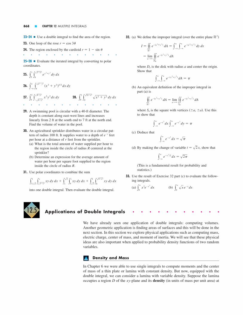
Applications of Double Integrals � � � � � � � � � � �
We have already seen one application of double integrals: computing volumes.Another geometric application is finding areas of surfaces and this will be done in thenext section. In this section we explore physical applications such as computing mass,electric charge, center of mass, and moment of inertia. We will see that these physicalideas are also important when applied to probability density functions of two randomvariables.
Density and Mass
In Chapter 6 we were able to use single integrals to compute moments and the centerof mass of a thin plate or lamina with constant density. But now, equipped with thedouble integral, we can consider a lamina with variable density. Suppose the laminaoccupies a region of the -plane and its density (in units of mass per unit area) at xyD
12.5

a point in is given by , where is a continuous function on . Thismeans that
where and are the mass and area of a small rectangle that contains andthe limit is taken as the dimensions of the rectangle approach 0. (See Figure 1.)
To find the total mass of the lamina we divide a rectangle containing intosubrectangles of the same size (as in Figure 2) and consider to be 0 outside
. If we choose a point in , then the mass of the part of the lamina thatoccupies is approximately , where is the area of . If we add allsuch masses, we get an approximation to the total mass:
If we now increase the number of subrectangles, we obtain the total mass of thelamina as the limiting value of the approximations:
Physicists also consider other types of density that can be treated in the same man-ner. For example, if an electric charge is distributed over a region and the chargedensity (in units of charge per unit area) is given by at a point in , thenthe total charge is given by
EXAMPLE 1 Charge is distributed over the triangular region in Figure 3 so that thecharge density at is , measured in coulombs per square meter(C�m ). Find the total charge.
SOLUTION From Equation 2 and Figure 3 we have
Thus, the total charge is C.
Moments and Centers of Mass
In Section 6.5 we found the center of mass of a lamina with constant density; here weconsider a lamina with variable density. Suppose the lamina occupies a region andhas density function . Recall from Chapter 6 that we defined the moment of a��x, y�
D
524
� 12 y
1
0 �2x 2 � x 3 � dx �
1
2 2x 3
3�
x 4
4 �0
1
�5
24
� y1
0
x y 2
2 �y�1�x
y�1
dx � y1
0 x
2 �12 � �1 � x�2 � dx
Q � yyD
��x, y� dA � y1
0 y
1
1�x xy dy dx
2��x, y� � xy�x, y�
D
Q � yyD
��x, y� dA2
QD�x, y���x, y�
D
m � lim k, l l �
�k
i�1 �
l
j�1 ��xij*, yij*� �A � yy
D
��x, y� dA1
m
m � �k
i�1 �
l
j�1 ��xij*, yij*� �A
Rij�A��xij*, yij*� �ARij
Rij�xij*, yij*�D��x, y�Rij
DRm
�x, y��A�m
��x, y� � lim �m
�A
D���x, y�D�x, y�
SECTION 12.5 APPLICATIONS OF DOUBLE INTEGRALS � 869
FIGURE 1
0 x
y
D
(x, y)
FIGURE 2
Rijy
0 x
(x*ij, y*
ij )
FIGURE 3
1
y
0 x
(1, 1)y=1
y=1-x
D

particle about an axis as the product of its mass and its directed distance from the axis.We divide into small rectangles as in Figure 2. Then the mass of is approximately
, so we can approximate the moment of with respect to the -axis by
If we now add these quantities and take the limit as the number of subrectangles be-comes large, we obtain the moment of the entire lamina about the x-axis:
Similarly, the moment about the y-axis is
As before, we define the center of mass so that and . Thephysical significance is that the lamina behaves as if its entire mass is concentrated atits center of mass. Thus, the lamina balances horizontally when supported at its cen-ter of mass (see Figure 4).
The coordinates of the center of mass of a lamina occupying theregion and having density function are
where the mass is given by
EXAMPLE 2 Find the mass and center of mass of a triangular lamina with vertices, , and if the density function is .
SOLUTION The triangle is shown in Figure 5. (Note that the equation of the upperboundary is .) The mass of the lamina is
� 4 y1
0 �1 � x 2 � dx � 4 x �
x 3
3 �0
1
�8
3
� y1
0
y � 3xy � y 2
2 �y�0
y�2�2x
dx
m � yyD
��x, y� dA � y1
0 y
2�2x
0 �1 � 3x � y� dy dx
y � 2 � 2x
��x, y� � 1 � 3x � y�0, 2��1, 0��0, 0�
m � yyD
��x, y� dA
m
y �Mx
m�
1
m yy
D
y��x, y� dAx �My
m�
1
m yy
D
x��x, y� dA
��x, y�D�x, y�5
my � Mxmx � My�x, y�
My � lim m, n l �
�m
i�1 �
n
j�1 xij* ��xij*, yij*� �A � yy
D
x��x, y� dA4
Mx � lim m, n l �
�m
i�1 �
n
j�1 yij* ��xij*, yij*� �A � yy
D
y��x, y� dA3
���xij*, yij*� �A� yij*
xRij��xij*, yij*� �ARijD
870 � CHAPTER 12 MULTIPLE INTEGRALS
FIGURE 4
D(x, y)
FIGURE 5
0
y
x(1, 0)
(0, 2)
y=2-2x
” , ’38
1116
D

Then the formulas in (5) give
The center of mass is at the point .
EXAMPLE 3 The density at any point on a semicircular lamina is proportional to thedistance from the center of the circle. Find the center of mass of the lamina.
SOLUTION Let’s place the lamina as the upper half of the circle (see Fig-ure 6). Then the distance from a point to the center of the circle (the origin) is
. Therefore, the density function is
where is some constant. Both the density function and the shape of the laminasuggest that we convert to polar coordinates. Then and the region is given by , . Thus, the mass of the lamina is
Both the lamina and the density function are symmetric with respect to the -axis, sothe center of mass must lie on the -axis, that is, . The -coordinate is given by
Therefore, the center of mass is located at the point .�0, 3a��2���
�3
�a 3 2a 4
4�
3a
2�
�3
�a3 y�
0 sin � d� y
a
0 r3 dr �
3
�a 3 [�cos �]0� r 4
4 �0
a
y �1
m yy
D
y��x, y� dA �3
K�a3 y�
0y
a
0 r sin � ��r� r dr d�
yx � 0yy
� K� r 3
3 �0
a
�K�a 3
3
� y�
0 y
a
0 �Kr� r dr d� � K y
�
0 d� y
a
0 r 2 dr
m � yyD
��x, y� dA � yyD
Ksx 2 � y 2 dA
0 � � � �0 � r � aDsx 2 � y 2 � r
K
��x, y� � Ksx 2 � y 2
sx 2 � y 2
�x, y�x 2 � y 2 � a 2
( 38 , 11
16 )
�1
4 7x � 9
x 2
2� x 3 � 5
x 4
4 �0
1
�11
16
� 14 y
1
0 �7 � 9x � 3x 2 � 5x 3 � dx �
3
8 y
1
0
y 2
2� 3x
y 2
2�
y 3
3 �y�0
y�2�2x
dx
y �1
m yy
D
y��x, y� dA � 38 y
1
0 y
2�2x
0 �y � 3xy � y 2 � dy dx
�3
2 y
1
0 �x � x 3 � dx � x 2
2�
x 4
4 �0
1
�3
8
�3
8 y
1
0
xy � 3x 2y � x y 2
2 �y�0
y�2�2x
dx
x �1
m yy
D
x��x, y� dA � 38 y
1
0 y
2�2x
0 �x � 3x 2 � xy� dy dx
SECTION 12.5 APPLICATIONS OF DOUBLE INTEGRALS � 871
FIGURE 6
0
y
xa_a
a
D
≈+¥=a@
”0, ’3a2π
� Compare the location of the center of mass in Example 3 with Example 6 in Section 6.5 where we found that the center of mass of a lamina with the same shape but uniform density islocated at the point .�0, 4a��3���

Moment of Inertia
The moment of inertia (also called the second moment) of a particle of mass about an axis is defined to be , where is the distance from the particle to the axis.We extend this concept to a lamina with density function and occupying aregion by proceeding as we did for ordinary moments. We divide into small rect-angles, approximate the moment of inertia of each subrectangle about the -axis, andtake the limit of the sum as the number of subrectangles becomes large. The result isthe moment of inertia of the lamina about the x-axis:
Similarly, the moment of inertia about the y-axis is
It is also of interest to consider the moment of inertia about the origin, also calledthe polar moment of inertia:
Note that .
EXAMPLE 4 Find the moments of inertia , , and of a homogeneous disk withdensity , center the origin, and radius .
SOLUTION The boundary of is the circle and in polar coordinates isdescribed by , . Let’s compute first:
Instead of computing and directly, we use the facts that and (from the symmetry of the problem). Thus
In Example 4 notice that the mass of the disk is
m � density � area � ���a 2 �
Ix � Iy �I0
2�
��a 4
4
Ix � IyIx � Iy � I0IyIx
� � y2�
0 d� y
a
0 r 3dr � 2�� r 4
4 �0
a
���a 4
2
I0 � yyD
�x 2 � y 2 �� dA � � y2�
0 y
a
0 r 2 r dr d�
I00 � r � a0 � � � 2�Dx 2 � y 2 � a 2D
a��x, y� � �DI0IyIx
I0 � Ix � Iy
I0 � lim m, n l �
�m
i�1 �
n
j�1 ��xij*�2 � �yij*�2� ��xij*, yij*� �A � yy
D
�x 2 � y 2 ���x, y� dA8
Iy � lim m, n l �
�m
i�1 �
n
j�1 �xij*�2��xij*, yij*� �A � yy
D
x 2��x, y� dA7
Ix � lim m, n l �
�m
i�1 �
n
j�1 �yij*�2��xij*, yij*� �A � yy
D
y 2��x, y� dA6
xDD
��x, y�rmr 2
m
872 � CHAPTER 12 MULTIPLE INTEGRALS

so the moment of inertia of the disk about the origin (like a wheel about its axle) canbe written as
Thus, if we increase the mass or the radius of the disk, we thereby increase the mo-ment of inertia. In general, the moment of inertia plays much the same role in rota-tional motion that mass plays in linear motion. The moment of inertia of a wheel iswhat makes it difficult to start or stop the rotation of the wheel, just as the mass of acar is what makes it difficult to start or stop the motion of the car.
Probability
In Section 6.7 we considered the probability density function of a continuous ran-dom variable X. This means that for all x, , and the proba-bility that X lies between a and b is found by integrating f from a to b:
Now we consider a pair of continuous random variables X and Y, such as the life-times of two components of a machine or the height and weight of an adult femalechosen at random. The joint density function of X and Y is a function f of two vari-ables such that the probability that lies in a region D is
In particular, if the region is a rectangle, the probability that X lies between a and band Y lies between c and d is
(See Figure 7.)
The probability that X lies between a and b and Y lies between c and d is the volume that liesabove the rectangle D=[a, b]x[c, d] and below the graph of the joint density function.
c
d
yx
z
a
D
b
z=f(x, y)
FIGURE 7
P�a � X � b, c � Y � d � � yb
a y
d
c f �x, y� dy dx
P��X, Y� � D� � yyD
f �x, y� dA
�X, Y�
P�a � X � b� � yb
a f �x� dx
x�
�� f �x� dx � 1f �x� � 0
f
I0 � 12 ma 2
SECTION 12.5 APPLICATIONS OF DOUBLE INTEGRALS � 873

Because probabilities aren’t negative and are measured on a scale from 0 to 1, thejoint density function has the following properties:
As in Exercise 32 in Section 12.4, the double integral over is an improper integraldefined as the limit of double integrals over expanding circles or squares and we canwrite
EXAMPLE 5 If the joint density function for X and Y is given by
find the value of the constant C. Then find .
SOLUTION We find the value of C by ensuring that the double integral of f is equal to 1. Because outside the rectangle , we have
Therefore, and so .Now we can compute the probability that X is at most 7 and Y is at least 2:
Suppose X is a random variable with probability density function and Y is arandom variable with density function . Then X and Y are called independentrandom variables if their joint density function is the product of their individual den-sity functions:
In Section 6.7 we modeled waiting times by using exponential density functions
where is the mean waiting time. In the next example we consider a situation withtwo independent waiting times.
�
f �t� � �0
��1e�t��
if t 0
if t � 0
f �x, y� � f1�x� f2�y�
f2�y�f1�x�
�868
1500� 0.5787
�1
1500 y
7
0 [xy � y 2]y�2
y�10 dx �1
1500 y
7
0 �8x � 96� dx
P�X � 7, Y � 2� � y7
�� y
�
2 f �x, y� dy dx � y
7
0 y
10
2 11500 �x � 2y� dy dx
C � 115001500C � 1
� C y10
0 �10x � 100� dx � 1500C
y�
�� y
�
�� f �x, y� dy dx � y
10
0 y
10
0 C�x � 2y� dy dx � C y
10
0 [xy � y 2]y�0
y�10 dx
�0, 10� � �0, 10�f �x, y� � 0
P�X � 7, Y � 2�
f �x, y� � �0
C�x � 2y�otherwise
if 0 � x � 10, 0 � y � 10
yy�2
f �x, y� dA � y�
�� y
�
�� f �x, y� dx dy � 1
�2
yy�2
f �x, y� dA � 1f �x, y� � 0
874 � CHAPTER 12 MULTIPLE INTEGRALS

EXAMPLE 6 The manager of a movie theater determines that the average time movie-goers wait in line to buy a ticket for this week’s film is 10 minutes and the averagetime they wait to buy popcorn is 5 minutes. Assuming that the waiting times areindependent, find the probability that a moviegoer waits a total of less than 20 min-utes before taking his or her seat.
SOLUTION Assuming that both the waiting time X for the ticket purchase and the wait-ing time Y in the refreshment line are modeled by exponential probability densityfunctions, we can write the individual density functions as
Since X and Y are independent, the joint density function is the product:
We are asked for the probability that :
where D is the triangular region shown in Figure 8. Thus
This means that about 75% of the moviegoers wait less than 20 minutes beforetaking their seats.
Expected Values
Recall from Section 6.7 that if X is a random variable with probability density func-tion , then its mean is
Now if X and Y are random variables with joint density function f, we define the X-mean and Y-mean, also called the expected values of X and Y, to be
�2 � yy�2
yf �x, y� dA�1 � yy�2
x f �x, y� dA9
� � y�
�� x f �x� dx
f
� 110 y
20
0 �e�x�10 � e�4ex�10 � dx � 1 � e�4 � 2e�2 � 0.7476
� 110 y
20
0 e�x�10�1 � e �x�20��5 � dx
� 150 y
20
0 [e�x�10��5�e�y�5]y�0
y�20�xdx
P�X � Y 20� � yyD
f �x, y� dA � y20
0 y
20�x
0 150 e�x�10e�y�5 dy dx
P�X � Y 20� � P��X, Y� � D�
X � Y 20
f �x, y� � f1�x� f2�y� � � 150 e�x�10e�y�5
0
if x � 0, y � 0
otherwise
f2�y� � �015 e�y�5
if y 0
if y � 0f1�x� � �0
110 e�x�10
if x 0
if x � 0
SECTION 12.5 APPLICATIONS OF DOUBLE INTEGRALS � 875
FIGURE 8
20
20
D
0
y
x
x+y=20

Notice how closely the expressions for and in (9) resemble the moments andof a lamina with density function in Equations 3 and 4. In fact, we can think of
probability as being like continuously distributed mass. We calculate probability theway we calculate mass—by integrating a density function. And because the total“probability mass” is 1, the expressions for and in (5) show that we can think ofthe expected values of X and Y, and , as the coordinates of the “center of mass”of the probability distribution.
In the next example we deal with normal distributions. As in Section 6.7, a singlerandom variable is normally distributed if its probability density function is of theform
where is the mean and is the standard deviation.
EXAMPLE 7 A factory produces (cylindrically shaped) roller bearings that are sold ashaving diameter 4.0 cm and length 6.0 cm. In fact, the diameters X are normallydistributed with mean 4.0 cm and standard deviation 0.01 cm while the lengths Y arenormally distributed with mean 6.0 cm and standard deviation 0.01 cm. Assumingthat X and Y are independent, write the joint density function and graph it. Find theprobability that a bearing randomly chosen from the production line has eitherlength or diameter that differs from the mean by more than 0.02 cm.
SOLUTION We are given that X and Y are normally distributed with ,and . So the individual density functions for X and Y are
Since X and Y are independent, the joint density function is the product:
A graph of this function is shown in Figure 9.Let’s first calculate the probability that both X and Y differ from their means by
less than 0.02 cm. Using a calculator or computer to estimate the integral, we have
Then the probability that either X or Y differs from its mean by more than 0.02 cm isapproximately
1 � 0.91 � 0.09
� 0.91
�5000
� y
4.02
3.98 y
6.02
5.98 e�5000��x�4�2�� y�6�2� dy dx
P�3.98 X 4.02, 5.98 Y 6.02� � y4.02
3.98 y
6.02
5.98 f �x, y� dy dx
�5000
� e�5000��x�4�2�� y�6�2�
f �x, y� � f1�x� f2�y� �1
0.0002� e��x�4�2�0.0002e��y�6�2�0.0002
f2�y� �1
0.01s2� e�� y�6�2�0.0002f1�x� �
1
0.01s2� e��x�4�2�0.0002
�1 � �2 � 0.01�2 � 6.0,�1 � 4.0
��
f �x� �1
�s2� e��x���2��2� 2�
�2�1
yx
�My
Mx�2�1
876 � CHAPTER 12 MULTIPLE INTEGRALS
FIGURE 9Graph of the bivariate normal jointdensity function in Example 7
1500
1000
500
0
y6.05
65.95
x
4.05
4
3.95

SECTION 12.5 APPLICATIONS OF DOUBLE INTEGRALS � 877
17–18 � Use a computer algebra system to find the mass, cen-ter of mass, and moments of inertia of the lamina that occupiesthe region and has the given density function.
17. ;
18. is enclosed by the cardioid ;
� � � � � � � � � � � � �
19. The joint density function for a pair of random variables and is
(a) Find the value of the constant .(b) Find .(c) Find .
20. (a) Verify that
is a joint density function.(b) If and are random variables whose joint density
function is the function in part (a), find
(i) (ii)(c) Find the expected values of and .
21. Suppose and are random variables with joint density function
(a) Verify that is indeed a joint density function.(b) Find the following probabilities.
(i) (ii)(c) Find the expected values of and .
22. (a) A lamp has two bulbs of a type with an average lifetimeof 1000 hours. Assuming that we can model the proba-bility of failure of these bulbs by an exponential densityfunction with mean , find the probability thatboth of the lamp’s bulbs fail within 1000 hours.
(b) Another lamp has just one bulb of the same type as inpart (a). If one bulb burns out and is replaced by a bulb of the same type, find the probability that the two bulbsfail within a total of 1000 hours.
23. Suppose that and are independent random variables,where is normally distributed with mean 45 and standarddeviation 0.5 and is normally distributed with mean 20and standard deviation 0.1.(a) Find .(b) Find .P�4�X � 45�2 � 100�Y � 20�2 � 2�
P�40 � X � 50, 20 � Y � 25�
YX
YXCAS
� � 1000
YXP�X � 2, Y � 4�P�Y � 1�
f
f �x, y� � �0.1e��0.5x�0.2y�
0
if x � 0, y � 0
otherwise
YX
YXP(X �
12 , Y �
12 )P(X �
12 )
fYX
f �x, y� � �4xy
0
if 0 � x � 1, 0 � y � 1
otherwise
P�X � Y � 1�P�X � 1, Y � 1�
C
f �x, y� � �Cx�1 � y�0
if 0 � x � 1, 0 � y � 2
otherwise
YX
��x, y� � sx 2 � y 2
r � 1 � cos �D
��x, y� � xyD � ��x, y� 0 � y � sin x, 0 � x � �
D
CAS1. Electric charge is distributed over the rectangle ,so that the charge density at is
(measured in coulombs per squaremeter). Find the total charge on the rectangle.
2. Electric charge is distributed over the disk so that the charge density at is
(measured in coulombs persquare meter). Find the total charge on the disk.
3–8 � Find the mass and center of mass of the lamina that occupies the region and has the given density function .
3. ;
4. ;
5. is the triangular region with vertices , , ;
6. is bounded by the parabola and the -axis;
7. is bounded by the parabola and the line ;
8. ;� � � � � � � � � � � � �
9. A lamina occupies the part of the disk in thefirst quadrant. Find its center of mass if the density at anypoint is proportional to its distance from the -axis.
10. Find the center of mass of the lamina in Exercise 9 if the density at any point is proportional to the square of its dis-tance from the origin.
11. Find the center of mass of a lamina in the shape of anisosceles right triangle with equal sides of length if thedensity at any point is proportional to the square of the dis-tance from the vertex opposite the hypotenuse.
12. A lamina occupies the region inside the circle but outside the circle . Find the center of massif the density at any point is inversely proportional to itsdistance from the origin.
13. Find the moments of inertia , , for the lamina of Exercise 3.
14. Find the moments of inertia , , for the lamina of Exercise 10.
15. Find the moments of inertia , , for the lamina of Exercise 7.
16. Consider a square fan blade with sides of length 2 and thelower left corner placed at the origin. If the density of theblade is , is it more difficult to rotate the blade about the -axis or the -axis?yx
��x, y� � 1 � 0.1x
I0IyIx
I0IyIx
I0IyIx
x 2 � y 2 � 1x 2 � y 2 � 2y
a
x
x 2 � y 2 � 1
��x, y� � xD � ��x, y� 0 � y � cos x, 0 � x � ��2
��x, y� � 3y � x � 2x � y 2D
��x, y� � yxy � 9 � x 2D
��x, y� � x � y�0, 3��2, 1��0, 0�D
��x, y� � cxyD � ��x, y� 0 � x � a, 0 � y � b
��x, y� � xy 2D � ��x, y� 0 � x � 2, �1 � y � 1
�D
��x, y� � x � y � x 2 � y 2�x, y�x 2 � y 2 � 4
��x, y� � 2xy � y 2�x, y�0 � y � 2
1 � x � 3
Exercises � � � � � � � � � � � � � � � � � � � � � � � � � �12.5

tance between them. Consider a circular city of radius 10 miin which the population is uniformly distributed. For anuninfected individual at a fixed point , assume thatthe probability function is given by
where denotes the distance between and .(a) Suppose the exposure of a person to the disease is the
sum of the probabilities of catching the disease from allmembers of the population. Assume that the infectedpeople are uniformly distributed throughout the city,with infected individuals per square mile. Find a double integral that represents the exposure of a personresiding at .
(b) Evaluate the integral for the case in which is the cen-ter of the city and for the case in which is located onthe edge of the city. Where would you prefer to live?
AA
A
k
APd�P, A�
f �P� � 120 �20 � d�P, A��
A�x0, y0 �
24. Xavier and Yolanda both have classes that end at noon andthey agree to meet every day after class. They arrive at thecoffee shop independently. Xavier’s arrival time is andYolanda’s arrival time is , where and are measured inminutes after noon. The individual density functions are
(Xavier arrives sometime after noon and is more likely toarrive promptly than late. Yolanda always arrives by 12:10 P.M. and is more likely to arrive late than promptly.)After Yolanda arrives, she’ll wait for up to half an hour forXavier, but he won’t wait for her. Find the probability thatthey meet.
25. When studying the spread of an epidemic, we assume thatthe probability that an infected individual will spread thedisease to an uninfected individual is a function of the dis-
f2�y� � � 150 y
0
if 0 � y � 10
otherwisef1�x� � �e�x
0
if x � 0
if x 0
YXYX
Surface Area � � � � � � � � � � � � � � � � �
In this section we apply double integrals to the problem of computing the area of asurface. We start by finding a formula for the area of a parametric surface and then, asa special case, we deduce a formula for the surface area of the graph of a function oftwo variables.
We recall from Section 10.5 that a parametric surface is defined by a vector-valued function of two parameters
or, equivalently, by parametric equations
where varies throughout a region in the -plane.We will find the area of by dividing into patches and approximating the area of
each patch by the area of a piece of a tangent plane. So first let’s recall from Sec-tion 11.4 how to find tangent planes to parametric surfaces.
Let be a point on with position vector . If we keep constant by put-ting , then becomes a vector function of the single parameter anddefines a grid curve lying on . (See Figure 1.) The tangent vector to at isobtained by taking the partial derivative of with respect to :
Similarly, if we keep constant by putting , we get a grid curve given bythat lies on , and its tangent vector at is
ru ��x
�u �u0, v0� i �
�y
�u �u0, v0� j �
�z
�u �u0, v0� k3
P0Sr�u, v0 �C2v � v0v
rv ��x
�v �u0, v0� i �
�y
�v �u0, v0� j �
�z
�v �u0, v0� k2
vrP0C1SC1
vr�u0, v�u � u0
ur�u0, v0 �SP0
SSuvD�u, v�
x � x�u, v� y � y�u, v� z � z�u, v�
r�u, v� � x�u, v� i � y�u, v� j � z�u, v� k1
S
12.6
878 � CHAPTER 12 MULTIPLE INTEGRALS
FIGURE 1
0 u
D
√=√¸
(u¸, √¸)
u=u¸
√
0
z
yx
C¡
C™
rur√
P¸
r
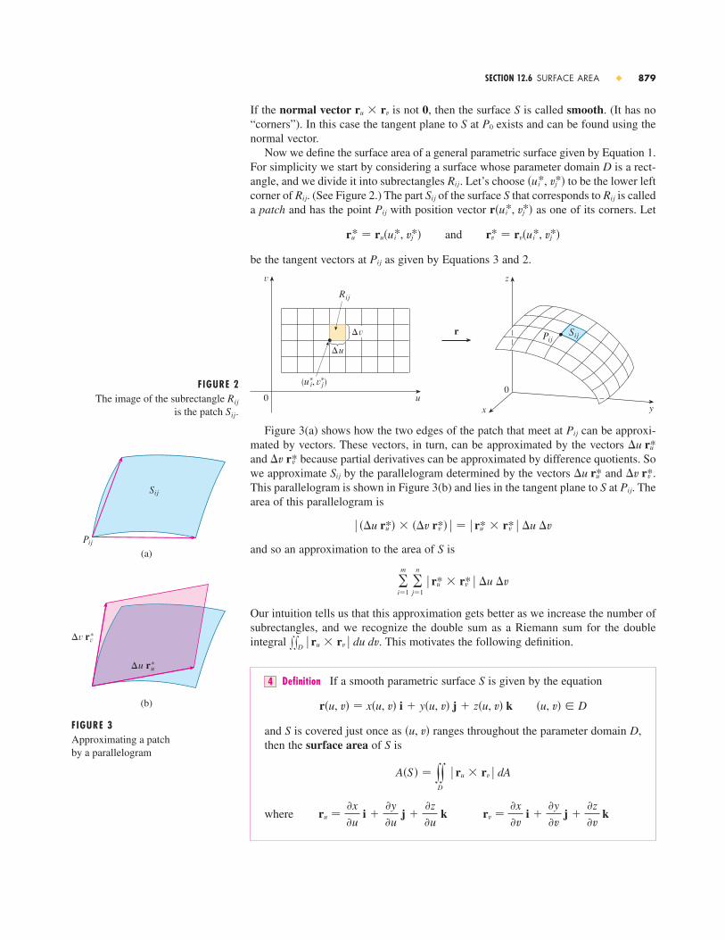
If the normal vector is not , then the surface is called smooth. (It has no“corners”). In this case the tangent plane to at exists and can be found using thenormal vector.
Now we define the surface area of a general parametric surface given by Equation 1.For simplicity we start by considering a surface whose parameter domain is a rect-angle, and we divide it into subrectangles . Let’s choose to be the lower leftcorner of . (See Figure 2.) The part of the surface that corresponds to is calleda patch and has the point with position vector as one of its corners. Let
be the tangent vectors at as given by Equations 3 and 2.
Figure 3(a) shows how the two edges of the patch that meet at can be approxi-mated by vectors. These vectors, in turn, can be approximated by the vectors and because partial derivatives can be approximated by difference quotients. Sowe approximate by the parallelogram determined by the vectors and .This parallelogram is shown in Figure 3(b) and lies in the tangent plane to at Thearea of this parallelogram is
and so an approximation to the area of is
Our intuition tells us that this approximation gets better as we increase the number ofsubrectangles, and we recognize the double sum as a Riemann sum for the doubleintegral . This motivates the following definition.
Definition If a smooth parametric surface is given by the equation
and is covered just once as ranges throughout the parameter domain ,then the surface area of is
where rv ��x
�v i �
�y
�v j �
�z
�v kru �
�x
�u i �
�y
�u j �
�z
�u k
A�S � � yyD
ru � rv dA
SD�u, v�S
�u, v� � Dr�u, v� � x�u, v� i � y�u, v� j � z�u, v� k
S4
xxD ru � rv du dv
�m
i�1 �
n
j�1 ru* � rv* �u �v
S
��u ru*� � ��v rv*� � ru* � rv* �u �v
Pij.S�v rv*�u ru*Sij
�v rv*�u ru*
Pij
FIGURE 2The image of the subrectangle Rij
is the patch Sij.
0
y
z
x
PijSijr
(u*i, √*
j)
0 u
√
Îu
Î√
Rij
Pij
rv* � rv�ui*, vj*�andru* � ru�ui*, vj*�
r�ui*, vj*�Pij
RijSSijRij
�ui*, vj*�Rij
D
P0SS0ru � rv
SECTION 12.6 SURFACE AREA � 879
FIGURE 3Approximating a patchby a parallelogram
(b)
Î√ r*√
Îu r*u
(a)Pij
Sij

EXAMPLE 1 Find the surface area of a sphere of radius .
SOLUTION In Example 4 in Section 10.5 we found the parametric representation
where the parameter domain is
We first compute the cross product of the tangent vectors:
Thus
since for . Therefore, by Definition 4, the area of the sphere is
Surface Area of a Graph
For the special case of a surface with equation , where lies in andhas continuous partial derivatives, we take and as parameters. The parametric
equations are
so
and
rx � ry � i
1
0
j
0
1
k�f
�x
�f
�y � �
�f
�x i �
�f
�y j � k5
ry � j � � �f
�y� krx � i � � �f
�x� k
z � f �x, y�y � yx � x
yxfD�x, y�z � f �x, y�S
� a 2 y2�
0 d� y
�
0 sin � d� � a 2�2��2 � 4�a 2
A � yyD
r� � r� dA � y2�
0 y
�
0 a 2 sin � d� d�
0 � � � �sin � � 0
� sa 4 sin4� � a 4 sin2� cos2� � a 2ssin2� � a 2 sin �
r� � r� � sa 4 sin4� cos2� � a 4 sin 4� sin2� � a 4 sin2� cos2�
� a 2 sin2� cos � i � a 2 sin2� sin � j � a 2 sin � cos � k
r� � r� � i�x
��
�x
��
j�y
��
�y
��
k�z
��
�z
�� � i
�a cos � cos �
�a sin � sin �
ja cos � sin �
a sin � cos �
k�a sin �
0
D � ���, �� 0 � � � �, 0 � � � 2�
z � a cos �y � a sin � sin �x � a sin � cos �
a
880 � CHAPTER 12 MULTIPLE INTEGRALS

Thus, the surface area formula in Definition 4 becomes
EXAMPLE 2 Find the area of the part of the paraboloid that lies under theplane .
SOLUTION The plane intersects the paraboloid in the circle , . There-fore, the given surface lies above the disk with center the origin and radius 3. (SeeFigure 4.) Using Formula 6, we have
Converting to polar coordinates, we obtain
A common type of surface is a surface of revolution obtained by rotating thecurve , , about the -axis, where and is continuous. InExercise 23 you are asked to use a parametric representation of and Definition 4 toprove the following formula for the area of a surface of revolution:
A � 2� yb
a f �x�s1 � � f ��x��2 dx7
Sf �f �x� � 0xa � x � by � f �x�
S
� 2� ( 18 ) 2
3 �1 � 4r 2 �3�2 ]03
��
6 (37s37 � 1)
A � y2�
0 y
3
0 s1 � 4r 2 r dr d� � y
2�
0 d� y
3
0 rs1 � 4r 2 dr
� yyD
s1 � 4�x 2 � y 2 � dA
A � yyD
�1 � � �z
�x�2
� � �z
�y�2
dA � yyD
s1 � �2x� 2 � �2y� 2 dA
Dz � 9x 2 � y 2 � 9
z � 9z � x 2 � y 2
A�S � � yyD
�1 � � �z
�x�2
� � �z
�y�2
dA6
SECTION 12.6 SURFACE AREA � 881
� Notice the similarity between the surface area formula in Equation 6 and the arc length formula
from Section 6.3.
L � yb
a �1 � �dy
dx�2
dx
FIGURE 4
x
z
y3
D
9
6. The part of the surface that lies above the tri-angle with vertices , , and
7. The surface with parametric equations , ,,
8. The helicoid (or spiral ramp) with vector equation, ,
9. The part of the surface that lies between theplanes , , , and
10. The part of the paraboloid that lies inside thecylinder
11. The part of the surface that lies within the cylinderx 2 � y 2 � 1
z � xy
y 2 � z2 � 9x � y 2 � z2
z � 1z � 0x � 1x � 0y � 4x � z2
0 � v � �0 � u � 1r�u, v� � u cos v i � u sin v j � v k
u 2 � v2 � 1z � u � vy � u � vx � uv
�0, 1��1, 1��0, 0�z � x � y 21–12 � Find the area of the surface.
1. The part of the plane that lies above the rectangle
2. The part of the plane that lies inside thecylinder
3. The part of the plane that lies in the first octant
4. The part of the plane with vector equationthat is given by
,
5. The part of the hyperbolic paraboloid that liesbetween the cylinders and x 2 � y 2 � 4x 2 � y 2 � 1
z � y 2 � x 2
0 � v � 10 � u � 1r�u, v� � �1 � v, u � 2v, 3 � 5u � v�
3x � 2y � z � 6
x 2 � y 2 � 92x � 5y � z � 10
�0, 5� � �1, 4�z � 2 � 3x � 4y
Exercises � � � � � � � � � � � � � � � � � � � � � � � � � �12.6

; (b) Use the parametric equations in part (a) to graph thehyperboloid for the case , , .
(c) Set up, but do not evaluate, a double integral for the sur-face area of the part of the hyperboloid in part (b) thatlies between the planes and .
21. Find the area of the part of the sphere that lies inside the paraboloid .
22. The figure shows the surface created when the cylinderintersects the cylinder . Find the
area of this surface.
23. Use Definition 4 and the parametric equations for a surfaceof revolution (see Equations 10.5.3) to derive Formula 7.
24–25 � Use Formula 7 to find the area of the surface obtainedby rotating the given curve about the -axis.
24. , 25. ,� � � � � � � � � � � � �
26. The figure shows the torus obtained by rotating about the -axis the circle in the -plane with center and
radius . Parametric equations for the torus are
where and are the angles shown in the figure. Find thesurface area of the torus.
z
å¨
0
x
y
(x, y, z)
(b, 0, 0)
��
z � a sin �
y � b sin � � a cos � sin �
x � b cos � � a cos � cos �
a b�b, 0, 0�xzz
4 � x � 9y � sx0 � x � 2y � x 3
x
z
yx
x 2 � z 2 � 1y 2 � z 2 � 1
z � x 2 � y 2x 2 � y 2 � z2 � 4z
z � 3z � �3
c � 3b � 2a � 1
12. The surface , ,� � � � � � � � � � � � �
13. (a) Use the Midpoint Rule for double integrals (see Sec-tion 12.1) with four squares to estimate the surface area of the portion of the paraboloid that liesabove the square .
(b) Use a computer algebra system to approximate the sur-face area in part (a) to four decimal places. Comparewith the answer to part (a).
14. (a) Use the Midpoint Rule for double integrals withto estimate the area of the surface
, , .(b) Use a computer algebra system to approximate the sur-
face area in part (a) to four decimal places. Comparewith the answer to part (a).
15. Find the area of the surface with vector equation, ,
. State your answer correct to four decimalplaces.
16. Find, to four decimal places, the area of the part of the surface that lies above the square
. Illustrate by graphing this part of thesurface.
17. Find the exact area of the surface ,, .
18. (a) Set up, but do not evaluate, a double integral for the areaof the surface with parametric equations ,
, , , .(b) Eliminate the parameters to show that the surface is an
elliptic paraboloid and set up another double integral forthe surface area.
; (c) Use the parametric equations in part (a) with andto graph the surface.
(d) For the case , , use a computer algebra system to find the surface area correct to four decimalplaces.
19. (a) Show that the parametric equations ,, , , ,
represent an ellipsoid.
; (b) Use the parametric equations in part (a) to graph theellipsoid for the case , , .
(c) Set up, but do not evaluate, a double integral for the sur-face area of the ellipsoid in part (b).
20. (a) Show that the parametric equations ,, , represent a
hyperboloid of one sheet.z � c sinh uy � b cosh u sin v
x � a cosh u cos v
c � 3b � 2a � 1
0 � v � 2�0 � u � �z � c cos uy � b sin u sin vx � a sin u cos v
b � 3a � 2CAS
b � 3a � 2
0 � v � 2�0 � u � 2z � u 2y � bu sin vx � au cos v
0 � y � 11 � x � 4z � 1 � 2x � 3y � 4y 2CAS
x � y � 1z � �1 � x 2 ���1 � y 2 �
CAS
0 � v � 2�0 � u � �r�u, v� � �cos3u cos3v, sin3u cos3v, sin3v�
CAS
CAS
0 � y � 20 � x � 2z � xy � x 2 � y 2m � n � 2
CAS
�0, 1� � �0, 1�z � x 2 � y 2
0 � y � 10 � x � 1z � 23 �x 3�2 � y 3�2 �
882 � CHAPTER 12 MULTIPLE INTEGRALS
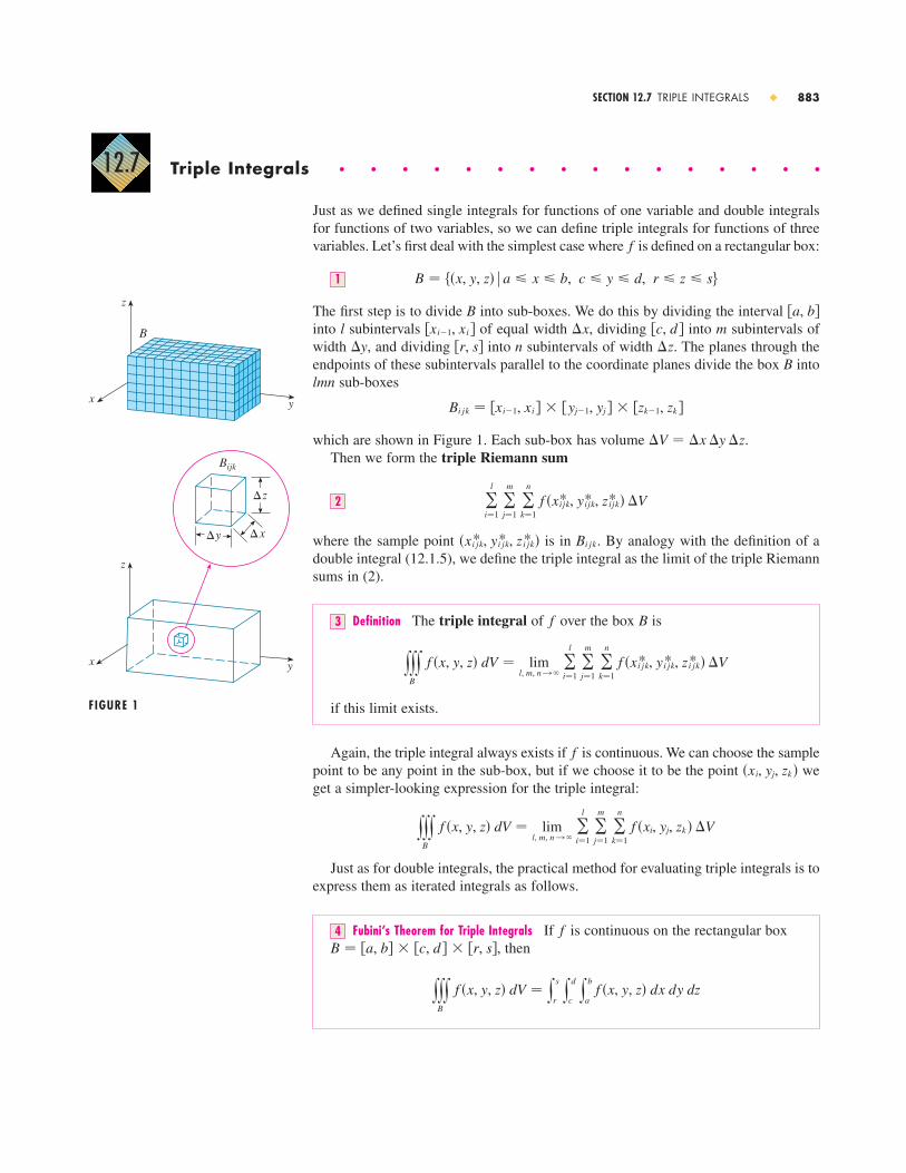
Triple Integrals � � � � � � � � � � � � � � � �
Just as we defined single integrals for functions of one variable and double integralsfor functions of two variables, so we can define triple integrals for functions of threevariables. Let’s first deal with the simplest case where is defined on a rectangular box:
The first step is to divide B into sub-boxes. We do this by dividing the interval into l subintervals of equal width , dividing into m subintervals ofwidth , and dividing into n subintervals of width . The planes through theendpoints of these subintervals parallel to the coordinate planes divide the box into
sub-boxes
which are shown in Figure 1. Each sub-box has volume .Then we form the triple Riemann sum
where the sample point is in . By analogy with the definition of adouble integral (12.1.5), we define the triple integral as the limit of the triple Riemannsums in (2).
Definition The triple integral of over the box is
if this limit exists.
Again, the triple integral always exists if is continuous. We can choose the samplepoint to be any point in the sub-box, but if we choose it to be the point weget a simpler-looking expression for the triple integral:
Just as for double integrals, the practical method for evaluating triple integrals is toexpress them as iterated integrals as follows.
Fubini’s Theorem for Triple Integrals If is continuous on the rectangular box, then
yyyB
f �x, y, z� dV � ys
r y
d
c y
b
a f �x, y, z� dx dy dz
B � �a, b� � �c, d � � �r, s�f4
yyyB
f �x, y, z� dV � lim l, m, n l �
�l
i�1 �
m
j�1 �
n
k�1 f �xi, yj, zk � �V
�xi, yj, zk�f
yyyB
f �x, y, z� dV � lim l, m, n l �
�l
i�1 �
m
j�1 �
n
k�1 f �xi jk* , yi jk* , zi jk* � �V
Bf3
Bi jk�xi jk* , yi jk* , zi jk* �
�l
i�1 �
m
j�1 �
n
k�1 f �xijk* , yijk* , zijk* � �V2
�V � �x �y �z
Bi jk � �xi�1, xi� � �yj�1, yj� � �zk�1, zk�
lmnB
�z�r, s��y�c, d ��x�xi�1, xi �
�a, b�
B � ��x, y, z� a � x � b, c � y � d, r � z � s1
f
12.7
SECTION 12.7 TRIPLE INTEGRALS � 883
FIGURE 1
z
yx
B
z
yx
Bijk
ÎxÎy
Îz

The iterated integral on the right side of Fubini’s Theorem means that we integratefirst with respect to (keeping and fixed), then we integrate with respect to (keep-ing fixed), and finally we integrate with respect to . There are five other possibleorders in which we can integrate, all of which give the same value. For instance, if weintegrate with respect to , then , and then , we have
EXAMPLE 1 Evaluate the triple integral , where is the rectangular boxgiven by
SOLUTION We could use any of the six possible orders of integration. If we choose tointegrate with respect to , then , and then , we obtain
Now we define the triple integral over a general bounded region E in three-dimensional space (a solid) by much the same procedure that we used for double integrals (12.3.2). We enclose in a box of the type given by Equation 1. Then wedefine a function so that it agrees with on but is 0 for points in that are out-side . By definition,
This integral exists if is continuous and the boundary of is “reasonably smooth.”The triple integral has essentially the same properties as the double integral (Proper-ties 6–9 in Section 12.3).
We restrict our attention to continuous functions and to certain simple types ofregions. A solid region is said to be of type 1 if it lies between the graphs of twocontinuous functions of and , that is,
where is the projection of onto the -plane as shown in Figure 2. Notice that theupper boundary of the solid is the surface with equation , while thelower boundary is the surface .
By the same sort of argument that led to (12.3.3), it can be shown that if is a type 1 region given by Equation 5, then
yyyE
f �x, y, z� dV � yyD
yu2�x, y�
u1�x, y� f �x, y, z� dz� dA6
Ez � u1�x, y�
z � u2�x, y�ExyED
E � ��x, y, z� �x, y� � D, u1�x, y� � z � u2�x, y�5
yxE
f
Ef
yyyE
f �x, y, z� dV � yyyB
F�x, y, z� dV
EBEfF
BE
� y3
0 3z2
4 dz �
z3
4 �0
3
�27
4
� y3
0 y
2
�1 yz2
2 dy dz � y
3
0
y 2z2
4 �y��1
y�2
dz
yyyB
xyz2 dV � y3
0 y
2
�1 y
1
0 xyz2 dx dy dz � y
3
0
y2
�1
x 2yz2
2 �x�0
x�1
dy dz
zyx
B � ��x, y, z� 0 � x � 1, �1 � y � 2, 0 � z � 3
BxxxB xyz2 dV
yyyB
f �x, y, z� dV � yb
a y
s
r y
d
c f �x, y, z� dy dz dx
xzy
zzyzyx
884 � CHAPTER 12 MULTIPLE INTEGRALS
FIGURE 2A type 1 solid region
z
0
xyD
E
z=u™ (x, y)
z=u¡ (x, y)
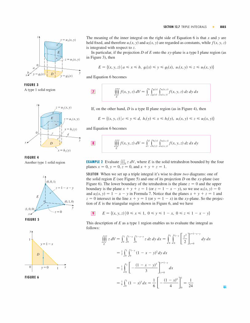
The meaning of the inner integral on the right side of Equation 6 is that and areheld fixed, and therefore and are regarded as constants, while is integrated with respect to .
In particular, if the projection of onto the -plane is a type I plane region (asin Figure 3), then
and Equation 6 becomes
If, on the other hand, is a type II plane region (as in Figure 4), then
and Equation 6 becomes
EXAMPLE 2 Evaluate , where is the solid tetrahedron bounded by the fourplanes , , , and .
SOLUTION When we set up a triple integral it’s wise to draw two diagrams: one of the solid region (see Figure 5) and one of its projection on the -plane (see Figure 6). The lower boundary of the tetrahedron is the plane and the upper boundary is the plane (or ), so we use and in Formula 7. Notice that the planes and
intersect in the line (or ) in the -plane. So the projec-tion of is the triangular region shown in Figure 6, and we have
This description of as a type 1 region enables us to evaluate the integral as follows:
� 16 y
1
0 �1 � x�3 dx �
1
6 �
�1 � x�4
4 �0
1
�1
24
� 12 y
1
0
��1 � x � y�3
3 �y�0
y�1�x
dx
� 12 y
1
0 y
1�x
0 �1 � x � y�2 dy dx
� y1
0
y1�x
0
z2
2 �z�0
z�1�x�y
dy dx yyyE
z dV � y1
0 y
1�x
0 y
1�x�y
0 z dz dy dx
E
E � ��x, y, z� 0 � x � 1, 0 � y � 1 � x, 0 � z � 1 � x � y9
Exyy � 1 � xx � y � 1z � 0
x � y � z � 1u2�x, y� � 1 � x � yu1�x, y� � 0z � 1 � x � yx � y � z � 1
z � 0xyDE
x � y � z � 1z � 0y � 0x � 0Exxx
E z dV
yyyE
f �x, y, z� dV � yd
c y
h2� y�
h1� y� y
u2�x, y�
u1�x, y� f �x, y, z� dz dx dy8
E � ��x, y, z� c � y � d, h1�y� � x � h2�y�, u1�x, y� � z � u2�x, y�
D
yyyE
f �x, y, z� dV � yb
a y
t2�x�
t1�x� y
u2�x, y�
u1�x, y� f �x, y, z� dz dy dx7
E � ��x, y, z� a � x � b, t1�x� � y � t2�x�, u1�x, y� � z � u2�x, y�
xyEDz
f �x, y, z�u2�x, y�u1�x, y�yx
SECTION 12.7 TRIPLE INTEGRALS � 885
FIGURE 3A type 1 solid region
z=u¡(x, y)
z=u™(x, y)
y=g™(x)y=g¡(x)
z
0
yx
a
D
E
b
FIGURE 4Another type 1 solid region
x
0
z
y
c d
z=u™(x, y)
x=h™(y)
x=h¡(y)
z=u¡(x, y)E
D
FIGURE 5
x
0
z
y(1, 0, 0)
(0, 1, 0)
(0, 0, 1)
E
z=1-x-y
z=0
0
y
1
x1y=0
y=1-x
D
FIGURE 6

A solid region is of type 2 if it is of the form
where, this time, is the projection of onto the -plane (see Figure 7). The backsurface is , the front surface is , and we have
Finally, a type 3 region is of the form
where is the projection of onto the -plane, is the left surface, andis the right surface (see Figure 8). For this type of region we have
In each of Equations 10 and 11 there may be two possible expressions for the inte-gral depending on whether is a type I or type II plane region (and corresponding toEquations 7 and 8).
EXAMPLE 3 Evaluate , where is the region bounded by the parab-oloid and the plane .
SOLUTION The solid is shown in Figure 9. If we regard it as a type 1 region, then weneed to consider its projection onto the -plane, which is the parabolic region inFigure 10. (The trace of in the plane is the parabola .)
From we obtain , so the lower boundary surface of is and the upper surface is . Therefore, the descriptionof as a type 1 region is
and so we obtain
yyyE
sx 2 � z 2 dV � y2
�2 y
4
x2 y
sy�x 2
�sy�x2 sx 2 � z 2 dz dy dx
E � {�x, y, z� �2 � x � 2, x 2 � y � 4, �sy � x 2 � z � sy � x 2}
Ez � sy � x 2z � �sy � x 2
Ez � �sy � x 2y � x 2 � z2
x0
y
y=4
y=≈
D¡
FIGURE 10Projection on xy-plane
FIGURE 9Region of integration
x
0
z
y4
y=≈+z@
E
y � x 2z � 0y � x 2 � z2xyD1
E
y � 4y � x 2 � z2Exxx
E sx 2 � z 2 dV
D
yyyE
f �x, y, z� dV � yyD
yu2�x, z�
u1�x, z� f �x, y, z� dy� dA11
y � u2�x, z�y � u1�x, z�xzED
E � ��x, y, z� �x, z� � D, u1�x, z� � y � u2�x, z�
yyyE
f �x, y, z� dV � yyD
yu2� y, z�
u1� y, z� f �x, y, z� dx� dA10
x � u2�y, z�x � u1�y, z�yzED
E � ��x, y, z� �y, z� � D, u1�y, z� � x � u2�y, z�
E
886 � CHAPTER 12 MULTIPLE INTEGRALS
0
z
yx E
D
x=u¡(y, z)
x=u™(y, z)
FIGURE 7A type 2 region
FIGURE 8A type 3 region
x
0
z
yy=u¡(x, z)
DE
y=u™(x, z)

Although this expression is correct, it is extremely difficult to evaluate. So let’sinstead consider as a type 3 region. As such, its projection onto the -plane isthe disk shown in Figure 11.
Then the left boundary of is the paraboloid and the right boundaryis the plane , so taking and in Equation 11, wehave
Although this integral could be written as
it’s easier to convert to polar coordinates in the -plane: , .This gives
Applications of Triple Integrals
Recall that if , then the single integral represents the area under thecurve from to , and if , then the double integral represents the volume under the surface and above . The correspondinginterpretation of a triple integral , where , is not veryuseful because it would be the “hypervolume” of a four-dimensional object and, ofcourse, that is very difficult to visualize. (Remember that is just the domain of thefunction ; the graph of lies in four-dimensional space.) Nonetheless, the triple inte-gral can be interpreted in different ways in different physical situa-tions, depending on the physical interpretations of , , and .
Let’s begin with the special case where for all points in . Then thetriple integral does represent the volume of :
For example, you can see this in the case of a type 1 region by putting in Formula 6:
yyyE
1 dV � yyD
yu2�x, y�
u1�x, y� dz� dA � yy
D
�u2�x, y� � u1�x, y�� dA
f �x, y, z� � 1
V�E � � yyyE
dV12
EEf �x, y, z� � 1
f �x, y, z�zyxxxx
E f �x, y, z� dV
ffE
f �x, y, z� � 0xxxE f �x, y, z� dVDz � f �x, y�
xxD f �x, y� dAf �x, y� � 0bay � f �x�x
ba f �x� dxf �x� � 0
� 2� 4r 3
3�
r 5
5 �0
2
�128�
15
� y2�
0 y
2
0 �4 � r 2 �r r dr d� � y
2�
0 d� y
2
0 �4r 2 � r 4 � dr
yyyE
sx 2 � z 2 dV � yyD3
�4 � x 2 � z 2 �sx 2 � z 2 dA
z � r sin �x � r cos �xz
y2
�2 y
s4�x2
�s4�x2 �4 � x 2 � z2 �sx 2 � z 2 dz dx
� yyD3
�4 � x 2 � z 2 �sx 2 � z 2 dA
yyyE
sx 2 � z 2 dV � yyD3
y4
x2�z2 sx 2 � z 2 dy� dA
u2�x, z� � 4u1�x, z� � x 2 � z2y � 4y � x 2 � z2E
x 2 � z2 � 4xzD3E
SECTION 12.7 TRIPLE INTEGRALS � 887
FIGURE 11Projection on xz-plane
x0
z
≈+z@=4
_2 2
D£
| The most difficult step in evaluating atriple integral is setting up an expressionfor the region of integration (such asEquation 9 in Example 2). Rememberthat the limits of integration in the innerintegral contain at most two variables,the limits of integration in the middle integral contain at most one variable,and the limits of integration in the outerintegral must be constants.

and from Section 12.3 we know this represents the volume that lies between the sur-faces and .
EXAMPLE 4 Use a triple integral to find the volume of the tetrahedron bounded bythe planes , , , and .
SOLUTION The tetrahedron and its projection on the -plane are shown in Figures 12 and 13. The lower boundary of is the plane and the upper boundary is the plane , that is, . Therefore, we have
by the same calculation as in Example 4 in Section 12.3.
(Notice that it is not necessary to use triple integrals to compute volumes. Theysimply give an alternative method for setting up the calculation.)
All the applications of double integrals in Section 12.5 can be immediately ex-tended to triple integrals. For example, if the density function of a solid object thatoccupies the region is , in units of mass per unit volume, at any given point
, then its mass is
and its moments about the three coordinate planes are
Mxy � yyyE
z��x, y, z� dV
Mxz � yyyE
y��x, y, z� dVMyz � yyyE
x��x, y, z� dV14
m � yyyE
��x, y, z� dV13
�x, y, z���x, y, z�E
FIGURE 12 FIGURE 13
y= x2
”1, ’12
x+2y=2 ”or y=1- ’x2
D
y
0
1
x1
(0, 1, 0)
(0, 0, 2)
y
x
0
z
x+2y+z=2x=2y
”1, , 0’12
T
� y1
0 y
1�x�2
x�2 �2 � x � 2y� dy dx � 1
3
V�T� � yyyT
dV � y1
0 y
1�x�2
x�2 y
2�x�2y
0 dz dy dx
z � 2 � x � 2yx � 2y � z � 2z � 0T
xyDT
z � 0x � 0x � 2yx � 2y � z � 2T
z � u2�x, y�z � u1�x, y�
888 � CHAPTER 12 MULTIPLE INTEGRALS

The center of mass is located at the point , where
If the density is constant, the center of mass of the solid is called the centroid of .The moments of inertia about the three coordinate axes are
As in Section 12.5, the total electric charge on a solid object occupying a regionand having charge density is
If we have three continuous random variables X, Y, and Z, their joint density func-tion is a function of three variables such that the probability that lies in E is
In particular,
The joint density function satisfies
EXAMPLE 5 Find the center of mass of a solid of constant density that is bounded bythe parabolic cylinder and the planes , , and .
SOLUTION The solid and its projection onto the -plane are shown in Figure 14.The lower and upper surfaces of are the planes and , so we describe as a type 1 region:
FIGURE 14
0
y
x
x=1x=¥
D
x
0
1
z
y
E
z=x
E � ��x, y, z� �1 � y � 1, y 2 � x � 1, 0 � z � x
Ez � xz � 0ExyE
x � 1z � 0x � zx � y 2
y�
�� y
�
�� y
�
�� f �x, y, z� dz dy dx � 1f �x, y, z� � 0
P�a � X � b, c � Y � d, r � Z � s� � yb
a y
d
c y
s
r f �x, y, z� dz dy dx
P��X, Y, Z� � E � � yyyE
f �x, y, z� dV
�X, Y, Z�
Q � yyyE
��x, y, z� dV
��x, y, z�E
Iz � yyyE
�x 2 � y 2 ���x, y, z� dV
Iy � yyyE
�x 2 � z2 ���x, y, z� dVIx � yyyE
�y 2 � z2 ���x, y, z� dV16
E
z �Mxy
my �
Mxz
mx �
Myz
m15
�x, y, z�
SECTION 12.7 TRIPLE INTEGRALS � 889

Then, if the density is , the mass is
Because of the symmetry of and about the -plane, we can immediately saythat and, therefore, . The other moments are
Therefore, the center of mass is
�x, y, z� � �Myz
m,
Mxz
m,
Mxy
m � � ( 57, 0, 5
14 )
��
3 y
1
0 �1 � y 6 � dy �
2�
7
� � y1
�1
y1
y2
z2
2 �z�0
z�x
dx dy ��
2 y
1
�1 y
1
y2 x 2 dx dy
Mxy � yyyE
z� dV � y1
�1 y
1
y2 y
x
0 z� dz dx dy
�2�
3 y
1
0 �1 � y 6 � dy �
2�
3 y �
y 7
7 �0
1
�4�
7
� � y1
�1 y
1
y2 x 2 dx dy � � y
1
�1
x 3
3 �x�y2
x�1
dy
Myz � yyyE
x� dV � y1
�1 y
1
y2 y
x
0 x� dz dx dy
y � 0Mxz � 0xz�E
� � y �y 5
5 �0
1
�4�
5
��
2 y
1
�1 �1 � y 4 � dy � � y
1
0 �1 � y 4 � dy
� � y1
�1 y
1
y2 x dx dy � � y
1
�1
x 2
2 �x�y2
x�1
dy
m � yyyE
� dV � y1
�1 y
1
y2 y
x
0 � dz dx dy
��x, y, z� � �
890 � CHAPTER 12 MULTIPLE INTEGRALS
3–6 � Evaluate the iterated integral.
3. 4.
5. 6.
� � � � � � � � � � � � �
y1
0 y
z
0 y
y
0 ze�y2
dx dy dzy3
0 y
1
0 y
s1�z 2
0 ze y dx dz dy
y1
0 y
2x
x y
y
0 2xyz dz dy dxy
1
0 y
z
0 y
x�z
0 6xz dy dx dz
1. Evaluate the integral in Example 1, integrating first withrespect to , then , and then .
2. Evaluate the integral , where
using three different orders of integration.
E � ��x, y, z� �1 � x � 1, 0 � y � 2, 0 � z � 1
xxxE �xz � y 3� dV
yxz
Exercises � � � � � � � � � � � � � � � � � � � � � � � � � �12.7

21–22 � Use the Midpoint Rule for triple integrals (Exer-cise 20) to estimate the value of the integral. Divide into eight sub-boxes of equal size.
21. , where
22. , where
� � � � � � � � � � � � �
23–24 � Sketch the solid whose volume is given by the iteratedintegral.
23.
24.
� � � � � � � � � � � � �
25–28 � Express the integral as an iteratedintegral in six different ways, where is the solid bounded bythe given surfaces.
25. , ,
26. , , ,
27. , ,
28.� � � � � � � � � � � � �
29. The figure shows the region of integration for the integral
Rewrite this integral as an equivalent iterated integral in thefive other orders.
0
z
1
x
1 y
z=1-y
y=œ„x
y1
0 y
1
sx y
1�y
0 f �x, y, z� dz dy dx
9x 2 � 4y 2 � z2 � 1
x 2 � 1 � yz � yz � 0
z � y � 2xy � 2x � 0z � 0
y � 6y � 0x 2 � z2 � 4
ExxxE f �x, y, z� dV
y2
0 y
2�y
0 y
4�y 2
0 dx dz dy
y1
0 y
1�x
0 y
2�2z
0 dy dz dx
B � ��x, y, z� 0 � x � 4, 0 � y � 2, 0 � z � 1xxx
B sin�xy 2z 3� dV
B � ��x, y, z� 0 � x � 4, 0 � y � 8, 0 � z � 4
xxxB 1
ln�1 � x � y � z� dV
B7–14 � Evaluate the triple integral.
7. , where
8. , where
9. , where lies under the plane and above the region in the -plane bounded by the curves
, , and
10. , where is the solid tetrahedron with vertices, , , and
11. , where is bounded by the planes , ,, , and
12. , where is bounded by the paraboliccylinder and the planes , , and
13. , where is bounded by the paraboloidand the plane
14. , where is bounded by the cylinder and the planes , , and in the first octant
� � � � � � � � � � � � �
15–18 � Use a triple integral to find the volume of the givensolid.
15. The tetrahedron enclosed by the coordinate planes and theplane
16. The solid bounded by the elliptic cylinder andthe planes and
17. The solid bounded by the cylinder and the planesand
18. The solid enclosed by the paraboloids and
� � � � � � � � � � � � �
19. (a) Express the volume of the wedge in the first octant thatis cut from the cylinder by the planes
and as a triple integral.(b) Use either the Table of Integrals (on the back Reference
Pages) or a computer algebra system to find the exactvalue of the triple integral in part (a).
20. (a) In the Midpoint Rule for triple integrals we use atriple Riemann sum to approximate a triple integral over a box , where is evaluated at the center
of the box . Use the Midpoint Rule to estimate , where is the cube definedby , , . Divide intoeight cubes of equal size.
(b) Use a computer algebra system to approximate the inte-gral in part (a) correct to two decimal places. Comparewith the answer to part (a).
CAS
B0 � z � 10 � y � 10 � x � 1BxxxB e�x 2�y 2�z2 dV
Bijk�xi, yj, zk �f �x, y, z�B
CAS
x � 1y � xy 2 � z2 � 1
z � 18 � x 2 � y 2z � x 2 � y 2
x � z � 1z � 0x � y 2
y � z � 2y � 04x 2 � z2 � 4
2x � y � z � 4
z � 0y � 3xx � 0y 2 � z2 � 9ExxxE z dV
x � 4x � 4y 2 � 4z2ExxxE x dV
z � 0x � yx � zy � x 2ExxxE �x � 2y� dV
x � z � 1y � z � 1z � 0y � 0x � 0ExxxE z dV
�0, 1, 1��1, 1, 0��0, 1, 0��0, 0, 0�ExxxE xz dV
x � 1y � 0y � sxxy
z � 1 � x � yExxxE 6xy dV
E � ��x, y, z� 0 � x � 1, 0 � y � x, x � z � 2xxxxE yz cos�x5 � dV
E � {�x, y, z� 0 � y � 2, 0 � x � s4 � y 2, 0 � z � y}xxxE 2x dV
SECTION 12.7 TRIPLE INTEGRALS � 891
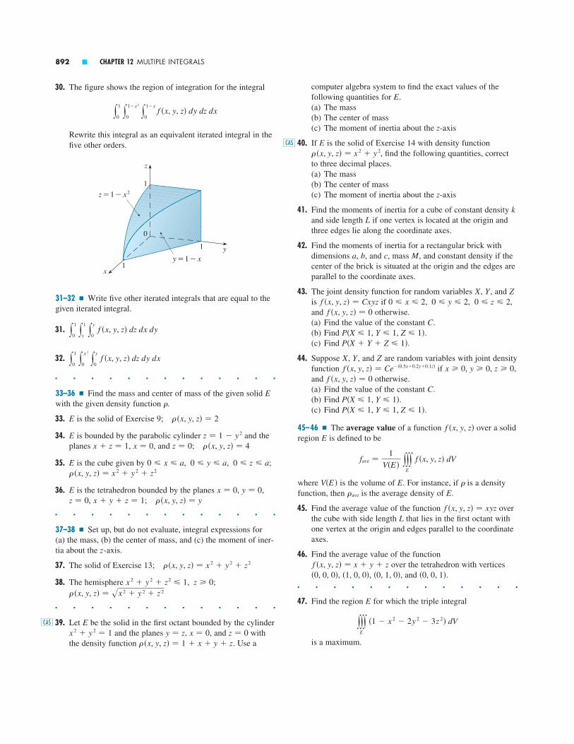
computer algebra system to find the exact values of the following quantities for .(a) The mass(b) The center of mass(c) The moment of inertia about the -axis
40. If is the solid of Exercise 14 with density function, find the following quantities, correct
to three decimal places.(a) The mass(b) The center of mass(c) The moment of inertia about the -axis
41. Find the moments of inertia for a cube of constant density and side length if one vertex is located at the origin andthree edges lie along the coordinate axes.
42. Find the moments of inertia for a rectangular brick withdimensions , , and , mass , and constant density if thecenter of the brick is situated at the origin and the edges areparallel to the coordinate axes.
43. The joint density function for random variables , , and is if ,and otherwise.(a) Find the value of the constant .(b) Find .(c) Find .
44. Suppose , , and are random variables with joint densityfunction if , , ,and otherwise.(a) Find the value of the constant .(b) Find .(c) Find .
45–46 � The average value of a function over a solidregion is defined to be
where is the volume of . For instance, if is a densityfunction, then is the average density of .
45. Find the average value of the function overthe cube with side length that lies in the first octant withone vertex at the origin and edges parallel to the coordinateaxes.
46. Find the average value of the functionover the tetrahedron with vertices
, , , and .� � � � � � � � � � � � �
47. Find the region for which the triple integral
is a maximum.
yyyE
�1 � x 2 � 2y 2 � 3z 2� dV
E
�0, 0, 1��0, 1, 0��1, 0, 0��0, 0, 0�f �x, y, z� � x � y � z
Lf �x, y, z� � xyz
E�ave
�EV�E �
fave �1
V�E� yyy
E
f �x, y, z� dV
Ef �x, y, z�
P�X � 1, Y � 1, Z � 1�P�X � 1, Y � 1�
Cf �x, y, z� � 0
z � 0y � 0x � 0f �x, y, z� � Ce��0.5x�0.2y�0.1z�ZYX
P�X � Y � Z � 1�P�X � 1, Y � 1, Z � 1�
Cf �x, y, z� � 0
0 � x � 2, 0 � y � 2, 0 � z � 2f �x, y, z� � CxyzZYX
Mcba
Lk
z
� �x, y, z� � x 2 � y 2ECAS
z
E30. The figure shows the region of integration for the integral
Rewrite this integral as an equivalent iterated integral in thefive other orders.
31–32 � Write five other iterated integrals that are equal to thegiven iterated integral.
31.
32.
� � � � � � � � � � � � �
33–36 � Find the mass and center of mass of the given solid with the given density function .
33. is the solid of Exercise 9;
34. is bounded by the parabolic cylinder and theplanes , , and ;
35. is the cube given by , , ;
36. is the tetrahedron bounded by the planes , ,, ;
� � � � � � � � � � � � �
37–38 � Set up, but do not evaluate, integral expressions for (a) the mass, (b) the center of mass, and (c) the moment of iner-tia about the -axis.
37. The solid of Exercise 13;
38. The hemisphere , ;
� � � � � � � � � � � � �
39. Let be the solid in the first octant bounded by the cylinderand the planes , , and with
the density function . Use a � �x, y, z� � 1 � x � y � zz � 0x � 0y � zx 2 � y 2 � 1
ECAS
� �x, y, z� � sx 2 � y 2 � z 2
z � 0x 2 � y 2 � z2 � 1
� �x, y, z� � x 2 � y 2 � z2
z
� �x, y, z� � yx � y � z � 1z � 0y � 0x � 0E
� �x, y, z� � x 2 � y 2 � z20 � z � a0 � y � a0 � x � aE
� �x, y, z� � 4z � 0x � 0x � z � 1z � 1 � y 2E
� �x, y, z� � 2E
�E
y1
0 y
x 2
0 y
y
0 f �x, y, z� dz dy dx
y1
0 y
1
y y
y
0 f �x, y, z� dz dx dy
y1
x1
z
1
z=1-≈
y=1-x
0
y1
0 y
1�x 2
0 y
1�x
0 f �x, y, z� dy dz dx
892 � CHAPTER 12 MULTIPLE INTEGRALS

Triple Integrals in Cylindrical and Spherical Coordinates � � � �
We saw in Section 12.4 that some double integrals are easier to evaluate using polarcoordinates. In this section we see that some triple integrals are easier to evaluateusing cylindrical or spherical coordinates.
Cylindrical Coordinates
Recall from Section 9.7 that the cylindrical coordinates of a point are , where, , and are shown in Figure 1. Suppose that is a type 1 region whose projection
on the -plane is conveniently described in polar coordinates (see Figure 2). In par-ticular, suppose that is continuous and
where is given in polar coordinates by
FIGURE 2
0
z
x
yD
r=h¡(¨)
r=h™(¨)
z=u™(x, y)
z=u¡(x, y)
D � ��r, �� � � � � , h1��� � r � h2���
D
E � ��x, y, z� �x, y� � D, u1�x, y� � z � u2�x, y�
fxyD
Ez�r�r, �, z�P
12.8
SECTION 12.8 TRIPLE INTEGRALS IN CYLINDRICAL AND SPHERICAL COORDINATES � 893
Volumes of Hyperspheres
In this project we find formulas for the volume enclosed by a hypersphere in -dimensionalspace.
1. Use a double integral and the trigonometric substitution , together with Formula 64 in the Table of Integrals, to find the area of a circle with radius .
2. Use a triple integral and trigonometric substitution to find the volume of a sphere with radius .
3. Use a quadruple integral to find the hypervolume enclosed by the hyperspherein . (Use only trigonometric substitution and the reduction
formulas for or .)
4. Use an -tuple integral to find the volume enclosed by a hypersphere of radius in -dimensional space . [Hint: The formulas are different for even and odd.]nn�nn
rn
x cosnx dxx sinnx dx�4x 2 � y 2 � z 2 � w 2 � r 2
r
ry � r sin �
n
DiscoveryProject
FIGURE 1
z
0
x
y
P(r, ̈ , z)
r
z¨

We know from Equation 12.7.6 that
But we also know how to evaluate double integrals in polar coordinates. In fact, com-bining Equation 1 with Equation 12.4.3, we obtain
Formula 2 is the formula for triple integration in cylindrical coordinates. It saysthat we convert a triple integral from rectangular to cylindrical coordinates by writing
, , leaving as it is, using the appropriate limits of integrationfor , , and , and replacing by . (Figure 3 shows how to remember this.)It is worthwhile to use this formula when is a solid region easily described in cylin-drical coordinates, and especially when the function involves the expression
.
EXAMPLE 1 A solid lies within the cylinder , below the plane ,and above the paraboloid . (See Figure 4.) The density at any pointis proportional to its distance from the axis of the cylinder. Find the mass of .
SOLUTION In cylindrical coordinates the cylinder is and the paraboloid is, so we can write
Since the density at is proportional to the distance from the -axis, the den-sity function is
where is the proportionality constant. Therefore, from Formula 12.7.13, the massof is
EXAMPLE 2 Evaluate .
SOLUTION This iterated integral is a triple integral over the solid region
E � {�x, y, z� �2 � x � 2, �s4 � x 2 � y � s4 � x 2, sx 2 � y 2 � z � 2}
y2
�2 y
s4�x2
�s4�x2 y
2
sx2�y2 �x 2 � y 2 � dz dy dx
� 2�K r 3 �r 5
5 �0
1
�12�K
5
� y2�
0 y
1
0 Kr 2 �4 � �1 � r 2 �� dr d� � K y
2�
0 d� y
1
0 �3r 2 � r 4 � dr
m � yyyE
Ksx 2 � y 2 dV � y2�
0 y
1
0 y
4
1�r2 �Kr� r dz dr d�
EK
f �x, y, z� � Ksx 2 � y 2 � Kr
z�x, y, z�
E � ��r, �, z� 0 � � � 2�, 0 � r � 1, 1 � r 2 � z � 4
z � 1 � r 2r � 1
Ez � 1 � x 2 � y 2
z � 4x 2 � y 2 � 1E
x 2 � y2f �x, y, z�
Er dz dr d�dV�rz
zy � r sin �x � r cos �
yyyE
f �x, y, z� dV � y
� y
h2���
h1��� y
u2�r cos �, r sin ��
u1�r cos �, r sin �� f �r cos �, r sin �, z� r dz dr d�2
yyyE
f �x, y, z� dV � yyD
yu2�x, y�
u1�x, y� f �x, y, z� dz� dA1
894 � CHAPTER 12 MULTIPLE INTEGRALS
z
dz
drr d¨
d¨
r
z
0
(1, 0, 0)
(0, 0, 1)
(0, 0, 4)
z=4
x
y
z=1-r@
FIGURE 3Volume element in cylindricalcoordinates: dV=r dz dr d¨
FIGURE 4

and the projection of onto the -plane is the disk . The lower sur-face of is the cone and its upper surface is the plane . (SeeFigure 5.) This region has a much simpler description in cylindrical coordinates:
Therefore, we have
Spherical Coordinates
In Section 9.7 we defined the spherical coordinates of a point (see Figure 6)and we demonstrated the following relationships between rectangular coordinates andspherical coordinates:
In this coordinate system the counterpart of a rectangular box is a spherical wedge
where , , and . Although we defined triple integrals bydividing solids into small boxes, it can be shown that dividing a solid into small spher-ical wedges always gives the same result. So we divide into smaller spherical wedges
by means of equally spaced spheres , half-planes , and half-cones. Figure 7 shows that is approximately a rectangular box with dimensions
, (arc of a circle with radius angle ), and (arc of a circlewith radius angle ). So an approximation to the volume of is given by
FIGURE 7
z
0
x
yri=∏i sin ˙k
ri Ψ=∏i sin ˙k Ψ
∏i Î˙
∏i sin ˙k Ψ Î∏
Î˙˙k
Ψ
���� � �� i ��� � �� i sin �k ��� � � i2 sin �k �� �� ��
Eijk��� i sin �k,� i sin �k ����� i,� i ����
Eijk� � �k
� � � j� � � iEijk
E
d � c � � � � � 2�a � 0
E � ���, �, �� a � � � b, � � � � , c � � � d
z � � cos �y � � sin � sin �x � � sin � cos �3
��, �, ��
� 2� [ 12 r 4 �
15 r 5 ]0
2�
16�
5
� y2�
0 d� y
2
0 r 3�2 � r� dr
� y2�
0 y
2
0 y
2
r r 2 r dz dr d�
y2
�2 y
s4�x2
�s4�x2 y
2
sx2�y2 �x 2 � y 2 � dz dy dx � yyy
E
�x 2 � y 2 � dV
E � ��r, �, z� 0 � � � 2�, 0 � r � 2, r � z � 2
z � 2z � sx 2 � y 2Ex 2 � y 2 � 4xyE
SECTION 12.8 TRIPLE INTEGRALS IN CYLINDRICAL AND SPHERICAL COORDINATES � 895
FIGURE 5
z=œ„„„„„≈+¥
z
x 2 y2
z=2
2
z
0
x
y
P(∏, ̈ , ̇ )∏
˙
¨
FIGURE 6Spherical coordinates of P

Thus, an approximation to a typical triple Riemann sum is
But this sum is a Riemann sum for the function
Consequently, the following formula for triple integration in spherical coordinatesis plausible.
where is a spherical wedge given by
Formula 4 says that we convert a triple integral from rectangular coordinates tospherical coordinates by writing
using the appropriate limits of integration, and replacing by .This is illustrated in Figure 8.
This formula can be extended to include more general spherical regions such as
In this case the formula is the same as in (4) except that the limits of integration for are and .
Usually, spherical coordinates are used in triple integrals when surfaces such ascones and spheres form the boundary of the region of integration.
EXAMPLE 3 Evaluate where is the unit ball:
B � ��x, y, z� x 2 � y 2 � z2 � 1
BxxxB e �x2�y2�z2�3�2 dV,
t2��, ��t1��, ���
E � ���, �, �� � � � � , c � � � d, t1��, �� � � � t2��, ��
FIGURE 8Volume element in spherical
coordinates: dV=∏@ sin ˙ d∏ d¨ d˙
z
0
x
yd¨
˙
∏ sin ˙ d¨
∏
∏ d˙
d∏
�2 sin � d� d� d�dV
z � � cos �y � � sin � sin �x � � sin � cos �
E � ���, �, �� a � � � b, � � � � , c � � � d
E
� yd
c y
� y
b
a f �� sin � cos �, � sin � sin �, � cos �� �2 sin � d� d� d�
yyyE
f �x, y, z� dV4
F��, �, �� � �2 sin � f �� sin � cos �, � sin � sin �, � cos ��
�l
i�1 �
m
j�1 �
n
k�1 f �� i sin �k cos�j, � i sin �k sin�j, � i cos �k� � i
2 sin �k �� �� ��
896 � CHAPTER 12 MULTIPLE INTEGRALS

SOLUTION Since the boundary of is a sphere, we use spherical coordinates:
In addition, spherical coordinates are appropriate because
Thus, (4) gives
NOTE � It would have been extremely awkward to evaluate the integral in Example 3without spherical coordinates. In rectangular coordinates the iterated integral wouldhave been
EXAMPLE 4 Use spherical coordinates to find the volume of the solid that lies abovethe cone and below the sphere . (See Figure 9.)
SOLUTION Notice that the sphere passes through the origin and has center . Wewrite the equation of the sphere in spherical coordinates as
The equation of the cone can be written as
This gives , or . Therefore, the description of the solid inspherical coordinates is
E � ���, �, �� 0 � � � 2�, 0 � � � ��4, 0 � � � cos �
E� � ��4sin � � cos �
� cos � � s�2 sin2� cos2� � �2 sin 2� sin2� � � sin �
� � cos �or�2 � � cos �
(0, 0, 12 )
yx
z(0, 0, 1)
≈+¥+z@=z
z=œ„„„„„≈+¥π4
FIGURE 9
x 2 � y 2 � z2 � zz � sx 2 � y 2
y1
�1 y
s1�x2
�s1�x2 y
s1�x2�y2
�s1�x2�y2 e �x2�y2�z2�3�2
dz dy dx
� [�cos �]0� �2�� [ 1
3e�3 ]0
1�
4�
3 �e � 1�
� y�
0 sin � d� y
2�
0 d� y
1
0 �2e �3 d�
yyyB
e �x2�y2�z2�3�2
dV � y�
0 y
2�
0 y
1
0 e��2�3�2
�2 sin � d� d� d�
x 2 � y 2 � z2 � �2
B � ���, �, �� 0 � � � 1, 0 � � � 2�, 0 � � � �
B
SECTION 12.8 TRIPLE INTEGRALS IN CYLINDRICAL AND SPHERICAL COORDINATES � 897
FIGURE 10
� Figure 10 gives another look (this time drawn by Maple) at the solid ofExample 4.

6.
� � � � � � � � � � � � �
7–14 � Use cylindrical coordinates.
7. Evaluate , where is the region that liesinside the cylinder and between the planes
and .
8. Evaluate , where is the solid in the firstoctant that lies beneath the paraboloid .
9. Evaluate , where is the solid that lies between the cylinders and , above the
-plane, and below the plane .z � x � 2xyx 2 � y 2 � 4x 2 � y 2 � 1
ExxxE y dV
z � 1 � x 2 � y 2ExxxE �x 3 � xy 2 � dV
z � 4z � �5x 2 � y 2 � 16
ExxxE sx 2 � y 2 dV
z
x y21
1–4 � Sketch the solid whose volume is given by the integraland evaluate the integral.
1. 2.
3.
4.
� � � � � � � � � � � � �
5–6 � Set up the triple integral of an arbitrary continuous func-tion in cylindrical or spherical coordinates over thesolid shown.
5. z
xy
3
2
f �x, y, z�
y2�
0 y
�
��2 y
2
1 �2 sin � d� d� d�
y��6
0 y
��2
0 y
3
0 �2 sin � d� d� d�
y��2
0 y
2
0 y
9�r 2
0 r dz dr d�y
4
0 y
2�
0 y
4
r r dz d� dr
898 � CHAPTER 12 MULTIPLE INTEGRALS
Exercises � � � � � � � � � � � � � � � � � � � � � � � � � �12.8
Figure 11 shows how E is swept out if we integrate first with respect to , then ,and then . The volume of E is
FIGURE 11¨ varies from 0 to 2π.∏ varies from 0 to cos ˙ while
˙ and ¨ are constant.˙ varies from 0 to π/4 while¨ is constant.
z
yx
z
yx
z
yx
�2�
3 y
��4
0 sin � cos3� d� �
2�
3 �
cos4�
4 �0
��4
��
8
� y2�
0 d� y
��4
0 sin � �3
3 ���0
��cos �
d�
V�E� � yyyE
dV � y2�
0 y
��4
0 y
cos �
0 �2 sin � d� d� d�
���

SECTION 12.8 TRIPLE INTEGRALS IN CYLINDRICAL AND SPHERICAL COORDINATES � 899
10. Evaluate , where is bounded by the planes, , and the cylinder in the half-
space .
11. Evaluate , where is the solid that lies within the cylinder , above the plane , and belowthe cone .
12. (a) Find the volume of the solid that the cylindercuts out of the sphere of radius centered at
the origin.
; (b) Illustrate the solid of part (a) by graphing the sphere andthe cylinder on the same screen.
13. Find the mass and center of mass of the solid bounded bythe paraboloid and the plane if has constant density .
14. (a) Find the volume of the region bounded by the parabo-loids and .
(b) Find the centroid of the region in part (a).� � � � � � � � � � � � �
15–24 � Use spherical coordinates.
15. Evaluate , where is the unit ball.
16. Evaluate , where is the hemisphericalregion that lies above the -plane and below the sphere
17. Evaluate , where lies between the spheresand in the first octant.
18. Evaluate , where is the solid that liesbetween the spheres and
in the first octant.
19. Evaluate , where is bounded belowby the cone and above by the sphere .
20. Find the volume of the solid that lies within the sphere, above the -plane, and below the cone
.
21. (a) Find the volume of the solid that lies above the coneand below the sphere .
(b) Find the centroid of the solid in part (a).
22. Let be a solid hemisphere of radius whose density atany point is proportional to its distance from the center ofthe base.(a) Find the mass of .(b) Find the center of mass of .(c) Find the moment of inertia of about its axis.
23. (a) Find the centroid of a solid homogeneous hemisphere ofradius .
(b) Find the moment of inertia of the solid in part (a) abouta diameter of its base.
a
HH
H
aH
� � 4 cos �� � ��3
z � sx 2 � y 2
xyx 2 � y 2 � z 2 � 4
� � 2� � ��6ExxxE sx 2 � y 2 � z 2 dV
x 2 � y 2 � z2 � 4x 2 � y 2 � z2 � 1
ExxxE xe �x2�y2�z2�2 dV
x 2 � y 2 � z 2 � 4x 2 � y 2 � z 2 � 1ExxxE z dV
x 2 � y 2 � z2 � 1.xy
HxxxH �x 2 � y 2 � dV
x 2 � y 2 � z2 � 1BxxxB �x 2 � y 2 � z2 � dV
Ez � 36 � 3x 2 � 3y 2z � x 2 � y 2
E
KSz � a �a 0�z � 4x 2 � 4y 2
S
ar � a cos �
z2 � 4x 2 � 4y 2z � 0x 2 � y 2 � 1
ExxxE x 2 dV
y � 0x 2 � y 2 � 1z � yz � 0
ExxxE xz dV 24. Find the mass and center of mass of a solid hemisphere of
radius if the density at any point is proportional to its distance from the base.
� � � � � � � � � � � � �
25–28 � Use cylindrical or spherical coordinates, whicheverseems more appropriate.
25. Find the volume and centroid of the solid that lies above the cone and below the sphere
.
26. Find the volume of the smaller wedge cut from a sphere ofradius by two planes that intersect along a diameter at anangle of .
27. Evaluate , where lies above the paraboloid and below the plane . Use either the
Table of Integrals (on the back Reference Pages) or a computer algebra system to evaluate the integral.
28. (a) Find the volume enclosed by the torus .
; (b) Use a computer to draw the torus.� � � � � � � � � � � � �
29. Evaluate the integral by changing to cylindrical coordinates:
30. Evaluate the integral by changing to spherical coordinates:
31. In the Laboratory Project on page 699 we investigated the family of surfaces that have been used as models for tumors. The “bumpy sphere” with
and is shown. Use a computer algebra systemto find its volume.
32. Show that
(The improper triple integral is defined as the limit of atriple integral over a solid sphere as the radius of the sphereincreases indefinitely.)
y�
�� y�
�� y�
�� sx 2 � y 2 � z2 e��x2�y2�z2� dx dy dz � 2�
n � 5m � 6
� � 1 �15 sin m� sin n�
CAS
y3
0 y
s9�y 2
0 y
s18�x 2�y 2
sx 2�y 2 �x 2 � y 2 � z2 � dz dx dy
y1
�1 y
s1�x 2
�s1�x 2
y2�x 2�y 2
x 2�y 2 �x 2 � y 2 �3�2 dz dy dx
� � sin �
z � 2yz � x 2 � y 2
ExxxE z dVCAS
��6a
x 2 � y 2 � z2 � 1z � sx 2 � y 2
E
a

900 � CHAPTER 12 MULTIPLE INTEGRALS
much work was done in forming Mount Fuji if the land was initially at sea level?
P
33. When studying the formation of mountain ranges, geolo-gists estimate the amount of work required to lift a moun-tain from sea level. Consider a mountain that is essentiallyin the shape of a right circular cone. Suppose that theweight density of the material in the vicinity of a point is and the height is .(a) Find a definite integral that represents the total work
done in forming the mountain.(b) Assume that Mount Fuji in Japan is in the shape of
a right circular cone with radius 62,000 ft, height12,400 ft, and density a constant 200 lb�ft . How 3
h�P�t�P�P
Roller Derby
Suppose that a solid ball (a marble), a hollow ball (a squash ball), a solid cylinder (a steelbar), and a hollow cylinder (a lead pipe) roll down a slope. Which of these objects reachesthe bottom first? (Make a guess before proceeding.)
To answer this question we consider a ball or cylinder with mass , radius , and momentof inertia (about the axis of rotation). If the vertical drop is , then the potential energy atthe top is . Suppose the object reaches the bottom with velocity and angular velocity
, so . The kinetic energy at the bottom consists of two parts: from translation(moving down the slope) and from rotation. If we assume that energy loss from rollingfriction is negligible, then conservation of energy gives
1. Show that
2. If is the vertical distance traveled at time then the same reasoning as used inProblem 1 shows that at any time . Use this result to show that satisfies the differential equation
where is the angle of inclination of the plane.
3. By solving the differential equation in Problem 2, show that the total travel time is
This shows that the object with the smallest value of wins the race.
4. Show that for a solid cylinder and for a hollow cylinder.
5. Calculate for a partly hollow ball with inner radius and outer radius . Express youranswer in terms of . What happens as and as ?
6. Show that for a solid ball and for a hollow ball. Thus, the objects finish inthe following order: solid ball, solid cylinder, hollow ball, hollow cylinder.
I* � 23I* � 2
5
a l ra l 0b � a�rraI*
I* � 1I* � 12
I*
T � �2h�1 � I*�t sin2�
�
dy
dt� � 2t
1 � I* �sin ��sy
ytv2 � 2ty��1 � I*�t,y�t�
where I* �I
mr 2v2 �2th
1 � I*
mth � 12 mv2 �
12 I�2
12 I�2
12 mv2v � �r�
vmthhI
rm
AppliedProject
å
h

Change of Variables in Multiple Integrals � � � � � � � � �
In one-dimensional calculus we often use a change of variable (a substitution) to sim-plify an integral. By reversing the roles of and , we can write the Substitution Rule(5.5.5) as
where and , . Another way of writing Formula 1 is as follows:
yb
a f �x� dx � y
d
c f �x�u��
dx
du du2
b � t�d �a � t�c�x � t�u�
yb
a f �x� dx � y
d
c f �t�u��t��u� du1
ux
12.9
SECTION 12.9 CHANGE OF VARIABLES IN MULTIPLE INTEGRALS � 901
The Intersection of Three Cylinders
The figure shows the solid enclosed by three circular cylinders with the same diameter thatintersect at right angles. In this project we compute its volume and determine how its shapechanges if the cylinders have different diameters.
1. Sketch carefully the solid enclosed by the three cylinders , ,and . Indicate the positions of the coordinate axes and label the faces withthe equations of the corresponding cylinders.
2. Find the volume of the solid in Problem 1.
3. Use a computer algebra system to draw the edges of the solid.
4. What happens to the solid in Problem 1 if the radius of the first cylinder is differentfrom 1? Illustrate with a hand-drawn sketch or a computer graph.
5. If the first cylinder is , where , set up, but do not evaluate, a doubleintegral for the volume of the solid. What if ?a 1
a 1x 2 � y 2 � a 2
CAS
y 2 � z 2 � 1x 2 � z 2 � 1x 2 � y 2 � 1
DiscoveryProject

A change of variables can also be useful in double integrals. We have already seen one example of this: conversion to polar coordinates. The new variables and arerelated to the old variables and by the equations
and the change of variables formula (12.4.2) can be written as
where is the region in the -plane that corresponds to the region in the -plane.More generally, we consider a change of variables that is given by a transforma-
tion from the -plane to the -plane:
where and are related to and by the equations
or, as we sometimes write,
We usually assume that is a C transformation, which means that and have con-tinuous first-order partial derivatives.
A transformation is really just a function whose domain and range are both sub-sets of . If , then the point is called the image of the point
. If no two points have the same image, is called one-to-one. Figure 1 showsthe effect of a transformation on a region in the -plane. transforms into aregion in the -plane called the image of S, consisting of the images of all pointsin .
If is a one-to-one transformation, then it has an inverse transformationfrom the -plane to the -plane and it may be possible to solve Equations 3 for and in terms of and :
EXAMPLE 1 A transformation is defined by the equations
Find the image of the square , .0 � v � 1S � ��u, v� 0 � u � 1
y � 2uvx � u 2 � v2
v � H�x, y�u � G�x, y�
yxvuuvxy
T�1T
0
√
0
y
u x
(u¡, √¡)(x¡, y¡)
S RT –!
T
FIGURE 1
SxyR
STuvSTT�u1, v1��x1, y1�T�u1, v1� � �x1, y1�� 2
T
ht1T
y � y�u, v�x � x�u, v�
y � h�u, v�x � t�u, v�3
vuyx
T�u, v� � �x, y�
xyuvT
xyRr�S
yyR
f �x, y� dA � yyS
f �r cos �, r sin �� r dr d�
y � r sin �x � r cos �
yx�r
902 � CHAPTER 12 MULTIPLE INTEGRALS

SOLUTION The transformation maps the boundary of into the boundary of the image.So we begin by finding the images of the sides of . The first side, , is given by
. (See Figure 2.) From the given equations we have ,, and so . Thus, is mapped into the line segment from toin the -plane. The second side, is and, putting
in the given equations, we get
Eliminating , we obtain
which is part of a parabola. Similarly, is given by , whoseimage is the parabolic arc
Finally, is given by whose image is , , that is,. (Notice that as we move around the square in the counterclockwise
direction, we also move around the parabolic region in the counterclockwise direc-tion.) The image of is the region (shown in Figure 2) bounded by the -axis andthe parabolas given by Equations 4 and 5.
Now let’s see how a change of variables affects a double integral. We start with asmall rectangle in the -plane whose lower left corner is the point andwhose dimensions are and . (See Figure 3.)
The image of is a region in the -plane, one of whose boundary points is. The vector
is the position vector of the image of the point . The equation of the lower sideof is , whose image curve is given by the vector function . The tangentvector at to this image curve is
ru � tu�u0, v0 � i � hu�u0, v0 � j ��x
�u i �
�y
�u j
�x0, y0 �r�u, v0�v � v0S
�u, v�
r�u, v� � t�u, v� i � h�u, v� j
�x0, y0 � � T�u0, v0 �xyRS
FIGURE 3
T
0
y
x
R(x¸, y¸)
r (u, √ ¸)
r (u¸, √)
0
√
u
Îu
Î√
√=√¸
u=u¸
S
(u¸, √ ¸)
�v�u�u0, v0 �uvS
xRS
�1 � x � 0y � 0x � �v2�0 � v � 1�u � 0S4
�1 � x � 0x �y 2
4� 15
�0 � u � 1�v � 1S3
0 � x � 1x � 1 �y 2
44
v
y � 2vx � 1 � v2
u � 1�0 � v � 1�u � 1S2,xy�1, 0��0, 0�S10 � x � 1y � 0
x � u 2�0 � u � 1�v � 0S1S
S
SECTION 12.9 CHANGE OF VARIABLES IN MULTIPLE INTEGRALS � 903
FIGURE 2
T
0
√
u
(0, 1) (1, 1)
(1, 0)
S
S£
S¡
S™S¢
0
y
x(_1, 0)
(0, 2)
(1, 0)
R
x=1-¥4x= -1
¥4
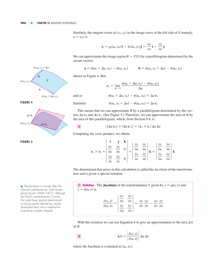
Similarly, the tangent vector at to the image curve of the left side of (namely,) is
We can approximate the image region by a parallelogram determined by thesecant vectors
shown in Figure 4. But
and so
Similarly
This means that we can approximate R by a parallelogram determined by the vec-tors and . (See Figure 5.) Therefore, we can approximate the area of bythe area of this parallelogram, which, from Section 9.4, is
Computing the cross product, we obtain
i j k
The determinant that arises in this calculation is called the Jacobian of the transforma-tion and is given a special notation.
Definition The Jacobian of the transformation given by andis
With this notation we can use Equation 6 to give an approximation to the area of :
where the Jacobian is evaluated at .�u0, v0 �
�A � � ��x, y���u, v� � �u �v8
R�A
��x, y���u, v�
� �x
�u
�y
�u
�x
�v
�y
�v ��x
�u �y
�v�
�x
�v �y
�u
y � h�u, v�x � t�u, v�T7
�x
�u
�y
�u
�x
�v
�y
�v k� �x
�u
�x
�v
�y
�u
�y
�v k � �x
�u
�x
�v
�y
�u
�y
�v
0
0 ru � rv �
��u ru � � ��v rv � � ru � rv �u �v6
R�v rv�u ru
r�u0, v0 � �v� � r�u0, v0 � � �v rv
r�u0 � �u, v0 � � r�u0, v0 � � �u ru
ru � lim �u l 0
r�u0 � �u, v0 � � r�u0, v0 �
�u
b � r�u0, v0 � �v� � r�u0, v0 �a � r�u0 � �u, v0 � � r�u0, v0 �
R � T�S �
rv � tv�u0, v0 � i � hv�u0, v0 �j ��x
�v i �
�y
�v j
u � u0
S�x0, y0 �
904 � CHAPTER 12 MULTIPLE INTEGRALS
� The Jacobian is named after the German mathematician Carl GustavJacob Jacobi (1804–1851). Althoughthe French mathematician Cauchy first used these special determinantsinvolving partial derivatives, Jacobi developed them into a method for evaluating multiple integrals.
r (u¸, √ ¸) Îu ru
Î√ r√
FIGURE 4
FIGURE 5
r (u¸, √ ¸)
r (u¸+Îu, √¸)
R
a
b
r (u¸, √¸+Î√)

Next we divide a region in the -plane into rectangles and call their imagesin the -plane . (See Figure 6.) Applying the approximation (8) to each weapproximate the double integral of over as follows:
where the Jacobian is evaluated at . Notice that this double sum is a Riemannsum for the integral
The foregoing argument suggests that the following theorem is true. (A full proofis given in books on advanced calculus.)
Change of Variables in a Double Integral Suppose that is a one-to-one transformation whose Jacobian is nonzero and that maps a region in the
-plane onto a region in the -plane. Suppose that is continuous on and that and are type I or type II plane regions. Then
Theorem 9 says that we change from an integral in and to an integral in andby expressing and in terms of and and writing
Notice the similarity between Theorem 9 and the one-dimensional formula in Equa-tion 2. Instead of the derivative , we have the absolute value of the Jacobian, thatis, .
As a first illustration of Theorem 9, we show that the formula for integration inpolar coordinates is just a special case. Here the transformation from the -planeto the -plane is given by
y � h�r, �� � r sin �x � t�r, �� � r cos �
xyr�T
��x, y����u, v� dx�du
dA � � ��x, y���u, v� � du dv
vuyxvuyx
yyR
f �x, y� dA � yyS
f �x�u, v�, y�u, v�� � ��x, y���u, v� � du dv
SRRfxyRuv
SC1T9
FIGURE 6
T
0
y
x
R
(xi, yj)
Rij
0
√
u
SÎ√
Îu
(u i, √ j)
Sij
yyS
f �t�u, v�, h�u, v�� � ��x, y���u, v� � du dv
�ui, vj�
� �m
i�1 �
n
j�1 f �t�ui, vj�, h�ui, vj�� � ��x, y�
��u, v� � �u �v
yyR
f �x, y� dA � �m
i�1 �
n
j�1 f �xi, yj� �A
RfRij,Rijxy
SijuvS
SECTION 12.9 CHANGE OF VARIABLES IN MULTIPLE INTEGRALS � 905
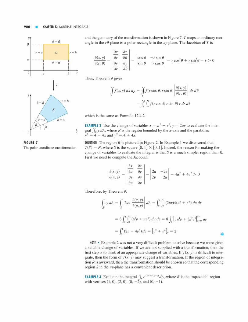
and the geometry of the transformation is shown in Figure 7. maps an ordinary rect-angle in the -plane to a polar rectangle in the -plane. The Jacobian of is
Thus, Theorem 9 gives
which is the same as Formula 12.4.2.
EXAMPLE 2 Use the change of variables , to evaluate the inte-gral , where is the region bounded by the -axis and the parabolas
and .
SOLUTION The region is pictured in Figure 2. In Example 1 we discovered that, where is the square . Indeed, the reason for making the
change of variables to evaluate the integral is that is a much simpler region than .First we need to compute the Jacobian:
Therefore, by Theorem 9,
NOTE � Example 2 was not a very difficult problem to solve because we were givena suitable change of variables. If we are not supplied with a transformation, then thefirst step is to think of an appropriate change of variables. If is difficult to inte-grate, then the form of may suggest a transformation. If the region of integra-tion is awkward, then the transformation should be chosen so that the correspondingregion in the -plane has a convenient description.
EXAMPLE 3 Evaluate the integral , where is the trapezoidal regionwith vertices , , , and .�0, �1��0, �2��2, 0��1, 0�
RxxR e �x�y���x�y� dA
uvSR
f �x, y�f �x, y�
� y1
0 �2v � 4v3 � dv � [v2 � v4 ]0
1� 2
� 8 y1
0y
1
0 �u3v � uv3 � du dv � 8 y
1
0 [ 1
4u4v �12 u2v3]u�1
u�0 dv
yyR
y dA � yyS
2uv � ��x, y���u, v� � dA � y
1
0y
1
0 �2uv�4�u2 � v 2 � du dv
��x, y���u, v�
� �x
�u
�y
�u
�x
�v
�y
�v � � 2u
2v
�2v
2u � � 4u 2 � 4v 2 0
RS�0, 1� � �0, 1�ST�S � � R
R
y 2 � 4 � 4xy 2 � 4 � 4xxRxx
R y dA
y � 2uvx � u 2 � v2
� y
� y
b
a f �r cos �, r sin �� r dr d�
yyR
f �x, y� dx dy � yyS
f �r cos �, r sin �� � ��x, y���r, �� � dr d�
��x, y���r, ��
� �x
�r
�y
�r
�x
��
�y
�� � � cos �
sin �
�r sin �
r cos � � � r cos2� � r sin2� � r 0
Txyr�T
906 � CHAPTER 12 MULTIPLE INTEGRALS
FIGURE 7The polar coordinate transformation
0
y
x
¨=∫ r=b
¨=år=a
∫å
R
0
¨
∫
å
ra b
¨=∫
r=a
¨=å
r=bS
T

SOLUTION Since it isn’t easy to integrate , we make a change of variablessuggested by the form of this function:
These equations define a transformation from the -plane to the -plane. Theorem 9 talks about a transformation from the -plane to the -plane. It isobtained by solving Equations 10 for and :
The Jacobian of is
To find the region in the -plane corresponding to , we note that the sides of lie on the lines
and, from either Equations 10 or Equations 11, the image lines in the -plane are
Thus, the region is the trapezoidal region with vertices , , , andshown in Figure 8. Since
Theorem 9 gives
Triple Integrals
There is a similar change of variables formula for triple integrals. Let be a transfor-mation that maps a region in -space onto a region in -space by means ofthe equations
z � k�u, v, w�y � h�u, v, w�x � t�u, v, w�
xyzRuvwST
� 12 y
2
1 �e � e�1 �v dv � 3
4 �e � e�1 �
� y2
1 y
v
�v eu�v( 1
2 ) du dv � 12 y
2
1 [veu�v ]u��v
u�v dv
yyR
e �x�y���x�y� dA � yyS
eu�v � ��x, y���u, v� � du dv
S � ��u, v� 1 � v � 2, �v � u � v
��1, 1���2, 2��2, 2��1, 1�S
v � 1u � �vv � 2u � v
uv
x � y � 1x � 0x � y � 2y � 0
RRuvS
��x, y���u, v�
� �x
�u
�y
�u
�x
�v
�y
�v � � 1212
�12
�12
� � �12
T
y � 12 �u � v�x � 1
2 �u � v�11
yxxyuvT
uvxyT�1
v � x � yu � x � y10
e �x�y���x�y�
SECTION 12.9 CHANGE OF VARIABLES IN MULTIPLE INTEGRALS � 907
FIGURE 8
T T –!
0
√
u
(_2, 2) (2, 2)
(_1, 1) (1, 1)
√=2
√=1
u=√u=_√ S
0
y
_1
_2
x
1 2
x-y=2
x-y=1
R

The Jacobian of is the following determinant:
Under hypotheses similar to those in Theorem 9, we have the following formula fortriple integrals:
EXAMPLE 4 Use Formula 13 to derive the formula for triple integration in sphericalcoordinates.
SOLUTION Here the change of variables is given by
We compute the Jacobian as follows:
Since , we have . Therefore
and Formula 13 gives
which is equivalent to Formula 12.8.4.
yyyR
f �x, y, z� dV � yyyS
f �� sin � cos �, � sin � sin �, � cos �� �2 sin � d� d� d�
� ��x, y, z����, �, �� � � ��2 sin � � �2 sin �
sin � � 00 � � � �
� ��2 sin � cos2� � �2 sin � sin2� � ��2 sin �
� � sin � �� sin2� cos2� � � sin2� sin2��
� cos � ���2 sin � cos � sin2� � �2 sin � cos � cos2��
� cos � � �� sin � sin �
� � sin � cos �
� cos � cos �
� cos � sin � � � � sin � � sin � cos �
sin � sin �
�� sin � sin ��
� sin � cos � � ��x, y, z����, �, ��
� sin � cos �
sin � sin �
cos �
�� sin � sin �
�� sin � cos �
0
� cos � cos �
� cos � sin �
�� sin � z � � cos �y � � sin � sin �x � � sin � cos �
� yyyS
f �x�u, v, w�, y�u, v, w�, z�u, v, w�� � ��x, y, z���u, v, w�
� du dv dw
yyyR
f �x, y, z� dV13
��x, y, z���u, v, w�
� �x
�u
�y
�u
�z
�u
�x
�v
�y
�v
�z
�v
�x
�w
�y
�w
�z
�w
12
3 � 3T
908 � CHAPTER 12 MULTIPLE INTEGRALS

SECTION 12.9 CHANGE OF VARIABLES IN MULTIPLE INTEGRALS � 909
; 16. , where is the region bounded by the curves, , , ; , .
Illustrate by using a graphing calculator or computer todraw .
� � � � � � � � � � � � �
17. (a) Evaluate , where is the solid enclosed by the ellipsoid . Use the transfor-mation , , .
(b) Earth is not a perfect sphere; rotation has resulted inflattening at the poles. So the shape can be approxi-mated by an ellipsoid with km and
km. Use part (a) to estimate the volume ofEarth.
18. Evaluate , where is the solid of Exercise 17(a).
19–23 � Evaluate the integral by making an appropriate changeof variables.
19. , where is the region bounded by the lines, , , and
20. , where is the parallelogram bounded
by the lines , , , and
21. , where is the trapezoidal region
with vertices , , , and
22. , where is the region in the firstquadrant bounded by the ellipse
23. , where is given by the inequality
� � � � � � � � � � � � �
24. Let be continuous on and let be the triangularregion with vertices , , and . Show that
yyR
f �x � y� dA � y1
0 uf �u� du
�0, 1��1, 0��0, 0�R�0, 1�f
x � y � 1RxxR e x�y dA
9x 2 � 4y 2 � 1RxxR sin�9x 2 � 4y 2 � dA
�0, 1��0, 2��2, 0��1, 0�
RyyR
cos� y � x
y � x� dA
x � 2y � 2x � 2y � 0y � x � 1y � x
RyyR
x � 2y
cos�x � y� dA
3x � y � �23x � y � 12x � y � �32x � y � 1RxxR xy dA
ExxxE x 2 y dV
c � 6356a � b � 6378
z � cwy � bvx � aux 2�a 2 � y 2�b 2 � z2�c 2 � 1
ExxxE dV
R
v � xy 2u � xyxy 2 � 2xy 2 � 1xy � 2xy � 1RxxR y 2 dA1–6 � Find the Jacobian of the transformation.
1. ,
2. ,
3. ,
4. ,
5. , ,
6. , ,
� � � � � � � � � � � � �
7–10 � Find the image of the set under the given transformation.
7. ;
8. is the square bounded by the lines , , ,; ,
9. is the triangular region with vertices , , ;,
10. is the disk given by ; ,� � � � � � � � � � � � �
11–16 � Use the given transformation to evaluate the integral.
11. , where is the region bounded by the lines , , , and ;
,
12. , where is the square with vertices ,, , and ; ,
13. , where is the region bounded by the ellipse ; ,
14. , where is the region bounded by the ellipse ;
,
15. , where is the region in the first quadrantbounded by the lines and and the hyperbolas
, ; , y � vx � u�vxy � 3xy � 1y � 3xy � x
RxxR xy dA
y � s2u � s2�3vx � s2u � s2�3vx 2 � xy � y 2 � 2
RxxR �x 2 � xy � y 2 � dA
y � 3vx � 2u9x 2 � 4y 2 � 36RxxR x 2 dA
y � 3u � 2vx � 2u � 3v�3, �2��5, 1��2, 3��0, 0�RxxR �x � y� dA
y � 13 �v � 2u�x � 1
3 �u � v�y � 3 � 2xy � �2xy � x � 2y � x
RxxR �3x � 4y� dA
y � bvx � auu 2 � v2 � 1S
y � vx � u2�0, 1��1, 1��0, 0�S
y � u�1 � v 2 �x � vv � 1v � 0u � 1u � 0S
x � 2u � 3v, y � u � vS � ��u, v� 0 � u � 3, 0 � v � 2
S
z � e u�v�wy � e u�vx � e u�v
z � uwy � vwx � uv
y � � cos x � � sin
y �v
u � vx �
u
u � v
y � u 2 � v2x � u 2 � v2
y � 3u � 2vx � u � 4v
Exercises � � � � � � � � � � � � � � � � � � � � � � � � � �12.9

6. Write an expression for the area of a surface for each ofthe following cases.(a) is a parametric surface given by a vector function
, .(b) has the equation .(c) is the surface of revolution obtained by rotating the
curve , , about the -axis.
7. (a) Write the definition of the triple integral of over a rectangular box .
(b) How do you evaluate ?
(c) How do you define if is a boundedsolid region that is not a box?
(d) What is a type 1 solid region? How do you evaluateif is such a region?
(e) What is a type 2 solid region? How do you evaluateif is such a region?
(f) What is a type 3 solid region? How do you evaluateif is such a region?
8. Suppose a solid object occupies the region and has den-sity function . Write expressions for each of thefollowing.(a) The mass(b) The moments about the coordinate planes(c) The coordinates of the center of mass(d) The moments of inertia about the axes
9. (a) How do you change from rectangular coordinates tocylindrical coordinates in a triple integral?
(b) How do you change from rectangular coordinates to spherical coordinates in a triple integral?
(c) In what situations would you change to cylindrical orspherical coordinates?
10. (a) If a transformation is given by , what is the Jacobian of ?
(b) How do you change variables in a double integral?(c) How do you change variables in a triple integral?
Ty � h�u, v�x � t�u, v�,T
��x, y, z�E
ExxxE f �x, y, z� dV
ExxxE f �x, y, z� dV
ExxxE f �x, y, z� dV
ExxxE f �x, y, z� dV
xxxB f �x, y, z� dVB
f
xa � x � by � f �x�S
z � f �x, y�, �x, y� � DS�u, v� � Dr�u, v�
S
S1. Suppose is a continuous function defined on a rectangle.
(a) Write an expression for a double Riemann sum of . If , what does the sum represent?
(b) Write the definition of as a limit.(c) What is the geometric interpretation of if
? What if takes on both positive and nega-tive values?
(d) How do you evaluate ?(e) What does the Midpoint Rule for double integrals say?(f) Write an expression for the average value of .
2. (a) How do you define if is a boundedregion that is not a rectangle?
(b) What is a type I region? How do you evaluateif is a type I region?
(c) What is a type II region? How do you evaluateif is a type II region?
(d) What properties do double integrals have?
3. How do you change from rectangular coordinates to polarcoordinates in a double integral? Why would you want to do it?
4. If a lamina occupies a plane region and has density func-tion , write expressions for each of the following interms of double integrals.(a) The mass(b) The moments about the axes(c) The center of mass(d) The moments of inertia about the axes and the origin
5. Let be a joint density function of a pair of continuous ran-dom variables and .(a) Write a double integral for the probability that lies
between and and lies between and .(b) What properties does possess?(c) What are the expected values of and ?YX
fdcYba
XYX
f
��x, y�D
DxxD f �x, y� dA
DxxD f �x, y� dA
DxxD f �x, y� dA
f
xxR f �x, y� dA
ff �x, y� � 0xx
R f �x, y� dA
xxR f �x, y� dA
f �x, y� � 0f
R � �a, b� � �c, d �f
12 ReviewC O N C E P T C H E C K
910 � CHAPTER 12 MULTIPLE INTEGRALS

CHAPTER 12 REVIEW � 911
4.
5. The integral
represents the volume enclosed by the cone and the plane .
6. The integral represents the moment of inertia about the -axis of a solid with constant density .kEz
xxxE kr 3 dz dr d�
z � 2z � sx 2 � y 2
y2�
0 y
2
0 y
2
r dz dr d�
y4
1 y
1
0 (x 2 � sy ) sin�x 2 y 2 � dx dy � 9Determine whether the statement is true or false. If it is true, explain why.
If it is false, explain why or give an example that disproves the statement.
1.
2.
3. If is the disk given by , then
yyD
s4 � x 2 � y 2 dA �16�
3
x 2 � y 2 � 4D
y1
�1 y
1
0 e x2�y2
sin y dx dy � 0
y2
�1 y
6
0 x 2 sin�x � y� dx dy � y
6
0 y
2
�1 x 2 sin�x � y� dy dx
T R U E – FA L S E Q U I Z
9–10 � Write as an iterated integral, where isthe region shown and f is an arbitrary continuous function on .
9. 10.
� � � � � � � � � � � � �
11. Describe the region whose area is given by the integral
12. Describe the solid whose volume is given by the integral
and evaluate the integral.
13–14 � Calculate the iterated integral by first reversing theorder of integration.
13. 14.
� � � � � � � � � � � � �
15–28 � Calculate the value of the multiple integral.
15. , where
,
16. , where, x 2 � 1 � y � x � 1D � ��x, y� �1 � x � 1
xxD x 3 dA
2 � y � 4R � ��x, y� 0 � x � 1
yyR
1
�x � y�2 dA
y1
0 y
1
y 2 y sin�x 2 � dx dyy
1
0 y
1
x e x�y dy dx
y2�
0 y
��6
0 y
3
1 �2 sin � d� d� d�
y�
0 y
1�sin �
1 r dr d�
0
4
y
x
R
4_40 42_2_4
y
x
R
2
4
RRxxR f �x, y� dA1. A contour map is shown for a function on the square
. Use a Riemann sum with nine terms toestimate the value of . Take the sample pointsto be the upper right corners of the squares.
2. Use the Midpoint Rule to estimate the integral in Exercise 1.
3–8 � Calculate the iterated integral.
3. 4.
5. 6.
7. 8.
� � � � � � � � � � � � �
y1
0 y
1
sy y
y
0 xy dz dx dyy
�
0 y
1
0 y
s1�y 2
0 y sin x dz dy dx
y1
0y
ex
x 3xy 2 dy dxy
1
0 y
x
0 cos�x 2 � dy dx
y1
0 y
1
0 ye xy dx dyy
2
1 y
2
0 �y � 2xe y � dx dy
y
0 x
1
1
1 2 3
2
3
2
3
45
89
10
67
xxR f �x, y� dAR � �0, 3� � �0, 3�
f
E X E R C I S E S

36. A lamina occupies the part of the disk thatlies in the first quadrant.(a) Find the centroid of the lamina.(b) Find the center of mass of the lamina if the density
function is .
37. (a) Find the centroid of a right circular cone with height and base radius . (Place the cone so that its base is inthe -plane with center the origin and its axis along thepositive -axis.)
(b) Find the moment of inertia of the cone about its axis(the -axis).
38. (a) Set up, but don’t evaluate, an integral for the surfacearea of the parametric surface given by the vector function , ,
.(b) Use a computer algebra system to approximate the sur-
face area correct to four significant digits.
39. Find the area of the part of the surface that liesabove the triangle with vertices (0, 0), (1, 0), and (0, 2).
40. Graph the surface , , ,and find its surface area correct to four decimal places.
41. Use polar coordinates to evaluate
42. Use spherical coordinates to evaluate
; 43. If is the region bounded by the curves and, find the approximate value of the integral .
(Use a graphing device to estimate the points of intersection of the curves.)
44. Find the center of mass of the solid tetrahedron withvertices , , , and densityfunction .
45. The joint density function for random variables and is
(a) Find the value of the constant .(b) Find .(c) Find .
46. A lamp has three bulbs, each of a type with average lifetime800 hours. If we model the probability of failure of thebulbs by an exponential density function with mean 800,find the probability that all three bulbs fail within a total of1000 hours.
P�X � Y � 1�P�X � 2, Y � 1�
C
f �x, y� � �C�x � y�0
if 0 � x � 3, 0 � y � 2
otherwise
YX
��x, y, z� � x 2 � y 2 � z2�0, 0, 3��0, 2, 0��1, 0, 0��0, 0, 0�
CAS
xxD y 2 dAy � e xy � 1 � x 2D
y1
0 y
s1�x 2
0 y
s1�x 2�y 2
0 �x 2 � y 2 � z2 �2 dz dy dx
ys2
0 y
s4�y 2
y
1
1 � x 2 � y 2 dx dy
�� � y � ��3 � x � 3z � x sin yCAS
z � x 2 � y
CAS
�3 � v � 30 � u � 3r�u, v� � v2 i � uv j � u2 k
z
zxy
ah
��x, y� � xy 2
x 2 � y 2 � a 217. , where is bounded by and
18. , where is bounded by , ,
19. , where is the region in the firstquadrant bounded by , ,
20. , where is the region in the first quadrant that liesabove the hyperbola and the line and belowthe line
21. , where is the region in the first quad-rant bounded by the lines and and the circle
22. , where is the closed disk with radius 1and center
23. , where, ,
24. , where is the tetrahedron bounded by the planes, , , and
25. , where is bounded by the paraboloidand the plane
26. , where is bounded by the planes , ,and the cylinder in the first octant
27. , where lies above the plane , below theplane , and inside the cylinder
28. , where is the solid hemispherewith center the origin, radius 1, that lies above the -plane
� � � � � � � � � � � � �
29–34 � Find the volume of the given solid.
29. Under the paraboloid and above the rectangle
30. Under the surface and above the triangle in the -plane with vertices , , and
31. The solid tetrahedron with vertices , ,, and
32. Bounded by the cylinder and the planes and
33. One of the wedges cut from the cylinder bythe planes and
34. Above the paraboloid and below the half-cone
� � � � � � � � � � � � �
35. Consider a lamina that occupies the region bounded bythe parabola and the coordinate axes in the firstquadrant with density function .(a) Find the mass of the lamina.(b) Find the center of mass.(c) Find the moments of inertia about the - and -axes.yx
��x, y� � yx � 1 � y 2
D
z � sx 2 � y 2
z � x 2 � y 2
z � mxz � 0x 2 � 9y 2 � a 2
y � z � 3z � 0x 2 � y 2 � 4
�2, 2, 0��0, 2, 0��0, 0, 1��0, 0, 0�
�4, 0��2, 1��1, 0�xyz � x 2 y
R � �0, 2� � �1, 4�z � x 2 � 4y 2
xyHxxxH z3
sx 2 � y 2 � z 2 dV
x 2 � y 2 � 4z � yz � 0ExxxE yz dV
y 2 � z2 � 1x � y � 2z � 0y � 0ExxxE z dV
x � 0x � 1 � y 2 � z2ExxxE y 2z2 dV
2x � y � z � 2z � 0y � 0x � 0TxxxT y dV
0 � z � x0 � y � 2xE � ��x, y, z� 0 � x � 2xxx
E x 2z dV
�0, 1�Dxx
D sx 2 � y 2 dA
x 2 � y 2 � 9y � s3xy � 0
DxxD �x 2 � y 2 �3�2 dA
y � 2y � xxy � 1
DxxD y dA
x � 0y � 0x � 1 � y 2Dxx
D �xy � 2x � 3y� dA
x � 1y � x 2y � 0DxxD xe y dA
y � xy 2 � x 3DxxD xy dA
912 � CHAPTER 12 MULTIPLE INTEGRALS

CHAPTER 12 REVIEW � 913
51. Use the change of variables formula and an appropriatetransformation to evaluate , where is the squarewith vertices , , , and .
52. (a) Evaluate , where is an integer and
is the region bounded by the circles with center the ori-gin and radii and , .
(b) For what values of does the integral in part (a) have alimit as ?
(c) Find , where is the region
bounded by the spheres with center the origin and radiiand , .
(d) For what values of does the integral in part (c) have alimit as ?r l 0�
n0 r RRr
EyyyE
1
�x 2 � y 2 � z2 �n�2 dV
r l 0�
n0 r RRr
DnyyD
1
�x 2 � y 2 �n�2 dA
�1, �1��2, 0��1, 1��0, 0�RxxR xy dA
47. Rewrite the integral
as an iterated integral in the order .
48. Give five other iterated integrals that are equal to
49. Use the transformation , to evaluate, where is the square with vertices
, , , and .
50. Use the transformation , , to find the volume of the region bounded by the surface
and the coordinate planes.sx � sy � sz � 1
z � w2y � v2x � u 2
�1, 3��2, 2��1, 1��0, 2�RxxR �x � y���x � y� dA
v � x � yu � x � y
y2
0 y
y 3
0 y
y 2
0 f �x, y, z� dz dx dy
dx dy dz
y1
�1 y
1
x 2 y
1�y
0 f �x, y, z� dz dy dx

1. If denotes the greatest integer in , evaluate the integral
where .
2. Evaluate the integral
where max means the larger of the numbers and .
3. Find the average value of the function on the interval .
4. If , , and are constant vectors, is the position vector , and is givenby the inequalities , , , show that
5. The double integral is an improper integral and could be defined
as the limit of double integrals over the rectangle as . But if weexpand the integrand as a geometric series, we can express the integral as the sum of aninfinite series. Show that
6. Leonhard Euler was able to find the exact sum of the series in Problem 5. In 1736 heproved that
In this problem we ask you to prove this fact by evaluating the double integral in Prob-lem 5. Start by making the change of variables
This gives a rotation about the origin through the angle . You will need to sketch thecorresponding region in the -plane.
[Hint: If, in evaluating the integral, you encounter either of the expressionsor , you might like to use the identity
and the corresponding identity for .]
7. (a) Show that
(Nobody has ever been able to find the exact value of the sum of this series.)
y1
0 y
1
0 y
1
0
1
1 � xyz dx dy dz � �
�
n�1
1
n 3
sin �cos � � sin����2� � ���cos ����1 � sin ���1 � sin ���cos �
uv��4
y �u � v
s2x �
u � v
s2
��
n�1
1
n 2 �� 2
6
y1
0 y
1
0
1
1 � xy dx dy � �
�
n�1
1
n 2
t l 1��0, t� � �0, t�
y1
0 y
1
0
1
1 � xy dx dy
yyyE
�a � r��b � r��c � r� dV ��� ��2
8 a � �b � c�
0 � c � r � �0 � b � r � 0 � a � r � �Ex i � y j � z krcba
[0, 1]f �x� � x1x cos�t 2 � dt
y 2x 2�x 2, y 2
y1
0 y
1
0 e max�x2, y2 dy dx
R � ��x, y� 1 � x � 3, 2 � y � 5
yyR
�x � y� dA
x�x�Focus on ProblemSolving
914

(b) Show that
Use this equation to evaluate the triple integral correct to two decimal places.
8. Show that
by first expressing the integral as an iterated integral.
9. If is continuous, show that
10. (a) A lamina has constant density and takes the shape of a disk with center the originand radius . Use Newton’s Law of Gravitation (see page 728) to show that themagnitude of the force of attraction that the lamina exerts on a body with mass located at the point on the positive -axis is
[Hint: Divide the disk as in Figure 4 in Section 12.4 and first compute the verticalcomponent of the force exerted by the polar subrectangle .]
(b) Show that the magnitude of the force of attraction of a lamina with density thatoccupies an entire plane on an object with mass located at a distance from theplane is
Notice that this expression does not depend on .d
F � 2�Gm�
dm�
Rij
F � 2�Gm�d�1
d�
1
sR 2 � d 2�z�0, 0, d �
mR
�
yx
0 y
y
0 y
z
0 f �t� dt dz dy � 1
2 yx
0 �x � t�2 f �t� dt
f
y�
0 arctan �x � arctan x
x dx �
�
2 ln �
y1
0 y
1
0 y
1
0
1
1 � xyz dx dy dz � �
�
n�1 ��1�n�1
n 3
915

13 Vector Calculus

Vector Fields � � � � � � � � � � � � � � � � � �
The vectors in Figure 1 are air velocity vectors that indicate the wind speed and direc-tion at points 10 m above the surface elevation in the San Francisco Bay area. We seeat a glance from the largest arrows in part (a) that the greatest wind speeds at that timeoccurred as the winds entered the bay across the Golden Gate Bridge. Part (b) showsthe very different wind pattern at a later date. Associated with every point in the airwe can imagine a wind velocity vector. This is an example of a velocity vector field.
(a) 5:00 P.M., August 6, 1997
FIGURE 1 Velocity vector fields showing San Francisco Bay wind patterns
(b) 2:00 P.M., March 7, 2000
13.1
917
In this chapter we study the calculus of vector fields.(These are functions that assign vectors to points inspace.) In particular we define line integrals (whichcan be used to find the work done by a force field inmoving an object along a curve). Then we define sur-face integrals (which can be used to find the rate of
fluid flow across a surface). The connections betweenthese new types of integrals and the single, double,and triple integrals that we have already met are given by the higher-dimensional versions of the Fundamental Theorem of Calculus: Green’s Theorem, Stokes’ Theorem, and the Divergence Theorem.

Other examples of velocity vector fields are illustrated in Figure 2: ocean currentsand flow past an airfoil.
Another type of vector field, called a force field, associates a force vector with eachpoint in a region. An example is the gravitational force field that we will look at inExample 4.
In general, a vector field is a function whose domain is a set of points in (or )and whose range is a set of vectors in (or ).
Definition Let be a set in (a plane region). A vector field on is afunction that assigns to each point in a two-dimensional vector
.
The best way to picture a vector field is to draw the arrow representing the vectorstarting at the point . Of course, it’s impossible to do this for all points
, but we can gain a reasonable impression of by doing it for a few representa-tive points in as in Figure 3. Since is a two-dimensional vector, we can writeit in terms of its component functions and as follows:
or, for short,
Notice that and are scalar functions of two variables and are sometimes calledscalar fields to distinguish them from vector fields.
Definition Let be a subset of . A vector field on is a function that assigns to each point in a three-dimensional vector .
A vector field on is pictured in Figure 4. We can express it in terms of its com-ponent functions , , and as
F�x, y, z� � P�x, y, z� i � Q�x, y, z� j � R�x, y, z� k
RQP� 3F
F�x, y, z�E�x, y, z�F� 3� 3E2
QP
F � P i � Q j
F�x, y� � P�x, y� i � Q�x, y� j � �P�x, y�, Q�x, y��
QPF�x, y�D
F�x, y��x, y�F�x, y�
F�x, y�D�x, y�F
� 2� 2D1
V3V2
� 3� 2
918 � CHAPTER 13 VECTOR CALCULUS
FIGURE 3Vector field on R@
x0
y
(x, y)
F(x, y)
FIGURE 4Vector field on R#
y
0
z
x
(x, y, z)
F (x, y, z)
Nova Scotia
(a) Ocean currents off the coast of Nova Scotia (b) Airflow past an inclined airfoil
FIGURE 2 Velocity vector fields

As with the vector functions in Section 10.1, we can define continuity of vector fields and show that is continuous if and only if its component functions , , and are continuous.
We sometimes identify a point with its position vector andwrite instead of . Then becomes a function that assigns a vector to a vector .
EXAMPLE 1 A vector field on is defined by
Describe by sketching some of the vectors as in Figure 3.
SOLUTION Since , we draw the vector starting at the point in Figure 5. Since , we draw the vector with starting point
. Continuing in this way, we draw a number of representative vectors to repre-sent the vector field in Figure 5.
It appears that each arrow is tangent to a circle with center the origin. To confirm this, we take the dot product of the position vector with the vector
:
This shows that is perpendicular to the position vector and is thereforetangent to a circle with center the origin and radius . Notice alsothat
so the magnitude of the vector is equal to the radius of the circle.
Some computer algebra systems are capable of plotting vector fields in two or threedimensions. They give a better impression of the vector field than is possible by handbecause the computer can plot a large number of representative vectors. Figure 6shows a computer plot of the vector field in Example 1; Figures 7 and 8 show twoother vector fields. Notice that the computer scales the lengths of the vectors so theyare not too long and yet are proportional to their true lengths.
5
_5
_5 5
6
_6
_6 6
5
_5
_5 5
FIGURE 6F(x, y)=k_y, xl
FIGURE 7F(x, y)=ky, sin xl
FIGURE 8F(x, y)=k ln(1+¥), ln(1+≈)l
F�x, y�
� F�x, y� � � s��y�2 � x 2 � sx 2 � y 2 � � x �
� x � � sx 2 � y 2
�x, y�F�x, y�
� �xy � yx � 0
x � F�x� � �x i � y j� � ��y i � x j�
F�x� � F�x, y�x � x i � y j
�0, 1���1, 0 �F�0, 1� � �i
�1, 0�j � �0, 1 �F�1, 0� � j
F�x, y�F
F�x, y� � �y i � x j
� 2
xF�x�FF�x, y, z�F�x�
x � �x, y, z��x, y, z�
RQPF
SECTION 13.1 VECTOR FIELDS � 919
FIGURE 5F(x, y)=_y i+x j
x0
y
F (1, 0)
F(0, 3)(0, 3)

EXAMPLE 2 Sketch the vector field on given by .
SOLUTION The sketch is shown in Figure 9. Notice that all vectors are vertical andpoint upward above the -plane or downward below it. The magnitude increaseswith the distance from the -plane.
We were able to draw the vector field in Example 2 by hand because of its partic-ularly simple formula. Most three-dimensional vector fields, however, are virtuallyimpossible to sketch by hand and so we need to resort to a computer algebra system.Examples are shown in Figures 10, 11, and 12. Notice that the vector fields in Figures10 and 11 have similar formulas, but all the vectors in Figure 11 point in the generaldirection of the negative y-axis because their y-components are all �2. If the vectorfield in Figure 12 represents a velocity field, then a particle would be swept upwardand would spiral around the -axis in the clockwise direction as viewed from above.
EXAMPLE 3 Imagine a fluid flowing steadily along a pipe and let be thevelocity vector at a point . Then assigns a vector to each point in acertain domain (the interior of the pipe) and so is a vector field on called avelocity field. A possible velocity field is illustrated in Figure 13. The speed at anygiven point is indicated by the length of the arrow.
Velocity fields also occur in other areas of physics. For instance, the vector field inExample 1 could be used as the velocity field describing the counterclockwise rota-tion of a wheel. We have seen other examples of velocity fields in Figures 1 and 2.
EXAMPLE 4 Newton’s Law of Gravitation states that the magnitude of the gravita-tional force between two objects with masses and is
where is the distance between the objects and is the gravitational constant. (This is an example of an inverse square law.) Let’s assume that the object with mass is located at the origin in . (For instance, could be the mass of Earth and theorigin would be at its center.) Let the position vector of the object with mass be
. Then , so . The gravitational force exerted on this r 2 � � x �2r � � x �x � �x, y, z�m
M� 3M
Gr
� F � �mMG
r 2
Mm
� 3VE�x, y, z�V�x, y, z�
V�x, y, z�
z
1
0
_1
y 10_1x1
0_1
FIGURE 10F(x, y, z)=y i+z j+x k
z
1
0
-1
y 10-1x1
0-1
FIGURE 11F(x, y, z)=y i-2 j+x k
z
5
3
1
y 10
_1 x1
0_1
FIGURE 12
F(x, y, z)= i- j+ kyz
xz
z4
z
xyxy
F�x, y, z� � z k� 3
920 � CHAPTER 13 VECTOR CALCULUS
FIGURE 9F(x, y, z)=zk
y
0
z
x
FIGURE 13Velocity field in fluid flow
z
yx
0

second object acts toward the origin, and the unit vector in this direction is
Therefore, the gravitational force acting on the object at is
[Physicists often use the notation instead of for the position vector, so you maysee Formula 3 written in the form .] The function given by Equa-tion 3 is an example of a vector field, called the gravitational field, because it asso-ciates a vector [the force ] with every point in space.
Formula 3 is a compact way of writing the gravitational field, but we can alsowrite it in terms of its component functions by using the facts that
and :
The gravitational field is pictured in Figure 14.
EXAMPLE 5 Suppose an electric charge is located at the origin. According toCoulomb’s Law, the electric force exerted by this charge on a charge located at a point with position vector is
where is a constant (that depends on the units used). For like charges, we haveand the force is repulsive; for unlike charges, we have and the force
is attractive. Notice the similarity between Formulas 3 and 4. Both vector fields areexamples of force fields.
Instead of considering the electric force , physicists often consider the force perunit charge:
Then is a vector field on called the electric field of .
Gradient Fields
If is a scalar function of two variables, recall from Section 11.6 that its gradient (or grad ) is defined by
Therefore, is really a vector field on and is called a gradient vector field.Likewise, if is a scalar function of three variables, its gradient is a vector field on given by
∇ f �x, y, z� � fx�x, y, z� i � fy�x, y, z� j � fz�x, y, z� k
� 3f� 2∇ f
∇ f �x, y� � fx�x, y� i � fy�x, y� j
f∇ ff
Q� 3E
E�x� �1
q F�x� �
�Q
� x �3 x
F
qQ � 0qQ � 0�
F�x� ��qQ
� x �3 x4
x � �x, y, z ��x, y, z�qF�x�
Q
F
F�x, y, z� ��mMGx
�x 2 � y 2 � z2 �3�2 i ��mMGy
�x 2 � y 2 � z2 �3�2 j ��mMGz
�x 2 � y 2 � z2 �3�2 k
� x � � sx 2 � y 2 � z 2x � x i � y j � z k
xF�x�
F � ��mMG�r 3 �rxr
F�x� � �mMG
� x �3 x3
x � �x, y, z�
�x
� x �
SECTION 13.1 VECTOR FIELDS � 921
FIGURE 14Gravitational force field
y
z
x

EXAMPLE 6 Find the gradient vector field of . Plot the gradientvector field together with a contour map of f. How are they related?
SOLUTION The gradient vector field is given by
Figure 15 shows a contour map of with the gradient vector field. Notice that thegradient vectors are perpendicular to the level curves, as we would expect fromSection 11.6. Notice also that the gradient vectors are long where the level curvesare close to each other and short where they are farther apart. That’s because thelength of the gradient vector is the value of the directional derivative of and closelevel curves indicate a steep graph.
A vector field is called a conservative vector field if it is the gradient of somescalar function, that is, if there exists a function such that . In this situation
is called a potential function for .Not all vector fields are conservative, but such fields do arise frequently in physics.
For example, the gravitational field F in Example 4 is conservative because if wedefine
then
In Sections 13.3 and 13.5 we will learn how to tell whether or not a given vector fieldis conservative.
� F�x, y, z�
��mMGx
�x 2 � y 2 � z2 �3�2 i ��mMGy
�x 2 � y 2 � z2 �3�2 j ��mMGz
�x 2 � y 2 � z2 �3�2 k
∇ f �x, y, z� ��f
�x i �
�f
�y j �
�f
�z k
f �x, y, z� �mMG
sx 2 � y 2 � z 2
FfF � ∇ ff
F
f
f
∇ f �x, y� ��f
�x i �
�f
�y j � 2xy i � �x 2 � 3y 2 � j
f �x, y� � x 2y � y 3
922 � CHAPTER 13 VECTOR CALCULUS
4
_4
_4 4
FIGURE 15
9. 10.� � � � � � � � � � � � �
11–14 � Match the vector fields with the plots labeled I–IV.Give reasons for your choices.
11.
12.
13.
14. F�x, y� � � ln�1 � x 2 � y 2 �, x�
F�x, y� � �sin x, sin y�
F�x, y� � �2x � 3y, 2x � 3y�
F�x, y� � � y, x�
F
F�x, y, z� � j � iF�x, y, z� � y j1–10 � Sketch the vector field by drawing a diagram like Figure 5 or Figure 9.
1. 2.
3. 4.
5. 6.
7.
8. F�x, y, z� � z j
F�x, y, z� � j
F�x, y� �y i � x jsx 2 � y 2
F�x, y� �y i � x jsx 2 � y 2
F�x, y� � x i � y jF�x, y� � x i � y j
F�x, y� � i � x jF�x, y� � 12�i � j�
F
Exercises � � � � � � � � � � � � � � � � � � � � � � � � � �13.1

use it to plot
Explain the appearance by finding the set of points such that .
20. Let , where and . Usea CAS to plot this vector field in various domains until youcan see what is happening. Describe the appearance of theplot and explain it by finding the points where .
21–24 � Find the gradient vector field of .
21. 22.
23. 24.� � � � � � � � � � � � �
25–26 � Find the gradient vector field of and sketch it.
25. 26.� � � � � � � � � � � � �
27–28 � Plot the gradient vector field of together with a con-tour map of . Explain how they are related to each other.
27. 28.� � � � � � � � � � � � �
29–32 � Match the functions with the plots of their gradientvector fields (labeled I–IV). Give reasons for your choices.
29. 30.
31. 32.
� � � � � � � � � � � � �
4
_4
_4 4
4
_4
_4 4
4
_4
_4 4
4
_4
_4 4
I II
III IV
f �x, y� � sx 2 � y 2f �x, y� � x 2 � y 2
f �x, y� � x 2 � y 2f �x, y� � xy
f
f �x, y� � sin�x � y�f �x, y� � sin x � sin y
ffCAS
f �x, y� � 14�x � y�2f �x, y� � xy � 2x
f∇ f
f �x, y, z� � x cos�y�z�f �x, y, z� � sx 2 � y 2 � z 2
f �x, y� � x �e��xf �x, y� � ln�x � 2y�
f
F�x� � 0
r � � x �x � �x, y�F�x� � �r 2 � 2r�xCAS
F�x, y� � 0�x, y�
F�x, y� � �y 2 � 2xy� i � �3xy � 6x 2 � j
� � � � � � � � � � � � �
15–18 � Match the vector fields on with the plots labeledI–IV. Give reasons for your choices.
15.
16.
17.
18.
� � � � � � � � � � � � �
19. If you have a CAS that plots vector fields (the command isfieldplot in Maple and PlotVectorField in Mathematica),
CAS
z
1
0
_1
y 10_1x1
0_1
z
1
0
_1
y 10_1x1
0_1
0y 1_1 x1 0 _1
z
1
0
_1
z
1
0
_1
y 10_1 1 0 _1x
I II
III IV
F�x, y, z� � x i � y j � z k
F�x, y, z� � x i � y j � 3 k
F�x, y, z� � i � 2 j � z k
F�x, y, z� � i � 2 j � 3 k
�3F
5
_5
_5 5
6
_6
_6 6
5
_5
_5 5
5
_5
_5 5
I II
III IV
SECTION 13.1 VECTOR FIELDS � 923

Line Integrals � � � � � � � � � � � � � � � � �
In this section we define an integral that is similar to a single integral except thatinstead of integrating over an interval , we integrate over a curve . Such inte-grals are called line integrals, although “curve integrals” would be better terminology.They were invented in the early 19th century to solve problems involving fluid flow,forces, electricity, and magnetism.
We start with a plane curve given by the parametric equations
or, equivalently, by the vector equation , and we assume that is a smooth curve. [This means that is continuous and . See Section 10.2.]If we divide the parameter interval into n subintervals of equal widthand we let and , then the corresponding points divide into subarcs with lengths (See Figure 1.) We choose any point
in the th subarc. (This corresponds to a point in .) Now if isany function of two variables whose domain includes the curve , we evaluate atthe point , multiply by the length of the subarc, and form the sum
which is similar to a Riemann sum. Then we take the limit of these sums and makethe following definition by analogy with a single integral.
Definition If is defined on a smooth curve given by Equations 1, thenthe line integral of f along C is
if this limit exists.
In Section 6.3 we found that the length of is
L � yb
a
��dx
dt 2
� �dy
dt 2
dt
C
yC f �x, y� ds � lim
n l
n
i�1 f �xi*, yi*� si
Cf2
n
i�1 f �xi*, yi*� si
si�xi*, yi*�fCf�ti�1, ti�ti*iPi*�xi*, yi*�
s1, s2, . . . , sn.nCPi�xi, yi �yi � y�ti�xi � x�ti�
�ti�1, ti ��a, b�r��t� � 0r�
Cr�t� � x�t� i � y�t� j
a � t � by � y�t�x � x�t�1
C
C�a, b�
13.2
solve the differential equations to find an equation ofthe flow line that passes through the point (1, 1).
34. (a) Sketch the vector field and thensketch some flow lines. What shape do these flow linesappear to have?
(b) If parametric equations of the flow lines are , what differential equations do these functions
satisfy? Deduce that .(c) If a particle starts at the origin in the velocity field
given by F, find an equation of the path it follows.
dy�dx � xy � y�t�
x � x�t�,
F�x, y� � i � x j
33. The flow lines (or streamlines) of a vector field are thepaths followed by a particle whose velocity field is thegiven vector field. Thus, the vectors in a vector field aretangent to the flow lines.(a) Use a sketch of the vector field to
draw some flow lines. From your sketches, can youguess the equations of the flow lines?
(b) If parametric equations of a flow line are, explain why these functions satisfy the differ-
ential equations and . Then dy�dt � �ydx�dt � xy � y�t�
x � x�t�,
F�x, y� � x i � y j
924 � CHAPTER 13 VECTOR CALCULUS
FIGURE 1
Pi-1P*i (x*i , y*i )
Pi
Pn
t i-1
t*i
t i
P¸
P¡
P™
C
a b
x0
y
t

A similar type of argument can be used to show that if is a continuous function, thenthe limit in Definition 2 always exists and the following formula can be used to eval-uate the line integral:
The value of the line integral does not depend on the parametrization of the curve, pro-vided that the curve is traversed exactly once as t increases from a to b.
If is the length of C between and , then
So the way to remember Formula 3 is to express everything in terms of the parameterUse the parametric equations to express and in terms of and write ds as
In the special case where is the line segment that joins to , using asthe parameter, we can write the parametric equations of as follows: , ,
. Formula 3 then becomes
and so the line integral reduces to an ordinary single integral in this case.Just as for an ordinary single integral, we can interpret the line integral of a posi-
tive function as an area. In fact, if , represents the area of oneside of the “fence” or “curtain” in Figure 2, whose base is and whose height abovethe point is .
EXAMPLE 1 Evaluate , where is the upper half of the unit circle.
SOLUTION In order to use Formula 3 we first need parametric equations to represent C.Recall that the unit circle can be parametrized by means of the equations
and the upper half of the circle is described by the parameter interval (See Figure 3.) Therefore, Formula 3 gives
� 2 �23
� y
0 �2 � cos2t sin t� dt � 2t �
cos3t
3 �0
� y
0 �2 � cos2t sin t�ssin2t � cos2t dt
yC �2 � x 2y� ds � y
0 �2 � cos2t sin t���dx
dt 2
� �dy
dt 2
dt
0 � t � .
y � sin tx � cos t
x 2 � y 2 � 1Cx
C �2 � x 2y� ds
f �x, y��x, y�C
xC f �x, y� dsf �x, y� � 0
yC f �x, y� ds � y
b
a f �x, 0� dx
a � x � by � 0x � xC
x�b, 0��a, 0�C
ds � ��dx
dt 2
� �dy
dt 2
dt
tyxt.
ds
dt� ��dx
dt 2
� �dy
dt 2
r�t�r�a�s�t�
yC
f �x, y� ds � yb
a f �x�t�, y�t����dx
dt 2
� �dy
dt 2
dt 3
f
SECTION 13.2 LINE INTEGRALS � 925
� The arc length function is discussed in Section 10.3.
s
FIGURE 2
y
z
x
0
f(x, y)
(x, y)
C
FIGURE 3
x0
y
1_1
≈+¥=1(y˘0)

Suppose now that is a piecewise-smooth curve; that is, is a union of a finitenumber of smooth curves where, as illustrated in Figure 4, the initialpoint of is the terminal point of Then we define the integral of along asthe sum of the integrals of along each of the smooth pieces of :
EXAMPLE 2 Evaluate , where consists of the arc of the parabola from to followed by the vertical line segment from to .
SOLUTION The curve is shown in Figure 5. is the graph of a function of , so wecan choose as the parameter and the equations for become
Therefore
On we choose as the parameter, so the equations of are
and
Thus
Any physical interpretation of a line integral depends on the physicalinterpretation of the function . Suppose that represents the linear density at apoint of a thin wire shaped like a curve . Then the mass of the part of the wirefrom to in Figure 1 is approximately and so the total mass of thewire is approximately . By taking more and more points on the curve,we obtain the mass of the wire as the limiting value of these approximations:
[For example, if represents the density of a semicircular wire, thenthe integral in Example 1 would represent the mass of the wire.] The center of massof the wire with density function is located at the point , where
Other physical interpretations of line integrals will be discussed later in this chapter.
y �1
m y
C y��x, y� dsx �
1
m y
C x��x, y� ds4
�x, y��
f �x, y� � 2 � x 2y
m � limn l
n
i�1 ��xi*, yi*� si � y
C ��x, y� ds
m� ��xi*, yi*� si
��xi*, yi*� siPiPi�1
C�x, y���x, y�f
xC f �x, y� ds
yC 2x ds � y
C1
2x ds � yC2
2x ds �5s5 � 1
6� 2
yC2
2x ds � y2
1 2�1���dx
dy2
� �dy
dy2
dy � y2
1 2 dy � 2
1 � y � 2y � yx � 1
C2yC2
� y1
0 2xs1 � 4x 2 dx � 1
4 � 23 �1 � 4x 2 �3�2]0
1 �5s5 � 1
6
yC1
2x ds � y1
0 2x��dx
dx2
� �dy
dx2
dx
0 � x � 1y � x 2x � x
C1xxC1C
�1, 2��1, 1�C2�1, 1��0, 0�y � x 2C1CxC 2x ds
yC f �x, y� ds � y
C1
f �x, y� ds � yC2
f �x, y� ds � � � � � yCn
f �x, y� ds
CfCfCi.Ci�1
C1, C2, . . . , Cn,CC
926 � CHAPTER 13 VECTOR CALCULUS
FIGURE 4A piecewise-smooth curve
x0
y
C£C™
C¡
C¢
C∞
FIGURE 5C=C¡ � C™
x(0, 0)
y
(1, 1)
(1, 2)
C¡
C™

EXAMPLE 3 A wire takes the shape of the semicircle , , and isthicker near its base than near the top. Find the center of mass of the wire if thelinear density at any point is proportional to its distance from the line .
SOLUTION As in Example 1 we use the parametrization , ,, and find that . The linear density is
where is a constant, and so the mass of the wire is
From Equations 4 we have
By symmetry we see that , so the center of mass is
See Figure 6.
Two other line integrals are obtained by replacing by either orin Definition 2. They are called the line integrals of along with
respect to x and y:
When we want to distinguish the original line integral from those inEquations 5 and 6, we call it the line integral with respect to arc length.
The following formulas say that line integrals with respect to and can also be evaluated by expressing everything in terms of : , , ,
.
yC f �x, y� dy � y
b
a f �x�t�, y�t��y��t� dt
yC f �x, y� dx � y
b
a f �x�t�, y�t�� x��t� dt7
dy � y��t� dtdx � x��t� dty � y�t�x � x�t�tyx
xC f �x, y� ds
yC f �x, y� dy � lim
n l
n
i�1 f �xi*, yi*� yi6
yC f �x, y� dx � lim
n l
n
i�1 f �xi*, yi*� xi5
Cfyi � yi � yi�1
xi � xi � xi�1si
�0, 4 �
2� � 2� � �0, 0.38�
x � 0
�4 �
2� � 2�
�1
� 2 y
0 �sin t � sin2t� dt �
1
� 2 [�cos t �
12 t �
14 sin 2t]0
y �1
m y
C y��x, y� ds �
1
k� � 2� y
C yk�1 � y� ds
� k[t � cos t]0
� k� � 2�
m � yC k�1 � y� ds � y
0 k�1 � sin t� dt
k
��x, y� � k�1 � y�
ds � dt0 � t � y � sin tx � cos t
y � 1
y � 0x 2 � y 2 � 1
SECTION 13.2 LINE INTEGRALS � 927
FIGURE 6
x0
y
1_1
1center ofmass

It frequently happens that line integrals with respect to and occur together.When this happens, it’s customary to abbreviate by writing
When we are setting up a line integral, sometimes the most difficult thing is tothink of a parametric representation for a curve whose geometric description is given.In particular, we often need to parametrize a line segment, so it’s useful to rememberthat a vector representation of the line segment that starts at and ends at is givenby
(See Equation 9.5.1 with .)
EXAMPLE 4 Evaluate , where (a) is the line segment fromto and (b) is the arc of the parabola fromto . (See Figure 7.)
SOLUTION(a) A parametric representation for the line segment is
(Use Equation 8 with and .) Then , ,and Formula 7 gives
(b) Since the parabola is given as a function of , let’s take as the parameter andwrite as
Then and by Formula 7 we have
Notice that we got different answers in parts (a) and (b) of Example 4 even thoughthe two curves had the same endpoints. Thus, in general, the value of a line integraldepends not just on the endpoints of the curve but also on the path. (But see Sec-tion 13.3 for conditions under which the integral is independent of the path.)
� �y 4
2�
y 3
3� 4y�
�3
2
� 40 56
� y2
�3 ��2y 3 � y 2 � 4� dy
yC
2
y 2 dx � x dy � y2
�3 y 2��2y� dy � �4 � y 2 � dy
dx � �2y dy
�3 � y � 2y � yx � 4 � y 2
C2
yy
� 5 25t 3
3�
25t 2
2� 4t�
0
1
� �5
6
� 5 y1
0 �25t 2 � 25t � 4� dt
yC1
y 2 dx � x dy � y1
0 �5t � 3�2�5 dt� � �5t � 5��5 dt�
dy � 5 dtdx � 5 dtr1 � �0, 2 �r0 � ��5, �3 �
0 � t � 1y � 5t � 3x � 5t � 5
�0, 2���5, �3�x � 4 � y 2C � C2�0, 2���5, �3�
C � C1xC y 2 dx � x dy
v � r1 � r0
0 � t � 1r�t� � �1 � t�r0 � t r18
r1r0
yC P�x, y� dx � y
C Q�x, y� dy � y
C P�x, y� dx � Q�x, y� dy
yx
928 � CHAPTER 13 VECTOR CALCULUS
FIGURE 7
x0
y
4
(_5, _3)
(0, 2)
C¡C™
x=4-¥

Notice also that the answers in Example 4 depend on the direction, or orientation,of the curve. If denotes the line segment from to , you can verify,using the parametrization
that
In general, a given parametrization , , , determines anorientation of a curve , with the positive direction corresponding to increasing valuesof the parameter (See Figure 8, where the initial point corresponds to the param-eter value and the terminal point corresponds to .)
If denotes the curve consisting of the same points as but with the oppositeorientation (from initial point to terminal point in Figure 8), then we have
But if we integrate with respect to arc length, the value of the line integral does notchange when we reverse the orientation of the curve:
This is because is always positive, whereas and change sign when we re-verse the orientation of .
Line Integrals in Space
We now suppose that is a smooth space curve given by the parametric equations
or by a vector equation . If is a function of three vari-ables that is continuous on some region containing , then we define the line integralof along (with respect to arc length) in a manner similar to that for plane curves:
We evaluate it using a formula similar to Formula 3:
Observe that the integrals in both Formulas 3 and 9 can be written in the more com-pact vector notation
yb
a f �r�t��� r��t� � dt
yC f �x, y, z� ds � y
b
a f �x�t�, y�t�, z�t����dx
dt 2
� �dy
dt 2
� �dz
dt2
dt9
yC f �x, y, z� ds � lim
n l
n
i�1 f �xi*, yi*, zi*� si
CfC
fr�t� � x�t� i � y�t� j � z�t� k
a � t � bz � z�t�y � y�t�x � x�t�
C
Cyixisi
y�C
f �x, y� ds � yC f �x, y� ds
y�C
f �x, y� dy � �yC f �x, y� dyy
�C f �x, y� dx � �y
C f �x, y� dx
ABC�C
t � bBaAt.
Ca � t � by � y�t�x � x�t�
y�C
1
y 2 dx � x dy �5
6
0 � t � 1y � 2 � 5tx � �5t
��5, �3��0, 2��C1
SECTION 13.2 LINE INTEGRALS � 929
FIGURE 8
B
A
ta b
C
_CA
B

For the special case , we get
where is the length of the curve (see Formula 10.3.3).Line integrals along with respect to , , and can also be defined. For example,
Therefore, as with line integrals in the plane, we evaluate integrals of the form
by expressing everything , , , , , in terms of the parameter
EXAMPLE 5 Evaluate , where is the circular helix given by the equa-tions , , , . (See Figure 9.)
SOLUTION Formula 9 gives
EXAMPLE 6 Evaluate , where consists of the line segment from to followed by the vertical line segment from to
.
SOLUTION The curve is shown in Figure 10. Using Equation 8, we write as
or, in parametric form, as
Thus
� y1
0 �10 � 29t� dt � 10t � 29
t 2
2 �0
1
� 24.5
yC1
y dx � z dy � x dz � y1
0 �4t� dt � �5t�4 dt � �2 � t�5 dt
0 � t � 1z � 5ty � 4tx � 2 � t
r�t� � �1 � t��2, 0, 0 � � t�3, 4, 5 � � �2 � t, 4t, 5t�
C1C
�3, 4, 0��3, 4, 5�C2�3, 4, 5��2, 0, 0�
C1CxC y dx � z dy � x dz
� s2 y2
0 12�1 � cos 2t� dt �
s2
2 [t �
12 sin 2t]0
2 � s2
� y2
0 sin2tssin 2t � cos2t � 1 dt
yC y sin z ds � y
2
0 �sin t� sin t��dx
dt 2
� �dy
dt 2
� �dz
dt2
dt
0 � t � 2 z � ty � sin tx � cos tCxC y sin z ds
t.dz�dydxzy�x
yC P�x, y, z� dx � Q�x, y, z� dy � R�x, y, z� dz10
� yb
a f �x�t�, y�t�, z�t��z��t� dt
yC f �x, y, z� dz � lim
n l
n
i�1 f �xi*, yi*, zi*� zi
zyxCCL
yC ds � y
b
a � r��t� � dt � L
f �x, y, z� � 1
930 � CHAPTER 13 VECTOR CALCULUS
FIGURE 9
1x
z
y
C
1
0
_1
0
_10
2
4
6
FIGURE 10
y
z
x
0
(3, 4, 5)
(3, 4, 0)
(2, 0, 0)
C¡ C™

Likewise, can be written in the form
or
Then , so
Adding the values of these integrals, we obtain
Line Integrals of Vector Fields
Recall from Section 6.5 that the work done by a variable force in moving a particle from to along the -axis is . Then in Section 9.3 we foundthat the work done by a constant force in moving an object from a point to anotherpoint in space is , where
lis the displacement vector.
Now suppose that is a continuous force field on , such asthe gravitational field of Example 4 in Section 13.1 or the electric force field ofExample 5 in Section 13.1. (A force field on could be regarded as a special casewhere and and depend only on and .) We wish to compute the workdone by this force in moving a particle along a smooth curve .
We divide into subarcs with lengths by dividing the parameter inter-val into subintervals of equal width. (See Figure 1 for the two-dimensional caseor Figure 11 for the three-dimensional case.) Choose a point on the thsubarc corresponding to the parameter value . If is small, then as the particlemoves from to along the curve, it proceeds approximately in the direction of
, the unit tangent vector at . Thus, the work done by the force in moving theparticle from to is approximately
and the total work done in moving the particle along is approximately
where is the unit tangent vector at the point on . Intuitively, we seethat these approximations ought to become better as becomes larger. Therefore, wedefine the work done by the force field as the limit of the Riemann sums in (11),namely,
Equation 12 says that work is the line integral with respect to arc length of the tangen-tial component of the force.
W � yC F�x, y, z� � T�x, y, z� ds � y
C F � T ds12
FWn
C�x, y, z�T�x, y, z�
n
i�1 �F�xi*, yi*, zi*� � T�xi*, yi*, zi*�� si11
C
F�xi*, yi*, zi*� � �si T�ti*�� � �F�xi*, yi*, zi*� � T�ti*�� si
PiPi�1
FPi*T�ti*�PiPi�1
siti*iPi*�xi*, yi*, zi*�
�a, b�siPi�1PiC
CyxQPR � 0
� 2
� 3F � P i � Q j � R kD � PQW � F � DQ
PFW � x
ba f �x� dxxba
f �x�
yC y dx � z dy � x dz � 24.5 � 15 � 9.5
yC2
y dx � z dy � x dz � y1
0 3��5� dt � �15
dx � 0 � dy
0 � t � 1z � 5 � 5ty � 4x � 3
r�t� � �1 � t��3, 4, 5 � � t�3, 4, 0 � � �3, 4, 5 � 5t�
C2
SECTION 13.2 LINE INTEGRALS � 931
FIGURE 11
y
z
x
0
F(x*i , y*i , z*i )
T(t*i )
Pi
Pn
P¸
Pi-1
P*i (x*i , y*i , z*i )

If the curve is given by the vector equation , then, so using Equation 9 we can rewrite Equation 12 in the form
This integral is often abbreviated as and occurs in other areas of physics aswell. Therefore, we make the following definition for the line integral of any contin-uous vector field.
Definition Let be a continuous vector field defined on a smooth curve given by a vector function , . Then the line integral of alongC is
When using Definition 13, remember that is just an abbreviation for, so we evaluate simply by putting , , and
in the expression for . Notice also that we can formally write.
EXAMPLE 7 Find the work done by the force field in moving aparticle along the quarter-circle , .
SOLUTION Since and , we have
and
Therefore, the work done is
NOTE � Even though and integrals with respect to arc lengthare unchanged when orientation is reversed, it is still true that
since the unit tangent vector is replaced by its negative when is replaced by �C.CT
y�C
F � dr � �yC F � dr
xC F � dr � xC F � T ds
� 2 cos3t
3 �0
�2
� �2
3
yC F � dr � y
�2
0 F�r�t�� � r��t� dt � y
�2
0 ��2 cos2t sin t� dt
r��t� � �sin t i � cos t j
F�r�t�� � cos2t i � cos t sin t j
y � sin tx � cos t
0 � t � �2r�t� � cos t i � sin t jF�x, y� � x 2 i � xy j
dr � r��t� dtF�x, y, z�z � z�t�
y � y�t�x � x�t�F�r�t��F�x�t�, y�t�, z�t��F�r�t��
yC F � dr � y
b
a F�r�t�� � r��t� dt � y
C F � T ds
Fa � t � br�t�CF13
xC F � dr
� yb
a F�r�t�� � r��t� dt
W � yb
a
F�r�t�� �r��t�
� r��t� � � � r��t� � dt
T�t� � r��t��� r��t� �r�t� � x�t� i � y�t� j � z�t� kC
932 � CHAPTER 13 VECTOR CALCULUS
y
x0 1
1
FIGURE 12
� Figure 12 shows the force field andthe curve in Example 7. The work doneis negative because the field impedesmovement along the curve.

EXAMPLE 8 Evaluate , where and is thetwisted cubic given by
SOLUTION We have
Thus
Finally, we note the connection between line integrals of vector fields and line inte-grals of scalar fields. Suppose the vector field on is given in component form bythe equation . We use Definition 13 to compute its line integralalong :
But this last integral is precisely the line integral in (10). Therefore, we have
For example, the integral in Example 6 could be expressedas where
F�x, y, z� � y i � z j � x k
xC F � drxC y dx � z dy � x dz
where F � P i � Q j � R kyC F � dr � y
C P dx � Q dy � R dz
� yb
a �P�x�t�, y�t�, z�t��x��t� � Q�x�t�, y�t�, z�t��y��t� � R�x�t�, y�t�, z�t��z��t�� dt
� yb
a �P i � Q j � R k� � �x��t� i � y��t� j � z��t� k� dt
yC F � dr � y
b
a F�r�t�� � r��t� dt
CF � P i � Q j � R k
� 3F
� y1
0 �t 3 � 5t 6 � dt �
t 4
4�
5t 7
7 �0
1
�27
28
yC F � dr � y
1
0 F�r�t�� � r��t� dt
F�r�t�� � t 3 i � t 5 j � t 4 k
r��t� � i � 2t j � 3t 2 k
r�t� � t i � t 2 j � t 3 k
0 � t � 1z � t 3y � t 2x � t
CF�x, y, z� � xy i � yz j � zx kxC F � dr
SECTION 13.2 LINE INTEGRALS � 933
� Figure 13 shows the twisted cubic in Example 8 and some typical vectorsacting at three points on .C
C
FIGURE 13
y
z
x
0
0.5
1
1.5
2
21
0
12 0
F{r (1)}
(1, 1, 1)
C
F{r(1/2)}
F{r(3/4)}
4. ,is the arc of the curve from to
5. , consists of line segments fromto and from to �3, 2��2, 0��2, 0��0, 0�
CxC xy dx � �x � y� dy
�1, 1��1, �1�x � y 4Cx
C sin x dx1–12 � Evaluate the line integral, where is the given curve.
1. ,
2. ,
3. , is the right half of the circle x 2 � y 2 � 16CxC xy 4 ds
C: x � t 4, y � t 3, 12 � t � 1x
C �y�x� ds
C: x � t 2, y � t, 0 � t � 2xC y ds
C
Exercises � � � � � � � � � � � � � � � � � � � � � � � � � �13.2
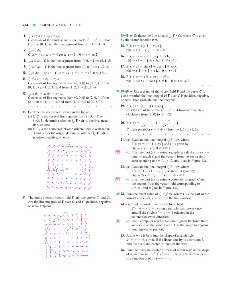
934 � CHAPTER 13 VECTOR CALCULUS
15–18 � Evaluate the line integral , where is givenby the vector function .
15. ,,
16. ,,
17. ,,
18. ,,
� � � � � � � � � � � � �
19–20 � Use a graph of the vector field F and the curve C toguess whether the line integral of F over C is positive, negative,or zero. Then evaluate the line integral.
19. ,is the arc of the circle traversed counter-
clockwise from (2, 0) to
20. ,
is the parabola from to (1, 2)� � � � � � � � � � � � �
21. (a) Evaluate the line integral , whereand is given by
, .
; (b) Illustrate part (a) by using a graphing calculator or com-puter to graph and the vectors from the vector fieldcorresponding to , , and 1 (as in Figure 13).
22. (a) Evaluate the line integral , whereand is given by
, .
; (b) Illustrate part (a) by using a computer to graph andthe vectors from the vector field corresponding to
and (as in Figure 13).
23. Find the exact value of , where is the part of theastroid , in the first quadrant.
24. (a) Find the work done by the force fieldon a particle that moves once
around the circle oriented in thecounterclockwise direction.
(b) Use a computer algebra system to graph the force fieldand circle on the same screen. Use the graph to explainyour answer to part (a).
25. A thin wire is bent into the shape of a semicircle, . If the linear density is a constant ,
find the mass and center of mass of the wire.
26. Find the mass and center of mass of a thin wire in the shape of a quarter-circle , , , if the den-sity function is .��x, y� � x � y
y � 0x � 0x 2 � y 2 � r 2
kx � 0x 2 � y 2 � 4
CAS
x 2 � y 2 � 4F�x, y� � x 2 i � xy j
y � sin3tx � cos3tCxC x 3y 5 dsCAS
�12t � �1
C�1 � t � 1r�t� � 2t i � 3t j � t 2 k
CF�x, y, z� � x i � z j � y kxC F � dr
1�s2t � 0C
0 � t � 1r�t� � t 2 i � t 3 jCF�x, y� � e x�1 i � xy j
xC F � dr
��1, 2�y � 1 � x 2C
F�x, y� �x
sx 2 � y 2 i �
y
sx 2 � y 2 j
�0, �2�x 2 � y 2 � 4C
F�x, y� � �x � y� i � xy j
CAS
0 � t � �2r�t� � sin t i � cos t j � t 2 kF�x, y, z� � x 2 i � xy j � z2 k
0 � t � 1r�t� � t 3 i � t 2 j � t kF�x, y, z� � sin x i � cos y j � xz k
0 � t � 2r�t� � t i � t 2 j � t 3 kF�x, y, z� � yz i � xz j � xy k
0 � t � 1r�t� � t 2 i � t 3 jF�x, y� � x 2y 3 i � ysx j
r�t�Cx
C F � dr6. ,
consists of the shortest arc of the circle fromto and the line segment from to
7. ,,
8. , is the line segment from (0, 6, �1) to (4, 1, 5)
9. , is the line segment from (0, 0, 0) to (1, 2, 3)
10. , : , , ,
11. ,consists of line segments from to , from
to , and from to
12. ,consists of line segments from to , from
to , and from to � � � � � � � � � � � � �
13. Let be the vector field shown in the figure.(a) If is the vertical line segment from to
, determine whether is positive, nega-tive, or zero.
(b) If is the counterclockwise-oriented circle with radius3 and center the origin, determine whether ispositive, negative, or zero.
14. The figure shows a vector field and two curves and .Are the line integrals of over and positive, negative,or zero? Explain.
y
x
C¡
C™
C2C1FC2C1F
y
x01
1
2 3
2
3
_3 _2 _1
_3
_2
_1
xC2 F � dr
C2
xC1 F � dr��3, 3�
��3, �3�C1
F
�1, 3, 0��1, 3, �1��1, 3, �1��2, 0, 0��2, 0, 0��0, 0, 0�C
xC yz dx � xz dy � xy dz
�1, 2, 4��1, 2, 3��1, 2, 3��0, 1, 1��0, 1, 1��0, 0, 0�C
xC z2 dx � z dy � 2y dz
0 � t � 1z � t 2y � tx � stCxC yz dy � xy dz
CxC xe yz ds
CxC x 2z ds
0 � t � �2C: x � 4 sin t, y � 4 cos t, z � 3tx
C xy 3 ds
�4, 3��0, 1��0, 1��1, 0�x 2 � y 2 � 1C
xC xsy dx � 2ysx dy

revolutions, how much work is done by the man againstgravity in climbing to the top?
36. Suppose there is a hole in the can of paint in Exercise 35and 9 lb of paint leak steadily out of the can during theman’s ascent. How much work is done?
37. An object moves along the curve shown in the figurefrom (1, 2) to (9, 8). The lengths of the vectors in the forcefield are measured in newtons by the scales on the axes.Estimate the work done by on the object.
38. Experiments show that a steady current in a long wire pro-duces a magnetic field that is tangent to any circle thatlies in the plane perpendicular to the wire and whose cen-ter is the axis of the wire (as in the figure). Ampère’s Lawrelates the electric current to its magnetic effects and statesthat
where is the net current that passes through any surfacebounded by a closed curve and is a constant called thepermeability of free space. By taking to be a circle withradius , show that the magnitude of the magneticfield at a distance from the center of the wire is
B
I
B ��0 I
2 r
rB � � B �r
C�0C
I
yC B � dr � �0 I
BI
0 1
1
y(meters)
x(meters)
C
C
FF
C
27. (a) Write the formulas similar to Equations 4 for the centerof mass of a thin wire with density function
in the shape of a space curve .(b) Find the center of mass of a wire in the shape of the
helix , , , , if thedensity is a constant .
28. Find the mass and center of mass of a wire in the shape ofthe helix , , , , if thedensity at any point is equal to the square of the distancefrom the origin.
29. If a wire with linear density lies along a plane curveits moments of inertia about the - and -axes are
defined as
Find the moments of inertia for the wire in Example 3.
30. If a wire with linear density lies along a spacecurve , its moments of inertia about the -, -, and -axesare defined as
Find the moments of inertia for the wire in Exercise 27.
31. Find the work done by the force fieldin moving an object along an arch
of the cycloid ,.
32. Find the work done by the force fieldon a particle that moves along the
parabola from to .
33. Find the work done by the force fieldon a particle that moves
along the curve , .
34. The force exerted by an electric charge at the origin on acharged particle at a point with position vector
is where is a constant. (SeeExample 5 in Section 13.1.) Find the work done as the par-ticle moves along a straight line from to .
35. A 160-lb man carries a 25-lb can of paint up a helical stair-case that encircles a silo with a radius of 20 ft. If the silo is 90 ft high and the man makes exactly three complete
�2, 1, 5��2, 0, 0�
KF�r� � Kr�� r �3r � �x, y, z ��x, y, z�
0 � t � 1r�t� � t 2 i � t 3 j � t 4 kF�x, y, z� � xz i � yx j � zy k
�2, 4���1, 1�y � x 2F�x, y� � x sin y i � y j
0 � t � 2 r�t� � �t � sin t� i � �1 � cos t� j
F�x, y� � x i � �y � 2� j
Iz � yC �x 2 � y 2 ���x, y, z� ds
Iy � yC �x 2 � z2 ���x, y, z� ds
Ix � yC �y 2 � z2 ���x, y, z� ds
zyxC��x, y, z�
Iy � yC x 2��x, y� dsIx � y
C y 2��x, y� ds
yxC,��x, y�
0 � t � 2 z � sin ty � cos tx � t
k0 � t � 2 z � 3ty � 2 cos tx � 2 sin t
C��x, y, z��x, y, z �
SECTION 13.2 LINE INTEGRALS � 935

The Fundamental Theorem for Line Integrals � � � � � � � �
Recall from Section 5.4 that Part 2 of the Fundamental Theorem of Calculus can bewritten as
where is continuous on . We also called Equation 1 the Total Change Theorem:The integral of a rate of change is the total change.
If we think of the gradient vector of a function of two or three variables as asort of derivative of , then the following theorem can be regarded as a version of theFundamental Theorem for line integrals.
Theorem Let be a smooth curve given by the vector function ,. Let be a differentiable function of two or three variables whose
gradient vector is continuous on . Then
NOTE � Theorem 2 says that we can evaluate the line integral of a conservative vec-tor field (the gradient vector field of the potential function ) simply by knowing thevalue of at the endpoints of . In fact, Theorem 2 says that the line integral of is the total change in f. If is a function of two variables and is a plane curve withinitial point and terminal point , as in Figure 1, then Theorem 2becomes
If is a function of three variables and is a space curve joining the point to the point , then we have
Let’s prove Theorem 2 for this case.
FIGURE 1
y
0
z
x
A(x¡, y¡, z¡)B(x™, y™, z™)
C
x0
y
A(x¡, y¡) B(x™, y™)
C
yC ∇ f � dr � f �x2, y2, z2 � � f �x1, y1, z1 �
B�x2, y2, z2 �A�x1, y1, z1 �Cf
yC ∇ f � dr � f �x2, y2 � � f �x1, y1 �
B�x2, y2 �A�x1, y1 �Cf
∇ fCff
yC ∇ f � dr � f �r�b�� � f �r�a��
C∇ ffa � t � b
r�t�C2
ff∇ f
�a, b�F�
yb
a F��x� dx � F�b� � F�a�1
13.3
936 � CHAPTER 13 VECTOR CALCULUS

Proof of Theorem 2 Using Definition 13.2.13, we have
(by the Chain Rule)
The last step follows from the Fundamental Theorem of Calculus (Equation 1).
Although we have proved Theorem 2 for smooth curves, it is also true for piecewise-smooth curves. This can be seen by subdividing into a finite number of smoothcurves and adding the resulting integrals.
EXAMPLE 1 Find the work done by the gravitational field
in moving a particle with mass from the point to the point along a piecewise-smooth curve . (See Example 4 in Section 13.1.)
SOLUTION From Section 13.1 we know that is a conservative vector field and, infact, , where
Therefore, by Theorem 2, the work done is
Independence of Path
Suppose and are two piecewise-smooth curves (which are called paths) thathave the same initial point and terminal point . We know from Example 4 in Sec-tion 13.2 that, in general, . But one implication of Theorem 2 isthat
whenever is continuous. In other words, the line integral of a conservative vectorfield depends only on the initial point and terminal point of a curve.
In general, if is a continuous vector field with domain , we say that the lineintegral is independent of path if for any two pathsxC1
F � dr � xC2 F � drxC F � dr
DF
∇ f
yC1
∇ f � dr � yC2
∇ f � dr
xC1 F � dr � xC2
F � drBA
C2C1
�mMG
s22 � 22�
mMG
s32 � 42 � 122� mMG� 1
2s2�
1
13 � f �2, 2, 0� � f �3, 4, 12�
W � yC F � dr � y
C ∇ f � dr
f �x, y, z� �mMG
sx 2 � y 2 � z 2
F � ∇ fF
C�2, 2, 0��3, 4, 12�m
F�x� � �mMG
� x �3 x
C
� f �r�b�� � f �r�a��
� yb
a
d
dt f �r�t�� dt
� yb
a � �f
�x dx
dt�
�f
�y dy
dt�
�f
�z dz
dt dt
yC ∇ f � dr � y
b
a ∇ f �r�t�� � r��t� dt
SECTION 13.3 THE FUNDAMENTAL THEOREM FOR LINE INTEGRALS � 937

and in that have the same initial and terminal points. With this terminologywe can say that line integrals of conservative vector fields are independent of path.
A curve is called closed if its terminal point coincides with its initial point, that is,. (See Figure 2.) If is independent of path in and is any
closed path in , we can choose any two points and on and regard as beingcomposed of the path from to followed by the path from to . (See Fig-ure 3.) Then
since and have the same initial and terminal points.Conversely, if it is true that whenever is a closed path in , then
we demonstrate independence of path as follows. Take any two paths and fromto in and define to be the curve consisting of followed by . Then
and so . Thus, we have proved the following theorem.
Theorem is independent of path in if and only if for every closed path in .
Since we know that the line integral of any conservative vector field is inde-pendent of path, it follows that for any closed path. The physical inter-pretation is that the work done by a conservative force field (such as the gravitationalor electric field in Section 13.1) as it moves an object around a closed path is 0.
The following theorem says that the only vector fields that are independent of pathare conservative. It is stated and proved for plane curves, but there is a similar versionfor space curves. We assume that is open, which means that for every point in there is a disk with center that lies entirely in . (So doesn’t contain any of itsboundary points.) In addition, we assume that is connected. This means that anytwo points in can be joined by a path that lies in .
Theorem Suppose is a vector field that is continuous on an open con-nected region . If is independent of path in , then is a conserva-tive vector field on ; that is, there exists a function such that .
Proof Let be a fixed point in . We construct the desired potential functionby defining
for any point in . Since is independent of path, it does not matter which path from to is used to evaluate . Since is open, thereexists a disk contained in with center . Choose any point in the diskwith and let consist of any path from to followed by thehorizontal line segment from to . (See Figure 4.) Then
f �x, y� � yC1
F � dr � yC2
F � dr � y�x1, y�
�a, b� F � dr � y
C2
F � dr
�x, y��x1, y�C2
�x1, y��a, b�C1Cx1 � x�x1, y��x, y�D
Df �x, y��x, y��a, b�CxC F � drD�x, y�
f �x, y� � y�x, y�
�a, b� F � dr
fDA�a, b�
∇ f � FfDFDx
C F � drDF4
DDD
DDPDPD
xC F � dr � 0
F
DCx
C F � dr � 0Dx
C F � dr3
xC1
F � dr � xC2
F � dr
0 � yC F � dr � y
C1
F � dr � y�C2
F � dr � yC1
F � dr � yC2
F � dr
�C2C1CDBAC2C1
DCxC F � dr � 0�C2C1
yC F � dr � y
C1
F � dr � yC2
F � dr � yC1
F � dr � y�C2
F � dr � 0
ABC2BAC1
CCBADCDxC F � drr�b� � r�a�
DC2C1
938 � CHAPTER 13 VECTOR CALCULUS
FIGURE 4
(a, b)
x0
y
D
(x¡, y)
C¡
C™
(x, y)
FIGURE 2A closed curve
C
FIGURE 3
C¡
C™
B
A
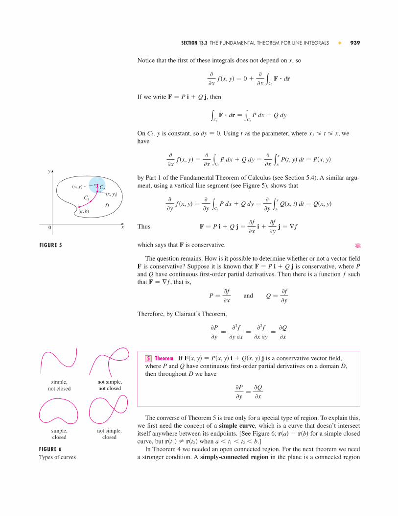
Notice that the first of these integrals does not depend on , so
If we write , then
On , is constant, so . Using as the parameter, where , wehave
by Part 1 of the Fundamental Theorem of Calculus (see Section 5.4). A similar argu-ment, using a vertical line segment (see Figure 5), shows that
Thus
which says that is conservative.
The question remains: How is it possible to determine whether or not a vector field is conservative? Suppose it is known that is conservative, where
and have continuous first-order partial derivatives. Then there is a function such that , that is,
Therefore, by Clairaut’s Theorem,
Theorem If is a conservative vector field,where and have continuous first-order partial derivatives on a domain ,then throughout we have
The converse of Theorem 5 is true only for a special type of region. To explain this,we first need the concept of a simple curve, which is a curve that doesn’t intersectitself anywhere between its endpoints. [See Figure 6; for a simple closedcurve, but when .]
In Theorem 4 we needed an open connected region. For the next theorem we needa stronger condition. A simply-connected region in the plane is a connected region
a � t1 � t2 � br�t1 � � r�t2 �r�a� � r�b�
�P
�y�
�Q
�x
DDQP
F�x, y� � P�x, y� i � Q�x, y� j5
�P
�y�
�2 f
�y �x�
�2 f
�x �y�
�Q
�x
Q ��f
�yandP �
�f
�x
F � ∇ ffQ
PF � P i � Q jF
F
F � P i � Q j ��f
�x i �
�f
�y j � ∇ f
�
�y f �x, y� �
�
�y y
C2
P dx � Q dy ��
�y y
y
y1
Q�x, t� dt � Q�x, y�
��
�x y
x
x1
P�t, y� dt � P�x, y� �
�x f �x, y� �
�
�x y
C2
P dx � Q dy
x1 � t � xtdy � 0yC2
yC2
F � dr � yC2
P dx � Q dy
F � P i � Q j
�
�x f �x, y� � 0 �
�
�x y
C2
F � dr
x
SECTION 13.3 THE FUNDAMENTAL THEOREM FOR LINE INTEGRALS � 939
FIGURE 5
(a, b)
x0
y
D
(x, y)
C¡
C™(x, y¡)
FIGURE 6Types of curves
simple,not closed
not simple,not closed
simple,closed
not simple,closed

such that every simple closed curve in encloses only points that are in . Noticefrom Figure 7 that, intuitively speaking, a simply-connected region contains no holeand can’t consist of two separate pieces.
In terms of simply-connected regions we can now state a partial converse to Theo-rem 5 that gives a convenient method for verifying that a vector field on is con-servative. The proof will be sketched in the next section as a consequence of Green’sTheorem.
Theorem Let be a vector field on an open simply-connectedregion . Suppose that and have continuous first-order derivatives and
Then is conservative.
EXAMPLE 2 Determine whether or not the vector field
is conservative.
SOLUTION Let and . Then
Since , is not conservative by Theorem 5.
EXAMPLE 3 Determine whether or not the vector field
is conservative.
SOLUTION Let and . Then
Also, the domain of is the entire plane , which is open and simply-connected. Therefore, we can apply Theorem 6 and conclude that is conservative.
In Example 3, Theorem 6 told us that is conservative, but it did not tell us howto find the (potential) function such that . The proof of Theorem 4 gives usa clue as to how to find . We use “partial integration” as in the following example.
EXAMPLE 4(a) If , find a function such that .(b) Evaluate the line integral , where is the curve given by
, .0 � t � r�t� � e t sin t i � e t cos t jCx
C F � dr
F � ∇ ffF�x, y� � �3 � 2xy� i � �x 2 � 3y 2 � j
fF � ∇ ff
F
F�D � � 2 �F
�P
�y� 2x �
�Q
�x
Q�x, y� � x 2 � 3y 2P�x, y� � 3 � 2xy
F�x, y� � �3 � 2xy� i � �x 2 � 3y 2 � j
F�P��y � �Q��x
�Q
�x� 1
�P
�y� �1
Q�x, y� � x � 2P�x, y� � x � y
F�x, y� � �x � y� i � �x � 2� j
F
throughout D�P
�y�
�Q
�x
QPDF � P i � Q j6
� 2
DDD
940 � CHAPTER 13 VECTOR CALCULUS
FIGURE 7
simply-connected region
regions that are not simply-connected
FIGURE 9
C™C¡
2
_2
_2 2
� Figures 8 and 9 show the vectorfields in Examples 2 and 3, respec-tively. The vectors in Figure 8 that starton the closed curve all appear topoint in roughly the same direction as
. So it looks as if andtherefore is not conservative. The calculation in Example 2 confirms thisimpression. Some of the vectors near the curves and in Figure 9 point in approximately the same direction asthe curves, whereas others point in theopposite direction. So it appears plau-sible that line integrals around all closedpaths are . Example 3 shows that isindeed conservative.
F0
C2C1
FxC F � dr � 0C
C
C
10
_10
_10 10
FIGURE 8

SOLUTION(a) From Example 3 we know that is conservative and so there exists a function with , that is,
Integrating (7) with respect to , we obtain
Notice that the constant of integration is a constant with respect to , that is, a func-tion of , which we have called . Next we differentiate both sides of (9) withrespect to :
Comparing (8) and (10), we see that
Integrating with respect to , we have
where is a constant. Putting this in (9), we have
as the desired potential function.
(b) To use Theorem 2 all we have to know are the initial and terminal points of ,namely, and . In the expression for in part (a),any value of the constant will do, so let’s choose . Then we have
This method is much shorter than the straightforward method for evaluating lineintegrals that we learned in Section 13.2.
A criterion for determining whether or not a vector field on is conservative isgiven in Section 13.5. Meanwhile, the next example shows that the technique for find-ing the potential function is much the same as for vector fields on .
EXAMPLE 5 If , find a function such that.
SOLUTION If there is such a function , then
fz�x, y, z� � 3ye 3z13
fy�x, y, z� � 2xy � e 3z12
fx�x, y, z� � y 211
f
∇ f � FfF�x, y, z� � y 2 i � �2xy � e 3z� j � 3ye 3z k
� 2
� 3F
� e 3 � ��1� � e 3 � 1
yC F � dr � y
C ∇ f � dr � f �0, �e � � f �0, 1�
K � 0Kf �x, y�r� � � �0, �e �r�0� � �0, 1�
C
f �x, y� � 3x � x 2y � y 3 � K
K
t�y� � �y 3 � K
y
t��y� � �3y 2
fy�x, y� � x 2 � t��y�10
yt�y�y
x
f �x, y� � 3x � x 2y � t�y�9
x
fy�x, y� � x 2 � 3y 28
fx�x, y� � 3 � 2xy7
∇ f � FfF
SECTION 13.3 THE FUNDAMENTAL THEOREM FOR LINE INTEGRALS � 941

Integrating (11) with respect to , we get
where is a constant with respect to . Then differentiating (14) with respect to, we have
and comparison with (12) gives
Thus, and we rewrite (14) as
Finally, differentiating with respect to and comparing with (13), we obtainand, therefore, , a constant. The desired function is
It is easily verified that .
Conservation of Energy
Let’s apply the ideas of this chapter to a continuous force field that moves an objectalong a path given by , , where is the initial point and
is the terminal point of . According to Newton’s Second Law of Motion(see Section 10.4), the force at a point on is related to the acceleration
by the equation
So the work done by the force on the object is
(Theorem 10.2.3, Formula 4)
(Fundamental Theorem of Calculus)
�m
2 (� r��b� �2 � � r��a� �2 )
�m
2 [� r��t� �2]a
b
�m
2 y
b
a
d
dt � r��t� �2 dt
�m
2 y
b
a
d
dt �r��t� � r��t�� dt
� yb
a mr��t� � r��t� dt
W � yC F � dr � y
b
a F�r�t�� � r��t� dt
F�r�t�� � mr��t�
a�t� � r��t�CF�r�t��
Cr�b� � Br�a� � Aa � t � br�t�C
F
∇ f � F
f �x, y, z� � xy 2 � ye 3z � K
h�z� � Kh��z� � 0z
f �x, y, z� � xy 2 � ye 3z � h�z�
t�y, z� � ye 3z � h�z�
ty�y, z� � e 3z
fy�x, y, z� � 2xy � ty�y, z�
yxt�y, z�
f �x, y, z� � xy 2 � t�y, z�14
x
942 � CHAPTER 13 VECTOR CALCULUS

Therefore
where is the velocity.The quantity , that is, half the mass times the square of the speed, is
called the kinetic energy of the object. Therefore, we can rewrite Equation 15 as
which says that the work done by the force field along is equal to the change inkinetic energy at the endpoints of .
Now let’s further assume that is a conservative force field; that is, we can write. In physics, the potential energy of an object at the point is defined
as , so we have . Then by Theorem 2 we have
Comparing this equation with Equation 16, we see that
which says that if an object moves from one point to another point under the influ-ence of a conservative force field, then the sum of its potential energy and its kineticenergy remains constant. This is called the Law of Conservation of Energy and it isthe reason the vector field is called conservative.
BA
P�A� � K�A� � P�B� � K�B�
� P�A� � P�B�
� ��P�r�b�� � P�r�a���
W � yC F � dr � �y
C ∇P � dr
F � �∇PP�x, y, z� � �f �x, y, z��x, y, z�F � ∇ f
FC
C
W � K�B� � K�A�16
12 m � v�t� �2
v � r�
W � 12 m � v�b� �2 �
12 m � v�a� �215
SECTION 13.3 THE FUNDAMENTAL THEOREM FOR LINE INTEGRALS � 943
3–10 � Determine whether or not is a conservative vectorfield. If it is, find a function such that .
3.
4.
5.
6.
7.
8.
9. F�x, y� � �ye x � sin y� i � �e x � x cos y� j
F�x, y� � �1 � 2xy � ln x� i � x 2 j
F�x, y� � �2x cos y � y cos x� i � ��x 2 sin y � sin x� j
F�x, y� � e y i � xe y j
F�x, y� � xe y i � ye x j
F�x, y� � �x 3 � 4xy� i � �4xy � y 3 � j
F�x, y� � �6x � 5y� i � �5x � 4y� j
F � � ffF
1
3
8
6
5
2
4
7
9
xy
0
1
2
0 1 21. The figure shows a curve and a contour map of a function
whose gradient is continuous. Find .
2. A table of values of a function with continuous gradient isgiven. Find , where has parametric equations
.x � t 2 � 1, y � t 3 � t, 0 � t � 1CxC � f � dr
f
y
x0
10
2030
4050
60
C
xC � f � drfC
Exercises � � � � � � � � � � � � � � � � � � � � � � � � � �13.3
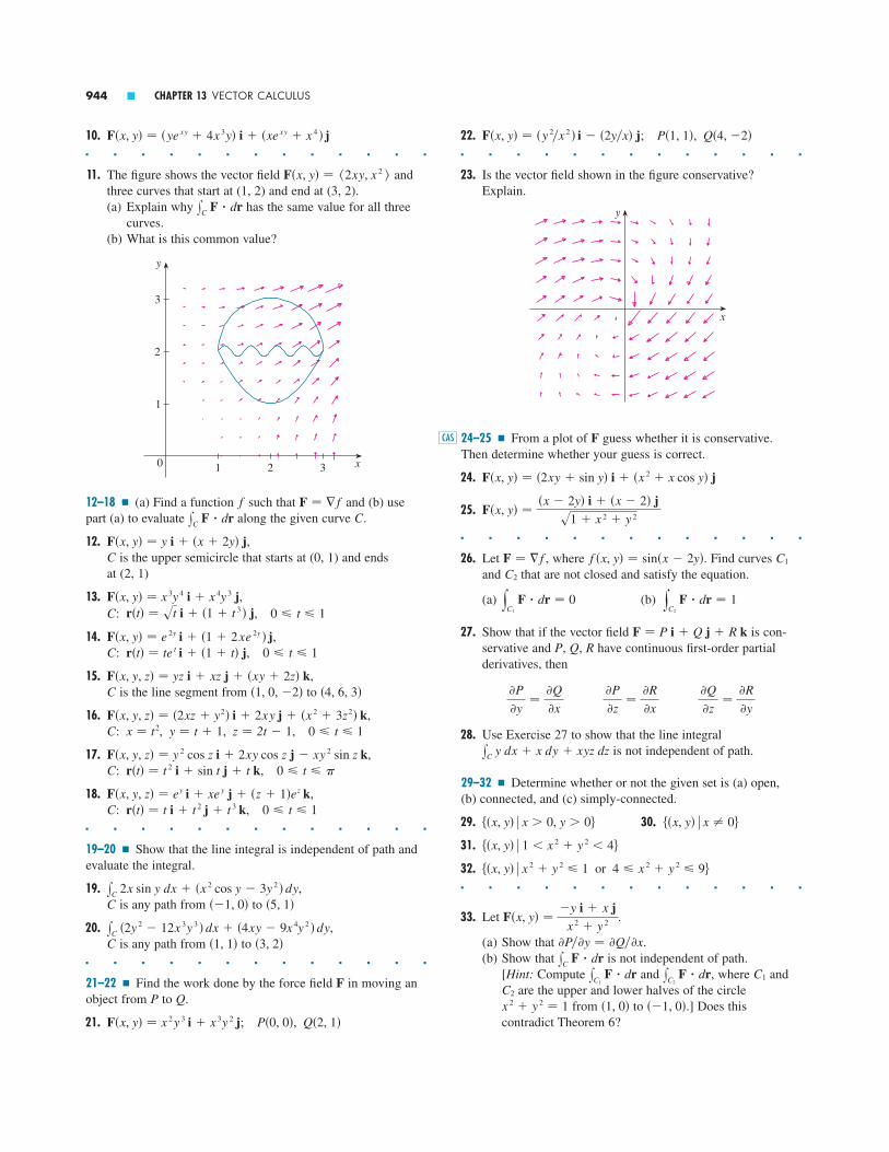
22. ; ,� � � � � � � � � � � � �
23. Is the vector field shown in the figure conservative?Explain.
24–25 � From a plot of guess whether it is conservative.Then determine whether your guess is correct.
24.
25.
� � � � � � � � � � � � �
26. Let , where . Find curves and that are not closed and satisfy the equation.
(a) (b)
27. Show that if the vector field is con-servative and , , have continuous first-order partialderivatives, then
28. Use Exercise 27 to show that the line integralis not independent of path.
29–32 � Determine whether or not the given set is (a) open,(b) connected, and (c) simply-connected.
29. 30.
31.
32.� � � � � � � � � � � � �
33. Let .
(a) Show that .(b) Show that is not independent of path.
[Hint: Compute and , where andare the upper and lower halves of the circle
from to .] Does thiscontradict Theorem 6?
��1, 0��1, 0�x 2 � y 2 � 1C2
C1xC2 F � drxC1
F � drxC F � dr�P��y � �Q��x
F�x, y� ��y i � x j
x 2 � y 2
��x, y� � x 2 � y 2 � 1 or 4 � x 2 � y 2 � 9�
��x, y� � 1 � x 2 � y 2 � 4�
��x, y� � x � 0���x, y� � x � 0, y � 0�
xC y dx � x dy � xyz dz
�Q
�z�
�R
�y
�P
�z�
�R
�x
�P
�y�
�Q
�x
RQPF � P i � Q j � R k
yC2
F � dr � 1yC1
F � dr � 0
C2
C1f �x, y� � sin�x � 2y�F � � f
F�x, y� ��x � 2y� i � �x � 2� j
s1 � x 2 � y 2
F�x, y� � �2xy � sin y� i � �x 2 � x cos y� j
FCAS
x
y
Q�4, �2�P�1, 1�F�x, y� � �y 2�x 2 � i � �2y�x� j10.� � � � � � � � � � � � �
11. The figure shows the vector field andthree curves that start at (1, 2) and end at (3, 2).(a) Explain why has the same value for all three
curves.(b) What is this common value?
12–18 � (a) Find a function such that and (b) usepart (a) to evaluate along the given curve .
12. ,is the upper semicircle that starts at (0, 1) and ends
at (2, 1)
13. ,: ,
14. ,: ,
15. ,is the line segment from to
16. ,: , , ,
17. ,: ,
18. ,: ,
� � � � � � � � � � � � �
19–20 � Show that the line integral is independent of path andevaluate the integral.
19. ,is any path from to
20. ,is any path from to
� � � � � � � � � � � � �
21–22 � Find the work done by the force field in moving anobject from to .
21. ; , Q�2, 1�P�0, 0�F�x, y� � x 2 y 3 i � x 3y 2 j
QPF
�3, 2��1, 1�Cx
C �2y 2 � 12x 3y 3 � dx � �4xy � 9x 4y 2 � dy
�5, 1���1, 0�Cx
C 2x sin y dx � �x 2 cos y � 3y 2 � dy
0 � t � 1r�t� � t i � t 2 j � t 3 kCF�x, y, z� � ey i � xe y j � �z � 1�ez k
0 � t � r�t� � t 2 i � sin t j � t kCF�x, y, z� � y 2 cos z i � 2xy cos z j � xy 2 sin z k
0 � t � 1z � 2t � 1y � t � 1x � t2CF�x, y, z� � �2xz � y2� i � 2xy j � �x 2 � 3z2� k
�4, 6, 3��1, 0, �2�CF�x, y, z� � yz i � xz j � �xy � 2z� k
0 � t � 1r�t� � te t i � �1 � t� jCF�x, y� � e 2y i � �1 � 2xe 2y � j
0 � t � 1r�t� � st i � �1 � t 3 � jCF�x, y� � x 3y 4 i � x 4y 3 j
CF�x, y� � y i � �x � 2y� j
CxC F � drF � ∇ ff
y
x0 3
3
2
1
21
xC F � dr
F�x, y� � �2xy, x 2 �
F�x, y� � �ye xy � 4x 3y� i � �xe xy � x 4 � j
944 � CHAPTER 13 VECTOR CALCULUS

(at a maximum distance of km from theSun) to perihelion (at a minimum distance of
km). (Use the values kg,kg, and
(c) Another example of an inverse square field is the elec-tric field discussed in Example 5 in Section 13.1. Suppose that an electron with a charge of
C is located at the origin. A positive unitcharge is positioned a distance m from the elec-tron and moves to a position half that distance from the electron. Use part (a) to find the work done by theelectric field. (Use the value .)� � 8.985 � 1010
10�12�1.6 � 10�19
E � �qQr�� r �3
N�m2�kg2.�G � 6.67 � 10�11M � 1.99 � 1030m � 5.97 � 10241.47 � 108
1.52 � 10834. (a) Suppose that is an inverse square force field, that is,
for some constant , where . Findthe work done by in moving an object from a point along a path to a point in terms of the distances and from these points to the origin.
(b) An example of an inverse square field is the gravita-tional field discussed in Example 4in Section 13.1. Use part (a) to find the work done bythe gravitational field when Earth moves from aphelion
F � ��mMG �r�� r �3
d2
d1P2
P1Fr � x i � y j � z kc
F�r� �cr
� r �3
F
Green’s Theorem gives the relationship between a line integral around a simple closedcurve and a double integral over the plane region bounded by . (See Figure 1.We assume that consists of all points inside as well as all points on .) In statingGreen’s Theorem we use the convention that the positive orientation of a simpleclosed curve refers to a single counterclockwise traversal of . Thus, if is givenby the vector function , , then the region is always on the left as thepoint traverses . (See Figure 2.)
Green’s Theorem Let be a positively oriented, piecewise-smooth, simpleclosed curve in the plane and let be the region bounded by . If and have continuous partial derivatives on an open region that contains , then
NOTE � The notation
gC
is sometimes used to indicate that the line integral is calculated using the positive ori-entation of the closed curve . Another notation for the positively oriented boundary C
P dx � Q dyor�yC P dx � Q dy
yC P dx � Q dy � yy
D
��Q
�x�
�P
�y dA
DQPCD
C
FIGURE 2 (a) Positive orientation (b) Negative orientation
y
x0
D
C
y
x0
D
C
Cr�t�Da � t � br�t�
CCC
CCDCDC
SECTION 13.4 GREEN’S THEOREM � 945
Green’s Theorem � � � � � � � � � � � � � � � �13.4
FIGURE 1
y
x0
D
C

curve of is , so the equation in Green’s Theorem can be written as
Green’s Theorem should be regarded as the counterpart of the Fundamental Theoremof Calculus for double integrals. Compare Equation 1 with the statement of the Funda-mental Theorem of Calculus, Part 2, in the following equation:
In both cases there is an integral involving derivatives ( , , and ) on theleft side of the equation. And in both cases the right side involves the values of theoriginal functions ( , , and ) only on the boundary of the domain. (In the one-dimensional case, the domain is an interval whose boundary consists of just twopoints, and .)
Green’s Theorem is not easy to prove in the generality stated in Theorem 1, but wecan give a proof for the special case where the region is both of type I and of type II(see Section 12.3). Let’s call such regions simple regions.
Proof of Green’s Theorem for the Case in Which Is a Simple Region Notice that Green’sTheorem will be proved if we can show that
and
We prove Equation 2 by expressing as a type I region:
where and are continuous functions. This enables us to compute the doubleintegral on the right side of Equation 2 as follows:
where the last step follows from the Fundamental Theorem of Calculus.Now we compute the left side of Equation 2 by breaking up as the union of the
four curves , , , and shown in Figure 3. On we take as the parameterand write the parametric equations as , , . Thus
Observe that goes from right to left but goes from left to right, so we canwrite the parametric equations of as , , . Therefore
yC3
P�x, y� dx � �y�C3
P�x, y� dx � �yb
a P�x, t2�x�� dx
a � x � by � t2�x�x � x�C3
�C3C3
yC1
P�x, y� dx � yb
a P�x, t1�x�� dx
a � x � by � t1�x�x � xxC1C4C3C2C1
C
� yb
a �P�x, t2�x�� � P�x, t1�x��� dx yy
D
�P
�y dA � y
b
a y
t2�x�
t1�x� �P
�y �x, y� dy dx4
t2t1
D � ��x, y� � a � x � b, t1�x� � y � t2�x��
D
yC Q dy � yy
D
�Q
�x dA3
yC P dx � �yy
D
�P
�y dA2
D
ba�a, b�
PQF
�P��y�Q��xF�
yb
a F��x� dx � F�b� � F�a�
yyD
��Q
�x�
�P
�y dA � y�D
P dx � Q dy1
�DD
946 � CHAPTER 13 VECTOR CALCULUS
� Green’s Theorem is named after theself- taught English scientist George Green (1793–1841). He worked full-time in his father’s bakery from the age of nine and taught himself mathe-matics from library books. In 1828 hepublished privately An Essay on theApplication of Mathematical Analysis tothe Theories of Electricity and Magne-tism, but only 100 copies were printedand most of those went to his friends.This pamphlet contained a theorem that is equivalent to what we know asGreen’s Theorem, but it didn’t becomewidely known at that time. Finally, atage 40, Green entered Cambridge Uni-versity as an undergraduate but died four years after graduation. In 1846William Thomson (Lord Kelvin) located a copy of Green’s essay, realized its significance, and had it reprinted. Green was the first person to try to formulate a mathematical theory of electricity and magnetism. His work was the basis for the subsequent electro-magnetic theories of Thomson, Stokes,Rayleigh, and Maxwell.
FIGURE 3
y
x0 a b
D
C¡
y=g™(x)
y=g¡(x)
C™
C£
C¢

On or (either of which might reduce to just a single point), is constant, soand
Hence
Comparing this expression with the one in Equation 4, we see that
Equation 3 can be proved in much the same way by expressing as a type II region(see Exercise 28). Then, by adding Equations 2 and 3, we obtain Green’s Theorem.
EXAMPLE 1 Evaluate , where is the triangular curve consisting ofthe line segments from to , from to , and from to .
SOLUTION Although the given line integral could be evaluated as usual by the methodsof Section 13.2, that would involve setting up three separate integrals along the threesides of the triangle, so let’s use Green’s Theorem instead. Notice that the region enclosed by is simple and has positive orientation (see Figure 4). If we let
and , then we have
EXAMPLE 2 Evaluate , where is the circleoriented counterclockwise.
SOLUTION The region bounded by is the disk , so let’s change topolar coordinates after applying Green’s Theorem:
� 4 y2
0 d� y
3
0 r dr � 36
� y2
0 y
3
0 �7 � 3� r dr d�
� yyD
�
�x (7x � sy 4 � 1) �
�
�y �3y � e sin x�� dA
�yC �3y � e sin x � dx � (7x � sy 4 � 1) dy
x 2 � y 2 � 9CD
x 2 � y 2 � 9C�x
C �3y � e sin x� dx � (7x � sy 4 � 1) dy
� �16 �1 � x�3 ]0
1� 1
6
� y1
0 [ 1
2 y 2 ]y�0y�1�x
dx � 12 y
1
0 �1 � x�2 dx
yC x 4 dx � xy dy � yy
D
��Q
�x�
�P
�y dA � y1
0 y
1�x
0 �y � 0� dy dx
Q�x, y� � xyP�x, y� � x 4CC
D
�0, 0��0, 1��0, 1��1, 0��1, 0��0, 0�CxC x 4 dx � xy dy
D
yC P�x, y� dx � �yy
D
�P
�y dA
� yb
a P�x, t1�x�� dx � y
b
a P�x, t2�x�� dx
yC P�x, y� dx � y
C1
P�x, y� dx � yC2
P�x, y� dx � yC3
P�x, y� dx � yC4
P�x, y� dx
yC2
P�x, y� dx � 0 � yC4
P�x, y� dx
dx � 0xC4C2
SECTION 13.4 GREEN’S THEOREM � 947
� Instead of using polar coordinates,we could simply use the fact that is a disk of radius 3 and write
yy
D
4 dA � 4 � �3�2 � 36
D
FIGURE 4
y
x
C
(1, 0)(0, 0)
(0, 1) y=1-x
D
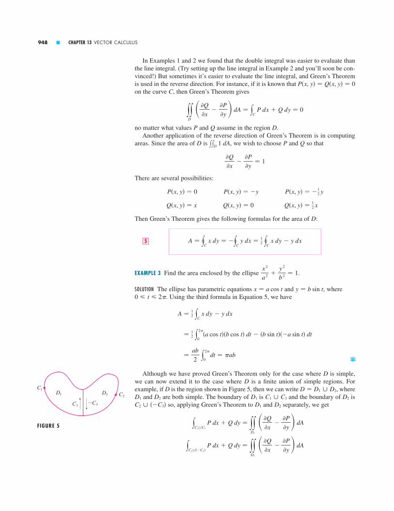
In Examples 1 and 2 we found that the double integral was easier to evaluate thanthe line integral. (Try setting up the line integral in Example 2 and you’ll soon be con-vinced!) But sometimes it’s easier to evaluate the line integral, and Green’s Theoremis used in the reverse direction. For instance, if it is known that on the curve , then Green’s Theorem gives
no matter what values and assume in the region .Another application of the reverse direction of Green’s Theorem is in computing
areas. Since the area of is , we wish to choose and so that
There are several possibilities:
Then Green’s Theorem gives the following formulas for the area of :
EXAMPLE 3 Find the area enclosed by the ellipse .
SOLUTION The ellipse has parametric equations and , where. Using the third formula in Equation 5, we have
Although we have proved Green’s Theorem only for the case where is simple,we can now extend it to the case where is a finite union of simple regions. Forexample, if is the region shown in Figure 5, then we can write , where
and are both simple. The boundary of is and the boundary of isso, applying Green’s Theorem to and separately, we get
yC2���C3�
P dx � Q dy � yyD2
��Q
�x�
�P
�y dA
yC1�C3
P dx � Q dy � yyD1
��Q
�x�
�P
�y dA
D2D1C2 � ��C3�D2C1 � C3D1D2D1
D � D1 � D2DD
D
�ab
2 y
2
0 dt � ab
� 12 y
2
0�a cos t��b cos t� dt � �b sin t���a sin t� dt
A � 12 y
C x dy � y dx
0 � t � 2 y � b sin tx � a cos t
x 2
a 2 �y 2
b 2 � 1
A � �yC x dy � ��y
C y dx � 1
2 �yC x dy � y dx5
D
Q�x, y� � 12 x Q�x, y� � 0 Q�x, y� � x
P�x, y� � �12 y P�x, y� � �y P�x, y� � 0
�Q
�x�
�P
�y� 1
QPxxD 1 dAD
DQP
yyD
��Q
�x�
�P
�y dA � yC P dx � Q dy � 0
CP�x, y� � Q�x, y� � 0
948 � CHAPTER 13 VECTOR CALCULUS
FIGURE 5
C¡
_C£C£
C™D¡ D™

If we add these two equations, the line integrals along and cancel, so we get
which is Green’s Theorem for , since its boundary is .The same sort of argument allows us to establish Green’s Theorem for any finite
union of simple regions (see Figure 6).
EXAMPLE 4 Evaluate , where is the boundary of the semiannularregion in the upper half-plane between the circles and .
SOLUTION Notice that although is not simple, the -axis divides it into two simpleregions (see Figure 7). In polar coordinates we can write
Therefore, Green’s Theorem gives
Green’s Theorem can be extended to apply to regions with holes, that is, regionsthat are not simply-connected. Observe that the boundary of the region in Fig-ure 8 consists of two simple closed curves and . We assume that these boundarycurves are oriented so that the region is always on the left as the curve is tra-versed. Thus, the positive direction is counterclockwise for the outer curve butclockwise for the inner curve . If we divide into two regions and by meansof the lines shown in Figure 9 and then apply Green’s Theorem to each of and we get
Since the line integrals along the common boundary lines are in opposite directions,they cancel and we get
which is Green’s Theorem for the region .
EXAMPLE 5 If , show that for everysimple closed path that encloses the origin.
SOLUTION Since is an arbitrary closed path that encloses the origin, it’s difficult tocompute the given integral directly. So let’s consider a counterclockwise-oriented circle
C
xC F � dr � 2 F�x, y� � ��y i � x j���x 2 � y 2 �
D
yyD
��Q
�x�
�P
�y dA � yC1
P dx � Q dy � yC2
P dx � Q dy � yC P dx � Q dy
� y�D�
P dx � Q dy � y�D�
P dx � Q dy
yyD
��Q
�x�
�P
�y dA � yyD�
��Q
�x�
�P
�y dA � yyD�
��Q
�x�
�P
�y dA
D�,D�D�D�DC2
C1
CDC2C1
DC
� y
0 sin � d� y
2
1 r 2 dr � [�cos �]0
[ 13 r 3 ]1
2�
14
3
� yyD
y dA � y
0 y
2
1 �r sin �� r dr d�
yC y 2 dx � 3xy dy � yy
D
�
�x �3xy� �
�
�y �y 2 �� dA
D � ��r, �� � 1 � r � 2, 0 � � � �
yD
x 2 � y 2 � 4x 2 � y 2 � 1DC�xC y 2 dx � 3xy dy
C � C1 � C2D � D1 � D2
yC1�C2
P dx � Q dy � yyD
��Q
�x�
�P
�y dA
�C3C3
SECTION 13.4 GREEN’S THEOREM � 949
FIGURE 8
D
C™
C¡
FIGURE 9
Dª
Dªª
FIGURE 7
0
y
x
C
≈+¥=4
≈+¥=1
D
FIGURE 6
C

with center the origin and radius , where is chosen to be small enough that lies inside . (See Figure 10.) Let be the region bounded by and . Then itspositively oriented boundary is and so the general version of Green’sTheorem gives
Therefore
that is,
We now easily compute this last integral using the parametrization given by, . Thus
We end this section by using Green’s Theorem to discuss a result that was stated inthe preceding section.
Sketch of Proof of Theorem 13.3.6 We’re assuming that is a vector fieldon an open simply-connected region , that and have continuous first-orderpartial derivatives, and that
If is any simple closed path in and is the region that encloses, then Green’sTheorem gives
A curve that is not simple crosses itself at one or more points and can be broken upinto a number of simple curves. We have shown that the line integrals of aroundthese simple curves are all 0 and, adding these integrals, we see that for any closed curve . Therefore, is independent of path in by Theo-rem 13.3.3. It follows that is a conservative vector field.F
DxC F � drC
xC F � dr � 0
F
�yC F � dr � �y
C P dx � Q dy � yy
R
��Q
�x�
�P
�y dA � yyR
0 dA � 0
CRDC
throughout D�P
�y�
�Q
�x
QPDF � P i � Q j
� y2
0 dt � 2
� y2
0 ��a sin t���a sin t� � �a cos t��a cos t�
a 2 cos2t � a 2 sin2t dt
yC F � dr � y
C� F � dr � y
2
0 F�r�t�� � r��t� dt
0 � t � 2 r�t� � a cos t i � a sin t j
yC F � dr � y
C� F � dr
yC P dx � Q dy � y
C� P dx � Q dy
� 0
� yyD
y 2 � x 2
�x 2 � y 2 �2 �y 2 � x 2
�x 2 � y 2 �2� dA
yC P dx � Q dy � y
�C� P dx � Q dy � yy
D
��Q
�x�
�P
�y dA
C � ��C��C�CDC
C�aaC�
950 � CHAPTER 13 VECTOR CALCULUS
FIGURE 10
y
xD
C
Cª

SECTION 13.4 GREEN’S THEOREM � 951
16. , where ,is the ellipse
� � � � � � � � � � � � �
17. Use Green’s Theorem to find the work done by the forcein moving a particle from the
origin along the -axis to , then along the line segment to , and then back to the origin along the -axis.
18. A particle starts at the point , moves along the -axisto , and then along the semicircle to thestarting point. Use Green’s Theorem to find the work doneon this particle by the force field .
19–20 � Find the area of the given region using one of the formulas in Equations 5.
19. The region bounded by the hypocycloid with vectorequation ,
20. The region bounded by the curve with vector equation,
� � � � � � � � � � � � �
21. (a) If is the line segment connecting the point tothe point , show that
(b) If the vertices of a polygon, in counterclockwise order,are , , show that the area ofthe polygon is
(c) Find the area of the pentagon with vertices , ,, , and .
22. Let be a region bounded by a simple closed path in the -plane. Use Green’s Theorem to prove that the coordi-
nates of the centroid of are
where is the area of .
23. Use Exercise 22 to find the centroid of the triangle with vertices , , and .
24. Use Exercise 22 to find the centroid of a semicircular regionof radius .
25. A plane lamina with constant density occupies aregion in the -plane bounded by a simple closed path .Show that its moments of inertia about the axes are
Iy ��
3 �y
C x 3 dyIx � �
�
3 �y
C y 3 dx
Cxy��x, y� � �
a
�0, 1��1, 0��0, 0�
DA
y � �1
2A �y
C y 2 dxx �
1
2A �y
C x 2 dy
D�x, y �xy
CD
��1, 1��0, 2��1, 3��2, 1��0, 0�
A � � �xn�1 yn � xn yn�1 � � �xn y1 � x1 yn ��
A � 12 ��x1 y2 � x2 y1 � � �x2 y3 � x3 y2 � � � � �
�xn, yn ��x2, y2 �, . . . , �x1, y1 �
yC x dy � y dx � x1 y2 � x2 y1
�x2, y2��x1, y1�C
0 � t � 2 r�t� � cos t i � sin3t j
0 � t � 2 r�t� � cos3t i � sin3t j
F�x, y� � �x, x 3 � 3xy 2 �
y � s4 � x 2�2, 0�x��2, 0�
y�0, 1��1, 0�x
F�x, y� � x�x � y� i � xy 2 j
4x 2 � y 2 � 1CF�x, y� � y 6 i � xy 5 jx
C F � dr1–4 � Evaluate the line integral by two methods: (a) directly
and (b) using Green’s Theorem.
1. ,is the rectangle with vertices (0, 0), (2, 0), (2, 3), and (0, 3)
2. ,is the circle with center the origin and radius 1
3. ,is the triangle with vertices (0, 0), (1, 0), and (1, 2)
4. , consists of the arc of theparabola from to and the line segmentsfrom to and from to
� � � � � � � � � � � � �
5–6 � Verify Green’s Theorem by using a computer algebrasystem to evaluate both the line integral and the double integral.
5. , ,is the circle
6. , ,consists of the arc of the parabola from (0, 0) to
(1, 1) followed by the line segment from (1, 1) to (0, 0)� � � � � � � � � � � � �
7–16 � Use Green’s Theorem to evaluate the line integral alongthe given positively oriented curve.
7. ,is the square with sides , , , and
8. ,is the triangle with vertices (0, 0), (1, 3), and (0, 3)
9. ,is the boundary of the region enclosed by the parabolas
and
10. ,is the boundary of the region enclosed by the parabola
and the line
11. , is the circle
12. , is the ellipse
13. ,consists of the line segment from to and the
top half of the circle
14. ,is the boundary of the region between the circles
and
15. , where ,consists of the circle from to
and the line segments from to and fromto �2, 0��0, 0�
�0, 0�(s2, s2)(s2, s2)�2, 0�x 2 � y 2 � 4C
F�x, y� � �y 2 � x 2 y� i � xy 2 jxC F � dr
x 2 � y 2 � 9x 2 � y 2 � 1CxC �x 3 � y 3 � dx � �x 3 � y 3 � dy
x 2 � y 2 � 4�2, 0���2, 0�C
xC xy dx � 2x 2 dy
x 2 � xy � y 2 � 1CxC sin y dx � x cos y dy
x 2 � y 2 � 4CxC y 3 dx � x 3 dy
y � 4y � x 2CxC �y 2 � tan�1x� dx � �3x � sin y� dy
x � y 2y � x 2CxC (y � esx ) dx � �2x � cos y 2 � dy
CxC x 2y 2 dx � 4xy 3 dy
y � 1y � 0x � 1x � 0CxC e y dx � 2xe y dy
y � x 2CQ�x, y� � x 2 sin yP�x, y� � y 2 sin x
x 2 � y 2 � 1CQ�x, y� � �x 7y 6P�x, y� � x 4y 5
CAS
�0, 0��0, 4��0, 4��2, 4��2, 4��0, 0�y � x 2
C�xC �x 2 � y 2 � dx � 2xy dy
C�xC xy dx � x 2y 3 dy
C�xC y dx � x dy
C�xC xy 2 dx � x 3 dy
Exercises � � � � � � � � � � � � � � � � � � � � � � � � � �13.4

where :
Here is the region in the -plane that corresponds to theregion in the -plane under the transformation given by
, .[Hint: Note that the left side is and apply the first
part of Equation 5. Convert the line integral over to aline integral over and apply Green’s Theorem in the
-plane.]uv�S
�RA�R�
y � h�u, v�x � t�u, v�uvS
xyR
yyR
dx dy � yyS
� ��x, y���u, v� � du dv
f �x, y� � 126. Use Exercise 25 to find the moment of inertia of a circulardisk of radius with constant density about a diameter.(Compare with Example 4 in Section 12.5.)
27. If is the vector field of Example 5, show thatfor every simple closed path that does not
pass through or enclose the origin.
28. Complete the proof of the special case of Green’s Theoremby proving Equation 3.
29. Use Green’s Theorem to prove the change of variables for-mula for a double integral (Formula 12.9.9) for the case
xC F � dr � 0F
�a
Curl and Divergence � � � � � � � � � � � � � � �
In this section we define two operations that can be performed on vector fields and thatplay a basic role in the applications of vector calculus to fluid flow and electricity andmagnetism. Each operation resembles differentiation, but one produces a vector fieldwhereas the other produces a scalar field.
Curl
If is a vector field on and the partial derivatives of , , andall exist, then the curl of is the vector field on defined by
As an aid to our memory, let’s rewrite Equation 1 using operator notation. We intro-duce the vector differential operator (“del”) as
It has meaning when it operates on a scalar function to produce the gradient of :
If we think of as a vector with components , , and , we can also con-sider the formal cross product of with the vector field as follows:
� curl F
� ��R
�y�
�Q
�z i � ��P
�z�
�R
�x j � ��Q
�x�
�P
�y k
∇ � F � � i�
�x
P
j�
�y
Q
k�
�z
R �F∇
���z���y���x∇
∇ f � i �f
�x� j
�f
�y� k
�f
�z�
�f
�x i �
�f
�y j �
�f
�z k
f
∇ � i �
�x� j
�
�y� k
�
�z
∇
curl F � ��R
�y�
�Q
�z i � ��P
�z�
�R
�x j � ��Q
�x�
�P
�y k1
� 3FRQP� 3F � P i � Q j � R k
13.5
952 � CHAPTER 13 VECTOR CALCULUS

Thus, the easiest way to remember Definition 1 is by means of the symbolic expression
EXAMPLE 1 If , find .
SOLUTION Using Equation 2, we have
Recall that the gradient of a function of three variables is a vector field on andso we can compute its curl. The following theorem says that the curl of a gradient vec-tor field is .
Theorem If is a function of three variables that has continuous second-order partial derivatives, then
Proof We have
by Clairaut’s Theorem.
Since a conservative vector field is one for which , Theorem 3 can be re-phrased as follows:
If is conservative, then .
This gives us a way of verifying that a vector field is not conservative.
curl F � 0F
F � ∇ f
� 0 i � 0 j � 0 k � 0
� � �2 f
�y �z�
�2 f
�z �y i � � �2 f
�z �x�
�2 f
�x �z j � � �2 f
�x �y�
�2 f
�y �x k
curl�∇ f � � ∇ � �∇ f � � �i�
�x
�f
�x
j�
�y
�f
�y
k�
�z
�f
�z�
curl�∇ f � � 0
f3
0
� 3f
� �y�2 � x� i � x j � yz k
� ��2y � xy� i � �0 � x� j � �yz � 0� k
� �
�x �xyz� �
�
�y �xz�� k
� �
�y ��y 2 � �
�
�z �xyz�� i � �
�x ��y 2 � �
�
�z �xz�� j
curl F � ∇ � F � � i�
�x
xz
j�
�y
xyz
k�
�z
�y 2 �curl FF�x, y, z� � xz i � xyz j � y 2 k
curl F � ∇ � F2
SECTION 13.5 CURL AND DIVERGENCE � 953
� Most computer algebra systems havecommands that compute the curl anddivergence of vector fields. If you haveaccess to a CAS, use these commandsto check the answers to the examplesand exercises in this section.
� Notice the similarity to what we knowfrom Section 9.4: for everythree-dimensional vector .a
a � a � 0
� Compare this with Exercise 27 in Section 13.3.

EXAMPLE 2 Show that the vector field is not conservative.
SOLUTION In Example 1 we showed that
This shows that and so, by Theorem 3, is not conservative.
The converse of Theorem 3 is not true in general, but the following theorem saysthe converse is true if is defined everywhere. (More generally it is true if the domainis simply-connected, that is, “has no hole.”) Theorem 4 is the three-dimensional ver-sion of Theorem 13.3.6. Its proof requires Stokes’ Theorem and is sketched at the endof Section 13.7.
Theorem If is a vector field defined on all of whose component func-tions have continuous partial derivatives and , then is a conserva-tive vector field.
EXAMPLE 3(a) Show that is a conservative vector field.(b) Find a function such that .
SOLUTION(a) We compute the curl of :
Since and the domain of is , is a conservative vector field by Theorem 4.
(b) The technique for finding was given in Section 13.3. We have
Integrating (5) with respect to , we obtain
Differentiating (8) with respect to , we get , so com-parison with (6) gives . Thus, and
fz�x, y, z� � 3xy 2z2 � h��z�
t�y, z� � h�z�ty�y, z� � 0fy�x, y, z� � 2xyz3 � ty�y, z�y
f �x, y, z� � xy 2z3 � t�y, z�8
x
fz�x, y, z� � 3xy 2z27
fy�x, y, z� � 2xyz36
fx�x, y, z� � y 2z35
f
F� 3Fcurl F � 0
� 0
� �6xyz2 � 6xyz2 � i � �3y 2z2 � 3y 2z2 � j � �2yz3 � 2yz3 � k
curl F � � � F � � i�
�x
y 2z 3
j�
�y
2xyz 3
k�
�z
3xy 2z 2 �F
F � � ffF�x, y, z� � y 2z3 i � 2xyz3 j � 3xy 2z2 k
Fcurl F � 0� 3F4
F
Fcurl F � 0
curl F � �y�2 � x� i � x j � yz k
F�x, y, z� � xz i � xyz j � y 2 k
954 � CHAPTER 13 VECTOR CALCULUS
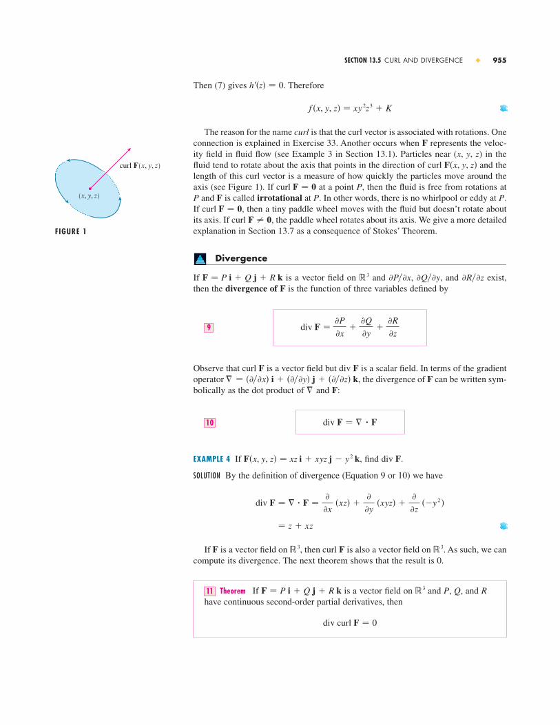
Then (7) gives . Therefore
The reason for the name curl is that the curl vector is associated with rotations. Oneconnection is explained in Exercise 33. Another occurs when represents the veloc-ity field in fluid flow (see Example 3 in Section 13.1). Particles near (x, y, ) in thefluid tend to rotate about the axis that points in the direction of and thelength of this curl vector is a measure of how quickly the particles move around theaxis (see Figure 1). If at a point , then the fluid is free from rotations at
and is called irrotational at . In other words, there is no whirlpool or eddy at P.If , then a tiny paddle wheel moves with the fluid but doesn’t rotate aboutits axis. If , the paddle wheel rotates about its axis. We give a more detailedexplanation in Section 13.7 as a consequence of Stokes’ Theorem.
Divergence
If is a vector field on and , , and exist,then the divergence of is the function of three variables defined by
Observe that is a vector field but is a scalar field. In terms of the gradientoperator , the divergence of can be written sym-bolically as the dot product of and :
EXAMPLE 4 If , find .
SOLUTION By the definition of divergence (Equation 9 or 10) we have
If is a vector field on , then is also a vector field on . As such, we cancompute its divergence. The next theorem shows that the result is 0.
Theorem If is a vector field on and , , and have continuous second-order partial derivatives, then
div curl F � 0
RQP� 3F � P i � Q j � R k11
� 3curl F� 3F
� z � xz
div F � � � F ��
�x �xz� �
�
�y �xyz� �
�
�z ��y 2 �
div FF�x, y, z� � xz i � xyz j � y 2 k
div F � � � F10
F�F� � ����x� i � ����y� j � ����z� k
div Fcurl F
div F ��P
�x�
�Q
�y�
�R
�z9
F�R��z�Q��y�P��x� 3F � P i � Q j � R k
curl F � 0curl F � 0
PFPPcurl F � 0
curl F�x, y, z�z
F
f �x, y, z� � xy 2z3 � K
h��z� � 0
SECTION 13.5 CURL AND DIVERGENCE � 955
FIGURE 1
(x, y, z)
curl F(x, y, z)

Proof Using the definitions of divergence and curl, we have
because the terms cancel in pairs by Clairaut’s Theorem.
EXAMPLE 5 Show that the vector field can’t be written as the curl of another vector field, that is, .
SOLUTION In Example 4 we showed that
and therefore . If it were true that , then Theorem 11 wouldgive
which contradicts . Therefore, is not the curl of another vector field.
Again, the reason for the name divergence can be understood in the context of fluidflow. If is the velocity of a fluid (or gas), then represents the net rate of change (with respect to time) of the mass of fluid (or gas) flowing from the point per unit volume. In other words, measures the tendencyof the fluid to diverge from the point . If , then is said to be incompressible.
Another differential operator occurs when we compute the divergence of a gradi-ent vector field . If is a function of three variables, we have
and this expression occurs so often that we abbreviate it as . The operator
is called the Laplace operator because of its relation to Laplace’s equation
We can also apply the Laplace operator to a vector field
in terms of its components:
� 2F � � 2P i � � 2Q j � � 2R k
F � P i � Q j � R k
� 2
� 2 f ��2 f
�x 2 ��2 f
�y 2 ��2 f
�z2 � 0
� 2 � � � �
� 2 f
div�� f � � � � �� f � ��2 f
�x 2 ��2 f
�y 2 ��2 f
�z2
f� f
Fdiv F � 0�x, y, z�div F�x, y, z��x, y, z�
div F�x, y, z�F�x, y, z�
Fdiv F � 0
div F � div curl G � 0
F � curl Gdiv F � 0
div F � z � xz
F � curl GF�x, y, z� � xz i � xyz j � y 2 k
� 0
��2R
�x �y�
�2Q
�x �z�
�2P
�y �z�
�2R
�y �x�
�2Q
�z �x�
�2P
�z �y
��
�x ��R
�y�
�Q
�z ��
�y ��P
�z�
�R
�x ��
�z ��Q
�x�
�P
�y div curl F � � � �� � F�
956 � CHAPTER 13 VECTOR CALCULUS
� Note the analogy with the scalartriple product: .a � �a � b� � 0
� The reason for this interpretation ofwill be explained at the end of
Section 13.8 as a consequence of theDivergence Theorem.
div F

Vector Forms of Green’s Theorem
The curl and divergence operators allow us to rewrite Green’s Theorem in versionsthat will be useful in our later work. We suppose that the plane region , its boundarycurve , and the functions and satisfy the hypotheses of Green’s Theorem. Thenwe consider the vector field . Its line integral is
and, regarding as a vector field on with third component , we have
Therefore
and we can now rewrite the equation in Green’s Theorem in the vector form
Equation 12 expresses the line integral of the tangential component of along as the double integral of the vertical component of over the region enclosedby . We now derive a similar formula involving the normal component of .
If is given by the vector equation
then the unit tangent vector (see Section 10.2) is
You can verify that the outward unit normal vector to is given by
(See Figure 2.) Then, from Equation 13.2.3, we have
� yC P dy � Q dx � yy
D
��P
�x�
�Q
�y dA
� yb
a P�x�t�, y�t�� y��t� dt � Q�x�t�, y�t�� x��t� dt
� yb
a P�x�t�, y�t�� y��t�
� r��t� � �Q�x�t�, y�t�� x��t�
� r��t� � � � r��t� � dt
�yC F � n ds � y
b
a �F � n��t� � r��t� � dt
n�t� � y��t�
� r��t� � i �x��t�
� r��t� � j
C
T�t� �x��t�
� r��t� � i � y��t�
� r��t� � j
a � t � br�t� � x�t� i � y�t� j
CFC
Dcurl FCF
�yC F � dr � yy
D
�curl F� � k dA12
�curl F� � k � ��Q
�x�
�P
�y k � k ��Q
�x�
�P
�y
curl F � � i�
�x
P�x, y�
j�
�y
Q�x, y�
k�
�z
0 � � ��Q
�x�
�P
�y k
0�3F
�yC F � dr � �y
C P dx � Q dy
F � P i � Q jQPC
D
SECTION 13.5 CURL AND DIVERGENCE � 957
FIGURE 2
0
y
x
D
C
r(t) n(t)
T(t)

by Green’s Theorem. But the integrand in this double integral is just the divergenceof . So we have a second vector form of Green’s Theorem.
This version says that the line integral of the normal component of along is equalto the double integral of the divergence of over the region enclosed by .CDF
CF
�yC F � n ds � yy
D
div F�x, y� dA13
F
958 � CHAPTER 13 VECTOR CALCULUS
9.
� � � � � � � � � � � � �
10. Let be a scalar field and a vector field. State whether each expression is meaningful. If not, explain why. If so,state whether it is a scalar field or a vector field.(a) (b)(c) (d)(e) (f)(g) (h)(i) ( j)(k) (l)
11–16 � Determine whether or not the vector field is conserva-tive. If it is conservative, find a function such that .
11.
12.
13.
14.
15.
16.� � � � � � � � � � � � �
17. Is there a vector field on such that? Explain.
18. Is there a vector field on such that? Explain.
19. Show that any vector field of the form
where , , are differentiable functions, is irrotational.htf
F�x, y, z� � f �x� i � t�y� j � h�z� k
curl G � yz i � xyz j � xy k� 3G
curl G � xy 2 i � yz2 j � zx 2 k� 3G
F�x, y, z� � yze xz i � e xz j � xye xz k
F�x, y, z� � e x i � e z j � e y k
F�x, y, z� � xy 2z 3 i � 2x 2yz 3 j � 3x 2y 2z 2 k
F�x, y, z� � 2xy i � �x 2 � 2yz� j � y 2 k
F�x, y, z� � x i � y j � z k
F�x, y, z� � yz i � xz j � xy k
F � ∇ ff
div�curl�grad f ���grad f � � �div F�div�div F�curl�curl F�grad�div f �div�grad f �grad�div F�grad Fcurl�grad f �div Fgrad fcurl f
Ff
y
x0
1–6 � Find (a) the curl and (b) the divergence of the vectorfield.
1.
2.
3.
4.
5.
6.
� � � � � � � � � � � � �
7–9 � The vector field F is shown in the xy-plane and looks thesame in all other horizontal planes. (In other words, F is inde-pendent of and its -component is 0.)(a) Is div F positive, negative, or zero? Explain.(b) Determine whether curl . If not, in which direction
does curl F point?
7.
8. y
x0
y
x0
F � 0
zz
x
x 2 � y 2 � z 2 i �y
x 2 � y 2 � z 2 j �z
x 2 � y 2 � z 2 kF�x, y, z� �
F�x, y, z� � e x sin y i � e x cos y j � z k
F�x, y, z� � xe y j � ye z k
F�x, y, z� � xyz i � x 2y k
F�x, y, z� � �x � 2z� i � �x � y � z� j � �x � 2y� k
F�x, y, z� � xy i � yz j � zx k
Exercises � � � � � � � � � � � � � � � � � � � � � � � � � �13.5

where and satisfy the hypotheses of Green’s Theorem and the appropriate partial derivatives of and exist andare continuous.
33. This exercise demonstrates a connection between the curl vector and rotations. Let be a rigid body rotating aboutthe -axis. The rotation can be described by the vector
, where is the angular speed of , that is, the tan-gential speed of any point in divided by the distance from the axis of rotation. Let be the positionvector of .(a) By considering the angle in the figure, show that the
velocity field of is given by .(b) Show that .(c) Show that .
34. Maxwell’s equations relating the electric field and mag-netic field as they vary with time in a region containingno charge and no current can be stated as follows:
where is the speed of light. Use these equations to provethe following:
(a)
(b)
(c) [Hint: Use Exercise 27.]
(d) � 2H �1
c 2 �2H�t 2
� 2E �1
c 2 �2E�t 2
� � �� � H� � �1
c 2 �2H�t 2
� � �� � E� � �1
c 2 �2E�t 2
c
curl H �1
c �E�t
curl E � �1
c �H�t
div H � 0 div E � 0
HE
0
z
y
¨
P
dB
w
x
v
curl v � 2wv � ��y i � �x j
v � w � rB�
Pr � �x, y, z�
dBPB�w � �k
zB
tfCD20. Show that any vector field of the form
is incompressible.
21–27 � Prove the identity, assuming that the appropriate partial derivatives exist and are continuous. If is a scalar fieldand , are vector fields, then , , and aredefined by
21. div
22. curl
23. div
24. curl
25. div
26. div
27.� � � � � � � � � � � � �
28–30 � Let and .
28. Verify each identity.(a) (b)(c)
29. Verify each identity.(a) (b)(c) (d)
30. If , find div . Is there a value of for which div ?
� � � � � � � � � � � � �
31. Use Green’s Theorem in the form of Equation 13 to proveGreen’s first identity:
where and satisfy the hypotheses of Green’s Theorem and the appropriate partial derivatives of and exist andare continuous. (The quantity occurs in theline integral. This is the directional derivative in the direc-tion of the normal vector and is called the normal deriva-tive of .)
32. Use Green’s first identity (Exercise 31) to prove Green’s second identity:
yyD
� f �2t � t�2f � dA � �y
C � f �t � t� f � � n ds
t
n
�t � n � Dn t
tfCD
yyD
f �2t dA � �y
C f ��t� � n ds � yy
D
� f � �t dA
F � 0pFF � r�r p
� ln r � r�r 2��1�r� � �r�r 3� � r � 0�r � r�r
� 2r 3 � 12r� � �rr� � 4r� � r � 3
r � � r �r � x i � y j � z k
curl curl F � grad div F � � 2F
�� f � �t� � 0
�F � G� � G � curl F � F � curl G
curl F � �� f � � F� f F� � f
div F � F � � f� f F� � f
�F � G� � curl F � curl G
�F � G� � div F � div G
�F � G��x, y, z� � F�x, y, z� � G�x, y, z�
�F � G��x, y, z� � F�x, y, z� � G�x, y, z�
� f F��x, y, z� � f �x, y, z�F�x, y, z�
F � GF � Gf FGFf
F�x, y, z� � f �y, z� i � t�x, z� j � h�x, y� k
SECTION 13.5 CURL AND DIVERGENCE � 959
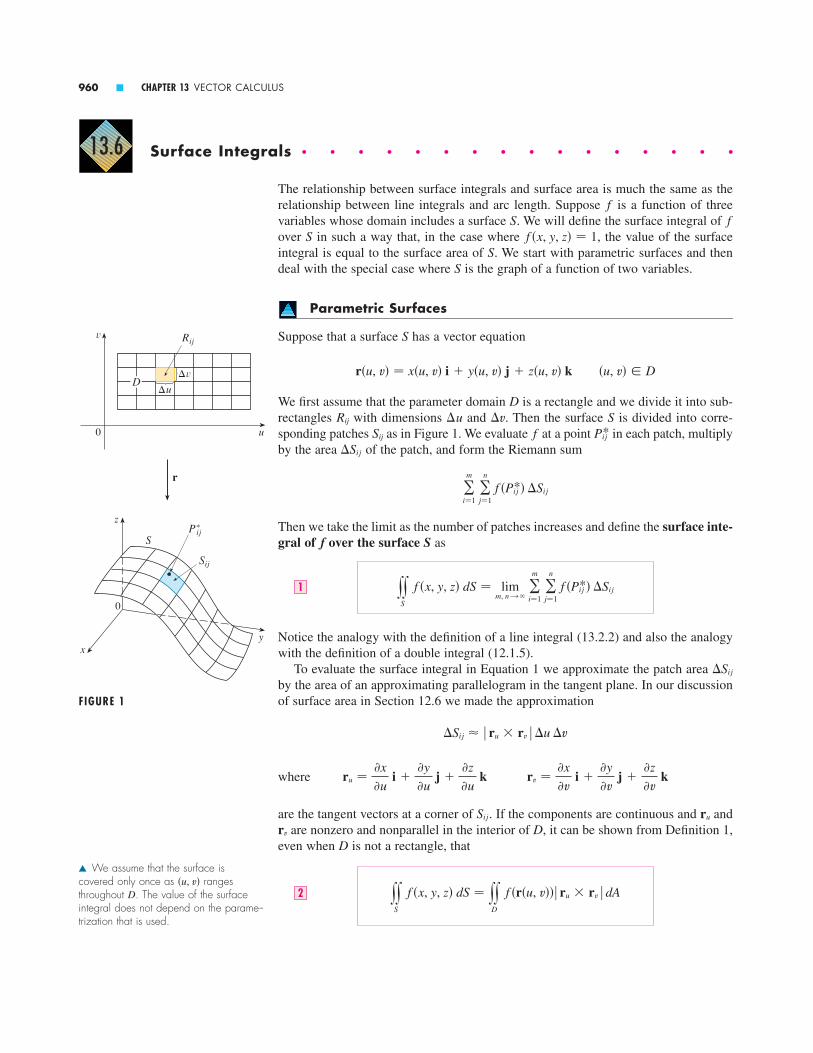
Surface Integrals � � � � � � � � � � � � � � � �
The relationship between surface integrals and surface area is much the same as therelationship between line integrals and arc length. Suppose is a function of threevariables whose domain includes a surface . We will define the surface integral of over in such a way that, in the case where , the value of the surfaceintegral is equal to the surface area of . We start with parametric surfaces and thendeal with the special case where is the graph of a function of two variables.
Parametric Surfaces
Suppose that a surface has a vector equation
We first assume that the parameter domain is a rectangle and we divide it into sub-rectangles with dimensions and . Then the surface is divided into corre-sponding patches as in Figure 1. We evaluate at a point in each patch, multiplyby the area of the patch, and form the Riemann sum
Then we take the limit as the number of patches increases and define the surface inte-gral of f over the surface S as
Notice the analogy with the definition of a line integral (13.2.2) and also the analogywith the definition of a double integral (12.1.5).
To evaluate the surface integral in Equation 1 we approximate the patch area by the area of an approximating parallelogram in the tangent plane. In our discussionof surface area in Section 12.6 we made the approximation
where
are the tangent vectors at a corner of . If the components are continuous and andare nonzero and nonparallel in the interior of D, it can be shown from Definition 1,
even when D is not a rectangle, that
yyS
f �x, y, z� dS � yyD
f �r�u, v��� ru � rv � dA2
rv
ruSij
rv ��x
�v i �
�y
�v j �
�z
�v kru �
�x
�u i �
�y
�u j �
�z
�u k
Sij � � ru � rv � u v
Sij
yyS
f �x, y, z� dS � lim m, n l
m
i�1
n
j�1 f �Pij*� Sij1
m
i�1
n
j�1 f �Pij*� Sij
Sij
Pij*fSij
SvuRij
D
�u, v� � Dr�u, v� � x�u, v� i � y�u, v� j � z�u, v� k
S
SS
f �x, y, z� � 1SfS
f
13.6
960 � CHAPTER 13 VECTOR CALCULUS
� We assume that the surface is covered only once as rangesthroughout . The value of the surfaceintegral does not depend on the parame-trization that is used.
D�u, v�
FIGURE 1
0
√
u
Rij
DÎ√
Îu
0
z
yx
P *ij
S
Sij
r

This should be compared with the formula for a line integral:
Observe also that
Formula 2 allows us to compute a surface integral by converting it into a doubleintegral over the parameter domain . When using this formula, remember that
is evaluated by writing , , and in the for-mula for .
EXAMPLE 1 Compute the surface integral , where is the unit sphere.
SOLUTION As in Example 4 in Section 10.5, we use the parametric representation
that is,
As in Example 1 in Section 12.6, we can compute that
Therefore, by Formula 2,
Surface integrals have applications similar to those for the integrals we have previ-ously considered. For example, if a thin sheet (say, of aluminum foil) has the shape ofa surface and the density (mass per unit area) at the point is , thenthe total mass of the sheet is
and the center of mass is , where
Moments of inertia can also be defined as before (see Exercise 35).
z �1
m yy
S
z��x, y, z� dSy �1
m yy
S
y��x, y, z� dSx �1
m yy
S
x��x, y, z� dS
�x, y, z�
m � yyS
��x, y, z� dS
��x, y, z��x, y, z�S
� 12 [� �
12 sin 2�]0
2 [�cos � �13 cos3�]0
�
4
3
� y2
0 12 �1 � cos 2�� d� y
0 �sin � � sin � cos2�� d�
� y2
0 y
0 sin2� cos2� sin � d� d� � y
2
0 cos2� d� y
0 sin3� d�
yyS
x 2 dS � yyD
�sin � cos ��2 � r� � r� � dA
� r� � r� � � sin �
r��, �� � sin � cos � i � sin � sin � j � cos � k
0 � � � 2 0 � � � z � cos �y � sin � sin �x � sin � cos �
x 2 � y 2 � z2 � 1SxxS x
2 dS
f �x, y, z�z � z�u, v�y � y�u, v�x � x�u, v�f �r�u, v��
D
yyS
1 dS � yyD
� ru � rv � dA � A�S�
yC f �x, y, z� ds � y
b
a f �r�t��� r��t� � dt
SECTION 13.6 SURFACE INTEGRALS � 961
� Here we use the identities
Instead, we could use Formulas 64 and67 in the Table of Integrals.
sin2� � 1 � cos2�
cos2� � 12 �1 � cos 2��

Graphs
Any surface with equation can be regarded as a parametric surface withparametric equations
and so we have
Thus
and
Therefore, in this case, Formula 2 becomes
Similar formulas apply when it is more convenient to project onto the -planeor -plane. For instance, if is a surface with equation and is its pro-jection on the -plane, then
EXAMPLE 2 Evaluate , where is the surface , ,. (See Figure 2.)
SOLUTION Since
Formula 4 gives
� s2(14 ) 2
3 �1 � 2y 2 �3�2]02
�13s2
3
� y1
0 dx s2 y
2
0 ys1 � 2y 2 dy
� y1
0 y
2
0 ys1 � 1 � 4y 2 dy dx
yyS
y dS � yyD
y�1 � � �z
�x2
� � �z
�y2
dA
�z
�y� 2yand
�z
�x� 1
0 � y � 20 � x � 1z � x � y 2SxxS y dS
yyS
f �x, y, z� dS � yyD
f �x, h�x, z�, z����y
�x2
� ��y
�z2
� 1 dA
xzDy � h�x, z�Sxz
yzS
yyS
f �x, y, z� dS � yyD
f �x, y, t�x, y���� �z
�x2
� � �z
�y2
� 1 dA4
� rx � ry � � �� �z
�x2
� � �z
�y2
� 1
rx � ry � ��t
�x i �
�t
�y j � k3
ry � j � � �t
�y krx � i � � �t
�x k
z � t�x, y�y � yx � x
z � t�x, y�S
962 � CHAPTER 13 VECTOR CALCULUS
FIGURE 2
y
x
z
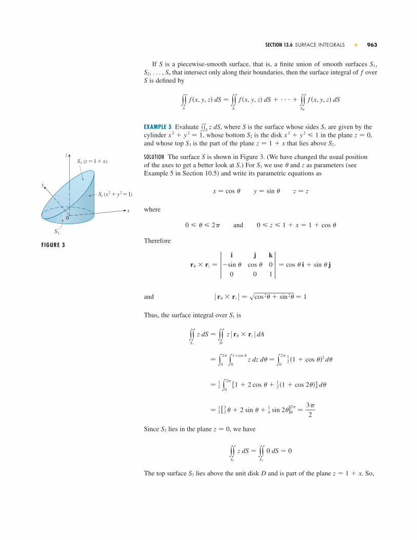
If is a piecewise-smooth surface, that is, a finite union of smooth surfaces ,that intersect only along their boundaries, then the surface integral of over
is defined by
EXAMPLE 3 Evaluate , where is the surface whose sides are given by thecylinder , whose bottom is the disk in the plane ,and whose top is the part of the plane that lies above .
SOLUTION The surface is shown in Figure 3. (We have changed the usual position of the axes to get a better look at .) For we use and as parameters (seeExample 5 in Section 10.5) and write its parametric equations as
where
Therefore
and
Thus, the surface integral over is
Since lies in the plane , we have
The top surface lies above the unit disk and is part of the plane . So,z � 1 � xDS3
yyS2
z dS � yyS2
0 dS � 0
z � 0S2
� 12 [ 3
2 � � 2 sin � �14 sin 2�]0
2 �
3
2
� 12 y
2
0 �1 � 2 cos � �
12 �1 � cos 2��� d�
� y2
0 y
1�cos �
0 z dz d� � y
2
0 12 �1 � cos ��2 d�
yyS1
z dS � yyD
z � r� � rz � dA
S1
� r� � rz � � scos2� � sin 2� � 1
r� � rz � � i�sin �
0
jcos �
0
k0
1 � � cos � i � sin � j
0 � z � 1 � x � 1 � cos �and0 � � � 2
z � zy � sin �x � cos �
z�S1SS
S2z � 1 � xS3
z � 0x 2 � y 2 � 1S2x 2 � y 2 � 1S1SxxS z dS
yyS
f �x, y, z� dS � yyS1
f �x, y, z� dS � � � � � yySn
f �x, y, z� dS
SfSnS2, . . . ,
S1S
SECTION 13.6 SURFACE INTEGRALS � 963
FIGURE 3
0
x
z
y
S¡ (≈+¥=1)
S™
S£ (z=1+x)

taking in Formula 4 and converting to polar coordinates, we have
Therefore
Oriented Surfaces
In order to define surface integrals of vector fields, we need to rule out nonorientablesurfaces such as the Möbius strip shown in Figure 4. [It is named after the Germangeometer August Möbius (1790–1868).] You can construct one for yourself by takinga long rectangular strip of paper, giving it a half-twist, and taping the short edgestogether as in Figure 5. If an ant were to crawl along the Möbius strip starting at apoint , it would end up on the “other side” of the strip (that is, with its upper sidepointing in the opposite direction). Then, if the ant continued to crawl in the samedirection, it would end up back at the same point without ever having crossed an edge. (If you have constructed a Möbius strip, try drawing a pencil line down themiddle.) Therefore, a Möbius strip really has only one side.
From now on we consider only orientable (two-sided) surfaces. We start with a sur-face that has a tangent plane at every point on (except at any boundarypoint). There are two unit normal vectors and at . (See Figure 6.)
FIGURE 6
0
y
z
x
n¡
n™
�x, y, z�n2 � �n1n1
S�x, y, z�S
FIGURE 5Constructing a Möbius strip
A
B
D
C
A
B
C
D
P
P
�3
2� 0 � s2 � ( 3
2 � s2)
yyS
z dS � yyS1
z dS � yyS2
z dS � yyS3
z dS
� s2 y2
0 ( 1
2 �13 cos �) d� � s2 �
2�
sin �
3 �0
2
� s2
� s2 y2
0 y
1
0 �r � r 2 cos �� dr d�
� y2
0 y
1
0 �1 � r cos ��s1 � 1 � 0 r dr d�
yyS3
z dS � yyD
�1 � x��1 � � �z
�x2
� � �z
�y2
dA
t�x, y� � 1 � x
964 � CHAPTER 13 VECTOR CALCULUS
FIGURE 4A Möbius strip
P

If it is possible to choose a unit normal vector at every such point so thatvaries continuously over , then is called an oriented surface and the given choice
of provides with an orientation. There are two possible orientations for any ori-entable surface (see Figure 7).
For a surface given as the graph of , we use Equation 3 to associatewith the surface a natural orientation given by the unit normal vector
Since the -component is positive, this gives the upward orientation of the surface.If is a smooth orientable surface given in parametric form by a vector function
, then it is automatically supplied with the orientation of the unit normal vector
and the opposite orientation is given by . For instance, in Example 4 in Sec-tion 10.5 we found the parametric representation
for the sphere . Then in Example 1 in Section 12.6 we found that
and
So the orientation induced by is defined by the unit normal vector
Observe that points in the same direction as the position vector, that is, outwardfrom the sphere (see Figure 8). The opposite (inward) orientation would have beenobtained (see Figure 9) if we had reversed the order of the parameters because
.For a closed surface, that is, a surface that is the boundary of a solid region , the
convention is that the positive orientation is the one for which the normal vectorspoint outward from , and inward-pointing normals give the negative orientation (seeFigures 8 and 9).
E
Er� � r� � �r� � r�
n
n �r� � r�
� r� � r� � � sin � cos � i � sin � sin � j � cos � k �1
a r��, ��
r��, ��
� r� � r� � � a 2 sin �
r� � r� � a 2 sin2� cos � i � a 2 sin2� sin � j � a 2 sin � cos � k
x 2 � y 2 � z2 � a 2
r��, �� � a sin � cos � i � a sin � sin � j � a cos � k
�n
n �ru � rv
� ru � rv �6
r�u, v�S
k
n �
��t
�x i �
�t
�y j � k
�1 � � �t
�x2
� � �t
�y25
tz � t�x, y�
FIGURE 7The two orientations of
an orientable surface
nn
n
nn
nn
n
n n
SnSSn
�x, y, z�n
SECTION 13.6 SURFACE INTEGRALS � 965
y
z
x
0
y
z
x
FIGURE 8Positive orientation
FIGURE 9Negative orientation

Surface Integrals of Vector Fields
Suppose that is an oriented surface with unit normal vector , and imagine a fluidwith density and velocity field flowing through . (Think of as animaginary surface that doesn’t impede the fluid flow, like a fishing net across astream.) Then the rate of flow (mass per unit time) per unit area is . If we divide into small patches , as in Figure 10 (compare with Figure 1), then is nearly pla-nar and so we can approximate the mass of fluid crossing in the direction of thenormal per unit time by the quantity
where , , and are evaluated at some point on . (Recall that the component of thevector in the direction of the unit vector is .) By summing these quantitiesand taking the limit we get, according to Definition 1, the surface integral of the func-tion over :
and this is interpreted physically as the rate of flow through .If we write , then is also a vector field on and the integral in Equation 7
becomes
A surface integral of this form occurs frequently in physics, even when is not ,and is called the surface integral (or flux integral ) of over .
Definition If is a continuous vector field defined on an oriented surface with unit normal vector , then the surface integral of over S is
This integral is also called the flux of across .
In words, Definition 8 says that the surface integral of a vector field over is equalto the surface integral of its normal component over (as previously defined).
If is given by a vector function , then is given by Equation 6, and fromDefinition 8 and Equation 2 we have
where is the parameter domain. Thus, we haveD
� yyD
F�r�u, v�� �ru � rv
� ru � rv � �� ru � rv � dA
yyS
F � dS � yyS
F �ru � rv
� ru � rv � dS
nr�u, v�SS
S
SF
yyS
F � dS � yyS
F � n dS
FnSF8
SF�vF
yyS
F � n dS
� 3FF � �vS
yyS
�v � n dS � yyS
��x, y, z�v�x, y, z� � n�x, y, z� dS7
S�v � n
�v � nn�vSijnv�
��v � n�A�Sij�
nSij
SijSij
S�v
SSv�x, y, z���x, y, z�nS
966 � CHAPTER 13 VECTOR CALCULUS
0
y
z
x
nF=∏v
S
Sij
FIGURE 10

EXAMPLE 4 Find the flux of the vector field across theunit sphere .
SOLUTION Using the parametric representation
we have
and, from Example 1 in Section 12.6,
Therefore
and, by Formula 9, the flux is
by the same calculation as in Example 1.
If, for instance, the vector field in Example 4 is a velocity field describing the flowof a fluid with density 1, then the answer, , represents the rate of flow through theunit sphere in units of mass per unit time.
In the case of a surface given by a graph , we can think of and asparameters and use Equation 3 to write
Thus, Formula 9 becomes
yyS
F � dS � yyD
��P �t
�x� Q
�t
�y� R dA10
F � �rx � ry� � �P i � Q j � R k� � �� �t
�x i �
�t
�y j � k
yxz � t�x, y�S
4 �3
�4
3
�since y2
0 cos � d� � 0� 0 � y
0 sin3� d� y
2
0 sin2� d�
� 2 y
0 sin2� cos � d� y
2
0 cos � d� � y
0 sin3� d� y
2
0 sin2� d�
� y2
0 y
0 �2 sin2� cos � cos � � sin3� sin2�� d� d�
yyS
F � dS � yyD
F � �r� � r� � dA
F�r��, ��� � �r� � r� � � cos � sin2� cos � � sin3� sin2� � sin2� cos � cos �
r� � r� � sin2� cos � i � sin2� sin � j � sin � cos � k
F�r��, ��� � cos � i � sin � sin � j � sin � cos � k
r��, �� � sin � cos � i � sin � sin � j � cos � k 0 � � � 0 � � � 2
x 2 � y 2 � z2 � 1F�x, y, z� � z i � y j � x k
yyS
F � dS � yyD
F � �ru � rv � dA9
SECTION 13.6 SURFACE INTEGRALS � 967
� Compare Equation 9 to the similarexpression for evaluating line integrals of vector fields in Definition 13.2.13:
yC F � dr � y
b
a F�r�t�� � r��t� dt
� Figure 11 shows the vector field in Example 4 at points on the unit
sphere.F
FIGURE 11
y
x
z

This formula assumes the upward orientation of ; for a downward orientation wemultiply by . Similar formulas can be worked out if is given by or
. (See Exercises 31 and 32.)
EXAMPLE 5 Evaluate , where and is theboundary of the solid region enclosed by the paraboloid and theplane .
SOLUTION consists of a parabolic top surface and a circular bottom surface . (SeeFigure 12.) Since is a closed surface, we use the convention of positive (outward)orientation. This means that is oriented upward and we can use Equation 10 with
being the projection of on the -plane, namely, the disk . Since
on and
we have
The disk is oriented downward, so its unit normal vector is and we have
since on . Finally, we compute, by definition, as the sum of thesurface integrals of over the pieces and :
Although we motivated the surface integral of a vector field using the example offluid flow, this concept also arises in other physical situations. For instance, if is anelectric field (see Example 5 in Section 13.1), then the surface integral
yyS
E � dS
E
yyS
F � dS � yyS1
F � dS � yyS2
F � dS �
2� 0 �
2
S2S1FxxS F � dSS2z � 0
yyS2
F � dS � yyS2
F � ��k� dS � yyD
��z� dA � yyD
0 dA � 0
n � �kS2
� y2
0 ( 1
4 � cos � sin �) d� � 14 �2 � � 0 �
2
� y2
0 y
1
0 �r � r 3 � 4r 3 cos � sin �� dr d�
� y2
0 y
1
0 �1 � 4r 2 cos � sin � � r 2 � r dr d�
� yyD
�1 � 4xy � x 2 � y 2 � dA
� yyD
��y��2x� � x��2y� � 1 � x 2 � y 2 � dA
yyS1
F � dS � yyD
��P �t
�x� Q
�t
�y� R dA
�t
�y� �2y
�t
�x� �2xS1
R�x, y, z� � z � 1 � x 2 � y 2Q�x, y, z� � xP�x, y, z� � y
x 2 � y 2 � 1xyS1DS1
SS2S1S
z � 0z � 1 � x 2 � y 2E
SF�x, y, z� � y i � x j � z kxxS F � dS
x � k�y, z�y � h�x, z�S�1
S
968 � CHAPTER 13 VECTOR CALCULUS
y
z
x
S™
S¡
FIGURE 12

is called the electric flux of through the surface . One of the important laws ofelectrostatics is Gauss’s Law, which says that the net charge enclosed by a closed sur-face is
where is a constant (called the permittivity of free space) that depends on the unitsused. (In the SI system, C � .) Therefore, if the vector field
in Example 4 represents an electric field, we can conclude that the charge enclosedby is .
Another application of surface integrals occurs in the study of heat flow. Supposethe temperature at a point in a body is . Then the heat flow is definedas the vector field
where is an experimentally determined constant called the conductivity of the sub-stance. The rate of heat flow across the surface in the body is then given by the sur-face integral
EXAMPLE 6 The temperature in a metal ball is proportional to the square of thedistance from the center of the ball. Find the rate of heat flow across a sphere of radius with center at the center of the ball.
SOLUTION Taking the center of the ball to be at the origin, we have
where is the proportionality constant. Then the heat flow is
where is the conductivity of the metal. Instead of using the usual parametrizationof the sphere as in Example 4, we observe that the outward unit normal to thesphere at the point is
and so
But on we have , so . Therefore, the rate ofheat flow across is
� �2aKCA�S� � �2aKC�4 a 2 � � �8KC a 3
yyS
F � dS � yyS
F � n dS � �2aKC yyS
dS
SF � n � �2aKCx 2 � y 2 � z2 � a 2S
F � n � �2KC
a �x 2 � y 2 � z2 �
n �1
a �x i � y j � z k�
�x, y, z�x 2 � y 2 � z2 � a 2
K
F�x, y, z� � �K ∇u � �KC�2x i � 2y j � 2z k�
C
u�x, y, z� � C�x 2 � y 2 � z2 �
aS
u
yyS
F � dS � �K yyS
∇u � dS
SK
F � �K ∇u
u�x, y, z��x, y, z�
Q � 4 �0�3SF
N�m22�0 � 8.8542 � 10�12�0
Q � �0 yyS
E � dS11
S
SE
SECTION 13.6 SURFACE INTEGRALS � 969

13. ,is the part of the plane that lies inside the
cylinder
14. ,is the boundary of the region enclosed by the cylinder
and the planes and
15. ,is the hemisphere ,
16. ,is the part of the sphere that lies above
the cone
17. ,is the part of the cylinder between the planes
and
18. ,consists of the cylinder in Exercise 17 together with its
top and bottom disks� � � � � � � � � � � � �
19–27 � Evaluate the surface integral for the givenvector field and the oriented surface . In other words, findthe flux of across . For closed surfaces, use the positive (outward) orientation.
19. , is the part of the paraboloid that lies above the square
, and has upward orientation
20. ,is the helicoid of Exercise 6 with upward orientation
21. ,is the part of the plane in the first octant
and has downward orientation
22. ,is the part of the cone beneath the plane
with downward orientation
23. ,is the sphere
24. , is the hemispherewith upward orientation
25. ,consists of the paraboloid , , and
the disk ,
26. ,is the surface of Exercise 14
27. ,is the cube with vertices
� � � � � � � � � � � � �
��1, �1, �1�SF�x, y, z� � x i � 2y j � 3z k
SF�x, y, z� � x i � y j � 5 k
y � 1x 2 � z2 � 10 � y � 1y � x 2 � z2S
F�x, y, z� � y j � z k
z � s16 � x 2 � y 2
SF�x, y, z� � �y i � x j � 3z k
x 2 � y 2 � z2 � 9SF�x, y, z� � x i � y j � z k
z � 1z � sx 2 � y 2S
F�x, y, z� � x i � y j � z4 k
x � y � z � 1SF�x, y, z� � xze y i � xze y j � z k
SF�x, y, z� � y i � x j � z2 k
0 � y � 10 � x � 1,z � 4 � x 2 � y 2
SF�x, y, z� � xy i � yz j � zx k
SFSFxxS F � dS
SxxS �x 2 � y 2 � z2 � dS
z � 2z � 0x 2 � y 2 � 9S
xxS �x 2 y � z2 � dS
z � sx 2 � y 2
x 2 � y 2 � z2 � 1Sxx
S xyz dS
z � 0x 2 � y 2 � z2 � 4Sxx
S �x 2z � y 2z� dS
x � y � 2y � 0x 2 � z2 � 1Sxx
S xy dS
x 2 � y 2 � 1z � y � 3S
xxS yz dS1. Let be the cube with vertices . Approximate
by using a Riemann sum as in Def-inition 1, taking the patches to be the squares that are thefaces of the cube and the points to be the centers of thesquares.
2. A surface consists of the cylinder ,, together with its top and bottom disks.
Suppose you know that is a continuous function with, and .
Estimate the value of by using a Riemannsum, taking the patches to be four quarter-cylinders andthe top and bottom disks.
3. Let be the hemisphere , and suppose is a continuous function with
, and . By dividing into four patches, estimate the value of
.
4. Suppose that , where is a function of one variable such that . Evaluate
, where is the sphere .
5–18 � Evaluate the surface integral.
5. ,is the surface with parametric equations ,
, ,
6. ,is the helicoid with vector equation
, ,
7. ,is the part of the plane that lies above
the rectangle
8. ,is the triangular region with vertices (1, 0, 0), (0, 2, 0),
and (0, 0, 2)
9. ,is the part of the plane that lies in the
first octant
10. ,is the surface , ,
11. ,is the surface , ,
12. ,is the part of the paraboloid that lies in
front of the plane x � 0x � 4 � y 2 � z2S
xxS �y 2 � z2 � dS
0 � z � 20 � x � 2y � x 2 � 4zSxxS x dS
0 � y � 10 � x � 1z � 23 �x 3�2 � y 3�2 �S
xxS y dS
x � y � z � 1SxxS yz dS
SxxS xy dS
�0, 3� � �0, 2�z � 1 � 2x � 3yS
xxS x2yz dS
0 � v � 0 � u � 1r�u, v� � u cos v i � u sin v j � v k
SxxS s1 � x 2 � y 2 dS
u 2 � v2 � 1z � u � vy � u � vx � uvS
xxS yz dS
x 2 � y 2 � z2 � 4SxxS f �x, y, z� dSt�2� � �5
tf �x, y, z� � t(sx 2 � y 2 � z 2 )
xxH f �x, y, z� dSH
f ��3, �4, 5� � 12f �3, �4, 5� � 8, f ��3, 4, 5� � 9f �3, 4, 5� � 7,f
x 2 � y 2 � z2 � 50, z � 0H
Sij
xxS f �x, y, z� dSf �0, 0, �1� � 4f �0, �1, 0� � 3f ��1, 0, 0� � 2,
f�1 � z � 1
x 2 � y 2 � 1S
Pij*Sij
xxS sx 2 � 2y 2 � 3z 2 dS��1, �1, �1�S
970 � CHAPTER 13 VECTOR CALCULUS
Exercises � � � � � � � � � � � � � � � � � � � � � � � � � �13.6
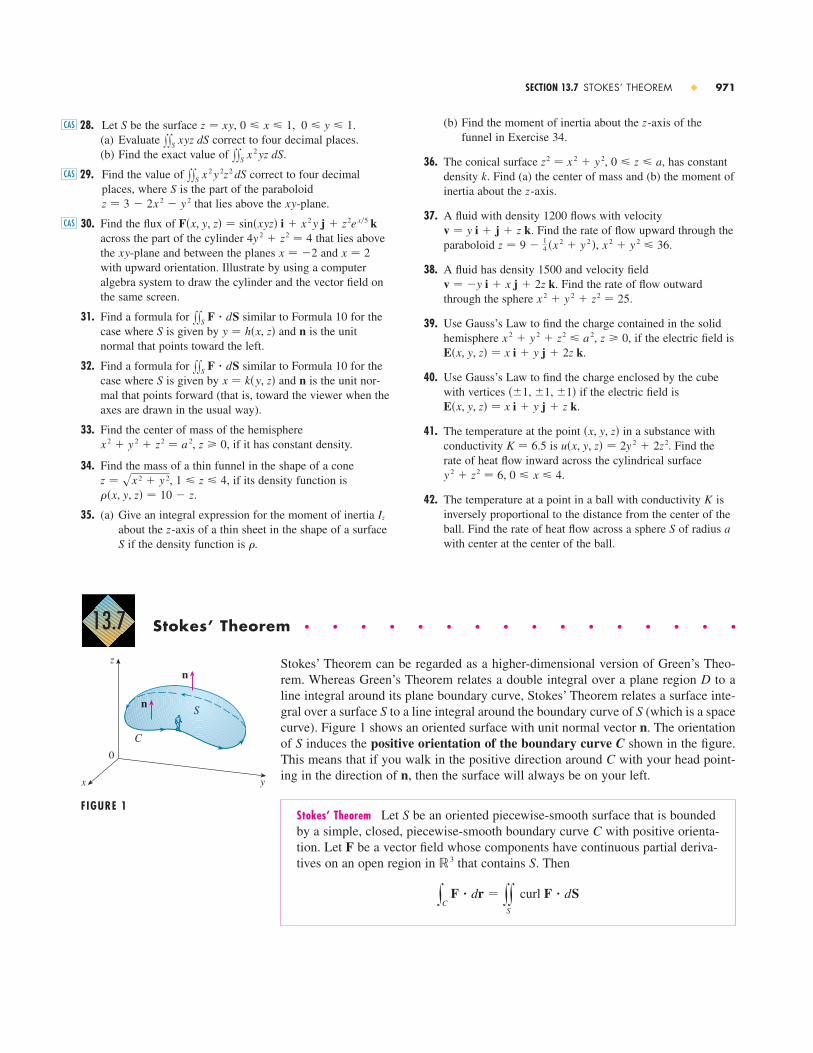
(b) Find the moment of inertia about the -axis of the funnel in Exercise 34.
36. The conical surface , , has constantdensity . Find (a) the center of mass and (b) the moment ofinertia about the -axis.
37. A fluid with density 1200 flows with velocity. Find the rate of flow upward through the
paraboloid , .
38. A fluid has density 1500 and velocity field. Find the rate of flow outward
through the sphere .
39. Use Gauss’s Law to find the charge contained in the solidhemisphere , , if the electric field is
.
40. Use Gauss’s Law to find the charge enclosed by the cube with vertices if the electric field is
.
41. The temperature at the point in a substance withconductivity is . Find therate of heat flow inward across the cylindrical surface
, .
42. The temperature at a point in a ball with conductivity isinversely proportional to the distance from the center of theball. Find the rate of heat flow across a sphere of radius with center at the center of the ball.
aS
K
0 � x � 4y 2 � z2 � 6
u�x, y, z� � 2y 2 � 2z2K � 6.5�x, y, z�
E�x, y, z� � x i � y j � z k��1, �1, �1�
E�x, y, z� � x i � y j � 2z kz � 0x 2 � y 2 � z2 � a 2
x 2 � y 2 � z2 � 25v � �y i � x j � 2z k
x 2 � y 2 � 36z � 9 �14 �x 2 � y 2 �
v � y i � j � z k
zk
0 � z � az2 � x 2 � y 2
z28. Let be the surface , , .(a) Evaluate correct to four decimal places.(b) Find the exact value of .
29. Find the value of correct to four decimalplaces, where is the part of the paraboloid
that lies above the -plane.
30. Find the flux of across the part of the cylinder that lies above the -plane and between the planes and with upward orientation. Illustrate by using a computeralgebra system to draw the cylinder and the vector field onthe same screen.
31. Find a formula for similar to Formula 10 for thecase where is given by and is the unitnormal that points toward the left.
32. Find a formula for similar to Formula 10 for thecase where is given by and is the unit nor-mal that points forward (that is, toward the viewer when theaxes are drawn in the usual way).
33. Find the center of mass of the hemisphere, , if it has constant density.
34. Find the mass of a thin funnel in the shape of a cone, , if its density function is
.
35. (a) Give an integral expression for the moment of inertia about the -axis of a thin sheet in the shape of a surface
if the density function is .�Sz
Iz
��x, y, z� � 10 � z1 � z � 4z � sx 2 � y 2
z � 0x 2 � y 2 � z2 � a 2
nx � k�y, z�SxxS F � dS
ny � h�x, z�SxxS F � dS
x � 2x � �2xy4y 2 � z2 � 4
F�x, y, z� � sin�xyz� i � x 2 y j � z2e x�5 kCAS
xyz � 3 � 2x 2 � y 2S
xxS x2 y 2z2 dSCAS
xxS x2 yz dS
xxS xyz dS0 � y � 10 � x � 1z � xySCAS
Stokes’ Theorem � � � � � � � � � � � � � � � �
Stokes’ Theorem can be regarded as a higher-dimensional version of Green’s Theo-rem. Whereas Green’s Theorem relates a double integral over a plane region to aline integral around its plane boundary curve, Stokes’ Theorem relates a surface inte-gral over a surface to a line integral around the boundary curve of (which is a spacecurve). Figure 1 shows an oriented surface with unit normal vector . The orientationof induces the positive orientation of the boundary curve C shown in the figure.This means that if you walk in the positive direction around with your head point-ing in the direction of , then the surface will always be on your left.
Stokes’ Theorem Let be an oriented piecewise-smooth surface that is boundedby a simple, closed, piecewise-smooth boundary curve with positive orienta-tion. Let be a vector field whose components have continuous partial deriva-tives on an open region in that contains . Then
yC F � dr � yy
S
curl F � dS
S� 3F
CS
nC
Sn
SS
D
13.7
SECTION 13.7 STOKES’ THEOREM � 971
S
y
z
x
C
0
n
n
FIGURE 1
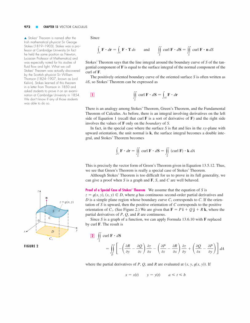
Since
Stokes’ Theorem says that the line integral around the boundary curve of of the tan-gential component of is equal to the surface integral of the normal component of thecurl of .
The positively oriented boundary curve of the oriented surface is often written as , so Stokes’ Theorem can be expressed as
There is an analogy among Stokes’ Theorem, Green’s Theorem, and the FundamentalTheorem of Calculus. As before, there is an integral involving derivatives on the leftside of Equation 1 (recall that is a sort of derivative of ) and the right sideinvolves the values of only on the boundary of .
In fact, in the special case where the surface is flat and lies in the -plane withupward orientation, the unit normal is , the surface integral becomes a double inte-gral, and Stokes’ Theorem becomes
This is precisely the vector form of Green’s Theorem given in Equation 13.5.12. Thus,we see that Green’s Theorem is really a special case of Stokes’ Theorem.
Although Stokes’ Theorem is too difficult for us to prove in its full generality, wecan give a proof when is a graph and , , and are well behaved.
Proof of a Special Case of Stokes’ Theorem We assume that the equation of is, where has continuous second-order partial derivatives and
is a simple plane region whose boundary curve corresponds to . If the orien-tation of is upward, then the positive orientation of corresponds to the positiveorientation of . (See Figure 2.) We are given that , where thepartial derivatives of , , and are continuous.
Since is a graph of a function, we can apply Formula 13.6.10 with replacedby . The result is
where the partial derivatives of , , and are evaluated at . If
a � t � by � y�t�x � x�t�
�x, y, t�x, y��RQP
� yyD
���R
�y�
�Q
�z �z
�x� ��P
�z�
�R
�x �z
�y� ��Q
�x�
�P
�y � dA
yyS
curl F � dS2
curl FFS
RQPF � P i � Q j � R kC1
CSCC1D
t�x, y� � Dz � t�x, y�,S
CSFS
yC F � dr � yy
S
curl F � dS � yyS
�curl F� � k dA
kxyS
SFFcurl F
yyS
curl F � dS � y�S
F � dr1
�SS
FF
S
yyS
curl F � dS � yyS
curl F � n dSandyC F � dr � y
C F � T ds
972 � CHAPTER 13 VECTOR CALCULUS
FIGURE 2
0
y
z
x D
C
S
z=g(x, y)
C¡
n
� Stokes’ Theorem is named after theIrish mathematical physicist Sir GeorgeStokes (1819–1903). Stokes was a pro-fessor at Cambridge University (in fact he held the same position as Newton,Lucasian Professor of Mathematics) andwas especially noted for his studies offluid flow and light. What we callStokes’ Theorem was actually discoveredby the Scottish physicist Sir WilliamThomson (1824–1907, known as LordKelvin). Stokes learned of this theorem in a letter from Thomson in 1850 andasked students to prove it on an exami-nation at Cambridge University in 1854.We don’t know if any of those studentswas able to do so.
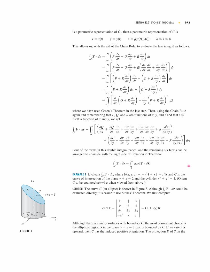
is a parametric representation of , then a parametric representation of is
This allows us, with the aid of the Chain Rule, to evaluate the line integral as follows:
where we have used Green’s Theorem in the last step. Then, using the Chain Ruleagain and remembering that , , and are functions of , , and and that isitself a function of and , we get
Four of the terms in this double integral cancel and the remaining six terms can bearranged to coincide with the right side of Equation 2. Therefore
EXAMPLE 1 Evaluate , where and is thecurve of intersection of the plane and the cylinder . (Orient
to be counterclockwise when viewed from above.)
SOLUTION The curve (an ellipse) is shown in Figure 3. Although could beevaluated directly, it’s easier to use Stokes’ Theorem. We first compute
Although there are many surfaces with boundary C, the most convenient choice isthe elliptical region S in the plane that is bounded by . If we orient upward, then has the induced positive orientation. The projection of on the SDC
SCy � z � 2
curl F � � i�
�x
�y 2
j�
�y
x
k�
�z
z2 � � �1 � 2y� k
xC F � drC
Cx 2 � y 2 � 1y � z � 2
CF�x, y, z� � �y 2 i � x j � z2 kxC F � dr
yC F � dr � yy
S
curl F � dS
� ��P
�y�
�P
�z �z
�y�
�R
�y �z
�x�
�R
�z �z
�y �z
�x� R
�2z
�y �x� dA
yC F � dr � yy
D
��Q
�x�
�Q
�z �z
�x�
�R
�x �z
�y�
�R
�z �z
�x �z
�y� R
�2z
�x �yyx
zzyxRQP
� yyD
�
�x �Q � R
�z
�y ��
�y �P � R
�z
�x� dA
� yC1
�P � R �z
�x dx � �Q � R �z
�y dy
� yb
a
�P � R �z
�x dx
dt� �Q � R
�z
�y dy
dt � dt
� yb
a
P dx
dt� Q
dy
dt� R� �z
�x dx
dt�
�z
�y dy
dt � dt
yC F � dr � y
b
a
�P dx
dt� Q
dy
dt� R
dz
dt dt
a � t � bz � t�x�t�, y�t��y � y�t�x � x�t�
CC1
SECTION 13.7 STOKES’ THEOREM � 973
FIGURE 3
0
y
z
x
CS
y+z=2
D

-plane is the disk and so using Equation 13.6.10 with, we have
EXAMPLE 2 Use Stokes’ Theorem to compute the integral , whereand is the part of the sphere that
lies inside the cylinder and above the -plane. (See Figure 4.)
SOLUTION To find the boundary curve we solve the equations and. Subtracting, we get and so (since ). Thus, is
the circle given by the equations , . A vector equation of is
so
Also, we have
Therefore, by Stokes’ Theorem,
Note that in Example 2 we computed a surface integral simply by knowing the val-ues of on the boundary curve . This means that if we have another oriented surfacewith the same boundary curve , then we get exactly the same value for the surfaceintegral!
In general, if and are oriented surfaces with the same oriented boundary curveand both satisfy the hypotheses of Stokes’ Theorem, then
This fact is useful when it is difficult to integrate over one surface but easy to integrateover the other.
yyS1
curl F � dS � yC F � dr � yy
S2
curl F � dS3
CS2S1
CCF
� s3 y2
0 cos 2t dt � 0
� y2
0 (�s3 sin2t � s3 cos2t) dt
yyS
curl F � dS � yC F � dr � y
2
0 F�r�t�� � r��t� dt
F�r�t�� � s3 sin t i � s3 cos t j � cos t sin t k
r��t� � �sin t i � cos t j
0 � t � 2 r�t� � cos t i � sin t j � s3 k
Cz � s3x 2 � y 2 � 1Cz � 0z � s3z2 � 3x 2 � y 2 � 1
x 2 � y 2 � z2 � 4C
xyx 2 � y 2 � 1x 2 � y 2 � z2 � 4SF�x, y, z� � yz i � xz j � xy k
xxS curl F � dS
� 12 �2 � � 0 �
� y2
0
r 2
2� 2
r 3
3 sin ��
0
1
d� � y2
0 ( 1
2 �23 sin �) d�
� y2
0 y
1
0 �1 � 2r sin �� r dr d�
yC F � dr � yy
S
curl F � dS � yyD
�1 � 2y� dA
z � t�x, y� � 2 � yx 2 � y 2 � 1xy
974 � CHAPTER 13 VECTOR CALCULUS
FIGURE 4
0
y
z
x
S
≈+¥+z@=4
C
≈+¥=1

We now use Stokes’ Theorem to throw some light on the meaning of the curl vec-tor. Suppose that is an oriented closed curve and represents the velocity field influid flow. Consider the line integral
and recall that is the component of in the direction of the unit tangent vector. This means that the closer the direction of is to the direction of , the larger the
value of . Thus, is a measure of the tendency of the fluid to move aroundand is called the circulation of around . (See Figure 5.)
Now let be a point in the fluid and let be a small disk with radius and center Then ( for all points on because iscontinuous. Thus, by Stokes’ Theorem, we get the following approximation to the cir-culation around the boundary circle :
This approximation becomes better as and we have
Equation 4 gives the relationship between the curl and the circulation. It shows thatis a measure of the rotating effect of the fluid about the axis n. The curling
effect is greatest about the axis parallel to .Finally, we mention that Stokes’ Theorem can be used to prove Theorem 13.5.4
(which states that if on all of , then is conservative). From our previous work (Theorems 13.3.3 and 13.3.4), we know that is conservative if
for every closed path . Given , suppose we can find an orientable sur-face whose boundary is . (This can be done, but the proof requires advanced tech-niques.) Then Stokes’ Theorem gives
A curve that is not simple can be broken into a number of simple curves, and the integrals around these simple curves are all 0. Adding these integrals, we obtain
for any closed curve .CxC F � dr � 0
yC F � dr � yy
S
curl F � dS � yyS
0 � dS � 0
CSCC0xC F � dr �
FF� 3curl F � 0
curl vcurl v � n
curl v�P0 � � n�P0 � � lim a l 0
1
a 2 yCa
v � dr4
a l 0
� yySa
curl v�P0 � � n�P0 � dS � curl v�P0 � � n�P0 � a 2
yCa
v � dr � yySa
curl v � dS � yySa
curl v � n dS
Ca
curl FSaPcurl F��P� � �curl F��P0�P0.aSaP0�x0, y0, z0 �
FIGURE 5
T
v
C
(b) jC v � dr<0, negative circulation
T
vC
(a) jC v � dr>0, positive circulation
CvCx
C v � drv � T
TvTvv � T
yC v � dr � y
C v � T ds
vC
SECTION 13.7 STOKES’ THEOREM � 975
� Imagine a tiny paddle wheel placedin the fluid at a point , as in Figure 6;the paddle wheel rotates fastest when itsaxis is parallel to .curl v
P
FIGURE 6
curl v

9. ,is the curve of intersection of the plane and
the cylinder
10. ,is the boundary of the part of the paraboloid
in the first octant� � � � � � � � � � � � �
11. (a) Use Stokes’ Theorem to evaluate , where
and is the curve of intersection of the planeand the cylinder oriented
counterclockwise as viewed from above.
; (b) Graph both the plane and the cylinder with domains chosen so that you can see the curve and the surface that you used in part (a).
; (c) Find parametric equations for and use them to graph .
12. (a) Use Stokes’ Theorem to evaluate , whereand is the curve of
intersection of the hyperbolic paraboloid and the cylinder oriented counterclockwiseas viewed from above.
; (b) Graph both the hyperbolic paraboloid and the cylinderwith domains chosen so that you can see the curve and the surface that you used in part (a).
; (c) Find parametric equations for and use them to graph .
13–15 � Verify that Stokes’ Theorem is true for the given vectorfield and surface .
13. ,is the part of the paraboloid that lies below
the plane oriented upward
14. ,is the part of the plane that lies in the
first octant, oriented upward
15. ,is the hemisphere , , oriented in
the direction of the positive -axis
� � � � � � � � � � � � �
16. Let
Let be the curve in Exercise 12 and consider all possiblesmooth surfaces whose boundary curve is . Find the val-ues of , , and for which is independent of thechoice of .S
xxS F � dScbaCS
C
F�x, y, z� � �ax 3 � 3xz2, x 2 y � by 3, cz3 �
yy � 0x 2 � y 2 � z 2 � 1S
F�x, y, z� � y i � z j � x k
2x � y � z � 2SF�x, y, z� � x i � y j � xyz k
z � 1,z � x 2 � y 2S
F�x, y, z� � y 2 i � x j � z 2 k
SF
CC
C
x 2 � y 2 � 1z � y 2 � x 2
CF�x, y, z� � x 2 y i �13 x 3 j � xy k
xC F � dr
CC
C
x 2 � y 2 � 9x � y � z � 1C
F�x, y, z� � x 2z i � xy 2 j � z2 k
xC F � dr
z � 1 � x 2 � y 2CF�x, y, z� � x i � y j � �x 2 � y 2 � k
x 2 � y 2 � 4z � x � 4C
F�x, y, z� � 2z i � 4x j � 5y k1. A hemisphere and a portion of a paraboloid are shown.Suppose is a vector field on whose components havecontinuous partial derivatives. Explain why
2–6 � Use Stokes’ Theorem to evaluate .
2. ,S is the part of the paraboloid that liesabove the plane , oriented upward
3. ,S is the hemisphere , ,oriented upward
4. ,is the part of the hemisphere that lies
inside the cylinder , oriented in the direction of the positive -axis
5. ,consists of the top and the four sides (but not the bottom)
of the cube with vertices , oriented outward[Hint: Use Equation 3.]
6. ,consists of the four sides of the pyramid with vertices
, , , , and that lie to the right of the -plane, oriented in the direction of thepositive -axis [Hint: Use Equation 3.]
� � � � � � � � � � � � �
7–10 � Use Stokes’ Theorem to evaluate . In each caseis oriented counterclockwise as viewed from above.
7. ,is the triangle with vertices (1, 0, 0), (0, 1, 0),
and (0, 0, 1)
8. ,is the boundary of the part of the plane
in the first octant2x � y � 2z � 2C
F�x, y, z� � e�x i � e x j � e z k
CF�x, y, z� � �x � y 2 � i � �y � z2 � j � �z � x 2 � k
Cx
C F � dr
yxz
�0, 1, 0��1, 0, 1��0, 0, 1��1, 0, 0��0, 0, 0�SF�x, y, z� � xy i � e z j � xy 2 k
��1, �1, �1�SF�x, y, z� � xyz i � xy j � x 2 yz k
xy 2 � z2 � 4
x � s9 � y 2 � z 2SF�x, y, z� � �x � tan�1yz� i � y 2z j � z k
z � 0x 2 � y 2 � z2 � 4F�x, y, z� � x 2e yz i � y 2e xz j � z2e xy k
z � 5z � 9 � x 2 � y 2
F�x, y, z� � yz i � xz j � xy k
xxS curl F � dS
H
4
z
x y22
P
4
z
x y22
yyH
curl F � dS � yyP
curl F � dS
�3FPH
976 � CHAPTER 13 VECTOR CALCULUS
Exercises � � � � � � � � � � � � � � � � � � � � � � � � � �13.7

WRITING PROJECT THREE MEN AND TWO THEOREMS � 977
Three Men and Two Theorems
Although two of the most important theorems in vector calculus are named after GeorgeGreen and George Stokes, a third man, William Thomson (also known as Lord Kelvin),played a large role in the formulation, dissemination, and application of both of theseresults. All three men were interested in how the two theorems could help to explain andpredict physical phenomena in electricity and magnetism and fluid flow. The basic facts ofthe story are given in the margin notes on pages 946 and 972.
Write a report on the historical origins of Green’s Theorem and Stokes’ Theorem. Explainthe similarities and relationship between the theorems. Discuss the roles that Green, Thom-son, and Stokes played in discovering these theorems and making them widely known.Show how both theorems arose from the investigation of electricity and magnetism andwere later used to study a variety of physical problems.
The dictionary edited by Gillispie [2] is a good source for both biographical and scientificinformation. The book by Hutchinson [5] gives an account of Stokes’ life and the book byThompson [8] is a biography of Lord Kelvin. The articles by Grattan-Guinness [3] and Gray [4] and the book by Cannell [1] give background on the extraordinary life and worksof Green. Additional historical and mathematical information is found in the books byKatz [6] and Kline [7].
1. D. M. Cannell, George Green, Mathematician and Physicist 1793–1841: The Back-ground to his Life and Work (London: Athlone Press, 1993).
2. C. C. Gillispie, ed., Dictionary of Scientific Biography (New York: Scribner’s, 1974).See the article on Green by P. J. Wallis in Volume XV and the articles on Thomson byJed Buchwald and on Stokes by E. M. Parkinson in Volume XIII.
3. I. Grattan-Guinness, “Why did George Green write his essay of 1828 on electricity andmagnetism?” Amer. Math. Monthly, Vol. 102 (1995), pp. 387–396.
4. J. Gray, “There was a jolly miller.” The New Scientist, Vol. 139 (1993), pp. 24–27.
5. G. E. Hutchinson, The Enchanted Voyage (New Haven: Yale University Press, 1962).
6. Victor Katz, A History of Mathematics: An Introduction (New York: HarperCollins,1993), pp. 678–680.
7. Morris Kline, Mathematical Thought from Ancient to Modern Times (New York: Oxford University Press, 1972), pp. 683–685.
8. Sylvanus P. Thompson, The Life of Lord Kelvin (New York: Chelsea, 1976).
WritingProject
� The photograph shows a stained-glass window at Cambridge Universityin honor of George Green.
19. If is a sphere and satisfies the hypotheses of Stokes’Theorem, show that .
20. Suppose and satisfy the hypotheses of Stokes’ Theoremand , have continuous second-order partial derivatives.Use Exercises 22 and 24 in Section 13.5 to show the following.(a)
(b)
(c) xC � f �t � t� f � � dr � 0
xC � f � f � � dr � 0
xC � f �t� � dr � xxS �� f � �t� � dS
tfCS
xxS curl F � dS � 0FS17. Calculate the work done by the force field
when a particle moves under its influence around the edgeof the part of the sphere that lies in thefirst octant, in a counterclockwise direction as viewed fromabove.
18. Evaluate ,where is the curve ,
. [Hint: Observe that lies on the surface.]z � 2xy
C0 � t � 2 r�t� � �sin t, cos t, sin 2t�C
xC �y � sin x� dx � �z2 � cos y� dy � x 3 dz
x 2 � y 2 � z2 � 4
F�x, y, z� � �x x � z2 � i � �y y � x 2 � j � �z z � y 2 � k

The Divergence Theorem � � � � � � � � � � � � �
In Section 13.5 we rewrote Green’s Theorem in a vector version as
where is the positively oriented boundary curve of the plane region . If we wereseeking to extend this theorem to vector fields on , we might make the guess that
where is the boundary surface of the solid region . It turns out that Equation 1 istrue, under appropriate hypotheses, and is called the Divergence Theorem. Notice itssimilarity to Green’s Theorem and Stokes’ Theorem in that it relates the integral of aderivative of a function ( in this case) over a region to the integral of the originalfunction over the boundary of the region.
At this stage you may wish to review the various types of regions over which wewere able to evaluate triple integrals in Section 12.7. We state and prove the Diver-gence Theorem for regions that are simultaneously of types 1, 2, and 3 and we callsuch regions simple solid regions. (For instance, regions bounded by ellipsoids orrectangular boxes are simple solid regions.) The boundary of is a closed surface, andwe use the convention, introduced in Section 13.6, that the positive orientation is out-ward; that is, the unit normal vector is directed outward from .
The Divergence Theorem Let be a simple solid region and let S be the boundarysurface of E, given with positive (outward) orientation. Let be a vector fieldwhose component functions have continuous partial derivatives on an openregion that contains . Then
Thus, the Divergence Theorem states that, under the given conditions, the flux ofacross the boundary surface of is equal to the triple integral of the divergence ofover .
Proof Let . Then
so yyyE
div F dV � yyyE
�P
�x dV � yyy
E
�Q
�y dV � yyy
E
�R
�z dV
div F ��P
�x�
�Q
�y�
�R
�z
F � P i � Q j � R k
EFEF
yyS
F � dS � yyyE
div F dV
E
FE
En
E
E
Fdiv F
ES
yyS
F � n dS � yyyE
div F�x, y, z� dV1
� 3DC
yC F � n ds � yy
D
div F�x, y� dA
13.8
978 � CHAPTER 13 VECTOR CALCULUS
� The Divergence Theorem is sometimescalled Gauss’s Theorem after the greatGerman mathematician Karl FriedrichGauss (1777–1855), who discoveredthis theorem during his investigation of electrostatics. In Eastern Europe theDivergence Theorem is known as Ostrogradsky’s Theorem after the Russianmathematician Mikhail Ostrogradsky(1801–1862), who published this resultin 1826.

If is the unit outward normal of , then the surface integral on the left side of theDivergence Theorem is
Therefore, to prove the Divergence Theorem, it suffices to prove the following threeequations:
To prove Equation 4 we use the fact that is a type 1 region:
where is the projection of onto the -plane. By Equation 12.7.6, we have
and, therefore, by the Fundamental Theorem of Calculus,
The boundary surface consists of three pieces: the bottom surface , the topsurface , and possibly a vertical surface , which lies above the boundary curve ofD. (See Figure 1. It might happen that doesn’t appear, as in the case of a sphere.)Notice that on we have , because k is vertical and n is horizontal, and so
Thus, regardless of whether there is a vertical surface, we can write
The equation of is , , and the outward normal pointsupward, so from Equation 13.6.10 (with replaced by ) we have
yyS2
R k � n dS � yyD
R�x, y, u2�x, y�� dA
R kFn�x, y� � Dz � u2�x, y�S2
yyS
R k � n dS � yyS1
R k � n dS � yyS2
R k � n dS6
yyS3
R k � n dS � yyS3
0 dS � 0
k � n � 0S3
S3
S3S2
S1S
yyyE
�R
�z dV � yy
D
�R�x, y, u2�x, y�� � R�x, y, u1�x, y��� dA5
yyyE
�R
�z dV � yy
D
yu2�x, y�
u1�x, y� �R
�z �x, y, z� dz� dA
xyED
E � ��x, y, z� � �x, y� � D, u1�x, y� � z � u2�x, y��
E
yyS
R k � n dS � yyyE
�R
�z dV4
yyS
Q j � n dS � yyyE
�Q
�y dV3
yyS
P i � n dS � yyyE
�P
�x dV2
� yyS
P i � n dS � yyS
Q j � n dS � yyS
R k � n dS
yyS
F � dS � yyS
F � n dS � yyS
�P i � Q j � R k� � n dS
Sn
SECTION 13.8 THE DIVERGENCE THEOREM � 979
FIGURE 1
0
y
z
x D
ES£
S™ {z=u™(x, y)}
S¡ (z=u¡(x, y))

On we have , but here the outward normal points downward, so we multiply by :
Therefore, Equation 6 gives
Comparison with Equation 5 shows that
Equations 2 and 3 are proved in a similar manner using the expressions for as atype 2 or type 3 region, respectively.
EXAMPLE 1 Find the flux of the vector field over the unitsphere .
SOLUTION First we compute the divergence of :
The unit sphere is the boundary of the unit ball given by .Thus, the Divergence Theorem gives the flux as
EXAMPLE 2 Evaluate , where
and is the surface of the region bounded by the parabolic cylinder and the planes , , and . (See Figure 2.)
0
y
z
(0, 0, 1)
(1, 0, 0) (0, 2, 0)x
y=2-z
z=1-≈FIGURE 2
y � z � 2y � 0z � 0z � 1 � x 2ES
F�x, y, z� � xy i � (y 2 � exz2)
j � sin�xy� k
yyS
F � dS
� V�B� � 43 �1�3 �
4
3
yyS
F � dS � yyyB
div F dV � yyyB
1 dV
x 2 � y 2 � z2 � 1BS
div F ��
�x �z� �
�
�y �y� �
�
�z �x� � 1
F
x 2 � y 2 � z2 � 1F�x, y, z� � z i � y j � x k
E
yyS
R k � n dS � yyyE
�R
�z dV
yyS
R k � n dS � yyD
�R�x, y, u2�x, y�� � R�x, y, u1�x, y��� dA
yyS1
R k � n dS � �yyD
R�x, y, u1�x, y�� dA
�1nz � u1�x, y�S1
980 � CHAPTER 13 VECTOR CALCULUS
� Notice that the method of proof of theDivergence Theorem is very similar tothat of Green’s Theorem.
� The solution in Example 1 should be compared with the solution in Example 4 in Section 13.6.

SOLUTION It would be extremely difficult to evaluate the given surface integraldirectly. (We would have to evaluate four surface integrals corresponding to the fourpieces of .) Furthermore, the divergence of is much less complicated than itself:
Therefore, we use the Divergence Theorem to transform the given surface integralinto a triple integral. The easiest way to evaluate the triple integral is to express asa type 3 region:
Then we have
Although we have proved the Divergence Theorem only for simple solid regions,it can be proved for regions that are finite unions of simple solid regions. (The proce-dure is similar to the one we used in Section 13.4 to extend Green’s Theorem.)
For example, let’s consider the region that lies between the closed surfaces and, where lies inside . Let and be outward normals of and . Then the
boundary surface of is and its normal is given by on andon . (See Figure 3.) Applying the Divergence Theorem to , we get
Let’s apply this to the electric field (see Example 5 in Section 13.1):
E�x� ��Q
� x �3 x
� �yyS1
F � dS � yyS2
F � dS
� yyS1
F � ��n1� dS � yyS2
F � n2 dS
yyyE
div F dV � yyS
F � dS � yyS
F � n dS7
SS2n � n2
S1n � �n1nS � S1 � S2ES2S1n2n1S2S1S2
S1E
� �y1
0 �x 6 � 3x 4 � 3x 2 � 7� dx �
184
35
� �12 y
1
�1 ��x 2 � 1�3 � 8� dx
�3
2 y
1
�1
��2 � z�3
3 �0
1�x2
dx
� 3 y1
�1 y
1�x2
0 �2 � z�2
2 dz dx
� 3 y1
�1 y
1�x2
0 y
2�z
0 y dy dz dx
yyS
F � dS � yyyE
div F dV � yyyE
3y dV
E � ��x, y, z� � �1 � x � 1, 0 � z � 1 � x 2, 0 � y � 2 � z�
E
� y � 2y � 3y
div F ��
�x �xy� �
�
�y (y 2 � exz2) �
�
�z �sin xy�
FFS
SECTION 13.8 THE DIVERGENCE THEOREM � 981
FIGURE 3
n¡
_n¡
n™
S¡S™

where is a small sphere with radius and center the origin. You can verify that(see Exercise 19). Therefore, Equation 7 gives
The point of this calculation is that we can compute the surface integral over because is a sphere. The normal vector at is . Therefore
since the equation of is . Thus, we have
This shows that the electric flux of is through any closed surface that con-tains the origin. [This is a special case of Gauss’s Law (Equation 13.6.11) for a singlecharge. The relationship between and is .]
Another application of the Divergence Theorem occurs in fluid flow. Let be the velocity field of a fluid with constant density . Then is the rate of flowper unit area. If is a point in the fluid and is a ball with center andvery small radius , then for all points in since is con-tinuous. We approximate the flux over the boundary sphere as follows:
This approximation becomes better as and suggests that
Equation 8 says that is the net rate of outward flux per unit volume at .(This is the reason for the name divergence.) If , the net flow is outwardnear and is called a source. If , the net flow is inward near and is called a sink.
PPdiv F�P� � 0PPdiv F�P� � 0
P0div F�P0 �
div F�P0 � � lim a l 0
1
V�Ba � yy
Sa
F � dS8
a l 0
� div F�P0 �V�Ba �
� yyyBa
div F�P0 � dV
yySa
F � dS � yyyBa
div F dV
Sa
div FBadiv F�P� � div F�P0 �aP0BaP0�x0, y0, z0 �
F � �v�v�x, y, z�
� � 1��4 �0 ��0�
S24 �QE
��Q
a 2 4 a 2 � 4 �Q
��Q
a 2 yyS1
dS ��Q
a 2 A�S1�
yyS2
E � dS � yyS1
E � n dS
� x � � aS1
��Q
� x �2 ��Q
a 2
E � n ��Q
� x �3 x � � x
� x � ��Q
� x �4 x � x
x�� x �xS1
S1
� yyS1
E � dS � yyS1
E � n dS
yyS2
E � dS � yyS1
E � dS � yyyE
div E dV
div E � 0aS1
982 � CHAPTER 13 VECTOR CALCULUS

For the vector field in Figure 4, it appears that the vectors that end near areshorter than the vectors that start near Thus, the net flow is outward near so
and is a source. Near on the other hand, the incoming arrows are longer than the outgoing arrows. Here the net flow is inward, so and is a sink. We can use the formula for F to confirm this impression. Since
, we have , which is positive when . So thepoints above the line are sources and those below are sinks.
FIGURE 4The vector field F=≈ i+¥ j
P¡
P™
y
x
y � �xy � �xdiv F � 2x � 2yF � x 2 i � y 2 j
P2
div F�P2 � � 0P2,P1div F�P1� � 0
P1,P1.P1
SECTION 13.8 THE DIVERGENCE THEOREM � 983
3–6 � Verify that the Divergence Theorem is true for the vectorfield on the region .
3. ,is the cube bounded by the planes , , ,
, , and
4. ,is the solid bounded by the paraboloid and
the plane
5. ,is the solid cylinder ,
6. ,is the unit ball
� � � � � � � � � � � � �
7–15 � Use the Divergence Theorem to calculate the surfaceintegral ; that is, calculate the flux of across .
7. ,is the surface of the box bounded by the planes ,
, , , , and
8. ,is the surface of the box with vertices
9. ,is the surface of the solid bounded by the cylinder
and the planes and x � 2x � �1y 2 � z2 � 1SF�x, y, z� � 3xy 2 i � xe z j � z3 k
��1, �2, �3�SF�x, y, z� � x 2z3 i � 2xyz3 j � xz4 k
z � 2z � 0y � 1y � 0x � 1x � 0S
F�x, y, z� � ex sin y i � ex cos y j � yz2 k
SFxxS F � dS
x 2 � y 2 � z2 � 1EF�x, y, z� � x i � y j � z k
0 � z � 1x 2 � y 2 � 1EF�x, y, z� � xy i � yz j � zx k
z � 1z � x 2 � y 2E
F�x, y, z� � xz i � yz j � 3z2 k
z � 1z � 0y � 1y � 0x � 1x � 0E
F�x, y, z� � 3x i � xy j � 2xz k
EF1. A vector field is shown. Use the interpretation of
divergence derived in this section to determine whetheris positive or negative at and at
2. (a) Are the points and sources or sinks for the vectorfield shown in the figure? Give an explanation basedsolely on the picture.
(b) Given that , use the definition of diver-gence to verify your answer to part (a).
2
_2
_2 2
P¡
P™
F�x, y� � �x, y 2�
FP2P1
2
_2
_2 2
P¡
P™
P2.P1div F
F
Exercises � � � � � � � � � � � � � � � � � � � � � � � � � �13.8

and components of the vector fields have continuous second-order partial derivatives.
21. , where is a constant vector
22. , where
23.
24.
25.
26.
� � � � � � � � � � � � �
27. Suppose and satisfy the conditions of the DivergenceTheorem and is a scalar function with continuous partialderivatives. Prove that
These surface and triple integrals of vector functions arevectors defined by integrating each component function.[Hint: Start by applying the Divergence Theorem to ,where is an arbitrary constant vector.]
28. A solid occupies a region with surface and is immersedin a liquid with constant density . We set up a coordinatesystem so that the -plane coincides with the surface of theliquid and positive values of are measured downward intothe liquid. Then the pressure at depth is , where is the acceleration due to gravity (see Section 6.5). The totalbuoyant force on the solid due to the pressure distribution isgiven by the surface integral
where is the outer unit normal. Use the result of Exer-cise 27 to show that , where is the weight ofthe liquid displaced by the solid. (Note that is directedupward because is directed downward.) The result isArchimedes’ principle: The buoyant force on an objectequals the weight of the displaced liquid.
zF
WF � �Wkn
F � �yyS
pn dS
tp � �tzzz
xy�
SE
cF � fc
yyS
f n dS � yyyE
� f dV
fES
yyS
� f �t � t� f � � n dS � yyyE
� f � 2t � t� 2f � dV
yyS
� f �t� � n dS � yyyE
� f � 2t � � f � �t� dV
yyS
Dn f dS � yyyE
� 2f dV
yyS
curl F � dS � 0
F�x, y, z� � x i � y j � z kV�E � � 13 yy
S
F � dS
ayyS
a � n dS � 0
10. ,is the surface of the solid bounded by the hyperboloid
and the planes and
11. ,is the ellipsoid
12. ,is the surface of the solid bounded by the paraboloid
and the -plane
13. ,is the sphere
14. ,is the surface of the solid bounded by the hemispheres
, and the plane
15. ,is the surface of the solid that lies above the -plane
and below the surface ,
� � � � � � � � � � � � �
16. Use a computer algebra system to plot the vector field
in the cube cut from the first octant by the planes ,, and . Then compute the flux across the
surface of the cube.
17. Use the Divergence Theorem to evaluate , where
and is the top half of the sphere .[Hint: Note that is not a closed surface. First compute integrals over and , where is the disk ,oriented downward, and .]
18. Let . Find the flux of across the part of the paraboloid
that lies above the plane and is oriented upward.
19. Verify that for the electric field
20. Use the Divergence Theorem to evaluate
where is the sphere .
21–26 � Prove each identity, assuming that and satisfy theconditions of the Divergence Theorem and the scalar functions
ES
x 2 � y 2 � z2 � 1S
yyS
�2x � 2y � z2 � dS
E�x� ��Q
� x �3 x
div E � 0
z � 1x 2 � y 2 � z � 2F
F�x, y, z� � z tan�1�y 2 � i � z3 ln�x 2 � 1� j � z k
S2 � S � S1
x 2 � y 2 � 1S1S2S1
Sx 2 � y 2 � z2 � 1S
F�x, y, z� � z2x i � ( 13 y
3 � tan z) j � �x 2z � y 2 � k
xxS F � dS
z � �2y � �2x � �2
F�x, y, z� � sin x cos2 y i � sin3y cos4z j � sin5z cos6x kCAS
�1 � y � 1�1 � x � 1,z � 2 � x 4 � y 4
xySF�x, y, z� � e y tan z i � ys3 � x 2 j � x sin y kCAS
z � 0z � s1 � x 2 � y 2z � s4 � x 2 � y 2
SF�x, y, z� � �x 3 � y sin z� i � �y 3 � z sin x� j � 3z k
x 2 � y 2 � z2 � 1SF�x, y, z� � x 3 i � y 3 j � z3 k
xyz � 4 � x 2 � y 2SF�x, y, z� � x 3 i � 2xz2 j � 3y 2z k
x 2�a2 � y 2�b2 � z2�c2 � 1SF�x, y, z� � xy sin z i � cos�xz� j � y cos z k
z � 2z � �2x 2 � y 2 � z2 � 1SF�x, y, z� � x 3y i � x 2y 2 j � x 2yz k
984 � CHAPTER 13 VECTOR CALCULUS

Summary � � � � � � � � � � � � � � � � � �
The main results of this chapter are all higher-dimensional versions of the Funda-mental Theorem of Calculus. To help you remember them, we collect them togetherhere (without hypotheses) so that you can see more easily their essential similarity.Notice that in each case we have an integral of a “derivative” over a region on the leftside, and the right side involves the values of the original function only on the bound-ary of the region.
Fundamental Theorem of Calculus
Fundamental Theorem for Line Integrals
Green’s Theorem
Stokes’ Theorem
Divergence Theorem E
S
n
nyyyE
div F dV � yyS
F � dS
C
S
n
yyS
curl F � dS � yC F � dr
C
DyyD
��Q
�x�
�P
�y dA � yC P dx � Q dy
r(a)
r(b)
Cy
C ∇ f � dr � f �r�b�� � f �r�a��
a byb
a F��x� dx � F�b� � F�a�
13.9
SECTION 13.9 SUMMARY � 985

986 � CHAPTER 13 VECTOR CALCULUS
9. Suppose is a vector field on .(a) Define curl .(b) Define div .(c) If is a velocity field in fluid flow, what are the physi-
cal interpretations of curl and div ?
10. If , how do you test to determine whether is conservative? What if is a vector field on ?
11. (a) Write the definition of the surface integral of a scalarfunction over a surface .
(b) How do you evaluate such an integral if is a para-metric surface given by a vector function ?
(c) What if is given by an equation ?(d) If a thin sheet has the shape of a surface , and the den-
sity at is , write expressions for themass and center of mass of the sheet.
12. (a) What is an oriented surface? Give an example of a nonorientable surface.
(b) Define the surface integral (or flux) of a vector field over an oriented surface with unit normal vector .
(c) How do you evaluate such an integral if is a para-metric surface given by a vector function ?
(d) What if is given by an equation ?
13. State Stokes’ Theorem.
14. State the Divergence Theorem.
15. In what ways are the Fundamental Theorem for Line Integrals, Green’s Theorem, Stokes’ Theorem, and theDivergence Theorem similar to each other?
z � t�x, y�Sr�u, v�
SnS
F
��x, y, z��x, y, z�S
z � t�x, y�Sr�u, v�
SSf
�3FFF � P i � Q j
FFF
FF
�3F
5. If and in an open region , then is conservative.
6.
7. If is a sphere and is a constant vector field, then.
8. There is a vector field such that
curl F � x i � y j � z k
F
xxS F � dS � 0FS
x�C f �x, y� ds � �xC f �x, y� ds
FDPy � QxF � P i � Q j
1. What is a vector field? Give three examples that have physi-cal meaning.
2. (a) What is a conservative vector field?(b) What is a potential function?
3. (a) Write the definition of the line integral of a scalar func-tion along a smooth curve with respect to arclength.
(b) How do you evaluate such a line integral?(c) Write expressions for the mass and center of mass of a
thin wire shaped like a curve if the wire has lineardensity function .
(d) Write the definitions of the line integrals along of ascalar function with respect to , , and .
(e) How do you evaluate these line integrals?
4. (a) Define the line integral of a vector field along asmooth curve given by a vector function .
(b) If is a force field, what does this line integralrepresent?
(c) If , what is the connection between theline integral of and the line integrals of the componentfunctions , , and ?
5. State the Fundamental Theorem for Line Integrals.
6. (a) What does it mean to say that is independent of path?
(b) If you know that is independent of path, whatcan you say about ?
7. State Green’s Theorem.
8. Write expressions for the area enclosed by a curve interms of line integrals around .C
C
FxC F � dr
xC F � dr
RQPF
F � �P, Q, R�
Fr�t�C
F
zyxfC
��x, y�C
Cf
Determine whether the statement is true or false. If it is true, explain why.If it is false, explain why or give an example that disproves the statement.
1. If is a vector field, then div is a vector field.
2. If is a vector field, then curl is a vector field.
3. If has continuous partial derivatives of all orders on ,then .
4. If has continuous partial derivatives on and is any circle, then .xC ∇ f � dr � 0
C� 3f
∇ f � � 0div�curl� 3f
FF
FF
T R U E – FA L S E Q U I Z
13 ReviewC O N C E P T C H E C K

CHAPTER 13 REVIEW � 987
E X E R C I S E S
12.� � � � � � � � � � � � �
13–14 � Show that is conservative and use this fact to evalu-ate along the given curve.
13. ,: ,
14. ,is the line segment from to
� � � � � � � � � � � � �
15. Verify that Green’s Theorem is true for the line integral, where consists of the parabola
from to and the line segment fromto .
16. Use Green’s Theorem to evaluate
where is the triangle with vertices , ,and
17. Use Green’s Theorem to evaluate where is the circle with counterclockwise orientation.
18. Find curl and div if
19. Show that there is no vector field such that
20. Show that, under conditions to be stated on the vector fieldsand ,
21. If is any piecewise-smooth simple closed plane curve andand are differentiable functions, show that
22. If and are twice differentiable functions, show that
23. If is a harmonic function, that is, , show that theline integral is independent of path in anysimple region .
24. (a) Sketch the curve with parametric equations
0 � t � 2 z � sin ty � sin tx � cos t
C
Dx fy dx � fx dy
� 2 f � 0f
� 2� ft� � f � 2t � t� 2f � 2� f � �t
tf
yC f �x� dx � t�y� dy � 0
tfC
curl�F � G� � F div G � G div F � �G � � �F � �F � � �G
GF
curl G � 2x i � 3yz j � xz2 k
G
F�x, y, z� � e�x sin y i � e�y sin z j � e�z sin x k
FF
x 2 � y 2 � 4CxC x 2 y dx � xy 2 dy
�1, 3�.�1, 0��0, 0�C
yC s1 � x 3 dx � 2xy dy
��1, 1��1, 1��1, 1���1, 1�y � x 2
CxC xy 2 dx � x 2 y dy
�4, 0, 3��0, 2, 0�CF�x, y, z� � e y i � �xe y � e z� j � ye z k
0 � t � 1r�t� � �t � sin t� i � �2t � cos t� jCF�x, y� � �4x 3y 2 � 2xy 3� i � �2x 4y � 3x 2y 2 � 4y 3� j
xC F � drF
F�x, y, z� � sin y i � x cos y j � sin z k1. A vector field , a curve , and a point are shown.(a) Is positive, negative, or zero? Explain.(b) Is positive, negative, or zero? Explain.
2–9 � Evaluate the line integral.
2. ,is the arc of the parabola from (0, 0) to (1, 1)
3. ,: , , ,
4. ,is the sine curve ,
5. ,is the circle with counterclockwise
orientation
6. ,is given by ,
7. ,consists of the line segments from to and
from to
8. , where and is given by,
9. , where and is given by ,
� � � � � � � � � � � � �
10. Find the work done by the force field
in moving a particle from the point to the pointalong
(a) A straight line(b) The helix , ,
11–12 � Show that is a conservative vector field. Then find afunction such that .
11. F�x, y� � �1 � xy�e xy i � �e y � x 2e xy� j
F � ∇ ffF
z � 3 sin ty � tx � 3 cos t
�0, �2, 3��3, 0, 0�
F�x, y, z� � z i � x j � y k
0 � t � 1r�t� � 2t i � t 2 j � t 4 kCF�x, y, z� � �x � y� i � z j � x 2 y kxC F � dr
0 � t � 1r�t� � t 2 i � t 3 jCF�x, y� � x 2 y i � e y jxC F � dr
�3, 1, 4��1, 1, 2��1, 1, 2��0, 0, 0�C
xC y dx � z dy � x dz
0 � t � 1r�t� � t i � t 2 j � t 3 kCxC x sin y dx � xyz dz
x 2 � y 2 � 1CxC x 3y dx � x dy
0 � x � �2y � sin xCxC xy dx � y dy
0 � t � �2z � 2 cos ty � tx � 2 sin tCxC x 3z ds
y � x 2CxC x ds
y
x
P
C
div F�P�xC F � dr
PCF
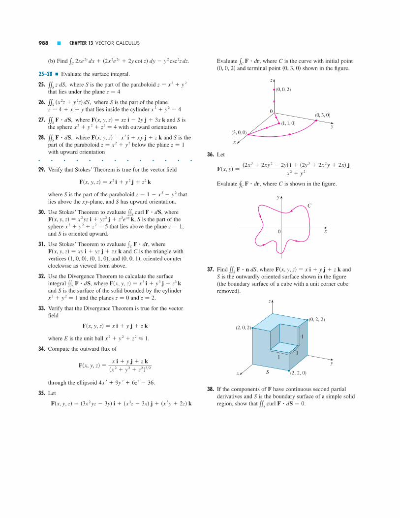
988 � CHAPTER 13 VECTOR CALCULUS
Evaluate , where is the curve with initial pointand terminal point shown in the figure.
36. Let
Evaluate , where is shown in the figure.
37. Find , where and is the outwardly oriented surface shown in the figure
(the boundary surface of a cube with a unit corner cuberemoved).
38. If the components of have continuous second partialderivatives and is the boundary surface of a simple solidregion, show that .xxS curl F � dS � 0
SF
y
z
x
(0, 2, 2)
(2, 0, 2)
(2, 2, 0)
1
1
S
1
SF�x, y, z� � x i � y j � z kxxS F � n dS
0 x
y
C
C�xC F � dr
F�x, y� ��2x 3 � 2xy 2 � 2y� i � �2y 3 � 2x 2 y � 2x� j
x 2 � y 2
0
z
x
y
(0, 0, 2)
(0, 3, 0)
(1, 1, 0)
(3, 0, 0)
�0, 3, 0��0, 0, 2�Cx
C F � dr(b) Find .
25–28 � Evaluate the surface integral.
25. , where is the part of the paraboloid that lies under the plane
26. , where is the part of the planethat lies inside the cylinder
27. , where and isthe sphere with outward orientation
28. , where and is thepart of the paraboloid below the plane with upward orientation
� � � � � � � � � � � � �
29. Verify that Stokes’ Theorem is true for the vector field
where is the part of the paraboloid thatlies above the -plane, and has upward orientation.
30. Use Stokes’ Theorem to evaluate , where, is the part of the
sphere that lies above the plane ,and is oriented upward.
31. Use Stokes’ Theorem to evaluate , whereand is the triangle with
vertices , , and , oriented counter-clockwise as viewed from above.
32. Use the Divergence Theorem to calculate the surfaceintegral , where and is the surface of the solid bounded by the cylinder
and the planes and .
33. Verify that the Divergence Theorem is true for the vector field
where is the unit ball .
34. Compute the outward flux of
through the ellipsoid .
35. Let
F�x, y, z� � �3x 2 yz � 3y� i � �x 3z � 3x� j � �x 3y � 2z� k
4x 2 � 9y 2 � 6z2 � 36
F�x, y, z� �x i � y j � z k
�x 2 � y 2 � z2 �3�2
x 2 � y 2 � z2 � 1E
F�x, y, z� � x i � y j � z k
z � 2z � 0x 2 � y 2 � 1S
F�x, y, z� � x 3 i � y 3 j � z3 kxxS F � dS
�0, 0, 1��0, 1, 0��1, 0, 0�CF�x, y, z� � xy i � yz j � zx k
xC F � dr
Sz � 1x 2 � y 2 � z2 � 5
SF�x, y, z� � x 2 yz i � yz2 j � z3e xy kxxS curl F � dS
Sxyz � 1 � x 2 � y 2S
F�x, y, z� � x 2 i � y 2 j � z2 k
z � 1z � x 2 � y 2SF�x, y, z� � x 2 i � xy j � z kxx
S F � dS
x 2 � y 2 � z2 � 4SF�x, y, z� � xz i � 2y j � 3x kxx
S F � dS
x 2 � y 2 � 4z � 4 � x � ySxx
S �x 2z � y 2z� dS
z � 4z � x 2 � y 2Sxx
S z dS
xC 2xe 2y dx � �2x 2e 2y � 2y cot z� dy � y 2 csc2z dz

1. Let be a smooth parametric surface and let be a point such that each line that startsat intersects at most once. The solid angle subtended by at is the set oflines starting at and passing through . Let be the intersection of with thesurface of the sphere with center and radius . Then the measure of the solid angle (insteradians) is defined to be
Apply the Divergence Theorem to the part of between and to show that
where is the radius vector from to any point on , , and the unit normalvector is directed away from .
This shows that the definition of the measure of a solid angle is independent of theradius of the sphere. Thus, the measure of the solid angle is equal to the area sub-tended on a unit sphere. (Note the analogy with the definition of radian measure.) Thetotal solid angle subtended by a sphere at its center is thus steradians.
2. Find the simple closed curve for which the value of the line integral
is a maximum.
3. Let be a simple closed piecewise-smooth space curve that lies in a plane with unitnormal vector and has positive orientation with respect to . Show thatthe plane area enclosed by is
12 y
C �bz � cy� dx � �cx � az� dy � �ay � bx� dz
Cnn � �a, b, c�
C
yC �y 3 � y� dx � 2x 3 dy
C
P
S
S(a)
a
4
a
Pnr � � r �SPr
� ��S � � � yyS
r � n
r 3 dS
SS�a���S �
� ��S � � �area of S�a�
a 2
aP��S �S�a�SP
PS��S �SPPS
989
Focus on ProblemSolving

4. The figure depicts the sequence of events in each cylinder of a four-cylinder internalcombustion engine. Each piston moves up and down and is connected by a pivoted armto a rotating crankshaft. Let and be the pressure and volume within a cylinderat time , where gives the time required for a complete cycle. The graphshows how and vary through one cycle of a four-stroke engine.
During the intake stroke (from � to �) a mixture of air and gasoline at atmosphericpressure is drawn into a cylinder through the intake valve as the piston moves down-ward. Then the piston rapidly compresses the mix with the valves closed in the compression stroke (from � to �) during which the pressure rises and the volumedecreases. At � the sparkplug ignites the fuel, raising the temperature and pressure atalmost constant volume to �. Then, with valves closed, the rapid expansion forces thepiston downward during the power stroke (from � to ). The exhaust valve opens,temperature and pressure drop, and mechanical energy stored in a rotating flywheelpushes the piston upward, forcing the waste products out of the exhaust valve in theexhaust stroke. The exhaust valve closes and the intake valve opens. We’re now back at� and the cycle starts again.(a) Show that the work done on the piston during one cycle of a four-stroke engine is
, where is the curve in the -plane shown in the figure.[Hint: Let be the distance from the piston to the top of the cylinder and note
that the force on the piston is , where is the area of the top of thepiston. Then , where is given by . Analternative approach is to work directly with Riemann sums.]
(b) Use Formula 13.4.5 to show that the work is the difference of the areas enclosed bythe two loops of .C
r�t� � x�t� i, a � t � bC1W � xC 1
F � drAF � AP�t� i
x�t�PVCW � xC P dV
P
V0
C
! @
#
$
%
Inta
ke
Com
pres
sion
Expl
osio
n
Exha
ustio
n
Flywheel
CrankshaftConnecting rod
Water
VPa � t � bt
V�t�P�t�
990


A1
Appendixes
A Intervals, Inequalities, and Absolute Values A2
B Coordinate Geometry A7
C Trigonometry A18
D Precise Definitions of Limits A29
E A Few Proofs A39
F Sigma Notation A44
G Integration of Rational Functions by Partial Fractions A50
H Polar Coordinates A58
I Complex Numbers A74
J Answers to Odd-Numbered Exercises A83

Notation Set description Picture Notation Set description Picture
�x � a � x � b��a, b�
�x � a � x � b��a, b�
�x � a � x � b��a, b�
�x � a � x � b��a, b�
Intervals, Inequalities, and Absolute Values � � � � � � � �
Certain sets of real numbers, called intervals, occur frequently in calculus and corre-spond geometrically to line segments. For example, if , the open interval from
to consists of all numbers between and and is denoted by the symbol .Using set-builder notation, we can write
Notice that the endpoints of the interval—namely, and —are excluded. This isindicated by the round brackets and by the open dots in Figure 1. The closed inter-val from to is the set
Here the endpoints of the interval are included. This is indicated by the square brack-ets and by the solid dots in Figure 2. It is also possible to include only one endpointin an interval, as shown in Table 1.
We also need to consider infinite intervals such as
This does not mean that (“infinity”) is a number. The notation stands for theset of all numbers that are greater than , so the symbol simply indicates that theinterval extends indefinitely far in the positive direction.
Table of Intervals
Inequalities
When working with inequalities, note the following rules.
Rules for Inequalities
1. If , then .
2. If and , then .
3. If and , then .
4. If and , then .
5. If , then .1�a � 1�b0 � a � b
ac � bcc � 0a � b
ac � bcc � 0a � b
a � c � b � dc � da � b
a � c � b � ca � b
1
�a�a, ���
�a, �� � �x � x � a�
� �
�a, b� � �x � a � x � b�
ba� �
ba
�a, b� � �x � a � x � b�
�a, b�babaa � b
A
A2 � APPENDIX A INTERVALS, INEQUALITIES, AND ABSOLUTE VALUES
� Table 1 lists the nine possible typesof intervals. When these intervals arediscussed, it is always assumed that
.a � b
a b
FIGURE 1Open interval (a, b)
a b
FIGURE 2Closed interval [a, b]
(set of all real numbers)����, ��
�x � x � b����, b�
�x � x � b����, b�
�x � x � a��a, ��
�x � x � a��a, ��a b
a b
a b
a b
a
a
b
b

Rule 1 says that we can add any number to both sides of an inequality, and Rule 2says that two inequalities can be added. However, we have to be careful with multi-plication. Rule 3 says that we can multiply both sides of an inequality by a positive
| number, but Rule 4 says that if we multiply both sides of an inequality by a negativenumber, then we reverse the direction of the inequality. For example, if we take theinequality and multiply by , we get , but if we multiply by , we get
. Finally, Rule 5 says that if we take reciprocals, then we reverse the direc-tion of an inequality (provided the numbers are positive).
EXAMPLE 1 Solve the inequality .
SOLUTION The given inequality is satisfied by some values of but not by others. Tosolve an inequality means to determine the set of numbers for which the inequalityis true. This is called the solution set.
First we subtract 1 from each side of the inequality (using Rule 1 with ):
Then we subtract from both sides (Rule 1 with ):
Now we divide both sides by (Rule 4 with ):
These steps can all be reversed, so the solution set consists of all numbers greaterthan . In other words, the solution of the inequality is the interval .
EXAMPLE 2 Solve the inequality .
SOLUTION First we factor the left side:
We know that the corresponding equation has the solutions 2and 3. The numbers 2 and 3 divide the real line into three intervals:
On each of these intervals we determine the signs of the factors. For instance,
Then we record these signs in the following chart:
x � 2 � 0 ? x � 2 ? x � ���, 2�
�3, ���2, 3����, 2�
�x � 2��x � 3� � 0
�x � 2��x � 3� � 0
x 2 � 5x � 6 � 0
(� 23, �)�
23
x � �46 � �
23
c � �16�6
�6x � 4
c � �7x7x
x � 7x � 4
c � �1
xx
1 � x � 7x � 5
�6 � �10�26 � 1023 � 5
APPENDIX A INTERVALS, INEQUALITIES, AND ABSOLUTE VALUES � A3
Interval
� � �
� � �
� � � x � 3 2 � x � 3
x � 2
�x � 2��x � 3�x � 3x � 2
FIGURE 3
x0
y
y=≈-5x+6
1 2 3 4
� A visual method for solving Example 2is to use a graphing device to graph the parabola (as in Figure 3) and observe that the curve lieson or below the -axis when .2 � x � 3x
y � x 2 � 5x � 6

Another method for obtaining the information in the chart is to use test values.For instance, if we use the test value for the interval , then substitu-tion in gives
The polynomial doesn’t change sign inside any of the three intervals,so we conclude that it is positive on .
Then we read from the chart that is negative when .Thus, the solution of the inequality is
Notice that we have included the endpoints 2 and 3 because we are looking for values of such that the product is either negative or zero. The solution is illustratedin Figure 4.
EXAMPLE 3 Solve .
SOLUTION First we take all nonzero terms to one side of the inequality sign and factorthe resulting expression:
As in Example 2 we solve the corresponding equation and usethe solutions , , and to divide the real line into four intervals
, , , and . On each interval the product keeps a constantsign as shown in the following chart.
Then we read from the chart that the solution set is
The solution is illustrated in Figure 5.
Absolute Value
The absolute value of a number , denoted by , is the distance from to on thereal number line. Distances are always positive or , so we have
For example,
� 3 � � � � � � 3� s2 � 1 � � s2 � 1
� 0 � � 0� �3 � � 3� 3 � � 3
for every number a� a � � 0
00a� a �a
�x � �4 � x � 0 or x � 1� � ��4, 0� � �1, ��
�1, ���0, 1���4, 0����, �4�x � 1x � 0x � �4
x�x � 1��x � 4� � 0
x�x � 1��x � 4� � 0 orx 3 � 3x 2 � 4x � 0
x 3 � 3x 2 � 4x
x
�x � 2 � x � 3� � �2, 3�
�x � 2��x � 3� � 02 � x � 3�x � 2��x � 3�
���, 2�x 2 � 5x � 6
12 � 5�1� � 6 � 2
x 2 � 5x � 6���, 2�x � 1
A4 � APPENDIX A INTERVALS, INEQUALITIES, AND ABSOLUTE VALUES
Interval x
� � � �
� � � �
� � � �
� � � � x � 1 0 � x � 1
�4 � x � 0 x � �4
x �x � 1��x � 4�x � 4x � 1
0 x2 3
+ - +
FIGURE 4
0 1_4
FIGURE 5

In general, we have
EXAMPLE 4 Express without using the absolute value symbol.
SOLUTION
Recall that the symbol means “the positive square root of.” Thus,| means and . Therefore, the equation is not always true. It is true
only when . If , then , so we have . In view of (2), wethen have the equation
which is true for all values of .Hints for the proofs of the following properties are given in the exercises.
Properties of Absolute Values Suppose and are any real numbers and is aninteger. Then
1. 2. 3.
For solving equations or inequalities involving absolute values, it’s often very help-ful to use the following statements.
Suppose . Then
4. if and only if
5. if and only if
6. if and only if or
For instance, the inequality says that the distance from to the origin isless than , and you can see from Figure 6 that this is true if and only if lies betweenand .a
�axax� x � � a
x � �ax � a� x � � a
�a � x � a� x � � a
x � a� x � � a
a � 0
� an � � � a �n�b � 0� a
b � � a �� b �� ab � � � a � � b �
nba
a
sa 2 � � a �3
sa 2 � �a�a � 0a � 0a � 0sa 2 � as � 0s 2 � r
sr � ss1
� 3x � 2
2 � 3x
if x �23
if x �23
� 3x � 2 � � 3x � 2
��3x � 2�if 3x � 2 � 0
if 3x � 2 � 0
� 3x � 2 �
� a � � �a if a � 0
� a � � a if a � 02
APPENDIX A INTERVALS, INEQUALITIES, AND ABSOLUTE VALUES � A5
� Remember that if is negative, then is positive.�a
a
0 a_a x
a a
| x |
FIGURE 6
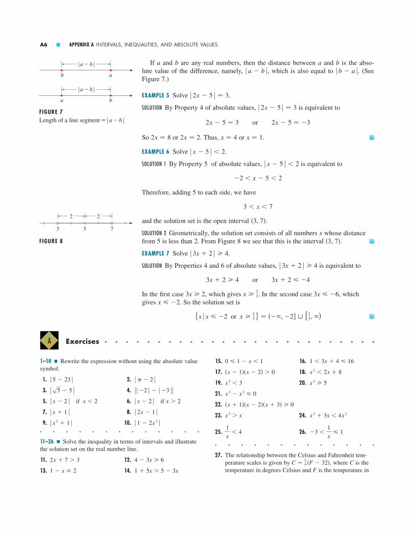
If and are any real numbers, then the distance between and is the abso-lute value of the difference, namely, , which is also equal to . (SeeFigure 7.)
EXAMPLE 5 Solve .
SOLUTION By Property 4 of absolute values, is equivalent to
So or . Thus, or .
EXAMPLE 6 Solve .
SOLUTION 1 By Property 5 of absolute values, is equivalent to
Therefore, adding 5 to each side, we have
and the solution set is the open interval .
SOLUTION 2 Geometrically, the solution set consists of all numbers whose distancefrom 5 is less than 2. From Figure 8 we see that this is the interval .
EXAMPLE 7 Solve .
SOLUTION By Properties 4 and 6 of absolute values, is equivalent to
In the first case , which gives . In the second case , whichgives . So the solution set is
{x � x � �2 or x �23 } � ���, �2� � [ 2
3, �)
x � �23x � �6x �
233x � 2
3x � 2 � �4or3x � 2 � 4
� 3x � 2 � � 4
� 3x � 2 � � 4
�3, 7�x
�3, 7�
3 � x � 7
�2 � x � 5 � 2
� x � 5 � � 2
� x � 5 � � 2
x � 1x � 42x � 22x � 8
2x � 5 � �3or2x � 5 � 3
� 2x � 5 � � 3
� 2x � 5 � � 3
� b � a �� a � b �baba
1–10 � Rewrite the expression without using the absolute valuesymbol.
1. 2.
3. 4.
5. if 6. if
7. 8.
9. 10.� � � � � � � � � � � � �
11–26 � Solve the inequality in terms of intervals and illustratethe solution set on the real number line.
11. 12.
13. 14. 1 � 5x � 5 � 3x1 � x � 2
4 � 3x � 62x � 7 � 3
� 1 � 2x 2 �� x 2 � 1 �� 2x � 1 �� x � 1 �
x � 2� x � 2 �x � 2� x � 2 ��� �2 � � � �3 ��� s5 � 5 �� � � 2 �� 5 � 23 �
A6 � APPENDIX A INTERVALS, INEQUALITIES, AND ABSOLUTE VALUES
15. 16.
17. 18.
19. 20.
21.
22.
23. 24.
25. 26.
� � � � � � � � � � � � �
27. The relationship between the Celsius and Fahrenheit tem-perature scales is given by , where is thetemperature in degrees Celsius and is the temperature in F
CC � 59 �F � 32�
�3 �1
x� 1
1
x� 4
x 3 � 3x � 4x 2x 3 � x
�x � 1��x � 2��x � 3� � 0
x 3 � x 2 � 0
x 2 � 5x 2 � 3
x 2 � 2x � 8�x � 1��x � 2� � 0
1 � 3x � 4 � 160 � 1 � x � 1
Exercises � � � � � � � � � � � � � � � � � � � � � � � � � �A
| a-b |
ab
| a-b |
ba
FIGURE 7Length of a line segment=| a-b |
3 5 7
22
FIGURE 8

31–32 � Solve the equation for .
31. 32.� � � � � � � � � � � � �
33– 40 � Solve the inequality.
33. 34.
35. 36.
37. 38.
39. 40.� � � � � � � � � � � � �
41. Solve the inequality for , assuming that ,, and are positive constants.
42. Solve the inequality for , assuming that , ,and are negative constants.
43. Prove that . [Hint: Use Equation 3.]
44. Show that if , then .a 2 � b 20 � a � b
� ab � � � a � � b �c
baxax � b � c
cbaxa�bx � c� � bc
� 5x � 2 � � 6� 2x � 3 � � 0.4
� x � 1 � � 3� x � 5 � � 2
� x � 6 � � 0.1� x � 4 � � 1
� x � � 3� x � � 3
� 3x � 5 � � 1� x � 3 � � � 2x � 1 �xdegrees Fahrenheit. What interval on the Celsius scale cor-
responds to the temperature range ?
28. Use the relationship between and given in Exercise 27to find the interval on the Fahrenheit scale corresponding tothe temperature range .
29. As dry air moves upward, it expands and in so doing coolsat a rate of about C for each 100-m rise, up to about12 km.(a) If the ground temperature is C, write a formula for
the temperature at height .(b) What range of temperature can be expected if a plane
takes off and reaches a maximum height of 5 km?
30. If a ball is thrown upward from the top of a building 128 fthigh with an initial velocity of 16 ft�s, then the height above the ground seconds later will be
During what time interval will the ball be at least 32 ftabove the ground?
h � 128 � 16t � 16t 2
th
h20
1
20 � C � 30
FC
50 � F � 95
Coordinate Geometry � � � � � � � � � � � � � � �
The points in a plane can be identified with ordered pairs of real numbers. We start bydrawing two perpendicular coordinate lines that intersect at the origin on each line.Usually one line is horizontal with positive direction to the right and is called the -axis; the other line is vertical with positive direction upward and is called the -axis.
Any point in the plane can be located by a unique ordered pair of numbers as fol-lows. Draw lines through perpendicular to the - and -axes. These lines intersectthe axes in points with coordinates and as shown in Figure 1. Then the point isassigned the ordered pair . The first number is called the x-coordinate of ;the second number is called the y-coordinate of . We say that is the point withcoordinates , and we denote the point by the symbol . Several points arelabeled with their coordinates in Figure 2.
0 x1 2 3 4 5_1_2_3
1
2
3
4
_2
_3
_1
y
_4
(5, 0)
(1, 3)(_2, 2)
(_3, _2)
(2, _4)
FIGURE 2
x1 2 3 4 5_1_2_3
a
O
2
4
_2
_1
b
y
1
3
P(a, b)
III
IVIII_3
FIGURE 1
_4
P�a, b��a, b�PPb
Pa�a, b�Pba
yxPP
yx
O
B
APPENDIX B COORDINATE GEOMETRY � A7

By reversing the preceding process we can start with an ordered pair andarrive at the corresponding point . Often we identify the point with the ordered pair
and refer to “the point .” [Although the notation used for an open intervalis the same as the notation used for a point , you will be able to tell from
the context which meaning is intended.]This coordinate system is called the rectangular coordinate system or the Car-
tesian coordinate system in honor of the French mathematician René Descartes(1596–1650), even though another Frenchman, Pierre Fermat (1601–1665), inventedthe principles of analytic geometry at about the same time as Descartes. The planesupplied with this coordinate system is called the coordinate plane or the Cartesianplane and is denoted by .
The - and -axes are called the coordinate axes and divide the Cartesian planeinto four quadrants, which are labeled I, II, III, and IV in Figure 1. Notice that the firstquadrant consists of those points whose - and -coordinates are both positive.
EXAMPLE 1 Describe and sketch the regions given by the following sets.
(a) (b) (c )
SOLUTION(a) The points whose -coordinates are 0 or positive lie on the -axis or to the rightof it as indicated by the shaded region in Figure 3(a).
(b) The set of all points with -coordinate 1 is a horizontal line one unit above the[see Figure 3(b)].
(c) Recall from Appendix A that
The given region consists of those points in the plane whose -coordinates liebetween and . Thus, the region consists of all points that lie between (but noton) the horizontal lines and . [These lines are shown as dashed linesin Figure 3(c) to indicate that the points on these lines don’t lie in the set.]
Recall from Appendix A that the distance between points and on a number lineis . Thus, the distance between points and ona horizontal line must be and the distance between and on a vertical line must be . (See Figure 4.)
To find the distance between any two points and , wenote that triangle in Figure 4 is a right triangle, and so by the PythagoreanP1P2P3
P2�x2, y2 �P1�x1, y1�� P1P2 �� y2 � y1 �
P3�x2, y1�P2�x2, y2 �� x2 � x1 �P3�x2, y1�P1�x1, y1�� a � b � � � b � a �
ba
y � �1y � 11�1
y
�1 � y � 1if and only if� y � � 1
x-axisy
FIGURE 3
x0
y
x0
y
y=1
x0
y
y=1
y=_1
(a) x � 0 (b) y=1 (c) | y |<1
yx
{�x, y� � � y � � 1}��x, y� � y � 1���x, y� � x � 0�
yx
yx� 2
�a, b��a, b��a, b��a, b�
PP�a, b�
A8 � APPENDIX B COORDINATE GEOMETRY
FIGURE 4
P¡(⁄, ›)
x⁄ ¤0
›
fi
y
P™(¤, fi)
P£(¤, ›)|¤-⁄|
|fi-›|

Theorem we have
Distance Formula The distance between the points and is
For instance, the distance between and is
Circles
An equation of a curve is an equation satisfied by the coordinates of the points on thecurve and by no other points. Let’s use the distance formula to find the equation of acircle with radius and center . By definition, the circle is the set of all points
whose distance from the center is . (See Figure 5.) Thus, is on thecircle if and only if . From the distance formula, we have
or equivalently, squaring both sides, we get
This is the desired equation.
Equation of a Circle An equation of the circle with center and radius is
In particular, if the center is the origin , the equation is
For instance, an equation of the circle with radius 3 and center is
EXAMPLE 2 Sketch the graph of the equation by firstshowing that it represents a circle and then finding its center and radius.
SOLUTION We first group the -terms and -terms as follows:
Then we complete the square within each grouping, adding the appropriate
�x 2 � 2x� � (y 2 � 6y� � �7
yx
x 2 � y 2 � 2x � 6y � 7 � 0
�x � 2�2 � (y � 5�2 � 9
�2, �5�
x 2 � y 2 � r 2
�0, 0�
�x � h�2 � (y � k�2 � r 2
r�h, k�
�x � h�2 � (y � k�2 � r 2
s�x � h�2 � � y � k�2 � r
� PC � � rPrC�h, k�P�x, y�
�h, k�r
s�5 � 1� 2 � �3 � ��2�� 2 � s42 � 52 � s41
�5, 3��1, �2�
� P1P2 � � s�x2 � x1�2 � �y2 � y1�2
P2�x2, y2 �P1�x1, y1�
� s�x2 � x1�2 � �y2 � y1�2
� P1P2 � � s� P1P3 �2 � � P2P3 �2 � s� x2 � x1 �2 � � y2 � y1 �2
APPENDIX B COORDINATE GEOMETRY � A9
C(h, k)
x0
y
rP(x, y)
FIGURE 5

constants (the squares of half the coefficients of and ) to both sides of the equation:
or
Comparing this equation with the standard equation of a circle, we see that and , so the given equation represents a circle with center and
radius . It is sketched in Figure 6.
Lines
To find the equation of a line we use its slope, which is a measure of the steepnessof the line.
Definition The slope of a nonvertical line that passes through the pointsand is
The slope of a vertical line is not defined.
Thus, the slope of a line is the ratio of the change in , , to the change in ,(see Figure 7). The slope is therefore the rate of change of y with respect to x. The factthat the line is straight means that the rate of change is constant.
Figure 8 shows several lines labeled with their slopes. Notice that lines with posi-tive slope slant upward to the right, whereas lines with negative slope slant downwardto the right. Notice also that the steepest lines are the ones for which the absolute valueof the slope is largest, and a horizontal line has slope 0.
Now let’s find an equation of the line that passes through a given point and has slope . A point with lies on this line if and only if the slopeof the line through and is equal to ; that is,
This equation can be rewritten in the form
and we observe that this equation is also satisfied when and . Therefore,it is an equation of the given line.
Point-Slope Form of the Equation of a Line An equation of the line passing throughthe point and having slope is
y � y1 � m�x � x1�
mP1�x1, y1�
y � y1x � x1
y � y1 � m�x � x1�
y � y1
x � x1� m
mPP1
x � x1P�x, y�mP1�x1, y1�
�xx�yy
m ��y
�x�
y2 � y1
x2 � x1
P2�x2, y2 �P1�x1, y1�
L
s3��1, 3�r � s3k � 3,
h � �1,
�x � 1�2 � (y � 3�2 � 3
�x 2 � 2x � 1� � (y 2 � 6y � 9� � �7 � 1 � 9
yx
A10 � APPENDIX B COORDINATE GEOMETRY
x0
y
1
(_1, 3)
FIGURE 6≈+¥+2x-6y+7=0
FIGURE 7
P™(x™, y™)
P¡(x¡, y¡)
L
Îy=fi-›=rise
Îx=¤-⁄=run
x0
y
x0
y
m=1
m=0
m=_1m=_2
m=_5
m=2m=5
m= 12
m=_ 12
FIGURE 8
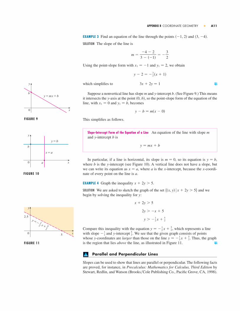
EXAMPLE 3 Find an equation of the line through the points and .
SOLUTION The slope of the line is
Using the point-slope form with and , we obtain
which simplifies to
Suppose a nonvertical line has slope and -intercept . (See Figure 9.) This meansit intersects the -axis at the point , so the point-slope form of the equation of theline, with and , becomes
This simplifies as follows.
Slope-Intercept Form of the Equation of a Line An equation of the line with slope and -intercept is
In particular, if a line is horizontal, its slope is , so its equation is ,where is the -intercept (see Figure 10). A vertical line does not have a slope, butwe can write its equation as , where is the -intercept, because the -coordi-nate of every point on the line is .
EXAMPLE 4 Graph the inequality .
SOLUTION We are asked to sketch the graph of the set and webegin by solving the inequality for :
Compare this inequality with the equation , which represents a linewith slope and -intercept . We see that the given graph consists of pointswhose -coordinates are larger than those on the line . Thus, the graphis the region that lies above the line, as illustrated in Figure 11.
Parallel and Perpendicular Lines
Slopes can be used to show that lines are parallel or perpendicular. The following factsare proved, for instance, in Precalculus: Mathematics for Calculus, Third Edition byStewart, Redlin, and Watson (Brooks�Cole Publishing Co., Pacific Grove, CA, 1998).
y � �12 x �
52y
52y�
12
y � �12 x �
52
y � �12 x �
52
2y � �x � 5
x � 2y � 5
y��x, y� � x � 2y � 5�
x � 2y � 5
axxax � a
yby � bm � 0
y � mx � b
bym
y � b � m�x � 0�
y1 � bx1 � 0�0, b�y
bym
3x � 2y � 1
y � 2 � �32 �x � 1�
y1 � 2x1 � �1
m ��4 � 2
3 � ��1�� �
3
2
�3, �4���1, 2�
APPENDIX B COORDINATE GEOMETRY � A11
x0
y
by=mx+b
FIGURE 9
0
y
b
xa
x=a
y=b
FIGURE 10
FIGURE 11
0
y
2.5
x5
y=_ x+1
2 52

Parallel and Perpendicular Lines
1. Two nonvertical lines are parallel if and only if they have the same slope.
2. Two lines with slopes and are perpendicular if and only if; that is, their slopes are negative reciprocals:
EXAMPLE 5 Find an equation of the line through the point that is parallel to theline .
SOLUTION The given line can be written in the form
which is in slope-intercept form with . Parallel lines have the same slope, sothe required line has slope and its equation in point-slope form is
We can write this equation as .
EXAMPLE 6 Show that the lines and are perpendicular.
SOLUTION The equations can be written as
from which we see that the slopes are
Since , the lines are perpendicular.
Conic Sections
Here we review the geometric definitions of parabolas, ellipses, and hyperbolas andtheir standard equations. They are called conic sections, or conics, because they resultfrom intersecting a cone with a plane as shown in Figure 12.
FIGURE 12Conics
ellipse parabola hyperbola
m1m2 � �1
m2 � 32andm1 � �
23
y � 32 x �
14andy � �
23 x �
13
6x � 4y � 1 � 02x � 3y � 1
2x � 3y � 16
y � 2 � �23 �x � 5�
�23
m � �23
y � �23 x �
56
4x � 6y � 5 � 0�5, 2�
m2 � �1
m1
m1m2 � �1m2m1
A12 � APPENDIX B COORDINATE GEOMETRY

Parabolas
A parabola is the set of points in a plane that are equidistant from a fixed point (called the focus) and a fixed line (called the directrix). This definition is illustratedby Figure 13. Notice that the point halfway between the focus and the directrix lies onthe parabola; it is called the vertex. The line through the focus perpendicular to thedirectrix is called the axis of the parabola.
In the 16th century Galileo showed that the path of a projectile that is shot into the air at an angle to the ground is a parabola. Since then, parabolic shapes have been used in designing automobile headlights, reflecting telescopes, and suspension bridges. (See Problem 16 on page 263 for the reflection property of parabolas that makes themso useful.)
We obtain a particularly simple equation for a parabola if we place its vertex at theorigin and its directrix parallel to the -axis as in Figure 14. If the focus is the point
, then the directrix has the equation and the parabola has the equation
(See Exercise 47.)
If we write , then the equation of the parabola becomes
Figure 15 shows the graphs of several parabolas with equations of the form for various values of the number . We see that the parabola opens upward if
and downward if (as in Figure 16). The graph is symmetric with respectto the -axis because its equation is unchanged when is replaced by . This corre-sponds to the fact that the function is an even function.
If we interchange and in the equation , the result is , which alsorepresents a parabola. (Interchanging and amounts to reflecting about the diagonal yx
x � ay 2y � ax 2yx
FIGURE 16
x0
y
(_x, y) (x, y) x
0
y
(a) y=a≈, a>0 (b) y=a≈, a<0
f �x� � ax 2�xxy
a � 0a � 0y � ax 2a
y � ax 2
y � ax 2
a � 1��4p�
FIGURE 14
x
y
O
F(0, p)
y=_p
P(x, y)
y
p
x 2 � 4py
y � �p�0, p�xO
F
APPENDIX B COORDINATE GEOMETRY � A13
axis
Ffocus
parabola
vertex directrix
FIGURE 13
y
x
y=2≈
y=≈
y=_≈
y=_2≈
y= ≈12
y=_ ≈12
FIGURE 15

line .) The parabola opens to the right if and to the left if (See Figure 17.) This time the parabola is symmetric with respect to the -axisbecause the equation is unchanged when is replaced by .
EXAMPLE 7 Sketch the region bounded by the parabola and theline .
SOLUTION First we find the points of intersection by solving the two equations. Substi-tuting into the equation , we get , whichgives
so or . Thus, the points of intersection are and , and wedraw the line passing through these points.
To sketch the parabola we start with the parabola in Figure 17(b) and shift one unit to the right. We also make sure it passes through the points and . The region bounded by and
means the finite region whose boundaries are these curves. It issketched in Figure 18.
Ellipses
An ellipse is the set of points in a plane the sum of whose distances from two fixedpoints and is a constant (see Figure 19). These two fixed points are called thefoci (plural of focus). One of Kepler’s laws is that the orbits of the planets in the solarsystem are ellipses with the Sun at one focus.
In order to obtain the simplest equation for an ellipse, we place the foci on the -axis at the points and as in Figure 20, so that the origin is halfway
between the foci. If we let the sum of the distances from a point on the ellipse to thefoci be , then we can write an equation of the ellipse as2a
�c, 0���c, 0�x
FIGURE 19
F¡ F™
P
FIGURE 20
F¡(_c, 0) F™(c, 0)0 x
y
P(x, y)
F2F1
x � y � 1 � 0x � 1 � y 2�0,�1���3, 2�
x � �y 2x � 1 � y 2x � y � 1 � 0
�0,�1���3, 2��1y � 2
0 � y 2 � y � 2 � �y � 2��y � 1�
�y � 1 � 1 � y 2x � 1 � y 2x � �y � 1
x � y � 1 � 0x � 1 � y 2
x0
y
x0
y
FIGURE 17 (a) x=a¥, a>0 (b) x=a¥, a<0
�yyx
a � 0.a � 0x � ay 2y � x
A14 � APPENDIX B COORDINATE GEOMETRY
x=1-¥
x+y+1=0
y
2
1
(_3, 2)
(0, _1)
10 x
FIGURE 18

where . (See Exercise 49 and Figure 21.) Notice that the -intercepts are, the -intercepts are , the foci are , and the ellipse is symmetric with
respect to both axes. If the foci of an ellipse are located on the axis at , thenwe can find its equation by interchanging and in (1).
EXAMPLE 8 Sketch the graph of and locate the foci.
SOLUTION Divide both sides of the equation by 144:
The equation is now in the standard form for an ellipse, so we have ,, , and . The -intercepts are and the -intercepts are .
Also, , so and the foci are . The graph issketched in Figure 22.
Like parabolas, ellipses have an interesting reflection property that has practicalconsequences. If a source of light or sound is placed at one focus of a surface withelliptical cross-sections, then all the light or sound is reflected off the surface to theother focus (see Exercise 55). This principle is used in lithotripsy, a treatment for kid-ney stones. A reflector with elliptical cross-section is placed in such a way that the kidney stone is at one focus. High-intensity sound waves generated at the other focusare reflected to the stone and destroy it without damaging surrounding tissue. Thepatient is spared the trauma of surgery and recovers within a few days.
Hyperbolas
A hyperbola is the set of all points in a plane the difference of whose distances fromtwo fixed points and (the foci) is a constant. This definition is illustrated inFigure 23.
Notice that the definition of a hyperbola is similar to that of an ellipse; the onlychange is that the sum of distances has become a difference of distances. It is left asExercise 51 to show that when the foci are on the -axis at and the differenceof distances is , then the equation of the hyperbola is
where . Notice that the -intercepts are again , But if we put in Equation 2 we get , which is impossible, so there is no -intercept. Thehyperbola is symmetric with respect to both axes.
To analyze the hyperbola further, we look at Equation 2 and obtain
x 2
a 2 � 1 �y 2
b 2 � 1
yy � �b 2x � 0axc 2 � a 2 � b 2
x 2
a 2 �y 2
b 2 � 12
� PF1 � � � PF2 � � 2a�c, 0�x
F2F1
(s7, 0)c � s7c 2 � a 2 � b 2 � 73y4xb � 3a � 4b 2 � 9
a 2 � 16
x 2
16�
y 2
9� 1
9x 2 � 16y 2 � 144
yx�0, c�y-
�c, 0�byaxc 2 � a 2 � b 2
x 2
a 2 � y 2
b 2 � 11
APPENDIX B COORDINATE GEOMETRY � A15
+ =1
FIGURE 21≈
a@
¥
b@
(c, 0)0 x
y
ab
c
(0, b)
(_c, 0)
(0, _b)
(a, 0)
(_a, 0)
0 x
y
(0, 3)
{œ„7, 0}
(4, 0)(_4, 0)
(0, _3)
{_œ„7, 0}
FIGURE 229≈+16¥=144
FIGURE 23P is on the hyperbola when| PF¡|-|PF™ |=2a
F™(c, 0)F¡(_c, 0) 0 x
y
P(x, y)

This shows that , so . Therefore, we have or .This means that the hyperbola consists of two parts, called its branches.
When we draw a hyperbola it is useful to first draw its asymptotes, which are thelines and shown in Figure 24. Both branches of the hyper-bola approach the asymptotes; that is, they come arbitrarily close to the asymptotes.If the foci of a hyperbola are on the -axis, we find its equation by reversing the rolesof and .
EXAMPLE 9 Find the foci and asymptotes of the hyperbola andsketch its graph.
SOLUTION If we divide both sides of the equation by 144, it becomes
which is of the form given in (2) with and . Since ,the foci are . The asymptotes are the lines and . The graphis shown in Figure 25.
FIGURE 259≈-16¥=144
0 x
y
(5, 0)(_5, 0)
(4, 0)(_4, 0)
y=_ x34
y= x34
y � �34 xy � 3
4 x�5, 0�c 2 � 16 � 9 � 25b � 3a � 4
x 2
16�
y 2
9� 1
9x 2 � 16y 2 � 144
yxy
y � ��b�a�xy � �b�a�x
x � �ax � a� x � � sx 2 � ax 2 � a 2
A16 � APPENDIX B COORDINATE GEOMETRY
11–24 � Find an equation of the line that satisfies the given conditions.
11. Through , slope
12. Through , slope
13. Through and
14. Through and
15. Slope , -intercept
16. Slope , -intercept
17. -intercept , -intercept
18. -intercept , -intercept
19. Through , parallel to the -axis
20. Through , parallel to the -axis
21. Through , parallel to the line x � 2y � 6�1, �6�
y�4, 5�
x�4, 5�
6y�8x
�3y1x
4y25
�2y3
�4, 3���1, �2�
�1, 6��2, 1�
�72��3, �5�
6�2, �3�
1–2 � Find the distance between the points.
1. , 2. ,� � � � � � � � � � � � �
3–4 � Find the slope of the line through and .
3. , 4. ,� � � � � � � � � � � � �
5. Show that the points , , , and arethe vertices of a square.
6. (a) Show that the points , , and are collinear (lie on the same line) by showing that
.(b) Use slopes to show that , , and are collinear.
7–10 � Sketch the graph of the equation.
7. 8.
9. 10.� � � � � � � � � � � � �
� y � � 1xy � 0
y � �2x � 3
CBA� AB � � � BC � � � AC �
C�5, 15�B�3, 11�A��1, 3�
��5, 3��1, 0��4, 6���2, 9�
Q�6, 0�P��1, �4�Q��1, �6�P��3, 3�
QP
�5, 7��1, �3��4, 5��1, 1�
Exercises � � � � � � � � � � � � � � � � � � � � � � � � � �B
FIGURE 24¥
b@- =1
≈
a@
(c, 0)0 x
y
(_c, 0)
(a, 0)(_a, 0)
y=_ xba y= xb
a

45. Find an equation of the perpendicular bisector of the linesegment joining the points and .
46. (a) Show that if the - and -intercepts of a line are nonzeronumbers and , then the equation of the line can beput in the form
This equation is called the two-intercept form of anequation of a line.
(b) Use part (a) to find an equation of the line whose -intercept is 6 and whose -intercept is .
47. Suppose that is any point on the parabola with focusand directrix . (See Figure 14.) Use the defi-
nition of a parabola to show that .
48. Find the focus and directrix of the parabola . Illus-trate with a diagram.
49. Suppose an ellipse has foci and the sum of the dis-tances from any point on the ellipse to the foci is .Show that the coordinates of satisfy Equation 1.
50. Find the foci of the ellipse and sketch itsgraph.
51. Use the definition of a hyperbola to derive Equation 2 for ahyperbola with foci .
52. (a) Find the foci and asymptotes of the hyperbolaand sketch its graph.
(b) Sketch the graph of .
53–54 � Sketch the region bounded by the curves.
53. and
54. and
� � � � � � � � � � � � �
55. Let be a point on the ellipse with foci and and let and be the angles betweenthe lines , and the ellipse as in the figure. Prove that
. This explains how whispering galleries and litho-tripsy work. Sound coming from one focus is reflected andpasses through the other focus. [Hint: Use the formula inProblem 15 on page 263 to show that .]
F¡ F™
P(⁄, ›)
0 x
y
∫
å
+ =1≈
a@
¥
b@
tan � tan �
� �PF2PF1
� F2F1
x 2�a 2 � y 2�b 2 � 1P1�x1, y1�
x � 2y � 2y � 4 � x 2
x � 2y 2 � 8x � 4y � 8
y 2 � x 2 � 1x 2 � y 2 � 1
�c, 0�
x 2 � 4y 2 � 4
P2aP�x, y�
�c, 0�
y � x 2
x 2 � 4pyy � �p�0, p�
P�x, y�
�8yx
x
a�
y
b� 1
bayx
B�7, �2�A�1, 4�22. -intercept , parallel to the line
23. Through , perpendicular to the line
24. Through , perpendicular to the line � � � � � � � � � � � � �
25–28 � Find the slope and -intercept of the line and draw its graph.
25. 26.
27. 28.� � � � � � � � � � � � �
29–36 � Sketch the region in the -plane.
29.
30.
31.
32.
33.
34.
35.
36.� � � � � � � � � � � � �
37–38 � Find an equation of a circle that satisfies the givenconditions.
37. Center , radius 5
38. Center , passes through � � � � � � � � � � � � �
39–40 � Show that the equation represents a circle and find thecenter and radius.
39.
40.� � � � � � � � � � � � �
41. Show that the lines and are notparallel and find their point of intersection.
42. Show that the lines andare perpendicular and find their point
of intersection.
43. Show that the midpoint of the line segment from to is
44. Find the midpoint of the line segment joining the pointsand .�7, 15��1, 3�
� x1 � x2
2,
y1 � y2
2 �P2�x2, y2 �
P1�x1, y1�
10x � 6y � 50 � 03x � 5y � 19 � 0
6x � 2y � 102x � y � 4
x 2 � y 2 � 6y � 2 � 0
x 2 � y 2 � 4x � 10y � 13 � 0
��4, �6���1, 5�
�3, �1�
{�x, y� � �x � y �12 �x � 3�}
��x, y� � 1 � x � y � 1 � 2x�
��x, y� � y � 2x � 1�
��x, y� � 0 � y � 4 and x � 2�
{�x, y� � � x � � 3 and � y � � 2}
{�x, y� � � x � � 2}
��x, y� � x � 1 and y � 3�
��x, y� � x � 0�
xy
4x � 5y � 103x � 4y � 12
2x � 3y � 6 � 0x � 3y � 0
y
4x � 8y � 1( 12, � 2
3 )
2x � 5y � 8 � 0��1, �2�
2x � 3y � 4 � 06y
APPENDIX B COORDINATE GEOMETRY � A17
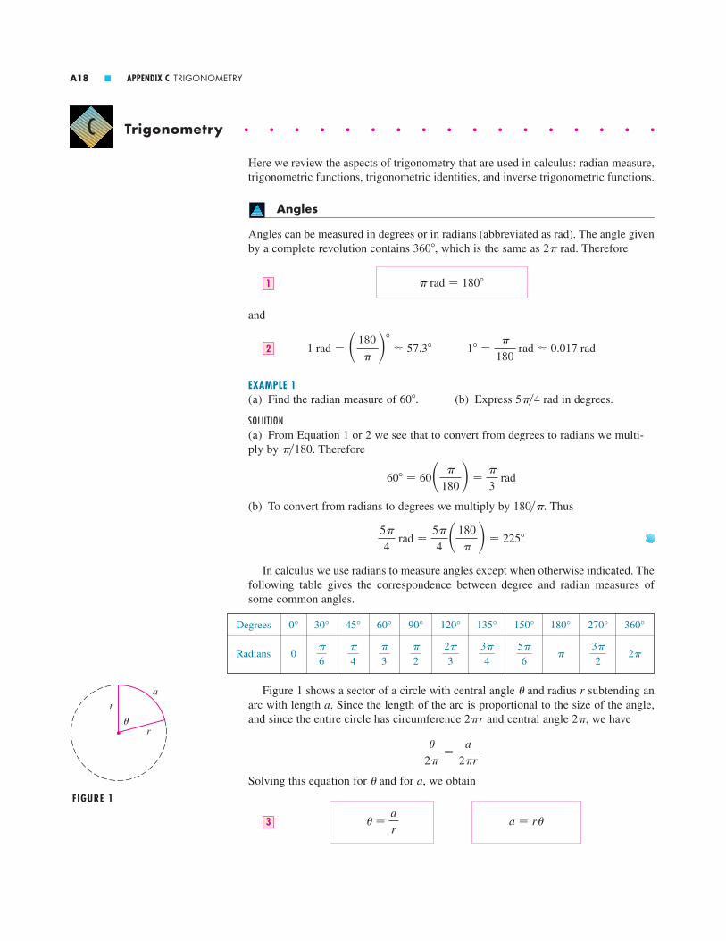
Trigonometry � � � � � � � � � � � � � � � � �
Here we review the aspects of trigonometry that are used in calculus: radian measure,trigonometric functions, trigonometric identities, and inverse trigonometric functions.
Angles
Angles can be measured in degrees or in radians (abbreviated as rad). The angle givenby a complete revolution contains , which is the same as rad. Therefore
and
EXAMPLE 1(a) Find the radian measure of . (b) Express rad in degrees.
SOLUTION(a) From Equation 1 or 2 we see that to convert from degrees to radians we multi-ply by . Therefore
(b) To convert from radians to degrees we multiply by . Thus
In calculus we use radians to measure angles except when otherwise indicated. Thefollowing table gives the correspondence between degree and radian measures ofsome common angles.
Figure 1 shows a sector of a circle with central angle and radius subtending anarc with length . Since the length of the arc is proportional to the size of the angle,and since the entire circle has circumference and central angle , we have
Solving this equation for and for , we obtain
a � r�� �a
r3
a�
�
2��
a
2�r
2�2�ra
r�
5�
4 rad �
5�
4 �180
�� � 225
180��
60 � 60� �
180� ��
3 rad
��180
5��460
1 ��
180 rad 0.017 rad1 rad � �180
��
57.32
� rad � 1801
2�360
C
A18 � APPENDIX C TRIGONOMETRY
Degrees 0° 30° 45° 60° 90° 120° 135° 150° 180° 270° 360°
Radians 0 2�3�
2�
5�
6
3�
4
2�
3
�
2
�
3
�
4
�
6
r
r
a
¨
FIGURE 1

Remember that Equations 3 are valid only when is measured in radians.In particular, putting in Equation 3, we see that an angle of 1 rad is the angle
subtended at the center of a circle by an arc equal in length to the radius of the circle(see Figure 2).
EXAMPLE 2(a) If the radius of a circle is 5 cm, what angle is subtended by an arc of 6 cm?(b) If a circle has radius 3 cm, what is the length of an arc subtended by a centralangle of rad?
SOLUTION(a) Using Equation 3 with and , we see that the angle is
(b) With cm and rad, the arc length is
The standard position of an angle occurs when we place its vertex at the origin ofa coordinate system and its initial side on the positive -axis as in Figure 3.
A positive angle is obtained by rotating the initial side counterclockwise until itcoincides with the terminal side. Likewise, negative angles are obtained by clockwiserotation as in Figure 4. Figure 5 shows several examples of angles in standard posi-tion. Notice that different angles can have the same terminal side. For instance, theangles , , and have the same initial and terminal sides because
and rad represents a complete revolution.
y
x0
¨=_ 5π4
0
y
x
¨=11π4
0
y
x
¨=3π4
0
y
x
¨=_ π2
0
y
x
¨=1
FIGURE 5Angles in standard position
2�
3�
4� 2� �
11�
4
3�
4� 2� � �
5�
4
11��4�5��43��4
0
y
x
¨ initial side
terminalside
FIGURE 3¨˘0
0
y
x¨
initial side
terminal side
FIGURE 4¨<0
x
a � r� � 3�3�
8 � �9�
8 cm
� � 3��8r � 3
� � 65 � 1.2 rad
r � 5a � 6
3��8
a � r�
APPENDIX C TRIGONOMETRY � A19
r
r
r
1 rad
FIGURE 2

The Trigonometric Functions
For an acute angle the six trigonometric functions are defined as ratios of lengths ofsides of a right triangle as follows (see Figure 6).
This definition does not apply to obtuse or negative angles, so for a general anglein standard position we let be any point on the terminal side of and we letbe the distance as in Figure 7. Then we define
Since division by 0 is not defined, and are undefined when andand are undefined when . Notice that the definitions in (4) and (5)
are consistent when is an acute angle.If is a number, the convention is that means the sine of the angle whose
radian measure is . For example, the expression implies that we are dealingwith an angle of 3 rad. When finding a calculator approximation to this number wemust remember to set our calculator in radian mode, and then we obtain
If we want to know the sine of the angle we would write and, with our cal-culator in degree mode, we find that
The exact trigonometric ratios for certain angles can be read from the triangles inFigure 8. For instance,
tan �
4� 1 tan
�
6�
1
s3 tan
�
3� s3
cos �
4�
1
s2 cos
�
6�
s3
2 cos
�
3�
1
2
sin �
4�
1
s2 sin
�
6�
1
2 sin
�
3�
s3
2
sin 3 0.05234
sin 33
sin 3 0.14112
sin 3�sin ��
�y � 0cot �csc �
x � 0sec �tan �
cot � �x
y tan � �
y
x
sec � �r
x cos � �
x
r
csc � �r
y sin � �
y
r5
� OP �r�P�x, y��
cot � �adj
opp tan � �
opp
adj
sec � �hyp
adj cos � �
adj
hyp
csc � �hyp
opp sin � �
opp
hyp4
�
A20 � APPENDIX C TRIGONOMETRY
P(x, y)
O
y
x
r
¨
FIGURE 7
1
1
2œ„
π4
π4
FIGURE 8
12 π
3
œ„3
π6
oppositehypotenuse
adjacent
¨
FIGURE 6

The signs of the trigonometric functions for angles in each of the four quadrantscan be remembered by means of the rule “All Students Take Calculus” shown inFigure 9.
EXAMPLE 3 Find the exact trigonometric ratios for .
SOLUTION From Figure 10 we see that a point on the terminal line for is. Therefore, taking
in the definitions of the trigonometric ratios, we have
The following table gives some values of and found by the method ofExample 3.
EXAMPLE 4 If and , find the other five trigonometric func-tions of .
SOLUTION Since , we can label the hypotenuse as having length 5 and the adjacent side as having length 2 in Figure 11. If the opposite side has length , then the Pythagorean Theorem gives and so , or . We can now use the diagram to write the other five trigonometric functions:
EXAMPLE 5 Use a calculator to approximate the value of in Figure 12.
SOLUTION From the diagram we see that
Therefore x �16
tan 40 19.07
tan 40 �16
x
x
cot � �2
s21sec � �
5
2csc � �
5
s21
tan � �s21
2sin � �
s21
5
x � s21x 2 � 21x 2 � 4 � 25x
cos � � 25
�0 � � � ��2cos � � 2
5
cos �sin �
csc 2�
3�
2
s3 sec
2�
3� �2 cot
2�
3� �
1
s3
sin 2�
3�
s3
2 cos
2�
3� �
1
2 tan
2�
3� �s3
r � 2 y � s3x � �1
P(�1, s3)� � 2��3
� � 2��3
APPENDIX C TRIGONOMETRY � A21
0
0 1 0 0
1 0 0 1�1�s3
2�
1
s2�
1
2
1
2
1
s2s3
2cos �
�11
2
1
s2s3
2s3
2
1
s2
1
2sin �
2�3�
2�
5�
6
3�
4
2�
3
�
2
�
3
�
4
�
6�
0
y
x
sin ¨>0
tan ¨>0
all ratios>0
cos ¨>0
FIGURE 9
y
0 x
2π3π
3
2œ„3
1
P {_1, œ„3}
FIGURE 10
5
2
¨
x= 21œ„„
FIGURE 11
16
40°
x
FIGURE 12

Trigonometric Identities
A trigonometric identity is a relationship among the trigonometric functions. Themost elementary are the following, which are immediate consequences of the defini-tions of the trigonometric functions.
For the next identity we refer back to Figure 7. The distance formula (or, equiva-lently, the Pythagorean Theorem) tells us that . Therefore
We have therefore proved one of the most useful of all trigonometric identities:
If we now divide both sides of Equation 7 by and use Equations 6, we get
Similarly, if we divide both sides of Equation 7 by , we get
The identities
show that is an odd function and is an even function. They are easily provedby drawing a diagram showing and in standard position (see Exercise 19).
Since the angles and have the same terminal side, we have
These identities show that the sine and cosine functions are periodic with period .The remaining trigonometric identities are all consequences of two basic identities
called the addition formulas:
cos�x � y� � cos x cos y � sin x sin y12b
sin�x � y� � sin x cos y � cos x sin y12a
2�
cos�� � 2�� � cos �sin�� � 2�� � sin �11
� � 2�����cossin
cos���� � cos �10b
sin���� � �sin �10a
1 � cot2� � csc2�9
sin2�
tan2� � 1 � sec2�8
cos2�
sin2� � cos2� � 17
sin2� � cos2� � y 2
r 2 �x 2
r 2 �x 2 � y 2
r 2 �r 2
r 2 � 1
x 2 � y 2 � r 2
cot � �cos �
sin �tan � �
sin �
cos �
cot � �1
tan �sec � �
1
cos �csc � �
1
sin �6
A22 � APPENDIX C TRIGONOMETRY
� Odd functions and even functions arediscussed in Section 1.1.

The proofs of these addition formulas are outlined in Exercises 51, 52, and 53.By substituting for in Equations 12a and 12b and using Equations 10a and
10b, we obtain the following subtraction formulas:
Then, by dividing the formulas in Equations 12 or Equations 13, we obtain the cor-responding formulas for :
If we put in the addition formulas (12), we get the double-angle formulas:
Then, by using the identity , we obtain the following alternateforms of the double-angle formulas for :
If we now solve these equations for and , we get the following half-angleformulas, which are useful in integral calculus:
There are many other trigonometric identities, but those we have stated are the onesused most often in calculus. If you forget any of them, remember that they can all bededuced from Equations 12a and 12b.
EXAMPLE 6 Find all values of in the interval such that .
SOLUTION Using the double-angle formula (15a), we rewrite the given equation as
sin x �1 � 2 cos x� � 0orsin x � 2 sin x cos x
sin x � sin 2x�0, 2��x
sin2x �1 � cos 2x
217b
cos2x �1 � cos 2x
217a
sin2xcos2x
cos 2x � 1 � 2 sin2x16b
cos 2x � 2 cos2x � 116a
cos 2xsin2x � cos2x � 1
cos 2x � cos2x � sin2x15b
sin 2x � 2 sin x cos x15a
y � x
tan�x � y� �tan x � tan y
1 � tan x tan y14b
tan�x � y� �tan x � tan y
1 � tan x tan y14a
tan�x y�
cos�x � y� � cos x cos y � sin x sin y13b
sin�x � y� � sin x cos y � cos x sin y13a
y�y
APPENDIX C TRIGONOMETRY � A23
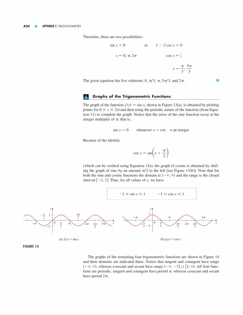
Therefore, there are two possibilities:
The given equation has five solutions: , , , , and .
Graphs of the Trigonometric Functions
The graph of the function , shown in Figure 13(a), is obtained by plottingpoints for and then using the periodic nature of the function (from Equa-tion 11) to complete the graph. Notice that the zeros of the sine function occur at theinteger multiples of , that is,
Because of the identity
(which can be verified using Equation 12a), the graph of cosine is obtained by shift-ing the graph of sine by an amount to the left [see Figure 13(b)]. Note that forboth the sine and cosine functions the domain is and the range is the closedinterval . Thus, for all values of , we have
The graphs of the remaining four trigonometric functions are shown in Figure 14and their domains are indicated there. Notice that tangent and cotangent have range
, whereas cosecant and secant have range . All four func-tions are periodic: tangent and cotangent have period , whereas cosecant and secanthave period .2�
����, �1� � �1, �����, ��
FIGURE 13
y
1
_1x
π_π
2π
3π
0_
π2
π2
3π2
5π2
(b) ©=cos x
y
1
_10 xπ_π 2π 3π
_π2
π2
3π2
5π2
(a) ƒ=sin x
�1 � cos x � 1�1 � sin x � 1
x��1, 1����, ��
��2
cos x � sin�x ��
2 �
whenever x � n�, n an integersin x � 0
�
0 � x � 2�f �x� � sin x
2�5��3���30
x � or x ��
3,
5�
3
x � 0, �, 2� or cos x � 12
sin x � 0 or 1 � 2 cos x � 0
A24 � APPENDIX C TRIGONOMETRY

Inverse Trigonometric Functions
When we try to find the inverse trigonometric functions, we have a slight difficulty:Because the trigonometric functions are not one-to-one, they don’t have inverse func-tions. The difficulty is overcome by restricting the domains of these functions so thatthey become one-to-one.
You can see from Figure 15 that the sine function is not one-to-one (usethe Horizontal Line Test). But the function (see Figure 16), is one-to-one. The inverse function of this restricted sine function existsand is denoted by or . It is called the inverse sine function or the arcsinefunction.
Since the definition of an inverse function says that
f �y� � x&?f �1�x� � y
y
0_π π xπ2
y=sin x
FIGURE 15
0
y
x
_ π2
π2
FIGURE 16
arcsinsin�1f
f �x� � sin x, ���2 � x � ��2y � sin x
� Inverse functions are reviewed in Section 1.6.
FIGURE 14
y
0xπ
_π
_1
1
y=cos x
_π2
π2
3π2
y
1
_1
0xπ
y=sin x
_π2
π2
3π2
y
0 xπ_π _π2
π2
3π2
y
1
_1
0xπ
_π
_π2
π2
3π2
(a) y=tan x (b) y=cot x
(c) y=csc x (d) y=sec x
APPENDIX C TRIGONOMETRY � A25

we have
| Thus, if , is the number between and whose sine is .
EXAMPLE 7 Evaluate (a) and (b) .
SOLUTION(a) We have
because and lies between and .
(b) Let . Then we can draw a right triangle with angle as in Figure 17and deduce from the Pythagorean Theorem that the third side has length
. This enables us to read from the triangle that
The cancellation equations for inverse functions [see (1.6.4)] become, in this case,
The inverse sine function, , has domain and range , and itsgraph, shown in Figure 18, is obtained from that of the restricted sine function (Fig-ure 16) by reflection about the line .
The tangent function can be made one-to-one by restricting it to the interval. Thus, the inverse tangent function is defined as the inverse of the func-
tion . (See Figure 19.) It is denoted by or arctan.tan�1f �x� � tan x, ���2 � x � ��2����2, ��2�
y
0 xπ2
π2_0
y
x1_1
π2
_ π2
FIGURE 19 y=tan x, _ <x<π2
π2FIGURE 18 y=sin–! x
y � x
����2, ��2���1, 1�sin�1
for �1 � x � 1 sin�sin�1x� � x
for ��
2� x �
�
2 sin�1�sin x� � x
tan(arcsin 13 ) � tan � �1
2s2
s9 � 1 � 2s2
�� � arcsin 13
��2���2��6sin���6� � 12
sin�1(12) �
�
6
tan(arcsin 13 )sin�1(12)
x��2���2sin�1x�1 � x � 1sin�1x �1
sin x
��
2� y �
�
2andsin y � x&?sin�1x � y
A26 � APPENDIX C TRIGONOMETRY
2 œ„2
3
¨
1
FIGURE 17

EXAMPLE 8 Simplify the expression .
SOLUTION 1 Let . Then and . We want to findbut, since is known, it is easier to find first:
Thus
SOLUTION 2 Instead of using trigonometric identities as in Solution 1, it is perhapseasier to use a diagram. If , then , and we can read from Fig-ure 20 (which illustrates the case ) that
The inverse tangent function, , has domain and its range is. Its graph is shown in Figure 21. We know that the lines are
vertical asymptotes of the graph of . Since the graph of is obtained by reflect-ing the graph of the restricted tangent function about the line , it follows that thelines and are horizontal asymptotes of the graph of .
Of the six inverse trigonometric functions, arcsin and arctan are the ones that aremost useful for the purposes of calculus. The inverse cosine function is investigated inExercise 46. The remaining inverse trigonometric functions don’t arise as frequently.
tan�1y � ���2y � ��2y � x
tan�1tanx � ��2����2, ��2�
�tan�1 � arctan
cos�tan�1x� � cos y �1
s1 � x 2
y � 0tan y � xy � tan�1x
cos�tan�1x� � cos y �1
sec y�
1
s1 � x 2
�since sec y � 0 for ���2 � y � ��2� sec y � s1 � x 2
sec2y � 1 � tan2y � 1 � x 2
sec ytan ycos y���2 � y � ��2tan y � xy � tan�1x
cos�tan�1x�
��
2� y �
�
2andtan y � x&?tan�1x � y
APPENDIX C TRIGONOMETRY � A27
5. Find the length of a circular arc subtended by an angle of rad if the radius of the circle is 36 cm.
6. If a circle has radius 10 cm, find the length of the arc sub-tended by a central angle of .
7. A circle has radius m. What angle is subtended at thecenter of the circle by an arc 1 m long?
8. Find the radius of a circular sector with angle and arclength 6 cm.
3��4
1.5
72
��121–2 � Convert from degrees to radians.
1. (a) (b)
2. (a) (b)� � � � � � � � � � � � �
3–4 � Convert from radians to degrees.
3. (a) (b)
4. (a) (b)
� � � � � � � � � � � � �
8�
3�
7�
2
�3�
84�
36�315
9210
Exercises � � � � � � � � � � � � � � � � � � � � � � � � � �C
œ„„„„„1+≈
1
y
x
FIGURE 20
FIGURE 21y=tan–! x=arctan x
π2
_ π2
y
0
x

27–28 � If and , where and lie between and , evaluate the expression.
27. 28.� � � � � � � � � � � � �
29–32 � Find all values of in the interval that satisfythe equation.
29. 30.
31. 32.� � � � � � � � � � � � �
33–36 � Find all values of in the interval that satisfythe inequality.
33. 34.
35. 36.� � � � � � � � � � � � �
37–40 � Graph the function by starting with the graphs in Fig-ures 13 and 14 and applying the transformations of Section 1.3where appropriate.
37. 38.
39. 40.
� � � � � � � � � � � � �
41–44 � Find the exact value of each expression.
41. (a) (b)
42. (a) (b)
43. (a) (b)
44. (a) (b)� � � � � � � � � � � � �
45. Prove that .
46. The inverse cosine function, , is defined as the inverse of the restricted cosine function ,
.(a) What are the domain and range of the inverse cosine
function?(b) Sketch the graph of arccos.
47. Find the domain and range of the function
; 48. (a) Graph the function and explain theappearance of the graph.
(b) Graph the function . How do youexplain the appearance of this graph?
t�x� � sin�1�sin x�
f �x� � sin�sin�1x�
t�x� � sin�1�3x � 1�
0 � x � �f �x� � cos x
cos�1 � arccos
cos�sin�1x� � s1 � x2
sin(2 sin�1(35))sec�arctan 2�
arcsin�sin 5�
4 �sin�sin�1�0.7��
arcsin 1tan�1s3
arctan��1�sin�1�0.5�
y � � sin x �y �1
3 tan�x �
�
2 �y � tan 2xy � cos�x �
�
3 �
sin x � cos x�1 � tan x � 1
2 cos x � 1 � 0sin x �12
�0, 2��x
� tan x � � 1sin 2x � cos x
2 sin2x � 12 cos x � 1 � 0
�0, 2��x
cos 2ysin�x � y�
��20yxsec y � 5
4sin x � 13
9–10 � Draw, in standard position, the angle whose measure isgiven.
9. (a) (b) rad
10. (a) rad (b) rad
� � � � � � � � � � � � �
11–12 � Find the exact trigonometric ratios for the angle whoseradian measure is given.
11. 12.
� � � � � � � � � � � � �
13–14 � Find the remaining trigonometric ratios.
13. ,
14. ,
� � � � � � � � � � � � �
15–18 � Find, correct to five decimal places, the length of theside labeled .
15. 16.
17. 18.
� � � � � � � � � � � � �
19–20 � Prove each equation.
19. (a) Equation 10a (b) Equation 10b
20. (a) Equation 14a (b) Equation 14b� � � � � � � � � � � � �
21–26 � Prove the identity.
21. 22.
23. 24.
25. 26.
� � � � � � � � � � � � �
cos 3� � 4 cos3� � 3 cos �tan 2� �2 tan �
1 � tan2�
�sin x � cos x�2 � 1 � sin 2xsin � cot � � cos �
sin�� � x� � sin xsin��
2� x� � cos x
22 cmx
3π8
8 cm
x
2π5
25 cm
x
40°10 cm
x
35°
x
0 � ��
2tan � 2
0 � � ��
2sin � �
3
5
4�
3
3�
4
�37�
3
�3�
4315
A28 � APPENDIX C TRIGONOMETRY
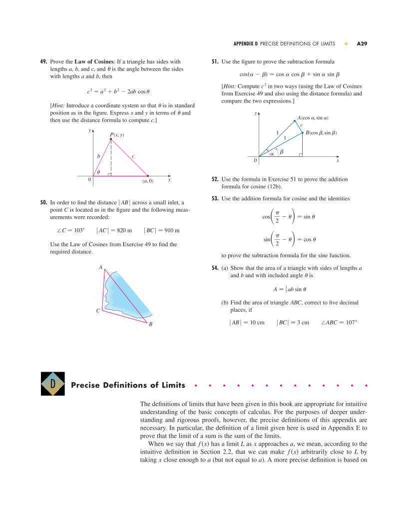
51. Use the figure to prove the subtraction formula
[Hint: Compute in two ways (using the Law of Cosinesfrom Exercise 49 and also using the distance formula) andcompare the two expressions.]
52. Use the formula in Exercise 51 to prove the additionformula for cosine (12b).
53. Use the addition formula for cosine and the identities
to prove the subtraction formula for the sine function.
54. (a) Show that the area of a triangle with sides of lengths and and with included angle is
(b) Find the area of triangle , correct to five decimalplaces, if
cm cm �ABC � 107� BC � � 3� AB � � 10
ABC
A � 12 ab sin �
�ba
sin��
2� �� � cos �
cos��
2� �� � sin �
0
y
B(cos ∫, sin ∫)
∫
1
A(cos å, sin å)
1
å
c
x
c2
cos� � �� � cos cos � � sin sin �
49. Prove the Law of Cosines: If a triangle has sides withlengths , , and , and is the angle between the sides with lengths and , then
[Hint: Introduce a coordinate system so that is in standardposition as in the figure. Express and in terms of andthen use the distance formula to compute .]
50. In order to find the distance across a small inlet, apoint is located as in the figure and the following meas-urements were recorded:
m m
Use the Law of Cosines from Exercise 49 to find therequired distance.
A
C
B
� BC � � 910� AC � � 820�C � 103
C� AB �
0
yP(x, y)
¨
cb
(a, 0) x
c�yx
�
c2 � a2 � b2 � 2ab cos �
ba�cba
APPENDIX D PRECISE DEFINITIONS OF LIMITS � A29
Precise Definitions of Limits � � � � � � � � � � � � �
The definitions of limits that have been given in this book are appropriate for intuitiveunderstanding of the basic concepts of calculus. For the purposes of deeper under-standing and rigorous proofs, however, the precise definitions of this appendix arenecessary. In particular, the definition of a limit given here is used in Appendix E toprove that the limit of a sum is the sum of the limits.
When we say that has a limit as approaches , we mean, according to theintuitive definition in Section 2.2, that we can make arbitrarily close to by taking close enough to (but not equal to ). A more precise definition is based on aax
Lf �x�axLf �x�
D

the idea of specifying just how small we need to make the distance in orderto make the distance less than some given number. The following exampleillustrates the idea.
EXAMPLE 1 Use a graph to find a number such that
whenever
SOLUTION A graph of is shown in Figure 1; we are interested in theregion near the point . Notice that we can rewrite the inequality
as
So we need to determine the values of for which the curve liesbetween the horizontal lines and . Therefore, we graph the curves
, , and near the point in Figure 2. Then we use the cursor to estimate that the -coordinate of the point of intersection of the line and the curve is about . Similarly,
intersects the line when . So, rounding to besafe, we can say that
This interval is not symmetric about . The distance from tothe left endpoint is and the distance to the right endpoint is 0.12.We can choose to be the smaller of these numbers, that is, . Then we canrewrite our inequalities in terms of distances as follows:
This just says that by keeping within 0.08 of 1, we are able to keep within 0.2 of 2.
Although we chose , any smaller positive value of would also haveworked.
Using the same graphical procedure as in Example 1, but replacing the number 0.2by smaller numbers, we find that
In each case we have found a number such that the values of the function�
� x � 1 � � 0.004whenever� �x 3 � 5x � 6� � 2 � � 0.01
� x � 1 � � 0.024whenever� �x 3 � 5x � 6� � 2 � � 0.05
� x � 1 � � 0.046whenever� �x 3 � 5x � 6� � 2 � � 0.1
�� � 0.08
f �x�x
� x � 1 � � 0.08whenever� �x 3 � 5x � 6� � 2 � � 0.2
� � 0.08�1 � 0.92 � 0.08
x � 1x � 1�0.92, 1.12�
0.92 � x � 1.12whenever1.8 � x 3 � 5x � 6 � 2.2
x 1.124y � 1.8y � x 3 � 5x � 60.911y � x 3 � 5x � 6y � 2.2
x�1, 2�y � 2.2y � 1.8y � x 3 � 5x � 6
y � 2.2y � 1.8y � x 3 � 5x � 6x
1.8 � x 3 � 5x � 6 � 2.2
� �x 3 � 5x � 6� � 2 � � 0.2
�1, 2�f �x� � x 3 � 5x � 6
� x � 1 � � �� �x 3 � 5x � 6� � 2 � � 0.2
�
� f �x� � L �� x � a �
A30 � APPENDIX D PRECISE DEFINITIONS OF LIMITS
� It is traditional to use the Greek letter (delta) in this situation.�
FIGURE 1
FIGURE 2
15
_5
_3 3
y=˛-5x+6
y=2.2
y=1.8
(1, 2)
0.8 1.2
2.3
1.7

lie in successively smaller intervals centered at 2 if the distancefrom to 1 is less than . It turns out that it is always possible to find such a number
, no matter how small the interval is. In other words, for any positive number , nomatter how small, there exists a positive number such that
This indicates that
and suggests a more precise way of defining the limit of a general function.
Definition Let be a function defined on some open interval that containsthe number , except possibly at itself. Then we say that the limit of as
approaches is , and we write
if for every number there is a corresponding number such that
Definition 1 is illustrated in Figures 3–5. If a number is given, then we drawthe horizontal lines and and the graph of . (See Figure 3.) If
, then we can find a number such that if we restrict to lie inthe interval and take , then the curve lies between the lines and . (See Figure 4.) You can see that if such a has beenfound, then any smaller will also work.
It’s important to realize that the process illustrated in Figures 3 and 4 must workfor every positive number no matter how small it is chosen. Figure 5 shows that if asmaller is chosen, then a smaller may be required.��
�
FIGURE 3 FIGURE 4 FIGURE 5
a0 x
y
y=L+∑
y=L-∑
a-∂ a+∂
L+∑
L-∑
0 x
y
a
y=L+∑
y=L-∑
a-∂ a+∂
∑∑L
when x is in here(x≠ a)
ƒis inhere
a0 x
yy=ƒ
y=L+∑
y=L-∑
∑∑L
��y � L � �y � L � �
y � f �x�x � a�a � �, a � ��x� � 0limx l a f �x� � L
fy � L � �y � L � �� � 0
0 � � x � a � � �whenever� f �x� � L � � �
� � 0� � 0
limx l a
f �x� � L
Laxf �x�aa
f1
limx l 1
�x 3 � 5x � 6� � 2
� x � 1 � � �whenever� �x 3 � 5x � 6� � 2 � � �
���
�xf �x� � x 3 � 5x � 6
APPENDIX D PRECISE DEFINITIONS OF LIMITS � A31
� The condition is justanother way of saying that .x � a
0 � � x � a �

EXAMPLE 2 Use the definition to prove that .
SOLUTION Let be a given positive number. According to Definition 1 with and, we need to find a number such that
that is,
But, since the square root function is an increasing function, we know that
So if we choose , then (see Figure 6). This shows that.
In proving limit statements it may be helpful to think of the definition of limit as achallenge. First it challenges you with a number . Then you must be able to producea suitable . You have to be able to do this for every , not just a particular .
Imagine a contest between two people, A and B, and imagine yourself to be B. Per-son A stipulates that the fixed number should be approximated by the values of to within a degree of accuracy (say, 0.01). Person B then responds by finding a num-ber such that whenever . Then A may becomemore exacting and challenge B with a smaller value of (say, 0.0001). Again B hasto respond by finding a corresponding . Usually the smaller the value of , thesmaller the corresponding value of must be. If B always wins, no matter how smallA makes , then
EXAMPLE 3 Prove that .
SOLUTION1. Preliminary analysis of the problem (guessing a value for ). Let be a
given positive number. We want to find a number such that
But . Therefore, we want
that is, whenever
This suggests that we should choose .2. Proof (showing that this works). Given , choose . If
, then
Thus
0 � � x � 3 � � �whenever� �4x � 5� � 7 � � �
� �4x � 5� � 7 � � � 4x � 12 � � 4� x � 3 � � 4� � 4��
4� � �
0 � � x � 3 � � �� � ��4� � 0�
� � ��4
0 � � x � 3 � � �� x � 3 � ��
4
0 � � x � 3 � � �whenever4� x � 3 � � �
� �4x � 5� � 7 � � � 4x � 12 � � � 4�x � 3� � � 4� x � 3 �
0 � � x � 3 � � �whenever� �4x � 5� � 7 � � �
���
limx l3
�4x � 5� � 7
lim x l a f �x� � L.��
���
0 � � x � a � � �� f �x� � L � � ���
f �x�L
�� � 0��
limx l 0 x 2 � 0x 2 � � &? � x � � �� � s�
x 2 � � &? sx 2 � s� &? � x � � s�
0 � � x � � �wheneverx 2 � �
0 � � x � 0 � � �whenever� x 2 � 0 � � �
�L � 0a � 0�
limx l
0 x 2 � 0�, �
A32 � APPENDIX D PRECISE DEFINITIONS OF LIMITS
FIGURE 6
x
y=∑ ∑
y
x0
y=≈
∂=œ„∑
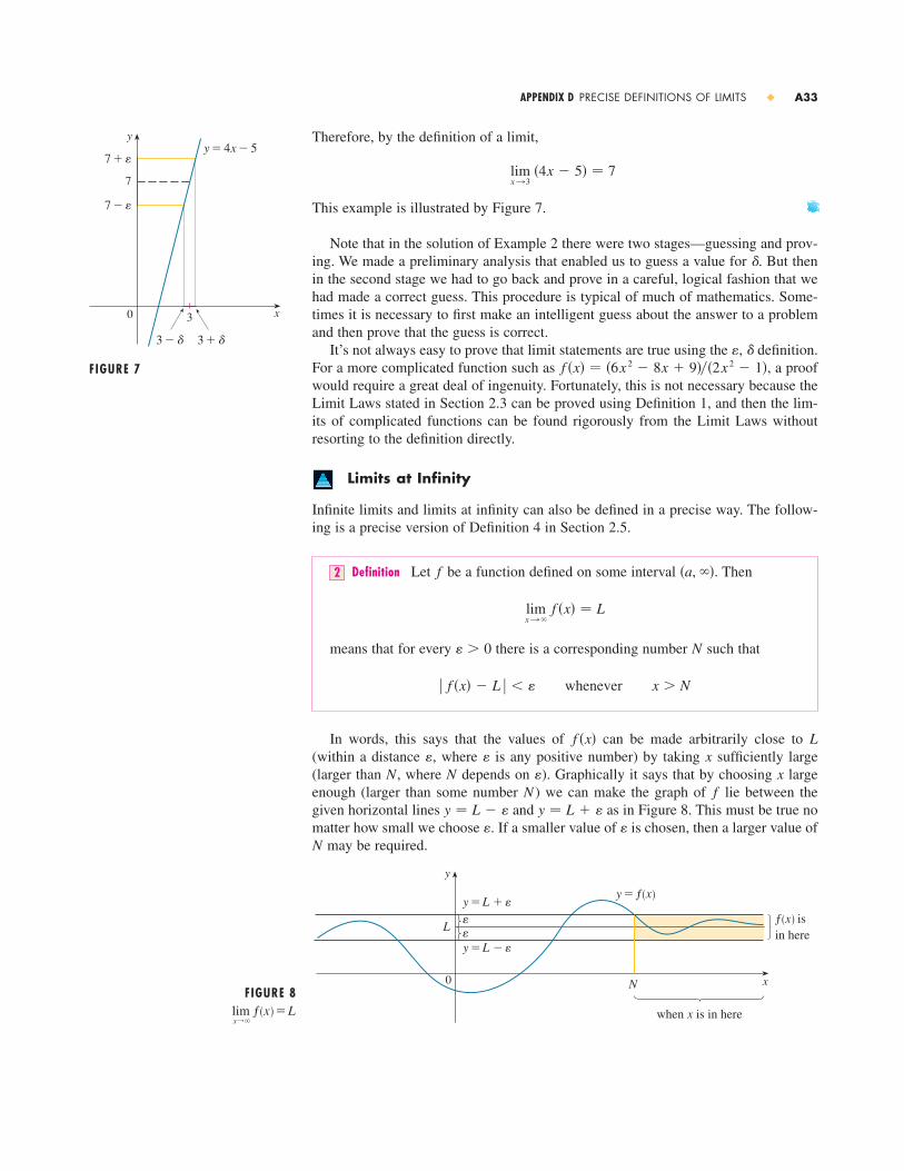
Therefore, by the definition of a limit,
This example is illustrated by Figure 7.
Note that in the solution of Example 2 there were two stages—guessing and prov-ing. We made a preliminary analysis that enabled us to guess a value for . But thenin the second stage we had to go back and prove in a careful, logical fashion that wehad made a correct guess. This procedure is typical of much of mathematics. Some-times it is necessary to first make an intelligent guess about the answer to a problemand then prove that the guess is correct.
It’s not always easy to prove that limit statements are true using the definition.For a more complicated function such as , a proofwould require a great deal of ingenuity. Fortunately, this is not necessary because theLimit Laws stated in Section 2.3 can be proved using Definition 1, and then the lim-its of complicated functions can be found rigorously from the Limit Laws withoutresorting to the definition directly.
Limits at Infinity
Infinite limits and limits at infinity can also be defined in a precise way. The follow-ing is a precise version of Definition 4 in Section 2.5.
Definition Let be a function defined on some interval . Then
means that for every there is a corresponding number such that
In words, this says that the values of can be made arbitrarily close to (within a distance , where is any positive number) by taking sufficiently large(larger than , where depends on ). Graphically it says that by choosing largeenough (larger than some number ) we can make the graph of lie between thegiven horizontal lines and as in Figure 8. This must be true nomatter how small we choose . If a smaller value of is chosen, then a larger value of
may be required.
0
y
xN
L
when x is in here
ƒ isin here
y=L-∑
y=L+∑
∑∑
y=ƒ
FIGURE 8lim ƒ=Lx `
N��
y � L � �y � L � �fN
x�NNx��
Lf �x�
x � Nwhenever� f �x� � L � � �
N� � 0
limx l �
f �x� � L
�a, ��f2
f �x� � �6x 2 � 8x � 9���2x 2 � 1��, �
�
limx l3
�4x � 5� � 7
APPENDIX D PRECISE DEFINITIONS OF LIMITS � A33
FIGURE 7
y
0 x
7+∑
7
7-∑
3-∂ 3+∂
3
y=4x-5

In Example 5 in Section 2.5 we calculated that
In the next example we use a graphing device to relate this statement to Definition 2with and
EXAMPLE 4 Use a graph to find a number such that
SOLUTION We rewrite the given inequality as
We need to determine the values of for which the given curve lies between thehorizontal lines and . So we graph the curve and these lines in Fig-ure 9. Then we use the cursor to estimate that the curve crosses the line when . To the right of this number the curve stays between the lines and . Rounding to be safe, we can say that
In other words, for we can choose (or any larger number) in Definition 2.
EXAMPLE 5 Use Definition 2 to prove that .
SOLUTION Let be a given positive number. According to Definition 2, we want tofind such that
In computing the limit we may assume , in which case
Therefore, we want
that is,
So if we choose , then . This proves the desired limit. 1�x � � &? x � NN � 1��
x � Nwheneverx �1
�
x � Nwhenever1
x� �
1
x� 0 � 1
x �1
x
x � 0
x � Nwhenever 1
x� 0 � �
N�
limx l �
1
x� 0
N � 7� � 0.1
x � 7whenever 3x 2 � x � 2
5x 2 � 4x � 1� 0.6 � 0.1
y � 0.7y � 0.5x 6.7
y � 0.5y � 0.7y � 0.5
x
0.5 �3x 2 � x � 2
5x 2 � 4x � 1� 0.7
x � Nwhenever 3x 2 � x � 2
5x 2 � 4x � 1� 0.6 � 0.1
N
� � 0.1.L � 35
limx l �
3x 2 � x � 2
5x 2 � 4x � 1�
3
5
A34 � APPENDIX D PRECISE DEFINITIONS OF LIMITS
FIGURE 9
1
0 15
y=0.7
y=0.5
y= 3≈-x-25≈+4x+1

Figure 10 illustrates the proof by showing some values of and the correspondingvalues of .
Infinite limits can also be formulated precisely. See Exercise 16.
Sequences
In Section 8.1 we used the notation
to mean that the terms of the sequence approach as becomes large. Notice thatthe following precise definition of the limit of a sequence is very similar to the defi-nition of a limit of a function at infinity (Definition 2).
Definition A sequence has the limit and we write
if for every there is a corresponding integer such that
Definition 3 is illustrated by Figure 11, in which the terms , , , . . . are plotted on a number line. No matter how small an interval is chosen,there exists an such that all terms of the sequence from onward must lie in thatinterval.
Another illustration of Definition 3 is given in Figure 12. The points on the graphof must lie between the horizontal lines and if . Thispicture must be valid no matter how small is chosen, but usually a smaller requiresa larger .N
��n � Ny � L � �y � L � ��an �
FIGURE 11 0 L-∑ L L+∑
a¡ a£ a¢a™ a∞aß a¶aˆ a˜aN+1 aN+2
aN�1N�L � �, L � ��
a3a2a1
n � Nwhenever� an � L � � �
N� � 0
an l L as n l �orlimn l �
an � L
L�an �3
nL�an �
limn l �
an � L
x
y
0 N=5
∑=0.2x
y
0 N=1
∑=1
x
y
0 N=10
∑=0.1
FIGURE 10
N�
APPENDIX D PRECISE DEFINITIONS OF LIMITS � A35

A36 � APPENDIX D PRECISE DEFINITIONS OF LIMITS
Comparison of Definitions 2 and 3 shows that the only difference betweenand is that is required to be an integer. The follow-
ing definition shows how to make precise the idea that becomes infinite as becomes infinite.
Definition If means that for every positive number there isan integer such that
EXAMPLE 6 Prove that .
SOLUTION Let be any positive number. (Think of it as being very large.) Then
So if we take , then Definition 4 shows that .
Functions of Two Variables
Here is a precise version of Definition 1 in Section 11.2:
Definition Let be a function of two variables whose domain includespoints arbitrarily close to . Then we say that the limit of as approaches is and we write
if for every number there is a corresponding number such that
Because is the distance between the numbers and , andis the distance between the point and the point ,
Definition 5 says that the distance between and can be made arbitrarily smallby making the distance from to sufficiently small (but not 0). An illustra-tion of Definition 5 is given in Figure 13 where the surface is the graph of . If is given, we can find such that if is restricted to lie in the disk withcenter and radius , and if , then the corresponding part of liesbetween the horizontal planes and .z � L � �z � L � �
S�x, y� � �a, b���a, b�D��x, y)� � 0
� � 0fS�a, b)�x, y)
Lf �x, y)�a, b)�x, y)s�x � a�2 � �y � b�2
Lf �x, y)� f (x, y) � L �
� f (x, y) � L � � � whenever �x, y� � D and 0 � s�x � a� 2 � �y � b� 2 � �
� � 0� � 0
lim�x, y� l �a, b�
f �x, y� � L
L�a, b)�x, y)f �x, y)�a, b�
Df5
limn l � sn � �N � M 2
sn � M &? n � M 2
M
limn l �
sn � �
an � M whenever n � N
NMlimn l � an � �4
n�an �nlimx l � f �x� � Llimn l � an � L
FIGURE 12 20 n
y
1 3 4
L
y=L+∑
N
y=L-∑
FIGURE 13
xy
z
0
L+∑L
L-∑
(a, b)D∂
S
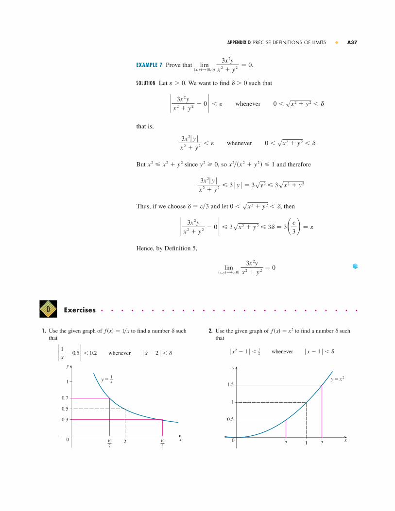
APPENDIX D PRECISE DEFINITIONS OF LIMITS � A37
EXAMPLE 7 Prove that .
SOLUTION Let . We want to find such that
that is,
But since , so and therefore
Thus, if we choose and let , then
Hence, by Definition 5,
lim�x, y� l �0, 0�
3x 2y
x 2 � y 2 � 0
3x 2y
x 2 � y 2 � 0 � 3sx 2 � y 2 � 3� � 3��
3� � �
0 � sx 2 � y 2 � �� � ��3
3x 2� y �x 2 � y 2 � 3 � y � � 3sy 2 � 3sx 2 � y 2
x 2��x 2 � y 2 � � 1y 2 � 0x 2 � x 2 � y 2
0 � sx 2 � y 2 � �whenever3x 2� y �x 2 � y 2 � �
0 � sx 2 � y 2 � �whenever 3x 2y
x 2 � y 2 � 0 � �
� � 0� � 0
lim�x, y� l �0, 0�
3x 2y
x 2 � y 2 � 0
2. Use the given graph of to find a number suchthat
x
y
? 1 ?0
1.5
1
0.5
y=≈
� x2 � 1 � �12 whenever � x � 1 � � �
�f �x� � x21. Use the given graph of to find a number suchthat
whenever
x
y
20
1
0.5
0.7
0.3
103
107
y=∆
� x � 2 � � � 1
x� 0.5 � 0.2
�f �x� � 1�x
Exercises � � � � � � � � � � � � � � � � � � � � � � � � � �D

A38 � APPENDIX D PRECISE DEFINITIONS OF LIMITS
(b) If the temperature is allowed to vary from by upto , what range of wattage is allowed for the inputpower?
(c) In terms of the definition of , whatis ? What is ? What is ? What is ? What valueof is given? What is the corresponding value of ?
; 13. Use a graph to find a number such that
; 14. For the limit
illustrate Definition 2 by finding values of that corre-spond to and .
15. (a) Determine how large we have to take so that
(b) Use Definition 2 to prove that
16. (a) For what values of is it true that
(b) The precise definition of states that forevery positive number (no matter how large) there isa corresponding positive number such that whenever . Use this definition to provethat .
; 17. (a) Use a graph to guess the value of the limit
(b) Use a graph of the sequence in part (a) to find the smallest values of that correspond to and
in Definition 3.
18. Use Definition 3 to prove that when .
19. Use Definition 3 to prove that if ,then .
20. Use Definition 4 to prove that .
21. Use Definition 5 to prove that .lim�x, y� l �0, 0�
xy
sx2 � y2 � 0
limn l �
n3 � �
limn l �
an � 0limn l �
� an � � 0
�r � � 1limn l �
rn � 0
� � 0.001� � 0.1N
limn l �
n5
n!
limx l 0 �1�x2� � �0 � � x � a � � �
f �x� � M�M
limx l a f �x� � �
1
x 2 � 1,000,000
x
limx l �
1
x2 � 0
1
x2 � 0.0001
x
� � 0.1� � 0.5N
limx l �
s4x2 � 1
x � 1� 2
x � Nwhenever 6x2 � 5x � 3
2x2 � 1� 3 � 0.2
N
��Laf �x�x
limx l a f �x� � L�, �
1 C200 C
; 3. Use a graph to find a number such that
; 4. Use a graph to find a number such that
; 5. For the limit
illustrate Definition 1 by finding values of that correspondto and .
; 6. For the limit
illustrate Definition 1 by finding values of that correspondto and
7. Use Definition 1 to prove that
8. (a) How would you formulate an definition of the one-sided limit ?
(b) Use your definition in part (a) to prove that.
9–10 � Prove the statement using the definition of limit andillustrate with a diagram like Figure 7.
9. 10.
� � � � � � � � � � � � �
11. A machinist is required to manufacture a circular metal diskwith area . (a) What radius produces such a disk?(b) If the machinist is allowed an error tolerance of
in the area of the disk, how close to the ideal radius inpart (a) must the machinist control the radius?
(c) In terms of the definition of , whatis ? What is ? What is ? What is ? What valueof is given? What is the corresponding value of ?
; 12. A crystal growth furnace is used in research to determinehow best to manufacture crystals used in electronic compo-nents for the space shuttle. For proper growth of the crystal,the temperature must be controlled accurately by adjustingthe input power. Suppose the relationship is given by
where is the temperature in degrees Celsius and is thepower input in watts.(a) How much power is needed to maintain the temperature
at ?200 C
wT
T�w� � 0.1w 2 � 2.155w � 20
��Laf �x�x
limx l a f �x� � L�, �
5 cm2
1000 cm2
limx l 4
�5 � 2x� � �3limx l 2
�3x � 2� � 4
�, �
limx l 0� sx � 0
limx l a� f �x� � L�, �
limx l 0 x3 � 0.
� � 0.1.� � 0.5�
limx l 0
ex
� 1
x� 1
� � 0.1� � 1�
limx l 1
�4 � x � 3x3� � 2
x ��
6 � �whenever| sin x �12 | � 0.1
�
� s4x � 1 � 3 � � 0.5 whenever � x � 2 � � �
�

A Few Proofs � � � � � � � � � � � � � � � � �
In this appendix we present proofs of some theorems that were stated in the main bodyof the text. We start by proving the Triangle Inequality, which is an important prop-erty of absolute value.
The Triangle Inequality If and are any real numbers, then
Observe that if the numbers and are both positive or both negative, then the twosides in the Triangle Inequality are actually equal. But if and have opposite signs,the left side involves a subtraction and the right side does not. This makes the TriangleInequality seem reasonable, but we can prove it as follows.
Notice that
is always true because equals either or . The corresponding statement foris
Adding these inequalities, we get
If we now apply Properties 4 and 5 of absolute value from Appendix A (with re-placed by and by ), we obtain
which is what we wanted to show.
Next we use the Triangle Inequality to prove the Sum Law for limits.
Sum Law If and both exist, then
Proof Let be given. According to Definition 1 in Appendix D, we must findsuch that
Using the Triangle Inequality we can write
� � f �x� � L � � � t�x� � M � � f �x� � t�x� � �L � M� � � � � f �x� � L� � �t�x� � M� �1
0 � � x � a � � �whenever� f �x� � t�x� � �L � M� � � �
� � 0� � 0
limx l a
� f �x� � t�x�� � L � M
limx l a t�x� � Mlimx l a f �x� � L
� a � b � � � a � � � b �� a � � � b �aa � b
x
�(� a � � � b �) � a � b � � a � � � b �
�� b � � b � � b �b
�� a �� a �a
�� a � � a � � a �
baba
� a � b � � � a � � � b �ba
E
APPENDIX E A FEW PROOFS � A39
� When combined, Properties 4 and 5of absolute value (see Appendix A) saythat
� x � � a &? �a � x � a
� The Sum Law was first stated in Section 2.3.
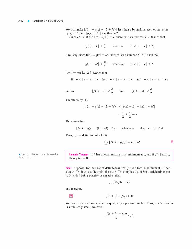
A40 � APPENDIX E A FEW PROOFS
We will make less than by making each of the termsand less than .
Since and , there exists a number such that
Similarly, since , there exists a number such that
Let . Notice that
and so
Therefore, by (1),
To summarize,
Thus, by the definition of a limit,
Fermat’s Theorem If has a local maximum or minimum at , and if exists,then .
Proof Suppose, for the sake of definiteness, that has a local maximum at . Then,if is sufficiently close to . This implies that if is sufficiently close
to 0, with being positive or negative, then
and therefore
We can divide both sides of an inequality by a positive number. Thus, if and is sufficiently small, we have
f �c � h� � f �c�h
� 0
hh � 0
f �c � h� � f �c� � 02
f �c� � f �c � h�
hhcxf �c� � f �x�
cf
f ��c� � 0f ��c�cf
limx l a
� f �x� � t�x�� � L � M
0 � � x � a � � �whenever� f �x� � t�x� � �L � M� � � �
��
2�
�
2� �
� f �x� � t�x� � �L � M� � � � f �x� � L � � � t�x� � M �
� t�x� � M � ��
2and� f �x� � L � �
�
2
0 � � x � a � � � 2and0 � � x � a � � �1then0 � � x � a � � �if
� � min ��1, � 2 �
0 � � x � a � � � 2whenever� t�x� � M � ��
2
� 2 � 0lim x l a t�x� � M
0 � � x � a � � �1whenever� f �x� � L � ��
2
�1 � 0lim x l a f �x� � L� 0��2��2� t�x� � M �� f �x� � L �
�� f �x� � t�x� � �L � M� �
� Fermat’s Theorem was discussed inSection 4.2.

APPENDIX E A FEW PROOFS � A41
Taking the right-hand limit of both sides of this inequality (using Theorem 2.3.2),we get
But since exists, we have
and so we have shown that .If , then the direction of the inequality (2) is reversed when we divide by :
So, taking the left-hand limit, we have
We have shown that and also that . Since both of these inequali-ties must be true, the only possibility is that .
We have proved Fermat’s Theorem for the case of a local maximum. The case ofa local minimum can be proved in a similar manner.
Clairaut’s Theorem Suppose is defined on a disk that contains the point If the functions and are both continuous on , then
.
Proof For small values of , , consider the difference
Notice that if we let , then
By the Mean Value Theorem, there is a number between and such that
Applying the Mean Value Theorem again, this time to we get a number between and such that
Combining these equations, we obtain
��h� � h 2fxy�c, d �
fx�c, b � h� � fx�c, b� � fxy�c, d �h
b � hbdfx ,
t�a � h� � t�a� � t��c�h � h � fx�c, b � h� � fx�c, b��
a � hac
��h� � t�a � h� � t�a�
t�x� � f �x, b � h� � f �x, b�
��h� � � f �a � h, b � h� � f �a � h, b�� � � f �a, b � h� � f �a, b��
h � 0h
fxy�a, b� � fyx�a, b�Dfyxfxy�a, b�.
Df
f ��c� � 0f ��c� � 0f ��c� � 0
f ��c� � limh l 0
f �c � h� � f �c�
h� lim
h l
0� f �c � h� � f �c�
h� 0
h � 0 f �c � h� � f �c�
h� 0
hh � 0f ��c� � 0
f ��c� � limh l 0
f �c � h� � f �c�
h� lim
h l
0� f �c � h� � f �c�
h
f ��c�
limh l
0� f �c � h� � f �c�
h� lim
h l
0� 0 � 0
� Clairaut’s Theorem was discussed inSection 11.3.

A42 � APPENDIX E A FEW PROOFS
If , then , so the continuity of at gives
Similarly, by writing
and using the Mean Value Theorem twice and the continuity of at , weobtain
It follows that .
Theorem If the partial derivatives and exist near and are continuousat , then is differentiable at .
Proof Let
According to Definition 11.4.7, to prove that is differentiable at we have toshow that we can write in the form
where and as .Referring to Figure 1, we write
Observe that the function of a single variable
is defined on the interval and . If we apply theMean Value Theorem to , we get
t�a � �x� � t�a� � t��u� �x
t
t��x� � fx�x, b � �y��a, a � �x�
t�x� � f �x, b � �y�
FIGURE 1x
y
0
R(a, √)
(a, b+Îy)
(a+Îx, b+Îy)
(u, b+Îy)
(a, b)
�z � � f �a � �x, b � �y� � f �a, b � �y�� � � f �a, b � �y� � f �a, b��3
��x, �y� l �0, 0��2 l 0�1
�z � fx�a, b� �x � fy�a, b� �y � �1 �x � �2 �y
�z�a, b�f
�z � f �a � �x, b � �y� � f �a, b�
�a, b�f�a, b��a, b�fyfx
fxy�a, b� � fyx�a, b�
lim h l 0
��h�h 2 � fyx�a, b�
�a, b�fyx
��h� � � f �a � h, b � h� � f �a, b � h�� � � f �a � h, b� � f �a, b��
lim h l 0
��h�h 2 � lim
�c, d� l �a, b� fxy�c, d � � fxy�a, b�
�a, b�fxy�c, d � l �a, b�h l 0
� This was stated as Theorem 8 in Section 11.4.

where is some number between and . In terms of , this equationbecomes
This gives us an expression for the first part of the right side of Equation 3. For the second part we let . Then is a function of a single variable definedon the interval and . A second application of the MeanValue Theorem then gives
where is some number between and . In terms of , this becomes
We now substitute these expressions into Equation 3 and obtain
where
Since and as and since and are continuous at , we see that and as .
Therefore, f is differentiable at .
Second Derivatives Test Suppose the second partial derivatives of are continu-ous on a disk with center , and suppose that and [that is, is a critical point of ]. Let
(a) If and , then is a local minimum.
(b) If and , then is a local maximum.
(c) If , then is not a local maximum or minimum.
Proof of part (a) We compute the second-order directional derivative of in thedirection of . The first-order derivative is given by Theorem 11.6.3:
Du f � fxh � fyk
u � �h, k�f
f �a, b�D � 0
f �a, b�fxx�a, b� � 0D � 0
f �a, b�fxx�a, b� � 0D � 0
D � D�a, b� � fxx�a, b� fyy�a, b� � � fxy�a, b��2
f�a, b�fy�a, b� � 0fx�a, b� � 0�a, b�
f
�a, b���x, �y� l �0, 0��2 l 0�1 l 0�a, b�fy
fx��x, �y� l �0, 0��a, v� l �a, b��u, b � �y� l �a, b�
�2 � fy�a, v� � fy�a, b�
�1 � fx�u, b � �y� � fx�a, b�
� fx�a, b� �x � fy�a, b� �y � �1 �x � �2 �y
� � � fy�a, v� � fy�a, b�� �y
� fx�a, b��x � � fx�u, b � �y� � fx�a, b�� �x � fy�a, b� �y
�z � fx�u, b � �y� �x � fy�a, v� �y
f �a, b � �y� � f �a, b� � fy�a, v� �y
fb � �ybv
h�b � �y� � h�b� � h��v� �y
h��y� � fy�a, y��b, b � �y�hh�y� � f �a, y�
f �a � �x, b � �y� � f �a, b � �y� � fx�u, b � �y� �x
fa � �xau
APPENDIX E A FEW PROOFS � A43
� The Second Derivatives Test was discussed in Section 11.7. Parts (b) and(c) have similar proofs.

A44 � APPENDIX E A FEW PROOFS
Applying this theorem a second time, we have
(by Clairaut’s Theorem)
If we complete the square in this expression, we obtain
We are given that and . But and arecontinuous functions, so there is a disk with center and radius suchthat and whenever is in . Therefore, by looking atEquation 4, we see that whenever is in . This means that if
is the curve obtained by intersecting the graph of with the vertical plane through in the direction of , then is concave upward on an inter-val of length . This is true in the direction of every vector , so if we restrict
to lie in , the graph of lies above its horizontal tangent plane at . Thus,whenever is in . This shows that is a local minimum.
Sigma Notation � � � � � � � � � � � � � � � �
A convenient way of writing sums uses the Greek letter (capital sigma, correspond-ing to our letter S) and is called sigma notation.
Definition If are real numbers and and are integerssuch that then
With function notation, Definition 1 can be written as
Thus, the symbol indicates a summation in which the letter (called the index ofsummation) takes on consecutive integer values beginning with m and ending with n,that is, . Other letters can also be used as the index of summation.m, m � 1, . . . , n
i�ni�m
�n
i�m f �i� � f �m� � f �m � 1� � f �m � 2� � � � � � f �n � 1� � f �n�
�n
i�m ai � am � am�1 � am�2 � � � � � an�1 � an
m � n, nmam, am�1, . . . , an1
�
F
f �a, b�B�x, y�f �x, y� � f �a, b�PfB�x, y�
u2�CuP�a, b, f �a, b��
fCB�x, y�Du
2 f �x, y� � 0B�x, y�D�x, y� � 0fxx�x, y� � 0
� � 0�a, b�BD � fxx fyy � f xy
2fxxD�a, b� � 0fxx�a, b� � 0
D2u f � fxx�h �
fxy
fxx k�2
�k 2
fxx � fxx fyy � f 2
xy�4
� fxxh2 � 2 fxyhk � fyyk 2
� � fxxh � fyxk�h � � fxyh � fyyk�k
D2u f � Du�Du f � �
�
�x �Du f �h �
�
�y �Du f �k
This tells us toend with i=n.
This tells usto add.
This tells us tostart with i=m.
µ ai
n
i�m

APPENDIX F SIGMA NOTATION � A45
EXAMPLE 1
(a)
(b)
(c)
(d)
(e)
(f)
EXAMPLE 2 Write the sum in sigma notation.
SOLUTION There is no unique way of writing a sum in sigma notation. We could write
or
or
The following theorem gives three simple rules for working with sigma notation.
Theorem If is any constant (that is, it does not depend on ), then
(a) (b)
(c)
Proof To see why these rules are true, all we have to do is write both sides inexpanded form. Rule (a) is just the distributive property of real numbers:
Rule (b) follows from the associative and commutative properties:
Rule (c) is proved similarly.
� �am � am�1 � � � � � an � � �bm � bm�1 � � � � � bn �
�am � bm � � �am�1 � bm�1� � � � � � �an � bn �
cam � cam�1 � � � � � can � c�am � am�1 � � � � � an �
�n
i�m �ai � bi� � �
n
i�m ai � �
n
i�m bi
�n
i�m �ai � bi� � �
n
i�m ai � �
n
i�m bi�
n
i�m cai � c �
n
i�m ai
ic2
23 � 33 � � � � � n 3 � �n�2
k�0 �k � 2�3
23 � 33 � � � � � n 3 � �n�1
j�1 � j � 1�3
23 � 33 � � � � � n 3 � �n
i�2 i 3
23 � 33 � � � � � n 3
�4
i�1 2 � 2 � 2 � 2 � 2 � 8
�3
i�1
i � 1
i 2 � 3�
1 � 1
12 � 3�
2 � 1
22 � 3�
3 � 1
32 � 3� 0 �
1
7�
1
6�
13
42
�n
k�1 1
k� 1 �
1
2�
1
3� � � � �
1
n
�5
j�0 2j � 20 � 21 � 22 � 23 � 24 � 25 � 63
�n
i�3 i � 3 � 4 � 5 � � � � � �n � 1� � n
�4
i�1 i 2 � 12 � 22 � 32 � 42 � 30

A46 � APPENDIX F SIGMA NOTATION
EXAMPLE 3 Find
SOLUTION
EXAMPLE 4 Prove the formula for the sum of the first positive integers:
SOLUTION This formula can be proved by mathematical induction (see page 89) or bythe following method used by the German mathematician Karl Friedrich Gauss(1777–1855) when he was ten years old.
Write the sum twice, once in the usual order and once in reverse order:
Adding all columns vertically, we get
On the right side there are terms, each of which is , so
EXAMPLE 5 Prove the formula for the sum of the squares of the first positive integers:
SOLUTION 1 Let be the desired sum. We start with the telescoping sum (or collapsingsum):
On the other hand, using Theorem 2 and Examples 3 and 4, we have
Thus, we have
n 3 � 3n 2 � 3n � 3S �32 n 2 �
52 n
� 3S � 3 n�n � 1�
2� n � 3S �
32 n 2 �
52 n
�n
i�1 ��1 � i �3 � i 3 � � �
n
i�1 �3i 2 � 3i � 1� � 3 �
n
i�1 i 2 � 3 �
n
i�1 i � �
n
i�1 1
� �n � 1�3 � 13 � n 3 � 3n 2 � 3n
�n
i�1 ��1 � i�3 � i 3 � � �23 � 13 � � �33 � 23 � � �43 � 33 � � � � � � ��n � 1�3 � n 3 �
S
�n
i�1 i 2 � 12 � 22 � 32 � � � � � n 2 �
n�n � 1��2n � 1�6
n
S �n�n � 1�
2or2S � n�n � 1�
n � 1n
2S � �n � 1� � �n � 1� � �n � 1� � � � � � �n � 1� � �n � 1�
S � n � �n � 1� � �n � 2� � � � � � 2 � 1
S � 1 � 2 � 3 � � � � � �n � 1� � n
S
�n
i�1 i � 1 � 2 � 3 � � � � � n �
n�n � 1�2
n
�n
i�1 1 � 1 � 1 � � � � � 1 � n
�n
i�1 1.
Most terms cancel in pairs.
n terms
APPENDIX F SIGMA NOTATION � A47
Solving this equation for , we obtain
or
SOLUTION 2 Let be the given formula.
1. is true because
2. Assume that is true; that is,
Then
So is true.
By the Principle of Mathematical Induction, is true for all .
We list the results of Examples 3, 4, and 5 together with a similar result for cubes(see Exercises 37–40) as Theorem 3. These formulas are needed for finding areas andevaluating integrals in Chapter 5.
Theorem Let be a constant and a positive integer. Then
(a) (b)
(c) (d)
(e) �n
i�1 i 3 � �n�n � 1�
2 �2
�n
i�1 i 2 �
n�n � 1��2n � 1�6�
n
i�1 i �
n�n � 1�2
�n
i�1 c � nc�
n
i�1 1 � n
nc3
nSn
Sk�1
��k � 1���k � 1� � 1��2�k � 1� � 1�
6
��k � 1��k � 2��2k � 3�
6
� �k � 1� 2k 2 � 7k � 6
6
� �k � 1� k�2k � 1� � 6�k � 1�
6
�k�k � 1��2k � 1�
6� �k � 1�2
12 � 22 � 32 � � � � � �k � 1�2 � �12 � 22 � 32 � � � � � k 2 � � �k � 1�2
12 � 22 � 32 � � � � � k 2 �k�k � 1��2k � 1�
6
Sk
12 �1�1 � 1��2 � 1 � 1�
6S1
Sn
S �2n 3 � 3n 2 � n
6�
n�n � 1��2n � 1�6
3S � n 3 �32 n 2 �
12 n
S
� See pages 89 and 92 for a more thorough discussion of mathematicalinduction.
� Principle of Mathematical InductionLet be a statement involving the positiveinteger . Suppose that1. is true.2. If is true, then is true.Then is true for all positive integers .nSn
Sk�1Sk
S1
nSn

A48 � APPENDIX F SIGMA NOTATION
7. 8.
9. 10.
� � � � � � � � � � � � �
11–20 � Write the sum in sigma notation.
11. 1 � 2 � 3 � 4 � � � � � 10
�n
i�1 f �xi � �xi�
n�1
j�0 ��1� j
�n�3
j�n j 2�
n
i�1 i 101–10 � Write the sum in expanded form.
1. 2.
3. 4.
5. 6. �8
k�5 xk�
4
k�0 2k � 1
2k � 1
�6
i�4 i 3�
6
i�4 3i
�6
i�1
1
i � 1�5
i�1 si
Exercises � � � � � � � � � � � � � � � � � � � � � � � � � �F
EXAMPLE 6 Evaluate .
SOLUTION Using Theorems 2 and 3, we have
EXAMPLE 7 Find .
SOLUTION
� 12 � 1 � 1 � 2 � 3 � 4
� lim n l �
�1
2� 1�1 �
1
n��2 �1
n� � 3� � lim
n l � �1
2�
n
n� �n � 1
n ��2n � 1
n � � 3� � lim
n l � � 3
n 3 n�n � 1��2n � 1�
6�
3
n� n�
� lim n l �
� 3
n 3 �n
i�1 i 2 �
3
n �
n
i�1 1�
lim n l �
�n
i�1 3
n �� i
n�2
� 1� � lim n l �
�n
i�1 � 3
n 3 i 2 �3
n�
lim n l �
�n
i�1 3
n �� i
n�2
� 1� �
n�n � 1��2n 2 � 2n � 3�2
�n�n � 1��2n�n � 1� � 3�
2
� 4�n�n � 1�2 �2
� 3 n�n � 1�
2
�n
i�1 i�4i 2 � 3� � �
n
i�1 �4i 3 � 3i� � 4 �
n
i�1 i 3 � 3 �
n
i�1 i
�n
i�1 i�4i 2 � 3�
� The type of calculation in Example 7arises in Chapter 5 when we computeareas.

is also the sum of the areas of the n “gnomons” , , . . . ,shown in the figure. Show that the area of is and
conclude that formula (e) is true.
41. Evaluate each telescoping sum.
(a) (b)
(c) (d)
42. Prove the generalized triangle inequality
43–46 � Find each limit.
43. 44.
45.
46.
� � � � � � � � � � � � �
47. Prove the formula for the sum of a finite geometric serieswith first term and common ratio :
48. Evaluate .
49. Evaluate .
50. Evaluate .�m
i�1 ��
n
j�1 �i � j ��
�n
i�1 �2i � 2 i �
�n
i�1
3
2 i�1
�n
i�1 ar i�1 � a � ar � ar 2 � � � � � ar n�1 �
a�r n � 1�r � 1
r � 1a
lim n l �
�n
i�1 3
n ��1 �
3i
n �3
� 2�1 �3i
n ��lim n l �
�n
i�1 2
n ��2i
n �3
� 5�2i
n ��lim n l �
�n
i�1 1
n �� i
n�3
� 1�lim n l �
�n
i�1 1
n � i
n�2
�ni�1
ai � �n
i�1 � ai �
�n
i�1 �ai � ai�1��
99
i�3 �1
i�
1
i � 1��100
i�1 �5 i � 5 i�1 ��
n
i�1 �i 4 � �i � 1�4 �
1 2 3 4 5 . . . n BA123
4
5
n
D
...
C
Gn
G™G£
G¢
G∞
. ..
i 3GiGn
G2G112.
13.
14.
15.
16.
17.
18.
19.
20.� � � � � � � � � � � � �
21–35 � Find the value of the sum.
21. 22.
23. 24.
25. 26.
27. 28.
29. 30.
31. 32.
33. 34.
35.
� � � � � � � � � � � � �
36. Find the number such that .
37. Prove formula (b) of Theorem 3.
38. Prove formula (e) of Theorem 3 using mathematical induction.
39. Prove formula (e) of Theorem 3 using a method similar tothat of Example 5, Solution 1 [start with .
40. Prove formula (e) of Theorem 3 using the following methodpublished by Abu Bekr Mohammed ibn Alhusain Alkarchiin about A.D. 1010. The figure shows a square inwhich sides and have been divided into segments oflengths , , , . . . , Thus, the side of the square haslength so the area is . But the area �n�n � 1��2�2n�n � 1��2
n.321ADAB
ABCD
�1 � i �4 � i 4 �
�n
i�1 i � 78n
�n
i�1 �i 3 � i � 2�
�n
i�1 i�i � 1��i � 2��
n
i�1 �i � 1��i � 2�
�n
i�1 �3 � 2i �2�
n
i�1 �i 2 � 3i � 4�
�n
i�1 �2 � 5i ��
n
i�1 2i
�4
i��2 23�i�
4
i�0 �2 i � i 2 �
�100
i�1 4�
20
n�1 ��1�n
�8
k�0 cos k��
6
j�1 3 j�1
�6
i�3 i�i � 2��
8
i�4 �3i � 2�
1 � x � x 2 � x 3 � � � � � ��1�nx n
x � x 2 � x 3 � � � � � x n
11 �
14 �
19 �
116 �
125 �
136
1 � 2 � 4 � 8 � 16 � 32
1 � 3 � 5 � 7 � � � � � �2n � 1�
2 � 4 � 6 � 8 � � � � � 2n
37 �
48 �
59 �
610 � � � � �
2327
12 �
23 �
34 �
45 � � � � �
1920
s3 � s4 � s5 � s6 � s7
APPENDIX F SIGMA NOTATION � A49

A50 � APPENDIX G INTEGRATION OF RATIONAL FUNCTIONS BY PARTIAL FRACTIONS
Integration of Rational Functions by Partial Fractions � � � � �
In this appendix we show how to integrate any rational function (a ratio of polynomi-als) by expressing it as a sum of simpler fractions, called partial fractions, that wealready know how to integrate. To illustrate the method, observe that by taking thefractions and to a common denominator we obtain
If we now reverse the procedure, we see how to integrate the function on the right sideof this equation:
To see how the method of partial fractions works in general, let’s consider arational function
where and are polynomials. It’s possible to express as a sum of simpler frac-tions provided that the degree of is less than the degree of . Such a rational func-tion is called proper. Recall that if
where , then the degree of is and we write .If is improper, that is, , then we must take the preliminary step
of dividing into (by long division) until a remainder is obtained such that. The division statement is
where and are also polynomials.As the following example illustrates, sometimes this preliminary step is all that is
required.
EXAMPLE 1 Find .
SOLUTION Since the degree of the numerator is greater than the degree of the denomi-nator, we first perform the long division. This enables us to write
�x 3
3�
x 2
2� 2x � 2 ln � x � 1 � � C
y x 3 � x
x � 1 dx � y �x 2 � x � 2 �
2
x � 1� dx
y x 3 � x
x � 1 dx
RS
f �x� �P�x�Q�x�
� S�x� �R�x�Q�x�
1
deg�R� � deg�Q�R�x�PQ
deg�P� � deg�Q�fdeg�P� � nnPan � 0
P�x� � anxn � an�1xn�1 � � � � � a1x � a0
QPfQP
f �x� �P�x�Q�x�
� 2 ln � x � 1 � � ln � x � 2 � � C
y x � 5
x 2 � x � 2 dx � y � 2
x � 1�
1
x � 2� dx
2
x � 1�
1
x � 2�
2�x � 2� � �x � 1��x � 1��x � 2�
�x � 5
x 2 � x � 2
1��x � 2�2��x � 1�
G
2 2x � 2 2x
x 2 � xx 2 � x
x 3 � x 2 x 3 � x 2 � x x 2 � x � 2
) x � 1

APPENDIX G INTEGRATION OF RATIONAL FUNCTIONS BY PARTIAL FRACTIONS � A51
The next step is to factor the denominator as far as possible. It can be shownthat any polynomial can be factored as a product of linear factors (of the form and irreducible quadratic factors (of the form , where ).For instance, if , we could factor it as
The third step is to express the proper rational function (from Equation 1)as a sum of partial fractions of the form
A theorem in algebra guarantees that it is always possible to do this. We explain thedetails for the four cases that occur.
CASE I � The denominator is a product of distinct linear factors.This means that we can write
where no factor is repeated. In this case the partial fraction theorem states that thereexist constants such that
These constants can be determined as in the following example.
EXAMPLE 2 Evaluate .
SOLUTION Since the degree of the numerator is less than the degree of the denomina-tor, we don’t need to divide. We factor the denominator as
Since the denominator has three distinct linear factors, the partial fraction decompo-sition of the integrand (2) has the form
To determine the values of , , and , we multiply both sides of this equation bythe product of the denominators, , obtaining
Expanding the right side of Equation 4 and writing it in the standard form forpolynomials, we get
x 2 � 2x � 1 � �2A � B � 2C �x 2 � �3A � 2B � C �x � 2A5
x 2 � 2x � 1 � A�2x � 1��x � 2� � Bx�x � 2� � Cx�2x � 1�4
x�2x � 1��x � 2�CBA
x 2 � 2x � 1
x�2x � 1��x � 2��
A
x�
B
2x � 1�
C
x � 23
2x 3 � 3x 2 � 2x � x�2x 2 � 3x � 2� � x�2x � 1��x � 2�
y x 2 � 2x � 1
2x 3 � 3x 2 � 2x dx
R�x�Q�x�
�A1
a1x � b1�
A2
a2x � b2� � � � �
Ak
akx � bk2
A1, A2, . . . , Ak
Q�x� � �a1x � b1 ��a2x � b2 � � � � �akx � bk�
Q�x�
Ax � B
�ax 2 � bx � c� jorA
�ax � b�i
R�x��Q�x�
Q�x� � �x 2 � 4��x 2 � 4� � �x � 2��x � 2��x 2 � 4�
Q�x� � x 4 � 16b 2 � 4ac � 0ax 2 � bx � c
ax � b�QQ�x�
� Another method for finding , , and is given in the note after thisexample.
CBA

A52 � APPENDIX G INTEGRATION OF RATIONAL FUNCTIONS BY PARTIAL FRACTIONS
The polynomials in Equation 5 are identical, so their coefficients must be equal. Thecoefficient of on the right side, , must equal the coefficient of onthe left side—namely, 1. Likewise, the coefficients of are equal and the constantterms are equal. This gives the following system of equations for , , and :
Solving, we get , , and , and so
In integrating the middle term we have made the mental substitution ,which gives and .
NOTE � We can use an alternative method to find the coefficients , , and inExample 2. Equation 4 is an identity; it is true for every value of . Let’s choose val-ues of that simplify the equation. If we put in Equation 4, then the second andthird terms on the right side vanish and the equation then becomes , or
. Likewise, gives and gives , so and. (You may object that Equation 3 is not valid for , , or , so why
should Equation 4 be valid for those values? In fact, Equation 4 is true for all valuesof , even , , and . See Exercise 35 for the reason.)
EXAMPLE 3 Find , where .
SOLUTION The method of partial fractions gives
and therefore
Using the method of the preceding note, we put in this equation and get, so . If we put , we get , so .
Thus
�1
2a [ln � x � a � � ln � x � a �] � C
y dx
x 2 � a 2 �1
2a y � 1
x � a�
1
x � a� dx
B � �1��2a�B��2a� � 1x � �aA � 1��2a�A�2a� � 1x � a
A�x � a� � B�x � a� � 1
1
x 2 � a 2 �1
�x � a��x � a��
A
x � a�
B
x � a
a � 0y dx
x 2 � a 2
�212x � 0x
�212x � 0C � �
110
B � 1510C � �1x � �25B�4 � 1
4x � 12A � 1
2
�2A � �1x � 0x
xCBA
dx � du�2du � 2 dxu � 2x � 1
� 12 ln � x � �
110 ln � 2x � 1 � �
110 ln � x � 2 � � K
y x 2 � 2x � 1
2x 3 � 3x 2 � 2x dx � y �1
2 1
x�
1
5
1
2x � 1�
1
10
1
x � 2� dx
C � �110B � 1
5A � 12
�2A � 2B � 2C � �1
3A � 2B � C � 2
2A � B � 2C � 1
CBAx
x 22A � B � 2Cx 2
� Figure 1 shows the graphs of the integrand in Example 2 and its indefiniteintegral (with ). Which is which?K � 0
FIGURE 1
_3
_2
2
3

APPENDIX G INTEGRATION OF RATIONAL FUNCTIONS BY PARTIAL FRACTIONS � A53
Since , we can write the integral as
CASE II � is a product of linear factors, some of which are repeated.Suppose the first linear factor is repeated times; that is,occurs in the factorization of . Then instead of the single term inEquation 2, we would use
By way of illustration, we could write
but we prefer to work out in detail a simpler example.
EXAMPLE 4 Find .
SOLUTION The first step is to divide. The result of long division is
The second step is to factor the denominator . Since, we know that is a factor and we obtain
Since the linear factor occurs twice, the partial fraction decomposition is
Multiplying by the least common denominator, , we get
Now we equate coefficients:
�A � B � C � 0
A � B � 2C � 4
A � B � C � 0
� �A � C �x 2 � �B � 2C �x � ��A � B � C �
4x � A�x � 1��x � 1� � B�x � 1� � C�x � 1�27
�x � 1�2�x � 1�
4x
�x � 1�2�x � 1��
A
x � 1�
B
�x � 1�2 �C
x � 1
x � 1
� �x � 1�2�x � 1�
x 3 � x 2 � x � 1 � �x � 1��x 2 � 1� � �x � 1��x � 1��x � 1�
x � 1Q�1� � 0Q�x� � x 3 � x 2 � x � 1
x 4 � 2x 2 � 4x � 1
x 3 � x 2 � x � 1� x � 1 �
4x
x 3 � x 2 � x � 1
y x 4 � 2x 2 � 4x � 1
x 3 � x 2 � x � 1 dx
x 3 � x � 1
x 2�x � 1�3 �A
x�
B
x 2 �C
x � 1�
D
�x � 1�2 �E
�x � 1�3
A1
a1x � b1�
A2
�a1x � b1�2 � � � � �Ar
�a1x � b1�r6
A1��a1x � b1�Q�x��a1x � b1�rr�a1x � b1�
Q�x�
y dx
x 2 � a 2 �1
2a ln x � a
x � a � C
ln x � ln y � ln�x�y�
� Another method for finding the coefficients:Put in (7): .Put : .Put : .A � B � C � 1x � 0
C � �1x � �1B � 2x � 1

A54 � APPENDIX G INTEGRATION OF RATIONAL FUNCTIONS BY PARTIAL FRACTIONS
Solving, we obtain , , and , so
CASE III � contains irreducible quadratic factors, none of which is repeated.If has the factor , where , then, in addition to the par-tial fractions in Equations 2 and 6, the expression for will have a term ofthe form
where and are constants to be determined. For instance, the function given byhas a partial fraction decomposition of the form
The term given in (8) can be integrated by completing the square and using the formula
EXAMPLE 5 Evaluate .
SOLUTION Since can’t be factored further, we write
Multiplying by , we have
Equating coefficients, we obtain
Thus , , and and so
y 2x 2 � x � 4
x 3 � 4x dx � y �1
x�
x � 1
x 2 � 4� dx
C � �1B � 1A � 1
4A � 4C � �1A � B � 2
� �A � B�x 2 � Cx � 4A
2x 2 � x � 4 � A�x 2 � 4� � �Bx � C �x
x�x 2 � 4�
2x 2 � x � 4
x�x 2 � 4��
A
x�
Bx � C
x 2 � 4
x 3 � 4x � x�x 2 � 4�
y 2x 2 � x � 4
x 3 � 4x dx
y dx
x 2 � a 2 �1
a tan�1� x
a� � C9
x
�x � 2��x 2 � 1��x 2 � 4��
A
x � 2�
Bx � C
x 2 � 1�
Dx � E
x 2 � 4
f �x� � x���x � 2��x 2 � 1��x 2 � 4��BA
Ax � B
ax 2 � bx � c8
R�x��Q�x�b 2 � 4ac � 0ax 2 � bx � cQ�x�
Q�x�
�x 2
2� x �
2
x � 1� ln x � 1
x � 1 � K
�x 2
2� x � ln � x � 1 � �
2
x � 1� ln � x � 1 � � K
y x 4 � 2x 2 � 4x � 1
x 3 � x 2 � x � 1 dx � y �x � 1 �
1
x � 1�
2
�x � 1�2 �1
x � 1� dx
C � �1B � 2A � 1

APPENDIX G INTEGRATION OF RATIONAL FUNCTIONS BY PARTIAL FRACTIONS � A55
In order to integrate the second term we split it into two parts:
We make the substitution in the first of these integrals so that. We evaluate the second integral by means of Formula 9 with :
EXAMPLE 6 Evaluate .
SOLUTION Since the degree of the numerator is not less than the degree of the denomi-nator, we first divide and obtain
Notice that the quadratic is irreducible because its discriminant is. This means it can’t be factored, so we don’t need to use the
partial fraction technique.To integrate the given function we complete the square in the denominator:
This suggests that we make the substitution . Then, and, so
NOTE � Example 6 illustrates the general procedure for integrating a partial fractionof the form
where b 2 � 4ac � 0Ax � B
ax 2 � bx � c
� x �18 ln�4x 2 � 4x � 3� �
1
4s2 tan�1�2x � 1
s2 � � C
� x �18 ln�u 2 � 2� �
1
4�
1
s2 tan�1� u
s2� � C
� x �14 y
u
u 2 � 2 du �
14 y
1
u 2 � 2 du
� x �12 y
12 �u � 1� � 1
u 2 � 2 du � x �
14 y
u � 1
u 2 � 2 du
y 4x 2 � 3x � 2
4x 2 � 4x � 3 dx � y �1 �
x � 1
4x 2 � 4x � 3� dx
x � �u � 1��2du � 2 dxu � 2x � 1
4x 2 � 4x � 3 � �2x � 1�2 � 2
b 2 � 4ac � �32 � 04x 2 � 4x � 3
4x 2 � 3x � 2
4x 2 � 4x � 3� 1 �
x � 1
4x 2 � 4x � 3
y 4x 2 � 3x � 2
4x 2 � 4x � 3 dx
� ln � x � �12 ln�x 2 � 4� �
12 tan�1�x�2� � K
y 2x 2 � x � 4
x�x 2 � 4� dx � y
1
x dx � y
x
x 2 � 4 dx � y
1
x 2 � 4 dx
a � 2du � 2x dxu � x 2 � 4
y x � 1
x 2 � 4 dx � y
x
x 2 � 4 dx � y
1
x 2 � 4 dx

A56 � APPENDIX G INTEGRATION OF RATIONAL FUNCTIONS BY PARTIAL FRACTIONS
We complete the square in the denominator and then make a substitution that bringsthe integral into the form
Then the first integral is a logarithm and the second is expressed in terms of .
CASE IV � contains a repeated irreducible quadratic factor.If has the factor , where , then instead of the single partial fraction (8), the sum
occurs in the partial fraction decomposition of . Each of the terms in (10)can be integrated by first completing the square.
EXAMPLE 7 Write out the form of the partial fraction decomposition of the function
SOLUTION
EXAMPLE 8 Evaluate .
SOLUTION The form of the partial fraction decomposition is
Multiplying by , we have
If we equate coefficients, we get the system
which has the solution , , , , and . E � 0D � 1C � �1B � �1A � 1
A � 1C � E � �12A � B � D � 2C � �1A � B � 0
� �A � B�x 4 � Cx 3 � �2A � B � D�x 2 � �C � E�x � A
� A�x 4 � 2x 2 � 1� � B�x 4 � x 2 � � C�x 3 � x� � Dx 2 � Ex
�x 3 � 2x 2 � x � 1 � A�x 2 � 1�2 � �Bx � C �x�x 2 � 1� � �Dx � E�x
x�x 2 � 1�2
1 � x � 2x 2 � x 3
x�x 2 � 1�2 �A
x�
Bx � C
x 2 � 1�
Dx � E
�x 2 � 1�2
y 1 � x � 2x 2 � x 3
x�x 2 � 1�2 dx
� A
x�
B
x � 1�
Cx � D
x 2 � x � 1�
Ex � F
x 2 � 1�
Gx � H
�x 2 � 1�2 �Ix � J
�x 2 � 1�3
x 3 � x 2 � 1
x�x � 1��x 2 � x � 1��x 2 � 1�3
x 3 � x 2 � 1
x�x � 1��x 2 � x � 1��x 2 � 1�3
R�x��Q�x�
A1x � B1
ax 2 � bx � c�
A2x � B2
�ax 2 � bx � c�2 � � � � �Arx � Br
�ax 2 � bx � c�r10
b 2 � 4ac � 0�ax 2 � bx � c�rQ�x�Q�x�
tan�1
y Cu � D
u 2 � a 2 du � C y u
u 2 � a 2 du � D y 1
u 2 � a 2 du
� It would be extremely tedious to workout by hand the numerical values of thecoefficients in Example 7. Most com-puter algebra systems, however, canfind the numerical values very quickly.For instance, the Maple command
or the Mathematica command
gives the following values:
I � �12 , J � 1
2
E � 158 , F � �
18 , G � H � 3
4 ,
A � �1, B � 18 , C � D � �1,
Apart[f]
convert�f, parfrac, x�

APPENDIX G INTEGRATION OF RATIONAL FUNCTIONS BY PARTIAL FRACTIONS � A57
Thus
� ln � x � �12 ln�x 2 � 1� � tan�1x �
1
2�x 2 � 1�� K
� y dx
x� y
x
x 2 � 1 dx � y
dx
x 2 � 1� y
x dx
�x 2 � 1�2
y 1 � x � 2x 2 � x 3
x�x 2 � 1�2 dx � y �1
x�
x � 1
x 2 � 1�
x
�x 2 � 1�2� dx
27. 28.
� � � � � � � � � � � � �
; 29. Use a graph of
to decide whether is positive or negative. Use thegraph to give a rough estimate of the value of the integraland then use partial fractions to find the exact value.
; 30. Graph both and an antiderivative on thesame screen.
31. One method of slowing the growth of an insect populationwithout using pesticides is to introduce into the population anumber of sterile males that mate with fertile females butproduce no offspring. If represents the number of femaleinsects in a population, the number of sterile males intro-duced each generation, and the population’s naturalgrowth rate, then the female population is related to time by
Suppose an insect population with 10,000 females grows ata rate of and 900 sterile males are added. Evaluatethe integral to give an equation relating the female popula-tion to time. (Note that the resulting equation can’t besolved explicitly for .)
32. The region under the curve
from to is rotated about the -axis. Find thevolume of the resulting solid.
33. (a) Use a computer algebra system to find the partial frac-tion decomposition of the function
f �x� �4x 3 � 27x 2 � 5x � 32
30x 5 � 13x 4 � 50x 3 � 286x 2 � 299x � 70
CAS
xx � 1x � 0
y �1
x 2 � 3x � 2
P
r � 0.10
t � y P � S
P��r � 1�P � S� dP
tr
SP
y � 1��x 3 � 2x 2�
x2
0 f �x� dx
f �x� �1
x 2 � 2x � 3
y x 4 � 1
x �x 2 � 1�2 dxy 2t 3 � t 2 � 3t � 1
�t 2 � 1��t 2 � 2� dt
1–10 � Write out the form of the partial fraction decomposition of the function (as in Example 7). Do not determine the numeri-cal values of the coefficients.
1. 2.
3. 4.
5. 6.
7. 8.
9. 10.
� � � � � � � � � � � � �
11–28 � Evaluate the integral.
11. 12.
13. 14.
15.
16.
17. 18.
19. 20.
21. 22.
23. 24.
25. 26. y x 4
x 4 � 1 dxy
1
x 3 � 1 dx
y2
1
x 2 � 3
x 3 � 2x dxy
3x 2 � 4x � 5
�x � 1��x 2 � 1� dx
y1
0
x � 1
x 2 � 2x � 2 dxy
1
0
x
x 2 � x � 1 dx
y x 2
�x � 3��x � 2�2 dxy 1
�x � 5�2�x � 1� dx
y3
2
1
x 3 � x 2 � 2x dxy
2
1
4y 2 � 7y � 12
y�y � 2��y � 3� dy
y2
0 x 3 � x 2 � 12x � 1
x 2 � x � 12 dx
y1
0
2x � 3
�x � 1�2 dx
y 1
�t � 4��t � 1� dty
4
2
4x � 1
�x � 1��x � 2� dx
y x
x � 5 dxy
x 2 � 2
x � 2 dx
1
x 6 � x 3
x 3 � x 2 � 1
x 4 � x 3 � 2x 2
x 4 � x 2 � 1
�x 2 � 1��x 2 � 4�2
x 2 � 2
x�x 2 � 2�
x 3 � 4x 2 � 2
�x 2 � 1��x 2 � 2�x 2 � 1
x 2 � 1
x 4 � x 3 � x 2 � x � 1
x 3 � x
1
x 4 � x 3
z 2 � 4z
�3z � 5�3�z � 2�5
2x 2 � 3x � 2
Exercises � � � � � � � � � � � � � � � � � � � � � � � � � �G
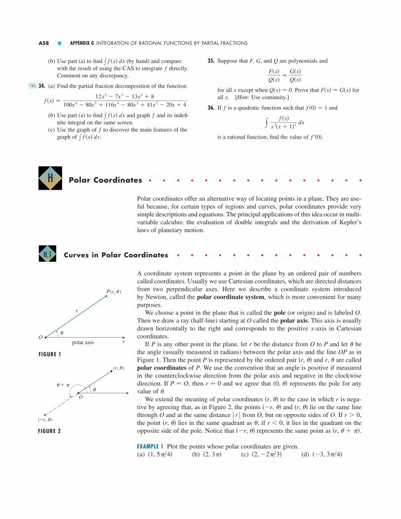
35. Suppose that , and are polynomials and
for all except when . Prove that for all . [Hint: Use continuity.]
36. If is a quadratic function such that and
is a rational function, find the value of .f ��0�
y f �x�
x 2�x � 1�3 dx
f �0� � 1f
xF�x� � G�x�Q�x� � 0x
F�x�Q�x�
�G�x�Q�x�
QF, G(b) Use part (a) to find (by hand) and comparewith the result of using the CAS to integrate directly.Comment on any discrepancy.
34. (a) Find the partial fraction decomposition of the function
(b) Use part (a) to find and graph and its indefi-nite integral on the same screen.
(c) Use the graph of to discover the main features of thegraph of .x f �x� dx
f
fx f �x� dx
f �x� �12x 5 � 7x 3 � 13x 2 � 8
100x 6 � 80x 5 � 116x 4 � 80x 3 � 41x 2 � 20x � 4
CAS
fx f �x� dx
Polar Coordinates � � � � � � � � � � � � � � � �
Polar coordinates offer an alternative way of locating points in a plane. They are use-ful because, for certain types of regions and curves, polar coordinates provide verysimple descriptions and equations. The principal applications of this idea occur in multi-variable calculus: the evaluation of double integrals and the derivation of Kepler’slaws of planetary motion.
Curves in Polar Coordinates � � � � � � � � � � � � � �
A coordinate system represents a point in the plane by an ordered pair of numberscalled coordinates. Usually we use Cartesian coordinates, which are directed distancesfrom two perpendicular axes. Here we describe a coordinate system introduced by Newton, called the polar coordinate system, which is more convenient for manypurposes.
We choose a point in the plane that is called the pole (or origin) and is labeled .Then we draw a ray (half-line) starting at called the polar axis. This axis is usuallydrawn horizontally to the right and corresponds to the positive -axis in Cartesiancoordinates.
If is any other point in the plane, let be the distance from to and let bethe angle (usually measured in radians) between the polar axis and the line as inFigure 1. Then the point is represented by the ordered pair and , are calledpolar coordinates of . We use the convention that an angle is positive if measuredin the counterclockwise direction from the polar axis and negative in the clockwisedirection. If , then and we agree that represents the pole for anyvalue of .
We extend the meaning of polar coordinates to the case in which is nega-tive by agreeing that, as in Figure 2, the points and lie on the same linethrough and at the same distance from , but on opposite sides of . If ,the point lies in the same quadrant as ; if , it lies in the quadrant on theopposite side of the pole. Notice that represents the same point as .
EXAMPLE 1 Plot the points whose polar coordinates are given.(a) (b) (c) (d) ��3, 3��4��2, �2��3��2, 3���1, 5��4�
�r, � � ����r, ��r � 0��r, ��
r � 0OO� r �O�r, ����r, ��
r�r, ���
�0, ��r � 0P � O
P�r�r, ��P
OP�POrP
xO
O
H.1
H
A58 � APPENDIX G INTEGRATION OF RATIONAL FUNCTIONS BY PARTIAL FRACTIONS
(_r, ¨)
O
¨
(r, ¨ )
¨+π
FIGURE 2
xO
¨
r
polar axis
P(r, ̈ )
FIGURE 1

SECTION H.1 CURVES IN POLAR COORDINATES � A59
SOLUTION The points are plotted in Figure 3. In part (d) the point islocated three units from the pole in the fourth quadrant because the angle is inthe second quadrant and is negative.
In the Cartesian coordinate system every point has only one representation, but inthe polar coordinate system each point has many representations. For instance, thepoint in Example 1(a) could be written as or or
. (See Figure 4.)
In fact, since a complete counterclockwise rotation is given by an angle 2 , thepoint represented by polar coordinates is also represented by
where is any integer.The connection between polar and Cartesian coordinates can be seen from Figure 5,
in which the pole corresponds to the origin and the polar axis coincides with the pos-itive -axis. If the point has Cartesian coordinates and polar coordinates then, from the figure, we have
and so
Although Equations 1 were deduced from Figure 5, which illustrates the casewhere and , these equations are valid for all values of and (Seethe general definition of and in Appendix C.)
Equations 1 allow us to find the Cartesian coordinates of a point when the polarcoordinates are known. To find and when and are known, we use the equations
which can be deduced from Equations 1 or simply read from Figure 5.
tan � �y
xr 2 � x 2 � y 22
yx�r
cos �sin ��.r0 � � � ��2r � 0
y � r sin �x � r cos �1
sin � �y
rcos � �
x
r
�r, ��,�x, y�Px
n
��r, � � �2n � 1���and�r, � � 2n��
�r, ���
O
13π4
”1, ’13π4
O
_ 3π4
”1, _ ’3π4
O
”1, ’5π4
5π4
O
”_1, ’π4
π4
��1, ��4��1, 13��4��1, �3��4��1, 5��4�
O
”_3, ’3π4
3π4
O
”2, _ ’2π3
2π3
_(2, 3π) O
3π
”1, ’5π4
5π4
O
FIGURE 3
r � �33��4
��3, 3��4�
O
y
x
¨
x
yr
P (r, ̈ )=P(x, y)
FIGURE 5
FIGURE 4

A60 � APPENDIX H POLAR COORDINATES
EXAMPLE 2 Convert the point from polar to Cartesian coordinates.
SOLUTION Since and , Equations 1 give
Therefore, the point is in Cartesian coordinates.
EXAMPLE 3 Represent the point with Cartesian coordinates in terms of polarcoordinates.
SOLUTION If we choose to be positive, then Equations 2 give
Since the point lies in the fourth quadrant, we can choose or. Thus, one possible answer is ; another is .
NOTE � Equations 2 do not uniquely determine when and are given because,as increases through the interval , each value of occurs twice.Therefore, in converting from Cartesian to polar coordinates, it’s not good enough justto find and that satisfy Equations 2. As in Example 3, we must choose so that thepoint lies in the correct quadrant.
The graph of a polar equation , or more generally , consistsof all points that have at least one polar representation whose coordinates sat-isfy the equation.
EXAMPLE 4 What curve is represented by the polar equation ?
SOLUTION The curve consists of all points with . Since represents thedistance from the point to the pole, the curve represents the circle with center
and radius . In general, the equation represents a circle with center andradius . (See Figure 6.)
EXAMPLE 5 Sketch the polar curve .
SOLUTION This curve consists of all points such that the polar angle is 1 radian.It is the straight line that passes through and makes an angle of 1 radian with the O
��r, ��
� � 1
FIGURE 6
x
r=12
r=1
r=2
r=4
� a �Or � a2O
r � 2rr � 2�r, ��
r � 2
�r, ��PF�r, �� � 0r � f ���
�r, ����r
tan �0 � � � 2��yx�
�s2, 7��4�(s2, ���4)� � 7��4� � ���4�1, �1�
tan � �y
x� �1
r � sx 2 � y 2 � s12 � ��1�2 � s2
r
�1, �1�
(1, s3)
y � r sin � � 2 sin �
3� 2 �
s3
2� s3
x � r cos � � 2 cos �
3� 2 �
1
2� 1
� � ��3r � 2
�2, ��3�
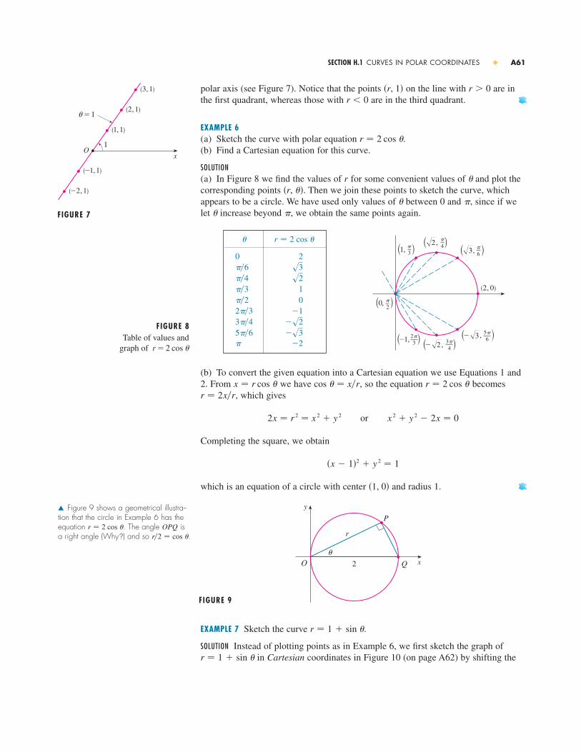
SECTION H.1 CURVES IN POLAR COORDINATES � A61
polar axis (see Figure 7). Notice that the points on the line with are inthe first quadrant, whereas those with are in the third quadrant.
EXAMPLE 6(a) Sketch the curve with polar equation .(b) Find a Cartesian equation for this curve.
SOLUTION(a) In Figure 8 we find the values of for some convenient values of and plot thecorresponding points . Then we join these points to sketch the curve, whichappears to be a circle. We have used only values of between 0 and , since if welet increase beyond , we obtain the same points again.
(b) To convert the given equation into a Cartesian equation we use Equations 1 and2. From we have , so the equation becomes
, which gives
or
Completing the square, we obtain
which is an equation of a circle with center and radius 1.
EXAMPLE 7 Sketch the curve .
SOLUTION Instead of plotting points as in Example 6, we first sketch the graph ofin Cartesian coordinates in Figure 10 (on page A62) by shifting the r � 1 � sin �
r � 1 � sin �
O
y
x2
¨
r
P
Q
FIGURE 9
�1, 0�
�x � 1�2 � y 2 � 1
x 2 � y 2 � 2x � 02x � r 2 � x 2 � y 2
r � 2x�rr � 2 cos �cos � � x�rx � r cos �
FIGURE 8Table of values and
graph of r=2 cos ¨
(2, 0)
2
”_1, ’2π3
”0, ’π2
”1, ’π3
”œ„, ’π4
”œ„, ’π63
”_ œ„, ’5π63
”_ œ„, ’3π42
����
�r, ���r
r � 2 cos �
r � 0r � 0�r, 1�
0 2
10
�1
�2��s35��6�s23��4
2��3��2��3
s2��4s3��6
r � 2 cos ��
� Figure 9 shows a geometrical illustra-tion that the circle in Example 6 has theequation . The angle isa right angle (Why?) and so .r�2 � cos �
OPQr � 2 cos �
Ox
1
(_1, 1)
(_2, 1)
(1, 1)
(2, 1)
(3, 1)
¨=1
FIGURE 7

A62 � APPENDIX H POLAR COORDINATES
sine curve up one unit. This enables us to read at a glance the values of that corre-spond to increasing values of . For instance, we see that as increases from 0 to ,
(the distance from ) increases from 1 to 2, so we sketch the corresponding partof the polar curve in Figure 11(a). As increases from to , Figure 10 showsthat decreases from 2 to 1, so we sketch the next part of the curve as in Figure 11(b).As increases from to , decreases from 1 to 0 as shown in part (c). Finally,as increases from to , increases from 0 to 1 as shown in part (d). If welet increase beyond or decrease beyond 0, we would simply retrace our path.Putting together the parts of the curve from Figure 11(a)–(d), we sketch the com-plete curve in part (e). It is called a cardioid because it’s shaped like a heart.
EXAMPLE 8 Sketch the curve .
SOLUTION As in Example 7, we first sketch , , in Cartesiancoordinates in Figure 12. As increases from 0 to , Figure 12 shows that decreases from 1 to 0 and so we draw the corresponding portion of the polar curvein Figure 13 (indicated by !). As increases from to , goes from 0 to .This means that the distance from increases from 0 to 1, but instead of being inthe first quadrant this portion of the polar curve (indicated by @) lies on the oppositeside of the pole in the third quadrant. The remainder of the curve is drawn in a simi-lar fashion, with the arrows and numbers indicating the order in which the portionsare traced out. The resulting curve has four loops and is called a four-leaved rose.
When we sketch polar curves it is sometimes helpful to take advantage of symme-try. The following three rules are explained by Figure 14.
(a) If a polar equation is unchanged when is replaced by , the curve is sym-metric about the polar axis.
���
¨=0¨=π
�
¨=3π4
¨=π2
¨=π4
FIGURE 12r=cos 2¨ in Cartesian coordinates
FIGURE 13Four-leaved rose r=cos 2¨
r
1
¨2ππ 5π4
π2
π4
3π4
3π2
7π4
!
@ # ^ &
% *$!
@ #
$
%
& ^
O�1r��2��4�
r��4�0 � � � 2�r � cos 2�
r � cos 2�
2��r2�3��2�r3��2��
r���2�
Or��2��
r
(a) (b) (c) (d) (e)
FIGURE 11Stages in sketching thecardioid r=1+sin ¨
O¨=π
¨=π2
O
¨=π¨= 3π
2
O
¨=2π¨= 3π
2
O
O ¨=0
¨=π2
1
2
FIGURE 10r=1+sin ¨ in Cartesian coordinates,0¯¨¯2π
0
r
1
2
¨π 2π3π2
π2
Module H helps you see howpolar curves are traced out
by showing animations similar to Fig-ures 10–13. Tangents to these polarcurves can also be visualized as in Figure 15.

SECTION H.1 CURVES IN POLAR COORDINATES � A63
(b) If the equation is unchanged when is replaced by , the curve is symmetricabout the pole. (This means that the curve remains unchanged if we rotate itthrough 180° about the origin.)
(c) If the equation is unchanged when is replaced by , the curve is sym-metric about the vertical line .
The curves sketched in Examples 6 and 8 are symmetric about the polar axis, since. The curves in Examples 7 and 8 are symmetric about
because and . The four-leaved rose is alsosymmetric about the pole. These symmetry properties could have been used in sketch-ing the curves. For instance, in Example 6 we need only have plotted points for
and then reflected about the polar axis to obtain the complete circle.
Tangents to Polar Curves
To find a tangent line to a polar curve we regard as a parameter and writeits parametric equations as
Then, using the method for finding slopes of parametric curves (Equation 3.5.7) andthe Product Rule, we have
We locate horizontal tangents by finding the points where (provided that). Likewise, we locate vertical tangents at the points where
(provided that ).Notice that if we are looking for tangent lines at the pole, then and Equation 3
simplifies to
For instance, in Example 8 we found that when or .This means that the lines and (or and ) are tangentlines to at the origin.r � cos 2�
y � �xy � x� � 3��4� � ��43��4� � ��4r � cos 2� � 0
dr
d�� 0if
dy
dx� tan �
r � 0dy�d� � 0
dx�d� � 0dx�d� � 0dy�d� � 0
dy
dx�
dy
d�
dx
d�
�
dr
d� sin � � r cos �
dr
d� cos � � r sin �
3
y � r sin � � f ��� sin �x � r cos � � f ��� cos �
�r � f ���
0 � � � ��2
cos 2�� � �� � cos 2�sin�� � �� � sin �� � ��2cos���� � cos �
O
(r, ¨)
(_r, ¨)O
(r, ¨)
(r, _¨)
_¨
¨
(a) (b) (c)
FIGURE 14
O
(r, ¨)(r, π-¨)
π-¨
¨
� � ��2� � ��
�rr

A64 � APPENDIX H POLAR COORDINATES
EXAMPLE 9(a) For the cardioid of Example 7, find the slope of the tangent linewhen .(b) Find the points on the cardioid where the tangent line is horizontal or vertical.
SOLUTION Using Equation 3 with , we have
(a) The slope of the tangent at the point where is
(b) Observe that
Therefore, there are horizontal tangents at the points , ,and vertical tangents at and . When , both and
are 0, so we must be careful. Using l’Hospital’s Rule, we have
By symmetry,
Thus, there is a vertical tangent line at the pole (see Figure 15).
lim� l �3��2��
dy
dx� ��
� �1
3 lim� l �3��2��
�sin �
cos �� �
� �1
3 lim� l �3��2��
cos �
1 � sin �
lim� l �3��2��
dy
dx� � lim
� l �3��2�� 1 � 2 sin �
1 � 2 sin ��� lim� l �3��2��
cos �
1 � sin ��dx�d�
dy�d�� � 3��2(32, 5��6)(3
2, ��6)(1
2, 11��6)(12, 7��6)�2, ��2�
when � �3�
2,
�
6,
5�
6 dx
d�� �1 � sin ���1 � 2 sin �� � 0
when � ��
2,
3�
2,
7�
6,
11�
6 dy
d�� cos � �1 � 2 sin �� � 0
�1 � s3
�1 � s3� �1
�12 (1 � s3)
(1 � s3�2)(1 � s3) �1 � s3
(2 � s3)(1 � s3)
dy
dx ����3
�cos���3��1 � 2 sin���3��
�1 � sin���3���1 � 2 sin���3��
� � ��3
�cos � �1 � 2 sin ��1 � 2 sin2� � sin �
�cos � �1 � 2 sin ��
�1 � sin ���1 � 2 sin ��
dy
dx�
dr
d� sin � � r cos �
dr
d� cos � � r sin �
�cos � sin � � �1 � sin �� cos �
cos � cos � � �1 � sin �� sin �
r � 1 � sin �
� � ��3r � 1 � sin �
5π6
” , ’32
7π6” , ’1
2 ” , ’11π6
12
32
π6” , ’
(0, 0)
m=_1”1+ , ’π
3œ„32
”2, ’π2
FIGURE 15Tangent lines for r=1+sin ¨

SECTION H.1 CURVES IN POLAR COORDINATES � A65
NOTE � Instead of having to remember Equation 3, we could employ the methodused to derive it. For instance, in Example 9 we could have written
Then we have
which is equivalent to our previous expression.
Graphing Polar Curves with Graphing Devices
Although it’s useful to be able to sketch simple polar curves by hand, we need to usea graphing calculator or computer when we are faced with a curve as complicated asthe one shown in Figure 16.
Some graphing devices have commands that enable us to graph polar curvesdirectly. With other machines we need to convert to parametric equations first. In thiscase we take the polar equation and write its parametric equations as
Some machines require that the parameter be called rather than .
EXAMPLE 10 Graph the curve .
SOLUTION Let’s assume that our graphing device doesn’t have a built-in polar graphingcommand. In this case we need to work with the corresponding parametric equa-tions, which are
In any case we need to determine the domain for . So we ask ourselves: How manycomplete rotations are required until the curve starts to repeat itself? If the answer is , then
and so we require that be an even multiple of . This will first occur when. Therefore, we will graph the entire curve if we specify that .
Switching from to , we have the equations
and Figure 17 shows the resulting curve. Notice that this rose has 16 loops.
EXAMPLE 11 Investigate the family of polar curves given by . Howdoes the shape change as changes? (These curves are called limaçons, after aFrench word for snail, because of the shape of the curves for certain values of .)
SOLUTION Figure 18 shows computer-drawn graphs for various values of . For there is a loop that decreases in size as decreases. When the loop disappears c � 1c
c � 1c
cc
r � 1 � c sin �
0 � t � 10�y � sin�8t�5� sin tx � sin�8t�5� cos t
t�0 � � � 10�n � 5
�16n��5
sin 8�� � 2n��
5� sin�8�
5�
16n�
5 � � sin 8�
5
n
�
y � r sin � � sin�8��5� sin �x � r cos � � sin�8��5� cos �
r � sin�8��5�
�t
y � r sin � � f ��� sin �x � r cos � � f ��� cos �
r � f ���
dy
dx�
dy�d�
dx�d��
cos � � 2 sin � cos �
�sin � � cos 2��
cos � � sin 2�
�sin � � cos 2�
y � r sin � � �1 � sin �� sin � � sin � � sin2�
x � r cos � � �1 � sin �� cos � � cos � �12 sin 2�
FIGURE 16r=sin ¨+sin#(5¨/2)
_1.4 1.4
_0.3
2
1
_1
_1 1
FIGURE 17r=sin(8¨/5)

A66 � APPENDIX H POLAR COORDINATES
c=2.5
FIGURE 18Members of the family oflimaçons r=1+c sin ¨
c=0 c=_0.2 c=_0.5 c=_0.8 c=_1
c=_2
c=1.7 c=1 c=0.7 c=0.5 c=0.2
9. ,
10. ,
,
12. ,� � � � � � � � � � � � �
13–16 � Find a Cartesian equation for the curve described bythe given polar equation.
13. 14.
16.� � � � � � � � � � � � �
17–20 � Find a polar equation for the curve represented by thegiven Cartesian equation.
17. 18.
19.� � � � � � � � � � � � �
21–22 � For each of the described curves, decide if the curvewould be more easily given by a polar equation or a Cartesianequation. Then write an equation for the curve.
21. (a) A line through the origin that makes an angle of with the positive -axis
(b) A vertical line through the point �3, 3�x
��6
x 2 � 4y20.x 2 � y 2 � 25
y � 2x � 1y � 5
r � 1��1 � 2 sin ��r 2 � sin 2�15.
r cos � � 1r � 3 sin �
��4 � � � 3��4�1 � r � 1
5��3 � � � 7��32 � r � 311.
���4 � � � ��41 � r � 3
��2 � � � �0 � r � 21–2 � Plot the point whose polar coordinates are given. Thenfind two other pairs of polar coordinates of this point, one with
and one with .
1. (a) (b) (c)
2. (a) (b) (c)� � � � � � � � � � � � �
3–4 � Plot the point whose polar coordinates are given. Thenfind the Cartesian coordinates of the point.
3. (a) (b) (c)
4. (a) (b) (c)� � � � � � � � � � � � �
5–6 � The Cartesian coordinates of a point are given.(i) Find polar coordinates of the point, where and
.(ii) Find polar coordinates of the point, where and
.
5. (a) (b)
6. (a) (b)� � � � � � � � � � � � �
7–12 � Sketch the region in the plane consisting of pointswhose polar coordinates satisfy the given conditions.
7. 8. 0 � � � ��4r � 1
��2, 3�(�1, �s3)(2s3, �2)�1, 1�
0 � � � 2�r � 0�r, ��
0 � � � 2�r � 0�r, ��
��2, �5��6��4, 3���2, 2��3�
��1, ��3�(2s2, 3��4)�3, ��2�
��1, ���2��2, ���7��3, 0�
�3, 2���2, ��4��1, ��2�
r � 0r � 0
Exercises � � � � � � � � � � � � � � � � � � � � � � � � � �H.1
and the curve becomes the cardioid that we sketched in Example 7. For between 1 and the cardioid’s cusp is smoothed out and becomes a “dimple.” When decreases from to 0, the limaçon is shaped like an oval. This oval becomes more circular as , and when the curve is just the circle .
The remaining parts of Figure 18 show that as becomes negative, the shapeschange in reverse order. In fact, these curves are reflections about the horizontal axis of the corresponding curves with positive .c
c
r � 1c � 0c l 0
12
c12
c
� In Exercise 39 you are asked toprove analytically what we have dis-covered from the graphs in Figure 18.

SECTION H.1 CURVES IN POLAR COORDINATES � A67
41–44 � Find the slope of the tangent line to the given polarcurve at the point specified by the value of .
41. ,
42. ,
43. , 44. ,� � � � � � � � � � � � �
45–48 � Find the points on the given curve where the tangentline is horizontal or vertical.
46.
47. 48.� � � � � � � � � � � � �
Show that the polar equation , where, represents a circle, and find its center and radius.
50. Show that the curves and intersectat right angles.
; 51–54 � Use a graphing device to graph the polar curve.Choose the parameter interval to make sure that you producethe entire curve.
51. (nephroid of Freeth)r � 1 � 2 sin���2�
r � a cos �r � a sin �
ab � 0r � a sin � � b cos �49.
r 2 � sin 2�r � 1 � cos �
r � e �r � 3 cos �45.
� � er � ln �� � ��6r � 1 � cos �
� � ��4r � cos � � sin �
� � ��3r � 3 cos �
�
I II
III IV
V VI
22. (a) A circle with radius 5 and center (b) A circle centered at the origin with radius 4
� � � � � � � � � � � � �
23–34 � Sketch the curve with the given polar equation.
23. 24.
25. 26.
, 28.
30.
32.
33. 34.� � � � � � � � � � � � �
35–36 � The figure shows the graph of as a function of inCartesian coordinates. Use it to sketch the corresponding polarcurve.
36.
� � � � � � � � � � � � �
37. Show that the polar curve (called aconchoid) has the line as a vertical asymptote byshowing that . Use this fact to help sketch the conchoid.
38. Show that the curve (called a cissoid of Diocles) has the line as a vertical asymptote. Showalso that the curve lies entirely within the vertical strip
. Use these facts to help sketch the cissoid.
(a) In Example 11 the graphs suggest that the limaçonhas an inner loop when .
Prove that this is true, and find the values of that correspond to the inner loop.
(b) From Figure 18 it appears that the limaçon loses itsdimple when . Prove this.
40. Match the polar equations with the graphs labeled I–VI.Give reasons for your choices. (Don’t use a graphingdevice.)(a) (b)(c) (d)(e) (f) r � 1�s�r � 1 � 4 cos 5�
r � � sin �r � sec�3��r � sin���4�r � sin���2�
c � 12
�� c � � 1r � 1 � c sin �
39.
0 � x � 1
x � 1r � sin � tan �
lim r l� x � 2x � 2
r � 4 � 2 sec �
¨
r
0 π 2π
2
_2
¨
r
0 π 2π
1
235.
�r
r � 2 cos �3��2�r 2 � 4 cos 2�
r � sin 5�r � 2 cos 4�31.
r � 2 � cos �r � 1 � 2 cos �29.
r � s�� � 0r � �27.
r � 1 � 3 cos �r � sin �
� � 3��4r � 5
�2, 3�

A68 � APPENDIX H POLAR COORDINATES
where and are positive real numbers. These curves arecalled the ovals of Cassini even though they are ovalshaped only for certain values of and . (Cassini thoughtthat these curves might represent planetary orbits better than Kepler’s ellipses.) Investigate the variety of shapes that these curves may have. In particular, how are and related to each other when the curve splits into two parts?
61. Let be any point (except the origin) on the curve .If is the angle between the tangent line at and the radialline , show that
[Hint: Observe that in the figure.]
62. (a) Use Exercise 61 to show that the angle between the tan-gent line and the radial line is at every pointon the curve .
; (b) Illustrate part (a) by graphing the curve and the tangentlines at the points where and .
(c) Prove that any polar curve with the propertythat the angle between the radial line and the tangentline is a constant must be of the form , where and are constants.k
Cr � Ce k�
�r � f ���
��2� � 0
r � e �
� � ��4
O
P
ÿ
¨˙
r=f(¨ )
� � � � �
tan � �r
dr�d�
OPP�
r � f ���P
ca
ca
ca52. (hippopede)
53. (butterfly curve)
54.� � � � � � � � � � � � �
; 55. How are the graphs of andrelated to the graph of ?
In general, how is the graph of related to thegraph of ?
; 56. Use a graph to estimate the -coordinate of the highestpoints on the curve . Then use calculus to find theexact value.
; 57. (a) Investigate the family of curves defined by the polarequations , where is a positive integer. Howis the number of loops related to ?
(b) What happens if the equation in part (a) is replaced by?
; 58. A family of curves is given by the equations, where is a real number and is a posi-
tive integer. How does the graph change as increases?How does it change as changes? Illustrate by graphingenough members of the family to support your conclusions.
; 59. A family of curves has polar equations
Investigate how the graph changes as the number changes.In particular, you should identify the transitional values of for which the basic shape of the curve changes.
; 60. The astronomer Giovanni Cassini (1625–1712) studied thefamily of curves with polar equations
r 4 � 2c 2r 2 cos 2� � c 4 � a 4 � 0
aa
r �1 � a cos �
1 � a cos �
cn
ncr � 1 � c sin n�
r � � sin n� �
nnr � sin n�
r � sin 2�y
r � f ���r � f �� � �
r � 1 � sin �r � 1 � sin�� � ��3�r � 1 � sin�� � ��6�
r � sin2�4�� � cos�4��
r � e sin � � 2 cos�4��
r � s1 � 0.8 sin 2�
Areas and Lengths in Polar Coordinates � � � � � � � � � � �
In this section we develop the formula for the area of a region whose boundary isgiven by a polar equation. We need to use the formula for the area of a sector of a circle
where, as in Figure 1, is the radius and is the radian measure of the central angle.Formula 1 follows from the fact that the area of a sector is proportional to its centralangle: .
Let be the region, illustrated in Figure 2, bounded by the polar curve and by the rays and , where is a positive continuous function and where
. We divide the interval into subintervals with endpoints ,�0�a, b�0 � b � a � 2�f� � b� � a
r � f ����A � ���2���r 2 � 1
2 r 2�
�r
A � 12 r 2�1
H.2
¨
r
FIGURE 1

, , . . . , and equal width . The rays then divide into smallerregions with central angle . If we choose in the th subinterval
, then the area of the th region is approximated by the area of the sectorof a circle with central angle and radius . (See Figure 3.)
Thus, from Formula 1 we have
and so an approximation to the total area of is
It appears from Figure 3 that the approximation in (2) improves as . But thesums in (2) are Riemann sums for the function , so
It therefore appears plausible (and can in fact be proved) that the formula for the areaof the polar region is
Formula 3 is often written as
with the understanding that . Note the similarity between Formulas 1 and 4.When we apply Formula 3 or 4 it is helpful to think of the area as being swept out
by a rotating ray through that starts with angle and ends with angle .
EXAMPLE 1 Find the area enclosed by one loop of the four-leaved rose .
SOLUTION The curve was sketched in Example 8 in Section H.1. Noticefrom Figure 4 that the region enclosed by the right loop is swept out by a ray thatrotates from to . Therefore, Formula 4 gives
We could evaluate the integral using Formula 64 in the Table of Integrals. Or, as inSection 5.7, we could use the identity to write
� 12 [� �
14 sin 4�]0
��4�
�
8A � y
��4
0 12 �1 � cos 4�� d�
cos2x � 12�1 � cos 2x)
A � y��4
���4 12 r 2 d� � 1
2 y��4
���4 cos2 2� d� � y
��4
0 cos2 2� d�
� � ��4� � ���4
r � cos 2�
r � cos 2�
baO
r � f ���
A � yb
a 12 r 2 d�4
A � yb
a 12 � f ����2 d�3
�A
limn l �
�n
i�1 12 � f �� i*��2 �� � y
b
a 12 � f ����2 d�
t��� � 12 � f ����2
n l �
A �n
i�1 12 � f �� i*��2 ��2
�A
�Ai 12 � f �� i*��2 ��
f �� i*���i�Ai�� i�1, � i�
i� i*�� � � i � � i�1
n�� � � i���n�2�1
SECTION H.2 AREAS AND LENGTHS IN POLAR COORDINATES � A69
FIGURE 2
O
¨=b
b¨=a
r=f(¨)
a
�
O
¨=b
¨=a
¨=¨i-1
¨=¨i
Ψ
f(¨i*)
FIGURE 3
r=cos 2¨ ¨=π4
¨=_π4
FIGURE 4

A70 � APPENDIX H POLAR COORDINATES
EXAMPLE 2 Find the area of the region that lies inside the circle and out-side the cardioid .
SOLUTION The cardioid (see Example 7 in Section H.1) and the circle are sketched inFigure 5 and the desired region is shaded. The values of and in Formula 4 aredetermined by finding the points of intersection of the two curves. They intersectwhen , which gives , so , . The desiredarea can be found by subtracting the area inside the cardioid between and
from the area inside the circle from to . Thus
Since the region is symmetric about the vertical axis , we can write
[because ]
Example 2 illustrates the procedure for finding the area of the region bounded bytwo polar curves. In general, let be a region, as illustrated in Figure 6, that isbounded by curves with polar equations , , , and , where
and . The area of is found by subtracting thearea inside from the area inside , so using Formula 3 we have
| CAUTION � The fact that a single point has many representations in polar coordinatessometimes makes it difficult to find all the points of intersection of two polar curves.For instance, it is obvious from Figure 5 that the circle and the cardioid have threepoints of intersection; however, in Example 2 we solved the equations and
and found only two such points, and . The origin isalso a point of intersection, but we can’t find it by solving the equations of the curvesbecause the origin has no single representation in polar coordinates that satisfies bothequations. Notice that, when represented as or , the origin satisfies
and so it lies on the circle; when represented as , it satisfiesand so it lies on the cardioid. Think of two points moving along the
curves as the parameter value increases from 0 to . On one curve the origin isreached at and ; on the other curve it is reached at . The pointsdon’t collide at the origin because they reach the origin at different times, but thecurves intersect there nonetheless.
Thus, to find all points of intersection of two polar curves, it is recommended thatyou draw the graphs of both curves. It is especially convenient to use a graphing cal-culator or computer to help with this task.
� � 3��2� � �� � 02��
r � 1 � sin ��0, 3��2�r � 3 sin �
�0, ���0, 0�
( 32, 5��6)(3
2, ��6)r � 1 � sin �r � 3 sin �
� 12 y
b
a �� f ����2 � �t����2 � d�
A � yb
a 12 � f ����2 d� � y
b
a 12 �t����2 d�
r � f ���r � t����A0 � b � a � 2�f ��� � t��� � 0
� � b� � ar � t���r � f ����
� 3� � 2 sin 2� � 2 cos �]��6
��2� �
sin2� � 12 �1 � cos 2�� � y
��2
��6 �3 � 4 cos 2� � 2 sin �� d�
� y��2
��6 �8 sin2� � 1 � 2 sin �� d�
A � 2�12 y
��2
��6 9 sin2� d� �
12 y
��2
��6 �1 � 2 sin � � sin2�� d��
� � ��2
A � 12 y
5��6
��6 �3 sin ��2 d� �
12 y
5��6
��6 �1 � sin ��2 d�
5��6��6� � 5��6� � ��6
5��6� � ��6sin � � 123 sin � � 1 � sin �
ba
r � 1 � sin �r � 3 sin �
FIGURE 5
O
¨=5π6
¨=π6
r=3 sin ̈
r=1+sin ¨
O
¨=b
¨=a
r=f(¨)
�
r=g(¨)
FIGURE 6

SECTION H.2 AREAS AND LENGTHS IN POLAR COORDINATES � A71
EXAMPLE 3 Find all points of intersection of the curves and .
SOLUTION If we solve the equations and , we get and,therefore, � , , , . Thus, the values of between 0 and that satisfy both equations are , , , . We have found fourpoints of intersection: , , and .
However, you can see from Figure 7 that the curves have four other points ofintersection—namely, , , , and . These can befound using symmetry or by noticing that another equation of the circle is and then solving the equations and .
Arc Length
To find the length of a polar curve , , we regard as a parameterand write the parametric equations of the curve as
Using the Product Rule and differentiating with respect to , we obtain
so, using , we have
Assuming that is continuous, we can use Formula 6.3.1 to write the arc length as
Therefore, the length of a curve with polar equation , , is
EXAMPLE 4 Find the length of the cardioid .
SOLUTION The cardioid is shown in Figure 8. (We sketched it in Example 7 inSection H.1.) Its full length is given by the parameter interval , so 0 � � � 2�
r � 1 � sin �
L � yb
a �r 2 � � dr
d��2
d�5
a � � � br � f ���
L � yb
a �� dx
d��2
� � dy
d��2
d�
f �
� � dr
d��2
� r 2
� � � dr
d��2
sin2� � 2r dr
d� sin � cos � � r 2 cos2�
� dx
d��2
� � dy
d��2
� � dr
d��2
cos2� � 2r dr
d� cos � sin � � r 2 sin2�
cos2� � sin2� � 1
dy
d��
dr
d� sin � � r cos �
dx
d��
dr
d� cos � � r sin �
�
y � r sin � � f ��� sin �x � r cos � � f ��� cos �
�a � � � br � f ���
r � �12r � cos 2�
r � �12
( 12, 5��3)(1
2, 4��3)(12, 2��3)(1
2, ��3)
(12, 11��6)(1
2, 5��6), ( 12, 7��6)(1
2, ��6)11��67��65��6��6� �
2��11��37��35��3��32�cos 2� � 1
2r � 12r � cos 2�
r � 12r � cos 2�
FIGURE 7
r=cos 2¨
12
r=” , ’
12
π3
” , ’12
π6
O
FIGURE 8r=1+sin ¨

A72 � APPENDIX H POLAR COORDINATES
Formula 5 gives
We could evaluate this integral by multiplying and dividing the integrand by, or we could use a computer algebra system. In any event, we find that
the length of the cardioid is L � 8.s2 � 2 sin �
� y2�
0 s2 � 2 sin � d�
L � y2�
0 �r 2 � � dr
d��2
d� � y2�
0 s�1 � sin ��2 � cos2� d�
15–18 � Find the area of the region enclosed by one loop of the curve.
15. 16.
17. (inner loop)
18. (inner loop)� � � � � � � � � � � � �
19–22 � Find the area of the region that lies inside the firstcurve and outside the second curve.
19. ,
20. ,
21. ,
22. ,� � � � � � � � � � � � �
23–26 � Find the area of the region that lies inside both curves.
23. , 24. ,
25. , 26. ,� � � � � � � � � � � � �
27. Find the area inside the larger loop and outside the smallerloop of the limaçon .
; 28. Graph the hippopede and the circleand find the exact area of the region that lies
inside both curves.
29–32 � Find all points of intersection of the given curves.
29. ,
30. ,
31. ,
32. ,� � � � � � � � � � � � �
; 33. The points of intersection of the cardioid andthe spiral loop , , can’t be foundexactly. Use a graphing device to find the approximate
���2 � � � ��2r � 2�r � 1 � sin �
r 2 � cos 2�r 2 � sin 2�
r � sin 2�r � sin �
r � sin 3�r � cos 3�
r � 1 � cos �r � cos �
r � sin �r � s1 � 0.8 sin2�
r � 12 � cos �
r � 1r 2 � 2 sin 2�r � cos 2�r � sin 2�
r � sin �r � sin 2�r � cos �r � sin �
r � 3 cos �r � 1 � cos �
r � 1 � cos �r � 3 cos �
r � 2 � cos �r � 3 cos �
r � 2r � 4 sin �
r � 2 � 3 cos �
r � 1 � 2 sin �
r � 4 sin 3�r � sin 2�
1–4 � Find the area of the region that is bounded by the givencurve and lies in the specified sector.
1. , 2. ,
3. ,
4. ,� � � � � � � � � � � � �
5–8 � Find the area of the shaded region.
5. 6.
7. 8.
� � � � � � � � � � � � �
9–12 � Sketch the curve and find the area that it encloses.
9. 10.
11. 12.� � � � � � � � � � � � �
; 13. Graph the curve and find the area that itencloses.
; 14. The curve with polar equation is called abifolium. Graph it and find the area that it encloses.
r � 2 sin � cos2�
r � 2 � cos 6�
r � sin 3�r � 4 � sin �
r � 3�1 � cos ��r 2 � 4 cos 2�
0 � � � �r � ssin �
��3 � � � 2��3r � sin �
� � � � 2�r � e ��20 � � � ��4r � s�
Exercises � � � � � � � � � � � � � � � � � � � � � � � � � �H.2
r=¨ r=1+sin ¨
r=sin 4¨r=4+3 sin ¨

DISCOVERY PROJECT CONIC SECTIONS IN POLAR COORDINATES � A73
Conic Sections in Polar Coordinates
In this project we give a unified treatment of all three types of conic sections in terms of afocus and directrix. We will see that if we place the focus at the origin, then a conic sectionhas a simple polar equation. In Chapter 10 we use the polar equation of an ellipse to deriveKepler’s laws of planetary motion.
Let be a fixed point (called the focus) and be a fixed line (called the directrix) in aplane. Let be a fixed positive number (called the eccentricity). Let be the set of allpoints in the plane such that
(that is, the ratio of the distance from to the distance from is the constant ). Notice thatif the eccentricity is , then and so the given condition simply becomesthe definition of a parabola as given in Appendix B.
1. If we place the focus at the origin and the directrix parallel to the -axis and units tothe right, then the directrix has equation and is perpendicular to the polar axis. Ifthe point has polar coordinates , use Figure 1 to show that
2. By converting the polar equation in Problem 1 to rectangular coordinates, show that thecurve is an ellipse if . (See Appendix B for a discussion of ellipses.)
3. Show that is a hyperbola if .
4. Show that the polar equation
represents an ellipse if , a parabola if , or a hyperbola if .
5. For each of the following conics, find the eccentricity and directrix. Then identify andsketch the conic.
(a) (b) (c)
6. Graph the conics with , 0.6, 0.8, and 1.0 on a commonscreen. How does the value of affect the shape of the curve?
7. (a) Show that the polar equation of an ellipse with directrix can be written in theform
r �a�1 � e2�
1 � e cos �
x � d
ee � 0.4r � e��1 � e cos ��
r �2
2 � cos �r �
8
3 � 3 cos �r �
4
1 � 3 cos �
e � 1e � 1e � 1
r �ed
1 � e cos �
e � 1C
e � 1C
r � e�d � r cos ��
�r, ��Px � d
dyF
� PF � � � Pl �e � 1elF
� PF �� Pl � � e
PCe
lF
DiscoveryProject
FIGURE 1
y
xF
l (directrix)
x=d
r cos ¨
P
¨
r
d
C
37. , 38. ,� � � � � � � � � � � � �
39–40 � Use a calculator or computer to find the length of theloop correct to four decimal places.
39. One loop of the four-leaved rose
40. The loop of the conchoid � � � � � � � � � � � � �
r � 4 � 2 sec �
r � cos 2�
0 � � � 2�r � �0 � � � 2�r � � 2values of at which they intersect. Then use these values toestimate the area that lies inside both curves.
; 34. Use a graph to estimate the values of for which the curvesand intersect. Then estimate the
area that lies inside both curves.
35–38 � Find the length of the polar curve.
35. , 36. , 0 � � � 2�r � e 2�0 � � � 3��4r � 5 cos �
r � 6 sin �r � 3 � sin 5��
�

A74 � APPENDIX H POLAR COORDINATES
(b) Find an approximate polar equation for the elliptical orbit of the planet Eartharound the Sun (at one focus) given that the eccentricity is about 0.017 and thelength of the major axis is about .
8. (a) The planets move around the Sun in elliptical orbits with the Sun at one focus. Thepositions of a planet that are closest to and farthest from the Sun are called its peri-helion and aphelion, respectively. (See Figure 2.) Use Problem 7(a) to show that theperihelion distance from a planet to the Sun is and the aphelion distance is .
(b) Use the data of Problem 7(b) to find the distances from Earth to the Sun at perihe-lion and at aphelion.
9. (a) The planet Mercury travels in an elliptical orbit with eccentricity 0.206. Its mini-mum distance from the Sun is . Use the results of Problem 8(a) to findits maximum distance from the Sun.
(b) Find the distance traveled by the planet Mercury during one complete orbit aroundthe Sun. (Use your calculator or computer algebra system to evaluate the definiteintegral.)
4.6 � 107 km
perihelionaphelionSun
planet
¨r
FIGURE 2
a�1 � e�a�1 � e�
2.99 � 108 km
Complex Numbers � � � � � � � � � � � � � � � �
A complex number can be represented by an expression of the form , where and are real numbers and is a symbol with the property that . The com-plex number can also be represented by the ordered pair and plotted asa point in a plane (called the Argand plane) as in Figure 1. Thus, the complex number
is identified with the point .The real part of the complex number is the real number and the imagi-
nary part is the real number . Thus, the real part of is and the imaginarypart is . Two complex numbers and are equal if and ,that is, their real parts are equal and their imaginary parts are equal. In the Argandplane the -axis is called the real axis and the -axis is called the imaginary axis.
The sum and difference of two complex numbers are defined by adding or sub-tracting their real parts and their imaginary parts:
For instance,
�1 � i� � �4 � 7i� � �1 � 4� � ��1 � 7�i � 5 � 6i
�a � bi� � �c � di� � �a � c� � �b � d �i
�a � bi� � �c � di� � �a � c� � �b � d �i
yx
b � da � cc � dia � bi�344 � 3ib
aa � bi�0, 1�i � 0 � 1 � i
�a, b�a � bii 2 � �1ib
aa � bi
I
FIGURE 1Complex numbers as points inthe Argand plane
Re
Im
0
i
_2-2i
_i
3-2i
2+3i
_4+2i
1

APPENDIX I COMPLEX NUMBERS � A75
The product of complex numbers is defined so that the usual commutative and dis-tributive laws hold:
Since , this becomes
EXAMPLE 1
Division of complex numbers is much like rationalizing the denominator of arational expression. For the complex number , we define its complex con-jugate to be . To find the quotient of two complex numbers we multiplynumerator and denominator by the complex conjugate of the denominator.
EXAMPLE 2 Express the number in the form .
SOLUTION We multiply numerator and denominator by the complex conjugate of, namely , and we take advantage of the result of Example 1:
The geometric interpretation of the complex conjugate is shown in Figure 2: isthe reflection of in the real axis. We list some of the properties of the complex con-jugate in the following box. The proofs follow from the definition and are requestedin Exercise 18.
Properties of Conjugates
The modulus, or absolute value, of a complex number is its dis-tance from the origin. From Figure 3 we see that if , then
Notice that
and so zz � � z �2
zz � �a � bi��a � bi� � a 2 � abi � abi � b 2i 2 � a 2 � b 2
� z � � sa 2 � b 2
z � a � biz � a � bi� z �
z n � z nzw � z wz � w � z � w
zz
�1 � 3i
2 � 5i�
�1 � 3i
2 � 5i�
2 � 5i
2 � 5i�
13 � 11i
22 � 52 �13
29�
11
29 i
2 � 5i2 � 5i
a � bi�1 � 3i
2 � 5i
z � a � biz � a � bi
� �2 � 5i � 6i � 15��1� � 13 � 11i
��1 � 3i��2 � 5i� � ��1��2 � 5i� � 3i�2 � 5i�
�a � bi��c � di� � �ac � bd � � �ad � bc�i
i 2 � �1
� ac � adi � bci � bdi 2
�a � bi��c � di� � a�c � di� � �bi��c � di�
Re
Im
0
bi
a
b
z=a+bi
|z |= a
@+b@
œ„„„„„
FIGURE 3
Re
Im
0
i
_i
z=a-bi–
z=a+bi
FIGURE 2

A76 � APPENDIX I COMPLEX NUMBERS
This explains why the division procedure in Example 2 works in general:
Since , we can think of as a square root of . But notice that we alsohave and so is also a square root of . We say that is the prin-cipal square root of and write . In general, if is any positive number,we write
With this convention the usual derivation and formula for the roots of the quadraticequation are valid even when :
EXAMPLE 3 Find the roots of the equation .
SOLUTION Using the quadratic formula, we have
We observe that the solutions of the equation in Example 3 are complex conjugatesof each other. In general, the solutions of any quadratic equation with real coefficients , , and are always complex conjugates. (If is real, , so
is its own conjugate.)We have seen that if we allow complex numbers as solutions, then every quadratic
equation has a solution. More generally, it is true that every polynomial equation
of degree at least one has a solution among the complex numbers. This fact is knownas the Fundamental Theorem of Algebra and was proved by Gauss.
Polar Form
We know that any complex number can be considered as a point andthat any such point can be represented by polar coordinates with . In fact,
as in Figure 4. Therefore, we have
Thus, we can write any complex number in the form
where tan � �b
aandr � � z � � sa 2 � b 2
z � r�cos � � i sin ��
z
z � a � bi � �r cos �� � �r sin ��i
b � r sin �a � r cos �
r � 0�r, ���a, b�z � a � bi
anxn � an�1 xn�1 � � � � � a1x � a0 � 0
zz � zzcba
ax 2 � bx � c � 0
x ��1 s12 � 4 � 1
2�
�1 s�3
2�
�1 s3 i
2
x 2 � x � 1 � 0
x ��b sb 2 � 4ac
2a
b 2 � 4ac � 0ax 2 � bx � c � 0
s�c � sc i
cs�1 � i�1i�1�i��i�2 � i 2 � �1
�1ii 2 � �1
z
w�
zw
ww�
zw
� w �2
Re
Im
0
a+bi
b
¨
r
a
FIGURE 4

The angle is called the argument of and we write . Note that isnot unique; any two arguments of differ by an integer multiple of .
EXAMPLE 4 Write the following numbers in polar form.(a) (b)
SOLUTION(a) We have and , so we can take .Therefore, the polar form is
(b) Here we have and . Since lies in the fourth quadrant, we take and
The numbers and are shown in Figure 5.
The polar form of complex numbers gives insight into multiplication and division.Let
be two complex numbers written in polar form. Then
Therefore, using the addition formulas for cosine and sine, we have
This formula says that to multiply two complex numbers we multiply the moduli andadd the arguments. (See Figure 6.)
A similar argument using the subtraction formulas for sine and cosine shows thatto divide two complex numbers we divide the moduli and subtract the arguments.
In particular, taking and , (and therefore and ), we havethe following, which is illustrated in Figure 7.
1
z�
1
r �cos � � i sin ��.thenz � r�cos � � i sin ��,If
� 2 � ��1 � 0z2 � zz1 � 1
z2 � 0z1
z2�
r1
r2 �cos��1 � �2 � � i sin��1 � �2 ��
z1z2 � r1r2�cos��1 � �2 � � i sin��1 � �2 ��1
� r1r2��cos �1 cos �2 � sin �1 sin �2 � � i�sin �1 cos �2 � cos �1 sin �2 ��
z1z2 � r1r2�cos �1 � i sin �1��cos �2 � i sin �2 �
z2 � r2�cos �2 � i sin �2 �z1 � r1�cos �1 � i sin �1�
wz
w � 2�cos���
6 � � i sin���
6 ��� � ���6
wtan � � �1�s3r � � w � � s3 � 1 � 2
z � s2 �cos �
4� i sin
�
4 �� � ��4tan � � 1r � � z � � s12 � 12 � s2
w � s3 � iz � 1 � i
2�zarg�z�� � arg�z�z�
APPENDIX I COMPLEX NUMBERS � A77
Re
Im
0
œ„3-i
2
1+i
œ„2
π4
_π6
FIGURE 5
FIGURE 6
Re
Im
z¡z™
¨¡+¨™
z™ z¡
¨¡
¨™
Re
Im
0
r
z
¨
_¨1r
1z
FIGURE 7

EXAMPLE 5 Find the product of the complex numbers and in polarform.
SOLUTION From Example 4 we have
and
So, by Equation 1,
This is illustrated in Figure 8.
Repeated use of Formula 1 shows how to compute powers of a complex number. If
then
and
In general, we obtain the following result, which is named after the French mathema-tician Abraham De Moivre (1667–1754).
De Moivre’s Theorem If and is a positive integer,then
This says that to take the nth power of a complex number we take the nth power ofthe modulus and multiply the argument by n.
EXAMPLE 6 Find .
SOLUTION Since , it follows from Example 4(a) that has thepolar form
So by De Moivre’s Theorem,
�25
210 �cos 5�
2� i sin
5�
2 � �1
32 i
�1
2�
1
2 i�10
� �s2
2 �10�cos 10�
4� i sin
10�
4 �
1
2�
1
2 i �
s2
2 �cos
�
4� i sin
�
4 �12 �
12 i1
2 �12 i � 1
2 �1 � i�
( 12 �
12 i)10
z n � �r�cos � � i sin ���n � rn�cos n� � i sin n��
nz � r�cos � � i sin ��2
z 3 � zz 2 � r 3�cos 3� � i sin 3��
z 2 � r 2�cos 2� � i sin 2��
z � r�cos � � i sin ��
� 2s2 �cos �
12� i sin
�
12� �1 � i�(s3 � i) � 2s2 �cos��
4�
�
6 � � i sin ��
4�
�
6 ��
s3 � i � 2�cos���
6 � � i sin���
6 �� 1 � i � s2 �cos
�
4� i sin
�
4 �
s3 � i1 � i
A78 � APPENDIX I COMPLEX NUMBERS
0 Re
Im
2
z=1+i
w=œ„3-i
zw
π12
2œ„2œ„2
FIGURE 8
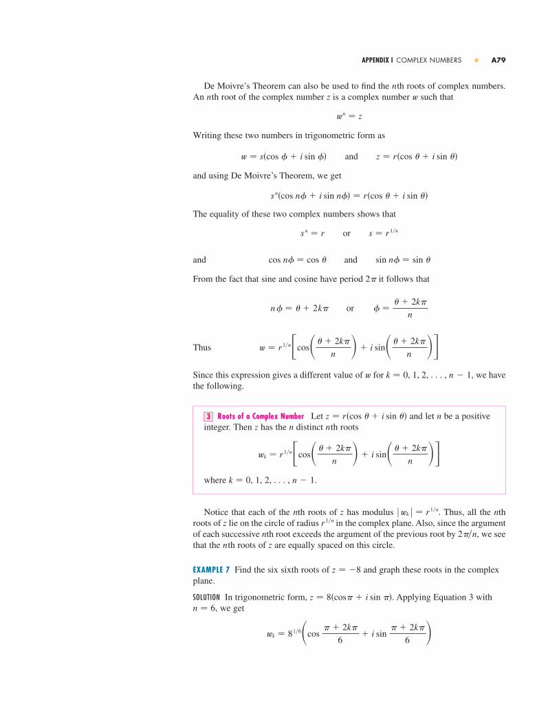
APPENDIX I COMPLEX NUMBERS � A79
De Moivre’s Theorem can also be used to find the th roots of complex numbers.An th root of the complex number is a complex number such that
Writing these two numbers in trigonometric form as
and using De Moivre’s Theorem, we get
The equality of these two complex numbers shows that
and
From the fact that sine and cosine have period it follows that
Thus
Since this expression gives a different value of for , 1, 2, . . . , , we havethe following.
Roots of a Complex Number Let and let be a positiveinteger. Then has the distinct th roots
where , 1, 2, . . . , .
Notice that each of the th roots of has modulus . Thus, all the throots of lie on the circle of radius in the complex plane. Also, since the argumentof each successive th root exceeds the argument of the previous root by , we seethat the th roots of are equally spaced on this circle.
EXAMPLE 7 Find the six sixth roots of and graph these roots in the complexplane.
SOLUTION In trigonometric form, . Applying Equation 3 with, we get
wk � 81�6�cos � � 2k�
6� i sin
� � 2k�
6 �n � 6
z � 8�cos� � i sin ��
z � �8
zn2��nn
r 1�nzn� wk � � r 1�nzn
n � 1k � 0
wk � r 1�n�cos� � � 2k�
n � � i sin� � � 2k�
n ��nnz
nz � r�cos � � i sin ��3
n � 1k � 0w
w � r 1�n�cos� � � 2k�
n � � i sin� � � 2k�
n ��� �
� � 2k�
norn� � � � 2k�
2�
sin n� � sin �andcos n� � cos �
s � r 1�norsn � r
sn�cos n� � i sin n�� � r�cos � � i sin ��
z � r�cos � � i sin ��andw � s�cos � � i sin ��
wn � z
wznn

A80 � APPENDIX I COMPLEX NUMBERS
We get the six sixth roots of by taking in this formula:
All these points lie on the circle of radius as shown in Figure 9.
Complex Exponentials
We also need to give a meaning to the expression when is a complexnumber. The theory of infinite series as developed in Chapter 8 can be extended to the case where the terms are complex numbers. Using the Taylor series for (Equa-tion 8.7.11) as our guide, we define
and it turns out that this complex exponential function has the same properties as thereal exponential function. In particular, it is true that
If we put , where is a real number, in Equation 4, and use the facts that
. . .
we get
Here we have used the Taylor series for and (Equations 8.7.16 and 8.7.15). sin ycos y
� cos y � i sin y
� �1 � y 2
2!�
y 4
4!�
y 6
6!� � � �� � i�y �
y 3
3!�
y 5
5!� � � ��
� 1 � iy � y 2
2!� i
y 3
3!�
y 4
4!� i
y 5
5!� � � �
e iy � 1 � iy ��iy�2
2!�
�iy�3
3!�
�iy�4
4!�
�iy�5
5!� � � �
i 5 � i,i 4 � 1,i 3 � i 2i � �i,i 2 � �1,
yz � iy
e z1�z2 � e z1e z25
e z � ��
n�0 zn
n!� 1 � z �
z2
2!�
z3
3!� � � �4
ex
z � x � iye z
s2
w5 � 81�6�cos 11�
6� i sin
11�
6 � � s2 �s3
2�
1
2 i�
w4 � 81�6�cos 3�
2� i sin
3�
2 � � �s2 i
w3 � 81�6�cos 7�
6� i sin
7�
6 � � s2 ��s3
2�
1
2 i�
w2 � 81�6�cos 5�
6� i sin
5�
6 � � s2 ��s3
2�
1
2 i�
w1 � 81�6�cos �
2� i sin
�
2 � � s2 i
w0 � 81�6�cos �
6� i sin
�
6 � � s2 �s3
2�
1
2 i�
k � 0, 1, 2, 3, 4, 5�8
FIGURE 9The six sixth roots of z=_8
Re
Im
0
w¡
w¢
w∞
w¸w™
w£
_œ„2 2œ„
2i_œ„
œ„2i

APPENDIX I COMPLEX NUMBERS � A81
The result is a famous formula called Euler’s formula:
Combining Euler’s formula with Equation 5, we get
EXAMPLE 8 Evaluate: (a) (b)
SOLUTION(a) From Euler’s formula (6) we have
(b) Using Equation 7 we get
Finally, we note that Euler’s formula provides us with an easier method of provingDe Moivre’s Theorem:
�r�cos � � i sin ���n � �re i� �n � rne in� � rn�cos n� � i sin n��
e�1�i��2 � e�1�cos �
2� i sin
�
2 � �1
e �0 � i�1�� �
i
e
e i� � cos � � i sin � � �1 � i�0� � �1
e�1�i��2e i�
ex�iy � exe iy � ex�cos y � i sin y�7
e iy � cos y � i sin y6
18. Prove the following properties of complex numbers.(a) (b)(c) , where is a positive integer
[Hint: Write , .]
19–24 � Find all solutions of the equation.
19. 20.
21. 22.
23. 24.� � � � � � � � � � � � �
25–28 � Write the number in polar form with argumentbetween and .
25. 26.
27. 28.� � � � � � � � � � � � �
29–32 � Find polar forms for , , and by first putting and into polar form.
29. ,
30. , w � 8iz � 4s3 � 4i
w � 1 � s3 iz � s3 � i
wz1�zz�wzw
8i3 � 4i
1 � s3 i�3 � 3i
2�0
z2 �12 z �
14 � 0z2 � z � 2 � 0
x 2 � 4x � 5 � 0x 2 � 8x � 17 � 0
x 4 � 14x 2 � 9 � 0
w � c � diz � a � binz n � z n
zw � z wz � w � z � w1–14 � Evaluate the expression and write your answer in the form .
1. 2.
3. 4.
5. 6.
7. 8.
9. 10.
11. 12.
13. 14.� � � � � � � � � � � � �
15–17 � Find the complex conjugate and the modulus of the given number.
15. 16.
17.� � � � � � � � � � � � �
�4i
s3 � i3 � 4i
s�3s�12s�25
i 100i 3
3
4 � 3i
1
1 � i
5 � i
3 � 4i
2 � 3i
1 � 5i
2i( 12 � i)12 � 7i
�4 � 7i ��1 � 3i ��3 � i ��4 � i �
�1 � i � � �2 � 3i ��3 � 2i � � �7 � 3i �
a � bi
Exercises � � � � � � � � � � � � � � � � � � � � � � � � � �I
A82 � APPENDIX I COMPLEX NUMBERS
48. Use Euler’s formula to prove the following formulas forand :
49. If is a complex-valued function of areal variable and the real and imaginary parts and
are differentiable functions of , then the derivative of is defined to be . Use this together with Equation 7 to prove that if , then
when is a complex number.
50. (a) If is a complex-valued function of a real variable, itsindefinite integral is an antiderivative of . Evaluate
(b) By considering the real and imaginary parts of the inte-gral in part (a), evaluate the real integrals
and
Compare with the method used in Example 4 in Sec-tion 5.6.
y e x sin x dxy e x cos x dx
y e �1�i �x dx
ux u�x� dxu
r � a � biF��x� � re rxF�x� � e rx
u��x� � f ��x� � it��x�uxt�x�
f �x�xu�x� � f �x� � it�x�
sin x �eix � e�ix
2icos x �
eix � e�ix
2
sin xcos x31. ,
32. ,� � � � � � � � � � � � �
33–36 � Find the indicated power using De Moivre’s Theorem.
33. 34.
35. 36.� � � � � � � � � � � � �
37–40 � Find the indicated roots. Sketch the roots in the com-plex plane.
37. The eighth roots of 1 38. The fifth roots of 32
39. The cube roots of 40. The cube roots of � � � � � � � � � � � � �
41–46 � Write the number in the form .
41. 42.
43. 44.
45. 46.� � � � � � � � � � � � �
47. Use De Moivre’s Theorem with to express andin terms of and .sin �cos �sin 3�
cos 3�n � 3
e 1�2ie 2�i�
e �i�e i3��4
e 2� ie i��2
a � bi
1 � ii
�1 � i �8(2s3 � 2i )5
(1 � s3 i )5�1 � i �20
w � �3 � 3iz � 4(s3 � i )w � �1 � iz � 2s3 � 2i

Answers to Odd-Numbered Exercises � � � � � � � � � �J
APPENDIX J ANSWERS TO ODD-NUMBERED EXERCISES � A83
33.
35.
37.39.
41.
43.45. 47.49.51. (a)
(b) $400, $1900(c)
53. (a) (b)55. Even 57. Neither 59. Odd
Exercises 1.2 � page 351. (a) Root (b) Algebraic (c) Polynomial (degree 9)(d) Rational (e) Trigonometric (f ) Logarithmic3. (a) h (b) f (c) t
y
0 x1
�1
0 1 x
y
��5, �3���5, 3�
T (in dollars)
0 I (in dollars)10,000 20,000
1000
2500
30,000
R(%)
0 I (in dollars)10,000 20,000
10
15
V�x� � 4x 3 � 64x 2 � 240x, 0 � x � 6S�x� � x 2 � �8�x�, x � 0A�x� � s3x 2�4, x � 0
A�L� � 10L � L2, 0 � L � 10
f �x� � x � 1
6 � 1.5x
if �1 � x � 2
if 2 � x � 4
f �x� � 1 � s�x
f �x� � �76 x �
43 , �2 � x � 4
x
y
1
�1 0
���, ��
0 x
1
y���, ��CHAPTER 1
Exercises 1.1 � page 221. (a) �2 (b) 2.8 (c) �3, 1 (d) �2.5, 0.3(e) (f )3.5. Yes, 7. No9. Diet, exercise, or illness11.
13.
15.
17. (a)
(b) 540, 145019. 12, 16, , , ,
, , ,,
21. , ,23.25. 27.29. 31.
x
2
y
0
4
t�1
y
0
2
���, 0� � �0, �����, �����, 0� � �5, ���0, ��
{x � x � 13} � (��, 13) � ( 1
3 , �)1 � 2x � hx � h � x 2 � 2xh � h2��h2 � 3h � 2�
3a2 � 6ah � 3h2 � a � h � 29a4 � 6a3 � 13a2 � 4a � 43a4 � a2 � 212a2 � 2a � 26a2 � 2a � 4
3a2 � 5a � 43a2 � a � 23a2 � a � 2
N
0 t1991 1993 1995
2500
500
1000
2000
1997
1500
Heightof grass
tWed. Wed. Wed. Wed. Wed.
T
tmidnight noon
T
0 t
��3, 2�, ��2, 2���85, 115�, ��325, 485�, ��210, 200�
��1, 3���3, 3�, ��2, 3�
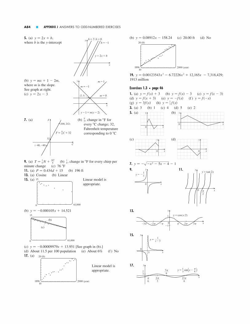
(b) (c) 20.00 ft (d) No
19. ;1913 million
Exercises 1.3 � page 461. (a) (b) (c)(d) (e) (f )(g) (h)3. (a) 3 (b) 1 (c) 4 (d) 5 (e) 25. (a) (b)
(c) (d)
7.
9. 11.
13.
15.
17.
x
y
13
2π3
7π6
13π6
π6
13
y= sin ”x- ’π6
3 x0
y
y=1
x-3
_π x
1
�1
y
y=Ł(x/2)
0 π 2π_3π 3π_2π
x
y
0 π2
y=g 2xy
x0
y � �1x
y � �s�x 2 � 5x � 4 � 1
y
0 x
y
0 x
y
0 x
y
0 x
y � 13 f �x�y � 3f �x�
y � f ��x�y � �f �x�y � f �x � 3�y � f �x � 3�y � f �x� � 3y � f �x� � 3
y � 0.00123543x 3 � 6.72226x 2 � 12,165x � 7,318,429
20 (ft)
102000 (year)1896
y � 0.08912x � 158.245. (a) ,where b is the y-intercept
(b) ,where m is the slope.See graph at right.(c)
7. (a) (b) , change in forevery change; 32,Fahrenheit temperaturecorresponding to
9. (a) (b) , change in for every chirp perminute change (c)11. (a) (b) 196 ft13. (a) Cosine (b) Linear15. (a) Linear model is
appropriate.
(b)
(c) [See graph in (b).](d) About 11.5 per 100 population (e) About 6% (f ) No17. (a)
Linear model isappropriate.
20 (ft)
102000 (year)1896
y � �0.00009979x � 13.951
15
0 61,000
(b)
(c)
y � �0.000105x � 14.521
15
0 61,000
P � 0.434d � 1576 F
F16T � 1
6 N �3076
0 C
CF9
5F
C
(100, 212)
F= C+3295
(_40, _40)
32
y � 2x � 3
y
x
m=_1
m=1
m=0
y-1=m(x-2)
(2, 1)
y � mx � 1 � 2m
y
x
b=3 b=0b=_1
y=2x+b
y � 2x � b
A84 � APPENDIX J ANSWERS TO ODD-NUMBERED EXERCISES
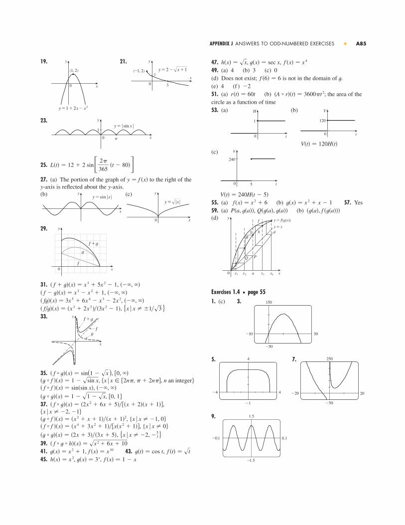
47. , ,49. (a) 4 (b) 3 (c) 0(d) Does not exist; is not in the domain of .(e) 4 (f )51. (a) (b) ; the area of thecircle as a function of time53. (a) (b)
(c)
55. (a) (b) 57. Yes59. (a) , (b)(d)
Exercises 1.4 � page 551. (c) 3.
5. 7.
9. 1.5
_1.5
_0.1 0.1
250
�50
�20 20
4
�1
�4 4
150
_50
30_10
x
y
a¤0 ‹ x¢
f
ghy=x
⁄
y=Ï
PQ
RS
�t�a�, f �t�a���Q�t�a�, t�a��P�a, t�a��t�x� � x 2 � x � 1f (x� � x 2 � 6
V�t� � 240H�t � 5�
V
t
240
0 5
V�t� � 120H�t�
V
t
120
0
H
t
1
0
�A � r��t� � 3600�t 2r�t� � 60t�2
tf �6� � 6
f �x� � x 4t�x� � sec xh�x� � sx19. 21.
23.
25.
27. (a) The portion of the graph of to the right of the -axis is reflected about the -axis.
(b) (c)
29.
31. ,,
,,
33.
35. ,,
,
,37. ,
,,
,
39.41. 43. ,45. , , f �x� � 1 � xt�x� � 3xh�x� � x 2
f �t� � stt�t� � cos tt�x� � x 2 � 1, f �x� � x 10
� f � t � h��x� � sx 2 � 6x � 10
{x � x � �2, �53}�t � t��x� � �2x � 3���3x � 5�
{x � x � 0�� f � f ��x� � �x 4 � 3x 2 � 1���x�x 2 � 1��{x � x � �1, 0��t � f ��x� � �x 2 � x � 1���x � 1�2
�x � x � �2, �1��2x 2 � 6x � 5����x � 2��x � 1��� f � t��x� �
�0, 1��t � t��x� � 1 � s1 � sx
���, ��� f � f ��x� � sin�sin x��x � x � �2n�, � � 2n��, n an integer��t � f ��x� � 1 � ssin x
�0, ��� f � t��x� � sin(1 � sx )
x
yf+g
fg
{x � x � 1�s3}� f�t��x� � �x 3 � 2x 2 ���3x 2 � 1����, ��� ft��x� � 3x 5 � 6x 4 � x 3 � 2x 2
���, ��� f � t��x� � x 3 � x 2 � 1���, ��� f � t��x� � x 3 � 5x 2 � 1
x
y
0
f
g
f+g
y
x0
y=œ„„|x|
x
yy=j |x|
yyy � f �x�
L�t� � 12 � 2 sin� 2�
365 �t � 80��
y
x0
y=| sin x |
π
1
3
x1
y
0
(_1, 2) y=2-œ„x+1
0 x
y
y=1+2x-≈
(1, 2)
APPENDIX J ANSWERS TO ODD-NUMBERED EXERCISES � A85

3. All approach 0 as, all pass through
, and all are increas-ing. The larger the base,the faster the rate ofincrease.
5. The functions with basegreater than 1 are increas-ing and those with baseless than 1 are decreasing.The latter are reflections of the former about the y-axis.
7. 9.
11.
13. (a) (b) (c)(d) (e)15. 21. At 23. (a) 3200 (b) (c) 10,159(d)
25. , where and; 5494 million; 7409 million
Exercises 1.6 � page 731. (a) See Definition 1.(b) It must pass the Horizontal Line Test.3. No 5. Yes 7. No 9. Yes 11. No13. No 15. No 17. 2 19. 021. ; the Fahrenheit temperature as a function ofthe Celsius temperature; 23. 25.27. y � e x � 3
f �1�x� � s3 ln xf �1�x� � �
13 x
2 �103 , x � 0
��273.15, ��F � 9
5 C � 32
b 1.01774077a 3.303902537 � 10�12y � ab t
t 26.9 h
60,000
0 40
100 � 2 t�3x 35.8f �x� � 3 � 2x
y � �e�xy � e�xy � �e xy � e x�2y � e x � 2
x
2
yy � 3
0
x_1
y
0
y=_2–®
x
_2
y
0
y=4®-3
y=_3
5
_2 2
y=3®y=10®
0
y=” ’®13
y=” ’®110
�0, 1�x l ��
y=20® y=5® y=´
y=2®
5
_1 20
11.
13. 15.
17. 9.05 19. 0, 0.88 21. 23.25. (a) (b)
(c)
(d) Graphs of even roots are similar to , graphs of odd rootsare similar to . As n increases, the graph of becomessteeper near 0 and flatter for .27.
If , the graph has three humps: two minimum points and amaximum point. These humps get flatter as c increases until at
two of the humps disappear and there is only one mini-mum point. This single hump then moves to the right andapproaches the origin as c increases.29. The hump gets larger and moves to the right.31. If , the loop is to the right of the origin; if , theloop is to the left. The closer c is to 0, the larger the loop.
Exercises 1.5 � page 631. (a) (b) (c)(d) See Figures 4(c), 4(b), and 4(a), respectively.
�0, ���f �x� � a x, a � 0
c � 0c � 0
c � 0
c � 0
6
_6
_2.5 2.5
2 0_2 _44
x � 1y � s
n xs3 x
sx
2
_1
_1 3
$œ„xœ„x Œ„x
%œ„x
2
_2
_3 3x %œ„x
Œ„x
3
_1
_1 4œ̂„x
$œ„xœ„x
�0.85 � x � 0.85t
4
0_5 5
1
_1
_1 1
1.5
_1.5
_250 250
A86 � APPENDIX J ANSWERS TO ODD-NUMBERED EXERCISES

Exercises 1.7 � page 811. 3.
5. (a) 7. (a)
(b) (b)9. (a) 11. (a)(b) (b)
13. (a) (b)
15. Moves counterclockwise along the circle fromto
17. Moves once clockwise around the ellipse, starting and ending at (0, 3)
19. It is contained in the rectangle described by and .21. 23. (b)
,
25. 3
�3
�3 3
0 � t � 1y � 7 � 8tx � �2 � 5t,
x
y
t=0
t= 12
1
1
2 � y � 31 � x � 4
�x 2�4� � �y 2�9� � 1
�1, 0���1, 0�x 2 � y 2 � 1
x
y
0 (1, 0)
(0, 1)
x � y � 1, 0 � x � 1
x
y
0
x
(0, 1)y
(0, _1)
0
y � 1�x, x � 0x 2 � y 2 � 1, x � 0y � 1 � x 2, x � 0y � 1
2 x � 3
0 x
(0, 1)
yy
x
_3
6
x
y
t=0 (0, 0)
t=π {0, π@}
5
5
x
y
t=0(1, 0)
t=5{1+œ„5, 5}
29. 31.
33. (a) It’s defined as the inverse of the exponential functionwith base a, that is, .(b) (c) (d) See Figure 11.35. (a) 6 (b)37. (a) 2 (b) 2 39.41. (a) 2.321928 (b) 2.02556343.
All graphs approach as , all pass through , andall are increasing. The larger the base, the slower the rate ofincrease.45. About 1,084,588 mi47. (a) (b)
49. (a) (b)51. (a) (b)53. (a) (b)55.
passes the Horizontal Line Test
,where ; two of the expressionsare complex.57. (a) ; the time elapsed whenthere are n bacteria (b) After about 26.9 h59. (a) (b) (c)(d) (e) (f ) (g)(h) y � e x � 3
y � �e xy � e�xy � e xy � ln��x�y � �ln xy � ln�x � 3�y � ln x � 3
f �1�n� � �3�ln 2� ln�n�100�
D � 3s3s27x 4 � 40x 2 � 16�(s3 4�6)(s3 D � 27x 2 � 20 � s
3 D � 27x 2 � 20 � s3 2 )
f �1�x� �
5
_1
4_2
x � 1�ex � ln 10
12 (1 � s1 � 4e )5 � log2 3 or 5 � �ln 3��ln 2
�ln 5se
1 x
y
0_5 _4 x
y
0
�1, 0�x l 0���
3
�5
4
y=log1.5 x
0
y=ln xy=log10 x
y=log50 x
ln 8�2��0, ��
loga x � y &? a y � x
y
x1
1f
f –!
4
_2
_2 4
f
f – !
f �1�x� � s2��1 � x�
APPENDIX J ANSWERS TO ODD-NUMBERED EXERCISES � A87

(e) Reflect the graph about the x-axis.(f ) Reflect the graph about the line (assuming f is one-to-one).11. 13.
15. 17. (a) Neither(b) Odd(c) Even(d) Neither
19. ,,
,,
21. ; about 77.6 years23. 1 25. (a) 9 (b) 227. (a) (b)(c) ; the time elapsed when there are m grams of (d) About 26.6 days29.
For , is defined everywhere. As c increases, the dip atbecomes deeper. For , the graph has asymptotes
at .31. (a) (b)
33. 7
_1
_1 7
f
f – !
y � slnxy
x1
(e, 1)
x � scc � 0x � 0
fc � 0
_13
_3
_5 5
4210
_4_2
100 Pdt�m� � �4 log2 m
m�t� � 2�t�4116 g
y � 0.2493x � 423.4818���, ���t � t��x� � �x 2 � 9�2 � 9
�1, ��� f � f ��x� � ln ln x�0, ���t � f ��x� � �ln x�2 � 9
���, �3� � �3, ��� f � t��x� � ln�x 2 � 9�
y
x0
y=1
x+212
x=_2
x
y
0
y=(1+´)/21 y=
12
y
x0
y=_sin 2x
π
y � x27. (a)(b)(c)29. (a)(b) (c) As b increases, the ellipse
stretches vertically.
33. , ellipse35.
37. For , there is a cusp; for , there is a loop whosesize increases as c increases.
39. As n increases, the number of oscillations increases; a and bdetermine the width and height.
Chapter 1 Review � page 85
True-False Quiz1. False 3. False 5. True 7. False 9. True11. False
Exercises
1. (a) 2.7 (b) 2.3, 5.6 (c) (d)(e) (f ) No; fails the Horizontal Line Test.(g) Odd; its graph is symmetric about the origin.3. (a) (b) 150 ft
5. 7.9. (a) Shift the graph 8 units upward.(b) Shift the graph 8 units to the left.(c) Stretch the graph vertically by a factor of 2, then shift it 1 unit upward.(d) Shift the graph 2 units to the right and 2 units downward.
�, �0, 2�[�2s3�3, 2s3�3], �0, 2�
d
0 t
50
2 4
100
150
3 51
f��4, 4���4, 4���6, 6�
3
0 1.5
_3
_1
00 1.5
1
_1
112
c � 0c � 0
y
O x
2a
x � a cos �, y � b sin �; �x 2�a 2 � � �y 2�b 2 � � 1
8
_8
_8 8b=1
b=2b=4
b=8
x � a sin t, y � b cos t, 0 � t � 2�x � 2 cos t, y � 1 � 2 sin t, ��2 � t � 3��2x � 2 cos t, y � 1 � 2 sin t, 0 � t � 6�
x � 2 cos t, y � 1 � 2 sin t, 0 � t � 2�
A88 � APPENDIX J ANSWERS TO ODD-NUMBERED EXERCISES

11. 0.806452, 0.641026, 0.510204, 0.409836, 0.369004,0.336689, 0.165563, 0.193798, 0.229358, 0.274725, 0.302115,0.330022; 13. 0.718282, 0.367879, 0.594885, 0.426123, 0.517092,0.483742, 0.508439, 0.491770, 0.501671, 0.498337; 15. (a) 417. (a) 2.71828(b)
19. (a) 0.998000, 0.638259, 0.358484, 0.158680, 0.038851,0.008928, 0.001465; 0(b) 0.000572, �0.000614, �0.000907, �0.000978,�0.000993, �0.001000; �0.00121. Within 0.182; within 0.095
Exercises 2.3 � page 1171. (a) 5 (b) 9 (c) 2 (d) (e) (f ) 0(g) Does not exist (h)
3. 75 5. �3 7. 9. 5 11. Does not exist
13. 15. 12 17. 19.21. (a), (b) 25. 1 29. 0
31. Does not exist33. (a) (i) 0 (ii) 0 (iii) 1 (iv) 1 (v) 0(vi) Does not exist(b)
35. (a) (i) (ii) Does not exist (iii)(b) (i) (ii) (c) is not an integer.43. 15;
Exercises 2.4 � page 128
1.3. (a) (removable), ( jump), 2 ( jump), 4 (infinite)(b) , neither; , left; 2, right; 4, right
5. 7. (a)
(b) Discontinuous at , 2, 3, 4t � 1
y
0 x2
1
Cost(in dollars)
0 Time(in hours)
1
1
�2�4�2�4
lim x l 4 f �x� � f �4�
�1ann � 1
�3�2
1 x
y
1
_1 0
23
�1
1616
65
18
�6
11
�38�
13
6
4_4
_2
12
13
Principles of Problem Solving � page 93
1. , where a is the length of the altitude and h is the length of the hypotenuse3.5. 7.
9. 11. 513.15.19.
CHAPTER 2
Exercises 2.1 � page 991. (a) �44.4, �38.8, �27.8, �22.2,(b) �33.3 (c)3. (a) (i) 0.333333 (ii) 0.263158 (iii) 0.251256(iv) 0.250125 (v) 0.2 (vi) 0.238095 (vii) 0.248756(viii) 0.249875 (b) (c)5. (a) (i) (ii) (iii)(iv) (b)7. (a) (i) (ii) (iii) (iv)(b)(c) (d)
9. (a) 0, 1.7321, �1.0847, �2.7433, 4.3301, �2.8173, 0,�2.1651, �2.6061, �5, 3.4202; no (c) �31.4
Exercises 2.2 � page 1081. Yes 3. (a) 2 (b) 3 (c) Does not exist(d) 4 (e) Does not exist5. (a) (b) (c) Does not exist (d) 2 (e) 0(f ) Does not exist (g) 1 (h) 37. (a) 1 (b) 0 (c) Does not exist9. y
0 x1
�2�1
21 t
1
s
2
tangent
s=t#6
1.5
2 31 t
1
s
2
3
4(i) (ii)
(iii)
(iv)
s=t#6
1.5
12 ft�s
331600 ft�s19
24 ft�s76 ft�s13
6 ft�s�24 ft�s�24.16 ft�s
�24.8 ft�s�25.6 ft�s�32 ft�sy � 1
4 x �14
14
�33 13
�16.6
fn�x� � x 2 n�140 mi�hx � [�1, 1 � s3) � (1 � s3, 3]
y
x10
1
x
y
1
1 x
y
�73 , 9
a � 4sh 2 � 16�h
APPENDIX J ANSWERS TO ODD-NUMBERED EXERCISES � A89
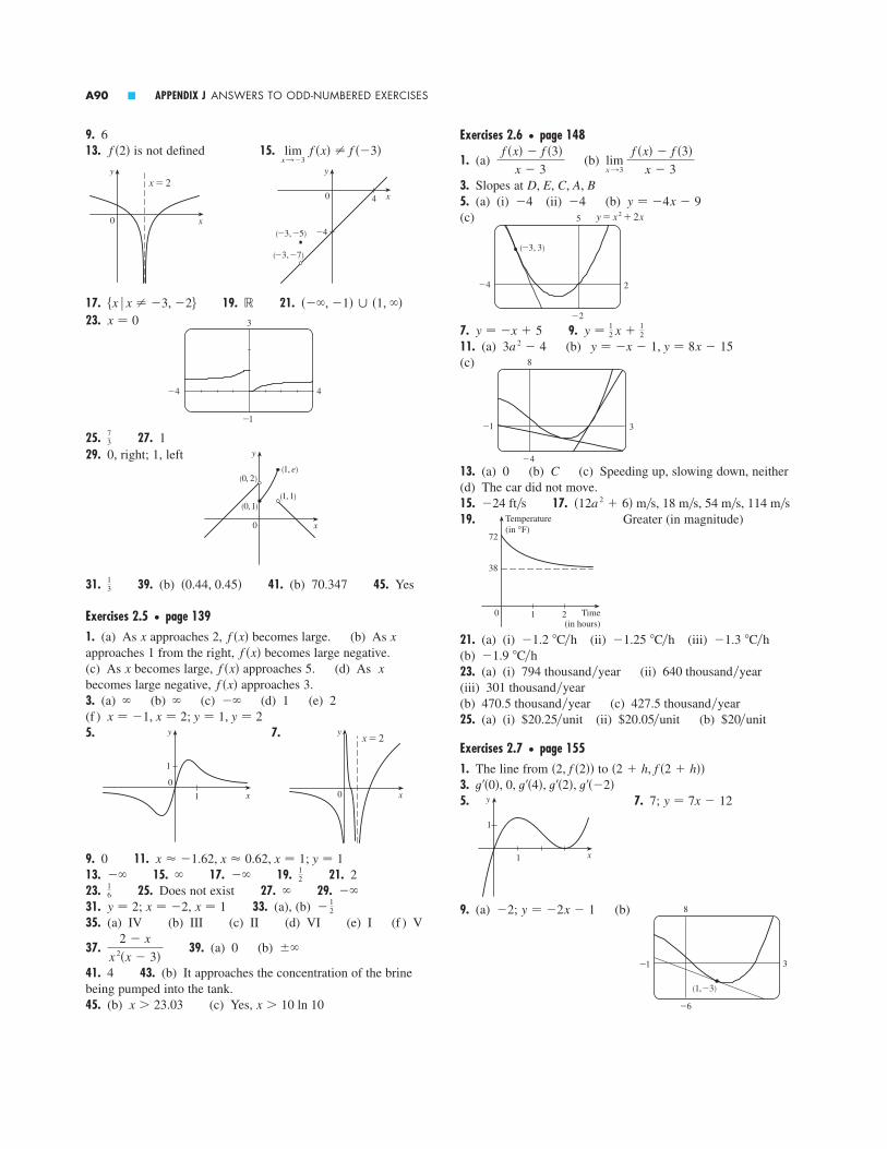
Exercises 2.6 � page 148
1. (a) (b)
3. Slopes at 5. (a) (i) �4 (ii) �4 (b)(c)
7. 9.11. (a) (b)(c)
13. (a) 0 (b) C (c) Speeding up, slowing down, neither(d) The car did not move.15. 17.19. Greater (in magnitude)
21. (a) (i) (ii) (iii)(b)23. (a) (i) (ii)(iii)(b) (c)25. (a) (i) (ii) (b)
Exercises 2.7 � page 1551. The line from to 3.5. 7. 7;
9. (a) �2; (b)
(1, _3)
8
3_1
_6
y � �2x � 1
y � 7x � 12
1 x
y
1
t��0�, 0, t��4�, t��2�, t���2��2 � h, f �2 � h���2, f �2��
$20�unit$20.05�unit$20.25�unit427.5 thousand�year470.5 thousand�year
301 thousand�year640 thousand�year794 thousand�year
�1.9 C�h�1.3 C�h�1.25 C�h�1.2 C�h
Temperature(in °F)
0 Time(in hours)
1
38
2
72
�12a 2 � 6� m�s, 18 m�s, 54 m�s, 114 m�s�24 ft�s
8
3_1
_4
y � �x � 1, y � 8x � 153a 2 � 4y � 1
2 x �12y � �x � 5
5
2_4
_2
(_3, 3)
y=≈+2x
y � �4x � 9D, E, C, A, B
lim x l3
f �x� � f �3�
x � 3
f �x� � f �3�x � 3
9. 613. is not defined 15.
17. 19. 21.23.
25. 27. 129. 0, right; 1, left
31. 39. (b) 41. (b) 70.347 45. Yes
Exercises 2.5 � page 1391. (a) As approaches 2, becomes large. (b) As approaches 1 from the right, becomes large negative.(c) As becomes large, approaches 5. (d) As becomes large negative, approaches 3.3. (a) (b) (c) (d) 1 (e) 2(f )5. 7.
9. 0 11.13. 15. 17. 19. 21. 223. 25. Does not exist 27. 29.31. ; , 33. (a), (b)35. (a) IV (b) III (c) II (d) VI (e) I (f ) V
37. 39. (a) 0 (b)
41. 4 43. (b) It approaches the concentration of the brinebeing pumped into the tank.45. (b) (c) Yes, x � 10 ln 10x � 23.03
�2 � x
x 2�x � 3�
�12x � 1x � �2y � 2
���16
12�����
x �1.62, x 0.62, x � 1; y � 1
x
y
0
x=2
x
y
0
1
1
x � �1, x � 2; y � 1, y � 2����
f �x�xf �x�x
f �x�xf �x�x
�0.44, 0.45�13
y
x0
(1, e)
(1, 1)(0, 1)
(0, 2)
73
3
4_4
_1
x � 0���, �1� � �1, ����x � x � �3, �2�
y
x0 4
_4(_3, _5)
(_3, _7)
x
y
0
x=2
limx l
�3 f �x� � f ��3�f �2�
A90 � APPENDIX J ANSWERS TO ODD-NUMBERED EXERCISES

15.
17. (a) 0, 1, 2, 4 (b) �1, �2, �4 (c)19.21.23.25. , ,
27. (a)29. (a) The rate at which the unemployment rate is changing,in percent unemployed per year(b)
31. 4 (discontinuity); 8 (corner); �1, 11 (vertical tangents)33.
Differentiable at �1; not differentiable at 0
35.37.39.
,
41. 43. (a)
, ,, f �4��x� � 0f ��x� � �6
f ��x� � 4 � 6xf ��x� � 4x � 3x 2
13 a�2�3
3
6�4
�7
f
fª
f·
fªªª
f ��x� � �2f ��x� � 4 � 2x
6
10�6
�10
ffª
f ·
a � acceleration, b � velocity, c � positiona � f, b � f �, c � f �
2
_1
_2 1
f ��x� � 1 � 2�x 2���, �1� � ��1, ��
���, �1� � ��1, ��G��t� � 4��t � 1�2
t��x� � 1�s1 � 2x, [� 12 , �), (� 1
2 , �)f ��x� � 3x 2 � 3, �, �f ��x� � �7, �, �
f ��x� � 2x
f ��x� � e xy
x1
1
0
f, f ª
11. (a) 3.296 (b) 3.313. 15.17. 19.21.23. 25.27. (a) The rate at which the cost is changing per ounce of goldproduced; dollars per ounce(b) When the 800th ounce of gold is produced, the cost of production is (c) Decrease in the short term; increase in the long term29. (a) The rate at which the fuel consumption is changingwith respect to speed; (b) The fuel consumption is decreasing by as the car’s speed reaches .31. The rate at which the temperature is changing with respectto time when ; 33. The rate at which the cash per capita in circulation ischanging in dollars per year; $39.90�year35. Does not exist
Exercises 2.8 � page 1671. (a) 1.5 (b) 1 (c) 0 (d) �4 (e) 0 (f ) 1 (g) 1.5
3. (a) II (b) IV (c) I (d) III5. 7.
9. 11.
13. 1963 to 1971
0.05
19901980197019601950
_0.03t
y=Mª(t)0.1
y
x0
y
f ª
x0
y
ƒ�
x
y
0
fªfª
x
y
0
x0
y
fª
1C�ht � 6
20 mi�h0.05 �gal�h���mi�h�
�gal�h���mi�h�
$17�oz.
�2 m�sf �x� � cos x, a � �f �x� � 2x, a � 5
f �x� � x 10, a � 1�1��2�a � 2�3�2�5��a � 3�2�2 � 8a
APPENDIX J ANSWERS TO ODD-NUMBERED EXERCISES � A91
t t
1989 0.30 19941990 0.75 19951991 0.95 19961992 0.05 19971993 1998 �0.40�0.70
�0.45�0.35�0.35�0.65
U��t�U��t�
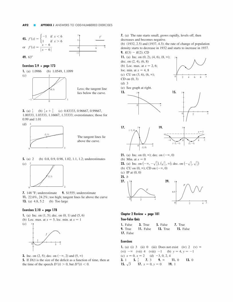
7. (a) The rate starts small, grows rapidly, levels off, thendecreases and becomes negative.(b) ; the rate of change of populationdensity starts to decrease in 1932 and starts to increase in 1937.9. ; CD11. (a) Inc. on (0, 2), (4, 6), ;dec. on (2, 4), (6, 8)(b) Loc. max. at ;loc. min. at (c) CU on (3, 6), ; CD on (0, 3)(d) 3(e) See graph at right.13. 15.
17. 19.
21. (a) Inc. on ; dec. on (b) Min. at 23. (a) Inc. on , ; dec. on (b) CU on ; CD on (c) IP at 25. b27. 29.
Chapter 2 Review � page 181True-False Quiz1. False 3. True 5. False 7. True9. True 11. False 13. True 15. False17. False
Exercises
1. (a) (i) 3 (ii) 0 (iii) Does not exist (iv) 2 (v)(vi) (vii) 4 (viii) �1 (b) ,(c) , (d) �3, 0, 2, 43. 1 5. 7. 3 9. 11. 0 13. 015. 17. 19. 1x � 0, y � 0s3
�32
x � 2x � 0y � �1y � 4��
�
0 2 x
0.5
4
F
y
x
y
0 2
F
�0, 0����, 0��0, ��
(�s13 , s
13)(s1
3 , �)(��, �s13)
x � 0���, 0��0, ��
x
y
0
y � 1
4_4
(_2, _1) (2, _1)x0
y
(1, 0)
(_1, 4)
y
0 x2
y
0 x
�6, ��x � 4, 8
x � 2, 6
x
y
0 2 4 6 8
�8, ��K�3� � K�2�
�1932, 2.5� and �1937, 4.3�45.
or
49.
Exercises 2.9 � page 1731. (a) 1.0986 (b) 1.0549, 1.1099(c)
Less; the tangent linelies below the curve.
3. (a) (b) (c) 0.83333, 0.96667, 0.99667,1.00333, 1.03333, 1.16667, 1.33333; overestimates; those for0.99 and 1.01
(d)
The tangent lines lieabove the curve.
5. (a) 2 (b) 0.8, 0.9, 0.98, 1.02, 1.1, 1.2; underestimates
(c)
7. ; underestimate 9. $1555; underestimate11. 22.6%, 24.2%; too high; tangent lines lie above the curve13. (a) 4.8, 5.2 (b) Too large
Exercises 2.10 � page 1781. (a) Inc. on ; dec. on (b) Loc. max. at , loc. min. at (c)
3. Inc. on ; dec. on 5. If is the size of the deficit as a function of time, then atthe time of the speech , but .D ��t� � 0D��t� � 0
D�t����, 2� and �5, ���2, 5�
y
0 x
1
5
f
x � 1x � 5�0, 1� and �5, 6��1, 5�
148 F
2
20
(1, 1)
2
20
(1, 1)
13 x �
23
13
2
1�10
(0, 1)
63
f ��x� �x � 6
� x � 6 �x
y
0 6
1
_1
f ªf ��x� � �1
1
if x � 6
if x � 6
A92 � APPENDIX J ANSWERS TO ODD-NUMBERED EXERCISES

43.
45. (a) About 35 ft�s (b) About (c) The point at which the car’s velocity is maximized
Focus on Problem Solving � page 1861. 3. �4 5. 1 7.9. (b) Yes (c) Yes; no 11.13. (a) 0 (b) 1 (c) 15.
CHAPTER 3
Exercises 3.1 � page 1961. (a) See Definition of the Number e (page 195).(b) 0.99, 1.03; 3. 5.7.9.11.13. 15.17.19.21.23. 25. 27.29. (a) 0.264 (b)31. 33.
35. (a) (c)
37.39.41. (a) (b)(c)43. 45. �1, 0�, (� 1
3 , 3227 )(ln 3
2 , �)a�1� � 6 m�s2
12 m�s2v�t� � 3t 2 � 3, a�t� � 6tf ��x� � 2 �
154 x�1�4, f ��x� � 15
16 x�5�4
f ��x� � 4x 3 � 9x 2 � 16, f ��x� � 12x 2 � 18x
100
�40
�3 5
50
�10
�3 5
4x 3 � 9x 2 � 12x � 7
(1, 2)
3
3
_2
_2
(2, 4)
10
10
_10
_10
y � 32 x �
12y � 4
22�5�5 0.2639021 � x�2�345x 14 � 15x 24x � 4x 3
z� � �10A�y11 � Be yv� � 2t � 3�(4ts
4 t 3)y� � 3
2 sx � (2�sx ) � 3�(2xsx )y� � 0F��x� � 12,288x 2
V��r� � 4�r 2G��x� � 1�(2sx ) � 2e xy� � �
25 x
�7�5f ��x� � 36x 3 � 6xf ��x� � 5
2.7 � e � 2.8
34f ��x� � x 2 � 1
(s3�2, 14 )a � 1
2 12 s52
3
�8, 180�
y
0x1
�2
9 12
x � 621. (a) (i) 3 (ii) 0 (iii) Does not exist (iv) 0 (v) 0(vi) 0 (b) At 0 and 3 (c)
25. (a) (i) (ii) (iii)(iv) (b)27.29. (a) (b)(c)
31. (a) The rate at which the cost changes with respect to theinterest rate; dollars�(percent per year)(b) As the interest rate increases past 10%, the cost is increas-ing at a rate of $1200�(percent per year).(c) Always positive33.
35. (a)
(b)(c)
37. �4 (discontinuity), �1 (corner), 2 (discontinuity),5 (vertical tangent)39. (a) 1 (b) (c) 0.8, 0.9, 0.99, 1.01, 1.1, 1.2(d) Underestimates; those for 41. (a) Inc. on ; dec. on (b) Max. at 0; min. at (c) CU on ; CD on (d)
x
y
0
1
��1, 1����, �1� and �1, ���2 and 2
���, �2� and �0, 2���2, 0� and �2, ��e�0.01 and e0.01
x � 1
6
1_3
_6
f
f ª
(��, 35 ], (��, 35 )f ��x� � �
52 �3 � 5x��1�2
x
y
0
fª
1.5
1.50
1
1
y �0.736x � 1.104�0.736f ��5�, 0, f ��5�, f ��2�, 1, f ��3�
2.5 m�s2.525 m�s2.625 m�s2.75 m�s3 m�s
x0
y
3
3
APPENDIX J ANSWERS TO ODD-NUMBERED EXERCISES � A93

(i) Speeding up when ; slowing down when
3. (a)(b) ; the velocity has an absolute minimum.5. (a) ; the rate at which the area is increasing withrespect to side length as x reaches 15 mm(b)7. (a) (i) (ii) (iii)(b) (c)9. (a) (b) (c)The rate increases as the radius increases.11. (a) (b) (c)At the right end; at the left end13. (a) 4.75 A (b) 5 A; 15. (a) (b) At the beginning17. (a) ; (b) , where ,
, , and (c)(d) (smaller); (smaller)(e)19. (a) (c) It approaches .(d) It approaches 0. (e) The reaction virtually stops.21. (a) ; ; 0(b) 0; ; (c) At the center; at the edge23. (a)(b) , the rate at which the cost is changing as the 100th pair of jeans is being produced; the cost of the 101st pair(c) $11.0725. (a) ; the average productivity increasesas new workers are added.27.29. (a) 0 and 0 (b)(c) ; it is possible for the species to coexist.
Exercises 3.4 � page 223
1. 3.5.7.9.11. 17.19. (a) (b)
21. (a)23. ; 25. , n an integer 27. ���3, 5��3��2n � 1�� ��3
2 cos � � � sin �� cos � � sin �2 � csc2x
(π, _π)
1
_5
_1 5
y � �xy � 2x � 1 � ��2sec � �sec2� � tan2��
�sin x � cos x � x sin x � x cos x���1 � sin 2x��x sec2x � tan x��x 2
�csc � cot � � e � �cot � � csc2��3t 2 cos t � t 3 sin t1 � 3 cos x
�0, 0�, �500, 50�C � 0
�0.2436 K�min
�xp��x� � p�x���x 2
$11�pairC��x� � 3 � 0.02x � 0.0006x 2
�185.2 �cm�s��cm�92.6 �cm�s��cm0.694 cm�s0.926 cm�s
a moles�La 2k��akt � 1�2
81.3 million�year75.1 million�year14.5 million�year
P��t� � 3at 2 � 2bt � cd � �7,318,429c � 12,165b � �6.72226
a � 0.00123543P�t� � at3 � bt 2 � ct � d78.5 million�year16 million�year
dV�dP � �C�P 2
t � 23 s
18 kg�m12 kg�m6 kg�m
24� ft2�ft16� ft2�ft8� ft2�ft�A 2�r �r4�
4.1�4.5�5��A 2x �x
30 mm2�mmt � 1.5 s
t � 4 s0 � t � 2 or 4 � t � 6
2 � t � 4 or t � 649. 51.
55.57. (a) ; infinitely many
(b)
(c)59. 61. 63. 1000
Exercises 3.2 � page 204
1. 3.5. 7.9.11. 13.15. 17.19.21. (a) (b)
23. (a) 25.27. (a) �16 (b) (c) 20 29. 731. (a) 0 (b) 33. $7.322 billion per year35. 37. Two,39. (c)41.
Exercises 3.3 � page 2151. (a) (b) (c)(d) (e)(f) (g)
(h)
s
40
80
�25
√
a
6t � 24; �6 m�s2
t � 2,s � 32t � 0,
s � 0
t � 6,s � 0
t � 8,s � 32
s0
96 m0 � t � 2, t � 6t � 2, 6�9 m�s3t 2 � 24t � 36
f (n)�x� � �x 2 � 2nx � n�n � 1��e x�x 2 � 8x � 12�e x, �x 2 � 10x � 20�e x;
�x 2 � 2x�e x, �x 2 � 4x � 2�e x, �x 2 � 6x � 6�e x,3e 3x
(�2 s3, (1 � s3)�2)��3, ���
23
�209
xe x, �x � 1�e xe x �x � 3��x 4
(_1, 0.5)
1.5
�0.5
�4 4
y � 12 x � 1
y � 2xf ��x� � 2cx��x 2 � c�2y� � 2v � 1�sv
y� � �r 2 � 2�e ry� � 2t�1 � t���3t 2 � 2t � 1�2H��x� � 1 � x�2 � 2x�3 � 6x�4
h��x� � �3��x � 1�2y� � �x � 2�e x�x 3
f ��x� � x �x � 2�e xy� � 5x 4 � 3x 2 � 2x
y � 316 x 3 �
94 x � 3a � �
12 , b � 2
F�x� � xn�1��n � 1� � C, C any real number
F�x� � 14 x
4 � C, 15 x
5 � C, C any real number
F�x� � 13 x
3 � C, C any real numberP�x� � x 2 � x � 3
0 x
yy=1-≈
(2, _3)
y
0 x
y=≈
{a, a@}
(0, _4)
y � 14 x �
72�2, 4�
A94 � APPENDIX J ANSWERS TO ODD-NUMBERED EXERCISES

69. (b) The factored form71. (b)
Exercises 3.6 � page 2431. (a)(b) ,3.5.7.9. 11.13. 15. 17.
19. (a) (b)
21. (a)Eight; (b) ,
(c)
23.25. (a)
(b)
27.
29.
31. 33.35.39.
41. 43.
x
y
x
y
A
B
200
300400
600800
f ��x� � e x � x 2��1 � x 2 � � 2x arctan xy� � sec2��s1 � tan2�H��x� � 1 � 2x arctan x
y� � 1��1 � x� � (tan�1sx )�sx
y� � 2x�s1 � x 4
�3x 2y4 � 3x6
y7
y� � �x 3�y 3(5s3�4, 5�4)
1 � s3�3y � 1
3 x � 2y � �x � 1
x 0.42, 1.584
5_2
_3
5
2_2
_2
(1, 2)
y � 92 x �
52
y � �913 x �
4013y � xy � �
54 x � 4
y� � 1 � e x�1 � x��sin�x � y�y� � tan x tan yy� � (4xysxy � y)�(x � 2x 2
sxy )y� � �3 � 2xy � y 2 ���x 2 � 2xy�y� � �x �3x � 2y���x 2 � 8y�
y� � ��4�x 2 � � 3y � �4�x� � 2 � 3xy� � ��y � 2 � 6x��x
�n cosn�1x sin��n � 1�x�29. (a) ,(b) ; to the left; speeding up31. 33. 35. ,37. 4 39. 41. 1
Exercises 3.5 � page 2331. 3. 5.7.9. 11.13. 15.17.19.21.23. 25.27.29.31.33. (a) (b)
35. (a) 37. 28 39. (a) 30 (b) 3641. (a) (b) Does not exist (c) �2 43. �17.445. (a) (b)47. (a) (b)49. , n an integer53. 55.57. (a) (b) 0.1659.
61. is the rate of change of velocity with respect to time;is the rate of change of velocity with respect to
displacement63. (a) (b)65.67. (a) ,(b) Horizontal at ; vertical at (c) 3
�3
�1 5
�0, 0��1, 2�y � �s3x � 3s3y � s3x � 3s3
y � �1���x � ��670.63 �Ay 100.012437e�10.005531t
dv�dsdv�dt
15
�7
0 2
2
�1
0 2
v�t� � 2e�1.5t�2� cos 2�t � 1.5 sin 2�t�dB�dt � �7��54� cos�2�t�5.4�
v�t� � �5��2� cos�10�t� cm�s�250 cos 2x����2� � 2n�, 3�, ��3��2� � 2n�, �1�
G��x� � e f �x� f ��x�F��x� � e x f ��e x�G��x� � h�(sx ���2sx )�0, ��
34
�1�(x 2s1 � x 2 )
3
_1.5
_3 3
(0, 1)
y � 12 x � 1
y � �x � �y� � cos(tan ssin x )(sec2
ssin x )[1�(2ssin x )]�cos x�y� � �2 cos � cot�sin �� csc2�sin ��
y� � 2sin �x�� ln 2� cos �xy� � �r 2 � 1��3�2F��y� � 39�y � 6�2��y � 7�4
y� � �cos x � x sin x�e x cos x
G��x� � 6�3x � 2�9�5x 2 � x � 1�11�85x 2 � 51x � 9�y� � e�x 2
�1 � 2x 2 �y� � �me�mxy� � �3x 2 sin�a 3 � x 3 �t��t� � �12t 3��t 4 � 1�4
F��x� � �2 � 3x 2���4�1 � 2x � x3�3�4�e sx�(2sx )�20x�1 � x 2�94 cos 4x
12
B � �1
10A � �310�cos x5 ft�rad
4s3, �4, �4s3a�t� � �8 sin tv�t� � 8 cos t
APPENDIX J ANSWERS TO ODD-NUMBERED EXERCISES � A95

25. 27.29.31. 33.35. (a)(b)
(c)
37.
The sizes of the oscillations of and are linked.39. (a) 2 (b) 4441.43.45.47.49.51. 53.55. ,
57.59. (a)(b) ; the approximate cost of producing the 101st unit(c)(d) About 95.24; at this value of the marginal cost is minimized.
61. (a) ,(b)63. 65.
Focus on Problem Solving � page 2621.3. (a)
(b)5. (a)(b)(c)9.11.15. (b) (i) (or ) (ii) (or )17. R approaches the midpoint of the radius AO.19. 21. s29�58�1, �2�, ��1, 0�
1176312753f �n��x� � n!��1 � x�n�1
xT � �3, ��, yT � �2, ��, xN � (0, 53 ), yN � (�52 , 0)
�480� sin � (1 � cos ��s8 � cos2� ) cm�s40(cos � � s8 � cos2� ) cm
4�s3�s11 6.56 rad�s�1�(8s3 � x s2 � s3 � x s1 � s2 � s3 � x )
��1, 2�(0, 54 )
14�cos ��������3 � �s3�2
�0.23 � x � 0.40s3 1.03 1.01L�x� � 1 � x, s3 1 � 3x 1 � x
xC�101� � C�100� � 0.10107
$0.10�unitC��x� � 2 � 0.04x � 0.00021x 2
4 kg�ma�t� � Ae�ct ��c 2 � �2 � cos��t � �� � 2c� sin��t � ���
v�t� � �Ae�ct �� sin��t � �� � c cos��t � ���( 2�s6, �1�s6)��3, 0�
h��x� � � f ��x��t�x��2 � t��x�� f �x��2 ��� f �x� � t�x��2
f ��x� � t��x��t�x�f ��x� � t��e x �e xf ��x� � 2t�x�t��x�f ��x� � 2xt�x� � x 2
t��x�
f �f
f
40
�50
_6π 6π
fª
esin x�x cos x � 1�
(4, 4)
10
_10
_10 10(1, 2)
ƒ
y � 74 x �
14 , y � �x � 8
�10 � 3x��(2s5 � x )2x �ln 2�n�120
cos(tan s1 � x 3 )(sec2s1 � x 3 )[3x 2�(2s1 � x 3 )]
�6x csc2�3x 2 � 5�5 sec 5x47. 49. 51. (b)53. (a) 0 (b)
Exercises 3.7 � page 2501. The differentiation formula is simplest.3. 5.
7. 9.11.13.15. 17.19. ;
21. ;
23. 25. (a) (b)
27.
29.
31. 33.35.37.39.
Exercises 3.8 � page 2561. 3.
5. ;,
7. 9.15. (b)17. (a) (b) ; 19. (a) , 0.01, 1% (b) , ,21.
Chapter 3 Review � page 258True-False Quiz1. True 3. True 5. False 7. False 9. True11. True
Exercises1. 3.5. 7.9. 11.13.15.17. 19.21. 23. 4x��1 � 16x 2� � tan�1�4x�cot x � sin x cos x
2���1 � 2x� ln 5��1 � c 2 �e cx sin x2 sec 2� �tan 2� � 1���1 � tan 2��2�1 � y 4 � 2xy���4xy 3 � x 2 � 3�
e�1�x�1�x � 1��t 2 � 1���1 � t 2�22 cos 2� esin 2�2�2x 2 � 1��sx 2 � 1
1� (2sx ) � 4�(3 s3 x7 )6x�x 4 � 3x 2 � 5�2�2x 2 � 3�
58 � 2 m3
0.6%0.00636 cm2270 cm30.01010.01dy � 1
10 ex�10 dx
�0.344 � x � 0.344�0.045 � x � 0.055�0.69 � x � 1.09
s0.99 0.995s0.9 0.95
3
3_3
_1
(0, 1)
(1, 0)
y=œ„„„„1-x
y=1- x12
s1 � x 1 �12 x
L�x� � �x ��2L�x� � 3x � 2
f �n��x� � ��1�n�1�n � 1�!��x � 1�ny� � 2x��x 2 � y 2 � 2y�y� � �ln x�x�1�ln x � ln ln x�
y� � x sin x��sin x��x � ln x cos x�y� � x x�1 � ln x�
y� �sin2x tan4x
�x 2 � 1�2 �2 cot x �4 sec2x
tan x�
4x
x 2 � 1�y� � �2x � 1�5�x 4 � 3�6� 10
2x � 1�
24x 3
x 4 � 3��0, ���0, 1�e�y � 4x � 8
�1, 1 � e� � �1 � e, ��
f ��x� �2x � 1 � �x � 1� ln�x � 1�
�x � 1��1 � ln�x � 1�� 2
e x�ln x � �2�x� � �1�x 2��e x��1�x� � ln x�y� � �x��1 � x�y� � �3x � 2���x �x � 1��
y� � �1 � x � x ln x���x �1 � x�2�F��t� � 6��2t � 1� � 12��3t � 1�
f ��x� � �2 � ln x��(2sx )f ��x� � 1�[5x s5 �ln x�4]f ��x� � 3���3x � 1� ln 2�f ���� � �tan �
�12
32��1, �1�, �1, 1�(s3, 0)
A96 � APPENDIX J ANSWERS TO ODD-NUMBERED EXERCISES

(c)
13. (a) (b)
15. Abs. max. 17. None19. Abs. and loc. max. ,abs. and loc. min. 21. Abs. max. 23. 25.27. 29. 31. (n an integer)33. 35. ,37. , 39. ,41. , 43.45. �1.3, 0.2, 1.1 47. (a) 9.71, �7.71 (b)49. (a) 0.32, 0 (b) 51.53. Cheapest, ; most expensive,55. (a) (b) (c)
Exercises 4.3 � page 288
Abbreviations: inc., increasing; dec., decreasing; CD, concavedownward; CU, concave upward; HA, horizontal asymptote;VA, vertical asymptote; IP, inflection point
1. 0.8, 3.2, 4.4, 6.13. (a) I /D Test (b) Concavity Test(c) Find points at which the concavity changes.5.7. (a) Inc. on , ; dec. on (b) Loc. max. ; loc. min. (c) CU on ; CD on ; IP 9. (a) Inc. on , ; dec. on ,(b) Loc. max. ;loc. min. ,(c) CU on , ; CD on ; IP , �2�, 2����, ����, 2���2�, 3���0, ��
f �7��3� � 7��3 � s3f ���3� � ��3 � s3f �5��3� � 5��3 � s3
�5��3, 7��3��0, ��3��7��3, 3�����3, 5��3�
�0, 1����, 0��0, ��f �2� � �15f ��2� � 17
��2, 2��2, �����, �2�x � 1, 7
√
0 r
kr#̧427
r¸23 r¸
v � 427 kr 0
3r � 23 r0
t 5.1309t � 10 3.9665 C3s3�16, 0
1 32s6�9f �1� � 1�e, f �0� � 0f �0� � 1f ���4� � s2
f �1� � 3f �2� � 5f �1� � 2f �3� � 66f �2� � �7f �0� � 51�e
n��40, 87, 41
0, (�1 s5 )�2�25f �0� � 1
f �3��2� � f ����2� � �1f ���2� � f ��3��2� � 1
f �1� � 5
y
0 x
y
0 x2
_1
y
0 x1
_1
2
1
2
3
CHAPTER 4
Exercises 4.1 � page 2691. 3. 705. (a) The rate of decrease of the surface area is .(b) The rate of decrease of the diameter when the diameter is10 cm(c) (d)
(e)
7. (a) The plane’s altitude is 1 mi and its speed is .(b) The rate at which the distance from the plane to the stationis increasing when the plane is 2 mi from the station(c) (d) (e)
9. 11.13. 15.17. 19.
21. 23. 25.27. 29. (a) (b)31. 33.
Exercises 4.2 � page 276
Abbreviations: max., maximum; min., minimum; loc., local;abs., absolute
1. Absolute minimum: smallest function value on the entiredomain of the function; local minimum at c: smallest functionvalue when x is near c3. Abs. max. at b, loc. max. at b and e, abs. min. at d,loc. min. at d and s5. Abs. max. ; abs. min. ; loc. max. and ; loc. min. and 7. 9.
11. (a) (b) y
0 x1
_1
2
1
3
y
0 x1
_1
2
1
3
y
0 x1
1
2
2
3
3
y
0 x1
1
2
2
3
3
f �5� � 2f �2� � 1f �6� � 3f �4� � 4f �7� � 0f �4� � 4
7s15�4 6.78 m�s1650�s31 296 km�h0.096 rad�s360 ft�s107
810 0.132 ��s80 cm3�min0.3 m2�s6��5�� 0.38 ft�min
103 cm�min10�s133 0.87 ft�s
72013 55.4 km�h�1.6 cm�min
837�s8674 8.99 ft�s65 mi�h
250s3 mi�hy 2 � x 2 � 1
y
x
1
500 mi�h
1��20�� cm�minS � �x 2
rx
1 cm2�mindV�dt � 3x 2 dx�dt
APPENDIX J ANSWERS TO ODD-NUMBERED EXERCISES � A97

27. (a) HA (b) Inc. on ; dec. on (c) Loc. min. ;
loc. max.
(d) CU on , ;
CD on , ;
IP (0, 0),(e) See graph at right.
29. (a) HA , VA (b) Inc. on ,(c) None(d) CU on , ; CD on ; IP (e) See graph at right.
31. (b) CD on ; CU on ; IP at
33. (a) Loc. and abs. max. , no min.(b)
35. CD on ; CU on
37.
39. When 41.45. 17
Exercises 4.4 � page 2971. Inc. on , ; dec. on , ;loc. max. , loc. min. ,
; CU on , ; CD on ; IP ,
3. Inc. on ; dec. on ; min. ;CU on ; CD on , ;IP ,
3
6_3
_2
�4.2, 0���1.2, 0��4.2, �����, �1.2���1.2, 4.2�
f �1.5� �1.9���, 1.5��1.5, ��
9
1.4_1.7
_2
�0.5, 6.5���0.5, 2.1���0.5, 0.5��0.5, �����, �0.5�f �0.7� 6.3
f ��1.1� �1.1f �0.3� 6.6�0.3, 0.7����, �1.1��0.7, ����1.1, 0.3�
f �x� � 19 �2x 3 � 3x 2 � 12x � 7�
t 7.17
y
xLL/20
�0.1, �����, 0.1�(3 � s17)�4
f �1� � s2
��2.11, 386�, �0.25, 1.3�, �1.86, �87���2.11, 0.25�, �1.86, ��
���, �2.11�, �0.25, 1.86�
(� 12 , 1�e 2)(� 1
2 , �)(�1, � 1
2 )���, �1�
��1, �����, �1�
x
y
0x=_1
y=1
x � �1y � 1
(3s3, s3�12)(0, 3s3)(��, �3s3)
(3s3, �)(�3s3, 0)f �3� � 1
6
f ��3� � �16
���, �3�, �3, ����3, 3�
y
x
”3, ’ 16
”_3, _ ’ 16
y � 011. (a) Inc. on ; dec. on (b) Loc. min. (c) CU on ; CD on ; IP
13. (a) Inc. on ; dec. on (b) Loc. max. (c) CU on ; CD on ; IP
15. Loc. max.
17. (a) Inc. on ;dec. on (b) Loc. max. ;loc. min. (c) CU on ; CD on ;IP (d) See graph at right.
19. (a) Inc. on , ;dec. on (b) Loc. max. ;loc. min. (c) CD on , ;CU on , ;IP ,(d) See graph at right.
21. (a) Inc. on ; dec. on (b) Loc. max. (c) CD on (d) See graph at right.
23. (a) Inc. on ; dec. on (b) Loc. max. (c) CD on ; CU on , ;IP (d) See graph at right.
25. (a) VA ; HA (b) Inc. on (0, 1), ; dec. on ,(c) Loc. min. (d) CU on ; CD on ,(e)
x
y
0
(0, 1)
y=_1
�1, �����, �1���1, 1�f �0� � 1
��1, 0����, �1��1, ��y � �1x � 1
(2��3, �14)
�2��3, �����, �2��3���2��3, 2��3�
x
y
_π
2
_2
πIP IP
f �0� � 2�0, �����, 0�
���, 5�f �10�3� � 10s15�9
y
x
” , ’103
10œ„„9
15( 103 , 5)(��, 10
3 )
(1�s2, 3 �78 s2)�0, 3�
(1�s2, �)(�1�s2, 0)(0, 1�s2)(��, �1�s2)
h�1� � 1h��1� � 5
��1, 1�
(1, 1)x
(_1, 5)y
0
�1, �����, �1�
( 12, � 13
2 )(��, 12 )( 1
2 , �)f �2� � �20
f ��1� � 7��1, 2�
y
0 x
(_1, 7)
(2, _20)
” , _ ’12
132
���, �1�, �2, ��
f ( 34 ) � 5
4
(e 8�3, 83 e�4�3 )�0, e 8�3 ��e 8�3, ��f �e 2 � � 2�e
�e 2, ���0, e 2 ���2, �2e�2 ����, �2���2, ��
f ��1� � �1�e���, �1���1, ��
A98 � APPENDIX J ANSWERS TO ODD-NUMBERED EXERCISES
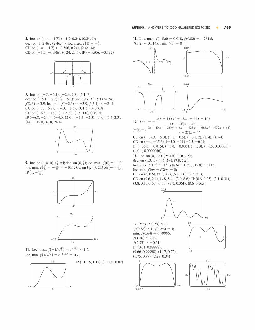
13. Loc. max. , ,; min.
15.
CU on , , , , ;CD on , ; IP , , , ,
17. Inc. on , , ;dec. on , , ;loc. max. , , ;loc. min. ;CU on , , , ;CD on , , ; IP , ,
, , ,
19. Max. ,, ;
min. ,,
;IP ,
, ,,
1
0.99970.55 0.73
1.2
_1.2
_2π 2π
�2.28, 0.34��1.75, 0.77��1.17, 0.72��0.66, 0.99998�
�0.61, 0.99998�f �2.73� �0.51f �1.46� 0.49
f �0.64� 0.99996f �1.96� 1f �0.68� 1
1.2
�1.2
0 π
f
f �0.59� 1
0.75
0 3π
f
�8.6, 0.065��7.0, 0.061��5.4, 0.11��3.8, 0.10��2.1, 0.31��0.6, 0.25��7.0, 8.6��3.8, 5.4��0.6, 2.1�
�8.6, 3���5.4, 7.0��2.1, 3.8��0, 0.6�f ��� � f �2�� � 0
f �7.8� 0.13f �4.6� 0.21f �1.3� 0.6�7.8, 3���4.6, 2���1.3, ��
�2�, 7.8���, 4.6��0, 1.3���0.1, 0.0000066�
��0.5, 0.00001���1, 0���5.0, �0.005���35.3, �0.015���0.5, �0.1���5.0, �1����, �35.3�
�4, ���2, 4���0.1, 2���1, �0.5���35.3, �5.0�
f ��x� � 2 �x � 1��x 6 � 36x 5 � 6x 4 � 628x 3 � 684x 2 � 672x � 64�
�x � 2�4�x � 4�6
f ��x� � �x �x � 1�2�x 3 � 18x 2 � 44x � 16�
�x � 2�3�x � 4�5
0.03
82.50
500
2�1
�1500
0.02
�3.5�8
�0.04
y
x
1
f �3� � 0f �5.2� 0.0145f �0.82� �281.5f ��5.6� 0.0185. Inc. on , , ;
dec. on , ; loc. max. ;CU on , , ;CD on , ; IP
7. Inc. on , , ; dec. on , ; loc. max. ,
; loc. min. , ; CU on , , , ; CD on , , , ; IP , , , , ,
,
9. Inc. on , ; dec. on ; loc. max. ;loc. min. ; CU on ; CD on ;IP
11. Loc. max. ;
loc. min. ;
IP ��0.15, 1.15�, ��1.09, 0.82�1.8
0_2 1.2
f (1�s3) � e�2 s3�9 0.7
f (�1�s3) � e 2 s3�9 1.5
_9.7
0.5_10.5
_0.3
40
2_1.5
_40
( 18, � 321
32 )(��, 1
8 )( 18 , �)f ( 1
4 ) � �16116 �10.1
f �0� � �10(0, 14 )( 14, �)���, 0�
25
_25
_7 7
�6.8, 24.4��4.0, �12.0��1.5, 2.3��0, 0���1.5, �2.3���4.0, 12.0���6.8, �24.4�
�6.8, 7��1.5, 4.0���1.5, 0���6.8, �4.0��4.0, 6.8��0, 1.5���4.0, �1.5���7, �6.8�f �5.1� �24.1f ��2.3� �3.9f �2.3� 3.9f ��5.1� 24.1�2.3, 5.1���5.1, �2.3�
�5.1, 7���2.3, 2.3���7, �5.1�
3
_3
_5 5
��0.506, �0.192��0.24, 2.46���1.7, �0.506��2.46, ����0.506, 0.24����, �1.7�
f �1� � �13�2.46, ���1, 2.46�
�0.24, 1���1.7, 0.24����, �1.7�
APPENDIX J ANSWERS TO ODD-NUMBERED EXERCISES � A99

31. (a) Positive (b)
Exercises 4.5 � page 305
1. (a) Indeterminate (b) 0 (c) 0(d) , , or does not exist (e) Indeterminate3. (a) (b) Indeterminate (c) 5. �2 7. 19. 11. 13. 15. 17. 1 19. 121. 0 23. 0 25. 0 27. 0 29. 1 31. 133. 35. 1 37. 5 39.41. HA
43. HA , VA
45. (a) (b)
(c) Loc. min. ;CD on ; CU on
47. (a) (b) ,
(c) Loc. max.
(d) IP at x 0.58, 4.37f �e� � e 1�e
lim x l � x 1�x � 1lim x l0� x 1�x � 02
_1
0 8
�e�3�2, ���0, e�3�2�f (1/se ) � �1��2e�
limx l 0� f �x� � 01
_0.25
_0.25 1.75
� , � �12e
1œ„e
y
0 x1 2 3 4 e3/2e
”e, ’1e
x � 0y � 0
21 x
y
0
”1, ’1e
y � 0
14e�2
12ln 53��p�q���
���
12
_12
_6 6
c=4c=1
c=0.5
c=_1
c=0.1c=0.2
c=0
c=_4
21.
Vertical tangents at , , ; horizontal tangentsat ,
23. For , there is a cusp; for , there is a loop whosesize increases as increases and the curve intersects itself at
; leftmost point , rightmost point
25. For , the maximum and minimum values are always, but the extreme points and IPs move closer to the y-axis as
c increases. is a transitional value: when c is replaced by, the curve is reflected in the x-axis.
27. There is no maximum or minimum, regardless of the value of c. For , there is a vertical asymptote at ,
, and .is a transitional value at which for .
For , , , and there aretwo IPs, which move away from the y-axis as .
29. For , there is no IP and only oneextreme point, the origin.For , there is amaximum point at theorigin, two minimumpoints, and two IPs,which move downwardand away from the origin as .c l ��
c � 0
4
_2.3
_2.1 2.1
_3
_2_114c � 0
c=_0.5
c=_2
c=_1
4
_1
_4 4
c=0.5
c=2c=1
2
_1
_4 4
c l �lim x l � f �x� � 1lim x l 0 f�x� � 0c � 0
x � 0f �x� � 1c � 0lim x l � f �x� � 1lim x l 0 f�x� � �
x � 0c � 0
0.6
�0.6
�5 5
0.20.51 2
�1
4
�cc � 0
12
c � 0
_3 3
1.5
0
1
12
1.5
_3 30
_1
0
(2cs3c�9, c�3)(�2cs3c�9, c�3)�0, c�
cc � 0c � 0
((2s3 � 5)�9, 2s3�9)(�(2s3 � 5)�9, �2s3�9)��8, 6�(� 3
16 , 38)�0, 0�
7.5
�1
�8.5 3
A100 � APPENDIX J ANSWERS TO ODD-NUMBERED EXERCISES

Exercises 4.7 � page 3221. (a) represents fixed costs, which are incurred evenwhen nothing is produced.(b) The marginal cost is a minimum there.(c)
3. ; the cost of producing the 1001st unit isabout $17.405. (a) $1,340,000; $1340�unit; $2300�unit(b) 200 (c) $700�unit7. (a) ,
(b) Between 208 and 209 units (c)(d) $3.22�unit9. 333 units 11. 10013. (a) About 200 yd (b) 192 yd15. (a) (b) $9.5017. (a) (b) $175 (c) $100
Exercises 4.8 � page 3271. 3. 5. 2.1148 7. 3.107232519. 1.895494 11. �1.39194691, 1.07739428, 2.7198782213. 15. 0.15438500, 0.8456150017. 0.52026899 19. (b) 31.62277725. (0.904557, 1.855277) 27. 11.28 ft 29. 0.76286%
Exercises 4.9 � page 3341. 3.5. ;7. 9.11. 13.15. 17.19. 21.23. 25. 1027. 29.
31. y
x
F
0 2 4 6
1
2
1
2
1 2 3
�2
�1
0
y
x
Fy
0 x1
_1
2
1
2
3
(1, 1)
(2, 2)
(3, 1)
f �x� � �ln x � �ln 2�x � ln 2
16 x 3 � 2x � 33 sin x � 5 cos x � 9
12 x 2 �
25126 x 14�5 � Cx � Dx 3 � x 4 � Cx � D
x 5 �13 x 6 � 4x 2 � 5 sin�1x � C
3 sin t � 4 cos t � C27 t 7�2 �
45 t 5�2 � C
�5��4x 8 � � C2 if x � 0�5��4x 8 � � C1 if x � 04x 5�4 � 4x 7�4 � C2x 3 � 4x 2 � 3x � C
�0.44285440
45x2 2.3, x3 3
p�x� � 550 � �x�10�p�x� � 19 � �x�3000�
c�209� $27.45�unitC��x� � 5 � 0.08x � 0.0009x 2
c�x� � 3700�x � 5 � 0.04x � 0.0003x 2
$17.40�unit
x
C �
0
C�0�49.
For , and . For , and . As increases, the maximum and minimum points and theIPs get closer to the origin.
55.
Exercises 4.6 � page 3121. (a) 11, 12 (b) 11.5, 11.5 3. 10, 105. 25 m by 25 m7. (a)
(b)
(c) (d) (e)(f )9. 13. 15.17.19. Width ; rectangle height 21. (a) Use all of the wire for the square(b) m for the square23.25. (a) (b)(c)27. ft from the stronger source29. 31. 9.35 m 35.37. 39. At a distance from A41. (a) About 5.1 km from B(b) C is close to B; C is close to D;
, where (c) ; no such value (d)43. (a) , ,
(c) c1 3.85, c2 7.66, h 0.42T3 � s4h2 � D 2�c1
T2 � �2h sec ���c1 � �D � 2h tan ���c2T1 � D�c1
s41�4 1.6 1.07x � � BC �W�L � s25 � x 2�x
5 � 2s5�L � W �2�2x � 6 in.y � �
53 x � 10
10s3 3�(1 � s
3 3 )6s[h � s�(2s2)]
cos�1(1�s3) 5532 s 2 csc � �csc � � s3 cot ��
V � 2�R3�(9s3)40s3�(9 � 4s3)
30��4 � �� ft60��4 � �� ft�r 2(1 � s5)
L�2, s3 L�4(� 2817 , 7
17 )4000 cm 3
14,062.5 ft 2A � 375x �
52 x 25x � 2y � 750A � xy
y
x
75
120 9000 ft@
250
50 12,500 ft@
125
100 12,500 ft@
169 a
� c �lim x l�� f �x� � 0lim x l � f �x� � �c � 0
lim x l�� f �x� � ��lim x l � f �x� � 0c � 0
3
3_3
_3
_2�1
0
1 2
APPENDIX J ANSWERS TO ODD-NUMBERED EXERCISES � A101

13. Inc. on , ;
dec. on , ;
loc. max. ,
loc. min. ;
CU on , ;
CD on , ;
IP ,
15. Inc. on , ; dec. on ,loc. max. ; loc. min. ,
; CU on , ; CD on ; IP ,
17.
; 19. Max. at , min. at , IP at 21. For , f is periodic with period and has local maxima at , n an integer. For , f has nograph. For , f has vertical asymptotes. For ,f is continuous on . As C increases, f moves upward and itsoscillations become less pronounced.23. 25. 27. 029. 31. 33. 35.37. 500, 125 39. 41. from ; at 43. 45. $11.50 47. �2.06342149.51. 53.55. (b)(c)
57. No59. (b) About 8.5 in. by 2 in. (c) in., in.61. (a)(b) , where k is theconstant of proportionality
dI�dt � �480k�h � 4����h � 4�2 � 1600�5�220s2 28 ft
20s2�320�s3
4
_1
�4
5
F
0.1e x � cos x � 0.9
120 x 5 �
16 x 3 � x � 12 arctan x � 1
F�x� � e x � 4sx � CL � C
CD4�s3 cm3s3r 213 ft�s400 ft�h1
3�13
�1��2��a � �3, b � 7
�
C � 1�1 � C � 1C � �12n� � ��2
2�C � �1x 0.52x 0.87x � 0
(s2�3, e�3�2 )�0.82, 0.22�
50
_5
1
2.5
0.4_0.51.5
ff
15
2.1_1
_20
�1.2, �12.1���0.12, 1.98���0.12, 1.24��1.24, �����, �0.12�f �1.62� �19.2f ��0.23� 1.96f �0� � 2�0, 1.62�;
���, �0.23��1.62, ����0.23, 0�(�s6, �5s6�36)(s6, 5s6�36)
(0, s6)(��, �s6)(s6, �)(�s6, 0)
f (�s3) � �2s3�9
f (s3) � 2s3�9
(s3, �)(��, �s3)ƒ
1.5
_1.5
_5 5
(0, s3)(�s3, 0)33.
35.37 (a) (b)(c) (d) About 9.09 s41. $742.08 43. 225 ft 45.49. (a) 22.9125 mi (b) 21.675 mi (c) 30 min 33 s(d) 55.425 mi
Chapter 4 Review � page 336True-False Quiz1. False 3. False 5. True 7. False 9. True11. True 13. False
Exercises
1. Abs. min. ; abs. and loc. max. 3. Abs. max. ; abs. and loc. min. 5. (a) None(b) Dec. on (c) None
(d) CU on ; CD on ; IP (e) See graph at right.
7. (a) None(b) Inc. on , dec. on
(c) Loc. max.
(d) CD on (e) See graph at right.
9. (a) None(b) Inc. on , n an integer;dec. on (c) Loc. max. ; loc. min. (d) CU on ;CD on ; IP (e)
11. (a) None(b) Inc. on ,dec. on (c) Loc. min.
(d) CU on(e) See graph at right.
���, ��f ( 1
4 ln 3) � 31�4 � 3�3�4
(��, 14 ln 3)
( 14 ln 3, �)
1 x
2
y
0
y
x
2
π
_2
_π
2π_2π
(2n� ���3�, � 14 )�2n� � ���3�, 2n� � �5��3��
�2n� � ���3�, 2n� � ���3��f �2n�� � �2f ��2n � 1��� � 2
��2n � 1��, �2n � 2����2n�, �2n � 1���
���, 1�f (3
4) � 54
( 34 , 1)(��, 34) y
0 x
1
1
�0, 2��0, �����, 0�
���, ��y
x
2
f ��1� � �1f �0� � 0f �3� � 64f �0� � 10
8815 ft�s2
�9.8s450�4.9 �93.9 m�ss450�4.9 9.58 ss�t� � 450 � 4.9t 2
s�t� � 1 � cos t � sin t
0.2
0
y
x0.4 0.8 1.2 1.6
0.4
0.6F
A102 � APPENDIX J ANSWERS TO ODD-NUMBERED EXERCISES

(c) 5.75, 5.9375
(d)7. 1.9835, 1.9982, 1.9993; 2 9. (a) Left: 4.5148, 4.6165,4.6366; right: 4.8148, 4.7165, 4.696611. 34.7 ft, 44.8 ft 13. 155 ft
15.
17. The region under the graph of from 0 to
19. (a)
(b) (c) 21. , 1
Exercises 5.2 � page 3671. 0.25
3. �0.856759
5. (a) 4 (b) 6 (c) 107. , 9. 6.4643 11. 1.810013. 1.81001414, 1.81007263, 1.8100834715. 2
17. 19. 21. 42 23.
25. 3.75 27. lim n l �
�n
i�1 �sin
5�i
n � �
n�
2
5
43y
1
0 �2x 2 � 5x� dxy
�
0 x sin x dx
�85�475
�1
0
1
y
x
The Riemann sum representsthe sum of the areas of the 2rectangles above the x-axisminus the sum of the areasof the 3 rectangles belowthe x-axis.
2
_2
0
2
y
x
The Riemann sum representsthe sum of the areas of the 2rectangles above the x-axisminus the sum of the areasof the 2 rectangles belowthe x-axis.
sin b323n 2�n � 1�2�2n 2 � 2n � 1��12
lim n l �
64
n 6 �n
i�1 i 5
��4y � tan x
limn l �
�n
i�1 s4 1 � 15i�n � �15�n�
M6
y
x0 1
2
y
x0 1
2
Focus on Problem Solving � page 3417. 9. 13.
15. (a)
(b)
17. (a) (b) 23.
CHAPTER 5
Exercises 5.1 � page 3551. (a) 40, 52
(b) 43.2, 49.2
3. (a) , underestimate (b) , overestimate
5. (a) 8, 6.875
(b) 5, 5.375 y
x0 1
2
y
x0 1
2
y
x0 1
2
y
x0 1
2
0.5
1.0
1.5
2 3 4
y
x0 1 5
0.5
1.0
1.5
2 3 4
y
x0 1 5
2512
7760
y
x0 5
5
y=ƒ
10
y
x0 5
5
y=ƒ
10
11.204 cm3�min12x��x 2 � 1�
b db
dt� c
dc
dt� �b
dc
dt� c
db
dt � sec �
sb 2 � c 2 � 2bc cos �
�tan � �1
c dc
dt�
1
b db
dt ��m�2, m 2�4�4
3��2, 4�, �2, �4�
APPENDIX J ANSWERS TO ODD-NUMBERED EXERCISES � A103
n
5 1.93376610 1.98352450 1.999342100 1.999836
Rn

7. 9.
11. 13.
15. 17.
19. (a) Loc. max. at 1 and 5;loc. min. at 3 and 7(b) 9(c)(d) See graph at right.
21. (a) , n an integer(b) , , and ,n an integer(c) 0.7423. 25.27. (b) Average expenditure over ; minimize average expenditure
Exercises 5.5 � page 3951. 3.5. 7.9. 11.13.15. 17.19. 21.23. 25.27. 29.31.
33. 35.
37. 0 39. 41. 0 43. 45.
47. 3 49. 0 51. 2 53. 55.57. All three areas are equal.59. 61. 5
Exercises 5.6 � page 4011. 3.5.7.9.11.13. 1
13 e 2��2 sin 3� � 3 cos 3�� � C
116 r 4�4 ln r � 1� � C
x �ln x�2 � 2x ln x � 2x � C
13 x 2 sin 3x �
29 x cos 3x �
227 sin 3x � C
�14 x cos 4x �
116 sin 4x � C
12 xe 2x �
14 e 2x � C1
2 x 2 ln x �14 x 2 � C
�5��4����1 � cos�2�t�5�� L
6�s3 �13
16152�e2 � e�182
9
0.35
_0.35
π0
F
ƒ
1.7
_1.7
1.5_0.75
f
F
14 sin4x � C
�1
6�3x 2 � 2x � 1�3 � C
tan�1x �12 ln�1 � x 2 � � C
13 sec3x � Cx � e�x � C�
23 �cot x�3�2 � C�
15 cos5x � C
23 �1 � e x �3�2 � C�
13 cos 3� � C
�2��5�t � 1�5 � � C2s1 � x � 2x 2 � C�
13 ln� 5 � 3x � � C
23 �x � 1�3�2 � C1
3�ln x�3 � C
15 �x 2 � 3�5 � C�1��1 � 2x�2 � C
29 �x 3 � 1�3�2 � C1
3 sin 3x � C
�0, t�f �x� � x 3�2, a � 9f �x� � x
x1 �2t�t� dt
� 0(s4n � 1, s4n � 1)(�s4n � 1, �s4n � 3)�0, 1�
� 0�2sn, s4n � 2
( 12, 2), �4, 6�, �8, 9� x
8642
1
0
_1
y
_2
s257t��x� ��2�4x 2 � 1�
4x 2 � 1�
3�9x 2 � 1�9x 2 � 1
cos sx
2xh��x� � �arctan�1�x��x 2
t��y� � y 2 sin yt��x� � s1 � 2x29. (a) 4 (b) 10 (c) �3 (d) 2 31. 10
33. 35. 0 37. 39.
41. �0.8 43. 3 45. 49.
Exercises 5.3 � page 377
1. The increase in the child’s weight (in pounds) between theages of 5 and 103. Number of gallons of oil leaked in the first 2 hours5. Increase in revenue when production is increased from 1000to 5000 units7. Newton-meters (or joules)9. 11. 138 13. 15. 17.19. 21. 23. 25.27. ln 3 29. 31. 33.35. 2 37. 0, 1.32; 0.8439. 3.75
43.
45. 47. 49.51. (a) (b)53. (a) (b)55. 57. 1.4 mi 59. $58,00061. (b) At most 40%; 63. 3
Exercises 5.4 � page 3861. One process undoes what the other one does. See theFundamental Theorem of Calculus, page 384.3. (a) 0, 2, 5, 7, 3 (d)
(b) (0, 3)(c)
5. t��x� � 1 � x 2
t
y
x
©
y=1+t@
0
x � 3
y
0 x
1
1
g
536
46 23 kg
416 23 mv�t� � 1
2 t 2 � 4t � 5 m�s
416 m�
32 m
43sec x � C2t � t 2 �
13 t 3 �
14 t 4 � C
12
_6
_1 5
5 3 0_2
_425 x 5�2 � C
x
y
0 2
�1
y=˛
1 � ��4��228�ln 22s3�329
35(s2 � 1)�2185 s2 �
125
78�2 � 1�e16
33643
y1
0 x 4 dxe 5 � e 3
y12
1 f �x� dx�
3833 � 9��4
A104 � APPENDIX J ANSWERS TO ODD-NUMBERED EXERCISES

33.
35. ;max. at , min. at 1; IP at , 0, and 1.7
37.
Exercises 5.9 � page 4251. (a)(b) is an underestimate, and are overestimates.(c) (d)3. (a) (underestimate)(b) (overestimate)
5. (a) 5.932957 (b) 5.8692477. (a) 0.746211 (b) 0.747131 (c) 0.7468259. (a) 2.031893 (b) 2.014207 (c) 2.02065111. (a) 0.451948 (b) 0.451991 (c) 0.45197613. (a) 1.064275 (b) 1.067416 (c) 1.07491515. (a)(b) ,(c) for , for 17. (a) , ;
,(b)(c) for , for , for 19. (a) 2.8 (b) 7.954926518 (c) 0.2894(d) 7.954926521 (e) The actual error is much smaller.(f ) 10.9 (g) 7.953789422 (h) 0.0593(i) The actual error is smaller. ( j)21.
n � 50
Snn � 8Mnn � 107Tnn � 151� ET � � 0.002266, � ES � � 0.0000016
ES �0.000001S10 1.718283ET �0.001432T10 1.719713
Mnn � 259Tnn � 366� EM � � 0.006� ET � � 0.013
T10 0.881839, M10 0.882202
T4 � I � M4
M4 0.908907T4 0.895759
Ln � Tn � I � Mn � RnT2 � 9 � IM2R2L2
L2 � 6, R2 � 12, M2 9.6
0.04
π0
F
ƒ
� 1128 cos3x sin x �
3256 cos x sin x �
3256 x
F�x� � �1
10 sin3x cos7x �380 sin x cos7x �
1160 cos5x sin x
4
f
F
�4
�1.1
0.6
�1.7�1F�x� � 1
2 ln�x 2 � x � 1� �12 ln�x 2 � x � 1�
2x�1s22x � 1
ln 2�
ln(s2 2x � 1 � 2x �2 ln 2
� C15. 17. 19.21. 23.25. 27.29.
31.
33. (b)35. (b) 39.41.
Exercises 5.7 � page 4081. 3.5.
7. 9.
11. 13.
15. (a) (b)
17. 19.
21.
23.
25. 27.
29. 31.
Exercises 5.8 � page 4141.3.5.7. 9.11. 13. 15.17.19.21.25.27.29.31. �ln � cos x � �
12 tan2x �
14 tan4x � C
110 �1 � 2x�5�2 �
16 �1 � 2x�3�2 � C
�15 sin2x cos3x �
215 cos3x � C
�14 x �5 � x 2 �3�2 �
58 xs5 � x 2 �
258 sin�1(x�s5) � C
se 2x � 1 � cos�1�e�x � � C
�1 � ex� ln�1 � ex� � ex � C1
15 ln � x 5 � sx 10 � 2 � � C
815
19 sin3x �3 ln�sin x� � 1� � C9��4
12 [x 2 sin�1�x 2 � � s1 � x 4 ] � C� 3 � 6�
(�s9x 2 � 1�x) � 3 ln � 3x � s9x 2 � 1 � � C
�1��2��� sec��x� tan��x� � �1��2��� ln � sec��x� � tan��x� � � C
12 x 2 � x � 4 ln�x 2 � 9� �
83 tan�1�x�3� � C
2
s3 tan�1 �2x � 1
s3 � � C2 � ln 259
12 �1 � ln 2�1
2 x 2 � x � ln � x � 1 � � C
12 ln�x 2 � 1� � (1�s2 ) tan�1(x�s2 ) � C
ln � x � 1 � �12 ln�x 2 � 9� �
13 tan�1�x�3� � C
12 ln 322 ln � x � 5 � � ln � x � 2 � � C
A
x � 1�
Bx � C
x 2 � x � 1
A
x � 4�
B
x � 1
��24 � s3�8 �14�
sx 2 � 4
4x� C
�s9 � x 2
x� sin�1 � x
3� � C13 sec3 x � sec x � C
38 t �
14 sin 2t �
132 sin 4t � C
�11384
15 cos5x �
13 cos3x � C
2 � e�t�t 2 � 2t � 2� mx ��ln x�3 � 3�ln x�2 � 6 ln x � 6� � C2
3 , 815
�14 cos x sin3x �
38 x �
316 sin 2x � C
7
�1
�3.5 1.5
ƒ F
�2x � 1�e x � C
1.2
�1.2
�2 2
ƒ
F
�x sin �x��� � �cos �x��� 2 � C�
12 � ��42(sin sx � sx cos sx ) � C
12 �ln 2 � 1�2 ln 4 �
32
112 (� � 12 � 6s3)�
121 � 2�e
APPENDIX J ANSWERS TO ODD-NUMBERED EXERCISES � A105
n
4 0.140625 0.390625 0.265625 0.2421888 0.191406 0.316406 0.253906 0.248047
16 0.219727 0.282227 0.250977 0.249512
MnTnRnLn
n
4 0.109375 �0.140625 �0.015625 0.0078138 0.058594 �0.066406 �0.003906 0.001953
16 0.030273 �0.032227 �0.000977 0.000488
EMETEREL

53. (a)
(b) The rate at which the fraction increases as t increases(c) 1; all bulbs burn out eventually55. 8264.5 years 57. 1000 61.
Chapter 5 Review � page 438True-False Quiz1. True 3. True 5. False 7. True 9. True11. False 13. False 15. False 17. False
Exercises
1. (a) 8 (b) 5.7
3. 5. 3 7.
9. 37 11. 13. 15. 17. 348019. 21.23. 25.
27. 29.
31. 33.35.37. 39.41.43.
45.
47. (a) 1.090608 (overestimate)(b) 1.088840 (underestimate)(c) 1.089429 (unknown)
49. (a) 0.00 , (b) ,51. (a) 3.8 (b) 1.7867, 0.000646 (c)
53. 55. 57. D
59. 2 61. C 63. (a) m (b) 29.5 m65. Number of barrels of oil consumed from Jan. 1, 2000,through Jan. 1, 2003
67. 69. e2x�1 � 2x���1 � e�x�Ce�x 2��4kt��s4�kt
29.16
1364 � y
3
1 sx 2 � 3 dx � 4s3
n � 30n � 1830.003n � 2596
38 ln (x �
12 � sx 2 � x � 1 ) � C
14 �2x � 1�sx 2 � x � 1 �
12 [e x
s1 � e 2x � sin�1�e x �] � C
y� � (2e x � e sx )��2x�F��x� � s1 � x 464
5
2s1 � sin x � C
ln � 1 � sec � � � C1625
12 ln � t � 2
t � 4 � � C�e�x�x 2 � 2x � 2� � C
2x � ln � 3x � 2 � � C�sin�1�t� � Cx sec x � ln � sec x � tan x � � C�1����e � � 1�
12 ln 21209
289
10
f � c, f �� b, yx
0 f �t� dt � a1
2 � ��4
6
2 x
2
0
y=ƒ
y
2 x
2
0
y=ƒ
6
y
C � 1; ln 2
F�t�
1
700 t0(in hours)
y
y=F(t)
23. (a) 11.5 (b) 12 (c) 25.27. 29. (a) 23.44 (b)31. 59.4
Exercises 5.10 � page 436Abbreviations: C, convergent; D, divergent
1. (a) Infinite interval (b) Infinite discontinuity(c) Infinite discontinuity (d) Infinite interval3. ; 0.495, 0.49995, 0.4999995; 0.55. 7. 1 9. D 11. D13. 0 15. D 17.19. D 21. 1 23. 25. D27. D 29. D 31.33. e
35.
37. Infinite area
39. (a)
It appears that the integral is convergent.(c)
41. C 43. C 45. D 47. 49. 1��1 � p�, p � 1�
1
�0.1
1 10
©=sin@ x
≈
ƒ=1≈
20
0π2
y=sec@ x
0.5
_7 7
29 y=
2≈+9
0
2�3
x
y
0
x � 1y � ex
1
83 ln 2 �
89
2s3e 2�4
112
12 � 1��2t 2 �
0.341310,177 megawatt-hours37.73 ft�s11.6
A106 � APPENDIX J ANSWERS TO ODD-NUMBERED EXERCISES
t
2 0.4474535 0.577101
10 0.621306100 0.668479
1,000 0.67295710,000 0.673407
yt
1 ��sin2x��x 2 � dx

9.
11.
13. 15. 0, 0.747; 0.13217. (a) Solid obtained by rotating the region ,
about the x-axis(b) Solid obtained by rotating the region ,
about the y-axis19. 21. 23.25. 27. 29. 2431. 2 33. 3
35. (a) (b)
37. (b) 39.
41.
43. 45. 82847.
Exercises 6.3 � page 471
1. 3.5. 8
0�25 2.5
s2 �e � � 1�x
21 s1 � 4t 2 dt3s10
0
y
x
x
1 2 3 4
2-x
x=2
10
y
x
y=x-≈
��2��15
8 xr0 sR 2 � y 2
sr 2 � y 2 dy
512 �r 3�r 2h
2� 2r 2R8�R xr0 sr 2 � y 2 dy
10 cm32b 2h�3�h2�r � �h�3���r 2h�31110 cm3
0 � y � 1y4 � x � y2
0 � x � ��20 � y � cos x
832��21
(1, 1)
x0
y
x=¥
y=≈
_1 x0
y
x=_1
29��30
x0
y
(1, 1)
x
0
y
y=x
y=œ„x
��6Focus on Problem Solving � page 4441. About 1.85 inches from the center 3. 5. 1
7. 9. Does not exist 11.13. 15. 0
19. (b)
CHAPTER 6
Exercises 6.1 � page 4521. 3. 5. 19.5 7. 9. 4
11. 13. 15.17. �1.02, 1.02; 2.70 19. 0, 0.70; 0.08 21. 118 ft23. 84 25.27. 29.31. 33. 35. 37.39. 41.
Exercises 6.2 � page 463
1.
3.
5.
7.
x0
y
(4, 2)
x0
y
x=2y
¥=x
64��15
x
y
0x
y
0
(1, 1)
y=≈
x=¥
3��10
x
y
0
(2, 4)
x
y
0
x=0
y=4
x=œ„y
8�
x
y
0x
y
0x=2x=1
y=1x
y=0
��2
0 � m � 1; m � ln m � 1f �t� � 3t 242�3624s3�51
2�e� �2 � 1��abrsR 2 � r 2 � �r 2�2 � R 2 arcsin�r�R�
12m2
� �23
83
323
16e � �1�e� �
103
323
y � �sL2 � x 2 � L ln�L � sL2 � x 2
x �s1 � sin4 x cos x
��1, 2�e�2
��2
APPENDIX J ANSWERS TO ODD-NUMBERED EXERCISES � A107
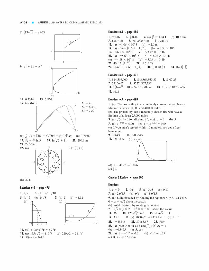
Exercises 6.5 � page 485
1. 3. 5. (a) (b) 10.8 cm7. 625 ft-lb 9. 650,000 ft-lb 11. 2450 J13. (a) (b)17. (a) (b)19. 21.23. (a) (b)(c) (d)25. 40, 12, 27.29. 31. 33. (b)
Exercises 6.6 � page 4911. $14,516,000 3. $43,866,933.33 5. $407.257. $4166.67 9. 3727; $37,75311. 13.15.
Exercises 6.7 � page 4981. (a) The probability that a randomly chosen tire will have alifetime between 30,000 and 40,000 miles(b) The probability that a randomly chosen tire will have a lifetime of at least 25,000 miles3. (a) for all x and (b) 5
7. (a) (b)(c) If you aren’t served within 10 minutes, you get a free hamburger.9. 11.13. (b) 0; (c)
(d)(e)
Chapter 6 Review � page 500
Exercises
1. 3. 5. (a) 0.38 (b) 0.877. (a) (b) (c)9. (a) Solid obtained by rotating the region ,
about the -axis(b) Solid obtained by rotating the region
about the -axis11. 36 13. 15.17. 3.2 J 19. (a) (b) 2.1 ft
21. 23. $7166.67 25.27. (a) for all x and (b) (c) 5, yes29. (a) (b)(c) 8 ln 2 5.55 min
e�5�4 0.291 � e�3�8 0.31 0.3455
x�
�� f �x� dx � 1f �x� � 0
f �x� 458 lb
8000��3 8378 ft-lb2(5s5 � 1)125s3�3 m3
x0 � x � 12 � sx � y � 2 � x 2,
x0 � x � ��20 � y � s2 cos x
8��15��62��159�e �
116
32 a0
1 � 41e�8 0.986
1x10¹⁰
0 4x10⁻¹⁰
a0
0.9545 44%
1 � e�2�2.5 0.55e�4�2.5 0.20
x�
�� f �x� dx � 1f �x� � 0
19 L�s
1.19 � 10�4 cm3�s23 (16s2 � 8) $9.75 million
(12 , 25)4
3 , 0, (0, 23 )�1��e � 1�, �e � 1��4��1.5, 1.2�(1, 10
3 ) 3.03 � 105 lb 4.88 � 104 lb
5.06 � 104 lb 5.63 � 103 lb 3.47 � 104 lb 6.5 � 106 N
8.50 � 109 JGm1m2��1�a� � �1�b�� 2.0 m 1.06 � 106 J
2524 1.04 J15
4 ft-lb9 ft-lb
7.
9.
11. 0.7314 13. 3.82015. (a), (b) ,
,
(c) (d) 7.7988
17. 19. 21. 209.1 m23. 29.36 in.27. (a)
(b)
Exercises 6.4 � page 475
1. 3.5. (a) (b) 7. (a) 2 (b)
(c) (c)
11.13. (a) (b)15. 5��4�� 0.4 L
220s2 311 V155�s2 110 V�50 � 28��� F 59 F
7
20
f
y=2
2 x
4
0
y
c
1.322�s383
�1 � e�25 ��102��
294
t � �0, 4��15
�15
�15 15
ln(s2 � 1)205128 �
81512 ln 3
x40 s1 � �4�3 � x���3�4 � x�2�3 ��2 dx
L4 7.50L2 6.43L1 � 43
0 4
21
�1�1 21
e 3 � 11 � e�8
2
�1
�1 2
(1, 1)
(13s13 � 8)�27
A108 � APPENDIX J ANSWERS TO ODD-NUMBERED EXERCISES

11. 13.
15.
17. ;
19. (a) (i) 1.4 (ii) 1.44 (iii) 1.4641(b) Underestimates
(c) (i) 0.0918 (ii) 0.0518 (iii) 0.0277It appears that the error is also halved (approximately).21. 23.25. (a) (i) 3 (ii) 2.3928 (iii) 2.3701 (iv) 2.3681(c) (i) �0.6321 (ii) �0.0249 (iii) �0.0022(iv) �0.0002It appears that the error is also divided by 10 (approximately).27. (a), (d) (b) 3
(c) Yes; (e) 2.77 C
Q � 3Q
0
2
2 t4
4
6
1.7616�1, �3, �6.5, �12.25
y
0
1.0
0.2 x0.4
1.1
1.2
1.3
1.4
1.5
0.1 0.3
y=´
h=0.1
h=0.2
h=0.4
y
0
_2
_1 t1
2
c=3
c=_3
c=_1
c=1
�2, 0, 2�2 � c � 2
3
0.5_3 3
y
x3_3
3
_3
y
x3_3
3
_3
Focus on Problem Solving � page 5021.3. (a)
(c)Advantage: the markings on the container are equally spaced.5.7. (b) 0.2261 (c) 0.6736 m(d) (i) (ii)11. (a)
(b)
13. Height , volume
15. 19.
CHAPTER 7
Exercises 7.1 � page 5113. (a) 5. (b) and (c)7. (a) It must be either 0 or decreasing(c) (d)9. (a) (b)(c)13. (a) At the beginning; stays positive, but decreases(c)
Exercises 7.2 � page 5191. (a) (b)
3. IV 5. III
7. 9. y
x3_3
3
_3
y
0 x_1_2 1 2
_1
_2
1
2
y � �2y � 0, y � 2,y
x
3
3_3
_3
(i)
(ii)
(iv)
(iii)
0
M
P(t)
t
P(0)
P � 0, P � 4200P � 42000 � P � 4200
y � 1��x � 2�y � 0
3
2��, 1��ln���2�( 28
27 s6 � 2)�b 3s2 b
�P0 � 0tH���r 2 � � 0tHe L�H xr�r e
x�H � 2sr 2 � x 2 dx
P�z� � P0 � t xz0 �x� dx
370��3 s 6.5 min1��105�� 0.003 in�s
f �x� � s2x��
f �y� � skA���C� y 1�4
V � xh0 � � f �y��2 dy
2��3 � s3�2
APPENDIX J ANSWERS TO ODD-NUMBERED EXERCISES � A109

Exercises 7.4 � page 5381. About 2353. (a) (b)(c) (d)5. (a) 1508 million, 1871 million (b) 2161 million(c) 3972 million; wars in the first half of century, increased lifeexpectancy in second half7. (a) (b)9. (a) (b) (c)11.13. (a) , ; (b) (c)15. (a) (b)17. (a) (i) $3828.84 (ii) $3840.25 (iii) $3850.08(iv) $3851.61 (v) $3852.01 (vi) $3852.08(b) ,19. (a) (b)(c) , (d) Declining
Exercises 7.5 � page 5481. (a) 100; 0.05 (b) Where is close to 0 or 100; on theline ; ; (c)
Solutions approach 100; some increase and some decrease,some have an inflection point but others don’t; solutions with
and have inflection points at (d) , ; other solutions move away from and toward 3. (a) (b)5. (a) , in billions(b) 5.49 billion (c) In billions: 7.81, 27.72(d) In billions: 5.48, 7.61, 22.417. (a) (b)(c) 3:36 P.M.11. (a) Fish are caught at a rate of 15 per week.(b) See part (d) (c)(d)
; ;P0 � 250: P l 750
P0 � 250: P l 2500 � P0 � 250: P l 0
0 t
P
1208040
1200
800
400
P � 250, P � 750
y � y0��y0 � �1 � y0 �e�kt �dy�dt � ky�1 � y�
PdP�dt � 1265 P�1 � P�100�
1.55 years3.23 � 107 kgP � 100
P � 0P � 100P � 0P � 50P0 � 40P0 � 20
P¸=140
P¸=120
P¸=80
P¸=40
P¸=20
P¸=60
0 t
P
604020
150
100
50
P0 � 1000 � P0 � 100P � 50P
m � kP0m � kP0
m � kP0P�t� � �m�k� � �P0 � m�k�e ktA�0� � 3000dA�dt � 0.05A
39.9 kPa 64.5 kPa 116 min 137 F
y�t� � 110e kty�0� � 110dy�dt � ky 2500 years
199.3 years 9.92 mg100 � 2�t�30 mg�2000 ln 0.9 211 sCe�0.0005t
�3 ln 60��ln 16 4.4 h18,631 cells�h 20,159500 � 16 t�3
Exercises 7.3 � page 5271. or 3.5. 7.9. 11.13. 15.17. (a)(b) ,
(c) No
19.
21. (a), (c) (b)
23. 25.
27. ; 3 29. ; M31. (a)
(b)
33. (a)(b) ; the concentration approaches regardless of thevalue of 35. (a) (b) 37.39. (a)
(b) , whereand
41. (b) (c) 144s6 s 5 min 53 sy�t� � (s6 �1
144 t)2A0 � A�0�C � (sM � sA0 )�(sM � sA0 )
A�t� � M ��CesM kt � 1���Ce sM kt � 1��2
dA�dt � ksA �M � A�t�k15e�0.2 12.3 kg15e�t�100 kg
C0
r�kr�kC�t� � �C0 � r�k�e�kt � r�k
t �2
ksa � b�tan�1� b
a � b� tan�1� b � x
a � b �x � a � 4�(kt � 2�sa)2
P�t� � M � Me�ktQ�t� � 3 � 3e�4 t
6
6
_6
_6
4
4
_4
_4
y 3 � 3�x � C�x 2 � 2y 2 � C
y � s2�x � C�5
5
_5
_5
5
2.50
�2.5
cos y � cos x � 1
�s��2 � x � s��2
1
0
y=sin ≈
_œ„„„π/2 œ„„„π/2
y � sin�x 2�sin�1y � x 2 � C
y � 7e x 4u � �st 2 � tan t � 25
x � s2�t � 1�e t � 3y � tan�x � 1�u � Ae 2 t�t 2�2 � 1y � s�3�te t � e t � C��2�3 � 1
x 2 � y 2 � Cy � 0y � �1��x � C�
A110 � APPENDIX J ANSWERS TO ODD-NUMBERED EXERCISES
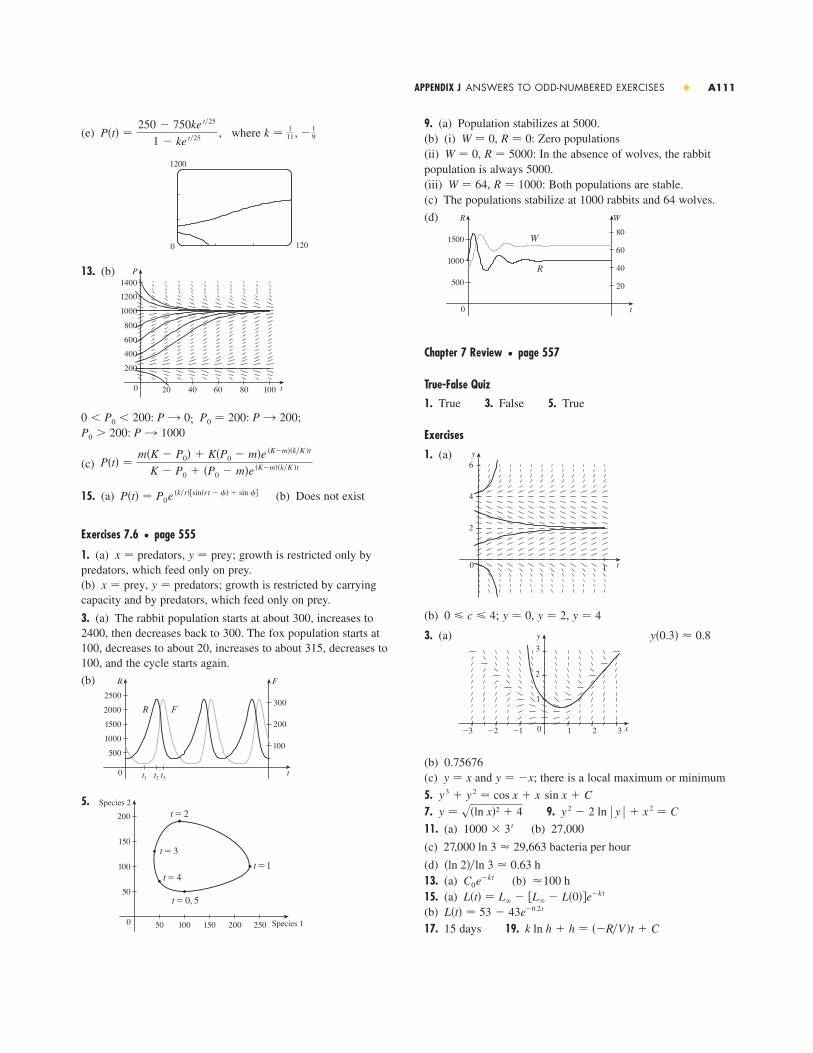
9. (a) Population stabilizes at 5000.(b) (i) , : Zero populations(ii) , : In the absence of wolves, the rabbitpopulation is always 5000.(iii) , : Both populations are stable.(c) The populations stabilize at 1000 rabbits and 64 wolves.
(d)
Chapter 7 Review � page 557
True-False Quiz1. True 3. False 5. True
Exercises
1. (a)
(b) ; , ,
3. (a)
(b) 0.75676(c) and ; there is a local maximum or minimum
5.7. 9.11. (a) (b) 27,000
(c)
(d)13. (a) (b)15. (a)(b)17. 15 days 19. k ln h � h � ��R�V �t � C
L�t� � 53 � 43e�0.2 t
L�t� � L� � �L� � L�0��e�kt
100 hC0e�kt
�ln 2��ln 3 0.63 h
27,000 ln 3 29,663 bacteria per hour
1000 � 3 t
y 2 � 2 ln � y � � x 2 � Cy � s�ln x�2 � 4y 3 � y 2 � cos x � x sin x � C
y � �xy � x
y�0.3� 0.8
0 x
y
1 2_1_2
1
2
3_3
3
y � 4y � 2y � 00 � c � 4
6
10 t
y
2
4
0 t
R
1000
W
40
1500
500
60
20
80W
R
R � 1000W � 64
R � 5000W � 0R � 0W � 0(e) , where
13. (b)
; ;
(c)
15. (a) (b) Does not exist
Exercises 7.6 � page 555
1. (a) , ; growth is restricted only by predators, which feed only on prey.(b) , ; growth is restricted by carryingcapacity and by predators, which feed only on prey.
3. (a) The rabbit population starts at about 300, increases to2400, then decreases back to 300. The fox population starts at100, decreases to about 20, increases to about 315, decreases to100, and the cycle starts again.
(b)
5.
0 Species 1
Species 2
50
200
100
50
100 150 200 250
t=3
t=0, 5
150
t=1
t=2
t=4
0 t
R
2000
t¡
1000
F
200
t™ t£
1500
500
2500300
100
R F
y � predatorsx � prey
y � preyx � predators
P�t� � P0e �k�r��sin�rt � �� � sin ��
P�t� �m�K � P0� � K�P0 � m�e �K�m��k�K �t
K � P0 � �P0 � m�e �K�m��k�K �t
P0 � 200: P l 1000 P0 � 200: P l 2000 � P0 � 200: P l 0
0 t
P
1008060
1400
800
400
4020
600
200
1200
1000
0 120
1200
k � 111 , � 1
9P�t� �250 � 750ke t�25
1 � ke t�25
APPENDIX J ANSWERS TO ODD-NUMBERED EXERCISES � A111

3. ,, ,,,,
Convergent,
5. , ,,,,,
Divergent
7. 0.64645, 0.80755,0.87500, 0.91056,0.93196, 0.94601,0.95581, 0.96296,0.96838, 0.97259Convergent,
9. (a) C (b) D11. 3 13. 15 15. D 17. D 19. 21.23. 25. 27. D 29. 31.33. 35.37. 39. for ,
41. (a) (b) 5
43. 45.47. The series is divergent.51. is bounded and increasing.53. (a)55. (a) (c) 1
Exercises 8.3 � page 5911. C
3. (a) Nothing (b) C5. -series; geometric series; ; 7. C 9. C 11. C 13. C 15. D 17. C19. D 21. C 23. D 25.27. (a) 1.54977, (b) 1.64522,(c)29. 2.61 31. 0.567975, 37. Yeserror � 0.0003
n � 1000error � 0.005error � 0.1
p � 1
�1 � b � 1b � �1p
0 x
y
1
. . .a™
a£ a¢ a∞
2 3 4
y=1
x1.3
12 , 56 , 23
24 , 119120; ��n � 1�! � 1���n � 1�!
0, 19 , 29 , 13 , 23 , 79 , 89 , 1�sn �
1��n�n � 1��(s3 � 1)�2
Sn � D�1 � c n ���1 � c�sum � 1n � 1a1 � 0, an � 2��n�n � 1��1
4
� x � � 1, x��x � 1��3 � x � 3; x��3 � x�
1138333
29
32sin 1
1736
34
sum � 1
1
100
ssnd
sand
�9.01610�9.66446�9.21214�2.41243�3.28388�2.992870.38764�0.77018
2
0 10
_10
ssnd
sand
�0.627631.55741
sum � �2�2.00000�2.00000�1.99999�2.00003�1.99987�2.00064�1.99680�2.01600
ssnd
1
0 10
_3
sand
�1.92000�2.4000021. (a) Stabilizes at 200,000(b) (i) , : Zero populations(ii) , : In the absence of birds, the insect population is always 200,000.(iii) , : Both populations are stable.(c) The populations stabilize at 25,000 insects and 175 birds.(d)
Focus on Problem Solving � page 5601. 5.7. (b) (c) No9. (a) 9.8 h (b) ; (c) 5.1 h11.
CHAPTER 8
Exercises 8.1 � page 571
Abbreviation: C, convergent; D, divergent
1. (a) A sequence is an ordered list of numbers. It can also be defined as a function whose domain is the set of positiveintegers.(b) The terms approach 8 as becomes large.(c) The terms become large as becomes large.
3. ; yes;
5. 7. 9. D
11. 5 13. 0 15. 0 17. D
19. 0 21. 0 23. 0 25. 0
27. D 29. 31. 0
33. (a) 1060, 1123.60, 1191.02, 1262.48, 1338.23 (b) D
35. (a) D (b) C 37. (b)
39. Decreasing; yes
41. Not monotonic; yes
43. Convergent by the Monotonic Sequence Theorem;
45. 47. 62
Exercises 8.2 � page 580
1. (a) A sequence is an ordered list of numbers whereas aseries is the sum of a list of numbers.(b) A series is convergent if the sequence of partial sums is a convergent sequence. A series is divergent if it is not convergent.
(3 � s5)�2
5 � L � 8
(1 � s5)�2
��4
5n � 3(� 23 )n�1
12
13 , 25 , 37 , 49 , 5
11 , 613
nan
nan
x 2 � �y � 6�2 � 25
6283 ft2�h31,900� 100,000 ft2
f �x� � �x 2 � L2 ���4L� � �L�2� ln�x�L�20 Cf �x� � 10e x
0 t
x
35,000
15,000
y
15025,000
5,000
45,000
200
100
250
(insects) (birds)
50
birds
insects
y � 175x � 25,000
y � 0x � 200,000y � 0x � 0
A112 � APPENDIX J ANSWERS TO ODD-NUMBERED EXERCISES

13.
15.
17.
19.
21. 23.
25. 0.199989 27. 0.000065 29. 0.0953131. (b) 0.920 35.
Exercises 8.7 � page 621
1. 3.
5.
7.
9. 11.
13. ,
17.
19.
21.
23. ��
n�1 ��1�n�122n�1x 2n
�2n�!, R � �
��
n�0 ��1�n
1
n! x n�2, R � �
��
n�0 ��1�n
1
2n � 1 x 2n�2, R � 1
��
n�0 ��1�n
� 2n
�2n�! x 2n, R � �
R � �
s2
2 �
�
n�0 ��1�n� 1
�2n�! �x �
�
4 �2n
�1
�2n � 1�! �x �
�
4 �2n�1���
n�0 ��1�n�x � 1�n, R � 1�
�
n�0 e 3
n! �x � 3�n, R � �
7 � 5�x � 2� � �x � 2�2, R � �
��
n�0 ��1�n
�n � 1��n � 2�2
x n, R � 1
��
n�0 ��1�n
x 2n
�2n�!, R � �b8 � f �8��5��8!
��1, 1�, ��1, 1�, ��1, 1�
C � ��
n�0 ��1�n
x 2n�1
�2n � 1�2C � ��
n�0 ��1�nx 4n�1
4n � 1
3
2
�3
�2
s∞=sßs¡=s™
f
s£=s¢
s¸
��
n�0
2x 2n�1
2n � 1, R � 1
3
6
�1.2
�4s¢
s∞ s£ s¡
s™
f
s¸
ln 3 � ��
n�1 ��1�n�1
n3n x n, R � 3
��
n�3 n � 2
2n�1 x n, ��2, 2�
ln 5 � ��
n�1
x n
n5n , R � 5Exercises 8.4 � page 5981. (a) A series whose terms are alternately positive and negative(b) and , where (c)3. C 5. C 7. D9. An underestimate 11. 13. 715. 0.8415
17. 0.6065 19. No21. No 23. Yes 25. Yes 27. Yes 29. D31. (a) and (d)35. (a) , (b) ,0.693109
Exercises 8.5 � page 604
1. A series of the form , where is a variableand and the ’s are constants3. 1, 5. 7.9.11. 13. 1, (0, 2) 15. 2,17. 0, 19. (a) Yes (b) No 21.23. (a)(b), (c)
25. 27. 2
Exercises 8.6 � page 610
1. 10 3. 5.
7. 9.
11. (a)
(b)
(c)1
2 �
�
n�2 ��1�nn�n � 1�x n, R � 1
1
2 �
�
n�0 ��1�n�n � 2��n � 1�x n, R � 1
��
n�0 ��1�n�n � 1�x n, R � 1
� ��
n�0
1
5n�1 x n, ��5, 5���
n�0 ��1�n
4n�1 x 2n, ��2, 2�
��
n�0 x 3n, ��1, 1��
�
n�0 ��1�nx n, ��1, 1�
��1, 1�, f �x� � �1 � 2x���1 � x 2 �
2
8
_2
_8
s¡
J¡
s¶ s¡¡s£
s∞ s˜
���, ��k k{ 1
2 }��4, 0�4, ��4, 4�
13 , [� 1
3 , 13 ]�, ���, ��1, ��1, 1���1, 1�
cnax��
n�0 cn�x � a�n
n � 11error � 0.00521661960 0.68854
1.5
_0.5
9
ssnd
sand_2
p � 0
� Rn � � bn�1
bn � � an �limn l � bn � 00 � bn�1 � bn
APPENDIX J ANSWERS TO ODD-NUMBERED EXERCISES � A113

(b)
11. (a) (b) 2
13. (a)
(b) 99,225
Exercises 8.9 � page 633
1. (a) ,,
(b)
(c) As increases, is a good approximation to on alarger and larger interval.
3.
5.
1.1
�1
�1 2
fT£
1
2�
s3
2 �x �
�
6 � �1
4 �x �
�
6 �2
�s3
12 �x �
�
6 �3
2
_5
_1 4
f
T¢
�x � 1� �12 �x � 1�2 �
13 �x � 1�3 �
14 �x � 1�4
f �x�Tn�x�n
2
2π
_2
_2π
T¢=T∞
T™=T£
T¸=T¡
Tß
f
T6�x� � 1 �12 x 2 �
124 x 4 �
1720 x 6
T4�x� � 1 �12 x 2 �
124 x 4 � T5�x�
T0�x� � 1 � T1�x�, T2�x� � 1 �12 x 2 � T3�x�
1 �x 2
2� �
�
n�2 ��1�n�1
1 � 3 � 5 � � � � � �2n � 3�2nn!
x 2n
��
n�1 nx n
x � ��
n�1 1 � 3 � 5 � � � � � �2n � 1�
�2n � 1�2nn! x 2n�125.
27.
29. 0.81873
31.
33.
35. 0.310 37. 0.09998750 39. 41.43. 45. 47.49. 51.
Exercises 8.8 � page 625
1.
3.
5.
7.
9. (a) 1 � ��
n�1 1 � 3 � 5 � � � � � �2n � 1�
2nn! x 2n
1
80
_8
f
T¡
T™
T£
1
2�
1
2 �
�
n�1 ��1�n1 � 4 � 7 � � � � � �3n � 2�
24nn! x n, R � 8
12 x � �
�
n�1 ��1�n
1 � 3 � 5 � � � � � �2n � 1�n!23n�1 x 2n�1, R � 2
��
n�0 ��1�n
�n � 1��n � 2�2n�4 x n, R � 2
1 �x
2� �
�
n�2 ��1�n�1
1 � 3 � 5 � � � � � �2n � 3�2nn!
x n, R � 1
e 3 � 11�s2
e�x 4�x �
12 x 2 �
13 x 31 �
32 x 2 �
2524 x 4
1120
13
C � x �x 4
8� �
�
n�2 ��1�n�1
1 � 3 � 5 � � � � � �2n � 3�2nn!�3n � 1�
x 3n�1
C � ��
n�0
��1�nx 4n�3
�4n � 3��2n � 1�!
1.5
1.5
_1.5
_1.5
Tˆ=T˜=T¡¸=T¡¡
T¢=T∞=Tß=T¶
T¸=T¡=T™=T£
f
��
n�0 ��1�n
1
�2n�! x 4n, R � �
2
20�1.2
T¢
T£
f
T¸
T™
T¡
1 �x
2� �
�
n�2 ��1�n�1
1 � 3 � 5 � � � � � �2n � 3�2nn!
x n, R � 1
A114 � APPENDIX J ANSWERS TO ODD-NUMBERED EXERCISES
x f
0.7071 1 0.6916 0.7074 0.7071
0 1 �0.2337 0.0200 �0.0009
�1 1 �3.9348 0.1239 �1.2114�
�
2
�
4
T6T4 � T5T2 � T3T0 � T1
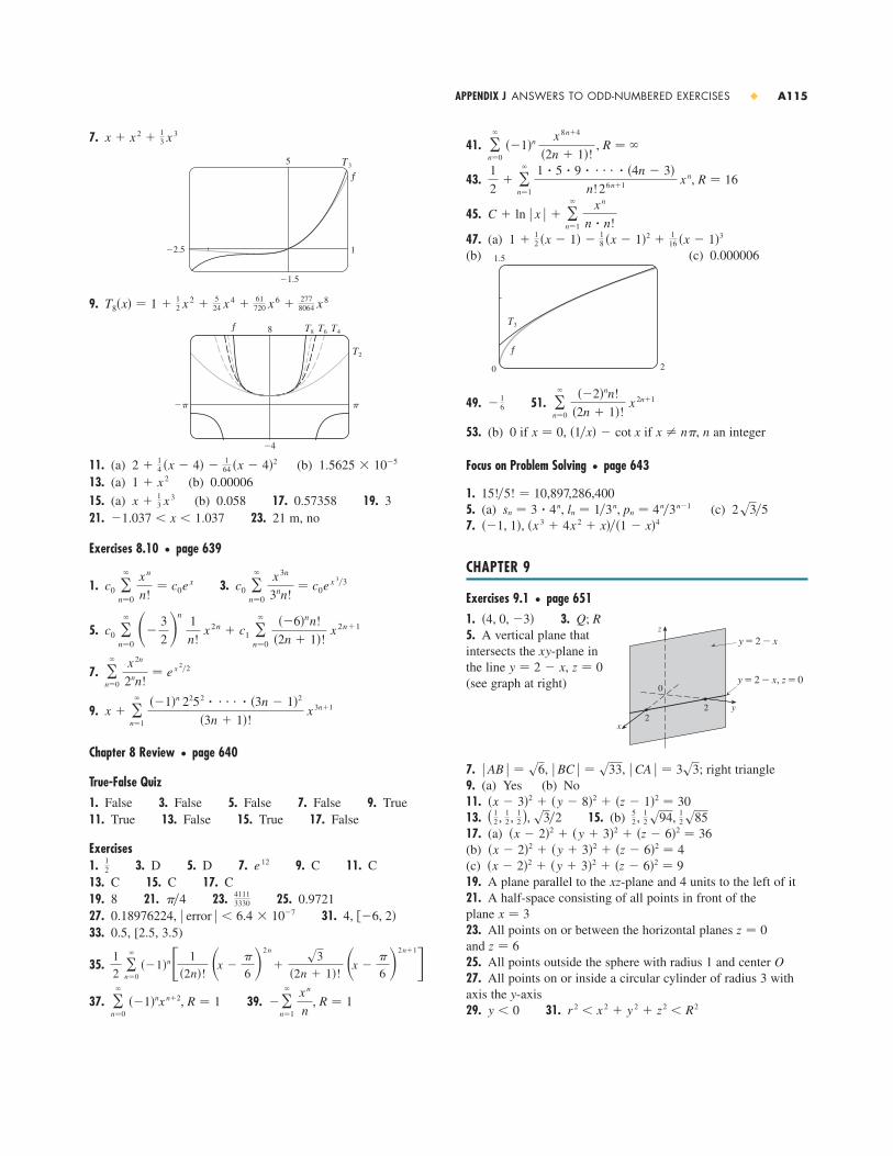
41.
43.
45.
47. (a)(b) (c) 0.000006
49. 51.
53. (b) 0 if , if , n an integer
Focus on Problem Solving � page 643
1.5. (a) (c)7.
CHAPTER 9
Exercises 9.1 � page 6511. 3.5. A vertical plane thatintersects the xy-plane inthe line ,(see graph at right)
7. , , ; right triangle9. (a) Yes (b) No11.13. 15. (b)17. (a)(b)(c)19. A plane parallel to the -plane and 4 units to the left of it21. A half-space consisting of all points in front of the plane 23. All points on or between the horizontal planes and 25. All points outside the sphere with radius 1 and center O27. All points on or inside a circular cylinder of radius 3 withaxis the y-axis29. 31. r 2 � x 2 � y 2 � z2 � R2y � 0
z � 6z � 0
x � 3
xz�x � 2�2 � �y � 3�2 � �z � 6�2 � 9�x � 2�2 � �y � 3�2 � �z � 6�2 � 4
�x � 2�2 � �y � 3�2 � �z � 6�2 � 36
52, 12 s94, 12 s85( 1
2, 12 , 12 ), s3�2�x � 3�2 � �y � 8�2 � �z � 1�2 � 30
� CA � � 3s3� BC � � s33� AB � � s6
z � 0y � 2 � x
z
y2
x
2
0
y=2-x
y=2-x, z=0
Q; R�4, 0, �3�
��1, 1�, �x 3 � 4x 2 � x���1 � x�42s3�5sn � 3 � 4n, ln � 1�3n, pn � 4n�3n�1
15!�5! � 10,897,286,400
x � n��1�x� � cot xx � 0
��
n�0
��2�nn!
�2n � 1�! x 2n�1�
16
1.5
20
T£
f
1 �12 �x � 1� �
18 �x � 1�2 �
116 �x � 1�3
C � ln � x � � ��
n�1
x n
n � n!
1
2� �
�
n�1 1 � 5 � 9 � � � � � �4n � 3�
n!26n�1 x n, R � 16
��
n�0 ��1�n
x 8n�4
�2n � 1�!, R � �
7.
9.
11. (a) (b)13. (a) (b) 0.00006
15. (a) (b) 0.058 17. 0.57358 19. 321. 23. 21 m, no
Exercises 8.10 � page 639
1. 3.
5.
7.
9.
Chapter 8 Review � page 640
True-False Quiz1. False 3. False 5. False 7. False 9. True11. True 13. False 15. True 17. False
Exercises1. 3. D 5. D 7. 9. C 11. C13. C 15. C 17. C19. 8 21. 23. 25. 0.972127. 0.18976224, 31. 4,33. 0.5, [2.5, 3.5)
35.
37. 39. � ��
n�1 x n
n, R � 1�
�
n�0 ��1�nx n�2, R � 1
1
2 �
�
n�0 ��1�n� 1
�2n�! �x �
�
6 �2n
�s3
�2n � 1�! �x �
�
6 �2n�1�
��6, 2�� error � � 6.4 � 10�7
41113330��4
e 1212
x � ��
n�1 ��1�n 2252 � � � � � �3n � 1�2
�3n � 1�! x 3n�1
��
n�0
x 2n
2nn!� e x 2�2
c0 ��
n�0
��3
2�n
1
n! x 2n � c1 �
�
n�0
��6�nn!
�2n � 1�! x 2n�1
c0 ��
n�0
x 3n
3nn!� c0e x 3�3c0 �
�
n�0
x n
n!� c0e x
�1.037 � x � 1.037x �
13 x 3
1 � x 2
1.5625 � 10�52 �14 �x � 4� �
164 �x � 4�2
_π
8
π
_4
f Tˆ Tß T¢
T™
T8�x� � 1 �12 x 2 �
524 x 4 �
61720 x 6 �
2778064 x 8
5
�1.5
�2.5 1.
f
T£
x � x 2 �13 x 3
APPENDIX J ANSWERS TO ODD-NUMBERED EXERCISES � A115

31.33. A sphere with radius 1, centered at
Exercises 9.3 � page 6661. (b), (c), (d) are meaningful 3. 5. �57. 32 9.13.15.17. (a) Neither (b) Orthogonal(c) Orthogonal (d) Parallel19.21. 23.27. or any vector of the form
29. 38 J 31. 33.35.
Exercises 9.4 � page 6741. (a) Scalar (b) Meaningless (c) Vector(d) Meaningless (e) Meaningless (f) Scalar3. 24; into the page 5.7. 9.11.13.15. 16 17. (a) (b) 19.21. 82 23. 21 27. (b)33. (a) No (b) No (c) Yes
Exercises 9.5 � page 6831. (a) True (b) False (c) True (d) False (e) False(f) True (g) False (h) True (i) True (j) False(k) True3. ;
, ,5. ;
, ,7. ;
9. , , ;
13. (a)(b)15. Skew 17. Parallel 19.21. 23.25. 27.29. 31. Neither, 60°33. Perpendicular35. (a)(b)37.39.41. and are parallel, and are identical43.45. 47. 51. 1�s67s6�1825
3
s22�5P4P2P3P1
x � 3t, y � 1 � t, z � 2 � 2t�x�a� � �y�b� � �z�c� � 1cos�1(�s6�5) 119 �or 61�
x � 2 � y���8� � z���7�
��3, �1, �2�x � 2y � 4z � �133x � 10y � 4z � 190
x � y � z � 22x � y � 3z � 0�2x � y � 5z � 1
(� 27 , 11
7 , 0), (� 43 , 0, 11
3 ), �0, 2, �1�x�2 � �y � 2��3 � �z � 1����7�
�x � 2��2 � 2y � 2 � �z � 3����4�z � �3 � 4ty � 1 �
12 tx � 2 � 2t
x � 3, y � 1 � �z � 1����5�x � 3, y � 1 � t, z � �1 � 5t
z � 6 � ty � 3tx � 1 � tr � �i � 6k� � t�i � 3 j � k�
z � 10 � 8ty � 4 � tx � �2 � 3tr � ��2 i � 4 j � 10k� � t�3 i � j � 8k�
s97�3
417 N72�6, 3, 2 �
��2�s6, �1�s6, 1�s6 �, �2�s6, 1�s6, �1�s6 �2 i � 13 j � 8k
t 4 i � 2t 3 j � t 2 k�i � j � 5k10.8 sin 80 10.6 J
cos�1(1�s3) 55
135250 cos 20 235 ft-lb
�s, t, 3s � 2s10 �, s, t � �
�0, 0, �2s10 �3�s5, � 6
5 , 35 , 0 �11�s13, � 2213 , 33
13 ��i � j � k��s3 [or ��i � j � k��s3]
cos�1(�1�(2s7)) 101
cos�1( 6365 ) 14
u � v � 12 , u � w � �
12
90s3
�x0, y0, z0 �a �0.50, 0.31, 0.81 �33. (a) (2, 1, 4) (b)
35. , a plane perpendicular to AB
Exercises 9.2 � page 6591. (a) Scalar (b) Vector (c) Vector (d) Scalar
3. ABl
� DCl
, DAl
� CBl
, DEl
� EBl
, EAl
� CEl
5. (a) (b)
(c) (d)
7. 9.
11. 13.
15.17.
19. 21.23. ,
25.27.29. (a), (b) (d) s � 9
7 , t � 117
y
x0
a
b
c
sa
tb
T1 �196 i � 3.92 j, T2 196 i � 3.92 js493 22.2 mi�h, N8W
� F � 13.5 lb, � 76F � (6s3 � 5s2) i � (6 � 5s2) j 3.32 i � 13.07 j
�2, 2s3 �89 i �
19 j �
49 k
3 i � 2 j � 11ks6, i � j � 3k, i � 3 j � k, 2 i � 4 j � 2k,5, �2, 5 � , ��10, 1 � , ��8, 6 � , �12, 17 �
�0, 0, 1�
z
y
x
�1, 0, 1�
�1, 0, 2�
y
x0k3, _1l
k_2, 4lk1, 3l
�1, 0, 2 ��1, 3 �
z
y
0
A(0, 3, 1)
aB(2, 3, _1)x
y
x0
B(_3, 4)
A(_1, _1)
a
a � �2, 0, �2 �a � ��2, 5 �
uw+v+u
wv
v+w
wv
u-v
u_vu+v
u
v
14x � 6y � 10z � 9
P
A
C
B
0
z
yx
L™
L¡
A116 � APPENDIX J ANSWERS TO ODD-NUMBERED EXERCISES
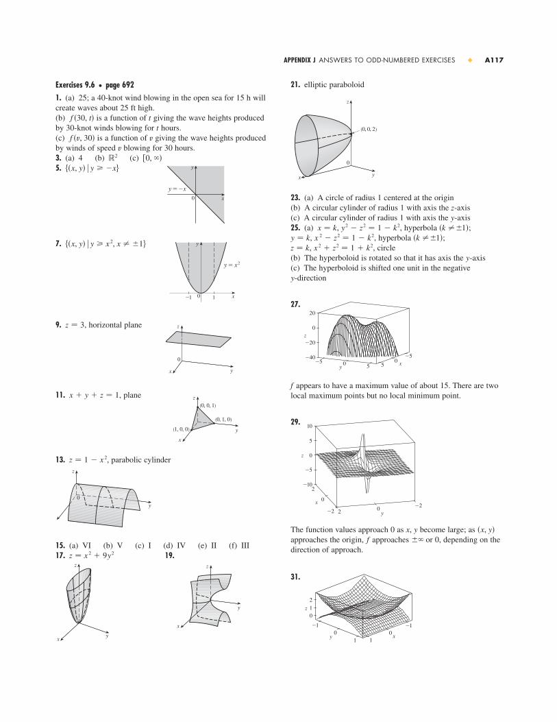
21. elliptic paraboloid
23. (a) A circle of radius 1 centered at the origin(b) A circular cylinder of radius 1 with axis the -axis(c) A circular cylinder of radius 1 with axis the -axis25. (a) , , hyperbola ;
, , hyperbola ;, , circle
(b) The hyperboloid is rotated so that it has axis the -axis(c) The hyperboloid is shifted one unit in the negative -direction
27.
f appears to have a maximum value of about 15. There are twolocal maximum points but no local minimum point.
29.
The function values approach 0 as x, y become large; as approaches the origin, f approaches or 0, depending on thedirection of approach.
31.
210
y1
0�1
x1
0�1
z
��x, y�
10
5
0
_5
_10
y2 0_2
x
2
0
_2
z
0
20
0
_20
_40
y 50_5 x5
_5
z
y
yx 2 � z2 � 1 � k2z � k
�k �1�x 2 � z2 � 1 � k2y � k�k �1�y2 � z2 � 1 � k2x � k
yz
x y
z
0
(0, 0, 2)
Exercises 9.6 � page 6921. (a) 25; a 40-knot wind blowing in the open sea for 15 h willcreate waves about 25 ft high.(b) is a function of giving the wave heights producedby 30-knot winds blowing for hours.(c) is a function of giving the wave heights producedby winds of speed blowing for 30 hours.3. (a) 4 (b) (c)5.
7.
9. , horizontal plane
11. , plane
13. , parabolic cylinder
15. (a) VI (b) V (c) I (d) IV (e) II (f) III17. 19.
z
y
x
z
xy
z � x 2 � 9y2
z
y
0
z � 1 � x 2
z
y
x
(0, 0, 1)
(0, 1, 0)
(1, 0, 0)
x � y � z � 1
z
y
0
x
z � 3
y
x0 1_1
y=≈
��x, y� � y � x 2, x � 1�
y
x0
y=_x
��x, y� � y � �x��0, ���2
vvf �v, 30�
ttf �30, t�
APPENDIX J ANSWERS TO ODD-NUMBERED EXERCISES � A117

Exercises1. (a)(b) ,(c) center , radius 53. ; ; out of the page5. 7. (a) 2 (b) �2 (c) �2 (d) 09. 11. (a) (b)13. 166 N, 114 N 15.17.19.21.23. Skew 25.27.
29. 31.
33. Ellipsoid
35. Circular cylinder
37.39.41. 43. z � 4r 2r 2 � z2 � 4, � 2
(1, s3, 2s3), (2, ��3, 2s3)(s3, 1, 2), (2s2, ��6, ��4)
(0, 1, 0)
(0, 0, 1)
z
x
y
(0, 0, 1)
(0, 1, 0)” , 0, 0’1
2
z
yx
yx
z
(0, 0, 4)
(0, 1, 0)
(2, 0, 0)
0
z
yx
(0, 2, 0)
(0, 0, 6)
(3, 0, 0)
x=¥
y
x0
��x, y� � x � y 2�22�s26
x � y � z � 4x � 2y � 5z � 8x � 1 � 4t, y � �3t, z � 1 � 5t
x � 1 � 2t, y � 2 � t, z � 4 � 3ts41�2�4, �3, 4 �cos�1( 1
3 ) 71�2, �4
� u � v � � 3s2u � v � 3s2�4, �1, �3�
x � 0�y � 2�2 � �z � 1�2 � 68�x � 1�2 � �y � 2�2 � �z � 1�2 � 69
Exercises 9.7 � page 6981. See pages 694–695.3. (a) (b)
(0, 3, 1)
5. (a) (b)7. (a) (b)
(0, 0, 1)
9. (a)(b)11. Circular cylinder, radius 3, axis the -axis13. Half-cone15. Circular paraboloid17. Circular cylinder, radius 1, axis parallel to the -axis19. Sphere, radius 5, center the origin21. (a) (b)23. (a) (b)25. 27.
29. Cylindrical coordinates: , ,
31.33.
Chapter 9 Review � page 700
True-False Quiz1. True 3. True 5. True 7. True 9. True11. False 13. False
0 � � � ��4, 0 � � cos �0 � z � 20
0 � � � 2�6 � r � 7
z
y
x
0
z
y
z=2-r@
x
1
0
z=r@
2
sin � � 2 sin �r � 2 sin � � 4r 2 � z2 � 16
z
z(2s2, ��2, 3��4)
�3, �, ��2�
( 12 s2, 1
2 s6, s2)
0
z
yx
”2, , ’
2
π4
π3
π3
π4
0
z
yx
(1, 0, 0)
1
(2, 4��3, 2)(s2, 7��4, 4)(2, �2s3, 5)
0
z
yx
”4, _ , 5’
5
4
π3
π3_
0
z
yx
”3, , 1’π2
π2
13
A118 � APPENDIX J ANSWERS TO ODD-NUMBERED EXERCISES
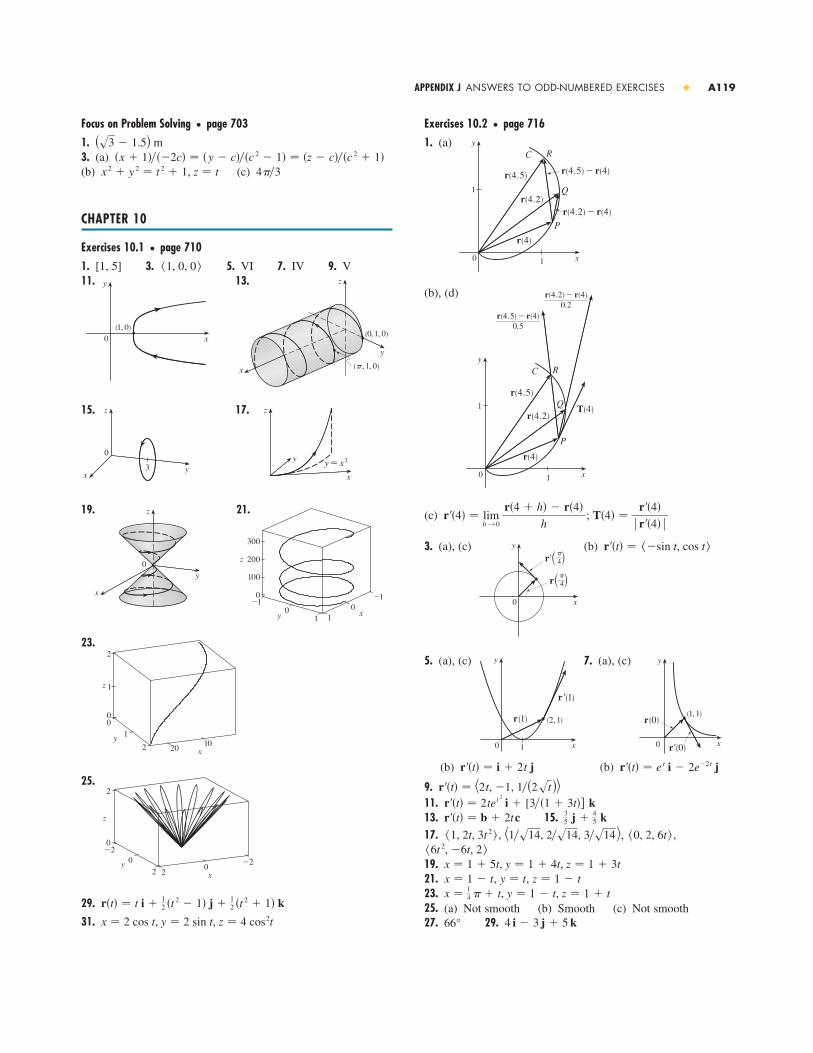
Exercises 10.2 � page 7161. (a)
(b), (d)
(c) ;
3. (a), (c) (b)
5. (a), (c) 7. (a), (c)
(b) (b)
9.11.13. 15.17. , , ,
19.21. , ,23.25. (a) Not smooth (b) Smooth (c) Not smooth27. 66° 29. 4 i � 3 j � 5 k
x � 14 � � t, y � 1 � t, z � 1 � t
z � 1 � ty � tx � 1 � tx � 1 � 5t, y � 1 � 4t, z � 1 � 3t
�6t 2, �6t, 2 ��0, 2, 6t��1�s14, 2�s14, 3�s14 ��1, 2t, 3t 2 �
35 j �
45 kr��t� � b � 2tc
r��t� � 2tet 2
i � [3��1 � 3t�� kr��t� � �2t, �1, 1�(2st )�
r��t� � e t i � 2e�2 t jr��t� � i � 2t j
y
x0
(1, 1)r(0)
rª(0)
y
x0 1
(2, 1)r(1)
rª(1)
r��t� � ��sin t, cos t�y
x0
rª ” ’π4
r ” ’π4
T�4� �r��4�
� r��4� �r��4� � lim h l 0
r�4 � h� � r�4�
h
y
x0 1
1
RC
Q
P
r(4.5)
r(4.2)
r(4)
r(4.5)-r(4)0.5
r(4.2)-r(4)0.2
T(4)
y
x0 1
1
RC
Q
P
r(4.5)
r(4.2)
r(4)
r(4.5)-r(4)
r(4.2)-r(4)
Focus on Problem Solving � page 7031.3. (a)(b) (c)
CHAPTER 10
Exercises 10.1 � page 7101. [1, 5] 3. 5. VI 7. IV 9. V11. 13.
15. 17.
19. 21.
23.
25.
29.
31. x � 2 cos t, y � 2 sin t, z � 4 cos2t
r�t� � t i �12 �t 2 � 1� j �
12 �t 2 � 1� k
02 2
�2
0
2
�2
0x
y
z
z
2
1
y2
1
0
x2010
0
_10
1 10
_1
300
200
100
0
z
y x
z
y
x
0
x
z
y y=≈
z
yx
0
3
y
x0
(1, 0)
z
y
x
(0, 1, 0)
(π, 1, 0)
�1, 0, 0 �
4��3x 2 � y 2 � t 2 � 1, z � t�x � 1����2c� � �y � c���c 2 � 1� � �z � c���c 2 � 1�
(s3 � 1.5) m
APPENDIX J ANSWERS TO ODD-NUMBERED EXERCISES � A119

5.
7.
9.11.13. ,
15. (a)(b)
17.19. ,21. (a) (b) (c)23.25. ,27. (a) 16 m (b) upstream
29. 31. 0, 1 33. 35.
Exercises 10.5 � page 7401. Circular paraboloid with axis the -axis3. Circular cylinder with axis the x-axis5.
2
0
_2
2
1
0
2
1.5
1
xy
z
√ constant
u constant
z
t � 14.5 cm�s2, 9.0 cm�s26t, 6
40
_12
0
12
40
_4
0
20
23.6 79.8 10.2
30 m�s500 m�s 3.2 km 22 km
� v�t� � � s25t 2 � 2r�t� � t i � t j �52 t 2 k
t � 4
z
yx
1.2
1
0.8
101.5
1
r�t� � �1 �12 t 2� i � t 2 j � �1 �
13 t 3�k
r�t� � t i � t j �12 t 2 kv�t� � i � j � t k
s2 i � e t j � e�t k, e t j � e�t k, e t � e�t
�1, 2t, 3t 2 � , �0, 2, 6t� , s1 � 4t 2 � 9t 4
� v�t� � � s2a�t� � �sin t i � cos t k
z
y
(0, 0, 1) v(0)
a(0)
x
v�t� � cos t i � j � sin t k
� v�t� � � se 2 t � e�2 t
a�t� � e t i � e�t jy
x0
(1, 1)
v(0)
a(0)
v�t� � e t i � e�t j31.33.35.41.
Exercises 10.3 � page 7231. 3. 5. 9.57067.
9.11. (a)
(b)13. (a)(b)15. 17. 19.21. 23.
25. ; approaches 027. (a) P (b)29.
31. is , is
33. 35.37.39.
41. 49.
Exercises 10.4 � page 7331. (a) , ,
,(b) , 2.583.
� v�t� � � s4t 2 � 1a�t� � �2, 0 �
y
x0
(0, 1)
v(1)
a(1)
v�t� � �2t, 1 �2.4 i � 0.8 j � 0.5k
2.8 i � 0.8 j � 0.4k2.8 i � 1.8 j � 0.3k2.0 i � 2.4 j � 0.6k1.8 i � 3.8 j � 0.7k
2.07 � 1010 Š2 m��1, �3, 1�
5
2.5�7.5
�5
(x �52 )2
� y 2 � 814 , x 2 � (y �
53 )2 � 16
9
y � 6x � �, x � 6y � 6�
� 23 , 23 , 13 �, �� 1
3 , 23 , � 23 �, �� 2
3 , 13 , 23 �1�(s2et)y � !�x�by � f �x�a
2.5
1.2�1.2
�0.5
y=x$
y=k(x)
1.3, 0.7(� 1
2 ln 2, 1�s2)15sx ��1 � 100x 3�3�26� x ���1 � 9x 4 �3�2
s2�4s2��1 � cos2t�3�22��4t 2 � 1�3�22��t 2 � 2�2
� t 2, 2t, 2 ���t 2 � 2�, �2t, 2 � t 2, �2t���t 2 � 2�
229
��sin t, 0, �cos t��(2�s29) cos t, 5�s29, (�2�s29) sin t�,
r�t�s�� � 3 sin�s�5� i � �4s�5� j � 3 cos�s�5�k� (1 � s�s2) cos[ln(1 � s�s2)] j
r�t�s�� � (1 � s�s2) sin[ln(1 � s�s2)] ie � e�120s29
1 � 4t cos t � 11t 2 sin t � 3t 3 cos t
13 t 3 i � �t 4 � 1� j �
13 t 3 k
e t i � t 2 j � �t ln t � t�k � C
12 i �
12 j � [�4 � ���(4s2)]k
A120 � APPENDIX J ANSWERS TO ODD-NUMBERED EXERCISES

3. ,5. 7. 15.9241 9.11. (a)
(b)
(c)13. 15.17. ,
,19. (a) About 3.8 ft above the ground, 60.8 ft from the athlete(b) (c) from the athlete21. , , ,
,23. (c)25. (b) ; no
Focus on Problem Solving � page 7451. (a) (c)3. (a) 5. (b)
7. (a) to the right of the table’s edge,(b) (c) to the right of the table’s edge
CHAPTER 11
Exercises 11.1 � page 756
1. (a) �7; a temperature of with wind blowing at feels equivalent to about without wind.(b) When the temperature is , what wind speed gives awind-chill of ? (c) With a wind speed of , what temperature gives awind-chill of ? (d) A function of wind speed that gives wind-chill values whenthe temperature is (e) A function of temperature that gives wind-chill values whenthe wind speed is 3. Yes5.
7. (a) (b) (c)9. 11. Steep; nearly flat13. z
14
yx
56, 35�1, ����x, y, z� � z � x 2 � y 2�e
y
x0
≈+¥=119
��x, y� � 19 x 2 � y 2 � 1�
50 km�h
�4 C
4 C�14 C80 km�h
20 km�h�26 C�12 C
�7 C60 km�h8 C
2.13 ft 7.6 15 ft�s 0.94 ft
�tm�k���m�k��1 � e�kt�m � � t� jR�t� � �m�k��1 � e�kt�m �v0 �90, v0
2��2t�a � ��2rv � �R��sin �t i � cos �t j�
P�x� � 3x5 � 8x4 � 6x3�2e�t vd � e�t R
��3 � � � 2��30 � � � 2�z � 2 cos �y � 2 sin � sin �x � 2 sin � cos �
64.2 ft 21.4 ft
a�t� � �1�t� i � e�t k� v�t� � � s2 � 2 ln t � �ln t�2 � e�2 t
v�t� � �1 � ln t� i � j � e�t kx � 2y � 2� � 012�173�2
st 8 � 4t 6 � 2t 4 � 5t 2��t 4 � t 2 � 1�2
�2t, 1 � t 4, �2t 3 � t��st 8 � 4t 6 � 2t 4 � 5t 2
� t 2, t, 1 ��st 4 � t 2 � 1��21
3 i � �2�� 2� j � �2���k0 � t � 2�r�t� � 4 cos t i � 4 sin t j � �5 � 4 cos t�k7. 9.
11. IV 13. I 15. II17.19.21. , ,
, ,
23. , , , ,
27. ,, ,
29. (b)
31. (a) Direction reverses (b) Number of coils doubles
Chapter 10 Review � page 742
True-False Quiz1. True 3. False 5. False 7. False 9. True
Exercises1. (a)
(b) ,r ��t� � �� 2 cos �t j � � 2 sin �t k
r��t� � i � � sin �t j � � cos �t k
z
y
x
(0, 1, 0)
(2, 1, 0)
2
0
�2
�2 �10 2 1 0
z
y x
0 � � � 2�0 � x � 3z � e�x sin �
20�101�1
0
1
y
z
x
x � x, y � e�x cos ��or x � x, y � y, z � 5, x 2 � y 2 � 16�
0 � � � 2�0 � r � 4z � 5y � r sin �x � r cos �[or x � x, y � y, z � s4 � x 2 � y 2, 2 � x 2 � y 2 � 4]
0 � � � 2�0 � � � ��4z � 2 cos �y � 2 sin � sin �x � 2 sin � cos �
x � x, z � z, y � s1 � x 2 � z 2
x � 1 � u � v, y � 2 � u � v, z � �3 � u � v
1
0
_1
10
_11
0
_1
x
y
z
√ constant
u constantz
1
0
_1
y
10
_1
x
1
0
_1
u constant
√ constant
APPENDIX J ANSWERS TO ODD-NUMBERED EXERCISES � A121
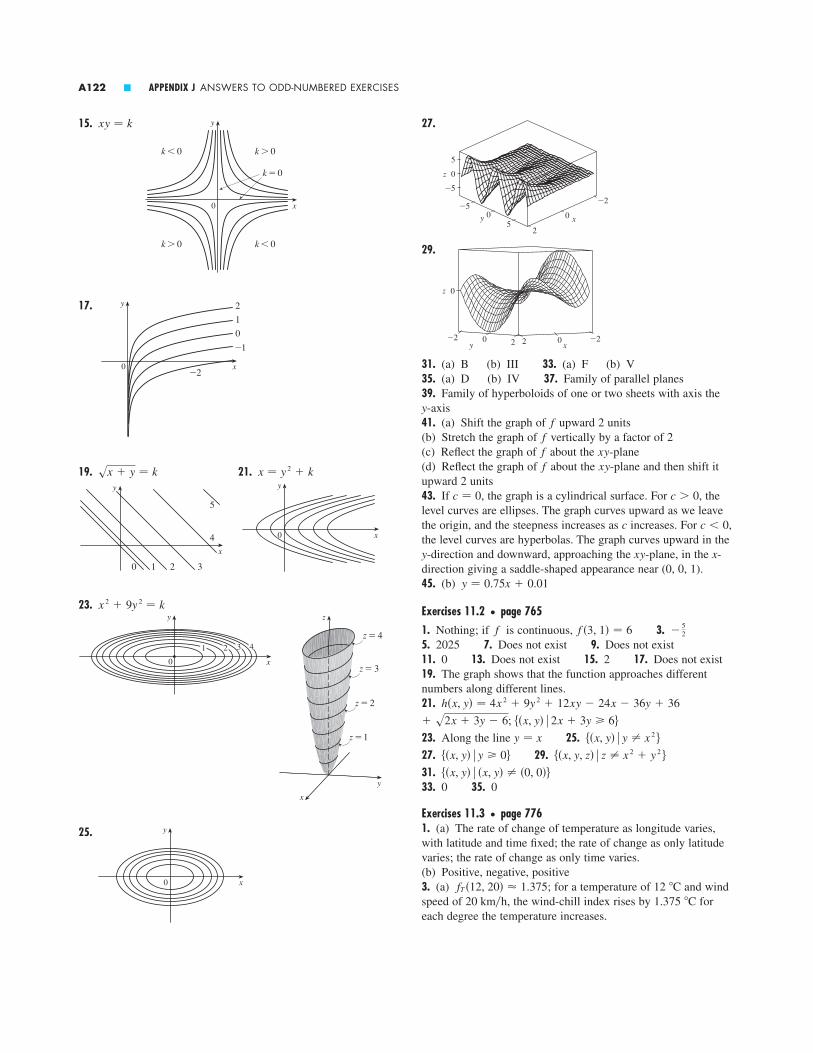
27.
29.
31. (a) B (b) III 33. (a) F (b) V35. (a) D (b) IV 37. Family of parallel planes39. Family of hyperboloids of one or two sheets with axis the y-axis41. (a) Shift the graph of upward 2 units(b) Stretch the graph of vertically by a factor of 2(c) Reflect the graph of about the -plane(d) Reflect the graph of about the -plane and then shift itupward 2 units43. If , the graph is a cylindrical surface. For , thelevel curves are ellipses. The graph curves upward as we leavethe origin, and the steepness increases as c increases. For ,the level curves are hyperbolas. The graph curves upward in they-direction and downward, approaching the xy-plane, in the x-direction giving a saddle-shaped appearance near (0, 0, 1).45. (b)
Exercises 11.2 � page 7651. Nothing; if is continuous, 3.5. 2025 7. Does not exist 9. Does not exist11. 0 13. Does not exist 15. 2 17. Does not exist19. The graph shows that the function approaches differentnumbers along different lines.21.
23. Along the line 25.27. 29.31.33. 0 35. 0
Exercises 11.3 � page 7761. (a) The rate of change of temperature as longitude varies,with latitude and time fixed; the rate of change as only latitudevaries; the rate of change as only time varies.(b) Positive, negative, positive3. (a) ; for a temperature of and windspeed of , the wind-chill index rises by foreach degree the temperature increases.
1.375 C20 km�h12 CfT �12, 20� 1.375
��x, y� � �x, y� � �0, 0����x, y, z� � z � x 2 � y 2 ���x, y� � y � 0�
��x, y� � y � x 2 �y � x
� s2x � 3y � 6; ��x, y� � 2x � 3y � 6�h�x, y� � 4x 2 � 9y 2 � 12xy � 24x � 36y � 36
�52f �3, 1� � 6f
y � 0.75x � 0.01
c � 0
c � 0c � 0
xyfxyf
ff
0
_2 0 2 2 0 _2y x
z
5
0
_5
y5
0_5
x
2
0
_2
z
15.
17.
19. 21.
23.
25. y
0 x
y
x
z
z=4
z=3
z=2
z=1
y
0 x
4321
x 2 � 9y 2 � k
y
x0
y
x
0 1 2 3
4
5
x � y 2 � ksx � y � k
y
0 x
2
1
0
_1
_2
y
0 x
k>0
k>0
k<0
k<0
k=0
xy � k
A122 � APPENDIX J ANSWERS TO ODD-NUMBERED EXERCISES

45. (a) (b)47. , ,49. , ,53. 55. 57.59.69. 73. No 75.77.79. (a)
(b) ,
(c) 0, 0 (e) No, since and are not continuous.
Exercises 11.4 � page 7881. 3.5.
7.
9. 11.
13. ; 15.17.19.21.23. 25. 27.29. 150 31. 33.35. 37.
Exercises 11.5 � page 796
1.3.5.
7. ,
�z
�t� e r�s cos � �
t
ss 2 � t 2 sin ��
�z
�s� e r�t cos � �
s
ss 2 � t 2 sin ��
�z��s � 2x � y � xt � 2yt, �z��t � 2x � y � xs � 2yse y�z�2t � �x�z� � �2xy�z2 ��� cos x cos y � �sin x sin y��(2st )
�1 � �x, �2 � �yx � 03x � y � 3z � 31
17 0.059 �16 cm35.4 cm2�z � 0.9225, dz � 0.9
dw � �x 2 � y 2 � z2 ��1�x dx � y dy � z dz�du � e t sin � dt � e t cos � d�
4T � H � 329; 129 F
37 x �
27 y �
67 z; 6.99142.846�
23 x �
73 y �
203
12 x � y �
14 � �
122x �
14 y � 1
0
2
42
0x4
02 y
z
400
200
0
y5 0 _5x10
0_10
z
x � 2y � z � 4z � �8x � 2y
fyxfxy
fy�x, y� �x 5 � 4x 3y 2 � xy 4
�x 2 � y 2 �2fx�x, y� �x 4y � 4x 2y 3 � y 5
�x 2 � y 2 �2
_0.2
0.2
0
_1
0
1y
10
_1
x
z
�2x � 1 � t, y � 2, z � 2 � 2tR2�R1
2
12.2, 16.8, 23.25�sin y48x 3y 3z2�48xy
utt � �e�s sin tust � �e�s cos t � utsuss � e�s sin tfyy � �18x 2yfxy � �18xy 2 � fyxfxx � 12x 2 � 6y 3
f ��x � y�, f ��x � y�f ��x�, t��y�; for a temperature of and wind speedof , the wind-chill index decreases by for each
the wind speed increases.(b) Positive, negative (c) 05. (a) Positive (b) Negative7.9. ,
11.
13.15.17.19.21.23. ,25.27. , ,
29. , ,31. , , ,
33. 35. 37.39. ,41.43. �x � y � z���x � z�, �y � x���x � z�
�y � z���x � y�, �x � z���x � y�fy�x, y� � 4y � xfx�x, y� � 2x � y
�13
35�u��xi � xi�sx1
2 � x22 � � � � � xn
2
ft � �x � y���z � t�2fz � �y � x���z � t�2fy � 1��t � z�fx � 1��z � t�
�u��� � xe�t cos ��u��t � �xe�t sin ��u��x � e�t sin ��w��z � 3��x � 2y � 3z�
�w��y � 2��x � 2y � 3z��w��x � 1��x � 2y � 3z�fx � y 2z3, fy � 2xyz3 � 3z, fz � 3xy 2z2 � 3y
�z��y � y�(x 2 � y 2 � xsx 2 � y 2 )�z��x � 1�sx 2 � y 2
fu � v��u 2 � v2 �, fv � �u��u 2 � v2 ��w�� � cos cos �, �w��� � �sin sin �fx�x, y� � 2y��x � y�2, fy�x, y� � �2x��x � y�2�z��x � e 3y, �z��y � 3xe 3yfx�x, y� � 3, fy�x, y� � �8y 3
fy
0
_20
2x _2 0 2y
z
10
0
_20
2x _2 0 2y
_10
zfx
10
0_2
02x _2 0 2
y
zf
fx � 2x � 2xy, fy � 2y � x 2
z
y
0
x
(1, 2, 8)
C¡
(1, 2)
2
16
4
z
y
0
x
(1, 2, 8)
C™
(1, 2)
2
16
4
fy�1, 2� � �4 � slope of C2fx�1, 2� � �8 � slope of C1
c � f, b � fx, a � fy
km�h0.3 C20 km�h
12 Cfv�12, 20� �0.3
APPENDIX J ANSWERS TO ODD-NUMBERED EXERCISES � A123

45.49.53. If and , then and are known, so we solve linear equations for and .
Exercises 11.7 � page 818
1. (a) f has a local minimum at (1, 1).(b) f has a saddle point at (1, 1).3. Local minimum at (1, 1), saddle point at (0, 0)5. Maximum 7. Minimum , saddle points 9. Saddle point (1, 2) 11. None13. Saddle points , n an integer15. Maximum , minimum ,saddle points 17. Maximum ,minimum 19. Minima , ,saddle point (0.312, 0), lowest point 21. Maxima , ,saddle points ,highest points 23. Maximum , minimum 25. Maximum , minimum 27. Maximum , minimum 29.
31. 33. 35.37. 39. 41. Cube, edge length 43. Square base of side 40 cm, height 20 cm
Exercises 11.8 � page 827
1. 3. Maxima , minima
5. Maxima , minima 7. Maximum , minimum
9. Maximum , minimum
11. Maximum , minimum 1
13. Maximum ,
minimum
15. Maximum ,minimum 17. Maximum , minimum
19. Maxima ,
minima f (1�s2, 1�(2s2)) � e�1�4
f (1�s2, �1�(2s2)) � e 1�4
12
32
f (1, �s2, s2) � 1 � 2s2f (1, s2, �s2) � 1 � 2s2
f (� 12 , � 1
2 , � 12 , � 1
2 ) � �2
f ( 12, 12 , 12 , 12 ) � 2
s3
�2�s32�s3f ��1, �3, �5� � �70
f �1, 3, 5� � 70f �2, �1� � �4f �2, 1� � 4
f �0, 1� � �1f �1, 0� � 1 59, 30
c�124316�s3
1003 , 100
3 , 1003�0, 0, 1�, �0, 0, �1�s3
_3
_2
_1
0
_1 0 1_2
24
x
y
z
(_1, 0, 0) (1, 2, 0)
f ��2, 4� � �9f �2, 4� � 3f �0, 0� � 4f �1, 1� � 7
f �0, 3� � �14f �2, 0� � 9�1.629, 1.063, 8.105�
��0.259, 0�, �1.526, 0�f �1.629, 1.063� 8.105f ��1.267, 0� 1.310��1.714, 0, �9.200�
f �1.402, 0� 0.242f ��1.714, 0� �9.200f �5��3, 5��3� � �3s3�2
f ���3, ��3� � 3s3�2�1, 1�
f �0, 2� � �2f �0, 0� � 2�0, n��
(s2, �1)f �0, 0� � 4f (�1, 12 ) � 11
fyfx
c fx � dfyafx � bfyv � �c, d �u � �a, b �x � �1 � 10t, y � 1 � 16t, z � 2 � 12t(s6�3, �2s6�3, s6�2)9. 62
11. , ,
13. ,
,
15. 2, 0 17. 0, 0, 419. , ,
21.
23. ,
25.
27.29.31. (a) (b) (c) 33.35. (a) ,
41.
Exercises 11.6 � page 808
1. 3. 0.83 5.7. (a)(b) (c)9. (a)(b) (c)11. 13. 15. 17.19. 21.23. (b) 25. All points on the line 27. (a)29. (a) (b) (c) 31.
35. (a) (b)
37. (a) (b)39. 41.
y
0 x
(2, 1)
±f(2, 1)
x+2y=4
1
_1
0
1
2
1 2x 2
z
y
�4, 8 � , x � 2y � 4x � 1 � y � �zx � y � z � 1
x � 4
8�
y � 1
�4�
z � 1
64x � 2y � 3z � 21
327132s406�38, 6, 12 �32�s3
�40�(3s3)y � x � 1��12, 92 �
s11, �1, �1, �3 �1, �0, 1 �2�5���(4s3)4�923�10
20�s3�4, �4, 12�" f �x, y, z� � � y 2z3, 2xyz3, 3xy 2z2 �
172�13��4, 16 �" f �x, y� � �5y 2 � 12x 2y, 10xy � 4x 3 �
516 s3 �
14 �0.1 millibar�mi
4rs �2z��x 2 � �4r 2 � 4s 2 ��2z��x �y � 4rs �2z��y 2 � 2 �z��y�z��� � ���z��x�r sin � � ��z��y�r cos �
�z��r � ��z��x� cos � � ��z��y� sin ��0.27 L�s0 m�s10 m2�s6 m3�s
�0.33 m�s per minute2 C�s
��e y � ze x ���y � e x �, ��xe y � z���y � e x �
�2xy � z2
2yz � x 2�y 2 � 2xz
2yz � x 2
sin�x � y� � e y
sin�x � y� � xe y
�u��t � 2��y � z� � 1�p�u��r � 0�u��p � 2�z � x���y � z�2 � �t�p 2
�v
�z�
�v
�p �p
�z�
�v
�q �q
�z�
�v
�r �r
�z
�v
�y�
�v
�p �p
�y�
�v
�q �q
�y�
�v
�r �r
�y
�v
�x�
�v
�p �p
�x�
�v
�q �q
�x�
�v
�r �r
�x
�u
�t�
�u
�x �x
�t�
�u
�y �y
�t
�u
�s�
�u
�x �x
�s�
�u
�y �y
�s
�u
�r�
�u
�x �x
�r�
�u
�y �y
�r
A124 � APPENDIX J ANSWERS TO ODD-NUMBERED EXERCISES

53. Maximum ; saddle points (0, 0), (0, 3), (3, 0)55. Maximum , minimum 57. Maximum , minima ,saddle points 59. Maximum ,minimum 61. Maximum 1, minimum 63.65.
Focus on Problem Solving � page 8361. 3. (a) (b) Yes9.
CHAPTER 12
Exercises 12.1 � page 8471. (a) �17.75 (b) �15.75 (c) �8.75 (d) �6.753. (a) 288 (b) 144 5. (a) �6 (b) �3.57. 9. (a) (b) 15.5 11. 6013. 3 15. 0.6065, 0.5694, 0.5606, 0.5585, 0.5579, 0.5578
Exercises 12.2 � page 8531. 3. 10 5.7. 9. 6 11. 13.15.17. 19. 37.5
21.23.25. 36
27. 29.
31. Fubini’s Theorem does not apply. The integrand has an infi-nite discontinuity at the origin.
Exercises 12.3 � page 8611. 3. 5. 7. 9.11. 13. 15. 0
17. 19. 21. 23. 25. 0, 1.213, 0.71327. 13,984,735,616�14,549,535
13
16
318
635
14720�1 � cos 1��2
12 ln 2256
21e � 149 e 3�2 �
3245
920
56
2
0
y1
0
x10
z
21e � 57
415 (2s2 � 1)16627
z
yx
0
1
1
4
[(s3 � 1)�2] � ���12�9 ln 221
2212 ln 2
415 (31 � 9s3)9 � 27y, 8x � 24x 2
248U � V � L
s6�2, 3s2�2x � w�3, base � w�3L2W 2, 14 L2W 2
P(2 � s3), P(3 � s3)�6, P(2s3 � 3)�3(3�1�4, 3�1�4
s2, 31�4 ), (3�1�4, �3�1�4s2, 31�4 )
�1f (s2�3, �1�s3) � �2�(3s3)
f (s2�3, 1�s3) � 2�(3s3)��1, 1�, �1, 0�
f �1, 1� � �3f ��1, 0� � 2f �2, 4� � �64f �1, 2� � 4
f �1, 1� � 125–35. See Exercises 31–41 in Section 11.7.37. Nearest , farthest 39. Maximum , minimum 41. (a) (b) When
Chapter 11 Review � page 832
True-False Quiz1. True 3. False 5. False 7. True 9. False11. True
Exercises1. 3.
5. 7.
9.11. (a) ,(b) by Equation 11.6.9 (Definition 11.6.2 gives .)(c)13. ,15. ,17. , ,19. , ,21. , ,
, ,,
25. (a) (b)
27. (a) (b)
29. (a)(b)31.33.35. 37.43. 45. 47.49. 51. Minimum f ��4, 1� � �11 5
8 knot�mis145�2, �4, 92 �43
5ze x sy �zsy, xz�(2sy ), 2��47, 108e t � 2�y�z��3t 2 � 4� � 2t�y 2�z2 �
60x �245 y �
325 z � 120; 38.656
(s2�7, 1�s14, �3�s14)x � 3 � 8t, y � 4 � 2t, z � 1 � 4t
4x � y � 2z � 6
x � 2
4�
y � 1
�4�
z � 1
�62x � 2y � 3z � 3
x � 1
8�
y � 2
4� 1 � zz � 8x � 4y � 1
f zz � m�m � 1�x k y lz m�2f yz � lmx k y l�1z m�1 � f zy
f yy � l�l � 1�x k y l�2z mf xz � kmx k�1y lz m�1 � f zx
f xy � klx k�1y l�1z m � f yxf xx � k�k � 1�x k�2 y lz mf yy � �2xf xy � �2y � f yxf xx � 24x
Tr � per��q � er �Tq � p��q � er �Tp � ln�q � er�tv � u��1 � v 2�tu � tan�1v
fy � y�s2x � y 2fx � 1�s2x � y 2
�0.25 1.1 C�m
0.35 C�m�3.0 C�m 3.5 C�m
23
x210
y
2
1
y
0 x
z
0
y1
x
1
1
y
0 x_1 1
��x, y� � �1 � x � 1�
x1 � x2 � � � � � xnc�n �5.3506 9.7938
��1, �1, 2�( 12, 1
2 , 12 )
APPENDIX J ANSWERS TO ODD-NUMBERED EXERCISES � A125

Exercises 12.6 � page 8811. 3. 5.7. 9.11. 13. (a) (b)15. 4.450617.19. (b)
(c)
21. 25.
Exercises 12.7 � page 8903. 1 5. 7. 4 9. 11.13. 15. 17.19. (a) (b)
21. 60.533 23.
25.
27.
29.
31.
� x10 x1
z xxz f �x, y, z� dy dx dz
� x10 xx
0 xxz f �x, y, z� dy dz dx� x1
0 xy0 x1
y f �x, y, z� dx dz dy
� x10 x1
z x1y f �x, y, z� dx dy dzx
10 xx
0 xy0 f �x, y, z� dz dy dx
�x10 x�1�z�2
0 x1�zsx
f �x, y, z� dy dx dz
� x10 x1�sx
0 x1�zsx
f �x, y, z� dy dz dx
� x10 x1�y
0 xy 2
0 f �x, y, z� dx dz dy� x10 x1�z
0 xy 2
0 f �x, y, z� dx dy dz
� x10 xy 2
0 x1�y0 f �x, y, z� dz dx dyx
10 x1
sx x1�y
0 f �x, y, z� dz dy dx
� x10 xs1�z
�s1�z x1�x 2
z f �x, y, z� dy dx dz
� x1�1 x
1�x 2
0 x1�x 2
z f �x, y, z� dy dz dx
� x10 xy
0 xs1�y�s1�y
f �x, y, z� dx dz dy
� x10 x1
z xs1�y
�s1�y f �x, y, z� dx dy dz� x1
0 xs1�y�s1�y
xy0 f �x, y, z� dz dx dy
x1�1 x
1�x 2
0 xy0 f �x, y, z� dz dy dx
� x2�2 x
s4�z 2
�s4�z 2 x6
0 f �x, y, z� dy dx dz
� x2�2 x
s4�x 2
�s4�x 2 x6
0 f �x, y, z� dy dz dx
� x60 x2
�2 xs4�z 2
�s4�z 2 f �x, y, z� dx dz dy
� x2�2 x
60 xs4�z 2
�s4�z 2 f �x, y, z� dx dy dz
� x60 x2
�2 xs4�x 2
�s4�x 2 f �x, y, z� dz dx dy
x2
�2 x6
0 xs4�x 2
�s4�x 2 f �x, y, z� dz dy dx
z
y
x
01
2
1
14 � �
13x
10 xx
0 xs1�y 2
0 dz dy dx
815
16316��3
112
6528
13 �e 3 � 1�
� (37s37 � 17s17)�64�
x2�
0 x�
0 s36 sin4u cos2v � 9 sin4u sin2v � 4 cos2u sin2u du dv
2
0
�2
�2 �10 2 1 0
z
y x
458 s14 �
1516 ln[(11s5 � 3s70)�(3s5 � s70)]
1.8616 1.83�2��3�(2s2 � 1)(s21�2) �
174 [ln(2 � s21) � ln s17]�(2s6 �
83 )
���6�(17s17 � 5s5)3s1415s26
29. 31.
33.
35. 37. 39. 41. 1
43. 47. 49.
Exercises 12.4 � page 867
1. 3.5.7.
9. 0 11. 13. 0
15. 17. 19.21. 23. 25.27. 29. 31.33. (a) (b)
Exercises 12.5 � page 8771. 3. 5.
7. 9.11. if vertex is (0, 0) and sides are along positive axes13. 15.
17. , , ,
,19. (a) (b) 0.375 (c)21. (b) (i)(ii) (c) 2, 523. (a) (b)25. (a) , where Dis the disk with radius 10 mi centered at the center of the city(b) , on the edge200�k�3 209k, 200(��2 �
89 )k 136k
xxD �k�20�[20 � s�x � x0 �2 � �y � y0 �2 ] dA
0.632 0.5001 � e�1.8 � e�0.8 � e�1 0.3481
e�0.2 0.8187
548 0.10421
2
I0 � � 4�16 � 9� 2�64Iy � �� 4 � 3� 2 ��16
Ix � 3� 2�64�x, y � � �2�
3�
1
�,
16
9��m � � 2�8
18920 , 1269
28 , 191735
45 , 83 , 52
15
�2a�5, 2a�5�( 3
8, 3��16)272 , ( 8
5 , 12 )6, ( 3
4 , 32 )43 , (4
3 , 0)643 C
s��2s��4
15161800� ft34��3
���4��e � 1���12�8��3�(64 � 24s3)�2��3�[1 � (1�s2)]4
3 �a 381��2
���2��1 � e�4 �
33��2y
0 x
4 7
R
x2�
0 x52 f �r cos �, r sin �� r dr d�
x2
�2 x2
x f �x, y� dy dxx2�
0 x20 f �r cos �, r sin �� r dr d�
2��38�0 � xxD sx 3 � y 3 dA � s2
(2s2 � 1)�314 sin 81�e 9 � 1��6
y
x0
x=2
y=2x4
2
(2, 4)
x10 x1
y f �x, y� dx dy
y
x0
x=2
y=ln x or x=e†
ln 2
1 2
y=0
y
x0
x=1y=x
y=0
1
1
xln 2
0 x2e y f �x, y� dx dyx
10 x1
y f �x, y� dx dy
A126 � APPENDIX J ANSWERS TO ODD-NUMBERED EXERCISES
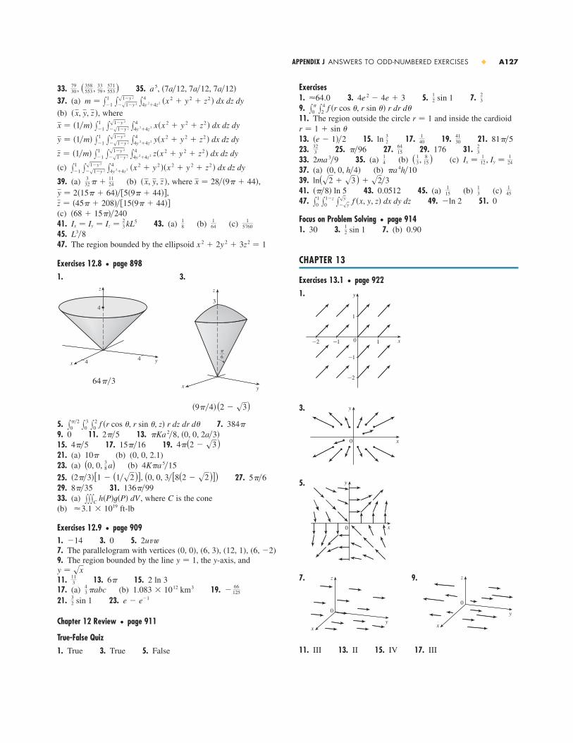
Exercises1. 3. 5. 7.9.11. The region outside the circle and inside the cardioid
13. 15. 17. 19. 21.23. 25. 27. 29. 176 31.33. 35. (a) (b) (c)37. (a) (b)39.41. 43. 0.0512 45. (a) (b) (c)47. 49. 51. 0
Focus on Problem Solving � page 9141. 30 3. 7. (b) 0.90
CHAPTER 13
Exercises 13.1 � page 9221.
3.
5.
7. 9.
11. III 13. II 15. IV 17. III
z
y
0
x
z
y
0
x
y
x0
y
x0
y
1
0
_1
1 x_1_2
_2
12 sin 1
�ln 2x10 x1�z
0 xsy�sy f �x, y, z� dx dy dz
145
13
115���8� ln 5
ln(s2 � s3) � s2�3�a 4h�10�0, 0, h�4�
Ix � 112 , Iy � 1
24 ( 13 , 8
15 )142ma 3�9
23
6415��9632
3
81��54130
140ln 3
2�e � 1��2r � 1 � sin �
r � 1x
�
0 x42 f �r cos �, r sin �� r dr d�
23
12 sin 14e 2 � 4e � 3 64.0
33. 35.37. (a)
(b) , where
(c)
39. (a) (b) , where ,,
(c)41. 43. (a) (b) (c)45.47. The region bounded by the ellipsoid
Exercises 12.8 � page 8981. 3.
5. 7.9. 0 11. 13.15. 17. 19.21. (a) (b) (0, 0, 2.1)23. (a) (b)
25. 27.29. 31.33. (a) , where is the cone(b) ft-lb
Exercises 12.9 � page 9091. �14 3. 0 5.7. The parallelogram with vertices (0, 0), (6, 3), (12, 1), (6, �2)9. The region bounded by the line , the y-axis, and
11. 13. 15. 2 ln 317. (a) (b) 19.21. 23.
Chapter 12 Review � page 911
True-False Quiz1. True 3. True 5. False
e � e�132 sin 1
�66
1251.083 � 1012 km343 �abc
6�113
y � sxy � 1
2uvw
3.1 � 1019Cxxx
C h�P�t�P� dV
136��998��355��6�2��3�[1 � (1�s2)], (0, 0, 3�[8(2 � s2)])
4K�a 5�15(0, 0, 38 a)
10�4�(2 � s3)15��164��5
�Ka 2�8, �0, 0, 2a�3�2��5384�x
��20 x3
0 x20 f �r cos �, r sin �, z� r dz dr d�
�9��4� (2 � s3)
64��3x y
z
π6
3
x 4 y4
z
4
x 2 � 2y 2 � 3z2 � 1L3�8
15760
164
18Ix � Iy � Iz � 2
3 kL5�68 � 15���240
z � �45� � 208���15�9� � 44��y � 2�15� � 64���5�9� � 44��
x � 28��9� � 44��x, y, z �332 � �
1124
x1�1 x
s1�y 2
�s1�y 2 x4
4y 2�4z 2 �x 2 � y 2 ��x 2 � y 2 � z2 � dx dz dy
z � �1�m� x1�1 x
s1�y 2
�s1�y 2 x4
4y 2�4z 2 z�x 2 � y 2 � z2 � dx dz dy
y � �1�m� x1�1 x
s1�y 2
�s1�y 2 x4
4y 2�4z 2 y�x 2 � y 2 � z2 � dx dz dy
x � �1�m� x1�1 x
s1�y 2
�s1�y 2 x4
4y 2�4z 2 x�x 2 � y 2 � z2 � dx dz dy
�x, y, z �m � x
1�1 x
s1�y 2
�s1�y 2 x4
4y 2�4z 2 �x 2 � y 2 � z2 � dx dz dy
a 5, �7a�12, 7a�12, 7a�12�7930 , ( 358
553 , 3379 , 571
553 )
APPENDIX J ANSWERS TO ODD-NUMBERED EXERCISES � A127
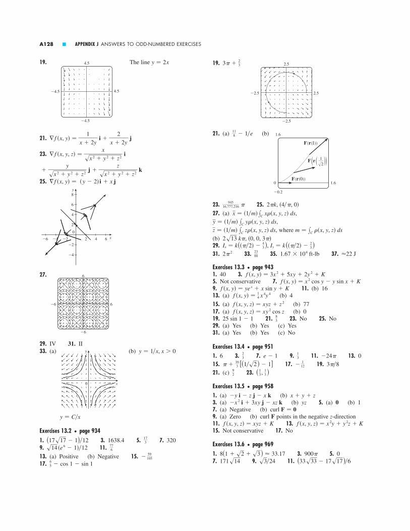
19.
21. (a) (b)
23. 25.27. (a) ,
,, where
(b)29. ,31. 33. 35. 37.
Exercises 13.3 � page 9431. 40 3.5. Not conservative 7.9. 11. (b) 1613. (a) (b) 4
15. (a) (b) 7717. (a) (b) 019. 21. 23. No 25. No29. (a) Yes (b) Yes (c) Yes31. (a) Yes (b) Yes (c) No
Exercises 13.4 � page 9511. 6 3. 7. 9. 11. 13. 015. 17. 19.21. (c) 23.
Exercises 13.5 � page 9581. (a) (b)3. (a) (b) 5. (a) 0 (b) 17. (a) Negative (b)9. (a) Zero (b) curl F points in the negative -direction11. 13.15. Not conservative 17. No
Exercises 13.6 � page 9691. 3. 5. 07. 9. 11. (33s33 � 17s17)�6s3�24171s14
900�8(1 � s2 � s3) 33.17
f �x, y, z� � x 2y � y 2z � Kf �x, y, z� � xyz � Kz
curl F � 0yz�x 2 i � 3xy j � xz k
x � y � z�y i � z j � x k
( 13, 13 )9
2
3��8�1
12� �163 [(1�s2) � 1]
�24�13e � 12
3
8325 sin 1 � 1
f �x, y, z� � xy 2 cos zf �x, y, z� � xyz � z 2
f �x, y� � 14 x 4y 4
f �x, y� � ye x � x sin y � Kf �x, y� � x 2 cos y � y sin x � K
f �x, y� � 3x 2 � 5xy � 2y 2 � K
22 J1.67 � 104 ft-lb23882� 2
Iy � k (���2� �23 )Ix � k(���2� �
43 )
2s13 k�, �0, 0, 3��m � xC �x, y, z� dsz � �1�m� xC z �x, y, z� ds
y � �1�m� xC y �x, y, z� ds
x � �1�m� xC x �x, y, z� ds
2�k, �4��, 0�94516,777,216 �
1.6
�0.2
0 1.6
F(r(1))
F(r(0))
F ”r ” ’’1
œ„2
118 � 1�e
2.5
�2.5
�2.5 2.5
3� �23
19. The line
21.
23.
25.
27.
29. IV 31. II33. (a) (b)
Exercises 13.2 � page 9341. 3. 1638.4 5. 7. 3209. 11.13. (a) Positive (b) Negative 15.17. 6
5 � cos 1 � sin 1�
59105
776s14 �e 6 � 1��12
173(17s17 � 1)�12
y � C�x
y � 1�x, x � 0y
x0
6
6�6
�6
y
2
0
_2
2 x_2_4
_4
4
4
6
_6 6
8
" f �x, y� � �y � 2� i � x j
�y
sx 2 � y 2 � z2 j �
z
sx 2 � y 2 � z2 k
∇ f �x, y, z� �x
sx 2 � y 2 � z2 i
∇ f �x, y� �1
x � 2y i �
2
x � 2y j
y � 2x4.5
�4.5
�4.5 4.5
A128 � APPENDIX J ANSWERS TO ODD-NUMBERED EXERCISES

15. 17.
19. 21.
23. 25.
27. 29. (a)(b) 31.33. 35. 37.39. 41.
Exercises B � page A161. 5 3.7. 9.
11. 13. 15.17. 19. 21.23.25. , 27. ,
29. 31. 33.
35.
37. 39.41. 45. y � x � 3�1, �2�
�2, �5�, 4�x � 3�2 � �y � 1�2 � 25
0
y
x
y=1-2x
y=1+x
�0, 1�
0
y
x
x � 2
y � 4
0
y
x_2 20
y
x
0 x
y
_3
0 x
y
b � �3m � 34b � 0m � �
13
y � 52 x �
12
y � �12 x �
112y � 5y � 3x � 3
y � 3x � 2y � �5x � 11y � 6x � 15
0 x
y
xy=0
0 3 x
y
x=3
�92
x � �a � b�c��ab��1.3, 1.7����, �7� � ��3, ���3, 5���3, 3�2, � 4
3�30 C � T � 20 CT � 20 � 10h, 0 � h � 1210 � C � 35
0 14
_1 10
���, 0� � ( 14, �)��1, 0� � �1, ��
0 1_œ„3 0 œ„3
���, 1�(�s3, s3)
1 20 1
���, 1� � �2, ���0, 1�13. 15. 17. 19.21. 23. 25. 0 27. 48 29. 3.489531. ,where projection on -plane33.35. (a) (b)37. 39. 41.
Exercises 13.7 � page 9753. 0 5. 0 7. �1 9.11. (a) (b)
(c) ,,
17. 16
Exercises 13.8 � page 9821. Negative at , positive at 7. 2 9.11. 0 13. 15.17.
Chapter 13 Review � page 985
True-False Quiz1. False 3. True 5. False 7. True
Exercises1. (a) Negative (b) Positive 3. 5.7. 9. 5 11. 13. 017. 25. 27.31. 35. 37. 21
APPENDIXES
Exercises A � page A61. 18 3. 5.
7. 9.
11. 13.
0_10_2
��1, ����2, ��
x 2 � 1� x � 1 � � x � 1
�x � 1
for x � �1
for x � �1
2 � x5 � s5
�4�12
�64��3�(391s17 � 1)�60�8�f �x, y� � e y � xe xy17
2
��4s5
13��20341s2�60 �
8120 arcsin(s3�3)12��5
9��2P2P1
0 � t � 2�z � 1 � 3�cos t � sin t�
_2
0
2
4
_2 0 2 20
_2
z
y x
x � 3 cos t, y � 3 sin t
�2
5
0
�5
z
0y
2�2 2
0x
81��2�4�
1248�8�a 3�0�3194,400�4329s2��5Iz � xxS �x 2 � y 2 � �x, y, z� dS
�0, 0, a�2�xzD �
xxS F � dS � xxD �P��h��x� � Q � R��h��z�� dA108��
16
71318016�16��s2�4
APPENDIX J ANSWERS TO ODD-NUMBERED EXERCISES � A129

9. 11.
13. 15. 17. 19.
21. 80 23. 3276 25. 0 27. 61 29.31. 33.35.41. (a) (b) (c) (d)
43. 45. 14 49.
Exercises G � page A57
1. 3.
5. 7.
9.
11.
13. 15.
17.
19.
21.23.
25.
27.29.31. , where
33. (a)
(b)
The CAS omits the absolute value signs and the constant of integration.
Exercises H.1 � page A66
1. (a) (b)
�2, 5��4�, ��2, 9��4��1, 5��2�, ��1, 3��2�
π4
”_2, ’π4
O
”1, ’π2
75,772
260,015s19 tan�1
2x � 1
s19� C
11,049
260,015 ln�x 2 � x � 5� �
3146
80,155 ln � 3x � 7 � �
4822
4879 ln � 5x � 2 � �
334
323 ln � 2x � 1 � �
1
260,015 22,098x � 48,935
x 2 � x � 5
24,110
4879
1
5x � 2�
668
323
1
2x � 1�
9438
80,155
1
3x � 7�
C 10.23t � �ln P �19 ln�0.9P � 900� � C
�12 ln 3 �0.55
12 ln�t 2 � 1� �
12 ln�t 2 � 2� � (1�s2) tan�1(t�s2) � C
13 ln � x � 1 � �
16 ln�x 2 � x � 1� �
1
s3 tan�1
2x � 1
s3� C
ln�x � 1�2 � ln sx 2 � 1 � 3 tan�1x � Cln s3 � (s3��18)
�1
36 ln � x � 5 � �
1
6
1
x � 5�
1
36 ln � x � 1 � � C
275 ln 2 �
95 ln 3 (or 95 ln 83)
2 ln 2 �12ln 3 � 3 ln 6 � 3 ln 4 � ln 81
8
12 x 2 � 2x � 6 ln � x � 2 � � C
A
x�
B
x 2 �Cx � D
x 2 � x � 2
A
x�
Bx � C
x 2 � 21 �
A
x � 1�
B
x � 1
A
x�
B
x 2 �C
x 3 �D
x � 1
A
2x � 1�
B
x � 2
2n�1 � n 2 � n � 213
an � a097
3005100 � 1n 4
n�n 3 � 2n 2 � n � 10��4n�n 2 � 6n � 11��3n�n 2 � 6n � 17��3
n�n � 1�
�n
i�1 x i�
5
i�0 2 i�
n
i�1 2i�
19
i�1
i
i � 1
�10
i�1 i1 � 1 � 1 � 1 � � � � � ��1�n�1
53.
Exercises C � page A271. (a) (b) 3. (a) (b)5. 7.9. (a) (b)
11. , , ,, ,
13. , , , ,15. 5.73576 cm 17. 24.62147 cm 27.29. 31.33. and 35.37.
39.
41. (a) (b) 43. (a) (b)
47. (a) (b)
Exercises D � page A371. (or any smaller positive number)3. 0.6875 (or any smaller positive number)5. 0.11, 0.012 (or smaller positive numbers)11. (a) (b) Within approximately 0.0445 cm(c) Radius; area; ; 1000; 5; 13. 15. (a) 17 (a) 0 (b) 9, 11
Exercises F � page A48
1. 3.
5. 7. 110 � 210 � 310 � � � � � n10�1 �13 �
35 �
57 �
79
34 � 35 � 36s1 � s2 � s3 � s4 � s5
x � 100N � 13 0.0445s1000��
s1000�� cm
47
����2, ��2�[� 23 , 0]
���40.7���4��6
y
0 x3π2
2πππ2
5π2
3π
y
0 x
112
π3
5π6
0 � x � ��4, 3��4 � x � 5��4, 7��4 � x � 2�5��6 � x � 2�0 � x � ��6��6, ��2, 5��6, 3��2��3, 5��3
(4 � 6s2)�15cot � � 4
3sec � � 54csc � � 5
3tan � � 34cos � � 4
5
cot�3��4� � �1sec�3��4� � �s2csc�3��4� � s2tan�3��4� � �1cos�3��4� � �1�s2sin�3��4� � 1�s2
0x
y
_3π4
0 x
y
315°
23 rad � �120���3� cm
�67.5720��207��6
0 x
y
1
5
A130 � APPENDIX J ANSWERS TO ODD-NUMBERED EXERCISES

27. 29.
31. 33.
35. 37.
39. (a) For , the loop begins at andends at ; for , it begins at
and ends at .41. 43.45. Horizontal at , ; vertical at 47. Horizontal at , , and the pole;vertical at (2, 0), ,49. Center , radius 51. 53.
55. By counterclockwise rotation through angle , , or about the origin57. (a) A rose with n loops if n is odd and 2n loops if n is even(b) Number of loops is always 2n59. For , the curve is an oval, which develops a dim-ple as . When , the curve splits into two parts, oneof which has a loop.
Exercises H.2 � page A721. 3. 5. 7. 41��4� 3�6��12 � s3�8� 2�64
a � 1a l1�
0 � a � 1
��3��6
_3 3
_2.5
3.5
_3.4 1.8
_2.6
2.6
sa 2 � b 2�2�b�2, a�2�( 1
2, 4��3)( 12, 2��3)
( 32, 5��3)( 3
2, ��3)�3, 0�, �0, ��2�
(�3�s2, 3��4)(3�s2, ��4)�11�s3
� � 2� � sin�1�1�c�� � � � sin�1�1�c�c � 1� � � � sin�1��1�c�
� � sin�1��1�c�c � �1
(2, 0) (6, 0)
O 1
1
2
¨=π4¨=π
8
O
(c)
3. (a) (b)
(c)
5. (a) (i) (ii)(b) (i) (ii)
7. 9.
11.
13. 15.17. 19.21. (a) (b)
23. 25.
O
”1, ’π2
O
(5, 0)
x � 3� � ��6r � 5r sin � � 5
�x 2 � y 2 �2 � 2xyx 2 � (y �32 )2 � ( 3
2 )2
O
r=2r=3
¨=7π3
¨=5π3
O
r=2
O
r � 1
��4, 5��6��4, 11��6�(�s2, 5��4)(s2, ��4)
(�12, �s3�2)π
3
”_1, ’π3
��2, 2��0, 3�
O
”2œ„2, ’3π4
3π4
O
”3, ’π2
π2
�3, 2 � 2��, ��3, 2 � ��
2
(3, 2)
O
APPENDIX J ANSWERS TO ODD-NUMBERED EXERCISES � A131

Exercises I � page A811. 3. 5. 7.9. 11. 13. 15.17. 19. 21.
23. 25.
27.
29. ,
31. ,,
33. 35.37. 39.
41. i 43. 45.47. ,sin 3� � 3 cos2� sin � � sin3�
cos 3� � cos3� � 3 cos � sin2��e 2(�1�s2) � (1�s2)i
0
Im
Re
_i
0
Im
Re
i
1
(s3�2) �12 i, �i1, i, (1�s2)�1 i �
�512s3 � 512i�1024
14 �cos���6� � i sin���6��(2s2)�cos�13��12� � i sin�13��12��
4s2 �cos�7��12� � i sin�7��12��
12 �cos����6� � i sin����6��
4�cos���2� � i sin���2��, cos����6� � i sin����6�5[cos(tan�1 (4
3)) � i sin(tan�1 (43))]
3s2 �cos�3��4� � i sin�3��4���12 (s7�2)i
4 i32 i4i, 4
3 � 4i, 55i�i12 �
12 i
�12 �
12 i12 � 7i13 � i10 � i
9. 4
11. 13.
15. 17. 19.21. 23. 25.27. 29. , and the pole
31. , and the pole33. Intersection at , 2.25; area 35.37. 39. 2.4228
3 ��� 2 � 1�3�2 � 1�15��4 3.46� 0.89
(s3�2, ��3), (s3�2, 2��3)( 1
2, ��3), ( 12 , 5��3)(� � 3s3)�4
���2� � 1�� � 2��8�
�4��3� � 2s3� � (3s3�2)��8
3.1
_3.1
_3.1 3.1
O
9��233��2
O
A132 � APPENDIX J ANSWERS TO ODD-NUMBERED EXERCISES

REF ERENCE PAGES
ALGEBRA � � � � � � � � � � � � � �
ARITHMETIC OPERATIONS
EXPONENTS AND RADICALS
FACTORING SPECIAL POLYNOMIALS
BINOMIAL THEOREM
where
QUADRATIC FORMULA
If , then .
INEQUALIT IES AND ABSOLUTE VALUE
If and , then .
If , then .
If and , then .
If and , then .
If , then
means or
means
means or
GEOMETRY � � � � � � � � � � � � �
GEOMETRIC FORMULAS
Formulas for area A, circumference C, and volume V:
Triangle Circle Sector of Circle
Sphere Cylinder Cone
DISTANCE AND MIDPOINT FORMULAS
Distance between and :
Midpoint of :
L INES
Slope of line through and :
Point-slope equation of line through with slope m:
Slope-intercept equation of line with slope m and y-intercept b:
CIRCLES
Equation of the circle with center and radius r:
�x � h�2 � �y � k�2 � r 2
�h, k�
y � mx � b
y � y1 � m�x � x1�
P1�x1, y1�
m �y2 � y1
x2 � x1
P2�x2, y2�P1�x1, y1�
� x1 � x2
2,
y1 � y2
2 �P1P2
d � s�x2 � x1�2 � �y2 � y1�2
P2�x2, y2�P1�x1, y1�
h
r
r
hr
A � 4�r 2
V � 13 �r 2hV � �r 2h V � 4
3 �r 3
r
r
r s
¨¨
ah
b
s � r� �� in radians� C � 2�r � 12 ab sin �
A � 12 r 2� A � �r 2 A � 1
2 bh
x � �ax � a� x � � a
�a � x � a� x � � a
x � �ax � a� x � � a
a � 0
ca � cbc � 0a � b
ca � cbc � 0a � b
a � c � b � ca � b
a � cb � ca � b
x ��b � sb 2 � 4ac
2aax 2 � bx � c � 0
�n
k� �n�n � 1� � � � �n � k � 1�
1 � 2 � 3 � � � � � k
� � � � � �n
k�x n�kyk � � � � � nxyn�1 � yn
�x � y�n � x n � nx n�1y �n�n � 1�
2 x n�2y2
�x � y�3 � x 3 � 3x 2y � 3xy2 � y3
�x � y�3 � x 3 � 3x 2y � 3xy2 � y3
�x � y�2 � x 2 � 2xy � y2�x � y�2 � x 2 � 2xy � y2
x 3 � y3 � �x � y��x 2 � xy � y2�
x 3 � y3 � �x � y��x 2 � xy � y2�
x 2 � y2 � �x � y��x � y�
n�x
y�
sn x
sn y
sn xy � s
n xsn y
x m�n � sn x m � (sn x )mx 1�n � s
n x
� x
y�n
�x n
yn�xy�n � x nyn
x�n �1
x n�x m�n � x mn
x m
x n � x m�nx mx n � x m�n
a
b
c
d
�a
b
d
c�
ad
bc
a � c
b�
a
b�
c
b
a
b�
c
d�
ad � bc
bda�b � c� � ab � ac
1

REF ERENCE PAGES
2
ANGLE MEASUREMENT
RIGHT ANGLE TRIGONOMETRY
TRIGONOMETRIC FUNCTIONS
GRAPHS OF THE TRIGONOMETRIC FUNCTIONS
TRIGONOMETRIC FUNCTIONS OF IMPORTANT ANGLES
radians
0 0 1 0
1
1 0 —��290
s31�2s3�2��360
s2�2s2�2��445
s3�3s3�21�2��630
0
tan �cos �sin ��
π 2π x
y y=cot x
x
1
_1
y
π 2π
y=sec xy=csc x
π 2π x
y
1
_1
x
y
π
2π
y=tan x
y=cos x
π 2π x
y
1
_1
y=sin x
x
y
1
_1
π 2π
cot � �x
y tan � �
y
x
sec � �r
x cos � �
x
r
(x, y)r
¨
x
y csc � �r
y sin � �
y
r
cot � �adj
opp tan � �
opp
adj
sec � �hyp
adj cos � �
adj
hyp¨
opp
adj
hyp csc � �hyp
opp sin � �
opp
hyp
�� in radians�
s � r�
1 rad �180
�1 �
�
180 rad
r
r
¨
s� radians � 180
TR IGONOMETRY � � � � � � � � � � � � � � � � � � � � � �
FUNDAMENTAL IDENTIT IES
THE LAW OF S INES
THE LAW OF COSINES
ADDITION AND SUBTRACTION FORMULAS
DOUBLE-ANGLE FORMULAS
HALF-ANGLE FORMULAS
cos2x �1 � cos 2x
2sin2x �
1 � cos 2x
2
tan 2x �2 tan x
1 � tan2x
cos 2x � cos2x � sin2x � 2 cos2x � 1 � 1 � 2 sin2x
sin 2x � 2 sin x cos x
tan�x � y� �tan x � tan y
1 � tan x tan y
tan�x � y� �tan x � tan y
1 � tan x tan y
cos�x � y� � cos x cos y � sin x sin y
cos�x � y� � cos x cos y � sin x sin y
sin�x � y� � sin x cos y � cos x sin y
sin�x � y� � sin x cos y � cos x sin y
c 2 � a 2 � b 2 � 2ab cos C
b 2 � a 2 � c 2 � 2ac cos B
a 2 � b 2 � c 2 � 2bc cos A
A
b
c
a
B
C
sin A
a�
sin B
b�
sin C
c
tan��
2� �� � cot �cos��
2� �� � sin �
sin��
2� �� � cos �tan���� � �tan �
cos���� � cos �sin���� � �sin �
1 � cot 2� � csc 2�1 � tan2� � sec 2�
sin2� � cos2� � 1cot � �1
tan �
cot � �cos �
sin �tan � �
sin �
cos �
sec � �1
cos �csc � �
1
sin �

3
D I F F ERENT IAT ION RULES � � � � � � � � � � � � � � � � � � �
GENERAL FORMULAS
1. 2.
3. 4.
5. (Product Rule) 6. (Quotient Rule)
7. (Chain Rule) 8. (Power Rule)
EXPONENTIAL AND LOGARITHMIC FUNCTIONS
9. 10.
11. 12.
TRIGONOMETRIC FUNCTIONS
13. 14. 15.
16. 17. 18.
INVERSE TRIGONOMETRIC FUNCTIONS
18. 20. 21.
22. 23. 24.
HYPERBOLIC FUNCTIONS
25. 26. 27.
28. 29. 30.
INVERSE HYPERBOLIC FUNCTIONS
31. 32. 33.
34. 35. 36.d
dx �coth�1x� �
1
1 � x 2
d
dx �sech�1x� � �
1
xs1 � x 2
d
dx �csch�1x� � �
1
� x �sx 2 � 1
d
dx �tanh�1x� �
1
1 � x 2
d
dx �cosh�1x� �
1
sx 2 � 1
d
dx �sinh�1x� �
1
s1 � x 2
d
dx �coth x� � �csch2x
d
dx �sech x� � �sech x tanh x
d
dx �csch x� � �csch x coth x
d
dx �tanh x� � sech2x
d
dx �cosh x� � sinh x
d
dx �sinh x� � cosh x
d
dx �cot�1x� � �
1
1 � x 2
d
dx �sec�1x� �
1
xsx 2 � 1
d
dx �csc�1x� � �
1
xsx 2 � 1
d
dx �tan�1x� �
1
1 � x 2
d
dx �cos�1x� � �
1
s1 � x 2
d
dx �sin�1x� �
1
s1 � x 2
d
dx �cot x� � �csc2x
d
dx �sec x� � sec x tan x
d
dx �csc x� � �csc x cot x
d
dx �tan x� � sec2x
d
dx �cos x� � �sin x
d
dx �sin x� � cos x
d
dx �loga x� �
1
x ln a
d
dx ln � x � �
1
x
d
dx �a x � � a x ln a
d
dx �e x � � e x
d
dx �x n � � nx n�1d
dx f �t�x�� � f ��t�x��t��x�
d
dx � f �x�
t�x� �t�x�f ��x� � f �x�t��x�
t�x��2
d
dx f �x�t�x�� � f �x�t��x� � t�x�f ��x�
d
dx f �x� � t�x�� � f ��x� � t��x�
d
dx f �x� � t�x�� � f ��x� � t��x�
d
dx cf �x�� � c f ��x�
d
dx �c� � 0
REF ERENCE PAGES

REF ERENCE PAGES
4
BASIC FORMS
1.
2.
3.
4.
5.
6.
7.
8.
9.
10.
FORMS INVOLVING
21.
22.
23.
24.
25.
26.
27.
28.
29. y du
�a 2 � u 2�3�2 �u
a 2sa 2 � u 2
� C
y du
u 2sa 2 � u 2
� �sa 2 � u 2
a 2u� C
y du
usa 2 � u 2� �
1
a ln � sa 2 � u 2 � a
u � � C
y u 2 du
sa 2 � u 2�
u
2 sa 2 � u 2 �
a 2
2 ln(u � sa 2 � u 2 ) � C
y du
sa 2 � u 2� ln(u � sa 2 � u 2 ) � C
y sa 2 � u 2
u 2 du � �sa 2 � u 2
u� ln(u � sa 2 � u 2 ) � C
y sa 2 � u 2
u du � sa 2 � u 2 � a ln � a � sa 2 � u 2
u � � C
y u 2 sa 2 � u 2 du �u
8 �a 2 � 2u 2� sa 2 � u 2 �
a 4
8 ln(u � sa 2 � u 2 ) � C
y sa 2 � u 2 du �u
2 sa 2 � u 2 �
a 2
2 ln(u � sa 2 � u 2 ) � C
sa 2 � u 2, a � 0
y sec u tan u du � sec u � C
y csc2u du � �cot u � C
y sec2u du � tan u � C
y cos u du � sin u � C
y sin u du � �cos u � C
y a u du �a u
ln a � C
y e u du � e u � C
y du
u� ln � u � � C
n � �1y u n du �u n�1
n � 1 � C,
y u dv � uv � y v du
TABL E OF INT EGRALS � � � � � � � � � � � � � � � � � � � � �
11.
12.
13.
14.
15.
16.
17.
18.
19.
20. y du
u 2 � a 2 �1
2a ln � u � a
u � a � � C
y du
a 2 � u 2 �1
2a ln � u � a
u � a � � C
y du
usu 2 � a 2�
1
a sec�1
u
a� C
y du
a 2 � u 2 �1
a tan�1
u
a� C
y du
sa 2 � u 2� sin�1
u
a� C
y csc u du � ln � csc u � cot u � � C
y sec u du � ln � sec u � tan u � � C
y cot u du � ln � sin u � � C
y tan u du � ln � sec u � � C
y csc u cot u du � �csc u � C

REF ERENCE PAGES
� � � � � � � � � � � � � � � � � � � � � � � � � � � � � � ✍
5
FORMS INVOLVING
30.
31.
32.
33.
34.
35.
36.
37.
38.
FORMS INVOLVING
39.
40.
41.
42.
43.
44.
45.
46. y du
�u 2 � a 2�3�2 � �u
a 2su 2 � a 2
� C
y du
u 2su 2 � a 2
�su 2 � a 2
a 2u� C
y u 2 du
su 2 � a 2�
u
2 su 2 � a 2 �
a 2
2 ln � u � su 2 � a 2 � � C
y du
su 2 � a 2� ln � u � su 2 � a 2 � � C
y su 2 � a 2
u 2 du � �su 2 � a 2
u� ln � u � su 2 � a 2 � � C
y su 2 � a 2
u du � su 2 � a 2 � a cos�1
a
� u � � C
y u 2su 2 � a 2 du �
u
8 �2u 2 � a 2� su 2 � a 2 �
a 4
8 ln � u � su 2 � a 2 � � C
y su 2 � a 2 du �u
2 su 2 � a 2 �
a 2
2 ln � u � su 2 � a 2 � � C
su 2 � a 2, a � 0
y du
�a 2 � u 2�3�2 �u
a 2sa 2 � u 2
� C
�3a 4
8 sin�1
u
a� Cy �a 2 � u 2�3�2 du � �
u
8 �2u 2 � 5a 2�sa 2 � u 2
y du
u 2sa 2 � u 2
� �1
a 2u sa 2 � u 2 � C
y du
usa 2 � u 2� �
1
a ln � a � sa 2 � u 2
u � � C
y u 2 du
sa 2 � u 2� �
u
2 sa 2 � u 2 �
a 2
2 sin�1
u
a� C
y sa 2 � u 2
u 2 du � �1
u sa 2 � u 2 � sin�1
u
a� C
y sa 2 � u 2
u du � sa 2 � u 2 � a ln � a � sa 2 � u 2
u � � C
y u 2sa 2 � u 2 du �
u
8 �2u 2 � a 2� sa 2 � u 2 �
a 4
8 sin�1
u
a� C
y sa 2 � u 2 du �u
2 sa 2 � u 2 �
a 2
2 sin�1
u
a� C
sa 2 � u 2, a � 0
TABL E OF INT EGRALS
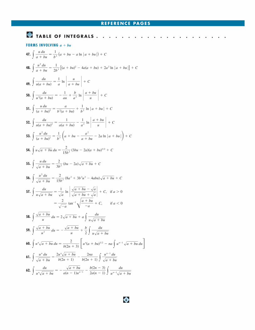
REF ERENCE PAGES
6
FORMS INVOLVING
47.
48.
49.
50.
51.
52.
53.
54.
55.
56.
57.
58.
59.
60.
61.
62. y du
u nsa � bu
� �sa � bu
a�n � 1�u n�1 �b�2n � 3�2a�n � 1�
y du
u n�1sa � bu
y u n du
sa � bu�
2u nsa � bu
b�2n � 1��
2na
b�2n � 1� y
u n�1 du
sa � bu
�2
b�2n � 3� �u n�a � bu�3�2 � na y u n�1 sa � bu duy u n
sa � bu du
y sa � bu
u 2 du � �sa � bu
u�
b
2 y
du
usa � bu
y sa � bu
u du � 2sa � bu � a y
du
usa � bu
�2
s�a tan�1�a � bu
�a� C, if a � 0
y du
usa � bu�
1
sa ln � sa � bu � sa
sa � bu � sa� � C, if a � 0
y u 2 du
sa � bu�
2
15b 3 �8a 2 � 3b 2u 2 � 4abu�sa � bu � C
y u du
sa � bu�
2
3b 2 �bu � 2a�sa � bu � C
y usa � bu du �2
15b 2 �3bu � 2a��a � bu�3�2 � C
y u 2 du
�a � bu�2 �1
b 3 �a � bu �a 2
a � bu� 2a ln � a � bu �� � C
y du
u�a � bu�2 �1
a�a � bu��
1
a 2 ln � a � bu
u � � C
y u du
�a � bu�2 �a
b 2�a � bu��
1
b 2 ln � a � bu � � C
y du
u 2�a � bu�� �
1
au�
b
a 2 ln � a � bu
u � � C
y du
u�a � bu��
1
a ln � u
a � bu � � C
y u 2 du
a � bu�
1
2b 3 [�a � bu�2 � 4a�a � bu� � 2a 2 ln � a � bu �] � C
y u du
a � bu�
1
b 2 (a � bu � a ln � a � bu �) � C
a � bu
TABL E OF INT EGRALS � � � � � � � � � � � � � � � � � � � � �

REF ERENCE PAGES
7
TRIGONOMETRIC FORMS
63.
64.
65.
66.
67.
68.
69.
70.
71.
72.
73.
74.
75.
INVERSE TRIGONOMETRIC FORMS
87.
88.
89.
90.
91. y u cos�1u du �2u 2 � 1
4 cos�1u �
us1 � u 2
4� C
y u sin�1u du �2u 2 � 1
4 sin�1u �
us1 � u 2
4� C
y tan�1u du � u tan�1u �12 ln�1 � u 2� � C
y cos�1u du � u cos�1u � s1 � u 2 � C
y sin�1u du � u sin�1u � s1 � u 2 � C
y tannu du �1
n � 1 tann�1u � y tann�2u du
y cosnu du �1
n cosn�1u sin u �
n � 1
n y cosn�2u du
y sinnu du � �1
n sinn�1u cos u �
n � 1
n y sinn�2u du
y csc3u du � �12 csc u cot u �
12 ln � csc u � cot u � � C
y sec3u du � 12 sec u tan u �
12 ln � sec u � tan u � � C
y cot3u du � �12 cot2u � ln � sin u � � C
y tan3u du � 12 tan2u � ln � cos u � � C
y cos3u du � 13 �2 � cos2u� sin u � C
y sin3u du � �13 �2 � sin2u� cos u � C
y cot2u du � �cot u � u � C
y tan2u du � tan u � u � C
y cos2u du � 12 u �
14 sin 2u � C
y sin2u du � 12 u �
14 sin 2u � C 76.
77.
78.
79.
80.
81.
82.
83.
84.
85.
86.
�sinn�1u cosm�1u
n � m�
m � 1
n � m y sinnu cosm�2u du
y sinnu cosmu du � �sinn�1u cosm�1u
n � m�
n � 1
n � m y sinn�2u cosmu du
y u n cos u du � u n sin u � n y u n�1 sin u du
y u n sin u du � �u n cos u � n y u n�1 cos u du
y u cos u du � cos u � u sin u � C
y u sin u du � sin u � u cos u � C
y sin au cos bu du � �cos�a � b�u
2�a � b��
cos�a � b�u2�a � b�
� C
y cos au cos bu du �sin�a � b�u
2�a � b��
sin�a � b�u2�a � b�
� C
y sin au sin bu du �sin�a � b�u
2�a � b��
sin�a � b�u2�a � b�
� C
y cscnu du ��1
n � 1 cot u cscn�2u �
n � 2
n � 1 y cscn�2u du
y secnu du �1
n � 1 tan u secn�2u �
n � 2
n � 1 y secn�2u du
y cot nu du ��1
n � 1 cot n�1u � y cot n�2u du
92.
93.
94.
95. y u n tan�1u du �1
n � 1 �u n�1 tan�1u � y
u n�1 du
1 � u 2 , n � �1
y u n cos�1u du �1
n � 1 �u n�1 cos�1u � y
u n�1 du
s1 � u 2, n � �1
y u n sin�1u du �1
n � 1 �u n�1 sin�1u � y
u n�1 du
s1 � u 2, n � �1
y u tan�1u du �u 2 � 1
2 tan�1u �
u
2� C
� � � � � � � � � � � � � � � � � � � � � � � � � � � � � � ✍TABL E OF INT EGRALS

REF ERENCE PAGES
8
EXPONENTIAL AND LOGARITHMIC FORMS
96.
97.
98.
99.
HYPERBOLIC FORMS
103.
104.
105.
106.
107.
FORMS INVOLVING
113.
114.
115.
116.
117.
118.
119.
120. y du
us2au � u 2� �
s2au � u 2
au� C
y u2 du
s2au � u 2� �
�u � 3a�2
s2au � u 2 �3a 2
2 cos�1�a � u
a � � C
y u du
s2au � u 2� �s2au � u 2 � a cos�1�a � u
a � � C
y du
s2au � u 2� cos�1�a � u
a � � C
y s2au � u 2
u 2 du � �2s2au � u 2
u� cos�1�a � u
a � � C
y s2au � u 2
u du � s2au � u 2 � a cos�1�a � u
a � � C
y us2au � u 2 du �2u 2 � au � 3a 2
6 s2au � u 2 �
a 3
2 cos�1�a � u
a � � C
y s2au � u 2 du �u � a
2 s2au � u 2 �
a 2
2 cos�1�a � u
a � � C
s2au � u2, a � 0
y sech u du � tan�1 � sinh u � � C
y coth u du � ln � sinh u � � C
y tanh u du � ln cosh u � C
y cosh u du � sinh u � C
y sinh u du � cosh u � C
y eau cos bu du �eau
a 2 � b2 �a cos bu � b sin bu� � C
y eau sin bu du �eau
a 2 � b 2 �a sin bu � b cos bu� � C
y u neau du �1
a u neau �
n
a y u n�1eau du
y ueau du �1
a 2 �au � 1�eau � C
108.
109.
110.
111.
112. y csch u coth u du � �csch u � C
y sech u tanh u du � �sech u � C
y csch2u du � �coth u � C
y sech2u du � tanh u � C
y csch u du � ln � tanh 12 u � � C
TABL E OF INT EGRALS � � � � � � � � � � � � � � � � � � � � �
100.
101.
102. y 1
u ln u du � ln � ln u � � C
y u n ln u du �u n�1
�n � 1�2 �n � 1� ln u � 1� � C
y ln u du � u ln u � u � C