End-point estimates for iterated commutators of multilinear singular integrals
Name: Paul HorigSupervisor: Don Grant
Elliptic Integrals: the Landen Transformation and Carlson Duplication
1
Name: Paul HorigSupervisor: Don Grant
Acknowledgements: I would like to thank Rod Deakin for suggesting this project and for his 2014 paper which formed the material for this project. Also I would like to thank Don Grant for direction and helpful comments in doing this project.
Abstract: The aim of this project was to show that the recursiveprocesses of the Landen transformation and Carlson forms can givearbitrary precision in problems involving elliptic integrals.Programs were written in MATLAB© to find Elliptic Integrals of theFirst and Second Kind using a Landen transformation and EllipticIntegrals of the Third Kind using Carlson Duplication. These wereused to calculate meridian distances and to solve the direct problemof geodesy. These techniques give mathematical precision up tomachine precision and were checked with MATLAB©’s ellipticF,ellipticE and ellipticPi inbuilt functions. These MATLAB© functionswere shown to give 15 decimal place precision and as such can be usedwith confidence to solve geodetic problems. It was found that CarlsonDuplication gives a straightforward technique to solve ellipticintegrals.
2
Name: Paul HorigSupervisor: Don Grant
Contents2. Introduction....................................................63. What is a Landen transformation?................................93.1 History of the Landen transformation and its use in geodesy.
104. MATLAB© First Kind program results.............................115. Elliptic Integrals of the Second Kind..........................156. MATLAB© Second Kind program results............................167. Meridian Arc Length Formula (Derivation given in Appendix L)...178. Results of Calculations of Arc Lengths along Meridians.........179. Ascending and Descending First Kind transformation.............1810. Landen’s descending transformation for Second Kind integrals. 2011. Ascending and Descending Second Kind transformation..........2012. Inverting Elliptic Integrals of the First Kind...............2213. MATLAB© First Kind Inversion program results..................2314. Evaluating General Elliptic Integrals of the Third Kind using Carlson Symmetric Forms............................................24
14.1 What are R functions (brief introduction of terms)?........2514.2 Elliptic Integral of the Third Kind with parameters useful ingeodesy..........................................................26
15. Inverting Elliptic Integrals of the Third Kind using Carlson form and a binary technique........................................2816. The Direct Geodetic Problem.................................2917. Geodesics (Rollin’s Method)..................................3018. My Direct.m results compared with Karney’s GEODRECKON........3419. Safeguards against the computer not preserving precision when implementing recursion.............................................3720. Conclusions:.................................................3721. Appendices...................................................41
1.
3
Name: Paul HorigSupervisor: Don Grant
Appendices
Appendix A MATLAB© code for determining elliptic integrals of the First Kind using Landen’s ascending transformation...............................41
Appendix B MATLAB© code for determining elliptic integral of the Second Kind...........................42
Appendix B.1............................Theory summary42
Appendix B.2.....................................Code42
Appendix B.3..................................Results43
Appendix C MATLAB© code for determining meridian distance M............................................44
Appendix D MATLAB© code First Kind integrals using Landen’sdescending transformation....................45
Appendix E MATLAB© code for finding the amplitude of a First Kind elliptic integral given the result of the integral (inverting the First Kind integral)....................................46
Appendix F MATLAB© code for determining elliptic integral of the Third Kind using Carlson..............47
Appendix G MATLAB© code for determining the inverse of an elliptic integral of the Third Kind using Carlson and a binary search technique........48
Appendix H MATLAB© code for solving the direct problem...51Appendix I MATLAB© code for testing the direct problem...55Appendix J Results of running the General Elliptic
Integrals of the Third Kind program ThirdCarlson and the inbuilt MATLAB© program ellipticPI...................................56
Appendix K Arc Length of a Curve........................59Appendix K.1...........Arc length given a polar equation
60Appendix K.2...................Arc Length of an Ellipse
60Appendix K.3 Parametric equations of the ellipse in terms of the latitude parameter..............................61Appendix K.4........Arc length as a function of Latitude
64Appendix K.5..Arc length as a function of Latitude using radius of curvature....................................65
4
Name: Paul HorigSupervisor: Don Grant
Appendix K.6. General Equation for the Radius of Curvature66
Appendix K.7......The Radius of Curvature of the Ellipse68
Appendix L Meridian Distance............................70Appendix M Evaluating Elliptic Integrals of the First
Kind.........................................74Appendix M.1................The modulus q is increasing
79Appendix M.2..............Determining the new amplitude
79Appendix M.3..The chain of transformed elliptic integrals
80Appendix N Landen’s descending transformation for First
Kind integrals...............................81Appendix O Evaluating Elliptic Integrals of the Second
Kind.........................................86Appendix P Abandoned working to find the amplitude given
the result of the integral: Second Kind......93Appendix P.1 Finding the latitude given meridian distance using the elliptic integral of the second kind.........93Appendix P.2..Inverting Elliptic Integrals of the Second Kind 93
Appendix Q Abandoned: Inverting Elliptic Integrals of the Third Kind using Carlson form and Newton-Raphson......................................97
Appendix R Abandoned: Inverting Elliptic Integrals of the Third Kind using Π=f(F,E) Newton-Raphson...105
Appendix S Abandoned working to evaluate Elliptic Integrals of the Third Kind using a Landen transformation..............................108
Appendix T Khan’s endpoint formula.....................112Appendix U MATLAB code to test Khan’s formula..........114Appendix V MATLAB code to change DD.MMSS into decimal
degrees.....................................116
5
Name: Paul HorigSupervisor: Don Grant
Figures Figure 1 Successive amplitudes tolerance 1E-3......................13Figure 2 Successive amplitudes beginning with 45°.................14Figure 3 Successive amplitudes beginning with 90°..................14Figure 4 Successive amplitudes beginning with 135°.................15Figure 5 The latitudes which result from equally spaced distances on the ellipse........................................................29Figure 6...........................................................30Figure 7 1000 successive 100km geodesics from a point near Chile...36Figure 8 1000 successive 100km geodesics from a point near Chile...37
2. Introduction
This thesis is concerned with calculating the First Kind,Second Kind and Third Kind of elliptic integral using a recursive technique. The formula for distance along a meridian is an elliptic integral of the Third Kind which can be changed into a Second Kind integral plus a constant. The Second Kind integral can be calculated using a Landen transformation.
The Third Kind integral will be calculated using the Carlson Symmetric Forms. Carlson provides a fast method of calculation of general Third Kind elliptic integrals –that is those with a characteristic and modulus which areunrelated. The Carlson forms have as special cases the Landen transformation and Gauss arithmetic-geometric meantransformation.
The particular Carlson method of solution of the general Third Kind integral used here is the duplication method. Carlson in his paper (Carlson B. C., 1979) adds an extra step of a Taylor’s series after convergence (p2) but the program presented here omits this step as speed has not been made a priority.
The calculation of meridian distances on the ellipsoid isa purely mathematical problem and distances between two points will depend on the ellipsoid chosen. The GRS80 ellipsoid is the one currently used in Australia and it has a semi-major axis of 6,378,137.0 metres and an inverse flattening of 298.257222101 (Geocentric Datum of Australia, 2014).
6
Name: Paul HorigSupervisor: Don Grant
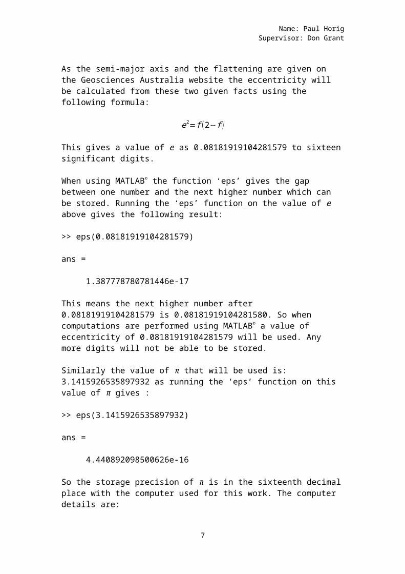
As the semi-major axis and the flattening are given on the Geosciences Australia website the eccentricity will be calculated from these two given facts using the following formula:
e2=f(2−f)
This gives a value of e as 0.08181919104281579 to sixteensignificant digits.
When using MATLAB© the function ‘eps’ gives the gap between one number and the next higher number which can be stored. Running the ‘eps’ function on the value of e above gives the following result:
>> eps(0.08181919104281579)
ans =
1.387778780781446e-17
This means the next higher number after 0.08181919104281579 is 0.08181919104281580. So when computations are performed using MATLAB© a value of eccentricity of 0.08181919104281579 will be used. Any more digits will not be able to be stored.
Similarly the value of π that will be used is: 3.1415926535897932 as running the ‘eps’ function on this value of π gives :
>> eps(3.1415926535897932)
ans =
4.440892098500626e-16
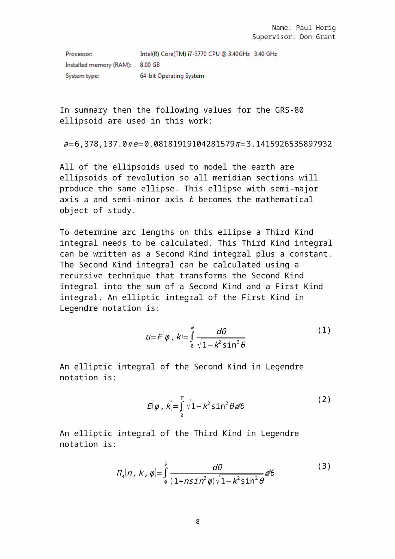
So the storage precision of π is in the sixteenth decimalplace with the computer used for this work. The computer details are:
7
Name: Paul HorigSupervisor: Don Grant
In summary then the following values for the GRS-80 ellipsoid are used in this work:
a=6,378,137.0me=0.08181919104281579π=3.1415926535897932
All of the ellipsoids used to model the earth are ellipsoids of revolution so all meridian sections will produce the same ellipse. This ellipse with semi-major axis a and semi-minor axis b becomes the mathematical object of study.
To determine arc lengths on this ellipse a Third Kind integral needs to be calculated. This Third Kind integralcan be written as a Second Kind integral plus a constant.The Second Kind integral can be calculated using a recursive technique that transforms the Second Kind integral into the sum of a Second Kind and a First Kind integral. An elliptic integral of the First Kind in Legendre notation is:
u=F (ϕ,k )=∫0
ϕ dθ√1−k2sin2θ
(1)
An elliptic integral of the Second Kind in Legendre notation is:
E (ϕ,k )=∫0
ϕ
√1−k2sin2θⅆθ(2)
An elliptic integral of the Third Kind in Legendre notation is:
Π3 (n,k,ϕ )=∫0
ϕ dθ(1+nsin2ϕ)√1−k2sin2θ
ⅆθ(3)
8
Name: Paul HorigSupervisor: Don Grant
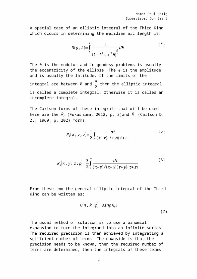
A special case of an elliptic integral of the Third Kind which occurs in determining the meridian arc length is:
Π(ϕ,k)=∫0
ϕ 1
(1−k2sin2θ)32
dθ(4)
The k is the modulus and in geodesy problems is usually the eccentricity of the ellipse. The ϕ is the amplitude and is usually the latitude. If the limits of the
integral are between 0 and π2 then the elliptic integral
is called a complete integral. Otherwise it is called an incomplete integral.
The Carlson forms of these integrals that will be used here are the RF (Fukushima, 2012, p. 3)and RJ (Carlson D. Z., 1969, p. 202) forms.
RF (x,y,z)=12∫0
∞ dt(t+x)(t+y)(t+z)
(5)
RJ (x,y,z,p)=32∫0
∞ dt(t+p)√(t+x)(t+y)(t+z)
(6)
From these two the general elliptic integral of the ThirdKind can be written as:
Π (n,k,ϕ )=sinϕRF ¿(7)
The usual method of solution is to use a binomial expansion to turn the integrand into an infinite series. The required precision is then achieved by integrating a sufficient number of terms. The downside is that the precision needs to be known, then the required number of terms are determined, then the integrals of these terms
9
Name: Paul HorigSupervisor: Don Grant
are determined which are programmed in and the summation achieved by computer which will take in as input the latitude. In unusual situations which call for an unusuallevel of precision there is some programming required unless the precision has been offered as part of the program used.
Another method of solution of the elliptic integrals is by Landen transformation when using the Legendre forms and by duplication when using the Carlson forms. These forms naturally lend themselves to recursion and so programming using recursion is straightforward. The advantage of this method is that the program to calculatethe integrals remains unchanged for different precision and just a precision parameter need be entered into the program.
In addition inversion programs to find latitudes which use numerical methods can only give precision which are as good as the programs to evaluate the original function. In the programs which are developed here a simple binary search technique is used but this will alsogive arbitrary precision as the forward program to go from latitude to integral result is giving arbitrary precision.
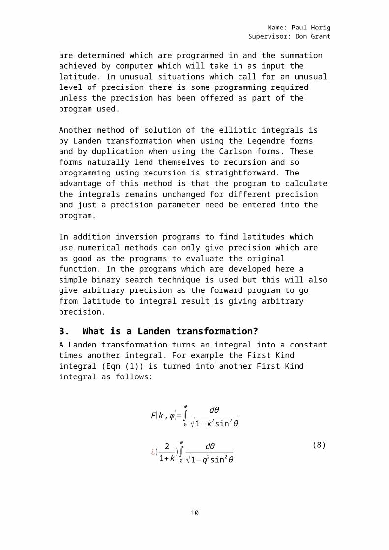
3. What is a Landen transformation?A Landen transformation turns an integral into a constanttimes another integral. For example the First Kind integral (Eqn (1)) is turned into another First Kind integral as follows:
F (k,ϕ )=∫0
ϕ dθ√1−k2sin2θ
¿(2
1+k )∫0
ψ dθ√1−q2sin2θ
(8)
10
Name: Paul HorigSupervisor: Don Grant
Note in the above example that there is a multiplying
factor in front, ( 21+k
¿, the ϕ has been changed to a ψ and
the k has been changed to a q. It may appear that this change has made things a little bit more complicated withthe appearance of the multiplying factor but if the process is continued then eventually the modulus (q) turns into a one.
The part to be integrated is then:
∫0
ψ dθ√1−12sin2θ
¿∫0
ψ dθ√1−sin2θ
¿∫0
ψ dθcos (θ)
which is easily integrated
as:
¿lntan(π4
+ψ2)
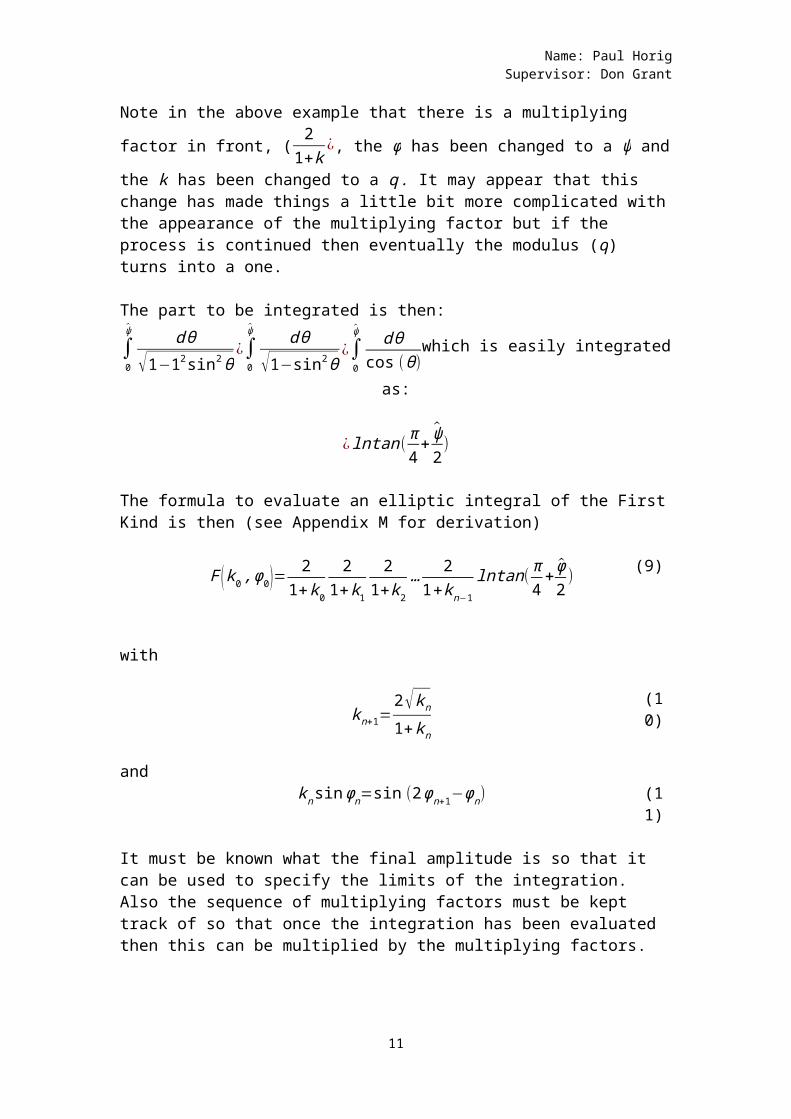
The formula to evaluate an elliptic integral of the FirstKind is then (see Appendix M for derivation)
F (k0,ϕ0)=2
1+k0
21+k1
21+k2
… 21+kn−1
lntan(π4
+ ϕ2
) (9)
with
kn+1=2√kn
1+kn
(10)
andknsinϕn=sin (2ϕn+1−ϕn) (1
1)
It must be known what the final amplitude is so that it can be used to specify the limits of the integration. Also the sequence of multiplying factors must be kept track of so that once the integration has been evaluated then this can be multiplied by the multiplying factors.
11
Name: Paul HorigSupervisor: Don Grant
The circumflex on the angle (ψ¿ indicates that this is the final angle at the point when the modulus has reachedits limit.
3.1History of the Landen transformation and its use in geodesy.
The Landen transformation was discovered by John Landen in the latter part of the eighteenth century and used by Legendre (Deakin, Elliptic Integrals and Landen's Transformation: What I should've known for Geodesy, 2014,p. 1). L.V. King published a book in 1924 which gives a detailed account of this transformation and its application to calculate elliptic integrals.
The textbook Geodesy the Concepts by Edward Krakiwsky published in 1986 says that elliptical integrals are usually carried out with power series (p34). Landen’s transformation is not mentioned in the index.
The power series method is one in which the integrand is converted into a power series using a binomial expansion.Each term of the expansion is then integrated. The algorithm can be defined recursively as given in Klotz (1993) (Dorrer p92).
Similarly the textbook Maths for Map Makers by Arthur Allan and published in 1997 says that the integrand of the elliptical integral can be converted into a series and integrated term by term (p238). Another method it gives is to use a numerical method (p238). Landen’s transformation is not mentioned in the index.
Gerstl in 1984 calculates complex elliptic integrals by means of a Landen transformation in his paper. The book Map Projections: Cartographic Information Systems by Erik W. Grafarend and Friedrich W. Krumm uses the Landen transformation.
Dorrer in 1999 published a paper called From Elliptic Arc Lengthto Gauss-Krueger Coordinates by Analytical Continuation. Landen transformations are used to calculate elliptic integrals
12
Name: Paul HorigSupervisor: Don Grant
and in particular uses complex numbers and the programming language called APL2.
Rösch in 2011 published a paper called The Derivation of Algorithms to Compute Elliptic Integrals of the First and Second Kind by Landen Transformation. The computer programming language usedis C. Rösch compares his results with those given by Maple V.
Deakin (2014) explicates the work of King and uses Maximaas the computer program. Results are compared with those achieved by Dorrer.
My report covers similar ground as Dorrer, Rösch and Deakin but uses MATLAB© as the computer programming language. In addition I have used the Carlson Duplicationmethod to calculate the elliptic integral of the Third Kind.
4. MATLAB© First Kind program results
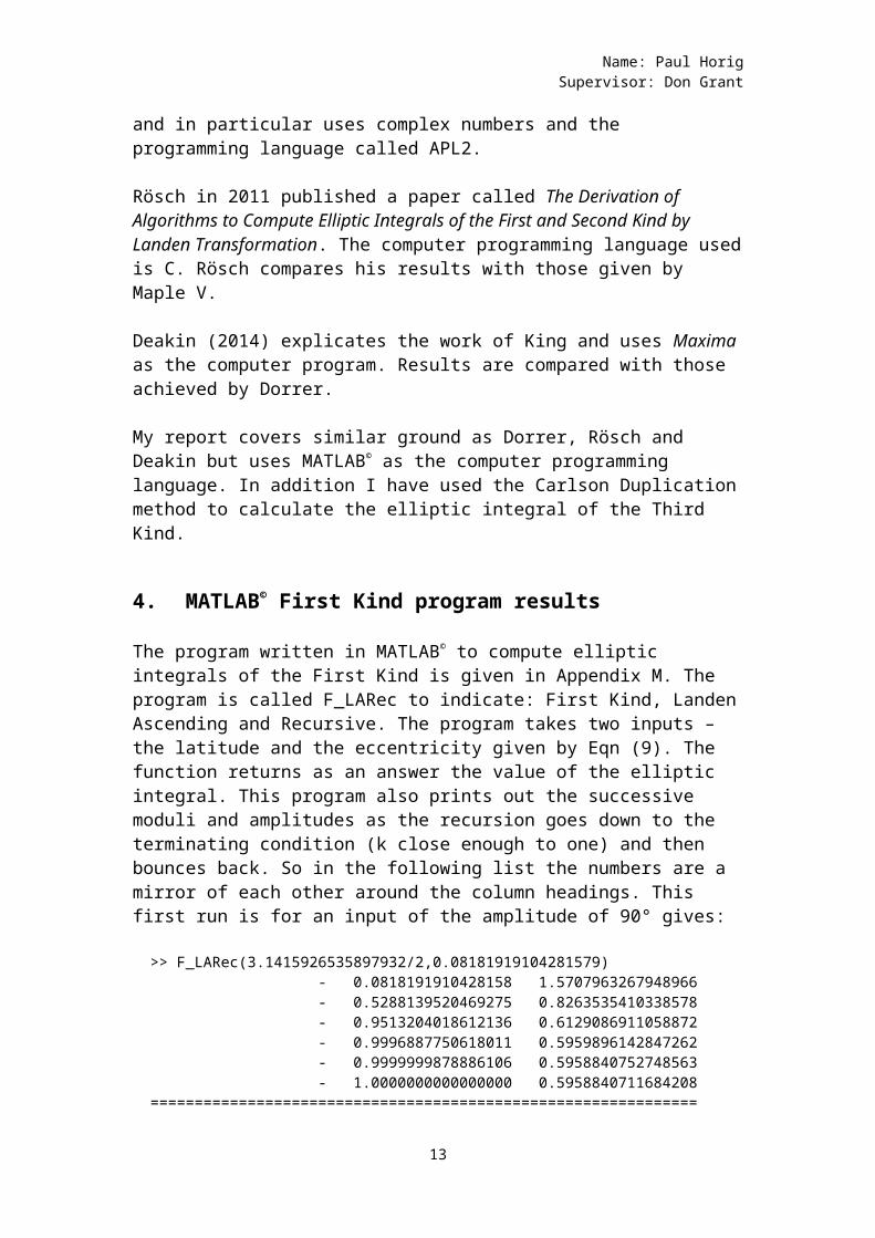
The program written in MATLAB© to compute elliptic integrals of the First Kind is given in Appendix M. The program is called F_LARec to indicate: First Kind, LandenAscending and Recursive. The program takes two inputs – the latitude and the eccentricity given by Eqn (9). The function returns as an answer the value of the elliptic integral. This program also prints out the successive moduli and amplitudes as the recursion goes down to the terminating condition (k close enough to one) and then bounces back. So in the following list the numbers are a mirror of each other around the column headings. This first run is for an input of the amplitude of 90° gives:
>> F_LARec(3.1415926535897932/2,0.08181919104281579) - 0.0818191910428158 1.5707963267948966 - 0.5288139520469275 0.8263535410338578 - 0.9513204018612136 0.6129086911058872 - 0.9996887750618011 0.5959896142847262 - 0.9999999878886106 0.5958840752748563 - 1.0000000000000000 0.5958840711684208==============================================================
13
Name: Paul HorigSupervisor: Don Grant
Integral k Amplitude============================================================== 0.6346425378629763 1.0000000000000000 0.5958840711684208 0.6347413115257022 0.9999999878886106 0.5958840752748563 0.6505762056505652 0.9996887750618011 0.5959896142847262 0.8510861701379811 0.9513204018612136 0.6129086911058872 1.5734351492093230 0.5288139520469275 0.8263535410338578
This is the how to call the inbuilt MATLAB© mupad functionfor the same amplitude specifying 40 digit precision in calculations:
DIGITS := 40:ellipticF(3.1415926535897932/2, 0.08181919104281579^2).
The eccentricity is squared because this is what the MATLAB© function accepts.
The first argument of the ellipticF function is π2. In the
following comparison rather than putting in pi()/2 as a first argument a constant was put in so the two functions– mine and MATLAB©’s – could be compared. That is, both mine and MATLAB©’s functions were fed exactly the same numbers as inputs. This methodology was followed throughout all the comparison tests which follow.
Latitude, eccentricity
MATLAB© ellipticF result
F_LARec result(ϕn−ϕn+1¿<10
−15
pi()/2,0.0818191910435 1.573435149209323129
1.573435149209323
pi()/4,0.0818191910435 0.785876554121529944
0.785876554121530
14
Name: Paul HorigSupervisor: Don Grant
3*pi()/4,0.0818191910435 2.360993744297116313
2.360993744297117
Table 1
How does the set tolerance for amplitude difference affect the precision of the results? As can be seen from the following table reducing the tolerance to 10−4 still gives precision such that the fourteenth decimal digit isthe same as the MATLAB© result. F_LARec result(ϕ0=90°)(ϕn−ϕn+1¿
¿10−15
¿10−14 ¿10−13 ¿10−12 ¿10−11 ¿10−10 ¿10−9
1.573435149209323
1.573435149209323
1.573435149209323
1.573435149209323
1.573435149209323
1.573435149209323
1.573435149209323
¿10−8 ¿10−7 ¿10−6 ¿10−5 ¿10−4 ¿10−3
1.573435149209323
1.573435149209323
1.573435149209323
1.573435149209323
1.573435149209323
1.573435151981971
Table 2
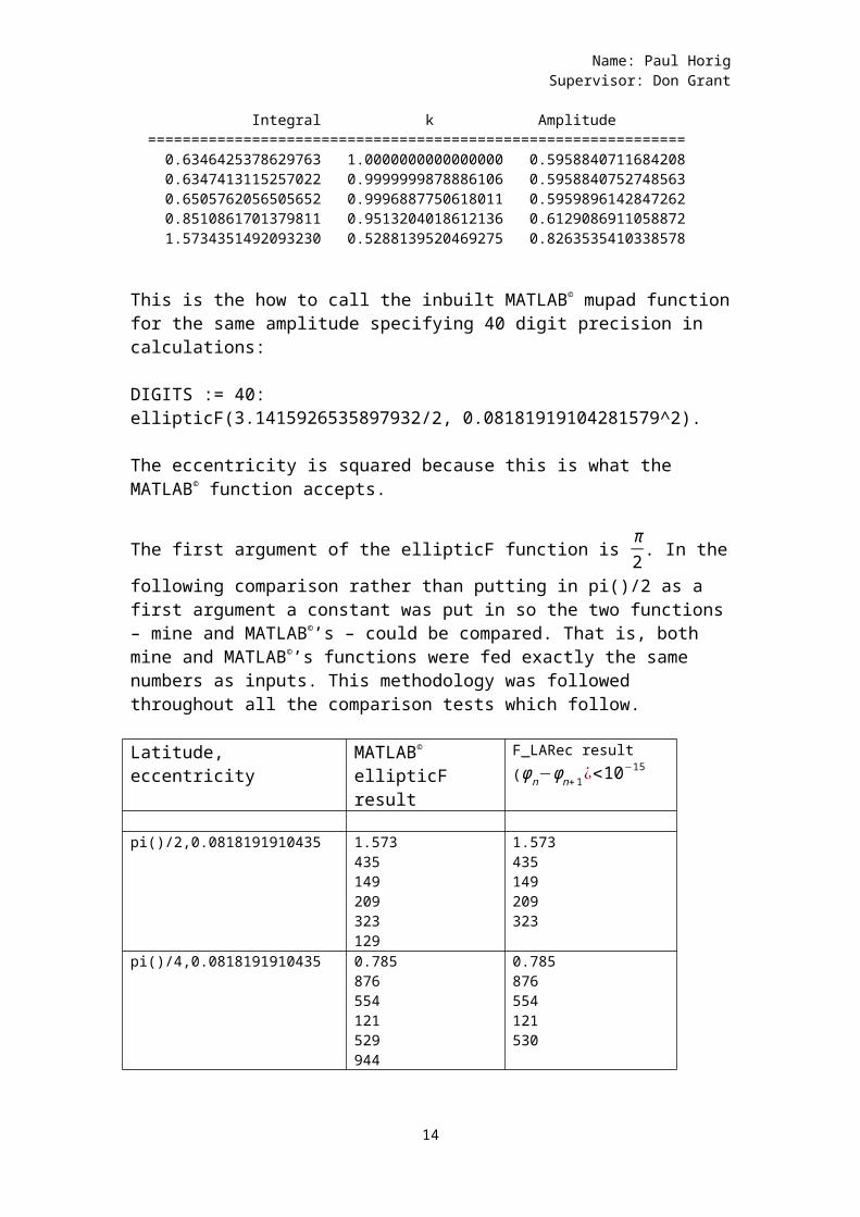
When the tolerance between the successive amplitudes is set to be less than 10−3 then the result for the integral changes as shown in table 2. The eighth decimal place changes. The plot for successive amplitudes for a tolerance of 10−3is shown:
15
Name: Paul HorigSupervisor: Don Grant
-2.5 -2 -1.5 -1 -0.5 0 0.5 1 1.5 2 2.50
0.5
1
1.5
2
2.5
3
3.5
4
Figure 1 Successive amplitudes tolerance 1E-3
The output trace is:
>> F_LARec(3.1415926535897932/2,0.08181919104281579) - 0.0818191910428158 1.5707963267948966 - 0.5288139520469275 0.8263535410338578 - 0.9513204018612136 0.6129086911058872 - 0.9996887750618011 0.5959896142847262============================================================== Integral k Amplitude============================================================== 0.6505762067969861 0.9996887750618011 0.5959896142847262 0.8510861716377330 0.9513204018612136 0.6129086911058872 1.5734351519819711 0.5288139520469275 0.8263535410338578
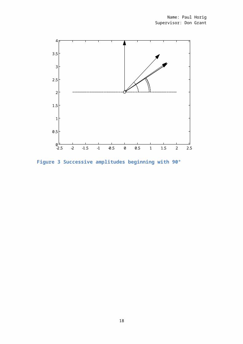
If we compare Figure 1 with Figure 3 it may appear that there is no difference. However Figure 3 actually has sixamplitudes present but only four can be distinguished. This can be seen from the output trace of amplitudes given above for the case where the beginning amplitude is90°.
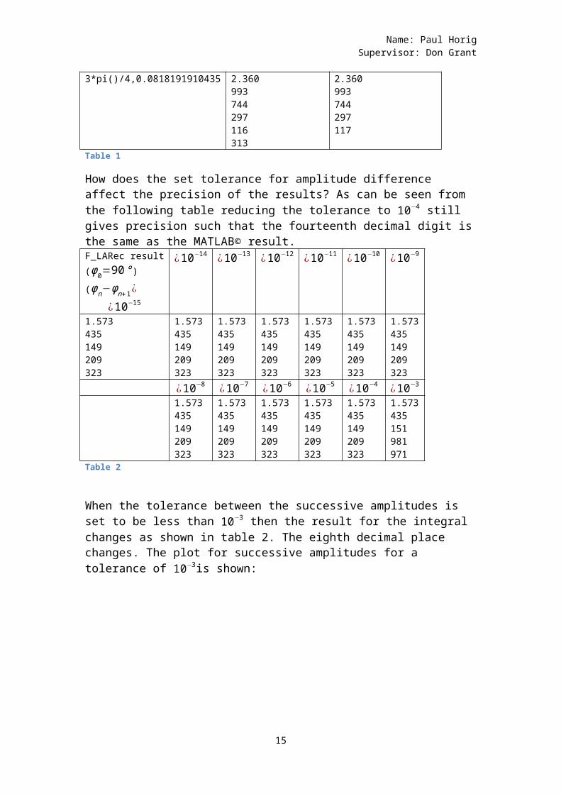
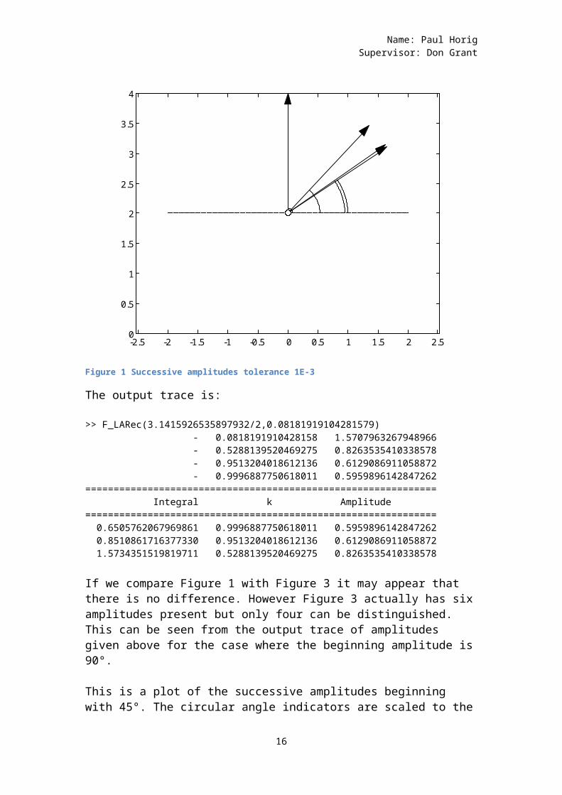
This is a plot of the successive amplitudes beginning with 45°. The circular angle indicators are scaled to the
16
Name: Paul HorigSupervisor: Don Grant
value of k. A value of k equal to one gives an angle indicator half the length of the arrow. As can be seen the initial value of k is quite small, barely larger thanthe marker indicating the centre of the circle.
-2.5 -2 -1.5 -1 -0.5 0 0.5 1 1.5 2 2.50
0.5
1
1.5
2
2.5
3
3.5
4
Figure 2 Successive amplitudes beginning with 45°
17
Name: Paul HorigSupervisor: Don Grant
-2.5 -2 -1.5 -1 -0.5 0 0.5 1 1.5 2 2.50
0.5
1
1.5
2
2.5
3
3.5
4
Figure 3 Successive amplitudes beginning with 90°
18
Name: Paul HorigSupervisor: Don Grant
-2.5 -2 -1.5 -1 -0.5 0 0.5 1 1.5 2 2.50
0.5
1
1.5
2
2.5
3
3.5
4
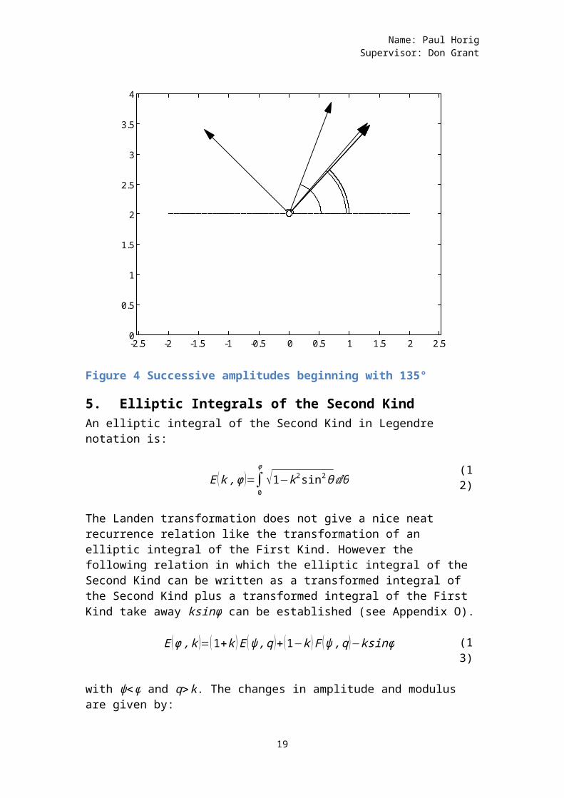
Figure 4 Successive amplitudes beginning with 135°
5. Elliptic Integrals of the Second KindAn elliptic integral of the Second Kind in Legendre notation is:
E (k,ϕ )=∫0
ϕ
√1−k2sin2θⅆθ(12)
The Landen transformation does not give a nice neat recurrence relation like the transformation of an elliptic integral of the First Kind. However the following relation in which the elliptic integral of the Second Kind can be written as a transformed integral of the Second Kind plus a transformed integral of the First Kind take away ksinϕ can be established (see Appendix O).
E (ϕ,k )=(1+k )E (ψ,q )+(1−k )F (ψ,q)−ksinϕ (13)
with ψ<ϕ and q>k. The changes in amplitude and modulus are given by:
19
Name: Paul HorigSupervisor: Don Grant
sin (2ψ−ϕ)=ksinϕ (14)
and
q=2√k1+k
(15)
Now as the modulus converges to unity and the amplitude converges toϕ the elliptic integral of the Second Kind in(41) will converge to
∫0
ϕ
√(1−12sin2ω )dω
¿∫0
ϕ
√1−sin2ωdω
¿∫0
ϕ
cosωdω
¿sin (ϕ)
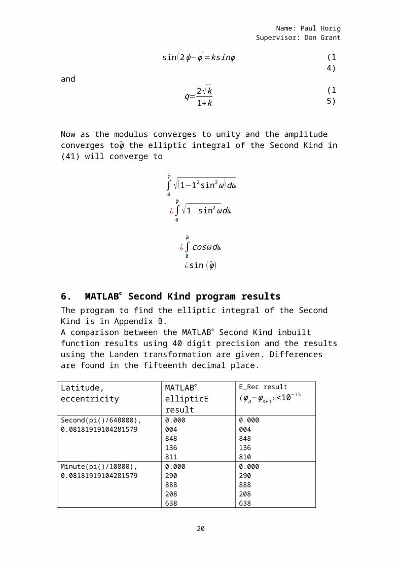
6. MATLAB© Second Kind program resultsThe program to find the elliptic integral of the Second Kind is in Appendix B.A comparison between the MATLAB© Second Kind inbuilt function results using 40 digit precision and the resultsusing the Landen transformation are given. Differences are found in the fifteenth decimal place.
Latitude, eccentricity
MATLAB© ellipticE result
E_Rec result(ϕn−ϕn+1¿<10
−15
Second(pi()/648000),0.08181919104281579
0.000004848136811
0.000004848136810
Minute(pi()/10800),0.08181919104281579
0.000290888208638
0.000290888208638
20
Name: Paul HorigSupervisor: Don Grant
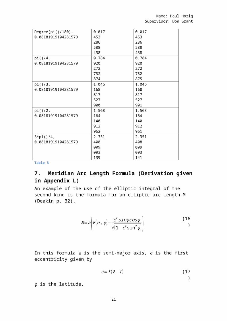
Degree(pi()/180),0.08181919104281579
0.017453286588438
0.017453286588438
pi()/4, 0.08181919104281579
0.784920272732874
0.784920272732875
pi()/3, 0.08181919104281579
1.046168817527900
1.046168817527901
pi()/2, 0.08181919104281579
1.568164140912962
1.568164140912961
3*pi()/4, 0.08181919104281579
2.351408009093139
2.351408009093141
Table 3
7. Meridian Arc Length Formula (Derivation givenin Appendix L)An example of the use of the elliptic integral of the second kind is the formula for an elliptic arc length M (Deakin p. 32).
M=a(E (e,ϕ)− e2sinϕcosϕ√(1−e2sin2ϕ ) )
(16)
In this formula a is the semi-major axis, e is the first eccentricity given by
e=f(2−f) (17)
ϕ is the latitude.
21
Name: Paul HorigSupervisor: Don Grant
As Equation (16) multiplies the elliptic integral of the second kind by the semi-major axis, which for the GRS80 ellipsoid is 6,378,137.0 metres, the error in the integration of the elliptic integral should be less than1⨯10−11 (Rösch, 2011, p. 5). This will give an accuracy of1mm. Rösch (p. 5) uses a tolerance of 1⨯10−15 in his recursive processes. However more work is needed to relate tolerance in the amplitude or tolerance in the modulus to the precision of the result.
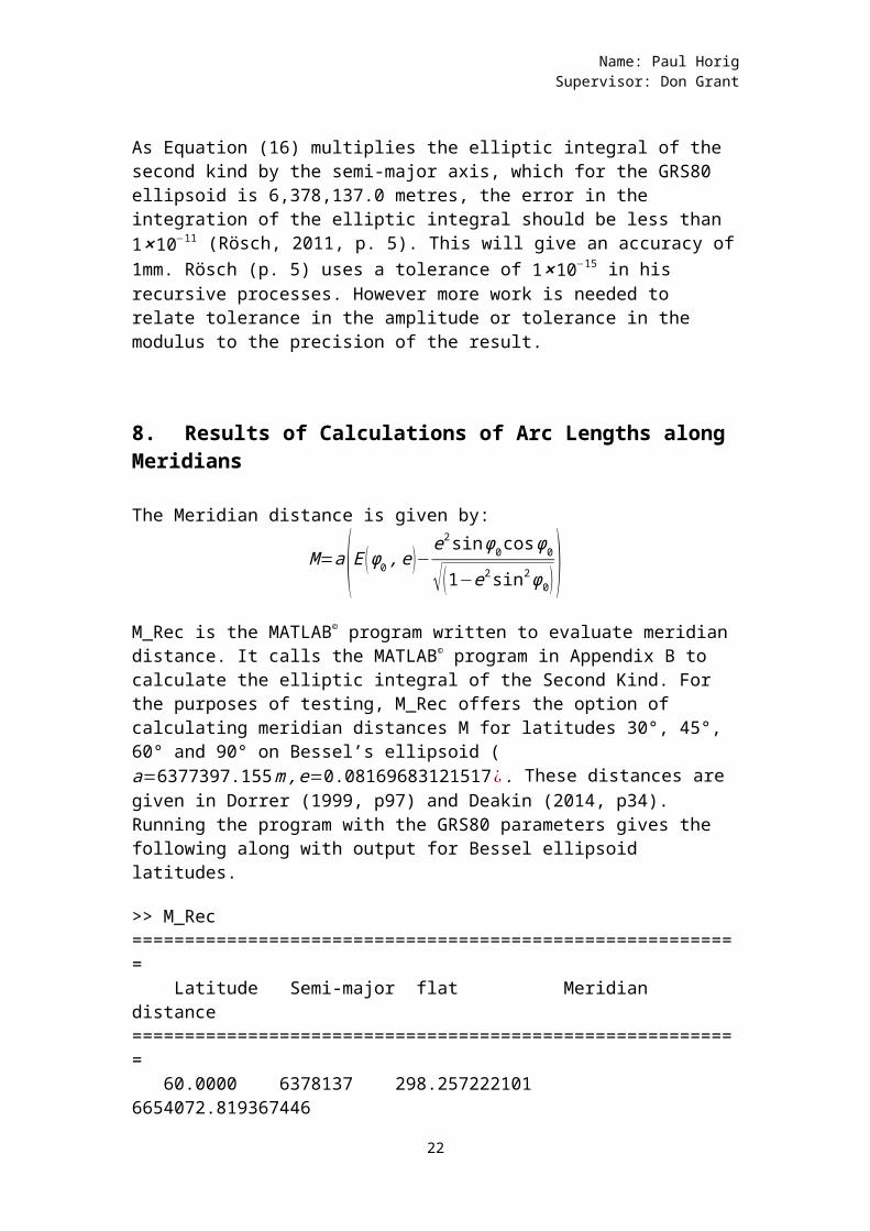
8. Results of Calculations of Arc Lengths along Meridians
The Meridian distance is given by:
M=a(E (ϕ0,e)−e2sinϕ0cosϕ0
√(1−e2sin2ϕ0) )M_Rec is the MATLAB© program written to evaluate meridian distance. It calls the MATLAB© program in Appendix B to calculate the elliptic integral of the Second Kind. For the purposes of testing, M_Rec offers the option of calculating meridian distances M for latitudes 30°, 45°, 60° and 90° on Bessel’s ellipsoid (a=6377397.155m,e=0.08169683121517¿. These distances are given in Dorrer (1999, p97) and Deakin (2014, p34). Running the program with the GRS80 parameters gives the following along with output for Bessel ellipsoid latitudes.
>> M_Rec========================================================== Latitude Semi-major flat Meridian distance========================================================== 60.0000 6378137 298.257222101 6654072.819367446
22
Name: Paul HorigSupervisor: Don Grant
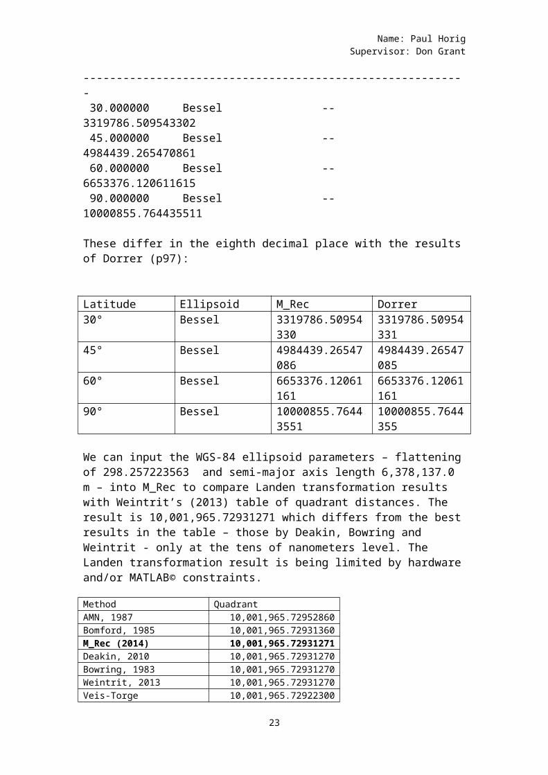
---------------------------------------------------------- 30.000000 Bessel -- 3319786.509543302 45.000000 Bessel -- 4984439.265470861 60.000000 Bessel -- 6653376.120611615 90.000000 Bessel -- 10000855.764435511
These differ in the eighth decimal place with the resultsof Dorrer (p97):
Latitude Ellipsoid M_Rec Dorrer30° Bessel 3319786.50954
3303319786.50954331
45° Bessel 4984439.26547086
4984439.26547085
60° Bessel 6653376.12061161
6653376.12061161
90° Bessel 10000855.76443551
10000855.7644355
We can input the WGS-84 ellipsoid parameters – flatteningof 298.257223563 and semi-major axis length 6,378,137.0 m – into M_Rec to compare Landen transformation results with Weintrit’s (2013) table of quadrant distances. The result is 10,001,965.72931271 which differs from the bestresults in the table – those by Deakin, Bowring and Weintrit - only at the tens of nanometers level. The Landen transformation result is being limited by hardwareand/or MATLAB© constraints.
Method QuadrantAMN, 1987 10,001,965.72952860Bomford, 1985 10,001,965.72931360M_Rec (2014) 10,001,965.72931271Deakin, 2010 10,001,965.72931270Bowring, 1983 10,001,965.72931270Weintrit, 2013 10,001,965.72931270Veis-Torge 10,001,965.72922300
23
Name: Paul HorigSupervisor: Don Grant
Pallikaris, 2009 10,001,965.72590000Table 4 Weintrit's (2013) quadrant distances
Weintrit’s formula is:Mϕaϕb=6367449.1458234Δϕ−6038.50862(sin (2ϕb)−sin (2ϕa ))
The other formulae are based on the binomial expansion ofthe elliptic integral of the Third Kind.
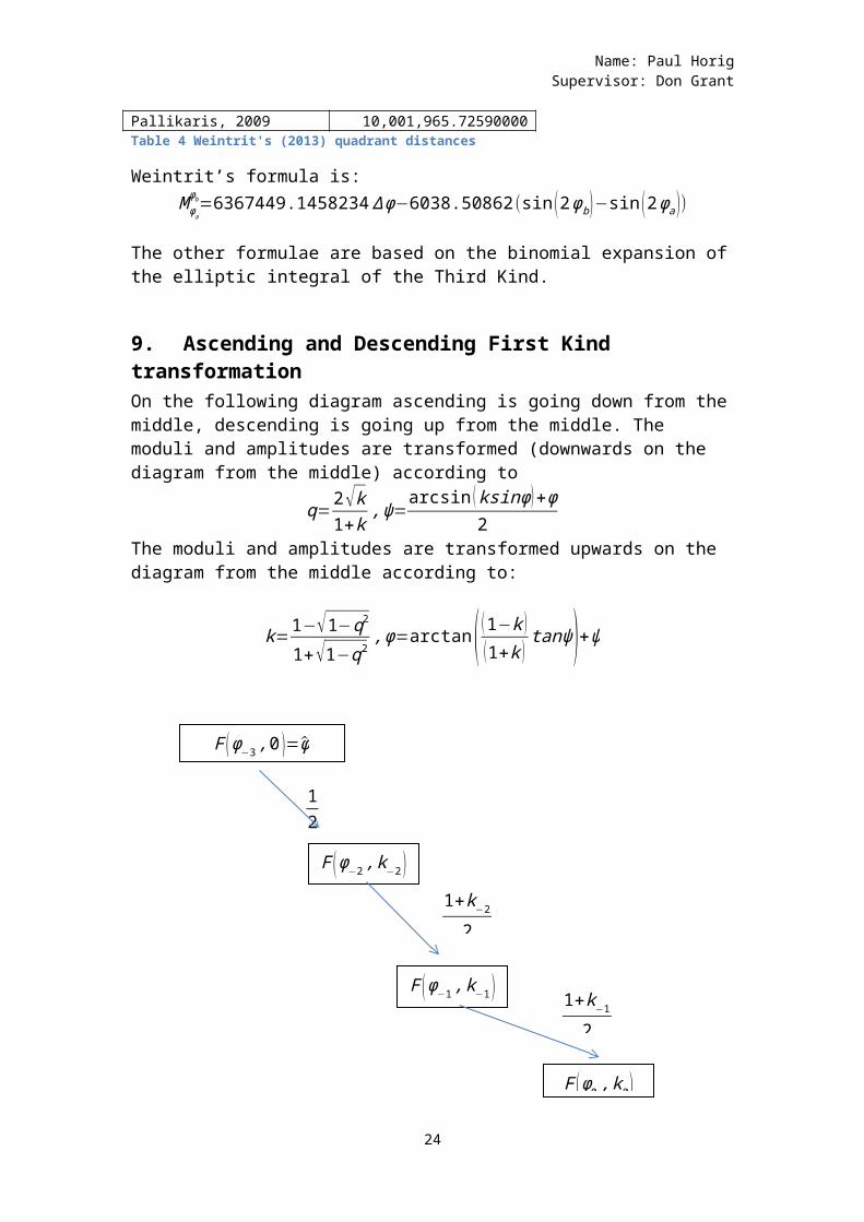
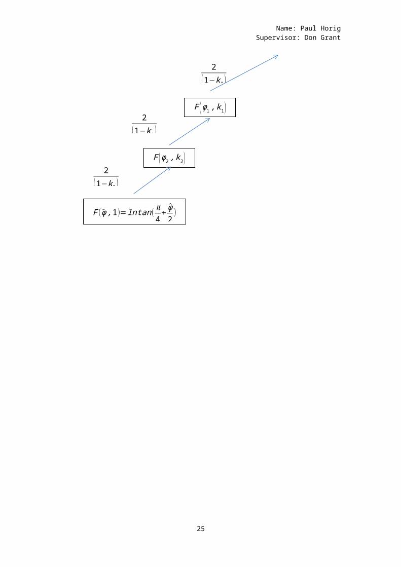
9. Ascending and Descending First Kind transformation On the following diagram ascending is going down from themiddle, descending is going up from the middle. The moduli and amplitudes are transformed (downwards on the diagram from the middle) according to
q=2√k1+k ,ψ=
arcsin (ksinϕ)+ϕ2
The moduli and amplitudes are transformed upwards on the diagram from the middle according to:
k=1−√1−q2
1+√1−q2,ϕ=arctan( (1−k )
(1+k )tanψ)+ψ
24
12
1+k−2
2
1+k−1
2
F (ϕ0,k0)
F (ϕ−1,k−1 )
F (ϕ−2,k−2 )
F (ϕ−3,0 )=ϕ
Name: Paul HorigSupervisor: Don Grant
25
2(1−k0 )
F (ϕ2,k2)
F(ϕ,1)=lntan(π4
+ϕ2
)
F (ϕ1,k1)2
(1−k1 )
2(1−k2 )
Name: Paul HorigSupervisor: Don Grant
10. Landen’s descending transformation for SecondKind integralsThe ascending transformation for elliptic integrals of the second kind is:
E (ϕ,k )+ksinϕ=(1+k )E (ψ,q)+ (1−k )F(ψ,q)
This can be rearranged as:
E (ϕ,k )−(1−k )F(ψ,q)+ksinϕ1+k =E (ψ,q)
11+k E (ϕ,k )− (1−k )
1+k F(ψ,q)+k
1+k sinϕ=E (ψ,q)
E (ψ,q)= 11+k E (ϕ,k )− (1−k)
1+k F (ψ,q)+ k1+k sinϕ
The new k is found from the old q by the previously derived formula:
k=1−√1−q2
1+√1−q2
(18)
And the new amplitude is found by the previously derived formula:
ϕ=arctan( (1−k )(1+k )
tanψ)+ψ (19)
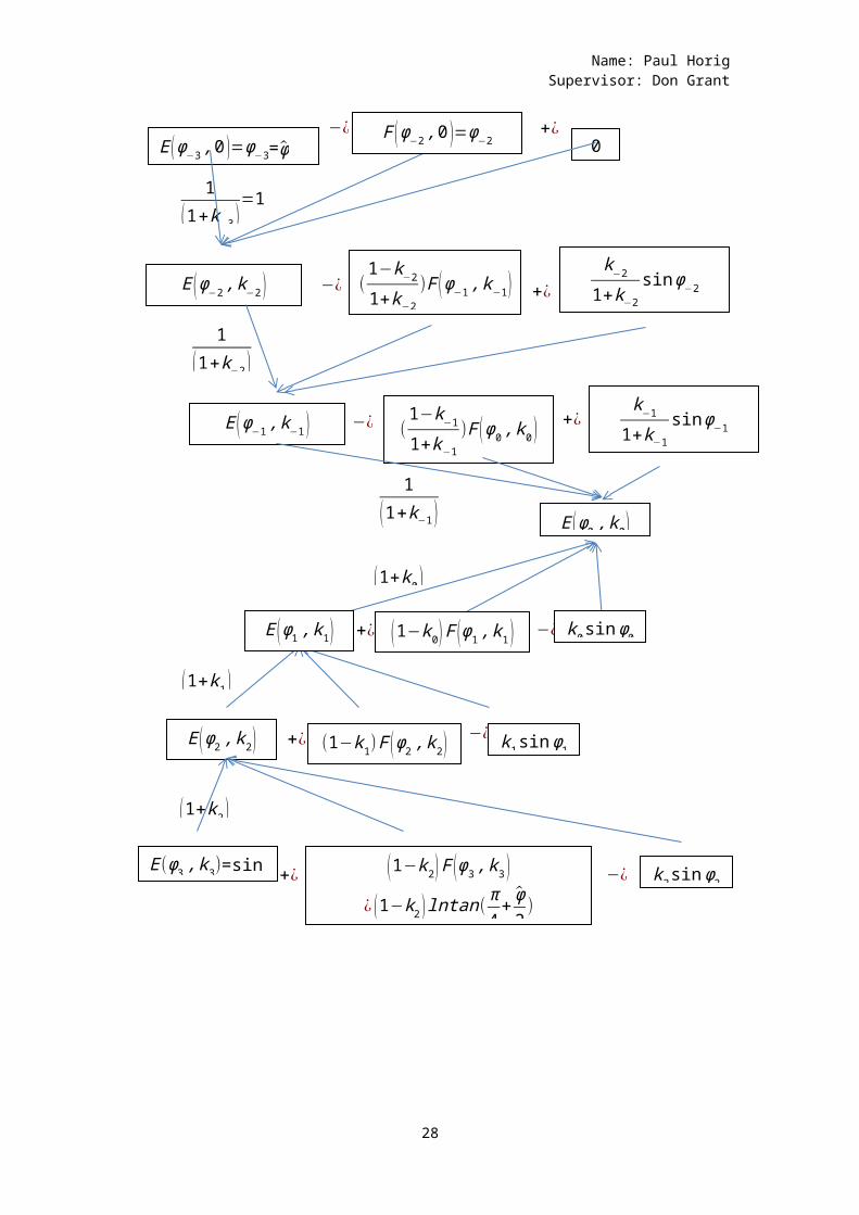
11. Ascending and Descending Second Kind transformation On this diagram ascending is going down descending is going up. The moduli and amplitudes are transformed (downwards on the diagram) according to
q=2√k1+k ,ψ=
arcsin (ksinϕ)+ϕ2
26
Name: Paul HorigSupervisor: Don Grant
The moduli and amplitudes are transformed upwards on the diagram according to:
k=1−√1−q2
1+√1−q2,ϕ=arctan( (1−k )
(1+k )tanψ)+ψ
27
Name: Paul HorigSupervisor: Don Grant
28
+¿ −¿
1(1+k−1 )
1(1+k−3 )
=1
−¿
(1+k0 )
(1+k2 )
(1+k1 )
+¿ −¿
+¿
E (ϕ0,k0)
E (ϕ2,k2)
E(ϕ3,k3)=sin
(1−k1)F (ϕ2,k2)
(1−k2)F (ϕ3,k3 )¿ (1−k2 )lntan(
π4
+ϕ2
)
k2sinϕ2−¿
k1sinϕ1
E (ϕ1,k1) (1−k0)F (ϕ1,k1 ) k0sinϕ0
k−1
1+k−1sinϕ
−1
E (ϕ−3,0 )=ϕ−3=ϕ+¿
0
−¿ +¿E (ϕ−1,k−1 ) (1−k
−1
1+k−1)F (ϕ0,k0 )
E (ϕ−2,k−2 ) (1−k
−2
1+k−2)F (ϕ−1,k−1)
k−2
1+k−2sinϕ
−2−¿ +¿
1(1+k−2 )
F (ϕ−2,0 )=ϕ−2
Name: Paul HorigSupervisor: Don Grant
12. Inverting Elliptic Integrals of the First KindAn Elliptic Integral of the First Kind can be written as:
u (x=sinϕ,k )=F (ϕ,k )= ∫0
sinϕ dt√(1−t2)(1−k2t2)
(20)
The substitution t=sinθ converts this integral to the familiar form:
F (ϕ,k )=∫0
ϕ dθ√1−k2sin2θ
The inverse of the elliptic integral finds the sine of the upper limit of the integration which is sinϕ which isthe sine of the amplitude.
x=sinϕ=sn(u,k) (21)
Further the cosine of the amplitude is cn(u,k) and the delta amplitude is dn (u,k ).
These three - sn,cn∧dn - are the Jacobi elliptic functions.
Landen’s descending transformation is:
u0=F (ψ,q )=1+k2
F(ϕ,k) (22)
k=1−√1−q2
1+√1−q2
(23)
ϕ=arctan( (1−k )(1+k )
tanψ)+ψ (24)
29
Name: Paul HorigSupervisor: Don Grant
Nowsn (u,q )=sin (ψ)
sn (u,q )=sn((1+k)2
u1,2√k1+k )=sin (ψ)
u1=F(ϕ,k)
where
k=1−√1−q2
1+√1−q2
ϕ=arctan( (1−k )(1+k )
tanψ)+ψ (25)
Eventually un will go to ψ which is the amplitude when k goes to zero.
ksinϕ=sin (2ψ−ϕ) (26)
arcsin (ksinϕ )+ϕ= 2ψ
ψ=arcsin (ksinϕ )+ϕ
2
sinψ=sinarcsin (ksinϕ )+ϕ2
sn (u,q )=sin ¿ (27)
If we just work with the amplitude then
AMP (u,q )=arcsin (ksinAMP (u1,k )¿+AMP(u1,k))
2
(28)
30
Name: Paul HorigSupervisor: Don Grant
where from (5) and (6)u1=
21+k
u
and
k=1−√1−q2
1+√1−q2
Also we know that
u=F (ϕ0,k0)=(1+k1 )2
(1+k2 )2
… ψ2
where ψ is the amplitude when k goes to zero. k close to zero is the terminating condition for the recursive algorithm used in the program to calculate the amplitude.
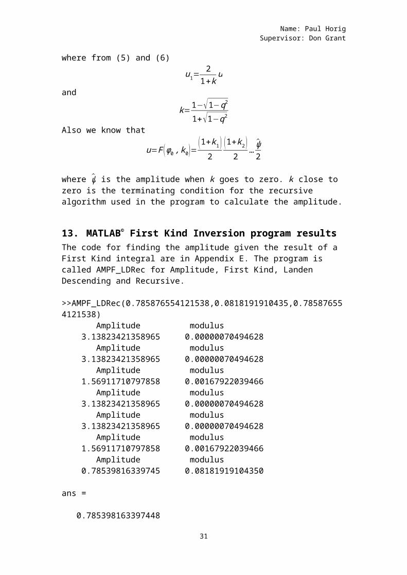
13. MATLAB© First Kind Inversion program resultsThe code for finding the amplitude given the result of a First Kind integral are in Appendix E. The program is called AMPF_LDRec for Amplitude, First Kind, Landen Descending and Recursive.
>>AMPF_LDRec(0.785876554121538,0.0818191910435,0.785876554121538) Amplitude modulus 3.13823421358965 0.00000070494628 Amplitude modulus 3.13823421358965 0.00000070494628 Amplitude modulus 1.56911710797858 0.00167922039466 Amplitude modulus 3.13823421358965 0.00000070494628 Amplitude modulus 3.13823421358965 0.00000070494628 Amplitude modulus 1.56911710797858 0.00167922039466 Amplitude modulus 0.78539816339745 0.08181919104350
ans =
0.785398163397448
31
Name: Paul HorigSupervisor: Don Grant
14. Evaluating General Elliptic Integrals of the Third Kind using Carlson Symmetric Forms
The Incomplete Elliptic Integral of the Third Kind in Legendre notation with Amplitude ϕ, Characteristic n, andModulus k is:
Π(ϕ,n,k)=∫0
ϕ 1(1−nsin2θ)√¿¿¿
¿(29)
The Carlson forms use a notation using x, y, and z ratherthan ϕ and k.The Carlson Symmetric Form of the First Kind elliptic integral is (Zill p200):
RF (x,y,z)=12∫0
∞ dt√(t+x)(t+y)(t+z)
=R(12; 12; 12; 12;x,y,z)
(30)
The following is the Carlson Symmetric Form of the Third Kind elliptic integral
RJ (x,y,z,p)=32∫0
∞ dt(t+p)√(t+x)(t+y)(t+z)
(31)
¿R(12; 12; 12; 12;1;x,y,z,p)
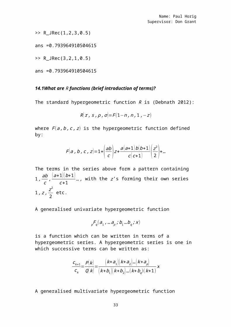
The Forms are called symmetric because the integrals are unchanged if the arguments are switched around. For example RF (1,2,3) is the same as RF (3,2,1). With the RJ Formthis is true with the x,y,z but not the p.
Running my program R_JRec with the arguments (1,2,3,0.5) gives the same result as running it with (3,2,1,0.5)
32
Name: Paul HorigSupervisor: Don Grant
>> R_JRec(1,2,3,0.5)
ans =0.793964910504615
>> R_JRec(3,2,1,0.5)
ans =0.793964910504615
14.1What are R functions (brief introduction of terms)?
The standard hypergeometric function R is (Debnath 2012):
R (r,s,ρ,σ )=F(1−n,n,1,−z)
where F(a,b,c,z) is the hypergeometric function defined by:
F (a,b,c,z )=1+(abc )z+a (a+1 )b (b+1 )
c (c+1 ) (z2
2 )+…The terms in the series above form a pattern containing
1, abc , (a+1) (b+1 )c+1
…, with the z’s forming their own series
1,z, z2
2 etc.
A generalised univariate hypergeometric function
Fq(a1,…ap;b1…bq;x)p
is a function which can be written in terms of a hypergeometric series. A hypergeometric series is one in which successive terms can be written as:
ck+1
ck=P (k )Q (k )
=(k+a1 )(k+a2 )… (k+ap)
(k+b1 )(k+b2)…(k+bq)(k+1)x
A generalised multivariate hypergeometric function
33
Name: Paul HorigSupervisor: Don Grant
Fqα(a1,…ap;b1…bq;x1,…xn)p
Can be written as:
∑k=0
∞
∑κ├k
(a1 )κ… (ap )κk! (b1)κ… (bq )κ
.Cκα(x1,…xn)
where the Pocchammer symbol is:
αk≡ ∏(i,j)∈κ
(a−i−1α
+j−1)
and the “C” Jack function is:
Cκα(x1,…xn)
The notation κ├ k means:
κ=(κ1,κ2,…)├kk=κ1+κ2+…
For example:
1=12=2¿1+13=3¿2+1¿1+1+1
14.2Elliptic Integral of the Third Kind with parameters useful in geodesyThe Elliptic Integral of the Third Kind with parameters useful in geodesy in terms of the Carlson Symmetric Formsis:
Π3 (ϕ,n,k )=¿
sinϕRF¿
+13nsin3ϕRj¿
(32)
34
Name: Paul HorigSupervisor: Don Grant
Now by the duplication theorem (Press p262):
RF (x,y,z)=RF(x+λ4
,y+λ4
,z+λ4 ) (3
3)
Let x0=x, y0=y, z0=z. Then iterate the series:
λn=√xnyn+√ynzn+√znxn
xn+1=xn+λn
4
yn+1=yn+λn
4
zn+1=zn+λn
4Now
RF (μ,μ,μ )=12∫0
∞ dt√(t+μ)(t+μ)(t+μ)
(34)
¿12∫0
∞ dt
(t+μ)32
¿12∫0
∞
(t+μ )−32 ⅆt
[−(t+μ)−12 ]0
∞
[0 ]−[−(0+μ )−12 ]
μ−12
35
Name: Paul HorigSupervisor: Don Grant
Calculating RJ(x,y,z,p)
RJ (x,y,z,p)=32∫0
∞ dt(t+p)√(t+x)(t+y)(t+z)
(35)
Now
RJ (x,y,z,p)=14RJ(x+λ
4, y+λ
4, z+λ
4, p+λ
4 )+6RF ¿(36)
whered=(√p+√x)(√p+√y)(√p+√z)
λ=√xy+√yz+√zx When the arguments converge to μ then Equation (35) becomes:
RJ (μ,μ,μ,μ )=32∫0
∞ dt(t+μ)√(t+μ)(t+μ)(t+μ)
(37)
RJ (μ,μ,μ,μ )=32∫0
∞ dt
(t+μ )52
RJ (μ,μ,μ,μ )=32∫0
∞
(t+μ)−52 dt
RJ (μ,μ,μ,μ )=32∫0
∞
(t+μ)−52 dt
[−(t+μ)−32 ]0
∞
36
Name: Paul HorigSupervisor: Don Grant
[0 ]−[−(0+μ )−32 ]
μ−32
The program to implement this I have called ThirdCarlson.The results of running this program and comparing it to the inbuilt MATLAB© program ‘ellipticPI(n,ϕ,m) can be found in Appendix J. There is no difference between my program and MATLAB©’s at the fourteenth decimal place.
Carlson’s form allows arbitrary ranges of integration (Press, 1992, p. 262).
15. Inverting Elliptic Integrals of the Third Kind using Carlson form and a binary technique
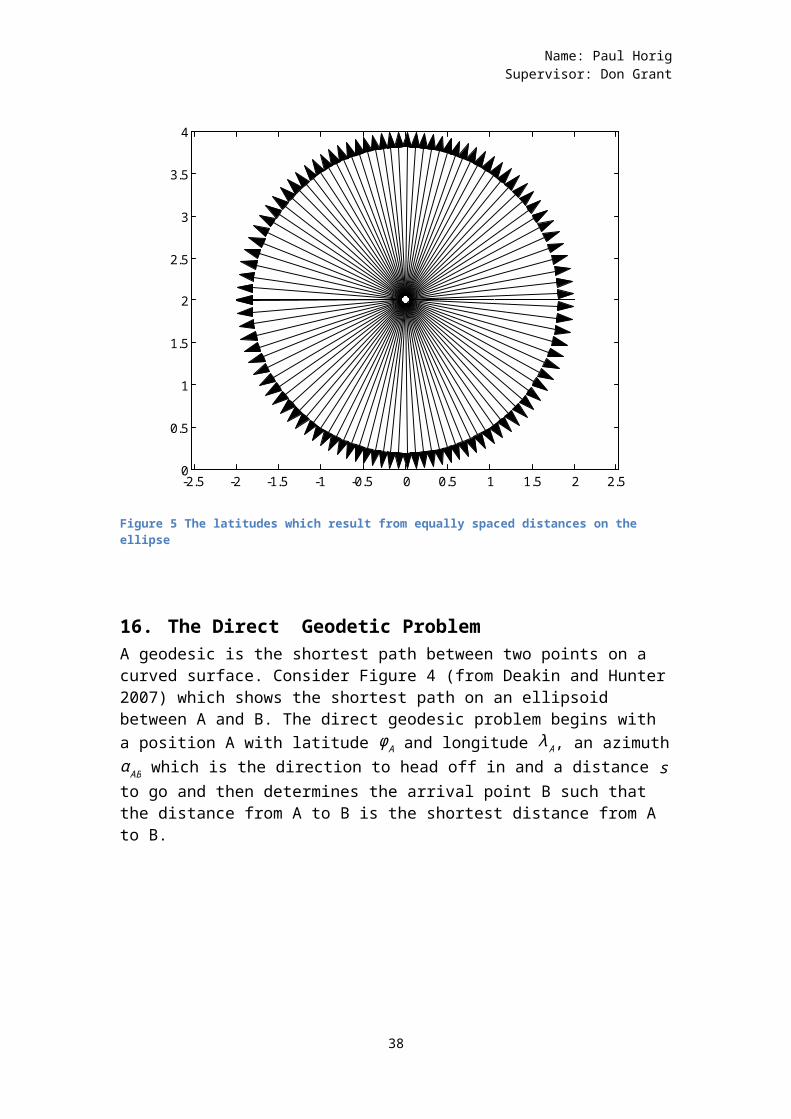
Appendix G has the code for inverting an elliptic integral of the Third Kind using a simple binary technique. Work was done trying to get a Newton-Raphson technique to work but this was abandoned as there were problems with convergence (see appendix R).The binary technique is extremely robust but takes about fifty iterations to achieve 1E-15 precision. The following is a test of this program usingn=0.333514524427718 and k=0.08181919104281579 and u ranging from -2*1.92764575848523 to 2*1.92764575848523.
37
Name: Paul HorigSupervisor: Don Grant
-2.5 -2 -1.5 -1 -0.5 0 0.5 1 1.5 2 2.50
0.5
1
1.5
2
2.5
3
3.5
4
Figure 5 The latitudes which result from equally spaced distances on the ellipse
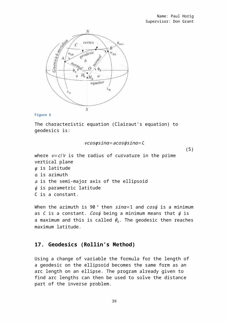
16. The Direct Geodetic ProblemA geodesic is the shortest path between two points on a curved surface. Consider Figure 4 (from Deakin and Hunter2007) which shows the shortest path on an ellipsoid between A and B. The direct geodesic problem begins with a position A with latitude ϕA and longitude λA, an azimuthαAB which is the direction to head off in and a distance sto go and then determines the arrival point B such that the distance from A to B is the shortest distance from A to B.
38
Name: Paul HorigSupervisor: Don Grant
Figure 6
The characteristic equation (Clairaut’s equation) to geodesics is:
νcosϕsinα=acosψsinα=C(5)
where ν=c /V is the radius of curvature in the prime vertical planeϕ is latitudeα is azimuth a is the semi-major axis of the ellipsoidψ is parametric latitudeC is a constant.
When the azimuth is 90° then sinα=1 and cosψ is a minimumas C is a constant. Cosψ being a minimum means that ψ is a maximum and this is called ψ0. The geodesic then reachesmaximum latitude.
17. Geodesics (Rollin’s Method)
Using a change of variable the formula for the length of a geodesic on the ellipsoid becomes the same form as an arc length on an ellipse. The program already given to find arc lengths can then be used to solve the distance part of the inverse problem.
39
Name: Paul HorigSupervisor: Don Grant
The formula for a latitude difference on the ellipse is (Rollins, 2010):
λ2−λ1=c∫β1
β2 √1−e2cos2βcosβ√cos2β−c2
dβ(38)
The formula for the geodesic length between two points ofa geodesic is:
s2−s1=a∫β1
β2 cosβ√1−e2cos2β√cos2β−c2
dβ(39)
The constant C is the Clairaut constant of the geodesic and is found from the following equation:
C=sinαcosϕ
√1−e2sin2ϕ=sinαcosβ (40
)
To find the Clairaut constant we must know the azimuth α,the latitude of the starting point on the ellipsoid ϕ andthe first eccentricity e.
β is the reduced latitude and is found from:
β=arctan ¿ (41)
Equations (1) and (2) work when the geodesic does not pass through a vertex. When the geodesic passes through avertex then the integration is divided up into two parts:one up to the vertex and then another from the vertex to the destination (Rollins, 2010, p. 21). For example the geodesic from New York to Paris would be made up of two calculations: from New York up to the vertex and from thevertex to Paris. That is:
∫β1
βmax
+¿∫β2
βmax
¿
By using a change of variable
40
Name: Paul HorigSupervisor: Don Grant
sinϕ=ksinθ (42)
with θ=0 at some Equator crossing ϕ=0 and with the constant k defined by (Rollins, 2010, p. 21):
k=√ 1−C2
1−C2e2
(43)
This change of variable changes Equations (38) and (39) into (Rollins, 2010, p. 22)
λB−λA=C(1−e2)
√1−C2e2∫θA
θB 1(1−k2sin2θ)√1−k2e2sin2θ
dθ(44)
This is an elliptic integral of the Third Kind with C andk being given by equations (40) and (43) and e being the first eccentricity. The corresponding geodesic distance is:
sB−sA=a(1−e2)
√1−C2e2∫θA
θB 1¿¿ ¿
(45)
which is also an elliptic integral of the Third Kind witha being the semi-major axis of the ellipse.
Now this is the formula for meridian arc length on an ellipse having a semi-major axis of length (Rollins, 2010, p. 22):
a1=a√(1−C2e2)
and eccentricity
e1=kebetween latitudes θA and θB.
Now the direct problem will require finding θBwith all theother variables knownAn advantage of equation (44) and (45) over (38) and (39)is that there is no need to break up geodesics which passthrough a vertex (Rollins, 2010, p. 23).
41
Name: Paul HorigSupervisor: Don Grant
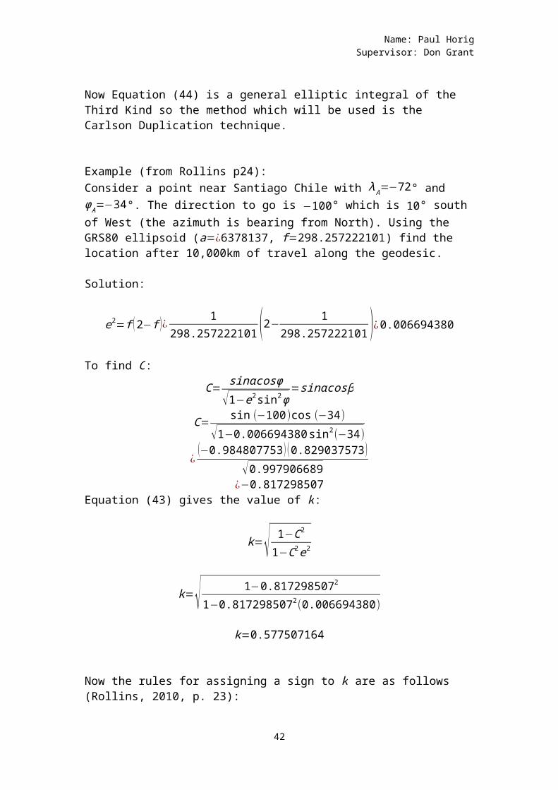
Now Equation (44) is a general elliptic integral of the Third Kind so the method which will be used is the Carlson Duplication technique.
Example (from Rollins p24):Consider a point near Santiago Chile with λA=−72° andϕA=−34°. The direction to go is −100° which is 10° south of West (the azimuth is bearing from North). Using the GRS80 ellipsoid (a=¿6378137, f=298.257222101) find the location after 10,000km of travel along the geodesic.
Solution:
e2=f (2−f )¿ 1298.257222101 (2−
1298.257222101 )¿0.006694380
To find C:C=
sinαcosϕ√1−e2sin2ϕ
=sinαcosβ
C=sin (−100)cos (−34)
√1−0.006694380sin2(−34)
¿(−0.984807753) (0.829037573)
√0.997906689¿−0.817298507
Equation (43) gives the value of k:
k=√ 1−C2
1−C2e2
k=√ 1−0.8172985072
1−0.8172985072(0.006694380)
k=0.577507164
Now the rules for assigning a sign to k are as follows (Rollins, 2010, p. 23):
42
Name: Paul HorigSupervisor: Don Grant
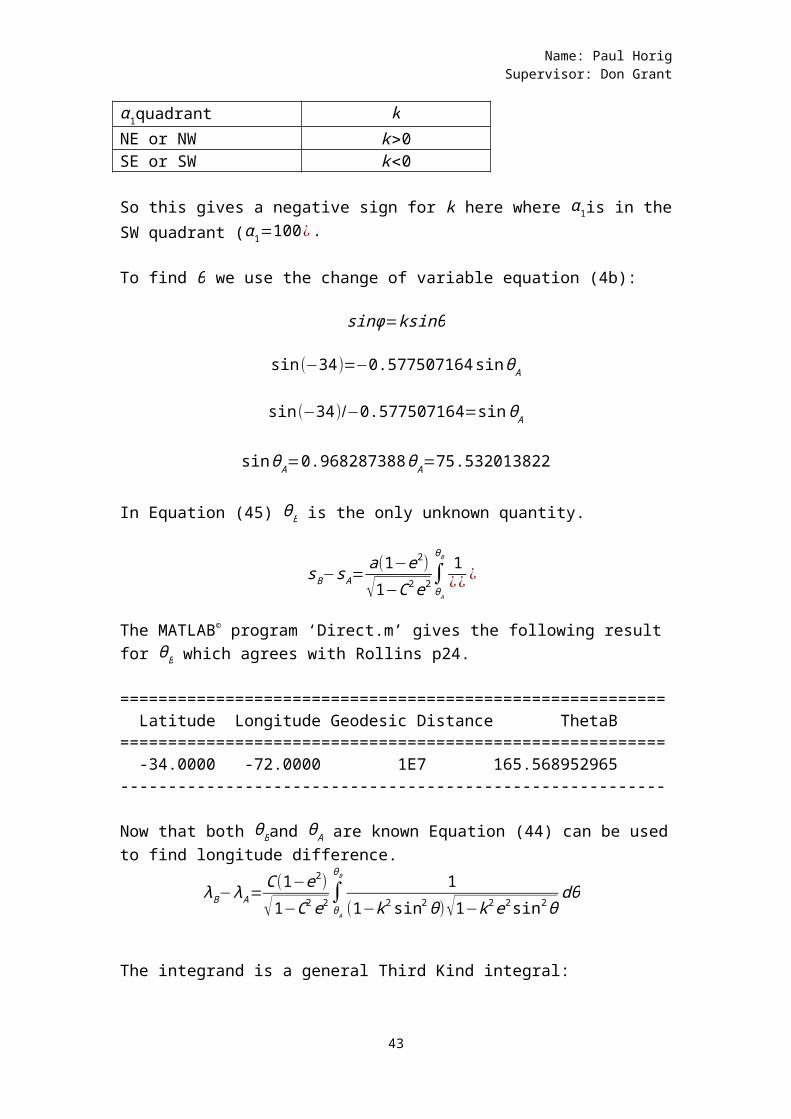
α1quadrant kNE or NW k>0SE or SW k<0
So this gives a negative sign for k here where α1is in theSW quadrant (α1=100¿.
To find θ we use the change of variable equation (4b):
sinϕ=ksinθ
sin(−34)=−0.577507164sinθA
sin(−34)/−0.577507164=sinθA
sinθA=0.968287388θA=75.532013822
In Equation (45) θB is the only unknown quantity.
sB−sA=a(1−e2)
√1−C2e2∫θA
θB 1¿¿ ¿
The MATLAB© program ‘Direct.m’ gives the following result for θB which agrees with Rollins p24.
========================================================= Latitude Longitude Geodesic Distance ThetaB========================================================= -34.0000 -72.0000 1E7 165.568952965---------------------------------------------------------
Now that both θBand θA are known Equation (44) can be usedto find longitude difference.
λB−λA=C(1−e2)
√1−C2e2∫θA
θB 1(1−k2sin2θ)√1−k2e2sin2θ
dθ
The integrand is a general Third Kind integral:
43
Name: Paul HorigSupervisor: Don Grant
∫θA
θB 1(1−k2sin2θ)√1−k2e2sin2θ
dθ
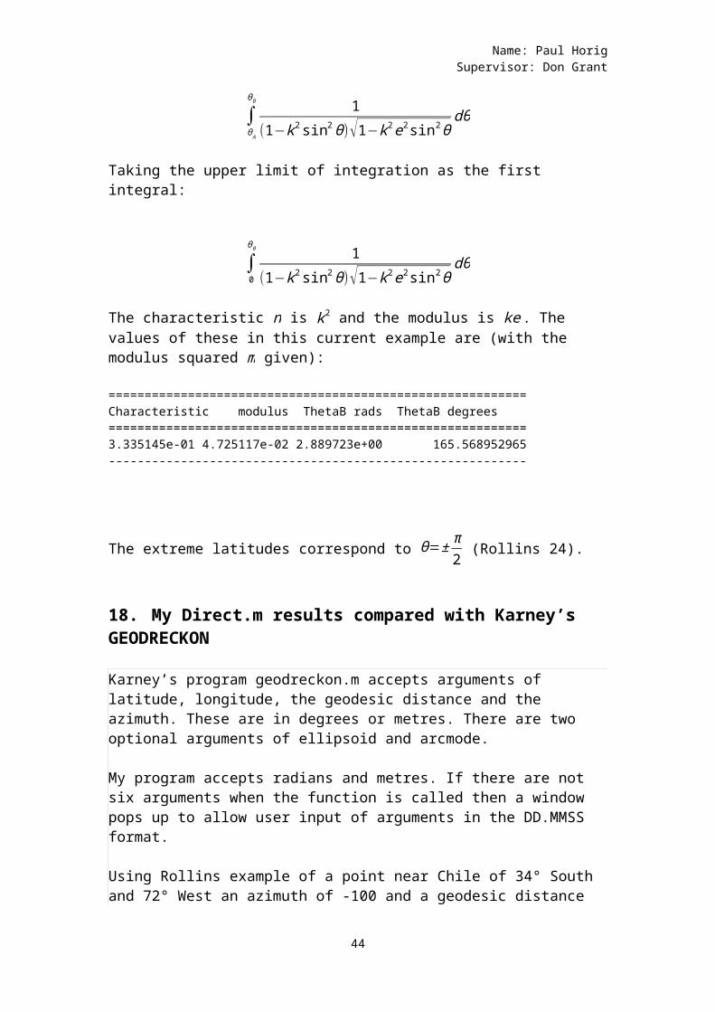
Taking the upper limit of integration as the first integral:
∫0
θB 1(1−k2sin2θ)√1−k2e2sin2θ
dθ
The characteristic n is k2 and the modulus is ke. The values of these in this current example are (with the modulus squared m given):
==========================================================Characteristic modulus ThetaB rads ThetaB degrees==========================================================3.335145e-01 4.725117e-02 2.889723e+00 165.568952965----------------------------------------------------------
The extreme latitudes correspond to θ=± π2 (Rollins 24).
18. My Direct.m results compared with Karney’s GEODRECKON
Karney’s program geodreckon.m accepts arguments of latitude, longitude, the geodesic distance and the azimuth. These are in degrees or metres. There are two optional arguments of ellipsoid and arcmode.
My program accepts radians and metres. If there are not six arguments when the function is called then a window pops up to allow user input of arguments in the DD.MMSS format.
Using Rollins example of a point near Chile of 34° South and 72° West an azimuth of -100 and a geodesic distance
44
Name: Paul HorigSupervisor: Don Grant
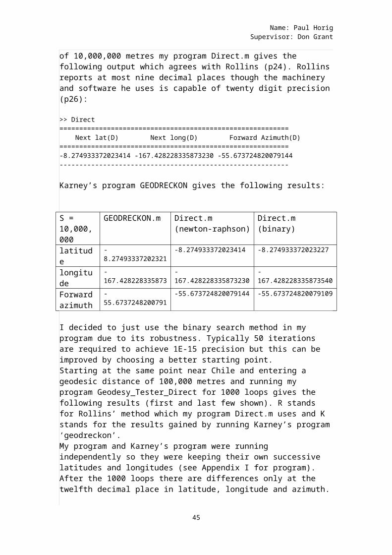
of 10,000,000 metres my program Direct.m gives the following output which agrees with Rollins (p24). Rollinsreports at most nine decimal places though the machinery and software he uses is capable of twenty digit precision(p26):
>> Direct========================================================== Next lat(D) Next long(D) Forward Azimuth(D)==========================================================-8.274933372023414 -167.428228335873230 -55.673724820079144----------------------------------------------------------
Karney’s program GEODRECKON gives the following results:
S = 10,000,000
GEODRECKON.m Direct.m (newton-raphson)
Direct.m (binary)
latitude
-8.27493337202321
-8.274933372023414 -8.274933372023227
longitude
-167.428228335873
-167.428228335873230
-167.428228335873540
Forwardazimuth
-55.6737248200791
-55.673724820079144 -55.673724820079109
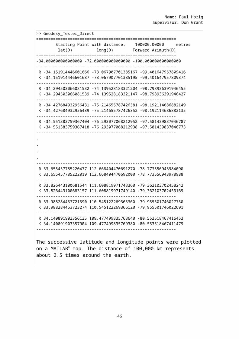
I decided to just use the binary search method in my program due to its robustness. Typically 50 iterations are required to achieve 1E-15 precision but this can be improved by choosing a better starting point.Starting at the same point near Chile and entering a geodesic distance of 100,000 metres and running my program Geodesy_Tester_Direct for 1000 loops gives the following results (first and last few shown). R stands for Rollins’ method which my program Direct.m uses and K stands for the results gained by running Karney’s program‘geodreckon’. My program and Karney’s program were running independently so they were keeping their own successive latitudes and longitudes (see Appendix I for program). After the 1000 loops there are differences only at the twelfth decimal place in latitude, longitude and azimuth.
45
Name: Paul HorigSupervisor: Don Grant
>> Geodesy_Tester_Direct========================================================== Starting Point with distance, 100000.00000 metres lat(D) long(D) Forward Azimuth(D)==========================================================-34.000000000000000 -72.000000000000000 -100.000000000000000---------------------------------------------------------- R -34.151914446601666 -73.067907701385167 -99.401647957809416 K -34.151914446601687 -73.067907701385195 -99.401647957809374---------------------------------------------------------- R -34.294503066081532 -74.139528183321204 -98.798936391946455 K -34.294503066081539 -74.139528183321147 -98.798936391946427---------------------------------------------------------- R -34.427684932956431 -75.214655787426381 -98.192114686882149 K -34.427684932956439 -75.214655787426352 -98.192114686882135---------------------------------------------------------- R -34.551383759367404 -76.293077068212952 -97.581439837046787 K -34.551383759367418 -76.293077068212938 -97.581439837046773----------------------------------------------------------....---------------------------------------------------------- R 33.655457785220477 112.668404470691270 -78.773556943984090 K 33.655457785222019 112.668404470692000 -78.773556943978988---------------------------------------------------------- R 33.826443100681544 111.608819971748360 -79.362103702458242 K 33.826443100683157 111.608819971749140 -79.362103702453169---------------------------------------------------------- R 33.988284453721590 110.545122269365360 -79.955501746027750 K 33.988284453723274 110.545122269366120 -79.955501746022691---------------------------------------------------------- R 34.140891903356135 109.477499835768640 -80.553518467416453 K 34.140891903357904 109.477499835769380 -80.553518467411479----------------------------------------------------------
The successive latitude and longitude points were plottedon a MATLAB© map. The distance of 100,000 km represents about 2.5 times around the earth.
46
Name: Paul HorigSupervisor: Don Grant
-200 -150 -100 -50 0 50 100 150 200-100
-50
0
50
100
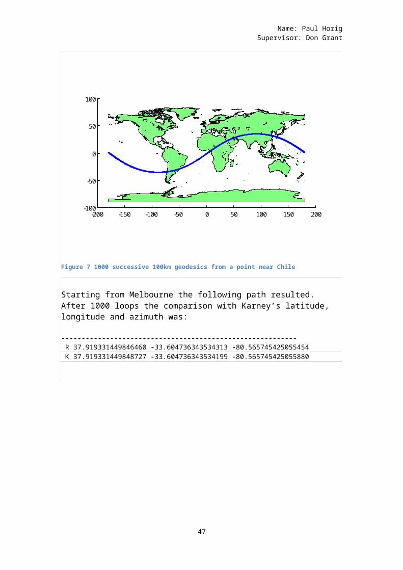
Figure 7 1000 successive 100km geodesics from a point near Chile
Starting from Melbourne the following path resulted. After 1000 loops the comparison with Karney’s latitude, longitude and azimuth was:
---------------------------------------------------------- R 37.919331449846460 -33.604736343534313 -80.565745425055454 K 37.919331449848727 -33.604736343534199 -80.565745425055880
47
Name: Paul HorigSupervisor: Don Grant
-200 -150 -100 -50 0 50 100 150 200-100
-50
0
50
100Succesive 100km geodesics from M elbourne. Starting azim uth = -100°
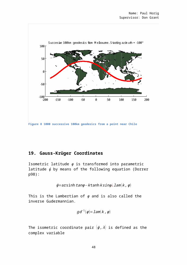
Figure 8 1000 successive 100km geodesics from a point near Chile
19. Gauss-Krüger Coordinates
Isometric latitude ϕ is transformed into parametric latitude ψ by means of the following equation (Dorrer p98):
ψ=arsinhtanϕ−ktanhksinϕ¿lam(k,ϕ)
This is the Lambertian of ϕ and is also called the inverse Gudermannian.
gd−1(ϕ)=lam(k,ϕ)
The isometric coordinate pair (ψ,λ ) is defined as the complex variable
48
Name: Paul HorigSupervisor: Don Grant
Λ=λ+jψ
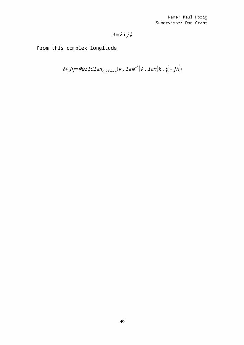
From this complex longitude
ξ+jη=MeridianDistance(k,lam−1 (k,lam (k,ϕ)+jλ))
49
Name: Paul HorigSupervisor: Don Grant
19.1amplitude in Landen’s descending transformation
The method used in the program in the appendix is
20. Calculation of UTM and Geodetic Coordinates
A Transverse Mercator Projection is defined by the following equations (Dozier, 1980, p. 2):
ζ=arctan (snω )−karctan(ksnω)
where snω is the Jacobian elliptic function sn (ω|m).
The Gauss-Krüger projection is one kind of Transverse Mercator Projection is:
za=(1−m )∫
0
ω
dn−2tdt
which can be written as:
za=E (ω|m )−msnωcnω
dnω
E (ω|m ) is an elliptic integral of the Second Kind. This canbe found using the arithmetic-geometric mean as describedin section 5 above.
An expression for snω is:
snω=2π
m12 K
∑n
∞ qn+
12
1−q2n+1 sin (2n+1) (πω2K )¿¿
50
Name: Paul HorigSupervisor: Don Grant
K is the elliptic integral of the First Kind and can be found using the arithmetic-geometric mean as described insection 4 above.
q is the nome and is defined by:
q=e−πK'K
21. Safeguards against the computer not preserving precision when implementing recursion
The advantages of using a recursion algorithm:1. Once the precision is specified then the recursions
are performed until the precision is met. 2. The intermediate results are passed on to the next
level3. The program structure remains the same regardless of
the ellipsoid used. With different constants just feed the new constants into the top level
The disadvantages of using a recursion algorithm1. The computer and software need to be able to manage
the recursion without losing precision.
22. Conclusions:
Carlson’s forms can be used for all three kinds of elliptic integrals when going forward from angle to result of integral and give arbitrary precision.The MATLAB© inbuilt functions ellipticF, ellipticE and ellipticPI are precise to machine precision and so they should be because they use a calculation method based on the arithmetic-geometric mean which is a specialized version of the Carlson Duplication technique. The MATLAB© Second Kind integral function ellipticE matches my SecondKind integral using the Landen transformation to the fourteenth decimal place (Section 6). So when writing geodetic programs in MATLAB© then we know we have at least14 decimal place precision with the elliptic integrals.
51
Name: Paul HorigSupervisor: Don Grant
Inversion of the First Kind integral is precise using theLanden transformation without any use of a numerical technique.The programs which invert the Third Kind integrals have used a simple binary search as this is easy to program and reliable with the downside that about fifty iterations are required for femtometre precision. The final program here – Direct.m – which finds successive latitude and longitude points when called to calculate 1000 successive geodesics takes 29.13 seconds to run. Calling the Karney program takes 5.6 seconds to do the same job. Calling both programs takes 29.73 seconds. Thismeans the Karney program without the calling program is taking 0.6 seconds to calculate the 1000 geodesics. My program Direct.m is taking 24 seconds. It is the binary search which takes up most of the time. So my Direct.m isan example of the precision of the Carlson method rather than a fast method of finding geodesics. Karney’s programuses the auxiliary sphere, series reversion and a Newton-Raphson step to increase precision.
Comparing my program to the precision of the Karney program ‘geodreckon.m’ it matches ‘geodreckon.m’s resultsto the eleventh decimal place. This shows that using femtometre precision allows the preservation of nanometreprecision after a lot of accumulated small error. The practical consequence of this is that when finding UTM grid coordinates using a high precision method based on Carlson Duplication then mm errors may be found at the edges of the UTM zone. If so then this has consequences for comparing the recorded permanent mark grid coordinates with what the GPS satellite says it should be.
In addition the Carlson Duplication technique does not produce singularities at the poles and this along with precision over the whole ellipsoid rather than just in 6°widths provides a precise grid system for the entire ellipsoid.
These things of course are also offered by Karney’s methods using an auxiliary sphere but the advantage of
52
Name: Paul HorigSupervisor: Don Grant
using direct calculation is a pedagogical one; there is no need to introduce the extra concept of an auxiliary sphere. This is also an advantage of Carlson Duplication over Landen transformation as the Landen transformation deals with two types of transformed quantities (angle andmodulus) while Carlson Duplication only deals with the independent variables. So using Carlson Duplication reduces the quantity of concepts to deal with.
In addition to the use of the Landen transformation and Carlson Forms these methods were implemented using recursive techniques. The advantage of the recursive technique is that it can give arbitrary accuracy up to the limits of machinery and software.
Another advantage of the recursive approach is that it can save space in documentation and programming. There isno need for lists of terms and the recursive technique means that the work of the program is done in two steps: the recursive line and the terminating condition.
So the final conclusion is that Carlson Duplication implemented using a recursive algorithm should be used for determining arc lengths for a worldwide grid coordinate system.
BibliographyGeocentric Datum of Australia. (2014). Retrieved from Geoscience Australia:
http://www.ga.gov.au/scientific-topics/positioning-navigation/geodesy/geodetic-datums/gda
Almkvist, G. (1988). Gauss, Landen, Ramanujan, the Arithmetic-Geometric Mean, Ellipses, pi, and the Ladies Diary. Amer. Math. Monthly, 585–607.
Blumel, R. (2011). Advanced Quantum Mechanics: The Classical-Quantum Connection.Connecticut: Jones and Bartlett.
Borwein, J. B. (1984). The Arithmetic Geometric Mean and Fast Computation of Elementary Functions. Society for Industrial and Applied Mathematics.
Carlson, B. C. (1965). On Computing Elliptic Integrals and Functions.J. Maths and Physics.
Carlson, B. C. (1979). Computing Elliptic Integrals by Duplication. Numerische Mathematik(33), 1-16.
Carlson, B. C. (1995). Numerical Calculation of Real or Complex Elliptic Integrals. Retrieved from arxiv.org.
53
Name: Paul HorigSupervisor: Don Grant
Carlson, D. Z. (1969). Symmetric Elliptic Integrals of the Third Kind. www.ams.org.
Deakin, R. (2010). Geometric Geodesy Part A. RMIT.Deakin, R. (2014). Elliptic Integrals and Landen's Transformation: What I should've
known for Geodesy. Debnath, L. (2012). Non-linear Partial Differential Equations for Scientists and
Engineers. New York: Springer.Diarmuid, M. (2008). Integrable Systems in Celestial Mechanics. Boston:
Birkhäuser.Dorrer, E. (1999). From Elliptic Arc Length to Gauss-Krueger
Coordinates by Analytical Continuation. Geodesy and Geoinformatics.Dozier, J. (1980). Improved Algorithm for Calculation of UTM and Geodetic
Coordinates. NOAA Technical Report NESS 81, U.S. Department of Commerce.
Fukushima, T. (2012). Numerical Inversion of General Incomplete Elliptic Integral. Journal of Computational and Applied Mathematics.
Gerstl, M. (1984). Die Gauss-Krugersche Abbildung des Erdellipsoides mit direkter Berechnung der elliptischen Integrale durch Landentransformation. Munich: Verlag.
Gray. (2001). Automatic Reduction of Elliptic Integrals Using Carlson's Relations.
Hankin, R. (2006). Introducing Elliptic, an R package for elliptic and modular functions. Retrieved from jstatsoft: www.jstatsoft.org/v15/i07/paper
Hunter, R. D. (2007). Geodesics on an Ellipsoid - Pottman's Method. Retrieved from academia.edu.
Jameson, G. (2014). Ellitpic integrals, the arithmetic-geometric mean and the Brent-Salamin algorithm for pi. Retrieved from www.maths.lancs.ac.uk/~jameson/ellagm.pdf
Karney, C. (2011). Geodesics on an ellipsoid of revolution. SRI International.
Karney, C. (2012). Geodesics on an Ellipsoid of Revolution. Retrieved September 30, 2014, from MATLAB Central.
Khan, M. F. (2013). Arc Length of an Elliptical Curve. International Journal of Scientific and Research Publications, 1-5.
King, L. V. (1924). On the Direct Numerical Calculation of Elliptic Functions and Integrals. London: CUP.
Klotz, J. (1993). Eine Analytische Lösung der Gauss-Krüger-Abbildung.ZfV 3/1993, 106-116.
Kos, S. a. (2012). On the Mathematics of Navigational Calculations for Meridian Sailing. Solstice: An Electronic Journal of Geography and Mathematics.
Krakiwsky, E. (1986). Geodesy the Concepts. Amsterdam: Elsevier.Landen, J. (1775, January). An Investigation of a General Theorem for Finding the
Length of Any Arc of Any Conic Hyperbola, by means of Two Elliptic Arcs, with Some Other new and Useful Theorems Deduced Therefrom. Retrieved October 10, 2014, from https://archive.org/details/jstor-106197
Press, F. T. (1992). Numerical Recipes in C: the Art of Scientific Computing. New York: University of Cambridge.
54
Name: Paul HorigSupervisor: Don Grant
Rollins, C. (2010, January). An Integral for Geodesic Length after Derivations by P. D. Thomas. Survey Review, pp. 20-26.
Rösch, N. (2011). The Derivation of Algorithms to Compute Elliptic Integrals of the First and Second Kind by Landen Transformation. Bol. Ciênc. Geod., sec. Artigos, Curitaba, 17, 03-22.
Sjöberg, L. E. (2012). Solutions to the ellipsoidal Clairaut constant and the inverse geodetic problem by numerical integration. Retrieved October 14, 2014, from Journal of Geodetic Science: http://adsabs.harvard.edu/abs/2012JGeoS...2..162S
Tkachev, V. G. (n.d.). Elliptic Functions: Introduction Course. Retrieved from URL: http://www.math.kth.se/˜tkatchev
Villarino, M. B. (6 July 2005). A Direct Proof of Landen’s Transformation. math.CA.
Weintrit, A. (2013). So, What is Actually the Distance from the Equator to the Pole? - Overview of the Meridian Distance Approximations. TransNav, 7(2).
55
Name: Paul HorigSupervisor: Don Grant
23. Appendices
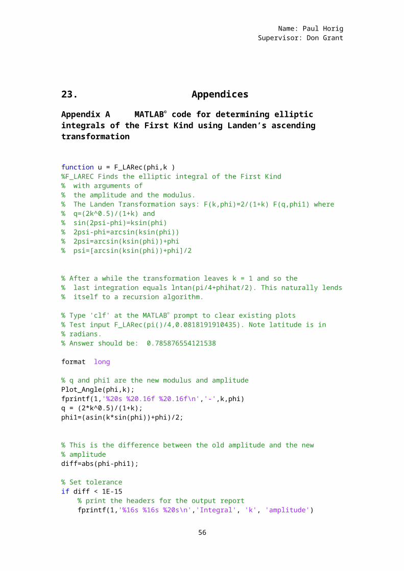
Appendix A MATLAB© code for determining elliptic integrals of the First Kind using Landen’s ascending transformation
function u = F_LARec(phi,k )%F_LAREC Finds the elliptic integral of the First Kind % with arguments of% the amplitude and the modulus.% The Landen Transformation says: F(k,phi)=2/(1+k) F(q,phi1) where% q=(2k^0.5)/(1+k) and % sin(2psi-phi)=ksin(phi)% 2psi-phi=arcsin(ksin(phi))% 2psi=arcsin(ksin(phi))+phi% psi=[arcsin(ksin(phi))+phi]/2 % After a while the transformation leaves k = 1 and so the% last integration equals lntan(pi/4+phihat/2). This naturally lends% itself to a recursion algorithm. % Type 'clf' at the MATLAB© prompt to clear existing plots% Test input F_LARec(pi()/4,0.0818191910435). Note latitude is in% radians.% Answer should be: 0.785876554121538 format long % q and phi1 are the new modulus and amplitudePlot_Angle(phi,k);fprintf(1,'%20s %20.16f %20.16f\n','-',k,phi)q = (2*k^0.5)/(1+k);phi1=(asin(k*sin(phi))+phi)/2; % This is the difference between the old amplitude and the new % amplitudediff=abs(phi-phi1); % Set toleranceif diff < 1E-15 % print the headers for the output report fprintf(1,'%16s %16s %20s\n','Integral', 'k', 'amplitude')
56
Name: Paul HorigSupervisor: Don Grant
u = (2/(1+k))*log(tan(pi()/4 + phi1/2)); return;end % This calls the function recursively. u is the integralu=(2/(1+k))*F_LARec(phi1,q);fprintf(1,'%20.16f %20.16f %20.16f\n',u,q,phi1)end
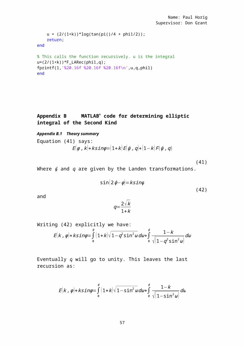
Appendix B MATLAB© code for determining elliptic integral of the Second Kind
Appendix B.1 Theory summary
Equation (41) says:E (ϕ,k )+ksinϕ=(1+k )E (ψ,q)+ (1−k )F(ψ,q)
(41)Where ψ and q are given by the Landen transformations.
sin (2ψ−ϕ)=ksinϕ(42)
and
q=2√k1+k
Writing (42) explicitly we have:
E (k,ϕ )+ksinϕ=∫0
ψ
(1+k )√1−q2sin2ωdω+∫0
ψ 1−k√(1−q2sin2ω )
dω
Eventually q will go to unity. This leaves the last recursion as:
E (k,ϕ )+ksinϕ=∫0
ψ
(1+k )√1−sin2ωdω+∫0
ψ 1−k√(1−sin2ω )
dω
57
Name: Paul HorigSupervisor: Don Grant
E (k,ϕ )+ksinϕ=∫0
ψ
(1+k )cosωdω+∫0
ψ 1−kcosωdω
E (k,ϕ )+ksinϕ=(1+k )(sin ϕ)+(1−k)lntan(π4
+ϕ2
)
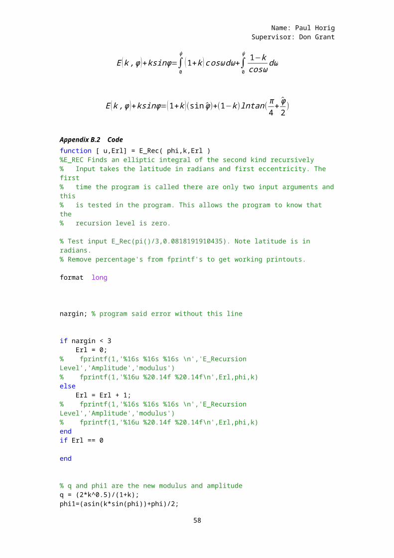
Appendix B.2 Codefunction [ u,Erl] = E_Rec( phi,k,Erl )%E_REC Finds an elliptic integral of the second kind recursively% Input takes the latitude in radians and first eccentricity. The first% time the program is called there are only two input arguments andthis% is tested in the program. This allows the program to know that the% recursion level is zero. % Test input E_Rec(pi()/3,0.0818191910435). Note latitude is in radians.% Remove percentage's from fprintf's to get working printouts. format long nargin; % program said error without this line if nargin < 3 Erl = 0;% fprintf(1,'%16s %16s %16s \n','E_Recursion Level','Amplitude','modulus')% fprintf(1,'%16u %20.14f %20.14f\n',Erl,phi,k)else Erl = Erl + 1;% fprintf(1,'%16s %16s %16s \n','E_Recursion Level','Amplitude','modulus')% fprintf(1,'%16u %20.14f %20.14f\n',Erl,phi,k)endif Erl == 0 end % q and phi1 are the new modulus and amplitudeq = (2*k^0.5)/(1+k);phi1=(asin(k*sin(phi))+phi)/2;
58
Name: Paul HorigSupervisor: Don Grant
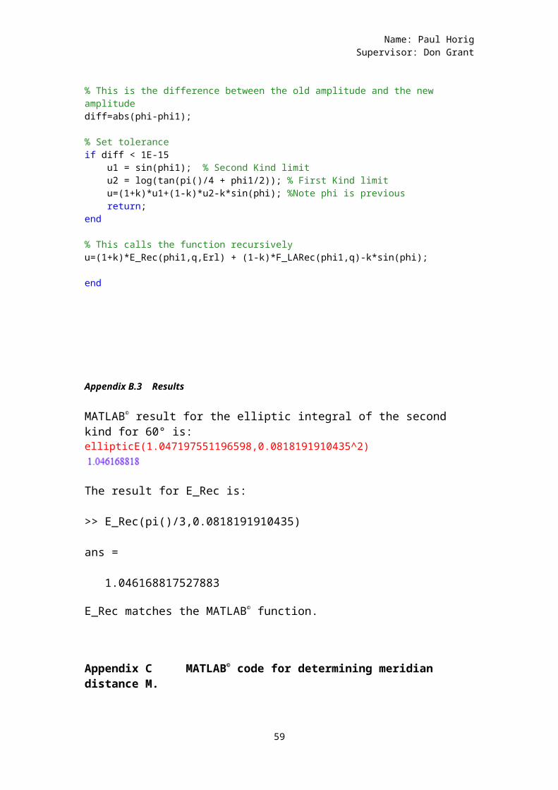
% This is the difference between the old amplitude and the new amplitudediff=abs(phi-phi1); % Set toleranceif diff < 1E-15 u1 = sin(phi1); % Second Kind limit u2 = log(tan(pi()/4 + phi1/2)); % First Kind limit u=(1+k)*u1+(1-k)*u2-k*sin(phi); %Note phi is previous return;end % This calls the function recursivelyu=(1+k)*E_Rec(phi1,q,Erl) + (1-k)*F_LARec(phi1,q)-k*sin(phi); end
Appendix B.3 Results
MATLAB© result for the elliptic integral of the second kind for 60° is:ellipticE(1.047197551196598,0.0818191910435^2)
The result for E_Rec is:
>> E_Rec(pi()/3,0.0818191910435)
ans =
1.046168817527883
E_Rec matches the MATLAB© function.
Appendix C MATLAB© code for determining meridian distance M.
59
Name: Paul HorigSupervisor: Don Grant
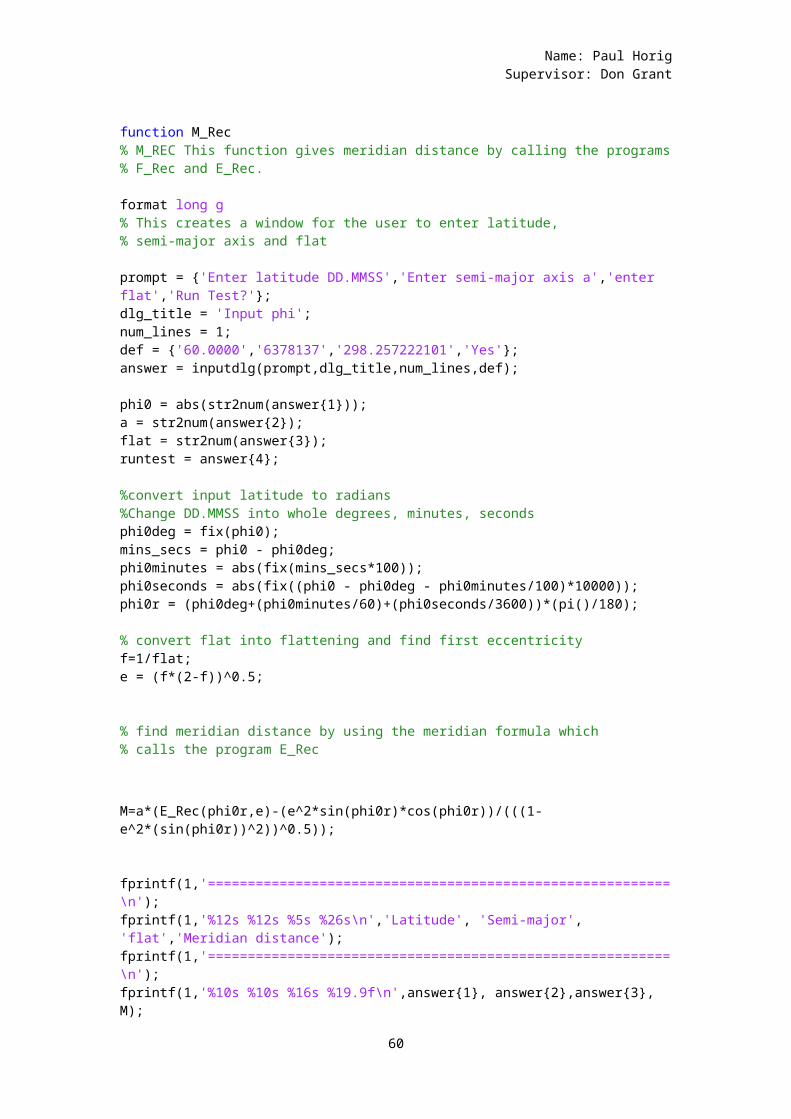
function M_Rec% M_REC This function gives meridian distance by calling the programs% F_Rec and E_Rec. format long g% This creates a window for the user to enter latitude,% semi-major axis and flat prompt = {'Enter latitude DD.MMSS','Enter semi-major axis a','enter flat','Run Test?'};dlg_title = 'Input phi';num_lines = 1;def = {'60.0000','6378137','298.257222101','Yes'};answer = inputdlg(prompt,dlg_title,num_lines,def); phi0 = abs(str2num(answer{1}));a = str2num(answer{2});flat = str2num(answer{3});runtest = answer{4}; %convert input latitude to radians%Change DD.MMSS into whole degrees, minutes, secondsphi0deg = fix(phi0);mins_secs = phi0 - phi0deg;phi0minutes = abs(fix(mins_secs*100));phi0seconds = abs(fix((phi0 - phi0deg - phi0minutes/100)*10000));phi0r = (phi0deg+(phi0minutes/60)+(phi0seconds/3600))*(pi()/180); % convert flat into flattening and find first eccentricityf=1/flat;e = (f*(2-f))^0.5; % find meridian distance by using the meridian formula which% calls the program E_Rec
M=a*(E_Rec(phi0r,e)-(e^2*sin(phi0r)*cos(phi0r))/(((1-e^2*(sin(phi0r))^2))^0.5)); fprintf(1,'==========================================================\n');fprintf(1,'%12s %12s %5s %26s\n','Latitude', 'Semi-major', 'flat','Meridian distance');fprintf(1,'==========================================================\n');fprintf(1,'%10s %10s %16s %19.9f\n',answer{1}, answer{2},answer{3}, M);
60
Name: Paul HorigSupervisor: Don Grant
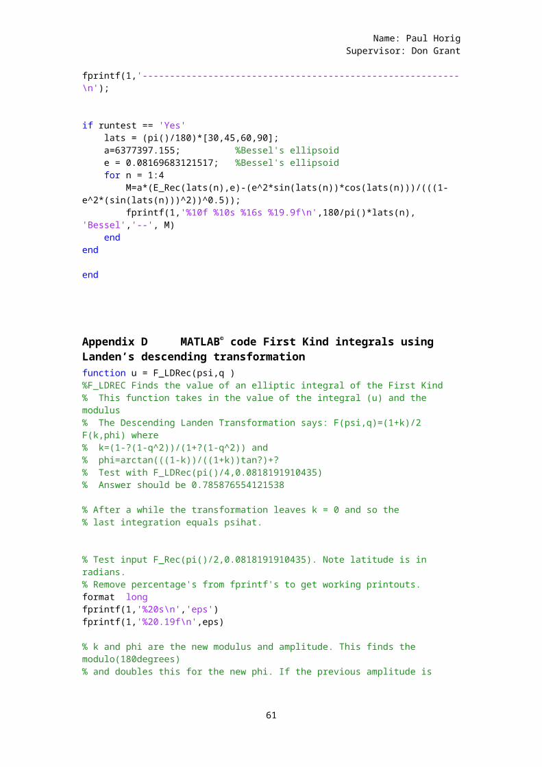
fprintf(1,'----------------------------------------------------------\n'); if runtest == 'Yes' lats = (pi()/180)*[30,45,60,90]; a=6377397.155; %Bessel's ellipsoid e = 0.08169683121517; %Bessel's ellipsoid for n = 1:4 M=a*(E_Rec(lats(n),e)-(e^2*sin(lats(n))*cos(lats(n)))/(((1-e^2*(sin(lats(n)))^2))^0.5)); fprintf(1,'%10f %10s %16s %19.9f\n',180/pi()*lats(n), 'Bessel','--', M) endend end
Appendix D MATLAB© code First Kind integrals using Landen’s descending transformationfunction u = F_LDRec(psi,q )%F_LDREC Finds the value of an elliptic integral of the First Kind% This function takes in the value of the integral (u) and the modulus% The Descending Landen Transformation says: F(psi,q)=(1+k)/2 F(k,phi) where% k=(1-?(1-q^2))/(1+?(1-q^2)) and % phi=arctan(((1-k))/((1+k))tan?)+?% Test with F_LDRec(pi()/4,0.0818191910435)% Answer should be 0.785876554121538 % After a while the transformation leaves k = 0 and so the% last integration equals psihat. % Test input F_Rec(pi()/2,0.0818191910435). Note latitude is in radians.% Remove percentage's from fprintf's to get working printouts.format longfprintf(1,'%20s\n','eps')fprintf(1,'%20.19f\n',eps) % k and phi are the new modulus and amplitude. This finds the modulo(180degrees)% and doubles this for the new phi. If the previous amplitude is
61
Name: Paul HorigSupervisor: Don Grant
% in the second quadrant then add pi() to the new amplitude. This needs% further refinement to cater for particular borderline cases.k = (1-(1-q^2)^0.5)/(1+(1-q^2)^0.5); n=floor(psi/(pi()));psito180=psi-n*pi(); if psito180 > pi()/2 & psi < pi() % psi in second quadrant phi=atan(((1-k)/(1+k))*tan(psito180))+pi()+2*n*pi() +psi;else phi=atan(((1-k)/(1+k))*tan(psito180))+2*n*pi()+psi;end % k will go to zero% Set toleranceif k < 1E-15 u = (1/2)*phi; fprintf(1,'%16s %16s %16s\n','Amplitude','Modulus','Integral') fprintf(1,'%20.14f %20.14f %20.14f\n',psi,q,u) return;end % This calls the function recursivelyu=((1+k)/2)*F_LDRec(phi,k); fprintf(1,'%16s %16s %16s\n','Amplitude','Modulus','Integral') fprintf(1,'%20.14f %20.14f %20.14f\n',psi,q,u)end
Appendix E MATLAB© code for finding the amplitude of aFirst Kind elliptic integral given the result of the integral (inverting the First Kind integral).
function psi = AMPF_LDRec(u,q,psihat)%AMPF_LDREC Finds the value of the amplitude of an elliptic integral of the First Kind% This function takes in the value of the integral (u) and the modulus% (q).% To begin with the value of psihat is input as the same as u the integral.% Test with AMPF_LDRec(0.785876554121538,0.0818191910435,0.785876554121538)% Answer should be pi()/4=0.785398163397448 % After a while the transformation leaves k = 0 and so the% last integration equals psihat.
62
Name: Paul HorigSupervisor: Don Grant
% Remove percentage's from fprintf's to get working printouts.format long%fprintf(1,'%20s\n','eps')%fprintf(1,'%20.19f\n',eps) % k and u1 are the new modulus and integral.% psihat1 is the cumulative product which eventually gives the final% amplitude.k = (1-(1-q^2)^0.5)/(1+(1-q^2)^0.5);u1=(2/(1+k))*u;psihatcum=psihat*(2/(1+k)); % k will go to zero% Set toleranceif k < 1E-15 psi = psihatcum/(2/(1+k)); % This reverses line above for last go% fprintf(1,'%16s %16s %16s\n','Amplitude','Modulus','Integral')% fprintf(1,'%20.14f %20.14f %20.14f\n',psihat,k,u) return;end % This calls the function recursivelypsi=(asin(k*sin(AMPF_LDRec(u1,k,psihatcum)))+AMPF_LDRec(u1,k,psihatcum))/2;fprintf(1,'%16s %16s\n','Amplitude','modulus')fprintf(1,'%20.14f %20.14f\n',psi,q) end
Appendix F MATLAB© code for determining elliptic integral of the Third Kind using Carlsonfunction THIRDC = ThirdCarlson(characteristic, modulus, amplitde)%THIRDCARLSON Calculates the elliptic integral of the Third Kind% The window input accepts DD.MMSS format. The function input accepts% radians.% This uses the Carlson form of the Third Kind integral% sin?R_F(cos^2?,1-k^2*sin^2*?,1)+% +(1/3)nsin^3?R_j(cos^2?,1-k^2sin^2?,1-nsin^2?) format long g% This creates a window for the user to enter latitude,% semi-major axis and flatif nargin == 3
63
Name: Paul HorigSupervisor: Don Grant
n = characteristic; k = modulus; phi = amplitde;else prompt = {'Enter characteristic n','Enter modulus k','Amplitude phi'};dlg_title = 'Input phi';num_lines = 1;def = {'0.333514524427718','0.08181919104281579','60.0000'};answer = inputdlg(prompt,dlg_title,num_lines,def); n = str2num(answer{1});k = str2num(answer{2});phi = DecDMStoRad(str2num(answer{3})); end% Plot the input angle% Plot_Angle(phi,k); if phi < 0 PositiveAngle = -1; phi = -1*phi;else PositiveAngle = 1;end if phi > pi()/2% Find the whole number of quadrantswhole_quadrants = floor(2*phi/(pi())); if (whole_quadrants/2-floor(whole_quadrants/2))<0.1 %whole quads even first_quad_amp = phi - whole_quadrants*pi()/2; THIRD = (whole_quadrants*ThirdCarlson(n,k,pi()/2))+ThirdCarlson(n,k,first_quad_amp); else first_quad_amp = (1+whole_quadrants)*pi()/2-phi; %whole quads odd THIRD = (whole_quadrants+1)*ThirdCarlson(n,k,pi()/2)-ThirdCarlson(n,k,first_quad_amp);endelse %fprintf(1,'==========================================================\n');%fprintf(1,'%15s %15s %15s %15s\n', 'x','y','z','p')%fprintf(1,'==========================================================\n'); % Plot the first quadrant angle
64
Name: Paul HorigSupervisor: Don Grant
% Plot_Angle(phi,k); % Call the functions to find the Third Kind integral THIRD=sin(phi)*R_F((cos(phi))^2,1-k^2*(sin(phi))^2,1)+... ((1/3)*n*(sin(phi))^3)*R_JRec((cos(phi))^2,1-k^2*(sin(phi))^2,1,1-n*(sin(phi))^2);end THIRDC = PositiveAngle*THIRD;end
Appendix G MATLAB© code for determining the inverse ofan elliptic integral of the Third Kind using Carlson and a binary search technique.
function phi = ThirdCarlsonInv_Binary(u,characteristic,modulus)%THIRDCARLSONINVERSION Inverts ThirdCarlson using Newton-Raphson% The default values in the dialog box correspond to the default values if nargin == 3 multiplying_factor = 1;end format long g% This creates a window for the user to enter latitude,% semi-major axis and flatif nargin == 3 arclength = u; n = characteristic; k = modulus;else N=20; % Makes the dialog box wide enough so that the title can be readprompt = {'Arc Length u','Enter characteristic n','Enter modulus k'};dlg_title = 'ThirdCarlson';num_lines = 1;def = {'1.39404451505814 ','0.333514524427718','0.08181919104281579'};%answer = inputdlg(prompt,dlg_title,num_lines,def);answer = inputdlg(prompt,dlg_title,[1, length(dlg_title)+N],def); %Change DD.MMSS into whole degrees, minutes, secondsarclength = str2num(answer{1});
65
Name: Paul HorigSupervisor: Don Grant
n = str2num(answer{2});k = str2num(answer{3});end % Change arclength into quadrant arc lengths plus an arc length in the% first quadrantevenquads = 0; % If in an even quadrant (2,4 ...) then work with the complement of the% angle whole_quadrant_arclength = ThirdCarlson(n,k,pi()/2);whole_quadrants = floor(arclength/whole_quadrant_arclength);if (whole_quadrants/2-floor(whole_quadrants/2))<0.1 %whole quads even evenquads = 1; first_quadrant_arclength = arclength - whole_quadrants*whole_quadrant_arclength; else first_quadrant_arclength = (1+whole_quadrants)*whole_quadrant_arclength-arclength; %whole quads oddend % Binary Search %fprintf(1,'=============================================================================\n');%fprintf(1,'%20s %20s %20s %20s\n','Theta0','fencelow','fencehigh','fx0');%fprintf(1,'=============================================================================\n'); Theta0 = pi()/4;fencelow = 0;fencehigh = pi()/2;countA = 0;diff = 1;while diff > 1E-12 fx0=sin(Theta0)*R_F((cos(Theta0))^2,1-k^2*(sin(Theta0))^2,1)+... (1/3)*n*(sin(Theta0))^3*...
66
Name: Paul HorigSupervisor: Don Grant
R_JRec((cos(Theta0))^2,1-k^2*(sin(Theta0))^2,1,1-n*(sin(Theta0))^2)-... first_quadrant_arclength/multiplying_factor; if fx0 == 0 %found solution breakend if countA == 50breakend if fx0 < 0 fencelow = Theta0; Theta0 = (Theta0 + fencehigh)/2;else fencehigh = Theta0; Theta0 = (Theta0 + fencelow)/2;end %fprintf(1,'%20.15f %20.15f %20.15f %20.15f\n',Theta0,fencelow,fencehigh,fx0); countA = countA + 1; end % Plot the found first quadrant angle%?Plot_Angle(Theta0,k); % if in the 3rd, 5th ... quadrant then just add the found first quadrant% angle to 180°, 360° etc. If in the 2nd, 4th ... quadrant then take away% the found first quadrant angle from the next higher complete quadrant% angle. if evenquads %whole quads even phi = whole_quadrants*pi()/2+Theta0;else phi = (1+whole_quadrants)*pi()/2-Theta0; %whole quads oddend % Plot_Angle(phi,k); end
67
Name: Paul HorigSupervisor: Don Grant
Appendix H MATLAB© code for solving the direct problemfunction NextPoint = Direct(lat, long, azi,s,a,flat)%UNTITLED Summary of this function goes here% This program solves the direct problem.With an input of a point (A)% with lat and long along with a distance s and an azimuth A% then point (B) is returned with latitude of B and longitude of B% along with the forward azimuth. % The procedure is as follows:% Do the Thomas change of variable.% Calculate the constant in front of the integral% Do Binary Search to find ThetaB% Find the longitude difference% From the starting longitude find the resulting longitude format long g % If there are six arguments to the function accept theseif nargin == 6 latitudeA = lat; longitudeA = long; azimuthA = azi; distance = s; else prompt = {'Enter latitude A DD.MMSS','Enter longitude A DD.MMSS',... 'Azimuth A','Enter geodesic distance AB','Enter semi-major axis a',... 'enter flat'};dlg_title = 'Input phi';num_lines = 1;def = {'-34','-72','-100','1E7','6378137','298.257222101'};answer = inputdlg(prompt,dlg_title,num_lines,def); %Change DD.MMSS into whole degrees, minutes, secondslatitudeA = DecDMStoRad(str2num(answer{1}));longitudeA = DecDMStoRad(str2num(answer{2}));azimuthA = DecDMStoRad(str2num(answer{3}));distance = str2num(answer{4});a = str2num(answer{5});flat = str2num(answer{6});end % westward azimuthif (azimuthA > -pi()) & (azimuthA < 0) westward = 1;else
68
Name: Paul HorigSupervisor: Don Grant
westward = 0;end % convert flat into flattening and find first eccentricityf=1/flat;e = (f*(2-f))^0.5; % Find the Clairaut constantC = (sin(azimuthA)*cos(latitudeA))/(1-e^2*(sin(latitudeA))^2)^0.5; % Find modulus kk = ((1-C^2)/(1-C^2*e^2))^0.5; % Assign a sign to k. Positive if azimuthA in NE% or NW quadrant.% SE and SW quadrants negative if (azimuthA < pi()/2) & (azimuthA > -pi()/2) k = abs(k);else k = -abs(k);end % Thomas change of variable sin?=ksin?% sin?=(sin?)/k% ?=arcsin((sin?)/k) ThetaA = asin((sin(latitudeA)/k)); % Calculate m (=k^2 in the notation) m = k^2*e^2; %binary % To call the CarlsonThirdInv program the value of the integral will be the% geodesic length multiplied by sqrt(1-c^2e^2)divided by a*(1-e^2) added to% the ThirdCarlson integral with ThetaA as the phi, n=k^2*e^2, k= ke.% So call ThirdCarlsonInv_Bin(distance, k^2*e^2, k*e)% This is Rollins (2010) equation (6) new_integral_result = distance*(1-C^2*e^2)^0.5/(a*(1-e^2))+ThirdCarlson(k^2*e^2,k*e,ThetaA); ThetaB = ThirdCarlsonInv_Binary(new_integral_result, k^2*e^2, k*e); %fprintf(1,'==========================================================\n');
69
Name: Paul HorigSupervisor: Don Grant
%fprintf(1,'%10s %10s %12s %12s\n','Latitude', 'Longitude','Geodesic Distance','ThetaB');%fprintf(1,'==========================================================\n');%fprintf(1,'%10s %10s %10s %19.9f\n',answer{1}, answer{2},answer{4}, ThetaB*180/pi());%fprintf(1,'----------------------------------------------------------\n'); %fprintf(1,'==========================================================\n');%fprintf(1,'%10s %10s %12s %15s\n','Characteristic', 'modulus','ThetaB rads','ThetaB degrees');%fprintf(1,'==========================================================\n');%fprintf(1,'%10s %10s %10s %19.9f\n',k^2, m^0.5, ThetaB,ThetaB*180/pi());%fprintf(1,'----------------------------------------------------------\n'); % difference in longitude equation Rollins (eq 5)%fprintf(1,'==========================================================\n');%fprintf(1,'%12s %15s\n','Theta1', 'Theta2');%fprintf(1,'==========================================================\n');%fprintf(1,'%10f %10f\n',ThetaA*180/pi(),ThetaB*180/pi());%fprintf(1,'----------------------------------------------------------\n'); Longitude_Difference = C*(1-e^2)/(1-C^2*e^2)^0.5*... (ThirdCarlson(k^2,k*e,ThetaB)-ThirdCarlson(k^2,k*e,ThetaA)); longitudeB = (Longitude_Difference + longitudeA); % keep longitude between -pi() and pi()if (longitudeB < -pi()) & (longitudeB > -2*pi()) longitudeB = longitudeB + 2*pi();endif (longitudeB > pi()) & (longitudeB < 2*pi()) longitudeB = longitudeB - 2*pi();endlongitudeBD = 180/pi()*longitudeB;
70
Name: Paul HorigSupervisor: Don Grant
%fprintf(1,'==========================================================\n');%fprintf(1,'%15s %10s %15s %10s\n','Longitude diff', 'Degrees','LongitudeB','Degrees');%fprintf(1,'==========================================================\n');%fprintf(1,'%18.15f %8.4f %18.15f %8.4f\n',Longitude_Difference, Longitude_Difference*180/pi(),longitudeB,180/pi()*longitudeB);%fprintf(1,'----------------------------------------------------------\n'); latitudeB = asin(k*sin(ThetaB));latitudeBD = (180/pi())*asin(k*sin(ThetaB)); azimuthA;azimuthB=asin((C*(1-e^2*(sin(latitudeB))^2)^0.5)/cos(latitudeB)); % Does the azimuth pass through -90°?% The extreme latitudes correspond to theta = pi()/2% So if thetaA to thetaB passes through -pi()/2 or pi()/2 then an extreme% latitude has been crossed. if (ThetaA < pi()/2) & (ThetaB < pi()/2) %does not pass through pi()/2 so keep quadrant of original azimuth. % if azimuthA is in the 3rd quadrant and azimuthB is in the 2nd then % change azimuthB to the 3rd quadrantif (azimuthA < -pi()/2) & (azimuthA > -pi()) & (azimuthB < 0) & (azimuthB > -pi()/2) azimuthB=-(pi()+(azimuthB));endend if (ThetaA < pi()/2) & (ThetaB > pi()/2) %passes through pi()/2 so change quadrant of azimuthB. % if azimuthA is in the 2nd quadrant and azimuthB is in the 2nd then % change azimuthB to the 3rd quadrantif (azimuthA > -pi()/2) & (azimuthA < 0) & (azimuthB < 0) & (azimuthB> -pi()/2) azimuthB=-(pi()+(azimuthB));endend%end
71
Name: Paul HorigSupervisor: Don Grant
%if westward & ((azimuthB > 0) & (azimuthB < pi()/2))% azimuthB = azimuthB + pi() %end%if westward & ((azimuthB > pi()/2) & (azimuthB < pi()))% azimuthB = azimuthB + pi() %end azimuthBD = azimuthB*180/pi();backazimuth = azimuthB+pi();backazimuthD = backazimuth*180/pi(); %fprintf(1,'==========================================================\n');%fprintf(1,'%15s %19s %25s\n','Next lat(D)', 'Next long(D)','Forward Azimuth(D)');%fprintf(1,'==========================================================\n');%fprintf(1,'%18.15f %18.15f %18.15f\n',latitudeBD,longitudeBD,azimuthBD);%fprintf(1,'----------------------------------------------------------\n'); % return the forward azimuthNextPoint=[latitudeB longitudeB azimuthB]; end
Appendix I MATLAB© code for testing the direct problem
function Geodesy_Tester_Direct%GEODESY_TESTER_DIRECT Tests the Direct function% format long g prompt = {'Enter latitude A DD.MMSS','Enter longitude A DD.MMSS',... 'Azimuth A','Enter geodesic distance AB','Enter semi-major axis a',... 'enter flat','Run Test?'};dlg_title = 'Input phi';num_lines = 1;def = {'-34','-72','-100','1E5','6378137','298.257222101','Yes'};answer = inputdlg(prompt,dlg_title,num_lines,def);
72
Name: Paul HorigSupervisor: Don Grant
%Change DD.MMSS into whole degrees, minutes, secondslatitudeA = DecDMStoRad(str2num(answer{1}));longitudeA = DecDMStoRad(str2num(answer{2}));azimuthA = DecDMStoRad(str2num(answer{3}));dist = str2num(answer{4});a = str2num(answer{5});flat = str2num(answer{6});runtest = answer{7}; %Initialize the mapfiguregeoshow('landareas.shp', 'FaceColor', [0.5 1.0 0.5]); %load geoid;%geoshow(geoid, geoidrefvec, 'DisplayType', 'texturemap'); % Calculate successive geodesics from start and plotRlooplat = latitudeA;Rlooplong = longitudeA;Rloopazimuth = azimuthA;Klooplat = (180/pi())*latitudeA;Klooplong = (180/pi())*longitudeA;Kloopazimuth = (180/pi())*azimuthA;s=dist;geoshow((180/pi())*latitudeA, (180/pi())*longitudeA,'DisplayType','point','MarkerEdgeColor','r','Marker', '.');fprintf(1,'==========================================================\n');fprintf(1,'%36s, %15.5f %10s\n','Starting Point with distance',s, 'metres');fprintf(1,'%15s %16s %25s\n','lat(D)', 'long(D)','Forward Azimuth(D)');fprintf(1,'==========================================================\n');fprintf(1,'%18.15f %18.15f %18.15f\n',180/pi()*Rlooplat,180/pi()*Rlooplong,180/pi()*Rloopazimuth);fprintf(1,'----------------------------------------------------------\n'); for i = 1:1000 NextPoint = Direct(Rlooplat, Rlooplong, Rloopazimuth,s,a,flat); KarneyPoint = geodreckon(Klooplat,Klooplong,s,Kloopazimuth, [a 0.08181919104281579]); geoshow((180/pi())*NextPoint(1), (180/pi())*NextPoint(2),'DisplayType','Line'); fprintf(1,'%2s %18.15f %18.15f %18.15f\n','R',(180/pi())*NextPoint(1),(180/pi())*NextPoint(2),(180/pi())*(NextPoint(3)));
73
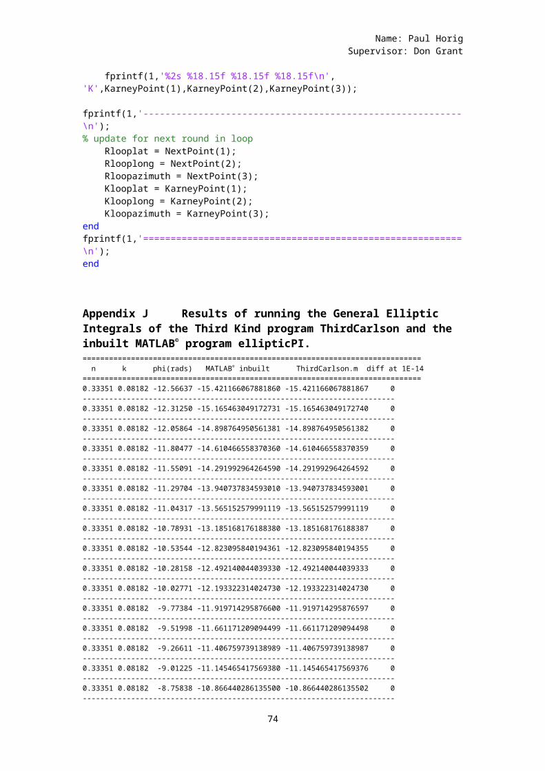
Name: Paul HorigSupervisor: Don Grant
fprintf(1,'%2s %18.15f %18.15f %18.15f\n', 'K',KarneyPoint(1),KarneyPoint(2),KarneyPoint(3)); fprintf(1,'----------------------------------------------------------\n');% update for next round in loop Rlooplat = NextPoint(1); Rlooplong = NextPoint(2); Rloopazimuth = NextPoint(3); Klooplat = KarneyPoint(1); Klooplong = KarneyPoint(2); Kloopazimuth = KarneyPoint(3); end fprintf(1,'==========================================================\n'); end
Appendix J Results of running the General Elliptic Integrals of the Third Kind program ThirdCarlson and the inbuilt MATLAB© program ellipticPI.============================================================================= n k phi(rads) MATLAB© inbuilt ThirdCarlson.m diff at 1E-14=============================================================================0.33351 0.08182 -12.56637 -15.421166067881860 -15.421166067881867 0-----------------------------------------------------------------------0.33351 0.08182 -12.31250 -15.165463049172731 -15.165463049172740 0-----------------------------------------------------------------------0.33351 0.08182 -12.05864 -14.898764950561381 -14.898764950561382 0-----------------------------------------------------------------------0.33351 0.08182 -11.80477 -14.610466558370360 -14.610466558370359 0-----------------------------------------------------------------------0.33351 0.08182 -11.55091 -14.291992964264590 -14.291992964264592 0-----------------------------------------------------------------------0.33351 0.08182 -11.29704 -13.940737834593010 -13.940737834593001 0-----------------------------------------------------------------------0.33351 0.08182 -11.04317 -13.565152579991119 -13.565152579991119 0-----------------------------------------------------------------------0.33351 0.08182 -10.78931 -13.185168176188380 -13.185168176188387 0-----------------------------------------------------------------------0.33351 0.08182 -10.53544 -12.823095840194361 -12.823095840194355 0-----------------------------------------------------------------------0.33351 0.08182 -10.28158 -12.492140044039330 -12.492140044039333 0-----------------------------------------------------------------------0.33351 0.08182 -10.02771 -12.193322314024730 -12.193322314024730 0-----------------------------------------------------------------------0.33351 0.08182 -9.77384 -11.919714295876600 -11.919714295876597 0-----------------------------------------------------------------------0.33351 0.08182 -9.51998 -11.661171209094499 -11.661171209094498 0-----------------------------------------------------------------------0.33351 0.08182 -9.26611 -11.406759739138989 -11.406759739138987 0-----------------------------------------------------------------------0.33351 0.08182 -9.01225 -11.145465417569380 -11.145465417569376 0-----------------------------------------------------------------------0.33351 0.08182 -8.75838 -10.866440286135500 -10.866440286135502 0-----------------------------------------------------------------------
74
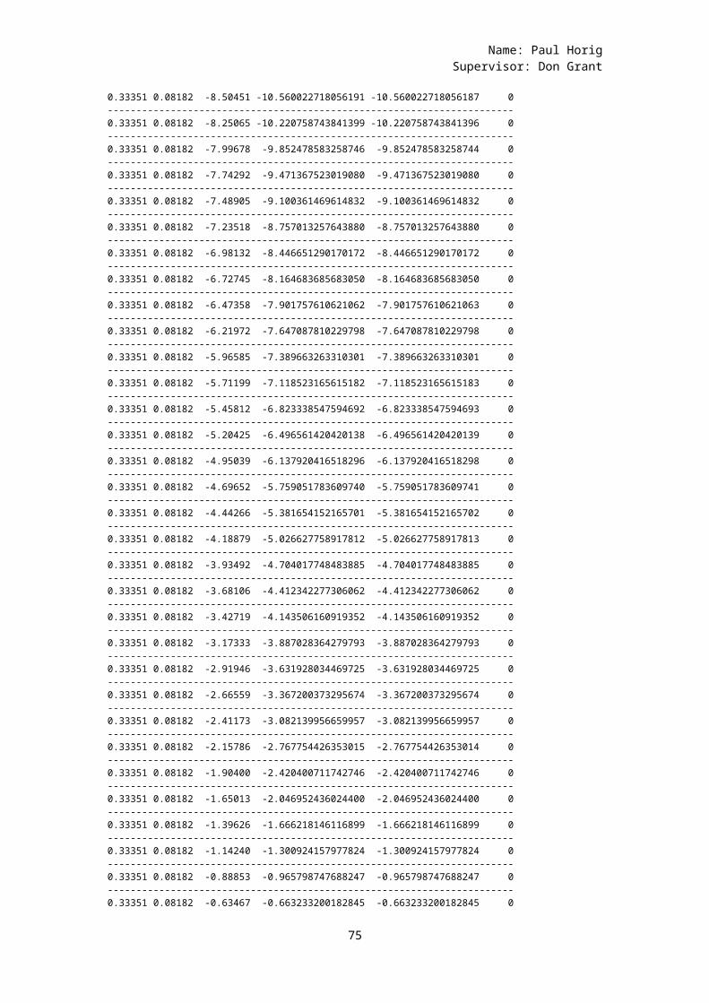
Name: Paul HorigSupervisor: Don Grant
0.33351 0.08182 -8.50451 -10.560022718056191 -10.560022718056187 0-----------------------------------------------------------------------0.33351 0.08182 -8.25065 -10.220758743841399 -10.220758743841396 0-----------------------------------------------------------------------0.33351 0.08182 -7.99678 -9.852478583258746 -9.852478583258744 0-----------------------------------------------------------------------0.33351 0.08182 -7.74292 -9.471367523019080 -9.471367523019080 0-----------------------------------------------------------------------0.33351 0.08182 -7.48905 -9.100361469614832 -9.100361469614832 0-----------------------------------------------------------------------0.33351 0.08182 -7.23518 -8.757013257643880 -8.757013257643880 0-----------------------------------------------------------------------0.33351 0.08182 -6.98132 -8.446651290170172 -8.446651290170172 0-----------------------------------------------------------------------0.33351 0.08182 -6.72745 -8.164683685683050 -8.164683685683050 0-----------------------------------------------------------------------0.33351 0.08182 -6.47358 -7.901757610621062 -7.901757610621063 0-----------------------------------------------------------------------0.33351 0.08182 -6.21972 -7.647087810229798 -7.647087810229798 0-----------------------------------------------------------------------0.33351 0.08182 -5.96585 -7.389663263310301 -7.389663263310301 0-----------------------------------------------------------------------0.33351 0.08182 -5.71199 -7.118523165615182 -7.118523165615183 0-----------------------------------------------------------------------0.33351 0.08182 -5.45812 -6.823338547594692 -6.823338547594693 0-----------------------------------------------------------------------0.33351 0.08182 -5.20425 -6.496561420420138 -6.496561420420139 0-----------------------------------------------------------------------0.33351 0.08182 -4.95039 -6.137920416518296 -6.137920416518298 0-----------------------------------------------------------------------0.33351 0.08182 -4.69652 -5.759051783609740 -5.759051783609741 0-----------------------------------------------------------------------0.33351 0.08182 -4.44266 -5.381654152165701 -5.381654152165702 0-----------------------------------------------------------------------0.33351 0.08182 -4.18879 -5.026627758917812 -5.026627758917813 0-----------------------------------------------------------------------0.33351 0.08182 -3.93492 -4.704017748483885 -4.704017748483885 0-----------------------------------------------------------------------0.33351 0.08182 -3.68106 -4.412342277306062 -4.412342277306062 0-----------------------------------------------------------------------0.33351 0.08182 -3.42719 -4.143506160919352 -4.143506160919352 0-----------------------------------------------------------------------0.33351 0.08182 -3.17333 -3.887028364279793 -3.887028364279793 0-----------------------------------------------------------------------0.33351 0.08182 -2.91946 -3.631928034469725 -3.631928034469725 0-----------------------------------------------------------------------0.33351 0.08182 -2.66559 -3.367200373295674 -3.367200373295674 0-----------------------------------------------------------------------0.33351 0.08182 -2.41173 -3.082139956659957 -3.082139956659957 0-----------------------------------------------------------------------0.33351 0.08182 -2.15786 -2.767754426353015 -2.767754426353014 0-----------------------------------------------------------------------0.33351 0.08182 -1.90400 -2.420400711742746 -2.420400711742746 0-----------------------------------------------------------------------0.33351 0.08182 -1.65013 -2.046952436024400 -2.046952436024400 0-----------------------------------------------------------------------0.33351 0.08182 -1.39626 -1.666218146116899 -1.666218146116899 0-----------------------------------------------------------------------0.33351 0.08182 -1.14240 -1.300924157977824 -1.300924157977824 0-----------------------------------------------------------------------0.33351 0.08182 -0.88853 -0.965798747688247 -0.965798747688247 0-----------------------------------------------------------------------0.33351 0.08182 -0.63467 -0.663233200182845 -0.663233200182845 0
75
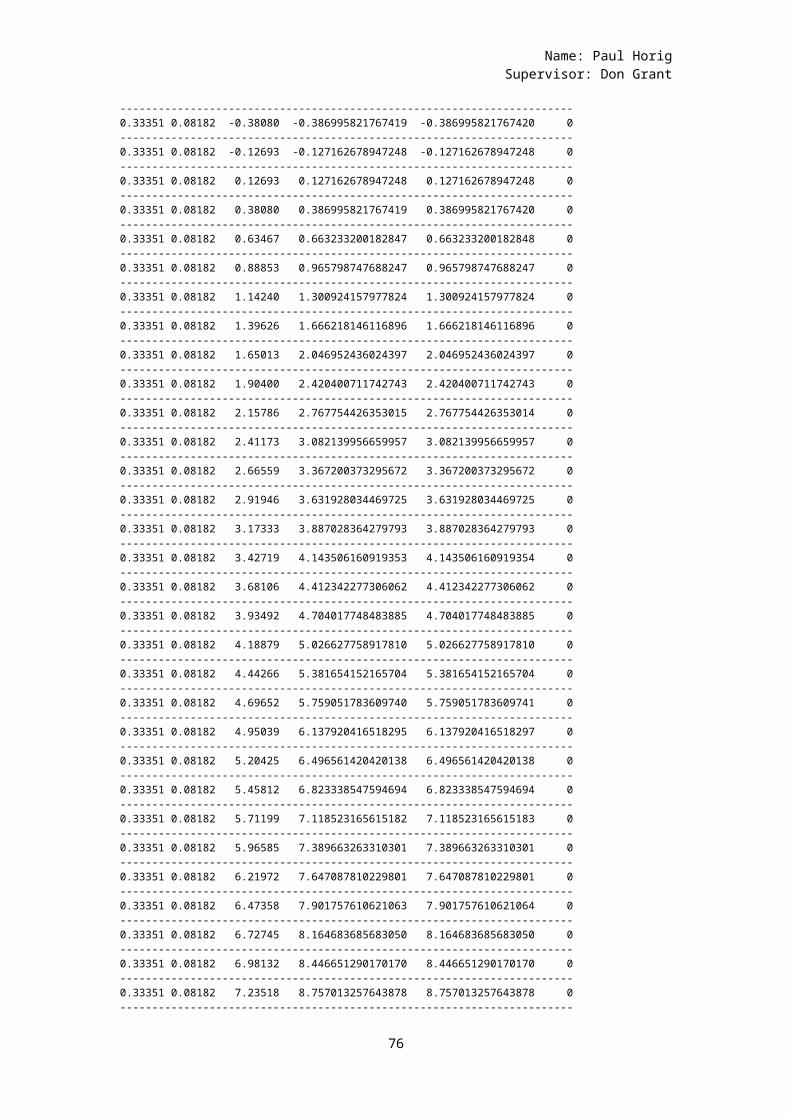
Name: Paul HorigSupervisor: Don Grant
-----------------------------------------------------------------------0.33351 0.08182 -0.38080 -0.386995821767419 -0.386995821767420 0-----------------------------------------------------------------------0.33351 0.08182 -0.12693 -0.127162678947248 -0.127162678947248 0-----------------------------------------------------------------------0.33351 0.08182 0.12693 0.127162678947248 0.127162678947248 0-----------------------------------------------------------------------0.33351 0.08182 0.38080 0.386995821767419 0.386995821767420 0-----------------------------------------------------------------------0.33351 0.08182 0.63467 0.663233200182847 0.663233200182848 0-----------------------------------------------------------------------0.33351 0.08182 0.88853 0.965798747688247 0.965798747688247 0-----------------------------------------------------------------------0.33351 0.08182 1.14240 1.300924157977824 1.300924157977824 0-----------------------------------------------------------------------0.33351 0.08182 1.39626 1.666218146116896 1.666218146116896 0-----------------------------------------------------------------------0.33351 0.08182 1.65013 2.046952436024397 2.046952436024397 0-----------------------------------------------------------------------0.33351 0.08182 1.90400 2.420400711742743 2.420400711742743 0-----------------------------------------------------------------------0.33351 0.08182 2.15786 2.767754426353015 2.767754426353014 0-----------------------------------------------------------------------0.33351 0.08182 2.41173 3.082139956659957 3.082139956659957 0-----------------------------------------------------------------------0.33351 0.08182 2.66559 3.367200373295672 3.367200373295672 0-----------------------------------------------------------------------0.33351 0.08182 2.91946 3.631928034469725 3.631928034469725 0-----------------------------------------------------------------------0.33351 0.08182 3.17333 3.887028364279793 3.887028364279793 0-----------------------------------------------------------------------0.33351 0.08182 3.42719 4.143506160919353 4.143506160919354 0-----------------------------------------------------------------------0.33351 0.08182 3.68106 4.412342277306062 4.412342277306062 0-----------------------------------------------------------------------0.33351 0.08182 3.93492 4.704017748483885 4.704017748483885 0-----------------------------------------------------------------------0.33351 0.08182 4.18879 5.026627758917810 5.026627758917810 0-----------------------------------------------------------------------0.33351 0.08182 4.44266 5.381654152165704 5.381654152165704 0-----------------------------------------------------------------------0.33351 0.08182 4.69652 5.759051783609740 5.759051783609741 0-----------------------------------------------------------------------0.33351 0.08182 4.95039 6.137920416518295 6.137920416518297 0-----------------------------------------------------------------------0.33351 0.08182 5.20425 6.496561420420138 6.496561420420138 0-----------------------------------------------------------------------0.33351 0.08182 5.45812 6.823338547594694 6.823338547594694 0-----------------------------------------------------------------------0.33351 0.08182 5.71199 7.118523165615182 7.118523165615183 0-----------------------------------------------------------------------0.33351 0.08182 5.96585 7.389663263310301 7.389663263310301 0-----------------------------------------------------------------------0.33351 0.08182 6.21972 7.647087810229801 7.647087810229801 0-----------------------------------------------------------------------0.33351 0.08182 6.47358 7.901757610621063 7.901757610621064 0-----------------------------------------------------------------------0.33351 0.08182 6.72745 8.164683685683050 8.164683685683050 0-----------------------------------------------------------------------0.33351 0.08182 6.98132 8.446651290170170 8.446651290170170 0-----------------------------------------------------------------------0.33351 0.08182 7.23518 8.757013257643878 8.757013257643878 0-----------------------------------------------------------------------
76
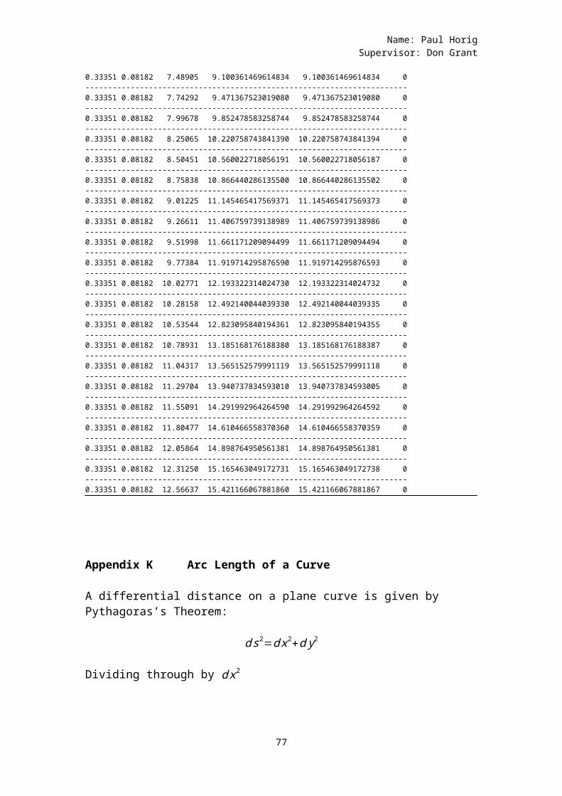
Name: Paul HorigSupervisor: Don Grant
0.33351 0.08182 7.48905 9.100361469614834 9.100361469614834 0-----------------------------------------------------------------------0.33351 0.08182 7.74292 9.471367523019080 9.471367523019080 0-----------------------------------------------------------------------0.33351 0.08182 7.99678 9.852478583258744 9.852478583258744 0-----------------------------------------------------------------------0.33351 0.08182 8.25065 10.220758743841390 10.220758743841394 0-----------------------------------------------------------------------0.33351 0.08182 8.50451 10.560022718056191 10.560022718056187 0-----------------------------------------------------------------------0.33351 0.08182 8.75838 10.866440286135500 10.866440286135502 0-----------------------------------------------------------------------0.33351 0.08182 9.01225 11.145465417569371 11.145465417569373 0-----------------------------------------------------------------------0.33351 0.08182 9.26611 11.406759739138989 11.406759739138986 0-----------------------------------------------------------------------0.33351 0.08182 9.51998 11.661171209094499 11.661171209094494 0-----------------------------------------------------------------------0.33351 0.08182 9.77384 11.919714295876590 11.919714295876593 0-----------------------------------------------------------------------0.33351 0.08182 10.02771 12.193322314024730 12.193322314024732 0-----------------------------------------------------------------------0.33351 0.08182 10.28158 12.492140044039330 12.492140044039335 0-----------------------------------------------------------------------0.33351 0.08182 10.53544 12.823095840194361 12.823095840194355 0-----------------------------------------------------------------------0.33351 0.08182 10.78931 13.185168176188380 13.185168176188387 0-----------------------------------------------------------------------0.33351 0.08182 11.04317 13.565152579991119 13.565152579991118 0-----------------------------------------------------------------------0.33351 0.08182 11.29704 13.940737834593010 13.940737834593005 0-----------------------------------------------------------------------0.33351 0.08182 11.55091 14.291992964264590 14.291992964264592 0-----------------------------------------------------------------------0.33351 0.08182 11.80477 14.610466558370360 14.610466558370359 0-----------------------------------------------------------------------0.33351 0.08182 12.05864 14.898764950561381 14.898764950561381 0-----------------------------------------------------------------------0.33351 0.08182 12.31250 15.165463049172731 15.165463049172738 0-----------------------------------------------------------------------0.33351 0.08182 12.56637 15.421166067881860 15.421166067881867 0
Appendix K Arc Length of a Curve
A differential distance on a plane curve is given by Pythagoras’s Theorem:
ds2=dx2+dy2
Dividing through by dx2
77
Name: Paul HorigSupervisor: Don Grant
ds2dx2
=dx2
dx2+dy2dx2
Taking the square root of both sides:
√ds2dx2=√dx2dx2
+dy2
dx2
dsdx=√1+
dy2
dx2
ds=√1+dy2
dx2dx
ds=√1+(dydx )2
dx
Integrating to find the curve distance between x=x1 andx=x2
s=∫x1
x2 √1+(dydx )2
dx(46)
If the curve is defined parametrically then Pythagoras’s Theorem is:
ds2 (t )=dx2(t)+dy2(t)
ds2 (t )dt2
=dx2 (t )dt2
+dy2 (t)dt2
ds(t)dt =√(dx (t)
dt )2
+(dy (t)dt )
2
Integrating between t1 and t2:
78
Name: Paul HorigSupervisor: Don Grant
s=∫t1
t2 √(dx (t )dt )
2
+(dy (t )dt )
2 (47)
Appendix K.1 Arc length given a polar equation
Given polar coordinatesr=f (θ )
Then the arc length is:
ds2=dr2+ (rdθ )2
Dividing through by dθ2
ds2dθ2
=dr2
dθ2+
(rdθ )2
dθ2
ds=√dr2
dθ2+(rdθ )2
dθ2 dθ
ds=√(drdθ )2
+(r2 )dθ
s=∫θ1
θ2 √(drdθ )2
+(r2)dθ
Appendix K.2 Arc Length of an Ellipse
Figure 1 shows the geometry of an ellipse with all relevant angles (from (Deakin, Geometric Geodesy Part A, 2010, p. 12))
79
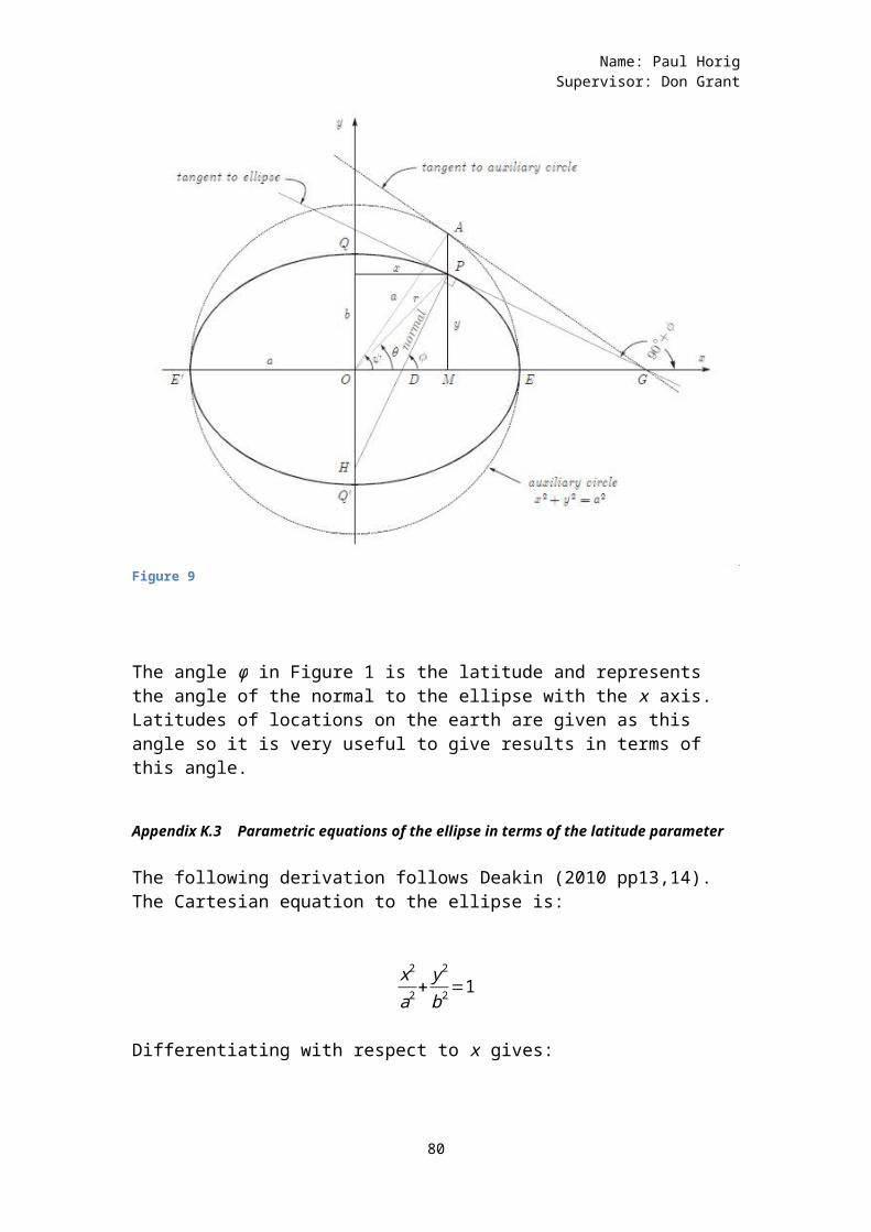
Name: Paul HorigSupervisor: Don Grant
Figure 9
The angle ϕ in Figure 1 is the latitude and represents the angle of the normal to the ellipse with the x axis. Latitudes of locations on the earth are given as this angle so it is very useful to give results in terms of this angle.
Appendix K.3 Parametric equations of the ellipse in terms of the latitude parameter
The following derivation follows Deakin (2010 pp13,14).The Cartesian equation to the ellipse is:
x2a2
+y2
b2=1
Differentiating with respect to x gives:
80
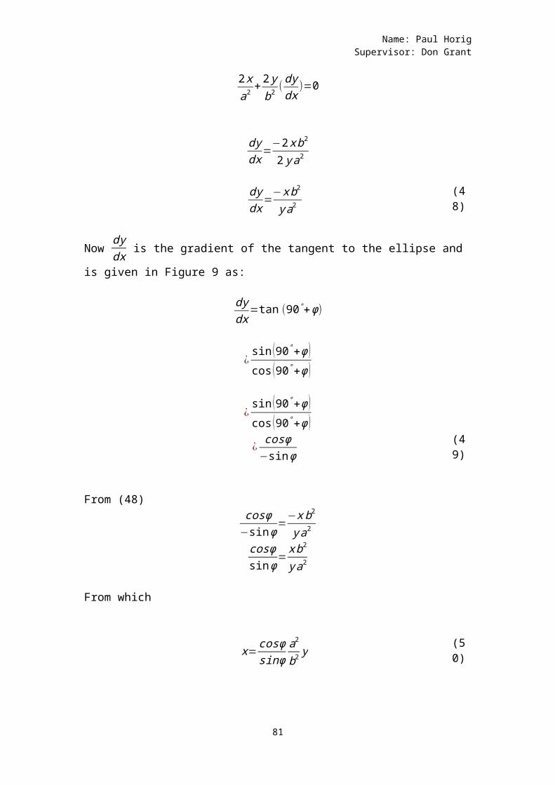
Name: Paul HorigSupervisor: Don Grant
2xa2 +
2yb2 (
dydx
)=0
dydx=
−2xb2
2ya2
dydx=
−xb2ya2
(48)
Now dydx is the gradient of the tangent to the ellipse and
is given in Figure 9 as:
dydx
=tan (90°+ϕ)
¿sin (90°+ϕ )cos (90°+ϕ )
¿sin (90°+ϕ )cos (90°+ϕ )¿cosϕ
−sinϕ(49)
From (48)cosϕ
−sinϕ=−xb2ya2
cosϕsinϕ=
xb2
ya2
From which
x=cosϕsinϕ
a2b2y (5
0)
81
Name: Paul HorigSupervisor: Don Grant
y=sinϕcosϕ
b2a2x (5
1)
Now the Cartesian equation to the ellipse is:
x2a2
+y2
b2=1
So substituting (50) into this equation gives:
(cosϕsinϕ
a2b2y)
2
a2+y2
b2=1
(52)
a2
tan2ϕb4y2+y
2
b2=1 (5
3)
Now the eccentricity e is defined as:
e2=a2−b2
a2
a2b2
=1
1−e2(54)
Bringing a2
b2 out of equation (52)
(y2b2
)((a2b2 )cos2ϕ
sin2ϕ+1)=1
Substituting in equation (54)
(y2b2
)(( 11−e2 )cos
2ϕsin2ϕ
+1)=1
Adding together the fraction inside the brackets
82
Name: Paul HorigSupervisor: Don Grant
(y2b2
)(cos2ϕ+ (1−e2)sin2ϕ
(1−e2)sin2ϕ)=1
(y2
b2)(cos2ϕ+ (sin2ϕ−e2sin2ϕ)
(1−e2)sin2ϕ)=1
(y2b2
)(1−e2sin2ϕ
(1−e2)sin2ϕ)=1
y2=b2 (1−e2 )sin2ϕ1−e2sin2ϕ
y2=b2 (1−e2 )sin2ϕ1−e2sin2ϕ
y=b√ (1−e2)sinϕ√1−e2sin2ϕ
(55)
Which is Deakin (2010) equation (42).
Similarly substituting (51) into the Cartesian equation of the ellipse so as to eliminate y:
x2a2
+y2
b2=1
x2a2
+(sinϕcosϕ
b2
a2 x)2
b2 =1
x2a2
+(sin2ϕcos2ϕ
b2
a4 x2)=1
83
Name: Paul HorigSupervisor: Don Grant
x2a2
(1+(sin2ϕcos2ϕb2a2 ))=1
Substituting in (54)
x2a2
(1+(sin2ϕcos2ϕ(1−e2)))=1
Adding the fractions in the brackets
x2a2
(cos2ϕ+sin2ϕ−e2sin2ϕ)cos2ϕ
=1
x2a2
(1−e2sin2ϕ )cos2ϕ
=1
x2=a2cos2ϕ
1−e2sin2ϕ
x=acosϕ
√1−e2sin2ϕ(56)
Now that we have parametric equations for the ellipse in terms of the latitude we can use equation (47) to find arc length as a function of latitude.
s=∫ϕ1
ϕ2 √(dx (ϕ )dϕ )
2
+(dy (ϕ )dϕ )
2 (57)
Appendix K.4 Arc length as a function of Latitude
Finding the integrand of (57):
x=acosϕ
√1−e2sin2ϕ
84
Name: Paul HorigSupervisor: Don Grant
dx(ϕ)dϕ =
asinϕ√1−e2sin2ϕ−acosϕ2e2sinϕcosϕ
2√1−e2sin2ϕ1−e2sin2ϕ
¿asinϕ√1−e2sin2ϕ√1−e2sin2ϕ−ae2cos2ϕsinϕ
¿¿
¿asinϕ ¿¿
y=b√ (1−e2)sinϕ√1−e2sin2ϕ
dydϕ
=b√ (1−e2)cosϕ√1−e2sin2ϕ−b√ (1−e2)sinϕ2e2sinϕcosϕ
2√¿¿¿¿¿
dydϕ
=b√(1−e2 )cosϕ(1−e2sin2ϕ)−b√(1−e2 )sin2ϕe2cosϕ
¿¿
dydϕ
=b√(1−e2 )cosϕ(1−e2sin2ϕ)−b√(1−e2 )sin2ϕe2cosϕ
¿¿
b√(1−e2 ) (cosϕ (1−e2sin2ϕ)−sin2ϕe2cosϕ )¿¿
Now find:
(dx (ϕ )dϕ )
2
+(dy (ϕ )dϕ )
2
¿a2sin2ϕ¿+ 2asinϕ¿+ b2 (1−e2 )¿
Appendix K.5 Arc length as a function of Latitude using radius of curvature
To find the arc length of an ellipse the easiest way determine the radius of curvature as a function of
85
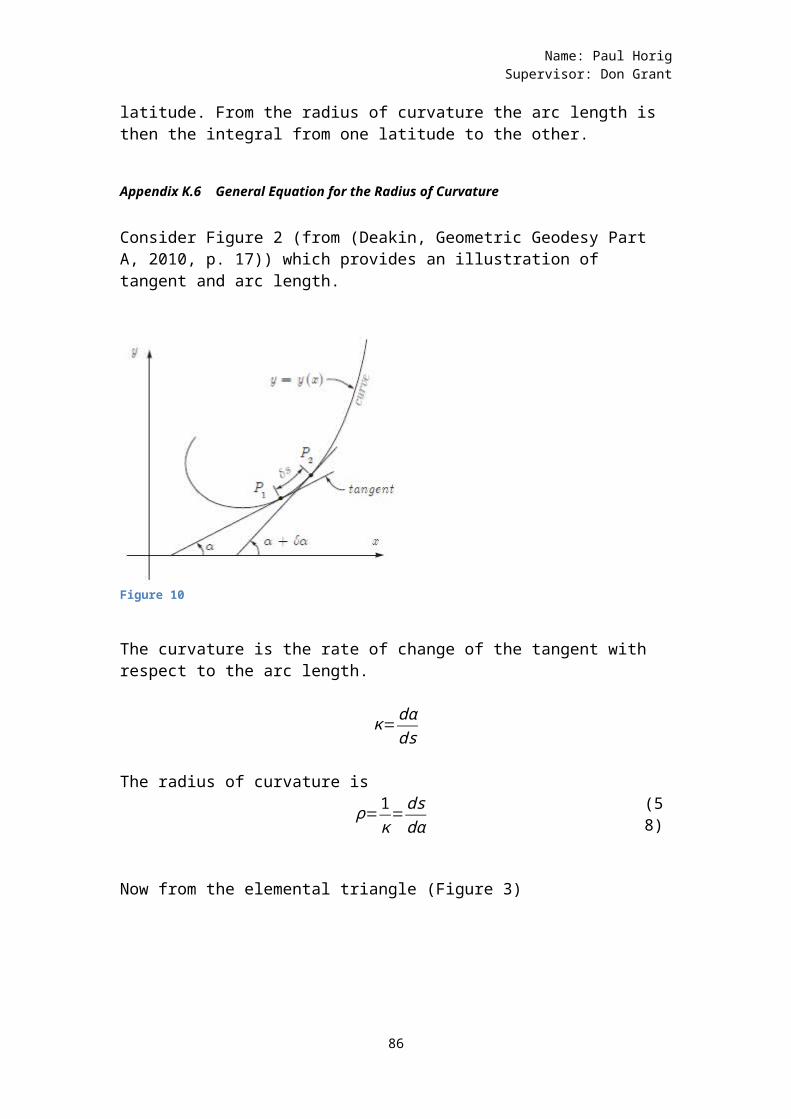
Name: Paul HorigSupervisor: Don Grant
latitude. From the radius of curvature the arc length is then the integral from one latitude to the other.
Appendix K.6 General Equation for the Radius of Curvature
Consider Figure 2 (from (Deakin, Geometric Geodesy Part A, 2010, p. 17)) which provides an illustration of tangent and arc length.
Figure 10
The curvature is the rate of change of the tangent with respect to the arc length.
κ=dαds
The radius of curvature is ρ=1
κ=dsdα
(58)
Now from the elemental triangle (Figure 3)
86
Name: Paul HorigSupervisor: Don Grant
Figure 11
cosα=dxds
1cosα
=dsdx
dsdx
=secα (59)
Also we know that the tangent to a curve is given by dydx.
So
dydx
=tanα
d2ydx2
=d (tanα )dα
dαdx
¿sec2α dαdx
¿sec2α dαds
dsdx
Substituting in (59)¿sec2α dα
dssecα
Giving
87
Name: Paul HorigSupervisor: Don Grant
d2ydx2
=sec3α dαds
dαds=
d2ydx2
1sec3α
Now from (58)
ρ=dsdα=
sec3αd2ydx2
(60)
Now from the elemental triangle (Fig. 11):
ds2=dx2+dy2
Dividing through by dx2
ds2dx2
=dx2
dx2+dy2dx2
Taking the square root of both sides:
√ds2dx2=√dx2dx2
+dy2
dx2
dsdx=√1+(dydx )
2 (61)
Also from (59) and (61)
sec3α=(dsdx )3
=(1+(dydx )2
)32
Therefore (60) becomes
88
Name: Paul HorigSupervisor: Don Grant
ρ=(1+(dydx )
2
)32
d2ydx2
(62)
Which is the general equation for the radius of curvature.
Appendix K.7 The Radius of Curvature of the Ellipse
Using equation (62) to find the equation to the radius ofcurvature of the ellipse first note equation (49) above;
dydx
= cosϕ−sinϕ
¿>d2ydx2=−¿¿
d2ydx2
=1
sin2ϕdϕdx
(63)
Equation (56) above gives x as a function of ϕ
x= acosϕ√1−e2sin2ϕ
Therefore
dx(ϕ)dϕ =
−asinϕ√1−e2sin2ϕ−acosϕ(2)(−e2)sinϕcosϕ2√1−e2sin2ϕ
1−e2sin2ϕ
¿
−asinϕ√1−e2sin2ϕ+acosϕ(e2)sinϕcosϕ
√1−e2sin2ϕ1−e2sin2ϕ
89
Name: Paul HorigSupervisor: Don Grant
¿−asinϕ√1−e2sin2ϕ√1−e2sin2ϕ+ae2cos2ϕsinϕ
¿¿
¿−asinϕ¿¿
¿−asinϕ+asinϕe2sin2ϕ+asinϕe2cos2ϕ
¿¿
¿−asinϕ+ae2sinϕ ¿¿¿
¿−asinϕ+ae2sinϕ
¿¿
¿asinϕ(e2−1)
¿¿
The accepted result is (1−e2) which is used in real world situations so the accepted result will be used:
Therefore inverting:
dϕdx
=¿¿
Substituting into (63)
d2ydx2
=1
sin2ϕ¿¿
¿¿¿
The general equation to the radius of curvature is
ρ=(1+(dydx )
2
)32
d2ydx2
90
Name: Paul HorigSupervisor: Don Grant
¿(1+( cosϕ
−sinϕ )2
)32
¿¿¿
¿(sin2ϕ+cos2ϕ
sin2ϕ )32
¿¿¿
¿asin3ϕ(e2−1)
sin3ϕ¿¿
¿a(e2−1)
¿¿
We only need the absolute value of the radius of curvature when finding meridian distances and as a is always positive and the denominator is always positive and e is always less than one then we can write the radius of curvature as:
ρ=a(1−e2)
¿¿(64)
Which agrees with Deakin (2010) equation (66).
Appendix L Meridian Distance
An infinitesimal distance on the ellipse is given (Deakin, 2010, p60)
dm=ρdϕ
Integration between latitudes will then give the meridiandistance between the two latitudes
M=∫ϕ1
ϕ2
ρdϕ
Substituting in (64) we get
91
Name: Paul HorigSupervisor: Don Grant
M=∫ϕ1
ϕ2 a(1−e2)¿¿ ¿
M=a(1−e2)∫ϕ1
ϕ2 1¿¿ ¿
(65)
This is an incomplete integral of the Third Kind defined in the general case by:
Π(n,ϕ,m)=∫0
ϕ 1(1−nsin2t)√¿¿¿
¿(66)
Note that in the above equation the n and the m can be different. Equation (65) is the special case in which then and the m are the same. In this special case Equation (65) can be transformed into an elliptic integral of the Second Kind minus a constant by the following algebra with this preliminary result:
Note:ddθ
(sinθcosθ
√1−e2sin2θ)
¿
(cosθcosθ−sinθsinθ) √1−e2sin2θ−sinθcosθ (−2e2 )sinθcosθ
2√1−e2sin2θ1−e2sin2θ
¿
(cos2θ−sin2θ) √1−e2sin2θ+sinθcosθ (e2 )sinθcosθ
√1−e2sin2θ1−e2sin2θ
¿
(cos2θ−sin2θ) √1−e2sin2θ+e2sin2θcos2θ√1−e2sin2θ
1−e2sin2θ
92
Name: Paul HorigSupervisor: Don Grant
¿ (cos2θ−sin2θ )¿¿¿
¿ (cos2θ−sin2θ )¿¿
¿ (cos2θ−sin2θ )−(cos2θ−sin2θ )¿¿
¿ (cos2θ−sin2θ )−¿¿
¿(cos2θ−sin2θ)+(sin4θe2)
¿¿
¿ (1−2sin2θ )−e2sin4θ¿ ¿¿¿
So this preliminary result is:ddθ
(sinθcosθ
√1−e2sin2θ)=(1−2sin2θ )−e2sin4θ¿ ¿
¿¿(67)
Multiplying both sides by e2
e2 ddθ
( sinθcosθ√1−e2sin2θ
)=e2 (1−2sin2θ)−e4sin4θ
¿¿
e2 ddθ (
sinθcosθ√1−e2sin2θ
)=e2−2e2sin2θ−e4sin4θ
¿¿
Adding one to and subtracting one from the right hand side:
93
Name: Paul HorigSupervisor: Don Grant
e2 ddθ (
sinθcosθ√1−e2sin2θ
)=1+e2−2e2sin2θ−e4sin4θ−1
¿¿
e2 ddθ (
sinθcosθ√1−e2sin2θ
)=1−2e2sin2θ−e4sin4θ+e2−1
¿¿
e2 ddθ
(sinθcosθ
√1−e2sin2θ)=¿¿
e2 ddθ
(sinθcosθ
√1−e2sin2θ)=¿¿
e2 ddθ ( sinθcosθ
√1−e2sin2θ)=√1−e2sin2θ+(e¿¿2−1)
¿ ¿ ¿
Rearranging:
e2 ddθ ( sinθcosθ
√1−e2sin2θ)=√1−e2sin2θ+(e¿¿2−1)
¿ ¿ ¿
−(e¿¿2−1)¿¿ ¿
(1−e¿¿2)¿¿ ¿
Integrating both sides
∫ϕ1
ϕ2 (1−e¿¿2)¿¿ ¿¿
94
Name: Paul HorigSupervisor: Don Grant
∫ϕ1
ϕ2 (1−e¿¿2)¿¿ ¿¿
(68)
With the right most term evaluated between the limits of integration. Which makes the right hand side:
∫ϕ1
ϕ2
√1−e2sin2θdθ+e2( sinϕ1cosϕ1√1−e2sin2θ )−e2( sinϕ2cosϕ2
√1−e2sin2θ )So we have arrived at a situation where the left hand side is the meridian arc length formula (19) without the factor a. So multiplying both sides by a we get:
∫ϕ1
ϕ2 a(1−e¿¿2)¿¿ ¿¿
(69)
Now ∫ϕ1
ϕ2
√1−e2sin2θdθ is an elliptic integral of the Second
Kind so we can write (22) as (when ϕ1=0):
∫0
ϕ2 a(1−e¿¿2)¿¿ ¿¿
(70)
Which is equation (14) in Deakin (2014) and equation (3) in Rösch (2011).
When neither latitude is zero:
∫ϕ1
ϕ2 a(1−e¿¿2)¿¿ ¿¿
95
Name: Paul HorigSupervisor: Don Grant
(71)
Where
E (ϕ1,ϕ2,e)=∫ϕ1
ϕ2
√1−e2sin2θdθ
Equation (71) is useful when the arc length is found between two latitudes neither of which are zero.
Appendix M Evaluating Elliptic Integrals of the FirstKind. Consider this incomplete integral of the First Kind:
F (k,ϕ )=∫0
ϕ dx√1−k2sin2x
(72)
Making the substitution (Rösch, 2011, p. 5)
x=tan−1( sin2ωk+cos2ω
) (73)
thendxdω
=( 11+u2 )(dudω )withu=
sin2ωk+cos2ω
Nowdudw
=2cos2ω (k+cos2ω )−(sin2ω (−2sin2ω) )
(k+cos2ω )2
¿2kcos2ω+2cos2 2ω+¿2sin22ω(k+cos2ω )2
¿
¿2kcos2ω+2(k+cos2ω )2
¿2kcos2ω+2(k+cos2ω )2
Now
96
Name: Paul HorigSupervisor: Don Grant
11+u2=(1+
sin22ω(k+cos2ω)2 )
−1
( (k+cos2ω )2+sin22ω(k+cos2ω )2 )
−1
¿(k+cos2ω )2
¿¿¿
¿(k+cos2ω )2
(k¿¿2+2kcos2ω+1)¿
Thereforedxdω
=(k+cos2ω )2
(k¿¿2+2kcos2ω+1)X 2kcos2ω+2(k+cos2ω )2
¿
¿2kcos2ω+2
k2+2kcos2ω+1
¿2 (kcos2ω+1)k2+2kcos2ω+1
Therefore
dx=2 (kcos2ω+1 )k2+2kcos2ω+1
dω (74)
Which is the same as Rösch gives as his equation (7). Theoriginal integral (Eq 1) is
F (k,ϕ )=∫0
ϕ dx√1−k2sin2x
(75)
Now it is known that:sintan−1x=
x√1+x2
(76)
97
Name: Paul HorigSupervisor: Don Grant
So substituting (73)
x=tan−1( sin2ωk+cos2ω )
into the denominator of the integrand of (75) gives:
√1−k2sin2x=√1−k2sin2(tan¿¿−1(sin2ω
k+cos2ω))¿
Which from (76) gives:
¿√1−k2(
sin2ωk+cos2ω)
2
1+(sin2ω
k+cos2ω)2
¿√1−k2(
sin2ωk+cos2ω )
2
(k+cos2ω )2+sin22ω(k+cos2ω )2
¿√1−k2sin22ω
((k+cos2ω)2+sin22ω )
¿√ (k+cos2ω )2+sin22ω−k2sin22ω((k+cos2ω)2+sin22ω )
¿√ (k2+2kcos2ω+cos22ω )+sin22ω−k2sin22ω((k+cos2ω)2+sin22ω)
¿√ (k2+2kcos2ω+cos22ω )+sin22ω−k2sin22ω( (k2+2kcos2ω+cos22ω)+sin22ω)
¿√ (k2+2kcos2ω+1 )−k2sin22ω( (k2+2kcos2ω+1) )
98
Name: Paul HorigSupervisor: Don Grant
¿√ (k2+2kcos2ω+1 )−k2¿¿¿¿
¿√ (k2+2kcos2ω+1 )−k2+k2cos22ω( (k2+2kcos2ω+1 ))
¿√ (2kcos2ω+1 )+k2cos22ω( (k2+2kcos2ω+1 ))
¿√¿¿¿
¿(1+kcos2ω)
√1+2kcos2ω+k2
So
√1−k2sin2x=(1+kcos2ω)
√1+2kcos2ω+k2(77)
Which agrees with Rösch equation (8).
Substituting (77) equation (1) gives:
F (k,ϕ )=∫0
ϕ (√1+2kcos2ω+k22 (kcos2ω+1)(1+kcos2ω ) (k2+2kcos2ω+1)
dω)F (k,ϕ )=∫
0
ϕ √1+2kcos2ω+k22 (kcos2ω+1 )(1+kcos2ω)(k¿¿2+2kcos2ω+1)
dω¿
F (k,ϕ )=∫0
ϕ 2√1+2kcos2ω+k2
dω(78)
Now the double angle formula for cosine is:
cos2ω=1−2sin2ω (79)
So (77) becomes after substituting (78):
99
Name: Paul HorigSupervisor: Don Grant
F (k,ϕ )=∫0
ϕ 2√1+2k(1−2sin2ω¿¿+k¿¿2¿)dω¿
¿
F (k,ϕ )=∫0
ϕ 2√1+2k−4ksin2ω+k2¿
¿dω
F (k,ϕ )=∫0
ϕ 2
√ (1+k )2−4ksin2ω¿¿dω
F (k,ϕ )=∫0
ϕ 2
(1+k)√1−4k
(1+k )2sin2ω ¿
¿dω
Bringing out the constants:
F (k,ϕ )= 2(1+k)
∫0
ϕ 1
√1−4k
(1+k )2sin2ω¿
¿dω
Changing the limits of integration to 0 and ω gives the final result:
F (k,ω )= 2(1+k)
∫0
ω 1
√1−4k
(1+k )2sin2ω¿
¿dω
This is also an elliptic integral but with a different modulus and amplitude. If we replace the modulus of our original elliptic integral of the First Find (1) with
q=√ 4k1+k2
¿2√k1+k
and change the limits of integration so that
100
Name: Paul HorigSupervisor: Don Grant
ϕ=tan−1( sin2ωk+cos2ω)
then do the integration and then multiply by
21+k
we will arrive at the same value of the integral. This procedure is summarised by:
F (k,ϕ )= 21+k
F(q,ω)
Appendix M.1 The modulus q is increasing
As the original modulus k is less than unity then the updated modulus q will be more than k. The argument is asfollows (Rösch, 2011, p. 6):
k<1(1+k )2<4
k (1+k )2<k4k<
4k(1+k )2
k<q2Due to k being less then unity then
k2<kSo
k2<k<q2k2<q2k<q
The modulus converges to unity.
Appendix M.2 Determining the new amplitude
101
Name: Paul HorigSupervisor: Don Grant
The new amplitude will be smaller than the old amplitude for an old amplitude between 0 and π /2. The new amplitudeis determined (Rösch, 2011, p. 7) from the following formula arising from the change of variable (13).
ϕ=tan−1( sin2ωk+cos2ω)
tan (ϕ)= sin2ωk+cos2ω
sin (ϕ )cos (ϕ )
=sin2ω
k+cos2ωsin (ϕ) (k+cos2ω)=cos (ϕ)sin2ωksinϕ=sin2ωcosϕ−cos2ωsinϕ
From the trigonometric identitysin (A−B)=sinAcosB−cosAsinB
ksinϕ=sin (2ω−ϕ) (80)
As the modulus k is less than unity then from (79):
sinϕ>sin (2ω−ϕ)ϕ>(2ω−ϕ)
For ϕ<π2
In which case ϕ> (2ω−ϕ )2ϕ>2ω
ϕ>ω (81)
Appendix M.3 The chain of transformed elliptic integrals
So we have for the Landen transformation of an incompleteelliptic integral of the First Kind:
F (k,ϕ )= 21+k
F(q,ω)
with
q=2√k1+k
102
Name: Paul HorigSupervisor: Don Grant
and
ksinϕ=sin (2ω−ϕ) (82)
In addition we know that for an amplitude in the first quadrant the modulus is increasing and the amplitude is decreasing. Beginning with an initial modulus of k0 and aninitial amplitude of ϕ0then one transformation will bring about this equality:
F (k0,ϕ0)=2
1+k0
F(q,ω)
Repeated transformations will bring about the following equality (Rösch, 2011, p. 7):
F (k0,ϕ0)=2
1+k0
21+k1
21+k2
… 21+kn−1
F(kn,ϕn)(83)
with:
kn+1=2√k1+kn
(84)
From equation (81) the transformed amplitude is ω from the previous amplitude ϕ. In the terminology of equation (83) ω is ϕn+1 and ϕ is ϕn. So equation (81) becomes in thenew terminology (Rösch, 2011, p. 7)
knsinϕn=sin (2ϕn+1−ϕn) (85)
Equations (82) and (84) are Landen’s Ascending Transformation (Deakin, 2014 p13).The last factor in the product (82) is:
F (kn,ϕn)=∫0
ϕn dx√1−kn
2sin2x
103
Name: Paul HorigSupervisor: Don Grant
As the limit of the moduli is unity and ϕnconverges to ϕ then this becomes
F(1,ϕ)=∫0
ϕ dx√1−sin2x
¿∫0
ϕ dx√cos2x
∫0
ϕ dxcosx
which from maths tables is:¿lntan(
π4
+ϕ2)
So the formula for the elliptic integral of the First Kind is:
F (k0,ϕ0)=2
1+k0
21+k1
21+k2
… 21+kn−1
lntan(π4
+ϕ2
)
with
kn+1=2√k1+kn
andknsinϕn=sin (2ϕn+1−ϕn)
Appendix N Landen’s descending transformation for First Kind integrals
Landen’s ascending transformation is (from (82), (83) and(84)):
F (ϕ,k )= 21+k
F(ψ,q)(86)
where
q=2√k1+k
(87)
and
104
Name: Paul HorigSupervisor: Don Grant
ψ=(arcsin (ksinϕ )+ϕ)
2(88)
with terminating value :F(ϕ,1)=lntan(
π4
+ϕ2
) (89)
where ϕ is the limit of the amplitude sequence.
Landen’s ascending transformation (1) can be rearranged as (Deakin, 2014 p15):
F (ψ,q)=1+k2
F(ϕ,k)(90)
Known values of amplitude ψ and modulus q are replaced with larger values of amplitude and a smaller modulus. Tofind the new modulus and amplitude equations (2) and (3) (Deakin, 2014 p15):
q=2√k1+k
q2=4k
(1+k )2
1−q2=1−4k
(1+k )2
¿(1+k )2
(1+k )2− 4k
(1+k )2
¿(1+k )2−4k
(1+k )2
¿1+2k+k2−4k
(1+k )2
105
Name: Paul HorigSupervisor: Don Grant
¿1−2k+k2
(1+k )2
¿(1−k )2
(1+k )2
1−q2=(1−k)2
(1+k )2
1=(1−k )2
(1+k )2+q2
(1−k )2
(1+k )2=1−q2
(1−k )(1+k )
=√1−q2
(1−k)=(1+k )√1−q2
(1−k)=√1−q2+k√1−q2
1−k−k√1−q2=√1−q2
1−k(1+√1−q2)=√1−q2
1−√1−q2=k(1+√1−q2)
k (1+√1−q2 )=1−√1−q2
k=1−√1−q2
1+√1−q2
(91)
Which is Deakin (2014) Eqn (66).
To obtain ϕ in terms of ψ:106
Name: Paul HorigSupervisor: Don Grant
Starting with the change of variable defining the Landen transformation (Deakin, 2014 p16):
ϕ=tan−1(sin2ψ
k+cos2ψ)
tanϕ=sin2ψ
k+cos2ψ
tanϕ=sin2ψ
k+cos2ψsinϕcosϕ
= sin2ψk+cos2ψ
sinϕ (k+cos2ψ )=cosϕsin2ψ
ksinϕ=sin2ψcosϕ−cos2ψsinϕ
From the trigonometric identitysin (A−B)=sinAcosB−cosAsinB
Soksinϕ=sin (2ψ−ϕ) (9
2)
ksinϕ=sin (−(ϕ−2ψ))
Now sin (−θ)=−sin (θ)
Soksinϕ=−sin (ϕ−2ψ )
ksinϕ=−sin ((ϕ−ψ)−ψ )
ksin(ϕ−ψ+ψ)=−sin ((ϕ−ψ)−ψ )
ksin((ϕ−ψ)+ψ)=−sin ((ϕ−ψ)−ψ )
Now sin (A−B)=sinAcosB−sinBcosAand sin (A+B )=sinAcosB+sinBcosA
107
Name: Paul HorigSupervisor: Don Grant
Sok [sin ( (ϕ−ψ )+ψ) ]=−[sin ( (ϕ−ψ )−ψ)]
k [sin (ϕ−ψ )cosψ+cos (ϕ−ψ)sinψ ]=−[sin (ϕ−ψ )cosψ−cos (ϕ−ψ )sinψ]
ksin (ϕ−ψ)cosψ+kcos(ϕ−ψ)sinψ=−sin (ϕ−ψ)cosψ+cos (ϕ−ψ )sinψ
ksin (ϕ−ψ)cosψ+sin (ϕ−ψ )cosψ=cos (ϕ−ψ)sinψ−kcos (ϕ−ψ)sinψ
(k+1)sin (ϕ−ψ )cosψ=(1−k)cos (ϕ−ψ )sinψ
(1+k)sin (ϕ−ψ )cosψ=(1−k)cos (ϕ−ψ )sinψ
sin (ϕ−ψ)cosψ=1−k1+k
cos (ϕ−ψ)sinψ
sin (ϕ−ψ)cos (ϕ−ψ)
=(1−k)(1+k)
sinψcosψ
tan (ϕ−ψ)=(1−k)(1+k)
tanψ (93)
From which
ϕ−ψ=arctan ( (1−k)(1+k )
tanψ)
ϕ=arctan( (1−k )(1+k )
tanψ)+ψ (94)
Equations (90) and (93) give the new moduli and amplitudes. In summary:
F (ψ,q)=1+k2
F(ϕ,k) (95)
108
Name: Paul HorigSupervisor: Don Grant
k=1−√1−q2
1+√1−q2
(96)
ϕ=arctan( (1−k )(1+k )
tanψ)+ψ (97)
As k goes to zero the amplitude will have ψ added to it each time. For example if at one point the amplitude is 20° then the sequence will be approximately:
20°, 40°, 80°, 160°, 320°, 640° …
However as k is positive an angle slightly less than ψ will be added to it each time if ψ is in the first quadrant and slightly larger if ψ is in the second quadrant.
The elliptic integral of the First Kind is:
F (k,ψ )=∫0
ψ dx√1−k2sin2x
Using Landen’s descending transformation in which k goes to zero the integrand becomes in the limit:
F (0,ψ)=∫0
ψ dx√1−02sin2x
F (0,ψ)=∫0
ϕ
1dx
F (0,ψ)=ψ
Knowing the integral as u:
u=(1+k0
2 )(1+k1
2 )…(1+kn2
) ψ
109
Name: Paul HorigSupervisor: Don Grant
Rearranging gives:
u( 21+k0 )( 2
1+k1 )…(2
1+kn)=ψ
Knowing ψ this value can be put in as the terminating value of the recursion:
F (ψ,q)=1+k2
F(ϕ,k)
How to handle the accumulating π’s for the increasing
Appendix O Evaluating Elliptic Integrals of the Second Kind
An Elliptic Integral of the Second Kind (Eqn 2) is
E (k,ϕ )=∫0
ϕ
√1−k2sin2θdθ
and this is used in the meridian distance calculation:
M=a(E (e,ϕ)− e2sinϕcosϕ√(1−e2sin2ϕ ) )
a is the semi-major axise is the first eccentricityϕ is the latitude
Now the idea is to be able to write this integral of the second kind as a factor times a transformed integral of the second kind. However this is not possible and the best that can be done is to write the integral of the second kind as the sum of a transformed integral of the second kind and a integral of the first kind. This is howit is done.
Adding ksinϕ to both sides of (26) we get (Deakin, 2014 p24):
110
Name: Paul HorigSupervisor: Don Grant
E (k,ϕ )+ksinϕ=∫0
ϕ
√1−k2sin2θdθ+ksinϕ
¿∫0
ϕ
√1−k2sin2θdθ+∫0
ϕ
kcosθdθ
¿∫0
ϕ
(√1−k2sin2θ¿+kcosθ)dθ¿ (98)
Now we make the substitution as was done with the Elliptic Integral of the First Kind:
θ=tan−1(sin2ω
k+cos2ω)
Which can be rearranged as:tanθ= sin2ω
k+cos2ωsinθcosθ
=sin2ω
k+cos2ω
ksinθ+sinθcos2ω=sin2ωcosθ
ksinθ=sin2ωcosθ−sinθcos2ω
ksinθ=sin (2ω−θ)
k2sin2θ=sin2(2ω−θ)
1−k2sin2θ=1−sin2(2ω−θ)
√1−k2sin2θ=√cos2(2ω−θ)
√1−k2sin2θ=cos(2ω−θ) (99)
Which agrees with Deakin (2014) Eqn (39).
and from (74) with θreplacing the x:
111
Name: Paul HorigSupervisor: Don Grant
dθ= 2 (kcos2ω+1 )k2+2kcos2ω+1
dω (100)
Now substituting (99) into (98):
¿∫0
ϕ
(cos(2ω−θ)¿+kcosθ)dθ¿(101)
Now from the trigonometric identitycos (A−B)=cosAcosB+sinAsinB
(101) becomes
¿∫0
ϕ
(cos2ωcosθ+sin2ωsinθ ¿¿¿+kcosθ)dθ¿
¿∫0
ϕ
(cos2ωcosθ+sin2ωsinθ¿+kcosθ)dθ¿
¿∫0
ϕ
(kcosθ+cos2ωcosθ¿¿+sin2ωsinθ¿)dθ¿
¿∫0
ϕ
¿¿ (102)
To make the change of variable in the integration consider the following diagram:
112
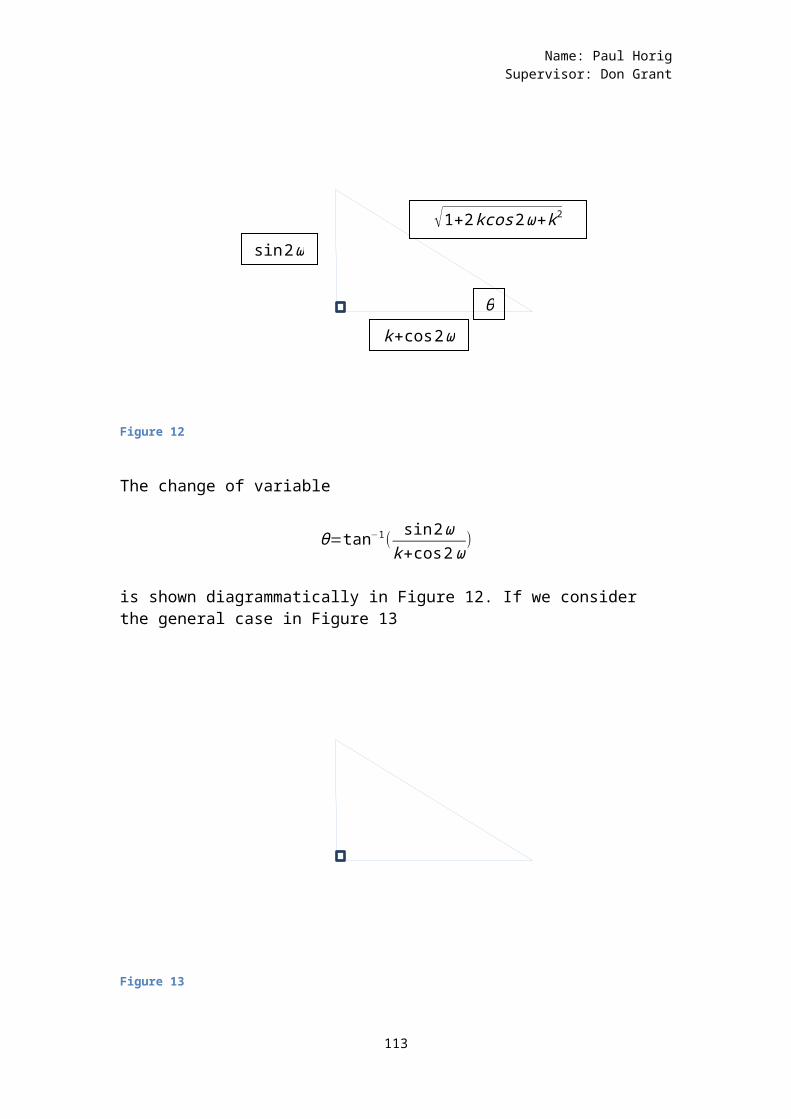
Name: Paul HorigSupervisor: Don Grant
Figure 12
The change of variable
θ=tan−1(sin2ω
k+cos2ω)
is shown diagrammatically in Figure 12. If we consider the general case in Figure 13
Figure 13
113
θ
√1+2kcos2ω+k2
sin2ω
k+cos2ω
Name: Paul HorigSupervisor: Don Grant
bcosθ+asinθ
¿b bc
+a ac¿
b2c +
a2
c¿1c
(b2+a2)¿c2c ¿c
So bcosθ+asinθ=c (10
3)
Applying this to (102) we obtain using Figure 12:
∫0
ϕ
¿¿
¿∫0
ϕ
√1+2kcos2ω+k2dθ
So far we have
E (k,ϕ )+ksinϕ=∫0
ϕ
√1+2kcos2ω+k2dθ(104)
which is equation (96) of Deakin (2014).
From the change of variableθ=tan−1(
sin2ωk+cos2ω
)
Then (74)
dθ= 2 (kcos2ω+1 )k2+2kcos2ω+1
dω
Substituting this into (104) and changing the limits of integration gives
E (k,ϕ )+ksinϕ=∫0
ψ
√1+2kcos2ω+k2 2 (kcos2ω+1 )(k¿¿2+2kcos2ω+1)dω¿
¿∫0
ψ 2 (kcos2ω+1 )√1+2kcos2ω+k2
dω
114
Name: Paul HorigSupervisor: Don Grant
¿∫0
ψ 2 (kcos2ω+1 )√1+2kcos2ω+k2
dω(105)
Now the double angle formula for cosine is:
cos2ω=1−2sin2ωSo (105) becomes
¿∫0
ψ 2 (kcos2ω+1 )√1+2k ¿¿¿
¿
¿∫0
ψ 2 (kcos2ω+1)√1+2k−4ksin2ω+k2
dω
¿∫0
ψ 2 (kcos2ω+1 )
√(1+k )2−4ksin2ωdω
¿∫0
ψ 2 (kcos2ω+1)
(1+k)√ (1+k )2
(1+k )2−
4k(1+k )2
sin2ω
dω
¿∫0
ψ 2 (kcos2ω+1)
(1+k)√1−4k
(1+k )2sin2ω
dω
So
E (k,ϕ )+ksinϕ=∫0
ψ 2 (kcos2ω+1 )(1+k)√1−q2sin2ω
dω(106)
Where
q=2√k1+k
sin (2ψ−ϕ)=ksinϕ
This last equation comes from the change of variable and is derived as equation (80) above.
115
Name: Paul HorigSupervisor: Don Grant
Through algebra the right hand side of (106) can be changed into a sum of an elliptic integral of the Second Kind and an elliptic integral of the First Kind. The elliptic integral of the Second Kind will have a modulus which will converge to unity on successive transformations.
This is the algebra (Deakin, 2014 p35). From (106)
E (k,ϕ )+ksinϕ=∫0
ψ 2 (kcos2ω+1 )(1+k)√1−q2sin2ω
dω
¿∫0
ψ 2(1+k) (kcos2ω+1)(1+k)2√1−q2sin2ω
dω (107)
¿∫0
ψ (2+2k) (kcos2ω+1)(1+k)2√1−q2sin2ω
dω
¿∫0
ψ (2kcos2ω+2+2kkcos2ω+2k )(1+k )2√1−q2sin2ω
dω
¿∫0
ψ (2kcos2ω+2+2kkcos2ω+2k )(1+k )2√1−q2sin2ω
dω(108)
From the trigonometric identity
cos2ω=1−2sin2ω
(108) becomes:
¿∫0
ψ
¿¿¿
¿∫0
ψ (2k−4ksin2ω+2+2k2−4k2sin2ω+2k )(1+k )2√1−q2sin2ω
dω
116
Name: Paul HorigSupervisor: Don Grant
¿∫0
ψ (2+4k+2k2−4ksin2ω−4k2sin2ω)(1+k )2√1−q2sin2ω
dω
¿∫0
ψ (2(1+2k+k2)−4ksin2ω−4k2sin2ω)(1+k )2√1−q2sin2ω
dω
¿∫0
ψ (2 (1+k )2−4ksin2ω−4k2sin2ω)(1+k )2√1−q2sin2ω
dω
¿∫0
ψ (2 (1+k )2
(1+k )2−
4k(1+k )2
sin2ω−4k2
(1+k )2sin2ω)
√1−q2sin2ωdω
¿∫0
ψ (2− 4k(1+k)2
sin2ω− 4k2
(1+k )2sin2ω)
√1−q2sin2ωdω
(109)
Substituting in
q=2√k1+k
(109) becomes
¿∫0
ψ (2−q2sin2ω−q2ksin2ω )√1−q2sin2ω
dω
¿∫0
ψ (1+1−q2sin2ω−q2ksin2ω)√1−q2sin2ω
dω
¿∫0
ψ
¿¿¿
¿∫0
ψ
¿¿¿
117
Name: Paul HorigSupervisor: Don Grant
¿∫0
ψ
¿¿¿
¿∫0
ψ
¿¿¿
¿∫0
ψ
(1+k)¿¿¿
¿∫0
ψ
( (1+k ) √1−q2sin2ω+1−k
√1−q2sin2ω)dωPutting in the left side of the equation which we startedwith (106):
E (k,ϕ )+ksinϕ=∫0
ψ
((1+k )√1−q2sin2ω+1−k
√1−q2sin2ω )dω
E (k,ϕ )+ksinϕ=(1+k )∫0
ψ
√1−q2sin2ωdω
+(1−k)∫0
ψ 1√(1−q2sin2ω )
dω(110)
So the integral of an elliptic integral of the Second Kind plus the modulus times the sine of the amplitude is the sum of another elliptic integral of the Second Kind with larger modulus and smaller amplitude and an ellipticintegral of the First Kind with the same larger modulus and smaller amplitude. Note the two multiplying factors on the right hand side.
Equation (40) can be written as:
E (ϕ,k )+ksinϕ=(1+k )E (ψ,q)+ (1−k )F(ψ,q) (111)
118
Name: Paul HorigSupervisor: Don Grant
with ψ<ϕ and q>k. The changes in amplitude and modulus are given by:
sin (2ψ−ϕ)=ksinϕ (112)
and
q=2√k1+k
(113)
Now as the modulus converges to unity and the amplitude converges toϕ (Deakin, 2014 p26) the elliptic integral ofthe Second Kind in (110) will converge to
∫0
ϕ
√(1−12sin2ω )dω
¿∫0
ϕ
√1−sin2ωdω
¿∫0
ϕ
cosωdω
¿sin (ϕ)
Appendix P Abandoned working to find the amplitude given the result of the integral: Second Kind.
Appendix P.1 Finding the latitude given meridian distance using the elliptic integral of the second kind.
Now the meridian distance formula is:
M=a(E(ϕ2,e)−e2( sinϕ2cosϕ2√1−e2sin2ϕ2 ))
Appendix P.2 Inverting Elliptic Integrals of the Second Kind
Now
119
Name: Paul HorigSupervisor: Don Grant
snE (u,q )=sin (ψ)
snE (uE,q )=snE( 1(1+k
−1)uE−1+(1−k−1
1−k−1
)F (ϕ0,k0)+k−1
1+k−1sinϕ−1¿,
2√k−1
1+k−1 )=sin (ψ)
uE−1=E(ϕ
−1,k−1)
WhereNote that k1 here is the first Landen descending transformation of the original k. So in the following equation which has been used above q=k0and k=k1.
k=1−√1−q2
1+√1−q2
(6)
ϕ=arctan( (1−k )(1+k )
tanψ)+ψ(8)
Eventually un will go to ψ which is the amplitude when k goes to zero.
Fromksinϕ=sin (2ψ−ϕ)
snE (uE,q )=sin ¿
Using a descending transformation and restricting to the case where the modulus goes to zero with ϕ=ϕ
−3:
E (ϕ0,k0)=
(1
1+k−1)(( 1
1+k−2)((
11+k−3
)ϕ−3−ϕ−2)−(1−k−2
1+k−2)F (ϕ−1,k−1 )+(
k−2
1+k−2)sinϕ−2)−(
1−k−1
1+k−1)F (ϕ0,k0 )
+(k
−1
1+k−1)sinϕ
−1
120
Name: Paul HorigSupervisor: Don Grant
E (ϕ0,k0)=
(1
1+k−1)(
11+k−2
)(1
1+k−3)ϕ
−3−( 11+k−1 )( 1
1+k−2 )ϕ−2−(
11+k−1
)(1−k
−2
1+k−2)F (ϕ−1,k−1)+(
11+k−1
)(k
−2
1+k−2)sinϕ
−2−(1−k
−1
1+k−1)
F (ϕ0,k0)+(k
−1
1+k−1)sinϕ
−1
E (ϕ0,k0)=
( 11+k−1
)( 11+k−2
)( 11+k−3
)ϕ−3−( 1
1+k−1 )( 11+k−2 )ϕ−2
−( 11+k−1
)(1−k
−2
1+k−2)(1+k
−2
2)(12) ϕ
−3+( 11+k−1
)(k
−2
1+k−2)sinϕ
−2−(1−k
−1
1+k−1)(1+k
−1
2)(1+k
−2
2)(12
)ϕ−3
+(k
−1
1+k−1)sinϕ
−1
`
Now with k−3=0
E (ϕ0,k0)=
(1
1+k−1)(
11+k−2
)ϕ−3−( 1
1+k−1 )( 11+k−2 )ϕ−2
−(1
1+k−1)(1−k
−2
1+k−2)(1+k
−2
2)(12
) ϕ−3+(
11+k−1
)(k
−2
1+k−2)sinϕ
−2−(1−k
−1
1+k−1)(1+k
−1
2)(1+k
−2
2)(12
) ϕ−3
+(k
−1
1+k−1)sinϕ
−1
Some simplifying
E (ϕ0,k0)=¿+(k
−1
1+k−1)sinϕ
−1
Now ϕ−3= 2ϕ−2 as k=0.
E (ϕ0,k0)=¿+(k
−1
1+k−1)sinϕ
−1
Simplifying
121
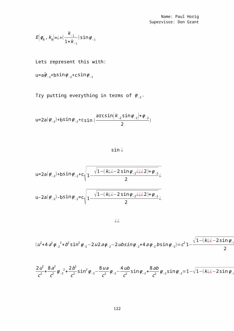
Name: Paul HorigSupervisor: Don Grant
E (ϕ0,k0)=¿+(k
−1
1+k−1)sinϕ
−1
Lets represent this with:
u=aϕ−3+bsinϕ−2+csinϕ−1
Try putting everything in terms of ϕ−2.
u=2a(ϕ−2)+bsinϕ−2+csin (arcsin(k−2sinϕ−2 )+ϕ−2
2)
sin ¿
u=2a(ϕ−2)+bsinϕ−2+c√1−√1−(k¿¿−2sinϕ−2¿¿¿2)+ϕ−2
2¿
u-2a(ϕ−2)-bsinϕ−2=c√1−√1−(k¿¿−2sinϕ−2¿¿¿2)+ϕ−2
2¿
¿¿
(u2+4a2ϕ−22+b2sin2ϕ−2−2u2aϕ−2−2ubsinϕ−2+4aϕ−2bsinϕ−2)=c21−
√1−(k¿¿−2sinϕ−2 ¿¿¿2)+ϕ−2
2¿
2u2c2 +
8a2
c2ϕ−2
2+2b2c2 sin2ϕ−2−
8uac2 ϕ−2−
4ubc2
sinϕ−2+8abc2
ϕ−2sinϕ−2=1−√1−(k¿¿−2sinϕ−2 ¿¿¿2)+ϕ−2¿
122
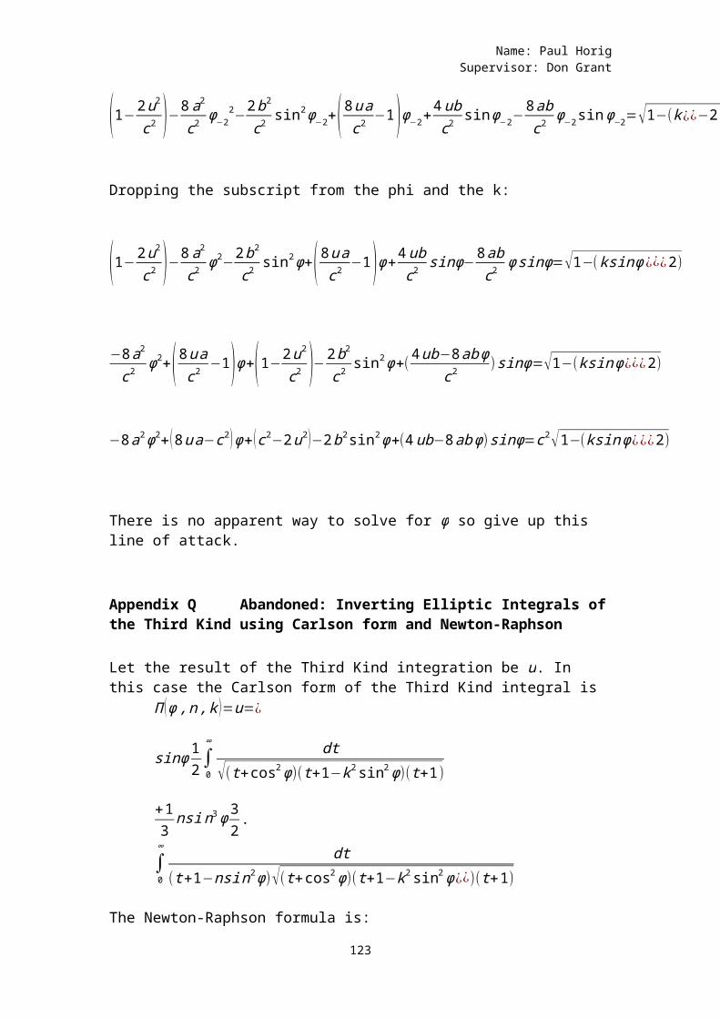
Name: Paul HorigSupervisor: Don Grant
(1−2u2c2 )−8a2
c2ϕ
−22−
2b2
c2sin2ϕ
−2+(8uac2 −1)ϕ−2+4ubc2
sinϕ−2−
8abc2 ϕ
−2sinϕ−2=√1−(k¿¿−2sinϕ−2¿¿¿2)¿
Dropping the subscript from the phi and the k:
(1−2u2c2 )−8a2
c2ϕ2−
2b2
c2sin2ϕ+(8uac2 −1)ϕ+
4ubc2
sinϕ−8abc2
ϕsinϕ=√1−(ksinϕ ¿¿¿2)
−8a2c2 ϕ2+(8uac2 −1)ϕ+(1−
2u2
c2 )−2b2c2 sin2ϕ+(
4ub−8abϕc2 )sinϕ=√1−(ksinϕ¿¿¿2)
−8a2ϕ2+(8ua−c2)ϕ+(c2−2u2)−2b2sin2ϕ+(4ub−8abϕ)sinϕ=c2√1−(ksinϕ¿¿¿2)
There is no apparent way to solve for ϕ so give up this line of attack.
Appendix Q Abandoned: Inverting Elliptic Integrals ofthe Third Kind using Carlson form and Newton-Raphson
Let the result of the Third Kind integration be u. In this case the Carlson form of the Third Kind integral is
Π (ϕ,n,k )=u=¿
sinϕ12∫0
∞ dt√(t+cos2ϕ)(t+1−k2sin2ϕ)(t+1)
+13nsin3ϕ3
2.
∫0
∞ dt(t+1−nsin2ϕ)√(t+cos2ϕ)(t+1−k2sin2ϕ¿¿)(t+1)
The Newton-Raphson formula is:
123
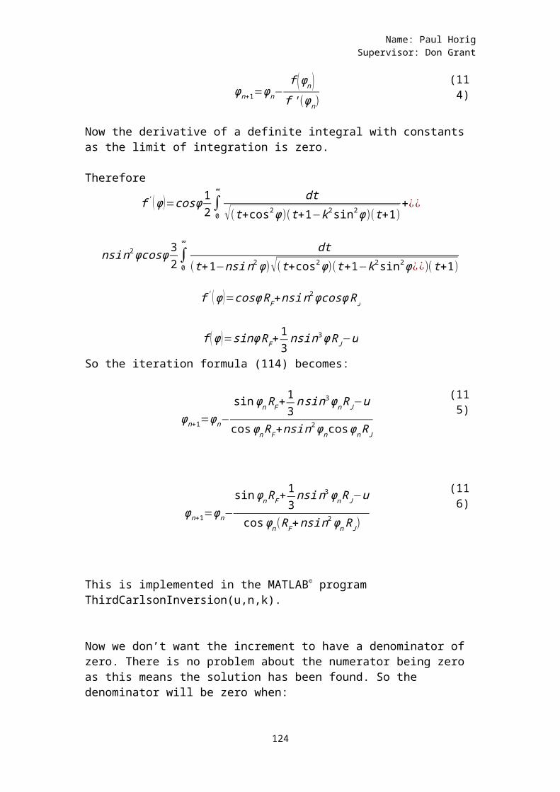
Name: Paul HorigSupervisor: Don Grant
ϕn+1=ϕn−f (ϕn )f'(ϕn)
(114)
Now the derivative of a definite integral with constants as the limit of integration is zero.
Therefore
f' (ϕ)=cosϕ12∫0
∞ dt√(t+cos2ϕ)(t+1−k2sin2ϕ)(t+1)
+¿¿
nsin2ϕcosϕ 32∫0
∞ dt(t+1−nsin2ϕ)√(t+cos2ϕ)(t+1−k2sin2ϕ¿¿)(t+1)
f' (ϕ)=cosϕRF+nsin2ϕcosϕRJ
f (ϕ)=sinϕRF+13nsin3ϕRJ−u
So the iteration formula (114) becomes:
ϕn+1=ϕn−
sinϕnRF+13nsin3ϕnRJ−u
cosϕnRF+nsin2ϕncosϕnRJ
(115)
ϕn+1=ϕn−
sinϕnRF+13nsin3ϕnRJ−u
cosϕn(RF+nsin2ϕnRJ)
(116)
This is implemented in the MATLAB© program ThirdCarlsonInversion(u,n,k).
Now we don’t want the increment to have a denominator of zero. There is no problem about the numerator being zero as this means the solution has been found. So the denominator will be zero when:
124
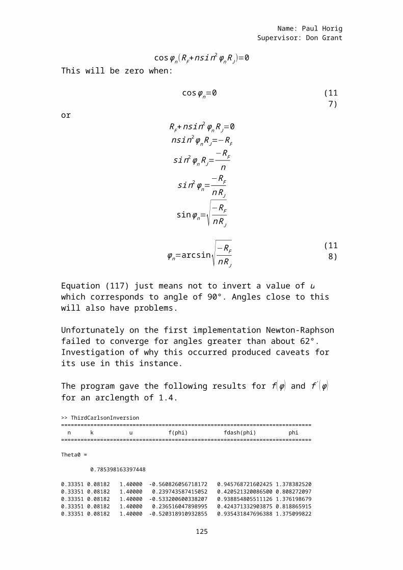
Name: Paul HorigSupervisor: Don Grant
cosϕn(RF+nsin2ϕnRJ)=0
This will be zero when:
cosϕn=0 (117)
orRF+nsin
2ϕnRJ=0nsin2ϕnRJ=−RF
sin2ϕnRJ=−RF
n
sin2ϕn=−RF
nRJ
sinϕn=√−RF
nRJ
ϕn=arcsin√−RF
nRJ
(118)
Equation (117) just means not to invert a value of u which corresponds to angle of 90°. Angles close to this will also have problems.
Unfortunately on the first implementation Newton-Raphson failed to converge for angles greater than about 62°. Investigation of why this occurred produced caveats for its use in this instance.
The program gave the following results for f (ϕ) and f' (ϕ) for an arclength of 1.4.
>> ThirdCarlsonInversion============================================================================= n k u f(phi) fdash(phi) phi=============================================================================
Theta0 =
0.785398163397448
0.33351 0.08182 1.40000 -0.560826056718172 0.945768721602425 1.3783825200.33351 0.08182 1.40000 0.239743587415052 0.420521320086500 0.8082720970.33351 0.08182 1.40000 -0.533200600338207 0.938854805511126 1.3761986790.33351 0.08182 1.40000 0.236516047898995 0.424371332903875 0.8188659150.33351 0.08182 1.40000 -0.520318910932855 0.935431847696388 1.375099822
125
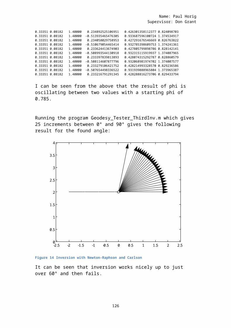
Name: Paul HorigSupervisor: Don Grant
0.33351 0.08182 1.40000 0.234892525106951 0.426301358112377 0.8240987030.33351 0.08182 1.40000 -0.513935465476305 0.933687596100724 1.3745349170.33351 0.08182 1.40000 0.234058029758953 0.427291676546669 0.8267638220.33351 0.08182 1.40000 -0.510679054465414 0.932785398609753 1.3742413610.33351 0.08182 1.40000 0.233624413674903 0.427805799898786 0.8281421410.33351 0.08182 1.40000 -0.508993544130918 0.932315115919937 1.3740879650.33351 0.08182 1.40000 0.233397839813893 0.428074315292787 0.8288605790.33351 0.08182 1.40000 -0.508114607877796 0.932068981974702 1.3740075770.33351 0.08182 1.40000 0.233279106421752 0.428214993328570 0.8292365860.33351 0.08182 1.40000 -0.507654498336522 0.931939888965804 1.3739653870.33351 0.08182 1.40000 0.233216791291345 0.428288816273706 0.829433794
I can be seen from the above that the result of phi is oscillating between two values with a starting phi of 0.785.
Running the program Geodesy_Tester_ThirdInv.m which gives25 increments between 0° and 90° gives the following result for the found angle:
-2.5 -2 -1.5 -1 -0.5 0 0.5 1 1.5 2 2.50
0.5
1
1.5
2
2.5
3
3.5
4
Figure 14 Inversion with Newton-Raphson and Carlson
It can be seen that inversion works nicely up to just over 60° and then fails.
126
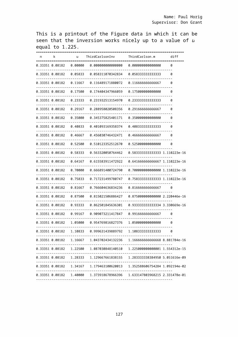
Name: Paul HorigSupervisor: Don Grant
This is a printout of the Figure data in which it can be seen that the inversion works nicely up to a value of u equal to 1.225.============================================================================= n k u ThirdCarlsonInv ThirdCarlson.m diff=============================================================================0.33351 0.08182 0.00000 0.000000000000000 0.000000000000000 0-----------------------------------------------------------------------0.33351 0.08182 0.05833 0.058311070342834 0.058333333333333 0-----------------------------------------------------------------------0.33351 0.08182 0.11667 0.116489171880072 0.116666666666667 0-----------------------------------------------------------------------0.33351 0.08182 0.17500 0.174404347966059 0.175000000000000 0-----------------------------------------------------------------------0.33351 0.08182 0.23333 0.231932513154970 0.233333333333333 0-----------------------------------------------------------------------0.33351 0.08182 0.29167 0.288958020508356 0.291666666666667 0-----------------------------------------------------------------------0.33351 0.08182 0.35000 0.345375825401171 0.350000000000000 0-----------------------------------------------------------------------0.33351 0.08182 0.40833 0.401093169358374 0.408333333333333 0-----------------------------------------------------------------------0.33351 0.08182 0.46667 0.456030746432471 0.466666666666667 0-----------------------------------------------------------------------0.33351 0.08182 0.52500 0.510123352512670 0.525000000000000 0-----------------------------------------------------------------------0.33351 0.08182 0.58333 0.563320050764462 0.583333333333333 1.110223e-16-----------------------------------------------------------------------0.33351 0.08182 0.64167 0.615583911472922 0.641666666666667 1.110223e-16-----------------------------------------------------------------------0.33351 0.08182 0.70000 0.666891400724790 0.700000000000000 1.110223e-16-----------------------------------------------------------------------0.33351 0.08182 0.75833 0.717231499780747 0.758333333333333 1.110223e-16-----------------------------------------------------------------------0.33351 0.08182 0.81667 0.766604636834236 0.816666666666667 0-----------------------------------------------------------------------0.33351 0.08182 0.87500 0.815021506886427 0.875000000000000 2.220446e-16-----------------------------------------------------------------------0.33351 0.08182 0.93333 0.862501845636301 0.933333333333334 3.330669e-16-----------------------------------------------------------------------0.33351 0.08182 0.99167 0.909073211417847 0.991666666666667 0-----------------------------------------------------------------------0.33351 0.08182 1.05000 0.954769816827376 1.050000000000000 0-----------------------------------------------------------------------0.33351 0.08182 1.10833 0.999631439889792 1.108333333333333 0-----------------------------------------------------------------------0.33351 0.08182 1.16667 1.043702434132236 1.166666666666668 8.881784e-16-----------------------------------------------------------------------0.33351 0.08182 1.22500 1.087030848140510 1.225000000000001 1.554312e-15-----------------------------------------------------------------------0.33351 0.08182 1.28333 1.129667661838155 1.283333338384950 5.051616e-09-----------------------------------------------------------------------0.33351 0.08182 1.34167 1.179463100620013 1.352588606754284 1.092194e-02-----------------------------------------------------------------------0.33351 0.08182 1.40000 1.373918678966396 1.633147803968215 2.331478e-01-----------------------------------------------------------------------
127
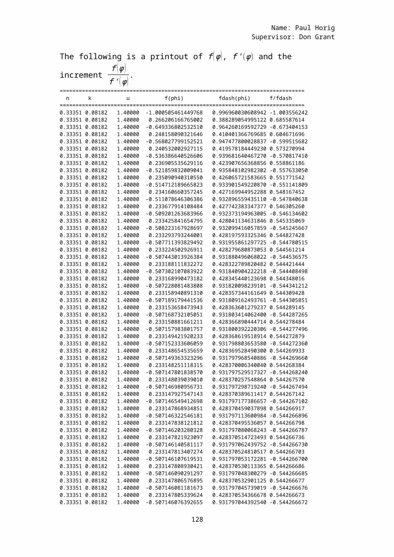
Name: Paul HorigSupervisor: Don Grant
The following is a printout of f (ϕ), f'(ϕ) and the
increment f (ϕ )f' (ϕ)
.============================================================================= n k u f(phi) fdash(phi) f/fdash=============================================================================0.33351 0.08182 1.40000 -1.000505461449768 0.996960030608942 -1.0035562420.33351 0.08182 1.40000 0.266206166765002 0.388289054995122 0.6855876140.33351 0.08182 1.40000 -0.649336802532510 0.964260169592729 -0.6734041530.33351 0.08182 1.40000 0.248158090321646 0.410401366769685 0.6046716960.33351 0.08182 1.40000 -0.568027799152521 0.947477800028837 -0.5995156820.33351 0.08182 1.40000 0.240532002927115 0.419578184449230 0.5732709940.33351 0.08182 1.40000 -0.536386640526606 0.939681640467270 -0.5708174100.33351 0.08182 1.40000 0.236905535629116 0.423907656368856 0.5588611860.33351 0.08182 1.40000 -0.521859832009041 0.935848102982302 -0.5576330500.33351 0.08182 1.40000 0.235090940310550 0.426065721583665 0.5517715420.33351 0.08182 1.40000 -0.514712189665823 0.933901549220870 -0.5511418090.33351 0.08182 1.40000 0.234160660357245 0.427169944952288 0.5481674520.33351 0.08182 1.40000 -0.511078646306386 0.932896559435110 -0.5478406380.33351 0.08182 1.40000 0.233677914108484 0.427742383347377 0.5463052600.33351 0.08182 1.40000 -0.509201263683966 0.932373194963005 -0.5461346020.33351 0.08182 1.40000 0.233425841654795 0.428041134631846 0.5453350690.33351 0.08182 1.40000 -0.508223167928697 0.932099416057859 -0.5452456670.33351 0.08182 1.40000 0.233293793244001 0.428197593325346 0.5448274280.33351 0.08182 1.40000 -0.507711393829492 0.931955861297725 -0.5447805150.33351 0.08182 1.40000 0.233224502926911 0.428279680873053 0.5445612140.33351 0.08182 1.40000 -0.507443013926384 0.931880496068022 -0.5445365750.33351 0.08182 1.40000 0.233188111832272 0.428322789820482 0.5444214440.33351 0.08182 1.40000 -0.507302107083922 0.931840904222218 -0.5444084980.33351 0.08182 1.40000 0.233168990473182 0.428345440123698 0.5443480160.33351 0.08182 1.40000 -0.507228081483808 0.931820098239101 -0.5443412120.33351 0.08182 1.40000 0.233158940891310 0.428357344161649 0.5443094280.33351 0.08182 1.40000 -0.507189179441536 0.931809162493761 -0.5443058510.33351 0.08182 1.40000 0.233153658473943 0.428363601279237 0.5442891450.33351 0.08182 1.40000 -0.507168732105051 0.931803414062400 -0.5442872650.33351 0.08182 1.40000 0.233150881661211 0.428366890444714 0.5442784840.33351 0.08182 1.40000 -0.507157983801757 0.931800392220306 -0.5442774960.33351 0.08182 1.40000 0.233149421920233 0.428368619518914 0.5442728790.33351 0.08182 1.40000 -0.507152333606059 0.931798803653580 -0.5442723600.33351 0.08182 1.40000 0.233148654535659 0.428369528490300 0.5442699330.33351 0.08182 1.40000 -0.507149363323296 0.931797968540886 -0.5442696600.33351 0.08182 1.40000 0.233148251118315 0.428370006340040 0.5442683840.33351 0.08182 1.40000 -0.507147801838570 0.931797529517327 -0.5442682400.33351 0.08182 1.40000 0.233148039039010 0.428370257548864 0.5442675700.33351 0.08182 1.40000 -0.507146980956731 0.931797298719240 -0.5442674940.33351 0.08182 1.40000 0.233147927547143 0.428370389611417 0.5442671420.33351 0.08182 1.40000 -0.507146549412698 0.931797177386657 -0.5442671020.33351 0.08182 1.40000 0.233147868934851 0.428370459037898 0.5442669170.33351 0.08182 1.40000 -0.507146322546181 0.931797113600984 -0.5442668960.33351 0.08182 1.40000 0.233147838121812 0.428370495536057 0.5442667980.33351 0.08182 1.40000 -0.507146203280328 0.931797080068243 -0.5442667870.33351 0.08182 1.40000 0.233147821923097 0.428370514723493 0.5442667360.33351 0.08182 1.40000 -0.507146140581117 0.931797062439752 -0.5442667300.33351 0.08182 1.40000 0.233147813407274 0.428370524810517 0.5442667030.33351 0.08182 1.40000 -0.507146107619531 0.931797053172281 -0.5442667000.33351 0.08182 1.40000 0.233147808930421 0.428370530113365 0.5442666860.33351 0.08182 1.40000 -0.507146090291297 0.931797048300279 -0.5442666850.33351 0.08182 1.40000 0.233147806576895 0.428370532901125 0.5442666770.33351 0.08182 1.40000 -0.507146081181673 0.931797045739019 -0.5442666760.33351 0.08182 1.40000 0.233147805339624 0.428370534366678 0.5442666730.33351 0.08182 1.40000 -0.507146076392655 0.931797044392540 -0.544266672
128
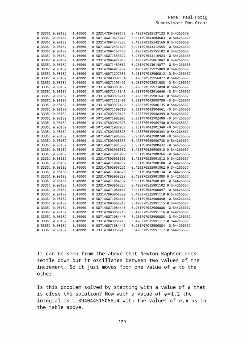
Name: Paul HorigSupervisor: Don Grant
0.33351 0.08182 1.40000 0.233147804689178 0.428370535137133 0.5442666700.33351 0.08182 1.40000 -0.507146073875021 0.931797043684683 -0.5442666700.33351 0.08182 1.40000 0.233147804347232 0.428370535542169 0.5442666690.33351 0.08182 1.40000 -0.507146072551475 0.931797043312555 -0.5442666690.33351 0.08182 1.40000 0.233147804167467 0.428370535755102 0.5442666680.33351 0.08182 1.40000 -0.507146071855672 0.931797043116923 -0.5442666680.33351 0.08182 1.40000 0.233147804072963 0.428370535867042 0.5442666680.33351 0.08182 1.40000 -0.507146071489881 0.931797043014077 -0.5442666680.33351 0.08182 1.40000 0.233147804023282 0.428370535925889 0.5442666670.33351 0.08182 1.40000 -0.507146071297586 0.931797042960012 -0.5442666670.33351 0.08182 1.40000 0.233147803997164 0.428370535956827 0.5442666670.33351 0.08182 1.40000 -0.507146071196491 0.931797042931588 -0.5442666670.33351 0.08182 1.40000 0.233147803983433 0.428370535973090 0.5442666670.33351 0.08182 1.40000 -0.507146071143346 0.931797042916646 -0.5442666670.33351 0.08182 1.40000 0.233147803976214 0.428370535981641 0.5442666670.33351 0.08182 1.40000 -0.507146071115405 0.931797042908789 -0.5442666670.33351 0.08182 1.40000 0.233147803972420 0.428370535986135 0.5442666670.33351 0.08182 1.40000 -0.507146071100719 0.931797042904661 -0.5442666670.33351 0.08182 1.40000 0.233147803970425 0.428370535988499 0.5442666670.33351 0.08182 1.40000 -0.507146071092995 0.931797042902489 -0.5442666670.33351 0.08182 1.40000 0.233147803969376 0.428370535989740 0.5442666670.33351 0.08182 1.40000 -0.507146071088937 0.931797042901348 -0.5442666670.33351 0.08182 1.40000 0.233147803968825 0.428370535990394 0.5442666670.33351 0.08182 1.40000 -0.507146071086802 0.931797042900748 -0.5442666670.33351 0.08182 1.40000 0.233147803968535 0.428370535990738 0.5442666670.33351 0.08182 1.40000 -0.507146071085679 0.931797042900432 -0.5442666670.33351 0.08182 1.40000 0.233147803968382 0.428370535990918 0.5442666670.33351 0.08182 1.40000 -0.507146071085089 0.931797042900266 -0.5442666670.33351 0.08182 1.40000 0.233147803968303 0.428370535991012 0.5442666670.33351 0.08182 1.40000 -0.507146071084782 0.931797042900180 -0.5442666670.33351 0.08182 1.40000 0.233147803968261 0.428370535991062 0.5442666670.33351 0.08182 1.40000 -0.507146071084620 0.931797042900134 -0.5442666670.33351 0.08182 1.40000 0.233147803968238 0.428370535991088 0.5442666670.33351 0.08182 1.40000 -0.507146071084532 0.931797042900109 -0.5442666670.33351 0.08182 1.40000 0.233147803968227 0.428370535991102 0.5442666670.33351 0.08182 1.40000 -0.507146071084487 0.931797042900097 -0.5442666670.33351 0.08182 1.40000 0.233147803968220 0.428370535991110 0.5442666670.33351 0.08182 1.40000 -0.507146071084461 0.931797042900090 -0.5442666670.33351 0.08182 1.40000 0.233147803968217 0.428370535991115 0.5442666670.33351 0.08182 1.40000 -0.507146071084448 0.931797042900086 -0.5442666670.33351 0.08182 1.40000 0.233147803968216 0.428370535991116 0.5442666670.33351 0.08182 1.40000 -0.507146071084443 0.931797042900085 -0.5442666670.33351 0.08182 1.40000 0.233147803968215 0.428370535991117 0.5442666670.33351 0.08182 1.40000 -0.507146071084441 0.931797042900084 -0.5442666670.33351 0.08182 1.40000 0.233147803968215 0.428370535991117 0.544266667
It can be seen from the above that Newton-Raphson does settle down but it oscillates between two values of the increment. So it just moves from one value of ϕ to the other.
Is this problem solved by starting with a value of ϕ thatis close the solution? Now with a value of ϕ=1.2 the integral is 1.39404451505814 with the values of n,k as inthe table above.
129
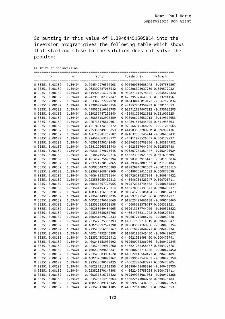
Name: Paul HorigSupervisor: Don Grant
So putting in this value of 1.39404451505814 into the inversion program gives the following table which shows that starting close to the solution does not solve the problem:
>> ThirdCarlsonInversionB============================================================================= n k u f(phi) fdash(phi) f/fdash=============================================================================0.33351 0.08182 1.39404 -0.994549976507908 0.996960030608942 -0.9975825970.33351 0.08182 1.39404 0.263307727066542 0.399206393037700 0.6595779320.33351 0.08182 1.39404 -0.619906514775918 0.959871616578652 -0.6458223200.33351 0.08182 1.39404 0.242955302387847 0.423795377647336 0.5732844560.33351 0.08182 1.39404 -0.533342572277920 0.940430416019172 -0.5671260340.33351 0.08182 1.39404 0.233860254059256 0.434557954359082 0.5381566530.33351 0.08182 1.39404 -0.498056816633785 0.930912024467212 -0.5350202850.33351 0.08182 1.39404 0.229232447202340 0.439981259621932 0.5210050250.33351 0.08182 1.39404 -0.480835102990859 0.925906772652213 -0.5193126530.33351 0.08182 1.39404 0.226736476819061 0.442891510844075 0.5119458630.33351 0.08182 1.39404 -0.471743124153772 0.923166315368299 -0.5110055650.33351 0.08182 1.39404 0.225350049756853 0.444503598289760 0.5069701360.33351 0.08182 1.39404 -0.466750981267582 0.921632386145014 -0.5064394310.33351 0.08182 1.39404 0.224567663225772 0.445411925526567 0.5041797270.33351 0.08182 1.39404 -0.463951930248445 0.920763190703996 -0.5038775820.33351 0.08182 1.39404 0.224122265358440 0.445928567044249 0.5025967880.33351 0.08182 1.39404 -0.462364279670645 0.920267244357477 -0.5024239240.33351 0.08182 1.39404 0.223867455239716 0.446223987921635 0.5016930090.33351 0.08182 1.39404 -0.461457875800394 0.919983150916442 -0.5015938340.33351 0.08182 1.39404 0.223721270132065 0.446393423087502 0.5011751040.33351 0.08182 1.39404 -0.460938487566389 0.919820046782669 -0.5011181150.33351 0.08182 1.39404 0.223637268849909 0.446490768411533 0.5008776990.33351 0.08182 1.39404 -0.460640238756144 0.919726284287024 -0.5008449220.33351 0.08182 1.39404 0.223588955402213 0.446546751423247 0.5007067110.33351 0.08182 1.39404 -0.460468767778955 0.919672343744862 -0.5006878490.33351 0.08182 1.39404 0.223561153176714 0.446578965391841 0.5006083370.33351 0.08182 1.39404 -0.460370116153010 0.919641299106494 -0.5005974790.33351 0.08182 1.39404 0.223545149380036 0.446597508141536 0.5005517170.33351 0.08182 1.39404 -0.460313336678669 0.919623427465188 -0.5005454660.33351 0.08182 1.39404 0.223535935503158 0.446608183579717 0.5005191210.33351 0.08182 1.39404 -0.460280649434065 0.919613137744266 -0.5005155220.33351 0.08182 1.39404 0.223530630257706 0.446614330311928 0.5005003540.33351 0.08182 1.39404 -0.460261829299843 0.919607212884755 -0.5004982810.33351 0.08182 1.39404 0.223527575380793 0.446617869714319 0.5004895470.33351 0.08182 1.39404 -0.460250992521290 0.919603801168966 -0.5004883540.33351 0.08182 1.39404 0.223525816256867 0.446619907840977 0.5004833240.33351 0.08182 1.39404 -0.460244752346898 0.919601836545450 -0.5004826370.33351 0.08182 1.39404 0.223524803261412 0.446621081498460 0.5004797410.33351 0.08182 1.39404 -0.460241158957992 0.919600705206936 -0.5004793450.33351 0.08182 1.39404 0.223524219919260 0.446621757358457 0.5004776780.33351 0.08182 1.39404 -0.460239089683841 0.919600053714036 -0.5004774500.33351 0.08182 1.39404 0.223523883994520 0.446622146560477 0.5004764890.33351 0.08182 1.39404 -0.460237898070162 0.919599678543231 -0.5004763580.33351 0.08182 1.39404 0.223523690547425 0.446622370687977 0.5004758050.33351 0.08182 1.39404 -0.460237211863355 0.919599462495516 -0.5004757300.33351 0.08182 1.39404 0.223523579147898 0.446622499755264 0.5004754110.33351 0.08182 1.39404 -0.460236816700820 0.919599338081003 -0.5004753680.33351 0.08182 1.39404 0.223523514996663 0.446622574080758 0.5004751840.33351 0.08182 1.39404 -0.460236589140145 0.919599266434852 -0.5004751590.33351 0.08182 1.39404 0.223523478054105 0.446622616882331 0.500475053
130
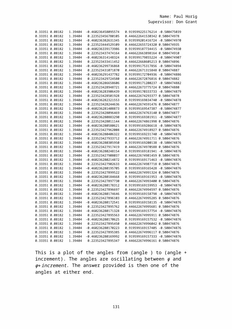
Name: Paul HorigSupervisor: Don Grant
0.33351 0.08182 1.39404 -0.460236458095574 0.919599225176214 -0.5004750390.33351 0.08182 1.39404 0.223523456780105 0.446622641530342 0.5004749780.33351 0.08182 1.39404 -0.460236382631345 0.919599201416724 -0.5004749700.33351 0.08182 1.39404 0.223523444529109 0.446622655724320 0.5004749350.33351 0.08182 1.39404 -0.460236339173986 0.919599187734415 -0.5004749300.33351 0.08182 1.39404 0.223523437474164 0.446622663898164 0.5004749100.33351 0.08182 1.39404 -0.460236314148324 0.919599179855224 -0.5004749070.33351 0.08182 1.39404 0.223523433411452 0.446622668605213 0.5004748960.33351 0.08182 1.39404 -0.460236299736868 0.919599175317856 -0.5004748940.33351 0.08182 1.39404 0.223523431071870 0.446622671315848 0.5004748870.33351 0.08182 1.39404 -0.460236291437782 0.919599172704936 -0.5004748860.33351 0.08182 1.39404 0.223523429724580 0.446622672876816 0.5004748820.33351 0.08182 1.39404 -0.460236286658606 0.919599171200237 -0.5004748820.33351 0.08182 1.39404 0.223523428948721 0.446622673775724 0.5004748800.33351 0.08182 1.39404 -0.460236283906439 0.919599170333733 -0.5004748790.33351 0.08182 1.39404 0.223523428501928 0.446622674293377 0.5004748780.33351 0.08182 1.39404 -0.460236282321553 0.919599169834740 -0.5004748780.33351 0.08182 1.39404 0.223523428244636 0.446622674591476 0.5004748770.33351 0.08182 1.39404 -0.460236281408873 0.919599169547387 -0.5004748770.33351 0.08182 1.39404 0.223523428096469 0.446622674763140 0.5004748770.33351 0.08182 1.39404 -0.460236280883290 0.919599169381911 -0.5004748770.33351 0.08182 1.39404 0.223523428011144 0.446622674861998 0.5004748760.33351 0.08182 1.39404 -0.460236280580621 0.919599169286618 -0.5004748760.33351 0.08182 1.39404 0.223523427962008 0.446622674918927 0.5004748760.33351 0.08182 1.39404 -0.460236280406322 0.919599169231740 -0.5004748760.33351 0.08182 1.39404 0.223523427933712 0.446622674951711 0.5004748760.33351 0.08182 1.39404 -0.460236280305950 0.919599169200138 -0.5004748760.33351 0.08182 1.39404 0.223523427917419 0.446622674970588 0.5004748760.33351 0.08182 1.39404 -0.460236280248154 0.919599169181941 -0.5004748760.33351 0.08182 1.39404 0.223523427908037 0.446622674981459 0.5004748760.33351 0.08182 1.39404 -0.460236280214872 0.919599169171463 -0.5004748760.33351 0.08182 1.39404 0.223523427902633 0.446622674987718 0.5004748760.33351 0.08182 1.39404 -0.460236280195705 0.919599169165428 -0.5004748760.33351 0.08182 1.39404 0.223523427899522 0.446622674991324 0.5004748760.33351 0.08182 1.39404 -0.460236280184668 0.919599169161953 -0.5004748760.33351 0.08182 1.39404 0.223523427897730 0.446622674993400 0.5004748760.33351 0.08182 1.39404 -0.460236280178312 0.919599169159953 -0.5004748760.33351 0.08182 1.39404 0.223523427896697 0.446622674994597 0.5004748760.33351 0.08182 1.39404 -0.460236280174646 0.919599169158798 -0.5004748760.33351 0.08182 1.39404 0.223523427896103 0.446622674995285 0.5004748760.33351 0.08182 1.39404 -0.460236280172541 0.919599169158135 -0.5004748760.33351 0.08182 1.39404 0.223523427895762 0.446622674995681 0.5004748760.33351 0.08182 1.39404 -0.460236280171328 0.919599169157754 -0.5004748760.33351 0.08182 1.39404 0.223523427895563 0.446622674995911 0.5004748760.33351 0.08182 1.39404 -0.460236280170625 0.919599169157532 -0.5004748760.33351 0.08182 1.39404 0.223523427895450 0.446622674996042 0.5004748760.33351 0.08182 1.39404 -0.460236280170223 0.919599169157405 -0.5004748760.33351 0.08182 1.39404 0.223523427895385 0.446622674996117 0.5004748760.33351 0.08182 1.39404 -0.460236280169992 0.919599169157333 -0.5004748760.33351 0.08182 1.39404 0.223523427895347 0.446622674996161 0.500474876
This is a plot of the angles from (angle ) to (angle + increment). The angles are oscillating between ϕ andϕ+increment. The answer provided is then one of the angles at either end.
131
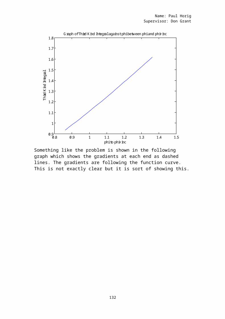
Name: Paul HorigSupervisor: Don Grant
0.8 0.9 1 1.1 1.2 1.3 1.4 1.50.9
1
1.1
1.2
1.3
1.4
1.5
1.6
1.7
1.8Graph of Third Kind Integral against phi between phi and phi+inc
phi to phi+inc
Third Kind
Integral
Something like the problem is shown in the following graph which shows the gradients at each end as dashed lines. The gradients are following the function curve. This is not exactly clear but it is sort of showing this.
132
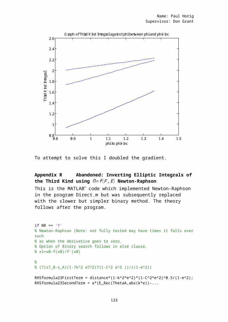
Name: Paul HorigSupervisor: Don Grant
0.8 0.9 1 1.1 1.2 1.3 1.4 1.50.8
1
1.2
1.4
1.6
1.8
2
2.2
2.4
2.6Graph of Third Kind Integral against phi between phi and phi+inc
phi to phi+inc
Third Kind
Integral
To attempt to solve this I doubled the gradient.
Appendix R Abandoned: Inverting Elliptic Integrals ofthe Third Kind using Π=f(F,E) Newton-RaphsonThis is the MATLAB© code which implemented Newton-Raphson in the program Direct.m but was subsequently replaced with the slower but simpler binary method. The theory follows after the program.
if NR == 'Y'% Newton-Raphson (Note: not fully tested may have times it falls oversuch% as when the derivative goes to zero.% Option of Binary search follows in else clause.% x1=x0-f(x0)/f'(x0) % % (?(s?_B-s_A)(1-?k^2 e?^2)?(1-C^2 e^2 ))/((1-e^2)) RHSformula23FirstTerm = distance*(1-k^2*e^2)*(1-C^2*e^2)^0.5/(1-e^2);RHSformula23SecondTerm = a*(E_Rec(ThetaA,abs(k*e))-...
133
Name: Paul HorigSupervisor: Don Grant
k^2*e^2*(sin(ThetaA)*cos(ThetaA))/((1-(k*e*sin(ThetaA))^2)^0.5)); % Dividing through by the 'a' on the left of equation (23) % leaves the Second Kind integral take away the sin cos bit SecondKind_Plus_sincosbit = (RHSformula23FirstTerm+RHSformula23SecondTerm)/a;Result = SecondKind_Plus_sincosbit; Theta0 = pi()/4;diff = 1;while diff > 1E-15 fx0=E_Rec(Theta0,abs(k*e))-... k^2*e^2*(sin(Theta0)*cos(Theta0))/(1-(k*e*sin(Theta0))^2)^0.5-... Result; fdashx0=(1-(k*e*sin(Theta0))^2)^0.5-... ((k*e)^2/((1-(k*e*sin(Theta0))^2)^1.5))*... ((1-(k*e*sin(Theta0))^2)+(sin(Theta0)*cos(Theta0))^2); Theta1 = Theta0-fx0/fdashx0; diff = abs(Theta1-Theta0); Theta0 = Theta1; end ThetaB = Theta0; % End of Newton-Raphson.
The following method converts the Third Kind integral into the sum of a First Kind and a Second Kind integration (see Appendix O). Then it finds the derivate in preparation for using Newton-Raphson to determine θB. The Newton-Raphson formula is:
θn+1=θn−f (θn )f'(θn)
(119)
Beginning with the geodesic length formula:
sB−sA=a(1−e2)
√1−c2e2∫θA
θB 1¿¿ ¿
134
Name: Paul HorigSupervisor: Don Grant
sB−sA=a(1−e2)
a(1−k2e2)√1−c2e2∫θA
θB a(1−k2e2)¿¿ ¿
(s¿¿B−sA)(1−k2e2)√1−c2e2
(1−e2)=∫
θA
θB a(1−k2e2)¿¿ ¿¿
(120)
Taking the Right Hand Side of Equation (37):
∫θA
θB a (1−k2e2 )¿¿ ¿
¿∫0
θB a(1−k2e2)¿¿ ¿
=
a(E (ϕB,ke)−k2e2( sinϕBcosϕB
√1−k2e2sin2ϕB))−a(E (ϕA,ke)−k2e2( sinϕAcosϕA√1−k2e2sin2ϕA ))
()The second term is known in the direct problem. So the entire equation is:
a(E (ϕB,ke)−k2e2( sinϕBcosϕB
√1−k2e2sin2ϕB))=(s¿¿B−sA)(1−k2e2)√1−C2e2
(1−e2)+a(E (ϕA,ke)−k2e2( sinϕAcosϕA
√1−k2e2sin2ϕA ))¿()
As we will find ϕB this can be simplified by substituting into the known values of ϕA,k,e,C,sB,sA .:
f (ϕB)=(E (ϕB,ke)−k2e2( sinϕBcosϕB√1−k2e2sin2ϕB ))−constant=0
f' (ϕB )=E' (ϕB,ke)−(k¿¿2e2( sinϕBcosϕB√1−k2e2sin2ϕB ))'¿
135
Name: Paul HorigSupervisor: Don Grant
Now the derivative of E (ϕB,ke) will be:
E (ϕB,ke)=∫0
ϕB
√1−k2e2sin2θⅆθ(121)
E' (ϕB,ke)=√1−k2e2sin2ϕB(122)
k2e2¿¿
Now(sinϕBcosϕB)
'=cos2ϕB+sin
2ϕB=1
k2e2¿
k2e2¿
k2e2
√1−k2e2sin2ϕB
+sinϕBcosϕBk
2e2sinϕBcosϕB
(1−k2e2sin2ϕB )32
k2e2((1−k2e2sin2ϕB)+sin
2ϕBcos2ϕB
(1−k2e2sin2ϕB )32
)
f'(ϕB)=√1−k2e2sin2ϕB−k2e2((1−k2e2sin2ϕB)+sin
2ϕBcos2ϕB
(1−k2e2sin2ϕB )32
)
f'(ϕB)=√1−k2e2sin2ϕB−k2e2((1−k2e2sin2ϕB)+sin
2ϕBcos2ϕB
(1−k2e2sin2ϕB )32
)
136
Name: Paul HorigSupervisor: Don Grant
Appendix S Abandoned working to evaluate Elliptic Integrals of the Third Kind using a Landen transformation
An elliptic integral of the Third Kind is:
Π(n,ϕ,m)=∫0
ϕ 1(1−nsin2t)√¿¿¿
¿
(1)
For the purposes of finding meridian distances the special case of this integral is when
n=m=k2
So equation (1) becomes:
Π(ϕ,k)=∫0
ϕ 1¿¿ ¿
(2)Applying the change of variable of the Landen transformation:
θ=tan−1(sin2ω
k+cos2ω)
Or as previously derived (see second kind above (30)):
√1−k2sin2θ=cos(2ω−θ)(2) becomes
Π(ϕ,k)=∫0
ϕ 1cos3(2ω−θ)
dθ
(3)
Π(ϕ,k)=∫0
ϕ 1cos3(2ω−θ)
dθ
(4)Now the denominator of the integrand can be expanded as:
¿
137
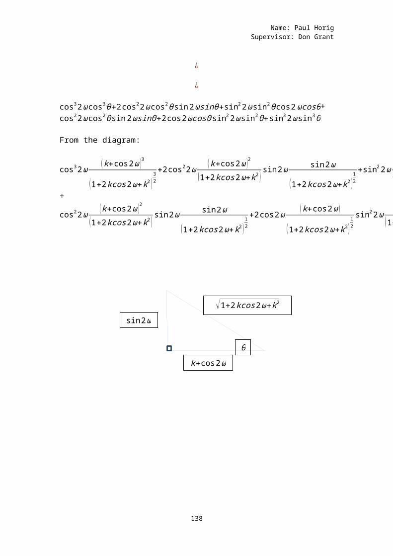
Name: Paul HorigSupervisor: Don Grant
¿
¿
cos32ωcos3θ+2cos22ωcos2θsin2ωsinθ+sin22ωsin2θcos2ωcosθ+cos22ωcos2θsin2ωsinθ+2cos2ωcosθsin22ωsin2θ+sin32ωsin3θ
From the diagram:
cos32ω (k+cos2ω )3
(1+2kcos2ω+k2 )32
+2cos22ω (k+cos2ω )2
(1+2kcos2ω+k2 )sin2ω sin2ω
(1+2kcos2ω+k2 )12
+sin22ω sin22ω(1+2kcos2ω+k2 )
cos2ω (k+cos2ω)
(1+2kcos2ω+k2 )12
+
cos22ω (k+cos2ω )2
(1+2kcos2ω+k2 )sin2ω sin2ω
(1+2kcos2ω+k2 )12
+2cos2ω (k+cos2ω )
(1+2kcos2ω+k2)12
sin22ω sin22ω(1+2kcos2ω+k2 )
+sin32ω sin32ω
(1+2kcos2ω+k2 )32
138
√1+2kcos2ω+k2
sin2ω
θk+cos2ω
Name: Paul HorigSupervisor: Don Grant
cos32ω (k+cos2ω )3
(1+2kcos2ω+k2 )32
+2cos22ωsin22ω (k+cos2ω )2
(1+2kcos2ω+k2)32
+sin42ωcos2ω (k+cos2ω )
(1+2kcos2ω+k2 )32
+
cos22ωsin22ω (k+cos2ω )2
(1+2kcos2ω+k2)32
+2cos2ω (k+cos2ω )
(1+2kcos2ω+k2 )32
sin42ω+sin32ω sin32ω
(1+2kcos2ω+k2 )32
cos32ω (k+cos2ω )3
(1+2kcos2ω+k2 )32
+2cos22ωsin22ω (k+cos2ω )2
(1+2kcos2ω+k2)32
+sin42ωcos2ω (k+cos2ω )
(1+2kcos2ω+k2 )32
+
cos22ωsin22ω (k+cos2ω )2
(1+2kcos2ω+k2)32
+2cos2ωsin42ω (k+cos2ω)
(1+2kcos2ω+k2 )32
+sin62ω 1
(1+2kcos2ω+k2 )32
1
(1+2kcos2ω+k2 )32
¿+sin62ω)
1
(1+2kcos2ω+k2 )32
¿+sin62ω)
1
(1+2kcos2ω+k2 )32
¿
1
(1+2kcos2ω+k2 )32
¿
(5)
1
(1+2kcos2ω+k2 )32
(kcos2ω+1 )3
139
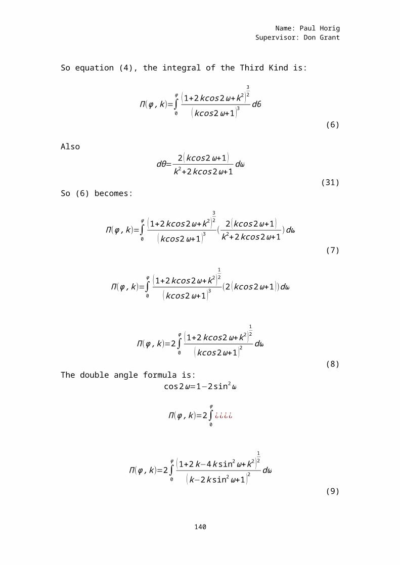
Name: Paul HorigSupervisor: Don Grant
So equation (4), the integral of the Third Kind is:
Π(ϕ,k)=∫0
ϕ (1+2kcos2ω+k2 )32
(kcos2ω+1 )3dθ
(6)
Also
dθ= 2 (kcos2ω+1 )k2+2kcos2ω+1
dω
(31)So (6) becomes:
Π(ϕ,k)=∫0
ϕ (1+2kcos2ω+k2 )32
(kcos2ω+1 )3(2 (kcos2ω+1 )k2+2kcos2ω+1
)dω
(7)
Π(ϕ,k)=∫0
ϕ (1+2kcos2ω+k2 )12
(kcos2ω+1 )3(2 (kcos2ω+1 ))dω
Π(ϕ,k)=2∫0
ϕ (1+2kcos2ω+k2 )12
(kcos2ω+1 )2dω
(8)The double angle formula is:
cos2ω=1−2sin2ω
Π(ϕ,k)=2∫0
ϕ
¿¿¿¿
Π(ϕ,k)=2∫0
ϕ (1+2k−4ksin2ω+k2 )12
(k−2ksin2ω+1 )2dω
(9)
140
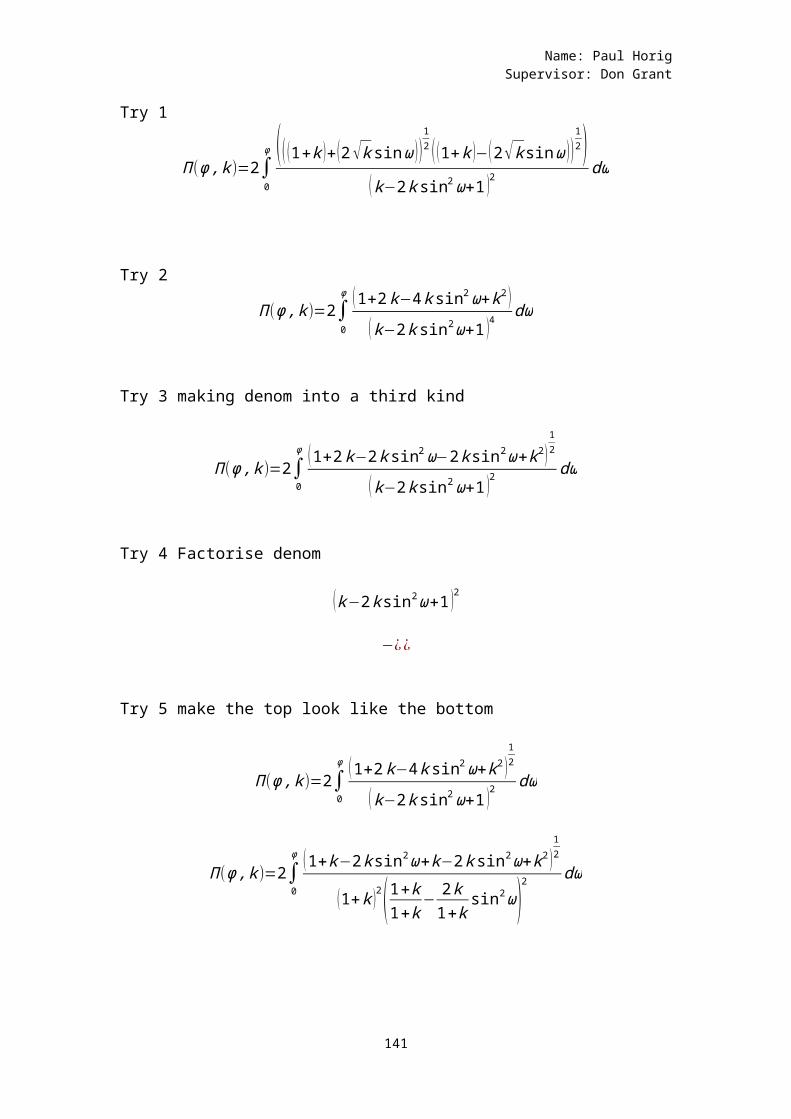
Name: Paul HorigSupervisor: Don Grant
Try 1
Π(ϕ,k)=2∫0
ϕ (( (1+k )+(2√ksinω ))12 ( (1+k )−(2√ksinω ))
12)
(k−2ksin2ω+1 )2dω
Try 2
Π(ϕ,k)=2∫0
ϕ (1+2k−4ksin2ω+k2 )(k−2ksin2ω+1 )4
dω
Try 3 making denom into a third kind
Π(ϕ,k)=2∫0
ϕ (1+2k−2ksin2ω−2ksin2ω+k2)12
(k−2ksin2ω+1 )2dω
Try 4 Factorise denom
(k−2ksin2ω+1 )2
−¿¿
Try 5 make the top look like the bottom
Π(ϕ,k)=2∫0
ϕ (1+2k−4ksin2ω+k2 )12
(k−2ksin2ω+1 )2dω
Π(ϕ,k)=2∫0
ϕ (1+k−2ksin2ω+k−2ksin2ω+k2 )12
(1+k )2(1+k1+k
−2k1+k
sin2ω)2 dω
141
Name: Paul HorigSupervisor: Don Grant
Π(ϕ,k)=2∫0
ϕ (1+k−2ksin2ω+k−2ksin2ω+k2 )12
(1+k )2(1−2k1+k
sin2ω)2 dω
Now the original integral of the Third Kind is before thechange of variable:
Π(ϕ,k)=∫0
ϕ 1¿¿ ¿
Appendix T Khan’s endpoint formula
My program M_Rec was used to test the precision of Khan’s endpoint formula. The formula was found to be only 5% precise.
Khan’s endpoint formula is:
L= π2√2
√¿¿
where (x1,y1) and (x2,y2) are the endpoints of the ellipse. This is given as approximation one in Weintrit (2013 p262).
Figure 6 shows the geometry of an ellipse with all relevant angles (from (Deakin, Geometric Geodesy Part A, 2010, p. 12))
142
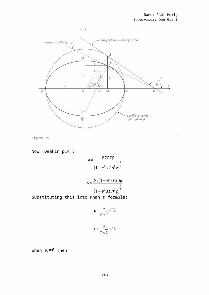
Name: Paul HorigSupervisor: Don Grant
Figure 15
Now (Deakin p14):x=
acosϕ
(1−e2sin2ϕ)12
y=b√(1−e2)sinϕ
(1−e2sin2ϕ)12
Substituting this into Khan’s formula:
L=π
2√2√¿¿
L= π2√2
√¿¿
When ϕ1=0 then
143
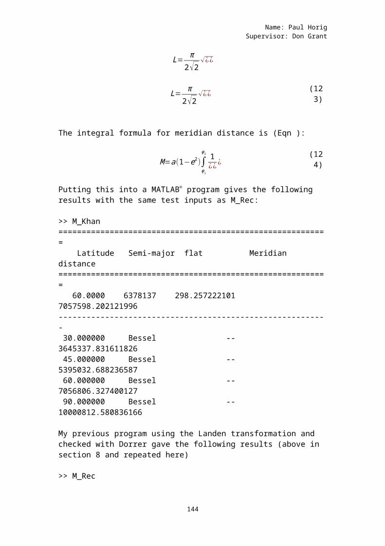
Name: Paul HorigSupervisor: Don Grant
L=π
2√2√¿¿
L= π2√2
√¿¿ (123)
The integral formula for meridian distance is (Eqn ):
M=a(1−e2)∫ϕ1
ϕ2 1¿¿ ¿
(124)
Putting this into a MATLAB© program gives the following results with the same test inputs as M_Rec:
>> M_Khan========================================================== Latitude Semi-major flat Meridian distance========================================================== 60.0000 6378137 298.257222101 7057598.202121996---------------------------------------------------------- 30.000000 Bessel -- 3645337.831611826 45.000000 Bessel -- 5395032.688236587 60.000000 Bessel -- 7056806.327400127 90.000000 Bessel -- 10000812.580836166
My previous program using the Landen transformation and checked with Dorrer gave the following results (above in section 8 and repeated here)
>> M_Rec
144
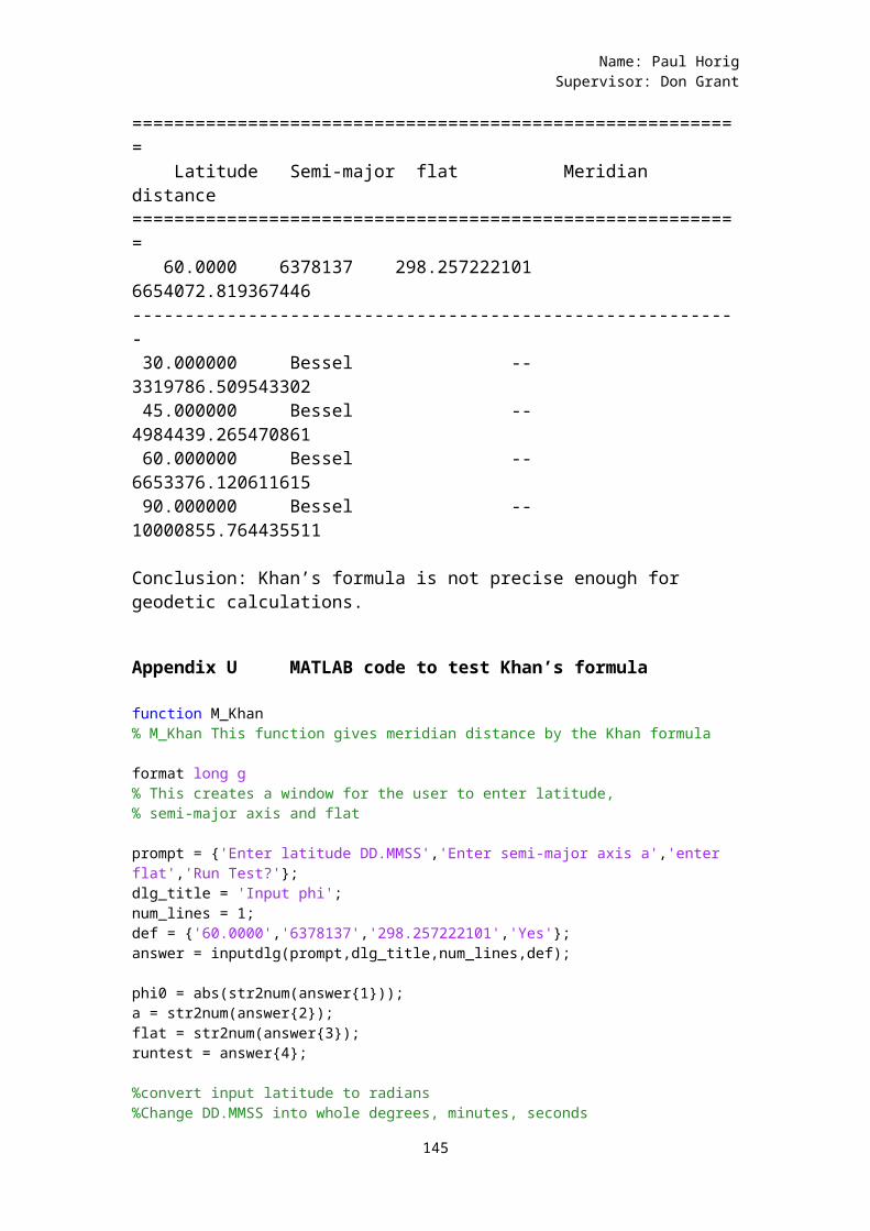
Name: Paul HorigSupervisor: Don Grant
========================================================== Latitude Semi-major flat Meridian distance========================================================== 60.0000 6378137 298.257222101 6654072.819367446---------------------------------------------------------- 30.000000 Bessel -- 3319786.509543302 45.000000 Bessel -- 4984439.265470861 60.000000 Bessel -- 6653376.120611615 90.000000 Bessel -- 10000855.764435511
Conclusion: Khan’s formula is not precise enough for geodetic calculations.
Appendix U MATLAB code to test Khan’s formula
function M_Khan% M_Khan This function gives meridian distance by the Khan formula format long g% This creates a window for the user to enter latitude,% semi-major axis and flat prompt = {'Enter latitude DD.MMSS','Enter semi-major axis a','enter flat','Run Test?'};dlg_title = 'Input phi';num_lines = 1;def = {'60.0000','6378137','298.257222101','Yes'};answer = inputdlg(prompt,dlg_title,num_lines,def); phi0 = abs(str2num(answer{1}));a = str2num(answer{2});flat = str2num(answer{3});runtest = answer{4}; %convert input latitude to radians%Change DD.MMSS into whole degrees, minutes, seconds
145
Name: Paul HorigSupervisor: Don Grant
phi0deg = fix(phi0);mins_secs = phi0 - phi0deg;phi0minutes = abs(fix(mins_secs*100));phi0seconds = abs(fix((phi0 - phi0deg - phi0minutes/100)*10000));phi0r = (phi0deg+(phi0minutes/60)+(phi0seconds/3600))*(pi()/180); % convert flat into flattening and find first eccentricityf=1/flat;e = (f*(2-f))^0.5;b=a*(1-f); % find meridian distance by using Khan's formula xcoord=a*cos(phi0r)/(1-e^2*(sin(phi0r))^2)^0.5;ycoord=(b*(1-e^2)^0.5*sin(phi0r))/(1-e^2*(sin(phi0r))^2)^0.5; M=(pi()/(2*2^0.5))*((xcoord-a)^2+ycoord^2)^0.5; fprintf(1,'==========================================================\n');fprintf(1,'%12s %12s %5s %26s\n','Latitude', 'Semi-major', 'flat','Meridian distance');fprintf(1,'==========================================================\n');fprintf(1,'%10s %10s %16s %19.9f\n',answer{1}, answer{2},answer{3}, M);fprintf(1,'----------------------------------------------------------\n'); if runtest == 'Yes' lats = (pi()/180)*[30,45,60,90]; a=6377397.155; %Bessel's ellipsoid e = 0.08169683121517; %Bessel's ellipsoid b=a*(1-f); %Bessel's ellipsoid for n = 1:4 xcoord=a*cos(lats(n))/(1-e^2*(sin(lats(n)))^2)^0.5; ycoord=(b*(1-e^2)^0.5*sin(lats(n)))/(1-e^2*(sin(lats(n)))^2)^0.5; M=(pi()/(2*2^0.5))*((xcoord-a)^2+ycoord^2)^0.5; fprintf(1,'%10f %10s %16s %19.9f\n',180/pi()*lats(n), 'Bessel','--', M) endend end
146
Name: Paul HorigSupervisor: Don Grant
Appendix V MATLAB code to change DD.MMSS into decimaldegrees
function phi0r = DecDMStoRad( phi )%DECDMSTORAD Decimal Degrees mins secs to radians% This converts an input of DD.MMSS into radiansphi0=abs(phi);phi0deg = fix(phi0);mins_secs = phi0 - phi0deg;phi0minutes = abs(fix(mins_secs*100));phi0seconds = abs(fix((phi0 - phi0deg - phi0minutes/100)*10000));phi0r = (phi0deg+(phi0minutes/60)+(phi0seconds/3600))*(pi()/180); if phi < 0 phi0r = -1*phi0r;end end
147
Copyright © 2022 FDOKUMEN